
PDF - COMSOL Multiphysics® - CSC
588
COMSOL Multiphysics ® V ERSION 3.4 USER’S GUIDE
-
Upload
khangminh22 -
Category
Documents
-
view
0 -
download
0
Transcript of PDF - COMSOL Multiphysics® - CSC

COMSOLMultiphysics ®
V E R S I O N 3 . 4
USER’S G
UIDE

How to contact COMSOL:
BeneluxCOMSOL BV Röntgenlaan 19 2719 DX Zoetermeer The Netherlands Phone: +31 (0) 79 363 4230 Fax: +31 (0) 79 361 [email protected] www.femlab.nl
Denmark COMSOL A/S Diplomvej 376 2800 Kgs. Lyngby Phone: +45 88 70 82 00 Fax: +45 88 70 80 90 [email protected] www.comsol.dk
Finland COMSOL OY Arabianranta 6FIN-00560 Helsinki Phone: +358 9 2510 400 Fax: +358 9 2510 4010 [email protected] www.comsol.fi
France COMSOL France WTC, 5 pl. Robert Schuman F-38000 Grenoble Phone: +33 (0)4 76 46 49 01 Fax: +33 (0)4 76 46 07 42 [email protected] www.comsol.fr
Germany FEMLAB GmbHBerliner Str. 4 D-37073 Göttingen Phone: +49-551-99721-0Fax: +49-551-99721-29 [email protected]
Italy COMSOL S.r.l. Via Vittorio Emanuele II, 22 25122 Brescia Phone: +39-030-3793800 Fax: [email protected]
Norway COMSOL AS Søndre gate 7 NO-7485 Trondheim Phone: +47 73 84 24 00 Fax: +47 73 84 24 01 [email protected] www.comsol.no Sweden COMSOL AB Tegnérgatan 23 SE-111 40 Stockholm Phone: +46 8 412 95 00 Fax: +46 8 412 95 10 [email protected] www.comsol.se
SwitzerlandFEMLAB GmbH Technoparkstrasse 1 CH-8005 Zürich Phone: +41 (0)44 445 2140 Fax: +41 (0)44 445 2141 [email protected] www.femlab.ch
United Kingdom COMSOL Ltd. UH Innovation CentreCollege LaneHatfieldHertfordshire AL10 9AB Phone:+44-(0)-1707 284747Fax: +44-(0)-1707 284746 [email protected] www.uk.comsol.com
United States COMSOL, Inc. 1 New England Executive Park Suite 350 Burlington, MA 01803 Phone: +1-781-273-3322 Fax: +1-781-273-6603 COMSOL, Inc. 10850 Wilshire Boulevard Suite 800 Los Angeles, CA 90024 Phone: +1-310-441-4800 Fax: +1-310-441-0868
COMSOL, Inc. 744 Cowper Street Palo Alto, CA 94301 Phone: +1-650-324-9935 Fax: +1-650-324-9936
For a complete list of international representatives, visit www.comsol.com/contact
Company home pagewww.comsol.com
COMSOL user forumswww.comsol.com/support/forums
COMSOL Multiphysics User’s Guide © COPYRIGHT 1994–2007 by COMSOL AB. All rights reserved
Patent pending
The software described in this document is furnished under a license agreement. The software may be used or copied only under the terms of the license agreement. No part of this manual may be photocopied or reproduced in any form without prior written consent from COMSOL AB.
COMSOL, COMSOL Multiphysics, COMSOL Reaction Engineering Lab, and FEMLAB are registered trademarks of COMSOL AB. COMSOL Script is a trademark of COMSOL AB.
Other product or brand names are trademarks or registered trademarks of their respective holders.
Version: October 2007 COMSOL 3.4

C O N T E N T S
C h a p t e r 1 : I n t r o d u c t i o n
The Documentation Set 2
Typographical Conventions . . . . . . . . . . . . . . . . . . . 4
About COMSOL Multiphysics 5
The COMSOL Multiphysics Environment 8
The COMSOL Modules 11
The AC/DC Module . . . . . . . . . . . . . . . . . . . . . 11
The Acoustics Module . . . . . . . . . . . . . . . . . . . . . 12
The Chemical Engineering Module . . . . . . . . . . . . . . . . 12
The Earth Science Module . . . . . . . . . . . . . . . . . . . 14
The Heat Transfer Module . . . . . . . . . . . . . . . . . . . 15
The MEMS Module . . . . . . . . . . . . . . . . . . . . . . 15
The RF Module . . . . . . . . . . . . . . . . . . . . . . . 16
The Structural Mechanics Module . . . . . . . . . . . . . . . . 17
The CAD Import Modules 19
Internet Resources 20
COMSOL Web Sites . . . . . . . . . . . . . . . . . . . . . 20
COMSOL User Forums . . . . . . . . . . . . . . . . . . . . 20
C h a p t e r 2 : G e o m e t r y M o d e l i n g a n d C A D To o l s
The COMSOL Multiphysics Geometry and CAD Environment 24
Overview of Geometry Modeling Concepts . . . . . . . . . . . . 24
Setting up Axes and Grid . . . . . . . . . . . . . . . . . . . . 25
Creating Cartesian and Cylindrical Coordinate Systems . . . . . . . . 27
The Status Bar . . . . . . . . . . . . . . . . . . . . . . . . 30
C O N T E N T S | i
ii | C O N T E N T S
Creating Composite Geometry Objects . . . . . . . . . . . . . . 31
Moving, Rotating, Scaling, and Mirroring Geometry Objects. . . . . . . 33
Creating an Array of Geometry Objects . . . . . . . . . . . . . . 34
Copying and Pasting Geometry Objects . . . . . . . . . . . . . . 34
Coercing Geometry Objects . . . . . . . . . . . . . . . . . . 34
Removing Interior Boundaries . . . . . . . . . . . . . . . . . . 35
Splitting Geometry Objects . . . . . . . . . . . . . . . . . . . 35
Geometry Domain Names . . . . . . . . . . . . . . . . . . . 35
Viewing Geometries . . . . . . . . . . . . . . . . . . . . . 36
Entering Draw Mode . . . . . . . . . . . . . . . . . . . . . 36
Creating a 1D Geometry Model 37
Creating a 2D Geometry Model 39
Using the 2D Draw Toolbar and the Draw Menu . . . . . . . . . . . 39
2D Solid Modeling Techniques . . . . . . . . . . . . . . . . . . 42
2D Boundary Modeling . . . . . . . . . . . . . . . . . . . . 46
Creating Fillets and Chamfers . . . . . . . . . . . . . . . . . . 49
Drawing Tangents . . . . . . . . . . . . . . . . . . . . . . 51
Editing Geometry Objects . . . . . . . . . . . . . . . . . . . 54
Creating a 3D Geometry Model 56
Using the 3D Draw Toolbar and Draw Menu . . . . . . . . . . . . 56
Creating 3D Geometries from 2D Geometric Objects . . . . . . . . 59
Creating and Using 2D Work Planes . . . . . . . . . . . . . . . 59
Extruding, Revolving, and Embedding . . . . . . . . . . . . . . . 63
Solid Modeling Using Solid Objects and Boolean Operations . . . . . . 67
Editing 3D Objects . . . . . . . . . . . . . . . . . . . . . . 75
Exploring Geometric Properties 77
Introduction . . . . . . . . . . . . . . . . . . . . . . . . 77
Using The Geometric Properties Dialog Box . . . . . . . . . . . . 77
Displaying Geometric Properties in the Message Log . . . . . . . . . 81
Centroid, Center of Gravity, and Distance in Electronic Conductor. . . . 81
Importing and Exporting Geometry Objects and CAD Models 85
Importing and Exporting COMSOL Multiphysics Files . . . . . . . . . 86
Importing and Exporting DXF Files . . . . . . . . . . . . . . . . 87
Importing STL and VRML Files . . . . . . . . . . . . . . . . . . 89
Creating a Geometry for Successful Analysis 92
Using Assemblies . . . . . . . . . . . . . . . . . . . . . . . 92
Using Symmetries . . . . . . . . . . . . . . . . . . . . . . 93
Removing Unnecessary Boundaries . . . . . . . . . . . . . . . . 93
Making the Geometry Match the Boundary Conditions . . . . . . . . 93
Avoiding Excessively Small Details, Holes, and Gaps. . . . . . . . . . 93
Avoiding Singularities and Degeneracies in the Geometry . . . . . . . 94
Associative Geometry . . . . . . . . . . . . . . . . . . . . . 94
C h a p t e r 3 : V i s u a l i z a t i o n a n d S e l e c t i o n T o o l s
Visualizing a Model 98
The Visualization/Selection Toolbar . . . . . . . . . . . . . . . . 99
Zooming . . . . . . . . . . . . . . . . . . . . . . . . . 100
Changing the View in 3D . . . . . . . . . . . . . . . . . . . 101
Using Lighting . . . . . . . . . . . . . . . . . . . . . . . 104
Changing the View to a Different Axis Plane . . . . . . . . . . . 112
Using Transparency in 3D Plots . . . . . . . . . . . . . . . . 112
Controlling the Resolution of the Visualization Mesh . . . . . . . . 113
Adding Labels to Domains . . . . . . . . . . . . . . . . . . 114
Rendering and Highlighting Geometry Objects . . . . . . . . . . 116
Scaling of Load and Constraint Symbols . . . . . . . . . . . . . 119
Saving Preferences for Labels, Rendering, and Highlighting . . . . . . 119
Suppressing the Display of Objects . . . . . . . . . . . . . . . 122
Rendering Large Geometry Objects . . . . . . . . . . . . . . 124
Viewing Multiple Geometries . . . . . . . . . . . . . . . . . 125
Selecting Domains 126
General Object Selection Methods . . . . . . . . . . . . . . . 126
Object Selection Methods in 2D . . . . . . . . . . . . . . . . 127
Object Selection Methods in 3D . . . . . . . . . . . . . . . . 127
C O N T E N T S | iii
iv | C O N T E N T S
C h a p t e r 4 : M o d e l i n g P h y s i c s a n d E q u a t i o n s
Variables and Expressions 138
Using Variables and Expressions . . . . . . . . . . . . . . . . 138
Variable Classification and Geometric Scope . . . . . . . . . . . 138
Defining Constants, Expressions, and Coupling Variables . . . . . . . 139
Specifying Varying Coefficients and Material Properties . . . . . . . 143
Copying Physics Settings . . . . . . . . . . . . . . . . . . . 144
Entering Vector-Valued Expressions . . . . . . . . . . . . . . . 145
Using Mathematical and Logical Operators and Functions . . . . . . 147
Specifying Discontinuous Functions . . . . . . . . . . . . . . . 149
Using Inline (Analytic) Functions . . . . . . . . . . . . . . . . 150
Piecewise Analytic Functions . . . . . . . . . . . . . . . . . 151
Using Functions Based on Interpolated Data . . . . . . . . . . . 154
Using COMSOL Script or MATLAB Functions . . . . . . . . . . . 158
Function Input/Output Considerations . . . . . . . . . . . . . 159
Using Special Operators . . . . . . . . . . . . . . . . . . . 160
Variable Naming Conventions . . . . . . . . . . . . . . . . . 164
Geometric Variables . . . . . . . . . . . . . . . . . . . . 165
Using Field Variables 170
Field Variable Definition and Categories . . . . . . . . . . . . . 170
Shape Function Variables . . . . . . . . . . . . . . . . . . . 171
Application Mode Variables . . . . . . . . . . . . . . . . . . 174
Expression Variables . . . . . . . . . . . . . . . . . . . . 175
Coupling Variables . . . . . . . . . . . . . . . . . . . . . 175
Special Variables . . . . . . . . . . . . . . . . . . . . . . 175
Specifying Model Settings 179
Generating Variables . . . . . . . . . . . . . . . . . . . . 179
Simplifying Expressions . . . . . . . . . . . . . . . . . . . 180
Selecting an Equation System Form . . . . . . . . . . . . . . . 180
Selecting a Geometry Shape Order . . . . . . . . . . . . . . . 181
Model Settings with Multiple Frames . . . . . . . . . . . . . . 181
Using Units 183
Unit Systems in COMSOL Multiphysics . . . . . . . . . . . . . 183
Specifying the Unit System . . . . . . . . . . . . . . . . . . 184
Using the Unit Syntax . . . . . . . . . . . . . . . . . . . . 187
Switching Unit System . . . . . . . . . . . . . . . . . . . . 189
About Temperature Units . . . . . . . . . . . . . . . . . . 190
SI Base Units, Derived Units, and Additional Units . . . . . . . . . 191
Special British Engineering Units . . . . . . . . . . . . . . . . 194
Special CGSA Units . . . . . . . . . . . . . . . . . . . . . 195
Special EMU Units . . . . . . . . . . . . . . . . . . . . . 196
Special ESU Units. . . . . . . . . . . . . . . . . . . . . . 197
Special FPS Units . . . . . . . . . . . . . . . . . . . . . . 198
Special IPS Units . . . . . . . . . . . . . . . . . . . . . . 198
Special MPa Units. . . . . . . . . . . . . . . . . . . . . . 198
Special Gravitational IPS Units . . . . . . . . . . . . . . . . . 199
Specifying Physics Settings 200
Opening the Physics Settings Dialog Boxes . . . . . . . . . . . . 200
Working with Domain Groups. . . . . . . . . . . . . . . . . 201
Specifying Subdomain Settings and PDE Coefficients 205
Using the Subdomain Settings Dialog Box . . . . . . . . . . . . 205
Specifying PDE Coefficients and Material Properties . . . . . . . . 207
Specifying Initial Conditions . . . . . . . . . . . . . . . . . . 209
Specifying the Finite Element Type . . . . . . . . . . . . . . . 211
Specifying Weak Terms . . . . . . . . . . . . . . . . . . . 212
Ideal and Non-Ideal Constraints . . . . . . . . . . . . . . . . 212
Viewing and Modifying the Full Equation System . . . . . . . . . . 213
Modeling Anisotropic Material . . . . . . . . . . . . . . . . . 215
Using the Model Tree 217
The Model Tree Views . . . . . . . . . . . . . . . . . . . . 217
Using the Overview View . . . . . . . . . . . . . . . . . . 218
Using the Detail View . . . . . . . . . . . . . . . . . . . . 219
Using the Inspect View . . . . . . . . . . . . . . . . . . . 221
Model Tree Settings . . . . . . . . . . . . . . . . . . . . . 222
Using the Materials/Coefficients Library 223
Using Material/Coefficient Data in Models . . . . . . . . . . . . 223
Using Your Own Material Data . . . . . . . . . . . . . . . . 226
C O N T E N T S | v
vi | C O N T E N T S
Using MatWeb Material Property Data . . . . . . . . . . . . . 228
Interpolation of Measured Data and Nonlinear Materials 229
Modeling Thermal Conductivity from Measurements . . . . . . . . 229
Specifying Boundary Conditions 234
Interior and Exterior Boundaries . . . . . . . . . . . . . . . . 234
Setting Conditions on Boundaries . . . . . . . . . . . . . . . 235
Modifying Boundary Settings for the Equation System . . . . . . . . 237
Setting Conditions on Interior Boundaries . . . . . . . . . . . . 239
Specifying Boundary Conditions for Identity Pairs . . . . . . . . . 241
Specifying Point and Edge Settings 242
Using Point Settings . . . . . . . . . . . . . . . . . . . . . 242
Using Edge Settings . . . . . . . . . . . . . . . . . . . . . 243
Setting Point and Edge Constraints . . . . . . . . . . . . . . . 244
Using Periodic Boundary Conditions 245
Periodic Boundary Condition Example. . . . . . . . . . . . . . 248
Specifying Application Scalar Variables 252
Computing Accurate Fluxes 253
Flux Computation Example . . . . . . . . . . . . . . . . . . 253
Using Coupling Variables 255
Integration Coupling Variables . . . . . . . . . . . . . . . . . 255
Integration Coupling Variables—Examples . . . . . . . . . . . . 258
Extrusion Coupling Variables . . . . . . . . . . . . . . . . . 261
Extrusion Coupling Variables—Example . . . . . . . . . . . . . 266
Projection Coupling Variables . . . . . . . . . . . . . . . . . 270
Projection Coupling Variables—Example . . . . . . . . . . . . . 276
General Issues When Using Coupling Variables . . . . . . . . . . 280
Using Boundary Distance Variables 281
Plotting Distances to Walls in Backstep Model. . . . . . . . . . . 282
C h a p t e r 5 : M e s h i n g
Creating Meshes 286
Mesh Elements. . . . . . . . . . . . . . . . . . . . . . . 286
Meshing Techniques . . . . . . . . . . . . . . . . . . . . . 286
Creating Free Meshes . . . . . . . . . . . . . . . . . . . . 287
Creating Free Quadrilateral (Quad) Meshes in 2D . . . . . . . . . 303
Meshing Progress Indication . . . . . . . . . . . . . . . . . . 304
Creating Mapped Meshes in 2D . . . . . . . . . . . . . . . . 305
Extruding and Revolving 2D Meshes . . . . . . . . . . . . . . 313
Creating Swept Meshes in 3D . . . . . . . . . . . . . . . . . 317
Creating Boundary Layer Meshes. . . . . . . . . . . . . . . . 321
Meshing Thin Structures . . . . . . . . . . . . . . . . . . . 325
Mesh Statistics . . . . . . . . . . . . . . . . . . . . . . . 326
Refining Meshes 327
Refinement Methods . . . . . . . . . . . . . . . . . . . . 327
Refining Selected Elements . . . . . . . . . . . . . . . . . . 327
Interactive Meshing 328
Using the Mesh Toolbar . . . . . . . . . . . . . . . . . . . 328
Deleting the Mesh . . . . . . . . . . . . . . . . . . . . . 331
Remeshing a Domain . . . . . . . . . . . . . . . . . . . . 331
Undoing Meshing Operations . . . . . . . . . . . . . . . . . 333
Creating a Combined Free and Mapped Mesh in 2D . . . . . . . . 333
Creating Swept Meshes Interactively . . . . . . . . . . . . . . 335
Creating Boundary Layer Meshes Interactively . . . . . . . . . . . 341
Copying Meshes . . . . . . . . . . . . . . . . . . . . . . 342
Importing and Exporting Meshes 346
Using COMSOL Multiphysics Files . . . . . . . . . . . . . . . 346
Importing NASTRAN Files . . . . . . . . . . . . . . . . . . 346
Creating a Geometry from a Mesh 351
Visualizing Meshes 352
Visualizing the Mesh Quality . . . . . . . . . . . . . . . . . 353
C O N T E N T S | vii
viii | C O N T E N T S
Mesh Cases 355
Avoiding Inverted Mesh Elements 356
Inverted Mesh Elements . . . . . . . . . . . . . . . . . . . 356
Using Linear Geometry Shape Order . . . . . . . . . . . . . . 356
Modifying the Geometry or Mesh . . . . . . . . . . . . . . . 357
Visualizing Inverted Mesh Elements . . . . . . . . . . . . . . . 357
C h a p t e r 6 : S o l v i n g t h e M o d e l
Selecting a Solver 360
The COMSOL Multiphysics Solvers . . . . . . . . . . . . . . . 360
Selecting an Analysis Type . . . . . . . . . . . . . . . . . . 360
Selecting a Stationary, a Time-Dependent, or an Eigenvalue Solver . . . 361
Linear Solvers vs. Nonlinear Solvers . . . . . . . . . . . . . . 362
Remarks on Solver-Related Model Characteristics . . . . . . . . . 363
The Solvers and Their Settings 365
The Stationary Solver . . . . . . . . . . . . . . . . . . . . 365
The Time-Dependent Solver . . . . . . . . . . . . . . . . . 370
The Eigenvalue Solver . . . . . . . . . . . . . . . . . . . . 376
The Parametric Solver . . . . . . . . . . . . . . . . . . . . 379
The Stationary Segregated Solver. . . . . . . . . . . . . . . . 384
The Parametric Segregated Solver . . . . . . . . . . . . . . . 387
Adaptive Mesh Refinement . . . . . . . . . . . . . . . . . . 388
Reference . . . . . . . . . . . . . . . . . . . . . . . . 391
The Linear System Solvers 392
Selecting a Linear System Solver . . . . . . . . . . . . . . . . 392
Linear System Solver Settings . . . . . . . . . . . . . . . . . 394
Linear System Solver Selection Guidelines . . . . . . . . . . . . 394
Selecting a Preconditioner . . . . . . . . . . . . . . . . . . 395
Preconditioner Selection Guidelines . . . . . . . . . . . . . . 396
Guidelines for Classifying Your PDE Problem . . . . . . . . . . . 397
The Preconditioned Linear System . . . . . . . . . . . . . . . 400
The Solver Manager and Solver Scripting 401
Initial Value Settings . . . . . . . . . . . . . . . . . . . . . 401
Choosing Variables for Which to Solve . . . . . . . . . . . . . 404
Selecting Variables for Solution Output . . . . . . . . . . . . . 406
Solver Scripting . . . . . . . . . . . . . . . . . . . . . . 408
Computing the Solution 410
Starting and Restarting the Solvers . . . . . . . . . . . . . . . 410
Updating a Model. . . . . . . . . . . . . . . . . . . . . . 410
Getting the Initial Value . . . . . . . . . . . . . . . . . . . 411
Solution Progress. . . . . . . . . . . . . . . . . . . . . . 411
Monitoring Memory Usage . . . . . . . . . . . . . . . . . . 417
C h a p t e r 7 : P o s t p r o c e s s i n g a n d V i s u a l i z a t i o n
Postprocessing Results 420
COMSOL Multiphysics Postprocessing Overview . . . . . . . . . 420
Postprocessing Expressions . . . . . . . . . . . . . . . . . . 420
Selection of Frames for Postprocessing . . . . . . . . . . . . . 421
Interpolating Expressions at Arbitrary Points . . . . . . . . . . . 421
Computing Quantities Using Integration . . . . . . . . . . . . . 422
Getting Numerical Results Directly . . . . . . . . . . . . . . . 423
Plotting Global Expressions . . . . . . . . . . . . . . . . . . 426
Visualization Using the Plot Parameters Dialog Box . . . . . . . . . 427
Cross-Section Plots . . . . . . . . . . . . . . . . . . . . . 436
Domain Plots . . . . . . . . . . . . . . . . . . . . . . . 438
Specifying Line and Surface Properties . . . . . . . . . . . . . . 439
Creating Animations . . . . . . . . . . . . . . . . . . . . 441
Plotting Values While Solving . . . . . . . . . . . . . . . . . 444
Exporting Data to a File . . . . . . . . . . . . . . . . . . . 449
Exporting the Current Plot to a File. . . . . . . . . . . . . . . 451
Exporting Data to COMSOL Script or MATLAB . . . . . . . . . . 452
Exporting Images . . . . . . . . . . . . . . . . . . . . . . 452
Using Max/Min Markers . . . . . . . . . . . . . . . . . . . 455
Postprocessing 2D Axisymmetric Models in 3D . . . . . . . . . . 455
C O N T E N T S | ix

x | C O N T E N T S
Postprocessing Results in 1D 456
1D Postprocessing Overview . . . . . . . . . . . . . . . . . 456
1D Standard Plots . . . . . . . . . . . . . . . . . . . . . 456
1D Cross-Section Plots . . . . . . . . . . . . . . . . . . . 457
1D Domain Plots . . . . . . . . . . . . . . . . . . . . . . 458
Postprocessing Results in 2D 460
2D Postprocessing Overview . . . . . . . . . . . . . . . . . 460
Using the 2D Plot Toolbar . . . . . . . . . . . . . . . . . . 460
2D Standard Plots . . . . . . . . . . . . . . . . . . . . . 461
2D Cross-Section Plots . . . . . . . . . . . . . . . . . . . 485
2D Domain Plots . . . . . . . . . . . . . . . . . . . . . . 487
Postprocessing Results in 3D 491
3D Postprocessing Overview . . . . . . . . . . . . . . . . . 491
Using the 3D Plot Toolbar . . . . . . . . . . . . . . . . . . 491
3D Standard Plots . . . . . . . . . . . . . . . . . . . . . 493
3D Cross-Section Plots . . . . . . . . . . . . . . . . . . . 503
3D Domain Plots . . . . . . . . . . . . . . . . . . . . . . 507
Using the Report Generator 510
Report Generator Overview . . . . . . . . . . . . . . . . . 510
Creating a Report . . . . . . . . . . . . . . . . . . . . . 511
Report Contents . . . . . . . . . . . . . . . . . . . . . . 514
C h a p t e r 8 : M o d e l M a i n t e n a n c e a n d M o d e l L i b r a r i e s
Opening and Saving COMSOL Multiphysics Models 522
Model Files Formats. . . . . . . . . . . . . . . . . . . . . 522
Opening a COMSOL Multiphysics Model . . . . . . . . . . . . . 522
Saving a COMSOL Multiphysics Model . . . . . . . . . . . . . . 523
Saving on Server Computer . . . . . . . . . . . . . . . . . . 524
Model MPH-files . . . . . . . . . . . . . . . . . . . . . . 524
Setting Model Properties . . . . . . . . . . . . . . . . . . . 525
Model M-Files 528
Using Model M-files . . . . . . . . . . . . . . . . . . . . . 528
Using the COMSOL Multiphysics Model Library 530
Models in the Model Library . . . . . . . . . . . . . . . . . 530
Creating a User Model Library 531
Saving Models for a User Model Library . . . . . . . . . . . . . 531
C h a p t e r 9 : G l o s s a r y
Glossary of Terms 534
INDEX 557
C O N T E N T S | xi

xii | C O N T E N T S

1
I n t r o d u c t i o n
Welcome to COMSOL Multiphysics®! This User’s Guide details features and techniques that help you throughout all of your COMSOL Multiphysics modeling. In this book, for example, we detail procedures to build model geometries in COMSOL Multiphysics, create a mesh for the finite elements, create variables and expressions you can use within a model, and solve and postprocess the solution. The explanations, tutorials, and examples show you, step by step, how to tap into many functions and capabilities available in the COMSOL environment.
This introductory chapter provides an overview of COMSOL Multiphysics and its product family.
1

2 | C H A P T E R
Th e Do cumen t a t i o n S e t
The full documentation set that ships with COMSOL Multiphysics consists of the following titles:
• COMSOL Quick Installation Guide—basic information for installing the COMSOL software and getting started. Included in the DVD/CD package.
• COMSOL New Release Highlights—information about new features and models in the 3.4 release. Included in the DVD/CD package.
• COMSOL License Agreement—the license agreement. Included in the DVD/CD package.
• COMSOL Installation and Operations Guide—besides covering various installation options, it describes system requirements and how to configure and run the COMSOL software on different platforms.
• COMSOL Multiphysics Quick Start and Quick Reference—provides a quick overview of COMSOL Multiphysics’ capabilities and how to access them. A reference section contains comprehensive lists of predefined variable names, mathematical functions, COMSOL Multiphysics operators, equation forms, and application modes.
• COMSOL Multiphysics User’s Guide—the book you are reading, it covers the functionality of COMSOL Multiphysics across its entire range from geometry modeling to postprocessing. It serves as a tutorial and a reference guide to using COMSOL Multiphysics.
• COMSOL Multiphysics Modeling Guide—provides an in-depth examination of the software’s application interfaces and how to use them to model different types of physics and to perform equation-based modeling using PDEs.
• COMSOL Multiphysics Model Library—consists of a collection of ready-to-run models that cover many classic problems and equations from science and engineering. These models have two goals: to show the versatility of COMSOL Multiphysics and the wide range of applications it covers; and to form an educational basis from which you can learn about COMSOL Multiphysics and also gain an understanding of the underlying physics.
1 : I N T R O D U C T I O N
• COMSOL Multiphysics Scripting Guide—shows how to access all of COMSOL Multiphysics’ capabilities from the COMSOL Script environment and the MATLAB programming environment.
• COMSOL Multiphysics Reference Guide—reviews each command that lets you access COMSOL Multiphysics functions from within COMSOL Script and MATLAB. Additionally, it describes some advanced features and settings in COMSOL Multiphysics and provides background material and references.
In addition, each of the optional modules
• AC/DC Module
• Acoustics Module
• Chemical Engineering Module
• Earth Science Module
• Heat Transfer Module
• MEMS Module
• RF Module
• Structural Mechanics Module
comes with its own User’s Guide and Model Library. Many modules also include a Reference Guide.
The documentation for the optional CAD Import Module is available in the CAD Import Module User’s Guide, and the documentation for the optional Material Library in the Material Library User’s Guide.
COMSOL Script comes with a COMSOL Script User’s Guide as well as a comprehensive COMSOL Script Command Reference, and its add-on labs—the COMSOL Reaction Engineering Lab, Optimization Lab, and Signals & Systems Lab— include documentation in separate User’s Guides.
Note: The full documentation set is available in electronic versions—as PDF files and Help Desk format—after installation.
T H E D O C U M E N T A T I O N S E T | 3

4 | C H A P T E R
Typographical Conventions
All COMSOL manuals use a set of consistent typographical conventions that should make it easy for you to follow the discussion, realize what you can expect to see on the screen, and know which data you must enter into various data-entry fields. In particular, you should be aware of these conventions:
• A boldface font of the shown size and style indicates that the given word(s) appear exactly that way on the COMSOL graphical user interface (for toolbar buttons in the corresponding tooltip). For instance, we often refer to the Model Navigator, which is the window that appears when you start a new modeling session in COMSOL; the corresponding window on the screen has the title Model Navigator. As another example, the instructions might say to click the Multiphysics button, and the boldface font indicates that you can expect to see a button with that exact label on the COMSOL user interface.
• The names of other items on the graphical user interface that do not have direct labels contain a leading uppercase letter. For instance, we often refer to the Draw toolbar; this vertical bar containing many icons appears on the left side of the user interface during geometry modeling. However, nowhere on the screen will you see the term “Draw” referring to this toolbar (if it were on the screen, we would print it in this manual as the Draw menu).
• The symbol > indicates a menu item or an item in a folder in the Model Navigator. For example, Physics>Equation System>Subdomain Settings is equivalent to: On the Physics menu, point to Equation System and then click Subdomain Settings. COMSOL Multiphysics>Heat Transfer>Conduction means: Open the COMSOL
Multiphysics folder, open the Heat Transfer folder, and select Conduction.
• A Code (monospace) font indicates keyboard entries in the user interface. You might see an instruction such as “Type 1.25 in the Current density edit field.” The monospace font also indicates COMSOL Script codes.
• An italic font indicates the introduction of important terminology. Expect to find an explanation in the same paragraph or in the Glossary. The names of books in the COMSOL documentation set also appear using an italic font.
1 : I N T R O D U C T I O N
Abou t COMSOL Mu l t i p h y s i c s
COMSOL Multiphysics is a powerful interactive environment for modeling and solving all kinds of scientific and engineering problems based on partial differential equations (PDEs). With this software you can easily extend conventional models for one type of physics into multiphysics models that solve coupled physics phenomena—and do so simultaneously. Accessing this power does not require an in-depth knowledge of mathematics or numerical analysis. Thanks to the built-in physics modes it is possible to build models by defining the relevant physical quantities—such as material properties, loads, constraints, sources, and fluxes—rather than by defining the underlying equations. You can always apply these variables, expressions, or numbers directly to solid domains, boundaries, edges, and points independently of the computational mesh. COMSOL Multiphysics then internally compiles a set of PDEs representing the entire model. You access the power of COMSOL Multiphysics as a standalone product through a flexible graphical user interface, or by script programming in the COMSOL Script language or in the MATLAB language.
Using these application modes, you can perform various types of analysis including:
• Stationary and time-dependent analysis
• Linear and nonlinear analysis
• Eigenfrequency and modal analysis
When solving the PDEs, COMSOL Multiphysics uses the proven finite element method (FEM). The software runs the finite element analysis together with adaptive meshing and error control using a variety of numerical solvers. A more detailed description of this mathematical and numerical foundation appears in the COMSOL Multiphysics User’s Guide and in the COMSOL Multiphysics Modeling Guide.
PDEs form the basis for the laws of science and provide the foundation for modeling a wide range of scientific and engineering phenomena. Therefore you can use COMSOL Multiphysics in many application areas, just a few examples being:
• Acoustics
• Bioscience
• Chemical reactions
• Diffusion
• Electromagnetics
A B O U T C O M S O L M U L T I P H Y S I C S | 5
6 | C H A P T E R
• Fluid dynamics
• Fuel cells and electrochemistry
• Geophysics
• Heat transfer
• Microelectromechanical systems (MEMS)
• Microwave engineering
• Optics
• Photonics
• Porous media flow
• Quantum mechanics
• Radio-frequency components
• Semiconductor devices
• Structural mechanics
• Transport phenomena
• Wave propagation
Many real-world applications involve simultaneous couplings in a system of PDEs—multiphysics. For instance, the electric resistance of a conductor often varies with temperature, and a model of a conductor carrying current should include resistive-heating effects. This book provides an introduction to multiphysics modeling in the section “A Quick Tour of COMSOL Multiphysics” on page 19. In addition, the COMSOL Multiphysics Modeling Guide covers multiphysics modeling techniques in the section “Creating Multiphysics Models”. The “Multiphysics” chapter in the COMSOL Multiphysics Model Library also contains several examples. Many predefined multiphysics couplings provide easy-to-use entry points for common multiphysics applications.
In its base configuration, COMSOL Multiphysics offers modeling and analysis power for many application areas. For several of the key application areas we also provide optional modules. These application-specific modules use terminology and solution methods specific to the particular discipline, which simplifies creating and analyzing models. The COMSOL 3.4 product family includes the following modules:
• AC/DC Module
• Acoustics Module
• Chemical Engineering Module
1 : I N T R O D U C T I O N

• Earth Science Module
• Heat Transfer Module
• MEMS Module
• RF Module
• Structural Mechanics Module
The CAD Import Module provides the possibility to import CAD data using the following formats: IGES, SAT (Acis), Parasolid, and Step. Additional add-ons provide support for CATIA V4, CATIA V5, Pro/ENGINEER, Autodesk Inventor, and VDA-FS.
You can build models of all types in the COMSOL Multiphysics user interface. For additional flexibility, COMSOL also provides its own scripting language, COMSOL Script, where you can access the model as a Model M-file or a data structure. COMSOL Multiphysics also provides a seamless interface to MATLAB. This gives you the freedom to combine PDE-based modeling, simulation, and analysis with other modeling techniques. For instance, it is possible to create a model in COMSOL and then export it to Simulink as part of a control-system design.
We are delighted you have chosen COMSOL Multiphysics for your modeling needs and hope that it exceeds all expectations. Thanks for choosing COMSOL!
A B O U T C O M S O L M U L T I P H Y S I C S | 7
8 | C H A P T E R
Th e COMSOL Mu l t i p h y s i c s En v i r o nmen t
This section describes the major components in the COMSOL Multiphysics environment.
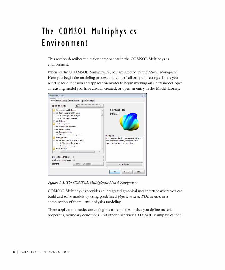
When starting COMSOL Multiphysics, you are greeted by the Model Navigator. Here you begin the modeling process and control all program settings. It lets you select space dimension and application modes to begin working on a new model, open an existing model you have already created, or open an entry in the Model Library.
Figure 1-1: The COMSOL Multiphysics Model Navigator.
COMSOL Multiphysics provides an integrated graphical user interface where you can build and solve models by using predefined physics modes, PDE modes, or a combination of them—multiphysics modeling.
These application modes are analogous to templates in that you define material properties, boundary conditions, and other quantities; COMSOL Multiphysics then
1 : I N T R O D U C T I O N
creates the PDEs. Application modes supply models for performing studies in areas such as:
• Acoustics
• Diffusion
• Electromagnetics
• Fluid mechanics
• Heat transfer
• Structural mechanics
• PDEs
2D, 3D, and axisymmetric variants are available for most application modes. You can find extensive information about the application modes in the COMSOL Multiphysics Modeling Guide.
To illustrate the uses of these application modes and other ways to put COMSOL Multiphysics to work, we include prewritten ready-to-run models of familiar and interesting problems in the Model Library. This consists of two elements: model files installed with COMSOL Multiphysics and a dedicated manual (the COMSOL Multiphysics Model Library). Simply load one of them into the Model Navigator and click the Solve button to watch it run. As noted earlier, each model includes extensive documentation complete with technical background, a discussion of the results, and step-by-step descriptions of how to set up the model.
In a short time, though, you will want to start creating your own models. An important part of the process is creating the geometry. The COMSOL Multiphysics user interface contains a set of CAD tools for geometry modeling in 1D, 2D, and 3D. The package can also import geometries using the DXF, GDS, STL, VRML, and COMSOL file formats. COMSOL Multiphysics can also directly import 3D meshes on NASTRAN format. In combination with the programming tools, you can even use images and magnetic resonance imaging (MRI) data to create a geometry.
In creating models you also have great flexibility in setting up various constants and variables using a number of variables as well as mathematical and logical functions. In the COMSOL programming environment you can work with the COMSOL Script language or the MATLAB language to define material properties, loads, sources, and boundary conditions.
T H E C O M S O L M U L T I P H Y S I C S E N V I R O N M E N T | 9
10 | C H A P T E R
When the geometry is complete and the parameters are defined, COMSOL Multiphysics automatically meshes the geometry. However, you can take charge of the mesh-generation process through a set of control parameters.
Next comes the solution stage. Here COMSOL Multiphysics comes with a suite of solvers, all developed by leading experts, for stationary, eigenvalue, and time-dependent problems. For solving linear systems, the software features both direct and iterative solvers. A range of preconditioners are available for the iterative solvers. COMSOL Multiphysics sets up solver defaults appropriate for the chosen application mode and automatically detects linearity and symmetry in the model. A segregated solver provides efficient solution schemes for large multiphysics models, turbulence modeling, and other challenging applications. You can record sequential solver calls to a solver script that you can further edit and run to automate the solution process.
For postprocessing, COMSOL Multiphysics provides tools for plotting and postprocessing any model quantity or parameter:
• Surface plots
• Slice plots
• Isosurfaces
• Contour plots
• Deformed shape plots
• Arrow plots
• Streamline plots and particle tracing
• Cross-sectional plots
• Animations
• Data display and interpolation
• Integration on boundaries and subdomains
In addition, you can continue the postprocessing in the COMSOL Script environment, where you can work with COMSOL Multiphysics data structures and functions using script programming.
To document your models, the COMSOL Multiphysics Report Generator provides a comprehensive report of the entire model, including graphics of the geometry, mesh, and postprocessing quantities. You can print the report directly or save it as an HTML file for viewing through a web browser and further editing.
1 : I N T R O D U C T I O N
Th e COMSOL Modu l e s
The optional modules
• AC/DC Module
• Acoustics Module
• Chemical Engineering Module
• Earth Science Module
• Heat Transfer Module
• MEMS Module
• RF Module
• Structural Mechanics Module
are optimized for specific application areas. They offer discipline-standard terminology and interfaces, materials libraries, specialized solvers, elements, and visualization tools.
The AC/DC Module
The AC/DC Module provides a unique environment for simulation of AC/DC electromagnetics in 2D and 3D. The AC/DC Module is a powerful tool for detailed analysis of coils, capacitors, and electrical machinery. With this module you can run static, quasi-static, transient, and time-harmonic simulations in an easy-to-use graphical user interface.
The available application modes cover the following types of electromagnetics field simulations:
• Electrostatics
• Conductive media DC
• Magnetostatics
• Low-frequency electromagnetics
Material properties include inhomogeneous and fully anisotropic materials, media with gains or losses, and complex-valued material properties. Infinite elements makes it possible to model unbounded domains. In addition to the standard postprocessing features, the AC/DC Module supports direct computation of lumped parameters such as capacitances and inductances as well as electromagnetic forces and torques. With the
T H E C O M S O L M O D U L E S | 11

12 | C H A P T E R
multiphysics capabilities of COMSOL Multiphysics, you can couple simulations with heat transfer, structural mechanics, fluid flow formulations, and any other physical phenomena.
The Acoustics Module
The Acoustics Module provides tailored interfaces for modeling of acoustics in fluids and solids. The module supports time-harmonic, modal, and transient analyses for fluid pressure as well as static, transient, eigenfrequency, and frequency-response analyses for structures. The available application modes include:
• Pressure acoustics
• Aeroacoustics (acoustics in an ideal gas with an irrotational mean flow)
• Compressible irrotational flow
• Plane strain, axisymmetric stress/strain, and 3D stress/strain
For the pressure acoustics applications, you can choose to analyze the scattered wave in addition to the total wave. PMLs (perfectly matched layers) provide accurate simulations of open pipes and other models with unbounded domains. The modeling domain can include dipole sources as well as monopole sources, and it is easy to specify point sources in terms of flow, intensity, or power. The module also includes modeling support for several types of damping. For postprocessing of pressure acoustics models, you can compute the far field.
Typical application areas for the Acoustics Module include:
• Automotive applications such as mufflers and car interiors
• Modeling of loudspeakers and microphones
• Aeroacoustics
• Underwater acoustics
Using the full multiphysics couplings within the COMSOL Multiphysics environment, you can couple the acoustic waves to, for example, an electromagnetic analysis or a structural analysis for acoustic-structure interaction.
The Chemical Engineering Module
The Chemical Engineering Module presents a powerful way of modeling equipment and processes in chemical engineering. It provides customized interfaces and
1 : I N T R O D U C T I O N

formulations for momentum, mass, and heat transport coupled with chemical reactions for applications such as:
• Reaction engineering and design
• Heterogeneous catalysis
• Separation processes
• Fuel cells and industrial electrolysis
• Process control together with Simulink
COMSOL Multiphysics excels in solving systems of coupled nonlinear PDEs that can include:
• Heat transfer
• Mass transfer through diffusion, convection, and migration
• Fluid dynamics
• Chemical reaction kinetics
• Varying material properties
The multiphysics capabilities of COMSOL Multiphysics can fully couple and simultaneously model fluid flow, mass and heat transport, and chemical reactions.
In fluid dynamics you can model fluid flow through porous media or characterize flow with the incompressible Navier-Stokes equations. It is easy to represent chemical reactions by source or sink terms in mass and heat balances. These terms can be of arbitrary order. All formulations exist for both Cartesian and cylindrical coordinates (for axisymmetric models) as well as for stationary and time-dependent cases.
The available application modes are:
• Momentum balances
- Incompressible Navier-Stokes equations
- Darcy’s law
- Brinkman equations
- Non-Newtonian flow
- Nonisothermal and weakly compressible flow
- Turbulent flow, k-ε turbulence model
- Turbulent flow, k-ω turbulence model
- Multiphase flow
T H E C O M S O L M O D U L E S | 13
14 | C H A P T E R
• Energy balances
- Heat conduction
- Heat convection and conduction
• Mass balances
- Diffusion
- Convection and diffusion
- Electrokinetic flow
- Maxwell-Stefan diffusion and convection
- Nernst-Planck transport equations
The Earth Science Module
The earth and planets are giant laboratories that involve all manner of physics. The Earth Science Module combines application modes for fundamental processes and links to COMSOL Multiphysics and the other modules for structural mechanics and electromagnetics analyses. New physics represented include heating from radiogenic decay that produces the geotherm, which is the increase in background temperature with depth. The variably saturated flow application modes analyze unsaturated zone processes (important to environmentalists) and two-phase flow (of particular interest in the petroleum industry as well as steam-liquid systems). Important in earth sciences, the heat transfer and chemical transport application modes explicitly account for physics in the liquid, solid, and gas phases.
Available application modes are:
• Darcy’s law for hydraulic head, pressure head, and pressure
• Solute transport in saturated and variably saturated porous media
• Richards’ equation including nonlinear material properties using van Genuchten, Brooks and Carey, or user-defined parameters.
• Heat transfer by conduction and convection in porous media with one mobile fluid, one immobile fluid, and up to five solids
• Brinkman equations
• Incompressible Navier-Stokes equations
The Earth Science Module Model Library contains a number of interesting examples, both single physics and multiphysics. The plate boundary example shows three ways to analyze heat transfer where two plates come together. Poroelasticity illustrates two-way
1 : I N T R O D U C T I O N

link solid displacement and movement of fluids in pore spaces. The volcano model combines fluid flow with electromagnetics application modes. Several examples demonstrate interpolation from experimental data. Multiple flow laws are linked in the two-phase flow and Darcy–Brinkman–Navier-Stokes example near a well. This module combines new and existing physics in a form that earth scientists can readily use.
The Heat Transfer Module
The Heat Transfer Module supports all fundamental mechanisms of heat transfer, including conductive, convective, and radiative heat transfer (both surface-to-surface and surface-to-ambient radiation). Using the application modes in this module along with inherent multiphysics capabilities of COMSOL Multiphysics, you can model a temperature field in parallel with other physics—a powerful combination that makes your models even more accurate and representative of the real world.
Available application modes are:
• General heat transfer, including conduction, convection, and surface-to-surface radiation
• Bioheat equation for heat transfer in biomedical systems
• Highly conductive layer for modeling of heat transfer in thin structures
• Nonisothermal flow appliction mode for nonisothermal incompressible fluid flow
• Turbulent flow, k-ε turbulence model
The Heat Transfer Module Model Library contains models, many with multiphysics couplings, that cover applications in electronics and power systems, process industries, and manufacturing industries. This Model Library also provides tutorial and benchmark models.
The MEMS Module
One of the most exciting areas of technology to emerge in recent years is MEMS (microelectromechanical systems), where engineers design and build systems with physical dimensions of micrometers. These miniature devices require multiphysics design and simulation tools because virtually all MEMS devices involve combinations of electrical, mechanical, and fluid-flow phenomena.
Available application modes are:
• Plane stress
T H E C O M S O L M O D U L E S | 15
16 | C H A P T E R
• Plane strain
• Axisymmetry, stress-strain
• Piezoelectric modeling in 2D plane stress and plane strain, axisymmetry, and 3D solids.
• 3D solids
• Electrokinetic flow
• General laminar flow
The MEMS Module Model Library contains a suite of models of MEMS devices such as sensors, actuators, and microfluidics systems. The models demonstrate a variety of multiphysics couplings and techniques for moving boundaries.
The RF Module
The RF Module provides a unique environment for the simulation of electromagnetic waves in 2D and 3D. With this module you can run harmonic, transient, and eigenfrequency simulations in an easy-to-use graphical user interface. For example, use the RF Module to simulate electromagnetic wave propagation in microwave components and photonic devices.
The RF Module is useful for component design in virtually all areas where you find electromagnetic waves, such as:
• Antennas
• Waveguides and cavity resonators in microwave engineering
• Optical fibers
• Photonic waveguides
• Photonic crystals
• Active devices in photonics
The available application modes cover the following types of electromagnetics field simulations:
• In-plane wave propagation
• Axisymmetric wave propagation
• Full 3D vector wave propagation
• Full vector mode analysis in 2D and 3D
1 : I N T R O D U C T I O N
Material properties include inhomogeneous and fully anisotropic materials, media with gains or losses, and complex-valued material properties. In addition to the standard postprocessing features, the RF Module supports direct computation of S-parameters and far-field patterns. You can add ports with a wave excitation with specified power level and mode type, and add PMLs (perfectly matched layers) to simulate electromagnetic waves that propagate into an unbounded domain. For time-harmonic simulations, you can use the scattered wave or the total wave. The multiphysics capabilities of COMSOL Multiphysics can couple simulations with heat transfer, structural mechanics, fluid flow formulations, and any physical phenomena.
The Structural Mechanics Module
The Structural Mechanics Module solves problems in structural mechanics and solid mechanics, adding special element types—beam, plate, and shell elements—for engineering simplifications.
Available application modes are:
• Plane stress
• Plane strain
• Axisymmetry, stress-strain
• Piezoelectric modeling
• 2D beams, Euler theory
• Thick plates, Mindlin theory
• 3D beams, Euler theory
• 3D solids
• Shells
Supporting both linear and nonlinear material models, the module’s analysis capabilities include static, eigenfrequency, transient, frequency response, and parametric analyses, as well as contact and friction.
The underlying equations for structural mechanics are always available—a feature unique to COMSOL Multiphysics. This equation-based modeling concept provides unsurpassed flexibility. The Structural Mechanics Module 3.4 includes interesting models that use this capability to model nonlinear materials such as rubber, viscoelastic, and viscoplastic materials. Material models can be isotropic, orthotropic, or fully anisotropic, and you can use local coordinate systems to specify material properties. In addition, advanced tools for fatigue analysis are available. The Structural
T H E C O M S O L M O D U L E S | 17

18 | C H A P T E R
Mechanics Module also features an extensible materials library and a beam cross-section library as well as command-line tools for flexible and extensible fatigue analysis tools from COMSOL Script or MATLAB.
1 : I N T R O D U C T I O N

T h e CAD Impo r t Modu l e s
COMSOL 3.4 includes packages for importing CAD drawings into COMSOL Multiphysics. A base package, the CAD Import Module, provides import of the most popular formats: Parasolid, SAT, STEP, and IGES. It also provides a live interface to SolidWorks. In addition, we provide a range of add-on modules that import additional formats.
• CAD Import Module, for importing CAD drawings in Parasolid, SAT (ACIS®), STEP, IGES formats, and a live interface to SolidWorks.
• Pro/E Import Module, which requires the CAD Import Module, imports CAD drawings in Pro/ENGINEER format.
• CATIA V4 Import Module, which requires the CAD Import Module, imports CAD drawings in CATIA V4 format.
• CATIA V5 Import Module, which requires the CAD Import Module, imports CAD drawings in CATIA V5 format.
• Inventor Import Module, which requires the CAD Import Module, imports CAD drawings in Autodesk Inventor format.
• VDA-FS Import Module, which requires the CAD Import Module, imports CAD drawings in VDA-FS format.
T H E C A D I M P O R T M O D U L E S | 19

20 | C H A P T E R
I n t e r n e t R e s ou r c e s
A number of Internet resources provide more information about COMSOL Multiphysics, including licensing and technical information. This section provides information about some of the most useful web links and email addresses.
COMSOL Web Sites
Main corporate website: http://www.comsol.com/
Worldwide contact information: http://www.comsol.com/contact/
Online technical support main page: http://www.comsol.com/support/
COMSOL Support Knowledge Base, your first stop for troubleshooting assistance, where you can search for answers to any COMSOL questions: http://www.comsol.com/support/knowledgebase/
Product updates: http://www.comsol.com/support/updates/
C O N T A C T I N G C O M S O L B Y E M A I L
For general product information, contact COMSOL at [email protected].
Send your COMSOL technical support questions to [email protected]. You will receive an automatic notification and a case number by email.
If you have suggestions for future product enhancements, please share them with us by sending an email to [email protected].
COMSOL User Forums
On the COMSOL web site, we maintain a list of current COMSOL user forums: http://www.comsol.com/support/forums/
These can be Usenet newsgroups or user forums on other websites where COMSOL users share solutions and tips on COMSOL modeling and other issues related to COMSOL products. These user forums are typically independent and unmoderated.
1 : I N T R O D U C T I O N

Note: COMSOL’s technical staff participates in these user forums as individuals. To receive technical support from COMSOL for the COMSOL products, please contact your local COMSOL representative or COMSOL office, or send your questions to [email protected].
I N T E R N E T R E S O U R C E S | 21

22 | C H A P T E R
1 : I N T R O D U C T I O N
2
G e o m e t r y M o d e l i n g a n d C A D T o o l s
The CAD tools in COMSOL Multiphysics provide many possibilities to create geometries using solid modeling and boundary modeling. This chapter covers geometry modeling in 1D, 2D, and 3D with examples of solid modeling, boundary modeling, Boolean operators, and other CAD tools in COMSOL Multiphysics. In addition, it shows how to use the tools for exploring geometric properties. This chapter also provides information about using external CAD data and geometries defined using image data.
23
24 | C H A P T E R
Th e COMSOL Mu l t i p h y s i c s Geome t r y and CAD En v i r o nmen t
Overview of Geometry Modeling Concepts
In COMSOL Multiphysics you can use solid modeling or boundary modeling to create objects in 1D, 2D, and 3D. They can be combined in the same geometry (hybrid modeling).
During solid modeling you form a geometry as a combination of solid objects using Boolean operations like union, intersection, and difference. Objects formed by combining a collection of existing solids using Boolean operations are known as composite solid objects. Boundary modeling is the process of defining a solid in terms of its boundaries. You can combine such a solid with geometric primitives—common solid modeling shapes like rectangles, circles, blocks, cones, and spheres, which are directly available in COMSOL Multiphysics.
In 3D, you can form 3D solid objects by defining 2D solids in work planes and then extrude and revolve these into 3D solids. It is also possible to embed 2D objects in the 3D geometry.
You can also overlay additional nonsolid objects on top of solid objects to control the distribution of the mesh and to improve postprocessing capabilities. For example, add a curve object to a geometry to control the element size along a 3D curve or add a point to guarantee a mesh vertex in a specific location.
All this means that you can work both with a “top-down” approach starting with geometric primitives and a “bottom-up” approach using boundary modeling.
You can import 2D geometries from DXF and GDS files and 3D geometries from STL and VRML files. See “Importing and Exporting Geometry Objects and CAD Models” on page 85 for a description of how to use these CAD file formats. The CAD Import Module provides an interface for import of Parasolid, SAT (ACIS), STEP, and IGES formats. In addition, the Pro/E Import Module, CATIA V4 Import Module, CATIA V5 Import Module, Inventor Import Module, and the VDA-FS Import Module are available for import of CAD data on the formats specific to those 3D CAD packages and standards.
2 : G E O M E T R Y M O D E L I N G A N D C A D TO O L S
For details on the following features that are available through scripting in COMSOL Script or MATLAB, see the COMSOL Multiphysics Scripting Guide and the COMSOL Multiphysics Reference Guide:
• Converting images and MRI data into a COMSOL Multiphysics geometry.
• Creating 2D and 3D spline curves and surface interpolation of measured data and insert objects into COMSOL Multiphysics.
Setting up Axes and Grid
In the COMSOL Multiphysics user interface you can set limits for the model axes and adjust the grid lines. The grid and axis settings help you get just the right view to produce a model geometry. To change these settings, use the Axes/Grid Settings dialog box that you open from the Options menu. You can also set the axis limits with the zoom functions.
A X I S S E T T I N G S
On the Axis page you can set the limits for all axes in the coordinate system.
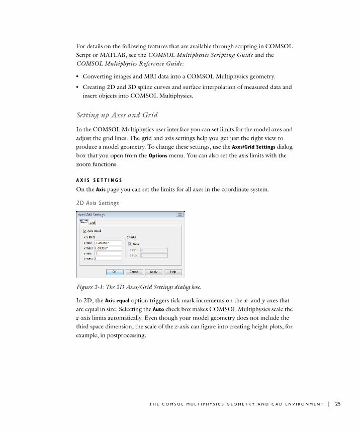
2D Axis Settings
Figure 2-1: The 2D Axes/Grid Settings dialog box.
In 2D, the Axis equal option triggers tick mark increments on the x- and y-axes that are equal in size. Selecting the Auto check box makes COMSOL Multiphysics scale the z-axis limits automatically. Even though your model geometry does not include the third space dimension, the scale of the z-axis can figure into creating height plots, for example, in postprocessing.
T H E C O M S O L M U L T I P H Y S I C S G E O M E T R Y A N D C A D E N V I R O N M E N T | 25
26 | C H A P T E R
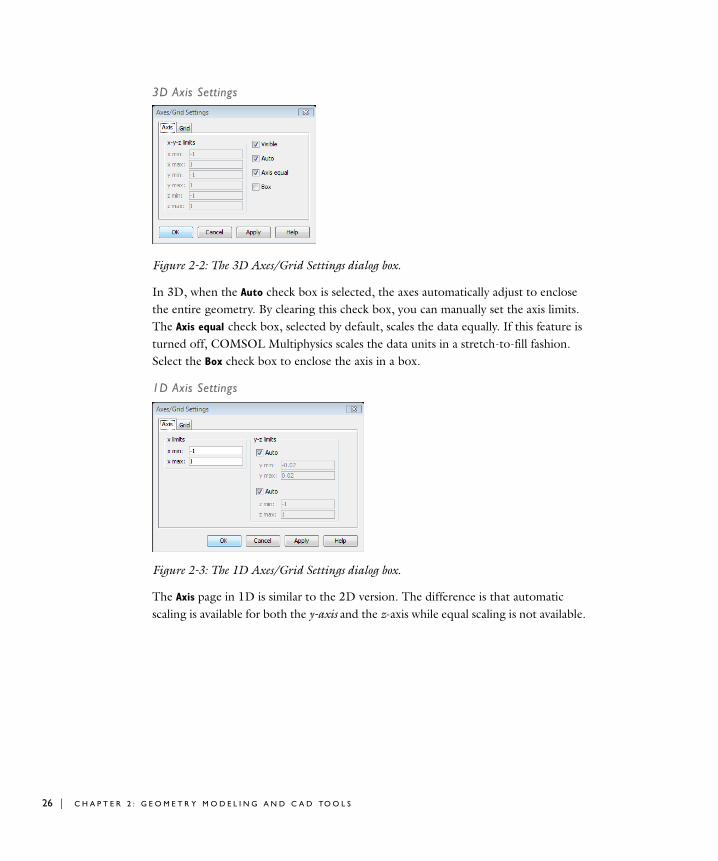
3D Axis Settings
Figure 2-2: The 3D Axes/Grid Settings dialog box.
In 3D, when the Auto check box is selected, the axes automatically adjust to enclose the entire geometry. By clearing this check box, you can manually set the axis limits. The Axis equal check box, selected by default, scales the data equally. If this feature is turned off, COMSOL Multiphysics scales the data units in a stretch-to-fill fashion. Select the Box check box to enclose the axis in a box.
1D Axis Settings
Figure 2-3: The 1D Axes/Grid Settings dialog box.
The Axis page in 1D is similar to the 2D version. The difference is that automatic scaling is available for both the y-axis and the z-axis while equal scaling is not available.
2 : G E O M E T R Y M O D E L I N G A N D C A D TO O L S
G R I D S E T T I N G S
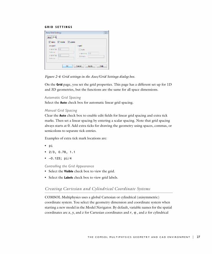
Figure 2-4: Grid settings in the Axes/Grid Settings dialog box.
On the Grid page, you set the grid properties. This page has a different set up for 1D and 3D geometries, but the functions are the same for all space dimensions.
Automatic Grid SpacingSelect the Auto check box for automatic linear grid spacing.
Manual Grid SpacingClear the Auto check box to enable edit fields for linear grid spacing and extra tick marks. Then set a linear spacing by entering a scalar spacing. Note that grid spacing always starts at 0. Add extra ticks for drawing the geometry using spaces, commas, or semicolons to separate tick entries.
Examples of extra tick mark locations are:
• pi
• 2/3, 0.78, 1.1
• –0.123; pi/4
Controlling the Grid Appearance• Select the Visible check box to view the grid.
• Select the Labels check box to view grid labels.
Creating Cartesian and Cylindrical Coordinate Systems
COMSOL Multiphysics uses a global Cartesian or cylindrical (axisymmetric) coordinate system. You select the geometry dimension and coordinate system when starting a new model in the Model Navigator. By default, variable names for the spatial coordinates are x, y, and z for Cartesian coordinates and r, , and z for cylindrical ϕ
T H E C O M S O L M U L T I P H Y S I C S G E O M E T R Y A N D C A D E N V I R O N M E N T | 27

28 | C H A P T E R
coordinates. These coordinate variables (together with the time for time-dependent models) make up the independent variables in COMSOL Multiphysics models.
T H E C O O R D I N A T E S Y S T E M S A N D T H E S P A C E D I M E N S I O N
The default names for coordinate systems vary with the space dimension:
• Models that you open using the space dimensions 1D, 2D, and 3D use the Cartesian coordinates x, y, and z.
• In 1D axisymmetric geometries the default coordinate is r, the radial direction. The x-axis represents r.
• In 2D axisymmetric geometries the x-axis represents r, the radial direction, and the y-axis represents z, the height coordinate.
For axisymmetric cases the geometry model must fall in the half plane r ≥ 0.
To select the coordinate system and space dimension, select 1D, 2D, 3D, Axial symmetry
(1D), or Axial symmetry (2D) from the Space dimension list in the Model Navigator. You can do this before starting a new model or by clicking the Add Geometry button when creating models with multiple geometries.
Note: Not all application modes are available for all coordinate systems and space dimensions.
2 : G E O M E T R Y M O D E L I N G A N D C A D TO O L S
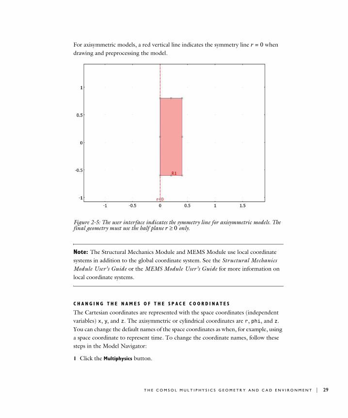
For axisymmetric models, a red vertical line indicates the symmetry line r = 0 when drawing and preprocessing the model.
Figure 2-5: The user interface indicates the symmetry line for axisymmetric models. The final geometry must use the half plane r ≥ 0 only.
Note: The Structural Mechanics Module and MEMS Module use local coordinate systems in addition to the global coordinate system. See the Structural Mechanics Module User’s Guide or the MEMS Module User’s Guide for more information on local coordinate systems.
C H A N G I N G T H E N A M E S O F T H E S P A C E C O O R D I N A T E S
The Cartesian coordinates are represented with the space coordinates (independent variables) x, y, and z. The axisymmetric or cylindrical coordinates are r, phi, and z. You can change the default names of the space coordinates as when, for example, using a space coordinate to represent time. To change the coordinate names, follow these steps in the Model Navigator:
1 Click the Multiphysics button.
T H E C O M S O L M U L T I P H Y S I C S G E O M E T R Y A N D C A D E N V I R O N M E N T | 29

30 | C H A P T E R
2 Click the Add Geometry button.
3 Select the space dimension from the Space dimension list. This provides the predefined names for the independent variables.
4 Replace the predefined names for the space coordinates by entering the names you want in the Independent variables edit field. Each name should be separated by a space, and the number of variables must equal the number of space dimensions.
Many 2D application modes use the third space dimension to represent other information, such as time. We recommend, therefore, that you always specify three different space coordinates. Note that if you do not specify a third space coordinate, COMSOL Multiphysics uses the default name (z for Cartesian geometries and phi for axisymmetric geometries).
5 Click OK.
6 Select one or more application modes and click Add to add physics or equations to the geometry unless you want to work with just the geometry and the mesh.
Note: Variables that depend on space coordinates, such as vector-field components and space derivatives, use the independent variable names for the geometry where they are defined. For example, if the dependent variable in the model is the pressure p, you access the derivative of pressure with respect to x by typing px in an edit field. These variable names change according to the names you assign to the independent variables. See “Variable Naming Conventions” on page 164 for more information about variable names.
The Status Bar
At the bottom of the COMSOL Multiphysics user interface a status bar shows information and provides buttons for changing some user interface properties. The contents depend on the space dimensions of the current geometry in your model.
Figure 2-6: The status bar.
2 : G E O M E T R Y M O D E L I N G A N D C A D TO O L S
Double-clicking a status bar button toggles its features on and off. The status bar components are (from left to right):
• Information field: Displays the current cursor position. In 2D Draw mode, this field shows displacements and dimensions of geometric objects when editing and creating those objects. In 3D, it shows the current operation (pan, dolly in/out, and so on) when you change the camera position, including the camera’s azimuth and elevation angles when orbiting.
• AXIS: Indicates the status of the axis (available in 3D only).
• GRID: Indicates the status of the grid lines.
• EQUAL: Indicates the status of the axis equal feature, where the aspect ratio is set for equal axis lengths (available in 2D and 3D only).
• SNAP: Indicates the status of the snap-to-grid and snap-to-vertex features (available in 1D and 2D Draw mode only).
• DIALOG: Indicates if geometry objects are specified using dialog boxes when using Draw toolbar buttons (available in 1D and 2D Draw mode only).
• MULTI: Indicates the status of the draw multiple objects property that lets you create multiple objects of the same type without having to clicking a Draw toolbar button for each object (available in 1D and 2D Draw mode only).
• SOLID: Indicates that geometry objects with closed boundaries are solidified (available in 2D Draw mode only).
• CSYS: Indicates the status (visible or hidden) of the 3D coordinate system in the lower left corner of the user interface (available in 3D only).
• Memory (in the lower right corner; available on Windows only): Displays the current and peak virtual memory usage in MB, separated by a slash. When the main user interface window is in focus and tooltip display is active, place the cursor over the Memory field to see also the current and peak physical memory usage. The physical memory usage includes, as a part, the Java heap, which holds the memory for postprocessing and visualization; see “Rendering and the Java Heap Space” on page 125 for more information on this topic.
Creating Composite Geometry Objects
You can form a composite geometry object by combining objects with Boolean operations: set union, set difference, and set intersection. You can form complex geometries using Boolean formulas that include multiple objects and operations. To
T H E C O M S O L M U L T I P H Y S I C S G E O M E T R Y A N D C A D E N V I R O N M E N T | 31

32 | C H A P T E R
perform Boolean operations, use the buttons in the Draw toolbar (2D and 3D) or work in the Create Composite Object dialog box.
U S I N G B O O L E A N O P E R A T I O N S F R O M T H E D R A W TO O L B A R
• Click the Union button to create the set union of the selected solid objects.
• Click the Intersection button to create the set intersection of the selected objects.
• Click the Difference button to create the set difference; this action subtracts the union of all other selected solid objects from the largest one.
U S I N G T H E C R E A T E C O M P O S I T E O B J E C T D I A L O G B O X
In 2D and 3D you can use the Create Composite Object dialog box to create a composite geometry object by combining the selected objects using Boolean operations. Open this dialog box from the Draw menu by choosing Create Composite Object or by pressing the Create Composite Object button on the Draw toolbar.
Figure 2-7: The Create Composite Object dialog box.
Using a Set FormulaChoose the solid objects that you want to work with from the list or select them directly in the drawing. Type a set formula that defines the Boolean operation into the Set formula edit field. The symbols +, -, and * represent set union, set difference, and set intersection, respectively. You can also use parentheses to form the set formulas. Click Apply to form a composite object by combining the selected solid objects according to the set formula. For example, typing (C1+R1)*E1 first forms the union of the rectangle R1 and the circle C1 and then forms the intersection of that union and the ellipse E1. Set formulas are only available for solid objects.
2 : G E O M E T R Y M O D E L I N G A N D C A D TO O L S

Using Shortcut ButtonsThe buttons in the Shortcuts area assist in forming unions and intersections of all selected objects. Use the Select All button to select every geometry object. By default, the set formula represents the union of all selected objects.
Keeping or Removing Interior Boundaries and EdgesSelect the Keep interior boundaries and Keep interior edges (3D only) check boxes to maintain the interior boundaries and edges for the different objects as you combine them. See “Removing Interior Boundaries” on page 35 for more information.
Repair of Composite ObjectsWhen creating a composite object, the software can repair the generated geometry object by removing small edges and faces. To use this feature, open the Create
Composite Object dialog box, select the Repair check box, then enter a value in the Repair tolerance edit field. This value is relative to the overall dimensions of the geometry. For example, if the dimensions are in meters, the default repair tolerance of 10−4 makes the geometry repair heal gaps that are smaller than about a tenth of a millimeter (10−4 m).
Forming Composite Geometry Objects from Nonsolid Geometry ObjectsTo create composite objects formed from a combination of solids, faces, curves, and points, you can also use the Coerce to Solid, Coerce to Face, or Coerce to Curve buttons on the Draw toolbar. For more information on coercing geometry objects, see “Coercing Geometry Objects” on page 34.
Moving, Rotating, Scaling, and Mirroring Geometry Objects
Moving, rotating, scaling, and mirroring are affine transformations that you can apply to geometry objects. The affine transformations appear on the Modify submenu in the Draw menu or by clicking the Move, Rotate, Scale and Mirror buttons on the Draw toolbar.
• Move—Specify displacements in all space directions
• Rotate—Specify the rotation angle with a rotation axis or center of rotation
• Scale—Specify scaling factors in all space directions
• Mirror—Specify the reflection axis or reflection plane
T H E C O M S O L M U L T I P H Y S I C S G E O M E T R Y A N D C A D E N V I R O N M E N T | 33
34 | C H A P T E R
Creating an Array of Geometry Objects
To create an array of identical geometry objects, choose Modify in the Draw menu and click Array or click the Array button in the Draw menu. This opens the Array dialog box where you can set the displacements and array size.
Copying and Pasting Geometry Objects
Press Ctrl+C or choose Copy from the Edit menu to copy the selected geometry objects to the COMSOL Multiphysics clipboard.
Press Ctrl+V or choose Paste from the Edit menu to paste the contents of the COMSOL Multiphysics clipboard into the current model. Use the Paste dialog box to specify the displacements of the pasted geometry objects. To paste many copies at the same time, specify several displacements as space-separated displacement coordinates. To paste duplicate geometry objects without using the Paste dialog box, choose Preferences in the Options menu and then clear the Paste geometry objects using dialog
box check box in the Preferences dialog box.
You can also create a copy of a geometry object by pressing the Ctrl key and then drag the copy of the selected object to a new location.
Coercing Geometry Objects
You can transform one or several geometry objects into an object of a different type by coercing the object, for example, from a solid to a curve. The resulting object is considered a composite object. The resulting object becomes a solid, face, curve, or point object depending on the target type that you choose in the Coerce To submenu in the Draw menu. You can also use the Coerce to Solid, Coerce to Face (3D only), and Coerce to Curve buttons as applicable.
The following combinations are meaningful:
2 D
• Coerce a solid object into a curve or point object.
• Coerce a curve object defining at least one closed domain into a solid object.
• Coerce a curve object into a point object.
3 D
• Coerce a solid object into a face, curve, or point object.
2 : G E O M E T R Y M O D E L I N G A N D C A D TO O L S
• Coerce a face object defining at least one closed domain into a solid object.
• Coerce a face object into a curve, or point object.
• Coerce a curve object into a point object.
Removing Interior Boundaries
Click the Delete Interior Boundaries toolbar button or choose the corresponding menu item in the Draw menu to delete interior boundaries. In 3D, this also removes edges that are not adjacent to any face and edges adjacent to one face only.
Splitting Geometry Objects
Split a geometry object into its parts by clicking the Split Object button on the Draw toolbar or by choosing Split Object in the Draw menu. This splits a solid object with several subdomains into solid objects representing each subdomain. It also splits face, curve, and point objects, which consist of several face, curve, and point segments, respectively, into face, curve, and point objects representing each segment.
Geometry Domain Names
Conceptually, a geometry is a collection of bounded geometric domains. The domains are connected manifolds, that is, volumes, surfaces, curves, or points. The following table summarizes the technical terms used for these domains:
Domains of maximal dimension are called subdomains. Domains of next to highest dimension are called boundaries. The boundaries are sometimes referred to as faces in 3D and edges in 2D. The vertices are also called points.
The following rules apply to the domains:
• The (interiors of the) domains are disjoint.
• Every domain is bounded by domains of smaller dimension. In particular, a subdomain (in 3D, 2D, or 1D) is bounded by boundaries, edges (in 3D), and
TABLE 2-1: DOMAIN NAMES IN DIFFERENT SPACE DIMENSIONS
DOMAIN DIMENSION NAME IN 3D NAME IN 2D NAME IN 1D NAME IN 0D
3 subdomain
2 boundary subdomain
1 edge boundary subdomain
0 vertex vertex boundary subdomain
T H E C O M S O L M U L T I P H Y S I C S G E O M E T R Y A N D C A D E N V I R O N M E N T | 35

36 | C H A P T E R
vertices (in 3D and 2D). A boundary (in 3D or 2D) is bounded by edges (in 3D) and vertices. An edge is bounded by vertices.
Viewing Geometries
When working with several geometries, you can display the active geometry along with several others. To do so, open the View Geometries dialog box from the Options menu. In the Visible geometries list select the ones to view in addition to the active geometry.
Entering Draw Mode
In certain situations, the Draw mode does not match the current analyzed geometry. This happens, for instance, when you replace the geometry and mesh by a deformed mesh, so that Draw mode still contains the original geometry while the analyzed geometry is the deformed geometry.
If you try to enter Draw mode when it does not match the analyzed geometry, the software displays the Enable Draw Mode dialog box where you can choose between keeping the geometry objects in Draw mode or replacing them with the analyzed geometry. When you have made your choice, click OK to enter Draw mode.
If there is no analyzed geometry, as when working with an imported mesh, the option to use the analyzed geometry is not available. In that case you can use the Create
Geometry From Mesh dialog box in the Mesh menu to create an analyzed geometry and a Draw mode object from the imported mesh.
Note: Opening Draw mode using the Use current Draw mode geometry objects option invalidates the old geometry, mesh, and solution.
2 : G E O M E T R Y M O D E L I N G A N D C A D TO O L S
C r e a t i n g a 1D Geome t r y Mode l
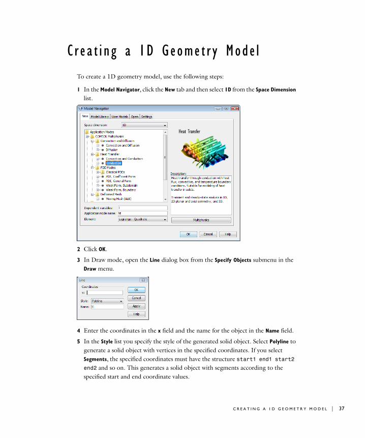
To create a 1D geometry model, use the following steps:
1 In the Model Navigator, click the New tab and then select 1D from the Space Dimension
list.
2 Click OK.
3 In Draw mode, open the Line dialog box from the Specify Objects submenu in the Draw menu.
4 Enter the coordinates in the x field and the name for the object in the Name field.
5 In the Style list you specify the style of the generated solid object. Select Polyline to generate a solid object with vertices in the specified coordinates. If you select Segments, the specified coordinates must have the structure start1 end1 start2 end2 and so on. This generates a solid object with segments according to the specified start and end coordinate values.
C R E A T I N G A 1 D G E O M E T R Y M O D E L | 37
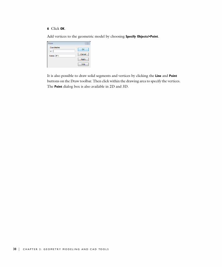
38 | C H A P T E R
6 Click OK.
Add vertices to the geometric model by choosing Specify Objects>Point.
It is also possible to draw solid segments and vertices by clicking the Line and Point buttons on the Draw toolbar. Then click within the drawing area to specify the vertices. The Point dialog box is also available in 2D and 3D.
2 : G E O M E T R Y M O D E L I N G A N D C A D TO O L S
C r e a t i n g a 2D Geome t r y Mode l
The first step in creating a 2D geometry model is to create a COMSOL Multiphysics model for that space dimension:
1 In the Model Navigator, click the New tab and then select 2D in the Space Dimension
list. Click OK.
2 Use the CAD tools in the Draw toolbar and the Draw menu to create the 2D geometry. (or import it from a DXF file).
See the following sections on how to use the 2D CAD tools.
Using the 2D Draw Toolbar and the Draw Menu
The default 2D Draw mode provides an additional toolbar for creating and editing geometry objects. This toolbar is also available in the 2D work planes of a 3D model. See the section “Creating and Using 2D Work Planes” on page 59 for details. All drawing tools that are available through the buttons are also accessible from the Draw
C R E A T I N G A 2 D G E O M E T R Y M O D E L | 39
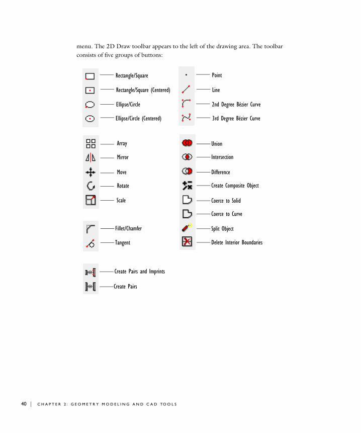
40 | C H A P T E R
menu. The 2D Draw toolbar appears to the left of the drawing area. The toolbar consists of five groups of buttons:
Rectangle/Square
Rectangle/Square (Centered)
Ellipse/Circle
Ellipse/Circle (Centered)
Point
Line
2nd Degree Bézier Curve
3rd Degree Bézier Curve
Array
Move
Rotate
Scale
Union
Intersection
Difference
Create Composite Object
Coerce to Curve
Split Object
Coerce to Solid
Delete Interior Boundaries
Fillet/Chamfer
Mirror
Tangent
Create Pairs and Imprints
Create Pairs
2 : G E O M E T R Y M O D E L I N G A N D C A D TO O L S

2 D G E O M E T R Y O B J E C T S
Figure 2-8: Different types of 2D geometry objects.
Using The Draw ToolbarThe Draw toolbar contains tools for creating 2D solid geometric primitives, lines, curves, and points:
• Rectangle/Square: Use the left mouse button to create a rectangle; use the right mouse button to create a square, with a reference point at the perimeter.
• Rectangle/Square (Centered): Use the left mouse button to create a rectangle; use the right mouse button to create a square, with a reference point at the center.
• Ellipse/Circle: Use the left mouse button to create an ellipse; use the right mouse button to create a circle, with a reference point at the perimeter.
• Ellipse/Circle (Centered): Use the left mouse button to create an ellipse; use the right mouse button to create a circle, with a reference point at the center.
• Point: Click in the drawing to add a point.
For all the above buttons, Shift-clicking the toolbar button opens a dialog box where you can specify the geometry object instead of creating it using the mouse. To make the dialog box appear directly (without Shift-clicking), double-click to select DIALOG in the status bar.
C R E A T I N G A 2 D G E O M E T R Y M O D E L | 41
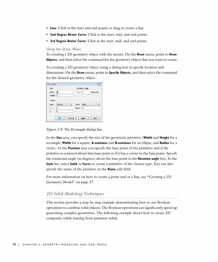
42 | C H A P T E R
• Line: Click at the start and end points or drag to create a line.
• 2nd Degree Bézier Curve: Click at the start, mid, and end points.
• 3rd Degree Bézier Curve: Click at the start, mid, and end points.
Using the Draw MenuTo creating a 2D geometry object with the mouse: On the Draw menu, point to Draw
Objects, and then select the command for the geometry object that you want to create.
To creating a 2D geometry object using a dialog box to specify location and dimensions: On the Draw menu, point to Specify Objects, and then select the command for the desired geometry object.
Figure 2-9: The Rectangle dialog box.
In the Size area, you specify the size of the geometric primitive (Width and Height for a rectangle, Width for a square, A-semiaxes and B-semiaxes for an ellipse, and Radius for a circle). In the Position area you specify the base point of the primitive and if the primitive is centered about that base point or if it has a corner in the base point. Specify the rotational angle (in degrees) about the base point in the Rotation angle box. In the Style list, select Solid or Curve to create a primitive of the chosen type. You can also specify the name of the primitive in the Name edit field.
For more information on how to create a point and or a line, see “Creating a 1D Geometry Model” on page 37.
2D Solid Modeling Techniques
This section provides a step-by-step example demonstrating how to use Boolean operations to combine solid objects. The Boolean operations can significantly speed up generating complex geometries. The following example shows how to create 2D composite solids starting from primitive solids.
2 : G E O M E T R Y M O D E L I N G A N D C A D TO O L S
S O L I D O B J E C T S
A solid object consists of an exterior boundary and an interior part. The boundary consists of edge segments. For example, a primitive solid rectangle has a boundary consisting of four line segments and one subdomain; a primitive solid circle has a boundary consisting of four circular arcs and one subdomain.
Sometimes a solid object has interior boundaries that divide it into more than one subdomain. Consider a square divided into four parts or subdomains. The subdomains can represent regions with different physics or material properties. You can also insert additional points and boundaries to control the mesh inside a solid object.
S T A R T I N G A 2 D M O D E L
Start a new 2D model by going to the Model Navigator and selecting 2D in the Space
dimension list on the New tab. Click OK.
C R E A T I N G H O L E S
First create a rectangle:
1 Click the corner-aligned rectangle button at the top of the Draw toolbar; alternately, go to the Draw menu, point to Draw Objects, and then click Rectangle/Square.
2 To describe the rectangle’s corners, click the left mouse button and drag the cursor from (−0.8, −0.8) to (0.8, 0.8).
Create a circular hole:
1 Click the centered ellipse button on the Draw toolbar.
2 Click the right mouse button and drag the cursor from (0, 0).
3 Release the mouse button when the solid circle has a radius of 0.4.
To drill a hole, create a composite solid object:
1 Press Ctrl+A to select both objects.
2 Click the Difference button on the Draw toolbar to create a hole.
COMSOL Multiphysics offers an alternative approach to drilling a hole:
1 Go to the Draw menu and choose Create Composite Object.
2 Click the Select All button.
C R E A T I N G A 2 D G E O M E T R Y M O D E L | 43
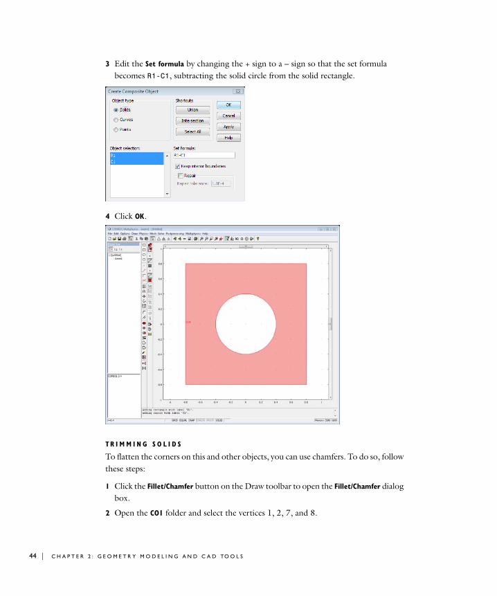
44 | C H A P T E R
3 Edit the Set formula by changing the + sign to a – sign so that the set formula becomes R1-C1, subtracting the solid circle from the solid rectangle.
4 Click OK.
TR I M M I N G S O L I D S
To flatten the corners on this and other objects, you can use chamfers. To do so, follow these steps:
1 Click the Fillet/Chamfer button on the Draw toolbar to open the Fillet/Chamfer dialog box.
2 Open the CO1 folder and select the vertices 1, 2, 7, and 8.
2 : G E O M E T R Y M O D E L I N G A N D C A D TO O L S
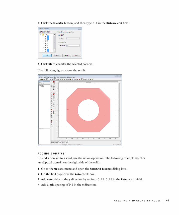
3 Click the Chamfer button, and then type 0.4 in the Distance edit field.
4 Click OK to chamfer the selected corners.
The following figure shows the result.
A D D I N G D O M A I N S
To add a domain to a solid, use the union operation. The following example attaches an elliptical domain on the right side of the solid:
1 Go to the Options menu and open the Axes/Grid Settings dialog box.
2 On the Grid page clear the Auto check box.
3 Add extra ticks in the y direction by typing -0.25 0.25 in the Extra y edit field.
4 Add a grid spacing of 0.1 in the x direction.
C R E A T I N G A 2 D G E O M E T R Y M O D E L | 45
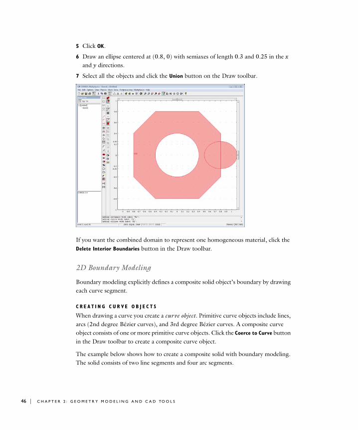
46 | C H A P T E R
5 Click OK.
6 Draw an ellipse centered at (0.8, 0) with semiaxes of length 0.3 and 0.25 in the x and y directions.
7 Select all the objects and click the Union button on the Draw toolbar.
If you want the combined domain to represent one homogeneous material, click the Delete Interior Boundaries button in the Draw toolbar.
2D Boundary Modeling
Boundary modeling explicitly defines a composite solid object’s boundary by drawing each curve segment.
C R E A T I N G C U R V E O B J E C T S
When drawing a curve you create a curve object. Primitive curve objects include lines, arcs (2nd degree Bézier curves), and 3rd degree Bézier curves. A composite curve object consists of one or more primitive curve objects. Click the Coerce to Curve button in the Draw toolbar to create a composite curve object.
The example below shows how to create a composite solid with boundary modeling. The solid consists of two line segments and four arc segments.
2 : G E O M E T R Y M O D E L I N G A N D C A D TO O L S
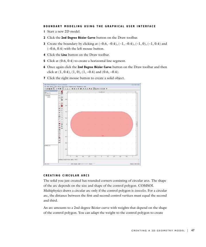
B O U N D A R Y M O D E L I N G U S I N G T H E G R A P H I C A L U S E R I N T E R F A C E
1 Start a new 2D model.
2 Click the 2nd Degree Bézier Curve button on the Draw toolbar.
3 Create the boundary by clicking at (−0.6, −0.4), (−1, −0.4), (−1, 0), (−1, 0.4) and (−0.6, 0.4) with the left mouse button.
4 Click the Line button on the Draw toolbar.
5 Click at (0.6, 0.4) to create a horizontal line segment.
6 Once again click the 2nd Degree Bézier Curve button on the Draw toolbar and then click at (1, 0.4), (1, 0), (1, −0.4) and (0.6, −0.4).
7 Click the right mouse button to create a solid object.
C R E A T I N G C I R C U L A R A R C S
The solid you just created has rounded corners consisting of circular arcs. The shape of the arc depends on the size and shape of the control polygon. COMSOL Multiphysics draws a circular arc only if the control polygon is isosceles. For a circular arc, the distance between the first and second control vertices must equal the second and third.
An arc amounts to a 2nd degree Bézier curve with weights that depend on the shape of the control polygon. You can adapt the weight to the control polygon to create
C R E A T I N G A 2 D G E O M E T R Y M O D E L | 47

48 | C H A P T E R
elliptical or circular curve segments. For more information on defining curves, see “Conic Sections” on page 483 in the COMSOL Multiphysics Reference Guide.
R A T I O N A L B É Z I E R C U R V E S
This section introduces the properties of rational Bézier curves.
Why Rational Bézier Curves?When you create a geometry object with a curved boundary, COMSOL Multiphysics represents it in terms of rational Bézier curves. Rational Bézier curves of 2nd degree represent all types of conic sections including circles, ellipses, parabolas, and hyperbolas. COMSOL Multiphysics includes 3rd degree rational Bézier curves to create additional free-form shapes. These include curves with inflection points (S-shaped curves) and advanced fillets.
Control Vertices and WeightsCOMSOL Multiphysics defines a rational Bézier curve of degree n in terms of a control polygon consisting of n+1 control vertices and n+1 associated control weights. The curve always interpolates the two end points of the control polygon. A change in the control polygon’s shape produces a change in the curve’s appearance. Its shape always mimics that of the control polygon. The higher the curve degree, n, the more complicated the shapes. Increasing the weight pulls the curve toward the corresponding control vertex.
This interaction between the control polygon and the curves makes the rational Bézier curve useful. Below are examples of how alterations in control vertices and weights affect curve shape.
Using the Graphical User InterfaceStart by examining an S-shaped 3rd degree rational Bézier curve. To produce this shape, position the control vertices at b0 = (−1, 0), b1 = (−0.4, 0.8), b2 = (0.6, −0.6),
2 : G E O M E T R Y M O D E L I N G A N D C A D TO O L S
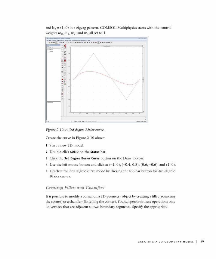
and b3 = (1, 0) in a zigzag pattern. COMSOL Multiphysics starts with the control weights w0, w1, w2, and w3 all set to 1.
Figure 2-10: A 3rd degree Bézier curve.
Create the curve in Figure 2-10 above:
1 Start a new 2D model.
2 Double-click SOLID on the Status bar.
3 Click the 3rd Degree Bézier Curve button on the Draw toolbar.
4 Use the left mouse button and click at (−1, 0), (−0.4, 0.8), (0.6, −0.6), and (1, 0).
5 Deselect the 3rd degree curve mode by clicking the toolbar button for 3rd-degree Bézier curves.
Creating Fillets and Chamfers
It is possible to modify a corner on a 2D geometry object by creating a fillet (rounding the corner) or a chamfer (flattening the corner). You can perform these operations only on vertices that are adjacent to two boundary segments. Specify the appropriate
C R E A T I N G A 2 D G E O M E T R Y M O D E L | 49
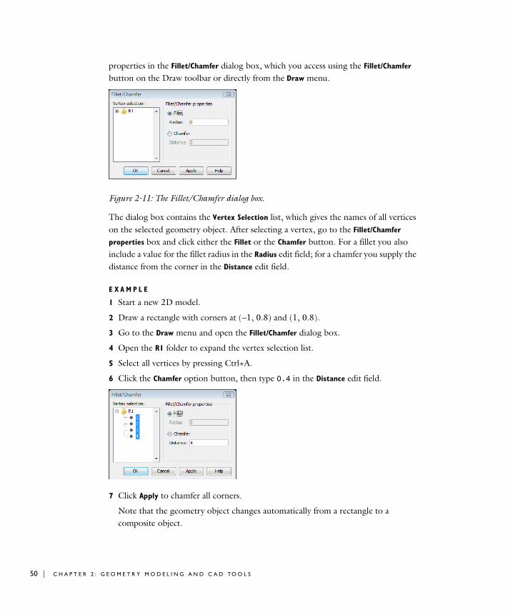
50 | C H A P T E R
properties in the Fillet/Chamfer dialog box, which you access using the Fillet/Chamfer button on the Draw toolbar or directly from the Draw menu.
Figure 2-11: The Fillet/Chamfer dialog box.
The dialog box contains the Vertex Selection list, which gives the names of all vertices on the selected geometry object. After selecting a vertex, go to the Fillet/Chamfer
properties box and click either the Fillet or the Chamfer button. For a fillet you also include a value for the fillet radius in the Radius edit field; for a chamfer you supply the distance from the corner in the Distance edit field.
E X A M P L E
1 Start a new 2D model.
2 Draw a rectangle with corners at (−1, 0.8) and (1, 0.8).
3 Go to the Draw menu and open the Fillet/Chamfer dialog box.
4 Open the R1 folder to expand the vertex selection list.
5 Select all vertices by pressing Ctrl+A.
6 Click the Chamfer option button, then type 0.4 in the Distance edit field.
7 Click Apply to chamfer all corners.
Note that the geometry object changes automatically from a rectangle to a composite object.
2 : G E O M E T R Y M O D E L I N G A N D C A D TO O L S
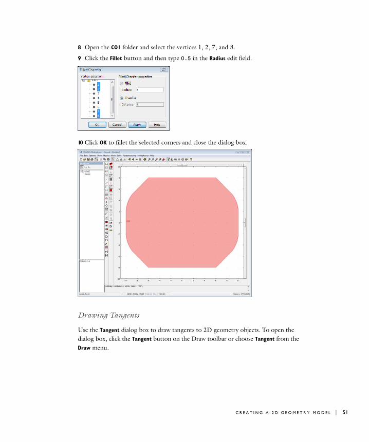
8 Open the CO1 folder and select the vertices 1, 2, 7, and 8.
9 Click the Fillet button and then type 0.5 in the Radius edit field.
10 Click OK to fillet the selected corners and close the dialog box.
Drawing Tangents
Use the Tangent dialog box to draw tangents to 2D geometry objects. To open the dialog box, click the Tangent button on the Draw toolbar or choose Tangent from the Draw menu.
C R E A T I N G A 2 D G E O M E T R Y M O D E L | 51
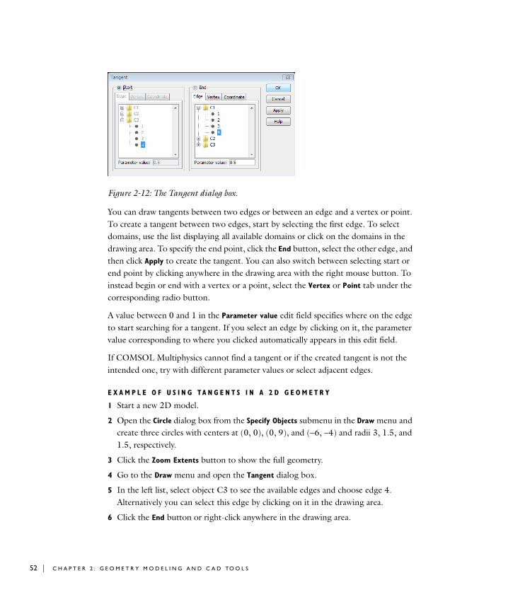
52 | C H A P T E R
Figure 2-12: The Tangent dialog box.
You can draw tangents between two edges or between an edge and a vertex or point. To create a tangent between two edges, start by selecting the first edge. To select domains, use the list displaying all available domains or click on the domains in the drawing area. To specify the end point, click the End button, select the other edge, and then click Apply to create the tangent. You can also switch between selecting start or end point by clicking anywhere in the drawing area with the right mouse button. To instead begin or end with a vertex or a point, select the Vertex or Point tab under the corresponding radio button.
A value between 0 and 1 in the Parameter value edit field specifies where on the edge to start searching for a tangent. If you select an edge by clicking on it, the parameter value corresponding to where you clicked automatically appears in this edit field.
If COMSOL Multiphysics cannot find a tangent or if the created tangent is not the intended one, try with different parameter values or select adjacent edges.
E X A M P L E O F U S I N G T A N G E N T S I N A 2 D G E O M E T R Y
1 Start a new 2D model.
2 Open the Circle dialog box from the Specify Objects submenu in the Draw menu and create three circles with centers at (0, 0), (0, 9), and (−6, −4) and radii 3, 1.5, and 1.5, respectively.
3 Click the Zoom Extents button to show the full geometry.
4 Go to the Draw menu and open the Tangent dialog box.
5 In the left list, select object C3 to see the available edges and choose edge 4. Alternatively you can select this edge by clicking on it in the drawing area.
6 Click the End button or right-click anywhere in the drawing area.
2 : G E O M E T R Y M O D E L I N G A N D C A D TO O L S

7 In the right list, select object C1 and choose edge 4. Alternatively you can select this edge by clicking on it in the drawing area.
8 Click Apply to create the tangent.
9 Repeat steps 4 and 5 to draw the following tangents:
- From object C1, edge 4 to object C2, edge 1.
- From object C2, edge 2 to object C1, edge 3.
- From object C1, edge 2 to object C3, edge 2.
10 Close the Tangent dialog box.
11 Select all geometries by pressing Ctrl+A and click the Coerce to Solid button in the Draw toolbar.
12 Double-click the object to display the Object Properties dialog box.
13 Select curve 3 and 4 and click the Delete button. Then close the dialog box.
14 Click the Fillet/Chamfer toolbar button in the Draw toolbar.
15 Select vertex 9, enter 2 in the Radius field, and click OK.
16 Open the Circle dialog box from the Specify Objects submenu in the Draw menu again and create three circles with centers at (0, 0), (0, 9), and (−6, −4) and radii 2, 1, and 1, respectively.
17 Select all geometries by pressing Ctrl+A and click the Difference toolbar button in the Draw toolbar.
C R E A T I N G A 2 D G E O M E T R Y M O D E L | 53
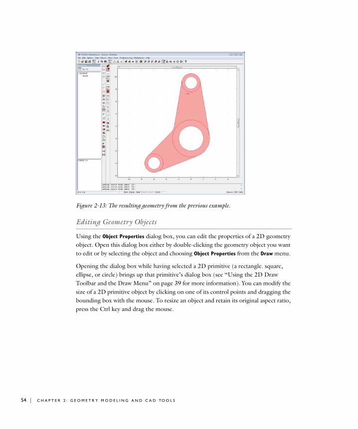
54 | C H A P T E R
Figure 2-13: The resulting geometry from the previous example.
Editing Geometry Objects
Using the Object Properties dialog box, you can edit the properties of a 2D geometry object. Open this dialog box either by double-clicking the geometry object you want to edit or by selecting the object and choosing Object Properties from the Draw menu.
Opening the dialog box while having selected a 2D primitive (a rectangle. square, ellipse, or circle) brings up that primitive’s dialog box (see “Using the 2D Draw Toolbar and the Draw Menu” on page 39 for more information). You can modify the size of a 2D primitive object by clicking on one of its control points and dragging the bounding box with the mouse. To resize an object and retain its original aspect ratio, press the Ctrl key and drag the mouse.
2 : G E O M E T R Y M O D E L I N G A N D C A D TO O L S
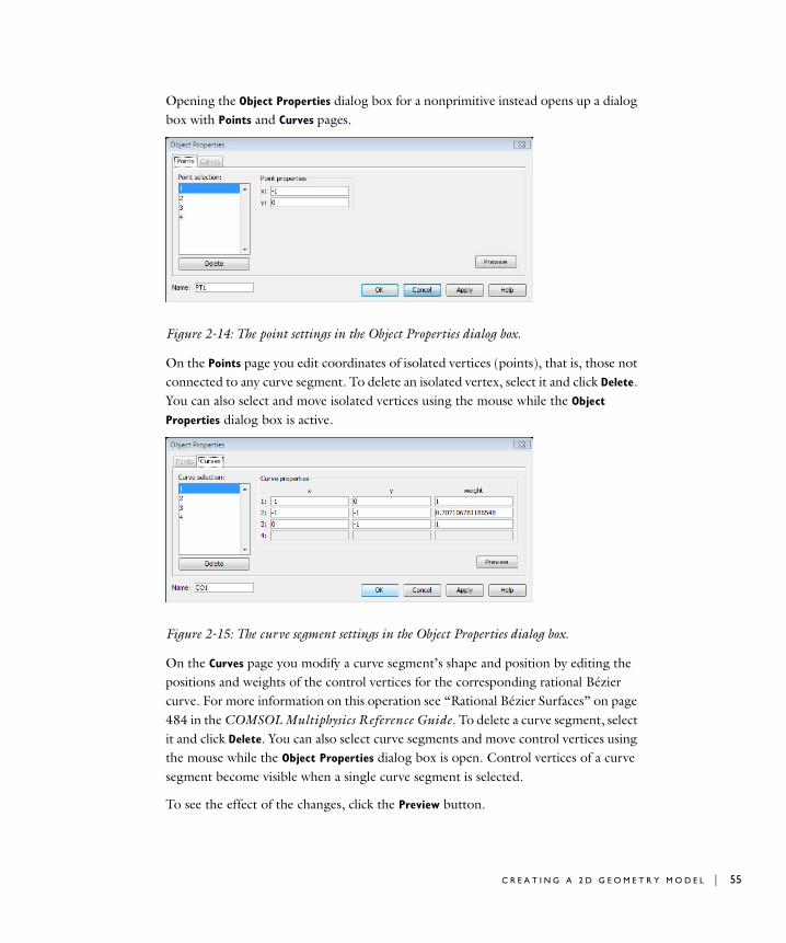
Opening the Object Properties dialog box for a nonprimitive instead opens up a dialog box with Points and Curves pages.
Figure 2-14: The point settings in the Object Properties dialog box.
On the Points page you edit coordinates of isolated vertices (points), that is, those not connected to any curve segment. To delete an isolated vertex, select it and click Delete. You can also select and move isolated vertices using the mouse while the Object
Properties dialog box is active.
Figure 2-15: The curve segment settings in the Object Properties dialog box.
On the Curves page you modify a curve segment’s shape and position by editing the positions and weights of the control vertices for the corresponding rational Bézier curve. For more information on this operation see “Rational Bézier Surfaces” on page 484 in the COMSOL Multiphysics Reference Guide. To delete a curve segment, select it and click Delete. You can also select curve segments and move control vertices using the mouse while the Object Properties dialog box is open. Control vertices of a curve segment become visible when a single curve segment is selected.
To see the effect of the changes, click the Preview button.
C R E A T I N G A 2 D G E O M E T R Y M O D E L | 55

56 | C H A P T E R
C r e a t i n g a 3D Geome t r y Mode l
The first step in creating a 3D geometry model is to create a COMSOL Multiphysics model with that space dimension:
1 In the Model Navigator, click the New tab and then select 3D from the Space
Dimension list. Click OK.
2 Use the tools in the Draw toolbar and the Draw menu to create the 3D geometry.
You can also start with a 2D geometry that acts as a work plane and then, for example, extrude the geometry into 3D space. This is often a better approach because you can use the 2D primitives, Boolean operators, and snapping tools before moving into 3D.
See the following sections on how to use the tools for creating 3D geometries.
Using the 3D Draw Toolbar and Draw Menu
The 3D Draw toolbar normally appears to the left of the drawing area. In the work planes an extended 2D Draw toolbar replaces the 3D Draw toolbar. You can access the drawing tools available via these buttons from the Draw menu as well. The toolbar contains four groups of buttons:
• Tools for drawing geometry primitives: solids, lines, and points
• Linear transformations
• Set operations and coercions
• Pair tools
2 : G E O M E T R Y M O D E L I N G A N D C A D TO O L S

Point
LineCone
Block
Cylinder
Sphere
Ellipsoid
Array
Move
Scale
Delete Interior Boundaries
Split Object
Coerce to Curve
Coerce to Face
Coerce to Solid
Create Composite Object
Difference
Intersection
Union
Rotate
Mirror
Create Pairs and Imprints
Create Pairs
C R E A T I N G A 3 D G E O M E T R Y M O D E L | 57
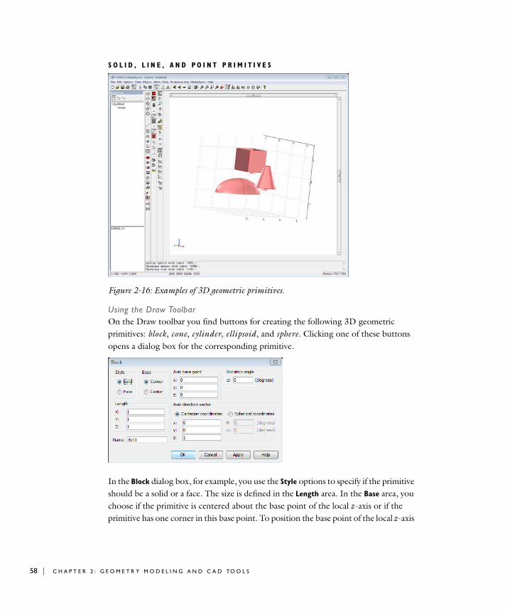
58 | C H A P T E R
S O L I D , L I N E , A N D P O I N T P R I M I T I V E S
Figure 2-16: Examples of 3D geometric primitives.
Using the Draw ToolbarOn the Draw toolbar you find buttons for creating the following 3D geometric primitives: block, cone, cylinder, ellipsoid, and sphere. Clicking one of these buttons opens a dialog box for the corresponding primitive.
In the Block dialog box, for example, you use the Style options to specify if the primitive should be a solid or a face. The size is defined in the Length area. In the Base area, you choose if the primitive is centered about the base point of the local z-axis or if the primitive has one corner in this base point. To position the base point of the local z-axis
2 : G E O M E T R Y M O D E L I N G A N D C A D TO O L S
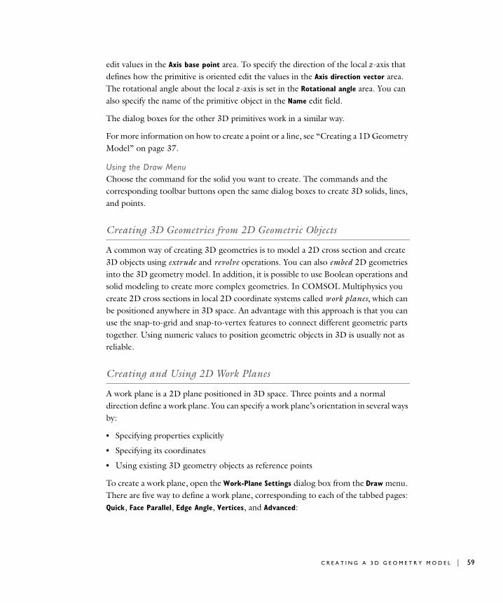
edit values in the Axis base point area. To specify the direction of the local z-axis that defines how the primitive is oriented edit the values in the Axis direction vector area. The rotational angle about the local z-axis is set in the Rotational angle area. You can also specify the name of the primitive object in the Name edit field.
The dialog boxes for the other 3D primitives work in a similar way.
For more information on how to create a point or a line, see “Creating a 1D Geometry Model” on page 37.
Using the Draw MenuChoose the command for the solid you want to create. The commands and the corresponding toolbar buttons open the same dialog boxes to create 3D solids, lines, and points.
Creating 3D Geometries from 2D Geometric Objects
A common way of creating 3D geometries is to model a 2D cross section and create 3D objects using extrude and revolve operations. You can also embed 2D geometries into the 3D geometry model. In addition, it is possible to use Boolean operations and solid modeling to create more complex geometries. In COMSOL Multiphysics you create 2D cross sections in local 2D coordinate systems called work planes, which can be positioned anywhere in 3D space. An advantage with this approach is that you can use the snap-to-grid and snap-to-vertex features to connect different geometric parts together. Using numeric values to position geometric objects in 3D is usually not as reliable.
Creating and Using 2D Work Planes
A work plane is a 2D plane positioned in 3D space. Three points and a normal direction define a work plane. You can specify a work plane’s orientation in several ways by:
• Specifying properties explicitly
• Specifying its coordinates
• Using existing 3D geometry objects as reference points
To create a work plane, open the Work-Plane Settings dialog box from the Draw menu. There are five way to define a work plane, corresponding to each of the tabbed pages: Quick, Face Parallel, Edge Angle, Vertices, and Advanced:
C R E A T I N G A 3 D G E O M E T R Y M O D E L | 59
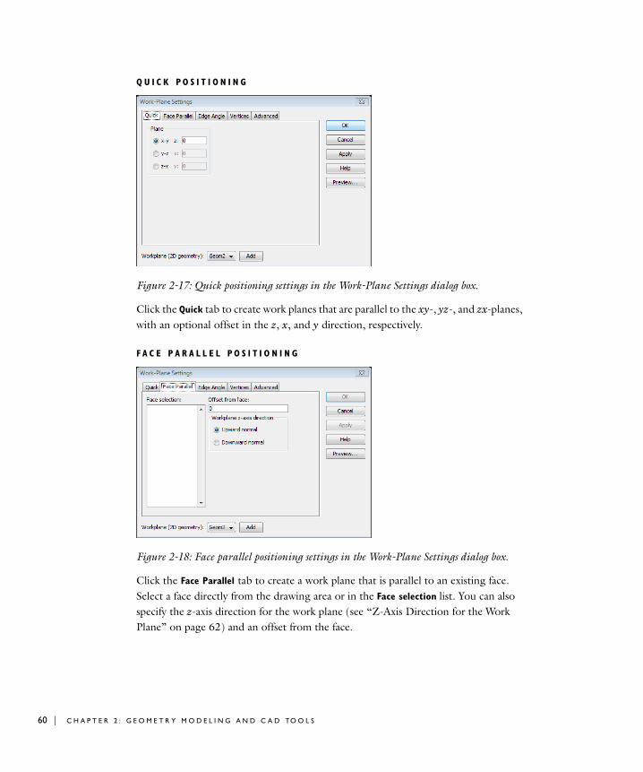
60 | C H A P T E R
Q U I C K P O S I T I O N I N G
Figure 2-17: Quick positioning settings in the Work-Plane Settings dialog box.
Click the Quick tab to create work planes that are parallel to the xy-, yz-, and zx-planes, with an optional offset in the z, x, and y direction, respectively.
F A C E P A R A L L E L P O S I T I O N I N G
Figure 2-18: Face parallel positioning settings in the Work-Plane Settings dialog box.
Click the Face Parallel tab to create a work plane that is parallel to an existing face. Select a face directly from the drawing area or in the Face selection list. You can also specify the z-axis direction for the work plane (see “Z-Axis Direction for the Work Plane” on page 62) and an offset from the face.
2 : G E O M E T R Y M O D E L I N G A N D C A D TO O L S
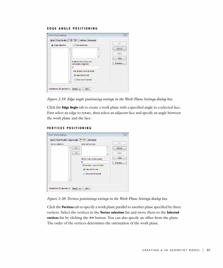
E D G E A N G L E P O S I T I O N I N G
Figure 2-19: Edge angle positioning settings in the Work-Plane Settings dialog box.
Click the Edge Angle tab to create a work plane with a specified angle to a selected face. First select an edge to rotate, then select an adjacent face and specify an angle between the work plane and the face.
VE R T I C E S P O S I T I O N I N G
Figure 2-20: Vertices positioning settings in the Work-Plane Settings dialog box.
Click the Vertices tab to specify a work plane parallel to another plane specified by three vertices. Select the vertices in the Vertex selection list and move them to the Selected
vertices list by clicking the >> button. You can also specify an offset from the plane. The order of the vertices determines the orientation of the work plane.
C R E A T I N G A 3 D G E O M E T R Y M O D E L | 61

62 | C H A P T E R
A D V A N C E D P O S I T I O N I N G
Figure 2-21: Advanced positioning settings in the Work-Plane Settings dialog box.
Click the Advanced page to define a work plane using three points in the 3D space. Type the coordinates for the three points in the edit fields in the Points in plane area.
Z-Axis Direction for the Work PlaneWhen defining a work plane parallel to the xy-plane, yz-plane, or zx-plane, using the Quick tab, the z-axis direction of the work plane is parallel to z-axis direction, x-axis direction, or y-axis direction of the 3D geometry model, respectively.
For the face parallel, edge angle, and vertices positioning, you can change the z-axis direction of the work plane by selecting the Upward normal or Downward normal button.
If you click the Advanced tab to define the work plane, the z-axis direction of the work plane is defined from the ordering of the specified vertices. The local z-axis direction is parallel to the cross product of the vector starting in the first vertex and ending in the second vertex with the vector starting in the first vertex and ending in the third vertex.
Preview SettingsTo help the creation of a work plane, the coordinate system and the geometry in the current work plane are visible while the Work-Plane Settings dialog is open. You can turn off the display of the coordinate system and the work plane geometry in the Preview Settings dialog box, which you open by clicking the Preview button.
2 : G E O M E T R Y M O D E L I N G A N D C A D TO O L S

Figure 2-22: The Preview Settings dialog box.
G E O M E T R Y P R O J E C T I O N I N WO R K P L A N E S
When you enter a work plane, a 2D Draw toolbar replaces the 3D Draw toolbar. See “Using the 2D Draw Toolbar and the Draw Menu” on page 39 for details. Three buttons in the Visualization/Selection toolbar determine which portion of the 3D geometry that the software projects onto the plane.
• Click the Projection of All 3D Geometries button to draw the projection of all 3D geometry edges
• Click the Project Work-Plane Intersection button to display only the edges that lie in the same plane as the work plane
• Click the No Projection button to display nothing of the 3D geometry.
Extruding, Revolving, and Embedding
COMSOL Multiphysics provides three ways of extending your 2D work plane geometries into 3D space:
• Extruding
• Revolving
• Embedding
Projection of All 3D Geometries
Project Work-Plane Intersection
No Projection
C R E A T I N G A 3 D G E O M E T R Y M O D E L | 63
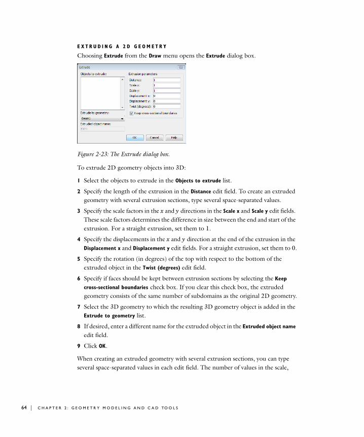
64 | C H A P T E R
E X T R U D I N G A 2 D G E O M E T R Y
Choosing Extrude from the Draw menu opens the Extrude dialog box.
Figure 2-23: The Extrude dialog box.
To extrude 2D geometry objects into 3D:
1 Select the objects to extrude in the Objects to extrude list.
2 Specify the length of the extrusion in the Distance edit field. To create an extruded geometry with several extrusion sections, type several space-separated values.
3 Specify the scale factors in the x and y directions in the Scale x and Scale y edit fields. These scale factors determines the difference in size between the end and start of the extrusion. For a straight extrusion, set them to 1.
4 Specify the displacements in the x and y direction at the end of the extrusion in the Displacement x and Displacement y edit fields. For a straight extrusion, set them to 0.
5 Specify the rotation (in degrees) of the top with respect to the bottom of the extruded object in the Twist (degrees) edit field.
6 Specify if faces should be kept between extrusion sections by selecting the Keep
cross-sectional boundaries check box. If you clear this check box, the extruded geometry consists of the same number of subdomains as the original 2D geometry.
7 Select the 3D geometry to which the resulting 3D geometry object is added in the Extrude to geometry list.
8 If desired, enter a different name for the extruded object in the Extruded object name edit field.
9 Click OK.
When creating an extruded geometry with several extrusion sections, you can type several space-separated values in each edit field. The number of values in the scale,
2 : G E O M E T R Y M O D E L I N G A N D C A D TO O L S

displacement, and twist edit fields must be single scalar values or equal to the number of values in the Distance edit field.
The figure below shows the result of an extrusion:
R E V O L V I N G A 2 D G E O M E T R Y
Choose Revolve from the Draw menu to open the Revolve dialog box. Here you create 3D objects by rotating the selected 2D geometry objects between two angles and about an axis of rotation:
Figure 2-24: The Revolve dialog box.
C R E A T I N G A 3 D G E O M E T R Y M O D E L | 65
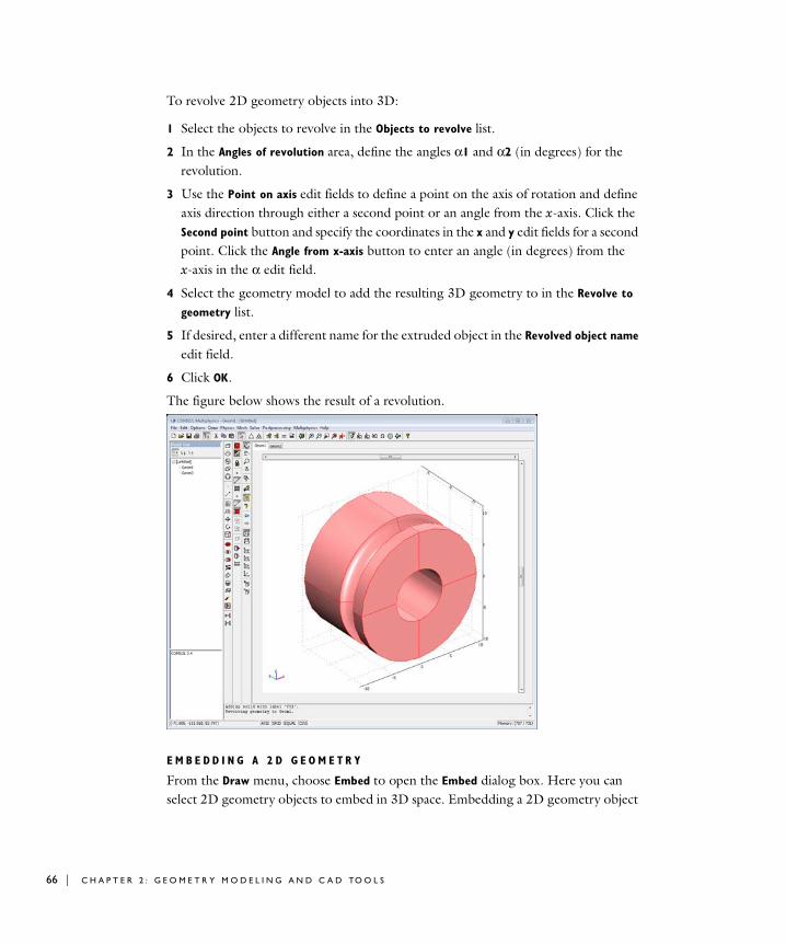
66 | C H A P T E R
To revolve 2D geometry objects into 3D:
1 Select the objects to revolve in the Objects to revolve list.
2 In the Angles of revolution area, define the angles α1 and α2 (in degrees) for the revolution.
3 Use the Point on axis edit fields to define a point on the axis of rotation and define axis direction through either a second point or an angle from the x-axis. Click the Second point button and specify the coordinates in the x and y edit fields for a second point. Click the Angle from x-axis button to enter an angle (in degrees) from the x-axis in the α edit field.
4 Select the geometry model to add the resulting 3D geometry to in the Revolve to
geometry list.
5 If desired, enter a different name for the extruded object in the Revolved object name edit field.
6 Click OK.
The figure below shows the result of a revolution.
E M B E D D I N G A 2 D G E O M E T R Y
From the Draw menu, choose Embed to open the Embed dialog box. Here you can select 2D geometry objects to embed in 3D space. Embedding a 2D geometry object
2 : G E O M E T R Y M O D E L I N G A N D C A D TO O L S
keeps its 2D properties while including it in the 3D geometry model. You can embed point objects, curve objects, and solid objects. You can also name the embedded object and select to which geometry model the software adds the resulting 3D geometry.
Solid Modeling Using Solid Objects and Boolean Operations
3 D S O L I D O B J E C T S
3D solid objects consist of a boundary part and an interior part. The boundary consists of face segments. A solid is defined by its exterior and interior boundaries. For example, a primitive solid block has a boundary that consists of six rectangular face segments and one subdomain. A primitive solid cylinder has a boundary consisting of two circular faces, four curved rectangular faces, and one subdomain.
S O L I D M O D E L I N G A N D B O O L E A N O P E R A T I O N S
The following example shows various solid modeling techniques, including the use of work planes and Boolean operations (union, intersection, and difference) to create composite solid objects. The Boolean operations are suited for swift generation of complex geometries. The example is not based on a real component. However, the intention is to cover 3D solid modeling in COMSOL Multiphysics for a geometry that could represent a common mechanical component.
C R E A T I N G A 3 D P U L L E Y G E O M E T R Y
This example creates a 3D pulley using two work planes from which you extrude and revolve 2D cross sections to create the full 3D geometry. Boolean operations, mirroring, rotations, and fillets help to create the 2D cross sections.
C R E A T I N G A 3 D G E O M E T R Y M O D E L | 67
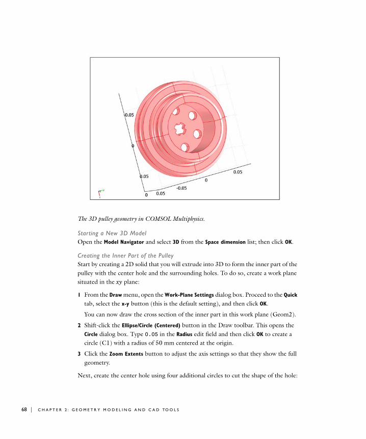
68 | C H A P T E R
The 3D pulley geometry in COMSOL Multiphysics.
Starting a New 3D ModelOpen the Model Navigator and select 3D from the Space dimension list; then click OK.
Creating the Inner Part of the PulleyStart by creating a 2D solid that you will extrude into 3D to form the inner part of the pulley with the center hole and the surrounding holes. To do so, create a work plane situated in the xy plane:
1 From the Draw menu, open the Work-Plane Settings dialog box. Proceed to the Quick tab, select the x-y button (this is the default setting), and then click OK.
You can now draw the cross section of the inner part in this work plane (Geom2).
2 Shift-click the Ellipse/Circle (Centered) button in the Draw toolbar. This opens the Circle dialog box. Type 0.05 in the Radius edit field and then click OK to create a circle (C1) with a radius of 50 mm centered at the origin.
3 Click the Zoom Extents button to adjust the axis settings so that they show the full geometry.
Next, create the center hole using four additional circles to cut the shape of the hole:
2 : G E O M E T R Y M O D E L I N G A N D C A D TO O L S
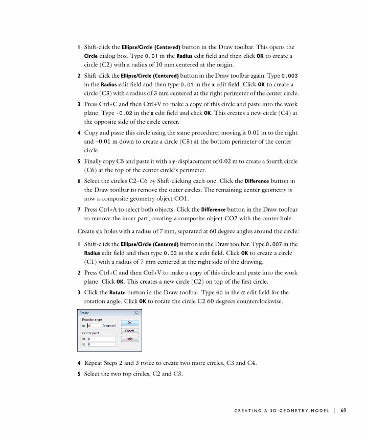
1 Shift-click the Ellipse/Circle (Centered) button in the Draw toolbar. This opens the Circle dialog box. Type 0.01 in the Radius edit field and then click OK to create a circle (C2) with a radius of 10 mm centered at the origin.
2 Shift-click the Ellipse/Circle (Centered) button in the Draw toolbar again. Type 0.003 in the Radius edit field and then type 0.01 in the x edit field. Click OK to create a circle (C3) with a radius of 3 mm centered at the right perimeter of the center circle.
3 Press Ctrl+C and then Ctrl+V to make a copy of this circle and paste into the work plane. Type -0.02 in the x edit field and click OK. This creates a new circle (C4) at the opposite side of the circle center.
4 Copy and paste this circle using the same procedure, moving it 0.01 m to the right and −0.01 m down to create a circle (C5) at the bottom perimeter of the center circle.
5 Finally copy C5 and paste it with a y-displacement of 0.02 m to create a fourth circle (C6) at the top of the center circle’s perimeter.
6 Select the circles C2–C6 by Shift-clicking each one. Click the Difference button in the Draw toolbar to remove the outer circles. The remaining center geometry is now a composite geometry object CO1.
7 Press Ctrl+A to select both objects. Click the Difference button in the Draw toolbar to remove the inner part, creating a composite object CO2 with the center hole.
Create six holes with a radius of 7 mm, separated at 60 degree angles around the circle:
1 Shift-click the Ellipse/Circle (Centered) button in the Draw toolbar. Type 0.007 in the Radius edit field and then type 0.03 in the x edit field. Click OK to create a circle (C1) with a radius of 7 mm centered at the right side of the drawing.
2 Press Ctrl+C and then Ctrl+V to make a copy of this circle and paste into the work plane. Click OK. This creates a new circle (C2) on top of the first circle.
3 Click the Rotate button in the Draw toolbar. Type 60 in the α edit field for the rotation angle. Click OK to rotate the circle C2 60 degrees counterclockwise.
4 Repeat Steps 2 and 3 twice to create two more circles, C3 and C4.
5 Select the two top circles, C2 and C3.
C R E A T I N G A 3 D G E O M E T R Y M O D E L | 69
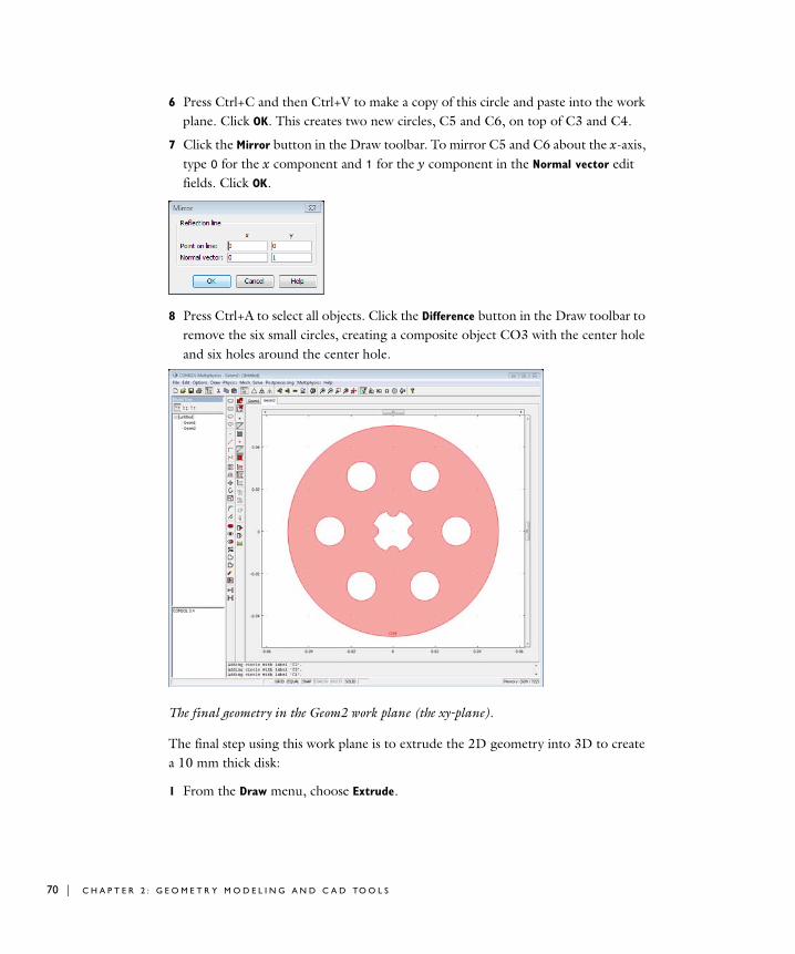
70 | C H A P T E R
6 Press Ctrl+C and then Ctrl+V to make a copy of this circle and paste into the work plane. Click OK. This creates two new circles, C5 and C6, on top of C3 and C4.
7 Click the Mirror button in the Draw toolbar. To mirror C5 and C6 about the x-axis, type 0 for the x component and 1 for the y component in the Normal vector edit fields. Click OK.
8 Press Ctrl+A to select all objects. Click the Difference button in the Draw toolbar to remove the six small circles, creating a composite object CO3 with the center hole and six holes around the center hole.
The final geometry in the Geom2 work plane (the xy-plane).
The final step using this work plane is to extrude the 2D geometry into 3D to create a 10 mm thick disk:
1 From the Draw menu, choose Extrude.
2 : G E O M E T R Y M O D E L I N G A N D C A D TO O L S
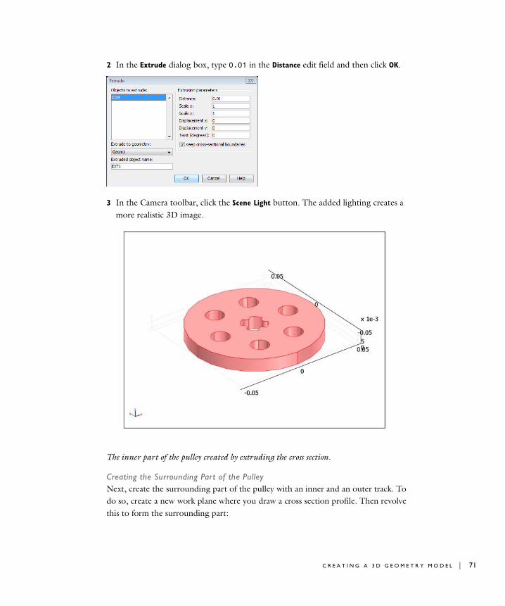
2 In the Extrude dialog box, type 0.01 in the Distance edit field and then click OK.
3 In the Camera toolbar, click the Scene Light button. The added lighting creates a more realistic 3D image.
The inner part of the pulley created by extruding the cross section.
Creating the Surrounding Part of the PulleyNext, create the surrounding part of the pulley with an inner and an outer track. To do so, create a new work plane where you draw a cross section profile. Then revolve this to form the surrounding part:
C R E A T I N G A 3 D G E O M E T R Y M O D E L | 71
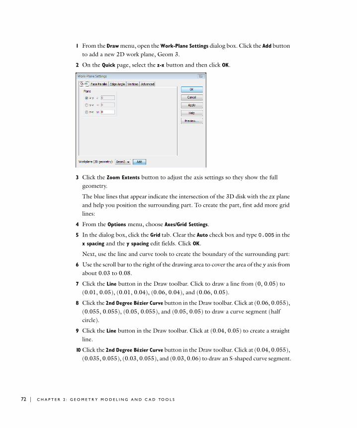
72 | C H A P T E R
1 From the Draw menu, open the Work-Plane Settings dialog box. Click the Add button to add a new 2D work plane, Geom 3.
2 On the Quick page, select the z-x button and then click OK.
3 Click the Zoom Extents button to adjust the axis settings so they show the full geometry.
The blue lines that appear indicate the intersection of the 3D disk with the zx plane and help you position the surrounding part. To create the part, first add more grid lines:
4 From the Options menu, choose Axes/Grid Settings.
5 In the dialog box, click the Grid tab. Clear the Auto check box and type 0.005 in the x spacing and the y spacing edit fields. Click OK.
Next, use the line and curve tools to create the boundary of the surrounding part:
6 Use the scroll bar to the right of the drawing area to cover the area of the y axis from about 0.03 to 0.08.
7 Click the Line button in the Draw toolbar. Click to draw a line from (0, 0.05) to (0.01, 0.05), (0.01, 0.04), (0.06, 0.04), and (0.06, 0.05).
8 Click the 2nd Degree Bézier Curve button in the Draw toolbar. Click at (0.06, 0.055), (0.055, 0.055), (0.05, 0.055), and (0.05, 0.05) to draw a curve segment (half circle).
9 Click the Line button in the Draw toolbar. Click at (0.04, 0.05) to create a straight line.
10 Click the 2nd Degree Bézier Curve button in the Draw toolbar. Click at (0.04, 0.055), (0.035, 0.055), (0.03, 0.055), and (0.03, 0.06) to draw an S-shaped curve segment.
2 : G E O M E T R Y M O D E L I N G A N D C A D TO O L S
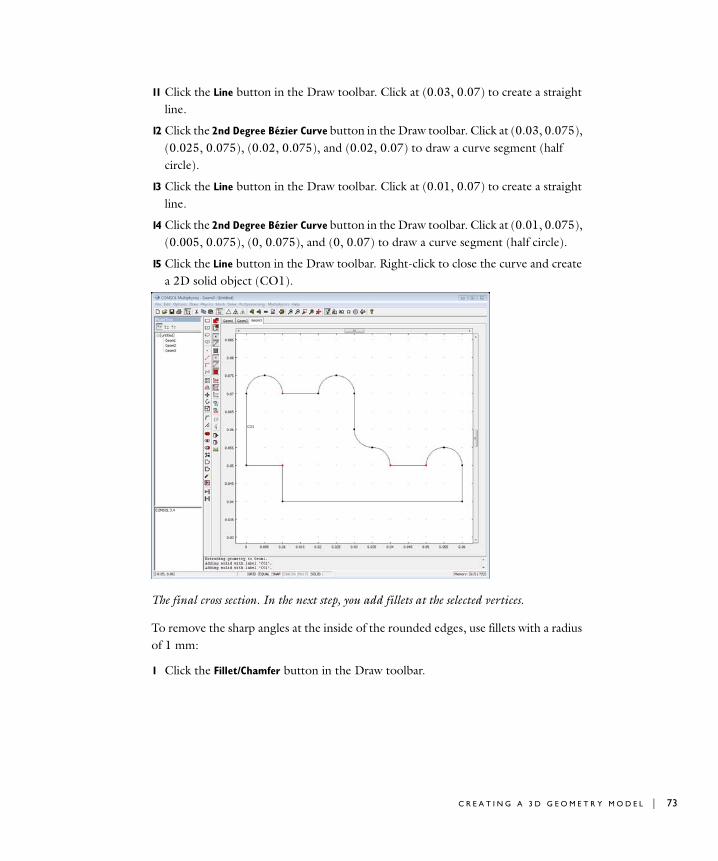
11 Click the Line button in the Draw toolbar. Click at (0.03, 0.07) to create a straight line.
12 Click the 2nd Degree Bézier Curve button in the Draw toolbar. Click at (0.03, 0.075), (0.025, 0.075), (0.02, 0.075), and (0.02, 0.07) to draw a curve segment (half circle).
13 Click the Line button in the Draw toolbar. Click at (0.01, 0.07) to create a straight line.
14 Click the 2nd Degree Bézier Curve button in the Draw toolbar. Click at (0.01, 0.075), (0.005, 0.075), (0, 0.075), and (0, 0.07) to draw a curve segment (half circle).
15 Click the Line button in the Draw toolbar. Right-click to close the curve and create a 2D solid object (CO1).
The final cross section. In the next step, you add fillets at the selected vertices.
To remove the sharp angles at the inside of the rounded edges, use fillets with a radius of 1 mm:
1 Click the Fillet/Chamfer button in the Draw toolbar.
C R E A T I N G A 3 D G E O M E T R Y M O D E L | 73

74 | C H A P T E R
2 Select Vertices (points) 5, 6, 12, and 13. Type 0.001 in the Radius edit field.
3 Click OK to create the fillets.
Finally, revolve this cross section a full revolution (360 degrees) about a rotation axis from (0, 0) to (1, 0) in the zx plane:
1 From the Draw menu, choose Revolve.
2 In the Revolve dialog box, type 1 in the x edit field and 0 in the y edit field under the Second point button in the Revolution axis area.
3 Click OK to create the 3D object and move to the 3D view.
4 Press Ctrl+A to select both 3D objects, click the Union button, and then click the Delete Interior Boundaries button (both in the Draw toolbar). This makes the entire pulley into one solid object with one single domain. If the parts are made of different materials, skip this step to keep two subdomains in the geometry.
This completes the pulley geometry. Meshing the geometry, you may have to adjust the resolution of narrow regions to avoid an excessive amount of mesh elements
2 : G E O M E T R Y M O D E L I N G A N D C A D TO O L S
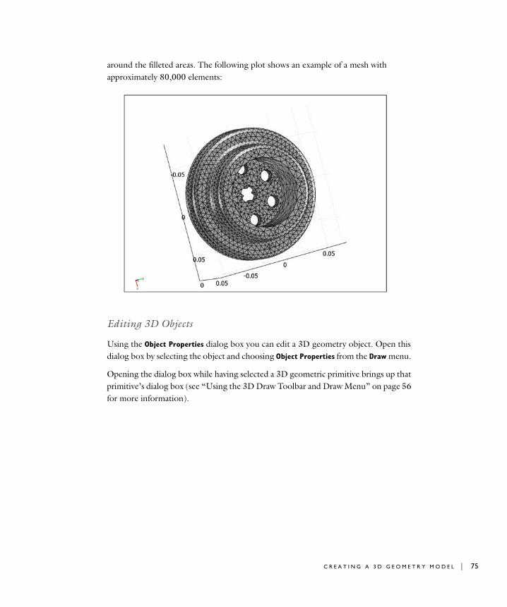
around the filleted areas. The following plot shows an example of a mesh with approximately 80,000 elements:
Editing 3D Objects
Using the Object Properties dialog box you can edit a 3D geometry object. Open this dialog box by selecting the object and choosing Object Properties from the Draw menu.
Opening the dialog box while having selected a 3D geometric primitive brings up that primitive’s dialog box (see “Using the 3D Draw Toolbar and Draw Menu” on page 56 for more information).
C R E A T I N G A 3 D G E O M E T R Y M O D E L | 75

76 | C H A P T E R
Opening the Object Properties dialog box when you have selected a nonprimitive object instead opens a dialog box where you can delete faces and change the name of the geometry object.
Figure 2-25: The Object Properties dialog box for a 3D solid object.
2 : G E O M E T R Y M O D E L I N G A N D C A D TO O L S
Exp l o r i n g Geome t r i c P r op e r t i e s
Introduction
COMSOL Multiphysics includes tools for exploring the following geometric properties of the model geometry:
• Volumes, areas, and lengths
• Surface areas, cross-section areas, and perimeters
• Point coordinates and distance between points
• Center of mass
• Moment of inertia (principal components and tensor components)
• Principal axes for the principal moment of inertia
The center of mass, moment of inertia, and principal axes depend on the density and are available during postprocessing only. The other geometric properties are available also during preprocessing and interactively from the Visualization/Selection toolbar.
You can select and copy the computed values for these geometric properties and then paste them into other settings in a model.
Using The Geometric Properties Dialog Box
You can open the Geometric Properties dialog box both from the Draw menu and from the Postprocessing menu.
G E O M E T R I C P R O P E R T I E S D I A L O G B O X O N T H E D R A W M E N U
The Geometric Properties dialog box on the Draw menu is available in Draw mode and includes the basic properties for the geometry objects in the model. It uses the rendering mesh and does not require a computational mesh or a solution. Use the following steps to display these geometric properties:
1 Make sure the user interface is in the Draw mode.
2 From the Draw menu, choose Geometric Properties.
3 In 3D, click the Subdomain tab to see the volume and surface area for the selected subdomains. The surface area is the area surrounding the selected domains and does not include any interior boundaries or free surfaces.
E X P L O R I N G G E O M E T R I C P R O P E R T I E S | 77
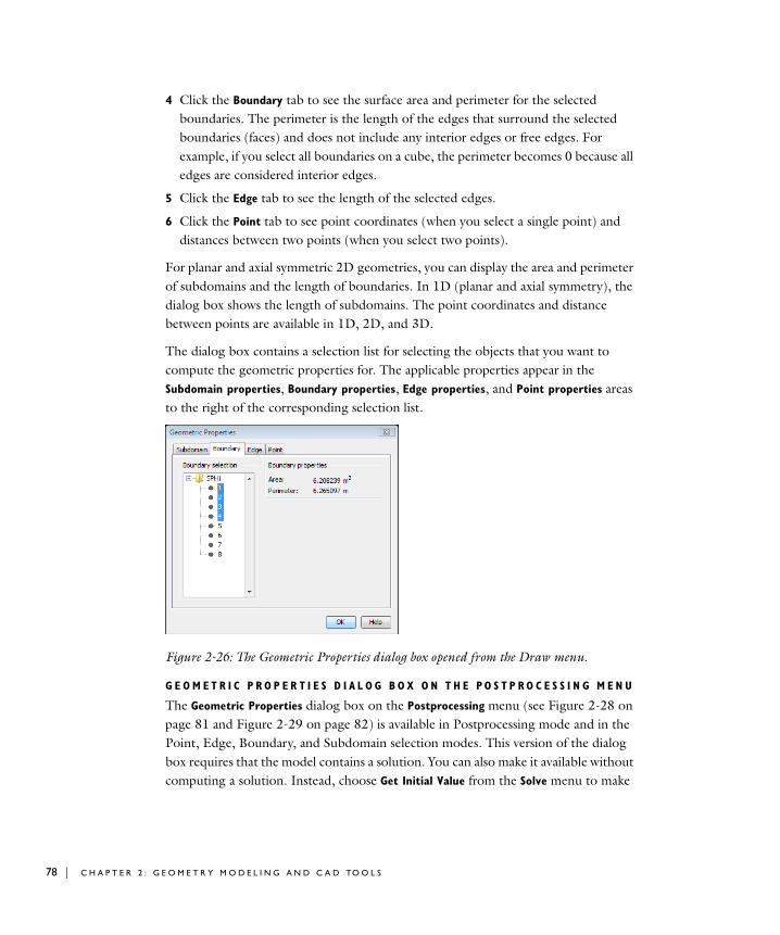
78 | C H A P T E R
4 Click the Boundary tab to see the surface area and perimeter for the selected boundaries. The perimeter is the length of the edges that surround the selected boundaries (faces) and does not include any interior edges or free edges. For example, if you select all boundaries on a cube, the perimeter becomes 0 because all edges are considered interior edges.
5 Click the Edge tab to see the length of the selected edges.
6 Click the Point tab to see point coordinates (when you select a single point) and distances between two points (when you select two points).
For planar and axial symmetric 2D geometries, you can display the area and perimeter of subdomains and the length of boundaries. In 1D (planar and axial symmetry), the dialog box shows the length of subdomains. The point coordinates and distance between points are available in 1D, 2D, and 3D.
The dialog box contains a selection list for selecting the objects that you want to compute the geometric properties for. The applicable properties appear in the Subdomain properties, Boundary properties, Edge properties, and Point properties areas to the right of the corresponding selection list.
Figure 2-26: The Geometric Properties dialog box opened from the Draw menu.
G E O M E T R I C P R O P E R T I E S D I A L O G B O X O N T H E P O S T P R O C E S S I N G M E N U
The Geometric Properties dialog box on the Postprocessing menu (see Figure 2-28 on page 81 and Figure 2-29 on page 82) is available in Postprocessing mode and in the Point, Edge, Boundary, and Subdomain selection modes. This version of the dialog box requires that the model contains a solution. You can also make it available without computing a solution. Instead, choose Get Initial Value from the Solve menu to make
2 : G E O M E T R Y M O D E L I N G A N D C A D TO O L S

COMSOL Multiphysics use the initial values as the solution for access to the material and geometric properties without a solution.
In addition to the geometric properties in the version on the Draw menu (but for the domains in the analyzed geometry instead of the geometry objects), this Geometric
Properties dialog box also contains the following properties for the domains in the analyzed geometry:
• The center of mass for subdomains (1D, 2D axial symmetry, and 3D), boundaries (2D and 3D), and edges (3D). For 2D axisymmetric models, the center of mass refers to the full 3D geometry and is always located on the z-axis. 1D axisymmetric models do not display the center of mass, which is always at the origin.
• The moment of inertia, which is available in two forms in 2D and 3D:
- Select Principal from the Moment of inertia list to display the principal moment of inertia (the mass moment of inertia J1, J2, and J3 in 3D; the area moment of inertia I1 and I2, and the mass moment of inertia about a z-axis through the center of mass Jzz in 2D), and the corresponding principal axes (e1, e2, and e3 in 3D; e1 and e2 in 2D)
- Select Tensor from the Moment of inertia list to display the tensor components for the moment of inertia: the mass moment of inertia Jxx, Jyx, Jyy, Jzx, Jzy, and Jzz in 3D; the area moment of inertia Ixx, Iyx, and Iyy, and the mass moment of inertia about a z-axis through the center of mass Jzz in 2D.
In 2D axisymmetric models, the moment of inertia has only one component: Jzz, the mass moment of inertia about the z-axis.
The mass moment of inertia has the SI unit kg·m2, and the area moment of inertia (second moment of inertia) has the SI unit m4. The moment of inertia is not available in 1D.
• For 2D axisymmetric models, the Geometric Properties dialog box shows the volume and surface area for the full 3D geometry (the cross section swept 360 degrees about the z-axis) in addition to the area and perimeter of the 2D cross section.
• For 1D axisymmetric models, the Geometric Properties dialog box shows the area and volume for the full 2D and 3D geometries (the cross section swept 360 degrees about the z-axis) in addition to the length of the 1D radius. For the volume, COMSOL Multiphysics uses the value in the Thickness dialog box.
The center of mass, moment of inertia, and principal axes also require that you provide the density in the Density expression edit field. The default value is 1, which means that the values for the center of mass becomes the centroid (center of mass for
E X P L O R I N G G E O M E T R I C P R O P E R T I E S | 79
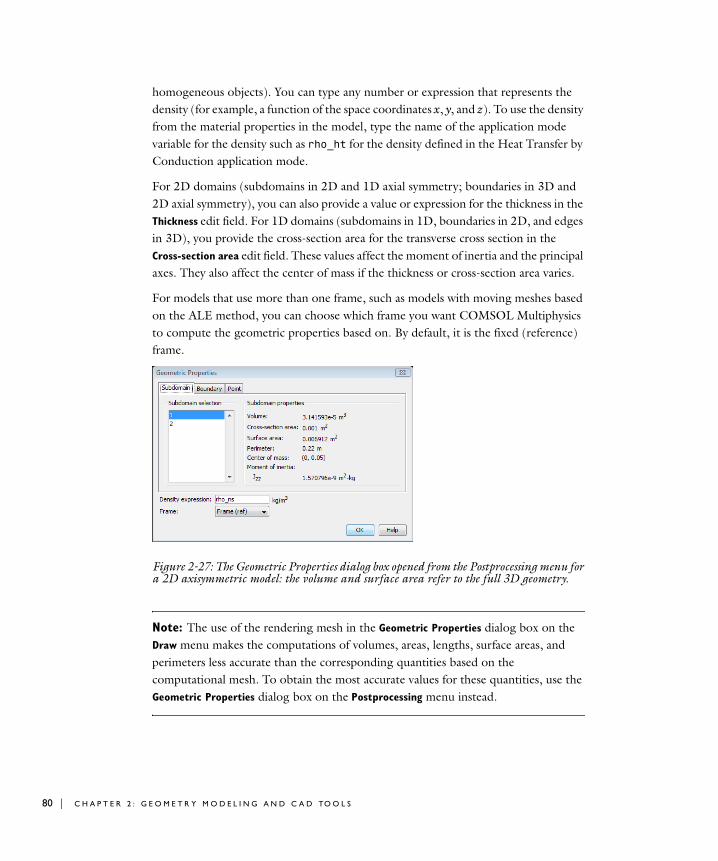
80 | C H A P T E R
homogeneous objects). You can type any number or expression that represents the density (for example, a function of the space coordinates x, y, and z). To use the density from the material properties in the model, type the name of the application mode variable for the density such as rho_ht for the density defined in the Heat Transfer by Conduction application mode.
For 2D domains (subdomains in 2D and 1D axial symmetry; boundaries in 3D and 2D axial symmetry), you can also provide a value or expression for the thickness in the Thickness edit field. For 1D domains (subdomains in 1D, boundaries in 2D, and edges in 3D), you provide the cross-section area for the transverse cross section in the Cross-section area edit field. These values affect the moment of inertia and the principal axes. They also affect the center of mass if the thickness or cross-section area varies.
For models that use more than one frame, such as models with moving meshes based on the ALE method, you can choose which frame you want COMSOL Multiphysics to compute the geometric properties based on. By default, it is the fixed (reference) frame.
Figure 2-27: The Geometric Properties dialog box opened from the Postprocessing menu for a 2D axisymmetric model: the volume and surface area refer to the full 3D geometry.
Note: The use of the rendering mesh in the Geometric Properties dialog box on the Draw menu makes the computations of volumes, areas, lengths, surface areas, and perimeters less accurate than the corresponding quantities based on the computational mesh. To obtain the most accurate values for these quantities, use the Geometric Properties dialog box on the Postprocessing menu instead.
2 : G E O M E T R Y M O D E L I N G A N D C A D TO O L S

Displaying Geometric Properties in the Message Log
To display basic geometric properties for the selected domains, click the Geometric
Properties button at the bottom of the Visualization/Selection toolbar. The geometric properties (for example, the volume and surface area for a 3D geometry object or subdomain) then appear in the message log at the bottom of the user interface.
Figure 2-28: The Geometric Properties button on the Visualization/Selection toolbar.
Centroid, Center of Gravity, and Distance in Electronic Conductor
The following example shows how to use the Geometric Properties dialog box and button to compute the centroid, center of gravity, and distance between two points in the Electronic Conductor model, which is available in the COMSOL Multiphysics Model Library’s Multiphysics folder.
1 Open the Model Navigator, and click the Model Library tab.
2 Select COMSOL Multiphysics>Multiphysics>Electronic Conductor and click OK.
3 From the Postprocessing menu, choose Geometric Properties.
4 In the Geometric Properties dialog box, click a subdomain in the Subdomain selection list and press Ctrl+A to select all subdomains. This provides a value for the
E X P L O R I N G G E O M E T R I C P R O P E R T I E S | 81
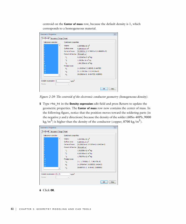
82 | C H A P T E R
centroid on the Center of mass row, because the default density is 1, which corresponds to a homogeneous material.
Figure 2-29: The centroid of the electronic conductor geometry (homogeneous density).
5 Type rho_ht in the Density expression edit field and press Return to update the geometric properties. The Center of mass row now contains the center of mass. In the following figure, notice that the position moves toward the soldering parts (in the negative y and z directions) because the density of the solder (60Sn-40Pb, 9000 kg/m3) is higher than the density of the conductor (copper, 8700 kg/m3).
6 Click OK.
2 : G E O M E T R Y M O D E L I N G A N D C A D TO O L S

7 Click the Point Mode button on the Main toolbar.
8 Click the Zoom Window button on the Main toolbar; then click and drag to zoom in the left soldering part.
9 Select the two bottom points along the front (Points 7 and 20). Then click the Geometric Properties button on the Visualization/Selection toolbar.
E X P L O R I N G G E O M E T R I C P R O P E R T I E S | 83
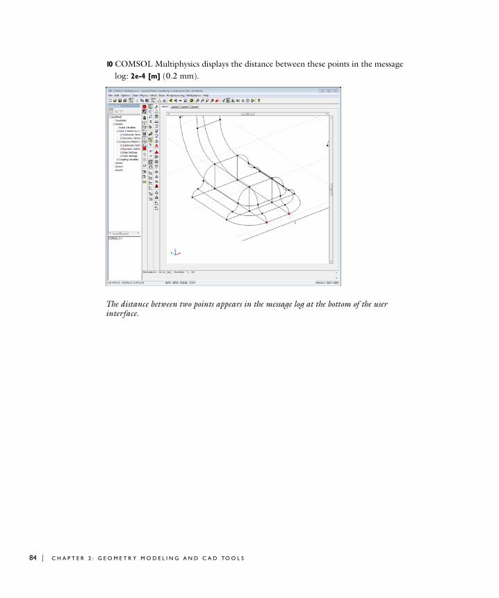
84 | C H A P T E R
10 COMSOL Multiphysics displays the distance between these points in the message log: 2e-4 [m] (0.2 mm).
The distance between two points appears in the message log at the bottom of the user interface.
2 : G E O M E T R Y M O D E L I N G A N D C A D TO O L S

Impo r t i n g and Expo r t i n g Geome t r y Ob j e c t s and CAD Mode l s
With COMSOL Multiphysics you can import and export geometries from a variety of file formats. A natural choice for storing geometries in 1D, 2D, and 3D is the native file format of COMSOL’s geometry kernel. You find more information on this file format in the section “Importing and Exporting COMSOL Multiphysics Files” on page 86.
In 2D, there is also the option of importing and exporting DXF files; for details, see the section “Importing and Exporting DXF Files” on page 87. You can also import GDS files (requires COMSOL Script or MATLAB). See geomimport in the COMSOL Multiphysics Reference Guide’s “Command Reference” chapter for details.
In 3D, it is possible to import surface meshes on the STL and VRML formats. For more information about this feature, see the section “Importing STL and VRML Files” on page 89.
COMSOL provides an optional CAD Import Module, which supports import of CAD data on Parasolid, SAT (ACIS), STEP, and IGES formats. Additional modules support the following formats: CATIA V4, CATIA V5, Pro/ENGINEER, Autodesk Inventor, and VDA-FS. The CAD Import Module User’s Guide covers these file formats in detail.
I M P O R T I N G A N D E X P O R T I N G G E O M E T R Y O B J E C T S A N D C A D M O D E L S | 85
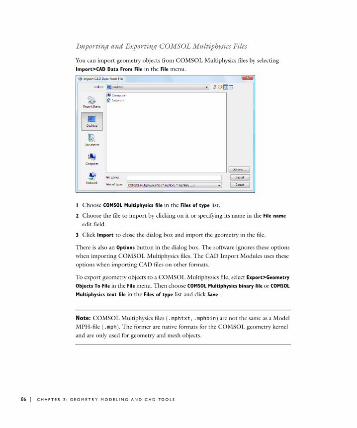
86 | C H A P T E R
Importing and Exporting COMSOL Multiphysics Files
You can import geometry objects from COMSOL Multiphysics files by selecting Import>CAD Data From File in the File menu.
1 Choose COMSOL Multiphysics file in the Files of type list.
2 Choose the file to import by clicking on it or specifying its name in the File name edit field.
3 Click Import to close the dialog box and import the geometry in the file.
There is also an Options button in the dialog box. The software ignores these options when importing COMSOL Multiphysics files. The CAD Import Modules uses these options when importing CAD files on other formats.
To export geometry objects to a COMSOL Multiphysics file, select Export>Geometry
Objects To File in the File menu. Then choose COMSOL Multiphysics binary file or COMSOL
Multiphysics text file in the Files of type list and click Save.
Note: COMSOL Multiphysics files (.mphtxt, .mphbin) are not the same as a Model MPH-file (.mph). The former are native formats for the COMSOL geometry kernel and are only used for geometry and mesh objects.
2 : G E O M E T R Y M O D E L I N G A N D C A D TO O L S
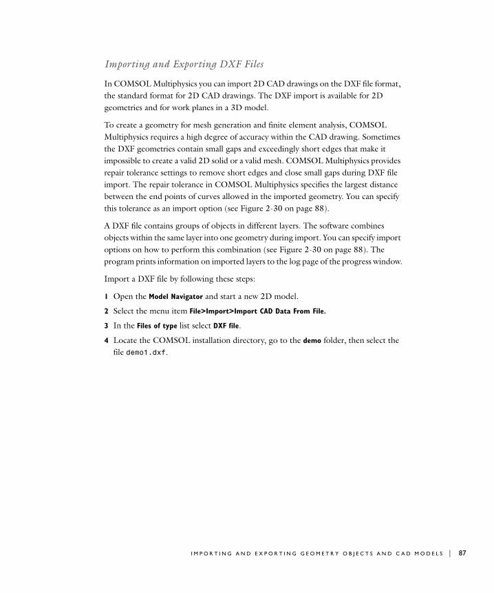
Importing and Exporting DXF Files
In COMSOL Multiphysics you can import 2D CAD drawings on the DXF file format, the standard format for 2D CAD drawings. The DXF import is available for 2D geometries and for work planes in a 3D model.
To create a geometry for mesh generation and finite element analysis, COMSOL Multiphysics requires a high degree of accuracy within the CAD drawing. Sometimes the DXF geometries contain small gaps and exceedingly short edges that make it impossible to create a valid 2D solid or a valid mesh. COMSOL Multiphysics provides repair tolerance settings to remove short edges and close small gaps during DXF file import. The repair tolerance in COMSOL Multiphysics specifies the largest distance between the end points of curves allowed in the imported geometry. You can specify this tolerance as an import option (see Figure 2-30 on page 88).
A DXF file contains groups of objects in different layers. The software combines objects within the same layer into one geometry during import. You can specify import options on how to perform this combination (see Figure 2-30 on page 88). The program prints information on imported layers to the log page of the progress window.
Import a DXF file by following these steps:
1 Open the Model Navigator and start a new 2D model.
2 Select the menu item File>Import>Import CAD Data From File.
3 In the Files of type list select DXF file.
4 Locate the COMSOL installation directory, go to the demo folder, then select the file demo1.dxf.
I M P O R T I N G A N D E X P O R T I N G G E O M E T R Y O B J E C T S A N D C A D M O D E L S | 87
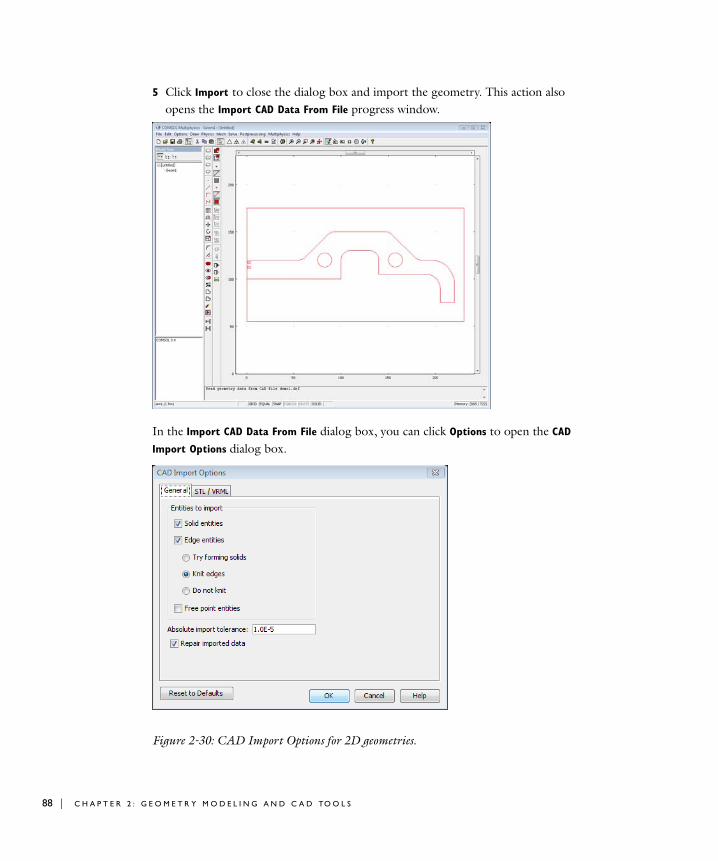
88 | C H A P T E R
5 Click Import to close the dialog box and import the geometry. This action also opens the Import CAD Data From File progress window.
In the Import CAD Data From File dialog box, you can click Options to open the CAD
Import Options dialog box.
Figure 2-30: CAD Import Options for 2D geometries.
2 : G E O M E T R Y M O D E L I N G A N D C A D TO O L S
In this dialog box you can control the following options:
• Select the Solid entities check box to import solid geometry objects.
• Select the Edge entities check box to import curve objects. To choose how to combine these entities:
- Click the Try forming solids button to combine the edges to form solid entities. If there are loose edges not adjacent to a subdomain, they are deleted.
- Click the Knit edges button to combine the edges to a curve object.
- Click the Do not knit button to create a separate geometry object for each edge.
• Select the Free point entities check box to import isolated points.
• Select the Repair imported data check box to remove small gaps and tiny edges from the geometry. Specify the tolerance in the Repair tolerance edit field.
For exporting geometry objects to a DXF file, select Export>Geometry To File in the File menu. Then, choose DXF file in the Files of type list and click Save.
Importing STL and VRML Files
You can import 3D surface meshes into COMSOL Multiphysics with STL and VRML 1.0, two formats for describing solids as surface meshes.
The STL format describes the boundary of a solid as a triangular mesh. STL files are either ASCII or binary, and COMSOL Multiphysics can import both ASCII and binary STL files. It is advisable to use binary files if possible to avoid a loss of precision.
The VRML format describes scenes (collections of independent objects that reside within a single “frame” or logical space), and it can describe the geometry in a scene as a triangular mesh. COMSOL Multiphysics ignores all other information in a VRML file. There are two versions of VRML, 1.0 and 2.0/97. COMSOL Multiphysics only imports VRML 1.0 files.
These two formats do not contain any information about to what face each triangle belongs. Instead, COMSOL Multiphysics uses heuristics to partition the triangles into faces. Usually the partition is reasonable for geometries containing sharp angles between faces, but the partitioning can appear arbitrary for curved geometries such as spheres and tori.
I M P O R T I N G A N D E X P O R T I N G G E O M E T R Y O B J E C T S A N D C A D M O D E L S | 89
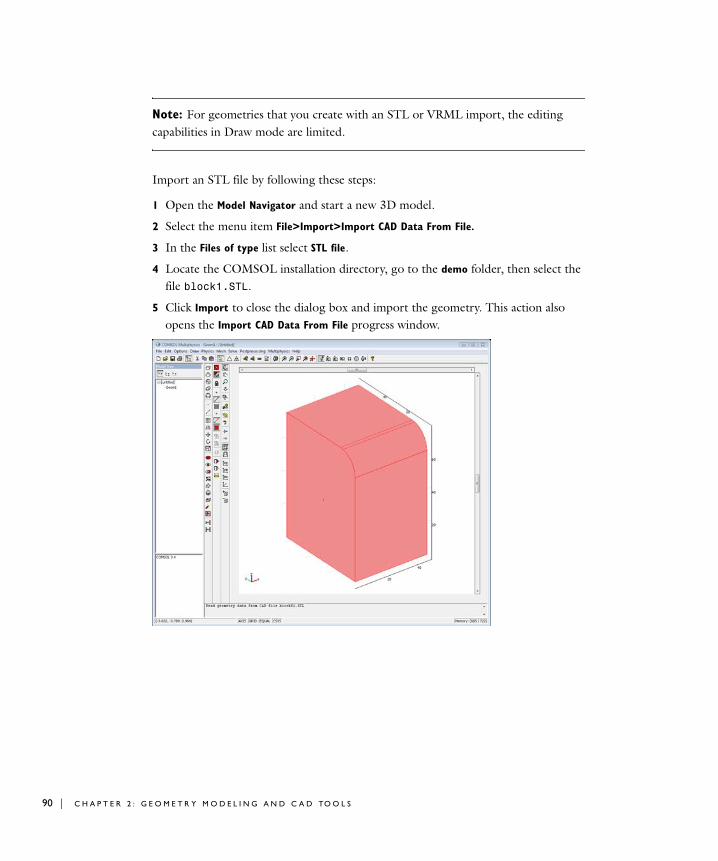
90 | C H A P T E R
Note: For geometries that you create with an STL or VRML import, the editing capabilities in Draw mode are limited.
Import an STL file by following these steps:
1 Open the Model Navigator and start a new 3D model.
2 Select the menu item File>Import>Import CAD Data From File.
3 In the Files of type list select STL file.
4 Locate the COMSOL installation directory, go to the demo folder, then select the file block1.STL.
5 Click Import to close the dialog box and import the geometry. This action also opens the Import CAD Data From File progress window.
2 : G E O M E T R Y M O D E L I N G A N D C A D TO O L S
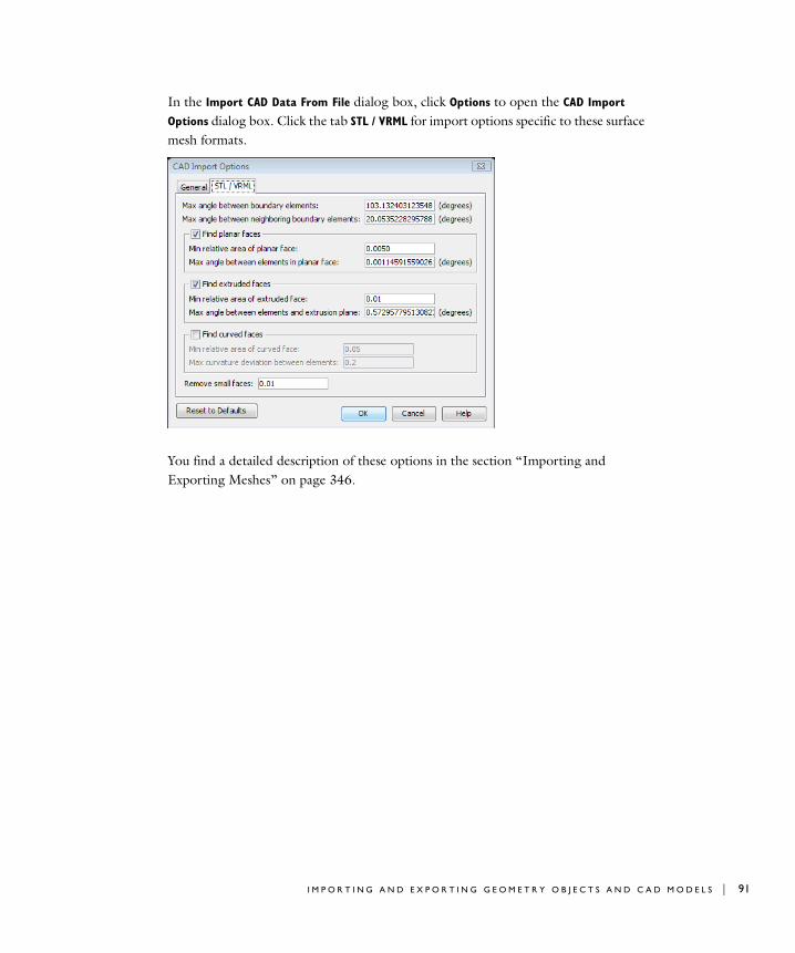
In the Import CAD Data From File dialog box, click Options to open the CAD Import
Options dialog box. Click the tab STL / VRML for import options specific to these surface mesh formats.
You find a detailed description of these options in the section “Importing and Exporting Meshes” on page 346.
I M P O R T I N G A N D E X P O R T I N G G E O M E T R Y O B J E C T S A N D C A D M O D E L S | 91

92 | C H A P T E R
C r e a t i n g a Geome t r y f o r S u c c e s s f u l Ana l y s i s
Several techniques can ensure that a geometry results in a good mesh and gives reasonable solution times for the finite element analysis. They include the use of symmetry, removing unnecessary boundaries, and eliminating gaps, holes, and singularities.
Using Assemblies
When you leave Draw mode COMSOL Multiphysics analyzes the geometry to find all subdomains, boundaries, edges, and points in the geometry. When doing this COMSOL Multiphysics creates an analyzed geometry that you apply the physics on. You can choose between two types of analyzed geometries:
• A composite geometry. The analyzed geometry object that the software creates is a single object, which effectively is the same objects you would get if you select all objects in Draw mode and create the union of them.
• An assembly. In this case you get an analyzed geometry that consists of several parts, where each object in Draw mode becomes a part of the assembly.
If there are no problems using a composite geometry this is usually to prefer, but there are some cases when an assembly is the best choice:
• Sometimes the software fails to create a composite geometry. In those cases it might be possible to use an assembly instead. It is a simpler operation to create an assembly, and it often succeeds even if creating a composite geometry fails.
• Each part in an assembly gets separate meshes. This can make it easier to mesh a complicated geometry, where the mesh generator fails to create a mesh for the composite geometry. Bear in mind that having separate meshes means that the meshes might not be compatible at the two sides of a border between two parts. This can give you a less accurate solution.
• Assemblies make it possible to apply boundary conditions where the dependent variable is discontinuous at the border between two parts. One example is a contact resistance boundary condition for electric currents where the electric potential is discontinuous.
2 : G E O M E T R Y M O D E L I N G A N D C A D TO O L S
To choose between using a composite geometry and using an assembly, toggle the Use Assembly menu item on the Draw menu.
For more information about modeling with an assembly, see “Using Assemblies” on page 351 in the COMSOL Multiphysics Modeling Guide.
Using Symmetries
Using symmetry is one of the most effective ways to reduce the size of a finite element model. See “Using Symmetries” on page 7 of the COMSOL Multiphysics Modeling Guide for advice on modeling with symmetries.
Removing Unnecessary Boundaries
Building a composite solid object from several geometry objects can introduce interior boundaries that split a domain into parts even though the same physical properties prevail in all of them. It is good practice to avoid these unnecessary interior boundaries because the extra points, lines, and surfaces they add cause the mesh generator to create extra mesh elements and might even prevent the mesh generator from producing a valid mesh that respects all boundaries. See “Removing Interior Boundaries” on page 35 for information on how to delete interior boundaries. Sometimes rebuilding a geometry is required to remedy unnecessary interior boundaries.
Making the Geometry Match the Boundary Conditions
In many modeling solutions, the modeling domain is unbounded or too large for successful meshing and analysis. For these cases a suitable boundary condition can replace the exterior of the domain. It is important for the geometry to be large enough to validate these boundary conditions. For outflows in fluid-flow models, for example, the boundary should be perpendicular to the fully developed flow. Inspections and modifications of the solved model might be necessary to verify the validity of the boundary condition.
Avoiding Excessively Small Details, Holes, and Gaps
Many geometries, especially those designed using a CAD system without finite element analysis, contain small holes, details, and gaps. These small features can make the domain unbounded and must be removed before analysis. Small details and holes
C R E A T I N G A G E O M E T R Y F O R S U C C E S S F U L A N A L Y S I S | 93
94 | C H A P T E R
can lead to large meshes and finite element models or even failure during mesh generation. To avoid small gaps and mismatches between the geometry objects, make sure the snapping feature is activated.
The DXF import routine has tolerance parameters that fill gaps and holes smaller than the tolerance. See “Importing and Exporting DXF Files” on page 87 for details.
The CAD Import Module contains tools for automatic and interactive repair and defeaturing of 3D CAD data.
Avoiding Singularities and Degeneracies in the Geometry
A singularity in a geometry is a sharp corner or angle that can create problems during meshing and analysis. In reality, a sharp reentrant corner leads to infinite stress values in a stress analysis of a perfectly elastic material. To avoid a singularity, round sharp corners using fillets. The stress value for a sharp corner is finite in the finite element analysis, but refinement of the mesh increases the stresses in the corner without limit.
A degeneracy in the geometry can occur during solid modeling. For example, fillet areas that taper to a point and the apex of a cone can become degenerate points. These degeneracies might cause problems for the mesh generator and problems during the analysis of the model. A common degeneracy in the geometry occurs when you create a 3D solid (for example, a cylinder) by rotation about an axis that touches the rotation area. In such cases, it is better to create the solid object by extruding a cross section or to use geometric 3D primitives.
Associative Geometry
Associative geometry is a concept for the automatic updating of applied physical properties, such as boundary conditions and equation coefficients, under geometric transformations. Thus, once you have defined the physical properties of a finite element model and return to Draw mode to modify the geometric model, COMSOL Multiphysics updates the physical properties according to the geometry modifications as you exit Draw mode.
The associative geometry functionality utilizes geometry-mapping information between the domain groups (vertices, edges, boundaries, and subdomains) in the analyzed geometry and the corresponding domain groups in the geometric model available in Draw mode.
2 : G E O M E T R Y M O D E L I N G A N D C A D TO O L S

This geometry mapping is not always without ambiguities. Thus, COMSOL Multiphysics makes some heuristic decisions when mapping the physical properties between the analyzed geometric object (the object on which the physical properties are imposed) and the geometric model available in Draw mode. In some cases the resulting updated physical properties might not be the ones that you would expect.
C R E A T I N G A G E O M E T R Y F O R S U C C E S S F U L A N A L Y S I S | 95

96 | C H A P T E R
2 : G E O M E T R Y M O D E L I N G A N D C A D TO O L S
3
V i s u a l i z a t i o n a n d S e l e c t i o n T o o l s
COMSOL Multiphysics provides a number of visualization tools for controlling the view of a model as well as zooming and orbiting around it. Other tools help in selecting domains for the modeling process. Advanced lighting and rendering features can create specialized visualizations. This chapter details how to use these tools.
97

98 | C H A P T E R
V i s u a l i z i n g a Mode l
COMSOL Multiphysics supplies a number of tools for zooming, orbiting, and panning to adjust the view of a model for preprocessing, postprocessing, and general visualization.
When building a model, the right view of a 3D geometry object facilitates not only understanding what the geometry looks like but also selecting features within it. The choice of visualization depends on the object types being rendered and the ones being highlighted. For example, you can view deselected faces as wireframe plots or highlight the faces that are selected using rendering options. Furthermore, you control visualization quality through the choice of the geometry mesh detail and lighting options.
For visualization of the results from an analysis, see “Postprocessing and Visualization” on page 419.
3 : V I S U A L I Z A T I O N A N D S E L E C T I O N TO O L S

The Visualization/Selection Toolbar
The COMSOL Multiphysics user interface contains a Visualization/Selection toolbar to the left of the drawing area. It provides easy access to various selection and rendering tools:
• For more information about the selection tools, see “Adjacency Selection Methods” on page 134.
• For more information about the rendering tools, see “Controlling the Rendering of Geometry Objects” on page 116.
• For more information about the highlighting tools, see “Controlling the Highlighting of Geometry Objects” on page 118.
• For more information about the projection tools, see “Geometry Projection in Work Planes” on page 63.
• For more information about the viewing and hiding geometries, see “Viewing Multiple Geometries” on page 125.
Selection tools
Rendering tools
Highlighting tools
Projection tools
View/Hide geometries
Update symbols
Draw points for coordinate probe plot
Hide selected objects
Show all hidden objects
Geometric properties
V I S U A L I Z I N G A M O D E L | 99
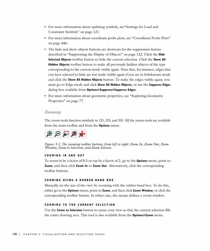
100 | C H A P T E
• For more information about updating symbols, see“Settings for Load and Constraint Symbols” on page 121.
• For more information about coordinate probe plots, see “Coordinate Probe Plots” on page 446.
• The hide and show objects buttons are shortcuts for the suppression feature described in “Suppressing the Display of Objects” on page 122. Click the Hide
Selected Objects toolbar button to hide the current selection. Click the Show All
Hidden Objects toolbar button to make all previously hidden objects of the type corresponding to the current mode visible again. Note that, for instance, edges that you have selected to hide are not made visible again if you are in Subdomain mode and click the Show All Hidden Objects button. To make the edges visible again, you must go to Edge mode and click Show All Hidden Objects, or use the Suppress Edges dialog box available from Options>Suppress>Suppress Edges.
• For more information about geometric properties, see “Exploring Geometric Properties” on page 77.
Zooming
The zoom tools function similarly in 1D, 2D, and 3D. All the zoom tools are available from the main toolbar and from the Options menu.
Figure 3-1: The zooming toolbar buttons, from left to right: Zoom In, Zoom Out, Zoom Window, Zoom to Selection, and Zoom Extents.
Z O O M I N G I N A N D O U T
To zoom in by a factor of 0.5 or out by a factor of 2, go to the Options menu, point to Zoom, and then click Zoom In or Zoom Out. Alternatively, click the corresponding toolbar buttons.
Z O O M I N G U S I N G A R U B B E R - B A N D B O X
Manually set the size of the view by zooming with the rubber-band box. To do this, either go to the Options menu, point to Zoom, and then click Zoom Window, or click the corresponding toolbar button. In either case, the mouse defines a zoom window.
Z O O M I N G T O T H E C U R R E N T S E L E C T I O N
Use the Zoom to Selection button to resize your view so that the current selection fills the entire drawing area. This tool is also available from the Options>Zoom menu.
R 3 : V I S U A L I Z A T I O N A N D S E L E C T I O N TO O L S

Z O O M I N G T O T H E E X T E N T S O F T H E G E O M E T R Y
If your geometry is extremely large or small relative to your choice of axis limits, you can quickly resize the view so that the geometry fits into the entire work area. To zoom in or out to the extents of the current geometry, go to the Options menu, point to Zoom, and then click Zoom Extents. Alternatively, use the corresponding toolbar button.
Changing the View in 3D
For 3D models you can click to select an object and then also either orbit, pan, or zoom from your mouse and keyboard. To only select an object but not perform the other operations, click the Orbit/Pan/Zoom button in the Camera toolbar once. This also enables selection using a rubber-band box. Click that toolbar button again to enable orbit, pan, and zoom.
To avoid rendering complicated models when orbiting, panning, zooming, or dollying, use the Move as Box mode. When Move as Box is active, COMSOL Multiphysics represents the geometry using its bounding box while performing the operation. You can specify the default setting of this mode on the Visualization page in the Preferences dialog box (on the Options menu).
O R B I T
Orbit rotates the camera position about the camera target. To orbit camera:
1 Click the Orbit/Pan/Zoom button to enable orbit.
Orbit/Pan/Zoom
Pan
Zoom
Dolly In/Out
Move as Box
Camera Parameters
V I S U A L I Z I N G A M O D E L | 101

102 | C H A P T E
2 Using the left mouse button, click in the drawing area and rotate the camera about the target while holding the mouse button down.
Use the arrow keys to orbit in small increments. Press the up arrow, down arrow, left arrow, or right arrow key to rotate the camera in the corresponding direction.
Pan is performed when arrow keys or left mouse button are used while Ctrl key is down. Zoom is performed when arrow keys or left mouse button are used while Shift key is down.
P A N
Pan moves the view horizontally and vertically by moving the camera position and target. To pan camera:
1 Click the Pan toolbar button to enable pan.
2 Using the left mouse button, click and drag the cursor to pan the camera in the corresponding direction.
Use the arrow keys to pan in small increments. Press the up arrow, down arrow, left arrow, or right arrow key to pan the camera in the corresponding direction.
Z O O M
Zoom makes objects larger or smaller on the screen by changing the camera view angle. Zooming does not change the camera position. To zoom in and out:
1 Click the Zoom toolbar button to enable zoom.
2 Using the left mouse button, click and move the mouse in the drawing area while holding the mouse button down.
Use the up arrow or down arrow keys to zoom in small increments.
D O L L Y I N A N D O U T O F 3 D G E O M E T R I E S
The Dolly In/Out function moves the camera position toward or away from the camera target while keeping the camera view angle constant. This makes it possible to move the camera through objects in a scene. To dolly the camera position in or out:
1 Click the Dolly In/Out toolbar button to enable this function.
2 Using the left mouse button, click and move the mouse in the drawing area while holding the mouse button down.
R 3 : V I S U A L I Z A T I O N A N D S E L E C T I O N TO O L S
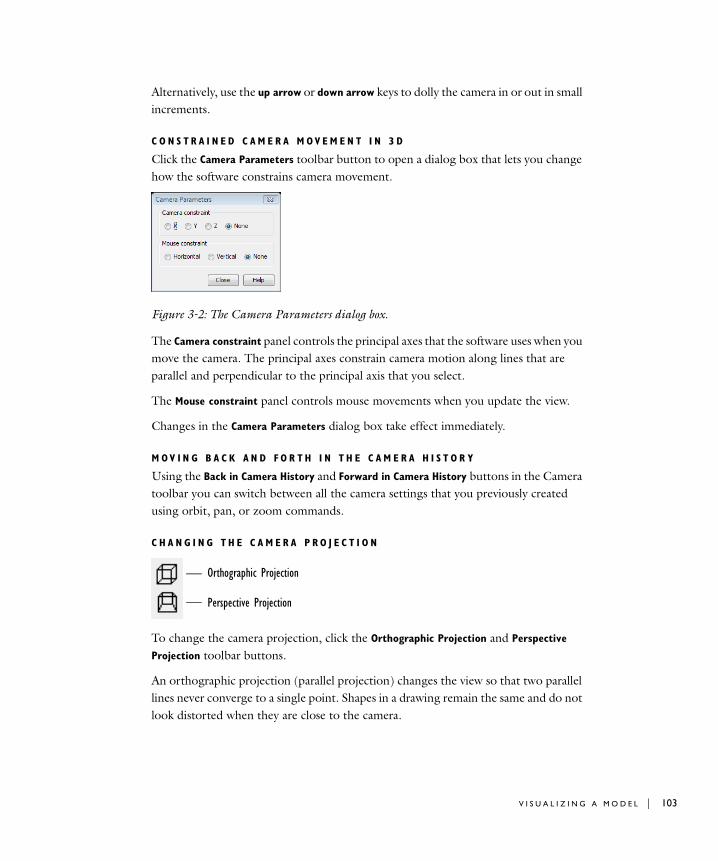
Alternatively, use the up arrow or down arrow keys to dolly the camera in or out in small increments.
C O N S T R A I N E D C A M E R A M OV E M E N T I N 3 D
Click the Camera Parameters toolbar button to open a dialog box that lets you change how the software constrains camera movement.
Figure 3-2: The Camera Parameters dialog box.
The Camera constraint panel controls the principal axes that the software uses when you move the camera. The principal axes constrain camera motion along lines that are parallel and perpendicular to the principal axis that you select.
The Mouse constraint panel controls mouse movements when you update the view.
Changes in the Camera Parameters dialog box take effect immediately.
M OV I N G B A C K A N D F O R T H I N T H E C A M E R A H I S T O R Y
Using the Back in Camera History and Forward in Camera History buttons in the Camera toolbar you can switch between all the camera settings that you previously created using orbit, pan, or zoom commands.
C H A N G I N G T H E C A M E R A P R O J E C T I O N
To change the camera projection, click the Orthographic Projection and Perspective
Projection toolbar buttons.
An orthographic projection (parallel projection) changes the view so that two parallel lines never converge to a single point. Shapes in a drawing remain the same and do not look distorted when they are close to the camera.
Orthographic Projection
Perspective Projection
V I S U A L I Z I N G A M O D E L | 103
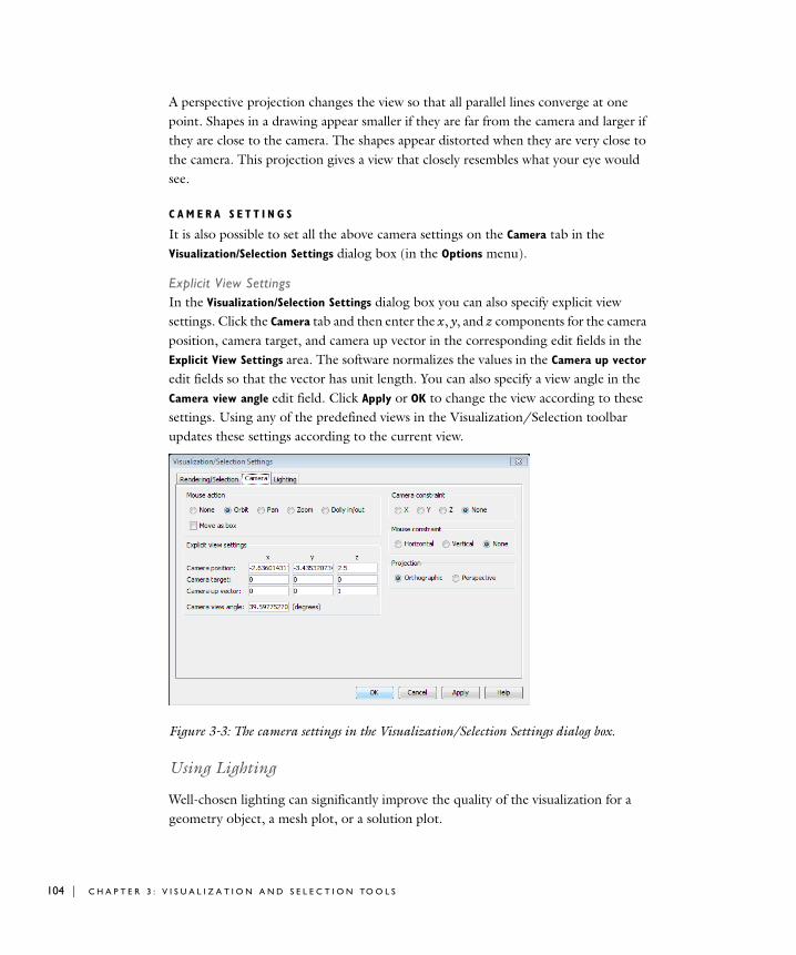
104 | C H A P T E
A perspective projection changes the view so that all parallel lines converge at one point. Shapes in a drawing appear smaller if they are far from the camera and larger if they are close to the camera. The shapes appear distorted when they are very close to the camera. This projection gives a view that closely resembles what your eye would see.
C A M E R A S E T T I N G S
It is also possible to set all the above camera settings on the Camera tab in the Visualization/Selection Settings dialog box (in the Options menu).
Explicit View SettingsIn the Visualization/Selection Settings dialog box you can also specify explicit view settings. Click the Camera tab and then enter the x, y, and z components for the camera position, camera target, and camera up vector in the corresponding edit fields in the Explicit View Settings area. The software normalizes the values in the Camera up vector edit fields so that the vector has unit length. You can also specify a view angle in the Camera view angle edit field. Click Apply or OK to change the view according to these settings. Using any of the predefined views in the Visualization/Selection toolbar updates these settings according to the current view.
Figure 3-3: The camera settings in the Visualization/Selection Settings dialog box.
Using Lighting
Well-chosen lighting can significantly improve the quality of the visualization for a geometry object, a mesh plot, or a solution plot.
R 3 : V I S U A L I Z A T I O N A N D S E L E C T I O N TO O L S
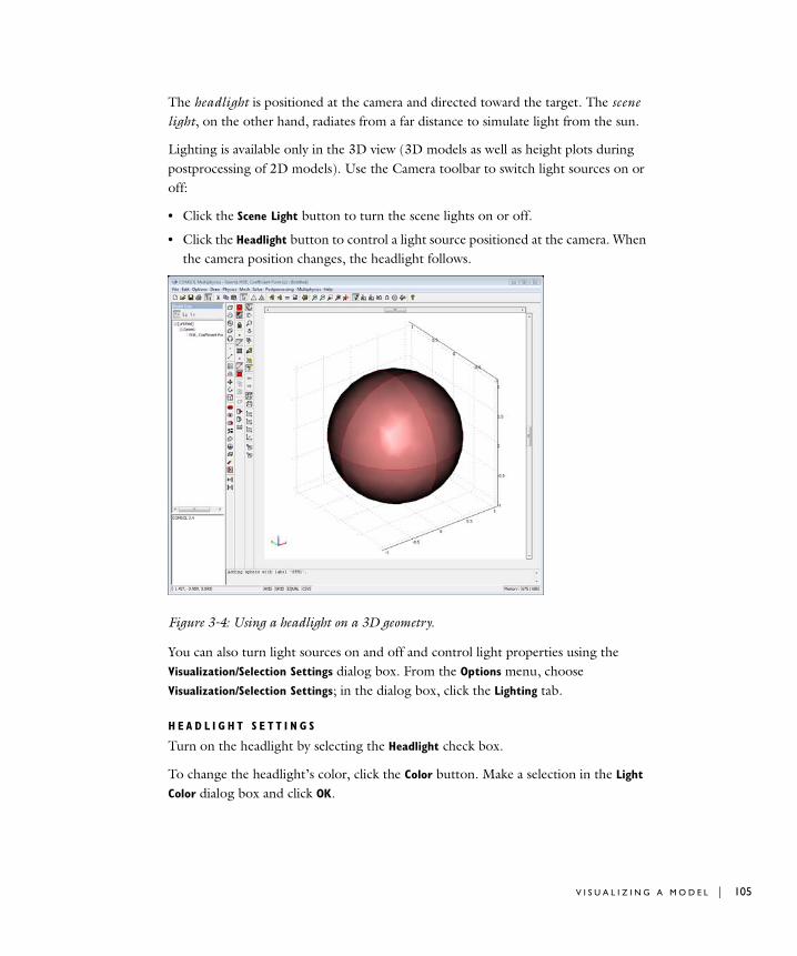
The headlight is positioned at the camera and directed toward the target. The scene light, on the other hand, radiates from a far distance to simulate light from the sun.
Lighting is available only in the 3D view (3D models as well as height plots during postprocessing of 2D models). Use the Camera toolbar to switch light sources on or off:
• Click the Scene Light button to turn the scene lights on or off.
• Click the Headlight button to control a light source positioned at the camera. When the camera position changes, the headlight follows.
Figure 3-4: Using a headlight on a 3D geometry.
You can also turn light sources on and off and control light properties using the Visualization/Selection Settings dialog box. From the Options menu, choose Visualization/Selection Settings; in the dialog box, click the Lighting tab.
H E A D L I G H T S E T T I N G S
Turn on the headlight by selecting the Headlight check box.
To change the headlight’s color, click the Color button. Make a selection in the Light
Color dialog box and click OK.
V I S U A L I Z I N G A M O D E L | 105
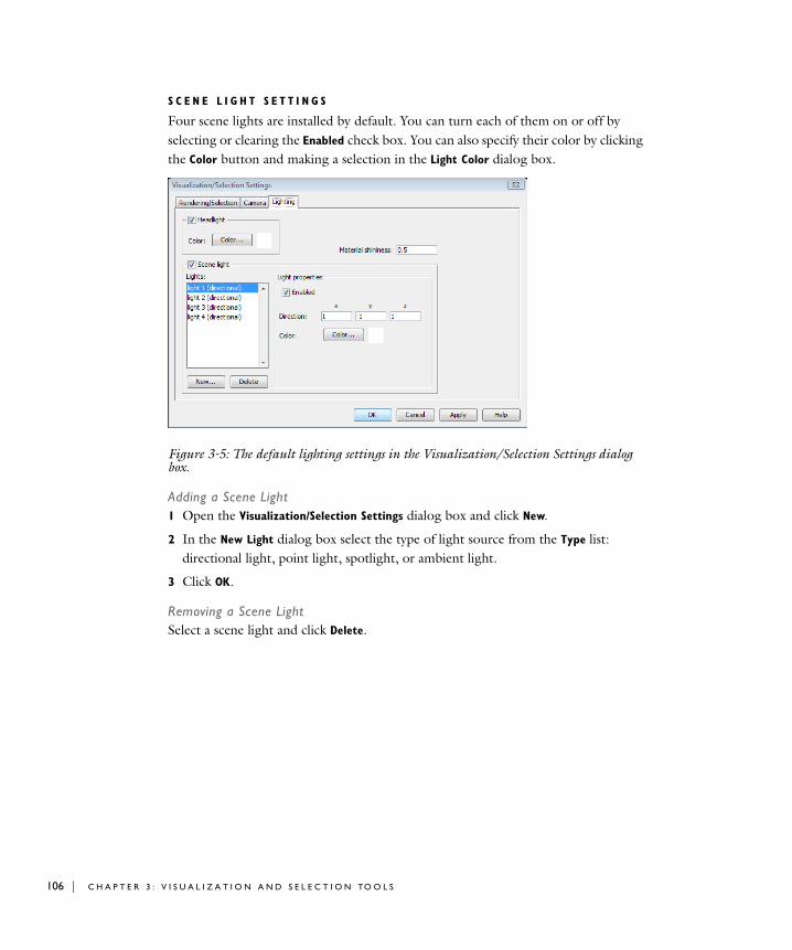
106 | C H A P T E
S C E N E L I G H T S E T T I N G S
Four scene lights are installed by default. You can turn each of them on or off by selecting or clearing the Enabled check box. You can also specify their color by clicking the Color button and making a selection in the Light Color dialog box.
Figure 3-5: The default lighting settings in the Visualization/Selection Settings dialog box.
Adding a Scene Light1 Open the Visualization/Selection Settings dialog box and click New.
2 In the New Light dialog box select the type of light source from the Type list: directional light, point light, spotlight, or ambient light.
3 Click OK.
Removing a Scene LightSelect a scene light and click Delete.
R 3 : V I S U A L I Z A T I O N A N D S E L E C T I O N TO O L S
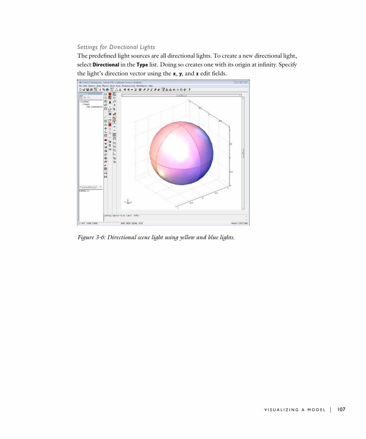
Settings for Directional LightsThe predefined light sources are all directional lights. To create a new directional light, select Directional in the Type list. Doing so creates one with its origin at infinity. Specify the light’s direction vector using the x, y, and z edit fields.
Figure 3-6: Directional scene light using yellow and blue lights.
V I S U A L I Z I N G A M O D E L | 107
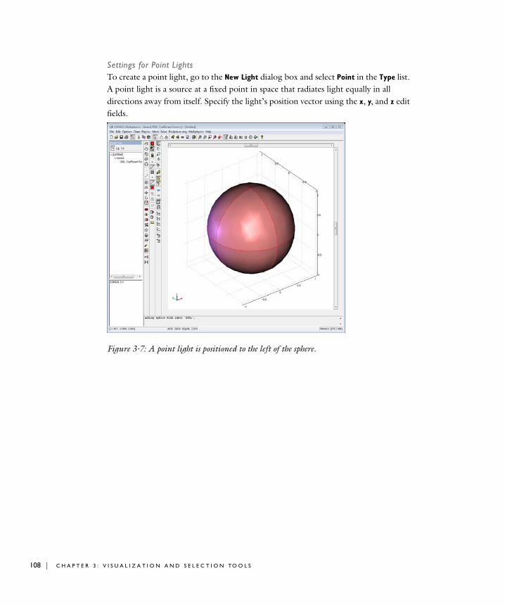
108 | C H A P T E
Settings for Point LightsTo create a point light, go to the New Light dialog box and select Point in the Type list. A point light is a source at a fixed point in space that radiates light equally in all directions away from itself. Specify the light’s position vector using the x, y, and z edit fields.
Figure 3-7: A point light is positioned to the left of the sphere.
R 3 : V I S U A L I Z A T I O N A N D S E L E C T I O N TO O L S
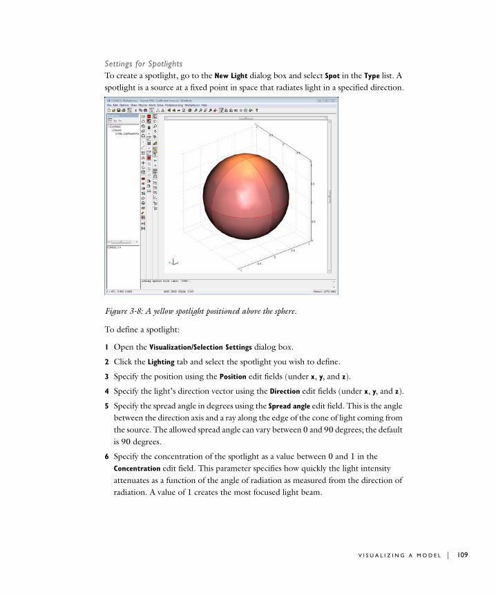
Settings for SpotlightsTo create a spotlight, go to the New Light dialog box and select Spot in the Type list. A spotlight is a source at a fixed point in space that radiates light in a specified direction.
Figure 3-8: A yellow spotlight positioned above the sphere.
To define a spotlight:
1 Open the Visualization/Selection Settings dialog box.
2 Click the Lighting tab and select the spotlight you wish to define.
3 Specify the position using the Position edit fields (under x, y, and z).
4 Specify the light’s direction vector using the Direction edit fields (under x, y, and z).
5 Specify the spread angle in degrees using the Spread angle edit field. This is the angle between the direction axis and a ray along the edge of the cone of light coming from the source. The allowed spread angle can vary between 0 and 90 degrees; the default is 90 degrees.
6 Specify the concentration of the spotlight as a value between 0 and 1 in the Concentration edit field. This parameter specifies how quickly the light intensity attenuates as a function of the angle of radiation as measured from the direction of radiation. A value of 1 creates the most focused light beam.
V I S U A L I Z I N G A M O D E L | 109
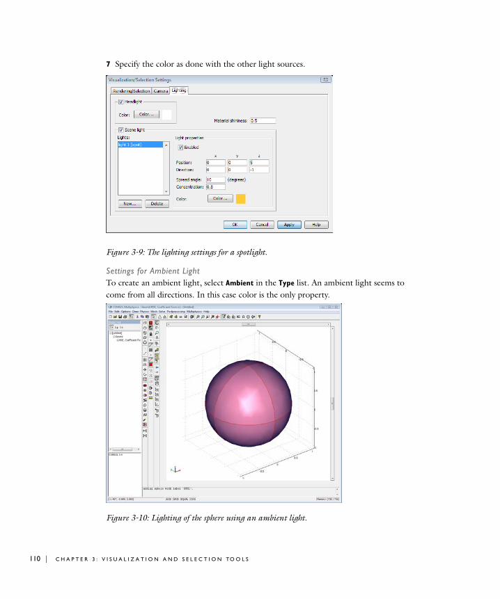
110 | C H A P T E
7 Specify the color as done with the other light sources.
Figure 3-9: The lighting settings for a spotlight.
Settings for Ambient LightTo create an ambient light, select Ambient in the Type list. An ambient light seems to come from all directions. In this case color is the only property.
Figure 3-10: Lighting of the sphere using an ambient light.
R 3 : V I S U A L I Z A T I O N A N D S E L E C T I O N TO O L S
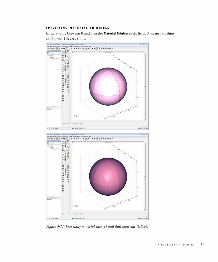
S P E C I F Y I N G M A T E R I A L S H I N I N E S S
Enter a value between 0 and 1 in the Material Shininess edit field; 0 means not shiny (dull), and 1 is very shiny.
Figure 3-11: Very shiny material (above) and dull material (below).
V I S U A L I Z I N G A M O D E L | 111

112 | C H A P T E
If you think a plot is too bright or dark, try to change the shininess, disable some lights, or use darker or brighter light colors.
Changing the View to a Different Axis Plane
Four buttons in the Camera toolbar provide quick settings to change the view to the various axis planes:
• Click the Go to XY View button to change the view to the xy-plane.
• Click the Go to YZ View button to change the view to the yz-plane.
• Click the Go to ZX View button to change the view to the zx-plane.
The first click on one of these buttons selects the plane view with a positive normal direction. A second click on the same button switches to a negative normal direction.
• Click the Go to Default 3D View button to change the view to the default.
Figure 3-12: A zx-plane view of a sphere.
Using Transparency in 3D Plots
Use the bottom two buttons in the Camera toolbar to change the geometry objects’ transparency. These buttons modify the so-called alpha-blending value, which varies
R 3 : V I S U A L I Z A T I O N A N D S E L E C T I O N TO O L S

from 1 (no transparency—fully opaque) to 0 (maximum transparency—invisible). Change the settings as follows:
• Click the Increase Transparency button to decrease the alpha-blending value in steps of 0.1.
• Click the Decrease Transparency button to increase the alpha-blending value in steps of 0.1.
You can also set a value for transparency in the Visualization/Selection Settings dialog box:
1 From the Options menu choose Visualization/Selection Settings.
2 In the Visualization/Selection Settings dialog box click the Rendering/Selection tab.
3 Enter an alpha-blending value in the Transparency edit field.
4 Click OK.
Figure 3-13: Slice plot using transparency for a see-through effect.
Controlling the Resolution of the Visualization Mesh
The resolution of the visualization mesh affects the visualization of geometry objects during modeling and preprocessing in several modes: edge selection mode, boundary selection mode, face selection mode, and subdomain selection mode. The resolution
V I S U A L I Z I N G A M O D E L | 113
114 | C H A P T E
setting controls the number of polygons that COMSOL Multiphysics uses when rendering geometry surfaces.
You can select a finer mesh to better resolve a geometry’s curvature or select a coarser mesh to reduce memory requirements for rendering. To change the visualization mesh resolution:
1 From the Options menu, choose Visualization/Selection Settings.
2 In the Visualization/Selection Settings dialog box click the Rendering/Selection tab.
3 Select Fine, Normal, or Coarse in the Visualization mesh list.
4 Click OK.
Note: The visualization mesh is independent of the mesh used for the finite element analysis. Changes to the visualization mesh do not affect analysis results.
Adding Labels to Domains
You can add labels to the following domain types:
• Geometry objects—these labels are visible only in Draw mode.
• Vertices—these labels are visible only in Point Selection mode.
• Edges—these labels are visible only in Edge Selection mode.
• Faces—these labels are visible only in Face Selection mode.
• Subdomains—these labels are visible only in Subdomain Selection mode.
R 3 : V I S U A L I Z A T I O N A N D S E L E C T I O N TO O L S
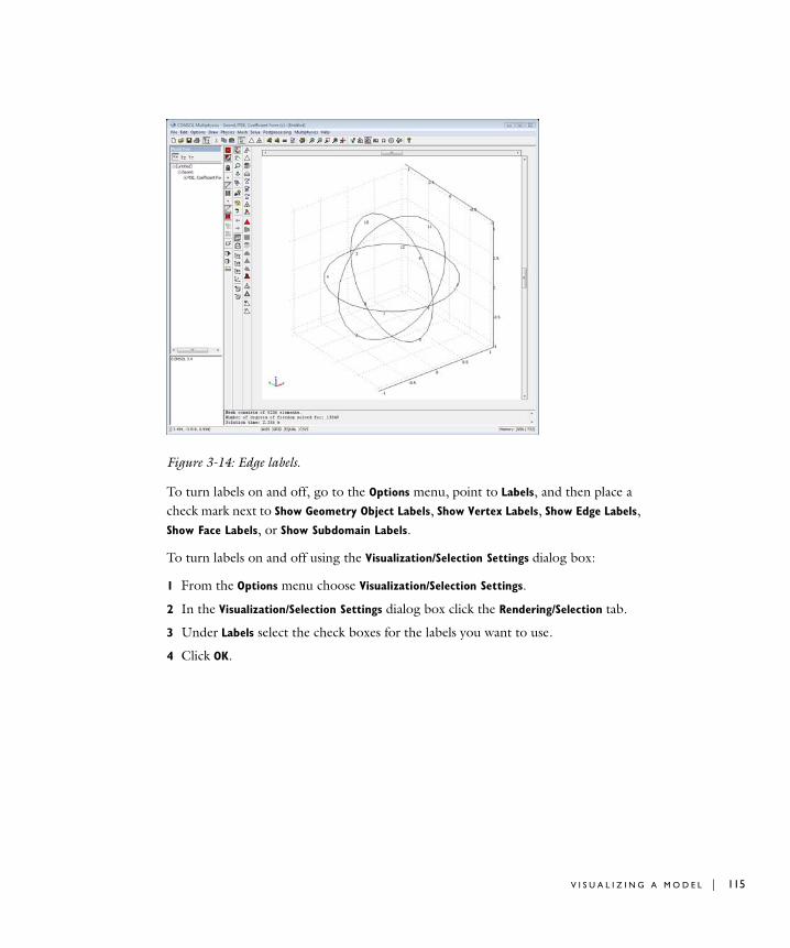
Figure 3-14: Edge labels.
To turn labels on and off, go to the Options menu, point to Labels, and then place a check mark next to Show Geometry Object Labels, Show Vertex Labels, Show Edge Labels, Show Face Labels, or Show Subdomain Labels.
To turn labels on and off using the Visualization/Selection Settings dialog box:
1 From the Options menu choose Visualization/Selection Settings.
2 In the Visualization/Selection Settings dialog box click the Rendering/Selection tab.
3 Under Labels select the check boxes for the labels you want to use.
4 Click OK.
V I S U A L I Z I N G A M O D E L | 115
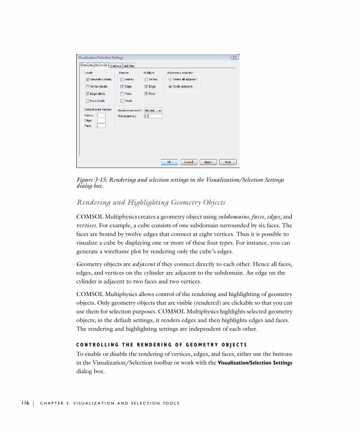
116 | C H A P T E
Figure 3-15: Rendering and selection settings in the Visualization/Selection Settings dialog box.
Rendering and Highlighting Geometry Objects
COMSOL Multiphysics creates a geometry object using subdomains, faces, edges, and vertices. For example, a cube consists of one subdomain surrounded by six faces. The faces are bound by twelve edges that connect at eight vertices. Thus it is possible to visualize a cube by displaying one or more of these four types. For instance, you can generate a wireframe plot by rendering only the cube’s edges.
Geometry objects are adjacent if they connect directly to each other. Hence all faces, edges, and vertices on the cylinder are adjacent to the subdomain. An edge on the cylinder is adjacent to two faces and two vertices.
COMSOL Multiphysics allows control of the rendering and highlighting of geometry objects. Only geometry objects that are visible (rendered) are clickable so that you can use them for selection purposes. COMSOL Multiphysics highlights selected geometry objects; in the default settings, it renders edges and then highlights edges and faces. The rendering and highlighting settings are independent of each other.
C O N T R O L L I N G T H E R E N D E R I N G O F G E O M E T R Y O B J E C T S
To enable or disable the rendering of vertices, edges, and faces, either use the buttons in the Visualization/Selection toolbar or work with the Visualization/Selection Settings dialog box.
R 3 : V I S U A L I Z A T I O N A N D S E L E C T I O N TO O L S
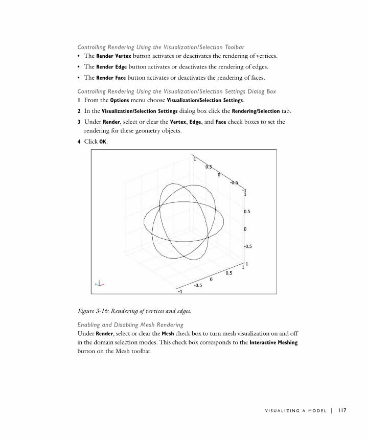
Controlling Rendering Using the Visualization/Selection Toolbar• The Render Vertex button activates or deactivates the rendering of vertices.
• The Render Edge button activates or deactivates the rendering of edges.
• The Render Face button activates or deactivates the rendering of faces.
Controlling Rendering Using the Visualization/Selection Settings Dialog Box1 From the Options menu choose Visualization/Selection Settings.
2 In the Visualization/Selection Settings dialog box click the Rendering/Selection tab.
3 Under Render, select or clear the Vertex, Edge, and Face check boxes to set the rendering for these geometry objects.
4 Click OK.
Figure 3-16: Rendering of vertices and edges.
Enabling and Disabling Mesh RenderingUnder Render, select or clear the Mesh check box to turn mesh visualization on and off in the domain selection modes. This check box corresponds to the Interactive Meshing button on the Mesh toolbar.
V I S U A L I Z I N G A M O D E L | 117
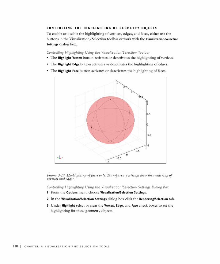
118 | C H A P T E
C O N T R O L L I N G T H E H I G H L I G H T I N G O F G E O M E T R Y O B J E C T S
To enable or disable the highlighting of vertices, edges, and faces, either use the buttons in the Visualization/Selection toolbar or work with the Visualization/Selection
Settings dialog box.
Controlling Highlighting Using the Visualization/Selection Toolbar• The Highlight Vertex button activates or deactivates the highlighting of vertices.
• The Highlight Edge button activates or deactivates the highlighting of edges.
• The Highlight Face button activates or deactivates the highlighting of faces.
Figure 3-17: Highlighting of faces only. Transparency settings show the rendering of vertices and edges.
Controlling Highlighting Using the Visualization/Selection Settings Dialog Box1 From the Options menu choose Visualization/Selection Settings.
2 In the Visualization/Selection Settings dialog box click the Rendering/Selection tab.
3 Under Highlight select or clear the Vertex, Edge, and Face check boxes to set the highlighting for these geometry objects.
R 3 : V I S U A L I Z A T I O N A N D S E L E C T I O N TO O L S
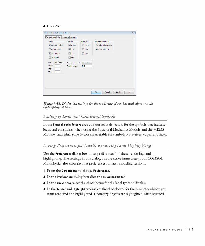
4 Click OK.
Figure 3-18: Dialog box settings for the rendering of vertices and edges and the highlighting of faces.
Scaling of Load and Constraint Symbols
In the Symbol scale factors area you can set scale factors for the symbols that indicate loads and constraints when using the Structural Mechanics Module and the MEMS Module. Individual scale factors are available for symbols on vertices, edges, and faces.
Saving Preferences for Labels, Rendering, and Highlighting
Use the Preferences dialog box to set preferences for labels, rendering, and highlighting. The settings in this dialog box are active immediately, but COMSOL Multiphysics also saves them as preferences for later modeling sessions.
1 From the Options menu choose Preferences.
2 In the Preferences dialog box click the Visualization tab.
3 In the Show area select the check boxes for the label types to display.
4 In the Render and Highlight areas select the check boxes for the geometry objects you want rendered and highlighted. Geometry objects are highlighted when selected.
V I S U A L I Z I N G A M O D E L | 119
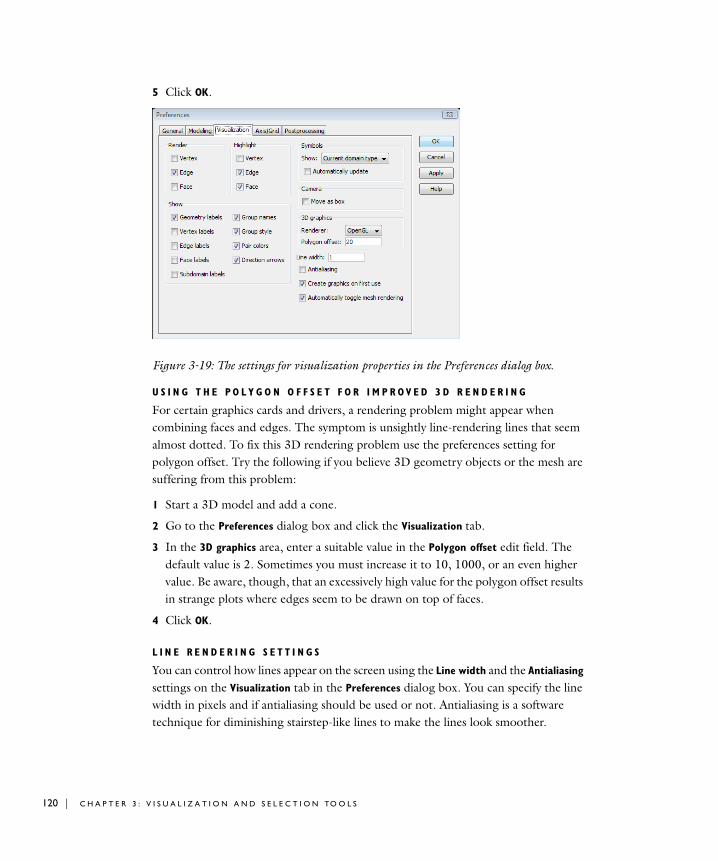
120 | C H A P T E
5 Click OK.
Figure 3-19: The settings for visualization properties in the Preferences dialog box.
U S I N G T H E P O L Y G O N O F F S E T F O R I M P R OV E D 3 D R E N D E R I N G
For certain graphics cards and drivers, a rendering problem might appear when combining faces and edges. The symptom is unsightly line-rendering lines that seem almost dotted. To fix this 3D rendering problem use the preferences setting for polygon offset. Try the following if you believe 3D geometry objects or the mesh are suffering from this problem:
1 Start a 3D model and add a cone.
2 Go to the Preferences dialog box and click the Visualization tab.
3 In the 3D graphics area, enter a suitable value in the Polygon offset edit field. The default value is 2. Sometimes you must increase it to 10, 1000, or an even higher value. Be aware, though, that an excessively high value for the polygon offset results in strange plots where edges seem to be drawn on top of faces.
4 Click OK.
L I N E R E N D E R I N G S E T T I N G S
You can control how lines appear on the screen using the Line width and the Antialiasing settings on the Visualization tab in the Preferences dialog box. You can specify the line width in pixels and if antialiasing should be used or not. Antialiasing is a software technique for diminishing stairstep-like lines to make the lines look smoother.
R 3 : V I S U A L I Z A T I O N A N D S E L E C T I O N TO O L S
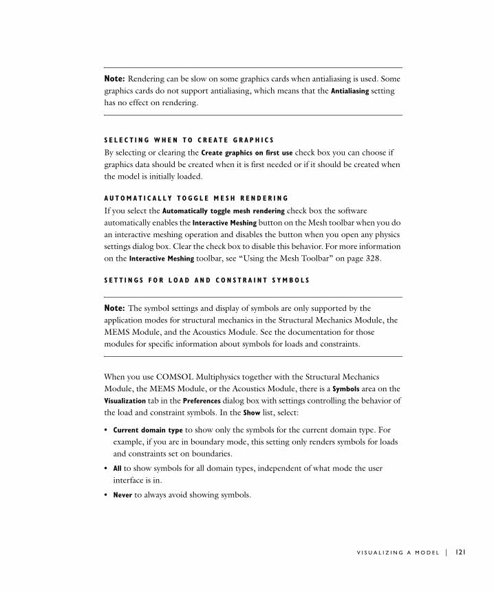
Note: Rendering can be slow on some graphics cards when antialiasing is used. Some graphics cards do not support antialiasing, which means that the Antialiasing setting has no effect on rendering.
S E L E C T I N G W H E N T O C R E A T E G R A P H I C S
By selecting or clearing the Create graphics on first use check box you can choose if graphics data should be created when it is first needed or if it should be created when the model is initially loaded.
A U T O M A T I C A L L Y T O G G L E M E S H R E N D E R I N G
If you select the Automatically toggle mesh rendering check box the software automatically enables the Interactive Meshing button on the Mesh toolbar when you do an interactive meshing operation and disables the button when you open any physics settings dialog box. Clear the check box to disable this behavior. For more information on the Interactive Meshing toolbar, see “Using the Mesh Toolbar” on page 328.
S E T T I N G S F O R L O A D A N D C O N S T R A I N T S Y M B O L S
Note: The symbol settings and display of symbols are only supported by the application modes for structural mechanics in the Structural Mechanics Module, the MEMS Module, and the Acoustics Module. See the documentation for those modules for specific information about symbols for loads and constraints.
When you use COMSOL Multiphysics together with the Structural Mechanics Module, the MEMS Module, or the Acoustics Module, there is a Symbols area on the Visualization tab in the Preferences dialog box with settings controlling the behavior of the load and constraint symbols. In the Show list, select:
• Current domain type to show only the symbols for the current domain type. For example, if you are in boundary mode, this setting only renders symbols for loads and constraints set on boundaries.
• All to show symbols for all domain types, independent of what mode the user interface is in.
• Never to always avoid showing symbols.
V I S U A L I Z I N G A M O D E L | 121

122 | C H A P T E
Select the Automatically update check box to update the view of the symbols automatically when applying new settings in the Subdomain Settings, Boundary Settings, Edge Settings, and Point Settings dialog boxes where you define the loads and constraints. When this option is disabled, update the view of the symbols by clicking the Update Symbols button in the respective dialog box, or by clicking the Update
Symbols toolbar button.
Note: The polygon offset setting affects 3D rendering only when your PC is using OpenGL; this technique is not useful if you are using DirectX.
Suppressing the Display of Objects
If you want to select objects buried deep inside a complex geometry, it can be useful to suppress parts of a geometry. The suppression feature makes selected objects invisible according to the visualization settings. By suppressing objects you can reveal hidden objects or clear the way to access objects that otherwise would be difficult to reach.
You can suppress the following types of geometry objects and domains:
• Geometry objects (for geometry modeling in Draw mode)
• Subdomains
• Boundaries
• Edges
To suppress geometry objects:
1 Go to the Options menu, point to Suppress, and place a check mark next to Suppress
Geometry Objects.
2 In the Suppress Geometry Objects dialog box, select the objects you want to suppress from Object selection list.
R 3 : V I S U A L I Z A T I O N A N D S E L E C T I O N TO O L S
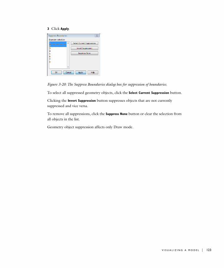
3 Click Apply.
Figure 3-20: The Suppress Boundaries dialog box for suppression of boundaries.
To select all suppressed geometry objects, click the Select Current Suppression button.
Clicking the Invert Suppression button suppresses objects that are not currently suppressed and vice versa.
To remove all suppressions, click the Suppress None button or clear the selection from all objects in the list.
Geometry object suppression affects only Draw mode.
V I S U A L I Z I N G A M O D E L | 123
124 | C H A P T E
Work in the same fashion with the Suppress Subdomains, Suppress Boundaries, and Suppress Edges dialog boxes.
Figure 3-21: The display of the sphere faces after suppressing boundaries 1 and 2.
Rendering Large Geometry Objects
This section describes some memory-saving techniques that can be useful when working with large models on a computer with limited processor capacity and memory.
R E N D E R I N G A W I R E F R A M E P L O T O N L Y
One way to conserve memory is to render as little as possible of the geometry. Face objects are the most memory-consuming objects. To remove all face rendering, turn off both rendering and highlighting of faces. To get a wireframe plot of the geometry make sure the edges are rendered.
U S E A C O A R S E V I S U A L I Z A T I O N M E S H
Using a coarse visualization mesh saves memory for rendering. This affects only the visualization of the geometry objects. For information about setting the visualization mesh detail see “Controlling the Resolution of the Visualization Mesh” on page 113.
R 3 : V I S U A L I Z A T I O N A N D S E L E C T I O N TO O L S
R E N D E R I N G A N D T H E J A V A H E A P S P A C E
Java allocates memory on a heap. This heap is initially quite small and then grows as more memory is needed. When a Java program such as COMSOL Multiphysics is launched, the maximum size for the Java heap must be specified. In COMSOL this value, called MAXHEAP, is set to 256 MB by default. If Java grows the size of the heap past MAXHEAP, you receive an out-of-memory error message, something that can happen when postprocessing or visualizing the mesh for large models. To change the value of MAXHEAP, do as follows:
• On Windows, change the MAXHEAP variable in the file comsol.opts, which is located in the bin directory under your COMSOL directory.
• On UNIX, Linux, and the Macintosh, edit the comsol shell script, located in the bin directory under your COMSOL directory.
See the section “Running COMSOL in Parallel” on page 63 in the COMSOL Installation Guide for further details on setting the Java heap size.
Note: The memory on the Java heap does not include memory usage in assembly routines and solvers.
Viewing Multiple Geometries
When working with several geometries, you can display the active geometry simultaneously with the outlines of several other geometries. To make other geometries visible:
1 Open the View Geometries dialog box from the Options menu.
2 In the Visible geometries list select those geometries that should be visible together with the active geometry.
3 Click OK.
You can also view all geometries or hide all other geometries by clicking the View All
3D Geometries or the Hide Other 3D Geometries buttons in the Visualization/Selection toolbar (and the corresponding buttons for 2D geometries).
The outlines of the other geometries are visible during all modeling stages. To remove them, open the View Geometries dialog box again and clear the selections by Ctrl-clicking in the Visible geometries list. Click Apply or OK to remove the outlines.
V I S U A L I Z I N G A M O D E L | 125
126 | C H A P T E
S e l e c t i n g Doma i n s
COMSOL Multiphysics offers several ways of selecting domains when assigning values and expressions to define a model:
• Select by clicking or enclosing the domains in the drawing area
• Select from a list in a dialog box
• Select using a shortcut key
Specific selection methods vary depending on if the model is in 1D, 2D, or 3D.
General Object Selection Methods
The following principles apply for selecting any object:
• To select a single geometry object, click it using the left mouse button.
• To select several objects or deselect some of them, Shift-click the objects.
• To open an object’s dialog box, double-click the object with the left (2D) or right (3D) mouse button.
• Clicking outside of the objects deselects all of them.
• To select all objects, choose Select All from the Edit menu or press Ctrl+A.
• To clear all selections, choose Deselect All from the Edit menu or press Ctrl+D.
You can also use a rubber-band box to select objects:
• The selection applies only to objects that the rubber-band box surrounds completely.
• Shift-clicking adds the rubber-band box selection to the current selection.
• In 2D, Ctrl-clicking performs an exclusive-OR operation with the current selection (presently selected objects becomes deselected when inside the rubber-band box and vice versa).
In 3D, Ctrl-clicking performs a logical AND operation with the current selection so that only the presently selected objects inside the rubber-band box stay selected. This makes it possible to select a detail from several selected objects.
To enable the selection function in 3D using a rubber-band box, deselect the Orbit/Pan/
Zoom button.
R 3 : V I S U A L I Z A T I O N A N D S E L E C T I O N TO O L S

S E L E C T I O N I N D I C A T I O N
COMSOL Multiphysics indicates selected objects with highlighting (see “Rendering and Highlighting Geometry Objects” on page 116). Additionally, selected lines have a thicker line width, and selected points are larger. The selection indications occur whether highlighting is active or not.
S E L E C T I N G I N A L I S T
In many dialog boxes you can select objects from a list. A direct correspondence exists between selections in a list and selections in the drawing area. Further, any list selection overrides any confirmed selections in a 3D model. Pressing Ctrl+A (select all selections) or Ctrl+D (clear all selections) also work in lists.
S E L E C T I N G B Y G R O U P
Set the Select by group check box in the physics settings dialog boxes to make the selection of one domain also select all other domains with identical settings. This is useful when working with many domains but using only a few different equation settings or materials.
Object Selection Methods in 2D
In a 2D geometry model, choose the selection method using the following geometry selection toolbar buttons:
• Select All Overlapping: With this feature active, clicking at the intersection of several objects selects all of them
• Select Smallest: With this feature active, clicking at the intersection of several objects selects the smallest of them
You can also click the boundary of a geometry object to select it alone. This is useful, for example, to select a small object embedded in a larger object.
Object Selection Methods in 3D
For 3D objects, similar principles apply for selecting geometry objects, subdomains, faces, edges, and points.
Select Smallest
Select All Overlapping
S E L E C T I N G D O M A I N S | 127

128 | C H A P T E
S E L E C T I N G A S I N G L E O B J E C T
Use the left mouse button to select only one object. COMSOL Multiphysics highlights selected objects in red. Other selection methods can be more efficient in certain circumstances. For example, with a face object you can select it by:
• Clicking the face object or its label
• Clicking the face object’s vertices or edges (see “Adjacency Selection Methods” on page 134 for details)
• Clicking the labels of the adjacent subdomains
To click on an object you must have already set its object type to be clickable. The rendering and highlighting settings also impose certain restrictions (see “Rendering and Highlighting Geometry Objects” on page 116).
O V E R L A P P I N G O B J E C T S
When you click on a 3D geometry, several objects might overlap at the cursor. What the click is meant to choose is then ambiguous. How does COMSOL Multiphysics handle this situation?
An object’s priority depends on its type. Labels have the highest priority, then vertices, edges, and finally face objects. As a result, you can always select a point or a curve object even if a face object in the foreground covers it.
Ordering within an object type exists only for faces. Faces are initially sorted based on their area:
• The smallest face has highest priority, so the first click on overlapping faces selects the smallest one.
• A subsequent click selects the second smallest face under the cursor, and so on.
Multiple clicking on overlapping faces cycles among them.
Selecting a Single Face ElementThis example demonstrates the selection of a single face segment and object precedence when clicking on overlapping faces.
1 In the Model Navigator click the Model Library tab.
2 Open the COMSOL Multiphysics folder, then the Structural Mechanics folder, and select the feeder clamp model.
3 Click OK.
4 Click the Boundary Mode button in the Main toolbar.
R 3 : V I S U A L I Z A T I O N A N D S E L E C T I O N TO O L S

5 Click the Go to Default 3D View button.
6 Click the Headlight button to turn off the lighting.
7 Click the Pan/Zoom/Rotate button to disable mouse movements during this example.
8 Move the mouse cursor to the position indicated by the arrow in the following figure and click once with the left button. As illustrated, two faces overlap at the cursor position, and your click selected the smaller of them.
The face and its adjacent edges are highlighted in red. Click again using the left mouse button without moving the mouse; doing so selects the larger face behind the previously selected face. If you continue to click the same spot, the selection cycles between the two faces.
S E L E C T I N G M U L T I P L E O B J E C T S
By Shift-clicking during selection you can include another object in the current selection. Making multiple selections by Shift-clicking is not always satisfactory when several objects are overlapping. To avoid such difficulties you can confirm selections as described in the next section.
Selecting Multiple Face ElementContinuing from the previous example, hold down the Shift key and click two times with the left mouse button in the same location as before; both overlapping faces are
S E L E C T I N G D O M A I N S | 129
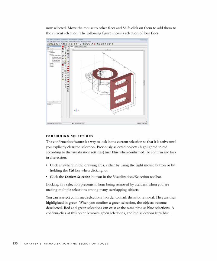
130 | C H A P T E
now selected. Move the mouse to other faces and Shift-click on them to add them to the current selection. The following figure shows a selection of four faces:
C O N F I R M I N G S E L E C T I O N S
The confirmation feature is a way to lock in the current selection so that it is active until you explicitly clear the selection. Previously selected objects (highlighted in red according to the visualization settings) turn blue when confirmed. To confirm and lock in a selection:
• Click anywhere in the drawing area, either by using the right mouse button or by holding the Ctrl key when clicking; or
• Click the Confirm Selection button in the Visualization/Selection toolbar.
Locking in a selection prevents it from being removed by accident when you are making multiple selections among many overlapping objects.
You can reselect confirmed selections in order to mark them for removal. They are then highlighted in green. When you confirm a green selection, the objects become deselected. Red and green selections can exist at the same time as blue selections. A confirm-click at this point removes green selections, and red selections turn blue.
R 3 : V I S U A L I Z A T I O N A N D S E L E C T I O N TO O L S
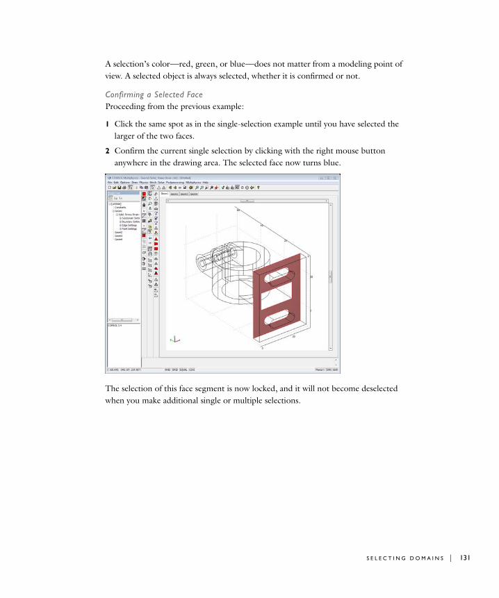
A selection’s color—red, green, or blue—does not matter from a modeling point of view. A selected object is always selected, whether it is confirmed or not.
Confirming a Selected FaceProceeding from the previous example:
1 Click the same spot as in the single-selection example until you have selected the larger of the two faces.
2 Confirm the current single selection by clicking with the right mouse button anywhere in the drawing area. The selected face now turns blue.
The selection of this face segment is now locked, and it will not become deselected when you make additional single or multiple selections.
S E L E C T I N G D O M A I N S | 131
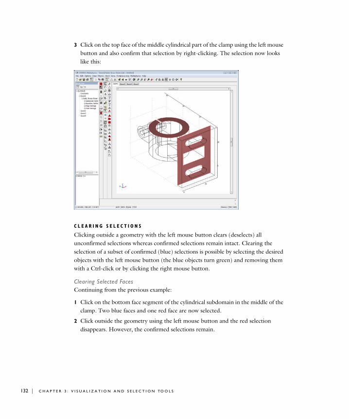
132 | C H A P T E
3 Click on the top face of the middle cylindrical part of the clamp using the left mouse button and also confirm that selection by right-clicking. The selection now looks like this:
C L E A R I N G S E L E C T I O N S
Clicking outside a geometry with the left mouse button clears (deselects) all unconfirmed selections whereas confirmed selections remain intact. Clearing the selection of a subset of confirmed (blue) selections is possible by selecting the desired objects with the left mouse button (the blue objects turn green) and removing them with a Ctrl-click or by clicking the right mouse button.
Clearing Selected FacesContinuing from the previous example:
1 Click on the bottom face segment of the cylindrical subdomain in the middle of the clamp. Two blue faces and one red face are now selected.
2 Click outside the geometry using the left mouse button and the red selection disappears. However, the confirmed selections remain.
R 3 : V I S U A L I Z A T I O N A N D S E L E C T I O N TO O L S
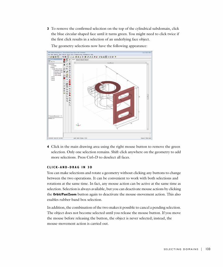
3 To remove the confirmed selection on the top of the cylindrical subdomain, click the blue circular-shaped face until it turns green. You might need to click twice if the first click results in a selection of an underlying face object.
The geometry selections now have the following appearance:
4 Click in the main drawing area using the right mouse button to remove the green selection. Only one selection remains. Shift-click anywhere on the geometry to add more selections. Press Ctrl+D to deselect all faces.
C L I C K - A N D - D R A G I N 3 D
You can make selections and rotate a geometry without clicking any buttons to change between the two operations. It can be convenient to work with both selections and rotations at the same time. In fact, any mouse action can be active at the same time as selection. Selection is always available, but you can deactivate mouse actions by clicking the Orbit/Pan/Zoom button again to deactivate the mouse-movement action. This also enables rubber-band box selection.
In addition, the combination of the two makes it possible to cancel a pending selection. The object does not become selected until you release the mouse button. If you move the mouse before releasing the button, the object is never selected; instead, the mouse-movement action is carried out.
S E L E C T I N G D O M A I N S | 133

134 | C H A P T E
A D J A C E N C Y S E L E C T I O N M E T H O D S
You can select 3D objects by clicking them or their adjacent objects. However, an adjacent object is often next to more than one object. In such a case, you can either choose to select all adjacent objects or cycle through them (multiple clicking selects adjacent objects one at a time). These two methods of selection are called adjacency selection methods; selecting by cycling through adjacent objects is the default.
Choosing the Adjacency Selection MethodChoose between the two methods using the Cycle Adjacent button and the Select All
Adjacent button on the top of the Visualization/Selection toolbar (see the example below), or use the Visualization/Selection Settings dialog box:
1 From the Options menu choose Visualization/Selection Settings.
2 In the Visualization/Selection Settings dialog box click the Rendering/Selection tab.
3 In the Adjacency selection area click either the Select all adjacent or the Cycle adjacent button.
4 Click OK.
Selecting Using Adjacent ObjectsContinuing from the previous example:
1 Display the boundaries and turn on vertex rendering by selecting the Render Vertex button in the Visualization/Selection toolbar.
2 At the top of the Visualization/Selection toolbar make sure that the Cycle Adjacent button is selected in the first group of buttons.
3 In the Options menu, point to Labels, and click Show Vertex Labels.
R 3 : V I S U A L I Z A T I O N A N D S E L E C T I O N TO O L S
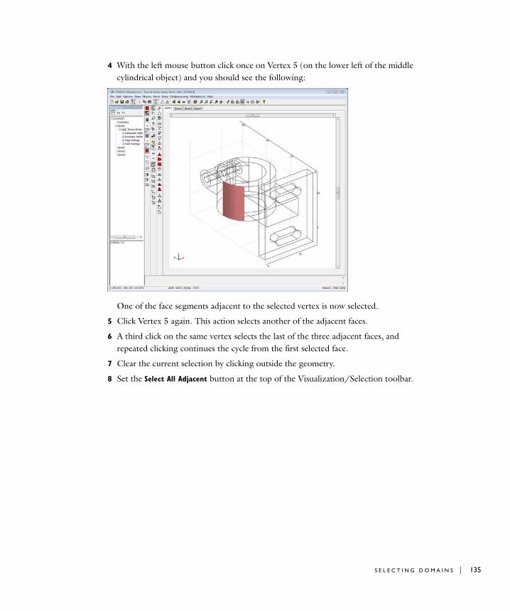
4 With the left mouse button click once on Vertex 5 (on the lower left of the middle cylindrical object) and you should see the following:
One of the face segments adjacent to the selected vertex is now selected.
5 Click Vertex 5 again. This action selects another of the adjacent faces.
6 A third click on the same vertex selects the last of the three adjacent faces, and repeated clicking continues the cycle from the first selected face.
7 Clear the current selection by clicking outside the geometry.
8 Set the Select All Adjacent button at the top of the Visualization/Selection toolbar.
S E L E C T I N G D O M A I N S | 135
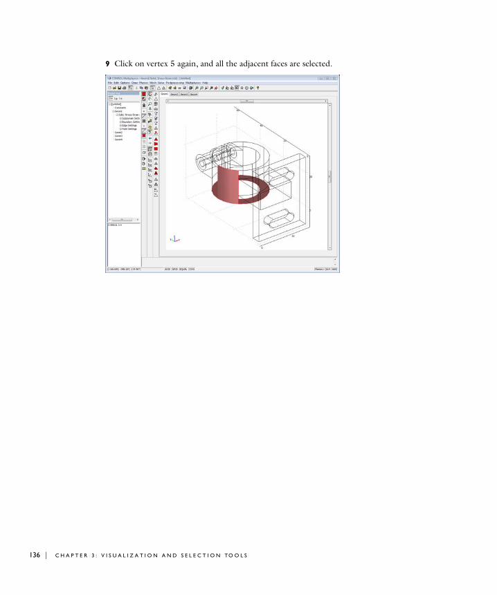
136 | C H A P T E
9 Click on vertex 5 again, and all the adjacent faces are selected.
R 3 : V I S U A L I Z A T I O N A N D S E L E C T I O N TO O L S
4
M o d e l i n g P h y s i c s a n d E q u a t i o n s
This chapter explains a range of methods you can use when building models in COMSOL Multiphysics. Read this chapter to learn several approaches for specifying physics, how to access predefined variables and create your own, how to specify and display units, how to explore the model using the Model Tree, how to use coupling variables, and much more.
Covering how to set up a model, this chapter outlines different options for the preprocessing steps needed to define:
• Boundary and interface conditions
• Material properties or domain equations
• Initial conditions
For flexible specification of these model properties, a great number of variables and functions are available.
For examples of modeling different types of physics and complete model examples, see the COMSOL Multiphysics Modeling Guide.
137
138 | C H A P T E
V a r i a b l e s and Exp r e s s i o n s
This section describes the syntax and names for variables and expressions that you define or that are predefined in a COMSOL Multiphysics application mode or model.
Using Variables and Expressions
To specify a coefficient or a material property, you can type a value or an expression directly in the corresponding edit field. Such an expression can contain:
• Numerical values
• Mathematical and logical functions
• Space coordinates, time, and the dependent variables in any application mode in the model as well as their space derivatives and time derivatives
• Application mode variables, which are predefined specifically for each application mode
• Other predefined variables
• Constants, expressions, coupling variables, and interpolation functions you have defined
• Units
• COMSOL Multiphysics functions and operators such as diff and flc1hs
• COMSOL Script functions
• MATLAB functions (only with the MATLAB interface)
You can use these types of variables and expressions in all the dialog boxes on the Physics menu for point settings, edge settings, boundary settings, and subdomain settings.
Variable Classification and Geometric Scope
COMSOL Multiphysics provides a set of variables you can use in expressions when specifying a model and for visualizing and postprocessing the solution. A number of variables are common to all application modes, one example being space coordinate variables such as x, y, and z. In addition, each application mode has its own set of variables that represent quantities relevant for the physics that it covers. This section describes the available variables and their naming and meanings.
R 4 : M O D E L I N G P H Y S I C S A N D E Q U A T I O N S
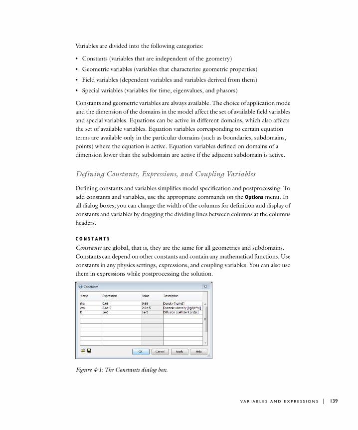
Variables are divided into the following categories:
• Constants (variables that are independent of the geometry)
• Geometric variables (variables that characterize geometric properties)
• Field variables (dependent variables and variables derived from them)
• Special variables (variables for time, eigenvalues, and phasors)
Constants and geometric variables are always available. The choice of application mode and the dimension of the domains in the model affect the set of available field variables and special variables. Equations can be active in different domains, which also affects the set of available variables. Equation variables corresponding to certain equation terms are available only in the particular domains (such as boundaries, subdomains, points) where the equation is active. Equation variables defined on domains of a dimension lower than the subdomain are active if the adjacent subdomain is active.
Defining Constants, Expressions, and Coupling Variables
Defining constants and variables simplifies model specification and postprocessing. To add constants and variables, use the appropriate commands on the Options menu. In all dialog boxes, you can change the width of the columns for definition and display of constants and variables by dragging the dividing lines between columns at the columns headers.
C O N S T A N T S
Constants are global, that is, they are the same for all geometries and subdomains. Constants can depend on other constants and contain any mathematical functions. Use constants in any physics settings, expressions, and coupling variables. You can also use them in expressions while postprocessing the solution.
Figure 4-1: The Constants dialog box.
V A R I A B L E S A N D E X P R E S S I O N S | 139
140 | C H A P T E
Adding ConstantsYou can add as many constants as desired:
1 In Options on the Main menu, choose Constants.
2 In the resulting Constants dialog box make an entry in the Name edit field.
3 Type the expression defining the value of the constant in the Expression edit field. This expression can include any constants already defined and also units. Click Apply or click in another edit field to evaluate the constant. The numeric value (and unit in the model’s base unit system, if applicable) appears in the Value column.
4 Add a description of the constant in the Description edit field. This optional description can be any string.
5 Add more constants by entering values in new rows in the table.
You can modify a constant by editing its expression.
You can resize the Constants dialog box by dragging it at any of the dialog box’s edges, which is useful if a model contains many constants.
Saving and Loading ConstantsYou can save the constants to a text file and also load constants from a text file into the Constants dialog box.
To save the constants to a file, click the Save button in the lower-left corner of the dialog box. COMSOL Multiphysics saves the information in three tab-separated columns to a text file that you define in the Export Variables dialog box. In each row, the first column contains the name of the constant, the second column contains the expression that defines its value, and the third column contains the description.
You can also load constants from a text file where each row—separated by tabs or colons—contains the name, expression, and description. Click the Open button in the lower left corner of the Constants dialog box. This opens the Import Variables dialog box, where you can browse for text files. COMSOL Multiphysics adds the constants to the end of the current list of constants in the dialog box.
Deleting a ConstantTo delete a constant:
1 Clear the Name edit field
2 Click Apply.
R 4 : M O D E L I N G P H Y S I C S A N D E Q U A T I O N S
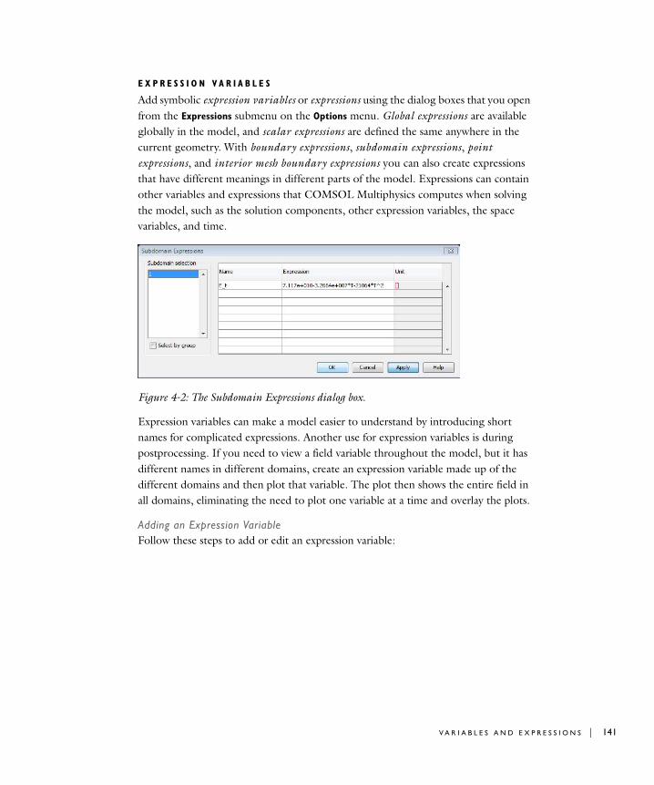
E X P R E S S I O N V A R I A B L E S
Add symbolic expression variables or expressions using the dialog boxes that you open from the Expressions submenu on the Options menu. Global expressions are available globally in the model, and scalar expressions are defined the same anywhere in the current geometry. With boundary expressions, subdomain expressions, point expressions, and interior mesh boundary expressions you can also create expressions that have different meanings in different parts of the model. Expressions can contain other variables and expressions that COMSOL Multiphysics computes when solving the model, such as the solution components, other expression variables, the space variables, and time.
Figure 4-2: The Subdomain Expressions dialog box.
Expression variables can make a model easier to understand by introducing short names for complicated expressions. Another use for expression variables is during postprocessing. If you need to view a field variable throughout the model, but it has different names in different domains, create an expression variable made up of the different domains and then plot that variable. The plot then shows the entire field in all domains, eliminating the need to plot one variable at a time and overlay the plots.
Adding an Expression VariableFollow these steps to add or edit an expression variable:
V A R I A B L E S A N D E X P R E S S I O N S | 141

142 | C H A P T E
1 Go to the Options menu, point to Expressions, and then click:
- Global Expressions to define expression variables that are valid everywhere in the model, including additional states for ODEs, algebraic equations, or other global equations that you specify in the Global Equations dialog box
- Scalar Expressions to define scalar expression variables that are valid on all geometry levels everywhere in the current geometry
- Subdomain Expressions to define expression variables for use on subdomains
- Boundary Expressions to define expression variables for use on boundaries
- Edge Expressions (appears only in 3D models) to define expression variables for use on edges
- Point Expressions to define expression variables for use on points
- Interior Mesh Boundary Expressions to define expression variables for use on interior mesh boundaries (see “Using Equation Contributions on Interior Mesh Boundaries” on page 273 in the COMSOL Multiphysics Modeling Guide)
2 Select the geometry domains where the expression variable exists (this step does not apply to global expressions and scalar expressions). A variable can use different expressions on different domains.
3 Make an appropriate entry in the Name edit field.
4 Make an entry in the Expression field to define the variable in all the domains where it exists.
5 For global expressions and scalar expressions, add a description of the variable in the Description edit field. This step is optional.
6 Click Apply.
To remove a global expression variable or a scalar expression variable, clear the Name edit field and click Apply.
Saving and Loading Global Expression Variables and Scalar Expression VariablesYou can save global expression variables and scalar expression variables to text files and also load such variables from text files into the Global Expressions and Scalar Expressions dialog boxes. This works in the same way as for constants; see “Saving and Loading Constants” on page 140 for more information.
C O U P L I N G V A R I A B L E S
Coupling variables are powerful options that can help you accomplish a number of important modeling goals. A generalization of ordinary expressions, coupling variables can define nonlocal couplings including mesh transformations, integrals over
R 4 : M O D E L I N G P H Y S I C S A N D E Q U A T I O N S
subdomains, and projections. The coupling variables are also the foundation of the extended multiphysics capabilities in COMSOL Multiphysics. With coupling variables you can take information from one type of model domain (a boundary, for example) and make it available on other model domains (a subdomain, for example). For more information on coupling variables, see the section “Using Coupling Variables” on page 255.
The definitions of expression variables and coupling variables are based on a geometry (except for scalar variables). To create such variables, make sure a geometry is already prescribed for the model.
M OV I N G A N D C L E A R I N G R O W S I N T A B L E S F O R V A R I A B L E S
In tables for variables and constants you can move rows up and down and also clear rows. This makes it possible to rearrange their order after you have created them. To do so:
1 In the table, select the row you wish to move or clear.
2 Right-click to open a shortcut menu.
3 Click Move Up on the shortcut menu to move the row up one step; click Move Down to move the row down one step; click Clear to remove the contents of the row.
This feature is available in the following dialog boxes:
• The Constants dialog box
• Dialog boxes for expression variables
• Dialog boxes for coupling variables
• The table containing application mode variables in the physics settings dialog boxes for the equation system that you reach by going to the Physics menu and pointing to Equation System.
Note: It is not possible to clear the contents of rows with application mode variables.
Specifying Varying Coefficients and Material Properties
When assigning varying material properties, for example, you can enter expressions that use the space variables, time, results from other application modes in the model, results from the current application mode, interpolation from gridded data that you
V A R I A B L E S A N D E X P R E S S I O N S | 143
144 | C H A P T E
enter into a table or have stored in a file, and interpolation from measured data. For more information on using interpolation to specify spatially varying and nonlinear material properties, see “Interpolation of Measured Data and Nonlinear Materials” on page 229.
The types of properties listed in the following sections are some of the most common for coefficients and material properties that vary during an analysis:
S P A C E - V A R Y I N G P R O P E R T I E S
Model properties can vary in space for all analysis types and solvers. When defining these properties, use the names of the space variables (independent variables), which are normally x, y, and z. The space variables in axisymmetric models are normally called r and z. You can also use space variables in expression variables and coupling variables. For example, you might type an expression such as K0+0.1*x in an edit field if thermal conductivity varies with x. You also need to use space variables when using interpolation commands with gridded and measured data sets. It is possible to change the names of the space variables when creating a new geometry and later refer to those names when specifying a property.
T I M E - V A R Y I N G P R O P E R T I E S
Model properties can vary in time for time-dependent analyses. When defining properties that vary in time, use the reserved variable name for time, t (see “The Time Variable” on page 175 for details).
N O N L I N E A R P R O P E R T I E S
In a nonlinear model, the model properties depend on the variables for which you solve (the dependent variables). For example, you might enter an expression like K0+0.1*T in an edit field if thermal conductivity varies linearly with temperature T. COMSOL Multiphysics automatically detects if a model is nonlinear and then uses a nonlinear solver. For a more exact definition of a nonlinear model, see “Which Models are Nonlinear?” on page 362.
See also “Interpolation of Measured Data and Nonlinear Materials” on page 229 for insight on how to specify material properties that vary with the dependent variable according to a trend in data.
Copying Physics Settings
You can copy and paste point, edge, boundary, and subdomain settings using the copy and paste commands from the Edit menu or the equivalent shortcut keys. It is also
R 4 : M O D E L I N G P H Y S I C S A N D E Q U A T I O N S
possible to copy the settings for coupling variables and point, edge, boundary, and subdomain expressions. COMSOL Multiphysics can copy the contents of the clipboard to multiple domains of the same type. The copy and paste functionality differs slightly depending on whether the dialog box for the physics setting is open or not:
• If the domain selection list in the dialog box has the input focus (being the location where the user is currently directing input), pressing Ctrl+C copies the physics settings from the dialog box to the clipboard, regardless of whether the settings are applied or not. Pressing Ctrl+V when the domain selection list in the dialog box has the input focus copies the contents of the clipboard to the edit fields of the dialog box, that is, the settings are not automatically applied.
• Otherwise, pressing Ctrl+C copies the physics settings for the currently selected application mode to the clipboard, and pressing Ctrl+V directly applies the contents of the clipboard to the selected domains.
The contents of the clipboard are preserved during a COMSOL Multiphysics session. This makes it possible to copy and paste model properties from one model to another.
You can also copy physics settings using the Model Tree (see “Using the Model Tree” on page 217).
Entering Vector-Valued Expressions
You can enter vector-valued expressions such as extra grid-line coordinates using the following formats:
• A space-separated list of values: 10 15 23 29.7 30.
• Equally spaced values using the colon operator as in start value:step:end value. For instance, 0:0.2:3 creates the values 0, 0.2, 0.4,..., 2.6, 2.8, 3.0. The step size is 1 if you provide only start and end values and skip the step value.
• Equally spaced values using the linspace function. For instance, linspace(0,100,15) creates a vector of 15 equally spaced values from 0 to 100. If you provide only start and stop values and do not indicate the number of values, linspace provides a vector of 100 equally spaced values.
• Logarithmically spaced values using the logspace function. For instance, logspace(x1,x2,n) generates a row vector of n logarithmically equally spaced values between decades 10x1 and 10x2. If X2 equals π, the values fall between 10x1 and π.
V A R I A B L E S A N D E X P R E S S I O N S | 145

146 | C H A P T E
You can combine these formats in one expression to create a vector of values that contains segments with linearly or logarithmically spaced values as well as other freely specified values.
The following modeling features support vector-valued expressions:
• Extra grid lines in the Axes/Grid Settings dialog box
• Line and point coordinates when using the Line and Point dialog boxes
• The times for output from the time-dependent solver and the list of parameter values for the parametric solvers in the Solver Parameter dialog box
• The contour levels, the streamline start-point coordinates, and the coordinates in arrow plots. These visualization settings appear in the Plot Parameters dialog box. Whenever you specify a number of coordinates in postprocessing dialog boxes, COMSOL Multiphysics uses scalar expansion—if one component is the same for all coordinates, you can enter a single number in the corresponding text field. For example, to get 100 linearly spaced points between y = 6 and y = 7 along x = 3, enter it as the single scalar 3 for x and then linspace(6,7,100) for y. Thus, you need not enter linspace(3,3,100) for x.
• The edge-vertex distribution on boundary segments in the Mapped Mesh Parameters dialog box.
• The element-layer distribution in the Extrude Mesh and Revolve Mesh dialog boxes.
Note: For these settings you have access both to the element-by-element operators .*, ./, and .^ as well as the matrix operators *, /, and ^ (multiply, divide, and power operators, respectively). You typically use the element-by-element operators for an expression such as [0:1/20:1].^2. (The matrix power operator does not work in this case because the matrix is not square.)
R 4 : M O D E L I N G P H Y S I C S A N D E Q U A T I O N S

Using Mathematical and Logical Operators and Functions
You can use many common mathematical and logical operators and functions along with constants to specify coefficients and material properties. The following tables show the available functions and operators:
TABLE 4-1: UNARY OPERATORS
OPERATOR DESCRIPTION
+ unary plus
- unary minus
~ logical not
TABLE 4-2: BINARY OPERATORS
OPERATOR DESCRIPTION
+ plus
- minus
* multiply
/ divide
^ power
== equal
~= not equal
> greater than
>= greater than or equal to
< less than
<= less than or equal to
| or
& and
TABLE 4-3: MATHEMATICAL FUNCTIONS AND CONSTANTS
FUNCTION DESCRIPTION SYNTAX EXAMPLE
abs absolute value abs(x)
acos inverse cosine acos(x)
acosh inverse hyperbolic cosine acosh(x)
acot inverse cotangent acot(x)
acoth inverse hyperbolic cotangent acoth(x)
acsc inverse cosecant acsc(x)
acsch inverse hyperbolic cosecant acsch(x)
V A R I A B L E S A N D E X P R E S S I O N S | 147

148 | C H A P T E
angle phase angle angle(x)
asec inverse secant asec(x)
asech inverse hyperbolic secant asech(x)
asin inverse sine asin(x)
asinh inverse hyperbolic sine asinh(x)
atan inverse tangent atan(x)
atan2 four-quadrant inverse tangent atan2(y,x)
atanh inverse hyperbolic tangent atanh(x)
besselj Bessel function of the first kind besselj(a,x)
bessely Bessel function of the second kind bessely(a,x)
besseli modified Bessel function of the first kind besseli(a,x)
besselk modified Bessel function of the second kind besselk(a,x)
conj complex conjugate conj(x)
cos cosine cos(x)
cosh hyperbolic cosine cosh(x)
cot cotangent cot(x)
coth hyperbolic cotangent coth(x)
csc cosecant csc(x)
csch hyperbolic cosecant csch(x)
eps floating point relative accuracy eps
erf error function erf(x)
exp exponential exp(x)
i, j imaginary unit i
imag imaginary part imag(u)
inf infinity inf
log natural logarithm log(x)
log10 common logarithm (base 10) log10(x)
log2 base 2 logarithm log2(x)
max maximum of two arguments max(a,b)
min minimum of two arguments min(a,b)
mod modulo operator mod(a,b)
TABLE 4-3: MATHEMATICAL FUNCTIONS AND CONSTANTS
FUNCTION DESCRIPTION SYNTAX EXAMPLE
R 4 : M O D E L I N G P H Y S I C S A N D E Q U A T I O N S
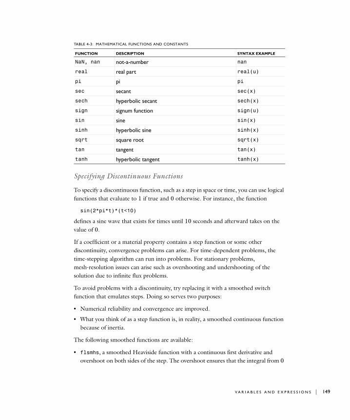
Specifying Discontinuous Functions
To specify a discontinuous function, such as a step in space or time, you can use logical functions that evaluate to 1 if true and 0 otherwise. For instance, the function
sin(2*pi*t)*(t<10)
defines a sine wave that exists for times until 10 seconds and afterward takes on the value of 0.
If a coefficient or a material property contains a step function or some other discontinuity, convergence problems can arise. For time-dependent problems, the time-stepping algorithm can run into problems. For stationary problems, mesh-resolution issues can arise such as overshooting and undershooting of the solution due to infinite flux problems.
To avoid problems with a discontinuity, try replacing it with a smoothed switch function that emulates steps. Doing so serves two purposes:
• Numerical reliability and convergence are improved.
• What you think of as a step function is, in reality, a smoothed continuous function because of inertia.
The following smoothed functions are available:
• flsmhs, a smoothed Heaviside function with a continuous first derivative and overshoot on both sides of the step. The overshoot ensures that the integral from 0
NaN, nan not-a-number nan
real real part real(u)
pi pi pi
sec secant sec(x)
sech hyperbolic secant sech(x)
sign signum function sign(u)
sin sine sin(x)
sinh hyperbolic sine sinh(x)
sqrt square root sqrt(x)
tan tangent tan(x)
tanh hyperbolic tangent tanh(x)
TABLE 4-3: MATHEMATICAL FUNCTIONS AND CONSTANTS
FUNCTION DESCRIPTION SYNTAX EXAMPLE
V A R I A B L E S A N D E X P R E S S I O N S | 149

150 | C H A P T E
to infinity is correct. y=flsmhs(x,scale) approximates the logical expression y = (x>0) by smoothing the transition within the interval −scale < x < scale. fldsmhs is the derivative of the smoothed Heaviside function.
• flsmsign, a smoothed sign function with a continuous first derivative. y = flsmsign(x,scale) approximates the function y = sign(x) by smoothing the transition within the interval −scale < x < scale. fldsmsign is the derivative of the smoothed sign function.
• flc1hs, a smoothed Heaviside function with a continuous first derivative without overshoot. Its syntax is similar to the functions just described.
• flc2hs, a smoothed Heaviside function with a continuous second derivative without overshoot. Its syntax is similar to the functions just described.
In the interval -scale<x<scale, the functions flsmhs and flsmsign are defined by a 7th-degree polynomial chosen so that the 2nd derivative is continuous. Moreover, the moments of order 0, 1, and 2 agree with those for the Heaviside function and the sign function, respectively. This implies that the functions have small overshoots.
Now consider an example. You can use flc1hs to model the heat capacity Cp of a phase-changing material. Assume that a crystalline material has a heat capacity of 1 kJ/kg. Its melting point at the present pressure is 273 K. The liquid phase has a heat capacity of 2 kJ/kg. Run the following commands in COMSOL Script or in MATLAB to generate this behavior and plot Cp around the melting point:
scale = 0.1;T = [272.5:.01:273.5];cp = 1+flc1hs(T-273,scale);plot(T,cp); axis([272 274 .8 2.1])
Using Inline (Analytic) Functions
Just as you can define variables, you can define inline functions. They extend variables with the ability to bind parameters during function calls. In other words, you need not know the actual names of the variables in an expression when you write the function. You define inline functions in the Functions dialog box.
Assume you want to define a function fun(a,b,c,d), which returns a+b*cos(c).
1 From the Options menu, choose Functions.
2 Click the New button.
3 In the New Function dialog box that appears, click the Analytic button and type fun in the Function name edit field. Click OK to return to the Functions dialog box.
R 4 : M O D E L I N G P H Y S I C S A N D E Q U A T I O N S
4 In the Arguments edit field type a,b,c,d.
5 In the Expression edit field type a+b*cos(c).
6 Click the Manual button in the Derivatives area, then type 1,cos(c), diff(a+b*cos(c),c),0 in the associated edit field.
7 Click OK.
COMSOL Multiphysics must know the derivative of a function if you are using a variable that depends on the solution in a function argument. To specify which derivatives to use, click the Manual button and enter the derivatives in the associated edit field. Notice the use of the diff operator (see “Using Special Operators” on page 160 for more information). If you click the Auto button in the Derivatives area, COMSOL Multiphysics uses the diff operator on the expression to get the derivatives. Select the May produce complex output for real arguments check box if the defined function works similarly to sqrt, that is, it sometimes returns complex values for a real-valued input.
Piecewise Analytic Functions
To define piecewise analytical functions, use the Functions dialog box. To define a new piecewise analytical function, do the following steps:
1 From the Options menu, choose Functions.
2 Click the New button.
V A R I A B L E S A N D E X P R E S S I O N S | 151
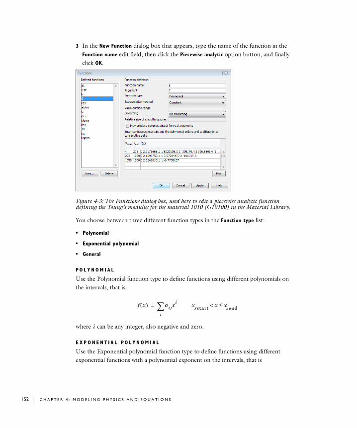
152 | C H A P T E
3 In the New Function dialog box that appears, type the name of the function in the Function name edit field, then click the Piecewise analytic option button, and finally click OK.
Figure 4-3: The Functions dialog box, used here to edit a piecewise analytic function defining the Young’s modulus for the material 1010 (G10100) in the Material Library.
You choose between three different function types in the Function type list:
• Polynomial
• Exponential polynomial
• General
P O L Y N O M I A L
Use the Polynomial function type to define functions using different polynomials on the intervals, that is:
where i can be any integer, also negative and zero.
E X P O N E N T I A L P O L Y N O M I A L
Use the Exponential polynomial function type to define functions using different exponential functions with a polynomial exponent on the intervals, that is
f x( ) aij
i∑ xi
= xjstart x xjend≤<
R 4 : M O D E L I N G P H Y S I C S A N D E Q U A T I O N S
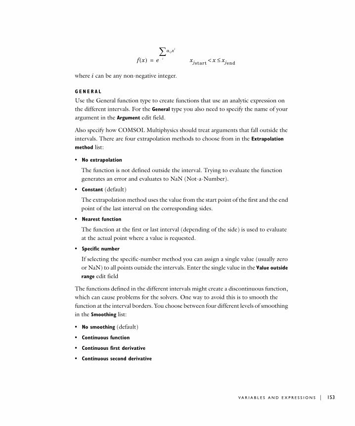
where i can be any non-negative integer.
G E N E R A L
Use the General function type to create functions that use an analytic expression on the different intervals. For the General type you also need to specify the name of your argument in the Argument edit field.
Also specify how COMSOL Multiphysics should treat arguments that fall outside the intervals. There are four extrapolation methods to choose from in the Extrapolation
method list:
• No extrapolation
The function is not defined outside the interval. Trying to evaluate the function generates an error and evaluates to NaN (Not-a-Number).
• Constant (default)
The extrapolation method uses the value from the start point of the first and the end point of the last interval on the corresponding sides.
• Nearest function
The function at the first or last interval (depending of the side) is used to evaluate at the actual point where a value is requested.
• Specific number
If selecting the specific-number method you can assign a single value (usually zero or NaN) to all points outside the intervals. Enter the single value in the Value outside
range edit field
The functions defined in the different intervals might create a discontinuous function, which can cause problems for the solvers. One way to avoid this is to smooth the function at the interval borders. You choose between four different levels of smoothing in the Smoothing list:
• No smoothing (default)
• Continuous function
• Continuous first derivative
• Continuous second derivative
f x( ) e
aij
i
∑ xi
= xjstart x xjend≤<
V A R I A B L E S A N D E X P R E S S I O N S | 153
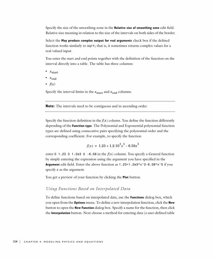
154 | C H A P T E
Specify the size of the smoothing zone in the Relative size of smoothing zone edit field. Relative size meaning in relation to the size of the intervals on both sides of the border.
Select the May produce complex output for real arguments check box if the defined function works similarly to sqrt; that is, it sometimes returns complex values for a real-valued input.
You enter the start and end points together with the definition of the function on the interval directly into a table. The table has three columns:
• xstart
• xend
• f(x)
Specify the interval limits in the xstart and xend columns.
Note: The intervals need to be contiguous and in ascending order.
Specify the function definition in the f(x) column. You define the function differently depending of the Function type. The Polynomial and Exponential polynomial function types are defined using consecutive pairs specifying the polynomial order and the corresponding coefficient. For example, to specify the function
enter 0 1.23 3 1.2e3 5 -6.58 in the f(x) column. You specify a General function by simply entering the expression using the argument you have specified in the Argument edit field. Enter the above function as 1.23+1.2e3*x^3-6.58*x^5 if you specify x as the argument.
You get a preview of your function by clicking the Plot button.
Using Functions Based on Interpolated Data
To define functions based on interpolated data, use the Functions dialog box, which you open from the Options menu. To define a new interpolation function, click the New
button to open the New Function dialog box. Specify a name for the function, then click the Interpolation button. Next choose a method for entering data (a user-defined table
f x( ) 1.23 1.2·103x3 6.58x5–+=
R 4 : M O D E L I N G P H Y S I C S A N D E Q U A T I O N S
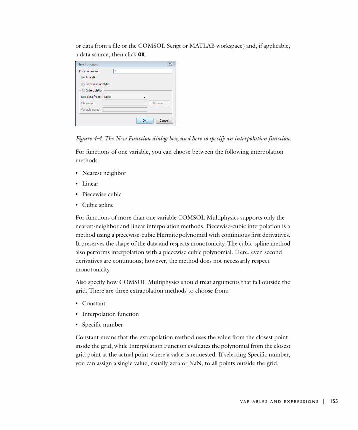
or data from a file or the COMSOL Script or MATLAB workspace) and, if applicable, a data source, then click OK.
Figure 4-4: The New Function dialog box, used here to specify an interpolation function.
For functions of one variable, you can choose between the following interpolation methods:
• Nearest neighbor
• Linear
• Piecewise cubic
• Cubic spline
For functions of more than one variable COMSOL Multiphysics supports only the nearest-neighbor and linear interpolation methods. Piecewise-cubic interpolation is a method using a piecewise-cubic Hermite polynomial with continuous first derivatives. It preserves the shape of the data and respects monotonicity. The cubic-spline method also performs interpolation with a piecewise cubic polynomial. Here, even second derivatives are continuous; however, the method does not necessarily respect monotonicity.
Also specify how COMSOL Multiphysics should treat arguments that fall outside the grid. There are three extrapolation methods to choose from:
• Constant
• Interpolation function
• Specific number
Constant means that the extrapolation method uses the value from the closest point inside the grid, while Interpolation Function evaluates the polynomial from the closest grid point at the actual point where a value is requested. If selecting Specific number, you can assign a single value, usually zero or NaN, to all points outside the grid.
V A R I A B L E S A N D E X P R E S S I O N S | 155
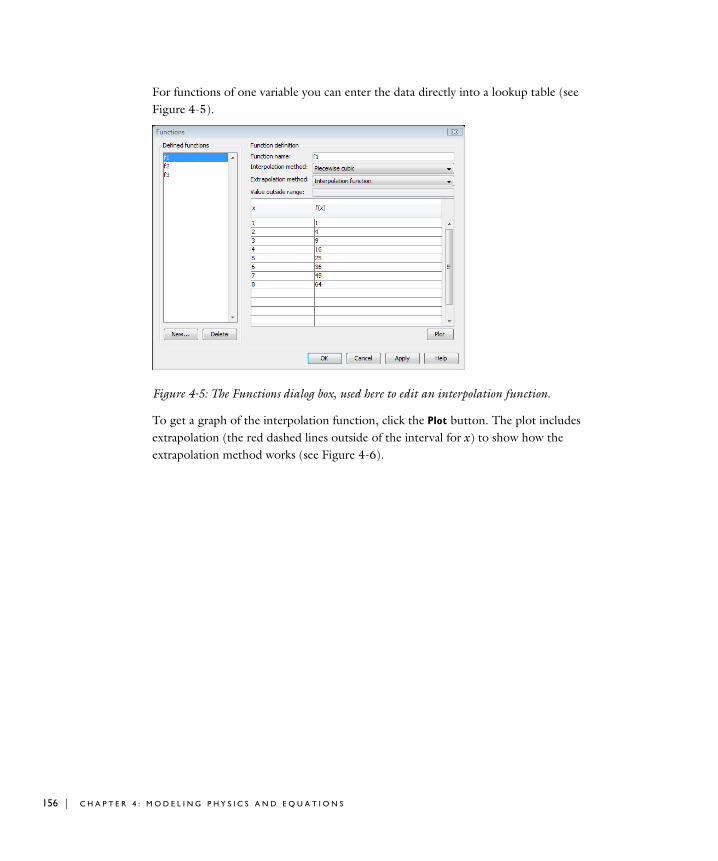
156 | C H A P T E
For functions of one variable you can enter the data directly into a lookup table (see Figure 4-5).
Figure 4-5: The Functions dialog box, used here to edit an interpolation function.
To get a graph of the interpolation function, click the Plot button. The plot includes extrapolation (the red dashed lines outside of the interval for x) to show how the extrapolation method works (see Figure 4-6).
R 4 : M O D E L I N G P H Y S I C S A N D E Q U A T I O N S
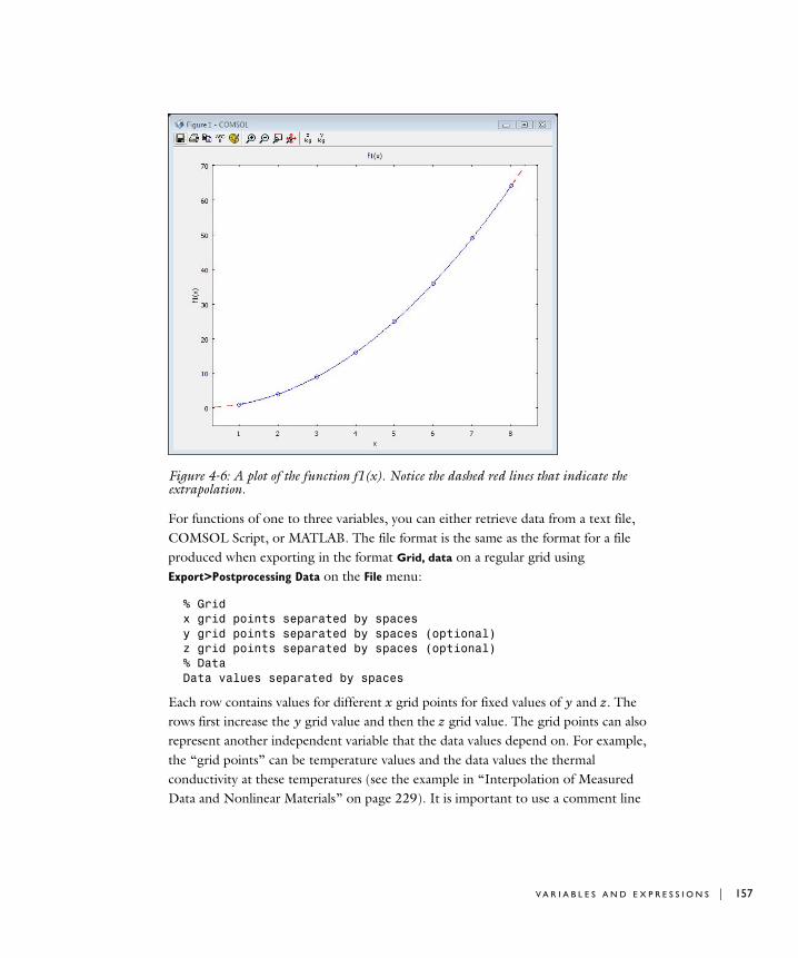
Figure 4-6: A plot of the function f1(x). Notice the dashed red lines that indicate the extrapolation.
For functions of one to three variables, you can either retrieve data from a text file, COMSOL Script, or MATLAB. The file format is the same as the format for a file produced when exporting in the format Grid, data on a regular grid using Export>Postprocessing Data on the File menu:
% Gridx grid points separated by spacesy grid points separated by spaces (optional)z grid points separated by spaces (optional)% DataData values separated by spaces
Each row contains values for different x grid points for fixed values of y and z. The rows first increase the y grid value and then the z grid value. The grid points can also represent another independent variable that the data values depend on. For example, the “grid points” can be temperature values and the data values the thermal conductivity at these temperatures (see the example in “Interpolation of Measured Data and Nonlinear Materials” on page 229). It is important to use a comment line
V A R I A B L E S A N D E X P R E S S I O N S | 157
158 | C H A P T E
starting with % to separate the grid points or other interpolation points and the data values that are associated with these coordinates or interpolation points.
To retrieve data from COMSOL Script or MATLAB, create a structure on the command line with the fields x, y (optional), z (optional), and data. Then x, y, and z are vectors specifying the grid, and data is a multidimensional array of the same format as produced by the function call [xx,yy,zz] = meshgrid(x,y,z);. For example, to define the function f (x, y, z) = x y sin( z) on a unit-cube grid and prepare it for export to COMSOL Multiphysics, type the following on the COMSOL Script or MATLAB command line:
x = linspace(0,1,11); y = linspace(0,1,11); z = linspace(0,1,11);[xx,yy,zz] = meshgrid(x,y,z);data = xx.*yy.*sin(zz);f.x = x; f.y = y; f.z = z; f.data = data;
When COMSOL Multiphysics evaluates the function, the software performs a structured interpolation from the data values on the grid to the coordinates where the function is evaluated. See “A Rock Fracture Flow Model” on page 270 in the COMSOL Multiphysics Model Library for an example using data interpolation.
COMSOL Multiphysics stores the data that it retrieves from COMSOL Script or MATLAB in the function when it is created, and the connection to the original structure is lost. When the data is stored in a text file, the function only stores the name of the text file and reads data from the file during the analysis.
Using COMSOL Script or MATLAB Functions
When running COMSOL Multiphysics with COMSOL Script or MATLAB, you can use command-line functions in a COMSOL Multiphysics expression. In fact, when COMSOL Multiphysics encounters an unknown function it assumes that it is a COMSOL Script or MATLAB function. COMSOL Multiphysics also assumes that the derivatives of the function with respect to its parameters are zero and that the function returns real values for real input arguments. You can use the Functions dialog box to change these defaults.
Assume, for instance, that you also want to use COMSOL Script’s or MATLAB’s Bessel function of the third kind (Hankel function) in COMSOL Multiphysics. Open
R 4 : M O D E L I N G P H Y S I C S A N D E Q U A T I O N S
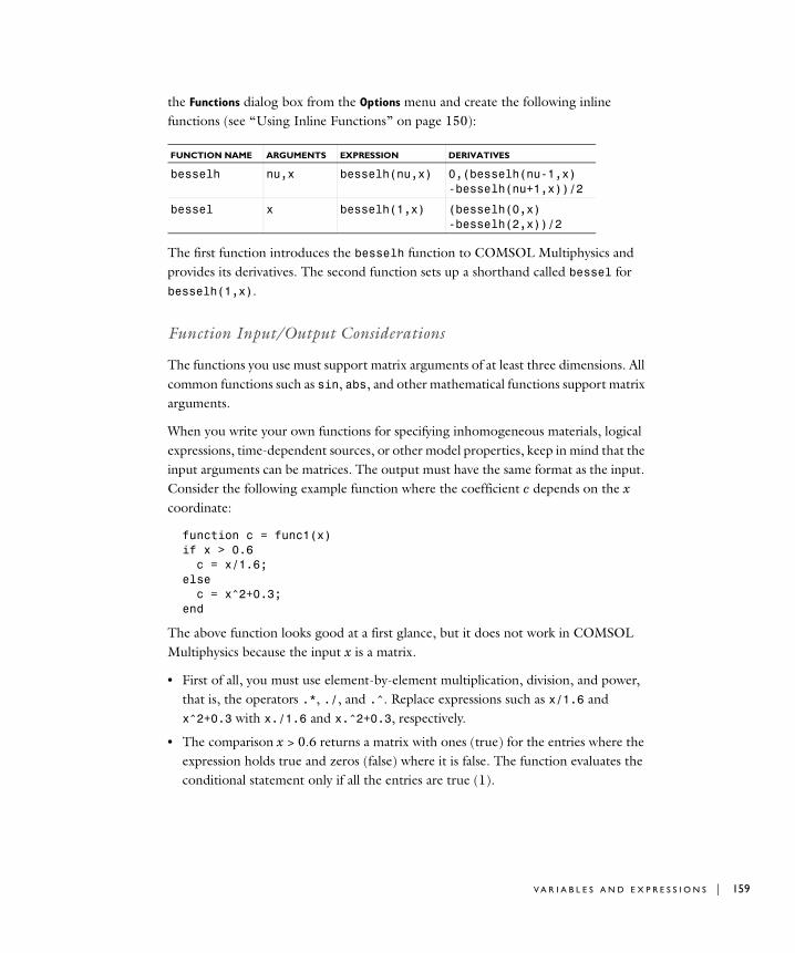
the Functions dialog box from the Options menu and create the following inline functions (see “Using Inline Functions” on page 150):
The first function introduces the besselh function to COMSOL Multiphysics and provides its derivatives. The second function sets up a shorthand called bessel for besselh(1,x).
Function Input/Output Considerations
The functions you use must support matrix arguments of at least three dimensions. All common functions such as sin, abs, and other mathematical functions support matrix arguments.
When you write your own functions for specifying inhomogeneous materials, logical expressions, time-dependent sources, or other model properties, keep in mind that the input arguments can be matrices. The output must have the same format as the input. Consider the following example function where the coefficient c depends on the x coordinate:
function c = func1(x)if x > 0.6 c = x/1.6;else c = x^2+0.3;end
The above function looks good at a first glance, but it does not work in COMSOL Multiphysics because the input x is a matrix.
• First of all, you must use element-by-element multiplication, division, and power, that is, the operators .*, ./, and .^. Replace expressions such as x/1.6 and x^2+0.3 with x./1.6 and x.^2+0.3, respectively.
• The comparison x > 0.6 returns a matrix with ones (true) for the entries where the expression holds true and zeros (false) where it is false. The function evaluates the conditional statement only if all the entries are true (1).
FUNCTION NAME ARGUMENTS EXPRESSION DERIVATIVES
besselh nu,x besselh(nu,x) 0,(besselh(nu-1,x) -besselh(nu+1,x))/2
bessel x besselh(1,x) (besselh(0,x) -besselh(2,x))/2
V A R I A B L E S A N D E X P R E S S I O N S | 159
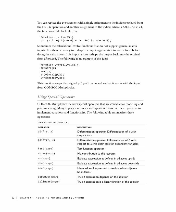
160 | C H A P T E
You can replace the if statement with a single assignment to the indices retrieved from the x > 0.6 operation and another assignment to the indices where . All in all, the function could look like this:
function c = func2(x)c = (x./1.6).*(x>0.6) + (x.^2+0.3).*(x<=0.6);
Sometimes the calculations involve functions that do not support general matrix inputs. It is then necessary to reshape the input arguments into vector form before doing the calculations. It is important to reshape the output back into the original form afterward. The following is an example of this idea:
function y=mypolyval(p,x)sx=size(x);x=x(:);y=polyval(p,x);y=reshape(y,sx);
This function wraps the original polyval command so that it works with the input from COMSOL Multiphysics.
Using Special Operators
COMSOL Multiphysics includes special operators that are available for modeling and postprocessing. Many application modes and equation forms use these operators to implement equations and functionality. The following table summarizes these operators:
TABLE 4-4: SPECIAL OPERATORS
OPERATOR DESCRIPTION
diff(f, x) Differentiation operator. Differentiation of f with respect to x
pdiff(f, x) Differentiation operator. Differentiation of f with respect to x. No chain rule for dependent variables
test(expr) Test function operator
nojac(expr) No contribution to the Jacobian
up(expr) Evaluate expression as defined in adjacent upside
down(expr) Evaluate expression as defined in adjacent downside
mean(expr) Mean value of expression as evaluated on adjacent boundaries
depends(expr) True if expression depends on the solution
islinear(expr) True if expression is a linear function of the solution
x 0.6≤
R 4 : M O D E L I N G P H Y S I C S A N D E Q U A T I O N S
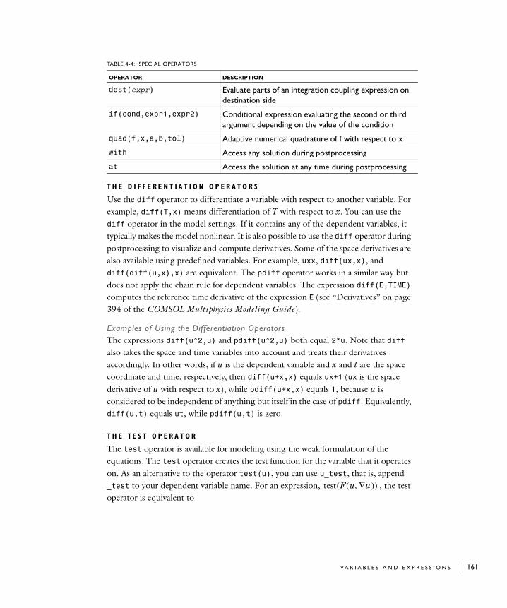
T H E D I F F E R E N T I A T I O N O P E R A T O R S
Use the diff operator to differentiate a variable with respect to another variable. For example, diff(T,x) means differentiation of T with respect to x. You can use the diff operator in the model settings. If it contains any of the dependent variables, it typically makes the model nonlinear. It is also possible to use the diff operator during postprocessing to visualize and compute derivatives. Some of the space derivatives are also available using predefined variables. For example, uxx, diff(ux,x), and diff(diff(u,x),x) are equivalent. The pdiff operator works in a similar way but does not apply the chain rule for dependent variables. The expression diff(E,TIME) computes the reference time derivative of the expression E (see “Derivatives” on page 394 of the COMSOL Multiphysics Modeling Guide).
Examples of Using the Differentiation OperatorsThe expressions diff(u^2,u) and pdiff(u^2,u) both equal 2*u. Note that diff also takes the space and time variables into account and treats their derivatives accordingly. In other words, if u is the dependent variable and x and t are the space coordinate and time, respectively, then diff(u+x,x) equals ux+1 (ux is the space derivative of u with respect to x), while pdiff(u+x,x) equals 1, because u is considered to be independent of anything but itself in the case of pdiff. Equivalently, diff(u,t) equals ut, while pdiff(u,t) is zero.
T H E T E S T O P E R A T O R
The test operator is available for modeling using the weak formulation of the equations. The test operator creates the test function for the variable that it operates on. As an alternative to the operator test(u), you can use u_test, that is, append _test to your dependent variable name. For an expression, , the test operator is equivalent to
dest(expr) Evaluate parts of an integration coupling expression on destination side
if(cond,expr1,expr2) Conditional expression evaluating the second or third argument depending on the value of the condition
quad(f,x,a,b,tol) Adaptive numerical quadrature of f with respect to x
with Access any solution during postprocessing
at Access the solution at any time during postprocessing
TABLE 4-4: SPECIAL OPERATORS
OPERATOR DESCRIPTION
test F u ∇u,( )( )
V A R I A B L E S A N D E X P R E S S I O N S | 161

162 | C H A P T E
,
for all dependent variables ui. For more information about test functions and variables for weak form modeling, see the chapter “The Weak Form” on page 291 in the COMSOL Multiphysics Modeling Guide.
T H E N O J A C O P E R A T O R
The nojac operator makes sure that any expression that it operates on is excluded from the Jacobian computation. This is useful if a Jacobian contribution is not strictly necessary and the computational requirements for it are high. The k-ε turbulence model in the Chemical Engineering Module is an application mode where the use of the nojac operator improves performance. For another example of its use, see the model “Process Control Using a PID Controller” on page 317 in the COMSOL Multiphysics Model Library.
T H E U P , D O W N , A N D M E A N O P E R A T O R S
COMSOL Multiphysics can evaluate expressions on both sides of a domain. These operators are available only on boundaries. For an expression or a variable that is discontinuous across a boundary, the value is different on either side, and COMSOL Multiphysics normally displays the mean values on the boundary. Use the up, down, and mean operators to evaluate an expression on the upside or downside of the boundary or the mean value on the boundary. If the upside or downside is outside of the geometry, or if the variables in the expression are not active on that side, the up or down operator returns 0. For more information about the upside and downside of a boundary, see “Tangent and Normal Variables” on page 167.
T H E D E P E N D S O P E R A T O R
The depends operator returns 1 if the expression that it operates on depends on the solution; otherwise it returns 0. You can use this operator to check user-defined expressions for dependency on the solution.
T H E I S L I N E A R O P E R A T O R
The islinear operator returns 1 if the expression that it operates on is a linear function of the solution; otherwise it returns 0. You can use this operator to check user-defined expressions for linearity with respect to the solution. The stationary solver does this automatically to choose between a linear or a nonlinear solver.
test ui( )ui∂∂ F ui ∇ui,( ) test ∇ui( )
∇ui∂∂ F ui ∇ui,( )+
i∑
R 4 : M O D E L I N G P H Y S I C S A N D E Q U A T I O N S
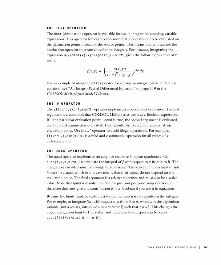
T H E D E S T O P E R A T O R
The dest (destination) operator is available for use in integration-coupling variable expressions. This operator forces the expression that it operates on to be evaluated on the destination points instead of the source points. This means that you can use the destination operator to create convolution integrals. For instance, integrating the expression u/((dest(x)-x)^2+(dest(y)-y)^2) gives the following function of x and y:
For an example of using the dest operator for solving an integro-partial differential equation, see “An Integro-Partial Differential Equation” on page 119 in the COMSOL Multiphysics Model Library.
T H E I F O P E R A T O R
The if(cond,expr1,expr2) operator implements a conditional expression. The first argument is a condition that COMSOL Multiphysics treats as a Boolean expression. If—at a particular evaluation point—cond is true, the second argument is evaluated, else the third argument is evaluated. That is, only one branch is evaluated at any evaluation point. Use the if operator to avoid illegal operations. For example, if(x==0,1,sin(x)/x) is a valid and continuous expression for all values of x, including x = 0.
T H E Q U A D O P E R A T O R
The quad operator implements an adaptive recursive Simpson quadrature. Call quad(f,x,a,b,tol) to evaluate the integral of f with respect to x from a to b. The integration variable x must be a single variable name. The lower and upper limits a and b must be scalar, which in this case means that their values do not depend on the evaluation point. The final argument is a relative tolerance and must also be a scalar value. Note that quad is mainly intended for pre- and postprocessing of data and therefore does not give any contribution to the Jacobian if you use it in equations.
Because the limits must be scalar, it is sometimes necessary to transform the integral. For example, to integrate f(x) with respect to x from 0 to u, where u is the dependent variable (not a scalar), introduce a new variable ξ such that x = uξ. This changes the upper integration limit to 1 (a scalar) and the integration expression becomes quad(f(xi*u)*u,xi,0,1,1e-6).
f x y,( ) u x' y',( )x x'–( )2 y y'–( )2
+----------------------------------------------- x'd y'd∫=
V A R I A B L E S A N D E X P R E S S I O N S | 163

164 | C H A P T E
T H E W I T H O P E R A T O R
Using the with operator, you can access any solution during postprocessing. For time-dependent problems, parametric problems, and eigenvalue problems, this makes it possible to use the solution at any of the time steps, the solution at any parameter value, or any eigensolution in a postprocessing expression. Use the solution number as the first input argument. The second input argument is the expression that you want to evaluate using this solution. For example,
with(3,u^2)
provides the square of the third eigensolution for an eigenvalue problem.
For an example using the with operator to verify that two eigensolutions are orthogonal, see the model “Isospectral Drums” on page 568 in the COMSOL Multiphysics Model Library.
T H E A T O P E R A T O R
Using the at operator during postprocessing, you can access solution to a time-dependent problem at any time. COMSOL Multiphysics provides the solution at that time using interpolation. The first input argument is the time. The second input argument is the expression that you want to evaluate using this solution. For example,
at(12.5,u)
is the solution at 12.5 s.
Variable Naming Conventions
V A R I A B L E N A M E S U F F I X E S
Each application mode variable gets an application mode suffix to avoid naming conflicts. The suffix is the application mode name that appears in the Model Navigator. and helps to clarify variable naming. If you change the application mode name, the variable name suffix changes accordingly.
For example, the variables derived from the application mode for a one-variable coefficient form PDE get the default suffix _c if this was the first application mode of this type. The next application modes of this type generates the suffixes _c2, _c3, and so on.
As another example, the default name for the Heat Transfer by Conduction application mode is ht. The name appears in the user interface when the application mode is active in your model. The dependent variable is the temperature T. To use the dependent
R 4 : M O D E L I N G P H Y S I C S A N D E Q U A T I O N S

variable in equations and postprocessing, type T in an edit field or in code. Likewise Tx is the temperature gradient in the x direction, and Tt is the temperature change in time. Expressions you input for coefficients and other application mode variables are designated by the suffix for the application mode name. By default the suffix is _ht. For example, to use the heat capacity in equations or postprocessing, type C_ht in an edit field.
For information on physics mode suffixes, see the chapter on physics modes in the COMSOL Multiphysics Modeling Guide.
N A M I N G O F S H A P E - F U N C T I O N V A R I A B L E S A N D E Q U A T I O N V A R I A B L E S
The naming of shape-function variables and equation variables follows a certain convention. The index number denotes the equation number to which the expression corresponds. For variables not including any contribution from a dependent variable (the dependent variable is not part of the name), the equation index number appears immediately after the variable name, for example, ga1x or g1. The letters x, y, and z at the end of a variable name denote the spatial coordinate component. You can change the names of dependent variables (field variables) when adding an application mode and change the names of independent variables (spatial coordinates) when adding a geometry. This does not change the name of equation variables such as au, beu, and dau.
In the following descriptions of geometric variables and field variables, replace all letters in italic font with the actual names for the dependent variables (solution components) and independent variables (spatial coordinates) in the model. Replace u with the names of the dependent variables in the model, and replace x, y, and z with the first, second, and third spatial coordinate variable, respectively. xi represents the ith spatial coordinate variable. If the model contains a deformed mesh, you can replace the symbols x, y, z with either the spatial coordinates (x, y, z by default) or the reference coordinates (X, Y, Z by default).
Geometric Variables
S P A C E C O O R D I N A T E V A R I A B L E S
The space coordinate variables (independent variables) x, y, z are available for all domain types. For a Cartesian geometry their default names are x, y, z. For axisymmetric geometries the space coordinates are normally called r and z. You can change the default names of the space coordinates when adding a geometry to a model (see “Changing the Names of the Space Coordinates” on page 29). If a deformed
V A R I A B L E S A N D E X P R E S S I O N S | 165
166 | C H A P T E
mesh is used, x, y, z can be both the spatial coordinates (x, y, z by default) and the reference coordinates (X, Y, Z by default); see “Mathematical Description of the Mesh Movement” on page 392 of the COMSOL Multiphysics Modeling Guide.
If the model includes a deformed mesh, the variables xTIME, yTIME, zTIME represent the mesh velocity. To access these variables, replace x, y, and z with the names of the spatial coordinates in the model (x, y, and z by default).
P A R A M E T E R I Z A T I O N V A R I A B L E S
The surface-boundary parameterization variables are useful for defining distributed loads and constraints such as a parabolic velocity profile. The available parameterization variables are:
• The curve parameter s in 2D. It is equivalent to the Bézier curve parameter, and it runs from 0 to 1 in the direction indicated by the arrows shown on the boundaries in boundary selection mode. You can use s on boundaries when specifying boundary conditions.
• The arc length parameters s1 and s2 in 3D are available on edges and are approximately equivalent to the arc length. In many cases they can be difficult to use because the relationship between x, y, and z (the space coordinates) and s1 and s2 is nonlinear. It is straightforward to use s1 and s2 in cases where a face is equivalent to an untrimmed patch, that is, a face that has no parts cut away. Often it is more convenient to use expressions with x, y, and z for specifying distributed boundary conditions. To see the values of s1 and s2, plot them using a surface or line plot.
Creating a Parabolic Velocity ProfileTo create a parabolic velocity profile with a maximum velocity of v0 on an inflow boundary in a 2D fluid-flow model, enter v0*4*s*(1-s) in the edit field for the appropriate velocity component (where v0 is a constant that you define in the model).
The Chemical Engineering Module, MEMS Module, and Earth Science Module have application modes for fluid flow with a predefined option for a laminar inflow, which provides a parabolic velocity profile.
Showing and Hiding Direction ArrowsTo control the display of the boundary-direction arrows, follow these steps:
1 From the Options menu choose Preferences.
2 In the Preferences dialog box click the Visualization tab.
3 In the Show area, select or clear the Direction arrows check box to show or remove the direction arrows.
R 4 : M O D E L I N G P H Y S I C S A N D E Q U A T I O N S
4 Click Apply.
TA N G E N T A N D N O R M A L V A R I A B L E S
The tangent and normal variables are components of the tangential and normal unit vectors.
Tangent Variables• In 2D, tx and ty define the curve tangent vector associated with the direction of
the boundary.
• In 3D, the tangent variables t1x, t1y, and t1z are defined on edges. The tangent variables t1x, t1y, t1z, t2x, t2y, and t2z are defined on surfaces according to
These most often define two orthogonal vectors on a surface, but the orthogonality can be ruined by scaling geometry objects. The vectors are normalized; ki is a normalizing parameter in the expression just given.
If you use a deformed mesh, the tangent variables are available only for the undeformed mesh. In that case, replace x, y, and z with the names of the reference coordinates (X, Y, Z by default).
Normal Variables• In 1D, nx is the outward unit normal pointing out from the subdomain.
• In 2D, nx and ny define a normal vector pointing outwards relative to the subdomains.
• In 3D, nx, ny, and nz define a normal vector pointing outwards relative to the subdomains.
Because the normal unit vector always points outward, it might be more convenient to use the vector components -ny and nx to represent the tangential unit vector.
Direction of the Normal Component on Interior BoundariesTo get control of the direction of the normal component on interior boundaries, the following variables are available:
• In 1D:
- unx, the outward unit normal seen from the upper subdomain
- dnx, the outward unit normal seen from the lower subdomain
tix tiy tiz, ,( ) kix s1 s2,( )∂
s∂ i-------------------------
y s1 s2,( )∂s∂ i
-------------------------z s1 s2,( )∂
si∂------------------------, ,⎝ ⎠
⎛ ⎞ i 1 2,=,=
V A R I A B L E S A N D E X P R E S S I O N S | 167
168 | C H A P T E
• In 2D:
- unx and uny for the up direction
- dnx and dny for the down direction
The upside is defined as the left side with respect to the parameterization of the curve in the variable s as described earlier in this chapter.
• In 3D:
- unx, uny, and unz for the up direction
- dnx, dny, dnz for the down direction
The up and down directions are with respect to the geometric parameterization of the boundary in the variables s1 and s2. The definition of the geometric normal direction is
.
The down-normal (defined by dnx, dny, and dnz) is equivalent to the geometric normal direction. The geometric normal is pointing into the upside of the geometry. The up-normal (defined by unx, uny, and unz) is pointing out from the upside of the geometry, for example, dnx =-unx, dny =-uny, and dnz =-unz.
To visualize any of these vector variables use arrow plots from the Plot Parameters dialog box.
If a deformed mesh is used, the normal variables are available both for the deformed configuration and for the undeformed configuration. In the first case, replace x, y, and z with the spatial coordinate names (x, y, and z by default). In the second case, replace x, y, and z with the reference coordinate names (X, Y, and Z by default).
Note: There are also outward normal component variables defined for each application mode. You can access these variables by appending an underscore plus the application mode’s name, for example, nx_ps for the unit normal x-direction component for a Plane Stress application mode. This is useful for interior boundaries that are exterior boundaries for the application mode. For example, at the borders between a fluid domain and a solid domain, the outward normal component variables for the structural mechanics application mode (which is turned off in the fluid domain) always point outward from the solid domain into the fluid domain.
ngeom t1x t1y t1z, ,( ) t2x t2y t2z, ,( )×=
R 4 : M O D E L I N G P H Y S I C S A N D E Q U A T I O N S
M I S C E L L A N E O U S V A R I A B L E S
• The variable h, available only in subdomains, represents the mesh-element size (of the undeformed mesh), that is, the length of the longest edge of the element.
• The variable dom is the domain number—the subdomain number, the boundary number, the edge number, or the vertex number. This variable takes only integer values. For subdomains the variable sd has the same meaning.
• The variable meshtype is the mesh type index for the mesh element. This is the index into the cell array structure variable returned by the command get(fem.mesh,'el').
• The variable meshelement is the mesh element number. This is the index of the mesh element within a mesh type structure variable returned by the command get(fem.mesh,'el').
• The variable dvol is the mesh element scale factor, which is the determinant of the Jacobian matrix for the mapping from local (element) coordinates to global coordinates. For 3D domains, this is the factor that COMSOL Multiphysics multiplies volumes by when moving from local coordinates to global coordinates. In 2D and 1D domains, it is an area scaling factor and length scaling factor, respectively. If a deformed mesh is used, dvol is the mesh element scale factor for the undeformed mesh. The corresponding factor for the deformed mesh is named dvol_appl, where appl is the name of the application mode that controls the mesh deformation (ale or pg). To change the default name of the mesh element scale factor for the different frames, use the Model Settings dialog box on the Physics menu.
• The variable qual contains a mesh quality measure. See “Visualizing the Mesh Quality” on page 353 for more information.
• The variable reldetjac is the determinant of the Jacobian matrix for the mapping from local (element) coordinates to global coordinates, normalized to that of a first-order element. In other words, it is the determinant of the Jacobian matrix for the mapping from the straight mesh element to the possibly curved element used when solving. Use this variable to measure the difference in shape between a curved element and the corresponding straight element. The variable reldetjacmin is a scalar for each element defined as the minimum value of the reldetjac variable for the corresponding element. A reldetjacmin value less than zero for an element means that the element is wrapped inside-out; that is, the element is an inverted mesh element. For more information on inverted mesh elements, see “Avoiding Inverted Mesh Elements” on page 356.
V A R I A B L E S A N D E X P R E S S I O N S | 169
170 | C H A P T E
U s i n g F i e l d V a r i a b l e s
Field Variable Definition and Categories
The field variables are the dependent variables and variables derived from them.
S U B D I V I S I O N O F F I E L D V A R I A B L E S
The field variables are divided into the following subcategories:
• Shape function variables—see “Shape Function Variables” on page 171.
• Application mode variables—see “Application Mode Variables” on page 174.
• Expression variables—“Expression Variables” on page 175.
• Coupling variables—see “Coupling Variables” on page 175.
• Equation variables (for PDE modes)—see “Equation Variables” on page 261 in the COMSOL Multiphysics Modeling Guide.
• Boundary-coupled equation variables (for PDE modes)—see “Boundary-Coupled Equation Variables” on page 262 in the COMSOL Multiphysics Modeling Guide.
• Special variables for the time, eigenvalues, and phasor—see “Special Variables” on page 175.
Shape function variables and boundary-coupled shape variables are related to the shape functions of the finite elements. The shape function variables are related to the degrees of freedom defined by a finite element.
Application mode variables are application-mode specific and consist of physically meaningful combinations of material properties and other variables. These variables are predefined for each application mode.
An expression variable is a user-defined shorthand for an expression involving other variables.
Coupling variables are user-defined variables for nonlocal couplings.
Equation variables and boundary-coupled equation variables are only accessible when you have selected the coefficient or general solution forms. These variables are shorthands for certain terms in the PDE and boundary conditions for the coefficient form or the general form. You normally use these variables only for postprocessing.
Special variables are variables that do not belong to any of the previous groups: variables that represent the time, eigenvalues, and phasor.
R 4 : M O D E L I N G P H Y S I C S A N D E Q U A T I O N S
Shape Function Variables
A finite element defines a number of variables, typically a dependent variables and its derivatives. Such variables are called shape functions variables because they can be computed directly from shape functions and the degrees of freedom. When you select an application mode, COMSOL Multiphysics asks you to provide names for the dependent variables. COMSOL Multiphysics uses these variable names to construct the finite elements. Find the finite elements of an application mode by opening the Element page of the Subdomain Settings dialog box. For example, when using the Navier-Stokes application mode the Shape functions edit field looks like
shlag(2,'u') shlag(2,'v') shlag(1,'p')
which means you have introduced two Lagrange finite elements of order two with dependent variable names u and v, respectively, and one Lagrange finite element of order one with dependent variable named p. The dependent variable name is the basis for additional variables names that the finite elements generate. For the Lagrange element the following table shows the available variable names, assuming you gave the name u as the argument to the shape function, and that you provided the names x, y, and z for the independent variables.
In the previous example with the Navier-Stokes application mode, you get the set of variables indicated above for u, v, and p, respectively.
DOMAIN \ SPACE DIM 1D 2D 3D
POINT u u
EDGE u, uTx, uTy, uTzBOUNDARY u, uTx, ut, uTxt u, uTx, uTy, ut,
uTxt, uTytu, uTx, uTy, uTz, ut, uTxt, uTyt, uTzt
SUBDOMAIN u, ux, uxx, ut, uxt, uxxt, utt, uxtt, uxxtt,
u, ux, uy, uxx, uxy, uyx, uyy, ut, uxt, uyt, uxxt, uxyt, uyxt, uyyt, utt, uxtt, uytt, uxxtt, uxytt, uyxtt, uyytt
u, ux, uy, uz, uxx, uxy, uxz, uyx, uyy, uyz, uzx, uzy, uzz, ut, uxt, uyt, uzt, uxxt, uxyt, uxzt, uyxt, uyyt, uyzt, uzxt, uzyt, uzzt, utt, uxtt, uytt, uztt, uxxtt, uxytt, uxztt, uyxtt, uyytt, uyztt, uzxtt, uzytt, uzztt,
U S I N G F I E L D V A R I A B L E S | 171

172 | C H A P T E
The variables ux, uy, and uz are the components of the gradient , that is, the 1st-order spatial derivatives.
The variables uxx, uxy, uxz, uyx, uyy, uyz, uzx, uzy, and uzz are the 2nd-order space derivative components. They are meaningful only if the degree of the polynomial shape function used in an element is high enough. For elements with 2nd-degree polynomial shape functions (2nd-order elements), the polynomial degree of the 2nd-order derivatives is zero, that is, the second derivatives are constant in each element. For element orders lower than two, the second derivatives evaluate to zero regardless of the values of the 2nd-order derivatives of the true solution.
Other finite elements such as the vector element, shvec, define slightly different sets of variable names. See the section “Finite Elements” on page 452 in the COMSOL Multiphysics Reference Guide for lists of variable name defined by each finite element.
If the model uses a deformed mesh, each finite element is associated with a certain frame (the spatial frame or the reference frame) given by the Frame property in the Shape functions edit field. This frame is determined by the Frame property of the application mode that defines the finite element (see “Frames in the Model Navigator” on page 396 of the COMSOL Multiphysics Modeling Guide.) The frame determines the names of the variables generated by the finite element. For instance, if the spatial frame is used, the Lagrange element computes derivatives with respect to the spatial coordinates, ux, uy, uz. If the reference frame is used, the Lagrange element computes derivatives with respect to the reference coordinates uX, uY, uZ.
T H E T I M E D E R I V A T I V E S O F T H E D E P E N D E N T V A R I A B L E S
The variable ut is the time derivative of the dependent variable u. You can also form mixed space-time derivatives as uxit, for example, uxt,
.
Note that the t must appear last in a mixed derivative. You can also use second time derivatives such as utt or uxtt (but not higher derivatives in time). To include the time derivatives in the solution output, you must select that option in the Solver
Manager before you start a time-dependent analysis. See “Selecting Variables for Solution Output” on page 406 for details.
The variables with time derivatives evaluate to the correct value independently of the selected solution form. However, the Jacobian contributions for the time derivatives is accurate only when you have selected the weak solution form, which is the default. If
u∇
x∂t
2
∂∂ u
R 4 : M O D E L I N G P H Y S I C S A N D E Q U A T I O N S

you change the solution form to coefficient form or general form, we recommend you use the da coefficient to introduce a time derivative into the problem.
If the model contains a deformed mesh, there is, in addition to the usual time derivative ut, the mesh time derivative uTIME (see “Mathematical Description of the Mesh Movement” on page 392 in the COMSOL Multiphysics Modeling Guide). This also holds for mixed space-time derivatives.
TA N G E N T I A L D E R I V A T I V E V A R I A B L E S
On boundaries, edges, and points you also have access to tangential derivative variables. They have names such as uTx, uTy, and uTz. Using these variables, it is possible to create models with phenomena on boundaries, edges, or points as described with PDEs. The tangential derivative variables represent the Cartesian components of the tangential projection of the gradient of shape function variables:
.
In this equation, is the tangential gradient, which consists of the tangential derivatives in each spatial direction, I is the unity tensor, n is the outward unit normal vector, and is the gradient of u.
More information about the use of tangential derivative variables appears in the chapter “The Weak Form” in the COMSOL Multiphysics Modeling Guide.
The tangential derivative variables evaluate to the correct value independently of the selected solution form. However, the Jacobian contributions for the tangential derivative variables are accurate only when you have selected the weak solution form. Therefore avoid using another solution form than the weak form (which is the one that the automatic solution form selection chooses in almost all cases) when you use tangential derivative variables in an equation. In addition, to get a divergence operator acting on expressions involving the tangential derivative variables, you must use the weak form to enter the problem. See “Theoretical Background” on page 310 in the COMSOL Multiphysics Modeling Guide for an example.
For an example of the use of tangential derivative variables, see “Transport and Adsorption” on page 30 in the COMSOL Multiphysics Model Library.
VA R I A B L E I N H E R I T A N C E
On boundaries, edges, and points, gradients and second derivatives of the shape functions are available by inheritance, that is, COMSOL Multiphysics computes the average of the values of the variables from the adjacent domains. This process can
u∇( )T I nnT–( ) u∇⋅=
u∇( )T
u∇
U S I N G F I E L D V A R I A B L E S | 173
174 | C H A P T E
progress for several levels. For example, ux is the average on a boundary from the adjacent subdomains, then the average on an edge from the adjacent boundaries, and finally, the average at the points from the adjacent edges. Avoid using variable inheritance for gradients and second derivatives in a model if possible. Instead, use the tangential derivative variables for PDE modeling on boundaries. Also, for best accuracy, use weak constraints for postprocessing of reaction forces and fluxes on boundaries instead of directly accessing the gradient through inheritance (see “Computing Accurate Fluxes” on page 253 for more information).
B O U N D A R Y C O U P L E D S H A P E V A R I A B L E S
Use the up and down operators to access values on either side of the boundary between subdomains (see “The Up, Down, and Mean Operators” on page 162). Explicit variable names for the gradient of the dependent variables on either side of a boundary can be made available by selecting the Boundary coupled shape variables check box in the Model Settings dialog box.
Let u be the name of the dependent variable and x be the name of a space coordinate. Then the following variables are available.
Application Mode Variables
Application mode variables are predefined variables that the application modes introduce. They are typically functions of the dependent variables. The COMSOL Multiphysics Modeling Guide provides documentation on these variables for each application mode. The application modes in the COMSOL add-on modules are documented in the respective module’s User’s Guide. To obtain a list of application mode variables, select the menu item Physics>Equation System>Subdomain Settings. Then click the Variables. Many application mode variables are also available in the Predefined quantities lists in the dialog boxes on the Postprocessing menu.
TABLE 4-5: BOUNDARY COUPLED SHAPE VARIABLES
VARIABLE MEANING
uux The value of ux taken from the adjacent subdomain in the up direction (see page 167). If ux is not defined on that subdomain, the variable uux is undefined.
dux The value of ux taken from the adjacent subdomain in the down direction (see page 167). If ux is not defined on that subdomain, the variable dux is undefined.
R 4 : M O D E L I N G P H Y S I C S A N D E Q U A T I O N S
Application mode variables include a suffix that indicated the application mode. See “Variable Naming Conventions” on page 164 for more information.
Expression Variables
Expression variables are ones that you define to simplify the modeling. They are similar to application mode variables because they are functions of the dependent variables. To define expression variables, use the Expressions choice on the Options menu. You can define expression variables globally or on subdomains, boundaries, edges, and points. If you define an expression variable on boundaries, it also becomes available on adjacent edges and points by variable inheritance. You can use expression variables in a model and during postprocessing. See “Defining Constants, Expressions, and Coupling Variables” on page 139 for information on how to define expression variables.
Coupling Variables
The coupling variables can map the value of an expression of field variables by integration, extrusion, or projections. For documentation on the coupling variables, see “Using Coupling Variables” on page 255.
Special Variables
The special variables are those that do not have a natural place under the categories already presented. These include the time variable, the eigenvalue variable, and the phasor variable.
T H E T I M E V A R I A B L E
For time-dependent problems, the time variable t is available. It can be part of any expression in the point, edge, boundary, and subdomain settings, as well as in postprocessing. It is always a scalar, even for time-dependent problems where the solution contains more than one output time. The value of t during postprocessing corresponds to the selection made in the Solution at time list.
T H E E I G E N V A L U E V A R I A B L E
When specifying an eigenvalue problem you can use the eigenvalue variable like any other variable. By default, the name of the eigenvalue variable is lambda, but you can change this in the Solver Parameters dialog box. The eigenvalue solver extracts the Jacobian, the damping matrix, and the mass matrix through Taylor expansion of the
U S I N G F I E L D V A R I A B L E S | 175
176 | C H A P T E
problem with respect to the eigenvalue variable around a specified eigenvalue linearization point (which is zero by default). Other solvers treat the eigenvalue variable as a constant with value zero, unless it is set by an eigenvalue solution used as initial solution.
You can also specify eigenvalue problems like time-dependent problems. COMSOL Multiphysics then replaces the time derivative ∂u / ∂t with −λu, and the second time derivative ∂2u / ∂t2 with λ2u, where λ is the eigenvalue. It also omits the source terms.
When specified using time derivatives, an eigenvalue problem in coefficient form reads
while on explicit form it is written as a static problem
where the coefficients may be functions of the eigenvalue variable. Clearly, it is possible to convert the first form to the second by adding ea λ2 − da λ to the a coefficient in the latter. For more information on the eigenvalue equation see “Using the Eigenvalue Solver” on page 376.
Consider the common case where ea = 0: a linear eigenvalue problem. For a 1-variable coefficient form eigenvalue PDE, the eigenvalue term is then
where da is a scalar, and the eigenvalue λ is by default available as the eigenvalue variable (default name: lambda). When written as a time-dependent problem, the eigenvalue term factor dau is available as the variable dau.
For a 2-variable coefficient form eigenvalue PDE, the first eigenvalue term is
.
The components of the vector on the right side are available as dau1 and dau2.
After solving an eigenvalue problem, the eigenvalue name is available as a scalar variable for use in postprocessing expressions. To choose between different eigenvalues, select one from the Eigenvalue list in any dialog box in the Postprocessing menu. The value of the eigenvalue variable corresponds to the selection made in the Eigenvalue list.
∇ c u∇– αu–( )⋅ β ∇u au+⋅+ λdau λ2eau–=
∇ c u∇– αu–( )⋅ β ∇u au+⋅+ 0=
λdau
λdau λda11 da12
da21 da22
u1
u2
λda11u1 da12u2+
da21u1 da22u2+= =
R 4 : M O D E L I N G P H Y S I C S A N D E Q U A T I O N S
T H E P H A S O R V A R I A B L E
In all physics application modes for the analysis of time-harmonic problems, COMSOL Multiphysics obtains the solution for a phasor variable, , defined by
.
The phasor contains the amplitude and phase information of u but is itself independent of t. The real part of is the value of u at time t = 0. To obtain the value of u at any other time you can specify a phase angle, , in all postprocessing dialog boxes. This phase angle equals ωt0 for a given time t0.
In the physics application modes, COMSOL Multiphysics multiplies the solution variable as well as all other time-harmonic application mode variables by the phase factor . When you define a problem using phasors with the PDE modes, the software multiplies only the solution variable by . For other harmonic fields, you must give the phase factor explicitly. Do so using the variable phase. Assume you have a quantity denoting an explicit load, specified by setting the coefficient form source term f equal to . To obtain the proper harmonic behavior of F, multiply
by exp(j*phase) during postprocessing.
The Phase Property and AnimationsWhen making animations, you must slightly modify the interpretation of the Phase property of the postprocessing functions and the interpretation of the variable phase. In this case you are not interested in the value just at a single time but in the entire time evolution.
The phase property that you can specify in the postprocessing dialog boxes is the phase at time t = 0. Thus the time evolution is given by a factor , where is taken from the phase property.
When specifying a phase factor exp(j*phase) using the variable phase, this factor is interpreted as the factor . Thus exp(j*phase) is the factor given by the phase property multiplied by the time evolution factor .
Phasor ProductsBe sure to take special care when evaluating products of phasors. Assume you want to evaluate the product uv of two time-harmonic variables u and v. The time evolution of uv is
.
u
u r t,( ) Re u r( ) ejωt( )=
uu
φφ
ejφ
ejφ
F F˜
ejωt=
F˜
F˜
ej ωt φ+( ) φ
ej ωt φ+( ) ejφ
ejωt
u t( )v t( ) Re uejωt( )Re vejωt( )=
U S I N G F I E L D V A R I A B L E S | 177
178 | C H A P T E
When evaluating uv at a given time or when animating the time evolution, be sure to give uv as real(u)*real(v).
Using the relationship
where b* is the complex conjugate of b, you can also express the time average of uv. Specifically,
.
Because the time average of the second term vanishes, you can obtain the average by evaluating 0.5*real(u*conj(v)).
Re a( )Re b( ) 12---Re ab* ab+( )=
Re uejωt( )Re vejωt( ) 12---Re uv
*uve2jωt
+( )=
R 4 : M O D E L I N G P H Y S I C S A N D E Q U A T I O N S
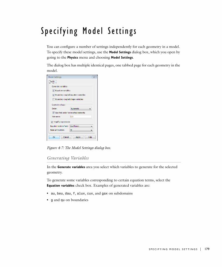
S p e c i f y i n g Mode l S e t t i n g s
You can configure a number of settings independently for each geometry in a model. To specify these model settings, use the Model Settings dialog box, which you open by going to the Physics menu and choosing Model Settings.
The dialog box has multiple identical pages, one tabbed page for each geometry in the model.
Figure 4-7: The Model Settings dialog box.
Generating Variables
In the Generate variables area you select which variables to generate for the selected geometry.
To generate some variables corresponding to certain equation terms, select the Equation variables check box. Examples of generated variables are:
• au, beu, dau, f, alux, cux, and gax on subdomains
• g and qu on boundaries
S P E C I F Y I N G M O D E L S E T T I N G S | 179
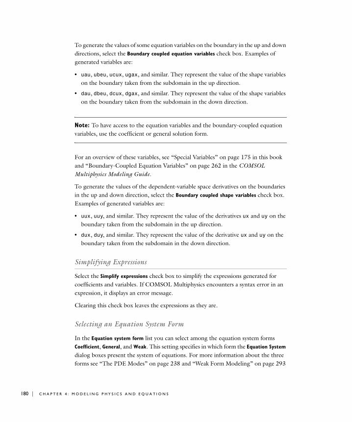
180 | C H A P T E
To generate the values of some equation variables on the boundary in the up and down directions, select the Boundary coupled equation variables check box. Examples of generated variables are:
• uau, ubeu, ucux, ugax, and similar. They represent the value of the shape variables on the boundary taken from the subdomain in the up direction.
• dau, dbeu, dcux, dgax, and similar. They represent the value of the shape variables on the boundary taken from the subdomain in the down direction.
Note: To have access to the equation variables and the boundary-coupled equation variables, use the coefficient or general solution form.
For an overview of these variables, see “Special Variables” on page 175 in this book and “Boundary-Coupled Equation Variables” on page 262 in the COMSOL Multiphysics Modeling Guide.
To generate the values of the dependent-variable space derivatives on the boundaries in the up and down direction, select the Boundary coupled shape variables check box. Examples of generated variables are:
• uux, uuy, and similar. They represent the value of the derivatives ux and uy on the boundary taken from the subdomain in the up direction.
• dux, duy, and similar. They represent the value of the derivative ux and uy on the boundary taken from the subdomain in the down direction.
Simplifying Expressions
Select the Simplify expressions check box to simplify the expressions generated for coefficients and variables. If COMSOL Multiphysics encounters a syntax error in an expression, it displays an error message.
Clearing this check box leaves the expressions as they are.
Selecting an Equation System Form
In the Equation system form list you can select among the equation system forms Coefficient, General, and Weak. This setting specifies in which form the Equation System dialog boxes present the system of equations. For more information about the three forms see “The PDE Modes” on page 238 and “Weak Form Modeling” on page 293
R 4 : M O D E L I N G P H Y S I C S A N D E Q U A T I O N S
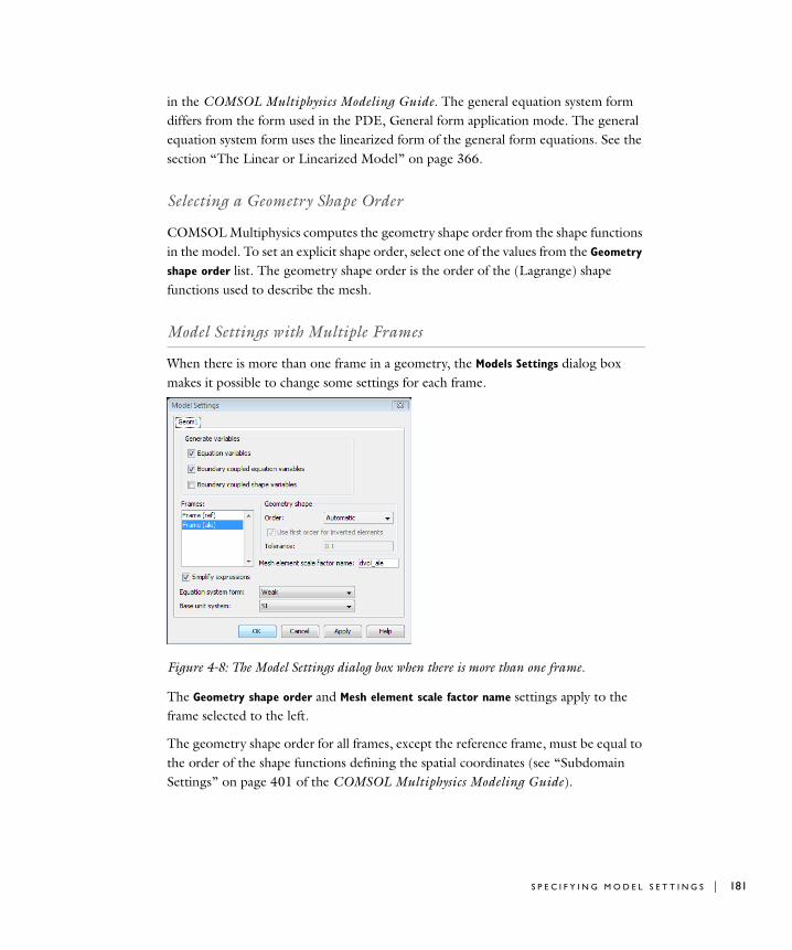
in the COMSOL Multiphysics Modeling Guide. The general equation system form differs from the form used in the PDE, General form application mode. The general equation system form uses the linearized form of the general form equations. See the section “The Linear or Linearized Model” on page 366.
Selecting a Geometry Shape Order
COMSOL Multiphysics computes the geometry shape order from the shape functions in the model. To set an explicit shape order, select one of the values from the Geometry
shape order list. The geometry shape order is the order of the (Lagrange) shape functions used to describe the mesh.
Model Settings with Multiple Frames
When there is more than one frame in a geometry, the Models Settings dialog box makes it possible to change some settings for each frame.
Figure 4-8: The Model Settings dialog box when there is more than one frame.
The Geometry shape order and Mesh element scale factor name settings apply to the frame selected to the left.
The geometry shape order for all frames, except the reference frame, must be equal to the order of the shape functions defining the spatial coordinates (see “Subdomain Settings” on page 401 of the COMSOL Multiphysics Modeling Guide).
S P E C I F Y I N G M O D E L S E T T I N G S | 181

182 | C H A P T E
The mesh element scale factor is the scaling factor for the volume (area, length) for the mapping from local to global coordinates in a mesh element.
R 4 : M O D E L I N G P H Y S I C S A N D E Q U A T I O N S
U s i n g Un i t s
Unit Systems in COMSOL Multiphysics
COMSOL Multiphysics supports the following unit systems:
M E T R I C U N I T S Y S T E M S
• SI units, the International System of Units (SI, Système International d’Unités). This is the default unit system (sometimes also called MKS). For a list of SI units in COMSOL Multiphysics, see “SI Base Units, Derived Units, and Additional Units” on page 191.
• CGSA units. The CGS system uses centimeter, gram, and second as basic units of length, mass, and time, respectively. The remaining basic units are identical to the SI units. The CGS unit system gives nice values for small lengths, masses, forces, pressures, and energies when working on a microscale and with weak electromagnetic forces. The derived units of force, pressure, and energy have well-known and widely used names: dyne, barye, and erg, respectively. CGSA adds ampere as the basic unit for electric current. For a list of the CGSA units, see “Special CGSA Units” on page 195.
• Electromagnetic units (EMU). This system is based on Ampère’s law, which defines the unit of electric current once you select an appropriate value for the constant C. When dealing exclusively with magnetic effects, it is convenient to set C = 1. If CGS units are used for the remaining basic dimensions, the current unit is called an abampere, and the corresponding coherent unit system is called electromagnetic units. Unique names for derived units have been introduced by prefixing the SI name with ab-. For a list of EMU units, see “Special EMU Units” on page 196.
• Electrostatic units (ESU). Based on Coulomb’s law for the force between point charges, ESU uses a unit of charge called the statcoulomb with CGS units for length, mass, and time. From there, the statampere, or franklin, and other derived units of the electrostatic unit system follow. For a list of ESU units, see “Special ESU Units” on page 197.
• MPa units. For stationary structural mechanics, where the density does not appear in the equations, it can be convenient to use a system where the newton and megapascal (hence the name the MPa system) are naturally derived units of force and pressure. Keeping the SI unit for time, the basic units of length and mass
U S I N G U N I T S | 183
184 | C H A P T E
become millimeter and tonne. Except for the force and pressure units, other derived units are nameless. For a list of MPa units, see “Special MPa Units” on page 198.
E N G L I S H U N I T S Y S T E M S
• Foot-pound-second unit system (FPS units). The original foot-pound-second system seems to be the absolute system using the pound as a unit of mass. This version of the FPS system is in agreement with the IEEE standard (the pound is a unit of mass and not of force). The natural derived unit of force is the poundal. For a list of FPS units, see “Special FPS Units” on page 198.
• British engineering units. An alternative to the standard FPS system is the British engineering unit system (also called gravitational foot-pound-second system or foot-slug-second system). Here, the pound force is the natural unit of force, which causes the introduction of the mass unit slug such that a pound force is a slug-foot per second squared. For a list of British engineering units, see “Special British Engineering Units” on page 194.
• Inch-pound-second unit system (IPS units). It is possible to define varieties of the FPS and British engineering systems based on the inch instead of the foot as basic unit of length. This gives rise to two distinct inch-pound-second systems: the absolute IPS system (just called IPS) and the gravitational IPS system. For a list of IPS units, see “Special IPS Units” on page 198.
• Gravitational IPS units. This alternative IPS unit system considers the pound a unit of weight rather than a unit of mass. For a list of Gravitational IPS units, see “Special Gravitational IPS Units” on page 199.
O T H E R
• Unitless (no units)
Specifying the Unit System
S E T T I N G T H E U N I T S Y S T E M F O R T H E C U R R E N T M O D E L
To set the unit system for the current model:
1 From the Physics menu choose Model Settings.
2 In the Model Settings dialog box select the unit system in the Base unit system list.
3 Click OK.
You can also specify the unit system when adding a geometry in the Model Navigator:
R 4 : M O D E L I N G P H Y S I C S A N D E Q U A T I O N S
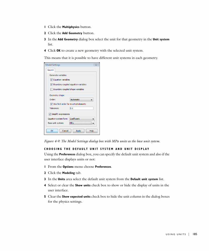
1 Click the Multiphysics button.
2 Click the Add Geometry button.
3 In the Add Geometry dialog box select the unit for that geometry in the Unit system list.
4 Click OK to create a new geometry with the selected unit system.
This means that it is possible to have different unit systems in each geometry.
Figure 4-9: The Model Settings dialog box with MPa units as the base unit system.
C H O O S I N G T H E D E F A U L T U N I T S Y S T E M A N D U N I T D I S P L A Y
Using the Preferences dialog box, you can specify the default unit system and also if the user interface displays units or not:
1 From the Options menu choose Preferences.
2 Click the Modeling tab.
3 In the Units area select the default unit system from the Default unit system list.
4 Select or clear the Show units check box to show or hide the display of units in the user interface.
5 Clear the Show expected units check box to hide the unit column in the dialog boxes for the physics settings.
U S I N G U N I T S | 185
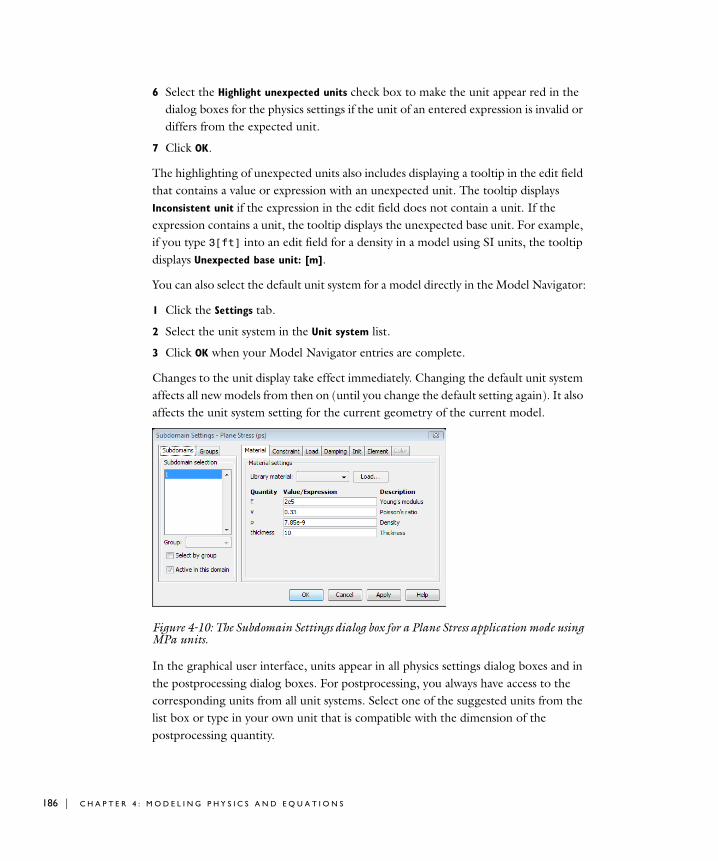
186 | C H A P T E
6 Select the Highlight unexpected units check box to make the unit appear red in the dialog boxes for the physics settings if the unit of an entered expression is invalid or differs from the expected unit.
7 Click OK.
The highlighting of unexpected units also includes displaying a tooltip in the edit field that contains a value or expression with an unexpected unit. The tooltip displays Inconsistent unit if the expression in the edit field does not contain a unit. If the expression contains a unit, the tooltip displays the unexpected base unit. For example, if you type 3[ft] into an edit field for a density in a model using SI units, the tooltip displays Unexpected base unit: [m].
You can also select the default unit system for a model directly in the Model Navigator:
1 Click the Settings tab.
2 Select the unit system in the Unit system list.
3 Click OK when your Model Navigator entries are complete.
Changes to the unit display take effect immediately. Changing the default unit system affects all new models from then on (until you change the default setting again). It also affects the unit system setting for the current geometry of the current model.
Figure 4-10: The Subdomain Settings dialog box for a Plane Stress application mode using MPa units.
In the graphical user interface, units appear in all physics settings dialog boxes and in the postprocessing dialog boxes. For postprocessing, you always have access to the corresponding units from all unit systems. Select one of the suggested units from the list box or type in your own unit that is compatible with the dimension of the postprocessing quantity.
R 4 : M O D E L I N G P H Y S I C S A N D E Q U A T I O N S
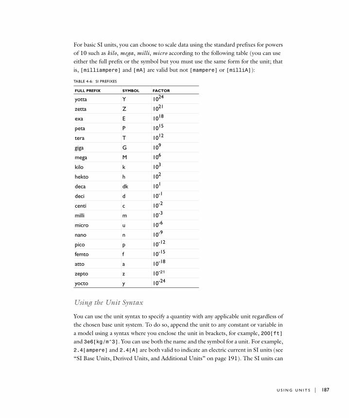
For basic SI units, you can choose to scale data using the standard prefixes for powers of 10 such as kilo, mega, milli, micro according to the following table (you can use either the full prefix or the symbol but you must use the same form for the unit; that is, [milliampere] and [mA] are valid but not [mampere] or [milliA]):
Using the Unit Syntax
You can use the unit syntax to specify a quantity with any applicable unit regardless of the chosen base unit system. To do so, append the unit to any constant or variable in a model using a syntax where you enclose the unit in brackets, for example, 200[ft] and 3e6[kg/m^3]. You can use both the name and the symbol for a unit. For example, 2.4[ampere] and 2.4[A] are both valid to indicate an electric current in SI units (see “SI Base Units, Derived Units, and Additional Units” on page 191). The SI units can
TABLE 4-6: SI PREFIXES
FULL PREFIX SYMBOL FACTOR
yotta Y 1024
zetta Z 1021
exa E 1018
peta P 1015
tera T 1012
giga G 109
mega M 106
kilo k 103
hekto h 102
deca dk 101
deci d 10-1
centi c 10-2
milli m 10-3
micro u 10-6
nano n 10-9
pico p 10-12
femto f 10-15
atto a 10-18
zepto z 10-21
yocto y 10-24
U S I N G U N I T S | 187

188 | C H A P T E
also contain standard prefixes. Note that appending a unit means that you multiply the constant or variable to the left of the unit declaration with this unit. This multiplication takes precedence over other operators so, for example, 1/2[m] evaluates to 0.5 m−1 (0.5[1/m]) whereas both (1/2)[m] and 1/2*1[m] evaluate to 50 cm (0.5[m]). Also, if L is a variable defined as 2[m], L[1/s] evaluates to 2[m/s].The following examples show how you can use the unit syntax:
• Adding two quantities of the same kind that use different units: 0.5[ft]+33[mm]. COMSOL Multiphysics converts the result to the base length unit for the model.
• Using multiplication with a unit to get consistent units for two quantities that you want to add, for example, 14[kg]+rho_ht[m^3], which works if rho_ht represents the density for a model using SI units.
• Making functions work independently of the unit system for a model. For example, assume you have a function k(T) that defines the thermal conductivity k as a function of the temperature T and returns the conductivity in W/(m·K) based on the temperature in kelvin. You can make this function also work with a unit system that uses degrees Fahrenheit for temperature (and a different unit for the thermal conductivity). To do so, use the following syntax to call the function:
k(T[1/K])[W/(m*K)]
When you use degrees Fahrenheit as the temperature unit, multiplying by [K] provides a conversion from kelvin to degrees Fahrenheit. Conversely, multiplying by [1/K] provides a a conversion from degrees Fahrenheit to kelvin so that T[1/K] converts the value of the temperature T from the base unit system to kelvin. This means that the output from the function k(T) always has the same numerical value regardless of the unit system that you use. The multiplication with [1/K] also makes the input dimensionless. The output from a function is also dimensionless. Multiplying the thermal conductivity with [W/(m*K)] provides a unit for k and a conversion to the base unit system’s unit for thermal conductivity.
It is possible to add constants (without units) to any quantity. COMSOL Multiphysics then assumes that this value has the unit of the base unit system for the model. You can also concatenate several units, for example, 3.6[N][m], which is equivalent to 3.6[N*m] and evaluates to 3.6[J].
The material libraries in COMSOL Multiphysics employ this unit syntax to make it possible to use the SI-based materials data with any base unit system.
R 4 : M O D E L I N G P H Y S I C S A N D E Q U A T I O N S

D E C L A R I N G U N I T S F O R C O N S T A N T S A N D E X P R E S S I O N V A R I A B L E S
If you use constants or expression variables in the physics settings dialog boxes, it is good practice to define them using the unit syntax. The Constants dialog box and the dialog boxes for expression variables display the resulting unit, in the base unit system, of the constants and expressions that you define. You can then verify that these variables have the expected unit before using them in the physics settings. The unit of constants and expression variables are otherwise undefined. Using properties with undefined units in a model does not affect the numerical results from the analysis, but in the postprocessing stages, expressions involving such constants and variables are also unitless. Using other units than the standard units for the chosen base unit system, or using SI prefixes, the conversion to the base unit system’s unit also affects the value (quantity) using a scaling factor (and an offset in the case of temperature units). The Value column in the Constants dialog box displays the quantity and unit in the base unit system so that you can see the result of the unit conversion. For example, if you define a constant as 3[ft] for a model using SI units, the result in the Value column is 0.9144[m].
I N D I C A T I O N O F U N E X P E C T E D U N I T S
If you select the Highlight unexpected units check box on Modeling page in the Preferences dialog box, the unit display appears red for the properties in the physics dialog boxes that have an invalid unit or a different unit than the expected one that the dialog box shows. A tooltip displays an error message at the corresponding text field. In the case of a valid but unexpected unit, this message contains the unexpected unit in the model’s base unit system.
Switching Unit System
If you switch the unit system during modeling or use a unit system other than SI, COMSOL Multiphysics does not convert the data in the model with the following exceptions:
• COMSOL Multiphysics converts the default values for all application scalar variables to the current unit system when you create an application mode. Switching the unit system resets the values of the application scalar variables to their default values and converts them to the current unit system.
• The default values for all physics settings are in the current unit system (COMSOL Multiphysics converts them from the original values in SI units both when starting an application mode and when switching unit system). The values for any data in the current model do not change.
U S I N G U N I T S | 189

190 | C H A P T E
All data in the materials libraries are in SI units, but you can use them with any unit system because COMSOL Multiphysics converts these values to the corresponding values in the model’s unit system. Note, however, that you must also declare the units of other input data for the model using the unit syntax (or convert the numerical values to the new units system). If the length unit changes, you must also convert the geometry dimensions to keep the size of the geometry using another length unit.
About Temperature Units
The relations between different temperature units involve an offset in addition to the usual scale factor. In many cases, the offset is not important to the physics equations because these equations are concerned only with temperature differences. There are, however, some cases where you must use an absolute or thermodynamic temperature measure. The most common example is the Stefan-Bolzmann law for black-body radiation used in radiation boundary conditions.
All predefined metric unit systems use the kelvin, which is an absolute temperature, as the basic unit of temperature. The English unit systems use the degree Fahrenheit as the basic unit of temperature, which, because the Fahrenheit scale is not absolute, is fine for most purposes except radiation. When modeling radiation in English units, you have to treat the temperature values as being given in degrees Rankine (which is the corresponding absolute scale). By doing so, the radiation terms are correct, but conversion to other units in postprocessing fails.
To declare temperature units in kelvin, use [K]. For degrees Fahrenheit use [degF], and for degrees Celsius use [degC].
D I F F E R E N T I A L V S . A B S O L U T E T E M P E R A T U R E
If the dimension of an expression that includes a unit is temperature or 1/temperature, COMSOL Multiphysics interprets the dimension as an absolute temperature. If the dimension is something other than temperature but the unit expression includes temperature, the temperature is a differential temperature; that is, COMSOL Multiphysics uses no offset when converting between different temperature units.
The following examples illustrate how the unit conversion works for different expressions that include temperature units:
• 100[degC] is an expression that has temperature as the dimension. COMSOL Multiphysics interprets it as an absolute temperature and evaluates it as 373.15 K.
R 4 : M O D E L I N G P H Y S I C S A N D E Q U A T I O N S

• 373.15[1/K] is also interpreted as an absolute temperature (but no conversion is necessary from kelvin to kelvin).
• 100[degC/K] is dimensionless, and the temperature is therefore a differential temperature; that is, the result is 100 because the conversion uses no offset.
• To make COMSOL Multiphysics interpret the previous example as an absolute temperature, split the expression using two separate expressions such as 100[degC]*1[1/K], which equals 373.15. This is also what occurs when you use a variable, for example, TC, defined as 100[degC]. TC[1/K] is then two expressions where both are interpreted as absolute temperature.
SI Base Units, Derived Units, and Additional Units
The SI units form an internationally accepted system with seven units for base quantities and a large number of derived units.
Table 4-7 lists the SI units for the seven base quantities plus the radius.
COMSOL Multiphysics supports the following SI derived units:
TABLE 4-7: BASE SI UNITS
BASE QUANTITY NAME SYMBOL
length meter, metre m
mass kilogram kg
time second s
electric current ampere A
temperature kelvin K
amount of substance mole mol
luminous intensity candela cd
radius meterradius, metreradius m, mr
TABLE 4-8: SI DERIVED UNITS IN COMSOL MULTIPHYSICS
BASE QUANTITY NAME SYMBOL
absorbed dose gray Gy
capacitance farad F
conductance siemens S
dose equivalent sievert Sv
electric charge coulomb C
electric resistance, impedance, reactance ohm Ω
U S I N G U N I T S | 191
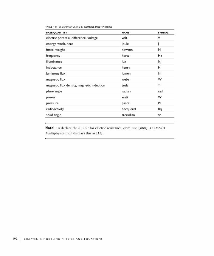
192 | C H A P T E
Note: To declare the SI unit for electric resistance, ohm, use [ohm]. COMSOL Multiphysics then displays this as [Ω].
electric potential difference, voltage volt V
energy, work, heat joule J
force, weight newton N
frequency hertz Hz
illuminance lux lx
inductance henry H
luminous flux lumen lm
magnetic flux weber W
magnetic flux density, magnetic induction tesla T
plane angle radian rad
power watt W
pressure pascal Pa
radioactivity becquerel Bq
solid angle steradian sr
TABLE 4-8: SI DERIVED UNITS IN COMSOL MULTIPHYSICS
BASE QUANTITY NAME SYMBOL
R 4 : M O D E L I N G P H Y S I C S A N D E Q U A T I O N S
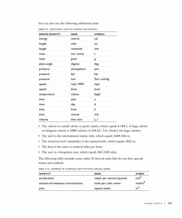
You can also use the following additional units:
• The calorie is a small calorie or gram calorie, which equals 4.184 J. A large calorie or kilogram calorie is 1000 calories (4.184 kJ). Use [kcal] for large calories.
• The mile is the international statute mile, which equals 1609.344 m.
• The nautical mile (nautimile) is the nautical mile, which equals 1852 m.
• The knot is the same as nautical miles per hour.
• The year is a Gregorian year, which equals 365.2425 days.
The following table includes some other SI derived units that do not have special names and symbols:
TABLE 4-9: ADDITIONAL UNITS IN COMSOL MULTIPHYSICS
DERIVED QUANTITY NAME SYMBOLS
energy calorie cal
length mile mi
length nautimile nmi
mass ton, tonne t
mass gram g
plane angle degree deg
pressure atmosphere atm
pressure bar bar
pressure torr Torr, mmHg
speed mph, MPH mph
speed knot knot
temperature celcius degC
time year a
time day d
time hour h
time minute min
volume liter, litre L, l
TABLE 4-10: EXAMPLES OF SI DERIVED UNITS WITHOUT SPECIAL NAMES
QUANTITY NAME SYMBOL
acceleration meter per second squared m/s2
amount-of-substance concentration mole per cubic meter mol/m3
area square meter m2
U S I N G U N I T S | 193
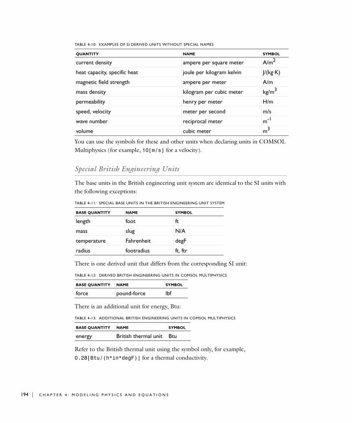
194 | C H A P T E
You can use the symbols for these and other units when declaring units in COMSOL Multiphysics (for example, 10[m/s] for a velocity).
Special British Engineering Units
The base units in the British engineering unit system are identical to the SI units with the following exceptions:
There is one derived unit that differs from the corresponding SI unit:
There is an additional unit for energy, Btu:
Refer to the British thermal unit using the symbol only, for example, 0.28[Btu/(h*in*degF)] for a thermal conductivity.
current density ampere per square meter A/m2
heat capacity, specific heat joule per kilogram kelvin J/(kg·K)
magnetic field strength ampere per meter A/m
mass density kilogram per cubic meter kg/m3
permeability henry per meter H/m
speed, velocity meter per second m/s
wave number reciprocal meter m-1
volume cubic meter m3
TABLE 4-11: SPECIAL BASE UNITS IN THE BRITISH ENGINEERING UNIT SYSTEM
BASE QUANTITY NAME SYMBOL
length foot ft
mass slug N/A
temperature Fahrenheit degF
radius footradius ft, ftr
TABLE 4-12: DERIVED BRITISH ENGINEERING UNITS IN COMSOL MULTIPHYSICS
BASE QUANTITY NAME SYMBOL
force pound-force lbf
TABLE 4-13: ADDITIONAL BRITISH ENGINEERING UNITS IN COMSOL MULTIPHYSICS
BASE QUANTITY NAME SYMBOL
energy British thermal unit Btu
TABLE 4-10: EXAMPLES OF SI DERIVED UNITS WITHOUT SPECIAL NAMES
QUANTITY NAME SYMBOL
R 4 : M O D E L I N G P H Y S I C S A N D E Q U A T I O N S
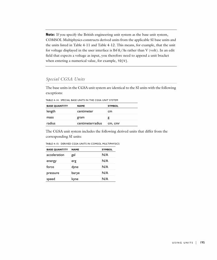
Note: If you specify the British engineering unit system as the base unit system, COMSOL Multiphysics constructs derived units from the applicable SI base units and the units listed in Table 4-11 and Table 4-12. This means, for example, that the unit for voltage displayed in the user interface is lbf·ft/As rather than V (volt). In an edit field that expects a voltage as input, you therefore need to append a unit bracket when entering a numerical value, for example, 10[V].
Special CGSA Units
The base units in the CGSA unit system are identical to the SI units with the following exceptions:
The CGSA unit system includes the following derived units that differ from the corresponding SI units:
TABLE 4-14: SPECIAL BASE UNITS IN THE CGSA UNIT SYSTEM
BASE QUANTITY NAME SYMBOL
length centimeter cm
mass gram g
radius centimeterradius cm, cmr
TABLE 4-15: DERIVED CGSA UNITS IN COMSOL MULTIPHYSICS
BASE QUANTITY NAME SYMBOL
acceleration gal N/A
energy erg N/A
force dyne N/A
pressure barye N/A
speed kyne N/A
U S I N G U N I T S | 195

196 | C H A P T E
Special EMU Units
The base units in the EMU unit system are identical to the SI units with the following exceptions:
The EMU unit system includes the following derived units that differ from the corresponding SI units:
TABLE 4-16: SPECIAL BASE UNITS IN THE EMU UNIT SYSTEM
BASE QUANTITY NAME SYMBOL
length centimeter cm
mass gram g
electric current abampere, biot N/A
radius centimeterradius cm, cmr
TABLE 4-17: DERIVED EMU UNITS IN COMSOL MULTIPHYSICS
BASE QUANTITY NAME SYMBOL
acceleration gal N/A
capacitance abfarad N/A
conductance absiemens N/A
electric charge abcoulomb N/A
electric resistance abohm N/A
electric potential difference, voltage abvolt N/A
energy erg N/A
force dyne N/A
inductance abhenry N/A
magnetic flux abweber
magnetic flux density abtesla N/A
pressure barye N/A
speed kyne N/A
R 4 : M O D E L I N G P H Y S I C S A N D E Q U A T I O N S

Special ESU Units
The base units in the ESU unit system are identical to the SI units with the following exceptions:
The ESU unit system includes the following derived units that differ from the corresponding SI units:
TABLE 4-18: SPECIAL BASE UNITS IN THE ESU UNIT SYSTEM
BASE QUANTITY NAME SYMBOL
length centimeter cm
mass gram g
electric current statampere, franklin N/A
radius centimeterradius cm, cmr
TABLE 4-19: DERIVED ESU UNITS IN COMSOL MULTIPHYSICS
BASE QUANTITY NAME SYMBOL
acceleration gal N/A
capacitance statfarad N/A
conductance statsiemens N/A
electric charge statcoulomb N/A
electric resistance statohm N/A
electric potential difference, voltage statvolt N/A
energy erg N/A
force dyne N/A
inductance stathenry N/A
magnetic flux statweber N/A
magnetic flux density stattesla N/A
pressure barye N/A
speed kyne N/A
U S I N G U N I T S | 197
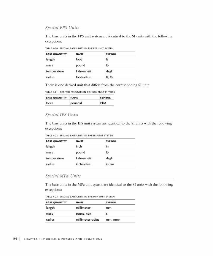
198 | C H A P T E
Special FPS Units
The base units in the FPS unit system are identical to the SI units with the following exceptions:
There is one derived unit that differs from the corresponding SI unit:
Special IPS Units
The base units in the IPS unit system are identical to the SI units with the following exceptions:
Special MPa Units
The base units in the MPa unit system are identical to the SI units with the following exceptions:
TABLE 4-20: SPECIAL BASE UNITS IN THE FPS UNIT SYSTEM
BASE QUANTITY NAME SYMBOL
length foot ft
mass pound lb
temperature Fahrenheit degF
radius footradius ft, ftr
TABLE 4-21: DERIVED FPS UNITS IN COMSOL MULTIPHYSICS
BASE QUANTITY NAME SYMBOL
force poundal N/A
TABLE 4-22: SPECIAL BASE UNITS IN THE IPS UNIT SYSTEM
BASE QUANTITY NAME SYMBOL
length inch in
mass pound lb
temperature Fahrenheit degF
radius inchradius in, inr
TABLE 4-23: SPECIAL BASE UNITS IN THE MPA UNIT SYSTEM
BASE QUANTITY NAME SYMBOL
length millimeter mm
mass tonne, ton t
radius millimeterradius mm, mmr
R 4 : M O D E L I N G P H Y S I C S A N D E Q U A T I O N S
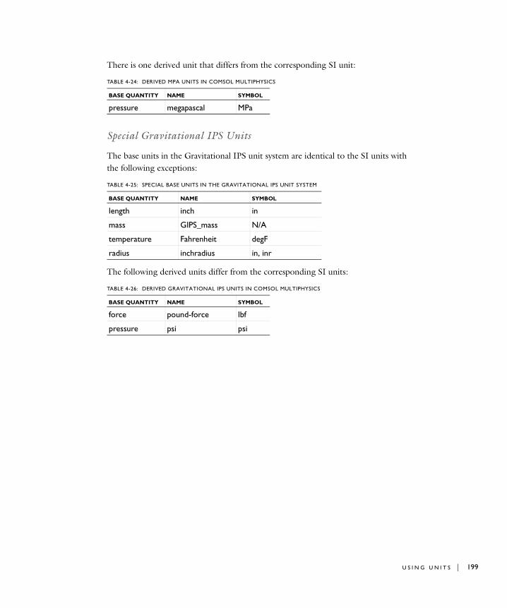
There is one derived unit that differs from the corresponding SI unit:
Special Gravitational IPS Units
The base units in the Gravitational IPS unit system are identical to the SI units with the following exceptions:
The following derived units differ from the corresponding SI units:
TABLE 4-24: DERIVED MPA UNITS IN COMSOL MULTIPHYSICS
BASE QUANTITY NAME SYMBOL
pressure megapascal MPa
TABLE 4-25: SPECIAL BASE UNITS IN THE GRAVITATIONAL IPS UNIT SYSTEM
BASE QUANTITY NAME SYMBOL
length inch in
mass GIPS_mass N/A
temperature Fahrenheit degF
radius inchradius in, inr
TABLE 4-26: DERIVED GRAVITATIONAL IPS UNITS IN COMSOL MULTIPHYSICS
BASE QUANTITY NAME SYMBOL
force pound-force lbf
pressure psi psi
U S I N G U N I T S | 199
200 | C H A P T E
S p e c i f y i n g Phy s i c s S e t t i n g s
From the Physics menu you can specify all the physics and equations that define a model including:
• Equations
• Boundary and interface conditions
• Material properties
• Initial conditions
In addition, you can specify weak form contributions and element types for additional flexibility.
Specifically, the settings are available on the following physical domains:
• Subdomains
• Boundaries
• Edges
• Points
• Scalar variables that are independent of the geometry
Not all of these options are available for all geometry types and application modes.
All dialog boxes for the specification of the physics and equations accept variables, constants, and expressions as input data (see “Variables and Expressions” on page 138).
Opening the Physics Settings Dialog Boxes
To open all the physics settings dialog boxes:
• Go to the Physics menu and choose the corresponding command, for example Boundary Settings to open the Boundary Settings dialog box.
• In the domain selection modes, double-click a domain to select it and open the associated dialog box. For example, double-clicking a boundary opens the Boundary
Settings dialog box and shows the present settings for the selected domains. For more on selection methods see “General Object Selection Methods” on page 126.
• In the Model Tree, using the Overview setting, right-click on the application mode for which you want to specify physics settings and select the appropriate dialog box.
R 4 : M O D E L I N G P H Y S I C S A N D E Q U A T I O N S
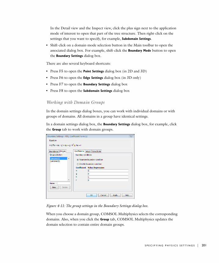
In the Detail view and the Inspect view, click the plus sign next to the application mode of interest to open that part of the tree structure. Then right-click on the settings that you want to specify, for example, Subdomain Settings.
• Shift-click on a domain-mode selection button in the Main toolbar to open the associated dialog box. For example, shift-click the Boundary Mode button to open the Boundary Settings dialog box.
There are also several keyboard shortcuts:
• Press F5 to open the Point Settings dialog box (in 2D and 3D)
• Press F6 to open the Edge Settings dialog box (in 3D only)
• Press F7 to open the Boundary Settings dialog box
• Press F8 to open the Subdomain Settings dialog box
Working with Domain Groups
In the domain settings dialog boxes, you can work with individual domains or with groups of domains. All domains in a group have identical settings.
In a domain settings dialog box, the Boundary Settings dialog box, for example, click the Group tab to work with domain groups.
Figure 4-11: The group settings in the Boundary Settings dialog box.
When you choose a domain group, COMSOL Multiphysics selects the corresponding domains. Also, when you click the Group tab, COMSOL Multiphysics updates the domain selection to contain entire domain groups.
S P E C I F Y I N G P H Y S I C S S E T T I N G S | 201
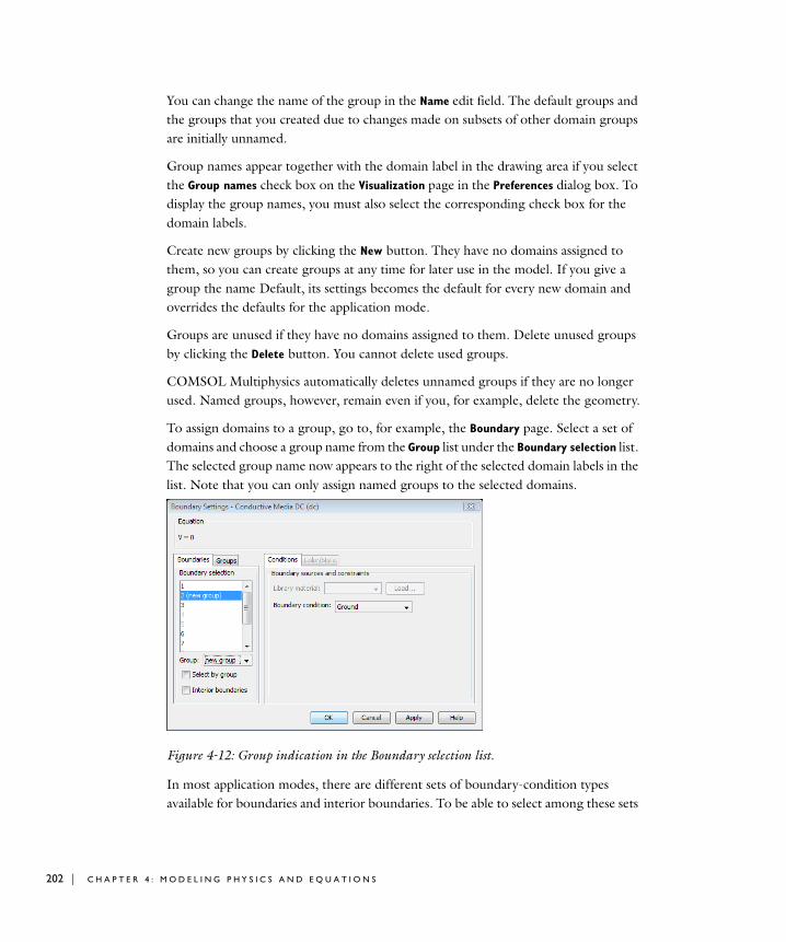
202 | C H A P T E
You can change the name of the group in the Name edit field. The default groups and the groups that you created due to changes made on subsets of other domain groups are initially unnamed.
Group names appear together with the domain label in the drawing area if you select the Group names check box on the Visualization page in the Preferences dialog box. To display the group names, you must also select the corresponding check box for the domain labels.
Create new groups by clicking the New button. They have no domains assigned to them, so you can create groups at any time for later use in the model. If you give a group the name Default, its settings becomes the default for every new domain and overrides the defaults for the application mode.
Groups are unused if they have no domains assigned to them. Delete unused groups by clicking the Delete button. You cannot delete used groups.
COMSOL Multiphysics automatically deletes unnamed groups if they are no longer used. Named groups, however, remain even if you, for example, delete the geometry.
To assign domains to a group, go to, for example, the Boundary page. Select a set of domains and choose a group name from the Group list under the Boundary selection list. The selected group name now appears to the right of the selected domain labels in the list. Note that you can only assign named groups to the selected domains.
Figure 4-12: Group indication in the Boundary selection list.
In most application modes, there are different sets of boundary-condition types available for boundaries and interior boundaries. To be able to select among these sets
R 4 : M O D E L I N G P H Y S I C S A N D E Q U A T I O N S
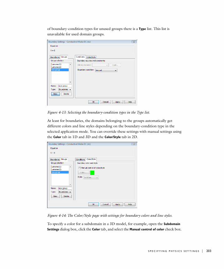
of boundary-condition types for unused groups there is a Type list. This list is unavailable for used domain groups.
Figure 4-13: Selecting the boundary-condition types in the Type list.
At least for boundaries, the domains belonging to the groups automatically get different colors and line styles depending on the boundary-condition type in the selected application mode. You can override these settings with manual settings using the Color tab in 1D and 3D and the Color/Style tab in 2D.
Figure 4-14: The Color/Style page with settings for boundary colors and line styles.
To specify a color for a subdomain in a 3D model, for example, open the Subdomain
Settings dialog box, click the Color tab, and select the Manual control of color check box.
S P E C I F Y I N G P H Y S I C S S E T T I N G S | 203

204 | C H A P T E
Then click the Color button to select a color. Add additional groups to display different colors in different parts of the geometry. The default setting is not to render faces in 3D, so click the Render Face button in the Visualization/Selection toolbar. Also notice that the Highlight Face button is selected by default. In that case, display of the domain group’s color applies only to the domains that are not selected.
To switch off the group color and line style, clear the Group style check box on the Visualization page in the Preferences dialog box
The predefined multiphysics couplings use groups to predefine couplings between the fields of physics in the participating application modes. For more information about predefined multiphysics couplings see “Multiphysics Modeling” on page 317 in the COMSOL Multiphysics Modeling Guide.
R 4 : M O D E L I N G P H Y S I C S A N D E Q U A T I O N S

S p e c i f y i n g S ubdoma i n S e t t i n g s and PDE Co e f f i c i e n t s
The subdomain settings describe the physics on a model’s main domain, which is divided into subdomains. You can set different values for each subdomain using settings of the following types:
• Coefficients that define the PDE on the subdomain. The PDE coefficient are available for PDE modes and the weak form modes.
• Material properties, sources, and sinks that define the physics in the subdomain. These properties are available in the physics modes and in the COMSOL Multiphysics modules. The software performs the translation into PDE coefficients automatically.
You can specify PDE coefficients for any COMSOL Multiphysics model using the Subdomain Settings dialog box for the equation system. See “Viewing and Modifying the Full Equation System” on page 213 for more information about the equation system view.
Using the Subdomain Settings Dialog Box
Figure 4-15: The Subdomain Settings dialog box for the Plane Stress structural mechanics application mode.
1 Go to the Physics menu and choose Subdomain Settings.
S P E C I F Y I N G S U B D O M A I N S E T T I N G S A N D P D E C O E F F I C I E N T S | 205

206 | C H A P T E
2 In the Subdomain Settings dialog box, make entries for the selected application mode and analysis type.
For a thorough description of the different application modes see the COMSOL Multiphysics Modeling Guide. The equations that the application mode solves appear at the top of the dialog box.
If you select multiple subdomains, the PDE coefficients and other settings you specify apply to all the selected subdomains. If the settings on the currently selected subdomains differ, the edit fields for those subdomains are locked, which they indicate with a yellow background. To clear the lock and overwrite the current settings for the selected domains, enter a new value or simply put the cursor in the edit field and press Enter.
D I S P L A Y I N G T H E E Q U A T I O N S
The Subdomain Settings dialog box for most application modes provide a display of the PDE that the application mode creates. The default setting is to show the equation. To show or hide the equations, do the following steps:
1 From the Options menu, choose Preferences.
2 In the Preferences dialog box, click the Modeling tab.
3 Click to select or clear the Show equations check box to show or hide the equations.
4 Click OK.
Figure 4-16: The Subdomain Settings dialog box for the Acoustics application mode, displaying the equation.
R 4 : M O D E L I N G P H Y S I C S A N D E Q U A T I O N S
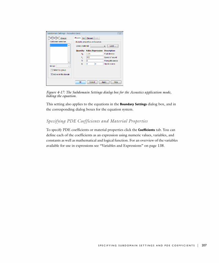
Figure 4-17: The Subdomain Settings dialog box for the Acoustics application mode, hiding the equation.
This setting also applies to the equations in the Boundary Settings dialog box, and in the corresponding dialog boxes for the equation system.
Specifying PDE Coefficients and Material Properties
To specify PDE coefficients or material properties click the Coefficients tab. You can define each of the coefficients as an expression using numeric values, variables, and constants as well as mathematical and logical function. For an overview of the variables available for use in expressions see “Variables and Expressions” on page 138.
S P E C I F Y I N G S U B D O M A I N S E T T I N G S A N D P D E C O E F F I C I E N T S | 207
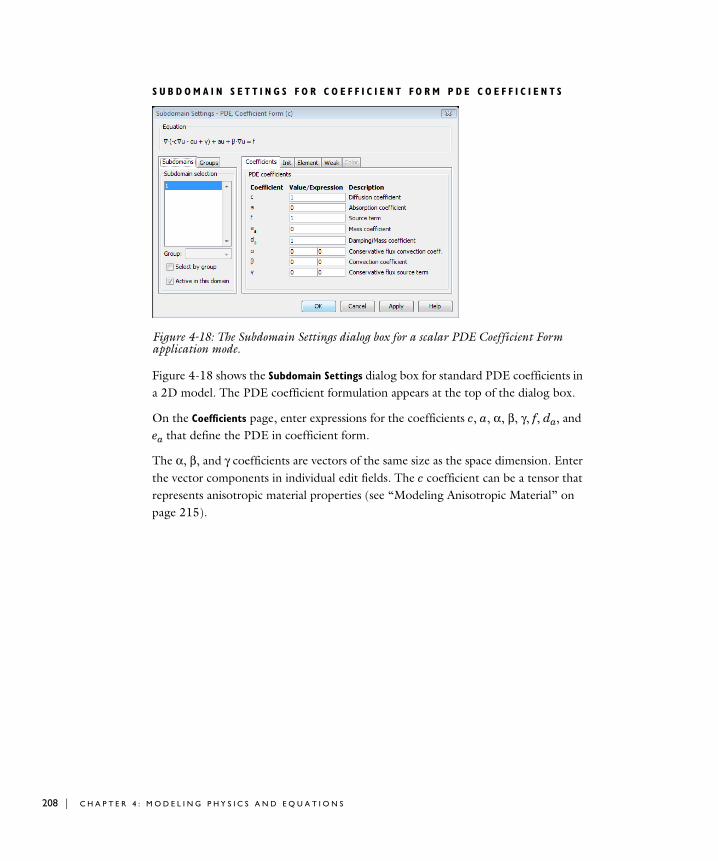
208 | C H A P T E
S U B D O M A I N S E T T I N G S F O R C O E F F I C I E N T F O R M P D E C O E F F I C I E N T S
Figure 4-18: The Subdomain Settings dialog box for a scalar PDE Coefficient Form application mode.
Figure 4-18 shows the Subdomain Settings dialog box for standard PDE coefficients in a 2D model. The PDE coefficient formulation appears at the top of the dialog box.
On the Coefficients page, enter expressions for the coefficients c, a, α, β, γ, f, da, and ea that define the PDE in coefficient form.
The α, β, and γ coefficients are vectors of the same size as the space dimension. Enter the vector components in individual edit fields. The c coefficient can be a tensor that represents anisotropic material properties (see “Modeling Anisotropic Material” on page 215).
R 4 : M O D E L I N G P H Y S I C S A N D E Q U A T I O N S
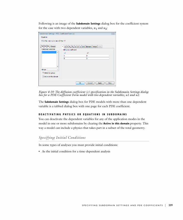
Following is an image of the Subdomain Settings dialog box for the coefficient system for the case with two dependent variables, u1 and u2:
Figure 4-19: The diffusion coefficient (c) specification in the Subdomain Settings dialog box for a PDE Coefficient Form model with two dependent variables, u1 and u2.
The Subdomain Settings dialog box for PDE models with more than one dependent variable is a tabbed dialog box with one page for each PDE coefficient.
D E A C T I V A T I N G P H Y S I C S O R E Q U A T I O N S I N S U B D O M A I N S
You can deactivate the dependent variables for any of the application modes in the model in one or more subdomains by clearing the Active in this domain property. This way a model can include a physics that takes part in a subset of the total geometry.
Specifying Initial Conditions
In some types of analyses you must provide initial conditions:
• As the initial condition for a time-dependent analysis
S P E C I F Y I N G S U B D O M A I N S E T T I N G S A N D P D E C O E F F I C I E N T S | 209
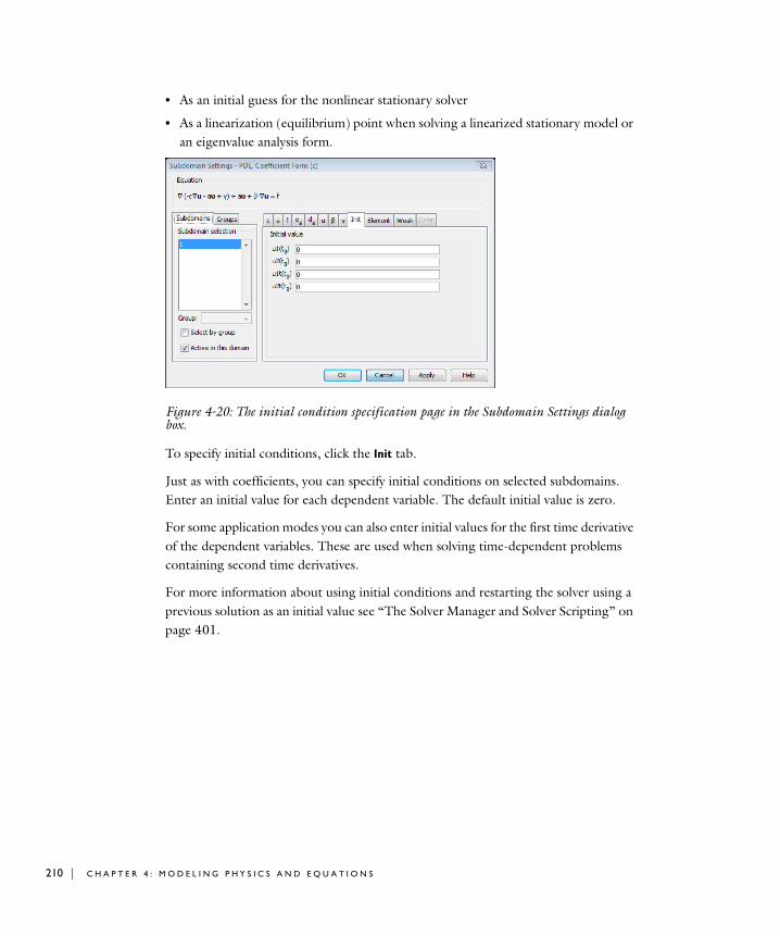
210 | C H A P T E
• As an initial guess for the nonlinear stationary solver
• As a linearization (equilibrium) point when solving a linearized stationary model or an eigenvalue analysis form.
Figure 4-20: The initial condition specification page in the Subdomain Settings dialog box.
To specify initial conditions, click the Init tab.
Just as with coefficients, you can specify initial conditions on selected subdomains. Enter an initial value for each dependent variable. The default initial value is zero.
For some application modes you can also enter initial values for the first time derivative of the dependent variables. These are used when solving time-dependent problems containing second time derivatives.
For more information about using initial conditions and restarting the solver using a previous solution as an initial value see “The Solver Manager and Solver Scripting” on page 401.
R 4 : M O D E L I N G P H Y S I C S A N D E Q U A T I O N S
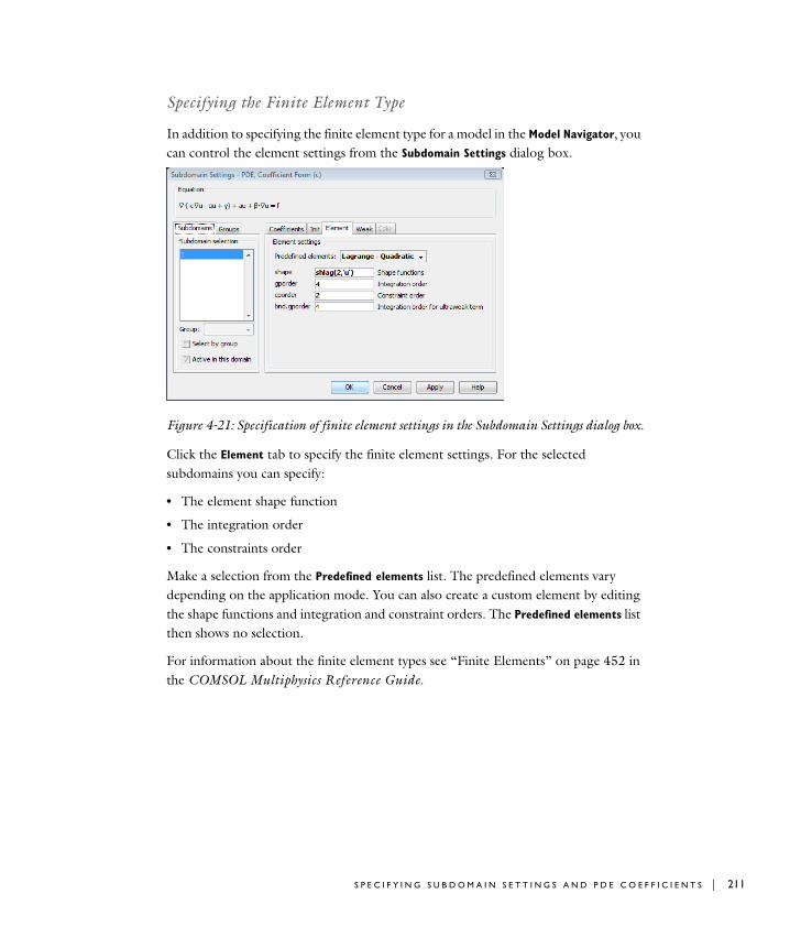
Specifying the Finite Element Type
In addition to specifying the finite element type for a model in the Model Navigator, you can control the element settings from the Subdomain Settings dialog box.
Figure 4-21: Specification of finite element settings in the Subdomain Settings dialog box.
Click the Element tab to specify the finite element settings. For the selected subdomains you can specify:
• The element shape function
• The integration order
• The constraints order
Make a selection from the Predefined elements list. The predefined elements vary depending on the application mode. You can also create a custom element by editing the shape functions and integration and constraint orders. The Predefined elements list then shows no selection.
For information about the finite element types see “Finite Elements” on page 452 in the COMSOL Multiphysics Reference Guide.
S P E C I F Y I N G S U B D O M A I N S E T T I N G S A N D P D E C O E F F I C I E N T S | 211

212 | C H A P T E
Specifying Weak Terms
Figure 4-22: The weak term settings in the Subdomain Settings dialog box.
To specify additional weak terms on selected subdomains click the Weak tab. For more information on modeling using weak form contributions see the chapter “The Weak Form” in the COMSOL Multiphysics Modeling Guide. You can also specify additional pointwise constraints in the constr edit field (these are not weak constraints).
Ideal and Non-Ideal Constraints
The application modes support two types of constraints, ideal and non-ideal constraints. You can choose which constraint type to use in the Application Mode
Properties dialog box on the Physics menu, except in the PDE modes, where you select the constraint type on the Weak page in the Subdomain Settings, Boundary Settings, Edge
Settings, or Point Settings dialog box.
Figure 4-23: The Application Mode Properties dialog box with the constraint type setting.
R 4 : M O D E L I N G P H Y S I C S A N D E Q U A T I O N S

The default constraint type is ideal, which means that the application modes derive the constraint force directly from the constraint at a boundary, edge, or point. You can also use the non-ideal constraints, which for constraints written as 0 = R on ∂Ω , changes the constraint force according to
where is an identity operator for points on the boundary ∂Ω . For example, using two variables u1 and u2 and the constraints
,
then the non-ideal constraint force is −µ acting on both equations for the boundary ∂Ω .
Viewing and Modifying the Full Equation System
In the equation system view you can view and modify the full system of equations for any model.
S P E C I F Y I N G P D E C O E F F I C I E N T S F O R T H E E Q U A T I O N S Y S T E M
To open the Subdomain Settings dialog box for the full equation system:
1 Go to the Physics menu, point to Equation System, and then click Subdomain Settings.
u∂∂R⎝ ⎠⎛ ⎞
Tµ I Ω∂ µ–→
I Ω∂
0 R1 u1 u2,( )= on ∂Ω
0 R2 u1 u2,( )= on ∂Ω⎩⎪⎨⎪⎧
S P E C I F Y I N G S U B D O M A I N S E T T I N G S A N D P D E C O E F F I C I E N T S | 213
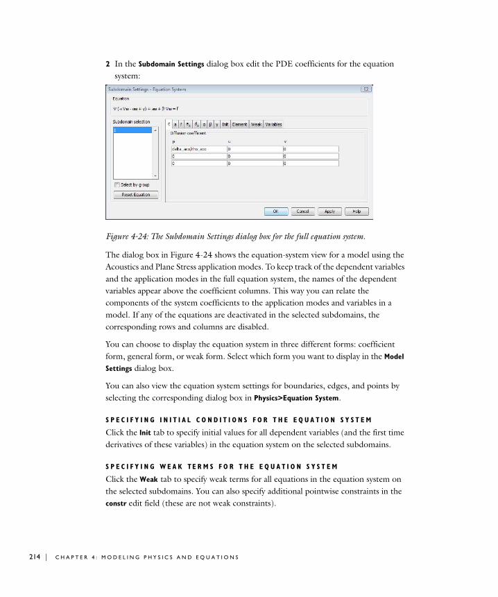
214 | C H A P T E
2 In the Subdomain Settings dialog box edit the PDE coefficients for the equation system:
Figure 4-24: The Subdomain Settings dialog box for the full equation system.
The dialog box in Figure 4-24 shows the equation-system view for a model using the Acoustics and Plane Stress application modes. To keep track of the dependent variables and the application modes in the full equation system, the names of the dependent variables appear above the coefficient columns. This way you can relate the components of the system coefficients to the application modes and variables in a model. If any of the equations are deactivated in the selected subdomains, the corresponding rows and columns are disabled.
You can choose to display the equation system in three different forms: coefficient form, general form, or weak form. Select which form you want to display in the Model
Settings dialog box.
You can also view the equation system settings for boundaries, edges, and points by selecting the corresponding dialog box in Physics>Equation System.
S P E C I F Y I N G I N I T I A L C O N D I T I O N S F O R T H E E Q U A T I O N S Y S T E M
Click the Init tab to specify initial values for all dependent variables (and the first time derivatives of these variables) in the equation system on the selected subdomains.
S P E C I F Y I N G W E A K TE R M S F O R T H E E Q U A T I O N S Y S T E M
Click the Weak tab to specify weak terms for all equations in the equation system on the selected subdomains. You can also specify additional pointwise constraints in the constr edit field (these are not weak constraints).
R 4 : M O D E L I N G P H Y S I C S A N D E Q U A T I O N S

S P E C I F Y I N G E L E M E N T TY P E S F O R T H E E Q U A T I O N S Y S T E M
Click the Element tab to specify shape functions, integration order, and constraints order for the equation-system variables on the selected subdomains. For more information of the element types see “Finite Elements” on page 452 in the COMSOL Multiphysics Reference Guide.
V I E W I N G A N D M O D I F Y I N G T H E A P P L I C A T I O N M O D E V A R I A B L E S
Click the Variables tab to see a list of the application mode variables in a model. They all appear with the following information:
• The variable name
• The expression that defines the variable
• A description of the variable
You can edit the expression to modify predefined application mode variables.
These application mode variables also appear in some of the postprocessing and visualization tools. See the documentation for the application modes in the COMSOL Multiphysics Modeling Guide for a complete list of variables.
Interior Mesh Boundary VariablesSome application modes define variables on interior mesh boundaries. If any of the application modes in the model define such variables, an additional tab Interior
Variables appears in the dialog box, where you can view and edit these variables.
L O C K E D S U B D O M A I N S E T T I N G S
If you change any PDE coefficients or other settings in the Subdomain Settings dialog box for the equation system, the original settings remain in the Subdomain Settings dialog boxes for the application modes. However, COMSOL Multiphysics locks them for any subdomains where you have changed them at the system level. COMSOL Multiphysics then uses the settings for the equation system. The software indicates locked subdomains in the Subdomain selection lists with a padlock symbol. To reset the equation system to the values based on the settings for the application modes, click the Reset Equation button in the Subdomain Settings dialog box for the equation system.
Modeling Anisotropic Material
The c coefficient in the coefficient form PDE corresponds to physical properties that can be anisotropic such as:
• Diffusion coefficient
S P E C I F Y I N G S U B D O M A I N S E T T I N G S A N D P D E C O E F F I C I E N T S | 215

216 | C H A P T E
• Permittivity
• Thermal conductivity
• Electric conductivity
For an anisotropic material, the c coefficient is a tensor with as many as four components in 2D and as many as nine components in 3D:
The edit field for the c coefficient and for anisotropic material properties in the physics modes expands to a matrix input for the tensor components. In the list you can choose from the following material models:
• Isotropic—enter only one value.
• Anisotropic - diagonal—enter the diagonal components for an anisotropic material with the main axes aligned with the model’s coordinate system.
• Anisotropic - symmetric—enter a symmetric matrix using the diagonal components and the upper off-diagonal components.
• Anisotropic - full—enter the full 2x2 (2D) or 3x3 (3D) matrix for an anisotropic material.
You can also enter the components of an anisotropic coefficient as space-separated entries in the edit field. Notice the order of the components for a c coefficient in a 3D model:
• Diagonal anisotropic material: c11 c22 c33
• Symmetric anisotropic material: c11 c12 c13 c22 c23 c33
• Full anisotropic material: c11 c21 c31 c12 c22 c32 c13 c23 c33
The ordering of components is similar in 2D.
Note: The Structural Mechanics Module and the MEMS Module support any anisotropic elasticity modulus defined in global or local coordinates.
c
c11 c12 c13
c21 c22 c23
c31 c32 c33
=
R 4 : M O D E L I N G P H Y S I C S A N D E Q U A T I O N S

U s i n g t h e Mode l T r e e
The Model Tree Views
The Model Tree, which appears to the left in the COMSOL Multiphysics user interface, provides three different views that provide access to the entire model. You select among these views using the toolbar buttons located at the very top of the Model Tree window.
Figure 4-25: The buttons for the Model Tree views: Overview (left), Detail (center), and Inspect (right).
• The Overview button provides an overview of geometries and application modes in the model.
• The Detail button brings up a detailed view of the model including settings and groups at all levels as well as constants, expressions, coupling variables, and other settings.
• The Inspect button provides a detailed view that includes only those settings that the model uses. Constants, expression variables, coupling variables, function definitions, ODEs and space-independent equations, and changes at the equation-system level appear in this view only if you have used these features. This makes it easier to find the actual settings that the model uses.
In each of these three views, the Model Tree displays the corresponding data in two areas or subwindows:
• The top area contains the tree structure where you can navigate to select a part of the model and access dialog boxes and commands related to that part of the model.
• The bottom area displays information about the part of the model that you have selected in the top area.
It is possible to change the sizes of these two areas; with the mouse drag the border between the top area and the bottom area and the border to the right of the Model Tree.
The following sections provide details about the three views. The figures show the look of the Model Tree for the model “Thermal Effects in Electronic Conductors”
U S I N G T H E M O D E L TR E E | 217
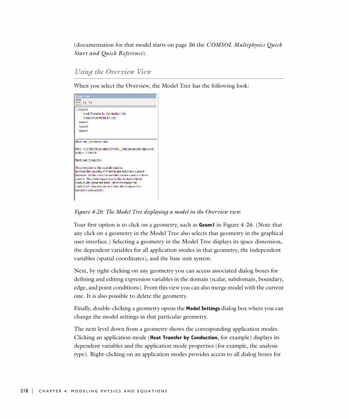
218 | C H A P T E
(documentation for that model starts on page 36 the COMSOL Multiphysics Quick Start and Quick Reference).
Using the Overview View
When you select the Overview, the Model Tree has the following look:
Figure 4-26: The Model Tree displaying a model in the Overview view.
Your first option is to click on a geometry, such as Geom1 in Figure 4-26. (Note that any click on a geometry in the Model Tree also selects that geometry in the graphical user interface.) Selecting a geometry in the Model Tree displays its space dimension, the dependent variables for all application modes in that geometry, the independent variables (spatial coordinates), and the base unit system.
Next, by right-clicking on any geometry you can access associated dialog boxes for defining and editing expression variables in the domain (scalar, subdomain, boundary, edge, and point conditions). From this view you can also merge model with the current one. It is also possible to delete the geometry.
Finally, double-clicking a geometry opens the Model Settings dialog box where you can change the model settings in that particular geometry.
The next level down from a geometry shows the corresponding application modes. Clicking an application mode (Heat Transfer by Conduction, for example) displays its dependent variables and the application mode properties (for example, the analysis type). Right-clicking on an application modes provides access to all dialog boxes for
R 4 : M O D E L I N G P H Y S I C S A N D E Q U A T I O N S
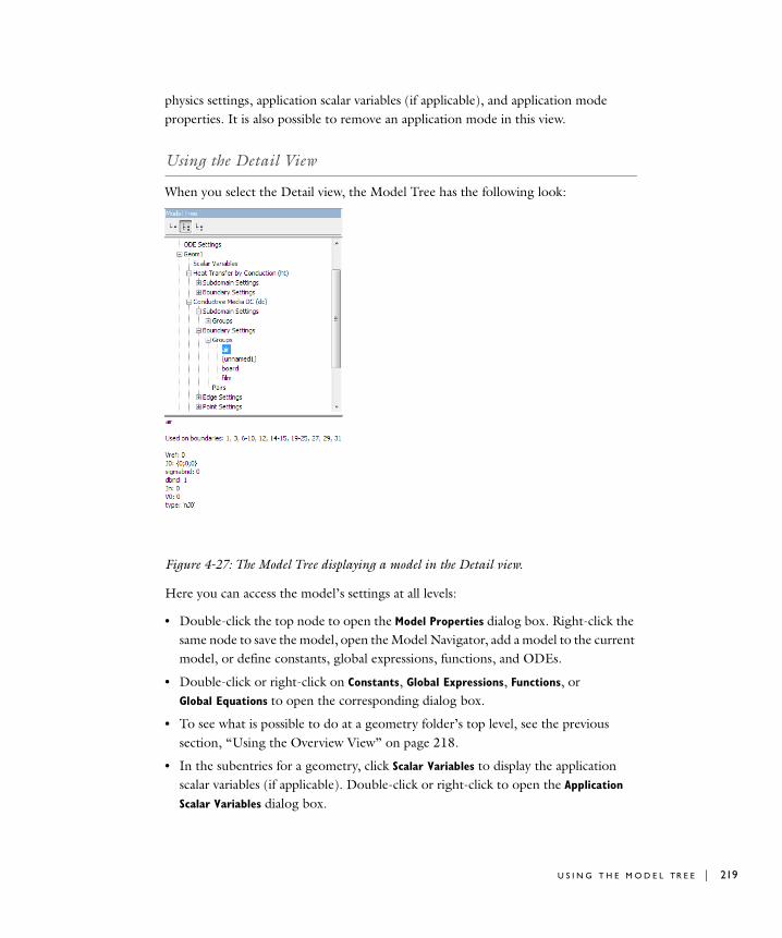
physics settings, application scalar variables (if applicable), and application mode properties. It is also possible to remove an application mode in this view.
Using the Detail View
When you select the Detail view, the Model Tree has the following look:
Figure 4-27: The Model Tree displaying a model in the Detail view.
Here you can access the model’s settings at all levels:
• Double-click the top node to open the Model Properties dialog box. Right-click the same node to save the model, open the Model Navigator, add a model to the current model, or define constants, global expressions, functions, and ODEs.
• Double-click or right-click on Constants, Global Expressions, Functions, or Global Equations to open the corresponding dialog box.
• To see what is possible to do at a geometry folder’s top level, see the previous section, “Using the Overview View” on page 218.
• In the subentries for a geometry, click Scalar Variables to display the application scalar variables (if applicable). Double-click or right-click to open the Application
Scalar Variables dialog box.
U S I N G T H E M O D E L TR E E | 219

220 | C H A P T E
• To see what is possible to do at an application mode folder’s top level, see the previous section, “Using the Overview View” on page 218.
• At the next level of an application mode folder, the contents include the Subdomain
Settings, Boundary Settings, Edge Settings, and Point Settings folders (not all of these appear in 1D and 2D geometries). Click these folders to display the dependent variables and the number of domains of that type in the geometry. Double-click, right-click, or use the corresponding shortcut keys (F5–F8) to open the dialog boxes for these settings.
Open these folders to display groups of settings. Click a group to display its settings and the domains where it is used. Doing so also selects these domains in the graphical user interface. Right-click a group to copy the settings from that group, to paste a copied group setting to a group, and to open the corresponding settings dialog box. You can also delete unused groups.
For the boundary, edge, and point settings you can also access the settings for pairs that you have defined for an assembly. Click on a pair to display its settings, including the source domains and destination domains. Selecting any pairs also selects the source and destination domains. Right-click a group to copy and paste settings and to open the corresponding settings dialog box.
• The Expressions folder contains subentries for each type of expression variables in the domain (scalar, subdomain, boundary, edge, and point conditions). Right-click the Expressions folder to open any of the dialog boxes for these types of expressions. Click a subentry to display a list of expression variables of the corresponding type. Double-click or right-click a subentry to open the dialog box for that particular type of expressions. Selecting Scalar Expressions lists all scalar expression variables in the bottom area of the Model Tree. If a model contains expression variables in this geometry, you can open the corresponding folder, for example, Subdomain
Expressions, and click on the individual groups to see which domains they include and the names and definitions for the expression variables in that group. Double-clicking or right-clicking provides access to the appropriate dialog box for the expression variables. By right-clicking on a group you can also copy and paste the expression variables from that group to another.
• The Equation System folder contains the settings for the underlying equation system. Open the folder to access the Subdomain Settings, Boundary Settings, Edge Settings, and Point Settings folders (not all of these appear in 1D and 2D geometries), which refer to the same dialog boxes as the entries under Physics>Equation System on the Main menu. You open the dialog boxes by double-clicking or right-clicking these folders. Normally you do not need to make any changes at the equation-system
R 4 : M O D E L I N G P H Y S I C S A N D E Q U A T I O N S

level, but these settings also include lists of variables, which you can see in the Model Tree by opening one of these folders, then opening the Variables folder, and finally selecting one of the groups. By default, there is only one group because the variable definitions are the same in all domains. For some models there are no variables defined on edges and points.
• In the application mode folder you can also find the Coupling Variables folder, which in turn contains three entries: Integration Coupling Variables, Extrusion Coupling
Variables, and Projection Coupling Variables. Right-click on any of these to open the corresponding dialog box for defining coupling variables in subdomains, on boundaries, or on points. By right-clicking Extrusion Coupling Variables you can also open the dialog boxes for periodic boundary conditions and identity boundary conditions.
Using the Inspect View
The Inspect view shows the same level of detail as the Detail view but without any of the settings that are empty or unchanged from their default values. This makes it easier to find the expression variables, coupling variables, user-defined functions, and equation modifications that a model contains.
U S I N G T H E M O D E L TR E E | 221
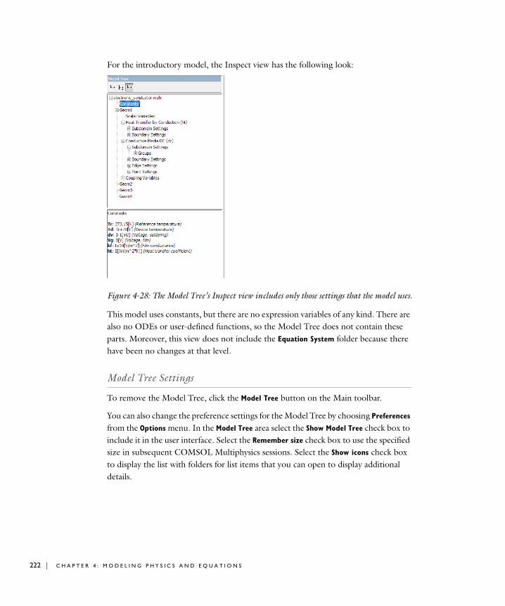
222 | C H A P T E
For the introductory model, the Inspect view has the following look:
Figure 4-28: The Model Tree’s Inspect view includes only those settings that the model uses.
This model uses constants, but there are no expression variables of any kind. There are also no ODEs or user-defined functions, so the Model Tree does not contain these parts. Moreover, this view does not include the Equation System folder because there have been no changes at that level.
Model Tree Settings
To remove the Model Tree, click the Model Tree button on the Main toolbar.
You can also change the preference settings for the Model Tree by choosing Preferences from the Options menu. In the Model Tree area select the Show Model Tree check box to include it in the user interface. Select the Remember size check box to use the specified size in subsequent COMSOL Multiphysics sessions. Select the Show icons check box to display the list with folders for list items that you can open to display additional details.
R 4 : M O D E L I N G P H Y S I C S A N D E Q U A T I O N S

U s i n g t h e Ma t e r i a l s / C o e f f i c i e n t s L i b r a r y
The Materials/Coefficients Library is a framework for a number of extensible databases with properties for a broad collection of physical, elastic, electromagnetic, fluid, and thermal properties of materials as well as heat transfer coefficients. In the Materials/Coefficients Library dialog box you can add and edit library entries. Further, you can define multiple material libraries, each stored in a separate data file. The COMSOL Material Library is a separate add-on product that provides data, primarily as piecewise polynomial functions of temperature, for approximately 2500 materials. COMSOL Multiphysics and some of the modules include smaller libraries of material properties or coefficients. The number displayed next to a material library in the Materials/Coefficients Library dialog box indicates the number of materials in the library.
Using Material/Coefficient Data in Models
You have access to the COMSOL Multiphysics Materials/Coefficients Library from the Subdomain Settings dialog box in the physics modes and in the optional COMSOL modules. Selecting a material transfers the applicable properties to the current model. It is not necessary to define all the properties for an entry.
The available properties are grouped together in different groups according to their physical context. The available default groups are the Physics, Elastic, Electric, Fluid, Piezoelectric, and Thermal groups, each available on a separate tabbed page in the Materials/Coefficients Library dialog box. In addition, there is always a tabbed page named All that displays all properties. If you want to group properties differently or change the description of a quantity, you can modify the default groups and create new groups by editing the library data file. When loading materials from a domain settings dialog box, there is an additional tab with the same name as the tab in the domain settings dialog box, displaying only the properties that apply to the domain settings. The same property can appear in several groups with different descriptions in different
U S I N G T H E M A T E R I A L S / C O E F F I C I E N T S L I B R A R Y | 223

224 | C H A P T E
groups. To view only the defined material properties, select the Hide undefined
properties check box in the Materials/Coefficients Library dialog box.
Figure 4-29: The Materials/Coefficients Library dialog box.
All Materials/Coefficients Libraries shipped with COMSOL Multiphysics and the optional modules are read-only. The User Defined Materials library is included as an example library to show how you can add and edit your own materials. When you open the Materials/Coefficients Library dialog box from a physics-settings dialog box such as the Subdomain Settings dialog box, all materials including the ones in your model, the User Defined Materials library, and optional user-added libraries are read-only. To edit a material you must open the dialog box from the Options menu.
U S I N G A L I B R A R Y M A T E R I A L O R C O E F F I C I E N T
1 From the Physics menu open the Subdomain Settings dialog box.
2 Click the Physics or Material tab depending on the application mode.
3 Click the Load button to open the Materials/Coefficients Library dialog box.
4 In the Materials list, select the material you want to use in your model.
5 Click OK.
R 4 : M O D E L I N G P H Y S I C S A N D E Q U A T I O N S
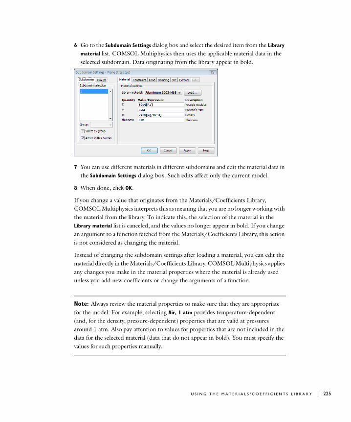
6 Go to the Subdomain Settings dialog box and select the desired item from the Library
material list. COMSOL Multiphysics then uses the applicable material data in the selected subdomain. Data originating from the library appear in bold.
7 You can use different materials in different subdomains and edit the material data in the Subdomain Settings dialog box. Such edits affect only the current model.
8 When done, click OK.
If you change a value that originates from the Materials/Coefficients Library, COMSOL Multiphysics interprets this as meaning that you are no longer working with the material from the library. To indicate this, the selection of the material in the Library material list is canceled, and the values no longer appear in bold. If you change an argument to a function fetched from the Materials/Coefficients Library, this action is not considered as changing the material.
Instead of changing the subdomain settings after loading a material, you can edit the material directly in the Materials/Coefficients Library. COMSOL Multiphysics applies any changes you make in the material properties where the material is already used unless you add new coefficients or change the arguments of a function.
Note: Always review the material properties to make sure that they are appropriate for the model. For example, selecting Air, 1 atm provides temperature-dependent (and, for the density, pressure-dependent) properties that are valid at pressures around 1 atm. Also pay attention to values for properties that are not included in the data for the selected material (data that do not appear in bold). You must specify the values for such properties manually.
U S I N G T H E M A T E R I A L S / C O E F F I C I E N T S L I B R A R Y | 225
226 | C H A P T E
Using Your Own Material Data
To extend the material data you can:
• Add new materials to the User Defined Materials database.
• Create your own materials library from scratch.
A D D I N G A N E N T R Y T O T H E L I B R A R Y
1 Go to the Options menu and choose Materials/Coefficients Library.
2 In the Materials/Coefficients Library dialog box, select the User Defined Materials
library in the Materials, or click the Add Library button to create a new library, or select an optional user defined library already available.
3 Click New.
4 Enter the name of the entry in the Name edit field under Material properties. By default, COMSOL Multiphysics names new entries Material 1, Material 2, and so on.
5 Enter values in the Value/Expression edit fields for the properties you want to define.
6 Click Apply.
You can also copy data from another library entry:
1 In the Materials list, select the library entry from which you want to copy data.
2 Click Copy.
3 In the Materials list, select the library entry to which you want to paste the data.
4 Click Paste.
U S I N G F U N C T I O N S I N A L I B R A R Y E N T R Y
It is possible to define functions that are local to a material in the Functions dialog box, which you open by clicking the Functions button in the Properties frame of the desired material. This opens a dialog box that looks and acts the same as the Functions dialog box accessible from the Options menu except that it only displays functions local to the selected entry. See “Using Inline (Analytic) Functions” on page 150 for more information on how to define functions.
For example, if rhofunction(x) is a locally defined function for a material, you can set the quantity rho to rhofunction(x). You can then specify the argument of the function when using the library entry in a domain settings dialog box such as the Subdomain Settings dialog box.
R 4 : M O D E L I N G P H Y S I C S A N D E Q U A T I O N S

To access a local material function from somewhere else than the material, prefix the name with the material tag, such that a function rhofunction(x) in a material with the tag mat1 can be referenced as mat1_rhofunction(x).
C R E A T I N G A N E W L I B R A R Y
The best way to create a new library is to copy the existing library data file data/mtrl_lib.txt in the COMSOL directory and alter it according to your needs. You can also append library entries to an existing library data file. For information about the data structure for materials and coefficient libraries, see “Materials/Coefficients Libraries” on page 33 in the COMSOL Multiphysics Scripting Guide.
D E F I N I N G G R O U P S O F P R O P E R T I E S I N A D A T A F I L E
You can define groups of parameters that appear on separate pages in the Materials/Coefficients Library dialog box. You define groups in the data files as, for example,
lib.groups1.name = 'Heat';lib.groups1.variables = 'h';lib.groups1.descr = 'Heat Transfer Coefficient';
The Materials/Coefficients Library dialog box then displays this group as a tab with the name Heat, and that group contains only the coefficient h with the description Heat
Transfer Coefficient.
A D D I N G A L I B R A R Y F I L E T O T H E D A T A B A S E
1 Go to the Options menu and select Materials/Coefficients Library.
2 In the Materials/Coefficients Library dialog box click the Add Library button.
3 In the Add Library dialog box, browse to the library data file and select it.
4 Click Open.
A new library with the data in your file is now available in the Materials list.
A D D I N G A N E W E M P T Y L I B R A R Y F I L E T O T H E D A T A B A S E
1 Go to the Options menu and select Materials/Coefficients Library.
2 In the Materials/Coefficients Library dialog box click the Add Library button.
3 In the Add Library dialog box, enter the new name you want to give your library in the File name edit field and click OK.
A new empty library is now available in the Materials list.
U S I N G T H E M A T E R I A L S / C O E F F I C I E N T S L I B R A R Y | 227

228 | C H A P T E
D E L E T I N G A L I B R A R Y E N T R Y O R L I B R A R Y
1 Select the library entry or library in the Materials list.
2 Click Delete.
Using MatWeb Material Property Data
MatWeb provides a service where you can export technical datasheets from MatWeb’s collection in the format for a COMSOL material library. After downloading material property data from MatWeb, add this library file using the Add Library dialog box (see the previous section). For more information about this service, visit www.matweb.com.
R 4 : M O D E L I N G P H Y S I C S A N D E Q U A T I O N S
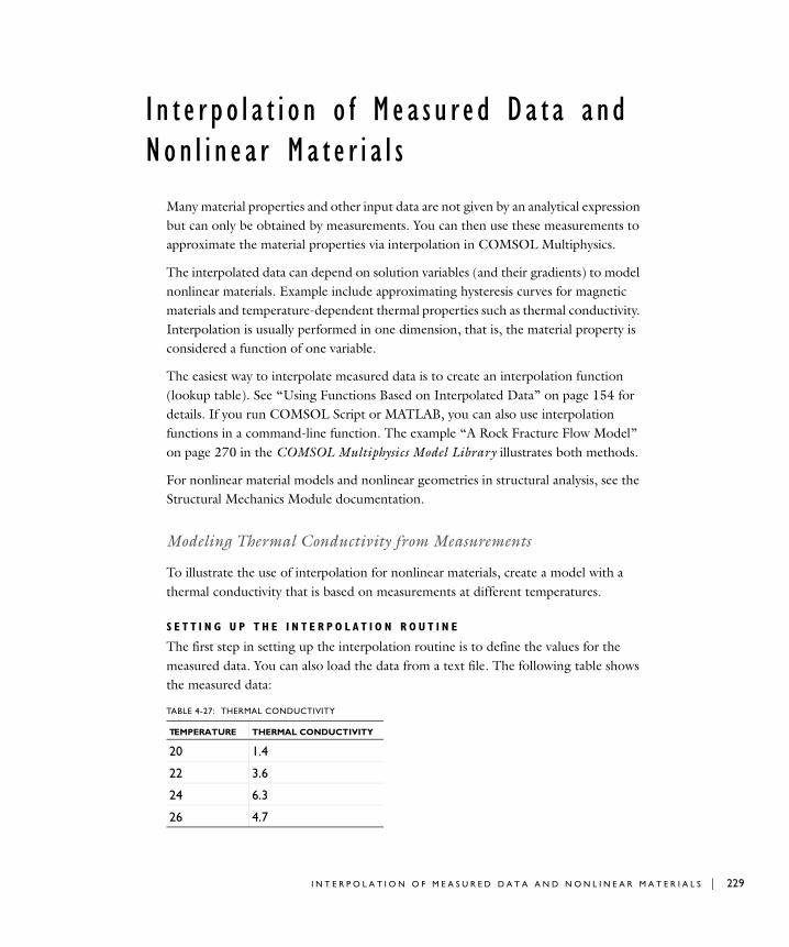
I n t e r p o l a t i o n o f Mea s u r e d Da t a and Non l i n e a r Ma t e r i a l s
Many material properties and other input data are not given by an analytical expression but can only be obtained by measurements. You can then use these measurements to approximate the material properties via interpolation in COMSOL Multiphysics.
The interpolated data can depend on solution variables (and their gradients) to model nonlinear materials. Example include approximating hysteresis curves for magnetic materials and temperature-dependent thermal properties such as thermal conductivity. Interpolation is usually performed in one dimension, that is, the material property is considered a function of one variable.
The easiest way to interpolate measured data is to create an interpolation function (lookup table). See “Using Functions Based on Interpolated Data” on page 154 for details. If you run COMSOL Script or MATLAB, you can also use interpolation functions in a command-line function. The example “A Rock Fracture Flow Model” on page 270 in the COMSOL Multiphysics Model Library illustrates both methods.
For nonlinear material models and nonlinear geometries in structural analysis, see the Structural Mechanics Module documentation.
Modeling Thermal Conductivity from Measurements
To illustrate the use of interpolation for nonlinear materials, create a model with a thermal conductivity that is based on measurements at different temperatures.
S E T T I N G U P T H E I N T E R P O L A T I O N R O U T I N E
The first step in setting up the interpolation routine is to define the values for the measured data. You can also load the data from a text file. The following table shows the measured data:
TABLE 4-27: THERMAL CONDUCTIVITY
TEMPERATURE THERMAL CONDUCTIVITY
20 1.4
22 3.6
24 6.3
26 4.7
I N T E R P O L A T I O N O F M E A S U R E D D A T A A N D N O N L I N E A R M A T E R I A L S | 229
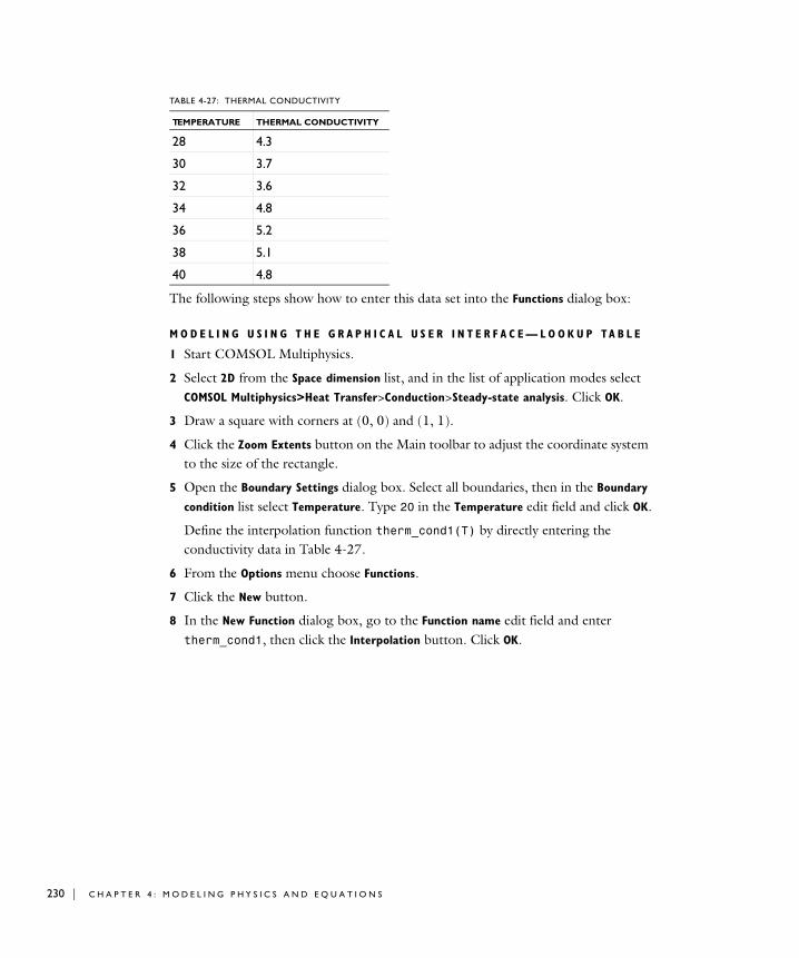
230 | C H A P T E
The following steps show how to enter this data set into the Functions dialog box:
M O D E L I N G U S I N G T H E G R A P H I C A L U S E R I N T E R F A C E — L O O K U P T A B L E
1 Start COMSOL Multiphysics.
2 Select 2D from the Space dimension list, and in the list of application modes select COMSOL Multiphysics>Heat Transfer>Conduction>Steady-state analysis. Click OK.
3 Draw a square with corners at (0, 0) and (1, 1).
4 Click the Zoom Extents button on the Main toolbar to adjust the coordinate system to the size of the rectangle.
5 Open the Boundary Settings dialog box. Select all boundaries, then in the Boundary
condition list select Temperature. Type 20 in the Temperature edit field and click OK.
Define the interpolation function therm_cond1(T) by directly entering the conductivity data in Table 4-27.
6 From the Options menu choose Functions.
7 Click the New button.
8 In the New Function dialog box, go to the Function name edit field and enter therm_cond1, then click the Interpolation button. Click OK.
28 4.3
30 3.7
32 3.6
34 4.8
36 5.2
38 5.1
40 4.8
TABLE 4-27: THERMAL CONDUCTIVITY
TEMPERATURE THERMAL CONDUCTIVITY
R 4 : M O D E L I N G P H Y S I C S A N D E Q U A T I O N S
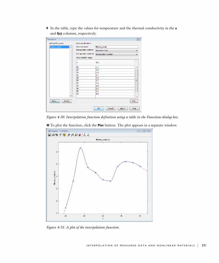
9 In the table, type the values for temperature and the thermal conductivity in the x and f(x) columns, respectively.
Figure 4-30: Interpolation function definition using a table in the Functions dialog box.
10 To plot the function, click the Plot button. The plot appears in a separate window.
Figure 4-31: A plot of the interpolation function.
I N T E R P O L A T I O N O F M E A S U R E D D A T A A N D N O N L I N E A R M A T E R I A L S | 231
232 | C H A P T E
11 Click OK.
Next use this data in the specification of the thermal conductivity:
12 Open the Subdomain Settings dialog box and type therm_cond1(T) in the Thermal
conductivity edit field. Type 750 in the Heat source edit field.
13 Click the Init tab and then type 20 in the Temperature edit field to set the initial value. Click OK.
14 Click the Initialize Mesh button on the Main toolbar to create a mesh.
15 Solve the problem by clicking the Solve button on the Main toolbar.
M O D E L I N G U S I N G T H E G R A P H I C A L U S E R I N T E R F A C E — D A T A F R O M F I L E
In this case the same interpolation data is available as a text file, thermcond.txt, with the following format:
% Temperatures20 22 24 26 28 30 32 34 36 38 40% Thermal conductivity1.4 3.6 6.3 4.7 4.3 3.7 3.6 4.8 5.2 5.1 4.8
Store a text file with this content as thermcond.txt somewhere on your file system. Then proceed as follows to retrieve the interpolation data from the file:
1 Follow Steps 1–7 from the previous section.
2 In the New Function dialog box, type therm_cond1 in the Function name edit field and click the Interpolation button. Select File from the Use data from list.
3 Click the Browse button, browse to the directory where you saved thermcond.txt, and select this file.
4 Click OK to close the New Function dialog box.
5 In the Functions dialog box, select Interpolation Function in the Extrapolation method list to extrapolate the thermal conductivity outside of the specified temperature range. Click OK.
6 Open the Subdomain Settings dialog box and type therm_cond1(T) in the Thermal
conductivity edit field. Type 750 in the Heat source edit field.
7 Click the Init tab and then type 20 in the Temperature edit field to set the initial value. Click OK.
8 Click the Initialize Mesh button to create a mesh.
9 Solve the problem by clicking the Solve button.
R 4 : M O D E L I N G P H Y S I C S A N D E Q U A T I O N S

U S I N G A PO L Y N O M I A L T O D E S C R I B E T H E D A T A
If possible, a preferred method is often to fit a polynomial to your data. Once you have an analytic function for a nonlinear material, for example, T = a + bT + cT2, you can enter that function directly using the edit field for the conductivity. Alternatively you can define the expression in the expression list. In that case, COMSOL Multiphysics takes care of the differentiation for the Jacobian contribution.
I N T E R P O L A T I O N O F M E A S U R E D D A T A A N D N O N L I N E A R M A T E R I A L S | 233
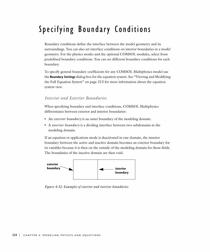
234 | C H A P T E
S p e c i f y i n g Bounda r y Cond i t i o n s
Boundary conditions define the interface between the model geometry and its surroundings. You can also set interface conditions on interior boundaries in a model geometry. For the physics modes and the optional COMSOL modules, select from predefined boundary conditions. You can set different boundary conditions for each boundary.
To specify general boundary coefficients for any COMSOL Multiphysics model use the Boundary Settings dialog box for the equation system. See “Viewing and Modifying the Full Equation System” on page 213 for more information about the equation system view.
Interior and Exterior Boundaries
When specifying boundary and interface conditions, COMSOL Multiphysics differentiates between exterior and interior boundaries:
• An exterior boundary is an outer boundary of the modeling domain.
• A interior boundary is a dividing interface between two subdomains in the modeling domain.
If an equation or applications mode is deactivated in one domain, the interior boundary between the active and inactive domain becomes an exterior boundary for its variables because it is then on the outside of the modeling domain for those fields. The boundaries of the inactive domain are then void.
Figure 4-32: Examples of exterior and interior boundaries.
exteriorinteriorboundary
boundary
R 4 : M O D E L I N G P H Y S I C S A N D E Q U A T I O N S
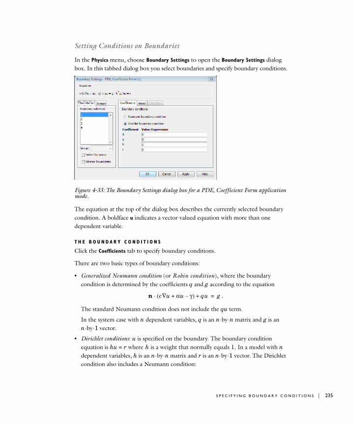
Setting Conditions on Boundaries
In the Physics menu, choose Boundary Settings to open the Boundary Settings dialog box. In this tabbed dialog box you select boundaries and specify boundary conditions.
Figure 4-33: The Boundary Settings dialog box for a PDE, Coefficient Form application mode.
The equation at the top of the dialog box describes the currently selected boundary condition. A boldface u indicates a vector-valued equation with more than one dependent variable.
T H E B O U N D A R Y C O N D I T I O N S
Click the Coefficients tab to specify boundary conditions.
There are two basic types of boundary conditions:
• Generalized Neumann condition (or Robin condition), where the boundary condition is determined by the coefficients q and g according to the equation
.
The standard Neumann condition does not include the qu term.
In the system case with n dependent variables, q is an n-by-n matrix and g is an n-by-1 vector.
• Dirichlet conditions: u is specified on the boundary. The boundary condition equation is hu = r where h is a weight that normally equals 1. In a model with n dependent variables, h is an n-by-n matrix and r is an n-by-1 vector. The Dirichlet condition also includes a Neumann condition:
n c u∇ αu γ–+( )⋅ qu+ g=
S P E C I F Y I N G B O U N D A R Y C O N D I T I O N S | 235
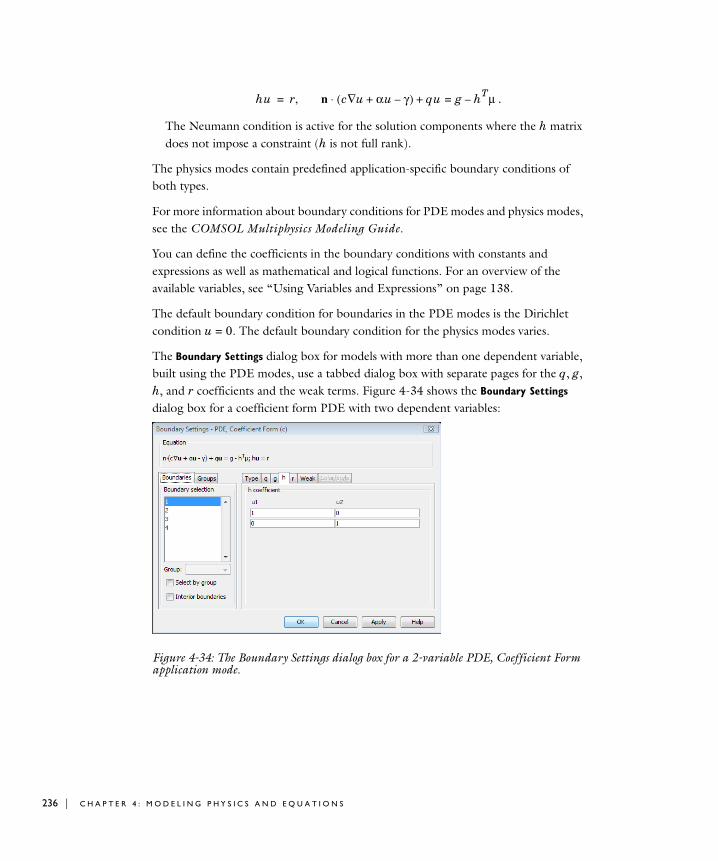
236 | C H A P T E
.
The Neumann condition is active for the solution components where the h matrix does not impose a constraint (h is not full rank).
The physics modes contain predefined application-specific boundary conditions of both types.
For more information about boundary conditions for PDE modes and physics modes, see the COMSOL Multiphysics Modeling Guide.
You can define the coefficients in the boundary conditions with constants and expressions as well as mathematical and logical functions. For an overview of the available variables, see “Using Variables and Expressions” on page 138.
The default boundary condition for boundaries in the PDE modes is the Dirichlet condition u = 0. The default boundary condition for the physics modes varies.
The Boundary Settings dialog box for models with more than one dependent variable, built using the PDE modes, use a tabbed dialog box with separate pages for the q, g, h, and r coefficients and the weak terms. Figure 4-34 shows the Boundary Settings
dialog box for a coefficient form PDE with two dependent variables:
Figure 4-34: The Boundary Settings dialog box for a 2-variable PDE, Coefficient Form application mode.
hu r n c u αu γ–+∇( )⋅ qu+ g hTµ–=,=
R 4 : M O D E L I N G P H Y S I C S A N D E Q U A T I O N S

T H E W E A K TE R M S
Figure 4-35: Weak term settings using the Boundary Settings dialog box.
Click the Weak tab to specify additional weak terms on selected boundaries. For more information on modeling using weak-form contributions, see the chapter “The Weak Form” in the COMSOL Multiphysics Modeling Guide. You can also specify additional pointwise constraints in the constr edit field (these are not weak constraints).
H A N D L I N G C O N F L I C T I N G S E L E C T I O N S
If you select multiple boundaries, the boundary settings apply to all the selected boundaries. If the boundary settings on the currently selected boundaries differ, the Boundary conditions button or list is locked, which COMSOL Multiphysics indicates with a yellow background color. To apply a new boundary setting for all selected boundaries, you must override the locked settings. To do so, enter the desired boundary settings, and the yellow background disappears.
Modifying Boundary Settings for the Equation System
To view and set the boundary conditions on the full equation system as standard boundary coefficients:
1 Go to the Physics menu, point to Equation System, and then click Boundary Settings.
2 In the Boundary Settings dialog box, edit the boundary coefficients for the equation system.
S P E C I F Y I N G B O U N D A R Y C O N D I T I O N S | 237
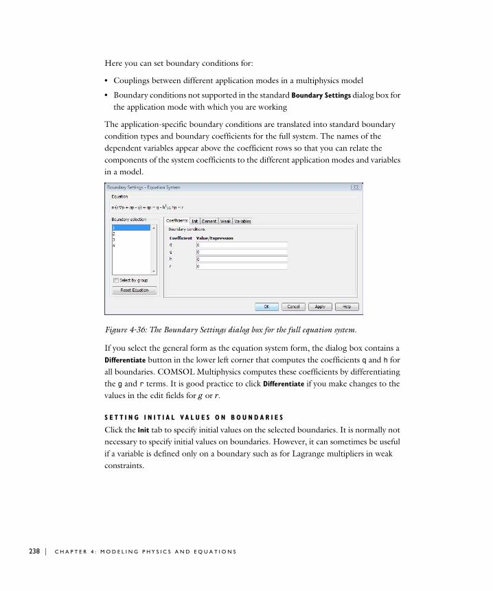
238 | C H A P T E
Here you can set boundary conditions for:
• Couplings between different application modes in a multiphysics model
• Boundary conditions not supported in the standard Boundary Settings dialog box for the application mode with which you are working
The application-specific boundary conditions are translated into standard boundary condition types and boundary coefficients for the full system. The names of the dependent variables appear above the coefficient rows so that you can relate the components of the system coefficients to the different application modes and variables in a model.
Figure 4-36: The Boundary Settings dialog box for the full equation system.
If you select the general form as the equation system form, the dialog box contains a Differentiate button in the lower left corner that computes the coefficients q and h for all boundaries. COMSOL Multiphysics computes these coefficients by differentiating the g and r terms. It is good practice to click Differentiate if you make changes to the values in the edit fields for g or r.
S E T T I N G I N I T I A L V A L U E S O N B O U N D A R I E S
Click the Init tab to specify initial values on the selected boundaries. It is normally not necessary to specify initial values on boundaries. However, it can sometimes be useful if a variable is defined only on a boundary such as for Lagrange multipliers in weak constraints.
R 4 : M O D E L I N G P H Y S I C S A N D E Q U A T I O N S
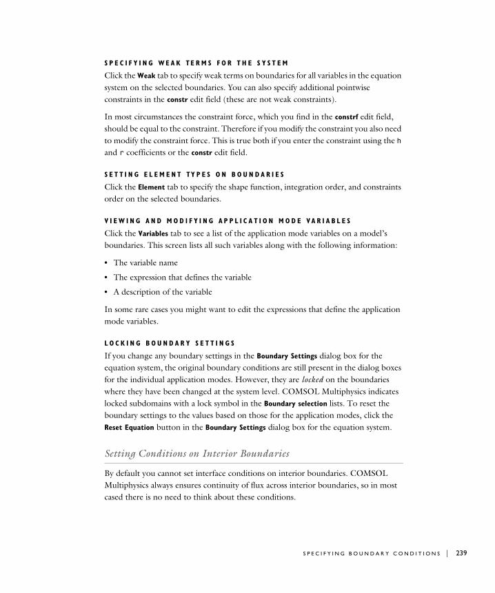
S P E C I F Y I N G WE A K TE R M S F O R T H E S Y S T E M
Click the Weak tab to specify weak terms on boundaries for all variables in the equation system on the selected boundaries. You can also specify additional pointwise constraints in the constr edit field (these are not weak constraints).
In most circumstances the constraint force, which you find in the constrf edit field, should be equal to the constraint. Therefore if you modify the constraint you also need to modify the constraint force. This is true both if you enter the constraint using the h and r coefficients or the constr edit field.
S E T T I N G E L E M E N T TY P E S O N B O U N D A R I E S
Click the Element tab to specify the shape function, integration order, and constraints order on the selected boundaries.
V I E W I N G A N D M O D I F Y I N G A P P L I C A T I O N M O D E V A R I A B L E S
Click the Variables tab to see a list of the application mode variables on a model’s boundaries. This screen lists all such variables along with the following information:
• The variable name
• The expression that defines the variable
• A description of the variable
In some rare cases you might want to edit the expressions that define the application mode variables.
L O C K I N G B O U N D A R Y S E T T I N G S
If you change any boundary settings in the Boundary Settings dialog box for the equation system, the original boundary conditions are still present in the dialog boxes for the individual application modes. However, they are locked on the boundaries where they have been changed at the system level. COMSOL Multiphysics indicates locked subdomains with a lock symbol in the Boundary selection lists. To reset the boundary settings to the values based on those for the application modes, click the Reset Equation button in the Boundary Settings dialog box for the equation system.
Setting Conditions on Interior Boundaries
By default you cannot set interface conditions on interior boundaries. COMSOL Multiphysics always ensures continuity of flux across interior boundaries, so in most cased there is no need to think about these conditions.
S P E C I F Y I N G B O U N D A R Y C O N D I T I O N S | 239
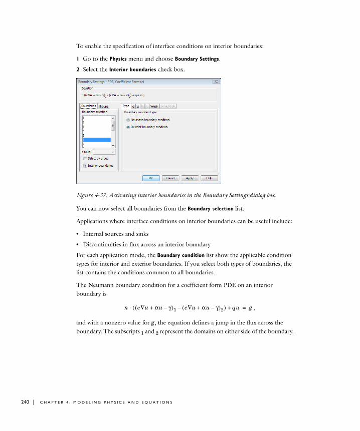
240 | C H A P T E
To enable the specification of interface conditions on interior boundaries:
1 Go to the Physics menu and choose Boundary Settings.
2 Select the Interior boundaries check box.
Figure 4-37: Activating interior boundaries in the Boundary Settings dialog box.
You can now select all boundaries from the Boundary selection list.
Applications where interface conditions on interior boundaries can be useful include:
• Internal sources and sinks
• Discontinuities in flux across an interior boundary
For each application mode, the Boundary condition list show the applicable condition types for interior and exterior boundaries. If you select both types of boundaries, the list contains the conditions common to all boundaries.
The Neumann boundary condition for a coefficient form PDE on an interior boundary is
,
and with a nonzero value for g, the equation defines a jump in the flux across the boundary. The subscripts 1 and 2 represent the domains on either side of the boundary.
n c u∇ αu γ–+( )1 c u∇ αu γ–+( )2–( )⋅ qu+ g=
R 4 : M O D E L I N G P H Y S I C S A N D E Q U A T I O N S

Note: When using normal and tangential vectors on interior boundaries, take care to distinguish between the upside and downside of the boundaries. See “Direction of the Normal Component on Interior Boundaries” on page 167 for more information.
Specifying Boundary Conditions for Identity Pairs
The identity pairs connect parts of an assembly. You can specify boundary conditions for these pairs by first clicking the Pairs tab in the Boundary Settings dialog box. The default boundary condition for the pair boundaries provides continuity for the field variable, but you can also select a number of other applicable boundary conditions from the Boundary condition list. In some applications modes, this list includes special “slit” boundary conditions such as contact resistance in the Conductive Media DC application mode. For more information about physics settings for identity pairs, see “Specifying Physics Settings on Pairs” on page 361 in the COMSOL Multiphysics Modeling Guide.
S P E C I F Y I N G B O U N D A R Y C O N D I T I O N S | 241
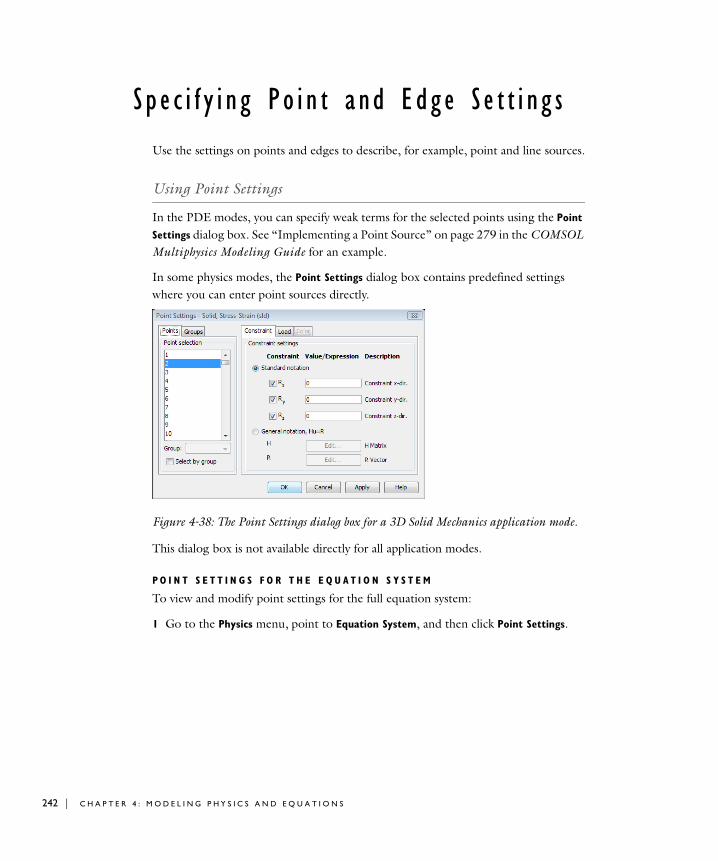
242 | C H A P T E
S p e c i f y i n g Po i n t a nd Edg e S e t t i n g s
Use the settings on points and edges to describe, for example, point and line sources.
Using Point Settings
In the PDE modes, you can specify weak terms for the selected points using the Point
Settings dialog box. See “Implementing a Point Source” on page 279 in the COMSOL Multiphysics Modeling Guide for an example.
In some physics modes, the Point Settings dialog box contains predefined settings where you can enter point sources directly.
Figure 4-38: The Point Settings dialog box for a 3D Solid Mechanics application mode.
This dialog box is not available directly for all application modes.
P O I N T S E T T I N G S F O R T H E E Q U A T I O N S Y S T E M
To view and modify point settings for the full equation system:
1 Go to the Physics menu, point to Equation System, and then click Point Settings.
R 4 : M O D E L I N G P H Y S I C S A N D E Q U A T I O N S
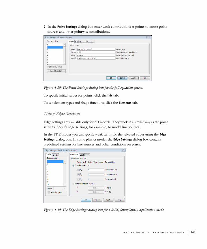
2 In the Point Settings dialog box enter weak contributions at points to create point sources and other pointwise contributions.
Figure 4-39: The Point Settings dialog box for the full equation system.
To specify initial values for points, click the Init tab.
To set element types and shape functions, click the Elements tab.
Using Edge Settings
Edge settings are available only for 3D models. They work in a similar way as the point settings. Specify edge settings, for example, to model line sources.
In the PDE modes you can specify weak terms for the selected edges using the Edge
Settings dialog box. In some physics modes the Edge Settings dialog box contains predefined settings for line sources and other conditions on edges.
Figure 4-40: The Edge Settings dialog box for a Solid, Stress/Strain application mode.
S P E C I F Y I N G P O I N T A N D E D G E S E T T I N G S | 243

244 | C H A P T E
This dialog box is not available directly for all application modes.
E D G E S E T T I N G S F O R T H E E Q U A T I O N S Y S T E M
To view and modify edge settings for the full equation system:
1 Go to the Physics menu, point to Equation System, and then click Edge Settings.
Figure 4-41: The Edge Settings dialog box for the full equation system.
2 In the Edge Settings dialog box, enter weak contributions on edges to create, for example, line sources.
3 To specify initial values on the edges click the Init tab.
4 To set element types and shape functions click the Elements tab.
Setting Point and Edge Constraints
You can define point and edge constraints using the Point Settings and Edge Settings dialog boxes for the equation system and directly using the PDE modes.
Use the Constr field to set a constraint. COMSOL Multiphysics constrains an expression written in the field to zero. For example, typing 0 v for a 2D structural mechanics model constrains the y-displacement v to zero.
Similarly, add a point load by typing u_test*load in the Weak field, where u is the variable associated with the load. For an example of how to use a point load, see “Implementing a Point Source” on page 279 in the COMSOL Multiphysics Modeling Guide.
R 4 : M O D E L I N G P H Y S I C S A N D E Q U A T I O N S
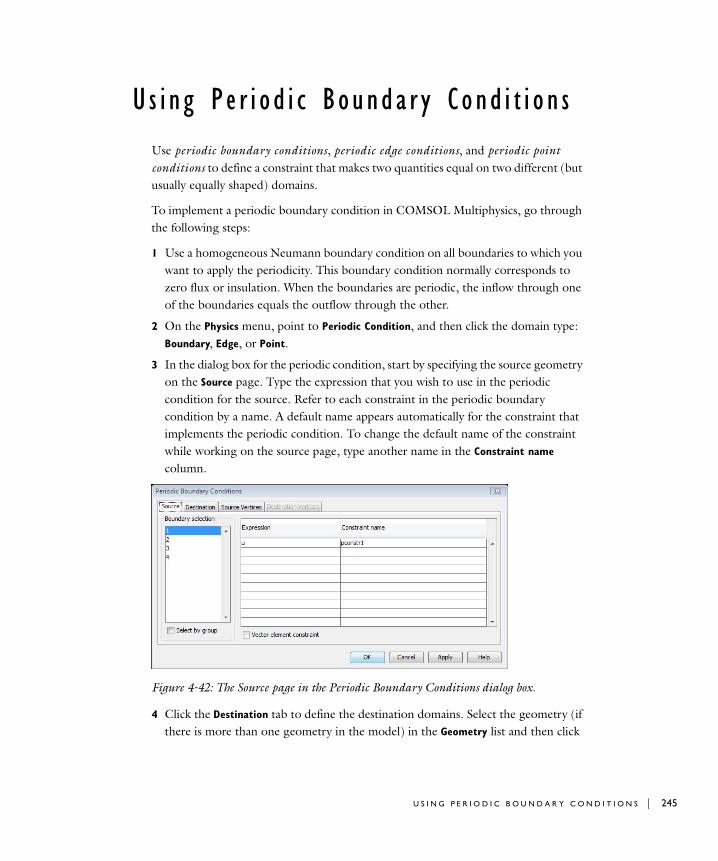
U s i n g P e r i o d i c Bounda r y Cond i t i o n s
Use periodic boundary conditions, periodic edge conditions, and periodic point conditions to define a constraint that makes two quantities equal on two different (but usually equally shaped) domains.
To implement a periodic boundary condition in COMSOL Multiphysics, go through the following steps:
1 Use a homogeneous Neumann boundary condition on all boundaries to which you want to apply the periodicity. This boundary condition normally corresponds to zero flux or insulation. When the boundaries are periodic, the inflow through one of the boundaries equals the outflow through the other.
2 On the Physics menu, point to Periodic Condition, and then click the domain type: Boundary, Edge, or Point.
3 In the dialog box for the periodic condition, start by specifying the source geometry on the Source page. Type the expression that you wish to use in the periodic condition for the source. Refer to each constraint in the periodic boundary condition by a name. A default name appears automatically for the constraint that implements the periodic condition. To change the default name of the constraint while working on the source page, type another name in the Constraint name column.
Figure 4-42: The Source page in the Periodic Boundary Conditions dialog box.
4 Click the Destination tab to define the destination domains. Select the geometry (if there is more than one geometry in the model) in the Geometry list and then click
U S I N G P E R I O D I C B O U N D A R Y C O N D I T I O N S | 245

246 | C H A P T E
to select the boundaries that become the destinations. You are free to use several boundaries and more than one geometry. You can also select boundaries by clicking in the geometry and then selecting the Use selected boundaries as destination check box. Continue by selecting the constraint that you wish to specify in the Constraint
name list. In the Expression edit field, type the expression that becomes equal to the expression on the source domain for the corresponding constraint; for a strictly periodic boundary condition, this is the same as the expression on the Source page. Set the constraint order to the same order as the elements. This is the default setting, except when you are using application modes with different element orders.
Figure 4-43: The destination page in the Periodic Boundary Conditions dialog box.
5 Click the Source Vertices tab to specify the transformation between the source and destination domains. Select 1, 2, 3, or 4 vertices that span the subspace constituted by the source domain. The number of vertices depends on the dimension of the source domain. For a periodic boundary, the number of vertices is the same as the dimension of the geometry. In a 2D simulation, the source vertices are typically the end points of the boundary.
6 Finally, click the Destination Vertices tab and select 1, 2, 3, or 4 vertices that span the subspace constituted by the destination domain; the number depends on the dimension of the destination domain, but you must provide the same number of points in both the source and destination domains. The source expression is projected onto this subspace. Its value at the first source vertex is projected to the first destination vertex, and so on. It is therefore important to assign the vertices in the correct order. Together the vertices on the source geometry and destination geometry define a linear transformation. See the following section for more information about the linear transformation from source geometry to destination geometry.
R 4 : M O D E L I N G P H Y S I C S A N D E Q U A T I O N S
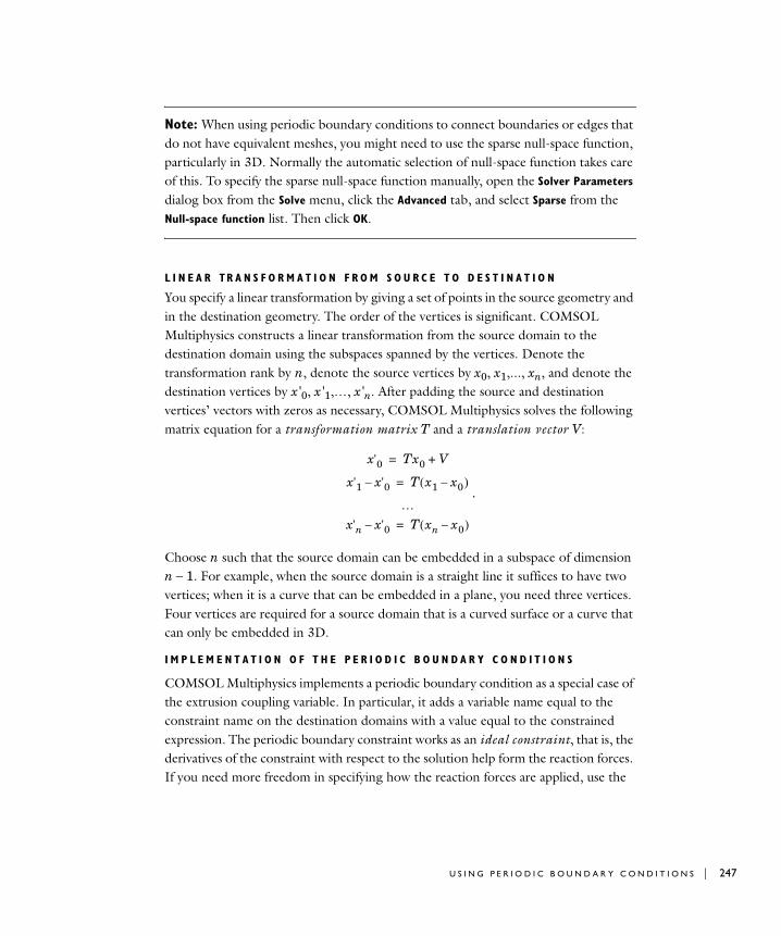
Note: When using periodic boundary conditions to connect boundaries or edges that do not have equivalent meshes, you might need to use the sparse null-space function, particularly in 3D. Normally the automatic selection of null-space function takes care of this. To specify the sparse null-space function manually, open the Solver Parameters dialog box from the Solve menu, click the Advanced tab, and select Sparse from the Null-space function list. Then click OK.
L I N E A R TR A N S F O R M A T I O N F R O M S O U R C E T O D E S T I N A T I O N
You specify a linear transformation by giving a set of points in the source geometry and in the destination geometry. The order of the vertices is significant. COMSOL Multiphysics constructs a linear transformation from the source domain to the destination domain using the subspaces spanned by the vertices. Denote the transformation rank by n, denote the source vertices by x0, x1,..., xn, and denote the destination vertices by x'0, x'1,…, x'n. After padding the source and destination vertices’ vectors with zeros as necessary, COMSOL Multiphysics solves the following matrix equation for a transformation matrix T and a translation vector V:
.
Choose n such that the source domain can be embedded in a subspace of dimension n − 1. For example, when the source domain is a straight line it suffices to have two vertices; when it is a curve that can be embedded in a plane, you need three vertices. Four vertices are required for a source domain that is a curved surface or a curve that can only be embedded in 3D.
I M P L E M E N T A T I O N O F T H E P E R I O D I C B O U N D A R Y C O N D I T I O N S
COMSOL Multiphysics implements a periodic boundary condition as a special case of the extrusion coupling variable. In particular, it adds a variable name equal to the constraint name on the destination domains with a value equal to the constrained expression. The periodic boundary constraint works as an ideal constraint, that is, the derivatives of the constraint with respect to the solution help form the reaction forces. If you need more freedom in specifying how the reaction forces are applied, use the
x'0 Tx0 V+=
x'1 x'0– T x1 x0–( )=
…x'n x'0– T xn x0–( )=
U S I N G P E R I O D I C B O U N D A R Y C O N D I T I O N S | 247
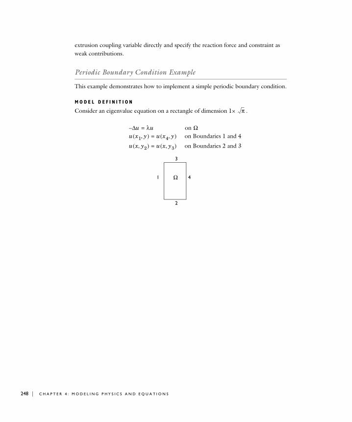
248 | C H A P T E
extrusion coupling variable directly and specify the reaction force and constraint as weak contributions.
Periodic Boundary Condition Example
This example demonstrates how to implement a simple periodic boundary condition.
M O D E L D E F I N I T I O N
Consider an eigenvalue equation on a rectangle of dimension 1× .π
4
3
2
1 Ω
u∆– λu= on Ωu x1 y,( ) u x4 y,( )= on Boundaries 1 and 4
u x y2,( ) u x y3,( )= on Boundaries 2 and 3
R 4 : M O D E L I N G P H Y S I C S A N D E Q U A T I O N S
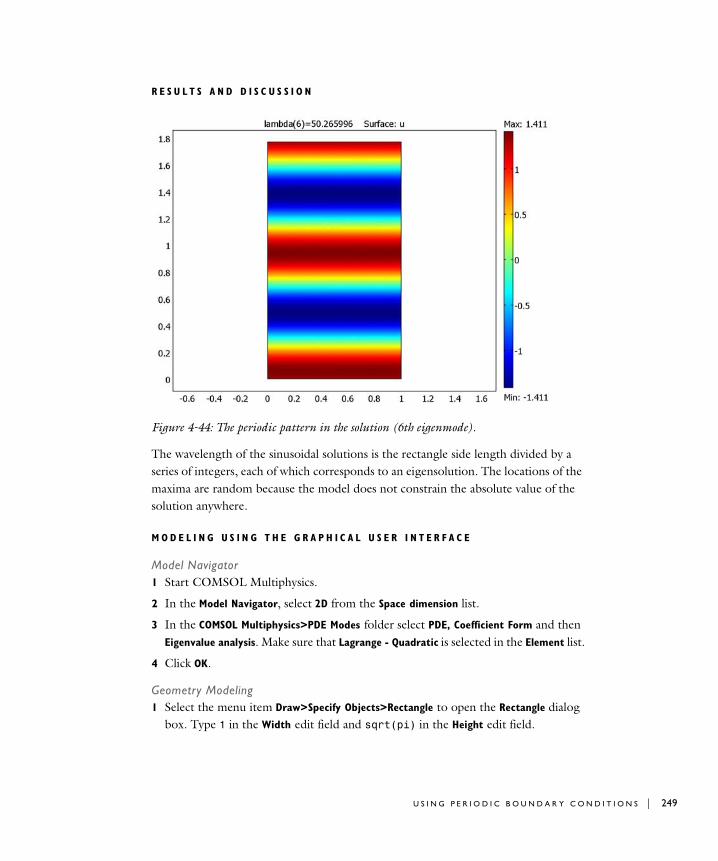
R E S U L T S A N D D I S C U S S I O N
Figure 4-44: The periodic pattern in the solution (6th eigenmode).
The wavelength of the sinusoidal solutions is the rectangle side length divided by a series of integers, each of which corresponds to an eigensolution. The locations of the maxima are random because the model does not constrain the absolute value of the solution anywhere.
M O D E L I N G U S I N G T H E G R A P H I C A L U S E R I N T E R F A C E
Model Navigator1 Start COMSOL Multiphysics.
2 In the Model Navigator, select 2D from the Space dimension list.
3 In the COMSOL Multiphysics>PDE Modes folder select PDE, Coefficient Form and then Eigenvalue analysis. Make sure that Lagrange - Quadratic is selected in the Element list.
4 Click OK.
Geometry Modeling1 Select the menu item Draw>Specify Objects>Rectangle to open the Rectangle dialog
box. Type 1 in the Width edit field and sqrt(pi) in the Height edit field.
U S I N G P E R I O D I C B O U N D A R Y C O N D I T I O N S | 249

250 | C H A P T E
2 Click OK.
3 Click the Zoom Extents button on the Main toolbar.
Physics Settings
Boundary Conditions
1 From the Physics menu open the Boundary Settings dialog box.
2 Select all boundaries and choose Neumann boundary conditions. Leave the default values.
3 Click OK.
Subdomain Settings
Use the default settings.
Periodic Boundary Conditions
1 On the Physics menu point to Periodic Conditions, and then click Periodic Boundary
Conditions.
2 On the Source page select Boundary 1. Type u in the Expression edit field, then press Enter.
3 Click the Destination tab. Select the check box for Boundary 4. Type u in the Expression edit field.
4 Click the Source Vertices tab. Add Vertices 1 and 2 to the Source vertices list.
5 Click the Destination Vertices tab. Add Vertices 3 and 4 to the Destination vertices list.
This concludes the periodicity across the vertical boundaries. Proceed to the next steps to make the solution periodic across the horizontal boundaries.
6 Click the Source tab and select Boundary 2. On the second row, type u in the Expression edit field and press Enter.
7 Click the Destination tab and select the check box for Boundary 3. Type u in the Expression edit field.
8 Click the Source Vertices tab and add Vertices 1 and 3 to the Source vertices list.
9 Click the Destination Vertices tab and add Vertices 2 and 4 to the Destination vertices list.
10 Click OK.
R 4 : M O D E L I N G P H Y S I C S A N D E Q U A T I O N S

Mesh Generation1 Click the Initialize Mesh button on the Main toolbar.
2 Click the Refine Mesh button once.
Computing the SolutionThe eigenvalue algorithm does not work reliably when the parameter that you specify in the Search for eigenvalues about edit field is equal to an eigenvalue. This particular problem has a zero eigenvalue, so you must change the value of this parameter.
1 Open the Solver Parameters dialog box.
2 Type 10 in the Search for eigenvalues around edit field.
3 Click the Solve button on the Main toolbar to compute the solution.
Postprocessing and VisualizationBy default COMSOL Multiphysics plots the first eigenmode, which in this case is a flat solution associated with a zero eigenvalue.
1 From the Postprocessing menu open the Plot Parameters dialog box.
2 Look at the solution for different eigenvalues by making a corresponding selection in the Eigenvalue list. Start with the last eigenvalue.
3 Click Apply to plot each eigenvalue.
4 When finished click OK.
U S I N G P E R I O D I C B O U N D A R Y C O N D I T I O N S | 251

252 | C H A P T E
S p e c i f y i n g App l i c a t i o n S c a l a r V a r i a b l e s
Some applications modes use scalar variables that take part in the mathematical model but are independent of the geometry and material. You can set the values of these variables in the Application Scalar Variables dialog box.
Figure 4-45: The Application Scalar Variables dialog box.
Go to the Physics menu and choose Scalar Variables to open the Application Scalar
Variables dialog box.
You can change the value of each scalar variable by making an entry in the edit field in the Expression column.
The COMSOL Multiphysics application modes that include scalar variables are:
• AC Power Electromagnetics, which includes scalar variables for angular frequency, permittivity of vacuum, and permeability of vacuum
• Electrostatics, which includes a scalar variable for the permittivity of vacuum
• Magnetostatics, which includes scalar variables for the permittivity of vacuum and permeability of vacuum
• Acoustics, which includes scalar variables for the frequency and the reference pressure
Several other scalar variables appear in application modes defined in the add-on modules.
If your model does not contain any scalar variables, this menu item is not available.
R 4 : M O D E L I N G P H Y S I C S A N D E Q U A T I O N S

Compu t i n g A c c u r a t e F l u x e s
COMSOL Multiphysics can compute accurate fluxes using higher-order elements and standard strong constraints. Use weak constraints (typically ideal weak constraints) to achieve optimal accuracy (for more information about weak constraints, see “Using Weak Constraints” on page 300 in the COMSOL Multiphysics Modeling Guide). The Lagrange multipliers are additional dependent variables in application modes using weak constraints (with variable names lm1, lm2, and so on). The Lagrange multipliers correspond to the following postprocessing variables:
The postprocessing variable names in the Incompressible Navier-Stokes application mode depend on the form of the stress tensor in the model.
COMSOL Multiphysics computes only the part of the boundary flux captured by the Lagrange multiplier. You might have additional flux coming from boundary sources or nonidentity constraint matrices. This should not happen in the physics modes, though.
Flux Computation Example
Consider computing the flux over the constrained boundary of a rectangle. The PDE of the rectangle is Poisson’s equation, ∆u = 1, with u = 0 on the boundary.
M O D E L N A V I G A T O R
1 From the Space dimension list select 2D.
2 In the COMSOL Multiphysics folder open PDE Modes and then PDE, Coefficient Form.
TABLE 4-28: PHYSICS MODES INTERPRETATION OF LAGRANGE MULTIPLIERS
PHYSICS MODE NAME QUANTITY CORRESPONDING VARIABLE
AC power electromagnetics Surface current i*omega*Js
Electrostatics Surface charge density
nD
Magnetostatics Surface current -Js, -Jsx, -Jsy, -Jsz
Conductive media DC Current flux -nJ
Heat transfer Heat flux -nflux
Diffusion Flux -nflux
Structural mechanics Force Tax, Tay, Taz
Incompressible Navier-Stokes Total force per area T_x, T_y, T_z
C O M P U T I N G A C C U R A T E F L U X E S | 253
254 | C H A P T E
3 Click OK.
G E O M E T R Y M O D E L I N G
Draw a single rectangle of any size.
C O M P U T I N G T H E S O L U T I O N
Click the Solve button on the Main toolbar.
P O S T P R O C E S S I N G
1 On the Postprocessing menu choose Subdomain Integration.
2 In the Subdomain Integration dialog box type 1 in the Expression edit field.
3 Select Subdomain 1 and click OK. The rectangle’s area appears in the message log.
4 Go to the Postprocessing menu and open the Boundary Integration dialog box.
5 Type nx*ux+ny*uy in the Expression edit field.
6 Select all boundaries and click OK. COMSOL Multiphysics computes influx over the boundaries as the normal component of the gradient of u.
The influx is approximately equal to the integral of the negative source term in Poisson’s equation.
P H Y S I C S S E T T I N G S
Application Mode Properties1 Go to the Physics menu and choose Properties.
2 Select On from the Weak constraints list and then click OK.
C O M P U T I N G T H E S O L U T I O N
Click the Solve button on the Main toolbar.
P O S T P R O C E S S I N G
1 Go to the Postprocessing menu and choose Boundary Integration.
2 Select lm1 from the Predefined quantities list.
3 Select Boundary 1 and click OK. COMSOL Multiphysics computes the flux over the boundary by using the weak constraint variable.
The integral of the flux exactly equals the integral of the finite-element projection of the source term in Poisson’s equation.
R 4 : M O D E L I N G P H Y S I C S A N D E Q U A T I O N S
U s i n g Coup l i n g V a r i a b l e s
Coupling variables are extremely powerful in their ability to make the value and the exact Jacobian of an expression available nonlocally. They are not only useful for modeling coupled problems—you can also use them solely for postprocessing and visualization purposes.
You define all coupling variables in two steps. First define the source, that is, which expression to evaluate and where to evaluate it; then define the destination, that is, the domains within which you want to use the resulting variable.
There are three major kinds of coupling variables available: integration, extrusion, and projection variables. This section describes them all. For all types of coupling variables, always add each coupling variable on a separate row in the table on the Source page, even if they are defined on different domains.
Integration Coupling Variables
An integration coupling variable is the value of an integral of an expression over a set of domains. Thus, the integration coupling variable is always a scalar quantity. The source of the variable can be an expression at a vertex, or the integral of an expression over one or several subdomains, boundaries, or edges. The destination of the integration coupling variable can be the global destination, subdomains, boundaries, edges, or vertices.
Define an integration coupling variable by going to the Options menu and pointing to Integration Coupling Variables. Then select Subdomain Variables, Boundary Variables, Edge Variables, or Point Variables, depending on your intended source for the coupling variable.
U S I N G C O U P L I N G V A R I A B L E S | 255
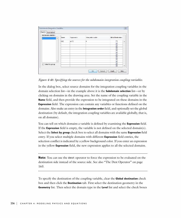
256 | C H A P T E
Figure 4-46: Specifying the sources for the subdomain integration coupling variables.
In the dialog box, select source domains for the integration coupling variables in the domain selection list—in the example above it is the Subdomain selection list—or by clicking on domains in the drawing area. Set the name of the coupling variable in the Name field, and then provide the expression to be integrated on these domains in the Expression field. The expression can contain any variables or functions defined on the domains. Also make an entry in the Integration order field, and optionally set the global destination (by default, the integration coupling variables are available globally, that is, on all domains).
You can tell on which domains a variable is defined by examining the Expression field. If the Expression field is empty, the variable is not defined on the selected domain(s). Select the Select by group check box to select all domains with the same Expression field entry. If you select multiple domains with different Expression field entries, the selection conflict is indicated by a yellow background color. If you enter an expression in the yellow Expression field, the new expression applies to all the selected domains.
Note: You can use the dest operator to force the expression to be evaluated on the destination side instead of the source side. See also “The Dest Operator” on page 163.
To specify the destination of the coupling variable, clear the Global destination check box and then click the Destination tab. First select the destination geometry in the Geometry list. Then select the domain type in the Level list and select the check boxes
R 4 : M O D E L I N G P H Y S I C S A N D E Q U A T I O N S
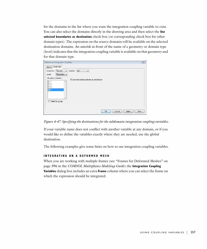
for the domains in the list where you want the integration coupling variable to exist. You can also select the domains directly in the drawing area and then select the Use
selected boundaries as destination check box (or corresponding check box for other domain types). The expression on the source domains will be available on the selected destination domains. An asterisk in front of the name of a geometry or domain type (level) indicates that the integration coupling variable is available on that geometry and for that domain type.
Figure 4-47: Specifying the destinations for the subdomain integration coupling variables.
If your variable name does not conflict with another variable at any domain, or if you would like to define the variables exactly where they are needed, use the global destination.
The following examples give some hints on how to use integration coupling variables.
I N T E G R A T I N G O N A D E F O R M E D M E S H
When you are working with multiple frames (see “Frames for Deformed Meshes” on page 396 in the COMSOL Multiphysics Modeling Guide) the Integration Coupling
Variables dialog box includes an extra Frame column where you can select the frame on which the expression should be integrated.
U S I N G C O U P L I N G V A R I A B L E S | 257
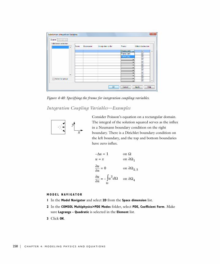
258 | C H A P T E
Figure 4-48: Specifying the frame for integration coupling variables.
Integration Coupling Variables—Examples
Consider Poisson’s equation on a rectangular domain. The integral of the solution squared serves as the influx in a Neumann boundary condition on the right boundary. There is a Dirichlet boundary condition on the left boundary, and the top and bottom boundaries have zero influx.
M O D E L N A V I G A T O R
1 In the Model Navigator and select 2D from the Space dimension list.
2 In the COMSOL Multiphysics>PDE Modes folder, select PDE, Coefficient Form. Make sure Lagrange - Quadratic is selected in the Element list.
3 Click OK.
x
y
u∆– 1= on Ωu x= on ∂Ω1
n∂∂u 0= on ∂Ω2 3,
n∂∂u u2 Ωd
Ω∫–= on ∂Ω4
R 4 : M O D E L I N G P H Y S I C S A N D E Q U A T I O N S
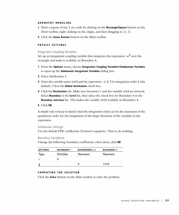
G E O M E T R Y M O D E L I N G
1 Draw a square of size 1 on a side by clicking on the Rectangle/Square button on the Draw toolbar, right-clicking on the origin, and then dragging to (1, 1).
2 Click the Zoom Extents button on the Main toolbar.
P H Y S I C S S E T T I N G S
Integration Coupling VariablesSet up an integration coupling variable that integrates the expression −u2 over the rectangle and make it available on Boundary 4.
1 From the Options menu, choose Integration Coupling Variables>Subdomain Variables to open up the Subdomain Integration Variables dialog box.
2 Select Subdomain 1.
3 Enter the variable name int2 and the expression -u^2. Use integration order 4 (the default). Clear the Global destination check box.
4 Click the Destination tab. Make sure Geometry 1 and the variable int2 are selected. Select Boundary in the Level list, then select the check box for Boundary 4 in the Boundary selection list. This makes the variable int2 available on Boundary 4.
5 Click OK.
A simple rule to keep in mind is that the integration order can be the maximum of the quadrature order for the integration of the shape functions of the variables in the expression.
Subdomain SettingsUse the default PDE coefficients (Poisson’s equation). That is, do nothing.
Boundary ConditionsChange the following boundary coefficients; when done, click OK.
C O M P U T I N G T H E S O L U T I O N
Click the Solve button on the Main toolbar to solve the problem.
SETTINGS BOUNDARY 1 BOUNDARIES 2, 3 BOUNDARY 4
Type Dirichlet Neumann Neumann
r 0
g 0 int2
U S I N G C O U P L I N G V A R I A B L E S | 259
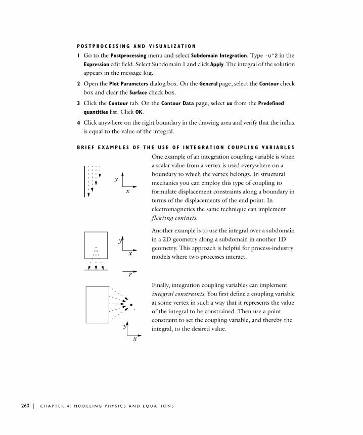
260 | C H A P T E
P O S T P R O C E S S I N G A N D V I S U A L I Z A T I O N
1 Go to the Postprocessing menu and select Subdomain Integration. Type -u^2 in the Expression edit field. Select Subdomain 1 and click Apply. The integral of the solution appears in the message log.
2 Open the Plot Parameters dialog box. On the General page, select the Contour check box and clear the Surface check box.
3 Click the Contour tab. On the Contour Data page, select ux from the Predefined
quantities list. Click OK.
4 Click anywhere on the right boundary in the drawing area and verify that the influx is equal to the value of the integral.
B R I E F E X A M P L E S O F T H E U S E O F I N T E G R A T I O N C O U P L I N G V A R I A B L E S
One example of an integration coupling variable is when a scalar value from a vertex is used everywhere on a boundary to which the vertex belongs. In structural mechanics you can employ this type of coupling to formulate displacement constraints along a boundary in terms of the displacements of the end point. In electromagnetics the same technique can implement floating contacts.
Another example is to use the integral over a subdomain in a 2D geometry along a subdomain in another 1D geometry. This approach is helpful for process-industry models where two processes interact.
Finally, integration coupling variables can implement integral constraints. You first define a coupling variable at some vertex in such a way that it represents the value of the integral to be constrained. Then use a point constraint to set the coupling variable, and thereby the integral, to the desired value.
x
y
x
y
r
x
y
R 4 : M O D E L I N G P H Y S I C S A N D E Q U A T I O N S
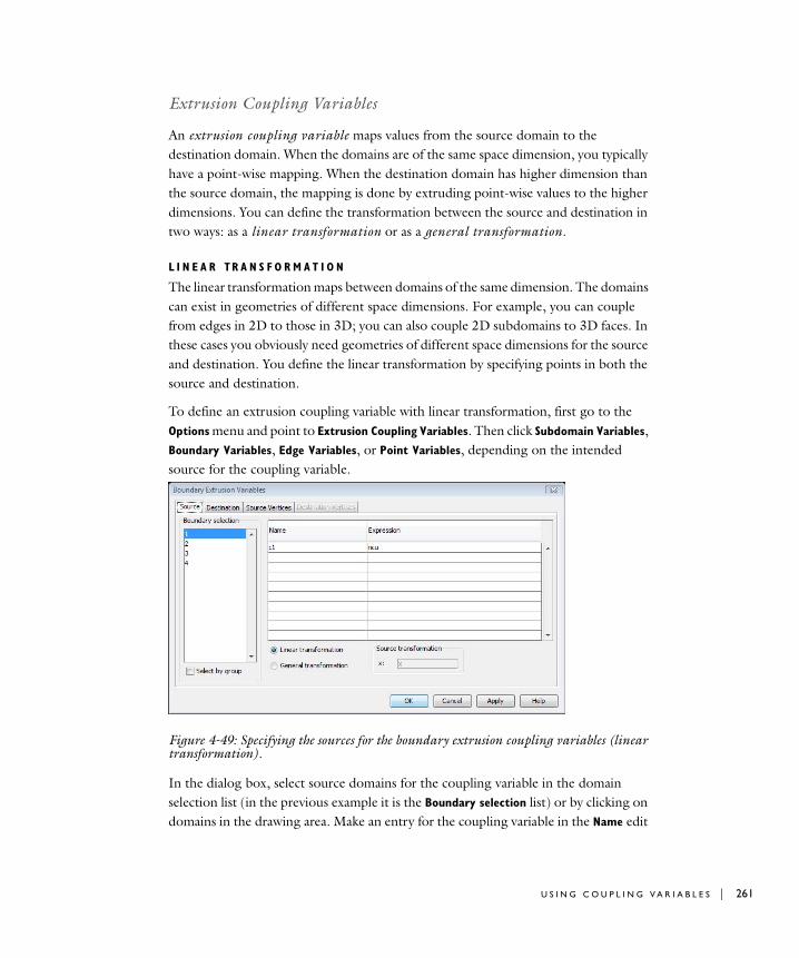
Extrusion Coupling Variables
An extrusion coupling variable maps values from the source domain to the destination domain. When the domains are of the same space dimension, you typically have a point-wise mapping. When the destination domain has higher dimension than the source domain, the mapping is done by extruding point-wise values to the higher dimensions. You can define the transformation between the source and destination in two ways: as a linear transformation or as a general transformation.
L I N E A R TR A N S F O R M A T I O N
The linear transformation maps between domains of the same dimension. The domains can exist in geometries of different space dimensions. For example, you can couple from edges in 2D to those in 3D; you can also couple 2D subdomains to 3D faces. In these cases you obviously need geometries of different space dimensions for the source and destination. You define the linear transformation by specifying points in both the source and destination.
To define an extrusion coupling variable with linear transformation, first go to the Options menu and point to Extrusion Coupling Variables. Then click Subdomain Variables, Boundary Variables, Edge Variables, or Point Variables, depending on the intended source for the coupling variable.
Figure 4-49: Specifying the sources for the boundary extrusion coupling variables (linear transformation).
In the dialog box, select source domains for the coupling variable in the domain selection list (in the previous example it is the Boundary selection list) or by clicking on domains in the drawing area. Make an entry for the coupling variable in the Name edit
U S I N G C O U P L I N G V A R I A B L E S | 261

262 | C H A P T E
field, and then provide an expression on these domains in the Expression edit field. Make sure that you have selected the Linear transformation button.
Now click the Destination tab. First select the geometry of the destination domain from the domains in the Geometry list. You can use the same geometry for both source and destination. The dimension of the destination domain is the same as the dimension of the source domain, regardless of the geometry dimensions. COMSOL Multiphysics transforms the expression on the source domains to the selected destination domains.
Figure 4-50: Specifying the destinations for the boundary extrusion coupling variables (linear transformation).
You can change the variable when working with the destination page. The default variable is the one selected on the source page.
Continue by specifying the linear transformation by giving a set of points in the source geometry and in the destination geometry. This works in exactly the same way as for periodic boundary conditions. See “Linear Transformation from Source to Destination” on page 247 for more information.
R 4 : M O D E L I N G P H Y S I C S A N D E Q U A T I O N S
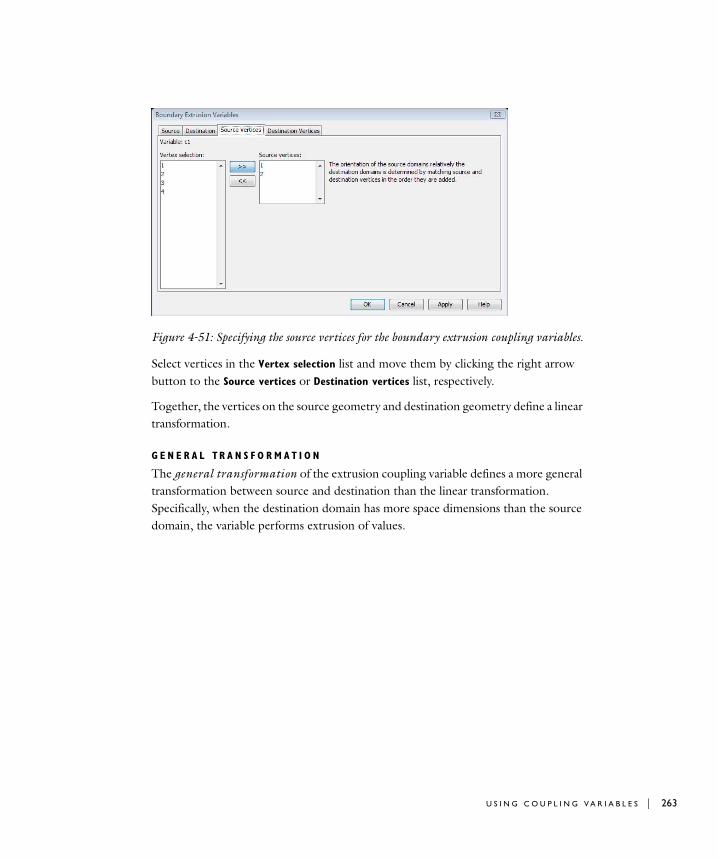
Figure 4-51: Specifying the source vertices for the boundary extrusion coupling variables.
Select vertices in the Vertex selection list and move them by clicking the right arrow button to the Source vertices or Destination vertices list, respectively.
Together, the vertices on the source geometry and destination geometry define a linear transformation.
G E N E R A L TR A N S F O R M A T I O N
The general transformation of the extrusion coupling variable defines a more general transformation between source and destination than the linear transformation. Specifically, when the destination domain has more space dimensions than the source domain, the variable performs extrusion of values.
U S I N G C O U P L I N G V A R I A B L E S | 263
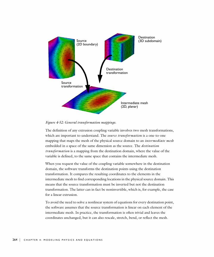
264 | C H A P T E
Figure 4-52: General transformation mappings.
The definition of any extrusion coupling variable involves two mesh transformations, which are important to understand. The source transformation is a one-to-one mapping that maps the mesh of the physical source domain to an intermediate mesh embedded in a space of the same dimension as the source. The destination transformation is a mapping from the destination domain, where the value of the variable is defined, to the same space that contains the intermediate mesh.
When you request the value of the coupling variable somewhere in the destination domain, the software transforms the destination points using the destination transformation. It compares the resulting coordinates to the elements in the intermediate mesh to find corresponding locations in the physical source domain. This means that the source transformation must be inverted but not the destination transformation. The latter can in fact be noninvertible, which is, for example, the case for a linear extrusion.
To avoid the need to solve a nonlinear system of equations for every destination point, the software assumes that the source transformation is linear on each element of the intermediate mesh. In practice, the transformation is often trivial and leaves the coordinates unchanged, but it can also rescale, stretch, bend, or reflect the mesh.
Source Destination
Intermediate mesh
Source
Destinationtransformation
transformation
(2D boundary)(3D subdomain)
(2D, planar)
R 4 : M O D E L I N G P H Y S I C S A N D E Q U A T I O N S

Choose the geometry of the source domain by opening the dialog box from that particular geometry. To define an extrusion coupling variable with general transformation, go to the Options menu and select Extrusion Coupling Variable. Then select Subdomain, Boundary, Edge, or Point, depending on the intended source for the coupling variable.
Figure 4-53: Specifying the sources for the boundary extrusion coupling variables (general transformation).
In the dialog box, select source domains for the coupling variable in the domain selection list; in the example above it is the Boundary selection list. Make an entry for the coupling variable in the Name edit field, and then provide an expression for the selected source domains in the Expression edit field. Make sure that you have selected the General transformation button.
Now define the source transformation that maps the source domain to the intermediate domain of the same dimension. The source transformation has the same number of fields as the dimension of the source domain. You can use expressions containing space coordinates in the source geometry when defining the transformation. Remember that the transformation must be approximately linear within each mesh element.
U S I N G C O U P L I N G V A R I A B L E S | 265
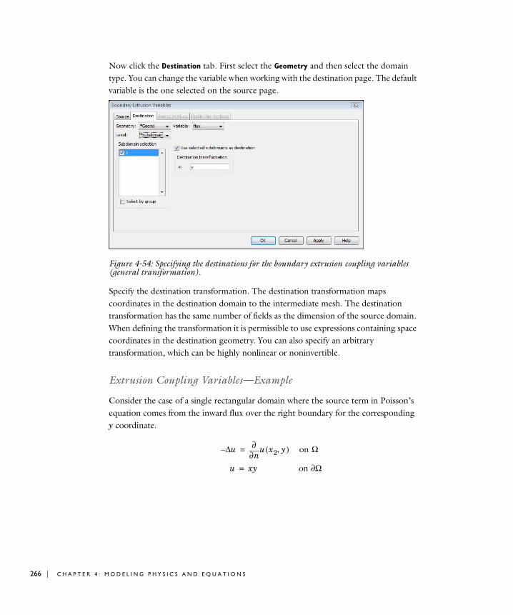
266 | C H A P T E
Now click the Destination tab. First select the Geometry and then select the domain type. You can change the variable when working with the destination page. The default variable is the one selected on the source page.
Figure 4-54: Specifying the destinations for the boundary extrusion coupling variables (general transformation).
Specify the destination transformation. The destination transformation maps coordinates in the destination domain to the intermediate mesh. The destination transformation has the same number of fields as the dimension of the source domain. When defining the transformation it is permissible to use expressions containing space coordinates in the destination geometry. You can also specify an arbitrary transformation, which can be highly nonlinear or noninvertible.
Extrusion Coupling Variables—Example
Consider the case of a single rectangular domain where the source term in Poisson’s equation comes from the inward flux over the right boundary for the corresponding y coordinate.
u∆–n∂
∂ u x2 y,( ) on Ω=
u xy on Ω∂=
R 4 : M O D E L I N G P H Y S I C S A N D E Q U A T I O N S
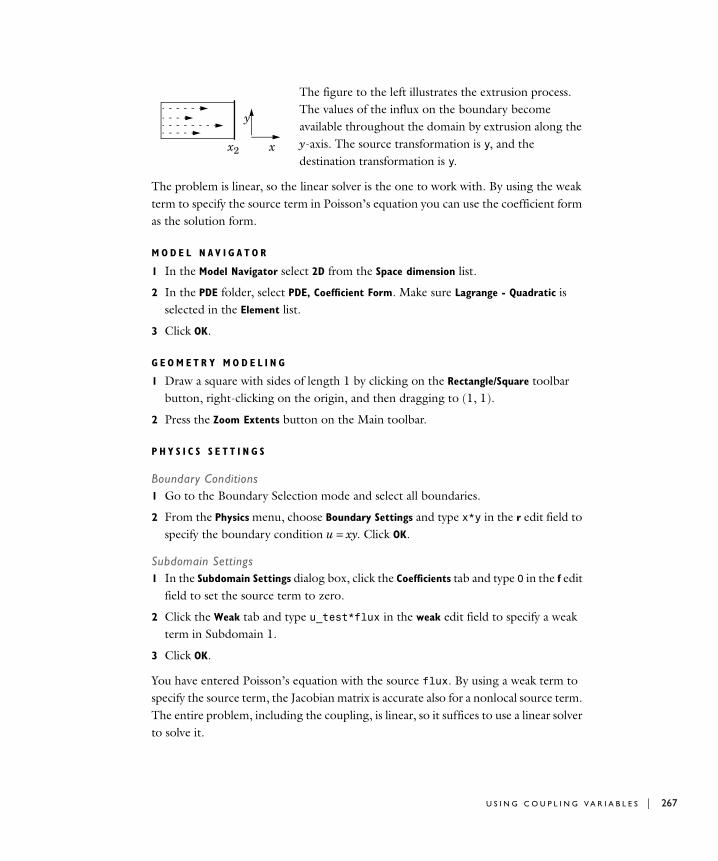
The figure to the left illustrates the extrusion process. The values of the influx on the boundary become available throughout the domain by extrusion along the y-axis. The source transformation is y, and the destination transformation is y.
The problem is linear, so the linear solver is the one to work with. By using the weak term to specify the source term in Poisson’s equation you can use the coefficient form as the solution form.
M O D E L N A V I G A T O R
1 In the Model Navigator select 2D from the Space dimension list.
2 In the PDE folder, select PDE, Coefficient Form. Make sure Lagrange - Quadratic is selected in the Element list.
3 Click OK.
G E O M E T R Y M O D E L I N G
1 Draw a square with sides of length 1 by clicking on the Rectangle/Square toolbar button, right-clicking on the origin, and then dragging to (1, 1).
2 Press the Zoom Extents button on the Main toolbar.
P H Y S I C S S E T T I N G S
Boundary Conditions1 Go to the Boundary Selection mode and select all boundaries.
2 From the Physics menu, choose Boundary Settings and type x*y in the r edit field to specify the boundary condition u = xy. Click OK.
Subdomain Settings1 In the Subdomain Settings dialog box, click the Coefficients tab and type 0 in the f edit
field to set the source term to zero.
2 Click the Weak tab and type u_test*flux in the weak edit field to specify a weak term in Subdomain 1.
3 Click OK.
You have entered Poisson’s equation with the source flux. By using a weak term to specify the source term, the Jacobian matrix is accurate also for a nonlocal source term. The entire problem, including the coupling, is linear, so it suffices to use a linear solver to solve it.
x
y
x2
U S I N G C O U P L I N G V A R I A B L E S | 267

268 | C H A P T E
Coupling Variables1 Go to the Options menu, point to Extrusion Coupling Variables, and then click
Boundary Variables to open up the like-named dialog box.
2 Select Boundary 1 and enter the variable name flux and the expression ncu.
3 Click the General transformation button. Type y as the source transformation in the x edit field.
4 Click the Destination tab. Select Subdomain in the Level list and then select Subdomain 1.
5 Type y as the destination transformation in the x edit field.
6 Click OK.
C O M P U T I N G T H E S O L U T I O N
To access the ncu variable, use the coefficient solution form:
1 From the Solve menu, choose Solver Parameters.
2 Click the Advanced tab.
3 Select Coefficient in the Solution form list.
4 Click OK.
5 Click the Solve button on the Main toolbar.
P O S T P R O C E S S I N G A N D V I S U A L I Z A T I O N
1 In the Plot Parameters dialog box, click the Surface tab.
2 On the Surface Data page, type flux in the Expression edit field.
3 Click the Height Data tab, select the Height data check box, and type flux in the Expression edit field.
4 Click the Boundary tab and then select the Boundary plot check box.
5 Type ncu in the Expression edit field on the Boundary Data page.
R 4 : M O D E L I N G P H Y S I C S A N D E Q U A T I O N S
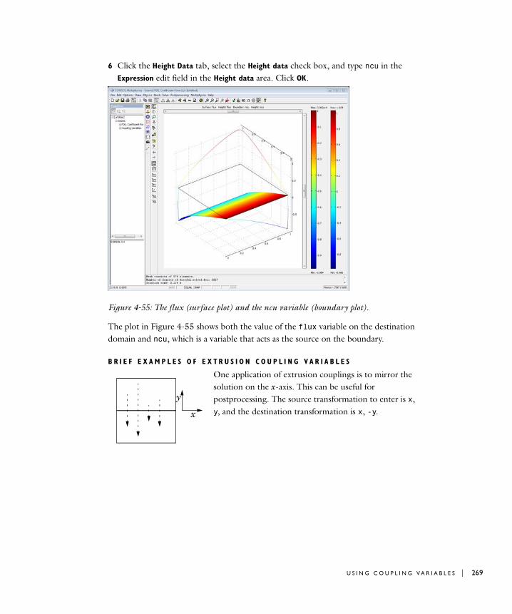
6 Click the Height Data tab, select the Height data check box, and type ncu in the Expression edit field in the Height data area. Click OK.
Figure 4-55: The flux (surface plot) and the ncu variable (boundary plot).
The plot in Figure 4-55 shows both the value of the flux variable on the destination domain and ncu, which is a variable that acts as the source on the boundary.
B R I E F E X A M P L E S O F E X T R U S I O N C O U P L I N G V A R I A B L E S
One application of extrusion couplings is to mirror the solution on the x-axis. This can be useful for postprocessing. The source transformation to enter is x, y, and the destination transformation is x, -y.x
y
U S I N G C O U P L I N G V A R I A B L E S | 269
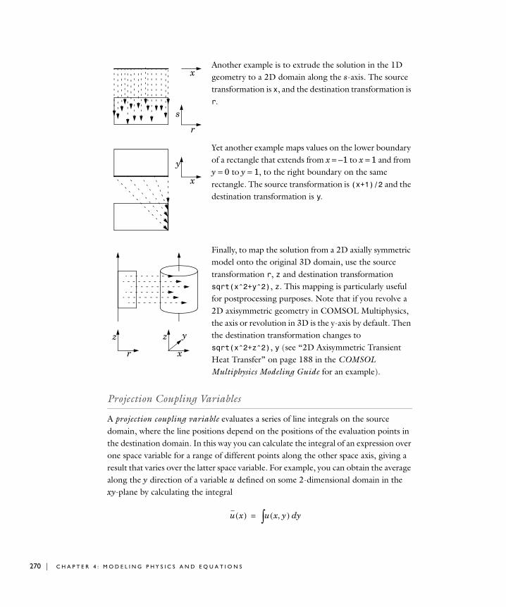
270 | C H A P T E
Another example is to extrude the solution in the 1D geometry to a 2D domain along the s-axis. The source transformation is x, and the destination transformation is r.
Yet another example maps values on the lower boundary of a rectangle that extends from x = –1 to x = 1 and from y = 0 to y = 1, to the right boundary on the same rectangle. The source transformation is (x+1)/2 and the destination transformation is y.
Finally, to map the solution from a 2D axially symmetric model onto the original 3D domain, use the source transformation r, z and destination transformation sqrt(x^2+y^2), z. This mapping is particularly useful for postprocessing purposes. Note that if you revolve a 2D axisymmetric geometry in COMSOL Multiphysics, the axis or revolution in 3D is the y-axis by default. Then the destination transformation changes to sqrt(x^2+z^2), y (see “2D Axisymmetric Transient Heat Transfer” on page 188 in the COMSOL Multiphysics Modeling Guide for an example).
Projection Coupling Variables
A projection coupling variable evaluates a series of line integrals on the source domain, where the line positions depend on the positions of the evaluation points in the destination domain. In this way you can calculate the integral of an expression over one space variable for a range of different points along the other space axis, giving a result that varies over the latter space variable. For example, you can obtain the average along the y direction of a variable u defined on some 2-dimensional domain in the xy-plane by calculating the integral
x
r
s
x
y
r
z
x
z y
u x( ) u x y,( ) yd∫=
R 4 : M O D E L I N G P H Y S I C S A N D E Q U A T I O N S
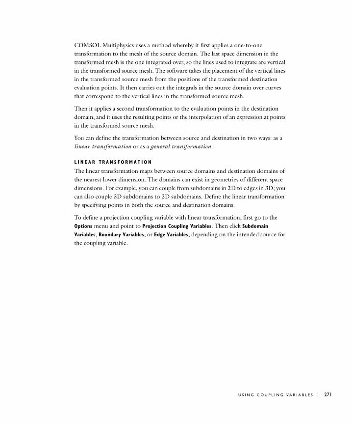
COMSOL Multiphysics uses a method whereby it first applies a one-to-one transformation to the mesh of the source domain. The last space dimension in the transformed mesh is the one integrated over, so the lines used to integrate are vertical in the transformed source mesh. The software takes the placement of the vertical lines in the transformed source mesh from the positions of the transformed destination evaluation points. It then carries out the integrals in the source domain over curves that correspond to the vertical lines in the transformed source mesh.
Then it applies a second transformation to the evaluation points in the destination domain, and it uses the resulting points or the interpolation of an expression at points in the transformed source mesh.
You can define the transformation between source and destination in two ways: as a linear transformation or as a general transformation.
L I N E A R TR A N S F O R M A T I O N
The linear transformation maps between source domains and destination domains of the nearest lower dimension. The domains can exist in geometries of different space dimensions. For example, you can couple from subdomains in 2D to edges in 3D; you can also couple 3D subdomains to 2D subdomains. Define the linear transformation by specifying points in both the source and destination domains.
To define a projection coupling variable with linear transformation, first go to the Options menu and point to Projection Coupling Variables. Then click Subdomain
Variables, Boundary Variables, or Edge Variables, depending on the intended source for the coupling variable.
U S I N G C O U P L I N G V A R I A B L E S | 271
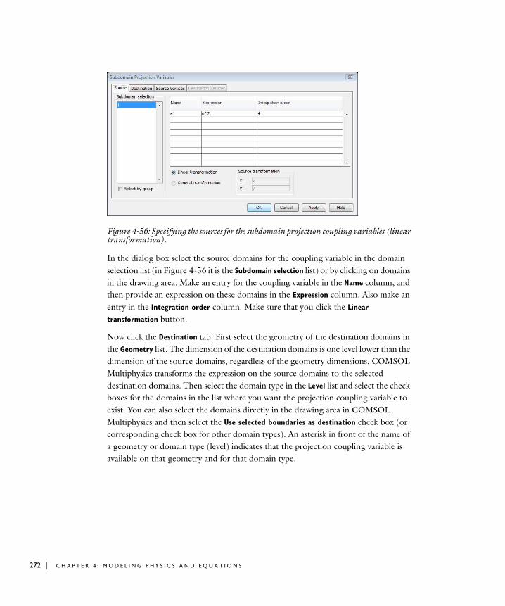
272 | C H A P T E
Figure 4-56: Specifying the sources for the subdomain projection coupling variables (linear transformation).
In the dialog box select the source domains for the coupling variable in the domain selection list (in Figure 4-56 it is the Subdomain selection list) or by clicking on domains in the drawing area. Make an entry for the coupling variable in the Name column, and then provide an expression on these domains in the Expression column. Also make an entry in the Integration order column. Make sure that you click the Linear
transformation button.
Now click the Destination tab. First select the geometry of the destination domains in the Geometry list. The dimension of the destination domains is one level lower than the dimension of the source domains, regardless of the geometry dimensions. COMSOL Multiphysics transforms the expression on the source domains to the selected destination domains. Then select the domain type in the Level list and select the check boxes for the domains in the list where you want the projection coupling variable to exist. You can also select the domains directly in the drawing area in COMSOL Multiphysics and then select the Use selected boundaries as destination check box (or corresponding check box for other domain types). An asterisk in front of the name of a geometry or domain type (level) indicates that the projection coupling variable is available on that geometry and for that domain type.
R 4 : M O D E L I N G P H Y S I C S A N D E Q U A T I O N S

Figure 4-57: Specifying the destinations for the subdomain projection coupling variables (linear transformation).
You can change the variable in the Variable list. The default variable is the one selected on the source page.
Now specify the linear transformation by giving a set of points in the source geometry and in the destination geometry. The order of the vertices is significant. COMSOL Multiphysics constructs a linear transformation from the source domain to the destination domain using the subspaces spanned by the vertices. Denote the transformation rank by n, denote the source vertices by x0, x1,..., xn, and denote the destination vertices by x'0, x'1,…, x'n. After padding the source and destination vertices’ vectors with zeros as necessary, the software solves the following matrix equation for a transformation matrix T and a translation vector V:
.
For the projection coupling variable you must have one more vertex in the source geometry than in the destination geometry. Choose n such that the source domain can be embedded in a subspace of dimension n − 1. For example, when the source domain is a straight line, it suffices to have two vertices; when it is a curve that can be
x'0 Tx0 V+=
x'1 x'0– T x1 x0–( )=
…x'n x'0– T xn x0–( )=
U S I N G C O U P L I N G V A R I A B L E S | 273
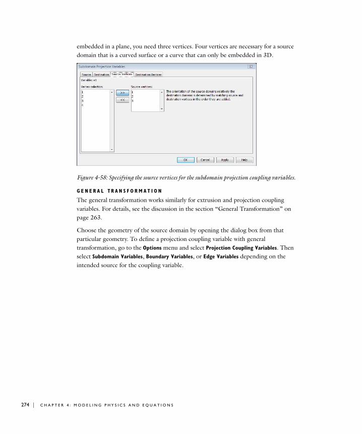
274 | C H A P T E
embedded in a plane, you need three vertices. Four vertices are necessary for a source domain that is a curved surface or a curve that can only be embedded in 3D.
Figure 4-58: Specifying the source vertices for the subdomain projection coupling variables.
G E N E R A L TR A N S F O R M A T I O N
The general transformation works similarly for extrusion and projection coupling variables. For details, see the discussion in the section “General Transformation” on page 263.
Choose the geometry of the source domain by opening the dialog box from that particular geometry. To define a projection coupling variable with general transformation, go to the Options menu and select Projection Coupling Variables. Then select Subdomain Variables, Boundary Variables, or Edge Variables depending on the intended source for the coupling variable.
R 4 : M O D E L I N G P H Y S I C S A N D E Q U A T I O N S
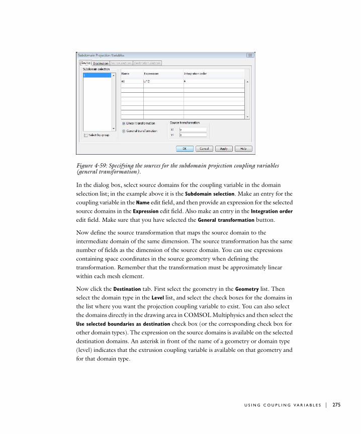
Figure 4-59: Specifying the sources for the subdomain projection coupling variables (general transformation).
In the dialog box, select source domains for the coupling variable in the domain selection list; in the example above it is the Subdomain selection. Make an entry for the coupling variable in the Name edit field, and then provide an expression for the selected source domains in the Expression edit field. Also make an entry in the Integration order edit field. Make sure that you have selected the General transformation button.
Now define the source transformation that maps the source domain to the intermediate domain of the same dimension. The source transformation has the same number of fields as the dimension of the source domain. You can use expressions containing space coordinates in the source geometry when defining the transformation. Remember that the transformation must be approximately linear within each mesh element.
Now click the Destination tab. First select the geometry in the Geometry list. Then select the domain type in the Level list, and select the check boxes for the domains in the list where you want the projection coupling variable to exist. You can also select the domains directly in the drawing area in COMSOL Multiphysics and then select the Use selected boundaries as destination check box (or the corresponding check box for other domain types). The expression on the source domains is available on the selected destination domains. An asterisk in front of the name of a geometry or domain type (level) indicates that the extrusion coupling variable is available on that geometry and for that domain type.
U S I N G C O U P L I N G V A R I A B L E S | 275
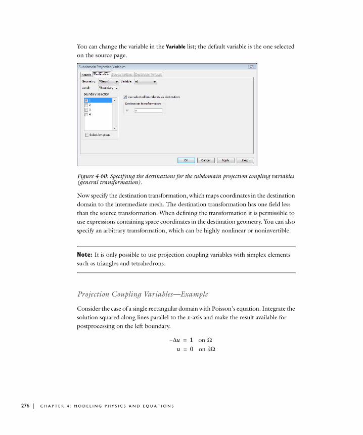
276 | C H A P T E
You can change the variable in the Variable list; the default variable is the one selected on the source page.
Figure 4-60: Specifying the destinations for the subdomain projection coupling variables (general transformation).
Now specify the destination transformation, which maps coordinates in the destination domain to the intermediate mesh. The destination transformation has one field less than the source transformation. When defining the transformation it is permissible to use expressions containing space coordinates in the destination geometry. You can also specify an arbitrary transformation, which can be highly nonlinear or noninvertible.
Note: It is only possible to use projection coupling variables with simplex elements such as triangles and tetrahedrons.
Projection Coupling Variables—Example
Consider the case of a single rectangular domain with Poisson’s equation. Integrate the solution squared along lines parallel to the x-axis and make the result available for postprocessing on the left boundary.
u∆– 1 on Ω=
u 0 on Ω∂=
R 4 : M O D E L I N G P H Y S I C S A N D E Q U A T I O N S

The figure to the left illustrates the projection process. Project the integral of the solution squared on the boundary. The source transformation is y, and the destination transformation is y.
M O D E L N A V I G A T O R
1 In the Model Navigator select 2D in the Space dimension list.
2 In the PDE folder select PDE, Coefficient Form. Make sure Lagrange - Quadratic is selected in the Element list.
3 Click OK.
G E O M E T R Y M O D E L I N G
1 Draw a square with sides of length 1 by clicking on the Rectangle/Square toolbar button, right-clicking on the origin, and then dragging to (1, 1).
2 Click the Zoom Extents toolbar button.
P H Y S I C S S E T T I N G S
Boundary ConditionsKeep the default setting, that is, homogeneous Dirichlet boundary conditions.
Subdomain SettingsKeep the default setting, that is, Poisson’s equation with a unit source.
Coupling Variables1 In the Options menu, point to Projection Coupling Variables, and then click Subdomain
Variables to open up the like-named dialog box.
2 Select Subdomain 1; enter the variable name e1 and the expression u^2.
3 Click the General transformation button. Type y as the source transformation in the x edit field and then type x in the y edit field.
4 Click the Destination tab.
5 Select Boundary in the Level list and then select Boundary 1.
6 Type y as the destination transformation in the x edit field.
7 Click OK.
Computing the SolutionClick the Solve button on the Main toolbar.
x
y
x2
U S I N G C O U P L I N G V A R I A B L E S | 277
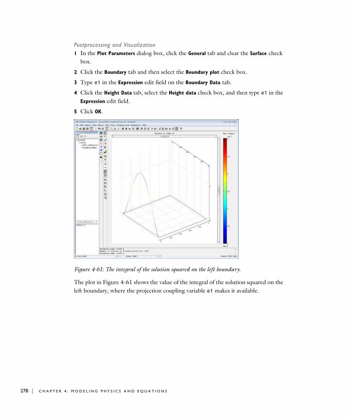
278 | C H A P T E
Postprocessing and Visualization1 In the Plot Parameters dialog box, click the General tab and clear the Surface check
box.
2 Click the Boundary tab and then select the Boundary plot check box.
3 Type e1 in the Expression edit field on the Boundary Data tab.
4 Click the Height Data tab, select the Height data check box, and then type e1 in the Expression edit field.
5 Click OK.
Figure 4-61: The integral of the solution squared on the left boundary.
The plot in Figure 4-61 shows the value of the integral of the solution squared on the left boundary, where the projection coupling variable e1 makes it available.
R 4 : M O D E L I N G P H Y S I C S A N D E Q U A T I O N S
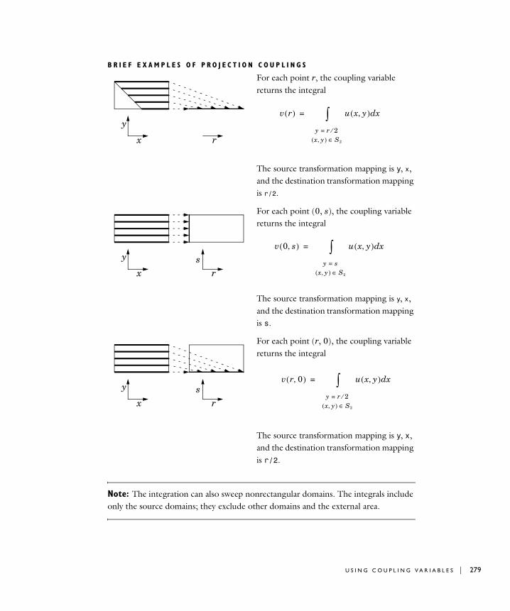
B R I E F E X A M P L E S O F P R O J E C T I O N C O U P L I N G S
For each point r, the coupling variable returns the integral
The source transformation mapping is y, x, and the destination transformation mapping is r/2.
For each point (0, s), the coupling variable returns the integral
The source transformation mapping is y, x, and the destination transformation mapping is s.
For each point (r, 0), the coupling variable returns the integral
The source transformation mapping is y, x, and the destination transformation mapping is r/2.
Note: The integration can also sweep nonrectangular domains. The integrals include only the source domains; they exclude other domains and the external area.
x r
yv r( ) u x y,( ) xd
y r 2⁄=
x y,( ) S2∈
∫=
x
y
rs
v 0 s,( ) u x y,( ) xd
y s=
x y,( ) S2∈
∫=
x
y
rs
v r 0,( ) u x y,( ) xd
y r 2⁄=
x y,( ) S2∈
∫=
U S I N G C O U P L I N G V A R I A B L E S | 279

280 | C H A P T E
General Issues When Using Coupling Variables
C H O O S I N G S O L U T I O N F O R M
The definitions of these coupling variables usually includes a dependency on the solution. If the variables are intended for postprocessing tasks, this condition poses no problem, but if they are to be involved in the coefficients of the PDE or boundary conditions, they should make contributions to the Jacobian matrix. For this to be possible, the model must be solved using the weak form, which is the default solution form. (From the command line, you can use flform to convert the model to the weak form before solving.)
N O N L O C A L C O U P L I N G S A N D T H E S P A R S I T Y O F T H E J A C O B I A N
The Jacobian for problems formulated using the finite element method is usually large but sparse. This is because the solution at each mesh node can depend at most on the degrees of freedom at the neighboring mesh elements. However, by introducing coupling variables, you create nonlocal dependencies that fill up the rows and columns of the affected source and destination nodes. These additional elements might make the Jacobian matrix only slightly less sparse, with marginal effects on solution speed; it can also make it a great deal less sparse, in which case memory use and CPU time involved in solving the problem increases considerably. For this reason, take particular care when introducing nonlocal couplings.
R 4 : M O D E L I N G P H Y S I C S A N D E Q U A T I O N S
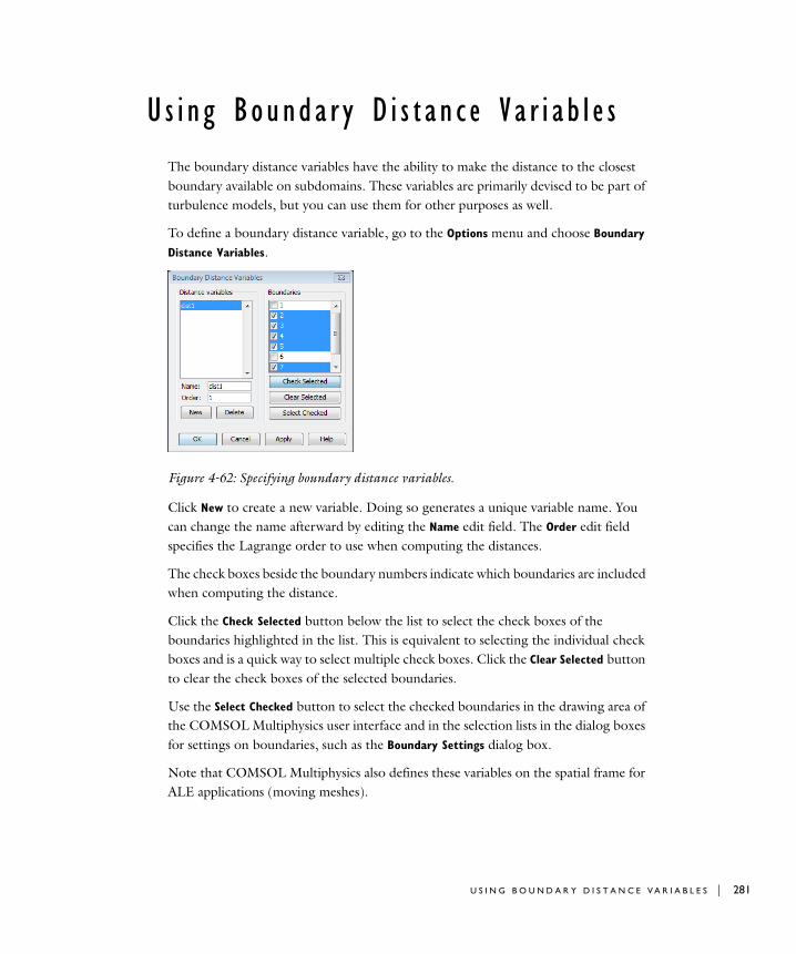
U s i n g Bounda r y D i s t a n c e V a r i a b l e s
The boundary distance variables have the ability to make the distance to the closest boundary available on subdomains. These variables are primarily devised to be part of turbulence models, but you can use them for other purposes as well.
To define a boundary distance variable, go to the Options menu and choose Boundary
Distance Variables.
Figure 4-62: Specifying boundary distance variables.
Click New to create a new variable. Doing so generates a unique variable name. You can change the name afterward by editing the Name edit field. The Order edit field specifies the Lagrange order to use when computing the distances.
The check boxes beside the boundary numbers indicate which boundaries are included when computing the distance.
Click the Check Selected button below the list to select the check boxes of the boundaries highlighted in the list. This is equivalent to selecting the individual check boxes and is a quick way to select multiple check boxes. Click the Clear Selected button to clear the check boxes of the selected boundaries.
Use the Select Checked button to select the checked boundaries in the drawing area of the COMSOL Multiphysics user interface and in the selection lists in the dialog boxes for settings on boundaries, such as the Boundary Settings dialog box.
Note that COMSOL Multiphysics also defines these variables on the spatial frame for ALE applications (moving meshes).
U S I N G B O U N D A R Y D I S T A N C E V A R I A B L E S | 281

282 | C H A P T E
Plotting Distances to Walls in Backstep Model
As an example of using a distance variable, plot the distances to the walls in the model of fluid flow over a backward-facing step. To do so, follow these steps:
M O D E L N A V I G A T O R
1 From the File menu, choose Open Model Library.
2 Select Model Library>COMSOL Multiphysics>Fluid Dynamics>backstep.
3 Click OK.
O P T I O N S A N D S E T T I N G S
Define the boundary distance variable for the distance to the wall boundaries.
1 From the Options menu, choose Boundary Distance Variables.
2 Click New to define a new boundary distance variable with the name dist1. Leave the order at the default values of 2.
3 Click the Clear Selected button to clear the default selection of all boundaries.
4 Select all the wall boundaries (Boundaries 2–5 and 7), either by clicking directly on the boundaries in the drawing area or, in the Boundary Settings dialog box, by selecting the Select by group check box and then selecting one of the wall boundaries.
5 In the Boundary Distance Variables dialog box, click the Check Selected button (see Figure 4-62 on page 281).
6 Click OK.
P O S T P R O C E S S I N G A N D V I S U A L I Z A T I O N
1 From the Solve menu, choose Update Model to evaluate the boundary distance function.
2 Click the Plot Parameters button on the Main toolbar.
3 In the Plot Parameters dialog box, click the Surface tab.
4 Type dist1 in the Expression edit field.
5 Click the General tab and clear the Streamline and Geometry edges check boxes.
6 Click OK to plot the distance to the wall as a surface plot (see Figure 4-63 on page 283).
R 4 : M O D E L I N G P H Y S I C S A N D E Q U A T I O N S
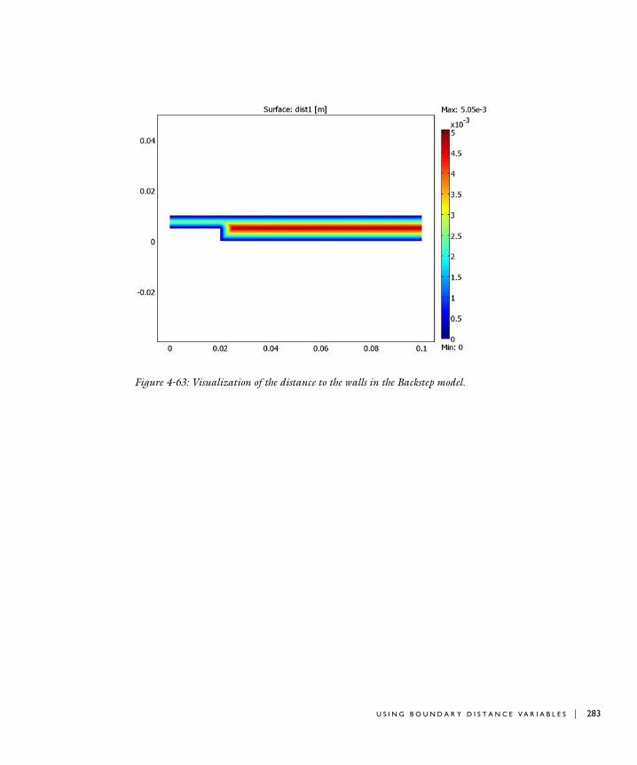
Figure 4-63: Visualization of the distance to the walls in the Backstep model.
U S I N G B O U N D A R Y D I S T A N C E V A R I A B L E S | 283

284 | C H A P T E
R 4 : M O D E L I N G P H Y S I C S A N D E Q U A T I O N S
5
M e s h i n g
This chapter covers how to create and control the mesh for 1D, 2D, and 3D geometries in COMSOL Multiphysics. It also explains the possibilities for importing and exporting meshes in different formats.
285
286 | C H A P T E
C r e a t i n g Me s h e s
A mesh is a partition of the geometry model into small units of simple shapes. It is possible to create free, mapped, extruded, revolved, swept, and boundary layer meshes. The mesh generator creating free meshes, also referred to as the free mesher, is the only mesher that can be used on all types of geometry objects.
Mesh Elements
For a 1D geometry the mesh generator partitions the subdomains (intervals) into smaller intervals (or mesh elements). The endpoints of the mesh elements are called mesh vertices.
For a 2D geometry the mesh generator partitions the subdomains into triangular or quadrilateral mesh elements. If the boundary is curved, these elements represent only an approximation of the original geometry. The sides of the triangles and quadrilaterals are called mesh edges, and their corners are mesh vertices. A mesh edge must not contain mesh vertices in its interior. Similarly, the boundaries defined in the geometry are partitioned (approximately) into mesh edges, so-called boundary elements, which must conform with the mesh elements of the adjacent subdomains. If there are isolated points in the geometry, these also become mesh vertices.
Similarly, in 3D the mesh generator partitions the subdomains into tetrahedral, hexahedral, or prism mesh elements whose faces, edges, and corners are called mesh faces, mesh edges, and mesh vertices, respectively. The boundaries in the geometry are partitioned into triangular or quadrilateral boundary elements. The geometry edges are partitioned into edge elements. Isolated geometry vertices become mesh vertices.
Meshing Techniques
For a 2D geometry, you can choose between creating a free mesh consisting of triangular elements, a free mesh consisting of quadrilateral elements, or a mapped mesh consisting of quadrilateral elements. Compared to a free mesh, a mapped mesh is structured in its pattern. If you want a mapped quadrilateral mesh on a geometry, you must build the geometry such that the subdomains are fairly regular in shape and do not contain holes.
For a 3D geometry you can choose between creating a free mesh containing tetrahedral elements, or a swept mesh containing prism elements or hexahedral
R 5 : M E S H I N G
elements. A swept mesh is structured in the sweep direction and can be either structured or unstructured orthogonally to the sweep direction.
You can also create a 3D mesh by extruding or revolving a 2D mesh. An extruded or revolved mesh is structured in the direction of the extrusion or revolution. When you extrude or revolve a 2D mesh into a 3D mesh, triangular elements and quadrilateral elements in the 2D mesh are extruded or revolved into prism (wedge) elements and hexahedral (brick) elements, respectively, in the resulting 3D mesh.
Furthermore, you can create a boundary layer mesh by inserting structured layers of elements along specific boundaries into an existing mesh.
Note: Argyris elements can be used only for triangular meshes. See “Finite Elements” on page 452 in the COMSOL Multiphysics Reference Guide for more information on the finite element types and the mesh types for which they are available.
Creating Free Meshes
The free mesher is available in all space dimensions, and you can use it for all types of geometries regardless of the topology and shape of a geometry. The free mesher automatically creates an unstructured mesh if you click the Initialize Mesh button on the Main toolbar and if you enter the Mesh mode with an empty mesh.
When you create a free mesh, the number of mesh elements is determined from the shape of the geometry and various mesh parameters. You control the mesh parameters for the free mesher by going to the Mesh menu and choosing Free Mesh Parameters, which opens the Free Mesh Parameters dialog box. With the mesh parameters you can specify local mesh-element sizes and control the element distribution. All mesh parameters aim at prescribing the maximum allowed mesh element size. This means that the size of a mesh element must not be larger than the minimum prescribed local element size determined by all mesh parameters.
C R E A T I N G F R E E M E S H E S I N 3 D
The Free Mesh Parameters dialog box for 3D geometries contains tabs named Global, Subdomain, Boundary, Edge, Point, and Advanced.
Click the Remesh button to delete the current mesh and create a new free mesh on the entire geometry according to the parameters in the dialog box. Clicking the Reset to
C R E A T I N G M E S H E S | 287
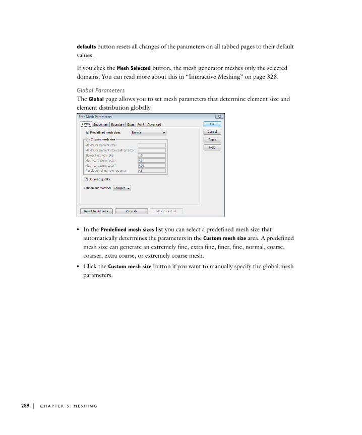
288 | C H A P T E
defaults button resets all changes of the parameters on all tabbed pages to their default values.
If you click the Mesh Selected button, the mesh generator meshes only the selected domains. You can read more about this in “Interactive Meshing” on page 328.
Global ParametersThe Global page allows you to set mesh parameters that determine element size and element distribution globally.
• In the Predefined mesh sizes list you can select a predefined mesh size that automatically determines the parameters in the Custom mesh size area. A predefined mesh size can generate an extremely fine, extra fine, finer, fine, normal, coarse, coarser, extra coarse, or extremely coarse mesh.
• Click the Custom mesh size button if you want to manually specify the global mesh parameters.
R 5 : M E S H I N G
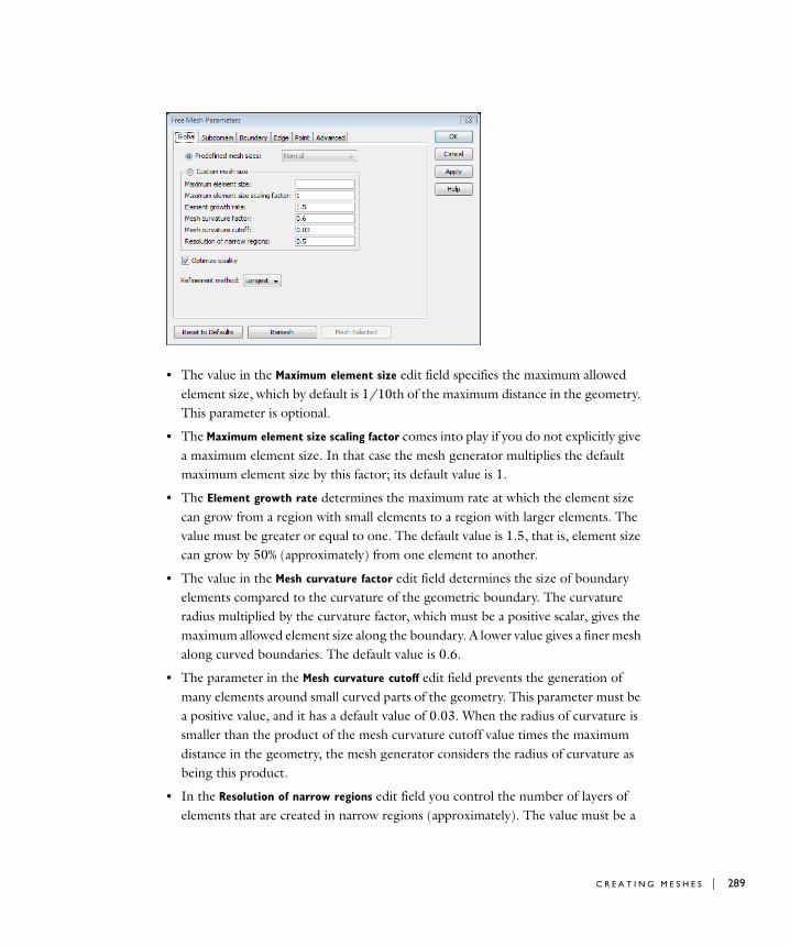
• The value in the Maximum element size edit field specifies the maximum allowed element size, which by default is 1/10th of the maximum distance in the geometry. This parameter is optional.
• The Maximum element size scaling factor comes into play if you do not explicitly give a maximum element size. In that case the mesh generator multiplies the default maximum element size by this factor; its default value is 1.
• The Element growth rate determines the maximum rate at which the element size can grow from a region with small elements to a region with larger elements. The value must be greater or equal to one. The default value is 1.5, that is, element size can grow by 50% (approximately) from one element to another.
• The value in the Mesh curvature factor edit field determines the size of boundary elements compared to the curvature of the geometric boundary. The curvature radius multiplied by the curvature factor, which must be a positive scalar, gives the maximum allowed element size along the boundary. A lower value gives a finer mesh along curved boundaries. The default value is 0.6.
• The parameter in the Mesh curvature cutoff edit field prevents the generation of many elements around small curved parts of the geometry. This parameter must be a positive value, and it has a default value of 0.03. When the radius of curvature is smaller than the product of the mesh curvature cutoff value times the maximum distance in the geometry, the mesh generator considers the radius of curvature as being this product.
• In the Resolution of narrow regions edit field you control the number of layers of elements that are created in narrow regions (approximately). The value must be a
C R E A T I N G M E S H E S | 289
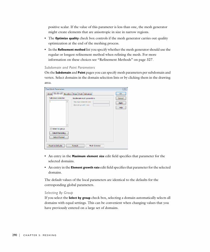
290 | C H A P T E
positive scalar. If the value of this parameter is less than one, the mesh generator might create elements that are anisotropic in size in narrow regions.
• The Optimize quality check box controls if the mesh generator carries out quality optimization at the end of the meshing process.
• In the Refinement method list you specify whether the mesh generator should use the regular or longest refinement method when refining the mesh. For more information on these choices see “Refinement Methods” on page 327.
Subdomain and Point ParametersOn the Subdomain and Point pages you can specify mesh parameters per subdomain and vertex. Select domains in the domain selection lists or by clicking them in the drawing area.
• An entry in the Maximum element size edit field specifies that parameter for the selected domains.
• An entry in the Element growth rate edit field specifies that parameter for the selected domains.
The default values of the local parameters are identical to the defaults for the corresponding global parameters.
Selecting By GroupIf you select the Select by group check box, selecting a domain automatically selects all domains with equal settings. This can be convenient when changing values that you have previously entered on a large set of domains.
R 5 : M E S H I N G
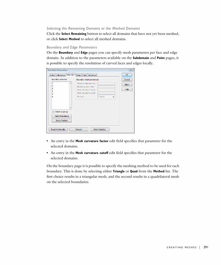
Selecting the Remaining Domains or the Meshed DomainsClick the Select Remaining button to select all domains that have not yet been meshed, or click Select Meshed to select all meshed domains.
Boundary and Edge ParametersOn the Boundary and Edge pages you can specify mesh parameters per face and edge domain. In addition to the parameters available on the Subdomain and Point pages, it is possible to specify the resolution of curved faces and edges locally.
• An entry in the Mesh curvature factor edit field specifies that parameter for the selected domains.
• An entry in the Mesh curvature cutoff edit field specifies that parameter for the selected domains.
On the boundary page it is possible to specify the meshing method to be used for each boundary. This is done by selecting either Triangle or Quad from the Method list. The first choice results in a triangular mesh, and the second results in a quadrilateral mesh on the selected boundaries.
C R E A T I N G M E S H E S | 291
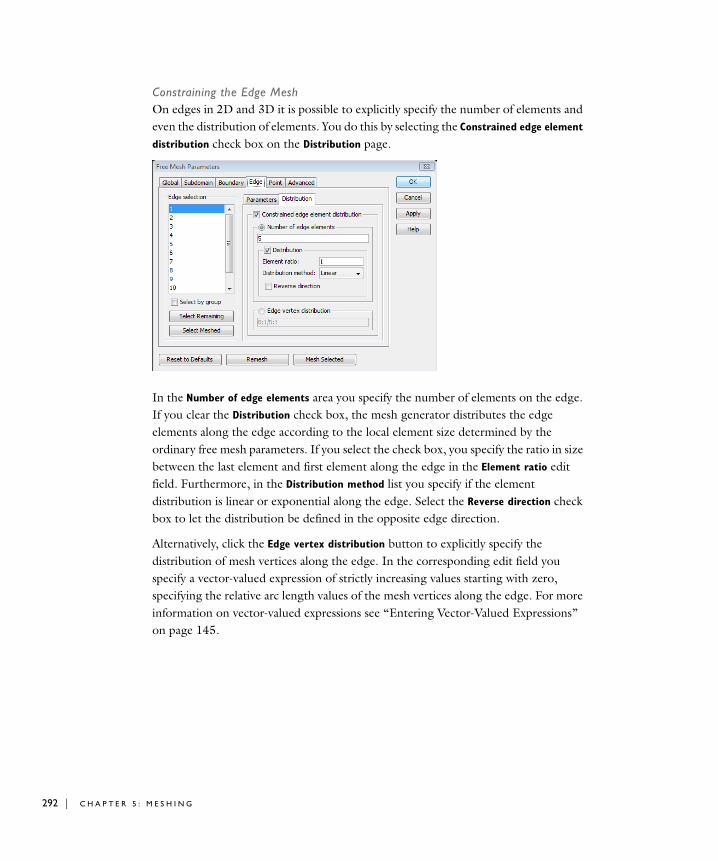
292 | C H A P T E
Constraining the Edge MeshOn edges in 2D and 3D it is possible to explicitly specify the number of elements and even the distribution of elements. You do this by selecting the Constrained edge element
distribution check box on the Distribution page.
In the Number of edge elements area you specify the number of elements on the edge. If you clear the Distribution check box, the mesh generator distributes the edge elements along the edge according to the local element size determined by the ordinary free mesh parameters. If you select the check box, you specify the ratio in size between the last element and first element along the edge in the Element ratio edit field. Furthermore, in the Distribution method list you specify if the element distribution is linear or exponential along the edge. Select the Reverse direction check box to let the distribution be defined in the opposite edge direction.
Alternatively, click the Edge vertex distribution button to explicitly specify the distribution of mesh vertices along the edge. In the corresponding edit field you specify a vector-valued expression of strictly increasing values starting with zero, specifying the relative arc length values of the mesh vertices along the edge. For more information on vector-valued expressions see “Entering Vector-Valued Expressions” on page 145.
R 5 : M E S H I N G
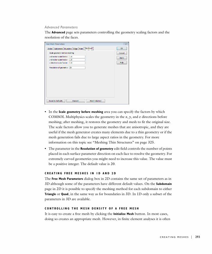
Advanced ParametersThe Advanced page sets parameters controlling the geometry scaling factors and the resolution of the faces.
• In the Scale geometry before meshing area you can specify the factors by which COMSOL Multiphysics scales the geometry in the x, y, and z directions before meshing; after meshing, it restores the geometry and mesh to fit the original size. The scale factors allow you to generate meshes that are anisotropic, and they are useful if the mesh generator creates many elements due to a thin geometry or if the mesh generation fails due to large aspect ratios in the geometry. For more information on this topic see “Meshing Thin Structures” on page 325.
• The parameter in the Resolution of geometry edit field controls the number of points placed in each surface parameter direction on each face to resolve the geometry. For extremely curved geometries you might need to increase this value. The value must be a positive integer. The default value is 20.
C R E A T I N G F R E E M E S H E S I N 1 D A N D 2 D
The Free Mesh Parameters dialog box in 2D contains the same set of parameters as in 3D although some of the parameters have different default values. On the Subdomain page in 2D it is possible to specify the meshing method for each subdomain to either Triangle or Quad, in the same way as for boundaries in 3D. In 1D only a subset of the parameters in 3D are available.
C O N T R O L L I N G T H E M E S H D E N S I T Y O F A F R E E M E S H
It is easy to create a free mesh by clicking the Initialize Mesh button. In most cases, doing so creates an appropriate mesh. However, in finite element analyses it is often
C R E A T I N G M E S H E S | 293

294 | C H A P T E
necessary to resolve a specific region in more detail, for instance, a particular region of a geometry that features more complicated solution patterns. The local element sizes and the distribution of elements within the geometry is controlled via the parameters in the Free Mesh Parameters dialog box.
This section shows the effects of the different mesh parameters on a 2D geometry.
1 Start a new 2D model.
2 In Draw mode, create a rectangle with corners at (−1, −0.8) and (1, 0.8).
3 Create a circle with radius of 0.05 centered at the origin, for example, by choosing Specify Objects>Circle from the Draw menu.
4 Subtract the circle from the rectangle.
5 From the Draw menu choose Specify Objects>Rectangle and create a rectangle with the width equal to 0.8, height equal to 0.2, and with the lower left corner positioned at (−0.4, −0.75).
6 Select all objects by pressing Ctrl+A, and then click the Union button on the Draw toolbar.
R 5 : M E S H I N G
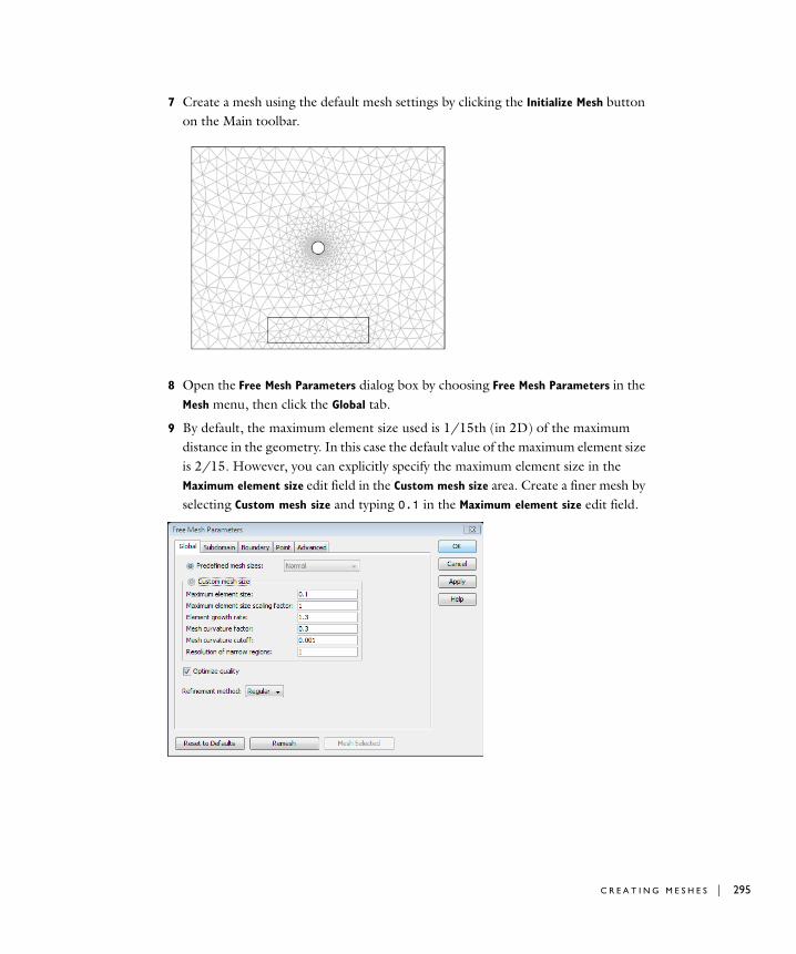
7 Create a mesh using the default mesh settings by clicking the Initialize Mesh button on the Main toolbar.
8 Open the Free Mesh Parameters dialog box by choosing Free Mesh Parameters in the Mesh menu, then click the Global tab.
9 By default, the maximum element size used is 1/15th (in 2D) of the maximum distance in the geometry. In this case the default value of the maximum element size is 2/15. However, you can explicitly specify the maximum element size in the Maximum element size edit field in the Custom mesh size area. Create a finer mesh by selecting Custom mesh size and typing 0.1 in the Maximum element size edit field.
C R E A T I N G M E S H E S | 295

296 | C H A P T E
10 Click the Remesh button on the Main toolbar.
Another way of controlling the maximum element size globally without having to bother about the scale of the geometry is to use the maximum element size scaling factor. If the maximum element size is not given, the maximum element size is multiplied by the value specified in the Maximum element size scaling factor edit field.
1 Create a coarser mesh than the default mesh by clearing the Maximum element size edit field and typing 2 in the Maximum element size scaling factor edit field.
R 5 : M E S H I N G
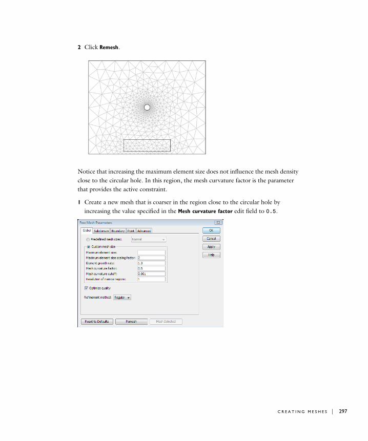
2 Click Remesh.
Notice that increasing the maximum element size does not influence the mesh density close to the circular hole. In this region, the mesh curvature factor is the parameter that provides the active constraint.
1 Create a new mesh that is coarser in the region close to the circular hole by increasing the value specified in the Mesh curvature factor edit field to 0.5.
C R E A T I N G M E S H E S | 297
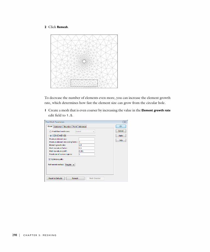
298 | C H A P T E
2 Click Remesh.
To decrease the number of elements even more, you can increase the element growth rate, which determines how fast the element size can grow from the circular hole.
1 Create a mesh that is even coarser by increasing the value in the Element growth rate edit field to 1.5.
R 5 : M E S H I N G
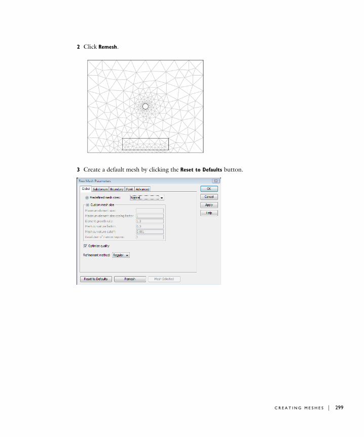
2 Click Remesh.
3 Create a default mesh by clicking the Reset to Defaults button.
C R E A T I N G M E S H E S | 299

300 | C H A P T E
4 Click Remesh.
You can prevent the circular hole from getting a fine resolution by increasing the mesh curvature cutoff value. The hole’s radius of curvature is considered to be the product of the mesh curvature cutoff value times the maximum distance in the geometry—if this product is greater than the radius of curvature. In this case the mesh curvature cutoff value needs to be greater than 0.025 to take effect.
1 Prevent the fine resolution of the circular hole by increasing the value in the Mesh
curvature cutoff edit field to 0.05.
R 5 : M E S H I N G
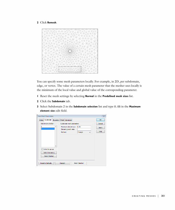
2 Click Remesh.
You can specify some mesh parameters locally. For example, in 2D, per subdomain, edge, or vertex. The value of a certain mesh parameter that the mesher uses locally is the minimum of the local value and global value of the corresponding parameter.
1 Reset the mesh settings by selecting Normal in the Predefined mesh sizes list.
2 Click the Subdomain tab.
3 Select Subdomain 2 in the Subdomain selection list and type 0.05 in the Maximum
element size edit field.
C R E A T I N G M E S H E S | 301
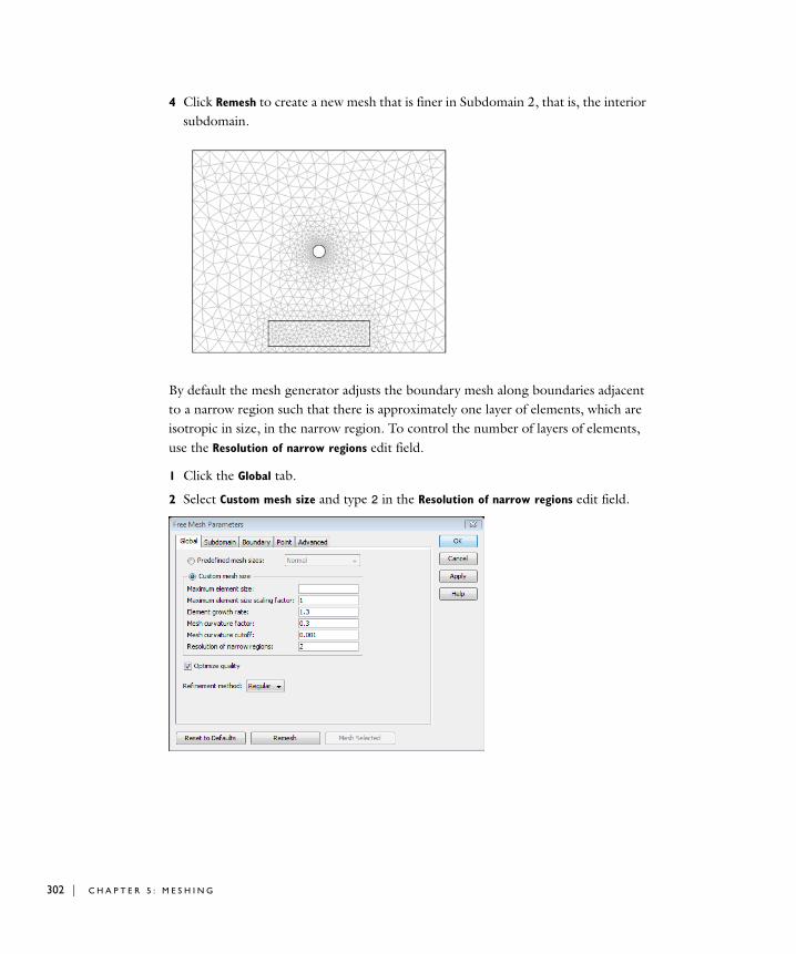
302 | C H A P T E
4 Click Remesh to create a new mesh that is finer in Subdomain 2, that is, the interior subdomain.
By default the mesh generator adjusts the boundary mesh along boundaries adjacent to a narrow region such that there is approximately one layer of elements, which are isotropic in size, in the narrow region. To control the number of layers of elements, use the Resolution of narrow regions edit field.
1 Click the Global tab.
2 Select Custom mesh size and type 2 in the Resolution of narrow regions edit field.
R 5 : M E S H I N G
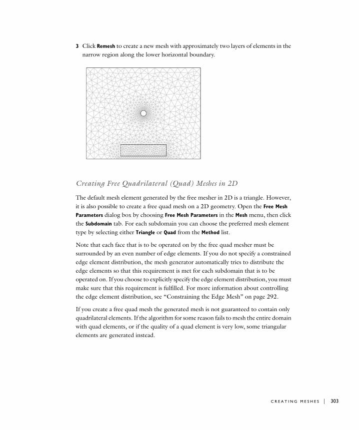
3 Click Remesh to create a new mesh with approximately two layers of elements in the narrow region along the lower horizontal boundary.
Creating Free Quadrilateral (Quad) Meshes in 2D
The default mesh element generated by the free mesher in 2D is a triangle. However, it is also possible to create a free quad mesh on a 2D geometry. Open the Free Mesh
Parameters dialog box by choosing Free Mesh Parameters in the Mesh menu, then click the Subdomain tab. For each subdomain you can choose the preferred mesh element type by selecting either Triangle or Quad from the Method list.
Note that each face that is to be operated on by the free quad mesher must be surrounded by an even number of edge elements. If you do not specify a constrained edge element distribution, the mesh generator automatically tries to distribute the edge elements so that this requirement is met for each subdomain that is to be operated on. If you choose to explicitly specify the edge element distribution, you must make sure that this requirement is fulfilled. For more information about controlling the edge element distribution, see “Constraining the Edge Mesh” on page 292.
If you create a free quad mesh the generated mesh is not guaranteed to contain only quadrilateral elements. If the algorithm for some reason fails to mesh the entire domain with quad elements, or if the quality of a quad element is very low, some triangular elements are generated instead.
C R E A T I N G M E S H E S | 303
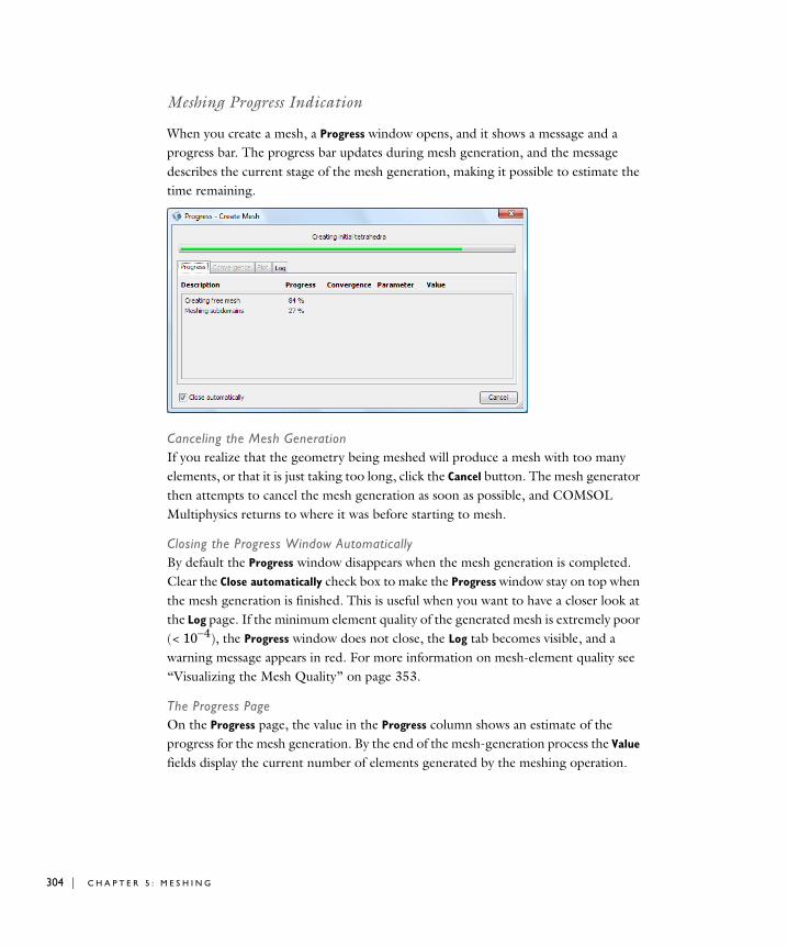
304 | C H A P T E
Meshing Progress Indication
When you create a mesh, a Progress window opens, and it shows a message and a progress bar. The progress bar updates during mesh generation, and the message describes the current stage of the mesh generation, making it possible to estimate the time remaining.
Canceling the Mesh GenerationIf you realize that the geometry being meshed will produce a mesh with too many elements, or that it is just taking too long, click the Cancel button. The mesh generator then attempts to cancel the mesh generation as soon as possible, and COMSOL Multiphysics returns to where it was before starting to mesh.
Closing the Progress Window AutomaticallyBy default the Progress window disappears when the mesh generation is completed. Clear the Close automatically check box to make the Progress window stay on top when the mesh generation is finished. This is useful when you want to have a closer look at the Log page. If the minimum element quality of the generated mesh is extremely poor (< 10−4), the Progress window does not close, the Log tab becomes visible, and a warning message appears in red. For more information on mesh-element quality see “Visualizing the Mesh Quality” on page 353.
The Progress PageOn the Progress page, the value in the Progress column shows an estimate of the progress for the mesh generation. By the end of the mesh-generation process the Value fields display the current number of elements generated by the meshing operation.
R 5 : M E S H I N G
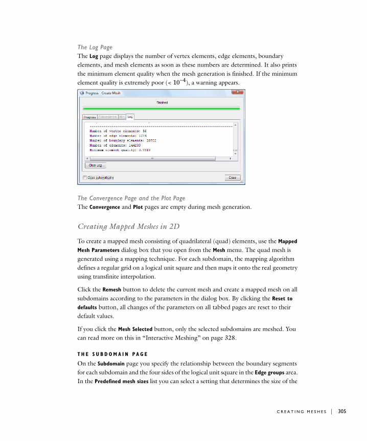
The Log PageThe Log page displays the number of vertex elements, edge elements, boundary elements, and mesh elements as soon as these numbers are determined. It also prints the minimum element quality when the mesh generation is finished. If the minimum element quality is extremely poor (< 10−4), a warning appears.
The Convergence Page and the Plot PageThe Convergence and Plot pages are empty during mesh generation.
Creating Mapped Meshes in 2D
To create a mapped mesh consisting of quadrilateral (quad) elements, use the Mapped
Mesh Parameters dialog box that you open from the Mesh menu. The quad mesh is generated using a mapping technique. For each subdomain, the mapping algorithm defines a regular grid on a logical unit square and then maps it onto the real geometry using transfinite interpolation.
Click the Remesh button to delete the current mesh and create a mapped mesh on all subdomains according to the parameters in the dialog box. By clicking the Reset to
defaults button, all changes of the parameters on all tabbed pages are reset to their default values.
If you click the Mesh Selected button, only the selected subdomains are meshed. You can read more on this in “Interactive Meshing” on page 328.
T H E S U B D O M A I N P A G E
On the Subdomain page you specify the relationship between the boundary segments for each subdomain and the four sides of the logical unit square in the Edge groups area. In the Predefined mesh sizes list you can select a setting that determines the size of the
C R E A T I N G M E S H E S | 305
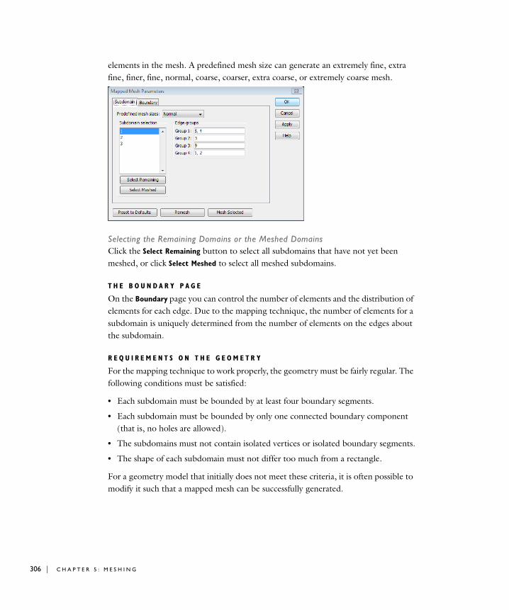
306 | C H A P T E
elements in the mesh. A predefined mesh size can generate an extremely fine, extra fine, finer, fine, normal, coarse, coarser, extra coarse, or extremely coarse mesh.
Selecting the Remaining Domains or the Meshed DomainsClick the Select Remaining button to select all subdomains that have not yet been meshed, or click Select Meshed to select all meshed subdomains.
T H E B O U N D A R Y P A G E
On the Boundary page you can control the number of elements and the distribution of elements for each edge. Due to the mapping technique, the number of elements for a subdomain is uniquely determined from the number of elements on the edges about the subdomain.
R E Q U I R E M E N T S O N T H E G E O M E T R Y
For the mapping technique to work properly, the geometry must be fairly regular. The following conditions must be satisfied:
• Each subdomain must be bounded by at least four boundary segments.
• Each subdomain must be bounded by only one connected boundary component (that is, no holes are allowed).
• The subdomains must not contain isolated vertices or isolated boundary segments.
• The shape of each subdomain must not differ too much from a rectangle.
For a geometry model that initially does not meet these criteria, it is often possible to modify it such that a mapped mesh can be successfully generated.
R 5 : M E S H I N G
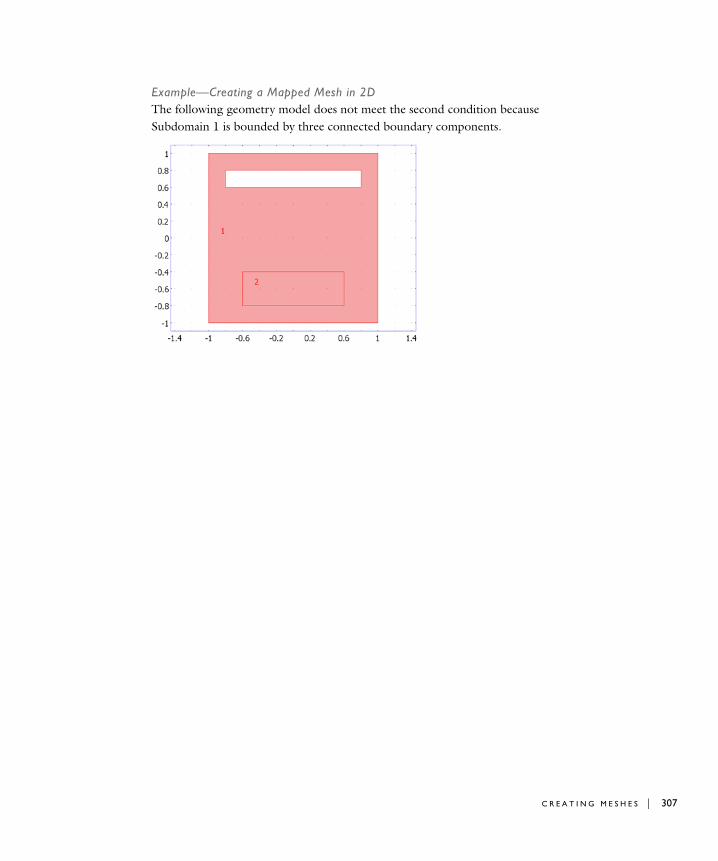
Example—Creating a Mapped Mesh in 2DThe following geometry model does not meet the second condition because Subdomain 1 is bounded by three connected boundary components.
C R E A T I N G M E S H E S | 307
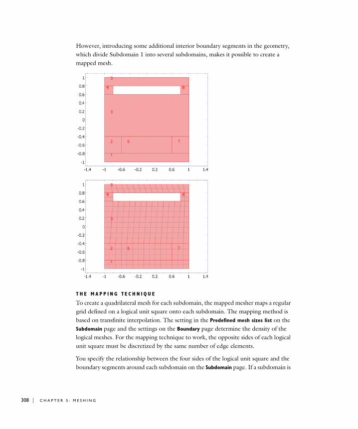
308 | C H A P T E
However, introducing some additional interior boundary segments in the geometry, which divide Subdomain 1 into several subdomains, makes it possible to create a mapped mesh.
T H E M A P P I N G T E C H N I Q U E
To create a quadrilateral mesh for each subdomain, the mapped mesher maps a regular grid defined on a logical unit square onto each subdomain. The mapping method is based on transfinite interpolation. The setting in the Predefined mesh sizes list on the Subdomain page and the settings on the Boundary page determine the density of the logical meshes. For the mapping technique to work, the opposite sides of each logical unit square must be discretized by the same number of edge elements.
You specify the relationship between the four sides of the logical unit square and the boundary segments around each subdomain on the Subdomain page. If a subdomain is
R 5 : M E S H I N G
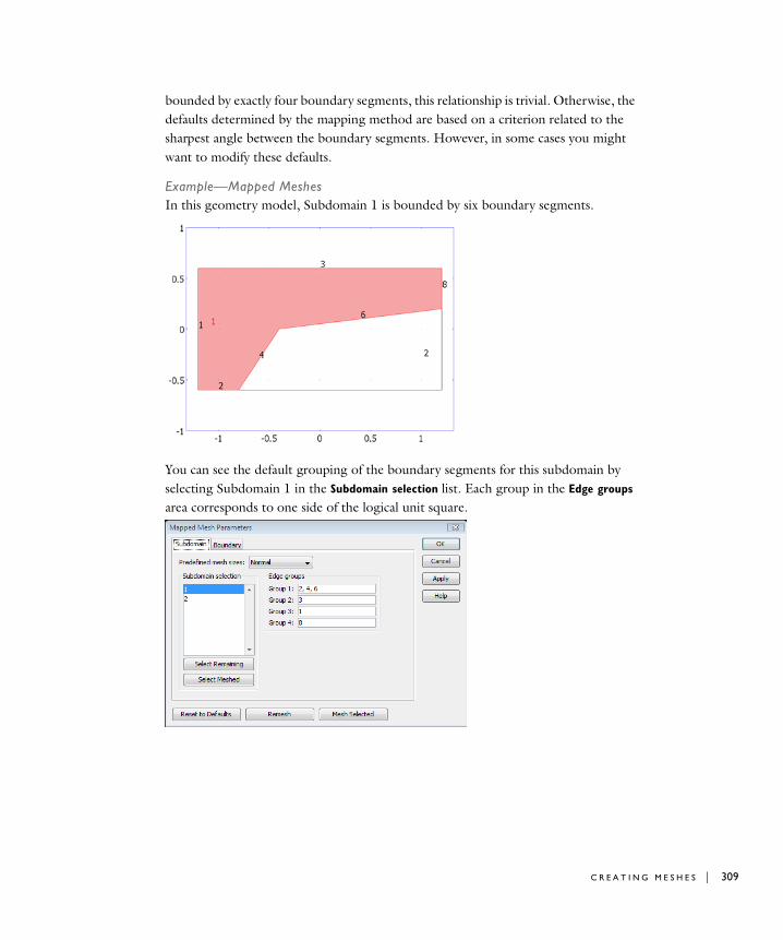
bounded by exactly four boundary segments, this relationship is trivial. Otherwise, the defaults determined by the mapping method are based on a criterion related to the sharpest angle between the boundary segments. However, in some cases you might want to modify these defaults.
Example—Mapped MeshesIn this geometry model, Subdomain 1 is bounded by six boundary segments.
You can see the default grouping of the boundary segments for this subdomain by selecting Subdomain 1 in the Subdomain selection list. Each group in the Edge groups area corresponds to one side of the logical unit square.
C R E A T I N G M E S H E S | 309
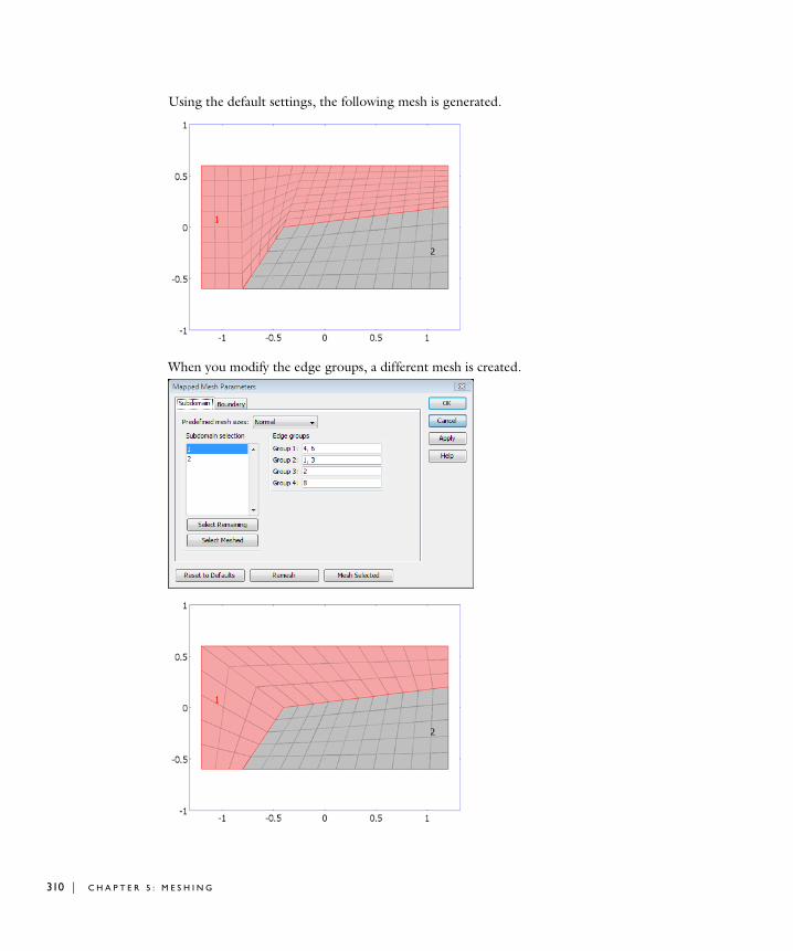
310 | C H A P T E
Using the default settings, the following mesh is generated.
When you modify the edge groups, a different mesh is created.
R 5 : M E S H I N G
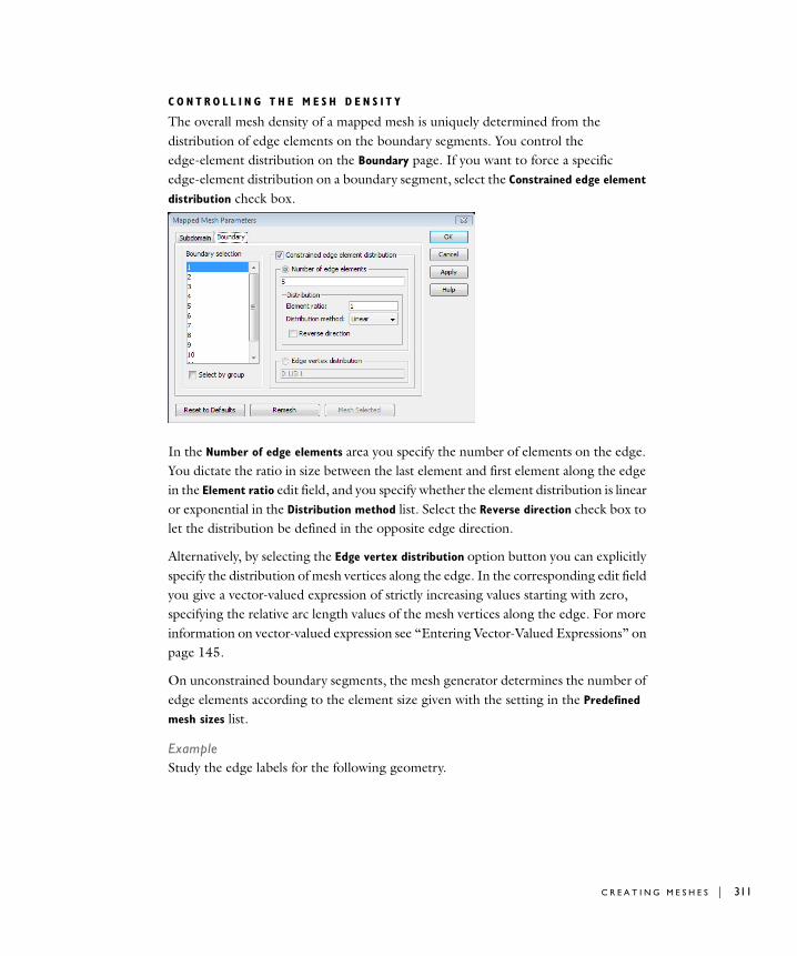
C O N T R O L L I N G T H E M E S H D E N S I T Y
The overall mesh density of a mapped mesh is uniquely determined from the distribution of edge elements on the boundary segments. You control the edge-element distribution on the Boundary page. If you want to force a specific edge-element distribution on a boundary segment, select the Constrained edge element
distribution check box.
In the Number of edge elements area you specify the number of elements on the edge. You dictate the ratio in size between the last element and first element along the edge in the Element ratio edit field, and you specify whether the element distribution is linear or exponential in the Distribution method list. Select the Reverse direction check box to let the distribution be defined in the opposite edge direction.
Alternatively, by selecting the Edge vertex distribution option button you can explicitly specify the distribution of mesh vertices along the edge. In the corresponding edit field you give a vector-valued expression of strictly increasing values starting with zero, specifying the relative arc length values of the mesh vertices along the edge. For more information on vector-valued expression see “Entering Vector-Valued Expressions” on page 145.
On unconstrained boundary segments, the mesh generator determines the number of edge elements according to the element size given with the setting in the Predefined
mesh sizes list.
ExampleStudy the edge labels for the following geometry.
C R E A T I N G M E S H E S | 311
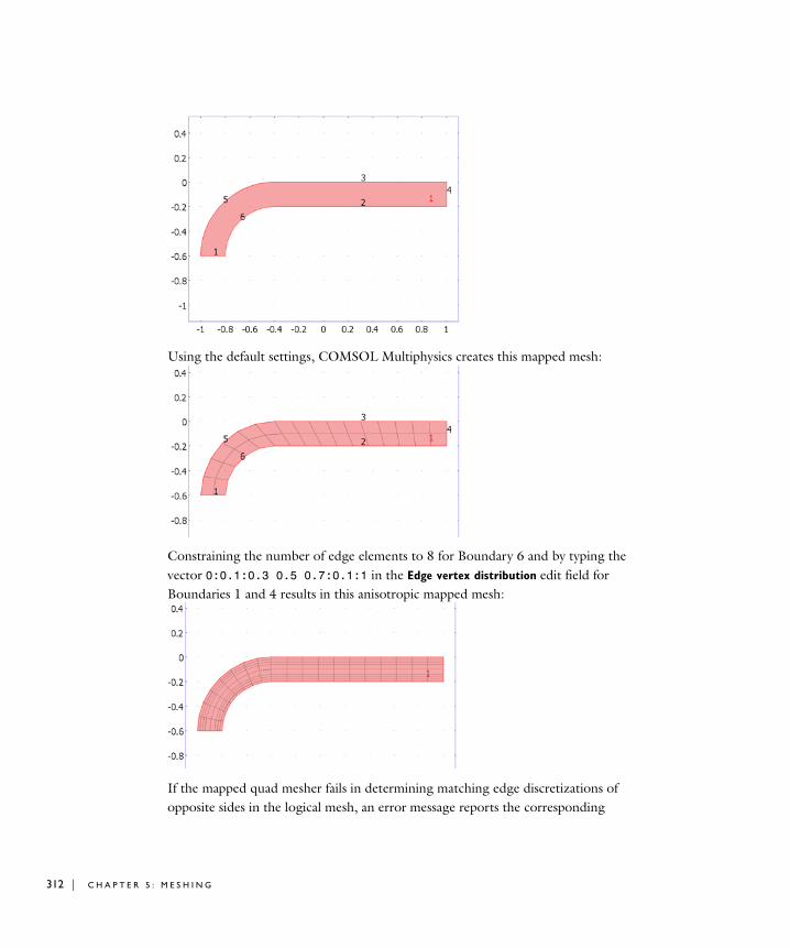
312 | C H A P T E
Using the default settings, COMSOL Multiphysics creates this mapped mesh:
Constraining the number of edge elements to 8 for Boundary 6 and by typing the vector 0:0.1:0.3 0.5 0.7:0.1:1 in the Edge vertex distribution edit field for Boundaries 1 and 4 results in this anisotropic mapped mesh:
If the mapped quad mesher fails in determining matching edge discretizations of opposite sides in the logical mesh, an error message reports the corresponding
R 5 : M E S H I N G

subdomain index. Often you can avoid this error by constraining the number of edge elements on the corresponding boundary segments such that matching edge discretizations are defined.
Extruding and Revolving 2D Meshes
It is also possible to create a 3D mesh by extruding or revolving a 2D mesh. Extrude or revolve a triangular mesh to create a prism (wedge) mesh, and extrude or revolve a quadrilateral mesh to create a hexahedral (block) mesh. The mesh generator creates the corresponding extruded or revolved geometry together with the mesh.
E X T R U D I N G A 2 D M E S H
Choosing Extrude Mesh from the Mesh menu opens the Extrude Mesh dialog box. On the Geometry page you specify the properties of the geometry extrusion. For more information on geometry-extrusion properties see “Extruding a 2D Geometry” on page 64.
C R E A T I N G M E S H E S | 313
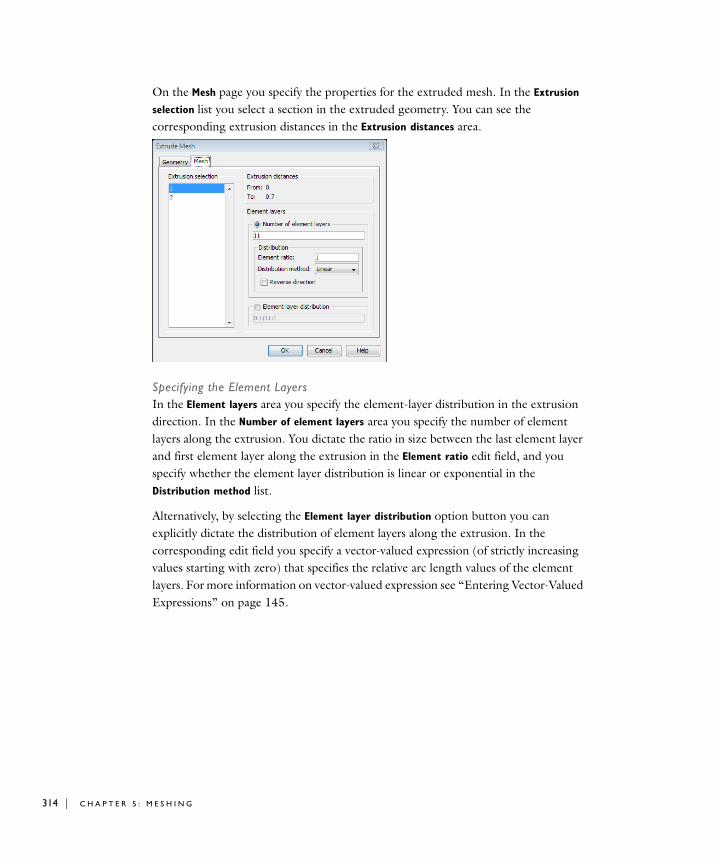
314 | C H A P T E
On the Mesh page you specify the properties for the extruded mesh. In the Extrusion
selection list you select a section in the extruded geometry. You can see the corresponding extrusion distances in the Extrusion distances area.
Specifying the Element LayersIn the Element layers area you specify the element-layer distribution in the extrusion direction. In the Number of element layers area you specify the number of element layers along the extrusion. You dictate the ratio in size between the last element layer and first element layer along the extrusion in the Element ratio edit field, and you specify whether the element layer distribution is linear or exponential in the Distribution method list.
Alternatively, by selecting the Element layer distribution option button you can explicitly dictate the distribution of element layers along the extrusion. In the corresponding edit field you specify a vector-valued expression (of strictly increasing values starting with zero) that specifies the relative arc length values of the element layers. For more information on vector-valued expression see “Entering Vector-Valued Expressions” on page 145.
R 5 : M E S H I N G
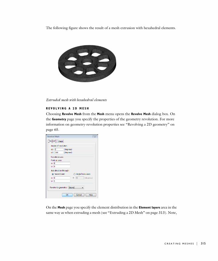
The following figure shows the result of a mesh extrusion with hexahedral elements.
Extruded mesh with hexahedral elements
R E V O L V I N G A 2 D M E S H
Choosing Revolve Mesh from the Mesh menu opens the Revolve Mesh dialog box. On the Geometry page you specify the properties of the geometry revolution. For more information on geometry-revolution properties see “Revolving a 2D geometry” on page 65.
On the Mesh page you specify the element distribution in the Element layers area in the same way as when extruding a mesh (see “Extruding a 2D Mesh” on page 313). Note,
C R E A T I N G M E S H E S | 315
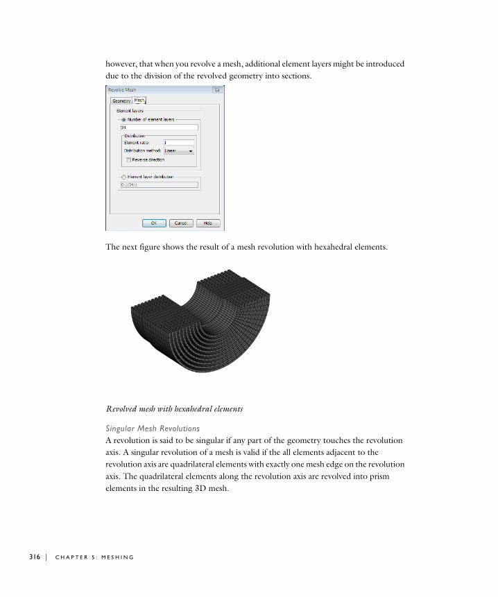
316 | C H A P T E
however, that when you revolve a mesh, additional element layers might be introduced due to the division of the revolved geometry into sections.
The next figure shows the result of a mesh revolution with hexahedral elements.
Revolved mesh with hexahedral elements
Singular Mesh RevolutionsA revolution is said to be singular if any part of the geometry touches the revolution axis. A singular revolution of a mesh is valid if the all elements adjacent to the revolution axis are quadrilateral elements with exactly one mesh edge on the revolution axis. The quadrilateral elements along the revolution axis are revolved into prism elements in the resulting 3D mesh.
R 5 : M E S H I N G
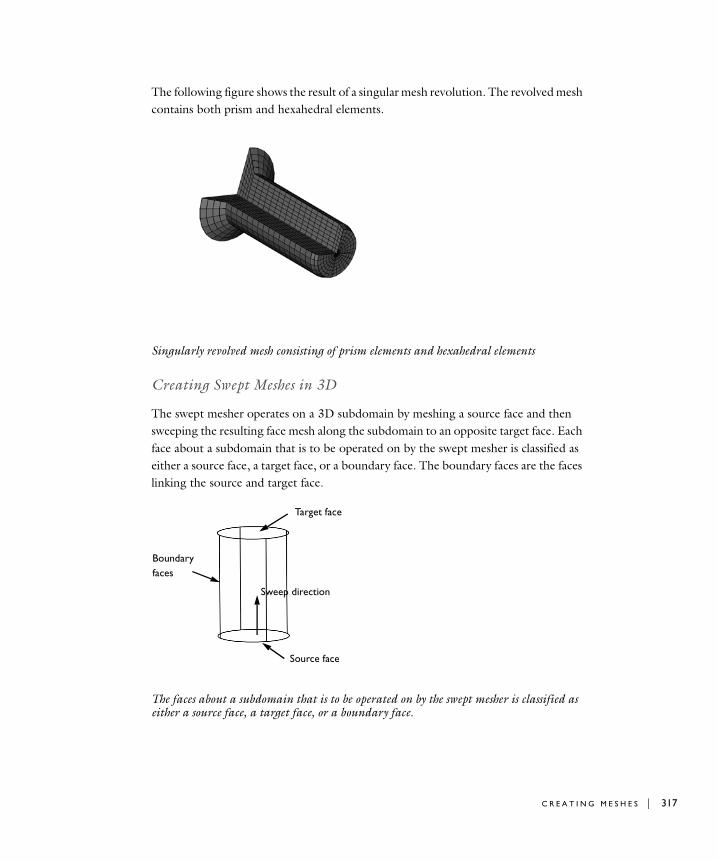
The following figure shows the result of a singular mesh revolution. The revolved mesh contains both prism and hexahedral elements.
Singularly revolved mesh consisting of prism elements and hexahedral elements
Creating Swept Meshes in 3D
The swept mesher operates on a 3D subdomain by meshing a source face and then sweeping the resulting face mesh along the subdomain to an opposite target face. Each face about a subdomain that is to be operated on by the swept mesher is classified as either a source face, a target face, or a boundary face. The boundary faces are the faces linking the source and target face.
The faces about a subdomain that is to be operated on by the swept mesher is classified as either a source face, a target face, or a boundary face.
Target face
Source face
Sweep direction
Boundaryfaces
C R E A T I N G M E S H E S | 317
318 | C H A P T E
The swept mesher can handle subdomains with multiple boundary faces in the sweep direction.
R E Q U I R E M E N T S O N T H E G E O M E T R Y
For the sweeping technique to work, the geometry must satisfy these criteria:
• Each subdomain must be bounded by one shell, that is, a subdomain must not contain holes except if they penetrate both the source and target face.
• There can be only one source face and one target face per subdomain.
• The source face and target face for a subdomain must be opposite each another in the subdomain’s topology.
• The cross section along the direction of the sweep for a subdomain must be topologically constant.
U S I N G T H E S W E P T M E S H P A R A M E T E R S D I A L O G B O X
To create a swept mesh on a 3D geometry use the Swept Mesh Parameters dialog box, which opens from the Mesh menu. Click the Remesh button to delete the current mesh and create a swept mesh on all subdomains as defined by the parameters in the dialog box. By clicking the Reset to Defaults button, you reset all parameter changes on all tabbed pages to their default values.
Following a click on the Mesh Selected button, the swept mesher creates a mesh only for the selected subdomains. You can read more on this in “Interactive Meshing” on page 328.
R 5 : M E S H I N G
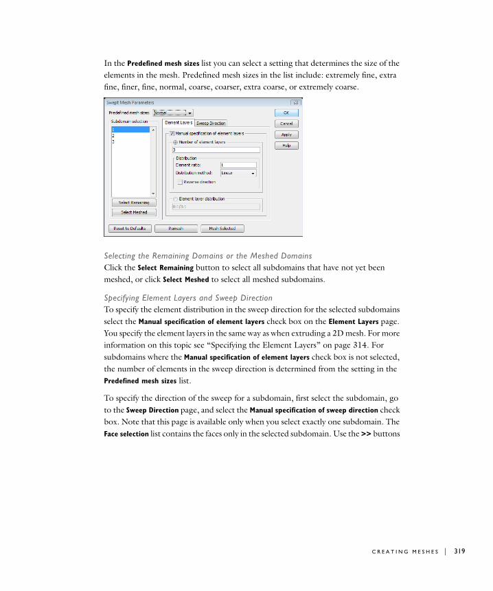
In the Predefined mesh sizes list you can select a setting that determines the size of the elements in the mesh. Predefined mesh sizes in the list include: extremely fine, extra fine, finer, fine, normal, coarse, coarser, extra coarse, or extremely coarse.
Selecting the Remaining Domains or the Meshed DomainsClick the Select Remaining button to select all subdomains that have not yet been meshed, or click Select Meshed to select all meshed subdomains.
Specifying Element Layers and Sweep DirectionTo specify the element distribution in the sweep direction for the selected subdomains select the Manual specification of element layers check box on the Element Layers page. You specify the element layers in the same way as when extruding a 2D mesh. For more information on this topic see “Specifying the Element Layers” on page 314. For subdomains where the Manual specification of element layers check box is not selected, the number of elements in the sweep direction is determined from the setting in the Predefined mesh sizes list.
To specify the direction of the sweep for a subdomain, first select the subdomain, go to the Sweep Direction page, and select the Manual specification of sweep direction check box. Note that this page is available only when you select exactly one subdomain. The Face selection list contains the faces only in the selected subdomain. Use the >> buttons
C R E A T I N G M E S H E S | 319
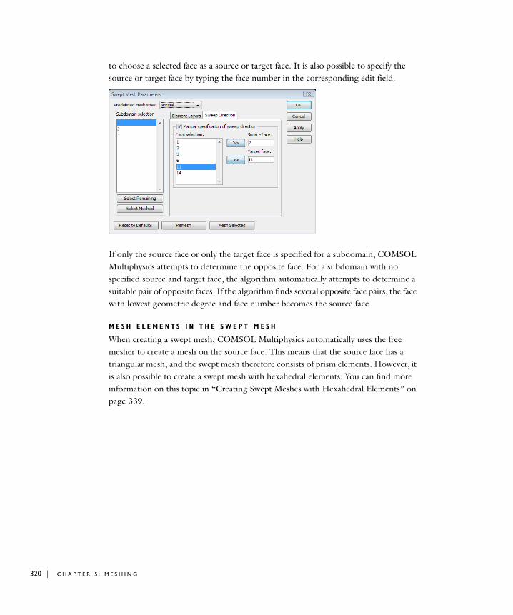
320 | C H A P T E
to choose a selected face as a source or target face. It is also possible to specify the source or target face by typing the face number in the corresponding edit field.
If only the source face or only the target face is specified for a subdomain, COMSOL Multiphysics attempts to determine the opposite face. For a subdomain with no specified source and target face, the algorithm automatically attempts to determine a suitable pair of opposite faces. If the algorithm finds several opposite face pairs, the face with lowest geometric degree and face number becomes the source face.
M E S H E L E M E N T S I N T H E S W E P T M E S H
When creating a swept mesh, COMSOL Multiphysics automatically uses the free mesher to create a mesh on the source face. This means that the source face has a triangular mesh, and the swept mesh therefore consists of prism elements. However, it is also possible to create a swept mesh with hexahedral elements. You can find more information on this topic in “Creating Swept Meshes with Hexahedral Elements” on page 339.
R 5 : M E S H I N G
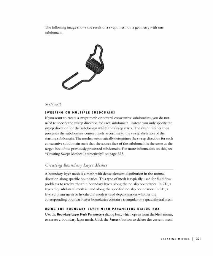
The following image shows the result of a swept mesh on a geometry with one subdomain.
Swept mesh
S W E E P I N G O N M U L T I P L E S U B D O M A I N S
If you want to create a swept mesh on several consecutive subdomains, you do not need to specify the sweep direction for each subdomain. Instead you only specify the sweep direction for the subdomain where the sweep starts. The swept mesher then processes the subdomains consecutively according to the sweep direction of the starting subdomain. The mesher automatically determines the sweep direction for each consecutive subdomain such that the source face of the subdomain is the same as the target face of the previously processed subdomain. For more information on this, see “Creating Swept Meshes Interactively” on page 335.
Creating Boundary Layer Meshes
A boundary layer mesh is a mesh with dense element distribution in the normal direction along specific boundaries. This type of mesh is typically used for fluid flow problems to resolve the thin boundary layers along the no-slip boundaries. In 2D, a layered quadrilateral mesh is used along the specified no-slip boundaries. In 3D, a layered prism mesh or hexahedral mesh is used depending on whether the corresponding boundary-layer boundaries contain a triangular or a quadrilateral mesh.
U S I N G T H E B O U N D A R Y L A Y E R M E S H P A R A M E T E R S D I A L O G B O X
Use the Boundary Layer Mesh Parameters dialog box, which opens from the Mesh menu, to create a boundary layer mesh. Click the Remesh button to delete the current mesh
C R E A T I N G M E S H E S | 321

322 | C H A P T E
and create a boundary layer mesh on all subdomains as defined by the parameters in the dialog box. By clicking the Reset to Defaults button, you reset all parameter changes on all tabbed pages to their default values.
When you create a boundary layer mesh using the Remesh button, the software automatically creates a free mesh according to the setting in the Predefined mesh sizes list. After that, it inserts boundary layer elements in the free mesh according to the boundary layer parameters specified on the Boundary page.
In the Predefined mesh sizes list you select a setting that determines the size of the elements in the initial free mesh. The available sizes are: extremely fine, extra fine, finer, fine, normal, coarse, coarser, extra coarse, and extremely coarse.
Following a click on the Mesh Selected button, the boundary layer mesher creates a mesh only for the selected subdomains. You can read more on this topic in the section “Interactive Meshing” on page 328.
Selecting the Remaining Domains or the Meshed DomainsClick the Select Remaining button to select all subdomains that have not yet been meshed, or click Select Meshed to select all meshed subdomains.
Specifying Boundary Layer ParametersSelect the Boundary layers check box on the Boundary page to activate an area where you can specify the boundary layer parameters for the boundaries selected in the Boundary selection list.
In the Initial layer thickness area you can specify the thickness of the first element layer, that is, the layer adjacent to the corresponding boundary. By default the thickness of the first layer is 1/50 of the size of the elements on the corresponding boundary. Use
R 5 : M E S H I N G
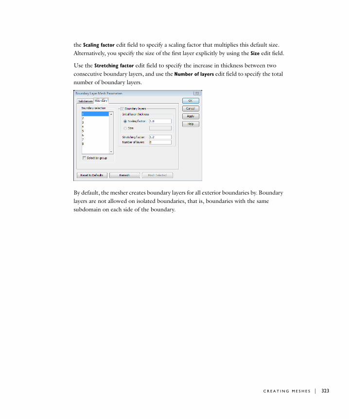
the Scaling factor edit field to specify a scaling factor that multiplies this default size. Alternatively, you specify the size of the first layer explicitly by using the Size edit field.
Use the Stretching factor edit field to specify the increase in thickness between two consecutive boundary layers, and use the Number of layers edit field to specify the total number of boundary layers.
By default, the mesher creates boundary layers for all exterior boundaries by. Boundary layers are not allowed on isolated boundaries, that is, boundaries with the same subdomain on each side of the boundary.
C R E A T I N G M E S H E S | 323
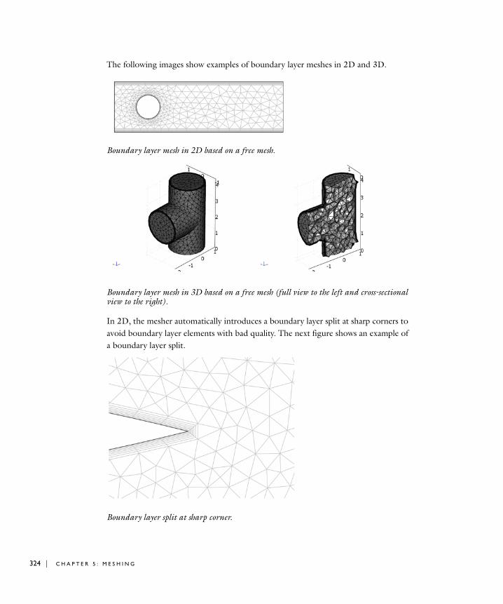
324 | C H A P T E
The following images show examples of boundary layer meshes in 2D and 3D.
Boundary layer mesh in 2D based on a free mesh.
Boundary layer mesh in 3D based on a free mesh (full view to the left and cross-sectional view to the right).
In 2D, the mesher automatically introduces a boundary layer split at sharp corners to avoid boundary layer elements with bad quality. The next figure shows an example of a boundary layer split.
Boundary layer split at sharp corner.
R 5 : M E S H I N G
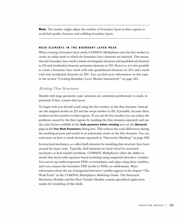
Note: The mesher might adjust the number of boundary layers in thin regions to avoid bad quality elements and colliding boundary layers.
M E S H E L E M E N T S I N T H E B O U N D A R Y L A Y E R M E S H
When creating a boundary layer mesh, COMSOL Multiphysics uses the free mesher to create an initial mesh in which the boundary layer elements are inserted. This means that the boundary layer mesh consists of triangular elements and quadrilateral elements in 2D and tetrahedral elements and prism elements in 3D. However, it is also possible to create a boundary layer mesh with only quadrilateral elements (in 2D) and a mesh with only hexahedral elements (in 3D). You can find more information on this topic in the section “Creating Boundary Layer Meshes Interactively” on page 341.
Meshing Thin Structures
Models with large geometric scale variations are sometimes problematic to mesh, in particular if they contain thin layers.
To begin with you should avoid using the free mesher on the thin domains. Instead use the mapped mesher in 2D and the swept mesher in 3D, if possible, because these meshers are less sensitive to thin regions. If you use the free mesher you can reduce the problems caused by the thin regions by meshing the thin domains separately and use the scale factors available in the Scale geometry before meshing area on the Advanced page in the Free Mesh Parameters dialog box. This reduces the scale differences during the meshing process and results in an anisotropic mesh on the thin domains. You can read more on how to mesh domains separately in “Interactive Meshing” on page 328.
In structural mechanics, so-called shell elements for modeling thin structure have been around for many years. Typically, shell elements are hard-wired for structural mechanics or heat transfer problems. COMSOL Multiphysics offers the ability to model thin layers with equation-based modeling using tangential derivative variables. You can set up multicomponent PDEs on boundaries and edges using these variables, and even connect the boundary PDE model to PDEs on subdomains. More information about the use of tangential derivative variables appears in the chapter “The Weak Form” in the COMSOL Multiphysics Modeling Guide. The Structural Mechanics Module and the Heat Transfer Module contain specialized application modes for modeling of thin shells.
C R E A T I N G M E S H E S | 325

326 | C H A P T E
Mesh Statistics
The Mesh Statistics dialog box, available from the Mesh menu, contains statistical data for the current mesh such as the number of elements and the minimum element quality. If the model contains one or more application modes, the number of degrees of freedom for the model is available as well. For more information on the number of degrees of freedom see “Finite Elements” on page 452 in the COMSOL Multiphysics Reference Guide.
Use the domain pages named Subdomain, Boundary, Edge, and Point to get mesh statistics for individual domains. Use the mouse to select domains directly in the geometry or select domains from the domain selection lists on each page. You can also press Ctrl+A to select all subdomains, boundaries, edges, or points. The statistical data that you see applies to all selected domains of that type.
R 5 : M E S H I N G
Re f i n i n g Me s h e s
When trying to solve a problem that does not converge, or having solved a problem where the solution does not seem properly resolved, there is often a need for re-solving the problem using a finer mesh. In these situations it is sometimes easier to refine the existing mesh than to regenerate the mesh from scratch using finer mesh settings. It is only possible to refine free meshes containing triangular elements, or tetrahedral elements, in 2D and 3D, respectively.
Refinement Methods
To refine a free mesh go to the Mesh menu and choose Refine Mesh, or click the Refine
Mesh button on the Main toolbar. In 1D, COMSOL Multiphysics always uses regular refinement, where it divides each element into two elements of the same shape. In 2D and 3D, however, two refinement methods are available: regular and longest. The regular refinement method divides each element into four triangular elements of the same shape in 2D, or eight tetrahedral elements of the same shape in 3D. The longest refinement method bisects the longest edge of each element.
Select the refinement method in the Free Mesh Parameters dialog box by looking on the Global page for the Refinement method list. For 2D geometries COMSOL Multiphysics defaults to the regular refinement method, and in 3D the longest refinement method is the default.
Refining Selected Elements
In 2D, you can refine a subset of elements in a free triangle mesh using the mouse to select an area in which you want a finer mesh:
1 Click the Refine Selection button on the Main toolbar.
2 Using the mouse, drag to enclose the mesh elements that you want to refine.
3 COMSOL Multiphysics refines all mesh elements that the selection encloses completely and possibly also some additional elements to take care of hanging nodes at the boundary of the refined area.
R E F I N I N G M E S H E S | 327
328 | C H A P T E
I n t e r a c t i v e Me s h i n g
The interactive meshing environment makes it possible to build a mesh in an incremental fashion where each meshing operation acts on a set of geometry domains. For example, you can start by creating a boundary mesh and then mesh each subdomain sequentially. This makes it easier to control the distribution of elements and the size of the mesh. Furthermore, using interactive meshing you can apply different meshing techniques to different domains of a geometry object.
Using the Mesh Toolbar
The Mesh toolbar is available in the selection modes and in Mesh mode. This toolbar contains buttons for all available meshing operations. All meshing tools that are available through the buttons are also available from the Interactive Meshing submenu on the Mesh menu.
Selecting the Interactive Meshing button on the top of the Mesh toolbar provides a display of the mesh in the selection modes such that you can see the domains that are meshed. Deselect the Interactive Meshing button to turn off the visualization of the mesh in the selection modes.
The Mesh toolbar consists of four groups of buttons:
• The first group corresponds to meshing tools that operate on the entire geometry or the part of the geometry that is currently not meshed; these operations are not affected by the current domain selection.
• The second group of buttons corresponds to meshing tools that operate only on the selected domains.
• The third group contains two buttons: one for selecting the remaining domains, that is, the domains that have not yet been meshed, and one for selecting the domains that have already been meshed.
• The fourth group, with two buttons, controls the predefined settings that determine the size of the mesh when creating one.
Clicking a button from the second group in the Mesh toolbar, that creates a mesh, is analogous to clicking the Mesh Selected button in the corresponding dialog box.
R 5 : M E S H I N G
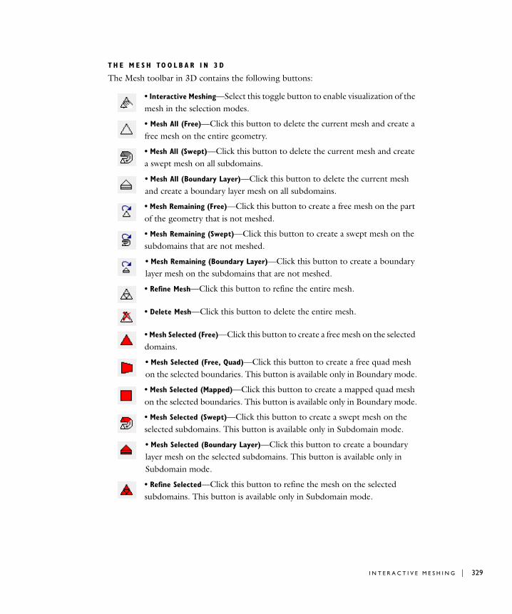
T H E M E S H TO O L B A R I N 3 D
The Mesh toolbar in 3D contains the following buttons:
• Interactive Meshing—Select this toggle button to enable visualization of the mesh in the selection modes.
• Mesh All (Free)—Click this button to delete the current mesh and create a free mesh on the entire geometry.
• Mesh All (Swept)—Click this button to delete the current mesh and create a swept mesh on all subdomains.
• Mesh All (Boundary Layer)—Click this button to delete the current mesh and create a boundary layer mesh on all subdomains.
• Mesh Remaining (Free)—Click this button to create a free mesh on the part of the geometry that is not meshed.
• Mesh Remaining (Swept)—Click this button to create a swept mesh on the subdomains that are not meshed.
• Mesh Remaining (Boundary Layer)—Click this button to create a boundary layer mesh on the subdomains that are not meshed.
• Refine Mesh—Click this button to refine the entire mesh.
• Delete Mesh—Click this button to delete the entire mesh.
• Mesh Selected (Free)—Click this button to create a free mesh on the selected domains.
• Mesh Selected (Free, Quad)—Click this button to create a free quad mesh on the selected boundaries. This button is available only in Boundary mode.
• Mesh Selected (Mapped)—Click this button to create a mapped quad mesh on the selected boundaries. This button is available only in Boundary mode.
• Mesh Selected (Swept)—Click this button to create a swept mesh on the selected subdomains. This button is available only in Subdomain mode.
• Mesh Selected (Boundary Layer)—Click this button to create a boundary layer mesh on the selected subdomains. This button is available only in Subdomain mode.
• Refine Selected—Click this button to refine the mesh on the selected subdomains. This button is available only in Subdomain mode.
I N T E R A C T I V E M E S H I N G | 329
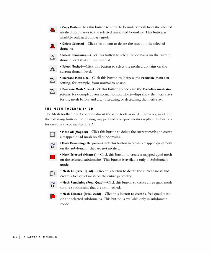
330 | C H A P T E
• Copy Mesh—Click this button to copy the boundary mesh from the selected meshed boundaries to the selected unmeshed boundary. This button is available only in Boundary mode.
• Delete Selected—Click this button to delete the mesh on the selected domains.
• Select Remaining—Click this button to select the domains on the current domain level that are not meshed.
• Select Meshed—Click this button to select the meshed domains on the current domain level.
• Increase Mesh Size—Click this button to increase the Predefine mesh size setting, for example, from normal to coarse.
• Decrease Mesh Size—Click this button to decrease the Predefine mesh size setting, for example, from normal to fine. The tooltips show the mesh sizes for the mesh before and after increasing or decreasing the mesh size.
T H E M E S H TO O L B A R I N 2 D
The Mesh toolbar in 2D contains almost the same tools as in 3D. However, in 2D the the following buttons for creating mapped and free quad meshes replace the buttons for creating swept meshes in 3D:
• Mesh All (Mapped)—Click this button to delete the current mesh and create a mapped quad mesh on all subdomains.
• Mesh Remaining (Mapped)—Click this button to create a mapped quad mesh on the subdomains that are not meshed.
• Mesh Selected (Mapped)—Click this button to create a mapped quad mesh on the selected subdomains. This button is available only in Subdomain mode.
• Mesh All (Free, Quad)—Click this button to delete the current mesh and create a free quad mesh on the entire geometry.
• Mesh Remaining (Free, Quad)—Click this button to create a free quad mesh on the subdomains that are not meshed.
• Mesh Selected (Free, Quad)—Click this button to create a free quad mesh on the selected subdomains. This button is available only in subdomain mode.
R 5 : M E S H I N G
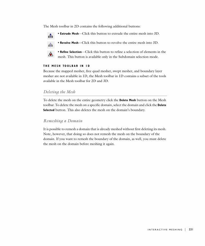
The Mesh toolbar in 2D contains the following additional buttons:
• Extrude Mesh—Click this button to extrude the entire mesh into 3D.
• Revolve Mesh—Click this button to revolve the entire mesh into 3D.
• Refine Selection—Click this button to refine a selection of elements in the mesh. This button is available only in the Subdomain selection mode.
T H E M E S H TO O L B A R I N 1 D
Because the mapped mesher, free quad mesher, swept mesher, and boundary layer mesher are not available in 1D, the Mesh toolbar in 1D contains a subset of the tools available in the Mesh toolbar for 2D and 3D.
Deleting the Mesh
To delete the mesh on the entire geometry click the Delete Mesh button on the Mesh toolbar. To delete the mesh on a specific domain, select the domain and click the Delete
Selected button. This also deletes the mesh on the domain’s boundary.
Remeshing a Domain
It is possible to remesh a domain that is already meshed without first deleting its mesh. Note, however, that doing so does not remesh the mesh on the boundary of the domain. If you want to remesh the boundary of the domain, as well, you must delete the mesh on the domain before meshing it again.
I N T E R A C T I V E M E S H I N G | 331
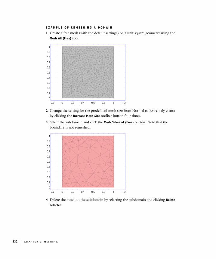
332 | C H A P T E
E X A M P L E O F R E M E S H I N G A D O M A I N
1 Create a free mesh (with the default settings) on a unit square geometry using the Mesh All (Free) tool.
2 Change the setting for the predefined mesh size from Normal to Extremely coarse by clicking the Increase Mesh Size toolbar button four times.
3 Select the subdomain and click the Mesh Selected (Free) button. Note that the boundary is not remeshed.
4 Delete the mesh on the subdomain by selecting the subdomain and clicking Delete
Selected.
R 5 : M E S H I N G
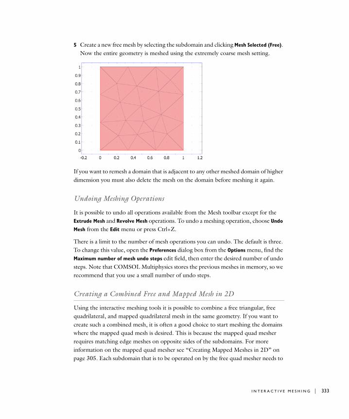
5 Create a new free mesh by selecting the subdomain and clicking Mesh Selected (Free). Now the entire geometry is meshed using the extremely coarse mesh setting.
If you want to remesh a domain that is adjacent to any other meshed domain of higher dimension you must also delete the mesh on the domain before meshing it again.
Undoing Meshing Operations
It is possible to undo all operations available from the Mesh toolbar except for the Extrude Mesh and Revolve Mesh operations. To undo a meshing operation, choose Undo
Mesh from the Edit menu or press Ctrl+Z.
There is a limit to the number of mesh operations you can undo. The default is three. To change this value, open the Preferences dialog box from the Options menu, find the Maximum number of mesh undo steps edit field, then enter the desired number of undo steps. Note that COMSOL Multiphysics stores the previous meshes in memory, so we recommend that you use a small number of undo steps.
Creating a Combined Free and Mapped Mesh in 2D
Using the interactive meshing tools it is possible to combine a free triangular, free quadrilateral, and mapped quadrilateral mesh in the same geometry. If you want to create such a combined mesh, it is often a good choice to start meshing the domains where the mapped quad mesh is desired. This is because the mapped quad mesher requires matching edge meshes on opposite sides of the subdomains. For more information on the mapped quad mesher see “Creating Mapped Meshes in 2D” on page 305. Each subdomain that is to be operated on by the free quad mesher needs to
I N T E R A C T I V E M E S H I N G | 333
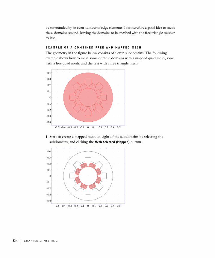
334 | C H A P T E
be surrounded by an even number of edge elements. It is therefore a good idea to mesh these domains second, leaving the domains to be meshed with the free triangle mesher to last.
E X A M P L E O F A C O M B I N E D F R E E A N D M A P P E D M E S H
The geometry in the figure below consists of eleven subdomains. The following example shows how to mesh some of these domains with a mapped quad mesh, some with a free quad mesh, and the rest with a free triangle mesh.
1 Start to create a mapped mesh on eight of the subdomains by selecting the subdomains, and clicking the Mesh Selected (Mapped) button.
R 5 : M E S H I N G
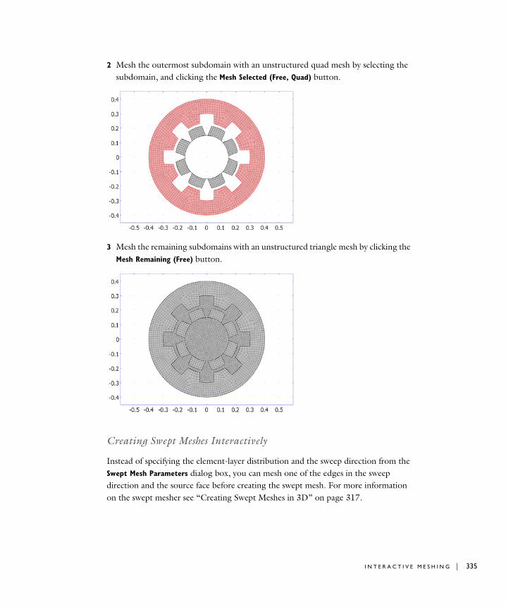
2 Mesh the outermost subdomain with an unstructured quad mesh by selecting the subdomain, and clicking the Mesh Selected (Free, Quad) button.
3 Mesh the remaining subdomains with an unstructured triangle mesh by clicking the Mesh Remaining (Free) button.
Creating Swept Meshes Interactively
Instead of specifying the element-layer distribution and the sweep direction from the Swept Mesh Parameters dialog box, you can mesh one of the edges in the sweep direction and the source face before creating the swept mesh. For more information on the swept mesher see “Creating Swept Meshes in 3D” on page 317.
I N T E R A C T I V E M E S H I N G | 335
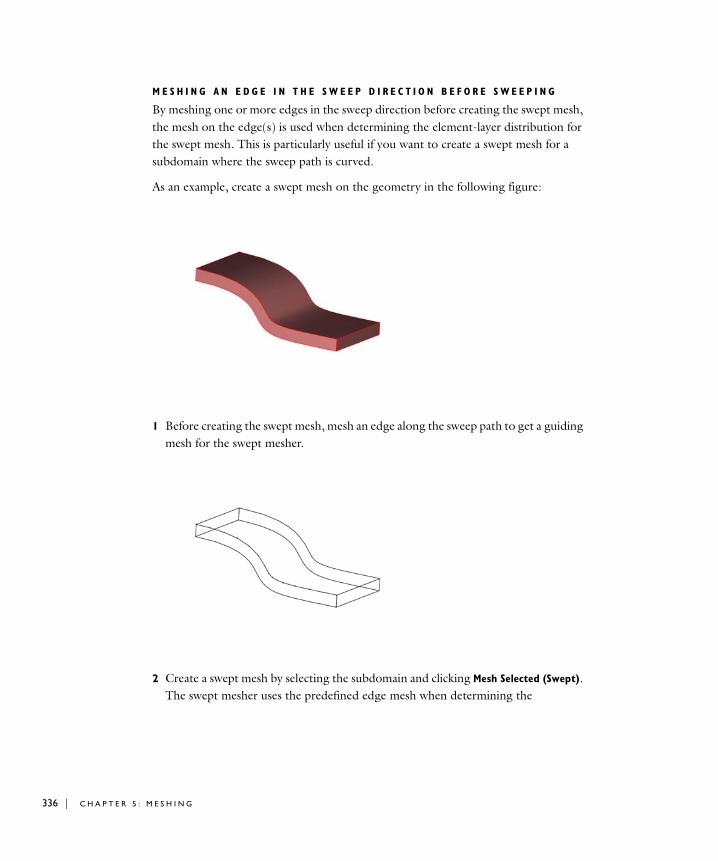
336 | C H A P T E
M E S H I N G A N E D G E I N T H E S W E E P D I R E C T I O N B E F O R E S W E E P I N G
By meshing one or more edges in the sweep direction before creating the swept mesh, the mesh on the edge(s) is used when determining the element-layer distribution for the swept mesh. This is particularly useful if you want to create a swept mesh for a subdomain where the sweep path is curved.
As an example, create a swept mesh on the geometry in the following figure:
1 Before creating the swept mesh, mesh an edge along the sweep path to get a guiding mesh for the swept mesher.
2 Create a swept mesh by selecting the subdomain and clicking Mesh Selected (Swept). The swept mesher uses the predefined edge mesh when determining the
R 5 : M E S H I N G
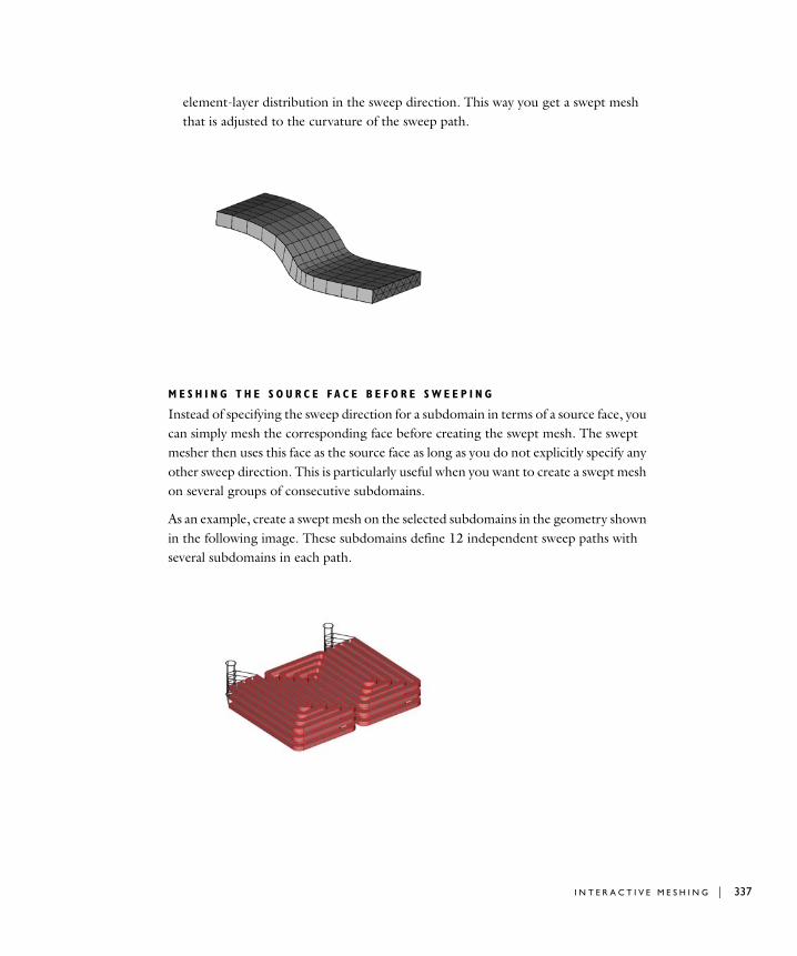
element-layer distribution in the sweep direction. This way you get a swept mesh that is adjusted to the curvature of the sweep path.
M E S H I N G T H E S O U R C E F A C E B E F O R E S W E E P I N G
Instead of specifying the sweep direction for a subdomain in terms of a source face, you can simply mesh the corresponding face before creating the swept mesh. The swept mesher then uses this face as the source face as long as you do not explicitly specify any other sweep direction. This is particularly useful when you want to create a swept mesh on several groups of consecutive subdomains.
As an example, create a swept mesh on the selected subdomains in the geometry shown in the following image. These subdomains define 12 independent sweep paths with several subdomains in each path.
I N T E R A C T I V E M E S H I N G | 337
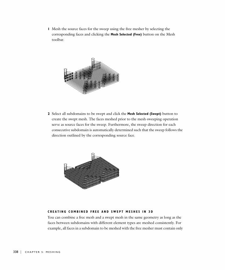
338 | C H A P T E
1 Mesh the source faces for the sweep using the free mesher by selecting the corresponding faces and clicking the Mesh Selected (Free) button on the Mesh toolbar.
2 Select all subdomains to be swept and click the Mesh Selected (Swept) button to create the swept mesh. The faces meshed prior to the mesh-sweeping operation serve as source faces for the sweep. Furthermore, the sweep direction for each consecutive subdomain is automatically determined such that the sweep follows the direction outlined by the corresponding source face.
C R E A T I N G C O M B I N E D F R E E A N D S W E P T M E S H E S I N 3 D
You can combine a free mesh and a swept mesh in the same geometry as long as the faces between subdomains with different element types are meshed consistently. For example, all faces in a subdomain to be meshed with the free mesher must contain only
R 5 : M E S H I N G
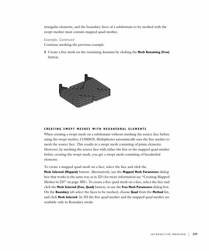
triangular elements, and the boundary faces of a subdomain to be meshed with the swept mesher must contain mapped quad meshes.
Example, ContinuedContinue meshing the previous example.
3 Create a free mesh on the remaining domains by clicking the Mesh Remaining (Free) button.
C R E A T I N G S W E P T M E S H E S W I T H H E X A H E D R A L E L E M E N T S
When creating a swept mesh on a subdomain without meshing the source face before using the swept mesher, COMSOL Multiphysics automatically uses the free mesher to mesh the source face. This results in a swept mesh consisting of prism elements. However, by meshing the source face with either the free or the mapped quad mesher before creating the swept mesh, you get a swept mesh consisting of hexahedral elements.
To create a mapped quad mesh on a face, select the face and click the Mesh Selected (Mapped) button. Alternatively, use the Mapped Mesh Parameters dialog box that works in the same way as in 2D (for more information see “Creating Mapped Meshes in 2D” on page 305). To create a free quad mesh on a face, select the face and click the Mesh Selected (Free, Quad) button, or use the Free Mesh Parameters dialog box. On the Boundary tab select the faces to be meshed, choose Quad from the Method list, and click Mesh Selected. In 3D the free quad mesher and the mapped quad mesher are available only in Boundary mode.
I N T E R A C T I V E M E S H I N G | 339
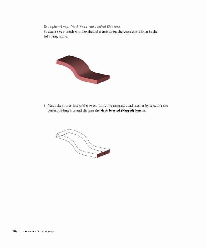
340 | C H A P T E
Example—Swept Mesh With Hexahedral ElementsCreate a swept mesh with hexahedral elements on the geometry shown in the following figure.
1 Mesh the source face of the sweep using the mapped quad mesher by selecting the corresponding face and clicking the Mesh Selected (Mapped) button.
R 5 : M E S H I N G

2 Create a swept mesh by selecting the subdomain and clicking Mesh Selected (Swept).
Creating Boundary Layer Meshes Interactively
If you click the Remesh button in the Boundary Layer Mesh Parameters dialog box or the Mesh All (Boundary Layer) button on the Mesh toolbar, COMSOL Multiphysics uses the free mesher to create an initial mesh in which the boundary layers are then inserted. For more information on the boundary layer mesher, see the section “Creating Boundary Layer Meshes” on page 321.
It is also possible to insert boundary layers into an existing mesh. You do this by selecting the subdomains to be processed and clicking the Mesh Selected button in the Boundary Layer Mesh Parameters dialog box or by clicking the Mesh Selected (Boundary
Layer) button on the Mesh toolbar.
I N T E R A C T I V E M E S H I N G | 341
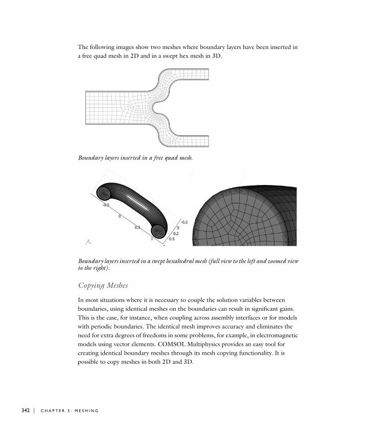
342 | C H A P T E
The following images show two meshes where boundary layers have been inserted in a free quad mesh in 2D and in a swept hex mesh in 3D.
Boundary layers inserted in a free quad mesh.
Boundary layers inserted in a swept hexahedral mesh (full view to the left and zoomed view to the right).
Copying Meshes
In most situations where it is necessary to couple the solution variables between boundaries, using identical meshes on the boundaries can result in significant gains. This is the case, for instance, when coupling across assembly interfaces or for models with periodic boundaries. The identical mesh improves accuracy and eliminates the need for extra degrees of freedoms in some problems, for example, in electromagnetic models using vector elements. COMSOL Multiphysics provides an easy tool for creating identical boundary meshes through its mesh copying functionality. It is possible to copy meshes in both 2D and 3D.
R 5 : M E S H I N G
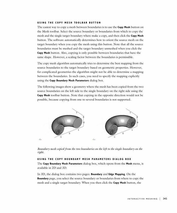
U S I N G T H E C O P Y M E S H TO O L B A R B U T T O N
The easiest way to copy a mesh between boundaries is to use the Copy Mesh button on the Mesh toolbar. Select the source boundary or boundaries from which to copy the mesh and the single target boundary where make a copy, and then click the Copy Mesh button. The software automatically determines how to orient the source mesh on the target boundary when you copy the mesh using this button. Note that all the source boundaries must be meshed and the target boundary unmeshed when you click the Copy Mesh button. Also, copying is only possible between boundaries that have the same shape. However, a scaling factor between the boundaries is permissible.
The copy mesh algorithm automatically tries to determine the best mapping from the source boundaries to the target boundary based on geometric properties. However, for complicated geometries the algorithm might not be able to determine a mapping between the boundaries. In such cases, you need to specify the mapping explicitly using the Copy Boundary Mesh Parameters dialog box.
The following images show a geometry where the mesh has been copied from the two source boundaries on the left side to the single boundary on the right side using the Copy Mesh toolbar button. Note that copying in the opposite direction would not be possible, because copying from one to several boundaries is not supported.
Boundary mesh copied from the two boundaries on the left to the single boundary on the right.
U S I N G T H E C O P Y B O U N D A R Y M E S H P A R A M E T E R S D I A L O G B O X
The Copy Boundary Mesh Parameters dialog box, which opens from the Mesh menu, is available in 2D and 3D.
In 3D, the dialog box contains two pages: Boundary and Edge Mapping. On the Boundary page, you select the source boundary or boundaries from where to copy the mesh and a single target boundary. When you then click the Copy Mesh button, the
I N T E R A C T I V E M E S H I N G | 343
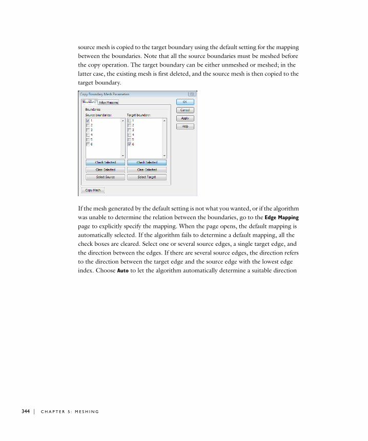
344 | C H A P T E
source mesh is copied to the target boundary using the default setting for the mapping between the boundaries. Note that all the source boundaries must be meshed before the copy operation. The target boundary can be either unmeshed or meshed; in the latter case, the existing mesh is first deleted, and the source mesh is then copied to the target boundary.
If the mesh generated by the default setting is not what you wanted, or if the algorithm was unable to determine the relation between the boundaries, go to the Edge Mapping page to explicitly specify the mapping. When the page opens, the default mapping is automatically selected. If the algorithm fails to determine a default mapping, all the check boxes are cleared. Select one or several source edges, a single target edge, and the direction between the edges. If there are several source edges, the direction refers to the direction between the target edge and the source edge with the lowest edge index. Choose Auto to let the algorithm automatically determine a suitable direction
R 5 : M E S H I N G
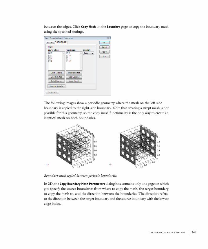
between the edges. Click Copy Mesh on the Boundary page to copy the boundary mesh using the specified settings.
The following images show a periodic geometry where the mesh on the left-side boundary is copied to the right-side boundary. Note that creating a swept mesh is not possible for this geometry, so the copy mesh functionality is the only way to create an identical mesh on both boundaries.
Boundary mesh copied between periodic boundaries.
In 2D, the Copy Boundary Mesh Parameters dialog box contains only one page on which you specify the source boundaries from where to copy the mesh, the target boundary to copy the mesh to, and the direction between the boundaries. The direction refers to the direction between the target boundary and the source boundary with the lowest edge index.
I N T E R A C T I V E M E S H I N G | 345
346 | C H A P T E
Impo r t i n g and Expo r t i n g Me s h e s
Importing a mesh into COMSOL Multiphysics completely eliminates the need for drawing, importing, or otherwise manipulating a geometry. This makes it possible to directly use a mesh that was created with an external program. COMSOL Multiphysics supports the most common 3D mesh format: the NASTRAN bulk data file. You can also import other mesh formats by translating them into this mesh format or into a COMSOL Multiphysics file.
Using COMSOL Multiphysics Files
It is possible to import or export a mesh object using a COMSOL Multiphysics file, which can exist in binary format (extension .mphbin) and text format (extension .mphtxt). More information on these file formats is available in the chapter “The COMSOL Multiphysics Files” in the COMSOL Multiphysics Reference Guide.
You export a mesh object to a COMSOL Multiphysics file by choosing Export>Mesh
To File from the File menu. To import a mesh stored in this file format, choose Import>Mesh From File from the File menu.
U S I N G A T E X T F I L E T O I M P O R T E X T E R N A L M E S H D A T A
You can also use a COMSOL Multiphysics text file to transfer externally generated mesh data into a mesh object. The easiest way to do so is to first export a mesh object to a COMSOL Multiphysics text file; then replace the data in the different entries in that file with the corresponding external data; finally import the resulting file. An alternative approach of importing external mesh data is described in the chapter “Creating Meshes” in the COMSOL Multiphysics Scripting Guide.
Importing NASTRAN Files
You can import 3D meshes in the NASTRAN bulk data format, the most common format for exchanging 3D meshes among programs. This format supports hundreds of NASTRAN entries describing elements, loads, and materials, making it possible to define a complete finite element model. When you import a NASTRAN bulk data file into COMSOL Multiphysics, the software imports only true mesh element information. You can let COMSOL Multiphysics determine the partitioning of the imported mesh elements into different domains according to material information in the file, if material information is available. The meshimport reference entry on page
R 5 : M E S H I N G
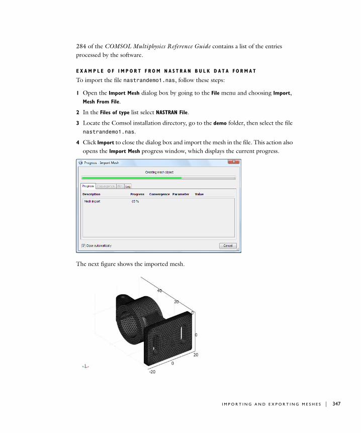
284 of the COMSOL Multiphysics Reference Guide contains a list of the entries processed by the software.
E X A M P L E O F I M P O R T F R O M N A S T R A N B U L K D A T A F O R M A T
To import the file nastrandemo1.nas, follow these steps:
1 Open the Import Mesh dialog box by going to the File menu and choosing Import, Mesh From File.
2 In the Files of type list select NASTRAN File.
3 Locate the Comsol installation directory, go to the demo folder, then select the file nastrandemo1.nas.
4 Click Import to close the dialog box and import the mesh in the file. This action also opens the Import Mesh progress window, which displays the current progress.
The next figure shows the imported mesh.
I M P O R T I N G A N D E X P O R T I N G M E S H E S | 347
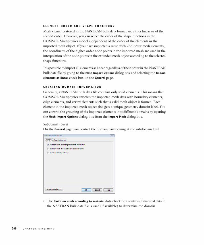
348 | C H A P T E
E L E M E N T O R D E R A N D S H A P E F U N C T I O N S
Mesh elements stored in the NASTRAN bulk data format are either linear or of the second order. However, you can select the order of the shape functions in the COMSOL Multiphysics model independent of the order of the elements in the imported mesh object. If you have imported a mesh with 2nd-order mesh elements, the coordinates of the higher-order node points in the imported mesh are used in the interpolation of the node points in the extended mesh object according to the selected shape functions.
It is possible to import all elements as linear regardless of their order in the NASTRAN bulk data file by going to the Mesh Import Options dialog box and selecting the Import
elements as linear check box on the General page.
C R E A T I N G D O M A I N I N F O R M A T I O N
Generally, a NASTRAN bulk data file contains only solid elements. This means that COMSOL Multiphysics enriches the imported mesh data with boundary elements, edge elements, and vertex elements such that a valid mesh object is formed. Each element in the imported mesh object also gets a unique geometry domain label. You can control the grouping of the imported elements into different domains by opening the Mesh Import Options dialog box from the Import Mesh dialog box.
Subdomain LevelOn the General page you control the domain partitioning at the subdomain level.
• The Partition mesh according to material data check box controls if material data in the NASTRAN bulk data file is used (if available) to determine the domain
R 5 : M E S H I N G
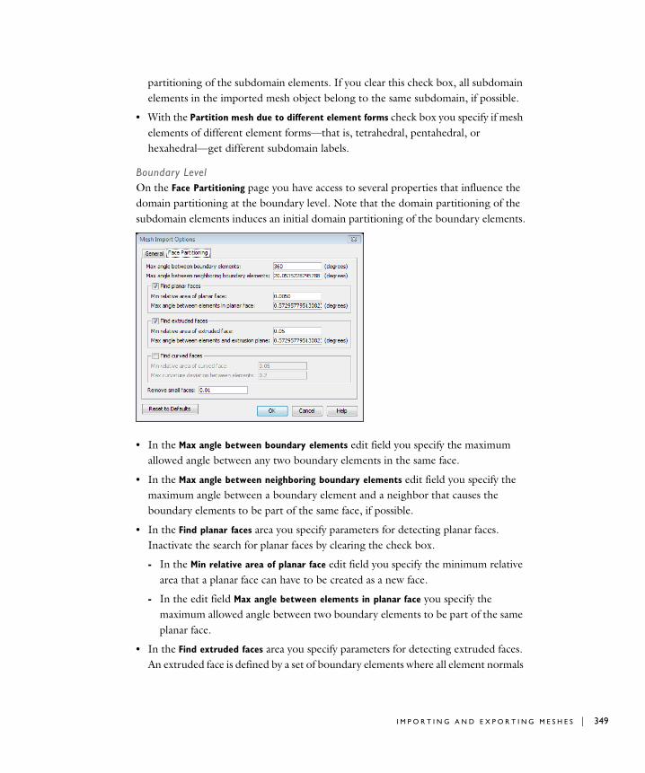
partitioning of the subdomain elements. If you clear this check box, all subdomain elements in the imported mesh object belong to the same subdomain, if possible.
• With the Partition mesh due to different element forms check box you specify if mesh elements of different element forms—that is, tetrahedral, pentahedral, or hexahedral—get different subdomain labels.
Boundary LevelOn the Face Partitioning page you have access to several properties that influence the domain partitioning at the boundary level. Note that the domain partitioning of the subdomain elements induces an initial domain partitioning of the boundary elements.
• In the Max angle between boundary elements edit field you specify the maximum allowed angle between any two boundary elements in the same face.
• In the Max angle between neighboring boundary elements edit field you specify the maximum angle between a boundary element and a neighbor that causes the boundary elements to be part of the same face, if possible.
• In the Find planar faces area you specify parameters for detecting planar faces. Inactivate the search for planar faces by clearing the check box.
- In the Min relative area of planar face edit field you specify the minimum relative area that a planar face can have to be created as a new face.
- In the edit field Max angle between elements in planar face you specify the maximum allowed angle between two boundary elements to be part of the same planar face.
• In the Find extruded faces area you specify parameters for detecting extruded faces. An extruded face is defined by a set of boundary elements where all element normals
I M P O R T I N G A N D E X P O R T I N G M E S H E S | 349

350 | C H A P T E
lie in the same plane, referred to as extrusion plane. Inactivate the search for extruded faces by clearing the check box.
- In the Min relative area of extruded face edit field you specify the minimum relative area that an extruded face can have to be created as a new face.
- In the Max angle between elements and extrusion plane edit field you specify the maximum angle between a boundary element normal and the extrusion plane that will cause the element to be part of the extruded face if possible.
• In the Find curved faces area you specify parameters for detecting faces with a constant curvature. This property is active only for meshes with 2nd-order elements. Inactivate the search for faces with constant curvature by clearing the check box.
- In the Min relative area of curved face edit field you specify the minimum relative area that a curved face is allowed to have to be created as a new face.
- In the Max curvature deviation between elements edit field you specify the maximum relative curvature difference between boundary elements that will cause the elements to be part of the same curved face if possible.
• In the Remove small faces edit field you specify a positive scalar controlling to which extent the software merges small faces with adjacent faces. If you get an imported mesh object with exceedingly small faces that you want to get rid of, increase the value of this property and re-import the file.
Note: When importing a mesh to COMSOL Multiphysics, there is no corresponding geometry object available. This means that it is not possible to refine an imported mesh, and you cannot use the adaptive solver unless you create a geometry object from the imported mesh.
R 5 : M E S H I N G
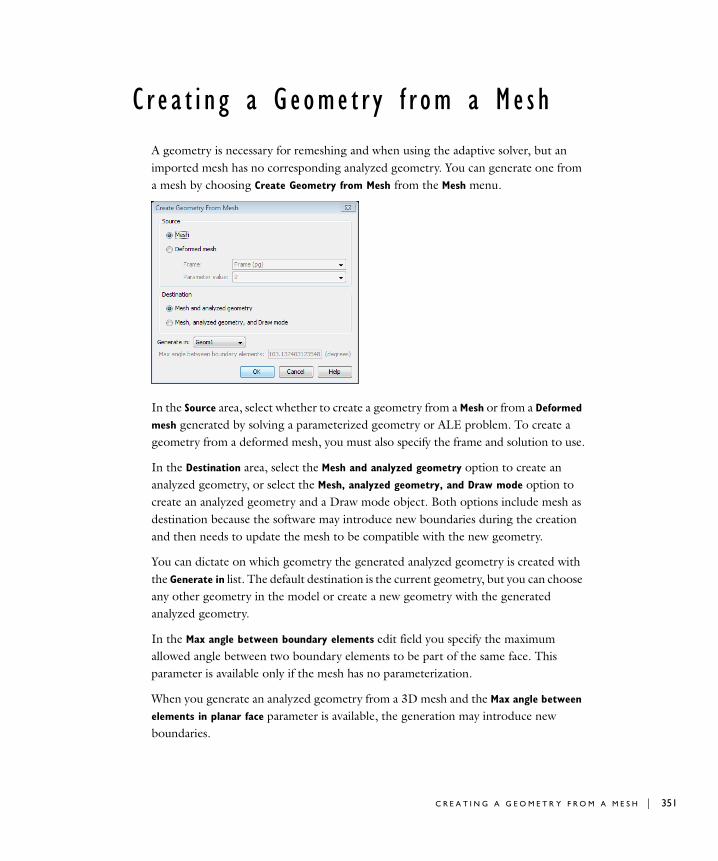
C r e a t i n g a G eome t r y f r om a Me s h
A geometry is necessary for remeshing and when using the adaptive solver, but an imported mesh has no corresponding analyzed geometry. You can generate one from a mesh by choosing Create Geometry from Mesh from the Mesh menu.
In the Source area, select whether to create a geometry from a Mesh or from a Deformed
mesh generated by solving a parameterized geometry or ALE problem. To create a geometry from a deformed mesh, you must also specify the frame and solution to use.
In the Destination area, select the Mesh and analyzed geometry option to create an analyzed geometry, or select the Mesh, analyzed geometry, and Draw mode option to create an analyzed geometry and a Draw mode object. Both options include mesh as destination because the software may introduce new boundaries during the creation and then needs to update the mesh to be compatible with the new geometry.
You can dictate on which geometry the generated analyzed geometry is created with the Generate in list. The default destination is the current geometry, but you can choose any other geometry in the model or create a new geometry with the generated analyzed geometry.
In the Max angle between boundary elements edit field you specify the maximum allowed angle between two boundary elements to be part of the same face. This parameter is available only if the mesh has no parameterization.
When you generate an analyzed geometry from a 3D mesh and the Max angle between
elements in planar face parameter is available, the generation may introduce new boundaries.
C R E A T I N G A G E O M E T R Y F R O M A M E S H | 351
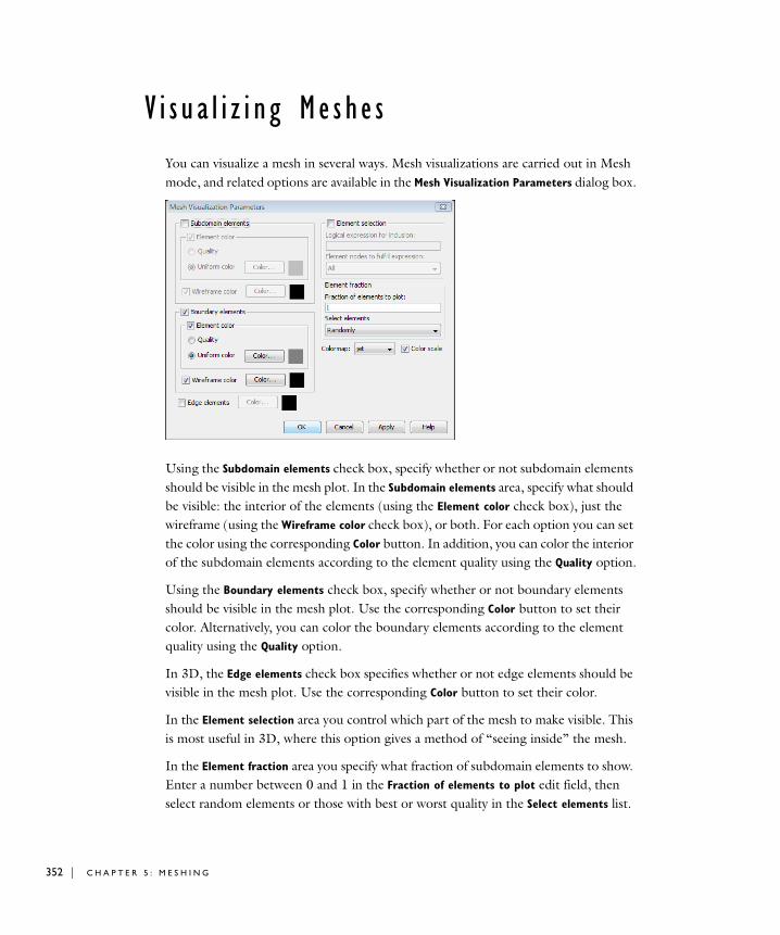
352 | C H A P T E
V i s u a l i z i n g Me s h e s
You can visualize a mesh in several ways. Mesh visualizations are carried out in Mesh mode, and related options are available in the Mesh Visualization Parameters dialog box.
Using the Subdomain elements check box, specify whether or not subdomain elements should be visible in the mesh plot. In the Subdomain elements area, specify what should be visible: the interior of the elements (using the Element color check box), just the wireframe (using the Wireframe color check box), or both. For each option you can set the color using the corresponding Color button. In addition, you can color the interior of the subdomain elements according to the element quality using the Quality option.
Using the Boundary elements check box, specify whether or not boundary elements should be visible in the mesh plot. Use the corresponding Color button to set their color. Alternatively, you can color the boundary elements according to the element quality using the Quality option.
In 3D, the Edge elements check box specifies whether or not edge elements should be visible in the mesh plot. Use the corresponding Color button to set their color.
In the Element selection area you control which part of the mesh to make visible. This is most useful in 3D, where this option gives a method of “seeing inside” the mesh.
In the Element fraction area you specify what fraction of subdomain elements to show. Enter a number between 0 and 1 in the Fraction of elements to plot edit field, then select random elements or those with best or worst quality in the Select elements list.
R 5 : M E S H I N G
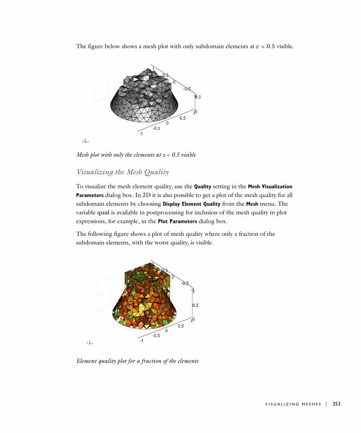
The figure below shows a mesh plot with only subdomain elements at z < 0.5 visible.
Mesh plot with only the elements at z < 0.5 visible
Visualizing the Mesh Quality
To visualize the mesh element quality, use the Quality setting in the Mesh Visualization
Parameters dialog box. In 2D it is also possible to get a plot of the mesh quality for all subdomain elements by choosing Display Element Quality from the Mesh menu. The variable qual is available in postprocessing for inclusion of the mesh quality in plot expressions, for example, in the Plot Parameters dialog box.
The following figure shows a plot of mesh quality where only a fraction of the subdomain elements, with the worst quality, is visible.
Element quality plot for a fraction of the elements
V I S U A L I Z I N G M E S H E S | 353
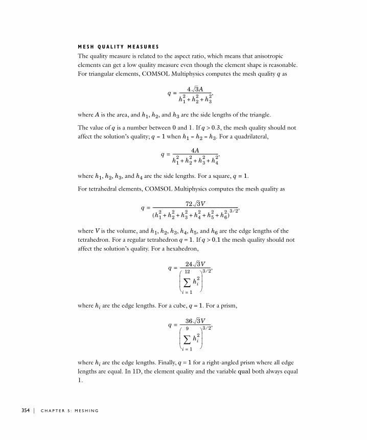
354 | C H A P T E
M E S H Q U A L I T Y M E A S U R E S
The quality measure is related to the aspect ratio, which means that anisotropic elements can get a low quality measure even though the element shape is reasonable. For triangular elements, COMSOL Multiphysics computes the mesh quality q as
where A is the area, and h1, h2, and h3 are the side lengths of the triangle.
The value of q is a number between 0 and 1. If q > 0.3, the mesh quality should not affect the solution’s quality; q = 1 when h1 = h2 = h3. For a quadrilateral,
where h1, h2, h3, and h4 are the side lengths. For a square, q = 1.
For tetrahedral elements, COMSOL Multiphysics computes the mesh quality as
where V is the volume, and h1, h2, h3, h4, h5, and h6 are the edge lengths of the tetrahedron. For a regular tetrahedron q = 1. If q > 0.1 the mesh quality should not affect the solution’s quality. For a hexahedron,
where hi are the edge lengths. For a cube, q = 1. For a prism,
where hi are the edge lengths. Finally, q = 1 for a right-angled prism where all edge lengths are equal. In 1D, the element quality and the variable qual both always equal 1.
q 4 3A
h12 h2
2 h32
+ +--------------------------------= ,
q 4A
h12 h2
2 h32 h4
2+ + +
---------------------------------------------= ,
q 72 3V
h12 h2
2 h32 h4
2 h52 h6
2+ + + + +( )
3 2⁄------------------------------------------------------------------------------------= ,
q 24 3V
hi2
i 1=
12
∑⎝ ⎠⎜ ⎟⎜ ⎟⎛ ⎞ 3 2⁄------------------------------= ,
q 36 3V
hi2
i 1=
9
∑⎝ ⎠⎜ ⎟⎜ ⎟⎛ ⎞ 3 2⁄------------------------------= ,
R 5 : M E S H I N G
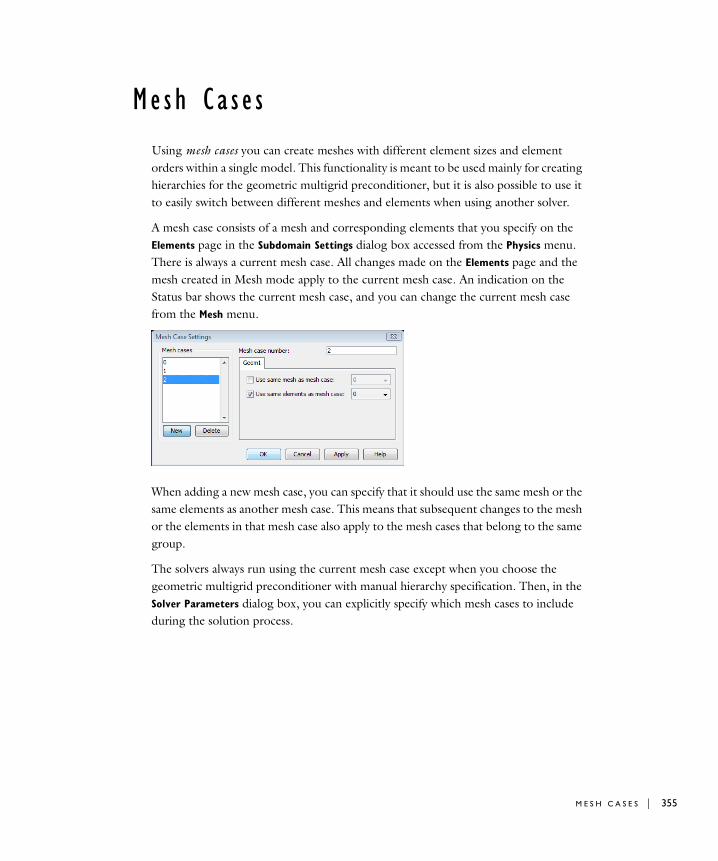
Me sh Ca s e s
Using mesh cases you can create meshes with different element sizes and element orders within a single model. This functionality is meant to be used mainly for creating hierarchies for the geometric multigrid preconditioner, but it is also possible to use it to easily switch between different meshes and elements when using another solver.
A mesh case consists of a mesh and corresponding elements that you specify on the Elements page in the Subdomain Settings dialog box accessed from the Physics menu. There is always a current mesh case. All changes made on the Elements page and the mesh created in Mesh mode apply to the current mesh case. An indication on the Status bar shows the current mesh case, and you can change the current mesh case from the Mesh menu.
When adding a new mesh case, you can specify that it should use the same mesh or the same elements as another mesh case. This means that subsequent changes to the mesh or the elements in that mesh case also apply to the mesh cases that belong to the same group.
The solvers always run using the current mesh case except when you choose the geometric multigrid preconditioner with manual hierarchy specification. Then, in the Solver Parameters dialog box, you can explicitly specify which mesh cases to include during the solution process.
M E S H C A S E S | 355
356 | C H A P T E
A vo i d i n g I n v e r t e d Me s h E l emen t s
Inverted Mesh Elements
If you have a mesh that is coarse along a curved boundary you might get problems with inverted mesh elements. This means that a mesh element is wrapped inside-out or has zero area (in 2D) or volume (in 3D). More precisely, there is some coordinate for which the Jacobian matrix for the mapping from local to global coordinates has a negative or zero determinant. In most cases, the linear (straight) mesh elements that you see in a mesh plot are not inverted, but the higher-order curved mesh elements used for computing the solution might be (see “Curved Mesh Elements” on page 454 in the COMSOL Multiphysics Reference Guide). Hence, studying the minimum element quality in the Mesh Statistics dialog box does not reveal the presence of inverted mesh elements in most cases.
Inverted mesh elements in themselves do not pose any immediate threat to the overall accuracy of your solution. However, if you are using an iterative solver, it may fail to converge. If you reach convergence and the solution looks good, it likely is. It is however worth bearing in mind that the faces along which there are inverted elements are less than perfectly resolved. If these faces are important for your results, you may want to pursue a mesh without inverted elements or at least make sure that the mesh resolution is sufficiently fine to guarantee an accurate solution. The easiest way to get an idea of the accuracy is to try a few different meshes and see how the solution changes. If the variation does not exceed your limits of acceptance, you are fine.
The solver prints warnings about inverted mesh elements to the Log page in the Progress window if they appear. You can avoid problems with inverted mesh elements by reducing the geometry shape order or by modifying the geometry or the mesh.
Using Linear Geometry Shape Order
When solving a model, the solver ensures that no inverted mesh elements are created. This is done by reducing the geometry shape order for the corresponding elements to first order. By default, the solver does this automatically. You can turn off this feature by clearing the Use first order for inverted elements check box in the Model Settings dialog box, opened from the Physics menu. In the corresponding Geometry shape area there is also a Tolerance edit field that specifies the minimum allowed value of the variable reldetjacmin for elements not to be considered as inverted elements. The
R 5 : M E S H I N G

default value of this tolerance is 0.1, which means that linear geometry shape order is also used for elements that are very close to being inverted. For more information on the variable reldetjacmin, see “Geometric Variables” on page 165.
Alternatively, you can avoid problems with inverted mesh elements by using linear geometry shape order for all elements. You do this by choosing Linear from the Order list in the Geometry shape area in the Model Settings dialog box.
Modifying the Geometry or Mesh
If you do not want to use linear geometry shape order to avoid problems with inverted mesh elements you can try any of the following:
• Create an extruded, revolved, or swept 3D mesh instead of using the free mesher.
• Avoid small curved boundaries such as fillets unless they are important for the result.
• Do not use the Refine Mesh button on the Main toolbar to create your mesh. Instead choose a finer mesh setting in the list of predefined mesh sizes or give a maximum element size that results in a mesh finer than the original mesh.
Visualizing Inverted Mesh Elements
You can visualize inverted mesh elements both in Mesh mode and in Postprocessing mode. To plot the inverted mesh elements in Mesh mode, follow these steps.
1 From the Mesh menu, open the Mesh Visualization Parameters dialog box.
2 Select the Subdomain elements check box and clear the Boundary elements check box.
3 Select the Element selection check box and type reldetjacmin<0 in the Logical
expression for inclusion edit field.
4 Click OK to plot the inverted mesh elements and close the dialog box.
If you clear the Use first order for inverted elements check box in the Model Settings dialog box or if you lower the corresponding tolerance value below zero before solving, you might get inverted mesh elements when solving the problem. To see where these elements are located using the postprocessing tools, follow these steps.
1 Open the Plot Parameters dialog box. On the General page, select the Subdomain and Geometry edges check boxes.
2 Select the Element selection check box and type reldetjacmin<0 in the Logical
expression for inclusion field.
3 Click the Subdomain tab and type reldetjacmin in the Expression field. Click OK.
A V O I D I N G I N V E R T E D M E S H E L E M E N T S | 357

358 | C H A P T E
R 5 : M E S H I N G
6
S o l v i n g t h e M o d e l
This chapter lists the various solvers in COMSOL Multiphysics and examines how to choose the best one for a given application. It also reviews which settings to select when solving a wide range of problems of different types and how to analyze the accuracy of the solution and improve convergence. Supplementary information appears in Chapter 5, “Advanced Solver Topics,” of the COMSOL Multiphysics Reference Guide.
359
360 | C H A P T E
S e l e c t i n g a S o l v e r
The COMSOL Multiphysics Solvers
COMSOL Multiphysics includes a number of different solvers for PDE-based problems. Table 6-1 summarizes the available types. They are described in more detail in the next section, “The Solvers and Their Settings” on page 365.
Selecting an Analysis Type
For most models, you do not need to select a solver explicitly. Instead, you choose an analysis type. The available analysis types depend on the application area; those you can expect to see include stationary, eigenfrequency, transient, time-dependent, and parametric analysis.
You select the analysis type in the Model Navigator. With the exception of the PDE modes, the analysis type is an application mode property that you can change later on. To do so, choose Properties in the Physics menu to open the Application Mode Properties dialog box or select it from the Analysis list in the Solver Parameters dialog box.
The analysis type sets up various equations for the application mode and suggests a default solver. To override this default, open the Solver Parameters dialog box and specify the solver of your choice from the Solver list. Note, however, that doing so may result in a solver setting that is incompatible with the equations you want to solve. You
TABLE 6-1: COMSOL MULTIPHYSICS SOLVERS
SOLVER TYPE USAGE
Stationary For stationary PDE problems (linear or nonlinear)
Time-dependent For time-dependent PDE problems (linear or nonlinear)
Eigenvalue For eigenvalue PDE problems
Parametric For parameterized sets of stationary PDE problems (linear or nonlinear)
Stationary segregated For stationary multiphysics PDE problems (linear or nonlinear)
Parametric segregated For parameterized sets of stationary multiphysics PDE problems (linear or nonlinear)
Adaptive For stationary (linear or nonlinear) or eigenvalue PDE problems using adaptive mesh refinement
R 6 : S O L V I N G T H E M O D E L
can disable the automatic solver selection based on the analysis type by clearing the Auto select solver check box under the Analysis list in the Solver Parameters dialog box.
For multiphysics models, the ruling application mode determines the analysis type and suggests a default solver. You can inspect or change the ruling application mode in the Ruling application mode list in the Model Navigator. If you change the ruling application mode or its analysis type, the program changes certain solver settings accordingly.
Beside the analysis type, the set of application mode properties include the default element type and weak constraints. The weak constraint property enables more accurate reaction-force computations by introducing an extra equation, which in turn means extra work for the solver. For additional application mode properties, specific to individual application modes, see the COMSOL Multiphysics Modeling Guide or the documentation for the module to which the application mode belongs.
Selecting a Stationary, a Time-Dependent, or an Eigenvalue Solver
The analysis type generally selects an appropriate solver, so normally you do not need to select one yourself. If you nevertheless prefer to make a selection, the first question to ask is whether the problem is stationary or time-dependent.
Most real-world phenomena develop in time, but you might know that the system under study approaches a steady state described by a stationary solution.
For a stationary problem, select the stationary solver. When solving the time-dependent coefficient form problem
the stationary solver searches for a solution where ∂u/∂t = 0.
The time-dependent solver and the stationary solver both handle linear as well as nonlinear problems.
In some cases you might want to study the natural harmonic oscillations of a time-dependent problem. This involves finding the eigensolutions u with their associated eigenvalues λ in a PDE problem of the following form:
eat2
2
∂
∂ u da t∂∂u ∇+ + c u∇– αu– γ+( )⋅ β ∇u au+⋅+ f=
∇ c u∇– αu–( )⋅ β ∇u au+⋅+ λdau λ2eau–=
S E L E C T I N G A S O L V E R | 361

362 | C H A P T E
Such an analysis is particularly interesting in electromagnetics, structural mechanics, acoustics, and wave propagation. To study the eigensolutions and compute the eigenvalues (or eigenfrequencies), select the eigenvalue solver.
Linear Solvers vs. Nonlinear Solvers
A U T O M A T I C N O N L I N E A R I T Y D E T E C T I O N
COMSOL Multiphysics automatically detects nonlinearity, so you normally do not need to decide whether to use a linear or a nonlinear solver.
The automatic detection works through analysis of the variables contributing to the residual Jacobian matrix and the constraint Jacobian matrix. If the algorithm finds that both these matrices are complete and do not depend on the solution, the stationary solver and the parametric solver use the linear solver. Otherwise, they use the nonlinear solver. Complete here means that the algorithm only found contributing variables for which the correct Jacobian will be computed.
O V E R R I D I N G T H E A U T O M A T I C N O N L I N E A R I T Y D E T E C T I O N
In some cases, you might want to specify explicitly that the stationary and parametric solvers use the linear solver or the nonlinear solver. Such cases include:
• Linear models where the automatic detection of linearity makes COMSOL Multiphysics use the nonlinear solver. This can happen, for example, for models that involve some less common types of coupling variables (directly or indirectly as part of some boundary conditions). The nonlinear solver usually converges directly for linear problems, but if that is not the case, you can switch to the linear solver.
• Using the linear solver to single-step Newton’s method for a nonlinear problem.
• Using the linear solver to solve a linearized (nonlinear) problem.
To explicitly control which solver algorithm the stationary and parametric solvers use, click the Stationary tab in the Solver Parameters dialog box. Then, in the Linearity list, select Linear to use the linear solver or Nonlinear to use the nonlinear solver. With the default setting, Automatic, COMSOL Multiphysics detects nonlinearity automatically.
W H I C H M O D E L S A R E N O N L I N E A R ?
How do you determine if a problem is linear or nonlinear? Finding out is not always easy, in particular because some physics modes hide their underlying equations.
For most of the standard application modes you can apply the following criterion: if any coefficient or material property contains a dependent variable the model is
R 6 : S O L V I N G T H E M O D E L

nonlinear. The same holds true for models based on a PDE in the coefficient form, again with the same criterion.
Note a few special cases that arise with some application modes. First, in the Heat Transfer application mode, if either of the coefficients Ctrans or C (for radiation terms that depend on temperature according to the Stefan-Boltzmann law) is nonzero, the problem is nonlinear. Second, the Incompressible Navier-Stokes application mode is always nonlinear unless ρ = 0, resulting in the linear Stokes equations.
Whether your problem is linear or nonlinear, it is important to realize that the solvers break it down into one or several linear systems of equations. The choice of solver for linear systems thus affects the solution time and memory requirements also for nonlinear models. The section “Linear System Solver Selection Guidelines” on page 394 advises on how to make this choice.
Remarks on Solver-Related Model Characteristics
T H E I M P O R T A N C E O F A C O R R E C T J A C O B I A N M A T R I X
As mentioned above, the solvers break down each problem—whether linear or nonlinear—into one or several linear systems of equations by approximating the given problem with a linearized problem. The coefficient matrix of the discretized linearized problem is called the Jacobian matrix (or stiffness matrix). In most cases COMSOL Multiphysics computes a correct Jacobian matrix, especially when using the weak solution form. For other cases, though, the software treats certain terms in the PDEs and boundary conditions as if they did not depend on the sought solution, and then an incorrect Jacobian results.
The consequences of an incorrect Jacobian matrix depend on the solver in use:
• The linear stationary solver and the eigenvalue solver simply give an incorrect solution.
• The nonlinear stationary solver and the time-dependent solver take longer time to convergence to the correct solution, and in some cases the solver even fails to find a solution. However, if the ignored terms have a very weak dependence on the sought solution, the impact on convergence speed is small.
S E L E C T I N G A S O L V E R | 363
364 | C H A P T E
An incorrect Jacobian matrix can occur in the following cases (see “The Linear or Linearized Model” on page 366):
• If you supply an incorrect derivative of some of the functions in the Functions dialog box, and the software uses this function in some PDE or boundary condition with arguments that depend on the solution.
• If you use a COMSOL Script or MATLAB M-file function for which you have specified no derivative, and then call this function in some PDE or boundary condition with arguments that depend on the solution. To avoid this problem, define the function and its derivatives in the Functions dialog box (see “Using Functions Based on Interpolated Data” on page 154).
• If you use nonanalytic functions in a complex-valued problem, for example real, imag, conj, abs, or angle.
• If you use the nojac operator.
• If you use a solution form that is not suited for the equations you are solving. Selecting Automatic in the Solution form list on the Advanced tab in the Solver
Parameters dialog box ensures a correct solution form (this is the default setting). See the section “Solution Form” on page 494 of the COMSOL Multiphysics Reference Guide for additional information.
WO R K I N G W I T H C O M P L E X - V A L U E D P R O B L E M S
When a problem contains complex numbers, be sure to consider the following two aspects:
• For time-dependent problems, the time-stepping algorithm must know if a problem is complex valued. If your model uses a complex-valued initial solution, COMSOL Multiphysics detects this and classifies the problem accordingly. If the problem is complex-valued because of a complex-valued PDE coefficient or other material property, go to the Solver Parameters dialog box, find the General tab, and select the Allow complex numbers check box.
• If you expect to receive complex outputs from real inputs in elementary functions such as sqrt, log, and asin, then go to the Solver Parameters dialog box, click the Advanced tab, and select the Use complex functions with real input check box. By default, COMSOL Multiphysics gives an error message if a real input to a function generates a complex output, for instance sqrt(-1).
R 6 : S O L V I N G T H E M O D E L
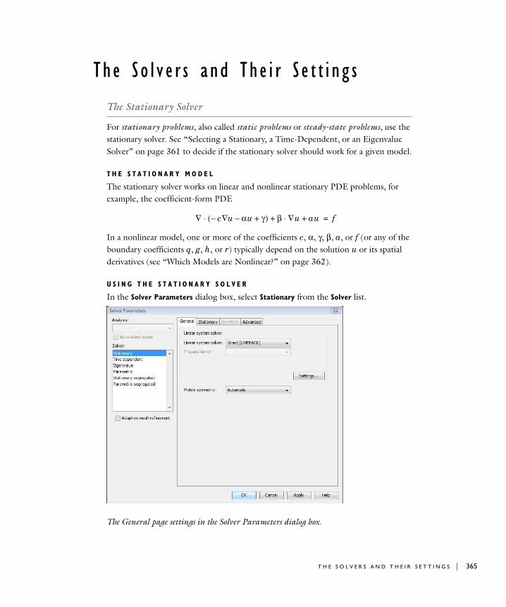
Th e S o l v e r s and Th e i r S e t t i n g s
The Stationary Solver
For stationary problems, also called static problems or steady-state problems, use the stationary solver. See “Selecting a Stationary, a Time-Dependent, or an Eigenvalue Solver” on page 361 to decide if the stationary solver should work for a given model.
T H E S T A T I O N A R Y M O D E L
The stationary solver works on linear and nonlinear stationary PDE problems, for example, the coefficient-form PDE
In a nonlinear model, one or more of the coefficients c, α, γ, β, a, or f (or any of the boundary coefficients q, g, h, or r) typically depend on the solution u or its spatial derivatives (see “Which Models are Nonlinear?” on page 362).
U S I N G T H E S T A T I O N A R Y S O L V E R
In the Solver Parameters dialog box, select Stationary from the Solver list.
The General page settings in the Solver Parameters dialog box.
∇ c u∇– αu– γ+( )⋅ β ∇u au+⋅+ f=
T H E S O L V E R S A N D T H E I R S E T T I N G S | 365
366 | C H A P T E
The choice of analysis type sets up a default for the linear system solver. The section “Selecting a Linear System Solver” on page 392 describes how to override the default settings. For the iterative linear solvers you can also select a preconditioner.
The stationary solver normally chooses a linear or nonlinear solver depending on the linearity of the model, but it is possible to override the automatic selection (see “Linear Solvers vs. Nonlinear Solvers” on page 362).
T H E L I N E A R O R L I N E A R I Z E D M O D E L
If a model is nonlinear, the linear solver solves the corresponding linearized model. In other words, the software approximates the nonlinear model with a linear model, and the approximation is valid when the solution is near the linearization point. The linearization point is a given solution that you specify in the Solver Manager. As the linearization point you can use the initial value, the current solution, the stored solution, or zero (see “The Solver Manager and Solver Scripting” on page 401).
If the software solves the model in the general form (by choosing the general solution form), the linearized model is
where , and u0 is the linearization point. The coefficients
are evaluated for u = u0. The meaning of these derivatives becomes clearer with indices:
∇ c u∇– αu– γ+( )⋅ β ∇u au+⋅+ f= in Ω
n c u αu γ–+∇( )⋅ qu = g hTµ–+ on Ω∂
hu r= on Ω∂⎩⎪⎪⎨⎪⎪⎧
u u u0–=
cu∇∂
∂Γ–=
f F=
αu∂
∂Γ–=
qu∂
∂G–=
γ Γ=
g G=
βu∇∂
∂F–=
hu∂
∂R–=
au∂
∂F–=
r R=
clkji
xi∂∂uk
⎝ ⎠⎜ ⎟⎛ ⎞
∂
∂Γlj–=
alk uk∂∂Fl–=
αlkj uk∂∂Γlj–=
qlk uk∂∂Gl–=
βlkj
xj∂∂uk
⎝ ⎠⎜ ⎟⎛ ⎞
∂
∂Fl–=
hmk uk∂∂Rm–=
R 6 : S O L V I N G T H E M O D E L
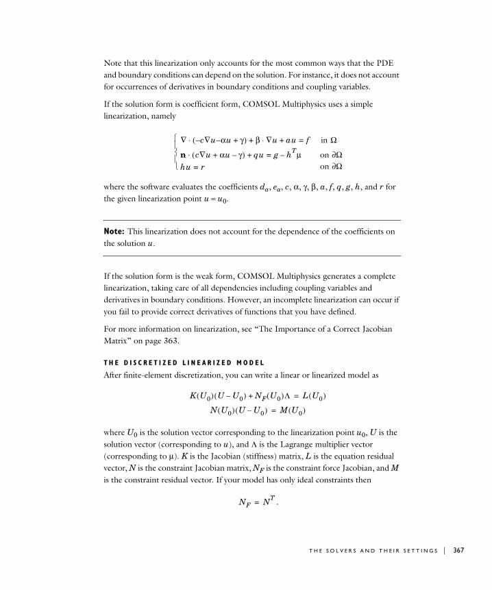
Note that this linearization only accounts for the most common ways that the PDE and boundary conditions can depend on the solution. For instance, it does not account for occurrences of derivatives in boundary conditions and coupling variables.
If the solution form is coefficient form, COMSOL Multiphysics uses a simple linearization, namely
where the software evaluates the coefficients da, ea, c, α, γ, β, a, f, q, g, h, and r for the given linearization point u = u0.
Note: This linearization does not account for the dependence of the coefficients on the solution u.
If the solution form is the weak form, COMSOL Multiphysics generates a complete linearization, taking care of all dependencies including coupling variables and derivatives in boundary conditions. However, an incomplete linearization can occur if you fail to provide correct derivatives of functions that you have defined.
For more information on linearization, see “The Importance of a Correct Jacobian Matrix” on page 363.
T H E D I S C R E T I Z E D L I N E A R I Z E D M O D E L
After finite-element discretization, you can write a linear or linearized model as
where U0 is the solution vector corresponding to the linearization point u0, U is the solution vector (corresponding to u), and Λ is the Lagrange multiplier vector (corresponding to µ). K is the Jacobian (stiffness) matrix, L is the equation residual vector, N is the constraint Jacobian matrix, NF is the constraint force Jacobian, and M is the constraint residual vector. If your model has only ideal constraints then
.
∇ c– ∇u α– u γ+( )⋅ β ∇u⋅ au+ + f= in Ω
n c∇u αu γ–+( )⋅ qu+ g hTµ–= on Ω∂hu r= on Ω∂⎩
⎪⎨⎪⎧
K U0( ) U U0–( ) NF U0( )Λ+ L U0( )=
N U0( ) U U0–( ) M U0( )=
NF NT=
T H E S O L V E R S A N D T H E I R S E T T I N G S | 367
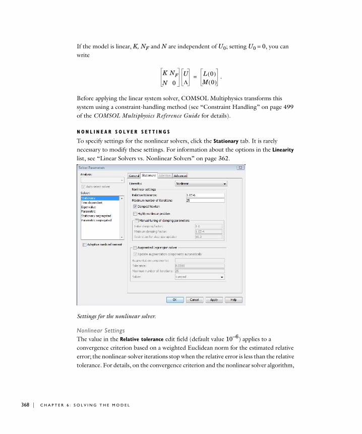
368 | C H A P T E
If the model is linear, K, NF and N are independent of U0; setting U0 = 0, you can write
.
Before applying the linear system solver, COMSOL Multiphysics transforms this system using a constraint-handling method (see “Constraint Handling” on page 499 of the COMSOL Multiphysics Reference Guide for details).
N O N L I N E A R S O L V E R S E T T I N G S
To specify settings for the nonlinear solvers, click the Stationary tab. It is rarely necessary to modify these settings. For information about the options in the Linearity list, see “Linear Solvers vs. Nonlinear Solvers” on page 362.
Settings for the nonlinear solver.
Nonlinear SettingsThe value in the Relative tolerance edit field (default value 10−6) applies to a convergence criterion based on a weighted Euclidean norm for the estimated relative error; the nonlinear-solver iterations stop when the relative error is less than the relative tolerance. For details, on the convergence criterion and the nonlinear solver algorithm,
K NF
N 0
UΛ
L 0( )M 0( )
=
R 6 : S O L V I N G T H E M O D E L

see “The Nonlinear Solver Algorithm” on page 501 of the COMSOL Multiphysics Reference Guide).
The value in the Maximum number of iterations edit field limits the number of nonlinear iterations (default = 25).
Normally, a damped Newton method is used. If you want the solver to always attempt to take full Newton steps, uncheck the Damped Newton check box.
If the problem is highly nonlinear, selecting the Highly nonlinear problem check box can help make the solver more careful. Try this option if the solver does not converge.
Manual Tuning of DampingTo tune the damping manually, select the Manual tuning of damping parameters check box.
The Minimum damping factor is a safeguard against perpetual Newton iterations. When the damping factor drops below the level specified in this edit field, the solver stops and issues the error message Failed to find a solution: No convergence, even when using
the minimum damping factor. Returned solution has not converged. The default value is 10−4 if the Highly nonlinear problem check box is cleared, otherwise it is 10−8.
The default value in the Initial damping factor edit field is 1 if the Highly nonlinear
problem check box is cleared or 10−4 if it is selected. The parameter in the Restriction
for stepsize update edit field (default = 10) sets a restriction for the damping-factor update in the Newton iteration. Each time the solver updates the damping factor, it can change up or down at most by this factor.
The Augmented Lagrangian solverIf you select the Augmented Lagrangian solver check box, the solving procedure is split into two substeps that the solver repeats until a convergence criterion is met or until the maximum number of iterations is reached. You control the splitting of the problem into substeps using the Augmentation components edit fields. The solver first computes the solution for the main components, which are the solution components that are not augmentation components, while keeping the augmentation components fixed. Then it solves for the augmentation components while keeping the main components fixed. This second solution step uses a linear solution approach. Therefore, with the main components fixed, the solver algorithm assumes that the augmentation components satisfy a linear equation. If you select the Update augmented components automatically check box, the application modes fill in these component names automatically.
T H E S O L V E R S A N D T H E I R S E T T I N G S | 369
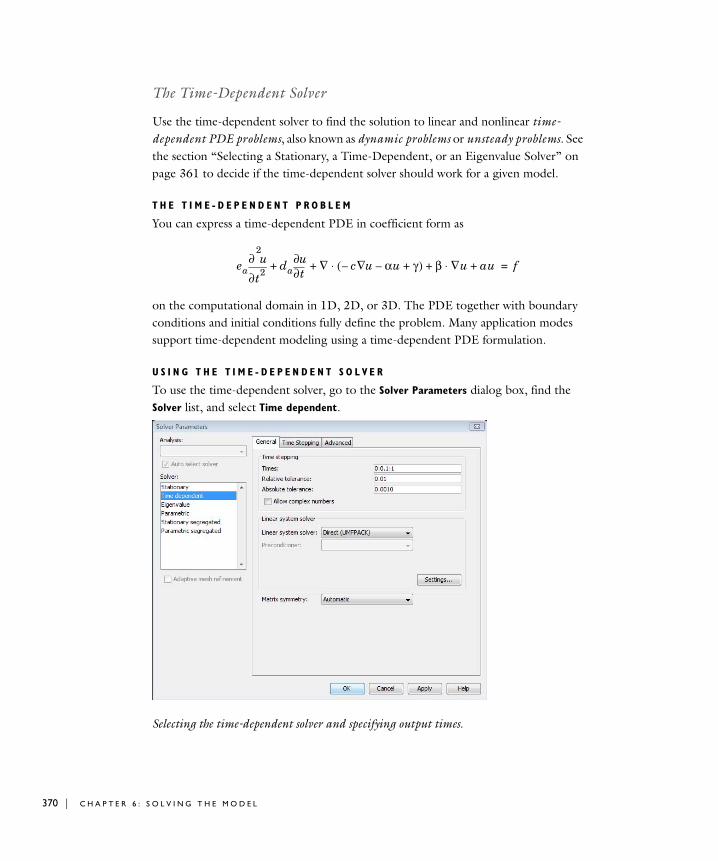
370 | C H A P T E
The Time-Dependent Solver
Use the time-dependent solver to find the solution to linear and nonlinear time-dependent PDE problems, also known as dynamic problems or unsteady problems. See the section “Selecting a Stationary, a Time-Dependent, or an Eigenvalue Solver” on page 361 to decide if the time-dependent solver should work for a given model.
T H E T I M E - D E P E N D E N T P R O B L E M
You can express a time-dependent PDE in coefficient form as
on the computational domain in 1D, 2D, or 3D. The PDE together with boundary conditions and initial conditions fully define the problem. Many application modes support time-dependent modeling using a time-dependent PDE formulation.
U S I N G T H E T I M E - D E P E N D E N T S O L V E R
To use the time-dependent solver, go to the Solver Parameters dialog box, find the Solver list, and select Time dependent.
Selecting the time-dependent solver and specifying output times.
eat2
2
∂∂ u da t∂
∂u ∇+ + c u∇– αu– γ+( )⋅ β ∇u au+⋅+ f=
R 6 : S O L V I N G T H E M O D E L
Specifying Output TimesIn the Time stepping area enter the output times in the Times edit field in the form of a vector of times at which you want the solution to the time-dependent model (for another option see “Setting the Time Steps for the Output and the Solver” on page 372). The syntax 0:0.1:1 represents a vector of times starting at 0 with steps of 0.1 up to 1. The relevant time span depends on the model’s dynamics.
Setting TolerancesIt is sometimes essential for accuracy or performance that you set absolute and relative tolerance parameters for the time-dependent solver. In the Relative tolerance edit field you enter a positive number (default = 0.01). In the Absolute tolerance edit field you enter a single positive number (default = 0.001) or a space-separated list whose entries alternate between degree-of-freedom names and positive scalars.
The absolute and relative tolerances control the error in each integration step. More specifically, let U be the solution vector corresponding to the solution at a certain time step, and let E be the solver’s estimate of the (local) error in U committed during this time step. The step is accepted if
where Ai is the absolute tolerance for DOF i, R is the relative tolerance, and N is the number of degrees of freedom. The accumulated (global) error can be larger than the sum of the local errors for all the integration steps. However, the solver’s error estimate is often too pessimistic, which means that the estimated local error typically is of the same order of magnitude as the true global error.
Note: If the solution is smaller than the absolute tolerance, there is no accuracy at all. Because the displacements in most structural-mechanics models are small, it is important to ensure that the absolute tolerance is smaller than the displacements.
Note: For DAEs (differential-algebraic equations), you can exclude the algebraic equations from the error estimation. See “Settings for Differential-Algebraic Equations” on page 374 for details.
1N----
Ei
Ai R Ui+--------------------------⎝ ⎠⎛ ⎞
2
i∑⎝ ⎠
⎜ ⎟⎛ ⎞ 1 2⁄
1<
T H E S O L V E R S A N D T H E I R S E T T I N G S | 371
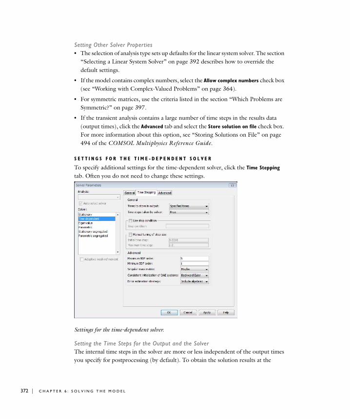
372 | C H A P T E
Setting Other Solver Properties• The selection of analysis type sets up defaults for the linear system solver. The section
“Selecting a Linear System Solver” on page 392 describes how to override the default settings.
• If the model contains complex numbers, select the Allow complex numbers check box (see “Working with Complex-Valued Problems” on page 364).
• For symmetric matrices, use the criteria listed in the section “Which Problems are Symmetric?” on page 397.
• If the transient analysis contains a large number of time steps in the results data (output times), click the Advanced tab and select the Store solution on file check box. For more information about this option, see “Storing Solutions on File” on page 494 of the COMSOL Multiphysics Reference Guide.
S E T T I N G S F O R T H E T I M E - D E P E N D E N T S O L V E R
To specify additional settings for the time-dependent solver, click the Time Stepping
tab. Often you do not need to change these settings.
Settings for the time-dependent solver.
Setting the Time Steps for the Output and the SolverThe internal time steps in the solver are more or less independent of the output times you specify for postprocessing (by default). To obtain the solution results at the
R 6 : S O L V I N G T H E M O D E L
internal time steps instead of the times in the Times edit field, go to the Times to store
in output list and select Time steps from solver. To view the time steps the solver takes, click the Log tab in the Progress window.
To control how the solver takes its internal time steps, select the appropriate option in the Time steps taken by solver list. For the Free option (the default) the solver chooses its time steps arbitrarily; in other words, it ignores the Times list when selecting them. For the Strict option, the solver must take a time step at each entry in the time list and it adds time steps in between as necessary. Use this feature when an equation involves impulses or irregularities that the time stepping must not skip over. Adding times around each impulse ensures that the solver can resolve them. For the Intermediate option, the solver must take at least one time step in each subinterval of the time list. This option is similar to Strict except it gives the solver somewhat more freedom and therefore is more efficient.
Selecting the Manual tuning of step size check box makes it possible to set the initial internal time step and an upper limit on the internal time steps.
Specifying a Stop ConditionYou can force the solver to stop based on a stop condition. To do so, select the Use stop
condition check box. The solver then stops before the expression in the Stop condition edit field becomes negative (the solver does not try to resolve the exact time for the zero crossing). The expression must be a scalar value that has no variation in space, typically a coupling variable with a global destination. For example, if you have defined an integration coupling variable utot that is the integral of the solution on the domain, typing 0.25-utot in the Stop condition edit field forces the solver to stop at the last time step before utot becomes larger than 0.25.
When using a deformed mesh with remeshing, the Moving Mesh (ALE) application mode provides a default expression that is the minimum quality of the deformed mesh minus 0.05 (see “Stop Condition” on page 406 in the COMSOL Multiphysics Modeling Guide).
Advanced Properties for the Time-Stepping AlgorithmIn the Advanced area you control additional settings for the time-stepping algorithm.
Order of the Time-Stepping Method Set the degree of the interpolating polynomial used in the time-stepping method (the backward differentiation formula, BDF) in the Maximum BDF order edit field. Supply an integer between 1 and 5 (the default). A smaller value results in a more stable numerical scheme. In wave-equation type problems, for example, decreasing the order to 2 often gives better results, because the
T H E S O L V E R S A N D T H E I R S E T T I N G S | 373
374 | C H A P T E
higher-order algorithms are only stable when the time step is small, while the order-2 algorithm is unconditionally stable. On the other hand, the low-order algorithms have more numerical damping than the higher-order algorithms. You can diminish the numerical damping by requiring the solver to take smaller time steps.
For some wave-equation type problems the solver will decrease the order of the BDF method at certain points of the simulation to an unnecessarily low order (typically from order 2 to order 1). In the Minimum BDF order edit field you can specify the lowest order the solver is allowed to use. Note that this minimum order does not apply to the start-up phase of the simulation, where the solver still will be allowed to use any order.
Settings for Differential-Algebraic Equations By default, the solver determines whether a system is differential algebraic (see “Differential-Algebraic Problems” on page 375) by looking for zero-filled rows or columns in the mass matrix (this corresponds to Maybe in the Singular mass matrix list). If the model includes a differential-algebraic equation (DAE) where the mass matrix has no zero-filled rows or columns, select Yes in the Singular mass matrix list.
A system of DAEs implies some constraints on the initial values, for instance, that a stationary (algebraic) equation must be satisfied. By default the solver perturbs the given initial values so that they become consistent with these constraints. For instance, you need not specify the correct initial value for the pressure in a Navier-Stokes model; the solver computes it automatically. The selection in the Consistent initialization of DAE
systems list controls how the solver perturbs the initial values:
• Select Backward Euler (the default) for index-1 and index-2 DAEs. The solver perturbs the initial values of all DOFs by taking a backward Euler step, giving a small perturbation to the differential DOFs.
• Select On for index-1 DAEs. The solver fixes the values of the differential DOFs (to those given by the initial value), and then it solves for the initial values of the algebraic DOFs and the time derivative of the differential DOFs. When applicable, this choice is preferable to Backward Euler because it does not perturb the values of the differential DOFs.
• Select Off to indicate that the initial values already are consistent, which means that the solver does not modify them. This is option is seldom useful.
For a DAE system, selecting Exclude algebraic from the Error estimation strategy list excludes the algebraic DOFs from the error norm when computing the time discretization error. For instance, the accuracy in the pressure in a Navier-Stokes model is sometimes not important. Using this option often results in a quicker time stepping.
R 6 : S O L V I N G T H E M O D E L
Manual Control of Reassembly If your model uses periodic boundary conditions, identity conditions, or coupling variables, you might be able to speed up the solving process by doing some manual tuning of the reassembly options; see “Manual Control of Reassembly” on page 496 of the COMSOL Multiphysics Reference Guide for more information.
D I F F E R E N T I A L - A L G E B R A I C P R O B L E M S
The system
(6-1)
is an example of a differential-algebraic system (DAE). The first equation is a differential equation, while the second is an algebraic relationship. You can derive a corresponding ODE system by differentiating the second equation with respect to t:
. (6-2)
Substituting the first equation in Equation 6-1 into Equation 6-2 leads to
,
which together with the first equation forms a system of ODEs. The variable v is of index 1 because it is necessary to differentiate the second equation one time to get an expression for the derivative of v. The variable u is of index 0 because you already have an equation for its derivative from the start.
If a system of PDEs contains both dynamic PDEs (with time derivatives) and stationary PDEs (without time derivatives), the corresponding space-discretized system is a DAE system. In other words, the mass matrix is singular because it contains zero-filled rows. For instance, the incompressible Navier-Stokes equations
t∂∂u v=
u2 v2+ 1=
2ut∂
∂u 2vt∂
∂v+ 0=
t∂∂v u–=
t∂∂u u
x∂∂u v
y∂∂u u
x∂∂p
+∆–+ + 0=
t∂∂v u
x∂∂v v
y∂∂v v
y∂∂p
+∆–+ + 0=
x∂∂u
y∂∂v
+ 0=
T H E S O L V E R S A N D T H E I R S E T T I N G S | 375
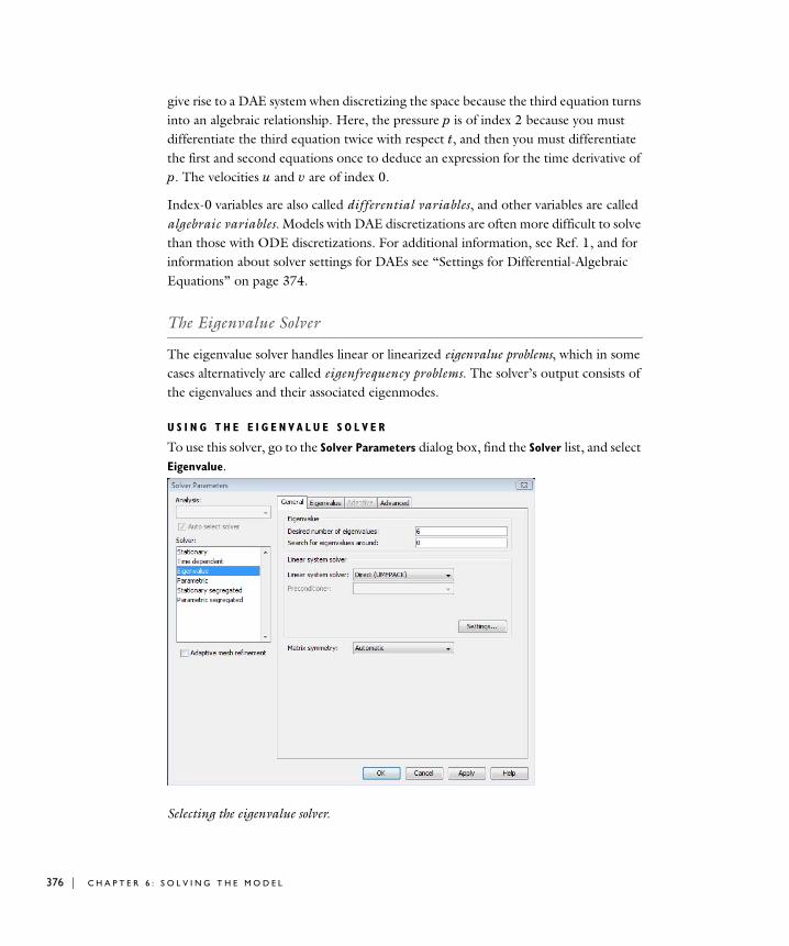
376 | C H A P T E
give rise to a DAE system when discretizing the space because the third equation turns into an algebraic relationship. Here, the pressure p is of index 2 because you must differentiate the third equation twice with respect t, and then you must differentiate the first and second equations once to deduce an expression for the time derivative of p. The velocities u and v are of index 0.
Index-0 variables are also called differential variables, and other variables are called algebraic variables. Models with DAE discretizations are often more difficult to solve than those with ODE discretizations. For additional information, see Ref. 1, and for information about solver settings for DAEs see “Settings for Differential-Algebraic Equations” on page 374.
The Eigenvalue Solver
The eigenvalue solver handles linear or linearized eigenvalue problems, which in some cases alternatively are called eigenfrequency problems. The solver’s output consists of the eigenvalues and their associated eigenmodes.
U S I N G T H E E I G E N V A L U E S O L V E R
To use this solver, go to the Solver Parameters dialog box, find the Solver list, and select Eigenvalue.
Selecting the eigenvalue solver.
R 6 : S O L V I N G T H E M O D E L
Enter the number of eigenvalues COMSOL Multiphysics should compute in the Desired number of eigenvalues edit field (default = 6).
Specify where to look for the desired eigenvalues in the Search for eigenvalues around
edit field. This value is often called the shift. Enter a real or complex scalar; the default value is 0, meaning that the solver tries to find eigenvalues close to 0. Often, but not always, the solver finds the desired number of eigenvalues that are closest to the shift. For example, for the default settings the solver tries to find the 6 smallest eigenvalues. Occasionally, the solver instead finds the 5 smallest eigenvalues and the seventh smallest eigenvalue. To find all the 6 smallest eigenvalues, increase the desired number of eigenvalues to 8, for instance.
Note: The eigenvalue algorithm does not work reliably when the value in the Search
for eigenvalues around edit field is equal to an eigenvalue.
Setting General Solver Properties• The selection of analysis type sets up a default for the linear system solver. The
section “Selecting a Linear System Solver” on page 392 describes how to override the default settings.
• For symmetric matrices, use the criteria given in the section “Which Problems are Symmetric?” on page 397.
• If the eigenvalue model is obtained as the linearization of a nonlinear model, specify the linearization point in the Solver Manager (see “Choosing the Values of Variables Not Solved For” on page 403 and “The Linear or Linearized Model” on page 366).
Normalization of the EigensolutionsYou can multiply a solution to an eigenvalue problem with an arbitrary nonzero number and still have an eigensolution. COMSOL Multiphysics normalizes the eigensolutions so that their discrete root-mean-square norm is 1, that is,
where Ui are the degrees of freedom solved for.
1N---- Ui
2
i 1=
N
∑ 1=
T H E S O L V E R S A N D T H E I R S E T T I N G S | 377
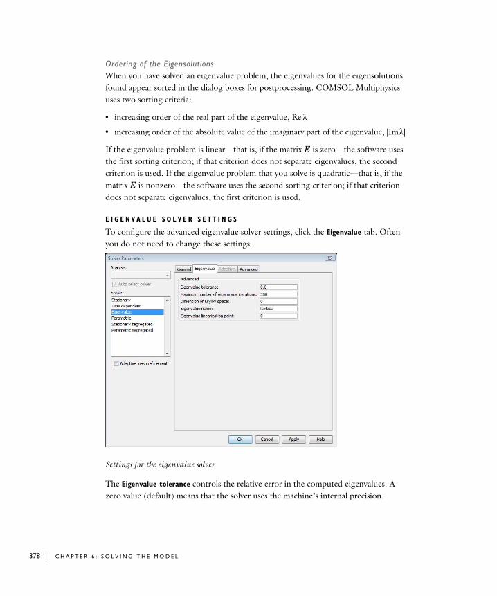
378 | C H A P T E
Ordering of the EigensolutionsWhen you have solved an eigenvalue problem, the eigenvalues for the eigensolutions found appear sorted in the dialog boxes for postprocessing. COMSOL Multiphysics uses two sorting criteria:
• increasing order of the real part of the eigenvalue, Re λ
• increasing order of the absolute value of the imaginary part of the eigenvalue, |Im λ|
If the eigenvalue problem is linear—that is, if the matrix E is zero—the software uses the first sorting criterion; if that criterion does not separate eigenvalues, the second criterion is used. If the eigenvalue problem that you solve is quadratic—that is, if the matrix E is nonzero—the software uses the second sorting criterion; if that criterion does not separate eigenvalues, the first criterion is used.
E I G E N V A L U E S O L V E R S E T T I N G S
To configure the advanced eigenvalue solver settings, click the Eigenvalue tab. Often you do not need to change these settings.
Settings for the eigenvalue solver.
The Eigenvalue tolerance controls the relative error in the computed eigenvalues. A zero value (default) means that the solver uses the machine’s internal precision.
R 6 : S O L V I N G T H E M O D E L
The eigenvalue solver is an iterative algorithm. The value in the Maximum number of
eigenvalue iterations edit field limits the number of iterations (default = 300).
The Dimension of Krylov space edit field controls the algorithm’s memory use. The default value of 0 means that the solver sets the dimension of the Krylov space to approximately twice the number of eigenvalues.
By default, the name of the eigenvalue is lambda when it appears in equations and postprocessing expressions. You can change this name in the Eigenvalue name edit field. The change affects both the interpretation of equations and the name of the eigenvalue in postprocessing.
Note: All application modes that use the eigenvalue explicitly in their equations expect the name of the eigenvalue to be lambda. Changing the name in the Solver
Settings dialog box does not update the application mode equations.
COMSOL Multiphysics reduces general nonlinear eigenvalue problems to a quadratic approximation around the value specified in the Eigenvalue linearization point field. The shift specified in the Search for eigenvalues around field is compensated accordingly. Therefore, changing the linearization point has no effect at all for linear or quadratic eigenvalue problems.
Eigenfrequencies vs. EigenvaluesFor many applications the eigenfrequency, f—or the corresponding angular frequency, ω—is a more interesting quantity than the eigenvalue, λ. Typically, these quantities are related as
In some application modes you can select whether to work with eigenvalues or eigenfrequencies, and sometimes also angular frequencies.
The Eigenvalue Solver AlgorithmFor a description of the algorithm used by the eigenvalue solver, see “The Eigenvalue Solver Algorithm” on page 503 in the COMSOL Multiphysics Reference Guide.
The Parametric Solver
Use the parametric solver to find the solution to a sequence of linear or nonlinear stationary PDE problems that arise when you vary a parameter of interest. The
ω 2πf iλ= =
T H E S O L V E R S A N D T H E I R S E T T I N G S | 379

380 | C H A P T E
parametric solver can also prove useful when it is difficult to get convergence in a nonlinear model. You can then introduce a parameter such that the solution is easy if the parameter is small; then, to obtain the solution for the desired value of the parameter, slowly increase its value, giving the nonlinear solver a good initial guess based on the solution for the previous parameter value. The parametric solver is sometimes called a continuation method or a path-following method. See the section “Selecting a Stationary, a Time-Dependent, or an Eigenvalue Solver” on page 361 to decide if the parametric solver should work for a given model.
U S I N G T H E P A R A M E T R I C S O L V E R S
To use the parametric solver, go to the Solver Parameters dialog box and select Parametric from the Solver list.
Selecting the parametric solver.
Specifying the Parameter and Its ValuesSpecify the parameter to vary in the Parameter name edit field. This parameter can occur in equations, constraints, or expressions.
R 6 : S O L V I N G T H E M O D E L
Note: You cannot vary parameters that control the geometry, mesh, or initial values through the parametric solver. To vary a geometric parameter, use the Parameterized Geometry application mode (in 2D) or use scripting to vary the geometry and compute the solution in a loop.
The list you enter in the Parameter values edit field consists of a vector of increasing or decreasing real values (for example, 0:0.1:1.5 or linspace(1,100,25)); see “Entering Vector-Valued Expressions” on page 145 for more information on how to enter a vector of values. If you have already given the parameter a value in the Constants dialog box, COMSOL Multiphysics overwrites its value using the values in this list when using the parametric solver. If you supply more than two parameter values, the solver computes solutions for all of them. The algorithm also solves for intermediate parameter values if necessary for convergence (these intermediate solutions do not appear in the output). If you supply exactly two values, the output also contains the solutions for all intermediate parameter values the solver finds.
Setting Other Solver Properties• The selection of analysis type sets up a default for the linear system solver. The
section “Selecting a Linear System Solver” on page 392 describes how to override the default settings.
• For symmetric matrices, use the criteria from the section “Which Problems are Symmetric?” on page 397.
• When using the parametric solver for a nonlinear model, you can tune the nonlinear solver settings on the Stationary page (see “Nonlinear Solver Settings” on page 368).
• If the parametric analysis contains a large number of parameter steps in the results data, click the Advanced tab and select the Store solution on file check box. For more information about this option, see “Storing Solutions on File” on page 494 of the COMSOL Multiphysics Reference Guide.
T H E S O L V E R S A N D T H E I R S E T T I N G S | 381
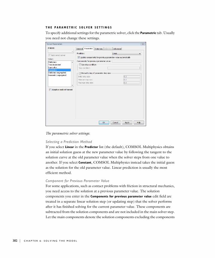
382 | C H A P T E
T H E P A R A M E T R I C S O L V E R S E T T I N G S
To specify additional settings for the parametric solver, click the Parametric tab. Usually you need not change these settings.
The parametric solver settings.
Selecting a Prediction MethodIf you select Linear in the Predictor list (the default), COMSOL Multiphysics obtains an initial solution guess at the new parameter value by following the tangent to the solution curve at the old parameter value when the solver steps from one value to another. If you select Constant, COMSOL Multiphysics instead takes the initial guess as the solution for the old parameter value. Linear prediction is usually the most efficient method.
Component for Previous Parameter ValueFor some applications, such as contact problems with friction in structural mechanics, you need access to the solution at a previous parameter value. The solution components you enter in the Components for previous parameter value edit field are treated in a separate linear solution step (or updating step) that the solver performs after it has finished solving for the current parameter value. These components are subtracted from the solution components and are not included in the main solver step. Let the main components denote the solution components excluding the components
R 6 : S O L V I N G T H E M O D E L
from previous step, and let pi denote the parameter value in the parameter step i. Then the following algorithm describes the procedure:
1 Set i = 1. Initialize all the solution components.
2 Solve for the main components and the parameter value, pi, while keeping the components from previous step fixed.
3 Make a linear solve for the components from the previous step, while keeping the main components fixed.
4 If pi is the last parameter, the procedure is complete, else let i = i + 1 and go to Step 2.
The linear system solver used in the linear solver (Step 3) is UMFPACK.
If you select the Update components for previous parameter value automatically check box, the application modes fill in these components automatically. For applications in contact modeling, see the Structural Mechanics Module User’s Guide.
Note: Entering variables in the Components for previous parameter value edit field does not formulate an updating equation. You must formulate the updating equations in the standard way through the application modes.
Specifying a Stop ConditionYou can force the solver to stop based on a stop condition. To do so, select the Use stop
condition check box. The solver then stops before the expression in the Stop condition edit field becomes negative. For more information, see “Specifying a Stop Condition” on page 373 in the section about the time-dependent solver.
Manual Tuning of the Parameter Step SizeBy selecting the Manual tuning of parameter step size check box, you control how many intermediate parameter values the algorithm solves for:
• The value in the Initial step size edit field is a positive number that determines the magnitude of the first parameter step. The default value of 0 means that the initial step equals the difference between the two first values in the Parameter values edit field. If the initial time step is too big, the solver might not converge after the first step, and it gradually lowers the step size until it obtains convergence. On the other hand, if the initial step size is too small, the solver might take an unnecessarily large number of small parameter steps.
T H E S O L V E R S A N D T H E I R S E T T I N G S | 383
384 | C H A P T E
• The value in the Minimum step size edit field is a safeguard against parameter steps that are too small. The default value of 0 means that the minimum step size is 1/200 of the parameter span. If the nonlinear Newton iteration diverges for a certain parameter value, the software reduces the step size, but if it goes below the minimum step size, the solver terminates with a warning. In this case the solution process might have reached some kind of singularity (a turning point or bifurcation) beyond which the continuation of the solution does not exist or is non-unique.
• The value in the Maximum step size edit field is an upper bound on the parameter step size. The default value of 0 means that the maximum step size equals the parameter span. Decrease this value if you suspect that the solver takes unnecessarily long steps and thereby switches branches or misses a singularity (alternatively, use more parameter values in the Parameter values edit field).
The Parametric Solver AlgorithmSee the section “The Parametric Solver Algorithm” on page 504 of the COMSOL Multiphysics Reference Guide.
The Stationary Segregated Solver
Use the stationary segregated solver for linear or nonlinear stationary PDE problems when you want to split the solution steps into substeps. You define the different substeps by grouping solution components’ names together. In a solution step for a substep, the segregated solver uses the damped Newton method and computes only the Jacobian related to the solution components, a procedure that can save both memory and assembly time. Also, it is possible to choose which linear system solver to use in a substep independently from other substeps. For problems where a full Newton approach does not converge, a segregated solution approach can sometimes work well. On the other hand, in the vicinity of a solution where the Newton approach converges quadratically, the segregated solver approach often converges more slowly.
For an example of how to use the stationary segregated solver, see “Example: Resistive Heating” on page 334 of the COMSOL Multiphysics Modeling Guide. Some fluid-flow models in the Chemical Engineering Module also use the segregated solver.
R 6 : S O L V I N G T H E M O D E L
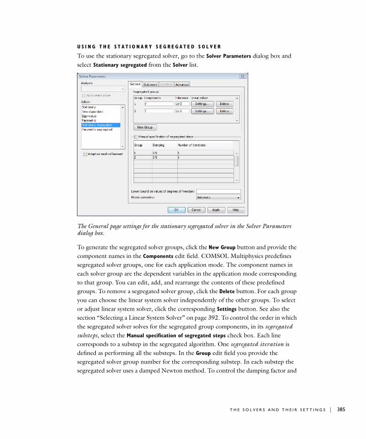
U S I N G T H E S T A T I O N A R Y S E G R E G A T E D S O L V E R
To use the stationary segregated solver, go to the Solver Parameters dialog box and select Stationary segregated from the Solver list.
The General page settings for the stationary segregated solver in the Solver Parameters dialog box.
To generate the segregated solver groups, click the New Group button and provide the component names in the Components edit field. COMSOL Multiphysics predefines segregated solver groups, one for each application mode. The component names in each solver group are the dependent variables in the application mode corresponding to that group. You can edit, add, and rearrange the contents of these predefined groups. To remove a segregated solver group, click the Delete button. For each group you can choose the linear system solver independently of the other groups. To select or adjust linear system solver, click the corresponding Settings button. See also the section “Selecting a Linear System Solver” on page 392. To control the order in which the segregated solver solves for the segregated group components, in its segregated substeps, select the Manual specification of segregated steps check box. Each line corresponds to a substep in the segregated algorithm. One segregated iteration is defined as performing all the substeps. In the Group edit field you provide the segregated solver group number for the corresponding substep. In each substep the segregated solver uses a damped Newton method. To control the damping factor and
T H E S O L V E R S A N D T H E I R S E T T I N G S | 385
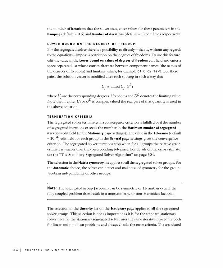
386 | C H A P T E
the number of iterations that the solver uses, enter values for these parameters in the Damping (default = 0.5) and Number of iterations (default = 1) edit fields respectively.
L O W E R B O U N D O N T H E D E G R E E S O F F R E E D O M
For the segregated solver there is a possibility to directly—that is, without any regards to the equations—impose a restriction on the degrees of freedoms. To use this feature, edit the value in the Lower bound on values of degrees of freedom edit field and enter a space-separated list whose entries alternate between component names (the names of the degrees of freedom) and limiting values, for example c1 0 c2 1e-3. For these pairs, the solution vector is modified after each substep in such a way that
where Uj are the corresponding degrees if freedoms and UL denotes the limiting value. Note that if either Uj or UL is complex valued the real part of that quantity is used in the above equation.
TE R M I N A T I O N C R I T E R I A
The segregated solver terminates if a convergence criterion is fulfilled or if the number of segregated iterations exceeds the number in the Maximum number of segregated
iterations edit field (in the Stationary page settings). The value in the Tolerance (default = 10−3) edit field for each group in the General page settings gives the convergence criterion. The segregated-solver iterations stop when for all groups the relative error estimate is smaller than the corresponding tolerance. For details on the error estimate, see the “The Stationary Segregated Solver Algorithm” on page 504.
The selection in the Matrix symmetry list applies to all the segregated solver groups. For the Automatic choice, the solver can detect and make use of symmetry for the group Jacobian independently of other groups.
Note: The segregated group Jacobians can be symmetric or Hermitian even if the fully coupled problem does result in a nonsymmetric or non-Hermitian Jacobian.
The selection in the Linearity list on the Stationary page applies to all the segregated solver groups. This selection is not as important as it is for the standard stationary solver because the stationary segregated solver uses the same iterative procedure both for linear and nonlinear problems and always checks the error criteria. The associated
Uj max Uj UL,( )=
R 6 : S O L V I N G T H E M O D E L
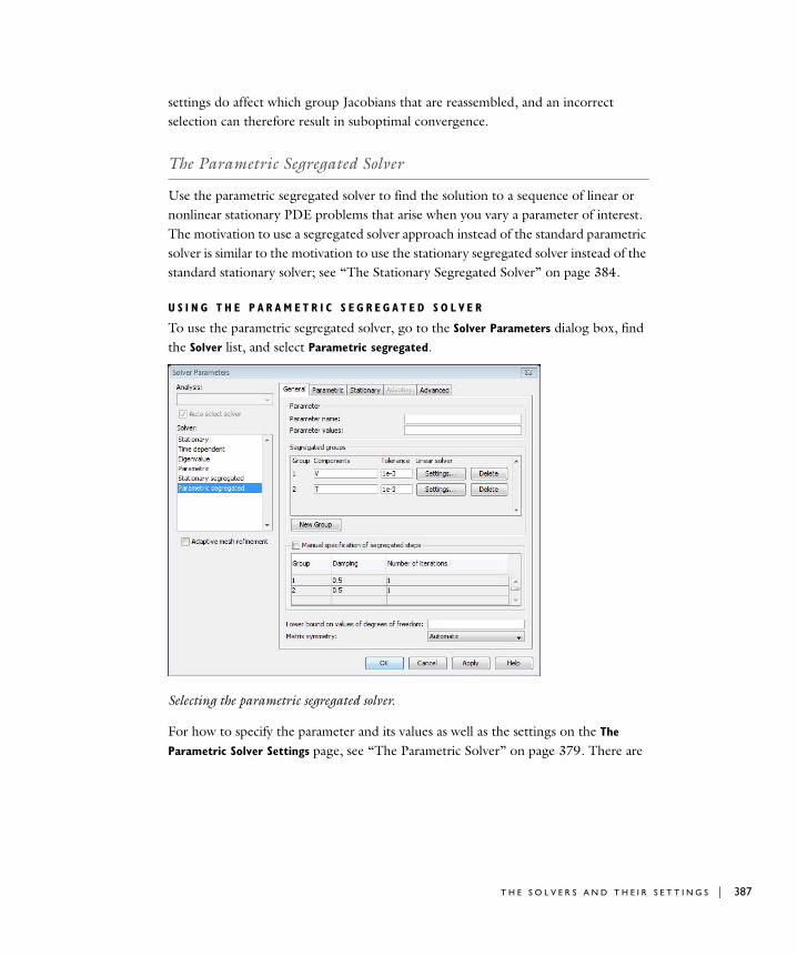
settings do affect which group Jacobians that are reassembled, and an incorrect selection can therefore result in suboptimal convergence.
The Parametric Segregated Solver
Use the parametric segregated solver to find the solution to a sequence of linear or nonlinear stationary PDE problems that arise when you vary a parameter of interest. The motivation to use a segregated solver approach instead of the standard parametric solver is similar to the motivation to use the stationary segregated solver instead of the standard stationary solver; see “The Stationary Segregated Solver” on page 384.
U S I N G T H E P A R A M E T R I C S E G R E G A T E D S O L V E R
To use the parametric segregated solver, go to the Solver Parameters dialog box, find the Solver list, and select Parametric segregated.
Selecting the parametric segregated solver.
For how to specify the parameter and its values as well as the settings on the The
Parametric Solver Settings page, see “The Parametric Solver” on page 379. There are
T H E S O L V E R S A N D T H E I R S E T T I N G S | 387

388 | C H A P T E
some minor differences between the parametric solver and the parametric segregated solver in the way COMSOL Multiphysics executes the parameter stepping:
• The parametric segregated solver can only fail for a parameter value when the segregated iteration number exceeds the value in the Maximum number of segregated
iterations edit field, whereas the standard parametric solver can also fail when the damping factor is too small. This can make the standard parametric solver more efficient for certain problems where there are several solver failures.
• After a successful step, the parametric solver chooses the next parameter step size based on the convergence speed of the Newton iteration. The parametric segregated solver uses a constant factor of 2 to increase the parameter step size.
Adaptive Mesh Refinement
When modeling, it is important to select a mesh that minimizes the errors in the quantities of interest. COMSOL Multiphysics provides several ways to set the mesh size manually (see the chapter “Meshing” on page 285). However, it is not easy to minimize the error in a desired quantity by manually specifying a mesh. In many applications, the algorithm must resolve the solution in great detail only on small portions of the domain (such as boundary layers, shocks, small geometrical details, or localized loads). For such situations, consider using adaptive mesh generation, which identifies the regions that require a high resolution and produces an appropriate mesh.
The adaptive solver works for linear and nonlinear stationary PDE problems (including parameter-dependent problems) and for eigenvalue PDE problems. It does not support quadrilateral, hexahedral (brick), or prism meshes. For models that include several geometries, COMSOL Multiphysics applies adaptive mesh generation to only one of them.
For a description of the algorithm on which adaptive mesh refinement in COMSOL Multiphysics is based, see the section “The Adaptive Solver Algorithm” on page 505 of the COMSOL Multiphysics Reference Guide.
U S I N G A D A P T I V E M E S H R E F I N E M E N T
To use adaptive mesh refinement, open the Solver Parameters dialog box and select the Adaptive mesh refinement check box. Adaptive mesh refinement works with all solvers except the time-dependent solver. After clicking Solve, the software returns with the adapted mesh and the corresponding solution (the original mesh disappears).
You can adjust the settings for adaptive mesh refinement on the Adaptive page.
R 6 : S O L V I N G T H E M O D E L
Note: The settings on the Adaptive page are with reference to the current mesh when you start the solver, if one exists. If no mesh exists when the solver starts, the software generates an initial mesh using the settings in the Free Mesh Parameters dialog box.
If your model contains more than one geometry, you can select the geometry for the adaptive solver from the Use adaptive mesh refinement in geometry list at the top of the page. The default setting is Current geometry.
Settings for adaptive mesh refinement.
In the Residual method list you can select the method to use when computing the PDE residual. This setting is included for possible backward compatibility issues, so for new models you can safely use the default method, Weak, which supports all solution forms. (The method Coefficient only supports the General and Coefficient solution forms; see the section “Solution Form” on page 494 of the COMSOL Multiphysics Reference Guide.)
The value in the Residual order edit field, a nonnegative integer, determines the order of decrease in equation residuals as the mesh size tends to zero (default = 0). You rarely need to modify this setting.
T H E S O L V E R S A N D T H E I R S E T T I N G S | 389
390 | C H A P T E
Terminating Adaptive Mesh GenerationThe adaptive solver terminates when it has obtained solutions for the number of refined meshes you specify in the Maximum number of refinements edit field. In 2D the default value is 2, which means that the software solves on the original mesh along with two refined meshes. In 3D the default value is 1, and in 1D it is 5. If the number of mesh elements exceeds the value specified in the Maximum number of elements edit field (default = 10,000,000), the solver terminates even if it has not reached the specified maximum number of refinements.
Adaptive Mesh Refinement MethodsThe refinement method determines how the algorithm refines the elements it selects on the basis of the settings in the Element selection method area. If you choose Longest from the Refinement method list (not available for 1D geometries), the adaptive solver refines only the longest edge of each selected element; if, instead, you select the option Regular (not available for 3D geometries), the solver refines these elements in a regular pattern. For both methods, some additional adjacent elements are refined to get a conformal mesh, that is, a mesh without hanging nodes. The default method in 2D is Longest. A third option, Meshinit, generates a completely new mesh where the mesh-element size at a particular location is roughly equal to that of the old mesh divided by a refinement factor determined by the settings in the Element selection method area.
Error Estimation SettingsFor eigenvalue problems, the error estimate is a weighted sum of the error estimates for the various eigenmodes. You can enter a space-separated list of positive weights in the Weights for eigenmodes edit field (only the relative weights matter). The default value of 1 means that all the weight is put on the first eigenmode.
COMSOL Multiphysics presently supports the L2 norm error estimate. You seldom need to change the associated settings in the L2 error norm area.
The Scaling factor edit field takes a space-separated list of scaling factors, one for each PDE in the system. When computing the local error estimate, the algorithm divides the error estimate for each PDE by the scaling factor before summing them. The default value of 1 means that all PDEs get the same weight in the error estimate.
The L2 norm error estimate is based on a stability estimate for the PDE. You can specify its order in the Stability estimate derivative order edit field (default = 2).
R 6 : S O L V I N G T H E M O D E L
Element Selection SettingsCOMSOL Multiphysics provides three ways to select which elements to refine; choose one of the following in the Element selection method list:
• Rough global minimum (the default) minimizes the error’s L2 norm by refining a fraction of the elements with the largest error in such a way that the total number of elements increases roughly by the factor specified in the Increase number of
elements by edit field. The default factor is 1.7, that is, a 70% increase. With this option, the software can refine some elements with a factor larger than 2.
• A fraction of worst error isolates those elements that have a local error indicator larger than a given fraction of the largest local error indicator. Enter this fraction in the Worst element fraction edit field (default = 0.5). The software refines the indicated elements just once.
• A fraction of elements refines a given fraction of the elements. Enter this fraction in the Element fraction edit field (default = 0.5). The software refines the selected elements just once.
Reference
1. E. Hairer and G. Wanner, Solving Ordinary Differential Equations II, Stiff and Differential-Algebraic Problems, Springer-Verlag, 1991.
T H E S O L V E R S A N D T H E I R S E T T I N G S | 391
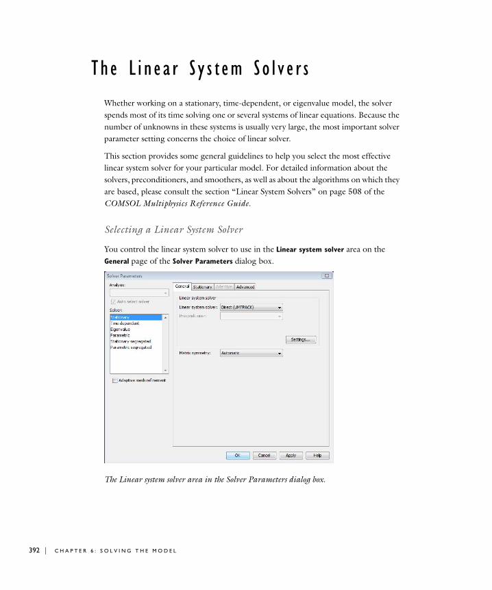
392 | C H A P T E
Th e L i n e a r S y s t em So l v e r s
Whether working on a stationary, time-dependent, or eigenvalue model, the solver spends most of its time solving one or several systems of linear equations. Because the number of unknowns in these systems is usually very large, the most important solver parameter setting concerns the choice of linear solver.
This section provides some general guidelines to help you select the most effective linear system solver for your particular model. For detailed information about the solvers, preconditioners, and smoothers, as well as about the algorithms on which they are based, please consult the section “Linear System Solvers” on page 508 of the COMSOL Multiphysics Reference Guide.
Selecting a Linear System Solver
You control the linear system solver to use in the Linear system solver area on the General page of the Solver Parameters dialog box.
The Linear system solver area in the Solver Parameters dialog box.
R 6 : S O L V I N G T H E M O D E L
In the Linear system solver list, you can choose between the following solvers, each of which is broadly categorized as direct or iterative:
T H E D I R E C T S O L V E R S
The direct solvers UMFPACK, SPOOLES, PARDISO, and TAUCS Cholesky are preferable for 1D and 2D models, and for 3D models with few degrees of freedom (roughly, fewer than 100,000). You can access the TAUCS solvers only if the selection in the Matrix symmetry list is Automatic (the default) and the software detects the problem as symmetric, or if you select one of the options Symmetric or Hermitian.
Note: PARDISO is available on Linux, Windows, and Intel Macs only. On Sun and PowerPC-based Macs, COMSOL Multiphysics switches to UMFPACK instead.
The direct solvers solve a linear system by Gaussian elimination. This stable and reliable process is well suited for ill-conditioned systems. In 1D and 2D, where a direct solver is the default setting, these solvers require less tuning and are often faster than the
LINEAR SYSTEM SOLVER USAGE
DIRECT SOLVERS
Direct (UMFPACK) A highly efficient direct solver for nonsymmetric systems
Direct (SPOOLES) An efficient direct solver for symmetric and nonsymmetric systems. It uses less memory than UMFPACK.
Direct (PARDISO) A highly efficient direct solver for symmetric and nonsymmetric systems. It often uses less memory than UMFPACK.
Direct Cholesky (TAUCS) An efficient direct solver for symmetric, positive-definite systems
ITERATIVE SOLVERS
GMRES An iterative solver for nonsymmetric problems
FGMRES An iterative solver for nonsymmetric problems. It can handle more general preconditioners, but it also uses more memory, than GMRES.
Conjugate gradients An iterative solver for symmetric positive definite problems
Geometric multigrid An iterative solver for elliptic or parabolic problems
T H E L I N E A R S Y S T E M S O L V E R S | 393
394 | C H A P T E
iterative solvers. The elimination process sometimes requires large memory resources and long computing times, an effect particularly noticeable for 3D models.
T H E I T E R A T I V E S O L V E R S
For models with many degrees of freedom (roughly, more than 100,000), the direct solvers typically need too much memory. In those cases, the more memory-efficient iterative solvers GMRES, FGMRES, Conjugate gradients, and Geometric multigrid perform better. However, iterative solvers are less stable than direct solvers in that they do not always converge (arrive at a solution). To improve the convergence of an iterative solver (except Geometric multigrid), it is important to select an appropriate preconditioner from the Preconditioner list that appears if you select an iterative solver. The default setting for 3D models calls on iterative solvers.
Linear System Solver Settings
Each linear solver has its own settings; to adjust them, click the Settings button to launch the Linear System Solver Settings dialog box. In this dialog box you can choose from a larger set of linear system solvers and preconditioners. However, the most appropriate solvers and preconditioners are all available in the Linear system solver area on the General page of the Solver Parameters dialog box. For the multigrid solvers/preconditioners it is also possible to select the smoothers and the coarse solver.
Linear System Solver Selection Guidelines
The ruling application mode selects a default linear system solver that usually is appropriate for the problem type, at least for single-physics models. If the default solver does not perform well, review the following guidelines to choose linear system solver.
1 Try the UMFPACK direct solver.
2 If the UMFPACK solver runs out of memory or slows down due to swapping during the matrix-factorization phase, try the PARDISO or SPOOLES direct solver. They often use less memory but are less stable. SPOOLES is also slower.
3 If the system is real symmetric or complex Hermitian (see “Which Problems are Symmetric?” on page 397), try the SPOOLES direct solver, which then saves half the memory because it stores only the upper triangular part of the matrix. If, in addition, the system is positive definite (see “Which Models Are Positive Definite?” on page 399), try the TAUCS Cholesky direct solver.
4 If the system is complex symmetric try the SPOOLES direct solver.
R 6 : S O L V I N G T H E M O D E L
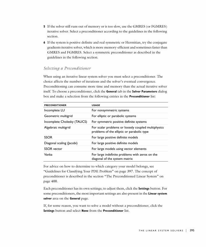
5 If the solver still runs out of memory or is too slow, use the GMRES (or FGMRES) iterative solver. Select a preconditioner according to the guidelines in the following section.
6 If the system is positive definite and real symmetric or Hermitian, try the conjugate gradients iterative solver, which is more memory-efficient and sometimes faster than GMRES and FGMRES. Select a symmetric preconditioner as described in the guidelines in the following section.
Selecting a Preconditioner
When using an iterative linear system solver you must select a preconditioner. The choice affects the number of iterations and the solver’s eventual convergence. Preconditioning can consume more time and memory than the actual iterative solver itself. To choose a preconditioner, click the General tab in the Solver Parameters dialog box and make a selection from the following entries in the Preconditioner list:
For advice on how to determine to which category your model belongs, see “Guidelines for Classifying Your PDE Problem” on page 397. The concept of preconditioner is described in the section “The Preconditioned Linear System” on page 400.
Each preconditioner has its own settings; to adjust them, click the Settings button. For some preconditioners, the most important settings are also present in the Linear system
solver area on the General page.
If, for some reason, you want to solve a model without a preconditioner, click the Settings button and select None from the Preconditioner list.
PRECONDITIONER USAGE
Incomplete LU For nonsymmetric systems
Geometric multigrid For elliptic or parabolic systems
Incomplete Cholesky (TAUCS) For symmetric positive definite systems
Algebraic multigrid For scalar problems or loosely coupled multiphysics problems of the elliptic or parabolic type
SSOR For large positive definite models
Diagonal scaling (Jacobi) For large positive definite models
SSOR vector For large models using vector elements
Vanka For large indefinite problems with zeros on the diagonal of the system matrix
T H E L I N E A R S Y S T E M S O L V E R S | 395
396 | C H A P T E
The Incomplete LU preconditioner works in a more general context than the others, but it might be impractical owing to its time and memory requirements; when they work, the multigrid preconditioners are always preferable. The TAUCS incomplete Cholesky preconditioner is a more memory-efficient version of the Incomplete LU preconditioner for symmetric positive definite matrices. The SSOR and diagonal-scaling preconditioners use less time and memory but only ensure convergence of the iterative solver for positive definite problems.
For detailed descriptions of the individual preconditioners, consult “Preconditioners for the Iterative Solvers” on page 516 of the COMSOL Multiphysics Reference Guide.
Preconditioner Selection Guidelines
The ruling application mode selects a default preconditioner that is usually appropriate for the problem type, at least for single-physics models. If the default does not perform well, select another one using the following guidelines:
1 Try the Incomplete LU preconditioner, which works for all linear systems. However, it requires the tuning of the drop tolerance; it can run out of memory; and in many cases it is not the most efficient preconditioner.
2 If the system is elliptic or parabolic (see “Elliptic and Parabolic Models” on page 400) use the Geometric multigrid preconditioner.
3 If, in addition, the system is a real-valued PDE for a single solution component (that is, a scalar problem) you can alternatively try the Algebraic multigrid preconditioner.
4 If the system is symmetric positive definite (see “Which Models Are Positive Definite?” on page 399) you can try the TAUCS incomplete Cholesky preconditioner. However, in this case Geometric multigrid likely performs better.
5 If the system is positive definite but so large that the other preconditioners run out of memory, try the SSOR or Diagonal scaling (Jacobi) preconditioners.
6 If you solve an electromagnetics problem using vector elements for a PDE containing the curl-curl operator, try the geometric multigrid preconditioner with the SOR vector presmoother and the SORU vector postsmoother, or try the SSOR vector preconditioner.
7 If you solve an indefinite problem with zeros on the diagonal of the system matrix, such as the Navier-Stokes equations, try the Vanka preconditioner or the Geometric multigrid preconditioner with Vanka or Incomplete LU as the smoother.
The Incomplete LU preconditioner and sometimes the multigrid preconditioners require some tuning to get fast convergence without running out of memory (see the
R 6 : S O L V I N G T H E M O D E L
appropriate sections in the following pages).
Guidelines for Classifying Your PDE Problem
W H I C H P R O B L E M S A R E S Y M M E T R I C ?
When the discretization of a PDE problem results in a symmetric Jacobian (stiffness) matrix (and a symmetric mass matrix for time-dependent or eigenvalue problems), you can often apply faster and less memory-consuming algorithms to solve the resulting linear systems. PDE problems with symmetric discretizations typically occur in models involving acoustics, diffusion, electromagnetics, heat transfer by conduction, and structural mechanics. In contrast, problems in fluid mechanics, convection-diffusion, and convection-conduction typically involve nonsymmetric Jacobian matrices.
If the model involves complex numbers you can distinguish between symmetric and Hermitian matrices. A Hermitian matrix A satisfies where T denotes the transpose and the bar denotes the complex conjugate.
COMSOL Multiphysics detects symmetry automatically for both symmetric and Hermitian matrices, so all you need to do to take advantage of the computational savings for a model with a symmetric matrix is to use a solver that utilizes the symmetry. The following linear system solvers and preconditioners do not take advantage of symmetric (or Hermitian) matrices:
• The UMFPACK direct solver
• The Vanka preconditioner
• The Incomplete LU preconditioner
• The algebraic multigrid solver/preconditioner
If you select the Use Hermitian transpose of constraint matrix and in symmetry detection
check box on the Advanced page, the automatic symmetry detection checks if the matrices are Hermitian. If the matrices are symmetric or Hermitian, the solver prints this information in the Solver log, and if the linear solver can take advantage of symmetric or Hermitian matrices, the storage format for the matrices changes. If you use a solver that cannot take advantage of the symmetry, the Solver log contains a warning.
If you want to override the automatic symmetry detection, go to the Solver Parameters dialog box, click the General tab, and select Symmetric, Hermitian, or Nonsymmetric
from the Matrix symmetry list.
AT
A=
T H E L I N E A R S Y S T E M S O L V E R S | 397
398 | C H A P T E
Note: In general, models with multiphysics couplings create nonsymmetric matrices, and selecting Symmetric then leads to an incorrect solution. In some cases, you can exploit the symmetry in the single-physics parts by using a sequential solution process, solving for one physics at the time.
Symmetry CriterionIf COMSOL Multiphysics solves a model using the general or coefficient solution form and the equations have no weak-form contributions, the following criterion determines whether the matrix is symmetric or not: Inspect the coefficients c, α, β, and a in the Equation System>Subdomain Settings dialog box and the coefficient q in the Equation System>Boundary Settings dialog box. The matrix is symmetric if
.
The indices k and l refer to the rows and columns in the equation system, while the indices i and j refer to the space coordinates and their corresponding derivatives (see “The Linear or Linearized Model” on page 366). Further, the matrix is Hermitian if
.
Symmetry DetectionCOMSOL Multiphysics performs symmetry detection numerically. It detects a problem as symmetric if, for all matrices A = Aij involved (stiffness matrix, mass matrix, and so on), it holds that
where εs is a symmetry tolerance. Similarly, the software detects a problem as Hermitian if, for all matrices A = Aij involved, it holds that
and
The symmetry tolerance εs is per default 10−10.
clkji cklij αlkj, βklj alk, akl qlk, qkl= = = =
clkji cklij αlkj, βklj alk, akl qlk, qkl= = = =
Aij Aji– εs Aij2 Aii Ajj+≤ for all i j≠
Aij Aji– εs Aij2 Aii Ajj+≤ for all i j≠
ImAii εs Aii≤ for all i
R 6 : S O L V I N G T H E M O D E L
W H I C H M O D E L S A R E P O S I T I V E D E F I N I T E ?
A model with a real symmetric or Hermitian system matrix is often also positive definite, which means that a number of efficient linear system solvers are applicable:
• The TAUCS Cholesky direct solver
• The Conjugate gradients iterative solver
• The TAUCS incomplete Cholesky preconditioner
Further, the simple preconditioners SSOR, SOR, SORU, diagonal scaling (Jacobi), and the multigrid solvers benefit from a positive definite matrix. A real symmetric or Hermitian matrix is positive definite if all its eigenvalues are positive.
For stationary problems, the system matrix is the Jacobian (stiffness) matrix A. This means that stationary models in diffusion, electromagnetics, heat transfer by conduction, and structural mechanics usually have a positive definite system matrix.
For time-dependent problems, the system matrix is of the form A + σB + σ2C, where B is the damping matrix, C is the mass matrix, and σ > 0 is inversely proportional to the time step (if C = 0, then B is often called the mass matrix). Because these matrices are often positive definite, time-dependent models in diffusion, electromagnetics, structural mechanics, and heat transfer by conduction usually have a positive definite system matrix.
For eigenvalue problems, the system matrix is of the form A − σB + σ2C, where σ is the shift, that is, the number around which the software searches for eigenvalues (specified in the Search for eigenvalues around edit field on the General tab of the Solver
Parameters dialog box; the default is 0). Because A, B, and C are usually positive definite, eigenvalue problems in acoustics, diffusion, electromagnetics, heat transfer by conduction, and structural mechanics usually have a positive definite system matrix if
.
If the model is stationary and you solve it with the general or coefficient solution forms, and if there are no weak-form contributions to the equations, the following sufficient criterion can determine whether the system matrix is positive definite: Inspect the coefficients c, α, β, and a in the Equation System>Subdomain Settings dialog box and the coefficient q in the Equation System>Boundary Settings dialog box. The system matrix is positive definite if α = β = 0 and the c, a, and q matrices are positive definite or zero (however, not all of them should be zero).
σ 0≤
T H E L I N E A R S Y S T E M S O L V E R S | 399
400 | C H A P T E
E L L I P T I C A N D P A R A B O L I C M O D E L S
The classes of elliptic and parabolic models include the positive definite models. For such models, the efficient multigrid preconditioners often perform well. A simplified definition of these classes reads as follows. A system of stationary or eigenvalue second-order PDEs is called elliptic if the second-order terms in the PDE give rise to a positive definite Jacobian matrix. A system of time-dependent PDEs in general or coefficient form has a time derivative term of the form , where the mass coefficient da is often a positive definite matrix and the ea coefficient is 0. Such a system is called parabolic if the second-order terms in the PDE give rise to a positive definite Jacobian matrix.
Stationary or eigenvalue models in acoustics, convection-diffusion, electromagnetics, heat transfer, and structural mechanics are usually elliptic. Likewise, time-dependent models in convection-diffusion, electromagnetics, and heat transfer are often parabolic. In contrast, the Navier-Stokes equations, wave-type equations, or formulations involving weak constraints are neither elliptic nor parabolic.
If the software solves the model using the general or coefficient solution forms, and if the equations have no weak-form contributions, the following sufficient criterion can determine whether a model is elliptic: If the coefficient c in Equation System>
Subdomain Settings is a positive definite matrix, then the system is elliptic (if it is a stationary or eigenvalue model). In addition, if the model is time dependent and the mass coefficient da is a positive definite matrix, and ea = 0, the system is parabolic.
The Preconditioned Linear System
If a linear system of equations is in the form A x = b, the preconditioner is a matrix M that approximates A (sometimes in a very rough sense). Two possible ways of applying the preconditioner are
and
,
where u = M x. Because the system matrices M−1A and A M−1 are close to the identity matrix (in some sense), the iterative linear system solver converges faster when applied to the preconditioned linear system. For most preconditioners, the solver computes neither the matrix M nor the matrix M−1; instead, it provides a routine that computes the vector M−1y given the vector y. When using right preconditioning the variable u is never computed explicitly.
dau·
M 1– Ax M 1– b= left preconditioning
AM 1– u b= right preconditioning
R 6 : S O L V I N G T H E M O D E L
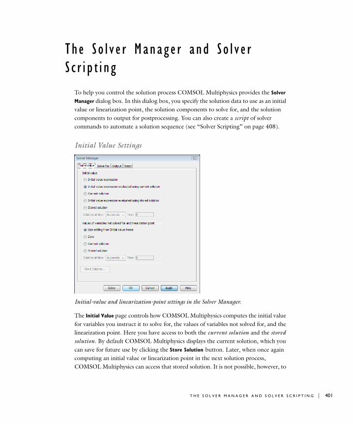
Th e S o l v e r Manag e r and S o l v e r S c r i p t i n g
To help you control the solution process COMSOL Multiphysics provides the Solver
Manager dialog box. In this dialog box, you specify the solution data to use as an initial value or linearization point, the solution components to solve for, and the solution components to output for postprocessing. You can also create a script of solver commands to automate a solution sequence (see “Solver Scripting” on page 408).
Initial Value Settings
Initial-value and linearization-point settings in the Solver Manager.
The Initial Value page controls how COMSOL Multiphysics computes the initial value for variables you instruct it to solve for, the values of variables not solved for, and the linearization point. Here you have access to both the current solution and the stored solution. By default COMSOL Multiphysics displays the current solution, which you can save for future use by clicking the Store Solution button. Later, when once again computing an initial value or linearization point in the next solution process, COMSOL Multiphysics can access that stored solution. It is not possible, however, to
T H E S O L V E R M A N A G E R A N D S O L V E R S C R I P T I N G | 401
402 | C H A P T E
access the stored solution for postprocessing purposes. For time-dependent, eigenvalue, and parametric analyses, you can choose to store only a subset of the solution in a multiple-selection list. The default settings store the entire solution.
Use the settings in the Initial value area to determine how COMSOL Multiphysics computes the value for the dependent variables (solution components) the software solves for at the beginning of the solution process (see “Choosing Variables for Which to Solve” on page 404). For a time-dependent problem this value determines the solution at the initial time; however, for a mixture of dynamic and stationary equations—a DAE system—the software modifies the initial value to become consistent with the equations (see “Settings for Differential-Algebraic Equations” on page 374). For stationary problems the initial value gives a first guess for the solution.
Settings in the Values of variables not solved for and linearization point area determine how COMSOL Multiphysics computes the values of the dependent variables (solution components) you choose not solve for. For the linear stationary solver and the eigenvalue solver, these settings also determine the linearization point, which is the value around which the software makes the linearization for the solution components it is solving for. If the model is linear, the linearization point is immaterial.
C H O O S I N G T H E I N I T I A L V A L U E
• Click the Initial value expression button to have the software calculate the initial value by evaluating the corresponding expressions on the Init tabs of the Subdomain
Settings, Boundary Settings, Edge Settings, and Point Settings dialog boxes (all of which appear on the Physics menu). If these expressions depend on some solution component, the software uses a zero solution.
• Click the Initial value expression evaluated using current solution button (the default) to have the software calculate the initial value by evaluating the corresponding expressions on the Init tabs of the Subdomain Settings, Boundary Settings, Edge
Settings, and Point Settings dialog boxes (all on the Physics menu). If these expressions depend on some solution component, the software uses the current solution for that solution component.
• Click the Current solution button to have the software take the initial value directly from the current solution.
• Click the Initial value expression evaluated using stored solution button to have the software calculate the initial value by evaluating the corresponding expressions on the Init tabs of the Subdomain Settings, Boundary Settings, Edge Settings, and Point
Settings dialog boxes (all on the Physics menu). If these expressions depend on some
R 6 : S O L V I N G T H E M O D E L

solution component, the software uses the stored solution for that solution component.
• Click the Stored solution button to have the software take the initial value directly from the stored solution.
C H O O S I N G T H E V A L U E S O F V A R I A B L E S N O T S O L V E D F O R
• Click the Use setting from Initial value frame button (the default) to have the software compute the values of solution components not solved for and the linearization point using the same settings as in the Initial value area.
• Click the Zero button to set the values of solution components not solved for and the linearization point to 0.
• Click the Current solution button to have the software take the value of solution components not solved for and the linearization point from the current solution.
• Click the Stored solution button to have the software take the value of solution components not solved for and the linearization point from the stored solution.
S P E C I F Y I N G T H E C U R R E N T S O L U T I O N O R S T O R E D S O L U T I O N
When working with a current solution or stored solution for a time-dependent, eigenvalue, or parametric analysis, you can choose which part of the solution to use.
For using these solutions in the Initial value area, the following options are available:
• Automatic selection (the default)
- The last time step for solutions to time-dependent problems
- The first eigenmode for eigenvalue problems
- The last parameter value for parametric analyses
• Interpolation (for solutions to time-dependent problems only). Make an entry between the starting and ending times in the Time edit field.
• A solution in the output data. Choose one by selecting the corresponding time, eigenvalue, or parameter value in the list.
For using these solutions in the Values of variables not solved for and linearization point frame, the following options are available:
• The same options as for the initial value: automatic selection, interpolation in time, or one of the solutions.
• All solutions from a stored solution or current solution (see below).
T H E S O L V E R M A N A G E R A N D S O L V E R S C R I P T I N G | 403

404 | C H A P T E
Select the option to use from the Solution at time, Eigenvalue, or Parameter value lists (depending on the analysis type) in the Initial value and Values of variables not solved
for and linearization point areas.
Using All Solutions from a Previous AnalysisSelecting All in the Solution at time list in the Values of variables not solved for and
linearization point area makes it possible to use all the solutions from a transient analysis as the value for the dependent variables not solved for in another transient analysis (the same applies to a parametric analysis). This method is effective when solving a one-way coupled time-dependent model. For example, start by solving for one dependent variable or application mode. Click the Store Solution button. Then click the Stored
solution option button in the Values of variables not solved for and linearization point area and select All in the Solution at time list. Choose another variable or application mode on the Solve For page and click Solve. The values of the variables not solved for are now time-dependent and interpolated from the stored solution (because the second analysis uses different time steps from the first one). Alternatively, you can instead click the Current solution option button, which eliminates the need to click Store Solution. The drawback with this alternative is that the first solution disappears when the second analysis is finished, which can be annoying if the second analysis returns an incomplete solution due to some failure.
To provide the best possible data for the interpolation in the second analysis, store the time steps from the solver instead of the specified output times. To do so, click the Time
Stepping tab in the Solver Parameters dialog box and select Time steps from solver in the Times to store in output list.
For an example of using this method to use solutions from a previous analysis, see “Peristaltic Pump” on page 408 in the COMSOL Multiphysics Model Library.
Choosing Variables for Which to Solve
Use the Solve For page to determine which dependent variables (solution components) to solve for. Select the application mode(s) to solve for in the list.
R 6 : S O L V I N G T H E M O D E L
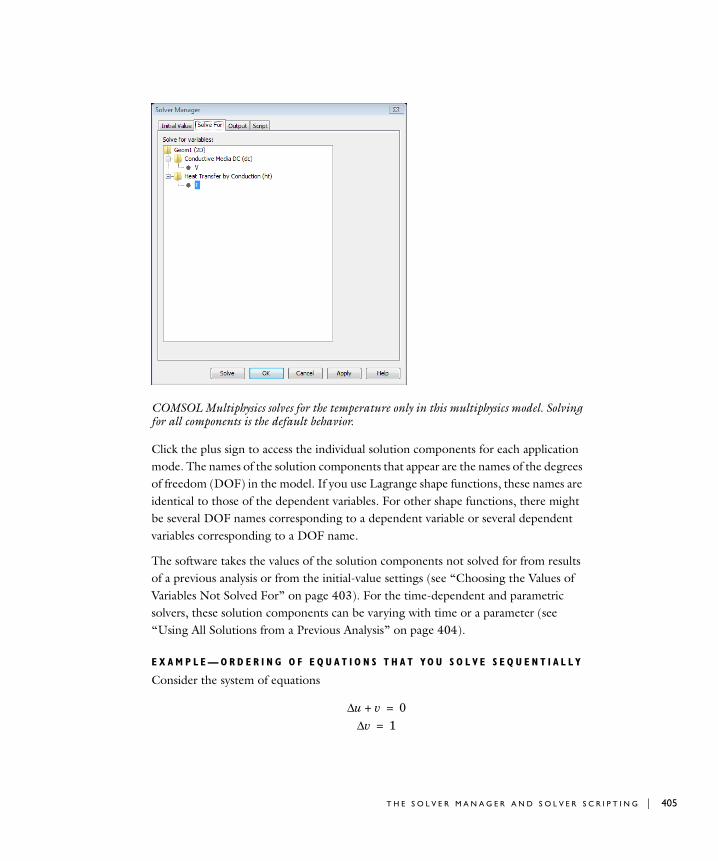
COMSOL Multiphysics solves for the temperature only in this multiphysics model. Solving for all components is the default behavior.
Click the plus sign to access the individual solution components for each application mode. The names of the solution components that appear are the names of the degrees of freedom (DOF) in the model. If you use Lagrange shape functions, these names are identical to those of the dependent variables. For other shape functions, there might be several DOF names corresponding to a dependent variable or several dependent variables corresponding to a DOF name.
The software takes the values of the solution components not solved for from results of a previous analysis or from the initial-value settings (see “Choosing the Values of Variables Not Solved For” on page 403). For the time-dependent and parametric solvers, these solution components can be varying with time or a parameter (see “Using All Solutions from a Previous Analysis” on page 404).
E X A M P L E — O R D E R I N G O F E Q U A T I O N S T H A T YO U S O L V E S E Q U E N T I A L L Y
Consider the system of equations
u∆ v+ 0=
v∆ 1=
T H E S O L V E R M A N A G E R A N D S O L V E R S C R I P T I N G | 405

406 | C H A P T E
where the variables u and v both are discretized with Lagrange elements. Then the corresponding degrees of freedom have the names u and v. Assume that you use a general form PDE application mode for the variables u and v (in this order) and that you enter the equations just mentioned in the displayed order. Then u corresponds to the first equation and v corresponds to the second one.
Assume that you solve only for u. Then the value of v is fixed to some given function, say v = x y. This means that COMSOL Multiphysics ignores the second equation and solves the single equation
.
If you instead enter the equations in the reverse order
then again the software ignores the second equation with the result
,
which is an equation with no solution. Thus some care is needed when choosing the order of variables and equations if you solve the equations sequentially using the settings on the Solve For tab.
Selecting Variables for Solution Output
Use the settings on the Output page to determine which solution components to save for postprocessing. Click the plus sign in the list as shown in the following figure to access the individual dependent variables (or degrees of freedom; see “Choosing Variables for Which to Solve” on page 404) for each application mode.
u∆ xy+ 0=
v∆ 1=
u v+∆ 0=
xy( )∆ 1=
R 6 : S O L V I N G T H E M O D E L
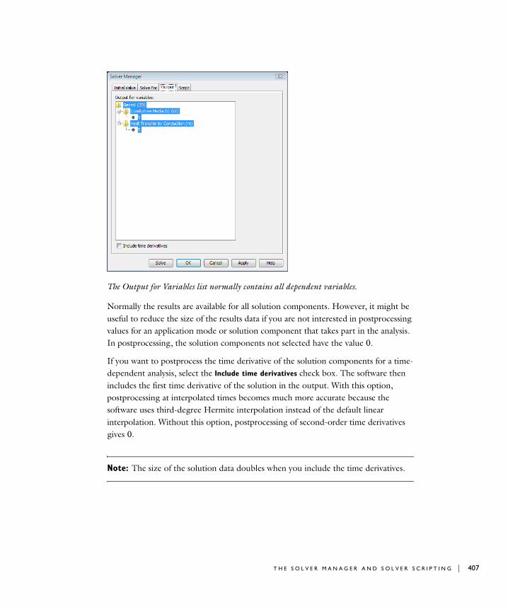
The Output for Variables list normally contains all dependent variables.
Normally the results are available for all solution components. However, it might be useful to reduce the size of the results data if you are not interested in postprocessing values for an application mode or solution component that takes part in the analysis. In postprocessing, the solution components not selected have the value 0.
If you want to postprocess the time derivative of the solution components for a time-dependent analysis, select the Include time derivatives check box. The software then includes the first time derivative of the solution in the output. With this option, postprocessing at interpolated times becomes much more accurate because the software uses third-degree Hermite interpolation instead of the default linear interpolation. Without this option, postprocessing of second-order time derivatives gives 0.
Note: The size of the solution data doubles when you include the time derivatives.
T H E S O L V E R M A N A G E R A N D S O L V E R S C R I P T I N G | 407
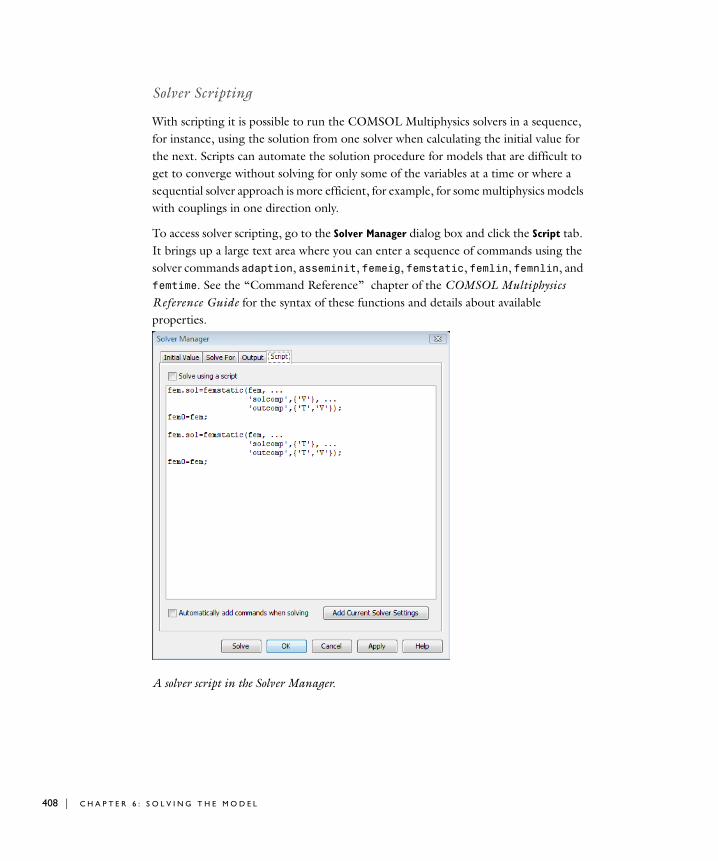
408 | C H A P T E
Solver Scripting
With scripting it is possible to run the COMSOL Multiphysics solvers in a sequence, for instance, using the solution from one solver when calculating the initial value for the next. Scripts can automate the solution procedure for models that are difficult to get to converge without solving for only some of the variables at a time or where a sequential solver approach is more efficient, for example, for some multiphysics models with couplings in one direction only.
To access solver scripting, go to the Solver Manager dialog box and click the Script tab. It brings up a large text area where you can enter a sequence of commands using the solver commands adaption, asseminit, femeig, femstatic, femlin, femnlin, and femtime. See the “Command Reference” chapter of the COMSOL Multiphysics Reference Guide for the syntax of these functions and details about available properties.
A solver script in the Solver Manager.
R 6 : S O L V I N G T H E M O D E L
C R E A T I N G A S O L V E R S C R I P T
Beside entering the script manually, you can generate it automatically in two ways:
• When you click the Add Current Solver Settings button, COMSOL Multiphysics automatically adds commands to the end of the script, commands corresponding to those it would use to solve the model at that moment. By changing settings between each click on this button you can generate a script without solving the model.
• If you select the Automatically add commands when solving check box, COMSOL Multiphysics adds commands to the end of the script each time you have it solve a model. Use this method to generate the script while manually solving a model using different settings, for example, on a coarse mesh to compute the solutions quickly.
Scripts can also include loops and branches. You could, for example, place for i=1:10 at the beginning of the solver command sequence and end at its end. Any loop variable is valid in the for statement.
S O L V I N G U S I N G A S O L V E R S C R I P T
When you select the Solve using a script check box, COMSOL Multiphysics uses the script to compute the solution; otherwise, it uses the solver selected in the Solver
Parameters dialog box.
The script runs in a context where fem0 is an FEM structure with an extended mesh and a solution corresponding to the current solution in the user interface; fem1 is the same except its solution corresponds to the stored solution. The FEM structure fem (or xfem, if multiple geometries are used) contains a newly created extended mesh. When the script has finished, the solution in fem is the one that COMSOL Multiphysics uses for postprocessing (the current solution).
Scripting is helpful for automating sequential solver steps where you first solve for one variable, then use that result to solve for another variable, and so on, or for switching between different solvers. To automatically run a solution and record the solver commands quickly, a good tip is to first use a coarse mesh and then re-solve using the script with desired mesh density.
T H E S O L V E R M A N A G E R A N D S O L V E R S C R I P T I N G | 409
410 | C H A P T E
Compu t i n g t h e S o l u t i o n
Starting and Restarting the Solvers
There are several ways to start the solvers for an analysis:
• Click the Solve button, choose Solve Problem from the Solve menu, or click Solve in the Solver Manager. Any of these actions starts the analysis using the solver selected in the Solver Parameters dialog box. The solver runs according to settings in the Solver Manager dialog box (see “The Solver Manager and Solver Scripting” on page 401).
• Click the Restart button or choose Restart from the Solve menu. Either action restarts the analysis using the current solution as an initial value, the current values of variables not solved for, and the linearization point. In other words, the solver operates as if you had selected the Current solution option in the Solver Manager dialog box. Restarting the solution process is helpful, for example, for using a stationary solver to first compute a good initial value for a nonlinear or transient analysis, or for interrupting and continuing a transient simulation. For a transient analysis that is not time invariant (where there is an explicit dependence on time in the equations), note that you probably want to change the time list in the Times edit field before restarting the solver.
Updating a Model
Use the Update Model command on the Solve menu to update the model in the following situations:
• You have added or edited variables and want to use the modified variables during postprocessing without solving the model again.
• You have edited the equations, material properties, or boundary conditions and want to use the modified equations during postprocessing without solving the model again.
• You have changed the element type or element order and want to interpolate the current solution onto the new elements for postprocessing purposes.
• You have remeshed a geometry or modified the geometry and want to interpolate the current solution onto the new mesh for postprocessing purposes.
R 6 : S O L V I N G T H E M O D E L

In all these cases, the software interpolates the current solution (or just passes it) to the Postprocessing mode. It does not recompute the solution to reflect any changes in variables, equations, mesh, and geometry.
Getting the Initial Value
The Get Initial Value command on the Solve menu evaluates the initial value for all solution components, it then passes the result to the Postprocessing mode so that it becomes the current solution. To compute the initial value, COMSOL Multiphysics uses the settings in the Initial value area in the Solver Manager. These settings apply to all solution components, even those the solver would not solve for. Therefore, for a time-dependent model, the result of the Get Initial Value command can sometimes differ from the solution at the initial time in the solution components not solved for.
The Get Initial Value command is useful when you want to:
• Plot and verify the initial conditions
• Postprocess the value of an expression without first solving the model
• Use a solution from a time-dependent or parametric analysis for further work
To do the latter, first store one of the solutions by clicking the Store Solution button on the Initial Value page of the Solver Manager, and then click the Stored solution option button in the Initial value area. You can then use the Get Initial Value command to make the current solution be this solution only. See “The Solver Manager and Solver Scripting” on page 401 for more information about the settings in the Solver Manager dialog box.
Note: The Get Initial Value command overwrites the current solution if one exists.
Solution Progress
When you solve a problem it is useful to know what is going on. For that purpose COMSOL Multiphysics provides a Progress window. It appears when you mesh a geometry, solve a problem, open a model or CAD file, or create a model report. At the top of the Progress window you can see what is going on at the moment. Just below is a progress bar displaying an estimate of the completed fraction of the total solving
C O M P U T I N G T H E S O L U T I O N | 411

412 | C H A P T E
process. In addition to progress information for the solvers, the Progress window provides
• Convergence plots (for the solvers that provide convergence information)
• Probe plots that show the current value of model quantities during solution (when you have defined such plots)
• A log of the solver commands
Using the mouse, you can resize the window to, for example, display more progress information or multiple plots.
C A N C E L I N G S O L V E R S
Sometimes you might realize that you are solving the wrong problem, or perhaps it is taking too long; in such situations simply click the Cancel button. The solver attempts to cancel the computation as soon as possible and return the program to where it was before starting to solve.
K E E P I N G T H E P R O G R E S S W I N D O W O P E N
By default the Progress window disappears when the solver has finished successfully. To make the Progress window stay open when the solver has finished, clear the Close
automatically check box. This option is useful, for example, for taking a closer look at the Log page. Note, though, that you can still examine the log when the Progress window is no longer open; go to the Solve menu and choose View Log.
If something goes wrong during the solution process, the Progress window does not close and the error message appears in red.
T H E P R O G R E S S P A G E
The solvers call each other in a hierarchical order: the adaptive solver calls the linear, nonlinear, parametric, or eigenvalue solver; the parametric solver calls the nonlinear or linear solver; the time-dependent, eigenvalue, linear, and nonlinear solvers all call both
R 6 : S O L V I N G T H E M O D E L
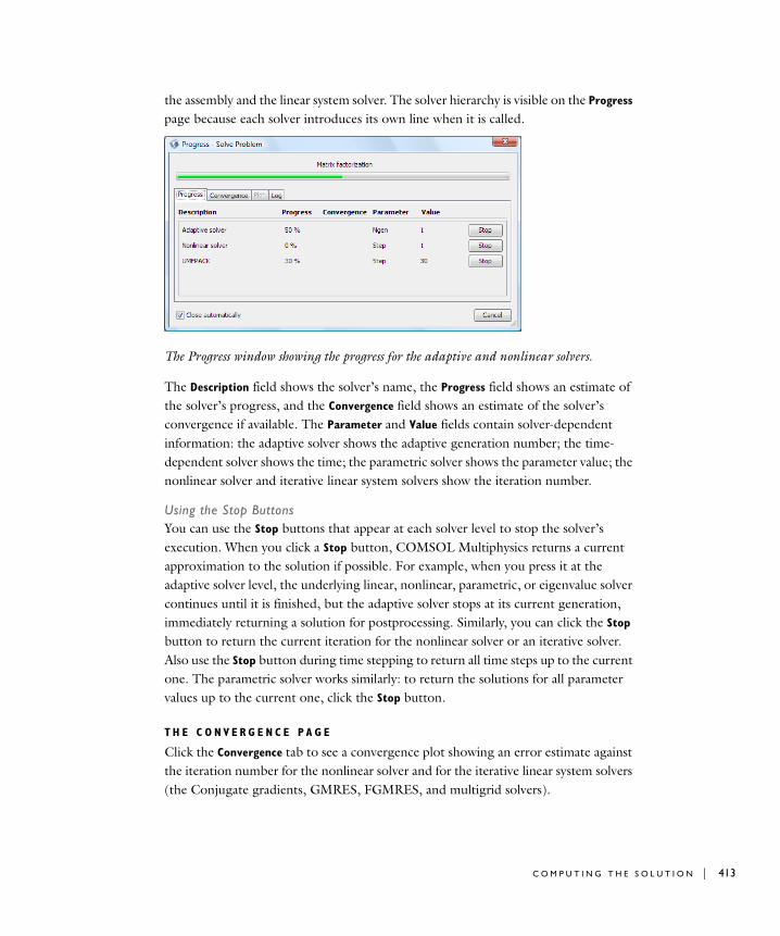
the assembly and the linear system solver. The solver hierarchy is visible on the Progress page because each solver introduces its own line when it is called.
The Progress window showing the progress for the adaptive and nonlinear solvers.
The Description field shows the solver’s name, the Progress field shows an estimate of the solver’s progress, and the Convergence field shows an estimate of the solver’s convergence if available. The Parameter and Value fields contain solver-dependent information: the adaptive solver shows the adaptive generation number; the time-dependent solver shows the time; the parametric solver shows the parameter value; the nonlinear solver and iterative linear system solvers show the iteration number.
Using the Stop ButtonsYou can use the Stop buttons that appear at each solver level to stop the solver’s execution. When you click a Stop button, COMSOL Multiphysics returns a current approximation to the solution if possible. For example, when you press it at the adaptive solver level, the underlying linear, nonlinear, parametric, or eigenvalue solver continues until it is finished, but the adaptive solver stops at its current generation, immediately returning a solution for postprocessing. Similarly, you can click the Stop button to return the current iteration for the nonlinear solver or an iterative solver. Also use the Stop button during time stepping to return all time steps up to the current one. The parametric solver works similarly: to return the solutions for all parameter values up to the current one, click the Stop button.
T H E C O N V E R G E N C E P A G E
Click the Convergence tab to see a convergence plot showing an error estimate against the iteration number for the nonlinear solver and for the iterative linear system solvers (the Conjugate gradients, GMRES, FGMRES, and multigrid solvers).
C O M P U T I N G T H E S O L U T I O N | 413

414 | C H A P T E
For the nonlinear solver, the convergence plot shows the relative error estimate (see “Nonlinear Solver Settings” on page 368) for each nonlinear iteration number. Note that this number also appears on the Log page as ErrEst.
For the iterative linear system solvers, the error estimate for each linear iteration is a factor times the relative (preconditioned) residual (see “Convergence Criteria” on page 513 of the COMSOL Multiphysics Reference Guide). This number also appears on the Log page as LinErr. When these solvers are used together with the nonlinear solver, the graphs for the different linear-system solution steps are merged, and the plots use the accumulated number of iterations.
When using the parametric solver, the graphs for the different parameter steps are merged, and the plots use the accumulated number of iterations.
Note that the error estimate numbers for the last iteration also appear in the Convergence column on the Progress page.
The Progress window’s Convergence page shows a convergence plot for the nonlinear solver.
Click the Copy to Figure button to create a copy of the convergence plot in a separate figure window.
R 6 : S O L V I N G T H E M O D E L
T H E P L O T P A G E
Click the Plot tab to see any probe plots that you have defined to monitor aspects of the solution. For more information, see “Plotting Values While Solving” on page 444.
T H E L O G P A G E
The Log page contains logs from the solvers. When a solver starts, the log window displays the solver call using COMSOL Multiphysics command-line syntax (see the “Command Reference” chapter of the COMSOL Multiphysics Reference Guide for more information), and the number of degrees of freedom solved for. This page contains logs from all solver calls during a session. Click the Clear Log button to start with a fresh log page.
Note: Clicking the Clear Log button only clears the log page, not any log files that you may be using. (See “Logging to a File” on page 417.) To clear the log file, choose Options>Preferences and click the Clear Log File button.
C O M P U T I N G T H E S O L U T I O N | 415
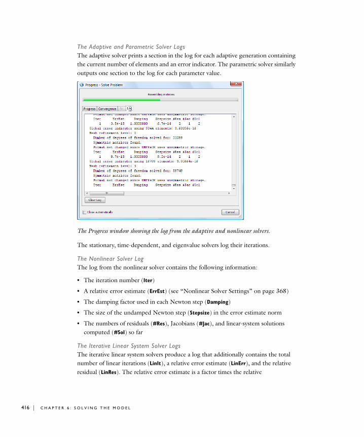
416 | C H A P T E
The Adaptive and Parametric Solver LogsThe adaptive solver prints a section in the log for each adaptive generation containing the current number of elements and an error indicator. The parametric solver similarly outputs one section to the log for each parameter value.
The Progress window showing the log from the adaptive and nonlinear solvers.
The stationary, time-dependent, and eigenvalue solvers log their iterations.
The Nonlinear Solver LogThe log from the nonlinear solver contains the following information:
• The iteration number (Iter)
• A relative error estimate (ErrEst) (see “Nonlinear Solver Settings” on page 368)
• The damping factor used in each Newton step (Damping)
• The size of the undamped Newton step (Stepsize) in the error estimate norm
• The numbers of residuals (#Res), Jacobians (#Jac), and linear-system solutions computed (#Sol) so far
The Iterative Linear System Solver LogsThe iterative linear system solvers produce a log that additionally contains the total number of linear iterations (LinIt), a relative error estimate (LinErr), and the relative residual (LinRes). The relative error estimate is a factor times the relative
R 6 : S O L V I N G T H E M O D E L
(preconditioned) residual (see “Convergence Criteria” on page 513 of the COMSOL Multiphysics Reference Guide). The relative residual is the Euclidean norm of the residual divided by the norm, | b |, of the linear system’s right-hand side.
The Time-Dependent Solver LogThe time-stepping algorithm produces a log that contains
• the time step number (Step)
• time (Time; output times are indicated with out)
• the number of residuals (Res), Jacobians (Jac), and linear system solutions (Sol) computed
You can also see the current internal polynomial order in the BDF method (Order), the number of error test failures in time stepping (Tfail), and the number of failures in the nonlinear iterations (NLfail). For iterative linear system solvers, the log also contains the total number of linear iterations, a linear error estimate, and a relative residual (see above).
The Eigenvalue Solver LogThe eigenvalue solver produces a log that contains the iteration number (Iter), an error estimate (ErrEst), the number of converged eigenvalues (Nconv), and— if you are using an iterative linear solver— the number of linear iterations (LinIt).
Logging to a FileYou can also direct the log from the Log page to a file. This is useful if the solver log becomes very long, or if you want to keep the log for further analysis or comparison. To activate logging to file, choose Preferences from the Options menu and select the Log to file check box. Choose a log file by typing in the path in the Log file edit field or browse to a file by clicking the Browse button. The file logging appends the log messages to any already existing content of the log file. To start with a new empty log file, click the Clear Log File button.
Monitoring Memory Usage
When running COMSOL Multiphysics on Windows, you can inspect the memory usage at any time during a modeling session in the Memory field at the bottom right of the user interface. This field displays the numbers in MB for the current and peak virtual memory usage, separated by a slash. When the main user interface window is in focus and tooltip display is active, placing the cursor over the Memory field additionally shows the current and peak physical memory usage.
C O M P U T I N G T H E S O L U T I O N | 417

418 | C H A P T E
R 6 : S O L V I N G T H E M O D E L
7
P o s t p r o c e s s i n g a n d V i s u a l i z a t i o n
To help you analyze results from its solvers, COMSOL Multiphysics provides numerous postprocessing and visualization tools, including advanced graphics, data display and export functions, and a report generator. The following chapter gives details on how to use these tools.
419
420 | C H A P T E
Po s t p r o c e s s i n g R e s u l t s
COMSOL Multiphysics Postprocessing Overview
COMSOL Multiphysics provides many tools for postprocessing and visualizing model quantities. It creates a wide variety of plots:
• Surface plots
• Slice plots
• Isosurface plots
• Contour plots
• Streamline plots
• Pathline plots that describe particle traces
• Principal stress/strain plots
• Combinations of these plots
In addition, animations reveal the dynamics in a solution. Cross-section plots can interpolate within a domain to extract mesh-independent plots, and the software can also extend these plots in time or along parametric solutions. Domain plots provide similar capabilities for geometric domains. Global plots can visualize globally defined variables, typically solutions to ODEs and algebraic equations. You can also compute numerical integrals of model quantities as well as display and save postprocessing data.
Postprocessing Expressions
COMSOL Multiphysics does not limit postprocessing to predefined quantities; you can postprocess any function by entering the corresponding expression. The software can postprocess expressions that combine user-defined variables, application mode variables, standard variables, mathematical and logical functions (see “Using Mathematical and Logical Operators and Functions” on page 147), and numbers. Enter the expression that you want to plot or evaluate in the Expression edit field in the dialog box for the type of postprocessing that you are interested in. This edit field is available for most plot types as well as for integration and data display and evaluation. Pressing Ctrl+Space opens the hierarchical list of predefined quantities that you also find in the corresponding Predefined quantities list. The difference between the two ways of accessing the list is that pressing Ctrl+Space and then selecting a quantity from the list adds the name of the corresponding variable to the Expression edit field at the
R 7 : P O S T P R O C E S S I N G A N D V I S U A L I Z A T I O N
current location instead of replacing any previous content (for example, pressing Ctrl+Space and selecting Plane Stress (ps)>Total displacement appends disp_ps to the expression in the Expression field). This makes it easier to build an expression with valid variable names.
A C C E S S I N G P R E D E F I N E D V A R I A B L E S
The COMSOL Multiphysics Modeling Guide lists all application mode variables. For a list of standard variables of this type, see “Variables and Expressions” on page 138.
A C C E S S I N G O T H E R S O L U T I O N S T H A N T H E S E L E C T E D S O L U T I O N
When you use the names of the dependent variables in a postprocessing expression, COMSOL Multiphysics uses the solution associated with the selected parameter value, eigenvalue, or time for a parametric analysis, eigenvalue analysis, or time-dependent analysis, respectively. To access other solutions in the model, use the with operator. For more information about how to use this operator, see “The With Operator” on page 164.
E V A L U A T I O N O F U N D E F I N E D Q U A N T I T I E S
During the evaluation of expressions, COMSOL Multiphysics does not always report partially undefined quantities, and the program plots a quantity where it is defined. If a postprocessing quantity is undefined, an error occurs for all plot types except arrow plots. For example, in a plot of the Lagrange multiplier on the boundary using weak constraints, that multiplier is undefined on unconstrained boundaries; but following the rule above, the software plots the Lagrange multiplier on constrained boundaries if at least one exists.
Selection of Frames for Postprocessing
When a model works with deformed meshes, the Frame list is enabled in all postprocessing dialog boxes, and it contains the names of all available frames. There you select which frame to use for the desired postprocessing task. For further information about frames and deformed meshes, see the section “Frames for Deformed Meshes” on page 396 in COMSOL Multiphysics Modeling Guide.
Interpolating Expressions at Arbitrary Points
The point cross-section plot makes it easy to view an expression at an arbitrary set of spatial coordinates and results in a line plot. To get the value of a certain subdomain expression or variable at any location in the geometry, use the Data Display dialog box.
P O S T P R O C E S S I N G R E S U L T S | 421
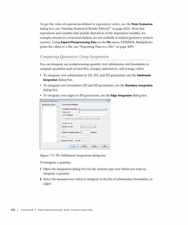
422 | C H A P T E
To get the value of expressions defined at a geometry vertex, use the Point Evaluation dialog box (see “Getting Numerical Results Directly” on page 423). Note that expressions and variables that include derivatives of the dependent variables, for example, stresses in a structural analysis, are not available at isolated geometry vertices (points). Using Export>Postprocessing Data on the File menu, COMSOL Multiphysics prints the values to a file (see “Exporting Data to a File” on page 449).
Computing Quantities Using Integration
You can integrate any postprocessing quantity over subdomains and boundaries to compute quantities such as total flux, charges, inductances, and average values.
• To integrate over subdomains in 1D, 2D, and 3D geometries, use the Subdomain
Integration dialog box.
• To integrate over boundaries 2D and 3D geometries, use the Boundary Integration dialog box.
• To integrate over edges in 3D geometries, use the Edge Integration dialog box.
Figure 7-1: The Subdomain Integration dialog box.
To integrate a quantity:
1 Open the integration dialog box for the domain type over which you want to integrate a quantity.
2 Select the domains over which to integrate in the list of subdomains, boundaries, or edges.
R 7 : P O S T P R O C E S S I N G A N D V I S U A L I Z A T I O N
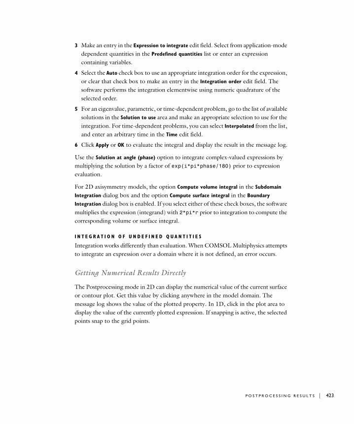
3 Make an entry in the Expression to integrate edit field. Select from application-mode dependent quantities in the Predefined quantities list or enter an expression containing variables.
4 Select the Auto check box to use an appropriate integration order for the expression, or clear that check box to make an entry in the Integration order edit field. The software performs the integration elementwise using numeric quadrature of the selected order.
5 For an eigenvalue, parametric, or time-dependent problem, go to the list of available solutions in the Solution to use area and make an appropriate selection to use for the integration. For time-dependent problems, you can select Interpolated from the list, and enter an arbitrary time in the Time edit field.
6 Click Apply or OK to evaluate the integral and display the result in the message log.
Use the Solution at angle (phase) option to integrate complex-valued expressions by multiplying the solution by a factor of exp(i*pi*phase/180) prior to expression evaluation.
For 2D axisymmetry models, the option Compute volume integral in the Subdomain
Integration dialog box and the option Compute surface integral in the Boundary
Integration dialog box is enabled. If you select either of these check boxes, the software multiplies the expression (integrand) with 2*pi*r prior to integration to compute the corresponding volume or surface integral.
I N T E G R A T I O N O F U N D E F I N E D Q U A N T I T I E S
Integration works differently than evaluation. When COMSOL Multiphysics attempts to integrate an expression over a domain where it is not defined, an error occurs.
Getting Numerical Results Directly
The Postprocessing mode in 2D can display the numerical value of the current surface or contour plot. Get this value by clicking anywhere in the model domain. The message log shows the value of the plotted property. In 1D, click in the plot area to display the value of the currently plotted expression. If snapping is active, the selected points snap to the grid points.
P O S T P R O C E S S I N G R E S U L T S | 423
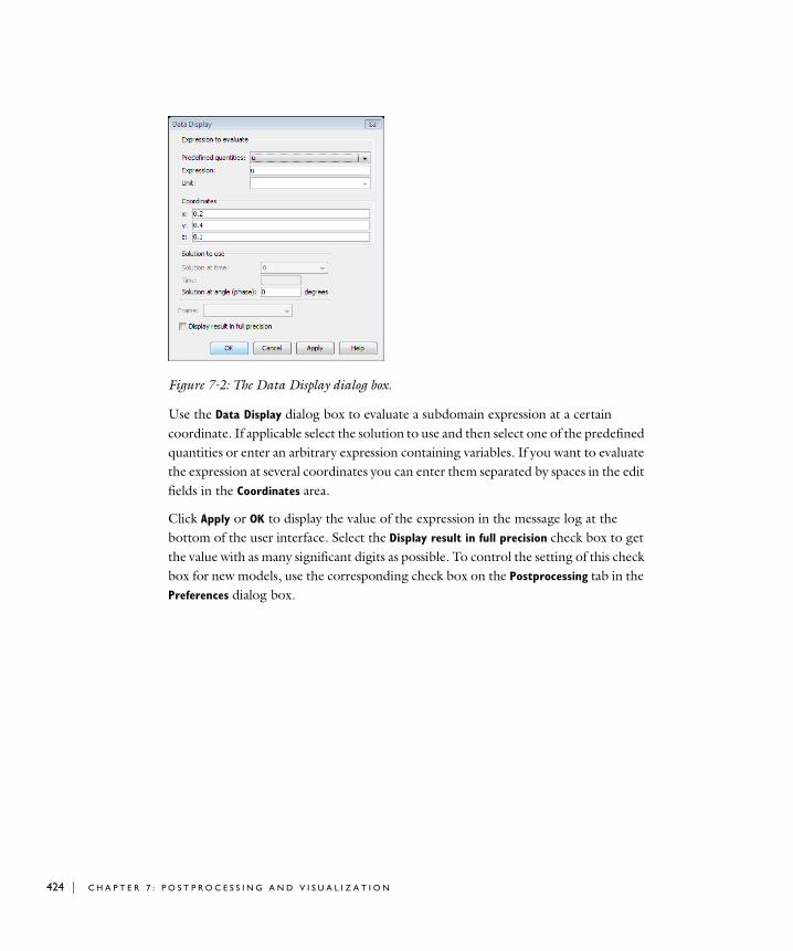
424 | C H A P T E
Figure 7-2: The Data Display dialog box.
Use the Data Display dialog box to evaluate a subdomain expression at a certain coordinate. If applicable select the solution to use and then select one of the predefined quantities or enter an arbitrary expression containing variables. If you want to evaluate the expression at several coordinates you can enter them separated by spaces in the edit fields in the Coordinates area.
Click Apply or OK to display the value of the expression in the message log at the bottom of the user interface. Select the Display result in full precision check box to get the value with as many significant digits as possible. To control the setting of this check box for new models, use the corresponding check box on the Postprocessing tab in the Preferences dialog box.
R 7 : P O S T P R O C E S S I N G A N D V I S U A L I Z A T I O N

Figure 7-3: The Point Evaluation dialog box.
Use the Point Evaluation dialog box to evaluate expressions defined in a geometry vertex. This dialog box works the same as the integration dialog boxes described in “Computing Quantities Using Integration” on page 422, but for vertices rather than subdomains, boundaries, and edges.
Figure 7-4: The Global Data Display dialog box.
To get the value of a globally defined quantity, use the Global Data Display dialog box. In the Expression to evaluate area choose the quantity to display. Either select from predefined quantities or enter an expression containing variables. If applicable, select the solution to use. Click Apply or OK to display the value of the expression in the message log at the bottom of the user interface.
P O S T P R O C E S S I N G R E S U L T S | 425
426 | C H A P T E
Plotting Global Expressions
To visualize globally defined variables, such as solutions to ODEs or coupling variables with global destination, use the Global Variables Plot dialog box.
Figure 7-5: The Global Variables Plot dialog box.
In the Predefined quantities list, the names of all variables from ODEs and other space-independent equations (defined in the Space-Independent Equations dialog box) and global expressions (defined in the Global Expressions dialog box) are present. To plot one or more of these, select them and click the > button to add them to the Quantities to plot list. When you select a name in the Predefined quantities list, the software displays its variable name in the text field below the list. You can edit this name and add the edited quantity using the > button to the right of the text field. To remove one or more expressions from the Quantities to plot list, select them and click the < button. You can use Shift-click and Control-click in both lists.
In the Solutions to use area, select which time steps to include in the plot. By choosing Interpolated times in the Select via list, you can enter any vector of times in the Times edit field, such as linspace(0,1,100) or 0:0.02:1. This way of choosing the times for plotting is also available in the Cross-Section Plot Parameters and Domain Plot
Parameters dialog boxes when postprocessing a time-dependent model.
R 7 : P O S T P R O C E S S I N G A N D V I S U A L I Z A T I O N
Control the quantity to plot on the x-axis in the x-axis data area. If Auto is selected, the x-axis corresponds to time.
The settings that you access by clicking the Line Settings button are described under “Line Settings” on page 440, and the settings that you specify by clicking the Title/Axis button are described under “Adjusting the Plot Title and Axis” on page 431. The settings in the Plot in list are described under “Plotting Multiple Data to Separate Figure Windows” on page 430, and the Solution at angle (phase) edit field is described under “Visualizing Complex-Valued Quantities” on page 429.
Visualization Using the Plot Parameters Dialog Box
To get visualizations on the solution domain using the common plot types, use the Plot
Parameters dialog box. The choices include:
• For all geometries: plot of the geometry edges
• In 1D: line plot
• In 2D: surface, contour, arrow, deformed shape, streamline, particle traces, and line plots
• In 3D: slice, isosurface, subdomain, boundary, edge, arrow, deformed shape, streamline plots, and particle traces
In addition, the choice of plotting principal stress/strain plots is available together with the Structural Mechanics Module and the MEMS Module.
To open the Plot Parameters dialog box, either click the Plot Parameters button in the main toolbar or choose Plot Parameters from the Postprocessing menu.
P O S T P R O C E S S I N G R E S U L T S | 427
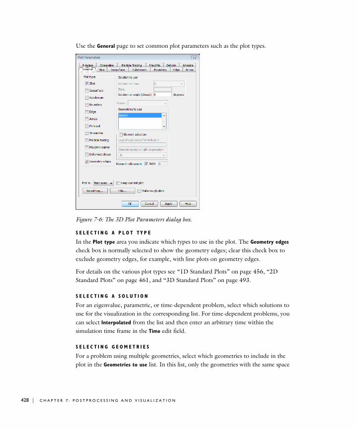
428 | C H A P T E
Use the General page to set common plot parameters such as the plot types.
Figure 7-6: The 3D Plot Parameters dialog box.
S E L E C T I N G A P L O T TY P E
In the Plot type area you indicate which types to use in the plot. The Geometry edges check box is normally selected to show the geometry edges; clear this check box to exclude geometry edges, for example, with line plots on geometry edges.
For details on the various plot types see “1D Standard Plots” on page 456, “2D Standard Plots” on page 461, and “3D Standard Plots” on page 493.
S E L E C T I N G A S O L U T I O N
For an eigenvalue, parametric, or time-dependent problem, select which solutions to use for the visualization in the corresponding list. For time-dependent problems, you can select Interpolated from the list and then enter an arbitrary time within the simulation time frame in the Time edit field.
S E L E C T I N G G E O M E T R I E S
For a problem using multiple geometries, select which geometries to include in the plot in the Geometries to use list. In this list, only the geometries with the same space
R 7 : P O S T P R O C E S S I N G A N D V I S U A L I Z A T I O N
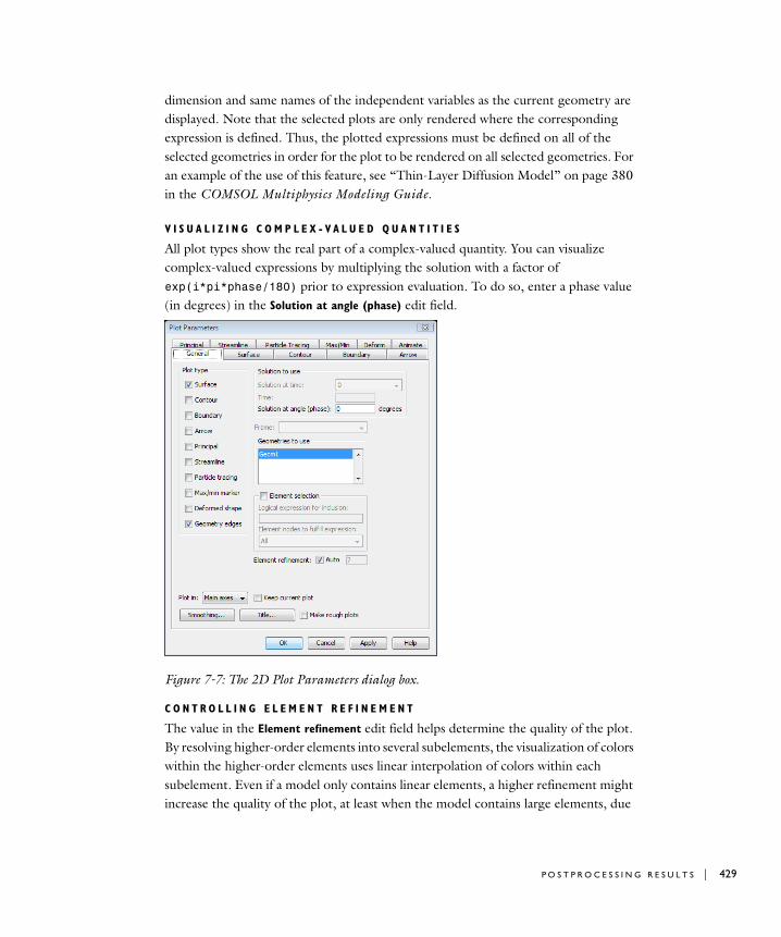
dimension and same names of the independent variables as the current geometry are displayed. Note that the selected plots are only rendered where the corresponding expression is defined. Thus, the plotted expressions must be defined on all of the selected geometries in order for the plot to be rendered on all selected geometries. For an example of the use of this feature, see “Thin-Layer Diffusion Model” on page 380 in the COMSOL Multiphysics Modeling Guide.
V I S U A L I Z I N G C O M P L E X - V A L U E D Q U A N T I T I E S
All plot types show the real part of a complex-valued quantity. You can visualize complex-valued expressions by multiplying the solution with a factor of exp(i*pi*phase/180) prior to expression evaluation. To do so, enter a phase value (in degrees) in the Solution at angle (phase) edit field.
Figure 7-7: The 2D Plot Parameters dialog box.
C O N T R O L L I N G E L E M E N T R E F I N E M E N T
The value in the Element refinement edit field helps determine the quality of the plot. By resolving higher-order elements into several subelements, the visualization of colors within the higher-order elements uses linear interpolation of colors within each subelement. Even if a model only contains linear elements, a higher refinement might increase the quality of the plot, at least when the model contains large elements, due
P O S T P R O C E S S I N G R E S U L T S | 429
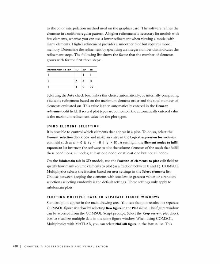
430 | C H A P T E
to the color interpolation method used on the graphics card. The software refines the elements in a uniform regular pattern. A higher refinement is necessary for models with few elements, whereas you can use a lower refinement when viewing a model with many elements. Higher refinement provides a smoother plot but requires more memory. Determine the refinement by specifying an integer number that indicates the refinement steps. The following list shows the factor that the number of elements grows with for the first three steps:
Selecting the Auto check box makes this choice automatically, by internally computing a suitable refinement based on the maximum element order and the total number of elements evaluated on. This value is then automatically entered in the Element
refinement edit field. If several plot types are combined, the automatically entered value is the maximum refinement value for the plot types.
U S I N G E L E M E N T S E L E C T I O N
It is possible to control which elements that appear in a plot. To do so, select the Element selection check box and make an entry in the Logical expression for inclusion edit field such as x > 0 & (y < -5 | y > 5). A setting in the Element nodes to fulfill
expression list instructs the software to plot the volume elements of the mesh that fulfill these conditions: all nodes; at least one node; or at least one but not all nodes.
On the Subdomain tab in 3D models, use the Fraction of elements to plot edit field to specify how many volume elements to plot (as a fraction between 0 and 1). COMSOL Multiphysics selects the fraction based on user settings in the Select elements list. Choose between keeping the elements with smallest or greatest values or a random selection (selecting randomly is the default setting). These settings only apply to subdomain plots.
P L O T T I N G M U L T I P L E D A T A T O S E P A R A T E F I G U R E W I N D O W S
Standard plots appear in the main drawing area. You can also plot results in a separate COMSOL figure window by selecting New figure in the Plot in list. This figure window can be accessed from the COMSOL Script prompt. Select the Keep current plot check box to visualize multiple data in the same figure window. When using COMSOL Multiphysics with MATLAB, you can select MATLAB figure in the Plot in list. This
REFINEMENT STEP 1D 2D 3D
1 1 1 1
2 2 4 8
3 3 9 27
R 7 : P O S T P R O C E S S I N G A N D V I S U A L I Z A T I O N
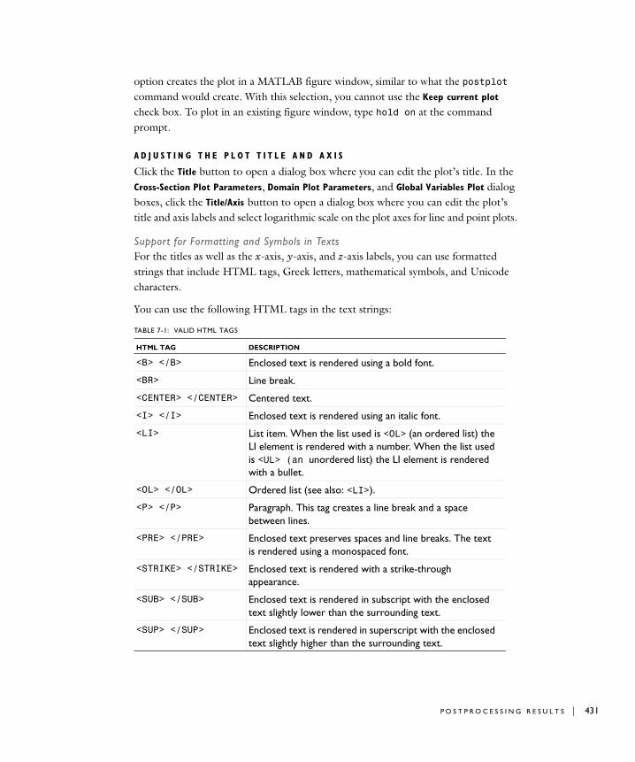
option creates the plot in a MATLAB figure window, similar to what the postplot command would create. With this selection, you cannot use the Keep current plot
check box. To plot in an existing figure window, type hold on at the command prompt.
A D J U S T I N G T H E P L O T T I T L E A N D A X I S
Click the Title button to open a dialog box where you can edit the plot’s title. In the Cross-Section Plot Parameters, Domain Plot Parameters, and Global Variables Plot dialog boxes, click the Title/Axis button to open a dialog box where you can edit the plot’s title and axis labels and select logarithmic scale on the plot axes for line and point plots.
Support for Formatting and Symbols in TextsFor the titles as well as the x-axis, y-axis, and z-axis labels, you can use formatted strings that include HTML tags, Greek letters, mathematical symbols, and Unicode characters.
You can use the following HTML tags in the text strings:
TABLE 7-1: VALID HTML TAGS
HTML TAG DESCRIPTION
<B> </B> Enclosed text is rendered using a bold font.
<BR> Line break.
<CENTER> </CENTER> Centered text.
<I> </I> Enclosed text is rendered using an italic font.
<LI> List item. When the list used is <OL> (an ordered list) the LI element is rendered with a number. When the list used is <UL> (an unordered list) the LI element is rendered with a bullet.
<OL> </OL> Ordered list (see also: <LI>).
<P> </P> Paragraph. This tag creates a line break and a space between lines.
<PRE> </PRE> Enclosed text preserves spaces and line breaks. The text is rendered using a monospaced font.
<STRIKE> </STRIKE> Enclosed text is rendered with a strike-through appearance.
<SUB> </SUB> Enclosed text is rendered in subscript with the enclosed text slightly lower than the surrounding text.
<SUP> </SUP> Enclosed text is rendered in superscript with the enclosed text slightly higher than the surrounding text.
P O S T P R O C E S S I N G R E S U L T S | 431

432 | C H A P T E
The texts in labels and titles support the following Greek character tags:
<TT> </TT> Enclosed text is rendered using a monospaced font.
<U> </U> Enclosed text will be underlined.
<UL> </UL> Unordered list (see also: <LI>).
TABLE 7-2: VALID GREEK SYMBOL TAGS
TAG SYMBOL TAG SYMBOL
\ALPHA Α \alpha α
\BETA Β \beta β
\GAMMA Γ \gamma γ
\DELTA ∆ \delta δ
\EPSILON Ε \epsilon ε
\ZETA Ζ \zeta ζ
\ETA Η \eta η
\THETA Θ \theta θ
\IOTA Ι \iota ι
\KAPPA Κ \kappa κ
\LAMBDA Λ \lambda λ
\MU Μ \mu µ
\NU Ν \nu ν
\XI Ξ \xi ξ
\OMICRON Ο \omicron ο
\PI Π \pi π
\RHO Ρ \rho ρ
\SIGMA Σ \sigma σ
\TAU Τ \tau τ
\UPSILON Υ \upsilon υ
\PHI Φ \phi
\CHI Χ \chi χ
\PSI Ψ \psi ψ
\OMEGA Ω \omega ω
TABLE 7-1: VALID HTML TAGS
HTML TAG DESCRIPTION
ϕ
R 7 : P O S T P R O C E S S I N G A N D V I S U A L I Z A T I O N
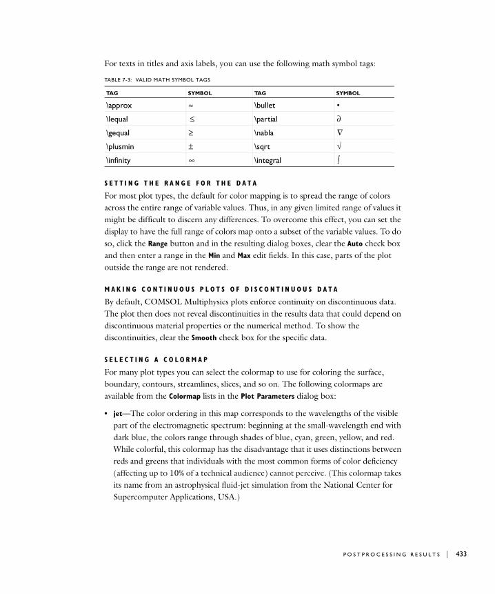
For texts in titles and axis labels, you can use the following math symbol tags:
S E T T I N G T H E R A N G E F O R T H E D A T A
For most plot types, the default for color mapping is to spread the range of colors across the entire range of variable values. Thus, in any given limited range of values it might be difficult to discern any differences. To overcome this effect, you can set the display to have the full range of colors map onto a subset of the variable values. To do so, click the Range button and in the resulting dialog boxes, clear the Auto check box and then enter a range in the Min and Max edit fields. In this case, parts of the plot outside the range are not rendered.
M A K I N G C O N T I N U O U S P L O T S O F D I S C O N T I N U O U S D A T A
By default, COMSOL Multiphysics plots enforce continuity on discontinuous data. The plot then does not reveal discontinuities in the results data that could depend on discontinuous material properties or the numerical method. To show the discontinuities, clear the Smooth check box for the specific data.
S E L E C T I N G A C O L O R M A P
For many plot types you can select the colormap to use for coloring the surface, boundary, contours, streamlines, slices, and so on. The following colormaps are available from the Colormap lists in the Plot Parameters dialog box:
• jet—The color ordering in this map corresponds to the wavelengths of the visible part of the electromagnetic spectrum: beginning at the small-wavelength end with dark blue, the colors range through shades of blue, cyan, green, yellow, and red. While colorful, this colormap has the disadvantage that it uses distinctions between reds and greens that individuals with the most common forms of color deficiency (affecting up to 10% of a technical audience) cannot perceive. (This colormap takes its name from an astrophysical fluid-jet simulation from the National Center for Supercomputer Applications, USA.)
TABLE 7-3: VALID MATH SYMBOL TAGS
TAG SYMBOL TAG SYMBOL
\approx ≈ \bullet •
\lequal \partial ∂
\gequal ≥ \nabla
\plusmin ± \sqrt √
\infinity \integral ∫
≤
∇
∞
P O S T P R O C E S S I N G R E S U L T S | 433

434 | C H A P T E
• cool—A colormap that consists of shades of cyan and magenta, where the red component varies linearly from 0 to 1, the green one from 1 to 0, and the blue one is held constant at 1.
• hot—This colormap ranges from black through red and yellow to white, which corresponds to the colors iron takes as it heats up.
• hsv—A colormap that varies the hue component of the hue-saturation-value color model, keeping the saturation and value constant (equal to 1). The colors begin with red, then pass through yellow, green, cyan, blue, magenta, and finally return to red. This map is particularly useful for displaying periodic functions, and has a sharp color gradient.
• wave—This colormap is particularly useful for data that naturally has a positive and negative attribute in addition to a magnitude. An example of a so-called double-ended scheme, it ranges linearly from blue to white, and then linearly from white to red. When the range of the visualized quantity is symmetric around zero, the color red or blue indicates whether the value is positive or negative, and the saturation indicates the magnitude. This color palette has the additional feature of being interpretable by color deficient users. Because it uses no red-green-gray distinctions, the palette is efficient for 99.98% of the population.
• gray—A colormap that uses no color, only the linear gray scale—the easiest palette to understand and order. Gray-scale plots are often much easier for a publisher to include in journal articles. Further, humans can perceive very fine structural detail in gray scale that would go unnoticed in color. Using gray scale also raises the probability that a plot will be correctly interpreted by individuals with certain visual disabilities. This map varies linearly from black (1, 1, 1) to white (0, 0, 0).
• grayprint—Varies linearly from dark gray (0.95, 0.95, 0.95) to light gray (0.05, 0.05, 0.05). This colormap overcomes two disadvantages that the standard gray colormap has when used for printouts on paper, namely that it gives the impression of being dominated by dark colors, and that white cannot be distinguished from the background.
• bone—A variant of the gray colormap with a tinge of blue.
• pink—A variant of the gray colormap with a tinge of red.
All colormaps are also available for surface plots generated using the Cross-Section Plot
Parameters and Domain Plot Parameters dialog boxes.
R 7 : P O S T P R O C E S S I N G A N D V I S U A L I Z A T I O N
U S I N G R O U G H P L O T S F O R L A R G E M O D E L S A N D Q U I C K V I S U A L I Z A T I O N S
The “rough plot” feature makes it possible to do quick visualizations and plots of large 3D models. This feature generates plots with a bit lower quality than normal for faster and more memory-efficient rendering. To achieve this, COMSOL Multiphysics lowers the element refinement for postprocessing by 2 steps in 3D and by 1 step in 2D. It also turns off the calculation of smooth normals, which means that lighting does not affect the plot. One way of working with a large 3D model is to select the Make rough plots check box on the General tab in the Plot Parameters dialog box while trying out different plots. When you get an interesting image, clear the check box to produce a high-quality plot. Use the preference setting Make rough plots on the Postprocessing tab in the Preferences dialog box to control the default setting when creating new models.
Opening Models Faster Using Rough PlotsCOMSOL Multiphysics does not store the current plot in the model but recreates it when you open the model again. Thus it can sometimes take a while to open a large 3D model that contains an advanced plot. To make COMSOL Multiphysics use rough plots when opening models, do the following:
1 Go to the Options menu and choose Preferences.
2 In the Preferences dialog box click the Postprocessing tab.
3 Select Rough in the Plots when opening models list.
4 Click OK.
It is also possible to avoid creating postprocessing plots when opening models. To do so, select None in the Plots when opening models list.
U P D A T I N G A P L O T A N D S A V I N G P L O T S E T T I N G S
• Click OK to apply the changes, plot the data, and close the dialog box.
P O S T P R O C E S S I N G R E S U L T S | 435

436 | C H A P T E
• Click Apply to apply the changes and plot the data and keep the dialog box open.
• If you have not yet solved the model, clicking either OK or Apply saves the plot parameter settings for future plots.
Figure 7-8: The 1D Plot Parameters dialog box.
Cross-Section Plots
Cross-section plots visualize a quantity as a family of plots on:
• Arbitrary planes (in 3D)
• An arbitrary line (in 2D or 3D)
• An arbitrary set of points (in 1D, 2D, or 3D)
The plots show the values over time, along a parametric solution, or for several eigenvalues.
To set common plot parameters, go to the Cross-Section Plot Parameters dialog box on the General page. For information on how to specify various cross-section plot types see “1D Cross-Section Plots” on page 457, “2D Cross-Section Plots” on page 485, and “3D Cross-Section Plots” on page 503.
R 7 : P O S T P R O C E S S I N G A N D V I S U A L I Z A T I O N

To create a cross-section plot, go to the Postprocessing menu and choose Cross-Section
Plot Parameters.
Figure 7-9: The 3D Cross-Section Plot Parameters dialog box.
Q U I C K C R O S S - S E C T I O N P L O T S
When working in 2D and 3D, you can obtain cross-section plots directly by defining points, lines, and faces using the mouse. To activate these quick plots, simply click the Draw Points for Cross-Section Point Plot, Draw Line for Cross-Section Line Plot, or Draw
Plane for Cross-Section Slice Plot buttons on the Plot toolbar.
If the Cross-Section Plot Parameters dialog box is closed when you define a point, line, or face using the mouse, COMSOL Multiphysics launches a cross-section plot using the settings from the Cross-Section Plot Parameters dialog box; if the dialog box is open, the program updates the point, line, or slice position data.
To draw a new line or point, simply click the corresponding button again. To remove just the line or point, click the button twice.
Notice that for a 3D slice plot, the view angle might make it difficult to see the cross section. In that case, rotate the 3D plot slightly for a better view.
P O S T P R O C E S S I N G R E S U L T S | 437
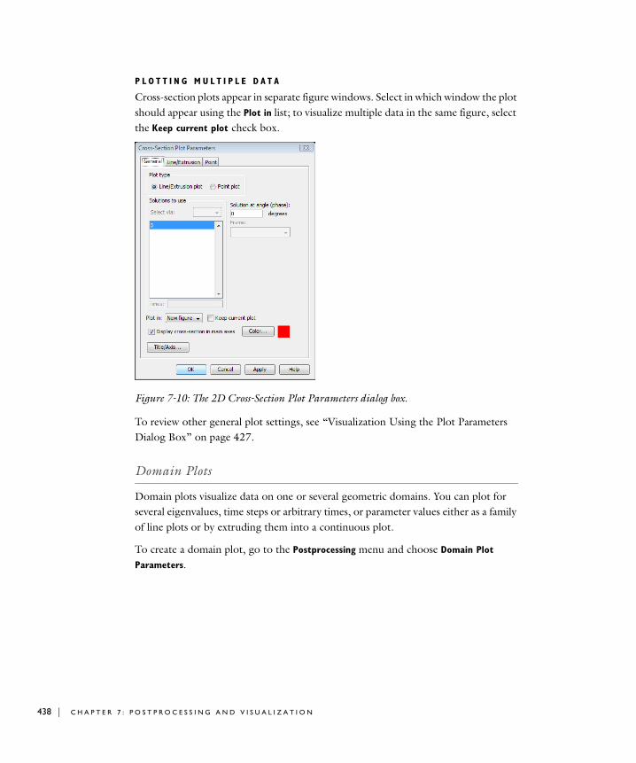
438 | C H A P T E
P L O T T I N G M U L T I P L E D A T A
Cross-section plots appear in separate figure windows. Select in which window the plot should appear using the Plot in list; to visualize multiple data in the same figure, select the Keep current plot check box.
Figure 7-10: The 2D Cross-Section Plot Parameters dialog box.
To review other general plot settings, see “Visualization Using the Plot Parameters Dialog Box” on page 427.
Domain Plots
Domain plots visualize data on one or several geometric domains. You can plot for several eigenvalues, time steps or arbitrary times, or parameter values either as a family of line plots or by extruding them into a continuous plot.
To create a domain plot, go to the Postprocessing menu and choose Domain Plot
Parameters.
R 7 : P O S T P R O C E S S I N G A N D V I S U A L I Z A T I O N
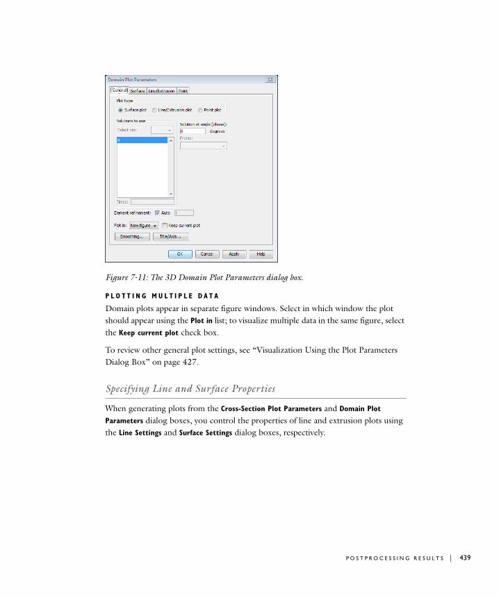
Figure 7-11: The 3D Domain Plot Parameters dialog box.
P L O T T I N G M U L T I P L E D A T A
Domain plots appear in separate figure windows. Select in which window the plot should appear using the Plot in list; to visualize multiple data in the same figure, select the Keep current plot check box.
To review other general plot settings, see “Visualization Using the Plot Parameters Dialog Box” on page 427.
Specifying Line and Surface Properties
When generating plots from the Cross-Section Plot Parameters and Domain Plot
Parameters dialog boxes, you control the properties of line and extrusion plots using the Line Settings and Surface Settings dialog boxes, respectively.
P O S T P R O C E S S I N G R E S U L T S | 439
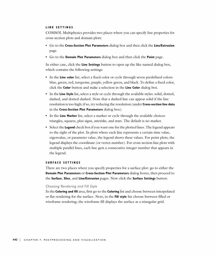
440 | C H A P T E
L I N E S E T T I N G S
COMSOL Multiphysics provides two places where you can specify line properties for cross-section plots and domain plots:
• Go to the Cross-Section Plot Parameters dialog box and then click the Line/Extrusion page
• Go to the Domain Plot Parameters dialog box and then click the Point page.
In either case, click the Line Settings button to open up the like-named dialog box, which contains the following settings:
• In the Line color list, select a fixed color or cycle through seven predefined colors: blue, green, red, turquoise, purple, yellow green, and black. To define a fixed color, click the Color button and make a selection in the Line Color dialog box.
• In the Line Style list, select a style or cycle through the available styles: solid, dotted, dashed, and dotted-dashed. Note that a dashed line can appear solid if the line resolution is too high; if so, try reducing the resolution (under Cross-section line data in the Cross-Section Plot Parameters dialog box).
• In the Line Marker list, select a marker or cycle through the available choices: triangles, squares, plus signs, asterisks, and stars. The default is no marker.
• Select the Legend check box if you want one for the plotted lines. The legend appears to the right of the plot. In plots where each line represents a certain time value, eigenvalue, or parameter value, the legend shows these values. For point plots, the legend displays the coordinate (or vertex number). For cross-section line plots with multiple parallel lines, each line gets a consecutive integer number that appears in the legend.
S U R F A C E S E T T I N G S
There are two places where you specify properties for a surface plot: go to either the Domain Plot Parameters or Cross-Section Plot Parameters dialog boxes, then proceed to the Surface, Slice, and Line/Extrusion pages. Now click the Surface Settings button.
Choosing Rendering and Fill StyleIn the Coloring and fill area, first go to the Coloring list and choose between interpolated or flat rendering for the surface. Next, in the Fill style list choose between filled or wireframe rendering; the wireframe fill displays the surface as a triangular grid.
R 7 : P O S T P R O C E S S I N G A N D V I S U A L I Z A T I O N
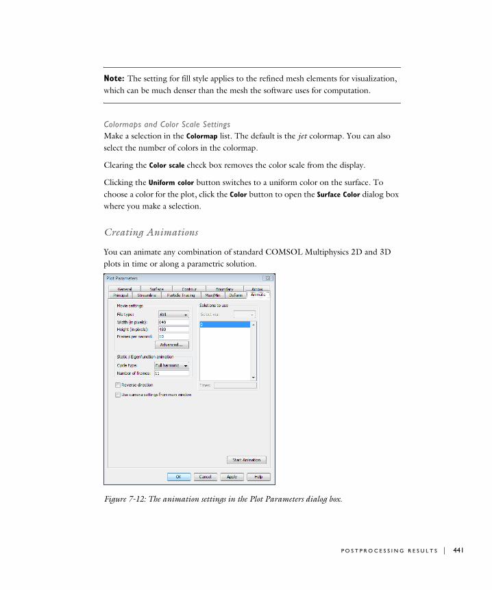
Note: The setting for fill style applies to the refined mesh elements for visualization, which can be much denser than the mesh the software uses for computation.
Colormaps and Color Scale SettingsMake a selection in the Colormap list. The default is the jet colormap. You can also select the number of colors in the colormap.
Clearing the Color scale check box removes the color scale from the display.
Clicking the Uniform color button switches to a uniform color on the surface. To choose a color for the plot, click the Color button to open the Surface Color dialog box where you make a selection.
Creating Animations
You can animate any combination of standard COMSOL Multiphysics 2D and 3D plots in time or along a parametric solution.
Figure 7-12: The animation settings in the Plot Parameters dialog box.
P O S T P R O C E S S I N G R E S U L T S | 441

442 | C H A P T E
First go to Movie settings and select the file format for the movie, either AVI or QuickTime. Also indicate the movie’s screen size in pixels and its frame rate. The screen size you enter will be increased if necessary to be at least 24x24 and a multiple of 8. Finally, select any subset of solutions to animate. For time-dependent problems, you can select Interpolated times from the Select via list, and enter any vector of times in the Times edit field, such as linspace(0,1,100) or 0:0.02:1 in the Times edit field.
To quickly get an animation of the current plot, click the Start Animation button.
When animating static and eigenvalue solutions, you must specify the animation cycle in the Cycle list. The available choices are:
• Full harmonic (a full sine wave)
• Half harmonic (half a sine wave)
• Linear (a linear ramp)
This provides a way of visualizing the time evolution of a time-harmonic model using a full sine wave as the animation cycle.
In the Number of frames edit field you specify how many frames the animation should include. The display cycles 360 degrees starting from the angle you specify in the Solution at angle (phase) edit field on the General page.
It is also possible to rewind the movie by selecting the Reverse direction check box.
The Use camera settings from main window check box controls the camera behavior when animating 2D height plots and is only visible in 2D mode. The default behavior of the camera is to zoom out to fit all data of the animation in the window. Select this option to override this behavior and use the camera settings from the main window instead.
When using the MATLAB interface, the Make movie in MATLAB check box is available. If you select it before you click Start Animation, the animation appears in a figure window in MATLAB, similar to an animation using the postmovie command.
A D V A N C E D A N I M A T I O N S E T T I N G S
You can choose which encoding format to use to encode the video in the Advanced
Animation Settings dialog box opened by clicking the Advanced button.
R 7 : P O S T P R O C E S S I N G A N D V I S U A L I Z A T I O N
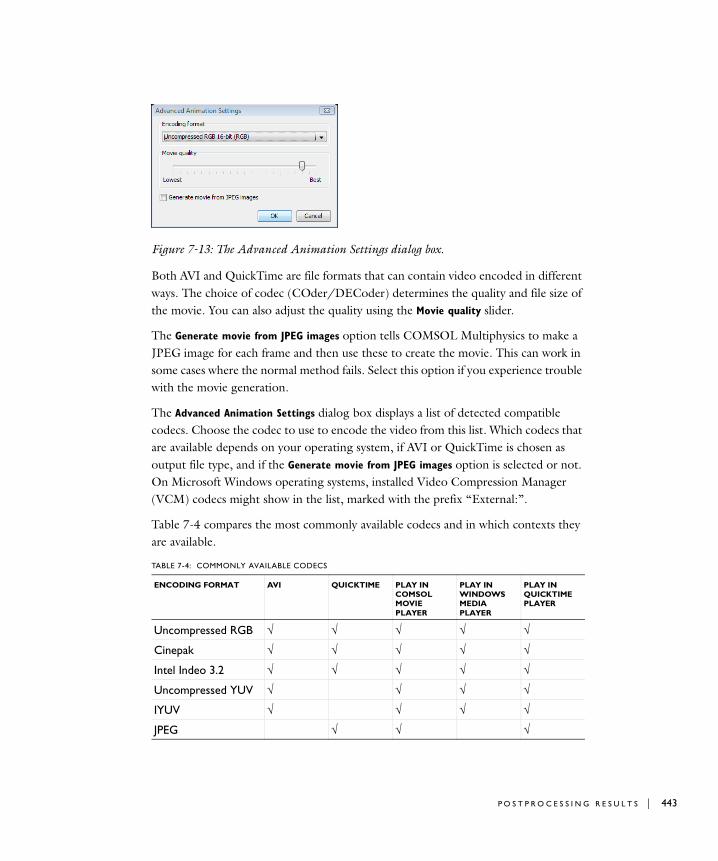
Figure 7-13: The Advanced Animation Settings dialog box.
Both AVI and QuickTime are file formats that can contain video encoded in different ways. The choice of codec (COder/DECoder) determines the quality and file size of the movie. You can also adjust the quality using the Movie quality slider.
The Generate movie from JPEG images option tells COMSOL Multiphysics to make a JPEG image for each frame and then use these to create the movie. This can work in some cases where the normal method fails. Select this option if you experience trouble with the movie generation.
The Advanced Animation Settings dialog box displays a list of detected compatible codecs. Choose the codec to use to encode the video from this list. Which codecs that are available depends on your operating system, if AVI or QuickTime is chosen as output file type, and if the Generate movie from JPEG images option is selected or not. On Microsoft Windows operating systems, installed Video Compression Manager (VCM) codecs might show in the list, marked with the prefix “External:”.
Table 7-4 compares the most commonly available codecs and in which contexts they are available.
TABLE 7-4: COMMONLY AVAILABLE CODECS
ENCODING FORMAT AVI QUICKTIME PLAY IN COMSOL MOVIE PLAYER
PLAY IN WINDOWS MEDIA PLAYER
PLAY IN QUICKTIME PLAYER
Uncompressed RGB √ √ √ √ √
Cinepak √ √ √ √ √
Intel Indeo 3.2 √ √ √ √ √
Uncompressed YUV √ √ √ √
IYUV √ √ √ √
JPEG √ √ √
P O S T P R O C E S S I N G R E S U L T S | 443
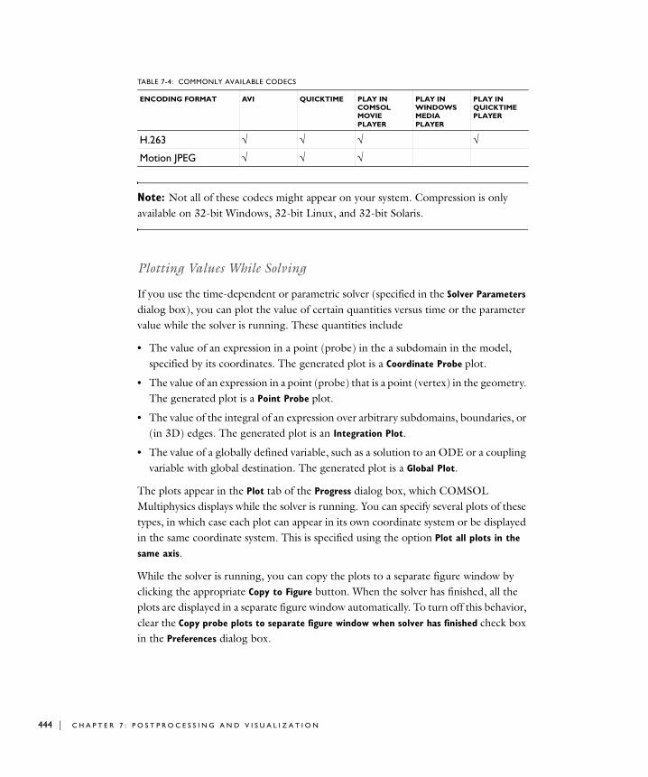
444 | C H A P T E
Note: Not all of these codecs might appear on your system. Compression is only available on 32-bit Windows, 32-bit Linux, and 32-bit Solaris.
Plotting Values While Solving
If you use the time-dependent or parametric solver (specified in the Solver Parameters dialog box), you can plot the value of certain quantities versus time or the parameter value while the solver is running. These quantities include
• The value of an expression in a point (probe) in the a subdomain in the model, specified by its coordinates. The generated plot is a Coordinate Probe plot.
• The value of an expression in a point (probe) that is a point (vertex) in the geometry. The generated plot is a Point Probe plot.
• The value of the integral of an expression over arbitrary subdomains, boundaries, or (in 3D) edges. The generated plot is an Integration Plot.
• The value of a globally defined variable, such as a solution to an ODE or a coupling variable with global destination. The generated plot is a Global Plot.
The plots appear in the Plot tab of the Progress dialog box, which COMSOL Multiphysics displays while the solver is running. You can specify several plots of these types, in which case each plot can appear in its own coordinate system or be displayed in the same coordinate system. This is specified using the option Plot all plots in the
same axis.
While the solver is running, you can copy the plots to a separate figure window by clicking the appropriate Copy to Figure button. When the solver has finished, all the plots are displayed in a separate figure window automatically. To turn off this behavior, clear the Copy probe plots to separate figure window when solver has finished check box in the Preferences dialog box.
H.263 √ √ √ √
Motion JPEG √ √ √
TABLE 7-4: COMMONLY AVAILABLE CODECS
ENCODING FORMAT AVI QUICKTIME PLAY IN COMSOL MOVIE PLAYER
PLAY IN WINDOWS MEDIA PLAYER
PLAY IN QUICKTIME PLAYER
R 7 : P O S T P R O C E S S I N G A N D V I S U A L I Z A T I O N

The axis limits in the coordinate systems are dynamic, and can thus change while the solver is running. To make probe plots with fixed axis limits, use the Manual
specification of axis limits setting, present in the plot definition area for each of the types of probe plot.
The following figure shows an example of how a probe for a velocity component appears in the Progress dialog box.
Figure 7-14: The Progress dialog box showing a probe plot.
For the Coordinate Probe Plot you can use the Draw Points for Coordinate Probe Plot toolbar button, available in the Subdomain, Boundary, Edge, and Point selection modes, to quickly specify the points in which to plot. Click this toolbar button, and then use the mouse to click where you want the points to be positioned. When finished, deselect the toolbar button by clicking it again. This creates a probe plot of the default subdomain plot quantity.
For all plot types, use the following steps to specify which quantities to plot:
P O S T P R O C E S S I N G R E S U L T S | 445
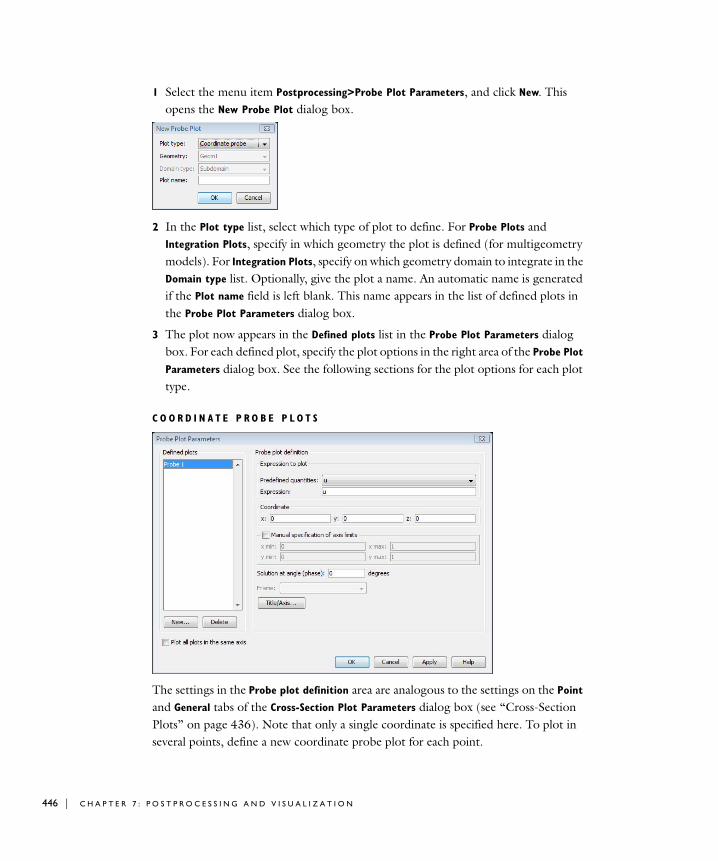
446 | C H A P T E
1 Select the menu item Postprocessing>Probe Plot Parameters, and click New. This opens the New Probe Plot dialog box.
2 In the Plot type list, select which type of plot to define. For Probe Plots and Integration Plots, specify in which geometry the plot is defined (for multigeometry models). For Integration Plots, specify on which geometry domain to integrate in the Domain type list. Optionally, give the plot a name. An automatic name is generated if the Plot name field is left blank. This name appears in the list of defined plots in the Probe Plot Parameters dialog box.
3 The plot now appears in the Defined plots list in the Probe Plot Parameters dialog box. For each defined plot, specify the plot options in the right area of the Probe Plot
Parameters dialog box. See the following sections for the plot options for each plot type.
C O O R D I N A T E P R O B E P L O T S
The settings in the Probe plot definition area are analogous to the settings on the Point and General tabs of the Cross-Section Plot Parameters dialog box (see “Cross-Section Plots” on page 436). Note that only a single coordinate is specified here. To plot in several points, define a new coordinate probe plot for each point.
R 7 : P O S T P R O C E S S I N G A N D V I S U A L I Z A T I O N

PO I N T P R O B E P L O T S
The settings in the Probe plot definition area are analogous to the settings on the Point and General tabs of the Domain Plot Parameters dialog box (see “Domain Plots” on page 438). Note that only a single geometry point is specified here. To plot in several points, define a new point probe plot for each point.
P O S T P R O C E S S I N G R E S U L T S | 447
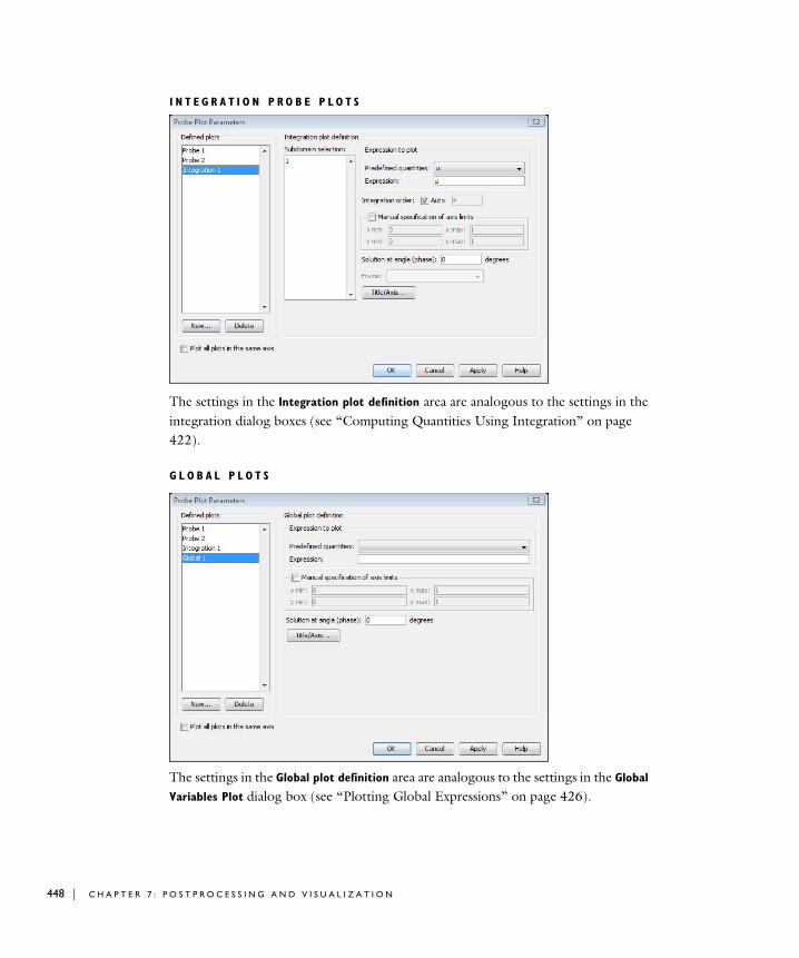
448 | C H A P T E
I N T E G R A T I O N P R O B E P L O T S
The settings in the Integration plot definition area are analogous to the settings in the integration dialog boxes (see “Computing Quantities Using Integration” on page 422).
G L O B A L P L O T S
The settings in the Global plot definition area are analogous to the settings in the Global
Variables Plot dialog box (see “Plotting Global Expressions” on page 426).
R 7 : P O S T P R O C E S S I N G A N D V I S U A L I Z A T I O N

Exporting Data to a File
As a complement to the visualizations, you can export results data to a text file for further postprocessing.
To export the data to a text file:
1 Select the menu item File>Export>Postprocessing Data.
Figure 7-15: The Export Data dialog box.
2 In the Export Data dialog box enter the name of the file or browse for it.
3 Select the domain type for the export. In the Export data from area select from: subdomains, boundaries, edges (3D), or points (2D).
4 If applicable, select the solutions to use (multiple solutions are permissible) when exporting the data to the file.
COMSOL Multiphysics then exports the data in several possible formats, which you select in the Format of exported data list. You have these choices:
Nodes, elements, data (available for all domain types). This option writes the coordinates for the nodes (in the % Coordinates section, where the ith row contains the coordinates for node i), how the nodes are connected (in the % Elements section, where the ith row contains the nodes that belong to element i), and the data values at each node point (in the % Data section, where the ith row contains the value of the data at node i).
P O S T P R O C E S S I N G R E S U L T S | 449

450 | C H A P T E
Grid, data (available only for subdomains). The first lines in the data file are the grid levels in each direction. The software then writes the data as a matrix in a format similar to that produced by the meshgrid function in COMSOL Script and MATLAB:
% Gridx grid points separated by spacesy grid points separated by spaces (optional)z grid points separated by spaces (optional)% DataData values separated by spaces
Each row contains values for different x grid points for a fixed y and z. The rows first increase the y grid value and then the z grid value.
Coordinates, data (available for all domain types). Using this option, the software writes a coordinate and its corresponding value in a separate row.
Select the Write script that creates postprocessing data check box to write an M-file with commands that create a structure of postprocessing data. You can find a description of the structure’s format under the entry for posteval on page 357 of the COMSOL Multiphysics Reference Guide.
Click the Subdomain tab to access the subdomain data-export page:
Figure 7-16: The subdomain settings in the Export Data dialog box.
Enter the name of the postprocessing expression that specifies the data on subdomains that you want to save to a file.
R 7 : P O S T P R O C E S S I N G A N D V I S U A L I Z A T I O N
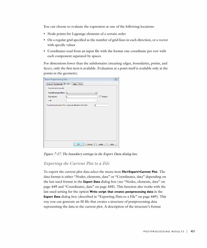
You can choose to evaluate the expression at one of the following locations:
• Node points for Lagrange elements of a certain order
• On a regular grid specified as the number of grid lines in each direction, or a vector with specific values
• Coordinates read from an input file with the format one coordinate per row with each component separated by spaces.
For dimensions lower than the subdomains (meaning edges, boundaries, points, and faces), only the first item is available. Evaluation at a point itself is available only at the points in the geometry.
Figure 7-17: The boundary settings in the Export Data dialog box.
Exporting the Current Plot to a File
To export the current plot data select the menu item File>Export>Current Plot. The data format is either “Nodes, elements, data” or “Coordinates, data” depending on the last-used format in the Export Data dialog box (see “Nodes, elements, data” on page 449 and “Coordinates, data” on page 450). This function also works with the last-used setting for the option Write script that creates postprocessing data in the Export Data dialog box (described in “Exporting Data to a File” on page 449). This way you can generate an M-file that creates a structure of postprocessing data representing the data in the current plot. A description of the structure’s format
P O S T P R O C E S S I N G R E S U L T S | 451
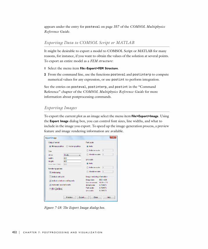
452 | C H A P T E
appears under the entry for posteval on page 357 of the COMSOL Multiphysics Reference Guide.
Exporting Data to COMSOL Script or MATLAB
It might be desirable to export a model to COMSOL Script or MATLAB for many reasons, for instance, if you want to obtain the values of the solution at several points. To export an entire model as a FEM structure:
1 Select the menu item File>Export>FEM Structure.
2 From the command line, use the functions posteval and postinterp to compute numerical values for any expression, or use postint to perform integration.
See the entries on posteval, postinterp, and postint in the “Command Reference” chapter of the COMSOL Multiphysics Reference Guide for more information about postprocessing commands.
Exporting Images
To export the current plot as an image select the menu item File>Export>Image. Using the Export Image dialog box, you can control font sizes, line widths, and what to include in the image you export. To speed up the image-generation process, a preview feature and image rendering information are available.
Figure 7-18: The Export Image dialog box.
R 7 : P O S T P R O C E S S I N G A N D V I S U A L I Z A T I O N
S E T T I N G S I N T H E E X P O R T I M A G E D I A L O G B O X
Output FormatIn the Output format area, click the Bitmap graphics button to export an image using a bitmap-based formats such as TIFF and JPEG. You select the format after clicking the Export button. Click the Vector graphics button to save the image as an EPS file (Encapsulated PostScript).
Image SizeIn the Image size area, you can specify the size of the image. Select the unit from the Units list: inches, centimeters, or pixels (pixels are available for bitmap graphics only).
When using inches or centimeters, you can set the size using the Width, Height, and Resolution (dpi) edit fields. When you use pixels as the unit, the Resolution (dpi) edit field is not available
ScalingThe settings in the Font scale and Line scale areas affect the scaling between the plot’s size on the screen and the size in the image (size = number of pixels):
• Click Auto to use the global scale (you see its value in the Image rendering information area; also see “The Global Scale” on page 454) if you specify the size in pixels (the software scales text, lines, and other graphics equally). If you specify the size in centimeters or inches, the automatic scale is based on the resolution that you. The font size and line width that you specify when creating the plot should be preserved if you export an image using a certain resolution in dpi (dots per inch) and import it to a document as an image using the same dpi number (a text with a certain size in the plot will look like a text with the same size in the document).
• Click Relative scale to use a total font scale that is the automatic scale times the relative scale that you specify.
• Click Absolute scale to use a total font scale that is equal to the absolute scale that you specify.
R E N D E R I N G O P T I O N S
The following settings are available in the Rendering options area:
AntialiasingSelect the Antialiasing check box to reduces stairstep-like lines (jaggies) and makes lines and edges look smooth
P O S T P R O C E S S I N G R E S U L T S | 453

454 | C H A P T E
Include Only PlotSelect the Include Only Plot check box to include only the graphics objects in the drawing area, excluding colorbars, axes, tick marks, titles, and labels.
Include Colorbars and LegendsSelect the Include Colorbars and Legends check box to include colorbars and legends, if present.
Automatic Axis Tick MarksSelect the Automatic axis tick marks check box to take advantage of a new feature that can hide axis tick marks if they overlap. Clear this check box if you want make sure that the image has the same axis tick marks as you see on the screen.
Rendering Thin Grid LinesSelect the Thin grid lines check box to render thin grid lines compared to other lines in the image. Use this option if you think that the grid is too dominating in the image.
Including the 3D AxisSelect the Include 3D axis check box to include the grid and coordinate system in the image.
T H E G L O B A L S C A L E
The global scale, which you find in the Image rendering information area, is the scale between the size of the plot on screen and the size of the image (size = number of pixels).
R 7 : P O S T P R O C E S S I N G A N D V I S U A L I Z A T I O N
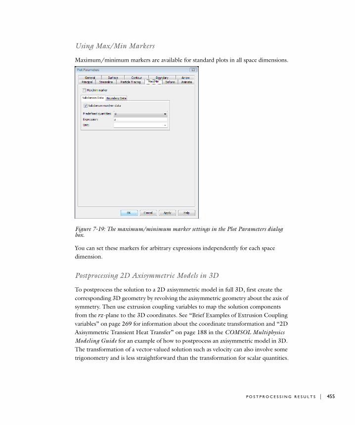
Using Max/Min Markers
Maximum/minimum markers are available for standard plots in all space dimensions.
Figure 7-19: The maximum/minimum marker settings in the Plot Parameters dialog box.
You can set these markers for arbitrary expressions independently for each space dimension.
Postprocessing 2D Axisymmetric Models in 3D
To postprocess the solution to a 2D axisymmetric model in full 3D, first create the corresponding 3D geometry by revolving the axisymmetric geometry about the axis of symmetry. Then use extrusion coupling variables to map the solution components from the rz-plane to the 3D coordinates. See “Brief Examples of Extrusion Coupling variables” on page 269 for information about the coordinate transformation and “2D Axisymmetric Transient Heat Transfer” on page 188 in the COMSOL Multiphysics Modeling Guide for an example of how to postprocess an axisymmetric model in 3D. The transformation of a vector-valued solution such as velocity can also involve some trigonometry and is less straightforward than the transformation for scalar quantities.
P O S T P R O C E S S I N G R E S U L T S | 455
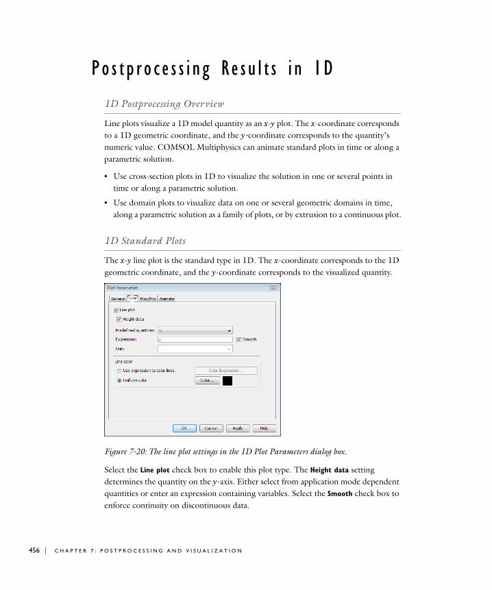
456 | C H A P T E
Po s t p r o c e s s i n g R e s u l t s i n 1D
1D Postprocessing Overview
Line plots visualize a 1D model quantity as an x-y plot. The x-coordinate corresponds to a 1D geometric coordinate, and the y-coordinate corresponds to the quantity’s numeric value. COMSOL Multiphysics can animate standard plots in time or along a parametric solution.
• Use cross-section plots in 1D to visualize the solution in one or several points in time or along a parametric solution.
• Use domain plots to visualize data on one or several geometric domains in time, along a parametric solution as a family of plots, or by extrusion to a continuous plot.
1D Standard Plots
The x-y line plot is the standard type in 1D. The x-coordinate corresponds to the 1D geometric coordinate, and the y-coordinate corresponds to the visualized quantity.
Figure 7-20: The line plot settings in the 1D Plot Parameters dialog box.
Select the Line plot check box to enable this plot type. The Height data setting determines the quantity on the y-axis. Either select from application mode dependent quantities or enter an expression containing variables. Select the Smooth check box to enforce continuity on discontinuous data.
R 7 : P O S T P R O C E S S I N G A N D V I S U A L I Z A T I O N
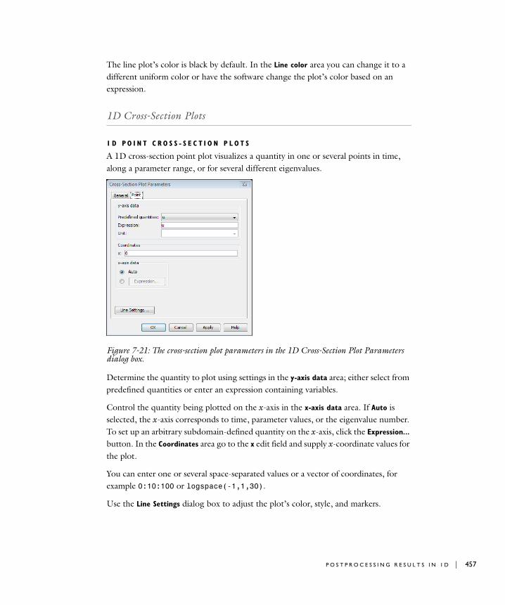
The line plot’s color is black by default. In the Line color area you can change it to a different uniform color or have the software change the plot’s color based on an expression.
1D Cross-Section Plots
1 D P O I N T C R O S S - S E C T I O N P L O T S
A 1D cross-section point plot visualizes a quantity in one or several points in time, along a parameter range, or for several different eigenvalues.
Figure 7-21: The cross-section plot parameters in the 1D Cross-Section Plot Parameters dialog box.
Determine the quantity to plot using settings in the y-axis data area; either select from predefined quantities or enter an expression containing variables.
Control the quantity being plotted on the x-axis in the x-axis data area. If Auto is selected, the x-axis corresponds to time, parameter values, or the eigenvalue number. To set up an arbitrary subdomain-defined quantity on the x-axis, click the Expression... button. In the Coordinates area go to the x edit field and supply x-coordinate values for the plot.
You can enter one or several space-separated values or a vector of coordinates, for example 0:10:100 or logspace(-1,1,30).
Use the Line Settings dialog box to adjust the plot’s color, style, and markers.
P O S T P R O C E S S I N G R E S U L T S I N 1 D | 457

458 | C H A P T E
1D Domain Plots
1 D L I N E / E X T R U S I O N D O M A I N P L O T S
This plot type visualizes the solution in one or several subdomains.
Figure 7-22: The line and extrusion plot parameters in the 1D Domain Plot Parameters dialog box.
To create a line plot or extruded surface plot on a 1D domain, do the following steps:
1 In the Plot type area click the Line plot check box to create a superimposed line plot, or click the Extrusion plot check box to have the software extrude the line plot into a continuous surface plot.
2 In the y-axis data area choose the quantity to display. Either select from predefined quantities or enter an expression containing variables.
3 Select the domains for the plot in the Subdomain selection list.
4 The software provides two ways to determine values on the x-axis. In the x-axis data area, either click the top button and select x (the values on the x-axis in the model geometry) or Arc-length (the arc length starts at 0 and represents the length of the arc); or click the bottom button, then click Expression to set x-axis data using another quantity.
5 For y-axis data, select a predefined quantity or enter an expression.
R 7 : P O S T P R O C E S S I N G A N D V I S U A L I Z A T I O N
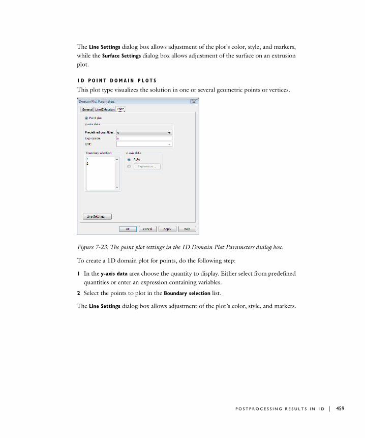
The Line Settings dialog box allows adjustment of the plot’s color, style, and markers, while the Surface Settings dialog box allows adjustment of the surface on an extrusion plot.
1 D P O I N T D O M A I N P L O T S
This plot type visualizes the solution in one or several geometric points or vertices.
Figure 7-23: The point plot settings in the 1D Domain Plot Parameters dialog box.
To create a 1D domain plot for points, do the following step:
1 In the y-axis data area choose the quantity to display. Either select from predefined quantities or enter an expression containing variables.
2 Select the points to plot in the Boundary selection list.
The Line Settings dialog box allows adjustment of the plot’s color, style, and markers.
P O S T P R O C E S S I N G R E S U L T S I N 1 D | 459
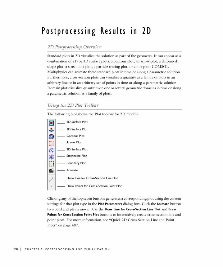
460 | C H A P T E
Po s t p r o c e s s i n g R e s u l t s i n 2D
2D Postprocessing Overview
Standard plots in 2D visualize the solution as part of the geometry. It can appear as a combination of 2D or 3D surface plots, a contour plot, an arrow plot, a deformed shape plot, a streamline plot, a particle tracing plot, or a line plot. COMSOL Multiphysics can animate these standard plots in time or along a parametric solution. Furthermore, cross-section plots can visualize a quantity as a family of plots in an arbitrary line or in an arbitrary set of points in time or along a parametric solution. Domain plots visualize quantities on one or several geometric domains in time or along a parametric solution as a family of plots.
Using the 2D Plot Toolbar
The following plot shows the Plot toolbar for 2D models:
Clicking any of the top seven buttons generates a corresponding plot using the current settings for that plot type in the Plot Parameters dialog box. Click the Animate button to record and play a movie. Use the Draw Line for Cross-Section Line Plot and Draw
Points for Cross-Section Point Plot buttons to interactively create cross-section line and point plots. For more information, see “Quick 2D Cross-Section Line and Point Plots” on page 487.
2D Surface Plot
3D Surface Plot
Contour Plot
Arrow Plot
2D Surface Plot
Streamline Plot
Boundary Plot
Animate
Draw Line for Cross-Section Line Plot
Draw Points for Cross-Section Point Plot
R 7 : P O S T P R O C E S S I N G A N D V I S U A L I Z A T I O N
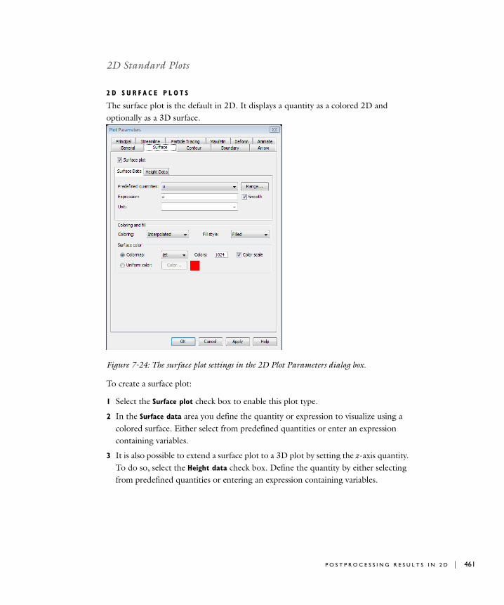
2D Standard Plots
2 D S U R F A C E P L O T S
The surface plot is the default in 2D. It displays a quantity as a colored 2D and optionally as a 3D surface.
Figure 7-24: The surface plot settings in the 2D Plot Parameters dialog box.
To create a surface plot:
1 Select the Surface plot check box to enable this plot type.
2 In the Surface data area you define the quantity or expression to visualize using a colored surface. Either select from predefined quantities or enter an expression containing variables.
3 It is also possible to extend a surface plot to a 3D plot by setting the z-axis quantity. To do so, select the Height data check box. Define the quantity by either selecting from predefined quantities or entering an expression containing variables.
P O S T P R O C E S S I N G R E S U L T S I N 2 D | 461
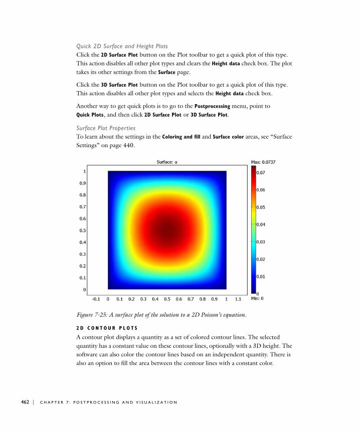
462 | C H A P T E
Quick 2D Surface and Height PlotsClick the 2D Surface Plot button on the Plot toolbar to get a quick plot of this type. This action disables all other plot types and clears the Height data check box. The plot takes its other settings from the Surface page.
Click the 3D Surface Plot button on the Plot toolbar to get a quick plot of this type. This action disables all other plot types and selects the Height data check box.
Another way to get quick plots is to go to the Postprocessing menu, point to Quick Plots, and then click 2D Surface Plot or 3D Surface Plot.
Surface Plot PropertiesTo learn about the settings in the Coloring and fill and Surface color areas, see “Surface Settings” on page 440.
Figure 7-25: A surface plot of the solution to a 2D Poisson’s equation.
2 D C O N T O U R P L O T S
A contour plot displays a quantity as a set of colored contour lines. The selected quantity has a constant value on these contour lines, optionally with a 3D height. The software can also color the contour lines based on an independent quantity. There is also an option to fill the area between the contour lines with a constant color.
R 7 : P O S T P R O C E S S I N G A N D V I S U A L I Z A T I O N
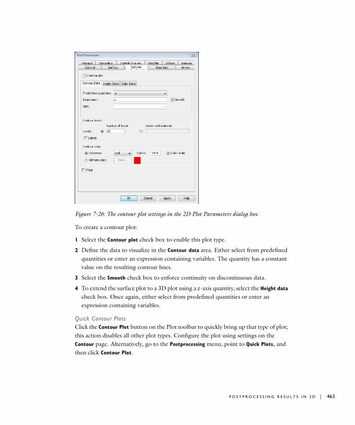
Figure 7-26: The contour plot settings in the 2D Plot Parameters dialog box.
To create a contour plot:
1 Select the Contour plot check box to enable this plot type.
2 Define the data to visualize in the Contour data area. Either select from predefined quantities or enter an expression containing variables. The quantity has a constant value on the resulting contour lines.
3 Select the Smooth check box to enforce continuity on discontinuous data.
4 To extend the surface plot to a 3D plot using a z-axis quantity, select the Height data check box. Once again, either select from predefined quantities or enter an expression containing variables.
Quick Contour PlotsClick the Contour Plot button on the Plot toolbar to quickly bring up that type of plot; this action disables all other plot types. Configure the plot using settings on the Contour page. Alternatively, go to the Postprocessing menu, point to Quick Plots, and then click Contour Plot.
P O S T P R O C E S S I N G R E S U L T S I N 2 D | 463

464 | C H A P T E
Filled Contour PlotsTo create a filled contour plot, select the Filled check box. This creates a plot with as many bands of constant color as you have specified in the Number of levels edit field. Alternatively, the filled contour plot is a contour plot with the levels specified in Vector
with isolevels edit field, where COMSOL Multiphysics then fills the area between the contour lines. The color of each filled area represents the data interval between the contour lines. The color scale shows these data intervals.
Defining Contour Levels and Adding LabelsGo to the Contour levels area to adjust the like-named settings. Click the button to the left of the Number of levels edit field to supply an integer that indicates the number of levels (the default is 20). Alternatively, click the button to the left of the Vector with
isolevels edit field to enter a vector, for example 0:10:100 or logspace(-1,1,30). To include contour labels, select the Labels check box in the Contour levels area.
Coloring ContoursBy default, COMSOL Multiphysics colors contour lines based on settings in the Contour data area, and it makes each line a uniform color. To instead color the contour lines based on an independent quantity, select the Color data check box and enter a predefined quantity or an expression.
For most plot types, the default for color mapping is to spread the range of colors across the entire range of variable values. Thus, in any given limited range of values it might be difficult to discern any differences. To overcome this effect, you can set the display to have the full range of colors map onto a subset of the variable values. To do so, click the Range button and in the resulting dialog box set the color range to zoom in on specific contours to reveal small differences at an interesting location.
Colormaps and Color Scale SettingsMake a selection in the Colormap list. The default colormap is cool, which varies smoothly from cyan to magenta. You can also select the number of colors a colormap uses.
Clearing the Color scale check box removes the color scale from the display.
R 7 : P O S T P R O C E S S I N G A N D V I S U A L I Z A T I O N

Clicking the Uniform color button switches the contours to a uniform color, whereas clicking the Color button opens the Contour Color dialog box where you can select a color for the plot.
Figure 7-27: A contour plot of the solution to a 2D Poisson’s equation.
P O S T P R O C E S S I N G R E S U L T S I N 2 D | 465
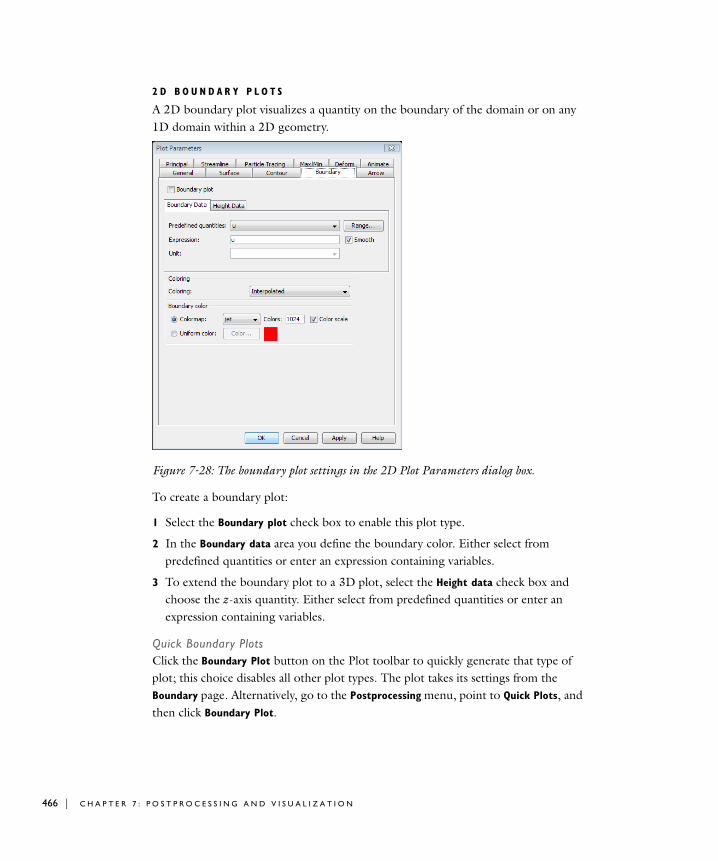
466 | C H A P T E
2 D B O U N D A R Y P L O T S
A 2D boundary plot visualizes a quantity on the boundary of the domain or on any 1D domain within a 2D geometry.
Figure 7-28: The boundary plot settings in the 2D Plot Parameters dialog box.
To create a boundary plot:
1 Select the Boundary plot check box to enable this plot type.
2 In the Boundary data area you define the boundary color. Either select from predefined quantities or enter an expression containing variables.
3 To extend the boundary plot to a 3D plot, select the Height data check box and choose the z-axis quantity. Either select from predefined quantities or enter an expression containing variables.
Quick Boundary PlotsClick the Boundary Plot button on the Plot toolbar to quickly generate that type of plot; this choice disables all other plot types. The plot takes its settings from the Boundary page. Alternatively, go to the Postprocessing menu, point to Quick Plots, and then click Boundary Plot.
R 7 : P O S T P R O C E S S I N G A N D V I S U A L I Z A T I O N
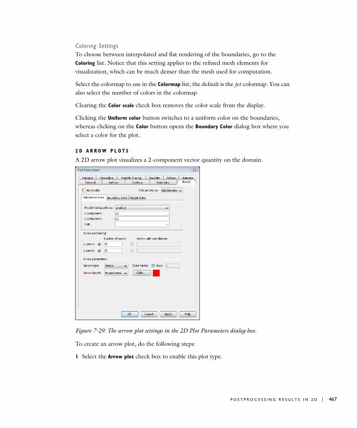
Coloring SettingsTo choose between interpolated and flat rendering of the boundaries, go to the Coloring list. Notice that this setting applies to the refined mesh elements for visualization, which can be much denser than the mesh used for computation.
Select the colormap to use in the Colormap list; the default is the jet colormap. You can also select the number of colors in the colormap.
Clearing the Color scale check box removes the color scale from the display.
Clicking the Uniform color button switches to a uniform color on the boundaries, whereas clicking on the Color button opens the Boundary Color dialog box where you select a color for the plot.
2 D A R R O W P L O T S
A 2D arrow plot visualizes a 2-component vector quantity on the domain.
Figure 7-29: The arrow plot settings in the 2D Plot Parameters dialog box.
To create an arrow plot, do the following steps:
1 Select the Arrow plot check box to enable this plot type.
P O S T P R O C E S S I N G R E S U L T S I N 2 D | 467
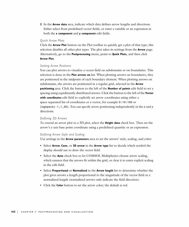
468 | C H A P T E
2 In the Arrow data area, indicate which data defines arrow lengths and directions. Either select from predefined vector fields, or enter a variable or an expression in both the x component and y component edit fields.
Quick Arrow PlotsClick the Arrow Plot button on the Plot toolbar to quickly get a plot of that type; this selection disables all other plot types. The plot takes its settings from the Arrow page. Alternatively, go to the Postprocessing menu, point to Quick Plots, and then click Arrow Plot.
Setting Arrow PositionsYou can plot arrows to visualize a vector field on subdomains or on boundaries. This selection is done in the Plot arrows on list. When plotting arrows on boundaries, they are positioned in the midpoint of each boundary element. When plotting arrows on subdomains, the arrows are positioned in a regular grid, selected in the Arrow
positioning area. Click the button to the left of the Number of points edit field to set a spacing using equidistantly distributed arrows. Click the button to the left of the Vector
with coordinates edit field to explicitly set arrow coordinates using either a space-separated list of coordinates or a vector, for example 0:10:100 or logspace(-1,1,30). You can specify arrow positioning independently in the x and y directions.
Defining 3D ArrowsTo extend an arrow plot to a 3D plot, select the Height data check box. Then set the arrow’s z-axis base point coordinate using a predefined quantity or an expression.
Defining Arrow Style and ScalingUse settings in the Arrow parameters area to set the arrows’ style, scaling, and color:
• Select Arrow, Cone, or 3D arrow in the Arrow type list to decide which symbol the display should use to draw the vector field.
• Select the Auto check box to let COMSOL Multiphysics choose arrow scaling, which ensures that the arrows fit within the grid, or clear it to enter explicit scaling in the edit field.
• Select Proportional or Normalized in the Arrow length list to determine whether the plot gives arrows a length proportional to the magnitude of the vector field or a normalized length (normalized arrows only indicate the field direction).
• Click the Color button to set the arrow color; the default is red.
R 7 : P O S T P R O C E S S I N G A N D V I S U A L I Z A T I O N

Figure 7-30: The arrows in this plot visualize the gradient of the solution to a 2D Poisson’s equations.
2 D P R I N C I P A L S T R E S S / S T R A I N P L O T S
A 2D principal stress/strain can visualize first, second, and third principal stress or principal strain directions and values. This plot type is available when COMSOL Multiphysics is used together with the Structural Mechanics Module or the MEMS Module.
P O S T P R O C E S S I N G R E S U L T S I N 2 D | 469
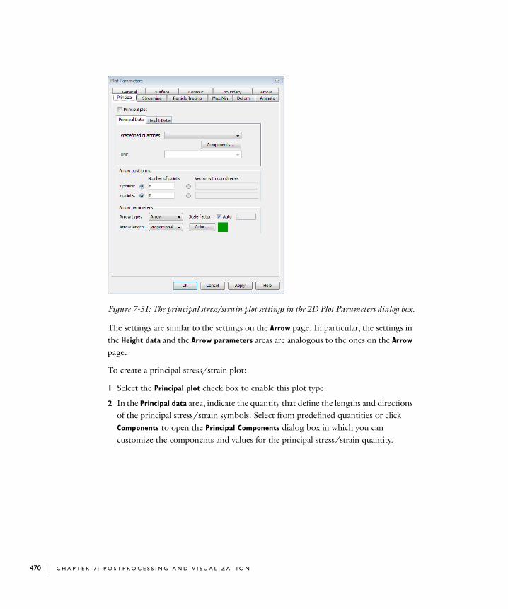
470 | C H A P T E
Figure 7-31: The principal stress/strain plot settings in the 2D Plot Parameters dialog box.
The settings are similar to the settings on the Arrow page. In particular, the settings in the Height data and the Arrow parameters areas are analogous to the ones on the Arrow page.
To create a principal stress/strain plot:
1 Select the Principal plot check box to enable this plot type.
2 In the Principal data area, indicate the quantity that define the lengths and directions of the principal stress/strain symbols. Select from predefined quantities or click Components to open the Principal Components dialog box in which you can customize the components and values for the principal stress/strain quantity.
R 7 : P O S T P R O C E S S I N G A N D V I S U A L I Z A T I O N
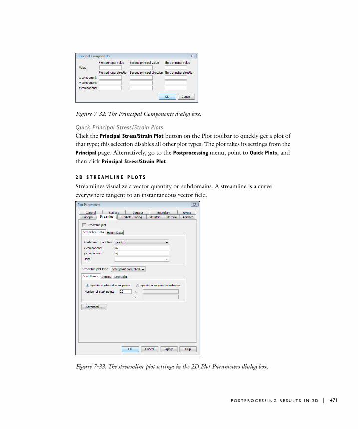
Figure 7-32: The Principal Components dialog box.
Quick Principal Stress/Strain PlotsClick the Principal Stress/Strain Plot button on the Plot toolbar to quickly get a plot of that type; this selection disables all other plot types. The plot takes its settings from the Principal page. Alternatively, go to the Postprocessing menu, point to Quick Plots, and then click Principal Stress/Strain Plot.
2 D S T R E A M L I N E P L O T S
Streamlines visualize a vector quantity on subdomains. A streamline is a curve everywhere tangent to an instantaneous vector field.
Figure 7-33: The streamline plot settings in the 2D Plot Parameters dialog box.
P O S T P R O C E S S I N G R E S U L T S I N 2 D | 471
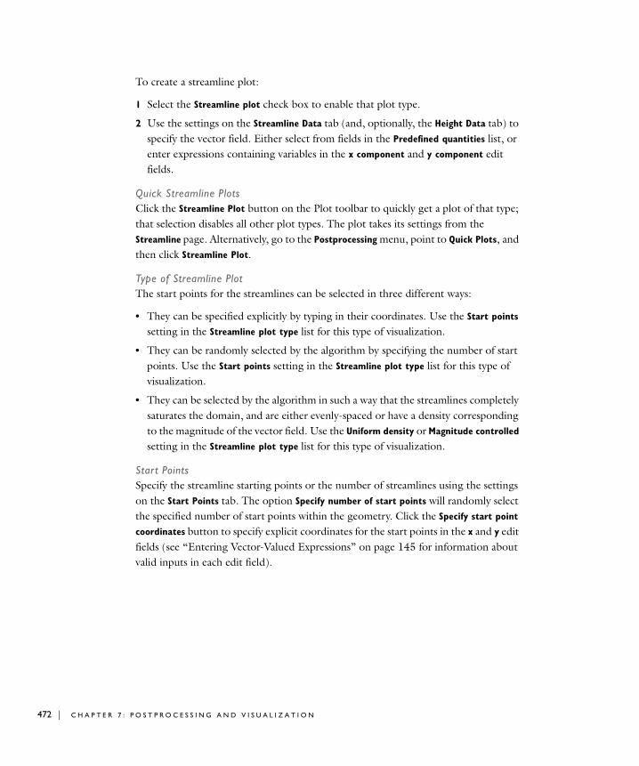
472 | C H A P T E
To create a streamline plot:
1 Select the Streamline plot check box to enable that plot type.
2 Use the settings on the Streamline Data tab (and, optionally, the Height Data tab) to specify the vector field. Either select from fields in the Predefined quantities list, or enter expressions containing variables in the x component and y component edit fields.
Quick Streamline PlotsClick the Streamline Plot button on the Plot toolbar to quickly get a plot of that type; that selection disables all other plot types. The plot takes its settings from the Streamline page. Alternatively, go to the Postprocessing menu, point to Quick Plots, and then click Streamline Plot.
Type of Streamline PlotThe start points for the streamlines can be selected in three different ways:
• They can be specified explicitly by typing in their coordinates. Use the Start points setting in the Streamline plot type list for this type of visualization.
• They can be randomly selected by the algorithm by specifying the number of start points. Use the Start points setting in the Streamline plot type list for this type of visualization.
• They can be selected by the algorithm in such a way that the streamlines completely saturates the domain, and are either evenly-spaced or have a density corresponding to the magnitude of the vector field. Use the Uniform density or Magnitude controlled setting in the Streamline plot type list for this type of visualization.
Start PointsSpecify the streamline starting points or the number of streamlines using the settings on the Start Points tab. The option Specify number of start points will randomly select the specified number of start points within the geometry. Click the Specify start point
coordinates button to specify explicit coordinates for the start points in the x and y edit fields (see “Entering Vector-Valued Expressions” on page 145 for information about valid inputs in each edit field).
R 7 : P O S T P R O C E S S I N G A N D V I S U A L I Z A T I O N

Density
Figure 7-34: The streamline density settings in the 2D Plot Parameters dialog box.
To create streamlines with a uniform density, select Uniform density in the Streamline
plot type list. To create streamlines with a variable density according to the magnitude of the specified vector field, select Magnitude controlled.
Uniform density With this setting, the algorithm saturates the entire domain with evenly spaced streamlines. To specify the separating distance between the streamlines, click the Density tab, and then enter the distance in the Separating distance edit field. The value for the separating distance is a fraction of the mean of the lengths of the bounding box of the geometry. In this case, a streamline stops whenever it gets too close to another streamline or itself (or if any of the general termination criteria specified in the Advanced Streamline Parameters dialog box is fulfilled).
Magnitude controlled This setting only gives proper streamline plots for incompressible flow fields. In this case, the algorithm places the streamlines so that the flow between each pair of adjacent streamlines is the same throughout the domain, giving streamlines that are more dense where the magnitude of the field is high. The density is controlled with the Density setting. This value is roughly the number of streamlines. Prior to streamline generation, the software computes a rough estimate of
P O S T P R O C E S S I N G R E S U L T S I N 2 D | 473

474 | C H A P T E
the total flow of the flow field in the model, divides this value with the specified Density setting, and uses the resulting value as the flow between each pair of adjacent streamlines. A streamline stops only if it exists the domain or gets too close to its own start point, using the Loop tolerance option in the Advanced Streamline Parameters dialog box (or if any of the general termination criteria specified in the Advanced
Streamline Parameters dialog box is fulfilled).
Advanced Density SettingsThe Settings button on the Density page opens the Advanced Density Settings dialog box.
Figure 7-35: The Advanced Density Settings dialog box.
Manually specify first start point The start point for the first streamline is chosen in the element where the highest value of the velocity of the specified vector field occurs. To override this choice, select this option and type in the coordinates.
Boundary element refinement This is a measurement of the density of points on the boundaries used to set up the structure used to measure distances between streamlines. If you experience that streamlines do not behave as expected near boundaries on a coarse mesh, this number might need to be increased. Refining the mesh in the problematic area can also resolve the problem.
Fraction of streamline length to ignore This option is only present when Uniform
density is selected in the Streamline plot type list. When a streamline is close to itself, typically for spiraling streamlines, this number controls how big part of the streamline, starting from its start point, that the streamline itself is allowed to get close to.
Starting distance factor In 2D, this option is only present when Uniform density is selected in the Streamline plot type list. This is a factor multiplied with the distance specified in Separating distance to get the minimum distance between streamlines and the start point for the next streamline. When the domain is close to be saturated with streamlines, new start points tend to be positioned where the streamline has nowhere
R 7 : P O S T P R O C E S S I N G A N D V I S U A L I Z A T I O N
to go before it gets too close other streamlines, resulting in short streamlines. A high value of this factor disqualifies the start point and thus reduces the number of short streamlines.
Terminating distance factor This option is only present when Uniform density is selected in the Streamline plot type list. This is a factor multiplied with the distance specified in Separating distance to get the minimum distance between any pair of streamlines. Thus, this distance is the minimal distance under which the integration of a streamline will stop.
Defining 3D StreamlinesSelecting the Height data check box on the Height Data tab extends a streamline plot to a 3D plot by setting the streamline’s z-coordinate using a predefined quantity or an expression.
Advanced Streamline SettingsClick the Advanced button to open the Advanced Streamline Parameters dialog box. It contains settings that you should not need to change very often. It allows user interaction with these fields and check boxes:
• The Maximum number of integration steps edit field; the default is 5000.
• The Maximum integration time edit field; the default is infinity (Inf).
• The Integration tolerance edit field; the default is 0.01.
• The Stationary point stop tolerance edit field; the default is 0.01.
• The Loop tolerance edit field; the default is 0.01. This is a fraction of the mean of the lengths of the bounding box of the geometry. If a streamline gets closer to its start point than this distance, the streamline will snap to its start point and thus will be plotted as a connected loop.
• The Allow backward time integration check box. This option is only present when Start Points is selected in the Control list. This option integrates points from the starting points both in the direction of the vector field and in the opposite direction. The default setting allows backward time integration.
• The Normalize vector field check box; the default is a vector field for the streamlines that is not normalized.
These settings have the following effects:
1 When calculating streamlines, the software selects a set of starting points (controlled by the streamline start points and the number of start points)
P O S T P R O C E S S I N G R E S U L T S I N 2 D | 475
476 | C H A P T E
2 The algorithm then finds the vectors of the given vector field at these points by interpolation. It normalizes the vector field if you select that option.
3 The algorithm integrates the points along the direction of the vector using the integration tolerance using a second-order Runge-Kutta algorithm.
4 At the new positions, the algorithm finds vector values by interpolation and performs another integration.
This process stops if:
• It reaches a predetermined number of integration steps (controlled by the maximum number of integration steps entry).
• The points end up outside the geometry.
• The points reach a “stationary point” where the vector field is zero. You control the meaning of “zero” with the stationary point stop tolerance.
• It has used a predetermined amount of “time” for integrating (you control this parameter with the Maximum integration time edit field).
Finally, the software connects the calculated points for each streamline consecutively with straight lines.
Note: When integrating, the software uses a pseudotime that has nothing to do with the time in time-dependent problems. Use the massless particle tracing tool to integrate in time-varying fields and to control the real time in stationary fields.
2 D P A R T I C L E T R A C I N G P L O T S
With this plot type, you can visualize pathlines, that is, trajectories of particles released in a flow field, which can be time-dependent or static. For time-dependent flows you can also use a snapshot in time of the flow field as a static field. The motion of the particles does not affect the flow field.
Selecting Particle TypeYou can create particle tracing plots for particles with mass or for massless particles. Select With mass or Massless in the Particle type list.
For particles with mass, the software generates the pathlines by solving the fundamental equation of motion
mx·· F t x x·, ,( )=
R 7 : P O S T P R O C E S S I N G A N D V I S U A L I Z A T I O N
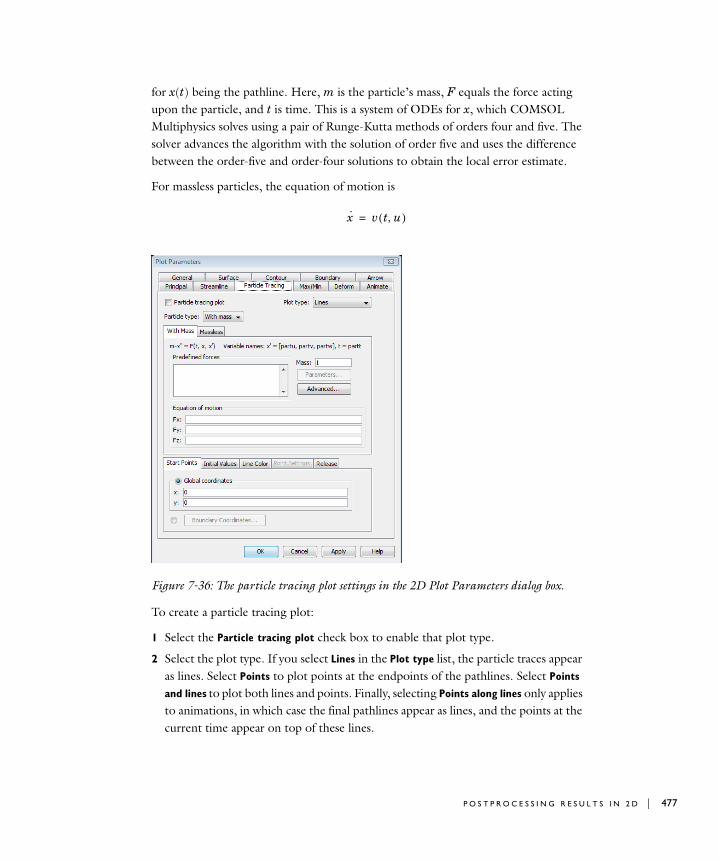
for x(t) being the pathline. Here, m is the particle’s mass, F equals the force acting upon the particle, and t is time. This is a system of ODEs for x, which COMSOL Multiphysics solves using a pair of Runge-Kutta methods of orders four and five. The solver advances the algorithm with the solution of order five and uses the difference between the order-five and order-four solutions to obtain the local error estimate.
For massless particles, the equation of motion is
Figure 7-36: The particle tracing plot settings in the 2D Plot Parameters dialog box.
To create a particle tracing plot:
1 Select the Particle tracing plot check box to enable that plot type.
2 Select the plot type. If you select Lines in the Plot type list, the particle traces appear as lines. Select Points to plot points at the endpoints of the pathlines. Select Points
and lines to plot both lines and points. Finally, selecting Points along lines only applies to animations, in which case the final pathlines appear as lines, and the points at the current time appear on top of these lines.
x· v t u,( )=
P O S T P R O C E S S I N G R E S U L T S I N 2 D | 477

478 | C H A P T E
3 Select the particle type in the Particle type list.
For particles with mass, use the settings on the With Mass tab. In the Predefined
forces area, select from the application mode’s predefined particle forces. For examples see “Electromagnetic Force for Particle Tracing” on page 81 or “Khan and Richardson Force for Particle Tracing” on page 147 in the COMSOL Multiphysics Modeling Guide. When selecting a predefined force, the corresponding force expression appears in the Equation of motion area. Here you can edit the expression or enter a custom force expression. To quickly clear the text fields, use Ctrl-click to deselect all forces in the list of predefined forces. Enter the particle mass in the Mass edit field. For some predefined forces, there are additional particle force parameters such as the particle radius. Click the Parameters button to define these additional parameters. If the equation of motion depends on the particle’s velocity, the top of the With Mass tab shows the variable names to use for the components of the particle’s velocity. Also, for static flows, this area shows the variable name to use for time. You can change these names in the Advanced
Parameters dialog box; see “Advanced Particle Tracing Settings” on page 481.
For massless particles, use the settings on the Massless tab. Select a quantity for the velocity field v in the Predefined quantities list. The contents of this list depends on the application; typically it is the velocity field or another vector field of interest. You can change the field components by editing the contents in the x component and y component edit fields. The Unit list contains a list of applicable units for the field components.
4 Click the Start points tab at the bottom of the dialog box and enter the appropriate coordinates. For information about valid inputs in each edit field, see “Entering Vector-Valued Expressions” on page 145. Click the option button to the left of the Boundary Coordinates button; then click that button to open the Boundary
Coordinates dialog box. Then elect the boundaries where you want your starting
R 7 : P O S T P R O C E S S I N G A N D V I S U A L I Z A T I O N
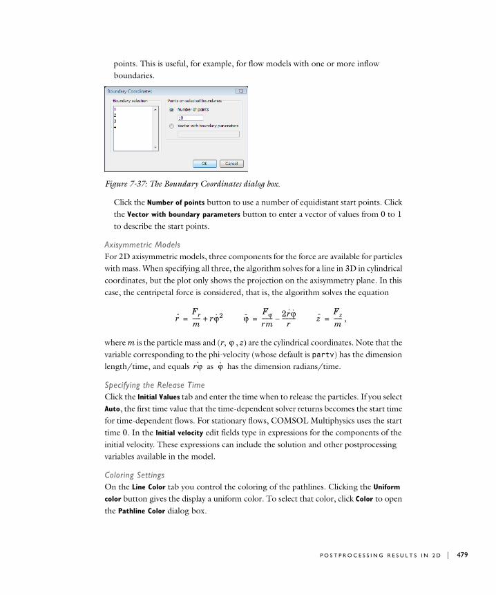
points. This is useful, for example, for flow models with one or more inflow boundaries.
Figure 7-37: The Boundary Coordinates dialog box.
Click the Number of points button to use a number of equidistant start points. Click the Vector with boundary parameters button to enter a vector of values from 0 to 1 to describe the start points.
Axisymmetric ModelsFor 2D axisymmetric models, three components for the force are available for particles with mass. When specifying all three, the algorithm solves for a line in 3D in cylindrical coordinates, but the plot only shows the projection on the axisymmetry plane. In this case, the centripetal force is considered, that is, the algorithm solves the equation
,
where m is the particle mass and (r, , z) are the cylindrical coordinates. Note that the variable corresponding to the phi-velocity (whose default is partv) has the dimension length/time, and equals as has the dimension radians/time.
Specifying the Release TimeClick the Initial Values tab and enter the time when to release the particles. If you select Auto, the first time value that the time-dependent solver returns becomes the start time for time-dependent flows. For stationary flows, COMSOL Multiphysics uses the start time 0. In the Initial velocity edit fields type in expressions for the components of the initial velocity. These expressions can include the solution and other postprocessing variables available in the model.
Coloring SettingsOn the Line Color tab you control the coloring of the pathlines. Clicking the Uniform
color button gives the display a uniform color. To select that color, click Color to open the Pathline Color dialog box.
r··Fr
m------ rϕ· 2+= ϕ··
Fϕrm-------- 2r·ϕ·
r----------–= z··
Fz
m------=
ϕ
rϕ· ϕ·
P O S T P R O C E S S I N G R E S U L T S I N 2 D | 479

480 | C H A P T E
It is possible to use an expression to color the pathlines. Click the Use expression button, then click the Color Expression button. In the Pathline Color Expression dialog box you select from predefined quantities or enter an expression. You can also specify a colormap, the number of colors, and turn the color scale on or off.
Point SettingsOn the Point Settings tab, set the color and radius scale for the points (used for the Plot
type settings Points, Points and lines, and Points along lines). The default is to use an automatic scaling of the radius; clear the Auto check box to enter another point radius scale factor. In the When particle leaves domain list, select the behavior of points that have left the domain. Select Stick to boundary to plot the points on the boundary at the exit point, and select Disappear to not render these points at all. For static fields, click the Advanced button to specify the end time in the Advanced Parameters dialog box. It is possible that all particles have left the domain at the selected time. In that case, all points appear at the outflow boundary if you select Stick to boundary, and no points appear if you select Disappear. To make the points appear, specify an earlier end time.
Starting at Multiple TimesOn the Release tab, select at which times to start the particle tracing algorithm. Click the Release once button to only start at the time specified on the Initial Values tab. Click the Time between releases button to specify a time interval between each start time value. Click the Release at times button to specify explicit time values at which to start as space-separated values.
R 7 : P O S T P R O C E S S I N G A N D V I S U A L I Z A T I O N

Advanced Particle Tracing SettingsClick the Advanced button to open the Advanced Parameters dialog box.
When solving the 2nd-order ODE for x, the solver first rewrites it as two coupled 1st-order ODEs: one for the position x and one for the velocity , each with two components in 2D and three components in 3D.
The value in the Relative tolerance edit field is the relative error tolerance that the ODE solver uses. It applies to all components of the particle’s position and velocity. The solver controls the step size so that the estimated error e in each integration step satisfies
(for all components of x), and
(for all components of ),
where rtol is the relative tolerance specified here, atolpos is the absolute tolerance for the particle’s position components, and atolvel equals the absolute tolerance for the particle’s velocity components. You specify these absolute tolerances in the Manual
tuning of absolute tolerances area. If you clear the check box at the top of this area, the software automatically computes absolute tolerances for the position and does not use absolute tolerances for the velocity. The automatic absolute tolerance for the position is the mean of the lengths of the bounding box to the geometry multiplied by the relative tolerance. If, on the other hand, you select this check box, you can type in your own values for the absolute tolerances in the text fields Position and Velocity. Each text field can either contain a single value, in which case this absolute tolerance is applied to all components of the position or velocity. Alternatively, it can contain a space or
mx·· F t x x·, ,( )=
x·
e max atolpos rtol, xi⋅( )< xi
e max atolvel rtol, x· i⋅( )< x· i x·
P O S T P R O C E S S I N G R E S U L T S I N 2 D | 481

482 | C H A P T E
comma separated list of values specifying individual absolute tolerances for the components of the position or velocity. Thus, in 2D, you can specify two values, and in 3D and 2D axisymmetry, you can specify three values in each of the text fields.
In the Manual tuning of step size area you specify an initial time step and an upper limit of the step size. If you clear the check box at the top of this area, the software automatically computes an initial time step and a maximum time step. To compute the automatic initial time step, the solver uses the initial value of the acceleration (force divided by mass) and the relative and absolute tolerances. The automatic maximum step size is 10% of the total simulation time for time-dependent flows as well as for static flows where you specify the end time manually in the End time for static flows edit field. For static flows where you do not set the end time manually, there is no upper limit of the step size. However, in this case, the initial time step is less than or equal to 0.1.
The maximum step size has higher priority than the initial step size, that is, if you specify an initial step size larger than maximum step size, the solver lowers the initial step size to the maximum step size.
Note that the initial step size, whether you enter it manually or the solver computes it automatically, is not necessarily the first step the solver takes but is rather a first try. If this step leads to an error such that the tolerances are not met, COMSOL Multiphysics lowers it.
If you clear the Manual tuning of step size check box, the software shows the automatically computed values for the previous plot in the corresponding edit fields. The value in the Maximum time step edit field is the longest time step the solver takes.
The Termination area contains settings that determines when to end the particle tracing simulation:
• In the End time for static flow fields edit field, specify the maximum time at which to end the particle-tracing simulation for static flow fields. (For time-dependent flows, the automatic end time is the last time that the time-dependent solver returns.) If you select the Auto check box, there is no upper limit of the time. In this case, the particle simulation goes on until all particles exit the geometry or the simulation reaches the maximum number of steps. If you activate the Auto setting, the edit field contains the time value at which the previous particle tracing plot ended.
• If you specify a limit in the Maximum number of steps edit field, the particle simulation ends after this number of steps. If you use the Auto setting the limit varies in this way: for static flow fields, the algorithm uses the value 1000; for
R 7 : P O S T P R O C E S S I N G A N D V I S U A L I Z A T I O N
time-dependent flows, there is no upper limit of the number of steps, and the particle simulation goes on until it reaches the end time. If you activate the Auto setting, the edit field displays the number of steps that the previous particle tracing plot took.
• The value in the Edge tolerance edit field is an absolute tolerance controlling how close to the geometry boundary the pathlines are cut when they exit the geometry. A lower value cuts the line closer to the geometry boundary.
In the Variable names area, specify the names of the particles’ velocity components and the time for static flow fields and particles with mass. For static flow fields and massless particles, you can specify the name of the variable for time. Normally there is no need to change the default names. You can use these names in expressions for the force as well as for the color when coloring the pathlines according to an expression.
For time-dependent problems, selecting the Use instantaneous flow field (for
time-dependent problems) check box freezes the time to the value specified using the Solution at time list on the General tab and considers this a static flow field.
The Resolution setting increases the number of output points by the specified factor by adding points between each time step taken in the ODE solver, using a 4th-order interpolation, to produce a smoother output.
Note: The true formulation of Newton’s second law of motion is , that is, you must consider the time derivative of the mass. The
particle-tracing algorithm does not solve this equation. Thus, if you specify an expression for the particle mass that depends on time, you will not get correct results.
2 D D E F O R M E D S H A P E P L O T S
It is also possible to visualize a vector field by deforming the geometrical shape. This plot type is primarily intended for visualizing x- and y-displacements (u and v) for problems in structural mechanics. By default, this method automatically scales the deformation to 10% of the geometric domain.
ddt------ mx·( ) F t x x·, ,( )=
P O S T P R O C E S S I N G R E S U L T S I N 2 D | 483
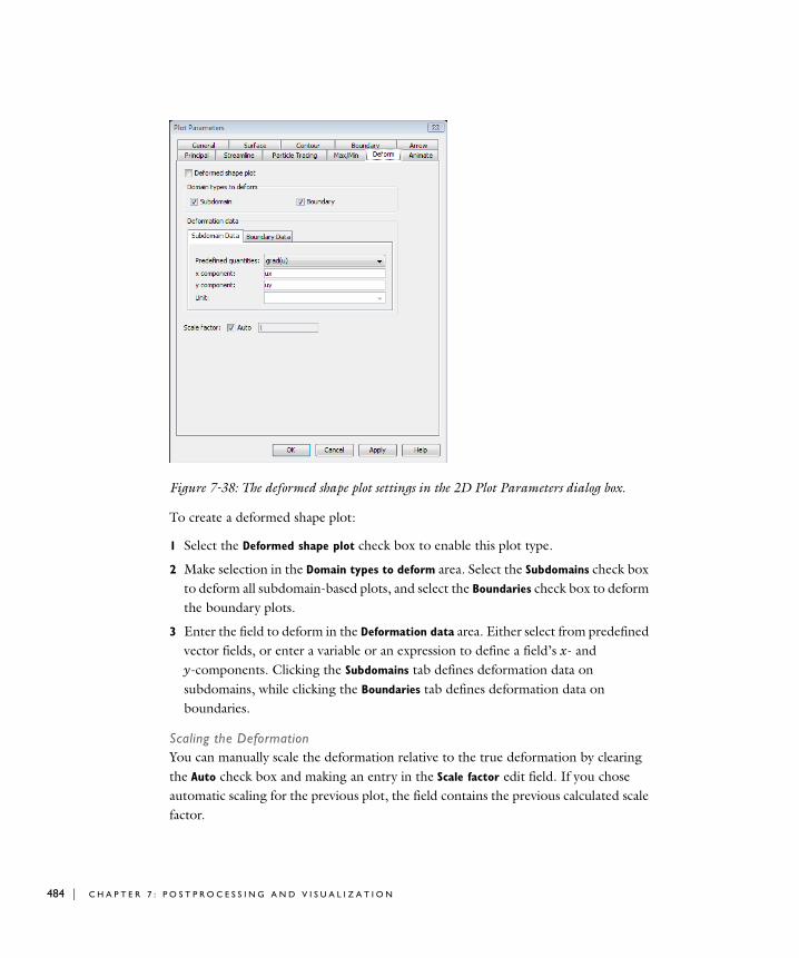
484 | C H A P T E
Figure 7-38: The deformed shape plot settings in the 2D Plot Parameters dialog box.
To create a deformed shape plot:
1 Select the Deformed shape plot check box to enable this plot type.
2 Make selection in the Domain types to deform area. Select the Subdomains check box to deform all subdomain-based plots, and select the Boundaries check box to deform the boundary plots.
3 Enter the field to deform in the Deformation data area. Either select from predefined vector fields, or enter a variable or an expression to define a field’s x- and y-components. Clicking the Subdomains tab defines deformation data on subdomains, while clicking the Boundaries tab defines deformation data on boundaries.
Scaling the DeformationYou can manually scale the deformation relative to the true deformation by clearing the Auto check box and making an entry in the Scale factor edit field. If you chose automatic scaling for the previous plot, the field contains the previous calculated scale factor.
R 7 : P O S T P R O C E S S I N G A N D V I S U A L I Z A T I O N
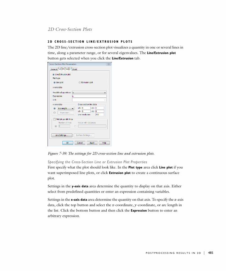
2D Cross-Section Plots
2 D C R O S S - S E C T I O N L I N E / E X T R U S I O N P L O T S
The 2D line/extrusion cross-section plot visualizes a quantity in one or several lines in time, along a parameter range, or for several eigenvalues. The Line/Extrusion plot button gets selected when you click the Line/Extrusion tab.
Figure 7-39: The settings for 2D cross-section line and extrusion plots.
Specifying the Cross-Section Line or Extrusion Plot PropertiesFirst specify what the plot should look like. In the Plot type area click Line plot if you want superimposed line plots, or click Extrusion plot to create a continuous surface plot.
Settings in the y-axis data area determine the quantity to display on that axis. Either select from predefined quantities or enter an expression containing variables.
Settings in the x-axis data area determine the quantity on that axis. To specify the x-axis data, click the top button and select the x-coordinate, y-coordinate, or arc length in the list. Click the bottom button and then click the Expression button to enter an arbitrary expression.
P O S T P R O C E S S I N G R E S U L T S I N 2 D | 485
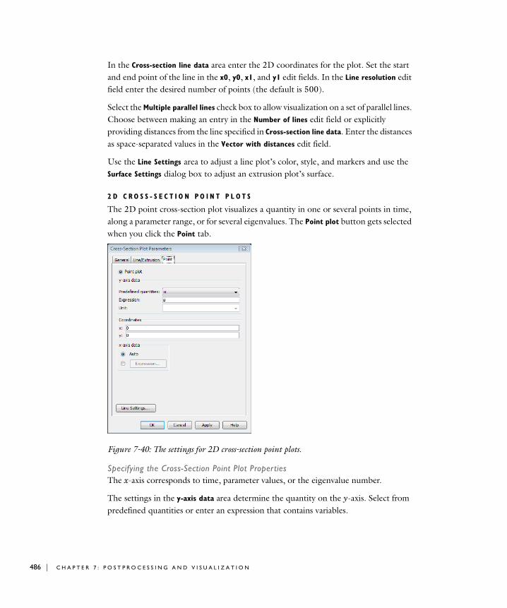
486 | C H A P T E
In the Cross-section line data area enter the 2D coordinates for the plot. Set the start and end point of the line in the x0, y0, x1, and y1 edit fields. In the Line resolution edit field enter the desired number of points (the default is 500).
Select the Multiple parallel lines check box to allow visualization on a set of parallel lines. Choose between making an entry in the Number of lines edit field or explicitly providing distances from the line specified in Cross-section line data. Enter the distances as space-separated values in the Vector with distances edit field.
Use the Line Settings area to adjust a line plot’s color, style, and markers and use the Surface Settings dialog box to adjust an extrusion plot’s surface.
2 D C R O S S - S E C T I O N P O I N T P L O T S
The 2D point cross-section plot visualizes a quantity in one or several points in time, along a parameter range, or for several eigenvalues. The Point plot button gets selected when you click the Point tab.
Figure 7-40: The settings for 2D cross-section point plots.
Specifying the Cross-Section Point Plot PropertiesThe x-axis corresponds to time, parameter values, or the eigenvalue number.
The settings in the y-axis data area determine the quantity on the y-axis. Select from predefined quantities or enter an expression that contains variables.
R 7 : P O S T P R O C E S S I N G A N D V I S U A L I Z A T I O N

In the Coordinates area enter the x- and y-coordinate values for the plot. Enter the same number of space-separated values in the x and y edit fields. Alternatively, enter a vector of coordinates, for example 0:10:100 or logspace(-1,1,30). For information about valid inputs in each edit field, see “Entering Vector-Valued Expressions” on page 145
Use the Line Settings dialog box to adjust the plot’s color, style, and markers.
Q U I C K 2 D C R O S S - S E C T I O N L I N E A N D P O I N T P L O T S
To get a quick cross-section line plot, click the Draw Line for Cross-Section Line Plot
button on the Plot toolbar and draw a line in the x-y plane using the mouse.
To get a quick cross-section point plot, click the Draw Point for Cross-Section Point Plot
button on the Plot toolbar and then click to draw one or more points in the x-y plane. When you have finished, click the button again to create the plot.
The plots appear in a separate figure window and show the currently plotted scalar quantity using surface data, or if it is not available, contour data. If neither is available, the message No scalar solution data on screen for cross-section quick plot appears in the message log.
2D Domain Plots
2 D D O M A I N S U R F A C E P L O T S
This plot type visualizes a quantity on one or several subdomains in time, along a parameter range, or for several eigenvalues. The Surface plot button gets selected when you click the Surface tab.
P O S T P R O C E S S I N G R E S U L T S I N 2 D | 487

488 | C H A P T E
Figure 7-41: The settings for surface plots on 2D domains.
Specifying Domain Surface Plot PropertiesDefine the surface color in the Color data area. Select from predefined quantities or enter an expression containing variables.
Make an appropriate selection for the plot in the Subdomain selection list.
Use the Surface Settings dialog box to adjust the surfaces’ color style.
R 7 : P O S T P R O C E S S I N G A N D V I S U A L I Z A T I O N
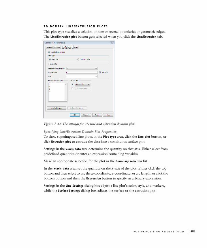
2 D D O M A I N L I N E / E X T R U S I O N P L O T S
This plot type visualize a solution on one or several boundaries or geometric edges. The Line/Extrusion plot button gets selected when you click the Line/Extrusion tab.
Figure 7-42: The settings for 2D line and extrusion domain plots.
Specifying Line/Extrusion Domain Plot PropertiesTo show superimposed line plots, in the Plot type area, click the Line plot button, or click Extrusion plot to extrude the data into a continuous surface plot.
Settings in the y-axis data area determine the quantity on that axis. Either select from predefined quantities or enter an expression containing variables.
Make an appropriate selection for the plot in the Boundary selection list.
In the x-axis data area, set the quantity on the x-axis of the plot. Either click the top button and then select to use the x-coordinate, y-coordinate, or arc length; or click the bottom button and then the Expression button to specify an arbitrary expression.
Settings in the Line Settings dialog box adjust a line plot’s color, style, and markers, while the Surface Settings dialog box adjusts the surface or the extrusion plot.
P O S T P R O C E S S I N G R E S U L T S I N 2 D | 489

490 | C H A P T E
2 D D O M A I N PO I N T P L O T S
This plot type visualizes the solution at one or several geometric points or vertices. The Point plot button gets selected when you click the Point tab.
Figure 7-43: The settings for 2D domain plots at points in the geometry.
Settings in the y-axis data area determine the quantity on that axis. Either select from predefined quantities or enter an expression containing variables.
Make an appropriate choice for the plot in the Point selection list.
Use the Line Settings dialog box to adjust the plot’s color, style, and markers; use the Surface Settings dialog box to adjust the surface or the extrusion plot.
R 7 : P O S T P R O C E S S I N G A N D V I S U A L I Z A T I O N
Po s t p r o c e s s i n g R e s u l t s i n 3D
3D Postprocessing Overview
Standard plots in 3D visualize the solution as part of the geometry. It can be a combination of a
• Slice plot
• Isosurface plot
• Subdomain plot
• Boundary plot
• Edge plot
• Arrow plot
• Principal stress/strain plot
• Deformed shape plot
• Streamline plot
• Pathline plots (particle traces)
The software can animate standard plots in time or a along a parametric solution. Cross-section plots can visualize a quantity as a family of plots in an arbitrary plane, line or in an arbitrary set of points in time or along a parametric solution. Domain plots visualize quantities on one or several geometric domains in time or along a parametric solution as a family of plots.
Using the 3D Plot Toolbar
The following plot shows the Plot toolbar for 3D models:
P O S T P R O C E S S I N G R E S U L T S I N 3 D | 491

492 | C H A P T E
Clicking any of the top eight buttons generates a corresponding plot using the current settings for that plot type in the Plot Parameters dialog box. Click the Animate button to record and play a movie.
Slice Plot
Subdomain Plot
Boundary Plot
Edge Plot
Arrow Plot
Principal Stress/Strain Plot
Streamline Plot
Animate
Isosurface Plot
R 7 : P O S T P R O C E S S I N G A N D V I S U A L I Z A T I O N
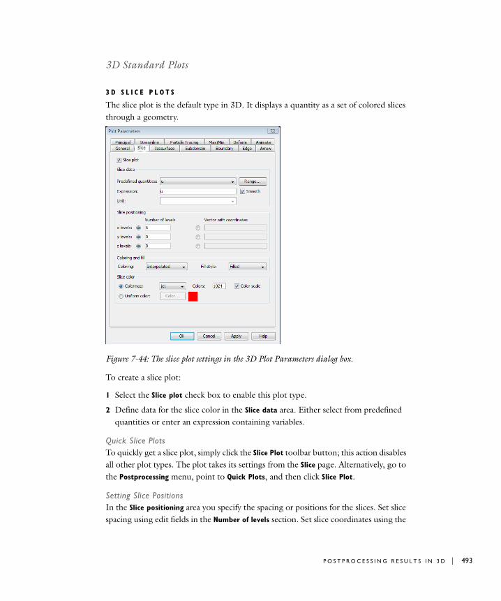
3D Standard Plots
3 D S L I C E P L O T S
The slice plot is the default type in 3D. It displays a quantity as a set of colored slices through a geometry.
Figure 7-44: The slice plot settings in the 3D Plot Parameters dialog box.
To create a slice plot:
1 Select the Slice plot check box to enable this plot type.
2 Define data for the slice color in the Slice data area. Either select from predefined quantities or enter an expression containing variables.
Quick Slice PlotsTo quickly get a slice plot, simply click the Slice Plot toolbar button; this action disables all other plot types. The plot takes its settings from the Slice page. Alternatively, go to the Postprocessing menu, point to Quick Plots, and then click Slice Plot.
Setting Slice PositionsIn the Slice positioning area you specify the spacing or positions for the slices. Set slice spacing using edit fields in the Number of levels section. Set slice coordinates using the
P O S T P R O C E S S I N G R E S U L T S I N 3 D | 493
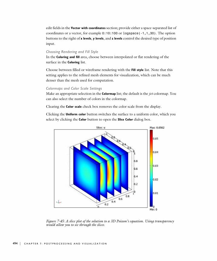
494 | C H A P T E
edit fields in the Vector with coordinates section; provide either a space-separated list of coordinates or a vector, for example 0:10:100 or logspace(-1,1,30). The option buttons to the right of x levels, y levels, and z levels control the desired type of position input.
Choosing Rendering and Fill StyleIn the Coloring and fill area, choose between interpolated or flat rendering of the surface in the Coloring list.
Choose between filled or wireframe rendering with the Fill style list. Note that this setting applies to the refined mesh elements for visualization, which can be much denser than the mesh used for computation.
Colormaps and Color Scale SettingsMake an appropriate selection in the Colormap list; the default is the jet colormap. You can also select the number of colors in the colormap.
Clearing the Color scale check box removes the color scale from the display.
Clicking the Uniform color button switches the surface to a uniform color, which you select by clicking the Color button to open the Slice Color dialog box.
Figure 7-45: A slice plot of the solution to a 3D Poisson’s equation. Using transparency would allow you to see through the slices.
R 7 : P O S T P R O C E S S I N G A N D V I S U A L I Z A T I O N
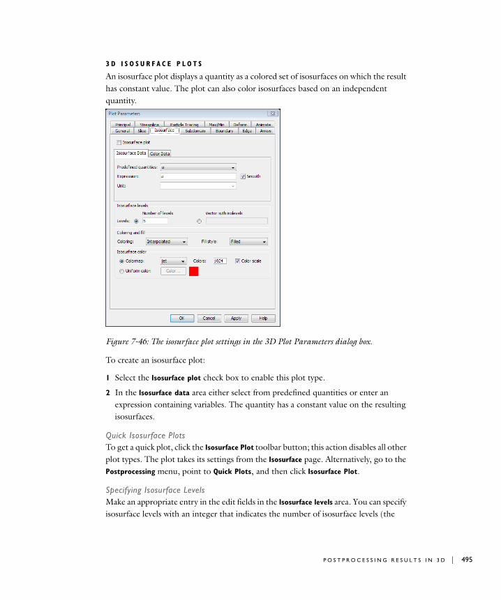
3 D I S O S U R F A C E P L O T S
An isosurface plot displays a quantity as a colored set of isosurfaces on which the result has constant value. The plot can also color isosurfaces based on an independent quantity.
Figure 7-46: The isosurface plot settings in the 3D Plot Parameters dialog box.
To create an isosurface plot:
1 Select the Isosurface plot check box to enable this plot type.
2 In the Isosurface data area either select from predefined quantities or enter an expression containing variables. The quantity has a constant value on the resulting isosurfaces.
Quick Isosurface PlotsTo get a quick plot, click the Isosurface Plot toolbar button; this action disables all other plot types. The plot takes its settings from the Isosurface page. Alternatively, go to the Postprocessing menu, point to Quick Plots, and then click Isosurface Plot.
Specifying Isosurface LevelsMake an appropriate entry in the edit fields in the Isosurface levels area. You can specify isosurface levels with an integer that indicates the number of isosurface levels (the
P O S T P R O C E S S I N G R E S U L T S I N 3 D | 495
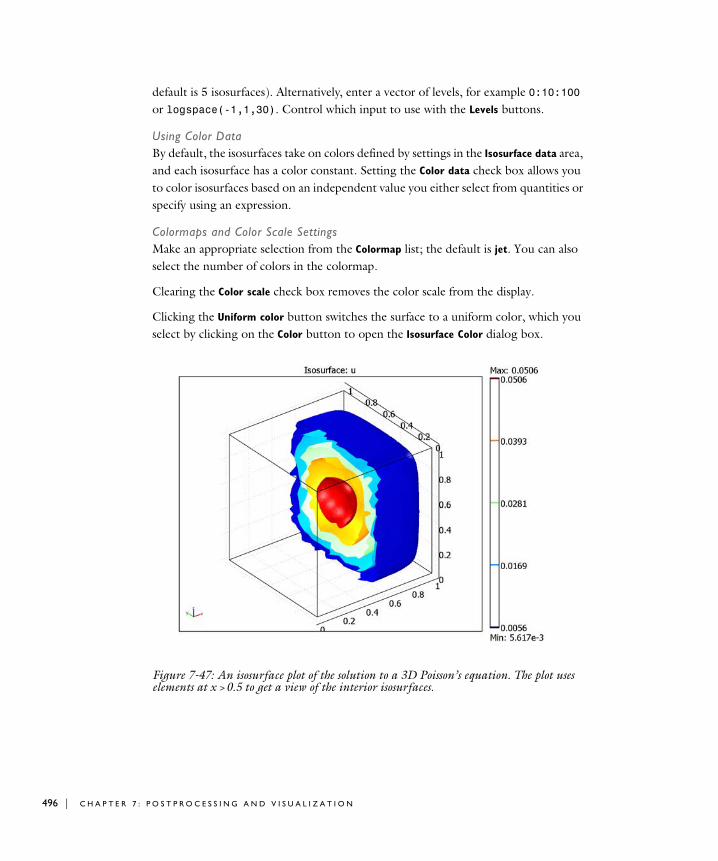
496 | C H A P T E
default is 5 isosurfaces). Alternatively, enter a vector of levels, for example 0:10:100 or logspace(-1,1,30). Control which input to use with the Levels buttons.
Using Color DataBy default, the isosurfaces take on colors defined by settings in the Isosurface data area, and each isosurface has a color constant. Setting the Color data check box allows you to color isosurfaces based on an independent value you either select from quantities or specify using an expression.
Colormaps and Color Scale SettingsMake an appropriate selection from the Colormap list; the default is jet. You can also select the number of colors in the colormap.
Clearing the Color scale check box removes the color scale from the display.
Clicking the Uniform color button switches the surface to a uniform color, which you select by clicking on the Color button to open the Isosurface Color dialog box.
Figure 7-47: An isosurface plot of the solution to a 3D Poisson’s equation. The plot uses elements at x > 0.5 to get a view of the interior isosurfaces.
R 7 : P O S T P R O C E S S I N G A N D V I S U A L I Z A T I O N
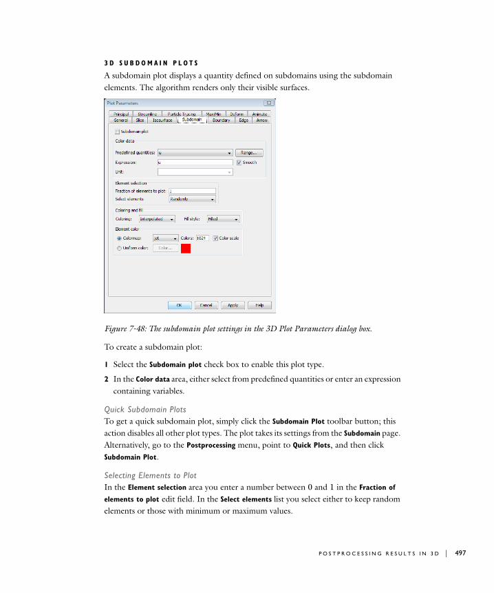
3 D S U B D O M A I N P L O T S
A subdomain plot displays a quantity defined on subdomains using the subdomain elements. The algorithm renders only their visible surfaces.
Figure 7-48: The subdomain plot settings in the 3D Plot Parameters dialog box.
To create a subdomain plot:
1 Select the Subdomain plot check box to enable this plot type.
2 In the Color data area, either select from predefined quantities or enter an expression containing variables.
Quick Subdomain PlotsTo get a quick subdomain plot, simply click the Subdomain Plot toolbar button; this action disables all other plot types. The plot takes its settings from the Subdomain page. Alternatively, go to the Postprocessing menu, point to Quick Plots, and then click Subdomain Plot.
Selecting Elements to PlotIn the Element selection area you enter a number between 0 and 1 in the Fraction of
elements to plot edit field. In the Select elements list you select either to keep random elements or those with minimum or maximum values.
P O S T P R O C E S S I N G R E S U L T S I N 3 D | 497
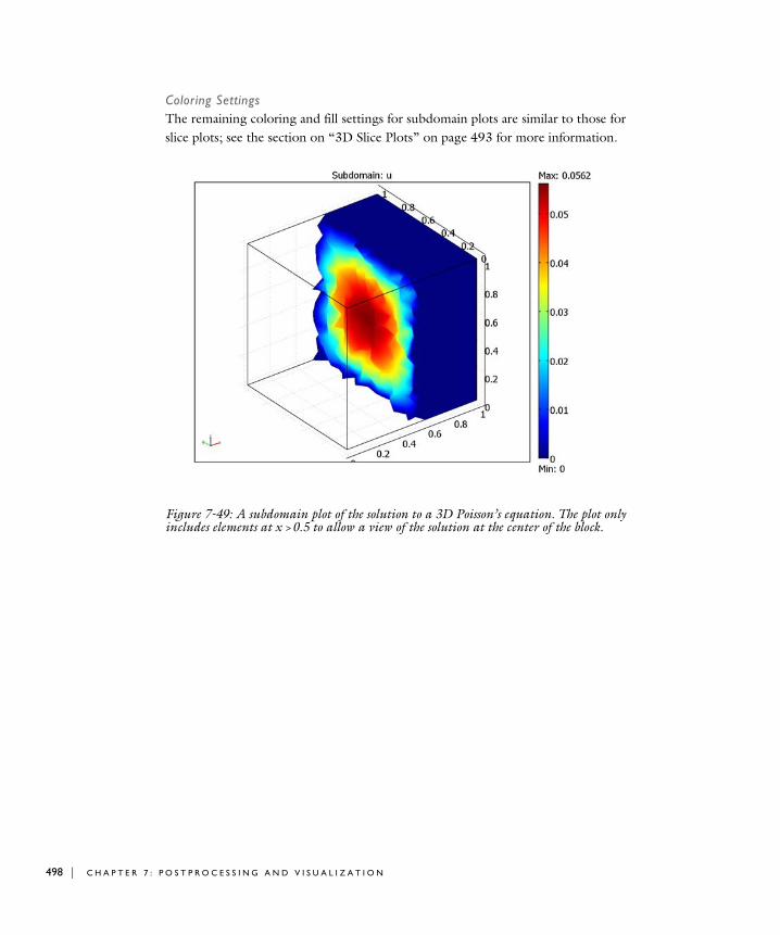
498 | C H A P T E
Coloring SettingsThe remaining coloring and fill settings for subdomain plots are similar to those for slice plots; see the section on “3D Slice Plots” on page 493 for more information.
Figure 7-49: A subdomain plot of the solution to a 3D Poisson’s equation. The plot only includes elements at x > 0.5 to allow a view of the solution at the center of the block.
R 7 : P O S T P R O C E S S I N G A N D V I S U A L I Z A T I O N

3 D B O U N D A R Y P L O T S
A boundary plot displays a quantity defined on a boundary.
Figure 7-50: The boundary plot settings in the 3D Plot Parameters dialog box.
To create a boundary plot:
1 Select the Boundary plot check box to enable this plot type.
2 In the Boundary data area either select from predefined quantities or enter an expression containing variables.
Quick Boundary PlotsTo get a quick boundary plot, simply click the Boundary Plot toolbar button; this action disables all other plot types. The plot takes its settings from the Boundary page. Alternatively, go to the Postprocessing menu, point to Quick Plots and then click Boundary Plot.
Other Boundary Plot SettingsThe rest of the settings for boundary plots are similar to those for slice plots; see the section on “3D Slice Plots” on page 493 for more information.
P O S T P R O C E S S I N G R E S U L T S I N 3 D | 499
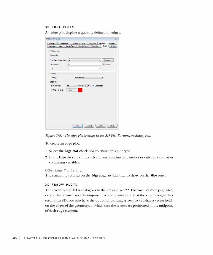
500 | C H A P T E
3 D E D G E P L O T S
An edge plot displays a quantity defined on edges.
Figure 7-51: The edge plot settings in the 3D Plot Parameters dialog box.
To create an edge plot:
1 Select the Edge plot check box to enable this plot type.
2 In the Edge data area either select from predefined quantities or enter an expression containing variables.
Other Edge Plot SettingsThe remaining settings on the Edge page are identical to those on the Slice page.
3 D A R R O W P L O T S
The arrow plot in 3D is analogous to the 2D case, see “2D Arrow Plots” on page 467, except that it visualizes a 3-component vector quantity and that there is no height data setting. In 3D, you also have the option of plotting arrows to visualize a vector field on the edges of the geometry, in which case the arrows are positioned in the midpoint of each edge element.
R 7 : P O S T P R O C E S S I N G A N D V I S U A L I Z A T I O N

3 D P R I N C I P A L S T R E S S / S T R A I N P L O T S
The principal stress/strain plot in 3D is analogous to the 2D case, see “2D Principal Stress/Strain Plots” on page 469, except that in the 3D case, it is also possible to plot principal stress/strain symbols on boundaries.
3 D D E F O R M E D S H A P E P L O T S
This type of plot visualizes a vector field by deforming the geometrical shape. This type is intended primarily for visualizing x-, y-, and z-displacements (u, v, and w) for problems in structural mechanics. By default, the software scales the deformation to 10% of the problem domain.
Figure 7-52: The deformed shape plot settings in the 3D Plot Parameters dialog box.
To create a deformed shape plot:
1 Select the Deformed shape plot check box to enable this plot type.
2 In the Domain types to deform area select which domain type to deform:
Select the Subdomains check box to deform all subdomain-based plots; select the Boundaries check box to deform boundary plots; select the Edge check box to deform edges.
P O S T P R O C E S S I N G R E S U L T S I N 3 D | 501
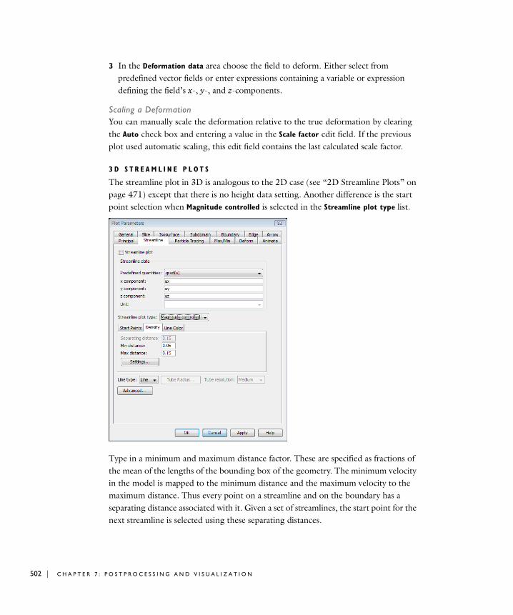
502 | C H A P T E
3 In the Deformation data area choose the field to deform. Either select from predefined vector fields or enter expressions containing a variable or expression defining the field’s x-, y-, and z-components.
Scaling a DeformationYou can manually scale the deformation relative to the true deformation by clearing the Auto check box and entering a value in the Scale factor edit field. If the previous plot used automatic scaling, this edit field contains the last calculated scale factor.
3 D S T R E A M L I N E P L O T S
The streamline plot in 3D is analogous to the 2D case (see “2D Streamline Plots” on page 471) except that there is no height data setting. Another difference is the start point selection when Magnitude controlled is selected in the Streamline plot type list.
Type in a minimum and maximum distance factor. These are specified as fractions of the mean of the lengths of the bounding box of the geometry. The minimum velocity in the model is mapped to the minimum distance and the maximum velocity to the maximum distance. Thus every point on a streamline and on the boundary has a separating distance associated with it. Given a set of streamlines, the start point for the next streamline is selected using these separating distances.
R 7 : P O S T P R O C E S S I N G A N D V I S U A L I Z A T I O N
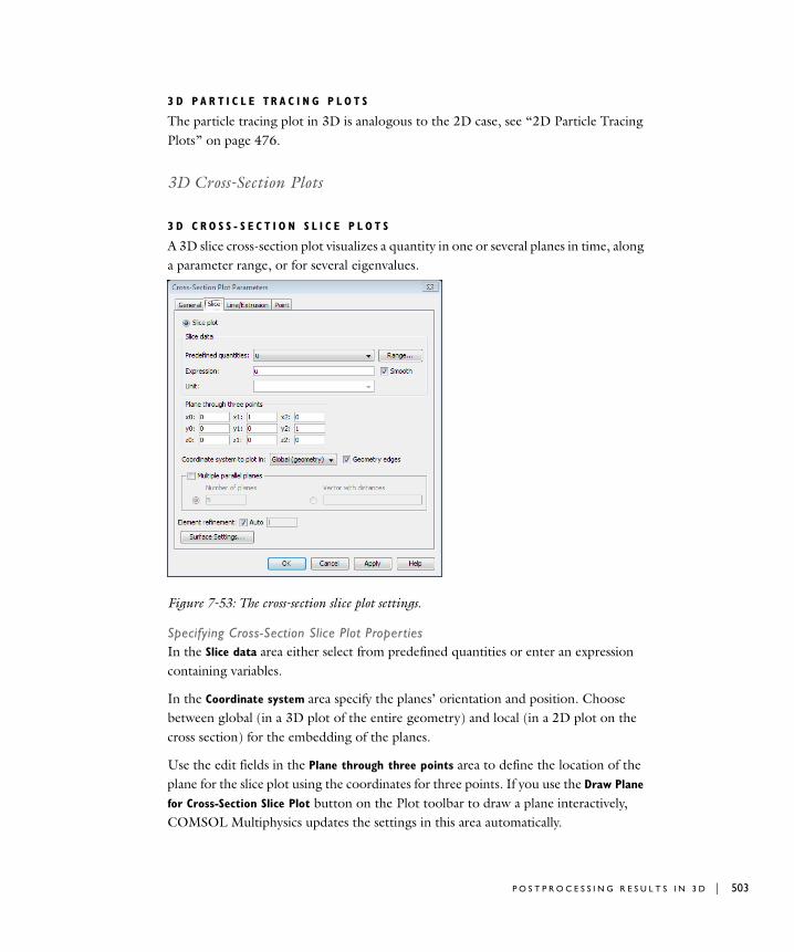
3 D P A R T I C L E T R A C I N G P L O T S
The particle tracing plot in 3D is analogous to the 2D case, see “2D Particle Tracing Plots” on page 476.
3D Cross-Section Plots
3 D C R O S S - S E C T I O N S L I C E P L O T S
A 3D slice cross-section plot visualizes a quantity in one or several planes in time, along a parameter range, or for several eigenvalues.
Figure 7-53: The cross-section slice plot settings.
Specifying Cross-Section Slice Plot PropertiesIn the Slice data area either select from predefined quantities or enter an expression containing variables.
In the Coordinate system area specify the planes’ orientation and position. Choose between global (in a 3D plot of the entire geometry) and local (in a 2D plot on the cross section) for the embedding of the planes.
Use the edit fields in the Plane through three points area to define the location of the plane for the slice plot using the coordinates for three points. If you use the Draw Plane
for Cross-Section Slice Plot button on the Plot toolbar to draw a plane interactively, COMSOL Multiphysics updates the settings in this area automatically.
P O S T P R O C E S S I N G R E S U L T S I N 3 D | 503
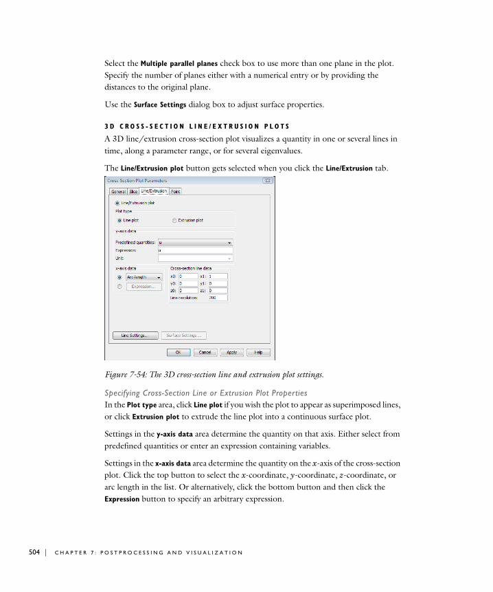
504 | C H A P T E
Select the Multiple parallel planes check box to use more than one plane in the plot. Specify the number of planes either with a numerical entry or by providing the distances to the original plane.
Use the Surface Settings dialog box to adjust surface properties.
3 D C R O S S - S E C T I O N L I N E / E X T R U S I O N P L O T S
A 3D line/extrusion cross-section plot visualizes a quantity in one or several lines in time, along a parameter range, or for several eigenvalues.
The Line/Extrusion plot button gets selected when you click the Line/Extrusion tab.
Figure 7-54: The 3D cross-section line and extrusion plot settings.
Specifying Cross-Section Line or Extrusion Plot PropertiesIn the Plot type area, click Line plot if you wish the plot to appear as superimposed lines, or click Extrusion plot to extrude the line plot into a continuous surface plot.
Settings in the y-axis data area determine the quantity on that axis. Either select from predefined quantities or enter an expression containing variables.
Settings in the x-axis data area determine the quantity on the x-axis of the cross-section plot. Click the top button to select the x-coordinate, y-coordinate, z-coordinate, or arc length in the list. Or alternatively, click the bottom button and then click the Expression button to specify an arbitrary expression.
R 7 : P O S T P R O C E S S I N G A N D V I S U A L I Z A T I O N
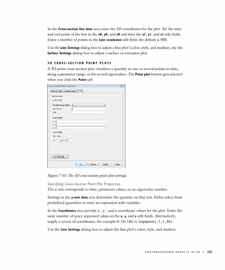
In the Cross-section line data area enter the 2D coordinates for the plot. Set the start and end point of the line in the x0, y0, and z0 and then the x1, y1, and z1 edit fields. Enter a number of points in the Line resolution edit field; the default is 500.
Use the Line Settings dialog box to adjust a line plot’s color, style, and markers; use the Surface Settings dialog box to adjust a surface or extrusion plot.
3 D C R O S S - S E C T I O N P O I N T P L O T S
A 3D point cross-section plot visualizes a quantity in one or several points in time, along a parameter range, or for several eigenvalues. The Point plot button gets selected when you click the Point tab.
Figure 7-55: The 3D cross-section point plot settings.
Specifying Cross-Section Point Plot PropertiesThe x-axis corresponds to time, parameter values, or an eigenvalue number.
Settings in the y-axis data area determine the quantity on that axis. Either select from predefined quantities or enter an expression with variables.
In the Coordinates area provide x-, y-, and z-coordinate values for the plot. Enter the same number of space-separated values in the x, y, and z edit fields. Alternatively, supply a vector of coordinates, for example 0:10:100 or logspace(-1,1,30).
Use the Line Settings dialog box to adjust the line plot’s color, style, and markers.
P O S T P R O C E S S I N G R E S U L T S I N 3 D | 505
506 | C H A P T E
Q U I C K 3 D C R O S S - S E C T I O N F A C E A N D L I N E P L O T S
To get a quick slice cross-section plot, click the Draw Plane for Cross-Section Slice Plot
button on the Plot toolbar and draw a line with the mouse. This defines a line in the plane of the screen. The software extrudes this line infinitely in the direction of the camera to define a plane that intersects the geometry. This intersection defines the cross-section plane for the plot.
To get a quick line cross-section plot, click the Draw Line for Cross-Section Line Plot
button on the Plot toolbar and click within the drawing area to draw points in the x-y plane. This action defines points for lines in the plane of the screen. COMSOL Multiphysics extruded these points infinitely to lines in the direction of the camera. The intersection of these lines and the geometry define the cross-section lines. To remove the points, click the button twice.
The plots show the currently plotted scalar quantity using slice data; or if it is not available, using isosurface data; or if it is not available, subdomain data. If none of these is available, the message No scalar solution data on screen for cross-section quick plot appears in the message log.
R 7 : P O S T P R O C E S S I N G A N D V I S U A L I Z A T I O N
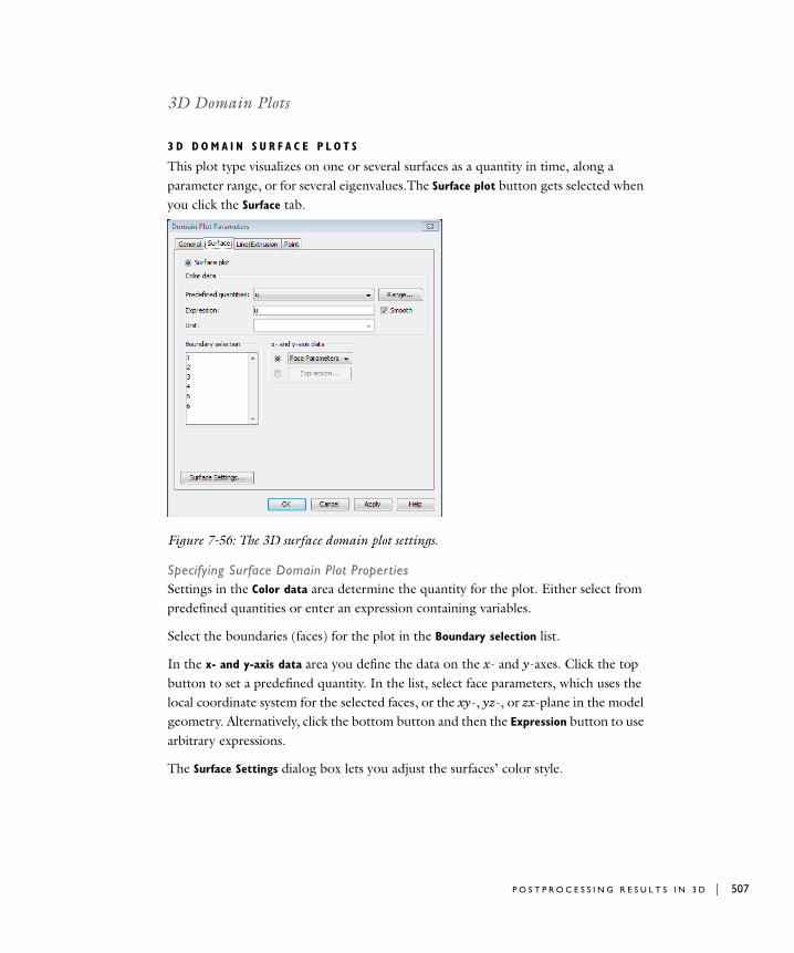
3D Domain Plots
3 D D O M A I N S U R F A C E P L O T S
This plot type visualizes on one or several surfaces as a quantity in time, along a parameter range, or for several eigenvalues.The Surface plot button gets selected when you click the Surface tab.
Figure 7-56: The 3D surface domain plot settings.
Specifying Surface Domain Plot PropertiesSettings in the Color data area determine the quantity for the plot. Either select from predefined quantities or enter an expression containing variables.
Select the boundaries (faces) for the plot in the Boundary selection list.
In the x- and y-axis data area you define the data on the x- and y-axes. Click the top button to set a predefined quantity. In the list, select face parameters, which uses the local coordinate system for the selected faces, or the xy-, yz-, or zx-plane in the model geometry. Alternatively, click the bottom button and then the Expression button to use arbitrary expressions.
The Surface Settings dialog box lets you adjust the surfaces’ color style.
P O S T P R O C E S S I N G R E S U L T S I N 3 D | 507
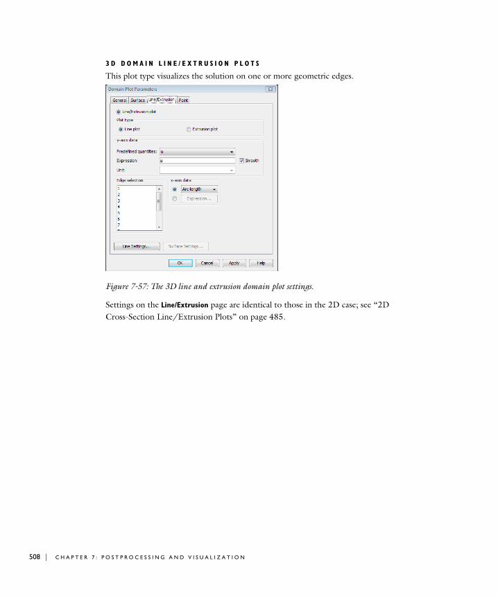
508 | C H A P T E
3 D D O M A I N L I N E / E X T R U S I O N P L O T S
This plot type visualizes the solution on one or more geometric edges.
Figure 7-57: The 3D line and extrusion domain plot settings.
Settings on the Line/Extrusion page are identical to those in the 2D case; see “2D Cross-Section Line/Extrusion Plots” on page 485.
R 7 : P O S T P R O C E S S I N G A N D V I S U A L I Z A T I O N
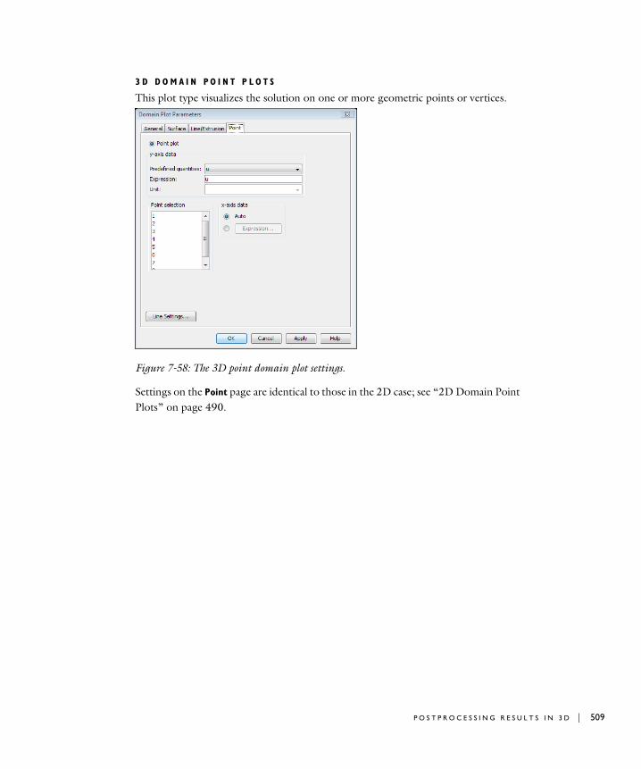
3 D D O M A I N P O I N T P L O T S
This plot type visualizes the solution on one or more geometric points or vertices.
Figure 7-58: The 3D point domain plot settings.
Settings on the Point page are identical to those in the 2D case; see “2D Domain Point Plots” on page 490.
P O S T P R O C E S S I N G R E S U L T S I N 3 D | 509
510 | C H A P T E
U s i n g t h e R epo r t Gen e r a t o r
Report Generator Overview
The Report Generator is a tool for reporting and documenting your modeling work in COMSOL Multiphysics. It creates a record of the entire model including all the settings you made during the modeling process.
The report this utility generates gives a complete overview of the model, including:
• Model properties
• Geometry
• Physics settings
- Point settings
- Edge settings
- Boundary settings
- Subdomain settings
- Other physics settings
• Mesh
• Solver parameters
• Visualization of the solution
During the modeling process, the Report Generator provides an overview of all work completed thus far. The report includes all settings you have made in the various dialog boxes across all application modes and geometries.
These reports are easy to publish either as printed hard copies or as electronic documents suitable for the Internet. The utility generates the HTML report in a file format that makes it possible to customize the report in Microsoft Word or any HTML editor.
R 7 : P O S T P R O C E S S I N G A N D V I S U A L I Z A T I O N

Figure 7-59: An example report. The first page contains model properties and a model description.
Creating a Report
To make a report, go to the File menu and choose Generate Report (or press Ctrl+G). There are two choices for the output format:
• Direct printing
• HTML
U S I N G T H E R E P O R T G E N E R A T O R | 511
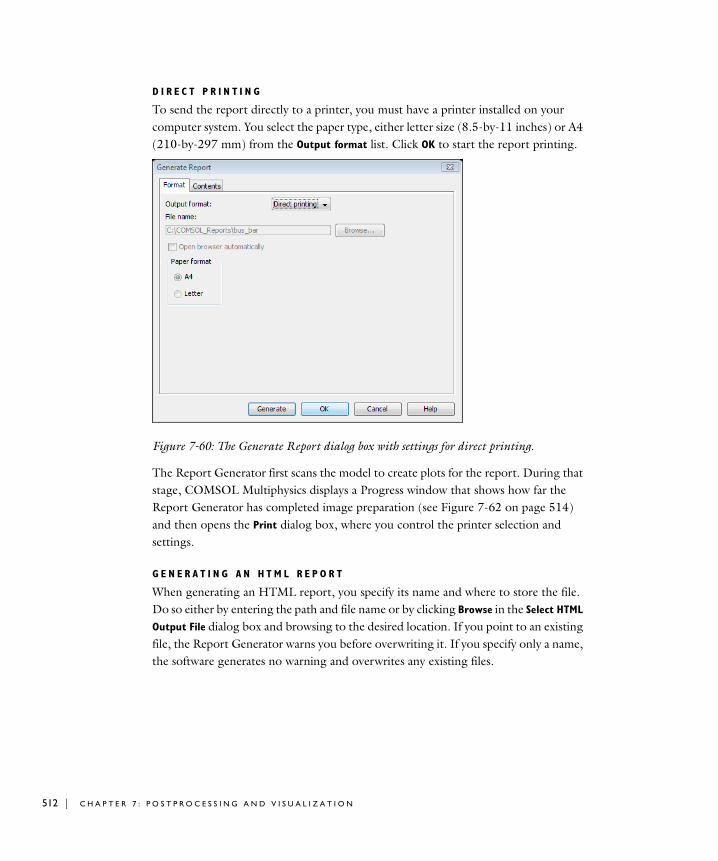
512 | C H A P T E
D I R E C T P R I N T I N G
To send the report directly to a printer, you must have a printer installed on your computer system. You select the paper type, either letter size (8.5-by-11 inches) or A4 (210-by-297 mm) from the Output format list. Click OK to start the report printing.
Figure 7-60: The Generate Report dialog box with settings for direct printing.
The Report Generator first scans the model to create plots for the report. During that stage, COMSOL Multiphysics displays a Progress window that shows how far the Report Generator has completed image preparation (see Figure 7-62 on page 514) and then opens the Print dialog box, where you control the printer selection and settings.
G E N E R A T I N G A N H T M L R E P O R T
When generating an HTML report, you specify its name and where to store the file. Do so either by entering the path and file name or by clicking Browse in the Select HTML
Output File dialog box and browsing to the desired location. If you point to an existing file, the Report Generator warns you before overwriting it. If you specify only a name, the software generates no warning and overwrites any existing files.
R 7 : P O S T P R O C E S S I N G A N D V I S U A L I Z A T I O N

Note: The Report Generator overwrites the HTML and associated image files if you reuse the same report name and path. To avoid overwriting a previous report, change the name or path of the HTML report.
Figure 7-61: The Generate Report dialog box with settings for a report in HTML format.
The Report Generator stores the report in a file with the chosen name and gives it the extension .html. It stores images included in the report in a subdirectory with the same name as the report plus the suffix _rep.
Select the Open browser automatically check box to view the report in a web browser as soon as it is available.
R E P O R T G E N E R A T O R P R O G R E S S W I N D O W
When you start the Report Generator, COMSOL Multiphysics displays a Progress window where you can monitor the utility’s progress as it creates the report. You can stop report generation at any time by clicking Cancel. The Progress window normally closes when the report is ready, but you can keep it open by clearing the Close
automatically check box. After printing the report or generating an HTML file, the
U S I N G T H E R E P O R T G E N E R A T O R | 513
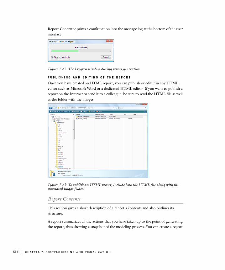
514 | C H A P T E
Report Generator prints a confirmation into the message log at the bottom of the user interface.
Figure 7-62: The Progress window during report generation.
P U B L I S H I N G A N D E D I T I N G O F T H E R E P O R T
Once you have created an HTML report, you can publish or edit it in any HTML editor such as Microsoft Word or a dedicated HTML editor. If you want to publish a report on the Internet or send it to a colleague, be sure to send the HTML file as well as the folder with the images.
Figure 7-63: To publish an HTML report, include both the HTML file along with the associated image folder.
Report Contents
This section gives a short description of a report’s contents and also outlines its structure.
A report summarizes all the actions that you have taken up to the point of generating the report, thus showing a snapshot of the modeling process. You can create a report
R 7 : P O S T P R O C E S S I N G A N D V I S U A L I Z A T I O N

at any stage in the modeling process to get an overview of the work thus far and then continue modeling.
Note: If you compute a solution and then change any settings in the model without re-solving it, the report includes the new settings but retains the old solution and postprocessing data. The Report Generator always create reports based on the models in their present state.
A report has three main sections:
• Introduction and model properties
• Geometry and physics settings
• Solution and postprocessing
Each section includes several subsections including all the model information.
I N T R O D U C T I O N A N D M O D E L P R O P E R T I E S
The first section, the report introduction, includes model properties and other definitions such as constants that are common throughout the different geometries in the model.
G E O M E T R Y A N D P H Y S I C S S E T T I N G S
The second section, with physics settings, repeats for each geometry in the model. In each case it lists the physics settings for each application mode that is active in that portion of the geometry. This section also includes a description of each application mode. It prints in bold font all physics settings that the user has changed and thus differ from the default values.
S O L U T I O N A N D P O S T P R O C E S S I N G
The last section contains the materials libraries, functions, and solver settings used to solve the model. The final chapter reviews postprocessing results. The solution and postprocessing sections are common to the entire model.
U S I N G T H E R E P O R T G E N E R A T O R | 515
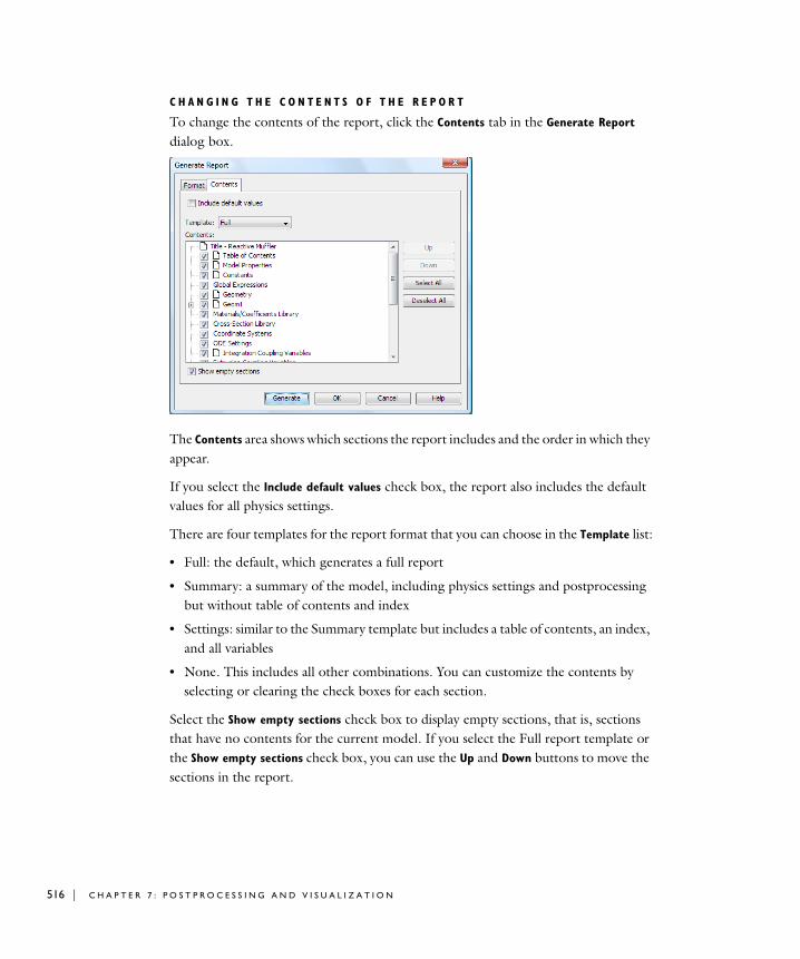
516 | C H A P T E
C H A N G I N G T H E C O N T E N T S O F T H E R E P O R T
To change the contents of the report, click the Contents tab in the Generate Report dialog box.
The Contents area shows which sections the report includes and the order in which they appear.
If you select the Include default values check box, the report also includes the default values for all physics settings.
There are four templates for the report format that you can choose in the Template list:
• Full: the default, which generates a full report
• Summary: a summary of the model, including physics settings and postprocessing but without table of contents and index
• Settings: similar to the Summary template but includes a table of contents, an index, and all variables
• None. This includes all other combinations. You can customize the contents by selecting or clearing the check boxes for each section.
Select the Show empty sections check box to display empty sections, that is, sections that have no contents for the current model. If you select the Full report template or the Show empty sections check box, you can use the Up and Down buttons to move the sections in the report.
R 7 : P O S T P R O C E S S I N G A N D V I S U A L I Z A T I O N
OV E R V I E W O F T H E S U B S E C T I O N S
A complete list of the subsections that the Report Generator can produce follows. A report of a COMSOL Multiphysics model contains any relevant subset of this list.
• Model properties, description and summary
• Constants
• Geometries (the report includes the following sections for each geometry)
- Draw mode
- Point mode
- Edge mode
- Boundary mode
- Subdomain mode
- Physics (for each geometry and each application mode)
* Scalar expressions
* Point expressions
* Edge expressions
* Boundary expressions
* Subdomain expressions
* Mesh and mesh cases
* Application mode
* Scalar variables
* Application mode properties
* Variables
* Point settings
* Edge settings
* Boundary settings
* Subdomain settings
• Materials libraries
• Functions
• Interpolation functions
U S I N G T H E R E P O R T G E N E R A T O R | 517

518 | C H A P T E
• Solver settings
- Linear solvers
- Nonlinear solver
- Time-dependent solver
- Eigenfrequency solver
- Parametric solver
- Adaptive solver
- Advanced solver settings
• Postprocessing
- Eigenvalues or eigenfrequencies
• Equations
• Variables
The report displays default settings in a regular font, and it lists in bold font any physics settings you have changed from the defaults. It leaves blank any settings that are inactive.
Model Properties, Description, and SummaryIn COMSOL Multiphysics it is possible to set some general model properties that in turn appear at the beginning of a report. These properties come from the Model
Properties dialog box, which you open by going to the File menu and choosing Model
Properties. See “Setting Model Properties” on page 525 for more information about the model properties. The Report Generator always includes certain model properties at the beginning of a report:
The report includes information from the Info tab in the Model Properties dialog box to show the COMSOL Multiphysics version as well as the modules and application modes with which the model was built.
Next it includes a separate section for each tab:
• General: Information about the model’s author and possibly a URL to a location where the reader can find more information about the model
• Description: An introductory description of the model
• Notes: This property can be used, for example, to accommodate comments on the modeling results
R 7 : P O S T P R O C E S S I N G A N D V I S U A L I Z A T I O N
GeometriesAll geometries that exist in a model appear in the report.
If a model includes multiple geometries, the report includes information about all geometries, including all application modes for each geometry.
Point, Edge, Boundary, and Subdomain ModeFor each mode, the report shows the geometry and labels for the points, edges, boundaries, and subdomains. The report uses these later when describing the corresponding settings for the included application modes.
Point SettingsFor each application mode, the report lists the point settings by groups with identical settings. It shows in bold font any settings that differ from their default values.
Edge SettingsFor each application mode, the report lists the edge settings by groups with identical settings; note that edge settings exist only in 3D models. It shows in bold font any settings that differ from their default values.
Boundary SettingsFor each application mode, the report lists the boundary settings by groups with identical settings, but only those boundaries active in the geometry. It shows in bold font any settings that differ from their default values.
Subdomain SettingsFor each application mode, the report lists the subdomain settings by groups with identical settings. It shows in bold font any settings that differ from their default values.
MeshTo document the mesh, the report includes a plot of the mesh along with mesh statistics. If the designer solved the model using mesh cases, the report includes a plot and statistics for each mesh case.
Materials LibrariesIf the model uses a materials library, the relevant materials appear in the report.
Solver SettingsThe report lists all solver settings, and when applicable it also includes a solver script. For the multigrid solver, the report lists all relevant settings for:
• Preconditioner
U S I N G T H E R E P O R T G E N E R A T O R | 519

520 | C H A P T E
• Presmoother and postsmoother
• Coarse solver
Note: The report includes only the current solver settings. If you solve the model in steps, we recommend you use solver scripting because the report contains the solver script and your work is documented automatically.
PostprocessingTo document model results, the Report Generator always includes the final postprocessing plot. If you want more postprocessing plots in the final report, you must copy/paste them there using functions on the Edit menu.
In addition, the report includes any eigenvalues or eigenfrequencies depending on the settings in the Application Mode properties.
Note: The report includes the last postprocessing plot the software created—even if you have changed the settings and have not re-solved the model.
R 7 : P O S T P R O C E S S I N G A N D V I S U A L I Z A T I O N

8
M o d e l M a i n t e n a n c e a n d M o d e l L i b r a r i e s
This chapter describes how to save and open COMSOL Multiphysics models. You also find a description of the different model formats. In addition, you find a list of models in the COMSOL Multiphysics Model Library and descriptions on how to create your own model library.
521

522 | C H A P T E
Open i n g and S a v i n g COMSOL Mu l t i p h y s i c s Mode l s
Model Files Formats
There are two different file formats for COMSOL Multiphysics models:
• Model MPH-file—the default file format
Consists of a binary part containing data such as the mesh and the solution, and a text-file part with other model information. Model MPH-files have extension .mph. Earlier versions of COMSOL Multiphysics (FEMLAB) used the file extension .fl.
See “Model MPH-files” on page 524 for more information.
• Model M-file—editable script file for COMSOL Script or MATLAB
Contains a sequence of COMSOL Multiphysics commands. Run the Model M-files in COMSOL Script or in MATLAB or open them in COMSOL Multiphysics. You can edit the file in a text editor to add additional commands.
See “Model M-Files” on page 528 for more information.
Opening a COMSOL Multiphysics Model
To open a saved COMSOL Multiphysics model, follow these steps:
1 From the File menu, choose Open.
2 From the Files of type list in the Open Model dialog box, choose the file type that matches your model. Use the Look in list to browse and select the file you want to open.
3 Click Open to open the model.
When the Preview button in the Open Model dialog box is pressed in, the dialog box shows the model image and model description, if they exist (for more information about saving model images and model descriptions, see “Setting Model Properties” on page 525). Click the Preview button to show or hide the preview.
R 8 : M O D E L M A I N T E N A N C E A N D M O D E L L I B R A R I E S
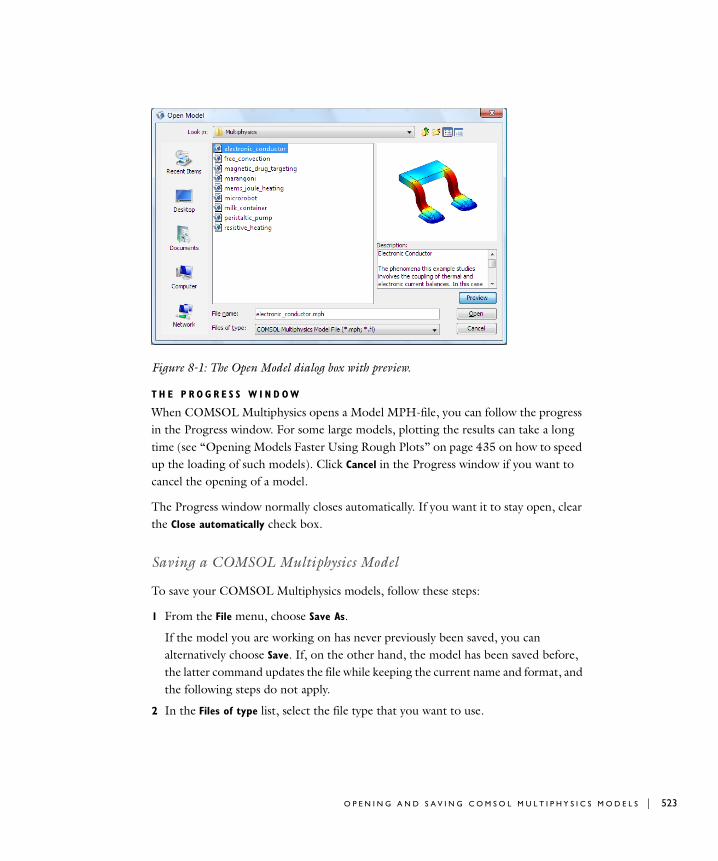
Figure 8-1: The Open Model dialog box with preview.
T H E P R O G R E S S W I N D O W
When COMSOL Multiphysics opens a Model MPH-file, you can follow the progress in the Progress window. For some large models, plotting the results can take a long time (see “Opening Models Faster Using Rough Plots” on page 435 on how to speed up the loading of such models). Click Cancel in the Progress window if you want to cancel the opening of a model.
The Progress window normally closes automatically. If you want it to stay open, clear the Close automatically check box.
Saving a COMSOL Multiphysics Model
To save your COMSOL Multiphysics models, follow these steps:
1 From the File menu, choose Save As.
If the model you are working on has never previously been saved, you can alternatively choose Save. If, on the other hand, the model has been saved before, the latter command updates the file while keeping the current name and format, and the following steps do not apply.
2 In the Files of type list, select the file type that you want to use.
O P E N I N G A N D S A V I N G C O M S O L M U L T I P H Y S I C S M O D E L S | 523
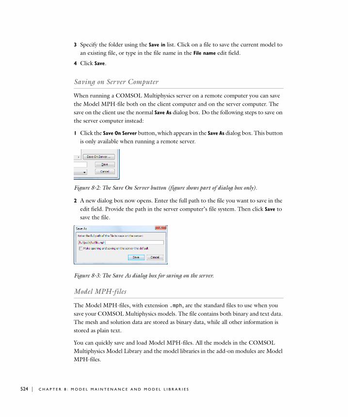
524 | C H A P T E
3 Specify the folder using the Save in list. Click on a file to save the current model to an existing file, or type in the file name in the File name edit field.
4 Click Save.
Saving on Server Computer
When running a COMSOL Multiphysics server on a remote computer you can save the Model MPH-file both on the client computer and on the server computer. The save on the client use the normal Save As dialog box. Do the following steps to save on the server computer instead:
1 Click the Save On Server button, which appears in the Save As dialog box. This button is only available when running a remote server.
Figure 8-2: The Save On Server button (figure shows part of dialog box only).
2 A new dialog box now opens. Enter the full path to the file you want to save in the edit field. Provide the path in the server computer’s file system. Then click Save to save the file.
Figure 8-3: The Save As dialog box for saving on the server.
Model MPH-files
The Model MPH-files, with extension .mph, are the standard files to use when you save your COMSOL Multiphysics models. The file contains both binary and text data. The mesh and solution data are stored as binary data, while all other information is stored as plain text.
You can quickly save and load Model MPH-files. All the models in the COMSOL Multiphysics Model Library and the model libraries in the add-on modules are Model MPH-files.
R 8 : M O D E L M A I N T E N A N C E A N D M O D E L L I B R A R I E S
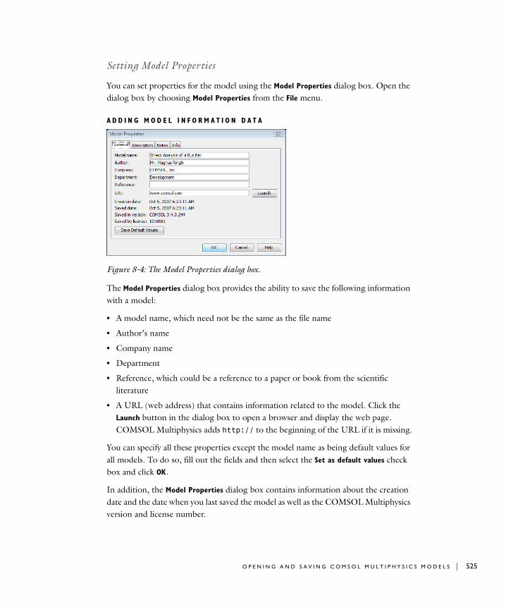
Setting Model Properties
You can set properties for the model using the Model Properties dialog box. Open the dialog box by choosing Model Properties from the File menu.
A D D I N G M O D E L I N F O R M A T I O N D A T A
Figure 8-4: The Model Properties dialog box.
The Model Properties dialog box provides the ability to save the following information with a model:
• A model name, which need not be the same as the file name
• Author’s name
• Company name
• Department
• Reference, which could be a reference to a paper or book from the scientific literature
• A URL (web address) that contains information related to the model. Click the Launch button in the dialog box to open a browser and display the web page. COMSOL Multiphysics adds http:// to the beginning of the URL if it is missing.
You can specify all these properties except the model name as being default values for all models. To do so, fill out the fields and then select the Set as default values check box and click OK.
In addition, the Model Properties dialog box contains information about the creation date and the date when you last saved the model as well as the COMSOL Multiphysics version and license number.
O P E N I N G A N D S A V I N G C O M S O L M U L T I P H Y S I C S M O D E L S | 525
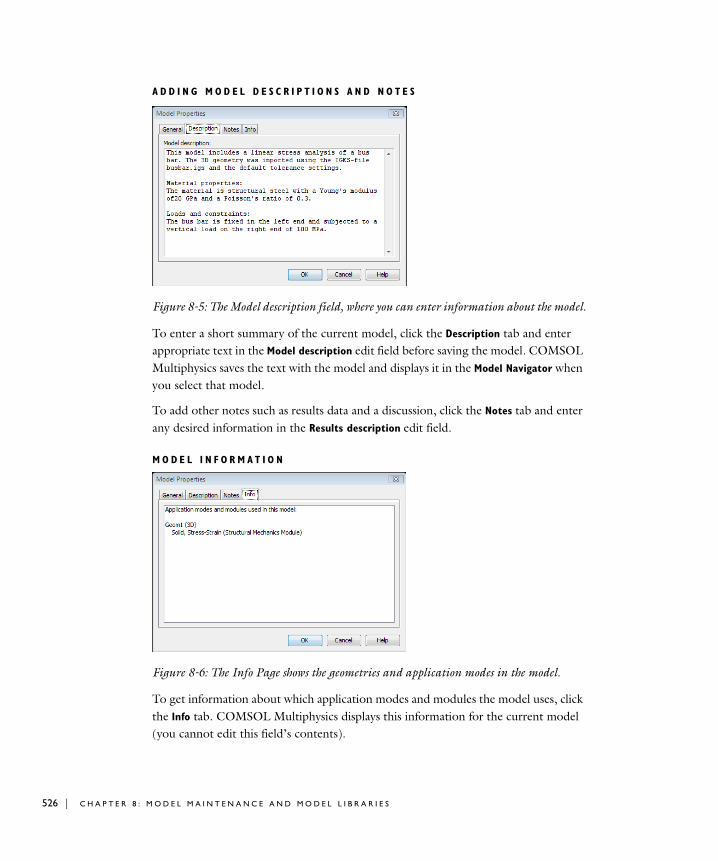
526 | C H A P T E
A D D I N G M O D E L D E S C R I P T I O N S A N D N O T E S
Figure 8-5: The Model description field, where you can enter information about the model.
To enter a short summary of the current model, click the Description tab and enter appropriate text in the Model description edit field before saving the model. COMSOL Multiphysics saves the text with the model and displays it in the Model Navigator when you select that model.
To add other notes such as results data and a discussion, click the Notes tab and enter any desired information in the Results description edit field.
M O D E L I N F O R M A T I O N
Figure 8-6: The Info Page shows the geometries and application modes in the model.
To get information about which application modes and modules the model uses, click the Info tab. COMSOL Multiphysics displays this information for the current model (you cannot edit this field’s contents).
R 8 : M O D E L M A I N T E N A N C E A N D M O D E L L I B R A R I E S

S A V I N G A M O D E L I M A G E
To illustrate the model, you can save a model image that will be displayed in the Model
Navigator. To save the current COMSOL Multiphysics plot as a model image, choose Save Model Image from the File menu. The model image is a copy of the current plot.
O P E N I N G A N D S A V I N G C O M S O L M U L T I P H Y S I C S M O D E L S | 527
528 | C H A P T E
Mode l M - F i l e s
You can save an entire modeling session as a sequence of commands. This command sequence is called a Model M-file. You can:
• Run these commands directly from the COMSOL Script or MATLAB command line or load the file into COMSOL Multiphysics
• Modify the Model M-file using COMSOL Script or MATLAB commands
If you want to open a modified Model M-file in COMSOL Multiphysics, it is important to follow the syntactic rules outlined in the COMSOL Multiphysics Scripting Guide.
Note: You can always load a Model M-file into COMSOL Multiphysics. To run the Model M-file from a command line, use COMSOL Script or MATLAB. Check the COMSOL Installation Guide for specific system requirements.
Using Model M-files
The Model M-file is useful for many reasons. For example, it makes it possible to:
• Easily document modeling in a readable format
• Work with COMSOL Multiphysics command-line functions in COMSOL Script or MATLAB
• Save, modify, and load Model M-file back into the COMSOL Multiphysics user interface
• Insert COMSOL Script or MATLAB commands anywhere in the Model M-file
• Start modeling in the COMSOL Multiphysics user interface, then save it as a Model M-file and continue the modeling in the COMSOL Script or in the MATLAB environments with a starting point that is a Model M-file with the correct syntax for reproducing the model that you created in the COMSOL Multiphysics user interface.
The Model M-file records your modeling session to a text file. This script contains all changes to the model. Using a text editor, you can manually edit, add, and remove commands from the Model M-files.
R 8 : M O D E L M A I N T E N A N C E A N D M O D E L L I B R A R I E S
M O D I F Y I N G M O D E L M - F I L E C O N T E N T S
You can modify some of the contents in the Model M-file to get a more or less compact representation of the model.
Including Default ValuesBy default, the Model M-file does not include fields with their default values. To include also the default values in the generated file, do as follows:
1 From the Options menu, open the Preferences dialog box.
2 Click the Modeling tab.
3 Select the Include default values check box in the Model M-file/FEM export area.
4 Click OK.
Note: This setting only affects the commands for subsequent modeling steps. It does not include default values for modeling steps that COMSOL Multiphysics has already recorded.
Shrinking CoefficientsBy default, COMSOL Multiphysics “shrinks” the coefficients in the physics settings to a more compact notation than the full syntax, which makes the Model M-file easier to read. To get the full syntax in the Model M-file, follow these steps:
1 From the Options menu, open the Preferences dialog box.
2 Click the Modeling tab.
3 Clear the Shrink coefficients check box in the Model M-file/FEM export area.
4 Click OK.
Resetting the Model and the Model M-file Command SequenceThe Model M-file command sequence can sometimes become quite long. The Reset Model command removes everything but the geometry-related commands from the Model M-file command sequence for the current model. It also removes all meshes and solutions in the model, so you might have to solve the model again. To reset the Model M-file and remove the meshes and solutions, choose Reset Model from the File menu.
M O D E L M - F I L E S | 529
530 | C H A P T E
U s i n g t h e COMSOL Mu l t i p h y s i c s Mode l L i b r a r y
The COMSOL Multiphysics Model Library is a collection of solved models from different application areas. All the files can be loaded as Model MPH-files for inspection and modification. Most models are also available as Model M-files. The models in the COMSOL Multiphysics Model Library provide a convenient starting point for models that share similar properties but have different geometry, material properties, and boundary conditions.
You find the Model Library models in the Model Navigator by clicking the Model Library tab. Choose Open Model Library from the File menu to open the Model Navigator with Model Library tab active.
Browse the Model Library using the list to the left. The models are grouped into application areas. Each model contains a model description and a model image, which you can see in the right part of the Model Navigator. To view the documentation for a model, select the model from the Model Library list and click the Documentation button. To load a model into COMSOL Multiphysics, double-click the model in the list or select a model and then click OK. The program sets the path to the Model Library during installation. If you need to set the root directory for the Model Library, click the Library Root button. To access the documentation for the current model choose Model Documentation from the Help menu.
Note: The COMSOL Multiphysics modules provide their own model libraries that work in the same way as the COMSOL Multiphysics Model Library but with a focus on the application areas that the module covers.
Models in the Model Library
The COMSOL Multiphysics Model Library consists of about 80 fully solved models which are documented in the Model Library. See the “COMSOL Multiphysics Model Library Models” on page 5 in the COMSOL Multiphysics Model Library for a table with information about all available models and page references to the documentation for each model.
R 8 : M O D E L M A I N T E N A N C E A N D M O D E L L I B R A R I E S

C r e a t i n g a U s e r Mode l L i b r a r y
You can create your own user model libraries for easy access and documentation of COMSOL Multiphysics models. To browse the user models, click the User Models tab in the Model Navigator. Specify the path to the user model library by clicking the Library
Root button. If you saved a model image along with a description they appear in the Model Navigator when you select the model. If there is HTML-based documentation for the model, click the Documentation button to view it.
Saving Models for a User Model Library
Save your models as Model MPH-files to dedicated folders to begin building your own model library. To add information about the model use the Model Properties dialog box and the Save Model Image command.
C R E A T I N G A U S E R M O D E L L I B R A R Y | 531

532 | C H A P T E
R 8 : M O D E L M A I N T E N A N C E A N D M O D E L L I B R A R I E S
9
G l o s s a r y
This glossary contains terms related to finite element modeling, mathematics, geometry, and CAD as they relate to the COMSOL Multiphysics software and documentation. For more application-specific terms, see the glossaries in the AC/DC Module, Acoustics Module, CAD Import Module, Chemical Engineering Module, Earth Science Module, Heat Transfer Module, MEMS Module, RF Module, and Structural Mechanics Module. For references to more information about a term, see the index.
533
534 | C H A P T E
G l o s s a r y o f T e rm sadaptive mesh refinement A method of improving solution accuracy by adapting the mesh to the problem’s physical behavior.
affine transformations Geometric transformations that are combinations of linear transformations and translations.
algebraic multigrid (AMG) An algebraic multigrid solver or preconditioner performs one or more cycles of a multigrid method using a coarsening of the discretization based on the coefficient matrix. Compare to geometric multigrid (GMG).
analysis type The analysis type is a top-level setting for the analysis of a model in any of the physics modes. The analysis type is available in the Model Navigator when starting a new model and in the Application Mode Properties and Solver Parameters dialog boxes. The analysis type determines suitable solver settings and, in some cases, equation settings. Typical analysis types include stationary, eigenfrequency, transient, time-dependent, and parametric analyses.
analyzed geometry A supported geometry description for modeling and analysis. It can be of any of the formats composite geometry object, assembly, Geometry M-file, or mesh.
anisotropy Variation of material properties with direction.
application mode A predefined interface or template for a specific type of physics or equation. Each application mode provides its own set of boundary conditions, material properties, equations, and postprocessing variables.
application programming interface (API) The API provides a set of documented functions and methods for interacting with COMSOL Multiphysics. Using the API, users can create their own applications with customized geometries, equations, and so on.
application scalar variable A scalar variable with the current geometry as its context, for example, an angular frequency. Application scalar variables are valid in the all of the model’s current geometry and include, but are not limited to, scalar numeric values.
R 9 : G L O S S A R Y

arbitrary Lagrangian-Eulerian formulation (ALE formulation) A formulation for a moving mesh where dependent variables represent the mesh displacement or mesh velocity. The COMSOL Multiphysics solvers have built-in support for the mesh movement.
arc A segment of the circumference of a circle or ellipse.
Argyris element A 2D, 6-node triangular finite element with a 5th-order basis function providing continuous derivatives between elements.
aspect ratio The ratio between the longest and shortest element or geometry dimension.
assemble Taking the local element stiffnesses, masses, loads, and constraints to form the stiffness matrix, mass matrix, load vector, constraint matrix, and constraint residual vector.
assembly An analyzed geometry where the original geometry objects remain as individual parts.
associative geometry An algorithm that maps data associated with a geometry to the new geometry entities when the geometry is modified.
backward differentiation formula (BDF) A multistep formula based on numerical differentiation for solutions to ordinary differential equations. A BDF method of order n computes the solution using an nth-grade polynomial in terms of backward differences.
basis function A function in the finite element space such that the ith degree freedom is 1, while all other degrees of freedom are 0. For the Lagrange finite element space, is a linear or higher order polynomial on each mesh element with value 1 in node i and 0 in all other nodes.
Bernstein polynomial See Bézier basis.
Bézier basis A set of polynomial functions that occur in the definition of a Bézier curve. These polynomial functions are often called Bernstein polynomials.
Bézier curve A rational Bézier curve is a parameterized curve formed as the quotient of two polynomials expressed in the Bézier basis. It is a vector-valued function of one
ϕi
ϕi
G L O S S A R Y O F TE R M S | 535

536 | C H A P T E
variable. The coefficients of a rational Bézier curve are geometrically interpreted as control points and control weights. A nonrational Bézier curve is a rational Bézier curve with all weights equal, thereby making the denominator polynomial equal to a constant. A nonrational Bézier curve is also called an integer Bézier curve.
Bézier patch, Bézier surface A Bézier patch or Bézier surface is a surface extension of the Bézier curve. The Bézier patch is a function of two variables with an array of control points.
Boolean operations Boolean operations are used to construct a geometry object from other solid geometry objects and rebuild it in a new form. At least two primary geometry objects are required to create a resultant new geometry object. That new object depends on the type of Boolean operation:
• Union (add): the resultant geometry object occupies all the space of the initial geometry objects
• Difference (subtract): the resultant geometry object occupies all the space of the first geometry object except for the space inside the second geometry object.
• Intersection: the resultant geometry object occupies only the space common to the initial geometry objects
boundary A domain with a space dimension one less than the space dimension for the geometry, for example, a face in a 3D geometry. In a mathematical context, the symbol ∂Ω represents the boundary of the domain Ω. Sometimes boundary is used in a narrower sense meaning an exterior boundary. See also interior boundary, exterior boundary.
border The interface between two parts in an assembly.
boundary modeling A geometry modeling method to create a geometry by defining its boundaries. Compare to solid modeling and surface modeling.
brick element See hexahedral element.
chamfer A CAD feature that trims off a corner with a plane or straight line.
Cholesky factorization A memory-saving version of LU factorization where U is the transpose of L. It requires that the coefficient matrix A (A = LU) be a symmetric positive definite matrix. See also LU factorization and positive definiteness.
R 9 : G L O S S A R Y

coefficient form PDE A PDE in the coefficient form is a PDE formulation suited for linear PDEs
coerce To convert a geometry object from one type to another, for example, from a curve object to s a solid object.
composite geometry object, composite solid object Geometric objects made up by combining primitive geometry objects and other composite objects. See also constructive solid geometry, primitive geometry object, and Boolean operations.
COMSOL Multiphysics binary file A binary data file with the extension .mphbin that contains geometry objects or mesh objects. Earlier versions of COMSOL Multiphysics used the file extension .flb.
COMSOL Multiphysics text file A text data file with the extension .mphtxt that contains geometry objects or mesh objects.
condition number A measure of the possible error in a solution due to ill-conditioning of the equations. See also ill-conditioning.
constant A named model property that has a constant numeric value.
constraint Restriction imposed upon the dependent variables, typically as a Dirichlet boundary condition. Neumann boundary conditions are not regarded as constraints. When Dirichlet boundary conditions are introduced, the finite element algorithm makes a corresponding change to the Neumann boundary conditions so that the resulting model becomes solvable. For an ideal constraint, COMSOL Multiphysics accomplishes this change by adding the transpose of the constraint matrix h times a vector of Lagrange multipliers to the right-hand side of the Neumann boundary condition. For a non-ideal constraint, the extra term is often some matrix times the vector of Lagrange multipliers. In a mechanical model, the extra term is called a constraint force.
eat2
2
∂∂ u da+
t∂∂u ∇+ c u∇– αu– γ+( )⋅ β ∇u au+⋅+ f= in Ω
n c u αu γ–+∇( )⋅ qu = g hTµ–+ on Ω∂
hu r= on Ω∂⎩⎪⎪⎪⎨⎪⎪⎪⎧
G L O S S A R Y O F TE R M S | 537
538 | C H A P T E
constructive solid geometry (CSG) A solid-modeling method that combines simple solid shapes, or primitives, to build more complex models using Boolean operations. See also solid modeling and primitive.
control point Bézier and NURBS curves and surfaces are defined by a set of points known as control points. The locations of the these points control the curve’s shape.
control weight Scalar values assigned to control points to further control the shape of a curve or surface.
contour plot A plot that shows the variation of a solution component or other quantity. Points with equal values of the plotted quantity are connected with contour lines.
convergence The tendency for a finite element solution to approach the exact solution within well-defined and specified tolerances, for example, by reducing the mesh element size or the time step.
coupling variable A variable used to couple solution data within a domain or between different domains. See also extrusion coupling variable, projection coupling variable, and integration coupling variable.
curl element See vector element.
curve The path of a point moving through space. See also Bézier curve, NURBS, and manifold.
curve object A geometry object consisting of only edges and vertices, for example a geometry object representing a curve.
curve segment An individual polynomial or rational polynomial curve. Compounded curves consist of several curve segments.
degree of freedom (DOF) One of the unknowns in a discretized finite element model. A degree of freedom is defined by a name and a node point. The degree of freedom names often coincide with the names of the dependent variables. The local degrees of freedom are all degrees of freedom whose node points are in one mesh element.
dependent variable A varying quantity whose changes are arbitrary, but they are regarded as produced by changes in other variables. For example, temperature is a
R 9 : G L O S S A R Y
function of the space coordinates and time. In a narrower sense, the dependent variables, or solution components, are the unknowns in a mathematical PDE model. Compare to independent variable.
differential-algebraic equation (DAE) A set of equations that includes both differential and algebraic equations. A DAE is classified in terms of its index, a positive integer, which is related to the minimum number of differentiations needed to transform a DAE to an ODE form.
direct solver A solver for a system of linear equation that uses some variant of Gaussian elimination. Compare to iterative solver.
Dirichlet boundary condition A Dirichlet boundary condition specifies the value of the function (dependent variable) on a boundary. Dirichlet boundary conditions are sometimes called essential boundary conditions or constraints. For a coefficient form PDE the Dirichlet boundary condition is
.
See also constraint.
discretization The process of dividing a continuous system into a finite number of elements with finite size. The difference between the finite-element representation and the real system, the discretization error, drops as the size of the elements decrease. For a time-dependent analysis, a discretization of time into steps provides an idealized behavior of the variations in the solution during these steps.
divergence element A finite element often used for electromagnetic vector fields. The degrees of freedom on the boundary of a mesh element correspond to normal components of the field. Also Nédélec’s divergence element.
domain A topological entity within a geometry model that describes bounded parts of the manifolds in the model, and also the relations between different manifolds in the geometry. The different domain types are the vertex, edge, face, and subdomain. A domain of dimension one less than the space dimension is referred to as a boundary. See also manifold.
domain group Domains that use the same physical properties, coefficient values, or boundary conditions form a domain group. A data structure called an index vector connects the settings for each group to the corresponding domains.
hu r=
G L O S S A R Y O F TE R M S | 539
540 | C H A P T E
drop tolerance A nonnegative scalar used in the incomplete LU preconditioner for the iterative solvers. See incomplete LU factorization.
dynamic model See time-dependent model.
edge, edge segment A domain representing a bounded part of a curve. An edge or edge segment is a boundary in a 2D geometry. See also domain.
edge element See vector element.
eigenvalue PDE A PDE that describes an eigenvalue problem with unknown eigenmodes (eigenfunctions) u and eigenvalues λ. The coefficient form eigenvalue PDE is:
elliptic PDE A linear stationary 2nd-order elliptic PDE has the form
where c is positive or negative definite, for example, Poisson’s equation.
embed To insert a 2D geometry into a 3D geometry model.
equation system form The form of the PDE that the Equation System dialog boxes use to display the system of equations. See also coefficient form, general form, solution form, and weak form.
error Deviations from the correct solution, primarily due to: poor modeling; discretization (such as insufficiently fine mesh, poor elements, or insufficiently short time steps); and roundoff and truncation (depending on numerical representation, ill-conditioning, or the solution algorithms).
error estimate An estimation of the error in the numeric solution to a problem, either locally or globally, primarily for use by an adaptive mesh refinement. See also adaptive mesh refinement, error.
equivalent boundaries Boundaries that are rigid transformations of each other and have compatible meshes. See also periodic boundary condition.
essential boundary condition See Dirichlet boundary condition.
λ2eau λd– au ∇+ c u∇– αu–( )⋅ β ∇u au+⋅+ 0=
∇ c u∇– αu– γ+( )⋅ β ∇u au+⋅+ f=
R 9 : G L O S S A R Y
expression variable A user-defined variable that is defined on any geometry domain in terms of dependent variables, independent variables, constants, application scalar variables, and other expression variables. Global expression variables are valid in all geometries; scalar expression variables are valid in the current geometry.
extended mesh structure A data structure that includes the full finite element mesh. See also mesh, node point.
extended multiphysics A model that includes nonlocal couplings and dependencies between variables, where the value at a point is the result of a computation elsewhere in the domain or in another geometry defined in the same model. Coupling variables provide the ability to project or extrude values from one geometry or domain to another. Compare to multiphysics.
exterior boundary An exterior boundary for a dependent variable u is a boundary such that u is defined only on one of the adjacent subdomains, that is, a boundary to the exterior of the computational domain. See also boundary.
extrude To create a 3D geometry object from a 2D geometry object in a work plane by translating (extruding) it along a path, often a straight line.
extruded mesh A 3D mesh created by extrusion of a 2D mesh. An extruded mesh can contain hexahedral elements and prism elements.
extrusion coupling variable A variable in the destination domain that takes values from the source domain by interpolation at points that depend on the position of the evaluation points in the destination domain.
face, face segment A domain describing a bounded part of a surface in a 3D geometry. A face or face segment is a boundary in a 3D geometry. See also domain.
face object A geometry object with no topological information on subdomains. Typically a trimmed surface is represented as a face object.
FEM See finite element method.
FEM structure The main data structure, containing all data for a model.
fillet A curved transition from one boundary to another, creating a rounded corner.
G L O S S A R Y O F TE R M S | 541
542 | C H A P T E
finite element In the mathematical sense, a mesh element together with a set of shape functions and corresponding degrees of freedom. The linear combinations of the shape functions form a space of functions called the finite element space. In the traditional FEA sense, the concept of a finite element also includes the discretized form of the PDEs that govern the physics. COMSOL Multiphysics generally uses finite element in the mathematical sense.
finite element analysis (FEA) A computer-based analysis method for field problems using the finite element method.
finite element method (FEM) A computational method that subdivides an object into very small but finite-size elements. The physics of one element is approximately described by a finite number of degrees of freedom (DOFs). Each element is assigned a set of characteristic equations (describing physical properties, boundary conditions, and imposed forces), which are then solved as a set of simultaneous equations to predict the object’s behavior.
finite element space The linear space of functions where the finite element approximation to the solution of a PDE problem is sought. The functions in the finite element space are linear combinations of basis functions (shape functions).
flux vector The vector . See also generalized Neumann boundary condition and normal flux.
free mesh An unstructured mesh that can represent any geometry. Compare to mapped mesh.
free mesher The mesh generator creating free meshes. The mesh generator creating triangular elements is also referred to as the free triangle mesher, and the mesh generator creating quadrilateral elements is also referred to as the free quad mesher.
free quad mesher The mesh generator creating unstructured quadrilateral meshes.
free triangle mesher The mesh generator creating unstructured triangular meshes.
Gauss point Sometimes improperly used as a synonym for integration point. See also integration point.
general form PDE A PDE in the general form is a PDE formulation suited for nonlinear PDEs
Γ c∇u– αu– γ+=
R 9 : G L O S S A R Y
generalized Neumann boundary condition A generalized Neumann boundary condition (also called a mixed boundary condition or a Robin boundary condition) specifies the value of a linear combination of the normal flux and the dependent variables on a boundary. For a coefficient form PDE, the generalized Neumann boundary condition is
The generalized Neumann condition is often called just Neumann condition in the documentation.
geometric multigrid (GMG) A geometric multigrid solver or preconditioner performs one or more cycles of a multigrid method, using a coarsening of the discretization based on a coarsening of the mesh or a reduction in the order of the shape functions. Compare to algebraic multigrid (AMG)
Geometry M-file A COMSOL Script M-file containing a 1D or 2D geometry description using vertices and intervals (1D) or parameterized edge segments (2D).
geometry model A collection of topological and geometric entities that form a complete geometric description of the model. The geometric entities that make up the geometry model are also called manifolds, and the topological entities are referred to as domains.
geometry object The objects that represent a geometry model. See also curve object, face object, primitive geometry object, solid object.
grid A grid usually refers to sets of evenly-spaced parallel lines at particular angles to each other in a plane, or the intersections of such lines. Compare to mesh.
eat2
2
∂∂ u da+
t∂∂u ∇+ Γ⋅ F= in Ω
n– Γ⋅ Gu∂
∂R⎝ ⎠⎛ ⎞
Tµ+= on ∂Ω
0 R= on ∂Ω⎩⎪⎪⎪⎨⎪⎪⎪⎧
n c u αu γ–+∇( )⋅ qu = g hTµ–+
G L O S S A R Y O F TE R M S | 543

544 | C H A P T E
Hermite element A finite element similar to the Lagrange element. The difference is that there are degrees of freedom for the (1st-order) space derivatives at the mesh vertices. See also Lagrange element.
hexahedral element A 3D mesh element with eight corners and six faces, also referred to as brick element; sometimes also called hex element as a short form.
higher-order element A finite element with basis functions that consists of polynomials of degree 2 or higher.
hybrid geometry modeling Creating a geometry model using a combination of boundary modeling/surface modeling and solid modeling.
hyperbolic PDE A typical example of a linear 2nd-order hyperbolic PDEs is the wave equation
where ea and c are positive.
ideal constraint See constraint.
identity condition A special case of the extrusion coupling variable used to couple solutions between identical coordinate points in different geometries.
identity pair A pair that connects parts in an assembly using constraints on the equations so that the solution becomes continuous across the border between the parts.
IGES file An IGES file contains 3D CAD data, including the 3D geometry, in an open format according to the Initial Graphics Exchange Specification. You can import an IGES file to COMSOL Multiphysics using the CAD Import Module.
ill-conditioning An ill-conditioned system is sensitive to small changes in the inputs and is susceptible to roundoff errors. See also condition number.
imprint An imprint of the smaller boundary on the larger boundary that makes the parts in a pair match. An imprint inserts points on the boundary in 2D and creates a curve on the boundary in 3D.
eat2
2
∂∂ u ∇+ c u∇– αu– γ+( )⋅ β ∇u au+⋅+ f=
R 9 : G L O S S A R Y

incomplete LU factorization An approximate LU factorization where small matrix elements are discarded to save memory and computation time. The drop tolerance is a relative measure of the smallness of the elements that should be discarded. See also LU factorization.
independent variable A variable that can cause variation in a second, dependent variable. The independent variables are most often space coordinates and time. Compare to dependent variable.
index, for DAE See differential-algebraic equation.
index vector See domain group.
initial condition The starting values for the dependent variables in a time-dependent analysis and for nonlinear iterations or other iterative solvers.
integration coupling variable A variable that evaluates integrals of expressions over the domains in the source and returns a single scalar value available in the destination domain.
integration point See numerical integration formula.
interactive meshing Building a mesh in an incremental fashion where each meshing operation acts on a set of geometry domains.
interior boundary An interior boundary for a dependent variable u is a boundary such that u is defined on both adjacent subdomains or in no adjacent subdomain. See also boundary.
interval The domain between two vertices in a 1D geometry. Also called a subdomain.
isoparametric element A finite element that uses the same shape function for the element shape coordinates as for the dependent variables.
isosceles triangle A triangle with at least two equal sides (and two equal angles).
iteration See iterative solver.
iterative solver A solver for a system of linear equations that uses an iterative method, computing a sequence of more and more accurate approximations to the solution.
G L O S S A R Y O F TE R M S | 545
546 | C H A P T E
Each step in this sequence is one linear iteration. This should not be confused with the Newtons iterations (nonlinear iterations) that occur in the solution of a nonlinear system of equations. Compare to direct solver and nonlinear iteration.
Jacobian matrix A matrix containing the first derivative of a vector-valued function of a vector variable. In particular, it is the derivative of the residual vector with respect to the solution vector. When used in this narrower sense, the term stiffness matrix is sometimes used.
Lagrange element A finite element with polynomial shape functions of a certain order. The value of the function is used as the degree of freedom, and the node points are evenly distributed within the mesh element.
Lagrange multiplier An extra dependent variable introduced in the Neumann boundary condition when a constraint is added. See also constraint.
linear iteration A step in a linear iterative solver. See iterative solver. Compare to nonlinear iteration.
linear PDE An equation where both sides are sums of a known function, the unknown functions, and their partial derivatives, multiplied by known coefficients that only depend on the independent variables. Other PDEs are called nonlinear.
loft To create a 3D geometry by smoothly fitting a surface to a series of cross sections.
LU factorization For a linear system of equations, a version of Gaussian elimination that produces a factorization A = LU of the coefficient matrix, where L and U are the lower and upper triangular matrices, respectively. This makes it easy to quickly solve a number of systems with the same coefficient matrix. See also direct solver.
manifold A mathematical function describing a surface, curve, or point in a geometry model of any dimension. See also domain.
mapped mesh A structured mesh with quadrilateral elements generated by mapping using transfinite interpolation.
mapped mesher The mesh generator creating mapped meshes
mass matrix The matrix E that multiplies the second time derivative of the solution vector in the linearized discretized form of a PDE problem. If there are no second time
R 9 : G L O S S A R Y
derivatives (i.e., if E=0), then the term mass matrix is often used for the matrix D that multiplies the first derivative of the solution vector (the D matrix is otherwise called the damping matrix).
mesh A subdivision of the domains of a geometric model into, for example, triangles (2D) or tetrahedrons (3D). These are examples of mesh elements. See also grid, structured mesh and unstructured mesh.
mesh element The individual elements in the mesh that together form a partitioning of the geometry, for example, triangular elements and tetrahedral elements. See also finite element.
mesh vertex An endpoint or corner of a mesh element. See also node point and vertex.
method of lines A method for solving a time-dependent PDE through a space discretization, resulting in a set of ODEs.
mixed boundary condition See generalized Neumann boundary condition.
mode reduction A model-reduction technique for reducing systems with many degrees of freedom, for example large finite element models, to a form with fewer degrees of freedom for dynamic system simulations and analysis. See also state-space model.
Model MPH-file A binary data file with the extension .mph that contains a COMSOL Multiphysics model. Often also just called model file. Earlier versions of COMSOL Multiphysics used the file extension .fl.
Model M-file An M-file containing commands that create a COMSOL Multiphysics model. Model M-files are text files that can be modified and used both with COMSOL Script and with MATLAB. The COMSOL Multiphysics graphical user interface can load a Model M-file. Compare to Model MPH-file.
MRI data Magnet resonance imaging (MRI) data is an image data format, primarily for medical use. MRI produces high-quality images of the inside of the human body. 3D MRI data is usually represented as a sequence of 2D images.
G L O S S A R Y O F TE R M S | 547
548 | C H A P T E
multidisciplinary models Multidisciplinary models combine PDE-based finite element modeling with other mathematical modeling techniques such as dynamic simulation in areas like automatic control and signal processing.
multigrid A solver or preconditioner for a linear system of equations that computes a sequence of increasingly accurate approximations of the solution by using a hierarchy of coarsened versions of the linear system (having fewer degrees of freedom). See also algebraic multigrid, geometric multigrid.
multiphysics Multiphysics models include more than one equation and variable from different types of physics. These variables can be defined in different subdomains. The equations can be coupled together through equation coefficients that depend on variables from other equations. Compare to extended multiphysics.
natural boundary condition See Neumann boundary condition.
Neumann boundary condition A Neumann boundary condition specifies the value of the normal flux across a boundary. Neumann boundary conditions are sometimes called natural boundary conditions. Compare to generalized Neumann conditions.
Newton’s method An iterative solver method, also called the Newton-Raphson method, for solving nonlinear equations. See also nonlinear iterations.
Newton-Raphson method See Newton’s method.
node point Any point in the mesh element where the degrees of freedom are defined. The node points often include the mesh vertices and possible interior or midpoint locations. See also degree of freedom (DOF) and mesh vertex.
non-ideal constraint See constraint.
nonlinear iteration A Newton step in the solution of a nonlinear PDE problem. Each nonlinear iteration involves the solution of a linear system of equations. Compare to linear iteration.
nonlinear PDE See linear PDE.
norm A scalar measure of the magnitude of a vector or a matrix. Several types of norms are used to measure the accuracy of numerical solutions.
R 9 : G L O S S A R Y
numerical integration formula A numeric-integration method that approximates an integral by taking the weighted sum of the integrand evaluated at a finite number of points, the integration points (sometimes improperly called Gauss points). Also called quadrature formula.
normal flux The normal component of the flux vector at a boundary.
NURBS The nonuniform rational B-spline (NURBS) is a popular curve and surface representation scheme. A NURBS representation can be divided into a number of rational Bézier curves or surfaces.
order of a finite element The degree of the polynomials that define the shape functions (basis functions).
ordinary differential equation (ODE) An equation involving functions and their derivatives. The derivatives are with respect to one independent variable only. Compare to partial differential equation (PDE).
pair Two sets of domains (for example, boundaries): one set with domains from one part, and a second set with domains in another part of an assembly.
parabolic PDE A typical example of a linear 2nd-order parabolic PDE is the heat equation
where da and c are positive.
parameter A constant that takes on different values for each model in a parametric analysis. See also constant.
partial differential equation (PDE) An equation involving functions and their partial derivatives; that is, an equation that includes derivatives with respect to more than one independent variable. Compare to ordinary differential equation (ODE).
PDE mode A type of application mode for modeling using PDEs. The PDE modes provide direct access to general PDE coefficients and boundary conditions. Compare to physics modes.
da t∂∂u ∇+ c u∇– αu– γ+( )⋅ β ∇u au+⋅+ f=
G L O S S A R Y O F TE R M S | 549
550 | C H A P T E
periodic boundary condition A boundary condition where the values of the solution appear in a periodic pattern, typically so that the value of the solution on one boundary is equal to the value on another boundary. See also equivalent boundaries.
phasor A complex number or a vector of complex numbers representing a sinusoidally varying current or voltage.
physics modes Application modes for different types of physics in the COMSOL Multiphysics graphical user interface. These application modes contain predefined equations and boundary conditions. Compare to PDE modes.
pivot Usually a value on the main diagonal of the stiffness matrix. Pivoting is the interchanging of rows and columns in order to place a particularly large element in the diagonal position. The value of the diagonal term when it is used to eliminate values below it is called the pivot value.
point A location in space.
point object A geometry object with only vertices.
positive definiteness A symmetric matrix is positive definite when all its eigenvalues are positive.
post data Data format used by the COMSOL Multiphysics postprocessing and visualization routines.
preconditioner The convergence rate of iterative methods depends on the spectral properties of the coefficient matrix. A preconditioner is a matrix that transforms the linear system into one that has the same solution but that has more favorable spectral properties. See also algebraic multigrid, geometric multigrid, incomplete LU factorization, iterative solver and SSOR.
primitive, primitive geometry object A geometry object with a basic shape such as a cube or a sphere. You can add primitives to a model, using arbitrary sizes and positions, and combine them to form complex shapes. See also constructive solid geometry, composite geometry object and Boolean operations.
prism element A 3D mesh element with six corners and five faces, also referred to as wedge element.
R 9 : G L O S S A R Y

projection coupling variable A variable that takes values from the source domain by evaluating line integrals over lines whose positions are dependent on the position of the evaluation points in the destination domain.
quadrature formula See numerical integration formula.
quadrilateral element A 2D mesh element with four corners and four edges; sometimes also called quad element as a short form.
rational Bézier curve See Bézier curve.
residual vector The vector L in the discretized form of a PDE problem. In the absence of constraints, the discrete form of a stationary equation is 0 = L(U) where U is the solution vector.
revolve To create a 3D geometry object from a 2D geometry object in a work plane by rotating it around an axis.
revolved mesh A 3D mesh created by revolving a 2D mesh. A revolved mesh can contain hexahedral elements and prism elements.
Robin boundary condition See generalized Neumann boundary condition.
ruling application mode The application mode in a multiphysics model that determines the analysis type. It is possible to select the ruling application mode in the Model Navigator.
shape function A basis function described in local element coordinates. See also basis function.
shift A value σ around which an eigensolver searches for eigenvalues.
simplex element Triangle element in 2D and tetrahedral element in 3D.
Simulink structure A MATLAB data structure for use in a Simulink model. The Simulink structure contains the COMSOL Multiphysics subsystem, including inputs and outputs.
solid A description of a part of the modeling space. See also subdomain.
G L O S S A R Y O F TE R M S | 551
552 | C H A P T E
solid modeling A 3D geometry modeling method that describes both the boundary and interior of the geometry using solid objects. See also constructive solid geometry (CSG) and solid.
solid object A geometry object representing one or several solids.
solution component See dependent variable.
solution form The form of a PDE that the solver uses. See also coefficient form, equation system form, general form, and weak form.
solution matrix A matrix that contains a sequence of solutions as columns. A steady-state problem results in a solution vector, but eigenvalue problems, time-dependent problems, and parametric analyses produce a solution matrix. See also solution structure.
solution structure A data structure that includes the solution vector or solution matrix and any associated data such as parameter values, output times, or eigenvalues.
solution vector A vector with all the degrees of freedom (values of the dependent variables) as its components. See also solution matrix and solution structure.
solver scripting To record and replay a sequence of solver commands and other related commands using a scripting language.
sparse matrix Matrix for which the number of zero elements is large enough to justify special data types and algorithms that avoid operations on zero elements.
split To divide a geometry object into its minimal parts.
stability A solver for a time-dependent model is unconditionally stable if the initial conditions are not amplified artificially and the roundoff errors do not grow, regardless of the size of the time step. A solver is conditionally stable if there is a maximum value of the time step above which the numerical solution is unstable.
state-space model A linear time-invariant representation of a dynamic system as a set of 1st-order ODEs of the form
x· Ax Bu+=
y· Cx Du+=
R 9 : G L O S S A R Y

where x is the state vector, u is the input, and y is the output. A, B, C, and D are the constant dynamics, input, output, and direct transmission matrices, respectively.
static model See stationary model.
stationary model A model where the dependent variables do not change over time. It typically represents a steady-state solution. Also called static model or steady model.
steady model See stationary model.
stiffness matrix See Jacobian matrix.
streakline The locus of particles that have earlier passed through a prescribed point in space. See also streamline.
streamline A curve that is everywhere tangent to the vector field (in particular a velocity field) at a given instant of time. Sometimes called a flow line or flux line. See also streakline.
streamline-diffusion stabilization A numerical technique for stabilization of the numeric solution to a PDE by artificially adding diffusion in the direction of the streamlines.
strong form A partial differential equation in the strong form is the standard formulation as an equality of functions. The strong form is divided into the coefficient form and the general form. Compare to coefficient form, general form and weak form.
structured mesh A mesh for which all elements and nodes have the same topology. Compare to unstructured mesh.
subdomain A topological part of the modeling space in a geometry model. The geometric representation of a subdomain is a line segment (interval) in 1D, an area in 2D, and a volume in 3D. In a mathematical context, the symbol Ω represents the domain where the equations are defined. See also domain.
surface A mathematical function (manifold) from 2D to 3D space.
surface normal A vector perpendicular to the surface.
G L O S S A R Y O F TE R M S | 553
554 | C H A P T E
surface modeling A 3D geometry modeling method to describe a geometry by defining its bounding surfaces. Compare boundary modeling and solid modeling.
swept mesh A 3D mesh generated by sweeping a face mesh along a subdomain.
symmetric matrix A matrix that equals its own transpose.
symmetric successive overrelaxation (SSOR) A symmetric successive overrelaxation (SSOR) preconditioner uses classic SSOR iterations.
symmetry The invariance of an object attribute or of the object itself under a well-defined operation or transformation such as inversion, rotation, or reflection. A symmetry allows for a reduction of the model geometry so that appropriate boundary conditions account for the redundant portions of the geometry. Axisymmetry is a common type of symmetry.
symmetry boundaries See equivalent boundaries.
test function See weak form.
tetrahedral element A 3D mesh element with four corners, six edges, and four triangular faces.
time-dependent model A model where at least one of the dependent variables changes over time, for example, the heat equation or the wave equation. Also called dynamic model, transient model, or unsteady model.
transient model See time-dependent model.
triangular element A 2D mesh element with three corners and three edges.
trimmed surface If the parameter space of a surface is divided into “valid” and “invalid” regions, the image of the valid regions is called the trimmed surface. This corresponds to the part of the surface limited by a closed loop of edges lying on the surface.
unstructured mesh A mesh without a specific pattern where the elements can have different shapes and the nodes can have different connectivities. Compare to structured mesh.
unsteady model See time-dependent model.
R 9 : G L O S S A R Y
vector element A finite element often used for electromagnetic vector fields. Each mesh element has degrees of freedom corresponding only to tangential components of the field. Also called curl element, Nédélec’s edge element or just edge element.
vertex A point in a geometry model, often an endpoint of a geometry segment or an intersection of geometry entities of higher degree such as edges or faces. A vertex is referred to as a point for the specification of point sources and other PDE modeling. See also domain.
wave extension An extension of a time-dependent PDE or system of PDEs into a corresponding system using 2nd-order derivatives with respect to time, which is typical for wave equations. The wave extension adds equations that define the 1st-order time derivatives of the original dependent variables.
weak constraint A reformulation of a Dirichlet boundary condition as a weak form equation. When using a weak constraint, the corresponding Lagrange multiplier becomes a solution component (dependent variable).
weak form A partial differential equation in the weak form is a more general formulation than the strong form. It is produced by multiplying the strong form PDE with an arbitrary function called the test function and integrating over the computational domain. Compare to strong form.
wedge element See prism element.
work plane An embedded 2D work space that can be positioned relative to the coordinate planes or an already existing geometry. Using work planes makes it possible to define a geometry in terms of previously created geometry objects such as points, edges, and faces.
G L O S S A R Y O F TE R M S | 555

556 | C H A P T E
R 9 : G L O S S A R Y
I N D E X
3D geometry objects
visualization of 98
3D primitives, editing 75
A A4 paper format 512
absolute IPS system 184
absolute tolerance 371
AC/DC Module
application areas 11
application modes 11
material properties supported in 11
accessing solutions 164
Acoustics Module
application areas 12
adaptive mesh refinement 388
adaptive solver
termination criteria for 390
using 388
adjacency selection methods 134
choosing 134
selecting objects using 134
adjacent objects
selecting all 134
affine transformations 33
algebraic variables 376
alpha-blending value
for transparency 112
ambient light 110
analysis type
selecting 360
analytic functions 150
animations 441
as MATLAB movies 442
encoding format 442
anisotropic mapped mesh 312
anisotropic material
modeling 215
anisotropic meshes 293
anisotropic properties 208
antialiasing 120, 453
application areas 5
application mode properties 361
application mode variables 170, 174
viewing and modifying 215
application modes
in the AC/DC Module 11
in the Chemical Engineering Module 13
in the Earth Science Module 14
in the Heat Transfer Module 15
in the MEMS Module 15
in the RF Module 16
in the Structural Mechanics Module 17
application scalar variables
specifying 252
arc length
on x-axis in plots 504
parameter for 166
arcs 47
area moment of inertia 79
areas, displaying 77
arrow keys
for orbit, pan, zoom operations 102
arrow plots 467
arrows
showing direction on boundaries 166
aspect ratio for equal axis length 31
assembly 92
associative geometry 94
augmented Lagrange solver 369
author name 525
automatic solution form 364
AVI movie format 442
axes
I N D E X | 557
558 | I N D E X
controlling in 3D 31
equal increments for 25
settings 25
settings for 25
axisymmetric models
postprocessing in 3D 455
B backward differentiation formulas 373
BDF order 373
beam cross-section library 18
Bessel functions 148, 158
Bézier curves 46, 48
bitmap graphics 453
bold font
indicating changed values 518
bone colormap 434
Boolean operations 24, 31
3D 67
on solid objects 42
set difference 32
set intersection 32
set union 32
boundary 35
exterior 234
interior 43, 234
boundary conditions
for identity pairs 241
setting 235
boundary coupled equation variables
170, 180
boundary coupled shape variables 174,
180
boundary distance variables 281
boundary elements 286
boundary integration 422, 509
boundary layer meshes 321, 341
boundary modeling 46
2D 46
boundary plot 499
boundary plots 466
boundary representation
of a 3D solid 67
boundary segment
removing 93
boundary settings 519
modifying 237
bounding box
representing the geometry when mov-
ing it 101
brick elements 287
brick mesh
creating 313
British engineering units 184
British thermal unit 194
C CAD files 85
calorie 193
camera history 103
camera movement
constraining 103
camera projection
changing 103
orthographic 103
perspective 104
Camera toolbar 101
canceling solvers 412
Cartesian coordinate system
specifying 27
center of mass 77
centroid 79
CGS units 183
chamfers
creating 49
changed values
indication of 518
Chemical Engineering Module
application areas 12
application modes 13
circle 48
circular arcs 47
creating 47
codec 443
coefficient form 361
coefficients
locked 206, 237
coercing
geometry objects 34
to a curve object 34
to a face object 34
to a solid object 34
color range 464
color scale 464, 494, 496
displaying 441
coloring of domain groups 203
colormap
list of 433
selecting 433
command sequence in Model M-files 529
complex-valued problems 364
complex-valued quantities
visualization of 423, 429
composite geometry 92
composite geometry objects 46
creating 31
composite solid object 24
COMSOL figure windows
plotting in 430
COMSOL Multiphysics
application areas for 5
COMSOL Multiphysics files 346
importing 86
COMSOL Multiphysics functions 2
COMSOL Multiphysics models
opening 522
saving 522
COMSOL Script
exporting data to 452
using interpolation data from 158
COMSOL Script functions
using in COMSOL Multiphysics 158
COMSOL web sites 20
comsol.opts
changing the maximum Java heap size
125
conditional expressions 163
confirming selections 130
conflicting selections 237
conic sections 48
connected manifolds 35
consistent initialization of DAE system
374
constant predictor 382
constants
adding 139
adding description of 140
deleting 140
mathematical 147
saving and loading 140
constraint type
ideal 212
non-ideal 212
constraints
edge 244
ideal and non-ideal 212
point 244
continuation method 380
contour labels 464
contour levels 464
contour plots 462
filled 464
control polygon 47
for Bézier curves 48
control vertices 47
for Bézier curves 48
I N D E X | 559
560 | I N D E X
convergence
for models with discontinuous func-
tions 149
convergence plots 413
convolution integrals 163
cool colormap 434
coordinate system display 31
copying
geometry objects 34
physics settings 144
copying boundary meshes 342
coupling variables 170, 255
destination 255
effect on the Jacobian matrix 280
extrusion 261
integration 255
projection 270
scalar 255
solution form when using 280
source 255
Create Geometry From Mesh 351
cross-section plots 503
in 2D points 486
line/extrusion in 2D 485
using 436
curl-curl operators
preconditioners for 396
current solution
accessing 401
cursor position, display of 31
curvature factor
for mesh 289
of mesh 297
curve object 46
curve parameter 166
curve segments
modifying shape and position of 55
cylindrical coordinate system
specifying 27
D DAE 375
index of 374
data
displaying in full precision 424
exporting to COMSOL Script 452
exporting to file 449
exporting to MATLAB 452
default element type 361
default values
indication of 518
deformed mesh, creating geometry from
351
deformed shape plots 483, 501
degeneracies
in the geometry 94
degree
of rational Bézier curve 48
deleting
boundary segment 93
interior boundaries 35
dependent variable 171
depends operator 162
derivatives
operators for 161
tangential 173
description
adding to constants 140
deselecting
all objects 126
selected geometry objects 132
dest operator 163
destination transformation 264
differential variables 376
differential-algebraic system 375
differentiation operators 161
direct printing 512
direct solvers 393

direction arrows
on 2D boundaries 166
directional light 107
Dirichlet boundary condition 235
discontinuous functions
using 149
discretization 367
discretized linearized model 367
display of objects, suppressing 122
distance between points 77
distance to boundaries 281
documentation 2
dolly in and out 102
domain groups 201
creating 202
default group 202
deleting unused 202
line styles and colors for 203
domain number, variable for 169
domain plots
in 3D 507
line/extrusion in 2D 489
on surfaces in 2D 487
domains
adding to a solid 45
in the geometry 35
names of 35
down operator 162
Draw mode, entering 36
Draw toolbar 39, 56
drawing multiple objects 31
dvol variable 169
DXF files
format 87
importing 87
dynamic problem 370
E Earth Science Module
application areas 14
application modes 14
edge 35
edge constraints 244
edge elements 286
edge integration 422
edge loads 244
edge plots 500
edge segments 43
edge settings 519
edge vertex distribution 292
editing
3D primitives 75
geometry objects 54
editing a report 514
eigenfrequency model 248
eigenfrequency problems 376
eigenmodes
weights for prioritizing 390
eigenvalue problems 376
normalization of solutions to 377
eigenvalue shift 377, 399
eigenvalue solver 376
eigenvalue variable 175
eigenvalues 361
electromagnetic units 183
electrostatic units 183
element growth rate 289, 298
element layers 314
element refinement
for postprocessing 429
selection methods for 391
element selection
for postprocessing 430
element size
maximum 295
element size, variable for 169
element types
default 361
I N D E X | 561
562 | I N D E X
in the Structural Mechanics Module 17
specifying 211
elements, curved vs. straight 169
ellipse 48
elliptic PDEs 400
elliptic problem 400
embedding
a 2D geometry in 3D 66
encoding format 442
energy balances 14
equation system form 180
equation variables 170, 179
equations
deactivating in subdomains 209
displaying and hiding 206
exponential polynomial functions 152
exporting
constants 140
data to files 449
mesh 346
scalar expression variables 142
expression
used in postprocessing 141
variables for 141
expression variables 141, 170, 175
expressions
enter during postprocessing 420
extruded mesh 287
extruding
a 2D geometry into 3D 64
meshes 313
extrusion coupling variables
applications using 269
general transformation of 263
linear transformations for 261
extrusion sections
creating 64
F face segments 67
faces 35
deleting 76
Fahrenheit 190
FEM. See finite element method
field variables 170
file formats
DXF file 87
model file 522
Model M-files 522
NASTRAN bulk data 346
STL file 89
VRML files 89
file names of generated files 513
filled contour plots 464
fillets 73
creating 49
finite element method 5
floating contacts 260
fluxes, accurate computation of 253
foot-pound-second unit system 184
frames
association with 172
frames, selecting for postprocessing 421
free quadrilateral meshes 303
full numeric precision
displaying data using 424
functions
analytic 150
based on interpolated data 154
inline 150
input and output formats 159
making independent of unit system 188
mathematical 147
piecewise analytic 151
G Gaussian elimination 393
general transformation 263
generalized Neumann boundary condi-
tions 235
geometric multigrid preconditioner 355
geometric primitives 24
in 2D 41
in 3D 58
geometric properties 77
geometric variables 165
geometries
including in plots 428
projecting in work plane 63
viewing 36
viewing simultaneously 125
geometry
assembly 92
composite 92
geometry edges 428
geometry modeling concepts 24
geometry objects
arraying 34
coercing 34
composite 46
copying and pasting 34
creating an array of 34
editing 54
mirroring 33
moving 33
rotating 33
scaling 33
specifying using dialog box 31
splitting 35
visualization of 98
geometry repair 33
geometry requirements
for mapped meshes 306
for swept meshes 318
geometry section 515
geometry shape order 181
using first order 356
global expressions 141
gradients, components of 172
gram calorie 193
gravitational IPS system 184
gray colormap 434
grayprint colormap 434
Greek characters 432
Gregorian year 193
grid
settings for 25, 27
snapping to 31
grid lines 31
group names
changing 202
displaying 202
group selection 127
groups
line styles and colors for 203
of material properties 227
H headlight 105
Heat Transfer Module
application areas 15
application modes 15
Heaviside functions 149
Hermitian matrices 397
hexahedral elements 287
hexahedral mesh
creating 313
highlighting
saving preferences for 119
settings for 116
highly nonlinear problem 369
hot colormap 434
hsv colormap 434
HTML editors 514
HTML formatting 431
HTML report 512
HTML tags 431
hue-saturation-value color model 434
I N D E X | 563
564 | I N D E X
hybrid modeling 24
hyperbola 48
I ideal constraints 212
identical boundary meshes 342
identity pairs
boundary conditions for 241
illegal operations, avoiding 163
image export 452
images
size of 453
importing
COMSOL Multiphysics files 86
constants 140
DXF files 87
mesh 346
NASTRAN files 346
scalar expression variables 142
STL files 89
VRML files 89
inch-pound-second unit system 184
including default values
in Model M-file 529
independent variables 28, 165
index
for DAEs 374
of a variable 375
inflection point 48
influx as integral of solution 258
inheritance
of variables 173
variable 175
initial conditions, using 209
initial values
evaluating for postprocessing 411
on boundaries 238
inline functions 150
integral constraints 260
integration
computing quantities using 422
on deformed meshes 257
integration coupling variables 255
interactive meshing 328
interior boundaries 43
keeping 33
normal component direction on 167
removing 35
setting conditions on 239
international statute mile 193
interpolated data, using functions based
on 154
interpolating in time 428
interpolation
of expressions for postprocessing 421
of measured data 229
transfinite 305
using data from COMSOL Script or
MATLAB 158
using splines 155
inverted mesh elements 169, 356
islinear operator 162
isosceles control polygon 47
isosurface levels 495
isosurface plots 495
iterative solvers 394
preconditioners for 395
J Jacobian
and coupling variables 280
avoiding contribution to 162
correct versus incorrect 363
reasons for an incorrect 364
symmetric 397
Jacobian matrix 362
Java heap size 125
jet colormap 433
K kilogram calorie 193
knot 193
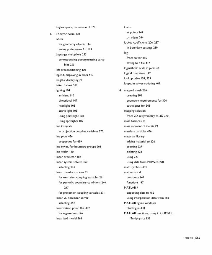
Krylov space, dimension of 379
L L2 error norm 390
labels
for geometry objects 114
saving preferences for 119
Lagrange multipliers 253
corresponding postprocessing varia-
bles 253
left preconditioning 400
legend, displaying in plots 440
lengths, displaying 77
letter format 512
lighting 104
ambient 110
directional 107
headlight 105
scene light 105
using point light 108
using spotlights 109
line integrals
in projection coupling variables 270
line plots 456
properties for 439
line styles, for boundary groups 203
line width 120
linear predictor 382
linear system solvers 392
selecting 394
linear transformations 33
for extrusion coupling variables 261
for periodic boundary conditions 246,
247
for projection coupling variables 271
linear vs. nonlinear solver
selecting 362
linearization point 366, 402
for eigenvalues 176
linearized model 366
loads
at points 244
on edges 244
locked coefficients 206, 237
in boundary settings 239
log
from solver 415
saving to a file 417
logarithmic scale in plots 431
logical operators 147
lookup table 154, 229
loops, in solver scripting 409
M mapped mesh 286
creating 305
geometry requirements for 306
techniques for 308
mapping solution
from 2D axisymmetry to 3D 270
mass balances 14
mass moment of inertia 79
massless particles 476
materials library
adding material to 226
creating 227
deleting 228
using 223
using data from MatWeb 228
math symbols 433
mathematical
constants 147
functions 147
MATLAB 7
exporting data to 452
using interpolation data from 158
MATLAB figure windows
plotting in 430
MATLAB functions, using in COMSOL
Multiphysics 158
I N D E X | 565
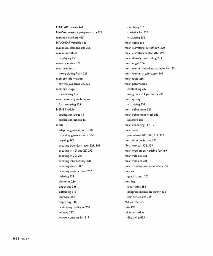
566 | I N D E X
MATLAB movies 442
MatWeb material property data 228
max/min markers 455
MAXHEAP variable 125
maximum element size 295
maximum values
displaying 455
mean operator 162
measurements
interpolating from 229
memory information
for the Java heap 31, 125
memory usage
monitoring 417
memory-saving techniques
for rendering 124
MEMS Module
application areas 15
application modes 15
mesh
adaptive generation of 388
canceling generation of 304
copying 342
creating boundary layer 321, 341
creating in 1D and 2D 293
creating in 3D 287
creating interactively 328
creating swept 317
creating unstructured 287
deleting 331
elements 286
exporting 346
extruding 313
identical 342
importing 346
optimizing quality of 290
refining 327
report contents for 519
revolving 313
statistics for 326
visualizing 352
mesh cases 355
mesh curvature cut off 289, 300
mesh curvature factor 289, 297
mesh density, controlling 293
mesh edges 286
mesh element number, variable for 169
mesh element scale factor 169
mesh faces 286
mesh parameters
controlling 287
using on a 2D geometry 294
mesh quality
visualizing 353
mesh refinement 327
mesh refinement methods
adaptive 388
mesh rendering 117, 121
mesh sizes
predefined 288, 305, 319, 322
mesh time derivative 173
Mesh toolbar 328, 329
mesh type index, variable for 169
mesh velocity 166
mesh vertices 286
mesh visualization parameters 352
meshes
quadrilateral 303
meshing
algorithms 286
progress indication during 304
thin structures 325
M-files 522, 528
mile 193
minimum value
displaying 455
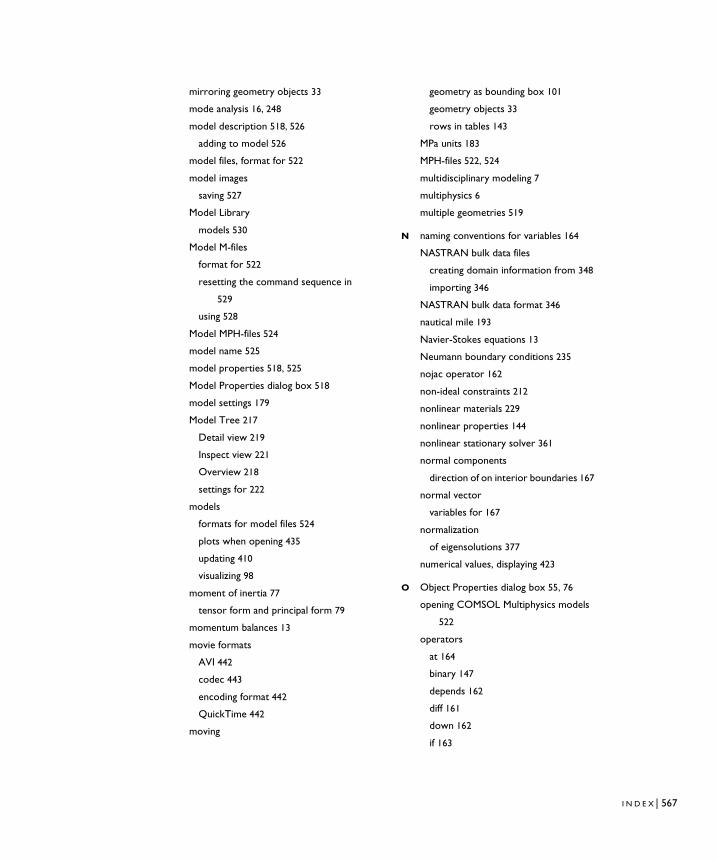
mirroring geometry objects 33
mode analysis 16, 248
model description 518, 526
adding to model 526
model files, format for 522
model images
saving 527
Model Library
models 530
Model M-files
format for 522
resetting the command sequence in
529
using 528
Model MPH-files 524
model name 525
model properties 518, 525
Model Properties dialog box 518
model settings 179
Model Tree 217
Detail view 219
Inspect view 221
Overview 218
settings for 222
models
formats for model files 524
plots when opening 435
updating 410
visualizing 98
moment of inertia 77
tensor form and principal form 79
momentum balances 13
movie formats
AVI 442
codec 443
encoding format 442
QuickTime 442
moving
geometry as bounding box 101
geometry objects 33
rows in tables 143
MPa units 183
MPH-files 522, 524
multidisciplinary modeling 7
multiphysics 6
multiple geometries 519
N naming conventions for variables 164
NASTRAN bulk data files
creating domain information from 348
importing 346
NASTRAN bulk data format 346
nautical mile 193
Navier-Stokes equations 13
Neumann boundary conditions 235
nojac operator 162
non-ideal constraints 212
nonlinear materials 229
nonlinear properties 144
nonlinear stationary solver 361
normal components
direction of on interior boundaries 167
normal vector
variables for 167
normalization
of eigensolutions 377
numerical values, displaying 423
O Object Properties dialog box 55, 76
opening COMSOL Multiphysics models
522
operators
at 164
binary 147
depends 162
diff 161
down 162
if 163
I N D E X | 567

568 | I N D E X
islinear 162
logical 147
mean 162
nojac 162
pdiff 161
quad 163
test 161
unary 147
up 162
with 164
optimizing mesh quality 290
orbit 101
orthographic projection 103
output formats 511
direct printing 512
HTML 512
output times 373
from time-dependent solver 371
overlapping objects 128
P pan 102
paper formats 512
parabola 48
parabolic PDEs 400
parabolic problem 400
parabolic velocity profile 166
parameter values for parametric solver
381
parameter values, accessing solution at
previous 382
parameterization variables
for surface boundaries 166
parametric segregated solver 387
parametric solver 379
list of parameter values for 381
settings for 382
stop conditions for 383
partial differential equations
application modes for 8
particle tracing 476
path-following method 380
pathlines 476
PDE
elliptic 400
parabolic 400
PDE modes 8
PDEs
stationary 361
time-dependent 361
perimeters 77
periodic boundary conditions 245
implementation of 247
linear transformations for 246
perspective projection 104
phase property 177
phasor variable 177
physical memory
current and peak usage 31, 417
physics modes 8
physics section 515
physics settings
copying 144
opening dialog boxes for 200
specifying 200
piecewise analytical functions 151
pink colormap 434
Plot toolbar
for 2D plots 460
for 3D models 491
plot types 420
selecting 428
plots
exporting data to file 451
on boundaries 466
when opening models 435
plotting
in COMSOL figure windows 430
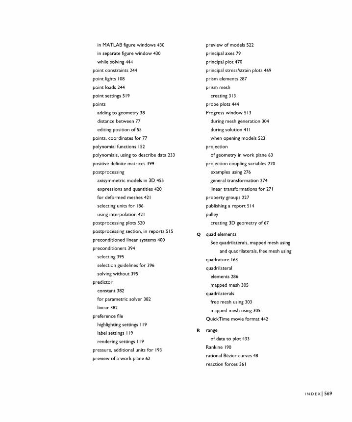
in MATLAB figure windows 430
in separate figure window 430
while solving 444
point constraints 244
point lights 108
point loads 244
point settings 519
points
adding to geometry 38
distance between 77
editing position of 55
points, coordinates for 77
polynomial functions 152
polynomials, using to describe data 233
positive definite matrices 399
postprocessing
axisymmetric models in 3D 455
expressions and quantities 420
for deformed meshes 421
selecting units for 186
using interpolation 421
postprocessing plots 520
postprocessing section, in reports 515
preconditioned linear systems 400
preconditioners 394
selecting 395
selection guidelines for 396
solving without 395
predictor
constant 382
for parametric solver 382
linear 382
preference file
highlighting settings 119
label settings 119
rendering settings 119
pressure, additional units for 193
preview of a work plane 62
preview of models 522
principal axes 79
principal plot 470
principal stress/strain plots 469
prism elements 287
prism mesh
creating 313
probe plots 444
Progress window 513
during mesh generation 304
during solution 411
when opening models 523
projection
of geometry in work plane 63
projection coupling variables 270
examples using 276
general transformation 274
linear transformations for 271
property groups 227
publishing a report 514
pulley
creating 3D geometry of 67
Q quad elements
See quadrilaterals, mapped mesh using
and quadrilaterals, free mesh using
quadrature 163
quadrilateral
elements 286
mapped mesh 305
quadrilaterals
free mesh using 303
mapped mesh using 305
QuickTime movie format 442
R range
of data to plot 433
Rankine 190
rational Bézier curves 48
reaction forces 361
I N D E X | 569
570 | I N D E X
refining meshes 327
regular font
indicating default values 518
relative tolerance 371
in nonlinear solver 368
reldetjac variable 169
reldetjacmin variable 169
release time for particles 479
remeshing domains 331
rendering
line settings 120
memory-saving techniques for 124
saving preferences for 119
settings for 116
repair of geometry objects 33
repair tolerance 33, 89
for DXF import 87
report generation 510
report sections
geometry 515
introduction 515
model properties 515
physics 515
postprocessing 515
solution 515
resetting the model 529
resolution
adjusting for dashed lines 440
for line plots 486, 505
of narrow regions 289
resolution, of images 453
restarting the solvers 410
results description
adding to model 526
revolved mesh 287
revolving
2D geometries into 3D 65
meshes 313
RF Module
application areas 16
application modes 16
material properties supported in 17
right preconditioning 400
Robin conditions. See generalized Neu-
mann boundary conditions
rotating geometry objects 33
rotation axis 74
rough plots 435
rubber-band box, zooming using 100
ruling application mode 361
Runge-Kutta methods
for solving particle equations of mo-
tion 477
S saving
COMSOL Multiphysics models 522
models on server 524
scalar variables
saving and loading 142
scaling
geometry before meshing 293
geometry objects 33
of images 453
of load and constraint symbols 119
scene light 105
scripting using solver commands 408
segregated solver
parametric 387
stationary 384
Select HTML Output File dialog box 512
selecting
2D geometry objects 127
3D objects 127
a single 2D geometry object 127
a single 3D object 128
a single face element 128
all objects 126
by group 127, 290
current suppression 123
domains 126
methods for 126
multiple objects 129
overlapping objects 128
remaining domains for meshing 291
times steps to plot 426
selection
by cycling adjacent objects 134
clearing of 132
confirmation of 130
conflicting 237
indication of 127
of all adjacent objects 134
using adjacency selection methods 134
selection, zooming to 100
server, saving models on 524
set difference 32
set formula, for Boolean operations 32
set intersection 32
set union 32
shape function variables 170
for time derivatives 172
shift 377, 399
shrinking coefficients
in Model M-file 529
SI units 191
sign function 150
simplify expressions 180
Simpson quadrature 163
singular mesh revolutions 316
singularities
avoiding 94
in the geometry 94
slice plots 493
snap
to grid 31
to vertex 31
solid
3D object 67
solid mechanics 17
solid modeling
2D 42
3D 67
solid objects 43
trimming 44
solidifying geometry objects 31
solution
interpolated 164
selecting for postprocessing 428
selecting variables in 406
storing and selecting for further analy-
sis 411
solution form
automatic 364
with coupling variables 280
solution process
canceling 412
plotting quantities during 444
stop buttons for 413
solution section, in reports 515
solution value
displaying 423
solutions
accessing for postprocessing 164
solutions from a previous analysis 404
solver algorithms 360
Solver Manager 401
solver scripting 408
commands for 408
solving using 409
using loops in 409
solver selection
automatic 361
solver settings 518, 519
I N D E X | 571
572 | I N D E X
solvers
canceling 412
for linear systems 392
hierarchical structure of 412
in COMSOL Multiphysics 360
logs from 415
restarting 410
selecting 360
starting 410
source transformation 264
space coordinate variables 165
changing the name of 29
space-varying properties 144
splines
for interpolations 155
splitting geometry objects 35
spotlights 109
starting the solvers 410
static problem 365
stationary PDE problem 365
stationary PDE problems 361
stationary segregated solver 384
stationary solver 365
stationary value 361
statistics, for mesh 326
status bar 30
stiffness matrix
correct versus incorrect 363
symmetric 397
STL files
format of 89
importing 89
Stokes equations 363
stop conditions
for the parametric solver 383
for the time-dependent solver 373
stored solution 401
streamline plots
in 2D 471
in 3D 502
Structural Mechanics Module
analysis types in 17
application areas 17
application modes 17
special element types in 17
subdomain integration 422
subdomain plots 497
subdomain settings 519
subdomains 35
subsections of a report 517
suffixes
in variable names 164
suffixes for report files 513
suppressing
display of objects 122
surface areas 77
surface integral 423
surface plots 461
properties for 439
swept meshes 317
combining with free meshes 338
geometry requirements for 318
mesh elements in 320
symmetric Jacobian matrix 397
symmetric matrices
when solving 397
symmetric stiffness matrix 397
symmetry detection 398
T table rows, moving and clearing 143
tangent vectors, variables for 167
tangential derivative variables 173, 325
tangents 51
technical support
email address for 20
online resources 20
temperature units 190
test operator 161
tetrahedral elements 286
text formatting and symbols 431
text symbols 433
The 387
thin structures
meshing 325
time derivatives
including in solution output 407
variables for 172
time steps
setting manually 373
taken by solver 373
time variable 144, 175
time, additional units for 193
time-dependent PDEs 361
time-dependent solver 370
order of the time-stepping method in
373
settings for 372
stop conditions for 373
using 370
times for output 371, 373
times, selecting for plotting 426, 442
time-varying properties 144
tolerance
absolute 371
for time-stepping solver 371
relative 371
transfinite interpolation 305
transformation matrix 247, 273
translation vector 247, 273
transparency in plots 112
triangular elements 286
trimming solids 44
typographical conventions 4
U undoing mesh operations 333
unexpected units 186, 189
unit systems
British engineering units 184
CGS 183
EMU 183
ESU 183
FPS 184
gravitational IPS 184
IPS 184
MPa 183
SI 183
switching 189
units
during postprocessing 186
highlighting unexpected 186, 189
multiplying with 187
SI system 191
using 183
unsteady problem 370
up and down directions, variables de-
fined in 180
up operator 162
updating models 410
URL for model information 525
user forums 20
user models, creating library for 531
V Vanka preconditioner/smoother 396
variable inheritance 175
variable name suffixes 164
variables
available by inheritance 173
boundary coupled shape 174
for gradient components 172
for mesh quality 353
for solution output 406
for space coordinates 165
for the eigenvalue 175
for time 175
geometric 165
I N D E X | 573
574 | I N D E X
naming convention for 164
to solve for 404
vector elements
preconditioners for 396
vector graphics 453
vector-valued expressions
entering 145
velocity profile, parabolic 166
vertex 35
vertices
adding to geometry 38
editing position of 55
snapping to 31
view
changing in 3D 101
explicit settings for 104
multiple geometries 36
virtual memory
current and peak usage 31, 417
Visualization/Selection toolbar 99, 116
visualizing
meshes 352
model geometries 98
volume integral 423
volumes, displaying 77
VRML files
format 89
importing 89
W wave colormap 434
wave propagation 16
weak constraints 361
web sites related to COMSOL 20
wedge elements. See prism elements
weights
for prioritizing eigenmodes 390
in control polygon 48
wireframe plot 124
work planes
at a specified edge angle 61
controlling 59
creating 59
example of using 67
parallel to a face 60
preview settings for 62
projecting geometry in 63
quick positioning of 60
specify by vertices 61
Z zoom 100, 102