INTRODUCTION TO

Design Module

C o n t a c t I n f o r m a t i o nVisit the Contact COMSOL page at www.comsol.com/contact to submit general inquiries, contact

Technical Support, or search for an address and phone number. You can also visit the Worldwide

Sales Offices page at www.comsol.com/contact/offices for address and contact information.

If you need to contact Support, an online request form is located at the COMSOL Access page at

www.comsol.com/support/case. Other useful links include:

• Support Center: www.comsol.com/support

• Product Download: www.comsol.com/product-download

• Product Updates: www.comsol.com/support/updates

• COMSOL Blog: www.comsol.com/blogs

• Discussion Forum: www.comsol.com/community

• Events: www.comsol.com/events

• COMSOL Video Gallery: www.comsol.com/video

• Support Knowledge Base: www.comsol.com/support/knowledgebase

Part number: CM024002

I n t r o d u c t i o n t o t h e D e s i g n M o d u l e© 2005–2019 COMSOL

Protected by patents listed on www.comsol.com/patents, and U.S. Patents 7,519,518; 7,596,474; 7,623,991; 8,457,932; 8,954,302; 9,098,106; 9,146,652; 9,323,503; 9,372,673; 9,454,625; and 10,019,544. Patents pending.

This Documentation and the Programs described herein are furnished under the COMSOL Software License Agreement (www.comsol.com/comsol-license-agreement) and may be used or copied only under the terms of the license agreement. Portions of this software are owned by Siemens Product Lifecycle Management Software Inc. © 1986–2019. All Rights Reserved. Portions of this software are owned by Spatial Corp. © 1989–2019. All Rights Reserved.

COMSOL, the COMSOL logo, COMSOL Multiphysics, COMSOL Desktop, COMSOL Compiler, COMSOL Server, and LiveLink are either registered trademarks or trademarks of COMSOL AB. ACIS and SAT are registered trademarks of Spatial Corporation. CATIA is a registered trademark of Dassault Systèmes or its subsidiaries in the US and/or other countries. Parasolid is a trademark or registered trademark of Siemens Product Lifecycle Management Software Inc. or its subsidiaries in the United States and in other countries. All other trademarks are the property of their respective owners, and COMSOL AB and its subsidiaries and products are not affiliated with, endorsed by, sponsored by, or supported by those or the above non-COMSOL trademark owners. For a list of such trademark owners, see www.comsol.com/trademarks.

Version: COMSOL 5.5

Contents

Introduction . . . . . . . . . . . . . . . . . . . . . . . . . . . . . . . . . . . . . . . . . . . 5

Creating Sketches with Constraints and Dimensions . . . . . . . . . 6

Working with the Loft Operation . . . . . . . . . . . . . . . . . . . . . . . . 22

About CAD File Formats . . . . . . . . . . . . . . . . . . . . . . . . . . . . . . . 28

Importing and Repairing a 3D CAD File . . . . . . . . . . . . . . . . . . . 30

Working with Defeaturing Tools . . . . . . . . . . . . . . . . . . . . . . . . . 37

Applying Virtual Geometry Operations . . . . . . . . . . . . . . . . . . . 43

Creating a Fluid Domain Around a Solid Structure. . . . . . . . . . 51

| 3

4 |

Introduction

This guide introduces you to the Design Module that provides tools such as constraints and dimensions to create 2D geometry, and the geometry features loft, thicken, midsurface, fillet, and chamfer, for creating geometry in 3D. Using the loft operation you can generate 3D geometry based on cross-sectional profiles, while the midsurface enables the simplification of imported geometry objects for shell type analyses. Using a combination of midsurface and thicken operations you can even re-parameterize and optimize the thickness of imported geometry. The module also adds support for importing several 3D CAD file formats, and includes repair and defeaturing functionality for preparing imported geometry for analysis.The detailed tutorials that follow start you off with becoming efficient in using the provided functionality.

| 5

Creating Sketches with Constraints and Dimensions

The constraint and dimension features enable an efficient workflow to create 2D geometries, including on work planes in 3D. By using the drawing tools available in sketch mode you can draw an initial sketch; then, by adding constraints and dimensions, you can obtain the final geometry.A constraint is a requirement on geometric entities that does not have a value; for example, a requirement that two edges should be parallel. A dimension is a requirement that has a value; for example, a requirement that specifies the distance between two vertices. The constraints and dimensions added to the geometry are visualized with symbols and arrows in the Graphics window.Follow this tutorial to learn how to use the drawing tools in sketch mode and to apply constraints and dimensions to create the geometry of the bracket pictured below.

Creating a New Model

1 Start COMSOL Multiphysics; then, under New, select Model Wizard.2 Select 2D, then click Done to skip the steps of selecting physics interfaces and

study types.3 Under Component 1, select Geometry 1.

6 |

4 In the Settings window, under Units, change Length unit to mm.The bracket is larger than the default zoom level in the Graphics window. Adding constraints and dimensions is easier if the original sketch is drawn closer to its final size; therefore you can start by zooming out a few steps.

5 In the Graphics toolbar, click Zoom Out ( ) five times.Your Graphics window should look similar to the one below.

Enabling Sketch Mode and Constraints and Dimensions

1 From the ribbon, select the Sketch tab.

| 7

2 Select Sketch ( ) to enable sketch mode.In sketch mode, you can draw the geometry directly in the Graphics window using the interactive drawing tools from the Sketch tab. Snapping to the grid and to the geometry while drawing are enabled by default. The Solid button determines the default output type of the shapes you draw. When the button is selected, solid objects are created; otherwise, curve objects are created. You can also change the object type in the settings for the created features. In sketch mode only the edges and the vertices of the geometry are visualized, the domains become visible after you exit sketch mode.

3 From the Model Builder select Geometry 1. In the settings for Geometry, under Use constraints and dimensions, select On.

This enables the use of Constraints and Dimensions in the geometry sequence. The setting Constraint and dimension features to build is initially set to All, meaning that such features in the geometry sequence are always active regardless of the currently built node. You can change this if you only want the constraints and dimensions up to a specific build target in the sequence to be active. This may be useful to debug a geometry sequence for example.When building a geometry there may be several solutions for the geometry shape given the applied constraints and dimensions. As you apply new constraint or dimension features to the geometry, the returned shape may not always correspond to the desired one. To avoid this effect, it is recommended to add constraints before adding dimensions. Constraint features define the relations between the geometric entities, thereby reducing the number of possible solutions when you start adding dimensions.If you are unhappy with the provided solution after adding a constraint or dimension, use undo; then use the mouse to drag the edges and vertices closer to the desired shape. It can also help if the initial sketch is not too different in size from the final object.

Drawing the Bracket

1 From the Sketch tab, select Polygon ( ).

8 |

2 In the Graphics window click to start drawing the bracket. Start at the corner highlighted below, and draw the first segment in the direction of the arrow.

3 Move the pointer to the right, and at the end of the first edge where the circular arc starts click once to place a vertex.

4 To switch to drawing a circular arc, on the Sketch tab, expand the Circular Arc ( ) list, then select Start, Center, Angle.

Drawing directionStart here

| 9

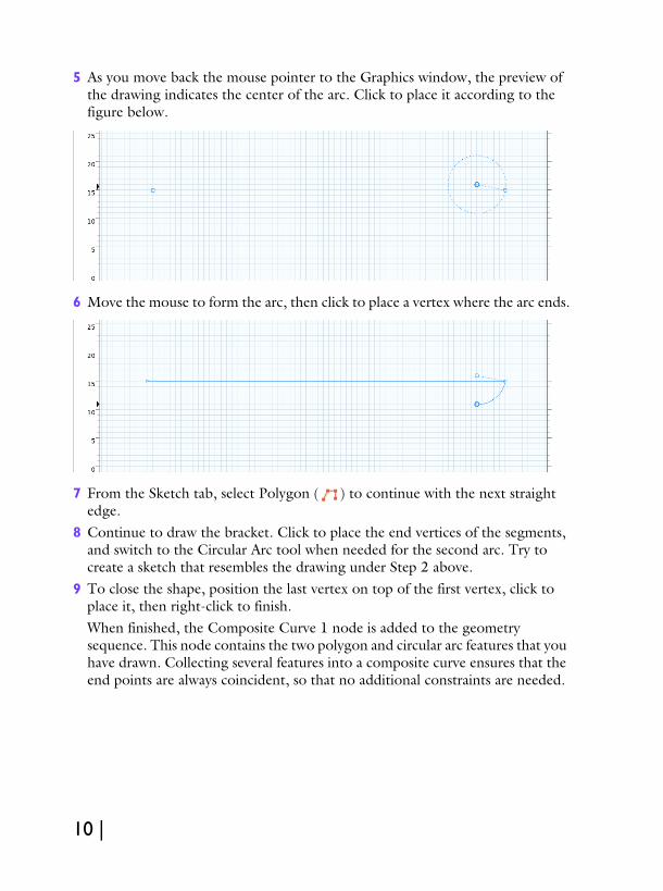
5 As you move back the mouse pointer to the Graphics window, the preview of the drawing indicates the center of the arc. Click to place it according to the figure below.

6 Move the mouse to form the arc, then click to place a vertex where the arc ends.

7 From the Sketch tab, select Polygon ( ) to continue with the next straight edge.

8 Continue to draw the bracket. Click to place the end vertices of the segments, and switch to the Circular Arc tool when needed for the second arc. Try to create a sketch that resembles the drawing under Step 2 above.

9 To close the shape, position the last vertex on top of the first vertex, click to place it, then right-click to finish.When finished, the Composite Curve 1 node is added to the geometry sequence. This node contains the two polygon and circular arc features that you have drawn. Collecting several features into a composite curve ensures that the end points are always coincident, so that no additional constraints are needed.

10 |

10Under Geometry 1, expand the Composite Curve 1 node, then click Polygon 1. The settings for Polygon contains a table with the point coordinates you have just drawn. In sketch mode you can modify the polygon by dragging the edges and vertices in the Graphics window.

11Drag an edge or vertex on the canvas. Before constraints and dimensions are applied to the sketch it is possible to move the entities without any restrictions. To restore the geometry click the Undo ( ) button, or press Ctrl+Z.Another way to modify the polygon is by editing the values in the coordinates table. The Constrain ( ) button next to the coordinates locks the vertex so that it is not possible to drag it in the Graphics window. The coordinates that are constrained this way become built-in dimensions and are not possible to modify by constraint and dimension features. For this example, leave all coordinates unconstrained as you will continue with applying constraints and dimensions to obtain the final shape of the bracket.

Adding Constraints to the Sketch

1 From the Sketch toolbar, select Constraint ( ).This activates the smart constraint mode where you can constrain geometric entities by selecting them in the Graphics window. Depending on the geometry and selected entities, a constraint is automatically suggested by the software. You may choose to apply the suggested constraint or change it to a different constraint.

| 11

2 From the Graphics window, select the two edges highlighted below.

The perpendicular constraint is suggested, and its symbol appears under the pointer.

3 Click in the Graphics window, close to the selected edges, to place the symbol for the perpendicular constraint. You can always drag the symbol to adjust its position after placing it. The drawing is updated right away.

Note that in the Model Builder, the Perpendicular 1 node has been added under the geometry sequence. Similar to all other geometry features, you can select the node to change its settings.

Perpendicular constraint symbol

12 |

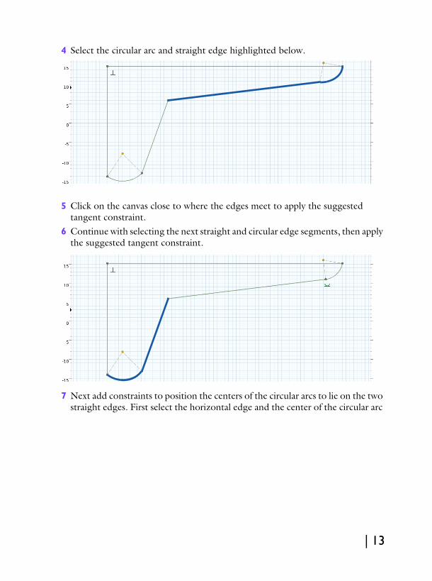
4 Select the circular arc and straight edge highlighted below.

5 Click on the canvas close to where the edges meet to apply the suggested tangent constraint.

6 Continue with selecting the next straight and circular edge segments, then apply the suggested tangent constraint.

7 Next add constraints to position the centers of the circular arcs to lie on the two straight edges. First select the horizontal edge and the center of the circular arc

| 13

to the right, apply the suggested coincident constraint, then repeat for the remaining arc and the vertical edge.

The geometry should now look similar to the one displayed below.

You have now applied the constraints needed to define the relations between the entities in the drawing.

8 On the Sketch tab click the Constraint ( ) button to exit the smart constraint mode.

9 Test again to drag an edge or a vertex of the geometry. Note how the relations prescribed by the constraints are maintained as you do this.The goal when applying constraints and dimensions is to obtain a fully constrained sketch that is not possible to modify by dragging in the Graphics window. Such a geometry is called well defined. The bracket geometry is currently still underdefined. It is not recommended to leave a sketch in an underdefined state as several solutions exists, and modifying a dimension, for example by a parametric sweep, may lead to unpredictable results.

Selection for first coincident constraint

Selection for second coincident constraint

14 |

10Press Ctrl+Z as needed to undo any changes to the sketch.11To check how many more

constraints or dimensions are needed until the geometry becomes well defined, click the Geometry 1 node in the Model Builder.As you can see from the information in the Settings window the geometry is underdefined, and it needs 9 more constraints or dimensions. The rigid body translational and rotational degrees of freedom are not yet locked, meaning that the entire sketch can be moved around freely as a rigid body.

Adding Dimensions to the Sketch

1 From the Sketch tab, select Dimension ( ) to enter the smart dimension mode.The smart dimension tool works similarly to the smart constraint tool: you start by selecting entities, then either apply the suggested dimension, or change it first, and finally enter a dimension value before continuing with adding more dimensions.

2 From the Graphics window, select the edge highlighted below.

| 15

3 To apply the suggested Distance dimension, click above the edge to place its symbol.The Distance 1 node is added to the geometry sequence, and the Settings window for Distance is displayed where you can edit the value.

4 In the Settings for Distance, in the Distance field enter 65[mm].5 Click Build Selected ( ), or press F7, to build the geometry using the new

value.6 Select the circular arc highlighted below.

7 Click to apply the suggested Radius constraint.8 In the Settings for Radius, in the Radius field enter 4[mm].9 Press F7 to build the geometry.

16 |

10Select the two edges highlighted below.

11Click somewhere between the edges to apply the suggested Angle dimension.12In the Settings for Angle, in the Angle field enter 3[deg].13Press F7 to build the geometry.14Repeat Steps 2–13 to add a distance, a radius, and an angle dimension for the

edges on the left side of the bracket, highlighted in the following figure. Use

| 17

the following dimension values: 30[mm] for the Distance dimension applied to the vertical edge, 6[mm] for the arc radius, and 20[deg] for the angle.

When done your drawing should look similar to the one displayed below.

15From the Sketch toolbar click Dimension ( ) to exit the smart dimension tool.

Adding Dimensions to Constrain the Rigid Body Degrees of Freedom

1 In the Model Builder click Geometry 1 to check the status for the geometry.According to the information, three more constraints or dimensions are needed to lock the rigid body degrees of freedom.

18 |

2 Try to drag the edges and vertices of the bracket in the Graphics window. Note that it is only possible to displace the bracket as a whole but not to change its shape. Press Ctrl+Z as many times as needed to restore the geometry.You can constrain the rigid body degrees of freedom by applying a combination of the Position, x-Distance, and y-Distance dimensions.

3 From the Sketch toolbar select Dimension ( ) to activate the smart dimension mode again.

4 Select the two vertices highlighted below.

5 Instead of accepting the suggested distance dimension, from the Sketch tab select x-Distance ( ).Since the selected vertices are sufficient for applying the dimension, the x-Distance feature is added immediately to the geometry sequence.

6 In the Settings window for x-Distance make sure that the Distance is 0. In case you need to change the value, press F7 to update the geometry.The edge between the vertices is now constrained to vertical, and it is no longer possible to rotate the sketch.

| 19

7 As the smart dimension mode is still active you can select the vertex for applying the last dimension.

8 Click close to the vertex to place the symbol for the suggested Position dimension.

9 In the settings for Position, x and y coordinates edit fields enter -35[mm] and 15[mm], respectively.

10Press F7 to build the geometry.The geometry is now fully defined. This is also indicated by the black color of the entities.

20 |

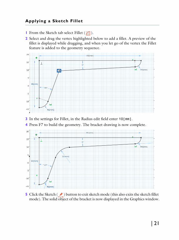
Applying a Sketch Fi l let

1 From the Sketch tab select Fillet ( ).2 Select and drag the vertex highlighted below to add a fillet. A preview of the

fillet is displayed while dragging, and when you let go of the vertex the Fillet feature is added to the geometry sequence.

3 In the settings for Fillet, in the Radius edit field enter 10[mm].4 Press F7 to build the geometry. The bracket drawing is now complete.

5 Click the Sketch ( ) button to exit sketch mode (this also exits the sketch fillet mode). The solid object of the bracket is now displayed in the Graphics window.

| 21

Working with the Loft Operation

The loft operation enables creating 3D surfaces based on cross-sectional profiles. The following tutorial demonstrates how to generate lofted surfaces with tangents matching the tangents of adjacent faces by specifying the loft direction and using guide curves.

The Geometry Sequence

1 Start COMSOL Multiphysics, then from the File menu select Open.2 Open the file bracket_geometry.mph, which is found in your COMSOL

installation directory, under the folder applications/Design_Module/Tutorial_Examples.The file contains a sequence of geometry operations that results in the geometry of the bracket displayed below.

22 |

3 In the Model Builder expand Component 1>Geometry 1 to see the sequence of geometry operations that builds the bracket.The sequence starts by creating the elbow, which is the output of the Revolve 1 operation. The output of the Loft 1 operation and its mirror (Mirror 1) connect the elbow to the two wings, which are the Block 1 and Block 2 operations. The holes in the bracket are generated by subtracting the cylinders from the geometry. Finally the Mirror 2 operation generates the full bracket geometry.

4 To study how the geometry is built, step through the sequence of operations by right-clicking on a node then selecting Build Selected.

The Loft Operation

1 Right-click the Loft 1 node , then select Build Preceding .2 In the Settings window for Loft, expand the Start Profile and End Profile

sections.The loft operation generates a solid object to connect the rectangular cross-section of the bracket with the cross-section of the elbow.

3 To get a better view of the start and end profiles click the Wireframe Rendering button on the Graphics toolbar.While in this case the input consists of a start and an end profile, it is possible to define additional profiles in the Profiles section.

4 On the Loft toolbar click the Build Selected button.

Start profile

End profile

| 23

LOFT DIRECTION

1 Click the Wireframe Rendering button on the Graphics toolbar.2 In the Graphics window move

and rotate the object to get a view perpendicular to the zx-plane. Then zoom in to get a view similar to that in the figure.In case on your screen the lofted object does not appear to match the start profile you can adjust the visualization settings for the Graphics window.

3 From the File menu select Preferences; then on the Graphics and Plot Windows page set Detail to Fine; confirm with clicking OK. The default setting for the start and end profiles does not prescribe a loft direction. As a result of this the tangent of the lofted surface does not match the tangent of the adjacent surfaces.In the following steps you will test the available loft direction options to create a surface with continuous tangent across the profile.

4 In the Start Profile section, from the Loft direction list select Parallel.5 In the End Profile section, from the Loft direction list select Parallel.6 For both the Start Profile and End Profile sections make sure that the Relative

to list is set to Adjacent faces.7 Click Build Selected .

With the loft direction parallel to the adjacent faces the tangent of the lofted surface matches that of the adjacent surfaces along the edges of the start and end profiles. While this results in a better surface close to the profiles it may be good to examine the surface in other places. In this case the edge highlighted in the figure is no longer straight.

8 In the Start Profile section, from the Loft direction list select Perpendicular.9 From the Relative to list select Profile faces.

24 |

10In the End Profile section, from the Loft direction list select Perpendicular.11From the Relative to list select Profile faces.

The perpendicular to profile faces loft direction ensures that the tangent of the lofted surfaces matches the normal vector of the profile faces at vertices along the profile curve. In this case there are four vertices, one at each corner of the start and end profiles.

12Click Build Selected .

The overall result is better compared to the Parallel loft direction, since the constraint on the tangent influences the entire surface, even though it is applied only at the vertices.

GUIDE CURVES

To get an even better result create guide curves to be used with the loft operation. The guide curves connect the profile curves, thus prescribing a shape that the

Vertices along the profile curves

| 25

lofted surface will follow. Each guide curve must have a continuous tangent, and intersect each profile curve exactly once. Note that the guide curves cannot be used with the loft direction set to parallel to adjacent faces. Both the Perpendicular and Not prescribed loft directions support the use of guide curves.1 In the Model Builder right-click the Loft 1 node, then select Build

Preceding .The above step is important as it makes the Block 1 node the current node, which is symbolized by a green square around the icon for the node. The geometry operations that you add to the sequence are going to be inserted after the current node.

2 On the Geometry toolbar click More Primitives , then choose Polygon .3 In the Settings window for Polygon, from the Data source list select Table.4 In the table enter the following coordinates:

You can copy and paste the expressions from the table above.5 Click Build Selected .6 To create the second curve right-click Polygon 1 and from the menu select

Duplicate.7 Use the following coordinates for Polygon 2:

Since the curve is a copy of the previous one you need only edit the y coordinates.

8 Click Build Selected .9 Right-click Polygon 2 and from the menu select Duplicate.10In the Coordinates table for Polygon 3 enter:

11Click Build Selected .

X (MM) Y (MM) Z (MM)

lX-rOut-2*thk lY/6-1 thk

lX-rOut lY/6-1 thk

X (MM) Y (MM) Z (MM)

lX-rOut-2*thk lY/3+1 thk

lX-rOut lY/3+1 thk

X (MM) Y (MM) Z (MM)

lX-rOut-2*thk lY/3+1 0

lX-rOut lY/3+1 0

26 |

12Finally, to create the last curve right-click Polygon 1 and from the menu select Duplicate.

13In the Coordinates table for Polygon 4 enter:

14Click Build Selected .

15In the Model Builder click the Loft 1 node, then in the Settings window for Loft expand the Guide Curves section.

16Under Guide objects click the Active button.17From the Graphics window select the four guide curves: pol1, pol2, pol3, pol4.

18Click Build Selected .Using a loft direction perpendicular to profile faces together with guide curves results in lofted surfaces that have desired continuity for the surface tangent.

X (MM) Y (MM) Z (MM)

lX-rOut-2*thk lY/6-1 0

lX-rOut lY/6-1 0

Guide curves

| 27

About CAD File Formats

To better understand the file import related functionality of the Design Module, first review some general background information about CAD file formats.

CAD Software, Geometry Kernels, and Fi le Formats

Each CAD program uses a geometry kernel to create a mathematical description of the objects and to calculate the results of solid-modeling operations. Parasolid® and ACIS® are the two most common kernels, and many CAD programs license these kernels. In addition, some programs use their own kernel (as does COMSOL). Each of these kernels has a native file format associated with it. For example, the Parasolid file format is simply called Parasolid, and the one from ACIS is called ACIS or SAT®.The geometry kernel defines the type of internal representations used for 3D modeling, which can vary considerably among different kernels. That explains why the representations stored in the various file formats are also very different. the Design Module can read several of these different descriptions of objects and translate them into a format that COMSOL can work with.In addition to the file formats that are native to a geometry kernel, yet other formats are based on neutral standards that were defined to ease the exchange of geometric models among CAD software applications. STEP and IGES are the two most popular such formats.Yet another class of files use surface-mesh geometry formats. They do not represent a model’s exact 3D geometry but store only triangular meshes of the surfaces. The most common examples of these types of formats are VRML and STL.

Translating 3D CAD Files Between Formats

Geometric models do not always pass flawlessly between different file formats due to the fact that they are represented differently. This means that the quality of a translation when importing a file to COMSOL depends on the file format. The smoothest way is to use the native format of your CAD system. If this is not an option, we in general recommend that you use Parasolid, STEP, or ACIS.Importing 3D CAD files into COMSOL is straightforward. Since the settings of the import operation have been tuned to suit the most common cases, the

28 |

majority of files import simply with the click of a button. During import the geometry is checked for errors and automatically repaired. The repair operation also removes small features that fall within the import tolerance.

| 29

Importing and Repairing a 3D CAD File

In this example, the Parasolid® file of a wheel rim contains a few small faces and slivers, which are not removed during import, since they fall outside the default import tolerance. The step-by-step instructions below demonstrate one way to locate and remove these features. The general workflow is:• Import the file• Create a mesh for quick examination of the geometry• Measure the size of the features you would like to remove• Repair the object• Create a new mesh for comparison

Model Wizard

1 Start COMSOL Multiphysics.2 Select Blank Model to skip the steps of selecting physics interfaces and study

type.3 On the Home toolbar, click Add Component and select 3D.

Importing the Geometry

1 On the Home toolbar click Import .2 In the Settings window for Import click the Browse button.3 In your COMSOL installation directory navigate to the folder applications/Design_Module/Tutorial_Examples and double click the file repair_demo_1.x_b.

4 Click Import.

30 |

As soon as the import is done the geometry appears in the Graphics window.

Creating a Surface Mesh

Creating a surface mesh for an imported solid is often the fastest way to assess the quality of the geometry and to identify regions needing repair or defeaturing.1 On the Mesh toolbar click Boundary and choose Free Triangular .2 Go to the Settings window for Free Triangular and from the Selection list box

select All boundaries.3 Click the Build All button to create the mesh.

As soon as the mesh is ready the Messages window displays the number of mesh elements, which is about 16,000. In addition, two warnings appear in the Messages window. These warnings indicate that the geometry contains edges that are much shorter than the minimum element size, and that there are faces which are smaller than the minimum element size.Two warning nodes, one for each type of warning, also appear under the Free Triangular 1 feature node in the mesh sequence. These nodes contain a list of entities, in this case short edges and small faces, causing problems. These entities are also highlighted in the geometry, and are usually surrounded by a denser mesh that indicates faces or edges significantly smaller in comparison to the size of the geometry.

| 31

4 Click the Warning 1 node in the meshing sequence, then in the Graphics window zoom in on the area around the bolt holes, shown below.

The areas of dense mesh, indicated by the arrows in the figure, are due to slivers and small faces. Zooming in even closer inside the blue rectangle reveals a small triangular face sitting adjacent to a sliver face. Two of these can be found around each bolt hole location. The edges that are highlighted in blue are listed in the Selection list of the Warning window.To get a representative size for these faces measure the length of one of its edges, number 646 in the list, which is marked with an arrow in the figure to the right.

5 Scroll down in the Selection list inside the Warning window, then click edge 646.

6 Click Measure in the Evaluate section of the Mesh toolbar.The Messages window displays the length of the edge, which is 2.556e-4 m — that is, 2.556·10-4 m or about 0.01 inch.Now take a closer look at some of the other short edges listed in the Warning window.

7 Scroll down to the end of the Selection list inside the Warning window, then click edge 958.

8 Click the Zoom selected button next to the list.The Graphics window centers and zooms in on the highlighted edge.

32 |

9 Using the mouse zoom out and pan to find where the edge is located on the wheel rim. It forms one side of a sliver face located in the region where two adjacent spokes connect to the rim.

Each spoke contains a similar sliver indicated by the arrows in the figure.10To get the width of the sliver face, click Measure on the Mesh tab, while the

edge is still highlighted in the list.

The length for edge 958 is 3.126·10-4 m (about 0.012 inch).

Repairing the Geometry

Now that you know the size of the faces to be removed you can repair the geometry.1 On the Geometry toolbar click Defeaturing and Repair and choose

Repair .2 In the Graphics window select the wheel rim to add it to the Input objects list.3 In the Absolute repair tolerance text field enter 3.2e-4.By keeping the repair tolerance close to the size of the features to be removed you can avoid removing anything else and breaking the geometry.

4 Click Build All Objects to perform the operation.

| 33

5 Examine the geometry. Pan and zoom to take a look at the areas that contained the slivers and small faces, which are now no longer present in the geometry.

Updating the Mesh and Continuing with the Repair

1 Right-click the Mesh 1 node and select Build All .This time the mesh contains about 1700 surface elements less than before the repair. The warning node informs that some edges are still shorter than the minimum element size.

34 |

2 Click the Warning 1 node, then use the Selection list and the Zoom selected button next to the list to find edges 684, 942, 979, and 983.

Three of these edges are located close to where the spokes connect to the rim, and one is found close to the center of the wheel. Similar edges occur on each spoke.

3 To find an appropriate repair tolerance measure the length of the edges using the Measure toolbar button. The Messages window reports the following

4 On the Geometry toolbar click Defeaturing and Repair and select Repair to continue with the repair of the geometry.

5 Select the wheel rim for the Input objects list.6 Enter 9e-4 in the Absolute repair tolerance text field.7 Click the Build All Objects button.

EDGE LENGTH

684 8.91e-4

942 6.61e-4

979 4.77e-4

983 8.33e-4

979 983

942

684

| 35

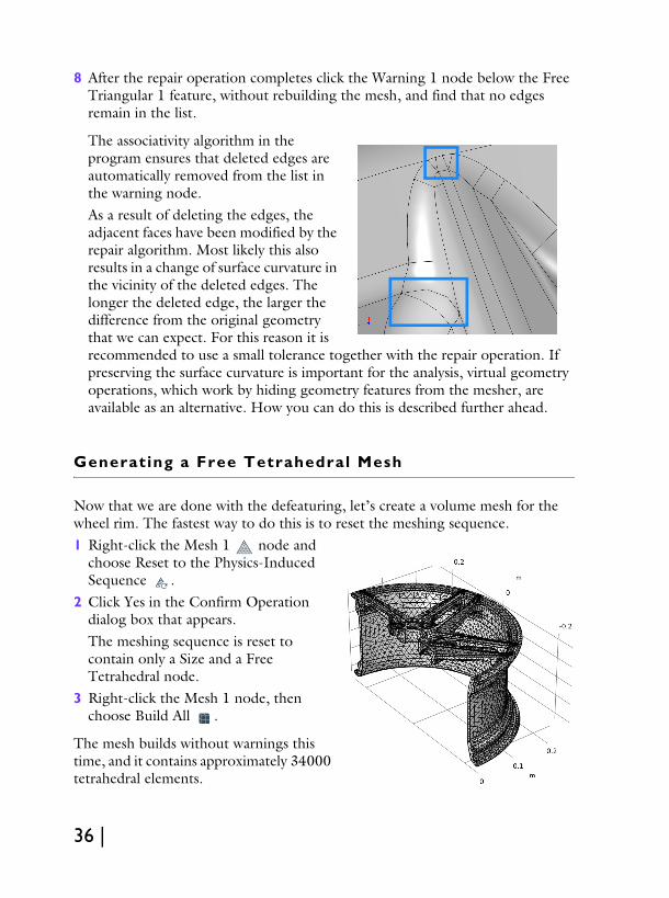
8 After the repair operation completes click the Warning 1 node below the Free Triangular 1 feature, without rebuilding the mesh, and find that no edges remain in the list.

The associativity algorithm in the program ensures that deleted edges are automatically removed from the list in the warning node.As a result of deleting the edges, the adjacent faces have been modified by the repair algorithm. Most likely this also results in a change of surface curvature in the vicinity of the deleted edges. The longer the deleted edge, the larger the difference from the original geometry that we can expect. For this reason it is recommended to use a small tolerance together with the repair operation. If preserving the surface curvature is important for the analysis, virtual geometry operations, which work by hiding geometry features from the mesher, are available as an alternative. How you can do this is described further ahead.

Generating a Free Tetrahedral Mesh

Now that we are done with the defeaturing, let’s create a volume mesh for the wheel rim. The fastest way to do this is to reset the meshing sequence.1 Right-click the Mesh 1 node and

choose Reset to the Physics-Induced Sequence .

2 Click Yes in the Confirm Operation dialog box that appears.The meshing sequence is reset to contain only a Size and a Free Tetrahedral node.

3 Right-click the Mesh 1 node, then choose Build All .

The mesh builds without warnings this time, and it contains approximately 34000 tetrahedral elements.

36 |

Working with Defeaturing Tools

As an alternative to the repair operation described in the previous example you can also apply defeaturing tools to remove small features from the geometry. Using these tools you can first search the geometry for features that fall within a set tolerance, then, after examining the search results, you can decide which ones to delete. While the repair operation has the advantage that it quickly removes every feature it can within a specified tolerance, the defeaturing tools gives you more control with selective removal of features.To search for and remove small features from a geometry using the defeaturing tools follow this general workflow:• Import the file• Search delete small faces• Search and delete sliver faces• Search and delete short edges

For the initial search for a feature it is good practice to use a tolerance slightly higher than the default import tolerance, 10-5 m. Thus, in a first attempt, search for small faces with a maximum size of 10-4 m. Continue by deleting all or some of the returned small faces, then search again with an even higher tolerance, for example 5·10-4 m.Meshing the geometry can also serve as a diagnostic tool for locating small features, and can be used in combination with the defeaturing tools. After meshing, you can measure some of the small edges and faces reported by the mesher to find a good starting point for a tolerance setting for the defeaturing tools.The step-by-step instructions below guide you through how to defeature the geometry of the wheel rim that appeared in the previous example.

Model Wizard

1 Start COMSOL Multiphysics.2 Select Blank Model to skip the steps of selecting physics interfaces and study

type.3 On the Home toolbar, click Add Component and select 3D.

| 37

Importing the Geometry

1 On the Home toolbar click Import .2 In the Settings window for Import click the Browse button.3 In your COMSOL installation directory navigate to the folder applications/Design_Module/Tutorial_Examples and double click the file repair_demo_1.x_b.

4 Click Import.

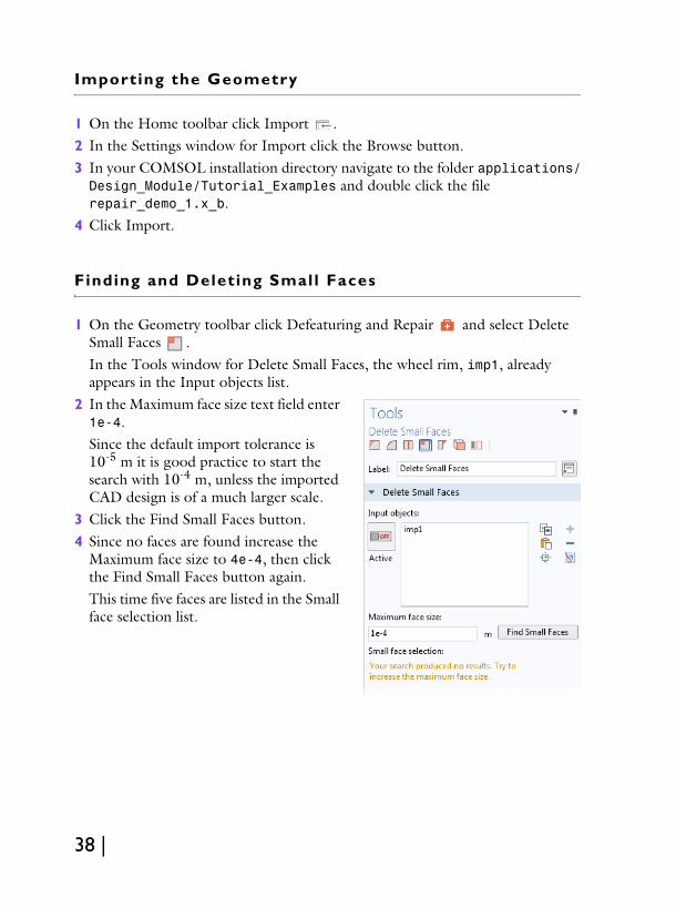
Finding and Deleting Small Faces

1 On the Geometry toolbar click Defeaturing and Repair and select Delete Small Faces .In the Tools window for Delete Small Faces, the wheel rim, imp1, already appears in the Input objects list.

2 In the Maximum face size text field enter 1e-4.Since the default import tolerance is 10-5 m it is good practice to start the search with 10-4 m, unless the imported CAD design is of a much larger scale.

3 Click the Find Small Faces button.4 Since no faces are found increase the

Maximum face size to 4e-4, then click the Find Small Faces button again.This time five faces are listed in the Small face selection list.

38 |

5 Use the Zoom to Selected button next to the list to find the faces on the rim, which are found around the bolt holes, as illustrated in the figure below.

6 To delete all faces in the list click the Delete All button.

The tool removes small faces by collapsing them into a vertex(point). Therefore it is not recommended to delete larger faces this way as it might result in unexpected changes to the geometry.

Note that as the operation is done the Delete Small Faces 1 (dsf1) node is added to the geometry sequence in the Model Builder tree. The node allows you to go back and edit the delete operation.The Tools window for Delete Small Faces continues to be displayed so that you can continue defeaturing using this or any of the other defeaturing tools.

| 39

Finding and Removing Sl iver Faces

Slivers are faces with high aspect ratio, just like the ones next to those small faces you have just deleted.1 From the toolbar in the upper left corner

of the Tools window for Delete Small Faces click the Delete Sliver Faces button.

2 Enter 4e-4 for the Maximum face width, then click Find Sliver Faces.A total of ten faces are found. In addition to the five slivers around the bolt holes, there are five more on the spokes. Use the Zoom to Selected button to find their location on the rim.

3 Click the Delete All button.

The tool removes sliver faces by collapsing them into an edge, and in this process it uses the tolerance specified for the search. For best results the tolerance needs to be close to the actual width of the face that is deleted. If it happens that a sliver cannot be deleted you can edit the settings for the operation to set a tolerance that is just slightly larger than the width of the face.

40 |

Finding and Removing Short Edges

1 From the toolbar in the upper left corner of the Tools window for Delete Sliver Faces click Delete Short Edges .

2 If not already selected, add the wheel rim to the Input objects list.

3 In the Maximum edge length text field enter 4e-4.

4 Click the Find Short Edges button.It seems that the previous operations have removed all edges that were shorter than this value.

5 Increase the Maximum edge length to 9e-4, then click the Find Short Edges button again.Take some time to find the edges in the list on the geometry and measure their length. They reoccur in similar places on each spoke. Some of the locations are indicated in the figure to the right.

| 41

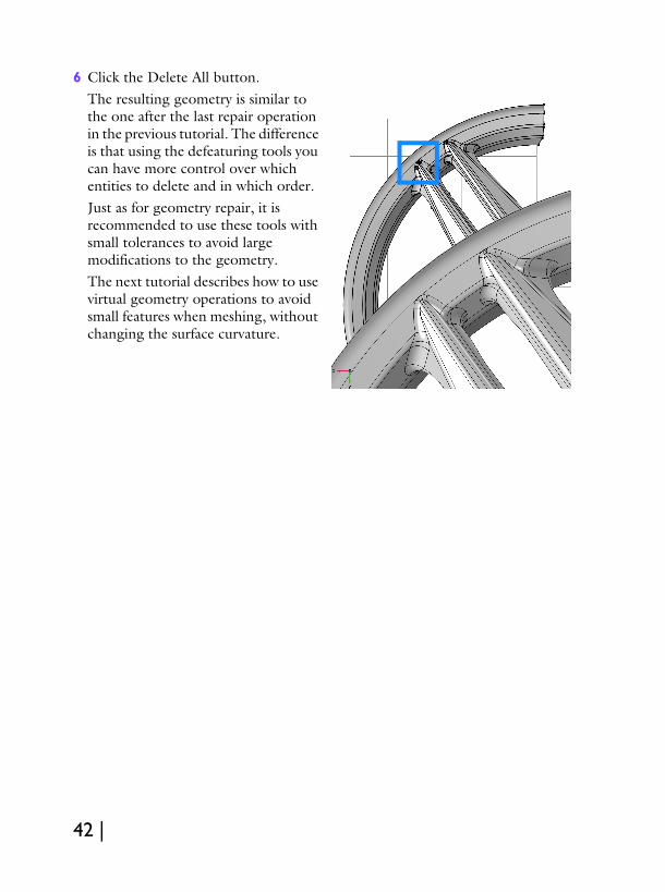
6 Click the Delete All button.The resulting geometry is similar to the one after the last repair operation in the previous tutorial. The difference is that using the defeaturing tools you can have more control over which entities to delete and in which order.Just as for geometry repair, it is recommended to use these tools with small tolerances to avoid large modifications to the geometry.The next tutorial describes how to use virtual geometry operations to avoid small features when meshing, without changing the surface curvature.

42 |

Applying Virtual Geometry Operations

The repair and defeaturing tools that find and delete small geometry features can operate only within the limits of what is allowed by the topology of the geometry. To handle more complex cases, where defeaturing fails, you can use virtual geometry operations. With these tools you can set geometric entities, such as vertices, edges, or faces, to be ignored by the mesher. Since selected elements are “hidden” from the mesher, meshing takes place on a virtual geometry, hence the name virtual operations.Other benefits of using virtual operations is that they work on the finalized geometry, and that they keep the curvature of the geometry. The latter is especially important when removing larger faces, or for certain physics applications when altering the curvature of the geometry can for example give rise to stress concentrations.Working with virtual geometry operations usually involves the first step of finding small features in the geometry. The general workflow is:• Import the file• Find small features by doing one, or both, of the following

- Search using the defeaturing tools- Create a surface mesh or a volume mesh and study the report returned by the

mesher• Use the appropriate virtual geometry tool to hide features.

Using the very same rim geometry as in the two previous examples in this guide, the step-by-step instructions below guide you through how to apply virtual geometry operations on various types of small features.

Model Wizard

1 Start COMSOL Multiphysics.2 Select Blank Model to skip the steps of selecting physics interfaces and study

type.3 On the Home toolbar, click Add Component and select 3D.

| 43

Importing the Geometry

1 On the Home toolbar, click Import .2 In the Settings window for Import, click Browse. 3 In your COMSOL installation directory navigate to the folder applications/Design_Module/Tutorial_Examples and double click the file repair_demo_1.x_b.

4 Click Import.

Creating a Surface Mesh

Creating a surface mesh for an imported geometry is often the fastest way to assess the quality of the geometry and to identify regions needing repair or defeaturing.1 On the Mesh toolbar click Boundary and select Free Triangular .2 Go to the Settings window for Free Triangular and from the Selection list box

select All boundaries.3 Click the Build All button to create the mesh.

In the Messages window you can see the number of mesh elements, which is about 16,000. In addition, two warnings are displayed, which indicate that the geometry contains edges that are much shorter than the minimum element size, and that there are faces which are smaller than the minimum element size.Next, examine the mesh and look for those areas where the mesher indicates small edges or faces. These regions usually correspond to a denser mesh, some of which are indicated in the figure to the right.

44 |

4 Using the Zoom Box button, zoom to the area shown below, where a spoke connects to the rim.

Each spoke contains a dense mesh area due to the small features indicated by the arrows in the figure.

On closer examination you can see that several edges in this area are highlighted as being too short to be meshed with the current mesh settings.

Ignore Edges and Form Composite Faces

1 On the Geometry toolbar click Virtual Operations and choose Ignore Edges .

2 In the graphics area select the edges 217, 219, and 222, highlighted in the figure, to add them to the Edges to ignore list.

| 45

3 Click the Build Selected button.The visualization of the rim in the Graphics window is updated to reflect that the selected edges, and, where applicable, adjacent vertices are no longer part of the geometry which is going to be meshed.

As an alternative to the Ignore Edges operation you can also use the Form Composite Faces operation.4 On the Geometry toolbar click Virtual

Operations and choose Form Composite Faces .

5 Select faces 112, 118, 122, and 126, as highlighted in the figure on the right.

6 Click the Build Selected button. The geometry in the Graphics window is updated with the new composite formed faces.

46 |

7 To view the new mesh of this region click the Mesh 1 node, then click the Build All button.

Editing the Geometry Sequence

1 Click the Zoom extents button to view the entire rim geometry again. Then zoom to the region shown below using the Zoom box button.

The short edges in this region form a small face which you remove using the Collapse Edges operation. The long edges of the sliver face can be removed by adding them to the existing Ignore Edges 1 operation in the geometry sequence.

| 47

2 Click the Ignore Edges 1 (ige1) node, then in the Settings window click the Activate button.

3 Select the edges 197 and 198, shown in the figure to the right. After this latest addition the list should now include edges 197, 198, 217, 219, 222.

4 Click the Build Selected button.5 Now continue by removing the small

triangular face. Before adding the operation to the sequence take a look in the Model Builder window.

A green rectangle is displayed around the Ignore Edges 1 node telling you that this is the current node. Any operations that you add to the sequence are placed directly after the current node. The Form Composite Faces 1 (cmf1) node is marked, which indicates that the node needs rebuilding.

6 Make sure that the next operation is the last one in the sequence by right-clicking the Form Composite Faces 1 (cmf1) node and choosing Build Selected .

Collapse Edges

1 On the Geometry toolbar click Virtual Operations and choose Collapse Edges .

2 Select edges 201-203 highlighted in the figure. Use the Select box button to select all three edges at once.

3 Click the Build Selected button.4 To build the mesh click first the Mesh 1 node,

then the Build All button.

48 |

5 The new mesh contains fewer elements since the sliver and small face are no longer visible to the mesher.

Ignore Vertices or Form Composite Edges

The last virtual geometry operation to try in this example is the Ignore Vertices operation to remove a short edge from a segmented edge. In this context the operation is equivalent to the Form Composite Edges operation.1 Click the Zoom extents button to view the entire rim geometry. Then zoom

in on the region shown below using the Zoom box button.

2 On the Geometry toolbar click Virtual Operations and choose Ignore Vertices .

| 49

3 Add vertex 108, highlighted in the figure below, to the list of Vertices to ignore, then click the Build Selected button.

4 To mesh the geometry once more right-click the Mesh 1 node and select Build All .

The mesher now sees the two edges as one unit, which is reflected in the way the elements are laid out in this new mesh.

As a last step find a similar short edge in another location on the rim and use the Form Composite Edge operation to hide it from the mesher.

50 |

Creating a Fluid Domain Around a Solid Structure

The majority of 3D CAD files include only the geometry of the product to be manufactured. For finite element analysis, however, you find yourself often in a situation where additional geometry is needed, for example, to analyze the flow inside or outside a device. The example in this section, involving the geometry for an exhaust manifold, demonstrates how to create an extra domain for flow analysis. The following steps are covered:• Importing a Parasolid® file.• Adding an explicit selection to the geometry sequence.• Using the cap faces operation to create the additional domain.• Controlling where an operation is inserted in the geometry sequence.• Finding and removing fillets from the geometry.

Model Wizard

1 Start COMSOL Multiphysics.2 Select Blank Model to skip the steps of selecting physics interfaces and study

type.3 On the Home toolbar, click Add Component and select 3D.

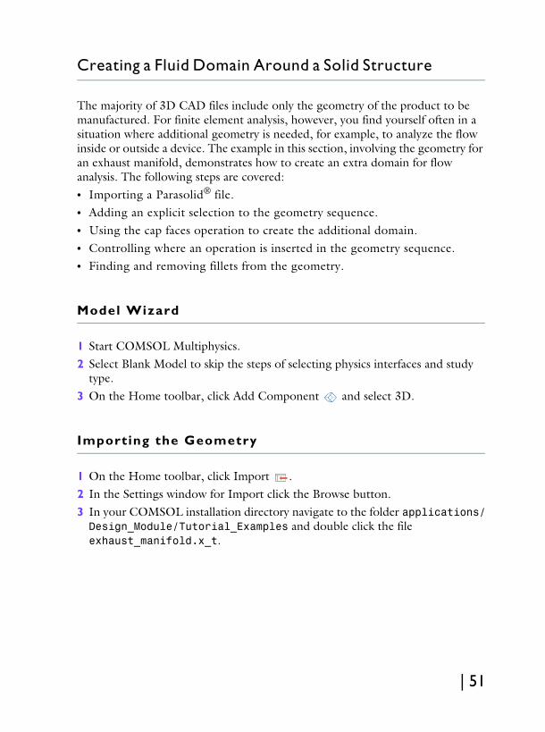
Importing the Geometry

1 On the Home toolbar, click Import .2 In the Settings window for Import click the Browse button.3 In your COMSOL installation directory navigate to the folder applications/Design_Module/Tutorial_Examples and double click the file exhaust_manifold.x_t.

| 51

4 Click Import.

As soon as the import is done the geometry appears in the Graphics window.

Rotate the geometry. As you can see it is hollow inside. As shown below, you can obtain the geometry for the inside in just one operation.

Creating an Explicit Selection

The Cap Faces operation needs an input in form of the bounding edges of the empty volume that should be turned into a solid. For this exhaust manifold these are the edges highlighted in the figure below.

52 |

These edges can be selected directly in the Cap Faces operation, however a more efficient way, which only requires the selection of one segment from each edge loop, is to use an explicit selection where you have the option to automatically include continuous edges in the selection.1 On the Geometry toolbar click Selections and choose Explicit Selection .2 In the Settings window for Explicit Selection select Edge from the Geometric

entity level list.3 Also select the Group by continuous tangent check box.4 From the Graphics window select one edge each from the edge loops

highlighted in the figure above. Continuous edges are automatically added to the selection. When done check that all edges are highlighted, just as in the figure.

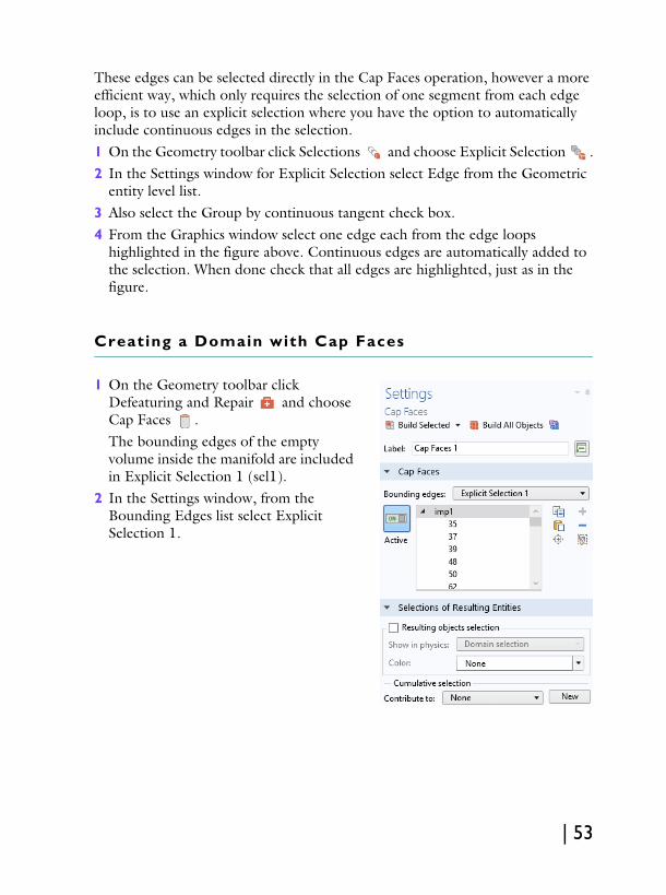
Creating a Domain with Cap Faces

1 On the Geometry toolbar click Defeaturing and Repair and choose Cap Faces .The bounding edges of the empty volume inside the manifold are included in Explicit Selection 1 (sel1).

2 In the Settings window, from the Bounding Edges list select Explicit Selection 1.

| 53

3 Click the Build Selected button to complete the operation.The operation closed off the inlets and outlets with new faces. The operation also created a solid domain where it used to be a void inside the exhaust manifold.

Let’s examine this new geometry object using the Measure tool.4 In the Model Builder tree, right-click Geometry 1 and choose Measure .

54 |

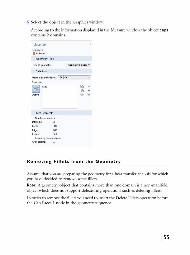
5 Select the object in the Graphics window.

According to the information displayed in the Measure window the object cap1 contains 2 domains.

Removing Fi l lets from the Geometry

Assume that you are preparing the geometry for a heat transfer analysis for which you have decided to remove some fillets.Note: A geometry object that contains more than one domain is a non-manifold object which does not support defeaturing operations such as deleting fillets.

In order to remove the fillets you need to insert the Delete Fillets operation before the Cap Faces 1 node in the geometry sequence.

| 55

1 Under the Geometry 1 node, right-click Cap Faces 1 (cap1) and choose Build Preceding .The Cap Faces 1 (cap1) node becomes unavailable, and the Explicit Selection 1 (sel1) node becomes the current node, which is indicated by a green rectangle around its icon. You can now apply the defeaturing operation, as it is inserted before the Cap Faces 1 (cap1) node.

2 On the Geometry toolbar click Defeaturing and Repair and choose Delete Fillets .

3 In the Tools window imp1 already appears in the Input objects list, and you can enter 0.003 in the Maximum fillet radius text field.

4 Click the Find Fillets button to search for fillets with a radius less than 0.003 m in the geometry.

56 |

5 Five fillets are found by the tool. These appear in the Fillet selection list, and they are also highlighted on the geometry.

6 Remove all fillets by clicking Delete All in the Tools Setting window.

As the operation completes and the fillets are removed note that the Delete Fillets 1 (dfi1) node is inserted into the geometry sequence, just above the Cap Faces 1 (cap1) node. The Cap Faces 1 (cap1) node is still unavailable, meaning that it is currently not built.

7 To re-build the entire geometry sequence click the Build All button on the Geometry toolbar.

| 57

The geometry is now ready for meshing and analysis!

58 |