MULTIPHYSICS SIMULATION AND INNOVATIVE

CHARACTERIZATION OF FREEZING SOILS

by

ZHEN LIU

Submitted in partial fulfillment of the requirements

For the degree of Doctor of Philosophy

Dissertation Advisor: Dr. Xiong Yu

Department of Civil Engineering

CASE WESTERN RESERVE UNIVERSITY

January, 2013

CASE WESTERN RESERVE UNIVERSITY

SCHOOL OF GRADUATE STUDIES

We hereby approve the thesis/dissertation of

______________________________________________________

candidate for the ________________________________degree *.

(signed) _______________________________________________

(chair of the committee)

________________________________________________

________________________________________________

________________________________________________

________________________________________________

________________________________________________

(date) _______________________

*We also certify that written approval has been obtained for any

proprietary material contained therein.

Dedication:

To my wife Ye Sun

I

TABLE OF CONTENTS

LIST OF TABLES ............................................................................................................ V

LIST OF FIGURES ........................................................................................................ VI

ACKNOWLEDGEMENT .............................................................................................. IX

ABSTRACT ..................................................................................................................... XI

1 Chapter One ................................................................................................................ 1

LITERATURE REVIEW: POROUS MATERIALS UNDER FROST ACTION............... 1

1.1 Overview .............................................................................................................. 1

1.2 Introduction .......................................................................................................... 1

1.3 Terminology ......................................................................................................... 7

1.4 Basic Mechanisms .............................................................................................. 12

1.4.1 Theoretical Perspectives of Thermally Induced Moisture Transfer ............ 13

1.4.2 Common Types of Models for Coupling Processes in Porous Materials

under Frost Effects .................................................................................................... 18

1.5 Explicit Relationships ........................................................................................ 27

1.5.1 SWCC ......................................................................................................... 27

1.5.2 Clapeyron Equation .................................................................................... 31

1.6 Implicit Relationships ........................................................................................ 32

1.6.1 Thermal Conductivity ................................................................................. 33

1.6.2 Heat Capacity .............................................................................................. 37

1.6.3 Permeability ................................................................................................ 37

1.7 Motivation and Organization of the Dissertation ............................................... 40

II

1.7.1 Motivation ................................................................................................... 40

1.7.2 Organization ................................................................................................ 42

2 Chapter Two .............................................................................................................. 45

MULTIPHYSICS SIMULATION FOR FREEZING SOILS: THEORETICAL

FRAMEWORK AND IMPLEMENTATION ................................................................... 45

2.1 Overview ............................................................................................................ 45

2.2 Introduction ........................................................................................................ 45

2.3 Theoretical Basis ................................................................................................ 47

2.3.1 Thermal Field .............................................................................................. 47

2.3.2 Hydraulic Field ........................................................................................... 49

2.3.3 Stress and Strain Field ................................................................................. 52

2.3.4 General Boundary Conditions ..................................................................... 54

2.4 Typical Model Implementation .......................................................................... 54

2.4.1 Inputs........................................................................................................... 55

2.4.2 Results and Analyses................................................................................... 59

2.5 Conclusions ........................................................................................................ 68

3 Chapter Three ............................................................................................................ 70

APPLICATIONS OF THERMO-HYDRO-MECHANICAL MODEL IN PAVEMENTS

AND BURIED PIPES....................................................................................................... 70

3.1 Overview ............................................................................................................ 70

3.2 Background ........................................................................................................ 71

3.2.1 Pavements ................................................................................................... 71

3.2.2 Pipes ............................................................................................................ 73

III

3.3 Applications to Pavements ................................................................................. 76

3.3.1 Model Simulation of Flexible Pavement .................................................... 77

3.3.2 Model Simulation of Rigid Pavement......................................................... 85

3.4 Applications to Buried Pipes .............................................................................. 92

3.4.1 Static Analysis ............................................................................................. 92

3.4.2 Dynamic Analysis ....................................................................................... 98

3.5 Conclusion ........................................................................................................ 102

4 Chapter Four ........................................................................................................... 105

A NEW METHOD FOR SOIL WATER CHARACTERISTIC CURVE

MEASUREMENT: THERMO-TIME DOMAIN REFLECTOMETRY IN FREEZING

SOILS ............................................................................................................................. 105

4.1 Overview .......................................................................................................... 105

4.2 Background ...................................................................................................... 106

4.2.1 Common Methods for SWCC Measurements .......................................... 106

4.2.2 Similarity between Wetting/Drying Process and Freezing/Thawing

Processes ................................................................................................................. 108

4.2.3 Time Domain Reflectometry .................................................................... 109

4.3 Theoretical Basis of the New Method for SWCC .............................................113

4.3.1 Soil Freezing Characteristic Curve (SFCC) and Its Relationship to SWCC

113

4.3.2 Experimental Apparatus: Thermo-TDR Sensor .........................................115

4.3.3 Measurement of the Degree of Freezing/Thawing ....................................117

4.4 Experimental Procedure and Data Analysis ..................................................... 120

IV

4.5 Discussion ........................................................................................................ 126

4.6 Conclusion ........................................................................................................ 130

5 Chapter Five ............................................................................................................ 131

SUMMARY ON THIS WORK, AND SUGGESTIONS FOR FUTURE RESEARCH 131

5.1 Summary on this Work ..................................................................................... 131

5.2 Recommendations for Future Research ........................................................... 134

REFERENCES .............................................................................................................. 139

V

LIST OF TABLES

Table Page

Table 1.1 Some frequently-used equations for soil water characteristic curves 28

Table 1.2 Some frequently-used equations for intrinsic permeability 38

Table 2.1 Constant parameters for simulation 57

Table 3.1 Constant parameters for the simulation of section 39201 78

Table 3.2 Constant parameters for the simulation of section 39204 89

Table 3.3 Parameters used for simulations of buried pipe 94

Table 4.1 Methods for suction and saturation measurement 107

Table 4.2 Index properties of soils tested in this study 120

VI

LIST OF FIGURES

Figure Page

Figure 1.1 Structure of a typical coupled thermo-hydro-mechanical model 4

Figure 1.2 Schematic overview of this study 6

Figure 1.3 The mechanisms proposed by a) Gilpin (1980) and b) Dash (1989) 16

Figure 2.1 FEM mesh of the computational domain with thermal boundary conditions 56

Figure 2.2 The variations of the thermal properties versus time 60

Figure 2.3 Temperature profile at different times 61

Figure 2.4 Variation of freezing point depression along the depth at 0, 12, 24 and 50

hours 62

Figure 2.5 The depths of frost penetration versus time 63

Figure 2.6 Distribution of the total volumetric water content at different times 64

Figure 2.7 Distribution of volumetric ice content at different times 65

Figure 2.8 Vertical distribution of matric potential head (absolute value) at different times66

Figure 2.9 Total vertical deformation versus time 67

Figure 2.10 Distribution of internal stress under freezing effects 68

Figure 3.1 Meshed computational domain and boundary (unit: m) 78

Figure 3.2 Simulated and measured temperatures versus time 81

Figure 3.3 Simulated and measured temperature distribution 82

Figure 3.4 Simulated and measured moisture content distribution 83

Figure 3.5 Unfrozen water contents at different points 83

Figure 3.6 Ice distribution 84

VII

Figure 3.7 Meshed computational domain and boundary (unit: m) 86

Figure 3.8 Soil water characteristic curves of base and subgrade 88

Figure 3.9 Hydraulic conductivity versus suction in base and subgrade 89

Figure 3.10 Simulated and measured temperature versus time 91

Figure 3.11 Simulated and measured temperatures distributions 91

Figure 3.12 Simulated and measured moisture content distribution 92

Figure 3.13 Typical distribution of vertical stress in the a) soil; and b) pipe (unit: Pa) 95

Figure 3.14 a) Variation of vertical tensile stress for Case 1; b) Case 2; and c) Case 3 96

Figure 3.15 a) Variation of maximum tensile stress in pipe; and b) fatigue life prediction

under different climate conditions 101

Figure 4.1 a) Schematic of an example TDR system and output signal; and b) a typical

TDR curve for soil and measurement of apparent length aL 110

Figure 4.2 a) Schematic design of thermal-TDR probe; b) photos of fabricated

thermo-TDR probe 116

Figure 4.3 Measured soil dielectric constant and electrical conductivity in freezing

process 119

Figure 4.4 Typical TDR signals during a thawing process 121

Figure 4.5 Comparison of measured SFCC and SWCC measured by ASTD D5298 for

soil #1 123

Figure 4.6 Comparison of measured SFCC versus SWCC measured by ASTD D5298 for

soil #1 at another density 124

Figure 4.7 Comparison of SWCC measured by the ASTM D 5298 and SFCC for soil #2125

VIII

Figure 4.8 Measured SWCC by filter paper method and measured SFCC with fast

thawing and freezing procedures 128

Figure 4.9 Measured temperatures at different locations and maximum differences among

measured temperatures 129

IX

ACKNOWLEDGEMENT

I would like to express my deepest gratitude to my advisor, Dr. Xiong (Bill) Yu, for his

excellent guidance, understanding, caring, patience, and most importantly, his friendship

during my graduate studies at Case Western Reserve University. His mentorship was

paramount in providing a well rounded experience consistent my long-term career goals.

I would also like to thank Dr. Adel Saada, Dr. Xiangwu Zeng, Dr. Brian Metrovich, Dr.

Robert Mullen, and Dr. David Gurarie for guiding my research for the past several years

and helping me to develop my background in civil engineering and mathematics. Special

thanks goes to Dr. Scott Painter and Dr. Weihong Guo, who were willing to participate in

my final defense committee at the last moment and offering many good suggestions to

improve this piece of work.

I would also like to recognize the generous assistance of Nancy Longo, who as the

department secretary, has always been willing to help and giving her best suggestions. I

would like to thank Jim Berilla, a great department engineer, who was always helpful

throughout my studies. I am extremely grateful to all my fellow civil engineering

graduate students: Xinbao Yu, Chunmei He, Bin Zhang, Yan Liu, Bo Li, Junliang Tao,

Yuru Li, Hao Yu, Rulan Hu, Guangxi Wu, Yuan Gao, Lin Wan, Kane Riggenbach,

Jingying Hu, Quan Gao, Jiale Li, Xuefei Wang, Daniel Lavarnway for their companies

and their great efforts in making the Department of Civil Engineering at Case Western

Reserve University into a competitive research group and a warm family.

X

I would like to thank the National Science Foundation for providing financial support

during my Ph.D. study. The supports to my research offered by the Ohio Department of

Transportation and Cleveland Division of Water are also highly appreciated.

Finally, and most importantly, I would like to thank my wife, Ye Sun. Her support,

encouragement, quiet patience, and unwavering love were undeniably the bedrock upon

which the past three years of my life have been built. Without her encouragement,

understanding, and love I could not have finished my studies. My appreciation is also

given to dear my parents, parents-in-law, and my younger sister for their everlasting

support and love.

XI

Multiphysics Simulation and Innovative Characterization of Freezing Soils

ABSTRACT

By

ZHEN LIU

Freezing soils are significant due to their wide occurrence in nature. A thorough

understanding of their behaviors is challenged by their susceptibilities to multiphysical

processes as the result of their porous nature. Further advancements in research related to

freezing soils call for holistic simulation techniques and innovative instruments. This

study reviewed previous research to lay down a knowledge base for investigating the

behaviors of porous materials under frost action. Based on the review, it was concluded

that more comprehensive multiphysics frameworks and innovative characterization

techniques are highly desirable for further advancing this topic. For the purpose, a

comprehensive multiphysics framework was developed by integrating and taking

advantage of the knowledge base. The new model couples heat equation for heat transfer,

modified Richards’ equation for fluid transfer, and mechanical constitutive relationships.

Auxiliary relationships, such as the similarity between drying and freezing processes and

the Clapeyron equation for phase equilibrium during phase transition, were utilized to

describe the frost action. The coupled nonlinear equation system was solved under typical

boundary conditions using the finite element method. To further test the performance and

applicability of the model, the simulation code was implemented and verified on

instrumented pavement sections and in typical buried pipe scenarios. For pavements, both

XII

flexible and rigid pavements were simulated. The simulation results were compared with

instrumented data on these test pavements. For pipes, cases involving static and dynamic

loads were studied, respectively. Phenomena typical of pipe-soil interactions under frost

action were reproduced and several detrimental factors on the safety and durability of

buried pipes under frost action were identified. On the experimental side, a new

instrumentation technique, i.e., thermo-Time Domain Reflectometry (TDR) sensor, was

developed to characterize the behaviors of freezing soils. The thermo-TDR combines

temperature sensors and a conventional TDR module. The TDR module and algorithm

measured the bulk free water content of soils during the freezing/thawing process, while

the built-in thermocouples measured the variation of the internal temperature. The Soil

Water Characteristic Curve (SWCC) was obtained from the simultaneously measured

TDR and temperature data. The new characterization technique was verified by the filter

paper method (ASTM D5298).

1

1 CHAPTER ONE

LITERATURE REVIEW: POROUS MATERIALS UNDER FROST ACTION

1.1 Overview

This chapter reviews the knowledge basis for investigating the behaviors of porous

materials under frost action. An attempt was made to categorize the previous research to

understand the frost-induced coupled processes. The importance of the coupled processes

between the thermal, hydraulic and mechanical fields in porous materials was

emphasized. Methods to describe such coupling actions were classified into basic

governing mechanisms as well as the explicit and implicit relationships between

individual parameters. Analytical models developed from soil science, civil engineering

and engineering mechanics were summarized. Various terminologies and expressions

from different disciplines were discussed in relationship to the general physical

mechanisms. Based on the introduction, it was concluded that multiphysics simulations

and innovative characterizations using sensors are highly desirable to further advance the

studies on freezing soils.

1.2 Introduction

Porous materials (or medium), which consist of a solid (often called frame or matrix)

permeated by an interconnected network of pores (voids) filled with fluids (liquid or gas),

have aroused a wide range of interest (Coussy, 2004). Such materials are frequently

2

found as civil construction materials, i.e., soils, concrete, asphalt concrete, and rock.

However, the applications of porous materials also include areas such as catalysis,

chemical separation, tissue engineering and microelectronics (Davis, 2002; Cooper,

2003).

There is growing interest in studying the behaviors of porous materials under frost action

(Sliwinska-Bartkowiak et al., 2001; Fen-Chong et al., 2006). This topic has been studied

by researchers in civil engineering, soil science, and agriculture science due to the

common interest in frost impacts (Anderson and Morgenstern, 1973; O’Neill, 1983). The

term, porous materials, here mainly refers to geomaterials such as soils, rocks, cement

and concrete (Murton et al., 2006; Coussy and Monteiro, 2007, 2008). This literature

review focuses on various aspects for analyzing porous materials under frost action, with

recognition of the similarities among different disciplines. An emphasis is put on soils

considering the purpose of this study and the fact that most relevant research is based on

this type of porous material.

The substantial amount of published literature tends to leave a false impression that there

has been little consensus among researchers about how to analyze the physical processes

involved in frost action (Newman and Wilson, 1997). As pointed out by Newman and

Wilson (1997), civil engineers are more concerned about the mechanical behaviors of

freezing or frozen soils, such as the failure and deformation (e.g., frost heave and creep),

while soil scientists usually focus on predicting the temperature and water content

profiles in agricultural soils. This divergence in goals is responsible for the use of

3

different terms, definitions, and expressions for similar or even the same relationships.

Besides, different ways to formulate the mathematical models, can also lead to distinct

models. This seemingly discrepancy can be reconciled by studying the origins and basic

assumptions of the commonly used models in different disciplines.

The behaviors of porous materials under frost action can be studied by experimental,

analytical or numerical approaches. Existing literature has focused on the parameters of

porous materials, e.g., the hydraulic conductivity (Gardner, 1958; Mualem, 1976, 1986;

van Genechten, 1980; Lundin, 1989; Fredlund et al., 1994; Simunek et al., 1998), or the

relationships between different parameters, e.g., soil water characteristic curve (SWCC)

(Koopmans and Miller, 1966; van Genuchten, 1980; Fredlund and Xing, 1994; Schofield,

1935; Mizoguchi, 1993; Reeves and Celia, 1996). Previous works have also investigated

the mechanisms (Horiguchi and Miller, 1980; Gilpin, 1980; Dash, 1989; Philip and de

Vries, 1957; Cary, 1965, 1966), or discussed the forms of the governing equations (Celia

et al., 1990; Celia and Binning, 1992).

The previous research have contributed to an ultimate goal of holistically modeling the

processes in unsaturated soils that involve coupling of more than one physical field, e.g.,

thermo-hydraulic (TH) or thermo-hydro-mechanical (THM) models. The structure of a

typical THM model is shown in Figure 1.1. The governing equations and auxiliary

relationships are demonstrated. Such multiphysics models together with boundary

conditions are usually solved by numerical methods (finite difference method, finite

element method or finite volume method) and independently verified by experimental

4

data.

Figure 1.1 Structure of a typical coupled thermo-hydro-mechanical model

Progress in modeling the multiphysical processes in unsaturated soils has been made by

researchers in different areas. For example, there are substantial numbers of papers

designated to study the coupled thermo-hydraulic, thermo-hydro-mechanical or

thermo-hydro-mechanico-chemical field (THMC) for rocks and soils from the Earth

Sciences (Kay and Groenevelt, 1974; Sophocleous, 1979; Flerchinger and Pierson, 1991;

Nassar and Horton, 1992; Scanlon and Milly, 1994; Noborio et al., 1996a; Nassar and

Horton, 1997; Jansson and Karlberg, 2001; Painter, 2010) and Civil Engineering

(Christopher and Milly, 1982; Thomas, 1985; Thomas and King, 1991; Thomas and He,

1995, 1997; Sahimi, 1995; Noorishad et al., 1992; Noorishad and Tsang, 1996;

Stephansson et al., 1997; Bai and Elsworth, 2000; Rutqvist et al., 2001a, 2001b; Wang et

5

al., 2009). Most of these models are free from phase change of water (or free from

freezing/thawing processes). These models were either developed from the theory of

non-isothermal consolidation of deformable porous media or from extending Biot′s

phenomenological approach with a thermal component to account for thermal-induced

hydraulic flow (Biot, 1941). They can be extended to accommodate the influence of

phase change of water (at freezing or thawing).

This chapter summarizes the knowledge base for modeling freezing porous materials,

with an emphasis on the coupling of physical fields, which are also necessary for the

characterization of porous materials. For a better understanding of the coupling actions,

the interactions between physical fields in porous materials subject to frost action are

grouped into three layers. The first layer is the BASIC MECHANISMS. The second

layer is the EXPLICIT RELATIONSHIPS, i.e., the relationships between the state

variables that may be treated as the independent variables of the governing equations.

The third layer is the IMPLICIT RELATIONSHIPS, i.e., the dependence of material

properties on the state variables and other parameters. Figure 1.2 illustrates the focus of

this chapter and its role in the whole study, that is, developing multiphysics simulations

for field applications and instruments for innovative characterizations. BASIC

MECHANISMS are designated to the establishment of the governing partial differential

equations (PDE). The formulation for the first layer of coupling actions is usually

straightforward, and the relevant actions (e.g., the influence of energy carried by

convective fluid mass on thermal field) can be readily taken into account by adding

corresponding terms into the governing PDEs. EXPLICIT RELATIONSHIPS and

6

IMPLICIT RELATIONSHIPS, combined as AUXILIARY RELATIONSHIPS, are

necessary for solving the governing PDEs. AUXILIARY RELATIONSHIPS in fact

correspond to different quantities for characterizing porous materials under frost action.

Figure 1.2 Schematic overview of this study

As illustrated in Figure 1.2, the multiphysics models of porous media under frost action

can be categorized based on the types of physical fields considered or based on their

interactions (circles on the left). These models can be utilized to solve different

engineering problems (on the right side of this figure). The degree of complexity is

dependent upon the major factors involved. A common pool of knowledge serves as the

theoretical basis for investigating freezing soils using methods such as simulation

approaches. Understanding these basics is necessary for a sound model simulation. The

focus of this chapter is to summarize and categorize the technical basis for porous media

7

under frost action. Additionally, contributions from different disciplines are summarized

to reconcile the seemingly discrepancy and to identify the similarities. The use of this

knowledge base, e.g., theoretical models and numerical implementations, application to

infrastructures in cold regions, and instruments using innovative sensors, will be

discussed in following chapters of this study. It is expected that this investigation will

contribute to research on freezing soils, or more broadly, porous materials in soil science,

geotechnical engineering, and mechanics, etc.

In Chapter One, to present in a logical way, this literature review will first discuss the

terminology, which is very significant yet could be fairly confusing. In what follows is

the introduction to the basic mechanisms. It intends to be concise and comprehensible,

highlighting the contributions from different disciplines. The other two layers of

interactions for characterizing freezing soils, i.e., the explicit relationships and the

implicit relationships, are then discussed sequentially.

1.3 Terminology

Among the few terms that can serve as the independent variables of an individual

physical field (e.g., suction, water pressure, temperature, water content, ice content, and

displacement), suction/water pressure are the ones that tend to cause confusion and

therefore require special attention. The concept of suction, which is also known as

moisture suction or tension, was first introduced by the agricultural researchers at the end

of 19th century (Briggs, 1897) and then by Buckingham (1907) and Schofield and da

8

Costa (1938). Suction in the agricultural research refers to any measured negative pore

pressure, which is now widely referenced to in soil science. But in civil engineering,

where the effects of applied stress on the suction of soil carry practical significance,

another term, negative pore pressure, was reserved for any pressure deficiency (below

atmospheric pressure) measured under loading condition (Croney and Coleman,1961).

The term ‘suction’ in the sense of civil engineering, as commented by Cooling (1961),

was rather vague, and can be alternatively replaced by currently used term ‘matric

suction’. Matric suction, which was originally expressed in terms of the free energy of the

water system with reference to a standard energy level, was defined as the amount of

work per unit mass of water for the transport of an infinitesimal quantity of soil solution

from the soil matrix to a reference pool of the same soil solution at the same elevation,

pressure and temperature (Campbell, 1985). In the mathematic form, the matric suction

can be obtained from Equation (1.1),

a ws p p= − (1.1)

where s is the matric suction, ap is the pore air pressure, wp is the pore water

pressure.

Matric potential is sometimes used in the place of matric suction (or suction). This is due

to the fact that the unit of pressure ( -2N m⋅ or Pa) can also be expressed in the form of

energy ( 3J m−⋅ ). Matric potential has an identical absolute value to matric suction; the

only difference lies in the sign, i.e.,

m sψ = − (1.2)

where mψ is the matric potential.

9

If there exists solute in pore water, the osmotic potential, which also contributes to the

total potential (or suction), needs to be taken into account. Osmotic potential indicates the

additional energy required to equilibrate the solution with pure water across a perfect

semi-permeable membrane (Campbell, 1985). Among the terms composing the total

potential, osmotic potential and matric potential are the ones which are affected by the

liquid water content. They are therefore frequently combined as the (soil) water potential.

In civil engineering, soil matric suction is frequently adopted for issues such as frost

heave because the effect of solution is negligible; however, we must keep in mind that

soil water potential is more accurate under the condition of saline solution. In the

following context, soil water potential that has been frequently used is, more accurately,

matric potential.

Some other factors, such as the overburden pressure, pneumatic pressure and

gravitational force can also have certain influences on the behaviors of porous materials

under frost action. Taking the overburden pressure as an example, many researchers, e.g.,

Konrad and Morgenstern (1982b), Gilpin (1980), O’Neill and Miller (1985), and Sheng

et al. (1995), have noticed its effects on the rate of frost heave, and proved this tendency

by both modeling and experiments. Even for gravitational force, which was neglected by

most researchers in their models for simplification, was proved to be considerable under

some circumstance (Thomas, 1985). Therefore, the total potential, ψ , in porous

medium can be written in complete form as Equation (1.3)(Campbell, 1985; Mizoguchi,

1993; Scanlon et al., 1997; Hansson, 2005),

10

m o g e aψ ψ ψ ψ ψ ψ= + + + + (1.3)

where oψ is the osmotic potential, gψ is the gravitational potential, eψ is the envelop

potential resulting from overburden pressures, aψ is the pneumatic potential.

The matric potential (or matric suction), is usually believed to result from the

combination of surface tension and absorption. In soils which have a relatively small

amount of colloidal mineral substance, the influence of absorption is negligible. In this

case, matric suction can be considered as an absolute product of air-water interface and

given by the capillary rise equation (Equation (1.4)),

( )m wwa rψ σ ρ= − (1.4)

where waσ is the water-air surface tension, r is the radius of curvature of the interface,

wρ is the density of water. Schofield (1935) stated that surface tension theories should be

applicable down to particle sizes of 20 µm (Miller and Miller, 1955).

Differences also need to be pointed out in the usage of water content and ice content. In

soil science, volumetric water content, θ , is conventionally used; while in geotechnical

engineering, gravimetric water content, w , is commonly used. The degree of

saturation or water saturation expressed as the ratio of water volume to pore volume is

usually used in soil mechanics and petroleum engineering. The term effective saturation

(also called normalized saturation) is frequently adopted in the formation of SWCC as

Equation (1.5),

( ) ( )r s rθ θ θ θΘ = − − (1.5)

11

where Θ is the effective saturation, rθ is the residual water content as the ratio of the

volumetric water gradient to suction approaches zero, sθ is the saturated water content

which is approximately equal to porosity.

A few important terms are involved in describing the transport processes in porous

materials. The transport of heat and mass in porous materials can be formulated in the

same form as the Fick’s first law (Equation (1.6)).

J u= − ⋅∇D

(1.6)

where in heat transfer, J

is the flux of heat transfer, D is equal to λ (thermal

conductivity), and u is the independent variable such as temperature, T . In mass

transfer, J

is the flux of mass transfer, D is the hydraulic conductivity, u is the

independent variable, i.e., the water potential.

The properties of hydraulic conductivity under drying or freezing conditions have been

investigated by many researchers (Richards, 1931; Brooks and Corey, 1964; Campbell,

1974; Fredlund et al., 1994). The intrinsic permeability, defined in Equation (1.7), is a

fundamental hydraulic property of porous materials.

wgK k

ρµ

= (1.7)

where K is the hydraulic conductivity, µ is the viscosity of the liquid, k is the

intrinsic permeability (or permeability in short), g is the gravitational acceleration. It

therefore can be seen that k is an intrinsic materials property of solid matrix while K

depends additionally on the properties of fluids such as the density and viscosity.

12

Another important parameter for describing frozen unsaturated materials is the concept of

the apparent specific heat capacity (gravimetric), aC . Instead of the (actual) specific

heat capacity pC , the term is usually adopted when a phase transition occurs. The only

difference is that the apparent heat capacity includes the heat released or adsorbed by the

phase change of water. More details are provided in the subsection of IMPLICIT

RELATIONSHIPS.

1.4 Basic Mechanisms

The basic mechanisms governing the coupled processes in freezing porous materials

include three major components, i.e., the mechanisms for the thermal process, the

hydraulic process and the mechanical process. Figure 1.2 gives a schematic of the

relationships among these mechanisms. The external excitation and the way it induces the

coupled processes are the basis of various models. Typical TH or THM processes are

triggered by a disturbance at the thermal boundary. The resultant thermally induced fluid

flow or change in the microstructure of porous materials has been an area of interest to

the research and the practical application communities.

In fact, among the theories describing the basic mechanisms, the ones concerning

thermally induced moisture transfer have received the most attention; as such models

are the key components of the multiphysical interaction processes.

13

1.4.1 Theoretical Perspectives of Thermally Induced Moisture Transfer

Philip and de Vries (1957) developed a theory based on thermodynamics to explain the

moisture movement in porous materials under temperature gradients (i.e., Equation

(1.8)).

av a a a a

a

a ad Dv gJ Dv Dv TdT RTρ αθ ρ ψαθ ρ αθ θ

θ∂

= − ∇ = − ∇ − ∇∂

(1.8)

where vJ

is the gravimetric vapor flux, D is the molecular diffusivity of water vapor in

air, v is the mass-flow factor, α is a tortuosity factor allowing for extra path length, aθ

is the volumetric air content of the medium, aρ is the density of water vapor, R is the

gas constant, ψ is the water potential. The density of saturated water vapor is related to

that at reference temperature by a,0a exp( / )g RTρ ρ ψ= (Edlefsen and Anderson, 1943),

in which a,0ρ is the density of saturated water vapor and T is temperature.

The migration of moisture under gravimetric potential is given by Equation (1.9):

l w w wdJ K KidT

ψ σ ψρ ρ θ ρσ θ

∂= − − ∇ −

∂

(1.9)

where lJ

is the gravimetric liquid flux, σ is the surface tension of soil water that is

temperature dependent, i

is the unit vector in the direction of gravity.

Cary (1965, 1966) summarized that surface tension, soil moisture suction and kinetic

energy changes associated with the hydrogen bond distribution, as well as thermally

induced osmotic gradients should be responsible for the thermally induced moisture flow.

14

Based on this recognition, he made modifications to Philip’s theory (Philip and de Vries,

1957). Dirksen and Miller (1966) used similar concepts but with an emphasis on the

mechanical analysis. Studies from physical chemistry emphasized the influence of

surface tension (Nimmo and Miller, 1986; Grant and Salehzadeh, 1996; Grant and

Bachmann, 2002) and kept calling for attention to the role of water vapor adsorption

process (Or and Tuller, 1999; Bachmann and van der Ploeg, 2002; Bachmann et al.,

2007). Coussy (2005) described the transport of water and vapor as the result of density

difference, the interfacial effects, and the drainage due to expelling, cryo-suction and

thermomechanical coupling. Most of the hydrodynamic models were developed from

these thermodynamics theories or theories in similar forms (Harlan, 1973; Guymon and

Luthin, 1974; Noborio et al., 1996a; Hansson et al., 2004; Thomas et al., 2009).

A few researchers, however, described the transport of water in response to a temperature

gradient and the transport of heat in response to a water pressure gradient using theory of

nonequilibrium thermodynamics (Taylor and Cary, 1964; Cary, 1965; Groenevelt and

Kay, 1974; Kay and Groenevelt, 1974). Taking Kay’s theory for example, it was

developed by exploiting the appropriate energy dissipation equation and the Clapeyron

equation for the three-phase relationship. Transport equations were then obtained from

energy dissipation equation and Clapeyron equation as Equations (1.10)-(1.12),

'q l

el

TTS J J V pT∇

= − ⋅ − ⋅ ∇ (1.10)

'q T Tw

el

TJ L L V pT∇

= − − ∇

(1.11)

15

l Tw we

lTJ L L V p

T∇

= − − ∇

(1.12)

where S is the entropy product; elV are the volume and pressure of the ‘extramatric

liquid’, which refers to the water outside of the direct influence of the matrix but in

equilibrium with the water within the direct influence; p is the pressure of the

‘extramatric water’. 'qJ

is the so called reduced heat flux, TL , TwL , and wL are

coefficients of transport which have been deduced as functions of other parameters such

as vapor conductivity, latent heat and volume of vapor. Theories from nonequilibrium

thermodynamics are seldom adopted due to the difficulties for numerical

implementations (Kay and Groenevelt, 1974).

Thermo-hydraulic coupling theories based on either thermodynamics or nonequilibrium

thermodynamics, as described above, are applicable for both saturated and unsaturated

porous materials. Cases have been reported where both types of theories have been used

successfully for unsaturated soils. But they failed to describe the freezing or thawing

process when the phase transition between ice and water occurs. Dirksen and Miller

(1966) found that the rate of mass transport within the frozen soil exceeded by several

orders of magnitude that could be accounted for as vapor movement through the unfilled

pore space. It was therefore concluded that the flux must have taken place in the liquid

phase (by a factor at least 1000 times faster than that predicted by Philip and subsequent

researchers). That is to say, a mechanism other than the ones above-mentioned is

responsible for the process of mass transfer, at least at the zones experiencing frost heave.

To reconcile the paradox, Miller (1978) proposed the “rigid ice model”. In his model, ice

16

pressure was non-zero (as opposite to that assumed in the previous hydrodynamic model)

and was related to water pressure through the Clapeyron equation. Moreover, a variable

called mean curvature was adopted. Hence the movement of ice (which is a function of

mean curvature and was decided by the water content, hydraulic conductivity and stress

partition function) that happened in the form of ice regulation (Horiguchi and Miller,

1980) was obtained. The liquid flux was assumed to obey Darcy’s law. In summary, the

“rigid ice model” assumed non-zero ice pressure and introduced the relationship between

the mean curvature and other variables. This together with the Clapeyron equation and

Darcy’s law set the basis of the multiphysics model as Equation (1.13).

avel w

( ) ( )k rJ J iρ ψµ

= = +∇

(1.13)

where the hydraulic permeability k is a function of the mean curvature , aver .

(a) Gilpin (1980) (b) Dash(1989)

Figure 1.3 The mechanisms proposed by a) Gilpin (1980) and b) Dash (1989)

17

Starting from a nonzero ice pressure, Gilpin (1980) developed a theory by assuming that

the movement of water in the liquid layer is totally controlled by normal pressure-driven

viscous flow. As illustrated in Figure 1.3a, water is ‘sucked’ toward the base of ice lens

because of the existence of the curvature. This curvature of interface, which inherently

varies in porous material, leads to nonequilibrium between pressure and temperature in

local freezing zone such as the freezing fringe. Consequently, unfrozen water has to move

toward the ice lens to reach equilibrium that is described by the Clapeyron equation. The

thermal-induced liquid flow was calculated by Equation (1.14),

s fl s

l s 0w ( )V L TkJ J p

V V Tρ

µ= = − ∇ +

(1.14)

where fL is the gravimetric latent heat of melting or freezing, sV and lV are the

specific volume of solid and liquid, sp is the pressure of solid and 0T is the freezing

point of bulk water in kelvin. The other terms are defined as before. A similar

interpretation was given by Scherer in the term of interfacial energy (Scherer, 1999).

Dash (1989) proposed an explanation that appears similar to Gilpin’s but actually differs.

The driving force was attributed to the lowering of the interfacial free energy of a solid

surface by a layer of the melted material (Figure 1.3b), which occurs for all solid

interfaces that are wetted by the melted liquid. Without a substrate, a mass flow occurs

due to the difference in the thickness of melted layer (liquid) along the interface of liquid

and solid layers. This results in a thermomolecular pressure in order to reach equilibrium

(Equation (1.15)),

18

m l mP L Tδ ρ δ= − (1.15)

where mPδ is the thermomolecular pressure, lρ is density of bulk liquid, mL is the

latent heat of melting per molecule, and 0 0( )T T T Tδ = − .

There are other models such as Konrad’s model (Konrad and Morgenstern, 1980, 1981,

1982a). In these models, the coupling was simplified by introducing an experimental

relationship that the rate of water migration was proportional to the temperature gradient

in the frost fringe.

1.4.2 Common Types of Models for Coupling Processes in Porous Materials under

Frost Effects

When porous medium is subjected to freezing conditions, the thermal disturbance will

lead to change of the state variables (i.e., temperature, water contents, and displacements)

and parameters related to material properties (i.e., thermal and hydraulic conductivities

and mechanical moduli). The variations of these variables with time characterize the

coupled processes. In general, the purpose of the various coupling models is to simulate

the variations. The distributions of temperature and water content as well as the

associated volume change have been the focus of investigations. Hydrodynamic models

and rigid ice models are two of the most common types of models for this purpose.

If there is no ice lens in the porous medium, the process of transport and deformation of

soil matrix can be formulated with the same method for continuous solid medium. That is,

19

the heat and mass transfer can be described by a parabolic partial differential equation

(PDE) (i.e., Equation (1.16)); the displacement of skeleton can be described by an elliptic

(Poisson’s) PDE (i.e., Equation (1.17)). By solving the equation system, the transient

thermal and hydraulic fields as well as the mechanical field at every point of the medium

can be obtained.

Parabolic PDE: C C( )ud K J ft

∂= −∇⋅ +

∂

, J u= −∇

(1.16)

Elliptic PDE: ( ) f−∇⋅ ∇ =u (1.17)

where Cd , CK are constants, J

is a vector which represents either heat or mass flux,

f is the source or sink term, u is a tensor if two or three dimensional geometry is

considered, and t is time. The Fick-type parabolic PDE above (Equation (1.16)) is

written in the simplest form. The elliptic PDE used for mechanical field is actually

Navier’s equation in mechanics. It can appear in a more complicated form when dealing

with the plastic behaviors of unsaturated porous media. In such cases, the form with

deviatoric tensors regarding surface state theory is necessary (Alonso et al., 1990). On the

other hand, under certain circumstances, it is not necessary to incorporate all the partial

differential equations above for a complete form for the reason that a specific governing

equation for an individual field can be simplified or even omitted under certain

assumptions. The main stream of existing models is briefly introduced in the following

paragraphs.

1.4.2.1 Hydrodynamic Model

20

The hydrodynamic models, in general, cover the various models developed by soil

physicists to predict the water and temperature redistribution in unsaturated soils. Most of

these models are TH models. There are emerging tendencies within geotechnical

engineering community to establish THM model by importing the TH framework

(Nishimura et al., 2009; Thomas et al., 2009). The characteristic of these models is that

the ice pressure is usually assumed to be zero or the changes in the ice pressure is ignored.

This assumption is seldom questioned except in case such as ground heaving (Miller,

1973; Spaans and Baker, 1996; Hansson et al., 2004).

One early TH model which is widely referenced is the coupled heat-fluid transport model

developed by Harlan (1973). The key factors for this coupled model include the

analytical expression for the Gibbs free energy (equivalent to SWCC), an assumed unique

relationship between soil-water potential and liquid water content, and the similarity

between a freezing and a drying process (Harlan 1973, i.e., Equations (1.18) and (1.19)). .

l al a

l

( ) ( ) ( )C T JT C Tdtρ λ ρ

ρ∂

= ∇⋅ ∇ − ∇

(1.18)

l l ( )( ) ( )g

i idd Kdt dt

ρθρθ ψ+ = ∇⋅ ∇ (1.19)

where iθ is the volumetric ice content and iρ is the density of ice. Equations (1.18)

and (1.19) give out a coupled hydrodynamic model. The subscript ‘l’ can be exchanged

with ‘w’ when pore liquid is water.

Just as pointed out above, lθ is a function of ψ (definition of SWCC). The original

21

one dimensional equation system in Harlan (1973) was written in three dimensional

forms here. Besides, the change in ice per unit volume per unit time is rewritten as the

function of ice content. By comparison with Equation (1.17), the only substantial

difference in Harlan’s equations is the additional convection term in the heat transfer

equation.

Later researchers such as Guymon and Luthin (1974) confirmed that soil moisture and

thermal states were coupled, particularly during freezing and thawing processes. Based

on this, models similar to Harlan’s model were developed. The differences lied in the

different correlations used to fit the relationships between parameters such as the

hydraulic conductivities and other independent variables. Guyman and Luthin (1974)

estimated ice content by an empirical relationship suggested by Nakano and Brown (1972)

instead of combining SWCC and the Clapeyron equation. Other researchers, e.g., Taylor

and Luthin (1978), Jame and Norum (1980), Hromadka and Yen (1986), Noborio et al.

(1996a), Newman and Wilson (1997) and Hansson et al. (2004), established other models

in a similar way which could be regarded as modifications to Harlan’s model. Taking the

more recent model presented by Hansson et al. (2004) for example, the governing

equations are in exactly the same form if vapor terms were neglected. The various

modifications mainly updated the models on more recently proposed relationships and

numerical strategies (Celia et al., 1990). Results of simulations compared well with

experimental results (Mizoguchi, 1990).

One important divergence in different modeling approaches is the choice of water content

22

or pressure as the independent variable. This has repeatedly been the subject of

discussions. Dirksen and Miller (1966) seemed to favor the pressure type Richards

equation for the reason that Briggs (1897) had pointed out, i.e., flow could actually be

contrary to water content gradient but would not be contrary to pressure/tension gradient.

Celia et al. (1990) supported the mixed type Richards equation because of its advantage

in avoiding large errors in mass balance that the pressure type model usually resulted in.

This viewpoint won popularity among many researchers in the choice for the mixed type

Richards equation.

1.4.2.2 Rigid Ice Model (Miller Type)

This type of model assumes that ice pressure is not necessarily zero. A great collection of

research has been conducted since late 1970s when engineering problems such as frost

heave began to receive more and more attention. This kind of problem cannot be

described by applying the governing equations in thermodynamic model directly, due to

the existence of an ice lens.

The Miller type of rigid ice model is in fact similar to thermodynamic models with a

nonzero ice pressure. The breakthrough of Miller’s model lies in the dependence of ice

pressure on a newly introduced term, that is, the mean curvature (Miller, 1978). With

relationships derived from this dependency, ice lens initiation can be investigated by

analyzing the force balance (Equations (1.20) and (1.21)).

w a w f( ) ( ) ( )C T L Tt t

ρ ρ θ λ∂ ∂+ = ∇⋅ ∇

∂ ∂ (1.20)

23

l il i i i

i

( )J v Jρ ρρ θρ

−∇ = + ∇

(1.21)

where iv is the rate of frost heave. Miller (1980) applied the model to simulating very

simple quasi-static state with a simplified set of equations. O’Neill and Miller (1982)

provided a strategy for obtaining numerical solutions of the full set of equations for

simple boundary conditions. The physical basis of the formulation, mathematical

expression and implementation was expanded by O’Neill and Miller (1985).

The model proposed by Gilpin (1980) was conventionally categorized as a rigid ice

model; however, it actually differs significantly from Miller’s model. The Gilpin (1980)

model was based on a new perspective in the coupling mechanism. It is not really a

coupled model because of the quasi-static strategy that has been introduced. Aiming at an

overall prediction but with local information obtained by continuum mechanics, the

author divided a freezing sample into frozen zone, frozen fringe and unfrozen zone.

Solution was obtained by ensuring the energy and mass balance across individual zones.

The model succeeded in explaining the formation of discreet ice lenses and predicting the

rate of frost penetration and extent of frost heave. The idea of this model was referenced

by subsequent researchers in studying frost heave, i.e., Sheng et al. (1995).

1.4.2.3 Semi-Empirical Model

The type of model originally proposed by Konrad and Morgenstern (1980, 1981, 1982a)

won a lot of respect in 1980s and early 1990s. Starting from a practical standpoint, these

24

models provided good prediction of experimental observations. The models are

constantly regarded as rigid ice models because of the use of nonzero ice pressure in

some literature. However, it should be noted that the role of ice pressure was negligible in

the original model (Konrad and Morgenstern, 1980, 1981). Ice pressure was introduced

later for the purpose of considering the effects of applied pressure on freezing soils

(Konrad and Morgenstern, 1982b). These models, which had been calibrated from

experimental data, have allowed for engineering frost-heave calculations (Kujala, 1997).

For example, these models were extended for applications such as estimation of frost

heave beneath pipelines (Nixon, 1992). This is the main reason that we introduce this

type of model as an independent group of models.

The development of the methods were based on the assumption that the rate of heaving

(water intake velocity) was directly related to the temperature gradient at the frost front in

either steady state (Konrad and Morgenstern, 1981) or transient state (Konrad and

Morgenstern, 1982a). The corresponding proportionality was called segregation potential.

The segregation potential was treated as an important property for characterizing a

freezing soil. The segregation potential depends on pressure, suction at the frost front,

cooling rate, soil type, and so forth (Nixon, 1992). Frost heave can be calculated once the

segregation potential and other parameters temperature gradients are available. The

mathematic representation of the segregation potential is Equation (1.20)

( ) ( )( )

wv tSP t

T t=∇

(1.22)

where SP is the segregation potential, wv is the water intake velocity, and T∇ is the

25

temperature gradient at the frost front. All of the three quantities are functions of time.

The original equation in one dimension was extended to three dimensions for a general

description.

1.4.2.4 Poromechanical Model

The development of poromechanics offers a new perspective of modeling porous

materials exposed to freezing conditions. Poromechanics was developed from Biot’s

theory of dynamic poroelasticity (Biot, 1941), which gives a complete and general

description of the mechanical behavior of a poroelastic medium. One representative

poromechanical model was developed by Coussy (2005) and Coussy and Monteiro

(2008). The dependency of saturation and temperature at freezing temperature was

obtained by upscaling from the elastic properties of the solid matrix (Dormieux et al.,

2002), pore access radius distribution and capillary curve. It also features the advantage

that the microscopic properties are linked to the bulk properties such as bulk modulus,

thermal volumetric dilation coefficient of the solid matrix. The original Biot’s theory

consists of four distinct physical constants accounting for mechanical properties (Biot

and Willis, 1957). Coussy (2005) and Coussy and Monteiro (2008) introduced other

parameters to account for the ice formation and thermal expansion, which can be reduced

to four independent parameters. The micro-macro relationships extended from Biot’s

coefficients are listed as Equations (1.23)-(1.25),

SC L

S

1 Kb b bk

+ = = − (1.23)

26

0

S

1 1 j j

jj LC

b SN N k

φ−+ = (1.24)

S 0( )j j ja b Sα φ= − (1.25)

where, SK is the drained bulk modulus, b and N are the Biot coefficient and the

Biot modulus respectively, ja is the thermal volumetric dilation coefficient of the true

porous solid. These macroscopic properties are linked to the bulk modulus of solid

particles, Sk , and the thermal volumetric dilation coefficient of the solid matrix, sα . 0φ

is the initial Lagrangian porosity and j is a dummy index for phase j , The subscript C

and L indicate solid and liquid phases respectively. The generalized Biot coupling moduli

jkN satisfy the Maxwell symmetry relations: LC CLN N= .

This poromechanical model provides comprehensive quantitative predictions for the

mechanical behavior while accounting for the multi-scale physics of the confined

crystallization of ice. The constitutive relationship of Coussy’s poromechanical theory

was developed from Biot’s general theory of consolidation (Biot, 1941). It is therefore

safe to infer that the model accounted for the existence of air bubbles. However, Coussy

used the term “unsaturated” to stress the difference between this air-entrained state and a

full saturated state which was adopted in Power’s model (Power, 1949). This

modification was based on the fact that Power’s model (Power, 1949) may lead to

unrealistic prediction of pressure and shrinkage by neglecting the entrained air bubbles.

With the assistance of poroelasticity, volume change attributed to a different mechanism

can be analyzed with the constitutive relation. But it have to be noted that theoretical

extension from saturated condition to unsaturated condition for mechanical field is still

27

far from well developed, though several methods based on experiment are available

(Alonso et al., 1990; Lu and Likos, 2006). Some other challenges of poromechanical

models include information about the porous media such as the morphology and surface

chemistry of constituents, which are obviously difficult to obtain and formulate.

There are also other types of models such as the thermomechanical models (Duquennoi et

al., 1989; Fremond and Mikkola, 1991; Li et al., 2000, 2002). As summarized in Li et al.

(2002), the thermomechanical modeling by Fremond and Mikkola (1991) took the

deformation factors and the phase-changing behaviors into account. The behaviors of the

thermal-moisture induced deformation of freezing soils were described using the

mechanical theory of mixtures in such models.

1.5 Explicit Relationships

The second layer of interactions, which is termed as Explicit Relationships in this article,

has strong influence on the coupling processes. Although it does not affect the process as

direct as the first layer does, it turns out that the solution to the PDEs is very sensitive to

these explicit relationships. The existence of these relationships has been repeatedly

proved, while the way to interpret them is continuously improving. The SWCC and

Clapeyron equation are two of the most frequently referenced explicit relationships,

which are categorized in the second layer of interactions in this review.

1.5.1 SWCC

28

The soil water characteristic curve (water retention curve or soil moisture characteristic

curve) is the relationship between the water content (volumetric or gravimetric, or

saturation) and the soil water potential (or suction, Williams and Smith, 1989). This curve

is the characteristics of different types of soils and is commonly used for investigating

drying/wetting processes in soils. Because of the analogy between drying and freezing

process (Koopmans and Miller, 1966), this relationship was also widely used in the

analyses of freezing process of porous materials. In the past decades, numerous empirical

equations have been proposed for SWCCs, which are summarized in Table 1.1 (Brooks

and Corey, 1964; van Genuchten, 1980; Fredlund and Xing, 1994; Fayer, 2000; Vogel et

al., 2001).

Table 1.1 Some frequently-used equations for soil water characteristic curves

Reference Equation

Gardner, 1958 11 nαψ

Θ =+

Brooks and Corey, 1964 e

λψψ

Θ =

Haverkamp et al., 1977 b

aa ψ

Θ =+

van Genuchten, 1980 11 ( )

m

nαψΘ =

+

Williams et al., 1983 1exp (ln )a

bθ ψ= −

Bond et al., 1984 2 3 4log( ) log ( ) log ( ) log ( )a b c d eθ ψ ψ ψ ψ= + + + + Mckee and Bumb, 1984 [ ]exp ( ) /a bψΘ = − −

Bumb, 1987 ( )/

11 a be ψ −

Θ =+

29

Fredlund and Xing, 1994 s

1ln ( / )

m

ne aθ θ

ψ=

+

Note: Θ is the relative degree of saturation, ψ is the soil water potential, a, b, m, n,

α are empirical constants.

Van Genuchten’s function has gained popularity. The functional form was obtained by

van Genuchten (1980) when he was trying to derive a closed-from equation for the

hydraulic conductivity. It came from the functions similar to Haverkamp’s that had been

successfully used in many studies to simulate SWCC (Ahuja and Swartzendruber, 1971;

Endelman et al., 1974; Haverkamp et al., 1977). Fredlund and Xing (1994) commented

that the assumed correlation between m and n in van Genuchten’s equation reduces the

flexibility of the equation. Therefore, Fredlund and Xing (1994) derived a new

relationship for SWCCs.

In terms of thermodynamics, the SWCC is attributable to the chemical thermodynamics

of interfacial phenomena (Morrow, 1969; Hassanizadeh and Gary, 1993; Grant and

Salehzadeh, 1996). In other typical materials such as cement-based materials, three main

mechanisms can be identified for an equivalent relationship to the SWCC (Baron, 1982).

These include the capillary depression, the surface tension of colloidal particles, and the

disjointing pressure (Powers, 1958; Hua and Ehrlacher, 1995; Lura et al., 2003; Slowik et

al., 2009). The capillary effect on SWCCs was the most frequently studied for soils.

However, the effect of adsorption on SWCCs is receiving more and more attention in the

high matric suction range (dry region) (Fayer and Simmons, 1995; Webb, 2000; Khlasi et

30

al., 2006). The influence of the latter two mechanisms can be dominant in pores of

smaller sizes.

For practical applications, it is still acceptable to use a pore size distribution together with

the capillary law for the purpose of obtaining SWCCs. Zapata et al. (2000) presented

the empirical relationships between the coefficients in Fredlund’s function (Fredlund and

Xing, 1994) and soil properties such as the plastic index. The studies by Reeves and Celia

(1996) also shed light on the SWCC by analyzing an idealistic network model. A

hypothesis was developed to predict the functional relationship between capillary

pressure, water saturation and interfacial area.

The SWCC or similar relations has been widely adopted in most of the simulations of

freezing soils involving thermal and hydraulic fields. However, the direct introduction of

the SWCC to freezing porous materials to relate suction to saturation (unfrozen water

content) is questionable. According to Koopmans and Miller (1966), a direct relationship

between the moisture characteristic and the freezing characteristic can be drawn only for

adsorbed water; for capillary water, a constant parameter is required to apply SWCCs to

partially frozen soils. This constant is equal to the ratio of the surface tension of water-air

interface and that of water-ice interface. The matric suction in capillary-controlled range

develops on the water-air interface in unsaturated soil or water-ice interface in partially

frozen soils. However the surface tensions of the two surfaces are different (Bitteli, 2003).

Experimental results indicated that the SWCC can be directly applied to frozen soil at

suction greater than 50 kPa (Spaans and Baker, 1996). This has been confirmed by a few

31

other investigators (i.e., Stähli et al., 1999).

1.5.2 Clapeyron Equation

The Clapeyron equation describes the pressure-temperature relationship. The relationship

has been discussed since the beginning of the 20th century (Kay and Groenevelt, 1974),

i.e., by Hudson (1906) and Edlefsen and Anderson (1943). The Clapeyron equation,

which describes the relationship between two phases along an interface, has a unique

form, although it can be expressed in different ways and with different notations. The

Clapeyron equation can be derived from the equilibrium of interface between two phases

by applying the Gibbs-Duhem equation (de Groot and Mazur, 1984). Its application in

freezing porous material is not strictly valid because the Clapeyron equation assumes a

closed system while porous medium is an open system. It is reasonable to assume the

liquid, solid and air phase in pores tend to reach equilibrium near the interface. Moreover,

such equilibrium in the quasi-static sense can only be confidently ensured near the

interfaces. It therefore needs to be careful to use the Clapeyron equation across the whole

region (for every infinitesimal point), especially those with a rapid transient transport

process.

One common form of the Clapeyron equation, which also considers the effects of solute

on freezing, is as Equation (1.26) (Hansson, 2005),

2l

l l f i20 i

ln Tp L p icRTT

ρρρ

= + + (1.26)

32

where fL is gravimetric latent heat of pore liquid, i is the osmotic coefficient (van’t

Hoff), c is the concentration of the solute, R is the universal gas constant, lp and

ip are water pressure and ice pressure respectively. 0T is the freezing point of bulk

water at normal pressure in kelvin (K).

Relationships between the water content and temperature have also been developed for

freezing porous medium. The essence of such relationships is the combination of SWCC

and Clapeyron equation. One example is the thermodynamic state function proposed by

Coussy (2005). It was based on the similar thermodynamics theory as SWCCs and

Clapeyron equation do, but was expressed in the form of the saturation-temperature

relationship. This verified Harlan’s postulation (1973) that at subzero temperature the

energy state of liquid water in equilibrium with ice was a function of temperature (except

for very dry conditions) and was independent of the total water content.

1.6 Implicit Relationships

The third layer of interactions, which is termed Implicit Relationships in this review,

describes the change of the materials properties with the state variables. These parameters

include thermal conductivity, heat capacity, permeability (or hydraulic conductivity) etc.

Other parameters such as the hydraulic conductivity of vapor phase, coefficient of

convective conduction and various moduli are also functions of state variables.

Interactions in this layer can also have considerable influence on the coupling processes

and are partially responsible for the high non-linearity of the PDE system for freezing

33

porous media.

1.6.1 Thermal Conductivity

It is known that the thermal conductivity of soil is affected by density, water content,

mineral composition (i.e., the quartz content), particle size distribution, texture of soil and

organic matter content, etc (Kersten, 1949; Penner, 1970; Côté and Konrad, 2005). Air

space controls the thermal conductivity at low water content while solid phase becomes

more important at higher water content (Campbell, 1985). Efforts have been made to

simulate the thermal conductivity by means of physics-based models, empirical models

for unsaturated soils, and by extension to partially frozen soils.

The early attempts at physically based models usually adopted a geometry in which

inclusions in different shapes, e.g., cubic, sphere, ellipsoid or lamellae, are well arranged

in cubic lattice (Russell, 1935; Woodside, 1958; de Vries, 1963). Among them, the model

proposed by de Vries (1963) was designated to unsaturated soils. It is now widely used,

for example, in the SHAW model (Flerchinger, 2000). De Vries’ model stemmed from the

formulae for the electrical conductivity of a two-phase system consisting of uniform

spheres of one material arranged in cubic array of another material. According to

Woodside (1958), de Vries (1963) adopted and extended the form by Burger (1915) and

by Eucken (1932) to the case of ellipsoidal particles and multi-phase medium. The

equation was later applied to partially frozen soils by Penner (1970) in the form of

Equation (1.27).

34

M

w w i i1

w i

j j jj

j j

F

F

λ θ λθ λ θλ

θ θ θ=

+ +=

+ +

∑∑

(1.27)

where jF is the ratio of the average temperature gradient in the jth particles to the

average temperature gradient in the continuous medium. Here M is the number of types

of granules. Particles with the same shape and the same conductivity are considered as

one type. The quantity jF depends only on the shape and the orientation of the granules

and on the ratio of the conductivity, j wλ λ . It can be calculated with Equation (1.28).

1

, , w

1 1 13

jJ a

a b cF g

λλ

−

= + −

∑ (1.28)

where ag ( bg or cg ) is the depolarization factor of the ellipsoid in the direction of a (b

or c) axis. The quantities ag , bg , cg depend on the ratios of the axes a, b and c. Penner

(1970) supported the use of 0.125a bg g= = and 0.75cg = obtained by de Vries on a

trial and error basis. However, as commented by Lu et al. (2007), the model requires

many input parameters (Bachmann et al., 2001; Tarnawski and Wagner, 1992) and proper

selection of the shape factors (Horton and Wierenga, 1984; Ochsner et al., 2001) to

accurately predict the thermal conductivities.

Johansen (1975) proposed an empirical relationship for the thermal conductivities, which

was later modified by Côté and Konrad (2005) and Lu et al. (2007). The key concept in

these models is the unique relationship between the normalized thermal conductivity and

normalized saturation. The differences among the models are mainly the use of different

empirical equations to describe the relationships. In the reviews of Farouki (1981, 1982),

35

Johansen’s model was regarded as the one that gave the best prediction of thermal

conductivities for sands and fine-grained soils available in the literature. The later

modification by Côté and Konrad (2005) was developed based on a large pool of data

(220) and was believed to applicable to a wide range of soils and construction materials.

The subsequent study of Lu et al. (2007) indicated that Côté’s model (2005) does not

always perform well at low water contents, especially on fine-textured soils. Lu’s

improved model led to comparatively smaller root mean square errors (Lu et al., 2007).

The basic relations in these models are expressed by Equations (1.29) and (1.30).

dryr

sat dry

λ λλ

λ λ−

=−

(1.29)

( )r fλ = Θ (1.30)

where rλ is the normalized thermal conductivity; and λ , dryλ and satλ are the actual

thermal conductivity and the thermal conductivity of dry and saturated soils , respectively.

Θ is called normalized saturation which is equivalent to the effective saturation

mentioned in the section of basic terminology. The relationship between normalized

thermal conductivity and the normalized saturation (function f ) can be different for

different materials such as fine sands and fine-grained soils. Therefore, for the same soil,

the function can be much different if freezing happens. The functions for frozen soils can

be found in the papers of Johansen (1975) and Côté and Konrad (2005).

One empirical relationship for the thermal conductivity of partially frozen soils that has

been successfully applied in TH modeling is the one presented by Hansson et al.(2004)

(Equation (1.31)). This equation is a modification to the empirical equation proposed by

36

McInnes (1981) from experimental data. This original equation was verified by Cass et al.

(1981), who succeeded in using the modified equation to express the thermal

conductivity of a soil from the Hanford site.

52 2

CF F1 2 1 i i 1 4 3 1 i i t wwC C (1 F ) (C C ) exp C ( (1 F ) ) C Jλ θ θ θ θ θ θ β= + + + − − − + + +

(1.31)

where λ is the thermal conductivity, wθ is the volumetric water content, 1C , 2C , 3C ,

4C , and 5C are constants for curve fitting, tβ is the longitudinal thermal dispersivity,

wC is the heat capacity of water.

Many other simple empirical ways for predicting thermal conductivity as a function of

the state variables of frozen porous materials, i.e., temperature and water content are

available, such as the relationships suggested by Sawada (1977) (Equations (1.32) and

(1.33)).

BA Tλ = ⋅ (1.32)

DC weλ = ⋅ (1.33)

where w is the gravimetric water content, A , B , C and D are constants from

curve fitting.

It has been reported that the thermal conductivity of frozen soils may be lower than that

of unfrozen soils at low degrees of saturation (Kersten, 1949; Penner, 1975; Côté and

Konrad, 2005). This phenomenon generally can’t be described by the physics-based

models yet it can be considered in empirical ones.

37

1.6.2 Heat Capacity

Heat capacity is usually formulated as the weighted sum of different components of the

porous medium as Equation (1.34) (de Vries, 1963; Campbell, 1985; Williams et al.,

1989).

p w w w i i i s s s a air aC C C C Cρ ρ θ ρ θ ρ θ ρ θ= + + + (1.34)

where C is the gravimetric heat capacity and θ is the volumetric content. The

subscripts w, i, s and a denote water, ice, solid and air, respectively. pC is the actual

gravimetric heat capacity. The difficulties arise from the heat released or absorbed during

the phase transition of pore liquid, a key factor to couple thermal and hydraulic fields.

Direct treatment of heat phase transition is rare, as heat release or absorption occurs near

the freezing point of the pore liquid and gives rise to numerical instability (Hansson et al.,

2004). Alternatively, the latent heat is typically accounted for by use of the concept of

apparent heat capacity in Equation (1.35). This term was introduced by Williams (1964)

and later used by Anderson et al. (1973) to ensure the computational stability. In this

method, the released or absorbed energy was incorporated into heat capacity term. The

same concept has been used by many researchers (Harlan, 1973; Guymon and Luthin,

1974; Hansson et al., 2004, etc.).

ia p f

dC C LdTθ

= + (1.35)

where aC is the apparent gravimetric heat capacity.

1.6.3 Permeability

38

Permeability, or hydraulic conductivity, is one of the most challenging soil properties.

Because of this, great attention has been paid to its prediction by theoretical model

(Fredlund et al., 1994). Brutsaert (1967) presented a review on this topic. Most of the

early researchers used empirical methods, and usually described the permeability as

functions of soil suction, because soil suction was one of the two stress state variables

controlling the behaviors of unsaturated soils. The relationship between the volumetric

water content and the relative permeability was also frequently used. Table 1.2 lists a few

of such relationships (Fredlund et al., 1994),

Table 1.2 Some frequently-used equations for intrinsic permeability

Reference Equation Richards, 1931 k a bψ= + Wind, 1955 nk aψ −= Gardner, 1958 r exp( )k aψ= − and s / ( 1)nk k bψ= + Brooks and Corey, 1964 sk k= , aevψ ψ< ; ( )r aev/ nk ψ ψ −= , aevψ ψ> Rijtema, 1965 sk k= , aevψ ψ< ; [ ]r aevexp ( )k a ψ ψ= − − , aev lψ ψ ψ< < ;

( )l 1/ nk k ψ ψ −= , lψ ψ> Averjanov, 1950; Irmay, 1954 l

nk = Θ Davidson et al., 1969 [ ]s sexp ( )k k a θ θ= − Campbell, 1974 ( )s s/ nk k θ θ=

Note: sk is the relative permeability which denotes the ratio of permeability to the saturated permeability.

Some of the equations listed in Table 1.2 were originally written in the form of hydraulic

conductivity. They can be transformed into permeability only if viscosity does not vary

with other parameters, e.g., temperature. However, this may not be true since the

39

variation of viscosity from -20 °C to 20 °C is not negligible (Seeton, 2006).

Childs and Collis-George (1950) and Burdine (1953) developed statistical models to

predict permeability. The permeability functions were determined by using SWCC, or

more directly, the variation of pore size. These models based on the pore size distribution

represented by Childs and Collis-George (1950) were later improved by Marshall (1958)

and Kunze et al. (1968). This kind of statistical models received most attention in the past

thirty years. The first great breakthrough came from Mualem (1976), who derived

Equation (1.36) for predicting permeability based on a conceptual model similar to

Childs and Collis-George (1950).

S

r r

2

r ( ) ( )d dk

θ θ

θ θ

θ θψ θ ψ θ

= ∫ ∫ (1.36)

Van Genuchten (1980) developed a close-form for the model by using a particular form

of the incomplete Beta-function (Equation (1.37)).

( )2

112

r 1 1m

mk = Θ − −Θ

(1.37)

Fredlund et al. (1994) developed another similar form of equation, Equation (1.38), by

implying the SWCC curve proposed by Fredlund and Xing (1994).

( )( )

s

ln /mn

Ce a

θθ ψψ

= +

(1.38)

where a is the air-entry value of the soil, ( )C ψ is a special correcting function

defined by Fredlund et al. (1994). From the above introduction, one type of SWCC leads

to one type of model for predicting permeability. This viewpoint has been accepted and

40

employed in some simulation studies (Fayer, 2000).

The above models were originally developed for partially saturated soils. Their

applications were conventionally extended to frozen porous materials based on the

similarity between freezing/thawing process and drying/wetting (desorption/sorption)

process. A significant basis is the Harlan’s postulation that permeability versus suction

relationship for a partially frozen soil is the same as that of SWCC (Jame and Norum,

1980; Noborio et al., 1996b; Hansson et al., 2004). Some other relationships taking soil

suction as an independent variable are also widely employed in simulations (Guymon and

Luthin, 1974; Noborio et al., 1996b). Many researchers tended to use an impedance

factor to account for the effects of ice on the permeability (Lundin, 1990; Hansson et al.,

2004). However, a newer viewpoint stated that the impedance factor was not necessary

when an accurate SWCC was available (Newman and Wilson, 1997; Watanabe and Wake,

2008). On the other hand, there are reports that the magnitude of the hydraulic

conductivity increased by 1.5 to 2 orders of magnitude in compacted clays after being

subjected to freeze-thaw cycles. Horizontal and vertical cracks were believed to be

responsible for the increases in the bulk hydraulic conductivities (Benson and Othman,

1993; Othman and Benson, 1993). This phenomenon can poses a major impact on the

behavior of frozen soils.

1.7 Motivation and Organization of the Dissertation

1.7.1 Motivation

41

By reviewing the basic mechanisms, it is clear that soils are susceptible to multiphysical

phenomena due to their nature as a porous material. This distinct nature provides

favorable conditions for energy transfer (e.g., freezing), water migration and

geomechanical responses (e.g., soil expansion), which correspond to the variations in the

thermal, hydraulic, and mechanical fields, respectively. These physical processes are,

more or less, coupled in nature, so it is very difficult to separate one from the others.

Sometimes, single physical phenomenon can be analyzed individually without

significantly affecting the analysis results when only weak couplings exist between these

fields. This is in fact what is commonly done by geotechnical engineers when dealing

with issues related to freezing soils. However, in some cases, the couplings between

physical fields in some processes have an important effect on the geostructure. Typical

examples include the redistribution of temperature and moisture in pavements in frost

conditions, the performance of buried pipes in cold regions, the behavior of energy piles

and their influence on soil properties, energy harvesting from soils, and the influence of

thermal changes on soil properties, etc. Holistic studies of the phenomena require to

understand and properly account for coupled multiphysical processes. To make

contributions in such areas, a comprehensive THM framework is developed in this study.

The previous efforts for porous materials under frost action are integrated to develop a

unified theoretical framework described by mathematical equations. The solution to this

unified theory was implemented using a numerical method. Applications of the

framework are made to typical problems involving freezing soils, such as issues arising

when pavements or buried pipes subjected to freezing temperatures. The results of model

simulations were verified using field data.

42

One the other hand, various auxiliary relationships for freezing soils are also important

for accurately analyzing or predicting mulitiphysical processes in freezing soils. Such

auxiliary relationships establish the links between different physical fields and are

important for their mathematical closure. Among these auxiliary relationships, the

Clapeyron equation has been established based on the thermodynamics on the water-ice

interface. This relationship posses a unique physically based mathematical formulation.

Heat capacity is another essential properties commonly calculated by the mass-weighted

average of those of different components. Both physically based and empirical methods

have been developed for estimation of heat capacity during phase transition in freezing

soils. Hydraulic conductivity can be obtained based on the SWCC. Therefore, the SWCC

is the most critical and challenging auxiliary relationship for freezing soils. This study

proposes a new technique for measuring the SWCC in freezing soils. The technique

applies a thermo-TDR sensor to experimentally obtain SWCC of freezing soils based on

the similarity between freezing and drying. The necessary theoretical basis, sensor design,

standard experiment procedures and validation method are presented.

1.7.2 Organization

This dissertation presents a multiphysics framework and an innovative sensor technique

for the simulation and characterization of freezing soils, respectively. The work is

organized into five chapters as follows:

• Chapter one provides background information pertaining to this research. It

43

summarizes the previous studies on the porous materials under frost action with

an emphasis on freezing soils. The review provided a solid knowledge basis for

the multiphysics simulations, applications of the proposed THM framework, and

the innovative characterization technique. More specific backgrounds will be

provided in later chapters for the sub-topics.

• Chapter two introduces the development and implementation of a multiphysics

model for simulating the coupled hydro-thermo-mechanical processes in freezing

unsaturated porous materials. The mathematical framework to describe the

physical mechanisms is presented with details. FEM solution to the framework

was implemented to demonstrate its capacity of simulating the coupled processes.

• Chapter three applies the proposed multiphysics framework to analyze two typical

issues involving freezing soils, i.e., the coupled thermo-hydraulic field under

pavements, especially those in the unsaturated base and subgrade, and the

thermo-hydro-mechanical process around buried pipes which is responsible for

many pipe failures in cold regions. Two instrumented pavement sections (one

asphalt pavement and one concrete pavement) were used to validate the results of

the model simulations. Also, the theoretical framework was implemented to

analyze both static and dynamic responses of buried pipes subjected to frost

action.

• Chapter four presents a new method for SWCC measurements based on the

similarity between the freezing/thawing process and drying/wetting process in

soils. It firstly reviewed the theoretical basis for this method. The concept of Soil

Freezing Characteristic Curve (SFCC) is introduced to describe the relationship

44

between the unfrozen water content and matric suction in frozen soils. A new

procedure is developed to measure the SFCC of soils and estimate the SWCC

with a thermo-TDR sensor.

• Chapter five firstly summarizes the work and major discoveries. It also discusses

the challenges and provides recommendations on issues that deserve further

investigations.

45

2 CHAPTER TWO

MULTIPHYSICS SIMULATION FOR FREEZING SOILS: THEORETICAL

FRAMEWORK AND IMPLEMENTATION

2.1 Overview

This chapter introduces the development and implementation of a multiphysics model to

simulate the coupled hydro-thermo-mechanical processes in freezing unsaturated porous

materials. The model couples the Fourier’s law for heat transfer, the generalized

Richards’ equation for fluid transfer in unsaturated media, and the mechanical

constitutive relationships. Coupling parameters were defined to transfer information

between field variables. Relationships, such as the similarity between drying and freezing

processes and the Clapeyron equation for phase equilibrium during phase transition, were

utilized to describe the effects of frost action. The coupled nonlinear partial differential

equation system was solved under typical boundary conditions. The simulation results

indicate that the model properly captured the coupling characteristics such as the

thermally induced hydraulic and mechanical change in porous materials.

2.2 Introduction

Multiphysical processes are responsible for many interesting phenomena in unsaturated

porous materials, e.g., hydro-diffusion and subsidence, drying and shrinkage, freezing

and spalling, capillarity and cracking (Coussy, 2005). There are generally two or more

46

physical fields involved in these multiphysical processes. In some cases, the effects of

coupling are not only noticeable but also critical. For example, the

thermo-hydro-mechanical process can lead to noticeable stresses or deformations even

without external loads. In many cases, multiphysics modeling is not only theoretically

superior to solving individual unrelated process but also practically necessary. The

development of a sound multiphysics model requires understanding the fundamental

mechanisms, and properly application of modeling techniques to obtain reliable

simulation results.

The description of freezing porous materials inevitably involves more than one physical

field, e.g. TH or THM model. The development of modeling techniques for THM method

has benefited from the advances in multiphysics research and simulation tools. For

example, there are a substantial number of papers about the coupled THM model or

THMC for rocks and soils (Thomas, 1985; Thomas and King, 1991; Thomas and He,

1995; 1997; Sahimi, 1995; Noorishad et al., 1992; Stephansson et al., 1997; Bai and

Elsworth, 2000; Rutqvist et al., 2001). These models were developed either from the

non-isothermal consolidation of deformable porous media or an extension to Biot’s

phenomenological model and generally did not consider the phase change of water (i.e.,

freezing/thawing phenomena) in porous media. These models, however, can be extended

to account for the effects of phase changes of water. The coupling models were usually

solved by numerical method (Finite Difference (FD), Finite Element Method (FEM) or

Finite Volume (FV)) due to the highly nonlinear governing equations and complicated

boundary conditions.

47

In conjunction with theoretical modeling efforts, tremendous amounts of work have been

conducted to address practical issues in civil engineering, soil science and agricultural

engineering related to freezing porous materials, such as deterioration of freezing soils in

frost regions. Questions raised from practice include the prediction of frost heave, the

moisture and temperature redistribution, etc. Studies for addressing these issues usually

led to TH or THM models which can be categorized as rigid-ice models (Miller, 1978;

O’Neil and Miller, 1985; Sheng et al., 1995), thermodynamic models (Harlan, 1973;

Guymon and Luthin, 1974; Jame and Norum, 1980; Noborio et al., 1996a, 1996b;

Hansson et al., 2004; Nishimura et al., 2009), semi-empirical models (Konrad and

Morgenstern, 1981, 1994; Nixon, 1992), and poromechanical models (Coussy, 2005;

Coussy and Monteiro, 2007).

2.3 Theoretical Basis

2.3.1 Thermal Field

The thermal field is usually the main cause of multiphysical processes in freezing soils.

For example, during the frost heave process, the sub-freezing temperatures cause the

advancement of the frost front, which in return induces the fluid migration and soil

deformation. This process produced by energy dissipation within the multiphase media

can be alternatively explained as the result of the varied surface tension, soil moisture

suction and kinetic energy changes associated with the hydrogen bond distribution, as

well as thermally induced osmotic gradients (Cary, 1965, 1966). Besides the

48

temperature-induced moisture flux or deformation, the energy carried by migratory fluid

and the heat parameters influenced by fluid transport and metamorphic solid skeleton are

also assumed as the ‘reactions’ to the temperature field. To precisely formulate energy

transport in porous materials, a modified Fourier’s equation with both conduction and

convection terms (Equation (2.1)) was adopted.

( ) ( )a wTC T C Tt

λ∂= ∇⋅ ∇ − ∇

∂J (2.1)

where wC is the heat capacity of unfrozen water, aC is the apparent heat capacity and

λ is the thermal conductivity, T is the temperature, t is time and J is the water flux

from the hydraulic field. Both aC and λ are coupling variables. The moisture

migration changes the soil composition and consequently aC and λ , which in turn

affect the heat transfer process.

The effects of the air phase and radiation were neglected as the phase transition of water

predominates in the process of energy conversion. The apparent volumetric heat capacity

aC in Equation (2.1) takes into account the energy released/absorbed by the phase

change of water. Instead of being treated as an energy sink or source on the right hand

side of the Fourier’s equation, the enthalpy change due to the phase change can be

incorporated into the heat capacity to reduce the nonlinearity (Anderson, 1973).

( ) ia s s w w i i v w i f

dC C C C C n Ldtθθ θ θ θ θ= + + + − − + (2.2)

where sθ , wθ , iθ denote the volumetric content of soil mass, unfrozen water, and ice

particles respectively (the volume change of soil skeleton is neglected here). The same

49

convention on subscripts applies to the other parameters. fL is the latent heat.

The thermal conductivity λ in Equation (2.1) can be approximated by empirical

relationships such as Equation (2.3) (McInnes, 1981; Cass, 1981; Hansson, 2004).

There are also other similar relationships such as the equations proposed by Gardner

(1958), Sawada (1977) and Campbell (1985).

( ) ( ) 5C1 2 w i 1 4 3 w i iC +C (C -C ) exp CF Fλ θ θ θ θ θ= + − ⋅ − + + (2.3)

2F1 i1 FF θ= + (2.4)

where 1C , 2C , 3C , 4C , 5C , 1F , 2F are empirical curve fitting constants.

2.3.2 Hydraulic Field

For variably unsaturated porous media, the fluid movement is generally described by the

mixed-type Richards’ equation, which was shown to have good performance in ensuring

mass conservation (Celia, 1992). To extend the Richards’ equation, a term related to ice

formation needs to be added to the left hand side of the Richards’ equation to obtain

Equation (2.5).

( )w i iLh Lh LT

w

K h K K Tt tθ ρ θ

ρ∂ ∂

+ = ∇⋅ ∇ + + ∇∂ ∂

i (2.5)

where wθ is the volumetric content of water, iθ is the volumetric content of ice, wρ

is the density of water, iρ is the density of ice, LhK is the hydraulic conductivity, LTK

is the hydraulic conductivity due to thermal gradient, i is the unit vector along the

50

direction of gravity. h is the matric potential head (or pressure head). The matric

potential head is the equivalent water head (unit: m) of the matric potential (unit: Pa). The

two quantities are mathematically related via the unit weight of water. The concept of

matric potential is used throughout this study except for equations, where concept of the

matric potential head is used.

Based on the analogy of freezing and drying processes, it has been accepted that the

concept of the Soil Water Characteristic Curve (SWCC) can be extended to describe the

relationship between unfrozen water content and the matric potential (negative water

suction) (Koopmans and Miller, 1966; Spans and Baker, 1996). The hydraulic

conductivity can be estimated by integration of the SWCC (Childs and Collis-George,

1950; Mualem, 1976; Fredlund et al., 1994). This study employed either the simplified

van Genuchten’s equation (van Genuchten, 1980, Hansson et al., 2004, Equation (2.6)) or

Fredlund’s equation (Fredlund and Xing, 1994) when necessary data are available to

describe the SWCC. Different approaches were then adopted to predict the hydraulic

conductivity based on the SWCC.

( )-mnre

s r

1S hθ θ αθ θ−

= = +−

(2.6)

where eS is the effective saturation, sθ and rθ are the saturated and residual water

content respectively, and α , m , n are empirical parameters.

LhK and LTK are hydraulic conductivities related to pore water head and temperature,

respectively. One set of accepted relationships for these parameters is:

51

2m1

mLh s e e1 1K K S S

= − −

(2.7)

LT Lh wT0

1 dK K hGdTγ

γ

=

(2.8)

where γ denotes the surface tension of soil water, which is temperature-dependent and

can be approximated as 4 275.6 0.1425 2.38 10T Tγ −= − − × ; 0γ is the value of γ at 25

C , i.e., 3 30 71.89 10 kg mγ −= × ⋅ .

As shown in Equation (2.7), the hydraulic conductivity in partially saturated or partially

frozen soil, LhK , is obtained by multiplying the saturated conductivity with a

saturation-dependent ‘relative conductivity’ term. The thermal induced hydraulic

conductivity in Equation (2.8) was developed from the thermodynamics theory (Philip,

1957). wTG is a gain factor, which has a value of around 7 for coarse-grained soils

(Noborio et al., 1996b). The dependence of viscosity on temperature was neglected here

to unify the equations for the intrinsic hydraulic conductivity and the hydraulic

conductivity.

The role of ice as an impedance for fluid migration was first proposed by Harlan (1973)

while studying the unsaturated hydraulic conductivity in partially frozen media. This

viewpoint was confirmed by subsequent researchers such as Jame and Norum (1980) and

Hansson et al. (2004). An impedance factor was adopted to describe the effects of ice on

the fluid migration. However, a few pieces of recent research proposed that the

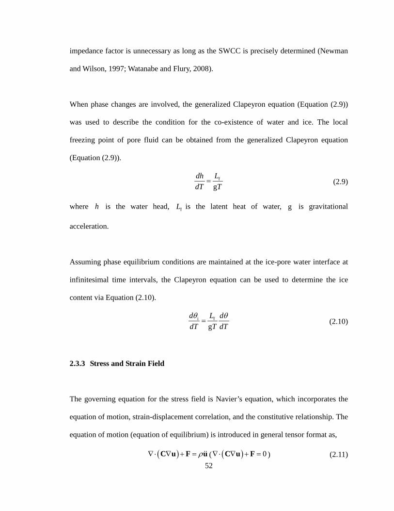
52

impedance factor is unnecessary as long as the SWCC is precisely determined (Newman

and Wilson, 1997; Watanabe and Flury, 2008).

When phase changes are involved, the generalized Clapeyron equation (Equation (2.9))

was used to describe the condition for the co-existence of water and ice. The local

freezing point of pore fluid can be obtained from the generalized Clapeyron equation

(Equation (2.9)).

f

gLdh

dT T= (2.9)

where h is the water head, fL is the latent heat of water, g is gravitational

acceleration.

Assuming phase equilibrium conditions are maintained at the ice-pore water interface at

infinitesimal time intervals, the Clapeyron equation can be used to determine the ice

content via Equation (2.10).

i f

gd L ddT T dTθ θ

= (2.10)

2.3.3 Stress and Strain Field

The governing equation for the stress field is Navier’s equation, which incorporates the

equation of motion, strain-displacement correlation, and the constitutive relationship. The

equation of motion (equation of equilibrium) is introduced in general tensor format as,

( ) ρ∇ ⋅ ∇ + =C u F u ( ( ) 0∇⋅ ∇ + =C u F ) (2.11)

53

where u is the displacement vector, C is the fourth-order tensor of material stiffness,

F is the body force vector.

The strain-displacement equation is,

( )12

T = ∇ + ∇ ε u u (2.12)

The constitutive equation is

=σ C : ε (2.13)

where, σ is the Cauchy stress tensor, ε is the infinitesimal strain tensor, the symbol

“:” stands for double contraction.

In order to consider the influence of the thermal field and the hydraulic field on the stress

field, the constitutive relationship for porous materials has to be formulated as,

el 0= +σ Dε σ (2.14)

where D is the stiffness matrix of soil skeleton, 0σ is the initial stress vector, and elε

is the elastic strain which can be obtained from the following relationship,

el th tr hp 0= + + + +ε ε ε ε ε ε (2.15)

where thε is the strain caused by thermal expansion, [ ]Tref refα( ),α( ),0T T T T− − ; trε is

the strain caused by the phase change of water, which was approximated as

[ ]T0.09 ,0.09 ,0Q Q when a unit localization tensor in mixture theory is followed, where

Q is the degree of water phase transition, 0.09 is the relative change of volume when

54

water turns into ice; 0ε is the initial strain; hpε is the strain resulting from the change

of the matric potential, which is calculated by [ ]T/ , / ,0h hH H . H is a parameter

similar to the modulus corresponding to matric potential. The value of H can be obtained

though experimental measurement. The use of H casts light on the independent role of

matric potential in the constitutive relationship of unsaturated porous media as indicated

in Biot’s model for unsaturated fluid with air bubble and in Fredlund’s method to address

volume change of unsaturated soil (Biot, 1941; Fredlund and Rahardjo, 1993).

2.3.4 General Boundary Conditions

The general boundary condition, which includes the special cases such as the Dirichlet

(first-type), Neumann (second-type) and Robin (third-type) boundary conditions, was

formulated by Equation (2.16),

T( )c u u quς γ δ⋅ ∇ + − + = −n h μ (2.16)

where n is the outward normal unit vector of a boundary, u is the dependent variable

of individual field (temperature, matric potential, displacements, etc.), c is a

conductivity term, ς is the conservative flux convection coefficient, γ is the source in

the subdomain, q is the boundary absorption coefficient, δ is the boundary source,

Th is a matrix designated for the flexibility of the constraint type, μ is the matrix of

Lagrange multiplier.

2.4 Typical Model Implementation

55

The couplings of the three physical fields (i.e., hydraulic, thermal and mechanical fields)

were realized by means of variables and parameters that transfer information interactively.

Due to the high non-linearity, the equations have to be solved numerically. The coupled

multiphysics model was solved with the assistance of COMSOL, a commercial

multiphysics simulation platform. Firstly, the model geometries were constructed by the

interactive graphic interface. The models were then customarily built, transformed into

the weak form and solved using the non-linear solver provided by COMSOL. The results

were analyzed using the post-processing functions provided by the software.

2.4.1 Inputs

Mizoguchi (1990) conducted a classic benchmark experiment where four identical

cylinder samples, which are 10 cm in length and 8 cm in height, were packed with sandy

loam. The initial temperature was 6.7 C and volumetric water content was 0.33. The

samples were thermally insulated in the sides and in the bottom. The top surface was

exposed to a constant temperature of -7 C . After 12, 24 and 50 hours respectively, the

samples were taken out and divided into 1-cm-thick slices to measure their water content

distributions. The process was simulated by Hansson et al. (2004) with a

thermo-hydraulic algorithm. This experiment was chosen as the prototype for

computational model construction in the simulation case.

56

Figure 2.1 FEM mesh of the computational domain with thermal boundary conditions

A computational domain that is 10 cm in length and 8 cm in height was used in the

simulation. The initial temperature was 6.7 C and volumetric water content was 0.33.

The samples were thermally insulated (Neumann boundary condition, zero thermal

gradient) in the sides and in the bottom. The top surface was exposed to a constant

temperature of -7 C . The thermal boundary conditions are shown in Figure 2.1. The heat

influx in the surface was described by Newton’s law of cooling as Equation (2.17),

( ) ( )c ambT h T Tλ⋅ ∇ = −n (2.17)

where λ is the thermal conductivity, ch is the coefficient of convective heat transfer,

ambT is the ambient temperature, T is the temperature at boundaries. All boundaries

57

were hydraulic insulated (Neumann boundary condition, zero hydraulic gradient or no

flow) to ensure mass conservation, which is mathematically described as,

( )Lh Lh Lh 0K h K K T⋅ ∇ + + ∇ =n i (2.18)

To implement the multiphysics simulation, the differential equations were first

transformed into weak forms. The weak forms of the governing equations (Equation (2.1),

(2.5), (2.11)) are,

( ) ( ) ( )a wTC T v dS T vdV C T dVt

λ λΩ ∂Ω Ω Ω

∂= ⋅ ∇ + ∇ ⋅∇ − ∇ ∂∫ ∫ ∫ ∫n J (2.19)

( ) ( )i iLh Lh Lh Lh Lh Lh

w

vdV K h K K T v dS K h K K T vdVt t

ρ θθρΩ ∂Ω Ω

∂∂+ = ⋅ ∇ + + ∇ + ∇ + + ∇ ⋅∇ ∂ ∂

∫ ∫ ∫n i i

(2.20)

( ) ( ) 0v dS vdV vdV∂Ω Ω Ω

⋅ ∇ + ∇ ⋅∇ + = ∫ ∫ ∫n C u C u F (2.21)

where v is a non-negative weighting function whose integration over domain Ω equals 1.

Some soil parameters for the hydraulic field can be found in Hansson’s study (Hansson,

2004). Other parameters were set based on experimental data and related literature

(Fredlund and Rahardjo, 1993; Rowe, 2001). The parameters are listed in Table 2.1.

Table 2.1 Constant parameters for simulation

Constant Value Units Description

ch 28 ( )2W/ m K⋅ Convection heat transfer coefficient

1C 0.55 ( )2W/ m K⋅ Constant for thermal conductivity 1

2C 0.8 ( )2W/ m K⋅ Constant for thermal conductivity 2

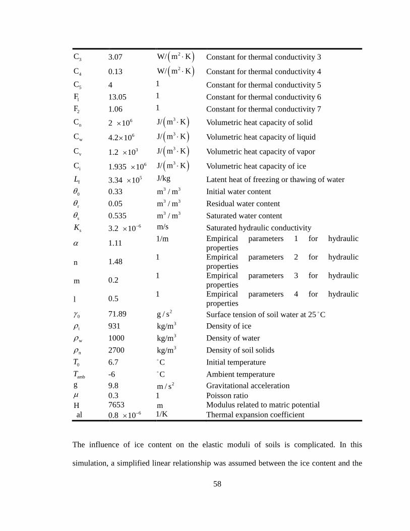
58

3C 3.07 ( )2W/ m K⋅ Constant for thermal conductivity 3

4C 0.13 ( )2W/ m K⋅ Constant for thermal conductivity 4

5C 4 1 Constant for thermal conductivity 5

1F 13.05 1 Constant for thermal conductivity 6

2F 1.06 1 Constant for thermal conductivity 7

nC 2 610× ( )3J/ m K⋅ Volumetric heat capacity of solid

wC 4.2 610× ( )3J/ m K⋅ Volumetric heat capacity of liquid

vC 1.2 310× ( )3J/ m K⋅ Volumetric heat capacity of vapor

iC 1.935 610× ( )3J/ m K⋅ Volumetric heat capacity of ice

fL 3.34 510× J/kg Latent heat of freezing or thawing of water

0θ 0.33 3 3m / m Initial water content

rθ 0.05 3 3m / m Residual water content

sθ 0.535 3 3m / m Saturated water content

sK 3.2 610−× m/s Saturated hydraulic conductivity

α 1.11 1/m Empirical parameters 1 for hydraulic properties

n 1.48 1 Empirical parameters 2 for hydraulic properties

m 0.2 1 Empirical parameters 3 for hydraulic properties

l 0.5 1 Empirical parameters 4 for hydraulic properties

0γ 71.89 2g / s Surface tension of soil water at 25 C iρ 931 3kg/m Density of ice

wρ 1000 3kg/m Density of water

nρ 2700 3kg/m Density of soil solids

0T 6.7 C Initial temperature

ambT -6 C Ambient temperature g 9.8 2m / s Gravitational acceleration µ 0.3 1 Poisson ratio H 7653 m Modulus related to matric potential al 0.8 610−× 1/K Thermal expansion coefficient

The influence of ice content on the elastic moduli of soils is complicated. In this

simulation, a simplified linear relationship was assumed between the ice content and the

59

modulus of elasticity. This assumption was based on the experimental results on the

effects of degree of freezing on the modulus of soils.

Square meshes of the same size (0.01 m) were used for the numerical implementation.

The finite elements used for all the physical fields were quadratic. Time stepping was

controlled using the default setting provided by COMSOL and automatic tuning of

nonlinear solver was employed. The default settings for the time dependent solver were

adopted for all the other solver parameters. A relative tolerance of 31 10−× was used

considering the balance between computing efforts and precision. The equation system

was solved with the direct linear system solver (UMFPACK).

2.4.2 Results and Analyses

The typical thermal properties, i.e., apparent heat capacity and thermal conductivity, are

heavily dependent on the hydraulic field and the phase change of water. This dependence

usually results in high nonlinearity which can significantly affect the multiphysical

process. Plotted in Figure 2.2 are the variations of the volumetric heat capacity and

thermal conductivity with time at heights of 5 cm, 10 cm, 15 cm and 18 cm. It can be

seen the apparent heat capacity in Figure 2.2a slightly decreases with time before

temperature drops below the freezing point. This agrees with the fact that the water

content decreased before ice starts to form. After icing starts, the progress of water

turning into ice releases a considerable amount of heat which decelerates substantially the

freezing process. This is equivalent to an increase in the apparent heat capacity. Therefore,

60

the sudden increase in apparent heat capacity indicates the increasing contribution of

latent heat of ice formation. The variation of the thermal conductivity follows a similar

pattern, but demonstrating a less extent of nonlinearity.

0 5 10 15 20 25 30 35 40 45 50106

107

108

Volu

met

ic he

at c

apac

ity (J

/(m3 K)

)

Time (hour)

5 cm 10 cm 15 cm 18 cm

0 5 10 15 20 25 30 35 40 45 50

0.5

0.6

0.7

0.8

0.9

1.0

1.1

1.2

Ther

mal

con

duct

ivity

(W/(m

K))

Time (hour)

5 cm 10 cm 15 cm 18 cm

(a) Volumetric heat capacity (b) Thermal conductivity

Figure 2.2 The variations of the thermal properties versus time

The temperature distributions at different times are sketched in Figure 2.3. Temperatures

at all points drop as energy is extracted from the upper boundary. The overall rate of

temperature change decreases as temperatures at some locales approach the freezing

point. But it is worthwhile to point out that the freezing point of pore water is slightly

lower than 0 C , a phenomena called freezing point depression. The depression of the

freezing point of pore water refers to the difference between the local freezing point and

the freezing point under standard atmospheric pressure (0 C ). The extent of freezing

point depression is determined by the pore size. Small pore produces large suction and

consequently causes a larger amount of freezing point depression. The depressions of the

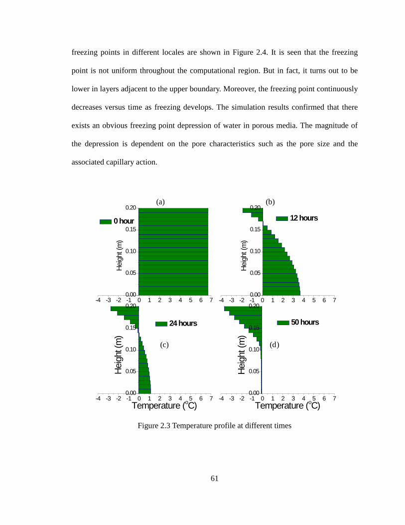
61

freezing points in different locales are shown in Figure 2.4. It is seen that the freezing

point is not uniform throughout the computational region. But in fact, it turns out to be

lower in layers adjacent to the upper boundary. Moreover, the freezing point continuously

decreases versus time as freezing develops. The simulation results confirmed that there

exists an obvious freezing point depression of water in porous media. The magnitude of

the depression is dependent on the pore characteristics such as the pore size and the

associated capillary action.

0.00

0.05

0.10

0.15

0.20

-4 -3 -2 -1 0 1 2 3 4 5 6 7

0 hour

Heig

ht (m

)

0.00

0.05

0.10

0.15

0.20

-4 -3 -2 -1 0 1 2 3 4 5 6 7

12 hours

Heig

ht (m

)

0.00

0.05

0.10

0.15

0.20

-4 -3 -2 -1 0 1 2 3 4 5 6 7

24 hours

Temperature (oC)

Heig

ht (m

)

0.00

0.05

0.10

0.15

0.20

-4 -3 -2 -1 0 1 2 3 4 5 6 7

50 hours

Temperature (oC)

Heig

ht (m

)

(a) (b)

(c) (d)

Figure 2.3 Temperature profile at different times

62

0 2 4 6 8 10 12 14 16 18 200.7

0.6

0.5

0.4

0.3

0.2

0.1

Free

zing

poin

t dep

ress

ion(

o C)

Height (cm)

0 hour 12 hour 24 hour 50 hour

Figure 2.4 Variation of freezing point depression along the depth at 0, 12, 24 and 50

hours

Accurate prediction of frost penetration, i.e., the depth of frost front, is essential for

studying the frost action in porous media and is thus of great practical interest. In this

study case, frost penetration can be plotted based on temperature variations in Figure 2.3

and freezing point depression in Figure 2.4. In comparison with the results predicted by

an empirical equation (Rowe, 2001), we found that the magnitude of the frost penetration

predicted by the current model is greater than that calculated by the empirical equation

(in Figure 2.5). One possible reason for the difference is that the empirical equation

overlooks the influence of the hydraulic field and consequently the dramatic change in

the thermal properties of soil. Therefore the calculation with constant soil properties in

the commonly used empirical equation may lead to a noticeable underestimation of the

frost penetration depth.

63

0 5 10 15 20 25 30 35 400.00

0.01

0.02

0.03

0.04

0.05

0.06

0.07

0.08

This model Empirical equation

Dept

h of

fros

t pen

etra

tion

(m)

Time (hour)

Figure 2.5 The depths of frost penetration versus time

Figure 2.6 plots the distribution of the total volumetric water content (the volumetric

water content plus the volumetric ice content) at different times. The curves clearly

demonstrate a trend that moisture migration moves towards the freezing front (Konrad,

1981, 1994). This is consistent with commonly observed frost heave phenomena. Such

phenomena have significant impacts on the pavement, foundations and infrastructures.

The total volumetric water content (including both in the liquid and solid state) is

determined by both the temperature and matric potential. The unfrozen water content is

determined by the water retention curve; while the amount of ice is decided by the

ice-water balance together with the mass balance. Temperature gradient is the driving

factor for all the migration phenomena in this case. This is because the temperature

gradient causes the hydraulic gradient, which then drives the moisture migration. When

the matric potential satisfies the required temperature and pressure conditions for ice

formation (described by the Clapeyron equation), water begins to turn into ice. In this

model simulation, it was assumed that the water-ice balance is maintained in each

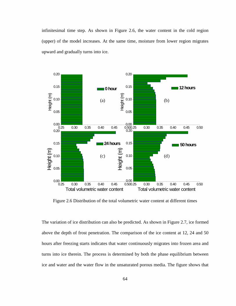
64

infinitesimal time step. As shown in Figure 2.6, the water content in the cold region

(upper) of the model increases. At the same time, moisture from lower region migrates

upward and gradually turns into ice.

0.00

0.05

0.10

0.15

0.20

0.25 0.30 0.35 0.40 0.45 0.50

0 hour

Heig

ht (m

)

0.00

0.05

0.10

0.15

0.20

0.25 0.30 0.35 0.40 0.45 0.50

12 hours

Heig

ht (m

)

0.00

0.05

0.10

0.15

0.20

0.25 0.30 0.35 0.40 0.45 0.50

24 hours

Total volumetric water content

Heig

ht (m

)

0.00

0.05

0.10

0.15

0.20

0.25 0.30 0.35 0.40 0.45 0.50

50 hours

Total volumetric water content

Heig

ht (m

)

(a) (b)

(c) (d)

Figure 2.6 Distribution of the total volumetric water content at different times

The variation of ice distribution can also be predicted. As shown in Figure 2.7, ice formed

above the depth of frost penetration. The comparison of the ice content at 12, 24 and 50

hours after freezing starts indicates that water continuously migrates into frozen area and

turns into ice therein. The process is determined by both the phase equilibrium between

ice and water and the water flow in the unsaturated porous media. The figure shows that

65

at the beginning of freezing, the velocity of ice formation is very fast. The surface layer

accumulates the greatest amount of ice.

0.000.020.040.060.080.100.120.140.160.180.20

0.00 0.05 0.10 0.15 0.20 0.25 0.30 0.35 0.40

Volumetric ice content

Heig

ht (m

)

12 hours 24 hours 50 hours

Figure 2.7 Distribution of volumetric ice content at different times

Matric potential is essential to the mechanical properties of unsaturated porous materials,

i.e., the shear strength of unsaturated soils (Vanapalli, 1996). In this simulation, matric

potential is a dependent variable of the hydraulic field that can be explicitly calculated.

As shown in Figure 2.8, the spatial distributions of matric potential head at different

freezing times. The matic suction head, which is the negative of the matric potential head,

is illustrated in Figure 2.8. Its magnitude is directly related to the liquid water content. It

is shown that suction increases as liquid water content decreases, although the total ice

and liquid water content may increase.

66

0.00

0.05

0.10

0.15

0.20

0 10 20 30 40 50 60 70

0 hour

Hei

ght (

m)

0.00

0.05

0.10

0.15

0.20

0 10 20 30 40 50 60 70

12 hours

Hei

ght (

m)

0.00

0.05

0.10

0.15

0.20

0 10 20 30 40 50 60 70

24 hours

Pressure head (m)

Heig

ht (m

)

0.00

0.05

0.10

0.15

0.20

0 10 20 30 40 50 60 70

50 hours

Pressure head (m)

Heig

ht (m

)

(a) (b)

(c) (d)

Figure 2.8 Vertical distribution of matric potential head (absolute value) at different times

Figure 2.9 shows the variation of vertical deformation (or frost action) versus time. Given

that the bottom of the sample was fixed, the vertical deformation can be determined from

the average displacement on the top of the specimen. The volume changes as a result of

the temperature change, the variation of matric potential, and the ice formation. The trend

of volume change occurs in stages. In the 1st stage, the volume change is dominated by

the thermal contraction of solids. However, the magnitude is negligible due to the small

soil thermal expansion coefficient and the small range of temperature variation. The

volume change is affected by two major phenomena in the 2nd stage, i.e., the volume

contraction due to increase of matric potential and the volume expansion due to phase

change (ice has around 10% larger specific volume than water). The increasing matric

67

potential (as seen in Figure 2.8) holds the particles tighter, leading to the amount of

volume reduction counteracting the increases in the volume due to phase change of water.

The trend of volume change from computational simulation implies that the effect of

matric potential on volume change dominates over that by the phase change. This even

caused volume contraction during certain period in the 2nd stage. In the 3rd stage, the

volume continues to increase due to the volume increase associated with phase transition.

The simulation is consistent with the experimental phenomena observed by Liu et al.

(2009).

Figure 2.9 Total vertical deformation versus time

Figure 2.10 shows the distribution of the vertical stress in the specimen due to freezing.

The positive sign indicates tension. Both the maximum tensile and compressive stresses

appear in the surface layer. The reason is that the moisture migrates and accumulates near

the surface. The volume expansion due to ice crystallization leads to the internal stresses.

It has been commonly observed that during thermal weathering of rocks in mountain

68

areas, cracks typically appear first on the surface and then progresses to the interior. The

stress distribution illustrated in Figure 2.10 gives an explicit explanation on the fracture

mechanism, since the high tension and compression zones close to the surface are likely

to initialize the formation of cracks. Besides, the simulation provides some insight on

factors that control the crack spacing. However, the relationship between the thermal

gradient, moisture gradient, internal stress and crack spacing requires further

investigations.

Length: m

Leng

th: m

Figure 2.10 Distribution of internal stress under freezing effects

2.5 Conclusions

A theoretical framework for multiphysics simulations of freezing porous materials was

presented in this chapter. The thermal, hydraulic and mechanical fields were coupled

69

together via partial differential equations. The effects of pores on individual physical

processes were described by the SWCC and the Clapeyron equation. The highly

non-linear system was solved numerically in a multiphysics simulation platform. The

following observations can be made from the simulation results. (1) The

thermal-hydro-mechanical fields are strongly coupled in porous materials. Heat transfer

induces change in the hydraulic and a stress field, the process is especially important

when phase change of pore solutions is involved. (2) Matric potential in unsaturated

porous media can cause the volume change pattern that is different that solely due to ice

formation. (3) Multiphysics simulation described reasonably well the temperature and

moisture variations observed under an in-service pavement.

70

3 CHAPTER THREE

APPLICATIONS OF THERMO-HYDRO-MECHANICAL MODEL IN PAVEMENTS

AND BURIED PIPES

3.1 Overview

Frost action is a major factor causing deteriorations of pavements in cold regions. The

resultant temperature and moisture redistributions play an important role in determining

the mechanical responses of pavement. In this chapter the aforementioned multiphysics

framework is adopted to analyze the coupled thermo-hydraulic field under pavements,

especially those in the unsaturated base and subgrade. Two instrumented pavement

sections (one asphalt pavement and one concrete pavement) were used to validate the

results of the model simulations. The simulation results match reasonably well with the

field monitored data.

Pipes, especially buried pipes, in cold regions generally experience a rash of failures

during cold weather snaps. However, the existing heuristic models are unable to explain

the basic processes involved in the frost action. This is because the frost action is not a

direct load but causes variations in pipe-soil interactions resulting from the coupled

thermo-hydro-mechanical process in soils. The proposed multiphysics framework is

employed for holistic simulations for pipe-soil systems suffering from freezing

temperatures. The theoretical framework was implemented to analyze both static and

dynamic responses of buried pipes subjected to frost action. The multiphysics simulations

71

reproduce the phenomena commonly observed during frost action, e.g., ice fringe

advancement and an increase in the internal stress of pipes. The influences of important

design factors, i.e., buried depth and overburden pressure, on pipe responses are

simulated. A fatigue cracking criteria was utilized to predict the crack initialization under

the joint effects of frost and dynamic traffic loads. The frost effects are found to have

detrimental effects for accelerating fatigue crack initialization in pipes.

3.2 Background

3.2.1 Pavements

Frost action has been recognized as a major factor causing the deteriorations of pavement

structures in cold regions (Simonsen, 1997). It can lead to considerable heaving in frost

susceptible subgrade soils during winter and a bearing capacity loss when frost-induced

segregation ice melts during spring (Dore, 2004). Studies conducted by Janoo and Berg

(1990) and Simonsen and Isacsson (1999) found the most important factors for pavement

performance under seasonal frost action were soil types, permeability, drainage

conditions and the rate of thawing. The damage to pavement structures could reveal itself

on the surface in the form of fatigue cracking and rutting due to deformations in the base

or subgrade (Janoo and Berg, 1990).

The modulus of each pavement layer is also greatly affected by the moisture content,

which significantly influences the pavement performance (Yuan and Nazarian, 2004).

Moisture-induced damage of asphalt mixtures, referred as stripping, is one of the most

72

detrimental factors affecting the in-service performance of asphalt pavements (Chen et

al., 2004). Besides, temperature, an important environmental factor, has a significant

effect on the mechanical properties of asphalt mixtures (Celauro, 2004; Yuan and

Nazarian, 2004). The spatial variation of temperature affects the stiffness of pavement

structure and causes the development of distresses such as rutting and thermal cracking

(Alkasawneh et al., 2006). Therefore, the ability to predict the temperature and moisture

content distributions in a pavement will help to assess the performance of the pavement.

Heat transfer under pavement involves coupling of thermal and hydraulic fields (Asaeda

and Ca, 1993). That is, temperature variations and moisture redistributions occur

simultaneously. Such coupling effects are significant in porous materials such as

pavement base, subbase and subgrade. This, in return, affects the mechanical behaviours

of pavement structures (Charlier et al. 2009). As a result, thermo-hydraulic modelling is

necessary for studying the effects of frost action on pavement performances.

A few simulation models have been developed to predict the effects of climate conditions,

i.e., the temperature and moisture distributions, on pavement performances (Shao, 1994;

Bentz, 2000; Yavuzturk and Ksaibati, 2002; Ariza, 2002). Most of these past studies only

involved one or two field dependent variables. The mechanical field, however, was not

coupled in these models. Properly simulating the coupling effects on the mechanical and

structural behaviors of pavement is essential for further advancing pavement research and

practices. The Enhanced Integrative Climate Model (EICM) was used in the

Mechanistic-Empirical Pavement Design Guide software. The limitations of EICM

73

include 1) one-dimensionality and 2) neglecting the coupling effects of different fields.

This research was conducted in view of three major needs for advancing freezing ground

mechanics and serving the pavement design in cold regions: 1) the need of a

comprehensive theoretical framework of coupled thermo-hydraulic process based on

thermodynamics; 2) the need to capture the essential processes involved in freezing

porous materials; 3) the need to link the model simulations to the real in-service

pavement.

3.2.2 Pipes

Pipes have been used for the transportation of many chemical stable substances such as

water (Walski, 1982), sewage (Fisher et al., 2001) , slurry (Dorona et al., 1987), oil (Nesic,

2007), natural gas (Konrad and Morgenstern, 1984) and other goods. They therefore do

not only form an essential component of the urban and transportation infrastructure, but

also serve as the lifeblood to the modern community (Rajani et al., 1996; Moser, 2008).

But unfortunately, their serviceability is jeopardized by intrinsic defects, environmental

threats and inadequate installations (Rajani and Kleiner, 2001; Hu and Hubble, 2007).

This situation turns out to be more serious when pipes are buried underground. This is

because more factors, e.g. soil pressure, traffic loading, frost loads, electro-chemical

attacks can be involved as the pipes interact with ground soils and with a possible third

party in or above the ground (Rajani and Kleiner, 2001; Maker, 2000).

74

The buried pipes are usually made of cast iron, ductile iron, polyvinyl chloride (PVC),

polyethylene (PE), asbestos cement or concrete. Taking water mains for example, cast

iron pipes were extensively used to build water distribution systems from the 1900s until

ductile iron pipes were introduced in the 1970s, followed by PVC water pipes which was

introduced in Europe and North America during the 1970s and the more recent

polyethylene (Rajani et al., 1996). It seems discouraging to find out that physical

mechanisms responsible for breakage vary from type to type leading to different failure

modes such as circumferential break, longitudinal break, joint failure, holes due to

corrosion and corporation cock failure. However, we can notice that some trends have

been found regardless of pipe types and failure modes. Among them, the detrimental

effects of temperature, especially that of cold temperatures, have long been documented

and investigated (Morris, 1967; Ciottoni, 1983).

This correlation between pipe failure risks and frost action has not only been frequently

noticed in practice but also been supported by experimental and theoretical analyses.

Firstly, it is common knowledge among those involved in the management of water

distribution systems that the onset of winter brings about an increase in maintenance

activities (Papadopoulos and Welter, 2001). Similarly, as indicated by (Rajani et al., 1996;

Zhan and Rajani, 1997), the disruption of water services as a consequence of water main

breaks is on the rise in most Canadian cities. The analysis on a typical annual pattern of

break rate revealed that the peak in break frequency occurred during the period when

ground temperatures were below normal. Similar studies (Needham and Howe, 1981;

Lochbaum, 1993) on the performance of gas mains essentially reached the same

75

conclusion. Morris (1967) and Ciottoni (1985) suggested that break frequency in winter

was at least twice as high as that in summer, which was confirmed by field validation

data (Rajani and Kleiner, 2001).

Both physically based methods (Rajani and Kleiner, 2001) and statistical methods

(Kleiner and Rajani, 2001) have been employed for the analyses and designs of buried

pipes. The strategy of physically based models is to evaluate or to predict the

performance of buried pipes by investigating the physical behaviors consisting of various

components, e.g. frictional resistance, thermal expansion, residual structural resistance.

And the mechanical behaviors of most of these components were fairly well established

and information is available through standards or textbooks (Moser, 2008; Rajani and

Kleiner, 2001; Young, 1984). But it is also a consensus that an analytical procedure that

satisfactorily explains why extreme cold temperatures lead to an increase in the number

of water main breaks is still in absence. In other words, the influences of frost

temperature on the properties of pipes and surrounding soils and on the interactions

between pipes and surrounding soils are unclear in existing theories.

Several reasons are responsible for the complexity of the frost effects. First of all, both

pipes and surrounding soils suffer from a volume change in response to a temperature

change. But the different thermal expansion coefficients can be much different.

Furthermore, the phase change of pore water happens as the temperature drops below the

freezing point. This will affect the heat transfer process since phase transition involves

energy. There is no doubt that the formation of ice in pores can significantly alter the soil

76

properties such as elastic moduli. Moreover, there is a fluid transfer due to the

temperature gradient (Philip and de Vries, 1957; Cary, 1965). The hydraulic process can

be considerable and consequently changes not only the water and ice distribution but also

the thermal and mechanical properties (e.g. volume change due to the phase transition of

water and due to suction change resulting from the desaturation of water) of the pipe-soil

system. Finally, the mechanical behavior is determined by the changes in the thermal and

hydraulic field as well as the constraints. Likewise, because of the existence of

constraints (gravity, friction, etc.), the mechanical field can only response partly to the

other fields and thus in return affect the other fields. Unfortunately, the aforementioned

mechanisms are excluded in most existing studies. All the above phenomena can be

coupled into a multiphysical process called thermo-hydro-mechanical process. The

mechanisms beneath the multiphysics in soils have been extensively studies by

researchers from soil science (Kay and Groenevelt, 1974; Sophocleous, 1979; Flerchinger

and Pierson, 1991; Nassar and Horton, 1992; Scanlon and Milly, 1994; Noborio et al.,

1996; Nassar and Horton, 1997; Jansson and Karlberg, 2001), and civil engineering

(Christopher and Milly, 1982; Thomas et al., 2009; Thomas and He, 1995; Sahimi, 1995;

Noorishad et al., 1992; Noorishad and Tsang, 1996; Stephanasson et al., 1997; Bai and

Elsworth, 2000; Rutqvist et al., 2001; Wang et al., 2009).

3.3 Applications to Pavements

Instrumented road sections in Ohio, USA were used as testbed to validate the simulation

model. The Ohio Department of Transportation launched a project in 1995 as a part of the

77

Strategic Highway Research Program (SHRP) (Masada and Sargand, 2002; Heydinger,

2003; Wolfe and Butalia, 2004). A series of 34 highly instrumented pavement test

sections were constructed on state road 23 in Delaware County, Ohio. The spatial

distribution of moisture content, electrical resistivity and frost depth as well as the air

temperature were monitored by field sensors. Two representative road sections, i.e.,

Section 39201 and Section 39204, were selected for this study. Section 390201 was

asphalt concrete (AC) pavement while section 39204 was Portland cement concrete (PCC)

pavement.

3.3.1 Model Simulation of Flexible Pavement

3.3.1.1 Inputs

Section 39201 consisted of a 0.203 m asphalt concrete layer and a 0.152 m aggregate

base (Figure 3.1). The period of simulation was between 3 December and 22 December

in 1999. The field temperature data and moisture data were collected with 18 temperature

gauges and 10 moisture gauges installed under the pavement. The hourly air temperature

and local soil temperatures at gauges were also available. The complete information on

the soil moisture content distributions was available on the 1st, 5th and 9th day.

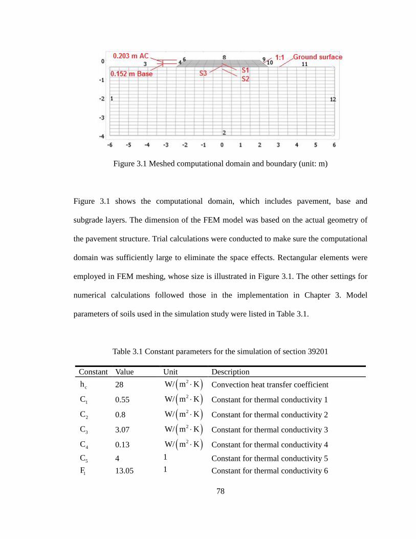
78

Figure 3.1 Meshed computational domain and boundary (unit: m)

Figure 3.1 shows the computational domain, which includes pavement, base and

subgrade layers. The dimension of the FEM model was based on the actual geometry of

the pavement structure. Trial calculations were conducted to make sure the computational

domain was sufficiently large to eliminate the space effects. Rectangular elements were

employed in FEM meshing, whose size is illustrated in Figure 3.1. The other settings for

numerical calculations followed those in the implementation in Chapter 3. Model

parameters of soils used in the simulation study were listed in Table 3.1.

Table 3.1 Constant parameters for the simulation of section 39201

Constant Value Unit Description

ch 28 ( )2W/ m K⋅ Convection heat transfer coefficient

1C 0.55 ( )2W/ m K⋅ Constant for thermal conductivity 1

2C 0.8 ( )2W/ m K⋅ Constant for thermal conductivity 2

3C 3.07 ( )2W/ m K⋅ Constant for thermal conductivity 3

4C 0.13 ( )2W/ m K⋅ Constant for thermal conductivity 4

5C 4 1 Constant for thermal conductivity 5

1F 13.05 1 Constant for thermal conductivity 6

79

2F 1.06 1 Constant for thermal conductivity 7

nC 2 610× ( )3J/ m K⋅ Volumetric heat capacity of solid

wC 4.2 610× ( )3J/ m K⋅ Volumetric heat capacity of liquid

vC 1.2 310× ( )3J/ m K⋅ Volumetric heat capacity of vapor

iC 1.935 610× ( )3J/ m K⋅ Volumetric heat capacity of ice

fL 3.34 510× J/kg Latent heat of freezing /thawing of water

0θ 0.33 1 Initial water content

rθ 0.05 1 Residual water content

sθ 0.535 1 Saturated water content

sK 3.2 610−× m/s Saturated hydraulic conductivity

α 1.11 1/m Empirical parameter 1 for hydraulic properties

n 1.48 1 Empirical parameter 2 for hydraulic properties

m 0.2 1 Empirical parameter 3 for hydraulic properties

l 0.5 1 Empirical parameter 4 for hydraulic properties

0γ 71.89 2g / s Surface tension of soil water at 25 C iρ 931 3kg/m Density of ice

wρ 1 310× 3kg/m Density of water

nρ 2.7 310× 3kg/m Density of soil solids

0T 6.7 C Initial temperature

ambT -6 C Ambient temperature g 9.8 2m / s Gravitational acceleration

pλ 0.9 W/( m K⋅ ) Thermal conductivity of AC pavement

ppC 2.1 610× J/( 3m K⋅ ) Volumetric heat capacity of AC pavement

3.3.1.2 Boundary and Initial Conditions

The simulated area was assumed to be hydraulically and thermally insulated with the

exception of the surface areas in contact with the atmosphere, including boundary 3, 4, 6,

8, 9, 10, and 11 in Figure 3.1. The energy exchange was described by Newton’s Law of

80

cooling (Equation (3.1)):

c amb( ) h ( )T T Tλ⋅ ∇ = −n (3.1)

where ambT is the ambient air temperature which was imported from the field monitored

data. ch is the convection heat transfer coefficient. Constant values of ch (25 and 35)

were assigned for pavement and soil respective, based on the duration of sunshine and

wind speed (Bentz, 2000). The effect of black body radiation was neglected.

The initial temperature and hydraulic field were determined by interpolating the field

monitoring data. Rainfall happened twice during the 20 day period. As detailed

precipitation data was available, the precipitation was transferred into infiltration flux

through upper boundaries by Equation (3.2).

Lh Lh LT( )K h K K T q⋅ ∇ + + ∇ =n (3.2)

where q is the infiltration intensity, which can be obtained by dividing the precipitation

by the duration of precipitation. The infiltration intensity changes with time, hence it also

needs to be incorporated as a function of time. The data of air temperature variations and

precipitation were applied during the simulations.

3.3.1.3 Result and Discussion

In spite of the complexities in constructing the theoretical framework, the coupled

equation system were solved smoothly. Figure 3.2 illustrates the comparison between the

measured and simulated temperature variations at gauge locations S1, S2 and S5. These

temperature gauges were buried at the depths of 0.025 m, 0.101 m and 0.33 m under the

81

pavement, respectively. Figure 3.2 shows that the simulation model reasonably captured

the trends of temperature variations at different depths. Potential sources of error included

overlooking the effects of solar radiation and assuming an initial distribution of

temperature and water content.

Simulated S1 Simulated S2 Simulated S5

0 1 2 3 4 5 6 7 8 9 10-12-10-8-6-4-202468

Time (day)

S1 S2 S5

Tem

pera

ture

(o C)

Figure 3.2 Simulated and measured temperatures versus time

The simulated results of the spatial temperature distributions with respect to depth on the

1st, 5th, 9th day of simulation period were plotted in Figure 3.3. The measured

temperature distributions at the 18 gauges were plotted. As can be seen, simulation results

succeeded in predicting the trends of the spatial temperature distribution. The error of

temperature prediction was no greater than 1 o C at most locations. However, predictions

for points adjacent to the inter-boundary between the base and subgrade layers exhibit

noticeable errors, especially those around 5th day in the AC layer. Possible reasons for

the differences between simulated and measured results include: 1) the AC layer has a

82

higher heat conductivity and low heat capacity than soil layers; in addition, it is the layer

directly influenced by the boundary conditions; hence it could be more easily affected by

changes and uncertainties in the boundary conditions (i.e. raining, solar radiation, etc); 2)

the boundary conditions between the pavement layer and the base are unknown.

0.0 0.2 0.4 0.6 0.8 1.0 1.2 1.4 1.6 1.8 2.0-6

-3

0

3

6

9

12

Depth (m)

Simulated 1 day 5 day 9 day

AC Base

Measured 1 day 5 day 9 day

Tem

pera

ture

(o C)

Figure 3.3 Simulated and measured temperature distributions

Figure 3.4 shows the comparison of simulated and measured moisture content

distributions at different times. The results of model simulation at smaller depths were

slightly better than those at greater depths. The slightly reduced accuracy of simulation

results at deeper positions might be attributed to the variation of ground water table,

which was not accounted for in this model simulations (i.e., a constant ground water table

at -3 m in Figure 3.1 was assumed in the model simulation).

83

Simulated 0 day 1 day 5 day 9 day 10 day

0.25 0.50 0.75 1.00 1.25 1.50 1.75 2.000.1

0.2

0.3

0.4

0.5

0.6

Measured 0day 10day

Tota

l vol

umet

ric w

ater

con

tent

Depth (m)

Base

Figure 3.4 Simulated and measured moisture content distributions

0 1 2 3 4 5 6 7 8 9 100.180.200.220.240.260.280.300.320.340.360.38

Unfro

zen

wate

r con

tent

Time (day)

(-4,-0.4) (-4,-2) (0,-0.4) (0,-2)

Figure 3.5 Unfrozen water contents at different points

The unfrozen water content was affected by both freezing-thawing processes and

precipitations. The variations of unfrozen water content at four different locations were

compared in Figure 3.5. Locations (0,-0.4) and (0, -2) (see Figure 3.1) were on the

vertical axis of the computational domain, while locations (-4,-0.4) and (-4,-2) were on

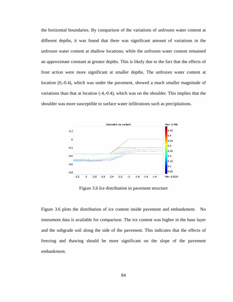
84

the horizontal boundaries. By comparison of the variations of unfrozen water content at

different depths, it was found that there was significant amount of variations in the

unfrozen water content at shallow locations; while the unfrozen water content remained

an approximate constant at greater depths. This is likely due to the fact that the effects of

frost action were more significant at smaller depths. The unfrozen water content at

location (0,-0.4), which was under the pavement, showed a much smaller magnitude of

variations than that at location (-4,-0.4), which was on the shoulder. This implies that the

shoulder was more susceptible to surface water infiltrations such as precipitations.

Figure 3.6 Ice distribution in pavement structure

Figure 3.6 plots the distribution of ice content inside pavement and embankment. No

instrument data is available for comparison. The ice content was higher in the base layer

and the subgrade soil along the side of the pavement. This indicates that the effects of

freezing and thawing should be more significant on the slope of the pavement

embankment.

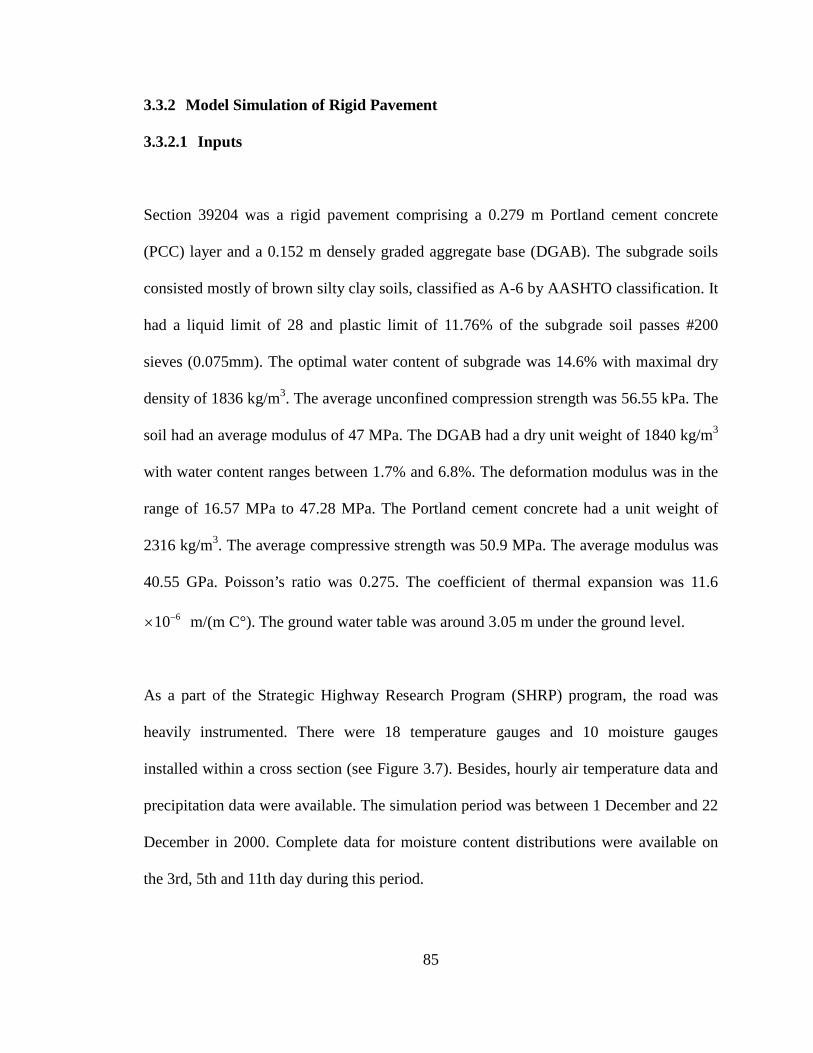
85

3.3.2 Model Simulation of Rigid Pavement

3.3.2.1 Inputs

Section 39204 was a rigid pavement comprising a 0.279 m Portland cement concrete

(PCC) layer and a 0.152 m densely graded aggregate base (DGAB). The subgrade soils

consisted mostly of brown silty clay soils, classified as A-6 by AASHTO classification. It

had a liquid limit of 28 and plastic limit of 11.76% of the subgrade soil passes #200

sieves (0.075mm). The optimal water content of subgrade was 14.6% with maximal dry

density of 1836 kg/m3. The average unconfined compression strength was 56.55 kPa. The

soil had an average modulus of 47 MPa. The DGAB had a dry unit weight of 1840 kg/m3

with water content ranges between 1.7% and 6.8%. The deformation modulus was in the

range of 16.57 MPa to 47.28 MPa. The Portland cement concrete had a unit weight of

2316 kg/m3. The average compressive strength was 50.9 MPa. The average modulus was

40.55 GPa. Poisson’s ratio was 0.275. The coefficient of thermal expansion was 11.6

610−× m/(m C°). The ground water table was around 3.05 m under the ground level.

As a part of the Strategic Highway Research Program (SHRP) program, the road was

heavily instrumented. There were 18 temperature gauges and 10 moisture gauges

installed within a cross section (see Figure 3.7). Besides, hourly air temperature data and

precipitation data were available. The simulation period was between 1 December and 22

December in 2000. Complete data for moisture content distributions were available on

the 3rd, 5th and 11th day during this period.

86

Due to the symmetry of the pavement structure, the computational domain was applied

on half of the pavement geometry as shown in Figure 3.7. This treatment helps save the

computational efforts. The geometry was developed based on the actual geometry of the

pavement. Both square and triangle meshes were used and their sizes can be identified in

Figure 3.7. The same values for solver parameters as those for the flexible pavement were

adopted.

Figure 3.7 Meshed computational domain and boundary (unit: m)

It is seen from the above case of flexible pavement that the material properties of base

and subgrade, especially the SWCC and hydraulic conductivity, could be crucial to the

simulation results. Thus a more rigorous technique was utilized to formulate these

parameters. The equations proposed by Fredlund and Xing (1994) were used to obtain

SWCC (Equation (3.3) and Equation (3.4)):

( ) sw cb

ln ea

C hh

θθ

= × +

(3.3)

87

( ) r6

r

ln 11

10ln 1

hh

C h

h

+

= −

+

(3.4)

where h is the soil matric suction in kPa, a is parameter dependent on air entry value

in kPa, b is a parameter dependent on the slope of SWCC curve after air entry value is

exceeded, c is a parameter dependent of the suction at the residual water content, rh is

a parameter dependent on the suction at the residual water content. It is noted that the

symbol ‘h’ used in the Equation (3.3) and Equation (3.4) are different from that used in

the rest of the paper.

An empirical approach suggested by Zapata et al. (2000) was adopted for the calculation

of the parameters in the SWCC equation (Equation (3.3) and Equation (3.4)). For soils

with plasticity index (PI) larger than 0, a parameter WPI was introduced by Zapata et al.

(2000), which is the product of PI and the ratio of soil passing ASTM No. 200 sieve

(0.075mm). The parameters were then estimated as:

( ) ( )3.35a=0.00364 WPI 4 WPI 11+ + (3.5)

( )0.14b 2.313 WPI 5c= − + (3.6)

( )0.465c=0.514 WPI 0.5+ (3.7)

0.0186WPIr 32.44eah= (3.8)

( )0.75s 0.0143 WPI 0.36θ = + (3.9)

88

The hydraulic conductivity was obtained through the relative permeability function

integrated from the SWCC as Equation (3.10). The effect of temperature-dependent fluid

viscosity was neglected for simplification.

( ) ( )( ) ( )

( )( ) ( )

aev

b '

ln

b s '

ln

ee d

e( )e

e de

yy

yhr y

yyh

hy

k h

y

θ θθ

θ θθ

−

=−

∫

∫ (3.10)

where b equals ( )ln 1000000 , y is a dummy variable of integration representing the

logarithm of suction, aevh is the air entry value of suction in kPa.

Computer codes were developed to obtain SWCC and the relative permeability. The

results are shown in Figure 3.8 and Figure 3.9.

0 0.5 1 1.5 2 2.5 3 3.50

0.1

0.2

0.3

0.4

0.5

log(h) (unit of h: kPa)

Vol

umet

ric w

ater

con

tent

BaseSubgrade

Figure 3.8 Soil water characteristic curves of base and subgrade

89

0 100 200 300 4000

0.2

0.4

0.6

0.8

1

Suction (h, kPa)

Rel

ativ

e pe

rmea

bilit

y

BaseSubgrade

Figure 3.9 Hydraulic conductivity versus suction in base and subgrade

Other parameters for simulation of this concrete pavement structure were listed in Table

3.2.

Table 3.2 Constant parameters for the simulation of section 39204

Constant Value Units Description s1θ 0.05 1 Saturated water content of base

s2θ 0.535 1 Saturated water content of subgrade

s1K 48.467 10−× m/s Saturated hydraulic conductivity of base

s2K 108.467 10−× m/s Saturated hydraulic conductivity of subgrade

1n 0.3 1 Porosity of base

1n 0.4 1 Porosity of subgrade pλ 1.3 W/( m K⋅ ) Thermal conductivity of PCC pavement

ppC 2 610× J/( 3m K⋅ ) Volumetric heat capacity of PCC pavement

Note: Refer to Table 3.1 for other model parameters.

3.3.2.2 Boundary and Initial Conditions

90

The boundary conditions were assigned in a similar way to the simulation for the flexible

pavement section 39201. Heat and mass exchanges were assumed to happen only in the

upper boundaries. The main difference lies in the conceptual model for the near-surface

water dynamics. The model by (Fayer, 2000) instead of a simplified treatment was

adopted for the PCC pavement as Equation (3.11).

=S P R E T D∆ − − − − (3.11)

where S∆ is the change in soil water storage, P is the precipitation, R is the amount

of water running off, E is the evaporation, T is the transpiration of plants, D is the

drainage. In this case study, T was neglected and E was assumed to be

70.225 10−× m/s. For the upper boundary of the subgrade, it was assumed that 6% of the

precipitation infiltrated into the subgrade soils according to local hydrology data

(Delaware County Water Resources). The depth of water table was 3.05 m. An equivalent

downward flux of 70.35 10−× m/s was assigned on the bottom of the computational

domain to account for the drain down effects of ground water table.

3.3.2.3 Results and Discussion

Figure 3.10 illustrates the comparison between measured and simulated temperature

variations with time at gauges S1, S3 and S5, which were buried 0.025 m, 0.178 m and

0.33 m under the pavement. As can be seen, the prediction of the temperature variations

at different locations under pavement is acceptable. Simulated and measured results of

temperature process at S1 and S5 almost coincide. The slight larger error at S3 is possibly

due to boundary conditions between pavement and base.

91

0 1 2 3 4 5 6 7 8 9 10-6-4-202468

1012141618

Simulated: S1 S3 S5 AirT

Tem

pera

ture

(o C)

Time (day)

Measured: S1 S3 S5

Figure 3.10 Simulated and measured temperature versus time

0.0 0.3 0.6 0.9 1.2 1.5 1.8 2.1 2.4-4-202468

1012141618

Simulated: Dec 3 Dec 5 Dec 11

Tem

pera

ture

(o C)

Depth (m)

Measured: Dec 3 Dec 5 Dec 11

PCC Base

Figure 3.11 Simulated and measured temperatures distributions

Figure 3.11 plots the simulated and monitored results of spatial temperature distributions

on the 3rd, 5th, 11th day. The simulation results closely match that from field

92

measurements. It is worthwhile to point out that the temperature process close to ground

surface was also closely predicted by the computational model in this simulation.

0.4 0.6 0.8 1.0 1.2 1.4 1.6 1.8 2.00.05

0.10

0.15

0.20

0.25

0.30

0.35

0.40

0.45

0.50

Simulated: Dec 3 Dec 11 Dec 22

Volu

met

ric M

oist

ure

cont

ent

Depth (m)

Base

Measured: Dec 3 Dec 11 Dec 22

Figure 3.12 Simulated and measured moisture content distributions

Figure 3.12 plots the simulated water content distribution versus those of monitored data

on the 3rd, 11th, and 22nd day of simulation period. The simulation results are reasonably

well for practical purpose.

3.4 Applications to Buried Pipes

3.4.1 Static Analysis

The behaviors of porous materials under frost action have been proved to be very

complicated. Especially, there exist high nonlinearities when coupling effects are

considered (Liu et al., 2012). In addition, our pilot calculations found that solving

93

three-dimensional models demand excessive computational time. Due to the restriction of

the computational resources, this study implemented model simulations under

two-dimensional geometries (plane strain conditions). A cross section of a pipe-soil

system was chosen for both static and dynamic analysis. This section was assumed to be

one representative of pipeline conditions. Non-homogeneities in the pipe and soil

properties can be studied by varying the materials properties.

The static analysis mainly focus on the response of a buried pipe to subfreezing air

temperature. The purpose was to examine if the ground freezing can lead to increase of

maximum tensile stress in the pipe. The effects of ground freezing were studied by

comparing two different buried depths of pipe. Besides, the influence of overburden

pressure was also studied since its influence on frozen ground has been extensively

reported (Konrad and Morgenstern, 1982).

Three cases were studied in the static analysis: 1) pipe buried at a depth of 1 m (from the

pipe center); 2) buried at a depth of 2.5 m; 3) buried at a depth of 1 m and suffering from

a constant overburden pressure of 0.1 MPa.

The configuration of a typical computational domain is illustrated by Figure 3.13a. The

mesh dimensions were chosen in a way that optimizes both ensure model accuracy and

the computation efficiency. An initial air temperature of 6.7 o C was set. The

temperature of inner boundary for pipe was assigned as 2 o C . This boundary condition

was adopted in order to simulate a fluid of 2 o C running through the pipeline (operating

94

temperature). Subsequently, the ground surface temperature was assumed to be

maintained at -10 o C . The simulated duration under freezing was one month. The pipe

was assumed to be a cast iron pipe with an outer diameter of 0.7 m and thickness of 0.03

m. The soil around the pipe was assumed to be an unsaturated soil (A6 soil according to

AASHTO classification) with an initial volumetric water content of 0.33. Meshing was

conducted with the triangle meshes of normal mesh size suggested by COMSOL based

on the geometry the computational domain. The solver parameters used in the

aforementioned simulations for pavements were used for the simulations of buried pipes

involving both static (3.4.1) and dynamic loads (3.4.2).

Table 3.3 Parameters used for simulations of buried pipe

Constant Value Units Description

0θ 0.33 1 Initial water content

rθ 0.031 1 Residual water content

sθ 0.428 1 Saturated water content

sK 65.806 10−× m/s Saturated hydraulic conductivity

α 1.202 1/m Empirical parameter 1 for hydraulic properties

n 1.377 1 Empirical parameter 2 for hydraulic properties

m 0.274 1 Empirical parameter 3 for hydraulic properties

μ 0.3 1 Poisson ratio H 7653 m Modulus related to pore pressure

pλ 1.3 W/(m K)⋅ Thermal conductivity of pipe (cast iron)

ppC 62 10× 3J/(m K)⋅ Volumetric heat capacity of pipe (cast iron)

pγ 2800 3kg/m Density of pipe (cast iron)

Note: for additional information, refer to Liu and Yu (2011).

Example of simulation results are presented in Figure 3.13. The soil temperature dropped

95

with the decrease of the air temperature. The frost penetration (frost front) went

downwards to a depth ranging from 0.8 to 1 m in all of these three cases. The

advancements of the frost penetration were similar in Case 1 and Case 3, although there

was an observable difference between them. A general trend is the frost fronts curved

slightly before they reached the crown of the pipe, due to the thermal boundary

conditions inside the pipe. An ice arching developed as the frost front advance beyond the

depth of the pipe for Cases 1 and 3. For Case 2, the frost front was approximately leveled

throughout the process. This is probably due to the fact that the influence of the pipe on

the developments of frost front gets lesser significant at deeper burial depth. In all three

cases, the internal stresses gradually increased both in the pipe and in the surrounding soil

upon ground freezing. A typical distribution of vertical stresses is shown in Figure 3.13.

Figure 3.13a clearly shows the arching effects that might be caused by ice front

development.

(a) (b)

Figure 3.13 Typical distribution of vertical stress in the a) soil; and b) pipe (unit: Pa)

The tensile stress plays an important role in pipe failure, especially for materials such as

2 m

4 m

(0.35,-0.7)

Frost front

96

cast iron whose tensile strength is much lower than the compressive strength. The point

associated with the maximum vertical tensile stresses is located near point (0.35,-0.7) or

its symmetry point. Figure 3.14 plots the time variations of the vertical tensile stresses in

all of the three cases.

0 5 10 15 20 25 302

3

4

5

6

7

8Ve

rtica

l stre

ss (M

Pa)

Time (day)0 5 10 15 20 25 30

20.20

20.24

20.28

20.32

20.36

20.40

Verti

cal s

tress

(MPa

)

Time (day)

(a) (b)

0 5 10 15 20 25 3035

40

45

50

55

60

65

Verti

cal s

tress

(MPa

)

Time (day)

(c)

Figure 3.14 a) Variation of vertical tensile stress for Case 1; b) Case 2; and c) Case 3

In Case 1 (Figure 3.14a), the stress value increased with the development of freezing at

the beginning. And it is noticed that the increase is dramatic. During the time, the pore

water around the pipe migrated upwards to the regions above the pipe where substantial

temperature gradients occurred. The increase in maximum vertical tensile stress slowed

down as temperature at some locations dropped below the freezing point. The maximum

vertical tensile stress continued increasing before it reached the peak at the 14th day. This

97

is exact the time when the front came into contact with the pipe crown. This simulated

phenomenon reproduced that happened in field experiments (Smith, 1976). After that

moment, the maximum tensile stress decreased rapidly to a value that was even smaller

than its initial value. In the meanwhile, we noticed that the shape of the frost front

changed from a small curve to an arch around the upper part of the pipe (Figure 3.13).

Therefore, the increasing arching effect reduced the soil pressure and frost load on the top

of the pipe. Moreover, the increasing soil modulus due to icing further added to effect.

The magnitude of simulated stress increase caused by frost action is close to field

measured data and results from other studies (Rajani et al., 1996).

For Case 2, where the pipe was buried in a depth larger than the maximum depth of frost

penetration, the maximum vertical tensile stress was found be close to a constant (Figure

3.14b). There was slight oscillation of the stress with magnitude no more than 0.2 MPa.

This might be a negligible error due to numerical errors, whose magnitude much small in

comparison with the absolute value of the maximum tensile stress. That is, the ground

freezing effects on pipe in Case 2 is rather limited. Detailed analysis found that there is

not much change in the soil water content beneath the pipe. The depth of frost penetration

is far from the buried depth of the pipe. This means a deeper burial depth helps to

alleviate climate effects under cold weather.

In Case 3, overburden pressure was applied in addition to simulated frozen ground

temperature. It is observed that the maximum tensile stress in the pipe varied in a similar

way to that of Case 1. The stress increases first and then decreases right after a peak,

98

which is also on about the 14th day after freezing started. The same explanation is

proposed for this pattern of variation in the maximum tensile stress. However, there are

noticeable differences between the two cases. Firstly, the influence of subfreezing

temperature on pipe is amplified by the external load. Secondly, the decrease of stresses

after passing the peak stress is not as rapid as that in Case 1. Therefore, more attention is

required for frost effects on pipes that are subjected to external loading.

3.4.2 Dynamic Analysis

3.4.2.1 Fracture Development under Random Loading

The static simulations clearly demonstrated that the drop in the air temperature can cause

significant increases in the internal stresses of buried pipes, a phenomenon that has been

repeatedly documented. However, frost load is not the only factor accounting for the pipe

breaks during winter season. Examine of historical record by Cleveland water department

reveals a periodic resurging of pipe line fractures. This resembles a fatigue related failure

pattern. Especially, pipes made from cast iron are believed to suffer mainly from fatigue

failure (Margevicius and Haddad, 2002). To study the fatigue failure, the effects dynamic

loading (e.g. traffic load) on the fatigue life of pipes need to be studied in addition to the

frost load.

The simulated geometry and boundary conditions was similar as that used for static study

of pipes. A periodical sinusoidal loading was applied on the upper boundary (ground

surface) to emulate traffic loading. For simplicity, the loading was assumed to be

99

sinusoidal shape with a period of 1 hour and an amplitude of 0.1 MPa. This long period

was used to save computational time. Because the rate of frost front advancement is

rather slow, the long dynamic duration was deemed feasible. In view of the results of the

static analysis, a computational duration of one month was chosen to ensure there is

enough time for freezing the surrounding soil.

Both the stress obtained in the static and dynamic analysis was found to be far below the

tensile strength of case iron. This prompted us to pay primary attention to the high-cycle

fatigue for which more than 104 cycles are required for failure. The fatigue crack growth

rate equation from Forman et al. (1967), which is a modified version of Paris’ equation,

was employed, i.e.,

( ) c1

nda C KdN R K K

∆=

− −∆ (3.12)

where C , n are the exponent and coefficient in Forman’s equation, and equal to

4.006 910−× and 3.18255 respectively; R is the stress ratio; and K∆ is the intensity

factor range.

Because dynamic load, such as real traffic load, mostly varies in magnitude. Even for

repeated dynamic loads of the same magnitude, the response (maximum and minimum

stresses) still can be different because frost is continuously developing due to variation of

ground conditions. Root mean squared approach, which is a fatigue life prediction model

for random loading conditions, was therefore utilized. This model provides a simple,

reliable, and efficient method to predict fatigue crack growth in a structural component

100

under random loading conditions (Kim et al., 2006). The mathematic formulation for this

method is given in Equation (3.13)-Equation (3.14). These formulae were implemented in

the computational simulations.

( ) ( )1 1

2 22 2

max min e1 1

1 1M M

i i

aK MM M Q

πσ σ= =

∆ = − ⋅ ∑ ∑ (3.13)

( ) ( )1 1

2 22 2

min max1 1

1 1M M

i iR

M Mσ σ

= =

= ∑ ∑ (3.14)

where minσ and maxσ are the minimum and maximum stress derived from random

stress history respectively, M is the total number of cycles, eM can be obtained

through shape properties of crack such as crack depth a and length c (Kim et al.,

2006).

3.4.2.2 Results and Analyses

Model simulation results show that point (0.35,-0.7) is one of the critical points on the

pipe. The variation of the maximum tensile stress at this point was therefore employed for

the dynamics analysis. As shown in Figure 3.15a, the maximum tensile stress increases as

temperature decreases. This condition is similar to the seasonally frost that happens after

the onset of the winter. There is a peak in the maximum tensile stress between the 14th

and 17th day after freezing begins. After that, the maximum tensile stress decreased

slightly and then increased again. This trend is distinct from the trend of maximum

vertical stress observed in static analysis. The increasing arching effect is assumed to be

the main causes in observed dynamic responses. The response of the unfrozen pipe-soil

101

system subjected to the same dynamic load has also been simulated. The pattern of

variation in the maximum tensile stress does not change with time in this case (Figure

3.15a).

0 3 6 9 12 15 18 21 24 27 302.8x107

3.0x107

3.2x107

3.4x107

3.6x107

3.8x107

4.0x107

Max

imum

tens

ile s

tress

(Pa)

Time (day)

Seasonal frost (upper) Unfrozen (lower)

Permafrost

0 0.5 1 1.5 2

x 1010

0

5

10

15

20

25

30

35

Number of stress cycle

Dep

th o

f cra

ck (m

m)

PermafrostSeasonal frostUnfrozen

Figure 3.15 a) Variation of maximum tensile stress in pipe; and b) fatigue life prediction

under different climate conditions

For three different conditions a) unfrozen condition (no ground ice formation); b)

seasonal frost (where the ice front advances less than the bury depth of pipe); and 3)

permafrost (where the ice front advances more than the bury depth of pipe), the influence

of frost action on pipe fatigue was simulated by assuming that the fatigue life the pipe is

controlled by the variations in maximum tensile stress. Figure 3.15b simulated the crack

development in the pipe under these conditions.

As can be seen, it takes different length for the depth of crack to develop from an initial

crack depth of 1.2 mm) to the thickness of the pipe of 30 mm in three cases. Pipe failures

were assumed to happen as the depth of crack reaches the thickness of the pipe. The

number of stress cycles, or fatigue life, was found to decrease by 50% as the pipe

102

transferred from the unfrozen condition to the seasonal frost. The condition turned out to

be even worse in the permafrost condition. The calculation thus directly illustrates the

reduction in fatigue life as a frost temperature happens. The combined effects of frost

action and traffic loading further accelerate pipe fatigue fracture in cold regions.

Therefore, the above simulation qualitatively demonstrated the detrimental effects of the

combination of frost and traffic loads on the durability of buried pipes under frost action.

However, it is worthwhile to point out that the simulation was conducted based on the

assumption that the high-cycle fatigue model is valid in the above cases. Nevertheless,

the trends revealed by the qualitative study are still beneficial, which numerically

confirmed those observations in engineering practice (Margevicius and Haddad, 2002).

The stress conditions in reality could be much more serious, which will exaggerate

aforementioned trends and thus result in failures in a limited time.

3.5 Conclusion

The theoretical model for simulating the multiphysical process in freezing soils were

applied to pavements and buried pipes under freezing soils. The model includes a group

of partial differential equation system to allow for the complex coupling effects between

thermal and hydraulic fields. Relationships such as the soil water characteristic curve and

Clapeyron equation were included to provide a closure for the equation system. The

thermal and hydraulic properties of materials were described with various widely

accepted relationships. The model has potential applications in quantitatively predicting

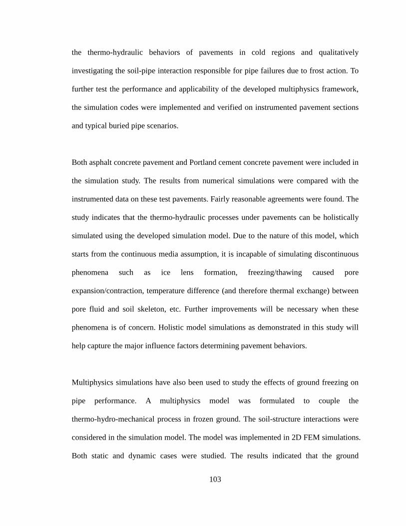
103

the thermo-hydraulic behaviors of pavements in cold regions and qualitatively

investigating the soil-pipe interaction responsible for pipe failures due to frost action. To

further test the performance and applicability of the developed multiphysics framework,

the simulation codes were implemented and verified on instrumented pavement sections

and typical buried pipe scenarios.

Both asphalt concrete pavement and Portland cement concrete pavement were included in

the simulation study. The results from numerical simulations were compared with the

instrumented data on these test pavements. Fairly reasonable agreements were found. The

study indicates that the thermo-hydraulic processes under pavements can be holistically

simulated using the developed simulation model. Due to the nature of this model, which

starts from the continuous media assumption, it is incapable of simulating discontinuous

phenomena such as ice lens formation, freezing/thawing caused pore

expansion/contraction, temperature difference (and therefore thermal exchange) between

pore fluid and soil skeleton, etc. Further improvements will be necessary when these

phenomena is of concern. Holistic model simulations as demonstrated in this study will

help capture the major influence factors determining pavement behaviors.

Multiphysics simulations have also been used to study the effects of ground freezing on

pipe performance. A multiphysics model was formulated to couple the

thermo-hydro-mechanical process in frozen ground. The soil-structure interactions were

considered in the simulation model. The model was implemented in 2D FEM simulations.

Both static and dynamic cases were studied. The results indicated that the ground

104

freezing caused an appreciable increase in the stresses in pipes. The pipe burial depth and

the overburden pressure were found to have important effects on the induced stresses in

pipes. The dynamics of crack development in pipe in response to the combination of

traffic and frost load was investigated using a fracture dynamics model. The results

indicated that the combined effects of ground freezing and dynamic loading can

significantly shorten the service life of pipes. Besides reproducing the engineering

observations, the current study demonstrated the capacity of the holistic multiphysics

simulation for studying the frost effects on underground pipes. This effort succeeded in

providing a multiphysics extension to the physical based methods for the analysis and

design of buried pipes, especially those in cold regions.

105

4 CHAPTER FOUR

A NEW METHOD FOR SOIL WATER CHARACTERISTIC CURVE

MEASUREMENT: THERMO-TIME DOMAIN REFLECTOMETRY IN FREEZING

SOILS

4.1 Overview

The soil water characteristic curve (SWCC) is the basis for explaining a variety of

processes in unsaturated soils, ranging from transport phenomena to mechanical

behaviors. It is also necessary for analyzing the hydraulic field in freezing soils. In this

chapter, a new method is developed for SWCC estimations based on the similarity

between the freezing/thawing process and drying/wetting process in soils. The theoretical

basis for this method was first reviewed. The concept of Soil Freezing Characteristic

Curve (SFCC) was introduced to describe the relationship between the unfrozen water

content and matric suction in freezing soils. The SFCC is analogous to SWCC in that

both of them describe the energy status of liquid water associated with liquid water

content. Relationships between the SWCC and SFCC were discussed. To measure SFCCs,

a thermo-TDR (time domain reflectometry) sensor was developed which combines both

temperature sensors and a conventional TDR sensor. The TDR module and algorithm

measure the unfrozen water content of soils during the freezing/thawing processes, while

the built-in thermocouples measure the temperature. The SFCC was obtained from the

simultaneously measured TDR and temperature data. Experiments were conducted on

two types of soils to validate this new approach. The SFCC was obtained from

106

thermo-TDR data which were collected in specimens subjected to a controlled thawing

process, while the SWCC was directly measured by the ASTM D5298 filter paper

method. Reasonable agreements were found between the measured SWCCs and SFCCs.

The experimental results implied that the SWCC could be estimated from SFCC using

the proposed method.

4.2 Background

The SWCC describes the relationship between soil water content (or saturation) and soil

water potential (or suction) (Williams and Smith, 1989). The SWCC of a soil is a

macroscopic symbol of its internal structure, mineral constitution and the interactions

among the liquid, solid, and gas phases (Mualem, 1976; Bachmann and van der Ploeg,

2002; Wang et al., 2008). The SWCC is therefore responsible for many important

phenomena in unsaturated (partially saturated) and freezing (partially frozen) soils, e.g.

fluid migration, heat transfer, and salt and ion transportation (Simunek et al., 1994;

Hansson et al., 2004). As a moisture retention property of unsaturated soil, the SWCC has

long been observed and studied by soil scientists (Briggs, 1907). More recently, the use

of SWCC has become generally accepted in geotechnical engineering in the construction

of the constitutive equations of unsaturated soils (Fredlund and Rahardjo, 1993).

4.2.1 Common Methods for SWCC Measurements

The measurement of SWCC is usually time-consuming and requires delicate

107

experimental controls. The accuracy and easiness of a measurement depend on the

operational principles for acquiring both soil suction and water content. For soil suction,

various approaches have been proposed, which can be classified as those based on

pressure balance, relative humidity, and resistivity, etc. These approaches have been

widely applied in scientific and practical activities. Apparatus based on pressure (suction)

balance include filter paper, pressure plate, suction plate, tensiometer and pressure

membrane, all of which measure pressure utilizing calibrated porous media. For water

content, a direct measurement by oven drying the soil is accurate yet destructive. When

testing a sample with a varying water content, non-destructive tools such as the magnetic

resonance or TDR can be employed. Table 4.1 summarizes the ranges and principles of

common approaches in SWCC measurements (Croney and Coleman, 1961; Scanlon et al.,

1997).

Table 4.1 Methods for suction and saturation measurements

SUCTION Range SUCTION Range Suction plate 0-100 kPa Odometer 10 kPa-1MPa Continuous flow 0-100 kPa Centrifuge 100 kPa-3MPa Rapid method 0-100 kPa Freezing Point depression 100 kPa-1MPa Field tensiometer 0-200 kPa Vacuum desiccator 10 MPa-1000MPa Pressure plate 1-100 kPa Sorption balance 10 MPa-1000MPa Pressure membrane 0-150 MPa Electrical resistance gauge 100 KPa-1000MPa SATURATION Mechanism SATURATION Mechanism Direct method Directly Ground penetrating radar Wave velocity TDR Permittivity Gama-ray Gama ray Neutron Probe Neutron Capacitance probe Capacitance FD Impedance/Capacitance GPR Electromagnetic radiation

Despite the progress in unsaturated soil mechanics, accurate measurements of SWCC

remain challenging. Therefore, researchers have also resorted to physically based and

semi-empirical methods. These methods were usually developed based on the

108

relationship between the SWCC and other intrinsic soil properties. Examples for

physically based methods include the theoretical models proposed by Mualem (1976),

and Fredlund and Xing (1994), both of which were on the basis of a ‘bundle of capillary

cylinder’ conceptualization. The applications of these theoretical models require

establishing the relationships between the SWCC and soil index properties or the

pore-size distribution (Zapata et al., 2000). There are also semi-empirical approaches for

SWCC predictions based on soil index properties such as the grain-size distribution (Arya

and Paris, 1999; Aung et al., 2001; Kosugi et al., 1998). Considering the important role of

SWCC for unsaturated soils, the development of an accurate and simple measurement

technique is highly desirable for both the research and practice community.

4.2.2 Similarity between Wetting/Drying Process and Freezing/Thawing Processes

The similarity between adsorption (wetting)/ desorption (drying) process and

thawing/freezing process has been observed for a long time. This similarity, however, has

not been paid sufficient attention. Buckingham (1907) and Gardner (1919) in their

pioneering work have worked out the similarity between the energy relationships for the

thermal process and drying process. Their study was followed by Schofield (1935), who

introduced the pF scale to indicate suction in the unit of cm H2O. A method named

freezing point depression was developed based on this concept (Croney, 1952). Although

a relationship was believed to exist between freezing/thawing and drying/wetting

processes, the mechanism was unfortunately obscure due to the incapability of the

surface tension theory as well as the lack of understanding in colloidal behaviors (Pires et

109

al., 2005). This dilemma was late reconciled by the breakthrough in observing the

similarity between the drying process and the freezing process, by means of the soil

freezing characteristic and soil moisture characteristic curve (Koopmans and Miller, 1966;

Spaans and Baker, 1996). The SFCC describes the relationship between the unfrozen

water content and soil suction in freezing soils. Microscopically, it represents the

derivative of system energy with respect to the amount of liquid water as

freezing/thawing progresses. The SFCC is analogous to SWCC in that both of them

describe the relationship between the energy status of liquid water and liquid water

content.

The idea of taking advantage of this resemblance leads to the possibility that SWCC can

be obtained by measuring temperature (freezing point depression) and degree of

freezing/thawing. This idea is distinct from common technologies for SWCC

measurements. On the other hand, recent developments in sensor technologies make it

possible to simultaneously measure temperature and liquid water content, and

consequently the degree of freeze/thawing. This provides sufficient technical support for

developing a convenient method for the SWCC measurement by means of the SFCC

measurements. In this chapter, we describe the procedures to estimate SWCCs from

SFCCs by use of a thermo-TDR sensor.

4.2.3 Time Domain Reflectometry

Time Domain Reflectometry (TDR) is a guided radar technology that was initially used

110

by electrical engineers to locate cable breakages. The technology was extended to

measuring soil water content due to the pioneering work of Topp et al. (1980). In civil

engineering, TDR has become an established technology for soil water content

measurement (O’Connor and Dowding, 1999; Benson, 2006; ASTM D6565 and ASTM

D6780). It features the advantages of being rugged, accurate and automatic.

(a)

(b)

Figure 4.1 a) Schematic of an example TDR system and output signal; and b) a typical

TDR curve for soil and measurement of apparent length aL (Drnevich et al., 2001)

111

The configuration of a typical TDR system is shown in Figure 4.1. The system generally

consists of a TDR device (including an electrical pulse generator and a sampler), a

connection cable, and a measurement probe (Figure 4.1a). TDR works by sending a fast

rising step pulse or impulse to the measurement probe and measuring the reflections due

to the change of material dielectric permittivity. Due to the large contrast between the

dielectric constant of water (around 81) and those of the air (1) or soil solids (the

dielectric constant for dry solids is typically between 3-7), the bulk dielectric constants of

soils are very sensitive to the water content. The large contrast in the dielectric properties

of air and soil solids causes one reflection when the electrical signal enters the soil from

the air; another reflection takes place when the electrical signal arrives at the end of the

measurement probe (Figure 4.1b). When displaying a TDR signal, the time scale, t, is

usually displaced by the round trip distance using Equation (4.1):

2a

ctL = (4.1)

where La is called apparent length, c is the speed of electromagnetic wave in the vacuum

(3.0×108 m/s), t is the time scale. From the apparent length, La, displayed on TDR signal

(Figure 4.1b), the round trip time required for an electrical pulse to travel through the

measurement probe can be determined as cLt a2

= .

The velocity of electromagnetic wave traveling in the testing material can then be

calculated by Equation (4.2).

112

2 2

2 /a a

L L Lv ct L c L

= = = (4.2)

where v is the velocity of an electromagnetic wave traveling in the material, La is the

apparent length from displayed TDR signal, L is the physical length of TDR sensor

section; t is the time difference between the two reflections that occur at the interfaces of

material layers.

The velocity of electric signal is inversely proportional to the square root of dielectric

constant, aK , (Ramo et al., 1994):

a

cvK

= (4.3)

Combining Equations (4.2) and (4.3), the dielectric constant of a material can be

calculated by

22

aa

LcKv L

= =

(4.4)

The dielectric constant, Ka, measured by TDR is typically called “apparent dielectric

constant” to reflect the fact that it does not consider the frequency-dependency of the

dielectric permittivity (Topp et al., 1980).

Siddiqui and Drnevich (1996) developed an equation that relates TDR measured

dielectric constant to gravimetric water content (gravimetric water content, w , i.e., mass

of water compared to mass of dry soil solids; volumetric water content, θ , i.e., volume

of water compared to total volume of soil). This equation accounts for the effects of soil

113

type and density by incorporating two calibration constants. This equation is shown

below.

wa

d

1w K ab

ρρ

= −

(4.5)

where dρ is the dry density of soil, wρ is the density of water, a and b are

soil-dependent calibration constants. Typically, a is 1, and b is 8.

4.3 Theoretical Basis of the New Method for SWCC

4.3.1 Soil Freezing Characteristic Curve (SFCC) and Its Relationship to SWCC

As mentioned above, the SFCC describes the relationship between the unfrozen water

content and soil suction in freezing soils. Microscopically, it represents the variation of

the amount of liquid water and its energy status as freezing/thawing progresses.

When freezing or thawing process occurs under small temperature gradients across a

specimen and its boundaries, phase change and mass migration of moisture are slow. In

virtue of this slow transient process, it is reasonable to assume that an equilibrium

between water and ice holds during every short time span inside the soil specimen.

Freezing point depression of water due to the existence of menisci of pore water-air/ice

interface is then described by the Clapeyron equation (Groenevelt and Kay, 1974).

w f ln273.15

TLψ ρ= (4.6)

where ψ is soil suction, wρ is water density, fL is the latent heat of water fusion, T

114

is temperature in kelvin, which can be easily measured with established technologies.

Soil suction at different freezing/thawing stages in freezing soils can be obtained by

integration of the measured temperature process with proper initial conditions via the

Clapeyron’s equation (Equation (4.6)). The SFCC can be obtained by plotting the soil

suction versus the corresponding unfrozen water content in soils subjected to a controlled

freezing/thawing process.

The SFCC is analogous to the SWCC in that both of them describe the energy status of

liquid water associated with liquid water content. Therefore, they are related in theory.

Schofield (1935) succeeded in indirectly obtaining a SWCC by measuring a SFCC.

Koopmans and Miller (1966) and Spaans and Baker (1996) suggested that a

soil-dependent constant may be needed to convert SFCCs to SWCCs. Equation (4.7) is a

general format summarizing these previous studies,

( )a w i wAu u u u− = ⋅ − (4.7)

where the difference between air and water pressure, a wu u− , is the soil suction in

unsaturated soils, and that between ice and water pressure, i wu u− , is the suction in

freezing soils. A is a conversion constant between the SWCC and the SFCC.

For colloidal soils, A was theoretically predicted to be 1 since the soil particles are

completely surrounded by adsorbed water (Schofield, 1935). For non-colloidal soils, the

value of A in Equation (4.7) was predicted by thermodynamics to be equal to the ratio of

surface tension of air-water and ice-water interfaces (Koopmans and Miller, 1966).

115

To estimate a SWCC from the similarity between the wetting process and the thawing

process, the SFCC needs to be obtained firstly. This can be accomplished by measuring 1)

the temperature process, and 2) the corresponding degree of thawing in freezing soils.

The soil suction can be obtained by integration of the Clapeyron equation (Equation

(4.7)). To ensure the phase equilibrium conditions required for Clapeyron equation, the

thermal boundary conditions around the testing specimen have to be controlled. The

measurements of temperature and the degree of freezing/thawing were accomplished in

this study by use of a thermo-TDR sensor, which is described in the following text.

4.3.2 Experimental Apparatus: Thermo-TDR Sensor

A thermo-TDR sensor was fabricated to simultaneously measure the internal temperature

and unfrozen water content. The geometry and components of the thermo-TDR sensor are

shown in Figure 4.2. The rods are 40 mm in length and spaced 6 mm apart. The diameter

of the probe rod is 1 mm. The probe design achieved an electrical impedance of 150

when exposed to the air (O’Connor et al., 1999). Instead of solid rods for traditional TDR

probe, hollow steel rods were used for the thermo-TDR probes. One type-K

thermocouple was installed in each rod. The tubes were then backfilled with high thermal

conductive epoxy.

The thermo-TDR combines the TDR module with the thermal measurement module. The

TDR module function is similar to conventional TDR sensors and provides accurate

116

measurements of unfrozen water content in freezing soils. The thermal module by the

thermocouples provides accurate measurements of temperature. The thermo-TDR

therefore offers a way to obtain the freezing status and temperature data synchronously.

(a)

(b)

Figure 4.2 a) Schematic design of thermal-TDR probe; b) photos of fabricated

117

thermo-TDR probe

4.3.3 Measurement of the Degree of Freezing/Thawing

The application of TDR to freezing soils is an extension of its application in measuring

the water content in unsaturated soils. Compared with unfrozen soil, the frozen soil is a

four-phase system containing solid mineral particles, ice inclusions (cementing ice and

interlayer ice), water in the bound and liquid states, and air. When a freezing process

occurs in fine grained soils, not all of pore water changes into ice immediately at the

freezing temperature of bulk water due to the presence of menisci at the water-ice

interface. With further decrease of the temperature, phase transition from water to ice

continues, but at a steadily decreasing rate (Lee, 1999).

Applications of TDR to freezing soils were investigated by Patterson and Smith (1981),

Smith and Tice (1988), Spaans and Baker (1995), and Kahimba and Ranjan (2007) etc.

TDR was found to be able to measure the amount of unfrozen water in soils, due to the

significant drop of the dielectric constant of free water (about 81) as it changes into ice

(about 3.2) (Warrick, 2002; Evett, 2003).

Based on the physical nature of freezing and thawing process, unfrozen water content is a

real indicator, instead of temperature, of freezing or thawing status. The degree of

freezing/thawing can be defined as the percentage of liquid water content. i.e.,

118

( )u f

% 100%t fw ww w−

Γ = ×−

(4.8)

where (%)Γ is the degree of thawing, uw is the gravimetric water content at completely

unfrozen status, tw is the gravimetric water content at time t of a freeze-thaw specimen,

fw is the gravimetric water content in a completely frozen sample. Γ is in fact the

"saturation" of a freezing soil, which represents the ratio of liquid (unfrozen) water

content to total water content.

Substituting TDR calibration equation (Equation (4.5)) into Equation (4.8), there is,

( ) a,t a,f a,t a,f

a,u a,fa,u a,f

% 100% 100%K K L L

L LK K

− −Γ = × = ×

−− (4.9)

where a,uK and a,uL are the dielectric constant and apparent length of an unfrozen

specimen, a,tK and a,tL are the dielectric constant and apparent length at time t of a

freeze-thaw sample, a,fK and a,fL are the dielectric constant and apparent length of a

completely frozen sample.

Equation (4.9) shows, for a given soil, there is a linear relationship between aK and

degree of freezing/thawing. As the soil dependent constants in Equation (4.5) were

automatically canceled from the numerator and denominator, the degree of

freezing/thawing in Equation (4.9) expressed in variables measured by a TDR is

independent of soil types. This is an advantage of TDR technology for measuring degrees

of freezing/thawing.

119

Figure 4.2 is an example of measured dielectric constants of a soil sample during a rapid

freezing process. Also plotted on the Figure 4.3 is the measured electrical conductivity

(inverse of resistivity) evolution. As shown in this figure, different stages of

freezing/thawing can be clearly identified from the evolution curve of measured dielectric

constants. The change of dielectric constant is attributed to the change of the physical

status of soil water. Degrees of freezing can be determined via Equation (4.9).

0 50 100 150 200 250 300 350 4000

2

4

6

8

10

12

TDR Dielectric Constant TDR Electric Conductivity

Mea

sure

d Q

uant

ities

Time (minute)

Initialization of freezing

Complete frozen

Figure 4.3 Measured soil dielectric constant and electrical conductivity in freezing

process

In summary, the ability of TDR to measure the unfrozen water content provides a method

to assess the status of freezing/thawing. The degree of freezing/thawing in freezing soils

obtained from TDR measurement can be directly translated into the saturation of liquid

water.

120

4.4 Experimental Procedure and Data Analysis

Laboratory experiments were conducted to measure SFCCs using the thermo-TDR sensor.

Experiments were conducted on two representative types of subgrade soils in the State of

Ohio, USA. The index properties of these soils are summarized in Table 4.2.

Table 4.2 Index properties of soils tested in this study

Soil Gravel %

Coarse Sand %

Fine Sand %

Silt %

Clay %

Liquid Limit

Plastic Limit

Plasticity Index

Soil #1 7 5 10 28 50 25 14 11 Soil #2 10 7 10 14 59 40 18 22

For soil #1, specimens were prepared using a Harvard Miniature compactor. The method

of compaction, i.e., the mass of soil solids in each layer and amount of compaction energy,

was carefully controlled to ensure that the specimen is uniform.

The SFCC measurement was taken during a thawing process of a frozen specimen. First,

the prepared specimen was sandwiched by two pieces of porous stone, wrapped up with a

permeable cloth and soaked in water for more than 48 hours. The purpose of soaking the

specimens in water was to make sure that they have sufficient water contents to cover the

range of SFCC curve. The thermo-TDR probe was then installed into the soil specimen.

The three probes were inserted mechanically in full depth in the direction of the axis of

the cylindrical soil specimens. Thus the axis of the middle probe coincides with that of

the specimens. The specimen and thermo-TDR were wrapped by a plastic wrap to

121

prevent evaporation. In addition to the three thermocouples built in the thermo-TDR, two

more thermocouples were installed to monitor the air temperature in the freezer and room

temperature, respectively. All the thermocouples were calibrated beforehand to ensure a

precision of 0.01 C . The specimens were then placed into a -24°C freezer for about 24

hours for the soil to be completely frozen.

The slow thawing process was started by unplugging the power of the freezer. The hope

was that the thermal insulation of the freezer could effectively ensure a sufficiently slow

thawing rate. The TDR reading was taken with Campbell Scientific TDR100 at one

minute intervals. Figure 4.4 shows an example of measured TDR signals during the

course of the experiment. As thawing develops, the TDR signals evolve in a well behaved

pattern. The TDR signals were analyzed using commonly used algorithm to determine the

dielectric constants. Based on the TDR measurements, the degree of thawing was

calculated using Equation (4.9).

1400 1420 1440 1460 1480 1500 1520 1540-0.3

-0.2

-0.1

0.0

0.1

0.2

Beginning 2 hour 4 hour 6 hour 8 hour 10 hour Ending

Volta

ge (V

)

Apparent length L

Figure 4.4 Typical TDR signals during a thawing process

122

Temperature data were also collected at one second intervals by use of TC-08 USB

thermocouple recording units produced by Pico technology Inc. The automatic

monitoring process continued until the specimen completely thawed.

The experimental data analyses involve:

1) Determine the degree of thawing or unfrozen water content from the TDR

measurements. From this calculate the unfrozen volumetric water content.

2) Determine the average temperature in soil specimens. Estimate the soil suction

from temperature using the Clapeyron equation (Equation (4.6)).

3) Plot the SFCC by plotting the unfrozen water content estimated from step 1) and

the corresponding (in time) soil suction estimated from step 2).

Experiments were also conducted to directly measure the SWCC by the filter paper

method (ASTM D5298). The filter paper used in the experiments was Whatman No. 42,

which is ash-free quantitative Type II filter paper.

123

0.01 0.1 1 10

0.0

0.2

0.4

0.6

0.8

1.0

Sat

urat

ion

Measured SFCC

Suction (Mpa)

Measured SWCC

Figure 4.5 Comparison of measured SFCC and SWCC measured by ASTD D5298 for

soil #1

Figure 4.5 plots the measured SFCC curve using the described experimental and analyses

procedures. The SWCC measured by the filter paper method is also plotted for

comparison. As can be seen, the values and trend of the SFCC match very well with the

SWCC, particularly for the range of soil suction commonly encountered in practice (from

several hundred kilopascals to several megapascals). The observation also implies the

conversion factor A (in Equation (4.7)) of approximate 1 between the SWCC and SFCC

for this soil.

To verify the repeatability, experiments (i.e., SFCC from controlled thawing and SWCC

by filter paper method) were conducted on another group of specimens made from Soil

#1 but at a different density. The results are summarized in Figure 4.6. Similar

observations can be found, i.e., the SFCC is close to the SWCC with a conversion factor

A about 1. The encouraging results indicate that the SFCC measured by the proposed

124

method provides a reasonable estimation for the SWCC for different soil densities.

0.01 0.1 1 10

0.0

0.2

0.4

0.6

0.8

1.0

Measured SFCCSatu

ratio

n

Suction(MPa)

Measured SWCC

Figure 4.6 Comparison of measured SFCC versus SWCC measured by ASTD D5298 for

soil #1 at another density

Experiments were also conducted to validate the applicability of the procedures to

specimens of different geometries. For this purpose, the specimens of soil #2 were

compacted in a steel circular ring with an inner diameter of 7.1 cm and a height of 20 cm.

100 g of soil was poured into the steel ring on a steel table. The upper surface of the soil

mass was flatted and then hammered by a 5 kg steel cylinder with a diameter of 7.1 cm

for 12 blows. For each blow, the steel cylinder was dropped from a height (distance

between bottom of the steel cylinder and the table) of 20 cm. The molded soil specimens

were cylinders with a diameter of 7.1 cm and a height about 1.2 cm. Due to the small

heights of the soils specimen, the thermo-TDR was inserted into the specimen with the

probes perpendicular to the axes of the cylindrical soil specimens. The middle probe

intersects the axes. Similar procedures were used to measure the SFCC: the specimen was

125

frozen under -24°C; it was then subjected to controlled thawing; the thermo-TDR sensor

was used to monitor the degree of thawing and corresponding temperature. The SFCC

was then determined from the TDR and temperature data collected by the thermo-TDR

sensor. The ASTM D5298 filter paper method was also used to measure the SWCC

directly.

Figure 4.7 plots the measured SFCC and SWCC for soil #2. Again, the two curves

coincide in most of the soil suction range. This good agreement indicates the satisfactory

performance of this new method in estimating the SWCC from SFCC. The result also

implies that the method can be applied to soil specimens of different geometries.

1E-5 1E-4 1E-3 0.01 0.1 1 10 1000.0

0.2

0.4

0.6

0.8

1.0

Measured SFCC

Satu

ratio

n

Suction (MPa)

Measured SWCC

Figure 4.7 Comparison of SWCC measured by the ASTM D 5298 and SFCC for soil #2

The procedures of the ASTD D5298 filter paper method took weeks to perform, while the

SFCC measurements by this new method takes less than 15 hours. Another advantage of

the new method is that more densely distributed data are obtained than that by the filter

126

paper method. This is because each datum point on the SWCC by the filter paper method

requires at least one week to obtain, while one datum point on the SFCC corresponds to a

time point during the thawing process.

4.5 Discussion

The theoretical basis of this new method requires 1) an equilibrium condition at the

water/ice interface; 2) accurate temperature measurements of the bulk specimen. This is

because the proposed method for SFCC measurements utilizes the Clapeyron equation,

which describes the equilibrium condition at the interfaces between different phases. But

the reality is that exchanges of energy with the external system inevitably occur during

the thawing process. Therefore, only quasi-equilibrium conditions are possible when the

thawing/freezing process is relative slow. This truth makes the rate of freezing/thawing

very critical during SFCC measurements. Measures need to be taken to make sure that

the thermal exchange is sufficiently slow to approximate quasi-equilibrium conditions.

Also, only in such a way different points in the specimen achieve similar thermodynamic

states so that temperatures measured at different locations are close.

To reduce the rate of thawing, the thawing process in the experiments was implemented

inside a freezer. Prior to thawing, the specimens were frozen in the freezer to -24°C (the

lowest temperature the freezer can achieve). It was found that about 15 hours were

required to complete the thawing process, while it only took about 30 minutes when

directly exposing the specimens to a room temperature of 22 C (fast thawing

127

procedure). Due to good thermal insulation provided by the freezer, the temperature

difference between the air temperature within freezer and the coldest location in the soil

sample (center) stayed within 4 C . According to the Newton’s law of cooling, the rate of

thermal energy exchange can be calculated with this temperature difference using

Equation (4.10).

( )envQ h A T T= ⋅ − (4.10)

where Q is the rate of thermal energy exchange (W), h is the convective heat transfer

coefficient, A is the surface area, envT is the environmental temperature, T is the surface

temperature of the specimen. For static air in an unplugged freezer, a conservative

assumption of the convective heat transfer coefficient is 5 W/m2·K (Burmeister, 1993).

Therefore, the magnitude of heat flux into the specimen per unit area is 20 W/m2. This

significantly reduced the rate of thawing and helped achieving phase equilibriums inside

the soil specimens. Comparisons indicated this treatment produced a thawing rate

sufficiently slow (more than 20 times slower than directly thawing the specimen in the

room temperature) to achieve quasi-equilibrium conditions.

The approximation of the phase equilibrium condition is dependent upon the rate of

thawing. Typically the faster the thawing process, the further away the soil state from the

equilibrium conditions. To investigate the effects of thawing rate on the SFCC

measurements, experiments were conducted using a fast thawing procedure in which the

freezing soil specimen is directly exposed to the room temperature. The SFCC was also

measured under a fast freezing procedure by monitoring the freezing process of specimen

directly placed in freezer at -24°C, for which no more than an hour was needed to

128

complete the freezing process. Figure 4.8 plots the SFCCs from the fast thawing and

freezing procedures for soil #1. The SWCC measured by the ASTM D5298 filter paper

method was also plotted for comparison. The comparison shows that the suction values of

the SFCCs measured using the fast freezing and thawing procedures are lower in the low

suction range and higher in the high suction range compared to the SWCC. The

discrepancy between the SWCC and SFCCs is likely caused by the non-equilibrium

conditions resulting from the fast freezing and fast thawing procedures.

0.01 0.1 1 10

0.0

0.2

0.4

0.6

0.8

1.0

Fast thaw SFCCSatu

ratio

n

Suction (MPa)

Measured SWCC Fast freeze SFCC

Figure 4.8 Measured SWCC by filter paper method and measured SFCC with fast

thawing and freezing procedures

The above observations indicate that properly maintaining phase equilibrium conditions

is necessary for estimating SWCCs from SFCC measurements. From the experimental

thawing condition in this study (thawing process was started by unplugging the freezer

and the specimen remained in the freezer throughout the thawing process), the rate of

129

thermal exchange was under 20 W/m2 during the thawing process. This might set the

criterion to ensure the quasi-equilibrium conditions for the proposed method. Further

validation of this criterion is necessary for specimens of different sizes.

The slow rate of thermal exchange ensures a relative uniform temperature distribution

inside the specimens. For example, the temperature process and the maximum differences

among measured temperatures inside a specimen are plotted in Figure 4.9. It can be seen

that the maximum temperature difference between sensors is lower than 0.1 C most of

the time and is 0.2 C to the maximum. The corresponding differences in suction values

are no more than 20 kPa. It is worthwhile to point out that the extent of error has been

further reduced by taking the average of the temperature data.

0 2 4 6 8 10 12 14-24

-20

-16

-12

-8

-4

0

Tem

pera

ture

(deg

C)

Time elapsed (hour)

Probe 2 Probe 3 Probe 4

0.00

0.02

0.04

0.06

0.08

0.10

0.12

0.14

0.16

0.18

0.20

Maximum temperature difference

Figure 4.9 Measured temperatures at different locations and maximum differences among

measured temperatures verse time

130

4.6 Conclusion

This chapter describes a new procedure to estimate the soil water characteristic curve

based on the soil freezing characteristic curve. This method is based on the similarity

between the freezing and drying processes. The chapter firstly presented the theoretical

basis for this method. The experimental measurements of the SFCC were carried out by

use of a thermo-TDR sensor. The thermo-TDR simultaneously measured the unfrozen

water content (or saturation) and soil temperature. The soil temperature was converted to

soil suction by use of the Clapeyron equation, which describes the pressure-temperature

relationship at interfaces between solid and liquid water under quasi-equilibrium

conditions. Therefore, the SFCC of a soil can be obtained by subjecting the soil to a

proper freezing or thawing process. The rate of thermal exchange between the specimen

and the environment during thawing was controlled so that quasi-equilibrium conditions

were approximated inside the soil specimens. The SFCCs obtained by this procedure

were found to match the SWCCs directly measured by the ASTM D5298 filter paper

method. Therefore, the new technique with the thermo-TDR sensor is a promising

alternative to conventional methods for SWCC measurements.

131

5 CHAPTER FIVE

SUMMARY ON THIS WORK, AND SUGGESTIONS FOR FUTURE RESEARCH

5.1 Summary on this Work

This study started with an introduction to the knowledge base for studying freezing

porous materials. Emphasis is on the coupling of physical fields, which are essential for

the characterization of porous materials. The review firstly discussed the terminology and

definitions used in different disciplines for the topic. For a better understanding of the

coupling actions, the review grouped the interactions between physical fields in porous

materials subject to frost action into three layers. The first layer is described as the basic

mechanisms, which are in charge of the multiphysical processes in freezing soils.

Relevant models were categorized and compared. The other two layers of interactions for

characterizing freezing soils are described as the explicit relationships and the implicit

relationships. Discussions on these two layers of interactions as well as their relationships

to the first layer of interaction are also provided.

The thesis then described the development of a theoretical framework for multiphysics

simulations of freezing porous materials. Thermal, hydraulic, and mechanical fields were

coupled together on the level of mathematical equations. The effects of pore morphology

and physical chemistry of phases on individual physical processes were described by the

SWCC and the Clapeyron equation. The highly nonlinear system was solved numerically

on a multiphysics simulation platform. The theoretical framework was found to be able to

132

be solved smoothly using typical computational domain and boundary conditions. The

following observations were made from the simulation results. (1) The

thermal-hydro-mechanical fields are strongly coupled in porous materials. For example,

heat transfer induces changes in the hydraulic and mechanical fields, which is especially

important when the phase change of pore liquid is involved. (2) Matric potential in

unsaturated porous media can cause the volume change pattern to be different from that

solely due to ice formation. (3) Multiphysics simulation described reasonably well the

temperature and moisture variations observed in unsaturated soils.

To verify the model simulation, the proposed theoretical model for the multiphysical

process in freezing soils was applied to analyzing the responses of pavements and buried

pipes under frost action. For pavements, both asphalt concrete pavement and Portland

cement concrete pavement were included in the simulation study. The results from

numerical simulations were compared with the instrumented data on these test

pavements. Reasonable agreements were found. The study indicates that the

thermo-hydraulic processes under pavements can be holistically simulated using the

developed simulation model. Multiphysics simulations were also used for studying the

effects of ground freezing on pipe performance. The soil-structure interactions were

considered in the simulation model. The model was implemented in 2D FEM simulations.

Responses of the pipe under both static and dynamic loads were studied. The results

indicated that the ground freezing caused an appreciable increase in the internal stresses

of pipes. The pipe burial depth and the overburden pressure were found to have important

effects on the induced stresses in pipes. The dynamics of crack development in the pipe

133

in response to the combination of traffic and frost load was investigated using a fracture

dynamics model. The results indicated that the combined effects of ground freezing and

dynamic loading can significantly shorten the service life of pipes. Besides reproducing

the engineering observations, this study demonstrated the capacity of the holistic

multiphysics simulation for studying the frost effects on underground pipes.

Finally, this study developed a new approach to estimate the Soil Water Characteristic

Curve, the most critical and challenging auxiliary relationship in freezing soils. This

method is based on the similarity between the freezing and drying processes in soils. The

study firstly presented the theoretical basis for this method. The experimental

measurements for SFCC were carried out by use of a thermo-TDR sensor. The

thermo-TDR simultaneously measured the unfrozen water content (or saturation) and soil

temperature. The soil temperature was converted to soil suction by use of the Clapeyron

equation, which describes the pressure-temperature relationship at interfaces between

solid and liquid water under quasi-equilibrium conditions. Therefore, the SFCC of a soil

can be obtained by subjecting the soil to a proper thawing procedure. The rate of thermal

exchange in the proposed thawing procedure was controlled so that a quasi-equilibrium

condition was achieved inside the soil specimens. The SFCCs obtained by the proposed

method were found to match the SWCCs directly measured by the ASTM D5298 filter

paper method. Therefore, the proposed approach with the thermo-TDR sensor is a

promising alternative method for SWCC measurements. In the scientific side, this study

provided another evidence on the similarities between freezing/thawing processes and

desorption/sorption processes.

134

5.2 Recommendations for Future Research

This study attempts to advance the state of the art in the modeling and characterization of

freezing soils. Despite the innovative efforts and progress that have been made, several

challenges have also been identified owning to this "learning by doing" experience.

Rational responses to these challenges, the author believe, will significantly deepen our

understanding of the distinctive nature of freezing soils, help improve numerical

simulation capacity, and promote innovative characterization techniques. The following

discussions provide the recommendations to address these unsolved challenges.

Firstly, understanding the fundamental phenomena will remain as a major driving force

for developing advanced theoretical, numerical, and experimental techniques. One

example is the thermally induced water flux, which is especially significant and thus of

special interest among all the couplings involved in the multiphysical process of freezing

soils. Most of the multiphysics simulations based on continuum mechanics were

developed based on the theory proposed by Philip and de Vries (Harlan, 1973; Guymon

and Luthin, 1974; Noborio et al., 1996b). This theory has also been applied to freezing

soils without ice lenses (Hansson et al., 2004; Thomas et al., 2009). However,

experimental evidences have repeatedly indicated that the above formulation

under-predicts the influence of temperature on water migration (Nimmo and Miller, 1986;

Constantz, 1991; Grant and Salehzadeh, 1996; Bachmann et al., 2002; Bachmann and van

der Ploeg, 2002) by a gain factor from 2 to more than 10, depending on soil types.

135

Unfortunately, the underestimation resulting from this widely used theory has not been

appropriately considered in previous investigations and was typically accounted for by an

empirical gain factor. The proposed multiphysics framework also used this approach by

employing a gain factor which was determined based on soil types. The framework can

thus be further improved by calculating this gain factor based on underlying physical

mechanisms. For example, these mechanisms may be revealed by investigating the

dependence of contact angle on temperature, saturation, and suction as well as other

dependent variables.

Another fundamental mechanism deserving close attention is the similarity between

freezing/thawing and drying/wetting processes. This is because this mechanism is critical

to both simulations and characterizations. For simulations, numerical calculations in this

study indicated that the transition from unfrozen to partially frozen status results in a very

high nonlinearity. When the soil is unsaturated, the coexistence of partially saturated and

partially frozen conditions makes the nonlinearity even more serious. It has never been

tried, but would be beneficial to reduce this nonlinearity by employing the similarity

between freezing and dry processes. Moreover, the simultaneous employment or

superposition of the SWCC and SFCC needs supports from more solid theoretical or

experimental evidences. For characterizations, the proposed method for SWCC

measurements was developed based on the similarity between freezing and dry processes.

Despite the encouraging results obtained by the new technique, several issues, such as the

effect of contact angle on the SWCC, have not been included in the consideration. If

these issues can be well addressed, the proposed technique will possibly be able to be

136

applied to exploring more phenomena, such as hysteresis in either freezing/thawing or

drying/wetting process. Furthermore, the underestimation of Philip and de Vries' theory

for thermally induced water flux may be disentangled for both partially frozen and

partially saturated conditions by investigating the contact angle variations in partially

saturated conditions.

Secondly, a holistic framework integrating studies on both saturated and unsaturated

conditions is currently in absence. To understand freezing/thawing phenomenon in soils,

different scholars have addressed relevant issues from different perspectives. The rich

collection of viewpoints, while helps understand this complex phenomena, can also cause

confusions and contradictions. A holistic framework is needed to reconcile the seemingly

inconsistencies and to unify the understandings of the freezing/thawing process under

both saturated and unsaturated conditions. For example, frost heave, which is generally

believed to occur in saturated soils, was also found to occur when the water saturation

reaches 80~90% rather than 100% (Dirksen and Miller, 1966). Dirksen and Miller's study

outlined a preliminary and interesting framework for integrating phenomena in both

saturated and unsaturated conditions. There were, however, very rare follow-up

investigations. As commented by Lundin (1990), efforts to extend models for freezing

saturated porous materials into partially saturated condition were scarce for a while. This

is also probably due to a lack of understanding on fundamental mechanisms and

complexity in solving the coupled nonlinear PDEs. This paper outlined a framework for

the case of unsaturated soils. Therefore, further efforts are required to test its validity

under nearly saturated conditions and to allow for the presence of ice lens.

137

Thirdly, the couplings between the mechanical field and the other two fields, especially

the coupling from mechanical field to the thermal or hydraulic fields, have received less

considerations in the literature due to the comparatively weaker coupling effects.

However, such couplings are important when the variations of stress or strain have a

significant influence on other physical fields. This study employed elastic constitutive

relationships for the small strain problems related to pavements and buried pipes.

However, more advanced mechanical models, e.g., plastic poromechanics, may be

needed in future studies. Poromechanics provides a robust approach to study phenomena

in porous materials based on mechanical principles. However, the definition of

“unsaturated” in current poromechanics is still distinct from the term used in geotechnical

engineering. Theories developed from Biot’s theory consider entrapped air bubbles (Biot,

1941). But it failed to cover all unsaturated conditions such as porous materials with

interconnected air phase. Also, the assumption of Biot’s theory that all pores deform in

the same way when subjected to the same pore pressure needs to be further validated.

Moreover, the current homogenization technology is still far from satisfactory for

considering the complex morphology of solid matrix and the variations caused by thermal

and hydraulic fields. Therefore, a new approach to define stress variables, which could be

much more complicated than the classic concepts in saturated and unsaturated soil

mechanics, should be found when more liquid phases are involved. Solutions to these

questions may benefit from incorporation of relevant theories such as the mixture theory.

The concept of matric suction, rather than the general concept of suction, was used in the

138

current study as well as most of the existing computational simulations. This, however,

reflects the fact that most studies focused on certain components of suction rather than all.

For example, the osmotic potential was generally ignored in simulations of frozen soil in

civil engineering applications (Nishimura et al., 2009; Thomas et al., 2009). This

approximation is acceptable only if one of the following conditions is satisfied: 1) the soil

is free of soluble salts or the influence of osmotic suction is negligible in comparison

with that of matric suction in the suction range of interest; 2) the SWCC is obtained with

respect to soil water suction instead of the matric suction. Otherwise, the osmotic suction

needs to be considered, because the soluble salts are excluded from the ice phase and

remain in the unfrozen water on freezing of moist soil (Banin and Anderson, 1974).

Consequently, osmotic suction can increase considerably in a freezing process. This is

similar to the role of osmotic suction in a drying process, which possibly prevails in most

of the suction range (Krahn and Fredlund, 1972). This effect should be considered in

future research to study practical issues in which such an effect is significant.

139

REFERENCES

Ahuja, L. R., and Swartzen, D. (1972). "An improved form of soil-water diffusivity

function." Soil Sci Soc Am Pro, 36(1), 9-14.

Alkasawneh, W., Pan, E., Han, F., Zhu, R., and Green, R. (2007). "Effect of temperature

variation on pavement responses using 3D multilayered elastic analysis."

International Journal of Pavement Engineering, 8(3), 203-212.

Alonso, E. E., Gens, A., and Josa, A. (1990). "A constitutive Model for partially saturated

soils." Geotechnique, 40(3), 405-430.

Anderson, D. M., and Morgenstern, N. R. "Physics, chemistry and mechanics of frozen

ground: a review." Proc., 2nd International Conference on Permafrost, National

Academy of Sciences, 257-288.

Anderson, D. M., and Morgenstern, N. R. "Physics, chemistry and mechanics of frozen

ground: a review." Proc., 2nd International Conference on Permafrost, National

Academy of Sciences, 257-288.

Anderson, D. M., Tice, A. R., and McKim, H. L. "The unfrozen water and the apparent

specific heat capacity of frozen soils." Proc., 2nd International Conference on

Permafrost, National Academy of Sciences, 289-295.

Ariza, P. (2002). "Evaluation of water flow though pavement systems." University of

Florida.

140

Arya, L. M., and Paris, J. F. (1981). "A physicoempirical model to predict the soil

moisture characteristic from particle-size distribution and bulk density data." Soil

Sci Soc Am J, 45(6), 1023-1030.

Asaeda, T., and Ca, V. T. (1993). "The subsurface transport of heat and moisture and its

effect on the environment: a numerical model." Boundary-Layer Meteorology,

65(1), 159-179.

Aung, K. K., Rahardjo, H., Leong, E. C., and Toll, D. G. (2001). "Relationship between

porosimetry measurement and soil–water characteristic curve for an unsaturated

residual soil." Geotechnical and Geological Engineering, 19(3), 401-416.

Averjanov, S. F. (1950). "About permeability of subsurface soils in case of incomplete

saturation." English Collection, 7, 19-21.

Bachmann, J., Deurer, M., and Arye, G. (2007). "Modeling water movement in

heterogeneous water-repellent soil: 1. development of a contact angle–dependent

water-retention model." Vadose Zone Journal, 6(3), 436-445.

Bachmann, J., Horton, R., Grant, S. A., and Van der Ploeg, R. R. (2002). "Temperature

dependence of water retention curves for wettable and water-repellent soils." Soil

Sci Soc Am J, 66(1), 44-52.

Bachmann, J., and van der Ploeg, R. R. (2002). "A review on recent developments in soil

water retention theory: interfacial tension and temperature effects." Journal of

Plant Nutrition and Soil Science, 165(4), 468.

Bachmann, J., van der Ploeg, R. R., Ren, T., and Horton, R. (2001). "Comparison of the

thermal properties of four wettable and four water-repellent soils." Soil Sci Soc

Am J, 65(6), 1675-1679.

141

Bai, M., and Elsworth, D. (2000). Coupled Processes in Subsurface Deformation, Flow,

and Transport, American Society of Civil Engineers.

Baker, J. M., and Spaans, E. J. A. (1996). "The soil freezing characteristic: its

measurement and similarity to the soil moisture characteristic." Soil Sci Soc Am J,

60(1), 13-19.

Banin, A., and Anderson, D. M. (1974). "Effects of salt concentration changes during

freezing on the unfrozen water content of porous materials." Water Resources

Research, 10(1), 124-128.

Baron, J. (1982). "Les retraits de la pate de ciment. Lebeton hydraulique." Lebeton

hydraulique, J. Baron, and R. Sauterey, eds., Presses de l’ENPC, Paris, France,

485-501.

Benson, C. H. "Plenary lecture: geotechnical applications of TDR." Proc., Proceedings of

the TDR 2006, 1.

Benson, C. H., and Othman, M. A. (1993). "Hydraulic conductivity of compacted clay

frozen and thawed in situ." Journal of Geotechnical Engineering, 119, 276-294.

Bentz, D. P. (2000). A Computer Model to Predict the Surface Temperature and

Time-of-Wetness of Concrete Pavements and Bridge Decks, US Department of

Commerce, Technology Administration, National Institute of Standards and

Technology.

Biot, M. A. (1941). "General theory of three-dimensional consolidation." Journal of

Applied Physics, 12(2), 155-164.

Biot, M. A., and Willis, D. G. (1957). "The elastic coefficients of the theory of

consolidation." Journal of Applied Physics, 24, 594-601.

142

Bittelli, M., Flury, M., and Campbell, G. S. (2003). "A thermodielectric analyzer to

measure the freezing and moisture characteristic of porous media." Water

Resources Research, 39(2), 1041.

Bond, F. W., Cole, C. R., and Gutknecht, P. J. (1984). "Unsaturated Groundwater Flow

Model (UNSAT1D) Computer Code Manual." Electric Power Research Institute,

Washington, D.C.

Briggs, L. J. (1897). "The Mechanics of Soil Moisture." USDA Bureau of Soils,

Washington, D.C.

Briggs, L. J., and McLane, J. W. (1907). The Moisture Equivalents of Soils, US

Government Printing Office.

Brooks, R. H., and Corey, A. T. (1964). "Hydraulic properties of porous media."

Hydrology Papers, Colorado State University.

Brutsaert, W. (1967). "Some methods of calculating unsaturated permeability."

Transactions of ASAE, 10(3), 400-404.

Buckingham, E. (1907). Studies on the Movement of Soil Moisture, USDA Bureau of

Soils.

Buiger, H. C. (1915). "Das lertvermogen verdummter mischristallfreier lonsungen." Phys.

Zs, 20, 73-76.

Bumb, A. C. (1987). "Unsteady-State Flow of Methane and Water in Coal Beds."

Wyoming Univ., Laramie (USA).

Burdine, N. (1953). "Relative permeability calculations from pore-size distribution data."

Transactions of AIME, 198(1), 71-78.

Burmeister, L. C. (1993). Convective Heat Transfer, Wiley-Interscience.

143

Campbell, G. S. (1974). "A simple method for determining unsaturated conductivity from

moisture retention data." Soil Science, 117(6), 311-314.

Campbell, G. S. (1985). Soil Physics with BASIC: Transport Models for Soil-Plant

Systems, Elsevier, Amsterdam, Netherlands.

Cary, J. W. (1965). "Water flux in moist soil: thermal versus suction gradients." Soil

Science, 100(3), 168-175.

Cary, J. W. "Soil moisture transport due to thermal gradients: practical aspects." 428-433.

Cass, A., Campbell, G. S., and Jones, T. L. (1981). "Hydraulic and Thermal Properties of

Soil Samples from the Buried Waste Test Facility." Pacific Northwest Lab.,

Richland, WA (USA).

Celauro, C. (2004). "Influence of the hourly variation of temperature on the estimation of

fatigue damage and rutting in flexible pavement design." International Journal of

Pavement Engineering, 5(4), 221-231.

Celia, M. A., and Binning, P. (1992). "A mass conservative numerical solution for

two-phase flow in porous media with application to unsaturated flow." Water

Resources Research, 28(10), 2819-2828.

Celia, M. A., Bouloutas, E. T., and Zarba, R. L. (1990). "A general mass-conservative

numerical solution for the unsaturated flow equation." Water Resources Research,

26(7), 1483-1496.

Charlier, R., Laloui, L., Brenčič, M., Erlingsson, S., Hansson, K., and Hornych, P. (2009).

"Modelling coupled mechanics, moisture and heat in pavement structures." Water

in Road Structures, 243-281.

144

Chen, J., Lin, K., and Young, S. (2004). "Effects of crack width and permeability on

moisture-induced damage of pavements." Journal of Materials in Civil

Engineering, 16, 276.

Childs, E. C., and Collis-George, N. (1950). "The permeability of porous materials."

Proceedings of the Royal Society of London. Series A. Mathematical and Physical

Sciences, 201, 392-405.

Ciottoni, A. S. "Computerized data management in determining causes of water main

breaks: the Philadelphia case study." Proc., International Symposium on Urban

Hydrology, Hydraulics and Sediment Control, University of Kentucky, 323-329.

Colling, L. F. "Discussion on session 3: roads and runways and agriculture." Proc.,

Conference on Pore Pressure and Suction in Soil, British National Society of Soil

Mechanics.

Cooper, A. I. (2003). "Porous materials and supercritical fluids." Advanced Materials,

15(13), 1049-1059.

Côté, J., and Konrad, J. M. (2005). "A generalized thermal conductivity model for soils

and construction materials." Can Geotech J, 42(2), 443-458.

Coussy, O. (2004). Poromechanics, John Wiley & Sons Inc.

Coussy, O. (2005). "Poromechanics of freezing materials." Journal of the Mechanics and

Physics of Solids, 53(8), 1689-1718.

Coussy, O., and Monteiro, P. (2007). "Unsaturated poroelasticity for crystallization in

pores." Computers and Geotechnics, 34(4), 279-290.

Coussy, O., and Monteiro, P. J. M. (2008). "Poroelastic model for concrete exposed to

freezing temperatures." Cement and Concrete Research, 38(1), 40-48.

145

Croney, D. (1952). The suction of moisture held in soil and other porous materials, HM

Stationery Off.

Croney, D., and Coleman, J. D. (1961). "Pore pressure and suction in soil." Proc., Pore

Pressure and Suction in Soil, British National Soc. of Soil Mechanics.

Dash, J. G. (1989). "Thermomolecular pressure in surface melting: motivation for frost

heave." Science, 246(4937), 1591.

Davidson, J. M., Stone, L. R., Nielsen, D. R., and Larue, M. E. (1969). "Field

measurement and use of soil-water properties." Water Resources Research, 5(6),

1312-1321.

Davis, M. E. (2002). "Ordered porous materials for emerging applications." Nature,

417(6891), 813-821.

de Vries, D. A. (1963). "Thermal properties of soils." Physics of Plant Environment, W.

R. van Wijk, ed., North-Holland Publishing Company, Amsterdam, Netherland,

210-235.

Dirksen, C., and Miller, R. D. (1966). "Closed-system freezing of unsaturated soil." Soil

Sci Soc Am J, 30(2), 168-173.

Dore, G. (2004). "Development and validation of the thaw-weakening index."

International Journal of Pavement Engineering, 5(4), 185-192.

Dormieux, L., Molinari, A., and Kondo, D. (2002). "Micromechanical approach to the

behavior of poroelastic materials." Journal of the Mechanics and Physics of

Solids, 50(10), 2203-2231.

146

Doron, P., Granica, D., and Barnea, D. (1987). "Slurry flow in horizontal

pipes--experimental and modeling." International Journal of Multiphase Flow,

13(4), 535-547.

Duquennoi, C., Fremond, M., and Levy, M. "Modelling of thermal soil behavior." Proc.,

The International Symposium on Frost in Geotechnical Engineering.

Edlefsen, N. E., and Anderson, A. В. (1943). "Thermodynamics of soil moisture."

Hilgardia, 15(2), 31-298.

Endelman, F. J., Box, G. E. P., Boyle, J. R., Hughes, R. R., Keeney, D. R., Norhtrup, M.

L., and Saffigna, P. G. (1974). "The Mathematical Modeling of Soil

Water-Nitrogen Phenomena." Oak Ridge National Laboratory, , Oak Ridge, TN,

USA.

Eucken, A. (1932). "Forsch." Gebiete Ingenieurw. B, 3, 16.

Evett, S. R. (2003). "Soil water measurement by time domain reflectometry."

Encyclopedia of Water Science, 894-898.

Farouki, O. T. (1981). "Thermal Properties of Soils." Unknown, United States Army

Corps of Engineers, Cold Regions Research and Engineering Laboratory,

Hanover, New Hampshire, USA.

Farouki, O. T. (1982). "Evaluation of Methods for Calculating Soil Thermal

Conductivity." United States Army Corps of Engineers, Cold Regions Research

and Engineering Laboratory, Hanover, New Hampshire, USA.

Fayer, M. J. (2000). "UNSAT-H Version 3.0: Unsaturated Soil Water and Heat Flow

Model, Theory, User Manual, and Examples." Pacific Northwest National

Laboratory, 13249.

147

Fayer, M. J., and Simmons, C. S. (1995). "Modified soil water retention functions for all

matric suctions." Water Resources Research, 31(5), 1233-1238.

Fen-Chong, T., Fabbri, A., and Azouni, A. (2006). "Transient freezing–thawing

phenomena in water-filled cohesive porous materials." Cold Regions Science and

Technology, 46(1), 12-26.

Fisher, A. K., Bullen, F., and Beal, D. (2001). "The durability of cellulose fibre

reinforced concrete pipes in sewage applications." Cement and Concrete

Research, 31(4), 543-553.

Flerchinger, G. N. (2000). "The Simultaneous Heat and Water (SHAW) Model:

Technical Documentation." Northwest Watershed Research Center USDA

Agricultural Research Service, Boise, Idaho, USA.

Flerchinger, G. N., and Pierson, F. B. (1991). "Modeling plant canopy effects on

variability of soil temperature and water." Agricultural and Forest Meteorology,

56(3), 227-246.

Forman, R. G., Kearney, V. E., and Engle, R. M. (1967). "Numerical analysis of crack

propagation in cyclic-loaded structures." Journal of Basic Engineering, 89, 459.

Fredlund, D. G., and Rahardjo, H. (1993). Soil Mechanics for Unsaturated Soils,

Wiley-Interscience.

Fredlund, D. G., and Xing, A. (1994). "Equations for the soil-water characteristic curve."

Can Geotech J, 31(4), 521-532.

Fredlund, D. G., Xing, A., and Huang, S. (1994). "Predicting the permeability function

for unsaturated soils using the soil-water characteristic curve." Can Geotech J,

31(4), 533-546.

148

Fredmond, M., and Mikkola, M. "Thermomechanical modeling of freezing soil." Proc.,

International Symposium on Ground Freezing, 6th, A.A. Balkema Publishers,

Rotterdam.

Gardner, W. (1919). "The movement of moisture in soil by capillarity." Soil Science, 7(4),

313-319.

Gardner, W. R. (1958). "Some steady-state solutions of the unsaturated moisture flow

equation with application to evaporation from a water table." Soil Science, 85(4),

228.

Gilpin, R. R. (1980). "A Model for the Prediction of Ice Lensing." Water Resources

Research, 16(5), 918-930.

Grant, S. A., and Bachmann, J. (2002). "Effect of temperature on capillary pressure."

Geophysical Monograph-American Geophysical Union, 129, 199-212.

Grant, S. A., and Salehzadeh, A. (1996). "Calculation of temperature effects on wetting

coefficients of porous solids and their capillary pressure functions." Water

Resources Research, 32(2), 261-270.

Groenevelt, P. H., and Kay, B. D. (1974). "On the interaction of water and heat transport

in frozen and unfrozen soils: II. the liquid phase." Soil Sci Soc Am Pro, 38(3),

400-404.

Groot, S. R., and Mazur, P. (1984). Non-Equilibrium Thermodynamics, General

Publishing Company, Ltd., Toronto, Canada.

Guymon, G. L., and Luthin, J. N. (1974). "A coupled heat and moisture transport model

for arctic soils." Water Resources Research, 10(5), 995-1001.

149

Hansson, K. (2003). "Water and Heat Transport in Road Structure." Uppsala: UPPSALA

University Press.

Hansson, K., Simunek, J., Mizoguchi, M., Lundin, L. C., and van Genuchten, M. T.

(2004). "Water flow and heat transport in frozen soil numerical solution and

freeze-thaw applications." Vadose Zone Journal, 3(2), 693-704.

Harlan, R. L. (1973). "Analysis of coupled heat-fluid transport in partially frozen soil."

Water Resources Research, 9(5), 1314-1323.

Hassanizadeh, S. M., and Gray, W. G. (1993). "Thermodynamic basis of

capillary-pressure in porous-media." Water Resources Research, 29(10),

3389-3405.

Haverkamp, R., Vauclin, M., Touma, J., Wierenga, P. J., and Vachaud, G. (1977). "A

comparison of numerical simulation models for one-dimensional infiltration." Soil

Sci Soc Am J, 41(2), 285-294.

Heydinger, A. (2003). "Monitoring seasonal instrumentation and modeling climatic

effects on pavements at the Ohio-SHRP test road."

Horiguchi, K., and Miller, R. D. (1980). "Experimental studies with frozen soil in an."

Cold Regions Science and Technology, 3(2-3), 177-183.

Horton, R., and Wierenga, P. J. (1984). "The effect of column wetting on soil thermal

conductivity." Soil Science, 138(2), 102.

Hromadka II, T. V., and Yen, C. C. (1986). "A diffusion hydrodynamic model (DHM)."

Adv Water Resour, 9(3), 118-170.

Hu, Y., and Hubble, D. W. (2007). "Factors contributing to the failure of asbestos cement

water mains." Canadian Journal of Civil Engineering, 34(5), 608-621.

150

Hua, C., Acker, P., and Ehrlacher, A. (1995). "Analyses and models of the autogenous

shrinkage of hardening cement paste: I. modelling at macroscopic scale." Cement

and Concrete Research, 25(7), 1457-1468.

Hudson, C. S. (1906). "The freezing of pure liquids and solutions under various kinds of

positive and negative pressure and the similarity between osmotic and negative

pressure." Physical Review (Series I), 22(5), 257.

Irmay, S. (1954). "On the hydraulic conductivity of unsaturated soils."

Transactions-American Geophysical Union, 35(3), 463-476.

Jame, Y. W., and Norum, D. I. (1980). "Heat and mass transfer in a freezing unsaturated

porous medium." Water Resources Research, 16(4), 811-819.

Janoo, V. C., and Berg, R. L. (1990). "Predicting the Behavior of Asphalt Concrete

Pavements in Seasonal Frost Areas Using Nondestructive Techniques." United

States Army Corps of Engineers, Cold Regions Research and Engineering

Laboratory.

Jansson, P. E. (2001). "Coupled Heat and Mass Transfer Model for

Soil-Plant-Atmosphere Systems." Royal Institute of Technology, Department of

Civil and Environmental Engineering, Stockholm.

Johansen, O. (1975). "Thermal Conductivity of Soils." Ph.D., Norwegian University of

Science and Technology, Trondheim.

Kahimba, F. C., and Ranjan, R. S. (2007). "Soil temperature correction of field TDR

readings obtained under near freezing conditions." Canadian Biosystems

Engineering, 49, 1.

151

Kay, B. D. (1974) and Groenevelt, P. H.. "On the interaction of water and heat transport

in frozen and unfrozen soils: I. Basic theory; the vapor phase." Soil Sci Soc Am J,

38(3), 395-400.

Kersten, M. S. (1949). "Laboratory Research for the Determination of the Thermal

Properties of Soils." United States Corps of Engineers, Engineering Experiment

Station, University of Minnesota, St. Paul, MN, USA.

Khlosi, M., Cornelis, W. M., Gabriels, D., and Sin, G. (2006). "Simple modification to

describe the soil water retention curve between saturation and oven dryness."

Water Resources Research, 42(12), W11501.

Kim, S. T., Tadjiev, D., and Yang, H. T. (2006). "Fatigue life prediction under random

loading conditions in 7475-T7351 aluminum alloy using the RMS model."

International Journal of Damage Mechanics, 15(1), 89-102.

Kleiner, Y., and Rajani, B. (2001). "Comprehensive review of structural deterioration of

water mains: statistical models." Urban Water, 3(3), 131-150.

Konrad, J. M. (1994). "Sixteenth Canadian Geotechnical Colloquium: Frost heave in soils:

concepts and engineering." Can Geotech J, 31(2), 223-245.

Konrad, J. M., and Morgenstern, N. R. (1980). "A mechanistic theory of ice lens

formation in fine-grained soils." Can Geotech J, 17(4), 473-486.

Konrad, J. M., and Morgenstern, N. R. (1981). "The segregation potential of a freezing

soil." Can Geotech J, 18(4), 482-491.

Konrad, J. M., and Morgenstern, N. R. (1982). "Effects of applied pressure on freezing

soils." Can Geotech J, 19(4), 494-505.

152

Konrad, J. M., and Morgenstern, N. R. (1982). "Prediction of frost heave in the

laboratory during transient freezing." Can Geotech J, 19(3), 250-259.

Konrad, J. M., and Morgenstern, N. R. (1984). "Frost heave prediction of chilled

pipelines buried in unfrozen soils." Can Geotech J, 21(1), 100-115.

Koopmans, R. W. R., and Miller, R. D. (1966). "Soil freezing and soil water

characteristic curves." Soil Sci Soc Am J, 30(6), 680-685.

Kosugi, K., and Hopmans, J. W. (1998). "Scaling water retention curves for soils with

lognormal pore-size distribution." Soil Sci Soc Am J, 62(6), 1496-1505.

Krahn, J., and Fredlund, D. G. (1972). "On total, matric and osmotic suction." Soil

Science, 114(5), 339-348.

Kujala, K. "Estimation of frost heave and thaw weakening by statistical analyses and

physical models." Proc., International Conference on Ground Freezing-Frost

Action in Soils, 31-41.

Kunze, R., Uehara, G., and Graham, K. (1968). "Factors important in the calculation of

hydraulic conductivity." Soil Sci Soc Am J, 32(6), 760-765.

Lee, W. (1999). "A Freeze-thaw Test on Halton Till Treated with Cement Kiln Dust."

Master, University of Toronto, Toronto, ON, Canada.

Li, N., Chen, B., Chen, F., and Xu, X. (2000). "The coupled heat-moisture-mechanic

model of the frozen soil." Cold Regions Science and Technology, 31(3), 199-205.

Li, N., Chen, F., Su, B., and Cheng, G. (2002). "Theoretical frame of the saturated

freezing soil." Cold Regions Science and Technology, 35(2), 73-80.

153

Liu, Y., Yu, X., and Yu, X. B. "Measurement of Soil Air Suction Change during

Freezing-Thawing Process." Proc., Geotechnical Special Publication, ASCE,

34-43.

Liu, Z., Sun, Y., and Yu, X. B. (2012). "Theoretical basis for modeling porous

geomaterials under frost actions: a review." Soil Sci Soc Am J, 76(2), 313-330.

Liu, Z., and Yu, X. (2011). "Coupled thermo-hydro-mechanical model for porous

materials under frost action: theory and implementation." Acta Geotechnica, 1-15.

Liu, Z., and Yu, X. B. "Coupled simulation model for ice migration." Proc., Earth and

Space 2010, ASCE.

Lochbaum, B. S. (1993). "PSE&G develop models to predict main breaks." Pipeline and

Gas Journal, 220, 20-27.

Lu, N., and Likos, W. J. (2006). "Suction stress characteristic curve for unsaturated soil."

Journal of Geotechnical and Geoenvironmental Engineering, 132, 131.

Lundin, L. C. (1989). "Water and Heat Flows in Frozen Soils. Basic Theory and

Operational Modeling." Uppsala University, Uppsala, Sweden.

Lundin, L. C. (1990). "Hydraulic properties in an operational model of frozen soil."

Journal of Hydrology, 118(1-4), 289-310.

Lura, P., Jensen, O. M., and van Breugel, K. (2003). "Autogenous shrinkage in

high-performance cement paste: An evaluation of basic mechanisms." Cement

and Concrete Research, 33(2), 223-232.

Makar, J. M. (2000). "A preliminary analysis of failures in grey cast iron water pipes."

Engineering Failure Analysis, 7(1), 43-53.

154

Margevicius, A., and Haddad, P. "Catastrophic Failures of Cleveland’s Large Diameter

Water Mains." Proc., Pipelines 2002, ASCE.

Marshall, T. J. (1958). "A relation between permeability and size distribution of pores."

Journal of Soil Science, 9(1), 1-8.

Masada, T. (2001). "Laboratory Characterization of Materials & Data Management for

Ohio-SHRP Projects (US 23)." Department of Civil Engineering, Ohio

University.

McInnes, K. (1981). "Thermal conductivities of soils from dryland wheat regions in

eastern Washington." Washington State University.

McKee, C. R., and Bumb, A. C. "The importance of unsaturated flow parameters in

designing a monitoring system for hazardous wastes and environmental

emergencies." Proc., Hazardous Materials Control Research Institute national

Conference 50-58.

Miller, E. E., and Miller, R. D. (1955). "Theory of capillary flow: I. Practical

implications." Soil Sci Soc Am J, 19(3), 267-271.

Miller, R. D. (1973). "Soil freezing in relation to pore water pressure and temperature."

2nd International Conference on Permafrost, National Academy of Sciences.

Miller, R. D. "Frost heaving in non-colloidal soils." Proc., 3rd International Conference

on Permafrost, National Academy of Sciences 708-713.

Miller, R. D. (1980). "Freezing phenomena in soils." Applications of Soil Physics,

254-299.

155

Milly, P. C. D. (1982). "Moisture and heat transport in hysteretic, inhomogeneous porous

media: a matric head-based formulation and a numerical model." Water

Resources Research, 18(3), 489-498.

Mizoguchi, M. (1990). "Water, heat and salt transport in freezing soil." Ph.D., Univ. of

Tokyo.

Mizoguchi, M. (1993). "A derivation of matric potential in frozen soil." Bulletin of the

Faculty of Bioresources, Mie University, 10, 175-182.

Morris, R. E. (1967). "Principal causes and remedies of water main breaks." American

Water Works Association, 59(7), 782-798.

Morrow, N. R. (1969). "Physics and thermodynamics of capillary." Symposium on Flow

Through Porous Media, The Carnegie Institute, Washington, D.C., USA.

Moser, A. P. (2001). Buried Pipe Design, McGraw-Hill Professional.

Mualem, Y. (1976). "A new model for predicting the hydraulic conductivity of

unsaturated porous media." Water Resources Research, 12(3), 513-522.

Mualem, Y. (1986). Hydraulic conductivity of unsaturated soils: prediction and

formulas.

Murton, J. B., Peterson, R., and Ozouf, J. C. (2006). "Bedrock fracture by ice segregation

in cold regions." Science, 314(5802), 1127-1129.

Nakano, Y., and Brown, J. (1972). "Mathematical modeling and validation of the thermal

regimes in tundra soils, Barrow, Alaska." Arctic and Alpine Research, 19-38.

Nassar, I. N., and Horton, R. (1992). "Simultaneous transfer of heat, water, and solute in

porous media: I. Theoretical development." Soil Sci Soc Am J, 56(5), 1350-1356.

156

Nassar, I. N., and Horton, R. (1997). "Heat, water, and solution transfer in unsaturated

porous media: I--theory development and transport coefficient evaluation."

Transport in Porous Media, 27(1), 17-38.

Needham, D., and Howe, M. (1981). "Why gas mains fail. Part 1. ." Pipe Line Industry,

55, 47-50.

Nesic, S. (2007). "Key issues related to modelling of internal corrosion of oil and gas

pipelines-A review." Corrosion Science, 49(12), 4308-4338.

Newman, G. P., and Wilson, G. W. (1997). "Heat and mass transfer in unsaturated soils

during freezing." Can Geotech J, 34(1), 63-70.

Nimmo, J. R. and Miller, E. E. (1986). "The temperature dependence of isothermal

moisture vs. potential characteristics of soils." Soil Sci Soc Am J, 50(5),

1105-1113.

Nishimura, S., Gens, A., Olivella, S., and Jardine, R. J. (2009). "THM-coupled finite

element analysis of frozen soil: formulation and application." Geotechnique, 59(3),

159-171.

Nixon, J. F. (1991). "Discrete ice lens theory for frost heave in soils." Can Geotech J,

28(6), 843-859.

Noborio, K., McInnes, K. J., and Heilman, J. L. (1996a). "Two-dimensional model for

water, heat, and solute transport in furrow-irrigated soil: I. theory." Soil Sci Soc

Am J, 60(4), 1001-1009.

Noborio, K., McInnes, K., and Heilman, J. (1996b). "Two-dimensional model for water,

heat, and solute transport in furrow-irrigated soil: II. Field evaluation." Soil Sci

Soc Am J, 60(4), 1010-1021.

157

Noorishad, J., and Tsang, C. F. (1996). "Coupled thermo-hydro-elasticity phenomena in

variably saturated fractured porous rocks-formulation and numerical solution."

Coupled Thermo-Hydro-Mechanical Processes of Fractured Media, O.

Stephansson, ed., Elsevier, Rotterdam.

Noorishad, J., Tsang, C. F., and Witherspoon, P. A. (1992). "Theoretical and field studies

of coupled hydromechanical behaviour of fractured rocks—1. development and

verification of a numerical simulator." International Journal of Rock Mechanics

and Mining Science, 29, 401-409.

O’Neill, K., and Miller, R. D. (1985). "Exploration of a rigid ice model of frost heave."

Water Resources Research, 21(3), 281-296.

Ochsner, T. E., Horton, R., and Ren, T. (2001). "A new perspective on soil thermal

properties." Soil Sci Soc Am J, 65(6), 1641-1647.

O'Connor, K. M., Dowding, C. H., and Dowding, C. M. (1999). Geomeasurements by

Pulsing TDR Cables and Probes, CRC.

O'Neill, K. (1983). "The physics of mathematical frost heave models: A review." Cold

Regions Science and Technology, 6(3), 275-291.

O'Neill, K., and Miller, R. D. (1982). "Numerical Solutions for a Rigid-Ice Model of

Secondary Frost Heave." United States Army Corps of Engineers, Cold Regions

Research and Engineering Laboratory, Hanover, NH, USA.

Or, D., and Tuller, M. (1999). "Liquid retention and interfacial area in variably saturated

porous media: Upscaling from single-pore to sample-scale model." Water

Resources Research, 35(12), 3591-3605.

158

Othman, M. A., and Benson, C. H. (1993). "Effect of freeze-thaw on the hydraulic

conductivity and morphology of compacted clay." Can Geotech J, 30(2),

236-246.

Painter, S. L. (2011). "Three-phase numerical model of water migration in partially

frozen geological media: model formulation, validation, and applications."

Computational Geosciences, 15(1), 69-85.

Papadopoulos, G., and Welter, G. J. "Predicting water main breaks in winter." Proc.,

2001 New Horizons in Drinking Water Annual Conference, 17.

Patterson, D. E., and Smith, M. W. (1981). "The measurement of unfrozen water content

by time domain reflectometry: results from laboratory tests." Can Geotech J,

18(1), 131-144.

Penner, E. (1970). "Thermal conductivity of frozen soils." Canadian Journal of Earth

Sciences, 7(3), 982-987.

Philip, J. R., and de Vries, D. A. (1957). "Moisture movement in porous materials under

temperature gradients." Transactions of American Geophysics Union, 38(2),

222-232.

Pires, L. F., Bacchi, O. O. S., and Reichardt, K. (2005). "Soil water retention curve

determined by gamma-ray beam attenuation." Soil and Tillage Research, 82(1),

89-97.

Powers, T. C. (1958). "Structure and physical properties of hardened Portland cement

paste." Journal of the American Ceramic Society, 41(1), 1-6.

Powers, T. C., and Willis, T. F. (1949). "The air requirement of frost resistant concrete."

Proceedings of Highway Research Board, PCA Bulletin, 34(29), 184-211.

159

Rajani, B., and Kleiner, Y. (2001). "Comprehensive review of structural deterioration of

water mains: physically based models." Urban Water, 3(3), 151-164.

Rajani, B. B., Zhan, C., and Kuraoka, S. (1996). "Pipe-soil interaction analysis of jointed

water mains." Can Geotech J, 33(3), 393-404.

Ramo, S., Whinnery, J. R., and van Duzer, T. (2007). Fields and Waves in

Communication Electronics, Wiley-India.

Reeves, P. C., and Celia, M. A. (1996). "A functional relationship between capillary

pressure, saturation, and interfacial area as revealed by a pore-scale network

model." Water Resources Research, 32(8), 2345-2358.

Ren, T., Lu, S., Gong, Y., and Horton, R. (2007). "An improved model for predicting soil

thermal conductivity from water content at room temperature." Soil Sci Soc Am J,

71(1), 8-14.

Resources, D. C. W., <http://ohioline.osu.edu/aex-fact/ 0480_21.html>.

Richards, L. A. (1931). "Capillary conduction of liquids through porous mediums."

Physics, 1(5), 318-333.

Rowe, R. K. (2001). Geotechnical and Geoenvironmental Engineering Handbook,

Springer.

Russell, H. W. (1935). "Principles of heat flow in porous insulators*." Journal of the

American Ceramic Society, 18(1-12), 1-5.

Rutqvist, J., Borgesson, L., Chijimatsu, M., Kobayashi, A., Jing, L., Nguyen, T. S.,

Noorishad, J., and Tsang, C. F. (2001). "Thermohydromechanics of partially

saturated geological media: governing equations and formulation of four finite

element models." Int J Rock Mech Min, 38(1), 105-127.

160

Rutqvist, J., Borgesson, L., Chijimatsu, M., Nguyen, T., Jing, L., Noorishad, J., and

Tsang, C. F. (2001). "Coupled thermo-hydro-mechanical analysis of a heater test

in fractured rock and bentonite at Kamaishi Mine—comparison of field results to

predictions of four finite element codes." Int J Rock Mech Min, 38(1), 129-142.

Sahimi, M. (2011). Flow and Transport in Porous Media and Fractured Rock: From

Classical Methods to Modern Approaches, Wiley-VCH.

Scanlon, B. R., and Milly, P. C. D. (1994). "Water and heat fluxes in desert soils. 2.

Numerical simulations." Water Resources Research, 30(3), 721-734.

Scanlon, B. R., Tyler, S. W., and Wierenga, P. J. (1997). "Hydrologic issues in arid,

unsaturated systems and implications for contaminant transport." Reviews of

Geophysics, 35(4), 461-490.

Scherer, G. W. (1999). "Crystallization in Pores." Cement and Concrete Research, 29(8),

1347-1358.

Schofield, R. K. (1935). "The pF of the water in soil." Transactions of 3rd International

Congress of Soil Science, 2, 37-48.

Schofield, R. K., and da Costa, J. V. (1938). "The measurement of pF in soil by

freezing-point." The Journal of Agricultural Science, 28(04), 644-653.

Seeton, C. J. (2006). "Viscosity–temperature correlation for liquids." Tribology Letters,

22(1), 67-78.

Seigo, S. (1977). "Temperature dependence of thermal conductivity of frozen soil."

Memoirs of The Kitami Institute of Technology, 9, 111-122.

161

Shao, J., Lister, P. J., and McDonald, A. (1994). "A surface‐temperature prediction model

for porous asphalt pavement and its validation." Meteorological Applications,

1(2), 129-134.

Sheng, D., Axelsson, K., and Knutsson, S. (1995). "Frost heave due to ice lens formation

in freezing soils 1. Theory and verification." Nordic Hydrology, 26(2), 125-146.

Shouse, P. J., Leij, F. J., van Genuchten, M. T., and Arya, L. M. (1999). "Scaling

parameter to predict the soil water characteristic from particle-size distribution

data." Soil Sci Soc Am J, 63(3), 510-519.

Siddiqui, S. I., and Drnevich, V. P. (1995). "A new method of measuring density and

moisture content of soil using the technique of time domain reflectometry." Joint

Transportation Research Program, Indiana Department of Transportation, Purdue

University.

Simonsen, E., and Isacsson, U. (1997). "Prediction of temperature and moisture changes

in pavement structures." Journal of Cold Regions Engineering, 11, 291.

Simonsen, E., and Isacsson, U. (1999). "Thaw weakening of pavement structures in cold

regions." Cold Regions Science and Technology, 29(2), 135-151.

Simunek, J., Sejna, M., and van Genuchten, M. T. (1998). "The Hydrus-1D software

package for simulating the one-dimensional movement of water, heat, and

multiple solutes in variably-saturated media, user' s manual version 2.0." U.S.

Salinity Laboratory, Agricultural Research Service, Riverside, CA.

Simunek, J., and Suarez, D. L. (1994). "Two-dimensional transport model for variably

saturated porous media with major ion chemistry." Water Resources Research,

30(4), 1115-1133.

162

Skempton, A. "Effective stress in soils, concrete and rocks." Proc., Conference on Pore

Pressure and Suction in Soils, 4-16.

Sliwinska-Bartkowiak, M., Dudziak, G., Sikorski, R., Gras, R., Gubbins, K. E.,

Radhakrishnan, R., and Kaneko, K. (2001). "Freezing behavior in porous

materials: theory and experiment." Polish Journal of Chemistry, 75(4), 547-556.

Slowik, V., Hübner, T., Schmidt, M., and Villmann, B. (2009). "Simulation of capillary

shrinkage cracking in cement-like materials." Cement and Concrete Composites,

31(7), 461-469.

Smith, M. W., and Tice, A. R. (1988). "Measurement of the unfrozen water content of

soils: comparison of NMR and TDR methods." United States Army Corps of

Engineers, Cold Regions Research and Engineering Laboratory.

Smith, W. H. (1976). "Frost loadings on underground pipe." Journal American Water

Works Association, 68(12), 673-674.

Sophocleous, M. (1979). "Analysis of water and heat flow in unsaturated-saturated

porous media." Water Resources Research, 15(5), 1195-1206.

Spaans, E. J. A., and Baker, J. M. (1995). "Examining the use of time domain

reflectometry for measuring liquid water content in frozen soil." Water Resources

Research, 31(12), 2917-2925.

Stähli, M., Jansson, P. E., and Lundin, L. C. (1999). "Soil moisture redistribution and

infiltration in frozen sandy soils." Water Resources Research, 35(1), 95-103.

Stephansson, O., Jing, L., and Tsang, C. F. (1997). Coupled Thermo-Hydro-Mechanical

Processes of Fractured Media: Mathematical and Experimental Studies, Elsevier.

163

Tarnawski, V. R., and Wagner, B. (1992). "A new computerized approach to estimating

the thermal properties of unfrozen soils." Can Geotech J, 29(4), 714-720.

Taylor, G. S., and Luthin, J. N. (1978). "A model for coupled heat and moisture transfer

during soil freezing." Can Geotech J, 15(4), 548-555.

Taylor, S. A., and Cary, J. W. (1964). "Linear equations for the simultaneous flow of

matter and energy in a continuous soil system." Soil Sci Soc Am J, 28(2), 167-172.

Thomas, H. R. (1985). "Modelling two-dimensional heat and moisture transfer in

unsaturated soils, including gravity effects." Int J Numer Anal Met, 9(6), 573-588.

Thomas, H. R., Cleall, P., Li, Y. C., Harris, C., and Kern-Luetschg, M. (2009).

"Modelling of cryogenic processes in permafrost and seasonally frozen soils."

Geotechnique, 59(3), 173-184.

Thomas, H. R., and He, Y. (1995). "Analysis of coupled heat, moisture and air transfer in

a deformable unsaturated soil." Geotechnique, 45(4), 677-689.

Thomas, H. R., and He, Y. (1997). "A coupled heat–moisture transfer theory for

deformable unsaturated soil and its algorithmic implementation." International

Journal for Numerical Methods in Engineering, 40(18), 3421-3441.

Thomas, H. R., and King, S. D. (1991). "Coupled temperature/capillary potential

variations in unsaturated soil." Journal of Engineering Mechanics, 117, 2475.

Tijtema, P. E. (1965). "An analysis of Actual Evapotranspiration." Agricultural

University, Pudoc, Wageningen, The Netherlands.

Topp, G. C., Davis, J. L., and Annan, A. P. (1980). "Electromagnetic determination of

soil water content: Measurements in coaxial transmission lines." Water Resources

Research, 16(3), 574-582.

164

Van Genuchten, M. T. (1980). "A closed-form equation for predicting the hydraulic

conductivity of unsaturated soils." Soil Sci Soc Am J, 44(5), 892-898.

Van Genuchten, M. T., Leij, F. J., and Yates, S. R. (1991). The RETC Code for

Quantifying the Hydraulic Functions of Unsaturated Soils, EPA.

Van Genuchten, M. T., and Wierenga, P. J. (1976). "Mass transfer studies in sobbing

porous media I. Analytical solutions." Soil Sci Soc Am J, 40, 473-480.

Vogel, T., van Genuchten, M. T., and Cislerova, M. (2000). "Effect of the shape of the

soil hydraulic functions near saturation on variably-saturated flow predictions."

Adv Water Resour, 24(2), 133-144.

Walski, T. M., and Pelliccia, A. (1982). "Economic analysis of water main breaks."

Journal American Water Works Association, 74(3), 140-147.

Wang, Y., Grove, S. M., and Anderson, M. G. (2008). "A physical-chemical model for

the static water retention characteristic of unsaturated porous media." Adv Water

Resour, 31(4), 701-713.

Wang, W., Kosakowski, G., and Kolditz, O. (2009). "A parallel finite element scheme for

thermo-hydro-mechanical (THM) coupled problems in porous media." Computers

& Geosciences, 35(8), 1631-1641.

Warrick, A. W. (2002). Soil Physics Companion, CRC.

Watanabe, K., and Flury, M. (2008). "Capillary bundle model of hydraulic conductivity

for frozen soil." Water Resources Research, 44, W12402.

Webb, S. W. (2000). "A simple extension of two-phase characteristic curves to include

the dry region." Water Resources Research, 36(6), 1425-1430.

165

Williams, J., Prebble, R. E., Williams, W. T., and Hignett, C. T. (1983). "The influence

of texture, structure and clay mineralogy on the soil moisture characteristic." Soil

Research, 21(1), 15-32.

Williams, P. J. (1964). "Specific heat and apparent specific heat of frozen soils." Proc.,

1st International Conference on Permafrost, National Academy of Sciences.

Williams, P. J., and Smith, M. W. (1989). The Frozen Earth: Fundamentals of

Geocryology, Cambridge University Press Cambridge, UK.

Wind, G. P. (1955). "A field experiment concerning capillary rise of moisture in a heavy

clay soil." Netherlands Journal of Agricultural Science, 3, 60-69.

Wolfe, W. E., and Butalia, T. S. (2004). Seasonal Instrumentation of SHRP Pavements,

Ohio State University, Department of Civil and Environmental Engineering and

Geodetic Science.

Woodside, W. (1958). "Calculation of the thermal conductivity of porous media."

Canadian Journal of Physics, 36(7), 815-823.

Yavuzturk, C., K Ksaibati, P. E., and AD Chiasson, P. E. (2005). "Assessment of

temperature fluctuations in asphalt pavements due to thermal environmental

conditions using a two-dimensional, transient finite-difference approach." Journal

of Materials in Civil Engineering, 17, 465.

Young, O. C., and Trott, J. J. (1984). Buried Rigid Pipes: Structural design of pipelines,

Elsevier.

Zapata, C. E., Houston, W. N., Houston, S. L., and Walsh, K. D. "Soil-water

characteristic curve variability " Proc., Advances in Unsaturated Geotechnics,

American Society of Civil Engineers, 84-124.

166

Zhan, C., and Rajani, B. B. (1997). "Estimation of frost load in a trench: theory and

experiment." Can Geotech J, 34(4), 568-579.