The Ray Optics Module User's Guide - COMSOL Documentation

Ray Optics ModuleUser’s Guide

C o n t a c t I n f o r m a t i o n

Visit the Contact COMSOL page at www.comsol.com/contact to submit general inquiries, contact Technical Support, or search for an address and phone number. You can also visit the Worldwide Sales Offices page at www.comsol.com/contact/offices for address and contact information.

If you need to contact Support, an online request form is located at the COMSOL Access page at www.comsol.com/support/case. Other useful links include:

• Support Center: www.comsol.com/support

• Product Download: www.comsol.com/product-download

• Product Updates: www.comsol.com/support/updates

• COMSOL Blog: www.comsol.com/blogs

• Discussion Forum: www.comsol.com/community

• Events: www.comsol.com/events

• COMSOL Video Gallery: www.comsol.com/video

• Support Knowledge Base: www.comsol.com/support/knowledgebase

Part number: CM024201

R a y O p t i c s M o d u l e U s e r ’ s G u i d e © 1998–2017 COMSOL

Protected by U.S. Patents listed on www.comsol.com/patents, and U.S. Patents 7,519,518; 7,596,474; 7,623,991; 8,457,932; 8,954,302; 9,098,106; 9,146,652; 9,323,503; 9,372,673; and 9,454,625. Patents pending.

This Documentation and the Programs described herein are furnished under the COMSOL Software License Agreement (www.comsol.com/comsol-license-agreement) and may be used or copied only under the terms of the license agreement.

COMSOL, the COMSOL logo, COMSOL Multiphysics, Capture the Concept, COMSOL Desktop, LiveLink, and COMSOL Server are either registered trademarks or trademarks of COMSOL AB. All other trademarks are the property of their respective owners, and COMSOL AB and its subsidiaries and products are not affiliated with, endorsed by, sponsored by, or supported by those trademark owners. For a list of such trademark owners, see www.comsol.com/trademarks.

Version: COMSOL 5.3

www.comsol.com/patents/

http://www.comsol.com/comsol-license-agreement/

http://www.comsol.com/contact/

http://www.comsol.com/contact/offices/

http://www.comsol.com/support/case/

http://www.comsol.com/support/

http://www.comsol.com/product-download/

http://www.comsol.com/support/updates/

http://www.comsol.com/trademarks/

http://www.comsol.com/blogs/

http://www.comsol.com/community/

http://www.comsol.com/events/

http://www.comsol.com/video/

http://www.comsol.com/support/knowledgebase/

C o n t e n t s

C h a p t e r 1 : I n t r o d u c t i o n

About the Ray Optics Module 8

The Ray Optics Module Physics Interface Guide . . . . . . . . . . . 8

Common Physics Interface and Feature Settings and Nodes. . . . . . . 9

Where Do I Access the Documentation and Application Libraries? . . . . 9

Overview of the User’s Guide 13

C h a p t e r 2 : R a y O p t i c s M o d e l i n g

Geometrical Optics 16

Introduction to Geometrical Optics Modeling . . . . . . . . . . . . 16

Domain Selection . . . . . . . . . . . . . . . . . . . . . . 18

Geometry and Mesh Settings . . . . . . . . . . . . . . . . . . 18

Quantities Computed by the Geometrical Optics Interface . . . . . . . 20

Special Variables . . . . . . . . . . . . . . . . . . . . . . . 28

Using Ray Release Features . . . . . . . . . . . . . . . . . . . 29

Releasing Polarized Rays . . . . . . . . . . . . . . . . . . . . 32

Boundary Conditions . . . . . . . . . . . . . . . . . . . . . 36

Using Ray Detectors . . . . . . . . . . . . . . . . . . . . . 36

Creating a Mesh for Geometrical Optics Modeling . . . . . . . . . . 37

Using the Ray Tracing Study Step . . . . . . . . . . . . . . . . . 38

Using the Bidirectionally Coupled Ray Tracing Study . . . . . . . . . 40

Postprocessing Tools . . . . . . . . . . . . . . . . . . . . . 41

Computing Monochromatic Aberrations . . . . . . . . . . . . . . 44

Component Couplings. . . . . . . . . . . . . . . . . . . . . 49

The Ray Optics Materials Database . . . . . . . . . . . . . . . . 50

Part Libraries . . . . . . . . . . . . . . . . . . . . . . . . 51

References . . . . . . . . . . . . . . . . . . . . . . . . . 53

C O N T E N T S | 3

4 | C O N T E N T S

C h a p t e r 3 : R a y O p t i c s

The Geometrical Optics Interface 56

Domain, Boundary, and Global Nodes for the Geometrical Optics

Interface. . . . . . . . . . . . . . . . . . . . . . . . . 62

Medium Properties . . . . . . . . . . . . . . . . . . . . . . 63

Wall. . . . . . . . . . . . . . . . . . . . . . . . . . . . 64

Axial Symmetry . . . . . . . . . . . . . . . . . . . . . . . 68

Accumulator (Boundary) . . . . . . . . . . . . . . . . . . . . 69

Material Discontinuity . . . . . . . . . . . . . . . . . . . . . 70

Thin Dielectric Film . . . . . . . . . . . . . . . . . . . . . . 74

Ray Properties . . . . . . . . . . . . . . . . . . . . . . . . 75

Photometric Data Import . . . . . . . . . . . . . . . . . . . 76

Release . . . . . . . . . . . . . . . . . . . . . . . . . . 77

Deposited Ray Power (Domain) . . . . . . . . . . . . . . . . . 84

Deposited Ray Power (Boundary) . . . . . . . . . . . . . . . . 84

Accumulator (Domain) . . . . . . . . . . . . . . . . . . . . 85

Nonlocal Accumulator. . . . . . . . . . . . . . . . . . . . . 86

Inlet . . . . . . . . . . . . . . . . . . . . . . . . . . . . 87

Inlet on Axis . . . . . . . . . . . . . . . . . . . . . . . . 91

Illuminated Surface . . . . . . . . . . . . . . . . . . . . . . 93

Grating . . . . . . . . . . . . . . . . . . . . . . . . . . 95

Diffraction Order . . . . . . . . . . . . . . . . . . . . . . 96

Linear Polarizer . . . . . . . . . . . . . . . . . . . . . . . 97

Ideal Depolarizer . . . . . . . . . . . . . . . . . . . . . . . 98

Linear Wave Retarder . . . . . . . . . . . . . . . . . . . . . 98

Circular Wave Retarder . . . . . . . . . . . . . . . . . . . . 99

Mueller Matrix . . . . . . . . . . . . . . . . . . . . . . . 100

Auxiliary Dependent Variable . . . . . . . . . . . . . . . . . 101

Release from Edge . . . . . . . . . . . . . . . . . . . . . 101

Release from Point . . . . . . . . . . . . . . . . . . . . . 102

Release from Point on Axis . . . . . . . . . . . . . . . . . . 102

Release from Grid . . . . . . . . . . . . . . . . . . . . . 102

Release from Grid on Axis . . . . . . . . . . . . . . . . . . 103

Release from Data File . . . . . . . . . . . . . . . . . . . . 103

Ray Continuity . . . . . . . . . . . . . . . . . . . . . . . 104

Solar Radiation . . . . . . . . . . . . . . . . . . . . . . 105

Ray Termination . . . . . . . . . . . . . . . . . . . . . . 108

Ray Detector . . . . . . . . . . . . . . . . . . . . . . . 109

Theory for the Geometrical Optics Interface 111

Introduction to Geometrical Optics. . . . . . . . . . . . . . . 111

Initial Conditions — Direction. . . . . . . . . . . . . . . . . 112

Material Discontinuity Theory . . . . . . . . . . . . . . . . . 114

Intensity, Wavefront Curvature, and Polarization . . . . . . . . . . 115

Wavefront Curvature Calculation in Graded Media . . . . . . . . . 124

Refraction in Strongly Absorbing Media . . . . . . . . . . . . . 129

Attenuation Within Domains . . . . . . . . . . . . . . . . . 131

Ray Termination Theory . . . . . . . . . . . . . . . . . . . 132

Illuminated Surface Theory . . . . . . . . . . . . . . . . . . 134

Theory of Mueller Matrices and Optical Components . . . . . . . . 136

Thin Dielectric Film Theory. . . . . . . . . . . . . . . . . . 138

Grating Theory . . . . . . . . . . . . . . . . . . . . . . 144

Interference Pattern Theory . . . . . . . . . . . . . . . . . 145

Accumulator Theory: Domains . . . . . . . . . . . . . . . . 147

Accumulator Theory: Boundaries . . . . . . . . . . . . . . . 148

References for the Geometrical Optics Interface . . . . . . . . . . 150

The Ray Heating Interface 151

Ray Heat Source . . . . . . . . . . . . . . . . . . . . . . 153

Theory for the Ray Heating Interface 154

Unidirectional and Bidirectional Couplings . . . . . . . . . . . . 154

Coupled Heat Transfer and Ray Tracing Equations . . . . . . . . . 154

Heat Source Calculation . . . . . . . . . . . . . . . . . . . 156

C h a p t e r 4 : G l o s s a r y

Glossary of Terms 160

Index 163

C O N T E N T S | 5

6 | C O N T E N T S

1

I n t r o d u c t i o n

This guide describes the Ray Optics Module, an optional add-on package for COMSOL Multiphysics®.

This chapter introduces you to the capabilities of this module. A summary of the physics interfaces and where you can find documentation and model examples is also included. The last section is a brief overview with links to each chapter in this guide.

In this chapter:

• About the Ray Optics Module

• Overview of the User’s Guide

7

8 | C H A P T E R

Abou t t h e Ra y Op t i c s Modu l e

These topics are included in this section:

• The Ray Optics Module Physics Interface Guide

• Common Physics Interface and Feature Settings and Nodes

• Where Do I Access the Documentation and Application Libraries?

The Ray Optics Module Physics Interface Guide

The Ray Optics Module extends the functionality of the physics interfaces of the base package for COMSOL Multiphysics. The details of the physics interfaces and study types for the Ray Optics Module are listed in the table. The functionality of the COMSOL Multiphysics base package is given in the COMSOL Multiphysics Reference Manual.

In the COMSOL Multiphysics Reference Manual:

• Studies and Solvers

• The Physics Interfaces

• For a list of all the core physics interfaces included with a COMSOL Multiphysics license, see Physics Interface Guide.

PHYSICS INTERFACE ICON TAG SPACE DIMENSION

AVAILABLE PRESET STUDY TYPE

Optics

Ray Optics

Geometrical Optics gop 3D, 2D, 2D axisymmetric

ray tracing; bidirectionally coupled ray tracing; time dependent

Ray Heating — 3D, 2D, 2D axisymmetric

ray tracing; bidirectionally coupled ray tracing; time dependent

1 : I N T R O D U C T I O N

Common Physics Interface and Feature Settings and Nodes

There are several common settings and sections available for the physics interfaces and feature nodes. Some of these sections also have similar settings or are implemented in the same way no matter the physics interface or feature being used. There are also some physics feature nodes that display in COMSOL Multiphysics.

In each module’s documentation, only unique or extra information is included; standard information and procedures are centralized in the COMSOL Multiphysics Reference Manual.

Where Do I Access the Documentation and Application Libraries?

A number of internet resources have more information about COMSOL, including licensing and technical information. The electronic documentation, topic-based (or context-based) help, and the application libraries are all accessed through the COMSOL Desktop.

T H E D O C U M E N T A T I O N A N D O N L I N E H E L P

The COMSOL Multiphysics Reference Manual describes the core physics interfaces and functionality included with the COMSOL Multiphysics license. This book also has instructions about how to use COMSOL Multiphysics and how to access the electronic Documentation and Help content.

In the COMSOL Multiphysics Reference Manual see Table 2-3 for links to common sections and Table 2-4 to common feature nodes. You can also search for information: press F1 to open the Help window or Ctrl+F1 to open the Documentation window.

If you are reading the documentation as a PDF file on your computer, the blue links do not work to open an application or content referenced in a different guide. However, if you are using the Help system in COMSOL Multiphysics, these links work to open other modules (as long as you have a license), application examples, and documentation sets.

A B O U T T H E R A Y O P T I C S M O D U L E | 9

10 | C H A P T E R

Opening Topic-Based HelpThe Help window is useful as it is connected to many of the features on the GUI. To learn more about a node in the Model Builder, or a window on the Desktop, click to highlight a node or window, then press F1 to open the Help window, which then displays information about that feature (or click a node in the Model Builder followed by the Help button ( ). This is called topic-based (or context) help.

Opening the Documentation Window

To open the Help window:

• In the Model Builder, Application Builder, or Physics Builder click a node or window and then press F1.

• On any toolbar (for example, Home, Definitions, or Geometry), hover the mouse over a button (for example, Add Physics or Build All) and then press F1.

• From the File menu, click Help ( ).

• In the upper-right corner of the COMSOL Desktop, click the Help ( ) button.

To open the Help window:

• In the Model Builder or Physics Builder click a node or window and then press F1.

• On the main toolbar, click the Help ( ) button.

• From the main menu, select Help>Help.

To open the Documentation window:

• Press Ctrl+F1.

• From the File menu select Help>Documentation ( ).


T H E A P P L I C A T I O N L I B R A R I E S W I N D O W

Each application includes documentation with the theoretical background and step-by-step instructions to create a model application. The applications are available in COMSOL as MPH-files that you can open for further investigation. You can use the step-by-step instructions and the actual applications as a template for your own modeling and applications. In most models, SI units are used to describe the relevant properties, parameters, and dimensions in most examples, but other unit systems are available.

Once the Application Libraries window is opened, you can search by name or browse under a module folder name. Click to view a summary of the application and its properties, including options to open it or a PDF document.

Opening the Application Libraries WindowTo open the Application Libraries window ( ):

To open the Documentation window:

• Press Ctrl+F1.

• On the main toolbar, click the Documentation ( ) button.

• From the main menu, select Help>Documentation.

The Application Libraries Window in the COMSOL Multiphysics Reference Manual.

• From the Home toolbar, Windows menu, click ( ) Applications

Libraries.

• From the File menu select Application Libraries.

To include the latest versions of model examples, from the File>Help menu, select ( ) Update COMSOL Application Library.

Select Application Libraries from the main File> or Windows> menus.

To include the latest versions of model examples, from the Help menu select ( ) Update COMSOL Application Library.

A B O U T T H E R A Y O P T I C S M O D U L E | 11

12 | C H A P T E R

C O N T A C T I N G C O M S O L B Y E M A I L

For general product information, contact COMSOL at [email protected].

To receive technical support from COMSOL for the COMSOL products, please contact your local COMSOL representative or send your questions to [email protected]. An automatic notification and a case number are sent to you by email.

C O M S O L O N L I N E R E S O U R C E S

COMSOL website www.comsol.com

Contact COMSOL www.comsol.com/contact

Support Center www.comsol.com/support

Product Download www.comsol.com/product-download

Product Updates www.comsol.com/support/updates

COMSOL Blog www.comsol.com/blogs

Discussion Forum www.comsol.com/community

Events www.comsol.com/events

COMSOL Video Gallery www.comsol.com/video

Support Knowledge Base www.comsol.com/support/knowledgebase


http://www.comsol.com

http://www.comsol.com/contact/

http://www.comsol.com/support/

http://www.comsol.com/product-download/

http://www.comsol.com/support/updates

https://www.comsol.com/blogs/

http://www.comsol.com/community

http://www.comsol.com/events/

http://www.comsol.com/video/

http://www.comsol.com/support/knowledgebase/

Ove r v i ew o f t h e U s e r ’ s Gu i d e

The Ray Optics Module User’s Guide gets you started with modeling using COMSOL Multiphysics. The information in this guide is specific to this module. Instructions how to use COMSOL in general are included with the COMSOL Multiphysics Reference Manual.

TA B L E O F C O N T E N T S A N D I N D E X

To help you navigate through this guide, see the Contents and Index.

R A Y O P T I C S M O D E L I N G

The Ray Optics Modeling chapter provides an overview of ray tracing simulation. It describes the major functionality groups that are included in The Geometrical Optics Interface, including topics such as Using Ray Release Features and Boundary Conditions. The dedicated study steps and postprocessing tools are also discussed.

R A Y O P T I C S

The Ray Optics chapter describes The Geometrical Optics Interface and includes the Theory for the Geometrical Optics Interface. It also describes The Ray Heating Interface, a dedicated Multiphysics interface for computing heat sources generated by attenuation of rays in absorbing media, and includes the Theory for the Ray Heating Interface.

As detailed in the section Where Do I Access the Documentation and Application Libraries? this information can also be searched from the COMSOL Multiphysics software Help menu.

O V E R V I E W O F T H E U S E R ’ S G U I D E | 13

14 | C H A P T E R

2

R a y O p t i c s M o d e l i n g

The Ray Optics Module provides tools for computing ray trajectories, intensity, and polarization. This chapter gives an overview of the Geometrical Optics interface and the modeling tools it includes.

In this chapter:

• Geometrical Optics

15

16 | C H A P T E R

Geome t r i c a l Op t i c s

In this section:

• Introduction to Geometrical Optics Modeling

• Domain Selection

• Geometry and Mesh Settings

• Quantities Computed by the Geometrical Optics Interface

• Special Variables

• Using Ray Release Features

• Releasing Polarized Rays

• Boundary Conditions

• Using Ray Detectors

• Creating a Mesh for Geometrical Optics Modeling

• Using the Ray Tracing Study Step

• Using the Bidirectionally Coupled Ray Tracing Study

• Postprocessing Tools

• Computing Monochromatic Aberrations

• Component Couplings

• The Ray Optics Materials Database

• Part Libraries

Introduction to Geometrical Optics Modeling

Geometrical optics provides a complement to other electromagnetics modeling techniques such as the finite element method. It can be used to efficiently model electromagnetic wave propagation when the wavelength is much smaller than the smallest geometric entity in the model. While propagating, waves are assumed to be locally plane; that is, the surfaces of constant electric field are either planar, or if they are curved, their radii of curvature are much larger than the wavelength. The effects of diffraction at edges and corners in the geometry are also neglected. When these assumptions are valid, geometrical optics provides an efficient means of modeling wave propagation through optically large systems.

2 : R A Y O P T I C S M O D E L I N G

The Geometrical Optics Interface is used to compute ray trajectories. For each ray, a set of two first-order differential equations are solved for each component of the position and wave vector of the ray, for a total of six degrees of freedom per ray in 3D or four degrees of freedom per ray in 2D. A Time Dependent study or the Ray Tracing study, which is a variant of the Time Dependent study, is used to solve these equations.

In order to compute ray trajectories with the Geometrical Optics interface, at least the following must be present:

• At least one release feature, such as the Release, Inlet, or Release from Grid node. Release features are used to specify the initial position and direction of rays. If other ray properties such as intensity are computed, they are initialized by release features as well. The Geometrical Optics interface also includes dedicated release features to release solar radiation and to release reflected or refracted rays from an illuminated boundary.

• Boundary conditions, such as the Material Discontinuity and Wall nodes, that determine how rays interact with their surroundings. By default, the Material

Discontinuity boundary condition is applied to all boundaries to model reflection and refraction between adjacent domains. The Wall feature can be used to reflect or absorb rays at selected boundaries. Specialized boundary conditions are also available to model optical devices such as polarizers and wave retarders.

• The Ray Properties node, which is present by default and cannot be removed. The Ray Properties node can be used to specify the frequency or free-space wavelength of the rays. If the Allow frequency distributions at release features check box is selected in the Settings window for the physics interface, the frequency is instead specified in the settings for the ray release features and can be assigned a different value for each ray, but the Ray Properties node still cannot be removed.

• The Medium Properties node, which is used to specify the refractive indices of the media through which rays propagate. The refractive index may either be a real or complex quantity, depending on whether the rays propagate through an absorbing medium.

In addition to the required functionality listed above, the Geometrical Optics interface also includes tools for coupling the results to other physics interfaces. Dedicated nodes called Accumulator nodes can be used to transfer information from rays to the domains they pass through or the boundaries they hit. The variable computed by an Accumulator node can represent any physical quantity and can be expressed in terms of variables that exist on rays, domains, and boundaries.

G E O M E T R I C A L O P T I C S | 17

18 | C H A P T E R

In addition, The Ray Heating Interface includes a dedicated multiphysics node that computes the heat source resulting from the attenuation of rays in absorbing media. This allows for easy coupling between the Geometrical Optics interface and a heat transfer interface, such as the Heat Transfer in Solids interface. Because the Geometrical Optics interface is compatible with moving meshes, it is possible to expand ray heating models to account for thermal expansion as well.

Domain Selection

It is possible for rays to pass through domains in the geometry and to propagate in the void region outside these domains. In addition, boundary conditions can be specified at any boundary, even at boundaries that are not adjacent to any domain in the geometry.

In the physics interface node’s Ray Release and Propagation section, the Refractive index

of exterior domains is specified. This refractive index is used in any domains outside of the selection for the Geometrical Optics interface, as well as the void domain outside the geometry. It is a constant, scalar-valued quantity; thus, the refractive index outside the domain selection cannot depend on field variables such as temperature and cannot be a graded-index medium.

Typically, the most efficient way to specify the domain selection is to select all dielectric media except the medium that occupies the greatest volume. For typical lens systems, this means that all lenses should be selected and that the air or vacuum surrounding the lenses can either be deselected or left as part of the exterior void domain.

A major advantage to excluding some domains from the selection for the physics interface is that these domains do not need to be meshed; see Creating a Mesh for Geometrical Optics Modeling for more details.

Note that some physics features require a domain mesh and will not function on domains outside the physics interface selection. This includes all types of Accumulator (Domain) feature, including the dedicated Ray Heat Source multiphysics feature.

Geometry and Mesh Settings

When rays reach the boundaries of geometric entities in a model, they do not interact with an exact parameterized representation of the geometry. Rather, they propagate through the mesh elements that discretize the modeling domain and interact with the boundary elements that cover the surfaces of the geometric entities.


R E P R E S E N T A T I O N O F C U R V E D S U R F A C E S

When the surfaces of the geometry are flat, the shape of the surface mesh is indistinguishable from the shape of the geometric entities themselves. Therefore, the fact that rays interact with the mesh instead of the geometry does not introduce any discretization error, and it is possible to accurately compute ray trajectories even when the mesh is extremely coarse.

Curved surfaces in the geometry, however, usually incur a significant amount of discretization error when predicting how rays will interact with them. The time and location at which the ray interacts with the boundary mesh element might be slightly different from the time at which it would have interacted with an exact representation of the surface. In addition, the tangential and normal directions on the boundary mesh element may differ from the tangential and normal directions on the surface, affecting the accuracy of boundary conditions that involve the tangential and normal directions, such as the Specular reflection condition.

The order of the curved mesh elements used to determine the geometry shape is controlled by the Geometry shape order list in the Model Settings section of the Settings window for the main Component node. If Automatic, the default, is selected, the curved mesh elements are usually represented by quadratic curves; in some cases, linear functions are used to prevent inverted mesh elements from being created.

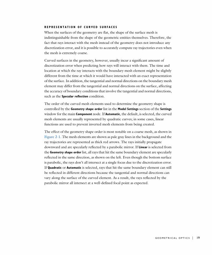
The effect of the geometry shape order is most notable on a coarse mesh, as shown in Figure 2-1. The mesh elements are shown as pale gray lines in the background and the ray trajectories are represented as thick red arrows. The rays initially propagate downward and are specularly reflected by a parabolic mirror. If Linear is selected from the Geometry shape order list, all rays that hit the same boundary element are specularly reflected in the same direction, as shown on the left. Even though the bottom surface is parabolic, the rays don’t all intersect at a single focus due to the discretization error. If Quadratic or Automatic is selected, rays that hit the same boundary element can still be reflected in different directions because the tangential and normal directions can vary along the surface of the curved element. As a result, the rays reflected by the parabolic mirror all intersect at a well-defined focal point as expected.


20 | C H A P T E R

Figure 2-1: Comparison of rays being specularly reflected at a curved boundary represented using linear elements (left) and quadratic elements (right).

R A Y TR A C I N G I N A N I M P O R T E D M E S H

It is also possible to compute ray trajectories in an imported mesh. The mesh can be imported from a COMSOL Multiphysics file (.mphbin for a binary file format or .mphtxt for a text file format) or from a NASTRAN file (.nas, .bdf, .nastran, or .dat).

If the mesh is imported from a COMSOL Multiphysics file, the imported mesh always uses linear geometry shape order for the purpose of modeling ray-boundary interactions, even if the model used to generate the mesh had a higher geometry shape order.

If the mesh is imported from a NASTRAN file, the ray-boundary interactions may be modeled using either linear or higher geometry shape order. If Export as linear elements is selected when generating the NASTRAN file, or if Import as linear elements is selected when importing the file, then linear geometry shape order will be used.

Quantities Computed by the Geometrical Optics Interface

By default, the Geometrical Optics interface declares dependent variables for the components of the ray position and wave vector. It is possible to define first-order differential equations for other dependent variables to be integrated over time or along the trajectory of each ray. An additional variable used to solve a user-defined first-order equation is called an Auxiliary Dependent Variable. It is possible to add an arbitrary


number of auxiliary dependent variables to the Geometrical Optics interface, resulting in an arbitrary number of first-order equations being solved.

In addition, several quantities that are often of interest in geometrical optics applications, such as intensity and phase, are computed using built-in auxiliary dependent variables that can be activated by selecting certain options in the physics interface node’s Settings window.

The following sections describe the quantities that can be computed by changing settings in the Geometrical Optics interface.

I N T E N S I T Y C A L C U L A T I O N

The calculation of ray intensity is controlled by the Intensity Computation setting in the Intensity Computation section of the physics interface node’s Settings window. The intensity is computed when the Intensity Computation is set to Compute intensity, Compute intensity and power, Compute intensity in graded media, or Compute intensity

and power in graded media.

When the ray intensity is computed, settings for specifying the initial ray intensity, wavefront shape, and polarization become available in all release features. It is possible to release polarized, unpolarized, and partially polarized rays. It is also possible to define the wavefront shape so that the ray intensity varies like that of a plane wave, spherical wave, or a wavefront with user-defined principal radii of curvature. These radii of curvature dictate whether the electromagnetic waves are converging or diverging, and the distance to the nearest focus (within the limits of the geometrical optics approximation).

The intensity of a ray is computed using four Stokes parameters that provide the flexibility to specify arbitrary states of polarization when releasing rays. The four Stokes parameters describe the ray intensity that would be observed by sending rays through certain combinations of polarizers and wave retarders. A comprehensive definition of the Stokes parameters is available in The Stokes Parameters in Theory for the Geometrical Optics Interface.

While the Stokes parameters determine the state of polarization of the rays, the magnitude of the intensity also depends on the degree to which a wavefront is converging or diverging. This information is stored by computing the principal radii of curvature of the wavefront. For more information on wavefront radii of curvature, see Principal Radii of Curvature in Theory for the Geometrical Optics Interface.


22 | C H A P T E R

Altogether, to compute the intensity of a wavefront in 3D using the method of principal curvatures, a total of 11 additional degrees of freedom are defined per ray, including the following:

• Four Stokes parameters,

• Two principal radii of curvature,

• Two initial principal radii of curvature, and

• Three components of a unit vector that is used to define a local coordinate system with respect to which the Stokes parameters are defined.

Information about the local coordinate system is needed because such a coordinate system must often undergo transformations when rays interact with boundaries. The coefficients of reflection and transmission depend on the orientation of the electric field of the incident ray with respect to the plane of incidence. In addition, when rays interact with curved boundaries, the reinitialized radii of curvature of the reflected and refracted rays depend on the curvature and orientation of the boundaries.

In 2D, only the four Stokes parameters, one principal radius of curvature, and one initial principal radius of curvature are required, for a total of 6 additional degrees of freedom per ray. The out-of-plane radius is assumed to be arbitrarily large, so all of the rays correspond to planar or cylindrical wavefronts.

In 2D axisymmetric models, the four Stokes parameters, two principal radii of curvature, and two initial principal radii of curvature are allocated for each ray, for a total of 8 additional degrees of freedom per ray. The in-plane and out-of-plane radii of curvature are both permitted to change, allowing rays to interact with boundaries as if they were surfaces of revolution having both in-plane and out-of-plane curvature.

If Compute intensity in graded media is selected, the information about ray intensity and polarization is computed using a total of 8 degrees of freedom in 3D or 5 degrees of freedom in 2D. However, the method of principal curvatures is recommended in most cases, despite requiring more degrees of freedom, because the solution is more accurate when the time step taken by the solver is large. The main advantage of the option Compute intensity in graded media is that it can be used to compute the ray intensity in graded media, in which the refractive index changes continuously, whereas the option Compute intensity is only valid in homogeneous media, where the refractive index is constant within each domain and only changes during ray-boundary interactions.


O P T I C A L P A T H L E N G T H C A L C U L A T I O N

It is possible to define an auxiliary dependent variable for the optical path length by selecting the Compute optical path length check box in the Additional Variables section of the physics interface node’s Settings window. Initially the optical path length is set to 0 for all released rays. It is possible to reset the optical path length to 0 when the rays interact with boundaries.

P H A S E C A L C U L A T I O N

The phase of a ray is necessary for some applications that require information about the instantaneous electric fields of multiple rays, such as interferometers. To define an auxiliary dependent variable for phase, select the Compute phase check box in the Intensity Computation section of the physics interface node’s Settings window. This check box is only available if the ray intensity is computed.

Because enabling the phase allows the instantaneous electric field of a ray to be plotted, phase calculation can be used to visualize the state of polarization of a system of rays.

Figure 2-2: Polarization of the reflected and refracted rays when an unpolarized ray crosses a material discontinuity at the Brewster angle, visualized using a Deformation node.

As shown in Figure 2-2, the polarization of a ray can be visualized when the free-space wavelength is sufficiently large by applying a Deformation node to a Ray Trajectories plot. A deformation proportional to the electric field can then be applied to the rays. The color expression corresponds to the degree of polarization of each ray; because the


24 | C H A P T E R

angle of incidence is equal to the Brewster angle, the reflected ray is completely polarized whereas the refracted ray is not.

A L L O W F R E Q U E N C Y D I S T R I B U T I O N S A T R E L E A S E F E A T U R E S

By default, the ray frequency or free-space wavelength is defined in the Ray Properties Settings window and has the same value for all rays. For some applications, however, it may be useful to model ray propagation over a wide range of frequency values. This can be accomplished by defining a parameter for the ray frequency and adding a Parametric Sweep to the study, but it is often more efficient to model the propagation of rays with a wide range of frequency values simultaneously. This can be accomplished by selecting the Allow frequency distributions at release features check box in the Ray

Release and Propagation section of the physics interface node’s Settings window.

Selecting the Allow frequency distributions at release features check box causes an auxiliary dependent variable to be defined for the ray frequency, enabling a unique frequency value to be assigned to each ray. In the Settings windows for release features it is possible to release either a single ray of a specified frequency or a distribution of frequency values.

C O M P U T I N G D E P O S I T E D R A Y PO W E R

The total power transmitted by a ray depends on the ray intensity and the solid angle subtended by the wavefront. Although the former is computed when the Intensity

computation is set to Compute intensity or Compute intensity in graded media in the Intensity Computation section of the physics interface node’s Settings window, the latter is not.

It is possible to model heat generation on domains or boundaries due to the attenuation or absorption of rays by setting Intensity computation to Compute intensity

and power or Compute intensity and power in graded media. In addition to the auxiliary dependent variables for the Stokes parameters, principal radii of curvature, and principal curvature direction, this option defines a variable for the total power transmitted by a ray. The changes in total ray power due to propagation in absorbing media and interaction with material discontinuities are proportional to the corresponding changes in the ray intensity. However, unlike the ray intensity, the total ray power is unaffected by changes in the principal radii of curvature.

Czerny-Turner Monochromator: Application Library path Ray_Optics_Module/Polychromatic_Light/czerny_turner_monochromator


When the variable for total ray power is computed, it is possible to compute the boundary heat source that is created when rays are absorbed at surfaces using the Deposited Ray Power (Boundary) subnode. In addition, if rays propagate through absorbing media, it is possible to model the changes in ray intensity and power and to compute the heat source resulting from the attenuation of rays. This heat source is automatically used to compute the temperature when The Ray Heating Interface is used. Alternatively, the coupling can be set up manually using the Ray Heat Source multiphysics node.

C O R R E C T I O N S F O R S T R O N G L Y A B S O R B I N G M E D I A

The classical implementation of Snell’s law and the Fresnel equations is valid for ray propagation between media that are non-absorbing or weakly absorbing, meaning that the imaginary part of the refractive index is much smaller in magnitude than the real part of the refractive index. In such cases it can be assumed that the surface in which ray amplitude is constant and the surface in which ray phase is constant are both normal to the direction of ray propagation.

However, in strongly absorbing media, the surfaces of constant amplitude and surfaces of constant phase are not always parallel to each other. As a result, corrections to Snell’s law and the Fresnel equations are required. These corrections can be enabled by selecting the Use corrections for strongly absorbing media check box in the Intensity

Computation section of the physics interface node’s Settings window. This check box is only available if the ray intensity is computed. To store information about the orientation of the surfaces of constant phase, selecting this check box causes three auxiliary dependent variables to be declared in 3D models or two auxiliary dependent variables in 2D models.

D E P E N D E N T V A R I A B L E S C R E A T E D B Y P H Y S I C S F E A T U R E S

The following dependent variables are created by adding specific physics features to the Geometrical Optics interface and changing their settings.

Initial Perturbation for Illuminated SurfacesThe Illuminated Surface feature includes an option to perturb the initial ray direction in order to model the effects of surface roughness. When the Include surface roughness check box is selected in the settings window for at least one Illuminated surface feature, an auxiliary dependent variable is declared. This auxiliary dependent variable is used to initialize the perturbed ray direction vectors.


26 | C H A P T E R

Total Power Transmitted and Reflected at GratingsThe Grating feature is used to model the transmission and reflection of rays at diffraction gratings. It includes a Diffraction Order subnode that can be used to release secondary rays of nonzero diffraction order. When the Intensity computation is set to Compute intensity and power or Compute intensity and power in graded media in the Intensity Computation section of the physics interface settings window, the Store total

transmitted power and Store total reflected power check boxes are shown in the Grating settings window. Selecting either of these check boxes causes an auxiliary dependent variable to be declared, storing the total power of the transmitted and reflected rays of all diffraction orders.

O R D E R O F I N I T I A L I Z A T I O N O F A U X I L I A R Y D E P E N D E N T V A R I A B L E S

When rays are released, the variables defined for each ray are initialized in a specific order. The initial values of ray variables can only depend on the values of variables that have already been defined. The order of dependent variable initialization is governed by the following rules:

• The initial ray position is always determined first.

• By default, user-defined auxiliary dependent variables (that is, those that are defined by adding an Auxiliary Dependent Variable node to the physics interface) are initialized after all other variables. They can instead be initialized immediately after

Diffraction Grating: Application Library path Ray_Optics_Module/

Tutorials/diffraction_grating


the ray position vector components by selecting the Initialize before wave vector

check box shown in all release features.

Figure 2-3: Settings for initializing auxiliary dependent variables before or after other degrees of freedom.

• If more than one user-defined auxiliary dependent variable is present, these variables are initialized in the order in which the corresponding Auxiliary Dependent Variable nodes appear in the Model Builder.

• The remaining degrees of freedom are defined in the following order (each listed group is initialized simultaneously, and the variables within a group cannot reliably be initialized in terms of each other):

- Help variable for the perturbation of initial ray direction at illuminated surfaces,

- Ray frequency,

- The wave vector components, optical path length, and total power transmitted and reflected by gratings,

- The components of the unit vector that indicates the direction corresponding to one of the principal radii of curvature,

- The principal radii of curvature, initial principal radii of curvature, the initial Stokes parameters, and help variables for computing the curvature tensor and intensity, and

- The total power transmitted by the ray.


28 | C H A P T E R

For example, the initial ray direction vector may depend on the ray frequency, but the initial principal radii of curvature may not depend on the total power transmitted by the ray.

Special Variables

The Geometrical Optics interface defines a number of special variables, some of which can only be used during results processing. These variables can be found in the Ray

statistics section in the Add/Replace Expression menus. All of the variables described in this section are preceded by the physics interface Name; see The Geometrical Optics Interface for more information.

The following variables are defined:

• Ray index, pidx. Each ray is assigned a unique index starting from 1 up to the total number of rays. This expression can be passed into a function, which can create random values that are unique for each ray. This is used, for example, to ensure that each ray’s probability of being specularly reflected at a mixed diffuse-specular surface is determined independently of other rays. Suppose a random function has already been defined with name rn1, which takes 2 input arguments. Then a random boundary interaction can be constructed with the expression rn1(pidx,t).

• Ray release feature, prf. If there are multiple release features in a model, it is useful to be able to visualize which rays correspond to each release feature. The Ray release

feature variable takes a numeric value, starting at 1, which is unique to each release feature. This variable can also be used to filter ray trajectories in postprocessing so that only the rays released by a specific feature are shown.

• Ray release time, prt. The Ray release time is the time at which the primary rays are released, which is usually zero for all rays. To allow other release times to be specified, select the Allow multiple release times check box in the physics interface Advanced Settings section.

If the Store ray status data check box is selected in the physics interface Additional

Variables section, then the following additional variables are created:

• The release time of a given ray (variable name rti). This works for secondary rays and thus allows for extraction of the time at which a secondary ray was released. This includes reflected rays at material discontinuities and higher diffraction orders at gratings.

• The time at which a ray stopped at a boundary (variable name st).


• The final status of the ray (variable name fs). This indicates the status of a ray at a given point in time. When used during postprocessing, the value always indicates the status of the ray at the last time step. The value is an integer which has one of the following values:

- 0 for unreleased rays.

- 1 for rays that are still propagating.

- 2 for frozen rays.

- 3 for stuck rays.

- 4 for rays that have disappeared.

• Total number of rays, Nt. This total includes both primary and secondary rays, and includes rays that have disappeared or have not been released.

• Total number of rays in selection, Nsel. If a selection has been applied to the Ray data set, the number of rays in that selection can be evaluated.

• Transmission probability, alpha. The probability of rays reaching a specified domain or boundary selection can be of interest in some Monte Carlo ray tracing calculations. The Transmission probability variable is the ratio of the number of rays in a selection to the total number of rays.

The following variables are found in the Release statistics plot group during results processing.

• Total number of rays released by feature, <tag>.Ntf, where <tag> is the tag of a ray release feature, such as the Inlet or Release from Grid feature. This global variable is uniquely defined for each release feature, and gives the total number of rays that are released by that feature. This includes rays that have disappeared or have otherwise stopped propagating due to interaction with the surrounding boundaries. It does not include any secondary rays.

Using Ray Release Features

Rays that are released using the Geometrical Optics interface are either primary or secondary rays. A ray is considered a primary ray if its initial position and wave vector

The following variables are only defined during results processing and can only be evaluated using the Global Evaluation node under Derived Values. They cannot be plotted as the Color Expression in a Ray Trajectories plot, or used in the equation system.


30 | C H A P T E R

are defined explicitly. A ray is considered a secondary ray if its release is dependent on the behavior of another ray that is already present in the model, which may either be a primary ray or a secondary ray that had been previously released.

For example, when a ray interacts with a Material Discontinuity without undergoing total internal reflection, two rays propagate away from the boundary, including one reflected ray and one refracted ray. The degrees of freedom from the incident ray are re-used as the refracted ray. The additional (reflected) ray that is created during interaction with the Material Discontinuity is a secondary ray because its initial conditions are not specified directly, but instead result from an existing ray interacting with a boundary. The reflected ray may only be released if the total number of released secondary rays in the model is less than the value of the Maximum number of secondary

rays in the settings window for the physics interface.

If the incident ray undergoes total internal reflection, there is no refracted ray, so the incident ray’s degrees of freedom are used to launch the reflected ray and no secondary ray degrees of freedom are used.

The following sections introduce the primary release features that are available in the Geometrical Optics interface.

G R I D - B A S E D R E L E A S E O F R A Y S

Use the Release from Grid feature to specify the initial positions of rays using a grid of points. It is useful to release rays from a grid when the initial ray position is known exactly. A grid-based release may be used, for example, when rays are released from the focus of a lens or when a system is excited by a laser. This is the easiest way to release rays from points in the void region outside the geometry.

M E S H - B A S E D R E L E A S E I N D O M A I N S

Use the Release feature to release rays from within a set of domains. The initial ray positions are based on the mesh elements within the domain. It is possible to assign a nonuniform initial distribution of rays by entering a function of the spatial coordinates in the Density proportional to text field.

R E L E A S E A T B O U N D A R I E S

The Inlet feature is used to release rays from boundaries. It is possible to release rays based on the boundary mesh, by specifying a function for the initial density of rays, or by projecting a grid of points onto the surface. The Inlet feature may be used when rays enter a system through an aperture of considerable size. It is also possible to initialize the principal radii of curvature of the rays using the curvature of the inlet surface.


When a mesh-based or density-based release of rays is used, the initial ray positions may not be the same in all COMSOL Multiphysics versions or when using different geometry kernels. However, when a density-based release is used, the total number of rays can always be specified exactly.

R E L E A S E U S I N G I M P O R T E D D A T A

The Release from Data File node can be used to import the initial ray positions and directions from a text file. It is also possible to import the initial values of user-defined auxiliary dependent variables.

I L L U M I N A T E D S U R F A C E S

Applications of geometrical optics frequently involve plane or spherical waves that reflect or refract off a large surface, then continue to interact with other nearby objects. In such cases, significant reduction in computation time, sometimes 50% or greater, can be achieved by using the Illuminated Surface feature. The Illuminated Surface feature releases the rays that would result from the reflection or refraction of a user-defined plane wave or spherical wave at a surface.

Figure 2-4: Comparison of the ray trajectories and intensity when sending rays at a wall and using a Bounce condition (left) and using the Illuminated Surface feature (right).

As shown in Figure 2-4, the Illuminated Surface feature can be used to compute the ray trajectories that result from launching a plane wave at a specularly reflecting surface. The Stokes parameters and the principal radii of curvature of the wavefront are also


32 | C H A P T E R

initialized based on the type of incident wave and the curvature of the surface. Therefore it is unnecessary to compute the trajectories of rays before they hit the surface, which may save a significant amount of time and make plots much easier to interpret.

S O L A R R A D I A T I O N

The Solar Radiation feature is similar to the Release from Grid feature but includes dedicated settings for computing the direction of incident radiation using the time and location on Earth’s surface. Because rays are given initial radii of curvature of the same order of magnitude as the distance from the earth to the sun, they behave as plane waves in most applications.

Releasing Polarized Rays

The default behavior of the ray release features is to treat the rays as unpolarized plane waves for the purpose of computing intensity and polarization. However, every release feature except the Solar Radiation node is capable of releasing wavefronts that are spherical or ellipsoidal in shape, with varying degrees of polarization.

I N I T I A L R A D I I O F C U R V A T U R E

In the Settings windows for release features, such as the Release, Release from Grid, and Inlet features, change the Wavefront shape setting to control the initial principal radii of curvature of the wavefront. The default setting, Plane wave, sets the initial principal radii of curvature to be approximately 8 orders of magnitude longer than the characteristic length of the geometry. In 2D it is also possible to release cylindrical waves with user-defined principal radii of curvature. The radius of curvature may be interpreted as the distance to a point at which the ray intensity becomes infinite within


the approximations of geometrical optics. This distance is considered positive if the wavefront is converging and negative if the wavefront is diverging.

Figure 2-5: Sign conventions associated with the principal radius of curvature of a cylindrical wave before and after encountering a caustic at point C.

In 3D it is possible to release spherical waves in which both principal radii of curvature are equal. The radii of curvature follow the same sign convention as that for wavefronts in 2D. It is also possible to define the Wavefront shape as an Ellipsoid for which both principal radii of curvature are initialized independently of each other. It is then necessary to define an Initial principal curvature direction e1,0.

Figure 2-6: Settings for specifying the initial radii of curvature in 3D.

The orientation of the wavefront is then defined so that the first principal curvature direction is the radius of the circular arc that is created via the intersection of the wavefront with a plane that contains the ray direction vector and the principal curvature direction vector.


34 | C H A P T E R

Figure 2-7: Interpretation of the two principal radii of curvature and the first principal curvature direction vector in 3D models.

I N I T I A L PO L A R I Z A T I O N

By default, the ray release features release unpolarized rays, but it is also possible to release rays with varying degrees of polarization.

The Stokes parameters of the ray are defined in a local coordinate system with axes parallel to the ray direction vector, the projection of the principal curvature direction vector onto a plane perpendicular to the ray direction vector, and the cross product of these two vectors.

When a Fully polarized or Partially polarized ray is released, select an option from the Initial polarization list: Along principal curvature direction or User defined. For Along

principal curvature direction the initial Stokes parameters is defined in the local coordinate system that is used to define the principal radii of curvature. For User

defined another coordinate system may be selected, and the Stokes parameters are automatically transformed to the coordinate system defined by the principal curvature direction. It is also possible to define a phase difference between the electric field components parallel to and perpendicular to the projection of the reference direction


onto the plane perpendicular to the ray direction vector, resulting in varying degrees of elliptical polarization.

Figure 2-8: Settings for specifying the initial polarization of a fully polarized ray.

Figure 2-9: Comparison of four initial polarization states. From left to right: Polarization parallel to the reference direction, polarization perpendicular to the reference direction, circular polarization, and no polarization.


36 | C H A P T E R

Similar options are available in the settings window for the Illuminated Surface node; the initial radii of curvature and Stokes parameters are then computed from the interaction of incident rays with a surface.

Boundary Conditions

The default boundary condition is the Material Discontinuity condition on all interior and exterior boundaries. For detailed descriptions of the available wall conditions, see Material Discontinuity and Wall.

When several different media are arranged in layers, it is possible for a very large number of secondary rays to be released as the incident ray undergoes a series of reflections between these layers. To prevent the creation of an arbitrarily large number of secondary rays of extremely low intensity, enter a value or expression in the Threshold

intensity text field in the Material Discontinuity settings window. The release of a secondary ray is suppressed if its initial intensity would have been less than the threshold intensity.

The Material Discontinuity node reinitializes ray trajectories whenever a ray crosses the boundary, even if the media on both sides of the boundary are equal. Although the resulting ray trajectories are correct and the unnecessary release of secondary rays can be suppressed, the reinitialization of ray trajectories requires more time than a typical time step in which all rays merely propagate within domains. To minimize solution time it is recommended that unnecessary interior boundaries should be removed from the geometry.

Using Ray Detectors

A Ray Detector feature is a domain or boundary feature that provides information about rays arriving on a set of selected domains or surfaces from a release feature. Such quantities include the number of rays transmitted, the transmission probability, and a logical expression for ray inclusion. The feature provides convenient expressions that can be used in the Filter node of the Ray Trajectories plot, which allows only the rays

The principal curvature direction and polarization reference direction do not need to be perpendicular to the initial ray direction, since their projections onto a perpendicular plane are computed internally. However, they must not be parallel to the initial ray direction vector.


which reach the ray detector selection to be visualized. The following variables are provided by the Ray Detector feature, with the feature tag <tag>:

• <tag>.Ntf is number of transmitted rays from the release feature to the ray detector at the end of the simulation.

• <tag>.alpha is the transmission probability from the release feature to the ray detector.

• <tag>.rL is a logical expression for ray inclusion. This can be set in the Filter node of the Ray Trajectories plot in order to visualize the rays which connect the release feature to the detector.

Creating a Mesh for Geometrical Optics Modeling

A mesh must be present on any boundary that the rays may interact with. In addition, any domains in the selection for the Geometrical Optics interface must be meshed. Domains outside the selection can be left unmeshed. They are assumed to have the same Refractive index of exterior domains that is used to model propagation in the exterior void domain; see the section Domain Selection.

In most cases, the main requirement for a suitable mesh is the resolution on curved surfaces. While the mesh within on flat surfaces may often be very coarse, the mesh on boundaries with small principal radii of curvature must be fine enough so that the direction of the surface normal can be determined accurately; this in turn improves the accuracy of the reinitialized wave vectors of the reflected and refracted rays. If virtual operations are included in the geometry sequence or if any form of mesh deformation is present in the model, then the accuracy of the reinitialized wavefront radii of curvature also depends on the resolution of the mesh on curved boundaries.

To reduce the mesh size on curved surfaces without creating an unnecessarily fine mesh elsewhere, reduce the Curvature factor in the Size settings window in the mesh sequence. A smaller curvature factor gives a finer mesh along curved boundaries. If the curved surfaces are very small relative to the rest of the geometry, it may be necessary to reduce the Minimum element size.

The Ray Detector feature only creates variables, which do not affect the solution. Therefore, they can be added to a model without the need to re-compute the solution, it just needs to be updated. To do this, right click on the Study node and select Update Solution. The new variables described above will be immediately available for results processing.


38 | C H A P T E R

Figure 2-10: Ray trajectories passing through a lens (left). A high-quality mesh (right) should be finer near the curved surface of the lens.

The following features are used to define dependent variables on domains or boundaries: Accumulator (Boundary), Accumulator (Domain), and Deposited Ray Power (Boundary). Because the dependent variables are defined on domain or boundary elements whereas the rays are treated as occupying infinitesimally small points in space, the values of the dependent variables that are created by these features are inherently mesh-dependent. If a very fine mesh is used when one of these features is present, it may be necessary to increase the total number of rays so that the number of rays passing through each mesh element is sufficiently large.

An alternative to using an extremely fine mesh is to manually increase the Geometry

shape order in the settings for the model component. By default, most boundary element surfaces are approximated as quadratic polynomials. Increasing the shape order to Cubic or Quartic can dramatically increase the accuracy of surface normals calculated by the Geometrical Optics interface. However, this may increase the computational cost of other, finite element-based physics interfaces.

Using the Ray Tracing Study Step

The preset study for the Geometrical Optics interface is the Ray Tracing study step. The Ray Tracing study step is similar to the Time Dependent study step but has a different default time step size, includes additional options for specifying a range of time steps, and includes built-in stop conditions for terminating a study when certain criteria are met.

S P E C I F Y I N G A L I S T O F T I M E S T E P S

By default, the Ray Tracing study step computes ray trajectories from t = 0 to t = 1 ns with a time step size of 0.01 ns. However, it is often useful to think of ray tracing in terms of the maximum distance of ray propagation instead of the maximum time. To


express the duration of the study in terms of a maximum optical path length, change the Time step specification setting from the default, Specify time steps, to Specify

maximum path length. Then select a Length unit (default m), enter a set of Lengths (default range(0,0.01,1)), and enter a Characteristic group velocity (default c_const), a built-in constant for the speed of light in a vacuum. With the default solver settings, the time-dependent solver must take at least one time step whenever the optical path length of a ray moving at the Characteristic group velocity would have reached one of the values in the list of Lengths.

B U I L T - I N S T O P C O N D I T I O N S

Select a Stop condition — None (the default), No active rays remaining, or Active rays

have intensity below threshold.

For None the study step does not create any stop conditions, although stop conditions can still be added to the solver sequence manually.

For No active rays remaining the study step ends if no rays are active. A ray is considered active if it has been released but has not reached a boundary with a Freeze, Stick, or Disappear wall condition.

For Active rays have intensity below threshold the study step ends if all remaining active rays have intensity less than the value entered in the Threshold ray intensity text field (default 1[W/m^2]). This option can only be selected if the ray intensity is computed; that is, the Intensity computation is set to Compute intensity or Compute intensity and

power in the Ray Properties section of the physics interface node’s Settings window. This option can be used to prevent computational resources from being wasted by computing the trajectories of rays of negligibly small intensity.

To account for thermal expansion or other types of structural deformation while tracing the rays, use a Moving Mesh (ALE) interface to model the mesh deformation or, for structural mechanics models, select the Include

geometric nonlinearity check box in the study step Study Settings section (requires the Structural Mechanics Module, MEMS Module, or Acoustics Module).


• Ray Tracing



40 | C H A P T E R

Using the Bidirectionally Coupled Ray Tracing Study

The Bidirectionally coupled ray tracing study step is a dedicated study step for ray heating and similar applications. It functions like a Ray tracing study step for the degrees of freedom defined by the Geometrical Optics interface but computes all other degrees of freedom using a Stationary solver. In addition to the settings that are available for the Ray tracing study step, it is possible to specify a Number of iterations. The default value is 5. If the Bidirectionally coupled ray tracing study step is used with The Ray Heating Interface, the following iterative solver loop is automatically set up to compute the ray trajectories and temperature:

1 Solve for the temperature field, assuming that the rays do not generate any heat source.

2 Using the value of the temperature computed during the previous step, compute the ray trajectories and any heat sources that occur due to the attenuation of rays in an absorbing medium.

3 Using the heat source computed in the previous step, compute the temperature field.

4 Alternate between steps 2 and 3 for the specified Number of iterations. Alternatively, the sequence can end when a specified variable converges to within a specified tolerance.

The result of the iterative solver loop is that the heat source generated by the attenuation of rays is taken into account when computing the temperature. If the refractive index of the medium is a expressed as a function of the temperature, then the temperature dependence of the refractive index is taken into account when computing the ray trajectories. Thus, a bidirectional coupling is automatically set up between the two physics interfaces.

It is possible to extend this bidirectional coupling to include other physical effects. For example, the addition of the Solid Mechanics interface and the Thermal Expansion and Temperature Coupling Multiphysics nodes.

To account for thermal expansion or other types of structural deformation while tracing the rays, use a Moving Mesh (ALE) interface to model the mesh deformation or, for structural mechanics models, select the Include

geometric nonlinearity check box in the study step Study Settings section (requires the Structural Mechanics Module, MEMS Module, or Acoustics Module).


Postprocessing Tools

The Ray Optics Module includes several tools for visualizing and analyzing ray trajectories. The following sections describe the dedicated postprocessing tools for the Geometrical Optics interface.

R A Y TR A J E C T O R I E S P L O T

The Ray Trajectories plot can be added to a 2D or 3D plot group. By default, the trajectory of each ray is plotted as a line. As shown in Figure 2-2, it is also possible to apply color expressions and deformations to Ray Trajectories plots.

When the ray intensity is computed, built-in variables for the semi-major and semi-minor axes of the polarization ellipse are declared. For a physics interface with name gop, the semi-major axis has components gop.pax, gop.pay, and gop.paz. The semi-minor axis has components gop.pbx, gop.pby, and gop.pbz.


• Bidirectionally Coupled Ray Tracing



42 | C H A P T E R

Figure 2-11: Polarization ellipses for a circularly polarized ray passing through a series of linear wave retarders with parallel fast axes.

R A Y P L O T

The Ray plot can be added to 1D plot groups. The Ray plot can be used to plot any ray property over time. Built-in data series operations allow quantities like the sum or maximum value of an expression over all rays to be computed easily.

Alternatively, two ray properties can be plotted against each other at a specific time. This can be used, for example, to compare ray intensity versus free-space wavelength, or to view optical path length as a function of radial position in a beam.


Figure 2-12: Reflectance of a distributed Bragg reflector with 21 dielectric layers is plotted as a function of free-space wavelength.

I N T E R F E R E N C E P A T T E R N P L O T

The pattern of fringes resulting from the interference of two or more rays can be plotted using the dedicated Interference Pattern plot. The Interference Pattern plot is available in 2D plot groups and requires a Cut Plane data set pointing to a Ray data set. The interference pattern is then plotted using the locations and properties of rays as they intersect the cut plane.

For the resulting interference pattern to be physically meaningful, it must be plotted over a region with a length scale that is much smaller than the principal radii of curvature of the incident wavefronts. This is equivalent to the assumption that the wavefront associated with each ray subtends a very small solid angle, and is necessary due to the approximation used to compute the incident intensity.


44 | C H A P T E R

Figure 2-13: Interference pattern resulting from two parallel rays with elliptical wavefronts of different principal radii of curvature.

PO I N C A R É M A P S A N D P H A S E PO R T R A I T S

A Poincaré Map can be used to plot the intersection points of rays with a plane. To use the Poincaré Map, a Cut Plane data set must first be defined.

By placing the Cut Plane data set at the image plane of an optical system, it is possible to use the Poincaré Map to create spot diagrams in order to evaluate the performance of the optical system.

A Phase Portrait can be used to plot the positions of rays in an arbitrarily defined phase space. For example, it is possible to plot rays in a 2D space in which one coordinate represents the optical path length and the other coordinate represents intensity.

Computing Monochromatic Aberrations

The Optical Aberration plot and the Aberration Evaluation derived values node are used to analyze the performance of lens systems within the limit of the geometrical optics

Interference Pattern Theory


approach. In order to use the Optical Aberration plot, the following prerequisites must be met:

• The model component must be 3D.

• An instance of the Geometrical Optics interface must be present and solved for.

• The Compute optical path length check box must be selected in the Geometrical Optics Settings window before solving.

• An Intersection Point 3D data set must be created. This data set must point to a Ray data set.

• In the Settings window for the Intersection Point 3D data set, Hemisphere must be selected from the Surface type list. The Center is the location of the focus and the Axis direction points from the focus toward the center of the exit pupil.

Using the hemisphere defined in the Intersection Point 3D data set, a Gaussian reference sphere is defined.

Z E R N I K E PO L Y N O M I A L S

A standard way to quantify monochromatic aberrations is to express the optical path difference of all incident rays as a linear combination of Zernike polynomials.

Several different standards exist for naming, normalizing, and organizing the Zernike polynomials. The approach used in this section follows the standards published by the International Organization for Standardization (ISO, Ref. 2) and the American National Standards Institute (ANSI, Ref. 3).

Each Zernike polynomial can be expressed as

where

• is the normalization term,

• is the radial term,

• is the meridional term or azimuthal term,

• ρ is the radial parameter, given by ρ = r/a where r is the distance from the aperture center and a is the aperture radius, so that 0 ≤ ρ ≤ 1,

• θ is the meridional parameter or azimuthal angle, 0 ≤ θ ≤ 2π,

• the lower index n is a nonnegative integer, n = 0,1,2…, and

• the upper index m is an integer, m = -n,-n+2…n-2,n so that is always even.

Znm

Znm Nn

mRnm ρ( )M mθ( )=

Nnm

Rnm

M mθ( )

n m–


46 | C H A P T E R

The normalization term is

where is the Kronecker delta,

The radial term is given by the equation

where “!” denotes the factorial operator; for nonnegative integers,

The meridional term is given by the equation

The Zernike polynomials thus defined are normalized Zernike polynomials. They are orthogonal in the sense that any pair of Zernike polynomials satisfy the equation

The normalized Zernike polynomials up to fifth order, along with their common names, are given in Table 2-1.

TABLE 2-1: ZERNIKE POLYNOMIALS

TERM EXPRESSION COMMON NAME

Piston

Vertical tilt

Nnm

Nnm 2 δ0 m,–( ) n 1+( )=

δ0 m,

δi j,10

=i j=

i j≠

Rnm ρ( ) 1–( )s n s–( )!

s! 0.5 n m+( ) s–[ ]! 0.5 n m–( ) s–[ ]!---------------------------------------------------------------------------------------------------ρn 2s–

s 0=

0.5 n m–( )

=

n!1

1 2 3 … n××××

=n 0=

n 0>

M mθ( )mθ( )cosm θ( )sin

=m 0≥m 0<

ρ ρ ZnmZn'

m' θd

0

2π

d

0

1

πδn n', δm m',=

Z00 1

Z11– 2ρ θ( )sin


† This term differs from the expression in Table E.1 in ISO 24157:2008 (Ref. 2), which contains an error.

‡ This term differs from the expressions in Table E.1 in ISO 24157:2008 (Ref. 2) and in Annex E in ANSI Z80.28-2010 (Ref. 3), both of which contain an error.

Horizontal tilt

Oblique astigmatism

Defocus

Astigmatism

Oblique trefoil

Vertical coma

Horizontal coma

Horizontal trefoil

Oblique trefoil

Oblique secondary astigmatism

Spherical aberration

Secondary astigmatism

Horizontal trefoil

‡

†

†

‡

TABLE 2-1: ZERNIKE POLYNOMIALS

TERM EXPRESSION COMMON NAME

Z11 2ρ θ( )cos

Z22– 6ρ2 2θ( )sin

Z20 3 2ρ2 1–( )

Z22 6ρ2 2θ( )cos

Z33– 8ρ3 3θ( )sin

Z31– 8 3ρ3 2ρ–( ) 3θ( )sin

Z31 8 3ρ3 2ρ–( ) 3θ( )cos

Z33 8ρ3 3θ( )cos

Z44– 10ρ4 4θ( )sin

Z42– 10 4ρ4 3ρ2–( ) 2θ( )sin

Z40 5 6ρ4 6ρ2– 1+( )

Z42 10 4ρ4 3ρ2–( ) 2θ( )cos

Z44 10ρ4 4θ( )cos

Z55– 12ρ5 5θ( )sin

Z53– 12 5ρ5 4ρ3–( ) 3θ( )sin

Z51– 12 10ρ5 12ρ3– 3ρ+( ) θ( )sin

Z51 12 10ρ5 12ρ3– 3ρ+( ) θ( )cos

Z53 12 5ρ5 4ρ3–( ) 3θ( )cos

Z55 12ρ5 5θ( )cos


48 | C H A P T E R

Figure 2-14: Zernike polynomials on the unit circle.


• Interference Pattern

• Optical Aberration

• Aberration Evaluation

• Ray (Plot)

• Ray Trajectories

• Filter for Ray and Ray Trajectories

• Phase Portrait

• Poincaré Map

• Ray (Data Set) and Data Sets

• Ray Evaluation and Derived Values and Tables

• Plot Groups and Plots


Component Couplings

The purpose of a model is often to compute the sum, average, maximum value, or minimum value of a quantity over a group of rays, such as the average intensity or the maximum path length. An instance of the Geometrical Optics interface with Name <name> creates the following four component couplings:

• <name>.<name>op1(expr) evaluates the sum of the expression expr over the rays. The sum includes all rays that are active, frozen, or stuck to boundaries. It excludes rays that have not yet been released and those that have disappeared.

• <name>.<name>op_all1(expr) evaluates the sum of the expression expr over all rays, including rays those that are not yet released or have disappeared. Since the coordinates of unreleased and disappeared rays are not-a-number (NaN), the sum may return NaN if the model includes unreleased or disappeared rays. An expression such as gop.gopop1(isnan(qx)) can be used to compute the total number of unreleased and disappeared rays.

• <name>.<name>aveop1(expr) evaluates the average of the expression expr over the active, frozen, and stuck rays. Unreleased and disappeared rays contribute to neither the numerator nor the denominator of the arithmetic mean.

• <name>.<name>aveop_all1(expr) evaluates the average of the expression expr over all rays. It is likely to return NaN if the model includes unreleased or disappeared rays.

• <name>.<name>maxop1(expr) evaluates the maximum value of the expression expr over all active, frozen, and stuck rays.

• <name>.<name>maxop_all1(expr) evaluates the maximum value of the expression expr over all rays.

• <name>.<name>minop1(expr) evaluates the minimum value of the expression expr over the active, frozen, and stuck rays.

• <name>.<name>minop_all1(expr) evaluates the minimum value of the expression expr over all rays.

• <name>.<name>maxop1(expr, evalExpr) evaluates the expression evalExpr for the ray that has the maximum value of the expression expr out of all active, frozen, and stuck rays. For example, the expression gop.gopmaxop1(gop.I, qx) would evaluate the x-coordinate qx of the ray with the greatest intensity gop.I.

• <name>.<name>maxop_all1(expr, evalExpr) evaluates the expression evalExpr for the ray that has the maximum value of the expression expr for all rays, including disappeared and unreleased rays.


50 | C H A P T E R

• <name>.<name>minop1(expr, evalExpr) evaluates the expression evalExpr for the ray that has the minimum value of the expression expr out of all active, frozen, and stuck rays. For example, the expression gop.gopminop1(gop.I, qx) would evaluate the x-coordinate qx of the ray with the minimum intensity gop.I.

• <name>.<name>minop_all1(expr, evalExpr) evaluates the expression evalExpr for the ray that has the minimum value of the expression expr for all rays, including disappeared and unreleased rays.

An instance of the Geometrical Optics interface with the default name gop defines the built-in component couplings shown in Table 2-2.

The Ray Optics Materials Database

The Ray Optics Module includes an additional Optical material database. This database includes frequency-dependent refractive index data for a variety of organic and inorganic materials and glasses.

TABLE 2-2: BUILT-IN COMPONENT COUPLINGS FOR THE GEOMETRICAL OPTICS INTERFACE

NAME DESCRIPTION

gop.gopop1(expr) Sum over rays

gop.gopop_all1(expr) Sum over all rays

gop.gopaveop1(expr) Average over rays

gop.gopaveop_all1(expr) Average over all rays

gop.gopmaxop1(expr) Maximum over rays

gop.gopmaxop_all1(expr) Maximum over all rays

gop.gopminop1(expr) Minimum over rays

gop.gopminop_all1(expr) Minimum over all rays

gop.gopmaxop1(expr, evalExpr) Evaluate at maximum over rays

gop.gopmaxop_all1(expr, evalExpr) Evaluate at maximum over all rays

gop.gopmaxop1(expr, evalExpr) Evaluate at minimum over rays

gop.gopmaxop_all1(expr, evalExpr) Evaluate at minimum over all rays

For detailed information about materials see Materials in the COMSOL Multiphysics Reference Manual.


Part Libraries

It is possible to define and store sequences of geometry instructions that can be called multiple times within a model. Such sequences of geometry instructions are called parts, and each appearance of a part in the geometry sequence is called a part instance. It is possible to create, save, and call instances of user-defined parts, which may contain complex combinations of geometry primitives, boolean operations, and programming instructions such as if/else statements.

A part instance can be treated as a highly application-specific geometry primitive that can be used to bypass repetitive tasks during the setup of complicated model geometries consisting of a large number of similar entities. Because parts can be fully parameterized, multiple instances of a single part can be used to create entities of many different sizes and shapes. For example, a single part representing a certain type of lens can be used to create multiple part instances corresponding to lenses of different diameters and focal lengths.

T H E R A Y O P T I C S M O D U L E P A R T L I B R A R Y

Several add-on modules include specialized, built-in parts that are distributed with the installation of COMSOL Multiphysics, similar to the way the Application Library examples are distributed. These can be accessed via the Part Libraries. The Ray Optics Module includes a part library containing standard geometric entities typically used in optics applications, such as the following:

• Spherical lenses

• Cylindrical lenses

• Beam splitters

• Parabolic mirrors

• Prisms

• Retroreflectors

All entities in the built-in Part Libraries are fully parameterized, making them easy to adapt to a wide range of large-scale industrial models.

P A R T V A R I A N T S

Many parts in the Part Library for the Ray Optics Module include several different combinations of parameters, any of which can uniquely specify the size and shape of a part instance. For example, it may be convenient to define the shape of a lens either by specifying its radii of curvature or by entering a focal length. Similarly, parabolic


52 | C H A P T E R

reflectors can be specified either by focal length or by diameter and rim angle. These alternative parameterizations of a single part are called part variants. If a part has two or more variants, then a part variant can be selected when loading the part into the model.

For example, in 3D the part spherical_plano_convex_lens_3d is available. This creates a lens with one convex surface and one flat surface. The lens dimensions can be specified in terms of any of the following combinations of input parameters:

• Diameter d, radius of curvature R, and edge thickness Te

• Diameter d, radius of curvature R, and center thickness Tc

• Diameter d, effective focal length f, refractive index n, and center thickness Tc

If a part supports multiple variants, then a dialog box appears when loading the part into the model. The dialog box in Figure 2-15 is shown when loading the spherical plano-convex lens described in the previous paragraph.

Figure 2-15: Setting to select a part variant when using the Ray Optics Module Part Library.

Part Libraries in the COMSOL Multiphysics Reference Manual


References

1. M. Born and E. Wolf, Principles of Optics, 7th ed., Cambridge, 1999.

2. ISO 24157:2008: Ophthalmic optics and instruments — Reporting aberrations of the human eye. International Organization for Standardization, Geneva, Switzerland.

3. ANSI Z80.28-2010: American National Standard for Ophthalmics — Methods of Reporting Optical Aberrations of Eyes. American National Standards Institute, Alexandria VA.


54 | C H A P T E R

3

R a y O p t i c s

This chapter describes the physics interfaces found under the Optics>Ray Optics

branch ( ).

In this chapter:

• The Geometrical Optics Interface

• Theory for the Geometrical Optics Interface

• The Ray Heating Interface

55

56 | C H A P T E R

Th e Geome t r i c a l Op t i c s I n t e r f a c e

The Geometrical Optics (gop) interface ( ), found under the Optics>Ray Optics

branch ( ) when adding a physics interface, computes the paths of electromagnetic rays. In addition, it can compute the ray intensity, polarization, phase, and optical path length. The physics interface works on geometries, deformed geometries, and with models utilizing ALE.

When this physics interface is added, these default nodes are also added to the Model

Builder—Medium Properties, Material Discontinuity, and Ray Properties. Then, from the Physics toolbar, add other nodes that implement, for example, boundary conditions. You can also right-click Geometrical Optics to select physics features from the context menu.

S E T T I N G S

The Label is the default physics interface name.

The Name is used primarily as a scope prefix for variables defined by the physics interface. Refer to such physics interface variables in expressions using the pattern <name>.<variable_name>. In order to distinguish between variables belonging to different physics interfaces, the name string must be unique. Only letters, numbers, and underscores (_) are permitted in the Name field. The first character must be a letter.

The default Name (for the first physics interface in the model) is gop.

R A Y R E L E A S E A N D P R O P A G A T I O N

The settings in this section affect the way in which primary and secondary rays are released.

Select the Allow frequency distributions at release features check box to allow radiation of multiple different frequency values to be modeled simultaneously. This option allocates an auxiliary dependent variable for the frequency of each ray, so the total number of degrees of freedom increases by 1 per ray. The ray frequency can be specified at release features by entering a value or expression, sampling the frequency from a distribution, or entering a list of values. By default, this check box is cleared so that all rays are assigned the same frequency, which is specified in the Ray Properties settings window.

Enter a value for the Refractive index of exterior domains (dimensionless). The default value is 1. This value of the refractive index is used when tracing rays outside of the

3 : R A Y O P T I C S

domain selection of the Geometrical Optics physics interface. It is also used when rays propagate in the void region outside the geometry. Some limitations apply, as described in the Domain Selection section of the Ray Optics Modeling chapter.

The Maximum number of secondary rays prevents an inordinate number of rays from being generated by capping them at the number supplied in the text field. The default is 500. Rather than being produced directly by release features such as the Release from Grid node, secondary rays are released when an existing ray is subjected to certain boundary conditions. For example, when a ray undergoes refraction at a Material Discontinuity between different media, the incident ray is refracted and a reflected ray is created; the degrees of freedom for this reflected ray are taken from one of the available secondary rays, which are preallocated when the study begins.

If an insufficient number of secondary rays are preallocated, a reflected ray may not be released when an existing ray undergoes refraction, even if some radiation should be reflected at the material discontinuity. However, if a very large number of secondary rays are preallocated, then the number of degrees of freedom may become unnecessarily large. Thus, the Maximum number of secondary rays should be large enough that all reflected rays which significantly affect the solution can be released. Note that rays undergoing total internal reflection at material discontinuities are not considered secondary rays and do not require extra preallocated degrees of freedom.

Secondary rays are also required to release reflected rays of order zero and all higher diffraction orders when the Grating node and Diffraction Order subnodes are used to model the interaction of radiation with diffraction gratings.

I N T E N S I T Y C O M P U T A T I O N

The settings in this section control the treatment of ray intensity and polarization. These settings are also important in multiphysics applications such as ray heating.

Select an option from the Intensity computation list — None (the default), Compute

intensity, Compute intensity and power, Compute intensity in graded media, or Compute

intensity and power in graded media. For None the ray intensity is not computed.

• For Compute intensity auxiliary dependent variables are used to compute the intensity and polarization of each ray. For a complete list of the auxiliary dependent variables that are defined, see Intensity, Wavefront Curvature, and Polarization in Theory for the Geometrical Optics Interface. This option is more accurate and is usually less computationally demanding than Compute intensity in graded media but is only valid for computing intensity in homogeneous (not graded index) media.

T H E G E O M E T R I C A L O P T I C S I N T E R F A C E | 57

58 | C H A P T E R

• For Compute intensity and power the total power transmitted by each ray is defined as an auxiliary dependent variable, in addition to the auxiliary dependent variables that are declared when Compute intensity is selected. The Deposited Ray Power (Boundary) subnode is available for the Wall feature. In addition, if a heat transfer interface such as the Heat Transfer in Solids interface is included in the model, the Ray Heat Source multiphysics node can be used to compute the heat source due to attenuation of rays within domains.

• For Compute intensity in graded media auxiliary dependent variables are used to compute the intensity and polarization of each ray. For a complete list of the auxiliary dependent variables that are defined, see Intensity, Wavefront Curvature, and Polarization in Theory for the Geometrical Optics Interface. This intensity computation method is valid for both homogeneous (constant refractive index) and graded media. If all media are homogeneous then it is recommended to select Compute intensity instead, since it is more accurate.

• For Compute intensity and power in graded media the total power transmitted by each ray is defined as an auxiliary dependent variable, in addition to the auxiliary dependent variables that are declared when Compute intensity in graded media is selected. The Deposited Ray Power (Boundary) subnode is available for the Wall feature. In addition, if a heat transfer interface like the Heat Transfer in Solids interface is included in the model, the Ray Heat Source multiphysics node can be used to compute the heat source due to attenuation of rays within domains. If all media are homogeneous then it is recommended to select Compute intensity and

power instead.

The Compute phase check box is shown when the Intensity computation is set to Compute intensity, Compute intensity and power, Compute intensity in graded media, or Compute intensity and power in graded media. Select the check box to allocate an auxiliary dependent variable for the phase of each ray. When the phase of each ray is computed, it is possible to plot interference patterns and visualize the instantaneous electric field components of polarized rays in postprocessing. When this check box is selected, the total number of degrees of freedom increases by 1 per ray.

The Use corrections for strongly absorbing media check box is shown when the Intensity

computation is set to Compute intensity, Compute intensity and power, Compute intensity

in graded media, or Compute intensity and power in graded media. Select the check box to accurately model reflection and refraction of rays at boundaries between strongly absorbing media, in which the imaginary part of the refractive index is very large. This option allocates two or three auxiliary dependent variables per ray based on space dimension. For more information about the way this option affects the intensity


calculation, see Refraction in Strongly Absorbing Media in Theory for the Geometrical Optics Interface.

When the Intensity computation is set to Compute intensity, Compute intensity and

power, Compute intensity in graded media, or Compute intensity and power in graded

media, enter a value or expression for the Reference intensity (SI unit: W/m2). The reference intensity represents the approximate order of magnitude of the intensity of a typical ray in the model. The default value is 1000 W/m2. It is recommended to change the reference intensity only when modeling systems of rays in which the intensity is many orders of magnitude greater than or less than 1000 W/m2. The reference intensity is used to define numerical tolerances that are used internally by some release features and boundary conditions.

When the Intensity computation is set to Compute intensity in graded media or Compute

intensity and power in graded media enter a Tolerance for curvature tensor computation (dimensionless). This tolerance is used internally when computing the principal radii of curvature of propagating wavefronts in a graded medium. A larger tolerance makes the solution less accurate but more stable.

A D D I T I O N A L V A R I A B L E S

The options in this section can be used to activate additional variables other than those that are used to compute intensity or define the ray frequency. By default, all of the check boxes in this section are cleared, meaning that none of the optional variables are declared.

Select the Compute optical path length check box to allocate an auxiliary dependent variable for the optical path length of each ray. It is possible to reset the optical path length to 0 when rays interact with boundaries.

Select the Store ray status data check box to add new variables for quantities that cannot necessarily be recovered from the ray trajectory data alone. This is especially true if automatic remeshing is used in a model. The following variables are created:

• The release time of a given ray (variable name rti).


60 | C H A P T E R

• The time at which a ray stopped at a boundary (variable name st).

• The final status of the ray (variable name fs). This indicates the status of a ray at the final time step. The value is an integer which has one of the following values:

- 0 for unreleased rays

- 1 for rays that are still in the modeling domain

- 2 for frozen rays

- 3 for stuck rays

- 4 for rays that have disappeared

To summarize the total number of rays having each final status, the following global variables are also defined.

The global variable names in Table 3-1 all take the unreleased secondary rays into account. For example, suppose an instance of the Geometrical Optics interface includes 100 primary rays and 100 allocated secondary rays. At the last time step, suppose that 80 of the primary rays have disappeared at boundaries and that 40 secondary rays have been emitted, all of which are still active. Then the variable gop.fac, the fraction of active rays at the final time step, would have the value (20 + 40)/(100 + 100) or 0.3.

A D V A N C E D S E T T I N G S

This section is only shown when Advanced Physics Options are enabled (click the Show button on the Model Builder).

The Wall accuracy order sets the accuracy order of the time stepping used for time steps during which a ray-wall interaction happens. Select an order of 1 to use a forward Euler step and compute the motion both before and after the wall interaction. Select an order of 2 (the default) to use a second-order Taylor method to compute the trajectory before the wall interaction. After the ray-wall interaction a second-order Runge-Kutta method is used.

TABLE 3-1: GLOBAL VARIABLES BASED ON RAY STATUS

NAME DESCRIPTION

fac Fraction of active rays at final time step

fds Fraction of disappeared rays at final time step

ffr Fraction of frozen rays at final time step

fse Fraction of secondary rays released

fst Fraction of stuck rays at final time step


Select an option from the Arguments for random number generation list — Generate

unique arguments (the default), Generate random arguments, or User defined. This setting determines how the additional argument to random functions is defined in features such as the Wall boundary condition with the Diffuse scattering wall condition. Typically the random numbers are functions of the ray index, position, time, and another argument i, defined as follows:

• For Generate unique arguments the additional argument is based on the position of each node in the Model Builder. As a result, random numbers generated in different nodes are created independently of each other, but the same result can be reproduced by running the same study several times.

• For Generate random arguments the additional argument is randomly created, causing the random functions to return different results each time the study is run.

• For User defined the additional argument is defined by a user input in the Settings window for each feature. Independent solutions can be obtained by running a parametric sweep for different values of i.

By default the Allow propagation outside selected domains check box is selected. When this check box is selected, rays can propagate in domains that are not included in the selection for the physics interface. These exterior domains do not need to be meshed. Rays can even propagate through the void region outside the geometry. However, all boundaries that the rays interact with must be meshed.

If a boundary condition is applied to a surface that is not adjacent to any domains in the selection for the physics interface, the default meshing algorithm will automatically create a boundary mesh as needed.

The Allow multiple release times check box, which is cleared by default, allows an array of release times for the rays to be specified in any of the ray release features. If the check box is cleared, all rays are released at time t = 0.

Enter a value for the Maximum number of wall interactions per time step. The default value is 1000. If a ray undergoes more than the specified number of boundary

There are a variety of ways to make rays propagate outside the geometry. The most straightforward ways are to use the Release from Grid feature and specify initial coordinates that are not within any domain. Alternatively, rays can escape from a domain into the exterior of the physics interface selection due to the Material Discontinuity boundary condition on exterior boundaries.


62 | C H A P T E R

interactions in a single time step taken by the solver, the ray will disappear. This is included as a safeguard to prevent rays from getting stuck in infinite loops if the time between successive ray-wall interactions becomes infinitesimally small.

D E P E N D E N T V A R I A B L E S

The dependent variables (field variables) are the components of the Ray position and Wave vector. The name can be changed but the names of fields and dependent variables must be unique within a model.

Domain, Boundary, and Global Nodes for the Geometrical Optics Interface

The Geometrical Optics Interface has these domain, boundary, and global nodes and subnodes (listed in alphabetical order) available from the Physics ribbon toolbar (Windows users), Physics context menu (Mac or Linux users), or right-click to access the context menu (all users).

• Domain, Boundary, and Global Nodes for the Geometrical Optics Interface

• Theory for the Geometrical Optics Interface

In general, to add a node, go to the Physics toolbar, no matter what operating system you are using. Subnodes are available by clicking the parent node and selecting it from the Attributes menu.



Medium Properties

Use the Medium Properties node to specify the refractive index of the medium.

• Accumulator (Boundary)

• Accumulator (Domain)

• Auxiliary Dependent Variable

• Axial Symmetry

• Circular Wave Retarder

• Deposited Ray Power (Boundary)

• Deposited Ray Power (Domain)

• Diffraction Order

• Grating

• Ideal Depolarizer

• Illuminated Surface

• Inlet

• Inlet on Axis

• Linear Polarizer

• Linear Wave Retarder

• Material Discontinuity

• Medium Properties

• Mueller Matrix

• Nonlocal Accumulator

• Photometric Data Import

• Ray Continuity

• Ray Detector

• Ray Properties

• Ray Termination

• Release

• Release from Data File

• Release from Edge

• Release from Grid

• Release from Grid on Axis

• Release from Point

• Release from Point on Axis

• Solar Radiation

• Thin Dielectric Film

• Wall



64 | C H A P T E R

M E D I U M P R O P E R T I E S

The default Refractive index n (dimensionless) uses values From material. For User

defined enter a value or expression. Only ray propagation in isotropic media can be modeled with the Geometrical Optics interface.

If the Intensity computation is set to Compute intensity, Compute intensity and power, Compute intensity in graded media, or Compute intensity and power in graded media under the physics interface Intensity Computation section, specify the Refractive index,

imaginary part k (dimensionless). By default the Refractive index, imaginary part k uses values From material. For User defined enter a value or expression. The convention followed by the Geometrical Optics interface is that an the imaginary part of the refractive index is negative in absorbing media. A positive value indicates a gain medium, meaning that the ray intensity will typically increase along the ray trajectory.

The refractive index can be a function of variables that are defined on the rays or on the domains. However, to make the refractive index a function of a ray property such as frequency or free-space wavelength, the ray variable must be enclosed in the noenv() operator. For example, to make the refractive index a linear function of the free-space wavelength, enter an expression such as 1.5-0.01*noenv(gop.lambda0/1[um]).

Wall

Use the Wall node to determine what happens to the rays when contact with a boundary is made.

The Accumulator (Boundary) subnode is available from the context menu (right-click the parent node) or from the Physics toolbar, Attributes menu. If the Intensity


in graded media, or Compute intensity and power in graded media under the physics interface Intensity Computation section, the Thin Dielectric Film subnode is also available. If the Intensity computation is set to Compute intensity and power or Compute

intensity and power in graded media, the Deposited Ray Power (Boundary) subnode is also available.


WA L L C O N D I T I O N

Select a Wall condition — Freeze (the default), Specular Reflection, Stick, Disappear, Pass

through, Diffuse scattering, Mixed diffuse and specular reflection, or General reflection.

TABLE 3-2: WALL CONDITION OPTIONS

OPTIONS DESCRIPTION

Freeze Select to fix the ray position and wave vector at the instant a wall is struck. So, the ray position no longer changes after contact with the wall and the wave vector of the ray remains at the same value as when the ray struck the wall. This boundary condition is typically used to recover the ray intensity or phase at the instant contact was made with the wall.

Specular Reflection

Select to specularly reflect from the wall. Reinitialization of the principal radii of curvature of the reflected ray is consistent with the algorithms used for reflected rays at material discontinuities. This means, for example, that the ray intensity may become very large or very small in magnitude after being specularly reflected by a curved surface, depending on the concavity.

Stick Select to fix the ray position at the instant the wall is struck. The wave vector components are set to zero.

Disappear This option means that the ray is not displayed once it has made contact with the wall. Use it if the ray location after contact with the wall is not of interest.

Pass through This option allows rays to cross the boundary unimpeded.

The Pass Through condition does not cause rays to be refracted at the boundary between different materials. If used at the boundary between two different media, it is possible for the resulting rays to undergo a non-physical change in angular frequency and wave vector magnitude. To model refraction, instead use the Material Discontinuity node.

Diffuse scattering

Select to reflect rays at a wall according to Lambert’s cosine law. That is, the probability of a reflected ray propagating in a given direction within a solid angle dω is given by cos(θ)dω where θ is the angle between the direction of the ray and the wall normal.

Mixed diffuse and specular reflection

Select to reflect rays at a wall either specularly or according to Lambert’s cosine law, based on a user-defined probability. By combining this wall condition with a Primary ray condition, it is possible to include up to three different types of ray-wall interactions at a single boundary.

General reflection

Select to allow an arbitrary direction vector to be specified after a ray makes contact with the wall. The ray direction vector components can be functions of the incident ray direction, phase, or any other quantity.


66 | C H A P T E R

G E N E R A L R E F L E C T I O N S E T T I N G S

This section is available when General reflection (see Table 3-2) is selected as the Wall

condition.

Enter values for the Reflected ray direction vector Lp (dimensionless) either in Cartesian coordinates (x, y, z) (the default) or select the Specify tangential and normal direction

vector components check box to enter coordinates in the tangent-normal coordinate system (t1, t2, n). In this case the normal direction is selected so that an incident ray is reflected back into the domain it previously occupied if the specified normal direction vector component is positive. The tangential directions are oriented so that they form a right-handed coordinate system, together with the normal direction.

P R I M A R Y R A Y C O N D I T I O N

Select a Primary ray condition — None (the default), Probability, or Expression. When the default, None, is kept, it means that the Wall condition is always respected by the incident rays.

ProbabilityIf Probability is selected, the Wall condition is applied with a certain probability. Enter a value for the Probability, γ (dimensionless). If the Wall condition is not used, the ray instead behaves according to the Otherwise setting.

For example, if the Wall condition is set to:

• Freeze and γ is set to 0.1, then for every 10 rays that strike the wall, on average one freezes and the remaining 9 rays behave according to the Otherwise setting.

• Stick and γ is set to 0.5 then on average half of the rays stick to the wall and the other half behave according to the Otherwise setting.

ExpressionIf Expression is selected, the Evaluation expression e (dimensionless) is evaluated whenever a ray strikes the wall. The default expression is 1. If the Evaluation expression is nonzero, the ray behaves according to the Wall condition, otherwise the ray behaves according to the Otherwise setting.

The value of γ should always be between 0 and 1.


OtherwiseThe options available for the Otherwise setting are the same as for the Wall Condition, except that General reflection and Mixed diffuse and specular reflection are not available. The Otherwise setting can be used to make rays interact with a wall differently with a certain probability or when a certain condition is satisfied. For example, to model reflection at a partially specular surface in which 50% of the ray intensity is absorbed and 30% is reflected specularly:

• Select Mixed diffuse and specular reflection as the Wall condition,

• set the Probability of specular reflection to 0.3/(1-0.5),

• set the Primary ray condition to Probability,

• set the Probability to 1-0.5, and

• select Freeze as the Otherwise option.

A B S O R P T I O N C O E F F I C I E N T

This section is available when

• the Intensity computation is set to Compute intensity, Compute intensity and power, Compute intensity in graded media, or Compute intensity and power in graded media under the physics interface Intensity Computation section, and

• the Wall condition is set to Specular Reflection, Diffuse scattering, General reflection, or Mixed diffuse and specular reflection.

Select one of the following from the Compute reflected intensity using list: Absorption

coefficients or Reflection coefficients.

For Absorption coefficients enter the Absorption coefficient α (dimensionless). The default is 0. The intensity of the reflected ray will be proportional to 1-α.

For Reflection coefficients enter the Reflection coefficient r (dimensionless). The default value is 1. The intensity of the reflected ray will be proportional to r2.

If the Wall condition is set to Mixed diffuse and specular reflection, this section is instead called Absorption Coefficients and the absorption coefficients for the diffusely and specularly reflected rays are specified separately. All of the text fields are given subscripts s and d for specularly and diffusely reflected rays, respectively.

N E W VA L U E O F A U X I L I A R Y D E P E N D E N T VA R I A B L E S

This section is available if an Auxiliary Dependent Variable has been added to the model.


68 | C H A P T E R

When a ray crosses or touches a boundary, the value of any user-defined auxiliary dependent variable can be changed. The value can be a function of any combinations of ray variables and variables defined on the boundary. A simple application is to use this to count the number of times a ray strikes the wall.

Select the Assign new value to auxiliary variable check box or boxes based on the number of auxiliary variables in the model. Then enter the new value or expression in the field. For example, if there is an auxiliary variable, psi, then enter a value for psinew in the field. So, to increment the value of psi by 1 when a ray touches or crosses a boundary, enter psi+1 in the text field for psinew.


If the Primary ray condition is set to Probability, or if the Diffuse scattering or Mixed

diffuse and specular reflection wall condition is used, then the Wall feature generates random numbers.

If, in addition, the Arguments for random number generation setting is set to User defined in the physics interface Advanced Settings section, the Advanced Settings section is available.

Enter the Additional input argument to random number generator i (dimensionless). The default value is 1.

The Advanced Settings section is also shown if the Compute optical path length check box is selected under the physics interface Additional Variables section. Select the Reset

optical path length check box to set the optical path length to 0 when a ray touches the wall.

Axial Symmetry

The Axial Symmetry node is automatically added to 2D axisymmetric models. The options available for the feature are the same as for Wall, except as follows. The Boundary Selection is locked and is only applicable to the symmetry axis. The only wall conditions available are Specular Reflection (the default), Freeze, Stick, and Disappear. In addition, the Primary Ray Condition section is not included. The Axial Symmetry


boundary condition does not affect ray intensity or polarization, except to introduce a phase delay of π to compensate for the change in the principal curvature direction.

Accumulator (Boundary)

The Accumulator subnode is available from the context menu (right-click the Wall or Material Discontinuity parent node) or from the Physics toolbar, Attributes menu. Each Accumulator subnode defines a variable, called the accumulated variable, on each boundary element in the selection of the parent node. The accumulated variables are incremented when rays interact with the boundaries where they are defined.

A C C U M U L A T O R S E T T I N G S

Select an option from the Accumulator type list — Density (default) or Count.

• For Density the accumulated variable is divided by the surface area of the boundary element where it is defined.

• For Count the accumulated variable is the sum of the source terms of all rays that hit the boundary element, and is unaffected by the boundary element size.

Select an option from the Accumulate over list — Ray-wall interactions (the default) or Rays in boundary elements.

• For Ray-wall interactions the accumulated variable is affected by all rays that hit the boundary element.

• For Rays in boundary elements the accumulated variable is only affected by rays that freeze or stick to the boundary element.

The Axial Symmetry condition only applies to straight boundaries that are both on the axis of symmetry and adjacent to a domain in the selection of the physics interface. If rays are propagating in the void region outside of the selected domains, it is possible for the rays to enter the region where r < 0, even though no geometry is defined there.

To ensure that rays cannot propagate into the region where r < 0, draw line segments on the parts of the symmetry axis where no geometric entities exist, then add the Wall node to these edges. Keep in mind that rays can only be subjected to boundary conditions if the corresponding boundaries are meshed.


70 | C H A P T E R

Enter the Accumulated variable name. The default is rpb. The accumulated variable is defined as <scope>.<name>, where <scope> includes the name of the physics interface node, parent boundary condition, and the Accumulator node, and <name> is the accumulated variable name.

For example, if the Accumulator subnode is added to a Wall node in an instance of the Geometrical Optics interface using the default variable name rpb, the accumulated variable name might be gop.wall1.bacc1.rpb.

Enter a Source R. The unit of the source term depends on the settings in the Units section. Whenever a ray collides with a boundary element in the selection of the parent node, the accumulated variable in that element is incremented by the source term. If the Accumulator type is set to Density, the source term is divided by the area of the boundary element (in 3D) or the length of the boundary element (in 2D).

For example, if the source is 1 and Count is selected from the Accumulator type list, a variable is created to store the number of times each boundary element is hit by a ray.

U N I T S

Select a Dependent variable quantity from the list; the default is Dimensionless [1]. To enter a unit, select None from the list and in the Unit field enter a value, for example, K, m/s, or mol/m^3.

S M O O T H I N G

The accumulated variables are computed using discontinuous shape functions. Select the Compute smoothed accumulated variable check box to compute a smoothed accumulated variable by computing the average value of the variable within a sphere of a user-defined radius. Then enter a Smoothing radius r (SI unit: m). The default is 0.1[m].

Material Discontinuity

The Material Discontinuity node is the default boundary feature on all boundaries. It computes the initial direction of the refracted ray using Snell’s law. If extra degrees of freedom have been allocated for secondary rays, a reflected ray is also produced. If the

Accumulator Theory: Boundaries


incident ray undergoes total internal reflection, no refracted ray is produced and no secondary rays are needed to release the reflected ray.

If Intensity computation is set to Compute intensity, Compute intensity and power, Compute intensity in graded media, or Compute intensity and power in graded media in the physics interface Intensity Computation section, the Material Discontinuity feature computes the radii of curvature and the Stokes parameters of the reflected and refracted rays.

The Accumulator (Boundary) subnode is available from the context menu (right-click the parent node) or from the Physics toolbar, Attributes menu. The Thin Dielectric Film subnode is also available if the following conditions are met:

• One of the following options is selected from the Intensity computation list in the physics interface Intensity computation section: Compute intensity, Compute intensity

and power, Compute intensity in graded media, or Compute intensity and power in

graded media.

• One of the following options is selected from the Thin dielectric films on boundary list in the Coatings section: Add layers to surface or Add layers to surface, repeating.

C O A T I N G S

This section is available if Intensity computation is set to Compute intensity, Compute

intensity and power, Compute intensity in graded media, or Compute intensity and power

in graded media under the Intensity Computation section for the physics interface. Use the options in this section to add thin dielectric layers to the boundary between the media. These thicknesses of these layers should be small relative to the coherence length of the radiation, and is often comparable in length scale to the free-space wavelength.

Select an option from the Thin dielectric films on boundary list — None (the default), Add layers to surface, Add layers to surface, repeating, Anti-reflective coating, Single-layer

coating, specified thickness, Single-layer coating, specified reflectance, or Single-layer

coating, specified transmittance.

• If None is selected, rays undergo reflection and refraction at the boundary as if there were no dielectric films present.

The maximum number of reflected rays can be controlled via the Maximum number of secondary rays text field, which is found under the Ray

Release and Propagation section for the physics interface.


72 | C H A P T E R

• If Add layers to surface is selected, apply thin dielectric layers to the Material

Discontinuity by adding one or more Thin Dielectric Film subnodes. If multiple thin films are added to a single surface, they are arranged in the same order as the corresponding Thin Dielectric Film subnodes in the Model Builder.

• If Add layers to surface, repeating is selected, apply thin dielectric layers to the Material Discontinuity by adding one or more Thin Dielectric Film subnodes. Also enter a value or expression for the Number of repeating unit cells N (dimensionless). The default value is 3. It is possible to choose which individual layers are included in the repeating unit cell and which layers only appear once in the settings for the Thin Dielectric Film subnodes. Use this option to specify periodic arrangements of dielectric layers for structures such as dielectric mirrors.

• If Anti-reflective coating is selected, enter a value or expression for the Vacuum

wavelength for specified film properties λ0 (SI unit: m). The default value is 660 nm. Enter a value or expression for the Angle of incidence for specified film properties θi (SI unit: rad). The default value is 0. Select an option from the Specified film

behavior applies to list — S-polarized radiation (the default) or P-polarized radiation. Select an option from the Specified film behavior applies to list — With respect to

upside (the default) or With respect to downside.

• If Single-layer coating, specified thickness is selected, enter a value or expression for the Film refractive index n (dimensionless). The default value is 1. Then enter a value or expression for the Film thickness t (SI unit: m). The default value is 1 μm.

• If Single-layer coating, specified reflectance is selected, select an option from the Specified film behavior applies to list — S-polarized radiation (the default) or P-polarized radiation. Select an option from the Specified film behavior applies to list — With respect to upside (the default) or With respect to downside. In addition, enter values or expressions for the following:

- Film refractive index n (dimensionless). The default is 1.

- Reflectance R (dimensionless). The default is 0.1.

- Vacuum wavelength for specified film properties λ0 (SI unit: m). The default is 660 nm.

- Angle of incidence for specified film properties θi (SI unit: m). The default is 0.

• If Single-layer coating, specified transmittance is selected, select an option from the Specified film behavior applies to list — S-polarized radiation (the default) or P-polarized radiation. Select an option from the Specified film behavior applies to list


— With respect to upside (the default) or With respect to downside. In addition, enter values or expressions for the following:

- Film refractive index n (dimensionless). The default is 1.

- Transmittance T (dimensionless). The default is 0.9.

- Vacuum wavelength for specified film properties λ0 (SI unit: m). The default is 660 nm.

- Angle of incidence for specified film properties θi (SI unit: m). The default is 0.

The option Anti-reflective coating automatically computes the refractive index and thickness of a single-layer dielectric coating to yield zero reflectance for the specified free-space wavelength, polarization, and angle of incidence. Similarly, the options Single-layer coating, specified reflectance and Single-layer coating, specified transmittance automatically compute the thickness of a dielectric layer of the specified refractive index to yield the specified reflectance or transmittance.

If the material properties on either side of the material discontinuity differ, rays with the same angle of incidence will be subjected to different reflectances, depending on which domain they approach the boundary from. Use the Specified film behavior applies

to list to determine whether the specified reflectance applies to rays incident from the upside or downside of the boundary. It is convenient to select the Show boundary

normal check box (see Advanced Settings below) when identifying the upside and downside of the boundary, since the boundary normal points from the upside to the downside.

T H R E S H O L D I N T E N S I T Y

This section is available if Intensity computation is set to Compute intensity, Compute

intensity and power, Compute intensity in graded media, or Compute intensity and power

in graded media under the Intensity Computation section for the physics interface.

Enter a Threshold intensity Ith (SI unit: W/m2). The default is 1·10-3 W/m2. If the interaction of a ray with a material discontinuity would create a reflected ray of intensity less than the threshold intensity, the release of this reflected ray is suppressed. This prevents an arbitrarily large number of degrees of freedom from being used to model the propagation of rays of exponentially decreasing intensity. When a nonzero threshold intensity is specified, some small decreases in the total energy of the system may be observed if the release of low-intensity secondary rays is suppressed.


74 | C H A P T E R

A U X I L I A R Y D E P E N D E N T V A R I A B L E S , R E F R A C T E D R A Y

If an Auxiliary Dependent Variable has been added to the model then there is an option to reinitialize the values of auxiliary dependent variables for the refracted ray. These setting are the same as in the New Value of Auxiliary Dependent Variables section for the Wall feature.

A U X I L I A R Y D E P E N D E N T V A R I A B L E S , R E F L E C T E D R A Y

If an Auxiliary Dependent Variable has been added to the model then there is an option to reinitialize the values of auxiliary dependent variables for the reflected ray. These setting are the same as in the New Value of Auxiliary Dependent Variables section for the Wall feature.


Select the Show boundary normal check box to view the boundary normal in the Graphics window.

If the Compute optical path length check box is selected in the physics interface Additional Variables section, select the Reset optical path length check box to set the optical path length of reflected and refracted rays to 0. Otherwise both the reflected and refracted ray inherit the optical path length of the incident ray.

Thin Dielectric Film

Use the Thin Dielectric Film subnode to model the interaction of rays with walls or material discontinuities that are coated with thin, transparent dielectric layers. The thickness of the film should be of approximately the same order of magnitude as the wavelength of the ray. The subnode is available from the context menu (right-click the Material Discontinuity or Wall parent node) or from the Physics toolbar, Attributes menu.

Visualization of the boundary normal is important when adding multiple Thin Dielectric Film subnodes, since the thin films are oriented from the upside of the boundary to the downside in the same order as displayed in the Model Builder.

Material Discontinuity Theory


The Thin Dielectric Film subnode is applied to all boundaries in the selection of the Wall or Material Discontinuity parent node. The effects of the Thin Dielectric Film subnodes are applied when computing the coefficients of reflection and transmission, which are necessary for the reinitialization of Stokes parameters during reflection and refraction when Intensity computation is set to Compute intensity, Compute intensity and power, Compute intensity in graded media, or Compute intensity and power in graded media under the Intensity Computation section for the physics interface

F I L M P R O P E R T I E S

Enter a Film refractive index n (dimensionless). The default value is 1. Then enter a Film

thickness t (SI unit m). The default is 1 μm.

R E P E A T I N G M U L T I L A Y E R F I L M S

If Add layers to surface, repeating is selected from the Thin dielectric films on boundary list in the Coatings section in the settings window for the parent node, this section is used to determine which layers are part of the repeating unit cell of a periodic multilayer film. If the Repeat layer in multilayer films check box is selected, the layer is repeated a number of times equal to the Number of repeating unit cells specified in the parent node settings window. If the check box is cleared, the layer will appear only once in multilayer films.

Ray Properties

The behavior of the Ray Properties node is based on whether the Allow frequency

distributions at release features check box is selected under the physics interface Ray

Release and Propagation section.

By default, the check box is not selected. Then the Ray Properties node is used to specify the free-space wavelength or frequency of the rays. When the check box is selected, the ray frequency is specified in the individual release features.

R A Y P R O P E R T I E S

This section is shown when the Allow frequency distributions at release features check box is cleared in the physics interface Ray Release and Propagation section.

Thin Dielectric Film Theory


76 | C H A P T E R

Select an option from the Ray property specification list — Specify vacuum wavelength (the default) or Specify frequency.

• For Specify vacuum wavelength enter a Vacuum wavelength λ0 (SI unit: m). The default is 660 nm.

• For Specify frequency enter a Ray frequency v (SI unit: Hz). The default is 4.54 × 1014 Hz.

Photometric Data Import

Use the Photometric Data Import node to import photometric data files that can be used to initialize the ray intensity and power as a function of the initial ray direction. The Photometric Data Import node supports the *.ies file extension, the standard photometric data file format of the Illuminating Engineering Society of North America (IESNA).

P H O T O M E T R I C D A T A I M P O R T

Enter a File name, or click the Browse button to locate a photometric data file. When a valid file path has been entered, click the Import button to load the photometric data into the model.

The Photometric Data Import node is only available in 3D.

It is also only available when Compute intensity, Compute intensity and

power, Compute intensity in graded media, or Compute intensity and power

in graded media is selected from the Intensity computation list in the physics interface Intensity Computation section.


If photometric data has already been loaded by the Photometric Data Import feature, instead click the Discard button to discard this data and clear the File name field.

Photometric Data FormattingThe format of the imported photometric data file must be consistent with ANSI/IESNA LM-63-02 (R2008), IESNA Standard file format for the electronic transfer of photometric data and related information, Illuminating Engineering Society (2002).

Release

Use the Release node to release rays within domains based on arbitrary expressions or based on the positions of the mesh elements.

R E L E A S E T I M E S

Enter Release times (SI unit: s) or click the Range button ( ) to select and define a range of specific times. At each release time, rays are released with initial position and ray direction vector as defined next.

After creating an instance of the Photometric Data Import feature and loading an appropriately formatted IES file into the model, initialize the ray intensity as a function of initial ray direction by changing the following settings in a ray release feature such as the Release or Release from Grid feature:

• Select Spherical, Hemispherical, Conical, or Lambertian from the Ray

direction vector list in the physics feature Ray Direction Vector section.

• Locate the Total Source Power section. From the Intensity initialization list, select an instance of the Photometric Data Import feature.

• Enter values or expressions for the Photometric horizontal and Photometric zero directions.

This section is only available when the Allow multiple release times property is active. This can be found in the Advanced section of the physics interface settings when Advanced Physics Options are shown in the Model Builder.


78 | C H A P T E R

I N I T I A L PO S I T I O N

Select an Initial position — Density (the default) or Mesh based.

DensityFor Density enter a value for the Number of rays per release N and the Density

proportional to ρ. Both are dimensionless numbers.

The Density proportional to ρ is an expression — the resulting ray distribution approximately has a density that is proportional to this expression. The resulting distribution looks a bit random, and it depends on the order in which the mesh elements are numbered. The distribution is probably not exactly the same in different COMSOL Multiphysics versions, but the total number of rays released is always N.

Select a Release distribution accuracy order between 1 and 5 (the default is 5), which determines the integration order that is used when computing the number of rays to release within each mesh element. The higher the accuracy order, the more accurately rays will be distributed among the mesh elements.

The Position refinement factor (default 0) must be a nonnegative integer. When the refinement factor is 0, each ray is always assigned a unique position, but the density is taken as a uniform value over each mesh element. If the refinement factor is a positive integer, the distribution of rays within each mesh element is weighted according to the density, but it is possible for some rays to occupy the same initial position. Further increasing the Position refinement factor increases the number of evaluation points within each mesh element to reduce the probability of multiple rays occupying the same initial position.

Mesh BasedFor Mesh based the rays are released from a set of positions determined by a selection of geometric entities (of arbitrary dimension) in the mesh. Given a Refinement factor between 1 and 5, the centers of the refined mesh elements are used. Thus, the number of positions per mesh element is refine^dim, except for pyramids, where it is (4*refine2-1)*refine/3.

The Density proportional to expression must be strictly positive.


R A Y D I R E C T I O N VE C T O R

Select an option from the Ray direction vector list — Expression (the default), Spherical, Hemispherical, Conical, or Lambertian (3D only).

• For Expression a single ray is released in the specified direction. Enter coordinates for the Ray direction vector L0 (dimensionless) based on space dimension.

• For Spherical a number of rays are released at each point, sampled from a spherical distribution in wave vector space. Enter the Number of rays in wave vector space Nw (dimensionless). The default is 50.

• For Hemispherical a number of rays are released at each point, sampled from a hemispherical distribution in wave vector space. Enter the Number of rays in wave

vector space Nw (dimensionless). The default is 50. Then enter coordinates for the Hemisphere axis r based on space dimension.

• For Conical a number of rays are released at each point, sampled from a conical distribution in wave vector space. Enter the Number of rays in wave vector space Nw (dimensionless). The default is 50. Then enter coordinates for the Cone axis r based on space dimension. Then enter the Cone angle α (SI unit: rad). The default is π/3 radians.

• The Lambertian option is only available in 3D. Anumber of rays are released at each point, sampled from a hemisphere in wave vector space with probability density based on the cosine law. Enter the Number of rays in wave vector space Nw (dimensionless). The default is 50. Then enter coordinates for the Hemisphere axis r based on space dimension.

If Conical is selected, select an option from the Conical distribution list — Uniform

density (the default), Specify polar and azimuthal distributions, Marginal rays only, or Marginal and axial rays only.

• For Uniform density rays are released with polar angles from 0 to the specified cone angle. The rays are distributed in wave vector space so that each ray subtends approximately the same solid angle.

• For Specify polar and azimuthal distributions specify the Number of polar angles Nφ (dimensionless) and the Number of azimuthal angles Nθ (dimensionless). Rays are released at uniformly distributed polar angles from 0 to the specified cone angle. A single axial ray (φ = 0) is also released. For each value of the polar angle, rays are released at uniformly distributed azimuthal angles from 0 to 2π. Unlike other options for specifying the conical distribution, it is not necessary to directly specify the Number of rays in wave vector space Nw (dimensionless), which is instead derived from the relation .Nw Nφ Nθ 1+×=


80 | C H A P T E R

• For Marginal rays only the rays are all released at an angle α with respect to the cone axis. The rays are released at uniformly distributed azimuthal angles from 0 to 2π.

• For Marginal and axial rays only the rays are all released at an angle α with respect to the cone axis, except for one ray which is released along the cone axis. The marginal rays are released at uniformly distributed azimuthal angles from 0 to 2π.

Figure 3-1: Comparison of the four available cone-based release distributions.

For Spherical, Hemispherical, Conical, and Lambertian, select an option from the Sampling from Distribution list — Deterministic (the default) or Random. If Deterministic is selected, the initial ray direction vectors are computed using an algorithm that seeks to distribute the rays as evenly as possible in wave vector space. This algorithm will give the same initial ray directions whenever the study is run. If Random is selected, the initial direction of each ray is sampled from a probability distribution in wave vector space using pseudorandom numbers. The result may be the same when rerunning the study multiple times on the same computer, but the solution is likely to be different on different architectures.

I N I T I A L R A Y F R E Q U E N C Y

This section is available when the Allow frequency distributions at release features check box is selected under the physics interface Ray Release and Propagation section.


Select a Distribution function — None (the default), Normal, Lognormal, Uniform, or List of values.

When None is selected, enter an initial value ν0. The default value is 4.54 × 1014 Hz.

Select Normal to create a normal distribution function, Lognormal to create a log-normal distribution function, or Uniform to create a uniform distribution function. For any of these selections, the Number of values sets the number of points in the distribution function. Enter a user-defined Mean (default 4.54 × 1014 Hz) and Standard deviation (default 1014 Hz). Select List of values to enter a list of distinct frequency values.

I N I T I A L P H A S E

This section is available when the Compute phase check box is selected under the physics interface Intensity Computation section. Enter an Initial phase Ψ0 (SI unit: rad). The default value is 0.

I N I T I A L I N T E N S I T Y

This section is available when:

• the Intensity computation is set to Compute intensity, Compute intensity and power, Compute intensity in graded media, or Compute intensity and power in graded media in the physics interface Intensity Computation section, and

• Expression is selected as the Ray direction vector.

Enter a value for the Initial intensity I0 (SI unit: W/m2). The default is 1000 W/m2.




• Expression is selected as the Ray direction vector.

Select a Wavefront shape. In 3D the available options are Plane wave (the default), Spherical wave, and Ellipsoid. In 2D the available options are Plane wave (the default) and Cylindrical wave.

• For an idealized plane wave the radii of curvature would be infinite. However, because the algorithm used to compute intensity requires finite values, when Plane


82 | C H A P T E R

wave is selected the initial radii of curvature are instead given an initial value that is 108 times greater than the characteristic size of the geometry.

• For a Spherical wave or Cylindrical wave, enter the Initial radius of curvature r0 (SI unit: m).

• For an Ellipsoid, enter the Initial radius of curvature, 1 r1,0 (SI unit: m) and the Initial

radius of curvature, 2 r2,0 (SI unit: m). Also enter the Initial principal curvature

direction, 1 e1,0 (dimensionless).

I N I T I A L PO L A R I Z A T I O N

This section is available when the Intensity computation is set to Compute intensity, Compute intensity and power, Compute intensity in graded media, or Compute intensity

and power in graded media under the physics interface Intensity Computation section.

Select an Initial polarization type — Unpolarized (the default), Fully polarized, or Partially

polarized.

Select an Initial polarization — Along principal curvature direction (the default) or User

defined.

• For Fully polarized and Partially polarized rays in 3D enter an Initial polarization

parallel to reference direction a1,0 (dimensionless), Initial polarization perpendicular

to reference direction a2,0 (dimensionless), and Initial phase difference δ0 (SI unit: rad).

• For Fully polarized and Partially polarized rays in 2D enter an Initial polarization, in

plane axy,1 (dimensionless), Initial polarization, out of plane az,0 (dimensionless), and Initial phase difference δ0 (SI unit: rad).

• For User defined also enter an Initial polarization reference direction u (dimensionless).

For Partially polarized, also enter an Initial degree of polarization P0 (dimensionless).

TO T A L S O U R C E PO W E R

This section is available:

• when the Intensity computation is set to Compute intensity or Compute intensity in

graded media under the physics interface Intensity Computation section, and

Principal Radii of Curvature


• when Spherical, Hemispherical, or Conical is selected as the Ray direction vector.

• It is also available when the Intensity computation is Compute intensity and power or Compute intensity and power in graded media under the physics interface Intensity

Computation section, and any choice of Ray direction vector displays this section.

Select an option from the Intensity initialization list. By default Uniform distribution is selected. If any Photometric Data Import nodes have been added to the model then they can also be selected from the list.

If Uniform distribution is selected, enter a Total source power Psrc (SI unit: W). The default is 1 W. In 2D, instead enter the Total source power per unit thickness Psrc (SI unit: W/m). The default is 1 W/m. If any Photometric Data Import feature is selected from the list, the source power is instead obtained directly from the imported photometric data (IES) file. Enter values or expressions for the components of the Photometric horizontal ph (dimensionless) and Photometric zero pz (dimensionless). By default these vectors point in the positive x- and z-axes, respectively.

I N I T I A L V A L U E O F A U X I L I A R Y D E P E N D E N T V A R I A B L E S


For each of the Auxiliary Dependent Variable nodes added to the model, select a Distribution function for the initial value of the auxiliary dependent variables and whether the initial value of the auxiliary dependent variables should be a scalar value or sampled from a distribution function.

The number of rays simulated can increase substantially and the following options are available for each Auxiliary Dependent Variable added to the model.

The relationship between the photometric horizontal, photometric vertical, and ray direction vector, and its effect on the initial ray intensity, is explained in ANSI/IESNA LM-63-02 (R2008), IESNA Standard file format for the electronic transfer of photometric data and related information, Illuminating Engineering Society (2002).

Currently the Photometric Data Import feature does not support the options TILT=INCLUDE or TILT=<FILENAME> that are included in some IES files. Only TILT=NONE is allowed.


84 | C H A P T E R

When None is selected, enter an initial value. The symbol for the initial value is the auxiliary variable name followed by a subscript 0, so for the default name rp the initial value has symbol rp0.

For the initial value of the auxiliary dependent variables, select Normal to create a normal distribution function, Lognormal to create a log-normal distribution function, or Uniform to create a uniform distribution function. For any selection, the Number of

values sets the number of points in the distribution function. Enter a user-defined Mean (default 0) and Standard deviation (default 1). Select List of values to enter a set of numerical values directly.

By default auxiliary dependent variables are initialized after all other degrees of freedom. Select the Initialize before wave vector check box to compute the initial value of the auxiliary dependent variable immediately after computing the initial wave vectors of the rays. By selecting this check box it is possible to define the initial ray direction as a function of the auxiliary dependent variables.

Deposited Ray Power (Domain)

The Deposited Ray Power node is used to compute a heat source based on the attenuation of rays as they propagate through a domain with a complex refractive index. This feature is available when the Intensity computation is set to Compute

intensity and power under the physics interface Intensity Computation section. The Deposited Ray Power node defines a dependent variable with default name <name>.Qsrc, where <name> is the name of the Geometrical Optics physics interface, for example gop.Qsrc.

Deposited Ray Power (Boundary)

When the Intensity computation is set to Compute intensity and power or Compute

intensity and power in graded media in the physics interface Intensity Computation

section, the Deposited Ray Power subnode is available from the context menu (right-click the Wall, parent node) or from the Physics toolbar, Attributes menu. The Deposited Ray Power subnode computes the total incident energy flux on a surface based on the power of incident rays.

Attenuation Within Domains


S M O O T H I N G

Select the Compute smoothed accumulated variable check box to enter a Smoothing

radius r (SI unit: m) The smoothing radius functions like the corresponding setting for the Accumulator (Boundary) node.

Accumulator (Domain)

Use the Accumulator node to define additional degrees of freedom on a domain. Each Accumulator defines a variable, called the accumulated variable, on each domain element in the selection list. The values of the accumulated variables are determined by the properties of rays in each domain element.


Select an Accumulator type — Density (default) or Count.

• For Density the accumulated variable is divided by the volume of the mesh element where it is defined.

• For Count the accumulated variable is unaffected by the element size.

Select an option from the Accumulate over list — Elements (the default) or Elements and

time.

• For Elements the value of the accumulated variable in an element is the sum of the source terms of all rays in that element. If the Accumulator type is set to Density, this sum is divided by the mesh element volume.

• For Elements and time the time derivative of the accumulated variable in an element is the sum of the source terms of all rays in that element. If the Accumulator type is set to Density, this sum is divided by the mesh element volume. As each ray propagates through a series of mesh elements, it leaves behind a contribution to the accumulated variable that remains even after the ray has moved on.

Enter the Accumulated variable name. The default is rpd. The accumulated variable is defined as <name>.<varname>, where <name> is the physics interface name and <varname> is the accumulated variable name. For example, in an instance of the Geometrical Optics interface with default name gopand default accumulated variable name rpd, the variable would be named gop.rpd.

Enter a Source R. The unit of the source depends on the settings in the Units section. The source term is used to calculate the accumulated variable in a manner specified by the Accumulate over and Accumulator type settings.


86 | C H A P T E R

If Elements and time is selected from the Accumulate over list, select an option from the Source interpolation list: Constant, Linear (the default), Quadratic, or Exponential. The Source interpolation determines what functional form the Source is assumed to follow during each time step taken by the solver. This information is used to compute the accumulated variable in mesh elements that the rays pass through during each time step.

U N I T S


Nonlocal Accumulator

Use the Nonlocal Accumulator subnode to communicate information from a ray’s current position to the position from which it was released.

The subnode is available from the context menu (right-click the Inlet parent node) or from the Physics toolbar, Attributes menu.

Each Nonlocal accumulator subnode defines a variable, called the accumulated variable, that is computed using variables defined on rays released by the parent Inlet node or on domains and boundaries encountered by such rays.


Select an Accumulator type — Density (default) or Count.

• For Density the accumulated variable is divided by the volume of the mesh element where it is defined.

• For Count the accumulated variable is unaffected by the element size.

Select an option from the Accumulate over list: Elements (default) or Elements and

time.

• For Elements the accumulated variable is proportional to the instantaneous value of the Source term R for all applicable rays.

• For Elements and time the time derivative of the accumulated variable is proportional to the instantaneous value of the Source term R for all applicable rays, and thus the accumulated variable considers the time history of rays in the modeling domain instead of just their current values.


Enter the Accumulated variable name. The default is rpi.

Enter a Source R. The unit of the source depends on the settings in the Units section. The source term is used to calculate the accumulated variable in a manner specified by the Accumulate over and Accumulator type settings.

Select a Source geometric entity level — Domains, Boundaries, or Domains and

boundaries.

• If Domains is selected, rays only contribute to the accumulated variable on their releasing surface if they are still active; that is, they are still propagating through a domain.

• If Boundaries is selected, the rays only contribute to the accumulated variable if they have become stuck or frozen to a boundary somewhere in the model.

• If Domains and boundaries is selected, all of the active, stuck, and frozen rays released by a feature can contribute to the accumulated variable.

U N I T S


S M O O T H I N G

Select the Compute smoothed accumulated variable check box to enter a Smoothing

radius r (SI unit: m). The default is 0.1 m.

Inlet

Use the Inlet node to determine how to release rays on an interior or exterior boundary in a specific direction.

The Nonlocal Accumulator subnode is available from the context menu (right-click the parent node) or from the Physics toolbar, Attributes menu.

See Release for information on the following sections: Release Times, Initial Ray

Frequency, Initial Phase, Initial Intensity, Total Source Power, Initial Polarization, and Initial Value of Auxiliary Dependent Variables.

C O O R D I N A T E S Y S T E M S E L E C T I O N

It is possible to specify the initial ray direction in terms of the global coordinates or in another coordinate system defined for the model Component. Select an option from


88 | C H A P T E R

the Coordinate system list. By default Global coordinate system is selected. If other coordinate systems are defined, they can also be selected from the list. When specifying the initial ray direction (see the Ray Direction Vector section), direction components can be specified using the basis vectors of whichever coordinate system has been selected from the list.

When a coordinate system other than Global coordinate system is selected from the Coordinate system list, arrows will appear in the Graphics window to indicate the orientation of the basis vectors of the coordinate system on the selected boundaries.


Select an Initial position — Uniform distribution (the default for 2D components) Projected plane grid (the default for 3D components), Mesh based, or Density. Mesh based and Density have the same settings as described for the Release node.


Select an option from the Ray direction vector list — Expression (the default), Hemispherical, Conical, or Lambertian (3D only).

• For Expression a single ray is released in the specified direction. Enter coordinates for the Ray direction vector L0 (dimensionless) based on space dimension. Select the Specify tangential and normal vector components check box to specify the initial direction using a coordinate system based on the directions tangential and normal to the surface (t1, t2, n).

• For Hemispherical a number of rays are released at each point, sampled from a hemispherical distribution in wave vector space. Enter the Number of rays in wave

vector space Nw (dimensionless). The default is 50. Then enter coordinates for the Hemisphere axis r based on space dimension. Select the Specify tangential and normal

For 2D components, if Uniform distribution is selected, enter the Number

of rays per release N (dimensionless). The union of the selected boundaries is divided into N segments of approximately equal length, and a ray is placed in the middle of each segment.

For 3D components, if Projected plane grid is selected, enter the Number

of rays per release N (dimensionless). The rays are distributed on a plane grid in planes that are approximately tangential to the selected boundaries (for a plane boundary, you get a uniform distribution).


vector components check box to specify the hemisphere axis using a coordinate system based on the directions tangential and normal to the surface (t1, t2, n).

• For Conical a number of rays are released at each point, sampled from a conical distribution in wave vector space. Enter the Number of rays in wave vector space Nw (dimensionless). The default is 50. Then enter coordinates for the Cone axis r based on space dimension. Then enter the Cone angle α (SI unit: rad). The default is π/3 radians. Select the Specify tangential and normal vector components check box to specify the cone axis using a coordinate system based on the directions tangential and normal to the surface (t1, t2, n).

• The Lambertian option is only available in 3D. A number of rays are released at each point, sampled from a hemisphere in wave vector space with probability density based on the cosine law. Enter the Number of rays in wave vector space Nw (dimensionless). The default is 50. Then enter coordinates for the Hemisphere axis r based on space dimension. Select the Specify tangential and normal vector

components check box to specify the hemisphere axis using a coordinate system based on the directions tangential and normal to the surface (t1, t2, n)

If Conical is selected, select an option from the Conical distribution list — Uniform

density (the default), Specify polar and azimuthal distributions, Marginal rays only, or Marginal and axial rays only.

• For Uniform density rays are released with polar angles from 0 to the specified cone angle. The rays are distributed in wave vector space so that each ray subtends approximately the same solid angle.

When the Specify tangential and normal vector components check box is selected, arrows indicating the normal direction on the selected boundaries will appear in the Graphics window.

Note that the normal direction may be opposite the built-in variable for the boundary normal (e.g.nx, ny, nz) to ensure that a positive value causes rays to be released into the simulation domain. This often occurs when the Inlet is applied to exterior boundaries.

When the normal direction used by the Inlet feature is opposite the normal vector defined by the geometry, the tangential directions are similarly inverted to ensure that the boundary coordinate system is right-handed.


90 | C H A P T E R

• For Specify polar and azimuthal distributions specify the Number of polar angles Nφ (dimensionless) and the Number of azimuthal angles Nθ (dimensionless). Rays are released at uniformly distributed polar angles from 0 to the specified cone angle. A single axial ray (φ=0) is also released. For each value of the polar angle, rays are released at uniformly distributed azimuthal angles from 0 to 2π. Unlike other options for specifying the conical distribution, it is not necessary to directly specify the Number of rays in wave vector space Nw (dimensionless), which is instead derived from the relation .

• For Marginal rays only the rays are all released at an angle α with respect to the cone axis. The rays are released at uniformly distributed azimuthal angles from 0 to 2π.

• For Marginal and axial rays only the rays are all released at an angle α with respect to the cone axis, except for one ray which is released along the cone axis. The marginal rays are released at uniformly distributed azimuthal angles from 0 to 2π.

The four Conical distribution options are illustrated in Figure 3-1.

For Hemispherical, Conical, and Lambertian, select an option from the Sampling from

Distribution list — Deterministic (the default) or Random. If Deterministic is selected, the initial ray direction vectors are computed using the same algorithm, which seeks to distribute the rays as evenly as possible in wave vector space, whenever the study is run. If Random is selected, the initial direction of each ray is sampled from a probability distribution in wave vector space using pseudo-random numbers.




• when Expression is selected as the Ray direction vector.

Nw Nφ Nθ 1+×=


Select a Wavefront shape. In 3D the available options are From surface curvature (the default), Plane wave, Spherical wave, and Ellipsoid. In 2D the available options are Plane

wave (the default) and Cylindrical wave.

• For a Spherical wave or Cylindrical wave, enter the Initial radius of curvature r0 (SI unit: m).

• For an Ellipsoid, enter the Initial radius of curvature, 1 r1,0 (SI unit: m) and the Initial

radius of curvature, 2 r2,0 (SI unit: m). Also enter the Initial principal curvature

direction, 1 e1,0 (dimensionless).

Inlet on Axis

Use the Inlet on Axis node to release rays from specified edges along the axis of symmetry in a 2D axisymmetric geometry. It functions like the Inlet node, except that it can only be applied to the axis of symmetry and that the options in the Ray Direction

Vector section are slightly different.


Frequency, Initial Phase, Initial Intensity, Initial Radii of Curvature, Total Source Power, Initial Polarization, and Initial Value of Auxiliary Dependent Variables.

I N I T I A L P O S I T I O N

Select an Initial position — Uniform distribution (the default), Mesh based, or Density. Mesh based and Density have the same settings as described for the Release node.

If Uniform distribution is selected, enter the Number of rays per release N (dimensionless). The default is 100. The union of the selected boundaries is divided into N segments of approximately equal length, and a ray is placed in the middle of each segment.


Select an option from the Ray direction vector list — Expression (the default), Spherical, or Conical.

• For Expression a single ray is released in the specified direction. Enter the radial and axial components of the Ray direction vector L0 (dimensionless).

Principal Radii of Curvature


92 | C H A P T E R

• For Spherical a number of rays are released at each point, from the negative z-direction to the positive z-direction in the half-plane with r > 0. These rays are sampled from an anisotropic hemispherical distribution in wave vector space, so that rays are more heavily weighted toward the r-direction rather than the ±z-directions. In 3D this would correspond to a spherical distribution of rays such that each ray subtends approximately the same solid angle in wave vector space.

Figure 3-2: The Spherical release of rays causes rays to be weighted more heavily at greater angles from the axis of symmetry.

Enter the Number of rays in wave vector space Nw (dimensionless). The default is 50. Then enter coordinates for the Hemisphere axis r based on space dimension. Select the Specify tangential and normal vector components check box to specify the hemisphere axis using a coordinate system based on the directions tangential and normal to the surface (t1, t2, n).

• For Conical a number of rays are released at each point, sampled from a conical distribution in wave vector space. Enter the Number of rays in wave vector space Nw


(dimensionless). The default is 50. Then enter coordinates for the Cone axis r based on space dimension. Then enter the Cone angle α (SI unit: rad). The default is π/3 radians. Unlike the Spherical distribution, the rays in the Conical distribution each subtend the same angle in 2D, not the same solid angle in 3D.

For Hemispherical and Conical, select an option from the Sampling from Distribution list — Deterministic (the default) or Random. If Deterministic is selected, the initial ray direction vectors are computed using the same algorithm, which seeks to distribute the rays as evenly as possible in wave vector space, whenever the study is run. If Random is selected, the initial direction of each ray is sampled from a probability distribution in wave vector space using pseudo-random numbers.

Illuminated Surface

Use the Illuminated Surface node to release rays under the assumption that the emitted rays are specularly reflected from an external radiation source. It is assumed that the entire selected surface has direct line of sight to the external radiation source; that is, shadowing due to other geometric entities is not taken into account.


Frequency, Initial Phase, Initial Polarization, and Initial Value of Auxiliary Dependent

Variables.

See Inlet for information on the following sections: Initial Position.


Select the Rays to release — Reflected (the default) or Refracted.

• For Reflected select the Reflection coefficient specification — Using absorption

coefficient (the default) or Using refractive indices.

• For Refracted enter a value for Refractive index of exterior domains next (dimensionless). The default is 1.

Select an Incident ray direction vector — User-defined direction (the default), User-defined point source, or Solar radiation (3D components only).

Then based on the selection enter the applicable information:

• For User-defined direction enter the components of the Incident ray direction vector

Li (dimensionless) based on space dimension.

• For User-defined point source enter the Point source location rsrc (SI unit: m).

• For Solar radiation see Solar Radiation for information about the options.


94 | C H A P T E R

A N G U L A R P E R T U R B A T I O N S

If User-defined direction or Solar radiation is selected from the Incident ray direction

vector list, select an option from the Corrections for finite source diameter list — None (the default), Create light cones at release points, or Sample from conical distribution.

• For None no perturbation to the initial ray direction is applied.

• For Create light cones at release points a cone-shaped distribution of rays is released at each point. Enter a value for the Number of rays in wave vector space (dimensionless) Nw (dimensionless). The default is 50. A cone-shaped distribution containing Nw rays is released at each point, which may cause a very large number of rays to be released.

• For Sample from conical distribution a single ray is released at each release point. This ray is given a random perturbation with uniform probability density within a cone-shaped distribution in wave vector space.

For Create light cones at release points and Sample from conical distribution, specify the Maximum disc angle Ψm (SI unit: rad). The default is 4.65 mrad.

For Create light cones at release points and Sample from conical distribution, select a Limb

darkening model — None (the default), Empirical power law, Linear, or User defined. The limb darkening model is typically used to reduce the intensity of solar radiation that is released from the periphery of the solar disk, relative to radiation that is released near the center. For Linear enter a Limb darkening coefficient β (dimensionless). The default value is 0.8. For User defined enter a Limb darkening coefficient fL (dimensionless). The default value is 1.

Select the Include surface roughness check box to include an additional perturbation term based on uncertainty in the orientation of the surface normal, which is common in imperfect reflecting surfaces. Enter a value or expression for the Surface slope error σφ (SI unit: rad). The default is 1 mrad. The surface normal is then perturbed by a random angle, which is sampled from a Rayleigh distribution.

I N C I D E N T R A Y I N T E N S I T Y

This section is available when the Intensity computation is set to Compute intensity, Compute intensity and power, Compute intensity in graded media, or Compute intensity

and power in graded media in the physics interface Intensity Computation section. Enter a value for the Incident ray intensity Ii (SI unit: W/m2). The default is 1000 W/m2.


TO T A L S O U R C E POW E R

This section is available:

• when the Intensity computation is set to Compute intensity or Compute intensity in

graded media under the physics interface Intensity Computation section, and

• when Spherical, Hemispherical, or Conical is selected as the Ray direction vector.

• It is also available when the Intensity computation is Compute intensity and power or Compute intensity and power in graded media under the physics interface Intensity

Computation section, and any choice of Ray direction vector displays this section.

Enter a Total source power Psrc (SI unit: W). The default is 1 W. In 2D, instead enter the Total source power per unit thickness Psrc (SI unit: W/m). The default is 1 W/m.

Grating

Use the Grating node to create reflected and refracted rays at a boundary. By adding Diffraction Order subnodes, it is possible to release secondary rays of nonzero diffraction order. It is available on interior and exterior boundaries. Accumulator (Boundary) and Diffraction Order subnodes are available from the context menu (right-click the parent node) or from the Physics toolbar, Attributes menu. Each Diffraction Order subnode added releases a transmitted and reflected ray of the specified diffraction order. If no Diffraction Order subnodes are present, only the reflected and refracted rays of order 0 are released.

Illuminated Surface Theory

The reflected ray of order 0 and all rays of higher diffraction orders are considered secondary rays. When modeling the propagation of a large number of rays through a grating, it may be necessary to increase the Maximum number of secondary rays under the physics interface Ray Release

and Propagation section.


96 | C H A P T E R

D E V I C E P R O P E R T I E S

Enter a Grating constant d (SI unit: m). The default is 600 nm.

The following settings are available when Intensity computation is set to Compute

intensity, Compute intensity and power, Compute intensity in graded media, or Compute

intensity and power in graded media in the physics interface Intensity Computation section:

• Enter the Reflectance R and the Transmittance T (both dimensionless).

• Select the Store total transmitted power and Store total reflected power check boxes to declare auxiliary dependent variables for the total power of all transmitted and reflected diffraction orders, respectively.


This section is available if an Auxiliary Dependent Variable has been added to the model. The settings are the same as for the Material Discontinuity feature.



Diffraction Order

Add the Diffraction Order subnode to the Grating feature. Each Diffraction Order subnode added releases a transmitted and reflected ray of the specified diffraction order. If no subnodes are present, only the reflected and refracted rays of order 0 are released.

For 3D components, select a Grating orientation specification — User

defined (the default) or Parallel to reference edge. If Parallel to reference

edge is selected, the Reference Edge Selection section is shown. Add an edge to this selection to specify the orientation of the grating. Only a single edge may be selected. The edge must be adjacent to one of the selected boundaries for the feature. If User defined is selected, enter the components of the Grating orientation direction T (dimensionless) directly.

Grating Theory



Enter a Diffraction order m (dimensionless). The default is 1.

When Intensity computation is set to Compute intensity, Compute intensity and power, Compute intensity in graded media, or Compute intensity and power in graded media in the physics interface Intensity Computation section, enter the Reflectance R and the Transmittance T (both dimensionless). If the reflectance or transmittance of a certain diffraction order is exactly zero, that diffraction order will not be released.





Linear Polarizer

Use the Linear Polarizer node to define a linear polarizer on a boundary selection. Add this node from the Optical Devices submenu when Intensity computation is set to Compute intensity, Compute intensity and power, Compute intensity in graded media, or Compute intensity and power in graded media in the physics interface Intensity

Computation section. The Accumulator (Boundary) subnode is available from the context menu (right-click the parent node) or from the Physics toolbar, Attributes menu.


Select a Transmission axis specification:

• User defined (the default). Then enter coordinates for the Transmission axis T (dimensionless).

• Parallel to reference edge (for 3D components). The Reference Edge Selection section is then shown. Add an edge to this selection to specify the transmission axis orientation. Only a single edge may be selected. The edge must be adjacent to a boundary in the physics feature selection.

• In-plane or Out-of-plane (for 2D and 2D axisymmetric components)


98 | C H A P T E R

N E W VA L U E O F A U X I L I A R Y D E P E N D E N T V A R I A B L E S

This section is available if an Auxiliary Dependent Variable has been added to the model. The settings are the same as for the Wall feature.

Ideal Depolarizer

Use the Ideal Depolarizer node to reinitialize the Stokes parameters so that the outgoing ray is completely unpolarized. Add this node from the Optical Devices submenu when Intensity computation is set to Compute intensity, Compute intensity and

power, Compute intensity in graded media, or Compute intensity and power in graded

media in the physics interface Intensity Computation section. The Accumulator (Boundary) subnode is available from the context menu (right-click the parent node) or from the Physics toolbar, Attributes menu.



Linear Wave Retarder

Use the Linear Wave Retarder node to define a linear wave retarder on a boundary selection. Add this node from the Optical Devices submenu when Intensity computation is set to Compute intensity, Compute intensity and power, Compute intensity in graded

media, or Compute intensity and power in graded media in the physics interface Intensity


Linear Polarizer Theory

Ideal Depolarizer Theory



Select a Fast axis specification:

• User defined (the default). Then enter coordinates for the Fast axis F (dimensionless).

• Parallel to reference edge (for 3D components). The Reference Edge Selection section is then shown. Add an edge to this selection to specify the fast axis orientation. Only a single edge may be selected. The edge must be adjacent to a boundary in the physics feature selection.

• In-plane or Out-of-plane (for 2D and 2D axisymmetric components)

For any selection, enter a value for the Retardance δ (SI unit: rad).



Circular Wave Retarder

Use the Circular Wave Retarder node to define a circular wave retarder on a boundary selection. Add this node from the Optical Devices submenu when Intensity computation is set to Compute intensity, Compute intensity and power, Compute intensity in graded

media, or Compute intensity and power in graded media in the physics interface Intensity



Enter a value for the Retardance δ (SI unit: rad).

By default the Sense of rotation depends on ray trajectory check box is not selected. This means a positive value of the retardance always corresponds to clockwise rotation of the polarization ellipse. Select the check box then a positive value of the retardance corresponds to clockwise rotation of the polarization ellipse only when the ray crosses the boundary in the direction indicated by the normal vector in the Graphics window.

Linear Wave Retarder Theory


100 | C H A P T E

The Reverse sense of rotation check box is available when the Sense of rotation depends

on ray trajectory check box is selected. Click to select this check box to reverse the direction of the normal vector shown in the Graphics window.



Mueller Matrix

Use the Mueller Matrix node to define Mueller matrices for customized optical components. Add this node from the Optical Devices submenu when Intensity


in graded media, or Compute intensity and power in graded media in the physics interface Intensity Computation section. The Accumulator (Boundary) subnode is available from the context menu (right-click the parent node) or from the Physics toolbar, Attributes menu.


Select a Reference axis specification:

• User defined (the default). Then enter coordinates for the Reference axis R (dimensionless).

• Parallel to reference edge (for 3D components). The Reference Edge Selection section is then shown. Add an edge to this selection to specify the reference direction orientation. Only a single edge may be selected. The edge must be adjacent to a boundary in the physics feature selection.

• In-plane or Out-of-plane (for 2D and 2D axisymmetric components).

For any choice, select Isotropic (the default), Diagonal, Symmetric, or Anisotropic from the list and then enter a value or expression for the Mueller matrix M in the matrix or field.

Circular Wave Retarder Theory

R 3 : R A Y O P T I C S



Auxiliary Dependent Variable

Use the Auxiliary Dependent Variable node to solve additional first-order ordinary differential equations for each ray released.

A U X I L I A R Y D E P E N D E N T V A R I A B L E

Enter a Field variable name. The default is rp and can be changed to anything provided it does not conflict with the name of the variables for the position or momentum degrees of freedom. The name should not conflict with other auxiliary dependent variables.

Enter a Source R. The unit of the source depends on the unit of the auxiliary dependent variable and the option selected from the Integrate list described below.

Select a way to Integrate the equation you have defined — With respect to time or Along

ray trajectory. If you are interested in the residence time of a group of rays in a given system then you can set the Source to 1 and set Integrate to With respect to time. To compute the length of the ray trajectory you can set the Source to 1 and set Integrate to Along ray trajectories.

U N I T S

These settings are the same as for Accumulator (Domain).

Release from Edge

Use the Release from Edge node to release rays from positions along a set of edges in a 3D geometry.

See Release for information on the following sections: Release Times, Ray Direction

Vector, Initial Ray Frequency, Initial Phase, Initial Intensity, Initial Radii of Curvature, Total

Source Power, Initial Polarization, and Initial Value of Auxiliary Dependent Variables.

Theory of Mueller Matrices and Optical Components


102 | C H A P T E


Select an Initial position — Mesh based (the default), Uniform distribution, or Density. Mesh based and Density have the same settings as described for the Release node. If Uniform distribution is selected, enter the Number of rays per release N (dimensionless). The union of the selected edges is divided into N segments of approximately equal length, and a ray is released from the middle of each segment.

Release from Point

Use the Release from Point node to release rays from a set of points in a geometry. By default one ray is released at every selected point, although it is possible to release multiple rays at each point if the initial direction or an auxiliary dependent variable is sampled from a distribution.




Release from Point on Axis

The Release from Point on Axis feature is similar to the Release from Point feature, except that it can only release rays from points along the axis of symmetry in a 2D axisymmetric geometry.

See Inlet for information on the following sections: Ray Direction Vector.

For all other sections, see Release from Point.

Release from Grid

Use the Release from Grid node to release rays from a user-defined grid of points.




I N I T I A L C O O R D I N A T E S

Enter Initial coordinates based on space dimension (qx,0, qy,0, and qz,0 for 3D components) for the ray positions or click the Range button ( ) to select and define a range of specific coordinates.


Select an option from the Grid type list: All combinations (the default) or Specified

combinations. If Specified combinations is selected, the number of initial coordinates entered for each space dimension must be equal, and the total number of rays released is equal to the length of one of the lists of initial coordinates. If All combinations is selected, the total number of rays released is equal to the product of the lengths of each list of initial coordinates.

For example, suppose a 2D component includes a Release from Grid node with the following initial coordinates:

• qx,0 = range(0,1,3)

• qy,0 = range(2,2,8)

If All combinations is selected, a total of 16 rays will be released, including every possible combination of the initial x- and y-coordinates. If Specified combinations is selected, 4 rays will be released with initial positions (0,2), (1,4), (2,6), and (3,8).

Release from Grid on Axis

The Release from Grid on Axis feature is similar to the Release from Grid feature, except that it can only release rays from a grid of points along the axis of symmetry in a 2D axisymmetric geometry; that is, qr,0 = 0 for all released rays.

See Inlet for information on the following sections: Ray Direction Vector.

For all other sections, see Release from Grid.

Release from Data File

Use a Release from Data File node to specify the initial ray position, direction, and values of auxiliary dependent variables using data from a text file.


Frequency, Initial Phase, Initial Intensity, Initial Radii of Curvature, Total Source Power, and Initial Polarization.

Formatting Guidelines for Files Containing Ray DataThe imported data file should be a text file (*.txt) arranged in a spreadsheet format; that is, each row corresponds to a distinct ray and should have the same number of columns as all other rows. Columns can be separated by spaces, tabs, or a combination of the two. Begin a line with the percent (“%”) character to include comments or empty lines in the data file.


104 | C H A P T E

For example, a data file containing the following text would release rays at the positions (0.1, 0.2, 0.6) and (0.2, 0.4, 0.8) in a three-dimensional geometry:

% Ray release positions% qx0 qy0 qz00.1 0.2 0.60.2 0.4 0.8


Browse your computer to select a text file, then click Import to import the data. To remove the imported data, click Discard. Enter the Index of first column containing

position data i to indicate which column represents the first coordinate of the ray position vectors. The default value, 0, indicates the first column.


Select an option from the Ray direction vector list — Expression (the default), From file, Spherical, Hemispherical, Conical, or Lambertian (3D only).

• For From file, enter the Index of first column containing velocity data i. The default is 3. The columns are zero-indexed; that is, an index of 0 corresponds to the first column.

• For all other settings, the settings are the same as for the Release node.

I N I T I A L V A L U E O F A U X I L I A R Y D E P E N D E N T V A R I A B L E S


For each of the active Auxiliary Dependent Variable nodes in the model, choose an option from the Distribution function list: From file, None (the default), Normal, Lognormal, Uniform, or List of Values.

• When From file is selected, enter the Index of column containing data. The default value is 3. The columns are zero-indexed; that is, an index of 0 corresponds to the first column.

For all other options, the settings are the same as for the Release node.

Ray Continuity

Use the Ray Continuity node to specify that rays should cross a pair boundary as if it were invisible. Pair boundaries appear when the geometry sequence ends in Form


Assembly instead of Form Union. Such boundaries require special handling because the mesh elements on either side of the pair boundary aren’t required to match up exactly.

P A I R S E L E C T I O N

Select one or more identity pairs to allow rays to cross between the source and destination boundaries of these pairs. Such identity pairs are typically created automatically on interior boundaries when the geometry sequence ends in a Form

Assembly node instead of a Form Union node.

Solar Radiation

The Solar Radiation node uses the solar position to specify the initial direction vector of rays. The node is selected from the Physics toolbar, Global menu.


Frequency, Initial Phase, and Initial Value of Auxiliary Dependent Variables.

I N I T I A L C O O R D I N A T E S

These settings are the same as for the Release from Grid node.

S O U R C E

Select an option from the Location defined by list — Coordinates (the default) or City.

For City select a predefined city and country combination from the list. Click to select the Include daylight saving time (Time zone + 1) check box to add one hour to the default setting for the city selected. For example, if New York City, USA is selected and the default standard time zone is UTC -5 hours. If the check box is selected, the daylight savings time is used instead (UTC -4 hours).

The Ray Continuity node does not cause the ray position components to change discontinuously; the source and destination boundaries for the identity pairs must be overlapping.

If the geometry sequence ends in a Form Union node, the Ray Continuity node usually isn’t necessary because rays can freely cross interior boundaries where no boundary condition has been applied.

North, West, and the up directions correspond to the x, y, and z directions, respectively.


106 | C H A P T E

If Coordinates is selected, or your city is not listed, in the Location table define the:

• Latitude, a decimal value, positive in the northern hemisphere (the default is Greenwich UK latitude, 51.479). Enter a value without a unit to avoid double conversion. This is because the latitude value is expected to represent degrees but the model’s unit for angles may be different (for example, the SI unit for the angle is radians).

• Longitude, a decimal value, positive at the East of the Prime Meridian (the default is Greenwich UK longitude, −0.01064). Enter a value without a unit to avoid double conversion. This is because the latitude value is expected to represent degrees but the model’s unit for angles may be different (for example, the SI unit for the angle is radians).

• Time zone, the number of hours to add to UTC to get local time (the default is Greenwich UK time zone, 0). For example in New York City, USA the time zone is UTC -5 hours (standard time zone) or UTC -4 hours (with daylight savings time).

For either selection, in the Date table enter the:

• Day, the default is 01. Enter a value without a unit to avoid double conversion. This is because the value is expected to represent days but the model’s unit for time may be different (for example, the SI unit for time is second).

• Month, the default is 6 (June). Enter a value without a unit to avoid double conversion. This is because the value is expected to represent months but the model’s unit for time may be different (for example, the SI unit for time is second).

• Year, the default is 2012. Enter a value without a unit to avoid double conversion. This is because the value is expected to represent years but the model’s unit for time may be different (for example, the SI unit for time is second). The solar position is accurate for a date between 2000 and 2199.

For either selection, in the Local time table enter the:

• Hour, the default is 12. Enter a value without a unit to avoid double conversion. This is because the value is expected to represent hours but the model’s unit for time may be different (for example, the SI unit for time is second).


• Minute, the default is 0. Enter a value without a unit to avoid double conversion. This is because the value is expected to represent minutes but the model’s unit for time may be different (for example, the SI unit for time is second).

• Second, the default is 0.

For either selection, in the Solar irradiance field Is (SI unit: W/m2) define the incident radiative intensity coming from the sun.

A N G U L A R P E R T U R B A T I O N S

Select an option from the Corrections for finite source diameter list — None (the default), Create light cones at release points, or Sample from conical distribution.

• For None no perturbation to the initial ray direction is applied.

• For Create light cones at release points a cone-shaped distribution of rays is released at each point. Enter a value for the Number of rays in wave vector space (dimensionless) Nw (dimensionless). The default is 50. A cone-shaped distribution containing Nw rays is released at each point, which may cause a very large number of rays to be released.

• For Sample from conical distribution a single ray is released at each release point. This ray is given a random perturbation with uniform probability density within a cone-shaped distribution in wave vector space.

For Create light cones at release points and Sample from conical distribution, specify the Maximum disc angle Ψm (SI unit: rad). The default is 4.65 mrad.

For Create light cones at release points and Sample from conical distribution, select a Limb

darkening model — None (the default), Empirical power law, Linear, or User defined. The limb darkening model is typically used to reduce the intensity of solar radiation that is

The sun position is updated if the location, date, or local time changes during a simulation. Because the time scale of ray propagation is typically many orders of magnitude smaller than the time scale for significant changes in solar position, modeling ray propagation at different times of day typically requires a Parametric Sweep over the larger time scale. Note that no validity range is prescribed on the time inputs. It is possible to enter values that exceed the expected boundary. For example, entering 5h 2min 81s is equivalent to 5h 3min 21s. This makes it easier, for example, to run a Parametric Sweep over the time of day using only a single parameter.


108 | C H A P T E

released from the periphery of the solar disk, relative to radiation that is released near the center. For Linear enter a Limb darkening coefficient β (dimensionless). The default value is 0.8. For User defined enter a Limb darkening coefficient fL (dimensionless). The default value is 1.

Ray Termination

Use the Ray Termination feature to remove rays from the model as they exit the geometry, or to annihilate rays of sufficiently low intensity or power.

TE R M I N A T I O N C R I T E R I A

If Compute intensity or Compute intensity in graded media is selected from the Intensity

computation list in the physics interface Intensity Computation section, enter the Threshold intensity Ith (SI unit: W/m2). The default is 1e-3[W/m^2]. Rays with intensity lower than the threshold will be annihilated.

If Compute intensity and power or Compute intensity and power in graded media is selected from the Intensity computation list, it is possible to terminate rays based on the ray intensity or power, which are stored as separate degrees of freedom for each ray.

The options for accounting for finite source diameter and solar limb darkening are discussed in the Illuminated Surface Theory section.

The Ray Termination feature can terminate rays at the exact time at which their intensity or power reaches the specified threshold, if there exists a closed-form analytic expression for this time. Such a closed-form analytic solution exists if:

• The rays represent planar wavefronts in an absorbing medium, or

• The rays represent spherical or ellipsoidal wavefronts in a non-absorbing medium.

Otherwise, the rays are stopped at the first time step for which the intensity or power is less than the threshold value.


Selection an option from the Termination Criteria list: Intensity (the default), Power, or Intensity and power. Based on this selection, enter the following:

• For Intensity or Intensity and power, enter the Threshold intensity Ith (SI unit: W/m2). The default is 1e-3[W/m^2].

• For Power or Intensity and power, enter the Threshold power Qth (SI unit: W). The default is 1e-3[W].

Regardless of whether the ray intensity is computed, select an option from the Spatial

extents of ray propagation list: Bounding box, from geometry (the default), Bounding box,

user defined, or None. This list controls whether rays are terminated based on their positions.

• For Bounding box, from geometry, a ray is immediately terminated if it reaches the surface of the bounding box of the geometry, defined as the smallest rectangle or rectangular prism with edges parallel to the axes of the global coordinate system that contains all of the geometric entities. This bounding box is extended by 5% in each direction so that rays can still interact with boundaries that coincide with the perimeter of the bounding box. Therefore rays can propagate a short distance away from the geometry before disappearing.

• For Bounding box, user defined, a ray is immediately terminated if it reaches the surface of a box of user-specified dimensions. To define the box, enter maximum and minimum values of each coordinate.

• For None, the rays that propagate outward from the geometry will continue to propagate until the study is complete. If the maximum path length for the Ray Tracing study step is too large, this may result in trajectories that are extremely long relative to the characteristic geometry size.

Ray Detector

Use the Ray Detector feature to compute information about rays that are located in a set of selected domains or on a set of selected boundaries. The detector may detect all rays or only the rays released by a specified release feature. Computed variables are the number of rays transmitted, the transmission probability, and a logical expression which can be used to filter the rendered rays during results processing.

Ray Termination Theory


110 | C H A P T E

The Ray Detector feature is also capable of computing the total transmitted ray power. If Compute intensity and power or Compute intensity and power in graded media is selected from the Intensity computation list in the physics interface Intensity

Computation section, then a global variable for the total power transmitted to the detector is available.

R AY D E T E C T O R

Select an option from the Release feature list—All (the default), or any of the features which are capable of releasing rays. When All is selected, the variables computed are summed over all release features in the model.


Th eo r y f o r t h e Geome t r i c a l Op t i c s I n t e r f a c e

The Geometrical Optics Interface theory is described in this section:

• Introduction to Geometrical Optics

• Material Discontinuity Theory

• Intensity, Wavefront Curvature, and Polarization

• Wavefront Curvature Calculation in Graded Media

• Refraction in Strongly Absorbing Media

• Attenuation Within Domains

• Ray Termination Theory

• Illuminated Surface Theory

• Theory of Mueller Matrices and Optical Components

• Thin Dielectric Film Theory

• Grating Theory

• Interference Pattern Theory

• Accumulator Theory: Domains

• Accumulator Theory: Boundaries

• References for the Geometrical Optics Interface

Introduction to Geometrical Optics

Assume that the electric field E of an electromagnetic wave can be represented in the form

where a is the slowly varying amplitude and the phase Ψ is a function of the position vector q and time t. If the field is observed only at locations that are very far from any source, the phase can be expressed as

E aeiΨ=

Ψ k q ωt– α+⋅=

T H E O R Y F O R T H E G E O M E T R I C A L O P T I C S I N T E R F A C E | 111

112 | C H A P T E

where k is the wave vector, ω is the angular frequency, and α is an arbitrary phase shift. In an isotropic medium, the wave vector and the angular frequency are further related by the expression

where n(q) is the refractive index of the medium. It follows that the wave vector and angular frequency can be expressed in terms of the phase:

Following Landau and Lifshitz in Ref. 1, the wave vector and frequency are analogous to the generalized momentum p and Hamiltonian H of a solid particle,

where S is the integral of the Lagrangian along the particle’s trajectory. From this analogy, it follows that the ray trajectory can be computed by solving six coupled first-order ordinary differential equations for the components of k and q:

In regions of constant refractive index, the simplified equations of motion are:

These first-order equations for the ray trajectory are only valid in regions that are many wavelengths away from any point source; that is, .

Initial Conditions — Direction

There are several options available for specifying the initial direction of rays. These options work by assigning values to the degrees of freedom corresponding to the wave vector k (SI unit: rad/m) of each ray.

ω c kn q( )------------=

k ∂Ψ∂q-------- ω ∂Ψ

∂t--------–==

p ∂S∂q------- H ∂S

∂t-------–==

dkdt-------- ∂ω

∂q------- dq

dt------- ∂ω

∂k-------=–=

dkdt-------- 0 dq

dt------- ck

n k----------==

Ψ 1»


E X P R E S S I O N

The default is to enter an expression for the Ray direction vector L0 (dimensionless). This vector need not have a magnitude of unity because it is always normalized automatically. The initial wave vector is

where ω (SI unit: 1/s) is the angular frequency, c = 299,792,458 m/s is the speed of light in a vacuum, and n (dimensionless) is the refractive index.

S P H E R I C A L

When Spherical is selected the initial wave vectors are sampled from a distribution in wave vector space at each release point. The number of rays released from each point is usually equal to the specified value Nw (dimensionless), although it may be larger if the initial values of any auxiliary dependent variables are also sampled from a distribution.

In 2D the initial wave vector components are

where θ goes from 0 to 2π in Nw steps. In 3D the initial wave vector components are sampled according to the expressions

The azimuthal angle θ is uniformly distributed from 0 to 2π. The polar angle ϕ is sampled from the interval [0, π] with probability density proportional to sin ϕ. The polar angle is arbitrarily chosen as the angle that the initial wave vector makes with the positive z-axis, but any direction could be chosen because the sphere is isotropic. Therefore each ray subtends approximately the same solid angle in wave vector space.

kωnL0c L0---------------=

kxωnc

-------- θcos=

kyωnc

-------- θsin=

kxωnc

-------- θ ϕsincos=

kyωnc

-------- θsin ϕsin=

kzωnc

-------- ϕcos=


114 | C H A P T E

H E M I S P H E R I C A L

The Hemispherical option is the same as the Spherical option, except that in 2D θ goes from 0 to π and in 3D ϕ goes from 0 to π/2. The angle (θ in 2D or ϕ in 3D) is measured from the direction given by the Hemisphere axis setting.

C O N I C A L

The Conical option is the same as the Spherical option, except that in 2D θ goes from 0 to α and in 3D ϕ goes from 0 to α. The angle (θ in 2D or ϕ in 3D) is measured from the direction given by the Cone axis setting.

L A M B E R T I A N

The Lambertian option releases rays within a hemisphere in 3D, but the probability distribution function is different from that of the Hemispherical option. Recall that for an isotropic hemispherical distribution the polar angle ϕ has a probability density proportional to sin ϕ; for the Lambertian distribution the probability density is instead proportional to sin ϕ cos ϕ. Because of this extra cosine term, distributions following this probability density are said to follow Lambert’s cosine law.

Material Discontinuity Theory

At a Material Discontinuity between two different media, the wave vector is reinitialized using Snell’s law. First, the angle of incidence θi is computed:

where ni is a unit vector in the direction of the incident ray and ns is a unit vector normal to the material discontinuity.

At a boundary between two isotropic, non-absorbing media, the refracted ray propagates in the direction nt given by the following relations:

θini ns⋅ni ns----------------- acos=

nt ηni γns+=

γ η θi θtcos+cos–=

ηn1n2------=

θt η θisin( )asin=


where the ray propagates from the medium with refractive index n1 into the medium with refractive index n2. Because the two media are non-absorbing, the quantities n1, n2, θi, and θt are real-valued. If the media are weakly absorbing, the real parts of n1 and n2, are used. If the media are strongly absorbing, several corrections to Snell’s law and the Fresnel equations must be made, as discussed in Refraction in Strongly Absorbing Media.

If the maximum number of secondary rays has not yet been released, a reflected ray is also released at the material discontinuity with the initial direction

If the ray intensity is computed, the release of secondary rays may be suppressed when the intensity of the reflected ray is less than the user-defined Threshold intensity Ith (SI unit: W/m2).

Intensity, Wavefront Curvature, and Polarization

When the Intensity computation is set to Compute intensity or Compute intensity and

power in the physics interface Intensity Computation section, the intensity and polarization of each ray is computed along its trajectory. The method used to compute the intensity and polarization treats each ray as a propagating wavefront. The wavefronts are assumed to subtend constant solid angles within each domain, which is valid only when the domains are homogeneous. The following auxiliary dependent variables are defined for each ray:

In 3D:

• Four initial Stokes parameters s00, s01, s02, and s03, which characterize the intensity and polarization of the ray. They are reinitialized at material discontinuities and walls.

• Two initial principal radii of curvature, r1,i and r2,i.

• Two principal radii of curvature, r1 and r2, which represent the maximum and minimum radii of curvature of the intersection of the wavefront with an arbitrary plane.

• Three components of a unit vector e1 in the direction corresponding to the first principal radius of curvature. This information is used to reinitialize the principal radii of curvature at curved boundaries.

nr ni 2ns θicos–=


116 | C H A P T E

In 2D:

• Four Stokes parameters s0, s1, s2, and s3, which characterize the intensity and polarization of the ray.

• One initial principal radius of curvature, r1,i.

• One radius of curvature r1 of the wavefront. All wavefronts are assumed to be converging or diverging cylindrical waves, so it is not necessary to define a second radius of curvature.

If the Intensity computation is set to Compute intensity in graded media or Compute

intensity and power in graded media, the intensity and polarization of each ray is computed along its trajectory. The method used to compute the intensity and polarization treats each ray as a propagating wavefront. Additional variables are defined to enable the calculation of wavefront curvature in graded media. The following auxiliary dependent variables are defined for each ray:

In 3D:

• The intensity help variable Γ and the normalized Stokes parameters sn01, sn02, and sn03, which characterize the intensity and polarization of the ray. They are reinitialized at material discontinuities and walls.

• Two principal curvature calculation help variables α1 and α2 and the rotation angle φ which indicates the orientation of the principal curvature directions. An additional help variable is used internally to detect poles in the local coordinate system definition and to redefine the local coordinate system accordingly.

In 2D:

• The intensity help variable Γ and the normalized Stokes parameters sn01, sn02, and sn03, which characterize the intensity and polarization of the ray. They are reinitialized at material discontinuities and walls.

• One principal curvature calculation help variable α1.

For Compute intensity and power and Compute intensity and power in graded media an additional auxiliary dependent variable is defined to indicate the total power transmitted by each ray. This is necessary for computing heat sources generated by the attenuation and absorption of rays.

T H E S T O K E S P A R A M E T E R S

The four Stokes parameters completely characterize the intensity and polarization of a fully polarized, partially polarized, or unpolarized ray. The Stokes parameters can be


interpreted as indicators of the ray intensity that would be measured when sending a ray through various arrangements of polarizers and wave retarders.

The Stokes parameters of a ray are defined as in Ref. 2 as follows. Consider a ray propagating along the z-axis of a Cartesian coordinate system, with electric field components polarized within the xy-plane. In 3D models the x-axis is parallel to the first principal curvature direction e1. In 2D models the x-axis is always oriented in the out-of-plane direction.

Let I(θ,ε) be the intensity of radiation polarized in the xy-plane at an angle θ counterclockwise from the x-axis, when a phase angle of ε is introduced between the x- and y-components. For example, I(0,0) is the intensity that would be measured after sending a ray through a linear polarizer with a transmission axis parallel to the x-axis, and I(π/4,π/2) is the intensity that would be measured after sending a ray through a system of polarizers and wave retarders that only transmits radiation with right-handed circular polarization. The four Stokes parameters are then defined as follows:

• is the sum of the intensity of linearly polarized light in the x- and y-directions. It represents the total intensity of the ray.

• is the difference in intensity between light that is linearly polarized in the x-direction and light that is linearly polarized in the y-direction.

• is the difference in intensity between linearly polarized light in the direction of the line and linearly polarized light in the direction of the line .

• is the difference in intensity between light with right-handed circular polarization and light with left-handed circular polarization.

For example, a ray with linear polarization parallel to the x-axis has Stokes parameters and . A fully polarized ray is characterized by the relation

A partially polarized or unpolarized ray is characterized by the relation

The degree of polarization P is defined as

s0 I 0 0,( ) I π 2⁄ 0,( )+=

s1 I 0 0,( ) I π 2⁄ 0,( )–=

s2 I π 4⁄ 0,( ) I 3π 4⁄ 0,( )–=

y x=

y x–=

s3 I π 4⁄ π 2⁄,( ) I 3π 4⁄ π 2⁄,( )–=

s0 s1 I= = s2 s3 0= =

s02 s1

2 s22 s3

2+ +=

s02 s1

2 s22 s3

2+ +≥

Ps1

2 s22 s3

2+ +

s0----------------------------------=


118 | C H A P T E

A degree of polarization P = 1 corresponds to fully polarized radiation, whereas a degree of polarization P = 0 corresponds to unpolarized radiation.

P R I N C I P A L R A D I I O F C U R V A T U R E

In 3D models, each ray is treated as a wavefront for which two principal radii of curvature, r1 and r2, are defined. In addition, the values of the two principal radii of curvature are stored as r1,i and r2,i whenever the ray reaches a boundary.

Within domains, the equations

are solved. Negative radii of curvature indicate that the wavefront is expanding as the ray propagates, while positive radii of curvature indicate that the wavefront is converging. A continuous locus of points at which either of the principal radii of curvature equals zero is called a caustic surface. The unit vector e1 is defined so that r1 is the radius of curvature of the intersection of the wavefront with the plane tangent to e1 and the wave vector k. Similarly, if a vector e2 is defined so that

Then r2 is the radius of curvature of the intersection of the wavefront with a plane tangent to e2 and k. The components of e1 are stored as auxiliary dependent variables for each ray. The components of e2 can then be derived from e1 and k at any time.

The principal radii of curvature are reinitialized at material discontinuities, and the orientation of the unit vectors e1 and e2 may change. If the unit vector in the direction of the incident ray ni is not parallel to the surface normal ns, then it is possible to define a unique tangent plane, called the plane of incidence, that contains the incident, reflected, and refracted rays. The unit vector normal to this plane, u0, is defined as

If the ray is normal to the surface, then the incident ray is parallel to the refracted ray and antiparallel to the reflected ray, and u0 can be any arbitrary unit vector orthogonal to ni. In addition to the unit vector normal to the plane of incidence, the following unit vectors tangent to the incident wavefront, refracted wavefront, reflected wavefront, and surface normal are defined:

dr1ds--------- 1

dr2ds--------- 1–=–=

e2k e× 1k e× 1------------------=

u0ni ns×ni ns×--------------------=


where the subscripts i, t, and r denote the incident, refracted, and reflected wavefronts, respectively. For a wavefront propagating in a direction n, with principal curvatures

and defined for directions e1 and e2, respectively, the principal curvatures in two other orthogonal directions and (both orthogonal to n) are

(3-1)

where θ is the angle of rotation about n which transforms the vectors e1 and e2 to and , respectively. Because and are not principal curvatures, it is necessary to include off-diagonal elements of the wavefront curvature tensor equal to .

The following algorithm is used to reinitialize the principal radii of curvature of the wavefront and their orientations. The reinitialization of the curvature variables follows the method of Stavroudis in Ref. 3.

1 Given ni and ns, compute unit vectors in the directions of the reflected and refracted rays, nr and nt.

2 Compute the vectors u0, ui, ut, ur, and us.

3 Compute the angle of rotation θ(i) needed to transform the local coordinate system with axes parallel to e1, e2, and ni to a local coordinate system with axes parallel to u0, ui, and ni.

4 Transform the principal curvatures to the local coordinate system defined by u0, ui, and ni by using Equation 3-1, substituting θ(i) for θ.

5 Given the two principal curvatures of the surface, k1,s and k2,s with directions e1,s and e2,s, transform the curvature variables to a local coordinate system with axes parallel to u0, us, and ns. Let the new curvature variables be denoted by , , and .

6 The curvatures of the wavefront and the surface have now been defined in coordinate systems that share the axis u0 and only differ by a rotation by the angle of incidence θi about u0. Defining the variables η and γ as in Material Discontinuity

ui ni u0×ut nt u0×ur nr u0×us ns u0×=

===

k1 1 r1⁄= k2 1 r2⁄=

e1' e2'

k1' k1 θcos2 k2 θsin2

k2'+

k1 θsin2 k2 θcos2

k12'+

k1 k2–( ) θ θsincos

=

=

=

e1'e2' k1' k2'

k12'

k1 s, ' k2 s, 'k12 s, '


120 | C H A P T E

Theory, compute the curvature variables of the refracted ray in a coordinate system defined by u0, ut, and nt using the equations

7 Obtain the principal curvatures of the refracted ray by rotating the coordinate system defined by u0, ut, and nt by an angle θ(t) about nt. The angle θ(t) is defined as

8 Reinitialize the principal curvatures of the refracted ray:

9 Invert the principal curvatures to obtain the principal radii of curvature of the refracted ray. Rotate u0 about nt by the angle θ(t) to obtain the reinitialized principal curvature direction e1,t.

10 If a reflected ray is released, compute the curvature variables of the reflected ray in a coordinate system defined by u0, ur, and nr using the equations

11 Obtain the principal curvatures of the reflected ray by rotating the coordinate system defined by u0, ur, and nr by an angle θ(r) about nr. The angle θ(r) is defined as

12 Initialize the principal curvatures of the reflected ray:

k1 t, ' ηk1' γk1 s, '

k12 t, 'η θicos

θtcos------------------k12' γ

θtcos--------------k12 s, '

k2 t, 'η θicos2

θtcos2--------------------k2' γ

θtcos2-----------------k2 s, '+=

+=

+=

θ t( ) 12---

2k12 t, 'k1 t, ' k2 t, '–---------------------------- atan=

k1 t, k1 t, ' θ t( )cos2 2k12 t, ' θ t( ) θ t( )sincos k2 t, ' θ t( )sin2

k2 t, k1 t, ' θ t( )sin2 2k12 t, ' θ t( ) θ t( )sincos– k2 t, ' θ t( )cos2+=

+ +=

k1 r, ' k1' 2k1 s, ' θi

k12 r, ' k– 12' 2k12 s, '

k2 r, ' k2' 2θicos

--------------k2 s, '–=

+=

cos–=

θ r( ) 12---

2k12 r, 'k2 r, ' k1 r, '–----------------------------- atan=


13 Invert the principal curvatures to obtain the principal radii of curvature of the reflected ray. Rotate u0 about nr by the angle θ(r) to obtain the initialized principal curvature direction e1,r.

In 2D components, only one principal radius of curvature is computed; each ray is treated as a cylindrical wave. In addition, no auxiliary degrees of freedom for the principal curvature direction are required because the out-of-plane direction can always be treated as one of the axes of the local coordinate system that defines the orientation of the wavefront.

In 2D axisymmetric model components, radii of curvature are computed for the in-plane direction, i.e. the rz-plane, as well as the out-of-plane or azimuthal directions. During ray-boundary interactions, these radii of curvature are reinitialized as if the ray interacted with a 3D surface of revolution, which may have finite radii of curvature in both the in-plane and out-of-plane directions.

S T O K E S VE C T O R C A L C U L A T I O N

The values of the Stokes parameters s0, s1, s2, and s3 are stored as the auxiliary dependent variables s00, s01, s02, and s03 when a ray is released. These auxiliary variables are updated when the ray hits a boundary. At any point along the ray’s trajectory, each Stokes parameter is equal to

In 2D, the second principal radius of curvature r2 is treated as an arbitrarily large distance that remains constant for each ray. Because s1 and s2 are based on the differences in intensity between orthogonal polarizations of radiation, a local coordinate system must be defined for the ray. Because auxiliary degrees of freedom have already been allocated for e1 as explained in Principal Radii of Curvature, a local coordinate system is defined with axes parallel to e1, e2, and k. The axes parallel to e1 and e2 then function as the x- and y-axes in The Stokes Parameters, respectively.

k1 r, k1 r, ' θ r( )cos2 2k12 r, ' θ r( ) θ r( )sincos k2 r, ' θ r( )sin2

k2 r, k1 r, ' θ r( )sin2 2k12 r, ' θ r( ) θ r( )sincos– k2 r, ' θ r( )cos2+=

+ +=

sj s0jr1 i, r2 i,

r1r2------------------- j 0 1 2 3, , ,{ }∈=


122 | C H A P T E

S T O K E S VE C T O R R E I N I T I A L I Z A T I O N

Reflection and Refraction of S- and P-polarized RaysWhen a fully polarized ray arrives at a material discontinuity, the intensity of the reflected and refracted rays can be computed using the Fresnel equations:

where the subscripts s and p denote s- and p-polarized rays, or rays with linear polarizations perpendicular to and parallel to the plane of incidence, respectively. The incident ray is assumed to move from a region of refractive index n1 toward a region of refractive index n2. The angles θi and θt are the angle of incidence and angle of refraction, respectively.

If and the angle of incidence exceeds the critical angle , the incident ray undergoes total internal reflection, and the reflected ray has intensity equal to that of the incident ray.

The intensity of the transmitted and reflected waves are related to the intensity of the incident wave Ii by the equations

for p-polarized rays, and

for s-polarized rays.

tp2n1 θicos

n2 θi n1 θtcos+cos------------------------------------------------

ts2n1 θicos

n1 θi n2 θtcos+cos------------------------------------------------

rpn2 θi n1 θtcos–cosn2 θi n1 θtcos+cos------------------------------------------------

rsn1 θi n2 θtcos–cosn1 θi n2 θtcos+cos------------------------------------------------

=

=

=

=

n1 n2> θc n2 n1⁄( )asin=

Ir Ii rp2

Itn2 θtcosn1 θicos---------------------Ii tp

2

=

=

Ir Ii rs2

Itn2 θtcosn1 θicos---------------------Ii ts

2

=

=


Phase Shift Calculation for Reflected and Refracted RaysAny fully polarized ray can be resolved into a pair of s- and p-polarized rays, with a phase shift δ between them. The reflected s- and p-polarized rays at a material discontinuity may then undergo different phase shifts; this may, for example, cause a linearly polarized incident ray to be yield a reflected ray with elliptical polarization. In addition, a phase shift may be applied to the transmitted ray if one or more Thin Dielectric Film subnodes are added to a Material Discontinuity node. The phase shifts of s- and p-polarized rays are computed from the complex-valued Fresnel coefficients:

Unpolarized and Partially Polarized RaysAn unpolarized ray has the following properties:

• The instantaneous intensity of the ray changes at random.

• At a given instant in time, the ray has an equal probability of being polarized in any direction orthogonal to the ray trajectory.

• The previous two properties are not affected by the transmission of the ray through a wave retarder or a polarization rotator.

An unpolarized ray has Stokes parameters .

A partially polarized ray is neither completely deterministic nor completely random. It is characterized by a degree of polarization between 0 and 1.

Born and Wolf (Ref. 2) analyze the polarization of partially polarized and unpolarized quasi-monochromatic rays. A ray is quasi-monochromatic if it has a finite range of frequencies that is much smaller than its mean frequency, . The Stokes vector

of a quasi-monochromatic, partially polarized ray is reinitialized by first expressing the ray as a combination of a fully polarized ray and an unpolarized ray:

Ψs r, rs( )Ψp r,

argrp( )

Ψs t,

argts( )

Ψp t,

argtp( )arg

====

s1 s2 s3 0= = =

Δω ω0«

s s0 s1 s2 s3, , ,( )≡

s s 1( ) s 2( )

s 1( )

+

sp s1 s2 s3, , ,( )

s 2( ) s0 sp– 0 0 0, , ,( )

sp s12 s2

2 s32

+ +

=

=

=

=


124 | C H A P T E

The unpolarized ray is then expressed as a linear combination of two fully polarized rays with linear, orthogonal polarizations. The Stokes parameters of the fully polarized rays are then reinitialized normally.

Wavefront Curvature Calculation in Graded Media

It is possible to compute the ray intensity by changing Intensity computation to Compute intensity or Compute intensity in graded media in the settings window for the Geometrical Optics interface. The options Compute intensity and power and Compute

intensity and power in graded media can also be used to compute intensity, with the only difference being that these options define an additional auxiliary dependent variable for the total power transferred by the ray. The setting Compute intensity is more robust and accurate than Compute intensity in graded media, but is only applicable to homogeneous media. The setting Compute intensity in graded media can be used for both homogeneous and graded media, but it introduces more numerical error than Compute intensity.

A S S U M P T I O N S F O R C O M P U T I N G I N T E N S I T Y I N H O M O G E N E O U S M E D I A

When Compute intensity is selected, the ray intensity is computed along each ray path using the following assumptions:

1 The wavefront represented by each ray subtends a constant plane angle (2D) or solid angle (3D), which can change only when rays are reflected or refracted at boundaries.

2 Given the radii of curvature at two positions within the same domain and the intensity at one of these two positions, the intensity at the other position can be computed using the relationship

3 Except when rays are reflected or refracted at boundaries, the principal radii of curvature change at a constant rate:

4 The principal curvature directions do not change, except when rays are reflected or refracted at boundaries.

I I0r1 0, r2 0,

r1r2---------------------=

dr1ds---------

dr2ds--------- 1–= =


These assumptions are not valid in graded media, in which the refractive index changes continuously as a function of position. It is possible for the angle between two different rays to change as they propagate through the medium, so the solid angle subtended by the wavefront is no longer constant. As a result, the ray intensity cannot be expressed using the ratio of initial and final principal radii of curvature.

C U R V A T U R E TE N S O R D E F I N I T I O N I N G R A D E D M E D I A

The calculation of ray intensity in graded media is based on the concept of a curvature tensor K, defined in terms of the principal curvatures κ1 and κ2 and the corresponding principal curvature directions e1 and e2:

Because e1 and e2 are orthogonal, it follows that κ1 and κ2 are eigenvalues of K. It also follows that K is singular because there is no contribution that is orthogonal to both e1 and e2.

The signs of the principal curvatures are chosen so that positive curvature indicates that the wavefront is converging, whereas negative curvature indicates that the wavefront is diverging.

The selection of the coordinate system in which the curvature tensor is defined is crucial. It is convenient to describe the coordinate system so that two of the coordinate axes lie in the plane containing e1 and e2, since this reduces the number of nonzero terms in K. Further reduction in the number of nonzero terms can be achieved if K can be defined in a coordinate system in which e1 and e2 are basis vectors. This is possible in 2D because one of the principal curvature directions is always parallel to the out-of-plane direction, but in 3D it is not feasible because the principal curvature directions can change as rays propagate through a graded medium.

In the most general 3D case, the curvature tensor is described using the following symbols, each of which corresponds to a different orthonormal basis:

• KX: curvature tensor defined in the Cartesian coordinate system with basis vectors x, y, and z.

• KW: curvature tensor defined in the coordinate system consisting of the two principal curvature directions e1 and e2 and the direction of propagation t.

• KS: curvature tensor defined in a coordinate system in which one basis vector is the direction of propagation t. The other two basis vectors s1 and s2 can be determined arbitrarily, as long as they are orthogonal to each other and to t, such that

K κ1e1e1T κ2e2e2

T+=


126 | C H A P T E

. It is more convenient to operate in this coordinate system if the basis vectors can be expressed strictly in terms of x, y, z, and t.

The basis vectors s1 and s2 are defined as follows:

To avoid poles in the definition of the basis vectors, the following alternative definitions are used when the rays propagate nearly parallel to the z-axis:

The relationship between s1, s2, e1, and e2 is given by

where the rotation angle φ is an auxiliary dependent variable that is stored for each ray.

The relationship between KS and KW is given by

where Q0 is the rotation matrix:

The relationship between KX and KS is given by

where Q is the rotation matrix:

s1 s2× t=

s1t z×t z×---------------=

s2 t s1×=

s1t x×t x×---------------=

s2 t s1×=

e1 s1 φ( ) s2 φ( )sin–cos=

e2 s1 φ( ) s2 φ( )cos+sin=

KS Q0KWQ0T

=

Q0

s1 e1⋅ s1 e2⋅ s1 t⋅

s2 e1⋅ s2 e2⋅ s2 t⋅

t e1⋅ t e2⋅ t t⋅

φ( )cos φ( )sin 0φ( )sin– φ( )cos 0

0 0 0

= =

KX QKSQT=


In 2D, one of the principal curvature directions is always known, so it is possible to define s1 and s2 so that they coincide with e1 and e2. The rotation matrix Q0 is the identity, and the auxiliary dependent variable for the angle φ can be omitted.

D E R I V A T I V E S O F T H E C U R V A T U R E TE N S O R

Following Ref. 5, the derivative of the curvature tensor along the ray trajectory in a graded medium is given by the expression

where the terms Mi correspond to the different ways in which the curvature can depend on the medium properties. They are defined using the following expressions:

where is the projection matrix:

The gradient operator consists of derivatives that are taken with respect to the local coordinates with basis vectors s1, s2, and t.

Q

x s1⋅ x s2⋅ x t⋅

y s1⋅ y s2⋅ y t⋅

z s1⋅ z s2⋅ z t⋅

=

dKS

ds------------ Mi

i 1=

5

=

M1 KS KS⋅=

M21n--- t ∇Sn⋅( )KS–=

M31n---Π ∇S ∇Sn⊗( )Π–=

M42n2------Π ∇Sn ∇Sn⊗( )Π=

M51n--- K∇Sn( ) t t ∇SnK⊗+⊗[ ]–=

Π

Π I t t⊗( )–=

∇S


128 | C H A P T E

D E R I V A T I V E S O F T H E P R I N C I P A L C U R V A T U R E S

By application of the chain rule, the derivatives of the nonzero elements of KS can be expressed in terms of the principal curvatures that occupy the diagonal elements of KW and the rotation angle φ:

N U M E R I C A L S T A B I L I Z A T I O N

The principal curvatures κ1 and κ2 are not ideal choices for the auxiliary dependent variables stored by each ray because their values can become arbitrarily large as rays approach caustics. Similarly, the principal radii of curvature r1 and r2 are not ideal choices because their values can become arbitrarily large when a diverging wavefront begins to converge while propagating through a graded medium.

Instead, the auxiliary dependent variables stored by each ray are the help variables α1 and α2. In 2D, only one help variable is allocated because the out-of-plane principal radius of curvature is assumed to be infinite. The principal curvatures are expressed in terms of the help variables using the expression

where κ0=1 1/m and . The derivatives are then related by the expression

Similarly, the intensity may become infinitely large at caustics, and its reciprocal becomes infinitely large as rays undergo attenuation, so a help variable Γ is used to represent the intensity of the ray:

where I0=1 W/m2. The relationship between the ray intensity help variable and the principal curvatures is

∂κ1∂s

---------∂KS 11,

∂s------------------ φ( )2 2

∂KS 12,∂s

------------------ φ( ) φ( )∂KS 22,

∂s------------------ φ( )2sin+cossin–cos=

∂κ2∂s

---------∂KS 11,

∂s------------------ φ( )2 2

∂KS 12,∂s

------------------ φ( ) φ( )∂KS 22,

∂s------------------ φ( )2cos+cossin+sin=

∂φ∂s------ 1

κ2 κ1–------------------

∂KS 12,∂s

------------------ 2φ( ) 12---

∂KS 11,∂s

------------------∂KS 22,

∂s------------------–

2φ( )sin+cos=

κi κ0 αtan=

i 1 2,[ ]∈

dαids--------- 1

κ0------

dκi

ds---------cos2αi=

I I0 Γtan=


where k0 is the free space wave number and κ is the imaginary part of the refractive index. Three additional auxiliary dependent variables are used to store information about the remaining Stokes parameters.

Refraction in Strongly Absorbing Media

The direction of ray propagation may be described via the loci of points having constant phase or amplitude. In a non-absorbing medium, one which may be described by a real-valued refractive index, changes in the ray intensity are caused only by the convergence or divergence of the wavefront, so the surfaces in which the phase is constant are parallel to the surfaces in which the amplitude is constant.

In a weakly absorbing medium, in which the attenuation of the power transmitted by each ray decays over a length scale much larger than the wavelength, it may be assumed that the surfaces of constant amplitude are still parallel to the surfaces of constant phase. The directions of the reflected and refracted rays at material discontinuities, as well as the Fresnel coefficients that govern their intensity, may be computed using the real parts of the refractive indices on either side of the boundary. However, as the imaginary part of the refractive index increases in magnitude, this assumption may begin to present a considerable source of error because the surfaces of constant amplitude and surfaces of constant phase are no longer parallel.

In the Settings window for the Geometrical Optics interface, select the Use corrections

for strongly absorbing media check box in the physics interface Intensity Computation section to modify Snell’s law and the Fresnel equations to accurately model refraction between media with complex refractive indices. This check box is available when Intensity computation is set to Compute intensity or Compute intensity and power.

Following Chang et al. in Ref. 6, the wave vector in an absorbing medium is treated as a bivector with complex components,

where k is the wave vector, k0 is the wave number in free space, and e and f are unit vectors with real-valued components indicating the normal direction to the surfaces of constant phase and surfaces of constant amplitude, respectively. The real-valued quantities N and K, sometimes called the apparent refractive indices, are related to the complex refractive index by the relations

dΓds------- 1

2--- 2Γ( ) κ1 κ2 2κk0–+[ ]sin=

k k0 Ne iKf–( )=


130 | C H A P T E

where n−iκ is the complex refractive index of the medium. From these relations the apparent refractive indices can be computed as long as the dot product is known. To store information about the value of this dot product, auxiliary dependent variables for the components of f are stored when the Use corrections for strongly absorbing media check box is selected.

At material discontinuities, the normal vectors to the surfaces of constant amplitude and phase follow a modified form of Snell’s law that uses the apparent refractive indices,

where θ and ψ are the acute angles between the surface normal and the normal vectors to the surfaces of constant phase and surfaces of constant amplitude, respectively. The real part of the apparent refractive index in the second domain is the root of the quartic equation

where and . The angle φ is the azimuthal angle between the normal to surfaces of constant amplitude and the plane of incidence.

The reinitialized unit normal vectors to the surfaces of constant amplitude and phase are

whereas for the reflected ray the reinitialized unit normal vectors are

N2 K2– n2 κ2

–=

NKe f⋅ nκ=

e f⋅

N1 θ1sin N2 θ2sin=

K1 Ψ1sin K2 ψ2sin=

N24 Ns

2 Ks2 n2

2 κ22

–( )+ +[ ]N22 Ns

2Ks2

n22 k2

s–( )N2

2 nk NsKs φcos–( )2–

+

+

–

0=

Ns N1 θ1sin= Ks K1 ψ1sin=

e2N1N2-------e1 θ2

N1N2------- θ1cos–cos

n+=

f2K1K2-------e1 ψ2

K1K2------- ψ1cos–cos

n+=

e2 e1 2n θcos–=


Attenuation Within Domains

Rays can gradually lose energy as they propagate through a domain in which the refractive index is complex. The convention of the Geometrical Optics interface is that a lossy medium has refractive index given by n-iκ. Given the electric field E0 at one location, the electric field of a ray with infinite wavefront radii of curvature as it propagates through a homogeneous, lossy medium is

where L is the optical path length between the points at which E and E0 are measured and k0 is the wave number in free space. In weakly absorbing media, N=n, K=κ, and α=0. If the Use corrections for strongly absorbing media check box is selected, N is the real part of the apparent refractive index, K is the complex part of the apparent refractive index, and α is the angle between the surfaces of constant amplitude and surfaces of constant phase; both of these concepts are explained in Refraction in Strongly Absorbing Media. The ray intensity and power are both proportional to the square of the electric field norm, so these quantities change according to the relations

When computing the ray intensity in absorbing media, the principal radii of curvature of the wavefront must also be considered. The two contributing factors are accounted for by allocating auxiliary dependent variables for the initial Stokes parameters following the most recent reinitialization of the wave vector, which are expressed as solutions to first-order differential equations of the form

where c is the speed of light in the medium and si,0 is value of one of the Stokes parameters of the ray before the effects of changes in the principal radii of curvature have been applied.

f2 f1 2n ψcos–=

E E0k0KL

N--------------- αcos–

exp=

I I02k0KL

N------------------- αcos–

P

exp

P02k0KL

N------------------- αcos–

exp

=

=

dsi 0,dt

------------- 2k0Kcsi 0,–=


132 | C H A P T E

Ray Termination Theory

The Ray Termination feature can annihilate rays when their intensity or power decreases below a specified threshold.

If the ray intensity is computed, then the threshold ray intensity Ith (SI unit: W/m2) can be specified. Then the termination criterion is

If the ray power is computed, then the threshold ray power Qth (SI unit: W) can be specified. Then the termination criterion is

It is also possible to specify termination criteria based on both intensity and power; in this case, the rays terminate if either criterion is satisfied.

Whenever possible, the Ray Termination feature attempts to stop rays at the exact instant when the ray intensity or power reaches a specified threshold value. A closed-form analytic solution for the exact stop time is available under the following circumstances:

• The rays represent planar wavefronts in an absorbing medium, or

• The rays represent spherical or ellipsoidal wavefronts in a non-absorbing medium.

If neither of these special conditions is met, the ray can only terminate if the termination criterion is met at the beginning of a time step taken by the solver; the ray intensity or power at the instant the ray is stopped may be less than the threshold.

P L A N A R WA V E F R O N T S I N A N A B S O R B I N G M E D I U M

In this special case, the principal wavefront radii of curvature are so large that the ray intensity can only change significantly in an attenuating medium. The exact time ts (SI unit: s) at which the ray intensity reaches the threshold value is

where

• t0 (SI unit: s) is the previous time step, reflection time, or refraction time,

• I (SI unit: W/m2) is the intensity at t0, and

• Ith (SI unit: W/m2) is the threshold intensity.

I Ith<

Q Qth<

ts t0 τ IIth------- log+=


If the termination criterion is based on the ray power Q (SI unit: W) instead of ray intensity, the analogous expression for the stop time is

The characteristic time for ray attenuation τ (SI unit: s) is

where

• λ0 (SI unit: m) is the free-space wavelength of the radiation,

• N − iK (dimensionless) is the apparent refractive index of the medium, where N and K are real numbers, and

• c = 299,792,458 m/s is the speed of light in a vacuum.

D I V E R G I N G WA V E F R O N T S I N A N O N - A B S O R B I N G M E D I U M

In a non-absorbing medium in which the wavefront is non-planar, the ray can only terminate due to the intensity decreasing below the threshold, since the power does not change. The time ts (SI unit: s) at which the ray intensity reaches the threshold in a non-attenuating, homogeneous medium is

where

• t0 (SI unit: s) is the previous time step, reflection time, or refraction time,

• Vg (SI unit: m/s) is the group velocity magnitude,

• r1 (SI unit: m) is the first principal radius of curvature of the wavefront at t0,

• r2 (SI unit: m) is the second principal radius of curvature of the wavefront at t0,

• I (SI unit: W/m2) is the intensity at t0, and

• Ith (SI unit: W/m2) is the threshold intensity.

In 2D models, or in 3D models where the wavefronts are cylindrical (one extremely large radius of curvature and one finite radius of curvature), the stop time is instead

ts t0 τ QQth--------- log+=

τλ0N

4πcK--------------=

ts t01

2Vg---------- r1 r2 r1 r2–( )2 4 I

Ith------- r1r2++ +

+=

ts t01

Vg------ r1

IIth------- r1+

+=


134 | C H A P T E

where r1 (SI unit: m) is the finite principal radius of curvature of the cylindrical wavefront.

Illuminated Surface Theory

The Illuminated Surface is used to simulate the emission of rays from a surface, under the assumption that the emitted rays are specularly reflected from an external radiation source. It is assumed that the entire selected surface has direct line of sight to the external radiation source; that is, shadowing due to other geometric entities is not taken into account.

If the Incident ray direction vector is a User defined direction or based on Solar position, the incident rays are treated as plane waves arriving from a distant source, and the intensity of the incident rays Ii is specified directly.

If the Incident ray direction vector is computed using a User defined point source, the principal radii of curvature of the incident wavefront are set equal to the distance from the source point to the initial ray position,

where q is the initial ray position, rsrc is the position vector of the point source, and r1 and r2 are the principal radii of curvature of the incident wavefront. In 2D, only one principal radius of curvature is defined. The incident ray intensity is derived from the total source power Psrc,

The principal radii of curvature of the reflected rays are then computed using the approach outlined in Principal Radii of Curvature. Because no thin films are present on the surface, the intensity of the reflected ray is equal to the intensity of the incident ray. The effect of specular reflection is to negate the third and fourth Stokes parameters of the ray.

P E R T U R B A T I O N S D U E T O L I M B D A R K E N I N G A N D S U R F A C E R O U G H N E S S

It is often necessary to take the finite size of a radiation source into account when modeling the reflection or refraction of rays at an illuminated surface. This is particularly true in solar energy applications, in which the finite size of the solar disk significantly affects the focusing capability of solar concentrating devices.

r1 r2 rsrc q––= =

IiPsrc

4π rsrc q–----------------------------=


To release rays with a distribution of initial directions based on the finite size of the radiation source, select Create light cones at release points or Sample from conical

distribution option from the Corrections for finite source diameter check box in the settings window for the Illuminated Surface feature.

Selecting Create light cones at release points causes a cone of rays to be released at each release point. Selecting Sample from conical distribution causes only a single ray to be released at each point, but each ray’s initial direction is sampled form a cone-shaped probability distribution function. The maximum angle between any incident ray and the specified incident ray direction is the user-defined maximum disk angle ψm (SI unit: rad).

The options described above are also available in the settings window for the Solar Radiation feature, in which they have the same effects on the initial direction of the solar radiation.

The default value of the maximum disk angle, or the maximum angle between the direction of the incident rays and the specified Incident ray direction vector, is ψm=4.65 mrad based on the following expressions (see for example Ref. 10):

When the finite size of the sun is taken into account, radiation from the center of the solar disc tends to be greater in intensity than radiation from the edges of the disc, a phenomenon known as limb darkening. If Empirical power law is selected from the Limb

darkening model list in the settings window for the Illuminated Surface or Solar Radiation feature, the solar radiation is assumed to follow a power law distribution. Given the intensity I(0) of radiation along a line intersecting the center of the sun, the incident solar radiation from any other point on the sun is given by the expression

where

ψmdsun2L0------------

dsun 1.392 109× m

L0 1.496 1011× m

=

=

asin=

I ψs( )I 0( )-------------- μα λ0( )

=

μ ψscos=


136 | C H A P T E

and ψs is the angle between a line of sight to the center of the sun and a line from the center of the sun to another visible point on its surface. The exponent α can vary from 0, for which all solar radiation is of uniform intensity, to 1, at which the intensity of solar radiation falls off linearly as a function of radial position on the visible solar disc. Based on Ref. 10 the exponent α is given as a function of the free-space wavelength λ0:

If Linear is selected from the Limb darkening model list, the distribution of solar intensity is instead

It is also possible to include the effect of surface roughness when computing the incident ray direction vector at illuminated surfaces by selecting the Include surface

roughness check box. The value of the Surface slope error σφ is used as the standard deviation in a Rayleigh distribution of perturbation angles about the unperturbed ray direction vector, from which a user-defined number of rays are sampled.

Theory of Mueller Matrices and Optical Components

Optical devices such as polarizers and wave retarders are often used to manipulate the polarization of radiation. These devices can be modeled by multiplying the Stokes vector of the incident ray si by a Mueller matrix M,

As explained in The Stokes Parameters, the Stokes vector requires a set of orthogonal coordinate axes to be defined at the location of a propagating ray. The x-axis of this local coordinate system, e1, is the first principal curvature direction in 3D models and the out-of-plane direction in 2D models.

Similarly, the Mueller matrix of an optical device is defined with respect to a local coordinate system. This system need not coincide with the coordinate system that defines the Stokes vector of the incident ray. Therefore it is usually necessary to apply a rotation to one of these local coordinate systems before applying the Mueller matrix:

a λ0( )

0.023– 0.292λ01–

+ λ01– 2.4μm 1–≤

0.3778 0.125λ01–

+ 2.4μm 1– λ01– 2.8μm 1–≤ ≤

0.507– 0.441λ01–

+ 2.8μm 1– λ01–≤

=

I ψs( )I 0( )-------------- 1 βμ+

1 β+----------------=

s Msi=


where R is the rotation matrix

where θ is the angle by which the local coordinate system of the ray must be rotated so that the x-axes of the two local coordinate systems both lie in the plane of incidence and the y-axes are parallel.

Mueller matrices of some common optical devices are tabulated in Ref. 7.

L I N E A R PO L A R I Z E R T H E O R Y

A Linear Polarizer is an optical device that produces linearly polarized light. An ideal linear polarizer transmits radiation that is polarized in one direction, indicated by the transmission axis T, while completely preventing the transmission of radiation polarized in the orthogonal direction.

In a local coordinate system in which the x-axis is parallel to the transmission axis, the Mueller matrix of the ideal linear polarizer is

L I N E A R WA V E R E T A R D E R T H E O R Y

A Linear Wave Retarder is an optical device that separates a ray into two rays with orthogonal linear polarizations, retards the phase of one of these rays with respect to the other, and then recombines the two rays. The direction of polarization that undergoes this retardation is called the slow axis, and the orthogonal direction is called the fast axis F. The phase delay between the two orthogonal components is the retardance δ of the device.

In a local coordinate system in which the x-axis is parallel to the fast axis, the Mueller matrix of an ideal linear wave retarder is

s R 1– MRsi=

R

1 0 0 00 2θ( )cos 2θ( )sin 00 2θ( )sin– 2θ( )cos 00 0 0 1

=

M 12---

1 1 0 01 1 0 00 0 0 00 0 0 0

=


138 | C H A P T E

For example, a quarter-wave retarder (δ = π/2) converts circularly polarized light to linearly polarized light, whereas a half-wave retarder (δ = π) converts left-handed circularly polarized light to right-handed circularly polarized light.

C I R C U L A R WAV E R E T A R D E R T H E O R Y

A Circular Wave Retarder, or polarization rotator, is an optical device that separates a ray into two rays with left-handed and right-handed circular polarizations, retards the phase of one of these rays with respect to the other, and recombines the two rays. A right circular polarization rotator is represented by the Mueller matrix

The circular retarder rotates the polarization ellipse of the incident ray by an angle about the origin.

I D E A L D E P O L A R I Z E R T H E O R Y

The Ideal Depolarizer converts radiation of any polarization to completely unpolarized radiation. The Mueller matrix of an ideal depolarizer is

Thin Dielectric Film Theory

Thin dielectric films can be used to change the reflection and transmission coefficients at boundaries. Individual dielectric layers can be applied to a boundary by using the Thin Dielectric Film subnode, which can be added to the Material Discontinuity and Wall nodes. The Thin Dielectric Film subnode can be added to the same boundary multiple times to create multilayer films. In general, the thickness of these thin

M

1 0 0 00 1 0 00 0 δcos δsin0 0 δsin– δcos

=

M

1 0 0 00 δcos δsin 00 δsin– δcos 00 0 0 1

=

δ 2⁄

M

1 0 0 00 0 0 00 0 0 00 0 0 0

=


dielectric films is comparable in magnitude to the wavelength of the rays; a minimum requirement is that the thickness of each layer is much less than the coherence length of the incident rays.

C O M P U T I N G T H E F R E S N E L C O E F F I C I E N T S O F B O U N D A R I E S W I T H T H I N

D I E L E C T R I C F I L M S

When the Thin Dielectric Film feature is used to model dielectric layers, the equivalent Fresnel coefficients for ray propagation through the layer are computed using a recursive algorithm. These equivalent Fresnel coefficients are, in general, complex-valued reflection and transmission coefficients that account for the phase delay and amplitude change in the reflected and transmitted rays resulting from the multiple reflections that the ray undergoes within the dielectric layer, all of which are considered to be coherent with each other. As these multiple reflected and refracted rays propagate into the domains adjacent to the film, they can interfere constructively or destructively with each other, which affects the total electric field amplitude that propagates into each domain. This is illustrated in Figure 3-3 below. Due to the rays’ capability to interfere constructively or destructively with each other, the optical thickness of the thin film has a significant effect on the amplitude and phase of the reflected and refracted rays.

Figure 3-3: One incident ray enters a thin dielectric film and produces a large number of coherent reflected and refracted rays in the adjacent semi-infinite media. These rays can interfere constructively or destructively with each other.


140 | C H A P T E

Consider, as shown above, a thin film of thickness d and refractive index n2 bounded by semi-infinite domains with refractive indices n1 and n3. Also consider a linearly polarized ray with electric field amplitude E0 that propagates through the domain of refractive index n1 and interacts with the thin film. Let the coefficients of refraction and transmission for a ray moving from the domain of refractive index na to the domain of refractive index nb be denoted rab and tab, respectively. When the ray arrives at the film, the refracted ray undergoes a series of reflections at the boundaries between the film and either adjacent domain. Following Ref. 2, the amplitudes of the refracted rays in either domain form a pair of converging geometric series with sums

for rays returning to the domain of refractive index n1, and

for rays entering the domain of refractive index n3. The angle β is the phase delay that is introduced when a ray propagates from one surface of the film to the other,

(3-2)

where λ0 is the free-space wavelength and θ2 is the angle between the wave vector of a ray within the thin film and the normal to the film. The dielectric film can be modeled as a material discontinuity with transmission and reflection coefficients teq = E3 / E0 and req = E1 / E0.

reqE1E0------- r12 t12t21r23e2iβ r21r23e2iβ( )k

k 0=

∞

+r12 r23e2iβ+

1 r12r23e2iβ+-------------------------------------= = =

teqE3E0------- t12t23eiβ r21r23e2iβ( )k

k 0=

∞

t12t23eiβ

1 r12r23e2iβ+-------------------------------------= = =

β2πn2d θ2cos

λ0---------------------------------=

Several derivations for the equivalent Fresnel coefficients are also given by Heavens in Ref. 8, including recursive algorithms and matrix formulations. However, the sign conventions and symbols used in this section have been selected to be consistent with Born and Wolf (Ref. 2) and therefore differ from those in Ref. 8.


A U T O M A T I C S E T U P O F S I N G L E - L A Y E R F I L M S

The Material Discontinuity node includes options for automatic setup of single-layer films with specified reflectance r or transmittance t. In either case the layers are assumed to be non-absorbing, so that r + t = 1.

The specified reflectance R of a thin film with refractive index n is valid only for certain values of the angle of incidence θi and free-space wavelength λ0. After computing the Fresnel coefficients for rays entering and leaving the layer, the reflectance can be expressed as

Solving this expression for β and substituting the result into Equation 3-2 yields

For nonzero angles of incidence, the layer thickness that yields a specified reflectance or transmittance depends on the ray polarization. The coefficients of reflection for rays propagating into or out of the layer are either those for S- or P-polarized radiation, depending on the selected option in the Specified film behavior applies to list.

A U T O M A T I C S E T U P O F A N T I - R E F L E C T I V E C O A T I N G S

It is often desirable to apply anti-reflective coatings at material discontinuities to minimize the intensity of reflected rays. The most general way to apply an anti-reflective coating is to select Add layers to surface or Add layers to surface, repeating from the Thin dielectric films on boundary list, then to add one or more Thin Dielectric Film subnodes to the Material Discontinuity node. Alternatively, the refractive index and thickness of a single-layer anti-reflective coating can be computed automatically by selecting Anti-reflective coating from the list.

Rr12 r23e2iβ+

1 r12r23e2iβ+-------------------------------------

2 r122 r23

2 2r12r23 2β( )cos+ +

r122 r23

2 2r12r23 2β( )cos 1+ +--------------------------------------------------------------------------= =

dλ0

4πn θ2cos--------------------------

r122 r23

2 R r122

– r232

– R+

2r122 r23

2 1 R–( )------------------------------------------------------------

acos=

In some cases, the specified transmittance or reflectance will be impossible to achieve, given the refractive indices of the layer and the surrounding media. In such cases, rays will pass through the boundary as if no dielectric layers were present.


142 | C H A P T E

For oblique incidence, the refractive index of the ideal single-layer coating differs for s- and p-polarized rays. For s-polarized rays, the refractive index n2 of a film between media with refractive indices n1 and n3 is

For p-polarized rays, the refractive index is

where

Either equation returns the value of n2 for which r12 = r23 for rays of the specified polarization at the specified angle of incidence. An ideal anti-reflective coating is obtained when the magnitude of the equivalent reflection coefficient is 0. This can be obtained when r12 = r23 and the phase delay δ is equal to π/2. Substituting this requirement into Equation 3-2 yields an expression for d:

S E T U P O F R E P E A T I N G M U L T I L A Y E R F I L M S

It is possible to identify a unit cell consisting of a small number of thin dielectric films and to repeat these layers a specified number of times. To set up repeating multilayer films, select Add layers to surface, repeating from the Thin dielectric films on boundary

list.

Select the Repeat layer in multilayer films check box in the Repeating Multilayer Films section of the Thin Dielectric Film settings window to include the layer in the unit cell of a repeating multilayer film. It is possible to include some layers in the unit cell while excluding others. This could be used, for example, to ensure that a repeating multilayer film begins and ends with the same layer, since in this case the last layer is not included in any unit cell. However, the Thin Dielectric Film nodes for all layers in the unit cell must be adjacent to each other in the Model Builder.

n2 n1 θisin( )2 n1 θi n32 n1 θisin( )2

–cos+=

n22

2-------

θinan1 n3 n32 4 θisin2θinan1n3cos–+( )cos

na θicos--------------------------------------------------------------------------------------------------------------------------=

nan3

2 n1 θisin( )2–

n32

-----------------------------------------≡

dλ0

4n2 θ2cos-------------------------=


Enter a value or expression for the Number of repeating unit cells N in the Material Discontinuity settings window. If there are x Thin Dielectric Film nodes in which the Repeat layer in multilayer films check box is selected and y Thin Dielectric Film nodes in which the Repeat layer in multilayer films check box is cleared, the total number of dielectric layers in the multilayer film Nt will be Nx + y.

The recursive algorithm described in the section Computing the Fresnel Coefficients of Boundaries with Thin Dielectric Films is not well-suited to the calculation of the effective Fresnel coefficients for an extremely large number of thin dielectric films. Instead, the following approach is used, in which the equivalent Fresnel coefficients are expressed in terms of the product of a large number of 2-by-2 matrices.

Let the electric field amplitude of the incident, reflected, and transmitted rays entering layer m be denoted , , and , respectively, where . The ratios of the incoming and outgoing electric field amplitudes in consecutive layers m and m+1 are

Where Cm is a 2-by-2 matrix:

where δm-1 is the phase shift within the layer, with δ0 = 0.

For a multilayer film containing Nt layers including N unit cells, the relationship between the incoming and outgoing electric field amplitudes can be expressed using the product of Nt + 1 matrices and Nt + 1 transmission coefficients:

To simplify the matrix multiplication, the product of the matrices can be expressed in the form

Emi Em

r Em 1+i m 1 Nt,[ ]∈

Emi

Emr

1t m 1–( ) m( )-------------------------Cm

Em 1+i

Em 1+r

=

CmCm 11, Cm 12,

Cm 21, Cm 22,

iδm 1––( )exp r m 1–( ) m( ) iδm 1––( )exp

r m 1–( ) m( ) iδm 1–( )exp iδm 1–( )exp= =

E0i

E0r

t m 1–( ) m( )

m 1=

Nt 1+

∏ 1–

Cm

m 1=

Nt 1+

∏ ENt 1+

i

ENt 1+r

=


144 | C H A P T E

where Cin is the product of the matrices for all layers prior to the unit cell, Cout is the product of the matrices for all layers following the unit cell, and Ccell is the matrix for all layers within one unit cell, including the interface between one unit cell and the next. Next an eigenvalue decomposition is performed on Ccell:

where D is a diagonal matrix with nonzero elements D11 and D22. The ratio of the incoming and outgoing electric field amplitudes can then be expressed as

Because there is no reflected ray beyond the last dielectric layer, and the equivalent Fresnel coefficients of the multilayer film can now be obtained:

Grating Theory

The Grating feature releases secondary rays of arbitrary diffraction order. The angles at which transmitted and reflected diffraction orders are released are those at which the waves generated by successive unit cells interfere constructively with each other. A transmitted wave of diffraction order m corresponds to an angle θm with the boundary normal so that

Cm

m 1=

Nt 1+

∏ Cin Ccell( )NCout=

Ccell XDX 1–=

E0i

E0r

t m 1–( ) m( )

m 1=

Nt 1+

∏ 1–

CinXD11

N 0

0 D22N

X 1– CoutENt 1+

i

ENt 1+r

=

ENt 1+r 0=

reqE0

r

E0i

-------=

teq

ENt 1+i

E0i

-----------------=

mλ0 d n2 θmsin n1 θisin–( )=


where λ0 is the vacuum wavelength, d is the grating constant, θi is the angle of incidence, and n1 and n2 are the refractive indices on the incoming and outgoing sides of the boundary, respectively. The corresponding relation for the reflected wave is

Interference Pattern Theory

The Interference Pattern plot can be used to visualize the fringes resulting from the interference of two or more rays at a surface. The interference pattern is only valid when it is plotted over an area with a length scale that is much smaller than the principal radius of curvature of any incident wavefront. This is a consequence of the treatment of each ray as a wavefront that subtends a small solid angle.

Given the phase Ψ0 of a ray at the point (qx, qy) where the ray intersects a plane, the phase Ψ at a nearby point (qx+Δx, qy+Δy) is computed as follows. Without loss of generality assume that the x- and y-axes are oriented so that they are parallel to the projections of the principal curvature directions onto the cut plane. For a spherical wavefront, the orientations of these axes may be determined arbitrarily as long as they are orthogonal. Let ni,x and ni,y denote the x- and y- components, respectively, of the normalized ray direction vector. Let r1 and r2 denote the principal radii of curvature in the directions parallel to the x- and y-axes, respectively. For an incident ray with wave vector magnitude k, the phase at (qx+Δx, qy) is

Where Δr1 is the change in the principal radius of curvature of the wavefront when moving between the two points.

Further simplification yields

This equation yields an indeterminate form in the limit of infinite radii of curvature, making it unsuitable for computing interference patterns involving plane waves. The equation can be made more robust for plane waves by applying a Taylor series approximation about Δx=0,

mλ0 dn1 θmsin θisin–( )=

Ψ qx Δx qy,+( ) Ψ qx qy,( ) kΔr1+=

r1 Δr1+( )2 r12 ni x, r1( )2

–[ ] ni x, r1 Δx+( )2+=

Δr1 r12 2ni x, r1Δx Δx2

+ + r1–=


146 | C H A P T E

Discarding terms of order Δx3 or higher yields

Similarly, the change in principal radius of curvature due to a small perturbation in the y-direction is

The rationale for discarding higher-order terms is that they all involve division by higher powers of r1 and r2. Therefore this series approximation is only valid when the perturbations in the x- and y-directions are much smaller than the principal radii of curvature. To assume otherwise would mean that the incident wavefronts subtend very large solid angles.

Combining the perturbations in the two principal radii of curvature yields an expression for the phase at any point (qx+Δx, qy+Δy) on the cut plane,

The incident Stokes vector is then converted to an incident electric field using the relation

and the electric field at the intersection of the ray with the cut plane can be used to compute the electric field at a nearby point using the relation

where it is again assumed that the ray subtends a small solid angle so that the intensity of the incident ray is approximately uniform over the region in which the interference

r12 2ni x, r1Δx Δx2

+ + r1 ni x, Δx 12r1--------- 1 ni x,

2–( )Δx2 O Δx3( )+ + +=

Δr1 ni x, Δx 12r1--------- 1 ni x,

2–( )Δx2

+=

Δr2 ni y, Δy 12r2--------- 1 ni y,

2–( )Δy2

+=

Ψ Ψ0 k ni x, Δx 12r1--------- 1 ni x,

2–( )Δx2 ni y, Δy 1

2r2--------- 1 ni y,

2–( )Δy2

+ + ++=

I n2---

ε0μ0------ E E∗⋅( )=

E qx Δx qy Δy+,+( ) E qx qy,( ) Ψ qx Δx qy Δy+,+( ) Ψ0–[ ]exp=


pattern is plotted. It is then straightforward to compute the sum of the electric fields of all incident rays and derive the total incident intensity from the electric field norm.

Accumulator Theory: Domains

The Accumulator (Domain) node is used to transfer information from rays to the domains they occupy or pass through. Each Accumulator defines a variable, called the accumulated variable, in the selected domains. The accumulated variable is discretized using constant shape functions, so its value is uniform over every mesh element and may be discontinuous between adjacent mesh elements.

The name of the accumulated variable is specified in the Accumulated variable name edit field in the Accumulator Settings section of the settings window. The default variable name, rpd, will be used in the remainder of this section when referring to the accumulated variable.

A C C U M U L A T O R T Y P E

The options in the Accumulator type list are Density and Count. If Density is selected, the source term is divided by the area or volume of the mesh element when calculating each ray’s contribution to the accumulated variable. If Count is selected, no division by the area or volume of the mesh element occurs.

The equations in the following section are valid for the Density type. The corresponding value of the accumulated variable for the Count type is

where V is the mesh element volume (in 3D) or area (in 2D).

A C C U M U L A T I O N O V E R E L E M E N T S

When Elements is selected from the Accumulate over list, the value of the accumulated variable in a mesh element is the sum of the source terms Ri evaluated for all rays in that mesh element:

Introduction to Geometrical Optics Modeling and Postprocessing Tools

rpdcount rpddensity V×=

rpd 1V---- Ri

i 1=

N

=


148 | C H A P T E

where N is the total number of rays in the element and V is the area or volume of the mesh element. In other words, the contribution of each ray to the accumulated variable is distributed uniformly over the mesh element the ray is in, regardless of the ray’s exact position within the element.

If Elements and time is selected from the Accumulate over list, then the sum of the source terms for rays in the mesh element is used to define the time derivative of the accumulated variable, rather than its instantaneous value:

Thus the value of the accumulated variable depends on the time history of rays in the mesh element, instead of the instantaneous positions of the rays. As each ray propagates, it will leave behind a trail based on its contributions to the accumulated variables in mesh elements it has traversed. The algorithm for accumulating over time takes into account the fraction of a time step taken by the solver that the ray spends in each mesh element, even if it crosses between elements during the time step.

Accumulator Theory: Boundaries

The Accumulator (Boundary) feature transfers information from rays to the boundaries they hit or pass through. Each Accumulator defines a variable, called the accumulated variable, on the selected boundaries. The accumulated variable is discretized using constant shape functions, so its value if uniform over every mesh element and may be discontinuous between adjacent mesh elements.

The name of the accumulated variable is specified in the Accumulated variable name edit field in the Accumulator Settings section of the settings window. The default variable name, rpb, will be used in the remainder of this section when referring to the accumulated variable.

The options in the Accumulator type list are Density and Count. If Density is selected, the source term is divided by the surface area or length of the boundary mesh element when calculating each ray’s contribution to the accumulated variable. If Count is selected, no division by the surface area or length of the boundary element occurs.

The equations in the following section are valid for the Density type. The corresponding value of the accumulated variable for the Count type is

d rpd( )dt

------------------- 1V---- Ri

i 1=

N

=


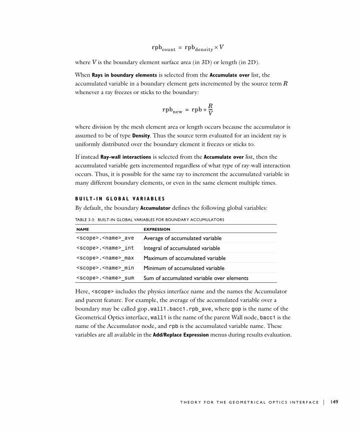
where V is the boundary element surface area (in 3D) or length (in 2D).

When Rays in boundary elements is selected from the Accumulate over list, the accumulated variable in a boundary element gets incremented by the source term R whenever a ray freezes or sticks to the boundary:

where division by the mesh element area or length occurs because the accumulator is assumed to be of type Density. Thus the source term evaluated for an incident ray is uniformly distributed over the boundary element it freezes or sticks to.

If instead Ray-wall interactions is selected from the Accumulate over list, then the accumulated variable gets incremented regardless of what type of ray-wall interaction occurs. Thus, it is possible for the same ray to increment the accumulated variable in many different boundary elements, or even in the same element multiple times.

B U I L T - I N G L O B A L V A R I A B L E S

By default, the boundary Accumulator defines the following global variables:

Here, <scope> includes the physics interface name and the names the Accumulator and parent feature. For example, the average of the accumulated variable over a boundary may be called gop.wall1.bacc1.rpb_ave, where gop is the name of the Geometrical Optics interface, wall1 is the name of the parent Wall node, bacc1 is the name of the Accumulator node, and rpb is the accumulated variable name. These variables are all available in the Add/Replace Expression menus during results evaluation.

TABLE 3-3: BUILT-IN GLOBAL VARIABLES FOR BOUNDARY ACCUMULATORS

NAME EXPRESSION

<scope>.<name>_ave Average of accumulated variable

<scope>.<name>_int Integral of accumulated variable

<scope>.<name>_max Maximum of accumulated variable

<scope>.<name>_min Minimum of accumulated variable

<scope>.<name>_sum Sum of accumulated variable over elements

rpbcount rpbdensity V×=

rpbnew rpb RV----+=


150 | C H A P T E

These global variables are computed by defining a set of component couplings on the selection of the parent physics feature, such as the Wall feature to which the Accumulators are added. The following expressions for the global variables are used.

Here, <wscope> is the scope of the parent boundary feature, e.g. goprac.wall1.

References for the Geometrical Optics Interface

1. L.D. Landau and E.M. Lifshitz, The Classical Theory of Fields, 4th ed., Butterworth-Heinemann, Oxford, 1975.

2. M. Born and E. Wolf, Principles of Optics, 7th ed., Cambridge, 1999.

3. O.N. Stavroudis, The Optics of Rays, Wavefronts, and Caustics, Academic, 1972.

4. B.E.A. Saleh and M.C.Teich, Fundamentals of Photonics, Wiley, 1991.

5. R.M. More and K. Kosaka, “Wave-front curvature in geometrical optics”, Phys. Rev. E, vol. 57, no. 5, pp. 6127–6134, 1998.

6. P.C.Y. Chang, J.G. Walker, and K.I. Hopcraft, “Ray tracing in absorbing media”, J. Quantitative Spectroscopy & Radiative Transfer, vol. 96, pp. 327–341, 2005.

7. W. A. Shurcliff, Polarized Light: Production and Use, Harvard, 1962.

8. O. S. Heavens, Optical Properties of Thin Solid Films, Dover, 1991.

9. H. Anders, Thin Films in Optics, Focal Press, 1967.

10. D. Hestroffer and C. Magnan, “Wavelength dependency of the Solar limb darkening”, Astron. Astrophysl, vol. 333, pp. 338–342, 1998.

TABLE 3-4: BUILT-IN GLOBAL VARIABLE DEFINITIONS FOR BOUNDARY ACCUMULATORS

NAME EXPRESSION

<scope>.<name>_ave <wscope>.aveop(<scope>.<name>)

<scope>.<name>_int <wscope>.intop(<scope>.<name>)

<scope>.<name>_max <wscope>.maxop(<scope>.<name>)

<scope>.<name>_min <wscope>.minop(<scope>.<name>)

<scope>.<name>_sum <wscope>.intop(<scope>.<name>/<scope>.meshVol)


Th e Ra y Hea t i n g I n t e r f a c e

The Ray Heating interface ( ) combines the Geometrical Optics interface with the Heat Transfer in Solids interface. The Ray Heat Source multiphysics feature is added automatically. The Ray Heating interface is used to model electromagnetic wave propagation in optically large systems in which the refractive index is temperature dependent. The energy lost due to the attenuation of rays in an absorbing medium creates a heat source that is included in the temperature computation.

When a predefined Ray Heating interface is added from the Optics>Ray Optics

branch ( ) of the Model Wizard or Add Physics windows, Geometrical Optics and Heat

Transfer in Solids interfaces are added to the Model Builder. A Multiphysics node is also added, which automatically includes the multiphysics coupling feature Ray Heat Source.

On the Constituent Physics InterfacesThe Geometrical Optics interface is used to model electromagnetic wave propagation when the wavelength is much smaller than the smallest geometric entity in the model. It includes built-in tools for computing the intensity, phase, and optical path length of rays. The rays can be polarized, unpolarized, or partially polarized. Frequency distributions and ray propagation in absorbing media are also supported.

The Heat Transfer in Solids interface is used to model heat transfer by conduction, convection, and radiation. A Heat Transfer in Solids model is active by default on all domains and a Heat Transfer in Fluids model is added with an empty selection. All functionality for including other domain types, such as a fluid domain, is also available. The temperature equation defined in solid domains corresponds to the differential form of the Fourier’s law that may contain additional contributions like heat sources.

S E T T I N G S F O R P H Y S I C S I N T E R F A C E S A N D C O U P L I N G F E A T U R E S

When physics interfaces are added using the predefined couplings, for example Ray

Heating, specific settings are included with the physics interfaces and the coupling features.

However, if physics interfaces are added one at a time, followed by the coupling features, these modified settings are not automatically included.

T H E R A Y H E A T I N G I N T E R F A C E | 151

152 | C H A P T E

For example, if single Geometrical Optics and Heat Transfer in Solids interfaces are added, COMSOL adds an empty Multiphysics node. You can choose from the available coupling features but the modified settings are not included.

P H Y S I C S I N T E R F A C E S A N D C O U P L I N G F E A T U R E S

Coupling FeaturesThe Ray Heat Source coupling feature node is described in this section.

Physics Interface FeaturesPhysics nodes are available from the Physics ribbon toolbar (Windows users), Physics context menu (Mac or Linux users), or right-click to access the context menu (all users).

Coupling features are available from the context menu (right-click the Multiphysics node) or from the Physics toolbar, Multiphysics menu.

TABLE 3-5: MODIFIED SETTINGS FOR A RAY HEATING INTERFACE

PHYSICS INTERFACE OR COUPLING FEATURE

MODIFIED SETTINGS (IF ANY)

Geometrical Optics Compute intensity and power is selected from the Intensity computation list in the physics interface Ray Properties section.

Heat Transfer in Solids No changes.

Ray Heat Source The Domain Selection is the same as that of the participating physics interfaces.

The corresponding Geometrical Optics and Heat Transfer in Solids interfaces are preselected in the Ray Heat Source section.

Use the online help in COMSOL Multiphysics to locate and search all the documentation. All these links also work directly in COMSOL Multiphysics when using the Help system.

In general, to add a node, go to the Physics toolbar, no matter what operating system you are using. Subnodes are available by clicking the parent node and selecting it from the Attributes menu.


• The available physics features for The Geometrical Optics Interface are listed in the section Domain, Boundary, and Global Nodes for the Geometrical Optics Interface.

• The available physics features for The Heat Transfer Interfaces are listed in the sections Domain Features, Boundary Features, and Edge and Point Features in the COMSOL Multiphysics Reference Manual.

Ray Heat Source

Use the Ray Heat Source multiphysics coupling ( ) to compute the heat source resulting from the attenuation of rays in an absorbing medium. This heat source is defined to a dependent variable that is defined on all domain mesh elements in the selection of the Ray Heat Source node.

S E T T I N G S

The Label is the default multiphysics coupling name.

The Name is used primarily as a scope prefix for variables defined by the coupling node. Refer to such variables in expressions using the pattern <name>.<variable_name>. In order to distinguish between variables belonging to different coupling nodes or physics interfaces, the name string must be unique. Only letters, numbers, and underscores (_) are permitted in the Name field. The first character must be a letter.

The default Name (for the first multiphysics coupling in the model) is rhs1.

R A Y H E A T S O U R C E

This section defines the physics involved in the multiphysics coupling. By default, the applicable physics interface is selected in the Source and Destination lists.

You can also select None from either list to uncouple the node from a physics interface. If the physics interface is removed from the Model Builder then the applicable list defaults to None as there is nothing to couple to.

If a physics interface is deleted and then added to the model again, and in order to re-establish the coupling, you need to choose the physics interface again from the Source or Destination lists. This is applicable to all multiphysics coupling nodes that would normally default to the once present physics interface. See Multiphysics Modeling Approaches in the COMSOL Multiphysics Reference Manual.

T H E R A Y H E A T I N G I N T E R F A C E | 153

154 | C H A P T E

Th eo r y f o r t h e Ra y Hea t i n g I n t e r f a c e

The Ray Heating Interface theory is described in this section:

• Unidirectional and Bidirectional Couplings

• Coupled Heat Transfer and Ray Tracing Equations

• Heat Source Calculation

Unidirectional and Bidirectional Couplings

The Ray Heating multiphysics interface combines geometrical optics with heat transfer to compute the heat source that is generated as rays propagate through an absorbing medium. The Ray Heating interface can either be used to set up a unidirectional or bidirectional coupling between the constituent physics interfaces.

If the medium properties are not temperature dependent and the domains do not undergo significant thermal expansion, then a unidirectional coupling is appropriate. The heat source generated by the attenuation of rays can be included in the heat transfer simulation by first computing the ray trajectories using a Ray Tracing study step, then computing the temperature using a Stationary study step. Both study steps are described in the COMSOL Multiphysics Reference Manual.

If the refractive index of the medium is temperature dependent, a more accurate approach is to set up a bidirectional coupling in which the attenuation of ray power affects the temperature distribution, which in turn affects the ray trajectories. The two physics can be solved for using an iterative solver loop consisting of a time-dependent solver for the ray trajectories and a stationary solver for the temperature. Such a solver sequence can be set up automatically using the Bidirectionally Coupled Ray Tracing study step, also described in the COMSOL Multiphysics Reference Manual.

Coupled Heat Transfer and Ray Tracing Equations

Under static conditions, the heat equation can be written as

ρCpu ∇T⋅ ∇ q⋅+ Q=

q k∇T–=


where

• ρ (SI unit: kg/m3) is the density,

• Cp (SI unit: J/(kg·K)) is the heat capacity at constant pressure,

• T (SI unit: K) is the temperature,

• Q (SI unit: W/m3) is the heat source, and

• k (SI unit: W/(m·K)) is the thermal conductivity.

The propagation of each ray can be modeled using a set of coupled first-order equations:

where k (SI unit: rad/m) is the wave vector, ω (SI unit: rad/s) is the angular frequency, t (SI unit: s) is time, and q (SI unit: m) is the ray position vector. In an isotropic medium, the frequency and wave vector are related by the expression

where c = 2.99792458 × 108 m/s is the speed of light in a vacuum and n (dimensionless) is the refractive index. If the medium is absorbing, then the intensity of the ray decreases and it deposits some power in the domain as it passes through. This is described in greater detail in the section Attenuation Within Domains in Theory for the Geometrical Optics Interface.

A bidirectional coupling between the Geometrical Optics and Heat Transfer interfaces may be required for any of the following reasons:

• The refractive index is temperature dependent.

• The medium undergoes thermal expansion and the refractive index is strain dependent.

• The medium undergoes thermal expansion, causing rays be reflected or refracted at different angles when entering or leaving the medium.

When none of these conditions is met, the Geometrical Optics interface affects the Heat Transfer interface, and a unidirectional coupling is sufficient.

dkdt------- ∂ω

∂q------- dq

dt------- ∂ω

∂k-------=–=

ω c kn q( )------------=

T H E O R Y F O R T H E R A Y H E A T I N G I N T E R F A C E | 155

156 | C H A P T E

Heat Source Calculation

Consider a ray j transferring an amount of power Qj through a domain. During a small time interval Δt, the ray propagates a short distance Δs from initial position qj to position qj+Δqj and its power decreases. The deposited ray power in the domain increases by an amount equal in magnitude to the power lost by the ray but opposite in sign:

where δ is the Dirac delta function. In the limit as this time derivative becomes arbitrarily small, this expression can be rewritten as

In this expression, every ray is treated as an infinitesimally small point source. This can lead to numerical issues because the heat source becomes infinitely large at the location of each point source. In the following section an alternative expression for the domain heat source is given.

C R E A T I N G A B O U N D E D H E A T S O U R C E TE R M

The Ray Heat Source node defines a variable for the contribution to the heat source by rays in each mesh element. This variable is discretized using constant shape functions that are, in general, discontinuous across boundaries between elements. For a mesh element j with volume Vj the average heat source Qsrc,j changes according to the expression

The integral on the right-hand side is a volume integral over element j. The resulting time derivative of the heat source is the average value over the mesh element, which may be written more concisely as

Qsrc r t Δt+,( ) Qsrc r t,( )∂Qj∂t

---------Δtδ r qj–( )

j 1=

N

–≈

dQsrcdt

---------------∂Qj∂t

---------δ r qj–( )

j 1=

N

–=

dQsrcdt

--------------- 1Vj-----

∂Qj

∂t--------- δ r qj–( ) Vd

j 1=

N

–=


where the sum is taken over all rays that are within mesh element j.

dQsrc j,dt

------------------- 1Vj-----–

∂Qj∂t

---------

i 1=

Nj

=

T H E O R Y F O R T H E R A Y H E A T I N G I N T E R F A C E | 157

158 | C H A P T E

4

G l o s s a r y

This Glossary of Terms contains modeling terms in a ray optics context. For mathematical terms as well as geometry and CAD terms specific to the COMSOL Multiphysics® software and documentation, see the glossary in the COMSOL Multiphysics Reference Manual. For references to more information about a term, see the index.

159

160 | C H A P T E

G l o s s a r y o f T e rm scoherence The degree to which two rays interfere with each other, or to which a ray may interfere with itself when subjected to a time delay.

diffraction order In a diffraction grating, an integer indicating the number of wavelengths between waves emanating from adjacent unit cells before they constructively interfere.

diffuse reflection Reflection at a surface in a random direction, following a probability distribution based on Knudsen's cosine law.

Fresnel equations A set of equations for computing the reflection coefficients and transmission coefficients for rays as they cross a boundary between two media with different refractive indices.

geometrical optics The analysis of electromagnetic wave propagation through electrically large domains by treating the electromagnetic waves as rays.

grating A periodic structure from which transmitted and reflected radiation can only propagate in specific directions governed by the frequency of radiation and the size of the unit cell.

intensity A measure of the energy density of an electromagnetic wave; for a plane polarized wave, the intensity is equal to the magnitude of the time-averaged Poynting vector.

monochromatic Llght Light of uniform frequency.

Mueller matrix A 4-by-4 matrix which can be multiplied by the Stokes vector to apply the effects of various optical components to a ray.

optical path length The integral of refractive index along the ray trajectory. Over a given time interval, the optical path length of a ray is equal to the distance the ray would have propagated in a vacuum.

phase The quantity that indicates the variation of the instantaneous electric field with respect to time and position.

R 4 : G L O S S A R Y

plane of incidence For non-normal incidence of a ray at a surface, the unique plane containing the surface normal and the incident ray direction vector. For normal incidence, any plane containing the surface normal may be selected.

polarization A description of the orientation of the electric field for a polarized or partially polarized ray, and for the way in which this electric field varies as the ray propagates.

polarization, circular The state of polarization in which the electric field amplitude has two orthogonal components of equal magnitude, with a phase shift of π/2 between them, such that the electric field vector traces a helical pattern as the ray propagates.

polarization, linear The state of polarization in which the electric field only oscillates within a single plane.

primary ray A ray that is released into a model independently of the trajectories of other rays. Primary rays are created by release features.

principal curvature direction A unit vector which, together with the normal to a surface, defines a plane in which one of the principal radii of curvature of a surface is defined.

polychromatic light Light with a wide distribution of frequencies; typically the variations in free-space wavelength are of the same order of magnitude as the average free-space wavelength.

principal curvature The reciprocal of one of the principal radii of curvature of a surface.

principal radii of curvature The maximum and minimum values of the radius of curvature of curves that can be obtained via the intersection of a surface with a plane.

quasi-monochromatic light Light with a distribution of frequencies in which the changes in free-space wavelength are much smaller than the average free-space wavelength.

reflection coefficient A dimensionless coefficient that is used to compute the intensity of reflected rays. At boundaries between media, reflection coefficients are computed using the Fresnel equations.

G L O S S A R Y O F TE R M S | 161

162 | C H A P T E

refractive index The ratio of the speed of light in a vacuum to the speed of light in a medium.

release feature A feature that releases a predetermined number of rays and assigns initial values to dependent variables associated with the rays.

secondary ray A ray that is produced by the interaction of existing rays with a domain or boundary feature. The degrees of freedom for all secondary rays are preallocated when beginning to run a study.

Snell’s law The set of equations that indicates the directions in which reflected and refracted rays will propagate when a ray interacts with a boundary between two media.

specular reflection Idealized reflection at a smooth surface in which the reflected ray lies within the plane of incidence and the angles of incidence and reflection are equal.

Stokes parameters The four Stokes parameters completely characterize the intensity and polarization of a fully polarized, partially polarized, or unpolarized ray. The Stokes parameters can be interpreted as indicators of the ray intensity that would be measured when sending a ray through various arrangements of polarizers and wave retarders.

transmission coefficient A dimensionless coefficient that is used to compute the intensity of refracted rays at boundaries between media. Transmission coefficients are computed using the Fresnel equations.

wave vector A vector in the direction of ray propagation, which indicates the spatial dependence of the instantaneous electric field for coherent radiation.

wave number The magnitude of the wave vector, equal to ω/c, where ω is the angular frequency and c is the speed of light in the medium.

wave retarder An optical component that applies a phase shift to radiation of a specific polarization with respect to radiation of an orthogonal polarization.

R 4 : G L O S S A R Y

I n d e x

A accumulator (node), boundaries 69

accumulator (node), domains 85

accuracy order, of time stepping 60

Allow frequency distributions at release

features 56, 75

Application Libraries window 11

application library examples

sparse flow 24, 26

auxiliary dependent variable 68

auxiliary dependent variable (node) 101

C caustic surface 118

circular wave retarder (node) 99

common settings 9

compute intensity 57

compute intensity and power 58

compute intensity and power in graded

media 58

compute intensity in graded media 58

Coupling Operators 49

D deposited ray power (node), boundaries

84

deposited ray power (node), domains 84

diffraction order (node) 96

diffuse scattering 61

diffuse scattering, wall condition 65

disappear, wall condition 65

documentation 9

E emailing COMSOL 12

F freeze, wall condition 65

G general reflection, wall condition 65

grating (node) 95

I ideal depolarizer (node) 98

illuminated surface (node) 93

inlet (node)

ray optics 87

inlet on axis (node) 91

intensity 57–59, 64, 67, 71, 81–82, 90

intensity computation 21, 115–116

interference 58

internet resources 9

K knowledge base, COMSOL 12

L latitude 106

linear polarizer (node) 97

linear wave retarder (node) 98

longitude 106

M material discontinuity (node) 70

medium properties (node) 63

mixed diffuse and specular reflection,

wall condition 65

MPH-files 11

Mueller matrix (node) 100

multiphysics

ray heat source 153

N nodes, common settings 9

nonlocal accumulator (node) 86

O optical path length 59, 68

P pass through, wall condition 65

phase 58

photometric data import (node) 76

physics interfaces, common settings 9

plane of incidence 118

polarization 58

principal radii of curvature 118

R random number generation 61, 68

ray continuity (node) 104

ray heat source (node), multiphysics 153

ray index 28

ray position 62

I N D E X | 163

164 | I N D E X

ray properties (node) 75

ray termination (node) 108

ray termination, theory 132

reference intensity 59

refractive index 64

Refractive index of exterior domains 18,

56

release (node) 77

release from data file (node) 103

release from edge (node) 101

release from grid (node) 102

release from grid on axis (node) 103

release from point (node) 102

release from point on axis (node) 102

S secondary rays 57

solar radiation (node) 105

specular reflection, wall condition 65

standard settings 9

stick, wall condition 65

Stokes parameters 71

store ray status data 59

sun position 107

T technical support, COMSOL 12

thin dielectric film (node) 74

time zone 106

total number of rays 29

transmission probability 29

W wall (node)

ray optics 64

wall condition 65

wave vector 62

websites, COMSOL 12

The Ray Optics Module User's Guide - COMSOL Documentation

Documents

Transcript of The Ray Optics Module User's Guide - COMSOL Documentation