arX

iv:1

204.

1330

v1 [

hep-

th]

5 A

pr 2

012

The Gravity Dual of a Density Matrix

Bart lomiej Czech, Joanna L. Karczmarek, Fernando Nogueira, Mark Van Raamsdonk

Department of Physics and Astronomy, University of British Columbia6224 Agricultural Road, Vancouver, B.C., V6T 1Z1, Canada

Abstract

For a state in a quantum field theory on some spacetime, we can associate a densitymatrix to any subset of a given spacelike slice by tracing out the remaining degrees offreedom. In the context of the AdS/CFT correspondence, if the original state has adual bulk spacetime with a good classical description, it is natural to ask how muchinformation about the bulk spacetime is carried by the density matrix for such a subsetof field theory degrees of freedom. In this note, we provide several constraints on thelargest region that can be fully reconstructed, and discuss specific proposals for thegeometric construction of this dual region.

1 Introduction

The AdS/CFT correspondence [1, 2] relates states of a field theory on some fixed spacetime Bto states of a quantum gravity theory for which the spacetime metric is asymptotically locallyAdS with boundary geometry B. The field theory provides a nonperturbative descriptionof the quantum gravity theory that is manifestly local on the boundary spacetime: for agiven spacelike slice of the boundary spacetime B, the degrees of freedom in one subset areindependent from the degrees of freedom in another subset. On the gravity side, identifyingindependent degrees of freedom is much more difficult; for example, the idea of black holecomplementarity [3] suggests that local excitations inside the horizon of a black hole cannotbe independent of the physics outside the horizon. It is therefore interesting to ask whetherwe can use our knowledge of independent field theory degrees of freedom to learn anythingabout which degrees of freedom on the gravity side may be considered to be independent.

In this paper, we consider the following question: Given a CFT on B in a state |Ψ〉 dualto a spacetime M with a geometrical description, and given a subset A of a spatial sliceof B, what part of the spacetime M can be fully reconstructed from the density matrix ρAdescribing the state of the subset of the field theory degrees of freedom in A?

An immediate question is why we expect there to be any region that can be reconstructed ifwe know only about the degrees of freedom on a subset of the boundary. If the map betweenboundary degrees of freedom and the bulk spacetime is sufficiently non-local, it could bethat information from every region of the boundary spacetime is needed to reconstruct anyparticular subset of M . However, there are various reasons to be more optimistic. It is wellknown that the asymptotic behavior of the fields in the bulk spacetime is given directly interms of expectation values of local operators in the field theory (together with the fieldtheory action). Equipped with this boundary behavior of the bulk fields in some regionof the boundary1 and the bulk field equations, we should be able to integrate these fieldequations to find the fields in some bulk neighborhood of this boundary region. We canalso compute various other field theory quantities (e.g. correlation functions, Wilson loops,entanglement entropies) restricted to the region A or its domain of dependence. Accordingto the AdS/CFT dictionary, these give us direct information about nearby regions of thebulk geometry.

The notion that particular density matrices can be associated with certain patches ofspacetime was advocated in [4].2 There, it was pointed out that a given density matrix mayarise from many different states of the full system, or from a variety of different quantumsystems that contain this set of degrees of freedom as a subset. Different pure states thatgive rise to the same density matrix for the subset correspond to different spacetimes witha region in common; this common region can be considered to be the dual of the densitymatrix.3

1As we recall below, knowledge of the field theory density matrix for a spatial region A allows us tocompute any field theory quantities localized to a particular codimension-zero region of the boundary, thedomain of dependence of A.

2For an earlier discussion of mixed states in the context of AdS/CFT, see [5].3As a particular example, it was pointed out in [4] that a CFT on Sd in a thermal density matrix,

1

In the bulk of this paper, we seek to understand in general the region of a bulk spacetimeM that can be directly associated with the density matrix describing a particular subset ofthe field theory degrees of freedom. We begin in Section 2 by reviewing some relevant factsfrom field theory and arguing that the density matrix associated with a region A may bemore naturally associated with the domain of dependence DA (defined below). In Section 3,we outline in more detail the basic question considered in the paper. In Section 4, we proposeseveral basic constraints on the region R(A) dual to a density matrix ρA. In Section 5, weconsider two regions that are plausibly contained in R(A). First, we argue that z(DA), theintersection of the causal past and causal future of DA, satisfies our constraints and shouldbe contained in R(A), as should its domain of dependence, z(DA).4 We note that in somespecial cases, R(A) cannot be larger than z(DA). However, in generic spacetimes, we arguethat entanglement observables that can be calculated from the density matrix ρA certainlyallow us to probe regions of spacetime beyond z(DA).5 This motivates us to consider an-other region, w(DA), defined as the union of surfaces used to calculate these entanglementobservables (defined more precisely below) according to the holographic entanglement en-tropy proposal [6, 7]. We show that w(DA) (or more precisely, its domain of dependencew(DA)) also satisfies our constraints, and that for a rather general class of spacetimes, thereis a sense in which R(A) cannot be larger than w(DA). On the other hand, we show that insome examples, R(A) must be larger than w(DA). We conclude in Section 6 with a summaryand discussion.

Note added: While this paper was in preparation, [8] appeared, which has some over-lap with our discussion. We also became aware of [9], which considers related questions.

2 Field theory considerations

To begin, consider a field theory on some globally hyperbolic spacetime B, and considera spacelike slice Σ that forms a Cauchy surface. Then, classically, the fields on this hy-persurface and their derivatives with respect to some timelike future-directed unit vectororthogonal to the hypersurface determine the complete future evolution of the field. Quan-tum mechanically, the fields on this hypersurface can be taken as the basic set of variablesfor quantization and conjugate momenta defined with respect to the timelike normal vector.

Now consider some region A of the hypersurface Σ. Since the field theory is local, thedegrees of freedom in A are independent from the degrees of freedom in the complement Aof A on Σ. Thus, the Hilbert space can be decomposed as a tensor product H = HA ⊗HA,

commonly understood to be dual to an AdS/Schwarzchild black hole, cannot possibly know whether thewhole spacetime is the maximally extended black hole; only the region outside the horizon is common toall states of larger systems for which the CFT on Sd forms a subset of degrees of freedom described by athermal density matrix.

4We denote domains of dependence in the boundary with D·(for example, DA), while domains of depen-

dence in the bulk are marked with a hat .5It is an open question whether these observables are enough to reconstruct the spacetime beyond z(DA),

so we cannot say with certainty that R(A) is larger than z(DA).

2

DA

ΣA

A~

Figure 1: A spacelike slice Σ of a boundary manifold B (= S1× time) with a region A andits domain of dependence DA. The same domain of dependence arises from any spacelikeboundary region A homologous to A with ∂A = ∂A.

and we can associate a density matrix ρA = TrA(|Ψ〉〈Ψ〉) to the degrees of freedom in A.This density matrix captures all information about the state of the degrees of freedom in Aand can be used to compute any observables localized to A.

In fact, the density matrix ρA allows us to compute field theory observables localized to alarger region DA known as the domain of dependence of A. The domain of dependence DA

is the set of points p in B for which every (inextensible) causal curve through p intersectsA (see Figure 1). Classically, the region DA is the subspace of B in which the field valuesare completely determined in terms of the initial data on A. Quantum mechanically, anyoperator in DA can be expressed in terms of the fields in A alone and therefore computedusing the density matrix ρA.

As can be seen from Figure 1, any other spacelike surface A homologous to A withboundary ∂A = ∂A shares its domain of dependence.6 Thus, in some other quantization ofthe theory based on a hypersurface Σ with A ⊂ Σ, we expect that the density matrix ρAcontains the same information as the density matrix ρA. It is then perhaps more natural toassociate density matrices directly with domain of dependence regions. This observation isimportant for our considerations below: in constructing the bulk region dual to a densitymatrix ρA, it is more natural to use the boundary region DA as a starting point, rather thanthe surface A.

It is useful to note that a quantum field theory on a particular domain of dependencecan be thought of as a complete quantum system, independent of the remaining degrees offreedom of the field theory. The observables of this field theory are the set of all operators

6To see this, we note that since A and A are homologous, we can deform A into A and define B to bethe volume bound by A and A. Then for any point p in B, consider an inextensible causal curve through p.Such a curve must necessarily pass through A. But it cannot pass through A twice, since A is spacelike. Onthe other hand, the curve must intersect the boundary of the region B twice (on the past boundary and onthe future boundary), so it must have an intersection with A.

3

built from the fields on A. The state of the theory is specified by a density matrix ρA,which allows us to compute any such observable. The spectrum of this density matrix, andassociated observables such as the von Neumann entropy, give additional information aboutthe system. We can interpret this in a thermodynamic way as giving information aboutthe ensemble of pure states described by the density matrix. Alternatively, viewing thissystem as a subset of a larger system that we assume is in a pure state, we can interpret thisadditional information as telling us about the entanglement between the degrees of freedomin our causal development region with other parts of the system.

3 The gravity dual of ρA

In this section, we consider the question of how much information the density matrix ρAcarries about the dual spacetime. We restrict the discussion to states of the full system thatare dual to some spacetime M with a good classical description. Specifically, we ask thequestion

Question: Suppose that a field theory on a spacetime B in a state |Ψ〉 has a dual spacetimeM with a good geometrical description (e.g. a solution to some low-energy supergravityequations). How much of M can be reconstructed given only the density matrix ρA for thedegrees of freedom in a subset A of some spacelike slice of the boundary?

Alternatively, we can ask:

Consider all states |Ψα〉 with dual spacetimes Mα that give rise to a particular density matrixρA for region A of the boundary spacetime. What is the largest region common to all theMαs?

We recall that knowledge of the density matrix ρA allows us to calculate any field theoryobservable involving operators localized in the domain of dependence DA, plus additionalquantities such as the entanglement entropy associated with the degrees of freedom on anysubset of A. According to the AdS/CFT dictionary, these observables give us a large amountof information about the bulk spacetime, particularly near the boundary region DA, so itis plausible that at least some region of the bulk spacetime can be fully reconstructed fromthis data. We will refer to this region as R(A). We expect that in general the densitymatrix ρA carries additional information about some larger region G(A), but this additionalinformation does not represent the complete information about G(A) −R(A).

In this paper, we do not attempt to come up with a procedure to reconstruct the regionR(A); rather we will attempt to use general arguments to constrain how large R(A) can be.

4 Constraints on the region dual to ρA

Before considering specific proposals for R(A), it will be useful to point out various con-straints that R(A) should satisfy. First, since the density matrices for any two subsets Aand A with the same domain of dependence D correspond to the same information in the

4

field theory, we expect that the region of spacetime that can be reconstructed from ρA is thesame as the region that can be reconstructed from ρA. Thus we have:

Constraint 1: If A and A have the same domain of dependence D, then R(A) = R(A).

For a particular boundary field theory, the bulk spacetime will be governed by some spe-cific low-energy field equations. We assume that we are working with a known example ofAdS/CFT so that these equations are known. If we know all the fields in some region R ofthe bulk spacetime M , we can use these field equations to find the fields everywhere in thebulk domain of dependence of R (which we denote by R). Since R(A) is defined to be thelargest region of the bulk spacetime that we can reconstruct from ρA, we must have:

Constraint 2: R(A) = R(A).

Now, suppose we consider two non-intersecting regions A and B on some spacelike slice ofthe boundary spacetime. The degrees of freedom in A and B are completely independent,so it is possible to change the state |Ψ〉 such that ρB changes but ρA does not.7 Changesin ρB will generally affect the region R(B) in the bulk spacetime, but as a consequence canalso affect any region in the causal future J+(R(B)) or causal past J−(R(B)) of R(B). Butthese changes can have no effect on the region R(A) since this region can be reconstructedfrom ρA, which does not change. Thus, we have:

Constraint 3: If A and B are non-intersecting regions of a spacelike slice of the boundaryspacetime, then R(A) cannot intersect J(R(B)).

Here we have defined J(R) = J−(R) ∪ J+(R). Note that whatever R(B) is, it certainlyincludes DB so as a corollary, we can say that R(A) cannot intersect J(DB). Taking B = A(i.e. as large as possible without intersecting A), we get a definite upper bound on the sizeof R(A): it cannot be larger than the complement of J(DA).

5 Possibilities for R(A)

Let us now consider some physically motivated possibilities for the region R(A). An opti-mistic expectation is that we could reconstruct the entire region G(A) of the bulk spacetimeM used in calculating any field theory observable localized in DA (for example, all pointstouched by any geodesic with boundary points in DA). However, this cannot be a candidatefor R(A), since it is easy to find examples of non-intersecting A and B on some spacelike sliceof a boundary spacetime such that geodesics with endpoints in B intersect with geodesicswith endpoints in A.8 Thus, G(A) ∩G(B) 6= ∅ (which implies G(A) ∩ J(G(B)) 6= ∅) and so

7Further, we expect that for some subset of these variations, the dual spacetime continues to have aclassical geometric description.

8For example, suppose we consider the vacuum state of a CFT on a cylinder and take A and B to be theregions θ ∈ (0, π/2)∪ (π, 3π/2) and θ ∈ (π/2, π)∪ (3π/2, 2π) on the τ = 0 slice. Then the lines of constant θare spatial geodesics in the bulk, and the region covered by such geodesics anchored in A clearly intersectsthe region of such geodesics anchored in B.

5

Figure 2: Causal wedge z(DA) associated with a domain of dependence DA.

Constraint 3 is violated.A lesson here is that even if field theory observables calculated from a boundary region

DA probe a certain region of the bulk, they cannot necessarily be used to reconstruct thatregion. Generally, we will have R(A) ⊂ G(A) ⊂ M , where ρA contains complete informationabout R(A), some information about G(A) and no information about G(A).

5.1 The causal wedge z(DA)

A simple region that is quite plausibly included in R(A) is the set of points z(DA) in the bulkthat a boundary observer restricted to DA can communicate with (i.e. send a light signal toand receive a signal back). For example, such an observer could easily detect the presenceor absence of an arbitrarily small mirror placed at any point in z(DA). Formally, this regionin the bulk is defined as the intersection of the causal past of DA with the causal futureof DA in the bulk, z(DA) ≡ J+(DA) ∩ J−(DA), as shown in Figure 2.9 These observationscorrespond to perturbing the spacetime at one point in the asymptotic region and observingthe asymptotic fields at another point at a later time. In the field theory language, suchobservations correspond to calculating response functions, in which the fields are perturbedat one point in DA and observed at another point in DA. Such calculations can be done

9Recall that the causal future J+(DA) of DA in the bulk is the set of points reachable by causal curvesstarting in DA while the causal past J−(DA) of DA is the set of points, from which DA can be reached alonga causal curve.

6

using only the density matrix ρA, thus we expect that z(DA) is included in the region R(A).By condition 2, we can extend this expectation to the proposal that z(DA) ⊂ R(A). It is

straightforward to check that z(DA) also satisfies condition 3.10 Thus, the suggestion thatz(DA) ⊂ R(A) is consistent with our Constraints 1, 2 and 3.

The boundary of the region z(DA) in the interior of the spacetime is a horizon with respectto the boundary region DA. Thus, the statement that we can reconstruct the region z(DA)is equivalent to saying that the information in DA is enough to reconstruct the spacetimeoutside this horizon. This horizon can be an event horizon for a black hole, but in generalis simply a horizon for observers restricted to the boundary region DA.

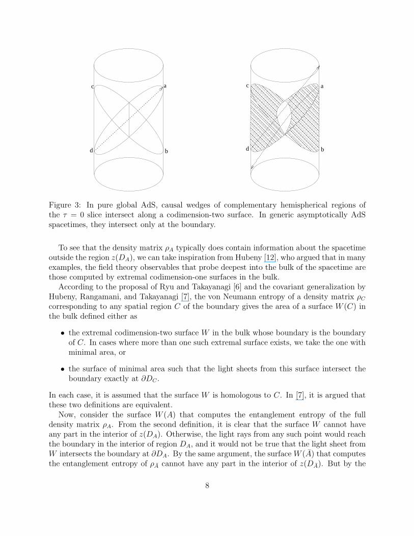
In certain simple examples, it is straightforward to argue that R(A) cannot be larger thanz(DA) or z(DA). For example, if M is pure global AdS spacetime and A is a hemisphere ofthe τ = 0 slice of the boundary cylinder, then z(DA) is the region bounded by the lightconesfrom the past and future tips of DA and the spacetime boundary, as shown in Figure 3. Anypoint outside this region is in the causal future or causal past of the boundary region DA,11

so by Constraint 3 (and the consequences discussed afterwards) such points cannot be inR(A).

Information beyond the causal wedge z(DA)

We might be tempted to guess that R(A) = z(DA) in general, but we will now see thatρA typically contains significant information about the spacetime outside the region z(DA).Consider the same example of a CFT on the cylinder with the same regions A and A, but nowconsider some other state for which the dual spacetime is not pure AdS. A key observation12

is that, generically, the wedges z(DA) and z(DA) do not intersect, except at the boundaryof A. This follows from a result of Gao and Wald [10] that light rays through the bulk of ageneric asymptotically AdS spacetime generally take longer to reach the antipodal point ofthe sphere than light rays along the boundary. Thus, the backward lightcone from the pointa in the right panel of Figure 3 is different from the forward lightcone from point d. We canstill argue that R(A) cannot overlap with the region J+(DA)∪J−(DA), but the complementof this region no longer coincides with z(DA). Thus, it is possible that R(A) is larger thanz(DA) in these general cases.13

10Suppose subsets A and B of a boundary slice do not intersect and suppose p ∈ J(z(DB)). Then thereexists a causal curve through p that intersects z(DB) and therefore intersects some q in z(DB). If p is alsoin z(DA), this same causal curve through p must intersect a point r in z(DA). Thus, there is a causal curvefrom q in z(DB) to r in z(DA). By definition of z, we must be able to extend this curve to a causal curveconnecting DA to DB. But in this situation, perturbations to the fields in DA could affect the fields in DB

(or vice versa), and this would violate field theory causality.11This relies on the fact that for pure global AdS, the forward lightcone from the past tip of DA (point

b in Figure 3) is the same as the backward lightcone from the future tip of DA (point c) and the backwardlightcone from the future tip of DA (point a in Figure 3) is the same as the forward lightcone from the pasttip of DA (point d).

12We are grateful to Veronika Hubeny and Mukund Rangamani for pointing this out.13As an explicit example of a spacetime with this property, we can take a static spacetime with a spherically

symmetric configuration of ordinary matter in the interior, e.g. the boson stars studied in [11].

7

a

b

c

d

c

b

a

d

Figure 3: In pure global AdS, causal wedges of complementary hemispherical regions ofthe τ = 0 slice intersect along a codimension-two surface. In generic asymptotically AdSspacetimes, they intersect only at the boundary.

To see that the density matrix ρA typically does contain information about the spacetimeoutside the region z(DA), we can take inspiration from Hubeny [12], who argued that in manyexamples, the field theory observables that probe deepest into the bulk of the spacetime arethose computed by extremal codimension-one surfaces in the bulk.

According to the proposal of Ryu and Takayanagi [6] and the covariant generalization byHubeny, Rangamani, and Takayanagi [7], the von Neumann entropy of a density matrix ρCcorresponding to any spatial region C of the boundary gives the area of a surface W (C) inthe bulk defined either as

• the extremal codimension-two surface W in the bulk whose boundary is the boundaryof C. In cases where more than one such extremal surface exists, we take the one withminimal area, or

• the surface of minimal area such that the light sheets from this surface intersect theboundary exactly at ∂DC .

In each case, it is assumed that the surface W is homologous to C. In [7], it is argued thatthese two definitions are equivalent.

Now, consider the surface W (A) that computes the entanglement entropy of the fulldensity matrix ρA. From the second definition, it is clear that the surface W cannot haveany part in the interior of z(DA). Otherwise, the light rays from any such point would reachthe boundary in the interior of region DA, and it would not be true that the light sheet fromW intersects the boundary at ∂DA. By the same argument, the surface W (A) that computesthe entanglement entropy of ρA cannot have any part in the interior of z(DA). But by the

8

first definition, the surface W (A) is the same as the surface W (A), since ∂A = ∂A.14 Sincez(DA) and z(DA) generally have no overlap in the bulk of the spacetime, it is now clear thatthe surface W lies outside at least one of z(DA) and z(DA).

To summarize, the area of surface W may be computed as the von Neumann entropy ofeither the density matrix ρA or the density matrix ρA. In the generic case where z(DA) andz(DA) do not intersect in the bulk, the surface W must lie outside at least one of z(DA)and z(DA). Thus, we can say that either the density matrix ρA carries some informationabout the spacetime outside z(DA) or the density matrix ρA carries information about thespacetime outside z(DA).15

5.2 The wedge of minimal-area extremal surfaces w(DA).

Based on these observations, and the observation of Hubeny that the extremal surfaces probedeepest into the bulk in various examples, it is natural to define a second candidate for theregion R(A) based on extremal surfaces.

The surface W (A) calculates the entanglement entropy associated with the entire domainof dependence DA (equivalently, the largest spacelike surface in DA). We can also considerthe entanglement entropy associated with any smaller causal development region within DA.For any such region C, there will be an associated surface W (C) (as defined above) whosearea computes the entanglement entropy (according to the proposal). Define a bulk regionw(DA) as the set of all points contained on some minimal-area16 extremal codimension-two surface whose boundary coincides with the boundary of a spacelike codimension-oneregion in DA. The area of each such codimension-two surface is (according to [7]) equal tothe entanglement entropy of the corresponding boundary region. Thus, the region w(DA)directly corresponds to the region of the bulk whose geometry is probed by entanglementobservables. As we have seen, the region w(DA) generally extends beyond the region z(DA).

From the region w(DA), we can define a larger region w(DA) as the domain of dependenceof the region w(DA). As discussed above, knowing the geometry (and other fields) in w(DA)and the bulk gravitational equations should allow us to reconstruct the geometry in w(DA).

We would now like to understand whether the region w(DA) obeys the constraints outlinedabove. Constraints 1 and 2 are satisfied by definition. It is straightforward to show thatConstraint 3 is satisfied assuming that the following conjecture holds:

Conjecture C1: If DA and DB are domains of dependence for non-intersecting regions Aand B of a spacelike slice of the boundary spacetime, then w(DA) and w(DB) are spacelike

14The equivalence of these surfaces and hence their areas is consistent with the fact that for a pure statein a Hilbert space H = HA ⊗HA, the spectrum of eigenvalues of ρA must equal the spectrum of eigenvaluesof ρA. Thus, the entanglement entropies S(ρA) and S(ρA) must agree. We do not consider here the casewhere the entire theory is in a mixed state.

15Again, it is easy to check this in specific examples. For explicit examples of spherically symmetric staticstar geometries asymptotic to global AdS with A equal to a hemisphere of the τ = 0 slice, the surface W (A)lies at τ = 0 and passes through the center of the spacetime, while the regions z(DA) and z(DA) do notreach the center.

16Here, we mean minimal area among the set of extremal surfaces with the same boundary.

9

separated.

Supposing that this holds, if p is in J(w(DB)), then there exists a causal curve through pintersecting w(DB), and by definition of w, this causal curve also intersects w(DB). If p isalso in w(DA), then every causal curve through p intersects w(DA). Thus, there exists acausal curve that intersects both w(DB) and w(DA), which violates C1. We conclude thatw(DA) satisfies Constraints 1, 2 and 3 assuming that Conjecture C1 holds.

Aside: proving Conjecture C1

While a proof (or refutation) of Conjecture C1 is left to future work, we make a few additionalcomments here.

For the case of static spacetimes, it is straightforward to prove a result similar to C1.

Let A1 and A2 be two non-intersecting regions of the t = 0 boundary slice of a static space-time, with B1 and B2 spacelike regions in A1 and A2, respectively. Let W (B1) and W (B2)be the minimal surfaces in the t = 0 slice of the bulk spacetime with ∂W (B1) = ∂B1 and∂W (B2) = ∂B2. Then W (B1) and W (B2) cannot intersect.

To show this, consider the part of W (B1) contained in the region of the t = 0 slice boundedby W (B2) and B2, and the part of W (B2) contained in the region of the t = 0 slice boundedby W (B1) and B1. If these two pieces have different areas, then by swapping the two pieces,either the new surface W (B1) or the new surface W (B2) will have a smaller area than before,contradicting the assumption that these were minimal-area surfaces. If the two pieces havethe same area, the modified surfaces will have the same area as before, but the new surfaceswill be cuspy17, such that we can decrease the area by smoothing the cusps.

In attempting a more general proof, it may be useful to note that Conjecture C1 is equiv-alent to the following statement (with some mild assumptions):

Conjecture C2: For any spacelike boundary region C, the surface W (C) is spacelike sepa-rated from the rest of w(DC).

To see the equivalence, assume first that C1 holds and let A = C and B = C. If weassume the generic case that W (C) is the same as W (C), then W (C) = W (B) ⊂ w(DB)must be spacelike separated from w(DA) = w(DC). Conversely, for two disjoint regions Aand B, let C be any region such that A ⊂ C and B ⊂ C. By definition, we have thatw(DA) ⊂ w(DC) and w(DB) ⊂ w(DC). Assuming again that W (C) = W (C), ConjectureC2 implies that there is a spacelike path connecting any point in w(DA) ⊂ w(DC) withany point p in W (C), and that there also exists a spacelike path connecting any point inw(DB) ⊂ w(DC) with the same point p. Therefore, there is a spacelike path (through p)connecting any point in w(DA) with any point in w(DB), as required for C1.

While C1 is immediately more useful, C2 might be easier to prove. Consider any bound-

17The surfacesW (B1) andW (B2) cannot be tangent at their intersection because there should be a uniqueextremal surface passing through a given point with a specified tangent plane to the surface at this point.

10

ary region C and any point p in w(DC). Then there exists a spacelike codimension-one regionIp in the domain of dependence DC such that p ∈ W (Ip). Ip can be extended to a spacelikesurface AI homologous with C, with the same boundary as C, δAI

= δC . The surface whichcalculates entanglement entropy is the same for AI and C: W (AI) = W (C). Consider nowa one-parameter family of surfaces S(λ), which continuously interpolate between AI = S(0)and Ip = S(1), and the corresponding family of bulk minimal surfaces W (S(λ)) interpolatingbetween W (C) and W (Ip). It is plausible that these bulk minimal surfaces change smoothlyand that their deformations are spacelike; following the flow, we can find a spacelike pathfrom p to W (C), which would complete the proof of the Conjecture C2.

We leave further investigation of the general validity of C1 as a question for future work.18

Possible connection between the geometry of W (A) and the spectrum of ρA

To summarize the discussion so far, the region w(DA) satisfies conditions 1, 2 and 3 assumingthat Conjecture C1 is correct. Thus, w(DA) is a possible candidate for the region R(A). Arather nice feature of this possibility is that w(DA) intersects w(DA) along the codimension-two surface W (A) = W (A) defined above. Thus, the surface W represents the informationin the bulk common to w(DA) and w(DA). The area of this surface corresponds to the vonNeumann entropy of ρA, which is the simplest information shared by ρA and ρA. We mightthen conjecture that the full spectrum of ρA (which is the same as the spectrum of ρA andrepresents the largest set of information common to ρA and ρA) encodes the full geometryof the surface W (i.e. the largest set of information common to w(DA) and w(DA)).

Reconstructing bulk metrics from extremal surface areas

Before proceeding, let us ask whether it is even possible that the areas of extremal surfaceswith boundary in some region DA carry enough information to reconstruct the geometry inw(DA).

Consider the simple case of a 1+1 dimensional CFT on a cylinder with DA a diamond-shaped region on the boundary. Given any state for the CFT, we could in principle computethe entanglement entropy associated with any smaller diamond-shaped region bounded bythe past lightcone of some point in DA and the forward lightcone of some other point.This would give us one function of four variables, since each of the two points defining thesmaller diamond-shaped region is labeled by two coordinates. Assuming the state has ageometrical bulk dual description, the bulk geometry will be described by a metric whichconsists of several functions of three variables.19 These functions allow us to determine theentanglement entropy from the geometry in the wedge w(DA) via the Takayanagi et. al.

18We note here that the restriction to minimal extremal surfaces (rather than all extremal surfaces)is essential for the validity of this conjecture. In static spacetimes with metric of the form ds2 =−f(r)dt2 + dr2/g(r) + r2dΩ2 where g(0) = 1 and g(r) → r2, it is possible that extremal surfaces boundedon one hemisphere intersect extremal surfaces bounded on the other hemisphere in cases where g(r) is notmonotonically increasing. For these examples, C1 would fail if the definition of w did not restrict to minimalsurfaces.

19We are ignoring the possible extra compact dimensions in the bulk.

11

proposal, so we have a map from the space of metrics to the space of entropy functions.Small changes in the geometry of the wedge w(DA) will generally affect the areas of some ofthe minimal surfaces, while small changes in the geometry outside the wedge will generallynot affect these areas. It is at least plausible that the entanglement information could beused to fully reconstruct the geometry in the wedge in some cases, since the map from wedgegeometries into the entanglement information is a map from finitely many functions of threevariables to a function of four variables, and it is possible for such a map to be an injection.

A proven result of this form in the mathematics literature [13] is that for two-dimensionalsimple20 compact Riemannian manifolds with boundary, the bulk geometry is completelyfixed by the distance function d(x, y) between points on the boundary (the lengths of theshortest geodesics connecting various points). This implies that for static three-dimensionalspacetimes, the spatial metric of the bulk constant time slices can be reconstructed in prin-ciple if the entanglement entropy is known for arbitrary subsets of the boundary. However,we are not aware of any results about the portion of a space that can be reconstructed if thedistance function is known only on a subset of the boundary, or of any results that apply toLorentzian spacetimes.

Cases when R(A) cannot be larger than w(DA)

We saw above that in special cases, z(DA) together with J(z(DA)) cover the entire spacetime,so Constraint 3 is just barely satisfied for z (or z). For these examples, if z(DA) is in R(A)then R(A) cannot possibly be larger than z(DA). On the other hand, for generic spacetimes,we argued that only a portion of the spacetime is covered by z(DA) and J(z(DA)), leaving thepossibility that R(A) could be larger than z(DA). In these examples, extremal surfaces fromA typically extend into the region not covered by z(DA) or z(DA) (or the causal past/futureof these), and this motivated us to consider w(DA) as a larger possibility for R(A).

We will now see that in a much wider class of examples, w(DA) together with J(w(DA)) docover the entire spacetime. To see this, recall that the surfaces W (A) and W (A) computingthe entanglement entropy of the entire regions A and A are the same by definition, aslong as A and A are homologous in the bulk.21 Now, suppose that for a one-parameterfamily of boundary regions B(λ) ⊂ A interpolating between A and a point (assuming Ais contractible), the surfaces W (B(λ)) change smoothly. Similarly, suppose that for a one-parameter family of boundary regions B′(λ) ⊂ A interpolating between A and a point(assuming A is contractible), the surfaces W (B′(λ)) change smoothly. Then the union of allsurfaces W (B(λ)) and W (B′(λ)) covers an entire slice of the bulk spacetime. In this case,for any point p in the bulk spacetime, either there is a causal curve through p that intersects∪λW (B(λ)) ⊂ w(DA) or else every causal curve through p intersects ∪λW (B′(λ)) ⊂ w(DA).This shows that w(DA) together with J(w(DA)) cover the entire spacetime.

To summarize, in cases where W (B) varies smoothly with B as described above, we havethat w(DA) together with J(w(DA)) cover the entire spacetime. Thus, by Constraint 3, with

20See [13] for the definition of a simple manifold.21The only possible exception would be the case where there are two extremal surfaces with equal area

having boundary ∂A. In this case, we might call one W (A) and the other W (A).

12

Figure 4: Different possible behaviors of extremal surfaces in spherically symmetric staticspacetimes. Shaded region indicates w(DA) where A is the right hemisphere. The boundaryof the shaded region on the interior of the spacetime is the minimal area extremal surfacebounded by the equatorial Sd−1.

this smoothness condition, if w(A) ⊂ R(A) then R(A) cannot be larger than w(DA).22 Whilethere are many examples of spacetimes for which this smooth variation does not occur (e.g.as described in the next section), spacetimes satisfying the condition are not particularlyspecial.

An example where R(A) is strictly larger than w(DA)

We have seen that w(DA) is in some sense a maximally optimistic proposal for R(A) incases where a particular smoothness condition is satisfied or when w(DA) ∪w(DA) includesa Cauchy surface. We will now see that these conditions can fail to be true in some cases,and that in these cases, R(A) must be larger than w(DA) for some choice of A.

Consider the simple example of static spherically symmetric spacetimes with metric of theform ds2 = −f(r)dt2 + dr2/g(r) + r2dθ2 where g(0) = 1 and g(r) → r2 for large r. For anyspacetime of this form, the extremal codimension-two surfaces bounded by spherical regionson the boundary will be constant-time surfaces in the bulk that can easily be computed. Bysymmetry, there always exists an extremal surface through the center of the spacetime whoseboundary is an equatorial Sd−1 of the boundary Sd. Now, moving out towards the boundaryalong some radial geodesic, there will be a unique extremal surface passing through eachpoint and normal to the radial line.

In some cases (e.g. pure AdS), the boundary spheres for these extremal surfaces shrinkmonotonically as we approach the boundary, as shown in the left half of Figure 4. However,there are other cases for which g(r) is not monotonic where the extremal surfaces shrinkin the opposite direction, then grow, then shrink again, as shown in the right half of Fig-

22An alternative condition that leads to the same conclusion is that w(DA) ∪ w(DA) includes a Cauchysurface.

13

Figure 5: Region w(DA) (shaded) where A is a boundary sphere of angular size greater thanπ. No minimal surface with boundary in A penetrates the unshaded middle region.

ure 4.23 In these cases, boundary spheres with angular radius in a neighborhood of π/2 willbound multiple extremal surfaces in the bulk. The extremal surface of minimum area inthese cases is always one that is contained within one half of the bulk space (otherwise wecould construct intersecting minimal surfaces bounding disjoint regions of the boundary).Considering only the minimal surfaces, we find that there exists a spherical region in themiddle of the spacetime penetrated by no such surface. Thus, even if we choose DA to bethe entire spacetime boundary, the region w(DA) excludes the region r < r0 for some r0. Inthis case, we have all information about the field theory (assumed to be a pure state), soR(A) should be the entire spacetime.

More generally, the region w(DA) in these cases will have a “hole” if A is chosen to beany boundary sphere with angular radius between π/2 and π, as shown in Figure 5. Note,however, that the central region is included in z(DA) for sufficiently large A, so z(DA) 6⊂w(DA) in these cases.

6 Discussion

In this note, we have presented various consistency constraints on the region R(A) ofspacetime which can in principle be reconstructed from the density matrix ρA for a spa-tial region A of the boundary with domain of dependence DA. We have argued that thez(DA) ≡ J+(DA) ∩ J−(DA) and its domain of dependence z(DA) should be contained in

23As an explicit example, we have considered the case of a charged massive scalar field coupled to gravity,with scalar field of the form φ(r) = eiωtf(r). Spherically-symmetric configurations of this type with non-zerocharge are known as “boson-stars” [11]. We find that for fixed ψ(0), the metric function g(r) is monotonicallyincreasing for sufficiently small values of the scalar field mass, while for sufficiently large values we can havethe behavior shown on the right in Figure 4.

14

Figure 6: Spatial t = 0 slice of w(DA) (light shaded plus dark shaded) and z(DA) (darkshaded) for a planar AdS black hole. The dashed curve is a spatial geodesic with endpointsin A. Knowledge of observables obtained from ρA alone allow us to compute the length ofthis geodesic.

R(A) and that z(DA) satisfies our consistency constraints. Since entanglement observablescalculated from ρA correspond to extremal surfaces that typically probe a region of space-time beyond z(DA), we have also considered the union of these surfaces w(DA) and itsdomain of dependence w(DA) as a possibility for R(A) that is often larger than z(DA). Wehave seen that w(DA) also satisfies our constraints (assuming Conjecture C1), and that ifw(DA) ⊂ R(A) generally, then R(A) = w(DA) for a broad class of spacetimes.

A false constraint

The constraints discussed in this note are essentially consistency requirements that do notmake use of details of the AdS/CFT correspondence. It is interesting to ask whether thereexist any more detailed conditions that could constrain the region R(A) further.

It may be instructive to point out a somewhat plausible constraint that turns out to befalse. For two non-intersecting regions A and B of the boundary spacetime, it may seemthat the region G(B) of the spacetime used to construct field theory observables in B shouldnot intersect the region R(A) dual to the density matrix ρA. The argument might be thatif the physics in R(A) is the bulk manifestation of information in ρA, we cannot expect tolearn anything about this region knowing only ρB. It would seem that this would be tellingus directly about ρA knowing only ρB. Perhaps surprisingly, it is easy to find an examplewhere neither w(DA) nor z(DA) satisfies this constraint, see Figure 6.

In the planar AdS black hole geometry, take the region A to be a ball-shaped region on the

15

Figure 7: The region of spacetime reconstructible from density matrices ρB and ρC (shaded,right hand side picture) is smaller than that reconstructible from ρB∪C (shaded, left handside picture). Reconstruction of R(B∪C)− (R(B)∪R(C)) (interior of dotted frame outsideof the two shaded regions) requires knowledge of entanglement between degrees of freedomin B and C.

boundary. In this case, it is straightforward to check that spatial geodesics with endpoints inA intersect both w(DA) and z(DA). Thus, the constraint R(A) ∩G(A) = ∅ can’t be correctif z(DA) ⊂ R(A). In hindsight, it is not difficult to understand the reason. Knowledge ofthe density matrix ρA allows us to reconstruct R(A). There could be many states of thefull theory that give rise to the same density matrix ρA. For any such state with a classicalgravity dual description, the dual spacetime geometry must be such that spatial geodesicsanchored in DA have the same lengths as in the original spacetime we were considering. Butthere can be many such spacetimes. So using the information in ρA, we are not learningdirectly about ρA, only about the family of density matrices ραA such that the pair (ρA, ρ

αA)

can arise from a pure state |Ψ〉 that has a geometrical gravity dual.

Spacetime emergence and entanglement

The observations in this note highlight the importance of entanglement in the emergence ofthe dual spacetime. Consider a collection Ai of subsets on the boundary such that ∪Ai

covers an entire boundary Cauchy surface. In a classical system, knowing the configurationand time derivatives of the fields in each of these regions would give us complete informationabout the physical system. Quantum mechanically, however, complete information about thesystem consists of two ingredients: (i) the density matrices ρAi

, and (ii) the entanglementbetween the various regions.

If we subdivide a set A → B,C and pass from ρA → ρB, ρC, we lose information

16

Figure 8: The region of spacetime reconstructible from density matrices ρAilies arbitrarily

close to the boundary (illustrated here on a spatial slice). The ability to reconstruct the bulkgeometry depends entirely on the knowledge of entanglement among the various boundaryregions.

about the entanglement between B and C. In the bulk picture, the region of spacetime thatwe can reconstruct (for any R satisfying our constraints) is significantly smaller than before,as we see in Figure 7. The region of spacetime that we can no longer reconstruct correspondsto the information about the entanglement between the degrees of freedom in B and C thatwe lost when subdividing.

As we divide the boundary into smaller and smaller sets Ai, we retain information aboutentanglement only at successively smaller scales, while the bulk space ∪R(Ai) that can bereconstructed retreats ever closer to the boundary (Figure 8). Conversely, knowledge ofthe bulk geometry at successively greater distance from the boundary requires knowledge ofentanglement at successively longer scales.24 In the limit where Ai become arbitrarily small,we know nothing about the bulk spacetime even if we know the precise state for each ofthe individual degrees of freedom via the matrices ρAi

. In this sense, the bulk spacetime isentirely encoded in the entanglement of the boundary degrees of freedom.

Acknowledgments

We are especially grateful to Veronika Hubeny and Mukund Rangamani for important com-ments and helpful discussions. This work is supported in part by the Natural Sciences andEngineering Research Council of Canada and by the Canada Research Chairs Programme.

24A very similar picture was advocated in [15].

17

References

[1] J. M. Maldacena, “The large N limit of superconformal field theories and supergrav-ity,” Adv. Theor. Math. Phys. 2, 231 (1998) [Int. J. Theor. Phys. 38, 1113 (1999)][arXiv:hep-th/9711200].

[2] O. Aharony, S. S. Gubser, J. M. Maldacena, H. Ooguri and Y. Oz, “Large N field the-ories, string theory and gravity,” Phys. Rept. 323, 183 (2000) [arXiv:hep-th/9905111].

[3] L. Susskind, L. Thorlacius and J. Uglum, “The Stretched Horizon And Black HoleComplementarity,” Phys. Rev. D 48, 3743 (1993) [arXiv:hep-th/9306069].

[4] M. Van Raamsdonk, “Comments on quantum gravity and entanglement,”arXiv:0907.2939 [hep-th]. M. Van Raamsdonk, “A patchwork description of dual space-times in AdS/CFT,” Class. Quant. Grav. 28 (2011) 065002.

[5] B. Freivogel, V. E. Hubeny, A. Maloney, R. C. Myers, M. Rangamani and S. Shenker,“Inflation in AdS/CFT,” JHEP 0603, 007 (2006) [arXiv:hep-th/0510046].

[6] S. Ryu and T. Takayanagi, “Holographic derivation of entanglement entropy fromAdS/CFT,” Phys. Rev. Lett. 96 (2006) 181602 [hep-th/0603001].

[7] V. E. Hubeny, M. Rangamani and T. Takayanagi, “A Covariant holographic entangle-ment entropy proposal,” JHEP 0707 (2007) 062 [arXiv:0705.0016 [hep-th]].

[8] R. Bousso, S. Leichenauer and V. Rosenhaus, “Light-sheets and AdS/CFT,”arXiv:1203.6619 [hep-th].

[9] V. E. Hubeny, M. Rangamani “Causal Holographic Information”, to appear.

[10] S. Gao and R. M. Wald, “Theorems on gravitational time delay and related issues,”Class. Quant. Grav. 17 (2000) 4999 [gr-qc/0007021].

[11] D. Astefanesei and E. Radu, “Boson stars with negative cosmological constant,” Nucl.Phys. B 665 (2003) 594 [gr-qc/0309131].

[12] V. E. Hubeny, “Extremal surfaces as bulk probes in AdS/CFT,” arXiv:1203.1044 [hep-th].

[13] L. Pestov, G. Uhlmann, “Two Dimensional Compact Simple Riemannian manifoldsare Boundary Distance Rigid,” Annals of Math., 161(2005), 1089-1106.

[14] M. Van Raamsdonk, “Building up spacetime with quantum entanglement,” Gen. Rel.Grav. 42 (2010) 2323 [Int. J. Mod. Phys. D 19 (2010) 2429] [arXiv:1005.3035 [hep-th]].

[15] B. Swingle, “Entanglement Renormalization and Holography,” arXiv:0905.1317 [cond-mat.str-el].

18