Technical solutions for low-temperature heat emission in buildings

Abstract

The European Union is planning to greatly decrease energy consumption during the coming

decades. The ultimate goal is to create sustainable communities that are energy neutral. One

way of achieving this challenging goal may be to use efficient hydronic (water-based) heating

systems supported by heat pumps.

The main objective of the research reported in this work was to improve the thermal

performance of wall-mounted hydronic space heaters (radiators). By improving the thermal

efficiency of the radiators, their operating temperatures can be lowered without decreasing

their thermal outputs. This would significantly improve efficiency of the heat pumps, and

thereby most probably also reduce the emissions of greenhouse gases. Thus, by improving the

efficiency of radiators, energy sustainability of our society would also increase. The objective

was also to investigate how much the temperature of the supply water to the radiators could

be lowered without decreasing human thermal comfort.

Both numerical and analytical modeling was used to map and improve the thermal efficiency

of the analyzed radiator system. Analyses have shown that it is possible to cover space heat

losses at low outdoor temperatures with the proposed heating-ventilation systems using low-

temperature supplies. The proposed systems were able to give the same heat output as

conventional radiator systems but at considerably lower supply water temperature.

Accordingly, the heat pump efficiency in the proposed systems was in the same proportion

higher than in conventional radiator systems.

The human thermal comfort could also be maintained at acceptable level at low-temperature

supplies with the proposed systems. In order to avoid possible draught discomfort in spaces

served by these systems, it was suggested to direct the pre-heated ventilation air towards cold

glazed areas. By doing so the draught discomfort could be efficiently neutralized.

Results presented in this work clearly highlight the advantage of forced convection and high

temperature gradients inside and alongside radiators - especially for low-temperature supplies.

Thus by a proper combination of incoming air supply and existing radiators a significant

decrease in supply water temperature could be achieved without decreasing the thermal output

from the system. This was confirmed in several studies in this work. It was also shown that

existing radiator systems could successfully be combined with efficient air heaters. This

would also allow a considerable reduction in supply water temperature without lowering the

heat output of the systems. Thus, by employing the proposed methods, a significant

improvement of thermal efficiency of existing radiator systems could be accomplished. A

wider use of such combined systems in our society would reduce the distribution heat losses

from district heating networks, improve heat pump efficiency and thereby most probably also

lower carbon dioxide emissions.

Keywords: Analytical and numerical modeling, baseboard (skirting) heating, building energy

performance, computational fluid dynamics (CFD), heat transfer, low-temperature heating,

thermal comfort

Sammanfattning Europeiska unionen planerar att kraftigt minska energiförbrukningen under de närmaste decennierna. Målet är att skapa hållbara samhällen som på nära sikt blir energineutrala. För att bidra till att uppnå detta utmanande mål föreslås här effektivta värmesystem (rumsvärmare) tillsammans med värmepumpar. Huvudsyftet med forskningen och detta arbete var att förbättra termiska effektiviteten hos vattenburna rumsvärmare. Målet var att förbättra den befintliga värmöverföringen i rumsvärmarna så att lägre framledingstemperaturer kan användas. Detta resulterar i förbättrad värmefaktorn hos värmepumpar och även i minskat utsläpp av växthusgaser. Syftet var även att undersöka hur mycket framledningstemperaturen kunde sänkas utan att minska den upplevda termiska komforten. Både numeriska och analytiska beräkningar har används i arbetet. Beräkningar och simuleringar har visat att det är fullt möjligt att täcka värmeförluster från byggnader med föreslagna lågtemperatursystem. Vidare framgår att föreslagna lågtemperatursystem kan avge samma värmeeffekt som konventionella radiatorsystem, men vid en betydligt lägre framledningstemperatur. Följaktligen blir värmefaktorn högre i motsvarande grad hos värmepumparna i föreslagna system. Studier har även visat att termiska komforten är god trots lägre framledningstemperaturer. För att undvika eventuella dragproblem i rum föreslås att förvärmd tilluft riktas mot kalla glasytor. Detta neutraliserar effektivt eventuella dragproblem. Resultat som presenteras i detta arbete belyser tydligt vikten av påtvingad konvektion och höga temperaturgradienter vid värmeöverföring. Stora insatser i detta arbete har därför lagts på att hitta metoder för att effektivt utnyttja detta. Resultaten visar att värmeavgivningen från radiatorer avsevärt förbättras genom en väl genomtänkt forcering av tilluften över radiatorytor. Det visas också att det är fullt möjligt att kombinera befintliga radiatorsystemen med effektiva luftvärmare. En betydlig sänkning av framledningstemperaturen kan även åstadkommas i denna kombination utan att värmeavgivningen från systemen minskar. Man kan av detta dra slutsatsen att termiska verkningsgraden avsevärt förbättras genom att använda förslagen lågtemperaturteknik jämfört med befintliga värmesystem. Slutligen kan man också konstatera att en bredare användning av föreslagna värmesystemen i vårt samhälle skulle minska värmeförluster i fjärrvärmenät, förbättra värmefaktorn hos värmepumpar och därmed sannolikt också minska koldioxidutsläppen.

Acknowledgement

I wish first and foremost to thank my supervisor Professor Sture Holmberg for giving me the

opportunity to be his student. I especially acknowledge his consistent confidence in me from

the day I started my doctoral studies. And, of course, also for all the time and inspiration he

has given me during our many spontaneous meetings. The major part of my research was

founded by the Swedish Energy Agency (Energimyndigheten) and the Swedish Construction

Development Fund (Svenska Byggbranschens Utvecklingsfond). Their financial support is

gratefully acknowledged. I would like to thank Heather Robertson and Christina Hörnell for

language correction and for improving my English. Their corrections and suggestions have

not only improved my language, but also helped me to create new ways of writing and

structuring my work. Special thanks go to my colleague Jonn Are Myhren for all discussions

we have shared, especially in the beginning of my doctoral studies. His knowledge

concerning heat transfer in buildings has greatly influenced me and contributed to the

direction of my research. I want also to thank Armin Halilović for his utter willingness and

preparedness to help me with mathematics whenever I needed. I would like to express my

sincere gratitude to Stephan Pitsch and Sven Alenius for introducing me to CFD and for their

help with my CFD modeling. My thanks go to Jan-Erik Nowacki for all his help in making

me understand heat pump technology. Gratitude goes also to Shia-Hui Peng for his help with

turbulence modeling and for all his explanations about this difficult area. I would also like to

thank my colleagues at Fluid and Climate Technology, Arefeh Hesaraki and Sasan

Sadrizadeh, for teamwork and many inspiring ideas. Especially Sasan for all the discussions

we have had during working hours as well as during our daily walks toward our homes.

I particularly wish to thank my wife Aida for her patience and the encouragement she has

given me during the whole of this demanding time. Her support has greatly helped me during

the difficult periods. Many great thanks go to my parents and sister for the unreserved love,

support and understanding they have given me for as long as I can remember. I also want to

thank the rest of my extensive family for their support during all these years. Finally, I would

like to express my deep gratitude to my dear cousin Ismar Karčić and friend Mustafa Šetkić

who have helped me when I mostly needed.

Contents

Title ................................................................................................. 3

Abstract .................................................................................................. 4

Acknowledgement ................................................................................. 5

List of papers ......................................................................................... 8

Nomenclature ......................................................................................... 9

1. Introduction .................................................................................... 11

1.1 Potential of thermal insulation............................................................. 11

1.2 Potential of heat pumps ....................................................................... 13

1.2.1 Heat pumps in Europe and Sweden ...................................................................... 14

1.3 Current classification of hydronic heating systems ............................. 15

1.4 Motivation for research work .............................................................. 16

1.5 Research objectives ............................................................................. 17

1.6 Hypothesis ........................................................................................... 18

2. Methods ............................................................................................... 18

2.1 Theoretical background ....................................................................... 18

2.2 Convective heat transfer from a vertical hot plate .............................. 20

2.2.1 Free, mixed and forced convection ...................................................................... 21

2.3 Computational Fluid Dynamics ........................................................... 23

2.3.1 Validation work .................................................................................................... 24

2.4 Analytical calculations ........................................................................ 25

3 Results and discussion ................................................................... 25

Paper 1 ........................................................................................................................... 25

Paper 2 ........................................................................................................................... 28

Paper 3 ........................................................................................................................... 26

Paper 4 ........................................................................................................................... 26

Paper 5 and Paper 6 ....................................................................................................... 27

3.1 Potential of proposed systems ............................................................. 27

4 Conclusions .................................................................................... 31

5 Future work .................................................................................... 32

6 References ...................................................................................... 34

List of papers

This doctoral thesis is a summary of the following papers, appended at the end of the text.

Paper 1 Ploskić A, Holmberg S. Heat emission from thermal skirting boards.

Building and Environment 45 (2010) 1123-1133.

Paper 2 Ploskić A, Holmberg S. Low-temperature baseboard heaters with

integrated air supply - An analytical and numerical investigation.

Building and Environment 46 (2011) 176-186.

Paper 3 Ploskić A, Holmberg S. Low-temperature ventilation pre-heater in

combination with conventional room heaters. Energy and Buildings 65

(2013) 248-259.

Paper 4 Ploskić A, Holmberg S. Performance evaluation of radiant baseboards

(skirtings) for room heating - An analytical and experimental approach.

Applied Thermal Engineering 62 (2014) 382-389

Paper 5 Holmberg S, Myhren J A, Ploskić A. Proceedings of International

Conference Clima 2010. 10th

Rehva World Congress on Sustainable

Energy Use in Buildings, Antalya - Turkey 2010.

Paper 6 Ploskić A, Holmberg S. Heat emission from skirting boards - An

analytical investigation. Proceedings of the 3rd

International Conference

on Built Environment and Public Health, EERB-BEPH 2009, Guilin -

China 2009.

The work presented this doctoral thesis began in January 2008 and ended in November 2013.

Professor Sture Holmberg has supervised all work reported in Papers 1-6.

Nomenclature

Latin letters

A Heat transferring area m2

cp Specific heat capacity J/(kg C)

CO2 Carbon dioxide mass/unit time

COP Coefficient of performance -

Gr ≡ -2

air

3

roomwallairυ y)θ(θβ g , Grashof number -

GSHP Ground-source heat pump -

g Gravitational acceleration m/s2

H Plate and radiator heights m

HSPF Heating seasonal performance factor -

n Number of plates number

Nu ≡ airair

λy / α , Nusselt number -

m Water mass flow kg/s

P Heat output / thermal power W

Pr ≡ 1

airairairpλ υρc

air

, Prandtl number -

Re ≡ -1

air y υv , Reynolds number -

v mean air velocity m/s

x Horizontal coordinate m

y Vertical coordinate m

Greek letters

α Heat transfer coefficient W/(m2 C)

Thermal expansion °C

∆ Difference C

Plate or layer thickness m

θ Excess temperature = mean temperature difference

between heater and surrounding air C

θ Temperature C

Thermal conductivity W/(m C)

υ Kinematic viscosity m2/s

Density kg/m3

Subscripts

air ≡ (wall + room)/2, Air film temperature

conv. Convection

eq Equivalent

free Free (convection)

forced Forced (convection)

mixed Mixed (convection)

layer Layer (thermal boundary layer)

return Return water temperature

room Room temperature

supply Supply water temperature

wall Plate wall or radiator wall

water Water

1. Introduction

The building sector stands for a large proportion of the energy usage and carbon dioxide

(CO2) emission in most countries. A usual estimation is that buildings consume about 20 to 40

% of primary energy, and are currently responsible for nearly 14 % of global CO2 emissions

[1, 2]. Presently the overwhelming majority of scientists believe that the prevailing Earth

warming is unnatural, and can be attributed to the increased CO2 emissions. The majority of

scientists also believe that current climate changes are much more rapid and forced than the

natural changes that took place before industrialization. Despite all appeals for reductions of

the world-wide CO2 emissions, the emissions have not yet started to decline. On the contrary,

the global greenhouse gas emissions have increased by 75 % between 1970 and 2004 [3].

Even in Europe CO2 emissions have continuously risen since 1990, reaching an all-time high

in 2006 [4]. Since then, the emissions have declined. In order to create a more energy-

sustainable society the governments of the European Union agreed to implement the so-called

20-20-20 plan in March 2007. Compared to levels in 1990 this means:

o 20 % reduction of greenhouse gas emissions,

o 20 % reduction of energy consumption through improved energy efficiency,

o 20 % increase of the renewable energy use by 2020.

Yet these targets should only be considered a first step toward a sustainable and low-carbon

future. According to the Intergovernmental Panel on Climate Change (IPCC), the

concentration of greenhouse gases in the atmosphere should not exceed 450 ppm CO2eq to

limit Earth warming to a maximum of 2 °C [4]. To achieve this, scientists believe that global

CO2 emissions need to be cut by 50 to 60 % by 2050. This requires a cut in industrialized

countries by at least 80 % compared to 1990 levels [4]. In order to meet these challenges,

investment in improvements in all sectors, including the building sector, is a must.

By 2009 residential buildings stood for 11 % of global CO2 emissions and consumed nearly

27 % of the produced energy in European Union in 2010 [5, 6]. In the same year these

buildings generated 6 % of global CO2 emissions and were responsible for 14 % of world-

wide energy consumption in 2012 [7, 8]. These facts clearly indicate that CO2 emissions

generated by residential buildings are connected to their energy consumption. Therefore, by

increasing the energy efficiency of these buildings their CO2 footprint can correspondingly be

decreased. In order to meet some parts of the 20-20-20 targets in residential buildings:

o their thermal insulation should be improved,

o the efficiency of their heating, cooling and ventilation systems should be increased,

o usage of efficient heat pumps should be increased.

1.1 Potential of thermal insulation

Several studies from various countries with different climate conditions have shown that

increased thermal insulation decreases the energy consumption of buildings [9-12]. An

illustration of how additional wall insulation may decrease the annual energy consumption

and specific heat loss of a building is given in Fig. 1. According to the figure an increase of

wall insulation from 3 to 30 cm would reduce the annual heating consumption by about 6.9

times. Although this is a large saving potential it should be remembered that this is only one

of many possibilities.

According to recent statistics by the Swedish Energy Agency, an average Swedish single-

family dwelling of 149 m2 floor area consumed in total about 21.3 MWh of energy in 2011.

Of this amount, approximately 4 MWh was used for household electricity [13], 3 MWh for

domestic hot water (DHW) [14] and 14.3 MWh for heating [13]. This implies that

transmission and ventilation heat losses stood for approximately two thirds of the total energy

consumption. Eriksson1 [15] and the Swedish Energy Agency

2 [16], respectively, found that

the building envelope alone was responsible for 32 and 36 % of annual energy use in an

average Swedish single-family dwelling built between 1940 and 1989. This implies that about

one third of the energy use in these building types could be saved by improving thermal

insulation of the envelope.

It should be noted that proportions of different energy needs vary greatly from one household

to another. The amount of consumed electricity and hot water is strongly influenced by the

habits and the number of persons living in the building. The distribution between transmission

and ventilation heat losses is highly controlled by the thermal properties of the building and

its ventilation system. Thus, the presented percentages in Fig. 2 should only be viewed as

general guideline values. Nevertheless, the figure demonstrates a typical distribution between

different energy needs for an average Swedish single-family dwelling built in the second half

of the 20th

century.

1 Average heat losses from single-family dwellings built between 1940 and 1980. 2 Average heat losses from a single-family dwelling built in 1970.

Fig. 1. The decrease of annual heating consumption

and specific heat loss per square meter floor area as

function of increased wall insulation are shown [12].

Fig. 2. The shares of the energy needs for an average

Swedish single-family dwelling built in the second half

of the 20th

century. The needs for domestic hot water

and household electricity were adopted from [14] and

[13], respectively.

1.2 Potential of heat pumps

Unlike transmission heat losses that can be reduced by static measures such as improved

thermal insulation, the thermal needs of domestic hot water and air supply must be met by an

active heat supply. One method for meeting these needs is to use sustainable energy supplies

by means of efficient heat pumps. A heat pump is a heat engine that moves free heat from a

cold reservoir (heat source) to a reservoir of higher temperature such as domestic hot water

and/or heating system (heat sink). To perform this refining process, additional mechanical

work must be supplied to the system. This additional work is often done by a compressor

which usually is driven by electricity. The heat source can be of various types. The free heat

stored in the ground, rock, groundwater, lakes, rivers and outdoor air can be effectively

extracted by heat pumps and converted to useful heat. The heat from exhaust air and waste

heat can also be recovered by heat pumps. Due to these possibilities heat pumps can be/are

used as heat-supplying system in buildings. A simple sketch showing components and

flowchart of a ground source heat pump connected to domestic hot water and heating system

is given by Fig. 3.

The efficiency of the heat pump is manly affected by the temperatures of the cold and the hot

reservoirs. The higher the temperature of the cold reservoir and the lower the temperature of

the hot reservoir the less the compressor work needed, and thereby the higher the heat pump

efficiency. The efficiency of a heat pump is defined by the ratio between the useful heat

energy produced and the energy consumed by the compressor. This ratio is known as the

Coefficient of Performance (COP) of a heat pump. The higher the COP the higher the

efficiency. Thus, a common goal of current researchers and operating engineers is to find

methods to increase the COP value of heat pumps.

Fig. 3. The sketch and flowchart of a ground source heat pump (GSHP) with working temperatures. The

dashed lines show the boundaries of the heat pump.

Electrical power supply

Expansion

valve

Evaporator

Condenser

Compressor

Domestic

hot water

Heating

system

Hot reservoir

Cold

reservoir

Cold

reservoir

Heat collector

Different types of heat pumps have different COP levels. Currently COPs are ranging from 2

to 4.5. This means that heat pumps are able to generate 2-4.5 kWh heat from 1 kWh of

electricity. This makes heat pumps more environmentally friendly than most traditional

heating options. Of course, this also largely depends on the cleanness of the consumed

electricity. Heat pumps are commonly designed to cover 50 to 90 % of annual heat demand in

residential buildings. They alone, however, are often incapable of overcoming the heating

peak loads during the coldest days. In these situations an auxiliary heat source is often

needed. It should also be remembered that the COP value varies during a heating season. The

value is highly dependent on building heat demand, which may oscillate greatly from day to

day. Therefore a Heating Seasonal Performance Factor (HSPF), which is an average COP

value taken over the whole heating season, is usually used to rate the system performance.

1.2.1 Heat pumps in Europe and Sweden

The installation of heat pumps in Europe has increased greatly during the last two decades.

Since the beginning of 1980s, Sweden and Switzerland were leading in using this technology

for heating. However, some other countries like Austria, Germany and France have lately

also shown a rapid increase in the number of installed units (Fig. 4) [17]. The International

Energy Agency Heat Pump Centre have found that if 80 % of the households in the OECD

(Organisation for Economic Co-operation and Development) countries replaced their oil

boilers with heat pumps of HSPF = 4, approximately 2.4 Tkg CO2 emissions could be saved.

This would reduce the global CO2 emission by nearly 10 % annually [18]. Also, according to

a recent report by the Swedish National Board of Housing, Building and Planning, the CO2

emissions from a single-family dwelling could be considerably reduced if the dwelling were

served by a heat pump of HSPF = 4 [19], as shown by Fig. 5. The question is; how to achieve

a HSPF value of 4?

Fig. 5. The CO2 emissions3 from five heating options

currently used in Swedish single-family dwellings [19].

3The CO2 emissions from district heating and for electricity generation were based on the average Swedish fuel mix in 2008. The emission

from a heat pump was recalculated to apply for HSPF = 4, instead of 2.5. The original emissions were also based on a total annual heat need

of 20 MWh. These were reduced by factor 1.16 to apply for a need of 17.3 MWh/year according to [13, 14].

Fig. 4. The number of installed ground source heat

pumps per square kilometer land area in some

European countries in 2007 [17].

According to Table 1, a supply water temperature of approximately 40 °C is needed to

achieve a HSPF value of about 4 for a ground source heat pump installed in an average

Swedish family house. The table also shows that water supplies of lower temperatures

generate higher HSPF values and lower CO2 emission rates. This implies that low-

temperature heating systems are both energy efficient and environmentally friendly options.

More detailed explanations what is meant by a low-temperature heating system will be given

in the following section.

Table 1. The variation of HSPF values for a ground-source heat pump at different supply and return water

temperatures. The pump serves a single-family dwelling with a time constant of 72 h, placed in the central part

of the Sweden. The temperature change of refrigerant in the vertical heat collector was set to 3 °C. The

calculations were performed using the commercial code Vitocalc [20]. Total energy and

power need Temperatures

Efficiency and

sustainability

Heat

demand

Heat pump

power

Design

outdoor

Annual

outdoor Indoor

Supply

water

Return

water

HSPF

value

CO2

emission

4MWh/year

5kW °C °C °C °C °C –

6kg/year

17.3 6.8 -16 6.6 20 75 65 2.0 262

17.3 6.8 -16 6.6 20 55 45 3.1 169

17.3 6.8 -16 6.6 20 45 35 3.5 142

17.3 6.8 -16 6.6 20 35 25 4.1 128

1.3 Current classification of hydronic heating systems

The total heat output from a hydronic heating system is mainly controlled by three

parameters. Namely by operating water flow, size of room heaters and temperature difference

between the room heaters and surrounding air. It should also be noted that the surface

temperature of the room heaters is controlled by supply and return temperatures and operating

water flow. Since the size of the room heaters is constant, their heat output can either be

controlled by the flow or the temperature control. Accordingly, the hydronics can be divided

into two sub-systems according to their operating conditions as shown in Table 2.

Table 2. Subdivision of current hydronic systems with corresponding water flows and temperature drops. The

approximate operating conditions for four hydronic systems are given, i.e. low-flow, high-temperature, high-

flow and low-temperature systems.

Water flow through room

heaters

Temperature drop across room

heaters

Hydronic system kg/s (l/h) °C

Low-flow ≈ high-temperature ≈ 0.011-0.004 (41-15) ≈ 15-40

High-flow ≈ low-temperature ≈ 0.034-0.017 (124-61) ≈ 5-10

The low-flow systems are presently characterized by high supply water temperatures and

large temperature drops across room heaters. Due to this the low-flow systems are also

4 Total annual heat demand according to [13, 14]. The heating need = 14.3 MWh. The domestic hot water need = 3 MWh. 5 Also, design heat power need of the selected single-family dwelling at an outdoor temperature of -16 °C. 6 The CO2 emission was adopted from [19], and was recalculated to apply for different HSPF values.

commonly high-temperature systems. On the contrary, in high-flow systems the supply water

temperatures and temperature drops are considerably lower. The high-flow systems are thus

also commonly low-temperature systems. This, however, must not always be the case. For

example, in buildings with low-to-moderate heating demands the hydronic systems can

simultaneously operate in both low-flow and low-temperature regime. Therefore, although

common, the subdivision given in Table 2 is not strict.

Approximately in the middle of the 20th

century, the process of switching from what was then

considered high-temperature systems (130/60/20 °C, 120/100/20 °C)7 to then considered low-

temperature system (90/70/20 °C) started in Europe [21, 22]. As heating demands of the

European buildings have constantly decreased since the 1950s, the old 90/70 system was

replaced by new 75/65 system in 1997 [23]. Also in Sweden the old high-temperature 80/60

system was replaced by new low-temperature 55/45 system in 1980 [24]. Since this system

has been the Swedish standard for more than two decades, Fahlén [25] proposed classifying it

as a medium-temperature system in 2003. He recommended the following classification:

o high-temperature system for supply temperatures > 55 °C

o medium-temperature system for 45 °C < supply temperatures < 55 °C

o low-temperature system for supply temperatures < 45 °C

A somewhat more detailed classification was also proposed by Boerstra et al. [26] in 2001, as

shown in Table 3.

Table 3. Classification of hydronic systems according to

Boerstra et al. [26].

Water temperatures

Hydronic system Supply/°C Return/°C

High-temperature 90 70

Medium-temperature 55 40-35

Low-temperature 45 35-25

Very low-temperature 35 25

In conclusion, it is obvious that system classification of hydronics is arbitrary and has been

constantly changing with time. In this work the hydronic system that could cover a given

space heat loss with supply water temperatures ≤ 45 °C has been regarded as a low-

temperature system, which is in line with both recommendations described above.

1.4 Motivation for research work

By 2007, single-family dwellings stood for about 45 % of the total heated area in Sweden

[27]. Of these 1.91 million building units around 25 % were heated by electric hydronic

systems in 2011 [13]. In this share both air-to-water and exhaust-air heat pumps are included.

In addition to these 25 %, an additional 11.5 % were served by closed-loop heat pump

systems [13]. This implies that approximately 36.5 % (= 697 880) of the country's single-

family dwellings were served by different types of hydronic systems supported by heat pumps

7 Supply/return/room temperature.

at the time. Due to this, many studies during the recent past have been made to rate and

increase HSPF values of the heat pumps in Sweden.

SP Technical Research Institute of Sweden has measured HSPF values of entire systems in

five single-family houses served by ground source heat pumps and hot-water radiators8 [28].

It was found that all five HSPFs were in close agreement, having an average value of 2.6 ±

0.39. In her doctoral thesis Kjellsson [29] showed that HSPF value of a ground source heat

pump could increase by 7.5 %10

by doubling the depth of borehole. She also showed that an

additional increase of about 3 % could be achieved by combining the heat pump with a solar

collector of 10 m2. Moreover, according to a recent report by Swedish Energy Agency the

HSPF values of heat pumps in Sweden have increased by approximately 2 % annually

between 1995 and 2009 [30]. This was mainly a result of long-term, continuous and goal-

oriented research on heat pump technology in the country.

Facts presented in this section and in section 1.2 suggest that heat pumps have a large saving

potential in Sweden, as the number of the installed units is quite large. Also, until now the

research and development was mostly focused on the cold side of the heat pumps and

improvement of their components. Data presented in sections 1.2 and 1.3 also show that

supply temperatures in hydronic systems supported by heat pumps must be much lower than

currently required by prevailing norms in order to achieve high HSPF values. According to

Table 1, about 32 % of annual CO2 emissions from a single-family dwelling could be saved if

supply temperature were to be reduced from 55 to 35 °C. Accordingly, approximately 19 Mkg

of annual Swedish CO2 emissions would be cut if every fourth single-family house would

switch from a 55/45 to a 35/25 system. This would reduce the total CO2eq emissions from the

country's housing stock by nearly 1.5 % [31].

1.5 Research objectives

Methods for increasing the heat outputs from different types of hydronic room heaters has

therefore been a main objective of research at KTH Royal Institute of Technology at the

Division of Fluid and Climate Technology between 2006 and 2013.

This research work is part of that endeavor. The main focus of this work was directed towards

finding methods to improve the thermal efficiency of low-temperature radiators. The goal was

to lay the ground for robust and efficient radiator systems capable of operating with low-

temperature water supplies without compromising the perceived thermal comfort. From an

engineering point of view there is a need for design requirements for such systems.

8 Here, as in the rest of this work, radiators mean vertical wall-mounted heat-emitters used for space heating in a room. 9 The houses were built between 1955 and 1970. The installed nominal power of the heat pumps ranged from 6.6 to 11 kW, and the deepness

of boreholes varied from 92 to 170 m with an average depth of 140 m. 10 Calculation was based on: total heat need of 29.4 MWh/year, a heat pump power of 7 kW and borehole depth increase from 80 to 160 m.

1.6 Hypothesis

“By decreasing the height and increasing the length of the radiators, their thermal efficiency

can be increased. By forcing the supply air to pass through room heaters, the supply

temperature to heaters can be decreased without decreasing their heat outputs. These two

actions will lead to improved system efficiency without compromising the perceived thermal

comfort”.

2. Methods

To test the hypothesis two main methods have been applied - numerical and analytical

calculations. The numerical calculations were performed using Computational Fluid

Dynamics (CFD) commercial tools, and analytical calculations were performed using well-

known mathematical and semi-empirical relations. It should be noted that in each paper the

used methods were described in detail. In addition to that a relevant literature review was also

given in each paper. Therefore, in following sections only a brief presentation of the main

methods used will be given. Beside that, a short theoretical background regarding the systems

investigated in this work is also given in the following section.

2.1 Theoretical background

In this section a brief review of mechanisms that control heat transfer from wall-mounted

radiators is given. The goal here is not to repeat the well-known theories regarding heat

transfer from vertical heaters. The goal is rather to present the most relevant parts of these

theories to explain reasons for the research work reported in this thesis, and to partly support

the hypothesis.

As mentioned earlier, the total heat output from a hydronic room heater is mainly controlled

by three parameters: operating water flow, size of heater and temperature difference between

heater and surrounding air. The joint influence of these three parameters is normally

summarized by a global energy balance as illustrated by Eq. 1.

U-value of room heater

-1n

supply return-1 -1 -1

p supply return water i i air

i=1 supply room return room

Δθ = excess temperature

θ - θP = m c (θ - θ ) = + A

ln (θ - θ )/(θ - θ )

(1)

Typically in water-to-air heat exchangers, the water-side heat transfer coefficient αwater is of

the order of several thousand, and the thermal conductivity λ of the metal plates ranges from

several tens to hundreds. In addition, the thicknesses of the plates δ are also often less than

1 mm. As the inverse of large numbers is small, the n

-1 -1

water i i

i=1

+ part usually ranges from

about 10-3

to approximately 10-4

and can thus be neglected without significantly decreasing

the calculation accuracy. Accordingly, the total heat transfer rate is therefore mainly

controlled by the αair value, as this parameter is the smallest in the series. For simplicity in

coming explanations, the logarithmic excess temperature Δθ is also here approximated as

wall room(θ - θ ). wall represents the mean temperature of all heat-emitting walls of the radiator,

and room stands for the surrounding (room) air temperature adjacent to all heat-emitting

surfaces. By doing so Eq. 1 can then be reduced to a more manageable expression as

illustrated by Eq. 1*.

p supply return air wall roomP = m c (θ - θ ) A (θ - θ ) (1*)

The left part of Eq. 1 and Eq. 1* is known as a steady-flow energy equation and shows the

enthalpy change of a given system, in this case a radiator. The right part of Eq. 1* is known as

Newton's Law of Cooling and refers to the ability of a system to exchange heat with its

surrounding. It should also be noted that the heat transfer coefficient αair consists of two parts,

a convective αconv. and a radiative part αrad. Since the radiative part (coefficient) is

approximately constant (≈ 6.0-5.4 W/m2·°C) for supply temperatures 55-35 °C, focus in this

section is directed on the convective part as this part varies strongly in this temperature range.

According to Eq. 1 and Eq. 1* the heat output P can be incased by increasing the water mass

flow m . In practice, when m increases the temperature difference supply return(θ - θ ) across the

radiator correspondingly decreases. Therefore by increasing m , the mean wall temperature of

the radiator wallθ will also increase. This will generate a higher αconv. value and thereby a

higher heat output, as αconv. is proportional to wall room(θ - θ ) in natural (free) convection.

This enhancing method, however, is not very energy efficient. As shown in Paper 4, a

doubling of the mass flow through a baseboard radiator would increase its heat output by

approximately 4.5 %. Donjerković [32] has also found that the output from a water-to-air

heater would be increased by 10 % by tripling the mass flow. Since for internal turbulent

flows the hydraulic power loss is proportional to 3m , it is obvious that heat transfer

enhancement by a large increase of mass flow is inefficient. The methods for improvements

must therefore be sought elsewhere.

2.2 Convective heat transfer from a vertical hot plate

In Fig. 6a, typical air movement behavior around a heat-emitting two-panel radiator is shown.

As can be seen, the temperature and velocity distribution across the adjacent layers is

identical in all there parts. Due to this symmetry the illustrated radiator can be approximated

by a hot vertical plate, as shown by Fig. 6b.

At the very moment the wall temperature of a plate is higher than that of the surrounding air,

a thin air film next to the entire plate height is established. This film is the thermal boundary

layer and it is normally only a few millimeters thick. Despite its relatively low thickness it

plays a vital role for the convective heat transfer - especially in free convection. This is

mainly due to the thermal property of the layer, i.e. air. Owing to its relatively low thermal

conductivity, the temperature drop across the adjacent layer is steep. This implies that the

thermal boundary layer behaves like an invisible insulating air film, blocking the heat transfer

to surrounding air. Therefore by reducing the height and/or thickness of a thermal boundary

layer, a higher convective heat flow to the surrounding air can be achieved.

The characteristics of a thermal boundary layer vary along a hot wall, and are mostly

determined by its height and wall-to-air temperature difference. For (wall - room) = 50 °C, the

transition from laminar-to-turbulent layer is likely to start at a height of 0.67 m [33]. Thus, in

this section, the maximum plate height was set to 0.6 m, in order to stay within the laminar

regime. It should also be stressed that the heights of most current conventional radiators are

lower or around 0.6 m. This reference height is thereby also reasonable from an engineering

point of view.

From Fig. 6a and 6b, it can be observed that boundary layer thickness grows rapidly alongside

a hot vertical wall. It can also be noticed that the thickness at the starting edge is much

smaller compared to the upper edge. As a result this, the layer temperature layer at the starting

edge (y = 0) is close to room temperature room, i.e. layer ≈ room. Consequently the convective

heat transfer at the lower part of the plate is high, since (wall - layer) ≈ (wall - room) and

wall > room. On the other hand at the upper edge at y = H and for x << δt, the layer

δt

Fig. 6a. A sketch of propagation of thermal

boundary layers, velocity and temperature changes

along four sides of a two-panel radiator.

layer

δt ~ y1/4

y = 0

y = H

H

wallθ

x

y

g = gravity force

layer (y = x = 0) ≈ room

layer (y = H, x << δt) ≈ wall

layer = f (y, x)

room

layer (x = δt) ≈ room

Fig. 6b. A sketch of the thermal boundary layer

alongside a hot vertical wall together with

associated temperatures and governing forces.

Buoyancy driven flow

room

δt = thermal boundary layer

Velocity profiles

Temperature profiles

δt δt

wallθ

Floor

Heat-emitting panels

room

room

room

room

layer

temperature is close to the wall temperature wall, i.e. layer ≈ wall. Accordingly, the convective

heat transfer in upper the part of the plate is quite low as the temperature difference between

the wall and the surrounding air is small. This shows that the αconv. value varies strongly

alongside a hot vertical wall, and follows the change of air temperature inside the thermal

boundary layer.

2.2.1 Free, mixed and forced convection

In Fig. 7a, the variation of the free convective heat transfer coefficient αfree, conv. along a 0.6 m

high hot vertical wall is shown. The graphs in the figure were constructed using the well-

known Nusselt relation for laminar free convection, i.e. Eq. 2 [34].

1/4

yfree conv. y, free 4/9

9/16air

0.67 (Gr Pr) yNu = 0.68 +

λ 1+(0.492/Pr)

Gry < 109, 10

-3 ≤ Pr ≤ 10

3 (2)

The graphs show that the αfree, conv. value declines exponentially up to about y/H = 0.35,

independently of excess temperature. After that the decline is constant and approaches an

asymptotic value. The drop of the αfree, conv. value is also considerably lower for a reduction of

excess temperature from 50 to 30 °C, compared with reduction from 30 to 10 °C. This

demonstrates that the heating power from free convection at low-temperature supply is much

weaker compared to medium and high-temperature supplies. This explains why low-

temperature radiators at standard operating conditions are not as powerful as medium and

high-temperature radiators. Data in Fig. 7a also suggest that radiators should be low and long

in order to have a high thermal efficiency. This finding partly supports the first part of the

hypothesis of this work.

In Fig. 7b the effect of a forced airflow of 0.2 m/s on convection rate is shown. The plots were

created using Nusselt relations for laminar forced and mixed convection, as shown by Eqs. 3

and 4 [35].

1/2 1/3forced conv. y, forced y

air

yNu = 0.664 Re Pr

λ

Rey < 5 ·10

5, Pr > 0.6 (3)

1/3

3 3mixed conv. y, mixed y, free y, forced

air

yNu = Nu + Nu

λ

(4)

The criteria for forced, mixed and natural convection were determined by generally accepted

Gry-to-Rey ratios as follows:

o y

2

y

Gr 1

Re forced convection

o y

2

y

Gr1 < 10

Re mixed convection

o y

2

y

Gr 10

Re free convection

It was observed that for an excess temperature of 10 °C forced convection dominated up to

y/H ≈ 0.08, and mixed convection for the rest of the plate. At an excess temperature of 30 °C,

the mixed convection started to dominated from y/H ≈ 0.03, and a strong presence of natural

convection was only observed at the y = H. It was also noted that the heat transfer coefficient

in mixed convection is noticeably higher than in both natural and forced convection. It

therefore seems reasonable to utilize this potential, and create the right conditions for

radiators to operate within this mode.

The plots in Fig. 7b suggest that the excess temperature could be lowered from 30 to 10 °C

without decreasing the αconv. value, by using a forced airflow of 0.2 m/s. The αconv. value

could be additionally enhanced by about 13 % if temperature difference (gradient) would be

increased from 20 to 2 °C. This means that by a proper combination of existing radiator

systems with add-on fans and/or cold supply air, the supply water temperature to the radiators

could be decreased from 55 to 35 °C without decreasing their thermal power. Having this in

mind, it becomes more understandable why Myhren and Holmberg [36, 37] have found that a

forced airflow of 7 l/s through a double-panel radiator would increase its output twice.

Similarly, Johansson and Wollerstrand [38] have also found that add-on fans of 3 W would

enable lowering of the supply water temperature from 55 to 45 °C without reducing the heat

output from a single-panel and column radiator.

The results presented in this section together with previous findings by others clearly

demonstrate the potential of forced airflow through and alongside radiators. It seems that to

additionally decrease the supply water temperatures in radiator systems the advantage of

forced convection and high thermal gradients should be utilized. It is obvious that large

improvements in convective heat transfer could be gained by relatively low air speeds of low

Fig. 7a. Variation of the laminar free convective heat

transfer coefficient along a hot vertical wall for excess

temperatures of 10, 30 and 50 °C is shown. The values

on the x-axis were normalized with maximum αfree, conv.

value at Δ = 50 °C and y/H ≈ 0.01.

Fig. 7b. Variation of laminar free, forced and mixed

convective heat transfer coefficients along a hot vertical

wall for excess temperatures 10 and 30 °C is shown.

The values on the x-axis were normalized with

maximum αfree, conv. value at Δ = 30 °C and y/H ≈ 0.01.

entering temperatures. This is especially favorable for Nordic countries where temperature

differences between outdoors and indoors are large, and where the heating need is the

dominant part of energy consumption in buildings. The results presented in Fig. 7b also partly

support the second part of the hypothesis of this research work. Thus the goal of this work

was also to give some practical design requirements for radiator systems in order to utilize the

above-presented potentials.

2.3 Computational Fluid Dynamics

The results presented in Papers 1-3 were mainly obtained using Computational Fluid

Dynamics (CFD). CFD in Papers 1-3 was used to analyze fluid movement and heat transfer

inside considered domains. CFD in general can be used for simulation of both internal and

external flows, in two or three dimensions. The simulations can be performed in transient of

steady-state regime. In this work the CFD was used to analyze internal airflows together with

heat transfer predictions. In all three studies the air and the thermal flows were simulated at

steady-state. The comprehensive possibility to visualize simulation results was utilized to

adjust the geometry and other design parameters to achieve the most favorable solution in all

three studies. In general, the results in CFD are obtained by numerical solutions of Navier-

Stokes equations including the continuity and energy equations. The turbulence is currently

predicted by various turbulence models, available in CFD codes. In Papers 1-3 the turbulence

was predicted by the Re-Normalization Group (RNG) k-є turbulence model. This model is a

further development of the standard k-є model, and it has improved ability to account for the

effects of smaller scales of fluid motion. Therefore this model is also suitable for simulations

of airflows in indoor environments. The discretization of governing equations can be handled

by finite-volume or finite-element based solvers. CFD codes used in this work had finite-

volume based solvers. The solvers also solved the governing equations in their time-averaged

and conservative form.

It was decided not to present the mathematical equations for continuity, momentum, energy

and turbulence model here - as these equations are presently well-known and available in

most handbooks of fluid mechanics. For readers interested in becoming familiar with the

derivation of these governing equations it is suggested to consult the recent book by Tu et al.

[39]. An example of the distribution of the unstructured and structured volume elements used

in Paper 3 is shown in Fig. 8.

Fig. 8. At left a sketch of the computational domain around a pipe wall surrounded by an airflow is shown

(Paper 3). The vertical and horizontal distribution of the unstructured and structured volume elements is shown

in the middle and at the right, respectively.

Pipe wall

Pipe wall

Airflow

Airflow

Airflow

Airflow

Airflow

Simulations in Papers 1-2 were performed using commercial CFD-codes Gambit and Fluent

6.3 while in Paper 3 the code Ansys 13 was used. Gambit is a pre-processing tool and was

used for geometry and computational grid (mesh) generation. After geometry and mesh were

constructed, the mesh file was manually imported to Fluent 6.3. In Fluent 6.3 the boundary

conditions were specified and the governing equations solved. After obtaining convergence,

solution results were post-processed either by Fluent 6.3 or by some other data-handling code.

In Ansys 13, unlike in Gambit and Fluent 6.3, the pre, processing and post-processing were

included in same code.

Although CFD simulations have a large design potential the proper selection of numerical

methods, turbulence model and boundary conditions play a decisive role for correct of results.

By numerical methods is here meant quality of mesh generation, selection of near-wall

treatment, pressure-velocity coupling and order of discretization scheme. The correct

selection of these parameters is not always obvious. On the other hand, an incorrect

employment of the parameters can lead to large errors in simulation results. Therefore it is

always desirable to validate CFD results with experimental data or analytical calculations.

This helps the CFD user to estimate the reliability of simulation results.

2.3.1 Validation work

A large effort was put on validation work in Papers 1-3. The main focus of the validation

work in these papers was to ensure the ability of CFD codes and the user to correctly predict

air movement and heat transfer. A key publication used as guideline in this process was “How

to Verify, Validate and Report Indoor Environment Modelling CFD Analyses” by Chen and

Srebrić [40]. Here a detailed validation procedure, including the judgment of CFD results,

was presented in several steps. The same validation modus was also applied in this work.

A room model previously used by Omori et al. [41, 42] was used for validation in Paper 1.

The room geometries and boundary conditions reported by Omori et al. were reproduced in

detail by Gambit and Fluent 6.3. The obtained CFD results were then compared with both

numerical and experimental findings reported by the above-mentioned authors. In addition to

this, the CFD-predicted mean room and inner glazing temperatures were also matched with

those analytically calculated. Detailed results of the validation work in Paper 1 can be found

in Fig. 4a-4d and Table 5 in the same article.

In Paper 2 well-known semi-empirical relations were used to validate results obtain by CFD

simulations. The objective of the validation work was to determine which model most

accurately predicted convective heat transfer inside a narrow heat-emitting channel. This

model was then used to represent the heat variation along the channel, and to demonstrate the

required channel surface temperatures to pre-heat different supply airflow rates to room

temperature. The results of the validation work were summarized in Fig. 2a-2d in Paper 2.

Also in Paper 3 semi-empirical relations were used to validate results predicted by Ansys 13.

After obtaining satisfying results, the CFD simulations were used to find the most favorable

geometrical design for a small shell-and-tube water-to-air heat exchanger. The results of the

validation work in Paper 3 were presented in Fig. 3a-3b and 4-4b.

2.4 Analytical calculations

As mentioned in the beginning of section 2, analytical calculations were also used in this

work. By analytical calculations are here meant semi-empirical and pure mathematical models

used for estimation of:

o convective and radiative heat transfer,

o thermal power and pressure losses,

o change of thermal properties of working media and

Different types of analytical calculations were applied in all articles, and the results in these

studies were partly or entirely based on this type of calculations. The applied calculation

models were used in their average form.

In Papers 1 and 3, analytical calculations were used to determine space heat losses from a

room. The losses were calculated by a global heat balance and with models suggested by

prevailing norms. As previously detailed, the analytical calculations were also used for

validation of CFD predictions in Papers 2 and 3. In these two papers this type of calculations

was applied for estimation of air pressure loss as well as for radiative and convective heat

transfer. The results obtained in Paper 4 were entirely based on analytical calculations. In this

article the standard method of least-squares was applied to approximate the solution. In Paper

5 both CFD and analytical calculations were used while Paper 6 analytical calculations were

used only.

3 Results and discussion

In this section a short summary of the most important results in Papers 1-6 is given. The

results from the papers were reported in detail in each paper thus only a brief outline is given

here. In addition, some part of the results that were not presented in the papers will be given

and discussed here.

Paper 1

The aim of study in Paper 1 was to map thermal performance of low-height radiators

(baseboard radiators) used for room heating. The performance was tested for different

medium and low-temperature water supplies. The study particularly focused on analyzing at

which supply temperature this hydronic system could suppress cold draught, created by

glazed surfaces and low outdoor temperature.

The CFD simulations in Paper 1 showed that baseboard radiators, supplied with 55, 45 and

40 °C water flow and installed along two, three and four walls, respectively, were able to

cover transmission heat losses of the investigated room space. Although the heaters were

placed at the bottom of the walls, the heat distribution inside the room was even. The most

symmetrical distribution was obtained with baseboards installed along three walls at 45 °C

water supply. At supplies of 45 and 40 °C the predicted draught discomfort at ankle level was

around or slightly above 15 %, which is currently the upper permissible limit according to

European norm EN ISO 7730 [43]. The draught discomfort at 55 °C water supply was lower

than 15 %.

Paper 2

The main focus in Paper 2 was to analyze thermal performance of a conventional baseboard

radiator with integrated supply air in a room. The primary goal was to investigate the effects

of forced cold airflow through a hot baseboard radiator. The goal was also to investigate

whether this combined system was able to:

o cover transmission losses of a modern office space,

o preheat supply air of moderate temperature to room temperature, and

o create a draught-free indoor climate at low-temperature water supply.

The investigation revealed that this integrated system was fully able to both cover

transmission heat losses and pre-heat an outdoor airflow of 14 l/s from -6 °C to room

temperature using water supply of 45 °C. At this supply temperature the integrated system

also efficiently countered cold draught from glazed areas. It was also found that this system

gave about 2.1 times more heat output than the conventional system at the same operating

temperature. The heat distribution inside the analyzed room space was uniform for both the

combined and the conventional baseboard system. The temperature variation across the room

length and height was less than 1.5 °C in both cases.

Paper 3

Paper 3 was a further development of the findings from Paper 2 and partly from Paper 1. The

main objective was to improve the thermal efficiency of an existing supply-air heater in order

to efficiently preheat the incoming supply air of low temperature using low-temperature water

supply. The goal was also to investigate the effects of combining this improved air-heater

with existing radiator systems in a room. The remaining goals were the same as in Paper 2.

It was shown that the proposed air heater was capable to preheat an outdoor airflow of 10 l/s

from -15 °C to 18.7 °C using 40 °C water supply. It was also shown that the supply

temperature to radiator systems could be decreased from 49 to 40 °C by combining them with

the proposed air-heater, without reducing the heat output. Accordingly, the heat pump

efficiency in these combined systems was 8 to 18 % higher than in conventional radiator

systems.

Paper 4

The main goal in Paper 4 was to design an easy-to-use equation for calculation of heat outputs

from radiant baseboards. In the study the heat emission from baseboard radiators was also

compared with emission from conventional panel radiators. The goal was to present current

knowledge on advantages and limitations regarding radiant baseboards.

The proposed equation was in excellent agreement with experimental data for excess

temperatures and heights commonly used for baseboard radiators in built environments. It

was also demonstrated that the total heat transfer of baseboard radiators was about 50 %

higher than that of conventional panel radiators. It was further found that 12 m long and 185

mm high baseboard radiators could replace a 1.2 m long and 0.6 m high conventional double-

panel radiator with two convector plates, i.e. of type 22.

Papers 5 and 6

The key objective in conference Paper 5 was to inform about different heating systems with

integrated air supply. The possibilities, operating conditions, energy performance and

sustainability of the integrated (combined) systems were presented. The role of the ventilation

rates on the occupants’ productivity was also included. In conference Paper 6 the thermal

potential of a low L-shaped aluminum room heater placed in the crossing between floor and

walls was presented.

In Papers 5 and 6 a brief summary of research conducted between 2006 and 2010 at the

Division of Fluid and Climate Technology was given. In Paper 5, a concise review of

achieved results and findings by others on similar topics was given. In one of our previous

studies it was shown that a ventilation radiator was able to operate at lower water temperature

than a conventional radiator generating approximately equal thermal conditions inside the

room. In another study it was confirmed that a combined baseboard heating-ventilation

system was fully able to cover both ventilation and transmission heat losses of a modern room

space at low-temperature water supply. In Paper 6 it was also shown that L-shaped (200 mm x

200 mm) room heaters placed along four room walls, were able to cover space heat losses at

outdoor temperature of -16 °C with a supply temperature of 35 °C.

3.1 Potential of proposed systems

An essential contribution of this work is presented in Fig. 9a to 9d. The objective of the

presented subplots is twofold. Firstly, to show the mutual dependence of governing

parameters that influence energy use in a building. Secondly, to demonstrate the connection

between thermal efficiency and sustainability of a building.

In Fig. 9a, the increase of space heat loss with decreasing outdoor temperature is shown. In

Fig. 9b, the supply water temperatures for different room heating systems required to meet the

heat loss from Fig. 9a are demonstrated. Accordingly, the graphs Fig. 9a and 9b are

interconnected, and the figures share x-axis. The change of HSPF value with supply water

temperature is illustrated in Fig. 9c, and the variation of annual CO2 emissions with HSPF

value for a single-family dwelling is shown in Fig. 9d. Thus also these two subplots are

connected via the joint x-axis. As can be observed, all four subplots are interconnected.

By following the path shown by the red line in Fig. 9a and 9b it can be seen that ventilation

and baseboard radiators are able to cover a space heat loss of 28 watts per square meter floor

area (W/m2) using a water supply temperature of 45 °C. If floor heating were to be used

instead, the supply water temperature could be additionally decreased by approximately

10 °C. With conventional radiator the supply temperature of 50 °C would be required to meet

the same heat loss. The plots also indicate that floor heating could cover a heat loss of about

49 W/m2 with a water supply temperature of 45 °C. This means that floor heating would be

able to operate within low-temperature mode at an outdoor temperature of -16 °C in an

average Norwegian single-family house built up to 2000 (Fig. 6a). It seems that the only way

to partly meet this ability with existing radiator systems is to combine them with efficient air

heaters. The potential of such a system was investigated in Paper 3, and it was revealed that a

space heat loss of 35.6 W/m2 could be met by a supply water temperate of 40 °C. This implies

that the proposed system could cover a space heat loss of 40 W/m2 using a supply temperature

of 45 °C. Accordingly, this system would be able to operate with the water supply at 45 °C at

an outdoor temperature of -9 °C (Fig. 9a). If, on the other hand, the proposed system were to

be installed in a dwelling built according to the German Energy Saving Regulation (EnEv)

from 2009 [44], it would be able to operate with a 45 °C water supply temperature at an

outdoor temperature of approximately -20 °C. This statement was derived from data presented

in Paper 3.

Data presented in Fig. 9a and 9b also show that supply temperatures to ventilation and

baseboard radiators are to a great extent determined by the thermal properties of the building.

Unlike floor heating, conventional, ventilation and baseboard radiators are most likely unable

to operate with low-temperature supplies in buildings with space heat losses higher than

28 W/m2. On the other hand, floor heating requires insulated glazing and high under-floor

insulation to operate properly. These findings once again highlight the importance of good

thermal insulation and air-tightness of buildings, regardless the system used for space heating.

Data in Fig. 9 c show that seasonal heat pump efficiency (HSPF) increases by approximately

1.7 % per degree, for a supply temperature decrease from 55 to 35 °C. Correspondingly, the

CO2 emission decreases by about 1.6 % per degree for the same temperature range. This

clearly shows that the thermal efficiency of a building is directly coupled to its energy

sustainability, as stated in the beginning of this work. It should also be noted that heat pump

efficiency is greatly affected by the production of domestic hot water (DHW). Therefore, by

reducing the energy need for preparation of DHW, the system efficiency would further

increase and thereby the CO2 footprint would be further decreased. This especially applies for

newly built houses where DHW usually accounts for about 40 % of the total energy use [45].

In Fig 9c, unlike in Table 1, the energy need for production of DHW was not included. The

presented HSPF values were exclusively based on the space heating demand, i.e. on

20 MWh/year.

According to Swedish norm SBN 1980 [24], the supply water temperature in current radiator

systems should not exceed 55 °C at any design outdoor temperature. In Paper 3 it was shown

that space heat losses of a room built according to EnEv 2009, could be covered with a water

supply at 40 °C at an outdoor temperature of -15 °C. Combining this result with the findings

presented in Fig. 9c, it can be concluded that the heat pump efficiency in a 40/30-system

would be 25.5 % higher than in a 55/45-system. Results also suggest that the CO2 footprint

would be lowered by 24 % when switching from a 55/45 to a 40/30-system (Fig. 9d). This

means that a large part of the European targets, regarding increase of energy efficiency and

reduction of greenhouse gas emissions, both with 20 %, by 2020 could be accomplished. It

should also be remembered that the availability of free and sustainable energy supply

increases considerably as the level of supply temperature in heating systems decreases. Thus

it can be expected that the sustainability of buildings with low-temperature heating systems

would be even higher if they were supported by renewable energy production systems.

As mentioned earlier, the cleanness of electricity is essential for the sustainability of buildings

when using heat pumps for space heating. In 2008, about 360 kg of CO2 emission was

required to produce 1 MWh of electric energy in the European Union [46]. The corresponding

emission rates for Sweden and the Nordic countries were in average around 20 kg and 100 kg,

respectively, for the same period [47]. This implies that electricity production in Sweden and

in the Nordic countries was 18 and 3.6 times cleaner, respectively, compared to the European

Union at that time. Thus the use of renewables for primary energy supply is vital for the total

sustainability in our society.

a)

b)

Figs. 9a-9d. a) Space heat loss versus outdoor temperature is shown [48]. b) Supply water temperatures for

four heating systems versus space heat loss are shown. The conventional and ventilation radiator was 1.2 m

long and 0.5 m high, and of type 21. Radiant baseboards were 12 m long and 0.15 m high. Center-to-center

pipe distance for floor heating was 0.3 m, and thermal resistance of parquet flooring was 0.15 m2·°C/W. The

heat outputs for radiator and floor heating systems were estimated at temperature drops of 10 and 5 °C,

respectively, according to [49-51]. The output for the ventilation radiator was also estimated at an airflow rate

of 7 l/s. Obtained heat outputs from radiator systems were then divided by room floor area of 20 m2 [52]. c)

Supply water temperature versus Heating Seasonal Performance Factor (HSPF) for a ground source heat pump,

at an annual heating demand of 20 MWh [20]. d) Annual CO2 emission as a function of HSPF for the same

building type as in c), according to data from [46, 53].

c)

d)

It should also be recalled that outdoor temperatures in range of -9 to -15 °C are often short-

lived during the winter season in most parts of Europe, and thus should be regarded as

extreme outdoor conditions. This can also be seen in Fig. 10. In this figure the variation of

daily outdoor temperature during an entire year in Stockholm is shown [54]. The values on

the y-axis represent the temperature variation, and the values on the x-axis show the time

scale in hours during an entire year. By using the graph in Fig. 10 it can be easily determined

for how many hours during a year the outdoor temperature is above or below a certain

temperature limit.

The temperature limit when active heat supply is need is not constant, and varies among

different building types. However, previous experience has shown that the limit for an

“average” building in Sweden starts at an outdoor temperature of 11 °C [55, 56]. This means

that the need for active heating in Stockholm is around 5950 h/year or 8.15 months/year. By

combining data from Fig. 9a-9b and 10 it can be seen that ventilation and baseboard radiators

would be able to operate with supply temperatures below 45 °C during a period of

4080 h/year or 5.6 months/year. Fig. 10 also shows that an outdoor temperature of -9 °C

would occur during approximately 360 h/year (0.5 months/year). As detailed earlier, space

heat loss generated by this outdoor temperature could be covered by the system proposed in

Paper 3 using a water supply of 45 °C. Accordingly, this means that the proposed heating-

ventilation systems in Papers 2-4 would be able to operate within low-temperature mode

during 94 % of the heating season in the Stockholm region, in most building types. This is,

however, not totally true - since the plot in Fig. 10 shows the variation of the daily mean

outdoor temperature. The local outdoor temperature during a day between December and

January can be much lower than -9 °C in Stockholm. Nevertheless, the plot clearly

demonstrates the potential of the proposed systems, and shows that these systems are fully

able to operate with low-temperature supplies during most of the heating season in the

Stockholm region. Finally, an additional example of the advantage of local air preheating is

shown in Fig. 11a-11b. As can be observed, an efficient air preheating would allowed a

reduction of the supply water temperature by 8-9 °C with maintained heat output.

Needed for active heating

Possible operation

range of the low-

temperature heating

systems proposed in

Papers 2-4

Figs. 10. Change of the mean daily outdoor air temperature during a year in

Stockholm [54].

4 Conclusions

Based on results presented in this work the following conclusions can be drawn.

Baseboard radiators are generally able to create a stable and comfortable indoor climate at

low-temperature supplies. However, problems with draught discomfort could occur at supply

temperatures ≤ 45 °C. To avoid this, thermal transmittance and the height of the glazed

surfaces should be less than 1.2 W/m2·°C and 2.0 m, respectively at an outdoor temperature of

-12 °C. The total heat emission form conventional baseboard radiators was approximately

equally divided between convection and thermal radiation.

Studies have also shown that it is favorable to combine a conventional baseboard radiator

with outdoor supply air. This combined system is able to both preheat the incoming outdoor

air and cover transmission heat losses using 45 °C water supply. With this supply

temperature, the system also provids a draught-free indoor climate. Unlike the case with

Figs. 11a-11b. Supply water temperatures needed to cover a space heat loss of 35.6 W per square meter

floor area. a) Case I: conventional panel radiators with slot openings. Case II: conventional panel radiators

with proposed air heater in Paper 3. b) Case I: baseboard radiators with slot openings. Case II: baseboard

radiators with proposed air heater in Paper 3. The incoming supply air was 10 l/s in all four cases. In cases

with slot openings, the supply air was not preheated. In cases with proposed air-heater, the supply-air was

preheated as described in Paper 3.

Slot openings

a) b)

Conventional

radiators

openings

Air-heater Air-heater Baseboard

radiators

conventional baseboard radiators, the heat emission from the combined system occures

mainly by convection.

The vertical air temperature stratification between floor and ceiling in a room served by both

systems did not differ more than 1.5 °C. The radiant asymmetry inside the room was around

4 °C, despite a large proportion of cold glazed areas and hot enclosing baseboard plates. It can

therefore be concluded that baseboard radiators both with and without supply air are able to

create comfortable indoor climate. It has also been found that by directing the preheated

airflow towards cold glazed areas the draught discomfort could be greatly reduced. Therefore

it seems reasonable to use this technique in spaces served by low-temperature radiators in

order to achieve a draught-free climate.

By combining the proposed air heater with existing radiator systems, the supply temperature

could be reduced from 49 to 40 °C without reducing the heat output from the system.

Accordingly, the heat pump efficiency in radiator systems with the proposed air-heater would

be 8 to 18 % higher than in systems without air heater. It was also shown that this combined

system is able to cover a space heat loss of 35.6 watts per floor area using a water supply

temperature of 40 °C. According to data presented in Fig. 9a, this rate of heat loss would

occur at an outdoor temperature of -6 °C in an average Norwegian building built until 2000.

This means that the proposed system is able to operate with low-temperature supplies during

most of the heating season in the great majority of buildings in the Stockholm region.

Results also suggest that for additional reduction of supply temperatures in current radiator

systems, the effects of forced convection and high-temperature gradients inside as well as

alongside radiator surfaces should be utilized. In addition, supplementing existing radiators

with efficient air heaters and radiant baseboards would also allow a considerable reduction of

supply water temperature in the systems. According to data in Fig. 2, an elimination of

ventilation and envelope heat losses would decrease annual energy consumption by about

55 % in an average Swedish family dwelling built during the period 1940-1989. All this

clearly shows the energy saving potential of thermal insulation and efficient heating-

ventilation systems. Several suggestions for improvements of the second option have been

presented in detail in this work.

Since the low-temperature heating systems operate at water temperatures ≤ 45 °C, they are

suitable for combination with renewable energy sources such as solar energy using heat

pumps. Also, different types of waste heat from buildings can be more efficiently utilized by

these systems. Besides, a wider use of low-temperature heating systems in our society would

also reduce the distribution heat losses from district heating networks and lower CO2

emissions.

5 Future work

A natural step in next phase would be implementation of the proposed systems. Long-term

energy monitoring in buildings served by the proposed systems would reveal the real potential

of systems. Currently there are only two studies dealing with energy utilization in buildings

served by ventilation radiators [45, 57]. Thus further investigations of energy use in buildings

served by the heating-ventilation systems proposed in this work also seems a natural step in

the near future. The potential of combining add-on fans with conventional and ventilation

radiators should also be further explored for use in single-family dwellings.

Besides, it would also be interesting to simulate the energy performance of a multi-family unit

equipped with fan radiators and local ventilation preheaters. At the moment there is no such

study. Further, more precise knowledge about maximum allowable temperature drop across

low-temperature radiators is also needed. By an additional temperature decrease between

supply and return flows, additional heat enhancement would be achieved. Of course, this heat

power gain must be matched with hydraulic power loss. It therefore seems reasonable to work

on mapping favorable operating water flows of the proposed systems in the next phase.

As the relative proportion of energy needed for domestic hot water in new single-family

dwellings is constantly increasing, it also seems sound to work on finding new methods for

efficient heat recovery from used tap water. Finally, as recently highlighted by Myhren [57],

more attention should be put on advisory services. The construction companies, district

heating companies, building owners and heat pump manufacturers must be informed about

the potential of heating-ventilation systems investigated in this work.

6 References [1] Nilsson PE (Editor). Achieving the Desired Indoor Climate. ISBN 91-44-03235-8; 2003,

Introduction and Chapter 3. pp. 1, 145-146.

[2] International Energy Agency. World Energy Outlook 2004. Chapter – Energy-related CO2

emissions, Table 2.3, p. 2. http://www.iea.org/textbase/nppdf/free/2004/weo2004.pdf

[accessed 23.08.2010]

[3] PBL Netherlands Environmental Assessment Agency,

http://www.pbl.nl/en/dossiers/Climatechange/TrendGHGemissions1990-2004 [accessed

30.07.2013]

[4] Bauermann K, Weber C. Heating Systems When Little Heating Is Needed. Energy,

Sustainability and the Environment 2011. ISBN 978-0-12-385136-9. Chapter 14. pp. 417-442.

[5] European Commission. Directorate-General for Energy. Market Observatory for Energy. Key

Figures. 2011. p. 25.

[6] Bertoldi P, Hirl B, Labanca N. Energy Efficiency Status Report 2012, Electricity

Consumption and Efficiency Trends in the EU-27. 2012. p. 9.

[7] International Energy Agency (IEA). CO2 emissions from fuel combustion. Highlights. 2012. p.

9.

[8] Bredenberg A. The Damage Done in Transportation - Which Energy Source Will Lead to the

Greenest Highways? Available from: http://news.thomasnet.com/green_clean/2012/04/30/the-

damage-done-in-transportation-which-energy-source-will-lead-to-the-greenest-highways/

[accessed 01.08.2013]

[9] Janson U, Berggren B, Sundqvist H. Improving the Energy Efficiency of Residential

Buildings by Retrofitting, Report Number EBD-R-08/22, ISBN-978-91-85147-32-8, Date: 26-11-

2008. (in Swedish)

[10] Gustafsson S-I. Optimisation of insulation measures on existing buildings, Energy and

Buildings 33 (2000) 49-55.

[11] Al-Sanea SA, Zedan MF. Improving thermal performance of building walls by optimizing

insulation layer distribution and thickness for same thermal mass, Applied Energy 88 (2011)

3113-3124.

[12] Leibundgut H, Baldini L, Sanchez J A. Energy Systems Analysis - Energy in Buildings. A

lecture on building systems in 6 modules - Part 2. Institute of Technology in Architecture /

Faculty of Architecture / ETH Zürich. 19-26 March 2012.

[13] Swedish Energy Agency. Energy statistics for one-and two-dwelling buildings in 2011. ISSN

1654-7543. ES 2012:04. pp. 12 and 16. Published in October 2012. (in Swedish)

[14] Swedish Energy Agency. Measurement of domestic cold and hot water consumption in 44

households. Improved energy statistics in buildings and industry. ISSN 1403-1892. ER 2009:26.

Figure 19, p. 38. Published in July 2009. (in Swedish)

[15] Eriksson B. Energy Saving Potential in the housing stock. Heat Balance Model. ELIB report

no. 8. Swedish Institute for Building Research. ISBN 91-7111-82-8. Gävle, December 1993. p.

32. (in Swedish)

[16] Swedish Energy Agency. Additional insulation in dwellings - facts, benefits and pitfalls.

Article Number: 2127. ID number: ET2009:19. 2009. p 9. (in Swedish)

[17] European Geothermal Energy Council. Geothermal Heat pumps - Ground source Heat

pumps. Brochure 2009. p. 3.

[18] SP Technical Research Institute of Sweden, Heat Pump Centre. Heat pumps can cut global

CO2 emissions by nearly 8%. Available from: http://www-

v2.sp.se/hpc/publ/HPCOrder/viewdocument.aspx?RapportId=451 [accessed 23.08.2010]

[19] Swedish National Board of Housing, Building and Planning. Alternative forms of heating in

existing permanently populated houses. ISBN: 978-91-85751-95-2. July 2008. pp. 32-38. (In

Swedish)

[20] Vitocalc 2005, version 1.0. Viessman Värmeteknik AB. (In Swedish)

[21] Banjac M, Vasiljević B, Gojak M. Low Temperature Hydronic Heating System with

Radiators and Geothermal Ground Source Heat Pump. Faculty of Mechanical Engineering,

Belgrade. FME Transactions (2007) 35, pp. 129-134.

[22] Peterson F. Heating system, conventional and low temperature. Third Edition. Compendium

I:4. Heating and Ventilation Technology, KTH Royal Institute of Technology, Stockholm. p. 20.

(in Swedish)

[23] TÜV Rheinland. DIN CERTCO, Certification Scheme DIN-Geprüft, Radiators and

Convectors according to DIN EN 442. Edition: August 2008, pp. 1-27.

[24] Swedish Constriction Norm SBN 1980. PFS 1980:1. ISBN 91-38-07565-2.1983. p. 307. (in

Swedish)

[25] Fahlén P. Heat pumps in hydronic heating systems - effective solutions for heating and

domestic hot water for conversion of electrically heated single-family dwellings. A final report

from eff-Sys. Installation Engineering, Chalmers University of Technology, Gothenburg 2003.

pp.17-18. (in Swedish)

[26] Boerstra A, Veld PO, Eijdems H. The Health, Safety and Comfort Advantages of Low

Temperature Heating Systems: A Literature Review. Proceedings of the 6th International

Conference on Healthy Buildings. 2000.

[27] Swedish Ventilation. Energy Efficient Installations, a new opportunity for Sweden. Technical

Brochure. 1 Profu 2009. p. 4.

[28] SP Technical Research Institute of Sweden. Measurement of annual performance of five

ground source heat pumps in Sjuhärad. 2005. pp. 8 and 24. Available from:

http://www.sp.se/sv/index/services/heatpump/fieldmeasurements_hp/Sidor/default.aspx [accessed

26.08.2013] (in Swedish)

[29] Kjellsson E. Solar Collectors Combined with Ground Source Heat Pumps in Dwellings -

Analyses of System Performance. Doctoral Thesis. ISBN 978-91-88722-40-9. Report TVBH-

1018. Building Physics, Lund Technical University 2009. pp. 65 and 101. (in Swedish)

[30] Swedish Energy Agency. Sweden – the leader in heat pumps. Heat pumps, successful

intervention in energy research ET 2009:23, (2009). (in Swedish)

[31] Ekonomifakta. Greenhouse gas emissions by sector. Available from:

http://www.ekonomifakta.se/sv/Fakta/Miljo/Utslapp-i-Sverige/Vaxthusgaser/ [accessed

27.08.2013] (in Swedish)

[32] Donjerković P. Fundamentals and Control of Heating, Ventilation and Air-Conditioning. Part

II. ISBN 953-168-069-8. 1996. Chapter 2. p. 53. (in Croatian)

[33] Bejan A. Convection Heat Transfer, second edition. ISBN 0-471-57972-6. 1995. Chapter 6.

p. 269.

[34] Churchill SW, Chu SHS. Correlation Equations for Laminar and Turbulent Free Convection

from a Vertical Plate. International Journal of Heat and Mass Transfer 1975 (18) 1323-1329.

[35] Çengel YA, Ghajar AJ. Heat and Mass Transfer – Fundamentals and Applications. ISBN

978-0-07-339812-9. 2010. Chapters 7 and 9. pp. 424 and 549.

[36] Myhren JA, Holmberg S. Design considerations with ventilation-radiators: comparisons to

traditional two-panel radiators, Energy and Buildings 41 (2009) 92-100.

[37] Myhren JA, Holmberg S. Improving the thermal performance of ventilation radiators – the

role of internal convection fins, International Journal of Thermal Sciences 50 (2011) 115-123.

[38] Johansson PO, Wollerstrand J. Improved Temperature Performance of Radiator Heating

System Connected to District Heating By Using Add-On-Fan Blowers. Proceedings of 12th

International Symposium on District Heating and Cooling. September 5th - 7th. 2010. Talinn,

Estonia.

[39] Tu J, Yeoh GH, Liu C. Computational Fluid Dynamics, A Practical Approach. ISBN 978-0-

7506-8563-4. First Edition 2008.

[40] Chen Q, Srebrić J. How to Verify, Validate and Report Indoor Environment Modelling CFD

Analyses. ASHRAE RP-133. June 29, 2001.

[41] Omori T, Tanabe S, Akimoto T. Evaluation of thermal comfort and energy consumption in a

room with different heating systems. Proceedings of 6th international conference in indoor air

quality, ventilation and energy conservation in buildings, IAQVEC 2007.

[42] Omori T, Tanabe S. Coupled simulation of convection–radiation–thermoregulation for

predicting human thermal sensation. Proceedings of 10th international conference on air

distribution in rooms, Roomvent 2007.

[43] European Norm EN ISO 7730. Moderate thermal environments. Determination of the PMV

and PPD indices and specifications of the conditions for thermal comfort (ISO Standard 1997)

1997.

[44] Radson. The guide to radiators for low temperature heating systems. Technical note.

DM023030150602 - 02/2012. (2012). pp. 25-33.

[45] Hesaraki A, Holmberg S. Energy performance of low temperature heating systems in five

new-built Swedish dwellings: A case study using simulations and on-site measurements. Building

and Environment 64 (2013) 85-93.

[46] European Environment Agency. CO2 Emissions per kWh of Electricity and Heat Output.

Available from: http://www.eea.europa.eu/data-and-maps/figures/co2-emissions-per-kwh-of

[accessed: 20.09.2013]

[47] Svenskt Näringsliv. Klimatkompassen. Calculation Methodology and Basic Assumptions.

Available from: http://www.klimatkompassen.se/index.php?id=348257 [accessed: 20.09.2013]

(in Swedish)

[48] Rekstad J, Meir M, Kristoffersen AR. Control and energy metering in low temperature

heating systems. Energy and Buildings 35 (2003) 281-291.

[49] Ploskić A, Holmberg S. Performance evaluation of radiant baseboards (skirtings) for room

heating - An analytical and experimental approach. Applied Thermal Engineering 62 (2014) 382-

389.

[50] Radiator heat output calculator. Manufacturer's data. In accordance with EN 442. Available

from: http://www.purmo.com/se/ladda-hem-filer/effektsimulering.htm [accessed 26.01.2012]. (in

Swedish)

[51] Floor heating heat output calculator, Manufacturer's data. In accordance with EN 1246.

Available from: http://www.purmo.com/de/produkte/flaechenheizung/planung-und-montage-

planungsgrundlagen-waermeleistungen.htm [accessed 12.09.2013] (in German)

[52] Dol K, Haffner M. Housing Statistics in the European Union. OTB Research Institute for the

Built Environment, Delft University of Technology. September 2010. pp 51-52.

[53] Sustainable Energy Ireland. Energy Policy Statistical Support Unit. Energy in the Residential

Sector. 2008. p. 17.

[54] FläktWoods. Technical handbook - Air handling technology. Chapter 7. p. 42. Available

from: http://www.flaktwoods.se/0/0/2/4293030b-bd15-4dad-9904-d9a0217086fa [accessed

10.10.2013] (in Swedish)

[55] Jensen L. Impact of outdoor temperature on annual energy demand - theory part. Report

number TVIT--08/7023. Faculty of Engineering at Lund Technical University, Department of

Building and Environmental Technology. 2008. pp. 6-7. (in Swedish)

[56] Warfvinge C. Compendium in HVAC technique for civil engineers. The Faculty of

Engineering at Lund Technical University. 2000. Chapter 6. p. 6:41 [in Swedish].

[57] Myhren JA. Potential of Ventilation Radiators, Performance Assessment by Numerical,

Analytical and Experimental Investigations. Doctoral Thesis. ISBN 978-91-7415-940-0. KTH

Royal Institute of Technology. Civil and Architectural Engineering. Stockholm, Sweden 2011.

lable at ScienceDirect

Building and Environment 45 (2010) 1123–1133

Contents lists avai

Building and Environment

journal homepage: www.elsevier .com/locate/bui ldenv

Heat emission from thermal skirting boards

Adnan Ploskic*, Sture HolmbergRoyal Institute of Technology, School of Architecture and Built Environment, Fluid and Climate Technology, Marinens vag 30, SE-13640 Handen, Stockholm, Sweden

a r t i c l e i n f o

Article history:Received 26 August 2009Received in revised form22 October 2009Accepted 25 October 2009

Keywords:CFD simulationsDraught (draft) sensationLow-temperature heatingSkirting (baseboard) heatingThermal comfort

* Corresponding author. Tel.: þ46 8 771 63 62; faxE-mail address: adnan.ploskic@sth.kth.se (A. Plosk

0360-1323/$ – see front matter � 2009 Elsevier Ltd.doi:10.1016/j.buildenv.2009.10.016

a b s t r a c t

The performance of three hydronic skirting heating systems was investigated. The main focus of thestudy was to ascertain whether thermal skirting boards served by low-temperature supply flow wereable to suppress strong downdraught. The evaluation was made for a two-person office room withmechanical ventilation. Computational Fluid Dynamics (CFD) simulations and three different draughtrating models were employed to predict the level of thermal discomfort inside the room. CFD resultswere validated against several analytical calculations and four sets of experimental data presented inprevious studies. Numerical simulations showed that all three skirting heating arrangements were ableto cover transmission and ventilation thermal losses of the office room. Horizontal and vertical heatdistribution inside the room was uniform for all heating systems. CFD simulations also showed thatthermal skirting boards served by 40 and 45 �C supply flow had difficulty in reducing the velocity of thedowndraught at ankle level. Consequently the draught rating in this region was around or slightly above15% for these cases. In contrast, heat-emitting skirting boards supplied by 55 �C hot water showeda better ability to suppress downdraught, and the proportion of people sensing draught at 0.1 m abovethe floor was low. The conclusion of this study was that thermal performance of hydronic skirting heaterswith low-temperature water supply must be improved in order to counter strong downdraughts, inparticular where such systems may be combined with heat pumps of other low-valued sustainableenergy sources.

� 2009 Elsevier Ltd. All rights reserved.

1. Introduction

The aim of this study was to investigate thermal performance ofthree water-based skirting heating systems in a modern office roomduring Swedish winter conditions. The study focused on whetherthermal skirting panels served by low-temperature supply flow,were powerful enough to counteract cold airflow created by largeglazing surfaces and a cold outdoor environment. Water-basedthermal skirting boards are low-profile heat emitters placed alongthe inner periphery of the room instead of traditional woodenskirtings. Usually this heat-emitting unit consists of one long U-tube(supply and return pipe), panel joints and a thin rectangular casingplate. Thermal energy, carried by hot water circulating inside theU-tube, is transmitted to the thin metal casting plate and further tothe ambient air. In view of the fact that nowadays modern officespaces often require not only energy efficiency but also cost efficientand well-designed heating systems, skirting heating can be appro-priate. These long, low-profile thermal emitters give designers moreflexibility to create an elegant and space-saving heating system.Skirting heating may also be installed in rooms where fast thermal

: þ46 8 790 48 00.ic).

All rights reserved.

response is needed. Figs. 1 and 2 illustrate placement of the skirtingheaters inside a typical office room.

In the past, occupied spaces with large areas of glazing and highventilation rates were likely to have problems with cold air down-flow (downdraught) and thermal discomfort during cold periods ofthe year. Commonly problems with cold air downdraught have beensolved by placing thermal sources underneath the coldest elementsin the room, i.e. the windows and the outer walls. Nowadaysbuildings are more tightly sealed and better thermally insulatedthan before. This means that problems with cold air downdraughthave considerably decreased. It also means that powerful radiatorsor convectors underneath cold surfaces may not always be needed.Heat emitters served by low-temperature supply flow can nowgradually replace conventional high-temperature heating devices.

There are various techniques to increase thermal output froma heat emitter at constant surface temperature. The most commonways are to enlarge the emitter’s heat-transferring surface, or toforce airflow along it. The latter is preferred especially where thetemperature difference between ambient air and heating unit islarge. By these means, supply flow temperature to the heater cancorrespondingly be decreased, leading to energy savings. Such heattransferring mechanisms are used for creating low-temperatureheating systems.

Nomenclature

Latin lettersAskr surface area of skirting board [m2]Atrans surface area of transmitting surface [m2]G incident thermal radiation [W/m2]Hgl, surf characteristic glazing height [m]hgl, sur total heat-transfer coefficient at inner glazing surface

[W/(m2 �C)]Lskr length of skirting board [m]Pskr total heat flux from skirting boards [W/m2]Qtrans transmission losses [W]Qvent ventilation losses [W]Trad thermal radiation temperature [K]Utrans thermal transmittance (U-factor) [W/(m2 �C)]vin, air indoor air velocity [m/s]vgl, ai air velocity next to inner glazing surface [m/s]x, y, z Cartesian coordinates [m]

Greek lettersatot total heat-transfer coefficient at skirting surface

[W/(m �C)]3 emissivity of inner surfaces, 0.9 used in study [�]Dqm mean temperature difference between heated skirting

surface and indoor air [�C]qcomfort comfort temperature [�C]qgl, surf surface temperature of the inner glazing [�C]qin, air mean indoor air temperature [�C]qopr mean operative temperature [�C]qout, air mean outdoor air temperature [�C]qreturn mean temperature of the return flow [�C]qskr, surf mean surface temperature of the skirting board [�C]qsupply mean temperature of the supply flow [�C]qsurf mean surface temperature of the enclosing elements

[�C]s Stefan–Boltzmann constant [W/(m2 K4)]Fskr heat output per skirting length metre [W/m]

A. Ploskic, S. Holmberg / Building and Environment 45 (2010) 1123–11331124

1.1. Low-temperature heating systems

Different studies have indicated that occupants living in buildingsserved by low-temperature heating systems are very satisfied withambient indoor conditions. In particular, perceived thermal comfortlevels are considered to be higher than in buildings served by high-temperature heating systems [1]. Low-temperature heating is alsobeneficial regarding distribution losses and efficiency of heatgeneration. Heat emitters with large emitting surface areacommonly known as floor, wall and ceiling heating, are typicalexamples of traditional low-temperature heating systems. Ventila-tion-radiators [2] and wall-mounted supply air convectors [3] areother types of thermal emitters that combine incoming ventilationair and heating. Large temperature differences between cold venti-lation inflow and the hot transferring surfaces increase convectiveheat transfer and enable these emitters to extract additional heatenergy from the supply flow. Low-temperature heating systems areusually combined with low-valued thermal energy, which can bedelivered by sustainable energy sources such as heat pumps, solar or

Fig. 1. Thermal skirting boards (heaters) placed along the inner perimeter of the room.Heat surrounds occupants in the room providing a ‘‘heat enclosure’’.

geothermal collectors, industrial waste heat and condensing boilers[4]. It has been established, both theoretically and in practice, thata combination of low-temperature heating systems and low-valuedenergy sources gives a higher Coefficient of Performance (COP). Thiscombination is an environmentally friendly alternative and alsoleads to lower energy costs for building owners.

However, sometimes there are reasons to use other types oflow-temperature heating solutions than traditional ones. Skirtingheaters, due to their large heat-emitting surface area and highconvective heat flux enable the supply flow temperature to belowered and therefore may also be used in a low-temperatureheating system. This paper presents the results from an evaluationof such a system.

1.2. Previous studies

Few studies have been performed on low-profile heat emitters.Molin [5] has analytically investigated the performance of radiatorsin low-temperature systems. He concluded that convective heat

Fig. 2. Cross-section of a typical office room, showing the relation between room,occupant and skirting heater height.

Table 1Dimensions of the office room and the position of glazed surfaces, skirting heaters,air intake and exhaust opening.

Item Length Width Height Location

Dx Dz Dy x y z

Room 5.3 3.8 2.6 0.0 0.0 0.0Glazing I 1.6 0.0 2.0 0.7 0.3 0.0Glazing II 1.6 0.0 2.0 3.0 0.3 0.0Diffuser 0.24 0.24 0.02 2.65 2.58 1.9Exhaust 0.3 0.02 0.15 2.65 2.23 3.8Skirting heater I 5.3 0.0 0.15 0.0 0.0 0.0Skirting heater II 0.0 3.8 0.15 0.0 0.0 0.0Skirting heater III 0.0 3.8 0.15 5.3 0.0 0.0Skirting heater IV 5.3 0.0 0.15 0.0 0.0 3.8

A. Ploskic, S. Holmberg / Building and Environment 45 (2010) 1123–1133 1125

transfer within natural convection is higher among low-profileradiators, especially when supply flow temperature was decreasedfrom 55 to 35 �C. Stålberg [6] showed that it is possible to warm-up anoffice room during the Swedish winter season using L-shapedaluminium baseboards heated by 35 �C supply temperature. Acomparison between three different heating systems was conductedby Chen [7]. He concluded that radiator heating creates the mostuniform temperature distribution in the room. It was also emphasizedthat airflow caused by radiator heating was laminar in most parts ofthe room. Similar results regarding temperature distribution wereobtained by Myhren and Holmberg [8]. Their investigation includedcomparison of four heating arrangements, of which two were radiatorsystems. They concluded that radiator heating systems caused onlysmall vertical temperature changes in the room. Indoor air velocityinduced by radiators was below the recommended limit in mostof theoccupied zone. Differences in heating performance between an air-conditioner and floor heating were analyzed by Omori et al. [9].Results from this study showed that floor heating needed 70% of thetotal heat energy consumed by an air-conditioner in order to createa similar thermal climate in the chamber. The heat distribution insidethe chamber was uniform in both cases but the temperature level forthe case with an air-conditioner was slightly higher.

Another important factor that has a large impact on the thermalsensation of occupants and general indoor air movement is colddowndraught. The characteristic of cold downdraught and itsbehaviour inside the room is mainly dependent on the differencebetween outside and inside temperature, and the height of the coldinner surface. Ge and Fazio [11] analyzed cold downdraught causedby extremely low outdoor temperature and two different glazingtypes. Measurements showed that glazing units with poor trans-mittance resistance in combination with extremely low outdoortemperature can generate air velocity up to 1.0 m/s at the coldglazed surface. The benefits of using well-insulating glazing unitsinstead of conventional ones, in order to reduce negative effects ofcold downdraught and thermal discomfort, have been reported byseveral researchers [11–14]. A general conclusion was that well-insulating glazing panels created a better thermal climate foroccupants. Apart from thermal properties of the glazing unit, theposition and design of the window sill also plays an important rolein velocity and momentum reduction of the downdraught [12].Jurelionis and Isevicius [15] observed that a radiator installed belowthe window sill in combination with free falling downdraught maygenerate both warm and cold air jets that flow directly into theoccupied zone. In order to prevent this phenomenon, the authorssuggested use of window sills with openings or grills. The perfor-mance of such an arrangement was evaluated by Rueegg et al. [14].Experimental investigation showed that only about 50% of the colddowndraught flowed through the openings in the window sill. The

Fig. 3. The room model used in this study.

vertical velocity magnitudes measured 0.5 m from the glazedsurface were strongly reduced in the case with openings, however.

Besides heating or cooling a room, ventilation also plays anessential role for well being of the occupants. Occupied placesneeded to be supplied with an adequate amount of fresh outdoorventilation air in order to provide a healthy indoor environmentand maintain productivity of employees. Mechanical ventilation isa primary mechanism used for creating and maintaining a desirablelevel of indoor climate and air quality in modern office spaces, andtherefore this ventilation system was used in the present study. Onthe other hand, an oversupply of ventilation air can also lead toenergy losses, so the ventilation rate used in this survey was chosenin line with current international norms.

2. Method

2.1. Description of the studied room

The comparisons between skirting heating arrangements wereperformed in a two-person office room. The modelled office spacehad one external wall that was exposed to the outdoor environment.This wall had two frameless glazed surfaces. The rest of the wallswere assumed to adjoin other indoor spaces of the building andtherefore were considered as non-conducting enclosing elements.Design outdoor temperature during the winter season in centralSweden is about�12 �C [18], so this temperature level was also usedas a reference in the present study. Heat-emitting skirtings placedalong the inner perimeter of the room were used for heating. Theventilation arrangement was modelled in agreement with Swedishconstruction regulation standard BFS 1998:38 and American Societyof Heating, Refrigerating and Air-Conditioning Engineers (ASHRAE)guide lines [16,17]. The studied room was regarded as an emptyoffice space without window sills, occupants or office-equipment. Adetailed room description is given in Fig. 3 and Table 1.

2.2. Quality control of CFD model

Computational Fluid Dynamics (CFD) is a powerful and widelyused engineering tool for prediction of air velocity, turbulenceintensity, temperature stratification and contaminant concentrationin indoor environments. Over past decades, CFD software hasshowed considerable potential and advantages for evaluatingproperties of indoor climate. The accurate specification of boundaryconditions plays a crucial role in CFD simulations, yet these oftenmust be simplified. All turbulence models that are commonly usedfor prediction of indoor air movement contain uncertainties.Therefore CFD simulation results require experimental validation.Comparison between simulation results and measurements helpsthe user to localize and estimate eventual errors in the CFD model.However, it is also important to highlight that experimental data are

Fig. 4. (a) Comparison between measurements and CFD simulated temperature profiles. The measurement points were at x¼ 2.0 m, Dy¼ 2.3 m, z¼ 0.4 m, with x giving chamberlength, y chamber height and z chamber width. (b) Comparison between measurements and CFD simulated temperature profiles. The measurement points were at x¼ 4.0 m,Dy¼ 2.3 m, z¼ 1.1 m, with x giving chamber length, y chamber height and z chamber width. (c) Comparison between measurements and CFD simulated temperature profiles. Themeasurement points were at x¼ 4.0 m, Dy¼ 2.3 m, z¼ 2.4 m, with x giving chamber length, y chamber height and z chamber width. (d) Comparison between measurements andCFD simulated temperature profiles. The measurement points were at x¼ 2.0 m, Dy¼ 2.3 m, z¼ 3.15 m, with x giving chamber length, y chamber height and z chamber width.

A. Ploskic, S. Holmberg / Building and Environment 45 (2010) 1123–11331126

not always fully reliable and that high quality measurements ofindoor climate are limited.

In the present study, a virtual model of an artificial climatechamber presented by Omori et al. [9,10] was reproduced by CFD. CFDcodes, GAMBIT (pre-processor) and FLUENT (post-processor), wereutilized in the investigation. This CFD model was validated againstnumerical and experimental findings reported by Omori and Tanabe[10]. Outdoor temperature level, air mass flow rate, size and positionof the glazed surfaces, air intakes and exhaust opening, were the sameas previously used by Omori et al. [9,10]. Inner surface temperatures ofthe enclosing elements and floor heaters, presented in these investi-gations, were also used as boundary conditions in this CFD model. Thehuman model was created with same surface area using rectangularblocks of different sizes. The model released heat to the office roomwith a constant heat flux of 61 W/m2. Originally, the modelled CFDroom contained about 1.17 million tetrahedral cells. The grid distri-bution inside the room was not uniform. A refined grid was appliednear important boundary zones, and an unrefined mesh was arrangedtowards the centre of the room. The grid independence was tested bydecreasing the original grid by 25%. In the important regions, such ascylindrical and rectangular air intakes, around the occupant andwindows where usually strong air diffusion occurs the face grid wasmaintained unchanged both with the original and the coarse grid.Instead the volume grid in the room was replaced. CFD simulationsperformed in this study showed that the ambient air temperatureinside the chamber was uniformly distributed for both (original andcoarse) grid arrangements and was around 21.8 �C. This temperaturelevel was in close agreement with numerical findings presented in

[10], where the predicted mean air temperature remained around 21–22 �C inside the room with insignificant vertical variations. Addi-tionally, a good agreement between simulated vertical temperaturevariations and experimental data was also obtained, see Fig. 4a–d. Thelocations of metering points shown in Fig. 4a–d are valid only for theclimate chamber presented by Omori et al. [9,10], and do not refer tothe room dimensions presented in Table 1.

2.3. Boundary conditions and ancillary models

In this section a detailed overview of boundary conditions andancillary models used in current investigation is given. The boundaryconditions are divided into two main categories. The first includesconditions for supply and exhaust airflow, while the second presentssettings for heat transfer from the heated objects. Additionally,reasons for choice of radiation and turbulence models are explained.

2.3.1. Ventilation systemThe ventilation system was of a mixing type that is widely utilized

in office buildings. The incoming ventilation air was supplied bya four-way radial diffuser placed at the centre of the ceiling. Thediffuser supplied incoming air through four equal rectangularopenings. Supply air was considered to be preheated and hada constant temperature. Ventilation flow rate was held constant andunchanged during the entire simulation process. Swedishconstruction regulation standards [16] and ASHRAE [17] recommend7.0 l/s and 10 l/s per person respectively, as minimum fresh airsupply for office spaces. Since the office space in the current

Table 2Initial boundary conditions for the four-way radial diffuser and exhaust openingused in this study.

Properties Unit Diffuser Exhaust

Air temperature �C 18 Predicted by CFDAir density kg/m3 1.2 Predicted by CFDAir mass flow rate kg/s 2.4 $ 10�2 Pressure outletAir turbulence intensity % 10 Predicted by CFDLength scale (height) m 2.0 $ 10�2 1.5 $ 10�1

A. Ploskic, S. Holmberg / Building and Environment 45 (2010) 1123–1133 1127

investigation was regarded as a two-person room, a constant supplyairflow of 20 l/s was used, giving about 1.4 hourly nominal changes ofindoor air. Ambient air was evacuated via an exhaust opening locatedopposite to the external wall. Detailed boundary conditions for thesquare diffuser and the exhaust opening are given in Table 2.

2.3.2. Heating systemThermal skirtings of 150 mm height placed along the inner

periphery of the room were used for heating. Three different caseswere investigated. In all cases there was a thermal skirting boardunderneath glazed areas.

(1) Case 1, skirting heaters placed along the external wall and threeinternal walls.

(2) Case 2, skirting heaters placed along the external wall and twointernal walls.

(3) Case 3, skirting heaters placed along the external and oneinternal wall.

In each case thermal power of the skirting heaters was adjustedto cover transmission and ventilation losses and to maintain indoorair temperature around 22 �C. Thermal transmission losses throughenclosing elements and heat release from the skirting heaters werecalculated by Eqs. (1)–(3) and used as thermal boundary conditionsin CFD. The simulations were made using a negative and constantheat flux on the glazed areas and external wall. The heat fluxmagnitude was the same for all three cases as presented in Table 3.Skirting heaters had a positive and fixed thermal flux, but intensityand surface area varied between cases as showed in Table 4. Overallheat-transfer coefficients atot at skirting surfaces were calculated bywell-known analytical models for natural convection and thermalradiation for a heated vertical plate inside an enclosure. The set ofequations used for estimation of atot was previously presented byMyhren and Holmberg [2]

Q trans [ Utrans $ ðqout;air L qin;airÞ (1)

Pskr [ atot $ Dqm (2)

Dqm ¼ qskr;surf � qin;air ¼qsupply � qreturn

ln�

qsupply�qin;air

qreturn�qin;air

� (3)

.

Table 3The initial thermal boundary condition for the external wall and the glazed surfaces(Qtrans) used in this study.

Transmission losses

Type of element qin, air qout, air Utrans Atrans Qtrans Case

�C �C W/(m2 �C) m2 W/m2

External wall 22 �12 0.25 6.6 �8.5 1, 2and 3Triple glazing,

with argon gasbetween the panesand low emissivecoating layer

22 �12 1.2 3.2 �40.8

2.3.3. Thermal radiation and turbulence modelIndoor airflow and thermal climate were analyzed employing the

SIMPLE computational algorithm and second-order upwind schemefor all differential equations. Thermal radiation was predicted by theDiscrete Ordinates (DO) radiation model. This model was available inFLUENT and can be used for heat-transferring problems rangingfrom surface-to-surface to participating radiation in combustionchambers. The DO radiation model is used when accurate predictionof the radiant temperature distribution inside an enclosure is ofinterest [19]. The Re-Normalization Group (RNG) turbulence modelwas employed to simulate indoor air movement. This turbulencemodel is similar in form to the standard k–3 model, but includesrefinements that account for a low Reynolds number, which ispreferable for indoor environment simulations. Chen [20] comparedfive different k–3 models and found that RNG showed better stabilitythan others and recommended it for simulations of indoor airflow.

2.4. Comparison between CFD predictions and analyticalcalculations

The reliability of the CFD results was verified by comparison withseveral analytical models. CFD-predicted surface temperature of theglazing and the air velocity in the boundary layer next to it werematched up with analytical calculations. The mean air temperatureat the centre of the inner glazed surface was calculated by Eq. (4). Thedowndraught velocity in the film layer at the centre of the glazingwas estimated by Eq. (5) [18], where Hgl, surf symbolized the char-acteristic glazing height above the centre-point. A more detailed andprecise equation for calculation of downdraught air velocity next toa cold surface can be found in [21]. Calculation of the total heat-transfer coefficient (hgl, surf) at the inner glazed surfaces is generallya complicated process that requires a climate laboratory, accuratemeasurements, and a rigorous mathematical approach. Thus, for thiscomparison, an average value of 7.6 W/(m2 �C) was taken accordingto findings by others [13,15,22]. Additionally, predicted mean indoorair temperature was compared to that obtained by Eq. (6), wheretransmission and ventilation losses are expressed in watts. A goodagreement between CFD-predicted and calculated values was found,as can be seen in Table 5. Obtained velocity magnitudes were also inline with experimental findings reported by Peng and Peterson [23],which were performed in a similar enclosure exposed to the sameoutdoor temperature as used in the current investigation.

qgl;surf ¼ qin;air �Utrans

hgl;surf$�qin;air � qout;air

�(4)

vgl;air ¼ 0:1$

ffiffiffiffiffiffiffiffiffiffiffiffiffiffiffiffiffiffiffiffiffiffiffiffiffiffiffiffiffiffiffiffiffiffiffiffiffiffiffiffiffiffiffiffiffiffiffiffiffiffiffiffiffi�qin;air � qgl;surf

�$Hgl;surf

r(5)

qin;air ¼ qskr;surf �P

Qtrans þ Qvent

atot$Askr(6)

3. Results

3.1. Thermal comfort analysis

Draught is a common cause of complaints in ventilated spaces. Itis defined as an unwanted local cooling of the body, and is a functionof air temperature, mean air velocity and turbulence intensity. Thepercentage of occupants in an occupied space who may experiencedraught discomfort is assessed by a draught rating index that can beestimated by several different draught models. Three models wereemployed here to map draught risk. Vertical temperature andvelocity profiles were also analyzed. Finally, radiant temperature

Table 4Thermal properties of skirting boards and heat fluxes (Pskr) used as boundary conditions in this study.

Skirting heaters

Thermal properties qin, air qout, air qsupply qreturn qskr, surf Lskr Askr atot Fskr Pskr

�C �C �C �C �C m m2 W/(m2 �C) W/m W/m2

Case 1 22 �12 40 34 37 18.2 2.73 10.13 22.7 152Case 2 22 �12 45 40 42 12.9 1.94 10.63 32.1 214Case 3 22 �12 55 44 49 9.1 1.37 11.23 45.6 304

A. Ploskic, S. Holmberg / Building and Environment 45 (2010) 1123–11331128

variation was investigated in order to evaluate its impact onperceived thermal comfort.

3.1.1. Temperature and velocity variationsCFD simulations showed that skirting heaters, served by low-

temperature supply water, were fully able to cover heat demand inthe office room and to create an even heat distribution throughoutthe whole room. Indoor air temperature in all investigated casesremained between 21.5 and 22.1 �C in the entire occupied space withvery small vertical variations. Vertical reference lines extendingfrom the floor to ceiling at the centre (x¼ 1.5 m) of Glazing I, and atdistance of 0.5,1.0 and 2.0 m away (in z-direction) were used to showvelocity and temperature profiles. Vertical temperature differencebetween head and ankle level was about 0.5 �C in all cases; see Figs.5a, 6a and 7a. In Cases 1 and 2, upright heat distributionwas the mostuniform and very similar, while in Case 3 hot ambient air accumu-lated in the upper regions below the ceiling. This should not besurprising, since the surface temperature of the skirting heaters inCase 3 was higher than in the other two cases.

Numerical simulations also indicated that skirting heaters inCases 1 and 2 were not powerful enough to fully overcome down-flow created by low outdoor temperature and large glazed surfaces.Thus air velocity at floor level in both cases was similar and rangedbetween 0.2 and 0.25 m/s. Only in Case 3 were the skirting heatersable to decrease velocity of the down-flow to the recommendedlevel. For Case 2, air velocity at floor level remained almost constantregardless of the distance from glazed surfaces. For Cases 1 and 3,air velocity between 0.5 and 2.0 m from the glazing decreased byapproximately 0.05 m/s, see Figs. 5b, 6b and 7b. The cooling effectdue to high air velocity in Cases 1 and 2 was also observed in thevertical temperature profiles. The temperature difference between0 and 0.3 m above the floor was about 0.2 �C. This may not beconsidered important, but the vertical temperature differenceshould be seen in relation to the total temperature variationbetween ankle and head level, which was around 0.5 �C. Temper-ature profiles also revealed the airflow pattern created by these twoskirting heating systems. The highest temperature level 0.5 m awayfrom the glazing was observed around 2.0 m above the floor. Later,at distances of 1.0 and 2.0 m away from the glazing, hot ambient airstarted to accumulate below the ceiling and began to cool and flowdownwards. This airflow movement was observed for all skirtingheating systems evaluated in the present study and is alsocommonly observed in rooms served by traditional radiatorheating.

Table 5Comparison between CFD-predicted and analytically calculated magnitudes. The estimatithe velocity, with x giving room length, y giving room height and z giving room width.

Indoor air temperature Glazed

CFD Analytical CFD

�C �C �C

Case 1 21.8 21.9 16.0Case 2 22.0 22.0 16.0Case 3 22.1 22.1 16.0

3.1.2. Draught riskCommonly, draught discomfort in ventilated spaces is estimated

by Eq. (7), where TI represents local turbulence intensity in percent.This Draught Rating (DR) model is included both in ASHRAE Stan-dard 55 [24] and EN ISO 7730 [25]. Fanger and Christensen [26]presented Eq. (8) for prediction of Percentage Dissatisfied (PD)people due to draught. The equation refers to sedentary peopleoccupying ventilated space with turbulence intensity rangingbetween 35 and 55%, having normal indoor clothing and exposed toindoor air velocity in the occupied zone. Berglund and Fobelets [27]put forward another mathematical model for predicting thePercentage Experiencing Draught (PED) for sedentary persons. Theirstudy involved 50 normally clothed persons exposed to severalsimultaneous local thermal discomfort factors in an environmentchamber. Turbulence intensity in their investigation was between5.0 and 44%. All three draught models (DR, PD and PED) were definedas Custom Field Functions in FLUENT and employed to estimate rateof draught discomfort. According to EN ISO 7730, standardpercentage dissatisfied due to draught should be less than 15% insidethe occupied zone.

DR¼�3:143þ0:3696$vin;air$TI

�$�34�qin;air

�$�vin;air�0:05

�0:6223

(7)

PD¼13:8$103$

2664

vin;air�0:04qin;air�13:7

þ2:93$10�2

!2

�8:54$10�4

3775

(8)

PED ¼ 113$�vin;air � 0:05

�� 2:15$qin;air þ 46 (9)

Horizontal lines, extending from the centrelines of glazed areas Iand II, at the external wall to the opposite wall, at 0.1, 1.1 and 1.7 mabove the floor, were used for construction of DR, PD and PEDprofiles. The comparison between three draught models for allthree skirting heating systems is given in the diagrams presented inFigs. 8a, b, 9a, b and 10a, b. Although thermal skirting boards servedby low-temperature supply showed difficulties in suppressingdowndraught, the temperature of downdraught air was similar tothat of ambient air. However, at 1.1 and 1.7 m above floor level, airvelocity inside the occupied zone had markedly declined in allcases and did not significantly contribute to unpleasantness. Thedraught rate in these regions was less than 10%. Therefore DR, PD

on point was at x¼ 1.5 m, y¼ 1.3 m, z¼ 0.0 m for the temperature, and z¼ 0.05 m for

surface temperature Air velocity next to glazing

Analytical CFD Analytical

�C m/s m/s

16.5 0.26 0.2316.6 0.25 0.2316.7 0.15 0.23

A. Ploskic, S. Holmberg / Building and Environment 45 (2010) 1123–1133 1129

and PED profiles at 1.1 and 1.7 m over the floor level were notshown in the diagrams below.

Eq. (8) gave higher percentage dissatisfied than Eqs. (7) and (9).The same phenomenon was also observed by Awbi [28] whoconcluded that the difference between PD and PED may be causedby a higher turbulence intensity used in the former. In contrast, theproportions of dissatisfied people predicted by DR and PED werevery similar. Analyzing draught rating, temperature and velocityprofiles for the whole office room, it was easily observed thathighest draught risk occurred at ankle level. Cold outdoor

Fig. 5. (a and b) Vertical temperature and velocity profil

Fig. 6. (a and b) Vertical temperature and velocity profil

Fig. 7. (a and b) Vertical temperature and velocity profil

environment, large and high glazed surfaces and relatively weakthermal power from the skirting heaters created high air velocity atankle level that markedly contributed to higher thermal discom-fort. In this part of the occupied zone the percentage dissatisfieddue to draught ranged between 15 and 22% for Cases 1 and 2,depending on which draught model was used. CFD simulations alsoshowed that the percentage of dissatisfied persons in front ofGlazing II was about 5.0–8.0% higher than at Glazing I. A clearreason for this behaviour could not be established since verticaltemperature and velocity variation in this part of the room was

es at x¼ 1.5 m, Dy¼ 2.6 m and z¼ 0.5 m (Glazing I).

es at x¼ 1.5 m, Dy¼ 2.6 m and z¼ 1.0 m (Glazing I).

es at x¼ 1.5 m, Dy¼ 2.6 m and z¼ 2.0 m (Glazing I).

Fig. 9. (a) PED profile at x¼ 1.5 m, y¼ 0.1 m and Dz¼ 3.8 m (Glazing I). (b) PED profile at x¼ 3.8 m, y¼ 0.1 m and Dz¼ 3.8 m (Glazing II). Predictions were performed according to Eq. (9).

Fig. 10. (a) DR profile at x¼ 1.5 m, y¼ 0.1 m and Dz¼ 3.8 m (Glazing I). (b) DR profile at x¼ 3.8 m, y¼ 0.1 m and Dz¼ 3.8 m (Glazing II). Predictions were performed according to Eq. (7).

Fig. 8. (a) PD profile at x¼ 1.5 m, y¼ 0.1 m and Dz¼ 3.8 m (Glazing I). (b) PD profile at x¼ 3.8 m, y¼ 0.1 m and Dz¼ 3.8 m (Glazing II). Predictions were performed according at toEq. (8).

A. Ploskic, S. Holmberg / Building and Environment 45 (2010) 1123–11331130

similar to those obtained near Glazing I. One possible explanationcould be the complex interaction between indoor air temperature,velocity and turbulence intensity occurring in every point or regioninside the room. Even if the heat and velocity distribution indoorswas uniform, total symmetry can never be expected. It should beemphasized, however, that the shapes of the graphs for all threedraught models were analogous. Outside the occupied space largethermal dissatisfaction was observed, probably caused by steeptemperature gradients and high air velocity.

3.1.3. Thermal environment considerationsUsually, indoor thermal environment is described using opera-

tive temperature qopr. This analytical model is defined as meantemperature of the indoor air temperature and the mean surfacetemperature of surrounding walls qsurf . Numerical simulationsshowed that the temperature of surrounding walls and ambient airwas similar in all cases. Only at floor surfaces was a temperaturevariation of 1.0 �C between different skirting heating systems

observed. Mean operative temperature and the temperature of theenclosing elements were also close and differed no more than0.5 �C between the three cases. A detailed overview of CFD-pre-dicted temperature levels inside the room is given in Table 6.

An additional factor influencing thermal sensation for occupantsis radiant asymmetry. Variation of thermal radiant temperature inthe present survey was demonstrated in a vertical section at thecentre of Glazing II using Eq. (11). Contours obtained in this sectionare presented in Fig. 11a–c. The employed radiation model Trad wasavailable in FLUENT and defined as the temperature a body wouldhave attained by absorbing the incident radiation assuming the bodywas black (3¼ 1.0) [29]. Since in this work all enclosing elements ofthe room, including equipment inside it, were considered as graybodies the emissivity factor 3 was changed to 0.9. Thermal radianttemperature variation between the glazed surface and the back wallwas around 4.0 �C for all skirting heating systems, and therefore didnot additionally contribute to thermal discomfort. A more preciseway to describe perceived indoor thermal comfort than using

Table 6Mean inner surface temperatures of enclosing elements of the room, together with mean operative temperatures of the room.

Mean inner surface temperature Mean operativetemperature

Floor Ceiling External wall Back wall Left wall Right wall Room

�C �C �C �C �C �C �C

Case 1 21.9 21.9 21.4 22.5 22.3 22.1 22.0Case 2 22.9 22.0 21.3 22.1 22.2 22.2 22.1Case 3 23.1 22.0 21.3 22.0 22.7 22.0 22.3

A. Ploskic, S. Holmberg / Building and Environment 45 (2010) 1123–1133 1131

operative temperature can be obtained by Eq. (12). In contrast tooperative temperature, comfort temperature considers the influenceof indoor air velocity and the radiant temperature induced byheating or cooling equipment. A detailed comparison betweenoperative and comfort temperature focusing on relative limitationsand advantages in predicting the perceived thermal climate wasmade by Myhren and Holmberg [30]. In the current study, comforttemperature was used to illustrate thermal climate in a horizontalsection placed 1.1 m above floor level, see Fig. 12a–c. Resultsconfirmed that temperature distribution across both room widthand length was uniform and ranged between 20–23 and 21.5–23 �C,respectively.

qopr ¼qin;air þ qsurf

2(10)

Trad ¼�

G4$s

�1=4

(11)

qcomfort ¼ðTrad � 273:15Þ þ qin;air$

ffiffiffiffiffiffiffiffiffiffiffiffiffiffiffiffiffiffiffi10$vin;air

q1þ

ffiffiffiffiffiffiffiffiffiffiffiffiffiffiffiffiffiffiffi10$vin;air

q (12)

4. Discussion

Recently reported studies have indicated that various heatingsystems operating within the range of natural convection maysometimes have difficulty in overcoming strong downdraughts. Inparticular, heating systems with large heat-emitting surfaces (floorand wall heating) and low-temperature supply showed a weakercounteraction of downdraught compared to medium and high-temperature radiators [8,15]. Numerical and experimental investi-gations showed that air velocity at floor level in rooms served bylarge surface heaters ranges between 0.22 and 0.3 m/s. [8,23]. Asa result, draught rating at floor level was considerably higher thanin the rest of the room. This of course should be avoided sinceoccupants are sensitive to cooling of feet and ankles. Usually,draught discomfort increases when the ambient air temperaturedecreases and the mean indoor air velocity and turbulence

Fig. 11. (a) (Case 1), (b) (Case 2), and (c) (Case 3). Radiant temperature v

intensity increase, which is commonly the case in regions exposedto downdraught.

Comparable patterns were also observed in the current investi-gation. Thermal skirting boards, with large heat-transferring surfaceareas (Cases 1 and 2) served by low-temperature supply flowbehaved in general like floor heating and also showed difficulties insuppressing strong downdraught. On the other hand, thermalskirtings installed along two adjoining walls and supplied by higherwater temperature, performed similarly to medium-temperatureradiators and managed to create a comfortable thermal climate atankle level. CFD simulations also showed that skirting heating hadsimilarities with both floor and radiator heating. Vertical tempera-ture variation created by thermal skirting boards was comparable tothat usually obtained by floor heating while airflow movement waslike that commonly observed in rooms served by radiator heating.The ratio between convective and radiative parts (C:R ratio) of thetotal heat flux released from skirting heaters to the office room wasroughly 45:55 in all cases. This was additional evidence that thermalskirting panels distribute heat in a similar way to floor or othertypical low-temperature heating systems.

It should be emphasized that many possibly important and highlyvariable factors have been omitted from this study. The effect ofglobal solar radiation on the indoor thermal conditions was dis-regarded. Also, air leakage (infiltration) and heat transfer (conduc-tion) between tubes and skirting casting plates were omitted fromconsideration here. Further, the study was performed in an emptyoffice room. In reality obstacles such as window sills, furniture,occupants and office-equipment have a major effect on the air andheat distribution inside a room. The influence of above-mentionedfactors on indoor air movement and thermal transfer should befurther investigated. Moreover, the temperature of supply and returnflow varies along the skirting heater which has an impact on itsoverall heat output. Since the water flow inside the skirting tubeswas not reproduced, a constant Logarithmic Mean TemperatureDifference (LMTD) Dqm was applied to calculate thermal boundaryconditions. The LMTD method is widely used in the design of heatexchangers because it gives an accurate representation of expo-nential temperature rise over the exchanger. It should also be notedthat the outdoor temperature used in the current survey does not

ariation in a vertical section at the centre of Glazing II (x¼ 3.8 m).

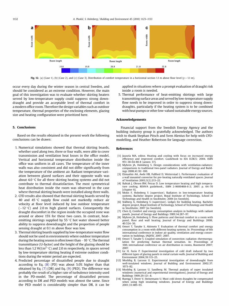
Fig. 12. (a) (Case 1), (b) (Case 2), and (c) (Case 3). Distribution of comfort temperature in a horizontal section 1.1 m above floor level (y¼ 1.1 m).

A. Ploskic, S. Holmberg / Building and Environment 45 (2010) 1123–11331132

occur every day during the winter season in central Sweden, andshould be considered as an extreme condition. However, the maingoal of this investigation was to evaluate whether skirting heatersserved by low-temperature supply could suppress strong down-draught and provide an acceptable level of thermal comfort ina modern office room. Therefore the design variables such as outdoortemperature, thermal properties of the enclosing elements, glazingsize and heating configuration were prioritized here.

5. Conclusions

Based on the results obtained in the present work the followingconclusions can be drawn:

1. Numerical simulations showed that thermal skirting boards,whether used along two, three or four walls, were able to covertransmission and ventilation heat losses in the office model.Vertical and horizontal temperature distribution inside theoffice was uniform in all cases. The temperature of the innerwalls was also consistent and did not differ significantly fromthe temperature of the ambient air. Radiant temperature vari-ation between glazed surfaces and their opposite walls wasabout 4.0 �C for all three skirting heating systems and did notcontribute to thermal dissatisfaction. The most symmetricalheat distribution inside the room was observed in the casewhere thermal skirting boards were installed along three walls.

2. CFD results also showed that thermal skirting boards served by40 and 45 �C supply flow could not markedly reduce airvelocity at floor level induced by low outdoor temperature(�12 �C) and 2.0 m high glazed surfaces. Consequently thedraught discomfort in the region inside the occupied zone wasaround or above 15% for these two cases. In contrast, heat-emitting skirtings supplied by 55 �C hot water showed betterability to suppress downdraught and the proportion of peoplesensing draught at 0.1 m above floor was low.

3. Thermal skirting boards supplied by low-temperature water flowshould not be used in environments where outdoor temperatureduring the heating season is often lower than�10 �C. The thermaltransmittance (U-factor) and the height of the glazing should beless than 1.2 W/(m2 �C) and 2.0 m respectively, in spaces servedby low-temperature skirting heating if extreme outdoor condi-tions during the winter period are expected.

4. Predicted percentage of dissatisfied people due to draughtaccording to Eq. (8) (PD) was about 5.0% higher than thatobtained by Eq. (7) (DR) and Eq. (9) (PED). The difference wasprobably the result of a higher rate of turbulence intensity usedin the PD-model. The percentage of dissatisfied personsaccording to DR and PED models was almost the same. Sincethe PED model is considerably simpler than DR, it can be

applied in situations where a prompt evaluation of draught riskinside a room is needed.

5. Thermal performance of heat-emitting skirtings with largetransmitting surface areas and served by low-temperature supplyflow needs to be improved in order to suppress strong down-draughts, particularly if the heating system is to be combinedwith heat pumps or other low-valued sustainable energy sources.

Acknowledgements

Financial support from the Swedish Energy Agency and thebuilding industry group is gratefully acknowledged. The authorswish to thank Stephan Pitsch and Sven Alenius for help with CFD-modelling, and Heather Robertson for language correction.

References

[1] Juusela MA, editor. Heating and cooling with focus on increased energyefficiency and improved comfort. Guidebook to IEA ECBCS; 2004. ISBN951-38-64-88-8 [annex 37].

[2] Myhren JA, Holmberg S. Design considerations with ventilation-radiators:comparisons to traditional two-panel radiators. Journal of Energy and Build-ings 2008;41:92–100.

[3] Elmualim AA, Awbi HB, Fullford D, Wetterstad L. Performance evaluation ofa wall mounted convector for pre-heating naturally ventilated spaces. Journalof Ventilation 2003;3(2):213–22.

[4] Babiak J, Olesen BW, Petras D. Low temperature heating and high tempera-ture cooling. REHVA guidebook;, ISBN 2-9600468-6-2; 2007. p. 64–70[chapter 6].

[5] Molin F, Holmberg S (supervisor). Radiators in low-temperature heatingsystems. Bachelor degree project, Royal Institute of Technology, School ofTechnology and Health in Stockholm; 2004 [in Swedish].

[6] Stålberg A, Holmberg S (supervisor). Ledges for building heating. Bachelordegree project, Royal Institute of Technology, School of Technology and Healthin Stockholm; 2007 [in Swedish].

[7] Chen Q. Comfort and energy consumption analysis in buildings with radiantpanels. Journal of Energy and Buildings 1989;14:287–97.

[8] Myhren JA, Holmberg S. Flow patterns and thermal comfort in a room withpanel, floor and wall heating. Journal of Energy and Buildings 2008;40:524–36.

[9] Omori T, Tanabe S, Akimoto T. Evaluation of thermal comfort and energyconsumption in a room with different heating systems. In: Proceedings of 6thinternational conference in indoor air quality, ventilation and energy conser-vation in buildings, IAQVEC 2007; 2007.

[10] Omori T, Tanabe S. Coupled simulation of convection–radiation–thermoregu-lation for predicting human thermal sensation. In: Proceedings of10th international conference on air distribution in rooms, Roomvent 2007;2007.

[11] Ge H, Fazio P. Experimental investigation of cold draft induced by twodifferent types of glazing panels in metal curtain walls. Journal of Building andEnvironment 2004;39:115–25.

[12] Moshfeg B, Larsson U. Experimental investigation of downdraught fromwell-insulated windows. Journal of Building and Environment 2002;37:1073–82.

[13] Moshfeg B, Larsson U, Sandberg M. Thermal analysis of super insulatedwindows (numerical and experimental investigations). Journal of Energy andBuildings 1999;29:121–8.

[14] Rueegg T, Dorer V, Steinemann U. Must cold down draughts be compensatedwhen using high insulating windows. Journal of Energy and Buildings2001;33:489–93.

A. Ploskic, S. Holmberg / Building and Environment 45 (2010) 1123–1133 1133

[15] Jurelionis A, Isevicius E. CFD predictions of indoor air movement induced bycold window surfaces. Journal of Civil Engineering and Management2008;14:29–38.

[16] Ekberg L. Guidelines for specification of indoor climate requirements. BFS1998:38;, ISBN 91-976271-0-0; 2006. p. 57 [in Swedish].

[17] McQuiston CF, Parker DJ, Spitler D. Heating, ventilating and air conditioning.6th ed. American Society of Heating, Refrigerating and Air-ConditioningEngineers, ISBN 978-0-471-47015-1; 2004. p. 104 [chapter 4].

[18] Warfvinge C. HVAC technique for civil engineers. The Faculty of Engineering atLund University; 2000. p. 1:5 [in Swedish].

[19] Braun S, Cremer I. Radiating warmth at a Raclette party, Fluent Germany,www.fluent.com/about/news/newsletters/04v13i2/a21.htm; 2004 [accessed02.05.09].

[20] Chen Q. Comparison of different k–e models for indoor airflow computations.Journal of Numerical Heat Transfer 1995;28:353–69.

[21] Zukowski M. A new formula for determining a minimum recommended valueof inlet air velocity from UFAD system to prevent occupants from draught risk.Journal of Building and Environment 2007;42:171–9.

[22] Griffin BT, Turler D, Arasteh D. Surface temperatures of insulated glazing units:infrared thermography laboratory measurements. ASHRAE Transactions1996;102:2.

[23] Peng S, Peterson F. Convection from a cold window with simulated floorheating by means of a transiently heated flat unit. Journal of Energy andBuildings 1995;23:95–103.

[24] ASHRAE Standard 55-1992. Thermal environmental conditions for humanoccupancy. American Society of Heating, Refrigerating, and Air ConditioningEngineers; 1992.

[25] Olsen BW, Parsons KC. Introduction to thermal comfort standards and theproposed new version of ISO EN 7730. Journal of Energy and Buildings2002;34:537–48.

[26] Fanger PO, Christensen NK. Perception of draught in ventilated spaces. Journalof Ergonomics 1986;29:215–35.

[27] Berglund L, Fobelets A. Subjective human response to low-level aircurrents and asymmetric radiation. ASHRAE Transactions 1987;93(1):497–523.

[28] Awbi H. Ventilation of buildings. 2nd ed.;, ISBN 0-415-27055-3; 2003. p. 29[chapter 1.5].

[29] Fluent 6.3 user’s guide. Alphabetical listing of field variables and their defi-nitions; 2009.

[30] Myhren JA, Holmberg S. Comfort temperatures and operative temperatures inan office with different heating methods. In: Proceedings of 8th InternationalConference on Healthy Buildings 2006, 2; 2006. p. 47–52.

lable at ScienceDirect

Building and Environment 46 (2011) 176e186

Contents lists avai

Building and Environment

journal homepage: www.elsevier .com/locate/bui ldenv

Low-temperature baseboard heaters with integrated air supply e An analyticaland numerical investigation

Adnan Ploski�c*, Sture HolmbergFluid and Climate Technology, School of Architecture and Built Environment, KTH, Marinens väg 30, SE-13640 Handen, Stockholm, Sweden

a r t i c l e i n f o

Article history:Received 7 May 2010Received in revised form12 July 2010Accepted 14 July 2010

Keywords:Baseboard (skirting) heatingLow-temperature hydronic heatingForced convective heat transferChannel airflowThermal comfortCFD

* Corresponding author. Tel.: þ46 8 790 48 84; faE-mail address: adnan.ploskic@byv.kth.se (A. Ploski

0360-1323/$ e see front matter � 2010 Elsevier Ltd.doi:10.1016/j.buildenv.2010.07.011

a b s t r a c t

The functioning of a hydronic baseboard heating system with integrated air supply was analyzed. Theaim was to investigate thermal performance of the system when cold outdoor (ventilation) airflow wasforced through the baseboard heater. The performance of the system was evaluated for differentventilation rates at typical outdoor temperatures during the Swedish winter season. Three differentanalytical models and Computational Fluid Dynamics (CFD) were used to predict the temperature rise ofthe airflow inside the baseboard heater. Good agreement between numerical (CFD) and analyticalcalculations was obtained. Calculations showed that it was fully possible to pre-heat the incomingairflow to the indoor temperature and to cover transmission losses, using 45 �C supply water flow. Theanalytical calculations also showed that the airflow per supply opening in the baseboard heater neededto be limited to 7.0 l/s due to pressure losses inside the channel. At this ventilation rate, the integratedsystem with one air supply gave about 2.1 more heat output than a conventional baseboard heatingsystem. CFD simulations also showed that the integrated systemwas capable of countering downdraughtcreated by 2.0 m high glazed areas and a cold outdoor environment. Draught discomfort in the case withthe conventional system was slightly above the recommended upper limit, but heat distribution acrosswhole analyzed office space was uniform for both heating systems. It was concluded that low-temper-ature baseboard heating systems with integrated air supply can meet both international comfortrequirements, and lead to energy savings in cold climates.

� 2010 Elsevier Ltd. All rights reserved.

1. Introduction

Water-based (hydronic) thermal devices are predominantlyused for internal heat emission within the residential sector andoffice buildings in Europe. Although the design of the thermal unitsis similar the variation of the supply water temperature is highamong the European countries, ranging from 55 to 90 �C for radi-ator/convector heating [1] and from 35 to 45 �C for floor heating [2].Generally hydronic heating systems are classified by their supplywater temperature. Heaters supplied by 75e90 �C water flow arenormally considered as high-temperature systems while 55 and45 �C supply flows are used in medium and low-temperatureheating systems, respectively. Thermal energy for the heatingsystems can be produced by several different methods. The mostenergy efficient and sustainable technical solution may be tocombine a heating systemwith a low-valued energy device such asa heat pump. To make this integration efficient the supply water

x: þ46 8 790 48 00.�c).

All rights reserved.

temperature to the heating units should be lower than 50 �C.Recent studies have shown that different kinds of heatingarrangements supplied with 45 �C water flow were fully able tocover transmission and ventilation heat losses of modern buildings[3,4]. Low-temperature heat emitters showed many advantages,such as energy savings and ability to generally create a good indoorthermal climate, but also a weakness in countering cold air down-flow (downdraught) [3,4]. Usually, the thermal energy supplied bythe conventional low-temperature heating systems is mainlyemitted by the thermal radiation. Natural convection is also presentbut its influence on air movement is much weaker than in tradi-tional high-temperature heating systems where natural convectionaccounts for the main part of total heat emission. Weak convectivepower among low-temperature heating systems is probably themain reason for problems with cold downdraught. Cold air down-flow, normally caused by low outdoor temperature and large areasof glazing, could be blocked by directing the warm ventilationairflow towards the glazed surfaces. This technical arrangementmight also be a solution to the elimination of cold draughts inspaces served by low-temperature heating systems.

Nomenclature

Latin lettersAc Cross-sectional area of baseboard channel [m2]As Inner surface area of baseboard channel [m2]cPair

Specific heat capacity of air, 1005 used in study[J/(kg �C)]

cPwaterSpecific heat capacity of water, 4180 used in study[J/(kg �C)]

Dh Hydraulic diameter of baseboard channel [m2]f Friction factor between air and inner channel surfaces

[e]g Gravitational acceleration, 9.81 used in study [m/s2]Gr Grashof number [e]L Baseboard channel or plate length [m]_mair Air mass flow [kg/s]_mwater Water mass flow [kg/s]Nu Nusselt number [e]P Inner perimeter of baseboard channel [m]pair Atmospheric pressure, 101325 used in study [Pa]Pext.wall Transmission loss through external wall [W]Pglazing Transmission loss through glazed areas [W]Pr Prandtl number [e]Pvent Ventilation heat demand [W]Qvent Ventilation flow rate per person [l/s/prs]Re Reynolds number [e]

Rair Specific gas constant for dry air, 287 used in study[J/(kg �C)]

Tmbt Absolute mean air bulk temperature [K]Ts Absolute mean surface (baseboard) temperature [K]vair Mean air velocity inside baseboard channel [m/s]vair,in Indoor air velocity [m/s]U-value Total thermal transmittance [W/(m2 �C)]x, y, z Cartesian coordinates [m]

Greek lettersaair Mean air-side convective heat transfer coefficient

[W/(m2 �C)]awater Mean water-side convective heat transfer coefficient

[W/(m2 �C)]bair Mean air thermal expansion [1/�C]qair,in Mean indoor air temperature [�C]qair,out Mean outdoor air temperature [�C]qcomfort Comfort temperature [�C]Dqlmtd Logarithmic mean temperature difference [�C]Dp Pressure loss [Pa]qmbt Mean air bulk temperature [�C]qs Mean surface (baseboard) temperature [�C]qwater,in Mean supply water flow temperature [�C]qwater,out Mean return water flow temperature [�C]qrad Radiation temperature [�C]lair Air thermal conductivity [W/m �C]mair Air dynamic (absolute) viscosity [kg/m s]rair Mean air density [kg/m3]

A. Ploski�c, S. Holmberg / Building and Environment 46 (2011) 176e186 177

Pre-heating of the ventilation air can be arranged in severalways. Onemethod is to force it along or through a heating unit. Thisheatingeventilation arrangement may not only pre-heat theventilating air but also enhance the total heat transfer from theheating unit. The higher the air velocity inside the unit, the higherthe heat output will be. Furthermore, the greater the temperaturedifference between the cold incoming air and the heating unit, thehigher the heat flow to the air will be. Consequently, the supplywater temperature to the heater can be lowered without affectingover-all thermal performance, which will most likely result inenergy savings. This technical design can be achieved by forcing

Fig. 1. (a) General illustration of integrated baseboard heating system with one air supply.channel consists of two feed and two return water heated pipes enclosed by thin metal pl

cold outdoor (ventilation) airflow throughout a baseboard(skirting) heater. The idea is to lead the cold outdoor airflow via oneor more openings in the building structure to the baseboard radi-ator. The incoming air is then pre-heated in the narrow horizontalbaseboard channel before it exits throughout the slot opening atthe top. The warm airflow is then directed towards glazed areas tomeet air down-flow crated by cold glazed surfaces. By these meansthe negative effects of downdraught might also be reduced inspaces served by low-temperature heating systems. The generalprinciple of baseboard heatingeventilation system is illustrated inFig. 1(a) and (b). In general, conventional baseboard radiators are

(b) Elevation (left) and section (right) of the four-pipe baseboard radiator system. Theates. Dimensions are given in millimetres.

A. Ploski�c, S. Holmberg / Building and Environment 46 (2011) 176e186178

long and low-profile heat-emitting panels installed at the bottom ofwalls along all or most of the inner periphery of a room. Moredetailed information about such heating systems was given byPloski�c and Holmberg [3].

The aim of this study was to estimate whether the suggestedbaseboard heatingeventilation system was powerful enough to:

� cover transmission losses of an office room,� pre-heat outside ventilation air to the room temperature,� create a draught-free indoor climate

at supply water temperatures lower than 50 �C during Swedishwinter conditions. The investigation also included a comparison inthermal performance between conventional and proposed base-board heating systems.

1.1. Previous studies

A similar heatingeventilation system was analyzed by Myhrenand Holmberg [5]. The main goal of their investigation was to mapthe interaction between a conventional two-panel radiator andventilation air supply. The thermal performance of such a systemwas evaluated at air velocities of 0.35 and 0.7 m/s between thepanels. It was found that the ventilationeradiator supplied withlow-temperature water flow had roughly the same heat output asthe conventional high-temperature radiator. Computational FluidDynamics (CFD) was also employed to analyze the heat distributioninside the room. Simulations showed that the ventilationeradiatorcreated a uniform heat distribution throughout whole roomwithout downdraught. Elmualim et al. [6] studied the performanceof a wall-mounted air supply convector installed underneath thewindow in a naturally ventilated test laboratory during winterconditions. The incoming outdoor airflow at a constant rate waspre-heated by various temperature levels of water circulatinginside the convector coil. They concluded that this hea-tingeventilation system installed at a low level could increase theventilation efficiency of the room and eliminate the problems withcold draught. The reported average indoor air temperature waslower than recommended by international standards but in linewith design temperatures. Jurelionis and Isevicius [7] investigatedthe behaviour of cold downdraught caused by different types ofglazing in various winter conditions. According to their CFD results,problems with cold draught may also appear in rooms with 2.0 mhigh super-insulating (U-value¼ 1.0 W/m2 �C) glazing at outdoortemperature of �6.0 �C if no heating equipment underneath theglazing is installed. CFD predictions also showed that a conven-tional low-profile heating convector was insufficient to suppresscold draught induced by 5.0 m high glazing and �20 �C externaltemperature. Despite the low U-value glazing and a powerfulheating device used in this case, the air speed at ankle level insidethe occupied zone was twice as high as recommended by currentinternational norms. They concluded that the best way to suppressstrong downdraught was to counter it with a warm air jet of 1.0 m/s. Zukowski [8] put forward an analytical model for predictinga minimum required air jet velocity to block downdraught.According to his model, an air velocity of 0.5 m/s was needed tosuppress colddowndraught createdby2.0 mhighglazing and�20 �Coutside temperature. The U-factor of the glazing was 1.0W/m2 �C inthis case. The analytical findings were also tested using CFD simu-lations. These showed that draught discomfort inside the occu-pied zone was below the allowed upper limit according tointernational standards. The temperature of air jets used in CFDmodels was 7.0e8.0 �C higher than the room temperature. Ganand Awbi [9] used CFD to study air movement and heat distri-bution inside a room with one 1.5 m high single-pane glazing

exposed to outdoor temperature of 10 �C. In order to createa draught-free climate they used an air jet of 1.1 m/s to meetcold air down-flow. The temperature of the jet was 5.5 �C higherthan the indoor temperature. Jägbeck et al. [10] reported resultsbased on field indoor climate measurements and extensiveinterviews with occupants in spaces with different heatingarrangements. Their general conclusion was that forced air-heating systems provided a draught-free indoor climate. Thesupply air temperatures in their investigation were around23e24 �C, while the air velocity ranged between 0.8 and 1.1 m/s.Based on the above findings two different conclusions can bedrawn. First, the combined heatingeventilation system signifi-cantly improved thermal power from the heating unit. Second,the most efficient way to neutralize the cold downward airflowwas to mix it with warm air jet. Therefore, the proposed inte-gration of baseboard radiator and ventilation air supply seemedto be well-founded.

2. Method

The main focus of the first part of the study was to analyze theheat transfer inside the baseboard channel. Detailed explanation ofall governing parameters and the theoretical background to theanalytical models used for analysis is presented. Both analyticalmodels and numerical (CFD) simulations were employed to predictthe temperature rise of airflow inside the baseboard channel.Ventilation rates were modeled in accordance with national andinternational recommendations of minimum fresh air requirementfor office users, of 7.0e10 l/s per person [11,12]. The performance ofthe system was evaluated for the Swedish winter climate. Accord-ing to the Swedish Meteorological and Hydrological Institute(SMHI), the mean outside temperature during the coldest monthsof the year (December, January and February) for the entire countryis around �6.0 �C [13]. The design external temperature, repre-senting extreme outdoor condition in central Sweden is about�12 �C [14]. Both temperature levels as inflow boundary conditionswere used here. In the second part of the study, CFD simulationswere used to analyze thermal climate inside the room for both theproposed and the conventional baseboard heating systems.

2.1. Heat exchange between baseboard channel and air supply

Thermal exchange between heated parts of the baseboardchannel and cold air supply, as illustrated by Fig. 1(a) and (b), wasestimated by the energy balance as shown in Equation (1).

_mair$cPair$�qair;out� qair;in

�|fflfflfflfflfflfflfflfflfflfflfflfflfflfflfflfflfflfflfflfflfflfflfflffl{zfflfflfflfflfflfflfflfflfflfflfflfflfflfflfflfflfflfflfflfflfflfflfflffl}

Ventilation heat demand

¼ _mwater$cPwater$�qwater;in� qwater;out

�|fflfflfflfflfflfflfflfflfflfflfflfflfflfflfflfflfflfflfflfflfflfflfflfflfflfflfflfflfflfflfflfflffl{zfflfflfflfflfflfflfflfflfflfflfflfflfflfflfflfflfflfflfflfflfflfflfflfflfflfflfflfflfflfflfflfflffl}

Water heat supply

z

�1

awaterþ 1

aair

��1$As$Dqlmtd|fflfflfflfflfflfflfflfflfflfflfflfflfflfflfflfflfflfflfflfflfflfflfflfflfflffl{zfflfflfflfflfflfflfflfflfflfflfflfflfflfflfflfflfflfflfflfflfflfflfflfflfflffl}

Watereair heat exchange

(1)

The first part of Equation (1) represents the heat energy required tobring airflow from outside up to indoor temperature. The middlepart represents the thermal energy produced by circulating waterinside the baseboard pipes, while the last (third) part refers to heatflow from hot water to the cold airflow. The four parameters in thelast part of Equation (1) represent respectively, the rate ofconvective thermal transfer fromwater to walls awater and betweenwalls and the cold air supply aair, the heat transmitting surface areaAs and the Logarithmic Mean Temperature Difference (LMTD)

A. Ploski�c, S. Holmberg / Building and Environment 46 (2011) 176e186 179

Dqlmtd. The average LMTD is usually used when designing heatexchangers because it gives an accurate representation of expo-nential temperature rise over the exchanger. Since both hot waterflow and cold airflow move in the same direction inside the base-board channel, LMTD for the parallel heat exchanger was used asshown in Equation (2).

Dqlmtd ¼�qwater;out � qair;out

���qwater;in � qair;in

�ln�qwater;out � qair;out

qwater;in � qair;in

�

¼�qair;in � qair;out

�ln�qs � qair;out

qs � qair;in

� (2)

Different dimensionless numbers such as Reynolds number Re,Prandtl number Pr, Grashof number Gr, and Nusselt number wereemployed to calculate the magnitude of the total convective heattransfer coefficient. A practical implication of Equation (1), for theinvestigated application where awater[ aair and thermal resis-tance of the heated walls is negligible, is that total heat transfer iscontrolled by aair. To illustrate this [15], a doubling of thewater-sideheat transfer coefficient (awater) increases the over-all heat transfercoefficient only by approximately 2%. On the other hand a doublingof the air-side heat transfer coefficient (aair) increases the over-allheat transfer coefficient by 93%. Therefore, the predicted over-allheat transfer coefficient values in this study were exclusively basedon the air-side heat transfer coefficient.

In view of the fact that all four dimensionless numbers usedhere are temperature dependent, all calculations were approxi-mated at mean air bulk temperature qmbt¼ (qair,inþ qair,out)/2. TheReynolds number was also estimated at average air velocity (vair)inside the channel as shown in Equation (3).

Re ¼ vair$Dh$rairmair

(3)

Where Dh ¼ 4$Ac=P, rair ¼ pair=Rair$Tmbt and

mair ¼ 1:458$10�6$ffiffiffiffiffiffiffiffiffiffiTmbt

p=1þ 110:4=Tmbt

Dh represents the hydraulic diameter, Ac the area and P theperimeter of the channel cross-section. The air density rair anddynamic viscosity mair were evaluated at absolute mean air bulktemperature Tmbt while the atmospheric pressure pair and specificgas constant Rair were considered as constants. The aboveempirical relationships can be found in Ref. [16]. The Prandtlnumber was calculated using Equation (4) where the air thermalconductivity was estimated by the following expressionlair¼ 0.0241 $ (1þ0.003 $ qmbt) [17].

Pr ¼cPair

$mair

lair(4)

In order to determine which Nusselt (heat transfer) correlationswere most suitable to use for correct prediction of convective heatflow rate, the convection characteristics inside the channelrequired definition. Normally, this would be determined by evalu-ating the ratio between Reynolds and Grashof number. Generally, itis accepted that when Gr/Re2�1, Gr/Re2z1 and Gr/Re2[ 1,convection is forced, mixed and natural (free), respectively. Themagnitude of the Grashof number was calculated by Equation (5)where the rate of air thermal expansion was estimated usingfollowing relation bair¼ 1/Tmbt.

Gr ¼ g$bair$ðqs � qmbtÞ$D3h$

�mairrair

��2(5)

The analytical calculations showed that the Prandtl number was0.715 and that the Reynolds number varied from about 5060 to8870, while the Gr/Re2 ratio is ranged from 0.002 to 0.005 in allinvestigated airflows. It was clear that flow inside the baseboardchannel was transitional-to-turbulent and that convection wasforced. Therefore three well-known Nusselt relations appropriatefor this convection and flow regime were employed to predict thetemperature increase of the airflow inside the channel, and forcomparison with CFD simulations.

Nu¼0:116$�Re2=3�125

�$Pr1=3$

"1þ

�DhL

�2=3#$

�TmbtTs

�3=8

(6)

The Nusselt relation expressed by Equation (6) was developed byHausen and is applicable for forced convective transitional flowregimes with constant heat flux. The equation is valid for2300< Re< 106 and 0.6< Pr< 500 according to Ref. [17] while inRef. [18] another range is suggested 2200< Re< 104 and Pr> 0.6.

Another widely used Nusselt relation (Equation (7)) forapproximation of transitional and turbulent forced convectiveflows, that can be applied both for thermal situations withuniform wall temperature and constant wall heat flux [19] wasput forwarded by Gnielinski [20]. This correlation is valid for3000< Re< 5 $106 and 0.5< Pr< 2000 where flow frictioninside the channel is evaluated by the following expressionf¼ (1.82 $ log(Re)� 1.64)�2. The friction factor is applicable forprediction of turbulent flow losses inside smooth ducts for sameReynolds number range as the Nusselt relation.

Nu ¼ ðf =8Þ$ðRe�1000Þ$Pr1þ12:7$

ffiffiffiffiffiffiffiffiffiffiffiðf =8Þ

p$�Pr2=3�1

�$"1þ

�DhL

�2=3#$

�TmbtTs

�3=8

(7)

The last semi-empirical expression used here to estimate the levelof the dimensionless heat transfer coefficient was the so-calledDittuseBoelter correlation [21], Equation (8). Originally this equa-tion was developed for high turbulent forced convection flowsbased on experimental data covering 104< Re< 1.2 $105 and0.7< Pr< 120, but it has been found that for fluids with relativelylow viscosity (mfluid< 2 $ mwater), as in this study, it can also beapplied for flow regimes with Reynolds numbers down to2300e3000 [22].

Nu ¼ 0:023$Re4=5$Pr2=5$

"1þ

�DhL

�2=3#$

�TmbtTs

�3=8

(8)

After the Nusselt number was computed, the total convective heattransfer coefficient between transmitting surfaces and the heatabsorbing airflow could easily be approximated by the next relationaair¼Nu $ lair/Dh. As it can be noticed, all three Nusselt relationsused here consisted of three different elements. The first (main)part was developed to predict the heat transfer rate for long ductswhere the internal flow is both fully thermodynamically andhydraulically developed, typically the expression applied for ductswith a length-to-hydraulic diameter ratio larger than 60. In view ofthe fact that the turbulent flow in short ducts, as was the case here,is often hydraulically developed but thermodynamically undevel-oped, use of entrance correction factor [1þ (Dh/L)2/3] is recom-mended. The third (last) multiplier on the right side of the Nusseltequations was used to correct the variation of fluid propertiesbetween hot duct surfaces Ts and the mean airflow temperature atthe channel centre Tmbt. In the literature various suggestions to theexponent n in (Tmbt/Ts)n ratio for (Ts/Tmbt)> 1 can be found. Theusual recommendations for n for air heating are 0.25 [23], 0.36 [24]

A. Ploski�c, S. Holmberg / Building and Environment 46 (2011) 176e186180

and 0.45 [20]. However, for the investigated configuration in thisstudy it was found that n¼ 3/8 gave best agreement with Equation(9) for a wide range of temperature variations. A more detailedexplanation of this equation and both correction factors can befound in Ref. [25].

�Ts

Tmbt

��½0:3 log�

TsTmbt

�þ0:36�

¼�TmbtTs

�n

where

n ¼ 3=8 whenTs

Tmbt> 1

(9)

The aim of this study was to investigate whether a balance betweentransmission and ventilation heat losses and heat supply could beachieved at acceptable pressure loss. Therefore the upper limit forpressure loss inside the baseboard pipes was set between 80 and100 Pa/m,which is also the usual practice in piping design. The totalpressure loss was estimated by combination of Equations (1) and(10) where friction factor was evaluated using a previously pre-sented expression in Equation (7). Equation (10) was also used forthe estimation of airflow friction (pressure) losses inside thebaseboard channel.

Dp ¼fLD$rv2

2

�pipes=channel

(10)

In order to make all presented equations and CFD modeling easierto handle, the following approximation was made. Since the totalsurface area of the vertical baseboard plate and its four attachedpipes, (Fig. 1(b)), is the same as that of the inner channel shell area,the pipes were omitted from further consideration. So instead ofa complex cross-section, a single rectangular channel 150 mm highand 20 mmwidewas analyzed. A detailed overviewof all calculatedgoverning parameters also used in the CFD simulations is given inTable 1.

2.2. CFD model of baseboard channel

The CFD code Gambit (pre-processor) was used to createchannel geometry and for computational grid (mesh) construction,while the Fluent 6.3 was utilized to post-process simulation results.A straight rectangular duct with one inlet and one outlet at theopposite side was analyzed. In order to create hydraulically fullydeveloped flow before it entered the heated part of the channel,a 350 mm long (10 $Dh) isothermal entrance length was modelled.Different airflow rates with corresponding uniform heat fluxmagnitudes Pheat, as illustrated in Table 1, were studied. Thetemperature of the cold air inflow was set to be the same for allcases while the temperature distribution inside the channel waspredicted by CFD. The prediction was performed using second-order discretization scheme for all differential equations. Thecoupling between the pressure and velocity was handled by theSimple algorithm. The standard wall function was also applied forsimulation of heat transfer and turbulence generation near thechannel walls. Different non-uniform structured (hexahedral)

Table 1The presented heat fluxes (Pheat) were used as thermal boundary conditions for CFD simulthe airflow from �6.0 to 21 �C using 45 �C supply and 40 �C return water flow.

Qvent,l/s/prs

vair,m/s

Dh,mm

L,m

Case 1 6.0 2.0 35.3 2.0Case 2 7.5 2.5 35.3 2.0Case 3 9.0 3.0 35.3 2.0Case 4 10.5 3.5 35.3 2.0

mesh arrangements and turbulence models were tested andcompared with analytical models. The computational grid insidethe channel was not uniformly distributed. A refined grid wasapplied near all solid walls while an unrefined grid was arrangedtowards the centre of the channel. The transition from refined tounrefined grid was made gradually in a smooth way. The gridindependence was checked by changing the grid density near solidwalls as well as around the channel centre. Convergent solutionswith consistent results were obtained in all cases regardless ofwhich grid arrangement was applied. Nevertheless, it was foundthat a 5.0 mmwide wall cell, which was the first grid cell adjoinedto solid walls, in combination with all available ke3 turbulencemodels in Flunet 6.3 gave best agreement with analytical calcula-tions. The mean air temperature variation inside the baseboardchannel calculated by different analytical equations and CFDsimulations using the Re-Normalization Group (RNG) turbulencemodel is shown in Fig. 2(a)e(d).

2.3. The room model

The indoor thermal climate inside a two-person empty officespace, served by the convectional baseboard heating system andthe heatingeventilation system proposed here was investigated.The room model geometries are described in Fig. 3 and Table 2where the dimensions are given in metres. The same room waspreviously used and validated against experimental data andanalytical calculations, and a good agreement was found betweenCFD predicted, measured and calculated values for this roomconfiguration [3].

The office roomwas considered as having one external wall withtwo frameless glazing areas. It was assumed that the whole wallsurface areawas exposed to an outdoor temperature of �12 �C. Themean U-values of the external wall and glazing areas were set to0.25 and 1.2 W/m2 �C, respectively. The other walls were regardedas thermally non-conducting (adiabatic) enclosing elements. In thesimulations, the heat loss through glazed surfaces was set to39.6 W/m2, and 8.25 W/m2 for the external wall. The transmissionlosses were estimated applying the calculation procedure reportedin Ref. [3]. The ventilation air supply was modelled in two differentways. In the case with conventional baseboard heating, a squarefour-way radial diffuser positioned at the centre of the ceiling wasused for air supply. The temperature of the supply air was heldconstant at 18 �C which was approximately 3.0 �C lower than theassumed room temperature. In the case of the proposed hea-tingeventilation system, supply air temperature was calculatedseparately. The temperature profile of supply air was separatelyapproximated by analytical models and CFD simulations, to be thenused as a boundary condition in the room model. In this case,ventilation flow at two different rates was supplied via two slotopenings placed underneath glazed areas I and II at the top of thebaseboard heater I. The air jets from these two slot openings weredirected towards glazed surfaces while the used indoor air wasevacuated through an opening positioned in the upper corner at theopposite side of the external wall. The transmission losses of the

ations. In all cases the heat fluxmagnitudes were adjusted to raise the temperature of

As,m2

Pr, e Re, e Gr/Re2, e Pheat,W/m2

0.68 0.715 5066 0.005 401.60.68 0.715 6332 0.003 501.90.68 0.715 7598 0.002 602.40.68 0.715 8865 0.002 702.8

Fig. 2. (a) Mean air temperature variation inside the channel at 2.0 m/s. (b) Mean air temperature variation inside the channel at 2.5 m/s. (c) Mean air temperature variation insidethe channel at 3.0 m/s. (d) Mean air temperature variation inside the channel at 3.5 m/s.

A. Ploski�c, S. Holmberg / Building and Environment 46 (2011) 176e186 181

roomwere covered by the heat emission from baseboard heaters IIand IV. The first computational grid point is set at 5.0 mm distancefrom all heat-emitting walls. This rate of near-wall grid refinementhas been recommended for spaces with natural convection whenstandard wall functions are applied in order to obtain an accurateheat transfer prediction [26]. All other CFD settings previouslypresented in Section 2.2 were also employed here to analyze thethermal climate conditions. In addition, radiative heat exchangebetween transmitting surfaces of the room was simulated usinga Discrete Ordinates (DO) radiation model. All room surfaces were

Fig. 3. The schematic view of the investigated office model.

assumed to be gray and have an emissivity factor 3 of 0.9. All theinvestigated cases were simulated using the same CFD settings butdifferent boundary conditions.

3. Results

Both analytical calculations and CFD simulations, as illustratedin Fig. 2(a)e(d), showed that it was fully possible to achievea balance between ventilation thermal demand and heat supplywith the proposed heatingeventilation system using 45 �C water

Table 2Dimensions of the office model and position of glazed surfaces, baseboard heaters,air intake and exhaust opening.

Item Length Width Height Location

Dx Dz Dy x y z

Room 5.3 3.8 2.6 0.0 0.0 0.0Glazing I 1.8 0.0 2.0 0.7 0.3 0.0Glazing II 1.8 0.0 2.0 3.0 0.3 0.04-Way radial diffuser 0.24 0.24 0.02 2.65 2.58 1.9Exhaust 0.3 0.02 0.15 2.65 2.23 3.8Baseboard heater I 5.3 0.0 0.15 0.0 0.0 0.0Baseboard heater II 0.0 3.8 0.15 0.0 0.0 0.0Baseboard heater III 0.0 3.8 0.15 5.3 0.0 0.0Baseboard heater IV 5.3 0.0 0.15 0.0 0.0 3.8

A. Ploski�c, S. Holmberg / Building and Environment 46 (2011) 176e186182

flow. In order to achieve this, the length-to-hydraulic diameterratio should be around 44. In practice this means that the length ofthe baseboard channel should be approximately 1.55 m per airsupply inlet. Fig. 2(a)e(d) also shows that the analytical modelbased on the Nusselt relation proposed by Gnielinski gave the bestagreement with CFD. The other two models based on equationsdeveloped by Hausen and DittuseBoelter showed generallya higher mean airflow temperature inside the baseboard channelcompared to CFD. In this context it should also be mentioned thatpredicted air temperature rise based on DittuseBoelter correlationagreed better with CFD for high Reynolds numbers, while thetemperature increase calculated by the Hausen relation wasroughly constant regardless of the air velocity level inside thechannel. Since the analytical model established on the Nusseltexpression proposed by Gnielinski showed the best agreementwith CFD for the wide range of Reynolds number used here, it wasutilized to demonstrate the variation of the Nusselt number asa function of the ratio between channel length and its hydraulicdiameter (L/Dh) as shown in Fig. 4(a). The same model was alsoapplied (Fig. 4(b)) to show the channel surface temperaturerequired to pre-heat different airflow rates at various inlet condi-tions to the room temperature. The nonlinear lines in Fig. 4(a)illustrate the change of the Nusselt number while the straightdiagonal lines represent the pressure loss increase along thebaseboard duct. The total pressure loss including the duct in thebuilding structure, channel changeover and baseboard channel, asillustrated in Fig. 1(a), was estimated by an extended version of theEquation (10), where the minor and the friction losses werecalculated at the prevailing dynamic pressure inside the baseboardduct. The minor contraction loss coefficient was taken to be 0.43[27]. Fig. 4(a) also shows that the heat transfer rate was highest forL/Dh� 20, after which the thermal exchange was nearly constantregardless of channel length. On the other hand the pressure lossgrew rapidly across the channel with increased air velocity.

Airflow rates of 7.0 and 10 l/s at inlet temperatures of 0.0, �6.0and �12 �C were used to test the performance of the proposedheatingeventilation system. Fig. 4(b) shows that the baseboardchannel length in the case with air inflow of -12 �C needed to beabout 29% longer compared to the inflow of 0.0 �C, to be able toraise its temperature to 21 �C. On the other hand, the channellength needed to be approximately 14% greater when air wasbrought in at -6.0 �C compared to 0.0 �C. Furthermore, in order topre-heat the outdoor airflow of 10 l/s to room temperature, the

Fig. 4. (a) Variation of the Nusselt number and pressure loss as function of L/Dh ratio at differthe outdoor air of 0.0, �6.0 and �12 �C to 21 �C at different ventilation rates.

channel length needed to be around 5.8% longer compared to thecase with a ventilation rate of 7.0 l/s.

Table 3 presents the balance between ventilation heat demands,transmission losses and the heat supply for the different casescenarios. Results indicated that in some cases it was fully possibleto cover both transmission and ventilation heat losses using low-temperature water supply. In the case with an airflow rate of 7.0 l/sat inlet temperature of �6.0 �C, the ventilation and transmissionlosses could be covered by a water supply at 45 �C. On the otherhand, in the case with the same airflow at�12 �C, a water supply at50 �Cwas required to cover both heat demands. The data presentedin Table 3 was based on the assumption that air inflow entered viatwo intakes placed along the centre baseboard heater I. One intakewas placed on the right hand side of glazing I while the other wasplaced at the left of the glazing II. Water flow temperatures andbaseboard channel lengths required to cover ventilation heat losseswere estimated by the model based on Gnielinski’s heat transferexpression. Baseboard lengths (baseboard heaters II and IV) withcorresponding water supply and return flow temperatures requiredto cover transmission losses were calculated using the expressionsa for heat-emitting vertical plate. The set of equations for estima-tion of the total heat transfer from a vertical flat plate can be foundin Ref. [5].

Heat output from baseboard heaters with one and two airsupplies was also compared to the thermal power produced by theconventional baseboard radiator system (without air supplies).Dimensions of baseboard heater I were taken as reference. Thecalculation procedure was as follows. The total heat output for theintegrated systemwas calculated in two steps. First, the magnitudeof forced convection for the channel lengths (2�1.55 m) where theairflow is pre-heated was estimated. The contribution of naturalconvection and thermal radiation for this channel part facing theroom was also included. Second, the remaining 2.2 m of baseboardlength was treated as a vertical flat plate and the levels of naturalconvection and thermal radiation for this part were calculated.These were then added to heat output of channel parts with forcedconvection. In the case with a conventional system, the wholebaseboard length (5.3 m) was seen as vertical flat plate, and themagnitudes of the natural convection and the thermal radiation forthis arrangement were estimated in line with this assumption. Thebaseboard height of 0.15 m was kept constant both for integratedand the conventional systems during all calculations. The findingsin Table 4 show that thermal emission from the integrated system

ent velocity levels. (b) The required baseboard channel surface temperature to pre-heat

Table 3Ventilation and transmission heat losses for the two-person room configuration shown in Table 2. The supply and returnwater flow temperatures required to cover both heatdemands are also given.

Ventilation Transmission

Heat demand Heat supply Heat demand Heat supply

Item Qvent,l/s/prs

Person qair,in/qair,out,�C

Pvent,W

qwater,in/qwater,out,�C

L,m

Pglazing,W

Pext. wall,W

qwater,in/qwater,out,�C

L,m

I 7.0 2 21/�6.0 478 45/40 2� 1.55 233 45 45/36 9.1II 10 2 21/�6.0 683 50/40 2� 1.55 233 45 50/33 9.1III 7.0 2 21/�12 590 50/45 2� 1.55 285 54 50/39 9.1IV 10 2 21/�12 843 55/45 2� 1.55 285 54 55/36 9.1

A. Ploski�c, S. Holmberg / Building and Environment 46 (2011) 176e186 183

with two air supplies (2�7.0 l/s) at total airflow rate of 14 l/s wasabout 3.3 times higher compared to the conventional system andaround 4.0 times higher in the case with airflow of 20 l/s (10 l/s persupply intake). The amount of radiative and convective heatoutputs per metre length for the conventional and integratedsystem with one air supply inlet is illustrated in Fig. 5. As it can beseen, the total heat output from the integrated system with singleair supply at airflow of 7.0 l/s with inlet temperature of �6.0 �C wasabout 2.1 times higher compared to the conventional system.Forced and natural convection stood for nearly 80% of total heatemission in this case, while thermal radiation contributed withabout 20%. In case with conventional system the proportion wasquite different. Natural convection stood for about 46% of the over-all heat release while thermal radiation contributed by approxi-mately 54%. On the other hand, the system with two air suppliesgave around 1.5 times more thermal power compared to thearrangement with one air supply under the same conditions.

3.1. Thermal comfort inside the office

Draught sensitivity of occupants in ventilated spaces iscommonly estimated by Equation (11), where TI represents localturbulence intensity in percent. This Draught Rating (DR) expres-sion is a result of empirical studies by Fanger et al. [28] and isincluded in ASHRAE Standard 55 [29] and EN ISO 7730 thermalcomfort standard [30]. The model predicts the percentage ofpersons dissatisfied due to draught. This draught model was alsoused here to predict the rate of draught discomfort at 0.1 m abovethe floor level. According to EN ISO 7730 standard, the percentageof dissatisfied people due to draught should be less than 15% insidethe occupied zone. The occupied zone is usually defined as thespace where the occupants normally dwell and is commonly set1.0 m away from the glazed areas, 0.6 m from the internal walls andbetween 0.1 and 1.8 m above floor level.

Table 4The heat outputs produced by conventional and integrated baseboard heatingsystem with two air supplies. Ventilation heat demands and temperature of thewater flows (heat supply) are as previously shown in Table 3.

Baseboard heater I

Conventional With air supply

Design parameters Natural convectionand thermalradiation

Forced and naturalconvectionþ thermal radiation

Item qwater,in/qwater,out L H Heat output Heat output

�C m m W/m W/m2 W W/m W/m2 W

I 45/40 5.3 0.15 34.4 229 182 114 762 606II 50/40 5.3 0.15 38.6 257 205 156 1041 828III 50/45 5.3 0.15 44.1 294 234 147 982 781IV 55/45 5.3 0.15 48.7 324 258 197 1311 1043

DR¼�3:143þ0:3696$vair;in$TI

�$�34�qair;in

�$�vair;in�0:05

�0:6223

(11)

As detailed in Section 2.3, three different ventilation casescenarios were simulated and compared. A conventional baseboardheating system where airflow of 20 l/s was supplied by a four-wayradial square ceiling diffuser was compared to baseboard heaterswith integrated air supplies. The performance of the integratedbaseboard system at airflows of 20 and 14 l/s was analyzed. Two0.5 m long and 20 mm wide slot openings positioned at the top ofthe baseboard I at the centre of glazings I and II were used forsupply of pre-heated airflow to the room. The indoor flow patternsinduced by air jets, of 1.0 m/s in the casewith airflow of 20 l/s and of0.7 m/s in the case with 14 l/s were investigated. The air jets in bothcases were directed towards cold glazed areas of the room. Themain goal of the comparison was to estimate the ability of eachsystem to block cold downdraught and to create an acceptablethermal climate. Two straight horizontal lines positioned at 0.1 mabove floor level and 0.5 m away from glazed areas I and II, andextending to the opposite wall were used for construction of DRprofiles.

The draught rating profiles presented in Fig. 6(a) and (b) indicatethat baseboard heaters with integrated air supplies were able toeliminate draught problems at the ankle level inside the occupiedzone. The percentage of predicted draught discomfort at this levelwas less than 15% inside the occuped space. In the case withconventional baseboard radiators a slightly higher proportion ofdraught discomfort was observed. The draught rating for the regionlocated between 1.0 and 2.8 m distant from the glazing II rangedfrom 18 to 15%. Also in front of glazing I the draught rating for theconventional system was slightly over the recommended limit.Apart from the draught rating index, the distribution of comfort

Fig. 5. Comparison of thermal radiation and convection heat outputs, for theconventional system and the integrated baseboard heating arrangement with one airsupply inlet. An airflow of 7.0 l/s at �6.0 �C was used.

Fig. 6. (a) DR profiles at x¼ 1.5 m, y¼ 0.1 m and Dz¼ 0.5e3.8 m (glazing I). (b) DR profile at x¼ 3.8 m, y¼ 0.1 m and Dz¼ 0.5e3.8 m (glazing II).

A. Ploski�c, S. Holmberg / Building and Environment 46 (2011) 176e186184

temperaturewas also used to investigate thermal climate inside thestudied room. Myhren and Holmberg [31] compared comforttemperature (Equation (12)) with operative temperature andconcluded that this model gave a more comprehensive picture ofperceived thermal climate. The mathematical expression used forcalculation of radiant temperature in Equation (12) can be found inRef. [3]. CFD simulations showed that the mean indoor airtemperature ranged from 20.4 to 20.9 �C and the temperaturestratification between the floor and ceiling was about 1.5 �C in allthree cases.

qcomfort ¼qrad þ qair;in$

ffiffiffiffiffiffiffiffiffiffiffiffiffiffiffiffiffiffiffi10$vair;in

q1þ

ffiffiffiffiffiffiffiffiffiffiffiffiffiffiffiffiffiffiffi10$vair;in

q (12)

Simulations also confirmed that heat inside the whole office roomwas evenly distributed both with the conventional and proposedsystems.

Fig. 7(a) and (b) shows heat distribution inside the officewith anintegrated baseboard system with airflow of 14 l/s (7.0 l/s persupply inlet). The red colour in the figures illustrates the placementof the heat-emitting baseboard panels. Two vertical sections

Fig. 7. (a) Comfort temperature distribution in vertical sections placed at x¼ 1.5 m (first from0.1 m above the floor level. (b) The comfort temperature variation in a horizontal section p

intersecting glazed areas I and II, and two horizontal sectionspositioned 0.1 and 1.1 m above the floor, were used to demonstratethe variation of comfort temperature (heat distribution). Simula-tion results showed that temperature variation across the roomlength ranged from 20.2 to 21.3 �C, while the difference along theroom height varied between 20 and 21 �C inside the occupied spacefor this case. The temperature scale in Fig. 7(a) and (b) was adjustedto give a readily apparent colour contrast for heat distributioninside the room, and a precise representation of glazing andbaseboard surface temperatures was not prioritized. It should bementioned that the temperature along width and length of glazedareas was uniformly distributed with an average variation of 0.5 �C.Themean surface temperature of glazings I and II was about 15.7 �Cand 15.5 �C, respectively.

4. Discussion

Analytical and numerical (CFD) calculations estimated for anaverage Swedish outdoor winter temperature, showed that thebaseboard heating systemwith integrated air supply was fully ableto cover both transmission and ventilation heat losses using low-

right) and at x¼ 3.8 m. Horizontal distribution is demonstrated in a plane positionedlaced at x¼ 1.1 m above floor level.

A. Ploski�c, S. Holmberg / Building and Environment 46 (2011) 176e186 185

temperature water supply. The arrangement was also able to coverboth these heat demands at design outdoor temperature in centralSweden, but in this case a water flow of 50 �C was required. Thiswater temperature level is usually taken as an upper limit whendesigning heat pump systems. Thus, when the heat pump is forcedto heat up the supply water to higher levels it starts to functionapproximately as an electrical boiler. Therefore a low supplytemperature is essential for the heat pump’s efficiency. For example,when the supply flow temperature in a hydronic heating system islowered from 50 to 45 �C the heat pump energy efficiency increasesby approximately 8.8% [5]. Although the proposed hea-tingeventilation baseboard systemneeded tooperate at 50 �Cwatersupply to pre-heat the outdoor airflow at design temperature, thiscondition shouldbe regardedas anextremeexternal situationwhichwould probably only occur for a few days during the heating seasonin central Sweden. Normally, the average outdoor temperatureduring Swedish winter period is around �6.0 �C, which means thatsystemwould often operate at water supply lower than 50 �C.

By forcing cold outdoor air through the baseboard heater twodifferent effects were simultaneously achieved. The thermal effi-ciency of the heating unit was automatically increased and theoutdoor ventilation air was directly heated inside the unit. Calcu-lations showed that thermal power from the heater increasedrapidly with change of convection characteristics. Turbulent forcedconvection inside the baseboard channel boosted the total heatoutput to more than twice that of the conventional system.Although heat transfer inside the heating unit increased rapidlywith higher air velocity rates, so did pressure losses. Thereforeexcessive air speed levels should be avoided due to large increasesin pressure loss. This would be particularly important in exhaust-ventilated buildings where the pressure difference between indoorand outdoor is the driving force for ventilation flow, and is normallyaround 10e15 Pa.

Calculations have also shown that total heat emission from theconventional system was fairly well balanced between convectionand thermal radiation while in the integrated system heat wasmainly transmitted by convection. Moreover, the integrated systemmight also contribute to healthier indoor environments sinceoutdoor ventilation air entered via a short duct where potential ofcontamination was limited. This contrasts with the conventionalapproach where ventilation air is handled in a separate unit anddistributed to the final users via long and complex ducts, whichrequire professional maintenance. In this arrangement, heating isexclusively used to cover transmission losses and suppress colddraughts. The proposed integrated system both heats and venti-lates at the same time.

Furthermore, in rooms served by heating systems where theenergy is mostly transmitted by natural convection and thermalradiation, problems with cold feet (downdraught) are not unusual[3,4,7]. One way of solving this is to direct warm ventilation airtowards the cold glazed areas of the room, as tested here usingheatingeventilation baseboards. The predicted percentage ofoccupants experiencing draught discomfort at ankle level wasunder the upper limit recommended by international comfortstandards [26,27]. All these findings confirmed that baseboardswith air supply are not only energy efficient, but also a solution forcreating a draught-free indoor environment.

5. Conclusions

Results presented in this work indicated that the proposedheatingeventilation baseboard system was able to cover bothventilation heat demand and transmission losses of a modern officeroom using low-temperature water flow. Apart from this, theproposed system efficiently countered cold downdraught.

Moreover, the low energy requirement of the systemmade possiblethe utilization of low-valued sustainable energy sources such asheat-pumps. Some detailed conclusions are given below.

Both analytical and numerical (CFD) calculations showed thatabaseboardheating systemwith integratedair supplyservedby45 �Cwaterflowwaspowerfulenoughtopre-heat theventilationairflowof7.0 l/s from -6.0 to 21 �C, with a baseboard channel length ofapproximately 1.55 m. Results also indicated that itwas fully possibleto pre-heat supply airflow of 10 l/s at �6.0 and �12 �C to roomtemperature using the same channel length, but that a supply watertemperatures of 50 and 55 �C respectively, would then be required.

The airflow rate per supply inlet in the baseboard heater shouldnot exceed 8.5 l/s and should preferably be limited to 7.0 l/s.Consequently, the internal channel air velocity should be around2.3e2.8 m/s. At these air speed levels the baseboard hea-tingeventilation arrangement, with the cross-sectional geometryused here, was fully capable to pre-heat the outdoor airflow of7.0e8.5 l/s at moderate channel pressure loss (5.0e7.1 Pa).

Thebaseboardheaterwith twoair inlets gave about1.5 timesmoreheat power than the heater with one inlet, which gave approximately2.1 times more thermal output than a conventional system (withoutair supplies)under thesameconditions.Byadditional improvementofthermal transfer inside the heating unit both transmission andventilation losses could be covered using two baseboard panelsinstalled along the external wall and one internal wall. This might notonly facilitate installationwork, but also reduce the interface betweenthe panels and furniture and save on material costs.

Of the total heat generated by the conventional system, around54% was transmitted by thermal radiation and 46% by naturalconvection. On the other hand, about 80% of total heat energyproduced by the integrated system with one air supply was trans-mitted by forced and natural convection but only around 20% bythermal radiation.

The conventional baseboard heating system served by 45 �Csupply water showed weakness in suppressing cold downdraught.The predicted draught discomfort at ankle level inside the occupiedzone was above 15%. In contrast, baseboard heating system withintegrated air supplies showed better ability to block downdraught.The percentage of dissatisfied people due to draught at ankle heightranged from 5.0 to 13% in this case. Heat distribution inside theoffice room was uniform for both systems and the temperaturevariation across both room length and height was less than 1.5 �C.

Acknowledgements

Financial support from the Swedish Energy Agency and thebuilding industry group is gratefully acknowledged. The authorsalso wish to thank Heather Robertson for language correction.

References

[1] Nilsson PE, editor. Achieving the desired indoor climate. ISBN 91-44-03235-8;2003. pp. 468e484 [chapter 9].

[2] SP Technical Research Institute of Sweden, IEA Heat Pump Centre. Availablefrom: http://www.heatpumpcentre.org/About_heat_pumps/HP_buildings.asp; 2010 [accessed 26.01.10].

[3] Ploskic A, Holmberg S. Heat emission from thermal skirting boards. Journal ofBuilding and Environment 2010;45:1123e33.

[4] Myhren JA, Holmberg S. Flow patterns and thermal comfort in a room withpanel, floor and wall heating. Journal of Energy and Buildings2008;40:524e36.

[5] Myhren JA, Holmberg S. Design considerations with ventilation-radiators:comparisons to traditional two-panel radiators. Journal of Energy and Build-ings 2008;41:92e100.

[6] Elmualim AA, Awbi HB, Fullford D, Wetterstad L. Performance evaluation ofa wall mounted convector for pre-heating naturally ventilated spaces. Journalof Ventilation 2003;3(2):213e22.

[7] Jurelionis A, Isevicius E. CFD predictions of indoor air movement induced by coldwindow surfaces. Journal of Civil Engineering andManagement 2008;14:29e38.

A. Ploski�c, S. Holmberg / Building and Environment 46 (2011) 176e186186

[8] Zukowski M. A new formula for determining a minimum recommended valueof inlet air velocity from UFAD system to prevent occupants from draught risk.Journal of Building and Environment 2007;42:171e9.

[9] Gan G, Awbi HB. Numerical simulation of the indoor environment. Journal ofBuilding and Environment 1994;29:449e59.

[10] Jägbeck PO, Werner G, Engwall K. Air heating systems in airtight multifamilyresidential builsings. Proceedings of 9th international conference on airinfiltration and ventilation centre. AIVC 1988; 1988.

[11] Ekberg L. Guide lines for specification of indoor climate requirements. BFS1998:38, ISBN 91-976271-0-0; 2006, pp. 57 (in Swedish).

[12] McQuiston CF, Parker Dj, Spitler JD. Heating, ventilating and air conditioning.ISBN 978-0-471-47015-1. 6th ed. American Society of Heating, Refrigeratingand Air-Conditioning Engineers; 2004. pp. 104 [chapter 4].

[13] Swedish Meteorological and Hydrological Institute, Faktablad (Data sheet) no.22, December 2004. Available from: http://www.smhi.se/sgn0102/n0205/faktablad_variationer_och_trender.pdf [accessed 05.02.10, in Swedish].

[14] Warfvinge C. HVAC technique for civil engineers. The Faculty of Engineering atLund University; 2000. pp. 1e5 [in Swedish].

[15] Long CA. Essential heat transfer. ISBN 0-582-29279-4; 1999. pp. 272e275[chapter 9].

[16] Çengel YA, Cimbala JM. Fluid mechanics fundamentals and applications. ISBN-13: 978-007-125764-0; 2006. pp. 49, 322e353 [chapters 2 and 8].

[17] Alvarez H. Energiteknik (Energy technology). ISBN 91-44-02894-6; 2003.pp. 360e374 [chapter 5.3, in Swedish].

[18] Young PL, Kandlikar SG. Surface roughness effects on heat transfer in micro-scale single phase flow: a critical review. Proceedings of 6th internationalconference ASME on Nanochannels. Microchannels and Minichannels ICNMM2008; 2008.

[19] Sunden B. Värmeöverföring (Heat transfer). ISBN 91-44-00087-1; 2006.pp. 182e183 [chapter 9, in Swedish].

[20] Gnielinski V. New equations for heat and mass transfer in turbulent pipe andchannel flow. Journal of International Chemical Engineering 1976;16:359e68.

[21] Dittus FW, Boelter LMK. Heat transfer in automobile radiators of the tubulartype, vol. 2. University of California at Berkley. Publications on Engineering;1930. pp. 443e461.

[22] Granryd E. Heat transfer e collection of formulas and tables of thermalproperties. Department of Applied Thermodynamics and Refrigeration, TheRoyal Institute of Technology; 2005. pp. 14.

[23] Thome JR. Engineering databook III. LTCM-BOOK-2005-003; 2004. pp. 5e4[chapter 5].

[24] Spang B. Correlations for convective heat transfer. The Chemical Engineers’Resource Page. Available from: http://www.cheresources.com/convection.shtml [accessed 13.10.09, chapters 1-3 and 1-4].

[25] Kakaç S, Hongtan L. Heat exchangers e selection, rating and thermal design.ISBN 0-8493-0902-6; 2002. pp. 89, 99e112 [chapters 3.2.3 and 3.5].

[26] Awbi HB. Calculation of convective heat transfer coefficient of room surfacesfor natural convection. Journal of Energy and Buildings 1998;28:219e27.

[27] Pal R, Hwang CJ. Flow of two-phase oil/water mixture through sudden expan-sions and contractions. Journal of Chemical Engineering 1997;68:157e63.

[28] Fanger PO, Melikov AK, Hanzawa H, Ring J. Air turbulence and sensation ofdraught. Journal of Energy and Buildings 1988;12:21e39.

[29] ASHRAE Standard 55-1992. Thermal environmental conditions for humanoccupancy. American Society of Heating, Refrigerating, and Air ConditioningEngineers; 1992.

[30] ISO 7730. Moderate thermal environments. Determination of the PMV andPPD indices and specifications of the conditions for thermal comfort (ISOStandard 1997); 1997.

[31] Myhren JA, Holmberg S. Comfort temperatures and operative temperatures inan office with different heating methods. Proceedings of 8th InternationalConference on Healthy Buildings 2006;2:47e52.

Lc

AKC

a

ARRA

KLFTEHRVC

1

1

mh9[wihwpelsthsth

0h

Energy and Buildings 65 (2013) 248–259

Contents lists available at ScienceDirect

Energy and Buildings

j ourna l ho me pa g e: www.elsev ier .com/ locate /enbui ld

ow-temperature ventilation pre-heater in combination withonventional room heaters

dnan Ploskic ∗, Sture HolmbergTH Royal Institute of Technology School of Architecture and Built Environment, Department of Civil and Architectural Engineering, Division of Fluid andlimate Technology, Brinellvägen 23, 10044 Stockholm, Sweden

r t i c l e i n f o

rticle history:eceived 18 October 2012eceived in revised form 4 February 2013ccepted 28 April 2013

eywords:ow-temperature heating

a b s t r a c t

The main focus of the present study was to find design requirements for an air-heater that would beable to operate at low pressure loss and low-temperature water supply. The idea was to combine thislow-temperature air-heater with existing radiator systems so that they can operate at similar low-temperature supply as used in floor heating systems. Results indicated that the proposed air-heaterwas able to lift the temperature of supply air at 10 l/s from −15 ◦C to 18.7 ◦C using 40 ◦C water supply.In addition, a thermal performance analysis showed that radiator systems equipped with the proposed

orced convective heat transferransitional flow regimenergy efficiencyeat exchangersadiator heatingentilationFD

air-heater could meet a space heat loss of 35.6 W per square meter floor area, using supply water of40 ◦C. It was also shown that the heat pump efficiency in the hydronic system with proposed air-heaterwas 8–18% higher than in system without air-heater. All results in the present study were obtained byanalytical (semi-empirical) and numerical (Computational Fluid Dynamics – CFD) calculations.

© 2013 Elsevier B.V. All rights reserved.

. Introduction

.1. Background

In 2009 Sweden stood for about half of the European heat pumparket [1]. At that time approximately 20% of Swedish family

omes were served by different kinds of heat pumps, while around0% of newly built homes were heated by exhaust-air heat pumps1]. The useful heat produced by the heat pumps or other systemsas usually distributed by different types of hydronic room heaters

n Swedish residential buildings [2]. In general, the efficiency ofeat pumps is measured by their Coefficient of Performance (COP),hich is the ratio between the consumed electrical power and theroduced useful heat by the heat pump. The COP is mainly influ-nced by the temperature of the heat source and the temperatureevel of the supply water to the room heaters. The higher the heatource temperature and the lower the supply water temperaturehe higher the COP of the heat pump [3]. Temperature level of theeat sources such as brine, ground and exhaust-air is relatively

table during the heating season. On the other hand, the tempera-ure level of the supply water to the room heaters depends on theeating demand of the building and the thermal efficiency of the

∗ Corresponding author. Tel.: +46 8 790 48 86; fax: +46 8 790 48 00.E-mail address: adnan.ploskic@byv.kth.se (A. Ploskic).

378-7788/$ – see front matter © 2013 Elsevier B.V. All rights reserved.ttp://dx.doi.org/10.1016/j.enbuild.2013.04.011

heaters. Heat losses of modern buildings have constantly decreasedover past decades due to better thermal insulation, which hasgreatly reduced their heating demand [4,5]. At the same time, as aresult of continuous and goal-oriented research and developmentin heat pump technology, the COP of heat pumps has increased byapproximately 2% per year since 1995 [1]. On the contrary, verylittle has been done on adapting the conventional convector andradiator systems for use with heat pumps. Conventional radia-tors and convectors are optimized to operate at high-temperature(75–90 ◦C) [6] water supply. This supply temperature range is notsuitable for heat pumps because it decreases their COP-value sig-nificantly. In order to increase the COP of the heat pumps, the roomheaters must operate with low-temperature (35–45 ◦C) [6] watersupply. At the moment, these operating temperatures are normallyused for room heaters with large transmitting surfaces such asfloor heating. In order to use similar operating temperatures forconventional radiator/convector systems, their thermal efficiencymust be improved. In addition, the low-temperature heating sys-tems can also be combined with other arrangements that extractthe heat from low-valued thermal sources besides the heat pumps[7]. Furthermore, the low-temperature heating systems could alsocontribute to reduction of heat losses in the distribution network

of district heating due to reduced thermal gradients [8].

Taking all the above-mentioned into account it can be con-cluded that low-temperature heating systems have an energysaving potential. However, some other studies also indicate that

A. Ploskic, S. Holmberg / Energy and Buildings 65 (2013) 248–259 249

Nomenclature

Latin lettersA area (m2)cP specific heat capacity of: air (1006), water (4175)

(J/(kg ◦C))D diameter (m)d outer diameter of pipe-loop of air-heater (m)H height (m)f flow friction factor between air and air-heaterL length (m)m mass flow (kg/s)N number of tube rows (piece)NuD ≡ ˛airD/�air Nusselt number based on diameter DNud ≡ ˛aird/�air Nusselt number based on diameter dP total wetted perimeter of flow cross-section(s) (m)Pr Prandtl number at mean bulk temperatureQ heat (thermal) loss/output/power/rate (W)R centreline radius (m)ReD ≡ Dvair/�air Reynolds number based on diameter D

and velocity vairRed,max ≡ dvmax/�air Reynolds number based on diameter d

and velocity vmax

S distance between two consecutive tubes (m)T absolute (thermodynamic) temperature (K)U-value total thermal transmittance (W/(m2 ◦C))V volume flow (l/s)vair mean air velocity (m/s)vapp mean approach air velocity outside tube bank (m/s)vmax ≡ Sxvapp/(Sx − d) maximum air velocity in mini-

mum flow area inside tube bank (m/s)

Greek letters˛ mean convective heat-transfer coefficient

(W/(m2 ◦C))� mean temperature (◦C)�� temperature difference (◦C)�p pressure difference or pressure loss (Pa)� thermal conductivity (at mean bulk temperature)

(W/m ◦C)� kinematic viscosity at mean bulk temperature

(m2/s)� density at mean bulk temperature (kg/m3)� correction factor for tube bank

Subscriptsair air/air-sideann inside annular passagebend bending or bendc cross-sectional (flow area) of wall channelc,i inner coilc,o outer coilcs coil spring or inside coil springfilter filterh hydraulici innerin inletlm logarithmic meanloss lossm mass-weighted meanmbt mean bulk temperatureo outer

tb tube banktot totaltube tubevertical vertical tube rows inside tube bankw wall/wall openingwater water/water-sidex in x-direction, coordinate

out outletpipe inside pipe passage

y in y-direction, coordinatez in z-direction, coordinate

radiant heaters may have problems in counteracting cold draughtwhich may cause thermal discomfort, especially around the footlevel [9,10]. Therefore, finding methods of increasing the heat out-put from different types of low-temperature hydronic radiatorswithout compromising the perceived thermal comfort has in recentyears been the main goal of research at the division of Fluid andClimate Technology at KTH Royal Institute of Technology in Stock-holm.

1.1.1. Potential of local air supply heatersIn the past, many studies have been performed to find meth-

ods of increasing thermal efficiency of different room heatersand ways of reducing transmission heat losses from the buildings[4,7,11–15]. In contrast, very few studies have focused on explor-ing the possibility of pre-heating cold incoming supply air, usingheating systems that are already in operation. One way to pre-heat the cold incoming air is to force it directly through an existingroom heater. By this arrangement three different benefits can besimultaneously achieved. The temperature of the incoming airflowwould be automatically raised, the heat output from the heaterinstantly improved and the potential for air contamination consid-erably reduced due to short ducting [16]. By forcing the enteringsupply air to pass through a room heater the convection characterinside the heater would also change. The forced convection woulddominate over the weaker natural convection which would consid-erably increase the internal convection heat transfer. In addition,large temperature difference between the heat-emitting surfacesof the room heater and the cold passing airflow would additionallyincrease the convective heat flow from the heater to the streamingair. As a result of this enhanced heat exchange, the supply watertemperature to the heater can correspondingly be decreased with-out lowering its heat output. Consequently, the efficiency of theheat pumps connected to these combined heating-ventilation sys-tems would be significantly increased.

The performance of such a combined system was analyzedby Myhren and Holmberg [17]. They investigated the effects offorced cold airflow through a hot double-panel radiator installedin an exhaust-ventilated room. The investigation was followed byanother study where the major focus was on finding the methodsfor additional improvement of internal convective heat transferby rearrangement of the inner fin design inside the radiator [18].The performance of the radiators in both studies was evaluatedat water supply temperatures of 35–40 ◦C and airflows of 7–10 l/sat −5 and 0 ◦C. The general conclusion from the studies was thatinternal forced airflow roughly doubled the radiator heat output.A similar study was performed by Ploskic and Holmberg [19] whoanalyzed the effects of forced airflow through a baseboard radiator.The investigation showed that incoming airflow of 10 l/s at −6 ◦Ccould be heated to 21 ◦C by water supply of 45 ◦C. Elmualim

et al. [20] investigated the performance of a wall-mountedvent-convector (air-heater) placed under the window in a natu-rally ventilated test laboratory. The cold outdoor air was forcedthrough vent-convector by artificially produced wind. The airflow

2 y and

awta[rvsfrsstv

bhtut(stS

1

wcctt

1

htwsTbabtecpc

1

achlstbaacp

50 A. Ploskic, S. Holmberg / Energ

t a constant rate and inlet temperatures varying from 2 to 10 ◦Cas heated by hot water of 67, 51 and 38 ◦C circulating inside

he convector coil. The airflow rates in their investigation werebout 15 times higher than in studies by Myhren and Holmberg17,18] and Ploskic and Holmberg [19]. Mundt et al. [21] reportedesults based on field measurements from two different exhaust-entilated school rooms, each served by three vent-convectorsimilar to those analyzed by Elmualim et al. [20]. The thermal per-ormance of the vent-convectors was evaluated at outdoor airflowsanging from 30 to 279 l/s at inlet temperatures of 4 and 10 ◦C. Mea-urements indicated that vent-convectors operating at 54 ◦C waterupply could not raise the temperature of airflow rates higherhan 82 l/s to an acceptable level. A separate hot-water circuit forent-convectors was suggested to overcome this problem.

Summarizing the results from earlier studies the following cane concluded. First, the thermal performance from existing roomeaters can considerably be increased through a proper combina-ion with supply air. Second, conventional vent-convectors maynder certain conditions have problems in lifting the tempera-ure of the cold supply air to an acceptable level. Third, the inletoutdoor) temperatures of the supply air used in most of earliertudies corresponded approximately to the mean Swedish winteremperatures [22] rather than to design temperatures in centralweden.

.2. Objectives

The main goal of the present study was therefore to investigatehether it was possible to pre-heat supply air at winter design

onditions in central Sweden using an improved version of vent-onvector, here called the proposed air-heater. The second goal waso analyze the effects of combining the proposed air-heater withwo different radiator systems in a room.

.3. Description of the proposed air-heater

The general principle of the analyzed system and proposed air-eater is illustrated in Fig. 1a–d. The pre-heating of supply air washought to occur in two steps. In the first step, the cold supply airas forced through the hot compact coil spring and in the second

tep through the hot finless tube bank, before it entered the room.he coil spring and the tube bank were assumed to be connectedy a mutual closed-loop piping system. The airflow through their-heater was driven by the negative pressure in the room causedy an exhaust fan. This exhaust-ventilation system is common inhe Swedish residential sector and normally the pressure differ-nce between outdoor and indoor ranges between 10 and 15 Pa. Toontrol ventilation flow rate in case of high outdoor wind loads theroposed air-heater was assumed to be equipped with a pressureontrolled wind damper.

.3.1. Impact of the pipe-loop design on controlling parametersThe rate of the internal heat transfer and pressure loss over the

ir-heater was mostly influenced by the pipe-loop design of theoil spring and the tube bank. The inner and outer coil diametersad a direct impact on the internal heat transfer and pressure

osses inside the wall channel. Moreover, the heat transferringurface area of the coil spring was also directly dependent onhe coil diameters. The design of the pipe-loop inside the tubeank had the same influence on these three governing parameters

s for the coil spring. Consequently, the upper limit for airflownd thereby the heat transfer through the entire air-heater wasontrolled by pressure loss over the air-heater. Therefore in theresent study much effort was made to find a pipe-loop design for

Buildings 65 (2013) 248–259

both coil spring and tube bank to achieve efficient air heating atlow pressure loss and low-temperature water supply.

2. Calculation methods

Both analytical and numerical calculations were applied toestimate the heat transfer and pressure loss inside the proposedair-heater. By analytical calculations are here meant models andestimations based on semi-empirical relations and by numericalcalculations predictions by CFD (Computational Fluid Dynamics;Ansys Fluent 13). The calculations were made in two stages. In thefirst (Fig. 1c, section A-A) the temperature lift of the passing air-flow through the wall channel was calculated using an analyticalmodel suggested by VDI Heat Atlas (VDI-model) [23], while theinternal pressure loss was estimated by available semi-empiricalexpressions. In the second part (Fig. 1d, section B-B), numericalcalculations were applied to estimate internal heat transfer andpressure loss inside the analyzed tube banks since the investigatedarrangements could not be addressed analytically.

2.1. Analytical model of the coil spring

2.1.1. General informationThe airflow through the coil spring was treated as pipe flow,

while the airflow in the gap between coil spring and wall channel asannular flow. These assumptions were the starting point for all ana-lytical calculations inside the wall channel. Pipe flow calculationswere based on the inner coil diameter Dc,i, and annular flow calcula-tions on the hydraulic diameter (Dw − Dc,o) of the annular passage.The amount of airflow passing through the pipe and annular pas-sage was determined by calculating the flow resistance (pressureloss) in each part.

In general, most of the presently available semi-empiricalheat transfer equations (Nusselt-relations) were originally con-structed for long circular ducts where entrance effects often can beneglected and where the internal flow is both thermally and hydro-dynamically fully developed. The relations were also restrictedfor predominantly laminar or high-turbulent pipe and/or annu-lar flows. In the present study neither of these was the case sincethe wall channel was short and the internal airflows were oftenin transition from laminar to turbulent flow regime. Because ofthis, the Nusselt-relations used here were supplemented withappropriate mathematical functions to include the effects of fourfactors: entrance (Eq. (4)), change of air properties due to temper-ature variation along the coil spring (Eq. (5)), undeveloped thermaland hydrodynamic flow conditions (Eq. (6)) and transitional flowregime. The functions are given in Table 1. The thermal air prop-erties such as density, conductivity, dynamic viscosity, expansioncoefficient and Prandtl number were calculated using expressionsgiven in [19].

2.1.2. Verification of analytical modelsIn order to ensure the correctness of the constructed VDI-model

the first step in creating the model was the reproduction of thecalculation examples given by Volker Gnielinski in VDI Heat Atlas[23]. In examples, a detailed calculation procedure for estimationof internal convective heat transfer through annular and pipe pas-sage was reported and followed here. After the results from thecreated VDI-model were found to be consistent with values givenin the examples, the fluid properties in the model were changedto those of air for the appropriate range. To further verify the cor-rectness of the VDI-model, the calculation results from this model

were also compared to results obtained by the model presentedin Table 1. The main difference between these two models lay incalculation of heat transfer in the transitional flow regime. In VDI-model an intermittency function was used to bridge the gap from

A. Ploskic, S. Holmberg / Energy and Buildings 65 (2013) 248–259 251

2

389

6 4

5

Cold side of the heat pump

in

out

Hot side of the heat pump

1

7

Window

External wall

Air filter

Tube bank

Hot water flow

Pre-heated air

Vertical tubesCoil spring

Wall channel

Cold air

A-AB-B

Sy

Dw

Dc,o

Dc,i

External wall

Hot water flow

Cold airflow

Pipe flowAnnular flow

Section A-A

(c)(b)

ShellHot water flow

Cold airflow

Sx

Sz

(d) Vertical tubes

Section B-B

y

z x

(a)

Fig. 1. (a) The schematics of the analyzed hydronic systems connected to a heat pump. Dashed lines illustrate the boundaries of the heat source and heat pump respectively.�in and �out represent, respectively, the supply and return water temperatures of the hydronic system. 1 = heat collector, 2 = evaporator, 3 = compressor, 4 = condenser,5 = expansion valve, 6 = proposed air-heater, 7 = air supply, 8 = radiator and 9 = heated space. (b) General illustration of proposed air-heater and its components. Verticalsection not to scale. (c and d) Illustration of the cold air and hot water flow through the coil spring (upper) and tube bank (lower). Vertical (upper) and horizontal (lower)s

lt[[

aattal7

ections not to scale.

aminar to turbulent flow, while in the model presented in Table 1his was done using the well-known Gnielinski’s Nusselt-relation24] together with appropriate equations for flow friction factor25,26].

The predictions of Nusselt-number by both models were in closegreement and did not deviate more than 5% for 2300 ≤ ReD ≤ 104,s can be seen in Fig. 2a. Moreover, calculations used for estima-ion of friction factors inside the wall channel were also compared

o chart data given in [26,28], as illustrated by Fig. 2b. The over-allgreement between calculations and charts was good and differedess than ±5% for 2300 ≤ ReD ≤ 104. A larger disagreement of about% was detected for ReD ≈ 3000 only. The results presented in Fig. 2a

and b confirm that created models for calculation of heat trans-fer and pressure loss inside the wall channel were reliable andconstructed in correct way.

2.2. Validation of CFD model

Since it was important to ensure the correctness of the CFD pre-dictions, the simulation results by CFD were first validated with

data obtained by semi-empirical relations. This validation methodwas also used in previous studies [29–32]. As in the analyzedarrangements (Fig. 1d, section B-B) the airflow was mostly in-line(parallel) with the tubes, the semi-empirical relations for in-line

252

A.

Ploskic, S.

Holm

berg /

Energy and

Buildings 65

(2013) 248–259

Table 1The mathematical and semi-empirical equations used for approximation of heat transfer and pressure loss through the coil spring and four-row square in-line tube bank. Eqs. (1)–(7) were used for comparison to an analyticalmodel based on VDI Heat Atlas, while Eqs. (8)–(10) were used for validation of CFD predictions.

Reference Equation Flow Geometry Correction/comment Validity

Gnielinski [24] INu = (f/8) · (ReD − 1000) · Pr

1 + 12.7 ·√

(f/8) · (Pr2/3 − 1)(1) Transitional and

fully developedturbulent

Circular 3000 ≤ ReD ≤ 105

0.5 ≤ Pr ≤ 2000L/D ≥ 10

Abraham et al. [25] f = 3.03 × 10−12 · Re3D − 3.67 × 10−8 · Re2

D + 1.46 × 10−4 · ReD − 0.151 (2) Transitional andfully developedturbulent

Circular 2300 ≤ ReD ≤ 4500

(Petukhov), Cengeland Ghajar [26]

f = [0.79 · ln(ReD) − 1.64]−2 (3) Transitional andfully developed

Circular 3000 ≤ ReD ≤ 105

(Hausen), Kakacand Hongtan [27]

C1 = 1 +(

D

L

)2/3

(4) Transitional andturbulent

Circular For entrance effects L/D ≤ 60

Kakac and Hongtan[27]

C2 =(

Ts

Tmbt

)−[0.3·log(Ts/Tmbt)+0.36]

(5) Transitional andturbulent

Circular For property variation Air

VDI Heat Atlas [23] IINu =(

21 + 22 · Pr

)1/6

·(

2300 · Pr · D

L

)1/2

(6) Transitional andturbulent

Circular For hydro-and-thermodynamicallydeveloping flow

ReD ≥ 2300Pr > 0.1

VDI Heat Atlas [23] NuD = [(INu · C1)3 + IINu3]1/3 · C2 (7) Circular

(Zukauskas),C engel andGhajar [26]

Nud = 0.52 · Re1/2d,max

· Pr0.36 ·(

Pr

Prs

)1/4

(8) Tube bank In-line arrangement 100 ≤ Red,max ≤ 103

0.7 ≤ Pr ≤ 500

(Zukauskas),C engel andGhajar [26]

Nud = F · 0.27 · Re0.63d,max · Pr0.36 ·

(Pr

Prs

)1/4

(9) Tube bank In-line arrangementF = 0.9 for Nx = 4

103 ≤ Red,max ≤ 2 × 105

0.7 ≤ Pr ≤ 500Nx = 4

(Zukauskas),Cengel andGhajar [26]

�ptb = Nx · � · ftb ·(�air · vmax

2

)2(10) Entire Tube bank � = 1 for square in-line

arrangement. Nx = 4.3 ≤ Red,max ≤ 106

A. Ploskic, S. Holmberg / Energy and Buildings 65 (2013) 248–259 253

5

15

25

35

2 4 6 8 10

Nu D

Re

a) b)

D

· 103

Eq. (7)VDI

0.025

0.030

0.035

0.040

0.045

2 4 6 8 10

f

ReD

· 103

ChartsEqs. (2, 3)

F ional,s nctiond

tdm

duinoiemT

2

9twcubvutuam0

Flt

ig. 2. (a) Variation of Nusselt-number as a function of Reynolds-number for transithow a deviation of ±5% from VDI-line. (b) Variation of flow friction factor as a fueviation of ±5% from VDI-line.

ube banks were used for validation. The used relations, originallyeveloped by Zukauskas, were taken from the book of heat andass transfer by C engel and Ghajar [26].A two-dimensional square in-line tube bank with equal longitu-

inal and transverse distance between two consecutive tubes wassed as a reference. The analyzed bank consisted of four tube rows

n the flow direction with four tubes in each row. The Reynolds-umbers (Red, max), in the analytical calculations were based on theuter tube diameter d and the maximum air velocity vmax occurringn the minimum flow cross-section between the tubes. All air prop-rties, except Prandtl number Prs, were evaluated at the arithmeticean of the air inlet and outlet temperatures as for the coil spring.

he values for Prs were evaluated at the tube wall temperature.

.2.1. Boundary conditions and computational mesh set-upThe CFD simulations started by reproducing a 140 mm long and

6 mm high tube bank with 16 tubes equally distributed acrosshe length and width of the surface. The outer walls of the bankere modelled as adiabatic while the tubes inside the bank had a

onstant wall temperature. The surface in front of the tubes wassed to specify the approach velocity while the rear end of theank was modelled as the outlet. Since the rate of the approachelocity (velocity outside the tube bank) was changed in each sim-lation to achieve the desired Reynolds-number inside the bank,he height of the nearest mesh cell normal to tube walls was man-

ally adjusted to maintain the non-dimensional wall distance y+

round 1.0, with an average deviation of 3%. The height of the firstesh cells tube walls was gradually decreased from about 0.32 to

.08 mm as the approach velocity was increased. The space in the

0

20

40

60

0 2 4 6

Nu d

Red, max

· 103

Eqs. (8, 9)

CFD (RNG)

a) b

ig. 3. (a) Variation of Nusselt-number as a function of Reynolds-number for a 4-row squaines show a deviation of ±8% from CFD-line. (b) Variation of pressure loss as a function ohe tubes was set to 38 ◦C. The dashed lines show a deviation of ±8% from CFD-line.

hydrodynamically and thermally undeveloped pipe flow, L/D = 10. The dashed lines of Reynolds-number for transitional pipe flow, L/D = 10. The dashed lines show a

regions immediately adjacent to the outer tube walls was meshedusing boundary layers. Five boundary layers of fine structured mesharound the tubes were applied in all simulations. The mesh dis-tribution within the boundary layers was performed smoothly byusing a size function available in the CFD-code. The transition(growth) factor between the layers was set to 1.3. The size functionwas also used to transform face mesh from the boundary layerstowards the outer flow regions using a growth factor 1.1. The mini-mum face cell was limited to 0.05 mm while the maximum face cellwas set to 2.0 mm. The transition from the smallest to the largestface cells was performed smoothly in order to obtain a high-qualitymesh distribution.

2.2.2. Ancillary and turbulence modelsThe CFD calculations were carried out applying a second-order

discretization scheme for all differential equations with a pressure-based solver. The pressure–velocity coupling was handled by theSimple algorithm. The turbulence generation and convective heattransfer around the tube walls were predicted by the turbulencemodels and enhanced wall treatment. Three k−ε turbulence mod-els Realizable, Re-Normalization Group (RNG) and standard weretested and compared to each other and to Eqs. (8)–(10). The effectof natural convection due to internal buoyancy was predicted bythe Boussinesq approximation.

2.2.3. Validation resultsValidation work showed that CFD calculations performed with

all three k−ε turbulence models were in close agreement witheach other and Eqs. (8)–(10). It was decided to persist with

0

5

10

15

20

0 2 4 6

p, P

a

Re

)

d, max

· 103

Eq. (10)

CFD (RNG)

+ 8 %

-8 %

re in-line tube bank. The wall temperature of the tubes was set to 38 ◦C. The dashedf Reynolds-number for a 4-row square in-line tube bank. The wall temperature of

254 A. Ploskic, S. Holmberg / Energy and Buildings 65 (2013) 248–259

19.4

19.6

19.8

20.0

20.2

0 4 8 12

Nu d

Grid nods

a)b)

x 104

17.5

19.0

20.5

22.0

0 1 2 3 4 5 6

Nu d

y+

CFD (RNG)

-5 %

+ 5 %

Eq. 9

F tube b1 re in-d

ke5laTid

icsp5TidoyFtao

2

cetpwdr

Q

-air⎤⎥⎦

ht

ig. 4. (a) Change in Nusselt-number as a function of grid nods for a square in-line

000 and y+ ≈ 1.0. (b) Change in Nusselt-number as a function of y+-value for a squaashed lines show a deviation of ±5% from Eq. (9) line.

−ε RNG turbulence model. The mean deviation between semi-mpirical and CFD calculations for Nusselt-number in the range of00 ≤ Red,max ≤ 5000 was about ±5% and around ±8% for pressure

oss, which can be seen in Fig. 3a and b. A larger disagreement ofbout 13% for the Nusselt-number was observed at Red,max ≈ 500.his was regarded as acceptable since the flow in the presentnvestigation was in the range of 1000 ≤ Red,max ≤ 2000 where theeviation was ±1 to 6% for both parameters.

For consistency of testing the numerical results, the mesh (grid)ndependence was checked by changing the mesh density. Bothoarser and finer mesh setups were tested by changing the den-ity near the tube walls as well as in the outer flow regions. Resultsresented in Fig. 4a show that a change of mesh density a factor of

affected CFD-prediction of the Nusselt-number by less than 3%.his verified that the predictions were mesh independent. Furthernvestigation of impact of near-wall mesh arrangement on pre-icted heat transfer rate have confirmed that the chosen y+-valuef around 1.0 was justified. The CFD prediction of heat transfer at+ ≈ 1.0 was within ±5% agreement with Eq. (9), as is illustrated inig. 4b. The convergence criterion for all balance equations was seto 10−4 except for energy equation for which it was set to 10−6. Inll simulations, convergent solutions with consistent results werebtained regardless of which mesh type was used.

.3. Heat transfer through the air-heater

The total temperature lift through the entire air-heater was cal-ulated by an energy balance using Eq. (11). The left side of thequation stands for the rate of thermal power required to heat uphe incoming airflow to a desired temperature, while the middleart represents the rate of thermal power given by hot circulatingater inside the air-heater. In both parts, the thermal power Q wasetermined by a steady-flow energy equation. The part at far rightepresents the total water-to-air heat transfer.

air = Qwater =

⎡⎢⎣

Water-to-tube wall︷ ︸︸ ︷dd−1

i˛−1

water +Tube wall resistance︷ ︸︸ ︷

0.5 d�−1tube ln(dd−1

i) +

Tube wall-to︷︸︸︷˛−1

air

Atube,o

�lm︷ ︸︸ ︷��1 − ��2

ln(��1��−12 )︸ ︷︷

Water-to-air heat transfer

The five variables on the right-hand side of Eq. (11) control theeat flow as follows. The ˛water governs the rate of convective heatransfer from circulating water to the tube walls. The middle part

ank. The tubes’ wall temperature was held constant at 38 ◦C and Red,max was set toline tube bank. The tubes’ wall temperature and Red,max was the same as in (a). The

−1

·

︸

(11)

stands for the thermal resistance of the tube wall, and the ˛air at farright controls the convective heat transfer between hot tube wallsand the cold passing airflow. Atube,o represents the outer heat trans-mitting surface area of the air-heater (entire pipe-loop) while ��lmstands for the logarithmic mean temperature difference betweenthe hot water and cold air. In ��lm, ��1 and ��2 represent thetemperature differences between the hot and cold fluids at thetwo ends of the air-heater. As in the investigated case ˛water � ˛air,�tube ≈ 400 W/(m ◦C) and di ≈ d, the overall convective heat trans-fer inside the air-heater was dominated by ˛air, since the inverseof large numbers is small and negligible. Therefore, the calculatedoverall heat transfer rate inside the air-heater was entirely basedon the air-side heat transfer coefficient ˛air. The values for ˛air wereobtained from the VDI-model and CFD predictions as described inSections 2.1 and 2.2.

3. Results

3.1. Temperature lift inside the wall channel

In order to calculate the total temperature lift of the air sup-ply inside the wall channel, the airflow rates passing through thecoil spring (pipe passage) and in the gap (annular passage) neededto be determined. This was done by manual adjustment of theairflow rates through annular and pipe passages until the samepressure loss in both parts was achieved. Once that was accom-plished, the flow velocities, air-side heat transfer coefficients andtemperature lift inside the annular and pipe passages were com-puted. Since neither the airflow rates nor the temperature increaseof the passing air inside the annular and pipe passages were thesame, the total temperature lift across the entire channel was cal-culated using the mass-weighted mean temperature, as shown inEq. (12). Moreover, as the cross-section of wall channel (Fig. 1c, sec-tion A-A) consisted of three coaxial circular sections, the hydraulic

diameter was applied to connect two flow cross-sections into oneentity. The hydraulic diameter (Dh = 4Ac/P) was based on total flowcross-sectional area Ac of the duct, together with the total wettedperimeter P of the flow cross-sections.

A. Ploskic, S. Holmberg / Energy and Buildings 65 (2013) 248–259 255

0.80

0.85

0.90

0.95

1.00

0 5 10 15 20

s, cs

x, m

) / (

s, cs

in, a

ir)

L/D

a) b)

h

0

1

2

3

4

0 5 10 15 20

p cs,

Pa

L/Dh

F meteV l sprin

�

ptbwdaimA�ci

lLta[ni0fa

1olcbflpfct

THs

ig. 5. (a) Variation of the dimensionless temperature with length-to-hydraulic diaariation of the pressure loss with length-to-hydraulic diameter ratio along the coi

x,m =(�x,ann. · mair/�air)annular + (�x,pipe · mair/�air)pipe

(mair/�air)annular + (mair/�air)pipe(12)

In Fig. 5a and b, the change of dimensionless temperature andressure loss as function of length-to-hydraulic diameter ratio ofhe coil spring is shown. In the estimation of the pressure lossesoth friction (major) losses and sharp-edged entrance (minor) lossere included. The temperature difference (�s,cs − �in,air) in theimensionless temperature is constant, while (�s,cs − �x,m) decayscross the coil x-axis. At Lcs = 0, the dimensionless temperatures equal to unity since (�s,cs − �in,air) = (�s,cs − �x,m). In practice this

eans that no air heating inside the wall channel has occurred.s Lcs → ∞, the dimensionless temperature approaches zero sinces,cs ≈ �x,m. This implies that airflow inside an infinitely long wallhannel would be able to receive all heat from the circulating waternside the coil spring.

From the figures it can also be observed that both temperatureift and pressure loss increased with the length of the coil springcs. This meant that the thickness of the outer wall, i.e. the length ofhe coil spring was a limiting factor for the temperature lift. Thus,n appropriate wall thickness needed to be selected. Janson et al.4] presented amongst other findings also the outer walls thick-esses of 11 different residential buildings. The thicknesses given

n their report ranged from 0.26 to 0.5 m, with an average value of.38 m, before adding a supplementary thermal insulation. There-ore in the present study the outer wall thickness of 0.3 m was useds a reference.

By some rearrangement of Fig. 5a and b it can be seen that00/80/50 coil spring of 0.3 m was able to raise inlet air temperaturef 10 l/s from −15 to −8.2 ◦C using 40 ◦C water supply at pressureoss of 2.6 Pa. Moreover, data reported in Table 2 show that theombination 100/80/50 also gave the most balanced airflow distri-ution through the wall channel. Approximately 53.5% of the airowed through the annular passage and about 46.5% through the

ipe passage of the coil spring. This internal flow distribution wasavourable for the heat transfer because the outer surface area of theoil, which was in contact with 53.5% of the airflow, was about 2.6imes larger than inner coil surface. On the other hand, the airflow

able 2ydraulic diameter, airflow rates and Reynolds-numbers for annular and pipe pas-

age for different spring coil combinations inside the wall channel at Lcs = 0.3 m.

Combination Dh (mm) Vair,cs (l/s) Re (–)

Annular Pipe Annular Pipe

100/80/50 26.5 5.35 4.65 3023 9625100/70/40 31.9 7.46 2.54 4463 6531100/60/30 38.4 8.84 1.16 5622 3932

r ratio along the coil spring for three different combinations at airflow of 10 l/s. (b)g for three different combinations at airflow of 10 l/s.

through the inner coil (pipe passage) was almost fully turbulent(Repipe = 9625) which contributed to high ˛air,pipe-values, i.e. highertemperature lift in this section. This cumulative effect of this coilspring arrangement gave thus a most favourable balance betweentemperature increase and pressure losses.

3.2. Temperature lift through tube bank

Since the pipe-loop inside the tube bank was assumed to becoiled into a closed-loop single piping system without feed pipes,an appropriate bending radius for the pipes needed to be selected.According to recent manufacturer’s guidelines, the minimum bend-ing radius for the thin-walled copper tubes should be around one toone and a half outer tube diameters, i.e. Rbend/d ≈ 1–1.5. Thereforein the present study the bending radius was set to Rbend = 1.25d. Themagnitude of the selected bending radius limited the size of tubebank in all three (z, y and z) directions. For practical reasons thedimensionless pitches in all three directions were set to be equal,i.e. Sx/d = Sy/d = Sz/d.

The airflow through the tube banks was simulated by apply-ing a fixed pressure difference �ptb between the inlet and outletof the tube bank. At the inlet, reference pressure was set to 2.6 Paand the air temperature to −8.2 ◦C. These values were the outletboundary conditions from the wall channel. The inlet pressure andtemperature were held constant in all simulations. At outlet of thetube banks, negative pressure was manually adjusted to obtain anairflow rate of approximately 10 l/s through the banks. All settingssuch as mesh set-up, turbulence model, near-wall treatment, y+-value and thermal boundary conditions were the same as usedduring the validation process.

Many different tube bank arrangements were tested in order tofind an arrangement that was able to efficiently lift the air temper-ature of 10 l/s from −8.2 ◦C to an acceptable level. In Fig. 6a and b,horizontal cross-sections of the two most relevant arrangementsare presented – one without (Fig. 6a) and one with (Fig. 6b) verticaltube rows. The outer diameter of horizontal tube rows in thesesystems was held constant at 15 mm, while the outer diameter ofthe vertical tube rows was varied. The investigations showed thata tube bank without vertical tube rows, consisting of 5 consecutivetubes in x and z-direction arranged in 10 rows in y-directiongave the most favourable balance between temperature lift andpressure loss. This arrangement was able to lift the air temperatureof 10 l/s from −8.2 to 18.7 ◦C, with tube surface temperature of

37 ◦C at pressure difference of 0.8 Pa. In the cases with verticaltube rows of 10 and 12 mm in diameter, 8 and 7 vertical tube rows(in y-direction) were required, to lift the inlet air temperature of−8.2 ◦C to the approximately same level as arrangement without

256 A. Ploskic, S. Holmberg / Energy and Buildings 65 (2013) 248–259

Fig. 6. (a) Tube bank arrangement without vertical tube rows. Water flow in x and z-direction. Airflow in y-direction. (b) Tube bank arrangement with vertical tube rows.Water flow in x, z and y-direction. Airflow in y-direction.

Table 3Presentation of the results based on CFD calculations for three different tube bank arrangements.

Tube bank arrangement Rbend/d = Rbend/dvertical = 1.25

Sx/d × Sy/d × Sz/d = 2.5 × 2.5 × 2.5

Vair,tb (l/s) �in,tb (◦C) �s,tb (◦C) �out,tb (◦C) d (mm) dvertical (mm) As,tb (m2) ˛air,tb (W/(m2 ◦C)) Ny (number) �ptb (Pa)

15

15

15

vttat

3

fIotcfit

Fa

Without vertical tube rows 10.1 −8.2 37.0 18.7

With vertical tube rows 9.79 −8.2 37.1 18.3

With vertical tube rows 9.45 −8.2 37.1 18.8

ertical tubes. On the other hand, the flow resistance in thesewo cases was much higher compared to the case without verticalubes and pressure difference of 2.2–2.4 Pa was required to obtainn airflow rate of approximately 10 l/s. More detailed results fromhe analyzed tube bank arrangements are presented in Table 3.

.3. Total pressure loss of proposed air-heater

In Fig. 7, the pressure loss variation of different air-filter typesor typical vent-convectors used in [20,21] at 10 l/s is given.t can be seen a medium fine filter inside a ∅ 100 mm wallpening generates about 6.5 Pa pressure loss. This means thathe tube bank arrangement without vertical tube rows and the

oil spring 100/80/50 of 0.3 m are able to operate with mediumne filter. As the total pressure loss of this combined sys-em (�ptb + �pfilter + �pcs = 0.8 + 6.5 + 2.6 = 9.9 Pa) is approximately

0

3

6

9

80 140 200 260 320

p, P

a

Dw, mm

Ultra fine

Medium fine

Standard

ig. 7. Variation of pressure loss with diameter of the wall channel Dw for differentir-filter types at the airflow rate of 10 l/s. Based on manufacturer’s data [33].

− 0.43 27.3 10 0.810 0.48 22.6 8 2.212 0.46 23.8 7 2.4

10 Pa, which was the available pressure potential, as detailed inSection 1.3. This also means that no extra fan power is needed forrunning the proposed air-heater. The 100/80/50 coil spring of 0.3 mcould also be combined with the tube bank arrangements with ver-tical tube rows, but in these systems a standard air-filter can be usedonly. Moreover, none of the investigated systems was able to oper-ate with an ultra fine filter (filter class EU7/F7) since the pressureloss for Dw = 100 mm at 10 l/s was around 8.0 Pa, which means thatabout 80% of pressure potential was consumed by the filter.

3.4. Effect of combined heating-ventilation systems

The effect of combining the proposed air-heater with two dif-ferent radiator systems in a 6 m long, 4 m wide and 2.6 m highroom is presented in this section (Fig. 8a and b). The room spaceunder consideration had two external walls, each having one 1.8 mby 1.8 m glazed area. The thermal transmittance (U-value) of theexternal walls was set to 0.17 W/(m2 ◦C) and to 1.1 W/(m2 ◦C) forglazing, which is close to current Swedish building practice. Theexternal walls, and thereby the glazed areas, were exposed to out-door temperature of −15 ◦C, while the indoor temperature was setto 20 ◦C. The rest of the walls were considered as adiabatic. Theinfiltration rate was estimated using American Society of Heating,Refrigerating and Air-Conditioning Engineers (ASHRAE) calculationprocedure [34]. The rate was approximated for a building structurehaving tight-walls [34], placed in an urban area at external windspeed of 5 m/s [35,36]. The calculated heat loss per square metrefloor area was 5% below field measurements performed in south-east Norway [37] and 2% below German Energy Saving RegulationEnEv 2009 [5].

Two different heating systems were analyzed. The first system

consisted of two conventional double-panel radiators (Fig. 8a). Thesecond included three radiant baseboard heaters distributed alongthe bottom of the room walls (Fig. 8b). In system illustrated byFig. 8a the used double-panel radiators were of type 21, meaning

A. Ploskic, S. Holmberg / Energy and Buildings 65 (2013) 248–259 257

Fig. 8. (a and b) The room space with different heating-ventilation systems. The outdoor air supply of 10 l/s was the same in (a) and (b). Diagrams not to scale.

Table 4Room heat losses and the heat outputs from the four heating-ventilation systems presented in Fig. 8a–c. The water supply (inlet) and return (outlet) temperatures used inthe systems are also given below.

Heat losses from the room

Transmission heat loss Ventilation heat loss Total heat loss

Glazings (W) Walls (W) Ventilation (W) Infiltration (W) Qloss

249 116 451 39 855

Heat supply to the room

Two conventional radiators (Fig. 8a) Three radiant baseboard heaters (Fig. 8b)

Ventilation system H (m) L (m) �in (◦C) �out (◦C) Qtot (W). H (m) L (m) �in (◦C) �out (◦C) Qtot (W).

8685

tceeb[o

sopodwvw

cruac

Slot openings 0.3 1.6 48 38.4

Proposed air-heater 0.3 1.6 40 30.6

hat the entire rear surface of the front panel was covered withonvection fins. The heat outputs from conventional radiators werestimated using a calculation code based on manufacturer’s heatmission data [38], while the thermal power from the radiant base-oards was calculated using a diagram presented by Siegenthaler39]. The total length of the baseboards was adjusted to cover threef four room walls.

Two different ventilation types in combination with radiatorystems were also analyzed. One was rather traditional with slotpenings above the windows, and another incorporated the pro-osed air-heater investigated in current study. In cases with slotpenings, the outdoor air supply of 10 l/s at −15 ◦C was broughtirectly into the room space without any pre-heating. In the casesith air-heater, the outdoor air was pre-heated as described in pre-

ious sections. Four different heating-ventilation systems (cases)ere analyzed and compared.

Case 1: Room a) – two conventional radiators in combination withslot openings.Case 2: Room a) – two conventional radiators in combination withproposed air-heater.Case 3: Room b) – three radiant baseboard heaters in combinationwith slot openings.Case 4: Room b) – three radiant baseboards heaters in combinationwith proposed air-heater.

In all cases considered, the heat outputs Qtot were adjusted toover both transmission and ventilation heat losses Qloss of the

oom space. The heat outputs presented in Table 4 were estimatednder the assumption that all thermal units (air-heater, baseboardsnd radiators) in all four cases were connected by a single-pipeircuit, i.e. the outlet temperature from one unit was the inlet

3 0.127 15 49 39.5 8578 0.127 15 40 30.7 849

temperature to the next lying behind. This was done so that all fivesystems could be assessed at same water mass flow rate of approx-imately 77.6 kg/h. This rate of water flow together with di = 13 mmgenerated a pressure loss of roughly 40 Pa/m which is much lowerthan 100 Pa/m, that is usually used as guideline value for dimen-sioning of heating pipe network. The �in in Table 4 represents thesupply (inlet) water temperature to the first thermal unit and �out

stands for outlet (return) water temperature from the last unit inthe circuit.

Results presented in Table 4 show that both conventional andbaseboard radiators needed to operate at almost the same watersupply temperatures to cover the space heat loss of the room.The effect of forcing the cold incoming air through the air-heater,instead of taking it directly from outside without any pre-heatingwas obvious. In cases when unheated outdoor air was broughtdirectly to the room, the supply water temperatures of the bothradiator systems needed to be 48–49 ◦C to compensate for the heatloss. On the other hand, both systems in combination with theproposed air-heater covered the space heat loss at a water tem-perature of 40 ◦C. This implied that supply water temperature inthe combined system could be lowered by 20–22.5%.

4. Discussion

Results from present study showed that it would be fullypossible to meet the space heat demand of a modern room withanalyzed heating-ventilation systems, with supply water tem-perature similar to that currently used in floor heating systems.

The results clearly highlight the advantage of local air pre-heatinginstead of taking air directly from outside without pre-heating.Calculations showed that supply water temperature in radia-tor systems equipped with the proposed air-heater could be

2 y and

sotwpp1[rp8tioem

isapdflhpdfOtlta

5

tIitidparnt

•

•

•

•

[

[

[

[

[

[

[

[

[

[

[

[

[

[

[

[

[

[

58 A. Ploskic, S. Holmberg / Energ

ignificantly lowered without decreasing the total heat outputf the systems. As a consequence of this, the efficiency (COP) ofhe heat pumps installed in these combined hydronic systemsill be higher than in systems without air-heating. Earlier studieserformed on different heating-ventilation systems served by heatumps indicated that lowering of supply water temperature by◦C would increase the heat pump efficiency by approximately 2%

40], 1.5–1.7% [17], and 1% [41]. By combining these findings withesults from the present study it can be concluded that local airre-heating could improve heat pump efficiency by approximately–18%. Moreover, in modern buildings outer wall thicknesses tendo be increasingly larger, due to addition of supplementary thermalnsulation. Thicker outer walls give more space for the instalmentf a larger heat exchanger (coil spring) inside the wall and thusnable the design of the wall-mounted unit (tube bank) to be evenore compact. This should be appreciated by most architects.In order to fully utilize the potential of the proposed air-heater,

n common with ventilation-radiator and vent-convector, theyhould be installed in rather air-tight buildings. All three preheaterslso require regular maintenance to operate optimally. For exam-le, major clogging of the air-filter or surface fouling would greatlyecrease their heat output, and thereby the entire advantage oforced airflow through them could be lost. In addition, if the ana-yzed heating-ventilation systems (Fig. 8a and b) or some otherydronic systems are to be combined with a heat pump, the heatump should operate with so-called floating condensation (i.e. con-ensation temperature follows the changes in heat demand) toully utilize the advantage of the low-temperature water supply.therwise, if the heat pump works with so-called fixed condensa-

ion (maintaining maximum temperature) the entire benefit of theow-temperature water supply could be lost. Finally, one impor-ant subject remains to be explored – to find the method to reduceir-filter resistance in the air-heater.

. Conclusions

The best known and most thoroughly investigated low-emperature heating system has until recently been floor heating.n the present article authors have investigated possibilities ofmproving the efficiency of the existing radiator systems so thathey can operate at similar supply temperatures as floor heat-ng systems. The first part of the study focused on finding theesign requirements for the proposed air-heater and the secondart focused on analyzing the effects of combining the proposedir pre-heater with two different radiator systems. Based on theesults obtained by the analytical (semi-empirical relations) andumerical (Computational Fluid Dynamics – CFD) calculations inhis study, following conclusions can be drawn:

At given conditions, the proposed air-heater is able to preheatairflow of 10 l/s from −15 to 18.7 ◦C using 40 ◦C water supply, ata pressure loss of approximately 10 Pa.Radiator systems equipped with the proposed air-heater are ableto cover a space heat loss of 35.6 W per square meter floor area,with water temperatures 20–22.5% lower than conventional radi-ator systems.Also, results from present study, in combination with earlier find-ings by others, indicate that heat pump efficiency in hydronicsystems with proposed air-heater would be 8–18% higher than

in systems without air-heater.In total, the findings from present study support the results fromearlier investigations and further enhance our understanding ofthe benefits of local air-heating.

[

[

Buildings 65 (2013) 248–259

Acknowledgements

Financial support from the Swedish Energy Agency and SwedishConstruction Development Fund (SBUF) is gratefully acknowl-edged. The authors also wish to thank Heather Robertson forlanguage correction and Aida Ploskic for her help with CAD mod-elling.

References

[1] Swedish Energy Agency, Heat Pumps, Successful Intervention in EnergyResearch: Sweden – The Leader in Heat Pumps, ET 2009:23, 2009 (in Swedish).

[2] F. Karlsson, M. Axell, P. Falén, Heat Pump System in Sweden – Country Reportfor IEA HPP Annex 28, SP AR 2003:01, 2003.

[3] J.M. Moran, H.N. Shapiro, Fundamentals of Engineering Thermodynamics, 5thed., 2006, pp. 196, 472–473, ISBN-10 0-470-03037-2 (Chapters 5 and 10).

[4] U. Janson, B. Berggren, H. Sundqvist, Improving the Energy Efficiency of Res-idential Buildings by Retrofitting, Report Number EBD-R-08/22, 2008, pp.65–88, ISBN 978-91-85147-32-8 (in Swedish).

[5] Radson, The Guide to Radiators for Low Temperature Heating Systems, Tech-nical Note, DM023030150602-02/2012, 2012, pp. 25–33.

[6] A. Boerstra, P.O. Veld, H. Eijdems, The health, safety and comfort advantages oflow temperature heating systems: a literature review, in: Proceedings of the6th International Conference on Healthy Buildings, vol. 2, 2000, pp. 629–634.

[7] J. Babiak, B.W. Olesen, D. Petras, Low Temperature Heating and High Tempera-ture Cooling, REHVA Guidebook, 2007, pp. 14–21, 64–70, ISBN 2-9600468-6-2(Chapters 3 and 6).

[8] S. Frederiksen, S. Werner, District Heating – Theory, Technique and Function-ality, Lund, Studentlitteratur, 1993 (in Swedish).

[9] J.A. Myhren, S. Holmberg, Flow patterns and thermal comfort in a room withpanel, floor and wall heating, Energy and Buildings 40 (2008) 524–536.

10] A. Ploskic, S. Holmberg, Heat emission from thermal skirting boards, Buildingand Environment 45 (2010) 1123–1133.

11] S.M.B. Beck, S.C. Grinsted, S.G. Blakey, K. Worden, A novel design for panelradiators, Applied Thermal Engineering 24 (2004) 1291–1300.

12] A.K.A. Shati, S.G. Blakey, S.B.M. Beck, The effect of surface roughness and emis-sivity on radiator output, Energy and Buildings 43 (2011) 400–406.

13] S.B.M. Beck, S.G. Blakey, M.C. Chung, The effect of wall emissivity on radiatorheat output, Building Services Engineering Research and Technology 22 (2001)185–194.

14] S.I. Gustafsson, Optimisation of insulation measures on existing buildings,Energy and Buildings 33 (2000) 49–55.

15] S.A. Al-Sanea, M.F. Zedan, Improving thermal performance of building walls byoptimizing insulation layer distribution and thickness for same thermal mass,Applied Energy 88 (2011) 3113–3124.

16] O. Wallin, Computer Simulation of Particle Deposition in Ventilating Duct Sys-tems, Building Services Engineering, Royal Institute of Technology, 1994, ISSN0284-141X (Doctoral Thesis).

17] J.A. Myhren, S. Holmberg, Design considerations with ventilation-radiators:comparisons to traditional two-panel radiators, Energy and Buildings 41 (2009)92–100.

18] J.A. Myhren, S. Holmberg, Improving the thermal performance of ventilationradiators – the role of internal convection fins, International Journal of ThermalSciences 50 (2011) 115–123.

19] A. Ploskic, S. Holmberg, Low-temperature baseboard heaters with integrated airsupply – an analytical and numerical investigation, Building and Environment46 (2011) 176–186.

20] A.A. Elmualim, H.B. Awbi, D. Fullford, L. Wetterstad, Performance evaluation ofa wall mounted convector for pre-heating naturally ventilated spaces, Journalof Ventilation 3 (2003) 213–222.

21] E. Mundt, M. Gustavsson, P. Leksell, Vent-convector – an experimental study, in:Proceedings of 8th International Conference on Indoor Air Quality and Climate.Indoor Air 99, vol. 5, 1999.

22] Swedish Meteorological and Hydrological Institute, Data SheetNo. 22, 2004, Available from: http://www.smhi.se/sgn0102/n0205/faktablad variationer och trender.pdf (accessed 01.06.11) (in Swedish).

23] Verein Deutscher Ingenieure, VDI-Gesellschaft Verfahrenstechnik undChemieingenieurwesen (GVC), VDI Heat Atlas, 2nd ed., Springer-Verlag, BerlinHeidelberg, 2010, pp. 693–708, ISBN 978-3-540-77876-9.

24] V. Gnielinski, New equations for heat and mass transfer in turbulent pipeand channel flow, Journal of International Chemical Engineering 16 (1976)359–368.

25] J.P. Abraham, E.M. Sparrow, W.J. Minkowycz, Internal-flow Nusselt numbers forthe low-Reynolds-number end of the laminar-to-turbulent transition regime,International Journal of Thermal Sciences 54 (2011) 584–588.

26] Y.A. C engel, A.J. Ghajar, Heat and Mass Transfer – Fundamentals and Applica-tions, 2010, pp. 439–444, 488–489, ISBN 978-0-07-339812-9 (Chapters 7 and8).

27] S. Kakac , L. Hongtan, Heat Exchangers – Selection, Rating and Thermal Design,

2002, pp. 89, 99–112, ISBN 0-8493-0902-6 (Chapters 3.2.3 and 3.5).

28] N.S. Cheng, Formulas for friction factor in transitional regimes, Journal ofHydraulic Engineering, ASCE 134 (9) (2008) 1357–1362.

29] P.L.C. Lage, J.F. Mitre, L.M. Santana, R.B. Damian, J. Su, Numerical study of tur-bulent heat transfer in 3D pin-fin channels: validation of a quick procedure to

y and

[

[

[

[

[

[

[

[

[

[

[

A. Ploskic, S. Holmberg / Energ

estimate mean values in quasi periodic flows, Applied Thermal Engineering 30(2010) 2796–2803.

30] C. Suárez, P. Joubert, J.L. Molina, F.J. Sánchez, Heat transfer and mass flowcorrelations for ventilated facades, Energy and Buildings 43 (2011) 3696–3703.

31] S.H. Hashemabadi, F.S. Mirhashemi, Experimental and CFD study of wall effectson orderly stacked cylindrical particles heat transfer in a tube channel, Inter-national Communications in Heat and Mass Transfer 39 (2012) 449–455.

32] A.K. Sharma, N.S. Thakur, CFD based fluid flow and heat transfer analysis of a vshaped roughened surface solar air heater, International Journal of EngineeringScience and Technology 4 (2012) 2115–2121.

33] Exhausto, Vent-convectors TK 35, TK 100, Product Information – Release 2.3002478 – 12.2005, 2005 (in Swedish).

34] C.Y. Shaw, G.T. Tamura, The calculation of air infiltration rates caused by windand stack action for tall buildings, ASHRAE Transactions 83 (2) (1977) 145–158.

35] P. Walgren, Good Examples of Airtight Building Design Solutions, SP TechnicalResearch Institute of Sweden, SP Rapport 2010:09, Borås, 2010, ISBN 978-91-86319-45-8 (in Swedish).

[

Buildings 65 (2013) 248–259 259

36] W.R. Chan, P.N. Price, A.J. Gadgil, Sheltering in buildings from large-scaleoutdoor releases, in: Air Infiltration and Ventilation Centre, Ventilation Infor-mation Paper LBNL-55575, 2004.

37] J. Rekstad, M. Meir, A.R. Kristoffersen, Control and energy meteringin low temperature heating systems, Energy and Buildings 35 (2003)281–291.

38] Radiator Heat Output Calculator, Manufacturer’s data, 2013, Available from:http://www.purmo.com/se/ladda-hem-filer/effektsimulering.htm (accessed26.01.12).

39] P.E.J. Siegenthaler, Modern hydronic heating for residential and light commer-cial buildings, 2nd ed., 2004, pp. 241, ISBN-10 0-7668-1637-0.

40] D. Schmidt, Design of low exergy buildings-method and a pre-design tool,

International Journal of Low Energy and Sustainable Buildings 3 (2004)1–47.

41] A. Ploskic, Low-temperature baseboard heaters in built environments, in:Licentiate Thesis in Technology, KTH Royal Institute of Technology, Stockholm,2010, pp. 8, ISBN 978-91-7415-744-4.

lable at ScienceDirect

Applied Thermal Engineering 62 (2014) 382e389

Contents lists avai

Applied Thermal Engineering

journal homepage: www.elsevier .com/locate/apthermeng

Performance evaluation of radiant baseboards (skirtings) for roomheating e An analytical and experimental approach

Adnan Ploski�c*, Sture HolmbergKTH Royal Institute of Technology, School of Architecture and the Built Environment, Fluid and Climate Technology, Brinellvägen 23, 100 44 Stockholm,Sweden

h i g h l i g h t s

� Thermal performance of radiant baseboards (RBs) used for space heating was analyzed.� The proposed heat output equation can be used with confidence for RBs heaters.� The heat transfer ability of RBs was 50% higher than that of panel radiators.� The heat emission from RBs increased by roughly 2.1% per centimeter of height.� The RBs of maximum height should be used for water supply temperatures below 45 �C.

a r t i c l e i n f o

Article history:Received 19 June 2013Accepted 27 September 2013Available online 8 October 2013

Keywords:Baseboard (skirting) heatingRadiator heatingSpace heatingEnergy efficiencyMeasurementsCurve fitting

* Corresponding author. Tel.: þ46 (0) 8 790 48 86;E-mail address: adnan.ploskic@byv.kth.se (A. Plosk

1359-4311/$ e see front matter � 2013 Elsevier Ltd.http://dx.doi.org/10.1016/j.applthermaleng.2013.09.05

a b s t r a c t

The aim of this study was to investigate the thermal performance of the hydronic radiant baseboardscurrently used for space heating in built environments. The presently available equations for determi-nation of heat outputs from these room heaters are valid for a certain height at a specific temperaturerange. This limitation needed to be addressed as radiant baseboards may be both energy and cost effi-cient option for space heating in the future. The main goal of this study was therefore to design anequation valid for all baseboard heights (100e200 mm) and excess temperatures (9e60 �C) usually usedin built environments.

The proposed equation was created by curve fitting using the standard method of least squarestogether with data from previous laboratory measurements. It was shown that the predictions by theproposed equation were in close agreement with reported experimental data. Besides, it was alsorevealed that the mean heat transfer coefficient of the investigated radiant baseboards was about 50%higher than the mean heat transfer coefficient of five conventional panel radiators of different types.

The proposed equation can easily be used or programed in energy simulation codes. Hopefully this willhelp engineers to quantify more accurately the energy consumption for space heating in buildings servedby radiant baseboards.

� 2013 Elsevier Ltd. All rights reserved.

1. Introduction

Different types of hydronic and electric systems are currentlyused for space heating in the Swedish residential sector [1]. Inhydronic systems, heat is usually distributed by conventional hot-water radiators while in electrical systems various distribution ar-rangements are used. Between 1960 and 2010 electrical systemswere predominantly used for space heating in Swedish single-family dwellings. Accordingly, approximately 70% of the country’s

fax: þ46 (8) 790 48 00.i�c).

All rights reserved.3

single-family houses either used or could use electricity for spaceheating in 2001. By that time, around 34% of 1.6 million Swedishsingle-family houses were heated by direct-acting electricity andwater-based electric heating [2]. In addition to these 34%, another36% had electric heating as an alternative heating system [2]. Thismeans that about 1.12 million of country’s single-family housesused electricity either as sole or as a supplementary heating systemin 2001.

In order to reduce the electrical peak loads and energy con-sumption during the heating season, the Swedish government hasundertaken a number of measures over the last decades. Thus,during the period between 2006 and 2010 the homeowners couldhave been refunded with up to 30% of their conversion costs, when

Nomenclature

Latin lettersA area m2

a constant in Eq. (3) -b, c and d exponents in Eq. (3) -cp specific heat capacity, J/(kg �C)d diameter, mH baseboard height, mh height of waterway, mf flow friction factor between water and waterwaysK heater constant, W/�Cn

k equation numberL length, m_m mass flow, g/sn temperature exponent or number of samplesP heat output/thermal power, Wq heat output per m, W/mRe Reynolds numberSEE standard error of estimate, W/mU total heat transfer coefficient, W/(m2 �C)v velocity of water, m/sw width of waterway, m

Greek letters3 absolute inner surface roughness, mq temperature, �CD percentage difference, %Dq excess temperature ¼ mean temperature difference

between room heater and room air, �CDp pressure loss, Pa

Subscriptsave averagecalc calculation by Eq. (9)eq equivalentmax maximumref reference valueroom roomrtn Returnsupp supply

conventional radiator types10 single panel11 single panel þ single convector plate21 two panels þ single convector plate22 two panels þ two convector plates33 three panels þ three convector plates

A. Ploski�c, S. Holmberg / Applied Thermal Engineering 62 (2014) 382e389 383

converting from electric to alternative heating systems [3]. As aresult of conversions between 2006 and 2010, the electrical energyconsumption for space heating in the residential sector has beendecreased by 476 GWh/year. It was estimated that about 34% of thistotal saving could be directly attributed to the government’sfinancial support [4].

In addition to the above-mentioned, the installation of heatpumps in Sweden increased greatly between 1994 and 2011. As aresult of this the one-millionth heat pump was put in operation insingle-family houses in 2010 [5]. The Swedish Heat Pump Associ-ation has estimated that by that time approximately half of theinstalled heat pumps were of the air-to-water and closed-looptypes [6]. By 2010, these two heat pump types stood for approxi-mately 490 MW of installed nominal power in Sweden [7].

As is generally known, the efficiency of the heat pump in aheating system is strongly dependent on the supply water tem-perature of the system. The lower the supply water temperature,the higher the efficiency of the heat pump. Up to now, the supplytemperature of the heating system in Swedish single-family houseswas usually decreased by increasing the number of room heaters.Although various types of the room heaters were available on themarket at that time, conventional radiators were mainly used forheat distribution in dwellings heated by heat pumps. Similarly,conventional radiators were also predominantly used when con-verting from direct-acting electricity to hydronic heating. Despitethe fact that perhaps some other types of room heaters could havebeen more appropriate option, especially for homes served by heatpumps.

It should also be noted that Sweden is not alone in making ef-forts to improve the efficiency of the heating systems. Differentresearch groups in several European countries are also currentlyworking on finding methods to improve thermal efficiency of theheating systems in residential buildings. Meir et al. [8] presented anew method for temperature control in buildings with floor heat-ing. The presented control method decreased the response timeand resulted in closer follow of changes in outdoor temperature.Consequently, this control method was more energy efficient than

the traditional one with conventional thermostats. The joint in-fluence of the enhanced emissivity and the surface roughness of awall behind a hot radiatorwas studied by Shati et al. [9]. They foundthat the total heat output from the radiator could be increased by26% through the use of a high emissivity saw-tooth wall surface.Pinard et al. [10] studied the possibility to enhance the heat outputfrom a room heater using induced stack effect. Reported resultssuggested that this method could improve the total heat output byapproximately 24%, at maximum. Badescu [11] investigated thepotential of using active solar heating in a passive house. He foundthat 62% of the total annual heat demand could be met by thissystem. Hewitt et al. [12] analyzed performance of an air-sourceheat pump connected to a radiator system. Not surprisingly, theyconcluded that low-temperature radiators would increase the heatpump efficiency.

In conclusion, findings from the presented studies clearly sug-gest that the need for efficient and flexible heating systems isbroad.

1.1. Potential of radiant baseboard heaters

A hydronic heating system that is still limitedly used in Swedishresidential sector is radiant baseboards (Fig. 1a). The radiant base-boards usually have two waterways. One supply and one returnpipe, which are attached to the enclosing metal plate (Fig. 1b). Thewaterways are also connected by a 180� u-bend at the opposite endof the circuit. The typical height of the radiant baseboards is be-tween 120 and 180mm, and their length is normally ranging from 8to 15 m per room. Since enclosing plates have no openings at thefront side, the adjacent room air is prevented from passing over theinner part of the unit. Consequently, a large portion of the emittedheat is transferred by thermal radiation [13]. An additional exampleof radiant baseboards placement in a real-life room is given byFig. 1c.

Due to their low height, the transferred convective heat fluxfrom radiant baseboards to the room air is high [15]. Also, sinceradiant baseboards are installed at the base of the walls they are

Fig. 1. a. Illustration of the placement of radiant baseboards along the inner periphery of a room [14]. b. The typical dimensions and vertical cross-section of a radiant baseboardheater. c. The installation of radiant baseboards under real-life conditions.

A. Ploski�c, S. Holmberg / Applied Thermal Engineering 62 (2014) 382e389384

exposed to colder room air along their entire length. This increasesthe thermal gradient and thus their ability to transfer heat to theroom. The cumulative effect of these two characteristics of theradiant baseboards is illustrated in Fig. 2a. As can be seen, the meanheat transfer coefficient of the radiant baseboard is much higherthan that of conventional panel radiators. The average heat transfercoefficients of the panel radiators ranged from 7.4 to 9.7 W/m2 �C,with a joint mean value of 8.4 W/m2 �C. On the other hand, themean heat transfer coefficient of the used radiant baseboardarrangement was 12.6 W/m2 �C. This means that the heat transferability of the used radiant baseboard was about 50% higher thanthat of the selected radiator types.

The total heat output as a function of the length of a 0.185 mhigh radiant baseboard is shown in Fig. 2b. In the same figure theoutputs from two panel radiators of different geometries and typesare also shown. It can be seen that 12 m long and 0.185 m highradiant baseboard, gave the same heat output (z890 W) as a 1.2 mlong and 0.5 m high panel radiator of type 22. This means that in a5 m by 3.5 m room space, the selected radiant baseboards installedalong three walls would be able to give the same amount of heat asthe above-mentioned radiator type.With thesewater temperaturesthe used radiant baseboard arrangement is also powerful enough tocover the heat loss of the considered room space at an outdoortemperature of �17 �C [8]. This temperature level presently cor-responds to the design outdoor temperature for buildings withtime constants between 24 and 72 h, placed in the central part ofSweden [16].

1.2. Previous studies on radiant baseboard heaters

In contrast tomost conventional hydronic room heaters, reliableheat emission data from radiant baseboards is still limited. Usuallythe data provided by the radiant baseboard manufacturers is bothlimited and often poorly presented. Consequently, the traceabilityof the presented data is very difficult or impossible and thereforethe validity might be questioned. According to the authors’ presentknowledge, four reliable reports dealing with heat emission fromradiant baseboards have been reported in the recent past. In aprevious study [15] we estimated heat emission from 0.15 m highradiant baseboards using well-known relations for natural con-vection and thermal radiation for a vertical flat plate. Russell [18,19]reported the measured heat outputs from 0.185 and 0.13 m highradiant baseboards. Siegenthaler [20] in his book presented a dia-gram with heat emission from a 0.127 m high radiant baseboardheater.

Summarizing the findings from previous studies presented inSections 1e1.3 the following can be concluded:

� There is a need for efficient and flexible hydronic heating sys-tems that can either be used as an alternative or as a comple-ment to existing room heaters.� The heat transfer ability of radiant baseboards is much higherthan that of conventional panel radiators. Radiant baseboardsmay therefore play an important role for space heating both innew-built and retrofitted buildings.

Fig. 2. a. The variation of the mean heat transfer coefficient U for considered roomheaters [17,18]. The heights for used radiant baseboards and conventional radiatorswere 0.185 m and 0.3 m, respectively. b. The required lengths of a 0.185 m high radiantbaseboard [18] to produce the same heat outputs as the different radiator types of1.6 m length and 0.3 m height, and 1.2 m length and 0.5 height [17].

A. Ploski�c, S. Holmberg / Applied Thermal Engineering 62 (2014) 382e389 385

� In the previous investigations, the heat emission from radiantbaseboards was either measured or calculated at a certainbaseboard height.

Table 1The ranges, uncertainties and calibration accuracies of instruments used for mea-surements in the testing chamber [18,19].

Item Instrument Range Uncertainty Calibrationaccuracy

Watertemperature

Resistancethermometer

30e90 �C �0.05 �C �0.02 �C

Air temperature Resistancethermometer

19e21 �C �0.04 �C �0.02 �C

Mass flow rate Mass flowmeter

10e113 g/s �0.02e0.04% �0.02e0.04%

Pressure Barometer 900e1066 mbar �1 mbar �0.02%

1.3. Objectives

Therefore, the main objective of this study was to design a reli-able equation for estimation of heat output from radiant baseboards.The aim was to design an equation that would be applicable for allbaseboard heights (0.1e0.2 m) and excess temperatures (9e60 �C)usually used for radiant baseboards in built environments.

2. Method

2.1. Laboratory measurements

The experimental data reported by Russell [18,19] was used asbase for designing the aimed equation. In these two reports, the

heat outputs from 0.13 and 0.185 m high radiant baseboardsoperated at different water temperatures were reported. The heatoutputs were measured in a testing chamber of 4 m (1ength)� 4 m(width)� 3m (height). The tested radiant baseboards consisted of a3 m long aluminum extrusion with two integral horizontal water-ways. The hot-water inlet and outlet were at the same end of thebaseboards, and connected with a return bend at the opposite end.Since the radiant baseboards were tested at different water tem-peratures, all chamber walls except the wall behind the baseboardswere also water-cooled. By doing so, the mean indoor air temper-ature in the chamber was kept at 20 �C. The air temperature wasmonitored at 0.75 m above the floor level at the center of thechamber. Thewall behind the baseboards was also well insulated toprevent heat losses.

The steady-state condition inside the chamber was maintainedfor at least 30 minutes before starting the measurements. Afterreaching steady state, the measurement data was automaticallylogged at 100 second intervals. The heat outputs from the base-boards were determined by measuring: 1) the change of watertemperature between inlet and outlet, 2) the water mass flow ratethrough the baseboards and 3) the air temperature inside thechamber. The water and air temperatures were measured byresistance thermometers, while the water flow rate was measuredby a mass flow meter. The air thermometer also had a protectingshield to minimize the influence of thermal radiation from thesurrounding walls. All used measuring instruments were calibratedwith probes of higher accuracy before testing, see Table 1. The datesof testing for both radiant baseboards werewithin the time range ofcalibration validity for all instruments.

It should be noted that the outputs were measured according toEuropean norm EN 442-2 from 1997. This norm defines proceduresfor determining the thermal power of the heating appliances fedwith water or steam at temperatures below 120 �C. In order to holdthe license for testing according to EN 442-2, the total precision ofthe performed measurements in the testing laboratory must bewithin �2% deviation of results obtained by other certificated lab-oratories [21]. Since 2003, this precision level is regularly controlledby a round-robin test at least once a year without prior notice. Theprecision and the accuracy levels of measurements performed bythe Building Services Research and Information Association (BSRIA)testing laboratory was checked regularly according to the abovedescribed method. The precision and the accuracy of data used forthis study lay within the above-specified range and as shown inTable 1.

2.1.1. Operating water flow rateThe thermal outputs of the radiant baseboards were measured

at three water flow rates, 10.6 g/s, 56.0 g/s and 112.5 g/s. In order todecide which flow rate was the most appropriate for the presentstudy, the Reynolds number and linear pressure loss for all threewater flow rates were calculated and compared to each other. The

A. Ploski�c, S. Holmberg / Applied Thermal Engineering 62 (2014) 382e389386

calculations were based on the equivalent diameter deq of an ovalcross section, as the waterways of the tested baseboards wereelliptical.

From Table 2 it can be seen that the water flow at 10.6 g/s waslaminar and generated a pressure loss of 3 Pa/m per waterway. At56.0 and 112.5 g/s the flow was turbulent and the pressure loss perwaterway was 54 and 180 Pa/m, respectively. Based on this, theheat outputs at 10.6 g/s were excluded from further considerationas this flow was not turbulent and thus should be avoided whendesigning baseboard heating systems [13,14]. Similarly, the heatoutputs at the flow rate of 112.5 g/s were also excluded as this flowgenerated a pressure loss 1.8 times higher than 100 Pa/m perwaterway. As this value is presently used as a guideline in dimen-sioning heating pipe networks [16]. Thus for the current study theheat outputs produced by the water flow of 56.0 g/s were used asreference in designing the aimed equation.

2.2. Equations for estimation of the heat output

In general, heat output from hydronic room heaters is mostlycontrolled by three parameters: the temperature of the heatersurface, the size of the heater surface area and the temperature ofthe room air. The total influence of these three parameters is nor-mally summarized by a global energy balance, as shown by Eq. (1).

P ¼ _mcp�qsupp�qrtn

�¼ UA

qsupp� qrtnln��qsupp� qroom

��ðqrtn� qroomÞ

�zfflfflfflfflfflfflfflfflfflfflfflfflfflfflfflfflfflfflfflfflfflfflfflfflfflfflfflfflfflfflffl}|fflfflfflfflfflfflfflfflfflfflfflfflfflfflfflfflfflfflfflfflfflfflfflfflfflfflfflfflfflfflffl{Dq

(1)

The magnitude of the heat transfer coefficient U is affected byseveral factors, such as the material, design, height and operatingwater temperatures of the heater. Due to this, the theoreticalcalculation of the U value is normally laborious. For room heaterswith a constant surface area, the heat output becomes a function ofthe heater constant and excess temperature only. Accordingly, thecomplexity of the right-hand side of Eq. (1) can be reduced to Eq.(2) [13]. In this expression, P represents the total heat output, K isthe heater constant and n is the temperature exponent. The valuesfor K and n are not universal and they apply to a certain heaterdimension only. Normally they are determined using anexperiment-based approach together with regression analysis. Forhydronic baseboard heaters, Eq. (2) was also used for estimation ofthe heat output per linear meter (W/m) for a fixed height [14].

PðDqÞ ¼ K Dqn (2)

Since the aim of this study was to design an equation that wouldbe valid for all heights and excess temperatures usually used forradiant baseboards in built environments, Eq. (2) needed to begeneralized. According to norm EN 442 the heat emission fromconventional radiators can also be estimated by Eq. (3) [22]. In thisequation, q stands for heat output per meter length (¼P/L), H forradiator height and a, b, c and d are polynomial coefficients. Alsohere, the coefficients are not universal and they apply for a certainradiator design only. As in case with Eq. (2), the values of the co-efficients are determined by measurements and regressionanalysis.

Table 2The geometries of a single waterway of the tested radiant baseboards, together with flow

Item _m g=sð Þ h (mm) w (mm) deq (mm)

I 10.6 20 15 17.4II 56.0 20 15 17.4III 112.5 20 15 17.4

qðH; DqÞ ¼ a HbDqc�d$H (3)

In the present study, the form of Eq. (3) was used to design theaimed equation. The adaptation of Eq. (3) occurred in two steps. Inthe first step, the heat output data for baseboard heights 0.1, 0.15and 0.2 m was extrapolated and interpolated linearly from theexperimental data obtained for heights 0.13 and 0.185 m [18,19].This was considered as acceptable since the baseboard heights of0.1, 0.15 and 0.2 m are sufficiently close to the heights of 0.13 and0.185m, respectively. In the second step, values of coefficients in Eq.(3) for baseboard heights of 0.1e0.2 m and excess temperatures of9e60 �C were determined using least squares method, as follows.First, the polynomial expression in Eq. (3) was linearized as shownby Eq. (4).

lnðaÞþb lnðHkÞþc lnðDqkÞþd HklnðDqÞ ¼ lnðqkÞ; where k

¼ 1;.;55: (4)

In a following step, the measured, extrapolated and interpolatedheat output values (qk) for the corresponding Hk and Dqk weresubstituted into Eq. (4). This resulted in a system of 55 equations.The generated equation system had the matrix form of AX ¼ B,where A was a 55 � 4 matrix with rows [1, ln (Hk), ln (Dqk), Hk ln(Dqk)], Bwas a 55 � 1 column matrix with entries ln (qk) and Xwasthe column vector with elements to be determined. The elementsof vector X are shown below.

X ¼

2664lnðaÞbcd

3775

Generally, vector X is a least squares solution of the systemAX¼ B if and only if it is a solution of the associated normal systemAT AX¼ AT B. As in our case AT A (4� 4) was invertible, the solutionfor X was thus obtained by Eq. (5).

X ¼�ATA

�1ATB (5)

2.3. Statistical comparison

The calculated heat outputs obtained by the modified Eq. (3)were also statistically compared with the measured, extrapolatedand interpolated values. For simplicity, these three types of valuesare in continuation collectively termed as reference values. In total,three equations have been used. Eqs. (6) and (7) were applied toquantify the absolute mean and maximum difference between thecalculated and reference values, and Eq. (8) was used to calculatethe Standard Error of Estimate (SEE) for the entire data set-up. TheSEE is a standard statistical tool for rating the standard deviation ofthe residuals (differences). Ideally, the SEE ¼ 0. In that case therewould be no difference between the reference and calculatedvalues. However, in reality, this is never the case. Therefore, inpractice, the goal is always to minimize the SEE.

parameters. The calculations were performed at a meanwater temperature of 50 �C.

v (m/s) Redeq3/deq f Dp/L (Pa/m)

0.05 1.43,103 8.6,10�5 0.045 30.24 7.53,103 8.6,10�5 0.033 540.48 1.51,104 8.6,10�5 0.028 180

Fig. 3. ae3d. Comparative plots of the measured, extrapolated and calculated heat outputs by Eq. (9). a) shows the plot for a baseboard height of H ¼ 0.1 m, b) for H ¼ 0.13 m, c) forH ¼ 0.185 m and d) for H ¼ 0.2 m. The range of excess temperatures was the same for all four cases, i.e. Dq ¼ 9e60 �C.

A. Ploski�c, S. Holmberg / Applied Thermal Engineering 62 (2014) 382e389 387

Dave ¼1n

Xni¼1

qcalc; i � qref ; i

qcalc; i

(6)

Dmax ¼ max

0B@qcalc; i � qref ;i

qcalc; i

1CA (7)

SEE ¼

ffiffiffiffiffiffiffiffiffiffiffiffiffiffiffiffiffiffiffiffiffiffiffiffiffiffiffiffiffiffiffiffiffiffiffiffiffiffiffiffiffiffiffiffiffiffiffiffiffiffiffiffiffiPni¼1

�qref ; i � qcalc; i

2n

vuut(8)

Table 3Overview of the absolute mean and maximum differences and SEE between thereference and values calculated by Eq. (9) for Dq ¼ 9e60 �C.

Item H (mm) Dave (%) Dmax (%) SEE (W/m)

I 100 0.78 1.35 1.09II 130 0.78 1.21 0.64III 185 0.32 0.72 0.42IV 200 0.57 1.60 0.35

3. Results

In general, the best curve fit in the least squares sense is ob-tained by minimizing the sum of squared differences between thereference and the calculated (fitted) values. Practically this meansthat in the present study the values of the elements in vector Xwere determined so that the absolute differences between thereference and the calculated values were the smallest possible. Theobtained values for elements in vector X, applying the conditionsand the calculation steps described at the end of Section 2.2, arepresented below.

X ¼

2664

0:7470:3131:246�0:147

3775

Accordingly, ln (a) ¼ 0.7475 a ¼ 2.110, b ¼ 0.313, c ¼ 1.246 andd ¼ �0.147 are the values of the constant and exponents for Eq. (3),respectively. Finally, the final form of the modified Eq. (3) is shownby Eq. (9).

qðH; DqÞ ¼ 2:110$H0:313$Dq1:246�0:147$H (9)

The comparative plots between the reference values and thosecalculated by Eq. (9) are demonstrated in Fig. 3aed. The ringsrepresent the reference values and the solid lines show the calcu-lated values. The plots confirm that the proposed Eq. (9) is appli-cable for all baseboard heights from 0.1 to 0.2 m and excesstemperatures from 9 to 60 �C. In that height and temperature range,the mean and maximum absolute differences between the refer-ence and calculated values were less than 0.8 and 1.6%, respectively(Table 3). The dispersion (SEE) between the values for Dq¼ 9e60 �Cand H¼ 0.1 mwas 1.09W/m, and�0.65W/m for H¼ 0.13e0.2 m. Itshould be noted that dispersion for H ¼ 0.1 m and Dq ¼ 9e46.6 �Cwas also �0.65 W/m. Practically this means that for supply watertemperatures between 35 and 71.5 �C and baseboard heights be-tween 0.1 and 0.2 m, themaximum uncertainty of the prediction byEq. (9) is �0.65 W/m.

Furthermore in Fig. 4a, the increase of relative heat output forfive different baseboard heights between 0.1 and 0.2 m is shown. Itcan be observed that heat emission on average increases byapproximately 2.1% per centimeter of height. The increase forheights between 0.1 and 0.15 m is somewhat higher than average,i.e. around 2.25%/cm, and for heights 0.15e0.2 m it is slightly lowerthan average, about 2.0%/cm. The increase for H ¼ 0.1e0.15 m andDq ¼ 9e60 �C is also approximately linear and constant, whilebetween H ¼ 0.15 m and H ¼ 0.2 m the increase is exponential. In

Fig. 4. a. The increase of relative heat output as a function of excess temperature for five baseboard heights between 0.1 and 0.2 m. b. The measured relation between the relativeheat output and relative water flow [18,19].

A. Ploski�c, S. Holmberg / Applied Thermal Engineering 62 (2014) 382e389388

particular for the range Dq ¼ 9e20 �C, or more precisely for supplywater temperatures 35e45 �C. Therefore, if radiant baseboards areto be operated at water supply temperatures lower than 45 �C theirheight should be the maximum possible in order to maximize thethermal output of the system.

Moreover, according to measurements the heat outputs at awater flow of 112.5 g/s were on average 4.5% higher than the out-puts at 56.0 g/s, which were about 10.5% higher than the outputs at10.6 g/s [18,19]. This finding is also illustrated in Fig. 4b. In otherwords, a doubling of the water flow through the radiant baseboardswould increase their total heat output by about 4.5%. On the otherhand, the pressure loss on thewater-side generated by the doublingof the flow would increase by approximately 230% (Table 2). Thismeans that for the case considered, the hydraulic power loss due toincreased water flow would be roughly 6.4 times higher than theheat power gain due to increased heat emission. This relation be-tween power loss and gain is not universal and applies for a certainbaseboard design at certain water flows only. However, this givesan indication of at which water flow rates radiant baseboardsshould be operated.

4. Discussion

Despite their potential and flexibility, the use of radiant base-boards for space heating in Sweden is still very limited. Besides,until now the linear heat outputs from radiant baseboards werepredicted by expressions valid for a certain baseboard height. Asthis heating systemmay play an important role for space heating inthe future, this limitation needed to be addressed. The main aim ofthe present study was therefore to design a reliable equation forprediction of linear heat output for baseboard heights between 0.1and 0.2 m and excess temperatures in range of 9e60 �C. For thispurpose, the recently reported measurements performed in theUnited Kingdom’s leading independent laboratory (BSRIA) wereused [18,19]. The proposed equation (Eq. (9)) is an adaptation of theexpression given by the European norm EN 442, and is a function ofboth baseboard height and excess temperature. It was shown thatthe predictions of linear heat outputs by the proposed equationwere in close agreement with experimental data obtained in thelaboratory.

The laboratory measurements also revealed that doubling thewater flow through the radiant baseboards will only slightly in-crease the heat emission. It is therefore recommended to use thecurrent guideline value of 100 Pa/m for water-side pressure loss forsystem design, for two reasons. Firstly, to keep the energy usage forpumping at a moderate level and secondly to ensure an acceptabletemperature drop across each baseboard heating circuit.

As also confirmed in this study, the basic advantage of theradiant baseboards lies in their placement along the bottom of theroom walls. The room air in these parts of the heated space isusually the coldest. Therefore, the heat transfer ability of theradiant baseboards is much higher compared to other conventionalradiator types. Since radiant baseboards are installed along the baseof the walls, they are also suitable for homes without basementswhere cold floors are common [13]. In addition, due to theirinstallation flexibility they can both operate as a sole heating sys-tem or be combined with already existing heating systems in thebuildings. Due to this characteristic, the radiant baseboards mightbe an alternativewhen converting from electric to hydronic heatingas well as for use in homes served by a heat pump. Other charac-teristics of the radiant baseboards are: I) elegant and discretedesign, II) minimal interference with furniture placement, and III)the heat distribution near the floor.

The penultimate statement is ambivalent e since placingfurniture close to baseboard heaters may degrade their heat output.In order to avoid this, a minimum of 150mmof free space should beavailable in front of any baseboard heater [20]. The last character-istic creates a floor-to-ceiling temperature difference of about 1e2 �C, and thus produces a uniform temperature distribution acrossthe entire heated space [15]. However, in the same study it wasfound that draught discomfort could occur at supply temperatureslower than 45 �C in a room with high glass surfaces.

Beside the operating water temperatures and the height, theheat emission from the radiant baseboards is strongly influenced bythe free wall perimeter of the room. These room heaters should nottherefore be installed in rooms with limited perimeter and highheating demand. A good practice guideline is that installed lengthof radiant baseboards per room should be around 12 m and notexceed 15 m. In this study it has been revealed that 12 m long and0.185mhigh radiant baseboards were able to give the same amountof heat as a 0.5 m high and 1.2 m long panel radiator of type 22. Thismeans that radiant baseboards with this arrangement are able toreplace most common radiator types used in built environments.However, it was also observed that a radiator of large dimensionsand more compact design, such as type 33, was able to give moreheat than the investigated radiant baseboards under the sameconditions.

The proposed equation can easily be used and programed inenergy simulation codes. In the future it would be interesting tosimulate energy consumption for space heating in a given buildingserved by radiant baseboards. This would further deepen theknowledge about advantages and limitations of this heating sys-tem. Another important subject remains to be explored. This iswhether the heat emission from radiant baseboards can further be

A. Ploski�c, S. Holmberg / Applied Thermal Engineering 62 (2014) 382e389 389

enhanced by an additional supply waterway (pipe), as a compli-ment to the existing one.

5. Conclusions

In this study the authors have investigated the thermal perfor-mance of hydronic radiant baseboards. The main goal was to designa reliable equation for prediction of heat output per unit length ofthe baseboard. Based on the obtained results the following can beconcluded:

� The heat outputs predicted by the proposed equation (Eq. (9))were in close agreement with the previous experimentalinvestigation. Therefore the proposed equations can be usedwith confidence for system design in practice.� A doubling of the water flow through the investigated base-boards would increase the total heat emission by only 4.5%. Itwas therefore recommended to use the current guideline valueof 100 Pa/m for water-side pressure loss for the system design.� Calculations showed that heat emission per unit length fromradiant baseboards increased by approximately 2.1% per centi-meter of height. It is therefore suggested to use radiant base-boards of maximum possible height if this heating system is tobe operated at supply water temperatures below 45 �C.� Because of their installation flexibility and discreet finish,radiant baseboards can be used both in new-built and in ret-rofitted buildings. Either as the sole or as an additional heat-distributing system.� Radiant baseboards should not be used in roomswith small wallperimeter and high heating demand.

Acknowledgements

Financial support from the Swedish Energy Agency and SwedishConstruction Development Fund (SBUF) is gratefully acknowl-edged. The authors also wish to thank Armin Halilovi�c for his helpwith mathematical modeling and company DiscreteHeat for thetechnical support.

References

[1] F. Karlsson, M. Axell, P. Falén, Heat Pump Systems in Sweden e CountryReport for IEA HPP, 2003. Annex 28, SP AR 2003:01.

[2] M. Sandberg, Conversion of Electrically Heated Houses e an Overview ofDifferent Configurations for Heating Systems. report number 2003:03, 2003,ISBN 91-7848-951-2 (in Swedish).

[3] M. Heymowska, L. Aspelin, Conversion of Direct-acting Electric Heating inResidential Buildings, County Administrative Board of Stockholm County,05.03.2012 (in Swedish).

[4] SwedishNational Board of Housing, Building and Planning, Evaluation of Supportfor the Conversion from Direct-acting Electric Heating in Residential Buildings.ISBN: 978-91-868271-59-5, report number 2011:20, 2011 (in Swedish).

[5] SwedishHeatPumpAssociation,More than1millionheat pumps in Sweden, pressrelease from 01.20.2011, available from: http://www.svepinfo.se/aktuellt/nyhetsarkiv/2011/fler-an-1-miljon-varmepumpar-i-sverige/, (accessed18.07.2012). ((in Swedish))

[6] Swedish Heat Pump Association, Sales of Heat Pumps in Sweden, 2002, 2011available from: http://www.svepinfo.se/usr/svep/resources/filearchive/10/diagram_forsaljning_2002_2011.pdf (accessed 18.07.2012). (in Swedish).

[7] SwedishHeat PumpAssociation, Heat PumpSales Expressed inNominal Outputfor the Years 1982e2011, available from: http://www.svepinfo.se/usr/svep/resources/filearchive/10/varmepumpsforsaljning_1982_2011.pdf, (accessed18.07.2012). (in Swedish)

[8] M. Meir, J. Rekstad, A.R. Kristoffersen, Control and energy metering in lowtemperature heating systems, Energy Build. 35 (2003) 281e291.

[9] A.K.A. Shati, S.G. Blakey, S.B.M. Beck, The effect of surface roughness andemissivity on radiator output, Energy Build. 43 (2011) 400e406.

[10] S. Pinard, G. Fraisse, C. Ménézo, V. Renzi, Experimental study of a chimneyenhanced heat emitter designed for internal renovation of buildings, EnergyBuild. 54 (2012) 169e178.

[11] V. Badescu, Simulation analysis for the active solar heating system of a passivehouse, Appl. Therm. Eng. 25 (2005) 2754e2763.

[12] N.J. Hewitt, M.J. Huang, M. Anderson, M. Quinn, Advanced air source heatpumps for UK and European domestic buildings, Appl. Therm. Eng. 31 (2011)3713e3719.

[13] American Society of Heating, Refrigerating and Air-Conditioning Engineers(ASHRAE), HVAC Systems and Equipment, 2008, ISBN 0-910110-86-7, p. 33.4(chapter 33).

[14] Thermodul Hekos, Skirting Board Heating System, Technical Manual, 2007,pp. 8 and 10.

[15] A. Ploskic, S. Holmberg, Heat emission from thermal skirting boards, Build.Environ. 45 (2010) 1123e1133.

[16] C. Warfvinge, M. Dahlblom, Design of HVAC Installations, first ed.:2, 2010,ISBN 978-91-44-05561-9 (chapter 4), pp. 4:5 and 4:6. (in Swedish).

[17] Radiator heat output calculator, manufacturer’s data, available from: http://www.purmo.com/se/ladda-hem-filer/effektsimulering.htm, (accessed26.01.2012).

[18] A. Russell, Thermal Tests on a Skirting Board Heater, Building ServicesResearch and Information Association (BSRIA), November 2007 report num-ber 513828.

[19] A. Russell, Radiator Tests, Building Services Research and Information Asso-ciation (BSRIA), August 2006 report number 40079/1.

[20] J.P.E. Siegenthaler, Modern Hydronic Heating for Residential and Light Com-mercial Buildings, second ed., 2004. http://www.google.se/search?tbo¼p&tbm¼bks&q¼inauthor:%22JohnþSiegenthaler%22. ISBN 10: 0-7668-1637-0, (chapter 8), p. 241 and 282.

[21] TÜVRheinland, DIN CERTCO, Certification Scheme DIN-geprüft, Radiators andConvectors According to DIN EN 442, August 2008, pp. 1e27.

[22] Thermopanel, Technical Manual, Design Brochure 11-2010, 2010, p. 5(in Swedish).

Clima 2010, Ref. Nr: 0572

Low-temperature heat emission with integrated ventilation air supply

Sture Holmberg, Jonn Are Myhren and Adnan Ploskic

Fluid and Climate Technology, Department of Civil and Architectural Engineering, Royal Institute of Technology, KTH

Marinens väg 30, SE-13640 Haninge-Stockholm, Sweden sture.holmberg@sth.kth.se

Keywords: heat emission, energy efficiency, thermal comfort and health, CFD, exhaust ventilation SUMMARY Sustainable energy sources are most often regarded as including renewable sources and usually also technologies that improve energy efficiency. Various techniques which combines heat emission and ventilation air supply have here been used to improve energy efficiency of heat emitters. The idea is to boost convective heat transfer by leading cold ventilation supply air through the heat emission device before it enters the room. As a result, a lower water temperature in the heat emitter is sufficient to provide the required heat output. Decreased supply water temperature to heat emitters results in energy savings in production and distribution of warm water for heating purposes. In heat pumps, for example, the condensation temperature can be lowered, which results in an increased Coefficient of Performance (COP) value. Results of this evaluation show that it is possible to lower the system supply temperature from 55 °C to 45 °C. Two different systems, i.e. a modified ventilation radiator and a thermal baseboard, were evaluated with Computational Fluid Dynamics (CFD) calculations, analytical models and measurements. Correct design parameters are critical for heat transfer conditions but also for the ventilation and thermal comfort conditions in the room. This study shows that combined heat emission and ventilation supply can provide a better overall performance compared to most conventional systems. Thermal radiation from enlarged heat emission surfaces (baseboard) can contribute to decreased room air temperature levels with constant operative temperature (comfort) levels. A lower room air temperature means energy savings both by decreased heat transmission through the building shell and by losses related to outgoing ventilation air. A correlation between sustainability and exergy is discussed in the report as well as the influence of indoor air quality and thermal comfort on health and work productivity.

INTRODUCTION The primary focus with an ongoing research projects at the division of Fluid and Climate Technology (KTH, Stockholm) is to improve heat emission from different types of hydronic thermal units. The goal is to find heating systems that are able to operate at sufficiently low supply temperature to justify heat pump systems. The lower the supply temperature is the higher the Coefficient of Performance (COP) for the heat pump will be resulting in a more energy efficient and environmental friendly solution. Apart from the energy efficiency good thermal comfort should also be provided for the occupants. Floor heating is by far the most common and investigated system where the thermal energy is distributed at low supply-water temperature. Its large heat emitting surface, the entire floor area, makes it possible to operate at low-temperature supply conditions. In addition to energy savings warm floor areas are popular and thermal comfort conditions are in general acceptable. However, complicated installation work, reported moister problems, restrictions in choosing appropriate floor material and a slow thermal response when using floor heating are reasons enough to try to find alternative low-temperature heating solutions. It is well-known that forced air movements along a heated plate or inside a heat emitting channel improve heat transfer. By using this technique, the supply flow temperature to the heat emitting unit can be decreased with constant or even increased heat output. Forced convection is therefore used to improve the function of existing heat emitters. Such units are particularly of interest in exhaust ventilated spaces, where the fresh ventilation air is supplied directly from outdoors to the room. By forcing the cold ventilation air between radiator plates or throughout a baseboard heater its thermal output will automatically increase. At the same time a high ventilation rate will be guaranteed with positive effect on health, work productivity and the wellbeing of occupants. Also, strong convection stream form the heat emitting devices can perfectly be used to meet cold draught from windows. By these means a high quality indoor thermal environment can be achieved. Hydronic supply temperature levels between 55-90 °C are used in Europe [1]. In order to create more sustainable and energy efficient conditions for a heat pump based system, the supply temperature should be lower the 50 °C. Hydronic panel and section radiators are the most common type of thermal units used for heat emission inside buildings. Traditionally, these thermal units are designed to operate at high-temperature supply. For good function at low-temperature water supply a different design should be applied. A ventilation radiator is a combined heat emitter and ventilation supply system with forced heat convection into the room, i.e. higher driving force between radiator panels compared to traditional radiators. Enlarged heat transferring surfaces to improve thermal efficiency can therefore be used. Figure 1 shows the principle of a ventilation radiator. Cold air enters a vent in the building wall, passes trough a wall channel and a filter before entering a channel formed by the radiator panels. Here the air is pre-heated to room air temperature by warm supply water in the radiator. The driving forces of ventilation air are buoyancy forces and pressure differences between outdoors and indoors created by an exhaust ventilation system in the building. The filter prevents contaminants in the incoming air from reaching the indoor environment.

Figure 1. The principle of a ventilation-radiator system. Cross-section below window (left); Front view from the room (right). Blue arrows denote cold inlet air, red arrows warm air entering the room.

Another efficient heat-emitting device is the baseboard radiator. This low profile radiator type is placed just above the floor level along the inner periphery of the room, see Figure 2. A typical baseboard radiator, like the one presented here, is about 150 mm high and 20 mm wide. This heat emitter can also be combined with ventilation air supply as shown in Figure 3. Ventilation supply inlets (below vertical arrows in Figure 3) should be installed underneath glazed surfaces and the rest of the heat-emitting panels along internal walls.

Both the ventilation radiator and the baseboard radiator are heat emitters integrated with supply of ventilation air direct from outdoors. The short duct systems used here are easy to keep clean from contaminants. This hygienic aspect is very important and difficult to realize with conventional central air supply duct systems. Both systems are designed to increase ventilation flow and thermal efficiency in buildings. Health conditions and conditions for work productivity are expected to be improved, see Figure 4.

Figure 2. Placement of the baseboard radiators inside the room, [2]

Figure 3. Baseboard radiator with a forced ventilation air flow through the supply channel

Figure 4. Improved performance of school work with increased ventilation rates, [3] METHOD OF LOW-TEMPERATURE SYSTEM DEVELOPMENT Air supply to the room is controlled by an under pressure in the room and buoyancy forces. Heat transfer versus pressure loss through the heat emitter can be controlled in different ways. This is either by variation of heat transferring areas, roughness of the areas or by controlling the speed and turbulence levels in the supply air. An upper limit for forced convection through the heat emitter is set by pressure drop, noise and draught requirements. Design work, research and development still remain to find optimal design parameters for ventilation and baseboard radiator systems. The main goal with the baseboard radiator study is to evaluate whether the suggested concept is powerful enough to raise the temperature of the incoming ventilation air from – 6 to 21 °C by water supply temperatures lower than 50 °C. The cold supply air is first brought via a duct through the room wall to the baseboard radiator. Then the ventilation air is pre-heated in the horizontal baseboard channel before it enters the room via an opening at the top of the channel. Since the cross section of the baseboard radiator is relatively small the air velocity inside the channel will be high. This will create a turbulent flow and forced convection inside the channel, which will enhance the total heat transfer. Heat transfer between heated channel walls and three different ventilation flows (7.0, 8.5 and 10 l/s) was analytically analyzed. Following well-known Equations (1-2) were used.

airwatertransferheatmSCairPwaterP Ahcmcm −∆⋅⋅=∆⋅⋅=∆⋅⋅••

)()()( θθθ (1) Where , cp and Δθ symbolize the mass flow rate, specific heat capacity and the temperature difference between inlet and outlet for the air and water side, respectively. While hC represent the convective heat transfer coefficient inside the channel, AS channel transmitting surface area, and Δθm, the logarithmic mean temperature difference between water and air side.

8/33/2

3/21

)1(Pr)8/(7.1207.1PrRe)8/(

⋅

+⋅

−⋅⋅+⋅⋅

=⋅

=W

MBTH

air

HC

TT

LD

ffDhNu

λ (2)

The temperature dependent properties such as Nusselt number Nu, Reynolds number Re, Prandtl number Pr and air conductivity λair are evaluated at mean fluid bulk temperature (θair, inlet + θair, outlet) / 2. The Reynolds number is also calculated using the hydraulic diameter DH = 4 · AC · P-1, where AC and P represent cross sectional area and perimeter of the channel.

Above presented Nusselt correlation was develop by Petukhov [4] and is applicable for fully developed turbulent flow for both smooth and rough tubes. This equation is the most used expression for evaluation of forced convective heat transfer inside tubes and channels. The correlation is accurate and reliable over a wide flow range, which is confirmed by many experimental investigations. The equation can be used both for constant wall temperature and constant wall heat flux [5]. The friction inside the channel was predicted by Equation 3:

( ) 264.1(Re)log82.1 −−⋅=f (3) This friction factor was also developed by Petukhov and can be applied for friction evaluation of turbulent flows inside smooth tubes and channels. The second part of the Nusselt equation is recommended to be used for more accurate heat transfer prediction inside short ducts. While the third part is used for correction of the temperature variation between wall temperatures TW and the fluid temperature at the channel centre (mean fluid bulk temperature) TMBT. Temperatures in this ratio are evaluated at thermodynamic (absolute) temperature.

RESULTS Figures 5 and 6 show how the heat output and pressure loss inside the baseboard channel vary with its length. The diagonal lines in Figure 5 show the variation of the thermal energy produced inside the channel while the horizontal lines illustrate the heat output needed to warm the ventilation air from – 6 to 21 °C. The supply and return water flow temperature levels used here are set to 45 and 40 °C, respectively. Straight lines in the diagrams demonstrate the system performance at 7.0 l/s (2.3 m/s), dashed lines at 8.5 l/s (2.8 m/s) and dash-point-dash lines at 10 l/s (3.3 m/s). The intersection between diagonal and horizontal lines in Figure 5 shows the point where the heat output and demand is in equilibrium. The mean channel length for all three cases that is needed to raise the temperature of ventilation air from – 6 to 21 °C is about 1.45 m. The pressure loss due to friction inside the channel is illustrated in Figure 6 and amounts to about 5.2 Pa for 7.0 l/s, 7.3 Pa for 8.5 l/s and 9.6 Pa for 10 l/s. Although heat transfer inside the baseboard channel increases with higher air velocity, too high air speed levels should be avoided due to rapid increase in pressure loss. This should particularly be noticed in exhaust ventilated spaces were the indoor and outdoor pressure difference (around 10 Pa) is the driving force for the ventilation flow.

Figure 6. Pressure losses as function of channel length

Figure 5. Heat output as function of channel length

In the next a study on how to improve the heat gain from an existing ventilation radiator is reported. Results from this study show that heat transfer can be increased in the section where ventilation air is brought into the room by slightly changing the geometry of the fins, decreasing the fin to fin distance and cutting off a middle section of the fin array. This change in internal design could mean considerable increase in thermal efficiency for the ventilation radiator as a whole and allow a lower water inlet temperature in the heating system with an unchanged heat output. The investigations were partly done by Computational Fluid Dynamics (CFD) simulations, while analytical calculations were used for verification of different flow and heat transfer mechanisms. Finally a prototype of a modified ventilation radiator was made and tested in a lab to validate and confirm the results. Thermal comfort with ventilation radiators was investigated in a previous study by Myhren and Holmberg [6]. Figure 7 shows predicted thermal comfort distribution in a room with a ventilation radiator, a traditional radiator of the same size and a floor heating system (for comparison). Notice that the surface temperature of the ventilation radiator could be set lower than that of the traditional radiator with the same comfort temperature in the middle of the room.

Ventilation radiator, 34.5 °C Traditional radiator, 42.3 °C Floor heating, 26.0 °C

Figure 7. Upper left: room geometries with dimensions, including ventilation openings and positions of heat emitters. Blue lines indicate positions of air inlets and directions of incoming air. Red lines indicate where air was sucked out through the exhaust unit. Upper right and below: Simulated comfort temperature sections, vertical plane at Y = L/2. Note that the comfort temperature, a measure of the perceived temperature, was the same in the middle of the room in every case.

For additional improvement of thermal efficiency low-temperature heat emitters are recommended to be a part of a heat-pump based heating system. Two examples where a heat pump has been integrated into the heating system design have been investigated by Schmidt [7]. In the first system solution, an electrically driven ground source heat pump was the heat generator and high temperature radiators were the heat emission system. The radiators regarded were designed with a supply temperature of 70 ºC. Because of this unfortunately high temperature level, the heat pump worked with a moderate COP of only 2.5. A better system design used the combination of a heat pump with a low temperature emission system. The same ground source heat pump was coupled with a low temperature floor heating system with a supply temperature of 35 ºC and had, therefore, an increased COP of 4.3. Extraction of heat from the surrounding was now more efficient. Flow of exergy can be estimated by Equation (4) below [7, 8],

(4) where ΔEx, P, Tinl, Tret and T0 are flow of exergy (W), heating power P, inlet, return and outdoor temperatures (K) respectively. By analyzing Equation 4 one can find out that a low-temperature heat emitter is not only an energy efficient choice it also means less generation of exergy than a traditional heating system. This means that the low-temperature system is more environmental friendly and sustainable.

CONCLUSIONS Based on the results of this study it can be concluded that baseboard radiators and ventilation radiators showed a good ability in combining heat emission with ventilation supply air. Analytical studies confirmed that this technology is capable to heat outside air from – 6 °C to 21 °C using a supply water temperature of 45 °C in a baseboard radiator. To be able to achieve this, the baseboard channel length must be around 1.45 m long. Furthermore, the air velocity inside the channel should not exceed 2.8 m/s due to high pressure loss. Both presented heating systems are able to operate at low temperature levels in the heat emitting system, which makes the combination with heat pumps energy efficient and sustainable. It has been concluded that the surface temperature of a ventilation radiator can be set lower than that of the traditional radiator with the same comfort temperature in the room. In addition to this Boerstra [9] has in a review article identified health advantages with low-temperature heat emission.

REFERENCES 1. Nilsson PE (Editor). Achieving the Desired Indoor Climate. ISBN 91-44-03235-8; 2003, Chapter 9; pp. 468-484 2. Ploskic A, Holmberg S. Heat emission from thermal skirting boards. Journal of Building and Environment 2010;45:1123-1133 3. Wargocki P, Ventilation and performance of school work, Proceedings, International REHVA Conference Clima 2005 4. Petukhov BS. Heat transfer and friction in turbulent pipe flow with variable physical properties. Advanced in Heat Transfer. Academic, New York; 1970, pp. 504-564 5. Sunden B. Värmeöverföring (Heat Transfer). ISBN 91-44-00087-1; 2006, Chapter 9, pp. 182-183. 6. J. A. Myhren, S. Holmberg, Design considerations with ventilation radiators: Comparisons to traditional two-panel radiators, Energy and Buildings 41 (2009), pp. 92–100 7. Schmidt, D, Design of Low Exergy Buildings Method and a Pre-Design Tool, International Journal of Low Energy and Sustainable Buildings, Vol. 3, 2003 8. Holmberg S, Modelling of low-temperature heating systems in buildings, World Renewable Energy Conference, WREC 2008, 19-25 July, Glasgow, 2008 9. Boerstra A, Veld PO and Eijdems H, The health, safety and comfort advantages of low

temperature heating systems: A literature review, Proceedings, Healthy Buildings, 2000

Heat emission from skirting boards – an analytical investigation Adnan Ploskić and Sture Holmberg

Fluid and Climate Technology, School of Technology and Health, KTH, Marinens väg 30, SE-13640 Haninge-Stockholm, Sweden

E-mail address: adnan.ploskic@sth.kth.se Phone number: + 46 - 8 - 790 48 41

Abstract Thermal insulation of buildings has greatly improved over past decades and thermal power needed to cover heat losses through the building envelope has markedly decreased. This means that powerful heating appliances are not always needed in modern buildings. Low-temperature thermal emitters can often replace conventional heating devices. Different studies have shown that people living in buildings with low-temperature heating systems were very satisfied with ambient indoor conditions. In particular; thermal comfort levels were considered to be higher than in buildings with a traditional heating system. Low-temperature heating systems distribute mainly radiant heat with small temperature differences and minimal air movement. This means less spread of allergens and pollutants in the room air and a healthier indoor environment. The general conclusion from this research is that low-temperature heating systems give not just energy savings but may also improve indoor conditions. A combination of low-temperature heating systems and low-valued energy sources, such as heat pumps, give a higher coefficient of performance (COP). This means an environmentally friendly alternative.

The primary aim of this study was to investigate heat transport through a skirting board. An analytical model for total heat transfer including governing equations and boundary conditions is presented. The goal was also to find out whether L-shaped aluminium skirting convectors were powerful enough to warm up an office room with a large thermal requirement. The skirting convectors consisted of one long supply pipe, and a vertical and horizontal plate attached perpendicularly to each other. These thermal emitters were placed along the inner periphery of the room instead of traditional wooden skirting boards. This study presents comparison of the thermal requirement of an office room and the heat generated from skirting convectors inside the room, at different supply temperatures.

The total heat power needed to cover heat losses through envelope of the office room at an outside temperature of -16 °C was calculated to be about 1390 W. Skirting boards supplied by 55 °C and 35 °C hot water gave a heat output of 2710 W and 1470 W, respectively. This means that the skirting convectors were powerful enough to produce the required thermal power at low supply temperature. General conclusion of this analysis is that the skirting convectors investigated in this study can be used as a low-temperature heating system in office rooms. Furthermore, in modern well-insulated office rooms where thermal requirement is low a horizontal heat emitting plate may not be needed. Low surface temperature makes these emitters suitable for use where safety of children or the elderly is needed. Skirting convectors may also be useful in rooms where wall space is limited.

Keywords: Heat requirement, Heat transfer, Low-temperature heating, Skirting heating, Thermal power

Nomenclature Latin letters AC Cross-section area [m2] Aj Wall surface area in office room [m2] cp (air) Specific heat capacity of indoor air [J/(kg·°C)] hplate Plate height [m] k Combined heat transfer coefficient [W/(m2·°C)] L Plate length [m] P Perimeter [m] Tx Plate surface temperature at certain - [K]

distance from heat source TRS Mean room surfaces temperature [K] t∞ Mean indoor air temperature [°C] Qleakage Uncontrolled ventilation flow (leakage) [m3/s] Qventilation Controlled ventilation flow [m3/s] Uj Heat transfer coefficient through room envelope [W/(m2·°C)] −

u Mean laminar sub-layer velocity [m/s] x Distance from heat source [m] Greek letters αC Convective heat transfer coefficient [W/(m2·°C)] αR Radiative heat transfer coefficient [W/(m2·K)] δ Insulating sub-layer thickness [m] ε Emissivity, 0.9 used in study [-] θB Base temperature in crossing between plates [°C] θindoor , θ∞ Mean indoor air temperature [°C] θoutdoor Mean outdoor air temperature [°C] θx Plate surface temperature at certain - [°C]

distance from heat source λ Thermal conductivity, 220 for aluminum [W/(m·°C)] ρ(air) Density of indoor air [kg/m3] σ Stefan–Boltzmann constant [W/(m2·K4)] Фcalc Calculated heat output [W] Фrequired Heat requirement of office room [W]

Introduction

Modern buildings have relatively air-tight construction and are thermally well insulated. This means that thermal power needed to cover heat losses through building envelope has considerably decreased. This also means that powerful radiators or convectors are not always needed in such buildings. Low-temperature heat emitters can now replace conventional heating devices. Different studies have shown that people living in buildings with low-temperature heating systems were very satisfied with ambient indoor conditions. Thermal comfort conditions in particular were considered better than in buildings with a traditional heating system [1]. Low-temperature heating is also beneficial with regard to distribution losses and efficiency of the generated heat [2]. Low-energy heating systems utilize low-valued thermal energy, which can be delivered by sustainable energy sources such as heat pumps [3]. It has been established, both theoretically and in practice, that a combination of low-temperature heating systems and heat pumps give higher coefficient of performance (COP). This is an environmentally friendly alternative and can also lead to lower energy costs for the building owner.

Thermal power from different kinds of heat emitters was analyzed in several separate studies at the Royal Institute of Technology, School of Technology and Health in Stockholm [4-7]. The main focus in these studies was to investigate possibilities of improving thermal efficiency of different heat emitters. Another important goal of ongoing research is to develop hydronic low-temperature heating systems that are powerful enough to cover heat requirements and provide sufficient levels of thermal comfort. Floor, wall and ceiling heating have so far been commonly used in low-energy heating systems. However, sometimes there are reasons to use other solutions. In rooms where the heat requirement varies during the day or where the wall space is a limiting factor, the use of skirting convectors could be appropriate. Skirting convectors are thermal emitters placed along inner periphery of the room instead of traditional wooden skirting boards. The heat transferring unit often consists of one long supply pipe and heat transmitting plates.

Molin (2005) has analytically analyzed performance of radiators in low-temperature system. He concluded that heat transfer with natural convection was higher for low profile heat emitters, especially when supply temperature was decreased from 55 °C to 35 °C. Air flow pattern along a vertical heated plate is affected by several different factors such as air velocity near the plate, its height and surface temperature. When buoyancy-driven air flow rises up along a heat transferring plate it forms an insulating laminar sub-layer. A high plate will result in a ticker insulating sub-layer. In order to increase the convective part of the total heat transfer this sub-layer must be reduced. Figure 1 shows propagation of this sub-layer next to the heated wall. Stålberg (2007) has investigated heat transfer from an L-shaped aluminium skirting board installed in an office. Below presents the results of the study.

Figure 1. Picture on left side shows velocity profile along a heated wall (plate). Hatched area on right side picture illustrates propagation of insulating sub-layer. This picture also shows velocity and temperature distribution alongside of heated wall.

Aim of study The goal of this study was to investigate heat transport through a skirting board; in particular to find out whether skirting heating is powerful enough to suit an office room with large thermal requirement, such as winter in northern Sweden. Finally a general discussion on the use of skirting convectors in low-temperature heating system is given.

Method

Description of the office model Performance of skirting heating was analytically investigated in an office room with dimensions 4.0 m x 3.0 m x 2.4 m. The office room is regarded as an artificial climate chamber. Thus, all external walls are assumed to be exposed to outdoor environment which represents a normal day during winter season in north Sweden. Office model has one wall with two large windows. The main characteristics of the office model are presented in Table 1. A constant air supply flow rate of 4.8 l/s was used for ventilation. The incoming ventilation air had a temperature of - 16 °C which corresponded to outside air temperature. Heat amount required for warming up the office room was calculated using Equation 1.

Фrequired = [(∑ Uj · Aj) + (Qleakage · cp (air) · ρ(air))] · (θindoor - θoutdoor) + [(Qventilation · cp (air) · ρ(air)) · (θindoor - θoutdoor)] (1)

Table 1. Mail characteristics of the office room

Enclosing elements

Dimensions [m x m]

Heat transfer

coefficient [W/(m²·°C)

]

Air supply [ACH]

Properties of indoor air

Window wall 3.0 x 2.4 0.25 Ventilation 0.5 Density 1.2 kg/m³ Back wall 3.0 x 2.4 0.25 Leakage 0.1 Specific heat 1000 J/(kg·°C) Side walls 4.0 x 2.4 0.25 Temperature 22 °C Ceiling 4.0 x 3.0 0.25 Floor 4.0 x 3.0 0.35 Window 1.5 x 1.2 2.0 Door 0.9 x 2.1 0.55

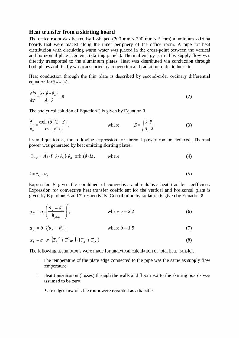
Heat transfer from a skirting board The office room was heated by L-shaped (200 mm x 200 mm x 5 mm) aluminium skirting boards that were placed along the inner periphery of the office room. A pipe for heat distribution with circulating warm water was placed in the cross-point between the vertical and horizontal plate segments (skirting panels). Thermal energy carried by supply flow was directly transported to the aluminium plates. Heat was distributed via conduction through both plates and finally was transported by convection and radiation to the indoor air.

Heat conduction through the thin plate is described by second-order ordinary differential equation for )(xθθ = .

0)(2

2

=⋅−⋅

− ∞

λθθθ

CAk

dxd (2)

The analytical solution of Equation 2 is given by Equation 3.

)(cosh))((cosh

LxL

B

X

⋅−⋅

=β

βθθ

, where λ

β⋅⋅

=CA

Pk (3)

From Equation 3, the following expression for thermal power can be deduced. Thermal power was generated by heat emitting skirting plates.

( ) )(tanh LAPk BCcalc ⋅⋅⋅⋅⋅⋅=Φ βθλ , where (4)

RCk αα += (5)

Expression 5 gives the combined of convective and radiative heat transfer coefficient. Expression for convective heat transfer coefficient for the vertical and horizontal plate is given by Equations 6 and 7, respectively. Contribution by radiation is given by Equation 8.

n

plate

XC h

a

−⋅= ∞θθα , where a = 2.2 (6)

3∞−⋅= θθα XC b , where b = 1.5 (7)

( ) ( )RSXRSXR TTTT +⋅+⋅⋅= 22σεα (8)

The following assumptions were made for analytical calculation of total heat transfer.

· The temperature of the plate edge connected to the pipe was the same as supply flow temperature.

· Heat transmission (losses) through the walls and floor next to the skirting boards was assumed to be zero.

· Plate edges towards the room were regarded as adiabatic.

The governing equations were implicitly solved. The starting point for all calculations was set at the point of intersection of the vertical and horizontal plates. Since the temperature of the skirting boards decreased with distance from the heat source, an average value was calculated. Heat emitting plates were considered as divided into 10 equal parts. For each part a mean value for surface temperature, convective and radiant heat transferring coefficient was calculated. Calculated values were then used for final computation of total heat release to the room. Vertical and horizontal plates were treated separately regarding calculation of total thermal power, but summarized afterwards. Figure 2 shows typical L-shaped skirting panels placed in a room.

Figure 2 shows typical L-shaped skirting boards placed along inner periphery of an office room.

Result and discussion The heating power needed for warming up the office room was calculated by Equation 1 and was about 1390 W. Skirting boards heated by 55 °C supply temperature gave a heat output of 2710 W. This means that the skirting boards discharged nearly twice as much heat power that required. This also means that temperature of supply flow could be decreased. After some optimization it was found that a supply temperature of 35 °C gave a heat output of 1470 W. This is clear evidence that the heat emitting skirting boards used in this study could be successfully used in a low-temperature system.

One drawback with L-shaped thermal panels could be limited furnishing of the room, due to the horizontal emitting plate. Further, single-pipe hydronic heating systems often requires more complex technical solutions. However it should be emphasized that these analytical calculations were made for an artificial climate chamber, where all walls were exposed to the outdoor environment. Regardless of this it was still possible to adequately warm the office room using low-temperature supply flow. Usually office rooms are placed with most walls adjacent to other indoor spaces. Thus, the spaces next to, below and above are assumed to have same thermal conditions as those of the room. In modern better sealed and insulated office spaces, heat power needed to cover transmissions losses is about 500 W. This is considerably lower than used in present study. However, heat losses through the outer walls are usually quite small compared to the transmission through windows. Figure 3 presents different heat requirements and outputs as results of this study.

The benefits of using well-insulated glazing units in order to reduce thermal requirements have already been shown in different studies [8-12]. Here it is concluded that these units provide better thermal climate for occupants and may also give energy savings. In some cases by employing well-insulating glazing, heating devices may not even be needed. All this indicates that horizontal heat emitting plate may not be needed in modern well-insulated office rooms. For single-family homes it could be an advantage to install thermal skirting boards for many different reasons. For example, a conversion from electrical to radiator heating could be very costly. A relatively simple and fast installation of hydronic thermal skirting boards may reduce this cost, especially if a heat pump is used as the thermal source. Furthermore, the low surface temperature makes these emitters suitable for use where safety of children or the elderly is needed. Skirting convectors may be also useful in rooms where wall space is limited.

Figure 3. Illustration of different heat outputs and requirements

Future work This study showed that it is fully possible to heat up an office room using L-shaped skirting panels. The next step is to evaluate how indoor thermal environment is affected by skirting heating. Computational Fluid Dynamics – CFD will be employed to map indoor thermal climate and to optimize heat output from the skirting convectors. Different heating arrangements, including skirting heating, will be compared to each other in a mechanically ventilated office room.

Acknowledgement Part of this work was done in a project degree work by Andreas Stålberg. His contribution is gratefully acknowledged. Authors also want to acknowledge Dr Heather Robertson for language correction.

Reference [1] M. A. Juusela (Ed.), Heating and Cooling with Focus on Increased Energy Efficiency and Improved Comfort, Guidebook to IEA ECBCS, Annex 37, (2004) [2] S. Frederiksen, S. Wener, District Heating – Theory, Technique and Functionality (in Swedish), Studentlitteratur, Lund, (1993) [3] J. Babiak, B. W. Olesen, D. Petras, Low temperature heating and high temperature cooling, Chapter 6, REHVA Guidebook, (2007) [4] J. A. Myhren and S. Holmberg, Flow patterns and thermal comfort in a room with panel, floor and wall heating, Energy and Buildings (2007) [5] J. A. Myhren and S. Holmberg, Design considerations with ventilation-radiators: Comparisons to traditional two-panel radiators, (2008) [6] F. Molin and S. Holmberg (supervisor), Radiators in low-temperature heating systems, Bachelor project, (in Swedish), Royal Institute of Technology, School of Technology and Health in Stockholm, (2004) [7] A. Stålberg and S. Holmberg (supervisor), Ledges for building heating, Bachelor project, (in Swedish), Royal Institute of Technology, School of Technology and Health in Stockholm, (2007) [8] B. Moshfeg and U. Larsson, Experimental investigation of downdraught from well-insulated windows, Energy and Buildings (2002) [9] B. Moshfeg, U. Larsson, M. Sandberg, Thermal analysis of super insulated windows (numerical and experimental investigations), Energy and Buildings, (1999) [10] T. Rueegg, V. Dorer, U. Steinemann, Must cold down draughts be compensated when using high insulating windows, Energy and Buildings, (2001) [11] H. Ge, P. Fazio, Experimental investigation of cold draft induced by two different types of glazing panels in metal curtain walls, Energy and Buildings (2004) [12] A. Jurelionis and E. Isevicius, CFD predictions of indoor air movement induced by cold window surfaces, Journal of Civil Engineering and Management (2008) [13] Long A Christopher, Essential Heat transfer, Pearson Education Limited, Edinburgh (1999) [14] Warfvinge Catarina, HVAC Technique for Civil Engineers, (in Swedish), The Faculty of Engineering at Lund University, (2000)