1 2 3 4 5 6 7 8 9 10 11 12 13 14 15 16 17 18 19 20 21 22 23 24 25 26 27 28 29 30 31 32 33 34 35 36 37 38 39 40 41 42 43 44 45 46 47 48 49 50 51 52 53 54 55 56 57 58 59 60 61 62 63 64 65

Sustainability and reliability assessment of microgridsin a regional electricity market

Chiara Lo Pretea,∗, Benjamin F. Hobbsa, Catherine S. Normana, Sergio Cano-Andradeb,Alejandro Fuentesb, Michael R. von Spakovskyb, Lamine Milic

aJohns Hopkins University, Department of Geography and Environmental Engineering, Baltimore, USAbVirginia Polytechnic Institute and State University, Department of Mechanical Engineering, Blacksburg, USA

cVirginia Polytechnic Institute and State University, Department of Electrical and Computer Engineering, Blacksburg, USA

Abstract

We develop a framework to assess and quantify the sustainability and reliability of different power production scenarios in a regionalsystem, focusing on the interaction of microgrids with the existing transmission/distribution grid. The Northwestern Europeanelectricity market (Belgium, France, Germany and the Netherlands) provides a case study for our purposes. We present simulationsof power market outcomes under various policies and levels of microgrid penetration, and evaluate them using a diverse set ofmetrics. This analysis is the first attempt to include exergy-based and reliability indices when evaluating the role of microgrids inregional power systems. The results suggest that a power network in which fossil-fueled microgrids and a price on CO2 emissionsare included has the highest composite sustainability index.

Keywords: Microgrids, sustainability, reliability, Northwestern Europe, exergy, economics, air pollution, multi-criteria decisionmaking.

1. Introduction

A microgrid (MG) is a localized grouping of electric andthermal loads, generation and storage that can operate in par-allel with the grid or in island mode and can be supplied byrenewable and/or fossil-fueled distributed generation. We quan-tify the sustainability and reliability of MGs in a regionalpowermarket in terms of multiple indices for the regional grid. Thesetting is the Northwestern European electricity market (Bel-gium, France, Germany and the Netherlands). This is a re-gional network whose national markets already influence eachother strongly and have taken steps to integrate even furtherinto a single market. Since 2006, for example, the Netherlands,France and Belgium have coupled their electricity exchangesthrough the Trilateral Market Coupling (TLC), ensuring theconvergence of spot electricity prices in the three countries. InNovember 2010, the TLC was replaced by the Central WesternEuropean Market Coupling (CWE), which also includes Ger-many [1] [2].

Sustainable development is often defined as “developmentthat meets the needs of the present without compromising theability of future generations to meet their own needs” [3].Translating this definition into quantifiable criteria thatcan beused to compare alternative power systems has proven difficult.For this reason, several authors have adopted a multi-criteria

∗Corresponding author at Johns Hopkins University, Department of Geog-raphy and Environmental Engineering, 3400 North Charles Street, 313 AmesHall. Baltimore, MD, 21218, USA. Email address: chiara.lo.prete@jhu.edu.Phone number: 410-516-5137. Fax number: 410-516-8996.

(or multiple objective) approach. The function of multi-criteriaanalysis is to communicate tradeoffs among conflicting criteriaand to help users quantify and apply value judgments in orderto recommend a course of action [4]. In this manner, a range ofdimensions of sustainability can be considered, while allowingstakeholder groups to have different priorities among the cri-teria. This method has been used, for example, to assess thetradeoffs in power system planning [5] and to evaluate the sus-tainability of power generation [6].

The main contribution of this paper is the quantification ofthe sustainability and reliability of alternative power generationpaths in a regional system with a diverse set of metrics. Weexplicitly simulate the impacts of a generation investmentde-cision on operations and investment elsewhere in the grid, asevaluation of the net sustainability impacts of a decision shouldconsider how a given investment choice propagates through thesystem. Our approach does not rely on multi-objective opti-mization; it presents instead a multi-criteria assessmentthroughthe use of indicators, which are calculated based on the re-sults of a single-objective optimization model and a reliabilitymodel.

Among the commonly used four dimensions to evaluate thesustainability of energy supply systems (social, economic, tech-nical and environmental) [7], the analysis emphasizes the latterthree. In terms of microgrid impact on social sustainability,several areas commonly cited as important are equity, com-munity impacts, level of participation in decision making andhealth impacts. The first three depend on how a given micro-grid is owned and managed. In general, it is plausible that theincreased impact that members of the microgrid-served pop-

Preprint submitted to Energy July 2, 2011

*ManuscriptClick here to download Manuscript: SustainabilityMG6.tex Click here to view linked References

1 2 3 4 5 6 7 8 9 10 11 12 13 14 15 16 17 18 19 20 21 22 23 24 25 26 27 28 29 30 31 32 33 34 35 36 37 38 39 40 41 42 43 44 45 46 47 48 49 50 51 52 53 54 55 56 57 58 59 60 61 62 63 64 65

ulation could have on ownership and management decisions,relative to populations served by conventional utilities,wouldcount as a positive impact on social sustainability. Addition-ally, shared community values may lead some stakeholders tovalue microgrids that use renewable energy more highly thaneither microgrids that do not or larger systems in which thecommunity has little choice about the source of electricity[8].Increased security of supply associated with microgrids mayalso offer social as well as economic benefits within and out-side the community served by a microgrid. Finally, microgridoperation may create jobs that offer social sustainability gainsfor the local community.

On the other hand, microgrids may have negative effects onresidents’ quality of life, if they increase the level of noise orhave aesthetic impacts on the landscape [9]. Health impactsof a microgrid may also be negative, as microgrids are likelyto have generation and thus pollution closer to the populationsthey serve than conventional distribution networks. How risksto life and health associated with local air pollution comparewith the ones from a conventional utility source will be verypopulation, site and technology specific.

While we can speculate on the likely direction of these im-pacts for the power system modeled in this paper, it is difficult toquantify them without reference to a specific location and pop-ulation whose views and willingness to pay can be surveyed orestimated. On the contrary, the methodology used in our anal-ysis aims at assessing the broader impacts of alternative powergeneration paths on a regional power system. For this reason,no direct quantification of social sustainability is offered in ourstudy. However, to account indirectly for this dimension weperform a sensitivity analysis on the results in order to assesswhether and how the introduction of a social sustainabilityin-dex would alter our conclusions.

We consider six alternative scenarios for satisfying the elec-tric power and thermal needs of a regional power market, andwe characterize their sustainability and reliability using foursets of indicators. The scenarios are various combinationsofmicrogrid implementation (with and without MGs), microgridgenerating mix (fossil-fueled only, or fossil-fueled and renew-able) and CO2 policies (with and without a price on CO2 emis-sion allowances). The first set of indices is based on CO2 andconventional air pollutant emissions (NOx and SOx). The sec-ond one emphasizes economic sustainability in terms of totalgeneration costs [10] and accounts for externalities of electric-ity generation. Externalities can be defined as “the costs andbenefits which arise when the social or economic activities ofone group of people have an impact on another, and when thefirst group fails to fully account for their impacts” [11]. Inthe1990s the importance of environmental costs as an input to theplanning and decision processes of electric power generationsystems was recognized in several studies [12] [13]. The thirdset of indices is based on thermodynamic energy and exergybased efficiencies, while the fourth considers effects on bulkpower system reliability.

Economic and environmental analyses of power systems in-cluding distributed generation are common (see, for exam-ple, [14] and [15]). Several studies assess the potential bene-

fits of distributed generation [16] [17] and evaluate its impacton sustainable development [18]. Others focus directly on theeconomic and regulatory issues of MG implementation [19],on the implications of environmental regulation on MG adop-tion [20], and on the improvement in power reliability providedto different types of buildings by the installation of a MG [21].In contrast, neither thermodynamic analyses considering the in-teraction of MGs with existing regional power systems nor theeffect of MG deployment on system reliability have been previ-ously published, to the best of our knowledge.

We include exergy because an analysis relying on first lawefficiency alone does not consider to what degree the outputs ofa power plant are useful. For example, electricity is more valu-able than steam, one of the typical by-products of power pro-duction, because the latter is characterized on a per unit energybasis by a lower value of exergy than electricity. Therefore, notall outputs should be valued in the same way: outputs having ahigher quality or exergy per unit energy (like electricity)shouldhave a higher unit price than those having a lower quality orexergy per unit energy (like steam) because the former possessa greater ability to do work. In contrast, when the second lawof thermodynamics is disregarded, the difference in quality ofthe various energy outputs is not considered and cannot be ef-fectively compared for different energy conversion processes.

Thus, the use of exergy-based indicators can help decisionmakers to improve the effectiveness of energy resource use in agiven system. Such indicators have been widely adopted in thesustainability literature. Yi et al. [22] use thermodynamic in-dices to assess the sustainability of industrial processes. Fran-gopoulos and Keramioti [23] evaluate the performance of dif-ferent alternatives to meet the energy needs of an industrialunit, taking into account several aspects of sustainability. vonSpakovsky and Frangopoulos [24] [25] use an environomic(thermodynamic, environmental and economic) objective forthe analysis and optimization of a gas turbine cycle with cogen-eration. Rosen [26] presents a thermodynamic comparison ofacoal and a nuclear power plant on the basis of exergy and en-ergy. Zvolinschi et al. [27] develop three exergy-based indicesto assess the sustainability of power generation in Norway.

In addition to sustainability, it is important to incorporate areliability analysis in the decision process because of theposi-tive impact that microgrids may have on power system reliabil-ity, and thereby on promoting their deployment. Therefore,weadd reliability to our suite of indices and quantify it usingtheannual Loss of Load Probability (LOLP) and Expected Loss ofEnergy (ELOE) [28] [29]. The reliability of a power system isthe probability that the system is able to perform its intendedfunction (generation meets load), under a contractual qualityof service, for a specified period of time. Reliability is quanti-fied here using the concept of “long-run average availability” ofthe bulk power system (supply-demand balance), without con-sideration of dynamic system response to disturbances, whichinstead is the concept of “security” [30].

We do not consider aspects of power quality that may alsobe controlled within MGs. It has been argued that microgridshave the potential to deliver different degrees of power qual-ity tailored for different customers’ needs, as they may be em-

2

1 2 3 4 5 6 7 8 9 10 11 12 13 14 15 16 17 18 19 20 21 22 23 24 25 26 27 28 29 30 31 32 33 34 35 36 37 38 39 40 41 42 43 44 45 46 47 48 49 50 51 52 53 54 55 56 57 58 59 60 61 62 63 64 65

ployed to control power quality locally according to customers’requirements. This may prove to be more beneficial than pro-viding a uniform level of quality and service to all customerswithout differentiating among their needs [31] [32]. However,the way in which microgrids may affect power quality in a re-gional grid is still under study and there are no definitive results.For this reason, we do not include power quality considerationsin our analysis, though we note they should be addressed infuture research.

We also do not consider customer outages arising at the sub-transmission or distribution-level. However, it is worth notingthat the majority of power interruptions experienced by cus-tomers in the countries we consider are not due to large eventsat the bulk level, but to more localized ones affecting the distri-bution system [33].

Section 2 describes our modeling approach, data and as-sumptions concerning alternative power systems (with andwithout MGs) and CO2 policies. Section 3 presents the six sce-narios considered in our analysis to satisfy the electric powerand thermal needs of the Northwestern European electricitymarket. Section 4 describes the indicators chosen in this paperto assess the sustainability and reliability of the network. Sec-tion 5 discusses the results of the analysis, while Section 6con-cludes.

2. Methodology and data

Two different models are used to quantify our indices. A re-gional power market model based on linear optimization meth-ods [10] [34] provides the information necessary for the eco-nomic, environmental and thermodynamic indices; the modelis presented in Section 2.1. A local reliability model basedonconvolution methods [28] [29], described in Section 2.2, isusedinstead to obtain the reliability indices.

2.1. Regional market simulation modelFor the purposes of this paper, we represent the Northwest-

ern European electricity market using COMPETES (Compre-hensive Market Power in Electricity Transmission and EnergySimulator) [35]. Our version of COMPETES is a quadraticallyconstrained model solved in ILOG OPL 6.3, using the opti-mizer Cplex12. COMPETES models twelve power producersin the four countries: eight of them are the largest ones in theregion (Electrabel, Edf, Eon, ENBW, RWE, Vattenfall, EssentNuon-Reliant), while the remaining four represent the compet-itive fringe in each country.

When no MGs are included, the electricity network is repre-sented by fifteen nodes. Each of the seven main nodes (Krim,Maas and Zwol in the Netherlands; Merc and Gram in Belgium;one node in France and one in Germany) has generation capac-ity and load. A DC power flow model is used to represent a sys-tem in which four intermediate nodes are distinguished in bothFrance (Avel, Lonn, Moul, Muhl) and Germany (Diel, Romm,Ucht, Eich); at these nodes, no generation or demand occurs(except for 2,000 MW of power exports to the UK at Avel).Three nodes representing groups of residential MGs are addedto the model in the MG scenarios.

The nodes of the network are connected by twenty-eight highvoltage transmission corridors (or arcs), each one with a maxi-mum MW transmission capacity. The groups of MGs are con-nected to the transmission system by radial links at nodes Krim,Maas and Zwol in the Netherlands. While by assumption we arefocusing on the impact of new microgrids in the Netherlands,to understand their impacts on the regional power grid it is nec-essary to consider the neighboring countries’ bulk power mar-kets. Of course, groups of microgrids could also be connectedto nodes in other countries. However, we would then need toconsider additional neighboring countries, such as Polandorthe Iberian peninsula.

Computational convenience suggests starting the analysiswith a competitive benchmark. Our application of COMPETEScalculates a competitive equilibrium among power producers,which under the assumption of perfectly inelastic demand isequivalent to minimization of total generation costs. Thisisdone for six representative hours in order to characterize thedistribution of operating costs.

We include resistance losses on high voltage transmissionflows to make the model more realistic because, on average,losses can contribute as much to spatial price variations ascon-gestion does. Losses vary as a quadratic function of flow, usingthe DC formulation with quadratic losses in [36]. In the ab-sence of other data, resistance loss coefficients, defined for thetwenty-eight corridors of the network, are assumed to be pro-portional to reactance. Therefore, we set them equal to the reac-tance on each corridor times a constantα, whose value is cho-sen so that high voltage transmission losses are approximatelyequal to 2% of generation during the peak hours.

2.1.1. Model formulationCOMPETES is a short-run market simulation model using an

optimization formulation: its objective function includes short-run marginal costs (i.e., fuel and other variable O&M costs)anddisregards long-run retirement and entry decisions. For eachMG and CO2 policy scenario, we solve the model for six differ-ent periods of the year representing a variety of load and gen-eration capacity conditions. The six periods are appropriatelyweighted by the number of hours in each period to estimate an-nual cost. The problem statement is as follows:

min∑

i

∑

j∈Ji

(MCi j +CO2Ei j)geni j (1)

subject to:∑

j∈Ji

geni j +∑

k∈Ai

[ fki(1− Losski fki) − fik] ≥ Li ∀i ∈ I (2)

∑

ik∈Mm

RikS ikm( fik − fki) = 0 ∀m ∈ M (3)

geni j ≤ Capi j ∀i ∈ I,∀ j ∈ Ji (4)

fik ≤ Tik ∀i, k ∈ I (5)

fik ≥ 0 ∀i, k ∈ I (6)

geni j ≥ 0 ∀i ∈ I,∀ j ∈ Ji (7)

3

1 2 3 4 5 6 7 8 9 10 11 12 13 14 15 16 17 18 19 20 21 22 23 24 25 26 27 28 29 30 31 32 33 34 35 36 37 38 39 40 41 42 43 44 45 46 47 48 49 50 51 52 53 54 55 56 57 58 59 60 61 62 63 64 65

A complete list of variable and parameter definitions is pro-vided in the nomenclature. The goal is to minimize the objec-tive function expressed as the total generation costs givenbyequation 1, where a linear short-run cost of production is as-sumed. The decision variables aregeni j (the generation fromaggregated power plantj located at nodei) and fik (the MWtransmission flow from nodei to a nearby nodek that is directlyconnected toi by a transmission corridor).

Equation 2 accounts for Kirchhoff’s Current Law (KCL), ap-plied to each node of the network.fik is the export flow fromnodei to nodek, while fki(1-Losski fki) represents the importflow (net of losses) into nodei from nodek. Equation 3 rep-resents Kirchhoff’s Voltage Law (KVL) constraint, defined foreach of the fourteen meshes (or loops) connecting the nodes.Equation 4 ensures that power generated at each node and eachstep is less than the available capacity at that location, whileequation 5 constrains the transmission flow on a given arc.Equations 6 and 7 are nonnegativity restrictions.

When microgrids are included, their generation costs areadded to equation 1. Since the groups of MGs are additionalnodes with autonomous loads, one KCL constraint is added inthe model for each MG node. However, no additional KVL isincluded because MGs are assumed to be radially connected tothe grid. The power generated at each MG node must satisfythe capacity constraint (equation 4) and the non-negativity con-straint (equation 7), and its flow to/from the grid must satisfybounds 5 and 6.

2.1.2. DataSimulations of power market outcomes are based on a mod-

ified version of the Energy Research Centre of the Netherlands(ECN) COMPETES database of transmission, demand and gen-eration [37].

This provides a multi-step supply function (one step per ag-gregate power plant) for each node where power generation oc-curs. Using the information in [38] and [39], generation costsand capacity of the original fifteen nodes of the network in [37]have been updated to 2008 (a leap year). Our version of thedatabase has also been modified to account for transmission re-sistance losses, exergetic and energetic efficiencies, and emis-sions.

In the scenarios including MGs, nine steps representing MGtechnologies (three for each node to which MGs are connected)have been added to the existing network. Generation costs,technology types and capacity for the MG nodes are obtainedfrom the literature.

In line with [37], in the scenarios without MGs the capac-ity database does not include renewable and combined heat andpower (CHP) generators. On the other hand, CHP capacity isinstalled at the MG nodes and we explicitly consider its contri-bution to the system.

Hourly loads in the four countries are based on [40] and re-fer to 2008. Since CHP and renewable generators are not in-cluded in the capacity database, their production is nettedfromthe hourly electricity demand of the network in [40]. Hourlyloads are organized in load duration curves (LDCs) and dividedinto six blocks: the first block averages the load of the first 100

hours, the second block of the following 900 hours, the thirdand fourth of the next 2,500 hours, the fifth of the next 2,284hours, the sixth of the last 500 hours. The average electricityconsumption of the residential customers in the MGs is basedon the load profiles in [41]. Information on total capacity, dom-inant fuel type, energy efficiency, exergy calculations, marginalcost function and average CO2, NOx, SOx emission rates for allthe nodes in the network is available from the authors.

2.2. Reliability valuation model

In addition to the market simulation model, we develop amodel to assess the reliability of the Dutch power system intwo scenarios (with and without MGs). We consider the Dutchsystem alone for two reasons. First, we focus our analysis onthe direct impact of MGs on the reliability in the country wherethey are installed. Second, the Netherlands is the most import-dependent of the four countries considered, and the adequacy ofgenerating capacity to meet future energy needs has been exten-sively debated over the last decade [42]. We include two relia-bility indices, the LOLP and the ELOE. The LOLP of a powersystem is the expected number of hours of capacity deficiencyin the system in a given period of time [29]. In our analysis,the LOLP is expressed in outage hours/10 years: an outage of 8hours in 10 years is typically considered a reasonable reliabilitytarget in industrialized countries. The ELOE gives an indica-tion of the amount of load that cannot be serviced in a givenperiod of time and is expressed in MWh/yr [28].

In our model, 2008 summer and winter LDCs are approx-imated using the mixture of normals approximation (MONA)technique detailed in [43]. Given z= 1,..,Z independent normalrandom variables, each with meanµz, varianceσ2

z , and cumu-lative distribution functionΦ(·; µz, σ2

z ), F(·) has a mixture ofnormals distribution with z components if

F(x) =∑

z

pzΦ(x; µz, σ2z ) (8)

∑

z

pz = 1; 0≤ pz ≤ 1 (9)

wherepz is the weight of the zth component. A LDC can beapproximated by

LDC(x) = 1− F(x) (10)

For our purposes, a two-component mixture of normals pro-vides an excellent approximation of the load duration curve; theweights, mean and variances in equation 8, different for win-ter and summer loads, are obtained by minimizing the squareddifference between the original and approximated distributions,with higher penalties on deviations during peak periods. Inthereliability analysis, loads include CHP and renewable produc-tion.

We define the expected available capacity and the variance ofavailable capacity of supply function stepj at nodei as:

E(Capi j) = [Capi j(1− FORi j)] (11)

4

1 2 3 4 5 6 7 8 9 10 11 12 13 14 15 16 17 18 19 20 21 22 23 24 25 26 27 28 29 30 31 32 33 34 35 36 37 38 39 40 41 42 43 44 45 46 47 48 49 50 51 52 53 54 55 56 57 58 59 60 61 62 63 64 65

Var(Capi j) =1

Ni j[(Capi j)

2FORi j(1− FORi j)] (12)

whereNi j is the number of individual power plants at aggregatestep j and FORi j is the forced outage rate of each individualpower plant in stepj. These expressions are based on a bi-nomial distribution approximation, assumingNi j independentgenerators in the step. The forced outage rates of the centralgenerators are obtained for each technology type from [44].Inthe absence of other specific data, we use [45] for the MG tech-nologies. We assume that summer and winter available gener-ating capacity follows a normal distribution, with mean equalto the total expected generating capacity and variance equal tothe sum of variances at all steps of the supply function.

In the reliability analysis, power generation capacity includesan estimate of the CHP capacity in the Netherlands. It also ac-counts for the maximum feasible flow of power imports to theNetherlands from neighboring countries, assuming that underhighly stressed conditions the Dutch system will maximize im-ports. The maximum flow is based on the COMPETES simula-tions under peak demand conditions.

Since wind power accounted for about 5% of 2008 electricitynet production in the Netherlands [39], its production should benetted from electricity demand in our reliability analysis. Thetime series of wind generation over 15-minute intervals in onerepresentative year [46] suggests that the density function ofwind power generation in the Netherlands may be adequatelyapproximated by an exponential distribution. This is confirmedby the non rejection of the Kolmogorov-Smirnov test of the ex-ponential distribution of this sample at a 1% significance level.We use two different exponential approximations, one for thewinter and one for the summer, with parameterλw equal to theaverage wind production in the Netherlands in the two seasons(556.5 MW in the summer and 378 MW in the winter, basedon [46]).

In season w, the LOLP of each component of the normal mix-ture approximation z (LOLPw,z) is defined as

LOLPw,z = Prob(Lz −Capw −Windw ≥ 0)=∫ ∞0

fLz−Capw (x)FWindW (x)dx(13)

where x represents the value of the thermal generation capacitydeficit (Lz−Capw), fLz−Capw (x) is the normal density function of(Lz−Capw) evaluated at x, andFWindW (x) is the exponential cu-mulative distribution function ofWindw evaluated at x. We canexpress the LOLPw,z as a product of functions because, accord-ing to [46], wind generation is largely independent of load inthat area of Europe. The four values of LOLPw,z (one for eachseason and each of the two components of our normal mixtureapproximation) are appropriately weighted by the probabilitiespz and the number of hours in each season to estimate the an-nual LOLP.

In season w, the ELOE of each component of the normalmixture approximation z (ELOEw,z) is defined as:

ELOEw,z =∫ ∞0

∫ x

0fLz−Capw (x) fWindW (y)(x − y)dydx

=∫ ∞0

fLz−Capw (x)[x + 1λw

(e−λw x − 1)]dx(14)

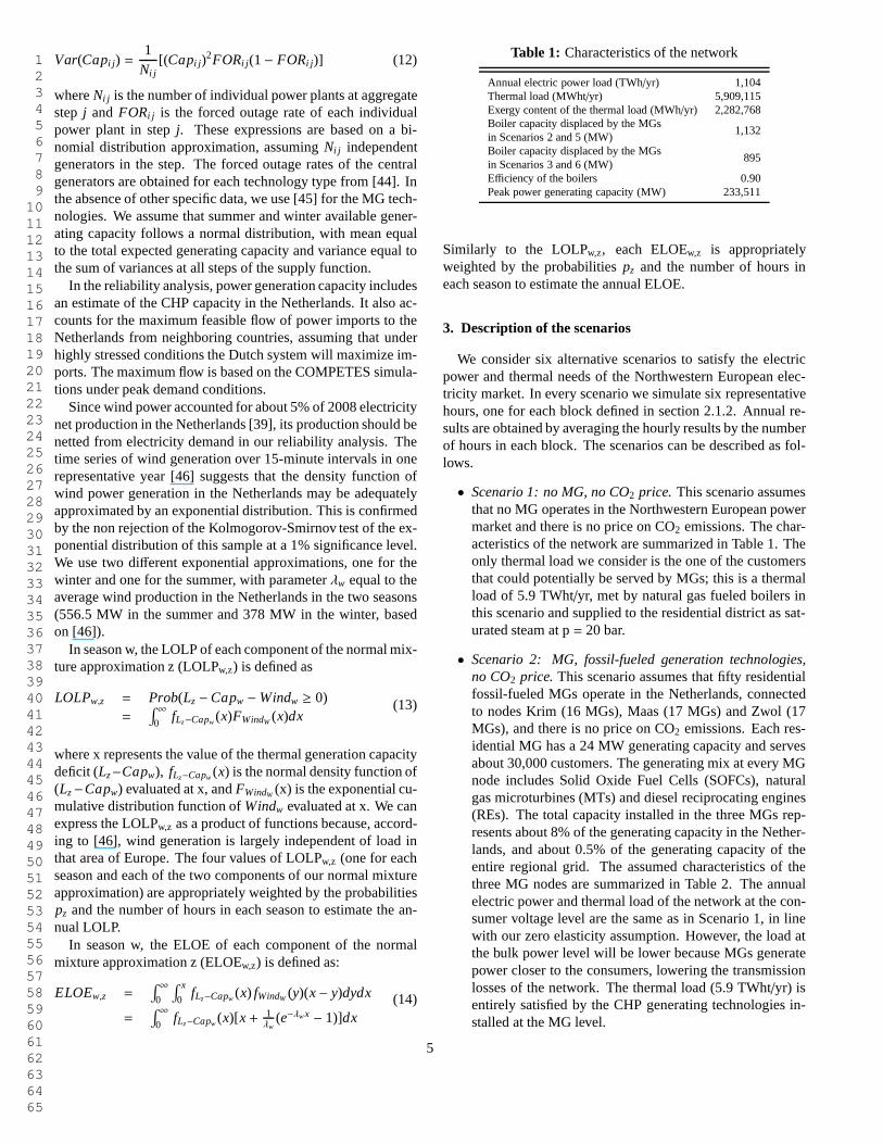
Table 1: Characteristics of the network

Annual electric power load (TWh/yr) 1,104Thermal load (MWht/yr) 5,909,115Exergy content of the thermal load (MWh/yr) 2,282,768Boiler capacity displaced by the MGs

1,132in Scenarios 2 and 5 (MW)Boiler capacity displaced by the MGs

895in Scenarios 3 and 6 (MW)Efficiency of the boilers 0.90Peak power generating capacity (MW) 233,511

Similarly to the LOLPw,z, each ELOEw,z is appropriatelyweighted by the probabilitiespz and the number of hours ineach season to estimate the annual ELOE.

3. Description of the scenarios

We consider six alternative scenarios to satisfy the electricpower and thermal needs of the Northwestern European elec-tricity market. In every scenario we simulate six representativehours, one for each block defined in section 2.1.2. Annual re-sults are obtained by averaging the hourly results by the numberof hours in each block. The scenarios can be described as fol-lows.

• Scenario 1: no MG, no CO2 price. This scenario assumesthat no MG operates in the Northwestern European powermarket and there is no price on CO2 emissions. The char-acteristics of the network are summarized in Table 1. Theonly thermal load we consider is the one of the customersthat could potentially be served by MGs; this is a thermalload of 5.9 TWht/yr, met by natural gas fueled boilers inthis scenario and supplied to the residential district as sat-urated steam at p= 20 bar.

• Scenario 2: MG, fossil-fueled generation technologies,no CO2 price. This scenario assumes that fifty residentialfossil-fueled MGs operate in the Netherlands, connectedto nodes Krim (16 MGs), Maas (17 MGs) and Zwol (17MGs), and there is no price on CO2 emissions. Each res-idential MG has a 24 MW generating capacity and servesabout 30,000 customers. The generating mix at every MGnode includes Solid Oxide Fuel Cells (SOFCs), naturalgas microturbines (MTs) and diesel reciprocating engines(REs). The total capacity installed in the three MGs rep-resents about 8% of the generating capacity in the Nether-lands, and about 0.5% of the generating capacity of theentire regional grid. The assumed characteristics of thethree MG nodes are summarized in Table 2. The annualelectric power and thermal load of the network at the con-sumer voltage level are the same as in Scenario 1, in linewith our zero elasticity assumption. However, the load atthe bulk power level will be lower because MGs generatepower closer to the consumers, lowering the transmissionlosses of the network. The thermal load (5.9 TWht/yr) isentirely satisfied by the CHP generating technologies in-stalled at the MG level.

5

1 2 3 4 5 6 7 8 9 10 11 12 13 14 15 16 17 18 19 20 21 22 23 24 25 26 27 28 29 30 31 32 33 34 35 36 37 38 39 40 41 42 43 44 45 46 47 48 49 50 51 52 53 54 55 56 57 58 59 60 61 62 63 64 65

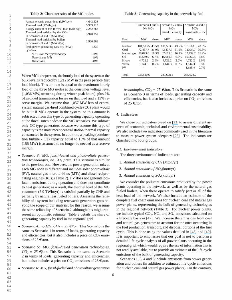
Table 2: Characteristics of the MG nodes

Annual electric power load (MWh/yr) 4,643,223Thermal load (MWht/yr) 5,909,115Exergy content of this thermal load (MWh/yr) 2,282,768Thermal load satisfied by the MGs

3,948,252in Scenarios 3 and 6 (MWht/yr)Thermal load satisfied by boilers

1,960,863in Scenarios 3 and 6 (MWht/yr)Peak power generating capacity (MW) 1,330of which:

SOFCs or PV system/battery 20%Natural gas MTs 40%Diesel REs 40%

When MGs are present, the hourly load of the system at thebulk level is reduced by 1,212 MW in the peak period (firstload block). This amount is equal to the maximum hourlyload of the three MG nodes at the consumer voltage level(1,036 MW, occurring during winter peak hours), plus 2%of avoided transmission losses on that load and a 15% re-serve margin. We assume that 1,057 MW less of centralsystem natural gas-fired combined cycle (CC) plant wouldbe built if MGs operate in the system, so this amount issubtracted from this type of generating capacity operatingat the three Dutch nodes in the MG scenarios. We subtractonly CC-type generators because we assume this type ofcapacity is the most recent central station thermal capacityconstructed in the system. In addition, a peaking (combus-tion turbine - CT) capacity equal to 15% of that amount(155 MW) is assumed to no longer be needed as a reservemargin.

• Scenario 3: MG, fossil-fueled and photovoltaic genera-tion technologies, no CO2 price. This scenario is similarto the previous one. However, the power generation mix ateach MG node is different and includes solar photovoltaic(PV), natural gas microturbines (MTs) and diesel recipro-cating engines (REs) (Table 2). PV does not generate pol-lutant emissions during operation and does not contributeto heat generation; as a result, the thermal load of the MGcustomers (5.9 TWht/yr) is satisfied partially by CHP andpartially by natural gas fueled boilers. Assessing the relia-bility of a system including renewable generators goes be-yond the scope of our analysis; for this reason, we assumethe same reliability of Scenario 2, although this might rep-resent an optimistic estimate. Table 3 details the share ofgenerating capacity by fuel in the regional grid.

• Scenario 4: no MG, CO2 = 25 C/ton. This Scenario is thesame as Scenario 1 in terms of loads, generating capacityand efficiencies, but it also includes a price on CO2 emis-sions of 25 C/ton.

• Scenario 5: MG, fossil-fueled generation technologies,CO2 = 25 C/ton. This Scenario is the same as Scenario2 in terms of loads, generating capacity and efficiencies,but it also includes a price on CO2 emissions of 25 C/ton.

• Scenario 6: MG, fossil-fueled and photovoltaic generation

Table 3: Generating capacity in the network by fuel

Scenario 1 and 4 Scenario 2 and 5 Scenario 3 and 6No MGs MGs MGs

Fossil fuels only Fossil fuels+ PV

Fuel MW share MW share MW share

Nuclear 101,583.5 43.5% 101,583.5 43.5% 101,583.5 43.3%Coal 72,437.7 31.0% 72,437.7 31.0% 72,437.7 30.8%Natural gas 38,073.0 16.3% 37,671.0 16.1% 37,432.7 15.9%Oil 15,549.9 6.7% 16,069.5 6.9% 16,069.5 6.8%Hydro 4,722.2 2.0% 4,722.2 2.0% 4,722.2 2.0%Waste 1,144.3 0.5% 1,144.3 0.5% 1,144.3 0.5%PV - - - - 1,638.4 0.7%

Total 233,510.6 233,628.1 235,028.2

technologies, CO2 = 25 C/ton. This Scenario is the sameas Scenario 3 in terms of loads, generating capacity andefficiencies, but it also includes a price on CO2 emissionsof 25 C/ton.

4. Indicators

We chose our indicators based on [23] to assess different as-pects of economic, technical and environmental sustainability.We also include two indicators commonly used in the literatureto measure power system adequacy [28]. The indicators areclassified into four groups.

4.1. Environmental Indicators

The three environmental indicators are:

1. Annual emissions of CO2 (Mton/yr)

2. Annual emissions of NOx(kton/yr)

3. Annual emissions of SOx(kton/yr)

We consider the pollutant emissions produced by the powerplants operating in the network, as well as by the natural gasfueled boilers, when these operate to satisfy part or all of theheat load of the network. We also include an estimate of thecomplete fuel chain emissions for nuclear, coal and naturalgaspower plants, representing the bulk of generating technologiesin the regional network (Table 3). For nuclear power plants,we include typical CO2, NOx and SOx emissions calculated ona lifecycle basis in [47]. We increase the emissions from coaland natural gas generators to account for the ones occurringinthe fuel production, transport, and disposal portions of the fuelcycle. This is done using the values detailed in [48] and [49].It is important to emphasize that our goal is not to perform adetailed life-cycle analysis of all power plants operatingin theregional grid, which would require the use of information that isnot readily available, but to provide an estimate of the life-cycleemissions of the bulk of generating capacity.

Scenarios 1, 3, 4 and 6 include emissions from power gener-ation and boilers (in addition to estimated life-cycle emissionsfor nuclear, coal and natural gas power plants). On the contrary,

6

1 2 3 4 5 6 7 8 9 10 11 12 13 14 15 16 17 18 19 20 21 22 23 24 25 26 27 28 29 30 31 32 33 34 35 36 37 38 39 40 41 42 43 44 45 46 47 48 49 50 51 52 53 54 55 56 57 58 59 60 61 62 63 64 65

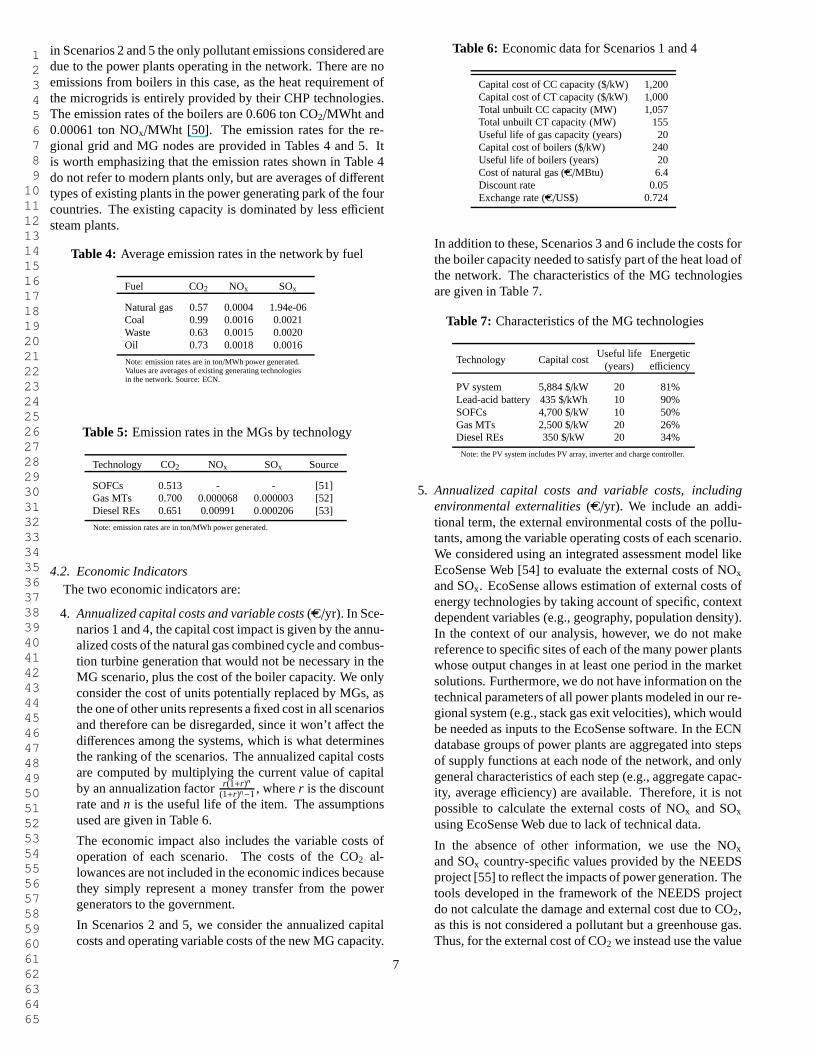
in Scenarios 2 and 5 the only pollutant emissions consideredaredue to the power plants operating in the network. There are noemissions from boilers in this case, as the heat requirementofthe microgrids is entirely provided by their CHP technologies.The emission rates of the boilers are 0.606 ton CO2/MWht and0.00061 ton NOx/MWht [50]. The emission rates for the re-gional grid and MG nodes are provided in Tables 4 and 5. Itis worth emphasizing that the emission rates shown in Table 4do not refer to modern plants only, but are averages of differenttypes of existing plants in the power generating park of the fourcountries. The existing capacity is dominated by less efficientsteam plants.

Table 4: Average emission rates in the network by fuel

Fuel CO2 NOx SOx

Natural gas 0.57 0.0004 1.94e-06Coal 0.99 0.0016 0.0021Waste 0.63 0.0015 0.0020Oil 0.73 0.0018 0.0016

Note: emission rates are in ton/MWh power generated.Values are averages of existing generating technologiesin the network. Source: ECN.

Table 5: Emission rates in the MGs by technology

Technology CO2 NOx SOx Source

SOFCs 0.513 - - [51]Gas MTs 0.700 0.000068 0.000003 [52]Diesel REs 0.651 0.00991 0.000206 [53]

Note: emission rates are in ton/MWh power generated.

4.2. Economic IndicatorsThe two economic indicators are:

4. Annualized capital costs and variable costs (C/yr). In Sce-narios 1 and 4, the capital cost impact is given by the annu-alized costs of the natural gas combined cycle and combus-tion turbine generation that would not be necessary in theMG scenario, plus the cost of the boiler capacity. We onlyconsider the cost of units potentially replaced by MGs, asthe one of other units represents a fixed cost in all scenariosand therefore can be disregarded, since it won’t affect thedifferences among the systems, which is what determinesthe ranking of the scenarios. The annualized capital costsare computed by multiplying the current value of capitalby an annualization factorr(1+r)n

(1+r)n−1, wherer is the discountrate andn is the useful life of the item. The assumptionsused are given in Table 6.

The economic impact also includes the variable costs ofoperation of each scenario. The costs of the CO2 al-lowances are not included in the economic indices becausethey simply represent a money transfer from the powergenerators to the government.

In Scenarios 2 and 5, we consider the annualized capitalcosts and operating variable costs of the new MG capacity.

Table 6: Economic data for Scenarios 1 and 4

Capital cost of CC capacity ($/kW) 1,200Capital cost of CT capacity ($/kW) 1,000Total unbuilt CC capacity (MW) 1,057Total unbuilt CT capacity (MW) 155Useful life of gas capacity (years) 20Capital cost of boilers ($/kW) 240Useful life of boilers (years) 20Cost of natural gas (C/MBtu) 6.4Discount rate 0.05Exchange rate (C/US$) 0.724

In addition to these, Scenarios 3 and 6 include the costs forthe boiler capacity needed to satisfy part of the heat load ofthe network. The characteristics of the MG technologiesare given in Table 7.

Table 7: Characteristics of the MG technologies

Technology Capital costUseful life Energetic

(years) efficiency

PV system 5,884 $/kW 20 81%Lead-acid battery 435 $/kWh 10 90%SOFCs 4,700 $/kW 10 50%Gas MTs 2,500 $/kW 20 26%Diesel REs 350 $/kW 20 34%

Note: the PV system includes PV array, inverter and charge controller.

5. Annualized capital costs and variable costs, includingenvironmental externalities (C/yr). We include an addi-tional term, the external environmental costs of the pollu-tants, among the variable operating costs of each scenario.We considered using an integrated assessment model likeEcoSense Web [54] to evaluate the external costs of NOx

and SOx. EcoSense allows estimation of external costs ofenergy technologies by taking account of specific, contextdependent variables (e.g., geography, population density).In the context of our analysis, however, we do not makereference to specific sites of each of the many power plantswhose output changes in at least one period in the marketsolutions. Furthermore, we do not have information on thetechnical parameters of all power plants modeled in our re-gional system (e.g., stack gas exit velocities), which wouldbe needed as inputs to the EcoSense software. In the ECNdatabase groups of power plants are aggregated into stepsof supply functions at each node of the network, and onlygeneral characteristics of each step (e.g., aggregate capac-ity, average efficiency) are available. Therefore, it is notpossible to calculate the external costs of NOx and SOx

using EcoSense Web due to lack of technical data.

In the absence of other information, we use the NOx

and SOx country-specific values provided by the NEEDSproject [55] to reflect the impacts of power generation. Thetools developed in the framework of the NEEDS projectdo not calculate the damage and external cost due to CO2,as this is not considered a pollutant but a greenhouse gas.Thus, for the external cost of CO2 we instead use the value

7

1 2 3 4 5 6 7 8 9 10 11 12 13 14 15 16 17 18 19 20 21 22 23 24 25 26 27 28 29 30 31 32 33 34 35 36 37 38 39 40 41 42 43 44 45 46 47 48 49 50 51 52 53 54 55 56 57 58 59 60 61 62 63 64 65

in [23]. External costs are calculated on all emissions, in-cluding the indirect ones related to the life-cycle of nu-clear, coal and natural gas power plants. The addition ofenvironmental costs allows us to assess the real cost of thepollutant emissions to the society, which cannot be donesimply by introducing CO2 allowances. On the other hand,counting both the external costs of pollution in the cost in-dices and emissions as separate pollution indices could beviewed as double counting. To account for this, we haveperformed a sensitivity analysis in Section 5.

4.3. Technical Indicators

The four technical indicators are

6. Annual energetic electric efficiency of the network. This in-dicator is obtained by dividing the annual power produc-tion by the annual fuel use for power production in eachscenario.

7. Annual energetic total efficiency of the network

ηtot =W + QWηe+

Qηb

(15)

The heat rate requirementQ is the same in all scenarios.However, in Scenarios 1 and 4 the thermal load has to bemet with separate boilers. In Scenarios 2 and 5 the MGsproduce heat, through cogeneration, to satisfy their load.Therefore, the second term in the denominator of equa-tion 15 is excluded in these scenarios, because all the fuelnecessary to produce both heat and power is already in-cluded in the first term. In Scenarios 3 and 6, however,PV does not contribute to heat generation, and as a resultthe heat load of the network is satisfied partially throughCHP and partially through boilers. The second term in thedenominator of equation 15 accounts only for the fuel useof the additional boilers needed in these scenarios.

8. Annual exergetic electric efficiency of the network

ζe =ηe

ϕe(16)

ϕe is the ratio of the total exergy of the annual fuel use forpower production and its total energy.

9. Annual exergetic total efficiency of the network

ζtot =W + EQ

S

Wζe+ ENG

(17)

ENG = MNG × HNG × ϕNG (18)

For the reasons explained for indicator 7, the last term in thedenominator is excluded in Scenarios 2 and 5, and includedwith reference to the additional boilers used to satisfy theheatload in Scenarios 3 and 6.ϕNG = 1.042 andHNG = 38.1 MJ/kg.The indicators in section 4.3 are described in [56].

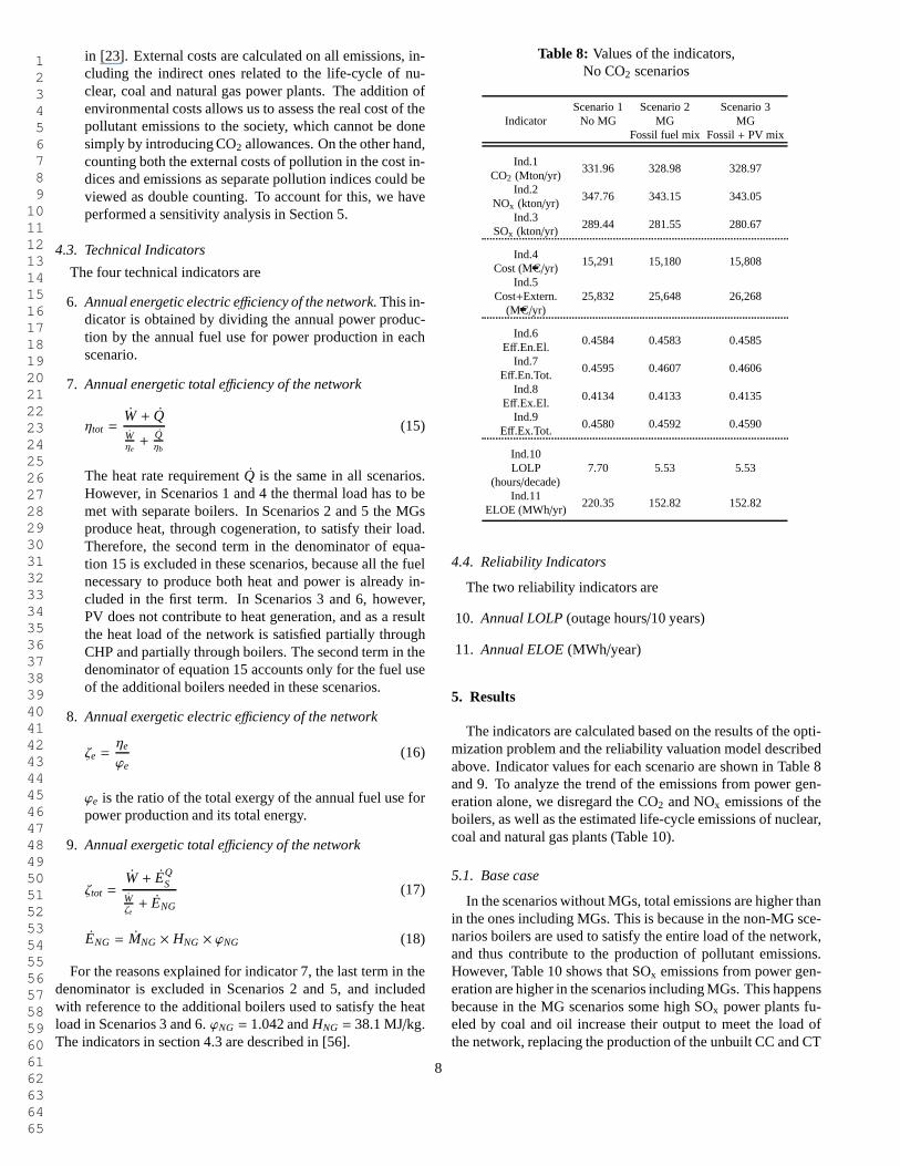
Table 8: Values of the indicators,No CO2 scenarios

IndicatorScenario 1 Scenario 2 Scenario 3

No MG MG MGFossil fuel mix Fossil+ PV mix

Ind.1331.96 328.98 328.97

CO2 (Mton/yr)Ind.2

347.76 343.15 343.05NOx (kton/yr)

Ind.3289.44 281.55 280.67

SOx (kton/yr)

Ind.415,291 15,180 15,808

Cost (MC/yr)Ind.5

25,832 25,648 26,268Cost+Extern.(MC/yr)

Ind.60.4584 0.4583 0.4585

Eff.En.El.Ind.7

0.4595 0.4607 0.4606Eff.En.Tot.

Ind.80.4134 0.4133 0.4135

Eff.Ex.El.Ind.9

0.4580 0.4592 0.4590Eff.Ex.Tot.

Ind.107.70 5.53 5.53LOLP

(hours/decade)Ind.11

220.35 152.82 152.82ELOE (MWh/yr)

4.4. Reliability Indicators

The two reliability indicators are

10. Annual LOLP (outage hours/10 years)

11. Annual ELOE (MWh/year)

5. Results

The indicators are calculated based on the results of the opti-mization problem and the reliability valuation model describedabove. Indicator values for each scenario are shown in Table8and 9. To analyze the trend of the emissions from power gen-eration alone, we disregard the CO2 and NOx emissions of theboilers, as well as the estimated life-cycle emissions of nuclear,coal and natural gas plants (Table 10).

5.1. Base case

In the scenarios without MGs, total emissions are higher thanin the ones including MGs. This is because in the non-MG sce-narios boilers are used to satisfy the entire load of the network,and thus contribute to the production of pollutant emissions.However, Table 10 shows that SOx emissions from power gen-eration are higher in the scenarios including MGs. This happensbecause in the MG scenarios some high SOx power plants fu-eled by coal and oil increase their output to meet the load ofthe network, replacing the production of the unbuilt CC and CT

8

1 2 3 4 5 6 7 8 9 10 11 12 13 14 15 16 17 18 19 20 21 22 23 24 25 26 27 28 29 30 31 32 33 34 35 36 37 38 39 40 41 42 43 44 45 46 47 48 49 50 51 52 53 54 55 56 57 58 59 60 61 62 63 64 65

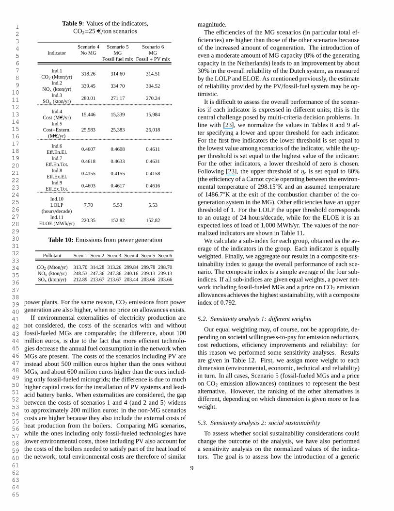
Table 9: Values of the indicators,CO2=25 C/ton scenarios

IndicatorScenario 4 Scenario 5 Scenario 6

No MG MG MGFossil fuel mix Fossil+ PV mix

Ind.1318.26 314.60 314.51

CO2 (Mton/yr)Ind.2

339.45 334.70 334.52NOx (kton/yr)

Ind.3280.01 271.17 270.24

SOx (kton/yr)

Ind.415,446 15,339 15,984

Cost (MC/yr)Ind.5

25,583 25,383 26,018Cost+Extern.(MC/yr)

Ind.60.4607 0.4608 0.4611

Eff.En.El.Ind.7

0.4618 0.4633 0.4631Eff.En.Tot.

Ind.80.4155 0.4155 0.4158

Eff.Ex.El.Ind.9

0.4603 0.4617 0.4616Eff.Ex.Tot.

Ind.107.70 5.53 5.53LOLP

(hours/decade)Ind.11

220.35 152.82 152.82ELOE (MWh/yr)

Table 10: Emissions from power generation

Pollutant Scen.1 Scen.2 Scen.3 Scen.4 Scen.5 Scen.6

CO2 (Mton/yr) 313.70 314.28 313.26 299.84 299.78 298.70NOx (kton/yr) 248.53 247.36 247.36 240.16 239.13 239.13SOx (kton/yr) 212.89 213.67 213.67 203.44 203.66 203.66

power plants. For the same reason, CO2 emissions from powergeneration are also higher, when no price on allowances exists.

If environmental externalities of electricity productionarenot considered, the costs of the scenarios with and withoutfossil-fueled MGs are comparable; the difference, about 100million euros, is due to the fact that more efficient technolo-gies decrease the annual fuel consumption in the network whenMGs are present. The costs of the scenarios including PV areinstead about 500 million euros higher than the ones withoutMGs, and about 600 million euros higher than the ones includ-ing only fossil-fueled microgrids; the difference is due to muchhigher capital costs for the installation of PV systems and lead-acid battery banks. When externalities are considered, thegapbetween the costs of scenarios 1 and 4 (and 2 and 5) widensto approximately 200 million euros: in the non-MG scenarioscosts are higher because they also include the external costs ofheat production from the boilers. Comparing MG scenarios,while the ones including only fossil-fueled technologies havelower environmental costs, those including PV also accountforthe costs of the boilers needed to satisfy part of the heat load ofthe network; total environmental costs are therefore of similar

magnitude.The efficiencies of the MG scenarios (in particular total ef-

ficiencies) are higher than those of the other scenarios becauseof the increased amount of cogeneration. The introduction ofeven a moderate amount of MG capacity (8% of the generatingcapacity in the Netherlands) leads to an improvement by about30% in the overall reliability of the Dutch system, as measuredby the LOLP and ELOE. As mentioned previously, the estimateof reliability provided by the PV/fossil-fuel system may be op-timistic.

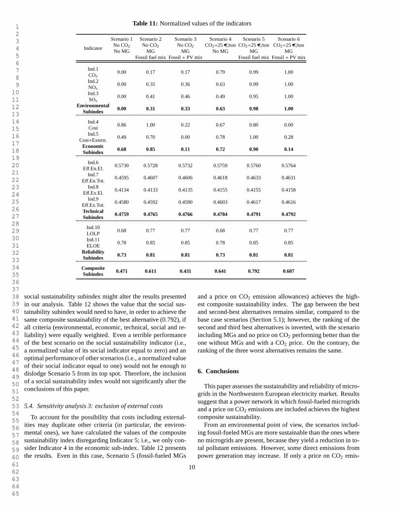
It is difficult to assess the overall performance of the scenar-ios if each indicator is expressed in different units; this is thecentral challenge posed by multi-criteria decision problems. Inline with [23], we normalize the values in Tables 8 and 9 af-ter specifying a lower and upper threshold for each indicator.For the first five indicators the lower threshold is set equal tothe lowest value among scenarios of the indicator, while theup-per threshold is set equal to the highest value of the indicator.For the other indicators, a lower threshold of zero is chosen.Following [23], the upper threshold ofηe is set equal to 80%(the efficiency of a Carnot cycle operating between the environ-mental temperature of 298.15K and an assumed temperatureof 1486.7K at the exit of the combustion chamber of the co-generation system in the MG). Other efficiencies have an upperthreshold of 1. For the LOLP the upper threshold correspondsto an outage of 24 hours/decade, while for the ELOE it is anexpected loss of load of 1,000 MWh/yr. The values of the nor-malized indicators are shown in Table 11.

We calculate a sub-index for each group, obtained as the av-erage of the indicators in the group. Each indicator is equallyweighted. Finally, we aggregate our results in a composite sus-tainability index to gauge the overall performance of each sce-nario. The composite index is a simple average of the four sub-indices. If all sub-indices are given equal weights, a powernet-work including fossil-fueled MGs and a price on CO2 emissionallowances achieves the highest sustainability, with a compositeindex of 0.792.

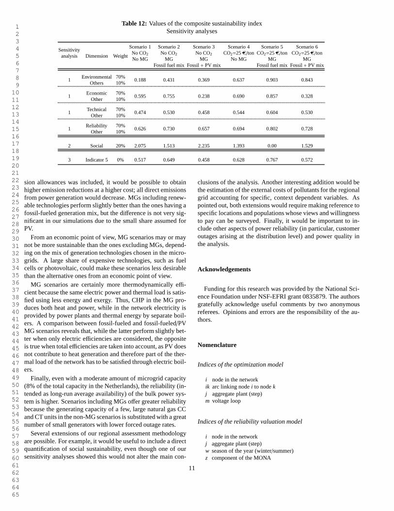
5.2. Sensitivity analysis 1: different weights

Our equal weighting may, of course, not be appropriate, de-pending on societal willingness-to-pay for emission reductions,cost reductions, efficiency improvements and reliability: forthis reason we performed some sensitivity analyses. Resultsare given in Table 12. First, we assign more weight to eachdimension (environmental, economic, technical and reliability)in turn. In all cases, Scenario 5 (fossil-fueled MGs and a priceon CO2 emission allowances) continues to represent the bestalternative. However, the ranking of the other alternatives isdifferent, depending on which dimension is given more or lessweight.

5.3. Sensitivity analysis 2: social sustainability

To assess whether social sustainability considerations couldchange the outcome of the analysis, we have also performeda sensitivity analysis on the normalized values of the indica-tors. The goal is to assess how the introduction of a generic

9

1 2 3 4 5 6 7 8 9 10 11 12 13 14 15 16 17 18 19 20 21 22 23 24 25 26 27 28 29 30 31 32 33 34 35 36 37 38 39 40 41 42 43 44 45 46 47 48 49 50 51 52 53 54 55 56 57 58 59 60 61 62 63 64 65

Table 11: Normalized values of the indicators

Indicator

Scenario 1 Scenario 2 Scenario 3 Scenario 4 Scenario 5 Scenario 6No CO2 No CO2 No CO2 CO2=25 C/ton CO2=25 C/ton CO2=25 C/tonNo MG MG MG No MG MG MG

Fossil fuel mix Fossil+ PV mix Fossil fuel mix Fossil+ PV mix

Ind.10.00 0.17 0.17 0.79 0.99 1.00

CO2Ind.2

0.00 0.35 0.36 0.63 0.99 1.00NOxInd.3

0.00 0.41 0.46 0.49 0.95 1.00SOx

Environmental0.00 0.31 0.33 0.63 0.98 1.00

Subindex

Ind.40.86 1.00 0.22 0.67 0.80 0.00

CostInd.5

0.49 0.70 0.00 0.78 1.00 0.28Cost+Extern.

Economic0.68 0.85 0.11 0.72 0.90 0.14

Subindex

Ind.60.5730 0.5728 0.5732 0.5759 0.5760 0.5764

Eff.En.El.Ind.7

0.4595 0.4607 0.4606 0.4618 0.4633 0.4631Eff.En.Tot.

Ind.80.4134 0.4133 0.4135 0.4155 0.4155 0.4158

Eff.Ex.El.Ind.9

0.4580 0.4592 0.4590 0.4603 0.4617 0.4616Eff.Ex.Tot.Technical

0.4759 0.4765 0.4766 0.4784 0.4791 0.4792Subindex

Ind.100.68 0.77 0.77 0.68 0.77 0.77

LOLPInd.11

0.78 0.85 0.85 0.78 0.85 0.85ELOE

Reliability0.73 0.81 0.81 0.73 0.81 0.81

Subindex

Composite0.471 0.611 0.431 0.641 0.792 0.607

Subindex

social sustainability subindex might alter the results presentedin our analysis. Table 12 shows the value that the social sus-tainability subindex would need to have, in order to achievethesame composite sustainability of the best alternative (0.792), ifall criteria (environmental, economic, technical, socialand re-liability) were equally weighted. Even a terrible performanceof the best scenario on the social sustainability indicator(i.e.,a normalized value of its social indicator equal to zero) andanoptimal performance of other scenarios (i.e., a normalizedvalueof their social indicator equal to one) would not be enough todislodge Scenario 5 from its top spot. Therefore, the inclusionof a social sustainability index would not significantly alter theconclusions of this paper.

5.4. Sensitivity analysis 3: exclusion of external costs

To account for the possibility that costs including external-ities may duplicate other criteria (in particular, the environ-mental ones), we have calculated the values of the compositesustainability index disregarding Indicator 5; i.e., we only con-sider Indicator 4 in the economic sub-index. Table 12 presentsthe results. Even in this case, Scenario 5 (fossil-fueled MGs

and a price on CO2 emission allowances) achieves the high-est composite sustainability index. The gap between the bestand second-best alternatives remains similar, compared tothebase case scenarios (Section 5.1); however, the ranking of thesecond and third best alternatives is inverted, with the scenarioincluding MGs and no price on CO2 performing better than theone without MGs and with a CO2 price. On the contrary, theranking of the three worst alternatives remains the same.

6. Conclusions

This paper assesses the sustainability and reliability of micro-grids in the Northwestern European electricity market. Resultssuggest that a power network in which fossil-fueled microgridsand a price on CO2 emissions are included achieves the highestcomposite sustainability.

From an environmental point of view, the scenarios includ-ing fossil-fueled MGs are more sustainable than the ones whereno microgrids are present, because they yield a reduction into-tal pollutant emissions. However, some direct emissions frompower generation may increase. If only a price on CO2 emis-

10

1 2 3 4 5 6 7 8 9 10 11 12 13 14 15 16 17 18 19 20 21 22 23 24 25 26 27 28 29 30 31 32 33 34 35 36 37 38 39 40 41 42 43 44 45 46 47 48 49 50 51 52 53 54 55 56 57 58 59 60 61 62 63 64 65

Table 12: Values of the composite sustainability indexSensitivity analyses

SensitivityDimension Weight

Scenario 1 Scenario 2 Scenario 3 Scenario 4 Scenario 5 Scenario 6

analysisNo CO2 No CO2 No CO2 CO2=25 C/ton CO2=25 C/ton CO2=25 C/tonNo MG MG MG No MG MG MG

Fossil fuel mix Fossil+ PV mix Fossil fuel mix Fossil+ PV mix

1Environmental 70%

0.188 0.431 0.369 0.637 0.903 0.843Others 10%

1Economic 70%

0.595 0.755 0.238 0.690 0.857 0.328Other 10%

1Technical 70%

0.474 0.530 0.458 0.544 0.604 0.530Other 10%

1Reliability 70%

0.626 0.730 0.657 0.694 0.802 0.728Other 10%

2 Social 20% 2.075 1.513 2.235 1.393 0.00 1.529

3 Indicator 5 0% 0.517 0.649 0.458 0.628 0.767 0.572

sion allowances was included, it would be possible to obtainhigher emission reductions at a higher cost; all direct emissionsfrom power generation would decrease. MGs including renew-able technologies perform slightly better than the ones having afossil-fueled generation mix, but the difference is not very sig-nificant in our simulations due to the small share assumed forPV.

From an economic point of view, MG scenarios may or maynot be more sustainable than the ones excluding MGs, depend-ing on the mix of generation technologies chosen in the micro-grids. A large share of expensive technologies, such as fuelcells or photovoltaic, could make these scenarios less desirablethan the alternative ones from an economic point of view.

MG scenarios are certainly more thermodynamically effi-cient because the same electric power and thermal load is satis-fied using less energy and exergy. Thus, CHP in the MG pro-duces both heat and power, while in the network electricity isprovided by power plants and thermal energy by separate boil-ers. A comparison between fossil-fueled and fossil-fueled/PVMG scenarios reveals that, while the latter perform slightly bet-ter when only electric efficiencies are considered, the oppositeis true when total efficiencies are taken into account, as PV doesnot contribute to heat generation and therefore part of the ther-mal load of the network has to be satisfied through electric boil-ers.

Finally, even with a moderate amount of microgrid capacity(8% of the total capacity in the Netherlands), the reliability (in-tended as long-run average availability) of the bulk power sys-tem is higher. Scenarios including MGs offer greater reliabilitybecause the generating capacity of a few, large natural gas CCand CT units in the non-MG scenarios is substituted with a greatnumber of small generators with lower forced outage rates.

Several extensions of our regional assessment methodologyare possible. For example, it would be useful to include a directquantification of social sustainability, even though one ofoursensitivity analyses showed this would not alter the main con-

clusions of the analysis. Another interesting addition would bethe estimation of the external costs of pollutants for the regionalgrid accounting for specific, context dependent variables.Aspointed out, both extensions would require making reference tospecific locations and populations whose views and willingnessto pay can be surveyed. Finally, it would be important to in-clude other aspects of power reliability (in particular, customeroutages arising at the distribution level) and power quality inthe analysis.

Acknowledgements

Funding for this research was provided by the National Sci-ence Foundation under NSF-EFRI grant 0835879. The authorsgratefully acknowledge useful comments by two anonymousreferees. Opinions and errors are the responsibility of theau-thors.

Nomenclature

Indices of the optimization model

i node in the networkik arc linking nodei to nodekj aggregate plant (step)m voltage loop

Indices of the reliability valuation model

i node in the networkj aggregate plant (step)w season of the year (winter/summer)z component of the MONA

11

1 2 3 4 5 6 7 8 9 10 11 12 13 14 15 16 17 18 19 20 21 22 23 24 25 26 27 28 29 30 31 32 33 34 35 36 37 38 39 40 41 42 43 44 45 46 47 48 49 50 51 52 53 54 55 56 57 58 59 60 61 62 63 64 65

Sets of the optimization model

I set of all nodesJ set of aggregate plants, differing in location,

ownership, fuel type and costJi set of aggregate plants at nodeiM set of Kirchhoff’s voltage loopsAi set of nodes adjacent to nodeiMm ordered set of linksik in voltage loopm

Parameters of the optimization model

CO2 CO2 price, C/tonLi power demand at nodei, MWRik reactance on arcikS ikm ± 1 depending on the orientation of arcik in loop mLossik resistance loss coefficient on arcik, 1/MWTik maximum transmission capacity on arcik, MWMC i j marginal cost for generation at nodei and stepj, C/MWhEi j CO2 emission rate at nodei and stepj, ton/MWhCapi j maximum generation capacity at nodei and stepj, MW

Parameters of the reliability valuation model

Capi j maximum generation capacity at nodei and stepj, MWFORi j forced outage rate for individual plants at nodei and stepjNi j number of individual power plants at nodei and stepjLz power demand of thezth component of the MONA, MWCapw expected generating capacity in seasonw, MWWindw wind generation in seasonw, MWλw parameter of the exponential approximation

to wind distribution in seasonw, MW

Decision variables of the optimization model

fik export flow from nodei to nodek, MWgeni j generation at nodei by aggregate plantj, MW

Decision variables of the reliability valuation model

µz mean of thezth component of the MONA, MWσ2

z variance of thezth component of the MONA, (MW)2

pz weight of thezth component of the MONA

Thermodynamic variables

W annual electric power load of the network, MWhQ annual heat load of the network, MWhtηb efficiency of the boilersηe annual energetic electric efficiency of the networkηtot annual energetic total efficiency of the networkζe annual exergetic electric efficiency of the networkζtot annual exergetic total efficiency of the networkϕe exergy to energy ratio of fuels used

for electricity generation in the networkEQ

S exergy content of the heat load, MWhENG exergy flow rate of natural gas, MJ/s*hourMNG mass flow rate of natural gas, kg/sHNG Lower Heating Value of natural gas, MJ/kgϕNG exergy to energy ratio of natural gas

References

[1] Market integration: coupling of the Euro-pean electricity markets [Internet]. Available from:http://www.tennettso.de/pages/tennettsoen/Press/Information Material/PDF/100478TEN Brochuremarktkoppeling.pdf [accessed 2011 Jun24].

[2] CWE Market integration [Internet]. Available from:http://www.apxendex.com/index.php?id=186 [accessed 2011 Jun24].

[3] Report of the United Nations World Commission on Environmentand Development. Our common future [Internet]. Available from:http://www.un-documents.net/wced-ocf.htm [accessed 2011 Jun 24].

[4] Hobbs, B.F., Meier, P. Energy decisions and the environment: a guide tothe use of multicriteria methods. Kluwer Academic Publishers; 2000.

[5] Lebre LaRovere, E., Borghetti Soares, J., Basto Oliveira, L., Lauria, T.Sustainable expansion of electricity sector: sustainability indicators asan instrument to support decision making. Renewable and SustainableEnergy Reviews 2010; 14: 422-9.

[6] Giannantoni, C., Lazzaretto, A., Macor, A., Mirandola,A., Stoppato, A.,Tonon, S. et al. Multicriteria approach for the improvementof energysystems design. Energy 2005; 30(10): 1989-2016.

[7] Wang, J., Jing, Y., Zhang, C., Zhao, J. Review on multi-criteria decisionanalysis aid in sustainable energy decision making. Renewable and Sus-tainable Energy Reviews 2009; 13: 2263-2278.

[8] Maruyama, Y., Nishikido, M., Iida, T. The rise of community wind powerin Japan: enhanced acceptance through social innovation. Energy Policy2007; 35(5): 2761-2769.

[9] Gallego Carrera, D., Mack, A. Sustainability assessment of energy tech-nologies via social indicators: results of a survey among European energyexperts. Energy Policy 2010; 38: 1030-1039.

[10] Turvey, R., Anderson, D. Electricity economics: essays and case studies.Baltimore: Johns Hopkins University Press; 1977.

[11] ExternE: externalities of energy, Vol.1; 1995 [Internet]. Available from:http://www.externe.info/ [accessed 2011 Jun 24]

[12] Ottinger, R.L., Wooley, D., Robinson, N., Hodas, D., Babb, S. Environ-mental costs of electricity. New York: Oceana Publications; 1990.

[13] Hohmeyer, O., and Ottinger, R.L., editors. External environmental costsof electric power: analysis and internalization. Proceedings of a German-American Workshop; 1990, October 23-25; Ladenburg, FRG. New York:Springer-Verlag; 1991.

[14] Gil, H.A. Models for quantifying the economic benefits of distributedgeneration. IEEE Transactions on Power Systems 2008; 23(2): 327-35.

[15] Tsikalakis, A.G., Hatziargyriou, N.D. Environmentalbenefits of dis-tributed generation with and without emissions trading. Energy Policy2007; 35(6): 3395-409.

[16] Hadley, S.W., Van Dyke, J.W., Poore III, W.P., Stovall,T.K. Quantitative assessment of distributed energy resourcebenefits [Internet]. Oak Ridge National Laboratory, Engi-neering Science and Technology Division. Available from:http://www.ornl.gov/∼webworks/cppr/y2001/rpt/116227.pdf. [accessed2011 Jun 24].

[17] U.S. Department of Energy. The potential benefits of distributed gen-eration and rate-related issues that may impede their expansion [In-ternet]. Available from: http://www.ferc.gov/legal/fed-sta/exp-study.pdf.[accessed 2011 Jun 24]

[18] Alanne, K., Sari, A. Distributed energy generation andsustainable devel-opment. Renewable and sustainable energy reviews 2006; 10(6): 539-58.

[19] Firestone, R., Marnay, C., Maribu, K.M. The value of distributed gener-ation under different tariff structures. Berkeley (CA): Lawrence BerkeleyNational Laboratory, Environmental Energy Technologies Division; 2006May. Report No.: LBNL-60589. Contract No.: DEAC0205CH11231.Sponsored by the US Department of Energy.

[20] Siddiqui, A.S., Marnay, C., Edwards, J.L., Firestone,R., Ghosh, S.,Stadler, M. Effects of a carbon tax on microgrid combined heat and poweradoption. Berkeley (CA): Lawrence Berkeley National Laboratory, Envi-ronmental Energy Technologies Division; 2004 Oct. Report No.: LBNL-51771. Contract No.: DEAC0376SF00098. Sponsored by the US Depart-ment of Energy.

[21] Marnay, C., Lai, J., Stadler, M., Siddiqui, A. Added value of reliability toa microgrid: simulations of three California buildings. Berkeley (CA):Lawrence Berkeley National Laboratory, Environmental Energy Tech-

12

1 2 3 4 5 6 7 8 9 10 11 12 13 14 15 16 17 18 19 20 21 22 23 24 25 26 27 28 29 30 31 32 33 34 35 36 37 38 39 40 41 42 43 44 45 46 47 48 49 50 51 52 53 54 55 56 57 58 59 60 61 62 63 64 65

nologies Division; 2009 Apr. Report No.: LBNL-1853E. Contract No.:DEAC0205H11231. Sponsored by the US Department of Energy.

[22] Yi, H., Hau, J.L., Ukidwe, N.U., Bakshi, B.R. Hierarchical thermody-namic metrics for evaluating the environmental sustainability of industrialprocesses. Environmental Progress 2004; 23(4): 302-14.

[23] Frangopoulos, C.A., Keramioti, D.E. Multi-criteria evaluation of energysystems with sustainability considerations. Entropy 2010; 12(5): 1006-20.

[24] Frangopoulos, C.A., von Spakovksy, M.R. A global environomic ap-proach for energy systems analysis and optimization. Proceedings of theEnergy Systems and Ecology Conference; 1993 July 5-9; Cracow, Poland.p.123-44.

[25] von Spakovksy, M.R., Frangopoulos, C.A. The environomic analysis andoptimization of a gas turbine cycle with cogeneration. American Societyof Mechanical Engineers (ASME) 1994; 33: 15-26.

[26] Rosen, M. Energy and exergy-based comparison of coal-fired and nuclearsteam power plants. Exergy 2001; 1(3): 180-92.

[27] Zvolinschi, A., Kjelstrup, S., Bolland, O., van der Kooi, H.J. Exergy sus-tainability indicators as a tool in industrial ecology. Journal of IndustrialEcology 2007; 11(4): 85-98.

[28] Billinton, R., Allan, R.N. Reliability evaluation of power systems: con-cepts and techniques. New York: Plenum Press; 1996.

[29] Stoll, H.G. Least-cost electric utility planning. NewYork: John Wiley andSons; 1989.

[30] Wood, A.J., Wollenberg. B.F. Power generation operation and control.New York: John Wiley and Sons; 1996.

[31] Marnay, C. Microgrids and heterogenous power quality and reliability.Berkeley (CA): Lawrence Berkeley National Laboratory, Environmen-tal Energy Technologies Division; 2008 Jul. Report No.: LBNL-777E.Contract No.: DEAC0205CH11231. Sponsored by the US Department ofEnergy.

[32] Chowdhury, S., Chowdhury, S.P., Crossley, P. Microgrids and active dis-tribution networks. London: The Institution of Engineering and Technol-ogy; 2009.

[33] Council of European Energy Regulators. Fourth benchmarking re-port on quality of electricity supply 2008 [Internet]. Availablefrom: http://www.autorita.energia.it/allegati/pubblicazioni/C08-EQS-24-04 4th BenchmarkingReportEQS 10-Dec-2008re.pdf [accessed 2011Jun 24].

[34] Hobbs, B.F. Models for integrated resource planning byelectric utilities.European Journal of Operational Research. 1995; 83(1): 1-20.

[35] Hobbs, B.F., Rijkers, F.A.M. Modeling strategic generator behavior withconjectured transmission price responses in a mixed transmission pricingsystem I: formulation, IEEE Transactions on Power Systems 2004; 19(2):707-17.

[36] Hobbs, B.F., Drayton, G., Bartholomew Fisher, E., Lise, W. Improvedtransmission representations in oligopolistic market models: quadraticlosses, phase shifters, and DC lines. IEEE Transactions on Power Sys-tems 2008; 23(3): 1018-29.

[37] Energy Research Centre of the Netherlands. COM-PETES input data [Internet]. Available from:http://www.ecn.nl/fileadmin/ecn/units/bs/COMPETES/cost-functions.xls[accessed 2011 Jun 24]

[38] International Energy Agency. Energy Prices and Taxes,energy end-useprices in national currencies, vol.2. Paris: International Energy Agency;2010.

[39] International Energy Agency. Electricity Information. Paris: InternationalEnergy Agency; 2010.

[40] European Network of Transmission System Operators forElectricity.Hourly load values for a specific country for a specific month [Internet].Available from: https://www.entsoe.eu/index.php?id=137 [accessed 2011Jun 24].

[41] International Energy Agency Energy Conservation in Build-ings and Community Systems, Annex 42 [Internet]. Stan-dard European Electrical Profiles. 2006. Available from:http://www.ecbcs.org/docs/Annex 42 EuropeanElectrical StandardProfilesAnnex 42 September2006.zip [accessed 2011 Jun 24].

[42] De Vries, L.J. Generation adequacy: helping the marketdo its job. Utili-ties Policy 2007; 15(1): 20-35.

[43] Gross, G., Garapic, N.V., McNutt, B. The mixture of normals approxima-tion technique for equivalent load duration curves. IEEE Transactions on

Power Systems 1988; 3(2): 368-74.[44] North American Electric Reliability Corporation. 2005-2009

Generating Availability Report [Internet]. Available from:http://www.nerc.com/page.php?cid=4|43|47 [accessed 2011 Jun 24].

[45] Energy and Environmental Analysis, Inc. Distributed gen-eration operational reliability and availability database.Executive summary report [Internet]. Available from:http://files.harc.edu/Sites/GulfCoastCHP/Publications/DistributedOperationalReliability.pdf [accessed 2011 Jun 24].

[46] Hargreaves, J.J., Hobbs, B.F. Optimal commitment and dispatch withuncertain wind generation using stochastic dynamic programming.Manuscript, Department of Geography & Environmental Engineering,Johns Hopkins University, 2010.

[47] AEA Technology. Environmental Product Declaration ofElectricityfrom Torness Nuclear Power Station - a technical report [Internet].Available from: http://www.british-energy.com/documents/EPD Doc -Final.pdf [accessed 2011 Jun 28].

[48] Spath, P.L., Mann, M.K., Kerr, D.R. Life cycle assessment of coal firedpower production. Golden (CO): National Renewable Energy Laboratory;1999 June.

[49] Spath, P.L., Mann, M.K. Life cycle assessment of a natural gas combined-cycle power generation system. Golden (CO): National Renewable En-ergy Laboratory; 2000 September.

[50] Kaewboonsong, W., Kuprianov, V.I., Chovichien, N. Minimizing fuel andenvironmental costs for a variable-load power plant (co-)firing fuel oil andnatural gas. Part 1. Modeling of gaseous emissions from boiler units. Fuelprocessing technology 2006; 87: 10851094.

[51] Boudghene Stambouli, A., Traversa, E. Solid oxide fuelcells (SOFCs):a review of an environmentally clean and efficient source of energy. Re-newable and Sustainable Energy Reviews 2002; 6: 433-455.

[52] Greenhouse Gas Technology Center - Southern Research Institute. En-vironmental technology verification report. Combined heatand power ata commercial supermarket - Capstone 60 kW microturbine CHP system[Internet]. Available from: http://www.capstoneturbine.com/ docs/EPA-C60testreport.pdf [accessed 2011 Jun 27].

[53] Pipattanasomporn, M., Willingham, M. White paper on dis-tributed generation [Internet]. Available from: http://www.idc-online.com/technical references/pdfs/electrical engineering/Distributed%20generation.pdf [accessed 2011 Jun 27].

[54] EcoSenseWeb [Internet]. Available from: http://ecosenseweb.ier.uni-stuttgart.de/.

[55] NEEDS - New Energy Externalities Developments for Sustainabil-ity. Report on the procedure and data to generate averaged/aggregatedata, RS3a-D1.1; 2008 [Internet]. Available from: http://www.needs-project.org/2009/ [accessed 2011 Jun 24].

[56] Bejan, A., Tsatsaronis, G., Moran, M. Thermal design and optimization.New York: John Wiley and Sons; 1996.

13

Sustainability and reliability assessment of microgridsin a regional electricity market

Chiara Lo Pretea,∗, Benjamin F. Hobbsa, Catherine S. Normana, Sergio Cano-Andradeb,Alejandro Fuentesb, Michael R. von Spakovskyb, Lamine Milic

aJohns Hopkins University, Department of Geography and Environmental Engineering, Baltimore, USAbVirginia Polytechnic Institute and State University, Department of Mechanical Engineering, Blacksburg, USA

cVirginia Polytechnic Institute and State University, Department of Electrical and Computer Engineering, Blacksburg, USA

Abstract

We develop a framework to assess and quantify the sustainability and reliability of different power production scenarios in a regionalsystem, focusing on the interaction of microgrids with the existing transmission/distribution grid. The Northwestern Europeanelectricity market (Belgium, France, Germany and the Netherlands) provides a case study for our purposes. We present simulationsof power market outcomes under various policies and levels of microgrid penetration, and evaluate them using a diverse set ofmetrics. This analysis is the first attempt to include exergy-based and reliability indices when evaluating the role of microgrids inregional power systems. The results suggest that a power network in which fossil-fueled microgrids and a price on CO2 emissionsare included has the highest composite sustainability index.

Keywords: Microgrids, sustainability, reliability, Northwestern Europe, exergy, economics, air pollution, multi-criteria decisionmaking.

1. Introduction

A microgrid (MG) is a localized grouping of electric andthermal loads, generation and storage that can operate in par-allel with the grid or in island mode and can be supplied byrenewable and/or fossil-fueled distributed generation. We quan-tify the sustainability and reliability of MGs in a regional powermarket in terms of multiple indices for the regional grid. Thesetting is the Northwestern European electricity market (Bel-gium, France, Germany and the Netherlands). This is a re-gional network whose national markets already influence eachother strongly and have taken steps to integrate even furtherinto a single market. Since 2006, for example, the Netherlands,France and Belgium have coupled their electricity exchangesthrough the Trilateral Market Coupling (TLC), ensuring theconvergence of spot electricity prices in the three countries. InNovember 2010, the TLC was replaced by the Central WesternEuropean Market Coupling (CWE), which also includes Ger-many [1] [2].

Sustainable development is often defined as “developmentthat meets the needs of the present without compromising theability of future generations to meet their own needs” [3].Translating this definition into quantifiable criteria that can beused to compare alternative power systems has proven difficult.For this reason, several authors have adopted a multi-criteria

∗Corresponding author at Johns Hopkins University, Department of Geog-raphy and Environmental Engineering, 3400 North Charles Street, 313 AmesHall. Baltimore, MD, 21218, USA. Email address: chiara.lo.prete@jhu.edu.Phone number: 410-516-5137. Fax number: 410-516-8996.

(or multiple objective) approach. The function of multi-criteriaanalysis is to communicate tradeoffs among conflicting criteriaand to help users quantify and apply value judgments in orderto recommend a course of action [4]. In this manner, a range ofdimensions of sustainability can be considered, while allowingstakeholder groups to have different priorities among the cri-teria. This method has been used, for example, to assess thetradeoffs in power system planning [5] and to evaluate the sus-tainability of power generation [6].

The main contribution of this paper is the quantification ofthe sustainability and reliability of alternative power generationpaths in a regional system with a diverse set of metrics. Weexplicitly simulate the impacts of a generation investment de-cision on operations and investment elsewhere in the grid, asevaluation of the net sustainability impacts of a decision shouldconsider how a given investment choice propagates through thesystem. Our approach does not rely on multi-objective opti-mization; it presents instead a multi-criteria assessment throughthe use of indicators, which are calculated based on the re-sults of a single-objective optimization model and a reliabilitymodel.

Among the commonly used four dimensions to evaluate thesustainability of energy supply systems (social, economic, tech-nical and environmental) [7], the analysis emphasizes the latterthree. In terms of microgrid impact on social sustainability,several areas commonly cited as important are equity, com-munity impacts, level of participation in decision making andhealth impacts. The first three depend on how a given micro-grid is owned and managed. In general, it is plausible that theincreased impact that members of the microgrid-served pop-

Preprint submitted to Energy July 2, 2011

*Marked-up ManuscriptClick here to view linked References

ulation could have on ownership and management decisions,relative to populations served by conventional utilities, wouldcount as a positive impact on social sustainability. Addition-ally, shared community values may lead some stakeholders tovalue microgrids that use renewable energy more highly thaneither microgrids that do not or larger systems in which thecommunity has little choice about the source of electricity [8].Increased security of supply associated with microgrids mayalso offer social as well as economic benefits within and out-side the community served by a microgrid. Finally, microgridoperation may create jobs that offer social sustainability gainsfor the local community.

On the other hand, microgrids may have negative effects onresidents’ quality of life, if they increase the level of noise orhave aesthetic impacts on the landscape [9]. Health impactsof a microgrid may also be negative, as microgrids are likelyto have generation and thus pollution closer to the populationsthey serve than conventional distribution networks. How risksto life and health associated with local air pollution comparewith the ones from a conventional utility source will be verypopulation, site and technology specific.

While we can speculate on the likely direction of these im-pacts for the power system modeled in this paper, it is difficult toquantify them without reference to a specific location and pop-ulation whose views and willingness to pay can be surveyed orestimated. On the contrary, the methodology used in our anal-ysis aims at assessing the broader impacts of alternative powergeneration paths on a regional power system. For this reason,no direct quantification of social sustainability is offered in ourstudy. However, to account indirectly for this dimension weperform a sensitivity analysis on the results in order to assesswhether and how the introduction of a social sustainability in-dex would alter our conclusions.

We consider six alternative scenarios for satisfying the elec-tric power and thermal needs of a regional power market, andwe characterize their sustainability and reliability using foursets of indicators. The scenarios are various combinations ofmicrogrid implementation (with and without MGs), microgridgenerating mix (fossil-fueled only, or fossil-fueled and renew-able) and CO2 policies (with and without a price on CO2 emis-sion allowances). The first set of indices is based on CO2 andconventional air pollutant emissions (NOx and SOx). The sec-ond one emphasizes economic sustainability in terms of totalgeneration costs [10] and accounts for externalities of electric-ity generation. Externalities can be defined as “the costs andbenefits which arise when the social or economic activities ofone group of people have an impact on another, and when thefirst group fails to fully account for their impacts” [11]. In the1990s the importance of environmental costs as an input to theplanning and decision processes of electric power generationsystems was recognized in several studies [12] [13]. The thirdset of indices is based on thermodynamic energy and exergybased efficiencies, while the fourth considers effects on bulkpower system reliability.

Economic and environmental analyses of power systems in-cluding distributed generation are common (see, for exam-ple, [14] and [15]). Several studies assess the potential bene-

fits of distributed generation [16] [17] and evaluate its impacton sustainable development [18]. Others focus directly on theeconomic and regulatory issues of MG implementation [19],on the implications of environmental regulation on MG adop-tion [20], and on the improvement in power reliability providedto different types of buildings by the installation of a MG [21].In contrast, neither thermodynamic analyses considering the in-teraction of MGs with existing regional power systems nor theeffect of MG deployment on system reliability have been previ-ously published, to the best of our knowledge.

We include exergy because an analysis relying on first lawefficiency alone does not consider to what degree the outputs ofa power plant are useful. For example, electricity is more valu-able than steam, one of the typical by-products of power pro-duction, because the latter is characterized on a per unit energybasis by a lower value of exergy than electricity. Therefore, notall outputs should be valued in the same way: outputs having ahigher quality or exergy per unit energy (like electricity) shouldhave a higher unit price than those having a lower quality orexergy per unit energy (like steam) because the former possessa greater ability to do work. In contrast, when the second lawof thermodynamics is disregarded, the difference in quality ofthe various energy outputs is not considered and cannot be ef-fectively compared for different energy conversion processes.

Thus, the use of exergy-based indicators can help decisionmakers to improve the effectiveness of energy resource use in agiven system. Such indicators have been widely adopted in thesustainability literature. Yi et al. [22] use thermodynamic in-dices to assess the sustainability of industrial processes. Fran-gopoulos and Keramioti [23] evaluate the performance of dif-ferent alternatives to meet the energy needs of an industrialunit, taking into account several aspects of sustainability. vonSpakovsky and Frangopoulos [24] [25] use an environomic(thermodynamic, environmental and economic) objective forthe analysis and optimization of a gas turbine cycle with cogen-eration. Rosen [26] presents a thermodynamic comparison of acoal and a nuclear power plant on the basis of exergy and en-ergy. Zvolinschi et al. [27] develop three exergy-based indicesto assess the sustainability of power generation in Norway.

In addition to sustainability, it is important to incorporate areliability analysis in the decision process because of the posi-tive impact that microgrids may have on power system reliabil-ity, and thereby on promoting their deployment. Therefore, weadd reliability to our suite of indices and quantify it using theannual Loss of Load Probability (LOLP) and Expected Loss ofEnergy (ELOE) [28] [29]. The reliability of a power system isthe probability that the system is able to perform its intendedfunction (generation meets load), under a contractual qualityof service, for a specified period of time. Reliability is quanti-fied here using the concept of “long-run average availability” ofthe bulk power system (supply-demand balance), without con-sideration of dynamic system response to disturbances, whichinstead is the concept of “security” [30].

We do not consider aspects of power quality that may alsobe controlled within MGs. It has been argued that microgridshave the potential to deliver different degrees of power qual-ity tailored for different customers’ needs, as they may be em-

2

ployed to control power quality locally according to customers’requirements. This may prove to be more beneficial than pro-viding a uniform level of quality and service to all customerswithout differentiating among their needs [31] [32]. However,the way in which microgrids may affect power quality in a re-gional grid is still under study and there are no definitive results.For this reason, we do not include power quality considerationsin our analysis, though we note they should be addressed infuture research.

We also do not consider customer outages arising at the sub-transmission or distribution-level. However, it is worth notingthat the majority of power interruptions experienced by cus-tomers in the countries we consider are not due to large eventsat the bulk level, but to more localized ones affecting the distri-bution system [33].

Section 2 describes our modeling approach, data and as-sumptions concerning alternative power systems (with andwithout MGs) and CO2 policies. Section 3 presents the six sce-narios considered in our analysis to satisfy the electric powerand thermal needs of the Northwestern European electricitymarket. Section 4 describes the indicators chosen in this paperto assess the sustainability and reliability of the network. Sec-tion 5 discusses the results of the analysis, while Section 6 con-cludes.

2. Methodology and data

Two different models are used to quantify our indices. A re-gional power market model based on linear optimization meth-ods [10] [34] provides the information necessary for the eco-nomic, environmental and thermodynamic indices; the modelis presented in Section 2.1. A local reliability model based onconvolution methods [28] [29], described in Section 2.2, is usedinstead to obtain the reliability indices.

2.1. Regional market simulation modelFor the purposes of this paper, we represent the Northwest-

ern European electricity market using COMPETES (Compre-hensive Market Power in Electricity Transmission and EnergySimulator) [35]. Our version of COMPETES is a quadraticallyconstrained model solved in ILOG OPL 6.3, using the opti-mizer Cplex12. COMPETES models twelve power producersin the four countries: eight of them are the largest ones in theregion (Electrabel, Edf, Eon, ENBW, RWE, Vattenfall, EssentNuon-Reliant), while the remaining four represent the compet-itive fringe in each country.

When no MGs are included, the electricity network is repre-sented by fifteen nodes. Each of the seven main nodes (Krim,Maas and Zwol in the Netherlands; Merc and Gram in Belgium;one node in France and one in Germany) has generation capac-ity and load. A DC power flow model is used to represent a sys-tem in which four intermediate nodes are distinguished in bothFrance (Avel, Lonn, Moul, Muhl) and Germany (Diel, Romm,Ucht, Eich); at these nodes, no generation or demand occurs(except for 2,000 MW of power exports to the UK at Avel).Three nodes representing groups of residential MGs are addedto the model in the MG scenarios.

The nodes of the network are connected by twenty-eight highvoltage transmission corridors (or arcs), each one with a maxi-mum MW transmission capacity. The groups of MGs are con-nected to the transmission system by radial links at nodes Krim,Maas and Zwol in the Netherlands. While by assumption we arefocusing on the impact of new microgrids in the Netherlands,to understand their impacts on the regional power grid it is nec-essary to consider the neighboring countries’ bulk power mar-kets. Of course, groups of microgrids could also be connectedto nodes in other countries. However, we would then need toconsider additional neighboring countries, such as Poland orthe Iberian peninsula.

Computational convenience suggests starting the analysiswith a competitive benchmark. Our application of COMPETEScalculates a competitive equilibrium among power producers,which under the assumption of perfectly inelastic demand isequivalent to minimization of total generation costs. This isdone for six representative hours in order to characterize thedistribution of operating costs.

We include resistance losses on high voltage transmissionflows to make the model more realistic because, on average,losses can contribute as much to spatial price variations as con-gestion does. Losses vary as a quadratic function of flow, usingthe DC formulation with quadratic losses in [36]. In the ab-sence of other data, resistance loss coefficients, defined for thetwenty-eight corridors of the network, are assumed to be pro-portional to reactance. Therefore, we set them equal to the reac-tance on each corridor times a constant α, whose value is cho-sen so that high voltage transmission losses are approximatelyequal to 2% of generation during the peak hours.

2.1.1. Model formulationCOMPETES is a short-run market simulation model using an

optimization formulation: its objective function includes short-run marginal costs (i.e., fuel and other variable O&M costs) anddisregards long-run retirement and entry decisions. For eachMG and CO2 policy scenario, we solve the model for six differ-ent periods of the year representing a variety of load and gen-eration capacity conditions. The six periods are appropriatelyweighted by the number of hours in each period to estimate an-nual cost. The problem statement is as follows:

min∑

i

∑j∈Ji

(MCi j + CO2Ei j)geni j (1)

subject to:∑j∈Ji

geni j +∑k∈Ai

[ fki(1 − Losski fki) − fik] ≥ Li ∀i ∈ I (2)

∑ik∈Mm

RikS ikm( fik − fki) = 0 ∀m ∈ M (3)

geni j ≤ Capi j ∀i ∈ I,∀ j ∈ Ji (4)

fik ≤ Tik ∀i, k ∈ I (5)

fik ≥ 0 ∀i, k ∈ I (6)

geni j ≥ 0 ∀i ∈ I,∀ j ∈ Ji (7)

3

A complete list of variable and parameter definitions is pro-vided in the nomenclature. The goal is to minimize the objec-tive function expressed as the total generation costs given byequation 1, where a linear short-run cost of production is as-sumed. The decision variables are geni j (the generation fromaggregated power plant j located at node i) and fik (the MWtransmission flow from node i to a nearby node k that is directlyconnected to i by a transmission corridor).

Equation 2 accounts for Kirchhoff’s Current Law (KCL), ap-plied to each node of the network. fik is the export flow fromnode i to node k, while fki(1-Losski fki) represents the importflow (net of losses) into node i from node k. Equation 3 rep-resents Kirchhoff’s Voltage Law (KVL) constraint, defined foreach of the fourteen meshes (or loops) connecting the nodes.Equation 4 ensures that power generated at each node and eachstep is less than the available capacity at that location, whileequation 5 constrains the transmission flow on a given arc.Equations 6 and 7 are nonnegativity restrictions.

When microgrids are included, their generation costs areadded to equation 1. Since the groups of MGs are additionalnodes with autonomous loads, one KCL constraint is added inthe model for each MG node. However, no additional KVL isincluded because MGs are assumed to be radially connected tothe grid. The power generated at each MG node must satisfythe capacity constraint (equation 4) and the non-negativity con-straint (equation 7), and its flow to/from the grid must satisfybounds 5 and 6.

2.1.2. DataSimulations of power market outcomes are based on a mod-

ified version of the Energy Research Centre of the Netherlands(ECN) COMPETES database of transmission, demand and gen-eration [37].

This provides a multi-step supply function (one step per ag-gregate power plant) for each node where power generation oc-curs. Using the information in [38] and [39], generation costsand capacity of the original fifteen nodes of the network in [37]have been updated to 2008 (a leap year). Our version of thedatabase has also been modified to account for transmission re-sistance losses, exergetic and energetic efficiencies, and emis-sions.

In the scenarios including MGs, nine steps representing MGtechnologies (three for each node to which MGs are connected)have been added to the existing network. Generation costs,technology types and capacity for the MG nodes are obtainedfrom the literature.

In line with [37], in the scenarios without MGs the capac-ity database does not include renewable and combined heat andpower (CHP) generators. On the other hand, CHP capacity isinstalled at the MG nodes and we explicitly consider its contri-bution to the system.

Hourly loads in the four countries are based on [40] and re-fer to 2008. Since CHP and renewable generators are not in-cluded in the capacity database, their production is netted fromthe hourly electricity demand of the network in [40]. Hourlyloads are organized in load duration curves (LDCs) and dividedinto six blocks: the first block averages the load of the first 100

hours, the second block of the following 900 hours, the thirdand fourth of the next 2,500 hours, the fifth of the next 2,284hours, the sixth of the last 500 hours. The average electricityconsumption of the residential customers in the MGs is basedon the load profiles in [41]. Information on total capacity, dom-inant fuel type, energy efficiency, exergy calculations, marginalcost function and average CO2, NOx, SOx emission rates for allthe nodes in the network is available from the authors.

2.2. Reliability valuation model

In addition to the market simulation model, we develop amodel to assess the reliability of the Dutch power system intwo scenarios (with and without MGs). We consider the Dutchsystem alone for two reasons. First, we focus our analysis onthe direct impact of MGs on the reliability in the country wherethey are installed. Second, the Netherlands is the most import-dependent of the four countries considered, and the adequacy ofgenerating capacity to meet future energy needs has been exten-sively debated over the last decade [42]. We include two relia-bility indices, the LOLP and the ELOE. The LOLP of a powersystem is the expected number of hours of capacity deficiencyin the system in a given period of time [29]. In our analysis,the LOLP is expressed in outage hours/10 years: an outage of 8hours in 10 years is typically considered a reasonable reliabilitytarget in industrialized countries. The ELOE gives an indica-tion of the amount of load that cannot be serviced in a givenperiod of time and is expressed in MWh/yr [28].

In our model, 2008 summer and winter LDCs are approx-imated using the mixture of normals approximation (MONA)technique detailed in [43]. Given z = 1,..,Z independent normalrandom variables, each with mean µz, variance σ2

z , and cumu-lative distribution function Φ(·; µz, σ2

z ), F(·) has a mixture ofnormals distribution with z components if

F(x) =∑

z

pzΦ(x; µz, σ2z ) (8)

∑z

pz = 1; 0 ≤ pz ≤ 1 (9)

where pz is the weight of the zth component. A LDC can beapproximated by

LDC(x) = 1 − F(x) (10)

For our purposes, a two-component mixture of normals pro-vides an excellent approximation of the load duration curve; theweights, mean and variances in equation 8, different for win-ter and summer loads, are obtained by minimizing the squareddifference between the original and approximated distributions,with higher penalties on deviations during peak periods. In thereliability analysis, loads include CHP and renewable produc-tion.

We define the expected available capacity and the variance ofavailable capacity of supply function step j at node i as:

E(Capi j) = [Capi j(1 − FORi j)] (11)

4

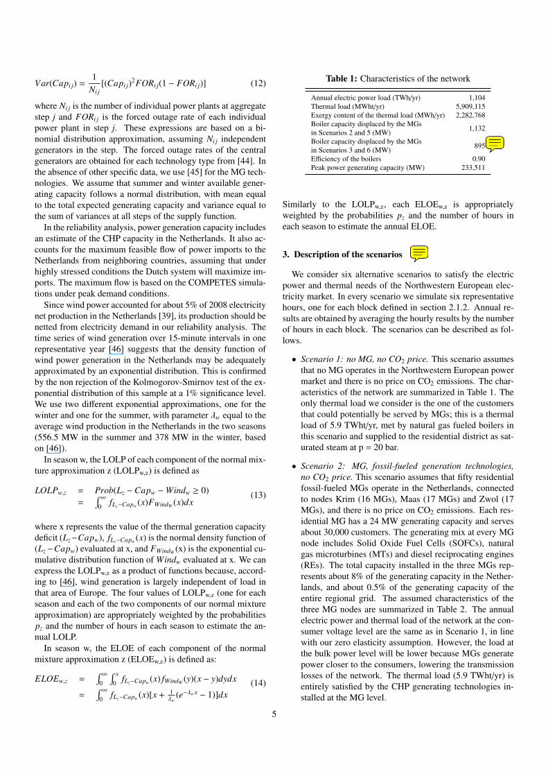
Var(Capi j) =1

Ni j[(Capi j)2FORi j(1 − FORi j)] (12)

where Ni j is the number of individual power plants at aggregatestep j and FORi j is the forced outage rate of each individualpower plant in step j. These expressions are based on a bi-nomial distribution approximation, assuming Ni j independentgenerators in the step. The forced outage rates of the centralgenerators are obtained for each technology type from [44]. Inthe absence of other specific data, we use [45] for the MG tech-nologies. We assume that summer and winter available gener-ating capacity follows a normal distribution, with mean equalto the total expected generating capacity and variance equal tothe sum of variances at all steps of the supply function.

In the reliability analysis, power generation capacity includesan estimate of the CHP capacity in the Netherlands. It also ac-counts for the maximum feasible flow of power imports to theNetherlands from neighboring countries, assuming that underhighly stressed conditions the Dutch system will maximize im-ports. The maximum flow is based on the COMPETES simula-tions under peak demand conditions.

Since wind power accounted for about 5% of 2008 electricitynet production in the Netherlands [39], its production should benetted from electricity demand in our reliability analysis. Thetime series of wind generation over 15-minute intervals in onerepresentative year [46] suggests that the density function ofwind power generation in the Netherlands may be adequatelyapproximated by an exponential distribution. This is confirmedby the non rejection of the Kolmogorov-Smirnov test of the ex-ponential distribution of this sample at a 1% significance level.We use two different exponential approximations, one for thewinter and one for the summer, with parameter λw equal to theaverage wind production in the Netherlands in the two seasons(556.5 MW in the summer and 378 MW in the winter, basedon [46]).

In season w, the LOLP of each component of the normal mix-ture approximation z (LOLPw,z) is defined as

LOLPw,z = Prob(Lz −Capw −Windw ≥ 0)=∫ ∞

0 fLz−Capw (x)FWindW (x)dx(13)

where x represents the value of the thermal generation capacitydeficit (Lz−Capw), fLz−Capw (x) is the normal density function of(Lz−Capw) evaluated at x, and FWindW (x) is the exponential cu-mulative distribution function of Windw evaluated at x. We canexpress the LOLPw,z as a product of functions because, accord-ing to [46], wind generation is largely independent of load inthat area of Europe. The four values of LOLPw,z (one for eachseason and each of the two components of our normal mixtureapproximation) are appropriately weighted by the probabilitiespz and the number of hours in each season to estimate the an-nual LOLP.

In season w, the ELOE of each component of the normalmixture approximation z (ELOEw,z) is defined as:

ELOEw,z =∫ ∞

0

∫ x0 fLz−Capw (x) fWindW (y)(x − y)dydx

=∫ ∞

0 fLz−Capw (x)[x + 1λw

(e−λw x − 1)]dx(14)

Table 1: Characteristics of the network

Annual electric power load (TWh/yr) 1,104Thermal load (MWht/yr) 5,909,115Exergy content of the thermal load (MWh/yr) 2,282,768Boiler capacity displaced by the MGs 1,132in Scenarios 2 and 5 (MW)Boiler capacity displaced by the MGs 895in Scenarios 3 and 6 (MW)Efficiency of the boilers 0.90Peak power generating capacity (MW) 233,511

Similarly to the LOLPw,z, each ELOEw,z is appropriatelyweighted by the probabilities pz and the number of hours ineach season to estimate the annual ELOE.

3. Description of the scenarios

We consider six alternative scenarios to satisfy the electricpower and thermal needs of the Northwestern European elec-tricity market. In every scenario we simulate six representativehours, one for each block defined in section 2.1.2. Annual re-sults are obtained by averaging the hourly results by the numberof hours in each block. The scenarios can be described as fol-lows.

• Scenario 1: no MG, no CO2 price. This scenario assumesthat no MG operates in the Northwestern European powermarket and there is no price on CO2 emissions. The char-acteristics of the network are summarized in Table 1. Theonly thermal load we consider is the one of the customersthat could potentially be served by MGs; this is a thermalload of 5.9 TWht/yr, met by natural gas fueled boilers inthis scenario and supplied to the residential district as sat-urated steam at p = 20 bar.

• Scenario 2: MG, fossil-fueled generation technologies,no CO2 price. This scenario assumes that fifty residentialfossil-fueled MGs operate in the Netherlands, connectedto nodes Krim (16 MGs), Maas (17 MGs) and Zwol (17MGs), and there is no price on CO2 emissions. Each res-idential MG has a 24 MW generating capacity and servesabout 30,000 customers. The generating mix at every MGnode includes Solid Oxide Fuel Cells (SOFCs), naturalgas microturbines (MTs) and diesel reciprocating engines(REs). The total capacity installed in the three MGs rep-resents about 8% of the generating capacity in the Nether-lands, and about 0.5% of the generating capacity of theentire regional grid. The assumed characteristics of thethree MG nodes are summarized in Table 2. The annualelectric power and thermal load of the network at the con-sumer voltage level are the same as in Scenario 1, in linewith our zero elasticity assumption. However, the load atthe bulk power level will be lower because MGs generatepower closer to the consumers, lowering the transmissionlosses of the network. The thermal load (5.9 TWht/yr) isentirely satisfied by the CHP generating technologies in-stalled at the MG level.

5

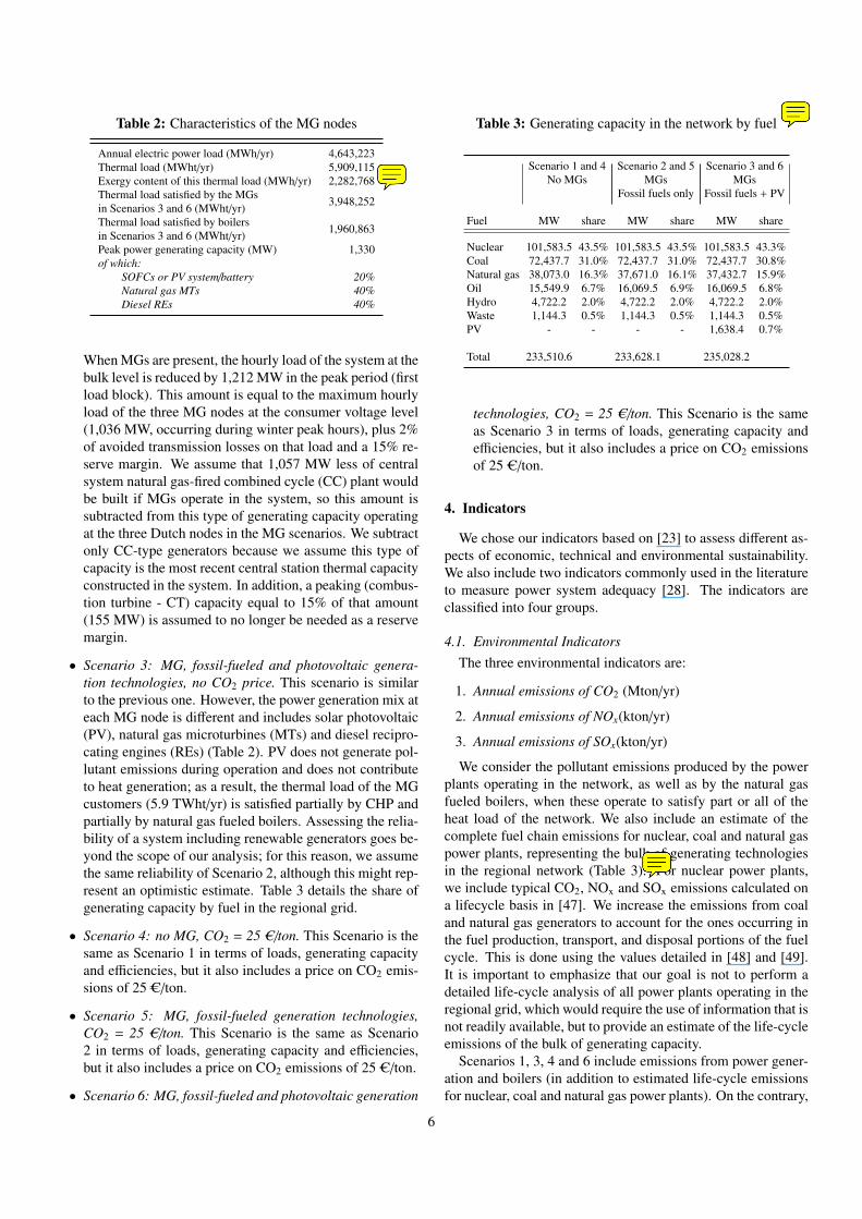
Table 2: Characteristics of the MG nodes

Annual electric power load (MWh/yr) 4,643,223Thermal load (MWht/yr) 5,909,115Exergy content of this thermal load (MWh/yr) 2,282,768Thermal load satisfied by the MGs 3,948,252in Scenarios 3 and 6 (MWht/yr)Thermal load satisfied by boilers 1,960,863in Scenarios 3 and 6 (MWht/yr)Peak power generating capacity (MW) 1,330of which:

SOFCs or PV system/battery 20%Natural gas MTs 40%Diesel REs 40%

When MGs are present, the hourly load of the system at thebulk level is reduced by 1,212 MW in the peak period (firstload block). This amount is equal to the maximum hourlyload of the three MG nodes at the consumer voltage level(1,036 MW, occurring during winter peak hours), plus 2%of avoided transmission losses on that load and a 15% re-serve margin. We assume that 1,057 MW less of centralsystem natural gas-fired combined cycle (CC) plant wouldbe built if MGs operate in the system, so this amount issubtracted from this type of generating capacity operatingat the three Dutch nodes in the MG scenarios. We subtractonly CC-type generators because we assume this type ofcapacity is the most recent central station thermal capacityconstructed in the system. In addition, a peaking (combus-tion turbine - CT) capacity equal to 15% of that amount(155 MW) is assumed to no longer be needed as a reservemargin.

• Scenario 3: MG, fossil-fueled and photovoltaic genera-tion technologies, no CO2 price. This scenario is similarto the previous one. However, the power generation mix ateach MG node is different and includes solar photovoltaic(PV), natural gas microturbines (MTs) and diesel recipro-cating engines (REs) (Table 2). PV does not generate pol-lutant emissions during operation and does not contributeto heat generation; as a result, the thermal load of the MGcustomers (5.9 TWht/yr) is satisfied partially by CHP andpartially by natural gas fueled boilers. Assessing the relia-bility of a system including renewable generators goes be-yond the scope of our analysis; for this reason, we assumethe same reliability of Scenario 2, although this might rep-resent an optimistic estimate. Table 3 details the share ofgenerating capacity by fuel in the regional grid.

• Scenario 4: no MG, CO2 = 25 C/ton. This Scenario is thesame as Scenario 1 in terms of loads, generating capacityand efficiencies, but it also includes a price on CO2 emis-sions of 25 C/ton.

• Scenario 5: MG, fossil-fueled generation technologies,CO2 = 25 C/ton. This Scenario is the same as Scenario2 in terms of loads, generating capacity and efficiencies,but it also includes a price on CO2 emissions of 25 C/ton.

• Scenario 6: MG, fossil-fueled and photovoltaic generation

Table 3: Generating capacity in the network by fuel

Scenario 1 and 4 Scenario 2 and 5 Scenario 3 and 6No MGs MGs MGs

Fossil fuels only Fossil fuels + PV

Fuel MW share MW share MW share

Nuclear 101,583.5 43.5% 101,583.5 43.5% 101,583.5 43.3%Coal 72,437.7 31.0% 72,437.7 31.0% 72,437.7 30.8%Natural gas 38,073.0 16.3% 37,671.0 16.1% 37,432.7 15.9%Oil 15,549.9 6.7% 16,069.5 6.9% 16,069.5 6.8%Hydro 4,722.2 2.0% 4,722.2 2.0% 4,722.2 2.0%Waste 1,144.3 0.5% 1,144.3 0.5% 1,144.3 0.5%PV - - - - 1,638.4 0.7%

Total 233,510.6 233,628.1 235,028.2

technologies, CO2 = 25 C/ton. This Scenario is the sameas Scenario 3 in terms of loads, generating capacity andefficiencies, but it also includes a price on CO2 emissionsof 25 C/ton.

4. Indicators

We chose our indicators based on [23] to assess different as-pects of economic, technical and environmental sustainability.We also include two indicators commonly used in the literatureto measure power system adequacy [28]. The indicators areclassified into four groups.

4.1. Environmental IndicatorsThe three environmental indicators are:

1. Annual emissions of CO2 (Mton/yr)

2. Annual emissions of NOx(kton/yr)

3. Annual emissions of SOx(kton/yr)

We consider the pollutant emissions produced by the powerplants operating in the network, as well as by the natural gasfueled boilers, when these operate to satisfy part or all of theheat load of the network. We also include an estimate of thecomplete fuel chain emissions for nuclear, coal and natural gaspower plants, representing the bulk of generating technologiesin the regional network (Table 3). For nuclear power plants,we include typical CO2, NOx and SOx emissions calculated ona lifecycle basis in [47]. We increase the emissions from coaland natural gas generators to account for the ones occurring inthe fuel production, transport, and disposal portions of the fuelcycle. This is done using the values detailed in [48] and [49].It is important to emphasize that our goal is not to perform adetailed life-cycle analysis of all power plants operating in theregional grid, which would require the use of information that isnot readily available, but to provide an estimate of the life-cycleemissions of the bulk of generating capacity.

Scenarios 1, 3, 4 and 6 include emissions from power gener-ation and boilers (in addition to estimated life-cycle emissionsfor nuclear, coal and natural gas power plants). On the contrary,

6

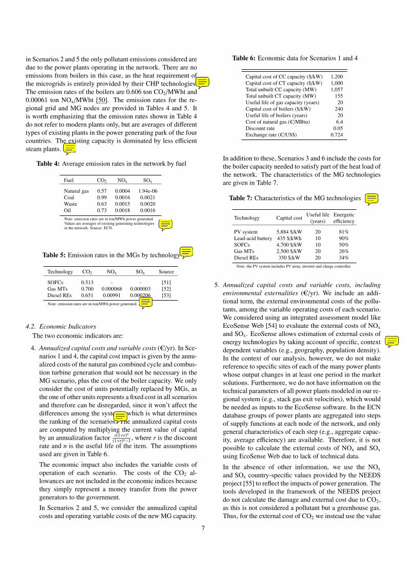
in Scenarios 2 and 5 the only pollutant emissions considered aredue to the power plants operating in the network. There are noemissions from boilers in this case, as the heat requirement ofthe microgrids is entirely provided by their CHP technologies.The emission rates of the boilers are 0.606 ton CO2/MWht and0.00061 ton NOx/MWht [50]. The emission rates for the re-gional grid and MG nodes are provided in Tables 4 and 5. Itis worth emphasizing that the emission rates shown in Table 4do not refer to modern plants only, but are averages of differenttypes of existing plants in the power generating park of the fourcountries. The existing capacity is dominated by less efficientsteam plants.

Table 4: Average emission rates in the network by fuel

Fuel CO2 NOx SOx

Natural gas 0.57 0.0004 1.94e-06Coal 0.99 0.0016 0.0021Waste 0.63 0.0015 0.0020Oil 0.73 0.0018 0.0016Note: emission rates are in ton/MWh power generated.Values are averages of existing generating technologiesin the network. Source: ECN.

Table 5: Emission rates in the MGs by technology

Technology CO2 NOx SOx Source

SOFCs 0.513 - - [51]Gas MTs 0.700 0.000068 0.000003 [52]Diesel REs 0.651 0.00991 0.000206 [53]Note: emission rates are in ton/MWh power generated.

4.2. Economic IndicatorsThe two economic indicators are:

4. Annualized capital costs and variable costs (C/yr). In Sce-narios 1 and 4, the capital cost impact is given by the annu-alized costs of the natural gas combined cycle and combus-tion turbine generation that would not be necessary in theMG scenario, plus the cost of the boiler capacity. We onlyconsider the cost of units potentially replaced by MGs, asthe one of other units represents a fixed cost in all scenariosand therefore can be disregarded, since it won’t affect thedifferences among the systems, which is what determinesthe ranking of the scenarios. The annualized capital costsare computed by multiplying the current value of capitalby an annualization factor r(1+r)n

(1+r)n−1 , where r is the discountrate and n is the useful life of the item. The assumptionsused are given in Table 6.

The economic impact also includes the variable costs ofoperation of each scenario. The costs of the CO2 al-lowances are not included in the economic indices becausethey simply represent a money transfer from the powergenerators to the government.

In Scenarios 2 and 5, we consider the annualized capitalcosts and operating variable costs of the new MG capacity.

Table 6: Economic data for Scenarios 1 and 4

Capital cost of CC capacity ($/kW) 1,200Capital cost of CT capacity ($/kW) 1,000Total unbuilt CC capacity (MW) 1,057Total unbuilt CT capacity (MW) 155Useful life of gas capacity (years) 20Capital cost of boilers ($/kW) 240Useful life of boilers (years) 20Cost of natural gas (C/MBtu) 6.4Discount rate 0.05Exchange rate (C/US$) 0.724

In addition to these, Scenarios 3 and 6 include the costs forthe boiler capacity needed to satisfy part of the heat load ofthe network. The characteristics of the MG technologiesare given in Table 7.

Table 7: Characteristics of the MG technologies

Technology Capital cost Useful life Energetic(years) efficiency

PV system 5,884 $/kW 20 81%Lead-acid battery 435 $/kWh 10 90%SOFCs 4,700 $/kW 10 50%Gas MTs 2,500 $/kW 20 26%Diesel REs 350 $/kW 20 34%

Note: the PV system includes PV array, inverter and charge controller.

5. Annualized capital costs and variable costs, includingenvironmental externalities (C/yr). We include an addi-tional term, the external environmental costs of the pollu-tants, among the variable operating costs of each scenario.We considered using an integrated assessment model likeEcoSense Web [54] to evaluate the external costs of NOxand SOx. EcoSense allows estimation of external costs ofenergy technologies by taking account of specific, contextdependent variables (e.g., geography, population density).In the context of our analysis, however, we do not makereference to specific sites of each of the many power plantswhose output changes in at least one period in the marketsolutions. Furthermore, we do not have information on thetechnical parameters of all power plants modeled in our re-gional system (e.g., stack gas exit velocities), which wouldbe needed as inputs to the EcoSense software. In the ECNdatabase groups of power plants are aggregated into stepsof supply functions at each node of the network, and onlygeneral characteristics of each step (e.g., aggregate capac-ity, average efficiency) are available. Therefore, it is notpossible to calculate the external costs of NOx and SOxusing EcoSense Web due to lack of technical data.

In the absence of other information, we use the NOxand SOx country-specific values provided by the NEEDSproject [55] to reflect the impacts of power generation. Thetools developed in the framework of the NEEDS projectdo not calculate the damage and external cost due to CO2,as this is not considered a pollutant but a greenhouse gas.Thus, for the external cost of CO2 we instead use the value

7

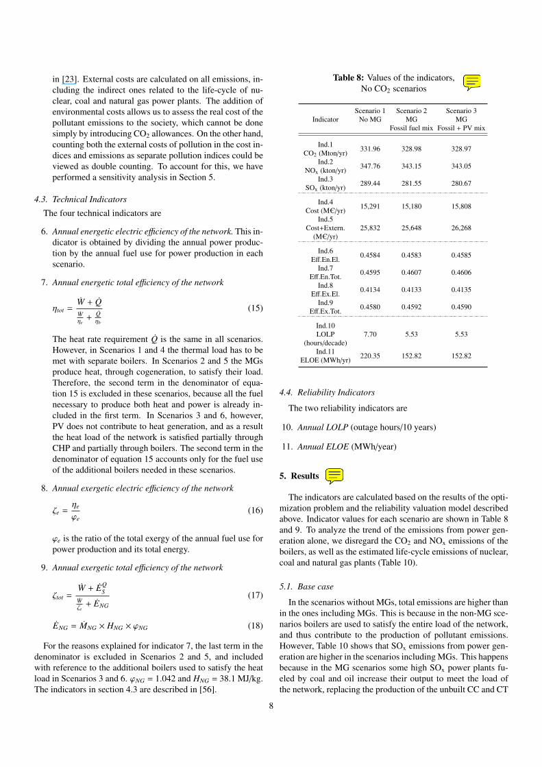
in [23]. External costs are calculated on all emissions, in-cluding the indirect ones related to the life-cycle of nu-clear, coal and natural gas power plants. The addition ofenvironmental costs allows us to assess the real cost of thepollutant emissions to the society, which cannot be donesimply by introducing CO2 allowances. On the other hand,counting both the external costs of pollution in the cost in-dices and emissions as separate pollution indices could beviewed as double counting. To account for this, we haveperformed a sensitivity analysis in Section 5.

4.3. Technical Indicators

The four technical indicators are

6. Annual energetic electric efficiency of the network. This in-dicator is obtained by dividing the annual power produc-tion by the annual fuel use for power production in eachscenario.

7. Annual energetic total efficiency of the network

ηtot =W + QWηe

+Qηb

(15)

The heat rate requirement Q is the same in all scenarios.However, in Scenarios 1 and 4 the thermal load has to bemet with separate boilers. In Scenarios 2 and 5 the MGsproduce heat, through cogeneration, to satisfy their load.Therefore, the second term in the denominator of equa-tion 15 is excluded in these scenarios, because all the fuelnecessary to produce both heat and power is already in-cluded in the first term. In Scenarios 3 and 6, however,PV does not contribute to heat generation, and as a resultthe heat load of the network is satisfied partially throughCHP and partially through boilers. The second term in thedenominator of equation 15 accounts only for the fuel useof the additional boilers needed in these scenarios.

8. Annual exergetic electric efficiency of the network

ζe =ηe

ϕe(16)

ϕe is the ratio of the total exergy of the annual fuel use forpower production and its total energy.

9. Annual exergetic total efficiency of the network

ζtot =W + EQ

SWζe

+ ENG

(17)

ENG = MNG × HNG × ϕNG (18)

For the reasons explained for indicator 7, the last term in thedenominator is excluded in Scenarios 2 and 5, and includedwith reference to the additional boilers used to satisfy the heatload in Scenarios 3 and 6. ϕNG = 1.042 and HNG = 38.1 MJ/kg.The indicators in section 4.3 are described in [56].

Table 8: Values of the indicators,No CO2 scenarios

IndicatorScenario 1 Scenario 2 Scenario 3

No MG MG MGFossil fuel mix Fossil + PV mix

Ind.1 331.96 328.98 328.97CO2 (Mton/yr)Ind.2 347.76 343.15 343.05NOx (kton/yr)Ind.3 289.44 281.55 280.67SOx (kton/yr)

Ind.4 15,291 15,180 15,808Cost (MC/yr)Ind.5

25,832 25,648 26,268Cost+Extern.(MC/yr)

Ind.6 0.4584 0.4583 0.4585Eff.En.El.Ind.7 0.4595 0.4607 0.4606Eff.En.Tot.Ind.8 0.4134 0.4133 0.4135Eff.Ex.El.Ind.9 0.4580 0.4592 0.4590Eff.Ex.Tot.

Ind.107.70 5.53 5.53LOLP

(hours/decade)Ind.11 220.35 152.82 152.82ELOE (MWh/yr)

4.4. Reliability Indicators

The two reliability indicators are

10. Annual LOLP (outage hours/10 years)

11. Annual ELOE (MWh/year)

5. Results

The indicators are calculated based on the results of the opti-mization problem and the reliability valuation model describedabove. Indicator values for each scenario are shown in Table 8and 9. To analyze the trend of the emissions from power gen-eration alone, we disregard the CO2 and NOx emissions of theboilers, as well as the estimated life-cycle emissions of nuclear,coal and natural gas plants (Table 10).

5.1. Base case

In the scenarios without MGs, total emissions are higher thanin the ones including MGs. This is because in the non-MG sce-narios boilers are used to satisfy the entire load of the network,and thus contribute to the production of pollutant emissions.However, Table 10 shows that SOx emissions from power gen-eration are higher in the scenarios including MGs. This happensbecause in the MG scenarios some high SOx power plants fu-eled by coal and oil increase their output to meet the load ofthe network, replacing the production of the unbuilt CC and CT

8

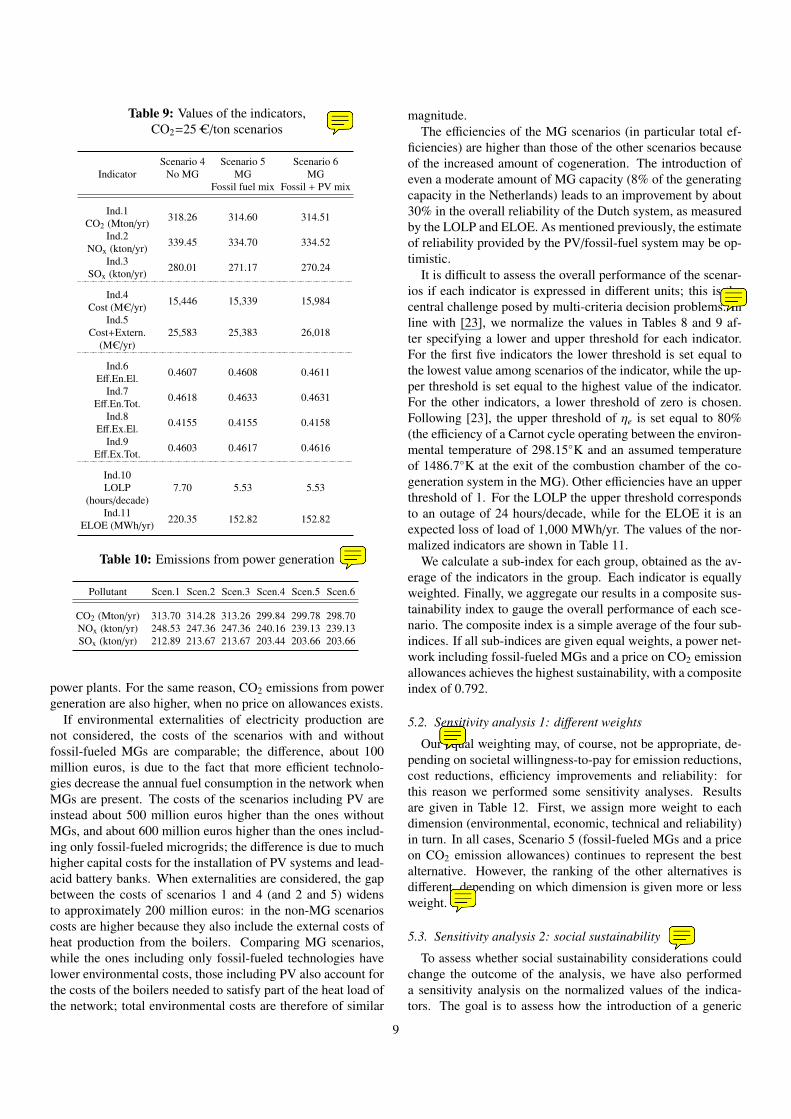
Table 9: Values of the indicators,CO2=25 C/ton scenarios

IndicatorScenario 4 Scenario 5 Scenario 6

No MG MG MGFossil fuel mix Fossil + PV mix

Ind.1 318.26 314.60 314.51CO2 (Mton/yr)Ind.2 339.45 334.70 334.52NOx (kton/yr)Ind.3 280.01 271.17 270.24SOx (kton/yr)

Ind.4 15,446 15,339 15,984Cost (MC/yr)Ind.5

25,583 25,383 26,018Cost+Extern.(MC/yr)

Ind.6 0.4607 0.4608 0.4611Eff.En.El.Ind.7 0.4618 0.4633 0.4631Eff.En.Tot.Ind.8 0.4155 0.4155 0.4158Eff.Ex.El.Ind.9 0.4603 0.4617 0.4616Eff.Ex.Tot.

Ind.107.70 5.53 5.53LOLP

(hours/decade)Ind.11 220.35 152.82 152.82ELOE (MWh/yr)

Table 10: Emissions from power generation

Pollutant Scen.1 Scen.2 Scen.3 Scen.4 Scen.5 Scen.6

CO2 (Mton/yr) 313.70 314.28 313.26 299.84 299.78 298.70NOx (kton/yr) 248.53 247.36 247.36 240.16 239.13 239.13SOx (kton/yr) 212.89 213.67 213.67 203.44 203.66 203.66

power plants. For the same reason, CO2 emissions from powergeneration are also higher, when no price on allowances exists.

If environmental externalities of electricity production arenot considered, the costs of the scenarios with and withoutfossil-fueled MGs are comparable; the difference, about 100million euros, is due to the fact that more efficient technolo-gies decrease the annual fuel consumption in the network whenMGs are present. The costs of the scenarios including PV areinstead about 500 million euros higher than the ones withoutMGs, and about 600 million euros higher than the ones includ-ing only fossil-fueled microgrids; the difference is due to muchhigher capital costs for the installation of PV systems and lead-acid battery banks. When externalities are considered, the gapbetween the costs of scenarios 1 and 4 (and 2 and 5) widensto approximately 200 million euros: in the non-MG scenarioscosts are higher because they also include the external costs ofheat production from the boilers. Comparing MG scenarios,while the ones including only fossil-fueled technologies havelower environmental costs, those including PV also account forthe costs of the boilers needed to satisfy part of the heat load ofthe network; total environmental costs are therefore of similar

magnitude.The efficiencies of the MG scenarios (in particular total ef-

ficiencies) are higher than those of the other scenarios becauseof the increased amount of cogeneration. The introduction ofeven a moderate amount of MG capacity (8% of the generatingcapacity in the Netherlands) leads to an improvement by about30% in the overall reliability of the Dutch system, as measuredby the LOLP and ELOE. As mentioned previously, the estimateof reliability provided by the PV/fossil-fuel system may be op-timistic.

It is difficult to assess the overall performance of the scenar-ios if each indicator is expressed in different units; this is thecentral challenge posed by multi-criteria decision problems. Inline with [23], we normalize the values in Tables 8 and 9 af-ter specifying a lower and upper threshold for each indicator.For the first five indicators the lower threshold is set equal tothe lowest value among scenarios of the indicator, while the up-per threshold is set equal to the highest value of the indicator.For the other indicators, a lower threshold of zero is chosen.Following [23], the upper threshold of ηe is set equal to 80%(the efficiency of a Carnot cycle operating between the environ-mental temperature of 298.15K and an assumed temperatureof 1486.7K at the exit of the combustion chamber of the co-generation system in the MG). Other efficiencies have an upperthreshold of 1. For the LOLP the upper threshold correspondsto an outage of 24 hours/decade, while for the ELOE it is anexpected loss of load of 1,000 MWh/yr. The values of the nor-malized indicators are shown in Table 11.

We calculate a sub-index for each group, obtained as the av-erage of the indicators in the group. Each indicator is equallyweighted. Finally, we aggregate our results in a composite sus-tainability index to gauge the overall performance of each sce-nario. The composite index is a simple average of the four sub-indices. If all sub-indices are given equal weights, a power net-work including fossil-fueled MGs and a price on CO2 emissionallowances achieves the highest sustainability, with a compositeindex of 0.792.

5.2. Sensitivity analysis 1: different weights

Our equal weighting may, of course, not be appropriate, de-pending on societal willingness-to-pay for emission reductions,cost reductions, efficiency improvements and reliability: forthis reason we performed some sensitivity analyses. Resultsare given in Table 12. First, we assign more weight to eachdimension (environmental, economic, technical and reliability)in turn. In all cases, Scenario 5 (fossil-fueled MGs and a priceon CO2 emission allowances) continues to represent the bestalternative. However, the ranking of the other alternatives isdifferent, depending on which dimension is given more or lessweight.

5.3. Sensitivity analysis 2: social sustainability

To assess whether social sustainability considerations couldchange the outcome of the analysis, we have also performeda sensitivity analysis on the normalized values of the indica-tors. The goal is to assess how the introduction of a generic

9

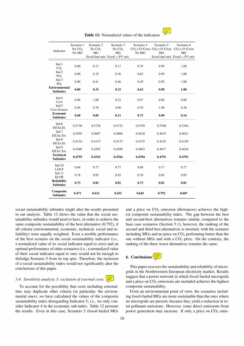
Table 11: Normalized values of the indicators

Indicator

Scenario 1 Scenario 2 Scenario 3 Scenario 4 Scenario 5 Scenario 6No CO2 No CO2 No CO2 CO2=25 C/ton CO2=25 C/ton CO2=25 C/tonNo MG MG MG No MG MG MG

Fossil fuel mix Fossil + PV mix Fossil fuel mix Fossil + PV mix

Ind.1 0.00 0.17 0.17 0.79 0.99 1.00CO2Ind.2 0.00 0.35 0.36 0.63 0.99 1.00NOxInd.3 0.00 0.41 0.46 0.49 0.95 1.00SOx

Environmental 0.00 0.31 0.33 0.63 0.98 1.00Subindex

Ind.4 0.86 1.00 0.22 0.67 0.80 0.00CostInd.5 0.49 0.70 0.00 0.78 1.00 0.28Cost+Extern.

Economic 0.68 0.85 0.11 0.72 0.90 0.14Subindex

Ind.6 0.5730 0.5728 0.5732 0.5759 0.5760 0.5764Eff.En.El.Ind.7 0.4595 0.4607 0.4606 0.4618 0.4633 0.4631Eff.En.Tot.Ind.8 0.4134 0.4133 0.4135 0.4155 0.4155 0.4158Eff.Ex.El.Ind.9 0.4580 0.4592 0.4590 0.4603 0.4617 0.4616Eff.Ex.Tot.

Technical 0.4759 0.4765 0.4766 0.4784 0.4791 0.4792Subindex

Ind.10 0.68 0.77 0.77 0.68 0.77 0.77LOLPInd.11 0.78 0.85 0.85 0.78 0.85 0.85ELOE

Reliability 0.73 0.81 0.81 0.73 0.81 0.81Subindex

Composite 0.471 0.611 0.431 0.641 0.792 0.607Subindex

social sustainability subindex might alter the results presentedin our analysis. Table 12 shows the value that the social sus-tainability subindex would need to have, in order to achieve thesame composite sustainability of the best alternative (0.792), ifall criteria (environmental, economic, technical, social and re-liability) were equally weighted. Even a terrible performanceof the best scenario on the social sustainability indicator (i.e.,a normalized value of its social indicator equal to zero) and anoptimal performance of other scenarios (i.e., a normalized valueof their social indicator equal to one) would not be enough todislodge Scenario 5 from its top spot. Therefore, the inclusionof a social sustainability index would not significantly alter theconclusions of this paper.

5.4. Sensitivity analysis 3: exclusion of external costs

To account for the possibility that costs including external-ities may duplicate other criteria (in particular, the environ-mental ones), we have calculated the values of the compositesustainability index disregarding Indicator 5; i.e., we only con-sider Indicator 4 in the economic sub-index. Table 12 presentsthe results. Even in this case, Scenario 5 (fossil-fueled MGs

and a price on CO2 emission allowances) achieves the high-est composite sustainability index. The gap between the bestand second-best alternatives remains similar, compared to thebase case scenarios (Section 5.1); however, the ranking of thesecond and third best alternatives is inverted, with the scenarioincluding MGs and no price on CO2 performing better than theone without MGs and with a CO2 price. On the contrary, theranking of the three worst alternatives remains the same.

6. Conclusions

This paper assesses the sustainability and reliability of micro-grids in the Northwestern European electricity market. Resultssuggest that a power network in which fossil-fueled microgridsand a price on CO2 emissions are included achieves the highestcomposite sustainability.

From an environmental point of view, the scenarios includ-ing fossil-fueled MGs are more sustainable than the ones whereno microgrids are present, because they yield a reduction in to-tal pollutant emissions. However, some direct emissions frompower generation may increase. If only a price on CO2 emis-

10

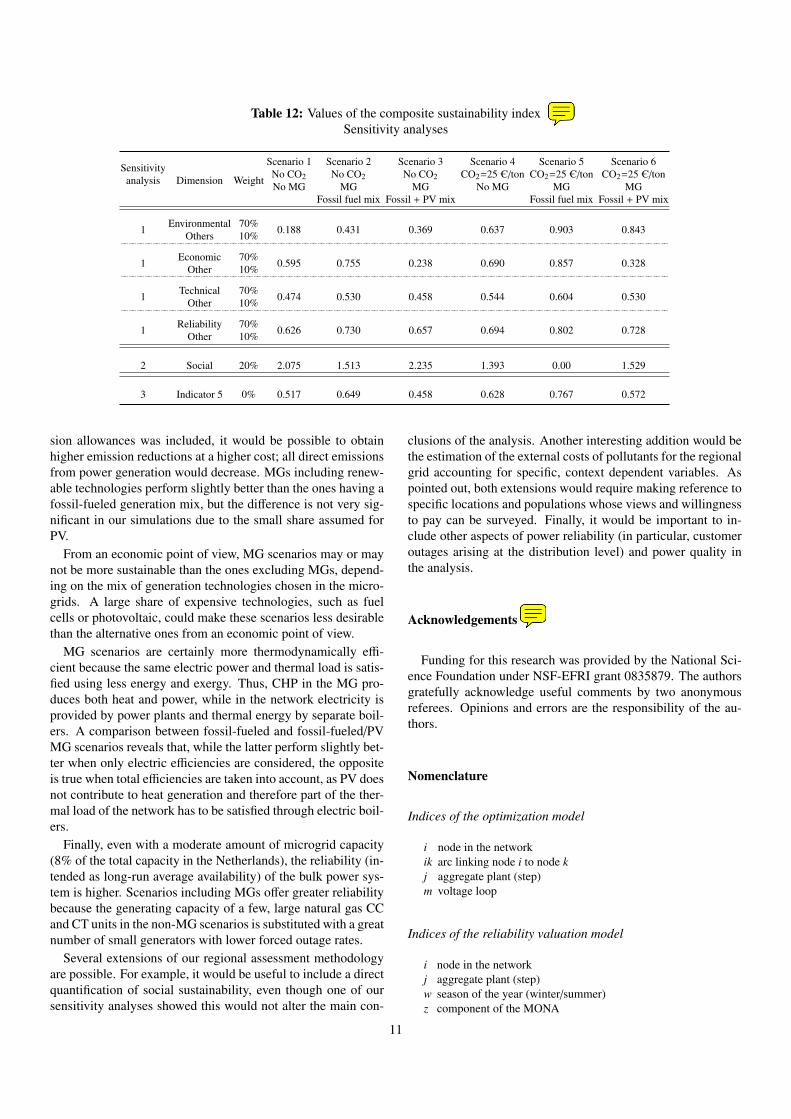
Table 12: Values of the composite sustainability indexSensitivity analyses

SensitivityDimension Weight

Scenario 1 Scenario 2 Scenario 3 Scenario 4 Scenario 5 Scenario 6

analysis No CO2 No CO2 No CO2 CO2=25 C/ton CO2=25 C/ton CO2=25 C/tonNo MG MG MG No MG MG MG

Fossil fuel mix Fossil + PV mix Fossil fuel mix Fossil + PV mix

1 Environmental 70% 0.188 0.431 0.369 0.637 0.903 0.843Others 10%

1 Economic 70% 0.595 0.755 0.238 0.690 0.857 0.328Other 10%

1 Technical 70% 0.474 0.530 0.458 0.544 0.604 0.530Other 10%

1 Reliability 70% 0.626 0.730 0.657 0.694 0.802 0.728Other 10%

2 Social 20% 2.075 1.513 2.235 1.393 0.00 1.529

3 Indicator 5 0% 0.517 0.649 0.458 0.628 0.767 0.572

sion allowances was included, it would be possible to obtainhigher emission reductions at a higher cost; all direct emissionsfrom power generation would decrease. MGs including renew-able technologies perform slightly better than the ones having afossil-fueled generation mix, but the difference is not very sig-nificant in our simulations due to the small share assumed forPV.

From an economic point of view, MG scenarios may or maynot be more sustainable than the ones excluding MGs, depend-ing on the mix of generation technologies chosen in the micro-grids. A large share of expensive technologies, such as fuelcells or photovoltaic, could make these scenarios less desirablethan the alternative ones from an economic point of view.

MG scenarios are certainly more thermodynamically effi-cient because the same electric power and thermal load is satis-fied using less energy and exergy. Thus, CHP in the MG pro-duces both heat and power, while in the network electricity isprovided by power plants and thermal energy by separate boil-ers. A comparison between fossil-fueled and fossil-fueled/PVMG scenarios reveals that, while the latter perform slightly bet-ter when only electric efficiencies are considered, the oppositeis true when total efficiencies are taken into account, as PV doesnot contribute to heat generation and therefore part of the ther-mal load of the network has to be satisfied through electric boil-ers.

Finally, even with a moderate amount of microgrid capacity(8% of the total capacity in the Netherlands), the reliability (in-tended as long-run average availability) of the bulk power sys-tem is higher. Scenarios including MGs offer greater reliabilitybecause the generating capacity of a few, large natural gas CCand CT units in the non-MG scenarios is substituted with a greatnumber of small generators with lower forced outage rates.

Several extensions of our regional assessment methodologyare possible. For example, it would be useful to include a directquantification of social sustainability, even though one of oursensitivity analyses showed this would not alter the main con-

clusions of the analysis. Another interesting addition would bethe estimation of the external costs of pollutants for the regionalgrid accounting for specific, context dependent variables. Aspointed out, both extensions would require making reference tospecific locations and populations whose views and willingnessto pay can be surveyed. Finally, it would be important to in-clude other aspects of power reliability (in particular, customeroutages arising at the distribution level) and power quality inthe analysis.

Acknowledgements

Funding for this research was provided by the National Sci-ence Foundation under NSF-EFRI grant 0835879. The authorsgratefully acknowledge useful comments by two anonymousreferees. Opinions and errors are the responsibility of the au-thors.

Nomenclature

Indices of the optimization model

i node in the networkik arc linking node i to node kj aggregate plant (step)m voltage loop

Indices of the reliability valuation model

i node in the networkj aggregate plant (step)w season of the year (winter/summer)z component of the MONA

11

Sets of the optimization model

I set of all nodesJ set of aggregate plants, differing in location,

ownership, fuel type and costJi set of aggregate plants at node iM set of Kirchhoff’s voltage loopsAi set of nodes adjacent to node iMm ordered set of links ik in voltage loop m

Parameters of the optimization model

CO2 CO2 price, C/tonLi power demand at node i, MWRik reactance on arc ikS ikm ± 1 depending on the orientation of arc ik in loop mLossik resistance loss coefficient on arc ik, 1/MWTik maximum transmission capacity on arc ik, MWMCi j marginal cost for generation at node i and step j, C/MWhEi j CO2 emission rate at node i and step j, ton/MWhCapi j maximum generation capacity at node i and step j, MW

Parameters of the reliability valuation model

Capi j maximum generation capacity at node i and step j, MWFORi j forced outage rate for individual plants at node i and step jNi j number of individual power plants at node i and step jLz power demand of the zth component of the MONA, MWCapw expected generating capacity in season w, MWWindw wind generation in season w, MWλw parameter of the exponential approximation

to wind distribution in season w, MW

Decision variables of the optimization model

fik export flow from node i to node k, MWgeni j generation at node i by aggregate plant j, MW

Decision variables of the reliability valuation model

µz mean of the zth component of the MONA, MWσ2

z variance of the zth component of the MONA, (MW)2

pz weight of the zth component of the MONA

Thermodynamic variables

W annual electric power load of the network, MWhQ annual heat load of the network, MWhtηb efficiency of the boilersηe annual energetic electric efficiency of the networkηtot annual energetic total efficiency of the networkζe annual exergetic electric efficiency of the networkζtot annual exergetic total efficiency of the networkϕe exergy to energy ratio of fuels used

for electricity generation in the networkEQ

S exergy content of the heat load, MWhENG exergy flow rate of natural gas, MJ/s*hourMNG mass flow rate of natural gas, kg/sHNG Lower Heating Value of natural gas, MJ/kgϕNG exergy to energy ratio of natural gas

References

[1] Market integration: coupling of the Euro-pean electricity markets [Internet]. Available from:http://www.tennettso.de/pages/tennettso en/Press/Information Material/PDF/100478 TEN Brochure marktkoppeling.pdf [accessed 2011 Jun24].

[2] CWE Market integration [Internet]. Available from:http://www.apxendex.com/index.php?id=186 [accessed 2011 Jun24].

[3] Report of the United Nations World Commission on Environmentand Development. Our common future [Internet]. Available from:http://www.un-documents.net/wced-ocf.htm [accessed 2011 Jun 24].

[4] Hobbs, B.F., Meier, P. Energy decisions and the environment: a guide tothe use of multicriteria methods. Kluwer Academic Publishers; 2000.

[5] Lebre LaRovere, E., Borghetti Soares, J., Basto Oliveira, L., Lauria, T.Sustainable expansion of electricity sector: sustainability indicators asan instrument to support decision making. Renewable and SustainableEnergy Reviews 2010; 14: 422-9.

[6] Giannantoni, C., Lazzaretto, A., Macor, A., Mirandola, A., Stoppato, A.,Tonon, S. et al. Multicriteria approach for the improvement of energysystems design. Energy 2005; 30(10): 1989-2016.

[7] Wang, J., Jing, Y., Zhang, C., Zhao, J. Review on multi-criteria decisionanalysis aid in sustainable energy decision making. Renewable and Sus-tainable Energy Reviews 2009; 13: 2263-2278.

[8] Maruyama, Y., Nishikido, M., Iida, T. The rise of community wind powerin Japan: enhanced acceptance through social innovation. Energy Policy2007; 35(5): 2761-2769.

[9] Gallego Carrera, D., Mack, A. Sustainability assessment of energy tech-nologies via social indicators: results of a survey among European energyexperts. Energy Policy 2010; 38: 1030-1039.

[10] Turvey, R., Anderson, D. Electricity economics: essays and case studies.Baltimore: Johns Hopkins University Press; 1977.

[11] ExternE: externalities of energy, Vol.1; 1995 [Internet]. Available from:http://www.externe.info/ [accessed 2011 Jun 24]

[12] Ottinger, R.L., Wooley, D., Robinson, N., Hodas, D., Babb, S. Environ-mental costs of electricity. New York: Oceana Publications; 1990.

[13] Hohmeyer, O., and Ottinger, R.L., editors. External environmental costsof electric power: analysis and internalization. Proceedings of a German-American Workshop; 1990, October 23-25; Ladenburg, FRG. New York:Springer-Verlag; 1991.

[14] Gil, H.A. Models for quantifying the economic benefits of distributedgeneration. IEEE Transactions on Power Systems 2008; 23(2): 327-35.

[15] Tsikalakis, A.G., Hatziargyriou, N.D. Environmental benefits of dis-tributed generation with and without emissions trading. Energy Policy2007; 35(6): 3395-409.

[16] Hadley, S.W., Van Dyke, J.W., Poore III, W.P., Stovall,T.K. Quantitative assessment of distributed energy resourcebenefits [Internet]. Oak Ridge National Laboratory, Engi-neering Science and Technology Division. Available from:http://www.ornl.gov/∼webworks/cppr/y2001/rpt/116227.pdf. [accessed2011 Jun 24].

[17] U.S. Department of Energy. The potential benefits of distributed gen-eration and rate-related issues that may impede their expansion [In-ternet]. Available from: http://www.ferc.gov/legal/fed-sta/exp-study.pdf.[accessed 2011 Jun 24]

[18] Alanne, K., Sari, A. Distributed energy generation and sustainable devel-opment. Renewable and sustainable energy reviews 2006; 10(6): 539-58.

[19] Firestone, R., Marnay, C., Maribu, K.M. The value of distributed gener-ation under different tariff structures. Berkeley (CA): Lawrence BerkeleyNational Laboratory, Environmental Energy Technologies Division; 2006May. Report No.: LBNL-60589. Contract No.: DEAC0205CH11231.Sponsored by the US Department of Energy.

[20] Siddiqui, A.S., Marnay, C., Edwards, J.L., Firestone, R., Ghosh, S.,Stadler, M. Effects of a carbon tax on microgrid combined heat and poweradoption. Berkeley (CA): Lawrence Berkeley National Laboratory, Envi-ronmental Energy Technologies Division; 2004 Oct. Report No.: LBNL-51771. Contract No.: DEAC0376SF00098. Sponsored by the US Depart-ment of Energy.

[21] Marnay, C., Lai, J., Stadler, M., Siddiqui, A. Added value of reliability toa microgrid: simulations of three California buildings. Berkeley (CA):Lawrence Berkeley National Laboratory, Environmental Energy Tech-

12

nologies Division; 2009 Apr. Report No.: LBNL-1853E. Contract No.:DEAC0205H11231. Sponsored by the US Department of Energy.

[22] Yi, H., Hau, J.L., Ukidwe, N.U., Bakshi, B.R. Hierarchical thermody-namic metrics for evaluating the environmental sustainability of industrialprocesses. Environmental Progress 2004; 23(4): 302-14.

[23] Frangopoulos, C.A., Keramioti, D.E. Multi-criteria evaluation of energysystems with sustainability considerations. Entropy 2010; 12(5): 1006-20.

[24] Frangopoulos, C.A., von Spakovksy, M.R. A global environomic ap-proach for energy systems analysis and optimization. Proceedings of theEnergy Systems and Ecology Conference; 1993 July 5-9; Cracow, Poland.p.123-44.

[25] von Spakovksy, M.R., Frangopoulos, C.A. The environomic analysis andoptimization of a gas turbine cycle with cogeneration. American Societyof Mechanical Engineers (ASME) 1994; 33: 15-26.

[26] Rosen, M. Energy and exergy-based comparison of coal-fired and nuclearsteam power plants. Exergy 2001; 1(3): 180-92.

[27] Zvolinschi, A., Kjelstrup, S., Bolland, O., van der Kooi, H.J. Exergy sus-tainability indicators as a tool in industrial ecology. Journal of IndustrialEcology 2007; 11(4): 85-98.

[28] Billinton, R., Allan, R.N. Reliability evaluation of power systems: con-cepts and techniques. New York: Plenum Press; 1996.

[29] Stoll, H.G. Least-cost electric utility planning. New York: John Wiley andSons; 1989.

[30] Wood, A.J., Wollenberg. B.F. Power generation operation and control.New York: John Wiley and Sons; 1996.

[31] Marnay, C. Microgrids and heterogenous power quality and reliability.Berkeley (CA): Lawrence Berkeley National Laboratory, Environmen-tal Energy Technologies Division; 2008 Jul. Report No.: LBNL-777E.Contract No.: DEAC0205CH11231. Sponsored by the US Department ofEnergy.

[32] Chowdhury, S., Chowdhury, S.P., Crossley, P. Microgrids and active dis-tribution networks. London: The Institution of Engineering and Technol-ogy; 2009.

[33] Council of European Energy Regulators. Fourth benchmarking re-port on quality of electricity supply 2008 [Internet]. Availablefrom: http://www.autorita.energia.it/allegati/pubblicazioni/C08-EQS-24-04 4th Benchmarking Report EQS 10-Dec-2008 re.pdf [accessed 2011Jun 24].

[34] Hobbs, B.F. Models for integrated resource planning by electric utilities.European Journal of Operational Research. 1995; 83(1): 1-20.

[35] Hobbs, B.F., Rijkers, F.A.M. Modeling strategic generator behavior withconjectured transmission price responses in a mixed transmission pricingsystem I: formulation, IEEE Transactions on Power Systems 2004; 19(2):707-17.

[36] Hobbs, B.F., Drayton, G., Bartholomew Fisher, E., Lise, W. Improvedtransmission representations in oligopolistic market models: quadraticlosses, phase shifters, and DC lines. IEEE Transactions on Power Sys-tems 2008; 23(3): 1018-29.

[37] Energy Research Centre of the Netherlands. COM-PETES input data [Internet]. Available from:http://www.ecn.nl/fileadmin/ecn/units/bs/COMPETES/cost-functions.xls[accessed 2011 Jun 24]

[38] International Energy Agency. Energy Prices and Taxes, energy end-useprices in national currencies, vol.2. Paris: International Energy Agency;2010.

[39] International Energy Agency. Electricity Information. Paris: InternationalEnergy Agency; 2010.

[40] European Network of Transmission System Operators for Electricity.Hourly load values for a specific country for a specific month [Internet].Available from: https://www.entsoe.eu/index.php?id=137 [accessed 2011Jun 24].

[41] International Energy Agency Energy Conservation in Build-ings and Community Systems, Annex 42 [Internet]. Stan-dard European Electrical Profiles. 2006. Available from:http://www.ecbcs.org/docs/Annex 42 European Electrical StandardProfiles Annex 42 September 2006.zip [accessed 2011 Jun 24].

[42] De Vries, L.J. Generation adequacy: helping the market do its job. Utili-ties Policy 2007; 15(1): 20-35.

[43] Gross, G., Garapic, N.V., McNutt, B. The mixture of normals approxima-tion technique for equivalent load duration curves. IEEE Transactions on

Power Systems 1988; 3(2): 368-74.[44] North American Electric Reliability Corporation. 2005-2009

Generating Availability Report [Internet]. Available from:http://www.nerc.com/page.php?cid=4|43|47 [accessed 2011 Jun 24].

[45] Energy and Environmental Analysis, Inc. Distributed gen-eration operational reliability and availability database.Executive summary report [Internet]. Available from:http://files.harc.edu/Sites/GulfCoastCHP/Publications/DistributedOperationalReliability.pdf [accessed 2011 Jun 24].

[46] Hargreaves, J.J., Hobbs, B.F. Optimal commitment and dispatch withuncertain wind generation using stochastic dynamic programming.Manuscript, Department of Geography & Environmental Engineering,Johns Hopkins University, 2010.

[47] AEA Technology. Environmental Product Declaration of Electricityfrom Torness Nuclear Power Station - a technical report [Internet].Available from: http://www.british-energy.com/documents/EPD Doc -Final.pdf [accessed 2011 Jun 28].

[48] Spath, P.L., Mann, M.K., Kerr, D.R. Life cycle assessment of coal firedpower production. Golden (CO): National Renewable Energy Laboratory;1999 June.

[49] Spath, P.L., Mann, M.K. Life cycle assessment of a natural gas combined-cycle power generation system. Golden (CO): National Renewable En-ergy Laboratory; 2000 September.

[50] Kaewboonsong, W., Kuprianov, V.I., Chovichien, N. Minimizing fuel andenvironmental costs for a variable-load power plant (co-)firing fuel oil andnatural gas. Part 1. Modeling of gaseous emissions from boiler units. Fuelprocessing technology 2006; 87: 10851094.

[51] Boudghene Stambouli, A., Traversa, E. Solid oxide fuel cells (SOFCs):a review of an environmentally clean and efficient source of energy. Re-newable and Sustainable Energy Reviews 2002; 6: 433-455.

[52] Greenhouse Gas Technology Center - Southern Research Institute. En-vironmental technology verification report. Combined heat and power ata commercial supermarket - Capstone 60 kW microturbine CHP system[Internet]. Available from: http://www.capstoneturbine.com/ docs/EPA-C60testreport.pdf [accessed 2011 Jun 27].

[53] Pipattanasomporn, M., Willingham, M. White paper on dis-tributed generation [Internet]. Available from: http://www.idc-online.com/technical references/pdfs/electrical engineering/Distributed%20generation.pdf [accessed 2011 Jun 27].

[54] EcoSenseWeb [Internet]. Available from: http://ecosenseweb.ier.uni-stuttgart.de/.

[55] NEEDS - New Energy Externalities Developments for Sustainabil-ity. Report on the procedure and data to generate averaged/aggregatedata, RS3a-D1.1; 2008 [Internet]. Available from: http://www.needs-project.org/2009/ [accessed 2011 Jun 24].

[56] Bejan, A., Tsatsaronis, G., Moran, M. Thermal design and optimization.New York: John Wiley and Sons; 1996.

13