Scholars' Mine Scholars' Mine

Doctoral Dissertations Student Theses and Dissertations

Spring 2018

Analysis of DC microgrids as stochastic hybrid systems Analysis of DC microgrids as stochastic hybrid systems

Jacob Andreas Mueller

Follow this and additional works at: https://scholarsmine.mst.edu/doctoral_dissertations

Part of the Electrical and Computer Engineering Commons

Department: Electrical and Computer Engineering Department: Electrical and Computer Engineering

Recommended Citation Recommended Citation Mueller, Jacob Andreas, "Analysis of DC microgrids as stochastic hybrid systems" (2018). Doctoral Dissertations. 2685. https://scholarsmine.mst.edu/doctoral_dissertations/2685

This thesis is brought to you by Scholars' Mine, a service of the Missouri S&T Library and Learning Resources. This work is protected by U. S. Copyright Law. Unauthorized use including reproduction for redistribution requires the permission of the copyright holder. For more information, please contact scholarsmine@mst.edu.

ANALYSIS OF DC MICROGRIDS AS STOCHASTIC HYBRID SYSTEMS

by

JACOB ANDREAS MUELLER

A DISSERTATION

Presented to the Graduate Faculty of the

MISSOURI UNIVERSITY OF SCIENCE AND TECHNOLOGY

In Partial Fulfillment of the Requirements for the Degree

DOCTOR OF PHILOSOPHY

in

ELECTRICAL ENGINEERING

2018

Approved by

Jonathan Kimball, AdvisorMariesa CrowMehdi FerdowsiBruce McMillinPourya Shamsi

Copyright 2018

JACOB ANDREAS MUELLER

All Rights Reserved

iii

PUBLICATION DISSERTATION OPTION

This dissertation consists of the following four articles which have been submitted

for publication, or will be submitted for publication as follows:

Paper I: Pages 15–53 have been accepted by IEEE Transactions on Power

Electronics.

Paper II: Pages 54–80 have been submitted to IEEE Transactions on Power

Electronics.

Paper III: Pages 81–115 have been accepted by IEEE Transactions on Smart

Grid.

Paper IV: Pages 116–148 are intended for submission to IEEE Transactions

on Control Systems Technology.

iv

ABSTRACT

Amodeling framework for dc microgrids and distribution systems based on the dual

active bridge (DAB) topology is presented. The purpose of this framework is to accurately

characterize dynamic behavior of multi-converter systems as a function of exogenous load

and source inputs. The base model is derived for deterministic inputs and then extended for

the case of stochastic load behavior. At the core of the modeling framework is a large-signal

DAB model that accurately describes the dynamics of both ac and dc state variables. This

model addresses limitations of existing DAB converter models, which are not suitable for

system-level analysis due to inaccuracy and poor upward scalability. The converter model

acts as a fundamental building block in a general procedure for constructing models of

multi-converter systems. System-level model construction is only possible due to structural

properties of the converter model that mitigate prohibitive increases in size and complexity.

To characterize the impact of randomness in practical loads, stochastic load descripti-

ons are included in the deterministic dynamic model. The combined behavior of distributed

loads is represented by a continuous-time stochastic process. Models that govern this load

process are generated using a new modeling procedure, which builds incrementally from

individual device-level representations. To merge the stochastic load process and deter-

ministic dynamic models, the microgrid is modeled as a stochastic hybrid system. The

stochastic hybrid model predicts the evolution of moments of dynamic state variables as a

function of load model parameters. Moments of dynamic states provide useful approxima-

tions of typical system operating conditions over time. Applications of the deterministic

models include system stability analysis and computationally efficient time-domain simu-

lation. The stochastic hybrid models provide a framework for performance assessment and

optimization.

v

ACKNOWLEDGMENTS

First and foremost I would like to thank my advisor, Dr. Jonathan Kimball, for

always knowing exactly what I needed to hear at exactly the moment I needed to hear it. He

has been a formational influence in my life, both personally and professionally. Without his

support none of this would be possible.

I am also grateful to the rest of my committee, all of whom have provided useful

insights and advice over the past six years.

Several of my peers at Missouri S&T have assisted me in building hardware expe-

riments and collecting results, but none more than Johann Voigtlander. His efforts have

significantly improved the quality of this work, and it has been a privilege to work with him.

This work was funded by the National Science Foundation, award 1406156, and by

a fellowship from the NASA-Missouri Space Grant Consortium.

Finally, I am grateful to my family for their patience, encouragement, and under-

standing. I am especially thankful for Kelsey and Finn, who stayed by my side for every

step of this journey. When I was lost, when I was tired, and when I was trapped by my own

doubts, their companionship kept me moving forward. They turned every insurmountable

obstacle into just another adventure.

vi

TABLE OF CONTENTS

Page

PUBLICATION DISSERTATION OPTION . . . . . . . . . . . . . . . . . . . . . . . . . . . . . . . . . . . . . . iii

ABSTRACT . . . . . . . . . . . . . . . . . . . . . . . . . . . . . . . . . . . . . . . . . . . . . . . . . . . . . . . . . . . . . . . . . . iv

ACKNOWLEDGMENTS . . . . . . . . . . . . . . . . . . . . . . . . . . . . . . . . . . . . . . . . . . . . . . . . . . . . . . v

LIST OF ILLUSTRATIONS . . . . . . . . . . . . . . . . . . . . . . . . . . . . . . . . . . . . . . . . . . . . . . . . . . . . xi

LIST OF TABLES . . . . . . . . . . . . . . . . . . . . . . . . . . . . . . . . . . . . . . . . . . . . . . . . . . . . . . . . . . . . . xiv

SECTION

1. INTRODUCTION. . . . . . . . . . . . . . . . . . . . . . . . . . . . . . . . . . . . . . . . . . . . . . . . . . . . . . . . . . 1

1.1. OVERVIEW .. . . . . . . . . . . . . . . . . . . . . . . . . . . . . . . . . . . . . . . . . . . . . . . . . . . . . . . . . . . . . . . . . . . . . 1

1.2. DETERMINISTIC MICROGRID MODELS. . . . . . . . . . . . . . . . . . . . . . . . . . . . . . . . . . . 4

1.2.1. Dual Active Bridge Converters . . . . . . . . . . . . . . . . . . . . . . . . . . . . . . . . . . . . . . . . . 4

1.2.2. DAB Models . . . . . . . . . . . . . . . . . . . . . . . . . . . . . . . . . . . . . . . . . . . . . . . . . . . . . . . . . . . . . 5

1.2.3. Development of a System-Level Model . . . . . . . . . . . . . . . . . . . . . . . . . . . . . . . . 8

1.3. INFLUENCE OF PRACTICAL LOADS . . . . . . . . . . . . . . . . . . . . . . . . . . . . . . . . . . . . . . . 10

1.3.1. Load Modeling . . . . . . . . . . . . . . . . . . . . . . . . . . . . . . . . . . . . . . . . . . . . . . . . . . . . . . . . . . 11

1.3.2. Stochastic Hybrid System . . . . . . . . . . . . . . . . . . . . . . . . . . . . . . . . . . . . . . . . . . . . . . . 13

PAPER

I. AN IMPROVED GENERALIZED AVERAGE MODEL OF DC-DC DUALACTIVE BRIDGE CONVERTERS . . . . . . . . . . . . . . . . . . . . . . . . . . . . . . . . . . . . . . . . . . 15

ABSTRACT . . . . . . . . . . . . . . . . . . . . . . . . . . . . . . . . . . . . . . . . . . . . . . . . . . . . . . . . . . . . . . . . . . . . . . . . . . . . 15

vii

1. INTRODUCTION . . . . . . . . . . . . . . . . . . . . . . . . . . . . . . . . . . . . . . . . . . . . . . . . . . . . . . . . . . . . . . . 16

2. BACKGROUND . . . . . . . . . . . . . . . . . . . . . . . . . . . . . . . . . . . . . . . . . . . . . . . . . . . . . . . . . . . . . . . . . 19

2.1. Original DAB Model . . . . . . . . . . . . . . . . . . . . . . . . . . . . . . . . . . . . . . . . . . . . . . . . . . . . 19

2.2. Origin of Steady-State Error . . . . . . . . . . . . . . . . . . . . . . . . . . . . . . . . . . . . . . . . . . . . 20

3. IMPROVED MODEL. . . . . . . . . . . . . . . . . . . . . . . . . . . . . . . . . . . . . . . . . . . . . . . . . . . . . . . . . . . . 22

3.1. Modulation Scheme Extension . . . . . . . . . . . . . . . . . . . . . . . . . . . . . . . . . . . . . . . . . 23

3.2. Correction of Large-Signal Error . . . . . . . . . . . . . . . . . . . . . . . . . . . . . . . . . . . . . . . 25

3.3. Model Organization . . . . . . . . . . . . . . . . . . . . . . . . . . . . . . . . . . . . . . . . . . . . . . . . . . . . . 29

3.4. Discussion . . . . . . . . . . . . . . . . . . . . . . . . . . . . . . . . . . . . . . . . . . . . . . . . . . . . . . . . . . . . . . . 30

4. PARTIAL DERIVATIVES AND SMALL-SIGNAL MODELS . . . . . . . . . . . . . . 32

4.1. Open-Loop System . . . . . . . . . . . . . . . . . . . . . . . . . . . . . . . . . . . . . . . . . . . . . . . . . . . . . . 32

4.2. Closed-Loop System . . . . . . . . . . . . . . . . . . . . . . . . . . . . . . . . . . . . . . . . . . . . . . . . . . . . 34

4.3. Switching Signal Derivatives . . . . . . . . . . . . . . . . . . . . . . . . . . . . . . . . . . . . . . . . . . . 34

4.4. Small-Signal Models . . . . . . . . . . . . . . . . . . . . . . . . . . . . . . . . . . . . . . . . . . . . . . . . . . . . 36

5. CONSIDERATIONS FOR SINGLE PHASE SHIFT MODULATION. . . . . . . 37

5.1. Model Simplifications . . . . . . . . . . . . . . . . . . . . . . . . . . . . . . . . . . . . . . . . . . . . . . . . . . . 37

5.2. Lossless Case . . . . . . . . . . . . . . . . . . . . . . . . . . . . . . . . . . . . . . . . . . . . . . . . . . . . . . . . . . . . 37

5.3. Lossy Case . . . . . . . . . . . . . . . . . . . . . . . . . . . . . . . . . . . . . . . . . . . . . . . . . . . . . . . . . . . . . . . 38

6. VERIFICATION . . . . . . . . . . . . . . . . . . . . . . . . . . . . . . . . . . . . . . . . . . . . . . . . . . . . . . . . . . . . . . . . . 41

6.1. Steady-State Accuracy . . . . . . . . . . . . . . . . . . . . . . . . . . . . . . . . . . . . . . . . . . . . . . . . . . 41

6.2. Dynamic Accuracy . . . . . . . . . . . . . . . . . . . . . . . . . . . . . . . . . . . . . . . . . . . . . . . . . . . . . . 44

7. CONCLUSION . . . . . . . . . . . . . . . . . . . . . . . . . . . . . . . . . . . . . . . . . . . . . . . . . . . . . . . . . . . . . . . . . . 47

APPENDIX . . . . . . . . . . . . . . . . . . . . . . . . . . . . . . . . . . . . . . . . . . . . . . . . . . . . . . . . . . . . . . . . . . . . . . . . . . . . . 49

REFERENCES . . . . . . . . . . . . . . . . . . . . . . . . . . . . . . . . . . . . . . . . . . . . . . . . . . . . . . . . . . . . . . . . . . . . . . . . . 50

II. MODELING DUAL ACTIVE BRIDGE CONVERTERS IN DC DISTRIBU-TION SYSTEMS. . . . . . . . . . . . . . . . . . . . . . . . . . . . . . . . . . . . . . . . . . . . . . . . . . . . . . . . . . . 54

viii

ABSTRACT . . . . . . . . . . . . . . . . . . . . . . . . . . . . . . . . . . . . . . . . . . . . . . . . . . . . . . . . . . . . . . . . . . . . . . . . . . . . 54

1. INTRODUCTION . . . . . . . . . . . . . . . . . . . . . . . . . . . . . . . . . . . . . . . . . . . . . . . . . . . . . . . . . . . . . . . 55

2. BASE DAB CONVERTER MODEL . . . . . . . . . . . . . . . . . . . . . . . . . . . . . . . . . . . . . . . . . . . 57

2.1. GAM Framework . . . . . . . . . . . . . . . . . . . . . . . . . . . . . . . . . . . . . . . . . . . . . . . . . . . . . . . . 57

2.2. Single Converter Model . . . . . . . . . . . . . . . . . . . . . . . . . . . . . . . . . . . . . . . . . . . . . . . . . 58

2.3. Decoupling Effect and Selective Averaging . . . . . . . . . . . . . . . . . . . . . . . . . . . . 61

3. SYSTEM-LEVEL MODEL . . . . . . . . . . . . . . . . . . . . . . . . . . . . . . . . . . . . . . . . . . . . . . . . . . . . . 63

3.1. Model Combination . . . . . . . . . . . . . . . . . . . . . . . . . . . . . . . . . . . . . . . . . . . . . . . . . . . . . 63

3.2. System-Level Organization . . . . . . . . . . . . . . . . . . . . . . . . . . . . . . . . . . . . . . . . . . . . . 64

4. TRANSFORMER CURRENT RECONSTRUCTION . . . . . . . . . . . . . . . . . . . . . . . . . 69

5. VERIFICATION . . . . . . . . . . . . . . . . . . . . . . . . . . . . . . . . . . . . . . . . . . . . . . . . . . . . . . . . . . . . . . . . . 71

5.1. 7-Bus Simulation . . . . . . . . . . . . . . . . . . . . . . . . . . . . . . . . . . . . . . . . . . . . . . . . . . . . . . . . 72

5.2. Hardware Experiment . . . . . . . . . . . . . . . . . . . . . . . . . . . . . . . . . . . . . . . . . . . . . . . . . . . 73

6. CONCLUSION . . . . . . . . . . . . . . . . . . . . . . . . . . . . . . . . . . . . . . . . . . . . . . . . . . . . . . . . . . . . . . . . . . 76

REFERENCES . . . . . . . . . . . . . . . . . . . . . . . . . . . . . . . . . . . . . . . . . . . . . . . . . . . . . . . . . . . . . . . . . . . . . . . . . 78

III. ACCURATE ENERGY USE ESTIMATION FOR NONINTRUSIVE LOADMONITORING IN SYSTEMS OF KNOWN DEVICES . . . . . . . . . . . . . . . . . . . . . . . . 81

ABSTRACT . . . . . . . . . . . . . . . . . . . . . . . . . . . . . . . . . . . . . . . . . . . . . . . . . . . . . . . . . . . . . . . . . . . . . . . . . . . . 81

1. INTRODUCTION . . . . . . . . . . . . . . . . . . . . . . . . . . . . . . . . . . . . . . . . . . . . . . . . . . . . . . . . . . . . . . . 82

2. BACKGROUND . . . . . . . . . . . . . . . . . . . . . . . . . . . . . . . . . . . . . . . . . . . . . . . . . . . . . . . . . . . . . . . . . 84

2.1. Device Modeling . . . . . . . . . . . . . . . . . . . . . . . . . . . . . . . . . . . . . . . . . . . . . . . . . . . . . . . . 85

2.2. Model Training . . . . . . . . . . . . . . . . . . . . . . . . . . . . . . . . . . . . . . . . . . . . . . . . . . . . . . . . . . 88

2.3. Scalability and State Inference . . . . . . . . . . . . . . . . . . . . . . . . . . . . . . . . . . . . . . . . . . 89

3. METHODOLOGY. . . . . . . . . . . . . . . . . . . . . . . . . . . . . . . . . . . . . . . . . . . . . . . . . . . . . . . . . . . . . . . 93

3.1. Model Combination . . . . . . . . . . . . . . . . . . . . . . . . . . . . . . . . . . . . . . . . . . . . . . . . . . . . . 93

3.1.1. Transition Matrix . . . . . . . . . . . . . . . . . . . . . . . . . . . . . . . . . . . . . . . . . . . . . 93

ix

3.1.2. Observation Matrix. . . . . . . . . . . . . . . . . . . . . . . . . . . . . . . . . . . . . . . . . . . 95

3.2. State Disaggregation . . . . . . . . . . . . . . . . . . . . . . . . . . . . . . . . . . . . . . . . . . . . . . . . . . . . 99

3.3. Prediction of Energy Use . . . . . . . . . . . . . . . . . . . . . . . . . . . . . . . . . . . . . . . . . . . . . . . 100

3.4. Discussion . . . . . . . . . . . . . . . . . . . . . . . . . . . . . . . . . . . . . . . . . . . . . . . . . . . . . . . . . . . . . . . 103

4. EXPERIMENTAL VERIFICATION . . . . . . . . . . . . . . . . . . . . . . . . . . . . . . . . . . . . . . . . . . . 105

4.1. Performance Assessments. . . . . . . . . . . . . . . . . . . . . . . . . . . . . . . . . . . . . . . . . . . . . . . 106

4.2. Results . . . . . . . . . . . . . . . . . . . . . . . . . . . . . . . . . . . . . . . . . . . . . . . . . . . . . . . . . . . . . . . . . . . 107

5. CONCLUSION . . . . . . . . . . . . . . . . . . . . . . . . . . . . . . . . . . . . . . . . . . . . . . . . . . . . . . . . . . . . . . . . . . 111

REFERENCES . . . . . . . . . . . . . . . . . . . . . . . . . . . . . . . . . . . . . . . . . . . . . . . . . . . . . . . . . . . . . . . . . . . . . . . . . 112

IV. MODELING AND ANALYSIS OF DC MICROGRIDS AS STOCHASTICHYBRID SYSTEMS . . . . . . . . . . . . . . . . . . . . . . . . . . . . . . . . . . . . . . . . . . . . . . . . . . . . . . . 116

ABSTRACT . . . . . . . . . . . . . . . . . . . . . . . . . . . . . . . . . . . . . . . . . . . . . . . . . . . . . . . . . . . . . . . . . . . . . . . . . . . . 116

1. INTRODUCTION . . . . . . . . . . . . . . . . . . . . . . . . . . . . . . . . . . . . . . . . . . . . . . . . . . . . . . . . . . . . . . . 117

2. BACKGROUND . . . . . . . . . . . . . . . . . . . . . . . . . . . . . . . . . . . . . . . . . . . . . . . . . . . . . . . . . . . . . . . . . 119

3. DYNAMIC MODEL AND LOAD PROCESS . . . . . . . . . . . . . . . . . . . . . . . . . . . . . . . . . 122

4. SHS MICROGRID MODEL . . . . . . . . . . . . . . . . . . . . . . . . . . . . . . . . . . . . . . . . . . . . . . . . . . . . 125

4.1. SHS Model. . . . . . . . . . . . . . . . . . . . . . . . . . . . . . . . . . . . . . . . . . . . . . . . . . . . . . . . . . . . . . . 125

4.2. Elimination of Redundant Second Order Moments . . . . . . . . . . . . . . . . . . . . 129

4.3. Final Model and Steady-State Moments. . . . . . . . . . . . . . . . . . . . . . . . . . . . . . . . 133

5. ANALYSIS OF ZVS PERFORMANCE . . . . . . . . . . . . . . . . . . . . . . . . . . . . . . . . . . . . . . . . 135

5.1. ZVS Conditions. . . . . . . . . . . . . . . . . . . . . . . . . . . . . . . . . . . . . . . . . . . . . . . . . . . . . . . . . . 135

5.2. ZVS Moments and Bounds . . . . . . . . . . . . . . . . . . . . . . . . . . . . . . . . . . . . . . . . . . . . . 135

6. VERIFICATION . . . . . . . . . . . . . . . . . . . . . . . . . . . . . . . . . . . . . . . . . . . . . . . . . . . . . . . . . . . . . . . . . 138

6.1. Moment Dynamics of X(t) . . . . . . . . . . . . . . . . . . . . . . . . . . . . . . . . . . . . . . . . . . . . . . 140

6.2. Moment Dynamics of ZVS Conditions. . . . . . . . . . . . . . . . . . . . . . . . . . . . . . . . . 140

6.3. Improving ZVS Performance . . . . . . . . . . . . . . . . . . . . . . . . . . . . . . . . . . . . . . . . . . . 142

x

7. CONCLUSION . . . . . . . . . . . . . . . . . . . . . . . . . . . . . . . . . . . . . . . . . . . . . . . . . . . . . . . . . . . . . . . . . . 145

REFERENCES . . . . . . . . . . . . . . . . . . . . . . . . . . . . . . . . . . . . . . . . . . . . . . . . . . . . . . . . . . . . . . . . . . . . . . . . . 146

SECTION

2. CONCLUSION . . . . . . . . . . . . . . . . . . . . . . . . . . . . . . . . . . . . . . . . . . . . . . . . . . . . . . . . . . . . 149

REFERENCES . . . . . . . . . . . . . . . . . . . . . . . . . . . . . . . . . . . . . . . . . . . . . . . . . . . . . . . . . . . . . . . . 151

VITA . . . . . . . . . . . . . . . . . . . . . . . . . . . . . . . . . . . . . . . . . . . . . . . . . . . . . . . . . . . . . . . . . . . . . . . . . 164

xi

LIST OF ILLUSTRATIONS

Figure Page

1.1. Modeling scope for each paper.. . . . . . . . . . . . . . . . . . . . . . . . . . . . . . . . . . . . . . . . . . . . . . . . . . . . . . 4

PAPER I

1. Dual active bridge topology. . . . . . . . . . . . . . . . . . . . . . . . . . . . . . . . . . . . . . . . . . . . . . . . . . . . . . . . . . 21

2. Triple phase shift modulation scheme. . . . . . . . . . . . . . . . . . . . . . . . . . . . . . . . . . . . . . . . . . . . . . . 25

3. Prototype DAB converter.. . . . . . . . . . . . . . . . . . . . . . . . . . . . . . . . . . . . . . . . . . . . . . . . . . . . . . . . . . . . 42

4. Comparison of relationships between phase shift inputs and output voltage fortriple phase shift modulation. . . . . . . . . . . . . . . . . . . . . . . . . . . . . . . . . . . . . . . . . . . . . . . . . . . . . . . . . 43

5. Comparison of relationships between phase shift inputs and output voltage fordual phase shift modulation. . . . . . . . . . . . . . . . . . . . . . . . . . . . . . . . . . . . . . . . . . . . . . . . . . . . . . . . . . 43

6. Comparison of relationships between phase shift and output voltage for singlephase shift modulation. . . . . . . . . . . . . . . . . . . . . . . . . . . . . . . . . . . . . . . . . . . . . . . . . . . . . . . . . . . . . . . 43

7. Open-loop voltage transient response for step changes in control inputs fortriple phase shift modulation. . . . . . . . . . . . . . . . . . . . . . . . . . . . . . . . . . . . . . . . . . . . . . . . . . . . . . . . . 45

8. Open-loop voltage transient response for step changes in control inputs fordual phase shift modulation. . . . . . . . . . . . . . . . . . . . . . . . . . . . . . . . . . . . . . . . . . . . . . . . . . . . . . . . . 45

9. Open-loop voltage transient response for step changes in phase shift.. . . . . . . . . . . . . 46

10. Magnitude responses of control-to-output transfer functions. . . . . . . . . . . . . . . . . . . . . . 48

11. Closed-loop transient response for step change reference voltage.. . . . . . . . . . . . . . . . . 49

PAPER II

1. Voltage-controlled DAB converter and control system . . . . . . . . . . . . . . . . . . . . . . . . . . . . . 59

2. Five-converter example system. . . . . . . . . . . . . . . . . . . . . . . . . . . . . . . . . . . . . . . . . . . . . . . . . . . . . . 64

3. Load disturbance responses of selected system bus voltages. . . . . . . . . . . . . . . . . . . . . . . 74

4. Load disturbance responses of selected system line currents. . . . . . . . . . . . . . . . . . . . . . . 74

5. Comparison of converter 2 transformer currents from simulation, results calcu-lated using the proposed harmonic reconstruction method, and first harmonicapproximations from the base model. . . . . . . . . . . . . . . . . . . . . . . . . . . . . . . . . . . . . . . . . . . . . . . . 75

xii

6. Hardware testbed. . . . . . . . . . . . . . . . . . . . . . . . . . . . . . . . . . . . . . . . . . . . . . . . . . . . . . . . . . . . . . . . . . . . . 75

7. Comparison of hardware measurements and model predictions for bus voltageand line current states. . . . . . . . . . . . . . . . . . . . . . . . . . . . . . . . . . . . . . . . . . . . . . . . . . . . . . . . . . . . . . . . 76

8. Comparison of hardware measurements and model predictions for controllerintegrator states. . . . . . . . . . . . . . . . . . . . . . . . . . . . . . . . . . . . . . . . . . . . . . . . . . . . . . . . . . . . . . . . . . . . . . . 77

9. Comparison of converter 2 transformer currents from hardware measurementsand harmonic reconstruction. . . . . . . . . . . . . . . . . . . . . . . . . . . . . . . . . . . . . . . . . . . . . . . . . . . . . . . . . 77

PAPER III

1. Example of a hidden Markov model structure for a 3-state device. . . . . . . . . . . . . . . . . 86

2. Normalized histogram of observations from dryer, stove, and dishwasher de-vices over a period of 10 days. . . . . . . . . . . . . . . . . . . . . . . . . . . . . . . . . . . . . . . . . . . . . . . . . . . . . . . . 88

3. Directed graph representation of two example devices and their potential tran-sitions. . . . . . . . . . . . . . . . . . . . . . . . . . . . . . . . . . . . . . . . . . . . . . . . . . . . . . . . . . . . . . . . . . . . . . . . . . . . . . . . . 94

4. Directed graph representation of a two-device example system. . . . . . . . . . . . . . . . . . . . 95

5. Average estimation accuracy by length of observation sequence. . . . . . . . . . . . . . . . . . 107

6. State RMSE of predicted observations plotted against the standard deviationof their observation distribution. . . . . . . . . . . . . . . . . . . . . . . . . . . . . . . . . . . . . . . . . . . . . . . . . . . . . 108

7. Difference in state RMSE values for predictions of the proposed method andexpectation method. . . . . . . . . . . . . . . . . . . . . . . . . . . . . . . . . . . . . . . . . . . . . . . . . . . . . . . . . . . . . . . . . . . 110

8. Comparison of ground truth and predicted observations for the refrigerator. . . . . . 110

9. Comparison of ground truth and predicted observations for the LCD TV. . . . . . . . . 111

PAPER IV

1. Single DAB converter and two-mode load process. . . . . . . . . . . . . . . . . . . . . . . . . . . . . . . . . 123

2. Example of transformation matrix Wm for a 3-state system. . . . . . . . . . . . . . . . . . . . . . . . 128

3. Decomposition of Wm into Ws, Wc, and I(N2) for a 3-state system. . . . . . . . . . . . . . . . 129

4. Specification of R from indicies of unique moments. . . . . . . . . . . . . . . . . . . . . . . . . . . . . . . 131

5. Sparsity pattern of final transformation matrices used to calculate reducedsubsystem matrices. . . . . . . . . . . . . . . . . . . . . . . . . . . . . . . . . . . . . . . . . . . . . . . . . . . . . . . . . . . . . . . . . . . 132

6. Pseudocode for construction of Wx and Wy. . . . . . . . . . . . . . . . . . . . . . . . . . . . . . . . . . . . . . . . . 133

7. 7-Bus Test System. . . . . . . . . . . . . . . . . . . . . . . . . . . . . . . . . . . . . . . . . . . . . . . . . . . . . . . . . . . . . . . . . . . . 139

xiii

8. Markov chains for loads in 7-bus system experiments. . . . . . . . . . . . . . . . . . . . . . . . . . . . . . 139

9. Comparison of first moment dynamics obtained fromMonte Carlo simulationsto SHS model predictions. . . . . . . . . . . . . . . . . . . . . . . . . . . . . . . . . . . . . . . . . . . . . . . . . . . . . . . . . . . . 140

10. Comparison of second moment dynamics obtained from Monte Carlo simula-tions to SHS model predictions. . . . . . . . . . . . . . . . . . . . . . . . . . . . . . . . . . . . . . . . . . . . . . . . . . . . . . 141

11. Comparison of E [hd(x, u)] and E[(hd(x, u))2

]obtained from Monte Carlo

simulations to SHS model predictions.. . . . . . . . . . . . . . . . . . . . . . . . . . . . . . . . . . . . . . . . . . . . . . 142

12. Comparison of ZVS probability bounds from SHS to results fromMonte Carlosimulations. . . . . . . . . . . . . . . . . . . . . . . . . . . . . . . . . . . . . . . . . . . . . . . . . . . . . . . . . . . . . . . . . . . . . . . . . . . . 143

13. Step-down ZVS limit and operating points for a three-mode load process. . . . . . . . 144

14. Maximization of ZVS probability using steepest descent on proportional gainparameter. . . . . . . . . . . . . . . . . . . . . . . . . . . . . . . . . . . . . . . . . . . . . . . . . . . . . . . . . . . . . . . . . . . . . . . . . . . . . . 145

xiv

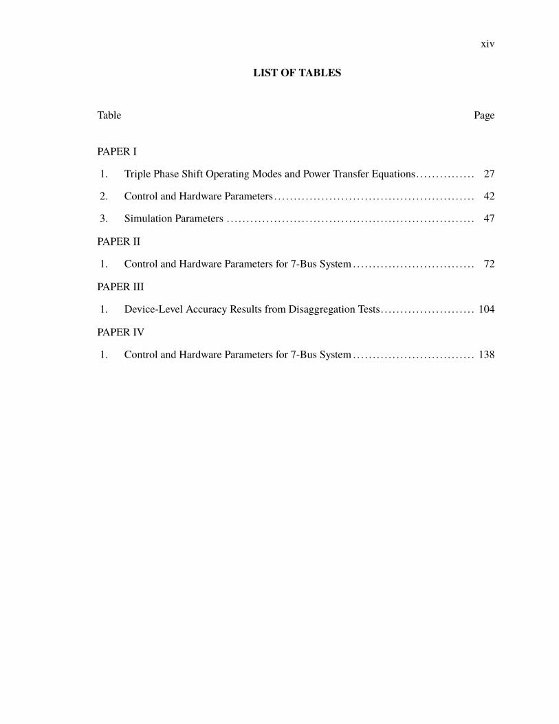
LIST OF TABLES

Table Page

PAPER I

1. Triple Phase Shift Operating Modes and Power Transfer Equations. . . . . . . . . . . . . . . 27

2. Control and Hardware Parameters . . . . . . . . . . . . . . . . . . . . . . . . . . . . . . . . . . . . . . . . . . . . . . . . . . . 42

3. Simulation Parameters . . . . . . . . . . . . . . . . . . . . . . . . . . . . . . . . . . . . . . . . . . . . . . . . . . . . . . . . . . . . . . . 47

PAPER II

1. Control and Hardware Parameters for 7-Bus System . . . . . . . . . . . . . . . . . . . . . . . . . . . . . . . 72

PAPER III

1. Device-Level Accuracy Results from Disaggregation Tests. . . . . . . . . . . . . . . . . . . . . . . . 104

PAPER IV

1. Control and Hardware Parameters for 7-Bus System . . . . . . . . . . . . . . . . . . . . . . . . . . . . . . . 138

SECTION

1. INTRODUCTION

1.1. OVERVIEW

Power electronics are indispensable components of modern power systems. The

range of applications for power electronic energy conversion is constantly expanding, driven

by advances in semiconductor technology. Power electronic interfaces are the connective

elements behind smart grids [1], microgrids [2], transportation electrification [3], and

dc power systems [4, 5]. However, converter circuits and control systems are inherently

nonlinear, and accurate models of their behavior are complex. When constructing models

of multi-converter systems, it is often difficult to obtain a usable balance of accuracy and

complexity. In some cases, tractable system-level representations are not possible without

simplifying assumptions that affect model validity. These challenges exist at the intersection

of power electronics and power systems, and require solutions that draw on methods from

both disciplines.

The objective of this work is develop accurate and computationally efficient mo-

dels of dc microgrids and distribution systems. Systems based on the dual active bridge

(DAB) topology are the specific focus. The modeling challenges for DAB converters are

emblematic of larger fundamental problems in modeling multi-converter systems. While

DAB converters are used in all the systems under consideration, the system-level modeling

solutions apply equally to other dc-dc converter topologies. The final models are inten-

ded for system-level design and analysis tasks, namely time-domain simulation, stability

assessment, and performance optimization.

2

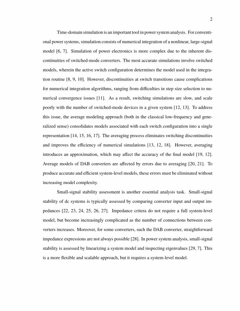
Time-domain simulation is an important tool in power system analysis. For conventi-

onal power systems, simulation consists of numerical integration of a nonlinear, large-signal

model [6, 7]. Simulation of power electronics is more complex due to the inherent dis-

continuities of switched-mode converters. The most accurate simulations involve switched

models, wherein the active switch configuration determines the model used in the integra-

tion routine [8, 9, 10]. However, discontinuities at switch transitions cause complications

for numerical integration algorithms, ranging from difficulties in step size selection to nu-

merical convergence issues [11]. As a result, switching simulations are slow, and scale

poorly with the number of switched-mode devices in a given system [12, 13]. To address

this issue, the average modeling approach (both in the classical low-frequency and gene-

ralized sense) consolidates models associated with each switch configuration into a single

representation [14, 15, 16, 17]. The averaging process eliminates switching discontinuities

and improves the efficiency of numerical simulations [13, 12, 18]. However, averaging

introduces an approximation, which may affect the accuracy of the final model [19, 12].

Average models of DAB converters are affected by errors due to averaging [20, 21]. To

produce accurate and efficient system-level models, these errors must be eliminated without

increasing model complexity.

Small-signal stability assessment is another essential analysis task. Small-signal

stability of dc systems is typically assessed by comparing converter input and output im-

pedances [22, 23, 24, 25, 26, 27]. Impedance critera do not require a full system-level

model, but become increasingly complicated as the number of connections between con-

verters increases. Moreover, for some converters, such the DAB converter, straightforward

impedance expressions are not always possible [28]. In power system analysis, small-signal

stability is assessed by linearizing a system model and inspecting eigenvalues [29, 7]. This

is a more flexible and scalable approach, but it requires a system-level model.

3

Performance optimization is a more open-ended task, but equally relevant to both

power electronics and power systems. In this context, performance optimization refers to

system design practices or control strategies that maximize some performance metric (e.g.

overall efficiency) or minimize some cost (e.g. total loss). When the mechanism through

which rewards (or costs) are incurred depends on the operating conditions of the system, the

process of constructing and solving an optimization problem requires quantitative descrip-

tions of the range of system operating conditions. These descriptions necessarily involve

detailed characterization of sources of uncertainty. For the systems under consideration,

uncertainty is introduced through load and source behavior. In order to assess and improve

system performance, load and source randomness—and the effect of random behavior on

system operation—must be properly specified.

Solutions to the problems above are presented here in four papers, organized as fol-

lows. The first two papers focus on the derivation of accurate and computationally efficient

dynamic models with deterministic load and source inputs. Paper I describes improvements

to generalized average models of dc-dc DAB converters. Paper II extends the modeling

improvements to multi-converter systems, and introduces a new harmonic reconstruction

method for predicting transformer currents. The second half of the dissertation considers

the effects of randomness in the load inputs. Paper III presents a method of generating

stochastic models of composite electrical loads. The load models are presented as an ele-

ment of a nonintrusive load monitoring algorithm, but are directly applicable to modeling

loads in dc distribution systems as well. In Paper IV, load and microgrid models are joined

together using the formalism of stochastic hybrid systems.

Themodels proposed in Paper I and Paper II describe dynamic behavior of converters

and systems as a function of external inputs. In the case of a dc microgrid, the inputs of

interest are loads and sources (or simply loads, understood to be possibly bidirectional).

Together, Paper III and Paper IV widen the scope of the models to include load behavior.

4

Figure 1.1. Modeling scope for each paper.

Paper III describes a method for building probabilistic load models; Paper IV merges these

load descriptions with the deterministic framework established in Paper I and Paper II. A

graphical representation of the modeling scope of each paper is shown in Fig. 1.1.

1.2. DETERMINISTIC MICROGRID MODELS

Accurate dynamic models are critical to analysis and design procedures, both for

individual converters and full microgrid systems. This section describes challenges involved

in modeling DAB converters and the important characteristics of system-level models.

Challenges and objectives outlined in this section set the stage for the modeling solutions

proposed in Paper I and Paper II.

1.2.1. Dual Active Bridge Converters. The DAB topology [30, 31, 32] consists

of two H-bridge circuits separated by a high-frequency transformer. The transformer is the

most important component of the converter: the transformer’s leakage inductance is the

primary energy storage element in the converter and the turns ratio is a significant factor

in determining voltage gain. The H-bridge circuits apply modulated voltages on either side

of the transformer, such that the transformer current is periodic at the converter switching

5

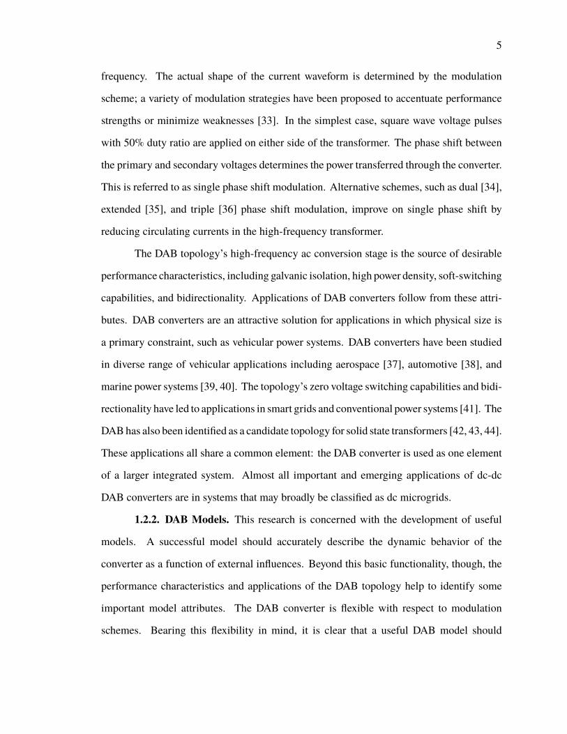
frequency. The actual shape of the current waveform is determined by the modulation

scheme; a variety of modulation strategies have been proposed to accentuate performance

strengths or minimize weaknesses [33]. In the simplest case, square wave voltage pulses

with 50% duty ratio are applied on either side of the transformer. The phase shift between

the primary and secondary voltages determines the power transferred through the converter.

This is referred to as single phase shift modulation. Alternative schemes, such as dual [34],

extended [35], and triple [36] phase shift modulation, improve on single phase shift by

reducing circulating currents in the high-frequency transformer.

The DAB topology’s high-frequency ac conversion stage is the source of desirable

performance characteristics, including galvanic isolation, high power density, soft-switching

capabilities, and bidirectionality. Applications of DAB converters follow from these attri-

butes. DAB converters are an attractive solution for applications in which physical size is

a primary constraint, such as vehicular power systems. DAB converters have been studied

in diverse range of vehicular applications including aerospace [37], automotive [38], and

marine power systems [39, 40]. The topology’s zero voltage switching capabilities and bidi-

rectionality have led to applications in smart grids and conventional power systems [41]. The

DABhas also been identified as a candidate topology for solid state transformers [42, 43, 44].

These applications all share a common element: the DAB converter is used as one element

of a larger integrated system. Almost all important and emerging applications of dc-dc

DAB converters are in systems that may broadly be classified as dc microgrids.

1.2.2. DAB Models. This research is concerned with the development of useful

models. A successful model should accurately describe the dynamic behavior of the

converter as a function of external influences. Beyond this basic functionality, though, the

performance characteristics and applications of the DAB topology help to identify some

important model attributes. The DAB converter is flexible with respect to modulation

schemes. Bearing this flexibility in mind, it is clear that a useful DAB model should

6

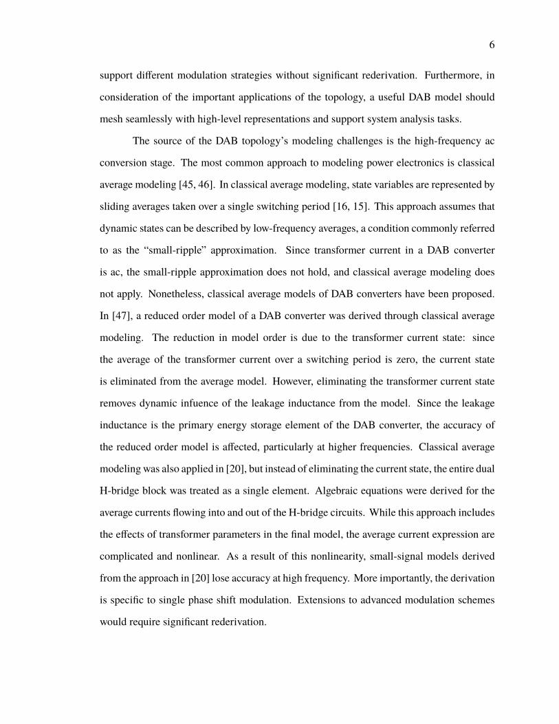
support different modulation strategies without significant rederivation. Furthermore, in

consideration of the important applications of the topology, a useful DAB model should

mesh seamlessly with high-level representations and support system analysis tasks.

The source of the DAB topology’s modeling challenges is the high-frequency ac

conversion stage. The most common approach to modeling power electronics is classical

average modeling [45, 46]. In classical average modeling, state variables are represented by

sliding averages taken over a single switching period [16, 15]. This approach assumes that

dynamic states can be described by low-frequency averages, a condition commonly referred

to as the “small-ripple” approximation. Since transformer current in a DAB converter

is ac, the small-ripple approximation does not hold, and classical average modeling does

not apply. Nonetheless, classical average models of DAB converters have been proposed.

In [47], a reduced order model of a DAB converter was derived through classical average

modeling. The reduction in model order is due to the transformer current state: since

the average of the transformer current over a switching period is zero, the current state

is eliminated from the average model. However, eliminating the transformer current state

removes dynamic infuence of the leakage inductance from the model. Since the leakage

inductance is the primary energy storage element of the DAB converter, the accuracy of

the reduced order model is affected, particularly at higher frequencies. Classical average

modeling was also applied in [20], but instead of eliminating the current state, the entire dual

H-bridge block was treated as a single element. Algebraic equations were derived for the

average currents flowing into and out of the H-bridge circuits. While this approach includes

the effects of transformer parameters in the final model, the average current expression are

complicated and nonlinear. As a result of this nonlinearity, small-signal models derived

from the approach in [20] lose accuracy at high frequency. More importantly, the derivation

is specific to single phase shift modulation. Extensions to advanced modulation schemes

would require significant rederivation.

7

Other modeling efforts have considered more powerful modeling tools to address

the deficiencies of classical average DAB models. The sampled-data modeling method

from [48] was applied to DAB converters in [49, 50, 38]. This method assumes that the

converter transitions cyclically through a set of fully characterized switching modes. Expli-

cit descriptions of each mode and a prespecified base period are required for this approach.

Of the existing DAB models, those derived using the sampled-data modeling approach are

the most accurate [20]. However, the price of this accuracy is model complexity: each

switch configuration is modeled independently. The additional switch configurations pre-

sent in advancedmodulation schemes increasemodel complexity, and the transitions through

switching modes are dependent on the modulation scheme. As a result, new modulation

schemes essentially require entirely new models. The most significant problem, however, is

how model size and complexity increases for models of multi-converter systems. The mo-

deling requirements–full characterizations of all switching modes and a system-wide base

period–quickly become unreasonable as the number of converters included in the system

increases.

Another approach to modeling DAB converters employs the generalized average

modeling (GAM) [17, 51] framework. GAM generalizes the approach of classical average

modeling by expanding state variables into Fourier series components before applying the

sliding average operation. An open-loop DAB model derived using GAM was proposed

in [21]. The model from [21] is central to this dissertation. All of the improvements and

extensions described in the following sections belong to a modeling genealogy that starts

with [21].

Like sampled-data modeling, GAM is subject to significant scalability issues. GAM

requires the specification of a base period, and involves an inherent tradeoff between

accuracy and model complexity [52, 46]. To ensure tractability in the final model, Fourier

series expansions of state variables are typically truncated after the first harmonic [21, 53],

a practice commonly referred to as the first harmonic approximaton. This approach avoids

8

prohibitive model complexity but limits accuracy. In particular, DAB models derived with

the first harmonic approximation are affected by persistent large-signal error. These errors

are especially problematic at the system level, since small errors in bus voltage lead to

incorrect power flow predictions. A correction factor was proposed in [53] to eliminate the

error, but only for single phase shift modulation. Even in operating regions where the large-

signal error has minimal effect, the transformer current predictions of GAM-based models

are limited in accuracy. When ac states are limited to first harmonic terms, transformer

currents are represented as sinusoids at the switching frequency. Sinusoidal approximations

poorly represent the complicated piecewise exponential waveforms observed in simulations

and hardware experiments. These deficiencies would seem to preclude the use of GAM

for system-level models. However, all of these issues may be addressed through model

improvements and manipulations.

1.2.3. Development of a System-LevelModel. Themost important characteristics

of a system-level model are accuracy, scalability, and modularity. The importance of

accuracy and scalability are straightforward, but modularity is equally critical. In this

context, modularity refers to the ability to combine, separate, and reconfigure the system-

level model without requiring full rederivation. That is, when a converter is added to the

system, the adjustment to the system-level model should only require operations that act on

the existing systemmodel and themodel of the newly added converter. Models derived using

classical averaged modeling are inherently modular [18, 12]. However, other methods do

not guarantee modularity. Both GAM and sampled-data modeling involve the specification

of a system-wide base period. If the base period changes when a converter is added to the

system, both of these modeling approaches will require ground-up rederivation.

Previous studies have considered the development of system-level models using

GAM [54, 55, 39, 56, 57]. The authors of [56] observe that GAM does not naturally support

multi-converter systems, and propose an extended averaging scheme that allows for the

inclusion of multiple switching frequencies. This approach makes it possible to accurately

9

model multiple switching frequencies at the cost of complexity: for a system with N states

and M dominant harmonics, the final model will include N(2M−1) state equations. Amore

scalable solution is described in [54]. The approach in [54] involves selecting the number of

Fourier series components on a state-by-state basis, rather than setting a globally-consistent

number of terms. This “selective averaging” approach assumes preexisting knowledge

of dominant system dynamics. To mitigate complexity, dynamic interactions between

converters are assumed to exist entirely in dc average states. In relation to the methods here,

selective averaging produces the same level of reduction in model complexity. However,

the methods described in Paper II achieve this reduction through structural properties of the

individual converter models and require no assumptions on the nature of system dynamics.

In summary, two fundamental problems obstruct models of multi-converter systems

containing DAB converters. The first problem is the inherent tradeoff between accuracy

and model complexity in GAM. Approximations necessary obtain tractable models, namely

the first harmonic approximation, limit large-signal accuracy. As a result, the models

are not suitable for time-domain simulation or load flow analysis. The second problem

is the requirement of a system-wide base period, which prevents modular approaches to

system-level modeling. The contributions of Paper I and Paper II are solutions to these

two fundamental problems. Paper I introduces a correction factor that eliminates the large-

signal error due to the first harmonic approximation without including additional Fourier

series terms as dynamic states. Moreover, the existing GAM-based DABmodel is extended

for general modulation schemes. Paper II addresses frequency dependence and proposes

a modular procedure for generating models of multi-converter systems. A decoupling

between state variables of the DAB converter, originally noted in [21], is preserved through

the model construction process. Because of this decoupling effect it is possible to represent

interactions between converters with dc average terms only, eliminating the the need for a

system-wide base period. Converter and system models derived using the methods from

10

Paper I and Paper II are suitable for stability assessments and load flow analyses. Their

most important feature, though, is that they enable accurate time-domain simulation at a

fraction of the computational cost of switched model alternatives.

1.3. INFLUENCE OF PRACTICAL LOADS

A common approach in modeling power electronics is to represent loads as either

fixed impedances or constant voltage/current sources. The parameters of these elements are

then defined according to maximum/minimum load power values. This load representation

is a practical choice for many anaysis and design objectives, particularly when scope is

limited to an individual converter. For instance, simplified load models are useful for

analyzing performance under worst-case conditions, where converters are most likely to

encounter stability issues. However, as systems increase in size, analysis and design

practices based on simplified worst case conditions become less useful. In a system with

many independent loads, the likelihood that all loads simultaneously operate at maximum

power is small, and designing the system to meet this rare condition is not a viable option.

The same situation occurs in conventional power systems, and has motivated a variety of

probabilistic load modeling solutions.

Another disadvantage of deterministic load models is that they offer no insight

on typical operating conditions over time. Specifications of ‘typical’ behavior require

descriptions of a probabilistic nature. The ability to quantify typical conditions—and the

possible deviations from these conditions—is a valuable analytical tool. Many aspects

of converter performance depend on system operating conditions. Converter efficiency is

perhaps the most obvious (and most important). Another example, one which is particularly

relevant to the DAB topology, is zero voltage switching (ZVS). ZVS occurs in a subset of

the possible operating space of a DAB converter, but has significant effect on switching loss

and semiconductor stresses [31, 37]. It is therefore desirable to operate the converter in the

ZVS region whenever possible. More generally, a microgrid may be stable and functional

11

over a wide range of operating conditions, but it is unlikely that all stable conditions are

equally desirable. For a given operating-point-dependent metric (e.g. efficiency, stability

margins, power quality, etc.), specifications of typical operating conditions make it possible

to assess the actual performance of the system.

The process of obtaining probabilistic operating point descriptions can be broken

into two subproblems: modeling practical load behavior and connecting load models to

dynamic states. These problems are addressed in Paper III and Paper IV, respectively.

Including stochastic load descriptions in the modeling framework is challenging task and

requires a more diverse set of tools than used in deterministic modeling efforts. Many of

these tools, such as the machine learning algorithms in Paper III and stochastic calculus in

Paper IV, are far removed from the skills normally associated with analysis and design of

power electronics. The driving motivation behind both of these papers is to provide models

and methods which are accessible to practicing engineers. Consequently, in comparison

to the first two papers, Paper III and Paper IV include more examples, simplifications, and

details related to practical implementation.

1.3.1. Load Modeling. Load modeling is a mature subfield of conventional power

system analysis. In large power systems, it is possible to rely on Gaussian process models

based on the central limit theorem [58, 59, 60]. Gaussian models are high-level abstractions

that apply when loads consist of many individual devices. However, as the size of a system

decreases, contributions of a single device become more significant with respect to the total

load profile, and Gaussian approximations become less accurate [61].

For loads that do not meet the criteria for Gaussian approximations, i.e. loads that

consist of a small number of devices, an alternative strategy is to build models upward from

individual device level. This approach is used in nonintrusive load monitoring (NILM) [62,

63, 64]. The objective of NILM is to extract individual device activity from measurements

of a composite load profile. To support this extraction, or disaggregation, composite load

models must retain the individual characteristics of their constituent devices.

12

Paper III describes a full NILM procedure. The loads are represented by hidden

Markov models (HMMs). HMM-based methods are a particularly successful subset of

NILM [65, 66, 67, 68, 69]. The most important contribution of Paper III, in the context

of modeling microgrid loads, is the process of constructing models of individual devices

and combining them into models of the composite load. In particular, the load modeling

approach outlined in Paper III is directly applicable to generating ‘typical’ load specifications

based on either composite load measurements or knowledge of the devices contained in the

load.

The scope of Paper III is defined to include “systems of known devices,” or systems

for which number and nature of loads is fully known. In residential systems, the original

target applications of theNILMconcept, complete knowledge of system loads is impractical.

However, the “known device” criterion is commonly met in dc microgrids and distribution

systems. In particular, the criterion is satisfied by industrial systems designed to support a

specific set of equipment, and it is inherently met by vehicular power systems. Removing

the possibility of unknown devices makes it possible to explore new NILM applications

without solving the problem of unmodeled loads. For instance, Paper III proposes a method

of device-level energy use estimation that significantly improves on the performance of

previous HMM-based algorithms.

The load representations in Paper III are discrete-time HMMs based on steady-state

conditions. These models only characterize the randomness in load behavior; they offer no

description of load influence on the local power system. In order to describe the effects

of load behavior on the system, the stochastic load models must be joined together with

the dynamic models proposed in Paper II. The ideal result of a combined model would be

closed-form distributions of dynamic states. However, it is only possible to produce full

distributions for a very narrow set of circumstances, such as linear systems with Gaussian

13

inputs [70]. In the present case, dynamic models are nonlinear and load models are not

Gaussian, so more powerful modeling methods must be employed to characterize stochastic

dynamic behavior.

1.3.2. Stochastic Hybrid System. Stochastic hybrid systems (SHSs) are a general

class of stochastic process that include continuous dynamics, instantaneous events, and a

wide variety of random effects [71]. The SHS framework is challenging due to its sheer

generality (see [72] for a review of models that fall within the SHS scope). However, SHS

models provide powerful tools for system analysis. In particular, SHS models describe the

evolution of moments of dynamic state variables. Moments provide useful descriptions of

dynamic state behavior in lieu of full state distributions.

Previous studies have used SHSmodels to describe power delivery systems. In [73],

the SHS framework was applied to a conventional power system. SHSmodels of microgrids

have been proposed for the purposes of simulation [74] and stability analysis [75]. Although

the application is different, the approach used here is heavily influenced by these previous

efforts, particularly [73]. The model in [73] consists of an affine power system model and

an input process described by a continuous-time Markov chain (CTMC). Key elements of

the SHS, namely test functions and reset maps, are defined in [73] such that the equations

which describe moment dynamics depend only moments of equal or lower order. The

same definitions are used here, and they affect the same simplification. Additionally, [73]

describes a general procedure for calculating moments of algebraic states. This procedure

forms the basis for a new set equations that encode ZVS conditions into the SHS model.

Paper IV describes an SHS model of a dc microgrid system. The model consists

of a CTMC, which is constructed from the stochastic load models in Paper III, and a

family of affine microgrid models, which are derived according to the methods in Paper II.

The SHS framework is applied according to [71] using the test function and reset maps

proposed in [73]. Since the objective of the paper is to provide an accessible tool for

practicing engineers, the general forms resulting from the methods of [71] and [73] are

14

further simplified. In particular, closed-form expressions are derived for the systems of

equations that describe first and second moment dynamics. This simplification makes it

possible to construct the full SHS model through linear operations. The simplified form

also provides useful insights into the relationships between moments and load process

parameters.

Paper IV also considers the practical problem of assessing ZVS performance for

DAB converters in multi-converter systems. First, ZVS conditions are introduced in the

SHS model as functions of the stochastic dynamic state processes. Analytic expressions

for the moments of these functions are then derived. Moments of the ZVS condition

functions are used to approximate the probability of ZVS for a given set of loads. While

the expressions apply for moments of any order, low order moments provide sufficiently

accurate approximations in practice. First and second order moments provide enough

information to define upper and lower bounds on ZVS probability. The ZVS performance

analysis in Paper IV addresses a practical issue specific to single phase shift modulated

DAB converters. More importantly, though, the assessments serve as an example of the

more general applications of an SHS model.

15

PAPER

I. AN IMPROVED GENERALIZED AVERAGE MODEL OF DC-DC DUALACTIVE BRIDGE CONVERTERS

Jacob A. Mueller and Jonathan W. Kimball

Department of Electrical & Computer Engineering

Missouri University of Science and Technology

Rolla, Missouri 65409–0050

Email: jam8z4@mst.edu

ABSTRACT

Improvements are proposed for generalized average models of dual active bridge (DAB)

converters. Generalized average modeling involves a trade-off between accuracy and trac-

tability. To maintain an acceptable level of complexity, existing DAB models are derived

using a first harmonic approximation. These models provide accurate small-signal repre-

sentations, but are limited as large-signal analysis tools due to persistent steady-state error.

This study proposes a modeling framework that provides accurate large and small-signal

models without significant increases in overall complexity. The framework describes DAB

operation with triple phase shift modulation, and is easily simplified for single, dual, or ex-

tended phase shift modulation schemes. The special case of single phase shift modulation,

which experiences the most significant large-signal error, is given additional consideration.

The framework is applied to open and closed-loop operation, and both large and small-signal

models are discussed. Models are validated in simulation and hardware experiments using

a small scale DAB prototype.

16

Keywords: average modeling, dual active bridge converter, generalized average model,

phase shift modulation

1. INTRODUCTION

The dual active bridge (DAB) topology features desirable performance characteris-

tics including galvanic isolation, high power density, low device stresses, and bidirectional

operation [1, 2]. Many of these attributes are due to a high-frequency ac conversion stage.

However, the associated ac state variables present challenges when developingmodels of the

converter’s behavior. In particular, the transformer current state precludes the “small-ripple”

approximation commonly employed in traditional modeling approaches, e.g. state-space

averaging and average circuit modeling.

Previous studies have addressed the challenges of modeling DAB converters. The

most common strategy uses the sampled-data modeling procedure from [3] to develop

discrete-time models. This approach was used in [4] to develop an open-loop DAB model,

and again in [5] to develop a more detailed model consisting of a converter, EMI filters,

and control system. In these models, the converter transitions through discrete modes of

operation, each described by a set of linear time-invariant ordinary differential equations

(ODEs). The transition times are either explicitly controlled (e.g. by gate driver signals) or

implicitly determined by device thresholds (e.g. by diode current zero crossings). The state

solution within each mode is explicitly determined by initial conditions at transition times

and state transition matrices consisting of matrix exponentials. In [6], matrix exponential

calculations were avoided through the use of bilinear approximations, leading to a simplified

discrete-time DAB model.

The advantage of the discrete-time models in [4, 6, 5] is that they explicitly describe

state trajectories in all subintervals of converter operation, meaning they are capable of pro-

viding exact solutions for ac state variables. In the case of DAB converters, these models

are able to accurately predict transformer currents and, as in [4], the current zero crossings

17

critical to zero voltage switching (ZVS) [7]. The capabilities of discrete-time representa-

tions notwithstanding, two factors motivate the development of accurate continuous-time

models. First, continuous-time models are still preferred for control design due to the

prevalence of simple and powerful design tools. Secondly, DAB converters are well-suited

to applications in multi-converter systems, such as solid state transformers [8], microgrids,

and dc distribution systems. The framework of [3] assumes cyclic transitions through fully

characterized modes of operation, and is not intended to produce models that are modular

elements of a larger system. Representing all possible switching modes at the system level

quickly becomes infeasible as the number of converters increases. Moreover, differences

in converter switching frequencies make it difficult to define a usable system-wide base

period. For the purposes of system-level analysis, more scalable alternatives are required.

Continuous-timeDABmodels have been proposed aswell. The simplestmodel, pro-

posed in [9], essentially results from the application of classical state-space averaging [10].

Since the dc average of transformer current is 0, the state is eliminated in the averaging

process, and its dynamics are lost in the final model. A more detailed approach was used

in [11] to derive both large and small-signal average models. The ac stage in these models

is represented by half period averages of the dc currents into and out of the H-bridges. This

allows the models to incorporate effects of transformer core and conduction losses, which

are omitted from the models in [9]. A similar procedure was used in [12] for the purposes

of steady-state analysis.

A continuous-time DAB model was derived using generalized average modeling

(GAM) in [13]. In GAM, state variables are expanded into Fourier series terms at multiples

of the converter switching frequency [14], providing straightforward representations of ac

states. However, theGAMframework involves a trade-off between accuracy and complexity.

Specifically, both accuracy and complexity increase with the number of Fourier series

terms included in the model. The model in [13] uses a first harmonic approximation, and

truncates the Fourier series at the first harmonic. When linearized, the model accurately

18

predicts small-signal responses, but the large-signal model is inaccurate at steady-state. The

accuracy of the model increases when more Fourier series terms are included (see e.g. [15]),

but the number of model states increases rapidly with the number of Fourier series terms

considered, so even small accuracy gains require substantial penalties in terms of model

complexity.

This steady-state error was previously noted in [11], and a method of correcting the

error was proposed [16]. The approach in [16] consists of applying a multiplicative cor-

rection factor to the load and state variables. However, the correction factor is only derived

for single phase shift operation. Furthermore, the method assumes lossless operation, and

neglects the effect of transformer winding resistance, which may be significant in practice.

This copper loss is particularly important for single phase shift operation, which produces

large circulating currents, or when the ratio of winding resistance to leakage reactance is

high [12].

This study presents the following contributions:

• The DAB model from [13] is extended to more general modulation strategies, inclu-

ding dual, extended, and triple phase shift modulation. Both large and small-signal

models are described.

• A new method of eliminating the error caused by truncating the Fourier series at the

first harmonic is proposed. The method involves deriving the relationship between

the equilibrium solution to the model equations and exact steady-state expressions,

and then including those relationships in the model itself.

• An additional correction factor that includes copper losses in the transformer is

derived for the special case of single phase shift modulation.

The structure of the paper is as follows. Section 2 briefly reviews the DAB model

from [13] and describes the steady-state model error in precise terms. The improved

DAB model is given in Section 4, starting with the extension to more general modulation

19

strategies, and then including the large-signal error correction. Model partial derivatives,

including those necessary to develop small-signal models, are given in Section 4. Special

consideration is given to the single phase shift case in Section 5, including the derivation

of a lossy correction factor. Verification experiments are described in Section 6.

2. BACKGROUND

This section reviews the DAB model from [13] to be improved in the following

section, establishes important terms and notation, and provides a mathematical description

of the steady-state error problem.

2.1. Original DABModel. The original DAB model proposed in [13] begins with

Ûvo =−1

RshCovo +

1Co

it s2(τ, d) −1

CoiL (1)

Ûit =1Ltvins1(τ, d) −

1Ltvos2(τ, d) −

Rt

Ltit (2)

where dot notation is used to indicate derivatives with respect to time. The signals and

parameters in these equations are identified in Fig. 1. All hardware parameters are referred

to the secondary side of the transformer. For simplicity, the derivation shown here assumes

a 1:1 turns ratio. The only modification necessary to include non-unity turns ratios in the

model is to replace all appearances of vin with n2n1vin. This is true for this model and for the

models proposed in the following section.

Switching signals s1(τ, d) and s2(τ, d) are the switching signals that drive the input

and output H-bridges, respectively. The model from [13] was derived for single phase shift

modulation. For time τ in a switching interval (0 ≤ τ < T) and phase shift argument d,

the single phase shift switching signals are

s1(τ, d) =

1, 0 ≤ τ < T2

−1, T2 ≤ τ < T

(3)

20

s2(τ, d) =

1, dT2 ≤ τ <

dT2 +

T2

−1, 0 ≤ τ < dT2 or dT

2 +T2 ≤ τ < T

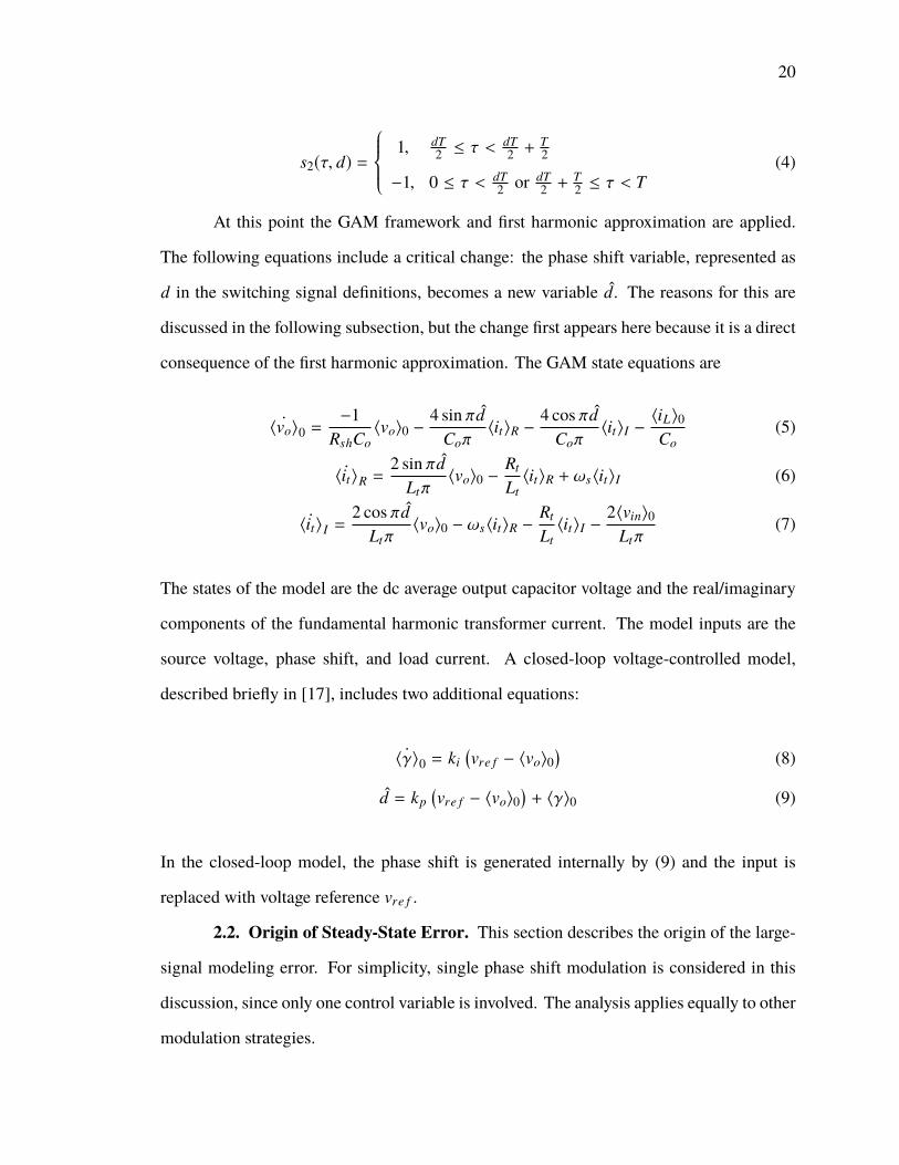
(4)

At this point the GAM framework and first harmonic approximation are applied.

The following equations include a critical change: the phase shift variable, represented as

d in the switching signal definitions, becomes a new variable d. The reasons for this are

discussed in the following subsection, but the change first appears here because it is a direct

consequence of the first harmonic approximation. The GAM state equations are

Û〈vo〉0 =−1

RshCo〈vo〉0 −

4 sin πdCoπ

〈it〉R −4 cos πd

Coπ〈it〉I −

〈iL〉0Co

(5)

Û〈it〉R =2 sin πd

Ltπ〈vo〉0 −

Rt

Lt〈it〉R + ωs〈it〉I (6)

Û〈it〉I =2 cos πd

Ltπ〈vo〉0 − ωs〈it〉R −

Rt

Lt〈it〉I −

2〈vin〉0Ltπ

(7)

The states of the model are the dc average output capacitor voltage and the real/imaginary

components of the fundamental harmonic transformer current. The model inputs are the

source voltage, phase shift, and load current. A closed-loop voltage-controlled model,

described briefly in [17], includes two additional equations:

Û〈γ〉0 = ki(vre f − 〈vo〉0

)(8)

d = kp(vre f − 〈vo〉0

)+ 〈γ〉0 (9)

In the closed-loop model, the phase shift is generated internally by (9) and the input is

replaced with voltage reference vre f .

2.2. Origin of Steady-State Error. This section describes the origin of the large-

signal modeling error. For simplicity, single phase shift modulation is considered in this

discussion, since only one control variable is involved. The analysis applies equally to other

modulation strategies.

21

Lt Rtn1:n2

vin

Co

iLvo

_

+

it

Q1 Q3

Q2 Q4

Q5 Q7

Q6 Q8

_ + Rsh

Figure 1. Dual active bridge topology.

The steady-state error manifests differently depending on how the model is used. If

a phase shift is specified as an exogenous input (as is the case with the open loop model) the

error will affect the output voltage. If an output voltage and load current are specified, the

error will affect the phase shift. Similarly, in closed-loop operation, if a voltage reference

and load current are specified, the phase shift will be affected.

For simplicity, consider a lossless closed-loop converter with current source load

(i.e. Rt → 0, Rsh →∞) in steady-state operation. The action of the controller forces output

voltage to the voltage reference at steady-state, so the error will be restricted to the phase

shift. The relationship in (7) reduces to 0 = it s2(τ, d) − iL , and the load current can be

expanded as an infinite Fourier series:

iL =

∞∑k=−∞

〈it s2(τ, d)〉k =∞∑

k=−∞

∞∑i=−∞

〈s2(τ, d)〉k−i 〈it〉i (10)

Considering only the dc average current, the equation is

〈iL〉0 = 〈it s2(τ, d)〉0 =∞∑

i=−∞

〈s2(τ, d)〉−i 〈it〉i (11)

Switching signal s2(τ, d) is a phase-shifted square wave, and only has nonzero Fourier series

coefficients at odd harmonics. The coefficients are functions of the phase shift, d.

〈s2(τ, d)〉k =−2 sin πkd

kπ+ j−2 cos πkd

kπfor k = 1, 3, . . . (12)

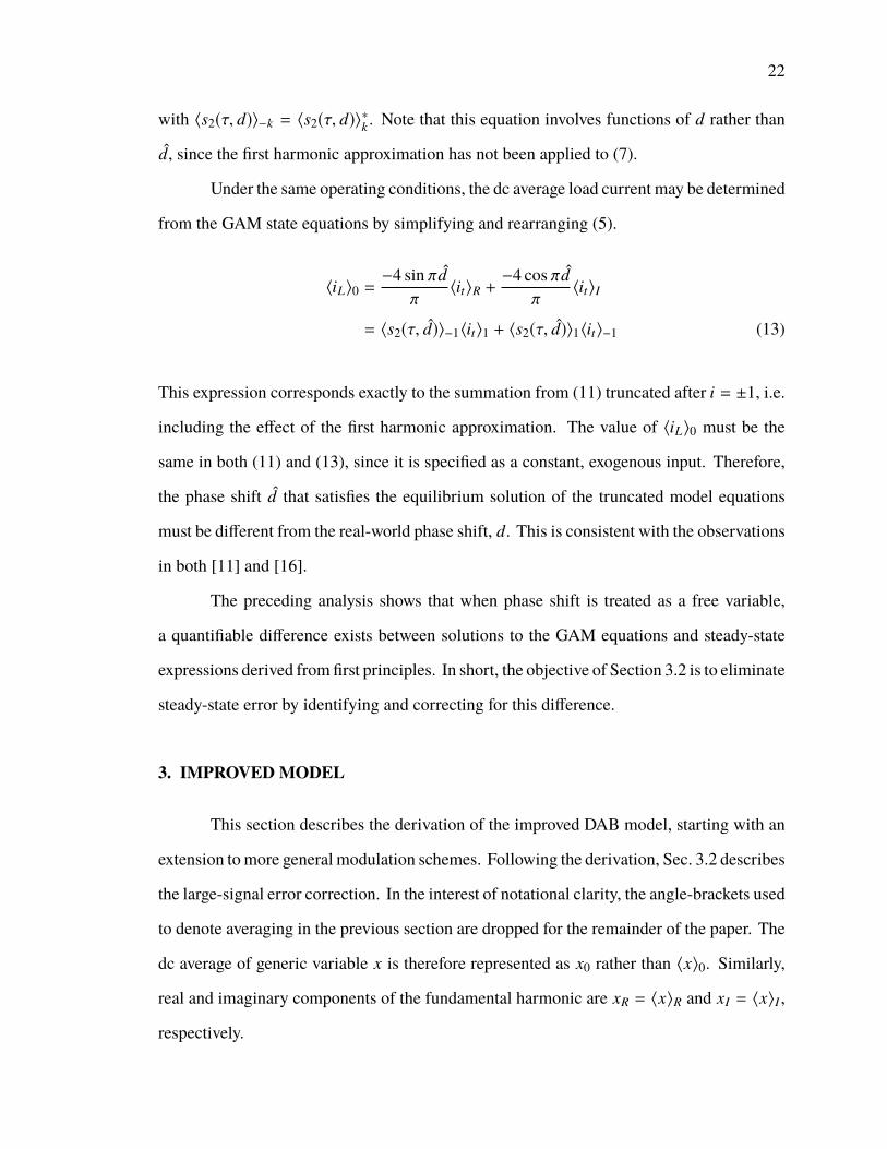
22

with 〈s2(τ, d)〉−k = 〈s2(τ, d)〉∗k . Note that this equation involves functions of d rather than

d, since the first harmonic approximation has not been applied to (7).

Under the same operating conditions, the dc average load current may be determined

from the GAM state equations by simplifying and rearranging (5).

〈iL〉0 =−4 sin πd

π〈it〉R +

−4 cos πdπ

〈it〉I

= 〈s2(τ, d)〉−1〈it〉1 + 〈s2(τ, d)〉1〈it〉−1 (13)

This expression corresponds exactly to the summation from (11) truncated after i = ±1, i.e.

including the effect of the first harmonic approximation. The value of 〈iL〉0 must be the

same in both (11) and (13), since it is specified as a constant, exogenous input. Therefore,

the phase shift d that satisfies the equilibrium solution of the truncated model equations

must be different from the real-world phase shift, d. This is consistent with the observations

in both [11] and [16].

The preceding analysis shows that when phase shift is treated as a free variable,

a quantifiable difference exists between solutions to the GAM equations and steady-state

expressions derived fromfirst principles. In short, the objective of Section 3.2 is to eliminate

steady-state error by identifying and correcting for this difference.

3. IMPROVED MODEL

This section describes the derivation of the improved DAB model, starting with an

extension tomore general modulation schemes. Following the derivation, Sec. 3.2 describes

the large-signal error correction. In the interest of notational clarity, the angle-brackets used

to denote averaging in the previous section are dropped for the remainder of the paper. The

dc average of generic variable x is therefore represented as x0 rather than 〈x〉0. Similarly,

real and imaginary components of the fundamental harmonic are xR = 〈x〉R and xI = 〈x〉I ,

respectively.

23

3.1. Modulation Scheme Extension. Applying the GAM framework to (7) and (2)

yields

Ûvo0 = −1

RshCovo0 +

1Co

it0s20 +2

CoitRs2R +

2Co

it I s2I −1

CoiL0 (14)

ÛitR =1Ltvin0s1R +

1LtvinRs10 −

1Ltvo0s2R −

1LtvoRs20 −

Rt

LtitR + ωsit I (15)

Ûit I =1Ltvin0s1I +

1LtvinI s10 −

1Ltvo0s2I −

1LtvoI s20 − ωsitR −

Rt

Ltit I . (16)

To prevent saturation of the transformer, switching signals are typically defined such that

their dc averages are zero, i.e. s10 = s20 = 0. Under this condition, the equations simplify:

Ûvo0 = −1

RshCovo0 +

2Co

itRs2R +2

Coit I s2I −

1Co

iL0 (17)

ÛitR =1Ltvin0s1R −

1Ltvo0s2R −

Rt

LtitR + ωsit I (18)

Ûit I =1Ltvin0s1I −

1Ltvo0s2I − ωsitR −

Rt

Ltit I (19)

The preceding equations are applicable to any modulation strategy, provided that the dc

average of the switching signals is zero. In the case of triple phase shift modulation, the

switching signals are functions of three control arguments: dφ, dp, and ds. These variables

are contained in vector D = [dφ dp ds]T . The switching signals are:

s1(τ,D) =

1, 0 ≤ τ < dpTs

2

0, dpTs2 ≤ τ <

Ts2 or (1+dp)Ts

2 ≤ τ < Ts

−1, Ts2 ≤ τ <

(1+dp)Ts2

(20)

s2(τ,D) =

1, dφTs

2 ≤ τ <(ds+dφ)Ts

2

0, 0 ≤ τ < dφTs2 or (ds+dφ)Ts

2 ≤ τ <(1+dφ)Ts

2 or (1+ds+dφ)Ts2 ≤ τ < Ts

−1, (1+dφ)Ts2 ≤ τ <

(1+ds+dφ)Ts2

(21)

24

This switching scheme is very general; single, dual, and extended phase shift are special

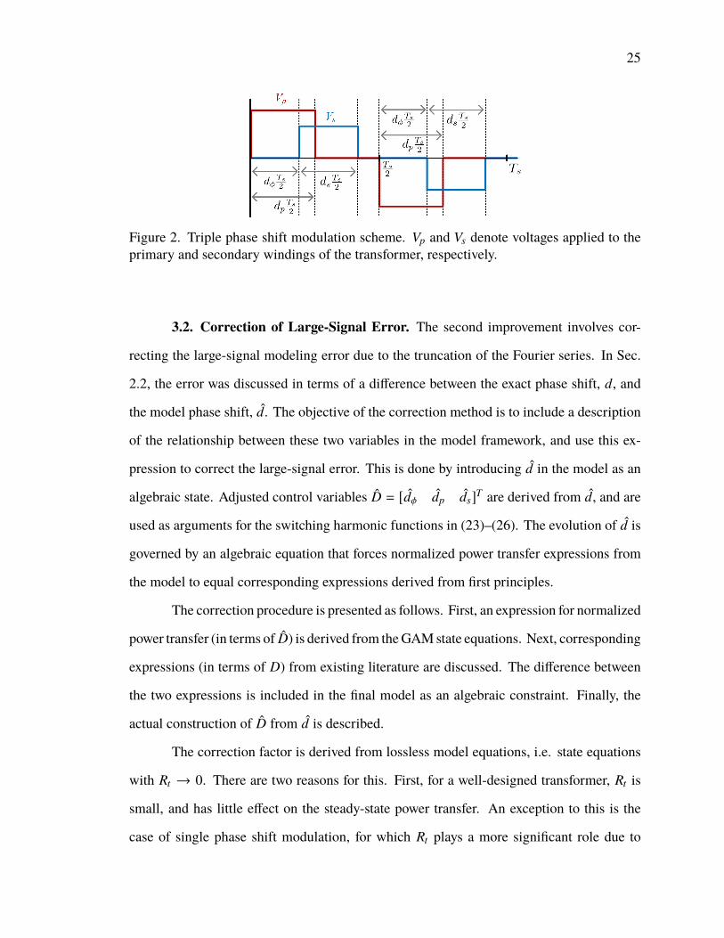
cases of triple phase shift modulation [18]. A visual representation of the triple phase shift

scheme is shown in Fig. 2. The three control variables describe the duty ratio of the voltages

applied to the primary winding (dp), secondary winding (ds), and the phase shift between

them (dφ). An additional phase shift defined by the distance between center points of the

primary and secondary voltage pulses is d. This is an important parameter for describing

triple phase shift operation [18], and is critical to the large-signal error correction method.

It may be be derived from the control variables as

d = dφ −dp

2+

ds

2. (22)

Switching signals for dual phase shift modulation may be recovered by fixing dp = ds, and

single phase shift may be recovered by further constraining dp = ds = 1. In both of these

cases, it is clear from (22) that d = dφ.

Taking the Fourier series of these signals, the real and imaginary components of the

switching functions are:

s1R(D) =sin(dpπ)

π(23)

s1I(D) = −2 sin

(dp

π2)2

π(24)

s2R(D) = −sin(dφπ) − sin

( (ds + dφ

)π)

π(25)

s2I(D) = −cos(dφπ) − cos

( (ds + dφ

)π)

π(26)

Substituting the switching signal harmonic components above into state equati-

ons (17)–(19) produces a generalized average model for a DAB with triple phase shift

modulation. Again, other modulation strategies can be recovered from these equations. For

instance, applying the single phase shift condition (dp = ds = 1) in the general equations

yields the original DAB model, i.e. (5)–(7).

25

Figure 2. Triple phase shift modulation scheme. Vp and Vs denote voltages applied to theprimary and secondary windings of the transformer, respectively.

3.2. Correction of Large-Signal Error. The second improvement involves cor-

recting the large-signal modeling error due to the truncation of the Fourier series. In Sec.

2.2, the error was discussed in terms of a difference between the exact phase shift, d, and

the model phase shift, d. The objective of the correction method is to include a description

of the relationship between these two variables in the model framework, and use this ex-

pression to correct the large-signal error. This is done by introducing d in the model as an

algebraic state. Adjusted control variables D = [dφ dp ds]T are derived from d, and are

used as arguments for the switching harmonic functions in (23)–(26). The evolution of d is

governed by an algebraic equation that forces normalized power transfer expressions from

the model to equal corresponding expressions derived from first principles.

The correction procedure is presented as follows. First, an expression for normalized

power transfer (in terms of D) is derived from theGAMstate equations. Next, corresponding

expressions (in terms of D) from existing literature are discussed. The difference between

the two expressions is included in the final model as an algebraic constraint. Finally, the

actual construction of D from d is described.

The correction factor is derived from lossless model equations, i.e. state equations

with Rt → 0. There are two reasons for this. First, for a well-designed transformer, Rt is

small, and has little effect on the steady-state power transfer. An exception to this is the

case of single phase shift modulation, for which Rt plays a more significant role due to

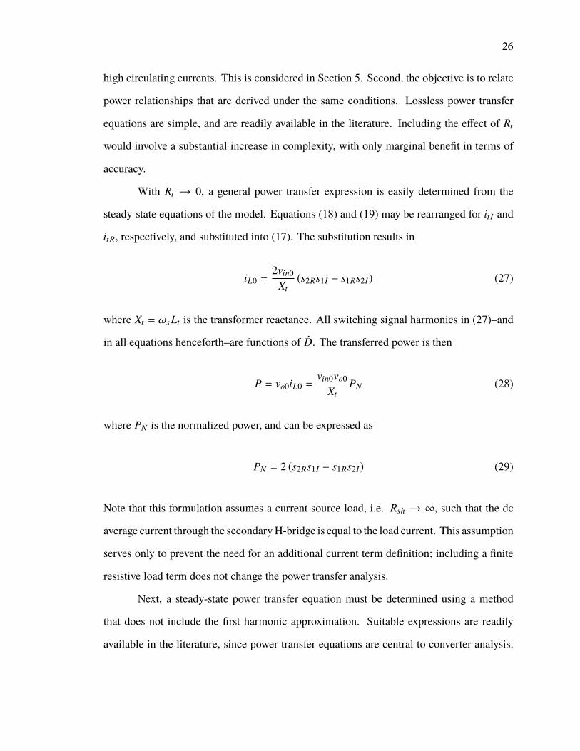
26

high circulating currents. This is considered in Section 5. Second, the objective is to relate

power relationships that are derived under the same conditions. Lossless power transfer

equations are simple, and are readily available in the literature. Including the effect of Rt

would involve a substantial increase in complexity, with only marginal benefit in terms of

accuracy.

With Rt → 0, a general power transfer expression is easily determined from the

steady-state equations of the model. Equations (18) and (19) may be rearranged for it I and

itR, respectively, and substituted into (17). The substitution results in

iL0 =2vin0

Xt(s2Rs1I − s1Rs2I) (27)

where Xt = ωsLt is the transformer reactance. All switching signal harmonics in (27)–and

in all equations henceforth–are functions of D. The transferred power is then

P = vo0iL0 =vin0vo0

XtPN (28)

where PN is the normalized power, and can be expressed as

PN = 2 (s2Rs1I − s1Rs2I) (29)

Note that this formulation assumes a current source load, i.e. Rsh → ∞, such that the dc

average current through the secondaryH-bridge is equal to the load current. This assumption

serves only to prevent the need for an additional current term definition; including a finite

resistive load term does not change the power transfer analysis.

Next, a steady-state power transfer equation must be determined using a method

that does not include the first harmonic approximation. Suitable expressions are readily

available in the literature, since power transfer equations are central to converter analysis.

27

For instance, [18], [19], and [20] provide appropriate equations for triple, dual, and extended

phase shift modulation, respectively. This function for power transfer is referred to as P∗,

to distinguish from the expression determined from model equations.

Because of the wide range of operating cases that occur in triple phase shift modu-

lation, no single expression for P∗ is sufficient. In [18], five separate modes of operation are

defined, each with their own power transfer expression. For full generality, P∗ is defined as

a piecewise function that selects between components according to the control inputs of the

model. Table 1 shows the five power transfer equations and the operating conditions under

which each is active. The active mode is determined by d, and is easily identified from the

control inputs.

The expressions in Table 1 are the same as those in [18], but are given in the

terminology used in this study, and are normalized as:

P∗ =vin0vo0

XtP∗N (30)

The reason for this normalization is to simplify expressions when relating P∗ to P. Clearly,

when P∗ and P are set equal, the leading fractional terms cancel out.

Table 1. Triple Phase Shift Operating Modes and Power Transfer Equations

Mode Operating Region Normalized Power ExpressionI 0 ≤ d ≤ ds

2 −dp

2 P∗N = πdp

(dφ −

dp

2 −ds2

)II 0 ≤ d ≤ dp

2 −ds2 P∗N = πds

(dφ −

dp

2 −ds2

)III

dp2 −

ds2

≤ d ≤ min

dp

2 +ds2 , 1 −

dp

2 −ds2

P∗N =

π2

(dp(ds + 2dφ) − d2

p − d2φ

)IV 1 − dp

2 −ds2 ≤ d ≤ dp

2 +ds2

P∗N =π2[2dφ(1 − dφ − ds + dp)

+ ds(2 + dp − ds) − d2p − 1

]V dp

2 +ds2 ≤ d ≤ 1 − dp

2 −ds2 P∗N =

π2 dpds

28

The final part of the correction procedure is determining how D is generated from

d. Because of the multiple degrees of freedom involved in triple phase shift modulation,

there are several viable ways to do this. The simplest method is to adjust only dφ. The

control variables are then

dφ = d +dp

2−

ds

2(31)

dp = dp (32)

ds = ds (33)

This approach is sufficient for correcting error over the full possible range of control inputs

for both single and dual phase shift modulation.

For triple phase shift modulation, an additional adjustment scheme is needed to

ensure that a solution to the algebraic power equation exists over the entire operating space.

For a solution to exist, the maximum normalized power transfer over the possible range of

d must exceed the corresponding value of P∗. In addition to the correction applied to dφ,

an adjustment can be applied to dp as

dφ = dφ (34)

dp = 2dφ − 2d + ds (35)

ds = ds (36)

For a given set of control inputs, the correction should be applied to either dφ or dp. The

selection is made according to which choice produces the larger maximum normalized

power transfer. This can be determined by the following condition:

sin(

dpπ

2

)> sin2

(π

2

(ds

2+ dφ

))(37)

29

If this condition is true, the correction should be applied to dφ. If not, the correction should

be applied to dp. This condition may be derived as follows. First, analytical expressions for

PN as functions of d are determined for each of the correction schemes. This is done by

substituting either (31), (32), and (33) or (34), (35), and (36) into (29). Next, the maximum

values of the expressions for PN are determined by setting derivatives with respect to d equal

to 0, solving for d, and substituting the results back into the PN expressions. The right and

left sides of (37) correpond to the two resultant expressions after common coefficients have

been eliminated. Therefore, when the inequality is true, applying the correction through dφ

yields the highermaximumnormalized power. This provides a simplemethod of identifying

the the proper correction scheme using only the control inputs to the model.

3.3. Model Organization. The structure of the proposed model framework is

Ûx = f (x, d, u) (38)

0 = g(x, d, u) (39)

where x is the state vector, u is the input vector, and d is an algebraic state variable. The

model state equations are contained in vector-valued function f (·). The scalar function g(·)

is defined as

g(x, d, u) , P∗ − P (40)

Together, f (·) and g(·) define a semi-explicit (or type 1) system of differential

algebraic equations (DAEs).

The state equations, state vector, and input vector differ according to whether an

open or closed-loop system is being modeled. Both are discussed below. Subscripts ‘o’

and ‘c’ are used to denote whether model elements (namely f (·), x, and u) pertain to the

open-loop or closed-loop systems, respectively.

30

The state and input vectors of the open-loop model are

xo = [vo0 itR it I]T (41)

uo = [vin0 iL0 dφ dp ds]T . (42)

The state equations in fo(·) are exactly those of the original DABmodel, shown in Section 2

as (5), (6), and (7). With respect to large-signal error correction, the critical point of

difference between this model and the model in [13] is that d, rather than d, is defined as

an input.

Triple phase shift modulation includes three control variables, and a wide variety of

control structures and feedback mechanisms are possible. To limit scope, the closed-loop

formulation in the present study considers a single controller that regulates output voltage

through the phase shift control variable, dφ. The state and input vectors of the closed-loop

model are

xc = [vo0 itR it I γ0]T (43)

uc = [vin0 iL0 vre f dp ds]T . (44)

The additional state, γ0, is contributed by the integral of a PI controller. In addition to the

open-loop state equations, fc(·) contains (8), which describes γ0. In the original model,

controller output was defined to be dφ (or, equivalently d), as shown in (9). In contrast,

controller output is defined in the present model as

dφ = kp(vre f − vo0

)+ γ0. (45)

3.4. Discussion. The system defined by (38) and (39) is a large-signal generalized

average model that is accurate in both transient and steady-state conditions. The model is

a semi-explicit DAE system. Models of this type are commonly used for describing power

31

systems [21] and are suitable for all applications expected of power electronics models. In

particular, they may be used for time-domain simulations, stability analyses, or linearized

to provide small-signal representations.

Both of the model improvements proposed here generalize the original DAB model

from [13]. Extension to more advanced modulation strategies is a fairly straightforward

improvement, but the inclusion of g(·), too, is a generalization of the original model. The

model from [13] implicitly assumes that d = d. This assumption may be included in the

proposed modeling framework by defining g(·) as 0 = d − d. The resulting structure, when

used with single phase shift modulation, is identical to the model in [13].

While the general model is a DAE system, in some operating cases (namely single

phase shift modulation) it is possible to define d as an explicit function of d, i.e. by solving

g(·) directly for d. When an explicit solution is possible, the model may be converted into

an equivalent system of ODEs.

In comparison to alternative continuous-time DAB modeling approaches, the pri-

mary advantage of the proposed modeling framework is flexibility. The most closely related

methods, i.e. [11] and [16], consider only single phase shift modulation. The method in [11]

is not affected by large-signal error, but its derivation is inherently tied to the modulation

strategy, meaning new modulation schemes would require a full rederivation. In contrast,

the proposed method is derived for general switching functions, so different modulation

schemes are be included by changing modular elements of the base model. Additionally,

the method in [11] models the ac stage by deriving averaged equations for the dc currents

into and out of the H-bridge circuits, effectively consolidating the switching circuit as a

single averaged element. As a result, frequency domain accuracy is limited to 1/10 the

switching frequency. In contrast, the original DAB model from [13] is accurate up to 1/3

of the switching frequency. The upper frequency bound is, in general, imposed by the

eigenvalues of the dynamic model [10, 22]. The proposed model maintains the small-signal

32

accuracy of the model from [13]; when linearized, the eigenvalues of the proposed model

are very close to those of the original model, meaning their upper-limits are similar as well.

This is further illustrated in Sec. 6.

The method from [16] is more closely related to the proposed framework than [11],

but differs in how the correction factor is applied. The correction factor in [16] modifies the

load and state variables directly, and the modifications required are different for each of the

state variables. In this study, error correction is applied through an algebraic equation rather

than through the model state variables, so modifications to the correction factor equation

do not change the base model. This makes it possible to include more general modulation

strategies or lossy correction factors within the same modeling framework.

4. PARTIAL DERIVATIVES AND SMALL-SIGNAL MODELS

Partial derivatives are central to many modeling applications. Partial derivatives are

used for calculating steady-state solutions to model equations, time-domain simulation via

numerical integration, and linearization for small-signal analysis. The partial derivatives of

the models under consideration are given in this section.

4.1. Open-Loop System. The partial derivatives of the open-loop model equations

are with respect to converter states are:

∂ fo∂xo=

−1

RshCo

2Co

s2R2

Cos2I

−1Lt

s2R−Rt

Ltωs

−1Lt

s2I −ωs−Rt

Lt

(46)

∂ fo∂ d=

2

Co

(itR

∂s2R∂ d+ it I

∂s2I∂ d

)1Lt

(vin0

∂s1R∂ d− vo0

∂s2R∂ d

)1Lt

(vin0

∂s1I∂ d− vo0

∂s2I∂ d

)

(47)

33

∂ fo∂uo= (48)

0 −1Co

2Co

(itR

∂s2R∂dφ+ it I

∂s2I∂dφ

)2

Co

(itR

∂s2R∂dp+ it I

∂s2I∂dp

)2

Co

(itR

∂s2R∂ds+ it I

∂s2I∂ds

)1Lt

s1R 0 1Lt

(vin0

∂s1R∂dφ− vo0

∂s2R∂dφ

)1Lt

(vin0

∂s1R∂dp− vo0

∂s2R∂dp

)1Lt

(vin0

∂s1R∂ds− vo0

∂s2R∂ds

)1Lt

s1I 0 1Lt

(vin0

∂s1I∂dφ− vo0

∂s2I∂dφ

)1Lt

(vin0

∂s1I∂dp− vo0

∂s2I∂dp

)1Lt

(vin0

∂s1I∂ds− vo0

∂s2I∂ds

)

The switching signal derivatives are shown in general form in these equations. The specific

derivatives for triple phase shift modulation are given in Sec. 4.3.

The partial derivatives of the algebraic function g(·) are

∂g

∂xo=

[0 0 0

](49)

∂g

∂ d= 2

(s1R

∂s2I

∂ d+ s2I

∂s1R

∂ d

)− 2

(s2R

∂s1I

∂ d+ s1I

∂s2R

∂ d

)(50)

∂g

∂uo=

[0 0 ∂g

∂dφ∂g∂dp

∂g∂ds

](51)

where ∂g∂dφ

, ∂g∂dp

and ∂g∂ds

are given by

∂g

∂dφ=∂P∗N∂dφ+ 2

(s1R

∂s2I

∂dφ+ s2I

∂s1R

∂dφ

)− 2

(s2R

∂s1I

∂dφ+ s1I

∂s2R

∂dφ

)(52)

∂g

∂dp=∂P∗N∂dp+ 2

(s1R

∂s2I

∂dp+ s2I

∂s1R

∂dp

)− 2

(s2R

∂s1I

∂dp+ s1I

∂s2R

∂dp

)(53)

∂g

∂ds=∂P∗N∂ds+ 2

(s1R

∂s2I

∂ds+ s2I

∂s1R

∂ds

)− 2

(s2R

∂s1I

∂ds+ s1I

∂s2R

∂ds

)(54)

The derivatives of P∗N with respect to control inputs depend on the operational mode. For

all of the cases shown in Table 1, these terms are straightforward derivatives of polynomial

functions.

34

4.2. Closed-Loop System. The partial derivatives of the closed-loop model equa-

tions are:

∂ fc∂xc=

−1RshCo

2Co

s2R2

Cos2I 0

−1Lt

s2R−Rt

Ltωs 0

−1Lt

s2I −ωs−Rt

Lt0

−ki 0 0 0

(55)

∂ fc∂ dφ=

∂ fo∂ dφ

0

(56)

where ∂ fo∂ dφ

is given in (47), and

∂ fc∂uc=

0 −1Co

0 2Co

(itR

∂s2R∂dp+ it I

∂s2I∂dp

)2

Co

(itR

∂s2R∂ds+ it I

∂s2I∂ds

)1Lt

s1R 0 0 1Lt

(vin0

∂s1R∂dp− vo0

∂s2R∂dp

)1Lt

(vin0

∂s1R∂ds− vo0

∂s2R∂ds

)1Lt

s1I 0 0 1Lt

(vin0

∂s1I∂dp− vo0

∂s2I∂dp

)1Lt

(vin0

∂s1I∂ds− vo0

∂s2I∂ds

)0 0 ki 0 0

(57)

∂g

∂xc=

[−kp

∂P∗N∂dφ

0 0 ∂P∗N∂dφ

](58)

The derivative ∂g

∂ dφis the same as for the open loop system, as shown in (50). Finally,

∂g

∂uc=

[0 0 kp

∂g∂dφ

∂g∂dp

∂g∂ds

](59)

where ∂g∂dφ

, ∂g∂dp

and ∂g∂ds

are given (52), (53) and (54), respectively.

4.3. Switching Signal Derivatives. When the correction factor is applied through

dφ, switching function s1 is only a function of control variable dp. Therefore, the partial

derivatives of s1R and s1I with respect to d, dφ, and ds are 0. The derivatives with respect

to dp are

35

∂s1R

∂dp= cos(dpπ) (60)

∂s1I

∂dp= − sin(dpπ) (61)

Switching function s2 is a function of variables d (through dφ), dp, and ds. Since dφ is

replaced, the derivatives with respect to dφ are 0. The remaining derivatives are

∂s2R

∂dp=

12

(cos((ds + dφ)π) − cos(dφπ)

)(62)

∂s2I

∂dp=

12

(sin(dφπ) − sin((ds + dφ)π)

)(63)

∂s2R

∂ds=

12

(cos((ds + dφ)π) + cos(dφπ)

)(64)

∂s2I

∂ds=−12

(sin(dφπ) + sin((ds + dφ)π)

)(65)

∂s2R

∂ d= cos((ds + dφ)π) − cos(dφπ) (66)

∂s2I

∂ d= sin(dφπ) − sin((ds + dφ)π) (67)

When the correction factor is applied through dp, switching function s1 depends on

d (through dp), ds, and dφ. Input d1 is replaced, so derivatives with respect to d1 are 0.

∂s1R

∂dφ= cos(dpπ) (68)

∂s1I

∂dφ= − sin(dpπ) (69)

∂s1R

∂ds= 2 cos(dpπ) (70)

∂s1I

∂ds= −2 sin(dpπ) (71)

36

∂s1R

∂ d= −2 cos(dpπ) (72)

∂s1I

∂ d= 2 sin(dpπ) (73)

Lastly, switching function s2 depends only on dφ and ds, so derivatives with respect to dp

and d are zero.∂s2R

∂dφ= cos((ds + dφ)π) (74)

∂s2I

∂dφ= − sin((ds + dφ)π) (75)

∂s2R

∂ds= cos((ds + dφ)π) − cos(dφπ) (76)

∂s2I

∂ds= sin(dφπ) − sin((ds + dφ)π) (77)

4.4. Small-Signal Models. For all models under consideration, the small-signal

models have the form

Ûx = Ax + Bu (78)

where x is a vector of small-signal deviations around a steady-state operating point. Matrices

A and B are calculated using matrix operations, give here in terms of generic functions f (·)

and g(·).

A =∂ f∂x−∂ f

∂ d

(∂g

∂ d

)−1∂g

∂x(79)

B =∂ f∂u−∂ f

∂ d

(∂g

∂ d

)−1∂g

∂u(80)

The derivation for these linearized matrices is given in the Appendix.

37

5. CONSIDERATIONS FOR SINGLE PHASE SHIFT MODULATION

Although single phase shift modulation has several performance deficiencies, it is

still commonly used in DAB literature due to its overall simplicity. In particular, single

phase shift is commonly used in studies that include DAB converters as elements of a larger

system [15, 23]. In light of this, a more detailed consideration of the single phase shift case

is given here. As a secondary benefit, this section provides a simple illustration of how the

general framework outlined in Section 4 may be applied to a specific modulation scheme.

5.1. Model Simplifications. Single phase shift modulation is a subset of triple

phase shift, and corresponds to the case in which dp and ds are constant and equal to 1. This

condition simplifies the model. With dp and ds fixed, it is not necessary to include these

variables as model inputs, and dφ = d.

The first harmonic components of switching functions for single phase shift modu-

lation may be recovered by fixing dp = ds = 1 in (23)–(26).

s1R(d) = 0 (81)

s1I(d) = −2π

(82)

s2R(d) = −2 sin(dπ)

π(83)

s2I(d) = −2 cos(dπ)

π(84)

Furthermore, single phase shift modulation restricts the operating region of the

converter. According to Table 1, single phase shift modulation is entirely contained in

Mode IV, so only one power transfer equation is necessary.

5.2. Lossless Case. Without including Rt , the procedure begins directly with nor-

malized power:

PN = 2(s2Rs1I − s1Rs2I) =8 sin(dπ)

π2 (85)

38

Next, the power transfer equation from Table 1 is reduced using the same condi-

tions on dp and ds. These conditions restrict the operating region to Mode IV, and the

corresponding equation simplifies to

P∗N = πd(1 − d). (86)

Therefore, the equation that relates d to d is

g(x, d, u) =π3d(1 − d)

8− sin πd (87)

5.3. Lossy Case. In the lossy case, Rt is nonzero. The parameter Rt is represents

winding losses in the transformer, but it can also be used as a lumped-element parameter to

represent conduction losses in the semiconductors as well. Including Rt in the large-signal

error correction requires a substantial increase in complexity, and is only necessary when

the losses modeled by Rt become significant. One case in which Rt plays an important role

is single phase shift modulation with high phase shift values. Under these conditions, the

transformer will experience high circulating currents, and conduction losses will be larger.

While this issue may be addressed through the use of more advanced modulation schemes,

there is still a need to accurately represent converter behavior under these conditions when

single phase shift modulation is used. The problem with including Rt in the error correction

is that the power transfer equations become dependent on state variables and hardware

parameters. In the previous cases, g(·) was only dependent on control variables. This is

not the case when Rt is included. Nevertheless, the procedure for deriving the correction

equation remains the same. The expression for iL0 in terms of d given in (27) was derived

with Rt → 0. When Rt included in the derivation, the resulting expression is

iL0 =2((s2RRt − s2I Xt) (vin0s1R − vo0s2R)

)R2

t + X2t

+2((s2I Rt + s2RXt) (vin0s1I − vo0s2I)

)R2

t + X2t

(88)

39

After applying the simplifications for single phase shift modulation, this may be

more conveniently written as

iL0 =2Xt

πR2t K(vin0Rt cos πd + vin0Xt sin πd − vo0Rt) (89)

where K is a hardware constant given by

K =π

4Xt(R2

t + X2t )

R2t

. (90)

The definition of K is arbitrary at this point, but substantially simplifies derivative terms

when linearizing the model.

The next step is to determine a corresponding expression in terms of d. Average

output current equations have previously been derived in the literature. One such equation

is used by the average value model proposed in [11]. However, the equation in question

(Eq. (19) in [11]) is valid only for unidirectional power flow, i.e. d > 0. A more suitable

equation is derived in [12] by integrating the instantaneous current terms, which are piece-

wise exponential, over the switching period. This expression (originally Eq. (6) in [12]) is

cumbersome; the authors of [12] spend considerable effort obtaining a more manageable

approximation. In this study, we use a simplified form of the exact equation:

i∗L0 =(vin0 − vo0)

Rt+

vo0θRt

tanh θ +d|d |

(vin0θRt

) [1 − 2θd − sech θ exp

(d|d |θ − 2θd

)](91)

where θ is a hardware constant.

θ =πRt

2Xt(92)

The expression in (91) is mathematically equivalent to Eq. (6) in [12]. The only

differences are that notational conventions have been changed (e.g. phase shift is defined as a

fraction of the switching period rather than an angle) and simplifications have been applied

using hyperbolic function identities. The exact conversion consists entirely of standard

40

algebraic manipulations, and the result is easily verified using a computer algebra system.

The final form of (91) is relatively simple. The arguments of hyperbolic functions tanh and

sech are hardware constants, so they have very little impact on complexity when applied

in the model. Furthermore, the sign factors d|d | are only necessary to support bidirectional

operation. For the unidirectional power flow case these may be eliminated entirely.

The final step is to form the algebraic correction equation. Since P = vo0iL0 and

P∗ = vo0i∗L0, the equation may be defined as

g(x, d, u) = i∗L0 − iL0

= −vin0Rt cos πd − vin0Xt sin πd + vo0Rt

+ K (vin0 − vo0) θ + Kvo0 tanh θ

+ Kvin0d|d |

(1 − 2θd − sech θ exp

(d|d |θ − 2θd

))(93)

Since (19) includes vo0 and vin0, some of the derivatives from Section 4 must be

changed. For the open-loop system, the derivatives of g(·) are

∂g

∂xo=

[Rt − K (θ − tanh θ) 0 0

](94)

∂g

∂ d= πvin0

(Rt sin πd − Xt cos πd

)(95)

∂g

∂uo=

[∂g∂vin0

0 ∂g∂d

](96)

where elements ∂g∂vin0

and ∂g∂d are given by

∂g

∂vin0= Kθ − Rt cos πd − Xt sin πd + K

d|d |

(1 − 2θd − sech θ exp

(d|d |θ − 2θd

))(97)

∂g

∂d=

(2dθKvin0|d |

) (sech θ exp

(d|d |θ − 2θd

)− 1

)(98)

41

For the closed-loop system, the derivatives of g(·) are

∂g

∂xc=

[Rt − K (θ − tanh θ) 0 0 ∂g

∂d

](99)

∂g

∂uc=

[∂g∂vin0

0 kp∂g∂d

](100)

where the elements ∂g∂vin0

and ∂g∂d are given in (97) and (98), respectively.

6. VERIFICATION

To validate the proposed models, experiments were performed to verify model accu-

racy both at steady-state and during transient response. The experiments were conducted

using a small-scale DAB prototype, shown in Fig. 3. Switching simulations performed in

PLECS supplement the hardware results. The prototype converter is controlled by a Texas

Instruments TMS320F28377S digital signal processor (DSP). Both the sampling rate and

switching frequency of the converter were 80 kHz. Switching dead time was td = 300 ns.

These and other important parameters are given in Table 2.

The effect of switching dead time on converter behavior is significant in practice.

Dead time introduces conduction modes that are not explicitly included in the model

derivation, and effectively changes the control inputs dφ, dp, and ds [24]. Including

conduction modes related to dead time in the model would require a substantial increase

in complexity. Alternatively, dead time compensation strategies may be employed in the

control system. The latter approach is used here: dead time is compensated in the controller

by applying phase shift corrections according to [25].

6.1. Steady-State Accuracy. The first test considers steady-state accuracy. The

converter output voltage is measured while varying dφ. A resistive load is used and input

voltage is fixed at 10 V throughout. Results for triple and dual phase shift modulation are

shown in Fig. 4 and Fig. 5, respectively. For these results, and the dual and triple phase shift

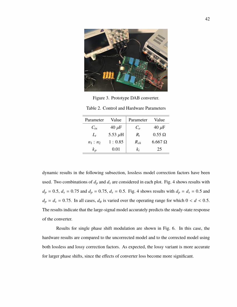
42

Figure 3. Prototype DAB converter.

Table 2. Control and Hardware Parameters

Parameter Value Parameter ValueCin 40 µF Co 40 µFLt 5.53 µH Rt 0.55 Ω

n1 : n2 1 : 0.85 Rsh 6.667 Ωkp 0.01 ki 25

dynamic results in the following subsection, lossless model correction factors have been

used. Two combinations of dp and ds are considered in each plot. Fig. 4 shows results with

dp = 0.5, ds = 0.75 and dp = 0.75, ds = 0.5. Fig. 4 shows results with dp = ds = 0.5 and

dp = ds = 0.75. In all cases, dφ is varied over the operating range for which 0 < d < 0.5.

The results indicate that the large-signal model accurately predicts the steady-state response

of the converter.

Results for single phase shift modulation are shown in Fig. 6. In this case, the

hardware results are compared to the uncorrected model and to the corrected model using

both lossless and lossy correction factors. As expected, the lossy variant is more accurate

for larger phase shifts, since the effects of converter loss become more significant.

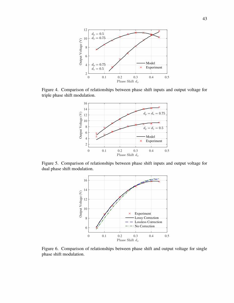
43

0 0.1 0.2 0.3 0.4 0.52

4

6

8

10

12

Outp

ut

Volt

age

(V)

Model

Experiment

Figure 4. Comparison of relationships between phase shift inputs and output voltage fortriple phase shift modulation.

0 0.1 0.2 0.3 0.4 0.5

2

4

6

8

10

12

14

16

Outp

ut

Volt

age

(V)

Model

Experiment

Figure 5. Comparison of relationships between phase shift inputs and output voltage fordual phase shift modulation.

0 0.1 0.2 0.3 0.4 0.5

6

8

10

12

14

16

Outp

ut

Volt

age

(V)

Experiment

Lossy Correction

Lossless Correction

No Correction

Figure 6. Comparison of relationships between phase shift and output voltage for singlephase shift modulation.

44

6.2. Dynamic Accuracy. The second set of tests consider dynamic response, na-

mely the output voltage transients for step changes in phase shift inputs. The experiment

uses same resistive load and 10 V input voltage as in the previous test. For triple phase shift

modulation, step changes to dp and ds are considered. The results are shown in Fig. 7. At

the start of the experiment, both dp and ds are 0.5; at t = 0 ms, ds steps from 0.5 to 0.75.

At t = 2 ms, dp steps from 0.5 to 0.75. The model predictions and experimental results are

consistent for both transients.

In dual phase shift modulation, dp and ds are equal, so only one step change is

considered. The results for dual phase shift modulation are shown in Fig. 8. At time

t = 0 ms, both dp and ds change from 0.5 to 0.75. Again, the model accurately predicts the

response.

For single phase shift, step changes in dφ are considered. As in the steady-state

experiments, hardware measurements are compared to the uncorrected model and to both

lossless and lossy variants of the corrected model. The results are shown in Fig. 9. In the

top plot, dφ steps from 0.15 to 0.3 at t = 0 ms; in the bottom plot dφ steps from 0.3 to

0.4. The plots show both the raw hardware measurements and dc sliding averages of the

measurements, taken over a single switching period. These averages are, by definition, the

experimental vo0.

The top plots of Fig. 9 show that if large phase shifts are avoided, the difference in

accuracy between the lossless and lossy model variants is negligible. However, the bottom

plots show a situation in which the lossy correction equation is measurably superior. This

is particularly clear when comparing model predictions to the dc average output voltage

measurements. In both cases, the inclusion of either correction factor consistently improves

accuracy with respect to the uncorrected model.

The results in Fig. 9 show that the proposed modeling framework improves on the

accuracy of the original model. However, these results use large-signal model predictions.

To assess the small-signal accuracy of the models, frequency-domain predictions are com-

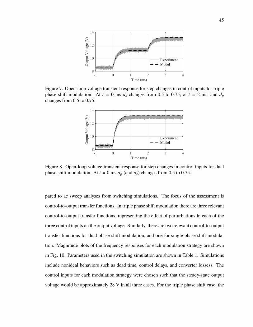
45

-1 0 1 2 3 4

Time (ms)

a) TPS Step Responses

8

10

12

14

Outp

ut

Volt

age

(V)

Experiment

Model

Figure 7. Open-loop voltage transient response for step changes in control inputs for triplephase shift modulation. At t = 0 ms ds changes from 0.5 to 0.75; at t = 2 ms, and dpchanges from 0.5 to 0.75.

-1 0 1 2 3 4

Time (ms)

b) DPS Step Response

8

10

12

14

Outp

ut

Volt

age

(V)

Experiment

Model

Figure 8. Open-loop voltage transient response for step changes in control inputs for dualphase shift modulation. At t = 0 ms dp (and ds) changes from 0.5 to 0.75.

pared to ac sweep analyses from switching simulations. The focus of the assessment is

control-to-output transfer functions. In triple phase shift modulation there are three relevant

control-to-output transfer functions, representing the effect of perturbations in each of the

three control inputs on the output voltage. Similarly, there are two relevant control-to-output

transfer functions for dual phase shift modulation, and one for single phase shift modula-

tion. Magnitude plots of the frequency responses for each modulation strategy are shown

in Fig. 10. Parameters used in the switching simulation are shown in Table 1. Simulations

include nonideal behaviors such as dead time, control delays, and converter lossess. The

control inputs for each modulation strategy were chosen such that the steady-state output

voltage would be approximately 28 V in all three cases. For the triple phase shift case, the

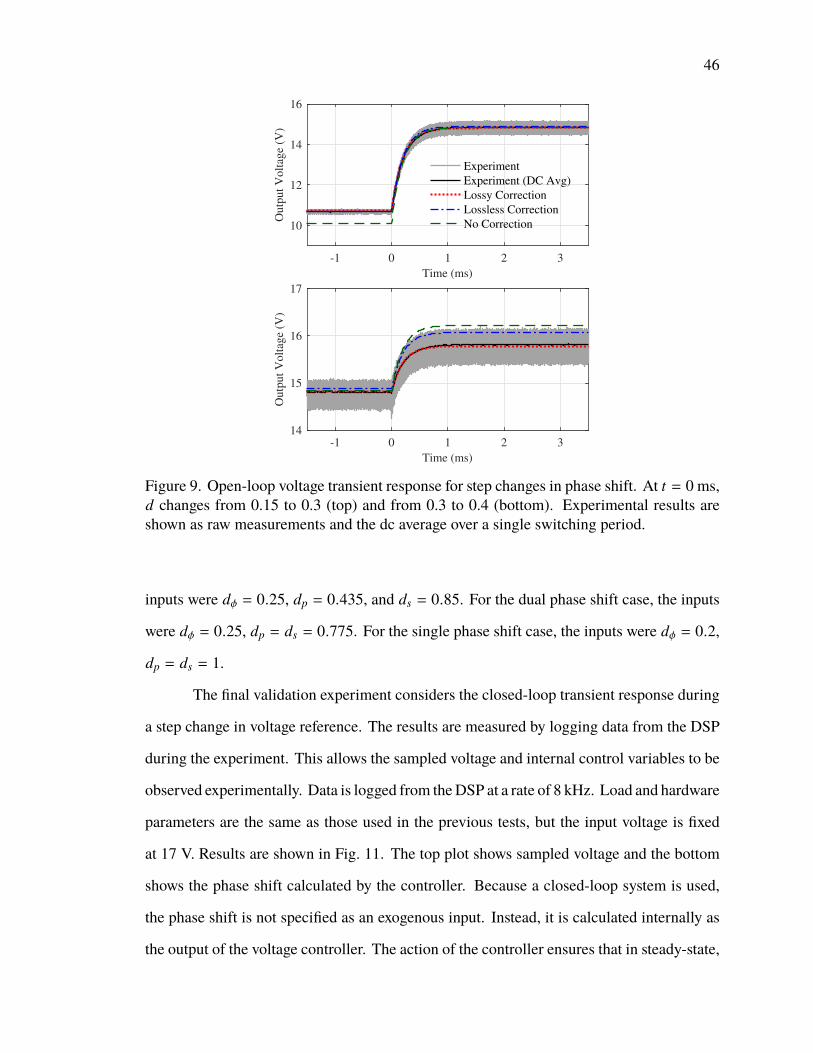
46

-1 0 1 2 3

Time (ms)

10

12

14

16

Outp

ut

Volt

age

(V)

Experiment

Experiment (DC Avg)

Lossy Correction

Lossless Correction

No Correction

-1 0 1 2 3

Time (ms)

14

15

16

17O

utp

ut

Volt

age

(V)

Figure 9. Open-loop voltage transient response for step changes in phase shift. At t = 0 ms,d changes from 0.15 to 0.3 (top) and from 0.3 to 0.4 (bottom). Experimental results areshown as raw measurements and the dc average over a single switching period.

inputs were dφ = 0.25, dp = 0.435, and ds = 0.85. For the dual phase shift case, the inputs

were dφ = 0.25, dp = ds = 0.775. For the single phase shift case, the inputs were dφ = 0.2,

dp = ds = 1.

The final validation experiment considers the closed-loop transient response during

a step change in voltage reference. The results are measured by logging data from the DSP

during the experiment. This allows the sampled voltage and internal control variables to be

observed experimentally. Data is logged from theDSP at a rate of 8 kHz. Load and hardware

parameters are the same as those used in the previous tests, but the input voltage is fixed

at 17 V. Results are shown in Fig. 11. The top plot shows sampled voltage and the bottom

shows the phase shift calculated by the controller. Because a closed-loop system is used,

the phase shift is not specified as an exogenous input. Instead, it is calculated internally as

the output of the voltage controller. The action of the controller ensures that in steady-state,

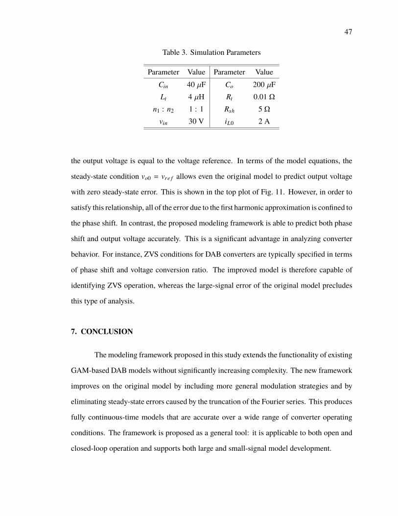
47

Table 3. Simulation Parameters

Parameter Value Parameter ValueCin 40 µF Co 200 µFLt 4 µH Rt 0.01 Ω

n1 : n2 1 : 1 Rsh 5 Ωvin 30 V iL0 2 A

the output voltage is equal to the voltage reference. In terms of the model equations, the

steady-state condition vo0 = vre f allows even the original model to predict output voltage

with zero steady-state error. This is shown in the top plot of Fig. 11. However, in order to

satisfy this relationship, all of the error due to the first harmonic approximation is confined to

the phase shift. In contrast, the proposed modeling framework is able to predict both phase

shift and output voltage accurately. This is a significant advantage in analyzing converter

behavior. For instance, ZVS conditions for DAB converters are typically specified in terms

of phase shift and voltage conversion ratio. The improved model is therefore capable of

identifying ZVS operation, whereas the large-signal error of the original model precludes

this type of analysis.

7. CONCLUSION

The modeling framework proposed in this study extends the functionality of existing

GAM-based DABmodels without significantly increasing complexity. The new framework

improves on the original model by including more general modulation strategies and by

eliminating steady-state errors caused by the truncation of the Fourier series. This produces

fully continuous-time models that are accurate over a wide range of converter operating

conditions. The framework is proposed as a general tool: it is applicable to both open and

closed-loop operation and supports both large and small-signal model development.

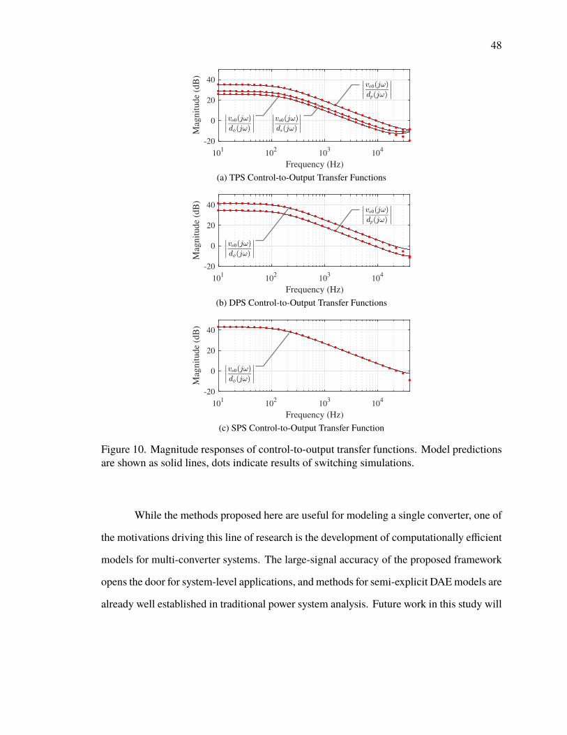
48

101

102

103

104

Frequency (Hz)

-20

0

20

40

Mag

nit

ud

e (d

B)

(a) TPS Control-to-Output Transfer Functions

101

102

103

104

Frequency (Hz)

-20

0

20

40M

agn

itu

de

(dB

)

(b) DPS Control-to-Output Transfer Functions

101

102

103

104

Frequency (Hz)

-20

0

20

40

Mag

nit

ud

e (d

B)

(c) SPS Control-to-Output Transfer Function

Figure 10. Magnitude responses of control-to-output transfer functions. Model predictionsare shown as solid lines, dots indicate results of switching simulations.

While the methods proposed here are useful for modeling a single converter, one of

the motivations driving this line of research is the development of computationally efficient

models for multi-converter systems. The large-signal accuracy of the proposed framework

opens the door for system-level applications, and methods for semi-explicit DAEmodels are

already well established in traditional power system analysis. Future work in this study will

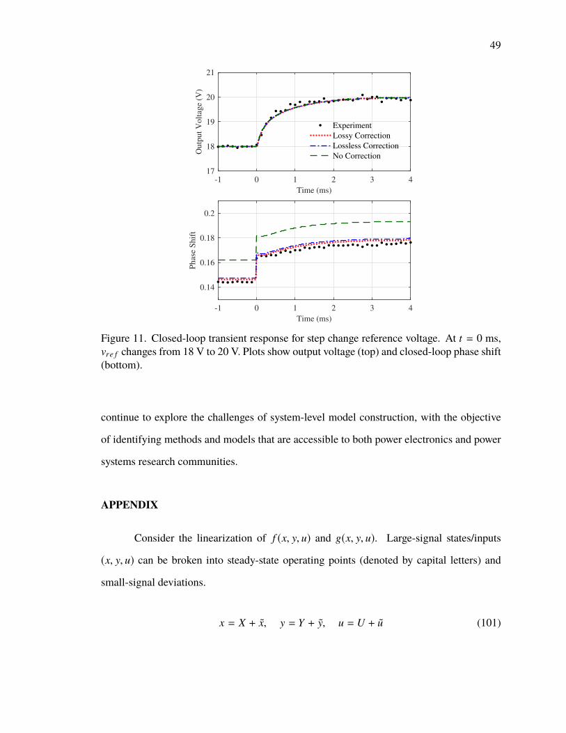
49

-1 0 1 2 3 4

Time (ms)

17

18

19

20

21

Outp

ut

Volt

age

(V)

Experiment

Lossy Correction

Lossless Correction

No Correction

-1 0 1 2 3 4

Time (ms)

0.14

0.16

0.18

0.2

Phas

e S

hif

t

Figure 11. Closed-loop transient response for step change reference voltage. At t = 0 ms,vre f changes from 18 V to 20 V. Plots show output voltage (top) and closed-loop phase shift(bottom).

continue to explore the challenges of system-level model construction, with the objective

of identifying methods and models that are accessible to both power electronics and power

systems research communities.

APPENDIX

Consider the linearization of f (x, y, u) and g(x, y, u). Large-signal states/inputs

(x, y, u) can be broken into steady-state operating points (denoted by capital letters) and

small-signal deviations.

x = X + x, y = Y + y, u = U + u (101)

50

The first order Taylor series expansion of f (·) is

Ûx = ÛX + Ûx ≈ f (X,Y,U) +∂ f∂x

x +∂ f∂y

y +∂ f∂u

u (102)

where ∂ f∂x ,

∂ f∂y , and

∂ f∂u are evaluated at (X,Y,U). By definition, ÛX = f (X,Y,U) = 0, so

Ûx =∂ f∂x

x +∂ f∂y

y +∂ f∂u

u (103)

Similarly, the Taylor series expansions of g(·) is

0 = g(X,Y,U) +∂g

∂xx +

∂g

∂yy +

∂g

∂uu (104)

Again, derivatives are evaluated at (X,Y,U), and 0 = g(X,Y,U). An expression for y may

be found by rearranging this equation.

y =

(∂g

∂y

)−1 (−∂g

∂xx −

∂g

∂uu)

(105)

Substituting this expression into (103) eliminates y. The resulting equation is

Ûx =∂ f∂x

x −∂ f∂y

(∂g

∂y

)−1 (∂g

∂xx +

∂g

∂uu)+∂ f∂u

u (106)

= Ax + Bu (107)

where A and B correspond to the expressions in (79) and (80), respectively.

REFERENCES

[1] R. W. A. A. DeDoncker, D. M. Divan, and M. H. Kheraluwala, “A three-phase

soft-switched high-power-density dc/dc converter for high-power applications,” IEEE

Trans. Ind. Appl., vol. 27, no. 1, pp. 63–73, 1991.

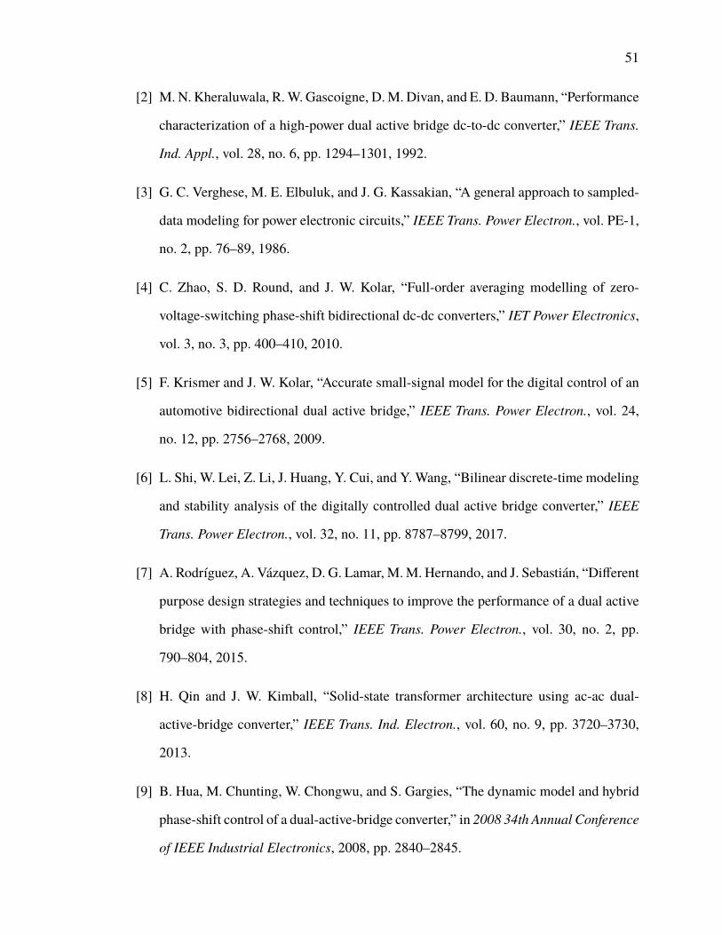
51

[2] M. N. Kheraluwala, R.W. Gascoigne, D.M. Divan, and E. D. Baumann, “Performance

characterization of a high-power dual active bridge dc-to-dc converter,” IEEE Trans.

Ind. Appl., vol. 28, no. 6, pp. 1294–1301, 1992.

[3] G. C. Verghese, M. E. Elbuluk, and J. G. Kassakian, “A general approach to sampled-

data modeling for power electronic circuits,” IEEE Trans. Power Electron., vol. PE-1,

no. 2, pp. 76–89, 1986.

[4] C. Zhao, S. D. Round, and J. W. Kolar, “Full-order averaging modelling of zero-

voltage-switching phase-shift bidirectional dc-dc converters,” IET Power Electronics,

vol. 3, no. 3, pp. 400–410, 2010.

[5] F. Krismer and J. W. Kolar, “Accurate small-signal model for the digital control of an

automotive bidirectional dual active bridge,” IEEE Trans. Power Electron., vol. 24,

no. 12, pp. 2756–2768, 2009.

[6] L. Shi, W. Lei, Z. Li, J. Huang, Y. Cui, and Y. Wang, “Bilinear discrete-time modeling

and stability analysis of the digitally controlled dual active bridge converter,” IEEE

Trans. Power Electron., vol. 32, no. 11, pp. 8787–8799, 2017.

[7] A. Rodríguez, A. Vázquez, D. G. Lamar, M.M. Hernando, and J. Sebastián, “Different

purpose design strategies and techniques to improve the performance of a dual active

bridge with phase-shift control,” IEEE Trans. Power Electron., vol. 30, no. 2, pp.

790–804, 2015.

[8] H. Qin and J. W. Kimball, “Solid-state transformer architecture using ac-ac dual-

active-bridge converter,” IEEE Trans. Ind. Electron., vol. 60, no. 9, pp. 3720–3730,

2013.

[9] B. Hua, M. Chunting, W. Chongwu, and S. Gargies, “The dynamic model and hybrid

phase-shift control of a dual-active-bridge converter,” in 2008 34th Annual Conference

of IEEE Industrial Electronics, 2008, pp. 2840–2845.

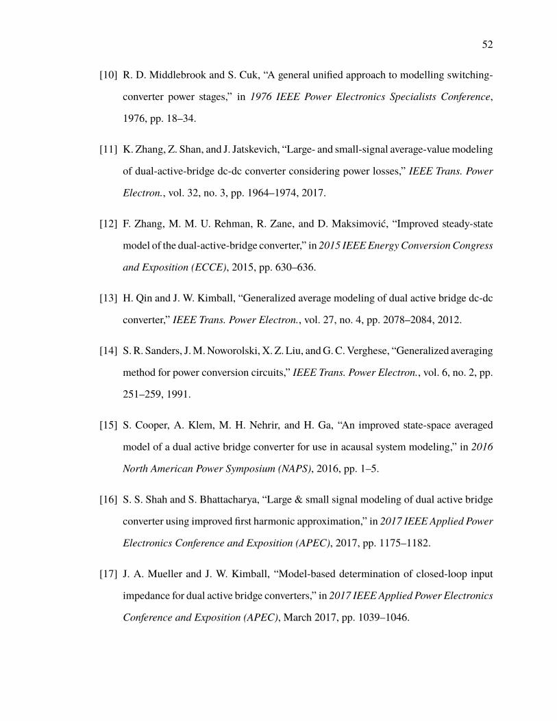
52

[10] R. D. Middlebrook and S. Cuk, “A general unified approach to modelling switching-

converter power stages,” in 1976 IEEE Power Electronics Specialists Conference,

1976, pp. 18–34.

[11] K. Zhang, Z. Shan, and J. Jatskevich, “Large- and small-signal average-valuemodeling

of dual-active-bridge dc-dc converter considering power losses,” IEEE Trans. Power

Electron., vol. 32, no. 3, pp. 1964–1974, 2017.

[12] F. Zhang, M. M. U. Rehman, R. Zane, and D. Maksimović, “Improved steady-state

model of the dual-active-bridge converter,” in 2015 IEEEEnergyConversionCongress

and Exposition (ECCE), 2015, pp. 630–636.

[13] H. Qin and J. W. Kimball, “Generalized average modeling of dual active bridge dc-dc

converter,” IEEE Trans. Power Electron., vol. 27, no. 4, pp. 2078–2084, 2012.

[14] S. R. Sanders, J.M.Noworolski, X. Z. Liu, andG.C.Verghese, “Generalized averaging

method for power conversion circuits,” IEEE Trans. Power Electron., vol. 6, no. 2, pp.

251–259, 1991.

[15] S. Cooper, A. Klem, M. H. Nehrir, and H. Ga, “An improved state-space averaged

model of a dual active bridge converter for use in acausal system modeling,” in 2016

North American Power Symposium (NAPS), 2016, pp. 1–5.

[16] S. S. Shah and S. Bhattacharya, “Large & small signal modeling of dual active bridge

converter using improved first harmonic approximation,” in 2017 IEEE Applied Power

Electronics Conference and Exposition (APEC), 2017, pp. 1175–1182.

[17] J. A. Mueller and J. W. Kimball, “Model-based determination of closed-loop input

impedance for dual active bridge converters,” in 2017 IEEE Applied Power Electronics

Conference and Exposition (APEC), March 2017, pp. 1039–1046.

53

[18] J. Huang, Y. Wang, Z. Li, and W. Lei, “Unified triple-phase-shift control to minimize

current stress and achieve full soft-switching of isolated bidirectional dc-dc converter,”

IEEE Trans. Ind. Electron., vol. 63, no. 7, pp. 4169–4179, 2016.

[19] B. Zhao, Q. Song, and W. Liu, “Power characterization of isolated bidirectional

dual-active-bridge dc-dc converter with dual-phase-shift control,” IEEE Trans. Power

Electron., vol. 27, no. 9, pp. 4172–4176, 2012.

[20] B. Zhao, Q. Yu, and W. Sun, “Extended-phase-shift control of isolated bidirectional

dc-dc converter for power distribution in microgrid,” IEEE Trans. Power Electron.,

vol. 27, no. 11, pp. 4667–4680, 2012.

[21] M. L. Crow, “Numerical integration,” in Computational Methods for Electric Power

Systems, 3rd ed. Boca Raton, FL: CRC Press, 2016.

[22] P. T. Krein, J. Bentsman, R. M. Bass, and B. L. Lesieutre, “On the use of averaging for

the analysis of power electronic systems,” IEEE Trans. Power Electron., vol. 5, no. 2,

pp. 182–190, 1990.

[23] D. Gonzalez-Agudelo, A. Escobar-Mejía, and H. Ramirez-Murrillo, “Dynamic model

of a dual active bridge suitable for solid state transformers,” in 2016 13th International

Conference on Power Electronics (CIEP), 2016, pp. 350–355.

[24] B. Zhao, Q. Song, W. Liu, and Y. Sun, “Dead-time effect of the high-frequency

isolated bidirectional full-bridge dc-dc converter: Comprehensive theoretical analysis

and experimental verification,” IEEE Trans. Power Electron., vol. 29, no. 4, pp. 1667–

1680, 2014.

[25] D. Segaran, D. G. Holmes, and B. P. McGrath, “Enhanced load step response for

a bidirectional dc-dc converter,” IEEE Trans. Power Electron., vol. 28, no. 1, pp.

371–379, 2013.

54

II. MODELING DUAL ACTIVE BRIDGE CONVERTERS IN DC DISTRIBUTIONSYSTEMS

Jacob A. Mueller and Jonathan W. Kimball

Department of Electrical & Computer Engineering

Missouri University of Science and Technology

Rolla, Missouri 65409–0050

Email: jam8z4@mst.edu

ABSTRACT

Modeling improvements are proposed for systems containing dual active bridge (DAB)

converters. First, a systematic approach to constructing models of multi-converter systems

is described. The method generates continuous-time large-signal average models that are

suitable for system-level analysis and efficient time-domain simulation. Although the base

DAB models are derived using generalized average modeling (GAM), the system-level

construction does not require the specification of a base period. Secondly, a method of

reconstructing currents in the high-frequency DAB transformer is proposed. This method

significantly improves accuracy in modeling transformer current, which is a critical we-

akness of DAB models derived using GAM. Furthermore, the method is applied offline

as needed, so it does not affect the computational complexity of time-domain simulation.

Both the system-level model construction procedure and harmonic reconstruction method

are validated in switching simulations and hardware experiments.

Keywords: average modeling, dual active bridge converter, generalized average model,

phase shift modulation

55

1. INTRODUCTION

Dual active bridge (DAB) converters are well-suited to applications in power distri-

bution systems due to their high power density, low device stresses, galvanic isolation, and

bidirectional operation [1, 2]. DAB converters have been considered as a candidate topology

for solid-state transformers [3, 4] and have been studied in the context of automotive [5],

aerospace [6], and marine power systems [7, 8]. In all of these applications, the ability

to accurately describe the behavior of the DAB converter–and its interactions with other

converters in the system–is of critical importance. System-level analyses, such as stability

assessments and time-domain simulation, depend on models that are both accurate and

scalable. This study is concerned with the development of models that meet these criteria.

Modeling DAB converters is difficult due to the presence of a high-frequency ac

conversion stage and ac state variables. The most popular strategy for dealing with this

challenge is to employ the sampled-data modeling method from [9]. This method produces

discrete-time models that provide exact state solutions for each sub-interval within the base

switching period. Models of this type are described in [10, 11, 5], among others. However,

this modeling approach assumes that the system cycles through a set of switching modes at

some base period, and requires explicit descriptions of each mode. These requirements are

trivial for a single converter, but more complicated when the system consists of multiple

converters, particularly when converters operate at different switching frequencies.

Continuous-time DAB models have been proposed as well, using both state-space

averaging and generalized averaging methods. Those derived using classical state-space

averaging either eliminate the ac transformer current state during the averaging process

(as in [12]), or represent the transformer by averaging the current into and out of the dual

H-bridge circuits [13, 14]. The disadvantage of these models is inherited from the basic

averaging framework: the models are derived by calculating the dc average over each

switching period and are therefore limited in their ability to represent dynamics at higher

frequencies [13].

56

Generalized average modeling (GAM) provides fully continuous-time representati-

ons that are capable of describing ac state variables [15]. This is accomplished by expanding

state variables into Fourier series components. A DABmodel derived using GAMwas pro-

posed in [16]. To achieve a balance of accuracy and complexity, this model was derived

under a first harmonic approximation, i.e. with the Fourier series truncated at the first har-

monic. The resulting model was accurate for small-signal disturbances, but inaccurate at

steady-state due to the first harmonic approximation. A corrective modification was propo-

sed in [17], leading to an improved large-signal model that is accurate in both transient and

steady-state operation. While the new model addresses large-signal error, it is still subject

to limitations of the first harmonic approximation. In particular, the transformer current

state is represented using only the first harmonic of its Fourier series, i.e. as a sinusoid at

the converter switching frequency.

Of the modeling approaches described here, the GAM framework is the most ap-

propriate for developing system-level models. GAM methods for constructing models of

multi-converter systems are available in existing literature [18]. In general, GAM com-

plexity scales poorly with system size [19], and the foremost challenge is preserving model

tractability. For instance, in [7], both state-space averaging and GAM were used to de-

rive large-signal models of a shipboard power system. The authors conclude that, despite

greater accuracy, the model derived using GAM is less suitable for efficient time-domain

simulation due to high computational complexity. However, in the case of a DAB converter

it is possible to mitigate scalability issues using structural properties of the model. In parti-

cular, the state equations of the original model in [16] are decoupled along lines of physical

relevance, making it possible to consider only the states of interest in the final model. The

same decoupling effect exists for systems of multiple DAB converters as well [20].

This study presents two contributions. The first is a method of constructing accurate

and scalable models of systems containing multiple DAB converters. Models generated

using this method are suitable for fast time-domain simulation or linearization for small-

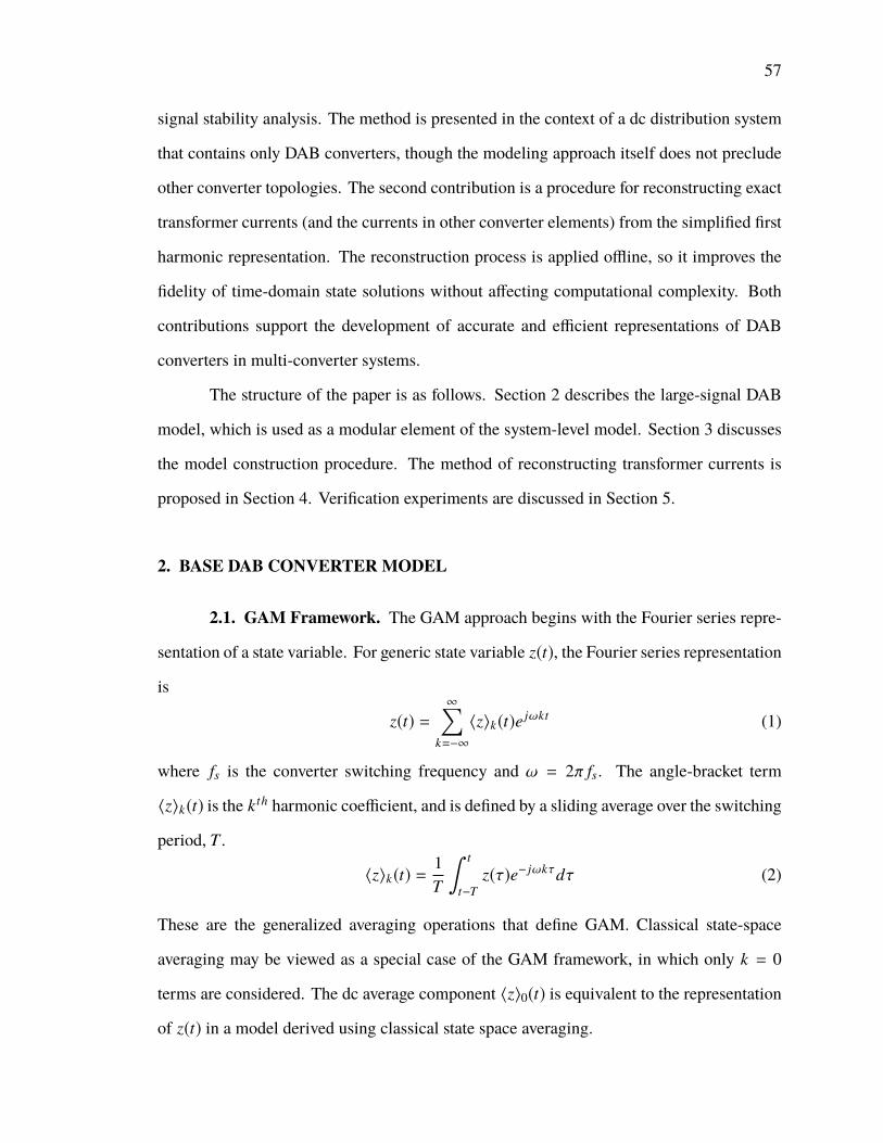
57

signal stability analysis. The method is presented in the context of a dc distribution system

that contains only DAB converters, though the modeling approach itself does not preclude

other converter topologies. The second contribution is a procedure for reconstructing exact

transformer currents (and the currents in other converter elements) from the simplified first

harmonic representation. The reconstruction process is applied offline, so it improves the

fidelity of time-domain state solutions without affecting computational complexity. Both

contributions support the development of accurate and efficient representations of DAB

converters in multi-converter systems.

The structure of the paper is as follows. Section 2 describes the large-signal DAB

model, which is used as a modular element of the system-level model. Section 3 discusses

the model construction procedure. The method of reconstructing transformer currents is

proposed in Section 4. Verification experiments are discussed in Section 5.

2. BASE DAB CONVERTER MODEL

2.1. GAM Framework. The GAM approach begins with the Fourier series repre-

sentation of a state variable. For generic state variable z(t), the Fourier series representation

is

z(t) =∞∑

k=−∞

〈z〉k(t)e jωkt (1)

where fs is the converter switching frequency and ω = 2π fs. The angle-bracket term

〈z〉k(t) is the k th harmonic coefficient, and is defined by a sliding average over the switching

period, T .

〈z〉k(t) =1T

∫ t

t−Tz(τ)e− jωkτdτ (2)

These are the generalized averaging operations that define GAM. Classical state-space

averaging may be viewed as a special case of the GAM framework, in which only k = 0

terms are considered. The dc average component 〈z〉0(t) is equivalent to the representation

of z(t) in a model derived using classical state space averaging.

58

Two additional relationships are used in the application of GAM [15, 21]. The

derivative of the harmonic coefficients is given by

ddt〈z〉k(t) =

⟨ddt

z⟩

k(t) − jωk 〈z〉k(t). (3)

The product of coefficients is

〈z · y〉k(t) =∞∑

i=−∞

〈z〉k−i(t) · 〈y〉i(t). (4)

Under a first harmonic approximation, (k = 0, ±1) the time-domain state may be

recovered from the harmonic components as

z(t) = 〈z〉1(t)e jωt + 〈z〉−1(t)e− jωt + 〈z〉0(t)

= 2(〈z〉R(t) cosωt − 〈z〉I(t) sinωt

)+ 〈z〉0(t) (5)

where 〈z〉R(t) = <[〈z〉1(t)] and 〈z〉I(t) = =[〈z〉1(t)] are the real and imaginary components

of the first harmonic coefficient. This approximation limits both the complexity and large-

signal accuracy of the final model, since higher-order terms are neglected. However, in

the case of a DAB converter, the large-signal error may be corrected through the use of an

algebraic correction factor [17].

2.2. Single ConverterModel. This study uses the improved DABmodel from [17]

as a fundamental building block for the construction of a system level model. The model

in [17] is based on [16], but includes a correction factor to eliminate large-signal errors

introduced by the first harmonic approximation. The correction equation does not change

the model state equations, so the original formulation in [16] is relevant to the present

discussion. Since the objective is to analyze the converter behavior in a full system, the

closed-loop formulation is used. A diagram of the converter and control system is shown

in Fig. 1.

59

Lt Rtn1:n2

iin

Co

iLvo

_

+

it

Q1 Q3

Q2 Q4

Q5 Q7

Q6 Q8

Rsh

Phase-ShiftModulation

+

_

vref

ki

+

+

s1 s2

dkp

Cin

vc

_

+

Figure 1. Voltage-controlled DAB converter and control system

Before applying the GAM framework, the state equations are:

Ûvc =1

Ciniin −

1Cin

s1it (6)

Ûvo =−1

RshCovo +

1Co

it s2 −1

CoiL (7)

Ûit =1Ltvins1 −

1Ltvos2 −

Rt

Ltit (8)

Dot notation is used in these equations to denote time derivatives, and hardware and control

parameters are identified in Fig. 1. When a voltage source is used instead of a current

source, vc is simply replaced by vin, and (6) is eliminated. Switching functions s1 and s2 are

s1 =

1, 0 ≤ τ < T

2

−1, T2 ≤ τ < T

(9)

s2 =

1, dT

2 ≤ τ <dT2 +

T2

−1, 0 ≤ τ < dT2 or dT

2 +T2 ≤ τ < T

(10)

where τ is the time within a single switching period and d is the converter phase shift.

Next the GAM framework is applied. In the following equations, angle brackets

for GAM states are dropped in the interest of readability, and states are identified using

subscripts. For example, the dc average of generic state z is denoted z0; real and imaginary

60

components of the first harmonic component are denoted zR and zI , respectively. This

notation is used for the remainder of the paper. To further simplify notation, transformers

are assumed to have a 1 : 1 turns ratio throughout.

The state and input vectors of the model are

x = [vc0 vo0 itR it I γ0]T (11)

u = [iin0 iL0 vre f ]T (12)

The GAM state equations are:

Ûvc0 =1

Ciniin0 +

4Cinπ

it I (13)

Ûvo0 =−1

RshCovo0 −

4 sin πdCoπ

itR −4 cos πd

Coπit I −

1Co

iL0 (14)

ÛitR =2 sin πd

Ltπvo0 −

Rt

LtitR + ωit I (15)

Ûit I =2 cos πd

Ltπvo0 − ωitR −

Rt

Ltit I −

2Ltπ

vc0 (16)

Ûγ0 = ki(vre f − vo0

)(17)

Again, in the case of a voltage source, vc0 is replaced by vin0 in (16), iin0 is replaced by vin0

in (12), and state equation (13) becomes unnecessary.

Note that the phase shift arguments in (13)–(17) appear as d, whereas phase shift

appears as d in (9), (10), and Fig. 1. This difference is intentional: for a given input

voltage/current and load, the phase shift value that satisfies the equilibrium solution of the

model equations (d) is not the same as the corresponding phase shift observed in switching

simulations or hardware experiments (d). If the two are assumed to be equal, the state

equations above will be affected by persistent steady-state error, and the large-signal model

will be inaccurate [13, 22].

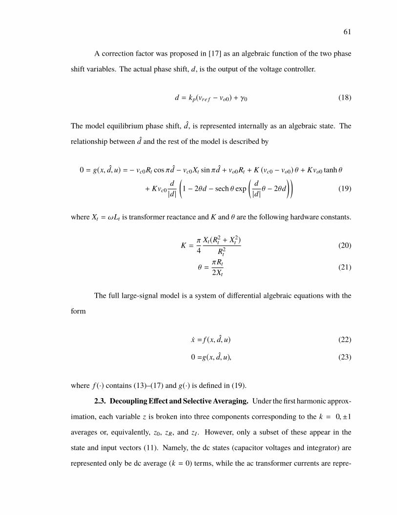
61

A correction factor was proposed in [17] as an algebraic function of the two phase

shift variables. The actual phase shift, d, is the output of the voltage controller.

d = kp(vre f − vo0) + γ0 (18)

The model equilibrium phase shift, d, is represented internally as an algebraic state. The

relationship between d and the rest of the model is described by

0 = g(x, d, u) = − vc0Rt cos πd − vc0Xt sin πd + vo0Rt + K (vc0 − vo0) θ + Kvo0 tanh θ

+ Kvc0d|d |

(1 − 2θd − sech θ exp

(d|d |θ − 2θd

))(19)

where Xt = ωLt is transformer reactance and K and θ are the following hardware constants.

K =π

4Xt(R2

t + X2t )

R2t

(20)

θ =πRt

2Xt(21)

The full large-signal model is a system of differential algebraic equations with the

form

Ûx = f (x, d, u) (22)

0 =g(x, d, u), (23)

where f (·) contains (13)–(17) and g(·) is defined in (19).

2.3. DecouplingEffect and SelectiveAveraging. Under the first harmonic approx-

imation, each variable z is broken into three components corresponding to the k = 0,±1

averages or, equivalently, z0, zR, and zI . However, only a subset of these appear in the

state and input vectors (11). Namely, the dc states (capacitor voltages and integrator) are

represented only be dc average (k = 0) terms, while the ac transformer currents are repre-

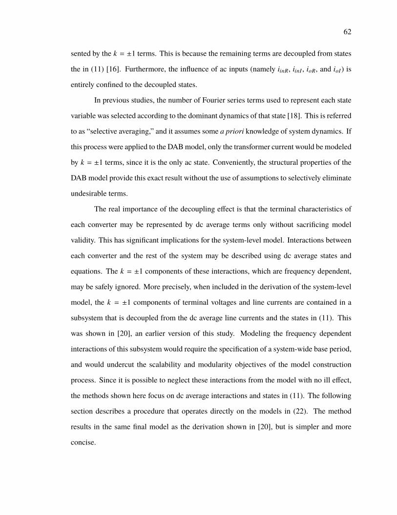
62

sented by the k = ±1 terms. This is because the remaining terms are decoupled from states

the in (11) [16]. Furthermore, the influence of ac inputs (namely iinR, iinI , ioR, and ioI) is

entirely confined to the decoupled states.

In previous studies, the number of Fourier series terms used to represent each state

variable was selected according to the dominant dynamics of that state [18]. This is referred

to as “selective averaging,” and it assumes some a priori knowledge of system dynamics. If

this process were applied to the DABmodel, only the transformer current would be modeled

by k = ±1 terms, since it is the only ac state. Conveniently, the structural properties of the

DABmodel provide this exact result without the use of assumptions to selectively eliminate

undesirable terms.

The real importance of the decoupling effect is that the terminal characteristics of

each converter may be represented by dc average terms only without sacrificing model

validity. This has significant implications for the system-level model. Interactions between

each converter and the rest of the system may be described using dc average states and

equations. The k = ±1 components of these interactions, which are frequency dependent,

may be safely ignored. More precisely, when included in the derivation of the system-level

model, the k = ±1 components of terminal voltages and line currents are contained in a

subsystem that is decoupled from the dc average line currents and the states in (11). This

was shown in [20], an earlier version of this study. Modeling the frequency dependent

interactions of this subsystem would require the specification of a system-wide base period,

and would undercut the scalability and modularity objectives of the model construction

process. Since it is possible to neglect these interactions from the model with no ill effect,

the methods shown here focus on dc average interactions and states in (11). The following

section describes a procedure that operates directly on the models in (22). The method

results in the same final model as the derivation shown in [20], but is simpler and more

concise.

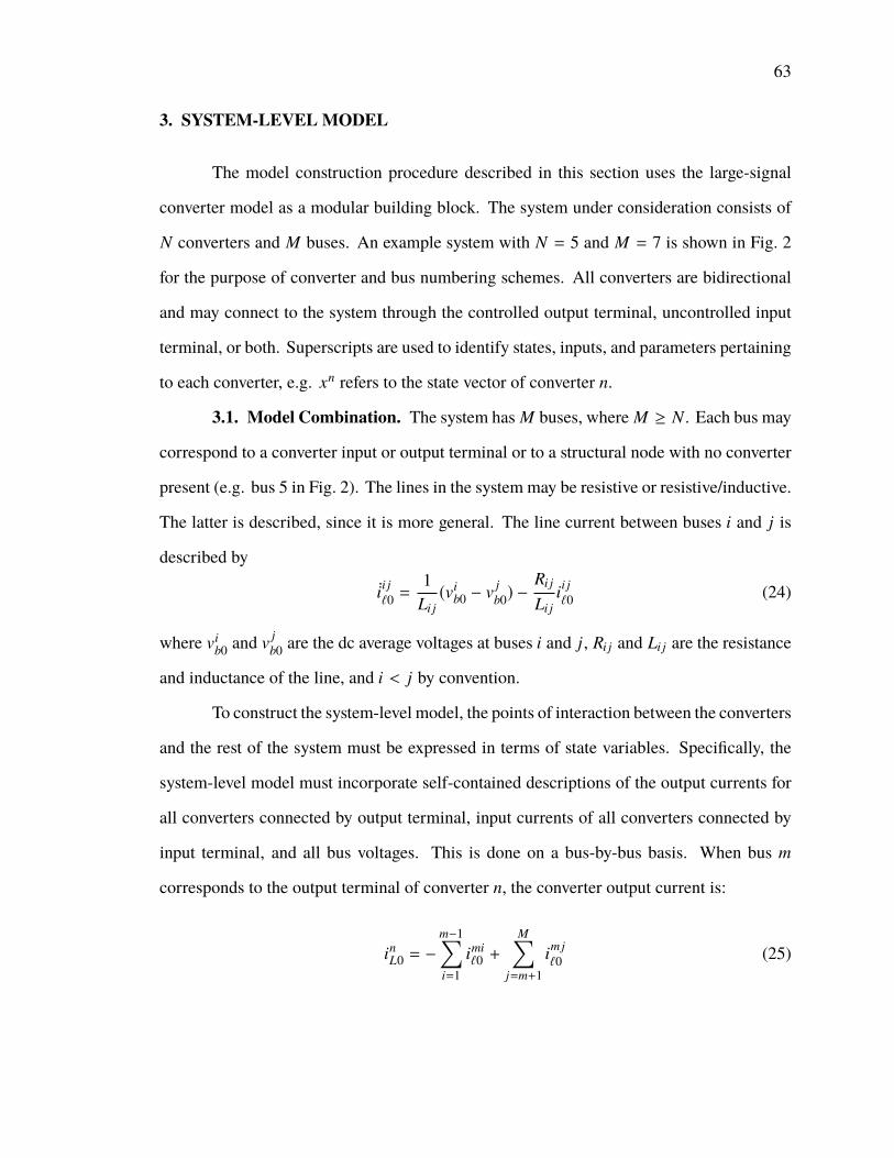
63

3. SYSTEM-LEVEL MODEL

The model construction procedure described in this section uses the large-signal

converter model as a modular building block. The system under consideration consists of

N converters and M buses. An example system with N = 5 and M = 7 is shown in Fig. 2

for the purpose of converter and bus numbering schemes. All converters are bidirectional

and may connect to the system through the controlled output terminal, uncontrolled input

terminal, or both. Superscripts are used to identify states, inputs, and parameters pertaining

to each converter, e.g. xn refers to the state vector of converter n.

3.1. Model Combination. The system has M buses, where M ≥ N . Each bus may

correspond to a converter input or output terminal or to a structural node with no converter

present (e.g. bus 5 in Fig. 2). The lines in the system may be resistive or resistive/inductive.

The latter is described, since it is more general. The line current between buses i and j is

described by

Ûii j`0 =

1Li j(vi

b0 − vjb0) −

Ri j

Li jii j`0 (24)

where vib0 and v

jb0 are the dc average voltages at buses i and j, Ri j and Li j are the resistance

and inductance of the line, and i < j by convention.

To construct the system-level model, the points of interaction between the converters

and the rest of the system must be expressed in terms of state variables. Specifically, the

system-level model must incorporate self-contained descriptions of the output currents for

all converters connected by output terminal, input currents of all converters connected by

input terminal, and all bus voltages. This is done on a bus-by-bus basis. When bus m

corresponds to the output terminal of converter n, the converter output current is:

inL0 = −

m−1∑i=1

imi`0 +

M∑j=m+1

imj`0 (25)

64

3

21 4 5 6

7

1

2

3

4

5

i1

in0

i3

L0

i4

L0

i5

L0

Figure 2. Five-converter example system. Each converter is shown a two-port element, withthe (controlled) output port denoted by a dot. Encircled integers are system bus numbers.The dotted line indicates the scope of the system-level model.

This follows from the application of KCL at bus m. Trivially, the bus voltage is equal to

the converter output voltage, i.e. vmb0 = vn

o0. Similarly, when bus m corresponds to the input

terminal of converter n, the converter input current is:

inin0 =

m−1∑i=1

imi`0 −

M∑j=m+1

imj`0 , (26)

In this case, the bus voltage is equal to the input capacitor voltage (vmb0 = vn

c0).

In the final case, bus m is not connected to a converter. Bus 5 in Fig. 2 is an example

of this case. By KCL, the current at this node is:

0 =m−1∑i=1

imi`0 −

M∑j=m+1

imj`0 (27)

Even though no converter is present, it is still necessary to represent the bus voltages in the

model, since they are used in the line current equations. These bus voltages are included

as algebraic state variables. For each bus m with no converter, the model contains both the

voltage at the bus and the corresponding node current expression.

3.2. System-Level Organization. The full system-level model has the form

Ûxsys = fsys(xsys, ysys, usys) (28)

0 = gsys(xsys, ysys, usys) (29)

65

The state vector xsys is

xsys = [x1 x2 · · · xN xline]T (30)

where each xn is a converter state vector and xline is a vector containing all line current

states. The algebraic state vector ysys contains all internal phase shift variables and all bus

voltages that are not already states in xsys. The vector is

ysys = [d1 d2 · · · dN ybus]T (31)

where ybus contains the voltage vmb0 of each bus m that does not correspond to the output

terminal of a source converter or input terminal of a load converter.

The system-level input vector usys contains all N control inputs and all current inputs

that are external to the system, i.e. all inin0 and in

L0 not described by equations (25) and (26).

The number of external connections depends on the topology of the system. For example,

the input vector for the system shown in Fig. 2 is

usys = [i1in0 v1re f v2

re f i3L0 v3re f i4L0 v4

re f i5L0 v5re f ]

T (32)

The four current terms in this vector correspond to the four external connections shown in

Fig. 2.

The system equations fsys(·) are (13)–(17) for each converter and (24) for each line

current. Likewise, the equations in gsys(·) are (19) for each converter and (27) for each

voltage in ybus.

To use the system-level model, partial derivative matrices are needed. For con-

venience, define function Ûxline = fline(·) to include all line current state equations and

0 = gline(·) to include all algebraic KCL equations for buses not connected to converters.

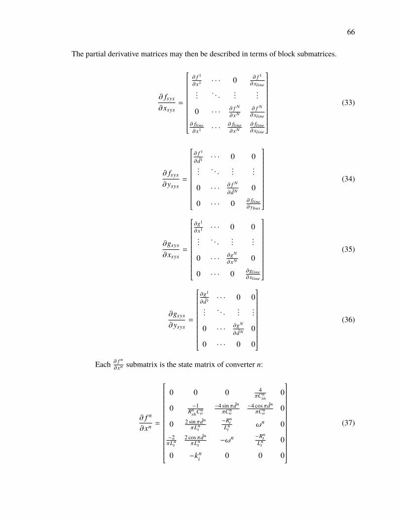
66

The partial derivative matrices may then be described in terms of block submatrices.

∂ fsys

∂xsys=

∂ f 1

∂x1 · · · 0 ∂ f 1

∂xline...

. . ....

...

0 · · ·∂ f N

∂xN

∂ f N

∂xline∂ fline∂x1 · · ·

∂ fline∂xN

∂ fline∂xline

(33)

∂ fsys

∂ysys=

∂ f 1

∂ d1 · · · 0 0...

. . ....

...

0 · · ·∂ f N

∂ dN0

0 · · · 0 ∂ fline∂ybus

(34)

∂gsys

∂xsys=

∂g1

∂x1 · · · 0 0...

. . ....

...

0 · · ·∂gN

∂xN 0

0 · · · 0 ∂gline∂xline

(35)

∂gsys

∂ysys=

∂g1

∂ d1 · · · 0 0...

. . ....

...

0 · · ·∂gN

∂ dN0

0 · · · 0 0

(36)

Each ∂ f n

∂xn submatrix is the state matrix of converter n:

∂ f n

∂xn =

0 0 0 4πCn

in0

0 −1Rnsh

Cno

−4 sin πdn

πCno

−4 cos πdn

πCno

0

0 2 sin πdn

πLnt

−Rnt

Lnt

ωn 0−2πLn

t

2 cos πdn

πLnt

−ωn −Rnt

Lnt

0

0 −kni 0 0 0

(37)

67

The columns of ∂ f n

∂xlineand rows of ∂ fline

∂xn are

∂ f n

∂ii j`0

=

[∂(Ûvn

c0)

∂ii j`0

∂(Ûvno0)

∂ii j`0

0 0 0]T

(38)

∂(Ûii j`0)

∂xn =

[∂(Ûii j

`0)

∂vnc0

∂(Ûii j`0)

∂vno0

0 0 0]

(39)

The elements of these vectors depend on how converter n connects to the system. For

generality, let the input and output terminals of converter n correspond to buses p and q,

respectively. Then vpb0 = vn

c0 and vqb0 = vn

o0, and the partial derivative elements are:

∂(Ûvnc0)

∂ii j`0

=

−1Cnin, p = i

1Cnin, p = j

0, else

∂(Ûvno0)

∂ii j`0

=

1

Cno, q = i

−1Cno, q = j

0, else

∂(Ûii j`0)

∂vnc0=

1

Li j, i = p

−1Li j, j = p

0, else

∂(Ûii j`0)

∂vno0=

1

Li j, i = q

−1Li j, j = q

0, else

Finally, submatrix ∂ fline∂xline

is diagonal with elements

∂(Ûii j`0)

∂ii j`0

= −Ri j

Li j. (40)

The nonzero submatrices of ∂ fsys∂ysys

are ∂ f n

∂ dnand ∂ fline

∂ybus. Each ∂ f n

∂ dnis a column:

∂ f n

∂ dn=

04

Cno

(intI sin πdn − in

tR cos πdn)

2vno0 cos πdn

Lnt

−2vno0 sin πdn

Lnt

(41)

68

Submatrix ∂ fline∂ybus

consists of elements ∂(Ûii j`0)

∂vmb0

for each line current ii j`0 ∈ xline and bus voltage

vmb0 ∈ ybus. These elements are:

∂(Ûii j`0)

∂vmb0=

1

Li j, i = m

−1Li j, j = m

0, else

(42)

Matrix ∂gsys∂xsys

is a block diagonal combination of submatrices ∂gn

∂xn and ∂gmline

∂xline. The

former is∂gn

∂xn =

[∂gn

∂vnc0

Rnt − Kn (θn − tanh θn) 0 0 ∂gn

∂dn

](43)

where ∂gn

∂vnc0and ∂gn

∂dn are

∂gn

∂vnc0= Knθn − Rn

t cos πdn − Xnt sin πdn

+ Kn dn

|dn |

(1 − 2θndn − sech θn exp

(dn

|dn |θn − 2θndn

))(44)

∂gn

∂dn =2dnθKnvn

c0|dn |

(sech θn exp

(dn

|dn |θn − 2θndn

)− 1

)(45)

Submatrix ∂gmline

∂xlinehas elements ∂g

mline

∂ii j`0

, where gmline(·) denotes the KCL equation applied

at bus m. These elements are:

∂gmline

∂ii j`0

=

1, m = i

−1, m = j

0, else

(46)

The last matrix ∂gsys∂ysys

has only diagonal elements ∂gn

∂ dn, which are:

∂gn

∂ dn= πvn

c0

(Rn

t sin πdn − Xnt cos πdn

)(47)

69

4. TRANSFORMER CURRENT RECONSTRUCTION

The preceding sections have described a general-purpose large-signal model. This

section is concerned with improving the fidelity of the time-domain transformer current

representations. The following analysis is applicable to any converter in the system; su-

perscript n is dropped for readability. Let vc, vo, it , and d be state trajectories resulting a

time-domain simulation of the proposed model. The voltages and phase shift are dc average

variables, so the state trajectories are give trivially by the states of the proposed model.

The transformer current is calculated from states itR and it I according to (5). The result

is a sinusoidal approximation of the transformer current. This approximation is suitable

for efficient small-signal analyses, but for many other purposes, such as evaluating device

current stresses or analyzing ZVS conditions, more accurate current representations are

required. As a direct consequence of the correction factor equations used in the proposed

model, it is possible to obtain accurate representations by reconstructing the full Fourier

series for the transformer currents.

Let vp = s1vc and vs = s2vo be the voltages across the primary and secondary

of the high frequency transformer. To simplify equations, assume that vc and vo may be

approximated as constant during a single switching period. This scenario would result from

sampling the continuous-time state trajectories at multiples of the switching period with a

zero-order hold. The transformer current is the solution to the forced differential equation:

Lt Ûit = vp − vs − it Rt (48)

The voltages can be expanded as Fourier series:

vp(τ) =

∞∑k=1

apk cosωkτ + bp

k sinωkτ (49)

vs(τ) =

∞∑k=1

ask cosωkτ + bs

k sinωkτ (50)

70

The coefficients are known, and equal to the Fourier series coefficients of s1 and s2 scaled

by vc and vo, respectively. The coefficients are:

apk = 0 bp

k =

4vckπ k odd

0 k even

ask =

−4vo sin dkπ

kπ k odd

0 k evenbs

k =

4vo cos dkπ

kπ k odd

0 k even

For any given k, the corresponding current solution may be determined using

Laplace transforms:

it(s)(Lt s + Rt) =(ap

k − ask)s

s2 + (ωk)2+(bp

k − bsk)ωk

s2 + (ωk)2(51)

Alternatively, this may be written as

it(s) =(

1Lt s + Rt

) (avk s + bvkωk

s2 + (ωk)2

), (52)

where avk = ap

k − ask and bvk = bp

k − bsk . The partial fraction decomposition of this equation

is:

it(s) =1Lt

(bvkωk − av

k(Rt

Lt)

(ωk)2 + (Rt

Lt)2

) (1

s + (Rt

Lt)−

ss2 + (ωk)2

)+

1ωkLt

[av

k +Rt

Lt

(bvkωk − av

k(Rt

Lt)

(ωk)2 + (Rt

Lt)2

)] (ωk

s2 + (ωk)2

)(53)

Taking the inverse Laplace transform yields the time-domain current solution.

it(τ) =1Lt

(bvkωk − av

k(Rt

Lt)

(ωk)2 + (Rt

Lt)2

) (e−RtLt

τ− cosωkτ

)+

1ωkLt

[av

k +Rt

Lt

(bvkωk − av

k(Rt

Lt)

(ωk)2 + (Rt

Lt)2

)]sinωkτ (54)

71

The quantity of interest is the periodic solution, so the decaying exponential term

may be discarded. The full current solution is the summation

it(τ) =1Lt

∞∑k=1

aik cosωkτ + bi

k sinωkτ, (55)

where aik and bi

k are the Fourier series coefficients of the transformer current, given by

aik = −

(bvkωk − av

k(Rt

Lt)

(ωk)2 + (Rt

Lt)2

)(56)

bik =

1ωk

(av

k +Rt

Lt

(bvkωk − av

k(Rt

Lt)

(ωk)2 + (Rt

Lt)2

)). (57)

The harmonic reconstruction method may be used in steady-state analysis or as a

postprocessing method for time-domain simulations. In the latter case, the reconstruction

is applied to state trajectories generated through numerical integration of the large-signal

model. Since the method is applied offline, the currents for each converter in a given system

and each time range of interest may be calculated separately. Moreover, the zero-order-hold

approximation allows each switching period to be treated independently. This means that

every combination of converter, harmonic number, and switching period in the time range

of interest may be considered as an independent, parallel computation.

5. VERIFICATION

Simulations and hardware experiments were used to validate the proposed methods.

The objective of the simulation experiments is to show that, in both transient and steady-

state conditions, the proposed model and harmonic reconstruction method provide accuracy

equivalent to switching simulations with significantly reduced computation time. The

objective of the hardware validation is to show the accuracy of the proposed methods with

respect to real-world converters.

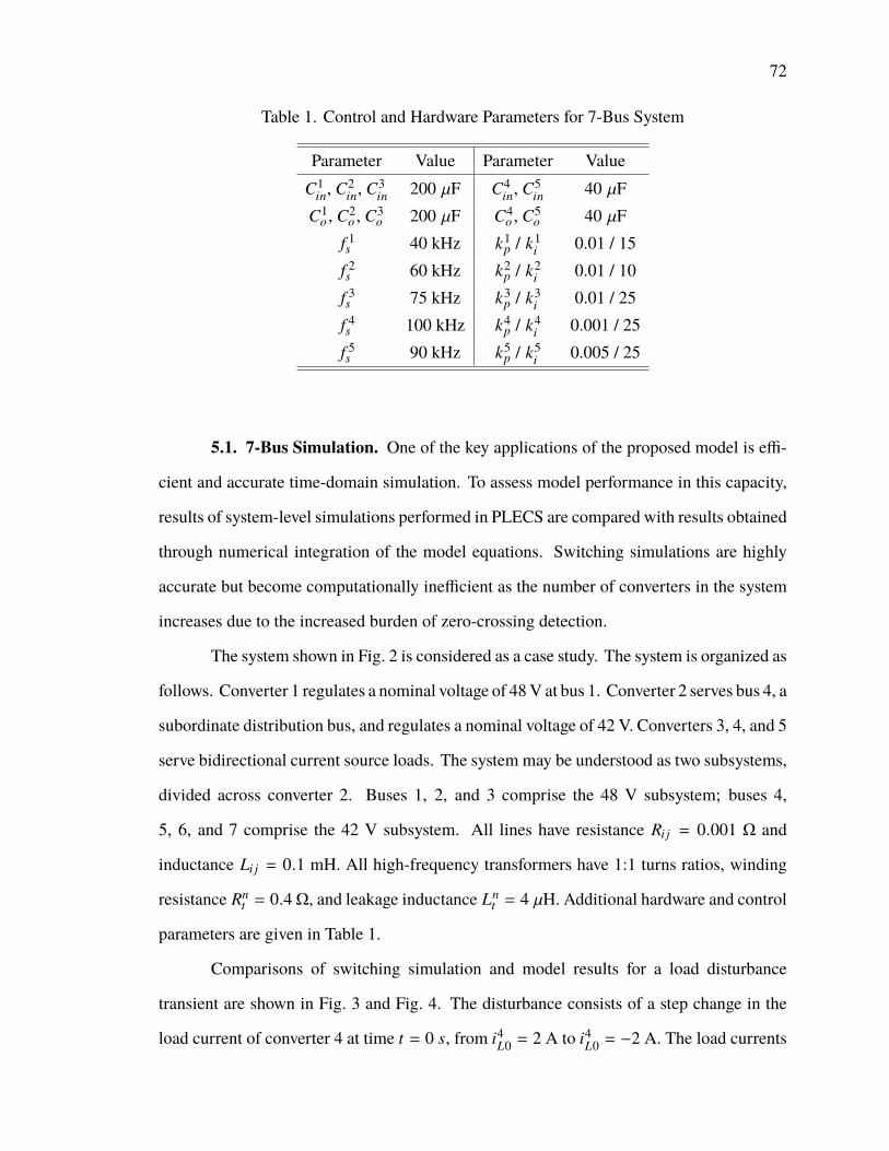
72

Table 1. Control and Hardware Parameters for 7-Bus System

Parameter Value Parameter ValueC1

in, C2in, C3

in 200 µF C4in, C5

in 40 µFC1

o , C2o , C3

o 200 µF C4o , C5

o 40 µFf 1s 40 kHz k1

p / k1i 0.01 / 15

f 2s 60 kHz k2

p / k2i 0.01 / 10

f 3s 75 kHz k3

p / k3i 0.01 / 25

f 4s 100 kHz k4

p / k4i 0.001 / 25

f 5s 90 kHz k5

p / k5i 0.005 / 25

5.1. 7-Bus Simulation. One of the key applications of the proposed model is effi-

cient and accurate time-domain simulation. To assess model performance in this capacity,

results of system-level simulations performed in PLECS are compared with results obtained

through numerical integration of the model equations. Switching simulations are highly

accurate but become computationally inefficient as the number of converters in the system

increases due to the increased burden of zero-crossing detection.

The system shown in Fig. 2 is considered as a case study. The system is organized as

follows. Converter 1 regulates a nominal voltage of 48V at bus 1. Converter 2 serves bus 4, a

subordinate distribution bus, and regulates a nominal voltage of 42 V. Converters 3, 4, and 5

serve bidirectional current source loads. The system may be understood as two subsystems,

divided across converter 2. Buses 1, 2, and 3 comprise the 48 V subsystem; buses 4,

5, 6, and 7 comprise the 42 V subsystem. All lines have resistance Ri j = 0.001 Ω and

inductance Li j = 0.1 mH. All high-frequency transformers have 1:1 turns ratios, winding

resistance Rnt = 0.4Ω, and leakage inductance Ln

t = 4 µH. Additional hardware and control

parameters are given in Table 1.

Comparisons of switching simulation and model results for a load disturbance

transient are shown in Fig. 3 and Fig. 4. The disturbance consists of a step change in the

load current of converter 4 at time t = 0 s, from i4L0 = 2 A to i4L0 = −2 A. The load currents

73

for converters 3 and 5 remain fixed at i3L0 = 4 A and i5L0 = 2 A throughout. A selection of

bus voltage responses are shown in Fig. 3; line current responses are shown in Fig. 4. The

figures show that the model and switching simulation are consistent in both transient and

steady-state response. The states not shown in these figures match with similar accuracy.

The foremost advantage of using the model for time-domain simulation is execution time.

All simulations were performed for a time range of 0.05 s and error tolerance of 10−5.

Using a standard explicit solver, the 5-converter switching simulation takes 61.67 s, while

integration of the large-signal model completes in 4.11 s. Since the large-signal model is a

DAE system, numerical integration using an explicit solver consists of two separate steps:

solving dynamic states at the next time step, and then solving the algebraic constraints.

Alternatively, the differential and algebraic equations may be solved simultaneously [23].

When this approach is used, numerical integration of the large-signal model completes in

0.466 s.

Despite the accuracy of the dc average states, the transformer currents predicted

by the base model are only sinusoidal approximations of the actual transformer current.

However, using the harmonic reconstruction method, the actual transformer currents may be

calculatedwith high accuracy aswell. A comparison of the transformer current for converter

2 from simulation, from the base model, and from the proposed harmonic reconstruction

method is shown in Fig. 5. The reconstruction includes up to the 35th harmonic of

the switching frequency. Since only odd harmonics are nonzero, this corresponds to 18

harmonic components.

5.2. Hardware Experiment. The hardware testbed is shown in Fig. 6. The testbed

consists of two DAB converters connected in series: the output of converter 1 is connected

to the input of converter 2 through a line impedance. The line impedance has both resistive

(0.25 Ω) and inductive (100 µH) components. The output of converter 2 is connected to a

current source load, which steps from 3 A to 3.5 A during the experiment. Both converters

regulate output voltages of 18 V, and operate with switching frequencies of 80 kHz and

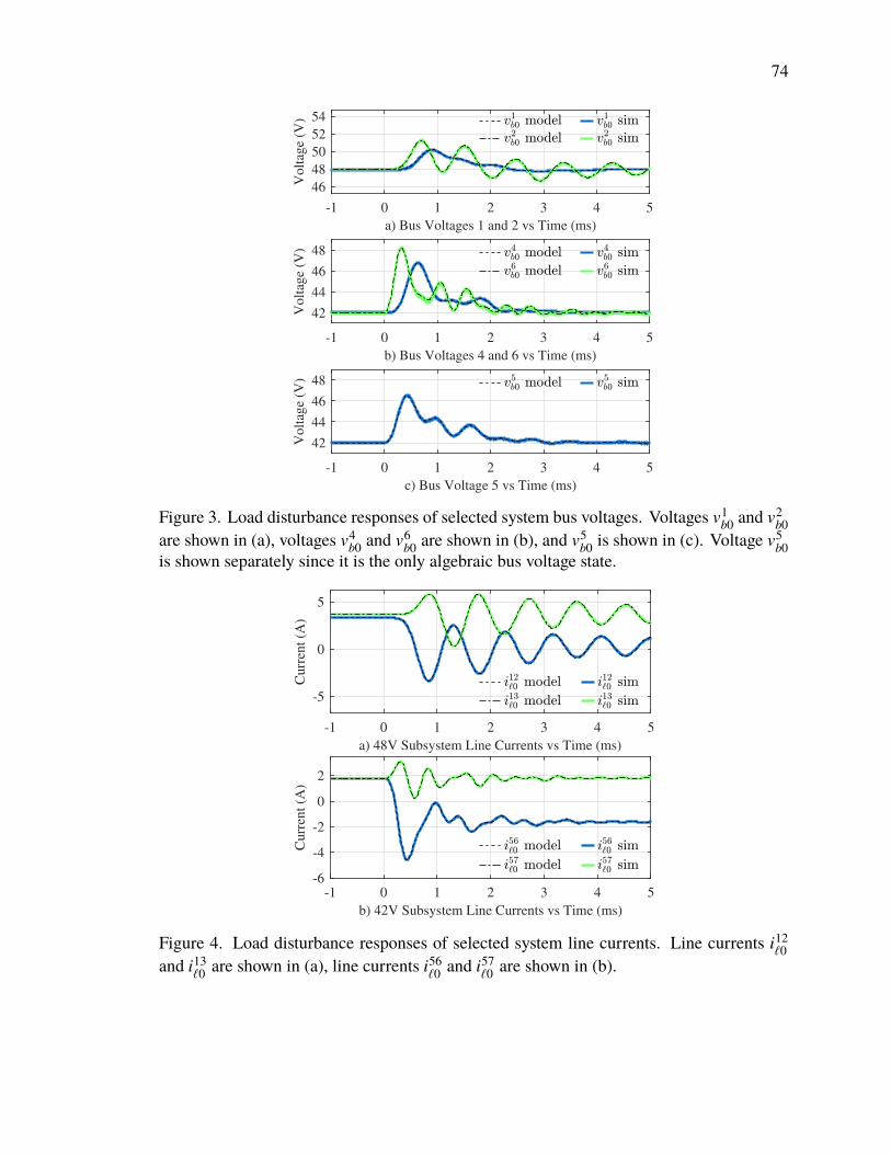
74

-1 0 1 2 3 4 5

a) Bus Voltages 1 and 2 vs Time (ms)

46

48

50

52

54

Volt

age

(V)

-1 0 1 2 3 4 5

b) Bus Voltages 4 and 6 vs Time (ms)

42

44

46

48

Volt

age

(V)

-1 0 1 2 3 4 5

c) Bus Voltage 5 vs Time (ms)

42

44

46

48

Volt

age

(V)

Figure 3. Load disturbance responses of selected system bus voltages. Voltages v1b0 and v

2b0

are shown in (a), voltages v4b0 and v

6b0 are shown in (b), and v

5b0 is shown in (c). Voltage v

5b0

is shown separately since it is the only algebraic bus voltage state.

-1 0 1 2 3 4 5

a) 48V Subsystem Line Currents vs Time (ms)

-5

0

5

Cu

rren

t (A

)

-1 0 1 2 3 4 5

b) 42V Subsystem Line Currents vs Time (ms)

-6

-4

-2

0

2

Cu

rren

t (A

)

Figure 4. Load disturbance responses of selected system line currents. Line currents i12`0

and i13`0 are shown in (a), line currents i56

`0 and i57`0 are shown in (b).

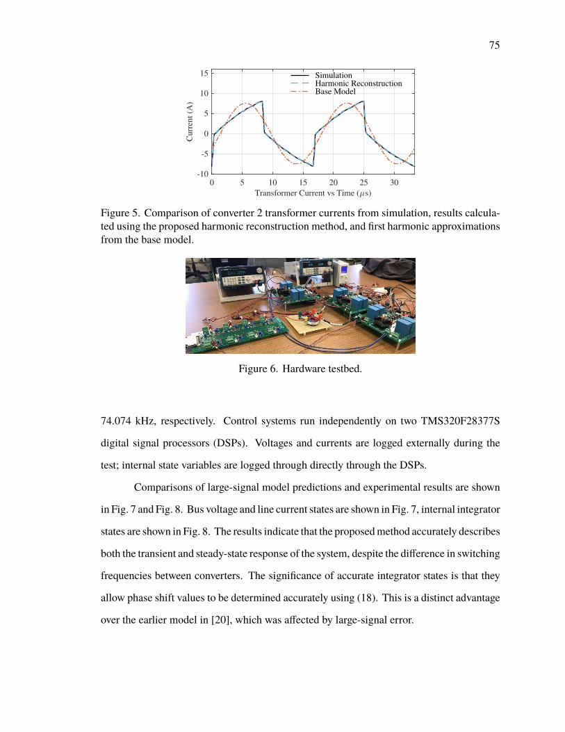
75

0 5 10 15 20 25 30

Transformer Current vs Time ( s)

-10

-5

0

5

10

15

Curr

ent

(A)

Simulation

Harmonic Reconstruction

Base Model

Figure 5. Comparison of converter 2 transformer currents from simulation, results calcula-ted using the proposed harmonic reconstruction method, and first harmonic approximationsfrom the base model.

Figure 6. Hardware testbed.

74.074 kHz, respectively. Control systems run independently on two TMS320F28377S

digital signal processors (DSPs). Voltages and currents are logged externally during the

test; internal state variables are logged through directly through the DSPs.

Comparisons of large-signal model predictions and experimental results are shown

in Fig. 7 and Fig. 8. Bus voltage and line current states are shown in Fig. 7, internal integrator

states are shown in Fig. 8. The results indicate that the proposedmethod accurately describes

both the transient and steady-state response of the system, despite the difference in switching

frequencies between converters. The significance of accurate integrator states is that they

allow phase shift values to be determined accurately using (18). This is a distinct advantage

over the earlier model in [20], which was affected by large-signal error.

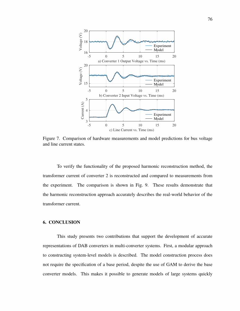
76

-5 0 5 10 15 20

a) Converter 1 Output Voltage vs. Time (ms)

16

18

20

Volt

age

(V)

ExperimentModel

-5 0 5 10 15 20

b) Converter 2 Input Voltage vs. Time (ms)

15

20

Volt

age

(V)

ExperimentModel

-5 0 5 10 15 20

c) Line Current vs. Time (ms)

3

4

5

Curr

ent

(A)

ExperimentModel

Figure 7. Comparison of hardware measurements and model predictions for bus voltageand line current states.

To verify the functionality of the proposed harmonic reconstruction method, the

transformer current of converter 2 is reconstructed and compared to measurements from

the experiment. The comparison is shown in Fig. 9. These results demonstrate that

the harmonic reconstruction approach accurately describes the real-world behavior of the

transformer current.

6. CONCLUSION

This study presents two contributions that support the development of accurate

representations of DAB converters in multi-converter systems. First, a modular approach

to constructing system-level models is described. The model construction process does

not require the specification of a base period, despite the use of GAM to derive the base

converter models. This makes it possible to generate models of large systems quickly

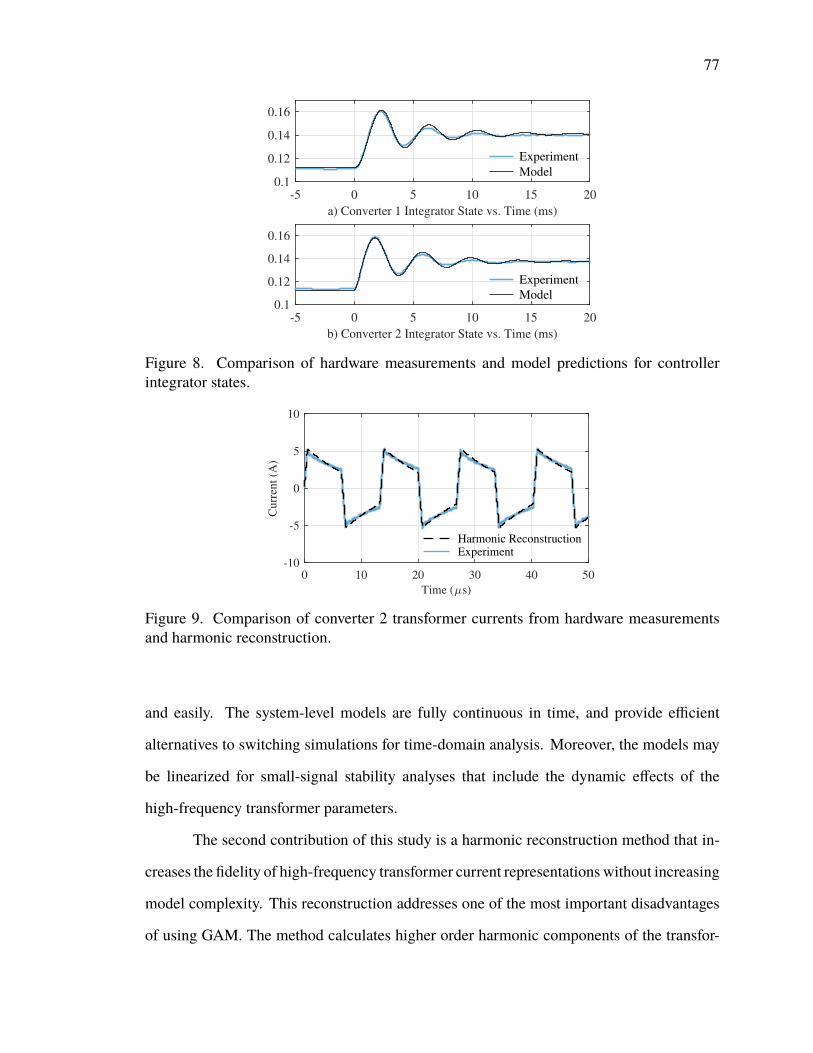
77

-5 0 5 10 15 20

a) Converter 1 Integrator State vs. Time (ms)

0.1

0.12

0.14

0.16

Experiment

Model

-5 0 5 10 15 20

b) Converter 2 Integrator State vs. Time (ms)

0.1

0.12

0.14

0.16

Experiment

Model

Figure 8. Comparison of hardware measurements and model predictions for controllerintegrator states.

0 10 20 30 40 50

Time ( s)

-10

-5

0

5

10

Cu

rren

t (A

)

ExperimentHarmonic Reconstruction

Figure 9. Comparison of converter 2 transformer currents from hardware measurementsand harmonic reconstruction.

and easily. The system-level models are fully continuous in time, and provide efficient

alternatives to switching simulations for time-domain analysis. Moreover, the models may

be linearized for small-signal stability analyses that include the dynamic effects of the

high-frequency transformer parameters.

The second contribution of this study is a harmonic reconstruction method that in-

creases the fidelity of high-frequency transformer current representationswithout increasing

model complexity. This reconstruction addresses one of the most important disadvantages

of using GAM. The method calculates higher order harmonic components of the transfor-

78

mer current without including these components as states of the GAM. Furthermore, since

the method is applied offline, it does not contribute additional computational complexity

when using the system-level model for time-domain simulations.

REFERENCES

[1] R. W. A. A. DeDoncker, D. M. Divan, and M. H. Kheraluwala, “A three-phase

soft-switched high-power-density dc/dc converter for high-power applications,” IEEE

Trans. Ind. Appl., vol. 27, no. 1, pp. 63–73, 1991.

[2] M. N. Kheraluwala, R.W. Gascoigne, D.M. Divan, and E. D. Baumann, “Performance

characterization of a high-power dual active bridge dc-to-dc converter,” IEEE Trans.

Ind. Appl., vol. 28, no. 6, pp. 1294–1301, 1992.

[3] A. Q. Huang, “Medium-voltage solid-state transformer: Technology for a smarter and

resilient grid,” IEEE Ind. Electron. Mag., vol. 10, no. 3, pp. 29–42, 2016.

[4] X. She, A. Q. Huang, and R. Burgos, “Review of solid-state transformer technologies

and their application in power distribution systems,” IEEE J. Emerg. Sel. Topics Power

Electron., vol. 1, no. 3, pp. 186–198, 2013.

[5] F. Krismer and J. W. Kolar, “Accurate small-signal model for the digital control of an

automotive bidirectional dual active bridge,” IEEE Trans. Power Electron., vol. 24,

no. 12, pp. 2756–2768, 2009.

[6] R. T. Naayagi, A. J. Forsyth, and R. Shuttleworth, “High-power bidirectional dc-dc

converter for aerospace applications,” IEEE Trans. Power Electron., vol. 27, no. 11,

pp. 4366–4379, 2012.

[7] B. Zahedi and L. E. Norum, “Modeling and simulation of all-electric ships with low-

voltage dc hybrid power systems,” IEEE Trans. Power Electron., vol. 28, no. 10, pp.

4525–4537, 2013.

79

[8] I. Y. Chung, W. Liu, M. Andrus, K. Schoder, L. Siyu, D. A. Cartes, and M. Steurer,

“Integration of a bi-directional dc-dc converter model into a large-scale system simu-

lation of a shipboard mvdc power system,” in 2009 IEEE Electric Ship Technologies

Symposium, 2009, pp. 318–325.

[9] G. C. Verghese, M. E. Elbuluk, and J. G. Kassakian, “A general approach to sampled-

data modeling for power electronic circuits,” IEEE Trans. Power Electron., vol. PE-1,

no. 2, pp. 76–89, 1986.

[10] C. Zhao, S. D. Round, and J. W. Kolar, “Full-order averaging modelling of zero-

voltage-switching phase-shift bidirectional dc-dc converters,” IET Power Electronics,

vol. 3, no. 3, pp. 400–410, 2010.

[11] L. Shi, W. Lei, Z. Li, J. Huang, Y. Cui, and Y. Wang, “Bilinear discrete-time modeling

and stability analysis of the digitally controlled dual active bridge converter,” IEEE

Trans. Power Electron., vol. 32, no. 11, pp. 8787–8799, 2017.

[12] H. Bai and C. Mi, “Eliminate reactive power and increase system efficiency of isolated

bidirectional dual-active-bridge dc-dc converters using novel dual-phase-shift control,”

IEEE Trans. Power Electron., vol. 23, no. 6, pp. 2905–2914, 2008.

[13] K. Zhang, Z. Shan, and J. Jatskevich, “Large- and small-signal average-valuemodeling

of dual-active-bridge dc-dc converter considering power losses,” IEEE Trans. Power

Electron., vol. 32, no. 3, pp. 1964–1974, 2017.

[14] F. Zhang, M. M. U. Rehman, R. Zane, and D. Maksimović, “Improved steady-state

model of the dual-active-bridge converter,” in 2015 IEEEEnergyConversionCongress

and Exposition (ECCE), 2015, pp. 630–636.

[15] S. R. Sanders, J.M.Noworolski, X. Z. Liu, andG.C.Verghese, “Generalized averaging

method for power conversion circuits,” IEEE Trans. Power Electron., vol. 6, no. 2, pp.

251–259, 1991.

80

[16] H. Qin and J. W. Kimball, “Generalized average modeling of dual active bridge dc-dc

converter,” IEEE Trans. Power Electron., vol. 27, no. 4, pp. 2078–2084, 2012.

[17] J. A. Mueller and J. Kimball, “An improved generalized average model of dc-dc dual

active bridge converters,” IEEE Trans. Power Electron., vol. PP, no. 99, pp. 1–1, 2018.

[18] A. Emadi, “Modeling and analysis ofmulticonverter dc power electronic systems using

the generalized state-space averaging method,” IEEE Trans. Ind. Electron., vol. 51,

no. 3, pp. 661–668, 2004.

[19] A. Frances, R. Asensi, O. Garcia, R. Prieto, and J. Uceda, “Modeling electronic power

converters in smart dc microgrids - an overview,” IEEE Trans. Smart Grid, vol. PP,

no. 99, pp. 1–1, 2017.

[20] J. A. Mueller and J. W. Kimball, “Generalized average modeling of dc subsystem in

solid state transformers,” in 2017 IEEE Energy Conversion Congress and Exposition

(ECCE), October 2017.

[21] S. Bacha, I. Munteanu, and A. I. Bratcu, Power electronic converters modeling and

control: with case studies, ser. Advanced Textbooks in Control and Signal Processing.

London: Springer, 2014.

[22] S. S. Shah and S. Bhattacharya, “Large & small signal modeling of dual active bridge

converter using improved first harmonic approximation,” in 2017 IEEE Applied Power

Electronics Conference and Exposition (APEC), 2017, pp. 1175–1182.

[23] M. L. Crow, “Numerical integration,” in Computational Methods for Electric Power

Systems, 3rd ed. Boca Raton, FL: CRC Press, 2016.

81

III. ACCURATE ENERGY USE ESTIMATION FOR NONINTRUSIVE LOADMONITORING IN SYSTEMS OF KNOWN DEVICES

Jacob A. Mueller and Jonathan W. Kimball

Department of Electrical & Computer Engineering

Missouri University of Science and Technology

Rolla, Missouri 65409–0050

Email: jam8z4@mst.edu

ABSTRACT

This study presents a method of nonintrusive loadmonitoring (NILM) for electrical systems

consisting of a fixed and known set of devices. This constraint is inherently met by

embedded and mobile power systems, and is also commonly satisfied in industrial settings.

The proposed NILM method provides time-accurate profiles of device behavior using only

probabilistic device models and system-level measurements. The full method consists of

model training, construction of a system-level model, and prediction of device-level energy

use. Energy use estimations are determined by maximizing the probability of the predicted

behavior given the system-level measurements, and are calculated online at each sampling

instant. Themethod is validated using test data from public databases, and its performance is

assessed using standard NILM accuracy metrics. The intended application of the proposed

method is to support system status assessments and to provide early indications of potential

equipment damage through identification of atypical device behavior.

Keywords: nonintrusive load monitoring, load disaggregation, device modeling, hidden

Markov models

82

1. INTRODUCTION

The objective of NILM is to determine individual contributions to combined energy

use in an electric system. This breakdown provides a detailed understanding of the active

devices in a system from measurements of its composite energy use profile. In a residential

setting, this profile can be a set of meter or main-breaker-level measurements. The disag-

gregated contributions to the total load provide a wealth of knowledge that would otherwise

be impractical to attain. This information has a wide variety of applications. For the

consumer, it informs decisions on appliance purchases or upgrades [1]. For governments

and utilities, disaggregated load profiles may be used to design and assess the efficacy of

energy conservation policies, such as conservation voltage reduction or dynamic pricing

structures [2, 3].

Many electrical characteristics have been used to identify andmodel devices [4, 5, 6].

Among these, some of the most successful approaches have used high frequency or transient

features. These include harmonics in current waveforms [7] or edge detection methods [8],

which identify devices by changes in power when turning on or off. One of the earliest

NILM approaches distinguished devices by grouping power changes by location on the P-Q

plane [2]. These high frequency characteristics require high sampling rates to accurately

record. As a result, models based on these characteristics require large volumes of data.

For practical reasons, large storage space requirements and high frequency sampling are

undesirable.

Recent research efforts have focused onNILMmethods using hiddenMarkovmodels

(HMMs) to describe electrical systems [9, 10, 11, 12, 13]. Interest in HMMs is motivated by

the simplicity with which they accomplish basic modeling functions. Namely, they support

an efficient means of parameter estimation (Baum-Welch method) and a straightforward

inference algorithm (the Viterbi algorithm) [14]. The general idea behind HMM-based

NILM methods is that device behavior can be represented by a latent state variable and an

observable output, which is commonly taken as active power or energy. Trained device

83

models are used to infer the most likely sequence of device states for a given set of

measurements. In this capacity, HMMs have been shown to accurately predict device

behavior using low frequency (≤1 Hz) measurements. This flexibility with respect to

sampling frequency is significant because it allows HMM-based NILM methods to be

implemented using existing instrumentation, such as power qualitymonitors or conventional

smartmeter products [12].

Methods of NILM based on HMMs have primarily been studied in the context of

residential applications [11, 13, 15]. The main objectives for these applications are to

generate cumulative energy usage and time-of-use profiles for each of the devices in the

electrical system. This information is not time critical, so offline methods are commonly

employed. A fundamental challenge for NILM in residential settings is that the set of

devices is continually changing as new devices are acquired and old devices are replaced.

This difficulty in handling unmodeled loads has motivated research in unsupervised model

training methods, which determine the number and nature of devices in the system and

adjust model parameters automatically.

The electrical systems under consideration in this study are assumed to be composed

of a fixed and known set of devices. While this assumption limits the applicability of the

proposed method in residential contexts, it is commonly met by a variety of pre-designed

electrical systems, including factories, data centers, satellites, and electric vehicles of all

kinds. Both the challenges and objectives of NILM in these settings are distinct from those

of traditional residential applications. The systems of interest serve specific purposes, rather

supporting the varied activities of occupants or customers. Because these systems are the

result of a premeditated design process, extensive device-level information is known a priori.

In addition to traditional NILMbenefits, such as increased energy efficiency and noninvasive

data collection, NILM methods in industrial and vehicular power systems provide a means

to assess system health and performance. By detecting and identifying anomalous device

behaviors, an industrial NILM system may provide early warnings of impending equipment

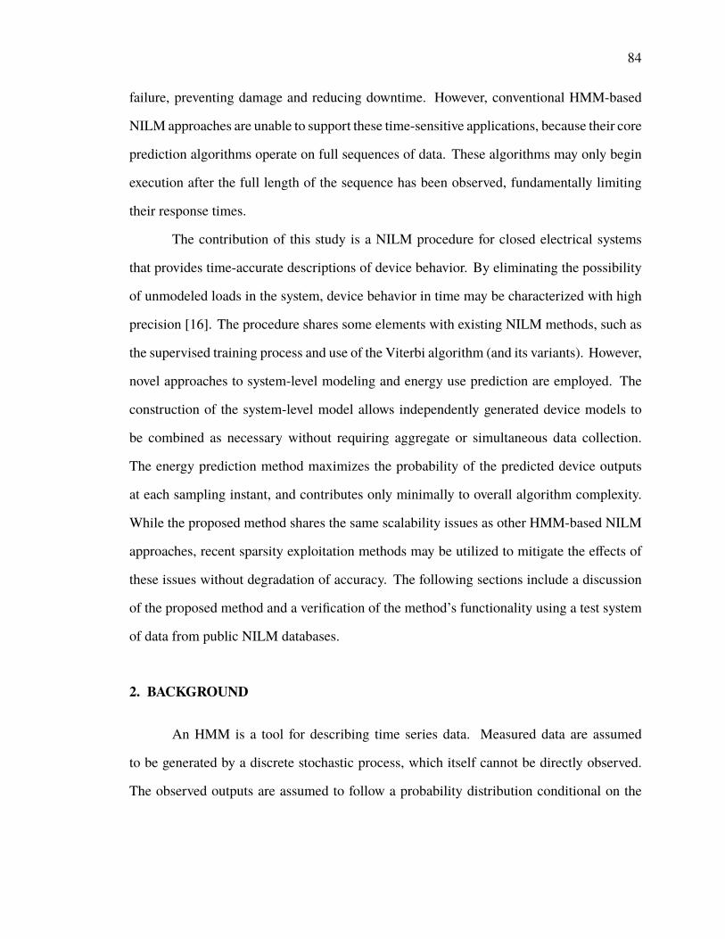
84

failure, preventing damage and reducing downtime. However, conventional HMM-based

NILM approaches are unable to support these time-sensitive applications, because their core

prediction algorithms operate on full sequences of data. These algorithms may only begin

execution after the full length of the sequence has been observed, fundamentally limiting

their response times.

The contribution of this study is a NILM procedure for closed electrical systems

that provides time-accurate descriptions of device behavior. By eliminating the possibility

of unmodeled loads in the system, device behavior in time may be characterized with high

precision [16]. The procedure shares some elements with existing NILM methods, such as

the supervised training process and use of the Viterbi algorithm (and its variants). However,

novel approaches to system-level modeling and energy use prediction are employed. The

construction of the system-level model allows independently generated device models to

be combined as necessary without requiring aggregate or simultaneous data collection.

The energy prediction method maximizes the probability of the predicted device outputs

at each sampling instant, and contributes only minimally to overall algorithm complexity.

While the proposed method shares the same scalability issues as other HMM-based NILM

approaches, recent sparsity exploitation methods may be utilized to mitigate the effects of

these issues without degradation of accuracy. The following sections include a discussion

of the proposed method and a verification of the method’s functionality using a test system

of data from public NILM databases.

2. BACKGROUND

An HMM is a tool for describing time series data. Measured data are assumed

to be generated by a discrete stochastic process, which itself cannot be directly observed.

The observed outputs are assumed to follow a probability distribution conditional on the

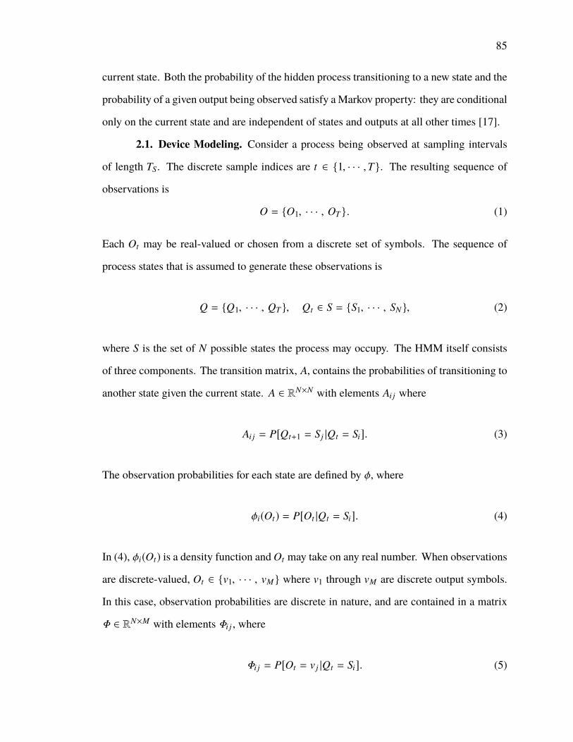
85

current state. Both the probability of the hidden process transitioning to a new state and the

probability of a given output being observed satisfy aMarkov property: they are conditional

only on the current state and are independent of states and outputs at all other times [17].

2.1. Device Modeling. Consider a process being observed at sampling intervals

of length TS. The discrete sample indices are t ∈ 1, · · · ,T. The resulting sequence of

observations is

O = O1, · · · , OT . (1)

Each Ot may be real-valued or chosen from a discrete set of symbols. The sequence of

process states that is assumed to generate these observations is

Q = Q1, · · · , QT , Qt ∈ S = S1, · · · , SN , (2)

where S is the set of N possible states the process may occupy. The HMM itself consists

of three components. The transition matrix, A, contains the probabilities of transitioning to

another state given the current state. A ∈ RN×N with elements Ai j where

Ai j = P[Qt+1 = Sj |Qt = Si]. (3)

The observation probabilities for each state are defined by φ, where

φi(Ot) = P[Ot |Qt = Si]. (4)

In (4), φi(Ot) is a density function and Ot may take on any real number. When observations

are discrete-valued, Ot ∈ v1, · · · , vM where v1 through vM are discrete output symbols.

In this case, observation probabilities are discrete in nature, and are contained in a matrix

Φ ∈ RN×M with elements Φi j , where

Φi j = P[Ot = v j |Qt = Si]. (5)

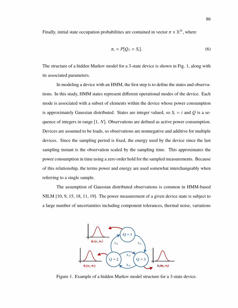
86

Finally, initial state occupation probabilities are contained in vector π ∈ RN , where

πi = P[Q1 = Si]. (6)

The structure of a hidden Markov model for a 3-state device is shown in Fig. 1, along with

its associated parameters.

In modeling a device with an HMM, the first step is to define the states and observa-

tions. In this study, HMM states represent different operational modes of the device. Each

mode is associated with a subset of elements within the device whose power consumption

is approximately Gaussian distributed. States are integer valued, so Si = i and Q is a se-

quence of integers in range [1, N]. Observations are defined as active power consumption.

Devices are assumed to be loads, so observations are nonnegative and additive for multiple

devices. Since the sampling period is fixed, the energy used by the device since the last

sampling instant is the observation scaled by the sampling time. This approximates the

power consumption in time using a zero order hold for the sampled measurements. Because

of this relationship, the terms power and energy are used somewhat interchangeably when

referring to a single sample.

The assumption of Gaussian distributed observations is common in HMM-based

NILM [10, 9, 15, 18, 11, 19]. The power measurement of a given device state is subject to

a large number of uncertainties including component tolerances, thermal noise, variations

Figure 1. Example of a hidden Markov model structure for a 3-state device.

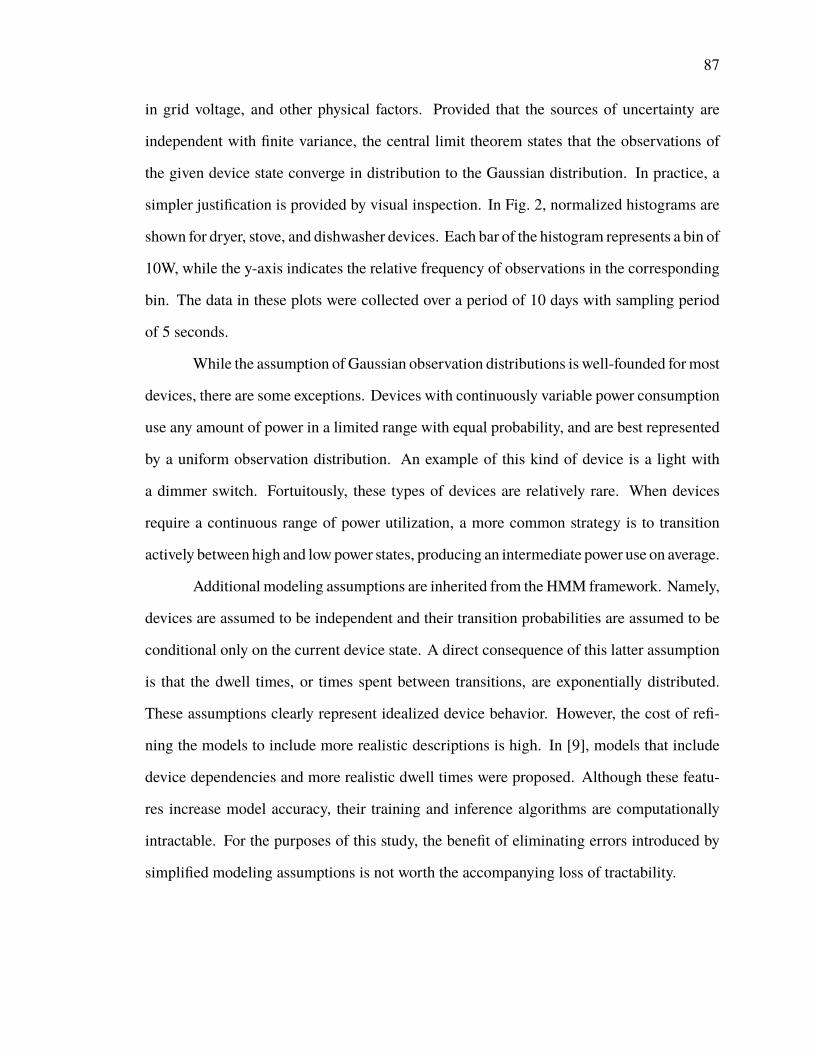
87

in grid voltage, and other physical factors. Provided that the sources of uncertainty are

independent with finite variance, the central limit theorem states that the observations of

the given device state converge in distribution to the Gaussian distribution. In practice, a

simpler justification is provided by visual inspection. In Fig. 2, normalized histograms are

shown for dryer, stove, and dishwasher devices. Each bar of the histogram represents a bin of

10W, while the y-axis indicates the relative frequency of observations in the corresponding

bin. The data in these plots were collected over a period of 10 days with sampling period

of 5 seconds.

While the assumption of Gaussian observation distributions is well-founded formost

devices, there are some exceptions. Devices with continuously variable power consumption

use any amount of power in a limited range with equal probability, and are best represented

by a uniform observation distribution. An example of this kind of device is a light with

a dimmer switch. Fortuitously, these types of devices are relatively rare. When devices

require a continuous range of power utilization, a more common strategy is to transition

actively between high and lowpower states, producing an intermediate power use on average.

Additional modeling assumptions are inherited from the HMM framework. Namely,

devices are assumed to be independent and their transition probabilities are assumed to be

conditional only on the current device state. A direct consequence of this latter assumption

is that the dwell times, or times spent between transitions, are exponentially distributed.

These assumptions clearly represent idealized device behavior. However, the cost of refi-

ning the models to include more realistic descriptions is high. In [9], models that include

device dependencies and more realistic dwell times were proposed. Although these featu-

res increase model accuracy, their training and inference algorithms are computationally

intractable. For the purposes of this study, the benefit of eliminating errors introduced by

simplified modeling assumptions is not worth the accompanying loss of tractability.

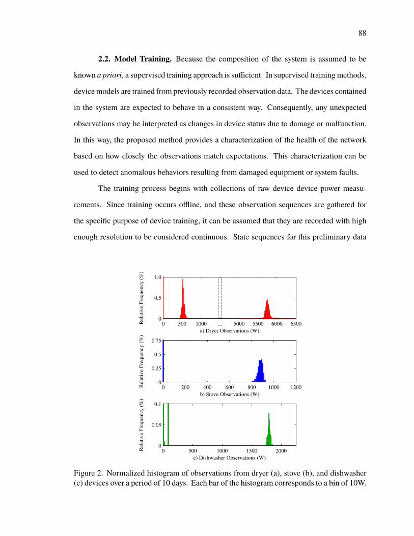
88

2.2. Model Training. Because the composition of the system is assumed to be

known a priori, a supervised training approach is sufficient. In supervised training methods,

devicemodels are trained from previously recorded observation data. The devices contained

in the system are expected to behave in a consistent way. Consequently, any unexpected

observations may be interpreted as changes in device status due to damage or malfunction.

In this way, the proposed method provides a characterization of the health of the network

based on how closely the observations match expectations. This characterization can be

used to detect anomalous behaviors resulting from damaged equipment or system faults.

The training process begins with collections of raw device device power measu-

rements. Since training occurs offline, and these observation sequences are gathered for

the specific purpose of device training, it can be assumed that they are recorded with high

enough resolution to be considered continuous. State sequences for this preliminary data

0 500 1000 ... 5000 5500 6000 65000

0.5

1.0

Rel

ativ

e F

req

uen

cy (

%)

a) Dryer Observations (W)

0 200 400 600 800 1000 12000

0.25

0.5

0.75

Rel

ativ

e F

req

uen

cy (

%)

b) Stove Observations (W)

0 500 1000 1500 20000

0.05

0.1

Rel

ativ

e F

req

uen

cy (

%)

c) Dishwasher Observations (W)

Figure 2. Normalized histogram of observations from dryer (a), stove (b), and dishwasher(c) devices over a period of 10 days. Each bar of the histogram corresponds to a bin of 10W.

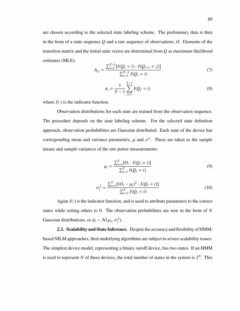
89

are chosen according to the selected state labeling scheme. The preliminary data is then

in the form of a state sequence Q and a raw sequence of observations, O. Elements of the

transition matrix and the initial state vector are determined from Q as maximum likelihood

estimates (MLE):

Ai j =

∑T−1t=1 [I(Qt = i) · I(Qt+1 = j)]∑T−1

t=1 I(Qt = i)(7)

πi =1

T − 1

T−1∑t=1

I(Qt = i) (8)

where I(·) is the indicator function.

Observation distributions for each state are trained from the observation sequence.

The procedure depends on the state labeling scheme. For the selected state definition

approach, observation probabilities are Gaussian distributed. Each state of the device has

corresponding mean and variance parameters, µ and σ2. These are taken as the sample

means and sample variances of the raw power measurements:

µi =

∑Tt=1[Ot · I(Qt = i)]∑T

t=1 I(Qt = i)(9)

σ2i =

∑Tt=1[(Ot − µi)

2 · I(Qt = i)]∑Tt=1 I(Qt = i)

(10)

Again I(·) is the indicator function, and is used to attribute parameters to the correct

states while setting others to 0. The observation probabilities are now in the form of N

Gaussian distributions, or φi ∼ N(µi, σ2i ).

2.3. Scalability andState Inference. Despite the accuracy andflexibility ofHMM-

based NILM approaches, their underlying algorithms are subject to severe scalability issues.

The simplest device model, representing a binary on/off device, has two states. If an HMM

is used to represent N of these devices, the total number of states in the system is 2N . This

90

exponential scaling in N is a problem on its own, but the more critical limiting influence

is the Viterbi algorithm, which has time complexity O(N2T), where T is the length of the

sequence of observations.

The proposed strategies for handling this fundamental limitation have split the field

of HMM-based NILM into two groups. The first approach is to use generalizations of

HMMs, such as factorial hidden Markov models (FHMMs), which describe multiple devi-

ces individually in a distributed state representation [20]. FHMMs have been successfully

applied to NILM [19, 9, 18, 21]. A variety of modified FHMM structures are proposed

and compared in [9]. The drawback to all of these methods is that exact inference is com-

putationally intractable, and approximate methods must be used. In [15], an approximate

inference method motivated by the NILM problem was proposed. The second group of

approaches uses the basic HMM structure and relies on the sparsity of matrices that com-

prise the system-level model to reduce the complexity of the problem. This approach relies

on alternative formulations of the Viterbi algorithm, such as those proposed in [22, 23].

One such method, the sparse Viterbi algorithm, was applied in [13] to a NILM system

consisting of over 109 states with high accuracy and dramatic reductions in execution time.

This greedy variant of the Viterbi algorithm maximizes the probability of each individual

state sequence transition, allowing online operation.

The NILM procedure proposed in this study uses the traditional HMM structure

and is compatible with any state inference method intended for basic HMMs. Since the

target applications of this method favor online disaggregation, the sparse Viterbi algorithm

is given particular consideration. In preparing the experimental results for this study, both

the standard Viterbi algorithm and the sparse Viterbi algorithm were used. For the sake

of completeness, a general review of the two algorithms is repeated in this section. More

detailed information is available in the accompanying references.

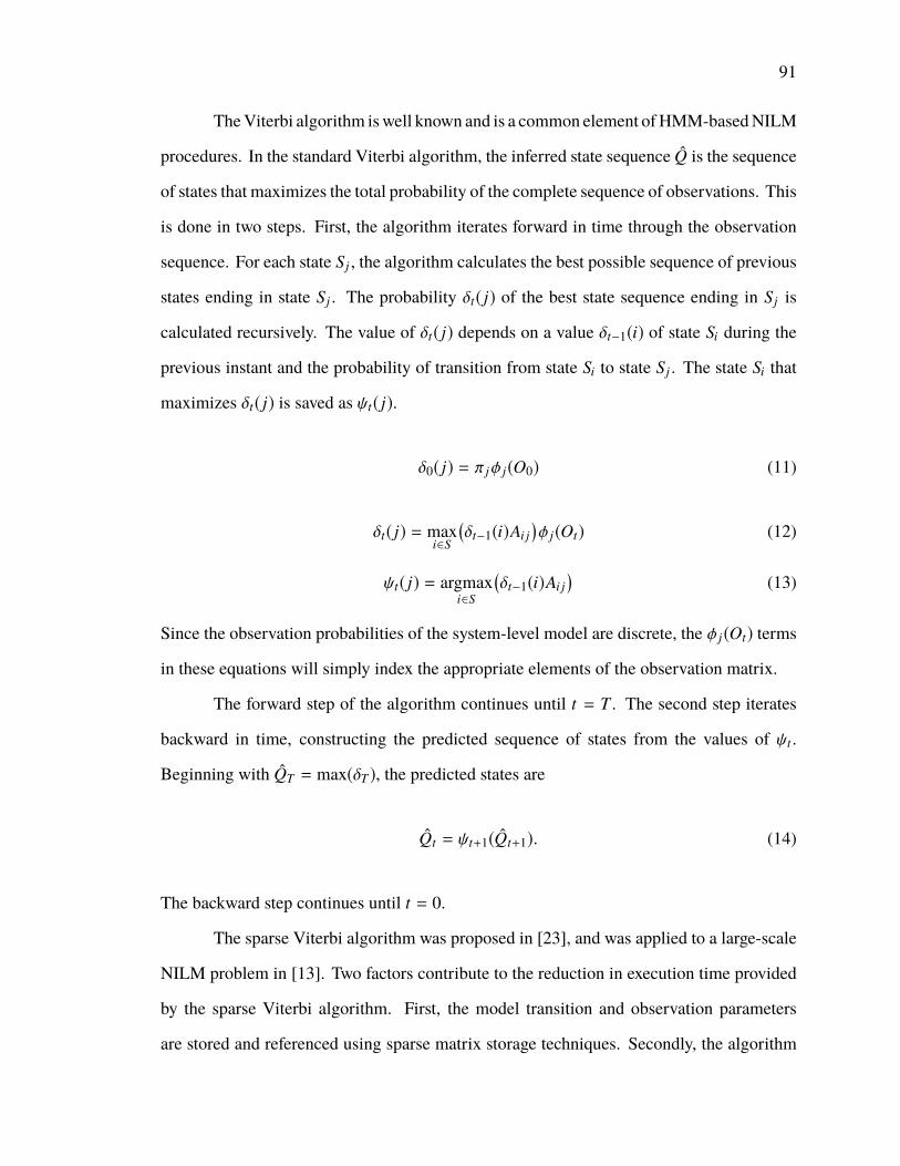
91

TheViterbi algorithm iswell known and is a common element ofHMM-basedNILM

procedures. In the standard Viterbi algorithm, the inferred state sequence Q is the sequence

of states that maximizes the total probability of the complete sequence of observations. This

is done in two steps. First, the algorithm iterates forward in time through the observation

sequence. For each state Sj , the algorithm calculates the best possible sequence of previous

states ending in state Sj . The probability δt( j) of the best state sequence ending in Sj is

calculated recursively. The value of δt( j) depends on a value δt−1(i) of state Si during the

previous instant and the probability of transition from state Si to state Sj . The state Si that

maximizes δt( j) is saved as ψt( j).

δ0( j) = π jφ j(O0) (11)

δt( j) = maxi∈S

(δt−1(i)Ai j

)φ j(Ot) (12)

ψt( j) = argmaxi∈S

(δt−1(i)Ai j

)(13)

Since the observation probabilities of the system-level model are discrete, the φ j(Ot) terms

in these equations will simply index the appropriate elements of the observation matrix.

The forward step of the algorithm continues until t = T . The second step iterates

backward in time, constructing the predicted sequence of states from the values of ψt .

Beginning with QT = max(δT ), the predicted states are

Qt = ψt+1(Qt+1). (14)

The backward step continues until t = 0.

The sparse Viterbi algorithm was proposed in [23], and was applied to a large-scale

NILM problem in [13]. Two factors contribute to the reduction in execution time provided

by the sparse Viterbi algorithm. First, the model transition and observation parameters

are stored and referenced using sparse matrix storage techniques. Secondly, the algorithm

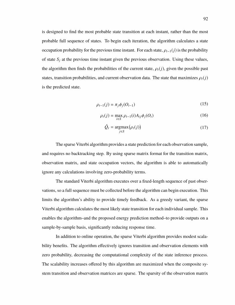
92

is designed to find the most probable state transition at each instant, rather than the most

probable full sequence of states. To begin each iteration, the algorithm calculates a state

occupation probability for the previous time instant. For each state, ρt−1( j) is the probability

of state Sj at the previous time instant given the previous observation. Using these values,

the algorithm then finds the probabilities of the current state, ρt( j), given the possible past

states, transition probabilities, and current observation data. The state that maximizes ρt( j)

is the predicted state.

ρt−1( j) = π jφ j(Ot−1) (15)

ρt( j) = maxi∈S

ρt−1(i)Ai jφ j(Ot) (16)

Qt = argmaxj∈S

(ρt( j)

)(17)

The sparse Viterbi algorithm provides a state prediction for each observation sample,

and requires no backtracking step. By using sparse matrix format for the transition matrix,

observation matrix, and state occupation vectors, the algorithm is able to automatically

ignore any calculations involving zero-probability terms.

The standard Viterbi algorithm executes over a fixed-length sequence of past obser-

vations, so a full sequence must be collected before the algorithm can begin execution. This

limits the algorithm’s ability to provide timely feedback. As a greedy variant, the sparse

Viterbi algorithm calculates the most likely state transition for each individual sample. This

enables the algorithm–and the proposed energy prediction method–to provide outputs on a

sample-by-sample basis, significantly reducing response time.

In addition to online operation, the sparse Viterbi algorithm provides modest scala-

bility benefits. The algorithm effectively ignores transition and observation elements with

zero probability, decreasing the computational complexity of the state inference process.

The scalability increases offered by this algorithm are maximized when the composite sy-

stem transition and observation matrices are sparse. The sparsity of the observation matrix

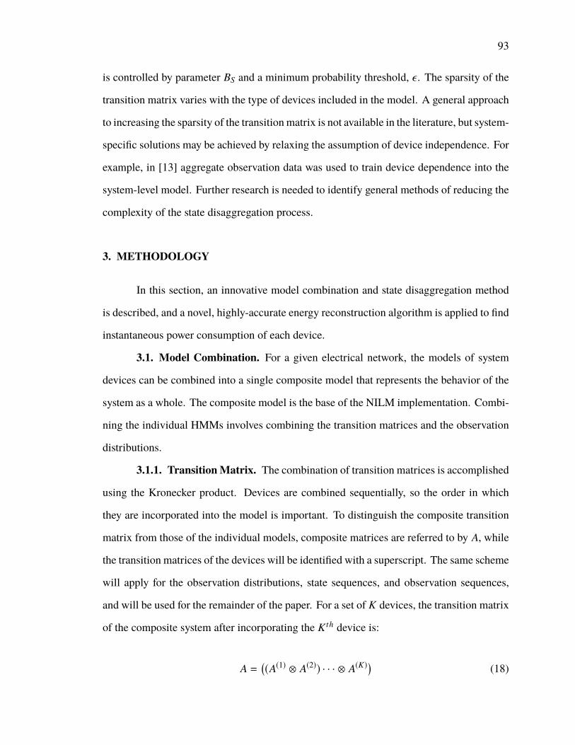
93

is controlled by parameter BS and a minimum probability threshold, ε . The sparsity of the

transition matrix varies with the type of devices included in the model. A general approach

to increasing the sparsity of the transitionmatrix is not available in the literature, but system-

specific solutions may be achieved by relaxing the assumption of device independence. For

example, in [13] aggregate observation data was used to train device dependence into the

system-level model. Further research is needed to identify general methods of reducing the

complexity of the state disaggregation process.

3. METHODOLOGY

In this section, an innovative model combination and state disaggregation method

is described, and a novel, highly-accurate energy reconstruction algorithm is applied to find

instantaneous power consumption of each device.

3.1. Model Combination. For a given electrical network, the models of system

devices can be combined into a single composite model that represents the behavior of the

system as a whole. The composite model is the base of the NILM implementation. Combi-

ning the individual HMMs involves combining the transition matrices and the observation

distributions.

3.1.1. TransitionMatrix. The combination of transition matrices is accomplished

using the Kronecker product. Devices are combined sequentially, so the order in which

they are incorporated into the model is important. To distinguish the composite transition

matrix from those of the individual models, composite matrices are referred to by A, while

the transition matrices of the devices will be identified with a superscript. The same scheme

will apply for the observation distributions, state sequences, and observation sequences,

and will be used for the remainder of the paper. For a set of K devices, the transition matrix

of the composite system after incorporating the K th device is:

A =((A(1) ⊗ A(2)) · · · ⊗ A(K)

)(18)

94

where⊗ denotes theKronecker product. Models are combined upwards from the first device,

and the order in which they are incorporated, k, is used to identify their parameters in the

disaggregation process. Alternatively, the composite matrix may be defined recursively as

A = A⊗ A(k), k = 1, 2, . . . ,K , where A is initialized as A = 1. The initial probability vector

of the combined system is calculated using (18) as well, the only difference being that the

result will remain a vector rather than a matrix.

To illustrate the combination process, consider a simplified example system of two

devices. Transition diagrams are shown for the devices in Fig. 3, with self-transitions

excluded for clarity. Device 1 consists of two states and device 2 consists of three states.

The directions on the edges of the graph indicate the possible transition directions. For

example, device 2 may transition freely between states 1 and 3, but may not transition to

state 2 from state 3. This is reflected in the transition matrix by a 0 element in column 3,

row 2. Possible transition matrices for these devices are

A(1) =

0.9 0.1

0.2 0.8

, A(2) =

0.8 0.1 0.1

0 0.4 0.6

0.5 0 0.5

.

These probabilities are simplified for the sake of illustration. When the two devices

are represented as a system, all possible transitions must be represented. This is shown

in Fig. 4. The system-level state, Q, is encircled in the nodes of the graph while the

Figure 3. Directed graph representation of two example devices and their potential transi-tions.

95

Figure 4. Directed graph representation of a two-device example system. Dotted linesindicate transitions in which both devices change state simultaneously.

corresponding device-level states are shown in the margins. The edges again indicate

potential transitions. Since device 2 is unable to transition from state 3 to state 2 at the

device level, the combined system is likewise unable to transition from states 3 or 6 to states

2 or 5. This restriction is again represented in the transition matrix.

A(1) ⊗ A(2) =

0.72 0.09 0.09 0.08 0.01 0.01

0 0.36 0.54 0 0.04 0.06

0.45 0 0.45 0.05 0 0.05

0.16 0.02 0.02 0.64 0.08 0.08

0 0.08 0.12 0 0.32 0.48

0.1 0 0.1 0.4 0 0.4

3.1.2. ObservationMatrix. To simplify the combination of observation probabili-

ties, the individual devices’ observation distributions are converted into discrete probability

mass functions, such that they may be described in matrix form. To convert the continuous

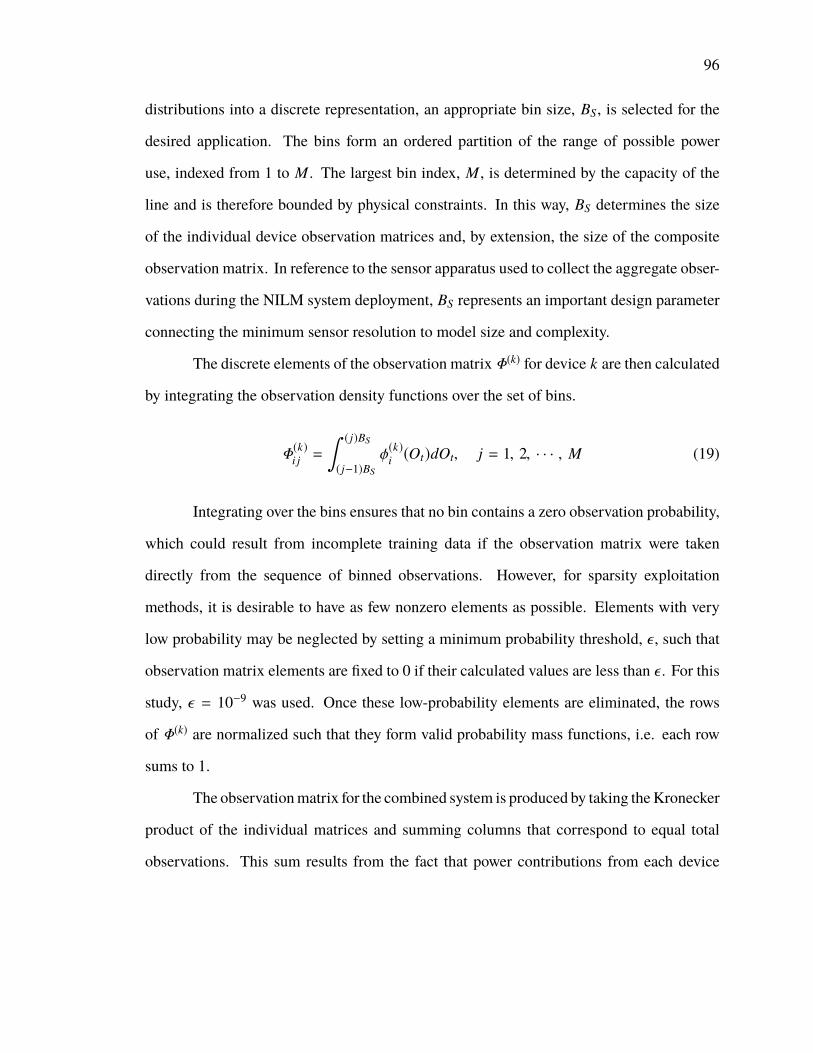
96

distributions into a discrete representation, an appropriate bin size, BS, is selected for the

desired application. The bins form an ordered partition of the range of possible power

use, indexed from 1 to M . The largest bin index, M , is determined by the capacity of the

line and is therefore bounded by physical constraints. In this way, BS determines the size

of the individual device observation matrices and, by extension, the size of the composite

observation matrix. In reference to the sensor apparatus used to collect the aggregate obser-

vations during the NILM system deployment, BS represents an important design parameter

connecting the minimum sensor resolution to model size and complexity.

The discrete elements of the observation matrix Φ(k) for device k are then calculated

by integrating the observation density functions over the set of bins.

Φ(k)i j =

∫ ( j)BS

( j−1)BS

φ(k)i (Ot)dOt, j = 1, 2, · · · , M (19)

Integrating over the bins ensures that no bin contains a zero observation probability,

which could result from incomplete training data if the observation matrix were taken

directly from the sequence of binned observations. However, for sparsity exploitation

methods, it is desirable to have as few nonzero elements as possible. Elements with very

low probability may be neglected by setting a minimum probability threshold, ε , such that

observation matrix elements are fixed to 0 if their calculated values are less than ε . For this

study, ε = 10−9 was used. Once these low-probability elements are eliminated, the rows

of Φ(k) are normalized such that they form valid probability mass functions, i.e. each row

sums to 1.

The observationmatrix for the combined system is produced by taking theKronecker

product of the individual matrices and summing columns that correspond to equal total

observations. This sum results from the fact that power contributions from each device

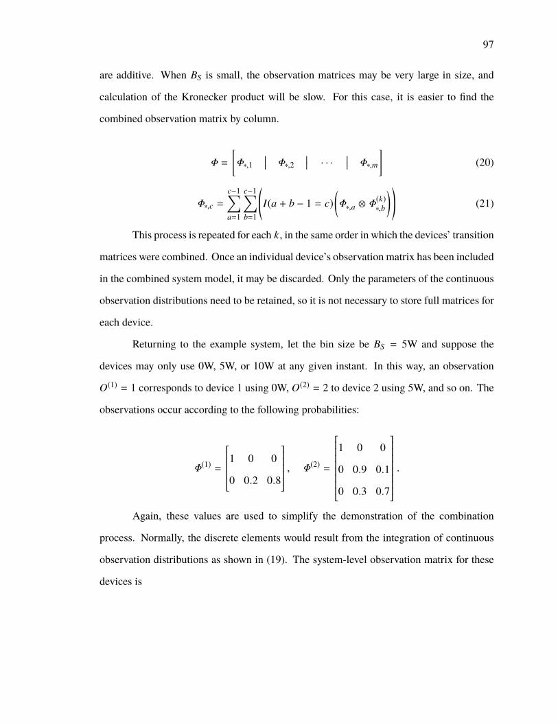
97

are additive. When BS is small, the observation matrices may be very large in size, and

calculation of the Kronecker product will be slow. For this case, it is easier to find the

combined observation matrix by column.

Φ =[Φ∗,1

Φ∗,2 · · ·

Φ∗,m]

(20)

Φ∗,c =c−1∑a=1

c−1∑b=1

(I(a + b − 1 = c)

(Φ∗,a ⊗ Φ(k)

∗,b

))(21)

This process is repeated for each k, in the same order in which the devices’ transition

matrices were combined. Once an individual device’s observation matrix has been included

in the combined system model, it may be discarded. Only the parameters of the continuous

observation distributions need to be retained, so it is not necessary to store full matrices for

each device.

Returning to the example system, let the bin size be BS = 5W and suppose the

devices may only use 0W, 5W, or 10W at any given instant. In this way, an observation

O(1) = 1 corresponds to device 1 using 0W, O(2) = 2 to device 2 using 5W, and so on. The

observations occur according to the following probabilities:

Φ(1) =

1 0 0

0 0.2 0.8

, Φ(2) =

1 0 0

0 0.9 0.1

0 0.3 0.7

.

Again, these values are used to simplify the demonstration of the combination

process. Normally, the discrete elements would result from the integration of continuous

observation distributions as shown in (19). The system-level observation matrix for these

devices is

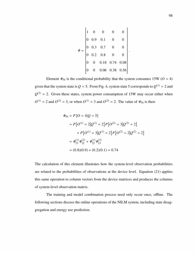
98

Φ =

1 0 0 0 0

0 0.9 0.1 0 0

0 0.3 0.7 0 0

0 0.2 0.8 0 0

0 0 0.18 0.74 0.08

0 0 0.06 0.38 0.56

.

Element Φ54 is the conditional probability that the system consumes 15W (O = 4)

given that the system state is Q = 5. From Fig. 4, system state 5 corresponds to Q(1) = 2 and

Q(2) = 2. Given these states, system power consumption of 15W may occur either when

O(1) = 2 and O(2) = 3, or when O(1) = 3 and O(2) = 2. The value of Φ54 is then:

Φ54 = P [O = 4|Q = 5]

= P[O(1) = 2

Q(1) = 2]P[O(2) = 3

Q(2) = 2]

+ P[O(1) = 3

Q(1) = 2]P[O(2) = 2

Q(2) = 2]

= Φ(1)23 Φ(2)22 + Φ(1)22 Φ(2)23

= (0.8)(0.9) + (0.2)(0.1) = 0.74

The calculation of this element illustrates how the system-level observation probabilities

are related to the probabilities of observations at the device level. Equation (21) applies

this same operation to column vectors from the device matrices and produces the columns

of system-level observation matrix.

The training and model combination process need only occur once, offline. The

following sections discuss the online operations of the NILM system, including state disag-

gregation and energy use prediction.

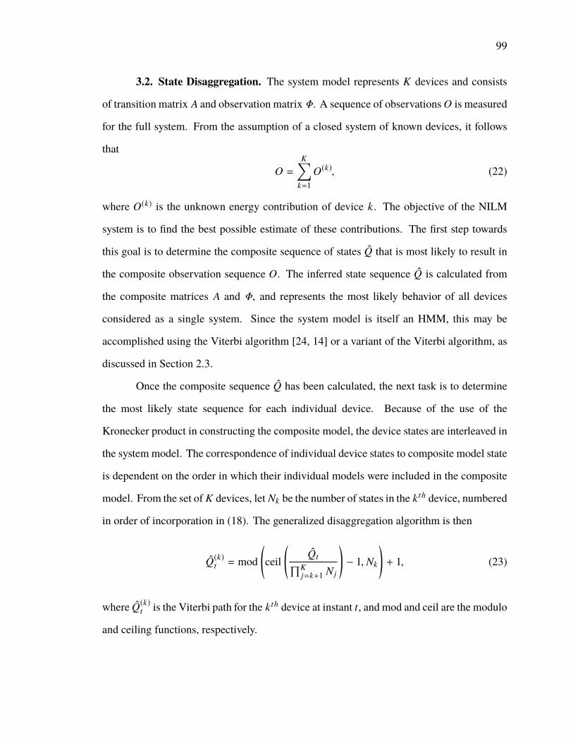
99

3.2. State Disaggregation. The system model represents K devices and consists

of transition matrix A and observation matrix Φ. A sequence of observations O is measured

for the full system. From the assumption of a closed system of known devices, it follows

that

O =K∑

k=1O(k), (22)

where O(k) is the unknown energy contribution of device k. The objective of the NILM

system is to find the best possible estimate of these contributions. The first step towards

this goal is to determine the composite sequence of states Q that is most likely to result in

the composite observation sequence O. The inferred state sequence Q is calculated from

the composite matrices A and Φ, and represents the most likely behavior of all devices

considered as a single system. Since the system model is itself an HMM, this may be

accomplished using the Viterbi algorithm [24, 14] or a variant of the Viterbi algorithm, as

discussed in Section 2.3.

Once the composite sequence Q has been calculated, the next task is to determine

the most likely state sequence for each individual device. Because of the use of the

Kronecker product in constructing the composite model, the device states are interleaved in

the system model. The correspondence of individual device states to composite model state

is dependent on the order in which their individual models were included in the composite

model. From the set of K devices, let Nk be the number of states in the k th device, numbered

in order of incorporation in (18). The generalized disaggregation algorithm is then

Q(k)t = mod

(ceil

(Qt∏K

j=k+1 Nj

)− 1, Nk

)+ 1, (23)

where Q(k)t is the Viterbi path for the k th device at instant t, and mod and ceil are the modulo

and ceiling functions, respectively.

100

For device K , the last included in the composite model, the form of (23) reduces to

Q(K)t = mod(Qt − 1, NK

)+ 1. (24)

The graph in Fig. 4 provides a visual representation of equations (23) and (24) for the

two-device example system. It is clear from the graph that system state Q = 5 corresponds

to device states Q(1) = 2 and Q(2) = 2. Equivalently, Q = 5 corresponds to Q(1) = 2

and Q(2) = 2 at any given instant. The disaggregation equations produce the same results.

Equation (23) must be used to calculate Q(1), while the reduced form in (24) may be used

to calculate Q(2). For this system, K = 2, N1 = 2, and N2 = 3.

Q(1) = mod

(ceil

(53

)− 1, 2

)+ 1 = 2

Q(2) = mod

(5 − 1, 2

)+ 1 = 2

3.3. Prediction of Energy Use. Once the estimated state sequences for the indi-

vidual devices have been found, it remains to predict the energy use of each device. The

simplest approach to this prediction is to use the best possible constant estimator. This is

given by the expected value of the observation, conditional on the current state.

O(k)t = E[O(k)t

Q(k)t = j]= µ

(k)j (25)

The total energy use predicted for device n is then

W (k) = TS

T∑t=1

O(k)t . (26)

101

This conventional method is useful in estimating cumulative energy use over a period of

time, but provides only a rough approximation of actual device behavior. The number of

possible observation predictions is limited to the number ofmodel states, and the predictions

of observations in time are constant when the state is not changing.

When the set of devices contained in the system is known and unchanging, a more

detailed estimate of the energy contributions from each device may be achieved by breaking

down the composite energy use according to the devices’ conditional observation distribu-

tions. The calculation of these predictions may be framed as a constrained optimization

problem, maximizing the total probability of the observations while constraining their sum

to equal the measured aggregate observation.

Let O be aK-vector of observation predictions for theK system devices. Because the

devices are assumed to operate independently, the probability of O given the disaggregated

state sequence is determined by

P[O] =K∏

k=1P

[O(k)

Q(k) = j]=

K∏k=1

φ(k)j

(O(k)

). (27)

To simplify notation, time indices t have been dropped in (27), and will be omitted for

the remainder of this section. Working in logspace, the product term in (27) becomes a

summation of terms, but the locations of critical points remain the same. The objective

function f is defined as

f (O) = ln(P[O]

)=

K∑k=1

ln

(φ(k)j

(O(k)

)). (28)

The equality constraint, g, is given by the assumption of known system composition and

additive observations.

g(O) =K∑

k=1O(k) −O = 0 (29)

102

Using Lagrange multipliers, ∇ f = λ∇g. The k th summation term of (28) depends

only on the k th element of O. For Q(i) = j, the partial derivative is then

∂ f (O)

∂O(k)=

∂

∂O(k)ln

(φ(k)j

(O(k)

) )=

(µ(k)j − O(k)

)(σ(k)j

)2 . (30)

The convenient linear form of this equation results from the assumption of Gaussian obser-

vation distributions. The k th term of λ∇g is

λ∂g(O)

∂O(k)= λ. (31)

Equating the derivatives in (30) and (31),

(µ(k)j − O(k)

)(σ(k)j

)2 = λ. (32)

By rearranging this equation, each O(k) may be expressed in terms of λ and mean and

variance parameters, which are known.

O(k) = µ(k)j − λ(σ(k)j

)2(33)

Substituting these terms into (29) yields an expression for λ in terms of the aggregate

observation and the sums of the means and variances of the appropriate device states.

λ =

(∑Kk=1 µ

(k)Q(k)

)−O∑K

k=1

(σ(k)Q(k)

)2 (34)

Finally, the individual observation predictions are then calculated by substituting λ back

into (33) for each device.

103

The final equations (33) and (34) are used to predict the device-level observations at

each time sample. This adds little in terms of computational complexity, as the summations

in (34) contain K terms, and only change when disaggregated state changes.

3.4. Discussion. In the context of HMM-based NILM procedures, the proposed

method features novel approaches to system-level modeling and energy use prediction.

The basic HMM framework is used at both the device and system level, allowing simple

and well-known methods to be used for training and state inference. The combination

process is modular in that devices may be modeled individually and used later to build

system-level models. A conceptually similar model combination process was employed

for two devices in [10], but was presented without the necessary mathematical framework,

and without the ability to break system-level states into individual device states. Methods

in other studies, such as [13], require system-specific training data. Beyond knowledge

of the devices contained in a system, the proposed method requires no system-specific

information. That is, the system-level model can be constructed without composite or

simultaneous submetered data collection.

In the process of combining device models, continuous observation distribution

parameters are converted into discrete probabilities. This allows sparsity exploitation

methods, i.e. the sparse Viterbi algorithm, to be employed in the state inference stage.

However, the continuous parameters are preserved, and are used after the state has been

disaggregated to provide more accurate energy use predictions.

Themost important element of the proposedmethod is the energy prediction process.

Other HMM-based NILM studies typically stop at state disaggregation, and provide energy

predictions as constant, one-to-onemappings between state and observation. This limitation

is dictated by application context; almost all other methods are intended for residential

systems in which unmodeled loads are likely present. The uncertainty introduced by

unknown devices prevents more refined predictions. For the applications of the proposed

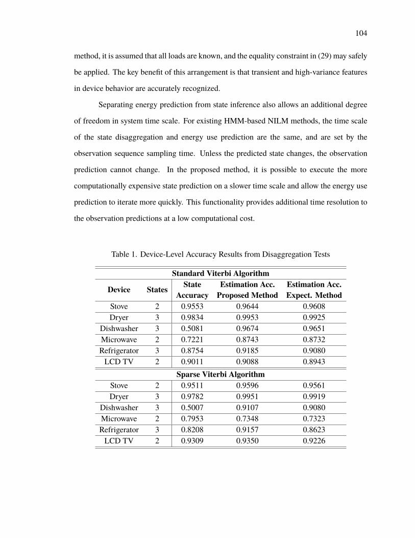
104

method, it is assumed that all loads are known, and the equality constraint in (29) may safely

be applied. The key benefit of this arrangement is that transient and high-variance features

in device behavior are accurately recognized.

Separating energy prediction from state inference also allows an additional degree

of freedom in system time scale. For existing HMM-based NILM methods, the time scale

of the state disaggregation and energy use prediction are the same, and are set by the

observation sequence sampling time. Unless the predicted state changes, the observation

prediction cannot change. In the proposed method, it is possible to execute the more

computationally expensive state prediction on a slower time scale and allow the energy use

prediction to iterate more quickly. This functionality provides additional time resolution to

the observation predictions at a low computational cost.

Table 1. Device-Level Accuracy Results from Disaggregation Tests

Standard Viterbi Algorithm

Device States State Estimation Acc. Estimation Acc.Accuracy Proposed Method Expect. Method

Stove 2 0.9553 0.9644 0.9608Dryer 3 0.9834 0.9953 0.9925

Dishwasher 3 0.5081 0.9674 0.9651Microwave 2 0.7221 0.8743 0.8732Refrigerator 3 0.8754 0.9185 0.9080LCD TV 2 0.9011 0.9088 0.8943

Sparse Viterbi AlgorithmStove 2 0.9511 0.9596 0.9561Dryer 3 0.9782 0.9951 0.9919

Dishwasher 3 0.5007 0.9107 0.9080Microwave 2 0.7953 0.7348 0.7323Refrigerator 3 0.8208 0.9157 0.8623LCD TV 2 0.9309 0.9350 0.9226

105

4. EXPERIMENTAL VERIFICATION

The objectives of the verification experiments were to demonstrate the functionality

of the NILM system and assess its performance. Specific performance metrics of interest

are how closely the system outputs (Q(k)t and O(k)t ) match the corresponding ground truth

sequences (Q(k)t and O(k)t ), which are unknown to the model during the system tests. For the

same test data, results are collected using the standard Viterbi algorithm and using the sparse

Viterbi algorithm. This allows the impact of the replacing the standard Viterbi algorithm to

be quantified in terms of system performance. Energy use estimations calculated using the

expected value and the method proposed in Section 3 are compared as well. Additionally,

energy predictions are calculated both when using the disaggregated states and when using

the ground truth states. This latter case represents an idealized situation in which no

errors are made in state disaggregation, i.e. Q = Q. While this is an unrealistic scenario

in practice, it effectively decouples the performance of the energy prediction methods

from errors introduced in state disaggregation, allowing fair comparison of the estimation

methods.

The experiments were conducted using individual appliance data from public data-

bases intended for NILM research. The resources used include the ECO [25], Smart∗ [26],

and GREEND [27] datasets. The datasets contain high quality data at the aggregate and

submetered level over a period of a few months. Although these datasets contain data from

residential systems, it was possible to generate test cases that meet the assumption of known

and fixed system composition by extracting device data from the datasets and summing

their measurements to construct an aggregate observation sequence. Since the experiment

is intended to assess the performance of the algorithms in systems with known composition,

rather than their ability to recognize specific types of devices, the actual devices used in

the tests is immaterial. The test systems contain residential devices simply because the

available public NILM databases that contain the amount of data required come exclusively

from residential settings.

106

For the full experiment, a 10-fold cross validation was used. For each monitored

device, 10 days of measurements were extracted from the datasets, ensuring that the device

in question was active on each day. From this collection, one day of data was selected

for each device and included in a composite test sequence. This was repeated 10 times,

such that 10 test sequences were created and each day of device data was included once.

For each test sequence, the 9 remaining days served as training data for the device models

used. The model was not trained on the data used in the test. This full procedure was

repeated 10 times, with randomly generated time shifts for each device, so that 10 different

aggregate test sequences were generated for each set of test devices. The sampling time

was set at 5 seconds for training and testing. For simplicity, the same time scale used for

the state disaggregation and energy use prediction functions. The time scale was limited

by the time resolution of the available device data. Setting the sampling time lower than

5 seconds would have required reconstruction of missing samples for some devices, which

would introduce bias in the experimental results.

4.1. Performance Assessments. Standard NILM performance metrics were used

to assess the accuracy of the methods. These methods are summarized in [28], and were

gathered from a variety of NILM studies. The state sequence accuracy of two-state devices

was assessed using F-Score. For devices with more than two states, the modified F-Score

proposed in [28] was used. This modified version is referred to as finite state F-score or FS-

Score, and is intended for finite state machine devices. For all devices, the energy accuracy

was assessed using estimation accuracy, proposed in [21]. To quantify the difference

between the energy prediction methods, root mean square error (RMSE) was calculated for

the predicted values as well. This metric was used in [11] for assessment at the device level.

Here, RMSE values are calculated by state:

RMSE (k)j =

(1Tj

∑t:Q(k)t = j

(O(k) −O(k)

)2)1/2

(35)

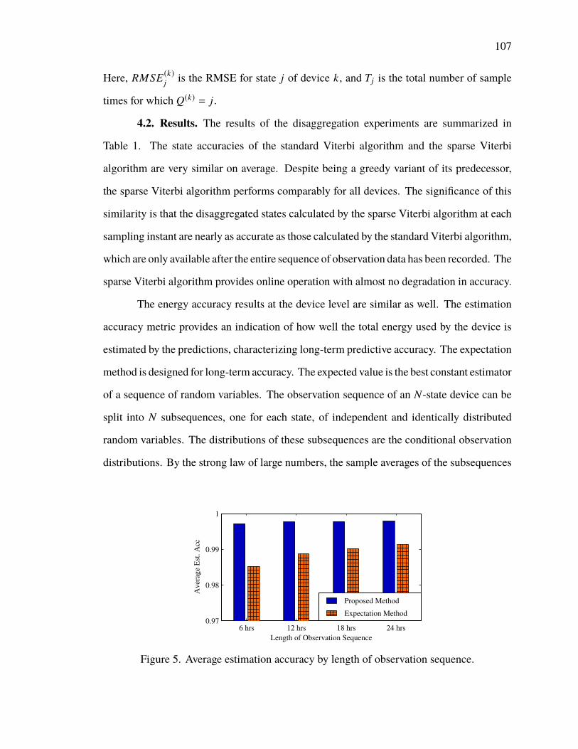
107

Here, RMSE (k)j is the RMSE for state j of device k, and Tj is the total number of sample

times for which Q(k) = j.

4.2. Results. The results of the disaggregation experiments are summarized in

Table 1. The state accuracies of the standard Viterbi algorithm and the sparse Viterbi

algorithm are very similar on average. Despite being a greedy variant of its predecessor,

the sparse Viterbi algorithm performs comparably for all devices. The significance of this

similarity is that the disaggregated states calculated by the sparse Viterbi algorithm at each

sampling instant are nearly as accurate as those calculated by the standard Viterbi algorithm,

which are only available after the entire sequence of observation data has been recorded. The

sparse Viterbi algorithm provides online operation with almost no degradation in accuracy.

The energy accuracy results at the device level are similar as well. The estimation

accuracy metric provides an indication of how well the total energy used by the device is

estimated by the predictions, characterizing long-term predictive accuracy. The expectation

method is designed for long-term accuracy. The expected value is the best constant estimator

of a sequence of random variables. The observation sequence of an N-state device can be

split into N subsequences, one for each state, of independent and identically distributed

random variables. The distributions of these subsequences are the conditional observation

distributions. By the strong law of large numbers, the sample averages of the subsequences

6 hrs 12 hrs 18 hrs 24 hrs0.97

0.98

0.99

1

Aver

age

Est

. A

cc

Length of Observation Sequence

Expectation Method

Proposed Method

Figure 5. Average estimation accuracy by length of observation sequence.

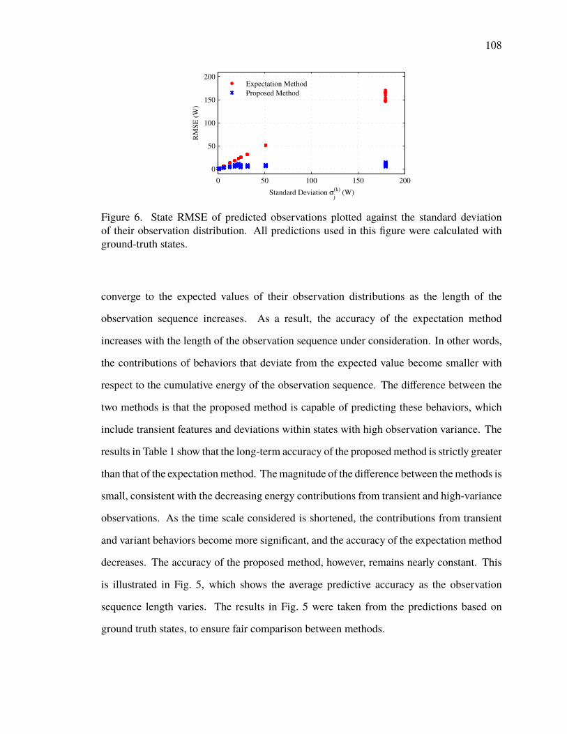
108

0 50 100 150 200

0

50

100

150

200Expectation Method

Proposed Method

Standard Deviation σj

(k) (W)

RM

SE

(W

)

Figure 6. State RMSE of predicted observations plotted against the standard deviationof their observation distribution. All predictions used in this figure were calculated withground-truth states.

converge to the expected values of their observation distributions as the length of the

observation sequence increases. As a result, the accuracy of the expectation method

increases with the length of the observation sequence under consideration. In other words,

the contributions of behaviors that deviate from the expected value become smaller with

respect to the cumulative energy of the observation sequence. The difference between the

two methods is that the proposed method is capable of predicting these behaviors, which

include transient features and deviations within states with high observation variance. The

results in Table 1 show that the long-term accuracy of the proposedmethod is strictly greater

than that of the expectationmethod. Themagnitude of the difference between themethods is

small, consistent with the decreasing energy contributions from transient and high-variance

observations. As the time scale considered is shortened, the contributions from transient

and variant behaviors become more significant, and the accuracy of the expectation method

decreases. The accuracy of the proposed method, however, remains nearly constant. This

is illustrated in Fig. 5, which shows the average predictive accuracy as the observation

sequence length varies. The results in Fig. 5 were taken from the predictions based on

ground truth states, to ensure fair comparison between methods.

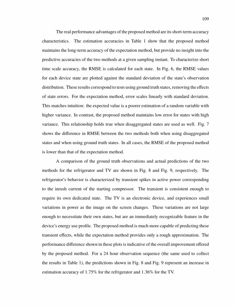
109

The real performance advantages of the proposedmethod are its short-term accuracy

characteristics. The estimation accuracies in Table 1 show that the proposed method

maintains the long-term accuracy of the expectation method, but provide no insight into the

predictive accuracies of the two methods at a given sampling instant. To characterize short

time scale accuracy, the RMSE is calculated for each state. In Fig. 6, the RMSE values

for each device state are plotted against the standard deviation of the state’s observation

distribution. These results correspond to tests using ground truth states, removing the effects

of state errors. For the expectation method, error scales linearly with standard deviation.

This matches intuition: the expected value is a poorer estimation of a random variable with

higher variance. In contrast, the proposed method maintains low error for states with high

variance. This relationship holds true when disaggregated states are used as well. Fig. 7

shows the difference in RMSE between the two methods both when using disaggregated

states and when using ground truth states. In all cases, the RMSE of the proposed method

is lower than that of the expectation method.

A comparison of the ground truth observations and actual predictions of the two

methods for the refrigerator and TV are shown in Fig. 8 and Fig. 9, respectively. The

refrigerator’s behavior is characterized by transient spikes in active power corresponding

to the inrush current of the starting compressor. The transient is consistent enough to

require its own dedicated state. The TV is an electronic device, and experiences small

variations in power as the image on the screen changes. These variations are not large

enough to necessitate their own states, but are an immediately recognizable feature in the

device’s energy use profile. The proposed method is much more capable of predicting these

transient effects, while the expectation method provides only a rough approximation. The

performance difference shown in these plots is indicative of the overall improvement offered

by the proposed method. For a 24 hour observation sequence (the same used to collect

the results in Table 1), the predictions shown in Fig. 8 and Fig. 9 represent an increase in

estimation accuracy of 1.75% for the refrigerator and 1.36% for the TV.

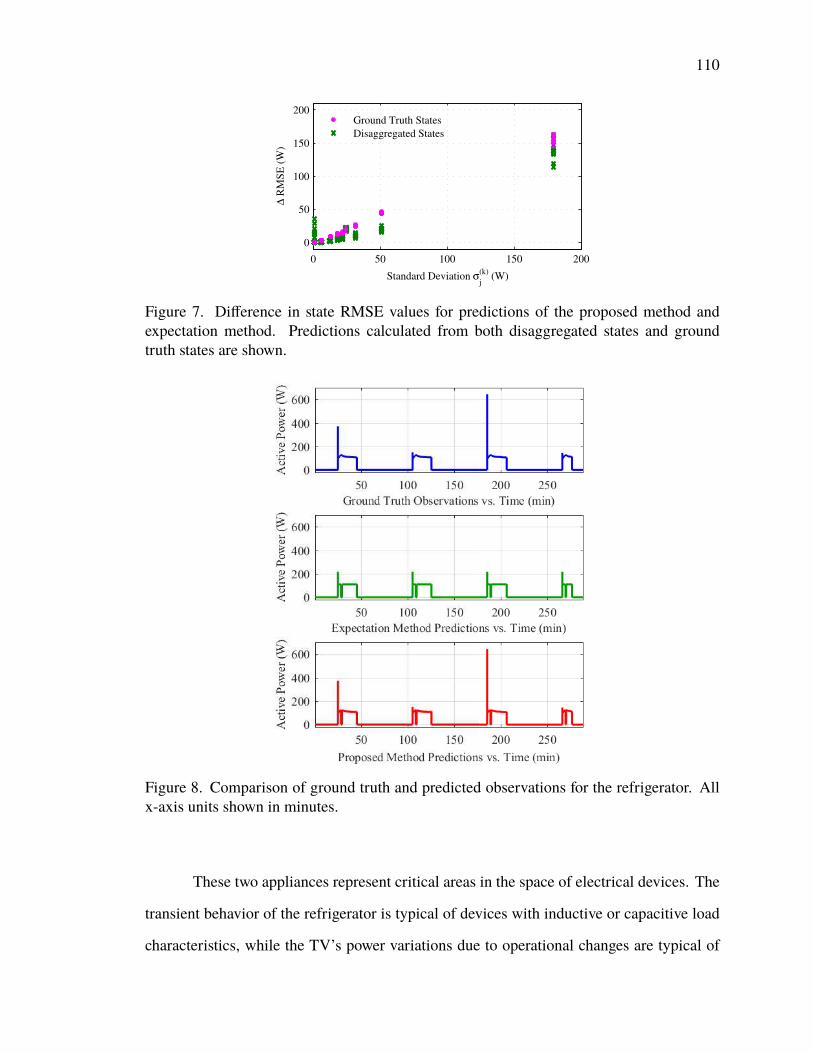
110

0 50 100 150 200

0

50

100

150

200Ground Truth States

Disaggregated States

Standard Deviation σj

(k) (W)

∆ R

MS

E (

W)

Figure 7. Difference in state RMSE values for predictions of the proposed method andexpectation method. Predictions calculated from both disaggregated states and groundtruth states are shown.

Figure 8. Comparison of ground truth and predicted observations for the refrigerator. Allx-axis units shown in minutes.

These two appliances represent critical areas in the space of electrical devices. The

transient behavior of the refrigerator is typical of devices with inductive or capacitive load

characteristics, while the TV’s power variations due to operational changes are typical of

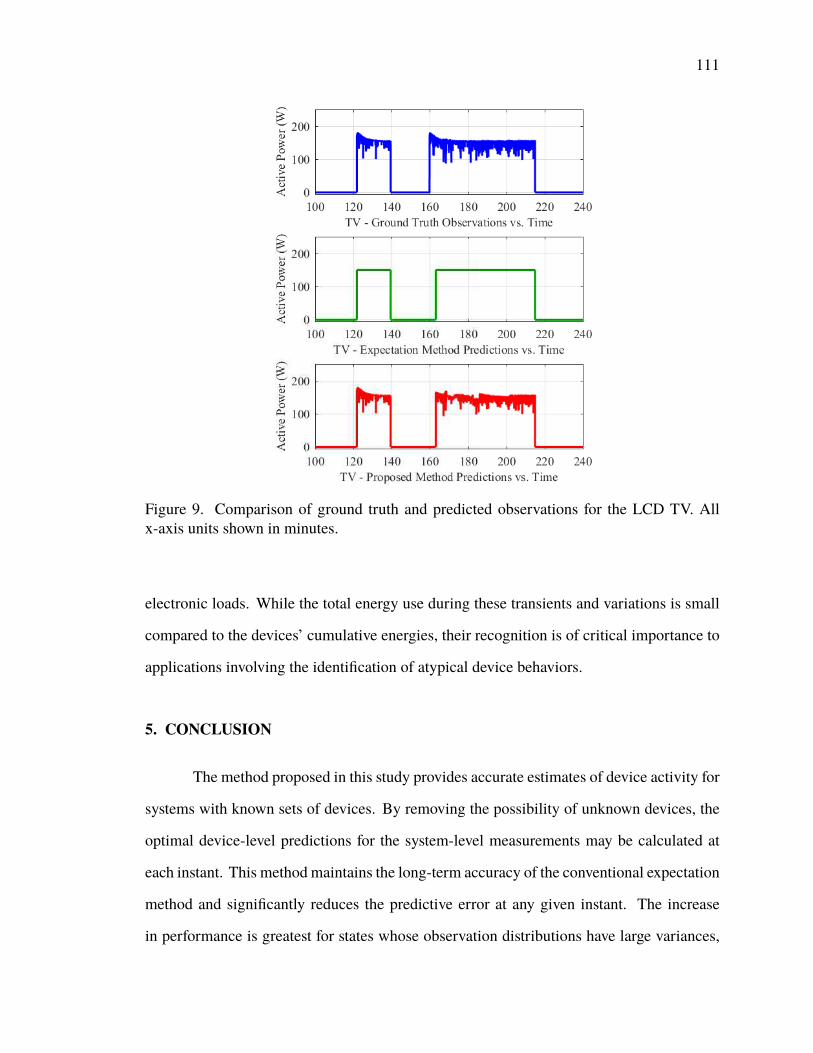
111

Figure 9. Comparison of ground truth and predicted observations for the LCD TV. Allx-axis units shown in minutes.

electronic loads. While the total energy use during these transients and variations is small

compared to the devices’ cumulative energies, their recognition is of critical importance to

applications involving the identification of atypical device behaviors.

5. CONCLUSION

The method proposed in this study provides accurate estimates of device activity for

systems with known sets of devices. By removing the possibility of unknown devices, the

optimal device-level predictions for the system-level measurements may be calculated at

each instant. This method maintains the long-term accuracy of the conventional expectation

method and significantly reduces the predictive error at any given instant. The increase

in performance is greatest for states whose observation distributions have large variances,

112

since the proposed method is capable of predicting transients and deviations from the mean,

while the expectation method ignores these features. Future work in this study will explore

new methods of state sequence determination. The state inference calculations are the

dominant limiting factors for both the accuracy and scalability of the method as a whole.

A more scalable means of calculating states would extend the applicability of the NILM

algorithm to much larger systems.

REFERENCES

[1] Z. Wang and G. Zheng, “Residential appliances identification and monitoring by a

nonintrusive method,” IEEE Trans. Smart Grid, vol. 3, no. 1, pp. 80–92, March 2012.

[2] G. Hart, “Nonintrusive appliance load monitoring,” Proc. IEEE, vol. 80, no. 12, pp.

1870–1891, Dec 1992.

[3] D. He, W. Lin, N. Liu, R. Harley, and T. Habetler, “Incorporating non-intrusive load

monitoring into building level demand response,” IEEE Trans. Smart Grid, vol. 4,

no. 4, pp. 1870–1877, Dec 2013.

[4] M. Zeifman and K. Roth, “Nonintrusive appliance load monitoring: Review and

outlook,” IEEE Trans. Consum. Electron., vol. 57, no. 1, pp. 76–84, February 2011.

[5] Y. F.Wong, Y.Ahmet Sekercioglu, T.Drummond, andV. S.Wong, “Recent approaches

to non-intrusive load monitoring techniques in residential settings,” in IEEE Symp.

Computational Intelligence Applications In Smart Grid (CIASG), April 2013, pp.

73–79.

[6] Y. Du, L. Du, B. Lu, R. Harley, and T. Habetler, “A review of identification and

monitoring methods for electric loads in commercial and residential buildings,” in

Energy Conversion Congress and Exposition (ECCE), 2010 IEEE, Sept 2010, pp.

4527–4533.

113

[7] C. Laughman et al., “Power signature analysis,” IEEE Power Energy Mag., vol. 1,

no. 2, pp. 56–63, Mar 2003.

[8] M. Berges, E. Goldman, H. S. Matthews, L. Soibelman, and K. Anderson, “User-

centered nonintrusive electricity loadmonitoring for residential buildings,” J. Comput.

Civ. Eng., vol. 25, no. 6, pp. 471–480, May 2011.

[9] H. Kim, M. Marwah, M. Arlitt, G. Lyon, and J. Han, “Unsupervised disaggregation

of low frequency power measurements,” in SDM, vol. 11, 2011, pp. 747–758.

[10] T. Zia, D. Bruckner, and A. Zaidi, “A hidden Markov model based procedure for

identifying household electric loads,” in 37th Conf. Industrial Electronics, Nov 2011,

pp. 3218–3223.

[11] O. Parson, S. Ghosh, M. Weal, and A. Rogers, “Non-intrusive load monitoring using

prior models of general appliance types,” in 26th Conference on Artificial Intelligence,

vol. 22, 2012, pp. 356–362.

[12] J. Liao, G. Elafoudi, L. Stankovic, and V. Stankovic, “Non-intrusive appliance load

monitoring using low-resolution smart meter data,” in IEEE Int.l Conf. Smart Grid

Communications (SmartGridComm), Nov 2014, pp. 535–540.

[13] S. Makonin, F. Popowich, I. Bajic, B. Gill, and L. Bartram, “Exploiting hmm sparsity

to perform online real-time nonintrusive load monitoring,” IEEE Trans. Smart Grid,

vol. PP, no. 99, pp. 1–11, 2015.

[14] L. Rabiner, “A tutorial on hidden Markov models and selected applications in speech

recognition,” Proc. IEEE, vol. 77, no. 2, pp. 257–286, Feb 1989.

[15] J. Z. Kolter and T. Jaakkola, “Approximate inference in additive factorial HMMs with

application to energy disaggregation,” in Proc. 15th Int. Conf. Artificial Intelligence

and Statistics, vol. 22, 2012, pp. 1472–1482.

114

[16] J. A. Mueller and J. W. Kimball, “An accurate method of energy use prediction for

systems with known composition,” in Proc. 3rd. Int. Workshop on Nonintrusive Load

Monitoring, May 2016.

[17] Z. Ghahramani, “An introduction to hidden Markov models and bayesian networks,”

Int. J. Pattern Recognition and Artificial Intell., vol. 15, no. 1, pp. 9–42, Jun. 2001.

[18] A. Zoha, A. Gluhak, M. Nati, and M. Imran, “Low-power appliance monitoring using

factorial hidden Markov models,” in IEEE 8th Int.l Conf. Intelligent Sensors, Sensor

Networks and Information Processing, April 2013, pp. 527–532.

[19] L. Wang, X. Luo, and W. Zhang, “Unsupervised energy disaggregation with factorial

hidden Markov models based on generalized backfitting algorithm,” in Proc. IEEE

Region 10 Conf., Oct 2013, pp. 1–4.

[20] Z. Ghahramani and M. I. Jordan, “Factorial hidden Markov models,” Mach. Learn.,

vol. 29, no. 2-3, pp. 245–273, Nov. 1997.

[21] J. Z. Kolter and M. J. Johnson, “REDD: A Public Data Set for Energy Disaggregation

Research,” in Proc. 2011 Workshop on Data Mining Applications in Sustainability

(SustKDD 2011), Aug 2011.

[22] M. Zeifman and K. Roth, “Viterbi algorithm with sparse transitions (vast) for nonin-

trusive load monitoring,” in Computational Intelligence Applications In Smart Grid

(CIASG), 2011 IEEE Symposium on, April 2011, pp. 1–8.

[23] S. Makonin, F. Popowich, and I. Bajic, “Efficient matrix processing for nonintru-

sive load monitoring (NILM),” in Proc. 2nd. Int. Workshop on Nonintrusive Load

Monitoring, June 2014.

[24] J. Forney, G.D., “The Viterbi algorithm,” Proc. IEEE, vol. 61, no. 3, pp. 268–278,

March 1973.

115

[25] C. Beckel, W. Kleiminger, R. Cicchetti, T. Staake, and S. Santini, “The ECO data set

and the performance of non-intrusive load monitoring algorithms,” in Proc. 1st ACM

Int.l Conf. Embedded Systems for Energy-Efficient Buildings (BuildSys 2014), Nov

2014, pp. 80–89.

[26] S. Barker et al., “Smart*: An open data set and tools for enabling research in sustai-

nable homes,” in Proc. 2012 Workshop on Data Mining Applications in Sustainability

(SustKDD 2012), Aug 2012.

[27] A.Monacchi, D. Egarter,W.Elmenreich, S.D’Alessandro, andA.Tonello, “GREEND:

An energy consumption dataset of households in Italy and Austria,” in IEEE Int. Conf.

Smart Grid Communications (SmartGridComm), Nov 2014, pp. 511–516.

[28] S. Makonin and F. Popowich, “Nonintrusive load monitoring (NILM) performance

evaluation,” Energy Efficiency, vol. 8, no. 4, pp. 809–814, 2014.

116

IV. MODELING AND ANALYSIS OF DC MICROGRIDS AS STOCHASTICHYBRID SYSTEMS

Jacob A. Mueller and Jonathan W. Kimball

Department of Electrical & Computer Engineering

Missouri University of Science and Technology

Rolla, Missouri 65409–0050

Email: jam8z4@mst.edu

ABSTRACT

This study proposes a method of predicting the influence of random load behavior on the

dynamics of dc microgrids and distribution systems. This is accomplished by combining

stochastic load models and deterministic microgrid models. Together, these elements con-

stitute a stochastic hybrid system. The resulting model enables straightforward calculation

of dynamic state moments, which are used to assess the probability of desirable operating

conditions. Specific consideration is given to systems based on the dual active bridge

(DAB) topology. Bounds are derived for the probability of zero voltage switching (ZVS)

in DAB converters. A simple example is presented to demonstrate how these bounds may

be used to improve ZVS performance as an optimization problem. Predictions of state

moment dynamics and ZVS probability assessments are verified through comparisons to

Monte Carlo simulations.

Keywords: Stochastic hybrid system, dual active bridge converter, generalized average

model, zero voltage switching

117

1. INTRODUCTION

Randomness and uncertainty are unavoidable in practical power systems. Rand-

omness is introduced by generation sources, loads, and even by tolerances of the passive

elements that make up the system. It is difficult, if not impossible, to include all sources of

uncertainty in system-level design and analysis. Often the most practical solution is to make

conservative simplifying assumptions and analyze for the worst possible cases of operation.

This is a common strategy when modeling loads in systems of power electronic converters.

In describing load behavior, simple specifications are useful for evaluating boundary cases

of operation (e.g. maximum/minimum power ratings), which are typically the most relevant

to stability and efficiency constraints.

However, this approach offers no insight into how operating conditions evolve within

conservative limits. While a system may be stable over a wide range of operation, certain

regions within the operating space are likely more desirable than others. For instance,

soft-switching significantly improves converter efficiency and reliability, but is typically

only possible for a subset of operating conditions. It is preferable to either operate the

converter in its soft-switching range as often as possible, or to design the soft-switching

range around the typical system operating conditions. In either case, there is a need for

quantitative descriptions of typical operating conditions as a function of the behavior of

loads within the system. This study proposes a method of obtaining these descriptions by

modeling converter and load behavior as a stochastic hybrid system (SHS).

The SHS framework is a powerful modeling tool that includes continuous dynamics,

instantaneous events, and a variety of random effects [1]. The framework is challenging

due to its sheer generality but offers powerful machinery for system analysis. In particular,

it is possible to describe the evolution of moments of dynamic states as a system of ordinary

differential equations (ODEs). In [2], a conventional power system was modeled as an SHS.

118

A similar approach was employed in [3] to analyze the stability of ac microgrid systems.

The procedure for applying the SHS framework here is heavily influenced by the methods

in [2], though the treatment of load behavior is different.

A central component of this study is the representation of practical loads. Practical

loads are a combination of multiple independent devices. The devices in a given load behave

randomly, and their cumulative current requirement is a function of their individual beha-

viors. A similar load modeling problem exists in the field of nonintrusive load monitoring

(NILM). The objective of NILM is to obtain a detailed description of the behavior of devices

in a system without monitoring each device individually [4, 5]. This is accomplished using

probabilistic models of device behavior. A successful subset of NILM methods employs

hidden Markov models (HMMs) to describe devices [6, 7, 8, 9]. The advantage of HMMs

is that they can be trained to represent individual device behavior and then combined as

needed to construct models of composite multi-device loads. This advantage is particularly

useful when modeling multiple devices at different locations in a distribution system. The

methods for constructing and manipulating device models proposed in [9] are the basis for

the load representation in this study.

This study presents two contributions. The first is a new method of characterizing

the dynamic behavior of dc microgrids and distribution systems as a function of random

load influences. This includes a systematic approach to modeling load behavior, generating

the SHS model, and solving for the important descriptors of system dynamics (namely

low order moments). The second contribution is a method of assessing the probability

of soft-switching for each of the converters in the system. In particular, the Cantelli

inequality is used to determine upper and lower bounds on the probability of zero voltage

switching (ZVS). While the tightness of the bounds depends on the combined influence of

loads throughout the system, the bounds provide a useful mechanism for improving ZVS

performance. The first contribution is applicable regardless of converter topology; the

second is specific to the ZVS conditions of dual active bridge (DAB) converters.

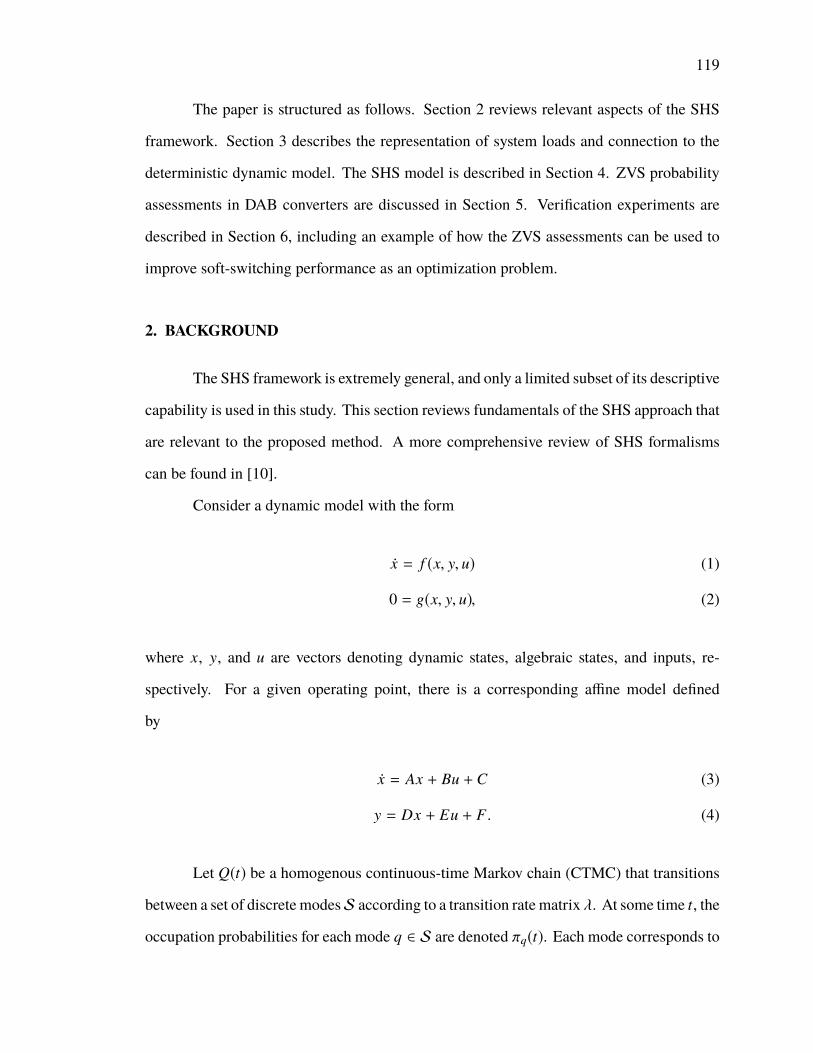
119

The paper is structured as follows. Section 2 reviews relevant aspects of the SHS

framework. Section 3 describes the representation of system loads and connection to the

deterministic dynamic model. The SHS model is described in Section 4. ZVS probability

assessments in DAB converters are discussed in Section 5. Verification experiments are

described in Section 6, including an example of how the ZVS assessments can be used to

improve soft-switching performance as an optimization problem.

2. BACKGROUND

The SHS framework is extremely general, and only a limited subset of its descriptive

capability is used in this study. This section reviews fundamentals of the SHS approach that

are relevant to the proposed method. A more comprehensive review of SHS formalisms

can be found in [10].

Consider a dynamic model with the form

Ûx = f (x, y, u) (1)

0 = g(x, y, u), (2)

where x, y, and u are vectors denoting dynamic states, algebraic states, and inputs, re-

spectively. For a given operating point, there is a corresponding affine model defined

by

Ûx = Ax + Bu + C (3)

y = Dx + Eu + F . (4)

Let Q(t) be a homogenous continuous-time Markov chain (CTMC) that transitions

between a set of discrete modesS according to a transition rate matrix λ. At some time t, the

occupation probabilities for each mode q ∈ S are denoted πq(t). Each mode corresponds to

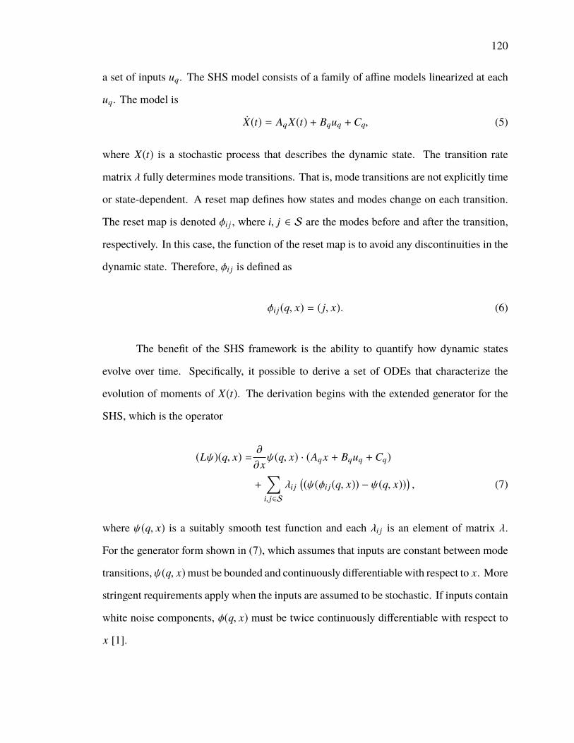
120

a set of inputs uq. The SHS model consists of a family of affine models linearized at each

uq. The model is

ÛX(t) = Aq X(t) + Bquq + Cq, (5)

where X(t) is a stochastic process that describes the dynamic state. The transition rate

matrix λ fully determines mode transitions. That is, mode transitions are not explicitly time

or state-dependent. A reset map defines how states and modes change on each transition.

The reset map is denoted φi j , where i, j ∈ S are the modes before and after the transition,

respectively. In this case, the function of the reset map is to avoid any discontinuities in the

dynamic state. Therefore, φi j is defined as

φi j(q, x) = ( j, x). (6)

The benefit of the SHS framework is the ability to quantify how dynamic states

evolve over time. Specifically, it possible to derive a set of ODEs that characterize the

evolution of moments of X(t). The derivation begins with the extended generator for the

SHS, which is the operator

(Lψ)(q, x) =∂

∂xψ(q, x) · (Aq x + Bquq + Cq)

+∑i, j∈S

λi j((ψ(φi j(q, x)) − ψ(q, x))

), (7)

where ψ(q, x) is a suitably smooth test function and each λi j is an element of matrix λ.

For the generator form shown in (7), which assumes that inputs are constant between mode

transitions, ψ(q, x)must be bounded and continuously differentiable with respect to x. More

stringent requirements apply when the inputs are assumed to be stochastic. If inputs contain

white noise components, φ(q, x) must be twice continuously differentiable with respect to

x [1].

121

The generator becomes useful in Dynkin’s formula, which describes the evolution

of the expected value of the test function.

ddtE [ψ(Q(t), X(t))] = E [(Lψ)(Q(t), X(t))] (8)

To extract conditional moments of X(t), the test function is defined as

ψ(m)i (q, x) = δi(q)x(m), (9)

where δi(q) is the Kronecker delta function and m is a vector of moment orders [2]. For a

system with N dynamic states, m is an N-element row vector and x(m) defined as

x(m) =N∏

i=1xmi

i . (10)

For a given mode i, the expected value of ψ(q, x) is equal to the conditional moments

of X(t).

E[ψ(m)i (q, x)

]= E

[X (m)(t)

Q(t) = i]πi(t) (11)

The unconditional moments of X(t) may then be computed by the law of total expectation.

E[X (m)(t)

]=

∑i∈S

E[ψ(m)i (q, x)

](12)

Therefore, the evolution of the dynamic state moments is described by the set of ODEs

corresponding to time derivatives of E[ψ(m)i (q, x)

]. To simplify notation, let the conditional

moments be denoted by

µ(m)i (t) = E

[ψ(m)i (q, x)

](13)

Then according to (8), the ODEs of interest are

Ûµ(m)i (t) = E

[(Lψ(m)i )(Q(t), X(t))

](14)

122

Conditional moments of algebraic states may be computed from the conditional moments of

X(t). Let conditional moments of the process Y (t) be denoted ζ (m)(t). Then the conditional

moments are

ζ(m)i (t) = E

[(Di X(t) + Eiui + Fi)

(m)Q(t) = i

]πi(t) (15)

Much of the practical difficulty in applying the SHS framework lies in computing

usable expressions for the right-hand sides of (14) and (15). An expression for the right-hand

side of (14) is given below, slightly modified from the form given in [2].

Ûµ(m)i (t) =

N∑p=1

mp

(N∑

r=1a(i)pr µ

(m−ep+er )i (t) + µ(m−ep)

i (t)vi,p

)+

∑j∈S−i

λ jiµ(m)j (t) −

∑k∈S+i

λik µ(m)i (t) (16)

In this equation, a(i)pr is the pth row, r th column element of Ai, vi,p is the pth element of

vector vi = Biui +Ci, ep and er are elementary row vectors, and S−i and S+i denote the sets

of modes that transition into and out of mode i, respectively.

3. DYNAMIC MODEL AND LOAD PROCESS

The dynamicmodel used in this study describes a dcmicrogrid or distribution system

consisting of loads, sources, and DAB converters. The deterministic model is constructed

according to the procedure in [11]. In principle, the SHS microgrid model described

in Sec. 4 is compatible with any system-level dynamic model that can be linearized and

expressed in the form of (3) and (4), regardless of the topology of the converters in the

system. The prediction of ZVS probabilities in Sec. 5, however, is specific to the DAB

topology.

In the simplest case, the dynamic model describes a single voltage-controlled DAB

with a current-source load. This is shown in Fig. 1. The inputs to the system-level model

are source voltages/currents, load currents, and voltage reference commands for closed-loop

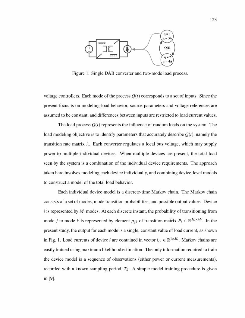
123

+

iL = 3A

q = 1

iL = 4A

q = 2

Q(t)

Figure 1. Single DAB converter and two-mode load process.

voltage controllers. Each mode of the process Q(t) corresponds to a set of inputs. Since the

present focus is on modeling load behavior, source parameters and voltage references are

assumed to be constant, and differences between inputs are restricted to load current values.

The load process Q(t) represents the influence of random loads on the system. The

load modeling objective is to identify parameters that accurately describe Q(t), namely the

transition rate matrix λ. Each converter regulates a local bus voltage, which may supply

power to multiple individual devices. When multiple devices are present, the total load

seen by the system is a combination of the individual device requirements. The approach

taken here involves modeling each device individually, and combining device-level models

to construct a model of the total load behavior.

Each individual device model is a discrete-time Markov chain. The Markov chain

consists of a set of modes, mode transition probabilities, and possible output values. Device

i is represented by Mi modes. At each discrete instant, the probability of transitioning from

mode j to mode k is represented by element p j k of transition matrix Pi ∈ RMi×Mi . In the

present study, the output for each mode is a single, constant value of load current, as shown

in Fig. 1. Load currents of device i are contained in vector iLi ∈ R1×Mi . Markov chains are

easily trained using maximum likelihood estimation. The only information required to train

the device model is a sequence of observations (either power or current measurements),

recorded with a known sampling period, TS. A simple model training procedure is given

in [9].

124

Individual device models are combined to generate models of composite loads. Let

M , P, and iL (with no subscripts) denote the parameters of the combined model. When

the first device is included in the composite model, M = M1, P = P1, and iL = iL1. For

including all other devices i > 1, the model combination equations are defined recursively:

P = P ⊗ Pi (17)

iL = iL ⊗ 1(Mi) + 1(M) ⊗ iLi (18)

M = M Mi, (19)

where ⊗ denotes the Kronecker product and 1(M) is a row vector of M elements equal

to 1. This combination process follows the procedure in [9], with small modifications for

constant load current outputs.

For the conceptual diagram in Fig. 1, which involves only one load, each mode

corresponds to a single scalar value. In the more general case, where loads exist at multiple

points in the system, each mode corresponds to a vector of load currents. The combination

in (18) applies regardless of the locations of loads in the system.

Once all individual devices have been included in the composite model, the M

modes of the Markov chain are exactly the modes of Q(t). However, Q(t) is continuous in

time, whereas the P defines a discrete-time Markov chain. In general, it is not possible to

convert a discrete-time Markov chain into a CTMC. However, since the device models are

trained using a known sampling time, it is possible to approximate the parameters of the

CTMC. The elements of the transition rate matrix λ can be determined from P as:

λii = −1 − pii

TS(20)

λi j = −λii pi j

1 − pii. (21)

125

4. SHS MICROGRID MODEL

4.1. SHS Model. Let µ|n|i (t) denote the set of all nth moments of X(t) conditional

on mode i. That is, µ|n|i (t) is a column vector of all moments defined in (13) for which the

one-norm of m is equal to n. In terms of the dynamic states, µ|n|i (t) can be understood as

µ|n|i (t) = E

[(n∏

k=0X(t)

) Q(t) = i

]πi(t), (22)

where the product symbol denotes the Kronecker product, such that the term in parentheses

is the Kronecker product of the state vector and itself n times. By convention, this term is

simply 1 for n = 0. In this way, the 0th ordermoments are themode occupation probabilities:

µ|0|i (t) = E

[1Q(t) = i

]πi(t) = πi(t). (23)

First and second order moments are

µ|1|i (t) = E

[X(t)

Q(t) = i]πi(t) (24)

µ|2|i (t) = E

[X(t) ⊗ X(t)

Q(t) = i]πi(t), (25)

where ⊗ is the Kronecker product. To represent moments for all modes, let vector µ|n|(t)

be defined as

µ|n|(t) =

µ|n|1 (t)...

µ|n|M (t)

. (26)

In this way, µ|0|(t) ∈ RM×1 contains mode occupation probabilities, µ|1|(t) ∈ RN M×1

contains all first order moments, µ|2|(t) ∈ RN2M×1, contains all second order moments, and

so on.

126

Note that this formulation draws a distinction between correlations e.g. E[X1(t)X2(t)]

and E[X2(t)X1(t)], while these two quantities are actually the same. For a system with N

dynamic states, the number of unique nth order moments is

Nu(n) =©­­«N + n − 1

n

ª®®¬ . (27)

The reason for this construction is to facilitate a simplified method of obtaining the set of

moment ODEs. Once the full linear system has been obtained, redundant moments are

eliminated through basic matrix operations. To distinguish between moment vectors, the

sets of unique moments are denoted µ|n|i (t). In the present study, this difference in notation

is only necessary for the second order moments, since µ|n|i (t) = µ|n|i (t) for n < 2.

For the SHS formulation used in this study, moment dynamic equations depend only

on moments of equal or lower order, avoiding the need for moment-closure methods [2].

In fact, (16) reveals that the dynamics of moments of order n are only directly dependent

on moments of order n and n − 1. For a given moment characterized by m, (16) shows

that Ûµ(m)i (t) depends on µ(m−ep+er )i (t), µ(m−ep)

i (t), µ(m)i (t), and µ(m)j (t) for other modes j ∈ S.

Recall that the order of moment µ(m)i (t) is equal to the one-norm of m. Trivially, µ(m)i (t) and

µ(m)j (t) have the same order. If the order of µ(m)i (t) is n, then since ep and er are unit vectors,

the orders of µ(m−ep+er )i (t) and µ(m−ep)

i (t) must be n and n − 1, respectively.

Consequently, it is possible to express the system of ODEs for nth order moments as

Ûµ|n|(t) = G(n)µ|n|(t) + H(n)µ|n−1|(t) (28)

Matrices G(n) and H(n) follow from (16), but provide a more manageable structure to the

definition of the SHS model.

127

Simplified expressions for G(n) and H(n) are given here for low-order moments. The

0th order moments are the mode occupation probabilities of the CTMC. Therefore H(0) = 0

and G(0) = λT , where the transpose is due to the fact µ|0|(t) is a column vector. For first and

second order moments, both G(n) and H(n) may be constructed primarily as block diagonal

combinations of submatrices for each mode:

G(n) =

G(n)1 0 · · · 0

0 G(n)2 · · · 0...

.... . .

...

0 0 · · · G(n)M

+

(λT ⊗ I(Nn)

)(29)

H(n) =

H(n)1 0 · · · 0

0 H(n)2 · · · 0...

.... . .

...

0 0 · · · H(n)M ,

(30)

where I(Nn) is the Nn-dimensional identity matrix. In the case of first order moments, the

submatrices for each mode are

G(1)i = Ai (31)

H(1)i = vi . (32)

For second order moments, the submatrices are calculated using a transformation

matrix, Wm, which is constant for all modes.

G(2)i = Wm (I(N) ⊗ Ai) (33)

H(2)i = Wm (I(N) ⊗ vi) . (34)

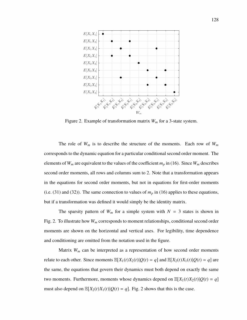
128

Figure 2. Example of transformation matrix Wm for a 3-state system.

The role of Wm is to describe the structure of the moments. Each row of Wm

corresponds to the dynamic equation for a particular conditional second order moment. The

elements ofWm are equivalent to the values of the coefficient mp in (16). SinceWm describes

second order moments, all rows and columns sum to 2. Note that a transformation appears

in the equations for second order moments, but not in equations for first-order moments

(i.e. (31) and (32)). The same connection to values of mp in (16) applies to these equations,

but if a transformation was defined it would simply be the identity matrix.

The sparsity pattern of Wm for a simple system with N = 3 states is shown in

Fig. 2. To illustrate howWm corresponds to moment relationships, conditional second order

moments are shown on the horizontal and vertical axes. For legibility, time dependence

and conditioning are omitted from the notation used in the figure.

Matrix Wm can be interpreted as a representation of how second order moments

relate to each other. Since moments E[X1(t)X2(t)|Q(t) = q] and E[X2(t)X1(t)|Q(t) = q] are

the same, the equations that govern their dynamics must both depend on exactly the same

two moments. Furthermore, moments whose dynamics depend on E[X1(t)X2(t)|Q(t) = q]

must also depend on E[X2(t)X1(t)|Q(t) = q]. Fig. 2 shows that this is the case.

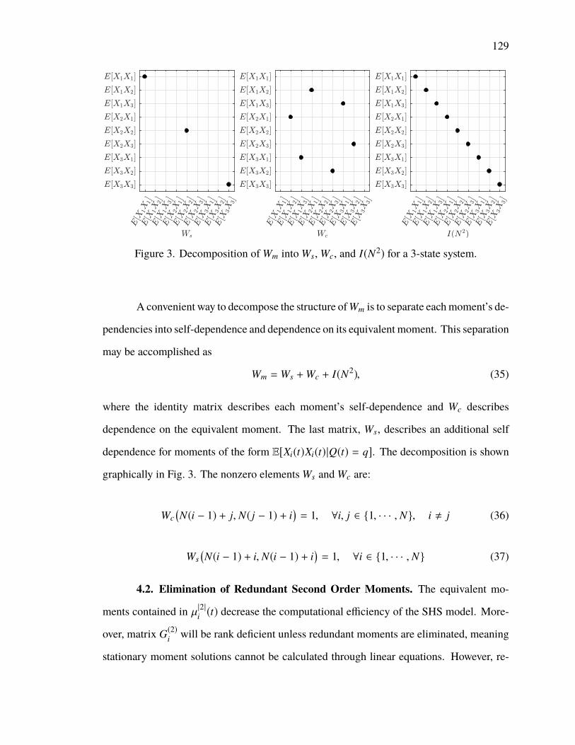
129

Figure 3. Decomposition of Wm into Ws, Wc, and I(N2) for a 3-state system.

A convenient way to decompose the structure ofWm is to separate eachmoment’s de-

pendencies into self-dependence and dependence on its equivalent moment. This separation

may be accomplished as

Wm = Ws +Wc + I(N2), (35)

where the identity matrix describes each moment’s self-dependence and Wc describes

dependence on the equivalent moment. The last matrix, Ws, describes an additional self

dependence for moments of the form E[Xi(t)Xi(t)|Q(t) = q]. The decomposition is shown

graphically in Fig. 3. The nonzero elements Ws and Wc are:

Wc(N(i − 1) + j, N( j − 1) + i

)= 1, ∀i, j ∈ 1, · · · , N, i , j (36)

Ws(N(i − 1) + i, N(i − 1) + i

)= 1, ∀i ∈ 1, · · · , N (37)

4.2. Elimination of Redundant Second Order Moments. The equivalent mo-

ments contained in µ|2|i (t) decrease the computational efficiency of the SHS model. More-

over, matrix G(2)i will be rank deficient unless redundant moments are eliminated, meaning

stationary moment solutions cannot be calculated through linear equations. However, re-

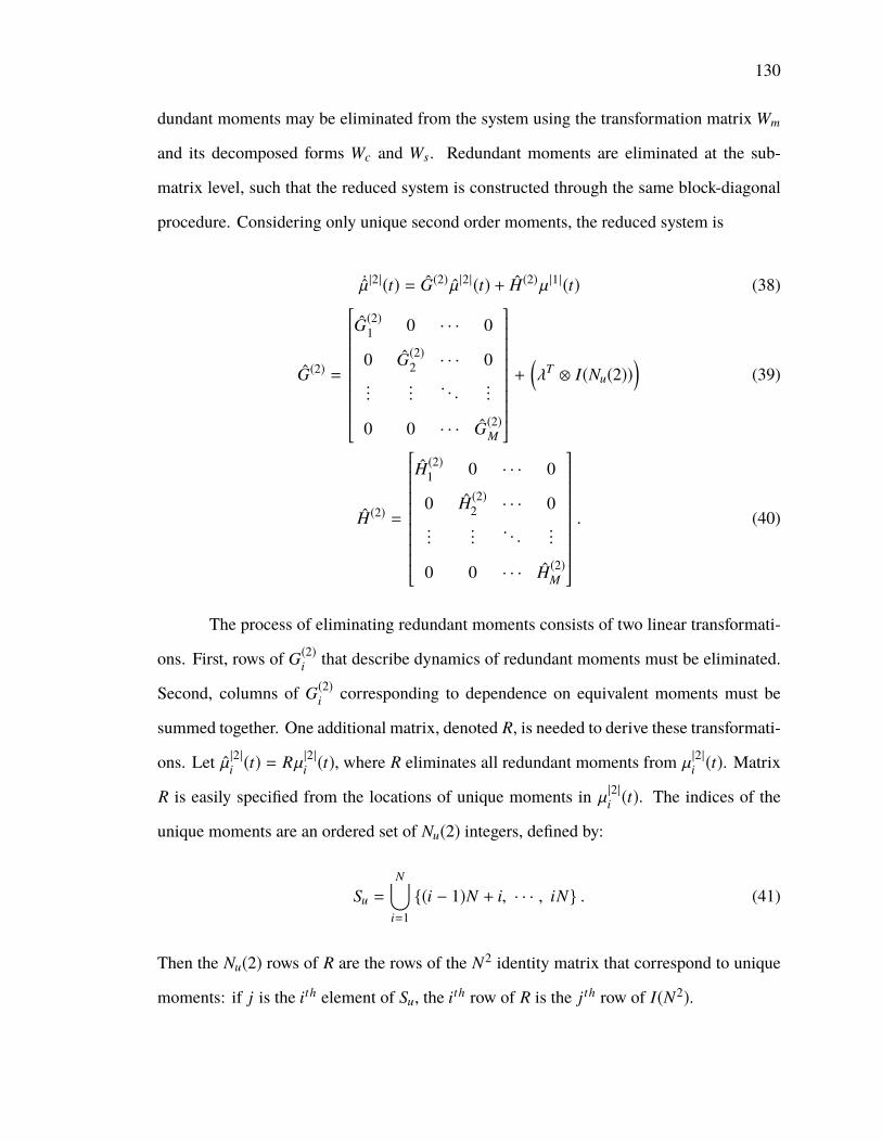
130

dundant moments may be eliminated from the system using the transformation matrix Wm

and its decomposed forms Wc and Ws. Redundant moments are eliminated at the sub-

matrix level, such that the reduced system is constructed through the same block-diagonal

procedure. Considering only unique second order moments, the reduced system is

Ûµ|2|(t) = G(2) µ|2|(t) + H(2)µ|1|(t) (38)

G(2) =

G(2)1 0 · · · 0

0 G(2)2 · · · 0...

.... . .

...

0 0 · · · G(2)M

+

(λT ⊗ I(Nu(2))

)(39)

H(2) =

H(2)1 0 · · · 0

0 H(2)2 · · · 0...

.... . .

...

0 0 · · · H(2)M

. (40)

The process of eliminating redundant moments consists of two linear transformati-

ons. First, rows of G(2)i that describe dynamics of redundant moments must be eliminated.

Second, columns of G(2)i corresponding to dependence on equivalent moments must be

summed together. One additional matrix, denoted R, is needed to derive these transformati-

ons. Let µ|2|i (t) = Rµ|2|i (t), where R eliminates all redundant moments from µ|2|i (t). Matrix

R is easily specified from the locations of unique moments in µ|2|i (t). The indices of the

unique moments are an ordered set of Nu(2) integers, defined by:

Su =

N⋃i=1(i − 1)N + i, · · · , iN . (41)

Then the Nu(2) rows of R are the rows of the N2 identity matrix that correspond to unique

moments: if j is the ith element of Su, the ith row of R is the j th row of I(N2).

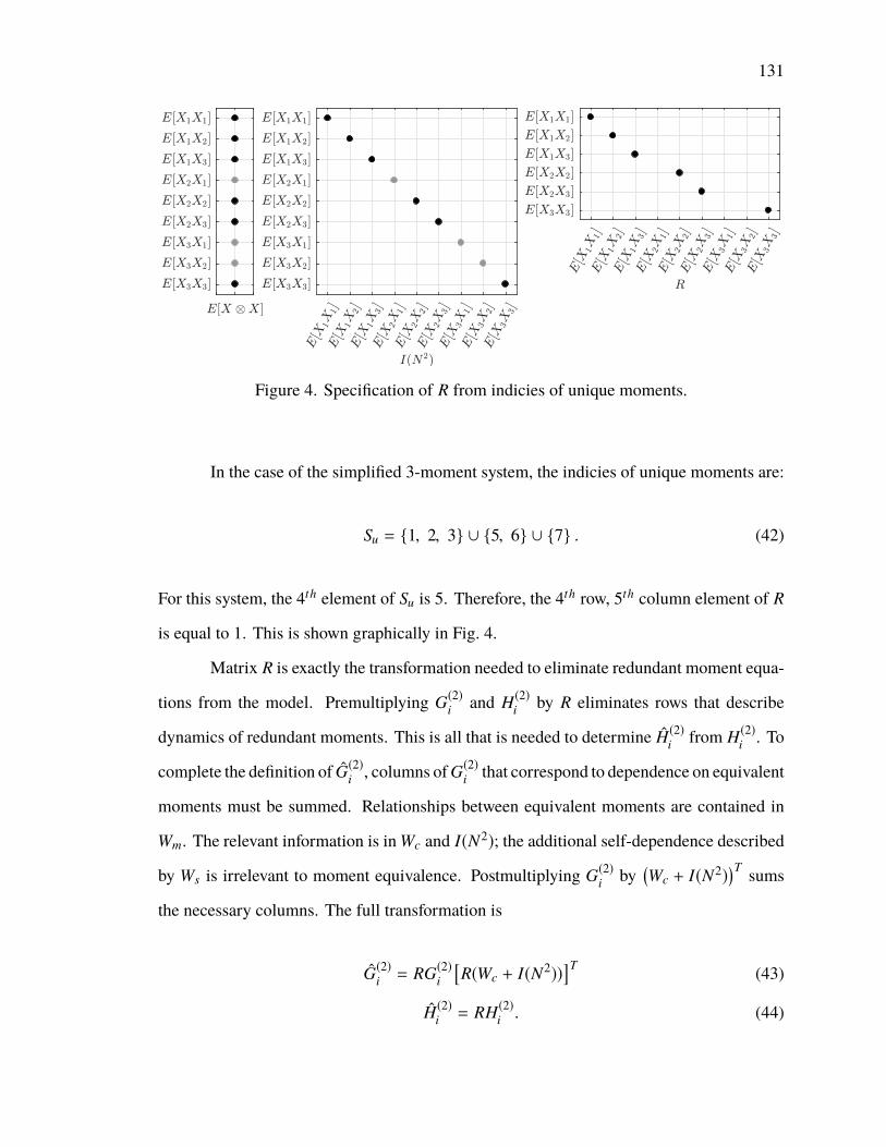
131

Figure 4. Specification of R from indicies of unique moments.

In the case of the simplified 3-moment system, the indicies of unique moments are:

Su = 1, 2, 3 ∪ 5, 6 ∪ 7 . (42)

For this system, the 4th element of Su is 5. Therefore, the 4th row, 5th column element of R

is equal to 1. This is shown graphically in Fig. 4.

Matrix R is exactly the transformation needed to eliminate redundant moment equa-

tions from the model. Premultiplying G(2)i and H(2)i by R eliminates rows that describe

dynamics of redundant moments. This is all that is needed to determine H(2)i from H(2)i . To

complete the definition of G(2)i , columns ofG(2)i that correspond to dependence on equivalent

moments must be summed. Relationships between equivalent moments are contained in

Wm. The relevant information is in Wc and I(N2); the additional self-dependence described

by Ws is irrelevant to moment equivalence. Postmultiplying G(2)i by(Wc + I(N2)

)T sums

the necessary columns. The full transformation is

G(2)i = RG(2)i

[R(Wc + I(N2))

]T (43)

H(2)i = RH(2)i . (44)

132

Figure 5. Sparsity pattern of final transformation matrices used to calculate reduced subsy-stem matrices.

In comparison to the submatrices in (33) and (34), these definitions produce a second order

system with significantly reduced size. More importantly, matrix G(2) will always have full

rank, making it possible to solve for stationary moments.

A more efficient alternative to (43) and (44) is to directly calculate G(2)i and H(2)i ,

rather than reducing them from G(2)i and H(2)i . Let two new transformations, Wx and Wy, be

defined as

Wx = R(Wc + I(N2)

)(45)

Wy = RWs . (46)

Sparsity patterns for these matrices are shown in Fig. 5. The reduced subsystem matrices

may be calculated from Wx and Wy as

G(2)i =(Wx +Wy

)(I(N) ⊗ Ai)

(WT

x

)(47)

H(2)i =(Wx +Wy

)(I(N) ⊗ vi) . (48)

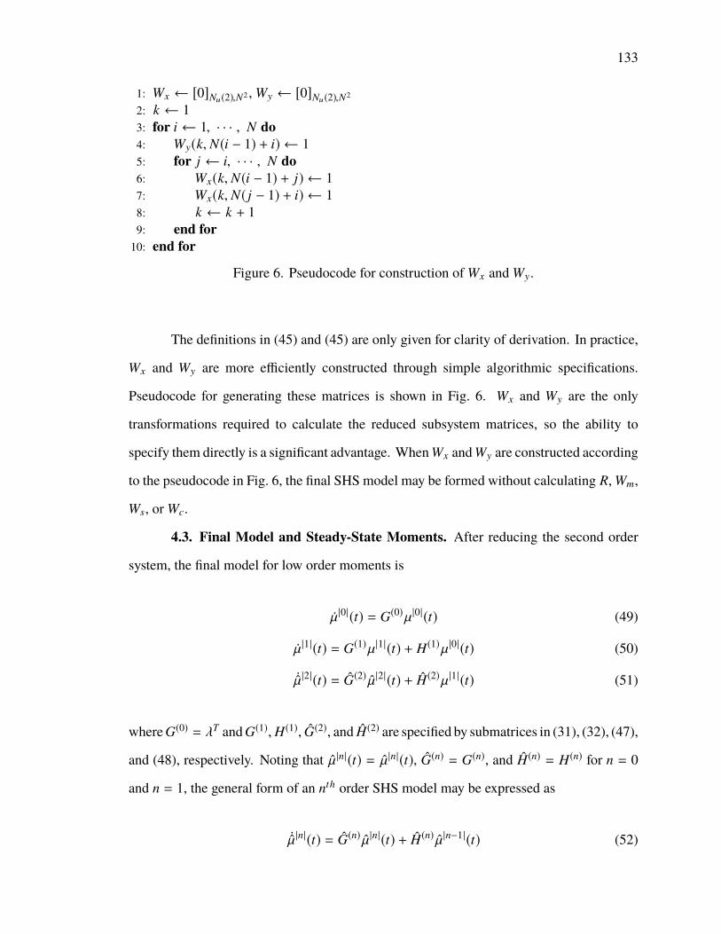
133

1: Wx ← [0]Nu(2),N2 , Wy ← [0]Nu(2),N2

2: k ← 13: for i ← 1, · · · , N do4: Wy(k, N(i − 1) + i) ← 15: for j ← i, · · · , N do6: Wx(k, N(i − 1) + j) ← 17: Wx(k, N( j − 1) + i) ← 18: k ← k + 19: end for10: end for

Figure 6. Pseudocode for construction of Wx and Wy.

The definitions in (45) and (45) are only given for clarity of derivation. In practice,

Wx and Wy are more efficiently constructed through simple algorithmic specifications.

Pseudocode for generating these matrices is shown in Fig. 6. Wx and Wy are the only

transformations required to calculate the reduced subsystem matrices, so the ability to

specify them directly is a significant advantage. WhenWx andWy are constructed according

to the pseudocode in Fig. 6, the final SHS model may be formed without calculating R, Wm,

Ws, or Wc.

4.3. Final Model and Steady-State Moments. After reducing the second order

system, the final model for low order moments is

Ûµ|0|(t) = G(0)µ|0|(t) (49)

Ûµ|1|(t) = G(1)µ|1|(t) + H(1)µ|0|(t) (50)

Ûµ|2|(t) = G(2) µ|2|(t) + H(2)µ|1|(t) (51)

whereG(0) = λT andG(1), H(1), G(2), and H(2) are specified by submatrices in (31), (32), (47),

and (48), respectively. Noting that µ|n|(t) = µ|n|(t), G(n) = G(n), and H(n) = H(n) for n = 0

and n = 1, the general form of an nth order SHS model may be expressed as

Ûµ|n|(t) = G(n) µ|n|(t) + H(n) µ|n−1|(t) (52)

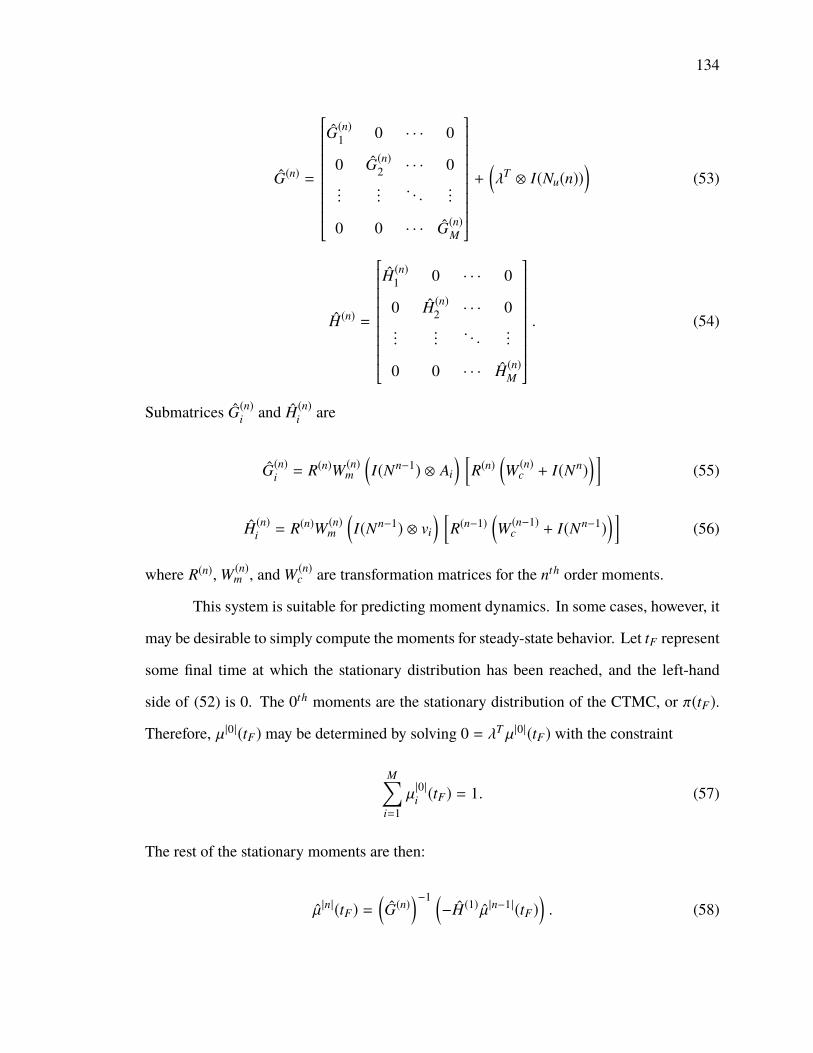
134

G(n) =

G(n)1 0 · · · 0

0 G(n)2 · · · 0...

.... . .

...

0 0 · · · G(n)M

+

(λT ⊗ I(Nu(n))

)(53)

H(n) =

H(n)1 0 · · · 0

0 H(n)2 · · · 0...

.... . .

...

0 0 · · · H(n)M

. (54)

Submatrices G(n)i and H(n)i are

G(n)i = R(n)W (n)m

(I(Nn−1) ⊗ Ai

) [R(n)

(W (n)c + I(Nn)

)](55)

H(n)i = R(n)W (n)m

(I(Nn−1) ⊗ vi

) [R(n−1)

(W (n−1)

c + I(Nn−1))]

(56)

where R(n), W (n)m , and W (n)c are transformation matrices for the nth order moments.

This system is suitable for predicting moment dynamics. In some cases, however, it

may be desirable to simply compute the moments for steady-state behavior. Let tF represent

some final time at which the stationary distribution has been reached, and the left-hand

side of (52) is 0. The 0th moments are the stationary distribution of the CTMC, or π(tF).

Therefore, µ|0|(tF) may be determined by solving 0 = λT µ|0|(tF) with the constraint

M∑i=1

µ|0|i (tF) = 1. (57)

The rest of the stationary moments are then:

µ|n|(tF) =(G(n)

)−1 (−H(1) µ|n−1|(tF)

). (58)

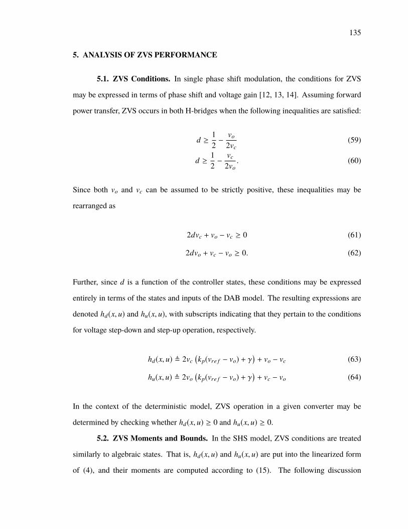
135

5. ANALYSIS OF ZVS PERFORMANCE

5.1. ZVS Conditions. In single phase shift modulation, the conditions for ZVS

may be expressed in terms of phase shift and voltage gain [12, 13, 14]. Assuming forward

power transfer, ZVS occurs in both H-bridges when the following inequalities are satisfied:

d ≥12−

vo

2vc(59)

d ≥12−

vc

2vo. (60)

Since both vo and vc can be assumed to be strictly positive, these inequalities may be

rearranged as

2dvc + vo − vc ≥ 0 (61)

2dvo + vc − vo ≥ 0. (62)

Further, since d is a function of the controller states, these conditions may be expressed

entirely in terms of the states and inputs of the DAB model. The resulting expressions are

denoted hd(x, u) and hu(x, u), with subscripts indicating that they pertain to the conditions

for voltage step-down and step-up operation, respectively.

hd(x, u) , 2vc(kp(vre f − vo) + γ

)+ vo − vc (63)

hu(x, u) , 2vo(kp(vre f − vo) + γ

)+ vc − vo (64)

In the context of the deterministic model, ZVS operation in a given converter may be

determined by checking whether hd(x, u) ≥ 0 and hu(x, u) ≥ 0.

5.2. ZVS Moments and Bounds. In the SHS model, ZVS conditions are treated

similarly to algebraic states. That is, hd(x, u) and hu(x, u) are put into the linearized form

of (4), and their moments are computed according to (15). The following discussion

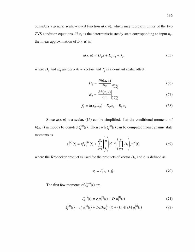
136

considers a generic scalar-valued function h(x, u), which may represent either of the two

ZVS condition equations. If xq is the deterministic steady-state corresponding to input uq,

the linear approximation of h(x, u) is

h(x, u) ≈ Dq x + Equq + fq, (65)

where Dq and Eq are derivative vectors and fq is a constant scalar offset.

Dq =∂h(x, u)∂x

x=xqu=uq

(66)

Eq =∂h(x, u)∂u

x=xqu=uq

(67)

fq = h(xq, uq) − Dq xq − Equq (68)

Since h(x, u) is a scalar, (15) can be simplified. Let the conditional moments of

h(x, u) in mode i be denoted ξ(n)i (t). Then each ξ(n)i (t) can be computed from dynamic state

moments as

ξ(n)i (t) = rn

i µ|0|i (t) +

n∑k=1

©­­«n

k

ª®®¬ rn−ki

©­«k∏

j=1Di

ª®¬ µ|n|i (t), (69)

where the Kronecker product is used for the products of vector Di, and ri is defined as

ri = Eiui + fi . (70)

The first few moments of ξ(n)i (t) are

ξ(1)i (t) = riµ

|0|i (t) + Diµ

|1|i (t) (71)

ξ(2)i (t) = r2

i µ|0|i (t) + 2riDiµ

|1|i (t) + (Di ⊗ Di) µ

|2|i (t) (72)

137

The second order moment can alternatively be expressed as a function of unique second

order dynamic state moments using the transformation from the previous section.

ξ(2)i (t) = r2

i µ|0|i (t)+2riDiµ

|1|i (t)

+ (Di ⊗ Di)

(WT

x

)µ|2|i (t) (73)

Finally, the unconditional moments are the sum of each the conditional moments for each

mode.

E [h(x, u)n] ≈ ξ(n)(t) =M∑

i=1ξ(n)i (t) (74)

The moments of hd(x, u) and hu(x, u) make it possible to assess the probability of

ZVS. The probability of ZVS corresponds to the probability these functions are greater than

zero, according to the ZVS condition equations. Using the Cantelli inequality, a bounds on

the probability of ZVS can be defined in terms of first and second moments. For generic

random variable X and constant a, the Cantelli inequality is [15]:

P [X − µX ≥ a]

≤

σ2X

σ2X+a2 a ≥ 0

≥ 1 − σ2X

σ2X+a2 a < 0

, (75)

where µX and σ2X are the first and second central moments of X . Letting a = −µX the

inequality is

P [X ≥ 0]

≤

σ2X

σ2X+µ

2X

µX < 0

≥ 1 − σ2X

σ2X+µ

2X

µX ≥ 0. (76)

Applying this inequality to h(x, u), and substituting raw moments for central moments, the

upper limits and lower limits on the probability P[h(x, u) ≥ 0] are:

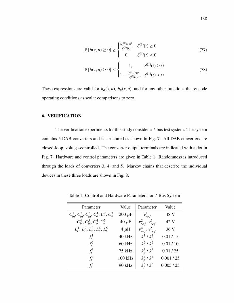
138

P [h(x, u) ≥ 0] ≥(ξ(1)(t))2

ξ(2)(t) , ξ(1)(t) ≥ 0

0, ξ(1)(t) < 0(77)

P [h(x, u) ≥ 0] ≤

1, ξ(1)(t) ≥ 0

1 − (ξ(1)(t))2

ξ(2)(t) , ξ(1)(t) < 0(78)

These expressions are valid for hd(x, u), hu(x, u), and for any other functions that encode

operating conditions as scalar comparisons to zero.

6. VERIFICATION

The verification experiments for this study consider a 7-bus test system. The system

contains 5 DAB converters and is structured as shown in Fig. 7. All DAB converters are

closed-loop, voltage-controlled. The converter output terminals are indicated with a dot in

Fig. 7. Hardware and control parameters are given in Table 1. Randomness is introduced

through the loads of converters 3, 4, and 5. Markov chains that describe the individual

devices in these three loads are shown in Fig. 8.

Table 1. Control and Hardware Parameters for 7-Bus System

Parameter Value Parameter ValueC1

in, C2in, C3

in, C1o , C2

o , C3o 200 µF v1

re f 48 VC4

in, C5in, C4

o , C5o 40 µF v2

re f , v3re f 42 V

L1t , L2

t , L3t , L4

t , L5t 4 µH v4

re f , v5re f 36 V

f 1s 40 kHz k1

p / k1i 0.01 / 15

f 2s 60 kHz k2

p / k2i 0.01 / 10

f 3s 75 kHz k3

p / k3i 0.01 / 25

f 4s 100 kHz k4

p / k4i 0.001 / 25

f 5s 90 kHz k5

p / k5i 0.005 / 25

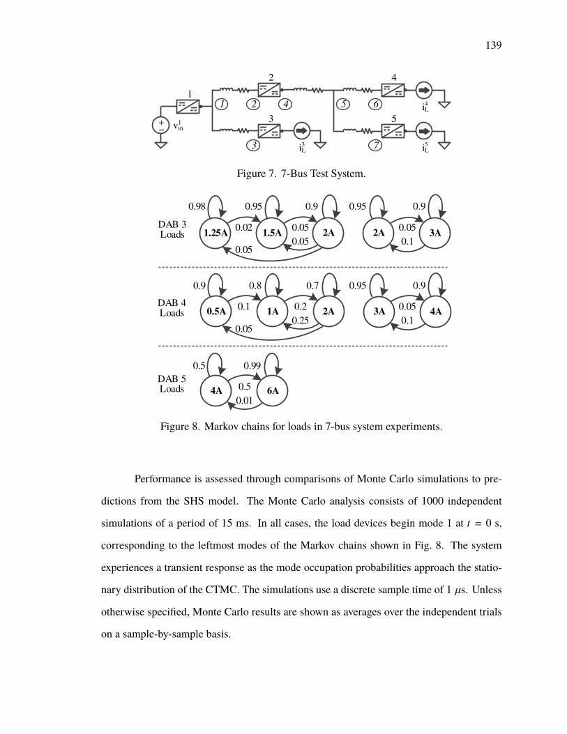
139

3

21 4 5 6

7

1

2

3

4

5v

1

in

i3

L

i4

L

i5

L

+

Figure 7. 7-Bus Test System.

0.5A 1A 2A 4A3A

1.25A 1.5A 2A 3A2A

6A4A

DAB 3

Loads

DAB 4

Loads

DAB 5

Loads

0.98 0.95 0.9 0.95 0.9

0.02 0.05

0.050.05

0.05

0.1

0.9 0.8 0.7 0.95 0.9

0.1 0.2

0.250.05

0.05

0.1

0.5 0.99

0.5

0.01

Figure 8. Markov chains for loads in 7-bus system experiments.

Performance is assessed through comparisons of Monte Carlo simulations to pre-

dictions from the SHS model. The Monte Carlo analysis consists of 1000 independent

simulations of a period of 15 ms. In all cases, the load devices begin mode 1 at t = 0 s,

corresponding to the leftmost modes of the Markov chains shown in Fig. 8. The system

experiences a transient response as the mode occupation probabilities approach the statio-

nary distribution of the CTMC. The simulations use a discrete sample time of 1 µs. Unless

otherwise specified, Monte Carlo results are shown as averages over the independent trials

on a sample-by-sample basis.

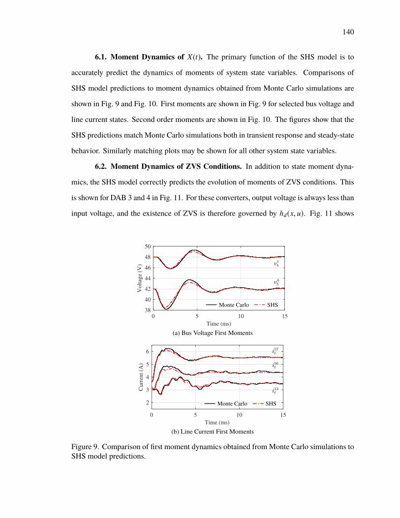
140

6.1. Moment Dynamics of X(t). The primary function of the SHS model is to

accurately predict the dynamics of moments of system state variables. Comparisons of

SHS model predictions to moment dynamics obtained from Monte Carlo simulations are

shown in Fig. 9 and Fig. 10. First moments are shown in Fig. 9 for selected bus voltage and

line current states. Second order moments are shown in Fig. 10. The figures show that the

SHS predictions match Monte Carlo simulations both in transient response and steady-state

behavior. Similarly matching plots may be shown for all other system state variables.

6.2. Moment Dynamics of ZVS Conditions. In addition to state moment dyna-

mics, the SHS model correctly predicts the evolution of moments of ZVS conditions. This

is shown for DAB 3 and 4 in Fig. 11. For these converters, output voltage is always less than

input voltage, and the existence of ZVS is therefore governed by hd(x, u). Fig. 11 shows

0 5 10 15

Time (ms)

38

40

42

44

46

48

50

Volt

age

(V)

Monte Carlo SHS

(a) Bus Voltage First Moments

0 5 10 15

Time (ms)

2

3

4

5

6

Curr

ent

(A)

Monte Carlo SHS

(b) Line Current First Moments

Figure 9. Comparison of first moment dynamics obtained fromMonte Carlo simulations toSHS model predictions.

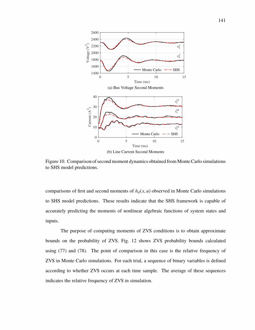
141

0 5 10 15

Time (ms)

1400

1600

1800

2000

2200

2400

2600

Volt

age

(V2)

Monte Carlo SHS

(a) Bus Voltage Second Moments

0 5 10 15

Time (ms)

0

10

20

30

40

Curr

ent

(A2)

Monte Carlo SHS

(b) Line Current Second Moments

Figure 10. Comparison of secondmoment dynamics obtained fromMonteCarlo simulationsto SHS model predictions.

comparisons of first and second moments of hd(x, u) observed in Monte Carlo simulations

to SHS model predictions. These results indicate that the SHS framework is capable of

accurately predicting the moments of nonlinear algebraic functions of system states and

inputs.

The purpose of computing moments of ZVS conditions is to obtain approximate

bounds on the probability of ZVS. Fig. 12 shows ZVS probability bounds calculated

using (77) and (78). The point of comparison in this case is the relative frequency of

ZVS in Monte Carlo simulations. For each trial, a sequence of binary variables is defined

according to whether ZVS occurs at each time sample. The average of these sequences

indicates the relative frequency of ZVS in simulation.

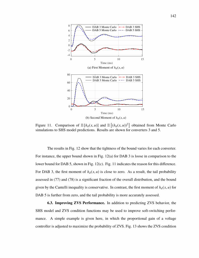
142

0 5 10 15

Time (ms)

-4

-2

0

2

4

6

8DAB 3 Monte Carlo DAB 3 SHS

DAB 5 Monte Carlo DAB 5 SHS

(a) First Moment of hd(x, u)

0 5 10 15

Time (ms)

0

20

40

60

80DAB 3 Monte Carlo DAB 3 SHS

DAB 5 Monte Carlo DAB 5 SHS

(b) Second Moment of hd(x, u)

Figure 11. Comparison of E [hd(x, u)] and E[(hd(x, u))2

]obtained from Monte Carlo

simulations to SHS model predictions. Results are shown for converters 3 and 5.

The results in Fig. 12 show that the tightness of the bound varies for each converter.

For instance, the upper bound shown in Fig. 12(a) for DAB 3 is loose in comparison to the

lower bound for DAB 5, shown in Fig. 12(c). Fig. 11 indicates the reason for this difference.

For DAB 3, the first moment of hd(x, u) is close to zero. As a result, the tail probability

assessed in (77) and (78) is a significant fraction of the overall distribution, and the bound

given by the Cantelli inequality is conservative. In contrast, the first moment of hd(x, u) for

DAB 5 is further from zero, and the tail probability is more accurately assessed.

6.3. Improving ZVS Performance. In addition to predicting ZVS behavior, the

SHS model and ZVS condition functions may be used to improve soft-switching perfor-

mance. A simple example is given here, in which the proportional gain of a voltage

controller is adjusted to maximize the probability of ZVS. Fig. 13 shows the ZVS condition

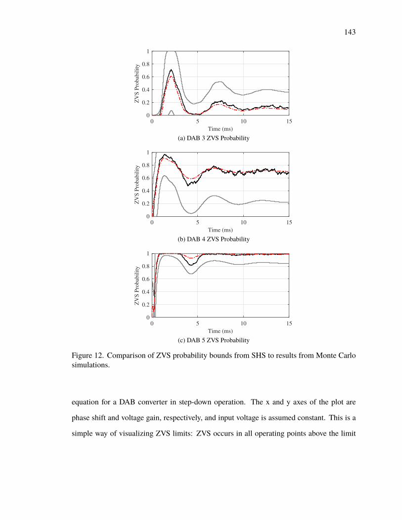
143

0 5 10 15

Time (ms)

0

0.2

0.4

0.6

0.8

1

ZV

S P

robab

ilit

y(a) DAB 3 ZVS Probability

0 5 10 15

Time (ms)

0

0.2

0.4

0.6

0.8

1

ZV

S P

robab

ilit

y

(b) DAB 4 ZVS Probability

0 5 10 15

Time (ms)

0

0.2

0.4

0.6

0.8

1

ZV

S P

robab

ilit

y

(c) DAB 5 ZVS Probability

Figure 12. Comparison of ZVS probability bounds from SHS to results from Monte Carlosimulations.

equation for a DAB converter in step-down operation. The x and y axes of the plot are

phase shift and voltage gain, respectively, and input voltage is assumed constant. This is a

simple way of visualizing ZVS limits: ZVS occurs in all operating points above the limit

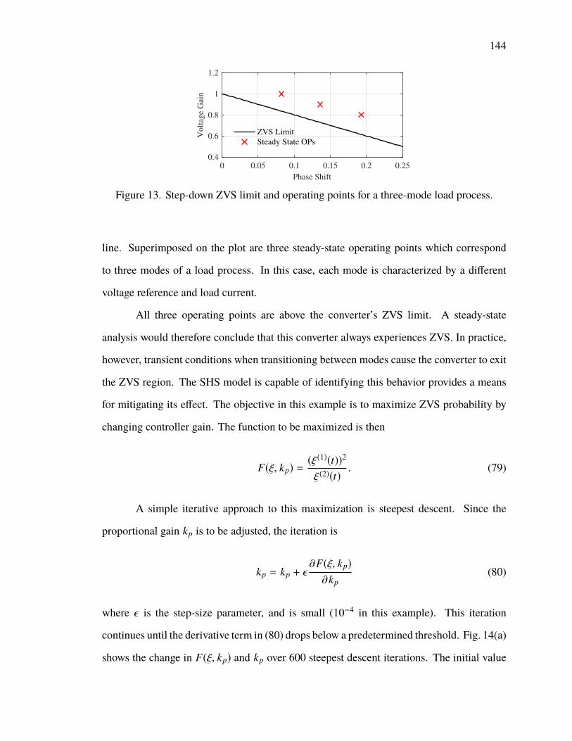
144

0 0.05 0.1 0.15 0.2 0.25

Phase Shift

0.4

0.6

0.8

1

1.2

Volt

age

Gai

n

ZVS Limit

Steady State OPs

Figure 13. Step-down ZVS limit and operating points for a three-mode load process.

line. Superimposed on the plot are three steady-state operating points which correspond

to three modes of a load process. In this case, each mode is characterized by a different

voltage reference and load current.

All three operating points are above the converter’s ZVS limit. A steady-state

analysis would therefore conclude that this converter always experiences ZVS. In practice,

however, transient conditions when transitioning between modes cause the converter to exit

the ZVS region. The SHS model is capable of identifying this behavior provides a means

for mitigating its effect. The objective in this example is to maximize ZVS probability by

changing controller gain. The function to be maximized is then

F(ξ, kp) =(ξ(1)(t))2

ξ(2)(t). (79)

A simple iterative approach to this maximization is steepest descent. Since the

proportional gain kp is to be adjusted, the iteration is

kp = kp + ε∂F(ξ, kp)

∂kp(80)

where ε is the step-size parameter, and is small (10−4 in this example). This iteration

continues until the derivative term in (80) drops below a predetermined threshold. Fig. 14(a)

shows the change in F(ξ, kp) and kp over 600 steepest descent iterations. The initial value

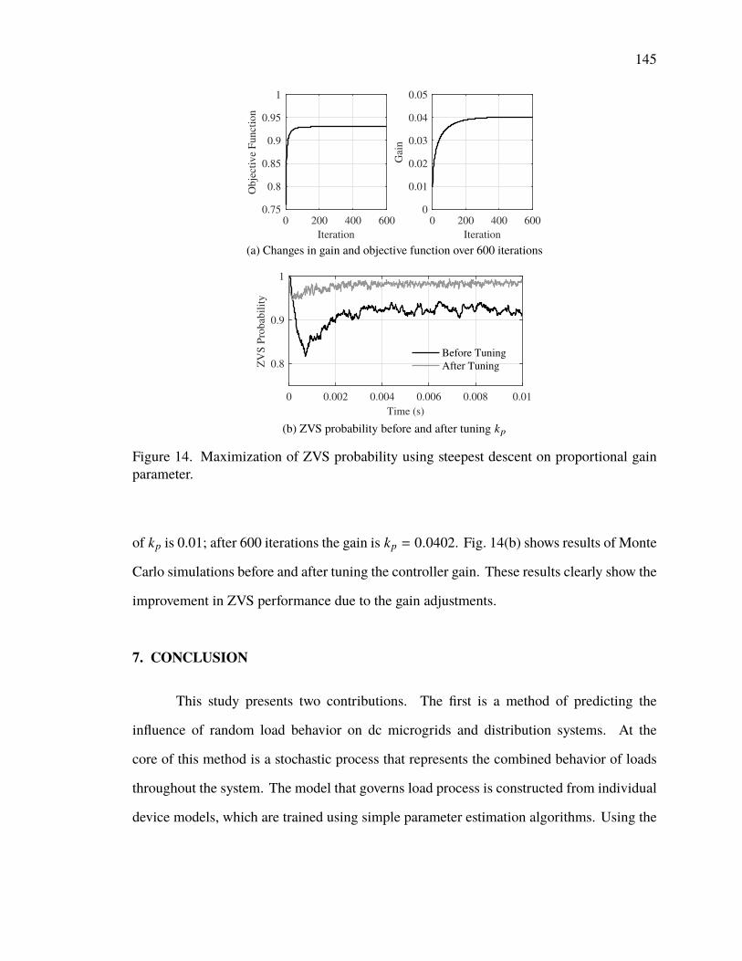
145

0 200 400 600

Iteration

0.75

0.8

0.85

0.9

0.95

1

Obje

ctiv

e F

unct

ion

0 200 400 600

Iteration

0

0.01

0.02

0.03

0.04

0.05

Gai

n

(a) Changes in gain and objective function over 600 iterations

0 0.002 0.004 0.006 0.008 0.01

Time (s)

0.8

0.9

1

ZV

S P

robab

ilit

y

Before Tuning

After Tuning

(b) ZVS probability before and after tuning kp

Figure 14. Maximization of ZVS probability using steepest descent on proportional gainparameter.

of kp is 0.01; after 600 iterations the gain is kp = 0.0402. Fig. 14(b) shows results of Monte

Carlo simulations before and after tuning the controller gain. These results clearly show the

improvement in ZVS performance due to the gain adjustments.

7. CONCLUSION

This study presents two contributions. The first is a method of predicting the

influence of random load behavior on dc microgrids and distribution systems. At the

core of this method is a stochastic process that represents the combined behavior of loads

throughout the system. The model that governs load process is constructed from individual

device models, which are trained using simple parameter estimation algorithms. Using the

146

SHS framework, the load process is combined with deterministic system-level models. The

resulting SHS model provides the tools necessary to analyze the effects of load behavior on

system dynamics.

The second contribution is a method of assessing the probability of ZVS in DAB

converters for a given set of load devices. ZVS conditions are encoded as a function of

dynamic state moments. Leveraging the functionality of the SHS model, moments of the

ZVS condition functions are obtained. These moments are used in Cantelli’s inequality

to produce a set of bounds on ZVS probability. While the proposed method of ZVS

assessment is specific to the DAB topology, it represents an example of how desirable

operating conditions may be represented in the SHS model.

REFERENCES

[1] J. P. Hespanha, “Modelling and analysis of stochastic hybrid systems,” IEE Procee-

dings - Control Theory and Applications, vol. 153, no. 5, pp. 520–535, 2006.

[2] S. V. Dhople, Y. C. Chen, L. DeVille, and A. D. Domínguez-García, “Analysis of

power system dynamics subject to stochastic power injections,” IEEE Trans. Circuits

Syst. I, vol. 60, no. 12, pp. 3341–3353, 2013.

[3] G. Mpembele and J. Kimball, “Analysis of a standalone microgrid stability using

generic markov jump linear systems,” in 2017 IEEE Power and Energy Conference at

Illinois (PECI), 2017, pp. 1–8.

[4] G. Hart, “Nonintrusive appliance load monitoring,” Proc. IEEE, vol. 80, no. 12, pp.

1870–1891, Dec 1992.

[5] F. Sultanem, “Using appliance signatures for monitoring residential loads at meter

panel level,” IEEE Trans. Power Del., vol. 6, no. 4, pp. 1380–1385, Oct 1991.

147

[6] A. Zoha, A. Gluhak, M. Nati, and M. Imran, “Low-power appliance monitoring using

factorial hidden Markov models,” in IEEE 8th Int.l Conf. Intelligent Sensors, Sensor

Networks and Information Processing, April 2013, pp. 527–532.

[7] T. Zia, D. Bruckner, and A. Zaidi, “A hidden Markov model based procedure for

identifying household electric loads,” in 37th Conf. Industrial Electronics, Nov 2011,

pp. 3218–3223.

[8] S. Makonin, F. Popowich, I. Bajic, B. Gill, and L. Bartram, “Exploiting hmm sparsity

to perform online real-time nonintrusive load monitoring,” IEEE Trans. Smart Grid,

vol. PP, no. 99, pp. 1–11, 2015.

[9] J. A. Mueller and J. W. Kimball, “Accurate energy use estimation for nonintrusive load

monitoring in systems of known devices,” IEEE Trans. Smart Grid, vol. PP, no. 99,

pp. 1–1, 2017.

[10] G. Pola, M. L. Bujorianu, J. Lygeros, and M. D. Di Benedetto, “Stochastic hybrid

models: An overview,” IFAC Proceedings Volumes, vol. 36, no. 6, pp. 45–50, 2003.

[11] J. A.Mueller and J. Kimball, “Modeling dual active bridge converters in dc distribution

systems,” IEEE Trans. Power Electron., 2018.

[12] M. N. Kheraluwala, R.W. Gascoigne, D.M. Divan, and E. D. Baumann, “Performance

characterization of a high-power dual active bridge dc-to-dc converter,” IEEE Trans.

Ind. Appl., vol. 28, no. 6, pp. 1294–1301, 1992.

[13] A. Rodríguez, A. Vázquez, D. G. Lamar, M.M. Hernando, and J. Sebastián, “Different

purpose design strategies and techniques to improve the performance of a dual active

bridge with phase-shift control,” IEEE Trans. Power Electron., vol. 30, no. 2, pp.

790–804, 2015.

148

[14] R. T. Naayagi, A. J. Forsyth, and R. Shuttleworth, “High-power bidirectional dc-dc

converter for aerospace applications,” IEEE Trans. Power Electron., vol. 27, no. 11,

pp. 4366–4379, 2012.

[15] I. R. Savage, “Probability inequalities of the tchebycheff type,” Journal of Research

of the National Bureau of Standards, vol. 65B, no. 3, pp. 211–226, 1961.

149

SECTION

2. CONCLUSION

The objective of this dissertation is to provide an accuratemodeling framework for dc

microgrids and distribution systems. The proposed framework is intended for time-domain

simulation, stability assessment, and performance optimization. Systems based on the

DAB topology are the primary focus of this research. The challenge of constructing multi-

converter system models is managing the tradeoff between accuracy and complexity. This

is true regardless of converter topology, but the DAB converter represents an extreme case.

Both the algebraic correction factor proposed in Paper I and the harmonic reconstruction of

transformer currents in Paper II improve model accuracy without significantly increasing

complexity. These improvements are specific to the DAB topology, but may serve to inform

similar average model solutions for converters with high-frequency ac conversion stages.

The most immediate possible extension is ac-ac DAB converters, for which no accurate

large-signal average model has yet been reported.

While aspects of the proposed methodology related to accuracy improvements are

specific to the DAB topology, the general model construction strategies are more widely

applicable without modification. The system-level model’s standardized form and modular

construction is specifically intended to facilitate different converter topologies without

adjustments to themodeling procedure. The loadmodels in Paper III are similarly extensible.

When combined with dynamic models in Paper IV, loads appear as controlled current

sources connected to output terminals of dedicated converters. However, this is just one

possible configuration. The methodology in Paper IV requires only that the load appear as

150

an exogenous input in the dynamic model, and is otherwise unaffected by changes in load

configuration. The load models could, for example, be used to represent the changes in

voltage and current set-points of photovoltaic sources with maximum power point trackers.

Of all the methods and models proposed in this dissertation, the SHSmodel presents

the most abundant avenues for future work. The modeling framework described in Paper IV

is intended for analysis and design, but potential applications also exist for online energy

management and supervisory control. The SHS model describes conditional moments of

dynamic states for each mode of the load process. A subset of the dynamic states are mea-

sured during normal operation, i.e. the controlled converter output voltages and internally

calculated integrator states. Using conditional moments and empirical observations, it is

possible to calculate the likelihood that the load process is in a given mode. If the actual

mode of the load process is also known, as in the case of a supervisory controller responsible

for scheduling device activity, low values likelihood values may be used to identify pro-

blems in device functionality. Paper III suggests a similar fault detection method using the

outputs of a NILM algorithm. However, a NILM-based approach is limited to parallel loads

at a single location, whereas an SHS-based approach could be used for loads distributed

throughout the system.

151

REFERENCES

[1] A. Q. Huang, M. L. Crow, G. T. Heydt, J. P. Zheng, and S. J. Dale, “The future

renewable electric energy delivery and management (freedm) system: The energy

internet,” Proc. IEEE, vol. 99, no. 1, pp. 133–148, 2011.

[2] R. H. Lasseter, “Microgrids,” in 2002 IEEE Power Engineering Society Winter

Meeting, vol. 1, 2002, pp. 305–308 vol.1.

[3] S. S. Williamson, A. K. Rathore, and F. Musavi, “Industrial electronics for electric

transportation: Current state-of-the-art and future challenges,” IEEE Trans. Ind.

Electron., vol. 62, no. 5, pp. 3021–3032, 2015.

[4] A. T. Elsayed, A. A. Mohamed, and O. A. Mohammed, “Dc microgrids and dis-

tribution systems: An overview,” Electric Power Systems Research, vol. 119, pp.

407–417, 2015.

[5] T. Dragicević, X. Lu, J. C. Vasquez, and J. M. Guerrero, “Dc microgrids part ii: A

review of power architectures, applications, and standardization issues,” IEEE Trans.

Power Electron., vol. 31, no. 5, pp. 3528–3549, 2016.

[6] M. L. Crow, “Numerical integration,” in Computational Methods for Electric Power

Systems, 3rd ed. Boca Raton, FL: CRC Press, 2016.

[7] P. W. Sauer and M. A. Pai, Power system dynamics and stability. Upper Saddle

River, N.J.: Prentice Hall, 1998.

[8] R. J. Dirkman, “The simulation of general circuits containing ideal switches,” in

1987 IEEE Power Electronics Specialists Conference, 1987, pp. 185–194.

152

[9] A.M. Luciano andA. G.M. Strollo, “A fast time-domain algorithm for the simulation

of switching power converters,” IEEE Trans. Power Electron., vol. 5, no. 3, pp. 363–

370, 1990.

[10] D. Bedrosian and J. Vlach, “Time-domain analysis of networks with internally con-

trolled switches,” IEEE Transactions on Circuits and Systems I: Fundamental Theory

and Applications, vol. 39, no. 3, pp. 199–212, 1992.

[11] N. Mohan, W. P. Robbins, T. M. Undeland, R. Nilssen, and O. Mo, “Simulation

of power electronic and motion control systems-an overview,” Proc. IEEE, vol. 82,

no. 8, pp. 1287–1302, 1994.

[12] H. N. Chandra and V. J. Thottuvelil, “Modeling and analysis of computer power

systems,” in 20th Annual IEEE Power Electronics Specialists Conference, 1989, pp.

144–151 vol.1.

[13] D. Maksimovic, A. M. Stankovic, V. J. Thottuvelil, and G. C. Verghese, “Modeling

and simulation of power electronic converters,” Proc. IEEE, vol. 89, no. 6, pp.

898–912, 2001.

[14] R.W. Erickson, S. Cuk, andR.D.Middlebrook, “Large-signalmodelling and analysis

of switching regulators,” in 1982 IEEE Power Electronics Specialists conference,

1982, pp. 240–250.

[15] R. D. Middlebrook and S. Cuk, “A general unified approach to modelling switching-

converter power stages,” in 1976 IEEE Power Electronics Specialists Conference,

1976, pp. 18–34.

[16] G. W. Wester and R. D. Middlebrook, “Low-frequency characterization of switched

dc-dc converters,” IEEE Transactions on Aerospace and Electronic Systems, vol.

AES-9, no. 3, pp. 376–385, 1973.

153

[17] S. R. Sanders, J. M. Noworolski, X. Z. Liu, and G. C. Verghese, “Generalized

averaging method for power conversion circuits,” IEEE Trans. Power Electron.,

vol. 6, no. 2, pp. 251–259, 1991.

[18] B. H. Cho and F. C. Y. Lee, “Modeling and analysis of spacecraft power systems,”

IEEE Trans. Power Electron., vol. 3, no. 1, pp. 44–54, 1988.

[19] P. T. Krein, J. Bentsman, R. M. Bass, and B. L. Lesieutre, “On the use of averaging

for the analysis of power electronic systems,” IEEE Trans. Power Electron., vol. 5,

no. 2, pp. 182–190, 1990.

[20] K. Zhang, Z. Shan, and J. Jatskevich, “Large- and small-signal average-value mo-

deling of dual-active-bridge dc-dc converter considering power losses,” IEEE Trans.

Power Electron., vol. 32, no. 3, pp. 1964–1974, 2017.

[21] H. Qin and J. W. Kimball, “Generalized average modeling of dual active bridge dc-dc

converter,” IEEE Trans. Power Electron., vol. 27, no. 4, pp. 2078–2084, 2012.

[22] R. D.Middlebrook, “Input filter considerations in design and application of switching

regulators,” in Rec. IEEE Ind. Appl. Soc. Annu. Meeting, 1976, pp. 366–382.

[23] A. Riccobono and E. Santi, “Comprehensive review of stability criteria for dc power

distribution systems,” IEEE Trans. Ind. Appl., vol. 50, no. 5, pp. 3525–3535, 2014.

[24] C. M. Wildrick, F. C. Lee, B. H. Cho, and B. Choi, “A method of defining the load

impedance specification for a stable distributed power system,” IEEE Trans. Power

Electron., vol. 10, no. 3, pp. 280–285, 1995.

[25] X. Feng, J. Liu, and F. C. Lee, “Impedance specifications for stable dc distributed

power systems,” IEEE Trans. Power Electron., vol. 17, no. 2, pp. 157–162, 2002.

[26] F. Liu, J. Liu, H. Zhang, andD.Xue, “Generalized stability criterion formulti-module

distributed dc system,” Journal of Power Electronics, vol. 1, no. 1, 2014.

154

[27] X. Zhang, X. Ruan, and C. K. Tse, “Impedance-based local stability criterion for dc

distributed power systems,” IEEE Trans. Circuits Syst. I, vol. 62, no. 3, pp. 916–925,

2015.

[28] J. A. Mueller and J. W. Kimball, “Model-based determination of closed-loop input

impedance for dual active bridge converters,” in 2017 IEEE Applied Power Electro-

nics Conference and Exposition (APEC), March 2017, pp. 1039–1046.

[29] P. Kundur, N. J. Balu, andM. G. Lauby, Power system stability and control, ser. EPRI

power system engineering series. New York: McGraw-Hill, 1994.

[30] R. W. A. A. DeDoncker, D. M. Divan, and M. H. Kheraluwala, “A three-phase soft-

switched high-power-density dc/dc converter for high-power applications,” IEEE

Trans. Ind. Appl., vol. 27, no. 1, pp. 63–73, 1991.

[31] M. N. Kheraluwala, R. W. Gascoigne, D. M. Divan, and E. D. Baumann, “Perfor-

mance characterization of a high-power dual active bridge dc-to-dc converter,” IEEE

Trans. Ind. Appl., vol. 28, no. 6, pp. 1294–1301, 1992.

[32] B. Zhao, Q. Song, W. Liu, and Y. Sun, “Overview of dual-active-bridge isolated bi-

directional dc-dc converter for high-frequency-link power-conversion system,” IEEE

Trans. Power Electron., vol. 29, no. 8, pp. 4091–4106, 2014.

[33] A. K. Jain and R. Ayyanar, “Pwm control of dual active bridge: Comprehensive

analysis and experimental verification,” IEEE Trans. Power Electron., vol. 26, no. 4,

pp. 1215–1227, 2011.

[34] H. Bai and C. Mi, “Eliminate reactive power and increase system efficiency of

isolated bidirectional dual-active-bridge dc-dc converters using novel dual-phase-

shift control,” IEEE Trans. Power Electron., vol. 23, no. 6, pp. 2905–2914, 2008.

155

[35] B. Zhao, Q. Yu, and W. Sun, “Extended-phase-shift control of isolated bidirectional

dc-dc converter for power distribution in microgrid,” IEEE Trans. Power Electron.,

vol. 27, no. 11, pp. 4667–4680, 2012.

[36] J. Huang, Y. Wang, Z. Li, and W. Lei, “Unified triple-phase-shift control to mini-

mize current stress and achieve full soft-switching of isolated bidirectional dc-dc

converter,” IEEE Trans. Ind. Electron., vol. 63, no. 7, pp. 4169–4179, 2016.

[37] R. T. Naayagi, A. J. Forsyth, and R. Shuttleworth, “High-power bidirectional dc-dc

converter for aerospace applications,” IEEE Trans. Power Electron., vol. 27, no. 11,

pp. 4366–4379, 2012.

[38] F. Krismer and J. W. Kolar, “Accurate small-signal model for the digital control of an

automotive bidirectional dual active bridge,” IEEE Trans. Power Electron., vol. 24,

no. 12, pp. 2756–2768, 2009.

[39] B. Zahedi and L. E. Norum, “Modeling and simulation of all-electric ships with

low-voltage dc hybrid power systems,” IEEE Trans. Power Electron., vol. 28, no. 10,

pp. 4525–4537, 2013.

[40] I. Y. Chung, W. Liu, M. Andrus, K. Schoder, L. Siyu, D. A. Cartes, and M. Steurer,

“Integration of a bi-directional dc-dc converter model into a large-scale system simu-

lation of a shipboard mvdc power system,” in 2009 IEEE Electric Ship Technologies

Symposium, 2009, pp. 318–325.

[41] S. Inoue and H. Akagi, “A bidirectional isolated dc-dc converter as a core circuit of

the next-generation medium-voltage power conversion system,” IEEE Trans. Power

Electron., vol. 22, no. 2, pp. 535–542, 2007.

[42] A. Q. Huang, “Medium-voltage solid-state transformer: Technology for a smarter

and resilient grid,” IEEE Ind. Electron. Mag., vol. 10, no. 3, pp. 29–42, 2016.

156

[43] X. She, A. Q. Huang, and R. Burgos, “Review of solid-state transformer technologies

and their application in power distribution systems,” IEEEJ. Emerg. Sel. Topics Power

Electron., vol. 1, no. 3, pp. 186–198, 2013.

[44] H. Qin and J. W. Kimball, “Solid-state transformer architecture using ac-ac dual-

active-bridge converter,” IEEE Trans. Ind. Electron., vol. 60, no. 9, pp. 3720–3730,

2013.

[45] R. W. Erickson and D. Maksimovic, Fundamentals of power electronics, 2nd ed.

Norwell, Mass.: Kluwer Academic, 2001.

[46] S. Bacha, I. Munteanu, and A. I. Bratcu, Power electronic converters modeling and

control: with case studies, ser. AdvancedTextbooks inControl and Signal Processing.

London: Springer, 2014.

[47] B. Hua, M. Chunting, W. Chongwu, and S. Gargies, “The dynamic model and

hybrid phase-shift control of a dual-active-bridge converter,” in 2008 34th Annual

Conference of IEEE Industrial Electronics, 2008, pp. 2840–2845.

[48] G. C. Verghese, M. E. Elbuluk, and J. G. Kassakian, “A general approach to sampled-

data modeling for power electronic circuits,” IEEE Trans. Power Electron., vol. PE-1,

no. 2, pp. 76–89, 1986.

[49] C. Zhao, S. D. Round, and J. W. Kolar, “Full-order averaging modelling of zero-

voltage-switching phase-shift bidirectional dc-dc converters,” IETPower Electronics,

vol. 3, no. 3, pp. 400–410, 2010.

[50] L. Shi, W. Lei, Z. Li, J. Huang, Y. Cui, andY.Wang, “Bilinear discrete-timemodeling

and stability analysis of the digitally controlled dual active bridge converter,” IEEE

Trans. Power Electron., vol. 32, no. 11, pp. 8787–8799, 2017.

157

[51] J. Mahdavi, A. Emaadi, M. D. Bellar, and M. Ehsani, “Analysis of power electronic

converters using the generalized state-space averaging approach,” IEEE Transactions

on Circuits and Systems I: Fundamental Theory and Applications, vol. 44, no. 8, pp.

767–770, 1997.

[52] V. A. Caliskan, O. C. Verghese, and A. M. Stankovic, “Multifrequency averaging of

dc/dc converters,” IEEE Trans. Power Electron., vol. 14, no. 1, pp. 124–133, 1999.

[53] S. S. Shah and S. Bhattacharya, “Large & small signal modeling of dual active bridge

converter using improved first harmonic approximation,” in 2017 IEEE Applied

Power Electronics Conference and Exposition (APEC), 2017, pp. 1175–1182.

[54] A. Emadi, “Modeling and analysis of multiconverter dc power electronic systems

using the generalized state-space averaging method,” IEEE Trans. Ind. Electron.,

vol. 51, no. 3, pp. 661–668, 2004.

[55] A. Frances, R. Asensi, O. Garcia, R. Prieto, and J. Uceda, “Modeling electronic

power converters in smart dc microgrids - an overview,” IEEE Trans. Smart Grid,

vol. PP, no. 99, pp. 1–1, 2017.

[56] P. Shamsi andB. Fahimi, “Stability assessment of a dc distribution network in a hybrid

micro-grid application,” IEEE Trans. Smart Grid, vol. 5, no. 5, pp. 2527–2534, 2014.

[57] J. A. Mueller and J. W. Kimball, “Generalized average modeling of dc subsystem in

solid state transformers,” in 2017 IEEE Energy Conversion Congress and Exposition

(ECCE), October 2017.

[58] G. Gross and F. D. Galiana, “Short-term load forecasting,” Proc. IEEE, vol. 75,

no. 12, pp. 1558–1573, 1987.

[59] M.T.Hagan andS.M.Behr, “The time series approach to short term load forecasting,”

IEEE Trans. Power Syst., vol. 2, no. 3, pp. 785–791, 1987.

158

[60] G. E. P. Box, G. M. Jenkins, G. C. Reinsel, and G. M. Ljung, Time Series Analysis:

Forecasting and Control, 5th ed. Hoboken, NJ: John Wiley & Sons, Inc., 2016.

[61] A. Marinescu, C. Harris, I. Dusparic, S. Clarke, and V. Cahill, “Residential electrical

demand forecasting in very small scale: An evaluation of forecasting methods,” in

2013 2nd International Workshop on Software Engineering Challenges for the Smart

Grid (SE4SG), 2013, pp. 25–32.

[62] G. Hart, “Nonintrusive appliance load monitoring,” Proc. IEEE, vol. 80, no. 12, pp.

1870–1891, Dec 1992.

[63] Y. F. Wong, Y. Ahmet Sekercioglu, T. Drummond, and V. S. Wong, “Recent appro-

aches to non-intrusive load monitoring techniques in residential settings,” in IEEE

Symp. Computational Intelligence Applications In Smart Grid (CIASG), April 2013,

pp. 73–79.

[64] Y. Du, L. Du, B. Lu, R. Harley, and T. Habetler, “A review of identification and

monitoring methods for electric loads in commercial and residential buildings,” in

Energy Conversion Congress and Exposition (ECCE), 2010 IEEE, Sept 2010, pp.

4527–4533.

[65] H. Kim, M. Marwah, M. Arlitt, G. Lyon, and J. Han, “Unsupervised disaggregation

of low frequency power measurements,” in SDM, vol. 11, 2011, pp. 747–758.

[66] T. Zia, D. Bruckner, and A. Zaidi, “A hidden Markov model based procedure for

identifying household electric loads,” in 37th Conf. Industrial Electronics, Nov 2011,

pp. 3218–3223.

[67] O. Parson, S. Ghosh, M. Weal, and A. Rogers, “Non-intrusive load monitoring

using prior models of general appliance types,” in 26th Conference on Artificial

Intelligence, vol. 22, 2012, pp. 356–362.

159

[68] J. Liao, G. Elafoudi, L. Stankovic, and V. Stankovic, “Non-intrusive appliance load

monitoring using low-resolution smart meter data,” in IEEE Int.l Conf. Smart Grid

Communications (SmartGridComm), Nov 2014, pp. 535–540.

[69] S. Makonin, F. Popowich, I. Bajic, B. Gill, and L. Bartram, “Exploiting hmm sparsity

to perform online real-time nonintrusive load monitoring,” IEEE Trans. Smart Grid,

vol. PP, no. 99, pp. 1–11, 2015.

[70] A. Papoulis, Probability, random variables, and stochastic processes, 3rd ed., ser.

McGraw-Hill series in electrical engineering Communications and signal processing.

New York: McGraw-Hill, 1991.

[71] J. P. Hespanha, “Modelling and analysis of stochastic hybrid systems,” IEE Procee-

dings - Control Theory and Applications, vol. 153, no. 5, pp. 520–535, 2006.

[72] A. R. Teel, A. Subbaraman, and A. Sferlazza, “Stability analysis for stochastic hybrid

systems: A survey,” Automatica, vol. 50, no. 10, pp. 2435–2456, 2014.

[73] S. V. Dhople, Y. C. Chen, L. DeVille, and A. D. Domínguez-García, “Analysis of

power system dynamics subject to stochastic power injections,” IEEE Trans. Circuits

Syst. I, vol. 60, no. 12, pp. 3341–3353, 2013.

[74] M. Strelec, K. Macek, and A. Abate, “Modeling and simulation of a microgrid as a

stochastic hybrid system,” in 2012 3rd IEEEPES Innovative Smart Grid Technologies

Europe (ISGT Europe), 2012, pp. 1–9.

[75] G. Mpembele and J. Kimball, “Analysis of a standalone microgrid stability using

generic markov jump linear systems,” in 2017 IEEE Power and Energy Conference

at Illinois (PECI), 2017, pp. 1–8.

160

[76] A. Rodríguez, A. Vázquez, D. G. Lamar, M. M. Hernando, and J. Sebastián, “Diffe-

rent purpose design strategies and techniques to improve the performance of a dual

active bridge with phase-shift control,” IEEE Trans. Power Electron., vol. 30, no. 2,

pp. 790–804, 2015.

[77] F. Zhang, M. M. U. Rehman, R. Zane, and D. Maksimović, “Improved steady-

state model of the dual-active-bridge converter,” in 2015 IEEE Energy Conversion

Congress and Exposition (ECCE), 2015, pp. 630–636.

[78] S. Cooper, A. Klem, M. H. Nehrir, and H. Ga, “An improved state-space averaged

model of a dual active bridge converter for use in acausal system modeling,” in 2016

North American Power Symposium (NAPS), 2016, pp. 1–5.

[79] B. Zhao, Q. Song, andW. Liu, “Power characterization of isolated bidirectional dual-

active-bridge dc-dc converter with dual-phase-shift control,” IEEE Trans. Power

Electron., vol. 27, no. 9, pp. 4172–4176, 2012.

[80] D. Gonzalez-Agudelo, A. Escobar-Mejía, and H. Ramirez-Murrillo, “Dynamic mo-

del of a dual active bridge suitable for solid state transformers,” in 2016 13th Inter-

national Conference on Power Electronics (CIEP), 2016, pp. 350–355.

[81] B. Zhao, Q. Song, W. Liu, and Y. Sun, “Dead-time effect of the high-frequency

isolated bidirectional full-bridge dc-dc converter: Comprehensive theoretical analy-

sis and experimental verification,” IEEE Trans. Power Electron., vol. 29, no. 4, pp.

1667–1680, 2014.

[82] D. Segaran, D. G. Holmes, and B. P. McGrath, “Enhanced load step response for

a bidirectional dc-dc converter,” IEEE Trans. Power Electron., vol. 28, no. 1, pp.

371–379, 2013.

161

[83] J. A. Mueller and J. Kimball, “An improved generalized average model of dc-dc dual

active bridge converters,” IEEE Trans. Power Electron., vol. PP, no. 99, pp. 1–1,

2018.

[84] Z. Wang and G. Zheng, “Residential appliances identification and monitoring by a

nonintrusive method,” IEEE Trans. Smart Grid, vol. 3, no. 1, pp. 80–92, March 2012.

[85] D. He, W. Lin, N. Liu, R. Harley, and T. Habetler, “Incorporating non-intrusive load

monitoring into building level demand response,” IEEE Trans. Smart Grid, vol. 4,

no. 4, pp. 1870–1877, Dec 2013.

[86] M. Zeifman and K. Roth, “Nonintrusive appliance load monitoring: Review and

outlook,” IEEE Trans. Consum. Electron., vol. 57, no. 1, pp. 76–84, February 2011.

[87] C. Laughman et al., “Power signature analysis,” IEEE Power Energy Mag., vol. 1,

no. 2, pp. 56–63, Mar 2003.

[88] M. Berges, E. Goldman, H. S. Matthews, L. Soibelman, and K. Anderson, “User-

centered nonintrusive electricity load monitoring for residential buildings,” J. Com-

put. Civ. Eng., vol. 25, no. 6, pp. 471–480, May 2011.

[89] L. Rabiner, “A tutorial on hidden Markov models and selected applications in speech

recognition,” Proc. IEEE, vol. 77, no. 2, pp. 257–286, Feb 1989.

[90] J. Z. Kolter and T. Jaakkola, “Approximate inference in additive factorial HMMswith

application to energy disaggregation,” in Proc. 15th Int. Conf. Artificial Intelligence

and Statistics, vol. 22, 2012, pp. 1472–1482.

[91] J. A. Mueller and J. W. Kimball, “An accurate method of energy use prediction for

systems with known composition,” in Proc. 3rd. Int. Workshop on Nonintrusive Load

Monitoring, May 2016.

162

[92] Z. Ghahramani, “An introduction to hidden Markov models and bayesian networks,”

Int. J. Pattern Recognition and Artificial Intell., vol. 15, no. 1, pp. 9–42, Jun. 2001.

[93] A. Zoha, A. Gluhak, M. Nati, andM. Imran, “Low-power appliance monitoring using

factorial hidden Markov models,” in IEEE 8th Int.l Conf. Intelligent Sensors, Sensor

Networks and Information Processing, April 2013, pp. 527–532.

[94] L. Wang, X. Luo, andW. Zhang, “Unsupervised energy disaggregation with factorial

hidden Markov models based on generalized backfitting algorithm,” in Proc. IEEE

Region 10 Conf., Oct 2013, pp. 1–4.

[95] Z. Ghahramani and M. I. Jordan, “Factorial hidden Markov models,” Mach. Learn.,

vol. 29, no. 2-3, pp. 245–273, Nov. 1997.

[96] J. Z. Kolter andM. J. Johnson, “REDD: A Public Data Set for Energy Disaggregation

Research,” in Proc. 2011 Workshop on Data Mining Applications in Sustainability

(SustKDD 2011), Aug 2011.

[97] M. Zeifman and K. Roth, “Viterbi algorithm with sparse transitions (vast) for nonin-

trusive load monitoring,” in Computational Intelligence Applications In Smart Grid

(CIASG), 2011 IEEE Symposium on, April 2011, pp. 1–8.

[98] S. Makonin, F. Popowich, and I. Bajic, “Efficient matrix processing for nonintru-

sive load monitoring (NILM),” in Proc. 2nd. Int. Workshop on Nonintrusive Load

Monitoring, June 2014.

[99] J. Forney, G.D., “The Viterbi algorithm,” Proc. IEEE, vol. 61, no. 3, pp. 268–278,

March 1973.

163

[100] C. Beckel, W. Kleiminger, R. Cicchetti, T. Staake, and S. Santini, “The ECO data

set and the performance of non-intrusive load monitoring algorithms,” in Proc. 1st

ACM Int.l Conf. Embedded Systems for Energy-Efficient Buildings (BuildSys 2014),

Nov 2014, pp. 80–89.

[101] S. Barker et al., “Smart*: An open data set and tools for enabling research in sustaina-

ble homes,” in Proc. 2012 Workshop on Data Mining Applications in Sustainability

(SustKDD 2012), Aug 2012.

[102] A. Monacchi, D. Egarter, W. Elmenreich, S. D’Alessandro, and A. Tonello, “GR-

EEND: An energy consumption dataset of households in Italy and Austria,” in IEEE

Int. Conf. Smart Grid Communications (SmartGridComm), Nov 2014, pp. 511–516.

[103] S. Makonin and F. Popowich, “Nonintrusive load monitoring (NILM) performance

evaluation,” Energy Efficiency, vol. 8, no. 4, pp. 809–814, 2014.

[104] F. Sultanem, “Using appliance signatures for monitoring residential loads at meter

panel level,” IEEE Trans. Power Del., vol. 6, no. 4, pp. 1380–1385, Oct 1991.

[105] J. A. Mueller and J. W. Kimball, “Accurate energy use estimation for nonintrusive

load monitoring in systems of known devices,” IEEE Trans. Smart Grid, vol. PP,

no. 99, pp. 1–1, 2017.

[106] G. Pola, M. L. Bujorianu, J. Lygeros, and M. D. Di Benedetto, “Stochastic hybrid

models: An overview,” IFAC Proceedings Volumes, vol. 36, no. 6, pp. 45–50, 2003.

[107] J. A. Mueller and J. Kimball, “Modeling dual active bridge converters in dc distri-

bution systems,” IEEE Trans. Power Electron., 2018.

[108] I. R. Savage, “Probability inequalities of the tchebycheff type,” Journal of Research

of the National Bureau of Standards, vol. 65B, no. 3, pp. 211–226, 1961.

164

VITA

Jacob Andreas Mueller was born and raised in St. Louis, Missouri. In Decem-

ber 2012, he received BS degrees in Electrical and Computer Engineering from Missouri

University of Science and Technology. He received the MS and PhD degrees in Electrical

Engineering from Missouri S&T in December 2014 and May 2018, respectively. Follo-

wing the completion of his PhD he joined Sandia National Laboratories as a postdoctoral

appointee in the Energy Storage Technology and Systems Department.