Transient Stability of Hybrid Stand-alone Microgrids ...

Transient Stability of Hybrid Stand-alone Microgrids Considering the DC-Side of Photovoltaics

Kishan Veerashekar, Anian Bichlmaier, Matthias Luther Institute of Electrical Energy Systems

Friedrich-Alexander University Erlangen-Nuremberg Erlangen, Germany

[email protected]

Abstract—In the quantitative transient stability assessment of hybrid stand-alone microgrids comprising synchronous generators and renewables, the system dynamics during the first hundreds of milliseconds are vital. Further, in contrast to transmission systems, curtailing the real current and giving entire priority to the reactive current has a negative influence on the transient stability in microgrids. Hence, a cluster of three exemplary off-grid hybrid microgrids with diesel generators and photovoltaics with their DC-side were modelled and studied to investigate mainly different ratios of active and reactive current provision. It can be concluded that, a 70 % improvement in the critical clearing time is observed in the case of providing exclusively active current. Therefore, unlike in transmission systems, it is not recommended to curtail the active power output of solar systems in hybrid microgrids in case of short-circuits.

Keywords-critical clearing time; diesel generators; off-grid hybrid microgrids; photovoltaics; reactive current provision; transient stability

I. INTRODUCTION

The number of installed off-grid microgrids in developing and under-developed countries has been increased significantly over the last few years. This trend will continue in the upcoming years and decades. [1] Unlike most of the previously realised microgrids, current and future microgrids will comprise of hybrid generation units: conventional synchronous generators like diesel generators (DG) and inverter-based renewables such as photovoltaics (PV), battery storage systems (BSS) etc. [2]. To increase the economic benefits and security of supply, several neighbouring hybrid microgrids can be interconnected [3].

Not only qualitative but also quantitative transient stability assessment (TSA) of such clustered microgrids is essential and should be performed considering three-phase short-circuits at different operating points. This requires a detailed modelling of hybrid microgrids and their generating units [4][5]. Usually, PV systems are modelled assuming a constant DC voltage source [6]. To achieve convincing results in the quantitative TSA, the microgrid dynamics during the first 100s of ms are crucial [4][5]. Therefore, PV systems should be modelled taking the DC-side and its controller into account.

Furthermore, the detailed modelling of PV systems is fundamental in the short-circuit investigations regarding reactive current / power provision [7]. Due to higher R/X ratio of low-voltage overhead lines [6][8], the 100 % provision of the reactive current, like in transmission systems, has a negative impact on the transient stability in hybrid microgrids [9]. Hence, it is essential to analyse different ratios of active and reactive current provision (ACP and RCP) in case of large disturbances.

Therefore, a cluster of three exemplary stand-alone hybrid microgrids with DG and PV – with a total installed capacity of 760 kW – with their DC-side for various RMS-simulations was studied. Following analyses were performed for a high loading condition, where the ratio of delivered power of DG to PV in the cluster grid model corresponds to 70:30:

Firstly, a sudden drop in the solar irradiance was takeninto consideration to analyse the power systembehaviour.

The second and the main goal of this paper was toinvestigate the effect of different ratios of ACP andRCP as well as to compare with respect to both rotorangle and voltage stability. The dynamics of the DC-side of PV systems were also discussed in detail.

Lastly, the influence of the disconnection of criticalgeneration units and the impact of the decentraldistribution of PV systems on the transient stabilitywere studied in brief.

The relevant fundamentals will be given in Chapter 2.Chapter 3 deals with the methodology of the research work. The results of the performed investigations will be presented and discussed in Chapter 4. Lastly, the conclusions and an outlook are given in Chapter 5.

II. FUNDAMENTALS

A. Block diagram of PV with DC-side

In microgrids with DG units, PV systems are usuallyoperated according to the current injection principle, so called grid-feeding. Using phase-locked loop (PLL), PV can be synchronised with microgrids. Based on the reference

4th International Hybrid Power Systems Workshop | Crete, Greece | 22 – 23 May 2019

power values, active and reactive power can be fed into the grid – acting as current sources. [6][10] Without droop control, PV systems cannot have a direct impact on the voltage and frequency in power systems [6][11]. The block diagram of the grid-feeding PV is illustrated in Fig. 1. The reference active power will be calculated based on the DC voltage UDC across the DC-link capacitance and the current of the PV generator IPV [11]. However, the reference reactive power in the steady-state can be zero, whereas for large voltage variations at the point of common coupling (PCC) corresponding reactive power can be given as reference [12].

Figure 1. Block diagram of the grid-feeding PV system with the DC-side

and corresponding controllers, according to [11][13]

Depending on the DC-link voltage deviations with respect to the voltage based on the maximum power point (MPP) tracking, the reference d-axis current I*

d,ref will be varied [11]. The detailed equations corresponding to each block can be found in [11][14]. Three PI-controllers are employed in every PV system: PLL, current controller and DC voltage controller [15]. The fundamentals of the dimensioning of the current and voltage controllers using the modulus and symmetrical optimum [11][15][16], respectively, will be discussed in the next section.

B. Modulus and symmetrical optimum for PV controllers

The block diagram of the inner current control loop is shown in Fig. 2. The block of the plant comprises three first order delay blocks, which are present because of the delay in calculation and pulse-width modulation (PWM) as well as the plant itself [11][15]. It should be noted that, to reduce the complexity in deriving the transfer function for the plant, an L-filter has been employed [11]. Due to the absence of the integration block in the plant, modulus optimum can be used for the dimensioning of the PI controller [11][16]. The parameters of the PI controller Kpc and Tic are given by [11]:

gpc

sc g sc2 2

T LK

T K T and ic gT T (1)

where, Tg = LΣ/RΣ and Kg = 1/RΣ. LΣ and RΣ correspond to the summation of equivalent short-circuit inductance and resistance at the PCC as well as the inductance and resistance of the L-filter. respectively. Tsc is the sum of time constants in the calculation delay and PWM delay: Tsc = Ts + 0.5Ts = 1.5Ts, Ts is the simulation / integration time-step.

Figure 2. Block diagram of the inner current loop (current control),

according to [11]

The outer DC voltage control loop (see Fig. 3) is slower compared to the inner current control loop [11][15]. The plant is among others made up of an integration element, which is due to the DC-link capacitance. The inner current control loop is described by a first order delay block. [15]

Figure 3. Block diagram of the outer current loop (DC voltage control),

according to [15]

In general, the PI controller values Kpv and Tiv can be represented as follows [15]:

DC DCpv

g sv

2

3

C UK

aE T and iv sv²T a T (2)

where, CDC, UDC and a represent DC-link capacitance, voltage across the DC-link capacitance and factor depending on phase margin as well as damping of the control loop, respectively. Eg is the peak value of the line-ground voltage, whereas Tsv is the summation of Ts and 2Tsc.

C. Reactive current provision

In transmission systems synchronous generators can provide short-circuit currents of up to 5-7 pu [17]. In case of DG, it can be even slightly higher [18]. However, the short-circuit current of power electronic based PV systems is limited to 1 pu [19]. Due to the low voltage ride through (LVRT) profiles in case of faults, the provision of reactive current is preferred over active current in transmission systems [12] – cf. red profile in Fig. 4. The active current is intentionally reduced to zero, so that the output current does not exceed the rated current. However, in case of major disturbances in microgrids with overhead lines having higher R/X ratios, this has a negative impact on the transient stability [9]. By giving more priority to active current, the provision of reactive current can be varied (blue, green and yellow profiles), as shown in Fig. 4.

Figure 4. Different degree of RCP in case of major

distrubances – red profile, according to [7]

III. METHODOLOGY

A. System modelling

The analysed cluster microgrid model in DIgSILENT® PowerFactory™ with a total installed capacity of 760 kW is depicted in Fig. 5. The network model with DG only presented in [20] has been extended with PV systems.


It was made sure that, even without PV systems the loads in the grids can be supplied by DG with a high degree of security. An overview of the nominal power of the generating units and loads is given in Table 1. The nominal power factor of DG, PV and load is 0.8, 1 and 0.97, respectively.

Figure 5. Topology of the investigated interconnected microgrid model

with DG and PV as well as composite loads

TABLE I. NOMINAL ACTIVE POWER (KW) OF DG, PV AND LOADS IN EACH MICROGRID AND IN THE CLUSTER MICROGRID

Generation

Load DG/Load Gen./Load DG PV Total

1 211 65 276 220 0.96 1.38

2 176 58 234 180 0.98 1.30

3 207 43 250 200 1.04 1.25

Σ 594 166 760 600 0.99 1.27

Since a high loading of 80 % of the nominal power of loads (i.e., approx. 480 kW) on a sunny day was investigated in the grid model, several DG (illustrated grey in Fig. 5) were disconnected to avoid wet stacking in diesel motors [21]. The loading of the active DG (stator current) lay between 65 - 75 %. As far as PV systems were concerned, an effective solar irradiance (due to lying dust) and the PV module temperature were assumed to be 900 W/m² and 60°C, respectively. This led to a reduction in the output power, which is around 80 % of the nominal power. Therefore, the ratio of the nominal active power of DG to PV at this operating point lies around 70:30 in the cluster grid – see Table II. The nominal power of DG is between 40 - 140 kVA (power factor of 0.8), whereas that of PV in each microgrid is 65, 58 and 43 kVA (unity power factor).

TABLE II. ACTUAL POWER (KW) OF DG, PV AND LOADS IN THE INVESTIGATED HIGH LOADING CONDITION

Generation Load DG : PV

DG PV Total 1 119 54 173 176 69 : 31 2 92 48 140 144 65 : 35 3 125 36 161 145 78 : 22 Σ 336 137 474 465 71 : 29

The DG were modelled using the 5th order detailed dynamic model of salient-pole synchronous generators [22][23]. The nominal power of diesel motors was chosen to be 110 % of the nominal power of DG for a power factor of 0.8. Since the considered loads’ nominal power factor was assumed to be 0.97, the remaining power in PQ diagram has been utilised. The speed governor and voltage regulator of the DG were implemented using the recommended models by IEEE – DEGOV1 and ESAC2A / ESAC3A [24] [25]. The effect of the saturation in the main synchronous generator and in the excitation machine was also taken into account. The calculated exponential parameters SG 10 and SG 12 of the main field saturation in the employed DG are 0.2 and 0.8, respectively [26][27].

The composite loads were assumed to be static and constant impedance – voltage dependent and frequency independent [23][28]. Further, the static loads belong to class G2 according to an international norm – ISO 8528-5 [29][30]. The overhead lines – nominal voltage of 0.4 kV – within the individual microgrids has a R/X ratio of 1.62 and that of the interconnectors lie about 1.07 [8]. However, the R/X ratio of transmission lines is close to 0.1 [31]. The length of the lines in the microgrids varies between 20 - 90 m, whereas that of interconnectors is between 750 - 1000 m.

B. Dimensioning of PV systems

In this section the dimensioning of the three main components of PV systems – PV generator, DC-link capacitor and L-filter – is described.

1) PV generator A PV generator is made up of several PV modules

connected in series and parallel. Each of the PV system with a nominal power shown in Table 1, comprise of 28 modules in series and 6-9 modules in parallel. The datasheet of the employed solar module can be found in [32]. It was made sure that, the power of every PV generator under standard test conditions (STC) is less than the maximum allowable size of PV generators for the respective inverters. The PV generator is usually designed to be larger than the rated output power of the solar inverter. Further, the open circuit voltage of each PV generator should lie between the max. and min. input voltage of solar inverters. Lastly, the MPP voltage of every PV generator should be within the allowable range of MPP voltage in inverters. The datasheet of the inverter used in PV 1 can be found in [33] and that of PV 2 and PV 3 in [34].

2) DC-link capacitor DC-link capacitors are essential to compensate for the

effect of inductance in solar inverters [35]. Further, these capacitors are used to filter the resulting voltage ripple on the DC-side of PV systems due to the high frequency switching in inverters e.g. PWM [36][37]. A DC/DC converter was not taken into consideration, since the nominal power of the PV systems is more than 30 kW [7]. Further, the voltage of the DC-link due to PV generators lies within the range of inverters’ ratings. For an effective PWM, the voltage of the DC-side should be more than a value, given as follows [15]:

LLD C

a

2 2

3

UU

m (3)


where, ULL is the line-line voltage of the AC-side. The value of the modulation index ma was assumed to be equal to 1, since the inverter will be in saturation condition for values above 1 [11][15]. In all the PV systems, the chosen output voltage (778 V) of the PV generators at MPP lies above the minimum value of UDC (653 V). The value of the DC-link capacitance of each PV system was calculated using the following equation [15]:

nDC

DC,ripple

0.9

4 2

IC

fU (4)

where, In, f and UDC,ripple is the nominal current of inverters, nominal grid frequency and allowable DC ripple voltage, respectively. According to [15] the latter was chosen empirically to be 1.5 %. Therefore, the capacitance CDC of PV 1 is 10 mF, whereas that of PV 2 and PV 3 is 9 mF.

3) Filter In general, an L- or LC- or LCL-filter can be employed

to reduce the harmonics [11]. As mentioned earlier, to simplify the transfer function of the plant, an L-filter was taken into account [11][15]. Furthermore, an almost identical behaviour of both LC- and L-filter can be observed for frequencies less than the half of the resonance frequency [11]. The calculation of the filter inductance Lf is based on [11]:

b lf

2

Z xL

f with

2LL

bn

UZ

P (5)

where, Zb is the base impedance, xl is the percentage of the inductive reactance of the filter with respect to Zb (1 % for PV systems smaller than 100 kW) and Pn is the nominal active power of the PV system. The value of Lf in all the three PV systems is 0.1 mH.

C. Calculation of the control parameters in PV systems

The calculated values of the PI controllers in the inner and outer control loop will be given in this subchapter. The corresponding bode plots of the open-loop transfer functions along with step-response will be also presented.

1) Inner current control loop According to (1) and for Ts of 1 ms the determined value

of Kpc in PV 1, PV 2 and PV 3 is 0.12, 0.14 and 0.12 pu, resp. Tic in PV 1 is equal to 0.005, whereas that of PV 2 and PV 3 is 0.004 s. The Bode magnitude and phase plot based on the open-loop transfer function are depicted in Fig. 6. The phase-margin lies around 65° (in general, should lie between 20° and 70°). Further, the step-response of the closed-loop transfer function is also shown in Fig. 6. It can be concluded that, both the open- and closed-loop transfer functions are stable. [16][38]

Figure 6. Bode plot and step-response of the inner control loop

2) Outer DC voltage control loop The calculated value of Kpv – using (2) – in PV 1 is

1.67 pu, while that in PV 2 and PV 3 is 1.50 pu. Since the parameter a can be between 2 and 4 [15], the chosen value for the critically damped case – phase margin of 45° and damping of 0.707 – is 2.414. Consequently, Tiv in each PV system is 0.023, which is more than factor 5 compared to Tic. According to Fig. 7, the open- and closed-loops are stable. [15][16][38]

Figure 7. Bode plot and step-response of the outer control loop

In spite of the calculated and validated values of Kpv and Tiv according to control theory, the results of several grid calculations were not satisfactory – oscillations lasting up to several seconds. Perhaps the ratio of Tiv to Tic was not large enough, so that the outer control loop was relatively faster. Thus, Tiv was exemplarily multiplied by 100 and is equal to 2.3 s. With this, the grid simulations were comprehensible and no long-lasting oscillations were observed.

D. Overview of the performed analyses

Before carrying out grid investigations, the cluster grid model was validated at the operating point in the steady-state and step-load change. Since there is no particular standard for the allowable range of voltage and frequency in microgrids, the validation was performed as per the international standard (ISO 8528-5) for reciprocating internal combustion engine driven AC generating sets [29][30]. In the steady-state, the voltage can vary between 0.975 - 1.025 pu. Further, in case of a step-load change, the limits for the voltage and frequency are between 0.8 - 1.25 pu and 0.9 - 1.12 pu, respectively. [29][30] In the following subsections, the performed investigations will be briefly described:

1) Sudden change in solar irradiance Fig. 8 shows a section of the measured solar irradiance

[39] on a sunny day with occasional clouds with a high resolution of 1 ms (averaged for 10 ms), where the irradiance gets reduced to 45 % within 2.5 s. Similarly, the irradiance reaches its initial value 1100 W/m² within 3 s. The temperature of the solar modules was assumed to be around 70°C. The main aim was to investigate the dynamic behaviour and stability of the cluster microgrid.

Figure 8. Profile of the measured solar irradiance [39]


It should be noted that, both the rotor angle and angular frequency were analysed in the centre of inertia (COI) reference frame [40]. If the rotor angle of any DG with respect to the COI reference machine exceeded 180°, the DG was considered to be out-of-step and no more in synchronism with the power system [41].

2) Different reactive current provision As per Fig. 4, various degrees of RCP were analysed for

the most critical 3-phase fault in the cluster microgrid model: 100, 50, 25 and 0 %. The fault location was on line L 3.3 very close to the busbar of DG 3.2 (cf. Fig. 5). The fault resistance was assumed to be 0.1 Ω and the fault clearance was performed at critical clearing time (CCT) by tripping the affected line (e.g. differential protection for high selectivity [42]). In case of 100 % RCP, the CCT of the analysed fault was equal to 185 ms.

The deadband of the voltage at the PCC was assumed to be between 0.9 - 1.1 pu. If the voltage at the PCC was no more in the deadband, the provision was made within 20 ms. Once the voltage at the PCC lay within the deadband, the corresponding reactive current (according to the dashed slope in Fig. 1) was provided for further 500 ms. This will prevent voltage fluctuations due to the continuous activation and deactivation of the reactive power provision. [12]

The scenario with 100 % was considered to be the reference scenario. Along with the system stability the dynamics of the DC-side of PV systems were analysed in detail. A comparison was made between two cases corresponding to 50 % and 0 %, where the active current gets the full priority in the latter case. To compare both the cases better, the duration between the fault occurrence and fault clearance (185 ms) was assumed to be identical. In the following two investigations, the best scenario of the RCP was taken into account.

3) Disconnection of critical generation units In general, if the rotor angle of any DG exceeds 180°

w.r.t. COI machine, then the corresponding DG is considered to be critical. However, in this subsection, the term critical is w.r.t. voltage at the PCC. Since there are no universal LVRT profiles in transmission networks and not to mention in microgrids, standard LVRT profile for generating units connected to the German low-voltage grids were taken as a reference [43]. If the voltage at the PCC of any DG exceeded 0.3 pu or of any PV was less than 0.15 pu, the corresponding generating unit was considered to be critical and disconnected from the microgrid.

Figure 9. Standard LVRT profile for synchronous generators (Type 1) and renewables like PV (Type 2) installed in the German low-voltage

grids, according to [43]

4) Central and decentral distribution of PV As the last investigation, the cluster microgrid (see

Fig. 5) with the shown PV systems (µHybrid 1) was

compared with another cluster microgrid with a decentral constellation of relatively smaller PV systems between 14 - 36 kW (µHybrid 2). The total load and the total installed power of PV in each microgrid remained unchanged. µHybrid 1 was altered slightly with additional lines for the distributed PV systems. Similar to µHybrid 1, µHybrid 2 was also validated as per the ISO standard.

IV. RESULTS AND DISCUSSION

The significant results of the above mentioned analyses will be presented and discussed in this chapter. The first two investigations regarding solar irradiance and RCP will be discussed in detail. As far as the last two simulations are concerned, only the main results are presented in the form of text.

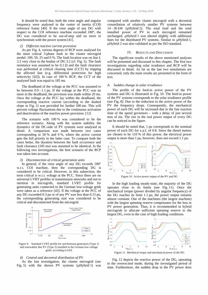
A. Sudden change in solar irradiance

The profile of the feed-in active power of the PV systems and DG is illustrated in Fig. 10. The feed-in power of the PV systems corresponds to the solar irradiance profile (see Fig. 8). Due to the reduction in the active power of the PV the frequency drops. Consequently, the mechanical power of each DG will be increased due to the fast reaction time of the speed governors – with a delay of just several tens of ms. The rise in the real power output of every DG can be noticed in the figure.

It should be noted that, 1 pu corresponds to the nominal power of each DG for a p.f. of 0.8. Since the diesel motors are chosen to be 110 % of this power, the electrical power output is more than 1 pu, however, does not exceed 1.1 pu.

Figure 10. Active power output of the PV and DG

In the high loading steady-state, the majority of the DG operates close to its limits (see Fig. 11). Once the mechanical torque (power divided by angular frequency) of the DG reaches its limit 1.1 pu, the power output remains almost constant. One of the machines (the largest machine) with the largest spinning reserve compensates for the loss in PV power generation. Thus, it is recommended in hybrid microgrids to allocate sufficient spinning reserve to the largest DG, even in the case of high loading conditions.

Figure 11. Mechnical torque and mechanical power of the DG

Fig. 12 depicts the reactive power of the DG, operating in the overexcited mode, during the investigated period of time. Furthermore, the sudden drop in the PV power does


not have a negative impact on the rotor angle stability. The power angle or rotor angle (COI) of each DG is far away from the limits ±180° – resulting in a very stable operation.

Figure 12. Reactive power and rotor angle of the DG

B. Different reactive current provision

In the first part of this section the results of the 3-phase fault in microgrid 3 with respect to 100 % RCP will be discussed in detail. The fault is cleared at its CCT, i.e., 185 ms. Subsequently, a comparison between 50 % and 0 % will be presented.

1) 100 % RCP a) Angular frequency and rotor angle

As mentioned earlier, both the angular frequency and rotor angle are analysed in the COI reference frame. The angular frequency of the DG located close to the fault location, i.e., DG 3.1 and DG 3.2, drops (see Fig. 13) because of mainly the subtransient short-circuit current and also residual voltage: Pe >> Pm. As a result of the drop in frequency, the speed governors increase the mechanical power input, with a delay of several ms. This leads to an increase in the frequency. In case of speed governors in transmission systems, the time delay is in the frame of several seconds [23][40]. However, in microgrids the assumption of a constant Pm will lead to incorrect results.

A significant positive deviation in the rotor angle of the two DG can be observed. If the fault were to be cleared 1 ms after the CCT, the rotor angle of DG 3.1 would have exceeded 180°. A stable operating point will be reached within 1 s after several non-critical rotor oscillations. Due to tripping of the faulty line, the pre-fault and post-fault stable operating points of the DG are slightly different.

Figure 13. Angular frequency and rotor angle of the DG

b) Active power of DG and PV The residual voltage in the affected microgrid drops up

to a value of 0.3 pu and the high subtransient current in DG 3.2 reduces over several 10s of ms. Therefore, during the end of the fault-on period the real power of DG 3.2 is the lowest among the DG. Since the residual voltage in the other microgrids is relatively higher, the power output of the DG is slightly higher.

Depending on the residual voltage at the PCC of the PV systems, the share of active and reactive currents with

respect to 1 pu will be adjusted. Soon after the fault occurrence, the PCC voltage of PV 3.1, which is located in the faulty grid, lies around 0.7 pu. As a result and acc. to Fig. 4 (red profile), the ratio of the active and reactive current will be approx. 50:50 (not shown). The corresponding power reduction in PV 3.1 is clearly observed in Fig. 14.

It should be noted that, the power output of the PV systems depends on the residual voltage. During the end of the fault-on period, the residual voltage in the other two microgrids drops up to value of 0.4 pu. Hence, as per Fig. 4 full priority is given to the reactive current. Consequently, the real power of PV 1.1 and PV 2.1 is almost reduced to zero.

Figure 14. Active power of the DG and PV

c) DC currents and DC-link voltage of PV The profile of the DC output current of the PV generator

IPV and profile of the DC input current of the inverter IDC in PV 3.1 are shown in Fig. 15. The latter is identical to the trajectory of the active power in PV 3.1. Soon after the fault occurrence, IPV remains unchanged, since it depends on the module temperature and solar irradiance. The current difference between IPV and IDC will flow into the DC-link capacitor (acting as short-term storage), thereby increasing UDC, which is however less than the maximum allowable DC input voltage (1000 V) of the inverters. As a result, the operating point of the PV generator will drift away from the MPP and IPV will get reduced accordingly. Due to the 100 % RCP, the IPV will be further decreased – up to zero.

Figure 15. DC currents of PV 3.1 and DC-link voltage of all the PV

As shown in Fig. 1, the DC voltage control restricts the sharp increase in UDC by reducing the signal I*

DC, which increases the amplitude of the reference current signal I*

d_ref. A clear distinction between the effect of the DC voltage control and 100 % reactive current is not possible, since both of them occur simultaneously.

In the post-fault period, the current will flow out of the DC-link capacitor until the difference between IPV and IDC is equal to zero. This corresponds to the drop and returning of UDC to its post-fault value.

d) Reactive power of DG and PV At the instant of fault clearing, the two DG in

microgrid 3 operates in the underexcited mode, whereas the


rest of the DG provides capacitive reactive power – see Fig. 16. This is due to the relatively higher residual (terminal) voltage of the DG in microgrid 1 and 2. Since the voltage at the PCC of the PV does not lie within the deadband, capacitive reactive power will be provided by them. It should be noted that, in the DG 1 pu corresponds to the nominal reactive power for the p.f. equal to 0.8. Whereas in the PV systems, 1 pu is based on the rated active power.

Figure 16. Reactive power of the DG and PV

In the post-fault period, DG 3.2 continues to operate in the underexcited mode, consuming the provided reactive power from the rest of the DG and PV. Further, the stator current of DG 3.2 reaches 2 pu, which is less than the rated continuous short-circuit current of the DG of about 3 pu [22]. Therefore, this is not considered as critical for the DG. On the other hand, the reactive power of the PV systems will increase sharply due to the sudden increase in the bus voltages soon after the fault is cleared. However, as the system voltages recover over time, a reduction in the reactive power of the PV is noticed.

Once the voltage at the PCC of the PV lies within the deadband, the reactive current will be provided for another 500 ms. Due to the tripping of the faulty line, the provision of the reactive power by DG will be slightly different.

e) Critical busbar voltage and frequency Fig. 17 illustrates the profile of voltage and frequency

observed at the critical busbar (BB) in each microgrid. The minimum voltage reached in microgrid 1-3 is equal to 0.55 pu, 0.51 pu and 0.28 pu, respectively. The system voltage recovery lasts for about 700 ms.

On the other hand, the measured minimum frequency in the cluster grid is about 44.4 Hz. These two profiles along with the other trajectories will be taken as reference for the discussion in the following subsection.

Figure 17. Voltage and frequency of the critical busbar in each microgrid

2) Comparision between 50 % and 0 % RCP As mentioned in the methodology, in both cases the fault

location as well as the fault clearing time are identical. Only in the first subsection, comparison based on the critical voltage and frequency in microgrid 3, for four different RCP will be presented.

a) Critical busbar voltage and frequency in microgrid 3

As far as the voltage profiles of busbar 3.3 (see Fig. 18) in the fault-on period (especially before the fault clearance) and post-fault is concerned, the case with 0 % RCP is assessed as the best case. Providing less reactive power in microgrids leads to better voltage profiles. In other words, a better system recovery is observed in all the three cases, where the active power of the PV is not constrained to zero.

During the subtransient period, the voltage profiles are almost identical. The subtle difference in the voltage profiles particularly just before clearing the fault has a significant impact on the system behaviour. Since particularly the magnitude of the electrical output power of the DG depends on the residual voltage, a slight improvement in the voltage profiles leads to a smaller difference of Pm and Pe. This in turn results in relatively less rotor angle deviations (see Fig. 24) and thereby has a positive impact on the CCT.

Figure 18. Voltage and frequency of busbar 3.3

(100, 50, 25 and 0 % RCP)

In general, due to the negative power difference between the generation and load, a frequency drop is observed soon after the fault. The complete curtailment of the active power of the PV systems (equivalent to a load increase) leads to the worst frequency profile in the case of 100 % RCP.

b) Active and reactive power of PV Compared to Fig. 14, a significant increase in the active

power output of the PV is noticed in Fig. 19. Even though 50 % of the priority is given to the active current, the profile of PV 3.1 in the below figure reaches 0 pu just before the fault clearance. It should be noted that, this trajectory depends also on the DC-link voltage.

Figure 19. Active power of the PV: 50 % and 0 %

Figure 20. dq-components of the reference and measured

output current of PV: 50 % and 0 %


The dq-components of the reference input current signals in the current controller as well as the dq-components of the measured output current are presented in Fig. 20.

The reduction in the provision of reactive power is evident in Fig. 21. Since the R/X ratio of the employed low-voltage overhead lines is slightly greater than 1, the grid voltages do not depend particularly on the reactive power – instead more on the active power.

Figure 21. Reactive power of the PV: 50 % and 0 %

c) Reactive power of DG The DG located near the fault do not operate in the

underexcited mode for a long time as against the case 100 % RCP. Further, since the reactive power is completely curtailed in the PV systems in the case 0 % RCP, DG 3.1 and DG 3.2 are not forced to consume the surplus capacitive reactive power – see Fig. 22.

Figure 22. Reactive power of the DG: 50 % and 0 %

d) Angular frequency and rotor angle As mentioned in the beginning of this subsection, the

influence of the different degrees of RCP in the subtransient period is in principle negligible. The profiles of angular frequency and rotor angle are identical in the first 50 ms after the fault occurrence. This is evident in Fig. 23 and Fig. 24.

Figure 23. Angular frequency of the DG: 50 % and 0 %

Figure 24. Rotor angle of the DG: 50 % and 0 %

However, due to the best voltage profile for 0 % RCP (see Fig. 18) and correspondingly because of the smaller difference between Pm and Pe, the maximum rotor angle reached in DG 3.2 is approximately 60°, whereas in 50 % RCP the value lies around 90°. Further, the rotor oscillations in 0 % RCP are relatively not prominent. It can be inferred that, 0 % RCP has a significant positive effect on the voltage stability and consequently on the rotor angle stability.

e) Influence of RCP on CCT In Table III the CCT with respect to different RCP are

listed and compared. Higher ratio of ACP to RCP leads to a significant increase in the CCT. By giving an entire priority to the active current, i.e., 0 % RCP, the CCT can be improved by about 70 %.

TABLE III. LIST OF THE CCT AND ITS COMPARISON FOR DIFFERENT RCP

Reactive current provision

100 % 50 % 25 % 0 % CCT in ms 185 224 272 311 Absolute

change in ms - +39 +87 +126

Absolute change in %

- +21 +47 +68

C. Disconnection of critical generation units

In this section the analyses are based on the best case corresponding to the RCP: 0 %. It can be inferred from the investigations corresponding to the disconnection of the critical PV and DG that, the transient stability can be still guaranteed.

None of the PCC voltage of the PV systems gets reduced to less than 0.15 pu, the PV with the least PCC voltage is disconnected at its least value, i.e., PV 3.1. As a result the CCT gets reduced from 312 ms to 297 ms, which corresponds to a decline of 5 %. This is as a result of total active power deficit and which in turn worsens the voltage profile. Therefore, the positive difference between Pm and Pe of DG 3.2 increases even further. Since DEGOV1 of the DG tries to increase the mechanical moment, the difference gets increased to a greater extent. If an additional PV were to be disconnected, the DG would have compensated for this loss, because of the very fast reacting speed governor. The duration of the system’s returning to a new stable operating point would slightly increase.

The voltage at the PCC of the critical DG does not exceed the minimum allowable voltage, as depicted in Fig. 9. Thus, the critical DG based on the global minimum PCC voltage is taken out of operation, once this voltage is reached. In spite of several DG getting additionally highly loaded, the transient stability is still guaranteed. Further, the system voltage and also system frequency recover relatively slowly: around 1 s.

From the system stability point of view, it is recommended to operate one of the DG, especially the largest machine, with a relatively larger spinning reserve not risking with the wet stacking of diesel motors. Since the acceleration time constant of the employed DG is between 0.5 - 1 s, the DG acting as reserve can be quickly taken into


operation once the system is returned to a post-fault steady-state.

D. Central and decentral distribution of PV

The CCT for the same fault close to DG 3.2 in µHybrid 2 gets increased by 5 % as against µHybrid 1. The voltage at the buses and its difference in microgrid 3 is presented in Fig. 25. It should be noted that, a sharp increase in the voltage difference around 2.3 s is due to the different fault clearing times. Decentral distribution of PV systems improves the voltage profile marginally during fault-on in case of the investigated fault, which in turn has a positive effect on the CCT. However, this is not always the case. A reduction by 17 % in the CCT is observed for a fault in microgrid 1. This calls for further investigations and perhaps with a different approach in detail.

Figure 25. Bus voltage in microgrid 3 as well as voltage difference in

microgrid 3 (µHybrid 1 and µHybrid 2)

V. CONCLUSIONS AND OUTLOOK

The main goal of this paper was to model and analyse the transient stability of a realistic hybrid microgrid (with a total installed capacity of 760 kW) comprising DG and PV considering the DC-side of the PV. Several investigations were carried out at a high loading condition, where the ratio of the actual power of DG to PV lay around 70:30.

In the first investigation, it can be concluded that, the significant reduction in the solar irradiance of about 55 % within 2.5 s does not have a negative impact on the transient stability of the studied microgrid.

The key findings of the performed short-circuit investigations are as follows: The higher the ratio of ACP to RCP is, the better is the effect on the voltage and transient stability. Compared to the case with 100 % RCP, an increase of the CCT by a factor of 0.2 in 50 % RCP is observed. If the provision is given entirely to the active current, a significant improvement in the CCT by a factor of 0.7 is noticed. Therefore, it is recommended not to provide reactive power and curtail the active power output of PV systems in case of short-circuits in hybrid microgrids.

Further, disconnection of the critical PV and DG does not pose serious problems regarding transient stability even in the high loading condition. The microgrid reaches the new post-fault steady-state slightly slower by 1 s. Nevertheless, it is advisable to install several DG as reserve and / or operate one of the active DG with a large spinning reserve from the system stability point of view.

Lastly, the decentral distribution of PV systems has both positive and negative effect on the transient stability. The CCT of one of the two faults increases by 5 %, whereas the CCT of the other fault is decreased by 17 %.

In a cluster microgrid environment, it is a tedious and ineffective process to assess or analyse solely the CCT using time-domain simulations. Further, with the help of a hybrid method [44][45] combining both time-domain simulations and energy function for DG, transient stability of hybrid microgrids – comprising DG, PV acting as current sources and BSS behaving as voltage sources – can be quantitatively assessed. Numerous scenarios like central vs. decentral distribution of PV, various operating points with different power allocation as well as controller settings etc. can be effectively studied and compared using the hybrid method in hybrid microgrids.

REFERENCES

[1] International Renewable Energy Agency (IRENA), “Off-grid

renewable energy systems: Status and methodological issues,” [Online] Available: https://www.irena.org/-/media/Files/IRENA /Agency/Publication/2015/IRENA_Off-grid_Renewable_Systems_ WP_2015.pdf

[2] Caterpillar, “Hybrid microgrids: the time is now,” [Online] Available: https://www.cat.com/en_US/by-industry/electric-power-generation/Articles/White-papers/white-paper-hybrid-microgrids-the-time-is-now.html

[3] United Nations (UN), “Multi-dimensional issues in international electric power grid interconnections,” [Online] Available: https://sustainabledevelopment.un.org/content/documents/interconnections.pdf

[4] Conseil International des Grands Réseaux Électriques (CIGRE), “Review of on-line dynamic security assessment tools and techniques,” [Online] Available: https://e-cigre.org/publication/325-review-of-on-line-dynamic-security-assessment-tools-and-techniques

[5] H. D. Chiang, Direct methods for stability analysis of electric power systems, New Jersey: Wiley, 2011.

[6] IEEE, “Microgrid stability definitions, analysis, and modeling,” [Online] Available: http://resourcecenter.ieee-pes.org/pes/product-/technical-publications/PES_TR0066_062018

[7] Y. Yang, W. Chen and F. Blaabjerg, “Advanced control of photovoltaic and wind wurbines power systems,” in Intelligent Control in Power Electronics and Drives, T. Orłowska-Kowalska, F. Blaabjerg and J. Rodríguez, Eds CH: Springer, Cham, 2014, pp. 41–89.

[8] General Cable, “Bare overhead distribution conductor,” [Online] Available: https://www.generalcable.com/na/us-can/products-solu-tions/energy/distribution-conductor-and-cable/overhead-conductor

[9] K. Veerashekar, S. Eichner and M. Luther, “Modelling and transient stability analysis of interconnected autonomous hybrid microgrids,” IEEE PES PowerTech, Milan, Italy, June 2019. (accepted paper)

[10] A. Yazdani and R. Iravani, Voltage-sourced converters in power systems: Modeling, control, and applications, New Jersey: Wiley, IEEE-Press, 2010.

[11] R. Teodorescu, M. Liserre and P. Rodríguez, Grid converters for photovoltaic and wind power systems, Chichester, UK: Wiley, 2011.

[12] E.ON “Grid connection regulation for high and extra high voltage,” Bayreuth, April 2006.

[13] J. Rocabert, A. Luna, F. Blaabjerg and P. Rodriguez, “Control of power converters in AC microgrids,” IEEE Trans. on Power Electronics, vol. 27, no. 11, pp. 4734–4749, November. 2012.

[14] N. Kroutikova, C. A. Hernandez-Aramburo and T. C. Green “State-space model of grid-connected inverters under current control mode,” IET Electric Power Applications, vol. 1, no. 3, pp. 329–338, May 2007.

[15] S. M Tripathi, A. M. Tiwari and D. Singh, “Optimum design of proportional-integral controllers in gridintegrated PMSG-based wind energy conversion system,” Int. Trans. on Electrical Energy Systems, vol. 26, no. 5, pp. 1006–1031, May 2016.

[16] D. Schröder, Electrical drives – Control of drive systems (German: Elektrische Antriebe – Regelung von Antriebssystemen), 4th ed., Berlin: Springer, 2015.


[17] National Grid ESO, “Fast fault current injection,” [Online] Available: https://www.nationalgrideso.com/document/104791/ download

[18] Stamford AvK, ”AGN 034 – alternator reactance,” [Online] Available: https://www.stamford-avk.com/sites/default/files/ AGN034_C.pdf

[19] SMA Solar Technology, “Short-circuit behavior of Sunny Central CP XT and Sunny Central Storage,” [Online] Available: http://files.sma.de/dl/22701/HK_Short-cuircuit-current_SC-SCS_en_10.pdf

[20] K. Veerashekar, M. Flick and M. Luther, “Small-signal stability of interconnected autonomous microgrids,” (German: „Kleinsignal-stabilität von vernetzten autonomen Mikronetzen”) ETG congress, Esslingen am Neckar, Germany, May 2019. (accepted paper)

[21] Clifford Power, “Wet stacking of generator sets and how to avoid it,” [Online] Available: http://www.cliffordpower.com/stuff/contentmgr-/files/0/971a5485c1088e9230413aa3d1189ef7/misc/is_09_wet_stacking.pdf

[22] German Generator / Stamford, “Industrial Power Generators” (German: „Industrielle Stromerzeuger,”) [Online] Available: https://germangenerator.de/produkte/industrielle-stromerzeuger/

[23] J. Machowski, J. W. Bialek and J. R. Bumby, Power system dynamics: Stability and control, 2nd ed., Chichester, UK: Wiley, 2012.

[24] PowerWorld Corporation, “Governor DEGOV1,” [Online] Available: https://www.powerworld.com/WebHelp/Content/ TransientModels_HTML/Governor%20DEGOV1.htm

[25] IEEE, “Recommended practice for excitation system models for power system stability studies,” New York: IEEE, 2005.

[26] P. M. Anderson and A. A. Fouad, Power system control and stability, 2nd ed., New Jersey: Wiley, IEEE-Press, 2003.

[27] DIgSILENT PowerFactory 2017, “Technical reference documentation: Synchronous machine,” Gomaringen, Germany, 2017.

[28] IEEE, “Load representation for dynamic performance analysis,” IEEE Trans. on Power Systems, vol. 8, no. 2, pp. 472–482, May 1993.

[29] FG Wilson, “Standard operating limits,” [Online] Available: http://www.fgwilson.ie/files/generator-set-iso8528-5-2005-operating-limits.pdf

[30] International Organization for Standardization (ISO), “ISO 8528-5:2013, Reciprocating internal combustion engine driven alternating current generating sets - Part 5: Generating sets,” Geneva: ISO, March 2013.

[31] A. Gomez-Exposito, A. J. Conejo and C. Canizares, Electric energy systems: analysis and operation, 2nd ed., Boca Raton, USA: CRC Press, 2018.

[32] Sharp, “Datasheet: NQ-R258H,” [Online] Available: https://www.sharp.de/cps/rde/xchg/de/hs.xsl/-/html/product-details-solar-modules.htm?product=NQR258H

[33] SMA Solar Technology, “Datasheet: Sunny Tripower 60,” [Online] Available: https://www.sma.de/en/products/solarinverters/sunny-tripower-60.html

[34] SMA Solar Technology, “Datasheet: Sunny Tripower Core 1,” [Online] Available: https://www.sma.de/en/products/solarinverters /sunny-tripower-core1.html

[35] M. Salcone and J. Bond, “Selecting film bus link capacitors for high performance inverter applications,” 2009 IEEE Int. Electric Machines and Drives Conference, pp. 1692–1699, Miami, USA, May 2009.

[36] M. Vujacic, M. Hammami, M. Srndovic and G. Grandi, “Analysis of dc-link voltage switching ripple in three-phase PWM inverters,” MDPI Energies, vol. 11, no. 2, February 2018.

[37] A. M. Hava, U. Ayhan and V. V. Aban, “A DC bus capacitor design method for various inverter applications,“ 2012 IEEE Energy Conversion Congress and Exposition, pp. 4592–4599, Raleigh, USA, September 2012.

[38] Roboternetz-Wissen, “Control Engineering,” (German: „Regelungs-technik“) [Online] Available: https://rn-wissen.de/wiki/index .php/Regelungstechnik

[39] Government of Canada, “High-resolution solar radiation datasets,” [Online] Available: https://www.nrcan.gc.ca/energy/renewable-electricity/solar-photovoltaic/18409

[40] P. Kundur, Power system stability and control, New York: McGraw-Hill, 1994.

[41] M. H. Haque, “Hybrid method of determining the transient stability margin of a power system,” IEE Proceedings - Generation, Transmission and Distribution, vol. 143, no. 1, pp. 27–32, January 1996.

[42] G. Ziegler, Numerical differential protection: Principles and applications, 2nd ed., Erlangen, GER: Publicis, 2011

[43] Association of Electrical Engineering, Electronics and Information Technology (German: VDE), “VDE-AR-N 4105: Generation units in the low-voltage network - Minimum technical requirements for connection and parallel operation of generation units in the low-voltage network”, Berlin: VDE Publisher, November 2018.

[44] K. Veerashekar, A. Goepel, M. Luther, “Large Signal Stability Analysis in Clustering of Microgrids Using A Hybrid Method,” 11th Mediterranean Conference on Power Generation, Transmission, Distribution and Energy Conversion (MEDPOWER), November 2018.

[45] K. Veerashekar, P. Schuehlein, M. Luther, “Quantitative Transient Stability Assessment in Power Systems Combining both Time-domain Simulations and Energy Function Analysis,” unpublished


Transient Stability of Hybrid Stand-alone Microgrids ...

Documents

Transcript of Transient Stability of Hybrid Stand-alone Microgrids ...