Battery performance characterisation for stand-alone ...
427
Battery Performance Characterisation for Stand-Alone Photovoltaic Systems CJ de V PURCELL, BSc (Chem), UCT Energy for Development Research Centre Energy Research Institute, University of Cape Town September 1991 c
-
Upload
khangminh22 -
Category
Documents
-
view
2 -
download
0
Transcript of Battery performance characterisation for stand-alone ...

Battery Performance Characterisation for Stand-Alone Photovoltaic Systems
CJ de V PURCELL, BSc (Chem), UCT
Energy for Development Research Centre Energy Research Institute, University of Cape Town
September 1991
c ~--- -~--·-- ~ ----~----·,·'

The copyright of this thesis vests in the author. No quotation from it or information derived from it is to be published without full acknowledgement of the source. The thesis is to be used for private study or non-commercial research purposes only.
Published by the University of Cape Town (UCT) in terms of the non-exclusive license granted to UCT by the author.

/,'
' {

DECLARATION
I declare that this dissertation is my own original work. It is being submitted in partial fulfilment for the degree of Master of Science in Applied Science at the University of Cape Town. It has not been submitted before for any degree or examination at any university .
..... ................ .
C J de V PURCELL
1<;���1'\91
Signature Removed

~··
... JJ'
,..

ABSTRACT
One of the main factors limiting optimisation of PV system designs over the life
of the system has been the lack of battery test data appropriate to PV applications.
The main objective of this study was to determine accurate empirical data for
locally available lead-acid batteries which could be used in photovoltaic systems
and to present this data in a format directly applicable to PV system designers.
The study included (i) a review of battery performance regimes typical of PV
systems; (ii) a literature review of lead-acid battery performance and reactions
important to PV applications, battery electrical models, battery life models, a
review of specialist PV battery designs and the interaction of battery and voltage
regulator in PV systems;. (iii) a review of testing and research literature, and the
design of a suite of experimental procedures suitable for characterising batteries
under PV operating regimes; (iv) the design and construction of a specialised
battery test-unit to automatically perform tests and capture data; (v) selection,
testing and characterisation of five generic types of batteries which could be used
in local PV applications.
The five types of lead-acid battery were:
1) conventional calcium alloy positive and negative grids, flat plate, flooded
electrolyte, vented casing;
2) low antimony alloy positive grid, conventional calcium negative grid, flat
plate, flooded electrolyte, vented casing;
3) low antimony alloy positive grid, heat treated calcium negative grid, flat
plate, immobilised absorbed electrolyte, sealed casing with 0 2 cycle gas
recombination;
4) antimony alloy positive and negative grids, flat plate, flooded electrolyte,
vented casing;
5) antimony alloy positive and negative grids, tubular plate, flooded
electrolyte, vented casing.
Selenium grid alloy cells and gelled electrolyte batteries were not represented
amongst the batteries tested, owing to problems of availability or cost.
i

/

Performance data presented at the temperatures and low currents typical of PV
applications include discharge and capacity curves, charge curves and charge
efficiency curves. Performance under PV cycling regimes is analysed. Life cycle
estimates and associated battery life cycle costs are tabulated, with discussion of
special considerations when selecting these batteries for a PV application. The
battery data generated has also been incorporated in a database battery model in
a PV system simulation package, PVPRO, for improved battery performance
modelling.
ii

\'

ACKNOWLEDGEMENTS
I would like to thank the following people and organisations for their
contributions to this research project:
Dr Anton Eberhard and Bill Cowan for their guidance and supervision at
various stages of this dissertation,
the organisations in the battery and photovoltaic industries that so readily
made their equipment available for testing,
colleagues at the Energy for Development Research Centre for their
persistent encouragement and interest,
Susan, especially, for her patience and understanding during this time.
iii


TABLE OF CONTENTS
ABSTRACT ACKNOWLEDGEMENTS TABLE OF CONTENTS LIST OF FIGURES LIST OF TABLES
1 INTRODUCTION 1.1 RATIONALE 1.2 OBJECTIVES 1.3 CONSTRAINTS 1.4 REPORT OUTLINE
2 PHOTOVOLTAIC SYSTEMS WITH BATTERY STORAGE 2.1 COMPONENTS OF A STAND-ALONE PV SYSTEM
2.1.1 Photovoltaic Panel Output 2.1.2 Battery 2.1.3 Regulator 2.1.4 Inverters
2.2 BATTERY OPERATING REGIMES IN PV SYSTEMS 2.2.1 System Sizing 2.2.2 System Simulation 2.2.3 Costing
2.3 CONCLUSIONS
3 THE LEAD-ACID BATTERY 3.1 HISTORY 3.2 BASICS: HOW A LEAD -ACID BATTERY WORKS 3.3 CELL DESIGN AND CONSTRUCTION
3.3.1 The Ideal Cell 3.3.2 Cell Components 3.3.3 Design of the Active Block
3.4 ELECTRICAL CHARACTERISTICS 3.4.1 Open Circuit Voltage and SG 3.4.2 Capacity 3.4.3 Voltage During Operation 3.4.4 Charging Methods 3.4.5 Equalising Charge and Defined Charge State 3.4.6 Energy and Energy Efficiency
· 3.4.7 Cycle Life
iv
i iii iv IX
xix
1.1 1.1 1.3 1.5 1.4
2.1 2.1 2.2 2.4 2.5 2.6 2.7 2.7 2.8 2.9
2.15
3.1 3.2 3.4 3.5 3.5 3.6 3.7
3.14 3.14 3.15 3.17 3.21 3.22 3.23 3.25

TABLE OF CONTENTS
3.5 BA ITERY TYPES 3.5.1 Starting, Lighting, Ignition Batteries 3.5.2 Electric Vehicle Batteries 3.5.3 Stationary Batteries
3.6 MICRO-PROCESSES DURING BATTERY OPERATION 3.6.1 Basic Lead-acid Electrodes 3.6.2 Processes in the Active Mass 3.6.3 Grid Processes (decay and life limiting processes)
3.7 POLARISATION AND OVERPOTENTIAL 3.7.1 Types of Polarisation 3.7.2 Hydrogen Overpotential 3.7.3 Oxygen Overpotential 3.7.4 Overpotential and Polarisation During Charge
3.8 MACRO-PROCESSES DURING OPERATION 3.8.1 Electrolyte Stratification and Recovery 3.8.2 ·Gassing and Related Phenomena
3.9 METHODS OF REDUCING WATER LOSS 3.9.1 Water Loss 3.9.2 Catalytic Recombination of H2 and 0 2
3.9.3 Closed O:i and H2 Cycles 3.9.4 Antimony-free Alloys
3.10 ELECTRICAL CHARACTERISATION MODELS 3.10.1 Introduction 3.10.2 Electrical Characterisation of the Battery 3.10.3 Capacity 3.10.4 Ah Charging Efficiency 3.10.5 Self-discharge 3.10.6 Conclusions
3.11 FAILURE AND WEAR 3.12 CYCLE-LIFE MODELS
3.12.1 Cycle Life vs DOD 3.12.2 Temperature Effects 3.12.3 Incremental Wear 3.12.4 Battery Strings 3.12.5 Conclusions
3.13 PHOTOVOLTAIC BATTERIES 3.13.1 Requirements of PV Batteries 3.13.2 Trends in the Design of PV Batteries 3.13.3 Electrolyte 3.13.4 Gassing and Gas Recombination Techniques 3.13.5 · Grid Composition 3.13.6 Positive Plate Design 3.13.7 Some State-of-the-art PV Batteries
v
3.27 3.27 3.30 3.31 3.35 3.35 3.38 3.41 3.46 3.46 3.49 3.50 3.52 3.53 3.53 3.54 3.57 3.57 3.58 3.59 3.64 3.65 3.65 3.65 3.69 3.70 3.71 3.72 3.73 3.75 3.75 3.77 3.78 3.79 3.79 3.80 3.80 3.80 3.81 3.84 3.85 3.86 3.87
TABLE OF CONTENTS
3.14 VOLTAGE REGULATION 3.14.1 Charge Regulators 3.14.2 Overdischarge Protection 3.14.3 Regulator Adjustment 3.14.4 Microprocessor-controlled Regulators 3.14.5 Regulator Efficiency 3.14.6 Reliability 3.14.7 Conclusions
4 LABORATORY TESTS OF PHOTOVOLTAIC BATTERIES 4.1 INTRODUCTION 4.2 BATTERY CHARACTERISATION TESTS
4.2.1 Discharge Capacity 4.2.2 Battery Charging Characteristics 4.2.3 Thermal Effects 4.2.4 Cycling Tests 4.2.5 Self-discharge 4.2.6 Life Cycle Tests 4.2.7 Scaling of Battery Test Results
4.3 BATTERY TEST DATA 4.3.1 Introduction 4.3.2 Data Quality 4.3.3 Data Available from Manufacturers 4.3.4 Standards and Standardisation
4.4 BATTERY TEST EQUIPMENT 4.4.1 Broad Equipment Requirements 4.4.4 System Power-handling and Test Equipment Sizing
5 EQUIPMENT DESIGN 5.1 INTRODUCTION AND OVERVIEW OF REQUIREMENTS
5.1.1 Overview of DC Power Supplies and Loads 5.1.2 Design Choice
5.2 ELECTRONIC DESIGN 5.2.1 Programmable Load Design 5.2.2 Power Supply Design, The Output Stage 5.2.3 Power Supply Design - LC Filter 5.2.4 Power Supply Design - SCR Tracking Pre-regulator 5.2.5 Power Supply Design - Isolation Transformer 5.2.6 Auxiliary Equipment, Safety and Layout 5.2.7 Digital Interface and Computer Control
5.3 CONTROL SOFTWARE 5.3.1 General Requirements 5.3.2 Implementation 5.3.3 Program
Vl
3.92 3.92 3.97
3.100 3.101 3.102 3.104 3.105
4.1 4.1 4.1 4.1 4.7
4.11 4.12 4.13 4.14 4.15 4.17 4.17 4.17 4.18 4.19 4.20 4.20 4.22
5.1 5.1 5.2 5.4 5.7 5.7
5.16 5.21 5.22 5.28 5.29 5.34 5.38 5.38 5.40 5.41

TABLE OF CONTENTS
5.3.4 Digital Feedback Loop Stability 5.41 5.3.5 PV Simulation 5.43
5.4 TEMPERATURE CONTROL 5.46
6 METHOD OF INVESTIGATION AND TESTING 6.1 6.1 BATTERY SELECTION 6.1 6.2 BATTERY TESTING METHOD 6.2
6.2.1 "On Delivery" Assessment 6.3 6.2.2 Initial Test and Forming Charge 6.4 6.2.3 Capacity Tests 6.5 6.2.4 Discharge Tests 6.6 6.2.5 Charging Curves 6.6 6.2.6 Charging Efficiency, Average and Instantaneous 6.9 6.2.7 Cycling Tests 6.15
6.3 REPORT FORMAT 6.20
7 TEST RESULTS 7.1 7.1 WILLARD 774 PORTABLE BATTERY 7.1
7.1.1 General Information 7.1 7.1.2 Physical 7.2 7.1.3 Basic Operating Data Available 7.3 7.1.4 Test Results and Discussion 7.5 7.1.5 Sizing and Selection: considerations in PV applications 7.18
7.2 RAYLITE RMT108 STANDBY CELL 7.19 7.2.1 General Information 7.19 7.2.2 Physical 7.20 7.2.3 Basic Operating Data Available 7.21 7.2.4 Test Results and Discussion 7.23 7.2.5 Sizing and Selection: considerations in PV applications 7.36
7.3 WILLARD VANTAGE LS90 UPS BATTERY 7.37 7.3.1 General Information 7.37 7.3.2 Physical 7.38 7.3.3 Basic Operating Data Available 7.39 7.3.4 Test Results and Discussion 7.41 7.3.5 Sizing and Selection: considerations in PV applications 7.52
7.4 GNB 12V-5000 PHOTOVOLTAIC BATTERY 7.53 7.4.1 General Information 7.53 7.4.2 Physical 7.54 7.4.3 Basic Operating Data Available 7.55 7.2.4 Test Results and Discussion 7.57 7.4.5 Sizing and Selection: considerations in PV applications 7.68
vii

TABLE OF CONTENTS
7.5 DELCO 1250 TRUCK/UPS BATTERY 7.70 7.5.1 General Information 7.70 7.5.2 Physical 7.71 7.5.3 Basic Operating Data Available 7.72 7.5.4 Test Results and Discussion 7.76 7.5.5 Sizing and Selection: considerations in PV applications 7.87
7.6 COMPARATIVE DISCUSSION 7.88 7.6.1 Initial costs 7.88 7.6.2 Charging parameters 7.89 7.6.3 Discharge parameters 7.92 7.6.4 Cycle performance 7.93 7.6.5 Cycle life 7.94 7.6.6 Conclusions 7.97
8 CONCLUSIONS 8.1 8.1 LITERATURE REVIEW 8.1 8.2 BATTERY TESTING FACILITY AND TEST METHODS 8.2 8.3 TEST RESULTS 8.4 8.4 BATTERY MODELLING 8.7 8.5 CHARGE AND LOAD SHED REGULA TOR SETTINGS 8.8 8.6 PV SYSTEM SIZING 8.9 8.7 RECOMMENDATIONS 8.10
Appendix A - References and Bibliography Appendix B - Life Cycle Costing and Assumptions Appendix C - Battery Sizing Considerations in Stand-alone
Photovoltaic Systems Appendix D - Manufacturers' Battery Data
Dl - Willard 774 D2 - Raylite RMT108 D3 - Willard LS90 D4 - GNB Mini.;Absolyte 12V-5000 DS - Delco 1250 D6 - BP Solar P-series D7 - Sonnenschein A600 Solar Battery
Appendix E - Electrical Data El - Heatsinking of 2N3442 Transistors E2 - Frequency Compensation for Electronic Load E3 - LC Filter Design E4 - Transistor Array SOAR and Current Gain ES - Program Data Flow E6 - Electrical Component Data
viii

LIST OF FIGURES
2.1 Components of a stand-alone PV system with battery storage: 2.1 PV array, charge regulator, battery, discharge regulator, DC load, optional inverter and AC load.
2.2 1-V characteristics of a crystalline silicon PV module as a 2.3 function of irradiance; cell temperature 25°C.
2.3 Effect of temperature on 1-V curve at 10oowm-2• 2.3
2.4 Projected energy cost for various batteries in USA. 2.5
2.5 Efficiency vs power output for a lkVA non-sinusoidal inverter 2.6 with resistive loads.
2.6 Operating conditions for System 1, supplier system. 2.11
2.7 Operating conditions for System 2, low cost modular system. 2.12
2.8 Life cycle costs for System 1, supplier system. 2.13
2.9 Life cycle costs for System 2, low cost modular system. 2.14
3.1 Construction of a modem standby cell. 3.6
3.2 Concentration of H2S04 at 25°C over the range used in 3.8 different batteries.
3.3 Effect of H2S04 concentration and temperature on resistivity 3.8 and viscosity.
3.4 Capacity vs plate thickness at different discharge rates. 3.11
3.5 Capacity vs tube diameter at different discharge rates. 3.12
3.6 Capacity vs cycle life of tubular batteries. 3.12
3.7 Relationship between cycle life and specific energy of tubular 3.13 and pasted plate designs.
3.8 Experimentally determined and calculated dependence of cell 3.14 voltage on H2S04 concentration.
3.9 Relationship between capacity and discharge current. 3.16
ix

LIST OF RGURES
3.10 Standard discharge curves for a 12V 90Ah SLI battery. 3.18 Temperature= 20°C.
3.11 SLI battery retained capacity during open circuit storage. 3.19
3.12 Three charging regimes during constant current charging, 3.20 showing voltage and temperature vs time.
3.13 Charge under controlled current-voltage conditions for a 3.22 lOOAh 12V battery.
3.14 Relationship between energy and discharge current for 4V 3.24 lOOAh cell to complete discharge.
3.15 Relationship between charging energy and controlled current- 3.24 voltage charging parameters.
3.16 Cycle life vs DOD for various battery designs. 3.26
3.17 Dependence of cycle life on temperature, lead-acid motive 3.26 power cell.
3.18 Gassing current vs voltage for various types of 12V, 77 Ah SLI 3.29 batteries.
3.19 Dependence of the corrosion rate at constant cell voltage on 3.32 the Sb content of the grid alloy.
3.20 Simplified potential/pH diagram of the Pb/H20 system. 3.37 according to Pourbaix, at 25°C, for unity hydrogen ion activity.
3.21 Cross-section of grid/ corrosion-layer I active mass of plates 3.42 with Pb-0.09% Ca, and Pb-4% Sb-0.2%.
3.22 Corrosion rate vs antimony content of spines, polarized under 3.43 three test conditions.
3.23 Spine corrosion rate as a function of the thickness of the active 3.44 mass.
3.24 Transient behaviour of transfer current UJ, electrode porosity 3.47 (E) and electrolyte concentration (c) within the cell during constant current discharge.
3.25 Variation of cell potential during discharge. Subscript r 3.48 denotes equilibrium conditions, subscript i denotes operating
x

LIST OF FIGURES
conditions, while subscripts a and c denote anodic and cathodic processes. Subscript fl denotes polarisation.
3.26 Current/potential curves for polarization of Pb/PbS04 and 3.49 H2/tt• electrodes in H2S04 solution.
3.27 Current/potential curves for polarization of Pb/PbS04 and 3.51 0 2;0· electrodes in H2S04 solution.
3.28 Variation of cell potential during charging. Subscript r denotes 3.52 equilibrium conditions, subscript i denotes operating conditions, while subscripts a and c denote anodic and cathodic processes. Subscript fl denotes polarisation, and subscript g gassing. The H2/tt• and H20/02 electrodes are superimposed.
3.29 Stratification of electrolyte measured during charging to 2% 3.53 overcharge and 100% DOD.
3.30 Charge acceptance of positive and negative plates at 40°C vs 3.55 time.
3.31 H2/02 ratio during charge acceptance. 3.56
3.32 Cross section of a catalytic plug. 3.59
3.33 Schematic of a cell with an auxiliary electrode. 3.60
3.34 Influence of 0 2 recombination on the polarization of the H2/tt• 3.61 electrode.
3.35 Comparison of Mobil-Tyco Model with measured data for 3.68 charging.
3.36 Comparison of Peukert and Liebnenov correlations with real 3.70 data.
3.37 Self-discharge of SLI batteries under open-circuit conditions 3.71 using the Lasnier model.
3.38 Self-discharge of SLI batteries under open-circuit conditions. 3.72
3.39 Typical representation of cycle life vs depth of discharge. 3.75
xi

LIST OF RGURES
3.40 Life cycle correlations for traction, SLI, and PV type lead-acid 3.76 batteries. (SLI = F.agle-Picher Carefree Sealed; EV = C&D; PV = C&D lead-calcium alloy grid)
3.41 Cycle life vs DOD and temperature for a lead-acid motive 3.77 power type battery.
3.42 Electrolyte stratification of a 200Ah tubular cell in comparison 3.83 to an A600 gelled cell.
3.43 End of discharge voltage of a sealed lOOAh battery and 3.83 comparable flooded electrolyte battery subjected to the deep cycle partial state-of-charge test.
3.44 Effect of electrolyte immobilization on cycle life. Cl 4 3.84 discharge to 60%, recharge at C/10 with 50% overcharge.
3.45 Gas recombination efficiencies of different cell designs using ·3.85 catalytic recombination devices.
3.46 Voltage regulator in a stand-alone PV system. 3.92
3.47 Typical situation for a PV installation, 1-V curves for 12 cell 3.93 45WP array, lOOAh lead-antimony battery. Tarray=47°C, I=lOOOW /m2
, Tbat=2D°C.
3.48 Self-regulation of a lOOAh lead-calcium sealed battery at 50%, 3.94 75% and 100% SOC (Tbat=20°C), with a 10 cell poly-crystalline 42W P PV panel at the specified irradiances and panel temperatures.
3.49 a) boost charge mode, b) float charge with current control, 3.96 c) auto boost mode. The solid line represents voltage, the dashed line represents current.
3.50 Effect of battery temperature on operating point for typical PV 3.97 installation. 1-V curves for a 12 cell 45WP array, lOOAh lead-antimony battery. Tarray=47°C, l=lOOOW /m2
, Tbat=20°C, SOC=l00%.
3.51 Standard battery discharge curves 3.98
3.52 Battery rise times at 0.5A/100Ah charging current following 3.99 various discharge currents, after load shedding at 1.9V /cell.
3.53 Battery drop-out voltage vs temperature and discharge current. 3.99
xii-

LIST OF RGURES
3.54 a) Shunt and b) series configurations 3.102
3.55 a) Shunt and b) series configurations, showing the PV 3.103 operating points during regulation.
4.1 Constant current discharge curves for a lead-acid battery. 4.2
4.2 Peukert curve for a lead-acid battery, showing time to cut-off 4.3 voltages.
4.3 Change in capacity and discharge current vs duration of 4.3 discharge under continuous and intermittent regimes.
4.4 Effect of constant-current, constant-resistance and constant- 4.4 power discharges on Ah capacity.
4.5 Effect of pulse current frequency on discharge performance of 4.5 lead-acid battery.
4.6 Effect of pulse to average current ratio on discharge 4.6 performance of lead-acid battery.
4.7 Load-shed settings as affected by current, SOC and 4.7 temperature.
4.8 Lead-acid battery charging curves, using constant current, 4.9 constant voltage method.
4.9 Lead-acid charge discharge cycling during PV operation. 4.9
4.10 Temperature effect on capacity. 4.11
4.11 Finishing current vs temperature during battery charging 4.12
4.12 Correlation of normalized Ah capacity with normalized charge 4.16 rate.
5.1 Block layout of the programmable battery test unit. Dashed 5.2 lines indicate communication linkages. I=current, V=voltage, T=temperature.
5.2 Electronic design components of the battery test unit. 5.5
5.3 Transistorised load operation 5.7
xiii

LIST OF RGURES
5.4 Load transistor array with FEf driver 5.9
5.5 Load current sensing and feedback amplifier 5.10
5.6 Block diagram of load control loop 5.11
5.7 Bode plot of CLG before and after frequency compensation. 5.12
5.8 Electronic load control loop circuit. 5.12
5.9 Buffered output current signal to AID and instrumentation 5.14 from electronic load.
5.10 Voltage measurement circuit 5.15
5.11 Linear regulator, principle of operation 5.16
5.12 Linear regulator base drive arrangement 5.17
5.13 Linear regulator array. 5.18
5.14 Return line current sensing 5.19
5.15 Current sensing amplifier 5.19
5.16 Bode plot for linear regulator 5.20
5.17 Harmonic content of SCR rectifier, 60V rms input. 5.22
5.18 SCR pre-regulator, principle of operation 5.22
5.19 Altronics opto-isolator 5.24
5.20 SCR tracking circuit 5.24
5.21 Bridge rectifier output waveforms. a) fully controlled bridge, b) 5.25 and c) half controlled bridge.
5.22 SCR minimum load circuit location 5.27
5.23 SCR minimum load control circuit 5.27
5.24 Auxiliary power supply for control electronics 5.29
5.25 Instrumentation power supply 5.30
xiv

LIST OF FIGURES
5.26 Fuses, transformers, switches and safety 5.31
5.27 Panel wiring showing main switches 5.32
5.28 Layout and cooling of the battery test unit 5.33
5.29 Startup procedure flowchart 5.37
5.30 Process characterization block diagram. 5.40
5.31 Digital control loop 5.42
5.32 Battery pseudo time constants. lOOAh battery response to step 5.42 change in current. Battery SOC = 90%, a) current change= lOA, b) current change= -lOA.
5.33 PV panel 1-V curves showing constants for PV modelling. 5.44
6.1 Experimental chargihg curves. 6.7
6.2 Compensated charging curves. 6.8
6.3 Quasi-constant current charging curves. 6.9
6.4 Standard shallow discharge cycle test for a SOAh battery. 6.17
6.5 Standard deep discharge cycle test for a 25Ah battery. 6.17
6.6 Partial SOC shallow cycle test for a lOOAh battery. 6.19
6.7 Partial SOC deep cycle test for a 25Ah battery. 6.19
7.1 Estimated cycle life vs depth of discharge. 7.4
7.2 Discharge curves at a) 0°C, b) 18°C, c) 35°C. Discharge 7.6 currents are lA, 2A, 4.SA, lOA and 20A in each case.
7.3 Discharge capacity vs temperature and discharge rate. 7.7
7.4 Cut-off voltages vs discharge rate, SOC and temperature. 7.7
. 7.5 Electrolyte SG and freezing points vs DOD. Triangles 7.7 represent measured data.
7.6 Quasi-constant current charging curve at 18°C. 7.9
xv

LIST OF RGURES
7.7 Gassing current determined by gas flow measurement, vs SOC 7.10 and charge potential.
7.8 Gassing current as function of voltage and temperature. 7.10
7.9 Compensated charging curves at a) D°C, b) 18°C, c) 35°C. 7.11 Charging currents are O.SA, lA, 2A, SA and lOA in all cases.
7.10 Deep cycle full SOC test. a) end-of-cycle conditions, 7.13 b) charging time, c) Wh cycle efficiencies.
7.11 Shallow cycle full SOC test a) end-of-cycle conditions, 7.15 b) charging time, c) Wh efficiencies.
7.12 Shallow cycle partial SOC test a) end-of-cycle conditions, b) 7.16 Wh efficiencies.
7.13 Size/ cost reduction for Ray lite RMT /RST batteries. ·7.19 (Rands/Wh cost assumes 4000 cycles·at 40% DOD)
7.14 Estimated cycle life vs DOD for Raylite RMT108. 7.22
7.15 Standard discharge curves at 18°C. 7.25
7.16 Ah and Wh capacities vs discharge current, showing the effect. 7.25 of stratification.
7.17 Capacity adjusted for temperature. 7.25
7.18 Electrolyte SG and freezing temperature vs Ah removed. 7.26
7.19 Cut-off voltages at 18°C, suitable for load shed settings. 7.26
7.20 Quasi-constant current charging curve at 18°C. Charging rates 7.27 used were 16A, 8.8A, 3.2A, 1.5A, and 0.7 A.
7.21 Gassing current as a function of voltage and temperature. 7.27
7.22 Compensated charging curves at a) D°C, b) 18°C and c) 35°C; 7.28 charging rates used were 16A, 8.8A, 3.2A, 1.5A, and 0.7 A.
7.23 Deep cycle partial SOC test. a) end-of-cycle conditions, 7.31 b) change of discharge profile with cycling, c) Wh efficiencies.
7.24 Deep cycle full SOC test. a) end-of-cycle conditions, b) Wh 7.32 efficiencies.
xvi

LIST OF FIGURES
7.2S Shallow cycle full SOC test. a) end-of-cycle conditions, b) Wh 7.34 efficiencies.
7.26 Overcharge requirements to overcome charging inefficiencies 7.3S and to prevent stratification during cyclic operation.
7.27 Estimated cycle life curve for Willard LS90. 7.40
7.28 Discharge curves at 18°C at lA, 2A, SA, lOA and 20A. 7.42
7.29 Electrolyte SG and freezing point vs DOD. 7.42
7.30 Quasi-constant current charging curve at 18°C. Charging rates 7.44 used were lOA, SA, 2A, lA, and O.SA.
7.31 Gassing current as function of voltage and temperature. 7.44 Gassing current determined by gas flow determination is shown superimposed.
7.32 Compensated charging curves at a) OOC, b) lB°C, c) 3S0 C. 7.4S Charging rates used were lOA, SA, 2A, lA, and 0.SA.
7.33 Shallow cycle full SOC test. a) end-of-cycle conditions, b) Ah 7.48 returned, c) Wh cycle efficiencies.
7.34 Shallow cycle partial SOC test a) end-of-cycle conditions, 7.49 b) variation in charging profile, c) Wh efficiencies.
7.3S Manufacturer's life cycle curve for GNB 12V-5000. 7.56
7.36 Discharge curves at 18°C. 7.S8
7.37 Discharge curves at 0°C. 7.S8
7.38 Retained capacity vs temperature. Triangles represent 7.S9 experimental data.
7.39 Capacity vs discharge current at 2S°C. Triangles represent 7.59 experimental data.
7.40 Cut-off voltages for regulator load shed settings. 7.S9
7.41 Quasi-constant current charging curve at 18°C. Charging rates 7.60 used were lOA, SA, 2A, lA, and O.SA.
7.42 Cassing current as a function of cell voltage and temperature. 7.61
xvii

LIST OF RGURES
7.43 Steady-state cell pressure vs charging voltage. 7.62
7.44 Gassing current as function of voltage and temperature. 7.62 Triangles represent the gassing current determined by monitoring cell pressure change.
7.4S Compensated charging curves at a) D°C, b) 18°C, c) 3S0 C. 7.63 Charging rates used were 10A, SA, 2A, 1A, and O.SA.
7.46 Shallow cycle partial SOC test. a) end-of-cycle conditions, 7.6S b) Wh cycle efficiencies.
7.47 Deep cycle full SOC test. a) end-of-cycle conditions, 7.67 b) charging profiles, c) Wh cycle efficiencies.
7.48 Life cycle curves to 50% loss of capacity. 7.74
7.49 Effective Ah over the battery life, to 50% loss in capacity. 7.74
7.50 Life cycle curves to 20% loss of capacity. 7.74
7.Sl Effective Ah over the battery life, to 20% loss in capacity. 7.7S
7.S2 Standard discharge curves at 25°C. 7.77
7.S3 Temperature effect on capacity. 7.78
7.54 Electrolyte SG and freezing point vs Ah removed. 7.78
7.SS Quasi-constant current charging curve. Charging rates used 7.79 were 10A, SA, 2A, 1A, and O.SA.
7.56 Gassing current as a function of temperature and voltage. 7.79
7.S7 Compensated charging curves at a) D°C, b) 18°C and c) 35°C. 7.80 Charging rates are 10A, SA, 2A, 1A, O.SA.
7.58 Shallow cycle full SOC test; a) end-of-cycle voltage and 7.82 current, b) Ah delivered, c) Wh efficiency.
• 7.59 Shallow cycle full SOC test; a) end-of-cycle voltage and 7.84
current, b) change in charging profile, c) Wh efficiency.
7.60 Gassing curves at 18°C for the five batteries. 7.90
7.61 Estimated cycle life curves for the five batteries. 7.95
xviii

•
LIST OF TABLES
3.1 Positive and negative active material characteristics of traction 2.1 cells.
3.2 Summary of electrolyte designs. 3.89
3.3 Summary of grid alloys. 3.90'
3A Summary of plate designs. 3.90
3.5 Summary of water loss prevention designs. 3.91
3.6 Approximate regulato! settings for generic battery types. 3.100
5.1 Overview of electronic load designs. 5.3
5.2 Overview of DC power supply designs. 5.3
7.1 Wh energy costs. 7.88
7.2 Cost per kilogram of lead. 7.89
7.3 Gassing and charge regulator variation with temperature. 7.91
7.4 Maintenance intervals. 7.92
7.5 Capacity variation with temperature. 7.93
7.6 Stored energy cost and battery value. 7.96
8.1 Summary of generic battery types. 8.5
xix

CHAPTER 1
INTRODUCTION
I.I RATIONALE
Most stand-alone photovoltaic (PV) systems incorporate a form of energy storage,
since many applications require power when sufficient solar energy is not
immediately available. Energy storage increases power availability. In
photovoltaic systems, energy storage is most commonly provided by
electrochemical batteries. In certain applications the collected energy may be
stored in other forms (for example, pumped water may be stored in a reservoir);
or storage may be avoided altogether, as in the case of grid-connected PV systems;
but in the majority of installations the electrochemical battery is an integral
component of stand-alone PV systems.
Photovoltaic technology is inherently reliable, but battery storage is subject to
many factors which can adversely affect battery lifetime and hence reduce the
reliability and increase the costs of energy available from a photovoltaic system
with battery storage.
When photovoltaic systems are used to power critical loads in remote locations
(such as telecommunications repeater stations) it is usual practice to oversize the
PV array and the battery capacity in relation to the load, in order to assure high
availability and reliability. Such oversizing reduces the cycling demands placed
upon the battery, and reliable battery performance can be expected.
Increasingly, however, small photovoltaic systems are used in underdeveloped
areas, remote from the grid, to supply electrical power for a variety of purposes
including domestic lighting, television and other appliances, vaccine refrigeration
and water pumping. In some of these applications the load is critical (such as
vaccine refrigeration); but in many cases it is desirable to economise as far as
possible on system costs while still providing for an acceptable level of power
availability. This leads to the design of minimally sized systems which are
intended to provide adequate power availability with mimimum surplus
1.1

INTRODUCTION 1.2
generating capacity. The aim is to reduce energy costs and to make PV power as
affordable as possible.
Research at the EDRC has shown that there is considerable scope for making
photovoltaic power more affordable through accurate design techniques, new
sizing methods, improved treatment of solar radiation data and reliable system
component characterisation data. At this stage, one of the main factors inhibiting
the optimisation of PV system design has been the lack of battery performance
data appropriate to PV applications.
Battery performance is particularly significant in the design of minimally sized PV
systems, in which cycling demands on the battery may be greater, and in which
there is less latitude for maintaining a suitable battery environment through a
range of operating conditions. There can be strong (and unanticipated) effects on
energy supply costs if batteries fail before they are expected to do so, especially
in cost-cutting system configurations. The people bearing these unforeseen costs are frequently those least able to afford the consequences of design mistakes.
It is reported internationally that batteries stand out as a weak link in the
reliability of stand-alone PV systems, especially in developing country
applications. Many of the problems are attributable to unsuitable selection of
batteries, unsuitable regulation of battery cycling or to inadequate adaptation of
operating parameters to local environmental conditions. Battery regulators are
reported as a further weak link. Faulty or unsuitable regulation contributes to premature battery failure.
Lead-acid batteries, which are nearly always the choice in PV systems, are a well
established technology. However lead-acid battery behaviour is extremely
complex and varies in significant ways according to battery design, battery history
and operating conditions. Consultation with local producers and suppliers of
batteries has shown there is a serious lack of available information about battery
performance characteristics relevant to PV system applications, while local PV
system designers and suppliers experience uncertainties in making decisions about what batteries to select, how they should be regulated and how long· they can be
expected to last. International research in batteries for PV applications has been
sproradic and does not yet provide the required information, although useful
methods are being developed. These factors led to the present project, which

INTRODUCTION 1.3
aimed to develop test equipment, test methods and obtain empirical battery
performance data relevant to battery operation in photovoltaic systems.
1.2 OBJECTIVES
The main objective of this study was to determine accurate empirical data for
locally available batteries which could be used in photovoltaic systems, and to
present this data in a format directly applicable to PV system designers.
Secondly, the experimental battery data and gains made in understanding battery
performance were intended to contribute to the accuracy of PV system simulation
methods being developed at EDRC. PV system simulation tools provide an effective way of evaluating and optimising system design options. Modelling
battery behaviour is a vital but presently problematic component in simulating PV
systems with battery storage.
These aims entailed the design, development and construction of specialised test
equipment to collect empirical battery data relevant to photovoltaic applications.
A microcomputer-controlled battery test-rig was developed which is capable of
variable charge and load cycling, automated data capture and PV emulation.
The unit consists of a 3kW (SOA, 60V) programmable power supply and a 1.8kW (30A, 60V) programmable electronic load, both constructed in house. The power
electronics is controlled through analog-digital converters by customised software
on the microcomputer. The software monitors the battery voltage, current,
temperature, ampere-hours and watt-hours removed and returned. The computer
switches the battery from charge to discharge at the appropriate times. The
computer also monitors the battery for out-of-limit alarm conditions and
automatically terminates the test if these conditions are exceeded. The parameters
are measured once a minute, and the accumulated data are stored on disk at user
specified time intervals. The software allows tabular or graphical display of any
of the accumulated battery parameters.
The test software supports conventional battery testing as well as PV system
emulation. Solar irradiation data, characteristic PV curves and load data are input,

INTRODUCTION 1.4
and the software-controlled power supply is able to emulate the PV array to
determine and display the battery and array operating points.
A temperature-controlled water bath enables battery temperature to be controlled.
Design of this equipment and development of appropriate testing procedures
were major interim objectives of this project.
Battery theory and research literature has been extensively reviewed from the
viewpoint of understanding battery behaviour in PV systems. Theory and
existing research are presented to provide background for the concerns and test
methods used in the present study. Existing models of battery performance are
discussed.
Batteries in stand-alone PV systems are generally subject to particular operating conditions such as low charging currents and variable depths of discharge. In the light of such requirements and theories of battery performance, innovative designs
for specialist PV-compatible batteries are described. Methods of battery charge
regulation, which should be adapted to battery performance characteristics and
operating conditions, are assessed.
The review of battery theory is selective, and is described mainly at the
phenomenological level. This review is essential for understanding major
mechanisms which determine battery behaviour.
Prior to data collection, the literature on testing methods was extensively searched
to establish suitable experimental techniques for particular batteries.
A short and elegant method of determining charge curves was developed. This
method entails periodically and incrementally varying the battery charging
current over a suitable range, and mairitaining the incremented current till the
battery charge voltage stabilises. The stabilised voltage is taken as one point on the charge curve and points of constant current can be combined to form the charging curve.
Instantaneous charging efficiencies were determined by monitoring gassing rates,
and quasi-constant current charging curves were generated by correcting the
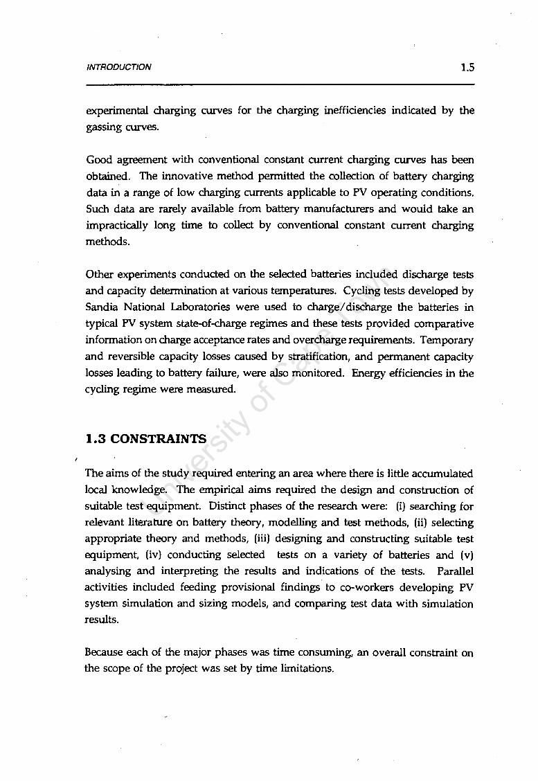
INTRODUCTION 1.5
experimental charging curves for the charging inefficiencies indicated by the
gassing curves.
Good agreement with conventional constant current charging curves has been
obtained. The innovative method permitted the collection of battery charging
data in a range of low charging currents applicable to PV operating conditions.
Such data are rarely available from battery manufacturers and would take an
impractically long time to collect by conventional constant current charging
methods.
Other experiments conducted on the selected batteries included discharge tests
and capacity determination at various temperatures. Cycling tests developed by
Sandia National Laboratories were used to charge/ discharge the batteries in
typical PV system state-of-charge regimes and these tests provided comparative
information on charge acceptance rates and overcharge requirements. Temporary
and reversible capacity losses caused by stratification, and permanent capacity
losses leading to battery failure, were also monitored. Energy efficiencies in the
cycling regime were measured.
1.3 CONSTRAINTS
The aims of the study required entering an area where there is little accumulated
local knowledge. The empirical aims required the design and construction of
suitable test equipment. Distinct phases of the research were: (i) searching for
relevant literature on battery theory, modelling and test methods, (ii) selecting
appropriate theory and methods, (iii) designing and constructing suitable test
equipment, (iv) conducting selected tests on a variety of batteries and (v)
analysing and interpreting the results and indications of the tests. Parallel
activities included feeding provisional findings to co-workers developing PV
system simulation and sizing models, and comparing test data with simulation
results.
Because each of the major phases was time consuming, an overall constraint on the scope of the project was set by time limitations.

INTRODUCTION 1.6
In particular, time constraints limited the battery tests to short-term
characterisation tests (at various battery temperatures). Short duration cycling
tests were conducted to assess electrical, chemical and physical equilibrium
stabilities under defined cycle conditions, but long duration life cycle tests were
not practicable. Budget constraints necessitated in-house design and construction
of a single test rig. This took time and the single rig restricted testing to one
battery at a time. Since relevant battery tests can take several days per test, it was
necessary to select a limited number of batteries for testing, representing major
types of battery available locally, and it was not possible to repeat tests on several
batteries of the same type to establish statistical variations in tested characteristics.
Tests were only repeated where ambiguous or unexpected results were observed.
These constraints limited the scope and statistical representativeness of the
empirical data obtained.
Although the batteries tested and the scope of the tests have been limited by time,
it has been valuable to obtain empirical data for key types of batteries which has
not previously been available and which will assist PV designers. Combining the
empirical findings with an attempt to understand observed behaviour in the light
of battery theory has contributed to a greater degree of understanding of
parameters which affect battery choice and cycle regulation in PV systems.
0

INTRODUCTION 1.7
1.4 REPORT OUTLINE
The outline of the report is as follows:
CHAPTER 2: An introduction to the components of stand-alone photovoltaic
systems with battery storage; a technical and economic comparison of two typical
system sizing approaches; the determination of typical battery charge operating
regimes based on the two system sizing approaches presented.
CHAPTER 3: A literature review of theory and research of lead-acid batteries; a
review of lead-acid battery models suitable for PV systems; a review of design
trends for specialist PV batteries; a review of voltage regulator operating modes
and charge and load shed regulator requirements.
CHAPTER 4: A literature review of PV battery testing; a· review of battery data
widely available and data quality; test equipment requirements and equipment
sizing.
CHAPTER 5: Experimental equipment design; electronic design of programmable
load and power supply; computer interface to power electronics; software design
and description; battery temperature control and measurement.
CHAPTER 6: Description of batteries selected for testing; detailed description of
the test procedures followed; explanation of the format in which test results are
presented.
CHAPTER 7: Test results of the five batteries selected; comparative discussion of
the results.
CHAPTER 8: Conclusions.
'

CHAPTER 2
PHOTOVOLTAIC. SYSTEMS WITH BATTERY
STORAGE
2.1 COMPONENTS OF A STAND-ALONE PV SYSTEM
A typical stand-alone photovoltaic system (SAPV) consists of photovoltaic (PV)
panels for conversion of solar radiation to DC electricity, batteries for DC energy
storage, battery regulation equipment, and high efficiency DC loads. An inverter
converts direct current power to alternating current if AC appliances are used.
CHARGE DISCHARGE DC LOADS PVARRAY >--- r-
REGULATOR REGULATOR
BATTERY
INVERTER >--- AC LOADS
Figure 2.1 Components of a stand-alone PV system with battery
storage: PV array, charge regulator, battery, discharge regulator, DC load, optional inverter and AC load.
The main components are examined individually to facilitate more detailed discussion in later chapters.
2.1

PV SYSTEMS: AN INTRODUCTION 2.2
2.1.1 Photovoltaic Panel Output
The PV cell is the basic building block of the PV panel. The PV cell is a semi
conductor device which converts solar energy directly into electrical energy by the
photovoltaic effect1• PV cells are connected in series and in parallel arrangements
to form integrated modules or panels which provide the desired electrical output
characteristics. Panels can be combined in series and parallel to form PV arrays,
which provide higher electrical power than the same single panels. For the PV
system designer, the PV panel is the basic building block of the PV array. Panels
come in a range of sizes, and the output of the panel is affected by solar
irradiance and the temperature of the cells. Figure 2.2 shows the output
characteristics of a small panel at various irradiance intensities and a cell junction
temperature of 25°C.
The power delivered by the panel is the product of the current and voltage on the
1-V curve. At open circuit voltage, V oc, the panel power falls to zero as no current
flows, and at short circuit the panel voltage falls to zero, but the current reaches
a maximum, Isc. Somewhere between these point the output power is maximised
at P maxi where the voltage and current are given by V mp and luip·
The effect of cell temperature on output is shown in Figure 2.3. It is common for increased temperatures to produce lower efficiencies in semiconductor devices.
In the case of crystalline PV modules, the primary effect of increasing cell
temperature is to depress output voltages. The relationship is nearly linear for the
operating temperature range of non-concentrating modules.
The power rating of a panel is specified for a defined cell junction temperature
and irradiance, usually lOOOwm-2 and 25°C. The rated power is the maximum
power, p maxi in the defined state, expressed in peak watts, WP.
There is abundant literature describing the photovoltaic effect, and how PV cells operate (for example SERl,1984). The discussion here is limited to PV output characteristics.

PV SYSTEMS: AN INTRODUCTION 2.3
I E = 100 mW/cm2
Tmp = 25°C
75mW/cm2
2-r------------------------SOmW/cm2
25 mW/cm2
10 mW/cm2
2 4 6 B 10 v
Figure 2.2 · 1-V characteristics of a crystalline silicon PV module as a
function of irradiance; cell temperature 25°C.
3------------------------------------------------.....,
2
Irr= 100mW/cm2
15 • c _ _.,_..,.._"'!'-_,...-\ 2s ·c -~~_,_.-"\ 1.0 ·c -~~-'\ so·c---6o•c--"""
OL-----------------.,.-----~----------r---_.__._..,..__.__.._~-
0 2 4 6 8 10 v
Figure 2.3 Effect of temperature on 1-V curve at lOOOwm-2•
r

PV SYSTEMS: AN INTRODUCTION 2.4
2.1.2 Battery
Batteries are used to store the PV energy for times when energy is not directly
available from the panels. Energy can be stored during the day for night use,
during sunny days to provide reserve for cloudy days, during peak solar seasons·
for poorer seasons, or even during the day for more intense use later that day.
The result of battery storage is that system sizes can be optimised since the PV
panel no longer needs to provide the peak energy demand. However, together
with the gains come losses. Battery energy storage necessitates some efficiency
losses, and only 75%-85% of energy stored is retrieved (for lead-acid batteries).
The size of the battery is described by the amount of electrical energy , in ampere
hours (Ah) or watt-hours (Wh), that can be delivered in a specified time. The
most commonly used basis is Ah at the 10 hour rate for automotive and electric
vehicle batteries. A battery rated as 90 Ah capacity at the 10 hour rate (C10) will
be able to deliver approximately 9A of current for 10 hours. At higher discharge
rates the battery will provide less than 90Ah, while at lower discharge rates than
9A the battery will deliver more than 90Ah. The state-of-charge (SOC) of a
battery is a percentage indicating the fullness of the battery. SOC is often
referenced to the C10 capacity. (Capacity, SOC, efficiency and other characteristics
are discussed in detail in following chapters.)
Most batteries used in PV systems are the lead-acid variety. There are several
other candidates, namely Nickel-Cadmium (Ni-Cd), Nickel-Iron (Ni-Fe), Iron-Air
(Fe-02), and Sodium-Sulphur (Na-S). Most of these batteries are simply too
expensive as the batteries are still in the development stage, or are not sufficiently
broadly used to bring elasticity to the prices. Some are plagued by low
efficiencies, requirements for complex thermal control or difficult manufacturing
processes (Rand,1984:721). The lead acid battery, although complex, is well . - " ~ ~: -~-·-·· - ,- -· --- .-· -
~nderstood, and ~lthough toxic can be recy~~-'!:~ Th_e_bafiei:y i~ relaJi~~)' __ 0~1?L~ and depending on the battery design anci operating C9J!Qi.ti9ns can la_stj!:_O!ll two r·. - . . . -- .. ·-· - ~ - ----·-~~
~o fifteen years in typical PV installations .. (Battery designs are discussed in detail
in Section 3.5). So far the projected cost reductions of alternatives have not been
realised.

PV SYSTEMS: AN INTRODUCTION
Zinc-chlorine Nickel-zinc Nickel-iron Sodium-sulphur
Figure 2.4 Projected energy cost for various batteries in USA.
(Source: Rand,1984).
2.5
The principal limitation of the lead-acid battery is the strict operafulg regime
required for long life, which gives rise to the need for battery regulation
equipment in the PV system. Lead-acid batteries may be damaged if they are
overcharged, if they are fully-discharged, or if they remain in a discharged state
for long periods. (Failure modes and other aspects of lead-acid batteries are
discussed in Section 3.11.)
2.1.3 Regulator
The two main regulator functions are prevention of battery overcharge and
prevention of over-discharge.
Overcharge protection, or charge regulation, is accomplished by controlling or
limiting the current flowing into the battery.
Over-discharge protection requires disconnection of the load before the battery
becomes discharged. The discorinection is called load-shedding, and is easily
accomplished when the load appliances are not connected directly to the battery,
but rather via the regulator.

PV SYSTEMS: AN INTRODUCTION 2.6
The merits of various charge/ discharge regulation methods, load-shedding
detection and other issues are discussed in detail· in Section 3.14.
2.1.4 Inverters
Inverters are used only in PV systems that require AC loads. If efficient DC loads
are available it is usually better to use them, as the efficiency losses associated
with inverters can be considerable if they are not operated at nearly full capacity.
The capacity of an inverter is measured in Volt-amperes (VA).
025 0.50 0.75 1.00 1.25 kW output
Figure 2.5 Efficiency vs power output for a lkVA non-sinusoidal
inverter with resistive loads. (Source: Bower,1988).
From the point of view of battery operation, typical inverter characteristics as a
load are high currents, direct connection to the battery and pulsing of the battery.
For example, a SOOVA inverter producing 350W output at 60% efficiency wil1
draw 48A from a 12V battery. Many inver~ers have their own independent load
s~ed detectors, and are not wired through the regulator. If DC and AC loads are
used together, they will not load-shed simultaneously. There may be some
unpredictable interaction between the two load-shed devices. Additionally, some
inverters "pulse" the battery during operation; they alternately charge and discharge current into the battery at twice the AC frequency (Williams,1989). This
could affect battery performance (Cataldo,1978).

PV SYSTEMS: AN INTRODUCTION 2.7
2.2 BATTERY OPERATING REGIMES IN PV SYSTEMS
It is useful at this stage to describe the range of operating conditions that batteries
experience in typical PV systems. These are illustrated by example, using two
systems that describe battery characteristics typical of PV installations.
1. A typical small system as would be supplied by a major panel
manufacturer. The system sizing has been obtained using the
manufacturer's design software. Such systems are usually sized for a
specific site by considering site-specific weather data and patterns.
2. A low cost modular system for household lighting. Such systems are
often sold in standard sizes and are not optimised for any particular
location. They are available off-the-shelf, for use in any South African
site.
For the purposes of comparison, the systems are scaled to provide the same
design load, taken as 200Wh/ day DC nighttime load in Nelspruit, Eastern
Transvaal, South Africa.
2.2.1 System Sizing
System 1 was sized using the ARCO Solar (1982) programme, "SASY-B". The load
was set at lkWh/day, with the system required to provide power for up to five
consecutive sunless days (5 days of autonomy). The system sizing results in a
requirement for a 325WP array and 540Ah deep cycle batteries at a nominal
system voltage of 12V. The sizing programme intimates that the batteries will be
fully charged at the end of each month. Scaling the system for a 200Wh/ day load
yields a panel power of 65WP and battery capacity 108Ah at 12V.
System 2, as a commercial package, is of a set size. The standard package that is
purchased comes complete with one 20W P panel, and two 15W high efficiency DC
lights. No charge regulator is provided, but protection against over-discharging
the battery is included. Daily load consumption is possibly 100Wh/ day
(determined by the time the lights are used, say 3 and a bit hours a day, times
30W). No battery is supplied or specified. Most users purchase the cheapest

PV SYSTEMS: AN INTRODUCTION 2.8
battery available, say a lOOAh "car battery"2• The system is relatively low cost,
in terms of capital outlay. Notionally scaling the system for a 200Wh/ day load
would result in a 40WP panel and 200Ah "car" battery.
2.2.2 System Simulation
The dynamic system parameters relevant to battery performance are shown for
both systems. These have been generated using PV simulation software
developed by Geerdts (1990). For the purposes of the present illustrations, generic
PV and battery models incorporated in this programme have been used. (The role
of this project in providing data for improved battery models is discussed in
Chapter 8). In simulating a typical years performance for each system, weather
data for Nelspruit was employed, with the PV array in each case tilted at an angle
of 25 degrees.
System 1
Figure 2.6 shows how the battery state-of charge (SOC) cycles between 98% and
85% throughout the year. The impact on cycle depth of seasonal variation in the
weather patterns is negligible. The daily overcharge (net current into the battery
that does not increase the state-of-charge) is however very seasonal, with the
regulator set at 14.2V. The maximum daily charging current into the battery is
not strongly affected by the seasons. It is interesting that the maximum current
is 4A/100Ah of installed battery capacity. The maximum array output is
4.3A/100Ah at the maximum power point under standard conditions. The
charging current into the battery is low; nearly 99% of the time that the battery
is charging the current is lower than 3A/100Ah, or 3% of C10 capacity. (In non
PV applications, typical starting charging rates for deep-cycle batteries vary from 15% of C10 to 7% of C10, depending on the initial SOC, and finish at 3% of C10
when the battery is fully charged (Vinal,1955:264).
2 A common choice in these circumstances is the Willard 77 4 •Leisure Pack", readily identified by its handles. Alternatively any battery to hand may be used, typically a car battery.

PV SYSTEMS: AN INTRODUCTION 2.9
System 2
By comparison, Figure 2.7 shows that System 2 would have a maximum array
output of only 1.25A/100Ah or 1.25% of C10• The charging current is less than
.7% of C10 for 98% of the time that the battery is charging, which is extremely low.
The battery cycles through about 5% of C10 capacity on a daily basis.
Superimposed on this is an SOC variation throughout the year that is strongly
affected by seasonal weather patterns, ranging between 100% SOC (summer) to
80% (winter). For one third of the year the simulation indicates that the battery
would never be fully charged, and would cycle in a partial state-of-charge. The
daily overcharge is similarly affected by seasonal variation.
2.2.3 Costing
Renewable energy systems -are usually costed over twenty years, the projected
useful life. For PV systems there are two major cost components, the initial
capital expenditure for the array, regulator, battery and perhaps some appliances; ·
and the operating costs for battery maintenance, and battery and regulator
replacement. Money to be spent in the future is discounted to the present value
using methods described in the Appendix Bl. Cost comparisons can be made
using the present value of money, and on this basis the life-cycle costs (LCC) of
the project can be projected. The unit energy cost is the levelised life-cycle cost
(LLCC) divided by the total amount of energy generated over the life of the
project.
The life cycle costs of the two systems show that the systems are fundamentally
different. System 1 has high capital outlay of 67% of the total LCC, with low
operating proportion mainly due to the forecast 10 year battery life expected for
the high quality batteries selected, operating in a narrow cycling regime. The unit
energy cost is 337c/kWh. System 2, while demanding only 40% of the forecast
LCC as capital outlay, is intensive in operating costs particularly due to the short
(three year) life expectancy .of the low cost battery. The unit energy cost is
416c/kWh. These are shown graphically in Figures 2.8 and 2.9. Costing and
assumptions are shown in Appendix B2.

PV SYSTEMS: AN INTRODUCTION 2.10
The battery lifetimes used above are based on cycle life expectancy for cycling in
fixed regimes. For tubular batteries 4000 cycles at 20% DOD is standard, and for
automotive types 900 cycles at 5% would be typical. In practice, forecast battery
life is strongly influenced by the operating conditions as well as DOD. The effects
on LLCC and maintenance costs can be severe. To illustrate the impact of varying
assumptions for battery lifetime, adjusted LLCC costs are shown in Figures 2.8
and 2.9.
In System 1, it is unlikely that battery life will be less that) five years if conditions
are moderate and the battery reaches full charge at the top of the cycle. The
energy cost would increase by 21%to410c/kWh for five year life. If battery life
were optimistically 15 years the energy cost would drop by 10% to 300c/kWh.
The battery in System 2 could conceivably last three years, perhaps two years
(550c/kWh), or even only one year (916c/kWh) if the user selected the "wrong"
battery incapable of dealing with prolonged partial SOC operation. Energy cost
increases very steeply if the battery life is under two years, and doubles if life is
only one year. System 2 is more sensitive to errors in battery life estimate than
System 1.

PV SYSTEMS: AN INTRODUCTION
Battery SOC
0 365 day
Ah Overcharge and Charge Current ------------------T10
0 day
Charging Current Cumulative Distribution
% of Cl 0 battery capacity
1%
365
0 10 20 30 40 50 60 70 80 90 100 %oflmp
Figure 2.6 Operating conditions for System 1, supplier system.
2.11

PV SYSTEMS: AN INTRODUCTION 2.12
Battery SOC
0 365 day
Ah Overcharge and Charge Current i:;,--~~~~~~~~~~~~~~"""T1o
0 day
Charging Current Cumulative Distribution
% of C1 0 battery capacity
0.5% 1%
0 10 20 30 40 50 60 70 BO 90 100 %oftmp
Figure 2.7 Operating conditions for System 2, low cost modular
system.

PV SYSTEMS: AN INTRODUCTION 2.13
Typical Supplier PV System Life-cycle costs
Panel 63%
Balance of Systems 3%
Battery 34%
Battery replacement 61%
Capital Costs 67o/o
Unit Energy cost=337c/kWh CR1990)
Supplier System Energy Cost Sensitivity to Battery Life
3 5 10 15 battery life (years)
Operating Costs 33°/o
Base Case Assumptions
Interest rate 5%
System life 20 years
Battery life 10 years
O&M costs 10% battery costs
Array size 325WP
Battery size 540Ah, 12V
Daily load 1000Wh/day
Array cost (R20/WP) R6500
Battery cost R3488
All prices R 1990
Figure 2.8 Life cycle costs for System 1, supplier system.

PVSYSTEMS:ANINTRODUCTION 2.14
Typical Low-cost PV System Life-cycle costs
Balance of Systems
Panel 60%
Capital Costs 40o/o
Unit Energy cost=416c/kWh CR 1990)
4%
Battery 36%
Low-cost PV System Energy Cost Sensitivity to Battery Life
2 3 4 battery life (years)
O&M 14%
Operating Costs 60°/o
Base Case Assumptions
Interest rate 5%
System life 20 years
Battery life 3 years
O&M costs 10% battery costs
Array size 40WP
Battery size 200Ah, 12V
Daily load 200Wh/day
Array cost (R20/WP) RSOO
Battery cost R500
All prices R 1990
Figure 2.9 Life cycle costs for System 2, low cost modular system.

PV SYSTEMS: AN INTRODUCTION 2.15
2.3 CONCLUSIONS
This chapter has introduced the basics components in a stand-alone PV system;
PV panel, battery, regulator, and the inverter.
Two typical systems were analysed to illustrate some important points about PV
systems in general, and about systems of supposedly similar capacities installed
at any one site:
Different panel/battery configurations are available which can provide
energy for the application.
Battery SOC profiles can be substantially different, depending on the
panel/battery configuration of the installation.
Some PV installations may require the battery to operate in a partial state-of
charge for several months before it can be completely recharged. This is
usually the result of matching large batteries with small arrays.
Charging currents in PV systems are relatively low, varying from 1 % C10 to
5% C10, but not normally higher. They can be regularly lower than this.
Minimising the installed cost of a system does not necessarily lead to
minimised operating costs. Conversely, minimising operating costs probably
requires higher installed costs.
Operating costs are affected by the type of battery selected, and its lifetime.
The battery should be suited to the prevalent operating regimes, such as
SOC profile, Ah overcharge and charging currents.
Over-estimating the cycle life of a battery during system sizing strongly
affects the effective LLCC and energy costs when the battery life is not
realised. This is particularly pertinent to systems that tend to have high
operating costs.

PV SYSTEMS: AN INTRODUCTION 2.16
This research focuses on the battery in the PV system, in particular the
performance under the typical operating regimes of PV systems. Emphasis is on
gathering empirical performance data relevant to PV operation. This data is to
be used
to provide battery data useful for PV system designers
for complementing and for quality checking of the manufacturer's data
where it is provided
to study behaviour of specific batteries under various states of charge and operating regimes
to provide data suitable for computer simulation of batteries in PV systems.

Chapter 3
THE LEAD-ACID BATTERY
This chapter describes the physical, chemical and electrical aspects of the lead-acid
battery.
Sections 3.1 to 3.4 are concerned with the history, basic chemical .operation of the
battery, cell design and construction and electrical characteristics.
Section 3.5 describes the requirements and designs of conventional battery types.
A more detailed electro-chemical discussion in Section 3.6 extracts from the
literature the most important micro-processes and side reactions, including
mechanisms of failure of the active mass and grid corrosion processes.
Polarisation and overpotential in Section 3.7 describe the mechanisms and effects
of gas evolution during battery charging. Section 3.8 describes the macro
processes, particularly stratification and gassing related issues. Section 3.9 presents
some discussion on methods of reducing water loss in lead-acid batteries.
Though these detailed sections are primarily of interest to battery modellers, they
provide invaluable insight into the operation and life limiting processes.
Section 3.10 describes electrical characterisation battery models suitable for PV
applications.
Failure modes of lead-acid batteries are presented in Section 3.11.
Battery life models are discussed in Section 3.12.
Section 3.13 illustrates battery design options available, and shows how these are
configured together to meet the requirements of modern photovoltaic batteries.
Section 3.14 describes voltage regulators in PV systems as they apply to the
battery and battery operating environment.
3.1

LEAD-ACID BATTERY OPERA T/ON 3.2
3.1 HISTORY
Plante, in 1859, passed current through two lead plates separated by rubber strips,
and submersed in dilute H2S04• After a short time, a 2V cell was formed. The
interesting characteristic of this cell was its reversibility. The cell could
accumulate charge by conversion of electrical energy into chemical energy, and
could transform the chemical energy to electrical in the reverse process.
The early lead-acid battery required several cycles to realise full capacity. This
formation process required the conversion of the lead sheets into a porous active
material, Pb02 on the positive and spongy lead on the negative electrodes.
The specific energy of the Plante cell was low, but it was shown that there was
a linear relationship between electrode surface area and capacity. In 1880 Faure
developed the method of ·covering the lead plates with powdered lead oxides
made up as pastes a mixture of lead oxides, H2S04 and water. The spongy nature
of these pastes results in the electrolyte diffusing through the pores and coming
into contact with a greater area of the active material.
The active material has no rigid structure, and the positive material is a relatively
poor conductor. Swan developed the method of mounting the active mass on
lead grids to maintain shape and to conduct current evenly through the active
material. Sellon introduced antimony as an alloy into the grid to increase
mechanical strength. The paste was then pressed onto the grid lattice, forming
plates. The flat plate grid is still used for both positive and negative plates. The
early cells had a cycle life of 300 charge/ discharge cycles before failure, usually
by shedding of the positive material.
The development of the Ni-Fe tubular cell by Edison had spin-offs for the lead
acid battery. The tubular plate design was applied to the positive plates of the
lead-acid cell. The tubular plate consists of a series of spines surrounded by glass
fabric tubing, forming an annulus which contains the active material. The spines
enhance current flow through the active material. Cycle life was improved to
1500 cycles.

LEAD-ACID BATTERY OPERA T/ON 3.3
From 1880, development in cell design was enhanced by a new range of
applications. Initially lead-acid batteries were used in power stations, followed
by traction and electric vehicle (EV) applications, submarines, railway lighting and
electronic equipment.
The breakthrough came with the boom in the automobile industry. The batteries
were used for vehicle lights, then later for starting the engine as well. The SLI
(starting, lighting, ignition) battery had arrived.
Fundamental research into the processes occurring in the lead-acid battery began
when Gladstone and Tribe (1882) detected lead sulphate, PbS04, at both
electrodes of a discharged cell. The "double sulphate theory" was evolved.
The lead-acid battery is described as a dynamic system, in which processes are
always in progress regardless of whether the battery is idle or at work. Pavlov
(1984) writes
" ... to understand these processes, it is necessary to differentiate between
them and to have knowledge of conditions under which a given process is
initiated, becomes dominant, or as a result of their own actions become
suppressed so a new process is promoted. It is considered that elucidation
of the complex array of chemical, physical, electrochemical, semiconductive
and crystallisation phenomena that take place in the electrolytic solution, the
electrode porous mass and the solid active material itself will assist attempts
to increase power, energy, reliability and life of lead-acid batteries."
Today, the lead-acid battery is relatively well understood. There is considerable
literature available on its origin, operation, and design. It is beyond the scope of
this thesis to regurgitate this, and only relevant phenomena are discussed.
Background information is available in the battery encyclopedias, Vinal (1955),
Smith (1964), Bode (1977), Mantell (1970). Detailed electrochemistry data is
widely published. Pavlov (1984) is particularly recommended.

LEAD-ACID BATTERY OPERATION 3.4
3.2 BASICS: HOW A LEAD-ACID BAITERY WORKS
Lead-acid battery electrochemical operation is the same regardless of the method
of construction.
A cell consists of positive and negative electrodes and an electrolyte. When the
cell is fully charged, the positive electrode consists of lead dioxide (Pb02), the
negative electrode of lead (Pb), and the electrolyte of dilute sulphuric acid
(H2S04). I
During discharge of the cell, lead dioxide is reduced to lead sulphate (PbS04) at
the positive electrode, while metallic lead is oxidised to lead sulphate at the
negative electrode: the "double sulphate theory". The sulphate is formed from
dissociated sulphuric acid. The acid becomes more dilute the longer the process
continues.
During charging the process is reversed, and the lead sulphate on the positive and
negative electrodes is converted to lead dioxide and spongy lead respectively.
The sulphate that is released combines with water in the electrolyte to reform
sulphuric acid. When the cell can no longer accept charge, the voltage rises, and
the excess charge is consumed in H2 and 0 2 gas evolution.
The half cell reactions and the overall cell reaction can be summarised as:
The rated voltage under open circuit conditions is
..lEe = 2.040V.

LEAD-ACID BATTERY OPERATION 3.5
3.3 CELL DESIGN AND CONSTRUCTION
3.3.1 The Ideal Cell
The ideal cell specific energy is expressed in watt-hours per kilogram of reactants
< (Wh/kg). The theoretical weight contributions of the reactants are:
207.2g Pb+ 239.2g Pb02 + 196g H2S04 ·= 642.4 g
According to Faraday's law 642.4g of reactants provide 2 moles of electrons, equal to:
2 * 96500 coulombs= 193000 coulombs = 53.61Ah
This is equivalent to:
3.865 gram/ Ah of negative active material (Pb)
4.462 gram/ Ah of positive active material (Pb02)
3.666 gram/ Ah of concentrated sulphuric acid (H2S04)
(equivalent to 8.46cc of 1.260 SG H2S04/ Ah)
for a total reacted active mass of
11.99 g/ Ah, yielding 83.4 Ah/kg or 170.2 Wh/kg for the cell
The theoretical specific energy is not realised in practice. Practically, the specific
energy of the active material varies from 32Wh/kg (64g/ Ah) to 10Wh/kg,
depending on the battery design (Pavlov,1984:203). To transform the basic lead
acid cell into a practical power source several modifications must be met.

LEAD-ACID BA ITERY OPERATION
3.3.2 Cell Components
6
7---48~~-:
8 ---ffi::=:'-4-ll!
11---l!"-l51q}
13--~llllll
10
12
17
ii!ll---19
iE---20
1. Vent plug 2. Lead-coated brass bott 3.Cover 4. Terminal post 5. PosVCover seal 6. large headroom.
Reduces need for topping up. Ideal for solar applications.
3.6
7. Terminal post sleeve prevenls loose male rial from post reaching plale.
8. Positive group bar submerged. Avoids flaking. 9. Container
10. Separator guard 11. Perforated separalor 12. Posttive plate (tubular) 13. Separator 14. Negative grid 15. Positive spines.
Spines are not in direct contact with electrolyteminimises corrosion
16. PG Tube TuQ<i holding active malerial reduces sedimenlalion
~~: ~~:~~~~~=;~~led. No shorts. 19.Rib 20. Bottom bar
Figure 3.1 Construction of a modern standby cell. (Source: Raylite standby
battery literature)
The positive active masses are porous, and part of the mass must act as a
conductive skeleton to carry the products, reactants and current to each point of
the active mass. The remainder is used for electrochemical conversion. The active
section of the active mass varies from 35% to 55%. The acid resistant grid
supporting the active masses adds further to the weight.
The positive and negative plates are separated by micro-porous separators.
The acid concentration used is usually 35% by weight (1.260 SG). The
conductivity is high, and the freezing point is low. The grids are resilient to
corrosive attack by the acid. On completion of discharge, excess electrolyte must
remain for electrical conductivity during the beginning of charge and end of
discharge.

LEAD-ACID BATTERY OPERATION 3.7
The active block is formed by the positive and negative plates and the separator,
together with the electrolyte in the pores. An electrolyte reservoir located above
the active block enhances H2S04 availability, as the H2S04 in the active block is
restricted. During discharge the acid moves from the reservoir to the active block,
and the weight of the active block is increased by the formation of PbS04• During
charge, H2S04 is generated and flows back to the reservoir.
The positive and negative plates are connected into cells, with external terminal
posts.
Water decomposition occurs at the end of charging. The evolved H2 and 0 2 is
vented through vent caps. The water that is lost through gassing is replaced by
removing the vent caps and adding water as required. The cells are mounted in
a container with a cover, and adjacent cells are joined with through-the-wall
connectors. The active block rests on an element rest. Active mass which is shed
is contained in the sediment space under the active block.
3.3.3 Design of the Active Block
The amount of active material theoretically required for reaction is determined by
Faraday's law. Practical requirements can be achieved by applying utilisation
coefficients taking into account limitations in the processes.
a) Electrolyte
In theory 3.666g of H2SO 4 is required for lAh of current. The real requirement
depends on the ampere-capacity, the range of H2S04 concentration during charge
and discharge, and the degree to which electrolyte in the upper and lower
reservoirs participates in the reactions.
The range of SG's normally used in the various applications is shown in Figure 3.2. The smaller the range the more electrolyte is required for a particular application. The effect of electrolyte concentration on resistivity (Q.cm-1) is shown
in Figure 3.3. SLI batteries are designed for high discharge current, and therefore
require low resistivity during normal operating conditions. In traction batteries,
there is a trade-off between volume (specific energy of the battery) and low

LEAD-ACID BATTERY OPERA noN 3.8
resistivity. Standby batteries are not specific energy limited, and can operate at
relatively low SG's.
500
400
2300
o End of discharge __ £ 200
traction battery
SU 100 2Dh
rate
0
Traction battery operation
toso uoo i.1so t 200 1 ;;so noo 1.350 SG at 25° c
Figure 3.2 Concentration of H2S04 at 25°C over the range used in different batteries. (Source: Pavlov,1984;fig 171).
7 0
6
10 'E 10
~ § 20 ~ 1.
30 ------'f: s 1. 30 a:
Figure 3.3 Effect of H2S04 concentration and temperature on resistivity and
viscosity. Resistivity is represented by the solid line, viscosity by the broken
line. Temperature is in degrees celsius. (Source: Vinal,1955;Tables 15, 19)
Most of the electrolyte is located between the active block and the upper and
lower reservoirs. The transfer of H2S04 from the lower reservoir to the active
block is slow, and only about 10-20% utilisation of this electrolyte is achieved

LEAD-ACID BATTERY OPERATION 3.9
(Pavlov,1984:355). The slow transfer process is largely due to the viscosity of the
electrolyte, which increases approximately linearly with concentration.
Within the active block, the electrolyte is located in the pores of the plates and the
separators, and in the spaces between the positive and negative plates. The
reactions below
Negative: Pb+ SO/.,. PbS04 + 2e·
show that the mass of electrolyte participating during discharge at the positive
plate is greater than at the negative. The water evolved at the positive plate
dilutes the neighbouring H2S04• The volume of the positive electrolyte space
must be greater than for the negative. This is another point indicating the
limiting role of the positive plate.
b) Positive and negative active material
3.865g of Pb and 4.462g of Pb02 are required for lAh of electricity. The actual
amount required will depend on the utilisation coefficient, which in turn depends
on the active mass porosity and micro-structure, plate thickness, and
charge/discharge conditions. Pavlov (1984:357) has determined that the average
active mass utilisation of the negative plate is 0.32 and for the positive is 0.34 for
traction cells in service. These cells have cycle-life of 1500 cycles. Increasing the
utilisation coefficients to 0.44 will decrease cycle-life to 300-500 cycles.
The number of negative plates is usually greater than the positive by one, and the
utilisation coefficient is reduced by the outer surfaces of the outer negative plates
not participating in the reaction. The outer negative plates have utilisation
coefficients of 0.28. The active mass/plate ratio and grid/plate ratio are useful for
determining the mechanical stresses and mass changes likely during cycling.
These are tabulated below for the positive and negative plates of traction cells.

LEAD-ACID BATTERY OPERATION 3.10
Table 3.1 Positive and negative active material characteristics of traction
cells. (Source: Pavlov,1984; Tables 23 and 24)
Weight (grams) Active mass Active Grid/
utilisation mass/ plate plate plate grid active coefficient ratio ratio
mass
Negative 1050 390 660 0.32 0.63 0.37
Positive 1400 600 800 0.34 0.57 0.43
c) Plate design
Two plate designs predominate. Flat pasted plate designs are conventionally used
for the negative electrodes, while the positive plate may be either the flat plate or tubular plate design.
Flat pasted plate design
The grid of the flat plate design consists of a planar conductive network of lead
alloy for supporting the active mass, and for facilitating good electrical conduction
throughout the plate. The active mass is "pasted" onto both sides of the grid.
The effect of positive plate thickness on performance is mainly related to the
access of H2S04 into the active mass. Figure 3.4 shows that at low discharge
current rates the flat plate capacity is more dependant on thickness than at high
currents. The advantages of thin plates with large area can be demonstrated by
comparing two cells with the same volume of active mass, one with two 2.4mm
thick plates and the other with one 4.8mm thick plate. Discharged over 30 hours,
the 2.4mm plates deliver 2*70Ah=140Ah, while the 4.8mm plate delivers 120Ah.
The effect of plate area on capacity is also a function of discharge rate.

LEAD-ACID BATTERY OPERATION
150 ...----.----,.-------,-.,
140
130
120
110
100
. 90
~ 80
1:: 70 "(j
g_ 60 c u 50
LO
30
20
10
o~~~~~~~ 0 0.8 1.6 2.4 3.2 LO L.B 5.6 6.L Thickness of the plate (mm)
Figure 3.4 Capacity vs plate thickness at different discharge rates.
(Source: Vinal, 1955:fig 63)
3.11
Vinal has shown that when both positive and negative plates are increased by the
same thickness, the negative plate shows a greater rise in capacity.·
Tubular plate design.
In tubular cells spines replace the conventional grid. The spines are located at the
centre of the tubes, made from braided acid-resistant glass wool. The active
material is contained between the wall of each tube and the central spine.
The principle of tubular design is that shedding of the active mass does not occur
as the active mass is held by the tube. The capacity of the tubular plate depends
on the diameter of the tube. At low discharge rates a 9mm tube yields the
optimum capacity (Figure 3.5), though tube diameters are usually 8-8.4mm with
an active mass thickness of 2-2.22mm.
The tube dimensions affect the corrosion process, as the spine is enclosed by a
layer of active material which protects it from corrosion. Figure 3.6 shows how
cycle life increases with tube diameter under deep discharge conditions. The
approximate cycle life relationship between tubular and flat plate cells of the same specific energy is shown in Figure 3.7.

LEAD-ACID BATTERY OPERATION 3.12
A disadvantage of the tubular plate is the cost, due of the labour intensive
technology, and the low utilisation coefficients usually achieved. At high current
drains the increased current density at the active mass/ spine interface may cause
local heating and cracking of the corrosion layer.
:?: ·;:; 0
£00
300
g. 200 u
100
Dischnrg.•, Current rate lhr) rate IA)
20 17,4·
10 31,£
s 56
3 82
2 112
185
0,5 295
0,25 472
7 B 9 10 Tube diameter Imm)
Figure 3.5 Capacity vs tube diameter at different discharge rates.
(Source: Pavlov,1984:fig.174)
.;:- 70 ·c:; g_ 60 c u 50 Depth of discharge : 65 %
Overcharge: 117 % Test temperature: L5° C
Capacity measured at 0.2°C discharge
Cycle life
7.5~ 65~ 10 ~ Tube diameter in mm
Figure 3.6 Capacity vs cycle life of tubular batteries.
(Source: Pavlov,1984:fig.176)

LEAD-ACID BATTERY OPERATION 3.13
1500
tube type
1000
Ill QI
~ u
500
20 l.[J 60 Wh/kg
Figure 3.7 Relationship between cycle life and specific energy of tubular
and pasted plate designs. (Source: Pavlov,1984:fig.177)
d) Active block dimensions
In large cells the transport of H2S04 between the active block and the reservoirs
has a marked effect on cell capacity at high discharge rates. During discharge an
acid concentration gradient is established over the height of the cell. The SG
decreases from the bottom to the top of. the block, and the effect is enhanced
during deep discharges. This effect is known as acid stratification. (See
Section 3.8.1.)
The path of the sulphuric acid flows tending to equalise the concentration
gradients depend strongly on the design of the active block. Pavlov (1984:362)
suggests that there is considerable scope for investigating active block designs
with a view to improving active mass utilisation coefficients.

LEAD-ACID BATTERY OPERATION 3.14
3.4 ELECTRICAL CHARACTERISTICS
3.4.1 Open Circuit Voltage and SG
The open circuit voltage of a cell depends on the electrolyte concentration and its
temperature, as described by the Nernst equation.
where
M 0 = 2.040V
R = gas constant (8.31441 J K-1 mol-1)
n = number of reacting electrons (2)
F = Faraday constant (9.648 x lc4 C mol-1)
T = temperature (K)
The measured temperature effect has been shown to be 0.00136V /°C, compared
with the theoretically calculated value of 0.00135V /°C (Vinal,1955:194).
Open circuit voltage is often used as an approximation of the state of charge
(SOC) of the cell. The relationship is given in Figure 3.8.
2.150~--------------,
2.100
2.050
> -: 2.000
• c
w .,
1.950
t900
.., Vosburg. and Graig
o Vinal and Graig
a Homed and Hamer
• Duisman and Gicnque I cakulatod data)
t 55D L---t.,+055,.---..,..,1.1.,.,,.10---,1+.,.155,.---,-;!1.20=0---..,..,1.2"""'1.0---;1.; 60
~SO, concentration ls.g.l
Figure 3.8 Experimentally determined and calculated dependence of cell
voltage on H2S04 concentration. (Source: Vinal,1955:Table 39)

LEAD-ACID BATTERY OPERATION 3.15
Limitations of voltage and SG as SOC indicators.
Voltage is approximately a linear function of concentration of the electrolyte in
contact with the active material.
SOC is a linear function of the average electrolyte concentration in the cell, by
nature of the stoichiometry of the reactions.
The measured SG is a measure of the bulk electrolyte concentration. Only after
the cell has stood in open circuit for several hours will the bulk fluid and average
fluid concentrations be equal. Oi:ily then will SG be an accurate indicator of SOC,
and only then will voltage be a reasonably accurate indicator of SG. (Fluid
concentration gradients are discussed in more detail in Sections 3.3.3(d) and 3.6.2.)
3.4.2 Capacity
The capacity of a cell during discharge (Cd) is determined by the amount of
electricity that can be delivered by the cell at constant current (Id) till the cut-off
voltage is reached. The cut-off voltage represents a certain active mass utilisation
coefficient.
where td is the time to reach the cut-off voltage (see Section 3.3.3(d)). Figure 3.9
shows the relationship between capacity and discharge current. Standards have
been introduced to compare different batteries. Most standards require the
capacity to be determined by discharge with a current at which the battery
reaches the cut-off voltage at 200C after 20 hours. The capacity is referred to as
C20, and is known as the rated capacity. ~The current is also referred to as C2°' or
as the 20 hour rate. Manufacturers normally recommend restrictions on the depth
of discharge, mainly to preserve the electrical contact between the active mass and
the grid.
Different types of batteries are rated at different discharge rates, but the 10 or 20
hour rates are most common.

LEAD-ACID BATTERY OPERATION
100
90
~ 80
?: 70 . u
! fiJ I 50
40.__.....___.____,_~..__-L---'---'-~"---'-~ 0 1 2 3 4 5 6 7 8 9 10
Duration of discharge (hours)
Figure 3.9 Relationship between capacity and discharge current.
Capacity is affected by the following factors:
3.16
i) Temperature: Capacity decreases with decreasing temperature. One percent
per degree Celsius is a well quoted factor (Vinal,1955:220). Temperature
enhances the electrolyte mobility.
ii) Aging: After an initial increase of 10% over the first few cycles, capacity
decreases with aging of the battery, and the battery is usually assumed
useless when the capacity has fallen to 80% of the rated capacity.
iii) Rate of discharge: Increasing the rate of discharge decreases . the
instantaneous capacity. (See Section 3.4.3(a))
iv) Previous discharge: The capacity is affected by the immediately preceding
discharges. The hysteresis effect shows that capacity is decreased if
preceded by a higher current, and is increased if preceded by a lower
current (Vinal,1955:228). Capacity is increased by intermittent discharge, but
the increase is less than 10% except for discharge rates shorter than about
5 hours.
v) Electrolyte concentration: Capacity increases with an increase in electrolyte
concentration (Vinal,1955:222). Increased concentration increases the
potential of the cell, decreases the electrolyte resistance, but increases the
viscosity (decreases mobility). Electrolyte diffusion is also concentration
related.

LEAD-ACID BATTERY OPERATION 3.17
3.4.3 Voltage During Operation
Because the electrochemical process in the battery is not fully reversible, the
voltage during discharge must be less than the open circuit voltage, and the
voltage during charge greater than the open circuit voltage. The voltage of the
cell depends on the magnitude and direction of the current, and the cell
temperature (and SOC of course).
The discharge voltage, Vd, of the cell is given by
and the charge voltage, V chi by
where r ch and rd are the (apparent and non-constant) internal resistances during
charge and discharge, and !ch and Id are the corresponding currents. Vr is the rest voltage.
a) Discharge curves
Figure 3.10 shows the discharge curves for a 12V 90Ah SLI battery for different
discharge currents at 20°C. After a given time voltage begins to decrease rapidly.
This is caused by an increase in internal resistance due to: dilution of the electrolyte (and drop in conductivity) and interference by physical processes in
the ion flow (observed as an increase in concentration and resistance overpotentials, see Section 3.7.1).
Since deep discharges have an adverse effect on battery performance, a limit is set
for the end-of-dischar~ voltage, and is termed the cut-off voltage. This is
typically 1.75V per cell Cifscharges longer than 20 hours. The mean discharge
voltage (Vd,meanl is shown in the Figure 3.10. This is necessary for calculating the energy and power characteristics of the battery.

LEAD-ACID BATTERY OPERATION 3.18
The discharge current is often represented as a function of the capacity, eg. the
discharge current resulting in the cut-off voltage after 20 hours is the "20 hour
rate" (CioJ. A lower current might be referred to as O.OSC20• Charging current is
referred to the same basis, eg. Cio·
12
11
10
v 12
11
10
9
8
SA
16 18 20 Time ( h)
1 2 4 6 8 10 12 14 16 18 20 22 24 26 28 30 Time (min)
Figure 3.10 Standard discharge curves for a 12V 90Ah SLI battery.
Temperature = 20°C. (Source: Pavlov,1984:fig.60)
b) Self-discharge
The self-discharge of the battery increases with temperature, age of the battery,
and the amount of antimony in the grid. Self-discharge consumes water. The
rate of self-discharge is usually measured as a percentage loss in capacity per
month, or drop in SG per month. The SG is measured after the electrolyte has been restored (topped up).

LEAD-ACID BATTERY OPERATION
100 ~--------------,
27°C \\ . 90 \\
'\\ >. 80
·;:; 0 a. 0 u 70 ,, QI
.!:: 0
f!i. 60
Calcium type
\"\ .
\ \ _Law \ Vantimony
\. High ~ \. antimony/\
50L--1----J'---1--l.--'--'---'---'---'-:---:!. O 2 ~ 6 8 10 12 14 16 · 1B 20
Shelf stand (months)
Figure 3.11 SLI battery retained capacity during open circuit storage.
(Source: Pavlov,1984:fig 66).
3.19
The self-discharge rate of lead-calcium grid cells is considerably lower than for the
other grid alloy types. The higher the antimony content of the grid alloy the
greater the self-discharge rate.
c) Charging curves
During cell charging the voltage is greater than the open circuit voltage of the cell.
The charging curve can be divided into three main regions, which are particularly
clear during constant current charging.
Efficient charge stage - The main reaction is the conversion of PbS04 to
Pb02• Charging is nearly 100% efficient. This stage lasts till SOC reaches
about 70%, when the voltage reaches 2.3V per cell.
Mixed stage - Water decomposition reactions begin to occur along with the
charge accumulation reaction. The voltage rises sharply, and the rate of cell
heating increases. Charge acceptance is reduced as current is increasingly
consumed by gassing.
Gas evolution stage - charge acceptance is complete, water decomposition
and gassing are the predominant reactions. The cell voltage tapers, and the
total charging current is used for gas evolution. Cell heating is increased further (Calder,1985).

LEAD-ACID BATTERY OPERATION 3.20
lime
Figure 3.12 Three charging regimes during constant current charging,
showing voltage and temperature vs time.
Charging at constant currents may not be the most effective way to charge the
battery. High or low rates of charge at the wrong time can cause damage to the
battery. The basic principle to be followed is, charge at maximum admissible
current during the efficient charge stage, and optimum current during the mixed
stage.
The main parameters describing the charge regimes are:
initial and final voltages
initial gas evolution voltage
charging current during the efficient stage
current at the beginning of the mixed stage
finishing charge current
SOC during efficient stage
upper temperature limit.
Both temperature arid aging decrease the voltage at which the battery begins to
gas, and therefore the finishing voltage should be decreased to compensate for
this effect. Increased temperature improves charge acceptance during the efficient
stage, and the current can be increased to take advantage of this. Excessive
temperatures may result in earlier onset of the mixed stage. Cooler temperatures
require both higher finishing voltage and slower charging during the efficient
stage. Aging of the battery is likely to cause increased internal resistance during the efficient stage.

. LEAD-ACID BATTERY OPERA T/ON 3.21
d) Ampere-hour efficiency
During the mixed charging stage, some of the charging current is consumed by
water electrolysis. Clearly battery charging is therefore not one hundred percent
efficient. The Ah efficiency is defined as:
Ahri= effective Ah input I total Ah input
Amper~hour efficiencies are typically around 90% or greater for deep cycling.
Recharging the battery from shallow DOD will result in lower efficiencies.
3.4.4 Charging Methods
Charging methods have generally been developed with the specific aims of:
minimising charging times, particularly for traction batteries.
minimising gassing for standby and SLI cells
Constant current charging - The current must be low enough not to cause
excessive heating during the mixed and gassing stages. As a result, the charging
time is long. A variation, the multi-step current charge, aims to reduce the
charging time and increase efficiency. In a method proposed by Smith (1964), the
initial current during the efficient charging stage is about 20-40% of the rated Ah
capacity of the battery, and is reduced by half each time the voltage reaches
2.4V /cell. There are many variations of the multi-step method.
Constant voltage - The voltage limits the current in the final stages of charge, but
the initial current may be large, unless the initial DOD is low as for an SLI
battery. For deep discharge applications the initial current may exceed the
recommended charging current, and the cost of equipment to satisfy the initial
current consumption will be prohibitive. This method is most suitable for float
charging of SLI and standby cells.
Controlled current-voltage - Charging is carried out under constant current
conditions during the efficient stage, followed by constant voltage charging (2.4V
per cell) for the remaining duration of the charge. The current decreases
exponentially during this stage as illustrated ip Figure 3.13. Charging is complete

LEAD-ACID BATTERY OPERATION 3.22
when the current has fallen to lA/lOOAh. The actual finishing voltage will
depend the initial DOD and temperature. At higher temperatures the current will
be higher at the same finishing voltage. The controlled current enables use of
smaller and less costly chargers.
14.--------------~12
14.W-------.r------.....
1
13
g, 13.
~ 13. > 13
12 12 .
\ voltage 10
' s I \ \:ummt 6 i
CD
'~:E .......... -..--.--....---.----.--.-....... -..---+o
50 100 150 200 250 300 350 400 450 500 Time (minutes)
Figure 3.13 Charge under controlled current-voltage conditions for a lOOAh
12V battery. (Source: Experimental data)
PV charging regimes - In terrestrial PV systems, constant current charging over
any length of time is virtually impossible due to irradiance and load variations.
Currents are usually lower than traction battery charging regimes, and are usually
voltage controlled at the end-of-charge by the voltage regulator.
3.4.5 Equalising Charge and Defined Charge State
A clear cut point which defines the end of charge does not exist. Furthermore,
the individual cells are not always in an equally charged state. To avoid charge
mismatch and to prolong the life of the battery, manufacturers recommend an
equalising charge at least once a month for deep-cycle batteries. This usually
involves prolonging the mixed charge stage, and charging at the recommended
finishing current till the voltage and SG of the cells in the battery do not change
over a two hour period. The SG and voltage can only be used as indicators of the
end of charge if the electrolyte levels have been corrected by water addition.

LEAD-ACID BATTERY OPERATION 3.23
Before capacity tests are determined the battery must be in a defined state.
Usually a current of five percent of C5 is passed through the battery till the
voltage and SG values do not change over a three hour period. This is similar to
equalise charging.
3.4.6 Energy and Energy Efficiency
The instantaneous energy transferred to the battery during· charge (Edt) or
delivered during discharge (Ed) under constant current conditions is given by
The energy delivered by the battery during discharge is the sum of the
instantaneous energies. The relationship between energy and discharge current
from full charge to 100% DOD is given in Figure 3.14.
The energy transferred to the cell during controlled charge depends on both the
charging current and the finishing voltage. Figure 3.15 shows the energy
requirements for the same cell from a fully discharged state, at different charge
rates and finishing voltages. At low charging currents the energy requirements
are low. At high currents and low finishing voltage the energy is moderate, and
at high finishing voltages the energy input requirements are higher.
Energy is usually measured in watt-hours (Wh).
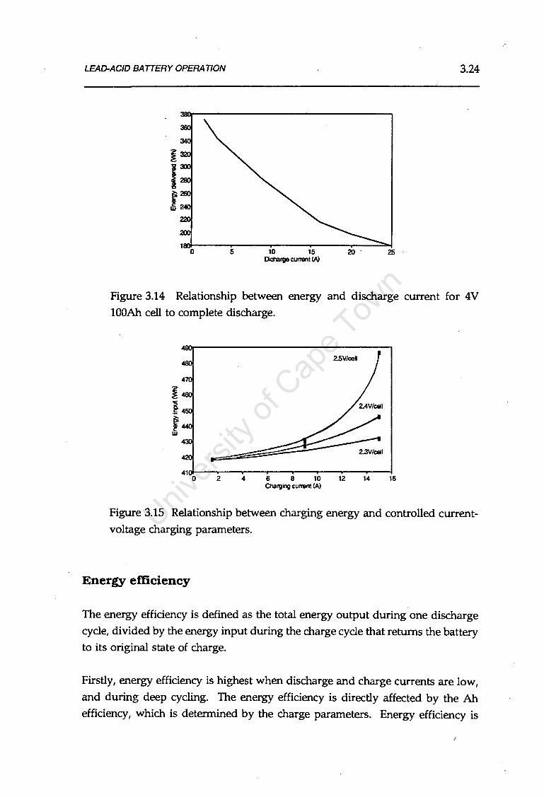
LEAD-ACID BATTERY OPERATION 3.24
5 10 15 20 . 25 . Dicharge current (A)
Figure 3.14 Relationship between energy and discharge current for 4V
lOOAh cell to complete discharge.
2 4 6 8 10 12 14 16 Charging current (A)
Figure 3.15 Relationship between charging energy and controlled current
voltage charging parameters.
Energy efficiency ·
The energy efficiency is defined as the total energy output during one discharge
cycle, divided by the energy input during the charge cycle that returns the battery
to its original state of charge.
Firstly, energy efficiency is highest when discharge and charge currents are low,
and during deep cycling. The energy efficiency is directly affected by the Ah
efficiency, which is determined by the charge parameters. Energy efficiency is

LEAD-ACID BATTERY OPERATION 3.25
more strongly affected by inefficient charging than Ah efficiency, as the voltage
during the gassing stage rises sharply as well. During shallow cycling a greater
percentage of the charging time is spent in the gassing region.
The watt-hour efficiency for deep-cycling is typically in the region of 85% at low
currents, but can drop to 75% at higher currents. For shallow cycling in the 10-
20% DOD region at low currents, the energy efficiency is typically 95% dropping
as low as 50% at higher currents and finishing voltages.
3.4. 7 Cycle Life
The service life of a battery is rated on the basis of the charge/ discharge cycles
obtained during laboratory bench tests. Most conventions specify cycle life as the
number of cycles a battery attains at the specified DOD before its capacity is
reduced by wear and aging to 80% of the rated value. Some manufacturers,
however, specify cycle life as the number of cycles to 50% loss of capacity.
A typical battery life decay curve has been shown in Figure 3.6. After 20% loss
in capacity, further degradation is usually rapid, so it makes only a slight
difference to cycle life whether the end of life is taken to occur at 80% or 50% of
capacity.
Battery cycle life as a function of depth of cycling is most often portrayed as a
straight line on a semi-logarithmic graph. Curves for various lead-acid types tend
to conform with this assumption (Figure 3.16). The different slopes of the curves
indicate various modes of wear or failure for the battery designs. The various
modes of failure are outlined in Section 3.11.
Some manufacturers represent cycle life as a straight line on a log-log curve
(Delco,1979), which gives very high cycle life for low DOD if data extrapolation
is used. Only the semi-log model is theoretically supported, and only in the range 10%-80% DOD. The issues are taken up in Section 3.12.

LEAD-ACID BATTERY OPERATION
75..------------------------------.
4+---.------------------..-------..------1 0 10 20 30 40 50 60 70 80 100
%000
Figure 3.16 Cycle life vs DOD for various battery designs.
(Sources: Sieger,1981; Delco,1979)
3.26
The actual life of the battery may be longer or shorter than the laboratory tests.
Other life-limiting factors may come into effect. Sieger (1981) finds that cycle life
also depends strongly on the frequency of cycling. Using 2, 5, and 10 cycles per
week, cycle life logarithmically depends on the frequency. He attributes this
mainly to the self-discharge process.
Bechtel National (1980) find a strong dependence of cycle life on temperature. If
the battery is used within normal temperature ranges (20-40°C}, at low rates of
discharge in the absence of deep discharge it will last longer.
7.8
7.6
~:::: 7.4 . ~ 7.2
~ u c 7.0
~~:: .. ~ } 6.8
~ 8.4
z 6.2
8.0
o 20 .to eo eo 100
Oeolh ol D11charo1. '
Figure 3.17 De~endence of cycle life on temperature, lead-acid motive
power cell. (Source: Sieger,1981)

LEAD-ACID BATTERY OPERATION 3.27
If current drain is heavy, operating temperature high or the electrolyte is affected
by impurities then life will be reduced.
3.5 BATTERY TYPES
This section introduces the common types of battery, and shows by example how
subtleties in cell design can affect the battery characteristics.
3.5. I Starting, Lighting, Ignition (SLI) Batteries
SLI or starter batteries are used for starting the motor vehicle, for lighting and for
ignition of the spark plugs. After the engine has started the basic energy
requirements are met by the generator. During conditions of heavy energy
demand, the battery covers the shortfall.
Use patterns affect the battery. In private vehicles the battery is subjected to
substantial idle periods. In taxis and urban driving stop-start conditions the
battery is often deep-cycled. In touring the battery is often overcharged.
a) Basic parameters affecting cell design.
Power
The primary requirement of SLI batteries is to provide high power for short
intervals to start the motor. High power is achieved by high current flows,
typically 300A for a lOOAh battery.
Power can be increased by:
decreasing plate thickness (typically neg=l-1.Smm, pos=l.3-1.8mm)
and increasing the number of plates
introduction of radial grids
reduction of the inter plate distance
use of thin micro-porous separators
increase in cross-section and reduction in length of inter-cell connectors.
./
LEAD-ACID BATTERY OPERATION 3.28
Capacity
The full capacity of the SLI battery is not used, normally 1 % of C2°' and at most
50% of Cio·
Cycle life
SLI batteries are designed to deliver high currents for short time duration, and
immediately be recharged. They are not designed. for. deep charge/ discharge
cycling, but can generally withstand overcharge or corrosion of the positive grid.
During cycling the active mass is subjected to heavy mechanical stresses due to
expansion, and the material tends to shed. Shedding can be restricted by
i) reducing the utilisation coefficient of the active mass by increasing the thickness
of the plates ii) wrapping the positive plate in a glass wool sheath to reinforce the
positive active mass.
Mechanical strength
Batteries for non .. stationary applications must not only have good electrical
properties, but also be resistant to mechanical and vibrational stresses likely during normal operation. These effects occur where the plates are fixed to the
strap of the semi-block, at the fixing points of the semi-block to the container.
Plates usually stand on rests on the bottom of the container, and are
asymmetrically fixed to the strap. To eliminate vibration of the individual plates,
the semi-blocks are bonded by a layer of epoxy resin. Only one end of the semi
block is fixed to the container through the inter-cell connection. In "heavy duty"
batteries, the free end of the strap is attached to the nearest partition by a plastic arrestor.
b) Maintenance-free batteries.
The conventional SLI battery has certain drawbacks
shelf life at open circuit is relatively short due to self discharge
water consumption during charging and open circuit is relatively high, necessitating regular water addition.

LEAD-ACID BATTERY OPERATION 3.29
The effects are mainly due to the presence of antimony in the metal grid.
Antimony contributes higher mechanical strength but decreases both the
hydrogen and oxygen overvoltages, (the gassing voltage), and enhances the
electrolysis of water (see Section 3.7.2). The development of low-antimony (1-3%
Sb) alloys which retain the favourable mechanical properties has given rise to low
maintenance (LM) batteries. These batteries may, however, need periodic topping
up during the second half of their life. 'Antimony-free batteries generally utilise
calcium grid alloys, and are referred to as maintenance-free (MF).
The relationship between gassing current and voltage is shown for the various
types of SLI battery. The MF batteries require the highest voltage to begin the
electrolysis process. Gassing is negligible below 14.lV for LM and MF types. As
the batteries age, the gassing current of the 5%Sb and the LM increases
considerably, while that of the MF does not change.
Further, the gassing current of the 5%Sb and LM is strongly affected by
temperature, while the MF is not (Pavlov,1984:213).
~ 40
c "' ~ 30 u
"' E' 0 20 .c:
. ~· QI" >
0 10
t = 65° c
14
5% Sb
15
Voltage applied ( V)
16 17
Figure 3.18 Gassing current vs voltage for various types of 12V, 77 Ah SLI
batteries. (Source: Pavlov,1984:fig.64)
The shelf life of MF batteries is considerably longer than for the other types.
The main shortcoming of the MF battery is its lack of performance under deep
cycle conditions. This is mainly due to the formation of a "non-conducting barrier
corrosion layer" of PbS04 which forms between the positive active mass and grid,

LEAD-ACID BATTERY OPERATION 3.30
and impedes current flow. The insoluble PbS04 reflects the lack of antimony,
rather than the presence of calcium (see Section 3.6).
Shedding of the active mass is generally negligible in MF batteries. The active
blocks can therefore stand directly on the base of the container. MF batteries are
often provided with a state of discharge indicator to help prevent deep-discharge.
3.5.2 Electric Vehicle (EV) BatteJ.jes
Electric vehicle batteries must provide high energy and power under deep
discharge conditions. Modern EV batteries typically provide 1500-1800 cycles at
80% DOD. Requirements are high specific energy, long life, easy and inexpensive
manufacturing, easy and cheap maintenance, and low initial investment. The
lead-acid battery is up to now the only battery suitable in terms of price, materials
and technology.
The life of the battery is determined by the irreversible processes taking place:
corrosion of the grids, processes in the corrosion layer, sulphation of the negative
plates, shorting, shedding of the positive mass (see Section 3.6.2).
EV battery design has resulted in an increase in specific power at the expense of
battery life. Methods include increasing utilisation of the active mass, higher
active mass/ grid ratios and increasing the normal depth of discharge during
cycling. Antimony grid alloys are favoured in the cycling environment.
Tubular and flat plate designs are used. The disadvantage of tubular plates is the
cost, and at high current drains the increased current density may cause local
heating and cracking of the corrosion layer. Tube diameters of 8-8.4rnm are
common, with an active mass thickness of 2-2.2mm.
Flat plate EV batteries have plates 4-6mm thick. The active mass has a lower
utilisation coefficient and higher density than SLI batteries.
Flat plate batteries display higher power density than tubular designs at the
expense of cycle life. Tubular plates typically achieve 2000 cycles, while flat plates
can achieve 800 cycles before corrosion sets in.

LEAD-ACID BATTERY OPERATION 3.31
3.5.3 Stationary Batteries
There are two main categories of stationary batteries,
I stand-by batteries: ·kept in a full state of charge to be used
immediately a power failure should occur.
load levelling and cyclic energy storage: often used to decrease system
costs by allowing optimal utilisation of off-grid energy generators like
electrical generator sets and PV systems, though also offering promise
for direct load levelling, within the utility network.
a) Stand-by batteries
Requirements are maximum reliability, long life under float charge conditions and
low maintenance.
Special designs include
Plante cells with positive plates made from pure lead
tubular plates with low antimony spines
pasted positive plates with calcium grids
Dilute H2S04 is used (1.2-1.25 SG) as electrolyte, which reduces grid corrosion
under the well controlled operating conditions.
The battery is kept topped up under float charge conditions (2.2-2.25V per cell).
Gassing is minimised. Charge/ discharge cycles are usually infrequent (less than
five per annum).
The choice of grid alloy most affects cell operation under float charge. High
antimony grids require low float charge voltages, and are most sensitive to
temperature (see Section 3.5.l(b)). The antimony content is also directly related
to the corrosion rate during float charge operation (Figure 3.19). During
overcharge, gassing causes antimony positive grids to corrode. Excess gassing
results in dissolution and transport of antimony to the negative plate (see
Section 3.6.3(e)), where it decreases the negative plate voltage (see Section 3.7.2).
The gassing must increase to keep the charge voltage constant (Figure 3.19). The
corrosion rate will be enhanced (see Section 3.6.3). There is a possibility of
runaway. The rate of water consumption will increase.

LEAD-ACID BATTERY OPERATION 3.32
:ro Corrosion Test on Battery Grids, (Tubular-Type, 70 Ah- Plate)
-L
Constant Cell Voltage " 0 t: 20 2.7 V/cell
"' ~ ~ 0 ._, :;: "' ; 10
0
0 0 3 ' 5 6
Antimony Content (%)
Figure 3.19 Dependence of the corrosion rate at constant cell voltage on the
Sb content of the grid alloy. (Source: Pavlov,1984:fig.70)
Calcium grids under float charge gas less readily, normally consume less water,
corrode less and are not as temperature sensitive as antimony grids. In ~ne case
of electrolyte contamination, the high gassing voltages will drop and more
current will be involved in water electrolysis. If the calcium grid cell is deep
discharged or remains in a partially discharged state for a long period, insoluble
PbS04 crystals will be formed in the corrosion layer and decrease the electrical
conductivity considerably.
Correct grid choice is a therefore the major factor in stand-by battery selection.
b) Cycling batteries
In grid utility or diesel-electrical generator (genset) load levelling applications the
main requirements of the battery are high charge acceptance rate, moderate
energy efficiency and good deep cycle life.
Charging requirements are similar to EV batteries, essentially as fast as possible.
Discharge requirements vary from mild low current discharges over several days
to complete discharge over a few hours. High efficiency is desirable, but is not
often attainable because of the high charge currents and reduced charging
efficiencies. Much work has been done to eliminate cell internal resistances at the
high currents. Low maintenance is low priority as personnel are usually on hand to tend to the electrical machinery.

LEAD-ACID BATTERY OPERATION 3.33
These batteries are well catered for by the conventional designs. Antimony
positive grid alloys provide ensure good grid life, while tubular positive plates
provide robust housing for, the active material and shield the grid from oxidation
during the frequent gassing and overcharge cycles. Copper negative grids
minimise cell internal resistance. In many cases EV batteries offer the best value.
c) Renewable energy cycling batteries
While batteries for renewable and solar PV applications fall into the stationary
cycling battery class, their typical operating regimes are considerably different to
the regimes experienced in the more conventional applications discussed till now.
Operating regimes are determined primarily by the availability of the solar resource, the profile of the load demand, and the match and configuration of the
solar charger and the battery. Some important points applying to PV systems are:
Different PV array and battery configurations can provide energy for the application.
Battery DOD, cycling and overcharge depends on the battery /array
configuration, and can vary substantially depending on the configuration.
In some installations the battery may be required to operate in a
partial state-of-charge for several months before it can be fully recharged.
Charging currents are relatively low, varying from 1 % to 5% of Cult
though they can be regularly lower than this.
Constant charging currents are virtually impossible to attain due to variations in irradiance and load currents.
Battery temperature variations may be high due harsh and variable climates where PV systems are typically installed.

LEAD-ACID BA ITERY OPERATION 3.34
Regular maintenance may be difficult due to the often remote and
inaccessible sites, or local maintenance personnel may not be on site
so that the installation is maintained only once problems have
occurred.
In the past specialist PV batteries have not been available, and battery choice has
depended on selecting from the conventional types the battery most suited to one
or other of these conditions. In some cases priorities have had to established, or
else the PV system has had to be designed to suite the available battery designs,
often at increased cost.
Additional theoretical knowledge is required before discussing specialist PV
battery designs, in Section 3.13. This theory is discussed in Sections 3.6 to 3.9.

LEAD-ACID BATTERY OPERA TJON 3.35
Sections 3.6, 3.7, 3.8 and 3.9 are theoretical discussions detailing the most
important requirements for understanding competing chemical processes, benefits
of particular designs, battery models and experimental procedures. These selected
sections are extracted from abundant electrochemical literature of the lead-acid
battery, and are considered the most relevant.
3.6 MICRO-PROCESSES DURING BATTERY OPERATION
This section discusses processes that occur during normal operation, as well as
others that predominate during open circuit conditions.
3.6.1 Basic Lead-Acid Electrodes
The positive and negative electrodes are not the only electrodes active in the lead
acid battery. Operation is determined both by electrolyte behaviour and the
interactions with further electrode systems operating on the positive and negative electrode surfaces.
a] Two stage electrolyte dissociation
The H2S04 two stage dissociation is a rate determining step (Pavlov,1984:eqn.24):
At pH<l, HS04- is the predominant species
at pH> 1, SO/- is the predominant species.
At the negative electrode there is an equilibrium between Pb and PbS04• The reduction reaction occurs either as:

LEAD-ACID BATTERY OPERATION 3.36
PbS04 +2e- ... Pb+SOt
&i = -0.356-0.029 log 850 4 2-
or PbS04+H•+2e- ... Pb+HS04-
&i = -0.302-0.029log pH-0.029 8HS04-
depending on which electrolyte ions are dominant (Pavlov,1984:eqns. 8, 9), and
&i is the equilibrium potential of the electrode.
Similarly, at the positive electrode the reduction reaction occurs either as
Pb02+SOt+4H·+2e- ... PbS04+2H20
&i = l.685-0.118pH+0.029log 85042-
or Pb02+HS04-+3H·+2e- ... PbS04+2H20
&i = 1.628-0.088pH +0.029log aHS04-
depending on which electrolyte ions are dominant (Pavlov,1984:eqns 13, 14).
The steady-state reduction potential of the lead-acid cell is
and using IUP Ac1 conventions,
~ight =l.685V E1eft =-0.356V Ece11 = 2.041V (Pavlov,1984)
These are the voltages under no-current situation. Several theoretical equations
exist which attempt to determine the potential at non-standard states or when
current flows. The Nemst equation determines the cell emf under open circuit
conditions as affected by temperature and reactant activities (Pavlov,1984:eqn.78).
The Butler-Volmer equation accounts for kinetic losses that occur during non-
IUPAC is the International Union of Pure and Applied Chemistry

LEAD-ACID BATTERY OPERATION 3.37
steady-state conditions (McNicol and Rand,1984:eqn.29). The limitation of these
equations is that they are only valid on the micro-scale, and are best left for
detailed modelling of the chemical processes themselves.
b) Complex electrode systems - Pourbaix diagram
The conventional method of illustrating complex electrode systems is the Pourbaix
diagram. Figure 3.20 shows that at a low pH typical of H2S04 solutions there are
several equilibria that are continuously competing, some of which have been
previously mentioned.
22 2.0
1.8
1.6
t4 .........
1.2 )· 1.0 o,
>. 0.8 H20
~ 0.6 Pb'• :z 0.4
-;;; 02 w ·~ 0 •..(H2 O> •• 0 ,__.......,,....--.._ --0.2 .. 0
i-0.4 .. ....... .. ..
-5-0.6 Pb n. -0.8
-1.0
-1.2
-u
.. .. .. .. .. .... ,.. ...... H° H,
-1.~2~ -:--0 -:-2~4-6o--;-8 "='="10....,.,12~14~1~6 -pH
Figure 3.20 Simplified potential/pH diagram of the Pb/H20 system. according to Pourbaix, at 25°C, for unity hydrogen ion activity. (Source: Pavlov, 1984:fig. l)
The main equilibria to be considered here are the
Pb /Pb2• equilibrium and Pb02/Pb2
• equilibrium
which form the main redox couple. The electrode potential is heavily depend~nt on the pH due to participation of HSQ4- ions in the process. The effect of pH on electrode potential (as described in Section 3.6.l(a)) can be seen graphically fu the Figure.

LEAD-ACID BATTERY OPERATION 3.38
Two other electrodes are central to the understanding of battery behaviour:
At low pH there is a potential exchange between the Pb /Pb2• and the
H2/H• electrodes, which could liberate H2 and oxidise Pb to PbS04•
A mixed potential is established between the two electrodes on the Pb
electrode surface.
At low pH a similar equilibrium exists between the Pb02/,Pb2• and the
0 2/H20 electrodes, which could result in 0 2 evolution and reduction
of Pb02 to PbS03• A second mixed potential is established on the
Pb02 electrode surface.
The Pourbaix diagram also shows that the corrosion of lead by oxidation passes
through a region of non-stoichiometric crystals (PbOx), and the final corrosion
mixture will consist of Pb02 and PbOx.
All of these processes are discussed ·in more detail in relation to the processes in
the active mass and grid.
3.6.2 Processes in the Active Mass
The fundamental electrochemical process in the active mass in the presence of
H2SO 4 can be described by
discharge + PbS04 + 2H + 2 e
charge
discharge
charge
where ~ is the current flowing through the electrolyte, and Ex is the current
through the external circuit.

LEAD-ACID BATTERY OPERATION 3.39
H2S04 plays a double role. Firstly, it reacts with the Pb2• ions and forms an
insoluble salt PbS04 when Pb2• ions are formed on the either electrode surface.
The lead of each electrode is not transported in the ion exchange process, and the
electrode maintains its mass. Secondly, the charge of the Pb2• ions formed are
replaced by the H• ions from the H2S04• Current is carried by H• and SOt ions
(not Pb2• ions). The high mobility of the H• ions is the reason for the low internal
resistance of the lead-acid cell.
a) Active mass as a porous electrode system.
Cells are designed with high electrode surface area to promote good power
performance. This is accomplished by using highly porous active masses.
However, the move from smooth to porous electrodes imposes two new
limitations.
Electrolyte concentration gradient
The transport properties of the electro-active species (H·, SOt and H20) in the
pores of the electrodes are related to the radii of the species. Diffusion limitations
alter the composition of the electrolyte in the pores of the plates. Subsequent
differences in the solution pH between the pores and the bulk solution may give
rise to concentration gradients and polarisation (Section 3.7). During open circuit
conditions the concentration gradient between the electrolyte in the pores and the
bulk solution will eventually be removed by diffusion. (The SG should be
measured after standing in open circuit for 24 hours.) Within a single cycle the
phenomenon is considered reversible.
Electrical continuity
As the transfer of electrons between the grid and each site of the active mass is
necessary to ensure good utilisation of the active mass, the Pb grid and the Pb02
active masses are made of separate crystals, and must maintain good electrical
contact to facilitate current flow during both charge and discharge. Part of the
active mass is required to act as an extension to the grid and may not take part
in the electrochemical process, while the remainder takes part and represents the
energy providing structure. Replacement of both grids by lighter less expensive
and H2S04 resistant material is an ongoing area of research. The material should

LEAD-ACID BATTERY OPERATION 3.40
be a good conductor, be immune to oxidation or reduction, and should not reduce
the hydrogen and oxygen equilibria on the electrode surfaces.
b) Structural problems of the macro-system
In order to ensure high capacity and cycle-life, the energy providing and skeletal
structures should be in an optimum ratio. The factors in play are the maintenance
of electrical contact between the crystals during charge/ discharge cycling, and
maximisation of mass and material utilisation.
The reactions occurring during discharge at each of the plates are well known.
At the negative plate Pb is converted to Pb2·, the ions diffuse into the solution in
the pores, PbS04 is formed in the pores, and tt• and SO/- diffuse between the
pores and the bulk solution. On the positive plate the same electrolyte diffusion
reactions occur, as well as solid-phase reactions in the Pb02 crystals. The
processes are reversed during charge.
The rates of reactions at each point in the active mass may be different due to the
participation of diffusion and ion migration fluxes. The plates can be considered
as several micro-systems, each associated with specific ion and electron fluxes and
definite crystals in the active mass. Depending on the charge/ discharge
conditions and the design of the plates and active block, a distribution of the
processes is observed. The distribution of reaction rates is according to the
separate micro-systems along the cross-section, height and width of the plate. The
distribution occurs during both charge and discharge.
In a given micro-system the elementary processes are not completely reproduced
in terms of rate and location during a charge/ discharge cycle. Irreversible
processes may be considered to occur, eg. the morphology and size of separate
crystals is altered during each charge discharge cycle. The micro-irreversible
processes may not affect the macro-structure. On a macro-scale the
skeletal/ energy providing structure should remain unchanged, and the macro
structure is considered to be in a reversible state in terms of capacity, electrical
and mechanical parameters.
If unidirectional changes in the micro-system occur during battery cycling then
the macro-system as a whole may become damaged to such an extent that the
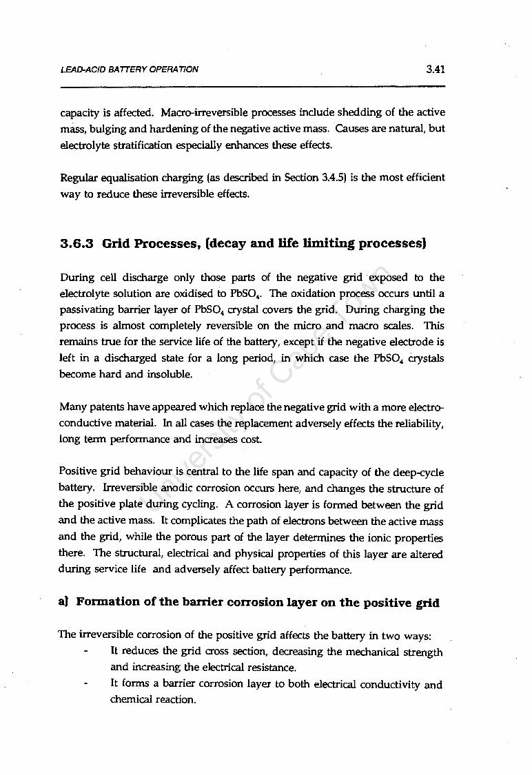
LEAD-ACID BATTERY OPERATION 3.41
capacity is affected. Macro-irreversible processes include shedding of the active
mass, bulging and hardening of the negative active mass. ·Causes are natural, but
electrolyte stratification especially enhances these effects.
Regular equalisation charging (as described in Section 3.4.5) is the most efficient
way to reduce these irreversible effects.
3.6.3 Grid Processes, (decay and life limiting processes)
During cell discharge only those parts of the negative grid ·exposed to the
electrolyte solution are oxidised to PbS04• The oxidation process occurs until a
passivating barrier layer of PbS04 crystal covers the grid. During charging the
process is almost completely reversible on the micro and macro scales. This
remains true for the service life of the battery, except if the negative electrode is
left in a discharged state for a long period, in which case the PbS04 crystals
become hard and insoluble.
Many patents have appeared which replace the negative grid with a more electro
conductive material. In all cases the replacement adversely effects the reliability, long term performance and increases cost.
Positive grid behaviour is central to the life span and capacity of the deep-cycle
battery. Irreversible anodic corrosion occurs here, and changes the structure of
the positive plate during cycling. A corrosion layer is formed between the grid
and the active mass. It complicates the path of electrons between the active mass
and the grid, while the porous part of the layer determines the ionic properties
there. The structural, electrical and physical properties of this layer are altered during service life and adversely affect battery performance.
a) Formation of the barrier corrosion layer on the positive grid
The irreversible corrosion of the positive grid affects the battery in two ways:
It reduces the grid cross section, decreasing the mechanical strength and increasing the electrical resistance.
It forms a barrier corrosion layer to both electrical conductivity and chemical reaction.
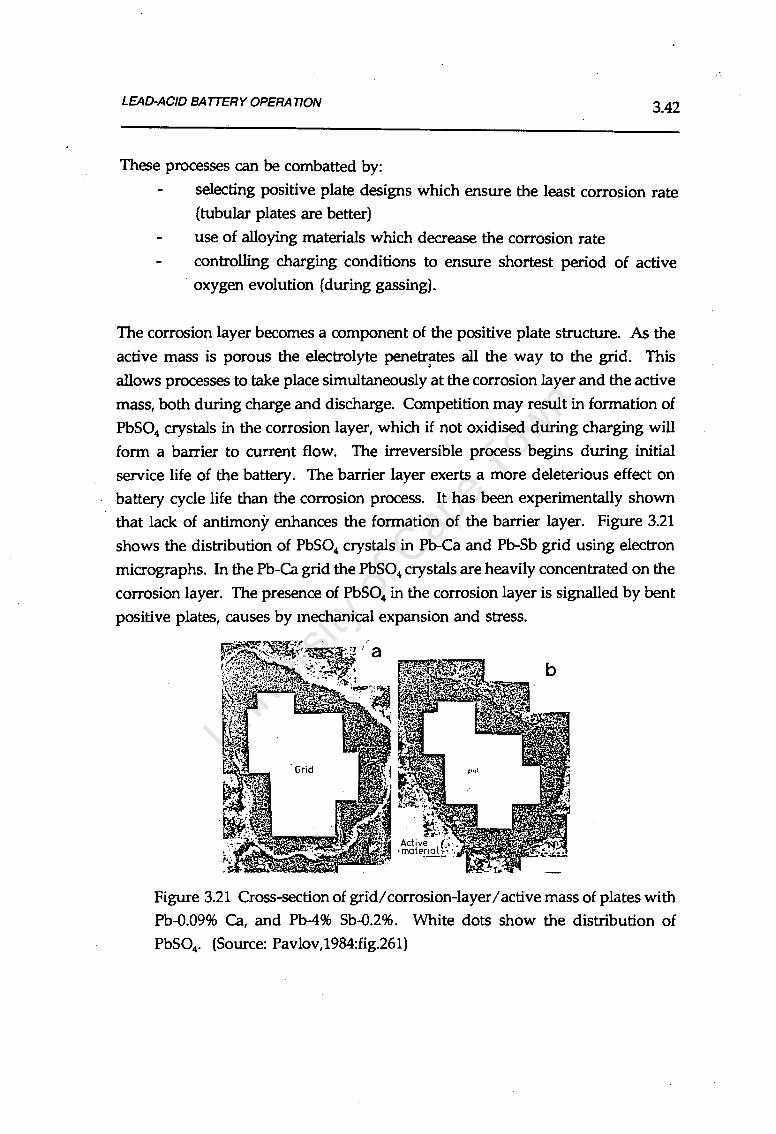
LEAD-ACID BATTERY OPERATION 3.42
These processes can be combatted by:
selecting positive plate designs which ensure the least corrosion rate (tubular plates are better)
use of alloying materials which decrease the corrosion rate
controlling charging conditions to ensure shortest period of active ·oxygen evolution (during gassing).
The corrosion layer becomes a component of the positive plate structure. As the
active mass is porous the electrolyte penetrates all the way to the grid. This . allows processes to take place simultaneously at the corrosion layer and the active
mass, both during charge and discharge. Competition may result in formation of
PbS04 crystals in the corrosion layer, which if not oxidised during charging will
form a barrier to current flow. The irreversible process begins during initial
service life of the battery. The barrier layer exerts a more deleterious effect on
battery cycle life than the corrosion process. It has been experimentally shown
that lack of antimony enhances the formation of the barrier layer. Figure 3.21
shows the distribution of PbS04 crystals in Pb-Ca and Pb-Sb grid using electron
micrographs. In the Pb-Ca grid the PbS04 crystals are heavily concentrated on the
corrosion layer. The presence of PbS04 in the corrosion layer is signalled by bent
positive plates, causes by mechanical expansion and stress.
Figure 3.21 Cross-section of grid/ corrosion-layer I active mass of plates with
Pb-0.09% Ca, and Pb-4% Sb-0.2%. White dots show the distribution of
PbS04• (Source: Pavlov,1984:fig.261)

LEAD-ACID BATTERY OPERATION 3.43
Experimental evidence shows that the corrosion rate is reduced when the grid is
effectively covered by the active mass in both pure lead and antimony alloy
spines. There is evidence that the amount of antimony adversely affects the
corrosion rate, but covering the grid with active mass eliminated this problem, during the float charge state (Pavlov,1984:476).
Further work by Pavlov shows that the corrosion rate is dependant on the type
of polarisation (ie. float or cyclic service). The corrosion rate. of pure lead in
charge/ discharge cycling is three times higher than during float charge. The
antimony alloy displayed a reverse effect: the corrosion rate is reduced during
cycling. The results provide a basis for selecting positive grid alloy of tubular plates.
- 0,08 .c
NE u ';;. 0D6 E
Continuous .po\ariza~
//::~ -/~ polarization
1 -.; o.04 I ~ I .2 "' e 0.02 L. 0 u
10 12 Sb content ( % l
Figure 3.22 Corrosion rate vs antimony content of spines, polarised under three test conditions. (Source: Pavlov,1984:fig.249)
Flat plates behave differently under similar conditions. For 2.5% Sb grids the
corrosion rate was 1.4 times higher under cycling than continuous polarisation.
The thickness of the active mass in tubular plates has also been shown to affect the corrosion rate. There is a critical thickness above below which grid corrosion is enhanced. Figure 3.23 equates cycle life to tube diameter.

LEAD-ACID BATTERY OPERATION 3.44
b) Effect of cycling on corrosion layer structure
Rand et al (1980) have determined that the corrosion layer is initially located
along the antimony rich eutectic zones between the solid solution dendrites3•
Due to changes in the i;nolar volume, internal stresses result in cracking, and the
corrosion layer is peeled from the grid. The cracking of the corrosion layer
adjacent to the grid changes the transport mode of the electrolyte and the
conduction paths through the corrosion layer.
5 • Pb
o t.,9%Sb
• 10.60%Sb
u
c.__~~~~~~~~~
0 2 3
Thickness of the active mass (mm)
Figure 3.23 Spine corrosion rate as a function of the thickness of the active
mass. (Source: Pavlov,1984:fig.250)
c) Corrosion and passivation during positive plate cycle life
The key to failure of the positive plate is the 0 2 flux through the corrosion layer
resulting from: gassing. For small flows, few molecules will reach the grid and the
corrosion rate will be low. The grid will last longer and the cycle life will be
good. The low fluxes will slowly oxidise PbO formed at the grid to form non
stoichiometric oxides with high ohmic resistances. The resultant voltage drop will
deer~ the output power and capacity of the battery.
Arrangements of the constituents in the alloy arising from their simultaneous crystallisation from the melt.
Treelike crystal formations.

LEAD-ACID BATTERY OPERATION 3.45
For high o- fluxes the oxides formed will have high stoichiometric coefficients and
good conductivity, and no passivating barrier layer is formed, but grid corrosion
will be enhanced.
The corrosion and passivation are opposed. Pavlov (1984:485) recommends
adding additives to the alloy that decrease the corrosion rate, yet act as impurities
in the semi-conductive oxide and increase the conductivity of the layer. The additives could also accelerate the oxidation process of PbO and maintain the high
stoichiometric coefficients and conductivity. Antimony is such an additive.
d) . Stress-corrosion of the positive grid
Stress corrosion cracking occurs along the entire cross-section of the grid, usually
following the grain boundaries of the positive grids. Often fissures are formed
and the electrical conductivity is compromised. The cracking originates firstly in the formation of micropores in the cooling of the grid casting. The micropores provide a path for oxygen and subsequent corrosion.
The second cause is the mechanical loads to which the grid is subjected by the
growth of the corrosion layer. The positive grid grows during cycling. The
strains initiated between the grid and the corrosion layer lead to cracking of the grid and the corrosion layer itself.
During charge/ discharge cycling the weight of the plate is increased and
decreased. If the plate is not securely fixed, the changes in weight as well as vibrations are transmitted to the grid, and stress-corrosion is enhanced.
e) Loss of antimony
During the life of the battery the grids of the positive plate are corroded, the
antimony from the grids moves into the corrosion layer, is dissolved into the electrolyte solution and is deposited onto the negative plate. The hydrogen overpotential (gassing voltage) of the negative plate is reduced. During overcharge, gaseous stibine (SbHJ is formed and leaves the cell. Antimony on
the negative plate can be oxidised by dissolved oxygen in the electrolyte, and be transported back to the positive plate via ionic migration.

LEAD-ACID BATTERY OPERATION 3.46
3. 7 POLARISATION AND OVERPOTENTIAL
In this section the concepts of polarisation and overpotential are introduced.
Emphasis thereafter is on the highly polarised hydrogen and oxygen electrodes.
on the plate surfaces.
3. 7. I Types of Polarisation
Analysis of the discharge reaction can provide a great deal of information into the
operation of the lead-acid battery. The battery electrolyte is an aqueous solution
of sulphuric acid. Sulphate ions are consumed at both electrodes during
discharge, while hydrogen ions are consumed only at the positive. Water is a by
product of the reaction at the positive electrode.
The depletion of the reactants at the electrodes and the production of water
contribute to a phenomenon called polarisation. Polarisation reduces the capacity
of the battery to do useful work, and is manifested as a voltage drop. Polarisation
is an indication of the cell's inability to do reversible work under dynamic
conditions. Polarisation is caused by overpotential.
There are three types of overpotential:
a) activation overpotential, resulting from limitations to the charge
transfer process. ie. a rate determining step involving an energy barrier.
b) concentration overpotential, caused by the slow movement of the
electro-active species, and the subsequent departure of the interfacial
concentrations (in the porous mass) from the bulk values. This has been
further divided into diffusion overpotential and reaction overpotential.
Diffusion overpotential is caused by the depletion of reactants at the
electrode surface. Reaction overpotential results from the existence of a rate
determining step.
c) resistance overpotential arising from hinderance by the products
of the reaction ie. formation of surface films of high resistance, such as the
barrier corrosion layer.

LEAD-ACID BATTERY OPERA T/ON 3.47
During battery discharge the voltage is less than the rated cell voltage or open
circuit voltage. Initially there is a voltage loss du~ to activation overpotential, (a·
loss typical of all lead-acid batteries) and a small loss due to internal resistance
of the cell. As the discharge continues the voltage decreases. The decrease in
voltage is due to the increase in diffusion polarisation effects, since to provide
current, the electrolyte must penetrate the active mass.
'. A .6 A
V:l,677
Q .1: 70 3 .S 3~__.-
c f ' 1 A 1
' .3
A .6 -A Vcl,877
C= 3.5 3 .s · 3 -.._ __ ..... c f
2 ·" 2.
' .J.'
• A ,6 A
V:l,984
Q=O 3·,.5-3-
c f '
1 ·" -2 -
I ,J - I
Figure 3~24 Transient behaviour of transfer current UJ, electrode porosity (E)
and electrolyte concentration (c) within the cell during constant current discharge. (Source: Tiedemann and Newman,1978:fig.5)
During battery cha:ging the voltage is greater than the rated cell voltage. The
losses are initially due to increased resistance of cell electrolyte. As the cell

LEAD-ACID BATTERY OPERATION 3.48
becomes charged, the conductivity of the electrolyte increases, but the ability of
the cell to completely utilise the charging current is limited by diffusion effects.
The charging current must be tapered (limited) to allow for limitations in the ion
transfer process. If the current is not tapered the excess current, which cannot be
usefully utilised for charging, is used to electrolytically dissociate water, as this
is the reaction with the next lowest activation overpotential. The voltage increases sharply when, the gassing phase.
The effect of polarisation on battery discharging and charging is shown in
Figure 3.25. The lead-acid battery is regarded as weakly polarised, ie. the
processes can proceed more or less reversibly until blocked by physical processes.
The "internal resistance" of the battery consists of both real resistance and
polarisation effects.
Cathode Anode
PbSO,~ Pb02 +j +j PbSO, ~Pb
6. • V, + IR x I .. , -- -- -! !--------:
v v i,
v.
Pb~ PbSO,
-i Pb02 ~ PbSO, -i
Figure 3.25 Variation of cell potential during discharge. Subscript r denotes
equilibrium conditions, subscript i denotes operating conditions, while
subscripts a and c denote anodic and cathodic processes. Subscript 11 denotes polarisation. (Source: McNicol and Rand,1984:fig.10)
The cell operating voltage is:
V;,cdl = V,,au+ IRxicdl+ V ri,Jreduction}-V ,,)oxidation}
Icdl = Ia = Ic <O for discharge

LEAD-ACID BA ITERY OPERATION 3.49
As described above, V11
varies with SOC, and internal resistance, IR, varies with
electrolyte concentration. Both are temperature dependant.
The Pourbaix diagram (Figure 3.20) showed that hydrogen and oxygen electrodes
are established on the lead surface. These electrodes are very interesting because
they are highly polarised, and their reactions proceed unidirectio~y. Hydrogen and oxygen overpotential are discussed below.
3. 7 .2 Hydrogen Overpotential
In addition to the Pb/PbS04 equilibrium on the negative electrode surface, there is a hydrogen equilibrium reaction.
At steady-state a potential of close to 0.3V exists between the Pb/PbS04
and
H2/H• electrodes. At non-steady state conditions both electrodes become
polarised. The relationship between the current and potential of the electrodes is shown in Figure 3.26.
Pb-PbS04
M vs NHE -0,6
+ I 2H + 2e-H2 /
'Y I
/ /
/-
+i
- 0,2
-i
Figure 3.26 Current/potential curves for polarisation of Pb/PbS04
and H2/H• electrodes in H2S04 solution. (Source: Pavlov,1984:fig.6)
Polarisation of the Pb/PbSQ4 electrode is slight, so that the oxidation of Pb and
the reduction of PbSQ4 proceed almost reversibly. The H2/H. electrode is very
highly polarised and is almost completely irreversible - the evolution potential of

LEAD-ACID BATTERY OPERATION 3.50
H2 has more negative values than the PbS04 reduction. The highly polarised
nature of this electrode has enabled its use in the lead-acid battery.
If the electrodes are stored in open circuit conditions a net reaction occurs
between the H2/tt• and Pb/PbS04 electrodes. At the steady-state potential of
-0.3V a very small steady-state exchange current is present. The current is so
small that the equilibrium potential may be assumed to be equal to the steady
state potentials. Clearly, as shown in the diagram, the electron exchange will
cause oxidation of Pb to PbS04 and reduction of tt• to H2• This reaction on the
negative electrode is the "self-discharge of the electrode".
During discharge conditions the H2/tt• electrode is too highly polarised to take
part in the reactions.
During charging conditions the ability of the Pb and PbS04 phases to exchange
electrons ions will determ!pe the period during which the Pb/PbS04 electrode will
accept current. The rate at which current can be accepted may be limited by
physical phenomena, such as blocking of ion exchange paths. If the potential
required to reduce tt• to H2 is less than the potential to overcome the physical
phenomena (diffusion overpotential), gassing in the form of H2 will be seen to
occur. The observed electrode potential on the Pb/PbS04 surface will be more
negative.
The effect of grid additives on hydrogen overpotential can now be fully
appreciated. Antimony and silver additives tend to decrease the hydrogen
overpotential. Expanders tend to increase the overvoltage. The charge and the
self-discharge of the negative plate is therefore directly affected by the use of
additives. The higher the H2/tt• electrode overvoltage, the more efficient the
charge and the lower the self-discharge.
3. 7 .3 Oxygen Overpotential
An oxygen equilibrium reaction co-exists with the Pb02/PbS04 equilibrium on the
positive plate in the same way as the hydrogen equilibrium co-exists on the
negative electrode. The equilibrium potential difference between the Pb02/PbS04
and H20/02 electrodes is about O.SV. The relationship between the current and

LEAD-ACID BATTERY OPERATION 3.51
potential of the electrodes is shown in Figure 3.27. The Pb02/PbS04 electrode is
considerably more polarised than the Pb/PbS04 electrode. The H20/02 electrode is very highly polarised and is completely irreversible; behaviour which has
enabled its use as one of the electrodes in the cell.
+i
1,0 1,2 1.3 1,4 lf>lVJ
PbOz -Pb504
Figure 3.27 Current/potential curves for polarisation of Pb/PbS04 and
0 210· electrodes in H2S04 solution. (Source: Pavlov,1984:fig.38)
During open circuit conditions the exchange current between the electrodes is
equal. The steady state current exchange between the electrodes is small, but is
sufficient to cause self-discharge of the negative plate over a prolonged period,
with simultaneous oxygen evolution.
During discharge conditions the H20/02 electrode is too highly polarised to take
part in the reactions.
During charging conditions the Pb02/PbS04 electrode will normally donate
electrons, as the potential required is lower than for the H20/02 oxidation. As
the battery becomes more fully charged the Pb02/PbS04 electrode becomes more polarised (due to diffusion overpotential or some other rate limiting steps) and
cannot donate electrons at the required rate. The oxygen evolution reaction will
begin. The positive plate potential will be increasingly better represented by the
oxygen electrode potential as more of the charging current is consumed in oxygen
evolution.
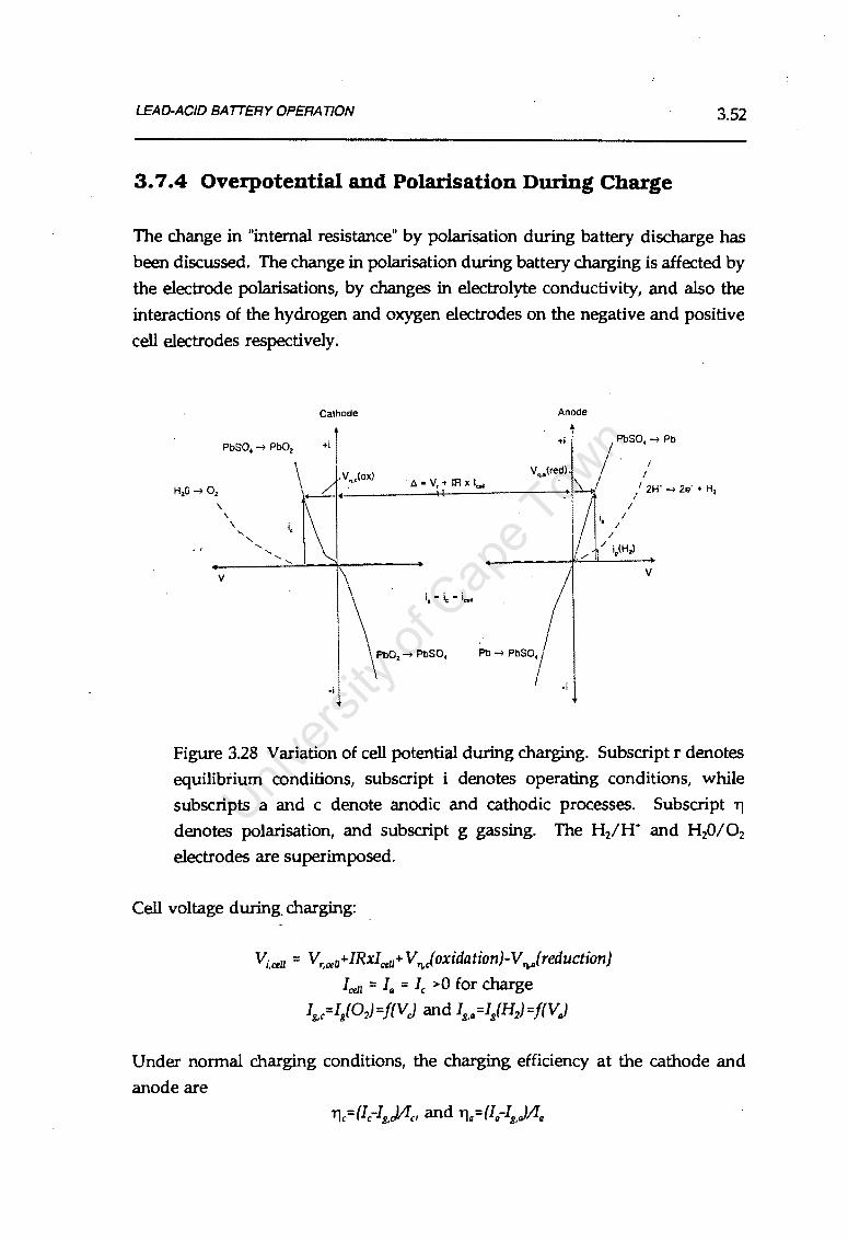
LEAD-ACID BATTERY OPERATION 3.52
3. 7 .4 Overpotential and Polarisation During Charge
The change in "internal resistance" by polarisation during battery discharge has
been discussed. The change in polarisation during battery charging is affected by
the electrode polarisations, by changes in electrolyte conductivity, and also the
interactions of the hydrogen and oxygen electrodes on the negative and positive
cell electrodes respectively.
H20-+ 0 2
\ \
', i,
Cathode Anode
+j
v •. .<ox)
I
PbSO,--+ Pb
I I
I I
/ 2H" --+ 2e· + H2
I
' ' ' ' '
1 i0(H,l
v v
Pb02 --+ PbSO, Pb-+ PbSO,
.j .j
Figure 3.28 Variation of cell potential during charging. Subscript r denotes
equilibrium conditions, subscript i denotes operating conditions, while
subscripts a and c denote anodic and cathodic processes. Subscript ri
denotes polarisation, and subscript g gassing. The H2/H. and H20/02
electrodes are superimposed.
Cell voltage during_ charging:
V;,ceu = Vr,au+IRxlce11+ VT},joxidation)-V.,.jreduction)
!cell = Ia = IC >O for charge Ig,c=Ig(02)=j(Vj and Ig,a=lg(H2)=j(V)
Under normal charging conditions, the charging efficiency at the cathode and
anode are

LEAD-ACID BATTERY OPERATION 3.53
As before, polarisation v,, varies with SOC, and internal resistance IR varies with
electrolyte concentration. Both are temperature dependent.
When the cell is fully charged, Vf1,C increases to correspond with the H20/02
polarisation curve, so that Ig,c=lc and all the charge current is consumed by
gassing at the cathode. A similar phenomenum occurs at the anode.
3.8 MACRO-PROCESSES DURING OPERATION ·
3.8.1 Electrolyte Stratification and Recovery
Electrolyte stratification is often observed in flooded electrolyte batteries.
The concentration of the electrolyte in the upper reservoir of the cell decreases
during discharge and increases during charge. During cycling processes
concentration gradients are formed.
Experimental evidence shows that stratification is enhanced during deep cycling,
and that concentration differences accumulate (Figure 3.29). It has also been
shown that concentration gradients between the bottom and middle of the cell are
less pronounced than the differences between the top and middle, implying that
the top half of the cell participates more actively in the discharge process. The
process can be visualised by considering the resistance paths and current flow.
1.30
E: ci, 1.25
>.
~ 1.20 c:
"' "O
"O 1.15 ~
1.10
0 L 80 L 80 L 80 Charge time ( h l
8
Figure 3.29 Stratification of electrolyte measured during charging to 2%
overcharge and 100% DOD. (Source: Pavlov,1984:fig.223)

LEAD-ACID BATTERY OPERATION 3.54
Because the electrolyte is an active material, stratification affects cell capacity. The
capacity losses are due to the concentration differences, and are termed diffusion
capacity losses. Diffusion losses are generally reversible: when the concentration
gradients are removed, the capacity is restored. Gas evolution during overcharge
causes efficient mixing by gas-lift stirring of the electrolyte, but it is has also been shown that excess gassing results in scrubbing of the active material, and leads
to an increase in the rate of active material shedding (Rand et al, 1980).
Stratification losses may not be reversible in the long term. On the macro-scale,
the cell is worked unevenly. As a result corrosion and slow PbS04 formation will
attack the grid unevenly ~d are likely to cause premature failure of the cell.
3.8.2 Gassing and Related Phenomena
Gassing in the lead-acid battery is central to the operation of the battery. The
voltage at which gassing occurs (determined by the 0 2 and H2 overpotentials) determines the self discharge of the battery. Gassing directly affects the charging
efficiency of the battery and is the only practical way to eliminate electrolyte stratification in flooded electrolyte cells. However, excess gassing may decrease
the life of the cell by increasing the rate of active material shedding. Gassing also
increases the flux of o- radicals and enhances the corrosion of the positive grid.
Gassing consumes water and determines the frequency of maintenance of the cell.
Further, the gassing voltage is negatively dependi?.nt on temperature, and is
dependant on grid alloys and additives. The H2/02 mixture is explosive, and in antimony grid cells the gas may contain traces of toxic gas.
a) Self-discharge
The discussion of hydrogen and oxygen overvoltage shows that the self-discharge produces H2 and 0 2 gas, and that self-discharge of the positive and negative plates need not proceed at the same rates. It is clear that the amount of gas
evolved during self-discharge is small. Typical self-discharge rates are 1 %-3% per
month for a low antimony grid cell and water loss is approximately 0.4ml/ Ah of
self-discharge. Self discharge is increased by increased antimony content, and also by temperature. (See Figure 3.11.)

. LEAD-ACID BATTERY OPERA T/ON 3.55
b) Charging Efficiency
The charging efficiency of the battery is, by definition, the amount of charge
stored relative to the amount being input by the charging system.· For input
current I, and gassing current 18
, the charge efficiency is
f1c1r=(I-IJII.
As the battery becomes fully charged the charge efficiency progressively falls.
The charge efficiency is related to the suppression of the H2 and 0 2 evolution and
enhancement of Pb and Pb02 formation rates. Further it is interesting to note that
charge acceptance of the po~itive plate does not reach zero (Figure 3.30). This is
because the reactions occur entirely within the potential region for 0 2 generation
(Lakeman,1989). The charge acceptance of the negative plate is almost 100% at
25°C (Bode in Pavlov,1984:422).
If the gas mixture is assumed stoichiometric (in H2 and 0 2) and the gas flow is
measured, then the instantaneous charging efficiency can be estimated. Lakeman (1989) has monitored the separate plates and found the error due to this
approximation is small. He finds that the gassing current can be easily estimated
from the individual plate potentials.
100 28
) c.t\ """''' ·-· - 80
.~ . ---<>-·.--.·--
~ .\ 2.6
(1J
g 60 ~ .::::. 0 c.. \ 2.L. ~ (1J .E u
./ g L.O ~ (1J
E' .~././ 22 0
\ c5 20 Positive plates
\, Negative plates 0 -~------o.- 2.0
0 2 3 Charge time (h) .
Figure 3.30 Charge acceptance of positive and negative plates at 40°C vs time. (Source: Pavlov,1984:fig.210)

LEAD-ACID BATTERY OPERATION 3.56
c) Gas Composition
The ratio of H2:02 is stoichiometric (2:1 ratio) when the cell voltage is high and
when gassing rates are high. At slight gassing rates the ratio will be closer to
1.1:1, as is not uncommon for one plate to begin gassing before the other (Vinal,
1955:262). In most cases the mixture will approximate stoichiometric.
····························································· HYDROGEN -·SEALED ••••••••••
80 at z· 0 j:: 60 HYDROGEN - FLOODED ii) 0 ~
~ 40 u OXYG!N - FLOODED Cf) <( -
0 20 ! ........ .
OXYGEN - SEALED ,,,,,''1 .................... ·······•'' 0-1---,.....;.;.;~:..:.:.:..1~ ........ f'UAl .................... l&UJ=r---...---r---.---+ -25 -20 -15 -10 -5 0 5
112081 STATE OF DISCHARGE.%
Figure 3.31 H2/02 ratio during charge acceptance.
(Source: Lakeman, 1989; Szymborski, 1982:fig.18)
L100% RETURN OF CHARGE
The transfer of antimony and arsenic to the negative plates during corrosion of
the positive grid can result in release of stibine (SbH3) and Arsine (AsH:J during
the gassing stage on the negative plate. Both these gases are extremely toxic.
Varma et al (1989) have shown that after 10 charge/discharge cycles the rate of
evolution of these toxic gases is reduced, and that by charging below 2.4V per cell
the evolution is suppressed. The movement of antimony in the cell has already
been discussed in Section 3.6.3(e).
d) Gassing and Grid Corrosion
Evolution of 0 2 at the positive plate enhances corrosion of the grid, but high flux
of o~ radicals will tend not to favour the formation of a low stoichiometric ratio
and lead-oxide barrier layer of PbOn with poor electrical characteristics. These competing reactions are discussed in Section 3.6.3.
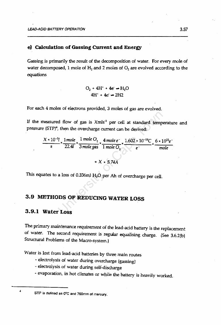
4
LEAD-ACID BAITERY OPERATION 3.57
e) calculation of Gassing CUrrent and Energy
Gassing is primarily the result of the decomposition of water. For every mole of
water decomposed, 1 mole of H2 and 2 moles of 0 2 are evolved according to the
equations
0 2 + 4H• + 4e- .,. H20
4H• + 4e- .,. 2H2
For each 4 moles of electrons provided, 3 moles of gas are evolved.
If the measured flow of gas is Xmis-1 per cell at standard temperature and pressure (STP)4
, then the overcharge current can be derived:
Xx10-31 1mole 1mole02 4molee- l.602x10-19C 6x10²³e-~~~x x x x x~---=-~
s 22.41 3 mole gas 1 mole 02
e mole
=Xx 5.74A
This equates to a loss of 0.336ml H20 per Ah of overcharge per cell.
3.9 METHODS OF REDUCING WATER LOSS
3.9.1 Water Loss
The primary maintenance requirement of the lead-acid battery is the replacement
of water. The second requirement is regular equalising charge. (See 3.6.2(b) Structural Problems of the Macro-system.)
Water is lost from lead-acid batteries by three main routes
- electrolysis of water during overcharge (gassing) - electrolysis of water during self-discharge
- evaporation, in hot climates or while the battery is heavily worked.
STP is defined as 0°C and 760mm of mercury.

LEAD-ACID BATTERY OPERATION 3.58
Maintenance of cells is time-consuming, yet neglect of the cells could result in
exposure of the plates to atmospheric 0 2 with subsequent oxidation corrosion.
Maintenance free characteristics may be desirable in remote power supply
applications.
In the most basic case, a simple vent plug vents the gases to atmosphere. Water
loss by gassing is not significantly reduced, typically only 5% reduction in
conventional cells, but the reduction in spillage loss through sputtering and
evaporation is noticeable in a well designed plug. The methods of reducing water
loss that are appropriate for PV applications, and becoming widely used in
specialised PV batteries, are:
- catalytic recombination of the gases
- auxiliary electrodes for closed H2 and 0 2 cycles
- increasing the 0 2 and H2 overvoltages by using antimony free alloys.
All of the methods affect the cell performance.
3.9.2 Catalytic Recombination of H2 and 0 2
The recombination of H2 and 0 2 tackles two problems simultaneously. Water loss
is reduced so water addition is not required, and the need for a gas vent is
eliminated. A catalytic plug is instead included. These plugs can easily be retro
fitted to most batteries.
H2 and 0 2 are recombined to gaseous water vapour over a platinum catalyst. The
water vapour is then condensed to liquid The recombination efficiency of the plug
is approximately 65%.
The gasses are required to be in a stoichiometric ratio for complete reaction, which
is not necessarily the case (see 3.8.2(c)). Substantial heat is evolved during the
recombination, and the temperature in the plug may reach 400°C (Pavlov, 1984:376)
when gas flow rates are high. This temperature is near the explosive point of the
mixture. The heating at the plug may cause heating in the battery, which will
decrease the 0 2 and H2 overvoltages and cause higher gas flows. The resultant
heating provides a path for a thermal run-away situation. The conversion
coefficient of the plug depends on the gas flow rate and temperature, the rate of

LEAD-ACID BATTERY OPERATION 3.59
product removal. The catalyst may become poisoned by impurities through use. Grid alloys which produce poisonous vapours during gassing are therefore not
viable options, yet it is precisely these grids that most require water recombination, as additives usually decrease the 0 2 and H2 overvoltages. Finally,
the cost of platinum-group metals for catalyst is prohibitive.
Vent hole
Filter (explosion proof)
Outer case
Inner case
Catalyst vessel
Catalyst
Mountin portion
Figure 3.32 Cross section of a catalytic plug.
(Source: Pavlov,1984:fig.180)
3.9.3 Closed 0 2 and f'2 cycles
When the gases are not evolved in stoichiometric amounts the full benefit of the
catalytic plug cannot be obtained. The excess 0 2 and H 2 can be fixed by introducing auxiliary electrodes into the cell.
a) Oxygen cycle with auxiliary electrode
The auxiliary electrode is a porous, hydrophobic, gas-diffusion, conductive, carbon
electrode immersed in the electrolyte. The electrode contains a catalyst for oxygen
reduction, and is maintained within a set voltage range by an external electronic circuit (Figure 3.33). Cobalt and iron will catalyse the reaction in the presence of acid.

LEAD-ACID BATTERY OPERATION
+
PbOz
0 t
0
~r 0
oz-
ED -
Pb
Figure 3.33 Schematic of a cell with an auxiliary electrode.
(Source: Pavlov,1984:fig.181)
3.60
The oxygen evolved at the positive plate is reduced at the auxiliary electrode, in
the presence of hydrogen ions and the electrode current, to form hydrogen peroxide. One oxygen molecule can be temporarily stored by only one hydrogen
molecule equivalent. When the negative electrode eventually begins gassing and
sufficient H2 is evolved, the peroxide is reduced to water by the second reduction
reaction. The second reduction is linked to oxidation of H2 at the negative plate.
The reactions are
Pb02 electrode:
Auxiliary electrode: 0 2 + 2H• + 2e- .. H20 2 (reduction) H20 2 +2H· +2e- .. 2H20
The process shows that the excess oxygen is fixed till it can be recombined with
hydrogen.

LEAD-ACID BATTERY OPERA T/ON 3.61
b) Simple oxygen cycle
A similar process proceeds without an auxiliary electrode. The oxygen evolved
at the positive plate is reduced at the negative plate by the self-discharge reaction:
This reaction may be used to remove oxygen in a sealed cell, but is limited in a
flooded electrolyte system by the rate of oxygen solubility and diffusion through
the electrolyte to the plate. The rate limiting factors can be overcome by
providing a direct pathway for gaseous oxygen. The oxygen is then consumed
by the negative electrode, which remains in a partial SOC and prevents hydrogen evolution.
The oxygen recombination has a depolarising effect on the negative plate, (Mahato
et al,1987; Maja and Penazzi,1989),and this is shown in Figure 3.34
(Tuphom, 1987). It is necessary to reduce the charging voltage once gassing has occurred, usually to 2.35V I cell.
Ii....__...__._ __ __. / .i
' ! I ! J ! I I
•I 21f"+2r- f f I iio+O
01 '°'°' + 21f< + 2r - H,of
H.o--+-..o,+2r
Figure 3.34 Influence of 0 2 recombination on the polarisation of the H2/tt•
electrode. (Source: Tuphom,1987)
Areas of negative plates of both 0 2 recombination types have been known to
sulphate, mainly due to the diffusion of the peroxide with subsequent oxidising
of the lead, which keeps the plate in a partial state-of-charge. During partial
state-of-charge operation large grain sulphate crystals may form. If the cell is not
air tight then the atmospheric 0 2 is reduced to peroxide, and increases the rate of

LEAD-ACID BATTERY OPERATION 3.62
negative plate self-discharge. The cells are usually sealed, operate at a slightly
positive pressure and are equipped with an emergency pressure release valve.
For the cell pressure to stay within limits the rate of gas recombination should be
greater than the rate of gassing. Ideally the rate of recombination should be
expressed as a current, and the finishing charge current should be less than this
current. A theoretical derivation for the current rate of 0 2 recombination (102)
follows.
During recombination: 0 2 + 2tt• + 2e- .,. H20 2
H20 2 + 2tt• + 2e- .,. 2H20
The reactions show that 4 moles of electrons are required per mole of 0 2
recombined.
As 0 2 is gas in excess, the rate of change of 0 2 is related to the pressure by
the ideal gas laws:
do V dP0 2 =---' dt RT dt
The recombination current can be related to the rate of 0 2 recombination by
Faraday's laws:
dO 4e- 4FV dP 0 I = --
2 F = ----'
o, dt mole02
RT dt
But pressure is exponential as the reaction is pseudo first order in 0 2, so
dlnP0
---' = k dt

LEAD-ACID BATTERY OPERATION 3.63
Integrating:
lnP0 =kt +C 2
Rearranging:
Now differentiating yields:
dP0 dlnP0 __ , = kecekt = 'p
dt dt o,
This result can be substituted back to yield:
4FV [dlnP0 ] I=- ' p o, RT dt o,
T.V
b) Hydrogen cycle
The design of the closed hydrogen cycle is similar to the oxyg~ cycle, but is
currently restricted by the cost of platinum-group catalysts. Further, it is normally
0 2, not H2, that is required to be stored as it is the first product of gassing.
LEAD-ACID BATTERY OPERATION 3.64
3.9.4 Antimony-free Alloys
The manner in which positive grid antimony alloys enhance battery cycle life, yet
increase self-discharge by decreasing gassing overvoltages have already been
discussed in detail.
Non-antimonial grid alloys that do not lower the 0 2 and H2 overvoltages will
decrease water loss considerably.
However, antimony-free cells are not suitable for cycling applications (due to the
formation of a passivating PbS04 in the corrosion layer during deep discharge).
Optimal performance is achieved in non-cycling applications, where the need for
gassing is minimal as the accumulation of electrolyte stratification is slight.
Gassing in antimony free cells is limited by maintaining the cells in a float
charged condition, nominally 2.3V per cell.

ELECTRICAL CHARACTERISATION MODELS
3.10 ELECTRICAL CHARACTERISATION MODELS
3.10.1 Introduction
There are two broad ·categories of battery models:
i) physical/ chemical ii) phenomenological.
3.65
The first category is generally complex, focusing on the physical and chemical dynamics, and is useful for understanding the processes in the battery itself. It
is a truly specialist approach, probably beyond the scope of the non-chemist or engineer. (For an illustrative example see Tiedemann and Newman (1978) in
Figure 3.24).
The phenomenological model is more of a black-box approach. Some measurable
parameters are input to the model, and some other measurable parameters are output. Little attempt is made to explain the dynamics, but emphasis is on
linking the interdependencies of the measurable parameters, eg. to provide current and voltage in both charge and discharge operation, at various states of
charge, different temperatures, etc. A phenomenological model, as applied to
batteries, is simply a predictor model. It cannot be deterministic, as only the
observed degrees of freedom (voltage, current, SOC, vs temperature) are
mathematically modelled. Factors such as degradation, which depend on internal
dynamics and cumulative effects, cannot be easily computed.
This review is concerned only with the phenomenological models of lead-acid
batteries. The following topics are discussed: electrical characterisation, capacity,
charging efficiency and self-discharge. Cycle life modelling is discussed in Section 3.12. -
3.10.2 Electrical Characterisation of the Battery
This section reviews models that could be used to describe the current, voltage,
SOC relationship in an operating battery. The models are considered for numerical simulation of PV systems.

ELECTRICAL CHARACTERISATION MODELS 3.66
a) Linear and non-linear circuit element analysis.
Some of the phenomenological models have used both linear and non-linear
circuit analogues to describe the electrical characteristics of the batteries (Klingeret
al,1980 and Waaben et al,1985). Linear analysis cannot simulate many non-linear
characteristics, such as transients, recovery from deep-discharge and gassing
effects. While non-linear analysis can be effective, integrated circuit simulation
computer programs are required to solve these complex problems. Modelling of
the battery in dynamic simulation environments is therefore too complex for
normal use.
b) Numerical modelling
Most numerical models draw heavily on previous work by Shepherd (1965) and
Lindstrom (1970), whose models are based on the variation of apparent "internal
resistance" of the battery with SOC and current. Lindstrom observed that voltage
during a constant-current discharge closely follows the relation:
v = E ( o/qmafl) ) - IR
where V is the voltage, E is the cell emf, q is the ampere hours discharged, qma(l)
is the ampere-capacity at current I, and R is a constant resistance term.
Hyman (1977) developed a Lindstrom/Shepherd model variation that is optimised
for large scale load-levelling discharge simulation. While accurate for high
current work, this model is inappropriate for low current PV simulation.
Facinelli (1983) proposes a PV battery model founded on modified Shepherd
(1965) discharge model, incorporating the temperature effect on voltage. A charge
model of similar form is proposed:
v = Ve+ !RC (1 + McO/{QC'-Q) ), I>O
V = Vd + !Rd (1 + MlQD-Q)/{QD'+Q) ), I<O
where open circuit voltages are
Ve= a1+b1T
Vd = a2+b2T
ELECTRICAL CHARACTERISATION MODELS
and internal resistances
Re= a3+bJOC
Rd= a4+b/QD
QC' =a5 QC
QD' =a6 QD
3.67
Charging efficiency is simply a function of state-of-charge. (see charging efficiency
modelling, Section 3.10.4.)
The Facinelli model is elegant, and contains sufficient variables to represent most
batteries, but appears to have been verified using only high discharge currents
and high charge currents (of about 18). This belief is supported by the fact that
discharge capacities are modelled using the Peukert equation (see capacity
modelling, Section 3.10.3), which is widely recognised as being inadequate for low
currents. The constants used in the Facinelli model are especially difficult to
regress successfully when low currents typical of PV systems are considered. It
remains, nevertheless, the most versatile model considered.
The Mobil-Tyco model was developed by Wood and Crutchen (1980), also for PV
battery modelling. Voltage and current are calculated from experimentally
derived expressions for cell internal resistance and open circuit voltage. The
internal resistance is dependant on SOC and whether the battery is charging or
discharging, but not the rate of charge (or discharge). Gassing is a function of
SOC rather than of charging voltage, and occurs at 64% SOC (see charging
efficiency model, Section 3.10.4). The model shows good correlations with
discharge profiles, but correlation with charging profiles is accurate only in the
40% to 70% SOC range, with poor correlation elsewhere (BDM,1983).

ELECTRICAL CHARACTER/SA TION MODELS
---MODEL
---DATA
2.•
HIGH RESISTANCE ABOVE'/ ' 116" OF SOC IN MODEL I
I I I
)1: I I I I :-----N~~~L,!!! -
MODEL INCLUDES GASSING
I I ! --------' , ..... RESISTANCE ATM" SOC ,,..---· ,,
u-1------------..------------........... ---------..,.---r--------. 0 IO IO 100 120
IT A TE OF CHARGE l"I
3.68
Figure 3.35 Comparison of Mobil-Tyco Model with measured data for
charging. (Source: BDM, 1983)
The BDM (1983) lead acid battery model was contracted by Sandia National
Laboratories after the shortcomings of the Mobil-Tyco PV battery model were
recognised. The model is formulated solely on the basis of the apparent resistance
(RA), dependant on current and SOC. RAsocs are calculated for constant-current
charging and discharging. The RA ratio, (RAsoclRAsoc=ioo), is independent of current, but dependant on whether the battery is charging or discharging. The
model requires fitting of a third order polynomial to the ordered RA ratio:SOC
data. This numerical approach can provide a far more satisfactory fit to measured
data than the Mobil-Tyco model, but contributes little to understanding battery
behaviour further than polynomial behaviour. Battery characteristics cannot be
easily or meaningfully altered by changing simple model parameters, so the
model becomes clumsy in that respect.
For precision modelling using real data, Liesgang et al (1988) propose a database
method designed for Ni-Cd and Ni-H2 cells. The database comprises families of
constant-current curves describing the voltage versus state-of-charge as

ELECTRICAL CHARACTERISATION MODELS 3.69
determined in the laboratory and supplemented by interpolated curves. Battery
modelling is accurate with minimal preprocessing requirements. This approach
has been adapted to lead-acid batteries by Geerdts (1990), for accurate PV system
simulation to obtain improved understanding of PV system sizing and dynamics.
3.10.3 Capacity
The standard model presenting capacity (Cd) as a function of discharge current (Id)
is the Peukert (1897) correlation.
K c ... _ d I ln-11
d
where K is a constant dependant on the temperature, electrolyte concentration and design of the active block, and n is a constant approximately equal to 1.4, and is the slope of the log-log plot of discharge time versus discharge current.
The Peukert equation has been adapted for temperature by Baikie (1972).The term K is modified for temperature:
K, ... K0 (1-at)
where K0 is the Peukert constant at 0°C, and a is the temperature coefficient of capacity.
The Peukert equation is not valid at low discharge currents, since when Id tends
to zero, the capacity tends to infinite values. In this case the Liebenov (1897) equation provides a better fit.
where A and B are constants.

ELECTRICAL CHARACTER/SAT/ON MODELS 3.70
For all the capacity models, the constants can be determined by suitable
regression of measured data.
140
130
120
~ 110
0 100 cE 5 90 I c( 80
70
60
50 0
Peukert assymtote
n=1.2, K=120 A Experimental data
Liebenov correlation
A=6000, 8=64
5 10 15 20 25 30 35 40 45 50 DISCHARGE CURRENT (A)
Figure 3.36 Comparison of Peukert and Liebnenov correlations with real
data.
For temperatures in a narrow band, the change in capacity is given by IEC (1967).
Cd= c:; (1-0.008 (t-30°))
3.10.4 Ah Charging Efficiency
Many charging efficiency models are SOC based, with a fall-off in charging
efficiency from about 85 percent SOC. Wood and Crutchen (1980) propose a
model expressing the maximum rate of charge acceptance as a linear function of state of charge. Efficiency begins to fall from 64% SOC onwards, reaching zero
at 100% SOC. This approach is theoretically incorrect, but can provide acceptable
results.
Theoretically, the inefficiencies are determined primarily by the individual
electrode voltages. A possible representation would present the gassing current
(non-accepted charge) as a function of voltage, and be independent of SOC. This
relationship is exponential, and is described in Section 3.7. The voltage-gassing
current model requires scaling for different battery sizes and types. I

ELECTRICAL CHARACTERISATION MODELS 3.71
3.10.5 Self-Discharge
Self discharge is usually quoted as the monthly loss of a percent of existing
capacity. Self discharge in modem batteries is generally low, but can vary from
10% per month for 5% Sb cells to less than 0.5% per month for antimony-free
grids. Lasnier et al (1988) have proposed an exponential self-discharge model
which is most applicable to the non-linear self-discharge of calcium grid cells.
soc : soc IC i./ct} 0
and k : 300 IC t!-440<Yf'J
where SOC0 is the initial SOC, T in Kelvin, t in hours and k in hours·1, k=0.0001
at room temperature for calcium grid cells.
100
90
.,,. 80 0 DEGREES
~ 70
0 60 ~ 5 50 0
40 w z
~ 30
a: 20
10 35DEGREES
0 0 2 3 4 5 6 7 8 9 10 11 12
SHELF STAND (MONTHS)
Figure 3.37 Self-discharge of SLI batteries under open-circuit conditions using the Lasnier model.
The concave shape of the Lasnier model is questionable. Some literature
(Pavlov,1984) presents self-discharge as a straight line (see Figure 3.11), while a
battery manufacturer shows the same graph as convex (see Figure 3.38) for
antimony grid and calcium grid alloys. It is debatable which model is correct.

ELECTRICAL CHARACTERISATION MODELS
SPECIFIC VOLTAGE GR<l,VITY
12.75 ..-----------------::-------~ 1.275
12.50
12.25 Range In which battery should start car', without Boost Charge
'
11.75
11.50
11.25
--'--i
1.250
1.225
1.200
1.175
1.150
1.125
3.72
Figure 3.38 Self-discharge of SLI batteries und~ open-circuit conditions.
(Source: Raylite SLI battery literature).
3.10.6 Conclusions
The first battery performance models originated from load levelling applications.
Subsequent advances in PV battery models draw heavily on this work. In
general, the models are optimised for high charge and discharge currents, and are
complex, and great care is required in applying these models to low current PV
simulations. In some cases the empirical database approach to characterisation
may be more satisfactory.
Capacity models are generally best represented by the Liebenov correlation, with
a temperature correction factor.
Charging efficiency is primarily voltage based, but unless real data is available
SOC based models are more easily implemented.
Self-discharge may be inconsequential, but is easily modelled as a simple monthly
capacity loss during open circuit conditions.

5
BATTERY FAILURE MODES 3.73
3.11 FAILURE AND WEAR
The lead-acid battery can fail in many ways, depending on the environment and
duty cycle of the service. Some battery designs are more suited to specific
applications than others. This section summarises the modes of failure that have
been discussed in detail in other sections.
The positive plate generally limits cycle life because of shedding of the active
material and corrosion of the grid.
Deep discharge of batteries having calcium alloy grids can lead to formation of
insoluble calcium sulphate in the corrosion layer, between the grid and the active
material. Proprietary processes5 during manufacture can prevent this corrosion,
but are costly. MF SLI batteries are not treated in this way, and may not be deep
discharged. PV batteries with treated calcium alloy grids are more costly, but can reach 1800 cycles at 8% DOD (Sieger,1981).
Tubular plate batteries are designed for deep-discharge service. The positive
tubular plate usually fails by stress cracking near the top of the lead spine. Pasted plate designs usually fail by shedding.
The mechanical stresses during cycling are due to volumetric and mass changes
in the active groups. Volumetric changes give rise to cracking of the corrosion
layer and loss of electrical contact. Thickening of the grid occurs during
prolonged deep-discharge when sulphation occurs. Irrecoverable sulphation may result if the batteries are not recharged.
The negative electrode can become sulphated during prolonged cycling. The large sulphate crystals cause loss of contact with the grid.
Repeated cycling can cause stratification of the electrolyte, which can contribute to uneven active material use and degradation in the long term.
Excess gassing can cause rapid corrosion of the grid in antimony alloy batteries. Gassing also causes water loss, which may expose the plates to the atmosphere.
Usually some form of heat treating of the negative grid.

BATTERY FAILURE MODES 3.74
The negative plates can self-discharge with the atmospheric 0 2• Sulphation will
occur.
Excess gassing can scrub some of the active material from the positive plate.
Active material or sulphate that is lost from the plates by shedding or scrubbing
will collect at the bottom of the battery as sediment. If the sediment reaches the
bottom of the plates it will cause shorting.
The sediment can be redeposited by electrolyte stirring during gassing on both the
positive negative plates. It is non-cohesive on the positive plates, and can easily
be scrubbed off again. Material deposited on the negative plate is cohesive, and
can accumulate to cause shorting around the separators. This is known as
mossing. Some of the colloidal lead-sulphate may be reduced to lead, which may
promote short circuiting. The negative mass may grow considerably, leading_to
stress of the grid.
Separators can degrade and cause shorting across the electrodes.
Operation of batteries at higher temperature promotes grid corrosion and reduces
cycle life. High acid concentration affects the cycle life of the negative electrode
by favouring corrosion processes.

CYCLE-LIFE MODELS 3.75
3.12 CYCLE-LIFE MODELS
3.12.1 Cycle Life vs DOD
An important consideration in the design of a PV system with battery storage is·
the durability of the batteries. Though the failure modes of the lead-acid battery
are well understood, real cycle life data can only be generated by controlled
testing. Cycle life tests require considerable investment, and most results are
heavily reliant on interpolation of available data using cycle life models. In the
case of lead-acid batteries the models are generally based on small data samples
only (Sieger,1981).
Battery life is usually represented as straight lines of cycles available versus DOD
on semi-logarithmic paper.
10000 !'-.
" ""-
"' !'-... ~
"" ~
1000 0 10 20 30 40 50 60 70 80 90 100
%DOD
Figure 3.39 Typical representation of cycle life vs depth of discharge.
Delco (1979), however, portray a log-log plot of cycle life vs DOD that is a straight
line for calcium grid cells. Sonnenschein literature for the A200 cell also fits the
log-log model, and the literature is apparently an extrapolation of it.
Bode (1977) and Kordesch (1977) contest that a linear relationship exists between
DOD and the logarithm of the number of cycles. Bode and Kordesch propose models of the form

CYCLE-LIFE MODELS 3.76
Log L = a-b (DOD)
Sieger (1981) provides an interesting derivation for the semi-log model, by
assuming that the molar volume effects of active material during cycling are the
main cause of failure. He expects that the differential change in cycle life is
proportional to cycle life and DOD of the cell. This takes into account the main
mode of failure in the DOD range 20% to 80%. Presumably, alternative models
could be derived for the different dominant failure modes under various
operating conditions, an area of possible future research. The model yields:
L""L0exp (a (1-DOD))
where L0 is the cycle life associated with 100% DOD, and a, the slope indicates the
failure mode. The derivation is shown in Appendix C. This model is not only
based on lead-acid battery data, but on data for batteries of all chemistries using
about four data points per battery. The lead-acid batteries tested include traction
(a=l.3), SLI MF (a=4.14) and PV types (a=3.47).
7.5...------------------,
~ 7 ::i
~ 6.5
~ LL. 6 0
§ 5.5 ...J
~ 5 ::l
~ z 4.5
4 o 10 20 30 40 50 60 70 80 90 100 %000
Figure 3.40 Life cycle correlations for traction, SLI, and PV type lead-acid
batteries. (SLI = Eagle-Picher Carefree Sealed; EV = C&D; PV = C&D
lead-calcium alloy grid) (Source: Sieger,1981)
Sieger (1981) also finds a strong dependence of cycle life on frequency of cycling.
The o/cle life is longer in batteries that are cycled more frequently, although

CYCLE-LIFE MODELS 3.77
actual life is less. He attributes this to self-discharge processes that occur to a
greater degree in less frequently cycled cells. Although insufficient data is
available to determine a functional relationship, on the data available Sieger finds
that cycle life depends logarithmically on the frequency for the single battery
make tested. This is based on frequencies of 2, 5, and 10 cycles per week.
3.12.2 Temperature Effects
Lasnier et al (1988) have proposed a model that incorporates the temperature
effect on battery life. In most cases data is unavailable from the manufacturer,
and the model can not easily be applied. Sieger (1981) found only three data
sources in the literature pertaining to temperature effects on cycle life. This data
suggested that cycle life is greatly reduced at elevated temperatures, mainly due
to higher rates of grid corrosion. At temperatures above 9D°F (30°C) the semi-log
relationship may no longer hold, indicating a different failure mechanism. This
finding suggests that just as temperature affects the failure mode and the cycle life
curve, so they could be affected by battery chemistry, and the Delco log-log life
curve for calcium grid batteries is not necessarily defective.
7.8
DegC 26.7 7.6 30 w
u. 7.4 ::::; 32.2
w ..J 7.2 (.) 35
~ ~ 7 u. 0 6.8 37.7 CJ 0 6.6 ..J ..J
CE 6.4 ::> ~ 6.2 z
6
5.8 40 50 60 70 80 90 100
%000
Figure 3.41 Cycle life vs DOD and temperature for a lead-acid motive
power type battery. (Source: Sieger,1981)

CYCLE-LIFE MODELS 3.78
3.12.3 Incremental Wear
Voss and Huster (1967) define an incremental wear due to each complete cycle
from 100% SOC to a defined DOD and back again to 100% SOC. The battery is
assumed to fail when the total incremental wear is unity.
where!). Wis the incremental wear, and Ldod is the expected cycles life at the cycle
DOD. This model is widely accepted, but its accuracy is limited by the
weaknesses of the original life cycle data.
The model is easily adapted for PV cycling to and from arbitrary DOD's, ie.
partial cycles. The wear from partial cycling between DOD1 and DOD2 is
calculated as:
This approach accounts for both cycling wear and a penalty for partial SOC
operation, though it seems extremely arbitrary as the weighting attributed to
partial cycling will certainly depend on the battery chemistry.
Lasnier et al (1988) treat the wear during partial cycling as if complete cycles were
occurring. The justification is that prolonged partial SOC operation may be just
as harmful in the long term as complete deep cycles with regular charging.
Partial SOC operation raises questions as to what constitutes a cycle. None of the
authors are clear, but it seems reasonable that as the manufacturers' data is based
on full cycles of 0-10% DOD and 0-80% DOD typically, that a cycle should
comprise at least a few percent change in DOD. In PV applications this is
complicated by the superimposition of smaller background cycles (noise caused
by clouds) on the main cycle pattern. In cases where the battery cycle has a
period of one year with prolonged partial SOC operation over a whole season, it
is unclear whether the period used for life cycle calculations is daily cycling or
annual cycling with some noise superimposed.

CYCLE-LIFE MODELS 3.79
The manufacturers' cycle life curves are constructed from cyclic operations within
strictly defined operating regimes, and prolonged partial SOC operation is not
usually considered a subset of those regimes. The validity and significance of all
the cycle life calculations and results based on these curves should be considered
in that context.
3.12.4 Battery Strings
Thaller (1983) develops an interesting method for evaluating the cycle life versus
DOD in single cells and cell strings using a statistical approach. This method is
unfortunately not easily applicable to PV cycling without some adaption, as it
draws heavily on the statistical data of expected cycle life of single cells.
3.12.5 Conclusions
Battery life modelling is complex and prone to errors as limited data is available
and the models are not wholly satisfactory. Either the semi-log or log-log
representations of cycle-life vs DOD should be considered. Compensation for
temperature and frequency of cycling is based on even less data.
The incremental wear approach for complete charge-discharge cycles is easily implemented. Wear for partial SOC cycling is not as simple, but the various
calculation techniques yield fairly similar results in typical PV operating regimes.
Special consideration of peculiar operating conditions is warranted, and sensitivity
to errors in the predicted life should be carefully considered.
Different models could fit different types of battery to a greater or lesser extent.
The cycle life models refer to regular modes of failure; in practice one can also
expect irregular failures due to deviations from controlled regimes and for variations in cell construction. These are not modelled.

PHOTOVOLTAIC BATTERIES 3.80
3.13 PHOTOVOLTAIC BATTERIES
3.13.l Requirements of PV Batteries
The main requirements of a PV battery are listed below. They are in some order,
but the priority depends on the site specific conditions, load demand profile and
the system sizing method used:
i) complete and detailed battery data
ii) long and predictable cycle life
iii) high reliability
iv) deep discharge capability for cost effective sizing and
robust power handling
v) low initial cost I Ah of storage
vi) low maintenance requirements for remote sites
vii) low cost I kWh of storage over battery life
viii) ability to withstand overcharge
ix) overcharge current, capacity and Wh output insensitive to
temperature changes
x) ability to withstand prolonged states of discharge
xi) low self-discharge rate
xii) replaceable in modular format
3.13.2 Trends in the Design of PV Batteries
Field experience has raised several problem areas linked with conventional
batteries installed in PV systems. Primarily, the duty cycle of PV batteries is quite
unlike that of any of the batteries previously discussed.
While PV systems can be designed to accommodate any of the common battery
types, the system design may require considerable overcompensation and
electronic control to ensure suitable operating regimes for the battery. (Heavy
duty EV type batteries typically require 6A charging current/lOOAh, regular boost

PHOTOVOLTAIC BATTERIES 3.81
charge). This can be both expensive in capital and inefficient in energy usage.
Batteries designed specifically for PV load-levelling applications may, in time,
offer the best solutions.
Specialist PV batteries are being developed now that the PV technology is
maturing. There are distinct trends in design towards realizing this goal. A
summary of the discussion is tabulated in Tables 3.2, 3.3, 3.4 and 3.5 at the end
of the section.
3.13.3 Electrolyte
a) Conventional or flooded electrolyte
The dilute sulphuric electrolyte in conventional cells is subject to stratification
during deep cycling. Excess gassing current is required to reverse this effect,
which is cumulative and can have long term deleterious effects. Excess gassing
itself causes deterioration of the positive plate (Mahato et al,1987), and results in
lower cycle efficiencies.
If· there is no mechanism for recombination, gassing leads to water loss, and
electrolyte must be topped up manually. An advantage of flooded cells in
transparent casing is that the behaviour can be monitored visually, but the
maintenance requirements are still a disadvantage in many PV applications. MF
versions of conventional batteries are discussed in section 3.5.2.
The low charging currents typical in PV batteries (2A-3A/100Ah) are unlikely to
generate sufficient gassing to eliminate stratification, particularly in tall cells.
Large and costly PV chargers are required to generate finishing currents of
6A/100Ah.
Immobilized electrolytes have been developed to eliminate stratification.
b) Gelled electrolyte
A gelled electrolyte is essentially H2S04 immobilized by suspension in a silicon
gel. Excess electrolyte can be designed into the battery to achieve good reserve

PHOTOVOLTAIC BATTERIES 3.82
capacity. Mossing, shorting and dendrite growth is limited by the inability of
lead to be absorbed into the electrolyte "solution".
It is important that gassing is limited. The gel develops fissures during gassing
as gases escape through it (Tuphorn,1987), and the gel shrinks as water is lost.
The fissures allow oxygen penetration to the plates where corrosion can occur,
and also reduce contact of the gel with the plates. This can lead to non-uniform
current distribution and unequal electrode utilization, and could result in
significantly shortened cycle life, and make cycle life difficult to estimate because of inconsistencies in the battery itself.
A further limitation in gelled electrolytes is their inherently high internal
impedance which limits high current performance. The insulating properties of
silica gel, combined with gel shrinkage contribute to high internal impedance
which is aggravated at deep discharges. Electrolyte conductivity after deep
discharge is often sustained by the presence of some phosphoric acid in the
electrolyte. The phosphoric acid does not react and is evenly distributed.
The useful life of the gel is also strongly dependent on temperature.
c) Absorbed electrolyte
Absorbed electrolytes are immobilized in a micro-porous absorbent matrix,
usually the separator. The specialised separators are usually made from boro
silicate glass fibres of 2.0 microns. The felt-like porous matrix is not totally saturated with electrolyte, and the free volume allows unimpeded flow of gas, but
not shorting of active material. Oxygen is often in direct contact with the positive
plates by the uniform distribution of gas paths.
Efficient charging is possible in both gelled and absorbed electrolyte cells, as
stratification is virtually eliminated and little gassing is required (Mahato,1987).
Figures 3.42 and 3.43 compare gelled and immobilised electrolyte performance
with flooded cells. Figure 3.44 compares the life of gelled and absorbed electrolyte systems under (unnaturally) prolonged overcharge conditions.

PHOTOVOLTAIC BATTERIES
I -:'
31
341
3ol
3:1
30
21
211
2•
Z2
20
.zo
uo 1.21
·-- ~ ·- I'\
1.22
"-·-1,ll
1,ll
""'
'
3.83
llOTTO.- UQUO ---~ --- ·~
"--"""-J .........._
-.,......___ ~
'ltJPUQUD
3 $ •
Figure 3.42 Electrolyte stratification of a 200Ah tubular cell in comparison
to an A600 gelled cell. (Source: Tuphorn,1987:fig.4)
~60.-----.----.---.------.---.-----.--, < t-o 5.8 > w ('.) 5 6 a: < i5 54 (/)
i5 u. 5 2 0 c - 1 ?OV. CELL z 5 .0 L-----1---1. _____ ...1...._.:.__;...___._--1 UJ 0 5 10 15 20 25 30 35 40
CYCLE NUMBER
Figure 3.43 End of discharge voltage of a sealed lOOAh battery and
comparable flooded electrolyte battery subjected to the deep cycle partial state-of-charge test (see Section 6.2.7)
(Source: GNB Technical Information:fig.8)

PHOTOVOLTAIC BATTER/ES
> !::: C.> :: 100
C3 -' < z ::E 0 z 1-z 60. w u a: ~ .. (10201
0
3.84
100 200 300 400 500 CYCLE NUMBER
Figure 3.44 Effect of electrolyte immobilization on cycle life. Cl 4 discharge
to 60%, recharge at C/10 with 50% overcharge.
(Source: Szymborski, 1982:fig.2)
Both gelled and absorbed electrolyte systems are highly dependent on gas
recombination cycles to prevent water loss, which would dry out the cell.
3.13.4 Gassing and Gas Recombination Techniques
Low antimony deep cycle flooded electrolyte solar batteries tend to have large
electrolyte reservoirs above the active block to reduce the frequency of watering.
The more exotic batteries using immobilised electrolytes require gas
recombination to prevent water loss as water cannot be added after manufacture.
Techniques are catalytic recombination and 0 2 or H2 closed cycles. Closed cycles
require sealed cells to prevent gas leakage. These methods have been discussed
in detail in Section 3.9.
The finishing charge voltage is strongly affected by the method of . water
recombination and may be temperature dependent. Oxygen cycles have a
depolarising effect on the negative plate, and require lower finishing voltages than
for conventional cells of the same design (Mahato et al,1987). The voltage should
be decreased further as the temperature and depolarisation increase due to

PHOTOVOLTAIC BATTERIES 3.85
gassing. It is possible to develop a thermal run-away situation, which highlights
the desirability of temperature compensated voltage regUlation in general.
100
Q ... Q
.... 80 8 ... "' ... 0 ... ,. _, ... ...
0 a: .. = ... w .. ... .... 60 ... < u ,. ... cu ... < .. ... ..,o ... ... 3: ,. ,. c= ... 0 ...I
... ... oC Q = 0 0 ...
< c"" ... ...... = = ... ,i= ... .. ... :: ... ~~ u u .... ... .... 40 ... ... c:I "'o w ... ... Ci: a: ...... ...
~~ 0 o"' Q w ... g ... : :: ::c "'= "' c:I• .... 20 =c = o,. 0 ~ ; :: ..
"' <• "' 0
CELL TYPE
Figure 3.45 Gas recombination efficiencies of different cell designs using
catalytic recombination devices. (Source: Szymborski,1982:fig.3)
3.13.5 Grid Composition
The grid composition has the largest single effect on battery characteristics. Grid
alloy is selected on the basis of its resistance to corrosion by sulphuric acid, its
overpotential characteristics and to facilitate manufacturing. Increasing antimony
content of the grid decreases the hydrogen overvoltage, decreasing the gassing
voltage and increasing its temperature coefficient~ self-discharge rate and water
consumption. Deep cycling ability in conventional cells is dependent on the
presence of antimony for bonding of the active material to the grid (BP Solar
Technical Specifications). Antimony also facilitates the manufacturing process.
1.4%-1.6% Sb is considered optimum for contributing to mechanical strength while
minimising the adverse effects. Antimony is a poison to some gelled electrolytes.
In an effort to reduce maintenance requirements and many of the side effects of
using antimony, researchers have endeavoured to develop alloys that perform
satisfactorily during deep discharge, but otherwise exhibit similar characteristics
to calcium grid cells, namely high gassing voltage and temperature independence
and low self discharge rate. It is well known that conventional calcium grid (MF)

PHOTOVOLTAIC BATTERIES 3.86
cells normally perform very poorly during cycling due to softening of the positive
active material, grid corrosion, grid growth and mossing (Enochs et al,1984).
Grid growth has been reduced by using Pb-Ca-Sn (ternary) alloys instead of the
usual Pb-Ca (binary) calcium alloy (Enochs et al,1984). · Arsenic, selenium,
cadmium, silver and other elements are alloyed to lead to add strength, improve
creep resistance, improve corrosion resistance, modify grain structure and alter
electrochemical characteristics.
Addition of phosphoric acid to the electrolyte increases the cycling capability
considerably by reducing the grid growth rate by up to 75%, and eliminating grid
growth as a life limiting factor (Enochs et al,1984). The addition of phosphoric
acid is not without side effects, as it may increase the tendency towards mossing
as it increases lead solubility. The working capacity of the cell is typically
reduced by 10-15%.
Grid corrosion is a common mode of failure. Calcium grid corrosion can be
reduced by increasing grid thickness. A 10% increase in thickness reduces
corrosion by 30% (Enochs et al,1984). Grid thickness may be from 1,19mm for SLI
type cells to 6.35mm for industrial types.
3.13.6 Positive Plate Design
The choice between tubular or flat plate positive designs has never been clear. In
most applications there are serious trade-offs. The favourable characteristics of
the flat plate are low cost, excellent high current capability and good utilisation
coefficients. Cycling ability is fair. The tubular plate design has excellent deep
discharge and cycling ability and long cycle life since shedding of the active
material is prevented by binding of the fibre sheath. The low utilisation
coefficient of the plate provides protection of the grid against corrosion, but at the
same time decreases the energy density and the stored energy cost (Eggers,1984).
PV batteries designed with antimony free grids should ideally incorporate the
tubular cell, as it protects the grid from corrosion, and contains the positive active
material that goes soft and most likely to shed. Mossing can be further limited by the tubular sheath (Sonnenschein A600 Technical Specifications). The
PHOTOVOLTAIC BATTERIES 3.87
'-\!('\
corresponding decrease energy density is unlikely to affect stationary
applications.
The flat plate design may be more cost effective where grid corrosion is not as
serious (1.696 Sb), or where high currents are required. Deep cycling is possible,
but cycle life performance is shorter than for the tubular design.
3.13. 7 Some State-of-the-art PV Batteries
The main features of three specialist PV batteries are described to illustrate how
some of the design options are engineered together. The present generation of lead-acid PV batteries yields improved performance over conventional batteries,
but at a higher initial cost. No figures are available for comparative costs over
system lifetime, but if. the batteries achieve their advertised cycle life, then they
will provide better value in the long term.
a) BP Solar P-series
• Pasted positive plate, low aritimonial grid for excellent cycle life (1200 cyCles at 8096 DOD). High current capability of flat plates not required.
• Flooded electrolyte enables regular and easy maintenance. Tubular cell can
withstand gassing, gassing overcomes many problems associated with
flooded electrolyte cells. Electrolyte SG can be selected to suit particular
climatic conditions.
• Extremely large electrolyte reservoir, to cater for water consumption
problems associated with antimonial grid cells. Topping up required only
every 2-4 years under normal operation.
• Catalytic recombination can be retrofitted to reduce maintenance in
extremely remote sites.
• Clear casing for ease of maintenance and monitoring.
but
• The batteries require substantial overcharge and high gassing currents to
avoid electrolyte stratification.

PHOTOVOLTAIC BATTERIES 3.88
b) Sonnenschein A600 Solar
• Tubular positive plate, pasted negative plate for good cycle life (10 year life
expectancy under undefined conditions).
• Gelled electrolyte reduces maintenance and stratification problems of
flooded systems. SG is optimised for high ambient temperature operation.
Possibility of freezing at low temperatures is eliminated. Cell exterior is
clean and acid free during operation.
• Antimony-free grid reduces water consumption and helps prevent drying
of gel. Pb-Ca-Sn ternary grid improves cycle service.
• Efficient closed 0 2 cycle for water recombination ensures minimal water
loss, and protects electrolyte from drying. Self-discharge rate is very low.
• Rigid charging specifications supplied in battery data, to protect electrolyte
against overcharge induced temperature increases.
but
• Well controlled charge regulation is required, particularly in warm climates.
c) GNB Mini-Absolyte 12V-5000
• Flat plate construction for moderate cycle life at low cost.
• Immobilized electrolyte reduces maintenance and stratification problems of
flooded cells. The temperature sensitivity familiar to gelled cells is also
avoided. Clean and acid free exterior during operation.
• Low antimony positive grid and heat treated lead-calcium negative reduce
water consumption and self-discharge.
• Efficient closed 0 2 cycle reduces rate of H20 loss.
but
• Excess gas recombination may result in premature grid corrosion.
\

PHOTOVOLTAIC BATTERIES 3.89
. TABLE 3.2 Swnmary of electrolyte designs
I Electrolyte design I Advantages I Disadvantages I flooded i) level can be maintained and i) requires overcharge t.o prevent
topped up stratification
ii) overcharge promotes active
mass shedding
ii) overcharge and shedding result
in dendrite growth
gelled i) no stratification ii temperature dependent
operation
ii) battery not required to be ii) thennal nmaway possible
upright during charging
iii) dendrite growth physically iii) cycle life is temperature
prevented dependent
iv) can withstand partial SOC iv) drying or fissuring of gel
operation during gassing . v) recombination required
absorbed i) no stratification i) less excess electrolyte than other
choices
ii) battery not required to be ii) recombination required upright
iii) less temperature dependent iii) continuous contact of 02 with than gel grid results in corrosion
iv) can withstand partial SOC iv) dendrite growth possible operation

PHOTOVOLTAIC BATTERIES 3.90
TABLE 3.3 Swnmary of grid alloys
I Pos. Grid Alloys I Advantages I Disadvantages I Antimony i) can withstand regular deep i) gases at low voltage. decreasing
(1.696 Sb) discharge with age and temperature
ii) high self-discharge rate
ii) high water loss and
maintenance
ii) transfer of Sb to negative plate,
corrosion, may poison electrolyte
pure lead i) no impurities introduced i) difficult to manufacture,
expensive
ii) cannot withstand deep
discharge
lead-calciwn i) high gassing voltage, higher i) poor deep cycle life
(binary) efficiencies
ii) resulting in low self-discharge
lead-calciwn-Sn i) as above ii higher cost
(ternary)
ii) better deep cycle life
TABLE 3.4 Swnmary of plate designs
I Plate Design
I Advantages
I Disadvantages
I flat plate i) low cost i) active material shedding during
overcharge
ii) high current density ii) low protection of calciwn grid
by shielding
iii) moderate cycle life in thick
plates
tubular plate i) no shedding of positive material ii higher cost
due to binding
ii) excellent deep cycle life ii) capacity very dependent on
discharge current
iii) good protection of grid against
corrosion by shielding

PHOTOVOLTAIC BATTERIES 3.91
TABLE 3.5'Swnmary of water loss prevention designs
I
Water Saving
I Advantages
I
Disadvantages
I Device
none ii cheap ii loss of h20
extra~ectrolyte ii cheap ii decrease in energy density
reservoir
iii less maintenance required
catalytic ii low maintenance i) high temperature 450oC
recombination
ii) can be retrofitted in vent cap ii) cause gassing voltage drop,
possibility of thermal runaway
iii) possibility of explosion
iv) Pt catalyst cost
v) requires stoichiometric H2 and
02 ratio
closed cycles i) recombines h2 and o2 even i) Pt catalyst cost
when not in stoichiometric ratio
ii) completely sealed cell ii) extra-electrode required
iii) low temperature iii) sulphation of negative plate
during recombination
iv) gassing voltage drops during
recombination, possibility of
runaway

VOLTAGE REGULATION 3.92
3.14 VOLTAGE REGULATION
The role of the voltage regulator in a PV system is to protect the battery, as
batteries operate most reliably and efficiently in well controlled environments.
The regulator restricts the range of battery state-of-charge (SOC) operation, and
provides protection against both overcharge and overdischarge. Most PV systems
require some form of voltage regulation.
CHARGE DISCHARGE LOADS PVARRAY - REGULATOR REGULATOR -
BATTERY
Figure 3.46 Voltage regulator in a stand-alone PV system.
The overcharge current and the accumulated Ah of overcharge in the battery must
be limited. Excessively deep discharges of the battery should be avoided.
Normally the battery is maintained within a specified SOC regime, and most
regulators use battery voltage as an SOC indicator. · In more sophisticated
regulators Ah integrators and voltage sensors together give a more reliable SOC
indication.
3.14.1 Charge Regulators
PV system costs can be reduced by efficient operation, that is by converting as
much available PV power as possible to stored battery energy at maximum charge
efficiency. The optimal method of charging a battery is by taper charging or
reducing the charge current as the battery SOC increases. Before gassing starts
any PV supply current available is approximately equally efficient in terms of
charge efficiency, and the efficiency of the process is determined by the match

6
VOLTAGE REGULATION 3.93
between array 1-V curves and battery acceptance 1-V curves. Figure 3.47 shows inefficient matching at 60% and 80% SOC. The currents in the non-gassing range
are effectively set by the irradiance.
Since the array is basically a current generator, tapered current charging is
intrinsically inefficient, but at this stage there is a surplus of PV power. The
charging currents can only be tapered by discarding surplus PV energy, usually
by charge regulation.
Figure 3.47 also shows a typical situation where a PV array without a regulator
produces more end-of-charge power than is ideal for the battery, a situation
which would occur if the array and panel were poorly matched. This mismatch also results in lower process efficiencies at lower SOC' s. When a regulator is
provided, voltage under dynamic conditions is used to determine SOC, and under
conditions of constant battery temperature, the current can be tapered and gassing
current can be limited (to about 0.5A/100Ah) by controlling the regulator output
voltage. Regulation is a necessity in most PV systems with battery storage.
3
2.5
g 2
I-z 1.5 60%SOC w
c:: c:: ::> (.)
float voltage
0.5 and current
0 12 13 14 15 16 17 18 19 20
VOLTAGE (V)
Figure 3.47 Typical situation for a PV installation, 1-V curves for 33 cell
45WP array, lOOAh lead-antimony battery6• Tarray=47°C, 1=1000W/m2,
Tba1=20oC.
In practice the effective PV array voltage may be lower, due to the voltage drop on array output of blocking diodes, regulator voltage drop and line losses.

VOLTAGE REGULATION 3.94
There is, of course, the possibility of using PV panels that are well matched to the
charging curves of the battery to eliminate the need for a regulator and to increase
the overall process efficiency.
Matching is theoretically possible if the recommended battery float voltage and
current are located below the knee of the PV 1-V curve, so the battery charge rate
naturally tapers as the SOC increases. The PV open circuit voltage decreases as
a function of cell temperature (Figure 2.3), corresponding to the decrease in
battery float voltage with temperature (Figure 3.48). The temperature coefficients
of the array open circuit voltage and battery float voltage depend on the type of
PV module and the type of battery.
50% 75% soc 100% soc 3.5 35"c 1~·c
3 1000W/m"2 o"c
r-"1'-::t::---!.I:__ g 2.5 I-
~ 2 a: a: 8 1.5~-t--+-..!._~
0.5
012 13 14 15 16 17 18 19 20
VOLTAGE (VJ
Figure 3.48 Self-regulation of a lOOAh lead-calcium sealed battery at 50%,
75% and 100% SOC (Tbat=20°C), with a 30 cell poly-crystalline 42WP PV panel at the specified irradiance and panel temperatures.
Practically, matching the array with the battery requires reliable battery, array,
irradiance and load profile data. Batteries with charge acceptance curves
relatively unaffected by temperature will simplify the matching considerably,
(here lead-calcium grid cells are preferable). · Self-regulation requires careful
consideration of battery characteristics, 1-V characteristics of the different types of
PV modules and estimates of PV module operating temperatures. Most panel
manufacturers offer panels of 30 or 33 series cells that are optimised for direct
connection to the battery. On a cautionary note, the designer should ensure that
the panel voltage is sufficient for battery charging even at elevated panel temperatures, and some provision may be required for loss of panel voltage due

VOLTAGE REGULATION 3.95
to shading of single PV cells. Normally series diodes are integral to self
regulating panels.
Self-regulating systems should be used regularly, as the charging current from the
self-regulating panel to a fully charged battery may overcharge the battery if the
system is not used for an extended time. The overcharge may result in high
electrolyte consumption.
If these conditions can not be met then it may be preferable to l,ISe some form of
charge regulation.
a) Charge regulator operation
Most charge/regulators can operate in one of two modes:
Boost mode:
Float mode:
charging current is unrestricted till the boost voltage is reached
(±2.4V /cell for deep cycle lead-antimony cells), whereupon the
voltage is clamped, and the charge current tapers to maintain the
clamp voltage. Boost mode is usually used for deep discharge
applications, or for periodic equalising charge (every month).
(See Figure 3.49(a).)
current is unrestricted till the float voltage is reached (2.3V I cell
for shallow cycle lead-antimony cells). The voltage is then
clamped as in the boost mode. After prolonged charge
regulation in float mode the current may be decreased to zero.
Once the battery voltage settles to a low voltage (about
2.17V /cell) the float charging resumes at the initial float voltage
(2.3V /cell). The high/low voltage hysteresis window is most
common in regulators where continuous voltage regulation is riot
possible (Relay type devices). (see Figure 3.49(b).)
Some regulators feature an auto boost mode. The charging current is unlimited
till the boost voltage is reached. At this time regulation at the float voltage
becomes predominant. Batteries charged in this mode will be boosted for a short
time during each cycle, but not as vigorously as for a complete boost charge. (See Figure 3.49(c).)

VOLTAGE REGULATION
=i...J w
~
2.4...---------------------6
························-····· 5
' 2 ··... 4 8
2.35
w 2.3 '···.,· ••• , 3 ~
........ , ...... , ______ :I ~ ~
2.25
2.2+--....---.---.---.--....--...... -.-----..-----.--+'0
TIME
2.35.....------------------~·4
2.3 ················-···\
=i- 2.25 \ ...J \
3 -
~ ~
~ \ ~ 2.2 \, w •• •• 2 1-
z w a: a: :::> 0
(!)< 2.15 •• •• , ---•• , __ ~ ... ,',,, ~ ' .. 0 ~ ~
> 2: '1 '-,_! l ~
2-t---...... --...---....--'----..----.---'--t-o TIME
2.4..-------------------~16
5
2.35 =i-...J w 0 ~ w 2.3 (!) < !:::; 0 >
2.25
2 4 8
('•,, ~ ..,_--.,..------------+3 ;: ·rii ···,·... as
'·... a:
·····-............................. -......... : 8
2.2-t--....---.---.---.----...--.-----..-----.--+10
TIME
3.96
Figure 3.49 a) boost charge mode, b) float charge with current control,
c) auto boost mode. The solid line represents voltage, the dashed line
represents current.

VOLTAGE REGULATION 3.97
b) Temperature compensation
Temperature strongly affects the maximum recommended charging voltage of
most batteries. The overcharge current of antimony grid batteries is particulary
temperature sensitive, and the life of such batteries is dependant on overcharge
control. Temperature compensation of the boost and float voltages is a very
desirable feature for applications where the battery temperature variations range
more than lO°C. This may be directly caused by climatic conditions, or indirectly by internal battery heating.
3
2.5
Battery curves .. Pl/ curve
g 2 35deg c
..... 18deg c z
1.5 w a: Odeg C a: :::> (.)
0.5
0 12 13 14 15 16 17 18 19 20
VOLTAGEM
Figure 3.50 Effect of battery temperature on operating point for typical PV
installation. 1-V curves for a 33 cell 45WP array, lOOAh lead-antimony
battery. Tarray=47°C, l=lOOOW /m2, Tbat=20°C, SOC=100%.
3.14.2 Overdischarge Protection
Overdischarge protection is. required to protect the battery from deep discharge
in the short and long term. Where DOD is indicated by the battery voltage, protection against overdischarge is usually accomplished by disconnecting the
loads that are the prime cause of the low voltage. All the loads, or some of the loads may be shed on a priority basis. Load shed is activated once the battery voltage falls below a selected drop-out voltage on the battery discharge curve.

VOLTAGE REGULATION
2.3,.....----------------
2.2
:::;- 2.1 _j
w u ~ 2 w
20%
~ 1.9 Discharge rates
~ 1.8
1.7
C/20
C/10
C/5 1.6+-----.---.,.---.----,--..----.----.--.-~----1
0 10 20 30 40 50 60 70 80 90 100 110 DOD (%of C20)
Figure 3.51 Standard battery discharge curves
3.98
As shown by Figure 3.51, the approximate discharge current must be known if
load shedding is to occur anywhere above 50% DOD, since the drop-out voltage
is a strong function of discharge current. For load shedding at deeper discharges
the current is not as critical.
The implications for shallow cycle batteries are that in cases of variable loads, voltage control load shed regulators will load shed over a wide range of DOD's.
Restriction of shallow cycle batteries to say 20% DOD becomes very difficult.
Improved protection can be provided if the load shed voltage is compensated for
load currents (decreasing the voltage setting with load current), or if Ah
integration is used for DOD determination.
In PV systems the typical drop-out voltage is l.9V /cell, as many regulators are
preset to this value. Once the load has been shed the voltage rises slowly
according to the relevant battery time constant. The load is typically reconnected
once a voltage of 2V I cell is reached. The actual time for the voltage to rise also
depends on the net charging current. When large discharge currents are load
shed and a net charge follows, it is possible that rapid oscillation between the
high and low voltages may result. The load shed voltage window should be set
to prevent load shed relay oscillation. Bower et al (1990) have observed
oscillation particularly with DC motors due to the high current drawn during
startup.

VOLTAGE REGULATION 3.99
Figure 3.52 shows measured rise times for a lOOAh flat plate Pb-Sb battery, under
0.5A/100Ah charging currents, after load shedding at 1.9V /cell at the specified
currents.
2.Q4i....----------------,
2.02
:::;- 2 ..J
~ ' ~ 1.98 UJ (!) f! 1.96 ..J
~ 1.94
1.92
from 10A
0.2 0.4 0.6 0.8 1 1.2 1.4 1.6 1.8 2 TIME (MINUTES)
Figure 3.52 Battery rise times at 0.5A/100Ah charging current following
various discharge currents, after load shedding at 1.9V I cell.
The battery drop-out voltage during discharge is relatively insensitive to
temperature during shallow cycling. Beyond 50% DOD voltage is more strongly
affected, as indicated by the broadening range of drop-out voltages in Figure 3.53,
and for regular deep-cycling some temperature compensation on the load shed should be provided.
2.05ir----------------. .---~
50 100 150 200 250 300 350 400 CURRENT (%of C10)
Figure 3.53 Battery drop-out voltage vs temperature and discharge current.

VOLTAGE REGULATION 3.100
3.14.3 Regulator Adjustment
It is possible that any one of a variety of generic battery types could be chosen for
the PV system. One type may even be substituted for one another in the same
system. As different batteries require different conditions for optimal operation,
it is crucial to be able to adjust the regulator accordingly. The table below relates
the various battery types and operating conditions to the most suitable regulator
settings, as recommended by the battery manufacturers.
Table 3.6 Approximate regulator settings for generic battery types
Float mode Boost mode Temperature
(V /cell) (V /cell) dependence (V !°CJ
(20"C) (20"C) Float Boost
596 Sb flat plate 2.3V 2.37V -0.0020 -0.0033
596 Sb tubular plate 2.3V 2.47V -0.0038 -0.0052
(8096 DOD)
LM 196 Sb 2.3V 2.5V -0.004 -0.007
MF Sb free 2.3V 2.53V -0.006 -0.006
Gelled electrolyte 2.3V 2.3V -0.006 -0.006
Sb free
Absorbed electrolyte 2.25V 2.45V -0.0055 -0.0055
Sb free
It is impractical and inefficient, not to mention costly in the long term, if the
regulator settings cannot be easily adjusted to suit specific applications. This
applies not only to the boost, float and load shed settings, but also the temperature compensation and voltage windows. Some of the regulators locally
available are not adjustable, or are delivered without literature on how to adjust
the settings (Langley,1990). The static, non-programmable nature of analogue
regulators makes them relatively inflexible. Essentially, analogue regulators
employ algorithms that are voltage driven and not easily compensated for various
effects. Temperature compensation is difficult as the electronics has thermal drifts
of its own, before the battery temperature coefficients are even considered.
Regulators with digital control algorithms may still be voltage driven and
accurately compensated, or they may rely on Ah integrators to determine DOD

VOLTAGE REGULATION 3.101
and the appropriate action. Interfacing digital circuitry with micro-processors
opens the door for software programmable regulation.
3.14.4 Microprocessor-controlled Regulators
There is abundant coverage of microprocessor-based PV regulators in the open
literature. Most work on digital regulation evolved in the course of the US space
programmes, but the falling cost of digital systems is making them a viable and
versatile alternative for other applications.
A typical system can accurately perform the following functions:
• Battery charge control • Battery discharge control • Array control or power maximisation
• Control panel display
• Status and self test
• Data logging via RS232C port
SOC accounting is by Ah integrator and voltage sensing. Gassing current is
estimated on the basis of SOC and voltage. Overcharge and overdischarge
protection are provided in a similar way to the conventional regulators, but with
additional capability to limit the Ah of overcharge.
Temperature compensation can be software controlled.
Equalisation charge is activated based on the number of partial charge/ discharge
cycles. The degree of overcharge required is calculated based on the number and
depth of cycles and can be limited to avoid excessive gassing.
Cells are individually monitored. An energy balance around the battery, together
with efficiencies, is logged and can be retrieved by digital computer via the
RS232C port.
For optimum operation the system requires substantial battery data at various
temperatures, charge and discharge rates.

VOLTAGE REGULATION 3.102
The microprocessor-controlled regulators are in an advanced state of development
internationally, and in developed countries ean be purchased in various
configurations. Higher reliability is expected than for analogue devices, as fewer
components are coupled with protection provided by intelligent software. Costs
of similar analogue and microprocessor-controlled regulators could be
comparable, but the extra display and interface features on the microprocessor
devices increase costs to twice or three times the analogue price. This price
difference limits their general applicability to larger systems in developing areas.
3.14.5 Regulator Efficiency
The efficiency of the regulator is dependant on the control algorithm, the power
electronics design and the choice of components. Control algorithms have been
briefly discussed. There are two main power electronics configurations for charge
regulators: series or shunt (see Figure 3.54); and two main component choices:
relay or solid state. These are described in depth in Lasnier et al (1988).
PV ARRAY OPTIONAL DIODE I PY
.---------------. V bat:
PV ARRAY I PY
SHUNT CONTROL ELEMENT
I aer.ies
SERIES
I bat i BATTERY
CONTROL I bat ELEMENT .r. BATTERY
Figure 3.54 a) Shunt and b) series configurations
Regulators should normally be V'ery efficient whether they employ relay or solid
state technology. Most often the greatest inefficiency is attributable to the 0.6V
blocking diode drop. The diode is used to prevent discharge of the battery into
the panel during times of no insolation. In 12V systems the diode can limit the
maximum charging efficiency to 95%, whereas in higher voltage systems the effect is less noticeable.

VOLTAGE REGULATION
2.:-r----t-:---~"--
g I shunt ~ ~ 1.5 + (.) 1 ........•.•..•••••.••••••••••••• ·····················-···--·-··········-···
0.5 1\ (Vbat,lbat)
~ o+--....--.....,_ ................. --.----.--.......,---.------1 12 13 14 15 16 17
VOLTAGE (V)
2.51.r------:---+--
g 2 l-
as 1.5 a: a: ::l (.')
0.5
( V bat, I bat)
,._vseries
18 19 20
(Vpv, I pv)
i o+--...--l...,.--'-~-----..--..--'-.----1 12 13 14 15 16 17 18 19 20
VOLTAGE (V)
3.103
Figure 3.55 a) Shunt and b) series configurations, showing the PV operating
points during regulation.
In the shunt regulator, 1i,v=Ishunt+Ibav Vpv=Vbat=Vshunt
In the series regulator, 1i,v=Ibai=Iseriest V series=Vpv-Vbat
The relay in a series configured relay charge regulator can be opened in times of
no insolation to prevent battery discharge, and the blocking diode can be omitted.
In normal operation the efficiency may therefore be higher than for a series solid
state regulator.

VOLTAGE REGULATION 3.104
Solid state charge regulators operate by controlling charge at constant voltage, and
can be designed to consume very little power.
Load shed regulators are generally the relay type, which consume a few µA
during relay excitation. Standby power consumption of the load shed unit is only
slightly affected by whether the relay is normally open or normally closed.
The efficiency of the regulator during regulation further depends on matching the
type of regulator to the PV array. This is because the series and shunt
configurations result in different PV array operating points. The series regulator
and the array have the same current, but operate at different voltages, whereas
the shunt regulator and panel operate at the same voltage but at different
currents. The different operating points are shown in Figure 3.55.
3.14.6 Reliability
The questions of reliability and efficiency, and the debates regarding which of
series, shunt, relay or solid state devices is best, are ongoing. Most international
regulator manufacturers can supply both shunt and series devices. Some
regulators incorporate simultaneous shunt and series regulation and improve
efficiency, but at the expense of simplicity. There is application for each type in
particular situations.
Generally, if a shunt regulator fails the PV system will still be operational, but in
the long term the battery may become overcharged. A failed series regulator may
cut out the PV charger, protecting the battery against overcharge; but the load
must simultaneously be disabled to prevent overdischarge of the battery. The
load will not be disabled if the load shed relay is of the normally closed type, and
will be disabled if it is of the normally open type. It follows that a series
regulator should preferably be used in conjunction with a normally open load
shed relay unit, and the shunt design used with a normally closed unit. The
application, degree of protection and approximate battery DOD profile will determine which is most appropriate.
Constructional aspects of regulator design are an important consideration.
Basically, reliability decreases exponentially as a function of the multiplicity of

VOLTAGE REGULATION 3.105
components. The exact relationship depends on the components used and their
individual reliabilities. Some components are necessary to provide protection and
have slight effect on operational reliability. Component reliability is usually
described by stress analysis. For example, a lOW resistor run at lOW will not be
as reliable as a lOW resistor run at SW, and a relay rated at lOA DC will last
much longer if it switches at only amperes. Specification sheets are available for higher quality components. Further than that, no generalisations can be made out
of context of specific designs and components.
In SA, as in USA (Maycock, 1990) there is general consensus that the regulator is
the weakest link in the PV system, followed closely by the battery. Battery
lifetime depends critically on optimal regulation. In turn, optimal regulator
design requires detailed knowledge of battery characteristics in a PV environment,
and these related factors have been a primary motive for the present research.
The relative importance of the reliability of the regulator, or the battery, can be
altered by the careful adjustment of system sizing. This is briefly discussed in a
sizing example in Chapter 8.
3.14.7 Conclusions
Most PV systems require voltage regulation, both , _ . for charge and discharge
protection. Temperature compensation of the charging voltage is a desirable
feature. Overdischarge protection at shallow DOD's is not easily accomplished.
Regulator efficiency is important for optimising the overall system efficiency, but
regulator reliability is far more important in the long term, as battery life may be
in question. There are several regulator designs and configurations that can be chosen depending on the particular application. In all cases good battery data is required.
EDRC has undertaken to perform a major research project investigating in depth
many of the above mentioned questions and aspects of battery regulation in PV
systems.

CHAPTER 4
LABORATORY TESTS OF PHOTOVOLTAIC
BATTERIES
4.1 INTRODUCTION
One of the main factors inhibiting the optimisation of PV system designs over the
life of the system, and limiting the thorough assessment of particular designs, has
been the lack of battery test data appropriate to PV applications. This situation
is slowly changing where specialist PV batteries are concerned, but in most cases
test data is unavailable that meets the needs of the PV system designer. The
objectives of this chapter are to discuss (i) types of battery tests needed, ,
(ii) battery test data presently available and (iii) test equipment and facilities
required.
The material presented is discussed from the point of the PV designer, and not /
from the electrochemist or battery designer. The procedures are
phenomenological in character, and references to electrochemistry are kept to a
minimum.
4.2 BATTERY CHARACTERISATION TESTS
4.2.1 Discharge Capacity.
be.. The first test likely to performed on a new battery is a determination of its
discharge capacity, which can be given in terms of Ah (ampere-hours) or Wh
(watt-hours). The tests would be done using a constant-current discharge. For
PV batteries the capacity is usually given in terms of Ah at the 100-h (C/100) rate,
with a specified cut-off voltage. The capacity can depend significantly on both
discharge rate and choice of cut-off voltage. This is especially true of lead-acid
batteries discharged at high currents, less so at low PV currents.
4.1

PV BATTERY LABORATORY TESTING 4.2
a) Constant current discharge
To characterise a battery for use in a PV system, a series of discharge tests at
various constant<urrents should be performed with discharge times ranging from
100 h to 3 h. In constant<urrent tests it is important to maintain constant current
during the entire test, even when the voltage begins to drop steeply near the end of the test (Figure 4.1). It is important to maintain a constant temperature for all the discharge tests, normally by providing a constant-temperature bath. Cell
temperatures should be measured during discharge tests. Battery tests are
normally performed at 20°C or 25°C for SLI batteries, and at 25°C for standby or
EV cells. Constant<urrent discharge capacity tests are often presented in terms of a Peukert curve, which is a log-log plot of discharge current vs discharge time.
A Peukert curve is presented in Figure 4.2, demonstrating the effect of cut-off voltage. For PV applications, the plot of capacity vs discharge current demonstrates more readily the limiting capacity available at low discharge rates.
PV battery discharge is not often in constant current mode, but may have an
intermittent component. For this reason it may be worthwhile determining the
effect of intermittent discharge on battery capacity using a simulated PV duty cycle.
~ 12 w
~ 11.5
> 11
10.5
20A 10~0---.---.-----.---~--..---..---.---....---.---1
10 20 30 40 50 60 70 80 90 100 DOD(Ah)
Figure 4.1 Constant current discharge curves for a lead-acid battery. (Source: experimental data)

PV BATTERY LABORATORY TESTING 4.3
1 10 100 TIME TO CUT-OFF VOLTAGE (HOURS)
Figure 4.2 Peukert curve for a lead-acid battery, showing time to cut-off
voltages. (Source: experimental data)
100
~ 90 <t
>-::: 80 u c a. c u 70
100_
"' QJ L-
BO~ ~
60 ~ L-:::> u
1.0 E> c .r::. u
20 .!!! a
0 6 7 8
60.____..~~~~~~~~~~~~~ 0 2 3 I. 5
Duration of discharge (hours)
Figure 4.3 Change in capacity and discharge current vs duration of
discharge under continuous and intermittent regimes. (Source: Pavlov,1984:fig 235)
b) Constant power and constant resistance discharge
The effect of constant-power discharge may be important in PV battery testing.
The main constant-power applications are DC-choppers for motor or pumping
optimisation, and when driving AC loads through an inverter. Constant-power
discharge results in rapid change in both battery voltage and current near the end

PV BATTERY LABORATORY TESTING 4.4
of discharge. This results in the capacity being smaller for constant-power than
for constant-current discharge.
Constant-resistance discharging will affect the capacity, as well as the end of
discharge current conversely to the constant-power discharge. Most static loads
are constant resistance.
The effect of the different discharge modes on the power output of the battery is not easily derived from the energy output curves.
110.n. -----------------,
Constant Resistance
~ 100.
~ 90. ~ ~ 80.
~ ll. 70. Constant Current
cs 60.
50.
1 10 100 STARTING DISCHARGE CURRENT (A)
Figure 4.4 Effect of constant-current, constant-resistance and constant-power discharges on Ah capacity.
c) Pulsed discharge
Batteries subjected to constant-power discharge generally experience a pulsed
controlled discharge, in which the peak current can be many times the average
discharge current. In motor applications, pulsing is most often by PWM (pulse
width modulation) at high frequency (2000Hz). In inverter applications the
frequency may be high if PWM is used, or at much lower mains frequency (50-60Hz) in non-PWM designs. Some inverter designs may actually pulse chargedischarge the battery, using is as a stabilising capacitance.
The effects of pulsing current have been studied in considerable detail
(Cataldo,1978). If one properly accounts for changes in battery temperature,
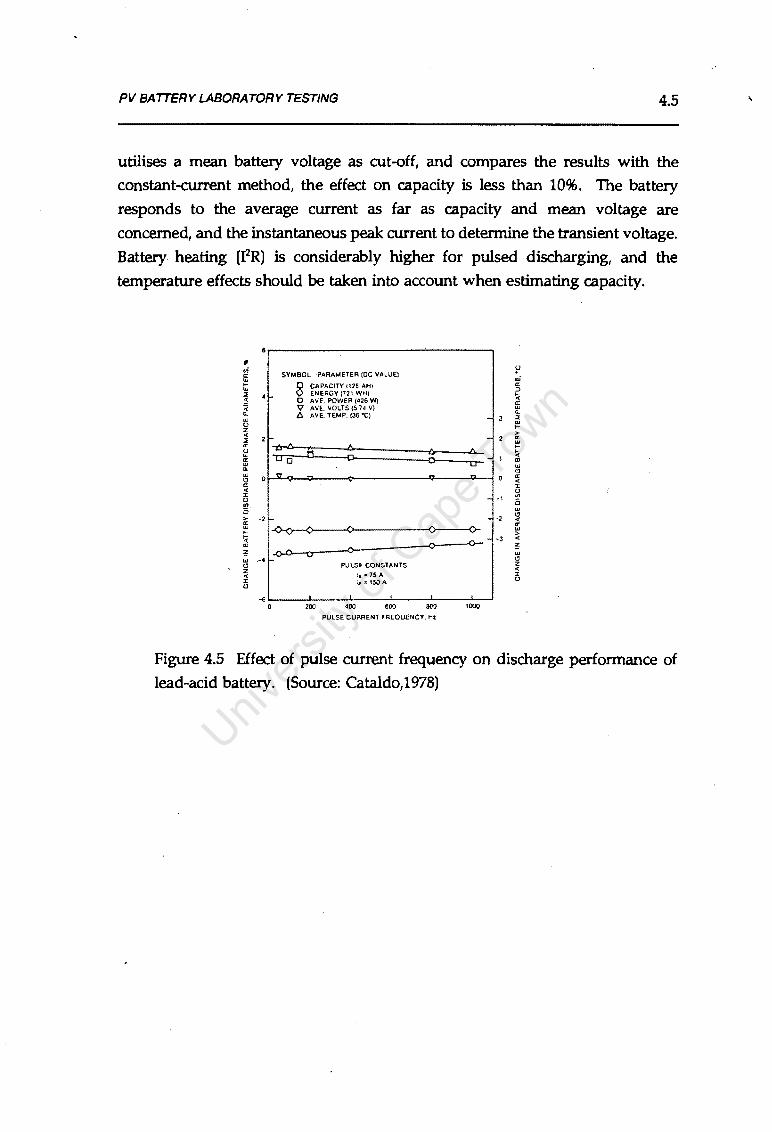
PV BATTERY LABORATORY TESTING 4.5
utilises a mean battery voltage as cut-off, and compares the results with the
constant-current method, the effect on capacity is less than 10%. The battery
responds to the average current as far as capacity and mean voltage are
concerned, and the instantaneous peak current to determine the transient voltage.
Battery heating (12R) is considerably higher for pulsed discharging, and the
temperature effects should be taken into account when estimating capacity.
"I .,;
SYMBOL ·PARAMETER (DC VALUE) ;>
a: ui w ... 8 CAPACITY (126 AH) a: w :> ::< • ENERGY (721 WH) ~ < 0 AVE. POWER (426 W) a: v AVE. VOLTS (5.74 V) ffi < Q_ Q_ A AVE. TEMP. (36 'C) w 3 ::<
w l> ... z >-< ::< 2 2 ffi a:
~ £\ ~ ...
fi' g ~ 1 ~
a: "' w w Q_
'~ w 0 0 a:
" < a: J: < l> J: -1 "' l> i5 !!?.
'" 0
" >- -2 -2 < a: a: w w ... > ~ -3 <
"' " " w w .-4 " " PULSE CONSTANTS z z < < 11. = 75 A J: J: Ip: 150A l> l>
-6 0 200 400 600 800 1000
PULSE CURRENT FREQUENCY, Hz
Figure 4.5 Effect of pulse current frequency on discharge performance of
lead-acid battery. (Source: Cataldo,1978)

PV BATTERY LABORATORY TESTING
# ui a: w 1-w ::; < a: < 0. w 0 z < ::;
2 0 a: w 0. w ~ -2 < l: 0
"' e """ a: w I-
~ ., :!: -6 w
" z < 5 -8
SYMBOL 'PARAMETER (DC VALUE)
O CAPACITY (138 AH) 0 ENERGY (798 WH) 0 AVE. POWER (435 Wl '1 AVE. VOLTS (5.81 V) 6 AVE. TEMP. (36.0 °C)
PULSE CONSTANTS
Fp = 200 Hz -10 IA = 75 A
1 (7S)
2 (150)
3 (225)
• (300)
6
-8
4.6
Figure 4.6 Effect of pulse to average current ratio on discharge performance
of lead-acid battery. (Source: Cataldo,1978)
d) Load shed settings (discharge termination)
Battery life in PV applications is optimal if the end-of-discharge SOC is limited,
usually to around 50% for deep cycle batteries. Voltage is often used as an
dynamic indicator of SOC in PV applications, but is not very reliable unless
several other parameters are also defined. The voltage/ current/ depth-of
discharge profile provides a means of estimating the regulator load-shed settings
for a given current and maximum DOD (Figure 4.7). It is, however, difficult to
provide reliable load shedding at less than 80% DOD, particularly when the load
current may vary over a large current range.

PV BATTERY LABORATORY TESTING 4.7
12.2
12.0 ..
60%000 Odegrees • 11.8 .. 11.6
~ 11.4 rees ~ 11.2 7-::···' < : ...
~ 11.0 ..__._ .. .. > 10.8 10.6
10.4
10.2
10.00 2 4 6 8 10 12 14 16 18 20
DISCHARGE CURRENT (A)
Figure 4.7 Load-shed settings as affected by current, SOC and temperature.
(Source: experimental data)
4.2.2 Battery Charging Characteristics
Battery charging data pertinent to PV charging are needed by the system designer. The charging currents are generally low (<SA peak per lOOAh) and the charging
times long (2-12h or as long as the solar charge current exceeds the load current).
(Refer to Chapter 2).
Tests to determine charging characteristics require a controllable power source.
The most important quantity to measure is voltage, which is greater than the open
circuit voltage in the case of charging. The voltage during charging should be
limited to some specified increment above V oc at 100% SOC to avoid damage to
the battery plates due to excessive gassing. Limiting voltage is strongly
temperature dependent.
The proper design of a PV energy system and charge controller requires
knowledge of the particular battery's charging characteristics, which can only be
determined by testing. Characteristics include: voltage vs current profiles during charging
charge termination criteria
the effect of DOD on charging requirements
the effect of battery temperature on charging requirements.

PV BATTERY LABORATORY TESTING 4.8
Charging characteristics vary significantly from battery type to battery type, and
further for different designs within battery types. Determining the proper
charging regimes and following them as closely as possible is critical to achieving
long battery life.
a) Current-voltage profiles
There is general agreement that the optimum way to charge lead I acid batteries
of all designs is to set and maintain a constant current until a specified maximum
charging voltage is reached, and then maintain the voltage by tapering the current
(controlled current-voltage current method). Charging is complete when some
charge termination criterion is met. It is important that the maximum charging
voltage is corrected for battery temperature, otherwise excessive gassing can
occur, and the battery can be damaged. It is important that the battery is charged
under the profiles recommended by the manufacturer, in order to attain a long
battery life.
It is clear that PV batteries cannot be maintained in a fully charged state, and
except in very specific cases cannot be charged according to the recommended
charging regime. The exception is when the PV panels have been . most
uneconomically oversized. Otherwise, PV batteries may in fact operate mostly in
partial state-of-charge, with slow state-of-charge changes during the day (see
Chapter 2). Recovery from deep discharge may require several days. It is
essential to appreciate the conditions that a battery typically experiences under a PV duty cycle.

PV BATTERY LABORATORY TESTING
14,4 . ..-------------------r12
14
~ w 13.6
~ I-' 5 13.2 >
12.8
\ Voltage 10 S
\ . 8 ~ \ ~
' s a \ w ' ~
' 4 ~
~21i 50 100 150 200 250 300
TIME (MINUTES) 350 400 450 508
4.9
Figure 4.8 Lead-acid battery charging curves, using constant current,
constant voltage method.
14...-------------------,4
w ~
13.5
~ 13 :..J g
12.5
12 24 36 48 60 72 84 HOURS OF SIMULATION
2
fil 0 ffi
0..
~
·2
Figure 4.9 Lead-acid charge discharge cycling during PV operation.
(Source: experimental data)
b) Charge termination criteria
Termination of charging without overcharging is a notable factor in achieving
long battery life, in managing water loss and limiting plate exposure. Usually a
manufacturer will specify the percent overcharge that is required and should not
be exceeded. There are a number of criteria that can be used to terminate
charging, namely: time after a specified event in the charging process, Ah

PV BATTERY LABORATORY TESTING 4.10
returned to the battery vs Ah removed, finishing current at a specified clamp
voltage, voltage gradient (dV /dT) at a specified finishing current. Applicable
charge termination criteria are required for both daily and equalising charging,
and for a wide range of DOD. Charge termination criteria should also
compensate for changes in battery temperature. The battery test data needed to
adopt charge termination criteria for specific applications is seldom available.
The simplest method is to set a number of Ah to be returned to the battery, and
to end charging when this is reached. This method requires m~surement of Ah
during discharge and charge. It is self adapting for aging and for temperature,
but requires sophisticated regulation.
An easier method to implement is to terminate charge at a specified time after an
identifiable event, eg attainment of a clamp voltage. This method makes it
difficult to overcharge by a specific percentage, as the corresponding overcharge
time varies widely with the initial Ah removed. Conditions appropriate for
charging from a deep discharge (80%) would significantly overcharge the battery
when it is charged from a shallow DOD (20%). This would damage the battery,
and shorten its life, as well as reduce the charge/ discharge efficiency, hence
increasing the life cycle cost (LCC) of the PV system operation.
Most PV voltage regulators clamp at the finishing voltage, and do not ever
actually terminate the charging process. The correct degree of overcharge can
only regularly achieved on systems with c;:ontrolled, predictable or regular loads
(remote repeater stations), they are unlikely to be satisfied otherwise. The
literature suggests that insufficient data exists on the profiles and variability of
typical household loads to be able to predict overcharge variation.
Some other methods use current or voltage gradient, which are unfortunately sensitive to battery temperature and overcharge required.
The most straight forward method of charge termination is the approach in which a target Ah in is set based on the previous discharge, and charge is terminated
when that Ah target is reached. This method requires the least extensive testing of the battery, and is most adaptable to batteries of different designs when
complete cycles are the order of the day. The partial cyclic operation in PV
applications makes determination of the target Ah more complex than for

PV BATTERY LABORATORY TESTING 4.11
complete cycles. It is difficult to predict whether the target Ah would be a
function of the DOD alone, or whether the number of cycles at partial SOC
(induced electrolyte stratification) should be part of the calculation. Only
experimentation will indicate the percent overcharge required for various
conditions.
4.2.3 Thermal Effects
The characteristics of a battery depend on temperature. In testing, the
environment should be known and controlled. Most often a constant temperature water-bath is used.
The temperature effect on capacity oi a lead-acid battery is typically about 0:75%
per degree Celsius. The cut-off voltage for discharging is also temperature
dependent.
The charging clamp voltage to limit gassing current is particularly sensitive to
temperature. The available data is limited, and testing is needed to evaluate
batteries for PV systems.
... Octegrees ... 18degrees •
35dearees
1 10 100 DISCHARGE CURRENT (A)
Figure 4.10 Temperature effect on capacity for a lOOAh flat plate flooded
electrolyte cell. (Source: Experimental data)

PV BATTERY LABORATORY TESTING
16.5-----------~-=--=--=--=.:::::.:.-:.-:.=-1 Odeg
15
~ w 1 ~ ~ 14. >
13.
2 3 4 5 6 7 CHARGING CURRE!IIT (A)
8 9 10
4.12
Figure 4.11 Finishing current vs temperature during battery charging for a lOOAh flat plate flooded electrolyte cell. (Source: Experimental data)
4.2.4 Cycling Tests
PV cycling of a shallow discharge battery usually results in the battery oscillating
between the 75% SOC and the 90% SOC zones, with a period of one to three days.
Typically the battery may bottom at 40% SOC. A deep discharge battery will
commonly move between 90% and 50% SOC, and load-shed at 80% DOD. (See
Chapter 2).
An effect of partial SOC operation is a temporary capacity loss due to electrolyte
stratification in flooded electrolyte batteries. This may be aggravated by unequal
utilisation of individual cells. Longer term life-limiting damage cannot be ruled
out. The stratification capacity loss is a function of the DOD and the number of
cycles before full charge is attained. The temporary capacity loss must be
engineered in to the system design if the system is to perform as expect~d. If
temporary, the loss may be recovered by a proloriged equalising or boost
charging.
A second life-limiting effect resulting from low frequency cycling is the slow
formation of large grain insoluble sulphate crystals by the self-discharge process.
The capacity is likely to be affected in the long term.

PV BATTERY LABORATORY TESTING 4.13
Verado (1981) of Sandia National Laboratories has developed a test method to
rank batteries according to the above mentioned failure modes. There are four
variations of essentially the same test. The tests are named:
standard shallow discharge cycle test
partial SOC shallow discharge cycle test
deep discharge cycle test
partial SOC deep discharge cycle test
The partial state of charge deep discharge cycle test is described here, while the
other tests are described in Chapter 6.
The battery under test is discharged to 80% DOD, and sufficient Ah
are added to return to 20% DOD, all at constant current (CS rate). The
battery is repeatedly cycled by discharging to 80% DOD. and
recharging to 20% SOC. The test terminates when the battery can no
longer deliver 60% of capacity before the cut-off voltage is reached.
The data of interest includes the end of charge and discharge voltages,
and loss of capacity as the test progresses.
4.2.5 Self Discharge
In many applications battery self discharge is sufficiently slow as to be
disregarded. In some PV systems partial SOC operation occurs for several
months of the year. In those systems (large battery, small panel), the self
discharge rate may be of the same order of magnitude as the panel current. Self
discharge is significant for a system with a battery that can completely self
discharge in 5 months. Self-discharge is responsible for the formation of hard
large grain sulphate crystals which are difficult to reconvert to active material.
Battery self discharge tests, or shelf life tests are usually open circuit tests, where
the battery stands idle and the decrease in capacity is indicated by measurement
of open circuit voltage and specific gravity. The limitations in open circuit tests
should be recognised.

PV BATTERY LABORATORY TESTING 4.14
4.2.6 Life Cycle Tests
The life of lead-acid batteries is the main concern of most PV system suppliers
and researchers. It has been emphasised throughout this chapter that .PV battery
cycling poses a tremendous stress on battery, particularly when it is deep cycled.
The prolonged periods in partial state-of-charge not only enhance sulphate build
up, but also subject the battery to severe mechanical stresses due to physical
expansion of the active masses, which could be damaging.
Life cycle testing cannot be done quickly, (compared with a few weeks for
performance testing), and is therefore very expensive and time consuming.
Testing of flooded electrolyte batteries can be accelerated to a degree by operating
at elevated temperatures. Matsumo (1984) has considered the applicability of
accelerated testing, and concludes that the statistical distribution of the failure
modes must be the same for both the standard and accelerated tests. The industry
standard for accelerated testing is documented by Clifford (1982). The
acceleration factor, F, is given by
I
In F = k (T-2S'C)
where F is the ratio of cycle life at 25°C to the cycle life at test temperature, T
(Miller,1988). The coefficient k is generally assumed to have value 0.02 for small antimony grid cells.
Accelerated testing of batteries under development must be carefully controlled.
Enochs (1984) shows a wide range of cycle life and failure modes for non
antimonial batteries under accelerated testing. It is uncertain whether the elevated
temperatures will produce the same failure modes suitable for PV life cycle
testing.
Lifetime is strongly affected by use-pattern and how the battery is charged (incomplete cycles, excessive overcharging). Battery lifetime is usually expressed
in terms of number of regular and controlled cycles to a specified DOD. For
example, lifetime stated as 500 cycles at 50% DOD, means that the battery could
be discharged to 50% DOD and fully charged 500 times before the capacity falls

PV BA ITERY LABORATORY TESTING 4.15
to 80% of the original usable value. Battery operation and failure is statistical in
nature, and should therefore be performed on a large sample.
The limitations of life cycle data when applied to PV systems are particularly
severe, and the repeated undercharging of the battery will certainly decrease the
battery life compared with the manufacturers life cycle data.
As far as this author is aware, no battery life cycle data is yet available using PV
simulated cycles. The Florida Solar Energy Center is working on this. Zmood
(1988) has also done work determining user energy demand profiles for this
purpose. Alternatively, the cycling tests developed by Verado (1981) of Sandia
National Laboratories can be continued till battery failure and used as a
approximation of PV conditions.
4.2. 7 Scaling of Battery Test Results
Scaling of battery test results is possible if the batteries being considered have
essentially the same active block design. The basis of the scaling is the thickness
and construction of the plates, although the size and number of plates may be
different. The Canadian Standards Association (1989) regard this data as
extrapolated data of Grade C quality (see Section 4 .. 3'. <J..)
The Ah capacity and charge/ discharge characteristics can be scaled with a
reasonable degree of confidence. Ah/ cell is a measure of plate area per cell, and
indicates current density (Ah/ cm2) in the cell. Batteries of similar construction,
operating at the same current density, will have the same voltage drop and
internal resistance, regardless of cell size.
If one has current/voltage data for a cell of a particular capacity Ah1/ cell, the
voltage/ current characteristics for a cell of capacity Ah2/ cell can be inferred by scaling the current as
l - I (AhJcell)
2 - Ahif cell 1

PV BATTERY LABORATORY TESTING 4.16
at the same relative depth-of-discharge. The internal resistance of small cells will
be higher than for large cells, but is of small importance in low current
applications. The resistance per cell is scaled as
r. = (Ahif cell) r 2 AkjceU · 1
The capacity as a function of discharge rate can be scaled by referencing the
discharge current and capacity to a fixed condition such as the C10 rate. The
smaller the discharge current, the better the correlation.
1.0
0.1 ..__ _______ __._ ________ _,
0.1 1.0 10
I BAT I I Cl.)
Figure 4.12 Correlation of normalised Ah capacity with normalised charge
rate. (Source: Burke, 1984:fig 39)
All the characteristics of a battery of a given type can be scaled. The rules apply
to single cells, and to some extent complete batteries. Batteries connected in
strings may be an exception to the rules, due to the statistical nature of their
behaviour. Life cycle data and capacities of strings may be suited to scaling.
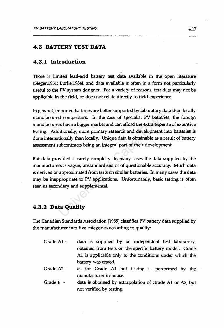
PV BATTERY LABORATORY TESTING 4.17
4.3 BATTERY TEST DATA
4.3.1 Introduction
There is limited lead-acid battery test data available in the open literature
(Sieger,1981; Burke,1984), and data available is often in a form not particularly useful to the PV system designer. For a variety of reasons, test data may not be
applicable in the field, or does not relate directly to field experience.
In general, imported batteries are better supported by laboratory data than locally
manufactured competitors. In the case of specialist PV batteries, the foreign
manufacturers have a bigger market and can afford the extra expense of extensive
testing. Additionally, more primary research and development into batteries is
done internationally than locally. Unique data is obtainable as a result of battery
assessment subcontracts being an integral part of their development.
But data provided is rarely complete. In many cases the data supplied by the
manufacturers is vague, unstandardised or of questionable accuracy. Much data
is derived or approximated from tests on similar batteries. In many cases the data
may be inappropriate to PV applications. Unfortunately, basic testing is often
seen as secondary and supplemental.
4.3.2 Data Quality
The Canadian Standards Association (1989) classifies PV battery data supplied by the manufacturer into five categories according to quality:
Grade Al -
Grade A2-
Grade B -
data is supplied by an independent test laboratory,
obtained from tests on the specific battery model. Grade Al is applicable only to the conditions under which the battery was tested.
as for Grade Al but testing is performed by the manufacturer in-house. data is obtained by extrapolation of Grade Al or A2, but not verified by testing.

PV BATTERY LABORATORY TESTING 4.18.
Grade C - scaled data. Derived on the basis of Grade A or B data, but
from batteries of different size or capacity.
Grade D - data other than defined for the above categories. It should
be evaluated for its validity and applicability for the given ' application.
This method of grading data is practical and concise, and is adopted for this
report. Most battery data finally used by PV modellers and designers is Grade
B or worse, as it must be extrapolated because of the difficulty in approximating
PV conditions.
4.3.3 Data Available from Manufacturers
Data most often found in the open literature is listed below. The order of listing
indicates the prospect of the data being available, and the data grading is shown
in parenthesis:
• nominal capacity at 25°C or 20°C (Al,A2)
• capacity as a function of discharge rate (Al,A2)
• capacity adjusted for temperature (A,B)
• discharge voltage profiles at one temperature (A)
• discharge cut-off voltages (A)
• self discharge rate (C)
• self discharge rate vs temperature (C, B) • cycle life vs DOD (B,C)1
• charge voltage (A,B)
• float charge voltage range (A,B)
• starting current for charging (C)
• finishing current for charging (C)
• charge voltage vs temperature (B)
• cycle life vs temperature (A,B,C)
Cycle life is usually presented versus DOD. Two test data points are usually available, and further points are extrapolated using models. Results depend strongly on which model is selected.

2
PV BATTERY LABORATORY TESTING 4.19
Data that is practically never offered is listed below. Its availability is usually the
result of specific requests.
• charging curves (A)
• charging efficiencies vs Temperature, Voltage (A)
• rate of water loss (where appropriate) (A)
• rate of acid stratification (A)
• overcharge requirements vs DOD (A,B)
4.3.4 Standards and Standardisation
Battery testing conducted by local manufacturers is mainly for quality control.
Typical tests conducted for either SLI or EV batteries2 are:
• High rate discharge: 3 second discharge @ SOOA, mainly applicable to
quality control of SLI type.
• Low temperature (-18°C) cranking test for SLI type.
• Capacity test @ various discharge rates.
• Overcharge test till failure: mainly applicable to SLI type. Of some
relevance to PV, but not directly transferable.
• Shelf life extremes 1,2,3 etc months at controlled temperatures.
• Life cycle (not directly transferable to the field).
• Other specific tests where requested.
· The focus of the tests is conformation to manufacturing standards (SAE for the
UK, DIN for Europe and SABS for South Africa). SABS standards for PV batteries
are non-existent, but standards are available for SLI and EV quality control. European and American standards exist only for PV installation and maintenance.
Discussion with Raylite Batteries

3
PV BATTERY LABORATORY TESTING 4.20
Battery characterisation standards exist (Canadian Standards Association,1989),
but the mandatory testing is limited and perhaps of questionable application in
the field3•
The introduction of standards has a further role over and above quality control,
which is to assist the manufacturers in offering data which conforms to
• specified formats, • according to specified and relevant test procedures, • and which allows transfer of the laboratory test data to real applications
outSide the laboratory environment.
Characterisation standards provide a means of ranking the batteries according to
their suitability for the application.
4.4 BATTERY TEST EQUIPMENT
4.4. l Broad Equipment Requirements
It is most often necessary to characterise a battery to aid component selection for PV systems development, or to generate characteristic data for computer
simulation. The battery data required may not be available from the battery
manufacturer, and the researcher may have to perform independent tests in the
laboratory.
The equipment needed to perform the typical battery characterisation tests (See Section 4.2) in a small scale laboratory environment is described below.
If only a few cells are to be tested at once, the power requirements are modest and the equipment is commercially available. If complicated test programme s
or high power tests are to be carried out, equipment is not always available or is expensive. The Battery Evaluation Laboratory at Sandia National Laboratories is
Canadian Standards specify a dynamic cycling test which is based on the cycling tests developed by Sandia Laboratories (see "cycle testing", Section 4.2.4). These test are not mandatory, and the focus of the Standards is on capacity, and average cycle efficiency during charge and discharge.

PV BATTERY LABORATORY TESTING 4.21
an example of a sophisticated system, with twenty test stations under computer
control and elaborate software for instantaneous performance readout
(Verado,1981). This system is beyond the means of most research budgets.
Kuiper (1989) has developed a versatile, small scale and lower cost battery test rig
suitable for battery characterisation and cycling.
a) Discharge testing
Voltage varies with SOC during battery discharging at constant-current. A
variable load is required to maintain constant-current or constant-power during
the discharge. If a resistive load is used, the resistance varies proportionally to
the voltage, and for constant power resistance varies as the square of the voltage.
For ease of testing it is desirable that the load be programmable so the discharge
current profiles can be easily maintained or changed.
Programmable solid-state or semi-conductor loads are commercially available in
the power ranges required. Most loads can be interfaced with a micro-computer
so discharge testing can be done under computer control. This is particularly
helpful for discharge testing under simulated load profiles, or for low current
discharge tests of long duration.
For constant current or constant power testing, the instantaneous load would be
programmed by a feedback signal derived from the measured battery current
and/ or voltage.
b) Charge testing
Equipment for charging batteries is commercially available for a wide range of
power requirements and resolutions. Equipment should be capable of constant
current and constant voltage operation. Both the current and voltage should be
adjustable. Interfacing the charging equipment with a micro-computer enables PV
charger simulation by feedback of the battery voltage and current. The
programmable charging capability can also be used for automatic correction of the
charging voltage for battery temperature, if a temperature sensor is interfaced to
the computer.

PV BATTERY LABORATORY TESTING 4.22
c) Temperature
Battery temperature is usually controlled during capacity determination, but in
overcharge testing is often an observed variable. A constant temperature water
bath is most often used in conjunction with a laboratory temperature controller. Basic controllers are widely available commercially; more sophisticated
controllers with a control and measurement interface to the computer can be
purchased.
d) Specific gravity
The SG of the electrolyte is important in lead acid battery testing. SG is normally
measured manually and intermittently using a hydrometer. Matsui (1987) of Yuasa Battery Co. has developed an optical hydrometer with digital output. With only a little adaption this device could be used for automatic SG data
capture on a computer or data-logger.
e) Software
Selection of suitable software for computer control is dependent on the type of
tests to be performed. In most cases the software can be quickly developed for
small scale systems. The software should include graphical outputs of selected
variables, automatic termination of cycles and easy programmability. The
frequency of data-logging (once every minute) does not necessitate especially high speed or complex software.
4.4.2 System Power-handling and Test Equipment Sizing
a) Programmable load
The programmable load should be capable of simulating typical PV load profiles,
as well as performing standard constant current/resistance/power discharges as described above.
•

PV BATTERY LABORATORY TESTING 4.23
The nominal system voltage of stand-alone PV systems is usually in the range
12-48V. Steady state load currents are typically in the range 0-lOA per lOOAh of
installed battery capacity for DC loads. Intermittent high discharge currents of
20-45A are possible when an inverter is used, or due to surge currents during DC
motor start-up. High inverter currents are typical of low voltage systems.
In some battery ranges (tubular cells) the smallest cell available for testing may
be 200Ah capacity. The programmable load current requirements for such a
battery are doubled, though, of course, scaling should be used where possible.
Scaling is of limited potential when strings of batteries are under consideration,
where it is advantageous to test the string as a whole. This is more economical
than conducting separate tests on each cell, and enables effective collection of
statistical data.
A programmable load capable of sinking 45A at 12V (the low voltage case), and
approximately 30A at 48V (60V nominal) should cater for most cases.
b) Power supply
The programmable battery charger should operate under constant current or
voltage control; and be capable of simulating PV array charging. The charger
should complement the programmable load: it should be capable of simultaneous
connection to the battery under test without danger of short-circuit · or
malfunction.
The charging voltage of small stand-alone PV systems typically ranges between
15-60V for 12-4BV systems. Operating currents are normally kept below 15A by
increasing the system operating voltage. For testing batteries of nominal capacity lOOAh, the charger should be capable of sourcing 0-lOA. For larger batteries, the
required current is scaled proportionally, eg. lOA/lOOAh. The charger should be
capable of charging entire strings of batteries (12-48V) to complement the
programmable load. 2V cells of 200Ah capacity are capable of sinking 15A even
under float charge mode. Three 2V cells are likely to be tested in series
connection to provide sufficient voltage for programmable load operation. Under
equalisation charge mode (parallel connection), these three cells will together sink at least 45A.

PV BATTERY LABORATORY TESTING 4.24
The charger should be capable of sourcing 45A at 3V (2V nominal) and lSA at 60V (48V nominal). If two supplies are available, then one precision supply in the
10A/60V range, and a lower precision supply in the SOA/36V range would
suffice.
c) Accuracy and precision
The desired programmable accuracy of the test equipment is generally specified as better than one percent over the entire range. The precision should be of the
same magnitude. The current measurement resolution required is the lesser of one percent or 20mA for both charge and discharge. The voltage resolution is
particularly crucial, as it is voltage change that is important. Voltage resolution should be within one percent or ±lSmV.
d) Temperature
Temperature effects are not particularly important over small ranges (1-2°C). Temperature control of the battery within ±1°C of the set value, and measurement of the electrolyte within ±0.5°C is sufficient.

CHAPTER 5
EQUIPMENT DESIGN
5.1 INTRODUCTION AND OVERVIEW OF REQUIREMENTS
Equipment requirements for small scale laboratory testing and battery
characterisation are discussed in detail in Section 4.4. The overall system
requirements have been specified as:
1) A micro-computer controlled battery test unit, with variable ·charge
and load cycling and automatic data capture. Software controls power
electronics to simulate PV system charge and discharge regimes.
2) A programmable DC power supply capable of sourcing 50A at 60V,
for a maximum power of 3000W. A matching programmable load
capable of sinking SOA at 12V, 30A at 60V for maximum power of
1800W.
3) Resolution for control and readback of battery voltage, supply current
and load current is to be better than 0.5%, with programmable
accuracy and precision to be better than 1 %.
4) A water bath to allow battery temperature control, and sensors to read back the water temperature to the computer.
The overall system layout is shown in Figure 5.1. The equipment design is
discussed sequentially, beginning with the electronics of the programmable load
and power supply, then the computer interface, control software, and temperature
control.
5.1

EQUIPMENT DESIGN: AN OVERVIEW 5.2
PC
SOFlWARE CONTROL
OATA LOGGING - --j INTERFACE INSTRUMENTATION
GRAPHIC OUTPUT I - - - __ _J _ - - - _ _l_ _ - -I A I I
POWER SUPPLY 0-- -\_F -0 PROGRAMMABLE LOAD I I I
SIMULATED
Pl/ SOURCE
THERMAL CONTROL
-·~' i BATTERY
UNDER
TEST
WATER BATH
LOAD SIMULATOR
I ______ _J
0
Figure 5.1 Block layout of the programmable battery test unit. Dashed lines indicate communication linkages. !=current, V=voltage, T=temperature.
The remainder of this chapter is concerned with test equipment design as follows:
5.1 Overview and selection of appropriate electronic design
5.2 Electronic design and component selection
5.3 Software requirements and design
5.4 Thermal control and measurement
5.1.1 Overview of DC Power Supplies and Loads
.. Many laboratory electronics equipment suppliers can provide excellent DC power
supplies and loads (Burke,1984:954). However, this apparatus is typically over
specified for battery testing, and is generally very costly. Suitable equipment can
be built in-house at lower cost, although there may be a significant equipment set
up time.
A broad range of basic el~tronic designs is available for DC power supplies and programmable loads. These are tabulated, listing the advantages and
disadvantages of each particular power electronics design.

EQUIPMENT DESIGN: AN OVERVIEW 5.3
Table 5.1 Overview of electronic load designs.
DESIGN DISADVANTAGES ADVANTAGES
Transistorised Load semi-conductor prevents full current low power requirement if FET driven
operation at low voltages
bulky due to transistors to dissipate simple to design
heat low cost
Digitally Switched bulky - large number of resistors operates at low voltages if required
Resistive Load high cost: precision resistors and extremely rugged
contactors
SCR Mains cost: requires professional to construct low heat dissipation: power
Regenerative regenerated to mains
cannot operate at very low voltages rugged SCR components
some research still required elegant solution
Table 5.2 Overview of DC power supply designs.
DESIGN DISADVANTAGES ADVANTAGES
SCR and Filter large filter required to eliminate mains uncomplicated to assemble
frequency voltage ripple
battery is an active component in filter, moderate response
causing battery heating
Series Linear high power dissipation over series high precision
Regulator transistor, low efficiency
bulky, large number of transistors to easy to design and construct
overcome heating very fast response
Switch Mode cannot operate at zero output current high precision in designed operating
Regulator (swinging choke saturates) region
tricky to design, build and protect small and compact, high efficiency
(80%)
output noisy, contains spikes fast response to load and line changes
Series Linear bulky, essentially two supplies in lower power dissipation over
Regulator with series; both SCR and low dissipation, transistors, higher efficiency than
SCR Tracking Pre- high current, linear regulator linear regulator
regulator more difficult to design, two control fast response
loops to consider
linear response slowed by pre- high precision industry standard
regulator design

EQUIPMENT DESIGN: AN OVERVIEW 5.4
5.1.2 Design Choice
a) Programmable load
The selected design is a transistorised electronic load operating as a current si?k,
with a grounded high current supply, which is actually the battery under test.;
The load is controlled by a 0-lOV analog signal, with analog current readback of 0-lOV for both current and voltage. The voltage programmable load is calibrated
to sink SOA for a lOV input. Load current can be read from the control panel.
The transistorised load is preferred to the other options on the grounds of
simplicity and cost. The cost is estimated at RlOOO. The resistive load design is estimated to cost RSOOO, mostly due to precision resistor windings and DC
contactors required for switching. The SCR mains regenerative device requires
further substantial development. The transistorised load is an industry standard
design which has superseded the more bulky resistive set-up (Hewlett-Packard, 1989).
The design of the programable load is covered in Section 5.2.1.
b) Power supply
The preferred design is a linear power supply with SCR tracking pre-regulator
using the grounded load configuration, with return line current sensing. The
power supply operates as a constant current source, and is calibrated to source
0-SOA for a 0-lOV analog input signal. Output current is read back by a 0-lOV
analog output signal. Simultaneous output to instrumentation is required.
This particular design is the only reasonable choice under the required range of operating conditions for the following reasons:
the power dissipation requirements are simply too high for a linear series pass regulator,
all advice recommended strongly against attempting to build a switch mode supply (Horowitz et al,1980:211).
The SCR rectifier, even with a filter, could generate sufficient mains frequency ripple current to cause heating to the battery under test,

EQUIPMENT DESIGN: AN OVERVIEW 5.5
thereby casting doubt over the suitability of the similar SCR mains
regenerative device as well. Although the regulator with pre-regulator is bulky, the efficiency is
moderate and the output quiet, with low noise and ripple. The supply
reacts quickly to line and load changes.
The SCR tracking pre-regulator with linear regulator design is an industry
standard for precision power supplies that are required to operate over a broad range of voltage and current conditions (Hewlett-Packard,1989; Fry,1973).
As the power supply consists of several discrete subsections, the power supply
design is covered linearly, beginning with the output stage in Sections:
5.2.2 Output stage, the linear regulator
5.2.3 LC filter 5.2.4 Tracking SCR pre-regulator
5.2.5 Isolation transformer
Safety considerations for the electronic load and power supply are discussed in
Section 5.2.6.
Figure 5.2 is an overview diagram of the load and power supply, and shows the
layout and main design sections.
TRANSF"ORP1ER LC F"ILTER
SCR REC TI F"I ER LINEAR REQULATOR
A4048
BATTERY
.1
.1
.1
PROQRAP1P1ABLE LOAD
A102A
Figure 5.2 Electronic design components of the battery test unit.

EQUIPMENT DESIGN: AN OVERVIEW 5.6
c) Electronics I computer interface
The programmable power electronics cannot be designed· without discussion of
the computer interface. The E.agle PC-30A/D-DAC Interface was selected for this
purpose. This versatile and simple, off-the-shelf card plugs into one expansion
slot of the IBM PC/XT I AT compatible computer, is favoured over a one-off design, or to interfacing to the power electronics via a parallel port interface and
analog/ digital converters mainly because of its quick set-up time. The parallel port interface option would only provide 8 bit resolution if a PC were used. A 16 or 32 bit machine is not justified for a single test rig, though for multi-tasking
the speed is required and the resolution is a valuable spin-off.
The PC-30 provides sufficient features and digital resolution for the control and readback signals. These are:
programmable load control; SOA, 12 bit DI A
programmable load current readback; SOA, 12 bit A/D
programmable load voltage readback; 60V, 12 bit A/D
power supply current control; SOA, 12 bit DI A
power supply current readback; SOA, 12 bit A/D
temperature readback, 2 off; 12 bit A/D
Section 5.2.7 covers computer interfacing and control.

EQUIPMENT DESIGN: PROGRAMMABLE LOAD 5.7
5.2 ELECTRONIC DESIGN
The electronic design is divided into six major sections. These are discussed as
follows:
5.2.1 programmable load design
5.2.2 power supply, output linear series regulator
5.2.3 power supply, LC filter
5.2.4 power supply, SCR pre-regulator
5.2.5 power supply, power transformer
5.2.6 safety circuits and switches
5.2.1 Programmable Load Design
a) Transistorised load - general description of operation ·
v J.n
Figure 5.3 Transistorised load operation
VI
.=_BATTERY
The battery provides the load voltage, Vu to the collector of transistor 0101. The
control voltage, Vin (0-lOV), is at the positive input of op-amp AlOlA. The op
amp provides base current to 0101, such that the voltage drop across resistor
RlOl is equal to Vin, by negative feedback. The current from the load is therefore
under linear control. The main limitation is the heat dissipation over 0101, which
is in reality an array of transistors.
b) Power transistors
The low cost 2N3442 NPN power transistors were chosen for the current sink
(specifications in Appendix E). The low cost 2N3442 has moderate current gain,

EQUIPMENT DESIGN: PROGRAMMABLE LOAD 5.8
and can dissipate up to 1 lSW at DC. There is no danger of second breakdoWn
at the maximum load voltage of 60V.
Heat dissipation of the array
The maximum electronic load current is SOA, and the maximum power handling
capability is 1.6kW over the transistor bank.
Calculations based on specified thermal resistances suggest that each 2N3442 can
dissipate 97W when derated for case temperature of 55°C.
The real heat dissipation was determined experimentally for six transistors mounted on a SOcm length of heavy duty heatsink cooled by forced convection. Under these conditions the maximum power dissipation per transistor is only
SSW. The actual case temperature under these conditions is 104°C at ambient
temperature of 40°C. The discrepancy in power dissipation is due to limitations
in the heatsink heat transfer convection coefficients. The transistors are certain of
safely dissipating a conservative 45W of heat even at ambient temperatures of 40°C. (See Appendix E for details of experiment and calculations).
Assuming 45W dissipation, the maximum power dissipation for six transistors is
270W per SOcm heatsink. Therefore six SOcm heatsinks, or 36 transistors, are needed to dissipate 1600W of heat. At the maximum load current of SOA, the
current per individual transistor is 1.39A, well within the SOAR (see Appendix E).
This conservative estimate of transistor power dissipation pays dividends in terms of current gain and base drive requirements.
Current gain
The DC current gain (HfJ is both temperature and collector current dependant, and is conservatively assumed to be 30 at the maximum current of 1.39A per transistor. The 36 individual transistors are connected in parallel to form the load array, which is assumed to have the same current gain. It follows that the base drive current for the transistor array is 1.66A at rated current.

EQUIPMENT DESIGN: PROGRAMMABLE LOAD 5.9
The base current to the load array is elegantly provided by MOS technology, the
power FET MTM15N45 is an N-channel enhancement mode device. The voltage
driven FET has the advantage of exerting no load on the op-amp. The FET easily
dissipates 3A at 60V at case temperatures approaching 60°C, but for safety the
FET is not mounted on the same heatsinks as the load array. The FET has
suitable on-region characteristics right down to V ns of 2V. (See specifications in Appendix E).
R47
Rbe
F109 - F114
R47 R47 R47 R47 R47
Re
Figure 5.4 Load transistor array with FET driver
Figure 5.4 shows the complete load array. This design is formally called a
"bipolar transistor booster". The emitter resistors (RJ are added to ensure that
each transistor carries the same current and heat load. The resistor (Rbe) from
base to emitter of the 2N3442 array improves array response as well as preventing
the FET leakage current from biasing the transistors into conduction.
The actual load array current gain at SOA was experimentally determined to be
40, and the graph of load array DC current gain is shown in Appendix E for
comparison with the data sheet.
c) CUrrent feedback measurement
The 0-SOA load current operating range requires a special measurement circuit to
ensure 1 % accuracy over the entire range. This can be achieved either by using
a low power current sensing resistor with expensive high gain instrumentation
amplifiers, or a larger high power and temperature stable resistor with more basic

EQUIPMENT DESIGN: PROGRAMMABLE LOAD 5.10
amplification. High gain amplifiers will degrade the feedback frequency response
of the constant current source.
Power resistor
Alkrothal temperature-stable wire rated for 1 % deviation at 30D°C was wound into a high power resistor which provides lV at SOA and dissipates SOW.
Experimental evidence shows that a stable temperature of 12D°C at SOA can be
maintained with fan cooling.
Current feedback measurement circuit
A differential amplifier amplifies the voltage signal from the current sensing resistor, even though the current sensing resistor is earthed. The differential configuration improves precision, since at high currents ·the spurious voltage
drops through the wiring between power resistor and earth become significant.
Figure 5.5 shows the basic current sensing amplifier. Note the trimming circuit
for trimming the input offset voltage so that the output of the amplifier can be zeroed. The versatile LM358 was chosen as it can be powered from a· single
supply, and the inputs can go all the way to ground, and even to 300mV below.
The gain is set at ten, so that the lV resistor signal is amplified to a lOV signal suitable for feedback.
Y C 12Y
lOOR
lOOR
7Y2 0101 ZENER
lR
lR
OR02
R101 POWER RESISTOR
lOOR
1.K V out: lOOR RA101
Figure 5.5 Load current sensing and feedback amplifier

EQUIPMENT DESIGN: PROGRAMMABLE LOAD 5.11
d) CUrrent control loop and stability
The high performance of the current sink control loop shown in Figure 5.3
depends on a high closed loop gain (CLG), in turn dependant on the gain of
amplifier AlOlA. This amplifier musfin differential configuration and the gain
is set nominally at 33. An LM358 single supply op-amp is used. Resistors are
chosen to ensure input impedance matching at the main control amplifier. The
control loop is shown in simplified block format in Figure 5.6.
com12onent
A101
0101
R101
A102
Figure 5.6
gain
A1=33
A2=50A/7V
A3=1V/50A
A4=10
FREQUENCY COMPENSATION
break QOint
bp=30kHz
bp>1MHz
no bp
bp=100kHz
Block diagram of load control loop
0101
R101
The gain of the load array was experimentally determined, and observed on a
digital storage oscilloscope to have excellent frequency response characteristics
beyond lMHz.
= 33 x SOA/7V x lV /SOA x 10 = 47 = 33dB
with breakpoints at 30kHz and lOOkHz.

EQUIPMENT DESIGN: PROGRAMMABLE LOAD 5.12
The Bode plot for the current control loop shows instability at frequencies beyond
lOOkHz due to the CLG roll-off at -12dB per octave. Some feedback compensation
is required.
33.4d8
30
23.0dB 20~··········''"H;•+ '++•+;;;~ ' 'iii
0'--..L..-1.-L-1..J..U..U..--l'--L-............ .........__.._._.._............_'--'-......... .LI..U....__~_,__,_,............,
0.1 10 100 1000 10000
frequency (Hz)
Figure 5.7 Bode plot of CLG before and after frequency compensation.
Lead-lag compensation is the most suitable in this case. The pole and zero are
marked on the Bode plot, which has a compensated gain roll-off of only -6dB per
octave. The frequency of the pole (fp) is 2.24kHz, and the frequer,icy of the zero
(f2 ) is 30kJ::Iz. The component values of the capacitor (ClOl) and resistors (R102,
R103) of the lead-lag network are calculated in Appendix E. The circuit diagram
of the complete control loop is displayed in Figure 5.8.
R102
:>.....-'-----"'6S"V4R'-r---------.r QNP.tBN1 C101
222PF
1001< RA101
.lu
R103 S6R
10k
10k lk
lk
Figure 5.8 Electronic load control loop circuit.
R101

EQUIPMENT DESIGN: PROGRAMMABLE LOAD 5.13
e) Protection
Current limiting
Simple current limiting is all that is required, since when the input to the current
sink is shorted to ground no current can flow. The current limit operates by
using the signal directly from the current measurement resistor (RlOl), buffered
by a unity gain op-amp. The op-amp output is adjusted by a trim-pot onto the
base of a transistor, which pulls down the control voltage of the main control loop
when current limiting is effected. The minimum current limit setting is about
30A.
Overcurrent protection
There is a further comparator circuit which normally provides base current to a
transistor that supplies the coil of a reed switch which controls input power to the
entire electronic load. When the load current resistor signal exceeds a set
reference (equivalent to 60A) the base current is removed, consequently tripping
out AC power to the entire system. The switches are shown in Section 5.2.6.
Finally, fuses are liberally placed to prevent runaway overcurrent. Most
importantly they are located on the load array, positioned at the drain of the FET
(2.5A) and one fuse (lOA) for every five 2N3442 transistors. The layout is shown
in Figure 5.4.
Power limiting
At voltages below 32V the current limit of SOA keeps power dissipation below
1600W. Additional current limiting is required at higher voltages. This is most
easily accomplished by software, rather than auto-ranging hardware, where the
product of measured voltage and current is kept within the power range by
limiting the output current set value.

EQUIPMENT DESIGN: PROGRAMMABLE LOAD 5.14
Q Measurement and instrumentation
Current readback measurement
The output signal from the current feedback amplifier (A102) cannot be used
'directly ~s input to an AID converter or long instrumentation lines without
affecting the feedback response, unless the signal is buffered. Further
amplification and trimming circuits f~r measurement, instrumentation and
accurate AID conversion are required. These are shown in Figure 5.9.
Cu,..r•nt 1'1•asur"'•rnent
B2k ~L-..-~vv-....----.----- ADC
1K RA1D6 1u
Figure 5.9 Buffered output current signal to AID and instrumentation from electronic load.
The feedback signal is fed to a buffer amplifier (A103D). The gain is set to give
a lOV signal at full current which is suitable for direct AID conversion. The same
lOV signal is divided down by pot R107 to give the SOOmV at SOA signal required for the panel instrumentation (lOmV=lA).
Voltage measurement
Voltages observed during battery testing typically do not vary by more than 20
percent on either side of the nominal. It is therefore important that small changes
in voltage are accurately detected. In particular, experiments measuring the
temperature effect on battery voltage are important. The use of a high quality temperature compensated amplifier is justified in this case.
The specified input voltage range is 0-60V. For a 12V battery, the variability of
voltage is usually 10V-14V .. Resolution and stability are of prime importance.
The complete measurement circuit is shown in Figure 5.10, together with a zero

EQUIPMENT DESIGN: PROGRAMMABLE LOAD 5.15
offset trimmer. This configuration requires a split supply, and the op-amp is
powered from a +12V -5V supply.
Figure 5.10 Voltage measurement circuit

EQUIPMENT DESIGN: POWER SUPPLY 5.16
5.2.2 Power Supply Design, The Output Stage
Serles Pass Regulator
It is conventional to begin the design by starting with the output stage, ensuring
that specifications are realised, then working back towards to the input stages, allowing for inefficiencies on the way (Fry,1973). The main electronic design
components are shown in Figure 5.2 in Section 5.1.2.
a) Linear current regulator - overview of operation
Q201 0201 Vdc u_n,._•<>_ul_••_•_d _• -------.NP_N _____ ___,
DIOOE
- BATTERY
R2Dl
Figure 5.11 Linear regulator, principle of operation
The SCR pre-regulator provides the rectified but unregulated power to the
collector of transistor Q201. The control voltage, Vin (0-lOV), is at the positive
input of op-amp A201A. The op-amp provides base current to Q201, such that
the voltage drop across resistor R201, amplified by op-amp A203A, is equal to Vin· Op-amp A203A simply ground references the current signal, which would otherwise be negative.
The result is a voltage programmable DC current source. As with all linear
regulators, the series transistors are most vulnerable to overheating.
b) Power transistors
2N3442 NPN power transistors were selected, as for the programmable load.

EQUIPMENT DESIGN: POWER SUPPLY 5.17
Heat dissipation in the transistors
The current rating for the regulator is SOA, and it is assumed that the pre
regulator maintains the voltage drop over the transistors at less than lOV. Then
the maximum power dissipation over the transistor bank is SOOW.
When six transistors are mounted per SOcm heatsink, each transistor can safely
dissipate 45W of heat even at ambient temperatures of 40°C. Therefore two such
heatsinks are required to dissipate SOOW of heat. For safety, 3 heatsinks are used,
giving a total of 18 transistors. At the maximum load current of SOA, the current
per individual transistor is 2.77 A, and this well within the SOAR (see
Appendix E).
Current gain
Assuming a conservative transistor gain of 30 at the maximum individual
transistor current of 2.77 A, the base drive current for the transistor array is l.66A
at rated current.
The base current to the regulator array cannot be directly supplied from the op
amp because the transistor base voltage requirements will in most cases be higher
than the power supply to the op-amp. The problem is easily resolved by driving
the power supply array with a PNP transistor, which is driven by a ground
referenced NPN transistor. (Figure 5.12).
Collector"' Emitter
. B•••
R
Figure 5.12 Linear regulator base drive arrangement
The PNP transistor selected is the MJ802 (Q203). The MJ802 easily dissipates 2A
at 60V at case temperatures approaching 60°C, but for safety the PNP is not

EQUIPMENT DESIGN: POWER SUPPLY 5.18
mounted on the same heatsinks as the regulator array. The DC current gain is
estimated to be 30. The base current to be removed from Q203 is a maximum of
55mA.
The PNP complementary transistor is driven by a TIP31C NPN power transistor
(Q202), capable of dissipating 35W at case temperatures of 45°C. The DC current
gain of the TIP31C at collector current of 55mA is close to 150, so the maximum
current to be supplied by the op-amp (A201A) is less than lmA. The collector
current through the TIP31 C is limited to a safe 0.5A by an emitter resistor of 22
ohms, which operates by pinching Vbe to less than 0.6V.
FIGURE 5.13 shows the complete power supply array and base drivers. The
design is formally named a "complementary Darlington".
F'201. F'202. F'204
Q202 COLLECTOR
F'USE
Figure 5.13 Linear re~ator array.
R47 R47 R47 R47 R47
The actual 2N3442 array current gain at rated current was experimentally
determined to be 35, and the graph of regulator array DC current gain is shown
in Appendix E for comparison with the data sheet.
c) Current feedback measurement
Similar problems apply to the power supply as to the programmable load, and the
same solutions were adopted, namely a high power resistor with modest amplification.

EQUIPMENT DESIGN: POWER SUPPLY 5.19
CUrrent feedback measurement circuit
The power resistor is positioned in the circuit for "return line current sensing".
It· is important to see that only the linear regulator current is sensed, and. base
drive current from 0202 is not included.
V unreoulated
.=_BATTERY
R201
Figure 5.14 Return line current sensing
A unity gain differential amplifier (A305A) is used to amplify the voltage signal
from the current sensing resistor. Figure 5.15 shows the basic current sensing
amplifier which operates below ground, with a maximum negative input voltage
of-1 volt. As the amplifier can handle only-300mV input from a positive supply, a split supply is required ( + 12V, -SV).
V C 12V
lODR
100R
7V2 0202 ZENER
VCC 12V
lR lOOR
lR
VCC -SY
OR02
R201 POWER RESISTOR
Figure 5.15 Current sensing amplifier
lK RA203
V out

EQUIPMENT DESIGN: POWER SUPPLY 5.20
d) CUrrent control loop and stability
The performance of the current source control loop depends on a high closed loop
gain.(CLG). The gain of differential amplifier A201A is set at 44.
The CLG (calculated as for the programmable before) is
= 44 x SOA/SV x lV /SOA = 8 = 19.SdB
with a breakpoint at 29kHz.
Figure 5.16 illustrates the Bode plot for the current control loop, which is
inherently stable at frequencies below 264kHz.
0.1 10 100 1000 10000
frequency (Hz)
Figure 5.16 Bode plot for linear regulator
e) Protection
CUrrent limiting
The current limit operates by using the signal directly from the current feedback
amplifier. The signal is adjusted by a trim-pot AR202 onto the base of a transistor, which pulls down the control voltage of the main control loop when
. current limiting is effected. The minimum current limit setting is about 20A.

EQUIPMENT DESIGN: POWER SUPPLY 5.21
Overcurrent protection
Fuses are liberally placed to prevent runaway overcurrent. Most importantly they
are located on the regulator array, positioned at the collector of the NPN (2.5A)
and one fuse (lOA) for every six 2N3442 transistors. The layout is shown in
Figure 5.13.
t) Current measurement and instrumentation
A buffered signal from the current feedback amplifier is used directly by the AID
converter and instrumentation, as for the programmable load.
5.2.3 Power Supply l)esign - LC filter
The main overview sketch of the test unit (Figure 5.2) shows that the linear charge
regulator is fed by a SCR pre-regulator. SCR rectifiers regulate voltage by
adjusting the phase angle at which SCR firing occurs, usually causing sharp
spikes in the output waveform. Not even a fast linear regulator would be able
to smooth such sudden peaks, so it is necessary to remove the steep rise of the
SCR output by filtering.
The LC filter is usually used for SCR output filtering, as it filters both current and
voltage. The filtering of the LC filter is given by
For SCR rectification, the second harmonic is the dominant source of distortion
at all firing delay angles (Figure 5.17), and this harmonic should be eliminated as
far as possible. The frequency of the second harmonic is lOOHz.
If the filter is to provide unity gain at lOHz, then we can solve for L given C.
Details of the calculation are given in Appendix E.
The final component choice for the filter is C301 = 30000uF, and L301 = 8.4mH.

EQUIPMENT DESIGN: POWER SUPPLY
voltage harmonica (rma) 70
60 mean
60 /
30
20
10
second harmonic
----.. -.. "' -------..
alxth harmonic
O'--~~,__~~-'--~~-'-~~-'--~~-l---",,....~
0 30 60 90 120 160 180
firing delay angle (degrees)
5.22
Figure 5.17 Harmonic content of SCR rectifier, 60Vnns input.
(Source: Lander,1981:270)
5.2.4 Power Supply Design - SCR Tracking Pre-regulator
The SCR pre-regulator has the role of rectifying the AC input voltage, and
maintaining the rectified voltage for a fixed voltage drop over the linear regulator,
regardless of regulator output. It is necessary to keep the voltage drop to a
minimum to prevent heating of the series pass transistors in the linear regulator.
a) SCR tracking pre-regulator - overview
AC
SCR
PHASE ANGLE
CONTROLLER
SCR
RECTIFIER
OPTO
ISOLATOR
FILTER
Vref
LINEAR CHARGE DC
REGULATOR
Figure 5.18 SCR pre-regulator, principle of operation

EQUIPMENT DESIGN: POWER SUPPLY 5.23
Differential amplifier A4A senses and amplifies the voltage drop over the linear
charge regulator. The amplified voltage drop is compared with the reference
voltage Vrei. in A4B, and the A4B's output drives the SCR phase angle controller.
For safety reasons the SCR phase angle controller is programmed through an
optical-isolator. The phase angle controller provides gate pulses to the SCR
bridge rectifier to pre-regulate the input voltage to the linear regulator as
required.
b) Altronics AM024 SCR converter
The Altronics AM024 SCR converter is an off-the-shelf board used for gate control
of SCR output. It has analog inputs and outputs, with digital logic circuits. It is
more than a simple phase angle controller, in that it has the following extra
features:
linear operation (input-output voltage is linear, rather than output-phase
angle being linear with input voltage).
maximum and minimum SCR output voltages can be set
maximum SCR current can be set
maximum SCR output dV I dt can be set
The main disadvantage with this card is that the inputs are not isolated from the
rest of the board, and an opto-isolator must be used in series between the
controller and any other control circuitry to prevent ground earths or shorting.
c) Optical isolator
An optical isolator was supplied by Altronics. A grounded DC differential signal,
is input, and the output is a floating differential signal that is isolated from the input by a transformer. There is some DC-AC-DC conversion on the way.
This isolator is versatile; it can accept inputs of 0-lOV, and provides floating
outputs of adjustable range, with an adjustable output minimum voltage as a
percentage of the range.

EQUIPMENT DESIGN: POWER SUPPLY 5.24
ISOLATED SIGNAL
SET RANGE
I SET MINIMUM VALUE
/ DC INPUT 0-10 V RANGE
DC GROUND
Figure 5.19 Altronics opto-isolator
d) SCR tracking circuit
The SCR tracking circuit overviewed in Figure 5.18 works on a feedback basis.
Its closed loop response time is not very fast, nor is it easy to pinpoint. It is easy
to see why the response time is slow without doing a thorough analysis:
the LC filter begins to roll-off from DC at lOHz
the Altronics AM024 converter has maximum dV /dt of 30V /s
the SCR can only respond every SOHz (once per cycle)
the SCR rectifier has inherent time· delays
V+ V-
S6K S6K
lOOK
lOOK lOK lOK
PC on/off't
lOOK
lOOK
A404A
YCC 12Y
22R
100K
RA410
Figure 5.20 SCR tracking circuit
lOK
lOK
100K
lOOK
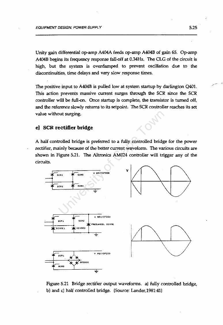
EQUIPMENT DESIGN: POWER SUPPLY 5.25
Unity gain differential op-amp A404A feeds op-amp A404B of gain 65. Op-amp
A404B begins its frequency response fall-off at 0.34Hz. The CLG of the circuit is
high, but the system is overdamped to prevent oscillation due to the
discontinuities, time delays and very slow response times.
The positive input to A404B is pulled low at system startup by darlington Q401.
This action prevents massive current surges through the SCR since the SCR
controller will be full-on. Once startup is complete, the transistor is turned off,
and the reference slowly returns to its setpoint. The SCR controller reaches its set
value without surging.
e) SCR rectifier bridge
A half controlled bridge is preferred to a fully controlled bridge for the power
rectifier, mainly because of the better current waveform. The various circuits are . shown in Figure 5.21. The Altronics AM024 controller will trigger any of the
circuits.
v
V RECTIF"ZED
BRIDGE
Figure 5.21 Bridge rectifier output waveforms. a) fully controlled bridge, b) and c) half controlled bridge. (Source: Lander,1981:41)

EQUIPMENT DESIGN: POWER SUPPLY 5.26
A half controlled bridge consists of two SCR's and a diode bridge, although the
same control as for four SCR's is required (see Figure 5.2l(b)). A free-wheel
(commutating) diode is required to provide a reverse current path for the SCR's
to regain their blocking states. In Figure 5.21(c) the bridge diodes double as
commutating diodes. The load voltage is always positive due to the presence of
the commutating diode. The half controlled bridge has a characteristically more
distorted input current waveform, and requires a larger isolation transformer on
the input.
The diode bridge selected is the AEG B2 250-30Si. This silicon bridge handles
250V and is rated at 30A continuous per diode. When connected as in
Figure 5.21(c) the diode bridge has a continuous rating of 60A. The SCR block
selected is the AEG TI45N 200 K power block, capable of lOOA maximum and
SlA continuous at 60°C. Maximum voltage is 200V, with gate turn-on typically
at 1.4V and 120mA. (see Appendix E for specifications).
The entire bridge is mounted on a large natural convection heatsink.
t1 SCR minimum load circuit
During testing of the SCR output it was observed that at very low currents the
SCR's failed to trigger on every AC cycle, resulting in current pulses of irregular
frequency. As the LC filter can only efficiently filter ripple of regular frequency
it is not surprising that down-the-line effects on the output of the linear
charge regulator are observed.
Further monitoring showed that a mean holding current of 7 A is required to
ensure that the SCR's are fired every cycle. This is mainly caused by the LC filter,
which has a ripple current of 7 ~eak (See LC filter in the Appendix E). To ensure
even and regular current SCR current flow, the mean current through the filter
must be greater than the ripple current.
A dummy load, consisting of two 2N3442 transistors driven by a TIP31C (Q402),
draws current in parallel to the linear regulator. The circuit operates to ensure
that at least 7 A flows through the low power resistor R401. The current flowing
through the dummy load does not affect current measurement for the linear regulator.

EQUIPMENT DESIGN: POWER SUPPLY 5.27
INDUCTOR Q201 ,..-------r---t-_,..L~30~1'--,...--+--'VV'---,--i------,:NP----~~
BRiroE
SCR RECTIFIER SCR FILTER
C301 CAP
DUP1MY LOAD
Figure 5.22 SCR minimum load circuit location
Q4D2 NPN
R201
; LINEAR . RECOULATOR
- BATTERY
The circuit to maintain the minimum current is shown in Figure 5.23. Pot RA406
is used to adjust the minimum current.
10k Y-
Y+ 10k
100k
220k
2k 10k RA40S ~----"'v'V'--"-1
100k
YCC 12Y
4YS D402
lK
10k
220k
lK
RA406
Figure 5.23 SCR minimum load control circuit
Although lower LC filter ripple current could have been achieved by using a
more expensive filter. (see Appendix E, LC filter design), the need of the dummy
load could not be totally eliminated as there is always some ripple.

EQUIPMENT DESIGN: POWER SUPPLY S.28
5.2.5 Power Supply Design - Isolation Transformer
The whole DC power supply should be isolated from the AC mains supply for
safety reasons. Additionally, the single phase mains supply can only normally
provide lSA at 220V, so some form of step down, current boosting transformer
is needed to achieve SOA DC output. The basic sizing for transformer TS follows.
Power transformer sizing
Transformer Primary V rms,primary = 220V
~s.primary = lSA maximum
Transformer Secondary For ~s.secondary = SOA
then
V rms,secondary .i 66V rms
and
Vs.max .i 93.3V
Vs.mean .i S9.4V
If Vs.mean is S9.4V, with losses over the regulator of 2.0V and similarly 2.0V over the SCR , then the maximum obtainable power supply output is SS.4V. This
estimate of the output voltage does not allow for mains voltage fluctuations, wM
which can be up to ± 1S% of the nominal. A constant voltage transformer found
to be extremely costly and therefore rejected.
Further, the transformer power rating should compensate for the distorted (non
sinusoidal) input current typical of half~ontrolled rectifiers. This factor is used to increase the core rating of the transformer. A factor of 20% is used.
The final sizing for transformer TS is
primary winding
Vp=220Vrms
lp=lS~s
secondary winding
Vs=66Vrms
ls=SOA
kVA rating is 220Vx1SA = 3.3kVA
compensated by 20% = 4.0kVA

EQUIPMENT DESIGN: SAFETY CIRCUITS 5.29
5.2.6 Auxiliary Equipment, Safety and Layout
In this section the safety requirements of both the power supply and
programmable load are considered.
a) Auxiliary power supplies
The control electronics of the load and power supply each require a 12V supply
capable of O.SA, and a low power -SV rail for the current sensing amplifiers.
·These are provided using 3-terminal regulators and standard circuits. The T8606
. inverting regulator is interesting because it uses capacitive pumping to generate
a negative rail from only a positive supply.
12V STABLE
100u 100n
W0-02
12V DC INPUT
Figure 5.24 Auxiliary power supply for control electronics
The SCR-controller is equipped with its own power supply operating directly off
the mains. As the rectifier is to run off a nominal 60V nns secondary of TS, it is
safer to take the 60V output and transform it back to 220V using T4, rather than
connecting directly to the mains (see Figure 5.26). For one, this approach ensures
that the SCR controller and the SCR's are always in phase.
b) Instrumentation and instrumentation power supply
An Eagle Electric digital volt meter (DVM) range 0-2V was selected for the panel
instrumentation. A selector switch allows either programmable load current or

EQUIPMENT DESIGN: SAFETY CIRCUITS 5.30
power supply current to be displayed. The DVM inputs are not isolated from its
power supply inputs, so a dedicated and isolated 5V power supply is provided
to enable the inputs to float above ground. Once again a 3-terminal regulator
rated at 500mA and standard circuitry is used.
SV DC STABLE
22DDu J.Du
Figure 5.25 Instrumentation power supply
c) Fuses and safety
Fuses are liberally placed to prevent accidental bum-out of major equipment.
These are shown in Figure 5.26. Additional fuses protect each heatsink of
transistors used in arrays 0101 and 0201.
d) Isolation and common point earthing
Figure 5.26 shows how the entire system is isolated from the mains supply. All
the power supply and load electronics is clearly common point earthed. The only
connection between the power supply electronics and the SCR controller is via an
op to-isolator.
The computer can be connected to the system via the same common point earth
without fear of ground earths interfering with accuracy or worse.
As the computer is isolated from the mains via its own power supply, there can
be no ground earths through the mains earth system. If the computer's power supply is not isolating, then the ground pin of the main power wall plug should be disconnected as a precaution.

EQUIPMENT DESIGN: SAFETY CIRCUITS
CB1 CIRCUIT
SV DC DC <OND
12V DC DC <OND -SV DC
v
K2 Kl REED RELAY 12V COIL
'f<lr' RELAY ~---~--~
L~-=-----_-_-_-_-_-=-._-_-_~ -~~~
12V SECONDARY
T4
220V
60V 4KV
OPTO
ISOLATOR
SCR CONTROL CARD
SCR
RECTIF"IER LC f"ILTERJ
SM3
SM SELECT
POMER SUPPLY CONTROL CARD
NPN ARRAY
Figure 5.26 Fuses, transformers, switches and safety
ELEC LOAD CONTROL CARD
d~ f"ET ARRAY
PC CONTROL
16 BIT A/D 2• 12 BIT OAC 24 I/O LINES
5.31

EQUIPMENT DESIGN: SAFETY CIRCUITS 5.32
e) Switches, relays, contactors
There are several switching devices in the system, both for safety and for control.
These are shown in Figure 5.27.
On the control panel is the main trip switch (CBl), with current trip rating at 15A.
This is the main on/ off switch for the system.
A 3 contact relay (Kl) with each contact rated at lOA AC is turned on by the
(normally open) start button (SWl) on the control panel, provided that the
computer gives the OK by activating the reed relay (K2). The (normally closed)
emergency stop button (SW2) on the control panel de-activates the 3-contact relay.
The reed relay coil is rated at 12V DC and is operated by the computer, while the
main contacts are rated at lA, which is sufficient to carry the coil current for the
3-contact relay. A DC contactor (K3) rated at 60A DC connects the battery under
test to the power circuit.
AC N AC L
L SW2 rN/C SW PUSHBUTTON
__ ..... J TI :1., ~· .,, °"'
AC N AC L
L SWl rN/O SW PUSHBUTTON
12V DC
DC +
DC <ONO
Figure 5.27 Panel wiring showing main switches

EQUIPMENT DESIGN: SAFETY CIRCUITS 5.33
fl Physical layout
The power supply and programmable load are mounted together in a single fan
cooled mounting.
The casing is divided into two compartments. The forced convection section,
located in the rear, is cooled by five fans and houses high heat dissipation
components such as transistor arrays and power resistors. The natural convection
section for low heat components contains the transformer, LC filter, SCR pre
regulator and control electronics. The lid of the casing is slightly raised to allow
heat to escape. Switches and instrumentation are mounted on the front of the
panel on the doors of the natural convection section. The layout is shown in Figure 5.28.
PLAN VIEW FORCED CONVECTION
4111,__R_Es_1s_T_o_R_s_A_N_D_H_EA_T_s_1N_K_s 4111
ICONTR.1
I AND I I FILTER I I I L __ _
lscR -, I. AND I I TRNF. I I I _ __ _J
\:TURAL CONVECTION
FRONT VIEW
,----, I CONTR. I I I
I L ___
----, I LC I I FILTER I I I L __ .....1
---1 I I SCR I I I L __ _I
,---I I I TRNF. I I I I I L----'
I sc;-j I AND I I CNTR. I L __ _
r-----, I TRANSFORM I I AND I I LC FILTER I I I ~---.....I
Figure 5.28 Layout and cooling of the battery test unit
DIMENSIONS(cm)
HEIGHT 800
LENGTH 650
DEPTH 600
SIDEVIEW ·
COOLING
FANS
POWER RESISTORS
AND
TRANSISTOR
ARRAYS

EQUIPMENT DESIGN: DIGITAL INTERFACE 5.34
5.2. 7 Digital Interface and Computer Control
The interface between the digital computer and the analog electronics is the Eagle
Electric PC-30 analog multi-function board. The PC-30 is a plug-in board with the
following features:
12 bit AID converter with 25µ5 conversion time (OV to lOV, -5 to +SV, or
-lOV to +lOV inputs)
16 channel AID multiplexer two 12 bit DI A converters with lµS conversion time (-lOV to lOV, or
OV to lOV outputs)
two 8 bit DI A converters with lµS conversion time (outputs as above) 24digital1/0 lines (8255A programmable peripheral interface, PPI)
The AID and DI A conversion utilities are required for:
programmable load control; 12 bit DI A
programmable load current readback; 12 bit AID
programmable load voltage readback; 12 bit AID
power supply current control; 12 bit DI A
power supply current readbac~; 12 bit AID
temperature readback, 2 channels; 12 bit AID
All ranges are set to OV to lOV for both input and output.
The Intel 8255A PPI is required for setting switches either on or off.
a) A/D & D/ A conversion channels
The base address of the PC-30 card is set to 1792 (700 Hex).
AID conversion for data input: The data is read by specifying the channel number (in the range 0 to 16), which is then accessed by the multiplexer and
the 12 bit word is read into the computer. The 12 bit word (value 0 to 4095)
is converted to the relevant units using calibrated curves.
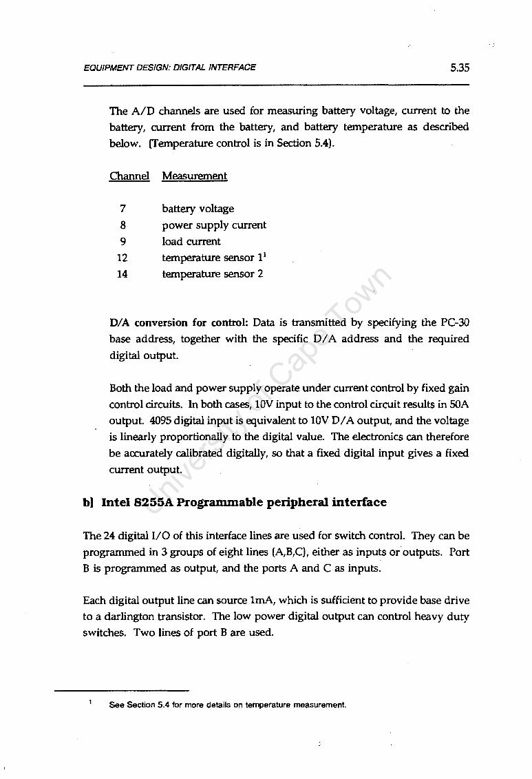
EQUIPMENT DESIGN: DIGITAL INTERFACE 5.35
The AID channels are used for measuring battery voltage, current to the
battery, current from the battery, and battery temperature as described
below. (Temperature control is in Section 5.4).
Channel Measurement
7 battery voltage
8 power supply current
9 load current
12 temperature sensor 11
14 temperature sensor 2
DI A conversion for control: Data is transmitted by specifying the PC-30
base address, together with the specific DI A address and the required
digital output.
Both the load and power supply operate under current control by fixed gain
control circuits. In both cases, lOV input to the control circuit results in SOA
output. 4095 digital input is equivalent to lOV DI A output, and the voltage
is linearly proportionally to the digital value. The electronics can therefore
be accurately calibrated digitally, so that a fixed digital input gives a fixed
current output.
b) Intel 8255A Programmable peripheral interface
The 24 digital 1/0 of this interface lines are used for switch control. They can be
programmed in 3 groups of eight lines (A,B,C), either as inputs or outputs. Port
B is programmed as output, and the ports A and C as inputs.
Each digital output line can source lmA, which is sufficient to provide base drive
to a darlington transistor. The low power digital output can control heavy duty
switches. Two lines of port B are used.
See Section 5.4 for more details on temperature measurement.

EQUIPMENT DESIGN: DIGITAL INTERFACE 5.36
Port B7 activates a darlington which excites the reed relay (Section 5.2.5(e)).
The reed relay (and the entire power system) can therefore be switched on
or off digitally.
Port B6 activates a darlington (0401) which switches the SCR tracker on or
off (Section 5.2.4(d)).
The input lines are used for status checking of power supply rails, relays, etc.
Port A4 provides status of the reed relay.
Port AO provides status of 12V power supply rail on the power supply
control card. Port A6 provides status of 12V power supply rail on the load control card.
The 1/0 lines are used by the computer to check system integrity, overriding the
manual start button until the main systems are properly connected and functional.
c) Startup procedure
A startup procedure has been designed which performs some simple system
checks before the power supply and load an be connected to the battery. the
checks are performed by software, in conjunction with the PPI. The startup
procedure is outlined in flow diagram format in Figure 5.29. The flowchart shows
the system checks that are performed, and which must be successful before the start button on the instrument panel becomes functional.

EQUIPMENT DESIGN: DIGITAL INTERFACE
Prepare Connections I
Tum off all switches! Connect battery power leads! Connect voltage sense leads!
)
v Run Program STARTUP
I B6, B7 turned off~I---------------------,
Ao. Al 4, A6 on?.• __ _ I Y-- Print "Tum off po"Jer"
N
I Print "Tum on TRIP SWITCH'
I Polarity correct?--- N--Print 'Bad polarity connection·------l
I . y
I A4 off? N- Print 'Reed relay error·---------!
I y
I AO, A6 on?----
1 y
I B7turned on . I
N- Print "No power on PS or load board"·-----1
..4~
A4 off?-----· N- Print "Reed relay error··---------1 I
y
I AO, A6 on?---- N--Print "No power on PS or load board""-----1
I y
I Print 'Press START BUTI'ON'
I AO, A6 on? N-- Print 'Switch trippedQf fuse blown·----
1 y
Loa1 and PS currents measured
I Load current>O.lA?- Y-- Print 'Hardware error on load'-----~
I N
I PS current>O.lA? --Y-- Print "Hardware error on PS"-------1
I N
I B6 turned on
I Pre-regulator active
I SUCCESS
\Y FAILURE
Figure 5.29 Startup procedure flowchart
5.37

EQUIPMENT DESIGN: CONTROL SOFTWARE 5.38
5.3 CONTROL SOFTWARE
5.3.1 General Requirements of the Control Software
The requirements are listed, with expansion where appropriate.
Remote data capture of about five main variables at regular intervals, and
storage of the five variables and permutations of them at selected intervals.
Battery tests normally take 50-100 hours to complete. It essential to be
able to capture data automatically.
Remote capture of various status/switch settings
Regular monitoring of the status settings of the electronic hard ware
ensures early warning of system failure, and enables the control
computer to terminate the test.
Remote control of the load in constant current mode and in pseudo-constant voltage mode by constant control of the current.
The load electronics are designed for constant current operation.
Constant resistance operation can be simulated by using the computer
as a digital feedback loop. This requires regular sampling of the
battery current and voltage, and adjustment of the current till the
required voltage:current ratio (resistance) is obtained.
Remote control of the power supply in constant current mode and in pseudo constant voltage mode and in pseudo PV simulation mode.
The power supply electronics are designed for constant current
operation. Constant voltage operation can be simulated by using the computer as a digital feedback loop. This requires regular sampling
of the battery current and voltage, and adjustment of the current till the required voltage is obtained.
EQUIPMENT DESIGN: CONTROL SOFTWARE 5.39
PV simulation can be achieved in much the same way. The current is adjusted till both current and voltage· fall on the PV operating curve.
This is best done by regular calculation of the battery resistance, and .
using adaptive feedback to solve for the expected operating point.
Real time numeric display of relevant variables.
Graphic display of any of selected variables vs any other.
Because the tests typically take so long to complete, it is useful to have
the facility to monitor the results from an early stage.
Ability to queue various operations,
to automatically terminate operations based on one or many
termination criteria,and to automatically begin the following operation
For some battery tests the computer executes charge discharge cycles
consisting of a series of sequentially executed operating steps. For
each cycle, control and limit values are used are used to establish the
operating condition and termination condition.
Limited operator control at any time
In any process control environment it is preferable to have operator
override in case of problems.
A Block diagram of the idealised process is shown in Figure 5.30.

EQUIPMENT DESIGN: CONTROL SOFTWARE
I End User I Computer System
I Printer I I Display I I Keyboard I I I I
t Data& I Computer : Program
I Storage
I Interface I . I
Data Acquisition System Interface Measurement
Control Functions
I Analogue Set Points I I Analog To Digital I Converter
I Multiplexer I I Switches and
I Actuators I Signal Conditioner J
Process
Figure 5.30 Process characterisation block diagram.
(Source: Hewlett-Packard)
5.3.2 Implementation
5.40
A single processor, standard IBM XT is used for control. The above processing requirements are formidable given the speed of the machine.
The power electronics that is controlled is simple, and it can be digitally
calibrated, yet it is all constant current operated without self-contained
microprocessors. The computer must perform all of the normal processing tasks,
and then regulate the power supply and load when they are used in non-constant current modes, by using a slow digital feedback loop.
The ideal situation, short of an on board micro-processor on the power supply
and load, would be some kind of priority scale run tasking by the computer.

EQUIPMENT DESIGN: CONTROL SOFTWARE 5.41
5.3.3 Program
In order to keep the system reasonably low cost, some precision has to be
sacrificed.
The power electronics control and data capture is executed every minute. This
is satisfactory (Verado et al,1981) if it is assumed that no significant drift away
from the set conditions will occur when in non-constant current modes.
While the PC is not controlling or capturing data it stands idle. During this time
the operator can select changes to the screen output parameters, change to
graphics mode, control the hardware etc. Thereafter control is transferred back
to the PC for further data capture and control functions.
Data Dow
The simplified program flow is described in Appendix E, with the subroutine
names in parentheses.
5.3.4 Digital Feedback Loop Stability
Non-constant current modes of operation include constant voltage operation and
PV simulation. These modes are emulated by periodically adjusting the current
so that the required output voltages are obtained.
The concept of a digital feedback loop has been raised to overcome limitations in
the electronic hardware, namely the presence of purely current control electronics.
Like any control loop, the digital loop must be stable, must not exhibit conditions
such as overshoot or ringing when subjected to a step change, but should not be
overdamped so that performance is unacceptably sluggish. The ·schematic for the
control loops is shown in Figure 5.31.
The battery is part of the loop, in the role of a current to voltage converter. The
conversion ratio (equivalent to the internal resistance) has been found to be in the
range 0.25 to 0.45 for a lOOAh 12V cell. The electrical pseudo time constant for
a step change in current is shown in Figure 5.32. It is expected that most lead
acid batteries will exhibit similar behaviour regardless of age.

EQUIPMENT DESIGN: CONTROL SOFTWARE
VOLTAGE DIGITAL
SETTING VOLTAGE
CONTROL
AID
Figure 5.31 Digital control loop
Vol!og• (Y) 12.a.:..:.:...:..:..:....:.-=---------------.
12.6
63% or AIMING VOLTAGt
TC
12'---'--'---'--'----'--'---'---''---....__...__..._~
0 0.5 1 1.5 2 2.5 3 3.5 4 4.5 5 5.5 6
Time (minutes}
12 _8 ;..:.vo::::llo:!.:o•~(V;.:_l ____________ ....,
TC
63% or AIMING VOLTAGt
12.2
12L---'-~-'-----'----''-----'----J 0 0.5 1.5 2.5
Time (minutes}
5.42
ANALOG
CURRENT
CONTROL
CURRENT
SENSE
BATTERY
Figure 5.32 Battery pseudo time constants. lOOAh battery response to step change in current. Battery SOC= 90%, a) current change= lOA, b) current change = -lOA.

EQUIPMENT DESIGN: CONTROL SOFTWARE 5.43
If the digital feedback system used continuous feedback, its speed would be
limited by the long battery time constant, and be inherently stable, as the software
is at least an order of magnitude faster than the battery in response time.
However, the software only samples for about 15 seconds of every minute, and
this discontinuous feedback causes its response to be correspondingly degraded.
The software must therefore become the slowest component for the loop to be
stable. This is achieved by limiting the step change in current output by the
digital feedback loop to 63% of the desired change. Satisfactory results have been
obtained for a range of battery sizes.
5.·3.5 PV Simulation
PV simulation is accomplished by software, with digital feedback and controlled
interaction between power supply current and voltage.
a) PV model
A PV model that is simple and easy to implement is used (Rausenbach,1980:59).
The model requires only four constants for complete definition of the base case, which is specified at 25°C and lOOOwm-2
:
V oc the open circuit voltage
Isc short circuit current
Imp current at maximum power
V mp voltage at maximum power
The four constants are shown on a typical PV curve in Figure 5.33.

EQUIPMENT DESIGN: CONTROL SOFTWARE 5.44
lsc
Voe
VOLTAGE(V)
Figure 5.33 PV panel 1-V curves showing constants for PV modelling.
The model is listed below for the base case.
where
and
Transformations are applied to the base case constants to obtain the 1-V curves at
any insolation, Insol, and temperature,T (Lasnier et al,1988:365):
where
lnsol I =I +u(T-25) +(---1)/ 1000 /IC
V = V +(3(T-25)
bl SC
a=-bT
bV (3=~
oT
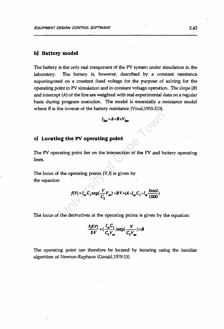
EQUIPMENT DESIGN: CONTROL SOFTWARE 5.45
b) Battery model
The battery is the only real component of the PV system under simulation in the
laboratory. The battery is, however, described by a constant resistance
superimposed on a constant fixed voltage for the purpose of solving for the
operating point in PV simulation and in constant voltage operation. The slope (B)
and intercept (A) of the line are weighted with real experimental data on a regular
basis during program execution. The model is essentially a resistance model
where Bis the inverse of the battery resistance (Vinal,1955:323).
c) Locating the PV operating point
The PV operating point lies on the intersection of the PV and battery operating ·lines.
The locus of the operating points (V,I) is given by
the equation:
V lnsol j{'V)=l C1exp(-V '+BV+(A-1 C1-l --) llC c ocJ llC llC 1000
2
The locus of the derivatives at the operating points is given by the equation:
The operating point can therefore be located by iterating using the familiar algorithm of Newton-Raphson (Gerald,1978:15).

EQUIPMENT DESIGN: TEMPERATURE CONTROL 5.46
5.4 TEMPERATURE CONTROL
The temperature control system should be able to keep the battery temperature
within ± 1°C of the control temperature. A temperature controlled water bath
facilitates good thermal contact with the battery and ensures short thermal lag
times. The water also has large thermal capacitance which prevents the battery from greatly affecting the water bath stability. The water bath temperature can
be controlled by a standard process plant temperature controller.
a) Water bath size
· The battery should be immersed to within 1-3 cm of the upper cell surface, and
water should circulate freely under the cell. To test tall tubular cells of between
400-600mm a depth of about 700mm is required. For the tank to maintain its
thermal inertia, at least as much water as is displaced by the cells should remain in the tank.
The water bath selected has dimensions:
length 800 mm x width 600 mm x height 700 mm
The normal operating volume is about 240 litres. An adjustable base tray able to support 70 kg is used to position batteries of various heights.
b) Heater size
The heater is used to keep the water bath temperature within ± 1°C of the set
point. In the worst allowable case the temperature oscillates between these
conditions. The period of the oscillation should be much less than the thermal
time constant of the battery, to ensure that the battery does not experience the temperature variations. The thermal pseudo-time-constant of a battery is typically 120 minutes.
The thermal heating rise time to heat the water from -1 to + 1°C of the set point,
depends on the element size. the heat input required, Q, for the two degree rise can be calculated from the water volume and water properties as:
Q = p x V x Cp x T

EQUIPMENT DESIGN: TEMPERATURE CONTROL 5.47
lkg/l x 2401 x 2°C x 4.17kJ/kg°C = 2003kJ
The rise time for a heater of power Pis Q/P. Any heater over lkW will have a
rise time shorter than 33 minutes and be sufficient. The larger the heater the
shorter the period of oscillation and rise time. The largest heater that can operate
from single phase supply using domestic connections is 3 kW, which is the size
selected.
c) Temperature controller
A Shimaden SRlO temperature controller with type K thermocouple was available.
Specifications are shown in Appendix E. The operating range is 0-1500°C, so the
accuracy in the 0-100°C range is limited. The minimum neutral zone in the
control output is 1 % of full scale or l.5°C. This corresponds to the worst case of allowable temperature deviation.
d) Temperature measurement
Temperature measurement is by two LM35D semi-conductor temperature sensing
devices. Two devices are used to obtain an average temperature reasonably independent of temperature gradients in the tank.
The LM35D output of 1 m V /°C is amplified using temperature compensated
amplification circuits (see Appendix E) to give outputs of 10 V at 6D°C. These
outputs are captured on computer via the Eagle PC-30 Interface through DI A channels 12 and 14.

CHAPTER 6
METHOD OF INVESTIGATION AND TESTING
The technical evaluatiOn of the selected batteries is based on a broad range of test
procedures. This chapter first presents the batteries selected for testing, then
describes each test procedure in detail, and ends with the outl~e for test result
presentation.
6.1 BATTERY SELECTION
The aims of evaluating batteries are to provide generic test data suitable for
photovoltaic system simulation, specific data on different batteries that are
suitable for PV applications and in so doing to investigate evaluation
methodologies suitable for the different battery types.
For this evaluation it is most important to select a range of batteries that includes
the most appropriate lead-acid types. Due to the nature of the battery industry,
and the similarities in short term performance between almost equivalent batteries
from different manufacturers, itis not efficient to test "competing" batteries of a
given type from the various manufacturers. Given that the time requirement for
complete characterisation tests on a single battery is 42 days, it is clear that some
rationalisation is needed. If cycle life tests are included then this is where the
difference in quality will show, and competing batteries should be tested.
The batteries selected for testing were chosen mainly on the basis of their
interesting physical characteristics. These are tabulated below.
6.1

EXPERIMENTAL METHOD 6.2
Table 6.1 Batteries selected for laboratory testing
Battery Design use Grid Plate Electrolyte Method of
Alloy Structure reducing
water loss
Delco 2000 Solar Pb-Ca Flat Flooded MF design,
single vent
GNB Absolyte 12V- Solar Pb-Sb Flat Immobilised Oxygen
5000 closed cycle
Raylite RMT108 Standby Pb-Sb Tubular Flooded none
Raylite Solar Solar -CSM NA NA NA
Sonnenschein A200 Standby I aircraft Sb-free, Flat Gelled Oxygen
Ternary closed Cycle
Pb-Ca
Willard 774 Portable/leisure Pb-Sb Flat Flooded none
Willard LS90 Vantage Standby /UPS +Pb-Sb Flat Flooded LM design,
- Pb-Ca single vent
LEGEND
CSM copper stretch metal (Raylite patent)
Of these, the Raylite Solar was not available at the time of testing.
The Sonnenschein A200 was selected for testing, but preliminary tests on two
'used' A200's made available showed that the condition of the batteries would
have compromised the tests results. The poor conditions are not a reflection of
the batteries themselves, but rather a reflection of the previous use patterns and
(lack of) maintenance. The A200's were omitted as the Rand cost of this imported
battery was excessive.
6.2 BATTERY TESTING METHOD
The main test procedures and related questions that arise are discussed in the
sections below.

EXPERIMENTAL METHOD
The areas of interest are:
Ah capacity
temperature effects
discharge curves and Wh capacity
charging curves
charging efficiency and gassing
specification of current and voltage ranges for charging
cycling effects
partial state of charge operation
stratification effects
6.2.1 "On Delivery" Assessment
6.3
Perform a visual inspection, reviewing data available from the manufacturer and
categorising data according to its quality. Categorise the battery according to
main features and operating characteristics as it is advertised.
Collect additional data from the manufacturers on physical structure, and perform
theoretical calculations regarding active mass utilisation coefficients.
If life cycle data is not available then estimate cycle life based on data for similar
batteries. Use cycle life models where necessary. The semi-log plot of cycle life
versus DOD requires only two data points. The cycle life data can be supported
by testing in many cases. The optimum DOD for cycling can be determined from
the cycle life data, corresponding to the optimum Ah delivered by the battery
over its entire life. The Ah delivered over entire life is calculated as:
Ahlife = C20 x DOD x Cyclesvov
Initial estimates of battery cost and battery value can made. Wh cost is the cost
per Wh as purchased. kWh value relates to the total kWh delivered over the battery life, and is usually calculated at the optimum DOD.
VVh cost = Cost in Rands I {C20 x nominal voltage)
kVVh value = Cost in Rands I (Ahlife x nominal voltage) x 1000

EXPERIMENTAL METHOD 6.4
Before embarking on any tests it is necessary to "size" the battery in relation to PV
systems. In other words, establish the range of charge and discharge currents the
battery could be exposed to if normal PV system sizing methods were used. A
battery of several hundred ampere-hours would be expected to handle many
amperes of charge and discharge current under normal operation, whereas a
ninety Ah battery would typically handle currents of less than ten amperes. This
sizing is done to ensure that tests are performed in the relevant current regimes.
Sizing the battery may require some calculated estimates of battery life vs DOD,
possibly based on data for similar batteries. Deep and shallow cycle batteries
have different operating parameters and test requirements. Shallow cycle cells
may be sensitive to certain conditions which need to be takeD into account in
"sizing" the battery.
All tests are performed using the programmable battery test-rig. Temperature
control is by a water bath at the relevant temperature, or an ice bath at D°C. The
battery is allowed 16 hours to acclimatise each time it is to be tested at a new
temperature. In each case the thermal time constant of the battery in water is
recorded.
6.2.2 Initial Test and Forming Charge
a) Determine the "as received" condition
Measure specific gravities, voltages and determine the "as received" capacity
at the C10 rate.
b) Forming charge
Most new lead-acid batteries require several cycles to convert residual lead
from manufacturing to active material, and to allow homogeneous grain
structure.
Recharge as recommended by the manufacturer, then discharge at the rated
current and recharge as recommended, cycling five times. Shallow cycle batteries are discharged to only 50% DOD to avoid damage. Follow by an
equalising charge after the last cycle. Establish a reference capacity.

EXPERIMENTAL METHOD 6.5
6.2.3 Capacity Tests
The capacity test starts with a battery that has been equalise charged, and the
battery temperature allowed to stabilise at the test temperature in the temperature
controlled water bath for up to 16 hours. SG's are recorded where possible. The
capacity tests are conducted at constant discharge current, and the battery voltage is recorded at regular intervals. The test is complete when the battery voltage drops to below the cut-off voltage recommended by the manufacturer. If no cutoff voltage is provided, then the knee of the (voltage vs natural logarithm of time)
curve determines the end of discharge.
a) Determine ~o (@ 35°C, 18°C, 0°C)
Capacity is a function of rate of discharge and temperature. Nominal capacities are usually given at 2D°C for the 20 hour rate (C20) for SLI (starting, lighting, ignition) cells and C10 for EV (electric vehicle) cells. The
three temperatures selected for testing cover the range of likely operating temperatures for batteries in PV systems. Determine the effect of
temperature on capacity at the rated current (eg. 110 @2D°C). All tests are followed by equalisation charge.
b) ·Determine C50 ~0 C10 C5 etc.
Determine the variation in capacity with discharge current. (For PV systems the relevant current is about the 20 or 30 hour rate). Temperature can be
included as a further variable if required. Care should be taken not to deep
discharge the battery below the knee of the discharge curve as subsequent
tests could be unreliable and inconsistent, particularly for lead-calcium grid
cells. Shallow cycle batteries can alternatively be discharged to a cut-off of
1.9V I cell, and the capacity compared with the capacity to 1.9V I cell obtained from that recorded at C20 rate.

EXPERIMENTAL METHOD 6.6
6.2.4 Discharge Tests
The capacity tests in Section 6.2.3 also yield discharge curves, of V ce11 as a function
of constant discharge current and ampere-hours removed. (DOD at any time is
less valuable as a variable than ampere-hours removed, because the number of
ampere-hours remaining in the cell depends on the subsequent discharge current.)
The discharge curves can be integrated to show the watt-hour capacity at constant
current. The discharge cut-off voltages as a function of current, DOD and
temperature can be determined from the discharge curves.
a) Investigate variable current discharge curves
Most PV loads vary throughout the day, particularly domestic loads, which
may draw on average less than ten amperes (per lOOAh battery), but could
for short periods draw close to one hundred amperes (per lOOAh battery).
Particular questions that arise are: How is capacity affected? What time is
required for the voltage to stabilise after a step change in output current?
(eg. the polarisation effect). Investigate this analytically in terms of the
active block design; the number of plates (eg. current d~sity), plate design
and thickness, electrolyte SG, temperature. The actual range of currents
selected for testing depends on how the battery is "sized" in a PV system.
6.2.5 Charging Curves
Charging of batteries can be by constant-current (CC), constant voltage (CV), CC
with voltage limit, CC with step current change, CV with step voltage change,
and many variations on these options. The charging curve in each case would
require charging from a defined DOD, plotting V ce11 vs Ah returned (or time), and
noting the current or voltage where step changes have occurred.
The charging method in typical PV systems corresponds to none of these, in the
same way as discharge current is not usually constant.
The best approximation is possibly a variable charging current with an upper
voltage limit representing voltage regulation. A charging test has been developed
which charges the battery at a constant typical PV current (2-3A/100Ah), with an

EXPERIMENTAL METHOD 6.7
upper voltage limit of approximately 2.37V I cell. Charging is in this mode till a
set number of Ah have been delivered to the battery (10Ah/100Ah battery). At
this stage a current scan is activated. During the scan the current is set to
10A/100Ah and held till the voltage stabilises, when the voltage, Ah returned and
charge _current are recorded. Time to stabilise is usually less than 10 minutes.
The scan current is consecutively set to SA, 2A, lA, O.SA /lOOAh and the relevant
recordings are taken. After the last current has been scanned charging is resumed at the constant PV current and the same upper voltage limit. The current scan is
repeated when a further set number of Ah have been delivered~ The process is
repeated till the battery is fully charged. The advantage of this method is that a range of charging data can be quickly generated in one test. Experimental charging results are shown in Figure 6.1 for a lOOAh battery recharged from 60% DOD.
2.7'..------------------,
2.6
2.5
~ -I 2.4 -I w ~ 2.3
~ 0 2.2 >
2.1
2
1.9 80 0 20 40 60 80 100 120 140 160 1
TOTAL AH DELIVERED
Figure 6.1 Experimental charging curves.
a) Determine experimental charging curves@ C50 c;0 C10 C5
(@ 35°C, l 8°C, 0°C)
Determine charging curves using the scanning method, at constant temperatures, ensuring operation in the PV charging regime. These curves will give V ce11 as a function of charging current and total Ah delivered.

EXPERIMENTAL METHOD 6.8
b) Generate compensated charging curves
Coulombic charging efficiency is less than 100%, mainly due to losses by
gassing at higher SOC' s. A charging curve that plots charging current and
voltage vs the Ah effectively delivered can be constructed by compensating
the experimental charging data for gassing losses. The gassing losS16are
defined as current loss as a function of the battery voltage, as determined
by the instantaneous charging efficiency (Section 6.2.6). The compensated
charging curve is easily constructed by considering the Ah delivered at a
particular voltage, and compensating this to effective Ah by multiplying by
the instantaneous coulombic efficiency. The points of equal current can be
joined to result in the compensated charging curve in Figure 6.2.
2.6
2.5
~ 2.4 _, w Q. 2.3 en ~ ~ 2.2
2.1
2
20 40 60 80 EFFECTIVE AH DELIVERED
Figure 6.2 Compensated charging curves.
100 120
c) Construct quasi-constant current charging curve
Each compensated charging curve can be "uncompensated" to show the total
Ah that would have to be delivered to fully charge the battery at constant
current. This is done simply by dividing the compensated Ah at a particular
voltage by the instantaneous coulombic efficiency at that voltage. The total
Ah required can be easily accumulated. The higher charging rates are
expected to require more Ah than the lower rates due to greater gassing
rates and gassing durations encountered. Figure 6.3 shows a set of quasi-

EXPERIMENTAL METHOD 6.9
constant current charging curve. These curves are not significantly different from real constant-current charging curves, are more representative of PV
charging, and are comparatively quickly generated.
2.7...-------------------,
20 40 60 80 100 120 140 AH DELIVERED
Figure 6.3 Quasi-constant current charging curves.
d) Investigate variable current charging in PV systems
Residual questions: How does charging under the PV regime compare with
the charging curves generated? What are the effects of transients? What time
is required for voltage to stabilise after a step change in charging current?
These questions are most easily answered by simulating PV charging
currents (using the PV simulator) and monitoring battery behaviour.
6.2.6 Charging Efficiency, Average and Instantaneous
The average coulombic charging efficiency in cells can be defined as the Ah
effectively delivered to the cell divided by the total Ah delivered. The deficit is
mostly caused by gassing. The average charging efficiency is useful for determining the overcharge required to fill a cell from a fixed DOD under fixed
charging conditions. The average charge efficiency is DOD and charge current
dependent, necessitating many repetitive and similar tests. Data collection is
complicated as charging efficiency is decreased in old or unhealthy batteries as
the gassing current increases.

EXPERIMENTAL METHOD 6.10
Average charging efficiency can be estimated by:
i) measuring the difference between Ah delivered and Ah recoverable.
The test requires repeatedly cycling between full charge and various
DOD's to determine the effect of DOD on charging efficiency.
ii) comparing Ah returned to the cell with SG, a linear indicator of SOC.
iii) by attempting to measure inefficiencies causing cell temperature
increases. The rate of battery temperature increase is related to the
gassing rate. However, it is probable that external factors will make
this method impractical. (Accurate determination of heat transfer
coefficients will be difficult).
If the instantaneous charging efficiency can be determined it provides a much
more useful method of analyzing battery performance. It can be used in
conjunction with charging curves to determine overcharge requirements
regardless of starting DOD. Instantaneous efficiency also provides information
on the instantaneous gassing rates, although it is complicated by different rates
of charge acceptance at the positive and negative plates (see Figure 3.30). Even
though errors may be introduced, instantaneous charging efficiency provides
greater insight into battery operation than average charging efficiency. The
instantaneous efficiency can be measured by:
iv) estimating current losses due to gassing by measuring gas flow rate.,
a method widely used by battery researchers. The SOC, temperature,
current, voltage are important parameters.
The instantaneous flow rate of gases evolved is measured by tapping
gas flow from the cells through a soap bubbler,.and recording the time
to produce a volume of gas. If the gas is assumed to consist of only
H2 ahd 0 2 in the ratio 2:1, then the current loss due to gassing is (see
Section 3.8.2e for derivation):

EXPERIMENTAL METHOD
where
I = XIN IC 5.74 IC P/1 IC 27l/f g
X = gas flow (cm3 /s)
N = number of cells tapped
P = gas pressure (atm)
T = gas temperature (kelvin)
6.11
If the gas composition can be determined (by mass spectrometer or
Orsat analysis), then the gassing current at each electrode can be calculated and correction made for the individual electrode efficiencies.
Because the positive and negative electrodes have different charge
acceptance rates the instantaneous gas compositions may be non
stoichiometric in different SOC regions, but they approach
stoichiometric at full charge (see Figure 3.31). Lakeman (1989) has
calculated that the average ratio H 2:02 over the charge regime
following deep discharge is very close to 2:1.
The gas flow method of charge efficiency determination will be
accurate when the gas mixture is stoichiometric, so at 100% SOC
should be reliable and accurate.
The gas measurement method is not recommended for sealed cells as
substantial electrolyte is lost and cannot be replaced. Allowance may
have to be made for some gas recombination in vented cells, typically
5%.
or
v) measuring the rate of recombination fu sealed cells.
Sealed cells with oxygen closed cycle gas recombination operate under
pressure (3 psi). As described in the theory (Section 3.9.3(b)), the rate
of recombination is limited almost entirely by the rate at which oxygen
can migrate to the negative electrode where hydrogen is generated.

EXPERIMENTAL METHOD 6.12
The theory shows that for a pseudo-first order reaction in oxygen, the
current equivalent (102) to the rate of oxygen recombination is:
4.FV [ dl: 0, 1· Io""-- Po • RT • ,v
where
V =volume of gas in the headspace (m3),
F = Faraday constant (9.648 x 1D4 C mol-1)
R = gas constant (8.31441 J K 1 mol-1)
T = gas temperature (kelvin)
P 02 = oxygen partial pressure (Pa)
If the cell is charged at constant potential the pressure in the cell
quickly settles at an equilibrium. At the equilibrium it can be assumed
that the rate of oxygen evolution at the positive electrode is equal to
the rate of oxygen recombination at the negative electrode at the
measured cell potential. If the charger is suddenly disconnected so
that the battery is in open circuit, then the rate of pressure drop can
be measured to determine the rate of 0 2 recombination, hence the rate
of 0 2 production at the charging current, voltage, SOC and
temperature. For every mole of 0 2 produced, 2 moles of H2 are
assumed to be evolved. The total gassing current can be shown to be
equal to the 0 2 recombination current.
The main limitation with this method is the error caused by the
difficulty in estimating the headspace volume, V, if the data is not
readily available from the manufacturer. If a manometer is used for
pressure measurement the free air in the manometer may be significant and should be accounted for.
Considerable flexibility is afforded if it is realised that the gassing currents (at
each plate) are related primarily to the plate potentials, vpos and vneg (see
Section 3.7.4). Although temperature dependence is significant, electrolyte
concentration influences gassing to a far lesser degree. The instantaneous

EXPERIMENTAL METHOD 6.13
charging efficiency at each plate can be inferred from the voltage at that plate
(Lakeman,1989). By a further approximation, the instantaneous charging
efficiency of the cell relates to the total cell voltage. Though there are disparities in charge efficiency behaviour between the positive and negative plates, the errors
anticipated by this overall approximation are small considering the usefulness and simplicity of the method. Lakeman (1989) finds that theoretically determined gas flow rates, using plate potentials and using overall cell potential, are in good
agreement with experimental determinations under controlled charge conditions.
He points out that unacceptable errors could occur from using c~ potential alone in uncontrolled charging regimes, with no voltage limit. However, PV charging
regimes are inherently controlled; and if not limited by the array output characteristics, are limited by voltage regulation. The result is that the gassing current can be estimated from the cell voltage and temperature alone. This assumption can be extended to good effect to generalise for the instantaneous charging efficiency determined in the two above methods.
The last method of estimating efficiency, applicable to all cell types, is by:
vi) measuring the end of charge current at constant potential
The assumption that charging efficiency is a function only of voltage and temperature has further implications. If the rate of charge acceptance of a fully charged cell is zero (true for negative plate, almost true for positive, see Section 3.8.2(b)), then the overall charging
efficiency is practically zero and the charging current into a fully
charged cell at constant potential is the gassing current. All that has
to be done to determine the gassing current vs voltage is to charge a
fully charged cell with several constant voltages and measure the
current. This provides a valuable cross-check for the other methods of calculating charging efficiency.
a) Determine the gassing currents at various states of charge (in the region of 70-95% SOC).
Determine the instantaneous charging efficiency using the method in 6.2.6vi, corroborated by as many other methods as possible. Investigate this in terms of the number of plates (ie. current density), plate design and
EXPERIMENTAL METHOD 6.14
thickness, grid design, electrolyte SG, temperature. It is eventually hoped
to show that this parameter is one of the most significant in PV battery
selection. In addition this test may indicate suitable cut-off voltages for
voltage regulator float, boost an~ equalisation charge settings. The test will
provide valuable data for designing microprocessor type energy
management systems. The gassing current data can be incorporated with
charging curve data to generate charging curves corrected for gassing loss.
(See instantaneous charging efficiency measurement in Section 6.2.6(iv))
b) Determine the average charging efficiency of the cell.
Determine the efficiency at the recommended starting and finishing charging
currents and voltages from a suitable DOD. This will not necessarily be the
upper limit for the charging efficiency. Method 6.2.6(i) may be most
appropriate, alternatively the average efficiency can be calculated from the
instantaneous charging efficiencies or from the quasi-constant-current
charging curve.
c) Determine the charging efficiency in the PV current regime.
Actual finishing current will most likely be far under the recommended
finishing current. The decreased gassing will probably yield a higher
charging efficiency than for (b). The reduced gassing is associated with a
degree of compromise between charging efficiency and cell life. A certain
amount of gassing is required to promote electrolyte mixing, reduce
stratification and prolong useful cell life. The quasi-constant-current
charging curves may be useful, although cycling tests (Section 6.2.7) may
also be required.
d) Estimate self-discharge rates.
Gassing and self-discharge of cells are together related to grid type. Cells
that can gas at low current will tend to have high rates of self discharge.
Estimate self discharge rates based on the charging efficiency curves.

EXPERIMENTAL METHOD 6.15
6.2. 7 Cycling Tests
Cycling tests provide early information on temporary or permanent, short or
longer term performance degradation. Through cycling batteries in defined
regimes, information on overcharge requirements, start and finishing currents and voltages can be determined. Capacity tests after cycling tests indicate any loss of
capacity during the testing. In the industry, cycling tests are conducted for several months at a time. In this programme time limitations generally restrict
cycle testing to only a few days.
Sandia National Laboratories (Verado,1981) have identified two modes of
operation in describing battery requirements for PV applications. If a battery has
been sized to provide long term energy storage for the time the PV array is unable to produce power then the battery will experience shallow cycling with
complete cycling once or twice a year (see Chapter 2). If the array is almost always able to provide the daily power demand, and the battery is only required
for foad-levelling or peak-lopping, then the battery will probably experience deep
cycling on a daily basis. In both cases, prolonged operation at partial state-of
charge is possible. The cycling tests described below were developed by Sandia
National Laboratories (Verado,1981). Although charge and discharge currents,
voltages, overcharge and times are specified, they are not intended to be rigid.
Sandia recommends that they be modified to suit particular batteries depending
on manufacturer's data and experience with particular batteries.
Analysis and interpretation of the tests provide useful comparative data on charge
acceptance rates, charging efficiencies, susceptibility to stratification, energy
efficiencies and changes in capacity. It may be preferable to perform the same tests on different batteries, so that the batteries are compared on the same basis,
rather than attempting to customise each test to suite individual batteries for which sparse data is available.

EXPERIMENTAL METHOD 6.16
Standard cycle tests
Fully charging cells from shallow or deep cycles results in reduced charging
efficiencies, and longer charging time requirements due to gassing losses in the
80%-100% SOC range. Some overcharge is required to overcome charging
inefficiencies, and some overcharge is required to prevent electrolyte stratification.
Charging voltages may have to be limited to control gas formation rates. The
standard cycling tests can be used in conjunction with charge and discharge
curves to determine whether these criteria are being met. Cycling may be deep
or shallow cycle depending on the battery.
i) Standard shallow discharge cycle test
A fully charged battery is discharged for two hours at the C20 rate, removing
10 ~cent of the rated capacity. It is then recharged for two hours using
constant potential with the current limited to C10 and the overcharge limited
to 10 percent of the Ah removed, theoretically sufficient to completely
recharge the battery. This charge/ discharge cycle is repeated for a
predetermined number of cycles, (six cycles per day are possible) and is
terminated with a battery capacity test. The form of the test is illustrated in Figure 6.4.
ii) Standard deep discharge cycle test
A fully charged battery is discharged for four hours at the C5 rate, removing
80 percent of the rated capacity. It is then recharged following the
manufacturer's specifications for eight hours using constant potential and
the overcharge limited to 15 percent of the Ah removed. This
charge/ discharge cycle is repeated for a predetermined number of cycles,
(see Figure 6.5) (two cycles per day are possible) and is terminated with a
battery capacity test. The test can be restarted once the battery is fully charged.
For the standard cycle tests trends in the end-of-discharge voltage, end-of
charge-current and lpss of capacity are particularly interesting.

EXPERIMENTAL METHOD 6.17
88
86
8 12 16 20 Tl._, (HOURS)
·1 0 12 16 20 TIME (HOURS)
Figure 6.4 Standard shallow discharge cycle test for a 50Ah battery.
10
0 20
i !Z ... a: a: a i'i: -2
~ ~ -6
-8
·1 0 4 20
Figure 6.5 Standard deep discharge cycle test for a 25Ah battery.
EXPERIMENTAL METHOD 6.18
Partial state of charge cycle tests
Deep discharge and subsequent slow recharging of batteries so that they remain
in a partial state of charge enhances electrolyte stratification in flooded electrolyte
cells, and promotes hard sulphate crystal formation on the negative electrodes of
all cells, leading to temporary (or permanent) losses of capacity and energy
efficiency. The aims of these tests are to investigate the effects of cycling without
overcharging and gassing, and to determine the magnitude of the reversible and
irreversible capacity and energy efficiency losses. As before, cycling may occur
at a deep or shallow cycle.
iii) Partial state-of-charge shallow discharge cycle test
Figure 6.6 shows the test cycle for simulating partial SOC operation at
shallow discharge. A fully charged battery is discharged for eight hours at
the C20 rate, removing 60 percent of the rated capacity. A cycle consists of
a two hour recharge at C20, followed by a two hour discharge at C20,
theoretically removing and returning 10 percent of the capacity each cycle,
cycling between sixty and fifty percent SOC. After the initial discharge, six
cycles per day are possible. This charge/ discharge cycle is repeated for a
predetermined number of cycles, and is again terminated with a battery
capacity test.
iv) Partial state-of-charge deep discharge cycle test
The test cycle is illustrated in Figure 6.7 is used for simulating partial SOC
operation at deep discharge. A fully charged battery is discharged for four
hours at the Cs rate, removing 80 percent of the rated capacity. The battery
is recharged at Cs till sixty percent of the charge has been replaced, and then
cycles continuously using a three hour discharge at C5, followed by a three hour charge at C5, theoretically cycling between 80 percent and 20 percent
SOC. After the initial discharge, four cycles can be completed per day. As
for the other tests this test is terminated with a battery capacity test.

EXPERIMENTAL METHOD
80
70
l 60
~
~= ::ii
i i a
30
20
10
0 4 12 16 TIME (HOURS)
1: _______ __ -6
-8
20
·1°"0---4--.-a ---,1.,..2 -......,16,...---.,20,.---'""ac
TIME (HOURS)
Figure 6.6 Partial SOC shallow cycle test for a lOOAh battery.
70
l 60
~
~= ::ii 30
20
10
i !z ... a: a: a !:: ·2 ... ~ ~
-6
-8
·1 0
8 12 16 20 TIME (HOURS)
4 8 12 16 20 TIME (HOURS)
Figure 6.7 Partial SOC deep cycle test for a 25Ah battery.
6.19

EXPERIMENTAL METHOD 6.20
a) Perform cycling tests
Conduct relevant cycling tests at suitable DOD, currents, voltages and time
constraints. These parameters are considered and determined separately for each
battery.
6.3 REPORT FORMAT
This section describes the presentation of the test results. The report numbering
is consistent for all the batteries examined.
7.x BATTERY NAME
7.x.1 General Information
Data summary
The battery is categorised, and overview data presented.
Costing
The battery cost (R),
Wh cost (R/(C20 x voltage)),
kWh value (R/(Ahover life x nominal voltage/1000)) at the
optimum DOD over the operational life is estimated. Operating
and maintenance costs and salvage value are excluded.
7.x.2 Physical
Physical construction
Relevant physical and chemical data is presented where
available.
Active mass utilisation coefficients
Active mass utilisation shows which active materials are limiting
in capacity and which may limit cycle life.
In addition, the excess electrolyte capacity and SG at deep
discharge are calculated to determine the danger of electrolyte

EXPERIMENTAL METHOD 6.21
freezing during operation.Low end-of-discharge SG's can also
adversely affect battery internal resistance.
7 .x.3 Basic Operating Data Available
Charging requirements and limits
Charging data provided or collected from similar batteries.
Discharge curves
Life cycle data
If cycle life curves are provided then they are presented,
otherwise cycle life estimates are made using data available from
similar batteries in conjunction with battery models.
Cycle life data is required for determining testing regimes as well
as estimates of the optimum DOD and Ah over the battery life.
The accuracies of these figures are verified by cycling tests where possible.
Extent of manufacturer's data
Extent of data is discussed and data graded according to quality. The gradings used are:
Grade Al - data from independent laboratory
Grade A2 - data from the manufacturer's laboratory
Grade B - extrapolated from Grade A data
Grade C - extrapolated from Grade A or B from batteries of
similar materials but different size
Grade D - other data
(See Section 4.3.2 for more details)
7.x.4 Test Results and Discussion
a) Capacity and discharge tests
Capacity, temperature effect on capacity, discharge curves and
suitable voltage regulator load shed settings are considered.

EXPERIMENTAL METHOD 6.22
b) Charging and efficiency tests The quasi-constant current charging curve is presented together
with the gassing current curve. The quasi-constant current curve
is compensated by the gassing inefficiencies to yield the
compensated charging curve. This sequence is used for ease of
presentation. The practical sequence (Section 6.2) is to determine
an experimental charging curve and gassing current curve, then calculate the compensated charging curve. The quasi-constant
current charging curve is derived from the compensated curve
and the gassing current curve.
c) Cycling tests Test selection
Relevant cycling tests and parameters are selected.
Analysis of cycling:
Deep cycle full SOC test
Deep cycle partial SOC test Shallow cycle full SOC test
Shallow cycle partial SOC test
Capacity at end of cycle tests
The change in' capacity is used to verify the cycle life curve
where possible.
H20 consumption
H20 loss rates are estimated and compared with experimental results.
Charging current and voltage requirements Charging requirements during cyclic operation are considered.
7 .x.5 Sizing and Selection: considerations in PV applications
Particular considerations are presented in order of priority.

CHAPTER 7
TEST RESULTS
This chapter presents and discusses the results of tests and experiments on
selected batteries.
7.1 WILLARD 774 PORTABLE BATTERY
7. I. I General Information
Data summary
Capacity:
Voltage:
Application:
Group:
Description:
c 20 = 90Ah @ 20°c
12V
leisure/portable power
flat plate, antimony grid, flooded
Flat plate 12V power pack. Vented with flooded electrolyte.
Essentially a modified SLI design, with thicker plates for better
cycle life. Antimony and other grid additives are used in the
positive and negative plates. Black plastic casing.
See Appendix Dl for manufacturer's data sheet.
Costing
Cost:
Wh cost:
Wh value:
R294 per battery (@ 23/10/1990)
R0.27/Wh
Rl.81/kWh over battery life, assuming 300 cycles at. ~0% DOD,
the optimum DOD. These figures should be regarded as approximate. (See Section 7.1.3.)
7.1

TEST RESULTS: WILLARD 774
7 .1.2 Physical
Physical construction
Dimensions:
Plates:
Grid:
Dry mass:
Electrolyte:
Wet mass:
Gas venting:
Casing:
Terminals:
height, width, length:
height over terminal:
mass:
design:
pos. active material:
neg. active material:
active block mass:
positive:
negative grid
grid mass:
17.7kg
SG:
volume:
mass:
25.6kg
automotive type vent caps
black plastic
standard lead pillar
225 x 172 x 342mm
225mm
25.6kg
15 flat plates/cell
7 positives, 8 negatives
97g
94g
2.768kg/cell
1.6% Sb
pure lead
1.107kg/cell
7.2
(40% of active block mass assumed)
1.260@ 200C
5.91
7.43kg

2
TEST RESULTS: WILLARD 774
Active mass utilisation coefficients: (Calculated)
Active mass
capacity @ 100% 152Ah
utilisation
utilisation @ nominal 59%
capacity (90Ah)
utilisation@ 100 hr rate 65% (98Ah) 1
utilisation@ opt. DOD 32.5%
(39Ah @ 40% DOD)2
7.3
Electrolyte SG@end
of test
121Ah 1.000
74% 1.055
80% 1.04
40% 1.17
Under normal operation, the SG of the electrolyte will limit capacity, as well as
resulting in higher internal resistances which reduce efficiencies.
7.1.3 Basic Operating Data Available
Charging requirements and limits
No charging data was provided. Data provided for charging a similar battery"
(Raylite R~2) following deep discharge is:
starting charge: 12.6A or 14.0% of C20
finishing charge: 6.3A or 7.0% of C20
equalising charge: 2.7A or 3.0% of C20
See discharge data in SECTION 7.1.5(a)
See life cycle data in SECTION 7.1.3

TEST RESULTS: WILLARD 774 7.4
These are figures used by manufacturers for many batteries, and represent a rule
of thumb. There are two limitations to charging current, both related to gassing.
Gassing must be limited to reduce grid corrosion, and to prevent physical
stripping of the active mass.
Discharge curves
Complete discharge curves at 200C are available ranging from 10 minute to 50
hour rates.
Life cycle data
No life cycle data is available. The manufacturer suggested that 200 cycles @ 80%
DOD and 400 cycles at 20% DOD was attainable under normal operating
conditions. The low cycle life is a reflection of the high active mass utilisation
coefficients. Similar batteries in SAPV's have achieved 700 cycles at 10% DOD,
and models suggest that 200 cycles at 80% represents 750 cycles at 10% DOD for
similar failure mechanisms (refer to Section 3.12 on Battery Models). Common
failure modes include grid corrosion and active mass shedding. The optimum
battery utilisation for the higher life estimate occurs in the range 40% to 60%
DOD. (See Figure 7.1.) The optimum cycle life is relatively insensitive to DOD
in this range.
(/) w _, (..)
~ LL. 0 d z
800 'r---------------.-16
700
600
400
300
200
100
......__optimum utilization 15 £' ,.. •••••• -··············-··········-....... 14 ~-
• 13 _(/)en .,. ............
.............. 12 ii .... c J: ·· .• 11 ~ <
:I w
10 ~ ~ (..)
9 ~
8
7
LL. w _, i5 E
0 0 '-+--.----.--.--.----.r--"'T""""-.----.r---.---+6
10 20 30 40 50 60 70 80 90 100 % DEPTH OF DISCHARGE
Figure 7.1 Estimated cycle life vs depth of discharge.

TEST RESULTS: WILLARD 774 7.5
Extent of manufacturer's data
Data Quality: The only data provided is the discharge and capacity data, which is Grade A2
(performed by the manufacturer in-house on the specific battery) .
. Data as purchased: No data was provided, except nominal capacity.
Additional data on request by personal communication:
Standard discharge curves were provided: (Grade A2).
Plate masses, (dry and wet), overall masses and dimensions,
Life cycle data: estimated at 200 cycles @80% DOD: (Grade C).
See Appendix Dl for manufacturer's data sheet.
7 .1.4 Test Results and Discussion
a) Capacity and discharge tests
Three complete sets of capacity tests were conducted, at 0°C, 18°C and 35°C.
Discharge currents were lA, 2A, 4.5A, lOA and 20A.
Before each test the battery was equalise charged, till the SG's were within
specification, ie 1.260. The battery was discharged to the manufacturer's cut-off
voltages (see manufacturer's data), and capacities achieved were within 5% of the
manufacturer's specifications, although usually a few percent below.
The standard discharge curves at the three temperatures are shown in Figure 7.2.
The variation in capacity with temperature is shown in Figure 7.3.
The available battery capacity (at lOA discharge current) decreased by less than
1 % below the initial capacity after all the discharge tests (15 discharges down to 100% DOD).

TEST RESULTS: WILLARD 774
w Cl ~ -'
~
w Cl ~ -' 0 >
w Cl
~ 0 >
13
12.5
12
11.5
.11
10.5
10 0 10 20 30 40 50 60 70 80 90 100 110
DOD(AH)
13
12.5
12
11.5
11
10.5
100 10 20 30 40 50 60 70 80 90 100 110
DOD (AH)
13
12.5
12
11.5
11
10.5
10+----t-~+--+~+--+~-+--+~-+---+~-+---1 0 10 20 30 40 50 60 70 80 90 100 110
DOD (AH)
7.6
Figure 7.2 Discharge curves at a) 0°C, b) 18°C, c) 35°C. Discharge currents are lA, 2A, 4.SA, lOA and 20A in each case.

TEST RESULTS: WILLARD 774
110. 0 ... • Odegrees
0 100.
90.
I • i Ill 18degrees
0
I ·1 x
I 'll • 35degrees 0 •
• .0 II
60. 0 H . 50. 0
--40. 0 1 10 100
DISCHARGE CURRENT (A)
Figure 7.3 Discharge capacity vs temperature and discharge rate.
12.00
11.75
11.50
w 11.25 Cl
~ 11.00
~ 10.75
10.50
10.25
... I.
aa
...
I!!! I
2
i 60%DOD ... I~ ·~
Odegrees
• ~~ • .~
18degrees . x
... 80%DOD 35degrees
• ~ 100%DOD
x ' I
4 6 8 10 12 14 16 18 20 DISCHARGE CURRENT (A)
Figure 7.4 Cut-off voltages vs discharge rate, SOC and temperature.
it; -it; -~ Cl en
60
50
30
1.150 15
1.100 7
1.050 3
l-~~....---..~....----.~...,....---,..---.-""""':r:--""."!"::-:'tO 1·000 0 10 20 30 40 50 60 70 80 90 100 110 DOD (AH)
6 Cl w c ..!,.
Cl z N w w a: u... w
~ 0 a: t> w .... w
7.7
Figure 7.5 Electrolyte SG and freezing points vs DOD. Triangles represent measured data.
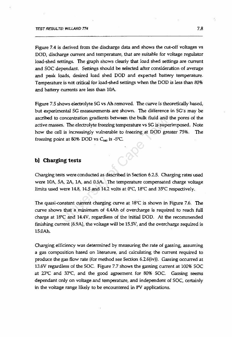
TEST RESULTS: WILLARD 774 7.8
Figure 7.4 is derived from the discharge data and shows the cut-off voltages vs
DOD, discharge current and temperature, that are suitable for voltage regulator
load-shed settings. The graph shows clearly that load shed settings are current
and SOC dependant. Settings should be selected after consideration of average
and peak loads, desired load shed DOD and expected battery temperature.
Temperature is not critical for load-shed settings when the DOD is less than 80%
and battery currents are less than lOA.
Figure 7.S shows electrolyte SG vs Ah removed. The curve is theoretically based,
but experimental SG measurements are shown. The difference in SG's may be
ascribed to concentration gradients between the bulk fluid and the pores of the
active masses. The electrolyte freezing temperature vs SG is superimposed. Note
how the cell is increasingly vulnerable to freezing at DOD greater 7S%. The
freezing point at 80% DOD vs C100 is -S0C.
b) Charging tests
Charging tests were conducted as described in Section 6.2.S. Charging rates used
were lOA, SA, 2A, lA, and O.SA. The temperature compensated charge voltage
limits used were 14.8, 14.S and 14.2 volts at 0°C, 18°C and 3S°C respectively.
The quasi-constant current charging curve at 18°C is shown in Figure 7.6. The
curve shows that a minimum of 4.4Ah of overcharge is required to reach full
charge at 18°C and 14.4V, regardless of the initial DOD. At the recommended
finishing current (6.9A), the voltage will be lS.SV, and the overcharge required is
lS.OAh.
Charging efficiency was determined by measuring the rate of gassing, assuming
a gas composition based on literature, and calculating the current required to
produce the gas flow rate (for method see Section 6.2.6(iv)). Gassing occurred at
13.6V regardless of the SOC. Figure 7.7 shows the gassing current at 100% SOC
at 23°C and 33°C, and the good agreement for 80% SOC. Gassing seems
dependant only on voltage and temperature, and independent of SOC, certainly
in the voltage range likely to be encountered in PV applications.

TEST RESULTS: WILLARD 774 7.9
A second method (Section 6.2.6(vi)) was used to corroborate the results of the first
method. The end-of-charge current is assumed to be equal to the gassing current.
This approach shows good agreement with the experimental method. The main
difference is probably due to the non-stoichiometric gas ratio that occurs in
reality. (See Figure 3.31.) The gassing curves are shown in Figure 7.8.
The charging curves after compensation for gassing and overcharge losses are shown in Figure 7.9.
w ~
~ 0 >
16.5
16 I I I
100% soc 95% -t--,-+--+-+----t----<l--+---1
15.5
15
14.5
!'::"- 90% --+-+----t----t-+----+---i ~ \~ ·,' \ • 80% -;-----;--r---t--T---1
i\-. "'~ \ "'\ 14
13.5
13
12.5
12'-t---+--t---+---+~---+----,t---+---+~----1 -30 -20 -10 0 10 20 30 40 50 60 70 80
DOD(AH)
Figure 7.6 Quasi-constant current charging curve at 18°C.

TEST RESULTS: WILLARD 774
10-r-~~~~~~~~~~~~~~~~----,
9
< 8 ~ 7 z ~ 6 a: i3 5
~ 4 c;; ~ 3
2
33 deg C, 100% SOC
23 deg C, 100% SOC
23 deg C, 80% SOC
01.J-~r::=~::::~~-r-~...,....-~..--~ 13.00 13.50 14.00 14.50 15.00 15.50 16.00 16.50
VOLTAGE
7.10
Figure 7.7 Gassing current determined by gas flow measurement, vs SOC
and charge potential.
16.5
16
15.5
~ 15 ~ ...J
/ .11'/
I~ v ~ 14.5
14 •'/ I ·' i/ 13.5
13
__,./ v ../'
~ v __..,..
.....----- ....... -r- Odeg -- 18deg - ---v r- - ---L----· 35deg i- -.--
I 0 2 3 4 5 6 7 8 9 10
GASSING CURRENT (A)
Figure 7.8 Gassing current as function of voltage and temperature.

TEST RESULTS: WILLARD 774
w Cl ~ ...J 0 >
w
16.5
16
15.5
15
14.5
14
13.5
13
12.5
16.5
16
15.5
15
Cl 14.5 ~ ...J g 14
13.5
10
['...
" \ ' '\ ~'
"' ~
20 30 40 50 60 70 80 DOD (AH)
"' "'-.. .......,
........... ""' ~ ,.._ - ---~ r--_ 13
12.5
....._
~- ::::::- f:::----..;;
90
120 10 20 30 40 50 60 70 80 90
DOD(AH)
w
16.5
16
15.5
15
Cl 14.5
~ g 14
13.5
13
12.5
I\
\""" ,\\ I"-~' I'---... ' ~ ·::::::::::-. p:::::::::
I
""-.... __ --..... .::::::::: t--
I :::-~ ~ :::--~
=--~ ---. 12
0 10 20 30 40 50 60 70 80 90 DOD(AH)
7.11
Figure 7.9 Compensated charging curves at a) 0°C, b) 18°C, c) 35°C. Charging currents are O.SA, lA, 2A, SA and lOA in all cases.

TEST RESULTS: WILLARD 774 7.12
c) Cycling tests
Cycling tests selection
The 774 battery is designed for portable power applications, where it can be
expected to be regularly deep cycled. Cycle life curves show an optimum DOD
of about 40-60% for regular cycling. In PV applications deep and shallow cycle
tests are relevant. A deep cycle full SOC cycling test is required to determine the
overcharge cycle to eliminate stratification, and to determine the effect on cycle
efficiency of deep cycling. A shallow cycle full SOC test is useful for determining
the minimum charge voltage during shallow cycling, particularly since
unnecessary gassing is to be avoided. In many PV applications the system size
(energy capacity) is increased by increasing battery size using low cost batteries
while maintaining the same panel area. This may result in shallow cycling at
partial SOC (see CHAPTER 2), so a partial SOC shallow cycle test is useful. The
cycling tests are described in Section 6.2.7. All cycling tests were conducted at
20°c.
Deep cycle full SOC test
The test was set-up so the battery was repeatedly cycled between a fully charged
state and 40% DOD. The discharge rate was ClO (9A). The battery was
recharged at 2.35V /cell, with a current limit of ClO, an overcharge limit of 10%
(3.6Ah/ cycle) and a maximum charge time of 5 hours. Any one of the charge
limitations could prevent the fully charged state from being attained.
Figure 7.lO(a) shows the increasing end-of<harge current and stable end-of
discharge voltage. The increase in the end-of-charge current signifies a decrease
in the end-of-charging<ycle SOC from cycle to cycle. The SOC stabilises at 97%
SOC (determined form the charging curves at 1.95A). Figure 7.lO(b) shows that
the time to recharge the battery decreases steadily as the end-of<ycle SOC
decreases and then stabilises, indicating that the set overcharge is insufficient to
recover full charge. The stable end-of-discharge voltage indicates that the 10% OC
provides sufficient gassing to restrict stratification.
The watt-hour efficiency for cycling is. stable at 82.5% and indicates a state of
dynamic equilibrium. The Ah efficiency is 87%. (See Figure 7.lO(c).) I

TEST RESULTS: WILLARD 774 7.13
2 12.8
1.8 eoc current 12.6 ~ g w ..... Cl z < w 1.6 12.4 !:::; cc
cc 0 :::> > (.) w w 1.4 12.2 ~ Cl cc ~ ::c
(..) (.)
eodvoltage !!2 1.2 12 c
-·-··---·--..--·-···-----··--·····-1 1211.8 0 2 4 6 8 10
CYCLE NUMBER
290
285
280
275
If) 270 w ..... :::> 265 z ~ 260
255
250
245
240 0 2 4 6 8 10 12
CYCLE NUMBER
80 85 Wh input
84 75 g ....
83 i'.; .... w
Whefficiency (.) z cc w w 70 C3 c..
82 tE ::c
== w ::c
65 Whout == 81
600 2 4 6 8 10 80
12 CYCLE NUMBER
Figure 7.10 Deep cycle full SOC test. a) end-of-cycle conditions, b) charging
time, c) Wh cycle efficiencies.
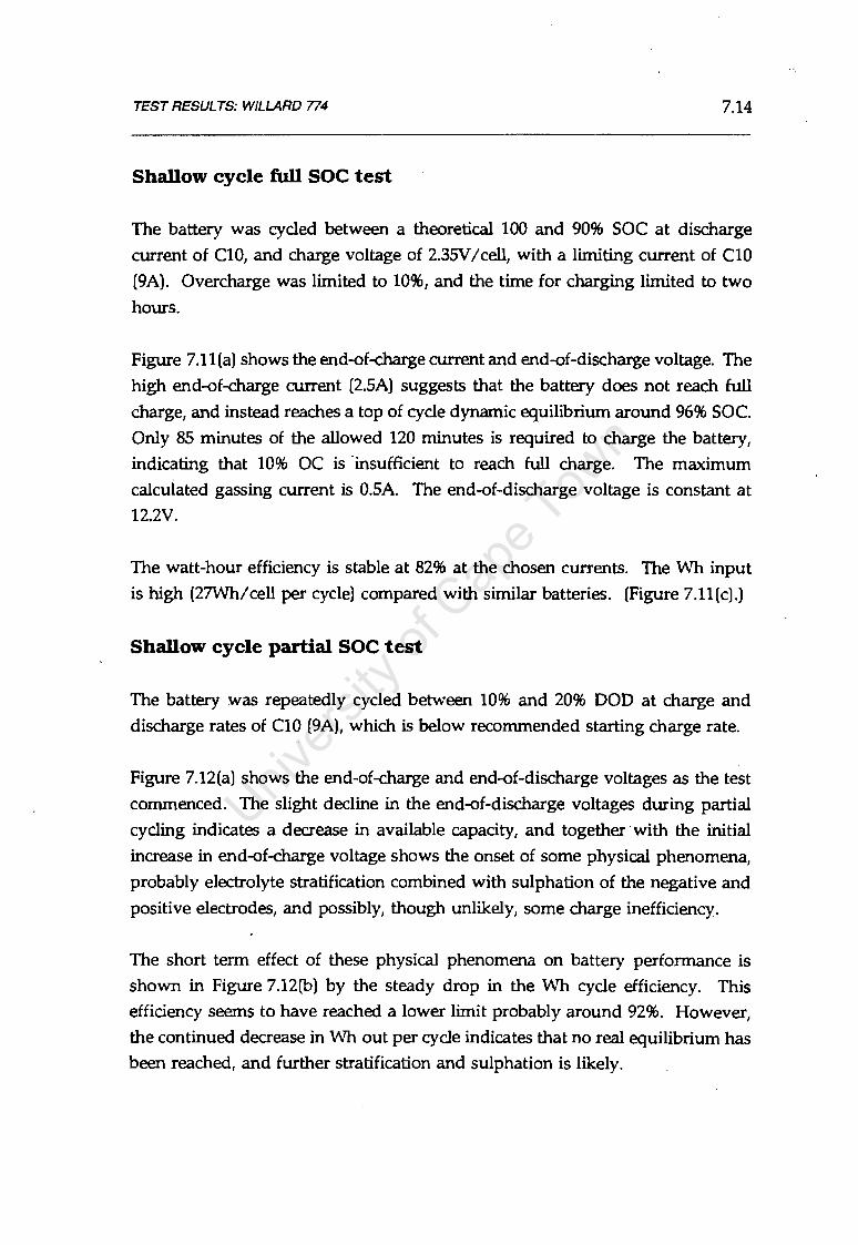
TEST RESULTS: WILLARD 774 7.14
Shallow cycle full SOC test
The battery was cycled between a theoretical 100 and 90% SOC at discharge
current of ClO, and charge voltage of 2.35V /cell, with a limiting current of ClO
(9A). Overcharge was limited to 10%, and the time for charging limited to two
hours.
Figure 7.ll(a) shows the end-of-charge current and end-of-discharge voltage. The
high end-of-charge current (2.SA) suggests that the battery does not reach full
charge, and instead reaches a top of cycle dynamic equilibrium around 96% SOC.
Only 85 minutes of the allowed 120 minutes is required to charge the battery,
indicating that 10% OC is ·insufficient to reach full charge. The maximum
calculated gassing current is O.SA. The end-of-discharge voltage is constant at
12.2V.
The watt-hour efficiency is stable at 82% at the chosen currents. The Wh input
is high (27Wh/cell per cycle) compared with similar batteries. (Figure 7.ll(c).)
Shallow cycle partial SOC test
The battery was repeatedly cycled between 10% and 20% DOD at charge and
discharge rates of ClO (9A), which is below recommended starting charge rate.
Figure 7.12(a) shows the end-of-charge and end-of-discharge voltages as the test
commenced. The slight decline in the end-of-discharge voltages during partial
cycling indicates a decrease in available capacity, and together ·with the initial
increase in end-of-charge voltage shows the onset of some physical phenomena,
probably electrolyte stratification combined with sulphation of the negative and
positive electrodes, and possibly, though unlikely, some charge inefficiency.
The short term effect of these physical phenomena on battery performance is
shown in Figure 7.12(b) by the steady drop in the Wh cycle efficiency. This
efficiency seems to have reached a lower limit probably around 92%. However,
the continued decrease in Wh out per cycle indicates that no real equilibrium has
been reached, and further stratification and sulphation is likely.

TEST RESULTS: WILLARD 774
_, _, w (.)
a: w c.. J: 3';
3.5,~-------------------...13
g 3 1-z w a: a: 8 2.5 w ~ a: ~ (.) 2 ···-··-----··-··-·-·-··-·-··--··-·-··--··-·····---·--··-··-·-···
eod voltage
12.8 ~ w ~ <
12.6 !:.:; ~ w
12.4 ~ ~
12.2 i5
1"5 J.o ___ 4 ___ 8 __ 1_2 ___ 16 ____ 20 __ ....,24-...--+2812
CYCLE NUMBER
4 8 12 16 20 24 28 CYCLE NUMBER
28 85
27 Wh input 84
26 l 83 ~
Whefficiency 25 z w t5
24 . 82 it w J:
23 Whout 3'; 81
22
80 21 0 4 8 12 16 20 24 28
CYCLE NUMBER
7.15
Figure 7.11 Shallow cycle full SOC test a) end'-Of-cycle conditions, b) charging time, c) Wh efficiencies.

TEST RESULTS: WILLARD 774
14.3...-------------------,
~ 13.8 w C)
~ _. ~ 13.3 w _. u i'.; 12.8 LL 0 Q z 12.3 w
25
24 _. _. w u er: 23 w Q..
::t: 3:
22
210
eocvoltage
••• eod voltage
~·--··-··---.. ·-··-··--··-··---·-··-··--.. -----.. -·--.. ---·-··---··· 4 8 12 16 20 24 28
CYCLE NUMBER
95
Whinput 94
l 93 i'.;
z w u
92 lE w ::t: 3:
Whout 91
90 4 8 12 16 20 24 28
CYCLE NUMBER
7.16
Figure 7.12 Shallow cycle partial SOC test a) end-of-cycle conditions, b) Wh
efficiencies.
Capacity at end of cycle tests
The cell was equalised and the capacity determined at the ClO rate to be 81.SAh,
compared with 83Ah at the start. The drop in capacity of 1.SAh represents 1.8%.
If the useful battery life is assumed complete when the drop in capacity is 20%,
then this cell has lost 9% of that 20%.
The percent of useful life used can be theoretically calculated using models (see
Section 3.12). The incremental wear due to:

TEST RESL!L TS: WILLARD 774
is
28 cycles@ 10% DOD (735 cycles expected over battery life)
28 cycles between 10% and 20% DOD (661 life cycles expected)
11cycles@40% DOD (403 cycles expected)
28/735 + 28/661 + 11/403 = .108 or 10.8%
H20 consumption
7.17
During the cycling tests the accumulated overcharge was approximately 56Ah,
which would account for a theoretical water loss of 20.5ml per cell (theoretically
0.366ml H20/Ah). Water consumption could not easily be measured because of
the non-translucent casings. Practical experience suggests that 5% gas
recombination efficiency by the vent plugs can be expected.
The vent plugs allowed considerable electrolyte seepage, particularly during
charging. This leakage not only necessitates more frequent maintenance, but is
dangerous and messy. The problem has since been rectified by the manufacturer.
Charging current and voltage requirements
The optimum charging requirements for the Willard 774 are difficult to determine
as there are two conflicting criteria. Prevention of stratification is obviously a
high priority, but at the same time gassing should be absolutely minimised.
Gassing in SLI type batteries quickly corrodes away the thin positive grids,
particularly in antimony cells. Additionally, gassing will expose the plates and
reduce available capacity.
For deep cycling to about 40% DOD, 3.6Ah of overcharge is sufficient to prevent
stratification, but just insufficient to fully recharge the battery at 9A and
2.35V I cell. Similarly, for shallow cycling to 10% DOD and charging at 9A and.
2.3V I cell, lAh of overcharge prevents stratification but does not allow complete
charging of the cell. The accumulation of undercharging during cycling results
in the gradual establishment of a SOC limit. For shallow cycling at 2.3V the OC
requirement due to gassing is about 1.5.Ah/ cycle, for deep cycling it may be 4.0 at 2.35V.

TEST RESULTS: WILLARD 774 7.18
Shallow cycling may be feasible if the amount of OC can be finely controlled to
just prevent stratification and limit gassing to a minimum. If gassing cannot be
easily restricted (due to temperature effects), then it will be better to cycle the
battery to about 40% DOD and use the excess gas for electrolyte mixing. The
shorter battery life (in years) will not be limited by grid corrosion, as may be the
case in the shallow cycle situation, where uncontrolled gassing may occur for long
periods. In either case, the charge regulator settings should be carefully
considered, and temperature compensated if possible.
7.1.5 Sizing and Selection: considerations in PV applications
1) Optimise battery life by choosing suitable daily DOD. Low DOD is
not necessarily optimal as overcharge may be excessive.
2) A void deep DOD for any period during very cold seasons, as
electrolyte freezing may occur.
3) A void excessive gassing during normal operation, which could
enhance corrosion of the thin SLI type grids. A charge regulator is
almost certainly required. Carefully select the regulator charge voltage
settings.
4) In extremely variable climates, watch for runaway gassing at higher ,
temperatures due to the high temperature coefficient of gassing.
Special care in regulator type selection may be required. Consider a
temperature compensated voltage regulator.
5) Minimise electrolyte stratification. The battery can easily recover form
short term stratification by gassing though this is best prevented,
by allowing up to 4Ah overcharge per deep cycle under carefully controlled chcµge conditions. However, such control may be difficult to achieve in small PV systems.
6) Calculate the maintenance period based on projected H20
consumption. Add a safety margin to allow for evaporative losses.
Water loss may expose the plates and cause permanent damage.

TEST RESULTS: RAYL/TE RMT108 7.19
7.2 RAYLITE RMT 108 STANDBY CELL
7 .2.1 General Information
Data summary
Capacity: Voltage:
Application:
Group:
Description:
Costing
Cost:
Wh cost:
Wh value:
c 10 = 108Ah@ 20°c
4V
standby power
tubular, antimony grid, flooded, tall Tubular, standby battery. Vented with flooded electrolyte, in
transparent EV A casing. A broad size range is available from the
RMT /RST family of batteries, from lSAh single plate cells to
2500Ah 20 plate cells. All are designed on the same principles,
are similar and test results are suitable for scaling across the size range.
R198 per cell (@ 23/10/1990)
R0.93/Wh as purchased (see Figure 7.13 for size/cost reduction for RMT range)
R0.58/kWh over battery life, assuming 4000 cycles at 40% DOD,
the optimum DOD. (See Section 7.2.3.)
450..-----------------:::--r2.5
\ 400 \
350 \
2.25
2
::l 300 \ i 1.75 ~
1.5 0 z
w (.)
~ 250 z ~ 200
150
100
\. "\.
·, ··. ·.
1.25 ~
0.75 ························-·-·-... ~~···-·········· 50,+-----r--r----r--r-~--r-----.-__,....~0.5
0 100 200 300 400 AH CAPACITY/CELL
Figure 7.13 Size/ cost reduction for Raylite RMT /RSTbatteries. (Rands/Wh cost assumes 4000 cycles at 40% DOD)

TEST RESULTS: RAYL/TE RMT108
7 .2.2 Physical
Physical construction
Dimensions:
Plates:
Grid:
height, width, length:
height over terminal:
mass:
positive design:
spines per positive:
positive plate weight:
negative design:
negative plate weight:
active block mass:
positive:
negative grid
grid mass:
312 x 208 x 180mm
360mm
23.2kg
3 x 36Ah tubular plates/ cell
NA
NA
flat pasted plate
NA
5.88kg/ cell
(80% of dry mass assumed)
1.6% Sb
pure lead
2.235kg/ cell
7.20
(40% of active block mass assumed) Dry cell mass: 14.7kg
Electrolyte: SG: 1.250@ 20oC
6.81
Wet mass:
Gas venting:
Casing:
Terminals:
volume:
mass: 8.Skg
23.2kg
screw type vent caps, rubber seal, sintered glass membrane
transparent EV A
bolt type, for which M6 316 stainless nuts, bolts, washer and
inter-cell connectors are supplied.

3
4
TEST RESULTS: RAYL/TE RMT108
Active mass utilisation coefficients (Calculated)
Active mass
capacity @ 100% 423Ah
utilisation
utilisation @ nominal 25%
capacity (108Ah)
utilisation@ lOOhr rate 43%
(180Ah)3
utilisation@ opt.DOD 10% (43Ah @ 40% DOD)4
7.21
Electrolyte SG@end
of test
385Ah 1.000
28% 1.190
47% 1.150
11% 1.230
Under normal operation, the SG will not fall below 1.19, but under extreme
conditions may drop to 1.15. The cell is designed with large reserve electrolyte
capacity.
7 .2.3 Basic Operating Data Available
Charging requirements and limits
(As recommended by the manufacturer, following deep discharge. No
specifications provided for shallow cycling or float charge operation) starting charge: 15A or 13.8% of ClO
finishing charge: 7.5A or 6.9% of ClO
equalising charge: 3A or 3.0% of ClO
See discharge tests in SECTION 7.2.4(a)
See SECTION 7.2.3

5
TEST RESULTS: RAYL/TE RMT108 7.22
Discharge curves
Complete discharge curves are provided for discharge rates greater than the 10
hour rate.
Life cycle data
No life cycle data is provided, but the manufacturer suggested that 1200 ~ycles @
80% DOD was possible, with a maximum life of 15 years under ideal conditions.
This seems reasonable as active mass utilisation coefficients are low at rated
capacity. On the basis of the utilisation coefficients and real test data for similar
tubular cells (grade A2 data: Lucas P series5), the RMT108 data was modelled to
produce a cycle life vs DOD curve. The similar shape curves indicate similar
failure mechanisms. This curve was used to infer an optimum DOD for the most
effective battery utilisation (Figure 7.14), which occurs in the range 30% to 60%
DOD.
10000
9000
8000
"' 7000 w -' 6000 (.)
i'.; 5000 u.. 0 4000 d z 3000
2000
1000
0 ~-,.----,.....--r----..-....--.---......--r----r--+40 10 20 30 40 50 60 70 80 90 100 0
% DEPTH OF DISCHARGE
Figure 7.14 Estimated cycle life vs DOD for Raylite RMT108
The Lucas P series, and indeed most tubular cells have similar active mass utilization coefficients, grid alloys, etc. Lucas P series life cycle curve is from personal communication with BP Solar (SA)

6
TEST RESULTS: RA YLITE RMT108 7.23
Extent of data from Manufacturer
Data Quality: All batteries in the RMT range are similar, and it seems unlikely that data has
been generated for each and every battery. While some data is specific
(Grade A2), most is probably scaled data of Grade C.
Data provided: Capacity and voltage vs discharge rate and discharge time. Format is
graphical and tabular: (Grade A2 or Grade CJ
Recommended charge rates (starting DOD not specified): (Grade C)
Masses, dimensions
See Appendix D2 for the manufacturer's data sheet.
Additional data on request by personal communication: Life cycle data: roughly estimated at 1200 cycles @80% DOD: (Grade C)
Float voltage operating parameters
Many SA cells are based on designs developed by parent companies. Raylite
tubular cells are based on the established Hagen design6• It is odd (and
reprehensible) that lifecycle data are not readily available for these important and widely used barreries.
7 .2.4 Test Results and Discussion
a) Capacity and discharge tests
Two sets of capacity tests were conducted at 18°C.
In the first set the cells were equalise charged, till the SG's were within
specification, ie 1.250. The cells were then discharged at 25A, 16A, 8.8A, 3.2A and
Hagen Batterie AG, Germany

TEST RESULTS: RA YLITE RMT108 7.24
1.5A till the recommended cut-off voltages (see manufacturer's data). Capacities
achieved were 20% higher than the manufacturers specifications. C100 is estimated
at 180Ah. (See Figure 7.15).
In the second set of discharge tests the cells were recharged with 15% overcharge
but not equalised. Average SG' s after charging were 1.220. The cells were then
discharged at the same rates as before. The capacities were 20% lower than
previously, but approximately coincident with the manufacturers specifications
at discharge rates greater than C3.
The variation in capacity between the equalised and partially stratified cells is
shown in Figure 7.16. The watt-hour capacity for the first test is included.
Further capacity tests were conducted at 0°C and 35°C at the 16A and B.BA rates,
starting from the defined state. The average change in capacity as a function of
temperature is shown in Figure 7.17.
Figure 7.18 shows the SG vs Ah removed, and the electrolyte freezing
temperature. It is clear from the discharge data that a maximum of 200Ah can be
removed at discharge rates higher than l.5A, before the voltage falls dramatically,
so the electrolyte SG will never be below 1.150. At low temperatures this capacity
is further reduced. The electrolyte is therefore never in danger of freezing at
temperatures above -lOOC. Active mass utilisation for both electrolyte and active
mass will normally be around 10% at 40% DOD cycling. The low utilisation is
typical of tubular batteries; the tubular construction allows higher active mass
utilisation while diffusion problems reduce the average effective performance at
higher currents. This can result in overspecification of the battery if operation is in the low discharge current regime.
Figure 7.19, derived from the discharge data, shows the cut-off voltages vs DOD
and discharge current, suitable for voltage regulator load-shed settings for
unstratified cells.

TEST RESULTS: RAYL/TE RMT108
_,
2.
2.
2.
1.
uj 1. (.)
1v
05
00
95
90
<n 1 ~
.85
!Z 1 .II(;
.75
.70
.65
r-::: ~ ~ :-- --t-- "-
'r---..... .......
SG=1.250 1
-:::::-r-......
'-'
~
...............,-- :::::::- ... ....
~ ""'- .... ~ ........... ' " '\ t'\ I\. '\
\ \ f\ \ \
\ \ 3.2A 1.5A 8.SA
16A -25A I I
I .uv
0 20 40 60 80 100 120 140 160 180 200 DOD(AH)
Figure 7.15 Standard discharge curves at 18°C.
200 400
170 340
Z' Z' $ 280 ~ ~ ~ u u ~ 110 220 ~ (3 (3
Ah capacity of partially stratified cell 80 160
50 100 0 5 10 15 20 25
DISCHARGE CURRENT (A)
7.25
Figure 7.16 Ah and Wh capacities vs discharge current, showing the effect. of stratification
130
(.) 120 C!! w 0 CD 110 -I-< ~ 100 u ~ < 90 (.) u.. 0 j use for Ah and Wh correction! * 80
70 0 5 10 15 20 25 30 35
TEMPERATURE (DEG C)
Figure 7.17. Capacity adjusted for temperature.

TEST RESULTS: RA YLITE RMT108
1.300+=============================r60
6 1250
.._,_ _____________ --150 ~w
. ~ c ...:..
~ 1.2001-1----~.---------------130 ~ ~It) [jj
15 wa: ~ 1.150+-------""<o-----------t u. ~ w
en 1.1001+----------..--------17 § g:
1.0501+-------------------13 @ .... w
1+--.----.---,.----.---r---.---..--....._.o 50 100 150 200 250 300 350 400
DOD(AH)
Figure 7.18 Electrolyte SG and freezing temperature vs Ah removed.
::::;....
2.05
2
1.95
~ 1.9 ~ w 1.85 ~
i5 .... 1.8
~ 1.75
1.7
)lt-w.
--•r--
><
r-
~ ~ ,.._ -
r-- r---~
r- iO-. 40%000 -- r---~ I I
I I I
60%000 -~
11 I I I I_
r-~ 80%000 r--,.._
1 I
1·65
0 2 4 6 8 10 12 14 16 18 20 22 24 26 28 30 DISCHARGE CURRENT (A)
Figure 7.19 Cut-off voltages at 18°C, suitable for load shed settings.
b) Charging tests
7.26
Charging tests were conducted as described in Section 6.2.5 using variable
charging current. Charging rates used were 16A, 8.8A, 3.2A, 1.5A, and 0.7 A. The
temperature compensated charge voltage limits used were 2.45, 2.35 and 2.28 volts
per cell at D°C, 18°C and 35°C respectively.
The charging curve at 18°C is shown in Figure 7.20. These curves show that a
minimum of 5.5Ah of overcharge is required to reach full charge at 18°C and
2.366V /cell, regardless of initial DOD. At the recommended finishing current
(7.5A), the voltage will be 2.45V /cell, and the overcharge required is 7.0Ah.

TEST RESULTS: RA YLITE RMT108 7.27
Instantaneous charging efficiency and gassing currents were determined by using
the end-of-charge voltage method in Section 6.2.6 (vi). The derived gassing or
overcharge current curves are shown in Figure 7.21.
The charging curves after compensation for gassing and overcharge losses are
shown in Figure 7.22. The end of charge voltage can be read from these curves,
as well as the sensitivity of end-of-charge current to the voltage setting. The
gradual increase of the slope of the compensated charging curves near full charge
indicates the early gassing, and relatively inefficient charging regime.
2.1...---~--.---r---r---r---.--..,....,.--,
2.6 100% soc --------+----+----!--!
::J' 2.5+---""l<---+---+----+-------1----+--t ..... w (.) ~ 2.4+--r~_.,,.,::-t-_-+---+---+--+---+--1
w Cl i5 2.3r----t"'t""<!-"':-tt-~-...c:---t---t-----t----t--I ..... §2 2.2+---+-~~,,..--~"""""-+...::::::.-i---1--~--1
0 20 40 60 80 100 120 DOD (AH)
Figure 7.20 Qua.si-constant current charging curve at 18°C. Charging rates used were 16A, B.BA, 3.2A, 1.SA, and 0.7 A.
2.7
2.6
18deg ::J' uj 2.5 (.) 35deg ~ w 2.4 Cl
~ 0 2.3 >
2.2
2.1 0 2 4 6 8 10 12 14 16
GASSING CURRENT (A)
Figure 7.21 Gassing current as a function of voltage and temperature.

TEST RESULTS: RA YLITE RMT108 .
2.7
2.6
=r- 2.5 _, w (..)
~ 2.4 w (!) ~ 2.3 _, §2 2.2
2.1
'-\
'\
~ ~
f'-.. r-.....
"' "" "'""- r--
r--...... ........ r--"'-- t---........... --
r-... ,.___ ......... ..__
t---- I""--~ - -- - t-- -.... ~ :::::: -- - .__ t--
-2o 10 20 30 40 50 60 70 80 90 100 110 120
DOD(AH)
2.7
2.6
=r- 2.5 _, w (..)
~ 2.4 w (!)
~ 2.3
§2 2.2
2.1
~ \ \. \
~ "' " """ " !'-.... ~ ~ ........_-
........ :---r--~
~ t-- --r--t-- ::::::: ::- -- -~ -~ --2 o 10 20 30 40 50 60 70 80 90 100 110 120 DOD (AH)
2.7
2.6
=r- 2.5 _, w (..) ~ 2.4 w (!) ~ 2.3 _, §2 2.2
2.1
~I
"" """ ~ ...........
~
"r-:::::-
"-.
!"-.... :---r--- r--......_ ;..._
----t---~ r--- r--r-: r-- t:::-r-- t::- t--._
._..__ -
2 o 10 20 30 40 50 60 70 80 90 100 110 120 DOD (AH)
7.28
Figure 7.22 Compensated charging curves at a) OOC, b) 18°C and c) 35°C;
charging rates used were 16A, B.BA, 3.2A, 1.SA, and 0.7 A.

TEST RESULTS: RA YUTE RMT108 7.29
c) Cycling tests
Cycling tests selection
The RMT108 battery is designed for deep cycle applications. However, the tall
flooded electrolyte cell it is particularly susceptible to electrolyte stratification. As
stratification is enhanced during partial state-of-charge operation, a deep cycle
partial SOC cycling test is.relevant. A deep cycle full SOC cycling test is required
to determine the overcharge cycle to eliminate stratification, and to determine the
effect on cycle efficiency. A shallow cycle full SOC test is useful for de~ing the minimum charge voltage during· shallow cycling, since unnecessary gassing
is to be avoided in antimony grid cells. Details of the tests are described in
Section 6.2.7.
Deep cycle partial SOC test
The battery was repeatedly cycled between 15% and 55% DOD at charge and
discharge rates of CB (15A), which is the recommended starting charge rate for
the cell. No overcharge allowance was made for the partial SOC tests.
Figure 7.23(a) shows the end-of-charge and end-of-discharge voltages as the test
proceded. The steady decline in the end-of-discharge voltages indicates a
decrease in available cell capacity. This phenomena is due partially to gassing
losses (±0.25Ah/cycle or 7.5Ah over the whole test). However, the drop in end
of-discharge voltage from 1.93V /cell to 1.8V /cell is equivalent to a gassing loss
(accumulated undercharge) of 50Ah, which cannot be entirely explained by
inefficiencies as the variation in charging curves from cycle to cycle are
remarkably consistent. The steeper slope of the end-of-test discharge curve
(Figure 7.23(b)) suggests that the only logical explanation is a change in dynamic
operation brought about by electrolyte stratification and negative grid sulphation, which is particularly clearly illustrated.
The short term effect of these physical phenomena on battery performance is shown in Figure 7.23(c) by the steady drop in the Wh output and Wh cycle
efficiency. This efficiency would reach an unspecified lower limit. The long term

TEST RESULTS: RA YLITE RMT108 7.30
effects of stratification would be seriously damaging. Gassing or equalisation
charging is the best remedy for removing stratification. Prolonged equalisation
may be required to reverse hard lead sulphate on the negative electrode. The
gassing rate of about 0.25Ah per cycle is unquestionably insufficient in this partial
SOC cycling regime.
The overcharge and equalisation charges to eliminate this stratification and
sulphation were determined by measuring the Ah input during equalisation
· charge. At the maximum gassing current of 3A, 60Ah of overcharge is required.
At a higher gassing current, say 7.SA (recommended after deep cycle), fewer Ah
would be required as mixing would be more effective, though the high end-of
charge voltage would promote grid corrosion.
The total Wh efficiency of the cycle test, including the equalisation charge to
return to the defined state, was 78%.
Deep cycle full SOC test
The battery was repeatedly cycled between full charge and 45% DOD. The
discharge rate was CB (15A). The battery was recharged at 2.4V /cell, with a
current limit of 15A. A high overcharge limit of 15% (6.75Ah/cycle) was chosen
to facilitate good electrolyte mixing.
Figure 7.24(a) shows the end-of-charge current and end-of-discharge voltages.
The slight decline in the end-of-charge current is probably due to good electrolyte mixing and reduced resistance as the test proceded.
The watt-hour efficiency for cycling is stable at 75.7% and indicates a dynamic
equilibrium; the gassing is at least sufficient to prevent stratification. If the cell
was regularly overcharged then the OC could be reduced below 15% accordingly.
The Ah efficiency is 87%. (See Figure 7.24(b).)
The Wh efficiency calculated from the charging curves is 74.2%. The end-of
charge current and voltage of 3.3A at 2.4V indicates that the battery is fully charged at the end of each cycle.

TEST RESULTS: RA YUTE RMT108 7.31
2.4 end of charge voltage
2.3
:::l' 2.2 _, w (.)
2.1 ~ w (!)
2 ~ _, 0 > 1.9
1.8 end of discharge voltage
1.7 0 4 8 12 16 20 24 28 32
CYCLE NUMBER
2.05
2
:::l' _, 1.95 w (.)
~ w 1.9 C!l ~ end-of-test discharge _,
1.85 0 >
1.8
20 40 60 80 100 120 AH REMOVED
90
100
89
_, 96 l _, 88 ~ w
(.) z a: w
·w u ~ 92 87 tE :r
3:: w :r 3::
88 86
Whout
84 85 0 4 8 12 16 20 24 28 32
CYCLE NUMBER
Figure 7.23 Deep cycle partial SOC test. a) end-of-cycle conditions, b) change of discharge profile with cycling, c) Wh efficiencies.

TEST RESULTS: RA YLITE RMT108
4.5..-----------------..2.2
4
g ~ 3.5 w a: a: 8 3 w C!l a: ~ 2.5 0
2
eoc current
=- ....... .....
······-·-······-···--····-------·-···--._. eodvohage
::::l' ...J w
2.1 g ;:::; w C!l
~ 2 §?
w ~ ~ 1.9 0 (/)
iS
1·5 +-0 - ......... --.2--.....3--4.-----.5---.-6---.-7 --+8 1·9
CYCLE NUMBER
120 78
115 Wh input n
110 l ...J
76 t ...J w
105 0 ·z w a:
Whefficiency 0 w Q. 100 75 it ::c :: w
::c 95 ::
Whout 74 90
85 73 0 2 3 4 5 6 7 8
CYCLE NUMBER
7.32
Figure 7.24 Deep cycle full SOC test. a) end-of-cycle conditions, b) Wh
efficiencies.
Shallow cycle full SOC Test
The battery was cycled between 100 and 90% SOC at discharge current of ClO,
and charge voltage of 2.3V /cell, with a limiting current of ClO (10.BA).
Overcharge was limited to 10%, and the time for charging limited to two hours.
The end-of-charge current and end-of-discharge voltage are shown in
Figilre 7.25(a). The maximum calculated gassing current is lA at 2.3V.

TEST RESULTS: RA YLJTE RMT108 7.33
The watt-hour efficiency is stable at 82.7% at the chosen currents (Figure 7.25(b)).
The efficiency from charging curves is estimated at 81 %. ·The overcharge of lAh
per cycle is easily sufficient to prevent stratification during shallow cycling. The
problem is that the battery is never fully charged, and reaches a maximum of
about 96% SOC. The long term effects of this will be permanent loss of capacity
in this uncharged 4% of the active material, followed by further capacity losses
in a similar manner. During shallow cycling to full charge most cells operate at
low efficiency, particularly the lead-antimony type. The Wh efficiency to
completely recharge the cell at 2.3V each cycle will be about 65% .(calculated from
the charging curves).
Capacity at end of cycle tests
The cell was equalised and the capacity determined at the ClO rate to be 141Ah,
indicating no significant capacity loss during the test. This showed that the
stratification and sulphation losses were totally reversible. The theoretical
capacity loss for the test cycles based on cycle life curves is also negligible.
H20 Consumption
During the cycling tests the accumulated overcharge was approximately 157 Ah,
which would account for a theoretical water loss of 52.7ml (theoretically 0.366ml
H20/ Ah). Water consumption was measured over the duration of the cycling
tests. On average SOml/ cell was lost by gassing and evaporation, indicating a 5%
gas recombination efficiency. This is consistent with practical experience for
vented cells. At no time did electrolyte splash or seep from these vent caps.
The volume of water contained between the maximum and minimum electrolyte
levels is 304ml. If the daily overcharge is lOAh (sufficient to prevent stratification,
little enough not to promote corrosion), then the time between refilling is about
87 days. · There is a further safety margin of 200ml before the plates are exposed.
The time will be dependent on several external factors such as temperature and humidity.

TEST RESULTS: RA YUTE RMT108
2.2..-------------------r2.3
2 eoc current
:::::t -' w
g 1.8 2.2 g
~ .... z w
w C!l ~ ~ 1.6
:::> u w 1.4 C!l
2.1 ~
a: < :c 1.2 u ...... , ........... __ .. _ .......................... --.-· ... - ...... --............ -----··-
eod voltage 2
0.8+--r--r---r--r---ir--r--r-"'"T""-r--r---ir--..---r-"".":"'-+1.9 0 4 8 12 16 20 24 28
CYCLE NUMBER
w
~ ~ u en i5
7.34
Figure 7.25 Shallow cycle full SOC test. a) end-of-cycle conditions, b) Wh
efficiencies.
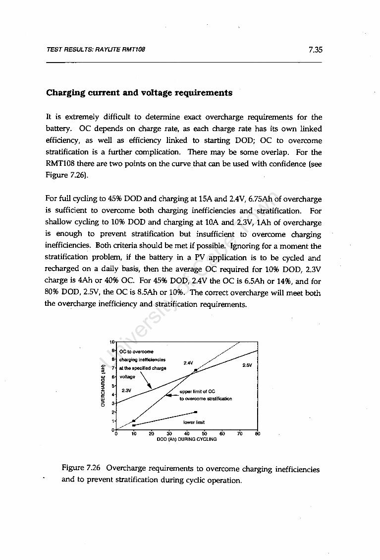
TEST RESULTS: RA YLITE RMT108 7.35
Charging current and voltage requirements
It is extremely difficult to determine exact overcharge requirements for the
battery. OC depends on charge rate, as each charge rate has its own linked
efficiency, as well as efficiency linked to starting DOD; OC to overcome
stratification is a further complication. There may be some overlap. For the
RMT108 there are two points on the curve that can be used with confidence (see Figure 7.26).
For full cycling to 45% DOD and charging at 15A and 2.4V, 6.75Ah of overcharge
is sufficient to overcome both charging inefficiencies and stratification. For
shallow cycling to 10% DOD and charging at lOA and 2.3V, lAh of overcharge
is enough to prevent stratification but insufficient to overcome charging
inefficiencies. Both criteria should be met if possible. Ignoring for a moment the
stratification problem, if the battery in a PV application is to be cycled and
recharged on a daily basis, then the average OC required for 10% DOD, 2.3V
charge is 4Ah or 40% OC. For 45% DOD, 2.4V the OC is 6.5Ah or 14%, and for
80% DOD, 2.SV, the OC is 8.5Ah or 10%. The correct overcharge will meet both
the overcharge inefficiency and stratification requirements.
10~-------------. .. .------.
.... ········· ... ··············
9 QC to overcome
8 charging inefficiencies 2.5V :C 7 at the specified charge
s. \ ~ 6 voltage
~ 5 ::c: ~ 4 w to overcome stratification e5 3
0 10 20 30 40 50 60 70 80 DOD (Ah) DURING CYCLING
Figure 7.26 Overcharge requirements. to overcome charging inefficiencies and to prevent stratification during cyclic operation.

TEST RESULTS: RAYL/TE RMT108 7.36
7 .2.5 Sizing and Selection:considerations in PV applications
1) Optimise battery life by choosing a suitable daily DOD.
2) A void or minimise electrolyte stratification by ensuring that both
charging and stratification prevention criteria are met. Equalising
charge is required approximately once a month, not more frequently, certainly no less.
3) Ensure suitable charging currents from the PV array. Low average currents will be insufficient to meet the charging needs.
4) Allow up to C10/10 Ah overcharge per deep cycle, though this will
make cycling less efficient.
5) The charge regulator setting is critical in controlling gassing. Excess
gassing will be damaging, but less so than for SLI type cells.
6) Take special care in regulator type selection, and consider temperature compensation of voltage regulator in extreme climates.
7) Calculate the maintenance period based on projected gassing and H20 consumption.
It is important to treat a long life battery moderately. If all these factors are taken
into account, the battery could provide 4000 cycles at 40% DOD, or last 10 years.

TEST RESULTS: WILLARD VANTAGE LS90 7.37
7.3 WILLARD VANTAGE LS90 UPS BATTERY
7 .3.1 General Information
Data Summary
Capacity: Voltage:
Application: Group:
Description:
C20 = 90Ah @ 20°c
12V
UPS/float charge applications
flat plate, antimony positive, calcium negative, flooded
Flat plate 12V power pack. Vented with flooded electrolyte, in
black casing. Essentially a modified SLI design, with thicker
plates. Antimony positive, lead-calcium negative.
See Appendix D3 for manufacturer's data sheet.
Costing
Cost:
Wh cost:
Wh value:
R364 per battery (@ 23/10/1990)
R0.34/Wh
RS.62/kWh over battery life, assuming 300 cycles at 20% DOD,
the optimum DOD. (See Section 7.3.3.)

TEST RESULTS: WILLARD VANTAGE LS90
7.3.2 Physical
Physical construction
Dimensions: height, width, length:
height over terminal:
mass:
Plates:
Grid:
Dry mass:
Electrolyte:
design:
positive plate weight:
negative plate weight:
active block mass:
positive:
negative grid
grid mass:
17.7kg
SG:
volume:
mass:
Wet mass: 25.6kg
220 x 172 x 342mm
235mm
25.6kg
15 flat plates/ cell
7 positives, 8 negatives
97g
94g
2.768kg/ cell
1.6% Sb
lead-calcium
1.107kg/ cell
7.38
(40% of active block mass assumed)
1.260@ 20oC
5.91
7.43kg
Gas venting: No vent caps, but single sintered glass gas escape. As far as the
user is concerned, the battery is MF. Casing: black plastic
Terminals: M6 316 stainless stud type. Washers and nuts are provided.

7
8
TEST RESULTS: WILLARD VANTAGE LS90
Active mass utilisation coefficients (Calculated)
Active mass
capacity @ 100% 152Ah
utilisation
utilisation @ nominal 59%
capacity (90Ah)
utilisation@ 100 hr rate 65% (98Ah)7
utilisation @ opt. DOD 12% (18Ah @ 20% DOD)8
7.39
Electrolyte SG@end
of test
121Ah 1.000
74% 1.055
80% 1.04
15% 1.25
Under normal operation (shallow cycling), the SG of the electrolyte is not limiting.
7.3.3 Basic Operating Data Available
Charging requirements and limits
The LS90 battery is normally operated in a very mild float charge mode. The
recommended voltage is 13.6V (2.226V I cell) at 20°C. Because antimony and
calcium grids are used, it is optimal to minimise overcharge to prevent
contamination of the negative by antimony transfer through gassing.
See discharge data in SECTION 7 .3.4(a).
. See life cycle data in SECTION 7.1.3

TEST RESULTS: WILLARD VANTAGE LS90 7.40
Discharge curves
Complete discharge curves at 200C are available ranging from 10 minute to 50.
hour rates.
Life cycle data
No life cycle data is available. The manufacturer suggested that possibly 100
cycles @ 80% DOD and 200-300 cycles at 20% DOD would be attainable under
normal operating conditions, but emphasised that the LS90 is not a cycling
battery, and would be optimal under float charge polarisation. The low cycle life
expectation is a reflection of the high active mass utilisation coefficients and
presence of a conventional calcium grid negative electrode. The optimum battery
utilisation for the estimated figures occurs in the DOD range greater than 40%
(see Figure 7.27), which conflicts with the assertion that the battery is not a
cycling battery. The tests confirm that the battery life during partial SOC cycling
is lower than projected. (See Section 7.3.4(c).)
400
350 Cf)
~ 300 ~ u 250 u. 0 0 200 z
150
100
10 20 30 40 50 60 70 % DEPTH OF DISCHARGE
Figure 7.27 Estimated cycle life curve for Willard LS90.
Extent of data from manufacturer
Data Quality:
The only data provided is the discharge and capacity data, which is Grade A2
(performed by the manufacturer in-house on the specific battery).
TEST RESULTS: WILLARD VANTAGE LS90 7.41
Data as purchased: Nominal capacity and discharge curves printed on battery casing.
Additional data on request by personal communication:
Plate masses, (dry and wet), overall masses and dimensions,
Life cycle data: estimated at 100 cycles @80% DOD, 200-300 cycles
@20% DOD: (Grade C).
See Appendix D3 for manufacturer's data sheet.
7 .3.4 Test Results and Discussion
a) capacity and discharge tests
Only one discharge test was performed because:
the battery is expected to lose capacity rapidly when repeatedly deep
discharged, invalidating the results of further tests,
the capacity is expected to change rapidly with age,
discharge curves for a new LS90 are available and can simply be verified,
the design and structure of the active mass is similar to the WILLARD 774,
which has been completely tested.
the battery will normally operate in the shallow discharge zone only, and
capacity limitations will not be encountered.
A new LS90 was equalised and stabilised at 18°C, then discharged to a cut-off of
10.8V at lOA. The discharge curve agreed exactly with manufacturers data.
Further, the WILLARD LS90 manufacturer's discharge curves were found to be
identical to WILLARD 774 discharge curves, which is not surprising as the active
block design is almost identical. The curves were accepted as valid for a new
battery. (See Figure 7.28.)
Two further LS90's were equalised and stabilised at 0°C and 35°C, and also
discharged at lOA to a 10.8V cut-off to determine the effect of temperature on
capacity. The measured capacities (62Ah and 85Ah respectively) represent a

TEST RESULTS: WILLARD VANTAGE LS90 7.42
change of ±0.66% per °C, and coincide approximately with the sensitivity
projected from the WILLARD 77 4 data.
There is generally no need for cut-off voltage curves for shallow cycle batteries,
but load shed settings at shallow DOD are strongly current dependent and load
shedding is this region is unlikely to be accurate (see Section 3.13).
Figure 7.29 shows electrolyte SG vs Ah removed, and the electrolyte freezing
temperature. Electrolyte freezing may occur if the cell is deep discharged.
Freezing point at 20% DOD vs ClOO is -S0C.
13
12.5
12 w C!>
~ 11.5 0 >
11
10.5
10 0 10 20 30 40 50 60 70 80 90 100 110
OOD(AH)
Figure 7.28 Discharge curves at 18°C at lA, 2A, SA, lOA and 20A.
1.300 60
6 1.250 50 C!> w c
...:,..
1.200 C!>
G;'" 30 z
N - w ii> w :::. 1.150 15 a: ..... C!> w rn
~ 1.100 7 0 a: .....
1.050 3 u w ..... w
+--r----.-~..---r----.-~...-'"T""---.-~.--'"T""--+o
10 20 30 40 50 60 70 80 90 100 110 OOD(AH)
Figure 7.29 Electrolyte SG and freezing point vs DOD.
TEST RESULTS: WILLARD VANTAGE LS90 7.43
b) Charging tests
Olarging tests were conducted as described in Section 6.2.5. Olarging rates used
were lOA, SA, 2A, lA, and O.SA. The temperature compensated charge voltage
limits used were 14.8, 14.5 and 14.2 volts at D°C, 18°C and 35°C respectively. In each case charging was started from 50% DOD.
The quasi-constant current charging curve at 18°C is shown in Figure 7.30. The
curve shows that a minimum of lAh of overcharge is required to reach full charge
at 18°C and 14.4V, regardless of the initial DOD. At the recommended float
voltage of 13.6V, the battery accepts virtually no charge.
Olarging efficiency was determined by the method in Section 6.2.6(vi). The end
of-charge current is assumed to be equal to the gassing current.
The charging efficiency was verified by a second method based on measuring the
rate of gassing, assuming a gas composition based on literature, and calculating
the current required to produce the gas flow rate (for method see
Section 6.2.6(iv)). This necessitated the removal of a plastic cover of the battery
to expose the sintered glass vent plugs. No gassing occurred till 14.0V at 100%
SOC. This approach shows good agreement with the first method. The main
difference is probably due to the non-stoichiometric gas ratio that occurs in
reality. The gassing curves are shown in Figure 7.31.
The charging curves after compensation for gassing and overcharge losses are
shown in Figure 7.32.

TEST RESULTS: WILLARD VANTAGE LS90 7.44
•
17
16.5
16
15.5
w 15
~ 14.5
§;? 14
13.5
13
12.5
100%
soc
~ 95% .. \\ f')_ I
l\' ; l \ 90%
~ .\i l '"1\'\ !\ \\\\ \ \\\.. ~' .......,, ~
~
::--: ~ ~ ~~ ~ ~ --=:::::::: :;;::,..:::__
~ 1~20 ·10 0 10 20 30 40 50 60 70
DOD (AH)
Figure 7.30 Quasi-constant current charging curve ~t 18°C. Charging rates
used were lOA, SA, 2A, lA, and O.SA.
17.5
17
16.5
~ 16
~ 15.5
~ 15
~ 14.5
14
13.5
II f...J lf
/ ~ ---v ~
/
-i.--r ~
t--
i--,._
_..; :.--L--- i.--
\ gas flow at 22 deg C
13 0 2 3 4 5 6 7 8 9 10
GASSING CURRENT (A)
-...-OdegC -18deg c
---35deg c
Figure 7.31 Gassing current as function of voltage and temperature.
Gassing current determined by gas flow determination is shown superimposed.

TEST RESULTS: WILLARD VANTAGE LS90
18
17.5
17
16.5
16
~ 15.5
~ 15 ..... ~ 14.5
"' " ~ '\
\ ,\ \\ \\ \ \.\.. '-....
!'...
'\ \
'\ \ \..
"-......
-- I"-.........
14
13.5
13
12.5
120 10 20
18
17.5
17
16.5
16
~ 15.5
~ 15 ..... ~ 14.5
r--. . '\ 1\ '\ 1\\ \\ I\ \.. 1'\ \..
'\
\ \..
................ i-...
" "-.... c--
30 40 DOD(AH)
14
13.5
13
12.5
120
- --- .:::---i:::::-._
w (!)
~ ..... 0 >
18
17.5
17
16.5
16
15.5
15
14.5
14
13.5
13
12.5
120
10 20
\ \ \ \ \ \ \
\ \ '\ \"-. .......
,....__.....__
-----= ;;:::: ~
10 20
30 40 DOD (AH)
:::::-... -----=:
30 40 DOD (~H)
7.45
-----=---50 60 70
~ ~ 50 60 70
50 60 70
Figure 7.32 Compensated charging curves at a) OOC, b) 18°C, c) 35°C. Charging rates used were lOA, SA, 2A, lA, and O.SA.

TEST RESULTS: WILLARD VANTAGE LS90 7.46
c) Cycling tests
Cycling tests selection
The LS90 battery is designed primarily for un-interruptible power supply (UPS)
applications, where it will normally be subjected to prolonged float charge
polarisation. Deep cycling would be infrequent. This type of operating regime
is unlikely in PV applications. It would be possible if the battery bank were
sufficiently large to restrict cycling to shallow DOD. Either way, only shallow
cycling is relevant. A shallow cycle full SOC test is useful for determining the
minimum charge voltage during shallow cycling, particularly since unnecessary
gassing is to be avoided. As mentioned, in many PV applications the system size
(energy capacity) is adjusted by increasing the installed battery capacity using low
cost batteries while maintaining the panel area. This may result in shallow
cycling at partial· SOC (see Chapter 2), so a partial SOC shallow cycle test is
useful. The cycling tests are described in Section 6.2.7. All cycling tests were
conducted at 20°C.
Shallow cycle full SOC test
The battery was repeatedly cycled between a fully charged state and 10% DOD.
The discharge rate was ClO (9A). The battery was recharged at 2.30V /cell, with
a current limit of ClO, and an overcharge limit of 10% (lAh/ cycle) for a
maximum of 2 hours per cycle.
Figure 7.33(a) shows the sharply decreasing end-of-charge current and end-of
discharge voltages. The decline in both current and voltage would normally
signify the onset of electrolyte stratification. Figure 7.33(b) shows that the amount
of charge that can be delivered at 2.3V in 2 hours is limited. Only after the
battery has adjusted to an equilibrium SOC can sufficient charge be delivered.
From this time continued stratification from undercharging is limited. The
efficient self-regulating or current tapering by the battery during constant voltage
charging is characteristic of the gassing curve, which is dependant on the high
polarisation potential of the lead-calcium negative electrode. (Compare gassing
curve with the WILLARD 774).

TEST RESULTS: WILLARD VANTAGE LS90 7.47
If the battery is operated in float charge mode, then stratification is minimal, and
the regulating effect will limit gassing. If the battery is cycled, then the self
regulating effect may limit gassing and charging rates so that either the cell
cannot be fully charged in the limited time available, or the lack of gassing results
in extreme and prolonged stratification setting in. Raising the charging voltage
will help in the short term, but in the long term the self-regulating effect will be
removed (by antimony transfer to the negative through gassing and reduction in
H2 polarisation potential), and the benefits of self-regulation destroyed.
The watt-hour efficiency for this controlled cycling stablilised at 86% and
indicated a state of dynamic equilibrium. (See Figure 7.33(c).) The Ah efficiency
is 86%.
Shallow cycle partial SOC test
The battery was repeatedly cycled between 10% and 20% DOD at charge and discharge rates of ClO (9A).
Figure 7.34(a) shows the end-of-charge and end-of-discharge voltages as the test
proceded. The slight decline in the end-of-discharge voltages indicates a decrease
in cell capacity, and together with the marked increase in end-of-charge voltage
shows the increase of cell internal resistance.
The change in charging curve cycle during the test is illustrated in Figure 7.34(b).
The rapid increase in the end-of-charge voltage is probably due to a combination
of electrolyte stratification and hard sulphation of the calcium alloy negative grid, leading to higher internal resistances. The theory has shown that calcium alloy
grids perform poorly under cycling polarisation, while the antimony positive is
unlikely to be seriously affected in the long term.
The short term effect of stratification on battery performance is shown in Figure 7.34(c} by the steady drop in the Wh cycle efficiency. This efficiency seems
to have reached a lower limit around 89.5%. However, the continued increase in end-of-charge voltage indicates that no real equilibrium has been reached, and further stratification and sulphation is likely.

TEST RESULTS: WILLARD VANTAGE LS90
Q w z c:: ::J I-w c:: J: <
1.5 ,.,..--------------------..12.8
1.3 g I-z w 1.1 c:: c:: ::J (.)
w 0.9 (!) c:: < J: (.)
0.7
· .. '· ..........
'·········-····-······~-~~~~: .•..•.. --•.. -.•.. -----...
12.6 ~ w (!)
~ 12.4 ..... §? w
12.2 ~ ~
12 i5
0·5+0---.,.....-4...--r-"""0.....-...---.12-..--1.,.6---.,.....-20...-"'T"""-2 ... 4-...---.20--+11 ·8
CYCLE NUMBER
11.35
11.3
11.25
11.2
11.15
11.1
11.05
11
10.95
10.9
10.85 0 4 8 12 16 20 24 28
CYCLE NUMBER
26 90
25 Wh input
89
l .....
88 ~ ..... 24 w
(.) z w c:: u w
D.. 87 ff: J: 23 w
== J:
== 22 86
21 85 0 4 8 12 16 20 24 28
CYCLE NUMBER
7.48
Figure 7.33 Shallow cycle full SOC test. a) end-of-cycle conditions, b) Ah returned, c) Wh cycle efficiencies.

TEST RESULTS: WILLARD VANTAGE LS90
14.5
14
w 13.5 ~
~ _, 13 §?
12.5
12 \.. eod voltage
... ·-··-----··---·-------·----------------·--·-·
w ~
14.5
i5 14 _, §?
13.5
4 8 12 16 20 24 28 CYCLE NUMBER
13.l-~~-==:;.~~~~--~~....-~---..,.--~---l 0 10 20 30 40 50 60
CHARGING TIME (MINUTES)
25 92 Wh input
91 24
l _, Whefficiency 90 ~
_, w 0 z
w a: 23 t3 w ~
89 ff :r: ;: w :r:
22 \ Whout ;:
88
21 87 0 4 8 12 16 20 24 28
CYCLE NUMBER
7.49
Figure 7.34 Shallow cycle partial SOC test a) end-of-cycle conditions, b) variation in charging profile, c) Wh efficiencies.

TEST RESULTS: WILLARD VANTAGE LS90 7.50
Capacity at end of cycle tests
The cell capacity at the end of the partial SOC test was 27 Ah to 10.SV. After
boost charging and equalisation at 14.2V (2.37V I cell) the capacity was determined
at the ClO rate to be 38Ah, and after further boosting at 15.0V (2.SV /cell) the
capacity was SOAh. The temporary loss in capacity due to stratification and
positive grid sulphation is therefore 23Ah during the partial SOC test.
The useful cell capacity after recovery was only SOAh compared with 82Ah at the
start. The permanent loss due to hard sulphation of the negative was 32Ah,
representing a 39% loss. The cell seems to have passed its useful life after only
29 full shallow cycles and 29 partial cycles.
A new LS90 was equalised, tested and subjected to the same shallow cycle partial
SOC test to determine the validity of the first test. The initial capacity was
81.48Ah (lOA, 18°C). After 30 cycles and a boost charge at 2.SV I cell the available
capacity was 70.47 Ah, representing a permanent capacity loss of 17%.
The incremental wear according to battery models based on the manufacturer's lifecycle estimates (see Section 3.12) is:
for the first battery:
29 cycles @ 10% DOD (400 cycles expected over battery life)
29 cycles between 10% and 20% DOD (300 life cycles expected)
=
29/400 + 29/300 = .169 or 16.9%
and for the second battery:
29 cycles between 10% and 20% DOD (300 life cycles expected)
=
29/300 = .0.966 or 9.7%
Finally, a third new battery was tested under shallow cycle full SOC regime for
35 cycles, artd the partial SOC regime was studiously avoided. The capacity at

TEST RESULTS: WILLARD VANTAGE LS90 7.51
the end of the test was 79Ah (lOA, 18°C). As there was no capacity determination
prior to cycling the drop in capacity cannot be accurately calculated. Based on the
initial capacities of the first two batteries the cell seemed to have retained about
96% of its initial capacity.
These batteries have a negative electrode that is limiting to cycle life (see
Section 3.6.3), and that life depends strongly on charging regimes and DOD.
Partial SOC is particularly damaging, as the difference in retained capacity
between batteries two and three shows. The cell was not tested in float mode,
where it would possibly (and probably) have lasted longer than most deep cycle
batteries. Therefore for float application this cell could possibly be considered.
H20 Consumption
The accumulated overcharge during the cycling tests was minimal. Water
consumption could not easily be measured because of the sealed nature of the
batteries. It can be deduced from the gassing curves that under continuous float
charge (13.6-14.0V at 20°C) water consumption should be negligible, and the
sealed battery should never suffer from plate exposure.
If strong gassing takes place the gassing current will increase in the long term,
and water loss may be sufficient to cause problems.
Charging current and voltage requirements
Optimal operation for the Willard LS90 is clearly in a float charge regime. The
charging voltage should provide sufficient gassing the prevent electrolyte
stratification. The manufacturers recommends 13.6V (2.27V I cell) regardless of
temperature, yet the gassing curves would suggest about 14.3V at 18°C, to provide
0.25A of gassing to prevent stratification. Electrolyte loss at 14.3V would be
minimal.

TEST RESULTS: WILLARD VANTAGE LS90 7.52
7 .3.5 Sizing and Selection: considerations in PV applications
1) Optimise battery life by choosing shallow cycle operation.
2) Avoid deep discharges, and any partial SOC operation at all. Partial
SOC operation will result in rapid battery failure.
3) Use system sizing rather than relying on load-shed regulators to limit
cycling to 20%. The regulator's ability to regulate accurately at this
DOD on the shallow slope of discharge curves depends on a good
knowledge of the average and peak load currents. Accurate load
shedding in this region is doubtful.
4) Minimise sulphation of the negative electrode and electrolyte
stratification by ensuring mild float charge operation for most of the
charging cycle. The battery cannot easily recover form short term
stratification by gassing as gassing is very low at the recommended
charge voltage. Prolonged float charge gassing is a feasible alternative.
5) Stay within the recommended charge voltages, as excess gassing could,
in the long term, cause a runaway situation by lowering the gassing
voltages and result in the battery plate exposure. Although 13.6V is
recommended by the manufacturer for UPS use, for PV applications
13.BV at 30°C and 14.2V at 15°C is recommended.
6) Consider self-regulation. The steep rise in the charging curve voltage
at full charge has a current-limiting, self-regulating action. By the
nature of these curves the LS90 may be suitable for a self-regulating
PV system with matched panels and no charge regulator. However,
caution is required to prevent excess gassing which would lead to
plate exposure if the panels are not matched to the recommended
charge voltage.

TEST RESULTS: GNB 12V-5000 7.53
7.4 GNB 12V-5000 PHOTOVOLTAIC BATTERY
7 .4.1 General Information
Data Summary
Capacity: Voltage:
Application:
Group:
Description:
C24 = 93Ah, c 100= lOOAh @ 20°c 12V
photovoltaic
flat plate, antimony alloy positive, treated calcium ternary
negative, absorbed immobilised electrolyte, sealed
Flat plate 12V power pack. Sealed and pressurised operating on
the closed 0 2 recombination cycle. Absorbed electrolyte
suspended in the separators, can operate in any orientation.
Pressure relief by safety vent at SPSI. Specialist PV design. Low
antimony alloy positive, treated lead-calcium-tin negative.
Maintenance free operation. In black polypropylene casing with orange cover.
See Appendix D4 for manufacturer's data sheet.
Costing
Cost:
Wh cost:
Wh value:
R659 per battery (@ 23/10/1990)
R0.59/Wh
Rl.14/kWh over battery life, assuming 1300 cycles at 40% DOD,
the optimum DOD. (See Section 7.4.3.) This can only be regarded as an estimate

TEST RESULTS: GNB 12V-5000 7.54
7 .4.2 Physical
Physical construction
Dimensions:
Plates:
Grid:
Electrolyte:
Gas venting:
Casing:
Terminals:
height, width, length:
mass:
design:
positive plate weight:
negative plate weight:
active block mass:
positive:
negative grid
grid mass:
NA, but estimated
216 x 173 x 324mm
but can operate in any orientation.
29kg
9 flat plates/cell
4 positives, 5 negatives
NA
NA
NA
low Sb alloy (unspecified %)
treated lead-calcium-tin
not specified, but thickened grid
used
SG = 1.260 @ 20oC
volume = ±5.91
mass = ±7.43kg
absorbed in the pores of the active material, or in the fibreglass
separator matrix (mean fibre diameter= 0.5 to 2.0 microns).
Six interconnected vent caps, for pressure control. Pressure relief
at 5PSI, self resealing. Vent caps are not for user removal. Battery design is MF.
black plastic
bolt type terminal, M6 316 stainless bolts and washers provided.

9
10
TEST RESULTS: GNB 12V-5000
Active mass utilisation coefficients (Calculated)
7.55
Accurate utilisation coefficients cannot be determined without figures for active
masses. These figures are estimates, based on batteries of similar mass.
Active mass Electrolyte SG@end
of test
capacity @ 100% 152Ah NA NA utilisation
utilisation @ nominal 61% NA NA capacity (93Ah)
utilisation @ 100 hr rate 66% NA NA (100h)9
utilisation @ opt. DOD 26% NA NA (40Ah @ 40% DOD)10
7 .4.3 Basic Operating Data Available
Charging requirements and limits
Charging of sealed batteries is usually voltage limited, as this is the easiest way
to control and prevent loss of water which cannot be replaced. Recommended charging voltages (specified at 25°C) are:
' 2.3V /cell for 0%-2% daily DOD
2.35V /cell for 0%-5% daily DOD
2.40V /cell for DOD above 5%.
Temperature compensation is -0.02V I cell per 0C.
See discharge data in SECTION 7.4.4(a).
See life cycle data in SECTION 7.4.3.

TEST RESULTS: GNB 12V-5000 7.56
Discharge curves
Complete discharge curves are not provided, however capacities to 1.75V I cell at
25°C are listed:
8hr 24hr
48hr lOOhr
85Ah 93Ah 96Ah lOOAh
A temperature compensation curve is provided, showing 0.85% loss per °C below
25°C.
Life cycle data
A life cycle cill-ve is provided, showing 500 cycles to 80% DOD and 1600 cycles
to 30% DOD. Additional text claims at least 1200 cycles to 20% DOD. The
optimum battery utilisation for the cycle life figures (based on the curve) occurs
at 40% to 50% DOD. (See Figure 7.35.)
en w _, u !'.; u.. 0 d z
1500
1000
500
/ / ! ! i :
I !
I 0
0 10 20 30 40 50 60 70 'lb DEPTH OF OICHARGE
Figure 7.35 Manufacturer's life cycle curve for GNB 12V-5000.

TEST RESULTS: GNB 12V-5000 7.57
Extent of manufacturer's data
Data Quality: The data provided is probably Grade A2 (performed by the manufacturer in
house on the specific battery).
Data as purchased: Nominal capacity and capacities at various discharge rates.
Temperature correction for capacity
Recommended charging voltages
Cycle life curve
Self-discharge rate
Safety valve relief pressure
Additional data on request by personal communication:
Experimental and research papers from manufacturer's laboratory,
though probably also available through open literature.
See Appendix E4 for manufacturer's data sheet.
7 .4.4 Test Results and Discussion
a) Capacity and discharge tests
A new battery was equalised and stabilised at 18°C, then discharged at lOA to a
cut-off of 10.6V to yield 74.8Ah. Conversion of this capacity to 2S°C using the
supplied capacity adjustment curve results in a capacity of 83.33Ah, or within 2%
of the rated capacity which is 8S.5Ah at lOA (to 10.SV). 10 Cycles of the battery
using 40% DOD cycles and 2.40V I cell charging increased the capacity by a further
2% to within specification. The full capacity was considered available, and
discharge tests performed at 18°C at lOA, SA and 2A are shown in Figure 7.36.
The battery was again equalised and stabilised at OOC, and discharged at lOA, SA,
2A and lA to a 10.8V cut-off to determine the effect of temperature on.capacity.
The discharge curves at 0°C are in Figure 7.37. The battery was also recharged

TEST RESULTS: GNB 12V-5000 7.58
and discharged at lOA at 35°C. The measured capacity change averaged 1.67%
per °C below 18°C and coincides with the expected sensitivity projected from the
manufacturer's data. (See Figure 7.38.)
Figure 7.39 shows the relationship between capacity at 25°C and the discharge
current, comparing manufacturer's data with temperature adjusted experimental
data.
Figure 7.40 shows cut-off voltages suitable for load shed setting for deep
discharge cycling.
w C> ~ ..... ~
13
12.5
12
11.5
11
10.5 10A 5A 2A
10+--+-+--+--+---+--+----1f---+--+---I 0 10 20 30 40 50 60 70 80 90 100
OOD(AH)
Figure 7.36 Discharge curves at 18°C.
w C> ~ ..... 0 >
13
12.5
12
11.5
11
10A 5A 2A 1A 10.5
10+--+-+--+--+---+--+----11---+--+---I 0 10 20 30 40 50 60 70 80 90 100
OOO(AH)
Figure 7.37 Discharge curves at 0°C.

TEST RESULTS: GNB 12V-5000 7.59
110
105
100
~ 95
~ 90
< 85 u LL 80 0 'i/I. 75
70
65 A
60 -5 5 15 25 35 45
TEMPERATURE (DEG C)
Figure 7 .38 Retained capacity vs temperature. Triangles represent
experimental data.
100
95
90
f 85 ~
~ 80 (3 < c..
75 < u
70
65
60 0 5 10 15 20 25
DISCHARGE CURRENT (A)
Figure 7.39 Capacity vs discharge current at 25°C. Triangles represent
experimental data.
2 3 4 5 6 7 8 9 10 DISCHARGE CURRENT (A)
....... Odeg C -18deg C
Figure 7.40 Cut-off voltages for regulator load shed settings.

TEST RESULTS: GNB 12V-5000 7.60
b) Charging tests
Charging tests were conducted as described in Section 6.2.S. Charging rates used
were lOA, SA, 2A, lA, and 0.SA. The temperature compensated charge voltage
limits used were lS.O, 14.6 and 14.1 volts at 0°C, 18°C and 3S°C respectively. In
eaCh case charging was started from 90% DOD.
The quasi-constant current charging curve at 18°C is shown in Figure 7.41. The
curve shows that a maximum of lAh of overcharge is required to reach full
charge at 18°C and 14.4V, regardless of the initial DOD. At the recommended
float voltage of 13.6V, the battery accepts virtually no charge (self-regulation by
current tapering).
-·- I I .5 100% soc . 95%
17
16
16
15
~ 15
~ 14 .... §; 14
.0
.5
.0
.5
-·-.5 13
13
12
.0
.5
\"' ,\ \ ~ ,\\\ ' I\; \ \ \ ~ '
" " !' ;..__' ... ~ ....... ~
I"-.. ........ --~ r-.
~ ~ -=---.0 12
.10.0 0.0 10.0 20.0 30.0 40.0 50.0 60.0 70.0 DOD(AH)
. Figure 7.41 Quasi-constant current charging curve at 18°C. Charging rates used were lOA, SA, 2A, lA, and 0.SA.
Charging efficiency was determined by the method in Section 6.2.6(vi). The end
of-charge current is assumed to be equal to the gassing current. The curves are shown in Figure 7.42.
The charging efficiency was verified, and other useful data generated, by
measuring the rate of gas recombination during and after gassing. The method
is described in Section 6.2.6(v) and necessitated the installation of a pressure
tapping in the casing. The volume of the headspace (0.00154m3) was determined
by compressing the gas in the headspace isothermally, measuring the volume

TEST RESULTS: GNB 12V-5000 7.61
change and applying the ideal gas law. This volume is the headspace above all
six cells. The fully charged cell was charged as described in the method at
constant potentials 14.2V, 14.4V, 14.6V, 15.0V, 15.SV and 16.0V. The equilibrium
cell pressures at these voltages are in Figure 7.43.
Some venting occurred at 3.8 PSI, at 16.0V (compared with specifications
presenting a venting pressure of 5 PSI ±2PSI). Clearly this is the limiting voltage
at 18°C.
The gassing curves determined by the two methods are in Figure 7.44, and there
is good agreement. No gassing occurred till 14.0V at 100% SOC. Determination
of the limiting charge voltage at different temperatures is difficult without
experimentation, as the rate of 0 2 recombination (which must be equal to the
gassing rate at steady state) is temperature dependant in addition to temperature
dependence of the rate of gas evolution. If the charging voltages are kept to the recommended values then there ought to be no gas venting.
The charging curves after compensation for gassing and overcharge losses are shown in Figure 7.45.
-·-17
-·-16
16 .0
w 15 .5
~ 15
~ .0
k--:: ----J ~I
// =-------f / 14 .5
f/ 14
. I /
13 .5
13 .0 0.0 1.0 2.0 3.0 4.0
GASSING CURRENT (A)
........ ~
OdegC --~ 18deg c --35deg c
5.0
Figure 7.42 Gassing current as a function of cell voltage and temperature.

TEST RESULTS: GNB 12V-5000 7.62
27 3.9
26 some venting occurs 3.7
25
24 3.5
[ 23 e 3.3 w 22 er 3.1 ::I 21 en en 2.9 w 20 er c..
19 2.7 18
17 2.5
16 2.3 14.00 14.50 15.00 15.50 16.00
CHARGE VOLTAGE (V)
Figure 7.43 Steady-state cell pressure vs charging voltage.
17.0
16.5
16.0
w 15.5 (!)
~ 15.0 ..... 0 > 14.5
14.0
13.5
13.0 0.0 1.0 2.0 3.0 4.0 5.0
GASSING CURRENT (A)
Figure 7.44 Gassing current as function of voltage and temperature.
Triangles represent the gassing current determined by monitoring cell
pressure change.

TEST RESULTS: GNB 12V-5000
-17.5
17.0
16.5
16.0
,._ -1\
15.5 w ~ 15.0
g 14.5
14.0
13.5
13.0
12.5
""' \ \ \ \ \
\ \' """'\
\ i\ \
\ ' \ \
""' ' ~
~ '\
"'-..._ _ ............ __ -............ ......
~ :::-._
12·i.o 10.0 20.0 30.o 40.o 50.o 60.o 10.0
w
17.5
17.0
16.5
16.0
15.5
~ 15.0
g 14.5
14.0
13.5
13.0
12.5
\ ' \ \ \ \
\ \ ' ,\... "-
DOD (AH)
\ \
r'- ""' _'-....... ~ -~ ---~ i-._ --~
~ ~
12.i.o 10.0 20.0 30.o 40.o 50.o 60.o 10.0
w
17.5
17.0
16.5
16.0
15.5
~ 15.0
§? 14.5
14.0
13.5
13.0
12.5
12.0
r\ f\\ \'\_
1\ \ 1\ \ " ............_,,
DOD(AH)
I'-,, ..... _ ............... ~
........... ::---,__ I ---
0.0 10.0 20.0 30.0 40.0 50.0 60.0 70.0 DOD(AH)
7.63
Figure 7.45 Compensated charging curves at a) OOC, b) 18°C, c) 35°C.
Charging rates used were lOA, SA, 2A, lA, and O.SA.

TEST RESULTS: GNB 12V·5000 7.64
c) Cycling tests
Cycling tests selection
The GNB 12-5000 is designed for deep cycling in PV applications. A deep cycle
full SOC test is useful to determine overcharge requirements, and a shallow cycle
partial SOC test to determine experimentally the effects of partial SOC operation
in the absence of stratification. The cycling tests are described in Section 6.2.7.
All cycling tests were conducted at 20°C. The lOA capacity before the tests was
75Ah.
Shallow cycle partial SOC test
The battery was repeatedly cycled between 10% and 20% DOD at charge and
discharge rates of ClO (lOA).
Figure 7.46(a) shows the end-of-charge and end-of-discharge voltages as the test
commenced. The slight decline in the end-of-discharge voltage indicates a
decrease in cell capacity, and has been identified by Szymborski (1982) as being
due to sulphation of the negative electrode and the possibility of slight charge
inefficiencies, and is typical of partial SOC operation in lead-acid batteries. The
slight increase in end-of-charge voltage is attributed to the formation of hard lead
sulphate which is difficult to charge, resulting in elevated end-of-charge
potentials. Hard sulphation of positive plates is reversible while the negatives
show a strong capacity loss.
The short term effect of sulphation on battery performance is shown in
Figure 7.46(b) by the gradual and continuing drop in the Wh cycle efficiency, and further sulphation is likely. Long term undercharging will result in irreversible
sulphation.
It is calculated from the charging curves that very little gassing occurs, so capacity
losses are therefore not due to gassing losses. The available capacity after 28
cycles was determined to be 57Ah (lOA, 18°C), representing a loss of 17Ah or
0.6Ah per cycle due only to the physiCal phenomena. Szymborski (1982) has

TEST RESULTS: GNB 12V-5000 7.65
determined that the rate of decay of capacity is related more to the time spent in
the discharged state than the cycling rate.
14.8~---------------,
14.3 w
~ 13.8 §2 w -J 13.3
~ ~ 12.8 0
eocvoltage
z w ···-·-·---··--··---··-··-··-··-·-·-··---··-··-··----·-·-··· 12.3
4
25
_, 24 _, w 0 a: w Q.
::c 3: 23
220 4
eodvoltage
8 12 16 20 24 28 CYCLE NUMBER
Wh input ----Wh efficiency
Whout
8 12 16 20 24 28 CYCLE NUMBER
95
94
l 93 ('.';
z w u
92 H: w ::c 3:
91
90
Figure 7.46 Shallow cycle partial SOC test. a) end-of-cycle conditions, b) Wh cycle efficiencies.
Deep cycle full SOC test
The battery was repeatedly cycled between a fully charged state and 45% DOD.
The discharge rate was ClO (lOA). The battery was recharged at 2.43V /cell, with
a current limit of ClO, and an overcharge limit of 15% (6.75Ah/cycle) for a maximum of 8 hours per cycle.

TEST RESULTS: GNB 12V-5000 7.66
Figure 7.47(a) shows the steady end-of-charge current and end-of-discharge
voltages as the test progressed. The end-of-charge current is very low, indicating
a fully charged battery. During the charging cycles only 48Ah could be returned
to the cell in the allowed time, ie only 3Ah of overcharge. This at first seems like
too little overcharge for deep cycling, but confirmation can be obtained from the
charging curve (Figure 7.41) which shows that at 2.43V /cell only lAh is required
to overcome inefficiencies. 2Ah are therefore used in overcharge and equalisation.
Examination of the charging profiles (Figure 7.47(b)) obtained from the first and
last charge cycles shows absolute coincidence, and therefore no physical effects
during the 10 cycles. The charging profile also shows the excellent self-regulating
nature of the battery which restricts charging current to 0.7 A at 2.43V I cell once
the battery is full.
The efficient self-regulating or pinching by the battery during charging is
characteristic of the gassing curve, which is to a high degree dependant on the
high polarisation potential of the lead-calcium-tin negative electrode. (Compare
gassing curve with the WILLARD 774).
The watt-hour efficiency for this controlled cycling was stable at 86%.
Capacity at end of cycle tests
The (ClO) cell capacity at the end of the partial SOC test was 57Ah to 10.SV. After boost. charging and equalisation the cell recovered full capacity. The
temporary loss in capacity due to reversible sulphation is therefore 17 Ah during
the partial SOC test, or 0.66Ah/ cycle.
The cell capacity after the deep cycling test was 83Ah (lOA, 2S°C), or 78Ah at 200C
ie an increase in capacity of 3Ah. The increase is probably due to the cycling in
a mild operating regime.

TEST RESULTS: GNB 12V-5000
12.8
eoc current 12.6 :?; 0.8
g w ... <!> z < w 0.6 12.4 !::; cc cc g ::> (.) w w 0.4 12.2 ~ <!> < cc ::c < eod voltage (.) ::c en (.)
12 i5 0.2
00 2 3 4 5 6 7 8 9 11.8
10 CYCLE NUMBER
11~~~~~~~~~~~~~~~~~--
10
9
g 8 ... a5 7 cc cc 6 ::>
~ 5
~ 4 ;! 3 (.)
..... ..... w (.)
cc w c.. ::c ;:
2
1
115
110
105
100
95
90 0
50 100 150 200 250 300 350 400 450 500 MINUTES
Wh input
Whefficiency -
Whout
90
89
88
87 l >-86 (.) z
85 !:!::! (.)
84 ff w
83 ::c ;: 82
81
80 2 3 4 5 6 7 8 9 10
CYCLE NUMBER
7.67
Figure 7.47 Deep cycle full SOC test. a) end-of-cycle conditions, b) charging profiles, c) Wh cycle efficiencies.

TEST RESULTS: GNB 12V-5000 7.68
H20 Consumption
The accumulated overcharge during the cycling tests was minimal, and water loss
could not easily be measured because of the sealed nature of the batteries, and the
difficulty in detecting the very small weight changes. It can be deduced from the
gassing curves and the pressure curve that as the charge voltage was maintained
below 16.0V, no venting occurred and therefore there was no water loss.
Charging current and voltage requirements
Charging requirements for the GNB 12-5000 revolve around keeping the cell
pressure below the venting point yet away from the partial SOC regime if
possible. The pressure limitation requires restricting the gassing current, which
may be indicated by the cell voltage if temperature compensation is used. The
gassing current limit is 2A. If the voltage (gassing current) is too high then the
cell may vent and become dried out and useless in a very short while. If the
charging voltage is too low then the self-regulating nature of the battery will
prevent recharging within a reasonable time, resulting in partial SOC operation.
Overcharge requirements are minimal as the battery is by nature very efficient,
and 3Ah per cycle should be sufficient for most deep cycle application, while for
shallow cycling lAh would be sufficient.
7 .4.5 Sizing and Selection:considerations in PV applications
1) Optimise battery life by choosing 40% daily DOD.
2) Charge the battery at a voltage which allows sufficient time for
recharging of the battery, with some overcharge, but do not exceed the
2A gassing current. Partial SOC operation is far less problematic than
for flooded electrolyte batteries as stratification is eliminated, but the
deleterious effects of hard sulphation can not be ignored.
3) Control pressure inside the battery, which could cause venting, water
loss and permanent damage. This is easily accomplished by charge voltage regulation. If the charge voltage is maintained below lSV then
no temperature compensation of the charge regulator is required.

TEST RESULTS: GNB 12V-5000 7.69
4) Consider using the self-regulating nature of the battery to full
advantage. This can be accomplished by using the battery without a
regulator with a well matched PV array, but is also subject to several
other constraints (Section 3.14.1). Particularly, the cell ventingpressure
should not be exceeded. This battery remains a prime candidate for
self-regulation provided matChing of the panel and battery with the
load avoids cell venting and overdischarge.

TEST RESULTS: DELCO 1250 7.70.
7.5 DELCO 1250 TRUCK/UPS BATTERY
7.5.1 General Information
Data summary
Capacity:
Voltage:
Application:
Description:
Cio = 105Ah; C100 = 115Ah 12V
UPS/float charge applications
Flat plate 12V power pack. Vented with flooded electrolyte, in
black casing. Essentially a modified SLI design, with thicker
plates. Lead-calcium negative and positive grids. Internal
optical SG hydrometer for instant SOC indication.
See Appendix DS for manufacturer's data sheet.
Costing
Cost:
Wh cost:
Wh value:
R280 per battery (@ 23/10/1990)
R0.22/Wh
R2.78/kWh over battery life, assuming 800 cycles at 10% DOD,
the optimum DOD. These figures are based on approximate
data. (See Section 7.5.3 for detailed discussion of life cycle data, and Section 7.5.4(c).)

11
12
TEST RESULTS: DELCO 1250
7.5.2 Physical
Physical construction
Dimensions:
Plates:
Grid:
Dry mass:
Electrolyte:
height, width, length:
height over tenninal:
mass:
design:
pos. active material:
neg. active material:
active block mass:
positive:
negative grid
grid mass:
17.18kg
SG:
volume:
mass:
Wet mass: 25.28kg
238.8 x 172 x 330.2mm
360mm
26.9kg
15 flat plates/ cell
8 positives, 7 negatives11
111.5g, 1.llmm thick
120.5g, 1.14mm thick
2.464kg/ cell
7.71
lead-calcium, 57.9g, 1.19mm thick
lead-calcium, 38.0g, 0.99mm thick
0.729kg/ cell
1.270@ 27'C
6.38!12
8.lkg
Gas venting: No vent caps, but single sintered glass gas escape. As far as the
user is concerned, the battery is maintenance-free. Casing: black plastic
SOC indicator: optical hydrometer,
Terminals: Two types are available.
model 1251:
models 1250 and 2000:
located in cell number 2 only
conventional lead post
stainless stud type
(MlO 316 stainless nuts and washers
not provided)
It is conventional for the number of negative plates to be equal the number of positive plates plus one.
The DELCO 2000 Photovoltaic battery is identical in all respects, except that is contains additional (unspecified amount) electrolyte, but of lower SG.

TEST RESULTS: DELCO 1250
Active mass utilisation coefficients (Calculated)
Active mass
Capacity@ 100% 199Ah
utilisation
utilisation @ nominal 53%
capacity (105Ah)
utilisation @ lOOhr rate 58%
(115Ah)
utilisation @ opt. DOD 5.8% (11Ah @ 10% DOD)
7.72
Electrolyte SG@end
of test
133Ah 1.000
78% 1.072
86% 1.050
8.6% 1.260
Under normal operation, the SG of the electrolyte will limit capacity, as well as
resulting in higher internal resistances which reduce efficiencies.
7.5.3 Basic Operating Data Available
Charging requirements and limits
(following deep discharge cycling)
fast charge: SOA for 1th hours (50% of C20)
slow charge: SA for 20 hours (5% of C20)
Equalising charge: 2.7A or 3.0% of C20
with the proviso that the voltage in all cases is less than 13.8V at 30°C in float
applications.
Discharge curves
Complete discharge curves are available, from lA to lOOA.

TEST RESULTS: DELCO 1250 7.73
Life cycle data
Delco Remy enclose unconventional cycle life curves with the comprehensive
battery literature. The curves show cycle life, till 50% capacity loss, vs DOD on
a log-log scale. (The conventional format is to show life till 20% capacity loss on
a semi-log scale). By their own admission, Delco have extrapolated the life cycle data from some experimental results. It is debatable which of the log-log and
semi-log model extrapolations is valid for this battery (see. comprehensive
discussion Section 3.12.). The semi-log and log-log models are compared in
Figure 7.48. In one case the semi-log model is based on the 10% DOD (2000
cycles) and 50% DOD (150 cycles) points, in the other case the 20% DOD (800
'cycles) and the 50% DOD points are common. The log-log model is very much
more optimistic at low DOD's, and the range of cycle lives suggested by the
different models at low DOD's is cause for concern. The optimum DOD is
equally uncertain. The manufacturer's model would indicate that cycle life
approaches infinity as DOD decreases. The semi-log models suggest that optimal DOD is in the range 20-30%. Basing an estimate on all three curves, a
conservative guess for optimal DOD might be in the region of 10% 'DOD, for
cycling to a loss of capacity of 50%. (See Figure 7.49.)
It is desirable to know the expected battery life to 20% loss of capacity. Several
·attempts were made to correct for this using models. Fortunately Delco released
an unofficial correction, which is once again shown as a log-log model
(Figure 7.50), with the corresponding semi-log models. The curves show the cycle
life on this basis to be more comparable to similar batteries. The suggested
optimum DOD is again around 10-20%, with considerable uncertainty involved
at lower DOD (Figure 7.51). The gains in effective Ah resulting from the log-log
model cannot match the potential deficits of the semi-log models, and it is safest
to select the shallowest DOD at which disagreement is least, say 10% to 20%
DOD. Lead-calcium batteries perform more optimally at shallow DOD if all else
is equal.

TEST RESULTS: DELCO 1250 7.74
5000
4500 \ 4000 \ 3500 \
U) \ w -' 3000 \ u >-
\ ... 4 manufacturer's log-log model u 2500
LL 0
2000 ·. d z 1500
1000
500
0 0 10 20 30 40 50
%DOD
Figure 7.48 Life cycle curves to 50% loss of capacity.
30
25 manufacturer's
w 20 LL 'iii' ::::; .., a: c ., w "' 15 > "' 0 0
::c E. < 10
5
0 0 10 20 30 40 50
%DOD
Figure 7.49 Effective Ah over the battery life, to 50% loss in capacity.
2000
1500 U) \ w
' -'
\.• u manufacturer's log-log model i:; 1000
LL 0 d semi-log models z
500
+ 0
0 10 20 30 40 50 %DOD
Figure 7.50 Life cycle curves to 20% loss of capacity.
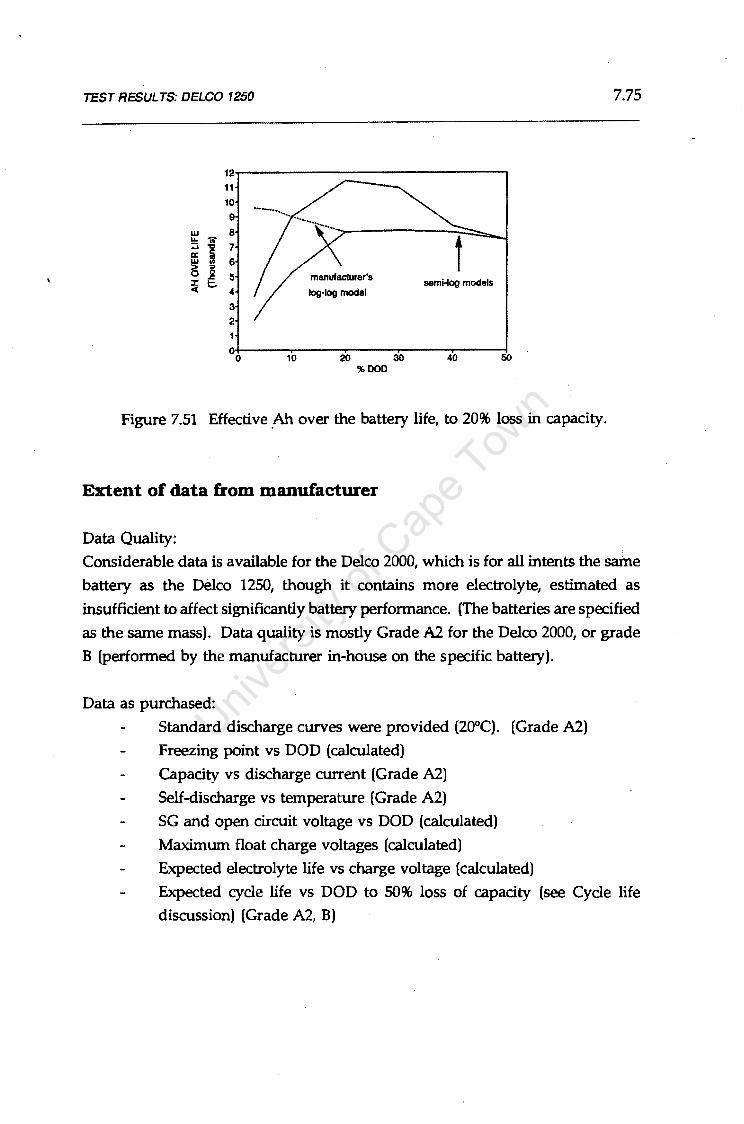
TEST RESULTS: DELCO 1250
12..-----------------. 11 10
9
w 8 ~ ~ 7
ffi ~ 6 > = ~ l 5 c( 4
3 2
10
semi-log models log-log model
20 30 40 50 %DOD
Figure 7.51 Effective Ah over the battery life, to 20% loss in capacity.
Extent of data from manufacturer
Data Quality:
7.75
Considerable data is available for the Delco 2000, which is for all intents the same
battery as the Delco 1250, though it contains more electrolyte, estimated as
insufficient to affect significantly battery performance. (The batteries are specified
as the same mass). Data quality is mostly Grade A2 for the Delco 2000, or grade
B (performed by the manufacturer in-house on the specific battery).
Data as purchased:
Standard discharge curves were provided (20°C). (Grade A2)
Freezing point vs DOD (calculated)
Capacity vs discharge current (Grade A2)
Self-discharge vs temperature (Grade A2)
SG and open circuit voltage vs DOD (calculated)
Maximum float charge voltages (calculated)
Expected electrolyte life vs charge voltage (calculated)
Expected cycle life vs DOD to 50% loss of capacity (see Cycle life
discussion) (Grade A2, B)

TEST RESULTS: DELCO 1250
Additional data on request by personal communication:
Plate masses, (dry and wet), overall masses and dimensions
Corrected life cycle data: to 20% loss of capacity (Grade C)
Test procedures used by Delco Remy
See Appendix DS for manufacturer's data sheet.
7.5.3 Test results and discussion
7.76
Two Delco 1250 batteries were purchased. These are referred to as 1250A and
1250B.
The Delco 1250 normally does not require water addition for the duration of its
operational life, and therefore no external filler caps are provided.· No convenient
method exists for SG measurement. The optical hydrometer located above cell 2
can be removed and SG measurements taken of that cell only, but it is a slow and
cumbersome process.
a) Capacity and discharge tests
As complete discharge curves are provided it is necessary only to verify some of
the curves. Limited discharging was performed for the same reasons as the
Willard LS90: the battery is expected to lose capacity rapidly when repeatedly deep cycled,
invalidating the results of future tests,
the capacity is expected to change rapidly with age,
discharge curves are available and can simply be verified,
the battery will normally operate in the shallow discharge zone only, and
capacity limitations will not be encountered.
Cell 1250A, new and equalised, was discharged at 10A and 18°C to 10.SV and
88Ah were obtained. The discharge curve in the data sheet shows 95Ah at 25°C,
equivalent to about 90Ah at 18°C. The battery was recharged and equalised, then
discharged as before to yield 86Ah. The capacity at 0°C was determined to be

TEST RESULTS: DELCO 1250 7.77
68Ah, and at 35°C to be 95Ah. (At this stage it was suspected that the run of
deep discharges were beginning to curtail the battery capacity).
Cell 1250B was twice equalised at 13,SV and discharged to 10.SV at 20A and 18°C,
yielding 81Ah and 78Ah. This is within 5% of the specifications, and is used as
the reference capacity for this cell.
The discharge capacities for the Delco 1250's verified the capacities presented for
the Delco 2000, which are accepted. The discharge curves at 25.°C are shown in
Figure 7.52.
It should be noted that load shedding at shallow DOD requires good knowledge
of the load current. The shallow slope of the discharge curves in that region
suggests that accurate load shedding may become problematic if load currents are
low and variable. ·As a result it may be difficult to control DOD optimally in a PV environment.
The effect of temperature on capacity is shown ~ Figure 7.53 based on limited
data, which compares with the manufacturer's estimated data.
The calculated SC vs Ah removed in Figure 7.54 is typical of SLI type batteries,
and does not indicate an excess of electrolyte as is advertised in the literature for the Solar 2000.
w (!>
12
~ 11.5+--+---+--+-____ ...........,, ___ ,..-+' __ --I
§Z
20A 10A 5A 2A 1A
10 0 10 20 30 40 50 60 70 80 90 100 110 120 130
DOD(AH)
Figure 7 .52 Standard discharge curves at 25°C.
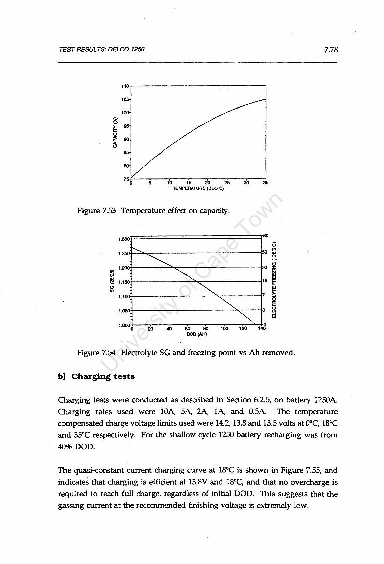
TEST RESULTS: DELCO 1250 7.78
110
105
100
g ~
95
u ~ 90 < u
85
80
5 10 15 20 25 30 35 TEMPERATURE (DEG C)
Figure 7.53 Temperature effect on capacity.
1.300 60
6 50 CJ
1.250 w c ...:.,
CJ ii) 1.200 30 z
iii ~ w ~ 1.150 15 a:
LI.. CJ w
"' ~ 1.100 7 0 a: I-
1.050 3 u w -' w
1.000 0 0 20 40 60 80 100 120 140
DOD(AH)
Figure 7.54 Electrolyte SC and freezing point vs Ah removed.
b) Charging tests
Charging tests were conducted as described in Section 6.2.5, on battery 1250A.
Charging rates used were lOA, SA, 2A, lA, and O.SA. The temperature
compensated charge voltage limits used were 14.2, 13.8 and 13.5 volts at 0°C, 18°C
and 35°C respectively. For the shallow cycle 1250 battery recharging was from
40% DOD.
The quasi-constant current charging curve at 18°C is shown in Figure 7.55, and
indicates that charging is efficient at 13.8V and 18°C, and that no overcharge is
required to reach full charge, regardless of initial DOD. This suggests that the gassing current at the recommended finishing voltage is extremely low.

TEST RESULTS: DELCO 1250
100%SOC - 95%
18
17.5
17
16.5 . ~
16 w 15.5
~ 15 ~ 14.5
14
13.5
13
12.5
12
·-·,
';
" K'\ \\ \
:j\ \ \ 1
\\ \ \
\ \ ' \. ......... ~ t'--...> ~ ~
........ ~~ ~
-20 -10 0 10 20 30 40 50 60 . DOD(AH)
7.79
Figure 7.55 Quasi-constant current charging curve. Charging rates used
were lOA, SA, 2A, lA, and O.SA.
Charging efficiency was determined by the method in Section 6.2.6(vi), where the
end-of-charge current is assumed to be the gassing current. The gassing current
curve is in Figure 7.56. At 13.BV the battery accepts virtually no charge, and is
self-regulating.
18
17.5
17
16.5
w 16 (!)
~ 15.5
~ 15
14.5
14
13.5
'
I /_/ // )
---VJ .....-.V/ ..--v
- -'- ___, .....- ~-
__.A -..-- ._....... ,.--
13 0 2 3 4 5 6 7 8 9 10
GASSING CURRENT (A)
-A-OdegC
---18deg c --35deg c
Figure 7.56 Gassing current as a function of temperature and voltage.
The charging curves after compensation for gassing and overcharge losses are
shown in Figure 7.57. The end of charge voltage can be read from these curves,
as well as the sensitivity of end-of-charge current to the voltage setting.

TEST RESULTS: DELCO 1250
18
17.5
17
16.5
16
~ 15.5
~ 15
~ 14.5
...._ ............... "...
"' ~ \ \
\ \ \ \ \ ~
I"' \
! \ \
\ ' " .......... '-...........
t'---.. -...... r--. ~
---=-- ,__ -r--_-...... ~ ------ ....
~~-
14
13.5
13
12.5
120 10 20 30 40
18
17.5
17
16.5
16
~ 15.5
~ 15 -' ~ 14.5
DOD (AH)
,..
.. "' "''\
\ \ \ .\ \ 1
,\\ \ I\
\\. ' \.. 14
13.5
13
12.5
120
'-.......~ t:'---................
18
17.5
17
16.5
16
~ 15.5
~ 15
~ 14.5
=- ~ --==-~ ~
............. 10 20 30 40
DOD (AH)
~ \ \ \\
.\ \ \ \\.,,_ 'r-. ~ t---_'-......1 ~ t:-=::::::::-- ----~
50
50
.14
13.5
13
12.5
12 0
~ §:--10 20 30 40 50
DOD (AH)
7.80
60
60
-
60
Figure 7.57 Compensated charging curves at a) 0°C, b) 18°C and c) 35°C.
Charging rates are lOA, SA, 2A, lA, O.SA.

TEST RESULTS: DELCO 1250 7.81
c) Cycling tests
Cycling tests selection
The 1250 battery is designed only for shallow cycle applications. As previously
discussed, cycle life curves suggest an optimum DOD in the region of 10% for
regular cycling. A shallow cycle full SOC cycling test is required to determine
whether stratification occurs, and if so the overcharge cycle to eliminate it. The
test is also useful for determining the minimum charge voltage during shallow
cycling, particularly since gassing in sealed vented MF batteries is to be avoided.
Shallow cycling at partial SOC is a useful indicator of both stratification and cycle
life limitations.
Shallow cycle full SOC Test
Battery 1250A was cycled between 100 and 90% SOC at discharge current of ClO, and charge voltage of 2.37 /cell, with a limiting current of ClO (lOA). Overcharge
was limited to 10%, and the time for charging limited to two hours.
Figure 7.58(a) shows the end-of-charge current and end-of-discharge voltage. The
decreasing end-of-charge current suggests that the battery reaches and maintains
a dynamic equilibrium close to 100% SOC. During the later charging cycles the
Ah delivered are limited by time constraints, by the self-regulating nature of the
charging curves (Figure 7.18(b)). The end-of-discharge voltage is relatively
constant at 12.12V.
The watt-hour efficiency initially increased (as fewer Ah were delivered), then
stabilised at 84.5% at the chosen currents.
Battery 1250B was cycled exactly as for battery 1250A for 26 cycles. The capacity at the end of the test and after equalisation was 59Ah.
\

TEST RESULTS: DELCO 1250
1.6-r-----------------"T12.8
1.4
g 1.2 .... z w cc cc 5 0.8 w ~ 0.6
~ (.) 0.4
0.2
11.9
11.8
c 11.7 w z cc ::::> 11.6 .... w cc :r < 11.5
11.4
28
27
..J 26
..J w (.)
cc 25 w C1.
:r 3: 24
23
12.6 2: w
------._ ____ -112.4 ~ ~ w
12.2 ~ ·····-···-····-........ _ ..... _ ..... - .... ___ ......... _____ .............. -----··· :I:
~ eod voltage 12 i5
4 8 12 16 20 CYCLE NUMBER
4 8 12 16 20 24 CYCLE NUMBER
90
Wh input 89
88
87 l 86 (:;
z 85 !:!!
(.)
84 ff w 83 :r
3: Whout 82
81
80 4 8 12 16 20 24
CYCLE NUMBER
7.82
Figure 7.58 Shallow cycle full SOC test; a) end-of-cycle voltage and current,
b) Ah delivered, c) Wh efficiency.

TEST RESULTS: DELCO 1250 7.83
Shallow cycle partial SOC test
Battery 1250A was cycled 39 times between 90% and 80% SOC at charge and
discharge rates of ClO (lOA), which is below the recommended starting charge
rate for the cell. Charging voltage was limited to 2.37V for safety, although the
charging curves indicated that the voltage would not reach this limit.
Figure 7.59(a) shows the end-of-charge current and voltage and end-of-discharge
voltages as the test commenced. The very rapid increase in the end-of-charge
voltages from 13.64V in cycle 1to14.0V in cycle 11, followed by a jump to 14.2V
in cycle 12 indicates a combination of the rapid onset of stratification and the
formation of a resistive sulphate layer on the plates, together with possible single
cell failure. (A practically identical rise in end-of-charge voltage was observed in
this cycling test on the Willard LS90, which also has a calcium grid negative
electrode, though some of these effects were identified as reversible). Szymborski
(1982) has identified the rapid rise in charging voltage as due to all of the above,
together with higher current densities as the calcium positive grid members
fracture. The suspected irrecoverable capacity loss was verified by the end of test
capacity, determined as 52Ah at lOA after 39 cycles. The end-of-test capacity
showed a sudden fall of voltage typical of single cell failure. The effect of
stratification/ sulphation on the charging profile between cycle 1 and cycle 12 is in Figure 7.59(b).
Figure 7.59(c) maps the Wh efficiency, which eventually settled at 90.5%.
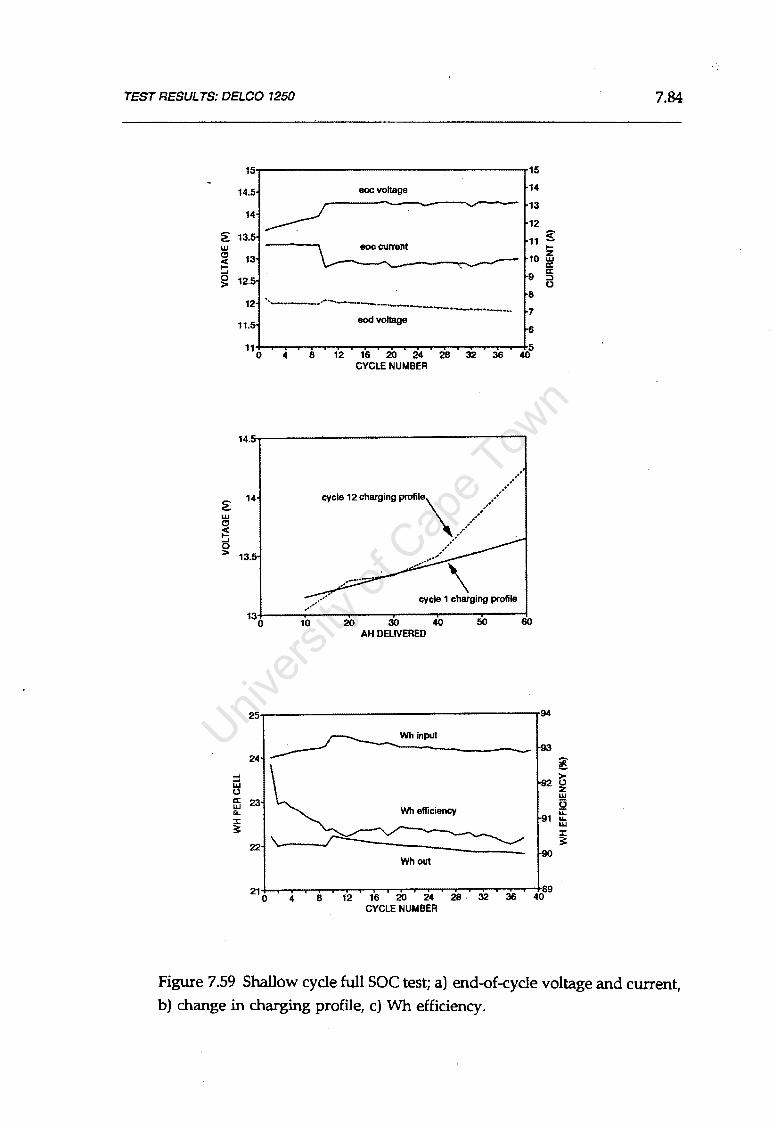
TEST RESULTS: DELCO 1250
2: w (!'
i5 ..J 0 >
2: w
~ ~
15 15
14.5 eocvoltage 14
13 14
12 13.5 11
g eoc current ....
13 10 as 12.5 9
8 12 .... __ .. ____ .,. .. -·-.. ----·-·-·----·-·---·---·---··
7 11.5
eod voltage 6
11 5 0 4 8 12 16 20 24 28 32 36 40
CYCLE NUMBER
14.5......-------------------,
14 "''" " ...... """'\///// ............ •""" 13.5
..J
..J w (.)
a:
cycle 1 charging profile
13·+0---1~0---20...---30...---40...---so:t:""----:jGO AH DELIVERED
25
24
23
a: a: :::> (.)
94
93
92
l t z w (3 w
1 it c.. :i: w s: :i:
22 \.... s: 90
Whout
21 89 0 4 8 12 16 20 24 28 32 36 40
CYCLE NUMBER
7.84
Figure 7.59 Shallow cycle full SOC test; a) end-of-cycle voltage and current, b) change in charging profile, c) Wh efficiency.

TEST RESULTS: DELCO 1250 7.85
Capacity at end of cycle tests
Battery 1250A was equalised and the capacity determined at the ClO rate to be
52Ah, compared with 88Ah at the start. The drop in capacity of 36Ah (41 % )
seems mainly due to sulphation of both electrodes during partial SOC operation,
and it is well known that calcium grid cells last longer under float polarisation
than under cycling polarisation. It is probable that the cycle life curves .are
invalid for partial cycle operation.
The percent of useful life used can also be theoretically calculated using the
manufacturer's log-log model for 20% loss of life (see earlier discussion on cycle
life). The incremental wear due to:
is
24 cycles @ 10% DOD (900 cycles expected over battery life)
40 cycles between 10% and 20% DOD (400 life cycles expected) 4 cycles@ 100% DOD (20 cycles expected)
3 cycles to 40% DOD (200 cycles expected)
28/900 + 40/400 + 4/20 +3/200 = .346 or 34.6%
The capacity of battery 1250B after full cycling only was 59Ah at the 20A rate,
down from the initial capacity of 80Ah. After a further 24 hours on float charge
at 14.SV the capacity remained at 59Ah, or a permanent 26% loss in capacity. After a 2nd equalisation the capacity was 56Ah.
The incremental calculated wear due to:
is
26 cycles@ 10% DOD (900 cycles expected over battery life)
2 cycles to 80% DOD (SO cycles expected)
1 cycles to 100% DOD (20 cycles expected)
26/900 + 2/50 + 1/20 = .119 or 11.89%
These limited life cycle tests show that the Delco 1250 performed below
expectations during both full and partial shallow cycling. While poor partial SOC
cycling may be expected for calcium grid cells, near optimal performance is
expected for shallow full cycles with float charge. The small samples used cannot

TEST RESULTS: DELCO 1250 7.86
be used to make statistically valid modifications to the life cycle curves, but
further investigation is certainly justified.
H20 Consumption
Very little overcharge was applied to the batteries during testing, and water loss
was expected to be minimal. At no time was the SOC indicator coloured yellow.
(Yellow indicates excessive loss of electrolyte and possible plate exposure).
Delco presents a curve of electrolyte life vs charge voltage which presumably
correlates loss of electrolyte with voltage. A calculation based on the
experimental gassing curves compares charging voltage with years of electrolyte
life and with centimetres of (estimated) electrolyte above the plates. Three
centimetres is considered the maximum possible. The calculated electrolyte life
is considerably less than specified. The difference could be due to variation in
gassing current, in excess electrolyte volume, or in the gas recovery rate.
In the Delco battery the gases from all the cells accumulate in a mixing chamber,
where some recombination occurs. Recombined condensate trickles back to the
electrolyte reservoirs, while excess gas escapes to atmosphere through a single
vent. After many cycles, the centre cells may accumulate more of the recombined
electrolyte than the others. However, these cells are likely to gas more, as their
insulated central positions will probably result in higher temperature operation.
The location of the optical hydrometer on the cell two probably indicates
electrolyte levels within a reasonable average of all the cells.
Charging CUrrent and Voltage Requirements
The main considerations are to prevent loss of electrolyte and to prevent
stratification, and to operate the battery in float mode (under voltage controlled
charging) for most of the time, as partial SOC operation is so damaging.
The charge voltage should allow use of the self-regulating nature of the battery
(see Section 3.14.1), but should also allow some gassing to mix the electrolyte.

TEST RESULTS: DELCO 1250 7.87
The manufacturer recommends a float voltage of 14.3V at 20°C, which would
provide less than 0.25A of gassing, but also minimise electrolyte loss.
7 .5.5 Sizing and selection: considerations in PV applications
1) Optimise battery life by allowing only shallow daily DOD, and avoid
partial SOC operation at all costs as it is battery life limiting.
2) A void excess gassing, which could enhance corrosion of the thin SLI
type grids, as well as consuming H20 which cannot be replaced.
3) Minimise electrolyte stratification and the possibility of negative
electrode failure by operating in float charge regime for as much time
as possible. Long float charge cycles are required as the gassing
current is negligible at the recommended charge voltage.
4) Consider using the self-regulating nature of the battery to full
advantage. The rapid rise in voltage of the charge curves make the
Delco 1250 a possible candidate battery for self-regulating PV systems.
Practical application will require careful combination with a self
regulating PV panel. This will facilitate float charge operation.
However, in most self-regulating systems overcharge of the battery can
occur and should be avoided by considering factors discussed in Section 3.14.1.

TEST RESULTS: COMPARATIVE DISCUSSION 7.88
7.6 COMPARATIVE DISCUSSION
The five batteries have been discussed individually in some detail. This section
compares, in much less detail, the main performance characteristics of the
batteries.
7 .6.1 Initial Costs
The batteries examined are approximately the same nominal ampere-hour
capacity, lOOAh, yet their prices range considerably for the different battery types.
Table 7.1 Wh energy costs
Cost (R) nominal nominal kWh of R/Wh
Ah v capacity Capacity
774 294 90 12 1.08 .27
RMT108 400 108 4 .43 .93
LS90 364 90 12 1.08 .34
GNB 12-5000 660 93 12 1.12 .59
DELCO 1250 280 105 12 1.26 .22
The cost (R) and R/Wh capacity figures reflect the initial costs of the battery only.
These vary considerably. The available capacity during normal use also differs
according to the type. However, the main costs are the lead costs, then labour
costs for special processes, and the costs of special chemical processes. Table 7.2
shows the comparative costs per mass of lead (approximated by the dry mass of
the cell) as the electrolyte is relatively cheap.

TEST RESULTS: COMPARATIVE DISCUSSION 7.89
Table 7.2 Cost per kilogram of lead
Cost (R) dry mass R/kg (kg)
774 294 17.7 16
RMT108 400 14.7 27
LS90 364 17.7 21
GNB 12-5000 660 ±17.7 37
DELCO 1250 280 17.2 16
The conventional flat plate flooded electrolyte batteries cost about R16-R20 per
dry kg. The tubular RMT108 costs R27 /kg, and this increment is probably a . reflection of the cost of the labour intensive tubular manufacturing process. The
GNB 12-5000 cost of R37 /kg is a reflection of the advanced technology used;
absorbed electrolyte, sealed recombination and proprietary Pb-Ca-Sn processes on the negative grid; as well as the cost of importing the battery. The Delco 1250 is
surprisingly low cost for an imported battery. Table 7.2 shows that the active
mass utilisation seems to be a reasonable basis for comparison. Overall, you pay
for what you get in terms of manufacturing costs. Lifetime R/kWh costs are
discussed later.
7 .6.2 Charging Parameters
Gassing curves
Gassing current/voltage is fundamental to determining charging regimes for
batteries in PV applications, where gassing is in most cases required yet must be restricted.
The gassing curves of the five batteries can be divided into two distinct groups,
those with calcium negative plates and those with antimony negatives. The

TEST RESULTS: COMPARATIVE DISCUSSION 7.90
gassing curves at 18°C are in Figure 7.60. The modified RMT108 gassing curve
is shown adjusted for utilisation coefficient (nominal capacity divided by capacity
if active materials were completely used), so that the batteries experience the same
current density. (Current density is used in the theoretical determination of
gassing overvoltage). The RMT108 and 774 curves are closely related. These
batteries gas heavily at 15.SV, while the calcium grid cells gas mildly at 15.SV.
13
12
11
10
9
g 8
!Z 7 w ~ 6 a s
4
3
2
1
,._ RMT108
RMT -_n4
)
:
I I :
I i I :
I l I I I
I i I //
'/--- .........
GNB LS90 DELCO
12-~~ _ 1250
/ I \ I .r I
.._, I I I I
I J ,,
II Ill
i/j/
,#"
h ~3.0 14.0 15.0 16.0 17.0 18.0
VOLTS (PER 12V BLOCK)
Figure 7.60 Gassing curves at 18°C for the five batteries. The dashed line
represents the RMT curve adjusted for utilisation coefficient.
Table 7..3 shows the change in gassing current with temperature at the
recommended charging voltages. This represents a situation where the charge
voltage is held constant by an uncompensated charge regulator while the battery
temperature varies. The RMT108 is most susceptible to uncontrolled gassing if
the charge voltage is not compensated for temperature. Table 7.3 also shows the
change in gassing current with temperature (M/ !::.. T) in the vicinity of lA gassing
current, and the temperature coefficient (!::..VI!::.. T) of voltage required to keep
gassing at that level. Temperature compensation coefficients are not the same for all batteries, and should ideally be set specifically for each battery.

TEST RESULTS: COMPARATIVE DISCUSSION 7.91
Table 7.3 Gassing and charge regulator variation with temperature
vch I, AA/AT Voltage AA/AT AV/AT
re com. (0-35°C) at I,=lA (0-35°C) (0-35°C)
® l8°C ®18°C
774 14.2 0.75 0.75 14.5 1.5 0.7
RMT108 14.2 1.5 5 14.0 3 1.2
LS90 13.8 0 0 15.5 1.5 1.8
GNB '12 14.4 0.25 1 15 1.5 0.5
-5000
DELCO 14.3 0.25 0 15.7 1.5 0.8
1250
Clearly some batteries gas only slightly at the recommended charge voltages. The
· reason for the low recommended voltages in these batteries is primarily to limit
water loss in the maintenance free designs, which cannot be topped up, as once
the electrolyte level has dropped to the level of the plates, plate exposure
prematurely ends battery life. The selection of a low charge voltage represents
a trade-off between maintenance free operation and reduced battery life due to
prolonged electrolyte stratification in the anticipated cycling regimes caused by
insufficient gassing. Cycle performance is discussed in Section 7.6.4. The theory
does not indicate that any chemical damage could occur to the plates at elevated
gassing voltages, but instead states explicitly that antimony-free cells perform
optimally in the gassing regime.
Water loss
Gassing and overcharge affect water loss and maintenance as described above. Table 7.4 shows the estimated time between water replacement maintenance (or
end of battery life for the MF LS90 at 0.5A gassing current) if the battery is
charged continuously at the recommended voltage, as well as the reduced
maintenance period if the temperature is increased without charge voltage compensation.

TEST RESULTS: COMPARATIVE DISCUSSION 7.92
Table 7.4 Maintenance intervals
Vch recom. Reserve Hours of Hours of
at 18°C electrolyte charge at charge at (ml) 1s0 c 35°C
774 14.2 176 698 460
RMT108 14.2 304 300 150
LS90 13.8 176 no gassing no gassing
LS90 15.0 (0.5A) 176 1047 523
GNB 12-5000 14.4 NA no H20 loss no H20 loss
DELCO 1250 14.3 180 2142 1071
7 .6.3 Discharge Parameters
The batteries are all of similar nominal capacities, but these are at different
discharge rates. The capacities at lOA and 2A discharges at 18°C are in Table 7.5.
Included is the capacity of the RMT108 after the current has been corrected by the
active mass utilisation coefficient. The capacity is still well above the comparable
capacities for flat plate cells. This difference is probably attributable to the large
excess electrolyte, which means that the electrolyte volume itself does not limit
capacity. The role of the electrolyte is more clearly indicated by the temperature
variation of capacity, which shows the change in capacity between 18°C and 0°C
as a percent. The typical flooded electrolyte figures show changes of -20% over
the range, while the RMT108 with the large electrolyte reservoir shows only a -
15% change. The starved electrolyte GNB 12-5000 shows a large -37% change,
emphasising the retarded electrolyte transport properties at reduced temperatures.

TEST RESULTS: COMPARATIVE DISCUSSION 7.93
Table 7.5 Capacity variation with temperature
Capacity at Capacity at % change in
lOA (Ah) 2A (Ah) capacity
(18-0°C)
774 79 91 -20%
RMT108 140 180 -15%
RMT108 (adjusted) 100 (23A) 160 (SA) -15%
LS90 79 91 -20%
GNB 12-5000 75 89 -37%
DELCO 1250 95 91 -18%
7 .6.4 Cycle Performance
There are three main concerns in discussing cycle performance: depth of
discharge, partial SOC operation or complete cycling, stratification and sulphation.
Energy efficiency is interesting only if the battery is capable of sustained operation
in the cycling regime under consideration.
The cycling tests showed that the antimony grid flooded cells (774 and RMT108)
can operate in either deep or shallow full cycles, that stratification and reversible
sulphation occur, but can be prevented or reversed by relatively short spells of
overcharge at the recommended charge voltages. The cells gas easily, but as the
gassing is damaging to the grids (especially for the flat plate 774) it is probably
optimal to avoid stratification and subsequent requirement for gassing where
possible.
These cells can also operate at partial SOC if the resulting stratification and
sulphation is subsequently reversed through gassing. Prolonged partial SOC
operation will eventually lead to deep rooted stratification and irreversible hard
sulphate formation.
TEST RESULTS: COMPARATIVE DISCUSSION 7.94 .
The cyclic energy efficiency is very dependent on the average amount of
overcharge per cycle. The overcharge requirements lead to reduced energy
efficiencies.
The antimony positive, calcium heat treated ternary negative, absorbed electrolyte
cell (GNB 12-5000) can operate in almost any regime cycling provided that the cell
internal pressure does not exceed the venting pressure. This cell does not stratify,
but the negative electrode is susceptible to hard sulphation at partial SOC cycling,
though this is reduced by proprietary processes used during manufacture. . The
high coulombic efficiency facilitates regular top-of-charge cycle overcharge for cell
equalisation and recovery from sulphation. Cycle efficiency can be high, since
mixed stage charging is minimised by the self-regulating nature of the charging
curves at the recommended voltage.
The conventional calcium negative grid, antimony positive LS90, and the calcium
grid Delco 1250 performed very poorly under (shallow) partial SOC operation,
losing capacity permanently within thirty cycles. This has been identified as
breakdown of the negative electrode under cyclic polarisation. The batteries
operate well urider full cycling provided that they are also under slight
overcharge for most of the cycle. Stratification of these cells is a problem, as the
gassing currents are so low at the recommended charge voltages as to be
ineffective in the short term. Long term overcharge polarisation is required to
recover from stratification.
7 .6.5 Cycle Life
Cycle life is one of the most important parameters in costing batteries for PV
systems. However, there is considerable uncertainty in the cycle life estimates for
the batteries tested, whether based on manufacturers' data or on data for similar
batteries.
The cycle life data additionally may apply to very specific conditions, and not to
the type of operating regimes encountered in some PV applications. The
experimental results have shown that the untreated calcium negative grid batteries
in general responded exceptionally (and unexpectedly) poorly to partial state of
charge operation.

TEST RES UL TS: COMPARATIVE DISCUSSION
Figure 7.61 shows the estimated cycle life curves for the batteries tested.
10000
- RMT108 -"" ......... .......... ...........
.............. ......... ..........._ ..........._
I"'--, ·····.RMT ...........
~I -' ...... s:::;;;:; GNB 12-5000 :
'- DELCO 1250 - I -~ ' ........ I
~---·-..... "' -----~ 774 _
--- -..... I -..... LS90 ..__ 100
0 10 20 30 40 50 60 70 80 90 100 000(%)
7.95
Figure 7.61 Estimated cycle life curves for the five batteries. The dashed
line represents the RMT curve adjusted for utilisation coefficient.
The RMT108 has by far the highest cycle life expectancy, but this is primarily a
reflection of the low utilisation coefficients. The cycle life adjusted for the
utilisation coefficient shows that under similar utilisation the life expectancy is
closer to the GNB 12-5000. The high life expectancy of the GNB 12-5000 at high ·
utilisation is the result of the manufacturing process and technology employed,
although it appears that this technology has not yet made cycle life gains over the
more conservative tubular designs. It is possible that the GNB 12-5000 could
withstand prolonged partial SOC operation for longer than the RMT108. The 774
cycle life is moderate, as expected of a conventional antimony battery, with good
deep cycle performance. The Delco 1250 cycle life estimates are questionable. The
slope of its curve, and that of the LS90 are dissimilar, although theo.~y and
practical experience suggest similar failure modes and preference for similar
operating regimes. Similarly sloped curves are expected. Delco 1250 cycle life is
probably closer to the LS90 than indicated.
The estimated optimum operating DOD and number of cycles expected for each
battery is shown in Table 7.6. The same uncertainties surrounding cycle life
estimates apply to the calculated figures in Table 7.6. The total energy stored over
the battery life is shown for the expected number of complete cycles between the

13
TEST RESULTS: COMPARATIVE DISCUSSION 7.96
optimum DOD and the fully charged state. The overall cost of that stored energy
provides an indication of the value of the battery. (Only the initial costs are
considered, maintenance and other costs are ignored). The expected battery life
in years assumes one cycle per day.
It is important to stress that cycle lives are based on manufacturers' data (where possible), and there are considerable limitations in the adequacy and reliability of
this data. The Delco 1250 figure is considered ambitious. The stored energy costs
are intended for approximate comparisons only. The PV system costs and balance
of system requirements, and resultant losses in system efficiency when sizing to
provide suitable operating regimes for the different batteries may alter the
comparative costs. In small PV systems, component choices may be limited to
discrete size increments, which can introduce a further cost factor.
Table 7.6 Stored energy cost and battery value
Cost DOD Cycles Stored Energy Life
(R) (%) energy cost (years)
(kWh) (R/kWh)
774 294 50 300 162 1.81 1
RMT108 400 40 4000 691 0.58 10
LS90 364 20 300 65 5.62 1
GNB 12- 660 40 1300 580' 1.14 3.5
5000
DELCO 280 10 800 101 2.78 2.5
1250 50013 63 4.44 1.5
The cycle life is most probably less than the 800 cycles claimed. 500 cycles at 10% is used for comparison.

TEST RESULTS: COMPARATIVE DISCUSSION 7.97
7 .6.6 Conclusions
There is no straight forward answer to the question, "Which battery is best for PV
applications?".
The answer is complex principally because there is great variety in PV
installations, and the relative performances of PV systems using battery storage are strongly dependent on the operating environment. The differences may be minor for similarly designed systems in dose proximity, but the simple analysis
in Chapter 2 has demonstrated how two installations designed for the same site
can present fundamentally different battery operating environments. No one
battery will work in all PV systems, let alone perform optimally.
Factors which strongly influence battery operating environment in a stand-alone
PV system include
a) site-dependent weather (primarily solar irradiation, and to a lesser extent
ambient temperature), and variability in weather over different time scales (days to months) (Cowan,1990);
b) load energy demand profiles, again over different timescales, in relation to (a);
c) the design loss of power probability of a system, reflecting system energy
capacity in relation to (a) and (b);
d) the design choice amongst array /battery combinations capable of satisfying (c);
e) the maximum battery DOD allowed, and load shed regulator settings;
f) the relation between maximum and average depths of discharge which is partly a function of (c) and (d);
g) charge regulator control.
System design decisions will largely determine the range of requirements placed
upon the batteries and thus influence choice of battery type and sizing of battery
capacity. System sizing and battery choice wi~ in tum affect aspects such as the
ratio between capital and running costs, maintenance frequency and the
predictability of battery performance (all of which could be design constraints).

TEST RESULTS: COMPARATIVE DISCUSSION 7.98
Factors affecting battery choice
Realising that different battery chemistries and designs have different operational
preferences the system designer must come to terms with the design features that
affect these preferences.
Special attention should be given to:
1) matching the expected cycle regime with a battery of suitable design and
grid chemistry;
2) effective charge and discharge regulation within the expected cycle regime
to minimise the onset of long term grid corrosion, stratification or
sulphation;
3) temperature compensation of charge and discharge regulation for expected
battery operating temperature;
4) array requirements to provide sufficient energy for overcoming inefficiencies
in the battery.
Some practical examples of concerns might be:
Immobilised electrolyte batteries perform better than flooded electrolyte
batteries in a partial SOC regime, but prolonged partial SOC operation will
also be detrimental in the long term.
Calcium and non-antimonial grid batteries are sometimes proposed to
reduce maintenance requirements. Under controlled charging they
demonstrate low water consumption. If overcharged they will consume as
much water as other batteries overcharged by the same ampere-hours. But
since they are usually cycled in shallow regimes they do not require the
same amount of overcharge. Batteries must be matched with suitable
regulators.
For deep cycling applications, the lowest life cycle battery costs appear to
come from tubular batteries, but capital costs tend to be high and it is
important that the array can source sufficient current to overcome self
discharge, charge inefficiencies and stratification limitations.

TEST RESULTS: COMPARATIVE DISCUSSION 7.99
The battery selected as being technically most suitable may not be the best choice
on economic grounds.
For example, high initial battery cost may discourage use of.some battery types;
selection of batteries with lower energy efficiencies or more demanding charging
requirements may increase costs elsewhere in the system; attempts to minimise
initial costs of array and batteries can lead to decreased battery lifetimes and
increased running costs.
In order to select an optimal trade-off between economical capital costs and
economical running costs over the lifetime of a system, it is desirable to be able
to predict running costs with a degree of certainty. Uncertainty in predicting battery lifetime is increased if batteries are not operated within fairly conservative
cycling regimes. For this reason it is advisable to apply battery design data
cautiously, even where operating conditions are similar to the cycling conditions under which the data was obtained. Extra caution is warranted if operating
conditions may deviate significantly form test conditions.
Uncertainties remaining
PV system sizing is a statistical problem because of uncertainties in solar
irradiance and system interaction with often uncertain load profiles. Battery
cycling regimes in PV systems are therefore also statistical in nature and subject
to uncertainties. Complete battery data covering all possible operating conditions
will probably never be available. The combination of incomplete battery
performance data and highly variable operating regimes leads to considerable
uncertainties in determining the impact of technical choice on system life cycle
costs.
Battery performance characterisation itself has a statistical aspect due to variations
amongst batteries of the same model. The data generated in this project has a non-statistical basis as time did not permit repetitive testing to statistically
validate the data. However it is doubtful whether this limitation is a major
contributor to uncertainty, relative to other sources of uncertainty, except perhaps
in cases where batteries degraded during testing.
TEST RESULTS: COMPARATIVE DISCUSSION · 7.100
However, with regard to life cycle data, tremendous uncertainties still exist.
Causal linkages between operating regimes and cycle life can be established (this
has been a primary motivation for documenting the battery theory in Chapter 3),
but there is a dearth of information describing the magnitude of the effects of
external variables on cycle life.
The empirical battery characterisation data from this study can be used in PV
system simulation programs to explore the long-term cycling conditions of specific
·batteries in specific PV systems. This will be a step towards greater predictability
of battery lifetimes in PV systems and identification of system design parameters
affecting battery life. However considerable ground would need to made in
modelling battery degradation and failure modes in order to achieve more
definitive understanding.
For most installations a high priority in designing systems to minimise costs is to
• understand with some certainty what the longer term effects of a particular design
and sizing will be. This chapter has endeavoured to remove some initial
uncertainties by providing comparative data concerning the principal problems
with batteries in small PV systems, namely continuous undercharging, partial
state-of-charge operation, stratification and sulphation; overcharging, gassing,
charge voltage temperature compensation and stratification elimination; and
primary implications for cycle life estimation and costing.
This data should already be useful for selection of batteries for specific PV
applications.

CHAPTER 8
CONCLUSIONS AND RECOMMENDATIONS
The main objective of this study was to determine accurate empirical data for
locally available batteries which could be used in photovoltaic systems, and to
present this data in a format directly applicable to PV system designers.
Secondly, the experimental battery data and gains made in under~tanding battery performance were intended to contribute to the accuracy of PV system simulation
methods being developed at EDRC. PV system simulation tools provide an
effective way of evaluating and optimising system design options. Modelling
battery behaviour is a vital but presently problematic component in simulating PV
systems with battery storage.
8.1 LITERATURE REVIEW
Battery theory and research literature has been extensively reviewed from the viewpoint of understanding battery behaviour in PV systems. Theory and
existing research were presented to provide background for the concerns and test
methods used in the present study. Existing models of battery performance were discussed.
The review was essential for understanding major mechanisms which determine
battery behaviour. In particular the examination of polarisation and overpotential
theory has enabled development of time efficient methods of battery charge curve
determination and charge efficiency measurement. The review of macro and
micr~processes provided insight into failure modes specific to certain generic
battery types in PV operating regimes.
Batteries in stand-alone PV systems are generally subject to particular operating
conditions such as low charging currents and variable depths of discharge. In the
light of such requirements and theories of battery performance, innovative designs
for specialist PV-compatible batteries were described. Methods of battery charge
8.1

CONCLUSIONS AND RECOMMENDATIONS 8.2
regulation, which should be adapted to battery performance characteristics and operating conditions, were assessed.
8.2 BATTERY TESTING FACILITY AND TEST METHODS
A major interim objective of this project was the design, development and
construction of specialised test equipment to collect empirical battery data relevant
to photovoltaic applications. A microcomputer-controlled battery testing unit was
developed which is capable of variable charge and load cycling, automated data
capture and PV emulation.
The unit consists of a 3kW (SOA, 60V) programmable power supply and a l.8kW
(30A, 60V) programmable electronic load, both constructed in house, contrdlled
through analog-digital converters by customised software.
The test software supports conventional battery testing as well as PV system
emulation. In the latter case, solar irradiation data, characteristic PV curves and
load data are input, and the software-controlled power supply is able to emulate
the PV array to determine and display the battery and array operating points.
The system has operated almost continually for 24 hours per day for more than
one year without serious or prolonged down time. The primary limitation of the
test-unit is the inability to test and monitor more than one string of batteries at
any time. (The software could be readily adapted, but for each additional battery
string another power supply and load are required.) This cost based limitation
reduced the scope for statistical testing of batches of batteries and required
thorough and efficient utilisation of the test-unit.
A range of lead-acid batteries was selected to cover the generic types most often
used in PV applications in Southern Africa. Because of the long test periods
required, care was taken to obviate unnecessary overlap or redundancy.
Prior to data collection, the literature on testing methods was extensively searched
to establish suitable experimental techniques for particular batteries.

CONCLUSIONS AND RECOMMENDATIONS 8.3
A short and elegant method of determining charge curves was developed. This method entails periodically and incrementally varying the battery charging current over a suitable range, and maintaining the incremented current till the
battery charge voltage stabilises. The stabilised voltage is taken as one point on
the charge curve and points of constant current can be combined to form the
charging curve.
Instantaneous charging efficiencies were determined by monitoring gassing rates, and quasi-constant current charging curves were generated by correcting the
experimental charging curves for the charging inefficiencies indicated by the
gassing curves.
Good agreement with conventional constant current charging curves has been obtained. The innovative method permitted the collection of battery charging data in a range of low charging currents applicable to PV operating conditions. Such data are rarely available from battery manufacturers and would take an
impractically long time to collect by conventional constant current charging methods.
Other experiments conducted on the selected batteries included discharge tests
and capacity determination at various temperatures. Cycling tests developed by
Sandia National Laboratories were used to charge/ discharge the batteries in
typical PV system state-of-charge regimes and these tests provided ~omparative information on charge acceptance rates and overcharge requirements. Temporary
and reversible capacity losses caused by stratification, and permanent capacity
losses leading to battery failure, were also monitored through the cycling tests.
CONCLUSIONS AND RECOMMENDATIONS 8.4
8.3 TEST RESULTS
The five types of lead-acid battery were:
1) conventional calcium alloy positive and negative grids, flat plate, flooded
electrolyte, vented casing (the Delco 1250 was selected)
2) low antimony alloy positive grid, conventional calcium negative grid, flat
plate, flooded electrolyte, vented casing (Willard Vantage selected)
3) low antimony alloy positive grid, heat treated calcium negative grid, flat
plate, immobilised absorbed electrolyte, sealed casing with 0 2 cycle gas
recombination. (GNB Mini-Absolyte selected)
4) antimony alloy positive and negative grids, flat plate, flooded electrolyte,
vented casing. (Willard 774 selected)
5) antimony alloy positive and negative grids, tubular plate, flooded
electrolyte, vented casing. (Raylite RMT tubular cells selected)
Selenium grid alloy cells and gelled electrolyte batteries were not represented
amongst the batteries tested, owing to problems of availability or cost.
The data collected in this project is already of practical use for PV system
designers. In some cases the information generated is the only relevant
performance information available for a particular battery, in other cases it
complements manufacturers' data but which is in a form that would otherwise
not be directly applicable for the PV system designer.
The comparative data provided indications of the differences between the generic
battery types. The main advantages and disadvantages of the generic battery
types in a PV application are summarised below.

CONCLUSIONS AND RECOMMENDATIONS 8.5
Table 8.1
SUMMARY OF GENERIC BA1TERY TYPES
Battery Type
conventional calcimn positive and negative grids, flat plate, flooded electrolyte, vented casing
low antimony alloy positive grid, conventional calcimn negative grid, flat plate, flooded electrolyte, vented casing
low antimony alloy positive grid, heat treated calcium negative grid, flat plate, immobilise absorbed electrolyte, sealed casing with 0 2 cycle gas recombination
Continued
Advantages Disadvantages
maintenance free in poor partial cycle life. specified voltage range.
low gassing rate.
maintenance free (but may require Hp addition in 2nd half of life).
low gassing rate.
moderate cycle life.
totally maintenance free in specified voltage range.
low gassing rate.
good cycle life at deep and shallow, full and partial soc1
•
no electrolyte stratification problems.
poor full cycle life.
electrolyte stratification.
poor partial cycle life.
electrolyte stratification difficult to eliminate once set in.
high temperature coefficient of capacity.
higher grid corrosion during gas recombination.
imported teclmology.
Conunents
poor cycle performance, suitable for float charge with occasional shallow cycle.
requires basic uncompensated voltage regulator to prevent fatal H20 loss.
low initial oost, high operating cost, though may require large PV array to ensure float charge operation.
suitable only for shallow cycling.
requires only basic regulator to prevent H20 loss.
moderate initial cost, high operating cost.
suitable for any operating regime, provided gassing is controlled.
requires basic voltage regulator.
high initial cost, moderate operating cost.

CONCLUSIONS AND RECOMMENDATIONS
Continued
Battery Type
antimony alloy positive and negative grids, flat plate, flooded electrolyte, vented casing
antimony alloy positive and negative grids, tubular plate, flooded electrolyte, vented casing
Advantages
moderate cycle life at deep and shallow full and partial SOC1
•
easy recovery from stratification.
excellent cycle life at deep and shallow full soc1
•
good deep and shallow cycle life at partial SOC1 if regularly equalised.
easy recovery from stratification.
can withstand · substantial overcharge.
Disadvantages
moderate gassing rate and gassing temperature dependence.
high maintenance requirements.
possible electrolyte freezing at deep discharges and low temperatures.
electrolyte stratification.
moderate gassing rate and temperature coefficient of gassing.
moderate-high maintenance requirements.
electrolyte stratification requires overcharge.
higher charging currents required.
lower cycle efficiency.
8.6
Comments
moderate cycle performance at deep cycle, float charge is best avoided.
gassing must be controlled to prevent H20 loss and fatal grid corrosion.
temperature compensated voltage regulator preferred.
low initial cost, high operating cost.
good deep full cycle performance.
gassing must be controlled and ensured to eliminate stratification.
temperature compensated voltage regulator desirable.
high initial cost, low operating cost.
Note 1• Partial state of charge operation implies prolonged periods of undercharge, while full
state of charge operation implies frequent overcharge.
Besides providing valuable empirical data for the generic battery types this project
has investigated the areas of battery modelling, charge and load shed regulation
requirements and battery selection for PV system sizing. The main conclusions
from these laboratory based investigations are outlined below.

CONCLUSIONS AND RECOMMENDATIONS 8.7
8.4 BATTERY MODELLING
Two fairly distinct concerns in assessing or simulating battery performance in PV
systems are ways of modelling electrical performance characteristics and ways of
modelling battery lifetime degradation.
For operating conditions typical of the PV environment, battery electrical
characteristics are most accurately represented by interpolating between empirical
data points rather than fitting known models. The latter tend to·be inaccurate at
the low current densities typical of PV systems. It is suggested that battery charge efficiency can most effectively be modelled as a function of the charge voltage determined from the empirical data interpolation. This hypothesis is based on the
non-linear overpotential variation indicated by the Bultler-Volmer equation.
Empirical battery performance data from the present study has been used to
establish database battery models in the PVPRO photovoltaic simulation program (Geerdts and Eberhard,1990).
Battery life modelling provides the only theoretical means for predicting battery
lifetimes in a range of PV system configurations. However, present battery life
models remain ambiguous and uncertain even when applied to normal battery failure modes associated with incremental wear. Incremental wear models have
been employed in this study for approximate estimations, but the estimates are
presented with caution. Premature failure due to inappropriate operating
conditions is not at all well modelled due to a deficiency of reliable statistical data
describing the specific failure modes associated with particular operation hazards for particular types of battery.
Available models for incremental wear have been used in conjunction with battery
characterisation data and PV simulation software, but tentatively, and there is clearly scope for further work in developing and implementing adequate battery life models. More accurate predictions of battery lifetime, according to system design parameters, battery selection and regulation, and long-term operating conditions are of considerable interest to PV system designers.

CONCLUSIONS AND RECOMMENDATIONS 8.8
8.5 CHARGE AND LOAD SHED REGULATORS
Battery lifetime depends critically on optimal regulation. It is rarely possible to
operate satisfactorily for sustained periods without charge and discharge
regulation.
There are several modes of charge regulation, most of which control the battery
charging voltage. Regulator voltage settings must take account of battery type
and operating temperatures. With some batteries it is advisable to use
temperature compensating regulators, particularly where the battery temperature
varies over an appreciable range. The battery temperature compensation
coefficient depends on the battery type.
Overdischarge protection is based most often on the battery operating voltage.
However, the approximate discharge current must also be known if load shedding
is to occur anywhere above 50% depth-of-discharge, since the cut-off voltage is
a strong function of discharge current. Locally available loadshedding units
which respond only to battery voltage could be ineffective in maintaining the
desired maximum depth of discharge in shallow cycling regimes. For load
shedding at deeper discharges the current is not as critical.
The battery drop-out voltage is relatively insensitive to temperature during
shallow cycling. Beyond 50% depth-of-discharge, however, voltage is strongly
affected by battery temperature. For regular deep-cycling, therefore, some
temper~ture compensation on the load shed should be provided.
The design, configuration and control algorithms of the regulator and load shed
units should be selected to complement the operational requirements of the
battery in the PV system. Not only should the charge and discharge control
settings be adjustable, but also the temperature (and discharge current)
compensation. The regulating units should be matched with the system design
as a whole, so that the battery is adequately protected against overcharge or deep
discharge even following regulator or load shed unit failure.

CONCLUSIONS AND RECOMMENDATIONS 8.9
Optimal regulator design therefore requires detailed knowledge of battery
characteristics in a PV environment, and this factor has been an important motive
for the present research.
8.6 PV SYSTEM SIZING
The main aims, priorities and trends in PV system sizing for low cost
developments are to minimise the lifetime costs of the system to make it as
affordable as possible. One approach is to size the system accurately so that is
just meets the load demand requirements. Loss of power probability methods
provide an elegant means of sizing and comparing systems that just meet this
need at selectable availabilicy levels.
There is a range of PV /battery combinations that can satisfy the selected loss of
power probability and specified load demand. The choice of PV /battery
combination will influence the effective average battery depth-of-discharge,
frequency of cycling, extent and frequency of overcharge. Together these have a
strong determining influence on the battery life, and hence system life cycle costs.
Current PV system sizing methods do not provide systematic means for taking
these effects into account.
The results of the present project in conjunction with PV system simulation and
sizing software can provide insight into the variable nature of the operating
parameters and enable more accurate estimation of battery life.
Costing
Although PV systems generally require relatively little maintenance, there remains
a balance between capital costs and operation and maintenance costs.
Minimising the installed cost of a system does not necessarily lead to minimised
operating costs. Conversely, minimising operating costs will usually result in higher installed costs.
Operating costs are primarily affected by the type of battery selected, and its
lifetime. Obviously the battery should be suited to the prevalent operating

CONCLUSIONS AND RECOMMENDA T/ONS 8.10
regimes. A comparative discussion of the performance characteristics of the
batteries tested in this project provides some guidance in the selection of
appropriate battery types.
8. 7 RECOMMENDATIONS
For most installations a high priority in designing systems to minimise costs is to
understand with some certainty what the longer term effects of a particular design
and sizing will be. This project has endeavoured to remove some initial
uncertainties by providing comparative data concerning the principal problems
with batteries in small PV systems. Recommended areas for future work focus
are detailed below.
Battery modelling
While electrical performance of batteries in good condition can be well modelled
using empirical data collected in the laboratory, (this applies to charge/discharge
curves and charge efficiency), electrical degradation can not be well modelled
because neither sufficient empirical data nor adequate electrical degradation
models exist. Electrical degradation models should be investigated in conjunction
with battery life models.
Battery life models are uncertain even when based only on normal failure modes
associated with incremental wear. There is clearly scope for further work in
developing adequate cycle life and degradation models incorporating possible
hazards and failure modes expected from specific batteries in PV operating
environments. Data and theory from this project can provide an initial basis for
identifying such failure modes.
Battery testing
Further categories of generic battery types available for PV applications in South
Africa should be electrically characterised based on the existing procedures to
provide additional comparative performance data. Selenium alloy grid batteries
and gel electrolyte batteries should be specifically included .. Additionally, a full
variety of specialist photovoltaic batteries should be tested.

CONCLUSIONS AND RECOMMENDATIONS 8.11
Useful performance and life cycle data should be accumulated by cycling batteries
in PV regimes using the cycling tests developed by Sandia National Laboratories,
described in Section 6.2.7. This data will assist model development.
Manufacturers should provide cycle life data together with detailed test
procedures used, especially for batteries for which cost effectiveness is dependent
on long cycle life. It would also be beneficial if manufacturers routinely supplied
more complete electrical performance characteristics.
Regulation and control
Charge voltage regulation has been identified as an area of particular weakness that is closely associated with the battery in PV systems. Potential exists for characterisation of locally available charge controllers to provide system design
information and for PV system simulation. These controllers should be suitably
grouped for use with generic battery types.
In future, designers of locally manufactured regulators should be informed by the improved battery performance data now becoming available.

Appendix A
A. References and Bibliography
Alzieu J, Koechlin N, Robert J, (1987). Internal Stress Variations in Lead-Acid
Batteries During Cycling, journal Electrochemical Society, 1987, 134(8A), 1881-4.
Anderson D J et al, (1981). Solar Energy Battery Storage, Final Report,
BDM/ A-81-058-TR, BDM Corporation
Arco.Solar, (1982). · SASY-B PV System Sizing Package for Stand-alone Systems with
Batteries, Arco Solar Inc.
Baikie PE, (1972). Effect of Temperature and Current Density on the Capacity of
Lead-Acid Battery Plates. Electrochim.Acta, 1972, 17, 839.
Bechtel National,(1980). Handbook for Battery Storage in Photovoltaic Power Systems,
Bechtel National Inc.
BDM,(1983). Leaa-Add Battery Model, Final Report, BDM/ A-82-175-TR, BDM
Corporation.
Bode H,(1977). Lead-Acid Batteries, The Electrochemical Society Series, Wiley
lnterscience, NY.
Borchers ML, (1988). A Decision Making Tool for Assessing Grid Electrification versus
Stand-Alone Power Supply Options for Remote Areas. Unpublished M.Sc.(Eng) thesis,
Energy Research Institute, University of Cape Town.
Borden CS, Volkmer K, Cochrane EH, Lawson AC, (1984). Stand-Alone Flat-Plate Photovoltaic Power Systems: system sizing and life-cycle costing for federal agencies, JPL
Publications 84-37, Pasedena, CA. Jet Propulsion Laboratories.
Bower W, (1988). Evaluation of Stand-Alone Inverters for Remote Applications.
Electrochemical Society Proceedings, Symposia on Stationary Energy Storage, 1988,
327-345.

Appendix A
Bower W, Dunlop J, Maytrott C, (1990). Performance of Battery Charge controllers.
An Interim Test Report, FSEC-PF-204-90, Florida Solar Energy Center.
Burke AF, (1984). Laboratory tests of Electric Vehicle Batteries. Power Sources for
Electric Vehicles. McNicol & Rand (ed), Elsevier.
Canadian Standards Association, (1989). Characterisation of Storage Batteries for
Photovoltaic Applications. Canadian Standards Association.CAN/CSA-F382-M89.
Calder S M, (1985). Effects of Charging Regimes on Lead-Acid Batteries. ILZRO
Project No. LE-344, International Lead Zinc Research Organization, Progress
Report No. 2, January - June 1985.
Cataldo R L, (1978). Responses of Lead-Acid Batteries to Chopper-Controlled
Discharge. 13th Intersociety Energy Conversion Engineering Conference, Proceedings, 1978, 764-8.
Cataldo R L and Thomas R D, (1981). Laboratory Evaluation of a Pilot Cell
Battery Protection System for Photovoltaic Applications. 16th Intersociety Energy . Conversion Engineering Conference, Proceedings, 1981, 689-694.
Chapman RN, (1987). Sizing Handbook for Stand-Alone Photovoltaic Storage Systems.
Internal Report Sand-87-1087, Sandia National Laboratories, Alberqueque, NM.
Chapman R N and Chamberlin J L, (1989). Sizing and Selection of Batteries for
Stand-alone Photovoltaic Systems. Internal Report SAND-89-2134C, Sandia National
Laboratories, Alberqueque, NM, 1989.
Clifford J E and Thomas RE, (1982). Study of Battery Accelerated Testing Techniques. Final Report, SAND-82-7049, Sandia National Laboratories, Alberqueque, NM, 1982.
Cowan W D, (1990). A Critical-Run Loss of Power Probability Method for Sizing
Stand-Alone Photovoltaic Systems With Battery Storage. Energy and the Environment into the 1990's -1st World Renewab_le Energy Conference, A AM Sayigh (ed), Pergamon Press, Oxford.

Appendix A
Davis M, (1990). POWERCOST 2.0, A Decision Making Tool for Assessing Grid
Electrification versus Stand-Alone Power Supply Options for Remote Areas. Energy for
Development Research Centre, Energy Research Institute, University of Cape
Town.
Delco, (1979). Delco Remy data package for heavy duty freedom batteries
DeLuca W H, Biwer R L, Yao NP, (1981). Effects of Constant-Current/Constant
Voltage Cahrge Parameters on Lead-Acid Traction Cell Performance. 16th
Intersociety Energy Conversion Engineering Conference, Proceedings, 1981, 674-679.
Eggers M, (1984). A Long-Life Deep Cycle Tubular Lead-Acid Battery. 18th
Intersociety Energy Conversion Engineering Conference, Proceedings, 1984, 868-874.
Enochs JS, Meighan RM, Fleischmann CW, Boden DP, (1984). Nonantimonal
Lead-Acid Batteries for Cycling Applications. 18th Intersociety Energy Conversion
Engineering Conference, Proceedings, 1984, 850-856.
Facinelli W A, (1983). Modelling and Simulation of Lead-Acid Batteries for
Photovoltaic Systems. 17th Intersociety Energy Conversion Engineering Conference,
Proceedings, Orlando, 1983, 4, 1582-88.
Fry M G, (1973). Precision DC Power Supplies. Intersociety Energy Conversion Engineering Conference, Proceedings, 1973, 332-50.
Fry M G, (1970). Magnetic Power Supply Practice since Oxford. International Conference on Magnetic Technology, Proceedings, 1970, 1261-74.
Geerdts P C and Eberhard AA, (1990). PVPRO, A New Computer Simulation
Model for Stand-alone Photovoltaic Systems. Energy and the Environment into the 1990's - 1st World Renewable Energy Conference, A A M Sayigh (ed), Pergamon
Press, Oxford.
Gerald C F, (1978). Applied Numerical Analysis. 2nd edition, Addison-Wesley
Publishing, California.

Appendix A
Grieve W, (1987). Developments in Stationary Maintenance-Free Lead-Acid
Batteries. journal of Power Sources, 1987, 378-86.
Gu H, (1989). The Distribution of Voltage Losses Among Components of a
Battery. journal of Applied Electrochemistry, 1989, 19, 505-11.
Hewlett-Packard, (1989). DC Power Supply Catalog with Electronic Loads. Hewlett
Packard
Hill R J, (1989). Hydrogen and Order-disorder in Pb02 in Lead-Acid Positive
Plates. journal of Power Sources, 1989, 25(4), 313-20.
Horowitz P and Hill W, (1980). The Art of Electronics. 1st edition, Cambridge
University Press, New York.
Hughes M, Barton RT, Karunathilaka S, Hampson NA, (1986). The Estimation
of the Residual Capacity of Sealed Lead-Acid Cells using the Impedance
Technique. journal of Applied Electrochemistry, 1986, 16, 555-64.
Hyman E A, (1977). Phenomenological Cell Modelling. Report RD77-1, PSE&G
Research Corporation, Newark, NJ
IEC, (1967). Publication No. 254, International Electrochemical Commission.
IEEE P1013, (1990). Recommended Practice for Sizing Lead-Acid Batteries for Photovoltaic Systems. Institute of Electronic and Electrical Engineers, February 1990.
Jensen J and Tofield B C, (1981). Advanced Batteries for Energy Storage.
International Conference on Energy Storage, Proceedings, Brighton, April 29-May 1
1981.
Klinger J, Yao NP, Cook GM, (1980). Simplified Computer Modelling of Battery
Behaviour under Various Load Profiles. Electrochemical Society, Proceedings, May 11-16, 1980.
Kuiper AC J, Einerhand REF, Visscher W, (1989). Computer Controlled Testing of Batteries. Computers in Chemistry, 1989, 13(1), 69-73.

Appendix A
Kuhn D J, (1988). Photovoltaic systems - Battery Sizing and Selection,
Electrochemical Society, Proceedings, Symposium on Stationary Energy Storage, 1988,
394-99.
Kurokawa K, Nozaki K, Tani T, Akai Y, Sekiguchi H, (1987). A Photovoltaic
Power Generating System Provided with Redox Flow Battery. International Solar Energy Society, Solar World Congress, Hamburg 13-18 Sept, 1987
Lakeinan J B, (1989). Real-time Charge Efficiency Monitoring and On-charge Gas
Evolution in Tall Lead-acid Traction Cells. Journal of Power Sources, 1989, 27(2),
155-65.
Lander CW, (1981). Power Electronics. 1st edition, McGraw-Hill, Maidenhead.
Langley P R, (1990). Evaluation of Solar Regulators. ESKOM Internal Report
TRR/E/90/002, Project no. E/90/C3010/I, Electricity Supply Commission, South
Africa.
Lasnier F and Gan Ang T, (1988). Solar Photovoltaic Handbook. 1st edition, Asian
Institute of Technology, Bangkok.
Liebenov C, (1897). Elektrochem.Z. 3, p71.
Liesgang T C, Johnson SJ, Hafen D P, (1988). Dynamic Perrformance Battery
Model. Intersociety Energy Conversion Engineering Conference, 1988, 23(2), 439-41.
Lindstrom 0, (1970). Structure of Wetted Porous Gas Diffusion Electrodes.Journal Electrochemical Society, 117.
Maja Mand Penazzi N, (1989). Sealed Gas Recombining Lead-Acid Batteries -analysis of real systems. Journal of Power Sources, 1989, 25(3), 229-38.
Mantel CL, (1970). Batteries and Energy Systems. McGraw-Hill,1970
Mahato B K and Bullock K R , (1987). A New Gelled Electrolyte Lead-Acid
Battery for Deep-Discharge Applications. Progress in Batteries & Solar Cells, 1987, 6, 136-139.

Appendi~A
Matsui T, (1987). Portable Type Optical Hydrometer for Lead-Acid Batteries.
Progress in Batteries and Solar Cells, 1987, 6, 130-132.
Matsumoto J H, Collins G, Hwang W C, (1984). Applicability of Accelerated
Testing. 19th Intersociety Energy Conversion Engineering Conference, Proceedings, 1984,
303-305.
Maycock P, (1990). Lecture on PV, Solar Energy Society of South Africa PV
Workshop, Pretoria, June 1990.
Miller J F, Mulcahey T P, (1988). Evaluation of Advanced Lead-Acid Batteries
Developed for Load Levelling Applications. Electrochemical Society Proceedings, Symposia on Stationary Energy Storage, 1988, 63-70.
Millner A R & Kaufman D L, (1984). Microprocessor Control of Photovoltaic
Systems. 18th Intersociety Energy Conversion Engineering Conference, Proceedings,
1984, 422-427.
Morris G J, (1988). Performance Evaluation of Photovoltaic and Diesel Electricity Generating Applications in the Kruger National Park. Unpublished M.Sc.(Eng) thesis,
Energy Research Institute, University of Cape Town.
Pavlov D, (1984). Aqueous Electrolyte Batteries-Lead-Acid. Power Sources for Electric Vehicles. McNicol and Rand (ed), Elsevier, 1984.
Peukert W, (1897). On the Dependence of Capacity on Discharge Current in Lead
Storage Batteries. Elek.Z, 1897, 18, 287.
Rahnmanai H, ljichi K, Claused NA, Lundorff 0, (1984). Microprocessor Based
Autonomous Nickel-Hydrogen Battery Management System. 18th Intersociety Energy Conversion Engineering Conference, Proceedings, 1984, 400-405.
Rand DA J, Barret D, Frost MT, Hamilton J A, Harris K, Moresby J F (1980).
ILZRO Project No. LE-290, International Lead Zinc Research Oranization, Progress
Report No. 2, December 1979 - July 1980.
Appendix A
Rand D A J, (1984). Overview of Candidate Battery Systems. Power Sources for
Electric Vehicles. McNicol and Rand (ed), Elsevier, 1984.
Rausenbauch, H S, (1980). Solar Cell Array Design Handbook. 1st edition, Van
Nostrand Reinhold, New York.
Roberge PR and Beaudoin R, (1989). Voltage Noise Measurements on Sealed
Lead-Acid batteries. Journal of Power Sources, 1989, 27(2), 177-86.
Shepherd CM, (1965). Design of Primary and Secondary Cells II, An Equation
Describing Battery Discharge. Journal Electrochemical Society, 1965, 112, 657.
Shimizu K,(1987). Lead-Acid Batteries for Solar Photovoltaic Systems. Journal
Power Sources, 1987, 19(2-3), 211-12.
Sieger H N, (1981). Effect of Depth of Discharge on Near-Term Batteries.
Intersociety Energy Conversion Enginering Conference, 1981, 16, 102-110.
Smith G, (1964). Storage Batteries. 2nd ed, Pitman, London.
Solar Energy Research Institute, (1984). Basic Photovoltaic Principles and Methods. Von Nostrand Reinhold Co, New York.
Szymborski J, (1982). Maintenance-Free Deep-Discharge Lead-Acid Battery for Photovoltaic Applications. Sandia National Laboratories Contractor Report
SAND-82-7026, April 1982.
Tiedmann W Hand Newman J, (1978). Mathematical Modeling of the Lead-Acid
Cell. Journal Electrochemical Society, 1978, 125(8).
Thaller L H,(1981). Sythenthetic Battery Cycling. Intersociety Energy Conversion Engineering. Conference, 1981, 16, 667-673.
Thaller L H, (1983). Expected Cycle Life vs. Depth of Discharge Relationships of
Well-Behaved Single Cells and Cell Strings. Journal Electrochemical Society, May
1983, 986-990.

Appendix A
Tuphorn H, (1987). Gel Type Batteries for Solar Applications. Progress in Batteries
& Solar Cells, 1987, 6, 145-149.
Waaben S, Moskowitz I, Federico J, Dyer C, (1985). Computer modelling of
Batteries from Non-linear Circuit Elements. Journal Electrochemical Society, Electrochemical Science and Technology, June 1985, 1356-62.
Williams AT, (1989). Off-Grid Small Power Supply Options for Rural Areas. Final
Report, GEN 130, Energy Research Institute, University of Cape Town.
Wood J R and ·crutchen J L, (1980). Handbook for Battery Energy Storage in Photovoltaic Power Systems. Final Report, SAND-80-7022.
Varma R, Tomczuk Z, Kazadi S, Yao NP, (1989). Stibine ~d Arsine Generation
from a Lead-acid Cell during Charging under a Utility Load-levelling Duty Cycle.
Journal Applied Electrochemistry, 1989, 19, 10-18.
Vinal G W, (1955). Storage Batteries. Wiley, New York, 1955.
Verardo A E, Butler PC, Bush D M, Miller D W, (1981). Testing Batteries for
Photovoltaic Power Systems. 16th Intersociety Energy Conversion Engineering Conference, Proceedings, 1981, 680-684.
Voss, E and Huster G, (1967). The Effect of Depth of Discharge on the Cycle Life
on Positive Lead Acid Plates. 29th Mtg AGARD prop and Energ Panel, Belgium.·
Zmood RB, McCluskey TA, Rand DA J, Baldsing W GA, Hill R J, (1988). Re
mote-Area Domestic Power Supplies: Simulated Load Profiles for Battery Testing.
Electrochemical Society Proceedings, Symposia on Stationary Energy Storage, 1988,
375-93.

APPENDIXB1
B 1. Life Cycle Costing
For renewable energy systems there are two major cost components: usually a
high capital outlay and the lower operating costs. Comparison with conventional
energy supply options is difficult unless the systems are compared on a cost per unit energy basis over the system lifetime.
Net present value methods (NPV) discount all money to be spent in the future to the present value. The NPV of the project indicates the project life cycle cost. The unit energy cost is the NPV divided by the total energy produced over the system lifetime.
NPV = JjsQ + L [ J, X (1 + VlOOt'}
where
NPV =net present value of the project at time t=O
I,=0 = expenditure at time t=O
I, = expenditure at time t
i = real interest rate
Energy cost = NPV I total energy produced
The life cycle costs and the unit energy cost for the systems analyzed in Chapter 2 are shown in Appendix B2.

APPENDIXB2
Base Case Assumptions
TYPICAL SUPPLIER SYSTEM Life Cycle Costing
Interest rate (%) 5 Battery life (years) 10 System life (years) 20
Panel (Wp) 325 Battery size (Ah) 540 Daily load (Wh) 1000
A deep cycle antimony battery is used. Daily DOD is 15%, with no seasonal element. Expected life is ten years under these mild conditions. Battery cost is R581 for a 2V 540Ah cell.
Panel cost is R20/WP.
The daily load of 1000Wh/day is actually a nighttime only load, so that 100% of the energy is cycled through the battery.
The ARCO sizing program showed 5 days of autonomy.
LIFE CYCLE COSTING: Variation with battery life
Battery life (years) 1 .2. 1Q 12.
Capital Costs panel 6480 6480 6480 6480 battery 3488 3488 3488 3488 balance of systems 344 344 344 344 TOTAL 10302 10302 10302 10302
O & M Costs Battery replacement 11642 7081 3111 1510 Maintenance 1956 1956 1956 1956 TOTAL 13598 9037 5067 3466
Life Cycle Cost (R) 23900 19339 15369 13768
Energy cost (c/kWh) 525 424 337 302

APPENDIXB2
Base Case Assumptions
LOW-COST PV SYSTEM Life Cycle costing
Interest rate (%) 5 Battery life (years) 2 System life (years) 20
Panel (Wp) 41 Battery size (Ah) 200 Daily load (Wh) 200
An automotive battery is used. Daily DOD is 5%, with seasonal DOD of 20%. Expected life is two years under these conditions. Battery cost is R250 for a 12V 100Ah cell.
Panel cost is R20/WP.
The daily load of 200Wh/day is actually a nighttime only load, so that 100% of the energy is cycled through the battery.
LIFE CYCLE COSTING: Variation with battery life
Battery life (years) 1 1. d .i
Capital Costs panel 820 820 820 820 battery 500 500 500 500 balance of systems ----11. ----11. ----11. ----11. TOTAL 1387 1387 1387 1387
O & M Costs Battery replacement 5832 2845 1735 1353 Maintenance 292 292 292 292 TOTAL 6124 3137 2027 1645
Life Cycle Cost (R) 7511 4524 3414 3032
Energy cost (c/kWh) 916 552 416 370

APPENDIXC
BATTERY SIZING CONSIDERATIONS IN STAND-ALONE
PHOTOVOLTAIC SYSTEMS
Introduction
, A full treatment of battery sizing in PV systems is outside the scope of the present
study. In fact a primary aim of this study was to obtain initial battery data
suitable for use in computer simulation modelling which is necessary in order to
assess detailed implications of array and battery sizing in relation to load and
climatic conditions.
At this stage, however, it may nonetheless be helpful to refer briefly to two
common stages in sizing batteries for PV systems. The first stage concerns
estimating the available battery storage required to provide a certain reliability of
power supply from the specified system. The second entails checking factors
which constrain battery sizing choices, taking into account factors such as
maximum allowable depth of discharge, temperature effects and charge rates.
Present PV sizing methods typically treat these as two distinct stages, but the
discussion which follows will show that they are interrelated, and that
considerable knowledge of battery operating environment and characteristics is
needed to make optimal choices.
PV System Sizing by Loss of Power Probability Methods
A wide variety of methods of sizing the major components of a PV system are in
use, ranging through rules of thumb, amp-hour methods through to statistical loss
of power probability (LOPP) methods. In contrast to many rule of thumb PV
sizing techniques, the LOPP method attempts to size systems for a specified loss
of system availability over the entire year. The LOPP method is attractive as it
provides a basis for comparing the performance of systems sized using this
technique, and in principle should lead to more exact determination of system
sizing for particular applications.

APPENDIXC
Major developments in LOPP techniques include methods put forward by Borden
et al (1984) and Chapman (1987). These are discussed in Borchers (1989) together
with recent advances by Cowan (1990).
For a given daily load demand and for a given geographical site there is a range
of PV /battery size combinations that will satisfy a specified LOPP, say 0.01. This
means that the system will be able to supply the given load demand 99% of the
time, on average over a duration of a several years at the particular site. Usually
one of the range of PV /battery combinations has the lowest levelised life cycle
cost (LCC) and is said to be the most cost effective power supply option over the
specified payback period. The life cycle costing includes estimates of battery
replacement costs, system maintenance costs and other relevant parameters
(Morris,1988).
Now as an illustration, consider a hypothetical system located in the Northern
Transvaal, designed to support a 180W daily load with a specified LOPP of 0.01.
The method of Cowan (1990) embodied in the POWERCOST sizing program
developed at EDRC (Borchers,1989; Davis,1990) yields a range of PV and battery
combinations, and is shown in Figure 1. The solid line in the figure is the locus
of points satisfying the LOPP requirements. The options range from large panel,
small battery systems to small panel, large battery systems. A system
configuration above the line is "oversized", and one beneath or to the left is
"undersized". The oversized system will pr~vide for more than the required
energy demand at the specified LOPP and is an under-utilised installation. The
undersized system will not support the required LOPP.
Consider again the options-that exactly satisfy the given LOPP. The choice of
PV /battery combination will determine the effective battery depth of discharge (DOD), frequency of cycling, extent and frequency of overcharge. Together these
have a strong deterministic effect on the battery life.
South African economic conditions and current PV module pricing tends to
favour the option with the smallest PV panel requirement, practically regardless
of the resultant battery size. This skewness is a result of the high i:nodule prices
compared to batteries.

APPENDIXC
500
! 400
?c 300 w OVERSIZED
s ID 200
UNDERSIZED 100
035 40 45 50 55 60 65 70 PV ARRAY (Wp)
Figure 1 PV Array /Battery combinations satisfying: load= 180W I day,
LOPP=0.01, DOD=20%, · site location Pretoria; using the method of
Cowan (1990).
It is quite possible that a purely cost based selection is in contradiction to guidelines for battery sizing specified by manufacturers. In particular, PV
charging currents may be less than the optimum current for the battery,
(IEEE,1990). Subjecting the battery to unfavourable operating conditions is likely
to shorten its projected life considerably. Compensation for decreased battery life
under unfavourable conditions is not included in most sizing programs.
The LOPP methods, like most sizing procedures, do not provide insight into the
dynamic operating parameters of the system. For instance, the battery depth of
discharge range is not easily pre-defined or predicted, and cannot obviously be
related to cycle life. There is scope for incorporating such improvements to
current methods, but simulation is required to gain more reliable understanding
of such dynamics.
The main considerations for selecting a battery when sizing a PV system with
battery storage are illustrated by means of an example.

APPENDIXC
Sizing Example
Site description
The site under consideration is in Pretoria, South Africa. The load is of a
domestic nature, typically 180Wh/ day throughout the year, and is drawn at night
times only. Appliances are restricted to a few lights and a television set.
Nominal system voltage is to be 12V.
LOPP sizing
Detailed historical weather data are available for Pretoria, including insolation,
wind speeds and ambient temperatures, so the LOPP method is an appropriate
method for determining the basic PV array /battery combinations that will provide
the load. The loss of power probability acceptable for domestic loads is usually
taken to be 1 % or 0.01. Figure 2 shows the range of array /battery combinations satisfying the LOPP for the given load in Pretoria. At this stage, the battery
capacities indicated by the sizing are the raw required capacities unadjusted for DOD or any other parameters.
140
120
100
:;: ::;.. 80 ~ w
~ 60 co
40
20
0 35 40 45 50 55 60 65 70
PV ARRAY f:Np)
Figure 2 PV Array /Battery combinations satisfying: load= 180Wh/ day, LOPP=0.01, DOD=100%, system voltage =12V, site location Pretoria; using the method of Cowan (1990).

APPEND/XC
Battery size selection
Each PV application can present the designer with requirements that are specific
to that application. The battery requirements are usually considered to ensure
reliable performance. Different batteries have different operating parameters, and
battery that performs exceptionally well in one application may perform poorly
in another.
In this example only flooded, vented, tubular antimony grid cells are considered.
They are suited to low discharge currents typical of domestic systems. They can
withstand considerable overcharge and often have large electrolyte reservoirs to
minimise maintenance requirements. They also have can have long life at deep
daily discharges.
Selecting the battery size requires determining which point on the LOPP curve
provides the most suitable operating regime once the battery has been derated
and checked for several factors. Systematic methods for appropriate derating and
checking procedures have recently been published by Chapman (1989) and IEEE
(1990). The most important considerations drawn from these are summarised as follows:
CRITERIA
1) operation within the voltage window required by the load. Certain
loads (motors and inverters) have maximum and minimum voltage
requirements, particularly during startup when high currents are drawn.
2) normal and maximum discharge currents less than the maximum discharge rate for the battery.
3) maximum depth-of-discharge (MDOD). Manufacturers usually specify
a DOD which should not be exceeded at any cost. For calcium grid
batteries the maximum is typically 40%, for deep cycle tubular 80% is
common. The adjustment is applied to the raw required capacity.
4) maximum daily dod (MMDOD). The daily depth of discharge
contributes towards the determination of battery cycle life. This

APPEND~XC
adjustment is applied to the maximum daily load (Ah), though there
is uncertainty attached to the optimllin DOD.
5) end-of-discharge (eod) voltage detectable by load-shed device.
6) temperature variation of eod voltage. If the system requires accurate
load shed protection, then the rate of voltage change at the load shed
should be easily detectable, and the temperature effects should be
small. If accurate regulators are not available, then some sizing
adjustment may be required.
7) SG at end-of-discharge (eod).
8) freezing point at eod, compared with minimum temperature.
9) temperature correction for capacity at minimum temperature.
10) Capacity correction for end-of-life factor. The rate of change m
available capacity at end-of-life is high. The raw required capacity is
adjusted is adjusted by the factor equal to the percent of original
capacity available at end-of-life.
11) Self-discharge rate included in load. Antimony batteries have high
relatively discharge rates, which contribute significantly to the load if
battery capacity is very large relative to the array.
Maximum array current at end-of-charge voltage and maximum array
current compatible with:
13) End-of charge voltage, and temperature variation. The PV array
should be capable of providing sufficient voltage to float the battery
(at least) even when array temperatures are high and the battery is
fully charged. Effect of battery temperature on the end-of-charge
voltage may be important.
14) Equalising charge rate. The array must provide at least sufficient
current to equalise the battery.
15) Finishing charge rate. Suitable for finishing charge.
16) Maximum charge rate. The maximum charging rate should not be
exceeded, and is usually array limited.
17) Sufficient gassing provided to prevent stratification. This is crucial for
most flooded electrolyte batteries, particular tall tubular. The amount

APPENDIXC
of gassing required will depend heavily on whether partial state of
charge operation occurs.
These factors should be considered when selecting battery I array points on the
LOPP curve, to get the actual battery size required and to check that criteria for
suitable charge/ discharge regimes are not violated.
The approach usually adopted follows. The raw required battery capacity from
the LOPP method should be separately derated for:
MDOD
MMDOD
end-of-life factor
maximum charge current
maximum discharge current
The maximum of these capacities provides the derated capacity, which is then
further derated for temperature to provide the required capacity. The results
should again be re-checked against operational requirements numbered above, to
ensure that the following are resolved:
1) maximum charge rate
2) overcharging
3) undercharging
4) high rate discharge
5) electrolyte freezing
6) self-discharge
7) electrolyte reserve/maintenance period
Some of these require knowledge of operating parameters not provided by sizing.
For this example the specifications and laboratory data of the RMT108 are used.
The data sheet and derating is shown in Tables 1 and 2. In most cases the depth
of-discharge is limiting. In the case of the RMT108 the charging current may be
critical, and should be at least 3% of the capacity to ensure should ensure
stratification prevention. The LOPP curves showing the raw and the required
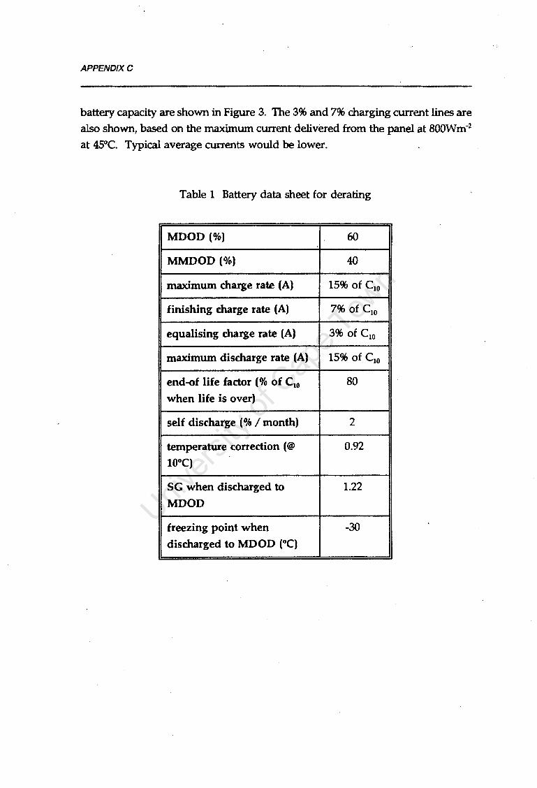
APPENDIXC
battery capacity are shown in Figure 3. The 3% and 7% charging current lines are also shown, based on the maximum current delivered from the panel at soowm-2
at 45°C. Typical average currents would be lower.
Table 1 Battery data sheet for derating
MDOD (%) 60
MMDOD (%) 40
maximum charge rat.e (A) 15% of C10
finishing charge rat.e (A) 7% of C10
equalising charge rat.e (A) 3% of C10
maximum discharge rat.e (A) 15% of C10
end-of life factor(% of C10 80
when life is over)
self discharge (% I month) 2
temperature correction(@ 0.92
10°c)
SG when discharged to 1.22
MOOD
freezing point when -30
discharged to MDOD (°C)

j
AP
PE
ND
IXC
Tab
le 2
D
erat
ing
of r
aw r
equi
red
batt
ery
capa
city
LO
PP
arr
ay s
ize
(Wp)
69
59
52
47
43
39
LO
PP
raw
bat
tery
siz
e (A
h)
15
20
32.3
40
60
12
0
Arr
ay Im
ax (
at 8
00W
m-2
& 4
5°C
) 3.
94
3.37
3.
91
2.69
2.
46
2.23
Arr
ay Ie
q (@
reg
ulat
or 1
3,8V
) 3.
68
3.14
2.
72
2.50
2.
30
2.08
Bat
tery
Ieq
(min
imu
m r
equi
red)
(1
.21)
(1
.21)
(1
.74)
(2
.16)
(3
.24)
(6
.48)
Der
atin
g o
f ra
w c
apac
ity
1) a
dju
st f
or M
DO
D
25.0
33
.3
53.8
66
.7
100.
0 20
0.0
2) a
dju
st f
or M
MD
OD
37
.5
37.5
37
.5
37.5
37
.5
37.5
3) a
dju
st f
or e
nd-o
f li
fe
18.8
25
.0
40.4
50
.0
75.0
15
0.0
4) a
dju
st f
or m
ax c
harg
e 32
.9
28.1
24
.3
22.4
20
.5
18.6
5) a
dju
st f
or m
ax d
isch
arge
23
.3
23.3
23
.3
23.3
23
.3
23.3
Der
ated
cap
acit
y [m
axim
um o
f 1)
to
6))
37
.5
37.5
53
.8
66.7
10
0.0
200.
0
Adj
ust
capa
city
for
tem
pera
ture
40
.5
40.5
58
.1
72.0
10
8.0
216.
0

APPENDIXC
A
200 derated storage capacity
3%1ine
raw ------capac!t}I B ___.-\ -··-··--·\·· ··-···-7%1ine
50
035 40 45 50 55 60 65 70 PV ARRAY fNp)
Figure 3 Adjusted LOPP curve after battery derating.
DOD determination
One could simply select the option with optimum cost from Figure 3.
Unfortunately the cost is directly related to the battery cycle llfe, which is in turn
determined by the operating conditions. For long life batteries like tubular cells
it is important that conditions are moderate, otherwise the long life may well not
be achieved. Here system simulation can be of value. PVPRO (Geerdts,1990) was
used to determine DOD profiles employing empirical data for the battery gained
from results presented in Chapter 7. The simulated DOD profiles of four systems
selected from the LOPP curve are shown in Figure 4. The systems are shown on
the LOPP curve and array and battery sizes tabulated below. The effect of PV
array /battery ratio on DOD profile is clearly demonstrated. As the array becomes
smaller, the period of extended partial SOC operation increases, and the battery
becomes less likely to be fully charged at all. Even if the cycle life projected by
battery models were the same for cases A,B,C and D, cases A and B would be
seriously stratified after one year, which could be irreversible and probably life
limiting. There is some scope for controlling and increasing gassing by adjusting
the charge regulator set points.

APPENDIXC
\_
Table 3 Array and battery sizes used in simulations
Array (Wp) Battery
(Ah)
Case A 39 216
Case B 43 110
CaseC 47 72
CaseD 52 58
Charge regulator settings and gassing determination
Daily Ah overcharge can also be easily determined from simulation. The Ah
overcharge for the four cases already simulated is shown in Figure 5. The peak
daily array currents obtained are also shown. The regulator voltage in the
simulations is set at 2.3V /cell (13.SV), and is not temperature compensated.
The overcharge is, as expected, highly seasonal. A single figure for measuring the
overcharge following the period of partial SOC operation might be the mean daily
overcharge divided by the battery capacity. This figure is called the daily
overcharge percent. The effect on daily overcharge percent of resetting the charge
voltage to 2.42V I cell (14.SV) is illustrated in Figure 6. For case A, the regulator
has almost no effect, while for case D overcharge is almost uncontrollable.
Cases B and C provide optimum overcharge and the ability to tune the system
after installation. Cases B and C correspond with the equalise and finishing rates
recommended by the battery manufacturer.
Sizing to alter the effect of regulator and battery
From the simulations it is clear that the battery in case C may be in danger of
being overcharged during regulator failure (depending on the regulator design),
and that the regulator is of prime importance. The normally ideal and mild

APPENDIXC
operating parameters experienced by the battery make its response predictable,
and its likelihood of premature failure during norinal regulator operation is low.
But the regulator in system C is critical, and failure of the regulator to regulate
will be disastrous. A series regulator, which shuts down completely on failure
may be the most appropriate choice. The heavy duty cycle of the regulator could
indeed accelerate its failure.
System B hardly requires a charge regulator, but the sizing of the system results
in a battery that is highly stressed and often in a partial state-of-charge.
Premature deterioration of the battery is the most likely failure route.
The relative stresses on the battery and regulator can be adjusted by altering the
panel/battery ratio in the sizing procedure. No quantitative data is available
however, so it is purely a matter of engineering judgement.
Costing
In principle the system with the lowest life cycle cost should be optimum. But
determining the life cycle cost brings many external parameters into play, each
with considerable uncertainty attached. There is uncertainty in component life,
in system usage, and in costing factors such as interest rates and escalation.
The simulations of the sizing options for this system present evidence that cases
A and D are totally impractical options. The battery is almost certain to suffer in
the short to medium term. Practical sizing would select be somewhere between
cases B and C, preferably located at the economic optimum.
Costing of small PV systems is further prone to errors in discretisation of
components. For instance, the optimum battery size may be 90Ah, but the
available tubular batteries are 72 and 108Ah. A similar predicament occurs for
panel selection, so optimisation is not linear, but rather stepwise. Discretisation
of components will alter system performance parameters. The choice of
components sizes and relative costs will depend on the system suppliers. Panel
prices may vary linearly with size, but tubular battery costs are non-linear for
small sizes.
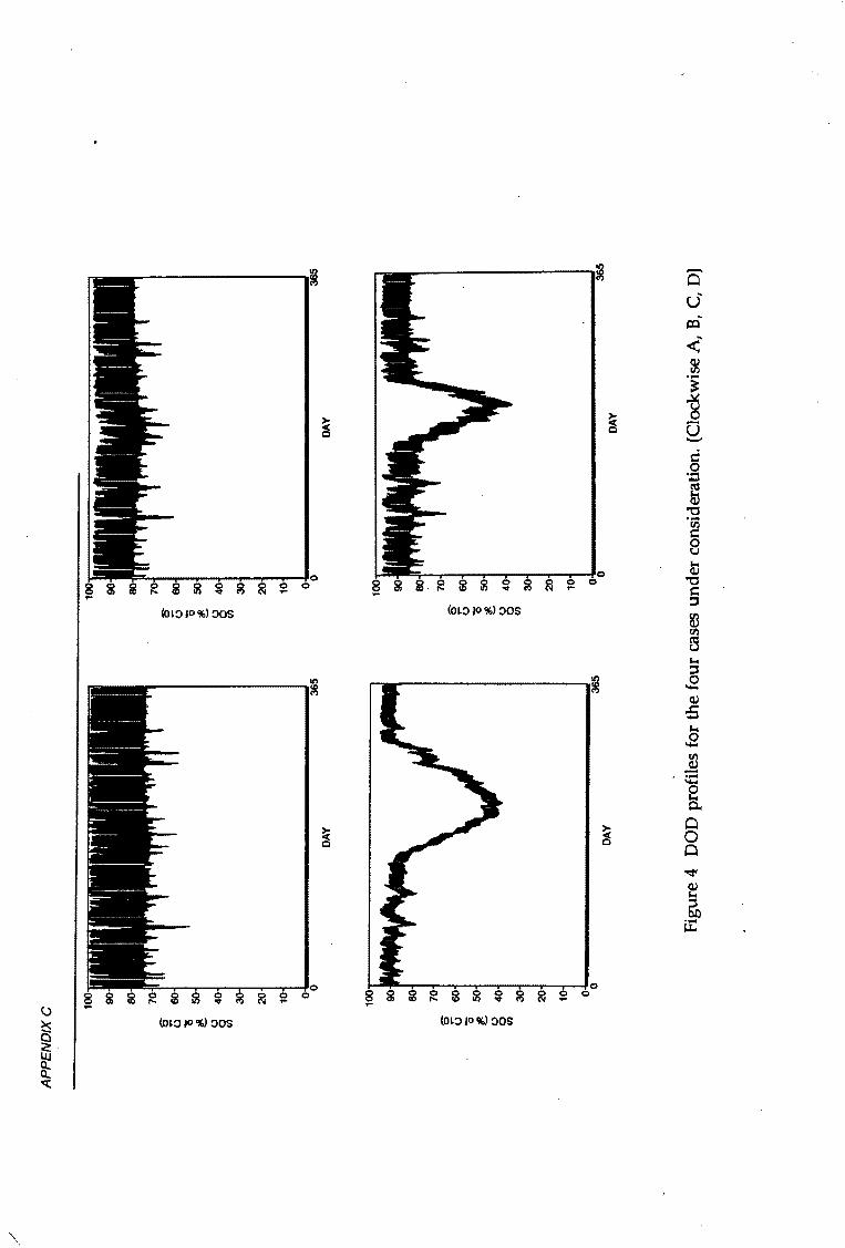
/
AP
PE
ND
IXC
100 90
80
70
6' 0
60
0 50
t.
(.
) 40
0 (/
)
30
20
10 0 0
100 90
80
70
6' 0
60
0 50
t.
(.
) 0 40
(/
)
30
20
10 0 0
6' 0 0 t.
(.)
0 (/)
365
DAY
6' 0 0 t.
(.) 0 (/)
365
DAY
100-r--~~~~~~~~~~~~--:':"':'":::::-::~
90
80
70
60
50
40
30
20
10
' I
I '
11
' I
1 I
I I
1
0'~0--------------------------------~365
DAY
100
90
80
70
60
50
40
30
20
10 0 0
365
DAY
Fig
ure
4 D
OD
pro
file
s fo
r th
e fo
ur c
ases
und
er c
onsi
dera
tion
. (C
lock
wis
e A
, B,
C,
D)

AP
PE
ND
IXC
30
10
16
10
9 9
25
14
s 8
s s
8 s
u u
u 12
u
7 7
0 20
0
0 0
t.
6 t.
t.
10
6 t.
w
w
w
w
0
15
5 0
0 8
5 0
a:
a:
a:
a:
<(
4 <
( <
( ~
::c
::c
::c
4 u
u u
6 u
a:
10
3 i
a:
i w
w
3
>
~ 4
0 2
-2
-5
2
0 0
0 0
365
0 DA
Y DA
Y
3 10
10
10
9 9
9 2.
5 8
s s
s 8
8 s
u 7
u u
7 7
u 0
2 0
0 0
t. 6
t. t.
6
6 t.
w
w
w
w
1.
5 5
0 0
5 5
0 0
a:
a:
a:
a:
~ <
( 4
~ ~
4 4
::c
u u
u u a:
3
i a:
3
3 i
w
w
~ 2
-~
2 2
-0.
5 0 0
00
0
365
DAY
DAY
Fig
ure
5 D
aily
ove
rcha
rge
prof
ile
for
case
s A
,B,C
and
D.
Cha
rge
regu
lato
r se
ttin
g =
13.8
V.
Das
hed
line
rep
rese
nts
char
ging
cur
rent
.

APPENDIXC
10
6' u 0 8
~ w ~ 6 a: < J: (.) a: 4 w i5
2
14.5V charge regulation
13.BV charge regulation
01+-~-r--~...--~.------,.----.~-"T~--r~-.-~-1
40 60 80 100 120 140 160 180 200 220 BAITERY(Ah)
Figure 6 Daily overcharge percent for cases A,B,C and D, showing effect of
charge regulator setting.

APPEND/XO
D. Manufacturers' Battery Data
This appendix contains the data provided by the manufacturers for the batteries
tested. The batteries are:
Willard 774
Raylite RMT108
Willard LS90
GNB Mini-Absolyte 12V-5000
Delco 1250
In addition, data for the specialist PV batteries discussed in Section 3.13 are
appended. These batteries are:
BP Solar P-series Tubular Cells
Sonnenschein A600 Solar Battery

12,6
11,4
v 0 l 1J
,8 T
s Xl
,2
. 9,
6
---I
-.___
--- -:--
..........
I ~
"'
.___ .....
..........
"-
~
I'- ""
~
\ \
\
1-\
\ \ v
-
/
' /
1·:£
20
3C20
13
5A
Y27
0A
'
.. --
- r--
-r-
--r-
-.
r::::::: F:
: "' ~
~
"'- ""' ['
,
"' I'\
\
\ \
\ Us
cio-L
...-
_ !..
SA
~20
90A
-~
r-....,
I'-~
\
\ \
J. ~
1BA
~
'\ ~
\~
\ -
·09l+
C2J
.osc
20
8,SA
4,
SA
-022
(20
2A
3.
6 9
12 1
5 30
1
2 3
4 5
10
~s
20
. 50
MIN
S
'=' .... .

APPENDIXD2
D2. RAYLITE RMTIOS
ii' <~ /
_-..,,;.§___.·_!!._{I/ CELL TYPES: 2RMT72
TYPICAL EXAMPLEfTIPIESE VOORBEELD
Specifications:
Number of cells calculation
Cut off voltage calculation
Cell size determination
Number of positive plates required
Jl]~&: ~:fut§
F~~)ili~
~~ili~i~~~
1~;
Float Voltage } 242V Vlot Spanning Discharge Current Ontladingstroom } 75,6Amps
V floaVbatlery 242 108cells =--=
Vfloavcell -2,23
Vminimum 189Vmin.
No.of cells 108cells = 1,75V/cell
= No. of 36 A/H plates available: 2 to 3
Discharge current
positive plate capability in amps at time to end point volts per cell 75,6
Amps = 3 plates = 25,2 Amps/plate
3RMT108 36 A/H plates
plate
Minimum Voltage Minimum Spanning Bridging Time } Oorbrugtyd
} 189Vmln.
30mlnutes
Berekening van aantalselle
Berekening van afsny spanning
Setgrootte be paling
Aantal positiewe plate benodig
V vloVbattery = ~ = V vloVsel 2,23
108selle
Vminimum
Aantalselle
189Vmin. = 1,75V/sell
108selle
= Aa~tal van 36 A/H plate beskikbaar: 2 tot 3
Ontladingstroom
positiewe plaat kapasiteit in ampere tot bestemmingspunt voltpersel
= 75
·6
Amp = 25,2 Amp/ptaat 3prate
] RAYLITE BAnERIES : '?':::! , , :,.:.:;:__.;_:,' .:.'12 .. t:::;.::CE::·o:.1i;~~c'.'::JL' ... :~.:J::::""Lc;z:;;,;r:·

APPENPIXD2
D2. RAYLITE RMT108
Lllalatroom Amper• I Afmetlngs I I uur vanael I Rayllte Dnlladlng ... DnUadlng• perpcs. / Lengte Hoogte I Gewlg
noodkrag .. Kapasltelt tyd 1troom Fina le Bogin Elndlg plHt Breedte bobattery·1 Sel Suur I Heeltemal Hiie A/uur uur omp
. 1p1nntng omp omp (10uur) Hoogte klem Droog a Ileen vol
Ch•rglng Current Amper• Length ! Rayltte HraJ Width we'lght
Slandby I I Discharge Discharge Poa. HelghV Height Acid I Complete Ii Power Capacity Time Current Final Stort. Finish. Plate Cell Over Dry Ceil Only Filled Cells A/Hrs. Hrs. Amps Voltage Amps. Amps. (10Hr) mm Terminal Kg Kg Kg
72 10 7,2 1,85 130 4V2RMT72 62 5 12,4 1,81 10 5 36 208 360 11 6,1 17,1
54 3 16 1,79 312
108 10 10,8 1,85 180 4V3RMT108 93 5 18,6 1,81 15 7.5 36 208 360 14,7 • 8.5 23.2
81 3 27 1,79 312
Typical arrangement - Tipiese rangskikking -double row double tier stand dubbel·ry stapelstaander
A B c D E F G H I J K I L
4V-2RMT72 1180 70 70 677 1130 850 312 1480 207 122 130 I 16
4V-3RMT108 1200 70 70 677 1130 850 312 1480 207 I 122 \ 180 i 1'
Typical arrangement - Tipiese rangskikking -single row double tier stand enkel-ry stapelstaander
A B c D E F G H I J K I L 4V-2RMT72 1180 70 70 370 1130 850 312 1480 207 122 130 I 16
4V-3RMT108 1200 70 70 370 1130 850 312 1480 207 122 180 I 16
H
A
Dimensions in Millimetres Afmelings in Millimeter

APPENDIXD2
D2. RAYLITE RMT108
Ueittroom Ampere- Afmeting• Hoogte A•yliH KllPMit•i1 Ontlading•· Ontt.dlng•· ...... "'"Ml Sol G1w6g
noodkrag- AJ11111 ..,.
~nniflg per pos Len11t• bo b1t11ry• Oroog Suur Hnh1m1l
Hiii amp llegin Eindig -· BrHchl kl•m .,... ••I omp amp UDuurl Ho0911
Rayllte CNrglng eurr.nt -- Ungth WeJ.gtlt St1ndby CaPICltT Dl.cl\lrge Dt•thal'Qt Final HrsJ Width Height ..... Compl1t1ly Power A/Hrs Time CuMnl ·Yoll8Q• Start. Finl ah. .... Heigh ti o ... Dry C.11 Only Filled Cells Hrs. Am po Ampo. Amp1. Plate C.11 T1nnlN1I
(10 HI) •• •• •• 15 •O 1.5 1.83 1o2
6Y 1AMT15 13.5 5 Z7 1$1 z1 1.0 15 1'6 2B5 ... "' 12 3 • 1.79 2B5
30 10 3 1.83 153 6V 2 RMT 3) 27 5 ... 1.81 •.2 z1 15 1'6 2B5 e.o 11.5
2• 3 8 1.79 2"" .. 10 •.5 1.83 211 6Y 3 AMT '5 .... 5 &1 1.81 6.3 3.1 15 158 285 11.5 5.8 17.3
36 3 12 1.79 2B5 .. 10 6 1.83 2B5 6V4RMTEO .. 5 10.8 1.81 B.• ... 15 158 2B5 .... 6,7 21.3
"' 3 16 1.79 2B5
n 10 7.2 1.83 130 4Y 2 AMT T2 62 5 1z• 1.81 10 36 208 360 11 6,1 17,1 .. 3 16 1,79 312 .
108 10 10.8 1.83 180 4Y 3 RMT 1a3 93 5 18.6 1.8• 15 7.5 36 208 360 14,7 &5 23.2
81 3 "'rT 1.79 312
150 10. 15 1.82 103 3 RST 150 .126 5 ' 25.2 1.79 23 11 50 206 435 13 5 18
113 3 37,6 1.78 355
200 10 20 1,82 103 4 AST 200 168 5 33.8 1.79 30 " 50 206 435 14,2 •.8 19
150 3 50 1,78 355
250 10 25 1.82 m 5 AST 250 210 5 .. 1.79 38 18 50 206 435 16,7 6,1 22
188 3 82,6 1,78 355
300 10 30 1,82 1'5 ~ 6 AST 300 252 5 50.• 1,79 45 21 50 205 435 19,8 7.3 26.9 -
225 3 75 1.78 355
350 10 35 1,81 m 5 RST 350 303 5 60,6 1.79 53 25 70 206 551 22,3 8,8 30,0
263 3 87,7 1.n "' •20 10 - 42 - 1,81 1'5
6 RST 420 363 5 72,8 1,79 63 29 70 206 551 2$,1 10,3 36,5 315 3 105 1.n "' ·-"'' 10 •• 1,81 168
7 AST •90 .,. 5 8',8 1,79 ,. 34 70 206 551 30,2 12,2 •2.2 :ma 3 122.7 1.n "' ·-f•lO 10 60 1,80 1'5
' 6 AST 600 519 5 103,8 1,76 90 •2 100 206 726 36,3 11,7 51 15J 3 150 t.76 8'6
7-:0 10 70 1.80 210 7 RST 700 &.:6 5 121,2 1,78 105 49 100 191 na •2,8 21 03,6
525 3 175 1,76 6'6
800 10 BO 1,80 210 8 RST 800 fi92 5 138,• 1,78 120 56 100 191 na 17,8 19,6 67,2
lOO 3 200 1,76 8'6
l'>lO 10 90 1,80 210 1
9 RST 900 779 5 155,8 1,78 135 63 100 233 726 53,9 25,8 79,7 675 3 225 1,76 6'6
1 000 10 100 1.80 210 10RST 100 665 5 173 1,78 150 70 100 233 726 58,9 2•.• 03,3
750 3 250 1,76 6'6
1 100 10 110 1,80 210
96.•() 11AST110 952 5 190,• 1,78 165 n 100 275 728 65.7 30,7 825 3 275 1,76 ...
1 200 10 120 1.80 210 12 RST 1 20I 1 038 5 207,6 1,78 180 8' 100 275 728 70,7 29,3 100
900 3 300 1,76 ... 1375 10 137,5 1.80 210
11AST1 375 1189 5 237B 1.78 "'6 96 125 275 851 78.2 :n1 107,2 1 031 3 3'3.6 1.76 771
1 500 10 150 1.80 210 t2RST 1500 1 297 5 259,• 1,78 225 105 125 275 851 78,6 31.5 110,1
1125 3 375 1,76 771
1625 10 16Z5 1.80 212 13 RST 1 625 1A05 5 281 1,78 2 .. "' 125 '1il7 851 es.• 34,5 119,9
1218 3 408 1.76 771
1750 10 175 1.80 212 11 RST 1 150 1 ~13 5 302.6 1,78 263 123 125 :Jl7 851 9Z3 37,• 129,7
1 312 3 ''"~ 1.78 771
1 875 10 187.S 1.80 212 15 RST 1 875 1 621 5 32U 1.78 281 131 125 '1il7 851 99.2 .... 139,6
1A05 3 '66.6 1.76 771
2 <XXl 10 200 1.80 212 16 RST 2 QXJ 1 730 • 3'6 1.78 XXl 1 .. •25 :Jl7 851 106,1 .... 1'9,4
1 500 3 500 1.76 771
2 125 10 212,5 1.80 212 17 AST 2 125 11tl8 5 367,6 1.78 319 1'9 125 '87 851 117,1 50.2 167,3
"'" 3 531 1.76 771
2 :!SO 10 225 1.80 212 -ia-Hl:i.:~
·~ , .389.2 1,,. ""' 158 125 '87 851 128,0 57.2 165.2
16!17 3 '6Z3 1.76 771
2 375 10 237.5 1.80 212 19 AST 2 375 205' 5 410,8 1.78 358 166 125 '87 851 138,9 6'.2 2031
1 781 3 593,6 1.76 771
2 500 10 :!SO 1.80 212 20 RST 2 500 2 •62 5 '32.• 1,78 375 175 125 '87 851 1'9.8 71.2 221,0
1875 3 625 1,76 m

APPENDIXD3
D3. WILLARD LS90
PERFORMANCE
3 I t 12\5 ..... " .. ..
The Willard LS90 is designed for a variety of standby applications. Calculation Methods: The following example is desi11ned to illustrate the method of determining the number of LS90 batteries required for a specific requirement Application - U.P.S. Sample of specifications • lnve"or of load - 45 kVA • P.F.- 0,8 • Minimum Voltage - 300 • Duty Period - 15 Minutes • lnve"or Efficiency - 90% • Maximum Voltage - 430V Step 1 - Conven kVA to kW
45 x 0,8 x 100% 90
c 40kW Step 2 - Conve" kW to load in Amperes
40x 1000 -~ m 133A
Step 3 - By reference to the above discharge graph a constant current of 135 A is available for 15 minutes down to 9,8 Volts per battery.
Step 4 - Determine number of batteries Minimum System Voltage Minimum Battery Voltage · i~a~ · 30,6 or 31 x 12 V LS90 batteries
Step 5 - Check recharge capability of system voltage Maximum S~stem Voltage Number of attenes
• ~ ~ 13,87 or 2,31 V /cell NB: Recommended Float Voltage at 25"C is 13,62 or 2,27 V/cell
-'™ CUAC!l!SWWWZ ==-==
APPLICATIONS
The Willard LS90 Maintenance Free battery provides ideal standby power for the following a~plications (Capacity 90 Ah):
• Microwave Communications Systems • Hydro Coal and Atomic Power Stations • Emergency lighting supplies • Diesel Starting • Earth-Satellite Stations • Railway signalling and substations • PABX Systems . • Uninterruptible Power Supply Systems
(UP.S.) • Radio Communication Equipment. Principal Advantages Versus Nickel Cadmium Before the LS90 was introduced, lead acid batteries already had many advantages over Nickel Cadmium batteries. Now, the superior quality intrinsic to the LS90 Maintenance Free battery makes it the sensible choice for standby applications.

APPENDIXD4
D4. GNB MINI-ABSOLYTE 12V-5000
RE-SOURCE™ Mini-ABSOLYTE , ..
Photovoltaic Battery
Mini~ ABSOLYTE'" TYPE 12-5000 Available in 12 volt units, GNB's MiniASSOL YTE"' battery provides the same quality, features and benefits as the tried and proven large ABSOL YTE II ® batteries - in a space saving, compact, power efficient mini-module. Cost saving, lightweight, transportable and totally maintenance-free, Mini-ASSOL YTE"' batteries are designed for a variety of applications including shallow or deep discharge cycling. Ideal for small power and portable installations. the MiniASSOL YTE"' battery line is the most cost effective and long lived battery of its class, with a design cycle life of more than 1200 shallow cycles.
Specifications
Container and cover: Separators: Safety Vent: Self Discharge: Terminals: Charge Voltage: Positive Plate: Negative Plate: Life:
Foam pblypropylene Spun glass microporous matrix 5 PSI (± 2 psil self-resealing 1.0% per month aher stabilizing Heavy duty integral copper inserts 2.25-2.45 VPC Special hybrid alloy Lead Calcium
500 cycles @> 80% DOD 800 cycles @ 50% DOD
1200 cycles @ 20% DOD
Innovative Features Sealed
• Never requires watering • Spillproof and leakproof • No gases escape during normal charging • Explosion resistant • Operates at low internal pressure • Increased operating safety
Completely sealed maintenance free battery incorporating GNB's patented ABSOLYTE~' Technology.
Recognizing the ever-increasing value and importance of renewable energy obtained from the sun and the wind, GNB has developed the RE-SOURCE line of lead-acid batteries that are ideally suited for use with photovoltaic or other renewable energy systems.
GNB has responded to this need by developing unique deep-cycle batteries. Because of cost, availability and reliability, photovoltaicpowered installations are being used more and more for telecommunications, railroads signals, irrigation pumps, cathodic pipeline, bridge protection and village electrification.
MtNl-A8$0LJYE•
CYCLE LIFE VS DEPTH DF DISCHARGE• CAPACITY ADJUSTED FOR TEMPERATURE
. LIFE DETERMINED BY AGE 100
90
~ 80 0
Immobilized Electrolyte g 1000
~ 70
0 60
~ 50 • Extended partial· state of charge operation (at reduced capacities)
• Freezing tolerated • Minimizes need for equalization
Patented Hybrid Alloy • Deep cycle capability • Long life • low self discharge rate
w ~ ::; J
w 0 500
0 10 20 30 40 50 60 70 80 90 100
OEPTH OF DISCHARGE % OF RATED CAPACITY
... ~ 40
ffi 30 .. 20
10
0 10 20 30 40 50 60 70 80 90 100110120
CELL TEMPERATURE •F
Physical Characteristics Electrical Performance Dmall~ ...... ...... IH Capcity I• 1.75 YPC .._ - - ......
"'"'" . .. .... .... 1DOIO ,,.. .. .. .. ... ••
12·5000 12.75 324 6.78 173 8.47 216 63 29 12 85 93 96 100
Accessories lntercell connectors (if required), installation and operating instructions, stainless steel bolts and lock washers matched to copper insert post threads, rope handle.
Please Note: Batteries are shipped at 90% of their final capacity. Designed capacity will be achieved after cycling. GNB reserve the right to change the design and specifications without notice.

APPENDIXD5
D5. DELCO 1250
Description Delco Heavy-Duty High-Cycle Freedom batleries are maintenance-free, 12-volt design combining both cranking and cycling abilities in.a· single power source.
Features True maintenance-free design eliminates watering and regular service. Heavy-duty construction and wrought lead-calcium grid resist vibration. shock, overcharge, heat, and thermal runaway. Special chemistry and plate formulation for extra life. extra reserve and extra cycling capability in moderate depth discharge. High-impact polypropylene case and cover permanently assembled by heat sealing. Low self-discharge permits long storage life. Standard size for simplified stocking and mounting flexibility. Built-in test hydrometer, LiQuid-Gas separator, ·and flame arrester protection. Available with sealed top terminals and stainless steel connecter stud or standard SAE tapered posts.
Application Recommended for heavy-duty applications where extra life and reserve e<1pacity is needed to car~ the entire electric..! load for short periods. Delco 1150 and 1151 ar~suited for heavy trucks in P&D, car carrier cir short-haul service and for emergency vehicles, buses. marine and off-road eQuipment. recreational vehicle auxiliary power. and trolling motors. For energy storage system use. photovoltaic or other stationary applications, Delco 2000 offers special electrotyle and other features not offered in vehicle batteries.
Specifications Voltage: 12-volt
Maximum Ambient Temperature: Continuous-52°C (125°F) lntermittent-77°C (170°F)
Mounting: Top retainer Performance: See table
.. ,. .. -· ~j Reserve
eo1a C.pacny Crank.mg Mmu1es
·.1 BCt Amps@ 0°F @ 80°F
1-18°Ci 127°C1 .. , Group 30·sec. 25A.
S•e 7.2V 10.5V
-1 31 ()80 180 :J . ·I
31 I 580 180
I
·I
I 31 All/l>HOUI Rate t100·h1) 105
{~.\ . .:..-...
._·._ .
. " ·~· .
~ Ma.umum Dimensions Replace- ~ Appro1 OR menl
Length Width He1grn Weight lrpe MOOel P•n ~ rn tmmJ in 1mm1 m 1mm) Lb lkgJ Termrnal Numbe1 Number
130 68 9.4 60 lop 514 1150 ~i 133021 11720) 12388) J2i 91 Stu a ~
~ 130 68 94 60 lop 8195 1151 . 1330 21 1172.0J 12388) 1269) Post
t 130 68 94 60 lop 860 2000 ~ 13302) 1172 OJ 123881 1269) Stud ~
·:·~-f~~A~

APPENDIXD5
D5. DELCO 1250
• INCREASED SERVICE LIFE E!iminating water filler caps prevents electrolyte contamination. overwatering or damage to internal elements. Vibration·resistant construction-with center lug connections. epaxy-anchored plates resting on flat case bottom. and separator envelopes-help prevent damage in rugged use. Eliminating antimony from the plates cuts gassing, resists overcharge, heat and thermal runaway. UniQue grid design with wrought alloy means less internal corrosion, more efficient current conductivity for more power and more lite. Generous electrolyte reserve. factory checked for purity and specific gravity, is sealed in to last the service life or the battery. The result is a battery that. when properly applied. provides real maintenance-free performance for long periods without service and inspection.
• HIGH CRANKING POWER Delco High-Cycle, rated at 580 CCA. packs plenty or power for raster stans with large diesels. A lour battery complement provides 2320 CCA, with nearly 1000 minutes reserve capacity. Thus. the Delco High-Cycle can provide subslar.tial advanlages in power. per1ormance and electrical hook·UP.
• SIMPLIFIED STOCKING AND STORAGE Delco High-Cycle can be fitted to almost any installation where cycling is expected. Two or more can be used in series. parallel or parallel·series to meet the cranking/cycling needs ot the application end engine. Plus. the battery comes fully activated. charged and ready to go. ,\At1mony-lree plates reduce selldischarge end increase wet storage life to a year or more in vehicle uses. This eliminates trickle charging, activation end acid handling.
• LONG CYCLING LIFE Until now, batteries were etther designed for cranking use-with high power output for shon periods of time-or they were designed for cycling use-long. steady drains. followed by recharge. Now. with the new plate design and maintenance-free technology. the Delco High-(;ycle offers both. The plates resist deterioration in cycling use ... where conventional battery plates rapidly wear out or warp, shed and eventually shon out. Standard tests show the High-Cycle to have about 75% greater cycling life than our best heavy-duty maintenance-free cranking battery and more than three times lhe
0
life ol our pepular Freedom battery when used in cycling applications.
• REDUCED MAINTENANCE Delco High-Cycle Heavy-Duty Freedom batteries never need water or checking for water. Antimony-free plates cut electrolyte loss from gassing. The special vent design with Liquid-Gas separator helps keep electrolyte inside the battery. Cover has no filler caps to allow electrolyte spill, splash and sP<>w. Sealed terminal design stops corrosion of terminals and cables. eliminates regular cleaning.
• MOUNTING FLEXIBILITY In addition to combining cranking and c·ycling properties. there are no routine service reQuirements with Delco High--Cycle. So. ii offers new possibilities in mounting. Batteries can be relocated to reduce harmful vipration. This also can permit savings on cables and mounting hardware."from better use of available space. or allow larger size fuel tanks.
nerco Remu _, 01111sm~; or crr;tP.f.l MJTO<:S Al\ornso~;.1,..J1:.l\A 46011

0 llJ >
0 2 Ill
(( > I H
LI
<t
Cl.. <t:
u
100 7 5 3 2 10 7
IL
5 0 J z llJ
u a: w
n.
3 2 1 10
0
DELC
O 20
00
CYCL
E L
IFE
'-.....
~
"'-
I"'-..
.. .....
.. ....
....
~
r---...
"-T
n i
:;n~
nc:r:
:.
TD
20
X _os~
..........
,....
~
I'-... .....
... r---
... ' ~
-'-
-......
-......
-......
-......
""'-
~
.....
........
... ~,
..........
.........
['...
!'-......
-.......
I'-.....
-,
-...... I'-
.
2 3
5 7
10
00
2
3 5
7 1
00
00
CY.C
L ES
t='
en
• .... t,:) en
0

APPENDIXD5
D5. DELCO 1250
DELC0-2000 CHARGE· VOLTAGE. ~ECOMMEHDATION FOR SOLAR APPLICATIONS 15.5
w 15.0 a----f---1-"""""---1-~--l-~4--I C!)
-< ~ 14.5 a-.-.. --+---+----+-----""~-'1f---i---I > &.U
~ 14.0 11----i---t---t---+---F""lo.;:---t--I
-<( ::I:= t...> 13.5 a------+---+--.J---1-....,.....---i----~
;:::;::; &.U c:>
13.0 '---"'--~_.....____... _________ _.. •20 ' 0 20 40 60 80 100 I 120
(-28.9) (-17.8) (-6.7) (4.4) (15.6). (26.7) (37.8) (48.9) UMPERATURE 0 f. (0
() I-BO
DELCO 2000 ELECTROLYTE LIFE IN SOLAR APPLICATIONS
~ ~ 40 11-------;-----------il --'= ...... '-' - c.:: ~~30~------+-----~---i--------+-~ C> 0.:: >i-- < t...,)~
~ffi20~-----+-----t-~~~--1-~ ...... Q.
~ V"I 0::. 0::
;:5 g 10 11---------+-----t---------1--1 >- ::c:
:::e
O'--------------------------~ 13.0 13.5 14.0 14.5
CHARGE VOLTAGE (25°() 1-80

APPENDIXD5
D5. DELCO 1250
V"I
150 130 110
-,_
DELCO 2000 CAPACITY .
;
g; 90 ~ 70 -- -- r-...... _
- - -0.. ~r--....,
10.S VOLT OUT POINT :i 50
.r-,.... 25°C • 0°c·
i-- . 20°c• . 30
0.5 ! I I
2 4 6 8 10 20 30 40 50
Of. U-1
CURRENT DRAIN {AMPS)
DELCO. 2000 SELF-DISCHARGE RATE
*l.lllHlllO • 1-10 .
0.. 6~---.,---.,--i---.,---.,--t---.,---.,----+-__,..-1-__,..t--V"I Of. :::::> ~ 4r---.,-__,..-1-__,..~-t-~__,..-,tf'0--__,..__,..t---
....... °' ....... ~ 2~---.,---.,--i-__,..-::.~~__,..--t-__,..__,..__,..i---
<C
Oa.------------------------------20 40 60 80 100 ·· l-6.n l4.4l l1S.6l l26.7) l37.8)
TEMPERATURE °F (0() • . 1-10
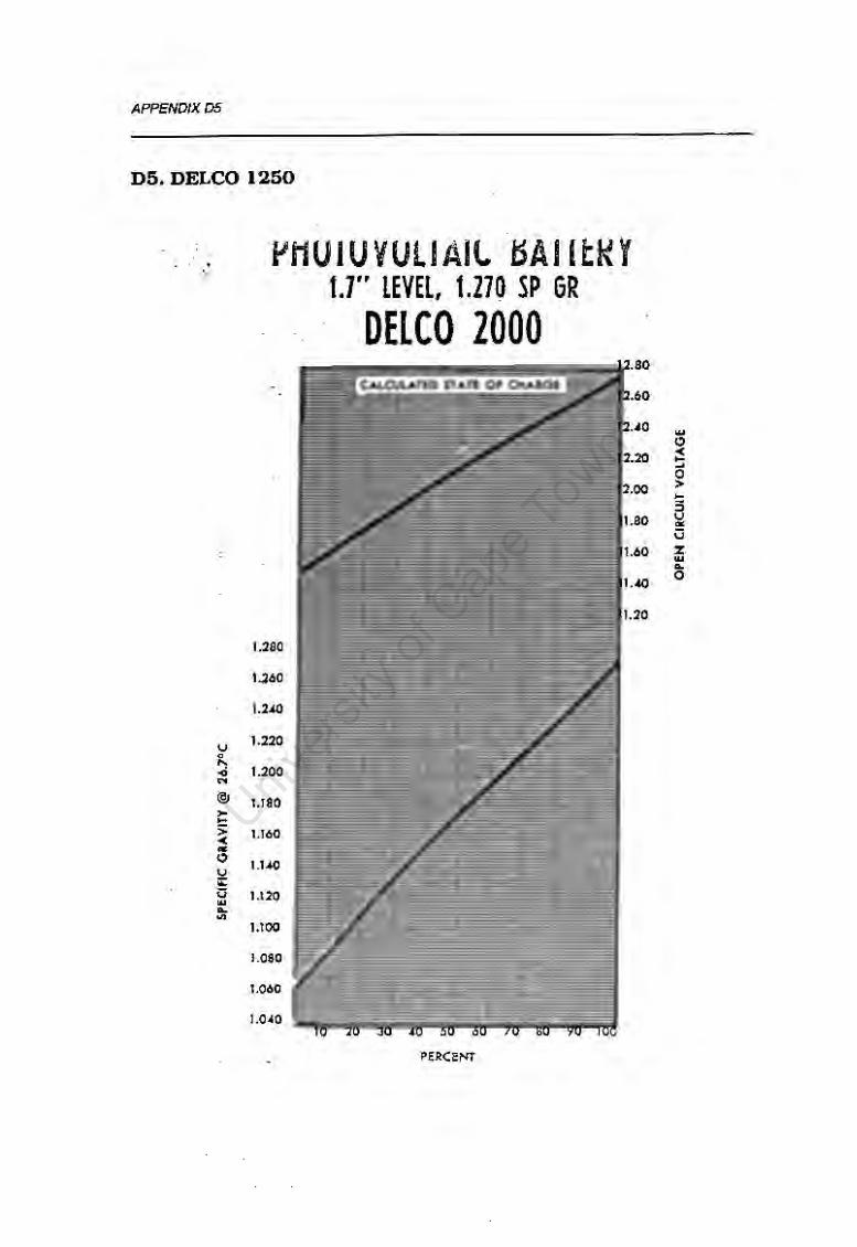
APPENDIX OS
D5. DELCO 1250
• \
u ()
" .0 N
@> >-I-
> ~ « <!> u ;;:: iJ IU ~ .,,
1-'HUIUVULIAll tsAI ltl<Y 1.7" LEVEL, 1.270 SP GR
t.280
1.260
1.2.40
1.220
1.200
1.180
1.160
1.1.40
1.120
1.100
1.080
1.060
1.0""40
DELCO 2000 CALCULATED STATE OF CHARGE
10 20 30 JO 50 60 70 80 90 100
PERCENT
12.60
12.-'0
12 . .20
12.00
11.SO
11.60
11.20
IU
<!> ~ ... 0 > l-s u « iJ z IU ~
0
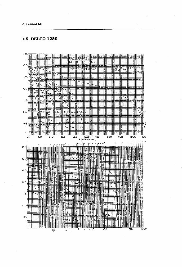
APPENDIXD5
D5. DELCO 1250
11.5
I l.O -
. co
13.5'
13D
12.5
120
11.5
11.0
10.5
-H-H+HH-ill•t Jt.. :1\ . ,. +-!i .....
-ff:: ttl=I. :J:l=i\j:j:tH -Ji·_:
120 24.0
".
--Le
!<'• l'i+ ICl"i'· ·~·A · 1•,
AH
0.5 1.0
-II-
46.0 GC1.0 72.0
.. till O'I .... C-tOI ' I 1 I I I I I I I I I I I
- -:t --
84.0
N
'
%0
·~ ...
_. 1-- .. ·1:.
1060
--1
I~ +.t I
ii A
120

APPENDIXD6
D6. BP SOLAR LUCAS P-SERIES
Technical Specification
All battery capacities are measured at 25°C, to an end voltage of 1.8 volts per cell, specification to ±10%.
Capacity (Ah) Dimensions imm) Weight(kg) Battery I Battery I Type Voll 10hr I 25 hr SO hr 100hr 120 hr Length Width Height Wet Dry
12P58 i 12 I 35 42 49 58 61 272. 205 379 335 20
12P108 i 12 ! 65 78 92 108 113 380 205 379 50 29
12P157; 12 I 94 114 133 157 165 380 205 379 I 56.5 37.5
6P207 : 6 124 150 176 207 217 272. 205 379 375 23
6P363 : 6 I 218 263 309 363 381 380 205 379 I 56.5 36.5
2P425 I 2 255 308 361 425 446 124 206 500 23.5 14.5
2P566 I 2 340 410 481 566 594 166 206 I 500 ·31.s 19
2P641 i 2 385 I 465 545 I 641 .:fff3~. I 166 206 j 500 I 33 21
2P779 i 2 467 565 662 779 818. I 191 210 I 675 I 46.5 26
2P886 I 2 532 642 753 886 930 191 210 675 I 49 29
,-'='· 0 g8J ! 2 I 592 716 839 I I 987 1036 I 191 210 i 675 j 51 31.5
~P1101 J 2 661 798 936 I 1101 1156 I 233 210 I
675 i 60.5 35.5 I
Larger capacities are obtainable by connecting like cells in parallel, higher voltages are obtainat:e from connecting like cells in series.
Performanci:: Characteristics Charging efficiency (up to 60% state of charge) 97%. Cycle life - to 10% discharge 7200 cycles (20 years estimated life)
- to 50% discharge 3000 cycles (8 years estimated life) - to 75% discharge 1500 cycles (4 years estimated life)
In typical photovoltaic applications the P-series battery cell gives a minimum life expectancy of 10-12 years.
l
<I lermonals !2. Electrolyte level markS (3 1 Ven1 plug w1tn recomo1nator @, Clear ou1er case ~. Harnes's suppor1
·1 • ,~ i>"
I-'~ So•:v ~»~"'.'"':.!. LT'l 1••sr-vcs :.,~ 11i::iri110 cn3ricp tne spccilsc;mo., 01 ;in..,
r><GOuCt'> •:'IC•""...:! on 1n1?. c.11i! .,.,ece1 10 1mor~ renaD•llllf. lunc110n ur OC:>'9n
Maintenance The specialist design of the P-series battery ensures minimal maintenance. Typical field maintenance at yearly intervals involves cleaning all electrodes and topping up with distilled wate':
Equipment Supply The P-series battery cells are supplied either wet charged, or dry charged (acid supplied separately) complete with flexible insulated terminal interconnectors. pole caps and fasteners. Batteries can be supplied with flame arrestors or a cataly1ic vent plug recombinator system upon request. (A recombinator fits into the banery vent plug and cataly1ically recombines the oxy-hydrogen gas evolved during boost charging back to water. This optional system reduces banery maintenance interval to 3-4 years. recombinators are available to fit 2. 6, and 12 volt nominal cells).
As a systems supplier BP Solar recommend the use of specially oes1gned GRP oanery boxes or steel banery racks to iacihtate cell storage with tne optimal system conf1gurat1on. Ancillary equipment includes on-sne installation/ maintenance kit consisting. apron. gloves. taceshield. thermometer hydrometer. tunnel water containe•. eye wash kit, and de-ioniser exchange column.
-Ff
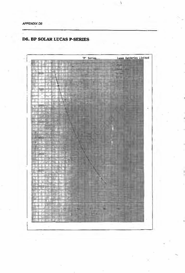
\
APPENDIXD6
D6. BP SOLAR LUCAS P-SERIES
'P' Series Lucas Batteries Limited
-..
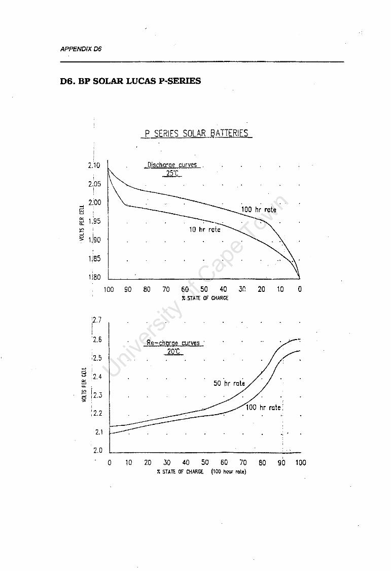
APPENDIXD6
D6. BP SOLAR LUCAS P-SERIES

APPENDIXDl
D7. SONNENSCHEIN A600 SOLAR
·sonnenschein Batteries
Sonnenschein
dryfit ~ @(Q)(Q) solar - The battery for alternative energy sources.
Alternative energy sources are always of interest where mains power is not available at the end of a plug.
tt has long been known that man could obtain power from the wind, the water or the sun. For solar energy to be used in electrical applies· tions, tt has to be stored. Sonnenschein, in their A 600 solar batte.Y- a further development from the A 600 industrial battery- have produced the ideal battery for solar energy storage. Since the efficiency of solar energy is dependent on the intensity and duration of solar raciation, tt is used primarily in hot areas.
Battery construction
- Plates The A 600 battery is fitted with positive tubular and ftal negative grid plates.
The positive plate mass is surrounded by a porous, extremely strong plastic jacket -the tube. Sonnenschein tubes have an exceptionally high retention capacity, giving long life even in cyclic operation. The lead cores are die cast in a special antimony-free alloy. MO'oporous plastic separators are fitted between the different polarity plates.
The maintenance-free A 600 solar battery has been designed for this specific purpose. Experience has shown that the conventional battery, with its regular maintenance requirement. is frequently the weak point in an installation, since in many cases service personnel are either untrained, or simply not available.
The A 600 solar battery has an exceptionally long, maintenance-tree life, despite exposure to a stringent cyclic load. a higher charge vollage, during heavily concentrated energy supply (e.g. midday solar peak), and high ambient temperatures.
- Electrolyte The electrolyte is contained in a thixotropic gel, its composition and amount especially designed for cyclic loads. The density of the acid, 1.2 kgn, is suitable for the high ambient temperatures expected to occur, hence attack by corrosion is extremely low. The large electrolyte reserve ensures that the specific gravity value of the acid remains high during discharge allowing the cell to be used at temperatures down to - 20 °C.
Simila~y unaffected by these are the fol:owing properties of the A 600 solar battery:
- low self-discharge rate - leakproof - deep discharge proof - cycle resistant - suitable for high and low ambient tempera-
tures.
The A 600 solar battery may, for example, be used: - to store energy from solar panels, wind and
wave generators - to supply buoys. drilling platlorrns, radio
and television relay transmitters and irriga· tionplants
·• in pipeline monitoring stations
- Cases The cell cases are made of SAN, a high· grade acid-resistant plastic.
The cases and cover are sealed, and are completely leak proof.
The newly developed terminal bushing and ·pressure relief valve provide an airtight seal for the cell, preventing ingress of any at· mospheric oxygen.
- Connection The individual cells. rated at 2 volts each, are interconnected by maintenance-free threaded connectors (tapered cone).

APPENDIXD7
D7. SONNENSCHEIN A600 SOLAR
Sonnenschein Batteries
Type Plates Rated Dimensions per cell capacity Length
c,. Width Height Height over terminal
Ah mm
2190 2 90 105 208 360 420
3/130 3 130 147 208 360 420
-·
3/190 3 190 147 208 475 535 .
3/270 3 270 147 208 650 710
4/360 4 360 193 212 650 710
5/450 5 450 235 212 650 710
6/540 6 540 277 212 650 710
6/680 6 680 277 212 800 865
Overall Discharge length capacity =case +gap
mm Ah
115 40 57 70 90
108 140
155 62 90
108 130 160 206
155 85 120 150 190 228 290
155 120 165 210 270 320 420
220 160 222 280 360 432 550
220 200 279 350 450 540 695
220 240 333 420 540 648 830
220 306 420 530 680 820
1050
Sonnenschein
Discharge Discharge Weight Number time current of terminals
h A kg
1 40 14 2 3 19 5 14
10 9 20 5.4
100 1.4
1 62 19 2 3 30 5 21.6
10 13 20 8
100 2.06
1 85 25 2 3 40 5 30
10 19 20 11.4
100 2.9
1 120 34.0 2 3 55 5 42
10 27 20 16
100 4.2
1 160 47 4 3 74 5 56
10 36 20 21.6
100 5.5
1 200 57 4 3 93 5 70
10 45 20 27
100 6.95
1 240 67 4 3 111 5 84
10 54 20 32.4
100 8.3
1 306 83 4 3 140 5 106
10 68 20 41
100 10.5

APPENDJXDl
D7. SONNENSCHEIN A600 SOLAR
Sonnenschein Batteries
dryflt A 600 solar discharge curves
The following diagram shows the voltage curve for various load currents.
Low sell-discharge rate
The A 600 solar battery has an extremely low rate of self-discharge. The primary energy is thus almost exclusively available for the load, since little energy is required to compensate for battery losses. It is therefore possible to span even relatively long periods of use with a low energy supply.
Rg.2 A 600 solar battery self-discharge at various temperatures compared with a conventional standard lead-acid battery. f = A 600 solar battery II = Standard lead-acid battery
"' C>
~ 0 > Qi (,)
"' :l5 .!l1 ... > .. ~ ~ l;l c. .. " " " e 0
"' en .. E " !: "' 0..
2,1
2.0·
1,9
1,8
1,7
1,6
1,5
Ah [%) 100
75
50
25
Temperature: 30 [°CJ
0,1
2o•c 40°C
3 6 No. of month' standing time
Sonnenschein
v, 1.76 (VJ
v, ~ 1.58 [VJ
10 100
Discharge time (hours)
30°C 2o•c 8"C
9 12 15 18 21 24

APPENDIXD7
D7. SONNENSCHEIN A600 SOLAR
Sonnenschein Batteries
Charger
The Sonnenschein solar charger is recommended as the ideal charging system for A 600 solar batteries. It provides optimum utilisation of the energy supplied. hence a long battery life. It other chargers are used, the charge voltage must be matched to the radiation and load profile.
Based on the rated value, the charge voltage must be adjusted to temperature variations as shown in fig. 3.
'ijl
~ .,; "' "' '5 >
" e> "' .c u
[VJ
2,8
2.7
2,6
2,5
2,4
2,3
2,2
2,1
.............
Sonnenschein
.......... ~
~ -...... :--..
-....._ -.
-30 -20 -10 0 +lo +20 +30 +40 +so ['CJ
Capacity curve and temperature profile
Temperature, of cource, affects the battery capacity. The graph and table show the capacity curves and discharge cut-off voltages for various load currents.
Ambient temperatures outside the range -20 •c to + 50 •c should be avoided.
Fig. 5 Discharge cut-ott voltage as a function of temperature and load (V per cell)
Fig. 3 Ambient temperature Charge voltage as a function of temperature
160 '
140
.. :0
120 lll ... > "' ~100 "' a.
"' " 0 80 c.i n; c: .E
60 0 c: 0
* 40
20
---,/
~/ - J20
/ .,.,........ -./ ~(.
J10
I / r ---/
/: / --- µs
~
.,.,........ J3
~ ~ /' ---/ J1 . . .
~ ~ ,,........... --
v ,
~ -- .·
0 -30 -20 -10 0 +10 +20 +30 +40 +50 ['CJ
Fig. 4 Discharge temperature Capacity as a function of temperature and load
Discharge temperature -20'C o•c +30'C +50°c
Discharge current I 1 1.39 1.45 1.58 1.61 1, 1.53 1.58 1.67 1.68 15 1.59 1.63- .. 1.70 1.72 l.o 1.66 1.68 1.73 1.75 120 1.72 1.73 1.75 1.77 l.oo 1.74 1.75 1.76 1.77

APPENDIXE1
El. Heatsinking of 2N3442 Transistors (An experimental determination)
Six 2N3442 transistors are mounted on SOcm length of heavy duty aluminium
heatsink. The total heat that can be dissipated by the heatsink and the transistors
is detennined experimentally, since the heat transfer coefficient from the heatsink
to the air (Rh_J cannot be otherwise determined.
For each transistor:
the junction to case resistance, R;-c = 1.51°C/W
and the case to heatsink resistance, Rc-h = 0.14°C/W
(if heatsink compound is used).
For the six transistors mounted on the heatsink the overall heat transfer network is
04 o~ Q,
f' f~:•L ,1~,
{2 i ·c. !~Li:C :-rCf.4 T,~
{'L,. h 1 Q<· ~ ~ R,. ~. \
I\~
• CH.<
The heatsink is assumed to be at uniform temperature, since all transistors (Ql to 06) carry the same current.
The circuit can be Thevenised to
\·
f
Oo..~roy ~
o,oJ..s~c/w le..
1~ o,o?. ~
0c. /w

APPENDIXE1
Methoc!
By discharging a battery through the six transistor heatsink array and measuring
power dissipation vs heatsink temperature (T hl, for a known air temperature (T al.
Steady state is assumed.
Sample Calculation
At 24V and 7.SA discharge rate through the array, the total power dissipation (Pl
is 180W. The power in each transistor (P tranl is 30W.
Ta = 20°C, and Th = 64°C at steady state.
now
Rh-a = (Th - Tall P = (64 - 201/180 = 0.244°C/W
Tc is assumed equal to Th
From the power derating curve in the specifications, the maximum power per
transistor (P maxl at Tc of 64°C is 90W. 30W is clearly within limits, and T; < 200°C as required.
Results
The experimental results are shown in Table 1 for Ta= 20°C.
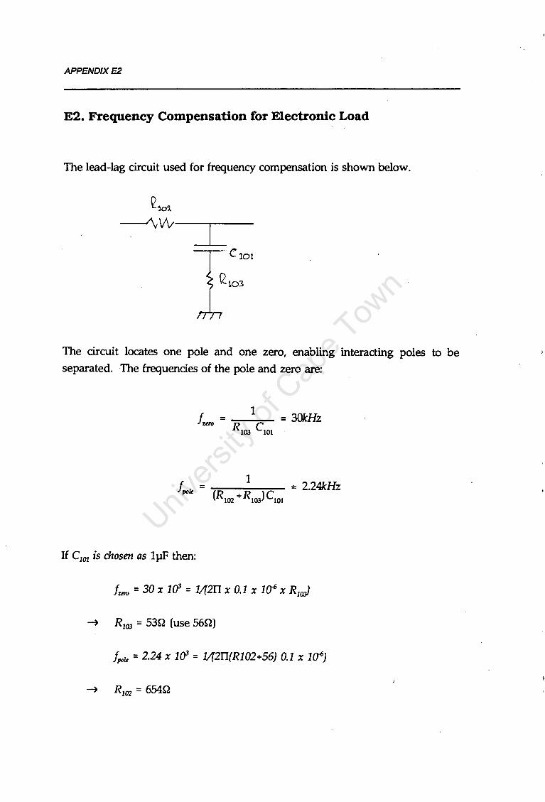
APPENDIXE2
E2. Frequency Compensation for Electronic Load
The lead-lag circuit used for frequency compensation is shown below.
TC101
~ R1o:s,
J_, The circuit locates one pole and one zero, enabling interacting poles to be
separated. The frequencies of the pole and zero are:
1 - l =30kHz )zero - R C
103 101
If C101 is chosen as lµF then:
furo = 30 x 1a3 = L12Il x 0.1 x Ur x R10.J
~ R103 = 53Q (use 56Q)
fpoie = 2.24 x 1a3 = L12Il(R102+56) 0.1 x 1~)
~ R102 = 654Q

APPENDIXE3
E3. LC Filter Design
Assume that the SCR AC input voltage is 60V nns at SOHz. The second harmonic
is the major harmonic, with a maximum of V 2nns = 38V nnsi and a frequency of
lOOHz. If the second harmonic is successfully filtered then the contributions from the remaining harmonics is likely to be insignificant.
The inductance ,L, required to attenuate the signal by -20dB at lOOHz (and zero
at lOHz) is given by
where C is the capacitance.
For capacitance of lOOOOuF, the inductance required is 25.3mH.
The impedance of the inductance at lOOHz is
The output current ripple due mainly to the second harmonic is given by
The peak ripple is given by
v2nns I nn.Jrippk =--= 1. 1A""'
XL
]maxrippk =/i.xl""'rlppk =2.4Amax
This calculation can be repeated for several sizes of capacitor, to determine
inductance and performance for fixed output voltage specifications. The results
are shown in both tabular and graphical format. The most cost effective option is a 20000uF capacitor and a 12.6mH inductor.

APPENDIXE3
Table 3 LC filter cost vs performance optimisation
OPTION NUMBER 1 - 2 3 4
Capacitance (uF) 10000 20000 30000 40000
Inductance (mH) 25.3 12.6 8.4 6
Irms ripple {A) 1.7 3.4 5.1 7.1
lmax ripple {A) 2.4 4.8 7.2 10
Capacitor cost1 (R) 39 78 117 156
Inductor cost2 (R) 280 140 115 110
Total cost (R) 319 218 232 266
1 Source: Hamrad Electronics 2 Source: Powerfonn Transformers
Cost (Rands) Current (A) 350 12
10 Fiiter cost
300 Ripple current 8
6
250 4
2
200'--~~-'-~~~....__~~--'-~~~--L-~~~o
o ro ~ ~ ~ ~
Capacitor size (1000 uF)
Figure 1 Graphical display of the tabular optimisation

APPENDIXE4
E4. Transistor Array SOAR and Current Gain
I c (A), per transistor 10::r:::==============s::::::==~::::::::ir:::='.'"--;;:::-::::::::::::--=:::::::---:::::::::-::::::::---::::::::::::-~ 7
5
3
2
0.7
0.5
0.3
0.2
2 3 5 7 10 20 30 50 70 100
V ce (V)
Figure 2 Load transistor operating region
I c (A), per transistor 10::r::::::::::============s::::==~~r==:s::;:::::-::::::::-=:-::::::::---:::::::::-=:-:--:::::::::-:;::-i 7
5 +·························'························
1
0.7
0.5
0.3
0.2
2 3 5 7 1 0 20 30 50 70 1 OD
V ce (V)
Figure 3 Power supply transistor operating region
500
300
200
H le, DC current gain
-.- -: ~.~. ~-L~_ri~25~~ Ti~2~~~c •••••••<), ~"C'V'-.:~:i::~,,
:J Vce=4.0V I
-. 100 ~;::::;;;;::::::;:;::::::;::;::::=:::::::::::~:-;:;:::::::;~~:==::::::::::::::::-::-:::::::---::=:~==--=~ 70
50
30
20 'x
10 '--~~-'-~-'-~'---'-......_...-'-........ ~~~-'-~-'--'---'"-'--'--_._._, 0.1 0.2 0.3 0.5 0. 7 1.0 2.0 3.0 5.0 7.0
I c (A), per transistor
Figure 4 Current gain of load and power supply transistor arrays

APPENDIXE5
E5. Program Data Flow
The data flow and sequence of the control software is outlined. Subroutine names
appear in parentheses.
Mainprogram (Mainprog)
end
open files for input and output define PV system (PVdefine)
read the input file (ReadNextOutputs)
adjust load current (LoadCurr)
adjust power supply current (PVCurr)
read the data channels (ReadAllChannels)
start the internal timer
default to numeric display (DisplayNumeric) enable menu use
repeat ·
repeat
wait for operator input
until 1 minute has elapsed
execute timed routine (Timed) until test finished
close all files

APPENDIXES
Timed Routine (Timed)
end
disable menu use
read the data channels (ReadAllChannels)
generate derived data (SumChannelData)
if operating cycle ended or termination criteria satisfied
read the input file (ReadNextOutputs)
write the data to disk
elseif log interval
write the data to disk
if loadmode = CC
then adjust load current (LoadCurr)
elseif loadmode = RC
then adjust load current (LoadShedSimulator)
if PSmode = CC
then adjust PS current (PVCurr)
elseif PSmode = CV
then adjust PS voltage (PVV olt)
elseif PSmode = PV
then find PV operating point (PVsim)
read the channels (ReadALLChannels)
if displaymode =numeric
then display numeric format (DisplayNumeric)
elseif displaymode = graphic
then display grapliic format (DisplayGraphic)
elseif displaymode = Control
then display operator control format (
enable menu

APPENDIXES
Adjust load current (LoadCurr)
end
Output the digital current
Read the current repeat
adjust digital
output digital current
read current
until current within tolerance or specified iterations .
Adjust PS current (PVCurr)
end
Output the digital current
Read the current
repeat
adjust digital
output digital current
read current
until current within tolerance or specified iterations
Adjust PS voltage (PWolt)
end
Repeat
Solve for the required current using battery operating line ( adjust the PS current (PVCurr)
read the voltage and current (MeasurePVOutputs)
update battery operating line (GetBatteryLine)
until voltage within tolerance or specified iterations

APPENDIXES
Find PV operating point (PVsim)
end
Repeat Solve for the operating point using Newtons Metho_d on the
battery operating line and PV operating curve (SolvePVPoint)
Adjust the operating point if voltage regulator is present (RegulatorSimulator)
adjust the PS current (PVCurr)
read the battery voltage and current (MeasurePVOutputs)
update battery operating line (GetBatteryLine) until voltage within tolerance or specified iterations
Display graphic format (DisplayGraphic)
end
Scan the output file for logged data (ScanDataForGraph)
Add new points to the graph array (AddPointsToArray)
Set up the axes (SetUpGraph) Plot (PlotGraph)

APPENDIXE6
E6. Electrical Component Data
This appendix contains manufacturers' technical specifications for the following
components:
LM-358
2N-3442
TIP-31C
MTM-15N45
MJ-802
AEG B2-250-30Si
AEG TT45N-200K
dual op-amp
NPN power transistor
NPN low power transistor
N-channel enhancement mode Mos-FET
PNP power transistor
power diode bridge
power SCR block
Shimaden Temperature Controller

~National ~ Semiconductor
Operational Amplifiers/B·u-ffer~ . I
LM158/LM258/LM358, LM158A/LM258A/LM358A, LM2904 Low Power Dual Operational Amplifiers General Description The LM 1 S8 ttrin con1i1t1 of two independent.. h"I' gain. internally fre~tl"cy compenHttd operational .-nplifitrs which ~• dnipd specifically to operate from 1 1il'91e power supply oYt"r 1 wide r1nve of vol~. Operation from 1pli1 pcJ'¥11'ef wppties it alW> possiblt and
• Allows di;ectly sensing nur GNO and VouT also goes 10 GNO
l. ~ • ComJNtible with 111 f01m1 of logic
• PoW.r drain auit1ibl1 IOI' bjautty operation lhe tow~' supply cur~nt drain is independent of lht
m.gnitude of the power supply Yolt•· ._.·.J. ... ~. ~- • Pin~•Jt same 11 LM1SS8/LMl458 du1I open1ion1I
Application •~at inctudt tunsductr amplifiers: de ;ain' -amplifier
blocks 1nd all 1ht conyention1I op amp circuits which · now C•n be mort 011ily implomenlod in singl• -· . Features. ··-supply systems. fot txMnplt. the LM 158 uries CM'\ be directly opruted off of tht 1t1nd1td •S Voe ~r supply vollaqe Wlich it "'ed in digicel tytlrmt and wttl usily provide the required in1erhc:t eltettonia without requiring tht additional ! 1 S V oc power supplies.
Unique Characteristics • In the linear mode the input common-mode vO::~
rangt i;,cludl's ground and the output 'fOltage ur: •:10 swing to ground, ~en though openttd lrom ONy a single power supply votuu;e. •
• The unity gai'!_ aoss frequency is temperan..re compensated.
• The inpu1 bias current is also temperaturt compensattd.
Advantages • Eliminates need for dual supplies
• Two internally compenuted O'-' amps in a sinii;te pack1ge
• Internally frtQuency compenultd for untty gain
• l1rge de vol11ge g1in 100 dB
• Wide bllndwidth (unity 91inl 1 MHz ltl'mpera1ure compensatedl
• \Vide Power 1uppl';' r1nge: Single supply J V cc 10 JO V cc or dual su'-lplies t tS Voe to! 15 Voe
• Very low 1uppy current drain ISOO...A) - essentially indtpend<nl of supply voh•ge (1 mW/op 1mp 11
+S Voci • Low in""t biasing current
(temperature compensated)
• Low inpu1 offset volt191 and offset current
45 nAcc
2mVcc SnAoc
• Input Cl)mmon·mode voltage range includes ground
• 01tterential input voltage rangt equal to the power supply voltage
• Large outpul voltage swing
• OVcc•oV'-1.SVcc
Connection Diagrams !Top Viowsl Schematic Diagra111 lEICh Amplifi•rl
_Me•~ c~. ,~ ....... _. _
Order Number LM158AH, LM158H, LM258AH, lM258H, lM3saAH or LM358H
Soo NS P1ck19e HoaC
... ,..,, ...
...... ,,., ...,., ..
.... ......,.,•n•t ,-11
Order Number LM358AH, LM3s.&H o< LM2904N 5" HS Pock19e N08B
-· --: •.. - - - ~ --- . -
.......

®MOTOROLA
I
I
HIGH-POWER INDUSTRIAL TRANSISTORS
UPN ,ii.con powtr 111n,iuors ck\ign~ for applications fn
1rid.1\tt1i1I Jnd co7ntT,ercii1I tQu1pmf'nt rnc1uding high fideli\'( 1ucho
;trr;>t•f1rr\, \eoet. i1nd shutu rtguli1tors •~Cl power sw11cht1 ..
• Low Colltetor·Emrtter SHu11t1on \101119" -
VcEh•tl. 1.0 Vdc (M••I {ii le. 2.0 Ade - 2N4347
• Co1ttetor-Em111.,, Suu1in1n9 Volute -
VcEOhusl • 120 voe •Mini - 1PrU34 7 "140 Vdc IMonl - 2N34'2
•MAXIMUM RATINGS
A•l'"f s.,.. .... 2-..0.0 21'11JU1
Coll•c•o· .( .... n"'' Vo•1'9'f Yr-c- no I 1'0
Co1i.cto•·6•~ VOlllOt' V•• 1•0 I 160
(,notlf'•·f•W \'Oii~ .. \'c• 1.0
c~n•c:o• ""'''""' - Co•'l•ftYCNI •c so 10 p,. ... 10 ,!! ••
&~ C ... •••" - Cu"''""'o"" •• J.O 10
·••II. 80
'~I~ ,0_1 D"••PIUOll ii 1 c • 25°C ·~ .I 100 "' D•••·• at.io ... 1s0 c 0 S7 067
Oo.-1•1tl'l1! lf'IO 5101e91 .tvt'CI"'" TJ. l"' -6~ 10•100 ,, ... ,.,. .. ., .• "•"9"
THERM.<.l CHARACTERISTICS
1t>"''"'•' i;;if1•1:a"Cr, Ju,.Cl•On IO C...w I F.,.J": I 1' I. 'l"C•U1n :~:)(C R•i•l1f•f'O 0'1•
'' y,.,, o•t• t;.i••"'"'' on IOG•ltO" to J(CEC 1•9•U••f'G O•t•
u"n Voe voe VOc .. , ...,
W•tn w,Oc •c.
.u ... 1
2N3442 2N4347
5.0 ANO 10 AMPERE
POWER TRANSISTORS NPN SILICON
120. UO VOL TS 100. '11 WATTS
r-i=·~-1 ' L' 11~· - I r --r I /_ ~··t' I
' si.:.turic
O••
'·""' -; --•---, ! r'--'1
STYllt: ,. ....... Sf
1.1 .. 1no tAS( [0U.lC1Dll
.1111u1.,.(l( S- urCMU
•I.
~-· .. to-Hl1"1C.lC4=>f 11·01
110 31

2N34
42,
2N43
47
EL
EC
TR
ICA
L C
HA
RA
CT
ER
IST
ICS
I T
c•
,so
c u
"'•"
o•"•
'""';"
"Ot.c
tl
C,,
_••<
1•,i
ltic
OF
F C
HA
A.A
CT
IJll
llS
T-C
S
Ccll
tttO
f·fl
ft•l
1"'
Sv
tu;,
.;,.
, V
olt
.. ,
lie •
20
0 m
Ao
c. 1
1 •
01
1N
•l4
:"
'2N
l•O
CO
llM
:IC
H c
..,1
011
Cu
rr'"
' IV
cE •
100
Vdc
.. 'a
. o•
'2
N•J
J1
IYC
E •
140
Vct
c, •
e.
O•
1N
l0J
Co
llec
tor
Cu
toff
CuH
et'll
ever
• n
s V
ft,
v1r1
0HJ.
1.5
vo
d
2N
4Jf.
7
'2N
J<U
J IV
CE
• 1
40
Vck
. V
U:l
olf
l •
I 5
Vd
el
0 ]N
f.]4
7
IVcE
• 1
10 V
ctc,
Ylf
.lo
fll
• 1.
5 V
dc. T
c.
ISO
0 C
l lN
J••J
IV
ct.
14
0 V
dc. V
efl
oll
l. l
.S V
dc. T
c. n
o
Cl
Em
•t1
t1 C
uto
ff c
..,.,'
"' IV
•
HJ
voe.
1
• 01
JN
04
17
.JN
JA
0
ON
CM
AA
AC
T[A
IST
ICS
111
OC
Cu
rrt"
' G
.i"
lie
• ,
o A
de, v
et•
.c.o
voc
1 2
N4
J'1
lie.
s.o A
de
. vc
E •
c.o
voc1
2
N•J
O
fie •
lo A
de,
vcE
•"
o v
ocl
2N
JUJ
fir
• 1
0 A
de. V
rf •
4.0
VC
ld
,,.,, .. ,
(01
1-.
c1
0f·
fn'l
iltt
• $
Hu
•tl>
O"
Vo
lt•t
e
tic •
2 .o
Ade
:, 1 11
• 20
0 "'
Ao
cl
2N
•J4
7
he
. s.
o A
dc,
111
• O
.&l
Ad
el
2N
•J4
7
llC •
10
Ade
:, 19
• )
.0 A
dr.I
1N
J .. 2
Bn
•·(
"'•
tlfl
0"'
Vol
t..,
_
''c. 2
.o •
«:V
er·
co
vo
d
2N
O.,
ti
c.
s.o
Ade
, v
cE •
•.o
vo
d,
2N
•l0
llr. 1
0 A
de, v
cr.
4.0
Voc
i 7
NJ•
•2
OY
NA
Mt(
CH
AA
AC
HA
IST
ICS
(Ytr
•"1
-G•;
"-S
.nd
,.o
ellf
'l ,,
fMJU
C1
121
. li
e•
o.s
Ade
, V
cE •
• o
vo
e.'
""• s
o li
Hrl
'N
•JO
fl
•
2 0
Aoc
. v
f •
•.O V
oe. '••t
i • •O
\Hll
2
.,.l
•O
Sm
•ll·
S ..
l'\al
C"''""'
C•i
" lie
. o.s
Ade
. V
ee.
4.0
Vdc
, I
• '.
0 \
Hll
2
N•J
O
fie.
l.O
Ao
c,v
E
• .c
.o v
oc,t
.. 1
.0 ..
Hrl
2
NJ•
O
. •1
n0
.a1
" JE
D E
C Rrotu~~ O
et•
NO
TE
S:
1, '"
'H T
"t:
'""'
Wcl
lJ\
• JO
C "
''· 0
v1Y
Cy
cl•
< 2
.0'W
i. 1.
ly •
lh
r 11
• lr
•n
I s.,
... 111
1°'
VcE
Oh
u1
I
1 CE
O.
ICE
.It
1 £8
0
"H
VcE
lw1
I
VB
(lo
"I
If
·Plt•
FIC
U ..
E 1
-'0
WIA
DlR
AT
INC
Mi"
' M
u
u,.a
l-1
Vd
c 12
') i•
O
mA
dc
100
..
200
.cn
.&d
c .•
...
J.
O
50
10
JO
""""<
5.0
15
60
10 ,.,
10
15
V<1
C .. , J.
O
5.0
Vd
c JO
l.
O
5.1
111.•
4•
70
0
10
•O
I)
,,
2N
34
42
,2N
43
47
AC
TIV
E R
EG
ION
SA
FE
OPE
RA
TIN
G A
RE
A I
NFO
RM
AT
ION
.. " .. ~ "
. "
. : ~
I.I
: i • '
·< §
•. I I s •
!J
U .. I
FIC
U"I
J -
JN.M
.tJ
..
lll
'° ,.
100
... v
u. co
utt
to1
t t1
111n
u •O
l fA
GC
1v
ou
si
FIC
UR
I: J
-JN
OO
-.... __
.... --
~ N
.:C
M.,,
... ~
.. r~ f'
i: I
' \
~· ......
,,.,.,
I
~·
t-1
-
. .
·-
CU
U(f
tflU
Uf
-------
.. 1
ttr1
1w
•lL
••1
1•r
c•n
•c
t--
Sll
tClt
f'U
UI
Ii --.__,....
Sl
CO
llO l
lil(A
CO
OW
ll U
MIJ
I
1-11
1111
1 ,. ,
I I
11
II
u JI
II
I.I
10
1'0
JO
WI
11
100
... - ... =
• • .. u
... ~Cl. c
au
rcra
ll.(
Mll
J(ll
VO
LfA
Gl
IYO
L Il
l
FIC
UfU
4 -
DC
CU
lll"
IJfT
CA
IN
111
~
v''"
''°''
'IC
(• t
IV
""I=
'~
~
·H'C
' ~" 1'
IJU
Ill.JU
U
JI
U
I.
I ti
'c
. tG
Ll(
CfO
ll C
UU
IJIT
IA
llll'I
Th
et•
.,.
'""° "'
"•IH
•Ol'
lol
°'"'
rt...
P
O-"
'-"C
I"''
ebdi
tw
ot
a ''•
"•in
or:
..,
.,,.
. iu
rc•O
O" '~
""''
•lid
MtO
l'ld
lbw"
•· e1
o~.
S.•• o
oer•
•""t
.,,
. '"
'"" •
"<1
01
1 •
c·Y
c1 t
tm.n
of
1tte
"'"
';.1
or
1~1
'""''
be
ob
w-f
d
fOf'
,..,.t>
I• OP
et"•t'°
"' f.
• .•
"''
'""•
ino
t "'"
''
tlO
t b
r 1 .
. tt1
«1
td
to p
ut•
d"
'''°"''
°"
1h
1"
rhe
Cu
n."
in
d<
•"·
Th
e d
•u o
f,.
_,.
, 1
1n
o J
ilt
NM
dO
ll T
JfO
flil
•70
0°C
:Tc
is d
ri.
tlil• d
•Nfl
d•f
tl O
" C
Oft
O•t
oOft
t • .
At
h.,
. U
N •
-o
itr•tV
t"ft
,
'"'"
"'"
lfm
•t•l
oO
l'I•
•ill
•""-
c. ,
,_ p
o-
'"-' ~ b
l N~
10
lll
luft
...
. '"
•"'t
h• I
Om
deto
Ol"
lt ~ b
t' M
CO
ncl
llf•
•kd
ow
ft.
FIC
U"t
S -
CO
Llf
CT
Oll
l-S
AT
Ufl
lAll
°" "
l:C
ION
··~~T1
·•1T11
~111'~
~..-l,
..,,l!
~IT)l~
;JJm-l
l-,,_.
..,...
, . .,.,,
....
,.--,
Q
• :·1
', ll_
__
:
t.H
-tc
•1
U0 -JI• ~•.u ~
11.t.
f-
~ 1-t4+f~#l--i·-,.-l-~.;i...-i,....~y..~¥+--i
:;; ti
I 11
··
I I
I
~ 1-
t44'
4µi1
, __
~1-·t:
:·:-.~·1 t=
=t=1
~~~s
n~:=
~ r
,,,_
~ ~
II I
· :;
·:
c It '-
Ti h
.. i..;
;"l,1t:.
:.t:::.t
j~~ilj~t
:_:i-f
~..
-.....
,_
11
! 1-~
.+++1~
1"4J..
~-?-~l
~~.~.~
• .;;
...~~.
~c-f.+
i-f~ll
f----f
g •
• I
I I
I '-
• i:1
1
~.: ·:-:··
~·. '"
: :
~:
JI
U
II
'11
M
••
JW
le.U
SC
CV
llll
lff.
...,
f
11
11
11
II
SO
I II
• lf
t

NPN
PN
P
TIP3
1 TI
P32
TIP3
1A T
IP32
A TI
P31B
TIP
32B
TIP3
1C T
IP32
C
®M
OT
OR
OL
A
CO
MPL
EM
EN
TA
RY
SIL
ICO
N P
LA
ST
IC
POW
ER
TR
AN
SIS
TO
RS
.. ,
d
11
irtd
fo
t uw
in
~"
''''
pu
rpc:
nt 1
mp
lifi
tr 1
nd
s ....
. icc
hing
1
pp
liU
1iO
t'\I
.
• C
oll
f'C
t0t·
Em
i1tr
r S
atu
rati
on
Vo
lu9
e -
Vce
1111
1 •
1.2
Vel
e IM
.. I" •
c.
3.0
Ad
e
• C
oll
KIO
t·E
mit
t" S
un1i
ning
Vol
t.1qe
-V
ceo
11
u1
I. •
O V
ele
IMin
l -
TIP
31,
TIP
32
•
60
Vdc
!M
ini
-T
IP3
1A
, T
IP3
2A
•
80
Vdc
!M
ini
-T
IP3
1a.
TIP
32B
•
100
Vel
e !M
ini
-T
IP31
C.
TIP
32C
• H
igh
Cut
1en1
G1i
n -
81nc
:!w
idth
Pro
du
ct
IT •
3.0
MH
z (M
ini ii •
c •
SC
O m
Adc
• C
omp.
1ct
T0
·22
0 A
B P
.cli:
.19t
• T
0·6
6 l
ud
lorm
Ah
o A
v11l
1ble
'MA
XIM
UM
RA
TIN
GS
TIP
'lt
l"llA
fl
PJI
B I fl
PJI
C
....... ,
s.,,,..,.
,. T
1r1
2
TIP
]JA
T
IPJ2
8
TIP
J2C
Co1
1.c1
.,,.
(,..
+11
e1 V
olt
•9"'
"C
EO
•O
6
0
BO
I 10
0
Co
lltc
t0t·
Lh
n V
o•u
p
vca
•O
60
8
0
I '""
(n•u
t1H
·8.t
M V
Qt1
_,.
VE
B so
----
Co
llt<
IOI'
Cu
n•"
I •
Con
11nv
Q1.
11
•c
JO
, ... so
a .
.. C
"'u,
...1
'e
1 0
10
1.r
P~r D
•UtO
ll•O
tl
'o
•TC
• :
s0 c
•O
D•u
te l
lbO
v• 1
s0c
0 J2
T o
nl P
o-r O
itto
p.t
liO
l'I
'o
•r,,
.-2
s0c
7.0
Oe•1t••~1s0c
0 0
16
U"'
<l.
.,..
tl'K
I l"
Cfu
<I•
...
J7
lo.d
E""
'fY
IU
o~.,,,... .,"
' S10
t...
,. 1
"'"'"'
'0"
1'J.
T11
9 ·6
S 1
0 •I
SO
---
Te-
np
rrei
u''
A..
,91
TH
ER
MA
L C
HA
RA
CT
ER
IST
ICS
Ch
.. K
•••f
lhC
I
s .. m
bo
l I
.... I
,,. .
....
...
An
•tl.
...C
I. "
'"C
l•&
" fO
c ...
. · -
-f
"•JC
f 3
11S
f y,
....,.
...,,
R•t
•llt
r'<
.I.
Jul\
Cli
on t
o A
...-..
ti••"
f I
Au
4
I 6
7S
I
llll
c• l
.SA
,L·
20
mH
,P.A
.F.•
IO
H1
.Vcc
· 1
ov
.nee •
10
01
1.
Un
•I
VO<
VJ<
V•IC
•<><
.. , Wan
• w
1°c
W1
11
1
w1°
c m
J •c
. u ...
. 0cr
'h
0cM
.l A
MP
ER
E
POW
ER
TR
AN
SIS
TO
RS
C
OM
PL
EM
EN
TA
RY
SIL
ICO
N
<I0
60
-t0
-t0
0V
Ol.
T$
·-
'0 W
AT
TS
:ir;._
c
l~li
A
L
,_J
I I~
r-1 ;i;
r L
!.
JU
Cl&
I
_J
r.--.
_,L
.,
CA
Sl
nu
.01
T
O 1
10
.t.I
EL
EC
TR
ICA
L C
HA
R..
lCT
ER
IST
ICS
rrc
• 1
s0c
url
lHt
ot"'
•"""
'i ..
"°t.
al
C
Cl'
llln
curi
nic
I
Sv~o
l O
FF
CH
AR
AC
TE
AIS
TIC
S
Col
l.c1o
r-E
1T11
111r
SuUI•"•~ '
/oll
•9"'
111
lie •
JO '"
"ck,
It.
• 01
Col
lect
or C
uto
ff C
urre
l'lt
rvce
·JO
voe
. 11
• 01
tv
cE •
60
Vd
c. •a
• 0
1 C
oll
tetO
t C
ulO
fl (
..,,
,..,
,
JIP
JI.
TIP
J2
TIP
JIA
. T
IPJ2
..-.
TIP
llB
. T
1Pl2
B
TIP
llC
. T
IP32
C
TIP
31
, T
IP31
A,
TIP
32,
TIP
32A
T
IP3
18
, T
IPJI
C,
TIP
32
8.
TIP
32C
IVcE
. 40
Vdc
, V
ea
. 01
.•
T
IP3
1, T
l'3
2
tvce.
60 V
dc,
Vf:
a •0
1
'''"
"·
TIP
J2A
•
IVce
• 8
0 V
dc,
V(9
. 01
T
IPll
l, T
IPJ2
8
VcE
Oh
utl
'CE
O
·ice
s
~-'~v~c~E-·~.'00.:..::...v:;""::.:.·V~E~B~·-·~·------.-:T~•·~l~·c~·~'~"~'.;..:2(~.l.------l-----+------~-----'
Em11
111
Cv
toll
Cu
rtt"
I IV
!IE
•
S.O
'Jd
c. l
e •
01
~-HARACTEAISTICS
,11
OC
Cu
"'"'
G•i
" li
e •
1.0
Ade
, v
cl
• '\
i ·1
dd
~~-0Ade,VC£ •
ol0
Vd
cl
Co
nec
1o
r-lm
•ltt
r S
.ti.
.,.r
·c.,
Yol
1a<>
e
lie·
lo A
oc, 1
8 • ~:s "
""-d
cl
81u-
Em
o111
1 O
" v
o1
u9
1
,.,..
• l
0A
dc,
Vee.'
CV
dd
OY
N.U
llC
CH
..-.
R..
-.C
t!il
llS
TIC
S
Cu
'""'
G1
il'I
-8andw•C'~
.. p
,oo
uct
121
C
le.
soo
'"A
de. V
e!
• 10
Yd
e. '1
111
• I
"'4H
1I
I 51"1
tll·
S•9
ft•I
Cu
utl
'll
C•·
" li
e •
0.5
Ade
. V
cE •
10
Vd
c, I
. '
..
H ..
.
Ill
Pu
lMT
Hl:
Pulw,'O•::~<JOOJ1t.01JltC.,c1•<2~.
vce
1w
11
Vee
1o
"J
'•
7S
10
J.O
I I
so
I 2
1.8
I I t2
1 It
•~ti
lt'• l
lHI
FIC
UR
E 1
-P
OW
ER
OE
RA
TIN
C
110
·~
f.1
1M
'(U
IU1
1ll
'CI
FIC
UA
l 1
-S
WIT
CH
INC
TIM
[ E
OU
IVA
LE
NT
CIR
CU
IT
FIC
UR
[ J
-T
UA
N.O
N T
IMI
IUlll
ill 0
.. ,_
,;c
.... on."
•II
Y
~•t
v.,.
0 •
--
--
y.,
.l'-
-'V
V--
--1
'.'(
!!·"·.--.•
, ,.
,
.. ~
·~~:~·fl· . ,..,
'.'.~/.o~~
«,~'''
\' •
-~
--
-.
--
,, ..
l'J
.. ,
' -
'1
--
OU
I• O
tllo
10
, ""
'"0
' ·tO
V
" oort::
L::
~
'•fl Y
ll·o
lfl
• 1
Cl v
=.
00
\ '-'-
~~11
,.,
I I
'" "'
OO
\ ou
r "
" ••
DI
" T
ue
, 0
11
'·.
ii
Ill&
.~.A(\ I
I i:
")
01
1A
•'i.
Q(S
IA(0
CU
All(
\I
Lh
'llS
VO
<
Vd
<
·""'
H.1
::::= t=
"

MO
TO
RO
LA
d
i SE
MIC
ON
DU
CT
OR
miw
mm
11u1
11M
B'l!
-lllll
!li11
1!:'.
B*•
*&&
m_1
m1 _
__
!11i&
B T
EC
HN
ICA
L D
ATA
De
sig
ne
r's
Dat
a S
he
et
Po
wer
Fie
ld E
ffec
t T
ran
sist
or
N-C
ha
nn
el
En
ha
nce
me
nt-
Mo
de
S
ilic
on
Ga
te T
MO
S
Th
ese
TM
OS
Po
we
r F
ET
s a
re d
esig
ne
d f
or
hig
h v
olt
ag
e,
hig
h
spee
d p
ow
er
swit
chin
g a
pplic
.atio
ns s
uch
as s
wit
chin
g r
eg
ula
tors
, co
nve
rte
rs,
sole
no
id a
nd r
ela
y d
rive
rs.
• S
ilic
on G
ate
for
Fas
t S
wit
chin
g S
pee
ds
-S
wit
chin
g T
imes
S
pe
cif
ied
at
1oo·
c •
De
sig
ne
r's D
ata
-lo
ss.
Vo
s(o
n)·
VG
S(t
h)
an
d S
OA
Sp
ecif
ied
at
Ele
vate
d T
empe
ratu
re
. •
Rug
ged
-S
OA
is
Pow
er D
issi
pati
on l
imit
ed
• S
ou
rce
-to
-Dra
in D
iode
Cha
ract
eriz
ed f
or
Use
Wit
h I
nd
uct
ive
Loa
ds
MA
XIM
UM
RA
TIN
GS
R1t
ing
MT
M
Sym
bo
l 15
N45
Dra
in-S
ou
rce
Vol
1age
V
oss
45
0
Dra
in-G
ate
Vo
ltag
e (
RG
s •
1 M
m
Vo
GR
4
50
Gat
e-S
ourc
e V
olta
ge
-C
on
tinu
ou
s V
GS
:
~20
-N
on
-re
pe
titi
ve (
tp "
SO
µs)
V
GS
M
!:4
0
Dra
in C
urr
en
t -
Co
ntin
uo
us
io
IS
-P
ulse
d lo
M
6S
To
tal
Pow
er D
issi
pa
tio
n@
Tc
• 2s
•c
Po
25
0 O
e,at
e a
bo
ve 2
5-C
2
-~
ilrr.
TM
OS
Un
it
ISN
SO
500
Vde
500
Vde
Vde
V
pk
Ad
e
Wa
ns
w,.
c
Op
era
ting
an
d S
tora
ge
Tem
pera
1ure
Ran
ge
TJ,
Tst
g -6
51
0 I
SO
"C
TH
ER
MA
L C
HA
RA
CT
ER
IST
ICS
Th
erm
al
Res
isla
nce
-Ju
ncl
ion
10
Cts
e
RB
JC
o.s
·r;
,w
-Ju
nct
ion
to
Am
bie
nt
R8J
A
30
Mn
imu
m le
ad
Te
mp
er•
tura
fo
r S
old
eri
ng
T
L
275
"C
Pur
pose
s. M
r fr
om
cas
e fo
r 5
seco
nds
MT
M1
5N
45
M
TM
15
N5
0
TM
OS
PO
WE
R F
ET
s 1
5 A
MP
ER
ES
•OS
(on
) =
0-4
OH
M
45
0 a
nd
500
VO
LT
S
CA
SE
19
7A
.02
T
0-2
04
AE
MT
M1
5N
45
, 50
EL
EC
TR
ICA
L C
HA
RA
CT
ER
IST
ICS
!T
c •
2
5'C
un
less
oth
erw
;se
no1
edl
I C
h•r
•cte
rist
ic
Sym
bo
l M
in
Max
U
nit
OF
F C
HA
RA
CT
ER
IST
ICS
Dra
in-S
ou
rce
Bre
akd
ow
n V
olla
ge
V
1BR
IDS
S
Vde
IV
Gs =
0 .. 1
0 =
0.2
5 m
A)
MT
MIS
N4
S
450
-M
TM
tSN
50
50
0 -
Ze
ro G
ale
Vo
llag
e D
rain
Cu
rre
nt
ioss
mA
dc
!Vo
s =
Rat
ed V
oss.
VG
s =
01
-0.
2 !V
os =
0.8
Ra1
ed V
oss.
VG
S =
o. T
J =
I 2S
'C)
-I
Ga
le-B
od
y le
aka
ge
Cu
rre
nt,
Fo
rwa
rd (
VG
SF
=
20 V
dc.
Vo
s =
0)
IGS
SF
-
100
nA
dc
Ga
te-B
od
y le
aka
ge
Cur
rent
, R
ever
se (
VG
SR
=
20
Vdc
. V
os "
" 01
1 G
SS
R
-10
0 n
Ad
c
ON
CH
AR
AC
TE
RIS
TIC
S•
Ga
te T
hre
sho
ld V
olta
ge
V
GS
!th
l V
de
!V
os =
VG
S· lo
= I
mA
) 2
4.5
TJ
• 1D
D'C
1.
5 4
Sta
tic
Dra
in-S
ou
rce
On·
Res
ista
nce
(VG
s "'
ID V
de,
lo •
7.
S A
de
l 'O
SI o
n)
-0.
4 O
hm
Dra
in-S
ou
rce
On
-Vo
llag
e f
VG
s =
IOV
I V
os1
on
l V
de
llo
•
7.S
Ad
el
-6
llo
= ts
Ade
, T
J •
1oo·
c1
-5.
8
Fo
rwa
rd T
rans
co.n
duct
ance
(V
os :
:!C
IS V
. lo
= 7
.5 A
l 9F
S
4 -
mh
os
DY
NA
MIC
CH
AR
AC
TE
RIS
TIC
S
Inp
ut
Cap
aci1
ance
!V
os •
2S
v. V
GS
=
o.
3000
p
f
Ou
tpu
t C
apac
itanc
e I• I
MH
zl
Cos
s 50
0
Rev
erse
Tra
nsfe
r C
apac
itanc
e S
ee F
igu
re 1
t 20
0
SW
ITC
HIN
G C
HA
RA
'.:T
ER
IST
ICS
• IT
J •
1oo·
c1
Tu
rn-O
n D
elay
Tim
f ld
(on
l -
60
ns
Ris
e T
ime
IV
oo
•
2s
v. lo
•
o.5
Ra
ted
10
•r
-18
0
Tu
rn-O
tt D
elay
Tim
e
R~en
• SO
oh
ms)
~
See
ig
ure
s 9,
13
an
d U
ld
lolll
450
Fal
l T
ime
If
-
180
To
tal
Gat
e C
harg
e !V
os •
o.
a R
a1ed
Vo
ss.
Og
110
ITyp
l 16
0 nC
Ga
te-S
ou
rce
Cha
rge
lo •
R
ated
lo
. V
Gs
• ID
VJ
Og
s 50
(T
ypl
-G
ate
-Dra
in C
harg
r.
See
Fig
ure
12
Og
d
60 (
Typ
J -
SO
UR
CE
DR
AIN
DIO
DE
CH
AR
AC
TE
RIS
TIC
S•
Fo
rwa
rd O
n-V
olla
ge
lls •
R
a1ed
10
Vso
1.
1 IT
ypl
I 1.
4 I
Vde
Fo
rwa
rd T
urn-
On
Tim
e
VG
S •D
I •o
n
Lim
iled
by
stra
y i~
duct
ance
Rev
erse
Rec
over
y T
ime
Ir
r 12
00 (
Typ
l I
-I
ns
INT
ER
NA
L P
AC
KA
GE
IN
DU
CT
AN
CE
Inte
rna
l D
rain
In
du
cta
nce
ld
S
ITvp
l -
nH
!M
ea
sure
d f
rom
th
e c
on
tact
scr
ew
on
th
e h
ea
de
r cl
ose
r to
th
e s
ou
rce
pin
an
d t
he
cen
ter
of
the
die
l
Inte
rna
l S
ou
rce
In
du
cta
nce
ls
12
.S !
Typ
l -
!Me
asu
red
fro
m t
he
so
urc
e p
in, 0.25~
fro
m t
he
pac
kage
to
th
e s
ou
rce
bo
nd
pa
dl
•Pul
se T
est:
Pul
se W
idth
.;
300
,.s.
Dut
y C
ycle
ill
2,.
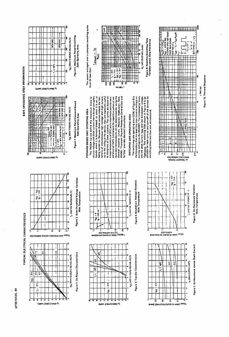
MT
M1
5N
35
, 40
TY
PIC
AL
ELE
CT
RIC
AL
CH
AR
AC
TE
RIS
TIC
S
lO
t8
iC t6
~
,. ~
12
iii a .1
0
" ~ p
~
I/
0 0
lO 8 6
~
2 0 0 1--
VGS
= lO
V
A
v_.....
l 10
V 1
--·~ ~
7V
TJ =
21'C
9?
' 8 v
1--z
,: A
w
6V
,,~
W'
,#
~
IV
-
r'
2 3
• I
6 7
8 V
os. O
RAIN
·ID·S
OURC
E VO
LTAG
E IV
OLI
SI
Fig
ure
1. O
n·R
egio
n C
har
acte
rist
ics
I/ II
TJ •
-l
l'C
/2
1·c
I/
I /t
OO
"C
,/
Vo
s• 1
0V
!/
I ,
Yi f J
:fl
l 3
• 1
VGS.
GA
THO
·!OU
RCE
VOLT
AGE
!VOL
TS!
Fig
ure
3. T
rans
fer
Ch
arac
teri
stic
s
I I
I VG
S •
10V
I
TJ •
10
0'C -i
--
I
10
........ 10
-
l 21·
c _::
:::::::- -
-ll'
C
I I .,
10
12
,.
16
18
20
IQ. O
RAJN
CUR
RENT
IAM
PSI
Fig
ure
5.
On
·Re
sist
an
ce v
ers
us
Dra
in C
urr
en
t
t.l 1
........
.. V
os =
VGS
"'-...
, to
= lm
A
1-......
... 1
1-......
...
o~
" !'-.
... ",
...... ,
0.1
~ J.7
~
-so
........
2
-15
15
50
75
100
121
T,1. J
UNCT
ION
TEM
PERA
TURE
l'C
l
Fig
ure
2. G
ate-
Thr
esho
ld V
olt
age
Var
iati
on
Wit
h T
em
pe
r1tu
re
1\
VGS
• 0
'ii -
0.7S
mA
·-
\ _
i--
_L
--
1 L--
-:
9 8 -so IO
i I
50
100
150
t J. J
UNCT
10N
TEM
FEft:
.tvA
E •
ci
Fig
ure
4.
Bre
1k
do
wn
Vo
ltag
e V
aria
tio
n
Wit
h T
emp
erat
ure
10
•00
TJ JL
;-.C
!tO~
tEM
f'ER
AT1.
;R£
· ('
Fig
ure
6. O
n-R
esis
tanc
e V
aria
tion
W
ith
Tem
per
atu
re
tlO 200 200
SA
FE
OP
ER
AT
ING
AR
EA
IN
FO
RM
AT
ION
too
--~
·-· .
....
.:r;
t:
-100
"'"'5:
: .__
-~-: ...
-l
4'-
,.!_
ms
. ~
' ;,
"-
10ms~
... -+
'- ==
~
'-
0.1
t
+-
--
--
-'D
Sioo
l llM
IT
;._de
--
-PA
Cl(A
GE L
IMIT
'=
Tl!E
RMAL
LIM
IT
I
Tc•
21'C
.~ M
TM11
N•I :~
VGS
• lO
V. S
INGL
E PU
LSE
MTM
1SNI
O ,~
, .. to
to
o Vo
s. OR
AJN.
TO·S
OURC
E VO
LTAG
E IV
OLTS
I
Fig
ure
7. M
axim
um R
ated
For
war
d B
iase
d S
afe
Op
erat
ing
Are
a
FOR
WA
RD
BIA
SED
SA
FE O
PER
AT
ING
AR
EA
10µs
tOOO
Th
e F
BS
OA
cu
rve
s d
efi
ne
th
e m
axim
um
dra
in-t
o
sou
rce
vo
lta
ge
and
dra
in c
urr
en
t th
at
a d
evi
ce c
an
sa
fely
h
an
dle
wh
en
it
is f
orw
ard
bia
sed
. o
r w
he
n i
t is
on,
or
be
ing
tu
rne
d o
n. B
ecau
se t
he
se c
urv
es
incl
ud
e t
he l
imi
tati
on
s o
f si
mu
fta
ne
ou
s h
igh
vo
lta
ge
an
d h
igh
curr
en
t,
up
to
th
e r
ati
ng
of
the
de
vice
. th
ey
are
esp
eci
ally
use
ful
to d
esi
gn
ers
of
line
ar
syst
em
s. T
he
cu
rve
s ar
e ba
sed
on
a
case
te
mp
era
turt
of 2
s·c a
nd
a m
axim
um
jun
ctio
n te
rn·
pe
ratu
re o
f 15
0°C
. lim
ita
tio
ns fo
r re
pe
titi
ve p
uls
es
at v
ar·
io
us
case
te
mp
era
ture
s ca
n b
e d
ete
rmin
ed
by
usi
ng
th
e
the
rma
l re
spo
nse
cu
rve
s.
Mo
toro
la
Ap
plic
ati
on
N
o1e.
A
N56
9. "
Tra
nsie
nt T
herm
al R
esis
tanc
e-G
ener
al D
ata
and
It
s U
se
" p
rovi
de
s d
eta
iled
in
stru
ctio
ns.
SWIT
CH
ING
SA
FE O
PER
AT
ING
AR
EA
The
sw
itch
ing
sale
ope
rati
ng a
rea
fSO
AI
of F
igur
e 8
is
the
bo
un
da
ry t
ha
t th
e lo
ad
lin
e m
ay t
rave
rse
wit
ho
ut
in·
.cur
ring
dam
age
to t
he M
OSF
ET
. T
he
fund
amen
tal
lim
its
are
th
e p
eak
curr
en
t, l
oM
an
d t
he
bre
akd
ow
n v
olta
ge
. V
fBR
IDSS
· T
he s
wit
chin
g SO
A s
ho
wn
in
Fig
ure
8 is
ap
plic
ab
le f
or
bo
th t
urn
-on
and
tu
rn-o
ff o
f th
e d
evi
ces
for
swit
chin
g t
ime
s le
ss t
ha
n o
ne
mic
rose
con
d.
1.0
o~
0.01
0
= =
·o -
o.s
D =
0.2
0 =
0 I
~
__. ..
....
.t
--~
~::::
SING
LE P
ULSE
II II 10
--
TJIC
tso;
MTM
ISNI
O -
MTM
llN•I
-
too
200
JOO
'llO
Vos
. ORA
lN·T
O-SO
URCE
VOi
.TAG
! IV
OU
SI
Fig
ure
8. M
axim
um R
ated
Sw
itch
ing
S
afe
Ope
rati
ng A
rea
- 500
The
po
we
r a
vera
ge
d o
ver
a co
mp
lete
sw
itch
ing
cyc
le
mu
st b
e l
ess
th
an
:
TJ!
max
l -
Tc
RB
JC
:--
1 10
JO
SO
10
0 X>
O SC
IO
1 •
RG. G
ATE
RESI
STAN
CE 1
0HM
SI
Fig
ure
9.
Res
isti
ve S~i
tchi
ng T
ime
V
aria
tion
ver
sus
Gat
e R
esis
t1nc
e
RBJc
lll =
~II
RBJ
c Re
JC -
Ol"
CW
MIJ
! D
CURV
ES A
PPLY
FOR
POW
ER
PULS
E TR
AIN
SHOW
N RE
AD T
IME
AT 11
TJ
fptl
-Tc
= Pl
pll R
BJC{
!I P
1pU
tJU
L
_,1
!--
I ~1
2-1
! DUT
Y cY
CLE.
0 •
11
17
too
1000
10
000
t TI
ME
lmsl
Fig
ure
10.
The
rmal
Res
po
nse

Ml Ml5N4~. 5
0
Fig
ure
13.
Sw
itch
' .,,.
m
g T
est
Cir
cuit
fig
ure
12.
Gat
e C
h G
ate-
to·S
er
ge v
ersu
s o
urc
e V
olt
age
Fig
ure
14.
Sw
ltch
ln 0
Wav
efo
rms
OU
TLI
NE
DIM
EN
SIO
NS
..,qs
I ~1
~~~~
~,.G
A~IO
U~'"
GPIR
A 7
C0 .
. 1'tO
UIJ
c(i [
)IV
[\S
()fr
ll IN
CH
H
SI
ST'fl
EJ
f'IN
I GA
Tt
7SC'
\.o11
Cl
CASI
"""
CA
SE 1
97A
·02
T0·
204A
E
Gle
lch
rich
t R
ect
ifie
r b
rf ~brucken
Po
nts
re
dr
ge
s -
ess
eu
rs
Typ
Typ
e
L------
8 ..
C80
0 B
8
.. CI~
.C1C
XlO
• ... ...
•.. '·'
A . . .
-· ' :I- . 1 "
o ... ,.Q
2,
m
•.~ . ~
-:: 1
I
! -
1...!
Si-
: i

Po
we
rblo
cks
fOr
netz
gefO
hrte
Str
om
rlch
ter
Pow
er m
od
ule
s fo
r lin
e c
om
mu
tate
d c
on
vert
ers
M
od
ule
s su
rmo
ule
s p
ou
r a
pp
lica
tion
s se
cte
ur
n .. N
• V
ollg
esto
uert
o K
ompa
ktba
uste
lne/
Ful
ly c
ontr
olle
d po
wer
mo
du
les/
Mo
du
les
surm
ou
l6s
A 2
th
yri
sto
rs
TD ..
N /
DT
.. N •
Hal
bgos
teuo
rte
Kom
pakt
baus
teln
e/H
all c
ontr
olle
d po
wer
mo
du
les/
Mo
du
les
surm
ou
les
mlx
tes
Typ
VO
RM
imM
SM
f-rsM
fi2 d
t f-r
AVMf
lc V(
TOI
rr
(di/
di)"
(d
v/dt
)"
Typ
o VR
AM
lp•1
0m
s tp
•10
ms
l,j•
l,
j-18
0".t
. "1
" "1
" """
'°'" n
och
DIN
'v
fmllX
45
"C
"1ma
x ••
'C
sin.
l,
jmu
l,
jmu
4
17
87
4
17
87
v A
A
A
A
2 s
A2 s
A
f'C
v m
n
Nu.
s V/
U.S
TI1
8N
40
0 80
0 12
00
40
350
390
·0,6
1 0,
76
25/6
0 1,
1 16
10
0 c
=
400
TD 1
8N
600
1100
14
00
xlo
' x
lo'
1816
5 F
=1
00
0
OT
18N
15
00•
TI2
5N
40
0 80
0 12
00
50
460
520
1,0!
1,
35
32/6
8 1,
05
11
100
c =
40
0 T
02
5N
60
0 11
00
1400
• x
lo'
xlo
' 25
/85
F =
10
00
D
T25
N
TI3
1N
e
400
1100
15
00•
50
68
0
780
2,3
3,04
48
150
0,95
6,
4 10
0 c
-40
0 T
D31
N
600
1200
x
lo'
xlo
' 31
/85
F =
10
00
D
T31
N
800
1400
TI3
2N
. 11
00
1400
75
62
0 70
0 1,
9:
2,45
48
152
1 7,
5 12
0 c
-40
0 12
00
1500
• x
lo'
xio
' 32
/85
F =
10
00
T
I36
N
200
800
1400
• 80
85
0 98
0 3,
6 4,
8 51
/60
1 6,
2 12
0 c
-40
0 T
D36
N
400
1100
x
lo'
xlo
' 36
/85
F a1
00
0
DT
36N
60
0 12
00
TI4
5N
80
0 12
00
1500
• 10
0 10
00
1200
5
7,2
63/5
9 0,
85
4,7
150
c =
40
0 T
04
5N
11
00
1400
x
lo'
xlo
' 45
/85
F •1
00
0
OT
45
N
TI4
6N
20
0 80
0 14
00
100
1000
11
50
5 6,
6 64
/61
0,95
4,
5 12
0 c
-40
0 T
D4
6N
40
0 11
00
1500
• x
lo'
xlo
' 46
/85
I'
-10
00
O
T 4
6N
60
0 12
00
TI5
6N
20
0 80
0 14
00
100
1350
15
00
9,1
11,2
5 64
/74
0,9
3,5
120
c -
400
T0
56
N
400
1100
15
00•
x1
o'
xlo
' 56
/85
F •1
00
0
DT
56N
60
0 12
00
TIS
ON
40
0 11
00
1500
• 12
0 14
00
1550
9,
8 12
76
/68
0,8
3,4
150
c -
400
TO
BO
N
600
1200
x
1o
' x
1o
' 60
/85
F •1
00
0
DT
60N
80
0 14
00
TI7
5N
40
0 80
0 12
00
150
1700
19
50
14,4
19
95
/70
0,85
2,
6 15
0 c
-40
0 T
D75
N
600
1100
14
00•
x1
o'
x1
o'
7518
5 F
•10
00
O
T75
N
TI8
8N
60
0 12
00
1800
• 16
0 18
00
2050
16
,2
21
102/
69
1 3.
5 15
0 c
-40
0 T
D6
8N
80
0 14
00
x1
o'
xlo
' 86
/85
F •1
00
0
OT
68N
11
00
1600
TI9
5N
40
0 11
00
1500
' 15
0 17
00
1950
14
,4
19
95/8
5 0,
85
2,6
150
c -
400
T0
95
N
eoo
1200
x
lo'
x1
o'
F -1
00
0
DT
95N
eo
o 14
00
TI1
06
N
600
1200
18
00•
180
2000
22
50
20
25,3
11
5/78
0,
9 2,
6 15
0 c
-40
0 TD
106
N
800
1400
x
1o
' x
lo'
106/
85
F =
10
00
O
T 10
6 N
11
00
1600
TI1
21 N
11
00
1600
20
0 23
50
2600
27
,6
33,8
12
8/81
0,
85
2 15
0 c
-40
0 TD
121
N
1200
18
00•
xlo
' x
lo'
121/
85
F •1
00
0
OT
121
N
1400
TI1
31
N
400
1100
22
0 32
00
3600
51
,2
64.8
14
1/80
0,
85
1,5
150
c =
40
0 T
D13
1 N
60
0 12
00
xlo
' x
lo'
131/
85
F =
10
00
O
T 13
1 N
eo
o 1
40
0'
TI
14
2N
e
400
1000
16
00'
230
4100
48
00
84
115
142/
85
0,9
1,1
150
c -
400
TO 1
42 N
60
0 12
00
xlo
' x
lo'
F =
10
00
O
T 14
2 N
80
0 14
00
TI
15
0N
e
1800
24
00
350
4000
45
00
80
101
223/
54
1,2
1,3
60
c =
400
20
00
2500
• x
lo'
xlo
' 15
0/85
F
= 1
000
2200
TI
16
2N
e
400
1000
18
00'
260
4400
52
00
97
135
162/
85
0,85
0,
95
150
c =
400
TD
162
N
600
1200
x
1o
' x
lo'
F =
1000
O
T 16
2 N
80
0 14
00
TI
170N
40
0 11
00
1600
35
0 46
00
5200
10
6 13
5 22
3/68
0,
95
1,0
150
c D
40
0 TD
170
N
600
1200
18
00'
xlo
' x
lo'
170/
85
F =
10
00
O
T 17
0N
800
1400
TI2
10
N
400
1100
16
00
410
5800
66
00
168
218
261/
73
1 0,
85
150
c D
40
0 T
D21
0N
800
1200
18
00'
x1
o'
xlo
' 21
0/85
F
= 1
000
OT
210
N
800
1400
-----··
----
---
--·-----~
·;.'
•',
,,:"
:_.:.
lq
Vor
lo
r
typ.
"1
" l,
j -
25'C
25
'C
u.s
v m
A
50
2,
5 15
0
60
2.5
150
60
2,
0 15
0
120
1,4
120
60
2,5
150
120
1,4
120
60
2,
5 15
0
80
2,
5 15
0
120
1,4
120
180
1,4
120
150
1,4
150
200
1,4
120
150
1,4
150
180
1,4
150
180
1,4
150
200
2,0
200
300
2,0
200
200
2,0
150
250
2,0
200
200
2,0
200
----
--·-
----
teo"
el.
aln.
!5)
S)
G
·ctw
·ctw
·c
Nm
g
1,2
0,2
125
4 16
0
MaB
blld
Oul
llne
F
igur
e
47
--+-__,l---+---1--..+---~ J
0.
12
o. 16
12
5 4
1so
48
I ~0.~6~5+:-0.-16--'~1-2-5-+~4--+-200--+--4-7--1
0,6
0,16
12
5 4
160
48
0,55
0,
16
125
4 16
0 47
A
K
0,52
0,
18
125
4 20
0
0,39
0,
1 12
5 4
200
0.37
0,
08
0,39
0,
1
0,33
0,
08
0,23
0,
06
0,23
0,
06
0,17
0,
04
0,13
0,
04
125
140
140
140
140
125
125
4 25
0
4 20
0
4 25
0
6 43
0
6 43
0
m.:
8 43
0 el
.:12
m.:
6 31
0 el
.:12
47
48
48
49
48
49
50
50
51
0, 1
3 0,
04
125
m.:
6 80
0 52
ol
.:12
0,13
0,
04
125
m.:
6 31
0 51
el
.:12
0, 1
7 0,
04
125
m.:
6 80
0 52
el
.:12
l AK r r A
K r
K
A
n~,i~r
K
A
n ~<Jr
Kl r
TI1
8N
TT
25
N
TI3
1N
T
I36
N
TI4
6N
TT
56
N
TD 1
8 N
T
D2
5N
T
03
1 N
T
D3
6N
T
D4
6N
T
05
6N
DT
18
N
OT
25
N
OT
31 N
D
T3
6N
D
T4
6N
D
T5
6N
K
A O
D3
1N
r r 0
06
1 N
--
00
76
N
'--"""kl~r-KJH--1
Str
uctu
ro l1
1tem
e: c
on
laci
90U
d6
TT
18
F
TT
25
F
TI3
2F
TT
42
F
TO 1
8 F
TD
25
F
TD
32
F
T0
42
F
OT
18
F
DT
25
F
OT
32
F
OT
42
F
00
21
s
00
22
$
00
31
s
00
45
$
00
53
$
00
68
$
ln!"
etll
l90l
allc
n /
lnte
ma
l ln1
ul9!
1on
/ l.
ofa
llo
n l
nl•
m•
Al2
'>;J
47
o~l~ll~~:r
0 1 !?: ~
-1~.
.:.. 2
0 _
:_ 2
0 J..
,~_;
I I ·~
~ --·---
oo
__
_ __
.I ! I
,_ __
___ ..
----
r r r
TI3
2N
T
I45
N
TIS
ON
T
I75
N
TI9
5N
n3
5F
n
45
F
K
A
TD
45
N
TD
35
F
l 1
J T
D6
0N
T
04
5F
I
. T
07
5N
..__
_,1<Jl
f+.- 1 -tE
I(];-+
. ~
TD 9
5 N
K
A
n~,~r
AD
50
F
AD
60
F
l.....
_K _i_
kJ__.f
~ 1 O
T4
5N
O
T3
5F
D
T6
0N
D
T4
5F
O
T7
5N
O
T9
5N
AK
K
l l
l<J I
lnn
•r•r
Auf
be.u
: O
rucl
dl.o
ntut
ln
lem
al c
onl1
NC
tlon
: p
rHsu
r• c
onta
ct
S!r
uctu
re l
ntt
m•:
co
nle
ct p
rets
6
DD
65
N
00
61
S
D0
85
N
00
62
$
00
81
s
00
82
$
lnn
.r.
lsol
atlo
n /I
nte
rnal
In
sula
tio
n/ l
totl
llo
n l
nt•
me
BeO
'I
48

1u1w
m;11
n1;t1
1;.m
•tt·11
• i D
igit
al I
ndic
atin
g S
erie
s S
R1
0
Ana
log
Dev
iati
on
Ser
ies
SR
l 1
f 1.1;1
.19;1m
cH·l·l
f:\1AH
•i1¥''M
M
5. N
AM
ES
& F
UN
CT
ION
rr~====~JJL __
SP
.10:
Dig
ital
Dis
play
SA
11:
Ana
log
Dev
iati
on
Digi
t~!
Set
Sw
tich
!E'.'.rca7~~~::::~ c
on
tro
l u
mp
Neu
tral
Zon
e (N
Z)
Var
iabl
e R
esis
tor.
1
-20
% v
aria
ble
lb,;;;;;;~~~~:!!--
~~cro!~;~~ ~~
~,~~;~
1~:~~;
::i~ot
ation
-------------
Ala
rm S
etti
ng
Var
iabl
e R
esis
tor
(Opt
ion)
A
larm
La
mp
IO
ptio
nl
Not
e:
Sin
ce t
his
devi
ce i
s pl
ug·i
n ty
pe
the
chas
sis
can
be
pull
ed o
ut
in
the
nate
of
wit
h w
irin
g.
Be
sure
to
cu
t o
ff t
he
line
paw
er b
efo
re l
oosi
ng s
crew
& p
ulli
ng
ou
t th
e ch
assi
s.
1: S
PE
CIF
ICA
TIO
NS
SR
10
Ind
icat
ing
Acc
urac
y ..
110
.5%
+ 1
-dig
it)
of
mea
suri
ng r
ange
S
R 11
Dev
iati
on R
ange
..•. t
10%
of
mea
suri
ng r
ange
(vs
. se
ttin
g
ran
ge
) T
her
mo
cou
ple
Ext
erna
l R
esis
tanc
e T
oler
able
Ran
ge ..
10
0 n
max
imu
m
Co
ld J
un
ctio
n T
emp
erat
ure
C
om
pen
sati
on
Ran
ge ..... 5
-45
°C
hh
erm
occ
up
le i
np
ut
on
ly)
Bu
rn-O
ut
Cir
cuit
.....•. S
tan
dar
d I
ther
mo
cou
ple
in
pu
t o
nly
) R
.T.O
. R
esis
tan
ce T
ole
rab
le
Ran
ge .•............ 5
n m
axim
um
/wir
e ,O
pera
ting
Am
bien
t .
Tem
per
atu
re &
Hu
mid
ity
..
-1
0-+
50
°C,
90%
RH
max
imu
m
Pow
er C
on
sum
pti
on
..... A
pp
rox
. 4
VA
In
sula
tion
Res
ista
nce ..... 5
00
V D
C 2
0 M
n m
inim
um
bet
wee
n
inp
ut
term
inal
an
d p
ow
er s
up
ply
ter
min
al
50
0 V
DC
20
Mn
min
imu
m b
etw
een
po
wer
sup
ply
term
inal
an
d e
arth
ter
min
al
Die
lect
ric
Str
eng
th ...... O
ne
min
ute
at
50
0 V
AC
bet
wee
n i
np
ut
term
inal
an
d e
arth
ter
min
al
One
min
ute
at
10
00
V A
C b
etw
een
po
wer
te
rmin
al a
nd
ear
th t
erm
inal
3. E
XT
ER
NA
L D
IME
NS
ION
S &
PA
NE
L C
UJO
U17
4. I
NS
TA
LL
AT
ION
WI M
ount
ing
Fix
ture
1
) P
repa
re a
pan
el c
uto
ut
of 6
8
S.t
Scr
ew
(HI
x 68
(W)
mm
w
ide
011
the
pane
l.
2) I
nser
t th
e un
it t
o t
he
pane
l cu
tou
t an
d fa
sten
wit
h t
he
mou
ntin
g fi
xtur
es.
3)
The
am
bien
t con
diti
ons s
hall
··
-···
be:
a.
Fre
e fr
om c
orro
sive
gas
ses
and
dust
y at
mos
pher
e,
b.
Wit
hin
-10
-+5
0°C
am
bien
t te
mpe
ratu
re a
nd
un
der
90%
R
H h
umid
ity,
c.
A
way
fr
om
dir
ect
sunl
ight
and
rad
iant
hea
t fr
om e
lect
ric
oven
s.
T•m
p•r
•tu
,• •
nd
Hur
t'ltd
1ty
Co
ntr
ol
ln&
tru
nw
nll
SH
IMA
DE
N C
O.,
LT
D.
Hu
d O
fl1c
e F
acto
ry
2·30
·10,
Ko
tam
ach
o,
Ne,
,ma·
ku
. T
ok
yo
176
Jap
an
Ph00
1e
1031
931
·911
1 Te
1e11
0
'72
27
78
SD
CL
J
iiM
WI
The
dim
ensi
on o
f te
rmin
al s
crew
(s)
is 3
.5 m
m d
iam
eter
and
8.0
mm
len
gth.
P
repa
re t
erm
inal
co
nn
ecti
on
of
7 .2
mm
max
. o
ute
r di
amet
er.
o:::Q)~.2
mm
max
. 1.
Wir
ing
for
Inp
ut
Cir
cuit
a)
T
herm
ocou
ple
Inpu
t T
ype:
·
C.o
nfir
m t
he
typ
e of
the
rmoc
uoµl
e an
d le
ad w
ire.
T
hen,
co
nn
ect
prop
erly
to
(+)
& (
-)te
rmin
als
as &
hew
n be
low
. b)
R
.T.D
. In
pu
t T
ype:
C
onne
ct p
rope
rly
RT
O (
Pt1
00 n
t to
(A
). (
Bl.
(8)
ter
min
als
as s
how
n be
low
. c)
C
urre
nt &
Vol
tage
Inp
ut T
yp
e:
• B
e su
re t
o c
onfi
rm t
he(
+)
& (
-) p
olar
itY
of
the
inp
ut
term
inal
s.
2. W
irin
g fo
r P
ower
Sup
ply
Rei
er t
o t
he
figu
res
belo
w.
• C
on
tact
Ou
tpu
t
Pow
er S
uppl
y 11
01 -12
uv
AC
(+)
Ana
log O~p
ut %
(O
ptio
n)
T
0-1
0m
V F
S (!
)
H
I ~
• O
n t
he
mo
del
s o
f R
TO
in
pu
t w
ith
ana
log
ou
tpu
t )
tefm
i·
nel
is
com
mo
n.
• O
n th
e m
od
els
of
wii
h an
alog
ou
tpu
t a
sere
" 1 ii p
rov
ided
on
4
· te
rmin
al.
•On
u·.
~ m
od
els
of
wit
h al
arm
scr
ews
are
pro
vid
td o
n
11l
&:
lft
term
inal
s.
Q•IQ
UMM
H
220-
240V
AC
RT
O
Aft
er i
nsta
llat
ion
and
wir
ing
star
t o
per
atio
n a
s be
low
. a)
S
et t
he
dini
tal
sett
ing
swit
ch(e
s) t
o t
he v
alue
req
uire
d.
b) T
urn
on
the
pow
er s
uppl
y an
d co
nfir
m i
i th
e co
ntro
l la
mp
ligh
ts.'
•Co
nta
ct C
apac
i\y:
2
40
V A
C 3
A/r
esis
tiv
e lo
ad
24
0 V
AC
1 ,
, fin
du
ctiv
e to
ad
c)
Set
th
e ne
:,ut
rol
zone
var
iabl
e re
sist
or (
NZ
, 1
-20
%F
S)
to t
he
val"
e re
quir
ed i
n th
e ap
plic
atio
n.
l:IB
-Jdi
;Ml·
liii
Qll'
9·@i
M'l!
·iiM
~i
A ~-
A ~-
A
Lo
we
r L
imit
L
o
Dig
ital
S.t
H1
U
pper
lim
it
CO
M ;:i
J:i-
:1 C!
!J (~V ~
~
Mea
suri
ng V
alue
< L
ow
er
lim
il
Con
trol
lam
p:
Gre
en
Val
ue w:
i IIT
Jrn
Lo
we
r li
mi1
<M
easu
r1ng
V11
lu1<
Upp
er l
imil
C
ontr
ol l
.-n
p:
Non
-lig
hlin
g
S:
0.2%
FS
ITl
IC·H
:O
NJ
")
..
i"Z
,, -.... 1
__
NZ
: N
eauo
11I
Zon
e N
Z V
aria
ble
A11
nge:
1-2
0%
FS
S:
Sen
siti
vity
Ad
juu
, 0.
2%F
S
FS:
Ful
l S
cale
Upp
er L
imit
<M
eatu
ring
Val
ue
Con
1tol
lam
p:
Red
•Ala
rm A
ctio
n L
ower
Ala
fm
Up
per
Ala
rm
/
'Ala
rm S
peci
fica
tion
s U
pper
/Low
er A
larm
A
larm
Set
ting
: B
y fr
ont
vari
able
re
sist
ors
(L A
ll-L
ow
"'
·•c.
Ala
rm,
(H
All
-Up
per
Ala
rm
and
(AL
)-A
LA
Hu
U
N
AL
AR
'-'
Upp
er/L
ower
Ala
rm
-i_
__
_r-
Ala
rm R
ange
: 1
-20
% v
aria
ble
vs.
cont
rol
set
valu
e A
A
'
Ala
rm S
ensi
tivi
ty:
0.2%
FS
fix
ed
I Ac
I
Ala
rm O
utp
ut:
Con
tact
2
40
V
A
C
3 A
/res
isti
ve
load
&
'··
"""I
'"'""
1
A/i
nduc
tive
loa
d A
larm
Ind
icat
ion:
By
fron
t ye
llow
LE
O l
ight
ing
,r;:"
(c·-:AI
; :\w
\ .
J
· .. \·n
r~r·
' "'
Ala
rmin
g P
oin
t A
lerm
: O
N
Co
n1
rol
Set
Po
int
Yel
low
LE
O
·Lig
hti
ng
Ala
rm:
OF
F
Ala
rm L
ED
-N
o·1
Lig
h1in
9
• U
pper
/Low
er
alar
m
is an
al
arm
m
od
e of
upp
er &
low
"'
sym
met
ric
sett
ing
vs.
cont
rol
setp
oint
. A
larm
ou
tpu
t fr
om
uppe
r &
low
er l
imit
is
from
th
e sa
me
alar
m r
elay
and
sam
1·
con
tact
. N
o id
enti
fica
tion
of
fr
om
up
per
or
low
er
i-.
avai
labl
e b
y r
elay
con
tact
ou
tpu
t.
• A
larm
wit
h s
tan
db
y m
ode
is a
n a
larm
ing
syst
em t
hat
upp
er.
low
er
or
uppe
r/lo
wer
al
arm
s w
ill
not
func
tion
un
til
tlw
te
mpe
ratu
re h
as
been
in
th
e
non-
alar
min
g ar
ea o
nce
afte
r th
e p
ow
er
sour
ce a
ppli
ed.