Review of the maximum power point tracking algorithms for stand-alone photovoltaic systems

ARTICLE IN PRESS

Solar Energy Materials & Solar Cells 90 (2006) 1555–1578

0927-0248/$ -

doi:10.1016/j

�CorrespoE-mail ad

www.elsevier.com/locate/solmat

Review

Review of the maximum power point trackingalgorithms for stand-alone photovoltaic systems

V. Salas�, E. Olıas, A. Barrado, A. Lazaro

Departamento de Tecnologıa Electronica/Grupo de Sistemas Electronicos de Potencia,

Universidad Carlos III de Madrid, Avda. de la Universidad, 30-28911 Leganes, Madrid, Spain

Received 7 May 2005; accepted 11 October 2005

Available online 10 January 2006

Abstract

A survey of the algorithms for seeking the maximum power point (MPP) is proposed. As has been

shown, there are many ways of distinguishing and grouping methods that seek the MPP from a

photovoltaic (PV) generator. However, in this article they are grouped as either direct or nondirect

methods. The indirect methods (‘‘quasi seeks’’) have the particular feature that the MPP is estimated

from the measures of the PV generator’s voltage and current PV, the irradiance, or using empiric

data, by mathematical expressions of numerical approximations. Therefore, the estimation is carried

out for a specific PV generator installed in the system. Thus, they do not obtain the maximum power

for any irradiance or temperature and none of them are able to obtain the MPP exactly.

Subsequently, they are known as ‘‘quasi seeks’’.

Nevertheless, the direct methods (‘‘true seeking methods’’) can also be distinguished. They offer

the advantage that they obtain the actual maximum power from the measures of the PV generator’s

voltage and current PV. In that case, they are suitable for any irradiance and temperature. All

algorithms, direct and indirect, can be included in some of the DC/DC converters, Maximum power

point trackings (MPPTs), for the stand-alone systems.

r 2005 Elsevier B.V. All rights reserved.

Keywords: Maximum power point; Maximum power point tracking (MPPT); Power electronics; Photovoltaic

energy

see front matter r 2005 Elsevier B.V. All rights reserved.

.solmat.2005.10.023

nding author. Fax: +34916249430.

dress: [email protected] (V. Salas).

www.elsevier.com/locate/solmat

ARTICLE IN PRESSV. Salas et al. / Solar Energy Materials & Solar Cells 90 (2006) 1555–15781556

Contents

1. Introduction . . . . . . . . . . . . . . . . . . . . . . . . . . . . . . . . . . . . . . . . . . . . . . . . . . . . . . 1556

2. Seeking algorithms classification . . . . . . . . . . . . . . . . . . . . . . . . . . . . . . . . . . . . . . . . 1560

2.1. The indirect control: the ‘‘quasi seeking’’ . . . . . . . . . . . . . . . . . . . . . . . . . . . . . 1561

2.1.1. Curve-fitting method . . . . . . . . . . . . . . . . . . . . . . . . . . . . . . . . . . . . . 1561

2.1.2. Look-up table method . . . . . . . . . . . . . . . . . . . . . . . . . . . . . . . . . . . . 1562

2.1.3. Open-circuit voltage photovoltaic generator method . . . . . . . . . . . . . . . 1562

2.1.4. Short-circuit photovoltaic generator method. . . . . . . . . . . . . . . . . . . . . 1563

2.1.5. Open-circuit voltage photovoltaic test cell method. . . . . . . . . . . . . . . . . 1563

2.2. Direct control: the ‘‘true seeking’’ . . . . . . . . . . . . . . . . . . . . . . . . . . . . . . . . . . 1564

2.2.1. Sampling methods . . . . . . . . . . . . . . . . . . . . . . . . . . . . . . . . . . . . . . . 1564

2.2.2. Methods by modulation . . . . . . . . . . . . . . . . . . . . . . . . . . . . . . . . . . . 1573

2.3. Other methods: artificial intelligence methods . . . . . . . . . . . . . . . . . . . . . . . . . . 1575

3. Conclusions. . . . . . . . . . . . . . . . . . . . . . . . . . . . . . . . . . . . . . . . . . . . . . . . . . . . . . . 1575

References . . . . . . . . . . . . . . . . . . . . . . . . . . . . . . . . . . . . . . . . . . . . . . . . . . . . . . . . . . . 1576

1. Introduction

In the current century, the world is increasingly experiencing a great need for additionalenergy resources so as to reduce dependency on conventional sources, and photovoltaic(PV) energy could be an answer to that need. PV cells are being used in space andterrestrial applications where they are economically competitive with alternative sources.Furthermore, the PV industry has demonstrated high growth rates over recent years, 30%per year in the late 1990s. By the year 2010, it is assumed that modules will cost 1.50 h/Wpand systems 3.00 h/Wp.Generally, PV systems can be divided into three categories: stand-alone, grid-connection

and hybrid systems. For places that are far from a conventional power generation system,stand-alone PV power supply systems have been considered a good alternative. Thesesystems can be seen as a well-established and reliable economic source of electricity in ruralremote areas, especially where the grid power supply is not fully extended. Such systemsare presented in two scales: applications at a smaller scale, from 1 to 10 kW, are used tosupply electric power in developing countries, the so-called solar home systems, SHS; andstand-alone PV systems of several hundred thousand watts in size, from 10 to 100 kW, onthe roofs of dwellings. In general, they have the advantages of using a simple systemconfiguration and simple control scheme. For our study, only DC loads will be considered.Typical DC voltage levels are 12, 24, 48 and 60V.In those systems, the performance of a PV system relies on the operating conditions.

Then, the maximum power extracted from the PV generator depends strongly on threefactors: insolation, load profile (load impedance) and cell temperature (ambienttemperature), assuming a fixed cell efficiency.The variation of the output I– V characteristic of a commercial PV module as a function

of temperature and irradiation is shown in Figs. 1–4. It can be observed that thetemperature changes mainly affect the PV output voltage, while the irradiation changesmainly affect the PV output current.Nevertheless, PV systems should be designed to operate at their maximum output power

levels for any temperature and solar irradiation level at all times. The last significant factor,which determines the PV throughput power, is the impedance of the load. In our case, this

ARTICLE IN PRESS

100

90

80

70

60

50

40

30

20

10

00 2 4 6 8 10 12 14 16 18 20 22

VPV (V)

PP

V (

W)

MPP

MPP

MPP

Maximum Power Point (MPP)

1000W/m2

700W/m2

500W/m2

300W/m2

Fig. 2. P– V photovoltaic characteristic for four different irradiation levels.

8

7

6

5

4

3

2

1

00 5 10 15 20

VPV (V)

I PV (

A)

MPP

MPP

MPP

MAXIMUM POWER POINT (MPP)

1000W/m2

700W/m2

500W/m2

300W/m2

Fig. 1. I– V photovoltaic characteristic for four different irradiation levels.

V. Salas et al. / Solar Energy Materials & Solar Cells 90 (2006) 1555–1578 1557

ARTICLE IN PRESS

4.00

3.50

3.00

2.50

2.00

1.50

1.00

0.50

0.000.00 5.00 10.00 15.00 20.00 25.00

PHOTOVOLTAIC VOLTAGE (V)

PH

OT

OV

OLT

AIC

CU

RR

EN

T (

A)

Tcells=0°C

Tcells=25°CTcells=50°C

MPP MPP MPP

Fig. 3. I– V characteristics for three temperatures level.

70.00

60.00

50.00

40.00

30.00

20.00

10.00

0.000.00 5.00 10.00 15.00 20.00 25.00

PHOTOVOLTAIC VOLTAGE (V)

PH

OT

OV

OLT

AIC

PO

WE

R (

W)

MPP

MPP

MPPTcells=0°CTcells=25°CTcells=50°C

Fig. 4. P– V characteristic for three temperatures level.

V. Salas et al. / Solar Energy Materials & Solar Cells 90 (2006) 1555–15781558

consists of a DC load and batteries. However, it should be noted, that such impedance isnot constant. When a PV generator is directly connected to the load, the system willoperate at the intersection of the I– V curve and load line, which can be far from themaximum power point (MPP).The maximum power production is based on the load-line adjustment under varying

atmospheric conditions.Another important element of a stand-alone PV system is the battery because of the

fluctuating nature of the output delivered by the PV array [1]. Moreover, the load, in manycases, requires a power level that is maintained constant. Commonly, lead-acid batteries

ARTICLE IN PRESS

Charging time (hours)T1 T4T2 T3

I stageBulk charge

I = constantV = increases

II stageAbsorption

V = constantI = decreases

III stageEqualization

IV stageFloat

V = constantFloat current

(1º)I = constantV = increases

(2º)V = constantI = decreases

V4V3

V1

Bat

tery

Vol

tage

(V

)

V2

Bat

tery

Cur

rent

(A

)

Fig. 5. General four step charging battery algorithm.


are used, because of their wide availability in many sizes, their low cost and their well-understood performance characteristics.

Thus, in most cases, a charge controller is an essential element [2], except in smallsystems with well-defined loads, using low voltage ‘‘self-regulating modules’’ or using alarge battery or small array. If finally, a battery charge is used, it will control the voltageand charge current that is applied to the battery in order to protect it from being overcharged, over discharged and from load control functions.

Depending on the level of sophistication in the charger technology, different chargealgorithms are presented, i.e., a collection of controls over electrical parameters and atiming, associated with multiple voltage and current levels, applied sequentially to thecharging system hardware for the express purpose of recharging the battery appropriately.Generally, battery manufacture refer to four distinct charging modes, or stages, within abattery charging cycle, Fig. 5: bulk, absorption, equalization and float. However, not allbattery chargers have the four stages.

The previous charging modes can be implemented in several possible ways. The mostcommon controller topologies for battery charge regulation are shunt and series typeconfiguration. The point is that in the two topologies, time after time, PV panels areusually forced to operate at the battery voltage. This is almost always below the peakpower point, so some of the power generating capability is lost.

In order to overcome the undesired effects on the output PV power and draw itsmaximum power, it is possible to insert a DC/DC converter between the PV generator andthe batteries, which can control the seeking of the MPP, besides including the typicalfunctions assigned to the controllers. These converters are normally named as maximumpower point trackers (MPPTs). They consist of a topology and control circuit where therewill be a MPP seeking algorithm. As Fig. 6 shows, the input DC–DC converter part isformed by the PV array and the output section by the batteries and load. The role of theMPPT is to ensure the operation of the PV generator at its MPP, extracting the maximumavailable power.

ARTICLE IN PRESS

Table 1

Possible variables for controlling in a DC/DC converter

Variables

VPV Output voltage photovoltaic generator Input voltage DC/DC converter

IPV Output current photovoltaic generator Input current DC/DC converter

Vo Output voltage DC/DC converter

Io Output voltage DC/DC converter

BATTERIES

IPV

VPV

++

--

PHOTOVOLTAICGENERATOR

LOAD

IPV

++

--

Vbat

VPV Vo

Io

Z

D

PWMCONTROL

DC/DC CONVERTER

Io

Fig. 6. General block diagram of a stand-alone PV system with MPPT.


However, their losses have to be small enough to improve the efficiency of the overallsystem. This could increase the gap between the PV peak power voltage and the voltage atwhich they are forced to operate in a system without a peak power tracking. Theoretically,it is foreseeable that a MPPT would yield the most impressive gains in cold weatherbecause that would raise the PV array’ peak power voltage point well above the usualbattery operating voltage.Fig. 6 shows the general block diagram for a charge batteries system, with MPPT, using

a generic DC/DC converter. This one is connected to the PV generator, a battery and aload profile (such as a resistance, DC/DC motory).The main objective is to obtain the maximum power from the PV generator for the first-

load batteries stage. That is to say, when the batteries are fully or partially discharged, insome state of charge less than 100%, then it is necessary to control one/or some of theinput/output following variables; Table 1.

2. Seeking algorithms classification

The first methods, used in aerospace applications, date from the 1970s, in companies orresearch centres such as Honeywell Inc. or NASA [3–9]. The methods developed up untilnow can be grouped by their different parameters. If they are grouped according to thecontrol variables involved (measured) in the seeking process they can be differentiated bytwo variable and one variable methods.

ARTICLE IN PRESSV. Salas et al. / Solar Energy Materials & Solar Cells 90 (2006) 1555–1578 1561

The two variables methods use the voltage measurements, VPV, and current, IPV of thePV output power. Among others, the differentiation, perturbation and observation (P&O)and the conductance incremental (C.I.) methods can be cited.

On the other hand, methods using one variable control can be distinguished as well.Pertaining to this group are the feedback voltage, open-voltage PV generator, open-voltagePV cell as well as the short circuit current method.

Other classifications can be based on the function of the methods or control strategiesused. Thus, two categories can be presented: direct and indirect methods. Thisclassification, therefore, will be presented in this paper, and will be developed in detailin the rest of this article.

2.1. The indirect control: the ‘‘quasi seeking’’

The indirect methods are based on the use of a database that includes parameters anddata such as, for instance, curves typical of the PV generator for different irradiances andtemperatures, or on the use of the mathematical functions obtained from empirical data toestimate the MPP. In most cases a prior evaluation of the PV generator is then required, orelse it is based on the mathematical relationship obtained from empirical data, which doesnot meet all climatologic conditions. The following methods belong to this category: curve-fitting, look-up table, open-voltage PV generator, short circuit PV generator and the open-circuit cell. These will be studied next in greater detail.

2.1.1. Curve-fitting method

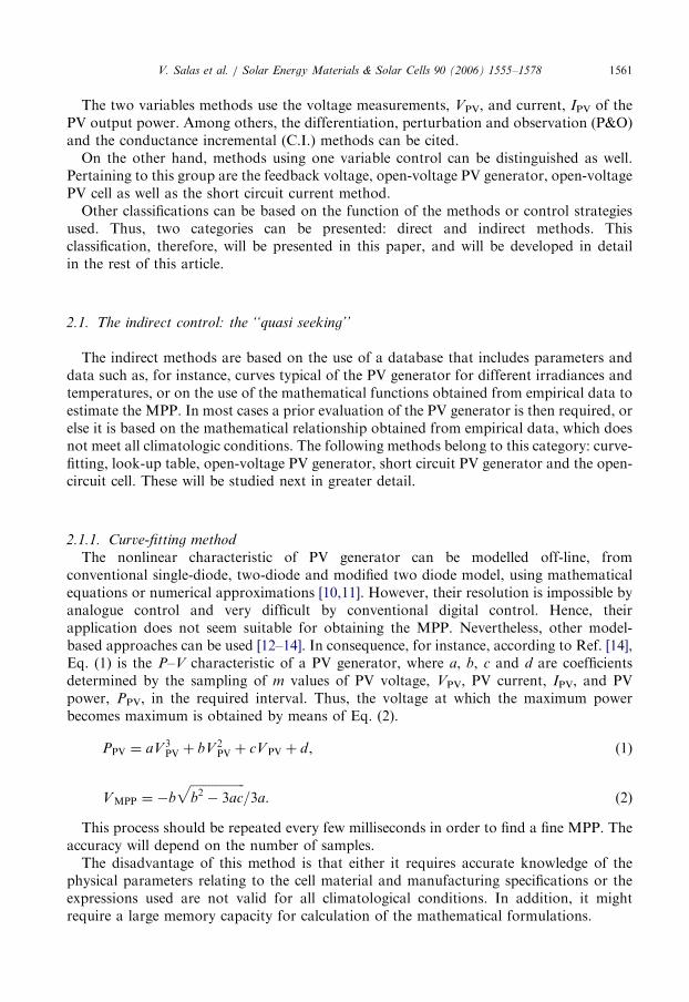
The nonlinear characteristic of PV generator can be modelled off-line, fromconventional single-diode, two-diode and modified two diode model, using mathematicalequations or numerical approximations [10,11]. However, their resolution is impossible byanalogue control and very difficult by conventional digital control. Hence, theirapplication does not seem suitable for obtaining the MPP. Nevertheless, other model-based approaches can be used [12–14]. In consequence, for instance, according to Ref. [14],Eq. (1) is the P–V characteristic of a PV generator, where a, b, c and d are coefficientsdetermined by the sampling of m values of PV voltage, VPV, PV current, IPV, and PVpower, PPV, in the required interval. Thus, the voltage at which the maximum powerbecomes maximum is obtained by means of Eq. (2).

PPV ¼ aV 3PV þ bV 2

PV þ cVPV þ d, (1)

VMPP ¼ �bffiffiffiffiffiffiffiffiffiffiffiffiffiffiffiffiffiffib2� 3ac

p=3a. (2)

This process should be repeated every few milliseconds in order to find a fine MPP. Theaccuracy will depend on the number of samples.

The disadvantage of this method is that either it requires accurate knowledge of thephysical parameters relating to the cell material and manufacturing specifications or theexpressions used are not valid for all climatological conditions. In addition, it mightrequire a large memory capacity for calculation of the mathematical formulations.


2.1.2. Look-up table method

In this case, the measured values of the PV generator’s voltage and current are comparedwith those stored in the control system, which correspond to the operation in themaximum point [15], under concrete climatological conditions. Then, this algorithm has asthe disadvantage that a large capacity of memory is required for storage of the data.Moreover, the implementation must be adjusted for a panel PV specific. In addition, it isdifficult to record and store all possible system conditions.

2.1.3. Open-circuit voltage photovoltaic generator method

This algorithm, used in Refs. [16–20], is based on the voltage of PV generator at theMPP which is approximately linearly proportional, k1, to its open-circuit voltage, Voc. Theproportional constant depends on the fabrication technologies solar cells technology, fillfactor and the meteorological conditions, mainly.

k1 ¼VMPP

VOCffi Constanto1. (3)

This property can be implemented by means of the flow chart shown in Fig. 7. Thus, thePV generator’s open-circuit voltage is measured by interrupting the normal operation ofthe system, with a certain frequency, storing the measured value. Later, the MPP is

Fig. 7. Open-circuit voltage photovoltaic generator algorithm flowchart.


calculated, according to Eq. (3), and the operation voltage is adjusted to the maximumvoltage point. This process will be repeated periodically. Although this method isapparently simple, it is difficult to choose an optimal value of the constant K1. However,the literature [20–22], reports K1 values ranging from 0.73 to 0.80, for polycrystalline PVmodules, as well as a typical interval of sampling of 15ms [20].

Since adjustment of the reference voltage of Voc is chosen as a fixed fraction, assumingthat it remains constant for a wide variation of temperature and insolation, and does notchange appreciably, with the aging of the array, this method cannot be integrated in one ofthe ‘true seeking methods’ of the MPP. The exactitude of the adjustment of the voltageoperation to the maximum voltage, VMPP, depends on the choice of this fraction,compared with the real relation that exists between VMPP and Voc.

Hence, this method has as an advantage that it is simple and low-priced. It uses only onefeedback loop. Nevertheless, its drawback is that the interrupted system operation yieldspower losses when scanning the entire control range. Thus, the real power extracted is notconsidered to be of (from) the panels. That is, as it is assumed that for given open-circuitvoltage the maximum point is determined if the operation point is incorrect, or slightlyinexact, the extracted power will not be the maxima.

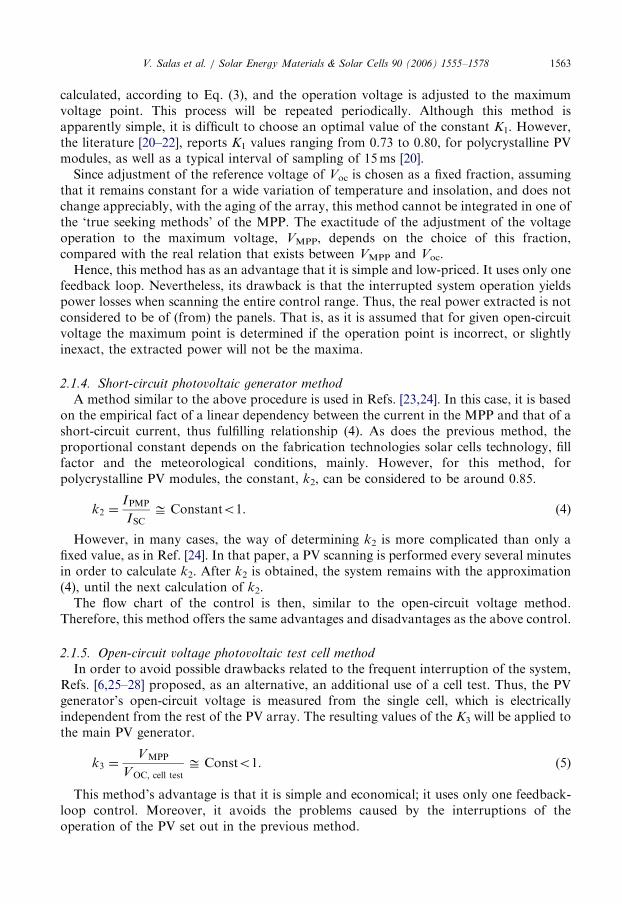
2.1.4. Short-circuit photovoltaic generator method

A method similar to the above procedure is used in Refs. [23,24]. In this case, it is basedon the empirical fact of a linear dependency between the current in the MPP and that of ashort-circuit current, thus fulfilling relationship (4). As does the previous method, theproportional constant depends on the fabrication technologies solar cells technology, fillfactor and the meteorological conditions, mainly. However, for this method, forpolycrystalline PV modules, the constant, k2, can be considered to be around 0.85.

k2 ¼IPMP

ISCffi Constanto1. (4)

However, in many cases, the way of determining k2 is more complicated than only afixed value, as in Ref. [24]. In that paper, a PV scanning is performed every several minutesin order to calculate k2. After k2 is obtained, the system remains with the approximation(4), until the next calculation of k2.

The flow chart of the control is then, similar to the open-circuit voltage method.Therefore, this method offers the same advantages and disadvantages as the above control.

2.1.5. Open-circuit voltage photovoltaic test cell method

In order to avoid possible drawbacks related to the frequent interruption of the system,Refs. [6,25–28] proposed, as an alternative, an additional use of a cell test. Thus, the PVgenerator’s open-circuit voltage is measured from the single cell, which is electricallyindependent from the rest of the PV array. The resulting values of the K3 will be applied tothe main PV generator.

k3 ¼VMPP

VOC; cell testffi Consto1. (5)

This method’s advantage is that it is simple and economical; it uses only one feedback-loop control. Moreover, it avoids the problems caused by the interruptions of theoperation of the PV set out in the previous method.


As a disadvantage, it supposes that the test cell has properties identical to each cell of thePV generator main. Therefore, Voc of the test cell is considered proportional to Voc of thePV unit used in the selection of the MPP. If the supposition is incorrect, maximum powerwill not be extracted. And, finally, it can be an unsuitable method for applications withsurface limitations (i.e. solar vehicles).

2.2. Direct control: the ‘‘true seeking’’

Direct methods include those methods that use PV voltage and/or current measure-ments. From those, and taking into account the variations of the PV generator operatingpoints, the optimum operating point is obtained. These algorithms have the advantage ofbeing independent from the a priori knowledge of the PV generator characteristics. Thus,the operating point is independent of isolation, temperature or degradation levels. Theproblems are undesirable errors which strongly affect tracker accuracy. The methodsbelonging to this group include the differentiation, feedback voltage (current), P&O, C.I.,auto-oscillation as well as the fuzzy logic, among others. Other types of classification,which distinguish between sample and modulation methods, can be included within thisgroup.

2.2.1. Sampling methods

In these procedures, a sample is made of the PV’s generator voltage and current.Afterwards, using diverse strategies, in every sampling, the PV output power, PPV (t) isgathered. Such sampling has as an objective for the determining of the relative timeevolution of the abovementioned variable. So, firstly, the PPV(t) is computed. At a stagetwo, the PV power PPV(t+Dt) is computed again. After gathering the past and the presentinformation on the PPV, the controller makes a decision depending on the location of theoperating point. This tracking process repeats itself indefinitely until the peak power pointis reached. In accordance with this principle, the following methods can be distinguished.

2.2.1.1. Differentation method. This technique is presented in Refs. [29,30], and is basedon the property in which the MPP is located by solving Eq. (6).

dPPV

dt¼ VPV;

dIPV

dtþ IPV

dVPV

dt¼ 0. (6)

However, in order to provide real time adjustments of the operating point, this equationmust be solved quickly. This is difficult because solving this equation requires, at least,eight calculations and measurements: a determination of present array voltage VPV; adetermination of present array current IPV; a measure of the change in voltage, dVPV, inthe face of a given operating point perturbation (dt); a measure of the change in current,dIPV, corresponding to the operating point perturbation; a calculation of the product VPV

times dIPV; a calculation of the product IPV times dVPV; a calculation of the resulting sumVPV dIPV+IPV dVPV; and a comparison of this sum to an equal perturbation on theopposite side of the operating point or the operating point power. Furthermore, if the finalsum is not zero, a ninth determination must be made of the sign of the dPPV sum. This signindicates the direction that the operating point must be adjusted to reach the MPP.


2.2.1.2. Feedback voltage (current) method. If there is no battery present in the system, inorder to tie the bus voltage at a nearly constant level, a simple control can be applied, as inRefs. [31,32]. Thus, the feedback of the PV voltage (current) and the comparison with aconstant voltage (current) can be used to continuously adjust the duty cycle (D) of a DC/DC converter, to operate the PV panel at a predefined operating point, close to the MPP,Fig. 8.

The disadvantages of this configuration are the same as for the method of directconnection (PV generator+load profile). That is, the system is not able to adapt tochangeable environmental conditions, such as irradiance and temperature. However, ifbatteries are present in the system, a common technique is to compare with a referenceconstant voltage, where it is assumed that it corresponds to the VMPP, underenvironmentally specific conditions. The resultant signal differentiation (error signal) isused to control the DC/DC converter.

Although the implementation of this variant is not relatively simple, it fails as well tofulfil the proposed objective because it does not take into account the effects of irradiationand temperature variations.

The advantages of this method are the same as the previous methods: it is a simple andeconomical method and uses only one feedback-loop control. Nevertheless, as has beenmentioned before, it presents the following disadvantages: it cannot be applied in ageneralized fashion in systems which do not consider the effect of variations of theirradiation and temperature of the PV panels. It cannot be applied to the systems withbatteries.

2.2.1.3. Perturbation and observe (‘‘P&O’’) method. The ‘‘P&O’’ method is that which ismost commonly used in practice by the majority of authors [33–38], among others. It is aniterative method of obtaining MPP. It measures the PV array characteristics, and thenperturbs the operating point of PV generator to encounter the change direction. The

Fig. 8. Voltage-feedback with PWM modulation.

ARTICLE IN PRESS

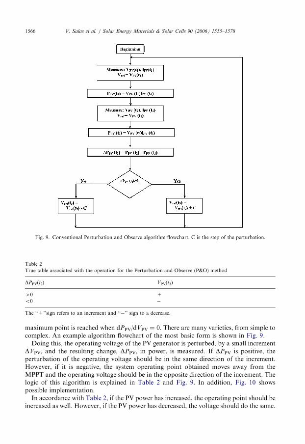
Fig. 9. Conventional Perturbation and Observe algorithm flowchart. C is the step of the perturbation.

Table 2

True table associated with the operation for the Perturbation and Observe (P&O) method

DPPV(t2) VPV(t3)

40 +

o0 �

The ‘‘+’’sign refers to an increment and ‘‘�’’ sign to a decrease.


maximum point is reached when dPPV/dVPV ¼ 0. There are many varieties, from simple tocomplex. An example algorithm flowchart of the most basic form is shown in Fig. 9.Doing this, the operating voltage of the PV generator is perturbed, by a small increment

DVPV, and the resulting change, DPPV, in power, is measured. If DPPV is positive, theperturbation of the operating voltage should be in the same direction of the increment.However, if it is negative, the system operating point obtained moves away from theMPPT and the operating voltage should be in the opposite direction of the increment. Thelogic of this algorithm is explained in Table 2 and Fig. 9. In addition, Fig. 10 showspossible implementation.In accordance with Table 2, if the PV power has increased, the operating point should be

increased as well. However, if the PV power has decreased, the voltage should do the same.

ARTICLE IN PRESS

Fig. 10. Example Perturbation and Observe implementation system [37].

Fig. 11. Deviation from the MPP with the Perturbation and Observation algorithm under rapidly changing

insolation levels [39,40].


Nevertheless, a disadvantage of this method, described by Hussein et al. [39], appears inthe case of a sudden increase of irradiance, Fig. 11, where the algorithm reacts as if theincrease occurred as a result of the previous perturbation of the operating voltage.

In order to better understand this phenomenon, see Fig. 11. Thus, the case is consideredin which the irradiance is such that it generates the P– V curve characteristics, curve 1. Inthis way, the operating voltage initially oscillates around the maximum point, from A toA1. Now, an increase in the power will be measured because the solar irradiation hasincreased from curve 1 to curve 2. Then, if one assumes that being in point A, that it comesfrom a diminution of the voltage, and before the following disturbance takes place, the


irradiance is increased, with the curve characteristic being now curve 2, and the operationpoint will occur at B1. Indeed, since there has been a positive increase in power, thedisturbance will continue in the same direction, see Table 2. In other words, the voltagewill diminish and go to point B. Furthermore, if the irradiance is increased again quickly tocurve 3, there will be another increase in positive power, with which the operation pointwill now be C. That is, due to two increases of irradiance, the operation point has beentransferred from A to C, moving away from the maximum point. This process remainsuntil the increase of the irradiance slows or stops.The advantages of this method can be summarized as follows: a previous knowledge is

not required of PV generator characteristics; it a relatively simple method. Nevertheless, intheir most simple form, at a steady state, the operating point oscillates around the MPP,giving rise to the wasting of some amount of available energy. In addition, it is anunsuitable method with rapidly changing atmospheric conditions [39]. However, theirreaction can be improved by increasing the speed of the execution of the control algorithmor introducing an optimization [41,42].

2.2.1.4. Conductance incremental method (‘‘C.I.’’). An alternative to the ‘‘P&O’’ methodwas proposed by Hussein et al. [39], developing the ‘‘C.I.’’ method. It is based on Eq. (7).That is, differentiating the PV power with respect to voltage and setting the result to zero,Fig. 12.

dPfv

dV fv¼ I fv

dV fv

dV fvþ V fv

dI fv

dV fv¼ I fv þ V fv

dI fv

dV fv¼ 0, (7)

�I fv

V fv¼

dI fv

dV fv. (8)

The left-hand side of Eq. (8) represents the opposite of the instantaneous conductance,G ¼ IPV=VPV, whereas the right hand side of the Eq. (8) represents its incrementalconductance. On the other hand, the incremental variations, dVPV and dIPV, can beapproximated by the increments of both the parameters, DVPV and DIPV, with the aim ofmeasuring the actual value VPV and IPV with the values measured in the previous instant,expressions (9) and (10), respectively.

dVPVðt2Þ � DVPVðt2Þ ¼ VPVðt2Þ � VPVðt1Þ, (9)

dIPVðt2Þ � DIPVðt2Þ ¼ IPVðt2Þ � IPVðt1Þ. (10)

P

V

dPdV

> 0 dPdV

< 0

dPdV

= 0

(PMP)

Fig. 12. Characteristics curve of the P– V photovoltaic generator. Variation of the dP/dV.

ARTICLE IN PRESS

Fig. 13. Incremental conductance algorithm flowchart.


Therefore, analyzing the derivative one can test whether the PV generator is operating atits MPP or far from it, Eqs. (11)–(13), Fig. 13. In addition, Fig. 14 shows, as an example,the flowchart implemented by Hussein et al. [39].

dPPV

dVPV40 for VPVoVPMP, (11)

dPPV

dVPV¼ 0 for VPV ¼ VPMP, (12)

dPPV

dVPVo0 for VPV4VPMP. (13)

ARTICLE IN PRESS

Fig. 14. Circuitry used to implement the parasitic capacitance method.


The main advantage of this algorithm is that it offers a good yield method under rapidlychanging atmospheric conditions. Also, it achieves lower oscillation around the MPP thanthe P&O method, even though, when the P&O method is optimized, the MPPT efficienciesof the incremental conductance and P&O MPPT algorithms are, essentially, the same[40,41]. Nonetheless, it has as drawback that it requires complex control circuit whichmight have resulted in a high cost system 10 years ago. However, today there are manyoptions for doing it much more cheaply.

2.2.1.5. Parasitic capacitance method. This method was developed by Branbrilla et al.[43], and is similar to the incremental conductance method, except that the effect of the PVcell’s parasitic union capacitance, cPV, is included. The analysis is carried out with Eq. (14),instantaneous PV output power, where PPV(t), IPV(t) and VPV(t) are the current andvoltage in the time function, respectively.

PPVðtÞ ¼ IPVðtÞVPVðtÞ. (14)

Then, if the current can be expressed as a time function, VPV(t), the power can beobtained by means of the expression (15).

PPVðtÞ ¼ F ðVPVðtÞÞVPVðtÞ. (15)

Then, the condition of the MPP is fulfilled for Eq. (16).

dPPVðtÞ

dVPVðtÞ¼

dF ðVPVðtÞÞ

dVPVðtÞþ F ðVPVðtÞÞ ¼ 0. (16)

That is, relation (17) is fulfilled.

gp � gl ¼ 0, (17)

where gp (the incremental conductance) and gl (instantaneous conductance) are defined bymeans of Eqs. (18) and (19), respectively. Later, applying the rule of the chain to gp it canbe expressed according to Eq. (20).

gp ¼dF ðVPVðtÞÞ

dVPVðtÞ, (18)

gl ¼ �F ðVPVðtÞÞ, (19)

gp ¼dF

dt

dt

dVPV. (20)


In this way, the Eq. (16) can be rewritten as Eq. (21).

IdPVðtÞVPVðtÞ þ IPVðtÞV

dPVðtÞ ¼ 0. (21)

Assuming that relation (22) is fulfilled, the power can now be expressed according toexpression (23). Then, the maximum power is transferred when Eq. (24) is suited, where thedot represents the first derived and both dots the second derived.

IPVðtÞ ¼ F ðVPVðtÞÞ þ cPVVd

PVðtÞ ¼ 0, (22)

PPVðtÞ ¼ ½F ðVPVðtÞÞ þ cPVVd

PVðtÞ�VPVðtÞ, (23)

dF ðVPVðtÞÞÞ

dVPVðtÞþ Cp

Vdd

PVðtÞ

Vd

PVðtÞ

þVd

PVðtÞ

VVðtÞ

0@

1A

�F ðvpÞ

vp¼ 0, ð24Þ

IPVðtÞ ¼ IPV;cc þX11

aIn cosðnootÞ þ bI

n sinðnootÞ, (25)

VPVðtÞ ¼ VPV;cc þX11

aVn cosðnootÞ þ bV

n sinðnootÞ, (26)

PPV ¼ VPV;ccIPV;cc þ1

2

X11

aInaV

n þ bInbV

n . (27)

In addition, the three terms of Eq. (24) represent the instantaneous conductance,incremental conductance and the induced ripple from the parasitic capacitance,respectively. The first and second derivatives take into account the AC ripple componentsgenerated by the converter. If cPV is equal to zero then expression (24) simplifies theincremental conductance method.

gp ¼Pgp

V 2o

¼

12

P1n¼1½a

inav

n þ binbv

n�

12

P1n¼1½ða

vnÞ

2þ ðbv

nÞ2�. (28)

The array differential conductance can be obtained by Eqs. (25)–(28), where Pgp is theaverage ripple power, Vo the voltage ripple and ai

n; avn; b

in; b

vn are the coefficients of the

Fourier series of the PV voltage and current ripple. In addition, the values of Pgp and Vo2

can be obtained in accordance with Fig. 14, which is the diagram used for theimplementation of this method. The two band-pass filters, HP, remove the continuouscomponent of VPV and IPV, retaining ripple components. Finally, the two low-pass filters,LP, remove the components in high frequency and retain only the continuous component,such as Pgp and Vo

2, with which g is obtained, Eq. (28). This can be used until it has fulfilledthe expression (17).

The disadvantage of this method is that it requires two multiplications with thefollowing complexity of the control circuit.

ARTICLE IN PRESS

Z

LT

VbatDPhotovoltaic +

-

+

-VPV

IPV

D

+

-

+

-

+

-Generator

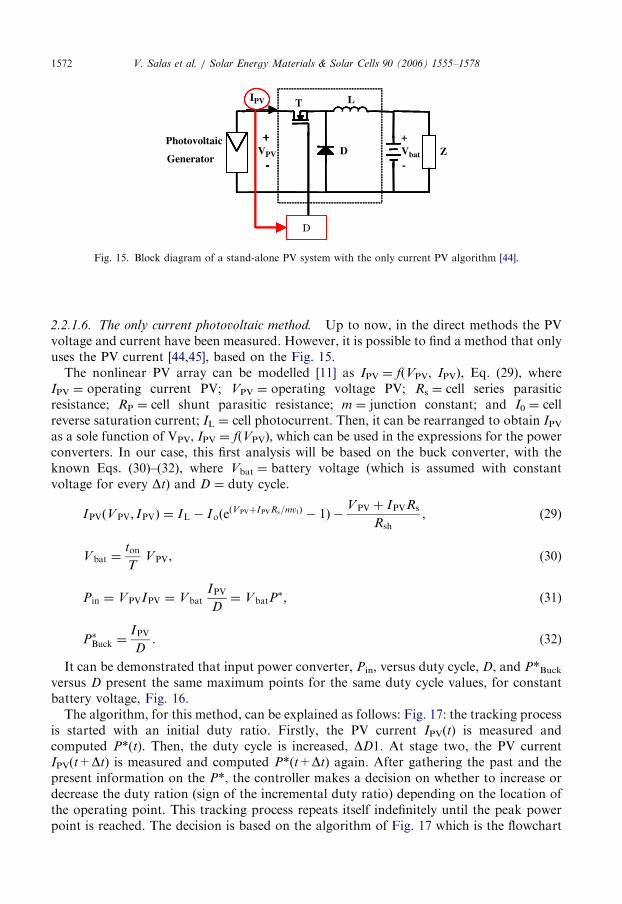
Fig. 15. Block diagram of a stand-alone PV system with the only current PV algorithm [44].


2.2.1.6. The only current photovoltaic method. Up to now, in the direct methods the PVvoltage and current have been measured. However, it is possible to find a method that onlyuses the PV current [44,45], based on the Fig. 15.The nonlinear PV array can be modelled [11] as IPV ¼ f(VPV, IPV), Eq. (29), where

IPV ¼ operating current PV; VPV ¼ operating voltage PV; Rs ¼ cell series parasiticresistance; RP ¼ cell shunt parasitic resistance; m ¼ junction constant; and I0 ¼ cellreverse saturation current; IL ¼ cell photocurrent. Then, it can be rearranged to obtain IPVas a sole function of VPV, IPV ¼ f(VPV), which can be used in the expressions for the powerconverters. In our case, this first analysis will be based on the buck converter, with theknown Eqs. (30)–(32), where Vbat ¼ battery voltage (which is assumed with constantvoltage for every Dt) and D ¼ duty cycle.

IPVðVPV; IPVÞ ¼ IL � IoðeðVPVþIPVRs=mvtÞ � 1Þ �

VPV þ IPVRs

Rsh, (29)

Vbat ¼ton

TVPV, (30)

Pin ¼ VPVIPV ¼ VbatIPV

D¼ VbatP

�, (31)

P�Buck ¼IPV

D. (32)

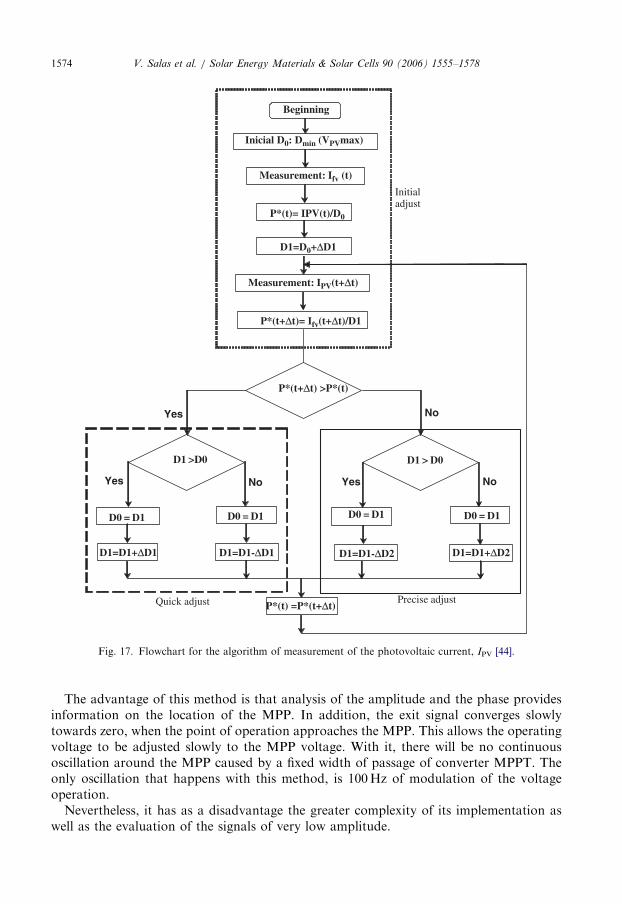
It can be demonstrated that input power converter, Pin, versus duty cycle, D, and P*Buckversus D present the same maximum points for the same duty cycle values, for constantbattery voltage, Fig. 16.The algorithm, for this method, can be explained as follows: Fig. 17: the tracking process

is started with an initial duty ratio. Firstly, the PV current IPV(t) is measured andcomputed P*(t). Then, the duty cycle is increased, DD1. At stage two, the PV currentIPV(t+Dt) is measured and computed P*(t+Dt) again. After gathering the past and thepresent information on the P*, the controller makes a decision on whether to increase ordecrease the duty ration (sign of the incremental duty ratio) depending on the location ofthe operating point. This tracking process repeats itself indefinitely until the peak powerpoint is reached. The decision is based on the algorithm of Fig. 17 which is the flowchart

ARTICLE IN PRESS

55

50

45

40

35

30

25

20

15

10

5

00.5 0.55 0.6 0.65 0.7 0.75 0.8 0.85 0.9 0.95 1

0

0.5

1

1.5

2

2.5

3

3.5

4

4.5

5

I PV/D

Pow

erP

V (

W)

Duty Cycle (D)

IPV/D

Power (W)

MPP

Fig. 16. Simulation results comparing the new algorithm with the photovoltaic power supply [44].


for the peak power tracking control. Then, four cases can be presented, Table 1, whereDP ¼ P�ðtþ DtÞ � P�ðtÞ and DD ¼ Dðtþ DtÞ �DðtÞ.

This method has as a major advantage, when compared with other direct methods, thefact that it only uses the measurement of the variable, PV current. In addition, thisalgorithm operates successfully even in cases of rapidly changing atmospheric conditionsand different sky conditions [44,45]. Furthermore, even though this description is made fora step-down DC/DC converter, it can be proven that this method is suitable for any DC/DC topology, step-down and step-up, as is reported in Ref. [44].

2.2.2. Methods by modulation

In the methods discussed earlier, the sampling methods, the appropriate adjustment forthe maximum voltage point leads a point close to and oscillating around the maximumpoint. These oscillations are generated automatically by the feedback control used.However, there are many other methods that add an oscillation. These algorithms areknown as forced oscillation methods.

2.2.2.1. Forced oscillations methods. Several articles have dealt with this subject [46,47].For example, Ref. [46] introduces a small voltage, 100Hz, that is added to the voltage ofoperation voltage of the PV generator. This leads to a ripple power, whose phaseand amplitude are dependent on the relative location of the operation point to the MPP,Fig. 18. If this modulation occurs in zone ‘‘A’’, the left side of the MPP the ripple voltageof the power will be perfectly in phase. However, if the modulation occurs in a point ofoperation of zone ‘‘B’’, to the right side of the MPP, the curling of the power output will be1801 out of phase with respect to the voltage. In case that the operation point is exactlythe MPP, the curling of power output will have twice the frequency of the curling of thevoltage, with very small amplitude.

ARTICLE IN PRESS

P*(t+∆t) >P*(t)

Yes

Yes

D1=D1+∆D1

D1 >D0

No

D0 = D1

No

Yes

D0 = D1

D1 > D0

No

D0 = D1D0 = D1

P*(t+∆t)= Ifv(t+∆t)/D1

Beginning

Inicial D0: Dmin (VPVmax)

Measurement: Ifv (t)

P*(t)= IPV(t)/D0

D1=D0+∆D1

Measurement: IPV(t+∆t)

P*(t) =P*(t+∆t)

D1=D1-∆D1 D1=D1-∆D2 D1=D1+∆D2

Initialadjust

Quick adjust Precise adjust

Fig. 17. Flowchart for the algorithm of measurement of the photovoltaic current, IPV [44].


The advantage of this method is that analysis of the amplitude and the phase providesinformation on the location of the MPP. In addition, the exit signal converges slowlytowards zero, when the point of operation approaches the MPP. This allows the operatingvoltage to be adjusted slowly to the MPP voltage. With it, there will be no continuousoscillation around the MPP caused by a fixed width of passage of converter MPPT. Theonly oscillation that happens with this method, is 100Hz of modulation of the voltageoperation.Nevertheless, it has as a disadvantage the greater complexity of its implementation as

well as the evaluation of the signals of very low amplitude.

ARTICLE IN PRESS

Fig. 18. Curve P–V for a PV generator with the power ripple caused by the photovoltaic voltage modulation.

Point ‘‘A’’ denotes the area of operation, on the left of the MPP, and point ‘‘B’’ the area on the right of the MPP.


2.3. Other methods: artificial intelligence methods

In recent years, the fuzzy logic controllers (FLCs) and neural network methods havereceived attention and increased their use very successfully in the implementation for MPPsearching [48–55]. The fuzzy controllers improve control robustness and have advantagesover conventional ones. They can be summarized in the following way [47]: they do notneed exact mathematical models; they can work with vague inputs and, in addition; theycan handle nonlinearities and are adaptative, in nature; likewise, their control gives themrobust performance, under parameter variation, load and supply voltage disturbances.

Based on their heuristic nature and fuzzy rule tables, these methods use differentparameters to predict the maximum power output: the output circuit voltage and shortcircuit current [49]; the instantaneous array voltage and current [50–52]; instantaneousarray voltage and reference voltage (obtained by an offline trained neural network) [48];instantaneous array voltage and current of the array and short circuit current and open-circuit voltage of a monitoring cell [53,54] and solar radiation, ambient temperature, windvelocity and instantaneous array voltage and current, used in Ref. [55].

Finally, it is of note that other methods have been implemented such as those that arebased on the use of the Fibonacci series [56]. Although, once again, two variables aremeasured: output voltage and current of the DC/DC converter.

3. Conclusions

In this paper, the state of the art of MPP algorithms has been reviewed. As has beendemonstrated, there are many ways of distinguishing and grouping the methods fortracking the MPP to the PV generator. However, in this article the direct and indirectmethods were those selected and developed in depth.


The indirect methods (‘‘quasi trackers’’) have the particular feature of not obtaining, butrather estimating, the maximum power for either irradiance or temperature. They mustmeasure some of the PV generator’s voltage and current PV (or both), the irradiance or useempirical data, by mathematical expressions of numerical approximations, to estimate theMPP from the specific PV generator installed in the system. Although, in many cases theycan be simple and inexpensive, they are not totally versatile with respect to load profile;none of them are able to obtain the MPP exactly, from PV in any atmospheric conditions.Subsequently, they are known as ‘‘quasi seeks’’.On the other hand, the direct methods can be also distinguished (‘‘true seeking

methods’’) which offer the following advantages: neither a large database nor a largememory is necessary for calculating the MPP; they are totally versatile with respect to theload profile; the seeking of MPP is independent of the variation of the parameters of thePV generator. Likewise, the control circuit does not have to be fit for a specific generator,nor must it update when varying their parameters; and it is not necessary to know the levelincident irradiance.Nevertheless, in all direct methods up to now the measurement of the voltage and

current of PV generator are required. Notwithstanding, it has been shown that in the directmethods, it is possible to develop a strategy that allows obtaining the MPP by measuringonly one variable, the current PV.Finally, it has been shown that other methods also exist, such as the artificial methods

and the Fibonacci series based but two variables must be measured, at least.

References

[1] G. Bopp, H. Galber, K. Preiser, D.U. Sauer, H. Schmidt, Energy Storage in photovoltaic stand-alone energy

supply systems, Prog. Photovoltaics: Res. Appl. 6 (4) (1998) 271–291.

[2] J.P. Dunlop, Batteries and charge control in stand-alone photovoltaic systems. Fundamentals and

Application, Sandia National Laboratories, 1997.

[3] G.M. Hans, Solar cell and test circuit, Patent US3, 350, 635, 1967.

[4] J.D. Hartman, Power conditioning system, Patent US3, 384, 806, 1968.

[5] T.O. Paine, Maximum Power Point Tracker, National Aeronautics and Space Administration, NASA,

Patent US3, 566, 143, 1969.

[6] A.U. Louis, System for detecting and utilizing the maximum available power from solar cells, Patent US3,

696,286, 1972.

[7] M. Togneri, H. Elliott, DC to AC and AC to DC converter systems, Patent, US3,825,816, 1974.

[8] A. Wilkerson, Power maximization circuit, Patent US4,200,833, 1980.

[9] R.H. Baker, US, Method of and apparatus for enabling output power of solar panel to be maximized, Patent

4,375,662, 1983.

[10] K. Nishioka, et al., Analysis of the temperature characteristics in polycrystalline Si solar cells using modified

equivalent circuit model, Jpn. J. Appl. Phys. 42 (12) (2003) 7175–7179.

[11] J.C.H. Phang, D.S.H. Chan, J.R. Phillips, Accurate analytical method for the extraction of solar cell,

Electron. Lett. 20 (10) (1984) 406–408.

[12] M.A. Hamdy, A new model for the current-voltage output characteristics of photovoltaic modules, J. Power

Sources 50 (1–2) (1994) 11–20.

[13] T. Takashima, T. Tanaka, M. Amano, Y. Ando, Maximum output control of photovoltaic (PV) array,

Intersociety Energy Conversion Engineering Conference and Exhibit (IECEC), 35th, Las Vegas, NV,

July 24–28, 2000, pp. 380–383.

[14] N. Takehara, S. Kurokami, Power control apparatus and method and power generating system using them.

Patent US5,654,883. 1997.


[15] H.E.-S.A. Ibrahim, et al., Microcomputer controlled buck regulator for maximum power point tracker for

DC pumping system operates from photovoltaic system, Fuzzy Systems Conference Proceedings, FUZZ-

IEEE ’99, 1999 IEEE International 1 (22–25) (1999) 406–411.

[16] D. Lafferty, Coupling network for improving conversion efficiency of photovoltaic power source,

US4,873,480, 1989.

[17] P. Chetty, Maximum power transfer system for a solar cell array, US4,604,567, 1986.

[18] M.A.S. Masoum, et al., Optimal power point tracking of photovoltaic system under all operating conditions,

in: 17th Congress of the World Energy Council, Houston, TX, 1998.

[19] M.A.S. Masoum, et al, Design, construction and testing of a voltage-based maximum power point tracker

(VMPPT) for small satellite power supply, in: 13th Annual AIAA/USU Conference, Small Satellite, 1999.

[20] J.J. Schoeman, J.D. van Wyk, A simplified maximal power controller for terrestrial photovoltaic panel

arrays, IEEE Power Electronics Specialists Conference. PESC ‘82 Record. New York, NY, 1982,

pp. 361–367.

[21] M. Andersen, T.B. Alvsten, 200W Low cost module integrated utility interface for modular photovoltaic

energy systems, Proceedings of IECON ‘95 1 (1995) 572–577.

[22] M. Abou El Ela, J. Roger, Optimization of the function of a photovoltaic array using a feedback control

system. Solar. Cells: Their Science,, Technology, Applications and Economics 13 (2) (1984) 185–195.

[23] S.M. Alghuwainem, Matching of a dc motor to a photovoltaic generator using a step-up converter with a

current-locked loop, IEEE Trans. Energy Conversion 9 (1994) 192–198.

[24] T. Noguchi, et al., Short-current pulse-based adaptive maximum power point tracking for a photovoltaic

power generation system, Elect. Eng. Japan 139 (1) (2002) 65–72.

[25] J.F. Schaefer, L. Hise, An inexpensive photovoltaic array maximum-power-point-tracking DC-to-DC

converter. Number NMSEI/TN-84-1 New Mexico Solar Energy Institute, Las Cruces, New Mexico 88003,

Mayo, 1984.

[26] Z. Salameh, F. Dagher, W. Lynch, Step-down maximum power point tracker for photovoltaic systems, Solar

Energy 46 (5) (1991) 279–282.

[27] D.L. Lafferty, Coupling network for improving conversion efficiency of photovoltaic power source

US4,873,480, 1989.

[28] D. Lafferty, Regulating control circuit for photovoltaic source employing switches, energy storage, and pulse

width modulation controller, Patent US5,270,636, 1993.

[29] J.H. David, Power conditioning system, US3,384,806, 1968.

[30] L.T.W. Bavaro, Power regulation utilizing only battery current monitoring, Patent, US4,794,272, 1988.

[31] H.D. Maheshappa, J. Nagaraju, M.V. Murthy, An improved maximum power point tracker using a step-up

converter with current locked loop, Renew. Energy 13 (2) (1998) 195–201.

[32] Ch. Hua, Ch. Shen, Comparative study of peak power tracking techniques for solar storage system, in: IEEE

Applied Power Electronics Conference and Exposition (APEC’98), vol. 2, 1998, pp. 679–685.

[33] Z. Salameh, D. Taylor, Step-up maximum power point tracker for photovoltaic arrays, Solar Energy 44 (1)

(1990) 57–61.

[34] W. Denizinger, Electrical power subsystem of globlastar, in: Proceedings of the European Space Conference,

1995, pp. 171–174.

[35] W.J.A. Teulings, J.C. Marpinard, A. Capel, A maximum power point tracker for a regulated power bus, in:

Proceedings of the European Space Conference, 1993.

[36] Y. Kim, H. Jo, D. Kim, A new peak power tracker for cost-effective photovoltaic power systems, IEEE Proc.

Energy Conversion Eng. Conf. IECEC 96 3 (1) (1996) 1673–1678.

[37] Ch. Hua, J. Lin, Ch. Shen, Implementation of a DSP-controlled PV system with peak power tracking, IEEE

Trans. Ind. Electron. 45 (1) (1998) 99–107.

[38] H. Al-Atrash, I. Batarseh, K. Rustom, Statistical modeling of DSP-based hill-climbing MPPT algorithms in

noisy environments Applied Power Electronics Conference and Exposition, 2005. APEC 2005, Twentieth

Annual IEEE, vol. 3, 6–10 March 2005, pp. 1773–1777.

[39] K.H. Hussein, I. Muta, T. Hoshino, M. Osakada, Maximum photovoltaic power tracking: an algorithm for

rapidly changing atmospheric conditions, IEE Proc. Generation Transmission Distrib. 142 (1) (1995) 59–64.

[40] D.P. Hohm, M.E. Ropp, Comparative study of maximum power point tracking algorithms, Prog. Photovolt:

Res. Appl. 11 (2003) 47–62.

[41] X. Liu, L.A.C. Lopes, An improved perturbation and observation maximum power point tracking algorithm

for PV arrays, in: Power Electronics Specialists Conference, 2004, PESC 04. 2004, IEEE 35th Annual vol. 3,

2004, 2005–2010.


[42] N. Femia, G. Petrone, G. Spagnuolo, M. Vitelli, Optimization of perturb and observe maximum power point

tracking method, IEEE Trans. Power Electron. 20 (4) (2005) 963–973.

[43] A. Branbrilla, M. Gambarara, A. Garutti, F. Ronchi, New approach to photovoltaic arrays maximum power

point tracking, in: 30th IEEE Power Electronics Conference, 1999, pp. 632–637.

[44] V. Salas, E. Olıas, A. Lazaro, A. Barrado, New algorithm using only one variable measurement applied to a

maximum power point tracker, Solar Energy Mater. Solar Cells 1–4 (2005) 675–684.

[45] V. Salas, E. Olıas, A. Lazaro, A. Barrado, Evaluation of a new maximum power point tracker (MPPT)

applied to the photovoltaic stand-alone systems, Solar Energy Mater. Solar Cells 87 (1–4) (2005) 807–815.

[46] K.K. Tse, H.S.H. Chung, S.Y.R. Hui, M.T. Ho, A novel maximum power point tracking technique for PV

panels, in: IEEE Power Electronics Specialists Conference, 2001, PESC. 2001 IEEE, vol. 4, 1970–1975.

[47] A. Cocconi, W. Rippel, Lectures from GM sunracer case history, lecture 3-1: the Sunracer power systems.

Number M-101, Society of Automotive Engineers, Inc., Warderendale, PA, 1990.

[48] M. Veerachary, T. Senjyu, K. Uezato, Neural-network-based maximum-power-point tracking of coupled-

inductor interleaved-boost-converter-supplied PV system using fuzzy controller, IEEE Trans. Ind. Electron.

50 (4) (2003) 749–758.

[49] B.M. Wilamowski, et al., Microprocessor implementation of fuzzy system and neural networks, in:

International Joint Conference on Neural Networks, vol. 1, Washington, DC, 2001, pp. 234–239.

[50] C.-Y. Won, D.-H. Kim, S.-C. Kim, W.-S. Kim, H.-S. Kim, A new maximum power point tracker of

photovoltaic arrays using fuzzy controller, in: 25th Annual IEEE Power Electronics Specialists Conference,

PESC ‘94 Record, vol. 1, 1994, pp. 396–403.

[51] A.N. Abd El-Shafy, H.F. Faten, E.M. Abou El-Zahab, Evaluation of a proper controller performance for

maximum-power point tracking of a stand-alone PV system, Solar Energy Mater. Solar Cells 75 (3–4) (2003)

723–728.

[52] N. Patcharaprakiti, S. Premrudeepreechacharn, Y. Sriuthaisiriwong, Maximum power point tracking using

adaptive fuzzy logic control for grid-connected photovoltaic system, Renew. Energy 30 (11) (2005)

1771–1788.

[53] T. Hiyama, et al., Identification of optimal operation point of PV modules using neural network for real time

maximum power tracking control, IEEE Trans. Energy Conversion 10 (1995) 360–367.

[54] T. Hiyama, et al., Evaluation of neural network based real time maximum power tracking controller for PV

system, IEEE Trans. Energy Conversion 10 (3) (1995) 543–548.

[55] T. Hiyama, et al., Neural network based estimation of maximum power generation, IEEE Trans. Energy

Conversion 12 (1997) 241–247.

[56] M. Miyatake, T. Kouno, M. Nakano, A simple maximum power point tracking control employing fibonacci

search algorithm for power conditioners of photovoltaic generators, EPE-PEMC’02, Cavtat & Dubrovnik,

2002.

Review of the maximum power point tracking algorithms for stand-alone photovoltaic systems

Documents

Transcript of Review of the maximum power point tracking algorithms for stand-alone photovoltaic systems