Voltage dependent overcurrent protection in microgrids with a ...
113
Benjamin Lukas Mößlang, BSc Voltage dependent overcurrent protection in microgrids with a high penetration of grid-forming inverters MASTER’S THESIS to achieve the university degree of Diplom-Ingenieur Master's degree programme: Electrical Engineering submitted to Graz University of Technology Supervisor Em.Univ.-Prof. Dipl.-Ing. Dr.techn. Lothar Fickert Institute of Electrical Power Systems Co-Supervisor Dipl.-Ing. (FH) Florian Fink, OMICRON electronics Dipl.-Ing. Dr.techn. Ziqian Zhang, Institute of Electrical Power Systems Graz, February 2022
-
Upload
khangminh22 -
Category
Documents
-
view
2 -
download
0
Transcript of Voltage dependent overcurrent protection in microgrids with a ...
Benjamin Lukas Mößlang, BSc
Voltage dependent overcurrent protection in microgrids with a high penetration of grid-forming inverters
MASTER’S THESIS to achieve the university degree of
Diplom-Ingenieur
Master's degree programme: Electrical Engineering
submitted to
Graz University of Technology
Supervisor Em.Univ.-Prof. Dipl.-Ing. Dr.techn. Lothar Fickert
Institute of Electrical Power Systems
Co-Supervisor
Dipl.-Ing. (FH) Florian Fink, OMICRON electronics
Dipl.-Ing. Dr.techn. Ziqian Zhang, Institute of Electrical Power Systems
Graz, February 2022

Institute of Electrical Power Systems
Voltage dependent overcurrent protection in microgrids with a high penetration of grid-forming inverters
A Master’s Thesis by
Benjamin Lukas Mößlang, BSc
Supervisor
Em.Univ.-Prof. Dipl.-Ing. Dr.techn Lothar Fickert
Co-Supervisor
Dipl. Ing. (FH) Florian Fink, OMICRON electronics
Dipl.-Ing. Dr.techn. Ziqian Zhang
Reviewer
Em.Univ.-Prof. Dipl.-Ing. Dr.techn Lothar Fickert
February 2022

Voltage dependent overcurrent protection in microgrids with a high penetration of grid-forming inverters
II
Graz University of Technology
Institute of Electric Power Systems
Inffeldgasse 18/I
8010 Graz
Austria
Head of Institute
Univ.-Prof. Dipl.-Ing. Dr. Robert Schürhuber
Supervisor
Em.Univ.-Prof. Dipl.-Ing. Dr.techn Lothar Fickert
Co-Supervisor
Dipl. Ing. (FH) Florian Fink, OMICRON electronics
Dipl.-Ing. Dr.techn. Ziqian Zhang
Reviewer
Em.Univ.-Prof. Dipl.-Ing. Dr.techn Lothar Fickert
A Master’s thesis by
Benjamin Lukas Mößlang, BSc
February 2022

Voltage dependent overcurrent protection in microgrids with a high penetration of grid-forming inverters
III
Statutory Declaration
I declare that I have authored this thesis independently, that I have not used other than the declared sources / resources, and that I have explicitly marked all material which has been quoted either literally or by content from the used sources.
Graz, 14.2.2022
Benjamin Lukas Mößlang
Eidesstattliche Erklärung
Ich erkläre an Eides statt, dass ich die vorliegende Arbeit selbstständig verfasst, andere als die angegebenen Quellen/Hilfsmittel nicht benutzt, und die den benutzten Quellen wörtlich und inhaltlich entnommenen Stellen als solche kenntlich gemacht habe.
Graz, am 14.2.2022
Benjamin Lukas Mößlang

Voltage dependent overcurrent protection in microgrids with a high penetration of grid-forming inverters
IV
Acknowledgements
First of all, I would like to thank my parents Gabriele and Günter for always supporting me and making it possible for me to start this study. Without them I would not be where I am today. Thank you, Mama and Papa.
I am also deeply grateful to my supervisor and mentor Em.Univ.-Prof. Dipl.-Ing. Dr.techn. Lothar Fickert, who has always supported me, helped me with words and deeds and, finally, has been very patient. Thank you for making this possible for me. And thank you for everything I learned from you.
I am also grateful to my siblings Madline and Dominik, as well as my girlfriend Stefanie, for their advice and motivation. Thank you for always supporting me and thank you for always showing understanding.
I would also like to thank my co-supervisor Dipl. Ing. Florian Fink for his mentoring and support. Furthermore, I would like to thank my boss Dipl. Ing. Christopher Pritchard for his understanding and constant motivation.
I would also like to thank my colleagues and friends for always motivating me and giving me advice.

Voltage dependent overcurrent protection in microgrids with a high penetration of grid-forming inverters
V
Abstract
The strive for decarbonization is leading to an ever-increasing amount of distributed generation in the distribution grids. Not only large photovoltaic power plants and wind farms are increasing, but also small PV plants in the low-voltage grid. These small PV plants all feed into the grid via inverters. If these generators displace conventional ones, new problems arise in the power grid. The aim of this work is to investigate whether the ANSI 51V protection function can also be used for protection in these new distribution grids. For this purpose, a state-of-the-art simulation model is analysed concerning of an improved protection concept. Using short-circuit simulations in a test grid, the protection system is designed, and it is shown that the protection concept can detect faults in the distribution grid. The protective relays can detect symmetrical faults in grids with low short-circuit power due to the additional depth of information obtained by considering the voltage. Furthermore, it is shown how this protection function can be tested.
Kurzfassung
Der Drang der Dekarbonisierung führt zu einer immer größer werdenden Anzahl an dezentraler Erzeugung in den Verteilnetzen. Es steigt nicht nur die Zahl großer Photovoltaik-Kraftwerke und Windpark, sondern auch die von kleinen PV Anlagen im Niederspannungsnetz. Diese kleinen PV Anlagen speisen alle mittels Wechselrichter in das Netz ein. Verdrängen nun diese Erzeuger konventionelle, so birgt dies neue Problemstellungen im Stromnetz. Ziel dieser Arbeit ist es zu untersuchen, ob die ANSI 51V Schutzfunktion auch im Hinblick auf den Schutz in Verteilnetzen verwendet werden kann. Dafür wird ein Simulationsmodell verwendet, welches die Auslegung des Schutzkonzeptes ermöglicht. Anhand von Kurzschlusssimulationen in einem Versuchsnetzes wird das Schutzsystem ausgelegt und es wird gezeigt, dass das Schutzkonzept symmetrische Fehler im Verteilnetz detektieren kann. Die Schutzrelais können durch die zusätzliche Informationstiefe, welche durch die Berücksichtigung der Spannung erzielt wird, Kurzschlüsse in Netzen mit geringer Kurzschlussleistung erkennen. Des Weiteren wird gezeigt, wie diese Schutzfunktion geprüft werden kann.
Voltage dependent overcurrent protection in microgrids with a high penetration of grid-forming inverters
VI
List of Abbreviations
AC Alternating Current
BJT Bipolar Junction Transistor
CCI Current-controlled inverter
CT Current Transformer
DACH Germany, Austria, Switzerland and Liechtenstein
DC Direct Current
DER Distributed Energy Resource
DG Distributed Generation
DIN Deutsches Institut für Normung
DSO Distribution System Operator
DVCO Directional Voltage Controlled Over Current Protection
EHV Extra High Voltage
EI Electrical Inertia
EM Electromagnetic
EMT Electromagnetic Transient
EMTP Electromagnetic Transient Program
ES Energy Storage
FAT Factory Acceptance Test
FET Field Effect Transistor
GFI Grid-forming Inverter
HV High Voltage
HVDC High Voltage Direct Current
IEC International Electrotechnical Commission

Voltage dependent overcurrent protection in microgrids with a high penetration of grid-forming inverters
VII
IEEE Institute of Electrical and Electronics Engineers
IT Information Technology
LV Low voltage
LVRT Low voltage ride through
MMC Modular Multilevel Converter
MV Medium Voltage
OC Over Current Protection
POC, POCC, POI Point of Common Coupling, Point of Interconnection
PV Photovoltaic
PWM Pulse-Width Modulation
RMU Ring Main Unit
SAT Site Acceptance Test
SC Short-circuit
VDE Verband der Elektrotechnik, Elektronik und Informationstechnik
VPP Virtual Power Plant
VT Voltage Transformer
WECC Western Electricity Coordinating Council
Voltage dependent overcurrent protection in microgrids with a high penetration of grid-forming inverters
VIII
Table of Contents
1 Introduction ...................................................................................... 1
1.1 Motivation........................................................................................................ 1
1.2 Structure and method ...................................................................................... 1
2 Distribution Grids ............................................................................ 3
2.1 General ........................................................................................................... 3
2.2 From a passive to an active distribution grid ................................................... 3
2.3 Microgrids ....................................................................................................... 5
2.3.1 What is a Microgrid? ....................................................................................... 5
2.3.2 Demarcation to Smart Grids and Virtual Powerplants ..................................... 7
2.3.3 Structure of a microgrid ................................................................................... 8
2.3.3.1 Power generation ..................................................................................... 8
2.3.3.2 Loads ....................................................................................................... 8
2.3.3.3 Storage and grid connection..................................................................... 9
2.3.3.4 Point of Common Coupling ...................................................................... 9
2.3.4 Control element ............................................................................................... 9
2.4 Synchronous and asynchronous machines as distributed energy resource interface ........................................................................................................ 11
2.5 Inverter as distributed energy resource interface .......................................... 12
2.5.1 Power Inverter Basics ................................................................................... 12
2.5.2 Terminology of control strategies .................................................................. 14
Voltage dependent overcurrent protection in microgrids with a high penetration of grid-forming inverters
IX
2.5.2.1 General .................................................................................................. 14
2.5.2.2 Control methods of a grid-forming inverter ............................................. 15
2.5.3 Fault current contribution .............................................................................. 16
2.5.4 Low Voltage Ride Through ............................................................................ 17
3 Protection of Distribution Grids ................................................... 21
3.1 Protection in distribution grids ....................................................................... 21
3.2 Protection in Microgrids ................................................................................. 22
3.3 Protection fundamentals ............................................................................... 26
3.3.1 Time-Overcurrent protection ......................................................................... 26
3.3.2 Distance protection ....................................................................................... 28
3.3.3 Differential protection .................................................................................... 30
3.4 Voltage restrained/controlled overcurrent in Distribution grids ...................... 31
3.4.1 General ......................................................................................................... 31
3.4.2 Usage in active distribution grids ................................................................... 32
4 Inverter Modelling .......................................................................... 35
4.1 General ......................................................................................................... 35
4.1.1 WECC models .............................................................................................. 35
4.1.1.1 PVD1 model ........................................................................................... 35
4.1.1.2 DER_A model ........................................................................................ 36
4.2 Theory of short-circuit and electro-magnetic transient simulation .................. 41
4.3 Models for SC simulation .............................................................................. 44
Voltage dependent overcurrent protection in microgrids with a high penetration of grid-forming inverters
X
4.3.1 Models in DigSILENT PowerFactory ............................................................. 44
4.3.1.1 Static generator ...................................................................................... 44
4.3.1.2 PWM Converter ...................................................................................... 49
4.4 Models for EMT simulation ............................................................................ 50
4.4.1 Models in DigSilent Powerfactory .................................................................. 51
4.4.1.1 Static generator ...................................................................................... 51
4.4.1.2 Pulse-width modulation converter .......................................................... 53
4.4.2 Simulations ................................................................................................... 54
4.4.2.1 Static generator ...................................................................................... 55
4.4.2.2 PWM converter ...................................................................................... 56
4.5 Summary of the models ................................................................................ 57
5 Short-circuit investigation of an exemplary grid model.............. 58
5.1 Grid model synthesis ..................................................................................... 58
5.2 Methodology of this investigation .................................................................. 59
5.3 Grid Condition A – Supply by transformer and inverters................................ 60
5.3.1 Power flow analysis....................................................................................... 60
5.3.2 Short-circuit ................................................................................................... 60
5.4 Grid Condition B – Supply by synchronous generator ................................... 62
5.4.1 Power flow analysis....................................................................................... 62
5.4.2 Short-circuit ................................................................................................... 62
5.5 Grid Condition C – Supply only by inverters .................................................. 64
Voltage dependent overcurrent protection in microgrids with a high penetration of grid-forming inverters
XI
5.5.1 Power flow analysis....................................................................................... 64
5.5.2 Short-circuit ................................................................................................... 64
5.6 Evaluation ..................................................................................................... 66
6 Directional Voltage Controlled Overcurrent ................................ 68
6.1 Settings ......................................................................................................... 68
6.2 Application of the protection concept in the example grid.............................. 70
6.3 Protection Testing ......................................................................................... 72
6.3.1 General ......................................................................................................... 72
6.3.2 Settings-based protection test ....................................................................... 73
6.3.1 System-based protection test ........................................................................ 77
7 Conclusion ..................................................................................... 79
8 References ..................................................................................... 81
9 Appendix ........................................................................................ 85
9.1 Exemplary grid .............................................................................................. 85
9.2 Grid Condition A ............................................................................................ 88
9.2.1 Power Flow Analysis ..................................................................................... 88
9.2.2 Short-Circuit calculation ................................................................................ 91
9.3 Grid Condition B ............................................................................................ 92
9.3.1 Power Flow Analysis ..................................................................................... 92
9.3.2 Short-Circuit calculation ................................................................................ 95
9.4 Grid Condition C ........................................................................................... 96

Voltage dependent overcurrent protection in microgrids with a high penetration of grid-forming inverters
XII
9.4.1 Power Flow ................................................................................................... 96
9.4.2 Short Circuit Calculation ................................................................................ 99
Introduction
1
1 Introduction
1.1 Motivation
The energy transition is a powerful driver of change and further development in our power grids. The energy transition is driving various D's. These include decarbonization, decentralization, digitalization, and democratization. If we now take up two of these D's and look at the developments in the area of decarbonization and decentralization, then it very quickly becomes apparent that one of the solutions, or rather developments, is that individual consumers are increasingly taking part in the energy transition. The expansion of distributed generators is progressing rapidly. Where once there were isolated small hydro power plants, today PV and small wind generators are joining the low-voltage distribution grid. This represents a paradigm shift in the power grid. Energy now does not necessarily come only from large, centralized power plants, but is generated where it is needed, at the consumers. This change leads to interesting developments such as microgrids, which can also be operated in isolated mode. However, such operation also poses problems. Insufficient amounts of short-circuit power can lead to problems in fault detection and thus to problems in the efficient operation of the grid protection. Goal
The objective of this work is to investigate the applicability of the ANSI 51V protection function in distribution networks. It is to be analyzed whether the additional information of the voltage is helpful to detect a faulty condition correctly.
Next, a simulation model for the inverter-based generators should be found, which is easy to use and yields useful results. The model should meet the requirements and need parameters that are available to a protection engineer in a utility.
Furthermore, settings are to be found which can protect a distribution grid. To ensure that the protection works safely, a test procedure should also be shown.
1.2 Structure and method
The first step is to define the terms and the scope of this work. A solid starting point should be defined so that subsequent investigations have a clear focus. The second step revolves around the protective function itself under investigation. It is described and adaptations for the application in the distribution network are made. The next major part of this work is the modelling of inverter-based generation, so that fault cases in the grid can be simulated for the design and testing of this protection function. For this purpose, models at the state of the art are searched and discussed. Subsequently, a short-circuit investigation is carried out on an exemplary test grid. In order to obtain data which are necessary for the design and verification of the protection concept. Finally, the protection concept is designed and verified. A proposal for protection testing is also provided.

Introduction
2
Distribution Grids
3
2 Distribution Grids
2.1 General
For electrical energy to be used, it must be transported from the producer to the consumer. This is done by the electrical power grid. The distance to be covered can vary in length. Different sections of the grid have different tasks and therefore differ in their characteristics. The networks can be classified according to various criteria. A criterion to differentiate the grid sections is the electrical voltage. In Europe four basic levels are used:
• Extra high voltage: 220 kV, 380 kV and higher. Used for transmission systems. • High voltage: 60 kV up to 110 kV. Also used for (sub-)transmission systems. • Medium voltage: 1 kV up to 63 kV. Used for distribution systems. • Low voltage: 230/400 V. Used for low voltage distribution.
The transmission grid transmits the electrical power over long distances from large scale producers to the distributors. The distribution grid distributes the energy from the transmission grid to industrial and commercial customers and also to ring main units, which transform the voltage to the low voltage level. In the low voltage distribution grid, the electrical energy is distributed to the customers.
In classic grid operation, the energy in the grid flows in one direction, from the large central generators to the distributed consumers. However, the energy supply system is subject to changes. In order to reduce dependence on fossil fuels, more and more renewable energy sources are being decentral integrated into the electrical power grid.
2.2 From a passive to an active distribution grid
From a historical point of view public distribution grids were to a large extent mostly passive, with some exceptions, like for example small hydropower plants. Large, centralized power plants generated electrical energy and the grids transported the energy to the distributed consumers. This made perfect sense in the context of the time. With the centralization of the generation of electrical energy, among other things from fossil fuels, the economy of scale could be exploited.
However, as mentioned at the beginning, there is a desire to move away from generation based on fossil fuels to emission-free generation using renewable energy sources. This leads to a paradigm shift in the distribution grid, where power can flow in both directions, downstream and upstream.
Distribution Grids
4
Conventional distribution grids have the main task of distributing energy to consumers. Because distribution grids were designed primarily to distribute energy to simple consumers, there was no need for any noticeable intelligence in the grids. Ancillary services such as scheduling and dispatch, reactive power and voltage, loss compensation, load balancing, energy imbalance were performed by the transmission system operators. This worked so well because, for the most part, the transmission grid was located between generation and distribution. However, if the desired decarbonization causes generation to become increasingly distributed, the distribution networks will also have to become more actively involved. Küppers describes this in his presentation about the next generation of distribution system operators (DSO)[1]. DSOs will be a user and provider of ancillary services in the area of voltage support and network management. The voltage support will cover reactive power control of the distributed generation, reactive power for voltage support and providing reactive power to the transmission grid. In terms of network management, the DSO will optimize the system, manage generation and storage of energy, and manage congestions. DSOs will provide frequency support via load- and generation management. DSOs will also take over an active part in the grid restoration process [1].
One form of active distribution grid is the "microgrid". This is primarily an academic term in the current period. Microgrids are the subject of research. It is expected that microgrids will be able to handle the majority of the generation and consumption on a small scale independently. The following section describes in more detail what a microgrid is.
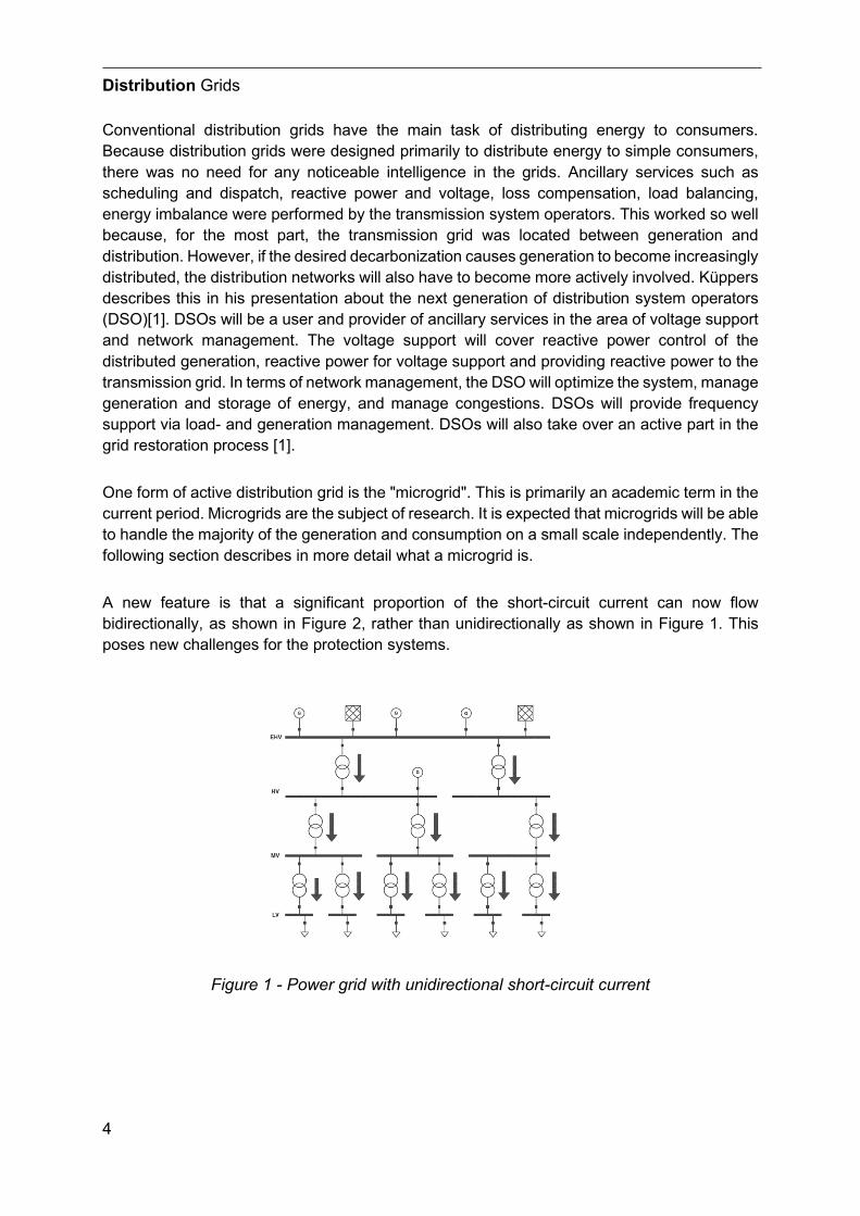
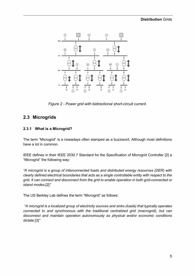
A new feature is that a significant proportion of the short-circuit current can now flow bidirectionally, as shown in Figure 2, rather than unidirectionally as shown in Figure 1. This poses new challenges for the protection systems.
Figure 1 - Power grid with unidirectional short-circuit current
Distribution Grids
5
Figure 2 - Power grid with bidirectional short-circuit current.
2.3 Microgrids
2.3.1 What is a Microgrid?
The term “Microgrid” is a nowadays often stamped as a buzzword. Although most definitions have a lot in common.
IEEE defines in their IEEE 2030.7 Standard for the Specification of Microgrid Controller [2] a “Microgrid” the following way:
“A microgrid is a group of interconnected loads and distributed energy resources (DER) with clearly defined electrical boundaries that acts as a single controllable entity with respect to the grid. It can connect and disconnect from the grid to enable operation in both grid-connected or island modes.[2]”
The US Berkley Lab defines the term “Microgrid” as follows:
“A microgrid is a localized group of electricity sources and sinks (loads) that typically operates connected to and synchronous with the traditional centralized grid (macrogrid), but can disconnect and maintain operation autonomously as physical and/or economic conditions dictate.[3]”
Distribution Grids
6
Li Fusheng defined in his book on microgrids the term as followed:
“A microgrid is a single, controllable, independent power system comprising distributed generation (DG), load, energy storage (ES), and control devices, in which DG and ES are directly connected to the user side in parallel. For the macrogrid, the microgrid can be deemed as a controlled cell; and for the user side, the microgrid can meet its unique demands, for example, less feeder loss and higher local reliability. Being capable of autonomous control, protection, and management, a microgrid can operate either in parallel with the main grid or in an intentional islanded mode.[4]”
Furthermore, he states: “A microgrid can be considered as a small electric power system that incorporates generation, transmission, and distribution, and can achieve power balance and optimal energy allocation over a given area, or as a virtual power source or load in the distribution network […].[4]”
Since the topic is not just present in the academic world, the big players of the energy market also have their definitions.
ABB refers to the term microgrid as “[…] distributed energy resources and loads that can be operated in a controlled, coordinated way; they can be connected to the main power grid, operate in “islanded” mode or be completely off-grid.[5]”
To achieve the microgrid operation ABB states: “The system is controlled through a microgrid controller incorporating demand-response so that demand can be matched to available supply in the safest and most optimized manner.[5]”
The definition by Siemens is congruently: “Microgrids contain all the elements of complex energy systems, they maintain the balance between generation and consumption, and they can operate on and/or off grid. They are ideal for supplying power to remote or poorly developed regions with no connection to a public network.[6]”
“Microgrids use a variety of energy sources, including photovoltaic and wind-power plants as well as small hydro-power and biomass-power plants. Biodiesel generators and emergency power units, storage modules, and intelligent control systems ensure the security of supply.[6]”
Based on the definitions listed above it is safe to say they have a few key characteristics in common:
• A clear separation from the main grid. • Capable of grid-connected and off-grid operation. • Combination of sources and loads. • Controllable (both supply and demand balancing).

Distribution Grids
7
Also, it is noteworthy that there is a special case; the off-grid-only microgrid. These microgrids are always in islanding mode and do not have a point of common coupling (POC) to a macro grid. They are mostly located in the Anglo-American area.
All the participants are also seeing a control entity, the so called “Microgrid Controller”. Control- and protection strategies are performed by this controller. This can be a single device or distributed over the smart devices in the microgrid.
2.3.2 Demarcation to Smart Grids and Virtual Powerplants
“Smart Grids are grids with communication infrastructure like smart meters and intelligent components like load management and a dynamic control of the production, but it does not have to operable self-sufficient.[7]”
This is very similar to the definition of a microgrid, although off-grid operation is not required. So, every microgrid is a smart grid, but not vice-versa.
“A virtual power plant is a system that integrates several types of power sources to give a reliable overall power supply.[8]”
A Virtual Power Plant (VPP) only covers the supply side and is separated from the demand side. Therefore, it is not a microgrid by the definitions in 2.3.1.
Distribution Grids
8
2.3.3 Structure of a microgrid
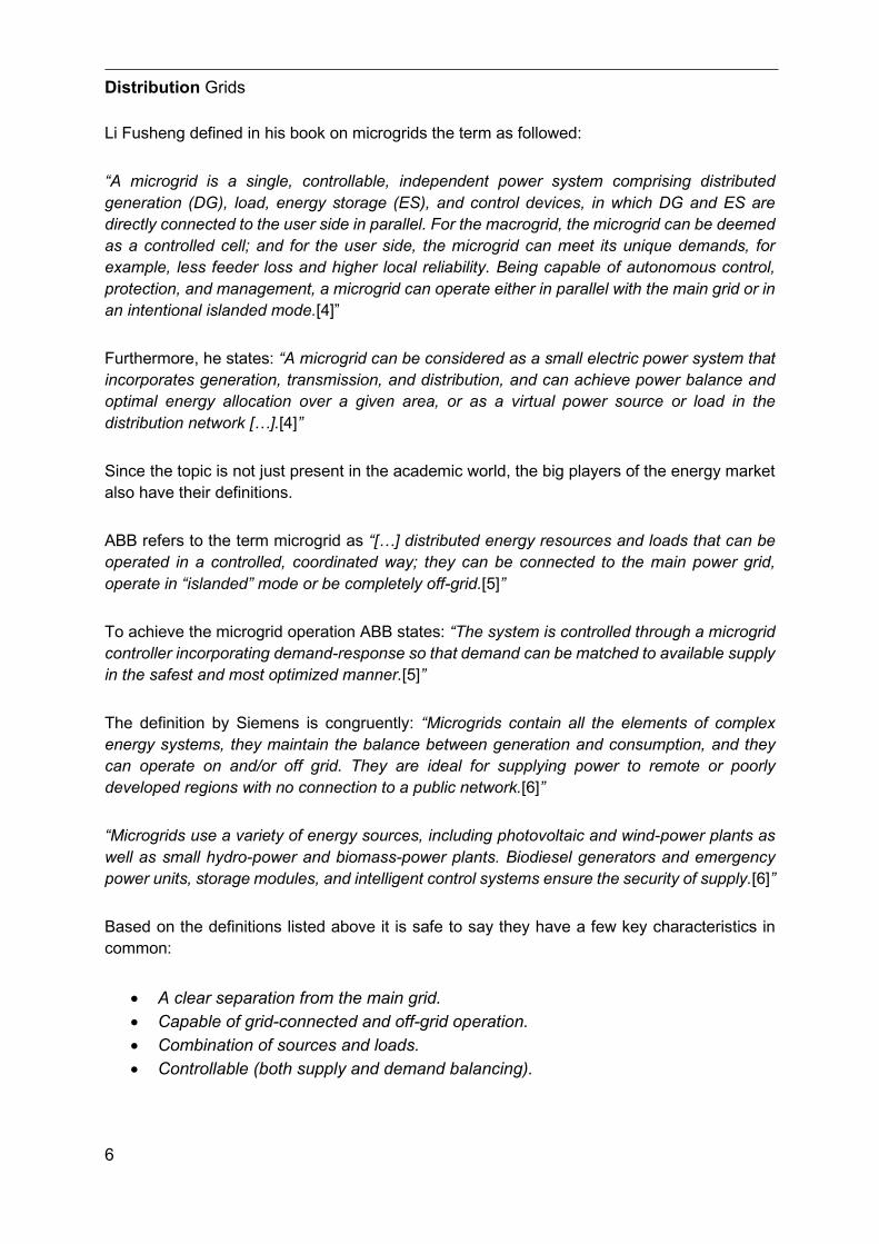
The definitions in 2.3.1 allow a basic anatomic view on microgrids, as seen in Figure 3 - Microgrid Anatomy [9].
Figure 3 - Microgrid Anatomy. Source:” Five minute guide to microgrids”[9]
2.3.3.1 Power generation
The power generation in a microgrid can be categorized according to its predictability. On one side there is the dispatchable power generation. This type of sources can be dispatched freely to the needs of the system, e.g., diesel generators and fuel cells. PV and micro hydro plants are less dispatchable in terms of providing energy to the system, but their behavior is predictable. Furthermore, there are power sources with a lower predictability, or the prediction is not even possible. Wind energy for example is the least predictable renewable energy source. Since the usage of wind energy is very common, microgrids need to adapt to these fluctuations.
2.3.3.2 Loads
The loads also have different behaviors. For example, data centers and life support machinery with a high criticality need to be supplied and must not be cut-off. Heating, cooling, and lighting can be adjusted. Charging of electric vehicles can be planned and adjusted too. Other loads that are not important can even be cut-off completely.
Distribution Grids
9
2.3.3.3 Storage and grid connection
To balance the difference in demand and supply, the system can vary the supply and demand, but also utilize energy storage to regulate the energy balance in the microgrid. Grid connected microgrids can also feed the surplus energy to the grid and if a deficit in the supplied energy is present, or dispatchable loads as diesel generators are only applicable in emergencies, the microgrid can also extract energy from the grid.
2.3.3.4 Point of Common Coupling
Microgrids are connected to the main grid via one connection, the so called “Point of Common Coupling” (PCC, POC) or Point of Interconnection (POI) (P. In IEEE1547 (IEEE Standard for Interconnecting Distributed Resources with Electric Power Systems), IEEE specifies this point for all distributed energy resources (DER).
One switching element connects the microgrid to the main grid. Since microgrids cannot only extract energy from the grid, but also feed into the grid. Microgrids need to be synchronized to the main grid, prior to the transition from off-grid operation to the grid-connected operation.
If the microgrids system nominal voltage differs from the grid voltage, a transformer is also needed. A DC microgrid also needs AC/DC converters to convert between these two domains.
2.3.4 Control element
According to the IEC standard 2030.7 [2] the following elements are included in the control element:
• “Microgrid control system - The microgrid local controller is a decision-making software and/or hardware of the microgrid. The scheduling of microgrid DER in grid-connected and islanded modes is performed by the controller based on economic and reliability considerations. Microgrid controller determines the microgrid interaction with the utility grid, the decision to switch between grid connected and islanded modes, frequency regulation and voltage control, and optimal operation of local resources. It also provides any decisions on load curtailment/shifting.
• Additional sensor, communication, and control elements—These include smart switches, communications networks, etc.[2]”
The microgrid control system can be implemented in different ways:
Centralized control: “This kind of control is performed by a single central controller, which requires an extensive communication system between the central controller and controlled units. All control decisions and signals are made by the central controller. Under centralized

Distribution Grids
10
control, one (or a group of) master DER can act as a synchronous generator with adjustable capacity for voltage and frequency regulation.[10]”
Decentralized control: “This kind of control is accomplished by the local controller at each individual controllable unit, which only receives information from locally measured data, such as system parameters (e.g. voltage and frequency), and uses the principle of self-regulation.[10]“
According to Hatziargyriou [11] the combination of centralized and decentralized control structures leads to a new classification, the “Hierarchical Control”
Distribution Grids
11
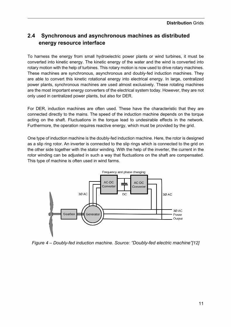
2.4 Synchronous and asynchronous machines as distributed energy resource interface
To harness the energy from small hydroelectric power plants or wind turbines, it must be converted into kinetic energy. The kinetic energy of the water and the wind is converted into rotary motion with the help of turbines. This rotary motion is now used to drive rotary machines. These machines are synchronous, asynchronous and doubly-fed induction machines. They are able to convert this kinetic rotational energy into electrical energy. In large, centralized power plants, synchronous machines are used almost exclusively. These rotating machines are the most important energy converters of the electrical system today. However, they are not only used in centralized power plants, but also for DER.
For DER, induction machines are often used. These have the characteristic that they are connected directly to the mains. The speed of the induction machine depends on the torque acting on the shaft. Fluctuations in the torque lead to undesirable effects in the network. Furthermore, the operation requires reactive energy, which must be provided by the grid.
One type of induction machine is the doubly-fed induction machine. Here, the rotor is designed as a slip ring rotor. An inverter is connected to the slip rings which is connected to the grid on the other side together with the stator winding. With the help of the inverter, the current in the rotor winding can be adjusted in such a way that fluctuations on the shaft are compensated. This type of machine is often used in wind farms.
Figure 4 – Doubly-fed induction machine. Source: “Doubly-fed electric machine”[12]

Distribution Grids
12
2.5 Inverter as distributed energy resource interface
2.5.1 Power Inverter Basics
In order to integrate energy sources into the grid that generate power as direct current, such as for example solar cells, devices must be used that convert the direct current into grid-compatible alternating current. This can be achieved in several ways, one of which is converting it using semiconductor-based inverters.
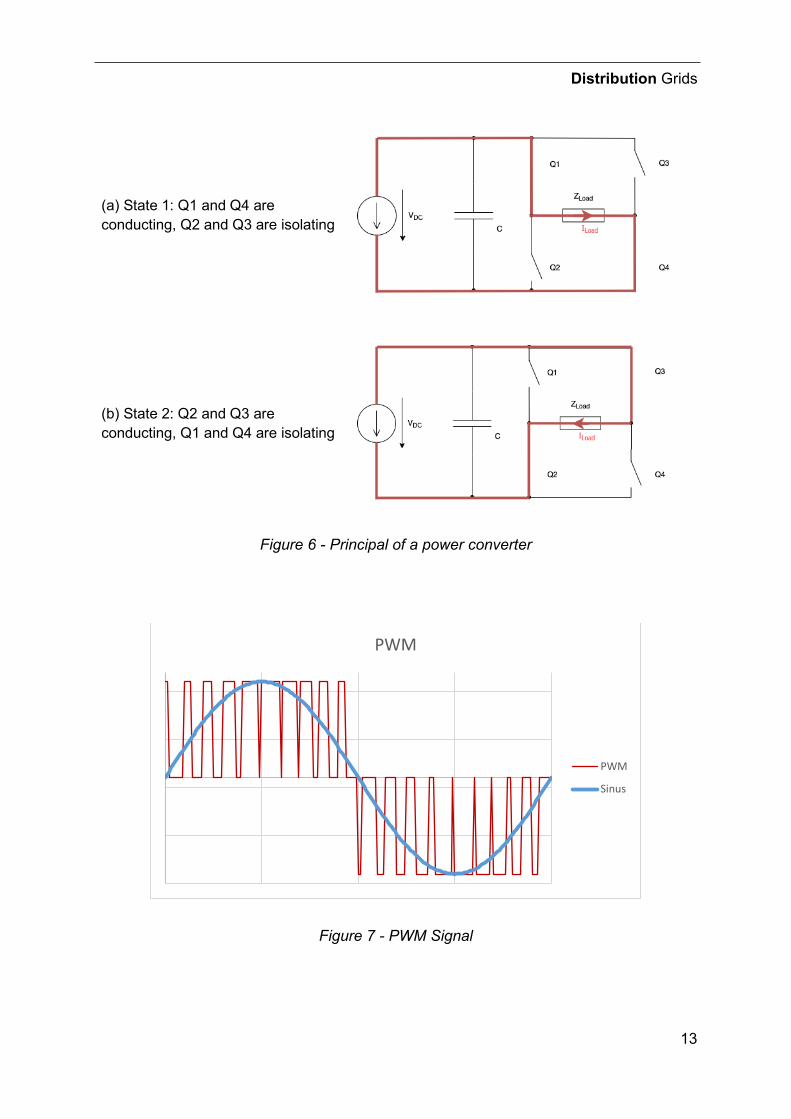
In inverters the direct voltage from the source is converted using electronic switches such as thyristors, field effect transistors (FET) or bipolar junction transistors (BJT). Figure 5 - Single phase inverter shows a schematic diagram of a single-phase inverter. This corresponds to an H-bridge.
Figure 5 - Single phase inverter
Figure 6 shows the two operating states of an inverter. In State 1 the switches Q1 and Q4 are conducting and Q3 and Q2 are isolating. In Figure 6 (a) it can be seen, that the current 𝐼𝐼𝐿𝐿𝐿𝐿𝐿𝐿𝐿𝐿 flows from the left side of the load to the right side. In Figure 6 (b) the current flows from the right side of the load to the left side. By alternating between these two states, an AC current is generated. However, the waveform does not correspond to a pure sinusoidal signal. Therefore, the output current is smoothed by a filter. Furthermore, the switches can be controlled with a pulse width modulation (PWM) signal, which can control the amplitude, as shown in Figure 7.
Q1 Q3
Q4Q2
ZLoad
CVDC
Distribution Grids
13
(a) State 1: Q1 and Q4 are conducting, Q2 and Q3 are isolating
(b) State 2: Q2 and Q3 are conducting, Q1 and Q4 are isolating
Figure 6 - Principal of a power converter
Figure 7 - PWM Signal
PWM
PWM
Sinus
Distribution Grids
14
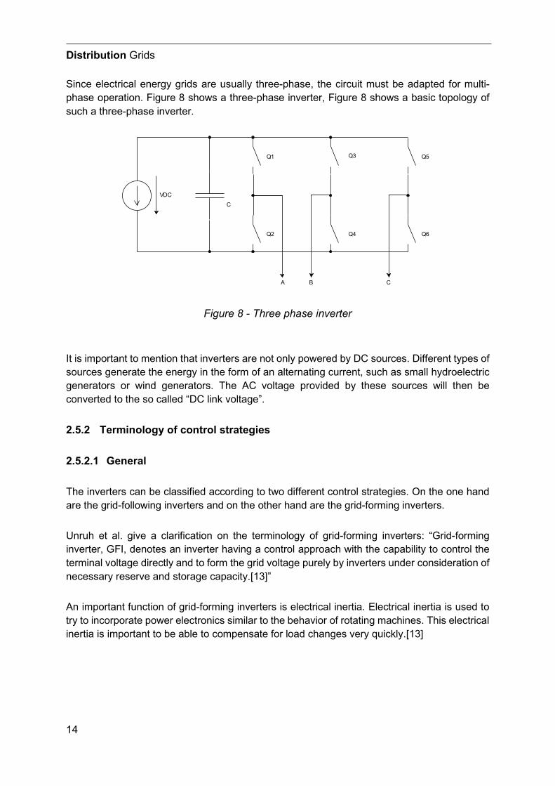
Since electrical energy grids are usually three-phase, the circuit must be adapted for multi-phase operation. Figure 8 shows a three-phase inverter, Figure 8 shows a basic topology of such a three-phase inverter.
Figure 8 - Three phase inverter
It is important to mention that inverters are not only powered by DC sources. Different types of sources generate the energy in the form of an alternating current, such as small hydroelectric generators or wind generators. The AC voltage provided by these sources will then be converted to the so called “DC link voltage”.
2.5.2 Terminology of control strategies
2.5.2.1 General
The inverters can be classified according to two different control strategies. On the one hand are the grid-following inverters and on the other hand are the grid-forming inverters.
Unruh et al. give a clarification on the terminology of grid-forming inverters: “Grid-forming inverter, GFI, denotes an inverter having a control approach with the capability to control the terminal voltage directly and to form the grid voltage purely by inverters under consideration of necessary reserve and storage capacity.[13]”
An important function of grid-forming inverters is electrical inertia. Electrical inertia is used to try to incorporate power electronics similar to the behavior of rotating machines. This electrical inertia is important to be able to compensate for load changes very quickly.[13]
Q1 Q3
Q4Q2
CVDC
Q5
Q6
A B C
Distribution Grids
15
2.5.2.2 Control methods of a grid-forming inverter
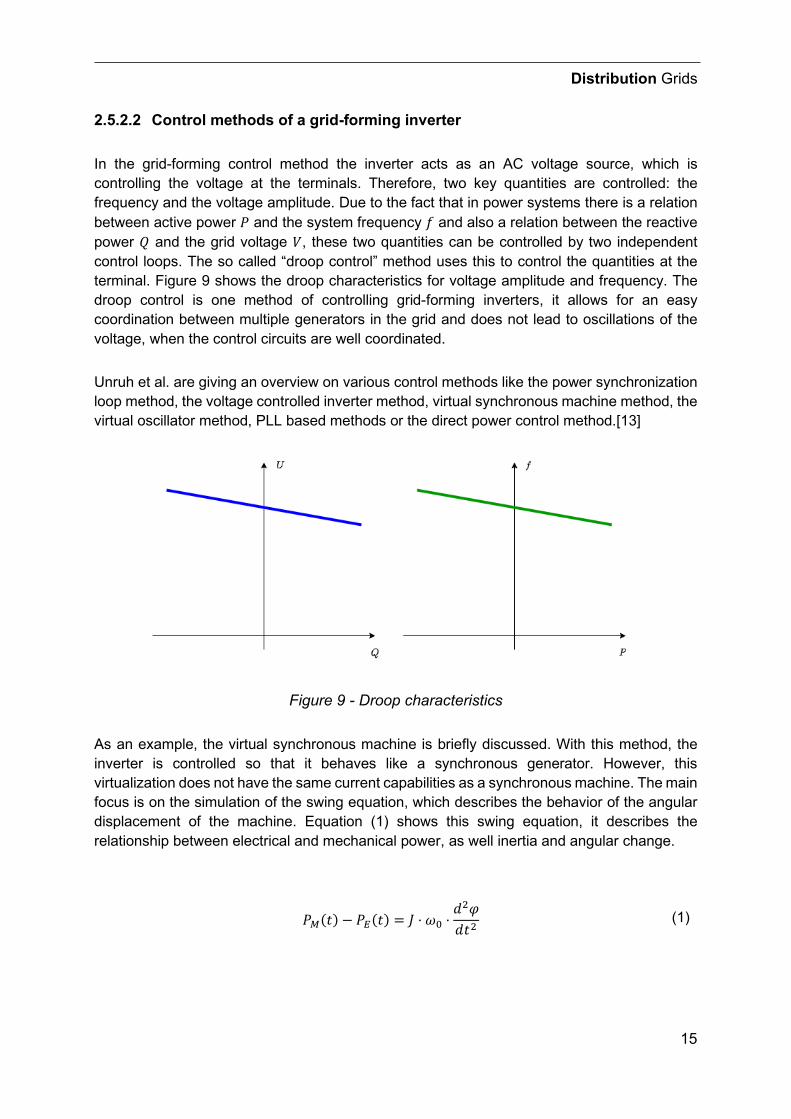
In the grid-forming control method the inverter acts as an AC voltage source, which is controlling the voltage at the terminals. Therefore, two key quantities are controlled: the frequency and the voltage amplitude. Due to the fact that in power systems there is a relation between active power 𝑃𝑃 and the system frequency 𝑓𝑓 and also a relation between the reactive power 𝑄𝑄 and the grid voltage 𝑉𝑉, these two quantities can be controlled by two independent control loops. The so called “droop control” method uses this to control the quantities at the terminal. Figure 9 shows the droop characteristics for voltage amplitude and frequency. The droop control is one method of controlling grid-forming inverters, it allows for an easy coordination between multiple generators in the grid and does not lead to oscillations of the voltage, when the control circuits are well coordinated.
Unruh et al. are giving an overview on various control methods like the power synchronization loop method, the voltage controlled inverter method, virtual synchronous machine method, the virtual oscillator method, PLL based methods or the direct power control method.[13]
Figure 9 - Droop characteristics
As an example, the virtual synchronous machine is briefly discussed. With this method, the inverter is controlled so that it behaves like a synchronous generator. However, this virtualization does not have the same current capabilities as a synchronous machine. The main focus is on the simulation of the swing equation, which describes the behavior of the angular displacement of the machine. Equation (1) shows this swing equation, it describes the relationship between electrical and mechanical power, as well inertia and angular change.
𝑃𝑃𝑀𝑀(𝑡𝑡) − 𝑃𝑃𝐸𝐸(𝑡𝑡) = 𝐽𝐽 ⋅ 𝜔𝜔0 ⋅
𝑑𝑑2𝜑𝜑𝑑𝑑𝑡𝑡2
(1)
Distribution Grids
16
The control now works in such a way that the swing equation of a previously defined machine is reproduced. The advantage of this method is that the fault behavior of synchronous machines has been researched for a very long time and is well understood by electrical engineers.
2.5.3 Fault current contribution
J. Keller and B. Kroposki describe the behavior of a DER that interfaces the grid via an inverter as followed: “Inverters do not dynamically behave the same as synchronous or induction machines. Inverters do not have a rotating mass component; therefore, they do not develop inertia to carry fault current based on an electro-magnetic characteristic. Power electronic inverters have a much faster decaying envelope for fault currents because the devices lack predominately inductive characteristics that are associated with rotating machines. These characteristics dictate the time constants involved with the circuit. Inverters also can be controlled in a manner unlike rotating machines because they can be programmed to vary the length of time it takes them to respond to fault conditions. This will also impact the fault current characteristics of the inverter.[14]”
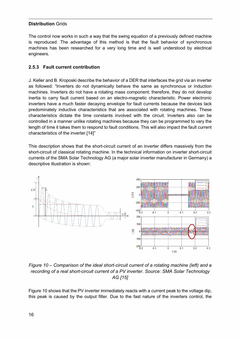
This description shows that the short-circuit current of an inverter differs massively from the short-circuit of classical rotating machine. In the technical information on inverter short-circuit currents of the SMA Solar Technology AG (a major solar inverter manufacturer in Germany) a descriptive illustration is shown:
Figure 10 – Comparison of the ideal short-circuit current of a rotating machine (left) and a recording of a real short-circuit current of a PV inverter. Source: SMA Solar Technology
AG [15]
Figure 10 shows that the PV inverter immediately reacts with a current peak to the voltage dip, this peak is caused by the output filter. Due to the fast nature of the inverters control, the
Distribution Grids
17
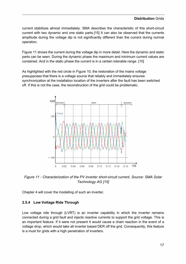
current stabilizes almost immediately. SMA describes the characteristic of this short-circuit current with two dynamic and one static parts.[15] It can also be observed that the currents amplitude during the voltage dip is not significantly different than the current during normal operation.
Figure 11 shows the current during the voltage dip in more detail. Here the dynamic and static parts can be seen. During the dynamic phase the maximum and minimum current values are contained. And in the static phase the current is in a certain tolerable range. [15]
As highlighted with the red circle in Figure 10, the restoration of the mains voltage presupposes that there is a voltage source that reliably and immediately ensures synchronization at the installation location of the inverters after the fault has been switched off. If this is not the case, the reconstruction of the grid could be problematic.
Figure 11 - Characterization of the PV inverter short-circuit current. Source: SMA Solar Technology AG [15]
Chapter 4 will cover the modelling of such an inverter.
2.5.4 Low Voltage Ride Through
Low voltage ride through (LVRT) is an inverter capability in which the inverter remains connected during a grid fault and injects reactive currents to support the grid voltage. This is an important feature. If it were not present it would cause a chain reaction in the event of a voltage drop, which would take all inverter based DER off the grid. Consequently, this feature is a must for grids with a high penetration of inverters.
Distribution Grids
18
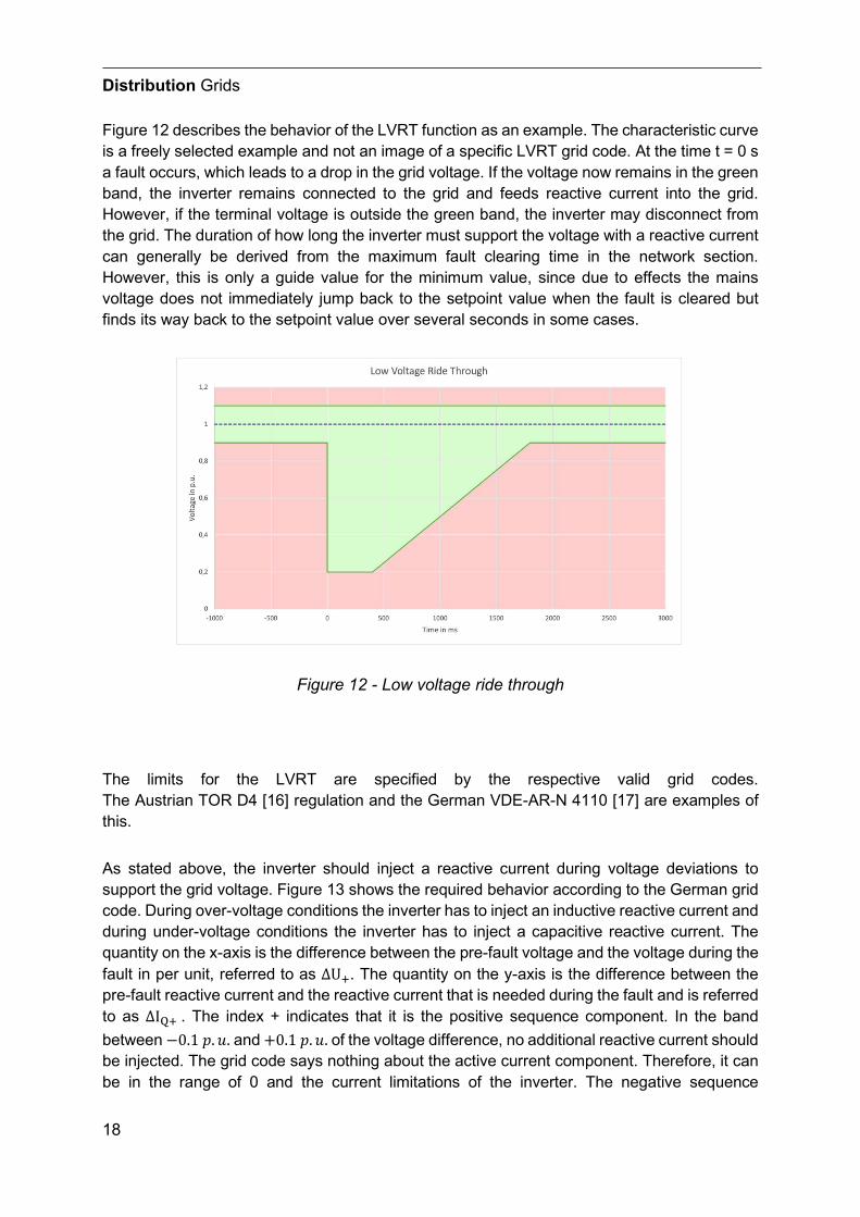
Figure 12 describes the behavior of the LVRT function as an example. The characteristic curve is a freely selected example and not an image of a specific LVRT grid code. At the time t = 0 s a fault occurs, which leads to a drop in the grid voltage. If the voltage now remains in the green band, the inverter remains connected to the grid and feeds reactive current into the grid. However, if the terminal voltage is outside the green band, the inverter may disconnect from the grid. The duration of how long the inverter must support the voltage with a reactive current can generally be derived from the maximum fault clearing time in the network section. However, this is only a guide value for the minimum value, since due to effects the mains voltage does not immediately jump back to the setpoint value when the fault is cleared but finds its way back to the setpoint value over several seconds in some cases.
Figure 12 - Low voltage ride through
The limits for the LVRT are specified by the respective valid grid codes. The Austrian TOR D4 [16] regulation and the German VDE-AR-N 4110 [17] are examples of this.
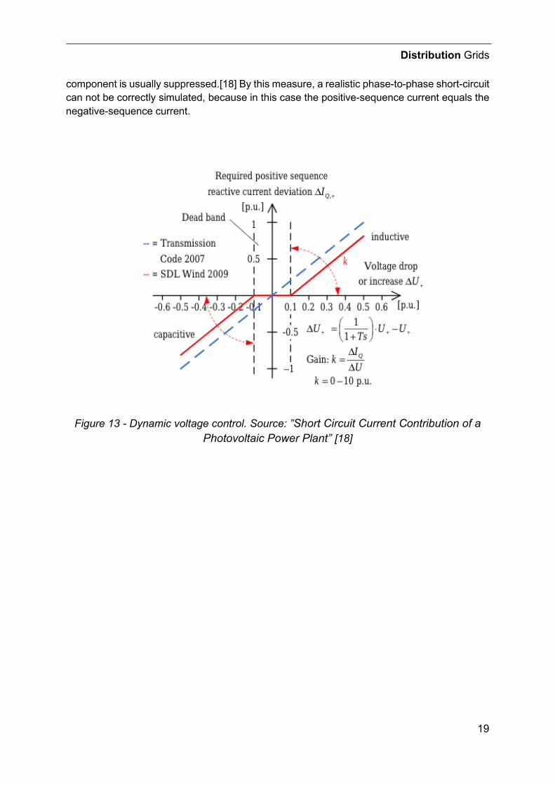
As stated above, the inverter should inject a reactive current during voltage deviations to support the grid voltage. Figure 13 shows the required behavior according to the German grid code. During over-voltage conditions the inverter has to inject an inductive reactive current and during under-voltage conditions the inverter has to inject a capacitive reactive current. The quantity on the x-axis is the difference between the pre-fault voltage and the voltage during the fault in per unit, referred to as ΔU+. The quantity on the y-axis is the difference between the pre-fault reactive current and the reactive current that is needed during the fault and is referred to as ΔIQ+ . The index + indicates that it is the positive sequence component. In the band between −0.1 𝑝𝑝.𝑢𝑢. and +0.1 𝑝𝑝.𝑢𝑢. of the voltage difference, no additional reactive current should be injected. The grid code says nothing about the active current component. Therefore, it can be in the range of 0 and the current limitations of the inverter. The negative sequence
Distribution Grids
19
component is usually suppressed.[18] By this measure, a realistic phase-to-phase short-circuit can not be correctly simulated, because in this case the positive-sequence current equals the negative-sequence current.
Figure 13 - Dynamic voltage control. Source: ”Short Circuit Current Contribution of a Photovoltaic Power Plant” [18]

Distribution Grids
20
Protection of Distribution Grids
21
3 Protection of Distribution Grids
3.1 Protection in distribution grids
The task of the power system protection is to detect faulty conditions in the grid and to take appropriate measures to eliminate the fault condition. Power system protection cannot prevent the occurrence of faults, but it can keep the effects as low as possible. The core of the whole is an efficient and fast detection of the fault.
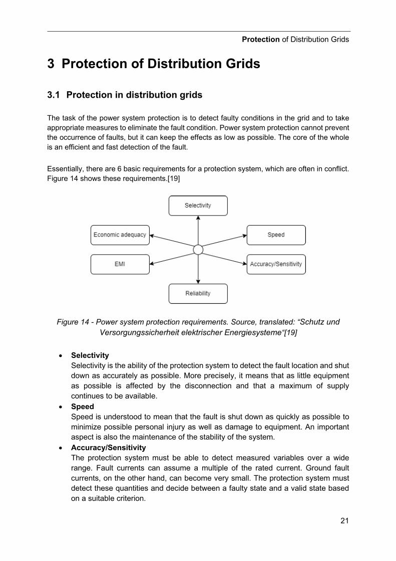
Essentially, there are 6 basic requirements for a protection system, which are often in conflict. Figure 14 shows these requirements.[19]
Figure 14 - Power system protection requirements. Source, translated: “Schutz und Versorgungssicherheit elektrischer Energiesysteme“[19]
• Selectivity Selectivity is the ability of the protection system to detect the fault location and shut down as accurately as possible. More precisely, it means that as little equipment as possible is affected by the disconnection and that a maximum of supply continues to be available.
• Speed Speed is understood to mean that the fault is shut down as quickly as possible to minimize possible personal injury as well as damage to equipment. An important aspect is also the maintenance of the stability of the system.
• Accuracy/Sensitivity The protection system must be able to detect measured variables over a wide range. Fault currents can assume a multiple of the rated current. Ground fault currents, on the other hand, can become very small. The protection system must detect these quantities and decide between a faulty state and a valid state based on a suitable criterion.
Protection of Distribution Grids
22
• Reliability The protection system must be reliable since a great deal depends on it. The entire protection chain consisting of transducer, protection device and circuit breaker must function.
• EMI The protection system must be able to withstand electromagnetic interference. The high voltage equipment can generate very strong electro-magnetic fields, which can cause interference in electronic equipment. The protection system must be protected from these fields.
• Economic adequacy Economic expenses for the protection system must be reasonable compared to the expected failures and damages. Part of these expenses are, among others, the acquisition costs and maintenance costs. Furthermore, it must be mentioned that especially in industrial networks it must be considered that supply failures are very expensive.
With increasing digitalization and greater networking in terms of the IT device, cyber-security is also increasingly coming into focus and becoming more relevant.
In distribution networks the economic factor is extremely important. This is a very price sensitive environment. The number of protection devices in distribution networks is very large, because the network has a large extension. Not only the purchase of protection devices is a cost driver, especially the maintenance costs a lot. After commissioning, the protective devices are regularly checked for functionality. This is very labor-intensive and therefore associated with high costs.
Outages of elements in the distribution network, like lines or transformers, are not as critical as in the transmission network because fewer customers are affected in the event of an outage. Consequently, the formal criteria are not as strict as in the transmission network. This, together with cost pressures, means that the protection functions chosen in the distribution network are of low complexity, and simpler implementations are often used.
3.2 Protection in Microgrids
Microgrids are used in a wide variety of applications, such as remote locations, hospitals, data centers, industrial parks or even for ordinary residential areas. Depending on the area of application, there are different requirements for such a microgrid. In a residential area, for example, the focus is on the low-cost use of energy, whereas in hospitals or data centers a very high level of reliability is paramount. Different requirements for the microgrid also lead to different expectations for the installed protection system. Special prerequisites in the microgrid pose challenges for the protection system. If there is a high percentage of DER with inverter-based feed in the microgrid, then there is not much inertia in the system. The effects or benefits of sufficient inertia in the system have already been discussed in chapter 2.5.3. However, as
Protection of Distribution Grids
23
already mentioned, there are microgrids in which the environmental concern is not paramount, but the requirement for reliability is. In such microgrids, sufficient inertia may well be present. This means that the initial situation for the protection system is different.
Microgrids are for the most part still academic in nature. And therefore, often used as a playground for novel protection concepts. However, this does not mean that only experimental protection is used in already existing microgrids.
Shiles et. al. are giving an overview on the protection methods used in microgrids in North America.[20]
The microgrid in Boston Bar, Canada, can be used as an example. “The Boston Bar microgrid consists of three 25 kV radial feeders that are supplied by a 69 kV substation through a 69 kV 125 kV transformer. The microgrid includes two 4.32 MVA hydro power generators with islanding capability, which are connected to one of the feeders with a peak load of 3MW”.[20] Here, overcurrent protection is used. However, the protection settings in island mode are adjusted according to the situation, using a set of parameters calculated in advance. Special measures are also taken to increase the fault current in the event of a fault in order to simplify fault localization. Circuit breaker positions are sent with the aid of communication devices to select the appropriate protection settings. The feeders are divided into sections so that the supply can be gradually restored.[21]
Another interesting micro grid is the microgrid from the Illinois Institute of Technology (IIT). “The IIT microgrid with a peak load of 12 MW embeds a variety of DERs including 8 MW natural gas turbine, 300 kW PV system, 5 kW wind generation, 500 kWh flow battery, and 4 MW backup generation. […] the micro grid is fed through two substations (i.e., north substation and south substation) to ensure seamless operation of the system if one of the feeders fails. Both substations are supplied by 12.47 kV / 4.16 kV transformers equipped with proper protective devices.[20]”
The protection system consists of a multi-hierarchical approach. Ordinary OC for the protection towards the loads, differential protection for the feeder loops, and OC protection with adaptive parameters at the feeder bays. Furthermore, there is protection at the power transformers, which also protects against faults in the higher-level network.[22]
Another approach is centralized protection of the microgrid. A central protection device collects distributed information from the protection devices and DER distributed in the microgrid and uses it to make a central decision on whether to trip a circuit breaker. This requires extensive communication. Such a system is proposed by Ustun et. al.[23]
Li et. al. describe the protection system of the campus microgrid of Beijing Jiaotong University. The microgrid is one that was built around the Faculty of Electrical Engineering. It is a 0.4 kV microgrid consisting of car charging stations, 20 kWp photovoltaic feed-in, a 500 kWh battery storage, various loads, and a feed-in power transformer that feeds the microgrid in grid-
Protection of Distribution Grids
24
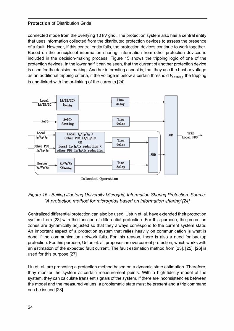
connected mode from the overlying 10 kV grid. The protection system also has a central entity that uses information collected from the distributed protection devices to assess the presence of a fault. However, if this central entity fails, the protection devices continue to work together. Based on the principle of information sharing, information from other protection devices is included in the decision-making process. Figure 15 shows the tripping logic of one of the protection devices. In the lower half it can be seen, that the current of another protection device is used for the decision making. Another interesting aspect is, that they use the busbar voltage as an additional tripping criteria, if the voltage is below a certain threshold 𝑉𝑉𝑆𝑆𝑆𝑆𝑆𝑆𝑆𝑆𝑆𝑆𝑆𝑆𝑆𝑆 the tripping is and-linked with the or-linking of the currents.[24]
Figure 15 - Beijing Jiaotong University Microgrid, Information Sharing Protection. Source: “A protection method for microgrids based on information sharing“[24]
Centralized differential protection can also be used. Ustun et. al. have extended their protection system from [23] with the function of differential protection. For this purpose, the protection zones are dynamically adjusted so that they always correspond to the current system state. An important aspect of a protection system that relies heavily on communication is what is done if the communication network fails. For this reason, there is also a need for backup protection. For this purpose, Ustun et. al. proposes an overcurrent protection, which works with an estimation of the expected fault current. The fault estimation method from [23], [25], [26] is used for this purpose.[27]
Liu et. al. are proposing a protection method based on a dynamic state estimation. Therefore, they monitor the system at certain measurement points. With a high-fidelity model of the system, they can calculate transient signals of the system. If there are inconsistencies between the model and the measured values, a problematic state must be present and a trip command can be issued.[28]
Protection of Distribution Grids
25
As can be seen from the examples given, a wide variety of principles and methods are applied. Often central units are used to evaluate the distributed information. But also, variations of conventional relays are used.
Protection of Distribution Grids
26
3.3 Protection fundamentals
3.3.1 Time-Overcurrent protection
The time-overcurrent protection is the most used protection principle, although its implementation can differ. For example, ordinary fuses and miniature circuit breakers work on this principle.
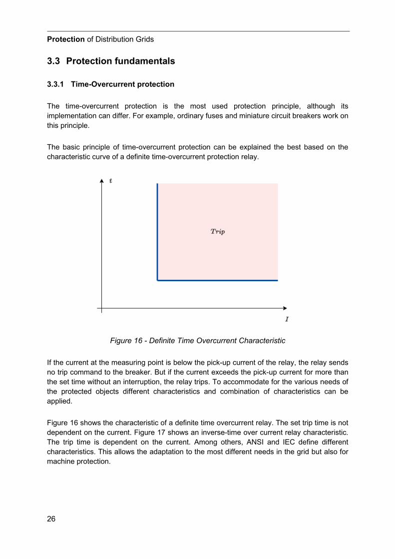
The basic principle of time-overcurrent protection can be explained the best based on the characteristic curve of a definite time-overcurrent protection relay.
Figure 16 - Definite Time Overcurrent Characteristic
If the current at the measuring point is below the pick-up current of the relay, the relay sends no trip command to the breaker. But if the current exceeds the pick-up current for more than the set time without an interruption, the relay trips. To accommodate for the various needs of the protected objects different characteristics and combination of characteristics can be applied.
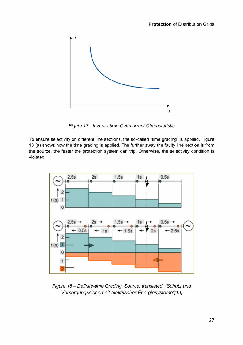
Figure 16 shows the characteristic of a definite time overcurrent relay. The set trip time is not dependent on the current. Figure 17 shows an inverse-time over current relay characteristic. The trip time is dependent on the current. Among others, ANSI and IEC define different characteristics. This allows the adaptation to the most different needs in the grid but also for machine protection.
Protection of Distribution Grids
27
Figure 17 - Inverse-time Overcurrent Characteristic
To ensure selectivity on different line sections, the so-called “time grading” is applied. Figure 18 (a) shows how the time grading is applied. The further away the faulty line section is from the source, the faster the protection system can trip. Otherwise, the selectivity condition is violated.
Figure 18 – Definite-time Grading. Source, translated: “Schutz und Versorgungssicherheit elektrischer Energiesysteme“[19]
Protection of Distribution Grids
28
The overcurrent criterion can also be combined with a directional criterion. This allows for directional dependent trip times. To get the information on the direction of the fault, it is necessary to measure the voltage and compare the phase angles between the respective voltages and currents.
3.3.2 Distance protection
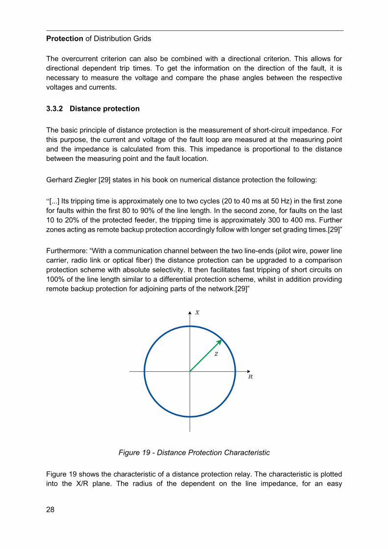
The basic principle of distance protection is the measurement of short-circuit impedance. For this purpose, the current and voltage of the fault loop are measured at the measuring point and the impedance is calculated from this. This impedance is proportional to the distance between the measuring point and the fault location.
Gerhard Ziegler [29] states in his book on numerical distance protection the following:
“[...] Its tripping time is approximately one to two cycles (20 to 40 ms at 50 Hz) in the first zone for faults within the first 80 to 90% of the line length. In the second zone, for faults on the last 10 to 20% of the protected feeder, the tripping time is approximately 300 to 400 ms. Further zones acting as remote backup protection accordingly follow with longer set grading times.[29]”
Furthermore: “With a communication channel between the two line-ends (pilot wire, power line carrier, radio link or optical fiber) the distance protection can be upgraded to a comparison protection scheme with absolute selectivity. It then facilitates fast tripping of short circuits on 100% of the line length similar to a differential protection scheme, whilst in addition providing remote backup protection for adjoining parts of the network.[29]”
Figure 19 - Distance Protection Characteristic
Figure 19 shows the characteristic of a distance protection relay. The characteristic is plotted into the X/R plane. The radius of the dependent on the line impedance, for an easy
Protection of Distribution Grids
29
understanding it can be assumed that the radius of the circle is equal to the absolute value of the line impedance. If the measured Impedance is outside of the red circle, the system is in its regular operation area. If the measured impedance is inside the red circle, a fault on the line must be present.
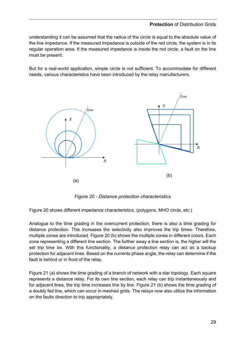
But for a real-world application, simple circle is not sufficient. To accommodate for different needs, various characteristics have been introduced by the relay manufacturers.
(a)
(b)
Figure 20 - Distance protection characteristics
Figure 20 shows different impedance characteristics, (polygons, MHO circle, etc.)
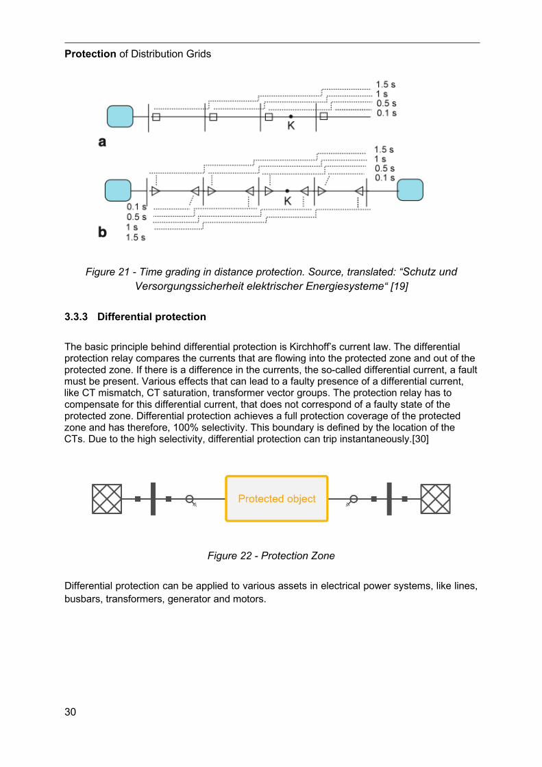
Analogue to the time grading in the overcurrent protection, there is also a time grading for distance protection. This increases the selectivity also improves the trip times. Therefore, multiple zones are introduced. Figure 20 (b) shows the multiple zones in different colors. Each zone representing a different line section. The further away a line section is, the higher will the set trip time be. With this functionality, a distance protection relay can act as a backup protection for adjacent lines. Based on the currents phase angle, the relay can determine if the fault is behind or in front of the relay.
Figure 21 (a) shows the time grading of a branch of network with a star topology. Each square represents a distance relay. For its own line section, each relay can trip instantaneously and for adjacent lines, the trip time increases line by line. Figure 21 (b) shows the time grading of a doubly fed line, which can occur in meshed grids. The relays now also utilize the information on the faults direction to trip appropriately.
Protection of Distribution Grids
30
Figure 21 - Time grading in distance protection. Source, translated: “Schutz und Versorgungssicherheit elektrischer Energiesysteme“ [19]
3.3.3 Differential protection
The basic principle behind differential protection is Kirchhoff’s current law. The differential protection relay compares the currents that are flowing into the protected zone and out of the protected zone. If there is a difference in the currents, the so-called differential current, a fault must be present. Various effects that can lead to a faulty presence of a differential current, like CT mismatch, CT saturation, transformer vector groups. The protection relay has to compensate for this differential current, that does not correspond of a faulty state of the protected zone. Differential protection achieves a full protection coverage of the protected zone and has therefore, 100% selectivity. This boundary is defined by the location of the CTs. Due to the high selectivity, differential protection can trip instantaneously.[30]
Figure 22 - Protection Zone
Differential protection can be applied to various assets in electrical power systems, like lines, busbars, transformers, generator and motors.
Protection of Distribution Grids
31
3.4 Voltage restrained/controlled overcurrent in Distribution grids
3.4.1 General
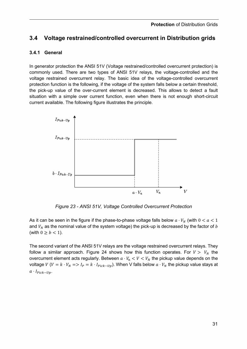
In generator protection the ANSI 51V (Voltage restrained/controlled overcurrent protection) is commonly used. There are two types of ANSI 51V relays, the voltage-controlled and the voltage restrained overcurrent relay. The basic idea of the voltage-controlled overcurrent protection function is the following, if the voltage of the system falls below a certain threshold, the pick-up value of the over-current element is decreased. This allows to detect a fault situation with a simple over current function, even when there is not enough short-circuit current available. The following figure illustrates the principle.
Figure 23 - ANSI 51V, Voltage Controlled Overcurrent Protection
As it can be seen in the figure if the phase-to-phase voltage falls below 𝑎𝑎 ⋅ 𝑉𝑉𝑁𝑁 (with 0 < 𝑎𝑎 < 1 and 𝑉𝑉𝑁𝑁 as the nominal value of the system voltage) the pick-up is decreased by the factor of 𝑏𝑏 (with 0 ≥ 𝑏𝑏 < 1).
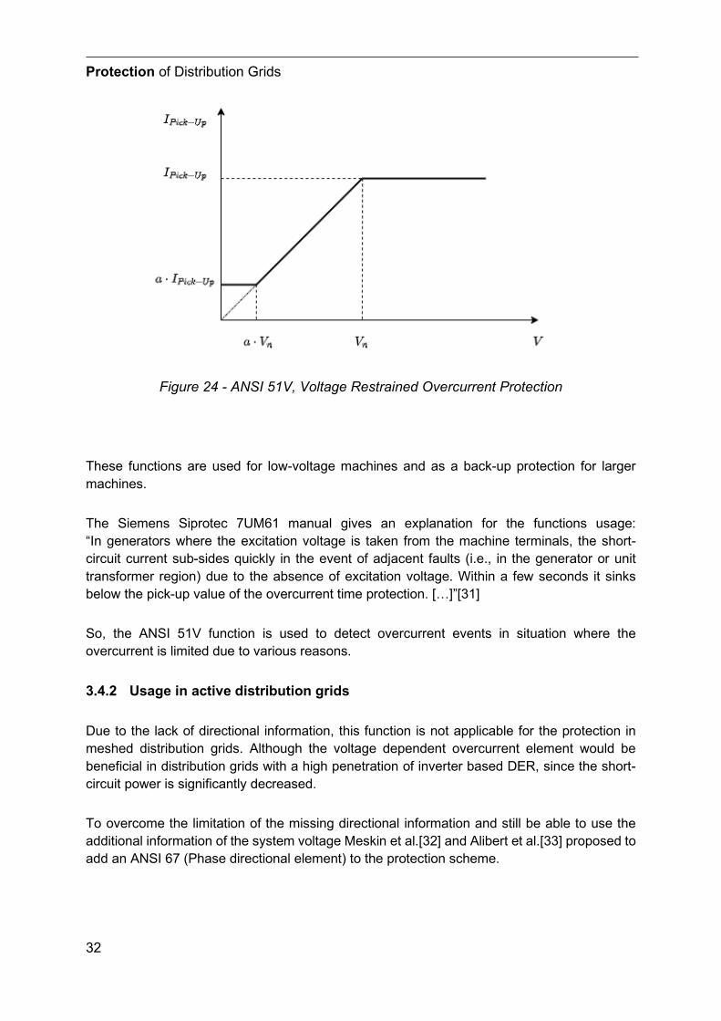
The second variant of the ANSI 51V relays are the voltage restrained overcurrent relays. They follow a similar approach. Figure 24 shows how this function operates. For 𝑉𝑉 > 𝑉𝑉𝑁𝑁 the overcurrent element acts regularly. Between 𝑎𝑎 ⋅ 𝑉𝑉𝑆𝑆 < 𝑉𝑉 < 𝑉𝑉𝑁𝑁 the pickup value depends on the voltage 𝑉𝑉 (𝑉𝑉 = 𝑘𝑘 ⋅ 𝑉𝑉𝑁𝑁 => 𝐼𝐼𝑃𝑃 = 𝑘𝑘 ⋅ 𝐼𝐼𝑃𝑃𝑆𝑆𝑃𝑃𝑃𝑃−𝑈𝑈𝑈𝑈). When V falls below 𝑎𝑎 ⋅ 𝑉𝑉𝑁𝑁 the pickup value stays at 𝑎𝑎 ⋅ 𝐼𝐼𝑃𝑃𝑆𝑆𝑃𝑃𝑃𝑃−𝑈𝑈𝑈𝑈.
Protection of Distribution Grids
32
Figure 24 - ANSI 51V, Voltage Restrained Overcurrent Protection
These functions are used for low-voltage machines and as a back-up protection for larger machines.
The Siemens Siprotec 7UM61 manual gives an explanation for the functions usage: “In generators where the excitation voltage is taken from the machine terminals, the short-circuit current sub-sides quickly in the event of adjacent faults (i.e., in the generator or unit transformer region) due to the absence of excitation voltage. Within a few seconds it sinks below the pick-up value of the overcurrent time protection. […]”[31]
So, the ANSI 51V function is used to detect overcurrent events in situation where the overcurrent is limited due to various reasons.
3.4.2 Usage in active distribution grids
Due to the lack of directional information, this function is not applicable for the protection in meshed distribution grids. Although the voltage dependent overcurrent element would be beneficial in distribution grids with a high penetration of inverter based DER, since the short-circuit power is significantly decreased.
To overcome the limitation of the missing directional information and still be able to use the additional information of the system voltage Meskin et al.[32] and Alibert et al.[33] proposed to add an ANSI 67 (Phase directional element) to the protection scheme.
Protection of Distribution Grids
33
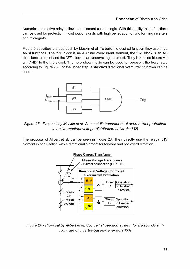
Numerical protective relays allow to implement custom logic. With this ability these functions can be used for protection in distributions grids with high penetration of grid forming inverters and microgrids.
Figure 5 describes the approach by Meskin et al. To build the desired function they use three ANSI functions. The “51” block is an AC time overcurrent element, the “67” block is an AC directional element and the “27” block is an undervoltage element. They link these blocks via an “AND” to the trip signal. The here shown logic can be used to represent the lower step according to Figure 23. For the upper step, a standard directional overcurrent function can be used.
Figure 25 - Proposal by Meskin et al. Source:” Enhancement of overcurrent protection in active medium voltage distribution networks”[32]
The proposal of Alibert et al. can be seen in Figure 26. They directly use the relay’s 51V element in conjunction with a directional element for forward and backward direction.
Figure 26 - Proposal by Alibert et al. Source:” Protection system for microgrids with high rate of inverter-based-generators”[33]

Protection of Distribution Grids
34
Inverter Modelling
35
4 Inverter Modelling
4.1 General
The modeling of an inverter depends on the application of the simulation. Some simulation applications expect a very deep level of detail, while for others a less detailed replica is sufficient. For an accurate analysis of the harmonics, the simulation of the semiconductor switching elements is also necessary, for stability studies the control loops are relevant. For load flow calculations, a less detailed model is sufficient. The work of Yamashita et. al. provides an overview of this. In their article "Industrial Recommendation of Modeling of Inverter-Based Generators for Power System Dynamic Studies With Focus on Photovoltaic" [34] they elaborate which studies have which requirements for the simulation model.
A study by Lammert et. al. shows that generic simulation models for inverter-based generators are already used to a large extent in the industry, but 35 % of the grid operators use negative load models for their analyses. Based on their research, the reasons are that there is often a lack of proven, practical models. Not only that, the requirements for such models are often lacking. In addition, there is often a lack of the necessary experience with the handling of the models.[35], [36]
In the daily practice of a utility, DER simulation is not a simple undertaking, because the utility’s protection engineer does not always have the data necessary for the model and often has to estimate it.
Disclaimer: In the following section, all quantities refer to symmetrical network situations (load, network faults). As can be shown, this is not valid for phase-to-phase faults, let alone phase-to-ground faults.
4.1.1 WECC models
4.1.1.1 PVD1 model
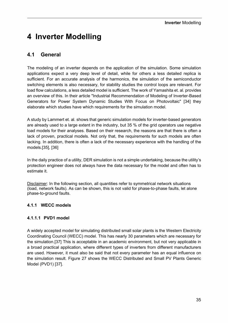
A widely accepted model for simulating distributed small solar plants is the Western Electricity Coordinating Council (WECC) model. This has nearly 30 parameters which are necessary for the simulation.[37] This is acceptable in an academic environment, but not very applicable in a broad practical application, where different types of inverters from different manufacturers are used. However, it must also be said that not every parameter has an equal influence on the simulation result. Figure 27 shows the WECC Distributed and Small PV Plants Generic Model (PVD1) [37].
Inverter Modelling
36
Figure 27 - WECC small PV plant simulation model. Source: WECC Distributed and Small PV Plants Generic Model (PVD1) [37]
4.1.1.2 DER_A model
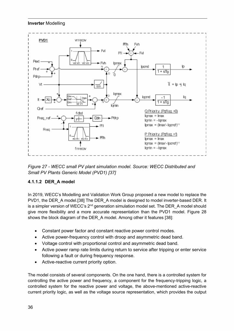
In 2019, WECC’s Modelling and Validation Work Group proposed a new model to replace the PVD1, the DER_A model.[38] The DER_A model is designed to model inverter-based DER. It is a simpler version of WECC’s 2nd generation simulation model set. The DER_A model should give more flexibility and a more accurate representation than the PVD1 model. Figure 28 shows the block diagram of the DER_A model. Among other it features [38]:
• Constant power factor and constant reactive power control modes. • Active power-frequency control with droop and asymmetric dead band. • Voltage control with proportional control and asymmetric dead band. • Active power ramp rate limits during return to service after tripping or enter service
following a fault or during frequency response. • Active-reactive current priority option.
The model consists of several components. On the one hand, there is a controlled system for controlling the active power and frequency, a component for the frequency-tripping logic, a controlled system for the reactive power and voltage, the above-mentioned active-reactive current priority logic, as well as the voltage source representation, which provides the output
Inverter Modelling
37
signal. This output signal can be used in the electromagnetic transient simulation for the averaged method.
Figure 28 - WECC DER_A Simulation Model Block Diagram. Source: ”Reliability Guideline - Parameterization of the DER_A Model”[38]
Figure 29 shows the section in model that is responsible for the active power-frequency control. The model offers two modes for the active power-frequency treatment. This is controlled via the 𝐹𝐹𝐹𝐹𝐹𝐹𝐹𝐹_𝑓𝑓𝑓𝑓𝑎𝑎𝑓𝑓. If 𝐹𝐹𝐹𝐹𝐹𝐹𝐹𝐹_𝑓𝑓𝑓𝑓𝑎𝑎𝑓𝑓 = 0 then the active power-frequency control is deactivated. If 𝐹𝐹𝐹𝐹𝐹𝐹𝐹𝐹_𝑓𝑓𝑓𝑓𝑎𝑎𝑓𝑓 = 1 then the control is activated. The filtered actual system frequency 𝐹𝐹𝐹𝐹𝐹𝐹𝐹𝐹 is taken as an input and compared against the frequency reference. A dead band filter then filters the frequency deviation, the output of this filter is fed into the over- and underfrequency droop gain control 𝐷𝐷𝑑𝑑𝐷𝐷 and 𝐷𝐷𝑢𝑢𝑝𝑝. The signal then is used to be compared with the filtered actual active power and the set reference power. The active power deviation is then used as an input to a PI controller. The so controlled signal is then limited in the changing rate, filtered and also limited in the maximum output values. To get the active current, the output of the power control loop is divided by the terminal voltage 𝑉𝑉𝑡𝑡.[38]

Inverter Modelling
38
Figure 29 - DER_An Active Power-Frequency Control. Source: ”Reliability Guideline - Parameterization of the DER_A Model”[38]
The reactive power-voltage control loop is shown in Figure 30. The 𝑃𝑃𝑓𝑓𝑓𝑓𝑎𝑎𝑓𝑓 selects between constant reactive power control or constant power factor control. To control the reactive power, the terminal voltage 𝑉𝑉𝑡𝑡 is filtered and compared against the set voltage value. The voltage error 𝑉𝑉𝐹𝐹𝐹𝐹𝐹𝐹 is then processed by a deadband filter and multiplied by the proportional control factor 𝐾𝐾𝐹𝐹𝐾𝐾 that also translate the reactive power to the reactive current 𝐼𝐼𝐹𝐹𝐾𝐾. The actual reactive power is derived from the measured active power and the internally calculated parameter 𝑝𝑝𝑓𝑓𝑎𝑎𝐹𝐹𝐹𝐹𝑓𝑓 and in conjunction with 𝐼𝐼𝐹𝐹𝐾𝐾 used to calculate the reactive output current 𝐼𝐼𝐹𝐹. 𝐼𝐼𝐹𝐹 is also limited by the maximum currents 𝐼𝐼𝐹𝐹𝐼𝐼𝑎𝑎𝐼𝐼 and 𝐼𝐼𝐹𝐹𝐼𝐼𝐼𝐼𝐷𝐷.[38]
Figure 30 - DER_A Reactive Power-Voltage Control. Source: ”Reliability Guideline - Parameterization of the DER_A Model”[38]
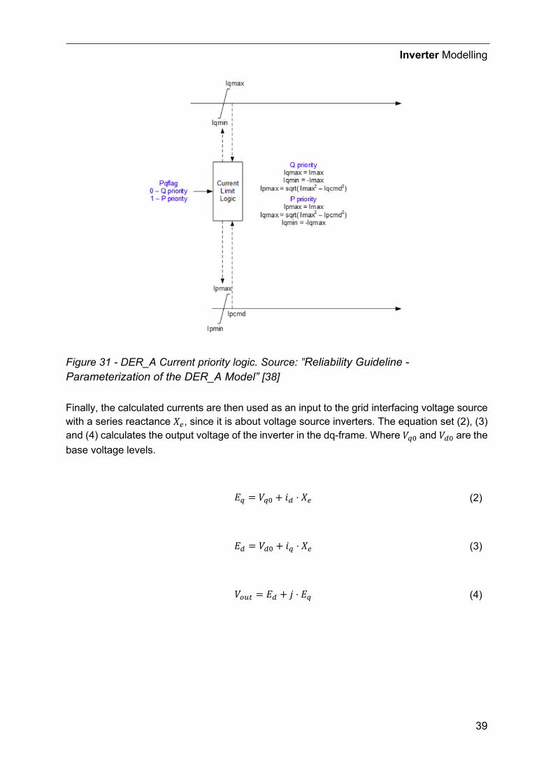
Figure 31 shows the active-reactive current priority logic of the model. Depending on the selected option of the 𝑃𝑃𝐹𝐹𝑓𝑓𝑓𝑓𝑎𝑎𝑓𝑓, the current for the reactive and active current are set to not exceed the inverters maximum current.[38]
Inverter Modelling
39
Figure 31 - DER_A Current priority logic. Source: ”Reliability Guideline - Parameterization of the DER_A Model” [38]
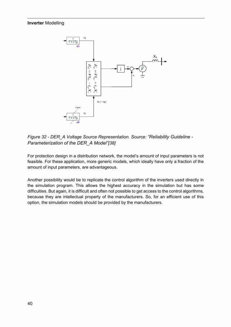
Finally, the calculated currents are then used as an input to the grid interfacing voltage source with a series reactance 𝑋𝑋𝑆𝑆, since it is about voltage source inverters. The equation set (2), (3) and (4) calculates the output voltage of the inverter in the dq-frame. Where 𝑉𝑉𝑞𝑞0 and 𝑉𝑉𝐿𝐿0 are the base voltage levels.
𝐸𝐸𝑞𝑞 = 𝑉𝑉𝑞𝑞0 + 𝐼𝐼𝐿𝐿 ⋅ 𝑋𝑋𝑆𝑆 (2)
𝐸𝐸𝐿𝐿 = 𝑉𝑉𝐿𝐿0 + 𝐼𝐼𝑞𝑞 ⋅ 𝑋𝑋𝑆𝑆 (3)
𝑉𝑉𝐿𝐿𝑜𝑜𝑆𝑆 = 𝐸𝐸𝐿𝐿 + 𝑗𝑗 ⋅ 𝐸𝐸𝑞𝑞 (4)
Inverter Modelling
40
Figure 32 - DER_A Voltage Source Representation. Source: ”Reliability Guideline - Parameterization of the DER_A Model”[38]
For protection design in a distribution network, the model’s amount of input parameters is not feasible. For these application, more generic models, which ideally have only a fraction of the amount of input parameters, are advantageous.
Another possibility would be to replicate the control algorithm of the inverters used directly in the simulation program. This allows the highest accuracy in the simulation but has some difficulties. But again, it is difficult and often not possible to get access to the control algorithms, because they are intellectual property of the manufacturers. So, for an efficient use of this option, the simulation models should be provided by the manufacturers.

Inverter Modelling
41
4.2 Theory of short-circuit and electro-magnetic transient simulation
The design of the electrical network requires a wide range of calculations. One of them is the short-circuit current calculation. This is necessary for the design of primary equipment. Equipment such as transformers must be able to carry the maximum short-circuit current for a certain period of time without being destroyed. For example, the surge short-circuit current leads to very strong mechanical forces on the windings of the transformer. But thermal stresses also occur as a result.
However, the minimum short-circuit current is also of high relevance for the design of the protection system, because the protection system must be sensitive enough to reliably detect even the smallest possible short-circuit currents and to initiate the necessary measures.
To ensure that manufacturers, operators and other parties have comparable information for their respective areas of responsibility, there are standards that define the calculation methods for short-circuit current calculations. The two standards IEC 60909-0 [39] and IEEE 141 [40] are mentioned as examples.
As an example, the calculation according to the 60909-0 standard is discussed in more detail in the following section.
Various simplifications can be assumed for the calculation according to the IEC 60909-0 standard. Since the level of detail achieved by a complete calculation is not necessary in most practical applications. In Figure 33, the two relevant values according to the standard are the surge short-circuit current 𝐼𝐼𝑈𝑈 and the RMS value of the steady-state short-circuit current 𝐼𝐼𝑃𝑃. The surge short-circuit current 𝐼𝐼𝑈𝑈 depends, among other things, on the grid frequency 𝑓𝑓, the DC component 𝐼𝐼𝐷𝐷𝐷𝐷, the ratio 𝑋𝑋 𝑅𝑅� of the grid impedance 𝑍𝑍, time constants in the grid and the time of fault occurrence.[39]
The following simplifications can be applied according to the standard [39]:
a) The short-circuit type remains unchanged during the short-circuit. b) b) The network remains in its state during the short-circuit occurrence. c) The transformer impedance refers to the position of the tap changer on the main
tap. d) Arc resistances are not considered. e) Cross admittances and non-motor loads shall be neglected in the positive, negative
and zero sequence systems. f) Neglect of line capacitances in the positive and negative sequence systems. Line
capacitances in the zero-sequence system shall be considered in the networks with low impedance star point grounding that have a ground impedance matching factor greater than 1.4.
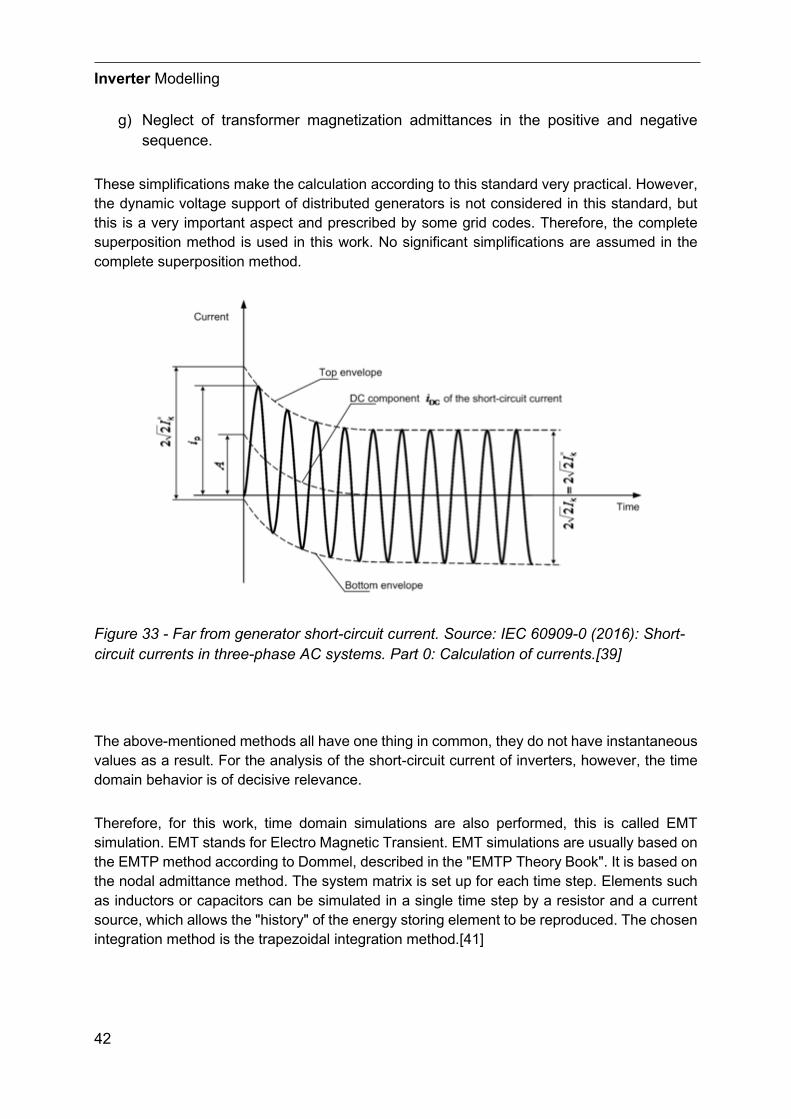
Inverter Modelling
42
g) Neglect of transformer magnetization admittances in the positive and negative sequence.
These simplifications make the calculation according to this standard very practical. However, the dynamic voltage support of distributed generators is not considered in this standard, but this is a very important aspect and prescribed by some grid codes. Therefore, the complete superposition method is used in this work. No significant simplifications are assumed in the complete superposition method.
Figure 33 - Far from generator short-circuit current. Source: IEC 60909-0 (2016): Short-circuit currents in three-phase AC systems. Part 0: Calculation of currents.[39]
The above-mentioned methods all have one thing in common, they do not have instantaneous values as a result. For the analysis of the short-circuit current of inverters, however, the time domain behavior is of decisive relevance.
Therefore, for this work, time domain simulations are also performed, this is called EMT simulation. EMT stands for Electro Magnetic Transient. EMT simulations are usually based on the EMTP method according to Dommel, described in the "EMTP Theory Book". It is based on the nodal admittance method. The system matrix is set up for each time step. Elements such as inductors or capacitors can be simulated in a single time step by a resistor and a current source, which allows the "history" of the energy storing element to be reproduced. The chosen integration method is the trapezoidal integration method.[41]
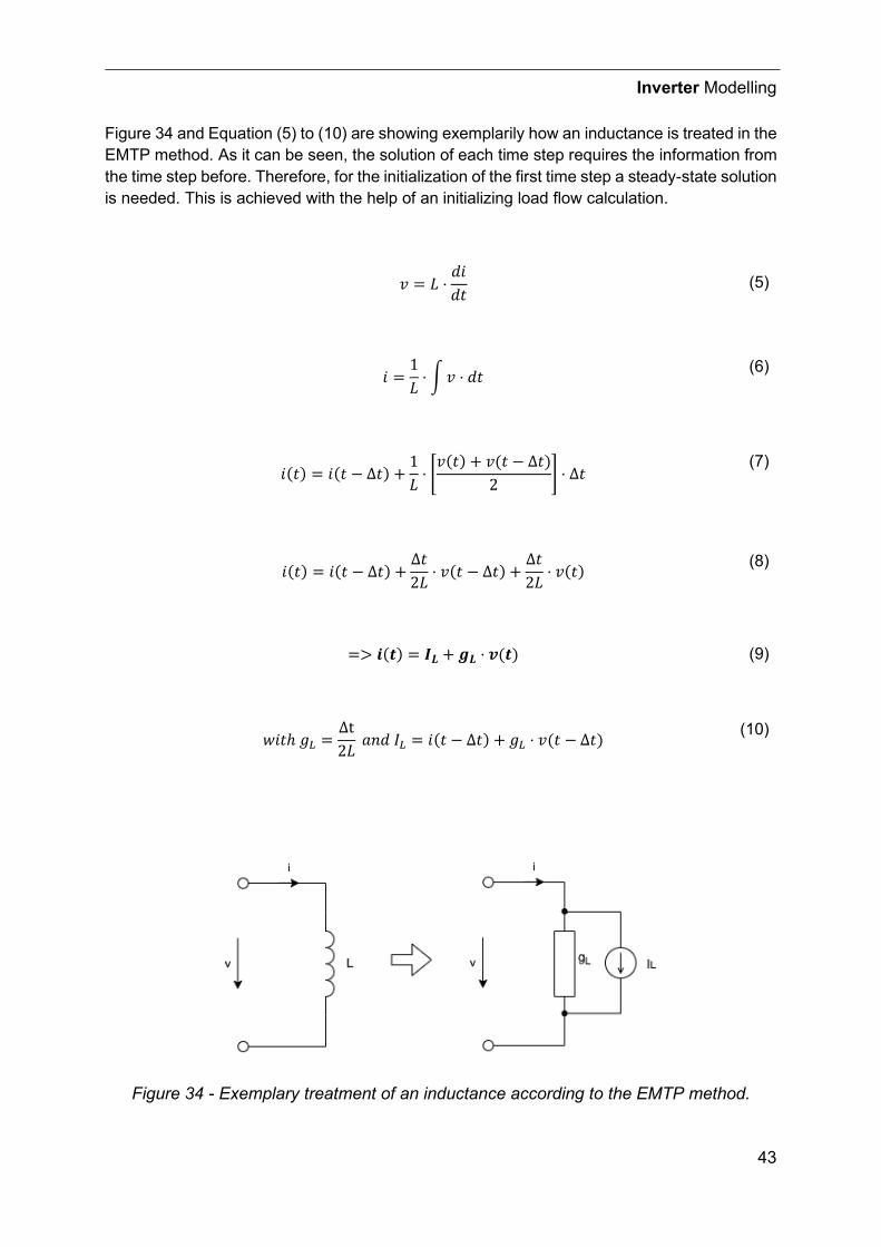
Inverter Modelling
43
Figure 34 and Equation (5) to (10) are showing exemplarily how an inductance is treated in the EMTP method. As it can be seen, the solution of each time step requires the information from the time step before. Therefore, for the initialization of the first time step a steady-state solution is needed. This is achieved with the help of an initializing load flow calculation.
𝐾𝐾 = 𝐿𝐿 ⋅𝑑𝑑𝐼𝐼𝑑𝑑𝑡𝑡
(5)
𝐼𝐼 =1𝐿𝐿⋅ �𝐾𝐾 ⋅ 𝑑𝑑𝑡𝑡 (6)
𝐼𝐼(𝑡𝑡) = 𝐼𝐼(𝑡𝑡 − Δ𝑡𝑡) +
1𝐿𝐿⋅ �𝐾𝐾(𝑡𝑡) + 𝐾𝐾(𝑡𝑡 − Δ𝑡𝑡)
2� ⋅ Δ𝑡𝑡
(7)
𝐼𝐼(𝑡𝑡) = 𝐼𝐼(𝑡𝑡 − Δ𝑡𝑡) +Δ𝑡𝑡2𝐿𝐿
⋅ 𝐾𝐾(𝑡𝑡 − Δ𝑡𝑡) +Δ𝑡𝑡2𝐿𝐿
⋅ 𝐾𝐾(𝑡𝑡) (8)
=> 𝒊𝒊(𝒕𝒕) = 𝑰𝑰𝑳𝑳 + 𝒈𝒈𝑳𝑳 ⋅ 𝒗𝒗(𝒕𝒕) (9)
𝑤𝑤𝐼𝐼𝑡𝑡ℎ 𝑓𝑓𝐿𝐿 =Δt2𝐿𝐿
𝑎𝑎𝐷𝐷𝑑𝑑 𝐼𝐼𝐿𝐿 = 𝐼𝐼(𝑡𝑡 − Δ𝑡𝑡) + 𝑓𝑓𝐿𝐿 ⋅ 𝐾𝐾(𝑡𝑡 − Δ𝑡𝑡) (10)
Figure 34 - Exemplary treatment of an inductance according to the EMTP method.
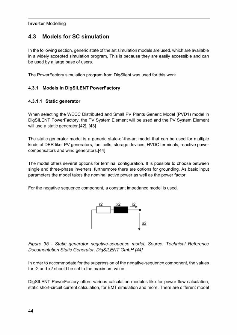
Inverter Modelling
44
4.3 Models for SC simulation
In the following section, generic state of the art simulation models are used, which are available in a widely accepted simulation program. This is because they are easily accessible and can be used by a large base of users.
The PowerFactory simulation program from DigSilent was used for this work.
4.3.1 Models in DigSILENT PowerFactory
4.3.1.1 Static generator
When selecting the WECC Distributed and Small PV Plants Generic Model (PVD1) model in DigSILENT PowerFactory, the PV System Element will be used and the PV System Element will use a static generator.[42], [43]
The static generator model is a generic state-of-the-art model that can be used for multiple kinds of DER like: PV generators, fuel cells, storage devices, HVDC terminals, reactive power compensators and wind generators.[44]
The model offers several options for terminal configuration. It is possible to choose between single and three-phase inverters, furthermore there are options for grounding. As basic input parameters the model takes the nominal active power as well as the power factor.
For the negative sequence component, a constant impedance model is used.
Figure 35 - Static generator negative-sequence model. Source: Technical Reference Documentation Static Generator, DigSILENT GmbH [44]
In order to accommodate for the suppression of the negative-sequence component, the values for r2 and x2 should be set to the maximum value.
DigSILENT PowerFactory offers various calculation modules like for power-flow calculation, static short-circuit current calculation, for EMT simulation and more. There are different model
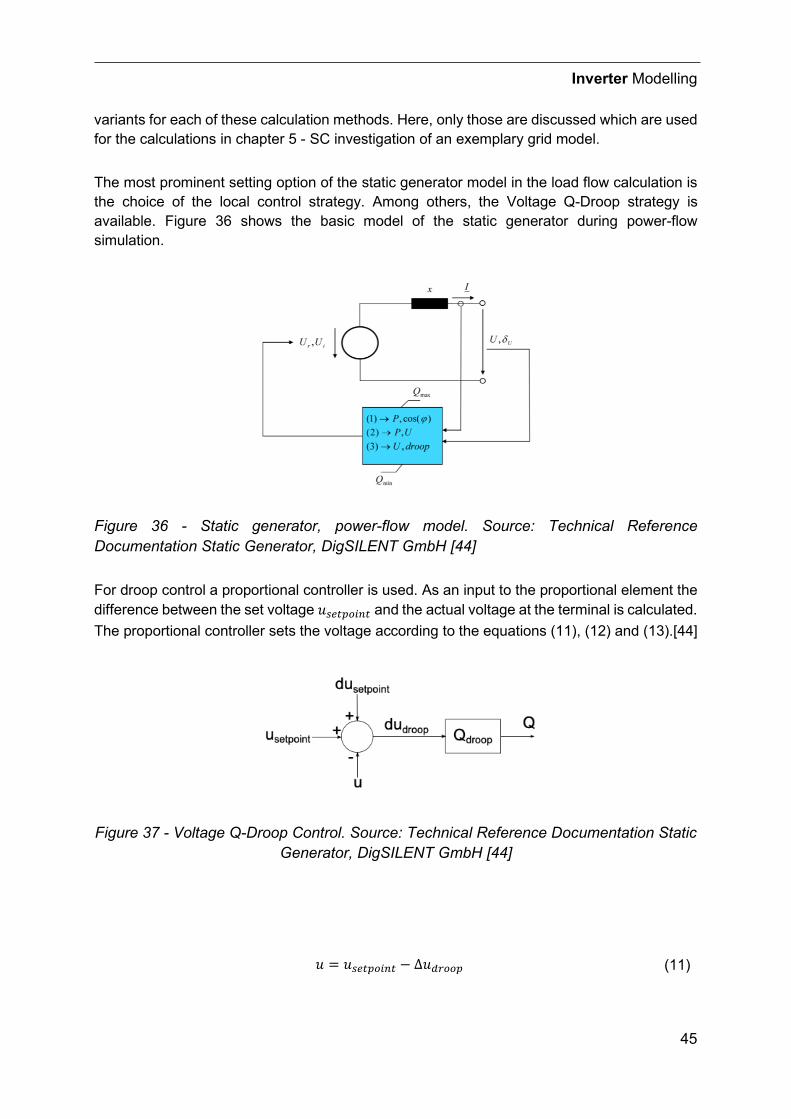
Inverter Modelling
45
variants for each of these calculation methods. Here, only those are discussed which are used for the calculations in chapter 5 - SC investigation of an exemplary grid model.
The most prominent setting option of the static generator model in the load flow calculation is the choice of the local control strategy. Among others, the Voltage Q-Droop strategy is available. Figure 36 shows the basic model of the static generator during power-flow simulation.
Figure 36 - Static generator, power-flow model. Source: Technical Reference Documentation Static Generator, DigSILENT GmbH [44]
For droop control a proportional controller is used. As an input to the proportional element the difference between the set voltage 𝑢𝑢𝑠𝑠𝑆𝑆𝑆𝑆𝑈𝑈𝐿𝐿𝑆𝑆𝑆𝑆𝑆𝑆 and the actual voltage at the terminal is calculated. The proportional controller sets the voltage according to the equations (11), (12) and (13).[44]
Figure 37 - Voltage Q-Droop Control. Source: Technical Reference Documentation Static Generator, DigSILENT GmbH [44]
𝑢𝑢 = 𝑢𝑢𝑠𝑠𝑆𝑆𝑆𝑆𝑈𝑈𝐿𝐿𝑆𝑆𝑆𝑆𝑆𝑆 − Δ𝑢𝑢𝐿𝐿𝑑𝑑𝐿𝐿𝐿𝐿𝑈𝑈 (11)
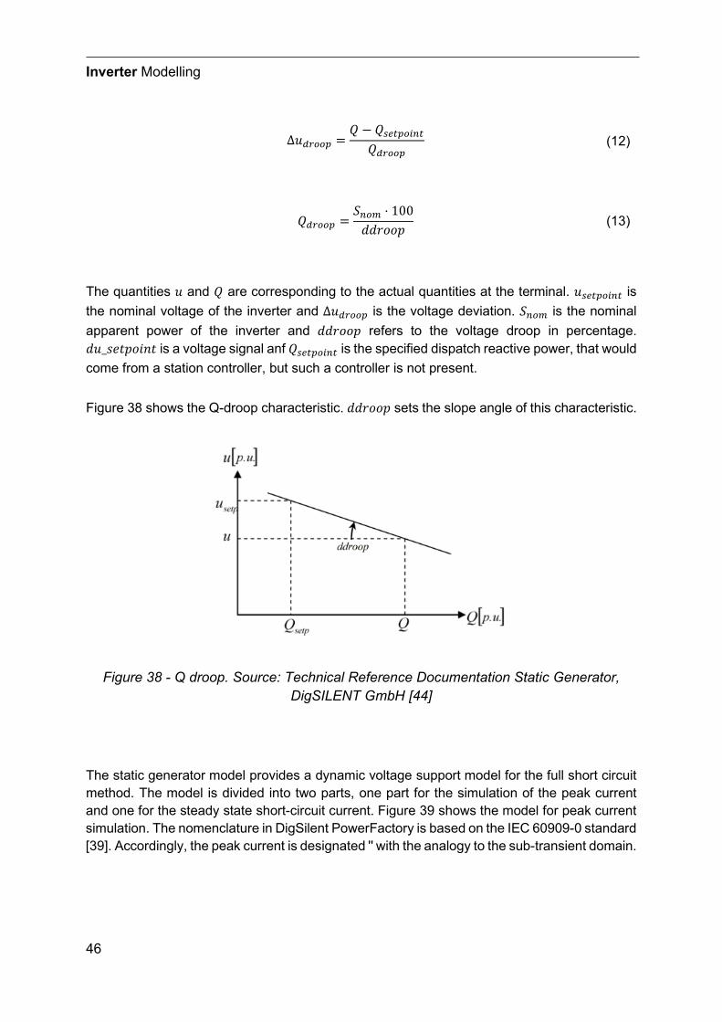
Inverter Modelling
46
Δ𝑢𝑢𝐿𝐿𝑑𝑑𝐿𝐿𝐿𝐿𝑈𝑈 =𝑄𝑄 − 𝑄𝑄𝑠𝑠𝑆𝑆𝑆𝑆𝑈𝑈𝐿𝐿𝑆𝑆𝑆𝑆𝑆𝑆
𝑄𝑄𝐿𝐿𝑑𝑑𝐿𝐿𝐿𝐿𝑈𝑈 (12)
𝑄𝑄𝐿𝐿𝑑𝑑𝐿𝐿𝐿𝐿𝑈𝑈 =𝑆𝑆𝑆𝑆𝐿𝐿𝑛𝑛 ⋅ 100𝑑𝑑𝑑𝑑𝐹𝐹𝑑𝑑𝑑𝑑𝑝𝑝
(13)
The quantities 𝑢𝑢 and 𝑄𝑄 are corresponding to the actual quantities at the terminal. 𝑢𝑢𝑠𝑠𝑆𝑆𝑆𝑆𝑈𝑈𝐿𝐿𝑆𝑆𝑆𝑆𝑆𝑆 is the nominal voltage of the inverter and Δ𝑢𝑢𝐿𝐿𝑑𝑑𝐿𝐿𝐿𝐿𝑈𝑈 is the voltage deviation. 𝑆𝑆𝑆𝑆𝐿𝐿𝑛𝑛 is the nominal apparent power of the inverter and 𝑑𝑑𝑑𝑑𝐹𝐹𝑑𝑑𝑑𝑑𝑝𝑝 refers to the voltage droop in percentage. 𝑑𝑑𝑢𝑢_𝑠𝑠𝐹𝐹𝑡𝑡𝑝𝑝𝑑𝑑𝐼𝐼𝐷𝐷𝑡𝑡 is a voltage signal anf 𝑄𝑄𝑠𝑠𝑆𝑆𝑆𝑆𝑈𝑈𝐿𝐿𝑆𝑆𝑆𝑆𝑆𝑆 is the specified dispatch reactive power, that would come from a station controller, but such a controller is not present.
Figure 38 shows the Q-droop characteristic. 𝑑𝑑𝑑𝑑𝐹𝐹𝑑𝑑𝑑𝑑𝑝𝑝 sets the slope angle of this characteristic.
Figure 38 - Q droop. Source: Technical Reference Documentation Static Generator, DigSILENT GmbH [44]
The static generator model provides a dynamic voltage support model for the full short circuit method. The model is divided into two parts, one part for the simulation of the peak current and one for the steady state short-circuit current. Figure 39 shows the model for peak current simulation. The nomenclature in DigSilent PowerFactory is based on the IEC 60909-0 standard [39]. Accordingly, the peak current is designated '' with the analogy to the sub-transient domain.
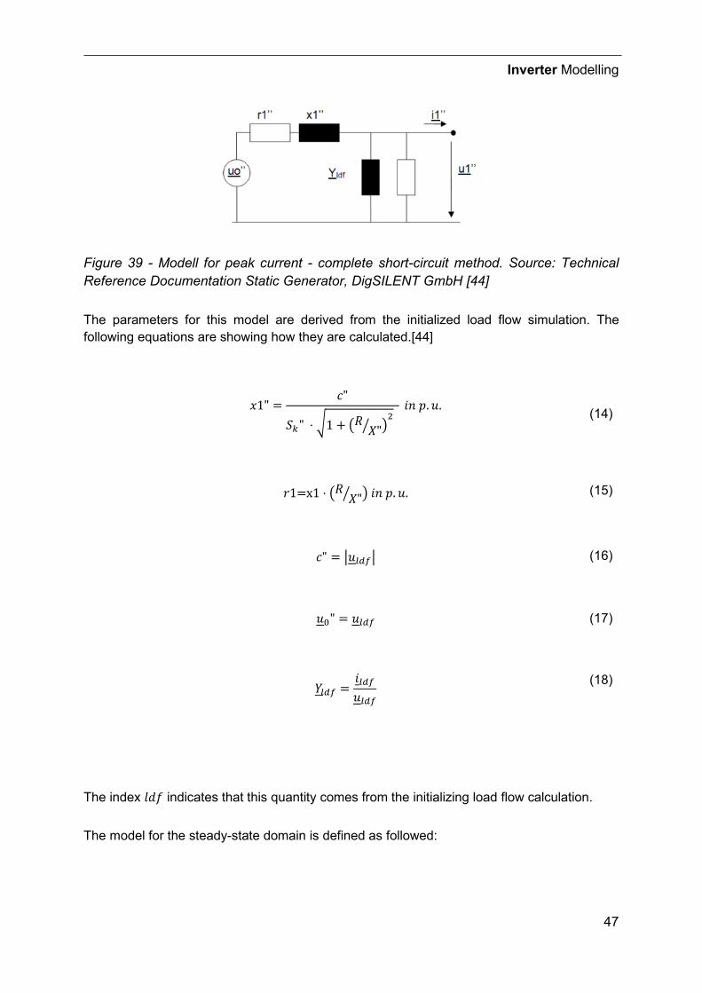
Inverter Modelling
47
Figure 39 - Modell for peak current - complete short-circuit method. Source: Technical Reference Documentation Static Generator, DigSILENT GmbH [44]
The parameters for this model are derived from the initialized load flow simulation. The following equations are showing how they are calculated.[44]
𝐼𝐼1" =𝑐𝑐"
𝑆𝑆𝑃𝑃" ⋅ �1 + �𝑅𝑅 𝑋𝑋"� �2
𝐼𝐼𝐷𝐷 𝑝𝑝.𝑢𝑢. (14)
𝐹𝐹1=x1 ⋅ �𝑅𝑅 𝑋𝑋"� � 𝐼𝐼𝐷𝐷 𝑝𝑝.𝑢𝑢. (15)
𝑐𝑐" = �𝑢𝑢𝑙𝑙𝐿𝐿𝑙𝑙� (16)
𝑢𝑢0" = 𝑢𝑢𝑙𝑙𝐿𝐿𝑙𝑙 (17)
𝑌𝑌𝑙𝑙𝐿𝐿𝑙𝑙 =𝐼𝐼𝑙𝑙𝐿𝐿𝑙𝑙𝑢𝑢𝑙𝑙𝐿𝐿𝑙𝑙
(18)
The index 𝑓𝑓𝑑𝑑𝑓𝑓 indicates that this quantity comes from the initializing load flow calculation.
The model for the steady-state domain is defined as followed:
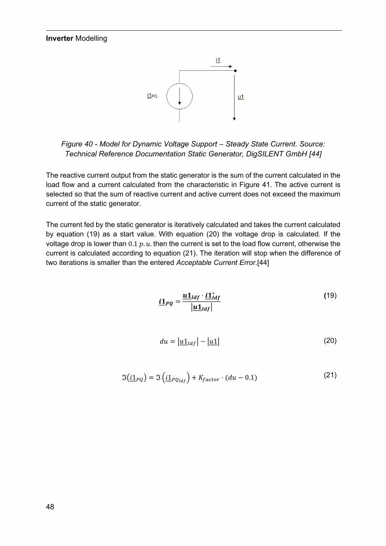
Inverter Modelling
48
Figure 40 - Model for Dynamic Voltage Support – Steady State Current. Source: Technical Reference Documentation Static Generator, DigSILENT GmbH [44]
The reactive current output from the static generator is the sum of the current calculated in the load flow and a current calculated from the characteristic in Figure 41. The active current is selected so that the sum of reactive current and active current does not exceed the maximum current of the static generator.
The current fed by the static generator is iteratively calculated and takes the current calculated by equation (19) as a start value. With equation (20) the voltage drop is calculated. If the voltage drop is lower than 0.1 𝑝𝑝.𝑢𝑢. then the current is set to the load flow current, otherwise the current is calculated according to equation (21). The iteration will stop when the difference of two iterations is smaller than the entered Acceptable Current Error.[44]
𝒊𝒊𝒊𝒊𝑷𝑷𝑷𝑷 =
𝒖𝒖𝒊𝒊𝒍𝒍𝒍𝒍𝒍𝒍 ⋅ 𝒊𝒊𝒊𝒊𝒍𝒍𝒍𝒍𝒍𝒍∗
�𝒖𝒖𝒊𝒊𝒍𝒍𝒍𝒍𝒍𝒍�
(19)
𝑑𝑑𝑢𝑢 = �𝑢𝑢1𝑙𝑙𝐿𝐿𝑙𝑙� − �𝑢𝑢1� (20)
ℑ�𝐼𝐼1𝑃𝑃𝑃𝑃� = ℑ�𝐼𝐼1𝑃𝑃𝑃𝑃𝑙𝑙𝑙𝑙𝑙𝑙�+ 𝐾𝐾𝑙𝑙𝐿𝐿𝑃𝑃𝑆𝑆𝐿𝐿𝑑𝑑 ⋅ (𝑑𝑑𝑢𝑢 − 0.1) (21)
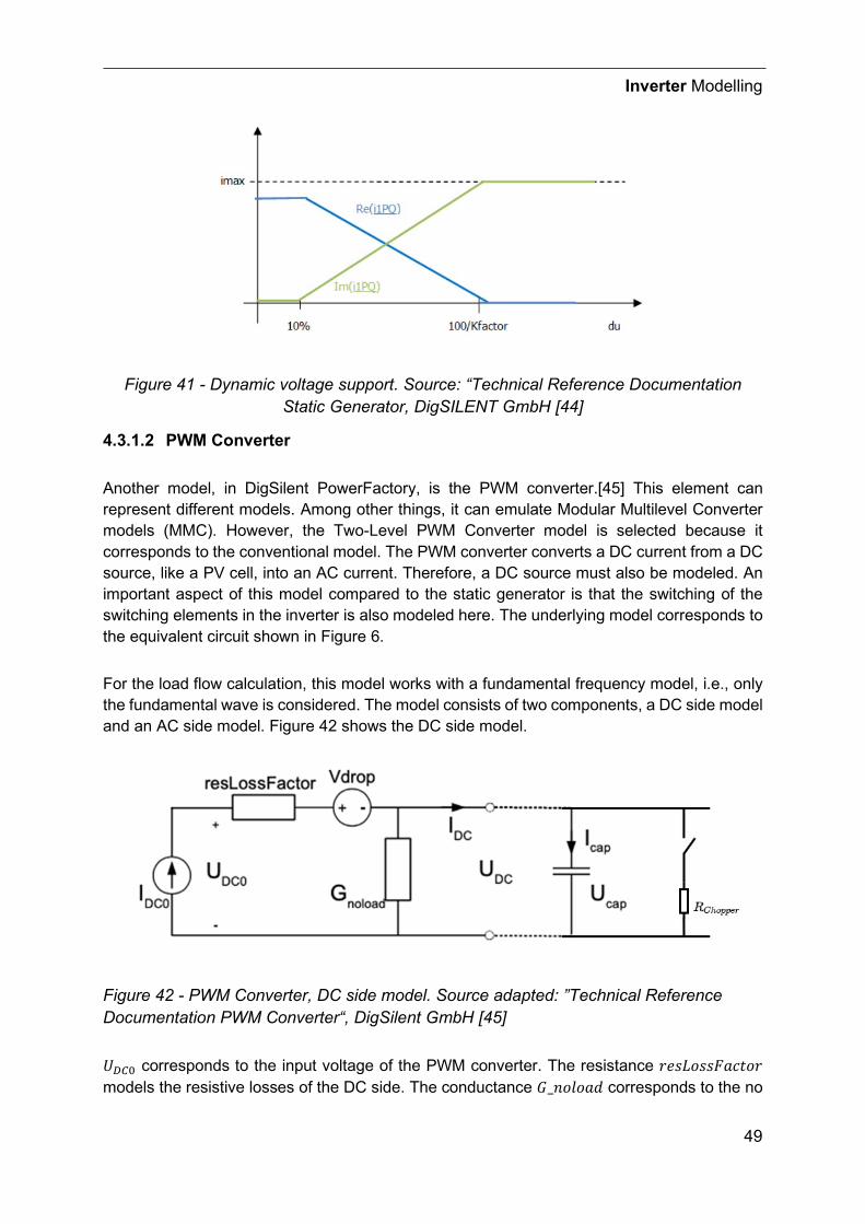
Inverter Modelling
49
Figure 41 - Dynamic voltage support. Source: “Technical Reference Documentation Static Generator, DigSILENT GmbH [44]
4.3.1.2 PWM Converter
Another model, in DigSilent PowerFactory, is the PWM converter.[45] This element can represent different models. Among other things, it can emulate Modular Multilevel Converter models (MMC). However, the Two-Level PWM Converter model is selected because it corresponds to the conventional model. The PWM converter converts a DC current from a DC source, like a PV cell, into an AC current. Therefore, a DC source must also be modeled. An important aspect of this model compared to the static generator is that the switching of the switching elements in the inverter is also modeled here. The underlying model corresponds to the equivalent circuit shown in Figure 6.
For the load flow calculation, this model works with a fundamental frequency model, i.e., only the fundamental wave is considered. The model consists of two components, a DC side model and an AC side model. Figure 42 shows the DC side model.
Figure 42 - PWM Converter, DC side model. Source adapted: ”Technical Reference Documentation PWM Converter“, DigSilent GmbH [45]
𝑈𝑈𝐷𝐷𝐷𝐷0 corresponds to the input voltage of the PWM converter. The resistance 𝐹𝐹𝐹𝐹𝑠𝑠𝐿𝐿𝑑𝑑𝑠𝑠𝑠𝑠𝐹𝐹𝑎𝑎𝑐𝑐𝑡𝑡𝑑𝑑𝐹𝐹 models the resistive losses of the DC side. The conductance 𝐺𝐺_𝐷𝐷𝑑𝑑𝑓𝑓𝑑𝑑𝑎𝑎𝑑𝑑 corresponds to the no
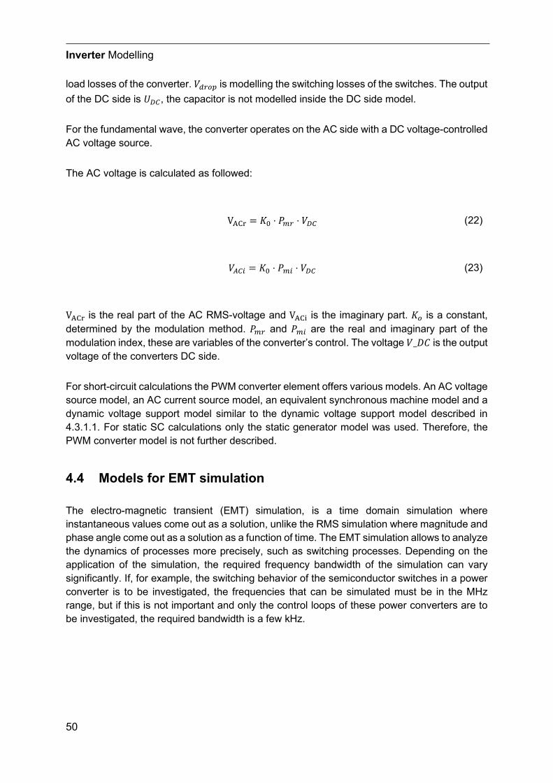
Inverter Modelling
50
load losses of the converter. 𝑉𝑉𝐿𝐿𝑑𝑑𝐿𝐿𝑈𝑈 is modelling the switching losses of the switches. The output of the DC side is 𝑈𝑈𝐷𝐷𝐷𝐷, the capacitor is not modelled inside the DC side model.
For the fundamental wave, the converter operates on the AC side with a DC voltage-controlled AC voltage source.
The AC voltage is calculated as followed:
VACr = 𝐾𝐾0 ⋅ 𝑃𝑃𝑛𝑛𝑑𝑑 ⋅ 𝑉𝑉𝐷𝐷𝐷𝐷 (22)
𝑉𝑉𝐴𝐴𝐷𝐷𝑆𝑆 = 𝐾𝐾0 ⋅ 𝑃𝑃𝑛𝑛𝑆𝑆 ⋅ 𝑉𝑉𝐷𝐷𝐷𝐷 (23)
VACr is the real part of the AC RMS-voltage and VACi is the imaginary part. 𝐾𝐾𝐿𝐿 is a constant, determined by the modulation method. 𝑃𝑃𝑛𝑛𝑑𝑑 and 𝑃𝑃𝑛𝑛𝑆𝑆 are the real and imaginary part of the modulation index, these are variables of the converter’s control. The voltage 𝑉𝑉_𝐷𝐷𝐷𝐷 is the output voltage of the converters DC side.
For short-circuit calculations the PWM converter element offers various models. An AC voltage source model, an AC current source model, an equivalent synchronous machine model and a dynamic voltage support model similar to the dynamic voltage support model described in 4.3.1.1. For static SC calculations only the static generator model was used. Therefore, the PWM converter model is not further described.
4.4 Models for EMT simulation
The electro-magnetic transient (EMT) simulation, is a time domain simulation where instantaneous values come out as a solution, unlike the RMS simulation where magnitude and phase angle come out as a solution as a function of time. The EMT simulation allows to analyze the dynamics of processes more precisely, such as switching processes. Depending on the application of the simulation, the required frequency bandwidth of the simulation can vary significantly. If, for example, the switching behavior of the semiconductor switches in a power converter is to be investigated, the frequencies that can be simulated must be in the MHz range, but if this is not important and only the control loops of these power converters are to be investigated, the required bandwidth is a few kHz.
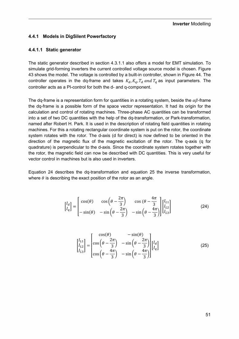
Inverter Modelling
51
4.4.1 Models in DigSilent Powerfactory
4.4.1.1 Static generator
The static generator described in section 4.3.1.1 also offers a model for EMT simulation. To simulate grid-forming inverters the current controlled voltage source model is chosen. Figure 43 shows the model. The voltage is controlled by a built-in controller, shown in Figure 44. The controller operates in the dq-frame and takes 𝐾𝐾𝐿𝐿 ,𝐾𝐾𝑞𝑞 ,𝑇𝑇𝐿𝐿 𝑎𝑎𝐷𝐷𝑑𝑑 𝑇𝑇𝑞𝑞 as input parameters. The controller acts as a PI-control for both the d- and q-component.
The dq-frame is a representation form for quantities in a rotating system, beside the 𝛼𝛼𝛼𝛼-frame the dq-frame is a possible form of the space vector representation. It had its origin for the calculation and control of rotating machines. Three-phase AC quantities can be transformed into a set of two DC quantities with the help of the dq-transformation, or Park-transformation, named after Robert H. Park. It is used in the description of rotating field quantities in rotating machines. For this a rotating rectangular coordinate system is put on the rotor, the coordinate system rotates with the rotor. The d-axis (d for direct) is now defined to be oriented in the direction of the magnetic flux of the magnetic excitation of the rotor. The q-axis (q for quadrature) is perpendicular to the d-axis. Since the coordinate system rotates together with the rotor, the magnetic field can now be described with DC quantities. This is very useful for vector control in machines but is also used in inverters.
Equation 24 describes the dq-transformation and equation 25 the inverse transformation, where 𝜃𝜃 is describing the exact position of the rotor as an angle.
�𝐼𝐼𝐿𝐿𝐼𝐼𝑞𝑞� = �
cos(𝜃𝜃) cos�𝜃𝜃 −2𝜋𝜋3� cos (𝜃𝜃 −
4𝜋𝜋3
− sin(𝜃𝜃) − sin�𝜃𝜃 −2𝜋𝜋3� − sin �𝜃𝜃 −
4𝜋𝜋3�� �𝐼𝐼𝐿𝐿1𝐼𝐼𝐿𝐿2𝐼𝐼𝐿𝐿3� (24)
�𝐼𝐼𝐿𝐿1𝐼𝐼𝐿𝐿2𝐼𝐼𝐿𝐿3� =
⎣⎢⎢⎢⎡
cos(𝜃𝜃) − sin(𝜃𝜃)
cos�𝜃𝜃 −2𝜋𝜋3� − sin�𝜃𝜃 −
2𝜋𝜋3�
cos�𝜃𝜃 −4𝜋𝜋3� − sin�𝜃𝜃 −
4𝜋𝜋3�⎦⎥⎥⎥⎤
�𝐼𝐼𝐿𝐿𝐼𝐼𝑞𝑞� (25)
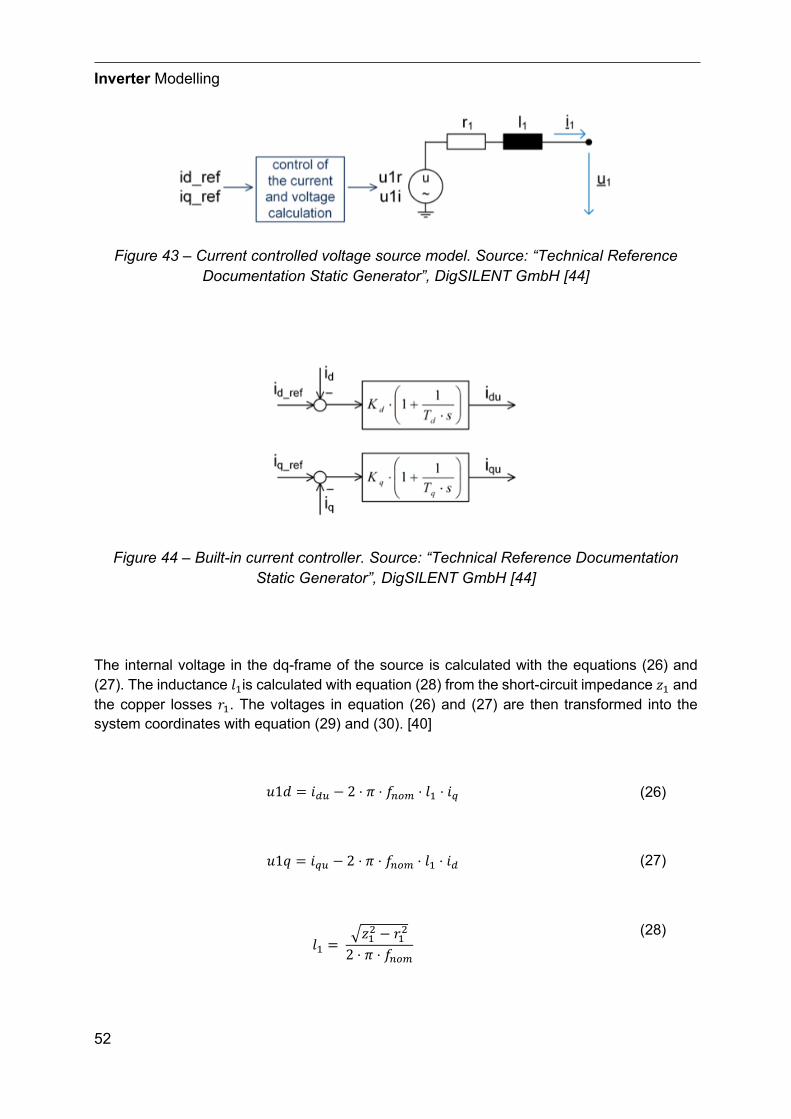
Inverter Modelling
52
Figure 43 – Current controlled voltage source model. Source: “Technical Reference Documentation Static Generator”, DigSILENT GmbH [44]
Figure 44 – Built-in current controller. Source: “Technical Reference Documentation Static Generator”, DigSILENT GmbH [44]
The internal voltage in the dq-frame of the source is calculated with the equations (26) and (27). The inductance 𝑓𝑓1is calculated with equation (28) from the short-circuit impedance 𝑧𝑧1 and the copper losses 𝐹𝐹1. The voltages in equation (26) and (27) are then transformed into the system coordinates with equation (29) and (30). [40]
𝑢𝑢1𝑑𝑑 = 𝐼𝐼𝐿𝐿𝑜𝑜 − 2 ⋅ 𝜋𝜋 ⋅ 𝑓𝑓𝑆𝑆𝐿𝐿𝑛𝑛 ⋅ 𝑓𝑓1 ⋅ 𝐼𝐼𝑞𝑞 (26)
𝑢𝑢1𝐹𝐹 = 𝐼𝐼𝑞𝑞𝑜𝑜 − 2 ⋅ 𝜋𝜋 ⋅ 𝑓𝑓𝑆𝑆𝐿𝐿𝑛𝑛 ⋅ 𝑓𝑓1 ⋅ 𝐼𝐼𝐿𝐿 (27)
𝑓𝑓1 = �𝑧𝑧12 − 𝐹𝐹12
2 ⋅ 𝜋𝜋 ⋅ 𝑓𝑓𝑆𝑆𝐿𝐿𝑛𝑛
(28)

Inverter Modelling
53
𝑢𝑢1𝐹𝐹 = cos𝑢𝑢 ⋅ 𝑢𝑢1𝑑𝑑 − sin𝑢𝑢 ⋅ 𝑢𝑢1𝐹𝐹 (29)
𝑢𝑢1𝐼𝐼 = sin𝑢𝑢 ⋅ 𝑢𝑢1𝑑𝑑 − cos𝑢𝑢 ⋅ 𝑢𝑢1𝐹𝐹 (30)
4.4.1.2 Pulse-width modulation converter
The PWM converter described in 4.3.1.2 also has a model for EMT simulations. A detailed model, which simulates the switching of the switches. And a controlled voltage source model, which averages the switching behavior. Since conventional protection relays have a low sampling rate and mostly operate with the fundamental wave, the additional information depth, gained by the simulation of the switching behavior, can be neglected. Therefore, the controlled voltage source model is chosen. This model is similar to the fundamental frequency model described in 4.3.1.2. The 3rd harmonic is injected based on a space vector modulation technique.[45]
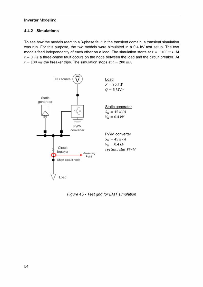
Inverter Modelling
54
4.4.2 Simulations
To see how the models react to a 3-phase fault in the transient domain, a transient simulation was run. For this purpose, the two models were simulated in a 0.4 kV test setup. The two models feed independently of each other on a load. The simulation starts at 𝑡𝑡 = −100 𝐼𝐼𝑠𝑠. At 𝑡𝑡 = 0 𝐼𝐼𝑠𝑠 a three-phase fault occurs on the node between the load and the circuit breaker. At 𝑡𝑡 = 100 𝐼𝐼𝑠𝑠 the breaker trips. The simulation stops at 𝑡𝑡 = 200 𝐼𝐼𝑠𝑠.
Load 𝑃𝑃 = 30 𝑘𝑘𝑘𝑘 𝑄𝑄 = 5 𝑘𝑘𝑉𝑉𝑘𝑘𝐹𝐹
Static generator 𝑆𝑆𝑁𝑁 = 45 𝑘𝑘𝑉𝑉𝑘𝑘 𝑉𝑉𝑁𝑁 = 0.4 𝑘𝑘𝑉𝑉
PWM converter 𝑆𝑆𝑁𝑁 = 45 𝑘𝑘𝑉𝑉𝑘𝑘 𝑉𝑉𝑁𝑁 = 0.4 𝑘𝑘𝑉𝑉 𝐹𝐹𝐹𝐹𝑐𝑐𝑡𝑡𝑎𝑎𝐷𝐷𝑓𝑓𝑢𝑢𝑓𝑓𝑎𝑎𝐹𝐹 𝑃𝑃𝑘𝑘𝑃𝑃
Figure 45 - Test grid for EMT simulation
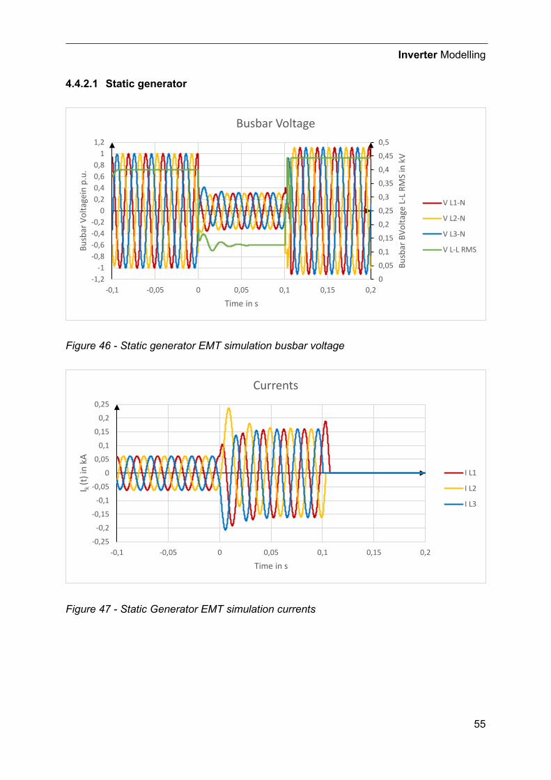
Inverter Modelling
55
4.4.2.1 Static generator
Figure 46 - Static generator EMT simulation busbar voltage
Figure 47 - Static Generator EMT simulation currents
0
0,05
0,1
0,15
0,2
0,25
0,3
0,35
0,4
0,45
0,5
-1,2-1
-0,8-0,6-0,4-0,2
00,20,40,60,8
11,2
-0,1 -0,05 0 0,05 0,1 0,15 0,2
Busb
ar B
Volta
ge L
-L R
MS
in k
V
Busb
ar V
olta
gein
p.u
.
Time in s
Busbar Voltage
V L1-N
V L2-N
V L3-N
V L-L RMS
-0,25
-0,2
-0,15
-0,1
-0,05
0
0,05
0,1
0,15
0,2
0,25
-0,1 -0,05 0 0,05 0,1 0,15 0,2
I k (t
) in
kA
Time in s
Currents
I L1
I L2
I L3
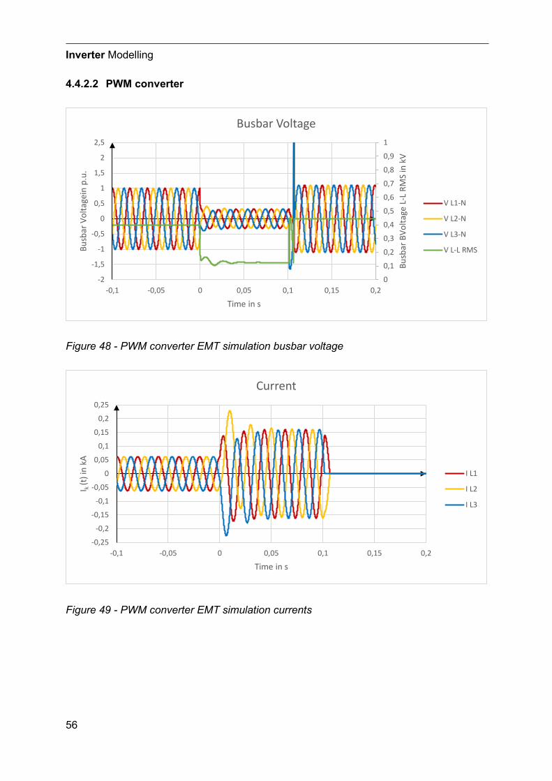
Inverter Modelling
56
4.4.2.2 PWM converter
Figure 48 - PWM converter EMT simulation busbar voltage
Figure 49 - PWM converter EMT simulation currents
0
0,1
0,2
0,3
0,4
0,5
0,6
0,7
0,8
0,9
1
-2
-1,5
-1
-0,5
0
0,5
1
1,5
2
2,5
-0,1 -0,05 0 0,05 0,1 0,15 0,2
Busb
ar B
Volta
ge L
-L R
MS
in k
V
Busb
ar V
olta
gein
p.u
.
Time in s
Busbar Voltage
V L1-N
V L2-N
V L3-N
V L-L RMS
-0,25
-0,2
-0,15
-0,1
-0,05
0
0,05
0,1
0,15
0,2
0,25
-0,1 -0,05 0 0,05 0,1 0,15 0,2
I k (t
) in
kA
Time in s
Current
I L1
I L2
I L3
Inverter Modelling
57
4.5 Summary of the models
Generic simulation models for load flow, short circuit and EMT simulations are shown. The two models of the WECC are generic standardized models, which cover a wide range of applications and also offer the possibility to control many aspects in detail. This is advantageous for many detailed investigations, but conversely requires a large number of parameters, which are not readily available. Therefore, generic models of a widely used simulation software were used for the investigations.
Since this work revolves around protection applications, this was given priority. As an example, it can be taken from the work of Yamashita et. al. that for the detection of faults, the following requirements for a model are not important: frequency deviations, large voltage deviations and small long term voltage deviations, but the handling of unintentional islanding is important.[34]
As already mentioned, models were chosen which correspond to the state of the art and have a high accessibility. The good accessibility is particularly important in the area of protection. Designing the protection in the laboratory is one thing. Ensuring that the protection system actually works in daily operation is another. The more useable a model is, the better it can be ensured that the protection system can actually detect faults. However, it must be said that accessibility must not take absolute priority over accuracy, because faulty states must still be reproduced with sufficient accuracy.
The described static generator and PWM converter models so not show much difference in load flow simulation and short circuit simulation. Also, for the selected EMT simulation models no large differences were recognizable. The gain in detail, which is due to the averaging of the switching is negligible. Detailed simulation of the switching is also not of great relevance since conventional protection relays operate with fundamental frequency phasors. Time domain protection relays, which operate with a very high sampling rate and other algorithms, such as incremental quantities algorithms, could benefit from a more accurate simulation. However, these usually work according to other principles.
Due to the less complex provision of parameters and the expected sufficient accuracy, the static generator model was chosen for further investigations. It is comparatively easy to handle and should provide results with sufficient accuracy.
Short-circuit investigation of an exemplary grid model
58
5 Short-circuit investigation of an exemplary grid model
5.1 Grid model synthesis
The investigations are carried out on an exemplary distribution grid. In the following it is described how this network is synthesized. Figure 63 in the appendix shows the MV section of this grid model. The network model represents a peripheral urban grid with a combination of cables and overhead lines. The model consists of a MV and a LV part.
The MV grid is operated at 20 kV, which corresponds to a common distribution grid in German-speaking countries. The LV grid, where the distributed feeders are located, is a typical 0.4 kV grid.
The MV grid is supplied from the 110 kV sub-transmission grid via a 32 MVA power transformer. In parallel with this is an identical back-up transformer. During regular operation, only one of the two is in operation. The transformer is operated at 54% of its rated power.
There is a single busbar in the substation, usually in the DACH region a double busbar would be used as this allows greater flexibility for maintenance and other work. The busbar has 9 bays. Two bays are for the transformers, one bay for a zigzag transformer and an arc suppression coil (ACS), and 6 feeders to supply the local substations.
With the ACS, the network is operated in the overcompensated state. The overcompensation was set to 10 A residual current with the coil controller.
For simplicity, all feeders are identical. The structure of such a feeder is as follows: starting from the busbar, an 8 km long underground cable leads to the local substations. After these 8 km, the underground cable comes out of the ground and becomes an overhead line for another 12 km.
On the underground cable section 10 identical local network stations were distributed equidistantly. This means that every 800 m there is a local network station. The overhead line section is constructed similarly. Here 6 identical local network stations are distributed equidistantly. This means that there is a local network station every 2 km on the overhead line. The lines are operated as open rings. This means that in each case two feeders can be connected at the end by means of a disconnector. If a fault occurs on one section of the line, this section can be disconnected from the network and the subsequent secondary substations can still be supplied by the other feeder.
Short-circuit investigation of an exemplary grid model
59
The underground cable section thus has an urban character and the overhead line section a rural one.
Each of the secondary substations for the cable line is populated with 10 residential and commercial buildings. Each of these buildings has a load of 20 kW. The buildings are connected by 40 m of 150 mm2 4-pole aluminum cable. To synthesize the PV generation of the buildings, a footprint of 140 m2 (20 m x 7 m) is assumed, and a maximum use of 50% of the building roof is also assumed. This results in an effective area of 70 m2 for the solar panels. Assuming a power coefficient of 215 W/m2 per square meter, the output power of the building's photovoltaic system is 15 kW. Figure 64 shows the LV grid of the urban cable section.
The secondary substations of the OHL section are supplying 20 houses. The houses are separated by 30 m of 150 mm2 4-pole aluminum cables. The PV generation of the houses is synthesized analogously to that of the buildings. Assuming a footprint of 50 m2, we obtain an output power of the solar system of 5 kW.
5.2 Methodology of this investigation
The tests in the example grid were carried out for two different states. In the first state (Grid Condition A), the feed-in power from the DER plants corresponds to 50% of the load. In this case, the remaining power of 50% is drawn from the higher-level grid via the transformer.
The second grid condition (Grid Condition B) corresponds to an isolated grid. First, an equivalent synchronous generator was used, which takes over the supply. The purpose of this partial investigation is to obtain short-circuit values which correspond to the classical synchronous machine. The behavior of synchronous machines is very familiar to protection engineers, so it is often used as a comparison. Subsequently, tests are carried out in which the complete supply is provided by the DER systems (Grid Condition C).
Each investigation of a condition includes a load flow analysis. First, it must be ensured that it is a valid grid condition in the first place.
The second calculation is a short circuit calculation analyzing the steady state behavior according to the complete short-circuit calculation method.

Short-circuit investigation of an exemplary grid model
60
5.3 Grid Condition A – Supply by transformer and inverters
In this grid condition the feed-in power from the DER plants corresponds to 50% of the load. The remaining 50% are drawn from the higher-level grid via the transformer.
5.3.1 Power flow analysis
Figure 66, in the appendix is visualizing the power flow in the MV grid. The green colored at the nodes is indicating that the voltage is inside the tolerable voltage band.
Figure 67 and Figure 68, in the appendix, are visualizing the power flow in the LV grids of the first and the last ring main units (RMU) of feeder A. The green color at the nodes is also showing that the voltage is inside the tolerable voltage band.
# Node
Voltage Supplied
power down stream cos phi
Magnitude Phaseangle Active Power
Reactive Power
1 kV ° MW Mvar 1 MV Busbar 20,27 28,77 0,81 -0,56 0,82 2 A01 MV Node 20,27 28,75 0,76 -0,51 0,83 3 A10 MV Node 20,26 28,66 0,3 -0,05 0,99 4 A11 MV Node 20,25 28,64 0,25 -0,04 0,99 5 A16 MV Node 20,23 28,60 0 0 1
Table 1 - Power Flow Grid Condition A
5.3.2 Short-circuit
For this investigation a 3-phase fault was placed at the MV nodes of each ring main unit of the feeder A. The fault’s location moves towards the end of the line. Figure 50 shows the peak fault current and Figure 51 shows the steady state fault current amplitude. A more detailed table can be found in the appendix, Table 5 - Grid condition A – short-circuit calculation.
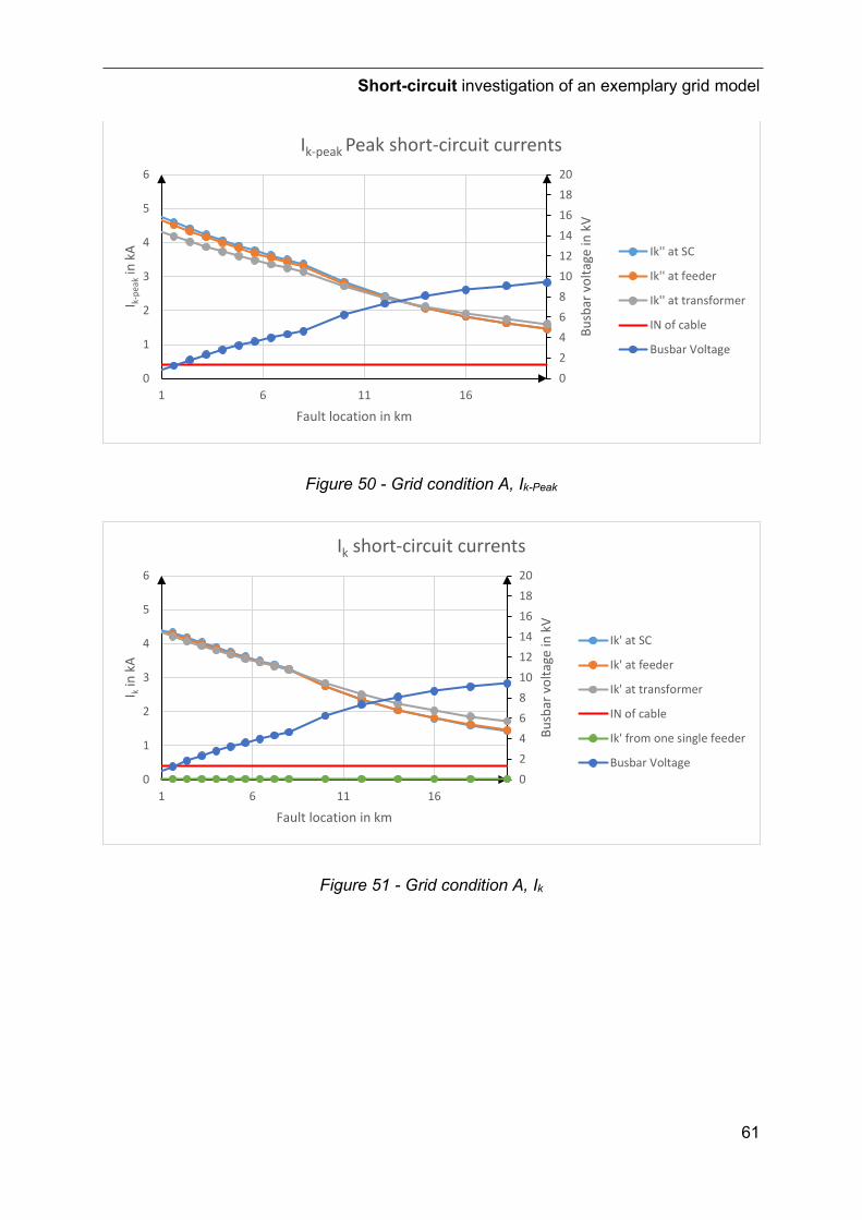
Short-circuit investigation of an exemplary grid model
61
Figure 50 - Grid condition A, Ik-Peak
Figure 51 - Grid condition A, Ik
02468101214161820
0
1
2
3
4
5
6
1 6 11 16
Busb
ar v
olta
ge in
kV
I k-pe
akin
kA
Fault location in km
Ik-peak Peak short-circuit currents
Ik'' at SC
Ik'' at feeder
Ik'' at transformer
IN of cable
Busbar Voltage
02468101214161820
0
1
2
3
4
5
6
1 6 11 16
Busb
ar v
olta
ge in
kV
I kin
kA
Fault location in km
Ik short-circuit currents
Ik' at SC
Ik' at feeder
Ik' at transformer
IN of cable
Ik' from one single feeder
Busbar Voltage
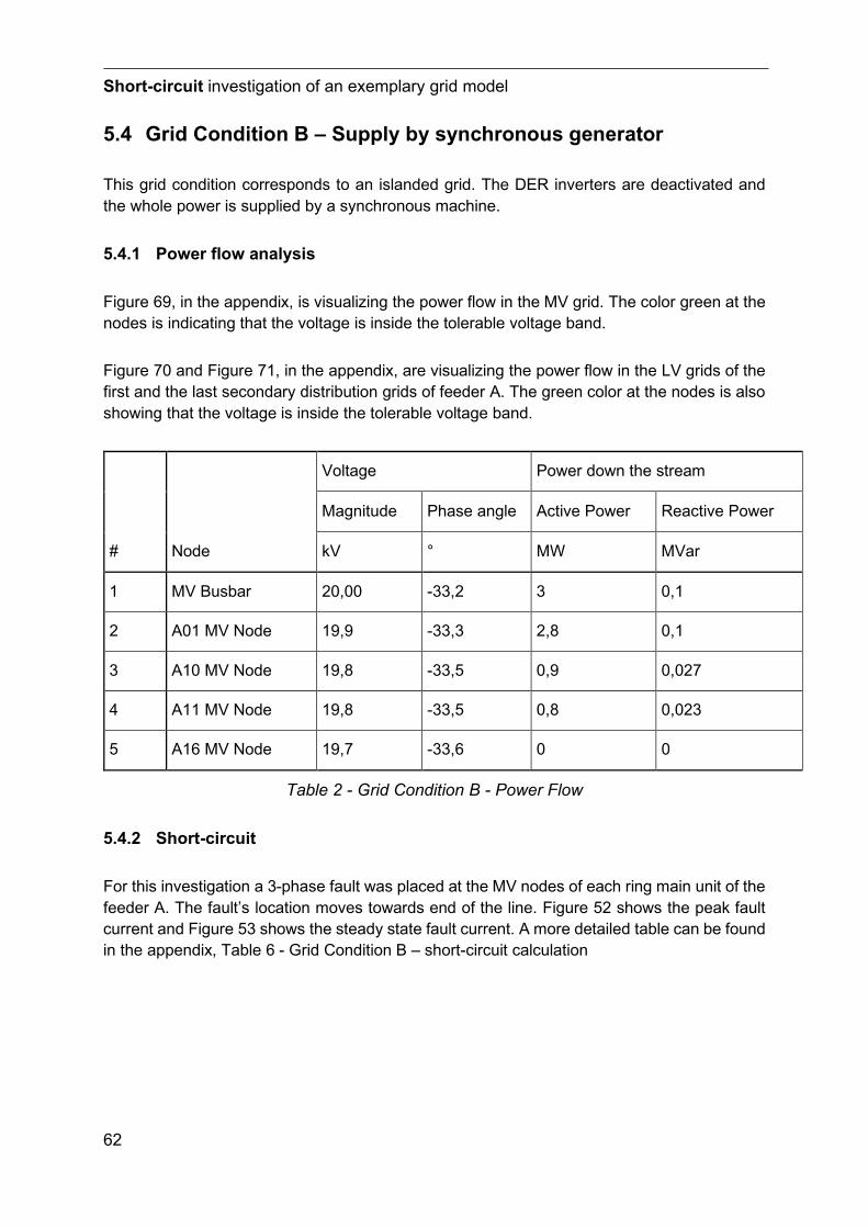
Short-circuit investigation of an exemplary grid model
62
5.4 Grid Condition B – Supply by synchronous generator
This grid condition corresponds to an islanded grid. The DER inverters are deactivated and the whole power is supplied by a synchronous machine.
5.4.1 Power flow analysis
Figure 69, in the appendix, is visualizing the power flow in the MV grid. The color green at the nodes is indicating that the voltage is inside the tolerable voltage band.
Figure 70 and Figure 71, in the appendix, are visualizing the power flow in the LV grids of the first and the last secondary distribution grids of feeder A. The green color at the nodes is also showing that the voltage is inside the tolerable voltage band.
# Node
Voltage Power down the stream
Magnitude Phase angle Active Power Reactive Power
kV ° MW MVar
1 MV Busbar 20,00 -33,2 3 0,1
2 A01 MV Node 19,9 -33,3 2,8 0,1
3 A10 MV Node 19,8 -33,5 0,9 0,027
4 A11 MV Node 19,8 -33,5 0,8 0,023
5 A16 MV Node 19,7 -33,6 0 0
Table 2 - Grid Condition B - Power Flow
5.4.2 Short-circuit
For this investigation a 3-phase fault was placed at the MV nodes of each ring main unit of the feeder A. The fault’s location moves towards end of the line. Figure 52 shows the peak fault current and Figure 53 shows the steady state fault current. A more detailed table can be found in the appendix, Table 6 - Grid Condition B – short-circuit calculation
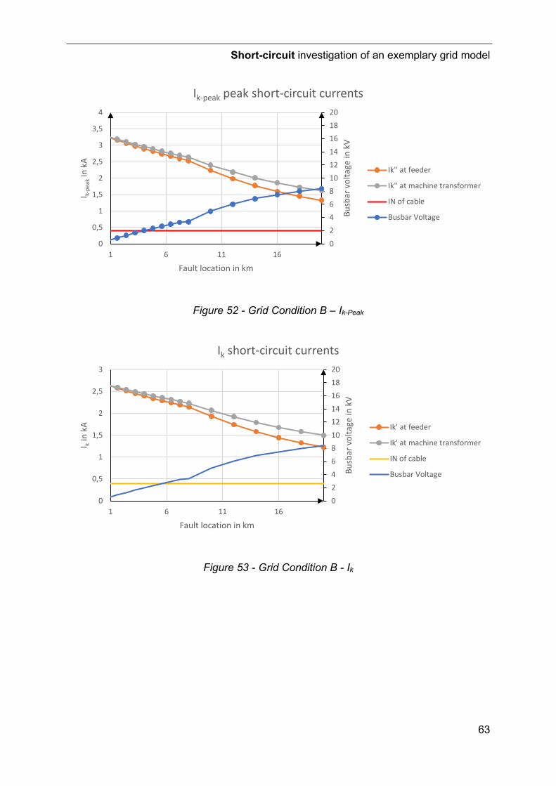
Short-circuit investigation of an exemplary grid model
63
Figure 52 - Grid Condition B – Ik-Peak
Figure 53 - Grid Condition B - Ik
02468101214161820
0
0,5
1
1,5
2
2,5
3
3,5
4
1 6 11 16
Busb
ar v
olta
ge in
kV
I k-pe
akin
kA
Fault location in km
Ik-peak peak short-circuit currents
Ik'' at feeder
Ik'' at machine transformer
IN of cable
Busbar Voltage
02468101214161820
0
0,5
1
1,5
2
2,5
3
1 6 11 16
Busb
ar v
olta
ge in
kV
I kin
kA
Fault location in km
Ik short-circuit currents
Ik' at feeder
Ik' at machine transformer
IN of cable
Busbar Voltage
Short-circuit investigation of an exemplary grid model
64
5.5 Grid Condition C – Supply only by inverters
In this grid condition, the grid operates in the islanding mode. The whole power is supplied by the DER inverters, which are grid-forming inverters.
5.5.1 Power flow analysis
Figure 72, in the appendix, is visualizing the power flow in the MV grid. The color green at the nodes is indicating that the voltage is inside the tolerable voltage band.
Figure 73 and Figure 74, in the appendix, are visualizing the power flow in the LV grids of the first and the last secondary distribution grids of feeder A. The green color at the nodes is also showing that the voltage is inside the tolerable voltage band.
# Node
Voltage Power down the stream
Magnitude Phase angle Active Power Reactive Power
kV ° MW MVar
1 MV Busbar 19,9 166,3 0 0
2 A01 MV Node 19,9 166,3 0,4 0,1
3 A10 MV Node 19,9 166,3 0,1 0,1
4 A11 MV Node 19,9 166,3 0 0
5 A16 MV Node 19,9 166,3 0 0
Table 3 - Grid Condition C - Power Flow
5.5.2 Short-circuit
For this investigation a 3-phase fault was placed at the MV nodes of each ring main unit of the feeder A. The fault’s location moves towards the end of the line. Figure 54 shows the peak fault current and Figure 55 shows the steady state fault current. A more detailed table can be found in the appendix, Table 7 - Grid Condition C - short-circuit calculation.
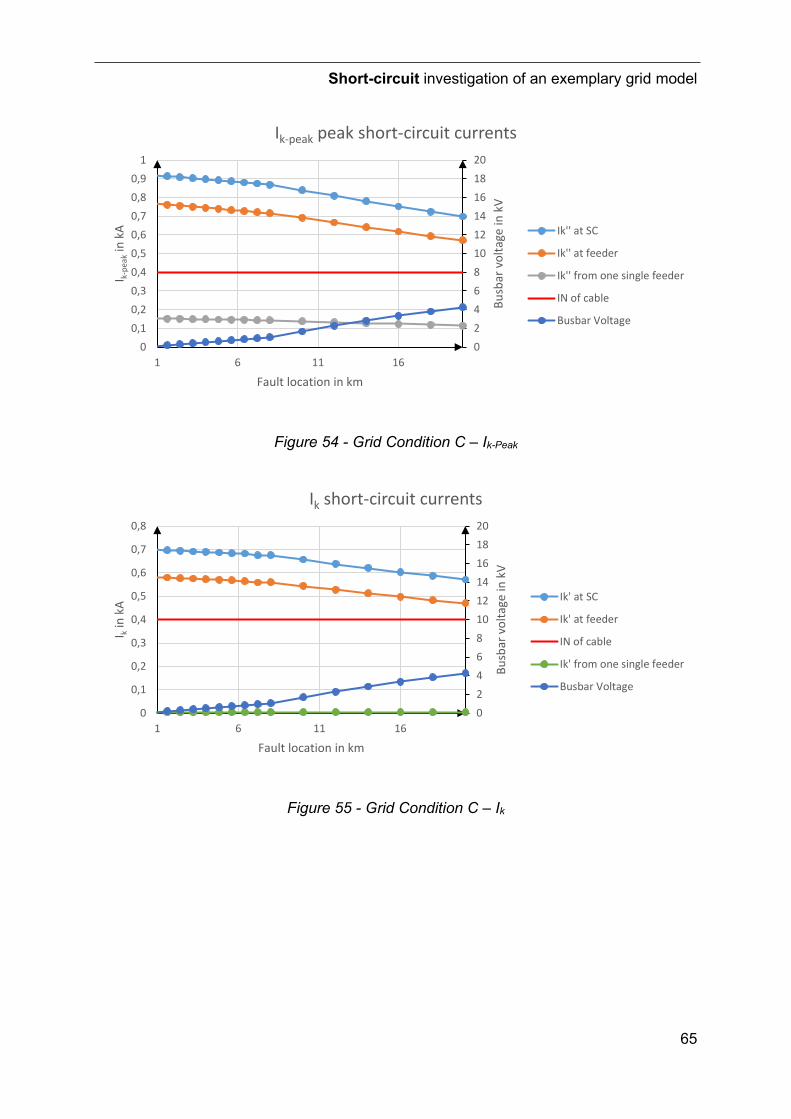
Short-circuit investigation of an exemplary grid model
65
Figure 54 - Grid Condition C – Ik-Peak
Figure 55 - Grid Condition C – Ik
02468101214161820
00,10,20,30,40,50,60,70,80,9
1
1 6 11 16
Busb
ar v
olta
ge in
kV
I k-pe
akin
kA
Fault location in km
Ik-peak peak short-circuit currents
Ik'' at SC
Ik'' at feeder
Ik'' from one single feeder
IN of cable
Busbar Voltage
02468101214161820
0
0,1
0,2
0,3
0,4
0,5
0,6
0,7
0,8
1 6 11 16
Busb
ar v
olta
ge in
kV
I kin
kA
Fault location in km
Ik short-circuit currents
Ik' at SC
Ik' at feeder
IN of cable
Ik' from one single feeder
Busbar Voltage
Short-circuit investigation of an exemplary grid model
66
5.6 Evaluation
Using the different grid conditions, states of the grid were calculated, which are relevant for the design of the protection. To achieve comparability with machine short circuits, 3-pole faults were simulated.
Grid Condition A corresponds to the regular operation for which the grid is designed. The load flow calculation converges and provides plausible results. The results can be seen in Table 1. Subsequently, short circuit calculations were performed. The fault location was varied, and it moves from the busbar along the line at feeder A to the end. The short circuit locations were each placed on the ring main unit. This allowed the progression of the short circuit current to be plotted. The peak and the steady-state current were recorded in each case.
Comparing the short-circuit current at the faulted feeder, the transformer bay and the other feeders, it can be seen that the short-circuit current is dominated by the current from the transformer. Since in the design of the grid, the PV feed was added to a normal grid, there is enough short circuit power available to run conventional protection. Expected behavior can also be observed in the voltage at the busbar. With the values obtained from Grid Condition A, the protection can be designed in grid connected operation. In the appendix section 9.2 more detailed results can be obtained.
Grid condition B is needed to obtain the load flow without the contribution of the PV inverters. Furthermore, with the short-circuit currents calculated in Grid Condition B, a comparison can be made between inverter dominated states (Grid Condition C) and conventional feed-in (Grid Condition B).
Methodically, the procedure was analogous to Grid Condition A. Here, too, the results were as expected. The load flow converged and showed plausible results and the short circuit currents were as expected. In the appendix section 9.3 more detailed results can be obtained.
Grid Condition C was now a purely inverter-powered condition. Here, the entire load was supplied from the distributed PV inverters. Again, the load flow converged and gave a plausible result.
However, if the short-circuit current in the steady state region is analyzed, it can be seen in Figure 55 that the short-circuit current is very close to the rated current of the ground cable and OHL. However, there is a margin to the ordinary load flow. The voltage at the busbar is very low for the fault cases. Here it would be necessary to investigate whether the voltage transformers can still measure this voltage sufficiently. In the appendix section 9.4 more detailed results can be obtained.
The results of these simulations are used to design the protection with the protection function given in section 3.4.2.

Short-circuit investigation of an exemplary grid model
67
Directional Voltage Controlled Overcurrent
68
6 Directional Voltage Controlled Overcurrent
6.1 Settings
In section 3.4.2 the principle of this protection function is explained.
In order for the protection system to work properly, the protection functions must be parameterized to meet the objects to be protected, according to the basic criteria mentioned in section 3.1. Based on the explanations in section 3.4, there are the following setting values that must be considered:
1. 𝐼𝐼𝑆𝑆ℎ … The current threshold for the OC element in forward direction. 2. 𝑡𝑡𝑙𝑙𝐿𝐿𝑑𝑑𝑓𝑓𝐿𝐿𝑑𝑑𝐿𝐿 … The trip time in forward direction, once 𝐼𝐼𝑆𝑆ℎ is exceeded. 3. 𝑏𝑏 … The current restraining factor in forward direction. 4. 𝑡𝑡𝑑𝑑𝑆𝑆𝑟𝑟𝑆𝑆𝑑𝑑𝑠𝑠𝑆𝑆 … The trip time in backward direction, once 𝐼𝐼𝑆𝑆ℎ is exceeded. 5. 𝑉𝑉𝑆𝑆ℎ𝑑𝑑𝑆𝑆𝑠𝑠ℎ𝐿𝐿𝑙𝑙𝐿𝐿 … The voltage threshold that initiates the restraining of the current
threshold. The design of this protection function performed here is based on the simulations in chapter 5. First, the trip times are defined. Since this is the last section in the medium voltage network, there is only the protection of the distribution transformers, which must be considered in the design of the trip times, as a lower limit. In most cases, these distribution transformers are protected by fuses on the upper voltage side. In a typical medium voltage system, the short circuit current is high enough to instantaneously trip the fuse for internal transformer faults. However, in isolated operation, the fault current may not be sufficient to trip the fuses, so for further design, a protection device is assumed which can clear faults in the transformer instantaneously.
For this clearing time, a time of ttransformer = 100 ms is assumed.
The further specifications are based on the setting guidelines of [46].
In order to now have sufficient reserve between the tripping of the protective device of the transformer and the feeder protection relay, a trip time of 𝑡𝑡𝑙𝑙𝐿𝐿𝑑𝑑𝑓𝑓𝐿𝐿𝑑𝑑𝐿𝐿 = 300 ms is used. This means that there is a time difference of Δ𝑡𝑡 = 200 ms. In the reverse direction, an additional grading time of 𝑡𝑡𝑆𝑆𝑑𝑑𝐿𝐿𝐿𝐿𝑆𝑆𝑆𝑆𝑆𝑆 = 300 𝐼𝐼𝑠𝑠 is added to the time in the forward direction. This results in a trip time of 𝑡𝑡𝑑𝑑𝑆𝑆𝑟𝑟𝑆𝑆𝑑𝑑𝑠𝑠𝑆𝑆 = 500 𝐼𝐼𝑠𝑠. The grading time 𝑡𝑡𝑆𝑆𝑑𝑑𝐿𝐿𝐿𝐿𝑆𝑆𝑆𝑆𝑆𝑆 is composed of the following time components[46]:
• The relay’s detection time • The relay’s maximum trip time
Directional Voltage Controlled Overcurrent
69
• The circuit breaker’s operating time • The relay’s drop-off time and • The arcing time
The next setting is the current threshold 𝐼𝐼𝑆𝑆ℎ. The maximum load current is derived from the load flow simulation in grid condition B, here the whole grid is supplied by a synchronous generator and the PV systems are out of operation. The current is calculated from the simulation results in Table 2 - Grid Condition B - Power Flow and the following equations:
𝐼𝐼𝐿𝐿𝐿𝐿𝑛𝑛𝐿𝐿𝐿𝐿 =
�𝑃𝑃2 + 𝑄𝑄2
√3 ⋅ 𝑉𝑉𝐿𝐿−𝐿𝐿=�(3 𝑃𝑃𝑘𝑘)2 + (0.1 𝑃𝑃𝐾𝐾𝑎𝑎𝐹𝐹)2
√3 ⋅ 20 𝑘𝑘𝑉𝑉= 91 𝑘𝑘 (31)
Next, the minimum short-circuit current in grid-connected mode is required. This is taken from the short-circuit calculation in grid-condition B. For this, the steady state short-circuit current for a fault at the end of the overhead line is selected, this is 𝐼𝐼𝑆𝑆𝐷𝐷𝑛𝑛𝑆𝑆𝑆𝑆 = 1226 𝑘𝑘. The threshold value 𝐼𝐼𝑆𝑆ℎ must now lie between 𝐼𝐼𝐿𝐿𝐿𝐿𝑛𝑛𝐿𝐿𝐿𝐿 and 𝐼𝐼𝑆𝑆𝐷𝐷𝑛𝑛𝑆𝑆𝑆𝑆. For reliable tripping, the safety margin factor 𝑘𝑘𝑑𝑑 = 2 is assumed.
𝐼𝐼𝐿𝐿𝐿𝐿𝑛𝑛𝐿𝐿𝐿𝐿 > 𝐼𝐼𝑆𝑆ℎ > 𝐼𝐼𝑆𝑆𝐷𝐷𝑛𝑛𝑆𝑆𝑆𝑆 (32)
𝐼𝐼𝑆𝑆ℎ ≤𝐼𝐼𝑆𝑆𝑆𝑆𝑆𝑆𝑆𝑆𝑆𝑆𝑃𝑃𝑟𝑟
= 1226 𝐴𝐴2
≅ 600 𝑘𝑘 (33)
The restraining factor 𝑏𝑏 is now chosen so that the minimum short-circuit current of grid-condition C (fault at the end of the overhead line) is detected with a safety margin factor 𝑘𝑘𝑑𝑑 = 2. For this purpose, the current is taken from Table 7 - Grid Condition C - short-circuit calculation, 𝐼𝐼𝑆𝑆𝐷𝐷𝑛𝑛𝑆𝑆𝑆𝑆 −𝐺𝐺𝐷𝐷 𝐷𝐷 = 470 𝑘𝑘 .
𝑏𝑏 ⋅ 𝐼𝐼𝑆𝑆ℎ ≤𝐼𝐼𝑆𝑆𝑆𝑆𝑆𝑆𝑆𝑆𝑆𝑆−𝐺𝐺𝑆𝑆 𝑆𝑆
𝑃𝑃𝑟𝑟= 470 𝐴𝐴
2= 235 𝑘𝑘 (34)
𝑏𝑏 =235 𝑘𝑘600 𝑘𝑘
≈ 0.4 (35)
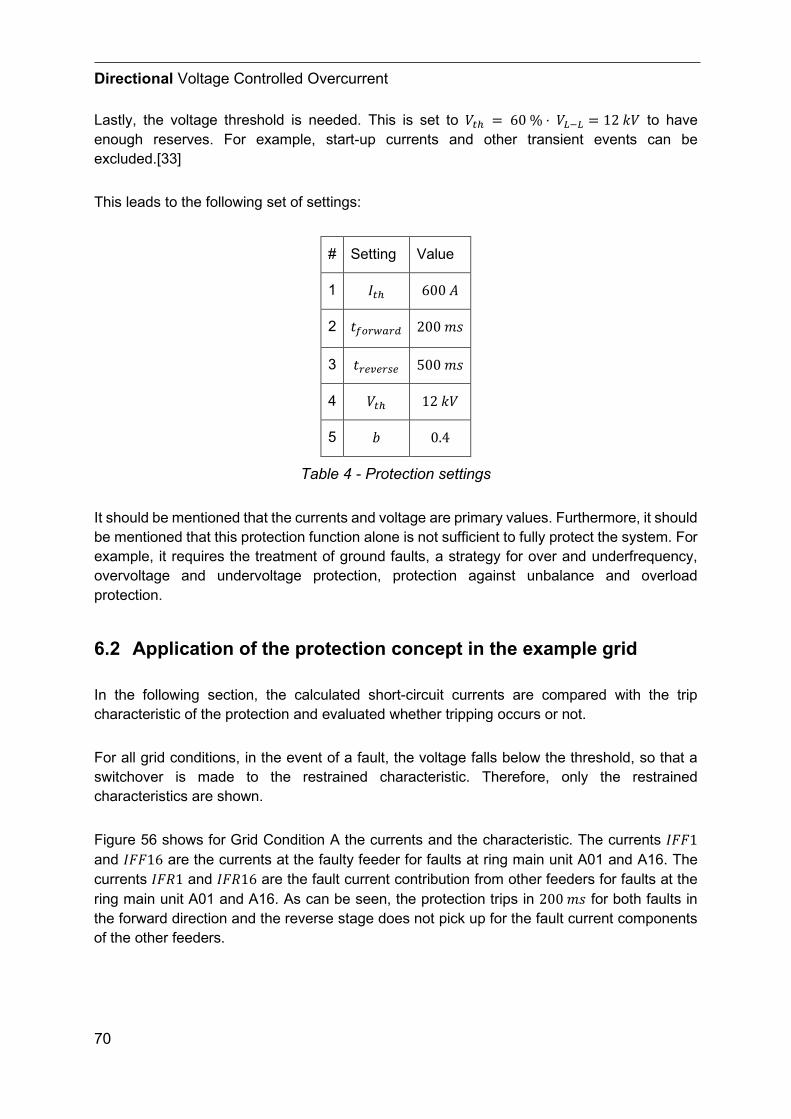
Directional Voltage Controlled Overcurrent
70
Lastly, the voltage threshold is needed. This is set to 𝑉𝑉𝑆𝑆ℎ = 60 % ⋅ 𝑉𝑉𝐿𝐿−𝐿𝐿 = 12 𝑘𝑘𝑉𝑉 to have enough reserves. For example, start-up currents and other transient events can be excluded.[33]
This leads to the following set of settings:
# Setting Value
1 𝐼𝐼𝑆𝑆ℎ 600 𝑘𝑘
2 𝑡𝑡𝑙𝑙𝐿𝐿𝑑𝑑𝑓𝑓𝐿𝐿𝑑𝑑𝐿𝐿 200 𝐼𝐼𝑠𝑠
3 𝑡𝑡𝑑𝑑𝑆𝑆𝑟𝑟𝑆𝑆𝑑𝑑𝑠𝑠𝑆𝑆 500 𝐼𝐼𝑠𝑠
4 𝑉𝑉𝑆𝑆ℎ 12 𝑘𝑘𝑉𝑉
5 𝑏𝑏 0.4
Table 4 - Protection settings
It should be mentioned that the currents and voltage are primary values. Furthermore, it should be mentioned that this protection function alone is not sufficient to fully protect the system. For example, it requires the treatment of ground faults, a strategy for over and underfrequency, overvoltage and undervoltage protection, protection against unbalance and overload protection.
6.2 Application of the protection concept in the example grid
In the following section, the calculated short-circuit currents are compared with the trip characteristic of the protection and evaluated whether tripping occurs or not.
For all grid conditions, in the event of a fault, the voltage falls below the threshold, so that a switchover is made to the restrained characteristic. Therefore, only the restrained characteristics are shown.
Figure 56 shows for Grid Condition A the currents and the characteristic. The currents 𝐼𝐼𝐹𝐹𝐹𝐹1 and 𝐼𝐼𝐹𝐹𝐹𝐹16 are the currents at the faulty feeder for faults at ring main unit A01 and A16. The currents 𝐼𝐼𝐹𝐹𝑅𝑅1 and 𝐼𝐼𝐹𝐹𝑅𝑅16 are the fault current contribution from other feeders for faults at the ring main unit A01 and A16. As can be seen, the protection trips in 200 𝐼𝐼𝑠𝑠 for both faults in the forward direction and the reverse stage does not pick up for the fault current components of the other feeders.
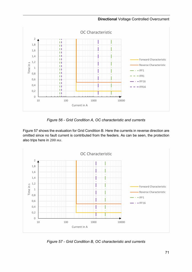
Directional Voltage Controlled Overcurrent
71
Figure 56 - Grid Condition A, OC characteristic and currents
Figure 57 shows the evaluation for Grid Condition B. Here the currents in reverse direction are omitted since no fault current is contributed from the feeders. As can be seen, the protection also trips here in 200 𝐼𝐼𝑠𝑠.
Figure 57 - Grid Condition B, OC characteristic and currents
0
0,2
0,4
0,6
0,8
1
1,2
1,4
1,6
1,8
2
10 100 1000 10000
Tim
e in
s
Current in A
OC Characteristic
Forward Characteristic
Reverse Characteristic
IFF1
IFR1
IFF16
IFR16
0
0,2
0,4
0,6
0,8
1
1,2
1,4
1,6
1,8
2
10 100 1000 10000
Tim
e in
s
Current in A
OC Characteristic
Forward Characteristic
Reverse Characteristic
IFF1
IFF16
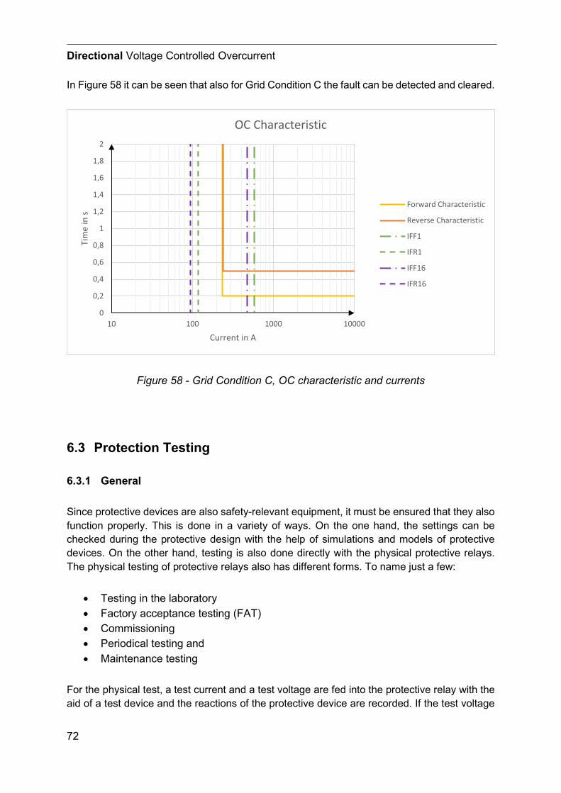
Directional Voltage Controlled Overcurrent
72
In Figure 58 it can be seen that also for Grid Condition C the fault can be detected and cleared.
Figure 58 - Grid Condition C, OC characteristic and currents
6.3 Protection Testing
6.3.1 General
Since protective devices are also safety-relevant equipment, it must be ensured that they also function properly. This is done in a variety of ways. On the one hand, the settings can be checked during the protective design with the help of simulations and models of protective devices. On the other hand, testing is also done directly with the physical protective relays. The physical testing of protective relays also has different forms. To name just a few:
• Testing in the laboratory • Factory acceptance testing (FAT) • Commissioning • Periodical testing and • Maintenance testing
For the physical test, a test current and a test voltage are fed into the protective relay with the aid of a test device and the reactions of the protective device are recorded. If the test voltage
0
0,2
0,4
0,6
0,8
1
1,2
1,4
1,6
1,8
2
10 100 1000 10000
Tim
e in
s
Current in A
OC Characteristic
Forward Characteristic
Reverse Characteristic
IFF1
IFR1
IFF16
IFR16
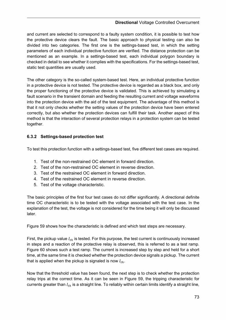
Directional Voltage Controlled Overcurrent
73
and current are selected to correspond to a faulty system condition, it is possible to test how the protective device clears the fault. The basic approach to physical testing can also be divided into two categories. The first one is the settings-based test, in which the setting parameters of each individual protective function are verified. The distance protection can be mentioned as an example. In a settings-based test, each individual polygon boundary is checked in detail to see whether it complies with the specifications. For the settings-based test, static test quantities are usually used.
The other category is the so-called system-based test. Here, an individual protective function in a protective device is not tested. The protective device is regarded as a black box, and only the proper functioning of the protective device is validated. This is achieved by simulating a fault scenario in the transient domain and feeding the resulting current and voltage waveforms into the protection device with the aid of the test equipment. The advantage of this method is that it not only checks whether the setting values of the protection device have been entered correctly, but also whether the protection devices can fulfill their task. Another aspect of this method is that the interaction of several protection relays in a protection system can be tested together.
6.3.2 Settings-based protection test
To test this protection function with a settings-based test, five different test cases are required.
1. Test of the non-restrained OC element in forward direction. 2. Test of the non-restrained OC element in reverse direction. 3. Test of the restrained OC element in forward direction. 4. Test of the restrained OC element in reverse direction. 5. Test of the voltage characteristic.
The basic principles of the first four test cases do not differ significantly. A directional definite time OC characteristic is to be tested with the voltage associated with the test case. In the explanation of the test, the voltage is not considered for the time being it will only be discussed later.
Figure 59 shows how the characteristic is defined and which test steps are necessary.
First, the pickup value 𝐼𝐼𝑆𝑆ℎ is tested. For this purpose, the test current is continuously increased in steps and a reaction of the protective relay is observed, this is referred to as a test ramp. Figure 60 shows such a test ramp. The current is increased step by step and held for a short time, at the same time it is checked whether the protection device signals a pickup. The current that is applied when the pickup is signaled is now 𝐼𝐼𝑆𝑆ℎ.
Now that the threshold value has been found, the next step is to check whether the protection relay trips at the correct time. As it can be seen in Figure 59, the tripping characteristic for currents greater than 𝐼𝐼𝑆𝑆ℎ is a straight line. To reliably within certain limits identify a straight line,
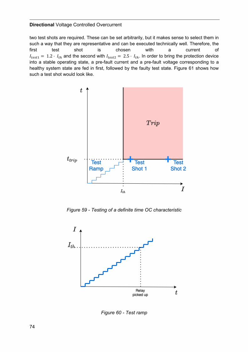
Directional Voltage Controlled Overcurrent
74
two test shots are required. These can be set arbitrarily, but it makes sense to select them in such a way that they are representative and can be executed technically well. Therefore, the first test shot is chosen with a current of 𝐼𝐼𝑆𝑆𝑆𝑆𝑠𝑠𝑆𝑆1 = 1.2 ⋅ 𝐼𝐼𝑆𝑆ℎ and the second with 𝐼𝐼𝑆𝑆𝑆𝑆𝑠𝑠𝑆𝑆2 = 2.5 ⋅ 𝐼𝐼𝑆𝑆ℎ. In order to bring the protection device into a stable operating state, a pre-fault current and a pre-fault voltage corresponding to a healthy system state are fed in first, followed by the faulty test state. Figure 61 shows how such a test shot would look like.
Figure 59 - Testing of a definite time OC characteristic
Figure 60 - Test ramp
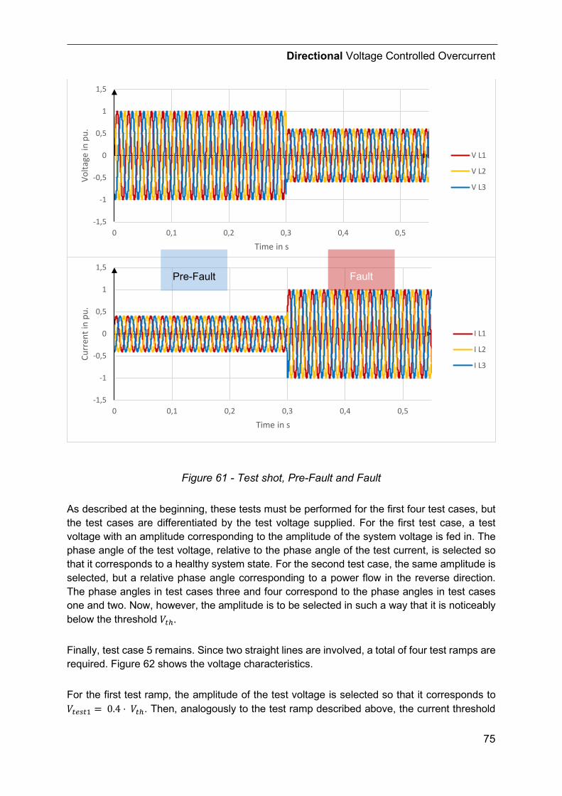
Directional Voltage Controlled Overcurrent
75
Figure 61 - Test shot, Pre-Fault and Fault
As described at the beginning, these tests must be performed for the first four test cases, but the test cases are differentiated by the test voltage supplied. For the first test case, a test voltage with an amplitude corresponding to the amplitude of the system voltage is fed in. The phase angle of the test voltage, relative to the phase angle of the test current, is selected so that it corresponds to a healthy system state. For the second test case, the same amplitude is selected, but a relative phase angle corresponding to a power flow in the reverse direction. The phase angles in test cases three and four correspond to the phase angles in test cases one and two. Now, however, the amplitude is to be selected in such a way that it is noticeably below the threshold 𝑉𝑉𝑆𝑆ℎ.
Finally, test case 5 remains. Since two straight lines are involved, a total of four test ramps are required. Figure 62 shows the voltage characteristics.
For the first test ramp, the amplitude of the test voltage is selected so that it corresponds to 𝑉𝑉𝑆𝑆𝑆𝑆𝑠𝑠𝑆𝑆1 = 0.4 ⋅ 𝑉𝑉𝑆𝑆ℎ. Then, analogously to the test ramp described above, the current threshold
-1,5
-1
-0,5
0
0,5
1
1,5
0 0,1 0,2 0,3 0,4 0,5
Volta
ge in
pu.
Time in s
V L1
V L2
V L3
-1,5
-1
-0,5
0
0,5
1
1,5
0 0,1 0,2 0,3 0,4 0,5
Curr
ent i
n pu
.
Time in s
I L1
I L2
I L3
Pre-Fault Fault
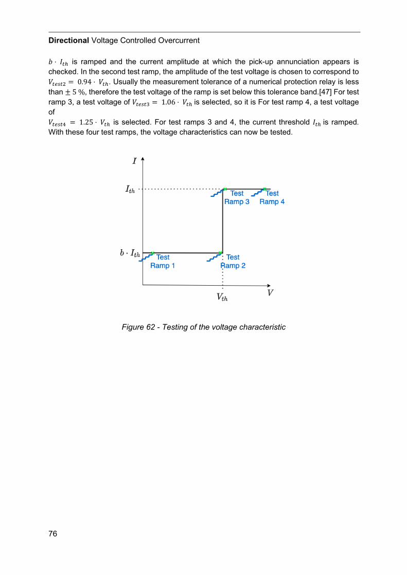
Directional Voltage Controlled Overcurrent
76
𝑏𝑏 ⋅ 𝐼𝐼𝑆𝑆ℎ is ramped and the current amplitude at which the pick-up annunciation appears is checked. In the second test ramp, the amplitude of the test voltage is chosen to correspond to 𝑉𝑉𝑆𝑆𝑆𝑆𝑠𝑠𝑆𝑆2 = 0.94 ⋅ 𝑉𝑉𝑆𝑆ℎ. Usually the measurement tolerance of a numerical protection relay is less than ± 5 %, therefore the test voltage of the ramp is set below this tolerance band.[47] For test ramp 3, a test voltage of 𝑉𝑉𝑆𝑆𝑆𝑆𝑠𝑠𝑆𝑆3 = 1.06 ⋅ 𝑉𝑉𝑆𝑆ℎ is selected, so it is For test ramp 4, a test voltage of 𝑉𝑉𝑆𝑆𝑆𝑆𝑠𝑠𝑆𝑆4 = 1.25 ⋅ 𝑉𝑉𝑆𝑆ℎ is selected. For test ramps 3 and 4, the current threshold 𝐼𝐼𝑆𝑆ℎ is ramped. With these four test ramps, the voltage characteristics can now be tested.
Figure 62 - Testing of the voltage characteristic

Directional Voltage Controlled Overcurrent
77
6.3.1 System-based protection test
Test cases in the system-based protection test concept differ fundamentally from test cases in the settings-based concept. Here, it is not the setting values that are tested but the ability of the protection to react to realistic scenarios. Test scenarios are therefore required which correspond to all representative operating conditions.
These test scenarios can be divided into two categories. On the one hand, the scenarios in which the stability of the protection is tested and, on the other hand, scenarios in which faulty states are simulated. For the stability test cases, the protection system must not trip.
The following test scenarios can be mentioned as examples:
• Stability test cases o Regular power flow down-stream o Power flow up-stream
• Fault scenarios o Line fault at the beginning of the line o Line fault at the end of the line o Line faults with varying fault impedances o Faults on a different feeder in reverse direction, with the main protection not
tripping.
For all these test scenarios, the reactions of the protection system are now recorded and evaluated based on the requirements for the protection system.

Directional Voltage Controlled Overcurrent
78
Conclusion
79
7 Conclusion
In this work, the ANSI 51V protection function was investigated for application in a distribution system with a high percentage of inverter-based generation and islanding capability. Furthermore, easy-to-use simulation models for these inverter-based generators were investigated.
For this purpose, first definitions and theoretical basics were presented, which are essential for a starting point. A description of distribution grids, in particular of active distribution grids and term definitions in the area of microgrids and smart grids define the playing field. The type of grid chosen in this thesis is to be assigned to microgrids on the basis of the definitions. In the next step, the inverter-based generators discussed in this thesis were discussed. Basic information and some relevant characteristics and regulations for grid operation were collected. Since this thesis is an investigation in the field of protection technology, protection principles and protection concepts in the field of distribution networks and microgrids were also dealt with. The use of the ANSI 51V protection function, which is largely used in generator protection, was also discussed. A large portion of this work revolves around the modeling of inverter-based generators. For this purpose, an extensive literature review is applied, which firstly captured what needs to be simulated and what requirements are important for short-circuit current calculations in the field of protection design. A state-of-the-art model that is easy to handle was then chosen for the further investigations, since complex data sets for the simulation are not available in the everyday life of a user. Such a model is given with the static generator model in DigSilent PowerFactory.
In the next step, an exemplary test grid is formulated. Load flow and short-circuit investigations were carried out for different states in the grid to be able to design the protection concept. With the results of these calculations, the ANSI 51V protection function was then applied to this exemplary grid. This protection function is combined with a directional element to obtain a better selectivity. Finally, it is checked if the protection can detect all relevant faults and a suggestion how to test this protection system was made.
The objective of this work is to investigate whether ANSI 51V protection can be applied in a distribution network with a high percentage of inverter-based generation.
Conclusion
80
This protection function in cooperation with a directional element can be applied in distribution networks. The additional criterion of voltage can be used for a clearer distinction between faulty condition and non-faulty condition. Compared to distance protection, the following points can be obtained:
• Time grading is simpler because no impedance zones need to be calculated and coordinated.
• The requirements on the accuracy of the voltage measurement can be lower. The Device only needs to distinguish between lower or higher the threshold voltage.
• This simple protection device has no fault locator, but this is a very important function in the operation of an electricity grid. This allows maintenance crews to act and restore the feeder faster, in case of a fault.
• In this special example automatic reclosing is not possible, because the device does not know if the fault is on the cable or OHL section. Otherwise, an additional device must be implemented.
The selected protection concept was able to detect all simulated faulty conditions in the grid and shut down the faulty feeder.
In this work it was assumed that the inverters still behave sinusoidally in the case of an external fault. Whether this is really the case is addressed by current research. If non-sinusoidal currents are present, then fault detection with incremental quantities functions could be interesting and worth investigating. However, it is questionable whether protection relays with this function will soon find application in distribution networks since they have a rather high price.
References
81
8 References
[1] Dr. Stefan Küppers, “DSO 2.0 – Entwicklung des Verteilnetzbetreibers durch die Energiewende.” Westnetz, Nov. 12, 2015. [Online]. Available: https://docplayer.org/20450127-Dso-2-0-entwicklung-des-verteilnetzbetreibers-durch-die-energiewende.html
[2] “IEEE Standard for the Specification of Microgrid Controllers,” IEEE Std 20307-2017, pp. 1–43, Apr. 2018, doi: 10.1109/IEEESTD.2018.8295083.
[3] Berkley Lab, “About Microgrids.” https://building-microgrid.lbl.gov/about-microgrids (accessed Aug. 23, 2020).
[4] Li Fusheng, Li Ruisheng, and Zhou Fengquan, Microgrid Technology and Engineering Application. Elsevier, 2016. doi: 10.1016/C2013-0-18521-2.
[5] ABB Ltd., “Introduction to microgrids.” https://new.stage.abb.com/distributed-energy-microgrids/introduction-to-microgrids (accessed Aug. 23, 2020).
[6] Siemens AG, “Efficient, resilient, beneficial and sustainable disrtibuted energy systems,” siemens.com Global Website. https://new.siemens.com/global/en/general/404.html (accessed Aug. 23, 2020).
[7] P. J. Rohrer, “Was ist der Unterschied zwischen Microgrids und Smart Grids?,” ZHAW Zürcher Hochschule für Angewandte Wissenschaften. https://www.zhaw.ch/de/404/ (accessed Aug. 23, 2020).
[8] P. Landsbergen, “Feasibility, beneficiality, and institutional compatibility of a micro-CHP virtual power plant in the Netherlands,” TU Delft, Delft, 2009.
[9] “Five minute guide to microgrids - Arup.” https://www.arup.com/perspectives/publications/promotional-materials/section/five-minute-guide-to-microgrids (accessed Aug. 23, 2020).
[10] “IEC TS 62898-1:2017 Guidelines for microgrid projects planning and specification,” 2017. https://webstore.iec.ch/publication/28363 (accessed Aug. 23, 2020).
[11] N. Hatziargyriou, “Microgrids: Architectures and Control | Wiley,” Wiley.com. https://www.wiley.com/en-us/Microgrids%3A+Architectures+and+Control-p-9781118720684 (accessed Aug. 23, 2020).
[12] “Doubly-fed electric machine,” Wikipedia. Oct. 16, 2021. Accessed: Nov. 29, 2021. [Online]. Available: https://en.wikipedia.org/w/index.php?title=Doubly-fed_electric_machine&oldid=1050284607
References
82
[13] P. Unruh, M. Nuschke, P. Strauß, and F. Welck, “Overview on Grid-Forming Inverter Control Methods,” Energ. Basel, vol. 13, no. 10, pp. 2589-, 2020, doi: 10.3390/en13102589.
[14] J. Keller and B. Kroposki, “Understanding Fault Characteristics of Inverter-Based Distributed Energy Resources,” NREL/TP-550-46698, 971441, Jan. 2010. doi: 10.2172/971441.
[15] SMA Solar Technology AG, “Technical Information - Short-Circuit Currents Information on short-circuit currents of SMA PV inverters.” SMA Solar Technology AG.
[16] E-Control, “Technische und organisatorische Regeln für Betreiber und Benutzer von Netzen - Teil D - Hauptabschnitt 4: Parallelbetrieb von Erzeugungsanlagen mit Verteilernetzen - Version 2.3.” Jan. 07, 2016.
[17] VDE FNN, “Technische Anschlussregel Mittelspannung (VDE-AR-N 4110).” VDE Verlag, Nov. 2018.
[18] T. Neumann and I. Erlich, “Short Circuit Current Contribution of a Photovoltaic Power Plant,” IFAC Proc. Vol., vol. 45, no. 21, pp. 343–348, 2012, doi: 10.3182/20120902-4-FR-2032.00061.
[19] Lothar Fickert, “Schutz und Versorgungssicherheit elektrischer Energiesysteme.” Graz University of Technology, 2008.
[20] J. Shiles et al., “Microgrid protection: An overview of protection strategies in North American microgrid projects,” in 2017 IEEE Power Energy Society General Meeting, Jul. 2017, pp. 1–5. doi: 10.1109/PESGM.2017.8274519.
[21] F. Katiraei, C. Abbey, S. Tang, and M. Gauthier, “Planned islanding on rural feeders — utility perspective,” in 2008 IEEE Power and Energy Society General Meeting - Conversion and Delivery of Electrical Energy in the 21st Century, Jul. 2008, pp. 1–6. doi: 10.1109/PES.2008.4596774.
[22] L. Che, M. E. Khodayar, and M. Shahidehpour, “Adaptive Protection System for Microgrids: Protection practices of a functional microgrid system.,” IEEE Electrification Mag., vol. 2, no. 1, pp. 66–80, Mar. 2014, doi: 10.1109/MELE.2013.2297031.
[23] T. S. Ustun, C. Ozansoy, and A. Zayegh, “A microgrid protection system with central protection unit and extensive communication,” 2011 10th Int. Conf. Environ. Electr. Eng. EEEICEU 2011 - Conf. Proc., May 2011, doi: 10.1109/EEEIC.2011.5874777.
References
83
[24] Z. C. Li, J. Hu, J. H. He, and T. Yip, “A protection method for microgrids based on information sharing,” in 12th IET International Conference on Developments in Power System Protection (DPSP 2014), Mar. 2014, pp. 1–5. doi: 10.1049/cp.2014.0069.
[25] T. S. Ustun, C. Ozansoy, and A. Zayegh, “A central microgrid protection system for networks with fault current limiters,” in 2011 10th International Conference on Environment and Electrical Engineering, May 2011, pp. 1–4. doi: 10.1109/EEEIC.2011.5874575.
[26] T. S. Ustun, C. Ozansoy, and A. Zayegh, “Implementation of Dijkstra’s algorithm in a dynamic microgrid for relay hierarchy detection,” in 2011 IEEE International Conference on Smart Grid Communications (SmartGridComm), Oct. 2011, pp. 481–486. doi: 10.1109/SmartGridComm.2011.6102370.
[27] T. S. Ustun, C. Ozansoy, and A. Zayegh, “Differential protection of microgrids with central protection unit support,” in IEEE 2013 Tencon - Spring, Apr. 2013, pp. 15–19. doi: 10.1109/TENCONSpring.2013.6584408.
[28] Y. Liu, A. P. Meliopoulos, L. Sun, and S. Choi, “Protection and control of microgrids using dynamic state estimation,” Prot. Control Mod. Power Syst., vol. 3, no. 1, p. 31, Oct. 2018, doi: 10.1186/s41601-018-0104-2.
[29] Ziegler, Gerhard, Numerical Distance Protection: Principles and Applications, 4th ed. Erlangen: Publicis Publishing, 2011.
[30] Ziegler, Gerhard, Numerical Differential Protection: Principles and Applications, 2nd ed. Publicis Publishing, Erlangen, 2012.
[31] “7UM61xx_Manual_A4_V041101_en.pdf.” Accessed: Aug. 02, 2020. [Online]. Available: https://cache.industry.siemens.com/dl/files/484/109743484/att_903798/v1/7UM61xx_Manual_A4_V041101_en.pdf
[32] M. Meskin, P. Iyer, A. Domijan, and I. Grinberg, “Enhancement of overcurrent protection in active medium voltage distribution networks,” in 2017 IEEE 6th International Conference on Renewable Energy Research and Applications (ICRERA), Nov. 2017, pp. 937–942. doi: 10.1109/ICRERA.2017.8191197.
[33] P. Alibert and S. Electric, “PROTECTION SYSTEMS FOR MICROGRIDS WITH HIGH RATE OF INVERTER- BASED-GENERATORS,” CIRED Workshop, no. 0316, p. 4, 2018.
[34] K. Yamashita et al., “Industrial Recommendation of Modeling of Inverter-Based Generators for Power System Dynamic Studies With Focus on Photovoltaic,” IEEE Power Energy Technol. Syst. J., vol. 5, no. 1, pp. 1–10, Mar. 2018, doi: 10.1109/JPETS.2018.2806744.
References
84
[35] G. Lammert et al., “Modelling and dynamic performance of inverter based generation in power system studies: an international questionnaire survey,” CIRED - Open Access Proc. J., vol. 2017, no. 1, pp. 1899–1902, Oct. 2017, doi: 10.1049/oap-cired.2017.0898.
[36] G. Lammert et al., “International Industry Practice on Modelling and Dynamic Performance of Inverter Based Generation in Power System Studies,” Cigre Sci. Eng., vol. 8, pp. 25–37, 2017.
[37] “WECC Distributed and Small PV Plants Generic Model (PVD1),” ESIG. https://www.esig.energy/wiki-main-page/wecc-distributed-and-small-pv-plants-generic-model-pvd1/ (accessed May 15, 2021).
[38] NERC - North American Electric Reliability Corporation, Ed., “Reliability Guideline - Prameterization of the DER_A Model.” Sep. 2019.
[39] IEC TC 73 - Short-circuit currents, “IEC 60909-0 (2016): Short-circuit currents in three-phase AC systems. Part 0: Calculation of currents.” IEC, Jan. 28, 2016.
[40] “IEEE 141-1993 - IEEE Recommended Practice for Electric Power Distribution for Industrial Plants.” https://standards.ieee.org/standard/141-1993.html (accessed Jul. 11, 2021).
[41] H. W. Dommel, EMTP Theory Book. Microtran Power System Analysis Corporation, 1992.
[42] DIgSILENT GmbH, “Technical Reference Documentation WECC PV Plant Models.” 2019.
[43] DIgSILENT GmbH, “Technical Reference Documentation PV System.” 2019.
[44] DIgSILENT GmbH, “Technical Reference Documentation Static Generator.” 2019.
[45] DIgSILENT GmbH, “Technical Reference Documentation PWM Converter.” 2019.
[46] Lothar Fickert, “EINSTELLREGELN - Netzschutz-Magazin,” Netzschutz - Das Magazin für Schutztechniker. https://www.netzschutz-magazin.com/umz-schutz/einstellregeln/ (accessed Jul. 10, 2019).
[47] OMICRON electronics GmbH, “OMICRON Test Universe Version 4.30 - Help Document.” Sep. 06, 2021.
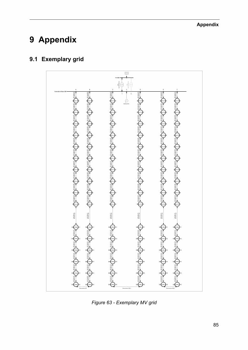
Appendix
85
9 Appendix
9.1 Exemplary grid
Figure 63 - Exemplary MV grid
A
1 2
B 3 FEC D
MV
-OH
L-Ty
peM
V-O
HL-
A12
MV
-OH
L-Ty
peM
V-O
HL-
A11
MV
-OH
L-Ty
peM
V-O
HL-
B12
MV
-OH
L-Ty
peM
V-O
HL-
B11
MV
-OH
L-Ty
peM
V-O
HL-
A13
MV
-OH
L-Ty
peM
V-O
HL-
B13
MV
-OH
L-Ty
peM
V-O
HL-
A14
MV
-OH
L-Ty
peM
V-O
HL-
B14
MV
-OH
L-Ty
peM
V-O
HL-
A15
MV
-OH
L-Ty
peM
V-O
HL-
B15
MV
-OH
L-Ty
peM
V-O
HL-
B16
MV
-OH
L-Ty
peM
V-O
HL-
A16
Disconnector-AB
MV
-OH
L-Ty
peM
V-O
HL-
C11
MV
-OH
L-Ty
peM
V-O
HL-
C12
MV
-OH
L-Ty
peM
V-O
HL-
C13
MV
-OH
L-Ty
peM
V-O
HL-
C14
MV
-OH
L-Ty
peM
V-O
HL-
C15
MV
-OH
L-Ty
peM
V-O
HL-
C16
MV
-OH
L-Ty
peM
V-O
HL-
D11
MV
-OH
L-Ty
peM
V-O
HL-
D12
MV
-OH
L-Ty
peM
V-O
HL-
D13
MV
-OH
L-Ty
peM
V-O
HL-
D14
MV
-OH
L-Ty
peM
V-O
HL-
D15
MV
-OH
L-Ty
peM
V-O
HL-
D16
Disconnector-AB(1)
MV
-Cab
le-T
ype
MV
-Cab
le-F
10M
V-O
HL-
Type
MV
-OH
L-F1
1
MV
-OH
L-Ty
peM
V-O
HL-
E11
MV
-Cab
le-T
ype
MV
-Cab
le-E
10M
V-O
HL-
Type
MV
-OH
L-E
16
Disconnector-AB(2)
MV
-OH
L-Ty
peM
V-O
HL-
F16
MV
-OH
L-Ty
peM
V-O
HL-
F13
MV
-OH
L-Ty
peM
V-O
HL-
E15
MV
-OH
L-Ty
peM
V-O
HL-
E14
MV
-OH
L-Ty
peM
V-O
HL-
E13
MV
-OH
L-Ty
peM
V-O
HL-
E12
MV
-OH
L-Ty
peM
V-O
HL-
F14
MV
-OH
L-Ty
peM
V-O
HL-
F12
MV
-OH
L-Ty
peM
V-O
HL-
F15
MV
-Cab
le-T
ype
MV
-Cab
le-D
10M
V-C
able
-Typ
eM
V-C
able
-D03
MV
-Cab
le-T
ype
MV
-Cab
le-D
04M
V-C
able
-Typ
eM
V-C
able
-D08
MV
-Cab
le-T
ype
MV
-Cab
le-D
07M
V-C
able
-Typ
eM
V-C
able
-D09
MV
-Cab
le-T
ype
MV
-Cab
le-D
06M
V-C
able
-Typ
eM
V-C
able
-D05
MV
-Cab
le-T
ype
MV
-Cab
le-D
02M
V-C
able
-Typ
eM
V-C
able
-D01
MV
-Cab
le-T
ype
MV
-Cab
le-C
06M
V-C
able
-Typ
eM
V-C
able
-C04
MV
-Cab
le-T
ype
MV
-Cab
le-C
07M
V-C
able
-Typ
eM
V-C
able
-C05
MV
-Cab
le-T
ype
MV
-Cab
le-C
10M
V-C
able
-Typ
eM
V-C
able
-C03
MV
-Cab
le-T
ype
MV
-Cab
le-C
02M
V-C
able
-Typ
eM
V-C
able
-C09
MV
-Cab
le-T
ype
MV
-Cab
le-C
08M
V-C
able
-Typ
eM
V-C
able
-C01
MV
-Cab
le-T
ype
MV
-Cab
le-E
07M
V-C
able
-Typ
eM
V-C
able
-E05
MV
-Cab
le-T
ype
MV
-Cab
le-E
02M
V-C
able
-Typ
eM
V-C
able
-E03
MV
-Cab
le-T
ype
MV
-Cab
le-E
01M
V-C
able
-Typ
eM
V-C
able
-E04
MV
-Cab
le-T
ype
MV
-Cab
le-E
06M
V-C
able
-Typ
eM
V-C
able
-E08
MV
-Cab
le-T
ype
MV
-Cab
le-F
09M
V-C
able
-Typ
eM
V-C
able
-F08
MV
-Cab
le-T
ype
MV
-Cab
le-E
09
MV
-Cab
le-T
ype
MV
-Cab
le-F
05M
V-C
able
-Typ
eM
V-C
able
-F06
MV
-Cab
le-T
ype
MV
-Cab
le-F
03M
V-C
able
-Typ
eM
V-C
able
-F04
MV
-Cab
le-T
ype
MV
-Cab
le-F
01M
V-C
able
-Typ
eM
V-C
able
-F07
MV
-Cab
le-T
ype
MV
-Cab
le-F
02Sternpunktbil..
MV
-Cab
le-T
ype
MV
-Cab
le-B
06M
V-C
able
-Typ
eM
V-C
able
-B04
MV
-Cab
le-T
ype
MV
-Cab
le-B
01M
V-C
able
-Typ
eM
V-C
able
-B07
MV
-Cab
le-T
ype
MV
-Cab
le-B
05M
V-C
able
-Typ
eM
V-C
able
-B10
MV
-Cab
le-T
ype
MV
-Cab
le-B
03M
V-C
able
-Typ
eM
V-C
able
-B02
MV
-Cab
le-T
ype
MV
-Cab
le-B
09M
V-C
able
-Typ
eM
V-C
able
-B08
MV
-Cab
le-T
ype
MV
-Cab
le-A
10M
V-C
able
-Typ
eM
V-C
able
-A09
MV
-Cab
le-T
ype
MV
-Cab
le-A
08M
V-C
able
-Typ
eM
V-C
able
-A07
MV
-Cab
le-T
ype
MV
-Cab
le-A
06M
V-C
able
-Typ
eM
V-C
able
-A05
MV
-Cab
le-T
ype
MV
-Cab
le-A
04M
V-C
able
-Typ
eM
V-C
able
-A03
MV
-Cab
le-T
ype
MV
-Cab
le-A
02M
V-C
able
-Typ
eM
V-C
able
-A01
T02
mai
nTra
nsfo
rmer
T01
mai
nTra
nsfo
rmer
Substation/Main-BB
HV-BB
SSS-OHL-A11 SSS-OHL-B11
SSS-OHL-A12 SSS-OHL-B12
SSS-OHL-A13 SSS-OHL-B13
SSS-OHL-A14 SSS-OHL-B14
SSS-OHL-B15SSS-OHL-A15
SSS-OHL-A16 SSS-OHL-B16
SSS-OHL-C11
SSS-OHL-C12
SSS-OHL-C13
SSS-OHL-C14
SSS-OHL-C15
SSS-OHL-D11
SSS-OHL-D12
SSS-OHL-D13
SSS-OHL-D14
SSS-OHL-D15
SSS-OHL-C16 SSS-OHL-D16
SSS-C-F10SSS-C-E10
SSS-OHL-E16 SSS-OHL-F16
SSS-OHL-E15
SSS-OHL-F13
SSS-OHL-F15
SSS-OHL-F11
SSS-OHL-F12SSS-OHL-E12
SSS-OHL-E11
SSS-OHL-E14
SSS-OHL-E13
SSS-OHL-F14
SSS-C-D04
SSS-C-D10
SSS-C-D07
SSS-C-D02
SSS-C-D03
SSS-C-D06
SSS-C-D01
SSS-C-D09
SSS-C-D05
SSS-C-D08
SSS-C-C07
SSS-C-C06
SSS-C-C10
SSS-C-C02
SSS-C-C05
SSS-C-C01
SSS-C-C09
SSS-C-C08
SSS-C-C04
SSS-C-C03
SSS-C-F04
SSS-C-E05
SSS-C-E07 SSS-C-F07
SSS-C-F05
SSS-C-E03
SSS-C-E06
SSS-C-F09SSS-C-E09
SSS-C-F06
SSS-C-E02
SSS-C-F03
SSS-C-F08SSS-C-E08
SSS-C-E01
SSS-C-E04
SSS-C-F02
SSS-C-F01
SSS-C-B07
SSS-C-B06
SSS-C-B10
SSS-C-B02
SSS-C-B05
SSS-C-B01
SSS-C-B09
SSS-C-B08
SSS-C-B04
SSS-C-B03
SSS-C-A10
SSS-C-A09
SSS-C-A08
SSS-C-A07
SSS-C-A06
SSS-C-A05
SSS-C-A04
SSS-C-A03
SSS-C-A02
SSS-C-A01
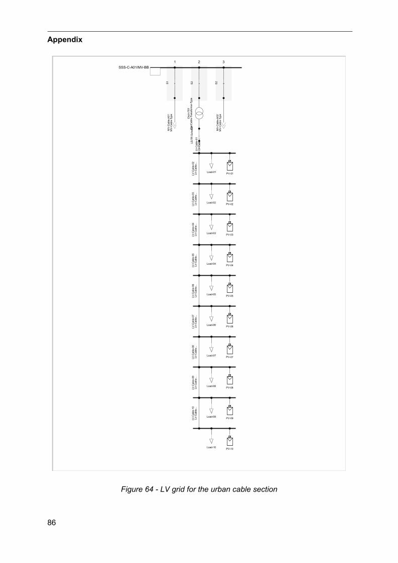
Appendix
86
Figure 64 - LV grid for the urban cable section
~
~
~
~
~
~
~
~
~
~
21 3
MV
-Cab
le-A
02M
V-C
able
-Typ
e
MV
-Cab
le-A
01M
V-C
able
-Typ
e
Load-10
LV-C
able
-..LV
-Cab
le-1
0
PV-10
Load-07 PV-07
LV-C
able
-..LV
-Cab
le-0
7
PV-08
LV-C
able
-..LV
-Cab
le-0
8
Load-08
LV-C
able
-..LV
-Cab
le-0
6
Load-06
Load-09 PV-09
PV-06
LV-C
able
-..LV
-Cab
le-0
9
Load-05 PV-05
LV-C
able
-..LV
-Cab
le-0
5LV
-Cab
le-..
LV-C
able
-04
Load-04 PV-04
LV-C
able
-..LV
-Cab
le-0
3
Load-03 PV-03
LV-C
able
-..LV
-Cab
le-0
2
PV-02Load-02
PV-01Load-01
LV-C
able
-01
LV-C
able
-..
LS/T
R S
chal
ter
Dis
tri-T
01D
istC
able
-Tra
nsfo
rmer
-Typ
e
S2S1
S2
SSS-C-A01/MV-BB

Appendix
87
Figure 65 - LV grid for the rural OHL section
~
~
~
~
~
~
~
~
~
~
~
~
~
~
~
~
~
~
~
~
21 3
MV
-OH
L-A
12M
V-O
HL-
Type
MV
-OH
L-A
11M
V-O
HL-
Type
LV-C
able
-Typ
eLV
-Cab
le-1
1
Load-20
LV-C
able
-..LV
-Cab
le-2
0
Load-14
PV-20
Load-17 PV-17
PV-18
Load-19
Load-18
LV-C
able
-..LV
-Cab
le-1
8LV
-Cab
le-..
LV-C
able
-16
Load-16
PV-15
LV-C
able
-..LV
-Cab
le-1
4LV
-Cab
le-..
LV-C
able
-13
Load-13 PV-13
PV-11
LV-C
able
-..LV
-Cab
le-1
7
PV-19
PV-16
Load-12
LV-C
able
-..LV
-Cab
le-1
9LV
-Cab
le-..
LV-C
able
-12
PV-12
LV-C
able
-..LV
-Cab
le-1
5
Load-15
PV-14
Load-11
Load-10
LV-C
able
-..LV
-Cab
le-1
0
PV-10
Load-07 PV-07
LV-C
able
-..LV
-Cab
le-0
7
PV-08
LV-C
able
-..LV
-Cab
le-0
8
Load-08
LV-C
able
-..LV
-Cab
le-0
6
Load-06
Load-09 PV-09
PV-06
LV-C
able
-..LV
-Cab
le-0
9
Load-05 PV-05
LV-C
able
-..LV
-Cab
le-0
5LV
-Cab
le-..
LV-C
able
-04
Load-04 PV-04
LV-C
able
-..LV
-Cab
le-0
3
Load-03 PV-03
LV-C
able
-..LV
-Cab
le-0
2
PV-02Load-02
PV-01Load-01
LV-C
able
-01
LV-C
able
-..
LS/T
R S
chal
ter
S2
Dis
tri-T
01D
istO
HL-
Tran
sfor
mer
-Typ
e
S1
S2
SSS-OHL-A11/MV-BB
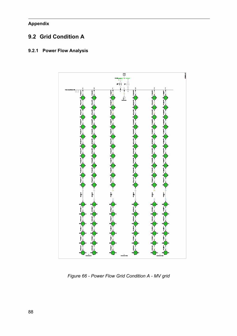
Appendix
88
9.2 Grid Condition A
9.2.1 Power Flow Analysis
Figure 66 - Power Flow Grid Condition A - MV grid
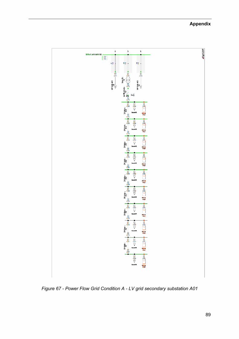
Appendix
89
Figure 67 - Power Flow Grid Condition A - LV grid secondary substation A01
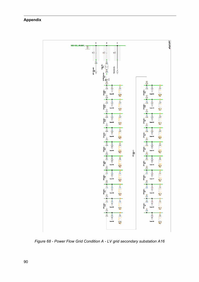
Appendix
90
Figure 68 - Power Flow Grid Condition A - LV grid secondary substation A16

Appendix
91
9.2.2 Short-Circuit calculation
Table 5 - Grid condition A – short-circuit calculation
Secondary Distance
Mag
PhaseM
agPhase
Mag
PhaseM
agPhase
Mag
PhaseM
agPhase
Mag
PhaseM
agPhase
AbsM
agSubstation
kmkA
°kA
°kA
°kA
° kA
°kA
°kA
°kA
°kV
°1
Busbar0
4,992-55,59
4,862-55,9
0,079118,27
0,058111,54
4,522125,06
4,522125,06
0,079118,27
0,058111,54
0-
2A01
0,84,786
-53,44,419
-56,614,708
-53,264,362
-56,464,347
127,514,37
127,440,073
117,510,059
33,990,66
-14,283
A021,6
4,591-51,4
4,325-54,46
4,514-51,22
4,272-54,23
4,181129,79
4,217129,73
0,068116,4
0,0648,26
1,26-12,25
4A03
2,44,406
-49,564,181
-52,554,33
-49,344,132
-52,244,023
131,94,071
131,860,064
114,950,06
51,391,82
-10,375
A043,2
4,231-47,86
4,034-50,81
4,156-47,6
3,988-50,43
3,873133,86
3,933133,85
0,06-47,6
0,06-50,43
2,33-86,65
6A05
44,065
-46,33,89
-49,213,992
-45,993,847
-48,763,733
135,693,8
135,710,057
111,160,06
52,362,8
-7,067
A064,8
3,909-44,85
3,751-47,72
3,838-44,51
3,712-47,2
3,6137,4
3,675137,46
0,054108,88
0,0652,18
3,23-5,59
8A07
5,63,762
-43,523,619
-46,363,693
-43,133,583
-45,763,475
1393,556
139,10,051
106,40,061
51,683,62
-4,239
A086,4
3,623-42,28
3,492-45,1
3,557-41,85
3,46-44,42
3,358140,51
3,444140,65
0,049103,75
0,06151,02
3,99-2,98
10A09
7,23,493
-41,133,376
-43,893,429
-40,663,343
-43,173,247
141,923,338
142,10,047
100,980,062
50,394,33
-1,8111
A108
3,37-40,06
3,262-42,79
3,309-39,55
3,233-41,99
3,144143,25
3,238143,48
0,04698,14
0,06249,82
4,65-0,73
12A11
102,832
-32,042,755
-34,722,787
-31,292,744
-33,612,716
152,452,837
152,650,039
82,120,064
42,666,25
1,2313
A1212
2,411-26,32
2,357-28,75
2,38-25,35
2,357-27,41
2,378159,27
2,506159,48
0,03867,55
0,06639,18
7,354,24
14A13
142,085
-22,112,045
-24,282,065
-20,932,054
-22,722,114
164,512,24
164,70,041
57,810,067
37,268,12
6,9215
A1416
1,829-18,92
1,797-20,87
1,818-17,52
1,813-19,1
1,907168,69
2,027168,81
0,04451,85
0,06836,06
8,689,14
16A15
181,625
-16,431,598
-18,191,621
-14,831,621
-16,211,741
172,111,855
172,150,047
48,160,069
35,329,1
10,9517
A1620
1,46-14,42
1,436-16,03
1,462-12,62
1,464-13,85
1,607174,98
1,714174,91
0,0545,8
0,06934,8
9,4312,32
#
Ik-Peak at SCIk at SC
Voltage at Busbar
Fault locationIk-Peak at feeder
Ik at feederIk-Peak at
transformer
Ik at transformer
Ik-Peak from other
feeder (single)Ik from
other feeder (single)

Appendix
92
9.3 Grid Condition B
9.3.1 Power Flow Analysis
Figure 69 - Power Flow Grid Condition B - MV grid
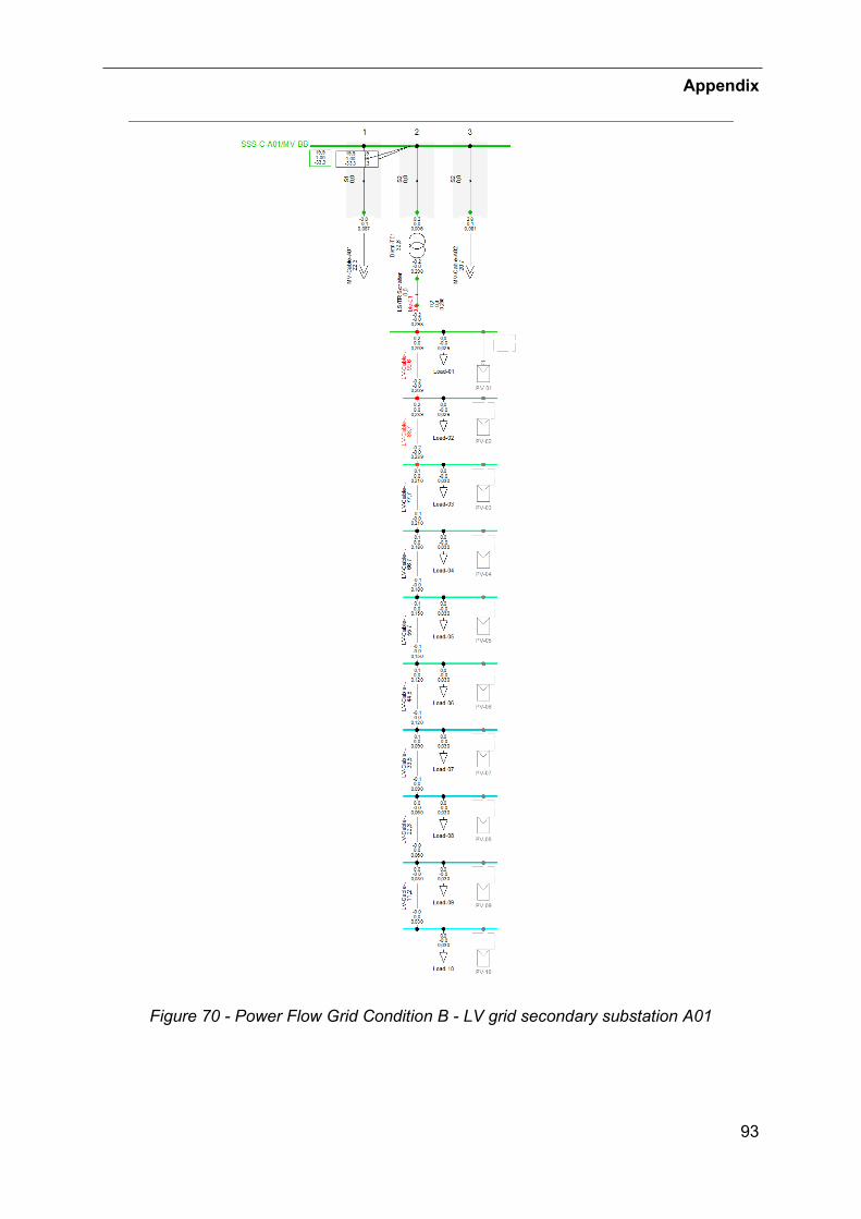
Appendix
93
Figure 70 - Power Flow Grid Condition B - LV grid secondary substation A01
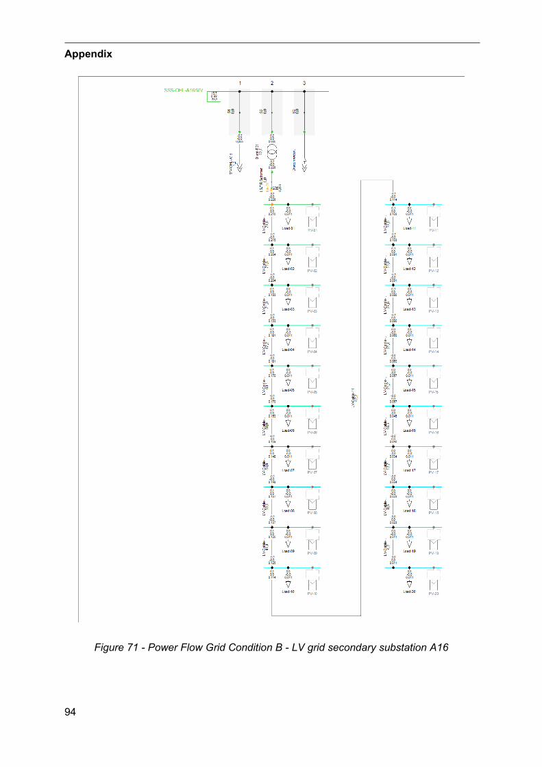
Appendix
94
Figure 71 - Power Flow Grid Condition B - LV grid secondary substation A16

Appendix
95
9.3.2 Short-Circuit calculation
Table 6 - Grid Condition B – short-circuit calculation
SecondaryDistance
Mag
PhaseM
agPhase
Mag
PhaseM
agPhase
AbsM
agSubstation
kmkA
°kA
°kA
°kA
° kV
°1
Busbar0
--
--
3,34865,71
2,767,88
00
2A01
0,83,251
-112,732,636
-110,93,265
67,452,647
69,280,45
-73,753
A021,6
3,158-111,27
2,573-109,75
3,18469,09
2,59570,61
0,88-72,29
4A03
2,43,068
-109,882,512
-108,643,107
70,652,544
71,891,29
-70,915
A043,2
2,982-108,58
2,453-107,59
3,03272,13
2,49573,11
1,67-69,61
6A05
42,898
-107,352,397
-106,592,96
73,532,447
74,292,02
-68,397
A064,8
2,819-106,18
2,342-105,63
2,8974,87
2,40175,42
2,36-67,22
8A07
5,62,742
-105,082,289
-104,722,824
76,142,357
76,52,68
-66,139
A086,4
2,669-104,03
2,238-103,84
2,7677,35
2,31477,54
2,98-65,1
10A09
7,22,599
-103,042,189
-103,012,698
78,512,272
78,543,27
-64,1211
A108
2,532-102,1
2,141-102,21
2,63979,61
2,23279,51
3,353-63,19
12A11
102,235
-95,211,928
-96,162,397
87,132,068
86,14,96
-62,3913
A1212
1,982-89,69
1,742-91,27
2,18593,07
1,9291,49
6,05-59,81
14A13
141,771
-85,41,581
-87,272,006
97,821,79
95,956,87
-57,1815
A1416
1,597-81,96
1,44-83,98
1,856101,69
1,67899,67
7,5-54,85
16A15
181,451
-79,161,326
-81,231,729
104,891,58
102,828
-52,8417
A1620
1,329-76,83
1,226-78,9
1,622107,59
1,496105,52
8,39-51,13
ik at machine
transformer
Voltage at Busbar
#
Fault locationIk-Peak at Feeder A
Ik at feeder AIk-Peak at m
achine transform
er
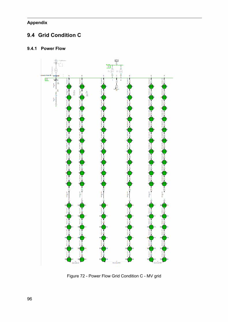
Appendix
96
9.4 Grid Condition C
9.4.1 Power Flow
Figure 72 - Power Flow Grid Condition C - MV grid
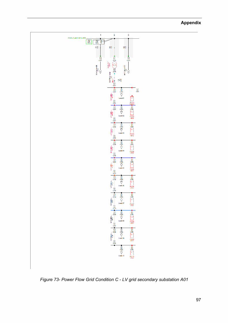
Appendix
97
Figure 73- Power Flow Grid Condition C - LV grid secondary substation A01
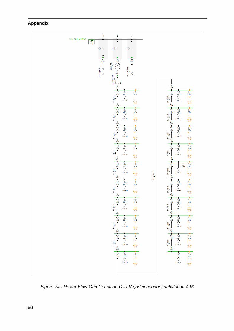
Appendix
98
Figure 74 - Power Flow Grid Condition C - LV grid secondary substation A16
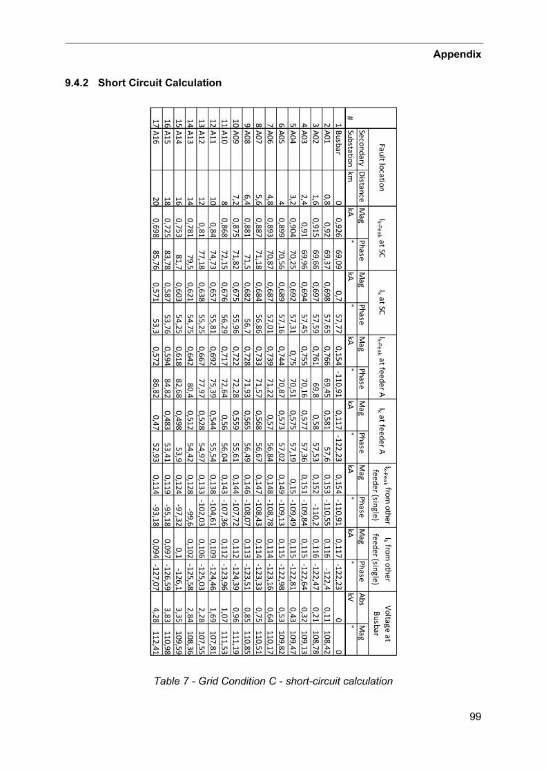
Appendix
99
9.4.2 Short Circuit Calculation
Table 7 - Grid Condition C - short-circuit calculation
SecondaryDistance
Mag
PhaseM
agPhase
Mag
PhaseM
agPhase
Mag
PhaseM
agPhase
AbsM
agSubstation
kmkA
°kA
°kA
°kA
° kA
°kA
°kV
°1
Busbar0
0,92669,09
0,757,77
0,154-110,91
0,117-122,23
0,154-110,91
0,117-122,23
00
2A01
0,80,92
69,370,698
57,650,766
69,450,581
57,60,153
-110,550,116
-122,40,11
108,423
A021,6
0,91569,66
0,69757,59
0,76169,8
0,5857,53
0,152-110,2
0,116-122,47
0,21108,78
4A03
2,40,91
69,960,694
57,450,755
70,160,577
57,360,151
-109,840,115
-122,640,32
109,135
A043,2
0,90470,25
0,69257,31
0,7570,51
0,57557,19
0,15-109,49
0,115-122,81
0,43109,47
6A05
40,899
70,560,689
57,160,744
70,870,573
57,020,149
-109,130,115
-122,980,53
109,827
A064,8
0,89370,87
0,68757,01
0,73971,22
0,5756,84
0,148-108,78
0,114-123,16
0,64110,17
8A07
5,60,887
71,180,684
56,860,733
71,570,568
56,670,147
-108,430,114
-123,330,75
110,519
A086,4
0,88171,5
0,68256,7
0,72871,93
0,56556,49
0,146-108,07
0,113-123,51
0,85110,85
10A09
7,20,875
71,820,675
55,960,722
72,280,559
55,610,144
-107,720,112
-124,390,96
111,1911
A108
0,86872,15
0,67656,29
0,71772,64
0,5656,04
0,143-107,36
0,112-123,96
1,07111,53
12A11
100,84
74,730,657
55,810,692
75,390,544
55,540,138
-104,610,109
-124,461,69
107,8113
A1212
0,8177,18
0,63855,25
0,66777,97
0,52854,97
0,133-102,03
0,106-125,03
2,28107,55
14A13
140,781
79,50,621
54,750,642
80,40,512
54,420,128
-99,60,102
-125,582,84
108,3615
A1416
0,75381,7
0,60354,25
0,61882,68
0,49853,9
0,124-97,32
0,1-126,1
3,35109,59
16A15
180,725
83,780,587
53,760,594
84,820,483
53,410,119
-95,180,097
-126,593,83
110,9817
A1620
0,69885,76
0,57153,3
0,57286,82
0,4752,93
0,114-93,18
0,094-127,07
4,28112,41
Ik-Peak from other
feeder (single)Ik from
other feeder (single)
Voltage at Busbar
#
Fault locationIk-Peak at SC
Ik at SCIk-Peak at feeder A
Ik at feeder A