Correcting Streaming Predictionsof an Electricity Load Forecast SystemUsing a Prediction Reliability Estimate

Zoran Bosnic, Pedro Pereira Rodrigues, Igor Kononenko, and João Gama

Abstract. Accurately predicting values for dynamic data streams is a challengingtask in decision and expert systems, due to high data flow rates, limited storage anda requirement to quickly adapt a model to new data. We propose an approach forcorrecting predictions for data streams which is based on a reliability estimate forindividual regression predictions. In our work, we implement the proposed tech-nique and test it on a real-world problem: prediction of the electricity load for aselected European geographical region. For predicting the electricity load values weimplement two regression models: the neural network and the k nearest neighborsalgorithm. The results show that our method performs better than the referentialmethod (i.e. the Kalman filter), significantly improving the original streaming pre-dictions to more accurate values.

Keywords: data stream, online learning, prediction accuracy, prediction correction.

1 Introduction

The main goal of the supervised learning models is to model the learning data accu-rately while also achieving the best possible prediction accuracy for unseen exam-ples that were not included in the learning process. The field of online learningfrom data streams is particularly challenging, since the sources of the data are

Zoran Bosnic · Igor KononenkoUniversity of Ljubljana, Faculty of Computer and Information Science,Tržaska cesta 25, Ljubljana, Sloveniae-mail: zoran.bosnic,igor.kononenko@fri.uni-lj.si

Pedro Pereira Rodrigues · João GamaLIAAD—INESC Porto, L.A. & Faculty of Medicine, University of Porto,Praça Gomes Teixeira, 4099-002 Porto, Portugale-mail: pprodrigues@med.up.pt,jgama@fep.up.pt

T. Czachórski et al. (Eds.): Man-Machine Interactions 2, AISC 103, pp. 343–350.springerlink.com c© Springer-Verlag Berlin Heidelberg 2011

344 Z. Bosnic et al.

characterized as being open-ended, flowing at high-speed, and generated by non-stationary distributions [8, 7]. Online learning algorithms should process examplesat the rate they arrive, using a single scan of data and fixed memory, maintain-ing a decision model at any time and being able to adapt the model to the mostrecent data [4]. In such demand-intensive environment, one does not have a lux-ury (in terms of time) of online testing and choosing among different models oriteratively optimizing them. The described situations may call for an alternative ap-proach which can be applying a corrective mechanism to improve the accuracy ofthe predictions.

In this work we propose an approach for correcting individual predictions of anonline learning system. We apply the approach to the problem of predicting theelectricity load demand, which requires an incremental model to continuously makepredictions in real time [5, 3]. For correcting the system’s regression predictions, wecompare two approaches: (i) correcting using the locality-based reliability estimateCNK [1] and (ii) correcting using the Kalman filter [6]. We empirically evaluate theperformance of both approaches using two regression models: neural networks andk nearest neighbors. The experiments were performed for three different variationsof the basic problem, i.e. predicting the electricity load for the next hour, the nextday (24 hours) and the next week (168 hours).

The paper is organized as follows. Section 2 summarizes the relevant work fromthe areas of online learning and individual prediction reliability estimation. Sec-tion 3 describes the proposed and the referential corrective mechanism, and Sect. 4gives an overview of the experimental methodology and presents the results. Sec-tion 5 provides the conclusions and ideas for further work.

2 Related Work

This section reports the relevant work from the areas of online learning and individ-ual reliability estimation.

2.1 Correcting Regression Predictions

For the evaluation of prediction accuracies, the averaged accuracy measures aremost commonly used, such as the relative mean squared error (RMSE). Althoughthese estimates evaluate the model performance, they provide no local informationabout the expected error of an individual prediction for a given unseen example. Toprovide such information, the reliability estimates (i.e. estimates of prediction errorfor yet unseen examples) are of a greater use.

In the previous work, Bosnic and Kononenko [2, 1] proposed and evaluated sev-eral different reliability estimates for regression predictions. Among nine proposedmodel-independent (i.e. the algorithms treat an underlying model as a black box) re-liability estimates, the estimate CNK, which estimates the prediction error by mod-eling it locally, is particularly interesting. This estimate is efficient to compute andthe sign of its value provides information about the direction of the error.

Correcting Predictions of an Electricity Load Forecasting System 345

In this work we use the reliability estimate CNK to estimate the prediction errorof data stream and modify its predictions to more accurate values. Our motivationstems from the previous work which presented some initial experiments that indi-cated feasibility of correcting predictions using some reliability estimates.

2.2 Reliability Estimation of Predictions in Data Streams

For solving the described electricity load prediction problem, the online neural net-work has already been applied [9]. In the previous work, Rodrigues et al. [10] havesupplemented the bare data stream predictions with some of the sooner mentionedreliability estimates based on the bagging variance and the local sensitivity analysis.The application of reliability estimates in an online learning environment has indi-cated some promising results. In this paper we continue this work by implementingthe correction of online predictions, which is a further step to only estimating theirreliabilities.

3 Correcting Online Predictions

In this section there are described the proposed and referential corrective mecha-nisms.

3.1 Correcting Predictions Using the CNK Reliability Estimate

The reliability estimate CNK for estimation of regression prediction error for a givenexample is defined as a local estimate of error. Let us denote with CNK the generalreliability estimate (i.e. the concept of the reliability estimation approach) and withCNKi an estimate value for some particular i-th example. For offline learning set-ting, the estimate CNK was defined as follows. Suppose we are given a learning setof n examples L = (x1,C1), . . . ,(xn,Cn) where xi, i = 1 . . .n denote the attributevectors and Ci, i = 1 . . .n denote the true target values of the examples (their labels).In our scenario, we are given an unseen example (xu, ) for which we wish to com-pute a prediction and supplement it with the reliability estimate CNKu.

The computation of CNK proceeds as follows. First, we induce a regressionmodel on L and output the prediction Ku for the example (xu, ). To compute CNKu,we first localize the set of the k nearest neighbors N = (xu1,Cu1), . . . ,(xuk,Cuk) ofthe example, N ⊆ L. CNKu is then defined as the difference between the averagelabel of the nearest neighbors and the example’s prediction Ku:

CNKu = ∑ki=1 Cui

k−Ku (1)

hence also the name CNK (average C of Neighbors minus K of the example). Inthe above equation, k denotes the number of neighbors, Cui denotes the neighbors’labels and Ku denotes the example’s prediction.

346 Z. Bosnic et al.

In our work we adapt this definition of CNK to the online learning scenario, i.e.we use an incremental online model instead of the model which learns from the thestationary learning set L. Since the storage of examples is of a limited size, only themost recent examples in the buffer B can participate as the nearest neighbors (ei-ther for computation of CNK or for predicting with the k nearest neighbors model),therefore N ⊆ B.

Note, that CNK is a reliability estimate that can be easily influenced by localnoise and subject to local bias. To robustly transform the value of CNKu to the valueof predicted error Cu − Ku, we apply a linear regression model for this task. Thelinear model f (CNKi) = (Ci − Ki) is built using the estimate values and the pre-diction error values of all examples in the buffer, of which the true target outcomesare already known (required for computation of the prediction error). The correctedprediction is finally computed as KCNKu = Ku + f (CNKu) .

3.2 Correcting Predictions Using the Kalman Filter

The Kalman filter [6] is a general and the most widely used in engineering for twomain purposes: for combining measurements of the same variables but from dif-ferent sensors, and for combining an inexact forecast of the system’s state with aninexact measurement of the state [9]. We use the Kalman filter to combine the pre-diction Ku for an example (xu, ) with the expected most correlated value Ku fromthe previous time point (depends on the prediction problem variant) and gain a cor-rected prediction KKalmanu :

KKalmanu = Ku + Fu · (Ku −Ku), (2)

where Fu is the filter transition weight which controls the influence of the pastprediction [6].

4 Experimental Evaluation

This section gives an overview of the experimental methodology and presentsresults.

4.1 Electricity Load Data and Predictive Models

For the purpose of experimental evaluation, the streaming data was converted intothe relational form, which is appropriate for supervised learning, where a buffer isused to keep recent historical data. The examples represent the electricity load val-ues for points in time1, with a resolution of 1 hour. The data consists of 10 attributeswhich include 4 cyclic variables (couples of sin and cos values which denote the

1 Original data is confidential, but was previously described and used in [9].

Correcting Predictions of an Electricity Load Forecasting System 347

hourly and weekly periods) and 6 historical load attributes. These attributes are spe-cific to three variations of the problem:

• the next hour prediction problem consists of 16200 examples and includes at-tributes describing load for t minus 1, 2, 3, 4, 168, 336 hours,

• the next day prediction problem consists of 16200 examples and includes thehistorical attributes for t minus 24, 144, 168, 169, 192, 336 hours,

• the next week prediction problem includes the attributes for t minus 168, 169,312, 336, 360, 504 hours. The data set consists of 15528 examples.

For all three problem variations, a buffer size of 336 was used, which correspondsto last 14 days of examples. For computation of the CNK estimate, 2 nearest neigh-bors were used (in the buffer of 14 days, the 2 examples from the same days inprevious weeks are expected to have the most correlated prediction error). Follow-ing the previous work [10], the expected most correlated value used in the Kalmanfilter was the example from the last hour for the first problem and the example fromthe previous week (168 hours) for the last two variants of the problem.

Our correction approach was tested using two different online learning models:

• neural network: consisting of 10 input neurons, a hidden layer of 5 neurons and1 output neuron. The tansig activation function was used in the hidden neuronsand the linear activation function in the output neuron,

• k nearest neighbors: k was chosen as 336 (all the examples in the buffer), theexamples were inversely weighted by their distance to the query example.

4.2 Model Evaluation

In the online learning setting, the typical definitions of the averaged accuracy mea-sures over all examples (such as the mean squared error—MSE) cease to be appro-priate. Namely, when averaged across the number of examples that increases overtime, the measure becomes increasingly stable (each new example represents onlysmall contribution to the sum of the errors) and as such it provides no informationabout the current model accuracy which corresponds to the current model adaptationto the data.

A possible approach to measuring how model accuracy evolves over time is touse the α-fading mean squared error statistic (αMSE) which is recursively updatedand emphasizes the model behavior on the most recent data.

For comparative performance assessment of two algorithms A and B on a stream,a Q statistic should be used [4], which is defined as a log ratio of αMSE statisticsof A and B. The value of the Q(A,B) statistic is easy to interpret: its negative valuesdenote the better performance of the algorithm A and its positive values denote thebetter performance of the algorithm B.

348 Z. Bosnic et al.

4.3 Experimental Results

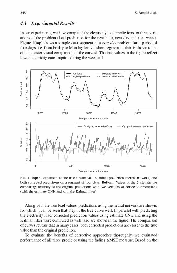
In our experiments, we have computed the electricity load predictions for three vari-ations of the problem (load prediction for the next hour, next day and next week).Figure 1(top) shows a sample data segment of a next day problem for a period offour days, i.e. from Friday to Monday (only a short segment of data is shown to fa-cilitate easier visual comparison of the curves). The true values in the figure reflectlower electricity consumption during the weekend.

10280 10300 10320 10340 10360

−0.

6−

0.4

−0.

20.

00.

20.

4

Example number in the stream

Pre

dict

ed lo

ad

true valueoriginal prediction

corrected with CNKcorrected with Kalman

0 5000 10000 15000

−1.

00.

00.

51.

01.

52.

02.

5

Example number in the stream

Q s

tatis

tic

Q(original, corrected w/CNK) Q(original, corrected w/Kalman)

Fig. 1 Top: Comparison of the true stream values, initial prediction (neural network) andboth corrected predictions on a segment of four days. Bottom: Values of the Q statistic forcomparing accuracy of the original predictions with two versions of corrected predictions(with the estimate CNK and with the Kalman filter)

Along with the true load values, predictions using the neural network are shown,for which it can be seen that they fit the true curve well. In parallel with predictingthe electricity load, corrected prediction values using estimate CNK and using theKalman filter were computed as well, and are shown in the figure. The comparisonof curves reveals that in many cases, both corrected predictions are closer to the truevalue than the original prediction.

To evaluate the benefits of corrective approaches thoroughly, we evaluatedperformance of all three predictor using the fading αMSE measure. Based on the

Correcting Predictions of an Electricity Load Forecasting System 349

computed performance measures, a Q statistic was computed for comparing the per-formance of the original model (αMSE) with the accuracy of each of the correctiveapproaches (αMSECNK and αMSEKalman). The computed values of the Q statisticfor the neural network are shown in Fig. 1(bottom). The figure reveals the domi-nantly positive values of the Q statistic for corrected predictions with the reliabilityestimate CNK, which clearly speaks in favor of this approach, whereas the perfor-mance of Kalman filter is not as clear.

Table 1 thus presents more detail statistical comparison of both corrective ap-proaches for neural network and k-NN predictor. The t-test was used to comparethe means of three Q statistics. The displayed values show that all means of the Qstatistics are positive if we compare the original predictions with the predictions,corrected with the estimate CNK. All the means are different from zero with a highlevel of significance (p<0.001); the gain in accuracy with this type of correction(CNK) was always significant. On the other hand, a gain in accuracy with the refer-ential method (the Kalman filter) was less conclusive. Namely, the results show thatthe statistical accuracy improvement with the Kalman filter correction was achievedonly with neural network and in the next day and the next week problem. The re-maining results indicate either that the original model was better (where μ < 0 andp < 0.001) or that the predictions are statistically equally accurate (p = 0.106).

Table 1 Results of the t-test for testing the equality of the Q statistic (for comparison of theoriginal and the corrected predictions) to the value 0. The table cells show the average valuesof the Q statistic for the three problem variants and for two regression models. The averagevalues of the Q statistic and the p-values for H0 are given

Problem Modelt-test for H0 : t-test for H0 :

Q(original,corr.w/CNK) = 0 Q(original,corr.w/Kalman) = 0

next hournn μ = 0.617, p < 0.001 μ = −0.012, p < 0.001knn μ = 0.438, p < 0.001 μ = −0.109, p < 0.001

next daynn μ = 0.463, p < 0.001 μ = 0.021, p < 0.001knn μ = 0.575, p < 0.001 μ = −0.007, p = 0.106

next weeknn μ = 0.575, p < 0.001 μ = 0.337, p < 0.001knn μ = 0.596, p < 0.001 μ = −0.046, p < 0.001

5 Conclusion

Accurately predicting values for dynamic data streams is a challenging task indecision and expert systems due to high data flow rates, limited storage and a re-quirement to quickly adapt a model to new data. In contrast to extensive onlinecomparison and selection of models, the use of corrective prediction mechanismintroduces less burden on the stream computational demands.

We have tested two such corrective approaches: using the reliability estimateCNK and using a referential method—the Kalman filter. The proposed approach

350 Z. Bosnic et al.

was tested on the electricity load data stream, which is a real-world case that hasa requirement for good prediction accuracy. The results show that our method per-forms better than the Kalman filter, significantly improving the original predictionstowards more accurate values.

Our further work shall include the evaluation of the proposed approach on theother real-world data streams. Additionally, several other online regression mod-els shall be included in our evaluation (e.g. linear regression). The third correctionapproach (using a sensitivity analysis based reliability estimate [2]) shall be imple-mented as well.

References

1. Bosnic, Z., Kononenko, I.: Comparison of approaches for estimating reliability of indi-vidual regression prediction. Data and Knowledge Engineering 67(3), 504–516 (2008)

2. Bosnic, Z., Kononenko, I.: Estimation of individual prediction reliability using the localsensitivity analysis. Applied Intelligence 29(3), 187–203 (2008)

3. Ferrer, F., Aguilar, J., Riquelme, J.: Incremental rule learning and border examples selec-tion from numerical data streams. Journal of Universal Computer Science 11(8), 1426–1439 (2008)

4. Gama, J., Sebastião, R., Rodrigues, P.: Issues in evaluation of stream learning algorithms.In: Proceedings of the 15th ACM SIGKDD International Conference on Knowledge Dis-covery and Data Mining, New York, USA, pp. 329–338 (2009)

5. Hulten, G., Spencer, L., Domingos, P.: Mining timechanging data streams. In: Proceed-ings of the 7th ACM SIGKDD International Conference on Knowledge Discovery andData Mining, pp. 97–106 (2001)

6. Kalman, R.: A new approach to linear filtering and prediction problems. Transactions ofthe ASME—Journal of Basic Engineering 82(D), 35–45 (1960)

7. Kifer, D., Ben-David, S., Gehrke, J.: Detecting change in data streams. In: Proceedingsof the 30th International Conference on Very Large Data Bases, pp. 180–191 (2004)

8. Muthukrishnan, S.: Data Streams: Algorithms and Applications. Now Publishers Inc.,New York (2005)

9. Rodrigues, P.P., Gama, J.: A system for analysis and prediction of electricity loadstreams. Intelligent Data Analysis 13(3), 477–496 (2009)

10. Rodrigues, P.P., Gama, J., Bosnic, Z.: Online reliability estimates for individual predic-tions in data streams. In: Proceedings of the IEEE International Conference on DataMining Workshops, pp. 36–45. IEEE Computer Society, Washington, USA (2008)