ERROR CORRECTING CODES

THESIS

Presented in Partial Fulfillment of the Requirements for the Degree Masters of

Science in the Graduate School of the Ohio State University

By

Peter M. Kosek, B.S. in Mathematics

Graduate Program in Mathematics

The Ohio State University

2014

Thesis Committee:

Matthew Kahle, Advisor

David Sivakoff

c© Copyright by

Peter M. Kosek

2014

ABSTRACT

Error correcting codes is an area of mathematics that combines many theoretical

concepts with a wide variety of applications. In this expository thesis, we will begin

by introducing many of the fundamental ideas in classical error correcting codes. The

goal of this is to introduce the reader to the field of coding theory and discuss a few

of the wide range of classical codes that have been studied. The second section will

discuss the recent findings in error correcting codes, namely their use in quantum

error correcting codes. This section uses much more theoretical areas of math, when

compared to the classical section, in the construction of quantum error correcting

codes. Most of the research discussed in this section has been completed within

the past six years. All of the research discoveries presented in this thesis have been

previously known.

ii

ACKNOWLEDGMENTS

I would like to thank Matthew Kahle for his willingness to serve as my advisor.

He has challenged me to learn topics I never imagined I would understand. I have

appreciated his feedback on my writings. I would also like to thank David Sivakoff

for being willing to be a member of my committee. I would very much like to thank

the both of these gentlemen and their wives for meeting last minute to allow me to

defend my thesis by the deadline. A very big thank you goes out to my wife, Amy,

for her hugs and encouragement throughout this entire process. I have benefitted

greatly from her encouragements to be diligent in writing and to not procrastinate.

I would also like to thank Howard Skogman for initially introducing me to the area

of error correcting codes and for making the topic come alive and create a desire to

learn more about the subject.

iii

VITA

2008 . . . . . . . . . . . . . . . . . . . . . . . . . . . . . . . . . . B.S. in Mathematics,

The College at Brockport, State Univer-sity of New York

2012-Present . . . . . . . . . . . . . . . . . . . . . . . . . . Graduate University Fellowship,

The Ohio State University

2013-Present . . . . . . . . . . . . . . . . . . . . . . . . . . Graduate Teaching Associate,

The Ohio State University

PUBLICATIONS

Firke, Frank; Kosek, Peter; Nash, Evan; Williford, JasonExtremal Graphs Without 4-Cycles

FIELDS OF STUDY

Major Field: Mathematics

iv

TABLE OF CONTENTS

Abstract . . . . . . . . . . . . . . . . . . . . . . . . . . . . . . . . . . . . . . . ii

Acknowledgments . . . . . . . . . . . . . . . . . . . . . . . . . . . . . . . . . . iii

Vita . . . . . . . . . . . . . . . . . . . . . . . . . . . . . . . . . . . . . . . . . iv

List of Figures . . . . . . . . . . . . . . . . . . . . . . . . . . . . . . . . . . . vi

CHAPTER PAGE

1 Classical Error Correcting Codes . . . . . . . . . . . . . . . . . . . . . 1

1.1 Motivation . . . . . . . . . . . . . . . . . . . . . . . . . . . . . . . 11.2 Minimum Distance Decoding . . . . . . . . . . . . . . . . . . . . . 4

1.2.1 t-error-correcting and t-error-detecting codes . . . . . . . . 71.3 The Main Coding Theory Problem . . . . . . . . . . . . . . . . . . 9

1.3.1 Bounds for Aq(n, d) . . . . . . . . . . . . . . . . . . . . . . 91.4 Linear codes . . . . . . . . . . . . . . . . . . . . . . . . . . . . . . 13

1.4.1 Syndrome decoding . . . . . . . . . . . . . . . . . . . . . . 151.5 Other examples of codes . . . . . . . . . . . . . . . . . . . . . . . . 18

1.5.1 Hamming codes . . . . . . . . . . . . . . . . . . . . . . . . 181.5.2 Non-linear codes . . . . . . . . . . . . . . . . . . . . . . . 21

2 Quantum Error Correcting Codes . . . . . . . . . . . . . . . . . . . . . 23

2.1 Motivation . . . . . . . . . . . . . . . . . . . . . . . . . . . . . . . 232.2 Calderbank–Shor–Steane codes . . . . . . . . . . . . . . . . . . . . 242.3 Recent research . . . . . . . . . . . . . . . . . . . . . . . . . . . . 262.4 Quantum LDPC codes based on homological properties . . . . . . 272.5 Quantum LDPC codes based on Cayley graphs . . . . . . . . . . . 29

Bibliography . . . . . . . . . . . . . . . . . . . . . . . . . . . . . . . . . . . . 33

v

LIST OF FIGURES

FIGURE PAGE

1.1 Fano plane . . . . . . . . . . . . . . . . . . . . . . . . . . . . . . . . 21

vi

CHAPTER 1

CLASSICAL ERROR CORRECTING CODES

1.1 Motivation

Let’s begin by creating a simple scenario. Suppose you are in communication with

another person at a distance using some noisy binary channel (i.e. a method of sending

0’s and 1’s in which errors may occur in which 0 gets switched to 1 and vice versa).

Assume that the chance of an error occurring for any bit is less likely than the

correct bit being received and that the likelihood of an error is independent of any

other error occurring. Furthermore, assume the only two phrases you would like to

send to one another are ‘yes’ and ‘no’. You have both decided that 0 represents no

and 1 represents yes. One day, you send the message 1, but due to the noise in the

channel, the other person receives 0. Since the chance of an error occurring is less

likely than the correct word being sent, the other person assumes that you said no.

Clearly, this is not good.

After learning your lesson, you realize that maybe you should not have the oc-

currence of one error result in another word. You both decide that from now on, 00

represents no and 11 represents yes. That way, it would take two errors occurring to

end up with the completely wrong word, and that has even less chance of occurring

than a single error occurring. Now, if either one of you receive 01 or 10, you know

that an error has occurred! However, you don’t know if they meant to send 00 or 11.

1

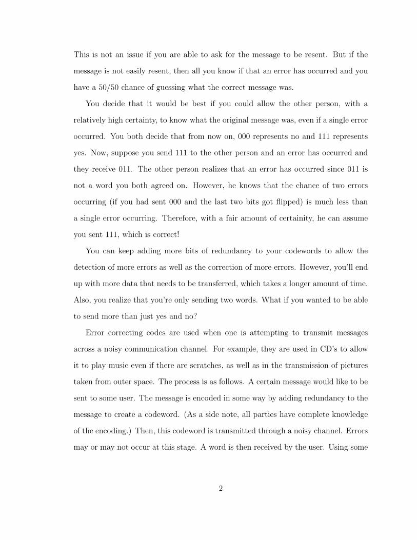
This is not an issue if you are able to ask for the message to be resent. But if the

message is not easily resent, then all you know if that an error has occurred and you

have a 50/50 chance of guessing what the correct message was.

You decide that it would be best if you could allow the other person, with a

relatively high certainty, to know what the original message was, even if a single error

occurred. You both decide that from now on, 000 represents no and 111 represents

yes. Now, suppose you send 111 to the other person and an error has occurred and

they receive 011. The other person realizes that an error has occurred since 011 is

not a word you both agreed on. However, he knows that the chance of two errors

occurring (if you had sent 000 and the last two bits got flipped) is much less than

a single error occurring. Therefore, with a fair amount of certainity, he can assume

you sent 111, which is correct!

You can keep adding more bits of redundancy to your codewords to allow the

detection of more errors as well as the correction of more errors. However, you’ll end

up with more data that needs to be transferred, which takes a longer amount of time.

Also, you realize that you’re only sending two words. What if you wanted to be able

to send more than just yes and no?

Error correcting codes are used when one is attempting to transmit messages

across a noisy communication channel. For example, they are used in CD’s to allow

it to play music even if there are scratches, as well as in the transmission of pictures

taken from outer space. The process is as follows. A certain message would like to be

sent to some user. The message is encoded in some way by adding redundancy to the

message to create a codeword. (As a side note, all parties have complete knowledge

of the encoding.) Then, this codeword is transmitted through a noisy channel. Errors

may or may not occur at this stage. A word is then received by the user. Using some

2

decoding method, the user will decode the word to be some message (it may or may

not be correct).

Definition 1.1.1. Let A = {a1, a2, . . . , aq} be a finite set, called a code alphabet.

Any codeword sent or received will be strings formed using elements from the code

alphabet.

We call a code over an alphabet of size q a q-ary code. Most often, the code

alphabets we use are {0, 1, 2, . . . , q−1}. However, there are other interesting examples

using other code alphabets.

Example 1.1.2. We could consider all street names in Columbus, OH as a 37-ary

code (26 letters, 10 digits, and a space). We see that this is an example of a very

poor code since EAST 4TH AVENUE and EAST 5TH AVENUE only differ in one

location, so if an error occurred in that location, we would not know that our received

street name was correct.

Example 1.1.3. The ISBN numbers in every book are examples of error correcting

codes. Older books have a 10-digit ISBN number while newer books have a 13-digit

ISBN number. The ISBN-10 code has codewords of the form (x1, x2, . . . , x10) where

x1 + 2x2 + 3x3 + · · · + 9x9 + 10x10 ≡ 0 mod 11 with x1, x2, . . . , x9 ∈ {0, 1, . . . , 9}

and x10 ∈ {0, 1, . . . , 9, X}. Since x10 is the check digit, if the previous numbers

require x10 = 10, it is denoted as an X. The ISBN-13 code had codewords of the form

(x1, x2, . . . , x13) where x1 + 3x2 + x3 + 3x4 + x5 + 3x6 · · · + 3x12 + x13 ≡ 0 mod 10

with x1, x2, . . . , x13 ∈ {0, 1, . . . 9}. In both of these codes, every two codewords differ

in at least two locations.

Example 1.1.4. The United States Postal Service used to use a code called POST-

NET (Postal Numeric Encoding Technique) to assist in the correct sending and re-

ceiving of mail [8]. It used a series of tall and short bars to encode information about

3

the letter being sent. The first five digits are your zip code, the next four digits are

the extended zip code, the next two digits are the delivery point digits and the last

digit is a check digit to ensure that the sum of all of the digits is congruent to 0 mod

10. The digits were encoded into bars by the following table:

number bar code

1 | | |∣∣∣ ∣∣∣

2 | |∣∣∣ | ∣∣∣

3 | |∣∣∣ ∣∣∣ |

4 |∣∣∣ | | ∣∣∣

5 |∣∣∣ | ∣∣∣ |

6 |∣∣∣ ∣∣∣ | |

7∣∣∣ | | | ∣∣∣

8∣∣∣ | | ∣∣∣ |

9∣∣∣ | ∣∣∣ | |

0∣∣∣ ∣∣∣ | | |

Suppose the Postal Service receives a letter in which the first five bars got smudged

and are unreadable. The rest of the code is readable and is

|∣∣∣ ∣∣∣ | | | | ∣∣∣ | ∣∣∣ | ∣∣∣ ∣∣∣ | | ∣∣∣ | ∣∣∣ | | | | ∣∣∣ ∣∣∣ | ∣∣∣ | | | ∣∣∣ | | | ∣∣∣ ∣∣∣ ∣∣∣ ∣∣∣ | | | | ∣∣∣ | ∣∣∣ | ∣∣∣ | | ∣∣∣ | | | ∣∣∣ | ∣∣∣.

Then, by decoding this back to digits, we get ?62693710582. Since we need the sum

to be congruent to 0 mod 10, we see that the initial digit must be 1.

1.2 Minimum Distance Decoding

In order to make progress in finding codes that could be more useful than other codes,

we must start to make certain assumptions regarding the channel we are using. The

4

assumptions we will make will agree with intuition. First, we’ll introduce the following

definition.

Definition 1.2.1. Let ~x and ~y be strings of the same length, over the same alphabet.

The Hamming distance, d(~x, ~y), beween ~x and ~y is the number of positions in which

~x and ~y differ.

As an example, consider ~x = 201021 and ~y = 221011. We see that d(~x, ~y) = 2,

since these two strings differ in exactly two positions (the second and the fifth).

An advantage of the Hamming distance is that it is a metric.

Theorem 1.2.2. Let An be the set of all words of length n over the alphabet A. Then,

the Hamming distance function d : An × An → N satisfies the following properties.

For all ~x, ~y, ~z ∈ An,

1) d(~x, ~y) ≥ 0, and d(~x, ~y) = 0 if and only if ~x = ~y.

2) d(~x, ~y) = d(~y, ~x).

3) d(~x, ~y) ≤ d(~x, ~z) + d(~z, ~y).

Therefore, (An, d) is a metric space.

If a codeword ~x is sent through our channel and the word ~y is received, then

the number of errors that occurred during the transmission is equal to the Hamming

distance d(~x, ~y). Therefore, we can determine the probability that we received the

word ~y given that the codeword ~x was sent is

p(~y | ~x) = pd(~x,~y)(1− p)n−d(~x,~y)

where n is the length of the codeword. Recall that we are assuming that the proba-

bility of an error occurring at any given position of our codeword is less than 1/2 and

that the events of multiple errors are all independent. Therefore, this above prob-

ability is greatest when d(~x, ~y) is smallest. Since we are interested decoding words

5

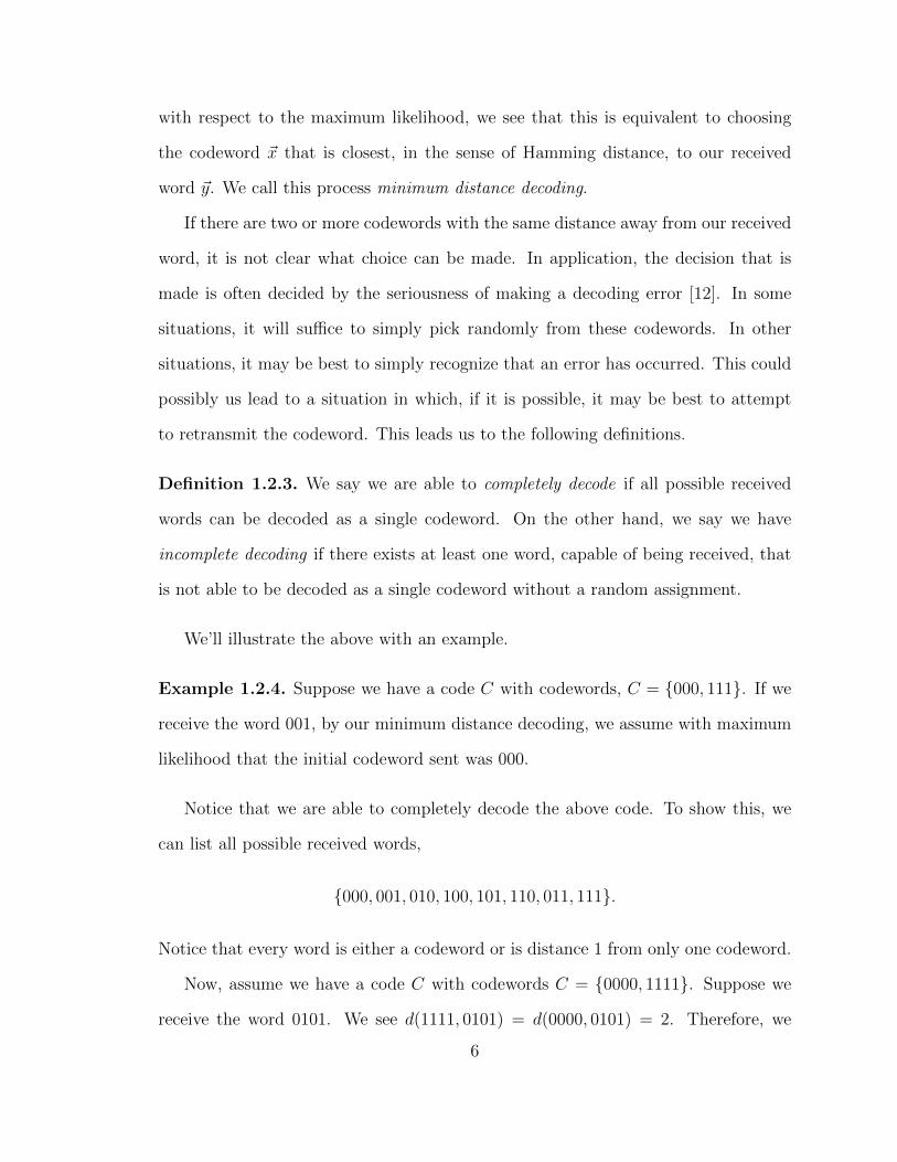
with respect to the maximum likelihood, we see that this is equivalent to choosing

the codeword ~x that is closest, in the sense of Hamming distance, to our received

word ~y. We call this process minimum distance decoding.

If there are two or more codewords with the same distance away from our received

word, it is not clear what choice can be made. In application, the decision that is

made is often decided by the seriousness of making a decoding error [12]. In some

situations, it will suffice to simply pick randomly from these codewords. In other

situations, it may be best to simply recognize that an error has occurred. This could

possibly us lead to a situation in which, if it is possible, it may be best to attempt

to retransmit the codeword. This leads us to the following definitions.

Definition 1.2.3. We say we are able to completely decode if all possible received

words can be decoded as a single codeword. On the other hand, we say we have

incomplete decoding if there exists at least one word, capable of being received, that

is not able to be decoded as a single codeword without a random assignment.

We’ll illustrate the above with an example.

Example 1.2.4. Suppose we have a code C with codewords, C = {000, 111}. If we

receive the word 001, by our minimum distance decoding, we assume with maximum

likelihood that the initial codeword sent was 000.

Notice that we are able to completely decode the above code. To show this, we

can list all possible received words,

{000, 001, 010, 100, 101, 110, 011, 111}.

Notice that every word is either a codeword or is distance 1 from only one codeword.

Now, assume we have a code C with codewords C = {0000, 1111}. Suppose we

receive the word 0101. We see d(1111, 0101) = d(0000, 0101) = 2. Therefore, we

6

know for sure that at least two errors have occurred but it is not clear if the initial

word transmitted was 0000 or 1111. This shows that we have an incomplete decoding

of this code.

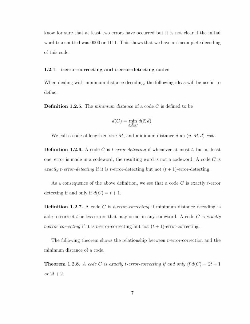
1.2.1 t-error-correcting and t-error-detecting codes

When dealing with minimum distance decoding, the following ideas will be useful to

define.

Definition 1.2.5. The minimum distance of a code C is defined to be

d(C) = min~c,~d∈C

d(~c, ~d).

We call a code of length n, size M , and minimum distance d an (n,M, d)-code.

Definition 1.2.6. A code C is t-error-detecting if whenever at most t, but at least

one, error is made in a codeword, the resulting word is not a codeword. A code C is

exactly t-error-detecting if it is t-error-detecting but not (t+ 1)-error-detecting.

As a consequence of the above definition, we see that a code C is exactly t-error

detecting if and only if d(C) = t+ 1.

Definition 1.2.7. A code C is t-error-correcting if minimum distance decoding is

able to correct t or less errors that may occur in any codeword. A code C is exactly

t-error correcting if it is t-error-correcting but not (t+ 1)-error-correcting.

The following theorem shows the relationship between t-error-correction and the

minimum distance of a code.

Theorem 1.2.8. A code C is exactly t-error-correcting if and only if d(C) = 2t+ 1

or 2t+ 2.

7

Proof. Suppose first that d(C) = 2t + 1 or 2t + 2. Suppose also that the received

word ~x differs from the original codeword ~y in at most t positions. This implies

that d(~x, ~y) ≤ t. Then, ~x is closer to ~y than any other codeword. Suppose to the

contrary that this is not the case. Then, there would exist some codeword ~z such

that d(~x, ~z) ≤ t. Applying the triangle inequality, we see

d(~y, ~z) ≤ d(~y, ~x) + d(~x, ~z) ≤ t+ t = 2t < d(C)

which is a contradiction. Hence, minimum distance decoding will correct t or fewer

errors.

Furthermore, if d(C) = 2t+1, then there exists codewords ~x, ~y such that d(~x, ~y) =

2t+1. In other words, by our definition of Hamming distance, ~x and ~y differ in exactly

2t+ 1 positions. Suppose that the codeword ~x is transmitted and the received word,

~z, has exactly t + 1 errors, all of which are located in these noted 2t + 1 positions,

and that ~z agrees with ~y in those t + 1 error positions. Then, d(~z, ~x) = t + 1, but

d(~z, ~y) = 2t + 1 − (t + 1) = t and so by our minimum distance decoding, we would

incorrectly decode ~z as the codeword ~y instead of ~x. Therefore, our code C is not

(t+ 1)-error-correcting. Thus, making our code C exactly t-error-correcing. We will

omit the proof of the case when d(C) = 2t+ 2 because it follows a similar argument.

Now, we will prove the converse. Suppose that C is exactly t-error-correcting. If

d(C) ≤ 2t, then there exists codewords ~x, ~y ∈ C such that d(~x, ~y) ≤ 2t. Suppose we

send the codeword ~x and the received word ~z has exactly t errors. Then we could

have d(~y, ~z) ≤ t = d(~x, ~z). But that contradicts C being t-error-correcting. Therefore,

d(C) ≥ 2t+ 1.

If d(C) ≥ 2t + 3 = 2(t + 1) + 1, then by our earlier argument, the code C would

be (t+ 1)-error-correcting. Therefore, d(C) = 2t+ 1 or 2t+ 2.

This gives us the following corollary.

8

Corollary 1.2.9. d(C) = d if and only if C is exactly b(d− 1)/2c-error-correcting.

1.3 The Main Coding Theory Problem

Suppose we create some arbitrary (n,M, d)-code. We would like to have our (n,M, d)-

code have a small value for n to allow for fast transmission of codewords, a large value

for M to allow for a wide variety of messages to be sent, as well as a large value for d to

ensure the proper correction of multiple errors. However, these goals are conflicting.

For example, we could create a code similar to the one we created in the motivation

section, in which our code has minimum distance 7, length 7, but the size of our

code would be 2. Therefore, our goal is to optimize one of the values of n,M, d with

respect to the other two. The most common problem, referred to as the main coding

theory problem is to optimize M with respect to a given code length and a given

minimum distance. It is customary to denote Aq(n, d) as the largest possible size of

M for which there exists a q-ary (n,M, d)-code.

Most of the results on the main coding theory problem have been in determining

Aq(n, d) for small values of q, n and d or by finding upper bounds on Aq(n, d). There

has also been a fair amount of results on determining the asymptotic behavior of

Aq(n, d) as a function of d/n as n → ∞. We call an (n,M, d)-code optimal if M =

Aq(n, d).

1.3.1 Bounds for Aq(n, d)

The best known lower bound for Aq(n, d), when q is any prime power, is the Gilbert-

Varshamov bound. It is stated in the following theorem.

9

Theorem 1.3.1. There exists a code C ⊂ Fnq , such that

Aq(n, d) ≥ qn

d−1∑i=0

(n

i

)(q − 1)i

.

To prove this, we will first prove the following lemma. For notation, we will say

B(v, r,Fn) := {w ∈ Fn | d(v, w) ≤ r} for v ∈ Fn.

Lemma 1.3.2. If 0 ≤ r ≤ n and q = |F| where q can be any prime power, then

|B(v, r,Fn)| =r∑i=0

(n

i

)(q − 1)i.

Proof. Let

Bi(v, r,Fn) = {w ∈ Fn | d(v, w) = i}.

This consists of all vectors with exactly i coordinates different from v. There are(n

i

)ways to choose i out of n coordinates. There are (q − 1)i ways to choose these

i coordinates to be different from those in v. Therefore,

|B(v, r,Fn)| =r∑i=0

|Bi(v, r,Fn)| =r∑i=0

(n

i

)(q − 1)i.

Now, we will prove the Gilbert-Varshamov bound.

Proof. Suppose that C has minimum distance d and length n. Furthermore, assume

that C is as large as possible with these properties. This implies that each v ∈ Fn

has distance less than or equal to d − 1 from some codeword in C. This implies

Fn ⊂⋃c∈C

B(c, d− 1,Fn). We see the inclusion must be true. Therefore, we have

Fn =⋃c∈C

B(c, d− 1,Fn).

10

By the lemma, all these balls B(c, d − 1,Fn) have the same cardinality. If we fix a

c0 ∈ C, then for each c ∈ C, |B(c, d− 1,Fn)| = |B(c0, d− 1,Fn)|. Therefore,

qn = |Fn| =∣∣∣ ⋃c∈C

B(c, d− 1,Fn)∣∣∣

≤∑c∈C

|B(c, d− 1,Fn)|

= |C| · |B(c0, d− 1,Fn)|

= |C|d−1∑i=0

(n

i

)(q − 1)i

There are many more results for upper bounds for Aq(n, d). We will list some of

the most well known bounds. The first, and simplest, upper bound is the Singleton

bound.

Theorem 1.3.3. Aq(n, d) ≤ qn−d+1

Proof. Let C be a q-ary (n,M, d)-code. If we remove the last d−1 coordinate positions

from each codeword in C, the resulting M words must be distinct. Since these words

have length n− d+ 1, we get M ≤ qn−d+1.

This bound has equality for certain linear codes called maximum distance separable

codes, or MDS codes. MDS codes are (n, qn−d+1, d)-codes and have the largest possible

distance between any two codewords for any code with given length and distance.

The next upper bound is called the Hamming bound, or sphere-packing bound.

Theorem 1.3.4. Let t :=⌊d− 1

2

⌋. Then, Aq(n, d) ≤ qn

t∑i=0

(n

i

)(q − 1)i

Proof. Let C be a q-ary (n,M, d)-code. For each codeword c ∈ C, construct a ball Bc

11

of radius t about it. These are nonintersecting, by definition of d and the Hamming

metric. By Lemma 1.3.2., each ball hast∑i=0

(n

i

)(q − 1)i

elements, and there are M such balls. Since⋃c∈C

Bc ⊂ Fn and |Fn| = qn, we get our

desired conclusion.

This leads us to the following definition.

Definition 1.3.5. A code is called perfect if it is a code for which equality holds in

the sphere packing bound.

When the minimum distance of a code is large, namely d >q − 1

qn, we get the

following Plotkin bound.

Theorem 1.3.6. Aq(n, d) ≤ qd

qd− (q − 1)n.

Proof. Let C be a q-ary (n,M, d)-code, and consider the sum of the distances between

codewords, which is given by

S =∑c1∈C

∑c2∈C

d(c1, c2).

Since the minimum distance of C is d, we have

S ≥M(M − 1)d.

On the other hand, suppose that the number of j’s in the i-th position of all codewords

in C is kij, where j = 0, . . . , q − 1. Then the i-th position contributes a total of

q−1∑j=0

kij(M − kij) = M2 −q−1∑j=0

k2ij ≤M2 − M2

q=q − 1

qM2

to S, since the last sum is smallest when kij = M/q. Since there are n positions, we

have

M(M − 1)d ≤ S ≤ q − 1

qM2n.

By solving for M , we get the desired result.

12

1.4 Linear codes

By choosing our alphabet to be Fq, we see that all words of length n over Fq is the n-

dimensional vector space over Fq. We would like to take advantage of this vector space

structure in order to perform vector space operations on our codewords. However, we

would need to ensure that the sum of any two codewords is a codeword and the scalar

multiple of a codeword is also a codeword. This leads us to the following definition.

Definition 1.4.1. A code, L ⊂ Fnq , is a linear code if it is a subspace of Fnq . If L has

dimension k over Fnq , we say that L is an [n, k]-code. Moreover, if L has minimum

distance d, we say that L is an [n, k, d]-code.

Notice that our code L must contain the codeword containing all zeros. We will

call this codeword the zero codeword.

Definition 1.4.2. The weight w(~x) of a word ~x ∈ Fnq is the number of nonzero

positions in ~x. The weight w(L) of a code L is the minimum weight of all nonzero

codewords in L.

As an immediate result of this definition, we see that d(~x, ~y) = w(~x − ~y). This

can be seen by noticing the places where ~x and ~y differ are exactly the places where

~x − ~y is nonzero. In an arbitrary (n,M)-code, finding the minimum distance can

be difficult and in general, it requires the checking of all(M

2

)Hamming distances.

However, one advantage of linear codes is that they come with a much simpler way

to find their minimum distance.

Theorem 1.4.3. For a linear code, L, we have d(L) = w(L).

Proof. There exists two codewords, ~c1, ~c2 ∈ L such that d(L) = d(~c1, ~c2) = w(~c1 −

~c2) ≥ w(L). On the other hand, there exists some codeword ~c ∈ L, such that

w(L) = w(~c) = d(~c,~0) ≥ d(L). Hence, d(L) = w(L).

13

Therefore, to find the minimum distance of a linear code with M codewords, we

simply need to make M − 1 calculations.

Another advantage of linear codes is how simple it is to find all of the codewords.

In an arbitrary code, you would have to list off all of the codewords. In an [n, k]

linear code, you can simply define a basis of k codewords.

Definition 1.4.4. Let L be an [n, k]-code. A k × n matrix, G, whose rows form a

basis for L is called a generator matrix for L.

We say that a generator matrix is in standard form if it is in the form G = (Ik | A)

where Ik is the identity matrix of size k. For any linear code, by applying elementary

row operations to its generator matrix, we can express its generator matrix in standard

form.

Example 1.4.5. The generator matrix of a linear code (this is a special type of linear

code called a Hamming code, which will be discussed in Section 1.5.1) is

G =

1 0 0 0 0 1 1

0 1 0 0 1 0 1

0 0 1 0 1 1 0

0 0 0 1 1 1 1

.

This code can take an vector x ∈ F42 and encode it in the following way:

xG =

[x1 x2 x3 x4

]

1 0 0 0 0 1 1

0 1 0 0 1 0 1

0 0 1 0 1 1 0

0 0 0 1 1 1 1

This gives us the following codeword,[

x1 x2 x3 x4 x2 + x3 + x4 x1 + x3 + x4 x1 + x2 + x4

]14

Notice that since G is in standard form, the codeword has a copy of the initial

vector in the first four entries. We call these the message digits. The other entries

are called check digits. These check digits add redundancy to the code which help us

correctly identify the initial codeword sent.

Since Fnq is equipped with a natural inner product (ı.e. the standard dot product

of two vectors) we can introduce the following definitions.

Definition 1.4.6. Let L be a linear [n, k]-code. The set

L⊥ = {x ∈ Fnq | x · c = 0 for all c ∈ L}

is called the dual code of L.

Definition 1.4.7. A linear code L is called self dual if L = L⊥.

Definition 1.4.8. A parity check matrix, H, for an [n, k]-code L is a generator matrix

of L⊥.

For any [n, k]-code, we have that L = L⊥⊥. This is due to L ⊂ L⊥⊥ and them

having the same dimension. Since L is an [n, k]-code, L⊥ an [n, n− k]-code. This is

due to L⊥ = {x ∈ Fnq | xGT = 0}. Therefore, H is an (n − k) × n matrix satisfying

GHT = 0. Parity check matrices lead to an efficient process in decoding linear codes

which is called syndrome decoding.

1.4.1 Syndrome decoding

Definition 1.4.9. Let L be an [n, k]-code, with parity check matrix H. For any

x ∈ Fnq , the word xHT is called the syndrome of x.

This is effective in the decoding of linear codes because x ∈ L if and only if the

syndrome of x is 0.

15

Theorem 1.4.10. Let L be an [n, k]-code, with parity check matrix H. Then ~x, ~y ∈ Fnq

have the same syndrome if and only if they lie in the same coset of the quotient space

Fnq /L.

Proof. Let ~x and ~y be in the same coset of the quotient space. Then, ~x+ L = ~y + L

if and only if ~x− ~y ∈ L if and only if (~x− ~y)HT = ~0 if and only if ~xHT = ~yHT .

Suppose a codeword is transmitted and we receive the vector ~x. By minimum

distance decoding, we must decode ~x as the codeword ~c such that d(~x,~c) = min d(~x, ~y),

∀~y ∈ L. Let ~z = ~x− ~y as ~y varies over L. Therefore, as ~y varies over L, we see that ~z

varies over the coset ~x + L. Hence, by the minimum distance decoding, we see that

our choice of ~c is the vector ~c = ~x− ~z where ~z is a word in ~x+ L of least weight, i.e.

the word with the same syndrome as ~x with smallest weight.

Definition 1.4.11. The vecor having minimum weight in a coset is called the coset

leader.

These coset leaders will be also be referred to as error vectors since they are

subtracted from our received word to determine the original codeword sent.

By Lagrange’s Theroem in group theory, we know that each coset has the same

number of elements and the number of elements in each coset divides the order of

group, which in our case is Fnq . Therefore, there should be qn−k cosets (as well as

syndromes). Once the elements in each coset have been determined, you simply

choose the element (or elements in the case of a tie) which has the smallest weight to

be the coset leader. Then, we can find the syndrome for each coset leader in the way

that was introduced above. We will illustrate syndrome decoding with an example.

16

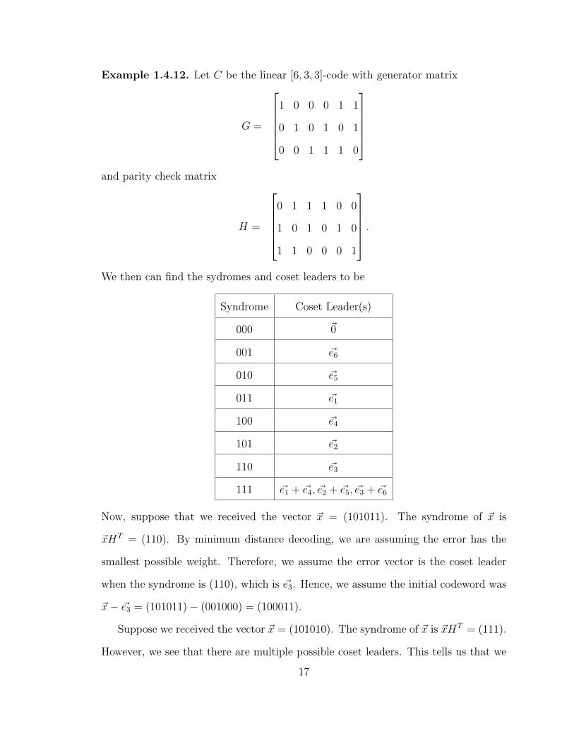
Example 1.4.12. Let C be the linear [6, 3, 3]-code with generator matrix

G =

1 0 0 0 1 1

0 1 0 1 0 1

0 0 1 1 1 0

and parity check matrix

H =

0 1 1 1 0 0

1 0 1 0 1 0

1 1 0 0 0 1

.We then can find the sydromes and coset leaders to be

Syndrome Coset Leader(s)

000 ~0

001 ~e6

010 ~e5

011 ~e1

100 ~e4

101 ~e2

110 ~e3

111 ~e1 + ~e4, ~e2 + ~e5, ~e3 + ~e6

Now, suppose that we received the vector ~x = (101011). The syndrome of ~x is

~xHT = (110). By minimum distance decoding, we are assuming the error has the

smallest possible weight. Therefore, we assume the error vector is the coset leader

when the syndrome is (110), which is ~e3. Hence, we assume the initial codeword was

~x− ~e3 = (101011)− (001000) = (100011).

Suppose we received the vector ~x = (101010). The syndrome of ~x is ~xHT = (111).

However, we see that there are multiple possible coset leaders. This tells us that we

17

don’t know if our initial codeword was ~x−(~e1+~e4) = (001110), ~x−(~e2+~e5) = (111000),

or ~x − (~e3 + ~e6) = (100011) since there are three error vectors that are each equally

likely to appear. This is an example of an incomplete decoding. All we know is that

since each of these coset leaders has weight 2, there were, most likely, two errors that

occurred.

1.5 Other examples of codes

1.5.1 Hamming codes

Hamming codes were founded independently in 1949 by Marcel Golay and in 1950 by

Richard Hamming [?]. They are perfect linear codes that come with a very elegant

method of decoding. We can define Hamming codes over any finite field of order q.

Definition 1.5.1. Let r > 1, and let q be a prime power. The Hamming [n, k, 3]-

code over Fq is the linear code with n = (qr − 1)/(q− 1), k = n− r, and parity check

matrix H is defined to be the matrix whose columns are all the distinct (up to a

scalar multiple) nonzero vectors in Frq, normalized to have first nonzero coordinate

equal to 1.

To clarify the above definition, we will construct the parity check matrix for the

ternary Hamming [4, 2]-code. We see that r = 2, so we are looking for the nonzero

vectors in F23. These are (1, 0)T , (2, 0)T , (0, 1)T , (0, 2)T , (1, 1)T , (2, 2)T , (1, 2)T , (2, 1)T .

Since (2, 2)T = 2(1, 1)T , these two vectors are not distinct since they only differ

by a scalar multiple. Since we are choosing our columns to have the first nonzero

coordinate equal to 1, we choose the vector (1, 1)T to be in our parity check matrix.

18

This process gives us the following distinct vectors: (0, 1)T , (1, 0)T , (1, 1)T , (1, 2)T .

Therefore, our parity check matrix is0 1 1 1

1 0 1 2

.For a fixed q and r, we call the associated Hamming code the q-ary Hamming code

of order r. For example, the 2-ary Hamming code of order 4 appeared in Example

1.4.5. As a side note, all binary Hamming codes are equivalent to cyclic codes, and

some, but not all, non-binary Hamming codes are equivalent to cyclic codes [?].

For any linear code, its minimum distance, d, is the smallest integer for which there

exists d linearly dependent columns of its parity check matrix. Since our Hamming

codes have minimum distance 3, the parity check matrix has the property that any

two columns are linearly independent but there exists some set of three which are

linearly dependent. This allows us to construct the parity check matrix of a Hamming

code in many ways since our choices of columns is not unique. However, by permuting

the columns and multiplying the rows by non-zero scalars, we can show any two parity

check matrices of the same Hamming code are equivalent. Therefore, Hamming codes

are uniquely determined by being a linear code with paramenters [(qr−1)/(q−1), n−

r, 3].

The most common alphabet used in Hamming codes is F2. These codes have

parameters [2r − 1, 2r − 1 − r, 3] and come with a very nice structure in its parity

check matrix. For example, the 2-ary Hamming code of order 3 has parity check

matrix

H =

0 0 0 1 1 1 1

0 1 1 0 0 1 1

1 0 1 0 1 0 1

.Notice that the columns of the parity check matrix are all non-zero elements less than

or equal to 23 written in binary (when viewed from the top to the bottom).

19

Hamming codes are equipped with a very nice method for decoding. First, when-

ever we write the parity check matrix for a binary Hamming code of order r, we

should write it in the above way. Then, we can notice that each column is the binary

representation for 1 to 2r in increasing order, like how we wrote the parity check

matrix for the binary Hamming code of order 3 above. Since Hamming codes are

perfect single error correcting codes, we see that besides in coset which has coset

leader of ~0, the coset leaders are every vector of weight 1. Notice that the syndrome

of a vector with a 1 in the i-th position and 0 elsewhere is (00 . . . 010 . . . 0)HT = HTi

where Hi is the i-th column of H. Therefore, this syndrome, when thought of as a

binary number, is the binary position of the error. Let’s look at an example.

Example 1.5.2. Suppose we use the binary Hamming code of order 3. Then, consider

the coset leader ~e6 = (0000010). We see the syndrome is (0000010)HT = (110) =

1102 = 610.

If we are considering a q-ary Hamming code where q 6= 2, we can choose the

columns of the parity check matrix in increasing size as q-ary numbers, but for those

in which the first non-zero entry in each column is a 1. For example, the parity check

matrix for a ternary Hamming code of order 3 is

H =

0 0 0 0 1 1 1 1 1 1 1 1 1

0 1 1 1 0 0 0 1 1 1 2 2 2

1 0 1 2 0 1 2 0 1 2 0 1 2

By the same reasoning as before, if an error occurs in the i-th position, the coset

leader will have the form kei where k is some nonzero scalar. Therefore, the syndrome

is keiHT . This is precisely k multiplied by the i-th column in H (when written as

a row). By our construction of the parity check matrix, we have that k is the first

nonzero entry in the syndrome. Also, if we multiply the syndrome by k−1, we end up

20

with the i-th column of our parity check matrix. Thus, we know exactly where the

error occurred.

Example 1.5.3. Suppose we use the above parity check matrix for the ternary Ham-

ming code of order 3. Furthermore, suppose we received the word (1101112211201).

Then, we see that the syndrome is (1101112211201)HT = (201) = 2(102) = 2 ×

7th column of H. Thus, by subtracting 2 from the 7th position of (1101112211201),

we get the initial codeword (1101110211201).

1.5.2 Non-linear codes

Non-linear codes can be constructed in many different ways. Most often, they are

created from some combinatorial object such as Latin Squares, block designs, and

cube-tilings [9].

A popular example of a combinatorial design is the Fano plane, as illustrated

below.

4 6

1

732

5

Figure 1.1: Fano plane

We can label the lines in the figure by l1 = 14, l2 = 16, l3 = 46, l4 = 15, l5 =

21

26, l6 = 34, l7 = 25. Notice in this construction, each line is incident to exactly three

points, every point is incident to exactly three lines, and each pair of lines meet at

exactly one point.

The incidence matrix of this graph is the matrix (aij) where

aij =

1 if line li contains point j

0 otherwise

The resulting matrix is

F =

1 1 0 1 0 0 0

1 0 1 0 0 1 0

0 0 0 1 1 1 0

1 0 0 0 1 0 1

0 1 0 0 0 1 1

0 0 1 1 0 0 1

0 1 1 0 1 0 0

Denote each row by ~bi. Since each line meets any other line at exactly one point,

each row shares exactly one non-zero entry with any other row. We see that every

row has weight 3. Therefore, d(~bi, ~bj) = 4 for any i 6= j for i, j ∈ [1, 2, . . . , 7].

Now, take each bi and replace the 0’s with 1’s and vice versa. Call this new row

~ai. Do this for all i = 1, 2, . . . , 7. Now, we can see that d(~ai, ~aj) = 4 for any i 6= j for

i, j ∈ [1, 2, . . . , 7].

Notice that when i 6= j, we have that ~bi and ~aj differ exactly where ~bi and ~bj

agree. Therefore, d(~bi, ~aj) = 3 for any i 6= j for i, j ∈ [1, 2, . . . , 7].

We see that d(~ai,~0) = 3, d(~ai,~1) = 4, d(~bi,~0) = 4 and d(~bi,~1) = 3. Therefore, the

code C = {~0,~1, ~a1, ~a2, . . . , ~a7, ~b1, ~b2, . . . , ~b7} is a (7, 16, 3)-code. Also, by plugging in

q = 2, n = 7, t = 1, we have equality in the sphere-packing bound. Hence, this code

is a perfect (7, 16, 3)-code.

22

CHAPTER 2

QUANTUM ERROR CORRECTING CODES

2.1 Motivation

For an in depth introduction to quantum error correcting codes, consider consulting

[11]. The introduction given in this thesis is designed to supply the reader with

just enough of the background of quantum error correcting codes to allow them to

understand the recent research in the area.

In the 1980’s, the field of quantum computing was first introduced [13]. Instead

of storing data on bits (0’s and 1’s), quantum computing stores data on quantum

bits (also known as qubits) which can be in any superposition of its two pure states,

which are denoted as |0〉 and |1〉. This means that the state of an individual qubit,

|φ〉, can be expressed as a linear combination of the two orthonormal basis states |0〉,

|1〉,

|φ〉 = α|0〉+ β|1〉

where |α|2 + |β|2 = 1.

The potential that quantum computing has is incredible. For example, Shor’s

algorithm, which is a quantum algorithm used for integer factorization, can factor

any integer in quantum polynomial time. Currently, the fastest known non-quantum

algorithm for integer factorization is sub-exponential and it is unknown if there would

ever be a non-quantum algorithm that could factor any integer in polynomial time

23

[15]. Unfortunately, due to the fragility of quantum states and how easily it is for a

qubit to change slightly to a different quantum state, errors in quantum computation

are extremely frequent. Therefore, if quantum computing is ever to become successful,

it will require the implementation of effective quantum error correcting codes.

Definition 2.1.1. A quantum error correcting code is a mapping of k qubits into

n qubits, where n > k. The k qubits are the qubits which store information and

we would like to have protected from error. The remaining n − k qubits are the

redundancy qubits we will use to minimize the effects of errors on the k encoded

qubits.

2.2 Calderbank–Shor–Steane codes

Calderbank–Shor–Steane codes, known as CSS codes, are one of the most popular

class of codes in quantum error correcting codes (QECC). CSS codes are very ap-

pealing due to their construction being based upon classical linear codes. A CSS

code is constructed by two classical linear codes, say C1 and C2, where C1 is a [n, k1]

code and C2 is a [n, k2] code. It is also necessary that C2 ⊂ C1 and C1 and C⊥2 both

correct t errors. Then, we can construct an [n, k1 − k2] quantum code capable of

correcting errors on up to t qubits. This claim is proven below in Proposition 2.2.1.

The construction of CSS codes is done in the following manner.

Let C1, C2 be two classical linear codes satisfying the necessary conditions listed

above. Let G1, G2 be the generator matrices of C1, C2 respectively. Also, let Let

H1, H2 be the parity check matrices of C1, C2 respectively. Then, the generator matrix

of the corresponding CSS code is of the formG1 0

0 G2

.

24

And the parity check matrix of the corresponding CSS code is of the formH2 0

0 H1

.

Proposition 2.2.1. The CSS code constructed from C1 and C2 is an [n, k1 − k2]

quantum code.

Proof. Let x ∈ C1 be a codeword. Define the quantum state |x+ C2〉 :=1√|C2|

∑y∈C2

|x+ y〉.

Note: + is bitwise addition modulo 2. To make the desired conclusion, we would like

to use coset arguments. Suppose there exists some x′ such that x − x′ ∈ C2. Then,

by the definition of the quantum state of |x + C2〉, we have |x + C2〉 = |x′ + C2〉.

Hence, the state |x + C2〉 depends only upon the coset of C1/C2 which x is in. If x

and x′ are in two distinct cosets of C2, then there does not exist y, y′ ∈ C2 such that

x + y = x′ + y′. Hence, |x + C2〉 and |x′ + C2〉 are orthonormal states. The CSS

code generated by C1 and C2 is defined to be the vector space spanned by the states

|x + C2〉 for all x ∈ C1. The number of cosets of C2 in C1 is |C1|/|C2|. Hence, the

dimension of our CSS code is |C1|/|C2| = 2k1/2k2 = 2k1−k2 . Therefore, our CSS code

is an [n, k1 − k2] quantum code, as desired.

A popular example of a CSS code is called the Steane Code. One reason this code

is important is because it is a perfect CSS code. For its construction, we start with

the binary Hamming code of order 3 which has the following parity check matrix:

H =

0 0 0 1 1 1 1

0 1 1 0 0 1 1

1 0 1 0 1 0 1

Now, let C denote this code. Then, let C1 := C and let C2 := C⊥. The binary

25

Hamming code of order 3 is a self dual code. Therefore, the Steane code has its

parity check matrix of the form: H 0

0 H

2.3 Recent research

We begin this section with a few definitions.

Definition 2.3.1. A sequence of codes, C, is called low density parity check (LDPC)

if C⊥ is spanned by vectors of bounded Hamming weight (ı.e. it has a sparse parity

check matrix).

This definition makes sense (and it not trivial) because we are considering infinite

sequences of codes. Notice that we are not restricting ourselves to only considering

codes whose code words in C⊥ have bounded Hamming weight, but rather when

C⊥ is generated by vectors of bounded Hamming weight. For example, we could

create a codeword in a LDPC code with unbounded Hamming weight. For example,

a codeword with unbounded Hamming weight could be generated by the vectors

(1, 0, 0, 0, . . . ), (0, 1, 0, 0, . . . ), (0, 0, 1, 0, . . . ), etc. (as n tends to infinity) each of

which have bounded Hamming weight but their sum could have unbounded weight.

Definition 2.3.2. A sequence of codes, C, is called good if the dimension and the

distance of the code grows at least linearly with the length of the code.

One recent goal in quantum error correcting codes has been to find good LDPC

codes. In classical error correcting codes, LDPC codes have had great success due

to their ability to rapidly determine errors which corrupt the data [4]. Therefore, it

makes sense that a lot of the recent effors in quantum error correcting codes are in

26

an attempt to research their generalization to quantum codes. Thus, we are led to

the following open problem.

Open problem 2.3.3. Do good LDPC quantum codes exist?

In classical error correcting codes, many constructions come from seemingly ran-

dom sources (such as the non-linear cases) and in many cases, end up being successful.

However, with the requirement of orthogonality between the two classical codes we

use in constructing QECC, random constructions rarely work. Therefore, there are

not as many constructions for LDPC quantum codes and many of these end up having

bounded minimum distance [14]. Unfortunately, bounded minimum distance is gen-

erally not sufficient in correcting the large number of errors which occur in quantum

computing. Very few constructions of quantum LDPC have unbounded minimum

distance. We will discuss two of these such constructions. One is based on homo-

logical properties regarding the tilings of higher dimensional manifolds. The other is

based on Cayley graphs.

2.4 Quantum LDPC codes based on homological properties

Larry Guth and Alexander Lubotzky recently published a paper titled, Quantum

error correcting codes and 4-dimensional arithmetic hyperbolic manifolds, [5]. In [16],

Zemor posed the following question: If C is an [[n, k, d]] homological quantum code,

then is it always true that kd2 ≤ n1+o(1)? It was essentially proven in [3] that this

inequality is true for codes coming from 2-dimensional surfaces. In [5], Guth and

Lubotzky showed that the inequality is not true for codes coming from 4-dimensional

manifolds. Using CSS-codes, they proved the following result:

Theorem 2.4.1. There exists ε, ε′, ε′′ > 0 and a sequence of 4-dimensional hyperbolic

27

manifolds M with triangulations X such that the associated homological quantum codes

constructed in C2(X,Z2) = C2(X,Z2) are [[n, ε′n, nε′′]] codes and so:

kd2 ≥ n1+ε.

Recall that in the construction of CSS-codes, it is necessary to find two orthogonal

subspaces, say W1,W2, such that W1 ⊆ W⊥2 and W2 ⊆ W⊥

1 . Before we announce

the choice of the two orthogonal subspaces, it is necessary to explain how manifolds

and simplicial complexes are used by Guth and Lubotzky in this construction of

homological codes.

Let X be a finite simplicial complex of dimension D (if M is a manifold, one can

replace M by a triangulation X of it), i.e., X is a set of subsets of X(0) of size ≤ D+1

with the property that if F ∈ X and G ⊆ F then G ∈ X. Let X(i) be the set of

subsets in X of size i. The space of mod 2 i-chains, Ci = Ci(X,Z2), is the Z2-vector

space spanned by X(i). The space of mod 2 i-cochains, Ci = Ci(X,Z2), is the space

of functions from X(i) to Z2.

Let ∂i : Ci → Ci−1 be the boundary map, i.e.,

∂i(F ) =∑G<F|G|=i

G for F ∈ X(i)

and its adjoint δi : Ci → Ci+1 the cobounding map,

δi(F ) =∑F<G|G|=i+2

G.

It is a standard fact that ∂i ◦ ∂i+1 = 0 and δi ◦ δi−1 = 0 for all i (see [6] for a

proof). Therefore, Bi := the i-boundaries = Im∂i+1 is contained in Zi := the i-cycles

= Ker∂i. Similarly, Bi := the i-coboundaries = Imδi−1 is contained in Zi := the

i-cocycles = Kerδi.

Since δi−1 is the adjoint of ∂i, we have that B⊥i = Zi and (Bi)⊥ = Zi. Hence, to

create the CSS-code, Bi and Bi are chosen to be the necessary orthogonal subspaces.

28

These codes have length n = |X(i)|, dimension k = dimZi/Bi = dimHi(X,Z2) =

dimZi/Bi = dimH i(X,Z2) (where Hi is the homology of X with coefficients in Z2

and H i is the i-cohomology group), and distance equal to the the Hamming weight

of a non-trivial homology or cohomology class, i.e., the minimum weight of an i-cycle

(which is not an i-boundary) or i-cocycle (which is not an i-coboundary).

One advantage that homological codes have is that if one lets M , a manifold, vary

over finite sheeted covers of a fixed compact manifold, then we are able to construct

quantum codes that are LDPC quantum codes. This is due to the fact that Bi (resp.

Bi) is generated by the images of the cells of dimension i+ 1 (resp. i− 1).

A necessary note is that in [5], Guth and Lubotzky were not the first to prove

the existence of LDPC quantum codes with parameters [[n, ε′n, nε′′]]. It was proven

in [14], by Tillich and Zemor, that LDPC quantum codes exist with parameters

[[n, ε′n, n0.5]]. However, the importance of the work done by Guth and Lubotzky is

due to the fact that their codes are homological.

2.5 Quantum LDPC codes based on Cayley graphs

Another mathematical structure that is used in the construction of quantum error

correcting codes is the Cayley graph. This construction was proposed by MacKay,

Mitchison, and Shokrollahi [10] and has been studied in [1]. Again, the construction

used in this quantum code is the CSS code. The primary focus in discussing the

construction of quantum error correcting codes using the Cayley graph will be from

studying a paper written by Delfosse, Li, and Thomasse [2].

Definition 2.5.1. Let G be a group and S be a set of elements of G such that s ∈ S

implies s−1 ∈ S. The Cayley graph Γ(G,S) is the graph with vertex set G such that

two vertices are adjacent if they differ by an element in S (ı.e. x and y are adjacent

if there exists some element t ∈ S such that xt = y.

29

In the paper by Delfosse et al. [2], they only considered the group G = Fn2 with the

set S = {e1, e2, . . . en}, the generating set of Fn2 where ei has a 1 in the i-th position

and zeros elsewhere. Therefore, Γ(G,S) has 2n vertices and it is a regular graph of

degree n.

To create a quantum code from a Cayley graph, we proceed in the following way.

Let H ∈ Mn,n(F2) be a binary matrix. If n is an even integer, then the adjacency

matrix of the graph G(H) is the generating matrix of a classical self-orthogonal code.

Since G(H) generates a self-orthogonal code, we have the necessary requirements for

the construction of a CSS code. Also, note that the generating matrix of the self-

orthogonal code is the adjacency matrix of G(H), which is sparse. This is due to the

length of the row vectors being 2n and each row having weight n. Therefore, by our

definition of LDPC codes, the quantum code constructed is a LDPC code.

The majority of [2] is dedicated to determining the minimum distance of the

above constructed quantum LDPC codes. The determining of the minimum distance

is interesting because the authors related this problem with a combinatorial problem

of the hypercube. To state the combinatorial problem, we must first introduce a few

definitions.

Definition 2.5.2. Let S be a subset of the vertex set of G(H). The border B(S) of

S in the graph G(H) is the set of vertices of G(H) which belong to an odd number

of neighborhoods N(v) for v ∈ S.

The above definition can be reworded to say that the border of a subset S is the

symmetric difference of all the neighborhoods N(v) for v ∈ S.

Definition 2.5.3. A pseudo-border in the graph G(H) is a family P of vertices of

G(H) such that the cardinality of N(v) ∩ P is even for every vertex v of G(H).

30

The above defined borders and pseudo-borders correspond to the vectors of the

classical code and its dual in the following way.

Lemma 2.5.4. Let x be a vector of F2n

2 . Then, x is the indicator vector of a subset

Sx of the vertex set of G(H). Hence, we have that x is a vector in the classical code

if and only if Sx is a border. Furthermore, x is a vector in the dual of the classical

code if and only if Sx is a pseudo-border.

This lemma, along with the construction of the quantum code from the Cayley

graph, shows that, when n is even, every border is a pseudo-border. There do indeed

exist some special cases in which every pseudo-border in a border. However, this is

not true in general. When G(H) contains pseudo-borders which are not borders, the

minimum distance of the quantum code associated with H is equal to

D = min{|S| | S is a pseudo-border which is not a border}.

In the paper, they showed that the graph G(H) is locally isomorphic to the hy-

percube of dimension n. This leads to the motivation behind considering the borders

and pseudo-borders of the hypercube. They introduce the last important defintion.

Definition 2.5.5. A t-pseudo-border is a subset of vertices of a ball of the hypercube

satisfying the conditions of the definition of a pseudo-border in the ball of radius

t < n centered in a specific corner of the hypercube.

We may obtain a t-psuedo-border of the hypercube by starting from a psuedo-

border of G(H) and using the above fact that G(H) is locally isomorphic to the

hypercube of dimension n. By finding a lower bound on the cardinality of t-pseudo-

borders, we find a minimum distance of our quantum code. This leads to the following

main result in the paper.

31

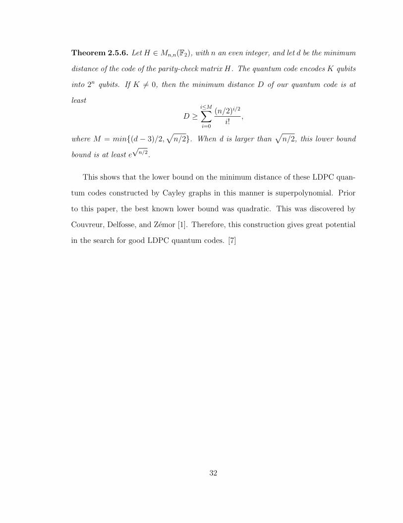
Theorem 2.5.6. Let H ∈Mn,n(F2), with n an even integer, and let d be the minimum

distance of the code of the parity-check matrix H. The quantum code encodes K qubits

into 2n qubits. If K 6= 0, then the minimum distance D of our quantum code is at

least

D ≥i≤M∑i=0

(n/2)i/2

i!,

where M = min{(d − 3)/2,√n/2}. When d is larger than

√n/2, this lower bound

bound is at least e√n/2.

This shows that the lower bound on the minimum distance of these LDPC quan-

tum codes constructed by Cayley graphs in this manner is superpolynomial. Prior

to this paper, the best known lower bound was quadratic. This was discovered by

Couvreur, Delfosse, and Zemor [1]. Therefore, this construction gives great potential

in the search for good LDPC quantum codes. [7]

32

BIBLIOGRAPHY

[1] Alain Couvreur, Nicolas Delfosse, and Gilles Zemor. A construction of quantumLDPC codes from Cayley graphs. IEEE Trans. Inform. Theory, 59(9):6087–6098, 2013.

[2] Nicolas Delfosse, Zhentao Li, and Stephan Thomasse. A note on the minimumdistance of quantum LDPC codes.

[3] Ethan Fetaya. Bounding the distance of quantum surface codes. J. Math.Phys., 53(6):062202, 12, 2012.

[4] R. G. Gallager. Low-density parity-check codes. IRE Trans., IT-8:21–28, 1962.

[5] Larry Guth and Alexander Lubotzky. Quantum error correcting codes and 4-dimensional arithmetic hyperbolic manifolds. J. Math. Phys., 55(6):082202, 13,2014.

[6] Allen Hatcher. Algebraic topology. Cambridge University Press, Cambridge,2006.

[7] Raymond Hill. A First Course in Coding Theory. Clarendon Press, Oxford,2004.

[8] David Joyner and Jon-Lark Kim. Selected Unsolved Problems in Coding Theory.Birkhauser/Springer-Verlag, New York, 2011.

[9] J. C. Lagarias and P. W. Shor. Cube-tilings of Rn and nonlinear codes. DiscreteComput. Geom., 11(4):359–391, 1994.

[10] David J. C. MacKay, Graeme Mitchison, and Paul L. McFadden. Sparse-graphcodes for quantum error correction. IEEE Trans. Inform. Theory, 50(10):2315–2330, 2004.

[11] Michael A. Nielsen and Isaac L. Chuang. Quantum computation and quantuminformation. Cambridge University Press, Cambridge, 2000.

[12] Steven Roman. Coding and Information Theory. Springer-Verlag, New York,1992.

33

[13] Andrew Steane. Quantum computing. Reports on Progress in Physics, 61(2):117,1998.

[14] Jean-Pierre Tillich and Gilles Zemor. Quantum LDPC codes with positive rateand minimum distance proportional to the square root of the blocklength. IEEETrans. Inform. Theory, 60(2):1193–1202, 2014.

[15] Samuel S. Wagstaff, Jr. The joy of factoring, volume 68 of Student MathematicalLibrary. American Mathematical Society, Providence, RI, 2013.

[16] Gilles Zemor. On Cayley graphs, surface codes, and the limits of homologicalcoding for quantum error correction. In Coding and cryptology, volume 5557 ofLecture Notes in Comput. Sci., pages 259–273. Springer, Berlin, 2009.

34