INFORMATION TO USERS

This manuscript has been reproduced from the microfilm master. UMI films the text directly from the original or copy submitted. Thus, some thesis and dissertation copies are in typewriter face, while others may be from any type of computer printer.

The quality of this reproduction is dependent upon the quality of the copy submitted. Broken or indistinct print, colored or poor quality illustrations and photographs, print bleedthrough. substandard margins, and improper alignment can adversely affect reproduction.

In the unlikely event that the author did not send UMI a complete manuscript arxf there are missing pages, these will be noted. Also. If unauthorized copyright material had to be removed, a note will indicate the deletion.

Oversize materials (e.g.. maps, drawings, charts) are reproduced by sectioning the original, beginning at the upper left-hand comer and continuing from left to right in equal sections with small overlaps.

Photographs included in the original manuscript have been reproduced xerographically in this copy. Higher quality 6” x 9” black and white photographic prints are available for any photographs or illustrations appearing in this copy for an additional charge. Contact UMI directly to order.

Bell & Howell Information and Learning 300 North Zeeb Road. Ann Arbor. Ml 48106-1346 USA

U K U800-521-0600

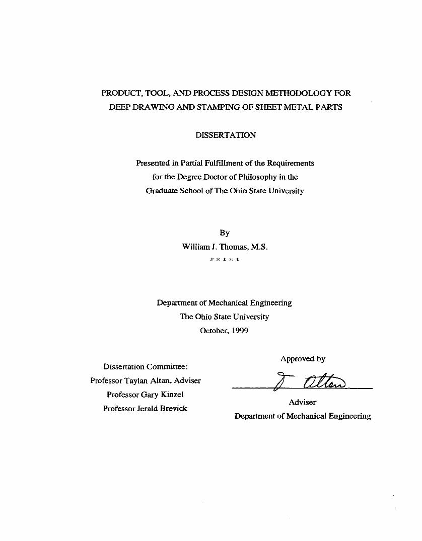
PRODUCT, TOOL, AND PROCESS DESIGN METHODOLOGY FOR

DEEP DRAWING AND STAMPING OF SHEET METAL PARTS

DISSERTATION

Presented in Partial Fulfillment of the Requirements

for the Degree Doctor of Philosophy in the

Graduate School of The Ohio State University

ByWilliam J. Thomas, M.S.

* * * * *

Department of Mechanical Engineering

The Ohio State University

October, 1999

Approved byDissertation Committee:

Professor Taylan Altan, Adviser ^ ______

Professor Gary KinzelAdviser

Professor Jerald BrevickDepartment of Mechanical Engineering

UMI Number 9951736

Copyright 1999 by Thomas. William James

All rights reserved.

UMIUMI Microform9951736

Copyright 2000 by Bell & Howell Information and Leaming Company. All rights reserved. This microform edition is protected against

unauthorized copying under Title 17, United States Code.

Bell & Howell Information and Leaming Company 300 North Zeeb Road

P.O. 80x1346 Ann Arbor, Ml 48106-1346

Copyright by

William James Thomas

October, 1999

"But neither politics nor ethics nor philosophy [nor science J is an end in itself, neither in

life nor in literature. Only Man is an end in himself "

- Ayn Rand, The Goal o f My Writing, Lewis and Clark College, October I, 1963

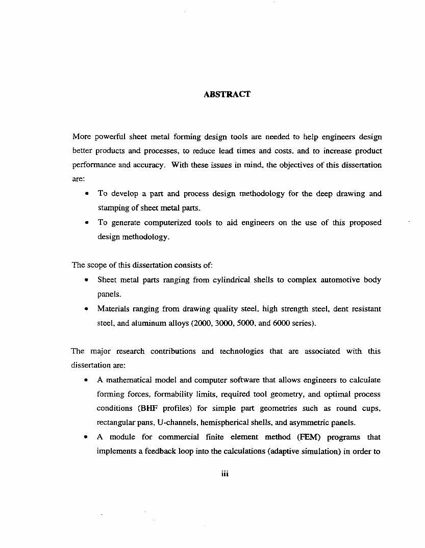
ABSTRACT

More powerful sheet metal forming design tools are needed to help engineers design

better products and processes, to reduce lead times and costs, and to increase product

performance and accuracy. With these issues in mind, the objectives of this dissertation

are:

• To develop a part and process design methodology for the deep drawing and

stamping of sheet metal parts.

• To generate computerized tools to aid engineers on the use of this proposed

design methodology.

The scope of this dissertation consists of:

• Sheet metal parts ranging from cylindrical shells to complex automotive body

panels.

• Materials ranging from drawing quality steel, high strength steel, dent resistant

steel, and aluminum alloys (2000, 3000, 5000, and 6000 series).

The major research contributions and technologies that are associated with this

dissertation are:

• A mathematical model and computer software that allows engineers to calculate

forming forces, forraability limits, required tool geometry, and optimal process

conditions (BHF profiles) for simple part geometries such as round cups,

rectangular pans, U-channels, hemispherical shells, and asymmetric panels.

• A module for commercial finite element method (FEM) programs that

implements a feedback loop into the calculations (adaptive simulation) in order to

i i i

determine optimal process conditions (BHF profiles) for general complex

geometries.

• Computerized tools that provide engineers with the effect o f process parameters

on part quality (sensitivity data) for various simple laboratory tool geometries

using laboratory experiments and computer simulations.

The prediction of optimal process parameters will focus primarily on determining the

optimum time and spatial variation of the blank holder force (BHF) given a particular

geometry. It has been proven in laboratories that drawability can be improved by

changing the blank holder force during the stroke of the press (i.e. during deformation).

Also, it has been observed that part quality can be enhanced by m o d i^ n g the distribution

of blank holder pressure (BHP) around the periphery of the blank. Thus, the question

becomes given a certain geometry what is the optimum spatial distribution and time

variation of the BHF? It is the goal of this work to contribute towards answering this

question.

IV

For my wife and newborn son

Laura and Ethan

oo oo oo oo oo

Vous êtes en mon coeur...

ACKNOWLEDGMENTS

I would like to thank the following people for taking the time to mentor and tutor me.

Their insight, wisdom, support, and friendship were indispensable.

• Prof. Taylan Altan, Director, ERC/NSM

• Leonard Delac, Vice President, MTD Products

I would also like to show my appreciation to the following coworkers for their expertise

and advice.

• Hsien Chih Wu

• Suwat Jirathearanat

• Alex Shr

• Serhat Kaya

• Matt Jolliff

• Collis Wagner

Prof. Gary Kinzel

Dr. Nuri Akgerman

Dr. Mustafa Ahmetoglu

David Osborn

Adam Grosz

Tolga Uludag

Mahmoud Shatla

Carmen Crowley

Toshi Oenoki

Leonid Shulkin

Xin Jun Li

Mark Diller

Paul Schauer

Peter Riegler

Further, I would like to thank the following governmental agencies, industrial companies,

and colleagues for their generous tlnancial and in-kind support.

• Engineering Research Center for Net Shape Manufacturing

• National Science Foundation

• National Institute of Science and Technology

• Auto Body Consortium (Emie Vahala)

• Joint Venture Members o f the Near Zero Stamping Project

VI

• Sekely Industries (Chris Burbick)

• Century Aluminum Company (Paul Smith)

• Battelle Memorial Institute (Rich Tenaglia)

• Modem Tool and Die Company (Len Delac)

• Eaton Corporation - Clutch Division (Steve Lepard)

• Dickey Manufacturing (Walt Quandt)

• Autodie International (Craig Wieberdink)

• Engineering Systems International (Olivier Morisot, Laurent Taupin)

• Forming Technologies Incorporated (Stephen Fysh)

I would like to send my love to my parents, Fred and Sun Ye, my brother Bob and my

sister Lyn. God bless you all.

In closing, I would acknowledge the support of everyone who contributed to this work

and were not listed here. To the unnamed — Cheers!

V ll

VITA

October 17, 1971............................................Bom - Stuttgart, Germany.

U.S. Army Base Camp.

1990 - 1995................................................... Cooperative Student.

Modem Tool & Die. - Cleveland, Ohio.

1995................................................................ B.S. Mechanical Engineering.

Kettering University - Hint, Michigan.

(Formerly GM3/EMI)

1997.................................. ........................... M.S. Mechanical Engineering.

The Ohio State University - Columbus, Ohio

1995 - Present............................................... Full Time Staff Engineer.

Engr. Research Center for Net Shape Mfg.

The Ohio State University - Columbus, Ohio

PUBLICATIONS

Thomas, W., Ahmetoglu, M., Altan, T. Sheet Metal Forming: Fundamentals and Applications - a Practical Handbook. Society of Manufacturing Engineers. To be Published.

V lll

Thomas, W., Altan, T. Part and Process Design Methodology for Deep Drawing and Stamping of Sheet Metals. PhJD. Dissertation. The Ohio State University. Columbus, Ohio. To be Published.

Thomas, W., Altan, T. Forming of Aluminum Sheet. Chapter 2 of the “Handbook of Aluminum.” Marcel Dekker. To be Published.

Thomas, W., Altan, T. Regular R&D Update Column of the Stamping Journal. Fabricators and Manufacturers Association International.

Thomas, W., Vazquez, V., Koc, M., Altan, T. (1999) Simulation o f Metal Forming Processes - Applications and Fumre Trends. Proceedings of the 6 th International Conference on Technology of Plasticity. September 19-23. Nuremberg, Germany.

Thomas, W., Johnson, G., Altan, T. (1999) Improving the Formability of Aluminum Alloy 3003-H14 With Computer Simulation. Keynote Paper. Proceedings of the 6 th International Conference on Technology of Plasticity. September 19-23. Nuremberg, Germany.

Thomas, W., Oenoki, T., Altan, T. (1999) Process Simulation In Stamping - Recent Applications for Product and Process Design. Special Issue of the Journal of Materials Processing Technology. Highlights of the 3rd Int’l Conference on Sheet Metal Forming Technology. Columbus, OH. October 3-5, 1998. Elsevier.

Thomas, W., Oenoki, T., Altan, T. (1999) Implementing FEM Simulation into the Concept to Product Process. 1999 SAE International Congress. 12th Session on Sheet Metal Stamping (jointly sponsored by NADDRG). March 1-4. Detroit, MI. No. 99M-176.

Thomas, W., Oenoki, T., Altan, T. (1998) Process Simulation In Stamping - Recent Applications for Product and Process Design. Proceedings of the 3rd Int’l Conference on Sheet Metal Forming Technology. Columbus, OH. October 3-5, 1998. Fabricators and Manufacturers Association International.

Thomas, W. Altan, T. (1998) Application of Computer Modeling in Part, Die, and Process Design for Manufacturing of Automotive Stampings. Steel Research. Vol. 69. No. 4, 5. Verein Deutscher Eisenhuttenleute. Max-Plank Institute.

Thomas, W. Altan, T. (1998) Applying Computer Simulation to Automotive Part Stamping. The Fabricator. February, 1998. Fabricators and Manufacturers Association International.

Diller, M., Thomas, W., Ahmetoglu, M., Akgerman, N., Altan, T. (1997) Applications of Computer Simulations for Part and Process Design for Automotive Stampings. SAE International Congress. Feb. 24-27, 1997. No. 970985.

Thomas, W., Kinzel, G. Altan, T. (1997) Improving The Deep Drawability Of 2008-T4 Aluminum and 1008 AKDQ EG Steel Sheet With Location Variable Blank Holder Force Control. M.S. Thesis. The Ohio State University. Columbus, OH.

IX

Thomas, W., Erevelles, W. Sullivan, L. (1995) Implementation and Automation of a Composite Extrusion System. B.S. Thesis. Kettering University(Formerly GMEEMD. Hint, ML

FIELDS OF STUDY

Major Field: Mechanical Engineering

Minor Fields: Sheet Metal Forming, Manufacturing, Machine Design

TABLE OF CONTENTS

Page

ABSTRACT................................................................................................................................iü

ACKNOWLEDGMENTS..........................................................................................................viVITA.........................................................................................................................................vüi

TABLE OF CONTENTS.......................................................................................................... xiLIST OF FIGURES................................................................................................................... xv

LIST OF TABLES..................................................................................................................xxii

NOMENCLATURE...............................................................................................................xxivPREFACE........................................................................ l

CHAPTER I: INTRODUCTION AND PROBLEM STATEMENT....................................4

LI Introduction...................................................................................................................... 4

LIT Classification of Sheet Metal Forming Processes................................................ 4

I. L.2 Sheet Metal Forming as a System.......................................................................... 6

1.2 Problem Statement...........................................................................................................7

1 .3 Dissertation Organization................................................................................................ 8

CHAPTER H: FUNDAMENTALS OF DEEP DRAWING AND STAMPING................ 9

2 .1 Deep Drawing - Process and Technology..................................................................... 9

2.1.1 Drawability of Round Cups....................................................................................102 .1 .2 Effect of Strain Hardening.....................................................................................1 1

2.1.3 Effect of Anisotropy............................................................................................... 12

2.1.4 Product Quality........................................................................................................ 152.1.5 Deep Drawing of Complex Geometries............................................................... 15

2 . 2 Stamping - Process and Technology............................................................................ 172.2.1 Product Quality........................................................................................................ 18

2.2.2 Effect of Material Properties..................................................................................18

XI

2.2.3 Automotive Body Stamping................................................................................. 20

2.3 Blank Holder Force.......................................................................................................23

2.3.1 Issues with Blank Holders.....................................................................................25

2.3.2 Blank Holder Design.................................................................................. 26

2.3.3 Blank Holder Force Control................................................................................. 332.3.4 Closed-Loop BHF Control....................................................................................38

2.3.4.1 Round Cups - Experimental Optimal BHF Profiles.................................. 38

2.3.4.2 Round Cups - Computer Simulation of Optimal BHF Profiles............... 41

2.3.4.3 Round Cups - Analytical Prediction of Optimal BHF Profiles................ 43

2.3.4.4 Non-Round Parts- Experimental Optimal BHF Profiles............................44

2.3.4.5 Non-Round Parts- Computer Simulation of Optimal BHF Profiles 47

2.4 Analysis Techniques.................................................................................................... 48

2.4.1 Mathematical Modeling........................................................................................48

2.4.1. 1 Round Cup Deep Drawing............................................................................ 48

2.4.1.2 Deep Drawing of Rectangular Pans.............................................................50

2.4.2 Computer Simulation............................................................................................ 52

2.4.3 Failure Prediction...................................................................................................56

2.5 Issues with Forming Aluminum Alloys......................................................................61

2.5.1 Product Design Considerations.............................................................................61

2.5.2 Die and Process Design Considerations.............................................................. 62

2.5.3 Material Considerations........................................................................................ 65

CHAPTER ni: RESEARCH PLAN...................................................................................... 70

3.1 Rationale for the Proposed Research.......................................................................... 70

3.2 Research Objectives...................................................................................................... 73

3.3 Research Approach....................................................................................................... 74

3.4 Research P lan.................................................................................................................75

Phase 1: Conduct Literature Review................................................................. 75

Phase 2: Build New Laboratory Tooling....................................................................... 75

Phase 3: Develop Analytical Models to Predict Optimal BHF Profiles for Simple Geometries..........................................................................................................................76

XU

Phase 4: Develop a Module for a Commercial FEM Code to Predict Optimal BHF Profiles for Complex Geometries (Adaptive Simulation)............................................ 76

Phase 5: Conduct Experiments and Validate Models..................................................77

Phase 6 : Develop Sheet Forming Design Methodology............................................. 79

Phase 7: Deliver Research Results................................................................................ 80

CHAPTER IV: ANALYTICAL AND NUMERICAL MODELING OF DEEP DRAWING AND STAMPING.............................................................................................. 85

4 . 1 Deep Drawing of Basic Geometries — Predicting Optimal BHF Profiles...............85

4.1.1 Conceptual Approach............................................................................................85

4.1.2 Round Cup Deep Drawing - Analytical Derivations.......................................... 8 6

4 .1.3 Rectangular Pan Deep Drawing — Adaptation of Equations.............................92

4.1.4 Computerization.................................................................................................... 93

4.1.5 Validation of Analytical Model............................................................................93

4 .1 . 6 Fracture Prediction................................................................................................ 96

4 .1.7 Correlation of LDR and r ................................................................................... 98

4.2 Stamping of Complex Geometries — Predicting Optimal BHF Profiles with Adaptive Simulation........................................................................................................... 103

4.2.1 Elasticity of the Blank Holder............................................................................ 104

4.2.2 Robustness of the Control Algorithm.................................................................105

4.2.3 Wrinkling Based Adaptive Simulation..............................................................107

4.2.4 Stress Based Adaptive Simulation....................................................................110

4.2.5 Strain Based Adaptive Simulation....................................................................113

4.2.6 Force Based Adaptive Simulation.....................................................................115CHAPTER V: EXPERIMENTAL INVESTIGATION OF DEEP DRAWING AND STAMPING............................................................................................................................ 119

5 .1 Round Cup Deep Drawing......................................................................................... 119

5.2 Rectangular Pan Deep Drawing.................................................................................124

5.3 Asymmetric Panel Stamping...................................................................................... 129CHAPTER VI: PART, DIE, AND PROCESS DESIGN METHODOLOGY FOR DEEP DRAWING AND STAMPING.............................................................................................142

6 .1 Near Zero Stamping................................................................................................... 1426.1.1 The Concept to Production Process................................................................... 143

xui

6 .1.2 Final Deliverables to NZS.................................................................................. L45

6 . 1.3 Reports, Case Studies, Databases, Modules, and Software............................. 149

6.2 Industrial Case Studies..............................................................................................150

6.2.1 Deck Lid Soft Tool Tryouts - Case Study......................................................... 150

6.2.2 Fender Outer Hard Die Tryouts - Case Study...................................................155

CHAPTER VÜ: CONCLUSIONS AND FUTURE WORK............................................. 1657.1 Summary..................................................................................................................... 1657.2 Research Results........................................................................................................ 166

7.3 Conclusions................................................................................................................. 1677.4 Future W ork................................................................................................................ 167

REFERENCES........................................................................................................................169

APPENDIX A: REFERENCE EQUATIONS FOR DEEP DRAWING.........................183

A.l Round Cup Deep Drawing......................................................................... 183

A.2 Rectangular Pan Deep Drawing............................................................................... 185

A.3 Elasticity Equations for Cylinder/Blank Holder Contact.......................................186

APPENDIX B: INSTRUCTIONS FOR SHEET FORMING DESIGN SYSTEM 188

APPENDIX C: INSTRUCTIONS FOR COMPILING ROUTINES INTO THE FEM CODE PAM-STAMP.............................................................................................................193

APPENDIX D: INSTRUCTIONS FOR WRINKLING BASED ADAPTIVE SIMULATION............................................................................................................ 203

APPENDIX E

APPENDIX F

APPENDIX G

APPENDIX H

INSTRUCTIONS FOR STRESS BASED ADAPTIVE SIMULATION 212

INSTRUCTIONS FOR STRAIN BASED ADAPTIVE SIMULATION.......................................................................................................................225INSTRUCTIONS FOR FORCE BASED ADAPTIVE SIMULATION

.......................................................................................................................233DELIVERABLES FOR THE NEAR ZERO STAMPING PROJECT......

....................................................... 240

XIV

LIST OF FIGURES

Page

Figure L I: Air bending (LivatyalL 1998).............................................................................. 5Figure 1.2: Stretch forming (Crowley, 1998).........................................................................5

Figure 1.3: Classical deep drawing.........................................................................................5Figure 1.4: Sheet forming as a system ....................................................................................6

Figure 2.1: The deep drawing process..................................................................................10

Figure 2.2: Deformation zones in deep drawing..................................................................1 0

Figure 2.3: The r-values in a sheet material (Crowley, 1998)............................................ 14Figure 2.4: Earing in deep drawing (Hosford and Caddell, 1993).....................................14

Figure 2.5: Yield surface as a function of r -value (Hosford and Caddell, 1993).............14

Figure 2.6: Rectangular pan deep drawing (Hobbs, 1974).................................................. 16

Figure 2.7: Drawbead cross section (Hosford and Caddell, 1993)..................................... 17

Figure 2.8: Schematic of a stamping process (Diller, 1997)...............................................17Figure 2.9: Stretch-draw process with pad action (Crowley, 1998).................................... 19

Figure 2.10: Effect of strain versus springbuck (Yoshida, 1987)........................................20

Figure 2.11: Effect of strain versus dent resistance (Vreede, 1996).................................. 20

Figure 2.12: Outer automotive body panels (Diller, 1997).................................................21

Figure 2.13: Various press and die configurations (Shulkin, 1998)...................................21

Figure 2.14: Wrinkling in experimental and simulated round cups (ERC/NSM labs).... 24

Figure 2.15: Fracture in experimental round cups (ERC/NSM labs)................................. 24

Figure 2.16: Drawability chart............................................................................................... 25

Figure 2.17: Load/stroke curve with high speed blank holder impact (Teledyne, 1993) 26Figure 2.18: Using drawbeads and blank holder simultaneously........................................ 28Figure 2.19: Types of binder surfaces (Doege, 1995).......................................................... 28

Figure 2.20: BHP distribution for a 25.4 mm (1”) thick blank holder.............................. 31

XV

Figure 2.21 : Segmented blank holder (Siegert^ 1995)........................................................ 31

Figure 2.22: One piece blank holder optimized for BHF control (Siegert, 1998).............31

Figure 2.23: Pressure pattern caused by deep drawing with a nitrogen or hydrauliccylinder (Shulkin, 1998)..................................................................................................32

Figure 2.24: Coupling factor..................................................................................................32

Figure 2.25: Reduction of draw ratio during the deep drawing process........................... 33

Figure 2.26: Predicted pressure concentrations on a rectangular pan due to materialthickening..................................................................................................................... 34

Figure 2.27: Blank holder force control using hydraulic cylinders in a rectangular pan tooling (ERC/NSM equipment)..................................................................................... 34

Figure 2.28: Four point blank holder force control system (Siegert, 1991 )...................... 34

Figure 2.29: Time variable BHF control strategies..............................................................36Figure 2.30: Location variable BHF control strategies (Doege, 1995)..............................37

Figure 2.31 : Pulsating BHF control strategies..................................................................... 37Figure 2.32: Passive blank holder force control system (ERC/NSM equipment, Shulkin,

1996).................................................................................................................................. 38

Figure 2.33: Measured BHF profile with closed-loop control based on wrinkling limit strategy — round cup deep drawing (Kergen, 1992).....................................................40

Figure 2.34: Measured BHF profile with closed-loop control based on fracture limitstrategy — round cup deep drawing (Kergen, 1992)..................................................... 40

Figure 2.35: Various optimal BHF profiles (Shulkin, 1998)...............................................41

Figure 2.36: Predicted BHF profile obtained from closed-loop controlled simulationbased on wrinkling and critical strain (Cao and Boyce, 1994)...................................43

Figure 2.37: Measured BHF profile with closed-loop BHF system and friction forcefeedback (Lubricants: ZEPH p=0.13, ZE p=0.11, KTL p=0.075) (Siegert, 1996) .46

Figure 2.38: Simulation of a rectangular pan deep drawing with an elastic blank holder (Thomas, 1997)................................................. 47

Figure 2.39: Simulation of a VPF formed non-symmetric panel with an elastic blankholder (Shulkin, 1998)..................................................................................................... 47

Figure 2.40: Symbols used for round cup analysis............................................................. 50

Figure 2.41 : Stress calculation locations.............................................................................. 50Figure 2.42: Symbols used for rectangular pan analysis.................................................... 52

Figure 2.43: Optimal blank shape prediction for the cab comer outer panel usingFAST_FORM3D (one-step FEM from FIT Inc.)......................................................... 54

XVI

Figure 2.44: Improvement of strain distribution in the cab comer by optimizing the blank shape (Pam-Stamp from ESI Int’l - incremental simulation).....................................55

Figure 2.45: Prediction o f splitting and distortions in a door outer panel (Pam-Stampfrom ESI Int’l - incremental simulation)...................................................................... 55

Figure 2.46: Various sheet failures shown on a forming limit diagram (Hosford andCaddell, 1993)............................................................................................................... 59

Figure 2.47: Failure prediction in finite element simulation............................................ 60

Figure 2.48: Effect of strain path on the failure limit in biaxial strain space (Arrieux,1995)................................................................................................................................60

Figure 2.49: Effect of strain path on the failure limit in biaxial stress space (Arrieux,1995)................................................................................................................................60

Figure 2.50: Minimum bend radius to thickness ratio versus tensile reduction of area (Kalpakjian, 1991 ) .......................................................................................................... 63

Figure 2.51 : Cracking due to violation of minimum bend radius (Livatyali, 1997)......63

Figure 2.52: Alternative hem designs for aluminum (Livatyali, 1997)...........................63

Figure 2.53: Effect of material temperature and strain rate on flow stress......................6 6

Figure 2.54 Warm forming tooling (Hayashi, 1984).........................................................6 6

Figure 2.55: Computer simulation of the piercing process with experimental comparison (Taupin, 1996)................................................................................................................ 6 6

Figure 2.56: Various stretcher strain phenomena............................................................... 6 8

Figure 2.57: Stretcher strain marking window of occurrence...........................................69

Figure 2.58: Orange peel (Hosford, 1993).......................................................................... 69

Figure 3.1: 160 ton hydraulic Minster press with die cushion and rectangular tooling... 80

Figure 3.2: Round cup deep draw tooling........................................................................... 8 1

Figure 3.3: Rectangular tooling with hydraulic BHF control system and insertabledrawbeads .......................................................................................................................82

Figure 3.4: Rectangular pan (5" depth, 50 tons BHF, AKDQ steel)................................ 82

Figure 3.5: Various part geometries of the rectangular tooling........................................82

Figure 3.6: Minster press with rectangular tooling and hydraulic BHF control system.. 83

Figure 3.7: Asymmetric tooling with drawbeads, insertable emboss, adjustable stopblocks, and nitrogen pad................................................................................................ 83

Figure 3.8: Nitrogen pad to reduce panel distortion due to embossing............................ 83

Figure 3.9: Minster press with asymmetric tooling............................................................ 84

xvii

Figure 3.10: Asymmetric panel with oval emboss (AKDQ steel, 100 tons BHF)............84

Figure 3.11: Various emboss geometries o f the asymmetric tooling............ 84

Figure 4.1: Stress conditions in the cup flange and wall (Crowley, 1998)........................87

Figure 4.2: Siebel s radial drawing model to analyze flange deformation (Lange, 1985)87

Figure 4.3: Model for friction at the die radius (Lange, 1985)...........................................8 8

Figure 4.4: Bending model used by Siebel (Lange, 1985).................................................. 90

Figure 4.5: Bend angle and geometric parameters in deep drawing.................................. 90

Figure 4.6: Sample BHF profile as calculated by the sheet forming design system(aluminum 6111-T4, 0.040" thickness, 2.17 LDR) ..............................................94

Figure 4.7: Comparison o f analytical predictions with experimental data for round cup deep drawing o f aluminum 1100-0 (Ahmetoglu, 1996)..............................................95

Figure 4.8: Comparison of analytical predictions with experimental data for round cup deep drawing of high strength steel (Ahmetoglu, 1996)..............................................95

Figure 4.9: Comparison of analytical predictions with experimental data for rectangular pan deep drawing of 3003-H13 aluminum........................................ 96

Figure 4.10: Comparison of Hill's failure criterion with an FLD........................................99

Figure 4.11: Comparison of Crockroft and Lantham's failure criterion with an FL D 99

Figure 4.12: Comparison o f proposed failure criterion with an FLD ................. 100

Figure 4.13: Geometric conventions for Whiteley's analysis............................................ 102

Figure 4.14: Comparison of experimental measurements and analytical predictions of thecorrelation of r and LDR (experimental data from Whiteley, 1960)....................... 102

Figure 4.15: Feedback algorithm for calculating optimal time and location variable BHF profiles using conrunercial FEM software - adaptive simulation...............................103

Figure 4.16: Computer simulation model utilizing a segmented blank holder................105

Figure 4.17: Step input function and typical response used to tune control systems......107

Figure 4.18: Steady state oscillation from proportional controller used to tune control systems............................................................ 107

Figure 4.19: Optimal predicted BHF time profile for 6 ” round cup and 12” aluminum 6111-T4 blank based on binder gap/wrinkling criterion............................................ 109

Figure 4.20: Thinning plot for constant and time variable BHF for a 6 ” round cup and 13" aluminum 6111-T4 blank after a 5.25" draw........................................................ 109

Figure 4.21: Optimal time and location variable BHF profiles for a 5” by 12”by15”rectangular pan and a 22.7” by 24.8” aluminum blank (6.75” chamfer) with eightpoint control based on binder gap/wrinkling criterion................................................1 1 0

xvm

Figure 4.22: Optimal BHF profile for plane strain U-channel draw bending of a 1” wide aluminum 6111-T4 blank based on stress criterion................................................... 112

Figure 4.23: Optimal BHF time profile for a 6 ” round cup and 12” aluminum 6111-T4 blank based on stress criterion...................................................................................... 113

Figure 4.24: Optimal BHF profile for 6 ” round cup and 12” aluminum 6111-T4 blank based on thinning criterion........................................................................................... 114

Figure 4.25: Optimal BHF profile for 6 ” round cup deep drawing and 12” aluminum6 11-T4 blank based on force criterion........................................................................ 117

Figure 4.26: Thinning plots for constant and variable BHF via force control strategy for a 6 ” round cup and 13” aluminum 6111-T4 blank after a 5.25” draw........................ 117

Figure 4.27: Optimal BHF profile for a 5” by 12”by 15”rectangular pan and a 22.7” by 24.8” aluminum blank (6.75” chamfer) based on punch force feedback.................. 118

Figure 4.28: Thinning contour plot for a 5” by 12”by 15”rectangular pan and a 22.7” by 24.8” aluminum blank (6.75” chamfer) based on punch force feedback.................. 118

Figure 5.1: Dome cup tooling geometry (in millimeters)..................................................119

Figure 5.2: Results of tensile tests of aluminum 6111-T4, AKDQ, high strength, andbake hard steels............................................................................................................... 1 2 1

Figure 5.3: BHF time-profiles used for the dome cup study............................................. 122

Figure 5.4: Experimental effect of time variable BHF on engineering strain in an AKDQ steel dome cup................................................................................................................. 123

Figure 5.5: Simulated effect o f time variable BHF on true strain in an AKDQ steel dome cup................................................................................................................................... 123

Figure 5.6: Comparison of experimental and simulated load-stroke curves for an AKDQ steel dome cup................................................................................................................. 124

Figure 5.7: Blank shapes used in the rectangular pan study............................................. 126

Figure 5.8: Experimental BHF patterns for the rectangular pan studies.......................... 126

Figure 5.9: Effect of location variable BHF control on rectangular pan drawing.......... 127Figure 5.10: Simulated BHF patterns for the rectangular pan study (see Figure 5.8)... 128

Figure 5.11: Predicted and measured punch force comparisons for 2008-T4 aluminum rectangular pan ................................................................................................................ 128

Figure 5.12: Predicted and measured strain comparisons for AKDQ steel rectangular pan ...........................................................................................................................................129

Figure 5.13: Chamfered blank shape for the asymmetric panel (in millimeters).............132

Figure 5.14: Oval embossed asymmetric panel.................................................................. 134Figure 5.15: Rectangular embossed asymmetric panel................................................. 134

x i x

Figure 5.16: Oblong embossed asymmetric panel............................................................135

Figure 5.17: Binder wrap asymmetric panel.......................................................................135

Figure 5.18: Asymmetric panel formed I " off bottom.......................................................135

Figure 5.19: Gridded parts and measurement point locations for the asynunetric panel ............................................................................................................. .......................... 136

Figure 5.20: Experimental strain distribution for the asymmetric panel.......................... 137Figure 5.21 : Computer simulation model of the asymmetric tooling.............................. 137

Figure 5.22: Major strain contour plot of the asymmetric panel.......................................138

Figure 5.23: Major strain versus curvilinear distance for the asymmetric panel............ 138

Figure 5.24: Velocity contour of oval embossed asymmetric panel..................................139

Figure 5.25: Z-displacement contour of oval embossed asymmetric panel...................... 139

Figure 5.26: Cross sectional cut of asymmetric panel shown in Figure 5 .25...................140

Figure 5.27: Rectangular embossed asymmetric panel showing defects around the emboss ........................................................................................................................................ 140

Figure 5.28: Local defects around the rectangular embossed asymmetric panel............ 141

Figure 5.29: Cross section of rectangular embossed asymmetric panel at lower left comer ........................................................................................................................................ 141

Figure 5.30: Cross section of rectangular emboss asymmetric panel at lower right comer ........................................................................................................................................ 141

Figure 6 . 1 : Current and proposed design methodology for sheet metal stampings 145

Figure 6.2: Auto body realization methodology................................................................ 147

Figure 6.3: Stamped part design methodology................................................................... 148

Figure 6.4: Stamping die build methodology..................................................................... 148

Figure 6.5: Blank and binder wrap sheet shapes for the deck lid.................................. 152

Figure 6 .6 : Prediction o f wrinkling and loose material in the deck lid............................ 153Figure 6.7: Using a drawbar to eliminate loose material.................................................. 153

Figure 6 .8 : Prediction o f splitting and material flow in the deck lid ................................154

Figure 6.9: Prediction o f trimming and springback in the deck lid...................................154

Figure 6 .10: Prediction of drawbead geometry for the deck lid........................................155

Figure 6.11: Finite element model of the fender................................................................ 157

Figure 6.12: Blank and drawbead layout for the fender.....................................................157

XX

Figure 6.13: Initial fender simulation results and comparisions with tryout (iockbead - BHF: 548 kN).............................................................................................................. 158

Figure 6.14: Secondary fender simulation results and comparisions with tryout(drawbead: 100 N/mm ~ BHF: 548 kN )..................................................................159

Figure 6.15: Tertiary fender simulation results - deformation history (drawbead: 139 N/mm ~ BHF: 786 kN ).............................................................................................. 160

Figure 6.16: Tertiary fender simulation results - material draw-in (drawbead: 139 N/mm -B H F: 786 kN)........................................................................................................... 160

Figure 6.17: Tertiary fender simulation results - low strain regions (drawbead: 139N/mm - BHF: 786 kN ).............................................................................................. 161

Figure 6.18: Eliminating low strain through the use of gainers...................................... 162

Figure 6.19: New process conditions for the fender........................................................ 162

Figure 6.20: Final simulation results for the fender..........................................................163

Figure 6.21: Trimmed fender results.................................................................................. 163

Figure 6.22: Rapid prototype of fender simulation - virtual processing.......................... 164

Figure B.l: Instruction page in the sheet forming design system................................... 189

Figure B.2: Round cup optimum BHF profile worksheet of sheet forming design system ........................................................................................................................................190

Figure B.3: Round cup load versus stroke worksheet of the sheet forming design system ........................................................................................................................................190

Figure B.4: Rectangular pan optimum BHF profile worksheet of sheet forming design system............................................................................................................................ 191

Figure B.5: Rectangular pan load versus stroke worksheet of the sheet forming design system......................................................................................................................... 191

Figure B . 6 Drawbead geometry worksheet of the sheet forming design system...........192

Figure B.7: Blank shape worksheet of the sheet forming design system........................192

Figure C. 1 : Required configuration for tool surfaces in an adaptive simulation...........202

Figure E. 1 : Definition of "Zone" for stress algorithm..................................................... 216

XXI

LIST OF TABLES

Page

Table 1.1 : Qualitative effect of process parameters on product quality............................... 7

Table 2.1: Limiting draw ratios and suitable lubricants for various materials (Lange,1985)................................................................................................................................... 12

Table 2.2: Comparison of blank shape predictions fo ra 12" by 15" rectangular panelwith I” flange....................................................................................................................52

Table 2.3: Commercially available FEM codes - their formulations and applications.... 56

Table 3 .1 : Summary of previous/current analytical work to predict optimal BHF profiles .....................................................................................................................................72

Table 3.2: Summary of previous and current E^EM work to predict optimal BHF profiles........................................................... 72

Table 3.3: Summary of previous and current experimental work to predict optimal BHF profiles................................................................................................................................73

Table 3.4: 160 ton hydraulic Minster press specifications..................................................8 1

Table 4 . 1 : Summary of control strategies and their pros and cons...................................104

Table 5 .1 : Materials used for the dome cup study............................................................ 119

Table 5.2: Tensile test data for aluminum 6111-T4, AKDQ, high strength, and bake hard steels................................................................................................................................. 1 2 1

Table 5.3: Limits of drawability for dome cup with constant B H F..................................122

Table 5.4: Process parameters for rectangular pan experiments....................................... 126

Table 5.5: AKDQ steel material properties..........................................................................132

Table 5.6: Results of asymmetric panel experiments......................................................... 133

Table 6 . 1 : List of Near Zero Stamping deliverables...........................................................149

Table 6.2: Process conditions for the deck lid simulations.............................................. 15 1Table 6.3: AKDQ steel and aluminum 6111-T4 material properties................................152

Table 6.4: Thinning and thickening for aluminum 6111-T4 and AKDQ steel deck lids ...........................................................................................................................................154

XXII

Table 6.5: Process parameters for the fender outer simulations.....................................157

Table H. 1 : List of Near Zero Stamping deliverables....................................................... 240

Table H.2: List of reports for NZS Task 1.2 - Simulation...............................................241

Table H.3: List of reports for NZS Task 1.3 - Sensitivity................................................241

Table H.4: List for reports for NZS Task L4 - Hemming...............................................242

Table H.5: Contents o f experience/sensitivity database...................................................242

Table H.6 : Project plan for NZS Task 1.2 - Simulation...................................................243

Table H.7: Project plan for NZS Task 1.3 - Sensitivity...................................................244

Table H.8 : Project plan for NZS Task 1A - Hemming....................................................245

x x m

NOMENCLATURE

Round Cuds Process Parameters

h = cup height Fb = blank holder force

do = initial blank diameter Pb = blank holder pressure

fo = initial blank radius (do/2) Ffr = fracture load

di = inner cup diameter p = coefficient of friction

r, = inner cup radius (d[/2) kp, ki, kd = proportional control constants

to = initial blank thickness = efficiency factor

dw = mean cup diameter = di + to “ = inch

f = flange length

df = instantaneous flange diameter Rectangular Pans

Td = die radius Wo = blank width

Tp = punch radius W[ = pan width

dp = punch diameter 1q = blank length

dd = die diameter 1[ = pan length

c = punch/die clearance ro = blank radius

a = wrap angle around die radius ri = comer radius of punch

Œf = mean flow stress in the flange Xj = distance of each cylinder i

Od = mean flow stress over the die radius Xij = distance between cylinders i, j

(Jw = mean flow stress in the wall r, = relative distance of each cylinder i

Fd = drawing load Fi = force of each cylinder i

Fb, M b, ctb, W b = Bending force, moment. re = effective range

stress, and work fc = coupling factor

XXIV

How Stress Acronvms

CT = K \ £ q + ë ] " = flow stress equation AKDQ = aluminum killed draw quality

CT = flow stress or equivalent stress

K = strength coefficient

Eo = prestrain

£ = true strain

n = strain hardening exponent

BHF = blank holder force

BHP = blank holder pressure

CAD = computer aided design

DR = draw ratio

ERC/NSM - Engineering Research Center for Net Shape Manufacturing

M = Hill’s non-quadratic parameter FDM = finite difference methodSy = yield strength FDM = fused deposition modelingSu = ultimate strength FEM = finite element methodCTu, Eu = ultimate tensile stress and strain FLC = forming limit curvecJx, CTy, (Jz = normal stress X,Y,Z-direction ETJD = forming limit diagramEx, Ey, Ez = normal strain X, Y,Z-direction LDR = limiting draw ratio

(Tt, (To, <5^ = principal stresses NC = numerically controlled

E%, E3 = principal strains NZS - Near Zero Stamping

d r, d t, = normal stress radial, tangential. PID = proportional, integral, derivativedirection STL = stereolithographyTxy - shear stress in the xy plane VPF = viscous pressure formingro, T4 5 , rgo = anisotropy in 0°, 45°, 90° to rolling direction

F = normal anisotropy

A r = planar anisotropy

C = critical damage value

T| = efficiency factor

Ra = surface roughness measurement

XXV

PREFACE

The low gasoline prices will not be enjoyed by the automotive industry indefinitely.

When gas prices go up, customers will be looking for more fuel efficient cars and

government regulations will become tighter. Among all the methods to increase

efficiency, weight reduction is by far the most effective. There are only two methods to

reduce weight - optimizing the design and changing the material. Aluminum is a good

candidate for weight reduction along with high strength steel and tailor welded blanks.

When compared to draw quality steel, aluminum has only one-third the density, a higher

strength to weight ratio, and has the potential to reduce the frame and body weight of an

automobile by 40-45% (McVay, 1998).

High strength steel has a higher strength and equivalent density when compared to draw

quality steel thus provides for good weight reduction. Tailor welded blanks offer the

designer greater possibility of designing products with varying thickness and materials.

This allows the designer to put strength in the product where necessary and take it out

when unnecessary.

The problematic issue within all this is that these low weight materials also suffer from

reduced formability when compared to draw quality steel. This situation puts a heavy

burden on new technologies and research. In particular, two technologies are at the

forefront of making the greatest impact on light weight less formable materials. The first

is blank holder force (BHF) control. This technology promises to increase the

formability of a material through high precision control of the process.

The second technology is computer simulation. Predictive software can optimize the

product, tool, and process before any metal is cut thus increasing the available forming

range and process robusmess. Both of these technologies are commercially available,

which thus leads to the question, what is the next step for researchers?

It is our belief that blank holder force control, albeit very effective, tends to increase the

number of process parameters that must be set by the press operator. Furthermore,

computer simulations, although accurate, inherently force the user to trial and error

tactics. Automatic predictive tools must be developed to provide an educated guess at

how to initially set sophisticated BHF control systems. Computer simulation codes must

be adapted to provide for this prediction capability without trial and error.

It is the goal of this dissertation to develop the next level of computer simulation -

namely Adaptive Simulation.

* * * * *

I would like to make one comment on the quote on the frontispiece of this dissertation. I

believe it is dreadfully important for all those who endeavor to complete works of

immense effort to maintain some kind of perspective on their lives. In particular, one

must put his or her work in context within the great scheme of things. I believe Ayn

Rand put it best with this quote:

"But neither politics nor ethics nor philosophy [nor science] is an end in itself, neither in

life nor in literature. Only Man is an end in himself "

- Ayn Rand, The Goal o f My Writing, Lewis and Clark College, October 1, 1963

Ayn Rand provided this in answer to the question, "Was the Fountainhead written for the

purpose of presenting your philosophy on life - Objectivism?" The Fountainhead is a

good reference, because the main character is Howard Roark an architect who loves

functionality over esthetics, not unlike an engineer. Objectivism is to ethics as capitalism

is the economics. This ideal is captured in her book of essays. The Virtue o f Selfishness.

The title just screams contradiction, but is in fact quite important. Ayn Rand was an

immigrated Russian who suffered within the socialist/communist system. I find this to be

an interesting point in fact in response to her beliefs. Furthermore, her faculty and

precision over the English language, albeit her second language, is astounding - a true

intellectual, no question.

Although, Ayn Rand's quote is in response to the above question, she does not waste the

answer and is more profound than necessary. In her response, we find that she is a

humanist above all else including her writing. She never loses her perspective despite her

deep convictions and her desire to document them in essays, fiction, and drama. Ayn

Rand reminds us all that we must put the ones we love including ourselves at highest

priority. My hat’s off to Ms. Rand for guiding me through this difficult task and helping

me to not forget what is important.

CHAPTER I

INTRODUCTION AND PROBLEM STATEMENT

1.1 Introduction1.1.1 Classification o f Sheet Metal Forming Processes

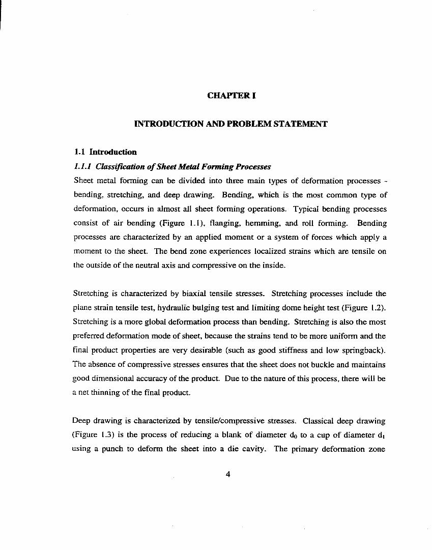
Sheet metal forming can be divided into three main types of deformation processes -

bending, stretching, and deep drawing. Bending, which is the most common type of

deformation, occurs in almost all sheet forming operations. Typical bending processes

consist of air bending (Figure 1.1), flanging, hemming, and roll forming. Bending

processes are characterized by an applied moment or a system of forces which apply a

moment to the sheet. The bend zone experiences localized strains which are tensile on

the outside of the neutral axis and compressive on the inside.

Stretching is characterized by biaxial tensile stresses. Stretching processes include the

plane strain tensile test, hydraulic bulging test and limiting dome height test (Figure 1.2).

Stretching is a more global deformation process than bending. Stretching is also the most

preferred deformation mode of sheet, because the strains tend to be more uniform and the

final product properties are very desirable (such as good stiffness and low springback).

The absence of compressive stresses ensures that the sheet does not buckle and maintains

good dimensional accuracy of the product. Due to the nature of this process, there will be

a net thinning of the final product.

Deep drawing is characterized by tensile/compressive stresses. Classical deep drawing

(Figure 1.3) is the process of reducing a blank of diameter do to a cup of diameter d,

using a punch to deform the sheet into a die cavity. The primary deformation zone

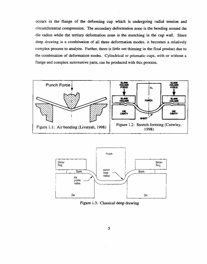
occurs in the flange of the deforming cup which is undergoing radial tension and

circumferential compression. The secondary deformation zone is the bending around the

die radius while the tertiary deformation zone is the stretching in the cup wall. Since

deep drawing is a combination of all three deformation modes, it becomes a relatively

complex process to analyze. Further, there is little net thinning in the final product due to

the combination of deformation modes. Cylindrical or prismatic cups, with or without a

flange and complex automotive parts, can be produced with this process.

BLANK BLWKPunch ForceFORCE Cl.

PUNCH

OECAMTY

DCCAVITY

Figure 1.2: Stretch forming (Crowley, 1998)Figure 1.1: Air bending (Livatyali, 1998)

Punch

j Bmder BinderRing

puncnnoseradius

Blank Blank

profileradius

Figure 1.3: C lassical deep drawing

1.1.2 Sheet Metal Forming as a System

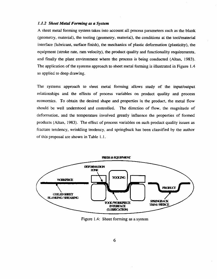
A sheet metal forming system takes into account all process parameters such as the blank

(geometry, material), the tooling (geometry, material), the conditions at the tool/material

interface (lubricant, surface finish), the mechanics of plastic deformation (plasticity), the

equipment (stroke rate, ram velocity), the product quality and functionality requirements,

and finally the plant environment where the process is being conducted (Altan, 1983).

The application of the systems approach to sheet metal forming is illustrated in Figure 1.4

as applied to deep drawing.

The systems approach to sheet metal forming allows study of the input/output

relationships and the effects of process variables on product quality and process

economics. To obtain the desired shape and properties in the product, the metal flow

should be well understood and controlled. The direction of flow, the magnitude of

deformation, and the temperature involved greatly influence the properties of formed

products (Altan, 1983). The effect of process variables on such product quality issues as

fracture tendency, wrinkling tendency, and springback has been classified by the author

of this proposal are shown in Table 1.1.

PRESS&BQPFIVCNr

DETORMVnONZONE

TOOLINGWORKHECE

PROWjCF

CXXLEDSŒET BLAMONG/SHEARING

SPRINGBACK TRIM/PIERCElOOLAMORKHECE

INTERFACE(LUBRICATION)

Figure 1.4: Sheet form ing as a system

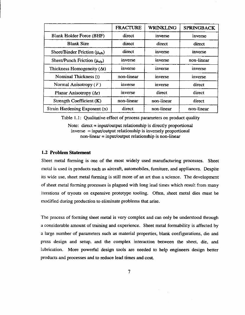
FRACTURE WRINKLING SPRINGBACKBlank Holder Force (BHF) direct inverse inverse

Blank Size direct direct direct

Sheet/Binder Friction (Ps^) direct inverse inverse

Sheet/Punch Friction (Ps/p) inverse inverse non-linear

Thickness Homogeneity (At) inverse inverse inverse

Nominal Thickness (t) non-linear inverse inverse

Normal Anisotropy ( r ) inverse inverse direct

Planar Anisotropy (Ar) inverse direct direct

Strength Coefficient (K) non-linear non-linear direct

Strain Hardening Exponent (n) direct non-linear non-linear

Table LI: Qualitative effect of process parameters on product quality

Note: direct = input/output relationship is directly proportional inverse = input/output relationship is inversely proportional

non-linear = input/output relationship is non-linear

1.2 Problem StatementSheet metal forming is one of the most widely used manufacturing processes. Sheet

metal is used in products such as aircraft, automobiles, furniture, and appliances. Despite

its wide use, sheet metal forming is still more of an art than a science. The development

of sheet metal forming processes is plagued with long lead times which result from many

iterations of tryouts on expensive prototype tooling. Often, sheet metal dies must be

modified during production to eliminate problems that arise.

The process of forming sheet metal is very complex and can only be understood through

a considerable amount of training and experience. Sheet metal formability is affected by

a large number of parameters such as material properties, blank configurations, die and

press design and setup, and the complex interaction between the sheet, die, and

lubrication. More powerful design tools are needed to help engineers design better

products and processes and to reduce lead times and cost.

Therefore the goal o f the proposed work is:

• To develop a part and process methodology for the deep drawing and stamping of

sheet metal parts.

• To generate computerized educational tools to instruct engineers on the use o f this

proposed design methodology.

1.3 Dissertation OrganizationFinally, the outline of this dissertation by chapters is:

1. Introduction and Problem Statement

2. Fundamentals of Deep Drawing and Stamping

3. Research Plan

4. Analytical and Numerical Modeling of Deep Drawing and Stamping

5. Experimental Investigation of Deep Drawing and Stamping

6 . Part and Process Design Methodology for Deep Drawing and Stamping

7. Conclusions and Future Work

8 . References

9. Appendices

CHAPTER n

FUNDAMENTALS OF DEEP DRAWING AND STAMPING

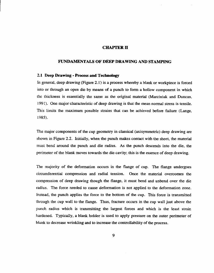
2.1 Deep Drawing - Process and TechnologyIn general, deep drawing (Figure 2.1) is a process whereby a blank or workpiece is forced

into or through an open die by means of a punch to form a hollow component in which

the thickness is essentially the same as the original material (Marciniak and Duncan,

1991). One major characteristic o f deep drawing is that the mean normal stress is tensile.

This limits the maximum possible strains that can be achieved before failure (Lange,

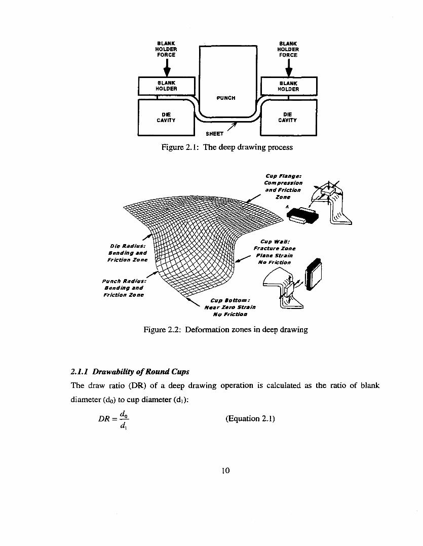
1985).

The major components of the cup geometry in classical (axisymmetric) deep drawing are

shown in Figure 2.2. Initially, when the punch makes contact with the sheet, the material

must bend around the punch and die radius. As the punch descends into the die, the

perimeter of the blank moves towards the die cavity; this is the essence of deep drawing.

The majority of the deformation occurs in the flange of cup. The flange undergoes

circumferential compression and radial tension. Once the material overcomes the

compression of deep drawing though the flange, it must bend and unbend over the die

radius. The force needed to cause deformation is not applied to the deformation zone.

Instead, the punch applies the force to the bottom of the cup. This force is transmitted

through the cup wall to the flange. Thus, fracture occurs in the cup wall just above the

punch radius which is transmitting the largest forces and which is the least strain

hardened. Typically, a blank holder is used to apply pressure on the outer perimeter of

blank to decrease wrinkling and to increase the controllability of the process.

BLANKHOLDERFO RC E

BLANKHOLDERFORCE

SH EET

BLANKHOLDER

BLANKHOLDER

DIECAVITY

DIECAVITY

PUNCH

Die Radius: Bending and Friction Zone

Punch Radius: Bending and Friction Zone

Figure 2 .1 : The deep drawing process

Cup Wall: Fracture Zone Plane Strain No Friction

Cup B ottom : N ear Zero Strain

No Friction

Cup Flange: Com pression and Friction

Zone

Figure 2.2: Deformation zones in deep drawing

2.1.1 Drawability o f Round Cups

The draw ratio (DR) of a deep drawing operation is calculated as the ratio of blank

diameter (do) to cup diameter (di):

D R = ^ (Equation 2.1)

10

The limiting draw ratio (LDR) is the maximum draw ratio that can be obtained under

perfect deep drawing conditions. LDR is considered a good measure of drawability o f a

material. To maximize the LDR (Lange, 1985):

• Decrease blank holder/sheet friction

• Increase punch/sheet friction

• Increase punch and die radius (this is limited by wrinkling)

• Increase strain hardening exponent (n-value in the equation â = + ë]" )

• Increase normal anisotropy ( r -value)

• Decrease planar anisotropy (Ar-value)

For cup geometries with draw ratios greater than the LDR o f a material, several drawing

stages must occur. This is referred to as redrawing. Typically, the LDR for second and

third drawing stages decreases significantly. To increase LDR for subsequent draw

stages, annealing of the drawn cup can be employed. LDR's for various draw stages and

different materials has been empirically determined as well as suitable lubricants. This

information is listed in Table 2.1.

2.1.2 Effect o f Strain Hardening

The strain hardening exponent n, in the equation â = K\Eo + £ ]" , plays a very crucial

role in sheet metal forming. Hosford and Caddell (1993) have shown that in a

dimensionally inhomogeneous specimen, the n-value plays a significant role in

maintaining strain uniformity. The relationship of n-value and drawability is ambiguous.

A higher n-value strengthens the cup wall, but it also strengthens the flange so more force

is needed to deform it. Nevertheless, the LDR increases with increasing n-value as

shown by (Zunkler, 1973):

ln(LDR) =1.1

(n +1) (Equation 2.2) (Zunkler, 1973)

11

Further, higher n-values improve deep drawing indirectly by increasing cup wall strength

which allows higher blank holder forces to be used. Therefore, the n-value can be

correlated to decreased wrinkling in deep drawing (Taylor, 1988).

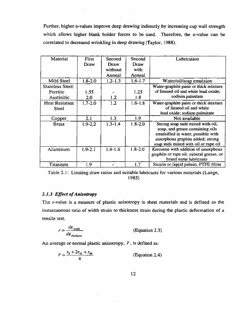
Material FirstDraw

SecondDraw

withoutArmeal

SecondDrawwith

Anneal

Lubrication

Mild Steel 1 .8 -2 . 0 1.2-1.3 1.6-1.7 Water/oil/soap emulsionStainless Steel:

Ferritic Austinitic

1.552 . 0 1 . 2

1.251 . 8

Water-graphite paste or thick mixture of linseed oil and white lead oxide;

sodium palmitateHeat Resistant

Steel1 .7-2.0 1 . 2 1 .6 - 1 . 8 Water-graphite paste or thick mixture

of linseed oil and white lead oxide; sodium palmitate

Copper 2 . 1 1.3 1.9 Not availableBrass 1 .9-2.2 1.3-1.4 1 .8 -2 . 0 Strong soap suds mixed with oil,

soap, and grease containing oils emulsified in water, possible with amorphous graphite added; strong

soap suds mixed with oil or rape oilAluminum 1 .9-2.1 I.4-1.6 1 .8 -2 . 0 Kerosene with addition of amorphous

graphite or rape oil, mineral grease, or brand name lubricants

Titanium 1.9 - 1.7 Stearin or liquid palmin, FIFE films

Table 2.1: Limiting draw ratios and suitable lubricants for various materials (Lange,1985)

2.1.3 Effect o f Anisotropy

The r-value is a measure of plastic anisotropy in sheet materials and is defined as the

instantaneous ratio of width strain to thickness strain during the plastic deformation of a

tensile test.

^ wiiUhcIe thickness

(Equation 2.3)

An average or normal plastic anisotropy, r , is defined as:

— _ ^ 0 2^5 + (Equation 2.4)

12

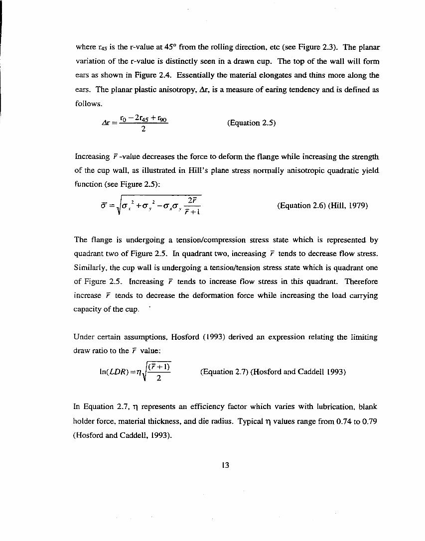
where r4 s is the r-value at 45° from the rolling direction, etc (see Figure 2.3). The planar

variation of the r-value is distinctly seen in a drawn cup. The top of the wall will form

ears as shown in Figure 2.4. Essentially the material elongates and thins more along the

ears. The planar plastic anisotropy, Ar, is a measure o f earing tendency and is defined as

follows.

Ar = —— ^0 (Equation 2.5)

Increasing r -value decreases the force to deform the flange while increasing the strength

of the cup wall, as illustrated in Hill’s plane stress normally anisotropic quadratic yield

function (see Figure 2.5):

(J = - i -c r /-cr.cr, (Equation 2.6) (Hill, 1979)

The flange is undergoing a tension/compression stress state which is represented by

quadrant two of Figure 2.5. In quadrant two, increasing r tends to decrease flow stress.

Similarly, the cup wall is undergoing a tension/tension stress state which is quadrant one

of Figure 2.5. Increasing r tends to increase flow stress in this quadrant. Therefore

increase r tends to decrease the deformation force while increasing the load carrying

capacity of the cup.

Under certain assumptions, Hosford (1993) derived an expression relating the limiting

draw ratio to the r value:

ln(LD/?) (Equation 2.7) (Hosford and Caddell 1993)

In Equation 2.7, T) represents an efficiency factor which varies with lubrication, blank

holder force, material thickness, and die radius. Typical t j values range from 0.74 to 0.79

(Hosford and Caddell, 1993).

13

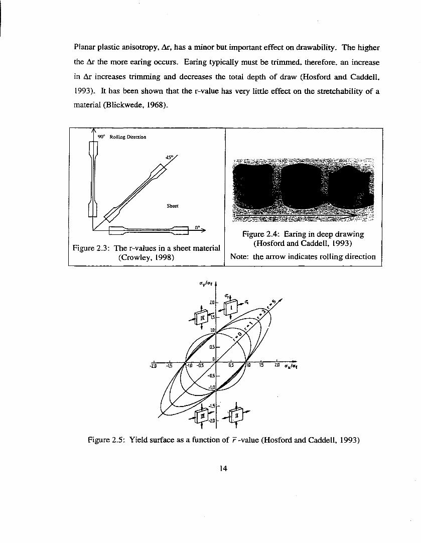
Planar plastic anisotropy, Ar, has a minor but important effect on drawability. The higher

the Ar the more earing occurs. Earing typically must be trimmed, therefore, an increase

in Ar increases trimming and decreases the total depth of draw (Hosford and Caddell,

1993). It has been shown that the r-value has very little effect on the stretchability of a

material (Blickwede, 1968).

90“ Rolling Direction

Sheet

0“.

Figure 2.3: The r-values in a sheet material (Crowley, 1998)

Figure 2.4: Earing in deep drawing (Hosford and Caddell, 1993)

Note: the arrow indicates rolling direction

-Z.0 -15

-as- 1.0

-1.5

Figure 2.5: Yield surface as a function of r-value (Hosford and Caddell, 1993)

14

2.1.4 Product Quality

Due to the circumferential compressive forces, buckling may occur in the sheet during

deep drawing. Buckling in the flange is typically called wrinkling while buckling in the

wall of a conical cup is called puckering- Wrinkling may be decreased or eliminated by

(Lange, 1985):

• Increasing blank holder force

• Increasing material thickness

• Increasing normal anisotropy ( r -value)

• Decreasing planar anisotropy (Ar-value)

When the punch/die clearance is large the drawn cups are referred to as tapered walled

cups. The difficulty in deep drawing tapered cups is that the wall is unsupported and

undergoing circumferential compression. Even though the wall in a straight walled cup is

also unsupported, at least wall wrinkling can be controlled by the tight punch/die

clearance. Puckering may also be reduced by the above means for reducing wrinkling in

straight walled cups or by the following additional means (Lange, 1985):

• Increasing the blank diameter

• Increasing blank holder/sheet friction

• Increasing drawbead restraint

In tapered cups, the only method to control puckering is to increase the radial tension in

the wall. This may be achieved by increasing blank diameter, increasing blank holder

force, increasing blank holder/sheet friction, and using drawbeads. There is a limit to the

amount of taper that can be deep drawn. Once, this limit is exceeded, puckering will

occur no matter how much blank holder force is applied.

2.1.5 Deep Drawing o f Complex Geometries

A typical geometry is the rectangular pan as shown in Figure 2.6. In the drawing of

rectangular shapes, the stresses are high in the comers due to the high deformation forces

15

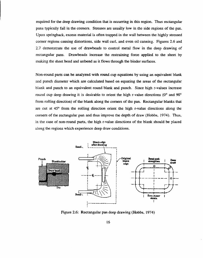
required for the deep drawing condition that is occurring in this region. Thus rectangular

pans typically fail in the comers. Stresses are usually low in the side regions of the pan.

Upon springback, excess material is often trapped in the wall between the highly stressed

comer regions causing distortions, side wall curl, and even oil canning. Figures 2.6 and

2.7 demonstrate the use o f drawbeads to control metal flow in the deep drawing of

rectangular pans. Drawbeads increase the restraining force applied to the sheet by

making the sheet bend and unbend as it flows through the binder surfaces.

Non-round parts can be analyzed with round cup equations by using an equivalent blank

and punch diameter which are calculated based on equating the areas of the rectangular

blank and punch to an equivalent round blank and punch. Since high r-values increase

round cup deep drawing it is desirable to orient the high r-value directions (0° and 90°

from rolling direction) of the blank along the comers of the pan. Rectangular blanks that

are cut at 45° from the rolling direction orient the high r-value directions along the

comers of the rectangular pan and thus improve the depth of draw (Hobbs, 1974). Thus,

in the case of non-round parts, the high r-value directions of the blank should be placed

along the regions which experience deep draw conditions.

Punch Blankholdar

B lanked^I after drawing

Bead

B endrsnd>straighUn

/-u n g in a / blank

edgeDeepdraw

Bead I Zero minor | atraia

Figure 2.6: Rectangular pan deep drawing (Hobbs, 1974)

16

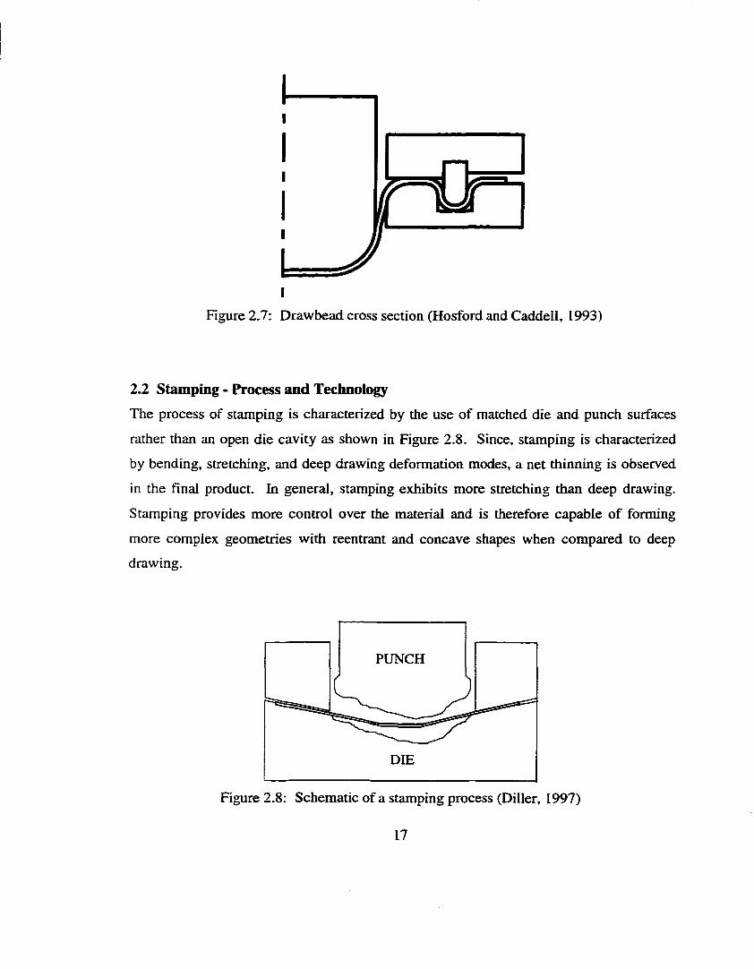
I

Figure 2.7: Drawbead cross section (Hosford and Caddell, 1993)

2.2 Stamping - Process and TechnologyThe process of stamping is characterized by the use of matched die and punch surfaces

rather than an open die cavity as shown in Figure 2.8. Since, stamping is characterized

by bending, stretching, and deep drawing deformation modes, a net thinning is observed

in the final product. In general, stamping exhibits more stretching than deep drawing.

Stamping provides more control over the material and is therefore capable of forming

more complex geometries with reentrant and concave shapes when compared to deep

drawing.

PUNCH

DIE

Figure 2.8: Schematic of a stamping process (Diller, 1997)

17

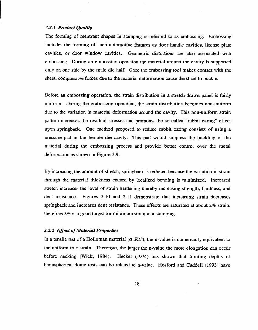
2.2.1 Product Quality

The forming of reentrant shapes in stamping is referred to as embossing. Embossing

includes the forming o f such automotive features as door handle cavities, license plate

cavities, or door window cavities. Geometric distortions are also associated with

embossing. During an embossing operation the material around the cavity is supported

only on one side by the male die half. Once the embossing tool makes contact with the

sheet, compressive forces due to the material deformation cause the sheet to buckle.

Before an embossing operation, the strain distribution in a stretch-drawn panel is fairly

uniform. During the embossing operation, the strain distribution becomes non-uniform

due to the variation in material deformation around the cavity. This non-uniform strain

pattern increases the residual stresses and promotes the so called “rabbit earing” effect

upon springback. One method proposed to reduce rabbit earing consists of using a

pressure pad in the female die cavity. This pad would suppress the buckling of the

material during the embossing process and provide better control over the metal

deformation as shown in Figure 2.9.

By increasing the amount of stretch, springback is reduced because the variation in strain

through the material thickness caused by localized bending is minimized. Increased

stretch increases the level of strain hardening thereby increasing strength, hardness, and

dent resistance. Figures 2.10 and 2.11 demonstrate that increasing strain decreases

springback and increases dent resistance. These effects are saturated at about 2% strain,

therefore 2 % is a good target for minimum strain in a stamping.

2.2.2 Ejfect o f Material Properties

In a tensile test of a Holloman material (c t= K e '^ ), the n-value is numerically equivalent to

the uniform true strain. Therefore, the larger the n-value the more elongation can occur

before necking (Wick, 1984). Hecker (1974) has shown that limiting depths of

hemispherical dome tests can be related to n-value. Hosford and Caddell (1993) have

18

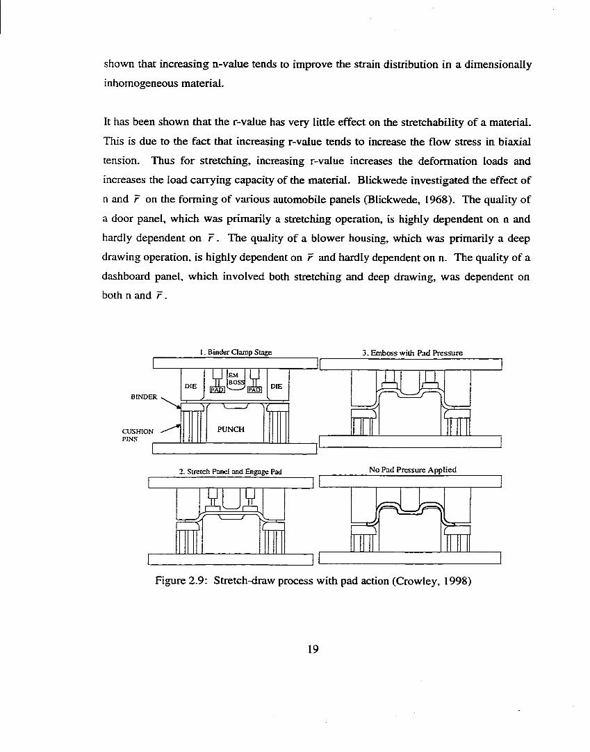
shown that increasing n-value tends to improve the strain distribution in a dim ensionally

inhomogeneous material.

It has been shown that the r-value has very little effect on the stretchability of a material.

This is due to the fact that increasing r-value tends to increase the flow stress in biaxial

tension. Thus for stretching, increasing r-value increases the deformation loads and

increases the load carrying capacity of the material. Blickwede investigated the effect of

n and r on the forming o f various automobile panels (Blickwede, 1968). The quality of

a door panel, which was primarily a stretching operation, is highly dependent on n and

hardly dependent on r . The quality of a blower housing, which was primarily a deep

drawing operation, is highly dependent on r and hardly dependent on n. The quality of a

dashboard panel, which involved both stretching and deep drawing, was dependent on

both n and r .

1. Binder Clamp Stage 3. Emboss with Pad Pressure

EMBOSSDIE DIEIPADT

BINDER

PUNCHCUSHIONPINS

2. Stretch Panel and Engage Pad

MUX\ /

No Pad Pressure Applied

Figure 2.9: Stretch-draw process with pad action (Crowley, 1998)

19

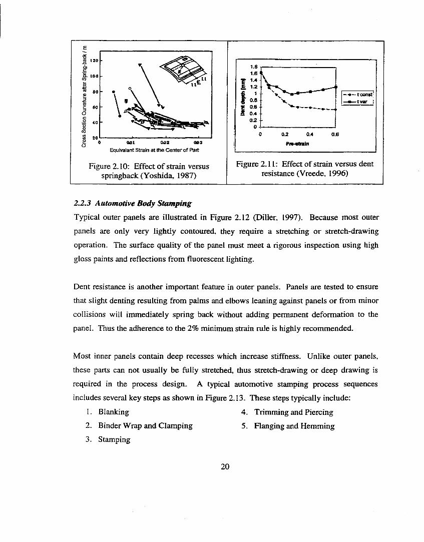
m 120

Q. 100

«as

üc

80

80

^ 40

% 2 00 001 002 003

Equivalant Strain at the Center of Part

Figure 2.10: Effect of strain versus springback (Yoshida, 1987)

1.8 1.6 I

I :— tcorwt;

# tvar !f 0.8 -g 0.6 - 8 0.4

0.2 -

0.4 0.6

Figure 2.11: Effect of strain versus dent resistance (Vreede, 1996)

2.2.3 Automotive Body Stamping

Typical outer panels are illustrated in Figure 2.12 (Diller, 1997). Because most outer

panels are only very lightly contoured, they require a stretching or stretch-drawing

operation. The surface quality of the panel must meet a rigorous inspection using high

gloss paints and reflections from fluorescent lighting.

Dent resistance is another important feature in outer panels. Panels are tested to ensure

that slight denting resulting from palms and elbows leaning against panels or from minor

collisions will immediately spring back without adding permanent deformation to the

panel. Thus the adherence to the 2% minimum strain rule is highly recommended.

Most inner panels contain deep recesses which increase stifftiess. Unlike outer panels,

these parts can not usually be fully stretched, thus stretch-drawing or deep drawing is

required in the process design. A typical automotive stamping process sequences

includes several key steps as shown in Figure 2.13. These steps typically include:

1. Blanking 4. Trinuning and Piercing

2. Binder Wrap and Clamping 5. Flanging and Hemming

3. Stamping

2 0

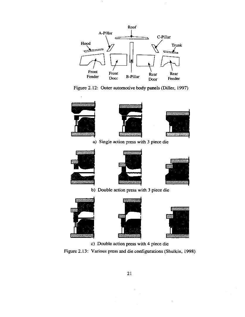
RoofA-Pillar

C-PülarHood Trunk

FrontFender

FrontDoor

RearFender

RearDoorB-Pillar

Figure 2.12: Outer automotive body panels (Diller, 1997)

a) Single action press with 3 piece die

b) Double action press with 3 piece die

c) Double action press with 4 piece die Figure 2.13: Various press and die configurations (Shulkin, 1998)

2 1

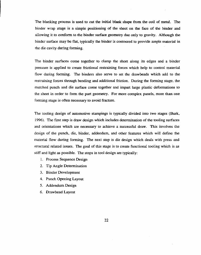
The blanking process is used to cut the initial blank shape from the coil of metal. The

binder wrap stage is a simple positioning of the sheet on the face o f the binder and

allowing it to conform to the binder surface geometry due only to gravity. Although the

binder surface may be flat, typically the binder is contoured to provide ample material in

the die cavity during forming.

The binder surfaces come together to clamp the sheet along its edges and a binder

pressure is applied to create frictional restraining forces which help to control material

flow during forming. The binders also serve to set the drawbeads which add to the

restraining forces through bending and additional friction. During the forming stage, the

matched punch and die surface come together and impart large plastic deformations to

the sheet in order to form the part geometry. For more complex panels, more than one

forming stage is often necessary to avoid fracmre.

The tooling design of automotive stampings is typically divided into two stages (Burk,

1996). The first step is draw design which includes determination of the tooling surfaces

and orientations which are necessary to achieve a successful draw. This involves the

design of the punch, die, binder, addendum, and other feamres which will define the

material flow during forming. The next step is die design which deals with press and

structural related issues. The goal of this stage is to create functional tooling which is as

stiff and light as possible. The steps in tool design are typically:

1. Process Sequence Design

2. Tip Angle Determination

3. B inder Development

4. Punch Opening Layout

5. Addendum Design

6 . Drawbead Layout

2 2

One consideration of binder design is whether the press is a single or double action and

whether à three or four piece die is required as shown in Figure 2.13. The curvature of

the binder affects the amount of material available within the die cavity during forming,

therefore, binder design is very important in inducing the appropriate amount of stretch in

the panel. The binder surface must be a developable surface which means that the sheet

should be able to conform to the binder without wrinkling or stretching.

The region between the part geometry and binder surface is called the addendum. The

addendum is often used to alter the material flow, to increase stretching in the part, and to

simplify subsequent operations as flanging (Burk, 1996). Drawbeads are often added to

the binder surface to further restrain material flow and cause further stretching in the

panel without increasing the amount of clamping force necessary to hold the blank.

Various mathematical models and design guidelines are available for designing

drawbeads which provide an appropriate amount of restraining force (Tufekci. 1994).

2.3 Blank Holder ForceThe blank holder's main function is to apply a blank holder pressure (BHP) onto the

flange to suppress wrinkling that may be caused the compressive stresses that occur there.

If a blank holder is not used or insufficient blank holder force (BHP) is applied, then the

cup may wrinkle as shown in Figures 2 .14a and b.

The secondary function of the blank holder is to control and restrain the material flow

into the die by increasing the friction forces in the flange and radial tension in the part.

The increased radial tension must be supported by the part wall, thus if too much BHF is

applied then fracture may result before the desired draw depth is attained as shown in

Figure 2.15a.

With a correctly applied BHF, a good part can be obtained as shown in Figure 2.15b.

Draw depth is therefore limited by the onset of wrinkling and fracture which can be

23

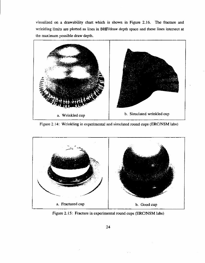
visualized on a drawability chart which is shown in Figure 2.16. The fracture and

wrinkling limits are plotted as lines in BHF/draw depth space and these lines intersect at

the maximum possible draw depth.

a. Wrinkled cup b. Simulated wrinkled cup

Figure 2.14: Wrinkling in experimental and simulated round cups (ERC/NSM labs)

a. Fractured cup b. Good cup

Figure 2.15: Fracture in experimental round cups (ERC/NSM labs)

24

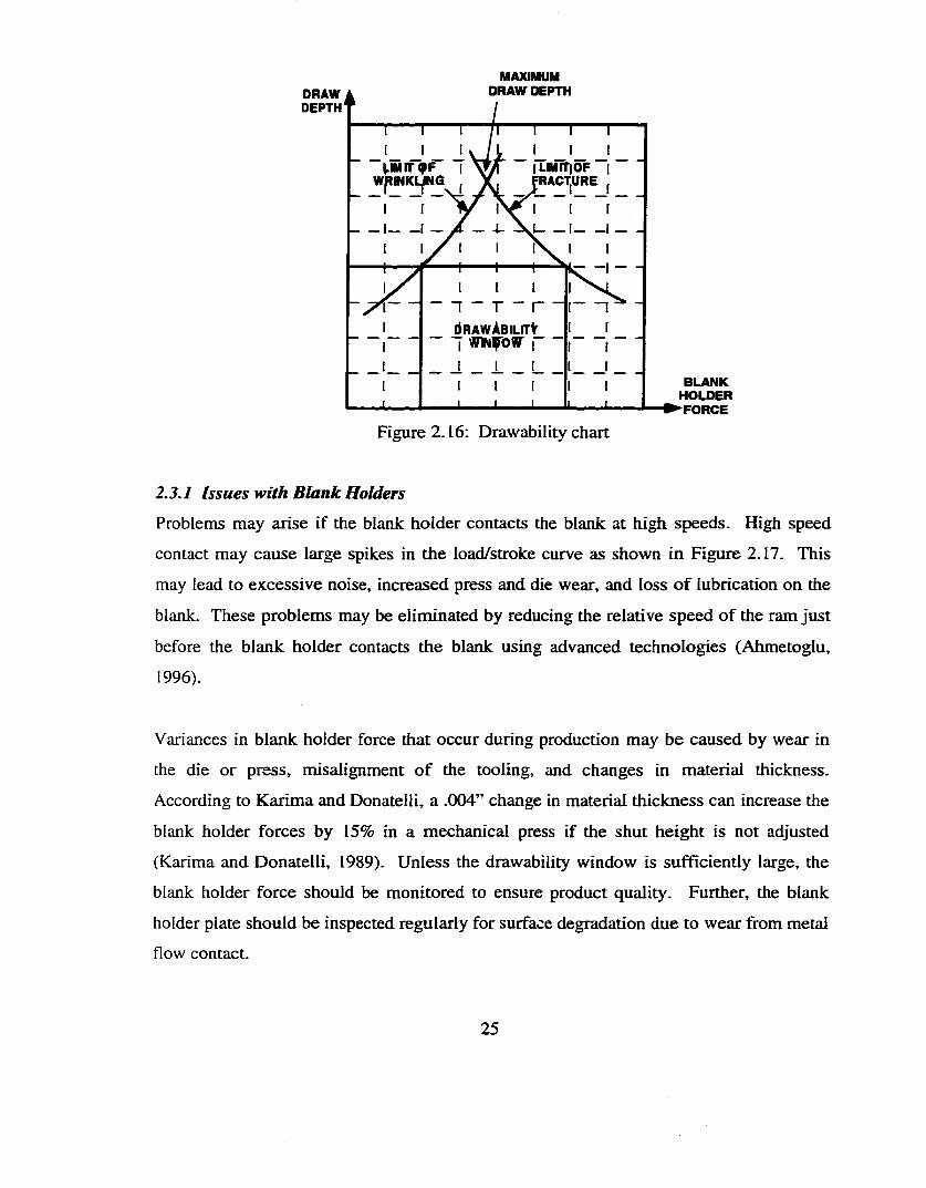
DRAW ▲ D E P T H ^

MAXIMUM DRAW DEPTH

|.iMir9 F [ [LMrriOFRACTUREwpwKywG

1

~ T ~ r

dR A W À B ILnt 7 WHfoir i~I I II I I

Figure 2.16: Drawability chart

BLANKHOLDER

►FORCE

2.3.1 Issues with Blank Holders

Problems may arise if the blank holder contacts the blank at high speeds. High speed

contact may cause large spikes in the load/stroke curve as shown in Figure 2.17. This

may lead to excessive noise, increased press and die wear, and loss o f lubrication on the

blank. These problems may be eliminated by reducing the relative speed of the ram just

before the blank holder contacts the blank using advanced technologies (Ahmetoglu,

1996).

Variances in blank holder force that occur during production may be caused by wear in

the die or press, misalignment o f the tooling, and changes in material thickness.

According to Karima and Donatelli, a .004” change in material thickness can increase the

blank holder forces by 15% in a mechanical press if the shut height is not adjusted

(Karima and Donatelli, 1989). Unless the drawability window is sufficiendy large, the

blank holder force should be monitored to ensure product quality. Further, the blank

holder plate should be inspected regularly for surface degradation due to wear from metal

flow contact.

25

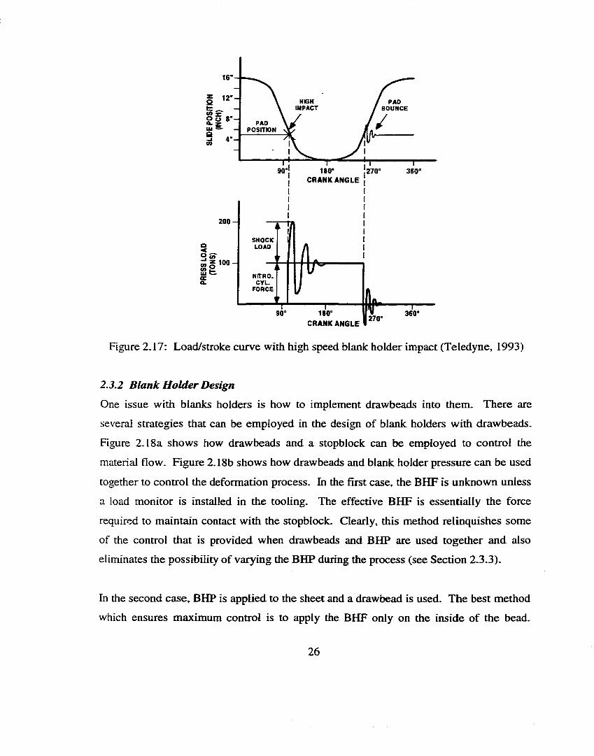
16"

HIGHIMPACT

PADBOUNCE

PADPOSITION

90° 180° CRANK ANGLE

360°270'

200 -

SHOCKLOADQ

NITRO.C Y U

FO RCE

90° 180°

CRANK ANGLE360°

Figure 2.17: Load/stroke curve with high speed blank holder impact (Teledyne, 1993)

2.3.2 Blank Holder Design

One issue with blanks holders is how to implement drawbeads into them. There are

several strategies that can be employed in the design of blank holders with drawbeads.

Figure 2.18a shows how drawbeads and a stopbiock can be employed to control the

material flow. Figure 2.18b shows how drawbeads and blank holder pressure can be used

together to control the deformation process. In the first case, the BHF is unknown unless

a load monitor is installed in the tooling. The effective BHF is essentially the force

required to maintain contact with the stopbiock. Clearly, this method relinquishes some

of the control that is provided when drawbeads and BHP are used together and also

eliminates the possibility of varying the BHP during the process (see Section 2.3.3).

In the second case, BHP is applied to the sheet and a drawbead is used. The best method

which ensures maximum control is to apply the BHF only on the inside of the bead.

2 6

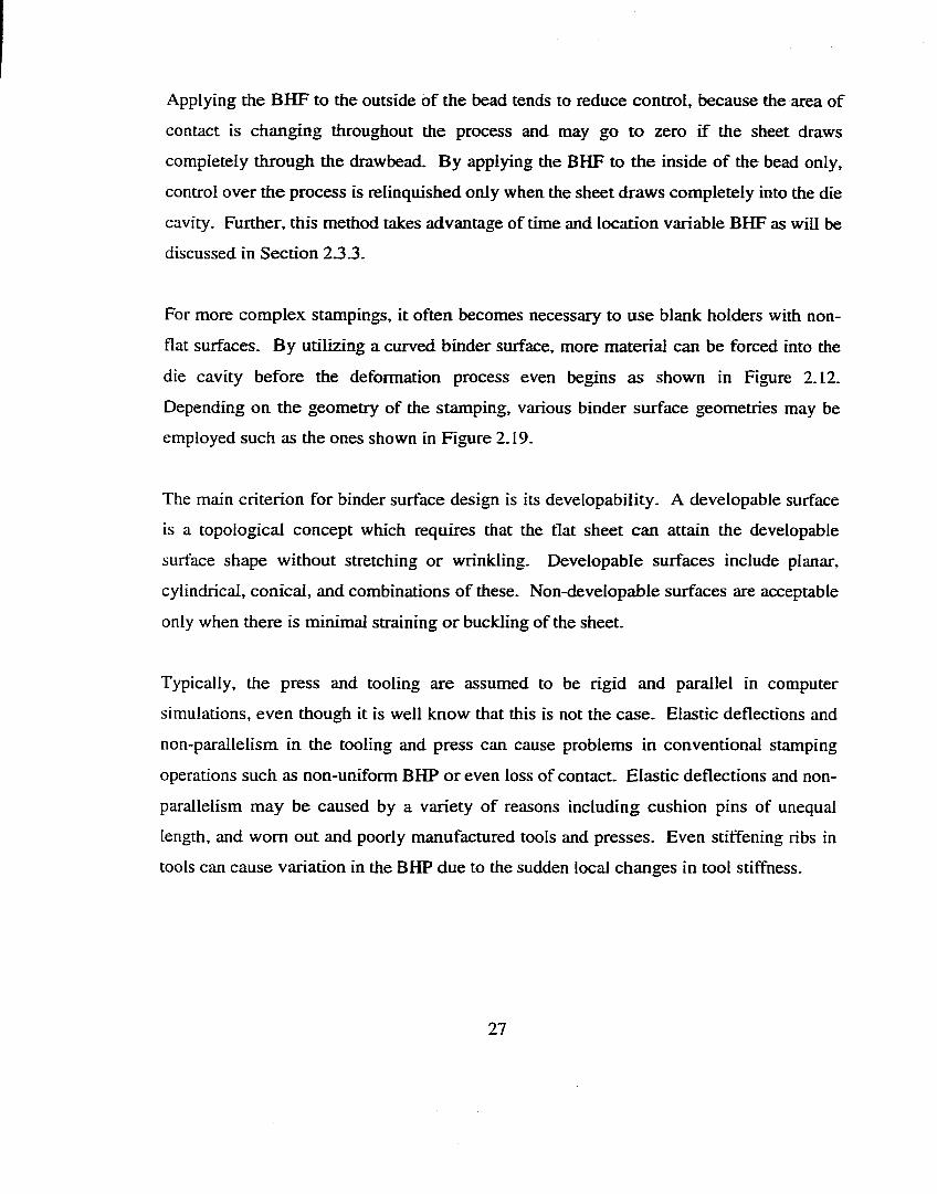
Applying the BHF to the outside of the bead tends to reduce control, because the area of

contact is changing throughout the process and may go to zero if the sheet draws

completely through the drawbead. By applying the BHF to the inside of the bead only,

control over the process is relinquished only when the sheet draws completely into the die

cavity. Further, this method takes advantage of time and location variable BHF as will be

discussed in Section 2.3.3.

For more complex stampings, it often becomes necessary to use blank holders with non­

flat surfaces. By utilizing a curved binder surface, more material can be forced into the

die cavity before the deformation process even begins as shown in Figure 2.12.

Depending on the geometry of the stamping, various binder surface geometries may be

employed such as the ones shown in Figure 2.19.

The main criterion for binder surface design is its developabiiity. A developable surface

is a topological concept which requires that the flat sheet can attain the developable

surface shape without stretching or wrinkling. Developable surfaces include planar,

cylindrical, conical, and combinations of these. Non-developable surfaces are acceptable

only when there is minimal straining or buckling of the sheet.

Typically, the press and tooling are assumed to be rigid and parallel in computer

simulations, even though it is well know that this is not the case. Elastic deflections and

non-parallelism in the tooling and press can cause problems in conventional stamping

operations such as non-uniform BHP or even loss of contact. Elastic deflections and non­

parallelism may be caused by a variety of reasons including cushion pins of unequal

length, and worn out and poorly manufactured tools and presses. Even stiffening ribs in

tools can cause variation in the BHP due to the sudden local changes in tool stiffness.

27

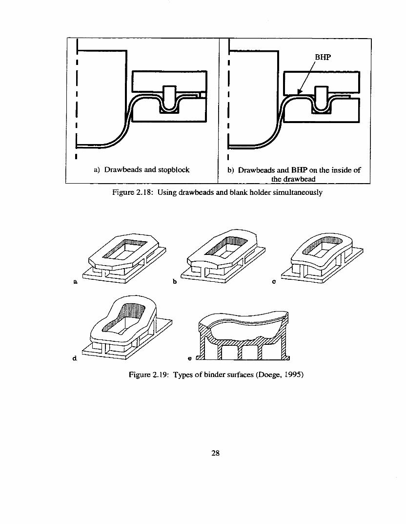
BHP

a) Drawbeads and stopbiock b) Drawbeads and BHP on the inside of the drawbead

Figure 2.18: Using drawbeads and blank holder simultaneously

a b c

e

Figure 2.19: Types o f binder surfaces (Doege, 1995)

28

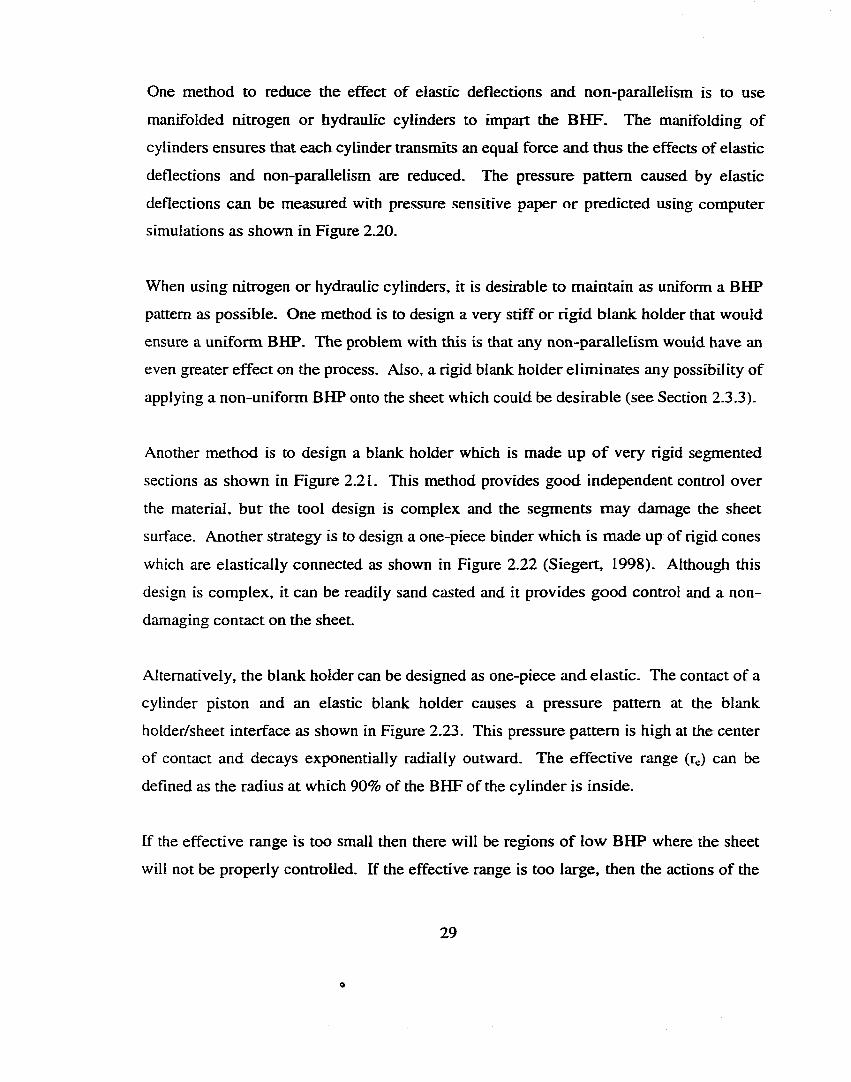
One method to reduce the effect of elastic deflections and non-parallelism is to use

manifolded nitrogen or hydraulic cylinders to impart the BHF. The manifolding of

cylinders ensures that each cylinder transmits an equal force and thus the effects of elastic

deflections and non-parallehsm are reduced. The pressure pattern caused by elastic

deflections can be measured with pressure sensitive paper or predicted using computer

simulations as shown in Figure 2.20.

When using nitrogen or hydraulic cylinders, it is desirable to maintain as uniform a BHP

pattern as possible. One method is to design a very stiff or rigid blank holder that would

ensure a uniform BHP. The problem with this is that any non-parallelism would have an

even greater effect on the process. Also, a rigid blank holder eliminates any possibility of

applying a non-uniform BHP onto the sheet which could be desirable (see Section 2.3.3).

Another method is to design a blank holder which is made up o f very rigid segmented

sections as shown in Figure 2.21. This method provides good independent control over

the material, but the tool design is complex and the segments may damage the sheet

surface. Another strategy is to design a one-piece binder which is made up of rigid cones

which are elastically connected as shown in Figure 2.22 (Siegert, 1998). Although this

design is complex, it can be readily sand casted and it provides good control and a non­

damaging contact on the sheet.

Alternatively, the blank holder can be designed as one-piece and elastic. The contact of a

cylinder piston and an elastic blank holder causes a pressure pattern at the blank

holder/sheet interface as shown in Figure 2.23. This pressure pattern is high at the center

of contact and decays exponentially radially outward. The effective range ( r j can be

defined as the radius at which 90% of the BHF of the cylinder is inside.

If the effective range is too small then there will be regions o f low BHP where the sheet

will not be properly controlled. If the effective range is too large, then the actions of the

29

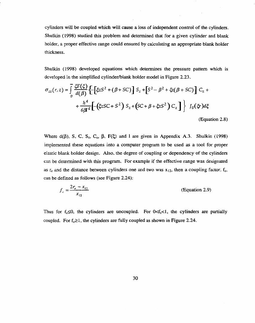
cylinders will be coupled which will cause a loss of independent control of the cylinders.

Shulkin (1998) studied this problem and determined that for a given cylinder and blank

holder, a proper effective range could ensured by calculating an appropriate blank holder

thickness.

Shulkin (1998) developed equations which determines the pressure pattern which is

developed in the simplified cylinder/blank holder model in Figure 2.23.

h4

4[ - ( 4 r S C + S ^ ) S , + ( S C + )3 + | z S ^ ) a ] j

6pi'

(Equation 2.8)

Where d(|3), S, C, 8%, €%, P, F (^ and 1 are given in Appendix A 3. Shulkin (1998)

implemented these equations into a computer program to be used as a tool for proper

elastic blank holder design. Also, the degree of coupling or dependency of the cylinders

can be determined with this program. For example if the effective range was designated

as re and the distance between cylinders one and two was Xi?, then a coupling factor, fc,

can be defined as follows (see Figure 2.24):

jr _ (Equation 2.9)

Thus for fe<0, the cylinders are uncoupled. For 0<fc<l, the cylinders are partially

coupled. For fc>l, the cylinders are fully coupled as shown in Figure 2.24.

30

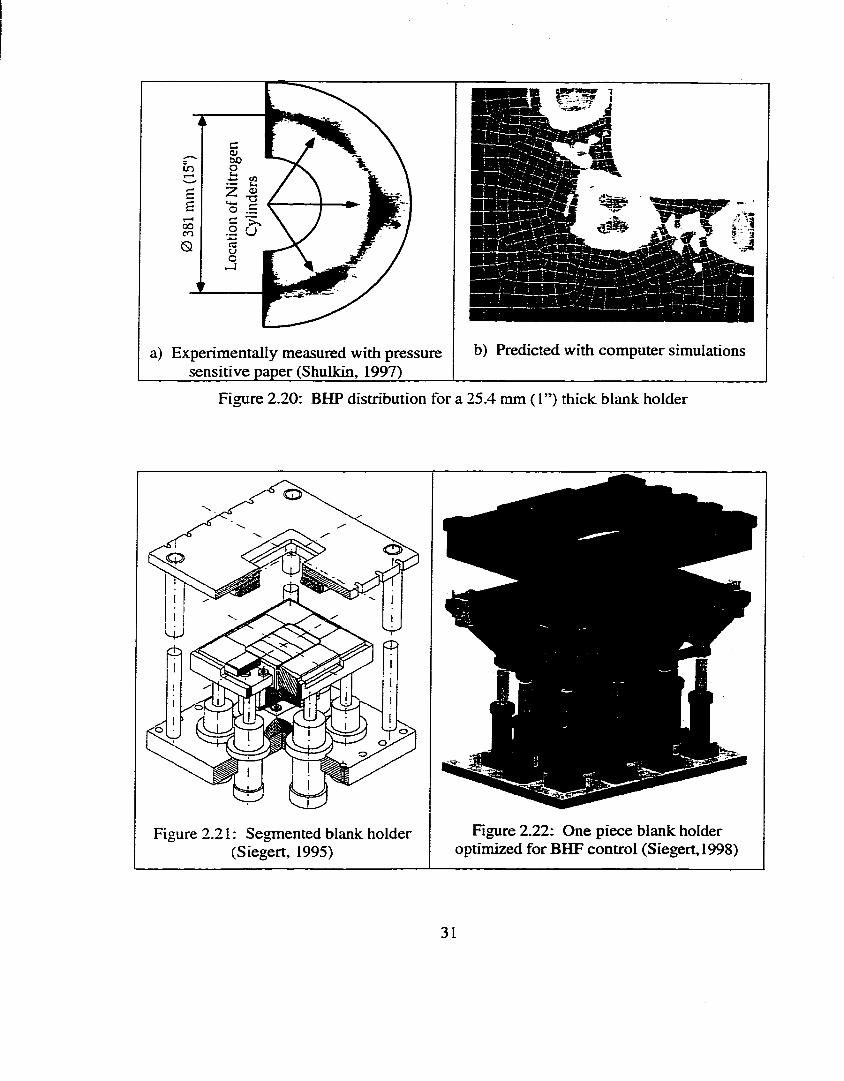
a) Experimentally measured with pressure sensitive paper (Shulkin, 1997)

b) Predicted with computer simulations

Figure 2.20: BHP distribution for a 25.4 ram ( I”) thick blank holder

O

Figure 2.21 : Segmented blank holder (Siegert, 1995)

Figure 2.22: One piece blank holder optimized for BHF control (Siegert, 1998)

31

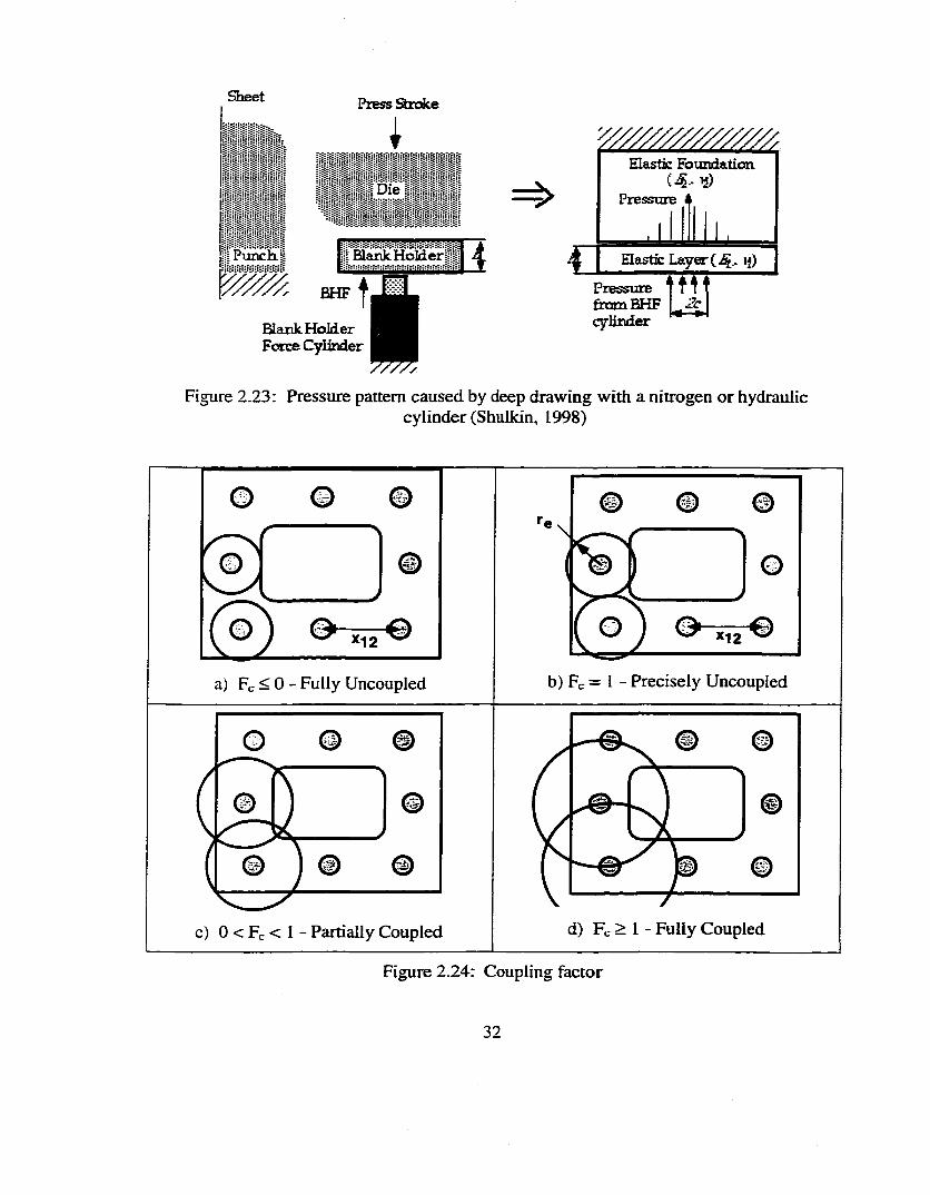
Sheet Press Stroke

IDie

iP u n c h

Blank Holder Force Cylinder

Blank H oM eri

Elastic Foundation ( 4 - Tf)

Pressure 4

Elastic Layer(j§.. ij)Pressure foam BHF cylinder

t f l f2c

Figure 2.23: Pressure pattern caused by deep drawing with a nitrogen or hydrauliccylinder (Shulkin, 1998)

a) Fc < 0 ' Fully Uncoupled b) Fc = 1 - Precisely Uncoupled

c) 0 < Fc < 1 - Partially Coupled d) Fc > 1 - Fully Coupled

Figure 2.24: Coupling factor

32

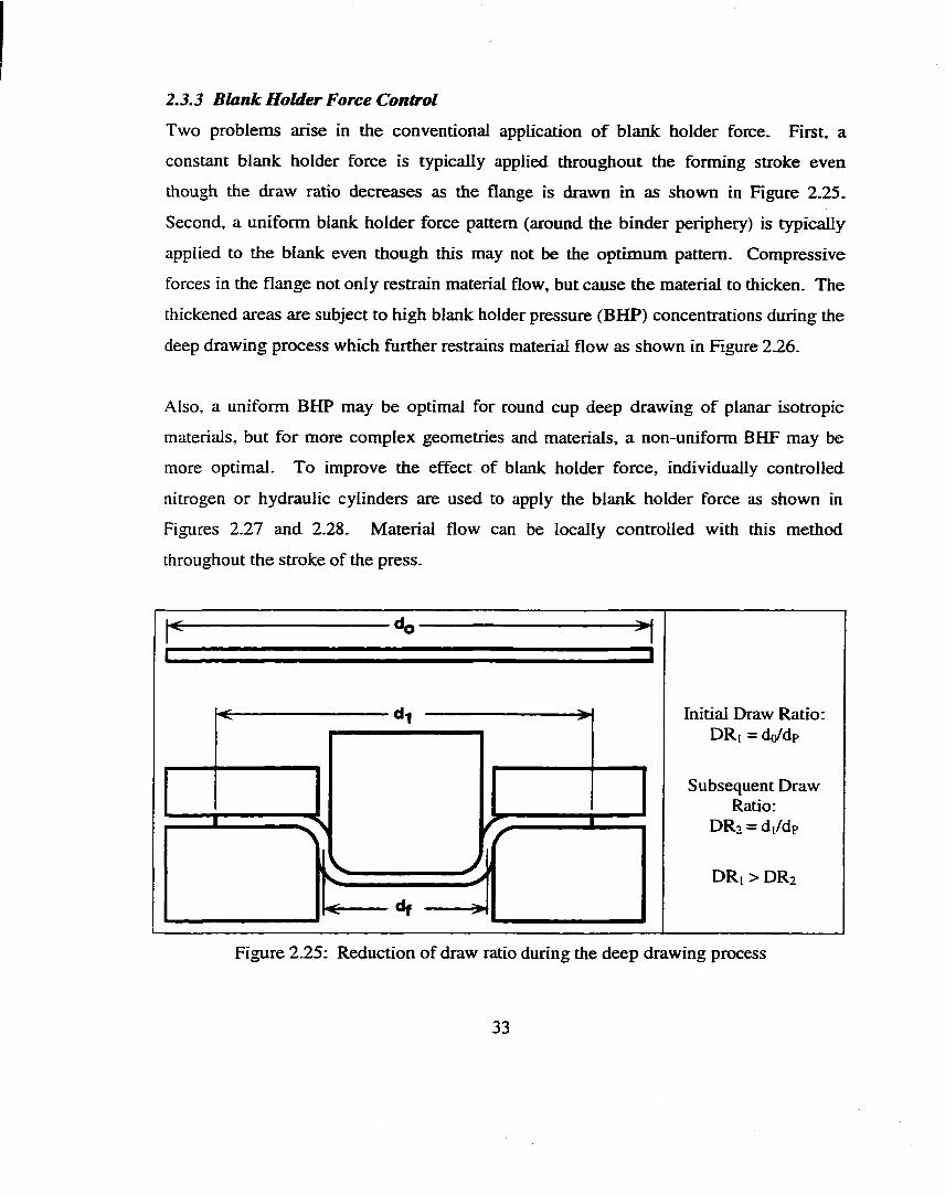
2.3.3 Blank H older Force Control

Two problems arise in the conventional application o f blank holder force. First, a

constant blank holder force is typically applied throughout the forming stroke even

though the draw ratio decreases as the flange is drawn in as shown in Figure 2.25.

Second, a uniform blank holder force pattern (around the binder periphery) is typically

applied to the blank even though this may not be the optimum pattern. Compressive

forces in the flange not only restrain material flow, but cause the material to thicken. The

thickened areas are subject to high blank holder pressure (BHP) concentrations during the

deep drawing process which further restrains material flow as shown in Figure 2.26.

Also, a uniform BHP may be optimal for round cup deep drawing of planar isotropic

materials, but for more complex geometries and materials, a non-uniform BHF may be

more optimal. To improve the effect of blank holder force, individually controlled

nitrogen or hydraulic cylinders are used to apply the blank holder force as shown in

Figures 2.27 and 2.28. Material flow can be locally controlled with this method

throughout the stroke of the press.

« 1

'A

Initial Draw Ratio: DR[ = d(/dp

Subsequent Draw Ratio:

DR% = di/dp

DRi > DR?

Figure 2.25: Reduction o f draw ratio during the deep drawing process

33

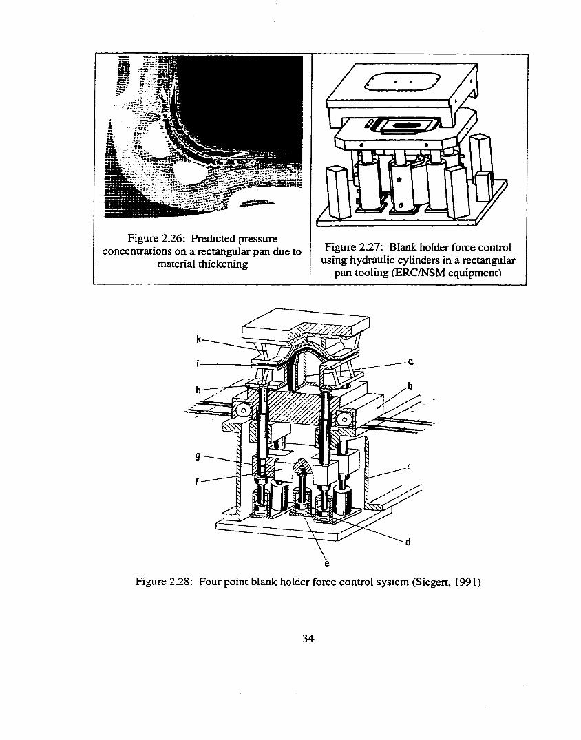
Figure 2.26: Predicted pressure concentrations on a rectangular pan due to

material thickeningFigure 2.27: Blank holder force control

using hydraulic cylinders in a rectangular pan tooling (ERC/NSM equipment)

Figure 2.28: Four point blank holder force control system (Siegert, 1991)

34

Time variable BHF does occur in industrial stamping processes, but typically not in an

optimal fashion. In double action mechanical presses, BHF is applied with a position

setting of the outer ram. Typically the BHF is not even known unless a loadcell is

installed. The BHF tends to vary with the action of the mechanical linkage. In air or

nitrogen cushions, the BHF typically increases slightly with ram stroke due to the

compression of the gas. In a hydraulic cushion, the BHF is typically constant throughout

the ram stroke. Each of these BHF profiles are not optimal because they do not vary in

time in the optimal manner.

Location variable BHF is applied in industry by experienced tryout personnel who grind

the die surface or shim the tooling sections or cushion pins. Using a system, such as the

one built by the Engineering Research Center for Net Shape Manufacturing (ERC/NSM)

and shown in Figure 2.27, can clearly improve the application of BHF when compared to

grinding and shimming.

There have been many proposals and investigations on how to vary the BHF as a function

of press stroke and position around the binder. A reasonable time varying BHF control

strategy which has been shown to improve on constant BHF is to vary the BHF from the

fracture limit to wrinkling limit of the BHF as shown in Figure 2.29b (Kurii, 1995).

Another empirical method for location variable BHF which improves on the uniform

BHF is to distribute the BHF in proportion to the length to width ratio of the die cavity as

shown in Figure 2.30b (Doege, 1995).

Another strategy for time varying BHF control is to pulsate the blank holder force. Two

pulsating BHF strategies are shown in Figure 2.31. This first pulsating strategy is to vary

the BHF sinusoidally within the fracture and wrinkling limits. The purpose of this

strategy is to reduce the frictional conditions at the binder/sheet interface (Siegert, 1997).

The second pulsating strategy is to allow the sinusoidal BHF to dip below the wrinkling

limit level. This allows the flange of the part to wrinkle slightly during the process,

35

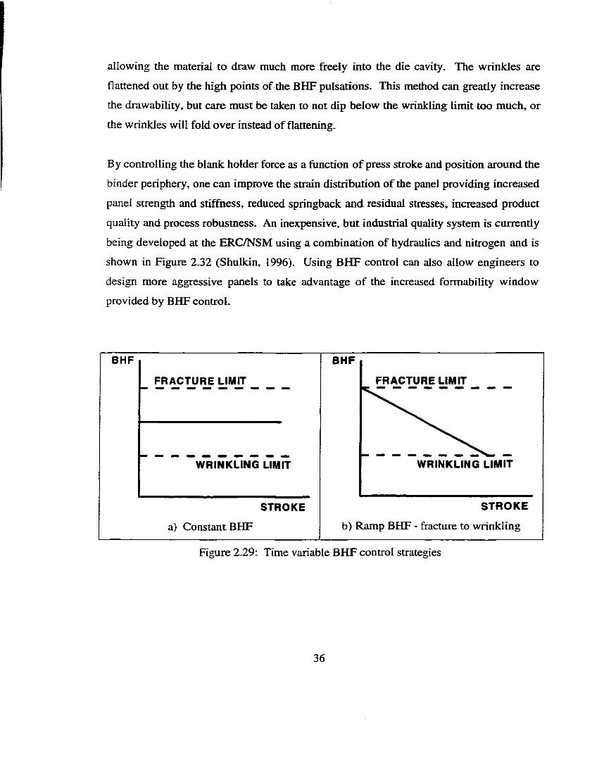
allowing the material to draw much more freely into the die cavity. The wrinkles are

flattened out by the high points of the BHF pulsations. This method can greatly increase

the drawability, but care must be taken to not dip below the wrinkling limit too much, or

the wrinkles will fold over instead of flattening.

By controlling the blank holder force as a function o f press stroke and position around the

binder periphery, one can improve the strain distribution of the panel providing increased

panel strength and stifftiess, reduced springbuck and residual stresses, increased product

quality and process robusmess. An inexpensive, but industrial quality system is currently

being developed at the ERC/NSM using a combination of hydraulics and nitrogen and is

shown in Figure 2.32 (Shulkin, 1996). Using BHF control can also allow engineers to

design more aggressive panels to take advantage of the increased formability window

provided by BHF control.

BHF

FRACTURE LIMIT

WRINKLING LIMIT

STROKE

BHF

FRACTURE LIMIT

WRINKLING LIMIT

STROKE

a) Constant BHF b) Ramp BHF - fracture to wrinkling

Figure 2.29: Time variable BHF control strategies

36

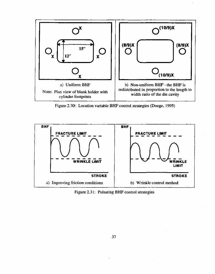
V i

a) Uniform BHF

Note: Plan view of blank holder with cylinder footprints

q ( 1 0 / 9 ) X

( 8 / 9 ) X ( 8 / 9 ) XO oV ■ >n

' ' ( 1 0 / 9 ) X

b) Non-uniform BHF - the BHF is redistributed in proportion to the length to

width ratio of the die cavity

Figure 2.30: Location variable BHF control strategies (Doege, 1995)

BHF

FRACTURE LIMIT

WRINKLE LIMIT

STROKE

a) Improving friction conditions

BHF

FRACTURE LIMIT

WRINKLELIMIT

STROKE

b) Wrinkle control method

Figure 2.31 : Pulsating BHF control strategies

37

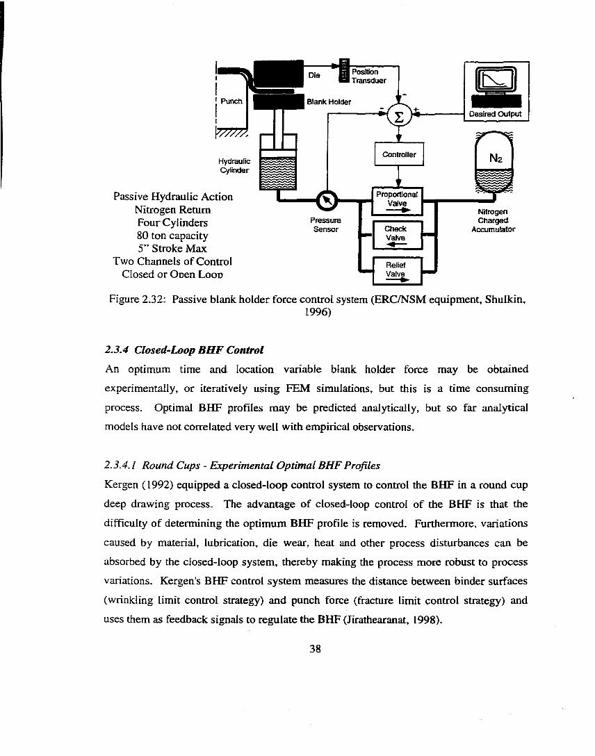
HydraulicCylinder

Position Transduer

Punch Blank HolderDesired Output

Controller

Proportional Valve

CheckValve

ReliefValve

NitrogenCharged

Accumulator

Passive Hydraulic Action Nitrogen Return Four Cylinders 80 ton capacity 5” Stroke Max

Two Channels of Control Closed or Onen Loon

Figure 2.32: Passive blank holder force control system (ERC/NSM equipment, Shulkin,1996)

2.3.4 Closed-Loop BHF Control

An optimum time and location variable blank holder force may be obtained

experimentally, or iteratively using FEM simulations, but this is a time consuming

process. Optimal BHF profiles may be predicted analytically, but so far analytical

models have not correlated very well with empirical observations.

2.3.4.1 Round Cups - Experimental Optimal BHF Profiles

Kergen ( 1992) equipped a closed-loop control system to control the BHF in a round cup

deep drawing process. The advantage of closed-loop control of the BHF is that the

difficulty of determining the optimum BHF profile is removed. Furthermore, variations

caused by material, lubrication, die wear, heat and other process disturbances can be

absorbed by the closed-loop system, thereby making the process more robust to process

variations. Kergen's BHF control system measures the distance between binder surfaces

(wrinkling limit control strategy) and punch force (fracture limit control strategy) and

uses them as feedback signals to regulate the BHF (Jirathearanat, 1998).

38

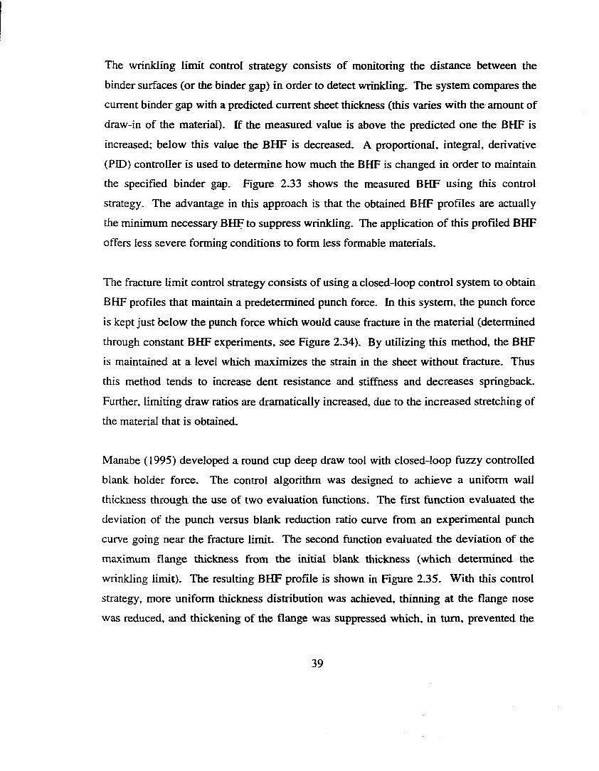
The wrinkling limit control strategy consists of monitoring the distance between the

binder surfaces (or the binder gap) in order to detect wrinkling. The system compares the

current binder gap with a predicted current sheet thickness (this varies with the amount of

draw-in of the material). If the measured value is above the predicted one the BHF is

increased; below this value the BHF is decreased. A proportional, integral, derivative

(PID) controller is used to determine how much the BHF is changed in order to maintain

the specified binder gap. Figure 2.33 shows the measured BHF using this control

strategy. The advantage in this approach is ± a t the obtained BHF profiles are actually

the minimum necessary BHF to suppress wrinkling. The application o f this profiled BHF

offers less severe forming conditions to form less formable materials.

The fracture limit control strategy consists of using a closed-loop control system to obtain

BHF profiles that maintain a predetermined punch force. In this system, the punch force

is kept just below the punch force which would cause fracture in the material (determined

through constant BHF experiments, see Figure 2.34). By utilizing this method, the BHF

is maintained at a level which maximizes the strain in the sheet without fracture. Thus

this method tends to increase dent resistance and stiffness and decreases springback.

Further, limiting draw ratios are dramatically increased, due to the increased stretching of

the material that is obtained.

Manabe (1995) developed a round cup deep draw tool with closed-loop fuzzy controlled

blank holder force. The control algorithm was designed to achieve a uniform wall

thickness through the use of two evaluation functions. The first function evaluated the

deviation of the punch versus blank reduction ratio curve from an experimental punch

curve going near the fracture limit. The second function evaluated the deviation of the

maximum flange thickness from the initial blank thickness (which determined the

wrinkling limit). The resulting BHF profile is shown in Figure 2.35. With this control

strategy, more uniform thickness distribution was achieved, thinning at the flange nose

was reduced, and thickening of the flange was suppressed which, in turn, prevented the

39

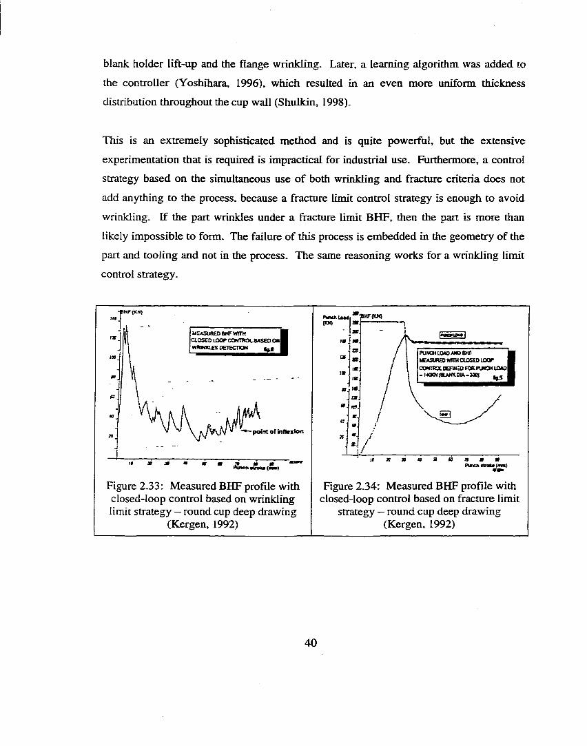
blank holder lift-up and the flange wrinkling. Later, a learning algorithm was added to

the controller (Yoshihara, 1996), which resulted in an even more uniform thickness

distribution throughout the cup wall (Shulkin, 1998).

This is an extremely sophisticated method and is quite powerful, but the extensive

experimentation that is required is impractical for industrial use. Furthermore, a control

strategy based on the simultaneous use o f both wrinkling and fracture criteria does not

add anything to the process, because a fracture limit control strategy is enough to avoid

wrinkling. If the part wrinkles under a fracture limit BHF, then the part is more than

likely impossible to form. The failure of this process is embedded in the geometry of the

part and tooling and not in the process. The same reasoning works for a wrinkling limit

control strategy.

149

UEASUREOBHTWtTHCLOSED LOOP CONTROL BASED ONWWWQ£SDETECTK3W I

pofnt of Intlcxfon

499 m

Figure 2.33: Measured BHF profile with closed-loop control based on wrinkling limit strategy — round cup deep drawing

(Kergen, 1992)

ZS.»19

re.m.

1 9 .

c.

Figure 2.34: Measured BHF profile with closed-loop control based on fracture limit

strategy — round cup deep drawing (Kergen, 1992)

4 0

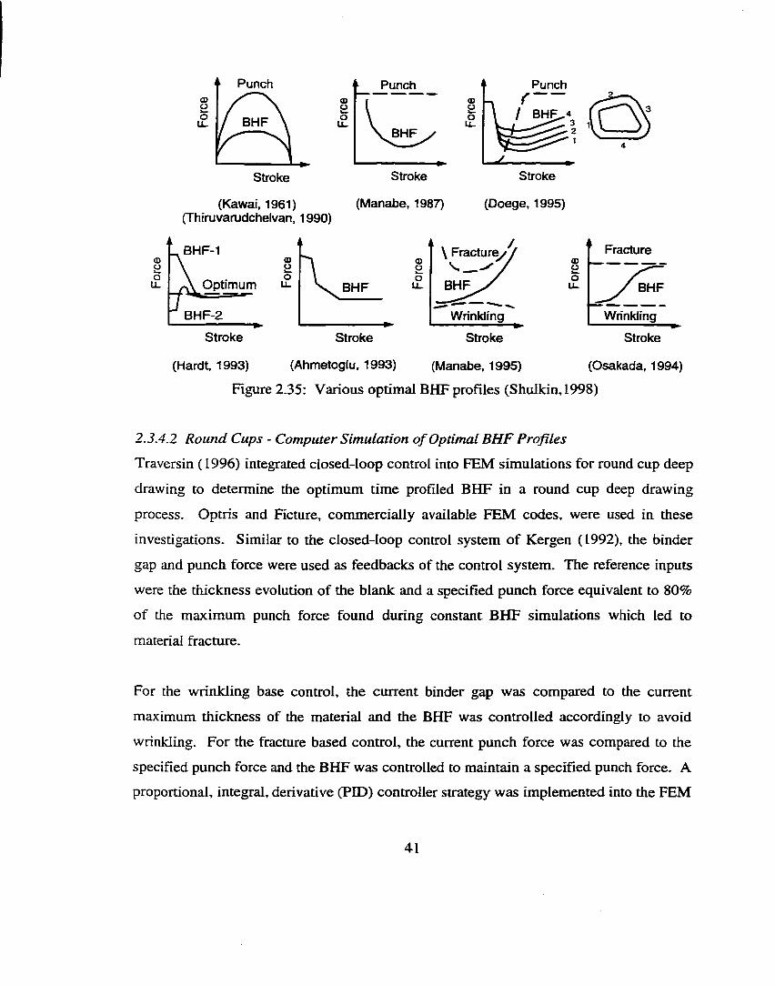
' ‘ Punch

BHFu_

Stroke

Punchou_

BHF

Stroke

321

Stroke

(Kawai, 1961) (Thiruvarudchelvan, 1990)

(Manabe, 1987) (Doege, 1995)

BHF-10)2

Optimum u- BHF

BHF-2Stroke Stroke

Si2

\ Fractur^ '' ^

Wnnkling

(Hardt, 1993) (Ahmetoglu, 1993)

Stroke

(Manabe, 1995)

Fracture

u_ BHF

WrinklingStroke

(Osakada, 1994)

Figure 2.35: Various optimal BHF profiles (Shulkin, 1998)

2.3.4.2 Round Cups - Computer Simulation o f Optimal BHF Profiles

Traversin ( 1996) integrated closed-loop control into FEM simulations for round cup deep

drawing to determine the optimum time profiled BHF in a round cup deep drawing

process. Optris and Ficture, commercially available FEM codes, were used in these

investigations. Similar to the closed-loop control system of Kergen (1992), the binder

gap and punch force were used as feedbacks of the control system. The reference inputs

were the thickness evolution of the blank and a specified punch force equivalent to 80%

of the maximum punch force found during constant BHF simulations which led to

material fracture.

For the wrinkling base control, the current binder gap was compared to the current

maximum thickness of the material and the BHF was controlled accordingly to avoid

wrinkling. For the fracture based control, the current punch force was compared to the

specified punch force and the BHF was controlled to maintain a specified punch force. A

proportional, integral, derivative (PID) controller strategy was implemented into the FEM

41

code to determine the amount the BHF needed to be changed in order to maintain the

specified punch force or binder gap.

The simulation results of Traversin’s work show good agreement with the experimental

results of Kergen. Kergen and Traversin explain the discrepancies as the results of

inappropriate friction conditions, improper reference inputs (i.e. thickness evolution), and

coarse time intervals. The problem with the work of Kergen and Traversin is that

wrinkling based strategy does not attempt to maximize the part strain in order to improve

final product properties such as dent resistance, stiffness, and springback. AJso, the

fracture based strategy relies on a specified punch force which was developed from

extensive constant BHF experiments. Also, punch force is not the best indicator of

fracture. Further, their work did not provide detailed information on control strategies for

location and time variable BHF.

Cao and Boyce (1994) implemented a closed-loop control strategy into the commercial

FEM code Abaqus for round cup deep drawing. A theoretical wrinkling based criterion

and the maximum major strain were used simultaneously as feedbacks to regulate the

BHF in round cup deep drawing. The predicted BHF profile (Figure 2.36) shows a

gradual increase of BHF with the punch displacement. The problem with Cao and

Boyce’s method is that the maximum strain is not the best indicator of fracture. The

maximum strain at fracture is a function of both major and minor strain. Only monitoring

the major strain will lead to under- or overestimation o f the failure limit. Furthermore,

their method controls the BHF using the wrinkling limit method at the beginning of the

process and the fracture limit method at the end. It could be possible in a complex

stamping, that fracture was more likely at the beginning than wrinkling and wrinkling

was more likely at the end, therefore Cao and Boyce’s control strategy would fail in this

case. Clearly, their strategy was formulated for simple round cups only. Finally, the use

of two feedbacks was unnecessary as previous explained.

42

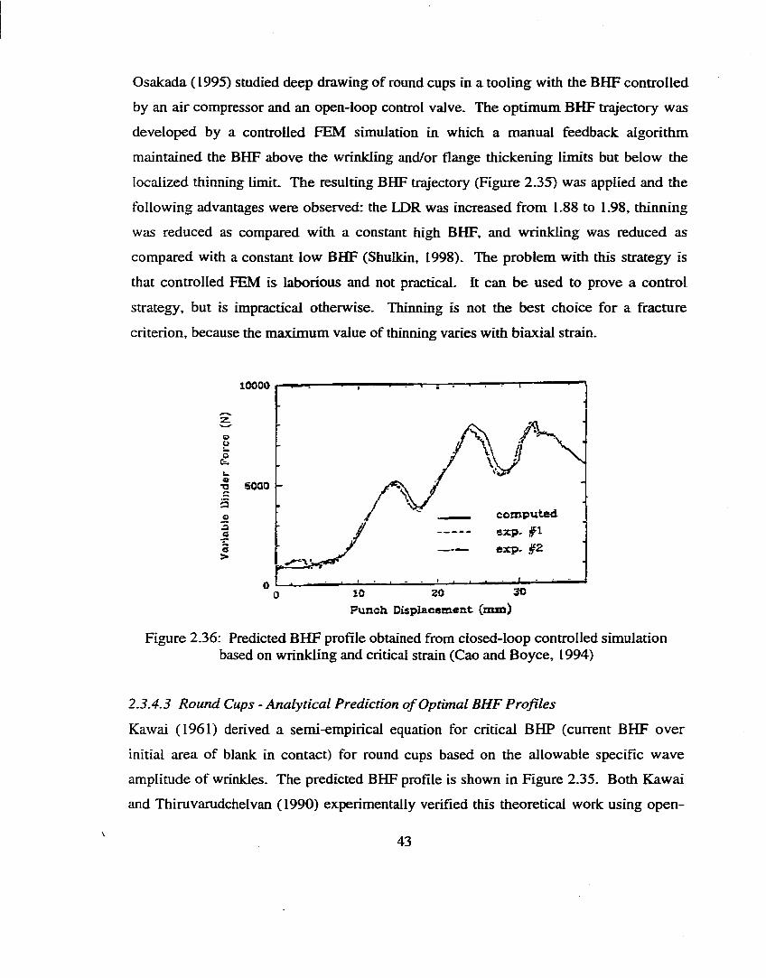
Osakada ( 1995) studied deep drawing of round cups in a tooling with the BHF controlled

by an air compressor and an open-loop control valve. The optimum BHF trajectory was

developed by a controlled FEM simulation in which a manual feedback algorithm

maintained the BHF above the wrinkling and/or flange thickening limits but below the

localized thinning limit. The resulting BHF traj'ectory (Figure 2.35) was applied and the

following advantages were observed: the LDR was increased from 1.88 to 1.98, thinning

was reduced as compared with a constant high BHF, and wrinkling was reduced as

compared with a constant low BHF (Shulkin, 1998). The problem with this strategy is

that controlled FEM is laborious and not practical. It can be used to prove a control

strategy, but is impractical otherwise. Thinning is not the best choice for a fracture

criterion, because the maximum value of thinning varies with biaxial strain.

lOOOO

z6>aê.k■a soaoa

e>

30to 30Punch Displacsment (nmt)

Figure 2.36: Predicted BHF profile obtained from closed-loop controlled simulation based on wrinkling and critical strain (Cao and Boyce, 1994)

2.3.4.3 Round Cups - Analytical Prediction o f Optimal BHF Profiles

Kawai (1961) derived a semi-empirical equation for critical BHP (current BHF over

initial area of blank in contact) for round cups based on the allowable specific wave

amplitude of wrinkles. The predicted BHF profile is shown in Figure 2.35. Both Kawai

and Thiruvarudchelvan (1990) experimentally verified this theoretical work using open-

43

loop BHF control. It was reported that the application o f Kawai’s method minimized

frictional resistance on the blank, eliminated flange wrinkling, reduced the punch force,

reduced thinning at the punch nose area, and increased the LDR by 5% when compared

with constant BHF (Shulkin, 1998). The problem with this work is that it is based on

wrinkling and does not attempt to maximize strain.

Manabe (1987) derived equations to calculate fracture limit BHF trajectories for round

cup deep drawing. However, the experimentally determined BHF curves differed

considerably from the ones predicted by the equations. Nevertheless, Manabe observed

dramatic improvement of the drawability using experimentally determined, fracture limit

based, closed-loop control BHF profiles as shown in Figure 2.35 (Shulkin, 1998). The

weakness in this investigation is that Manabe does not take into account anisotropy or

wrap angle in his derivations.

Ahmetoglu (1996) used finite difference method (FDM) analysis to develop an optimum

BHF variation for round cup deep drawing on a single action hydraulic press with an

open-loop controlled die cushion. The analysis was based on three criteria: 1)

maintaining the punch force below a calculated failure value, 2 ) maintaining the radial

sheet tension below a calculated failure value, and 3) maintaining the cup wall thickness

above a user specified value. The application o f the BHF profile obtained with the above

procedure (Figure 2.35) resulted in an increase of the LDR (Shulkin, 1998). The

weakness of this work is that three control criteria are required, making the control

strategy redundant and difficult to implement.

2.3.4A Non-Round Parts- Experimental Optimal BHF Profiles

Siegert (1996) designed a closed-loop, BHF control system for round cup and rectangular

pan deep draw tools. He used punch force, binder gap, friction force, and draw-in as

feedbacks to the control system. A piezoelectric sensor in the binder measured the

friction force during the process and was used as a feedback loop as shown in Figure

4 4

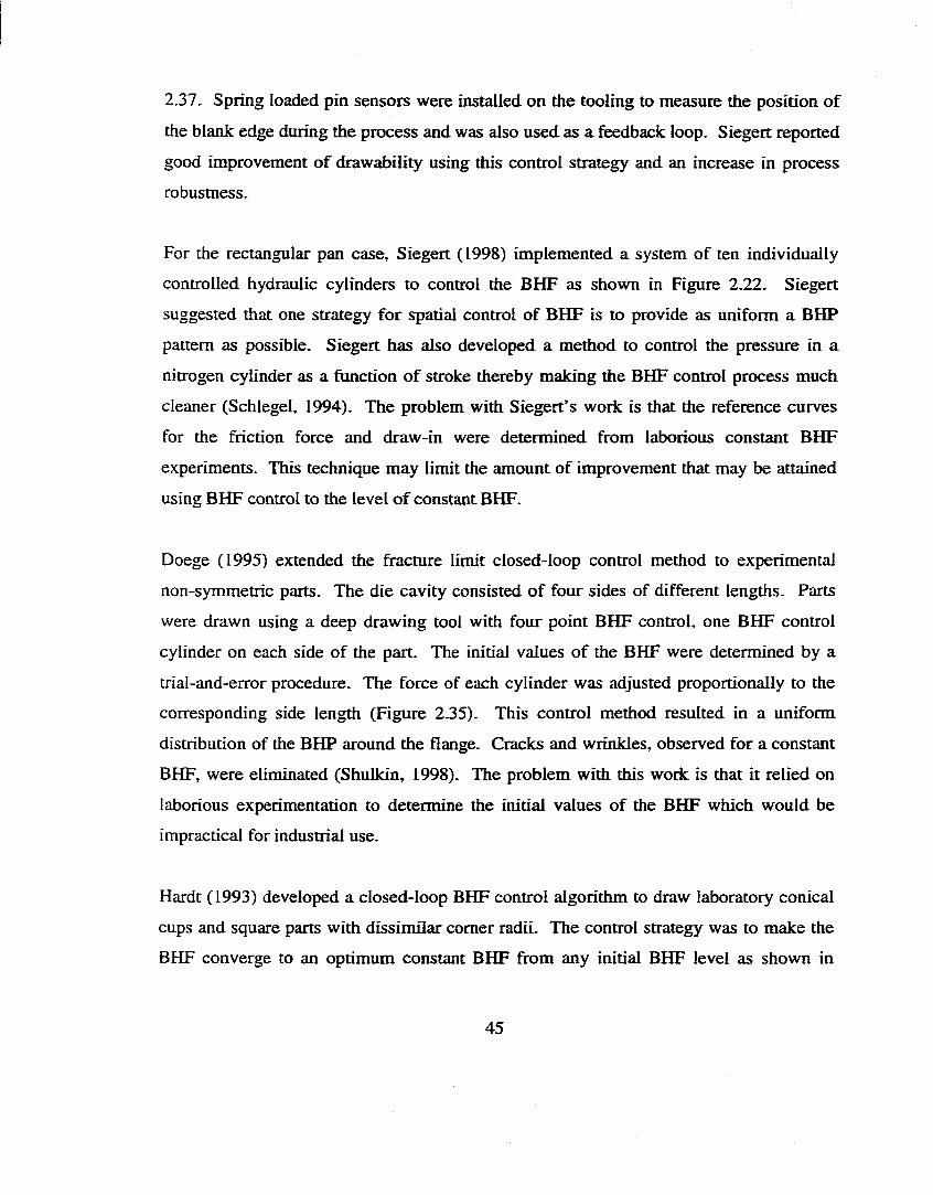
2.37. Spring loaded pin sensors were installed on the tooling to measure the position of

the blank edge during the process and was also used as a feedback loop. Siegert reported

good improvement of drawability using this control strategy and an increase in process

robusmess.

For the rectangular pan case, Siegert (1998) implemented a system of ten individually

controlled hydraulic cylinders to control the BHF as shown in Figure 2.22. Siegert

suggested that one strategy for spatial control of BHF is to provide as uniform a BHP

pattern as possible. Siegert has also developed a method to control the pressure in a

nitrogen cylinder as a function of stroke thereby making the BHF control process much

cleaner (Schlegel, 1994). The problem with Siegert's work is that the reference curves

for the friction force and draw-in were determined from laborious constant BHF

experiments. This technique may limit the amount of improvement that may be attained

using BHF control to the level o f constant BHF.

Doege (1995) extended the fracmre limit closed-loop control method to experimental

non-symmetric parts. The die cavity consisted of four sides of different lengths. Parts

were drawn using a deep drawing tool with four point BHF control, one BHF control

cylinder on each side of the part. The initial values of the BHF were determined by a

trial-and-error procedure. The force of each cylinder was adjusted proportionally to the

corresponding side length (Figure 2.35). This control method resulted in a uniform

distribution of the BHP around the flange. Cracks and wrinkles, observed for a constant

BHF, were eliminated (Shulkin, 1998). The problem with this work is that it relied on

laborious experimentation to determine the initial values of the BHF which would be

impractical for industrial use.

Hardt (1993) developed a closed-loop BHF control algorithm to draw laboratory conical

cups and square parts with dissimilar comer radii. The control strategy was to make the

BHF converge to an optimum constant BHF from any initial BHF level as shown in

45

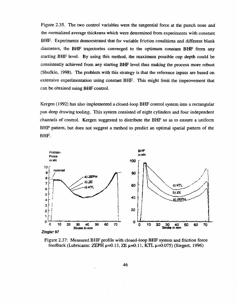
Figure 2.35. The two control variables were the tangential force at the punch nose and

the normalized average thickness which were determined from experiments with constant

BHF. Experiments demonstrated that for variable friction conditions and different blank

diameters, the BHF trajectories converged to the optimum constant BHF from any

starting BHF level. By using this method, the maximum possible cup depth could be

consistently achieved from any starting BHF level thus making the process more robust

(Shulkin, 1998). The problem with this strategy is that the reference inputs are based on

extensive experimentation using constant BHF. This might limit the improvement that

can be obtained using BHF control.

Kergen (1992) has also implemented a closed-loop BHF control system into a rectangular

pan deep drawing tooling. This system consisted of eight cylinders and four independent

channels of control. Kergen suggested to distribute the BHF so as to ensure a uniform

BHP pattern, but does not suggest a method to predict an optimal spatial pattern of the

BHF.

Friction- Force in KN

BHFInkN

100

a)2EPHb)ZEc)KTL

30 40 50 60Stroke in mm

C)KTL

20 30 40 50Strok» in mm

Ziegler 97

Figure 2.37: Measured BHF profile with closed-loop BHF system and friction force feedback (Lubricants: ZEPH |i=0.13, ZE p=0.11, KTL p=0.075) (Siegert, 1996)

46

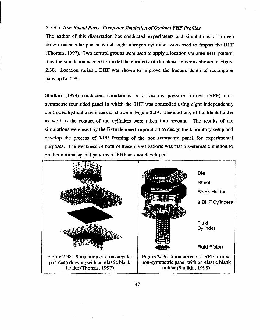
2.3 A .5 Non-Round Parts- Computer Simulation o f Optimal BHF Profiles

The author of this dissertation has conducted experiments and simulations o f a deep

drawn rectangular pan in which eight nitrogen cylinders were used to impart the BHF

(Thomas, 1997). Two control groups were used to apply a location variable BHF pattern,

thus the simulation needed to model the elasticity of the blank holder as shown in Figure

2.38. Location variable BHF was shown to improve the fracture depth of rectangular

pans up to 25%.

Shulkin (1998) conducted simulations of a viscous pressure formed (VPF) non-

symmetric four sided panel in which the BHF was controlled using eight independently

controlled hydraulic cylinders as shown in Figure 2.39. The elasticity of the blank holder

as well as the contact of the cylinders were taken into account. The results of the

simulations were used by the Extrudehone Corporation to design the laboratory setup and

develop the process of VPF forming of the non-symmetric panel for experimental

purposes. The weakness o f both of these investigations was that a systematic method to

predict optimal spatial patterns o f BHF was not developed.

Figure 2.38: Simulation o f a rectangular pan deep drawing with an elastic blank

holder (Thomas, 1997)

Die

S h eet

Blank Holder

8 BHF Cylinders

FluidCylinder

Fluid Piston

Figure 2.39: Simulation of a VPF formed non-symmetric panel with an elastic blank

holder (Shulkin, 1998)

47

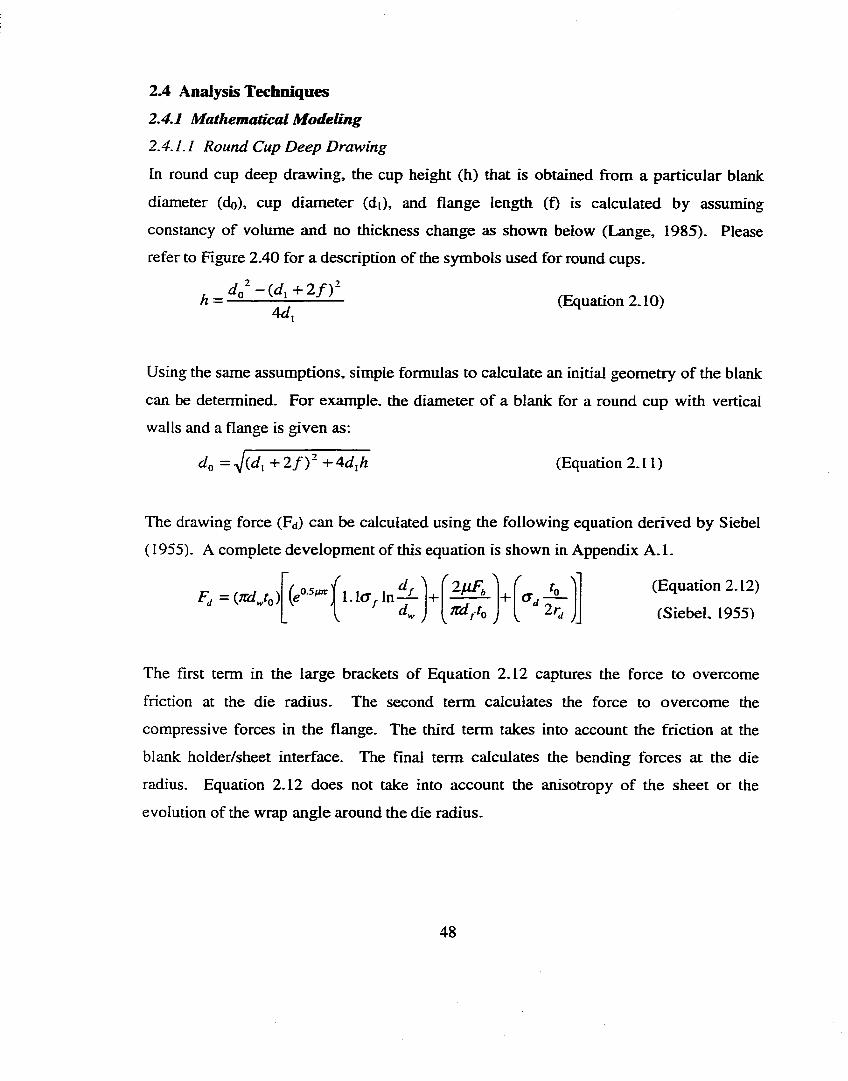
2.4 Analysis Techniques2.4.1 Mathenmtical Modeling

2.4.1.1 Round Cup Deep Drawing

In round cup deep drawing, the cup height (h) that is obtained from a particular blank

diameter (do), cup diameter (di), and flange length (f) is calculated by assuming

constancy of volinne and no thickness change as shown below (Lange, 1985). Please

refer to Figure 2.40 for a description of the symbols used for round cups.

A = — - (Equation 2.10)4d,

Using the same assumptions, simple formulas to calculate an initial geometry of the blank

can be determined. For example, the diameter of a blank for a round cup with vertical

walls and a flange is given as:

Jq = -y/(d, + 2f ) ~ +4dih (Equation 2.11)

The drawing force (Fd) can be calculated using the following equation derived by Siebel

( 1955). A complete development of this equation is shown in Appendix A .I.

Pad A (Equation 2.12)

(Siebel. 1955)

The first term in the large brackets of Equation 2.12 captures the force to overcome

friction at the die radius. The second term calculates the force to overcome the

compressive forces in the flange. The third term takes into account the friction at the

blank holder/sheet interface. The final term calculates the bending forces at ± e die

radius. Equation 2.12 does not take into account the anisotropy of the sheet or the

evolution of the wrap angle around the die radius.

48

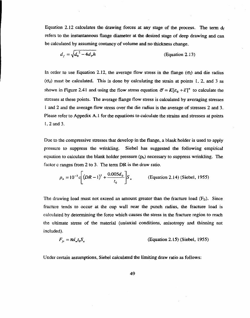
Equation 2 . 1 2 calculates the drawing forces at any stage of the process. The term df

refers to the instantaneous flange diameter at the desired stage of deep drawing and can

be calculated by assuming contancy of volume and no thickness change.

djr = jdo~ —4dph (Equation 2.13)

In order to use Equation 2.12, the average flow stress in the flange (ctf) and die radius

(cTd) must be calculated. This is done by calculating the strain at points 1, 2, and 3 as

shown in Figure 2.41 and using the flow stress equation a = K{£q +Ê]" to calculate the

stresses at these points. The average flange flow stress is calculated by averaging stresses

I and 2 and the average flow stress over the die radius is the average of stresses 2 and 3.

Please refer to Appedix A.1 for ± e equations to calculate the strains and stresses at points

I, 2 and 3.

Due to the compressive stresses that develop in the flange, a blank holder is used to apply

pressure to suppress tlie wrinkling. Siebel has suggested the following empirical

equation to calculate the blank holder pressure (pb) necessary to suppress wrinkling. The

factor c ranges from 2 to 3. The term DR is the draw ratio.

Ph = 1 0 (DR - ly-h (Equation 2.14) (Siebel, 1955)

The drawing load must not exceed an amount greater than the fracture load (Ffr). Since

fracture tends to occur at the cup wall near the punch radius, the fracture load is

calculated by determining the force which causes the stress in the fracture region to reach

the ultimate stress o f the material (uniaxial conditions, anisotropy and thinning not

included).

(Equation 2.15) (Siebel, 1955)

Under certain assumptions. Siebel calculated the limiting draw ratio as follows:

49

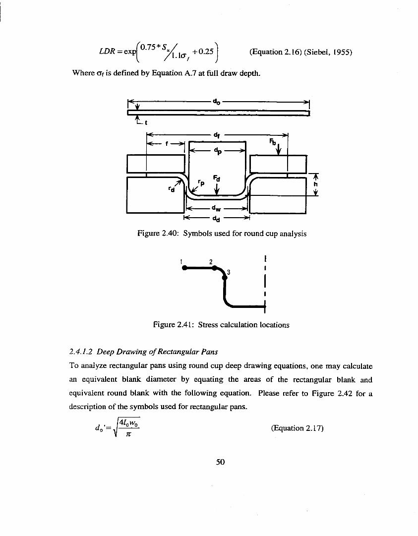
LD/?=exp| +0.25 (Equation 2.16) (Siebel, 1955)

Where df is defined by Equation A.7 at full draw depth.

T 7

'c

"4.

k ll1

“wdd

Th

Figure 2.40: Symbols used for round cup analysis

0 I1

Figure 2.41: Stress calculation locations

2.4.1.2 Deep Drawing o f Rectangular Pans

To analyze rectangular pans using round cup deep drawing equations, one may calculate

an equivalent blank diameter by equating the areas of the rectangular blank and

equivalent round blank with the following equation. Please refer to Figure 2.42 for a

description of the symbols used for rectangular pans.

(Equation 2.17)

50

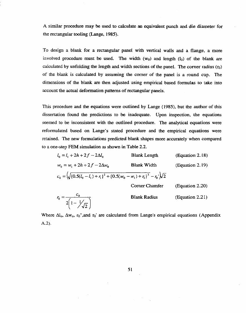
A similar procedure may be used to calculate an equivalent punch and die diameter for

the rectangular tooling (Lange, 1985).

To design a blank for a rectangular panel with vertical walls and a flange, a more

involved procedure must be used. The width ( wq) and length (lo) of the blank are

calculated by unfolding the length and width sections of the panel. The corner radius (ro)

of the blank is calculated by assuming the comer of the panel is a round cup. The

dimensions of the blank are then adjusted using empirical based formulas to take into

account the actual deformation patterns o f rectangular panels.

This procedure and the equations were outlined by Lange (1985), but the author of this

dissertation found the predictions to be inadequate. Upon inspection, the equations

seemed to be inconsistent with the outlined procedure. The analytical equations were

reformulated based on Lange’s stated procedure and the empirical equations were

retained. The new formulations predicted blank shapes more accurately when compared

to a one-step FEM simulation as shown in Table 2.2.

/q = /[ + 2A -h 2 / — 2A/q Blank Length (Equation 2.18)

Wq = W[ + 2/i -h 2 / — 2Awo Blank Width (Equation 2.19)

Co = ij[0.5(lo + + {0.5(Wo - Wi ) + /I}- - To ')>/2

Comer Chamfer (Equation 2.20)

/■(, = —T— —------^ Blank Radius (Equation 2.21)

V ' X i ï

Where Alo, Awq, ro",and ro' are calculated from Lange's empirical equations (Appendix

A.2).

51

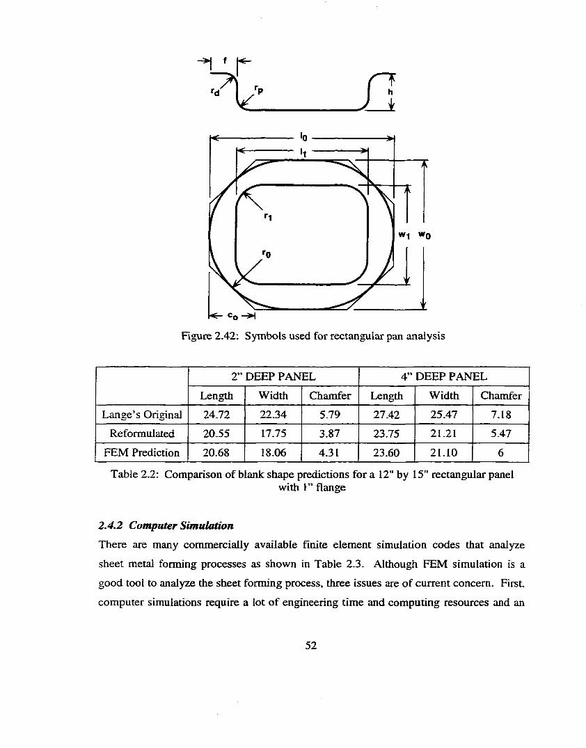
nW l WQ

Figure 2.42: Symbols used for rectangular pan analysis

2” DEEP PANEL 4” DEEP PANEL

Length Width Chamfer Length Width Chamfer

Lange’s Original 24.72 22.34 5.79 27.42 25.47 7.18

Reformulated 20.55 17.75 3.87 23.75 2 1 . 2 1 5.47

FEM Prediction 2 0 . 6 8 18.06 4.31 23.60 2 1 . 1 0 6

Table 2.2: Comparison of blank shape predictions for a 12" by 15" rectangular panelwith I” flange

2.4.2 Computer Simulation

There are many commercially available finite element simulation codes that analyze

sheet metal forming processes as shown in Table 2.3. Although FEM simulation is a

good tool to analyze the sheet forming process, three issues are of current concern. First,

computer simulations require a lot of engineering time and computing resources and an

52

experienced, well trained engineer to obtain reliable results. Second, the use of simple

equations may be enough to conduct certain analyses and may be even be more

advantageous than computer simulations. Third, add-on modules to commercial FEM

programs that implement a feedback loop into the calculations (adaptive simulation)

would be extremely useful to optimize the process.

Two types of FEM formulations are commonly used. In “one-step FEM”, the user inputs

the part geometry and optional process conditions and the solver unfolds the part shape

onto the binder surface. One-step FEM is computationally fast, can take into account

material properties and deformation, and can account for process conditions such as BHF,

drawbeads, friction, and bending if the user desires. Springbuck calculations are also

included with many one-step FEM packages. One-step FEM does not simulate the

deformation history, does not solve iterative calculations incrementally, and does not

simulate the material/tool contact.

The second most commonly used FEM codes are “incremental” type codes which are

based on dynamic explicit formulation, bicremental FEM simulates the sheet forming

process in exactly the same way the actual process occurs. The user inputs the tool and

material geometry, material properties, and boundary conditions (velocities, forces,

symmetry, rigidity, etc.) The solver then calculates the movement of the tools, the

contact of the materials and tools, friction at the interface, displacements of the nodes,

strains of the material, and workpiece and tool stresses. The entire sheet forming process

can be simulated including gravity/binder wrap, clamping, forming, trimming/piercing,

flanging/hemming, and springback.

The one-step FEM software that will be used with this research is FAST_FORM3D from

FTI Inc. (Ontario, Canada). An example of its use is shown in Figure 2.43. In this case

study, a cab comer outer for a light truck was press formed using the rectangular blank as

shown in Figure 2.43a. After fuü deformation, the blank would draw through the beads

53

as shown in Figure 2.43c. Drawing fully through the bead causes process instability and

non-uniformity of the part strain which increases springback and decreases the

formabihty window.

FAST_FORM3D was used to calculate a blank shape which would draw right to the

outside edge of the bead at every point as shown in Figures 2.43b and 2.43d. Using the

incremental FEM code Pam-Stamp (ESI Int’l - Paris, France) the original and optimized

blank was simulated and is shown in Figure 2.44. These simulations show that the

optimized blank improved the strain distributions significantly.

In another case study, Pam-Stamp was used to simulate a door outer panel that was in

hard tool production. Figure 2.45 shows how splitting and distortion were predicted to

occur on the part surface. Splitting did occur on the header of the door during physical

tool tryouts thus confirming the predictions. In order to eliminate the splitting condition,

some of the take up beads in the window cavity were removed.

a) Current blank shape b) Optimized blank shape

d) Optmuzed draw processc) Current draw process

Figure 2.43 : Optimal blank shape prediction for the cab comer outer panel using FAST_FORM3D (one-step FEM from FTI Inc.)

5 4

a) Rectangular blank shape 30% maximum thinning

b) Optimized blank shape 24% Maximum Thinning

Figure 2.44: Improvement of strain distribution in the cab comer by optimizing the blank shape (Pam-Stamp from ESI IntT - incremental simulation)

Compression at end of stroke. Bad surface quality.

Material drawn in at end of stroke. Possible panel distortion.

Excessive thinning >40%. Likely failure problems.

Loose area, <3% stretch. Possible panel distortion.

Local thinning >25%. Possible structural problem.

Figure 2.45: Prediction of splitting and distortions in a door outer panel (Pam-Stampfrom ESI DitT - incremental simulation)

55

NAME TYPE APPLICATIONS

Abaqus Implicit general non-linear

Mark Implicit general non-linear

Nike3D Implicit general non-linear

Larstran Implicit general non-linear

Epdan Implicit bulk, sheet forming

Indeed Implicit sheet forming

Robust explicit, static sheet forming

Dyna3D explicit, dynamic bulk, sheet forming

Pam-Stamp explicit, dynamic bulk, sheet forming

Optris explicit, dynamic sheet forming

Abaqus-Explicit explicit, dynamic bulk, sheet forming, general non-linear

UFO-3D explicit, dynamic sheet forming

Dedran special formulation sheet forming

Autoform special formulation sheet forming

Deform rigid viscoplastic bulk forming, forging

Forge 2/3 rigid viscoplastic forging

Icem-Stamp inverse method, deformation theory

sheet forming

Simex inverse theory sheet forming

Iso-Punch inverse theory sheet forming

FAST_FORM3D inverse theory Sheet forming

Table 2.3: Commercially available FEM codes - their formulations and applications

2.4.3 Failure Prediction

Failure may occur in sheet metal parts in a number of ways including:

1. Fracture

2. Necking

3. Wrinkling

56

4. Distortions

5. Undesirable Surface Textures

For most strain paths, necking precedes fracture, therefore necking prediction is of

greater concern (see Figure 2.46). Fracture may be observed as a split/tear (excessive

stretching), a surface crack (excessive bending), or an edge failure (caused by an

imperfection in the blanked edge).

Wrinkling or buckling is caused by compressive stresses and typically occurs on the

flange of the part. Often it may not be a concern if the flange is trimmed as with many

automotive parts. When the sheet experiences very low stresses, compressive or tensile,

then distortions may occur.

Residual stresses may also cause geometric distortions in the part. Large scale distortions

may take the form of highs or lows in the part surface or as oil canning (elastic

instabilities). Small scale distortions may take the form of rabbit earing, pie crust, crow’s

feet, or teddy bear ears.

Undesirable surface textures such as orange peel or stretcher strain markings may also

occur during deformation. Orange peel consists of a rough surface appearance typically

caused by the variation of flow stress properties of the various grains contained in the

material. Two types of stretcher strains are observed. The first type is caused by

discontinuous yielding at the yield point and is evidenced by irregular striations on the

surface of the sheet. The second type of stretcher strain marking is caused by

discontinuous yielding in the plastic region of the material and is evidenced by regular

striations on the surface of the sheet.

Finite element simulation is currently limited when it comes to predicting the exact time

of failure. This is demonstrated in Figure 2.47a. Clearly the cup has strained well

5 7

beyond the point of failure, but the deformation continues to be blindly calculated by the

solver. Further, even though failure is evident, it is not clear exactly when it occurs.

Many failure criteria have been proposed in the past. The thinning in the part has been

traditionally used to estimate proximity to failure and is demonstrated in Figure 2.47b.

This is an approximate method, because the limit of thinning can vary with strain path.

Biaxial strain has been proposed by Keeler (1965) and Goodwin (1968) to estimate

failure in the form of a forming limit diagram (FLD) as shown in Figure 2.46. It has been

shown by several researchers that the forming limit curve (FLC) is highly dependent on

strain path as shown in Figure 2.48 (Arrieux, 1995). Further, the measurement of a FLC

requires extensive and laborious experimentation. For steel, the following formula has

been experimentally developed to calculate the FLD as a function of n-value and material

thickness:

FZDo = (105.02 + 69.885f)noWhere Hq = n if n > 0.22, otherwise n„ = 0.22

g, = 0 5 3 3 8 8 * ( - g 2 + FZDo fo re , < 0 (Equation 2.22)

g[ = 1.3941 * + FZDq fo re , > 0 g[ = FLDq fo re , = 0

Other failure criteria have been proposed based on examining the stress in the part rather

than the strain. For example, it is noted that stress based fracture limits are insensitive to

strain paths as shown in Figure 2.49 (Arrieux, 1995). The most notable feature of Figure

2.49 is the fact that the failure limit in biaxial stress space resembles a yield siuface. This

gives credence to the use of a stress based limit to predict failure based on yield criteria

such a Tresca’s (normal stress limit). Von Mises (isotropic equivalent stress limit), or

Hill’s (anisotropic and/or non-quadratic equivalent stress limit).

The previous failure criteria were based on instantaneous values of stress and strain. A

failure criterion that considers the instantaneous stresses and the deformation history was

proposed by Cockroft and Latham (1968):

58

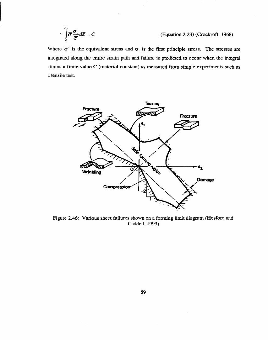
f â ^ d ë = C i (T

(Equation 2.23) (Crockroft, 1968)

Where â is the equivalent stress and Ci is the first principle stress. The stresses are

integrated along the entire strain path and failure is predicted to occur when the integral

attains a finite value C (material constant) as measured from simple experiments such as

a tensile test.

FractureTearing

Wrinkling ^/

CompressiiDamage

Figure 2.46: Various sheet failures shown on a forming limit diagram (Hosford andCaddell, 1993)

59

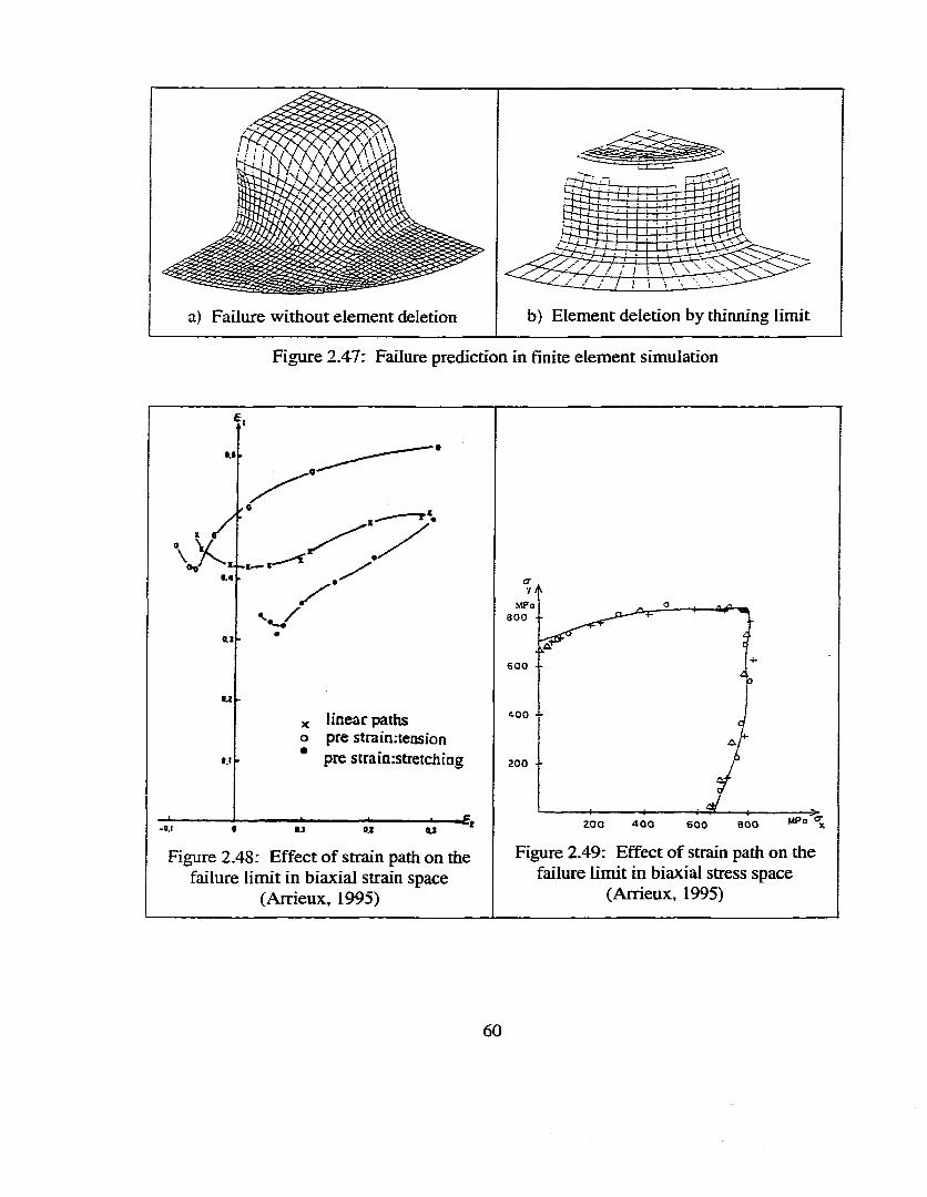
b) Element deletion by thinning limita) Failure without element deletion

Figure 2.47: Failure prediction in finite element simulation

V '*■1.4

X linear paths o pre strainrtension* pre strainrstretching

-1.1 u -ft

Figure 2.48: Effect of strain path on the failure limit in biaxial strain space

(Arrieux, 1995)

MPo

Figure 2.49: Effect of strain path on the failure limit in biaxial stress space

(Arrieux, 1995)

6 0

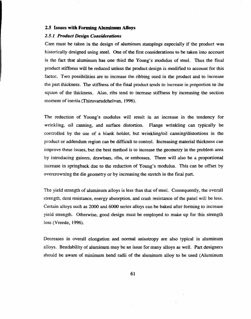
2.5 Issues with Forming Aluminum Alloys2.5.1 Product Design Considerations

Care must be taken in the design of aluminum stampings especially if the product was

historically designed using steel. One of the first considerations to be taken into account

is the fact that aluminum has one third the Young’s modulus of steel. Thus the final

product stiffiiess will be reduced unless the product design is modified to account for this

factor. Two possibilities are to increase the ribbing used in the product and to increase

the part thickness. The stiffness of the final product tends to increase in proportion to the

square of the thickness. Also, ribs tend to increase stiffness by increasing the section

moment of inertia (Thiravarudchelvan, 1996).

The reduction of Young’s modulus will result in an increase in the tendency for

wrinkling, oil canning, and surface distortion. Range wrinkling can typically be

controlled by the use of a blank holder, but wrinkling/oil canning/distortions in the

product or addendum region can be difficult to control. Increasing material thickness can

improve these issues, but the best method is to increase the geometry in the problem area

by introducing gainers, drawbars, ribs, or embosses. There will also be a proportional

increase in springback due to the reduction of Young’s modulus. This can be offset by

overcrowning the die geometry or by increasing the stretch in the final part.

The yield strength of aluminum alloys is less than that o f steel. Consequently, the overall

strength, dent resistance, energy absorption, and crash resistance of the panel will be less.

Certain alloys such as 2000 and 6000 series alloys can be baked after forming to increase

yield strength. Otherwise, good design must be employed to make up for this strength

loss (Vreede, 1996).

Decreases in overall elongation and normal anisotropy are also typical in aluminum

alloys. Bendability of aluminum may be an issue for many alloys as well. Part designers

should be aware of minimum bend radii of the aluminum alloy to be used (Aluminum

61

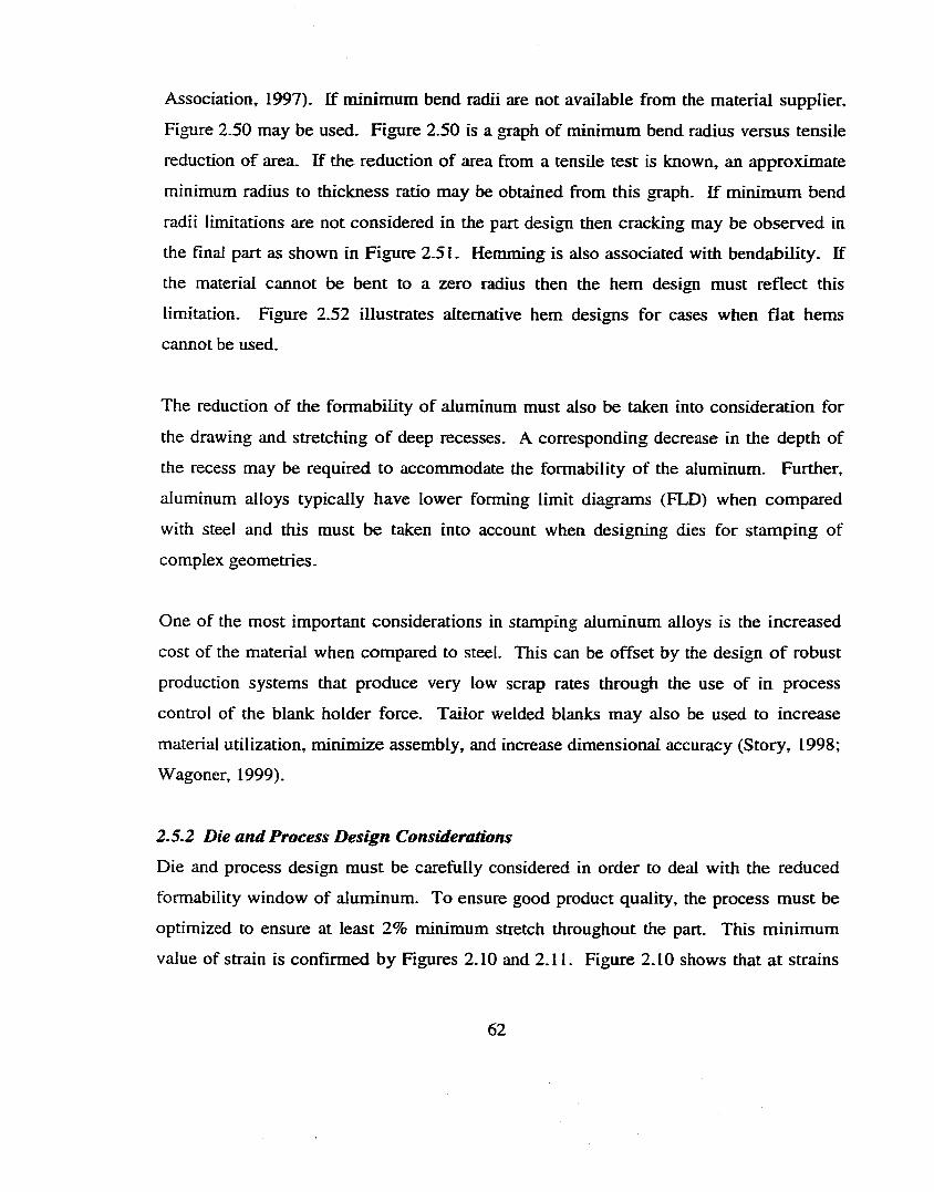
Association, 1997). If minimum bend radii are not available from the material supplier.

Figure 2.50 may be used. Figure 2.50 is a graph of minimum bend radius versus tensile

reduction of area. If the reduction of area from a tensile test is known, an approximate

minimum radius to thickness ratio may be obtained from this graph. If minimum bend

radii limitations are not considered in the part design then cracking may be observed in

the final part as shown in Figure 2.51. Hemming is also associated with bendability. If

the material cannot be bent to a zero radius then the hem design must reflect this

limitation. Figure 2.52 illustrates alternative hem designs for cases when flat hems

cannot be used.

The reduction of the formability of aluminum must also be taken into consideration for

the drawing and stretching o f deep recesses. A corresponding decrease in the depth of

the recess may be required to accommodate the formability o f the aluminum. Further,

aluminum alloys typically have lower forming limit diagrams (FLD) when compared

with steel and this must be taken into account when designing dies for stamping of

complex geometries.

One of the most important considerations in stamping aluminum alloys is the increased

cost of the material when compared to steel. This can be offset by the design o f robust

production systems that produce very low scrap rates through the use of in process

control of the blank holder force. Tailor welded blanks may also be used to increase

material utilization, minimize assembly, and increase dimensional accuracy (Story, 1998;

Wagoner, 1999).

2.5.2 Die and Process Design Considerations

Die and process design must be carefully considered in order to deal with the reduced

formability window of aluminum. To ensure good product quality, the process must be

optimized to ensure at least 2% minimum stretch throughout the part. This minimum

value of strain is confirmed by Figures 2.10 and 2.11. Figure 2.10 shows that a t strains

6 2

less that 2%, springback is greatly increased. Likewise, Figure 2.11 shows that 2% strain

is required to ensure good dent resistance properties. Both graphs show that springback

and dent resistance levels off at around 2 % stretch.

<0

s

IJie

Tensile redaction, of area (%)

Figure 2.50: Minimum bend radius to thickness ratio versus tensile reduction of

area (Kaipakjian, 1991)Figure 2.51: Cracking due to violation of minimum bend radius (Livatyali, 1997)

b) Tear drop hemc) Open hem

;) Modified rope hemcrf) Rope hem

Figure 2.52: Alternative hem designs for alum inum (Livatyali, 1997)

63

The decrease in formability o f aluminum can also be offset through the use o f advanced

die and process design and through the use of advanced technology (Ahmetoglu, 1996).

The clever use of advanced addendum design has been used successfully to widen the

formability margins so that complicated geometries may be formed from aluminum

(Burk, 1996). The addendum is defined as the portion of the die between the binder and

the trim line. The most typical addendum feature is the drawwall which is used to

connect the binder surface to the part geometry. Other addendum features include the use

of gainers and drawbars. The downside to increasing the addendum region is that

addendum is typically engineered scrap and thus this method tends to increase scrap

realized per part.

The use of advanced technologies such as blank holder force control, hydroforming, and

warm forming may also be use to increase the formability window of aluminum alloys.

The cost associated with this solution is the capital investment of the presses and

equipment needed to implement these processes. Blank holder force control has been

shown to increase drawability and process robustness. Similarly, hydroforming can

increase formability, strain uniformity, strain hardening, and decrease tooling costs.

Warm forming by definition is the forming of material at a temperature between cold

forming and hot forming. Typically hot forming is exhibited by temperatures just below

the melting temperature of the material while cold forming is conducted at room

temperature. Warm forming requires less energy, insulation, technology and logistics

than hot forming and thus is an attractive process for difficult to form parts. By

increasing the temperature of the aluminum sheet material, many advantages in terms of

formability can be obtained. As shown in Figure 2.53, the flow stress of the material

tends to decrease as temperature increases which thereby decreases forming loads.

Further investigations have shown that increasing material temperatures tends to increase

elongation, increase strain rate hardening, decrease ludering, and increase the forming

limit curve (Holt, 1998).

64

This increase o f material formability can be useful for forming deep recesses or

complicated geometries. Warm forming requires an investment in equipment. An oven

is needed to heat the incoming material and heater cores must be implemented into the

tooling as shown in Figure 2.54 for the example of steel. Insulation must also be used to

maintain die temperature efficiently. Further, different regions of the die require different

levels to heat to ensure that formability is improved requiring expensive controls and

electronics. In general, the binders should be heated for deep drawn parts and not heated

for stretched parts. Tight radii should not be heated while flat regions or regions with

low curvature should be heated (Ghosh, 1995). While warm forming offers advantages

in improving the formability o f aluminum alloys, it also increases the complexity o f die

design and process control.

During trimming and piercing operations, the production of slivers can cause problems.

Slivering can be reduced by trimming at an angle that is not perpendicular to the sheet

surface (Holt, 1998). This tends to decrease the shear stresses and increase the tensile

stresses at the trim edge. This in turn tends to reduce the burr height which consequently

reduces slivering. Since the knowledge base of aluminum forming is far less than that of

steel, computer simulation will play a key role in the implementation of aluminum as

shown in Figure 2.55. Decisions that were previously based on experience will be less

reliable for aluminum, unless they are backed up with results from process simulation

(Weinmann, 1995).

2.5,3 Material Considerations

During the stretching or forming operations of some metals, especially aluminum-

magnesium alloys and some low carbon steels, visible localized yielding occurs which

are commonly referred to as stretcher strain markings or luders lines. They are extremely

undesirable because of their negative influence on the surface quality of the parts. This

highly visible phenomenon cannot be concealed by painting and therefore poses a

problem for outer body panels.

65

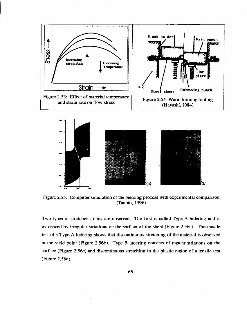
stra in RateCO IncreasingTemperature

StrainFigure 2.53: Effect of material temperature

and strain rate on flow stress

Rlank b o r d e rM a i n p t i n c h

i t i cS t e e l s h e e t P«nch

Figure 2.54 Warm forming tooling (Hayashi, 1984)

.Tat .im

Figure 2.55: Computer simulation of the piercing process with experimental comparison(Taupin, 1996)

Two types of stretcher strains are observed. The first is called Type A ludering and is

evidenced by irregular striations on the surface o f the sheet (Figure 2.56a). The tensile

test of a Type A ludering shows that discontinuous stretching of the material is observed

at the yield point (Figure 2.56b). Type B ludering consists of regular striations on the

surface (Figure 2.56c) and discontinuous stretching in the plastic region of a tensile test

(Figure 2.56d).

66

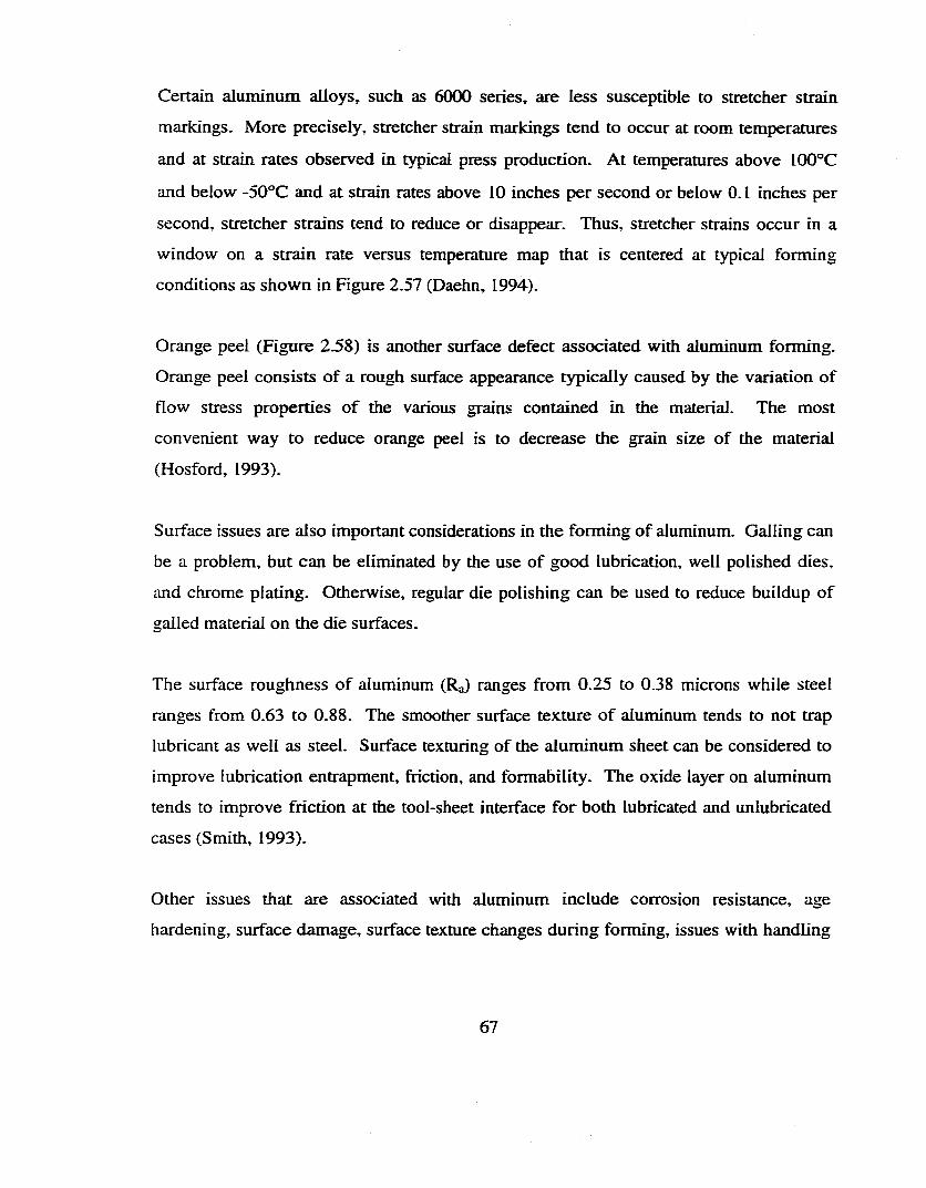
Certain aluminum alloys, such as 6000 series, are less susceptible to stretcher strain

markings. More precisely, stretcher strain markings tend to occur at room temperatures

and at strain rates observed in typical press production. At temperatures above IOO°C

and below -50°C and at strain rates above 10 inches per second or below 0.1 inches per

second, stretcher strains tend to reduce or disappear. Thus, stretcher strains occur in a

window on a strain rate versus temperature map that is centered at typical forming

conditions as shown in Figure 2.57 (Daehn, 1994).

Orange peel (Figure 2.58) is another surface defect associated with aluminum forming.

Orange peel consists of a rough surface appearance typically caused by the variation of

flow stress properties o f the various grains contained in the material. The most

convenient way to reduce orange peel is to decrease the grain size of the material

(Hosford, 1993).

Surface issues are also important considerations in the forming of aluminum. Galling can

be a problem, but can be eliminated by the use of good lubrication, well polished dies,

and chrome plating. Otherwise, regular die polishing can be used to reduce buildup of

galled material on the die surfaces.

The surface roughness of aluminum (RJ ranges from 0.25 to 0.38 microns while steel

ranges from 0.63 to 0.88. The smoother surface texture of aluminum tends to not trap

lubricant as well as steel. Surface texturing of the aluminum sheet can be considered to

improve lubrication entrapment, friction, and formability. The oxide layer on aluminum

tends to improve friction at the tool-sheet interface for both lubricated and unlubricated

cases (Smith, 1993).

Other issues that are associated with aluminum include corrosion resistance, age

hardening, surface damage, surface texture changes during forming, issues with handling

67

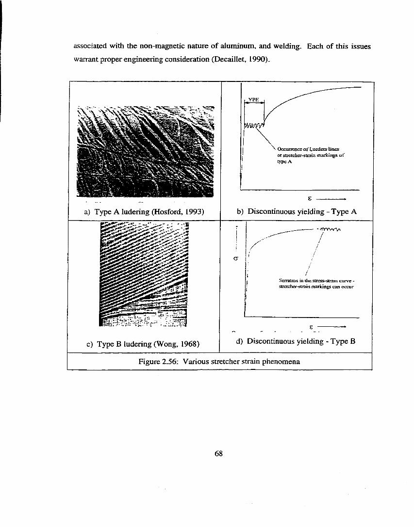
associated with the non magnetic nature of aluminum, and welding. Each of this issues

warrant proper engineering consideration (Decaiilet, 1990).

a) Type A ludering (Hosford, 1993)

YPE

\\ Occuncncc of Lucdea tines

or sirclchcr.5tnnn m aiiin g s o f type .A.

b) Discontinuous yielding - Type A

c) Type B ludering (Wong, 1968)

Scrratton itt tlicstrcsS'SCniiL curve - strcccher-strsin markings can occur

d) Discontinuous yielding - Type B

Figure 2.56: Various stretcher strain phenomena

68

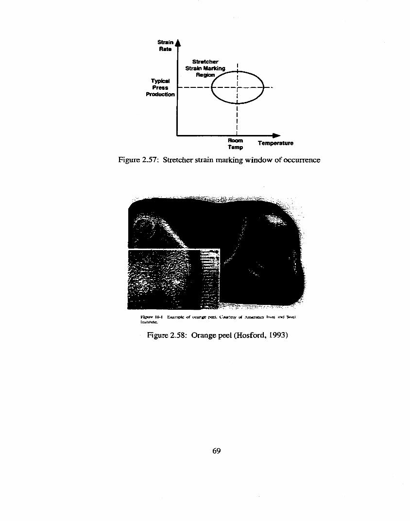
s t r a in A R a te

S tr e tc t ie r S tra in M ark ing

Region^^TypicalP r e s s

P ro d u c tio n

RoomT em p

T e m p e ra tu re

Figure 2.57: Stretcher strain marking window of occurrence

Kitrnrv 16-1 B u in p lc o f o n r g e po d . C o u rto y of A m o n a ia Irms r d Srud ItiUajic,

Figure 2.58: Orange peel (Hosford, 1993)

69

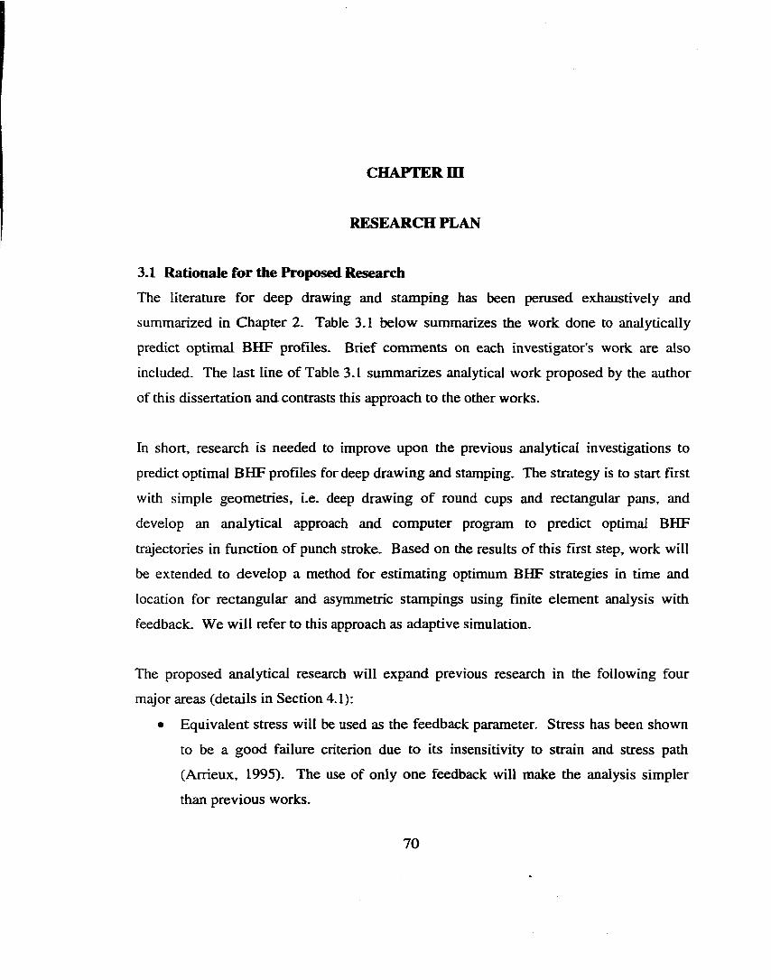
CHAPTER in

RESEARCH PLAN

3.1 Rationale for the Proposed ResearchThe literature for deep drawing and stamping has been perused exhaustively and

summarized in Chapter 2. Table 3.1 below summarizes the work done to analytically

predict optimal BHF profiles. Brief comments on each investigator's work are also

included. The last line of Table 3.1 summarizes analytical work proposed by the author

of this dissertation and contrasts this approach to the other works.

In short, research is needed to improve upon the previous analytical investigations to

predict optimal BHF profiles for deep drawing and stamping. The strategy is to start first

with simple geometries, i.e. deep drawing of round cups and rectangular pans, and

develop an analytical approach and computer program to predict optimal BHF

trajectories in function of punch stroke. Based on the results of this first step, work will

be extended to develop a method for estimating optimum BHF strategies in time and

location for rectangular and asymmetric stampings using finite element analysis with

feedback. We will refer to this approach as adaptive simulation.

The proposed analytical research will expand previous research in the following four

major areas (details in Section 4.1):

• Equivalent stress will be used as the feedback parameter. Stress has been shown

to be a good failure criterion due to its insensitivity to strain and stress path

(Arrieux, 1995). The use of only one feedback will make the analysis simpler

than previous works.

7 0

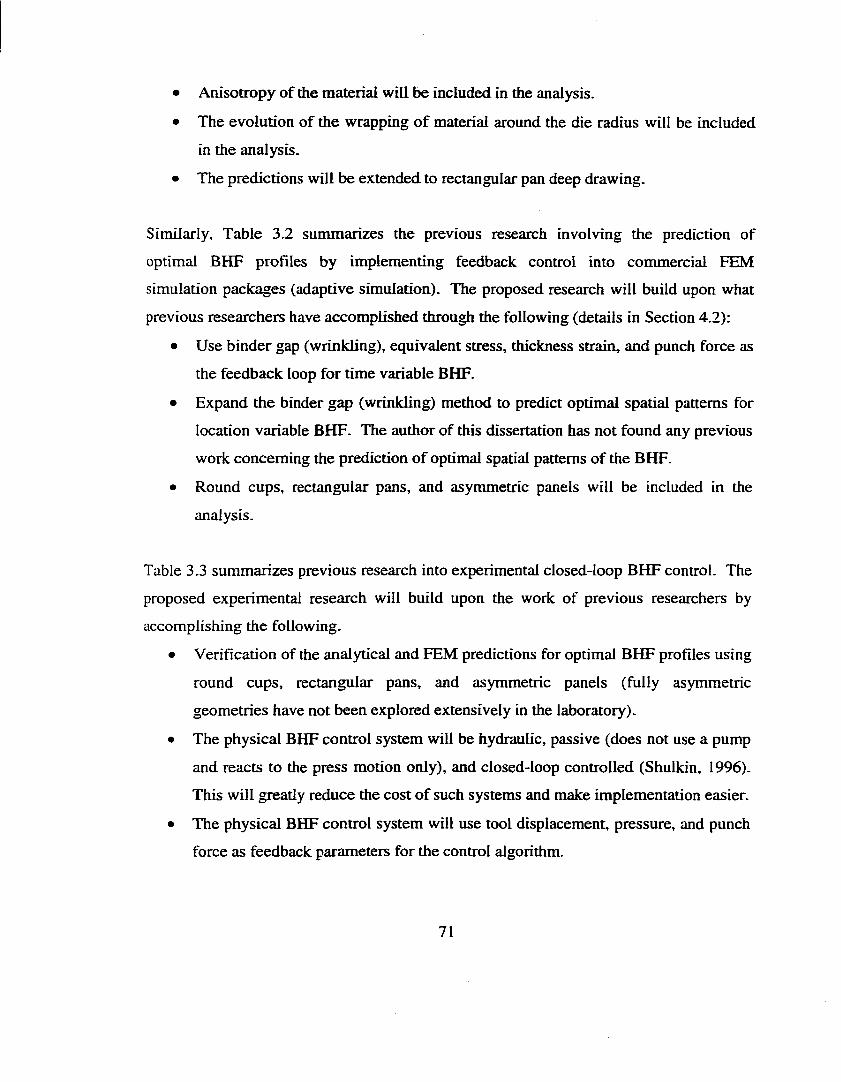
• Anisotropy of the material will be included in the analysis.

• The evolution of the wrapping o f material around the die radius will be included

in the analysis.

• The predictions will be extended to rectangular pan deep drawing.

Similarly, Table 3.2 summarizes the previous research involving the prediction of

optimal BHF profiles by implementing feedback control into commercial FEM

simulation packages (adaptive simulation). The proposed research will build upon what

previous researchers have accomplished through the following (details in Section 4.2):

• Use binder gap (wrinkling), equivalent stress, thickness strain, and punch force as

the feedback loop for time variable BHF.

• Expand the binder gap (wrinkling) method to predict optimal spatial patterns for

location variable BHF. The author of this dissertation has not found any previous

work concerning the prediction of optimal spatial patterns of the BHF.

• Round cups, rectangular pans, and asymmetric panels will be included in the

analysis.

Table 3.3 summarizes previous research into experimental closed-loop BHF control. The

proposed experimental research will build upon the work of previous researchers by

accomplishing the following.

• Verification of the analytical and FEM predictions for optimal BHF profiles using

round cups, rectangular pans, and asymmetric panels (fully asymmetric

geometries have not been explored extensively in the laboratory).

• The physical BHF control system will be hydraulic, passive (does not use a pump

and reacts to the press motion only), and closed-loop controlled (Shulkin, 1996).

This will greatly reduce the cost of such systems and make implementation easier.

• The physical BHF control system will use tool displacement, pressure, and punch

force as feedback parameters for the control algorithm.

71

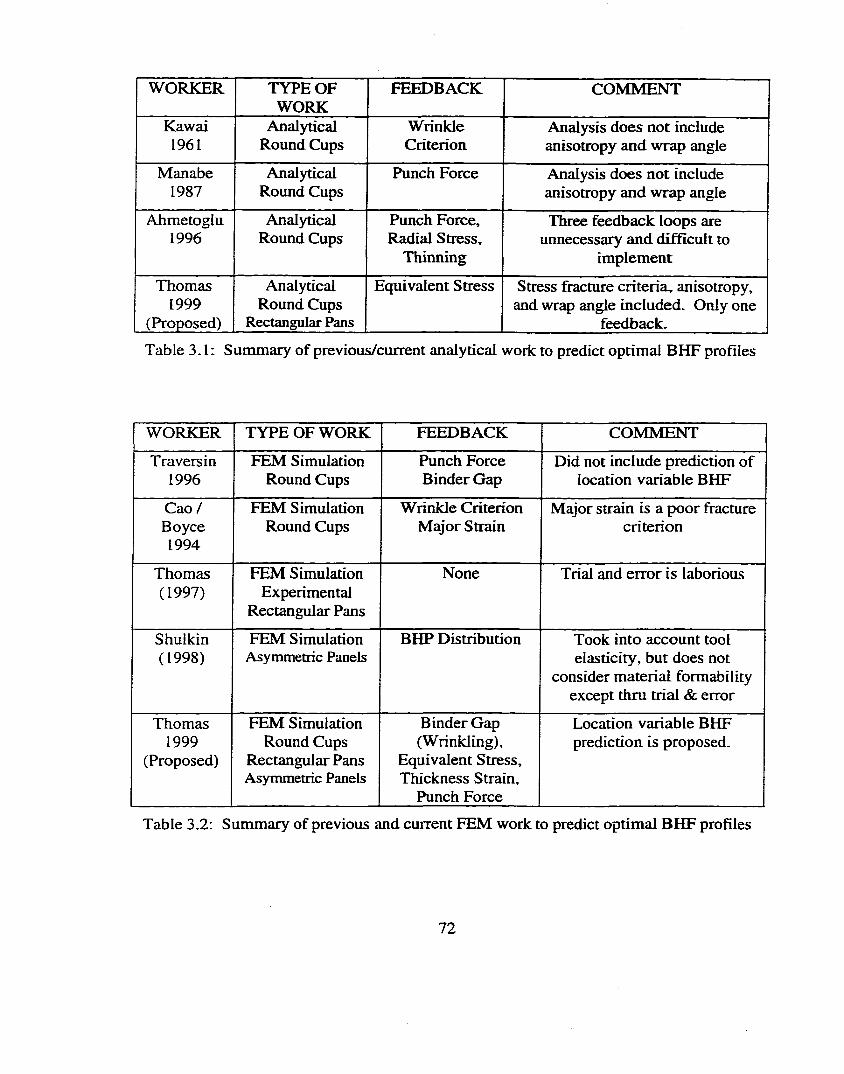
WORKER TYPE OF WORK

FEEDBACK COMMENT

Kawai1961

Analytical Round Cups

WrinkleCriterion

Analysis does not include anisotropy and wrap angle

Manabe1987

Analytical Round Cups

Punch Force Analysis does not include anisotropy and wrap angle

Ahmetoglu1996

Analytical Round Cups

Punch Force, Radial Stress,

Thinning

Three feedback loops are unnecessary and difficult to

implement

Thomas1999

(Proposed)

Analytical Round Cups

Rectangular Pans

Equivalent Stress Stress fracmre criteria, anisotropy, and wrap angle included. Only one

feedback.

Table 3.1: Summary of previous/current analytical work to predict optimal BHF profiles

WORKER TYPE OF WORK FEEDBACK COMMENT

Traversin1996

FEM Simulation Round Cups

Punch Force Binder Gap

Did not include prediction of location variable BHF

Cao / Boyce 1994

FEM Simulation Round Cups

Wrinkle Criterion Major Strain

Major strain is a poor fracture criterion

Thomas(1997)

FEM Simulation Experimental

Rectangular Pans

None Trial and error is laborious

Shulkin(1998)

FEM Simulation Asymmetric Panels

BHP Distribution Took into account tool elasticity, but does not

consider material formability except thru trial & error

Thomas1999

(Proposed)

FEM Simulation Round Cups

Rectangular Pans Asymmetric Panels

Binder Gap (Wrinkling),

Equivalent Stress, Thickness Strain,

Punch Force

Location variable BHF prediction is proposed.

Table 3.2: Summary of previous and current FEM work to predict optimal BHF profiles

72

WORKER TYPE OF WORK FEEDBACK COMMENT

Kergen1992

Experimental Round Cups

Punch Force Binder Gap

Binder gap feedback does not attempt to maximize stress in

part.

Siegert1998

Experimental Round Cups

Punch Force Binder Gap

Friction Force Draw In

Based on time consuming constant BHF experiments

Doege1995

Experimental 4 Side Asymmetric

Spatial Control

Punch Force Spatial Control

proportional to side length

Based on time consuming constant BHF experiments

Hardt1993

Experimental Round Cups

Square Asymmetric

Punch Force Thickening

Based on time consuming constant BHF experiments

Manabe1995

Experimental Fuzzy Control Round Cups

Draw Ratio Thickening

Punch force is a poor fracture criterion

Osakada1995

Experimental Round Cups

ThinningThickening

Thinning is a poor fracture criterion

Thomas1999

(Proposed)

Experimental Round Cups

Rectangular Pans Asymmetric Panels

Closed-loop control, analytical,

numerical, and empirically

predicted BHF profiles.

Verify predicted time and location variable BHF profiles

using a passive, hydraulic, closed and open-loop BHF control system. Time and

expense will be saved.

Table 3.3: Summary of previous and current experimental work to predict optimal BHFprofiles

3.2 Research ObjectivesThe objectives of the proposed research are to:

• Develop a part and process design methodology for the deep drawing and

stamping of sheet metal parts that will lead to a robust process with improved part

quality.

73

Develop a mathematical model and computer software that allows engineers to

calculate forming forces, formability limits, required tool geometry, and optimal

BHF profiles for simple part geometries such as round cups, rectangular pans, U-

channels, hemispherical shells, and asymmetric panels.

Develop a module for commercial finite element method (FEM) programs that

implements a feedback loop into the calculations (adaptive simulation) in order to

determine optimal BHF time trajectories and spatial patterns for general complex

geometries.

• Develop computerized tools that provide engineers with the effect of process

parameters on part quality (sensitivity data) for various simple tool geometries

using laboratory experiments and computer simulations.

The scope of this dissertation consists of:

• Sheet metal parts ranging from cylindrical shells to complex automotive body

panels.

• Materials ranging from drawing quality steel, high strength steel, dent resistant

steel, and aluminum alloys (2000, 3000,5000, and 6000 series).

3.3 Research ApproachThis research will be completed in six phases as follows:

Phase 1

Phase 2

Phase 3

Conduct Literature Review

Build New Laboratory Tooling

Develop Analytical Models to Predict Optimal BHF Profiles forSimple Geometries

Phase 4: Develop a Module for a Commercial E^M Code to Predict OptimalBHF Profiles for Complex Geometries (Adaptive Simulation)

Phase 5: Conduct Experiments and Validate Models

Phase 6 : Develop Sheet Forming Design Methodology

Phase 7: Deliver Research Results

74

3.4 Research PlanA detailed description of the seven phases of this research is given.

Phase 1: Conduct Literature Review

The objective of this phase is:

• To conduct a literature review to understand the current industrial part and

process design methodology for sheet metal stampings.

The tasks of this phase are:

1.1: Conduct a literature review of deep drawing and stamping.

1.2: Outline the current design process from concept to production.

1.3: Identify the tools that are needed by engineers to improve the current design

process. Determine the format of these tools and when in the design process are

they needed.

1.4: Collect all available part and process design rules from literamre and the current

research and put them in a computer module for easy use by an engineer.

Phase 2: Build New Laboratory Tooling

The objective of this phase is:

• To design, validate, build, and test new laboratory tooling.

The tasks of this phase are:

2.1: Design, validate, build, and test a new rectangular pan deep draw tooling for the

purpose of investigating time and location variable BHF control (see Figure 3.3).

2.2: Design, validate, build, and test a new asymmetric panel stretch-draw tooling for the

purpose of investigating the automotive outer body panel stamping process (see

Figure 3.7).

75

Phase 3: Develop Analytical Models to Predict Optimal BHF Profiles fo r Simple

Geometries

The objective of this phase is:

• To develop analytical models of the deep drawing o f round cups and rectangular

pans in order to calculate optimum BHF profiles and to create computer based

tools using these derivations.

The tasks of this phase are:

3.1: Develop equations for calculating optimal BHF profiles for round cup and

rectangular pan deep drawing. These derivations are included in Section 4.1.

3.2: Implement these derivations and other useful equations into a computer module.

This sheet forming design system will include the following types of calculations:

• Round Cups and Rectangular Pan Deep Drawing

• Optimal BHF Time Profiles

• Minimum and Maximum Constant BHF

• Load Versus Stroke

• Limiting Draw Ratio

• Drawbead Forces and Geometry

• Blank Shapes

• Forming Limit Diagrams

Phase 4: Develop a Module fo r a Commercial FEM Code to Predict Optimal BHF

Profiles fo r Complex Geometries (Adaptive Simulation)

The objective of this phase is:

• To implement a feedback loop into a commercially available analysis software

(adaptive simulation) in order to determine optimum BHF time profiles and

spatial patterns for complex geometries.

76

The tasks of this phase are:

4 .1 : "Manually" control an E^M simulation at discrete time intervals in order to prove

the concept of implementing a feedback loop for the prediction of optimal BHF time

profiles and spatial patterns for round, rectangular, and asymmetric parts.

4.2: Upgrade the commercially available FEM simulation software Pam-Stamp with a

closed-loop controller which will allow the prediction of optimal BHF time and

location variable profiles for any general geometry and process. The methodology

is outlined in Section 4.2.

Phase 5: Conduct Experiments and Validate Models

The objectives of this phase are:

• To vahdate the analytical tools with extensive laboratory experiments.

• To test these analytical tools in an industrial setting.

A series of experiments will be conducted at the ERC/NSM laboratories. These

experiments will be conducted in a 160 ton hydraulic Minster press with numerically

controlled (NC) die cushion (see Figure 3.1 and Table 3.4). The tasks of this phase are:

5 . 1 : Round Cup Deep Drawing Experiments (6 ” diameter, 7” deep, see Figure 3.2)

• Conduct full sensitivity analysis with experiments and simulations in order to

determine to the effect of all relevant process parameters on product quality.

• Verify predicted time variable BHF profiles from analytical equations and

FEM simulations using the NC press cushion (see Figure 3.1).

• Verify the blank shape prediction of analytical equations and one-step FEM.

• Investigate the formability of aluminum 6111-T4, AKDQ, bake hard, and high

strength steel.

77

5.2: Rectangular Pan Deep Drawing Experiments (12” by 15”, 7” deep, see Figure 33

through 3-6)

• Conduct full sensitivity analysis with experiments and simulations in order to

determine to the effect o f all relevant process parameters on product quality.

• Verify predicted time variable BHF profile from analytical equations using the

NC press cushion (see Figure 3.1).

• Verify predicted time and location variable BHF profiles from FEM

simulations using the hydraulic BHF control system (see Figure 2.32).

• Verify the blank shape prediction of analytical equations and one-step FEM.

• Investigate the formability of aluminum alloys 2008-T4, 3(X)3-H13, 6111-T4,

and AKDQ steel.

5.3: Asymmetric Panel Stretch-Draw Experiments (17” by 24”, 3” deep, see Figure 3.7

through 3.11)

• Conduct full sensitivity analysis with experiments and simulations in order to

determine to the effect of all relevant process parameters on product quality.

• Determine the interaction of BHF, drawbeads, and stopblocks (see Figure

3.7).

• Determine the effect of pad pressure on distortions caused by embossing (see

Figure 3.8 and 2.9).

• Investigate the formability of AKDQ steel.

5.4: Industrial Validation

• Test the tools developed in this project in an actual industrial setting. The

following phases of the current design process with be tested using the

proposed design methodology:

1. Product Design — Light Weight Closure and Cab Comer Case Study

2. Soft Tooling Tryout - Deck Lid Case Smdy

3. Hard Tooling Tryout - Fender and Door Outer Case Study

78

4. Production - Wheel Housing Case Study

Phase 6: Develop Sheet Forming Design Methodology

The objective of this phase is:

• To develop a sheet forming design methodology and the associated tools needed

to aid an engineer in the design of better sheet metal parts and processes.

The tasks of this phase are:

6 . 1 : To outline a new concept to production process utilizing these tools.

6.2: To develop educational modules which will instruct the engineer on the use o f the

proposed design methodology and associated tools. The modules will include:

• Sheet Forming Design Methodology

• Fundamentals of Deep Drawing and Stamping

• Presses and Equipment

• Tools and Dies

• Formability and Failure of Materials

• Friction and Lubrication

• Product Quality in Sheet Forming

• New Technologies in Sheet Forming (BHF control, hydroforming, tailor

welded blanks, light weight materials, warm forming, surface texturing)

• Database of Sensitivity Data (bending, flanging, hemming, drawbeads, U-

channels, round cups, rectangular pans, asymmetric panels)

• The Finite Element Method and Simulation Methodology (incremental and

one-step FEM)

• Industrial Case Studies (doors, deck lid, cabin inner, fender, roof, wheel

housings, cab comer)

79

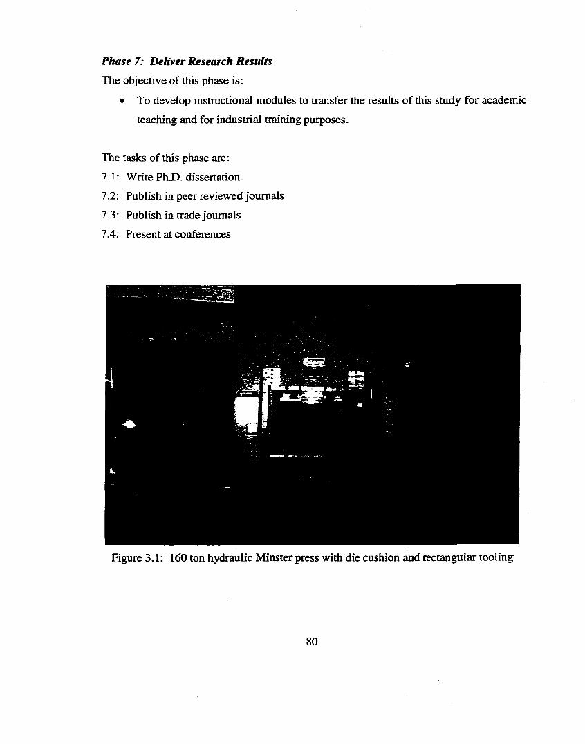
Phase 7: Deliver Research Results

The objective of this phase is:

• To develop instructional modules to transfer the results of this study for academic

teaching and for industrial training purposes.

The tasks of this phase are:

7 . 1 : Write PhD . dissertation.

7.2: Publish in peer reviewed journals

7.3: Publish in trade journals

7.4: Present at conferences

Figure 3.1: 160 ton hydraulic Minster press with die cushion and rectangular tooling

80

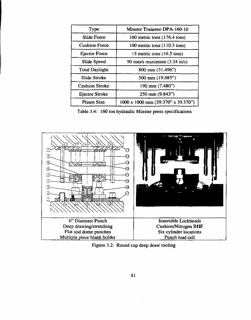
Type Minster Tranemo DPA-160-10

Slide Force 160 metric tons (176.4 tons)

Cushion Force 100 metric tons (110.3 tons)

Ejector Force 15 metric tons ( 16.5 tons)

Slide Speed 90 mm/s maximum (3.54 in/s)

Total Daylight 800 mm (31-496”)

Slide Stroke 500 mm (19.685”)

Cushion Stroke 190 mm (7.480”)

Ejector Stroke 250 mm (9.843”)

Platen Size 1000 X 1000 mm (39.370” x 39.370”)

Table 3.4: 160 ton hydraulic Minster press speciOcations

G

^

6 ” Diameter Punch Deep drawing/stretching Flat and dome punches

Multiple piece blank holder

Insertable Lockbeads Cushion/Nitrogen BHF Six cylinder locations

Punch load cell

Figure 3.2: Round cup deep draw tooling

81

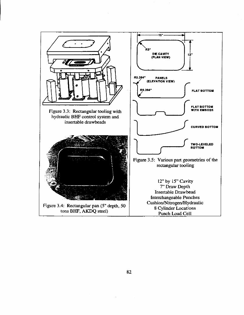
- 15 -

Figure 3.3: Rectangular tooling with hydraulic BHF control system and

insertable drawbeads

Figure 3.4: Rectangular pan (5" depth, 50 tons BHF, AKDQ steel)

f<TR 3 -

OIE CAVITY (PLAN VIEW)

1 2 -

R 0 .3 9 4 - PANELS _ y (ELEVATION VIEW)

R 0 J 9 4 - //

FLAT BOTTOM

%

/ /

FLAT BOTTOM WITH E M B O SS

CURVED BOTTOM

TW O LEVELED BOTTOM

Figure 3.5: Various part geometries of the rectangular tooling

12” by 15” Cavity 7” Draw Depth

Insertable Drawbead Interchangeable Punches

Cushion/Nitrogen/Hydraulic 8 Cylinder Locations

Punch Load Cell

82

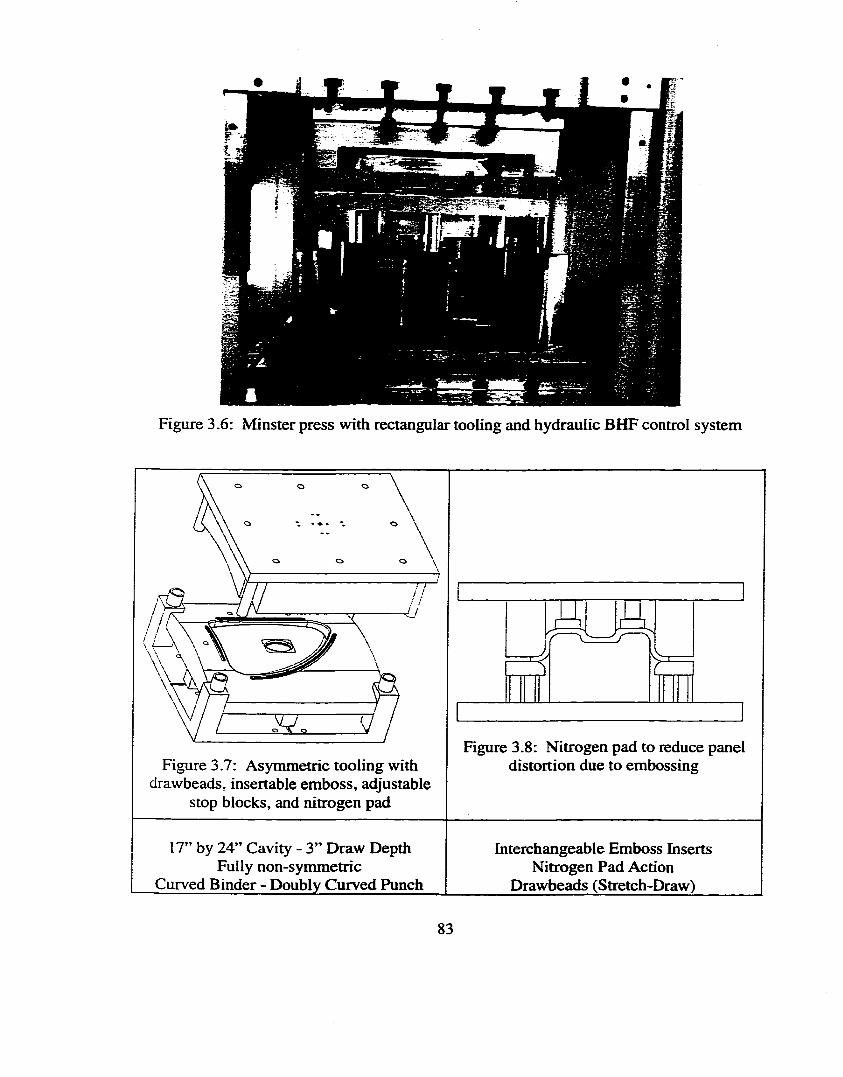
Figure 3.6: Minster press with rectangular tooling and hydraulic BHF control system

Figure 3.7: Asymmetric tooling with drawbeads, insertable emboss, adjustable

stop blocks, and nitrogen pad

Figure 3.8: Nitrogen pad to reduce panel distortion due to embossing

17” by 24” Cavity - 3” Draw Depth Fully non-symmetric

Curved Binder - Doubly Curved Punch

Interchangeable Emboss Inserts Nitrogen Pad Action

Drawbeads (Stretch-Draw)

83

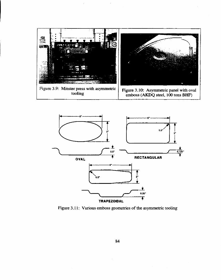
Figure 3.9: Minster press with asymmetric tooling

Figure 3.10: Asymmetric panel with oval emboss (AKDQ steel, ICO tons BHF)

OVAL

f{ 0.S-

0.5"

G

" 70.5"

RECTANGULAR

T2"

1

. _ t0.125-

0.25"

TTRAPEZOIDAL

Figure 3.11: Various emboss geometries o f the asymmetric tooling

84

CHAPTER IV

ANALYTICAL AND NUMERICAL MODELING OF DEEP DRAWING AND STAMPING

4.1 Deep Drawing of Basic Geometries — Predicting Optimal BHF Profiles4.1.1 Conceptual Approach

In order to determine the optimum variation of the BHF in function of time for round cup

deep drawing, the drawing load will be mathematically derived in terms of the process

parameters. Once the drawing load is known, the equations will be solved for BHF. The

final step will be to apply a failure criterion which involves the drawing load. This will

completely solve the equations for BHF. These equations will then be adapted to predict

optimal BHF profiles for deep drawing of a rectangular pan.

Siebel (1955) developed a closed form solution for the drawing load of round cups as

explained in Section 2.4.1. These equations did not take into account material anisotropy

or the evolution of material wrap around the die radius. The current work will take these

into account so that the drawing load can be calculated more accurately.

Further, previous researchers used rather unreliable failure criteria as part of their

analyses (see Sections 2.3.4, 2.4.3 and 3.1). Equivalent stress will be used as the failure

criterion because of its insensitivity to stress and strain path (Arrieux, 1995). Anisotropy

and thinning will also be included to improved upon Siebel’s failure criterion. This

should help to ensure the accuracy of the BHF profile that is predicted.

85

4.L2 Round Cup Deep Drawing - Analytical Derivations

Siebel divided the round cup geometry into four deformation zones: I) radial drawing in

the flange, 2) bending at the die radius, 3) friction in the flange, and 4) friction at the die

radius. He developed equations for the required forces for each o f these sections and then

summed them to obtain the drawing load. The following derivations are based on the

work of Siebel ( 1955). The author o f this dissertation has made various improvements as

was previously proposed in order to increase the accuracy o f the predictions.

Siebel (1955) analyzed the radial drawing in the flange as follows using the model and

conventions in Figures 4.1 and 4.2 (symbols are given in Figure 2.40 and the

Nomenclature section). He assumed that no thickening occurred in the flange.

Radial Direction :

(cr^ -td(j^){r + dr)dpÎQ —(T^rdPto +2[<T,|roJrsin

Replace sin

= 0(Equations 4.1 )

w ith f^ ^ and neglect product of differentials. (Siebel, 1955)I -

d(J^ — —((%r ) ----r

At this point. Siebel uses an isotropic yield criterion. In order to introduce anisotropy, the

author of this dissertation has implemented the work o f Leu ( 1997).

From Leu ( 1997), without any thickness strain in the flange and with Hill's

quadratic normal isotropic yield criterion we obtain : cr - cr =

We substitute into Siebel's work : da^ = — —V l + 2r r

r , , /2 ( l + f) f _ d rIntegrate : d(T =-- J —------- (T —A V l + 2 r 1 r

ov '2 (l + f) f dr (Equations 4.2)

<T,= 0 “ r=ra/2(l-hf), ^

1 + 2?Where <r is the average flow stress in the flange.

86

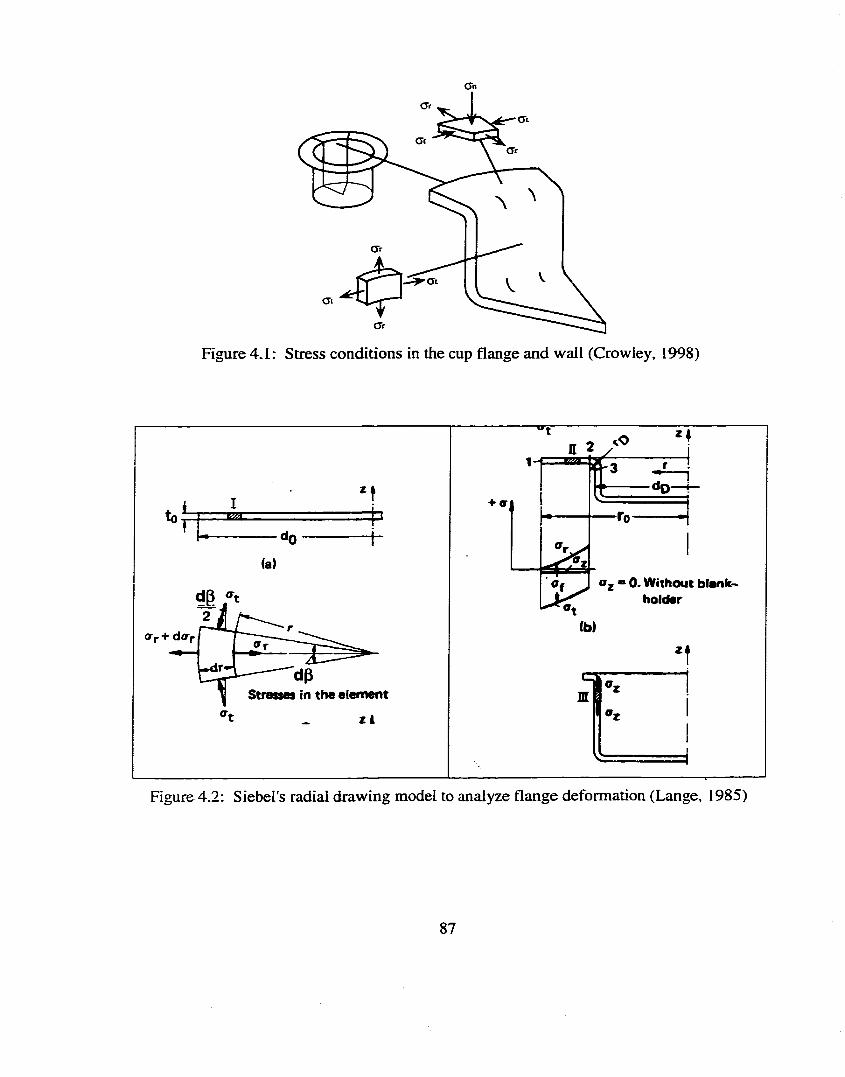
anar

ar

ar

- ^ a tat

at

Figure 4.1: Stress conditions in the cup flange and wall (Crowley, 1998)

1 -f

*2 " 0. Without blanks holder

Stratses in the element

Figure 4.2: Siebel’s radial drawing model to analyze flange deformation (Lange, 1985)

87

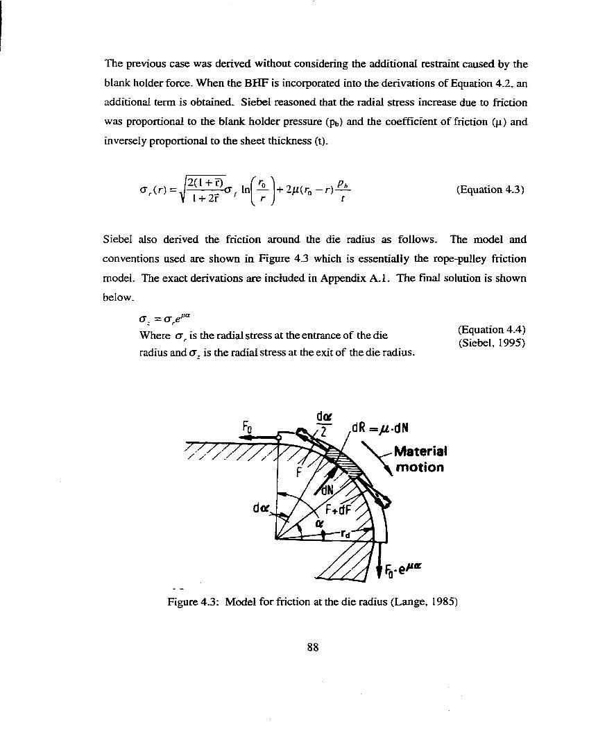
The previous case was derived without considering the additional restraint caused by the

blank holder force. When the BHF is incorporated into the derivations of Equation 4.2, an

additional term is obtained. Siebel reasoned that the radial stress increase due to friction

was proportional to the blank holder pressure (pb) and the coefficient of friction (p.) and

inversely proportional to the sheet thickness (t).

1 + 2F '+ 2 ^ ( r „ - r ) ^ (Equation 4.3)

Siebel also derived the friction around the die radius as follows. The model and

conventions used are shown in Figure 4.3 which is essentially the rope-pulley friction

model. The exact derivations are included in Appendix A .I. The final solution is shown

below.

(J = (j^e^Where cr is the radial stress at the entrance of the die radius and <T, is the radial stress at the exit of the die radius.

(Equation 4.4) (Siebel, 1995)

Materialm otion

dec.

Figure 4.3: M odel for friction at the die radius (Lange, 1985)

88

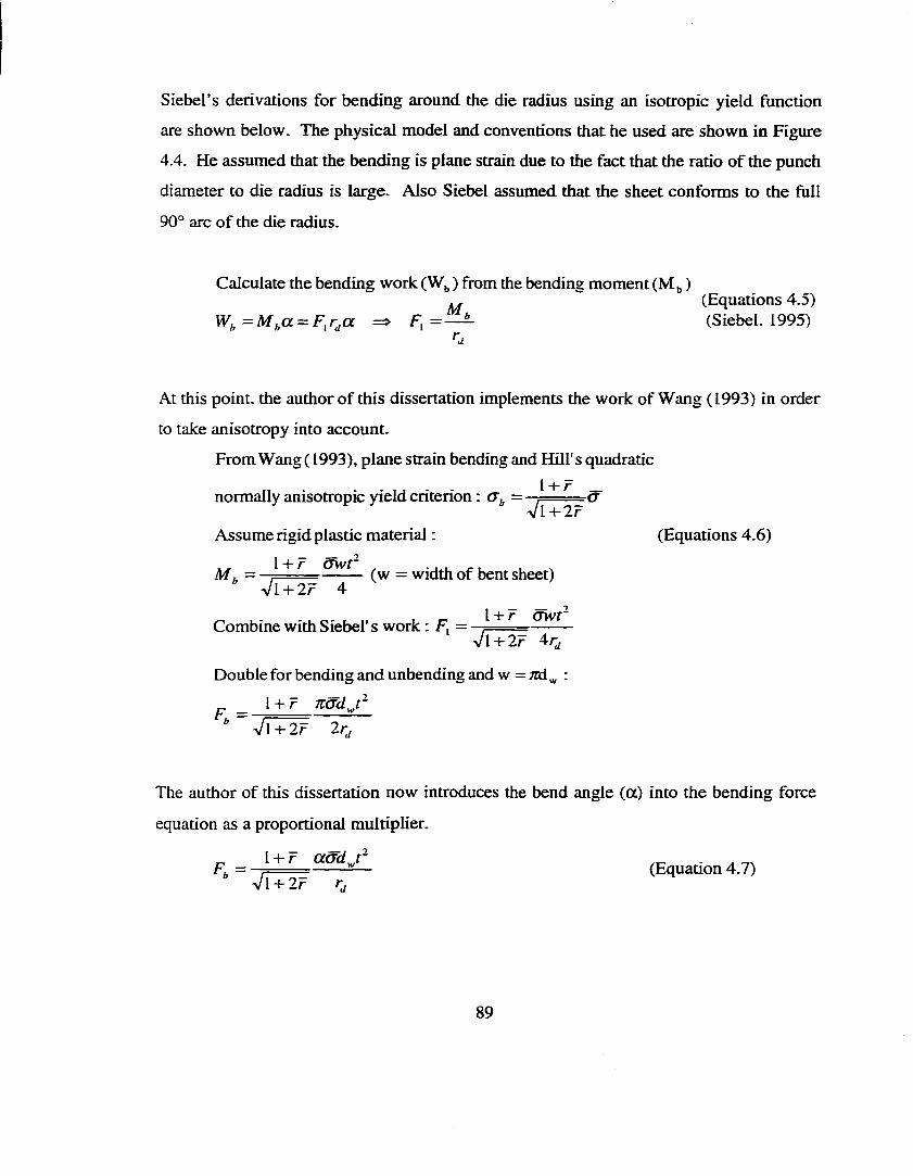
Siebel’s derivations for bending around the die radius using an isotropic yield function

are shown below. The physical model and conventions that he used are shown in Figure

4.4. He assumed that the bending is plane strain due to the fact that the ratio o f the punch

diameter to die radius is large. Also Siebel assumed that the sheet conforms to the full

90° arc o f the die radius.

Calculate the bending work (W^ ) from the bending moment (My )„ (Equations 4.5)

W ,= M ,a = F ,rja => F ,= — ^ (Siebel, 1995)

At this point, the author of this dissertation implements the work of Wang ( 1993) in order

to take anisotropy into account.

From Wang (1993), plane strain bending and Hill's quadratic

normally anisotropic yield criterion : <Jy = - ^ = = = â

Assume rigid plastic material : (Equations 4.6)

M. = (vv = width of bent sheet)Vl + 2 r 4

I + r â w rCombine with Siebel's work : FJ = •V l+ 2 r 4r.

Double for bending and unbending and w = :I + r Kâd...r

b Vl + 2 r 2 d

The author of this dissertation now introduces the bend angle (a) into the bending force

equation as a proportional multiplier.

Fy (Equation 4.7)Vl + 2 r

89

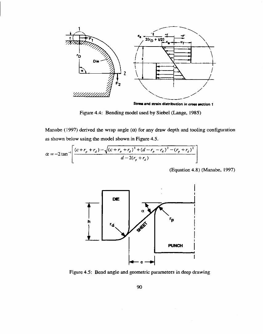
O ie

*<r

2

S tr e n e n d s tra in d is tr ib u t io n in c ro s s se c t io n 1

Figure 4.4: Bending model used by Siebel (Lange, 1985)

Manabe (1997) derived the wrap angle (a) for any draw depth and tooling configuration

as shown below using the model shown in Figure 4.5.

a = —2 tan -I + -h{cl - - r ^ Ÿ “ (/>d - 2 (r^ +r^)

(Equation 4.8) (Manabe, 1997)

OE

PUNCH

Figure 4.5: Bend angle and geometric parameters in deep drawing

90

Combining Equations 4.2, 4.3, 4.4, and 4.7, an expression for the drawing load (Fd) is

found. Please note that this equation takes anisotropy ( r ) and wrap angle (a) into

account, unlike Siebel’s (1955) equation (see Equation 2.12).

(Ty Iny 2(1-hr) l+ 2 f

+ +Vl + 2r ^

(Equation 4.9)

Now that we have a closed form solution for the drawing load o f the round cup deep

drawing process, we solve this equation for the blank holder force (Fy). Solving for BHF

has only been done by one other researcher namely Manabe ( 1987).

P'h =Lv

fia f 2 ( l+ f)I + 2F

atn l + r

yj 2 m

(Equation 4.10)

In order to calculate the instantaneous flange diameter (dp) and the average flow stress in

the flange (crp) and die radius (<Td) please refer to Appendix A.I. In order to calculate the

wrap angle (a), we use Equation 4.8.

Now, the only unknown parameter on the right side of Equation 4.10 is the drawing load

(Fd). We obtain this by utilizing a failure criterion that was proposed by Chiang and

Kobayashi (1966). This failure criterion calculates the maximum drawing load to avoid

failure in the cup. Chiang's criterion takes into account the anisotropy and thinning of the

sheet material. Chiang utilized Holloman’s flow stress laws to derive this criterion. The

author of this dissertation has implemented Swift’s hardening law as shown below.

Starting from Hill’s plane stress normally anisotropic quadratic yield function (Wagoner,

1997):

91

Plane Strain : de^ = 0 => <T, = ■r + I

Assume proportional path : e =

Substitute into Hill's equivalent stress formula : cT =

Instability Criterion for Swift Power Law O' = K ( e +£□)“Fora tensile test : = / ! —£(,

_ r + I _ Combining to obtain plane strain criterion : ... (n -£„ )V2r + 1

Substitute into Swift’s Law : a.. = K r + 1.V2 7 + I

Calculate the thickness at the failure zone

( /I—e o ) - ^ o

Volume Constancy : £ 3 = -£[ => In — = ----- '2^ + 1 gr + 1

VZr + l _ ■£r + 1

Calculate Critical Load

F„ =;rd^to exp(£o -n )Æ

f = fo exp(£g - n )

r + lV2r + l

( « —Cq) “ ^ 0

r + lV2r + l

(Equations 4.11)

4.1.3 Rectangular Pan Deep Drawing Adaptation o f Equations

To expand this work to rectangular pans, we will use the equivalent blank method as

outlined in Section 2.4.1.2. Essentially, equivalent round blanks and tool geometries are

calculated from the rectangular blanks and tool geometries based on equal areas as

follows (symbols are given in Figure 2.42 and the Nomenclature section):

K(Equation 4.12)

This method works extremely well for predicting load versus stroke curves for

rectangular pans as will be shown in Section 4.1.4. This method does not work well for

predicting the optimal BHF profiles. This is due to the fact that the wall stresses are not

92

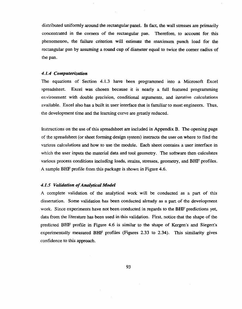
distributed uniformly around the rectangular panel. In fact, the wall stresses are primarily

concentrated in the comers of the rectangular pan. Therefore, to account for this

phenomenon, the failure criterion will estimate the maximum punch load for the

rectangular pan by assuming a round cup of diameter equal to twice the comer radius of

the pan.

4.1.4 Computerization

The equations of Section 4.1.3 have been programmed into a Microsoft Excel

spreadsheet. Excel was chosen because it is nearly a full featured programming

environment with double precision, conditional arguments, and iterative calculations

available. Excel also has a built in user interface that is familiar to most engineers. Thus,

the development time and the learning curve are greatly reduced.

Instructions on the use of this spreadsheet are included in Appendix B. The opening page

of the spreadsheet (or sheet forming design system) instructs the user on where to find the

various calculations and how to use the module. Each sheet contains a user interface in

which the user inputs the material data and tool geometry. The software then calculates

various process conditions including loads, strains, stresses, geometry, and BHF profiles.

A sample BHF profile from this package is shown in Figure 4.6.

4.1.5 Validation o f Analytical Model

A complete validation of the analytical work will be conducted as a part of this

dissertation. Some validation has been conducted already as a part of the development

work. Since experiments have not been conducted in regards to the BHF predictions yet,

data from the literature has been used in this validation. First, notice that the shape of the

predicted BHF profile in Figure 4.6 is similar to the shape o f Kergen's and Siegert’s

experimentally measured BHF profiles (Figures 2.33 to 2.34). This similarity gives

confidence to this approach.

93

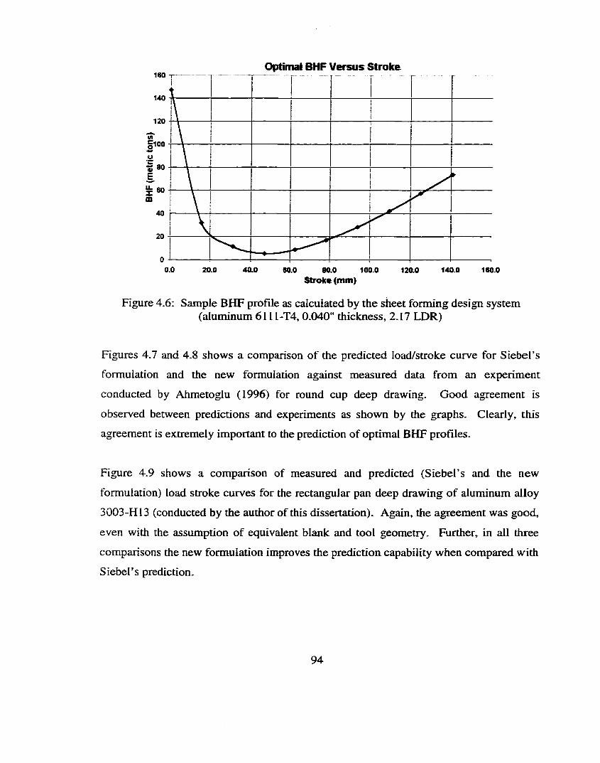
optimal BHF Versus Stroke160 T

140

120

■a 80

40

0.0 20.0 40.0 80.0 80.0 100.0Stroke (mm)

120.0 140.0 160.0

Figure 4.6: Sample BHF profile as calculated by the sheet forming design system (aluminum 6111-T4,0.040" thickness, 2.17 LDR)

Figures 4.7 and 4.8 shows a comparison of the predicted load/stroke curve for Siebel’s

formulation and the new formulation against measured data from an experiment

conducted by Ahmetoglu (1996) for round cup deep drawing. Good agreement is

observed between predictions and experiments as shown by the graphs. Clearly, this

agreement is extremely important to the prediction of optimal BHF profiles.

Figure 4.9 shows a comparison of measured and predicted (Siebel’s and the new

formulation) load stroke curves for the rectangular pan deep drawing o f aluminum alloy

3003-H13 (conducted by the author of this dissertation). Again, the agreement was good,

even with the assumption of equivalent blank and tool geometry. Further, in all three

comparisons the new formulation improves the prediction capability when compared with

Siebel’s prediction.

9 4

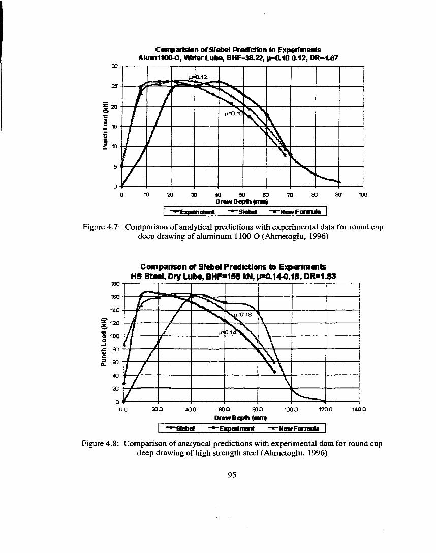
Comparision of Sîebel Predictnii to Experiments Alum1100-0, WMerLube, BHF=38.22, |i=ai0-ai2, DR=1.67

30

25

* 2 0

J 15

1 0 900 2 0 30 40 SO GO 80 10070Draw Depth (nnf

"^Experiment -Siebd •WewFomule

Figure 4.7; Comparison of analytical predictions with experimental data for round cup deep drawing of aluminum 1100-0 (Ahmetoglu, 1996)

Comparison of Siebel Predictions to Experiments HS Steel, Dry Lube, BHF=158 KN, p=0.140.18, DR» 1.83

180

160

140t.18

5 120

a 100

80

40

2 0

200 600 1200 14000.0 400 100.0Draw Depth (mn*

•Siebel -■-Experiment ‘NewFormjia

Figure 4.8: Comparison of analytical predictions with experimental data for round cup deep drawing of high strength steel (Ahmetoglu, 1996)

95

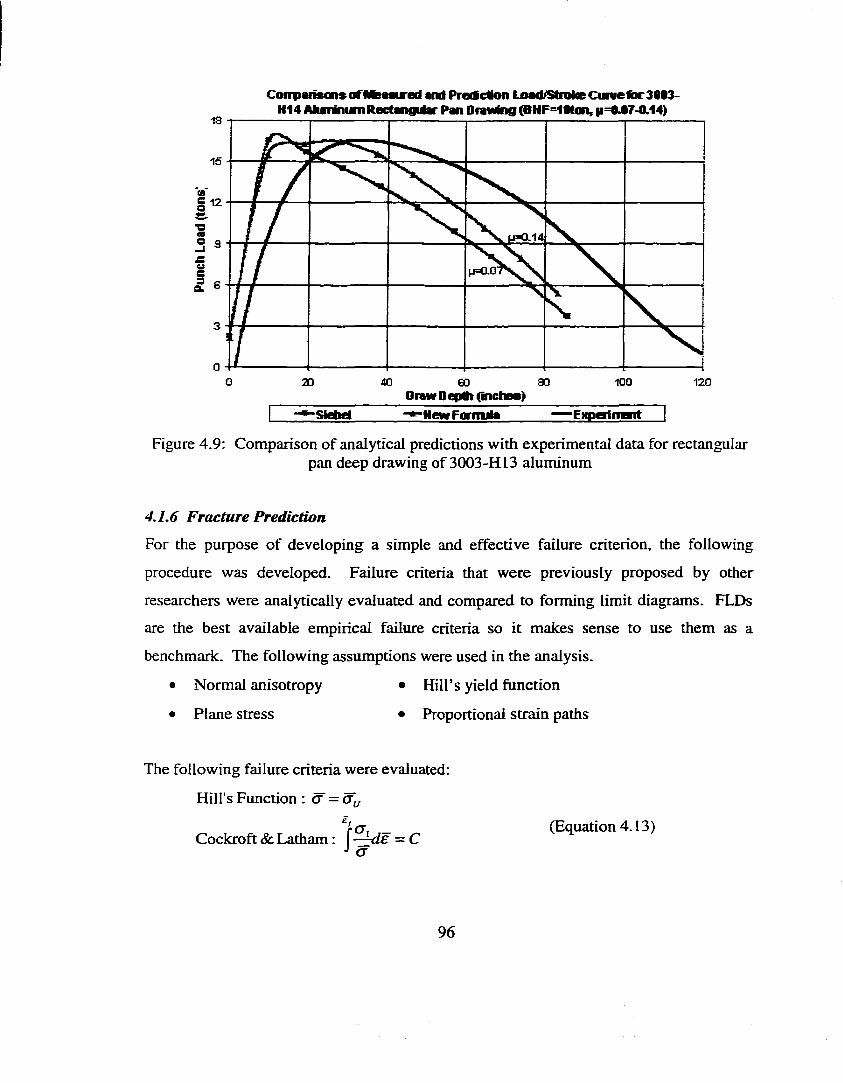
CotiparisonsoTMeMired and Preif cion Loafi/StniteCunie1br3i03-H14 AkannumRectangitfar Pan OmWng (BHF=10ton, p=*.#741.14)

■o

0 100 1202 0 40 8060Oiawr Depit (inches)

Siehel 'NeMrFormjIa •Expert nant

Figure 4.9: Comparison of analytical predictions with experimental data for rectangularpan deep drawing of 3003-H13 aluminum

4.1.6 Fracture Prediction

For the purpose of developing a simple and effective failure criterion, the following

procedure was developed. Failure criteria that were previously proposed by other

researchers were analytically evaluated and compared to forming limit diagrams. FLDs

are the best available empirical failure criteria so it makes sense to use them as a

benchmark. The following assumptions were used in the analysis.

• Normal anisotropy • Hill’s yield function

• Plane stress • Proportional strain paths

The following failure criteria were evaluated:

Hill's Function : a =(T,u

Cockroft & Latham : f = C a

(Equation 4.13)

96

The value C in the Crockroft and Lantham criterion can be evaluated with a tensile test.

Using the above assumptions and the the additional assumption of uniaxial stress in the

tensile test» the integrand becomes unity and the value C becomes exactly equal to the

strain in the axial direction at failure:

C — eA (Equation 4.14)

This simple result will be useful later. One problem with this development is the

assumption of proportional strain paths which is a good assumption in a tensile until

necking begins and is increasingly poor thereafter. Since failure proceeds necking

quickly, the final result is estimated to be within 1 0 % of actual, thus making the

assumption reasonable.

Now, we find the biaxial strain which satisfies each of the failure criteria above. The

same assumptions are made and in each case the integrand becomes constant functions of

material parameters. The following results are obtained:

Crockroft & Lantham : ffill's Function :C ( p / £ / (Equations 4.15)

—

Where p, X., tp, 5 are given as:

^ i ± Z ± I t/ ^ x L + r + r/3

f = J l + A-2FAl + r

(l + F)-1 V ( 1 + 2F)

2rP (1 + F)

(Equations 4.16)

97

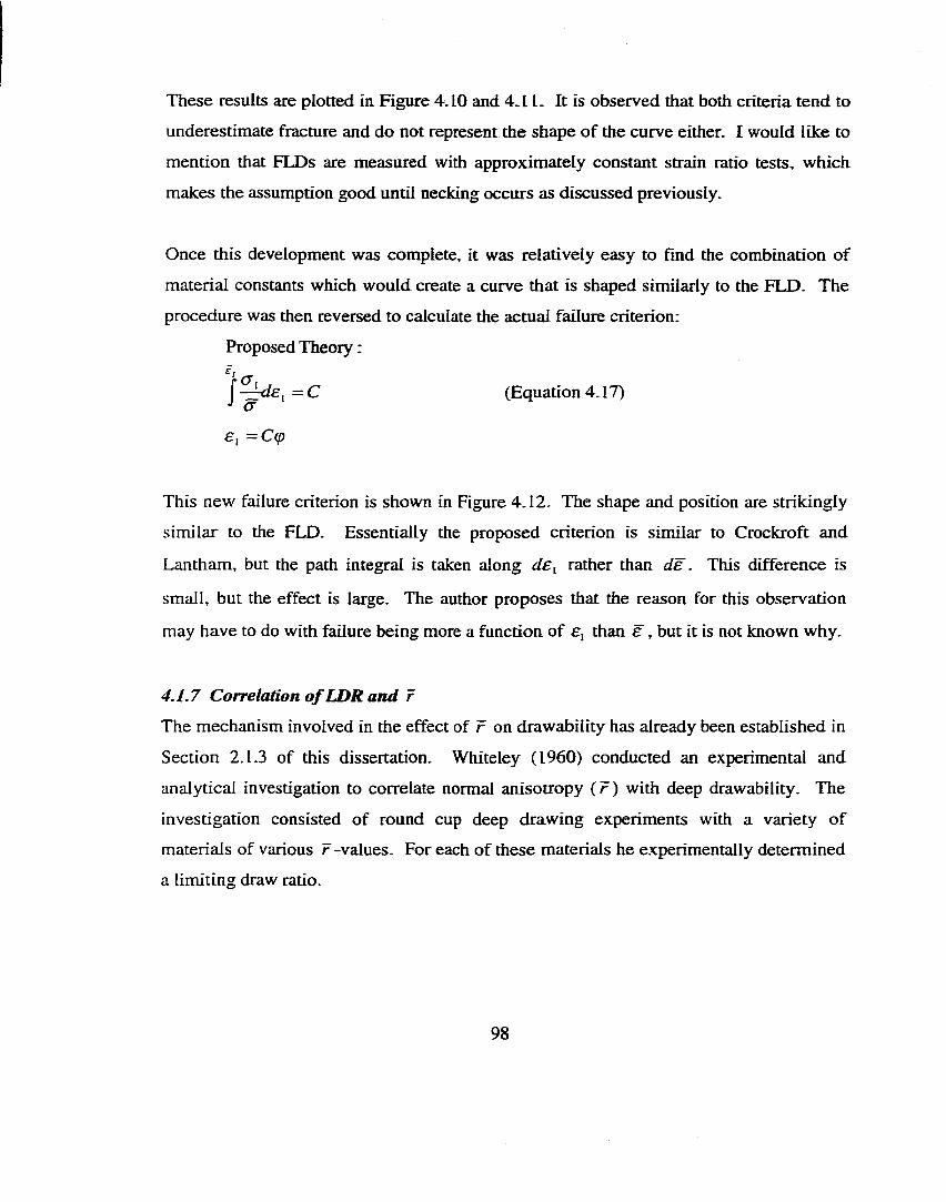
These results are plotted in Figure 4.10 and 4.11. It is observed that both criteria tend to

underestimate fracture and do not represent the shape o f the curve either. I would like to

mention that FLDs are measured with approximately constant strain ratio tests, which

makes the assumption good until necking occurs as discussed previously.

Once this development was complete, it was relatively easy to find the combination of

material constants which would create a curve that is shaped similarly to the FLD. The

procedure was then reversed to calculate the actual failure criterion:

Proposed Theory :

%(J

£, =Cq>

= C (Equation 4.17)J / T

This new failure criterion is shown in Figure 4.12. The shape and position are strikingly

similar to the FIX). Essentially the proposed criterion is similar to Crockroft and

Lantham, but the path integral is taken along de^ rather than de . This difference is

small, but the effect is large. The author proposes that the reason for this observation

may have to do with failure being more a function of e, than ë , but it is not known why.

4.1.7 Correlation o f LDR and ?

The mechanism involved in the effect of r on drawability has already been established in

Section 2.1.3 of this dissertation. Whiteley (1960) conducted an experimental and

analytical investigation to correlate normal anisotropy ( r ) with deep drawability. The

investigation consisted of round cup deep drawing experiments with a variety of

materials of various r -values. For each of these materials he experimentally determined

a limiting draw ratio.

98

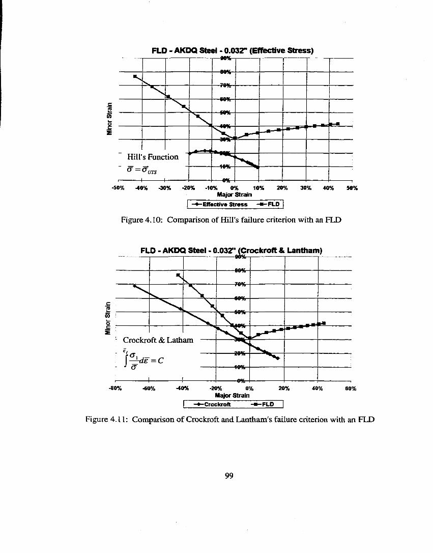
FLD - AKDQ Steel - 0.03Z' (Effècb've S tress)

c2

IHill's Function

«%-•50% -40% -30% 20% -10% 2 0 % 30% 40%1 0 % 50%0 %

M ajor S tra fn

•E ffec tive S t r e s s -FLD

Figure 4.10: Comparison of Hill's failure criterion with an FLD

2

o

------ 90%

_ g -Ji-

^.rucKroiL ot L,aui

J ^ £ = C- ■' ai------------ 1------------

am

------- 0 %-•80% •60% •40% •20% 0%

M ajor S tra in2 0 % 40% 60%

-C ro ck ro ft •FLD

Figure 4.11: Comparison o f Crockroft and Lantham's failure criterion with an FLD

99

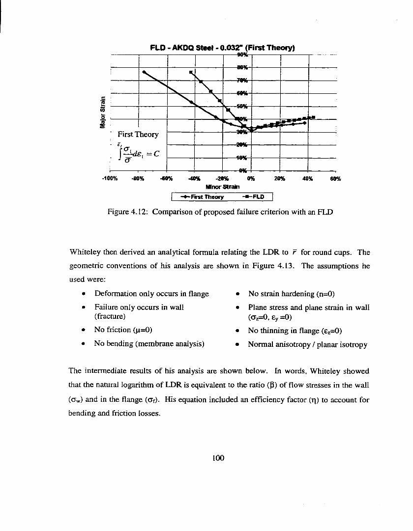
FLD - AKDO Steel - 0.032" (F irst Theory)

Ç2CO

IFirst Theory

4*-100% -60%•80% •40% 0 % 2 0 %-2 0 % 40% 60%

M inor S tra in

-F frst T h eo ry -FLD

Figure 4.12: Comparison of proposed failure criterion with an FLD

Whiteley then derived an analytical formula relating the LDR to r for round cups. The

geometric conventions of his analysis are shown in Figure 4.13. The assumptions he

used were:

Deformation only occurs in flange

Failure only occurs in wall (fracmre)

No friction (p=0)

No bending (membrane analysis)

No strain hardening (n=0)

Plane stress and plane strain in wall(<Tz=0 , £y =0 )

No thinning in flange (Ez=0)

Normal anisotropy / planar isotropy

The intermediate results of his analysis are shown below. In words, Whiteley showed

that the natural logarithm of LDR is equivalent to the ratio (P) of flow stresses in the wall

(CTw) and in the flange (cTf). His equation included an efficiency factor (q) to account for

bending and friction losses.

100

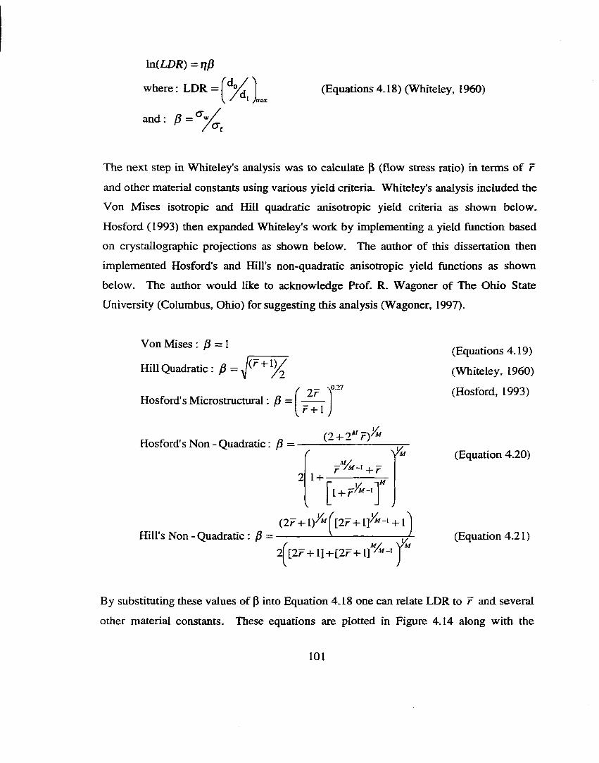
\n{LDR) = T]j3

where: LDR =

and : P = ^ '

(Equations 4.18) (Whiteley, I960)

The next step in Whiteley's analysis was to calculate p (flow stress ratio) in terms of r

and other material constants using various yield criteria. Whiteley's analysis included the

Von Mises isotropic and Hill quadratic anisotropic yield criteria as shown below.

Hosford (1993) then expanded Whiteley's work by implementing a yield function based

on crystallographic projections as shown below. The author of this dissertation then

implemented Hosford's and Hill's non-quadratic anisotropic yield functions as shown

below. The author would like to acknowledge Prof. R. Wagoner of The Ohio State

University (Columbus, Ohio) for suggesting this analysis (Wagoner, 1997).

Von Mises : p = l

Hill Quadratic : P =

Hosford's Microstructural : P = r 2 FF + l

Hosford's Non-Quadratic : P (2 -h2 * 'F )^

1 -f-M/

7 + rAf

Hill's Non - Quadratic : p —(2 F - t- l) '^ f [2 F + l]^ -‘ + l

/ Af/2 [2F + l]-i-[2F + l]^ ''- ' I

(Equations 4.19)

(Whiteley, I960)

(Hosford, 1993)

(Equation 4.20)

(Equation 4.21)

By substituting these values of P into Equation 4.18 one can relate LDR to r and several

other material constants. These equations are plotted in Figure 4.14 along with the

101

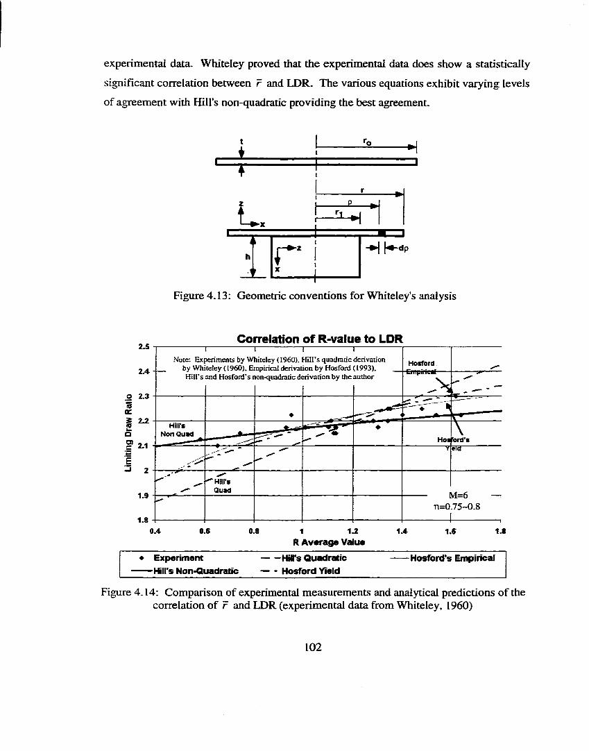
experimental data. Whiteley proved that the experimental data does show a statistically

significant correlation between r and LDR. The various equations exhibit varying levels

of agreement with Hill's non-quadratic providing the best agreement.

T

I rFigure 4.13: Geometric conventions for Whiteley's analysis

Correlation o f R value to LDR2.5

Note: Experiments by Whiteley (I960). Hill’s quadratic derivation by Whiteley ( I960). Empirical derivation by Hosford ( 1993). Hill's and Hosford’s non<(uadratic derivation by the author

HosfordEwpiriesi2 .4 - —

0 2.31 0£

2.2< ►

I Hill’s Non QuadQ

g» 2.1Hos lord's

E3Hill'sQuad M=6

n=0.75~0.81.9

1.80.6 0.8 1.2 1.80 .4 1

R Average Value♦ Experiment ----- Hill's Quadratic -----Hosford's Empirical

------Hill's Non-Quadratic ---- Hosford Yield

Figure 4.14: Comparison of experimental measurements and analytical predictions of the correlation of r and LDR (experimental data from Whiteley, 1960)

102

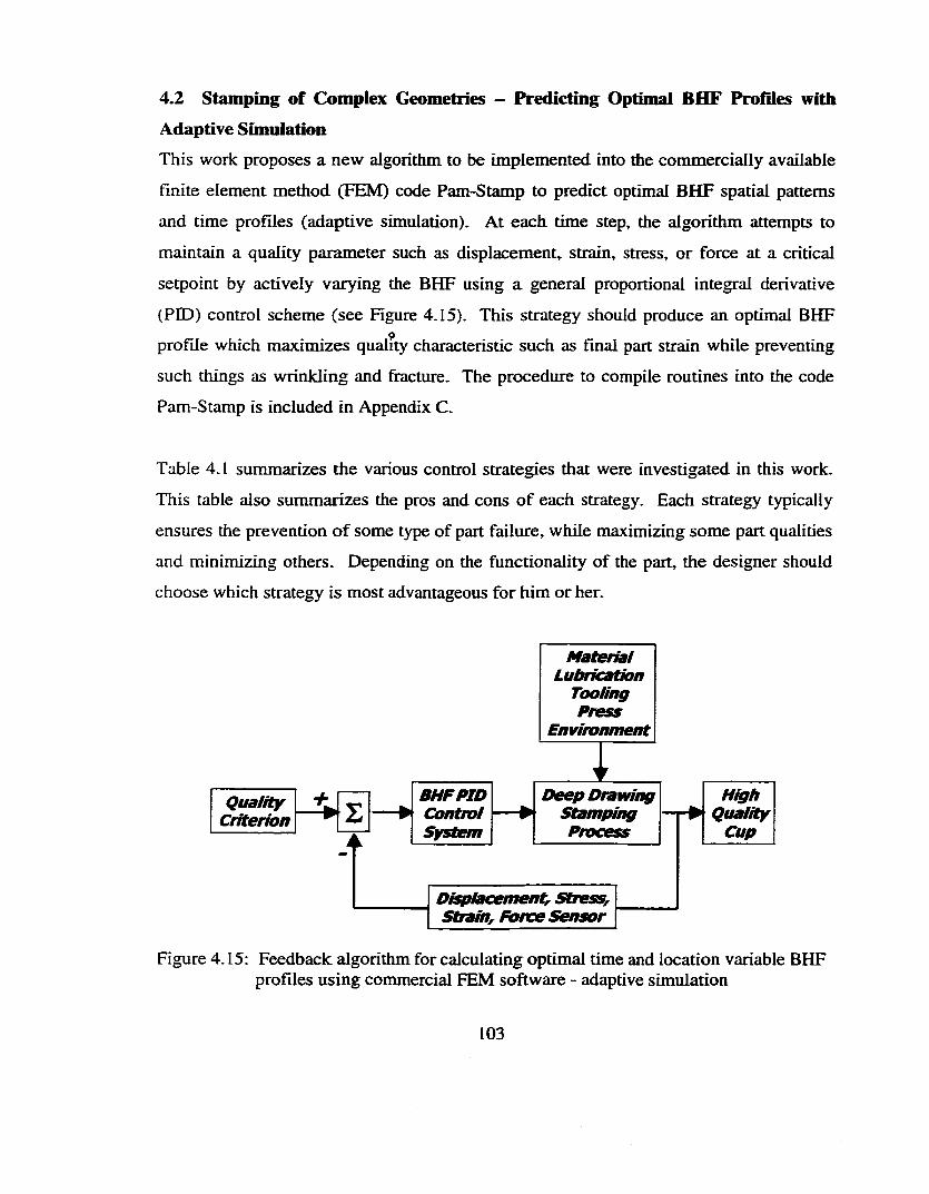
4.2 Stamping of Complex Geometries — Predicting Optimal BHF Profiles with Adaptive SimulationThis work proposes a new algorithm to be implemented into the commercially available

finite element method (FEM) code Pam-Stamp to predict optimal BHF spatial patterns

and time profiles (adaptive simulation). At each time step, the algorithm attempts to

maintain a quality parameter such as displacement, strain, stress, or force at a critical

setpoint by actively varying the BHF using a general proportional integral derivative

(FED) control scheme (see Figure 4.15). This strategy should produce an optimal BHF9

profile which maximizes quality characteristic such as final part strain while preventing

such things as wrinkling and fracture. The procedure to compile routines into the code

Pam-Stamp is included in Appendix C.

Table 4.1 summarizes the various control strategies that were investigated in this work.

This table also summarizes the pros and cons o f each strategy. Each strategy typically

ensures the prevention o f some type of part failure, while maximizing some part qualities

and minimizing others. Depending on the functionality of the part, the designer should

choose which strategy is most advantageous for him or her.

QuathyCriterion

HighQuality

Cup

BHFPIDControlSystem

Deep Drawing Stamping Process

Displacement, Stress, Strain, Force Sensor

MaterialLubrication

TooUngPress

Environment

Figure 4.15: Feedback algorithm for calculating optimal time and location variable BHF profiles using commercial E EM software - adaptive simulation

103

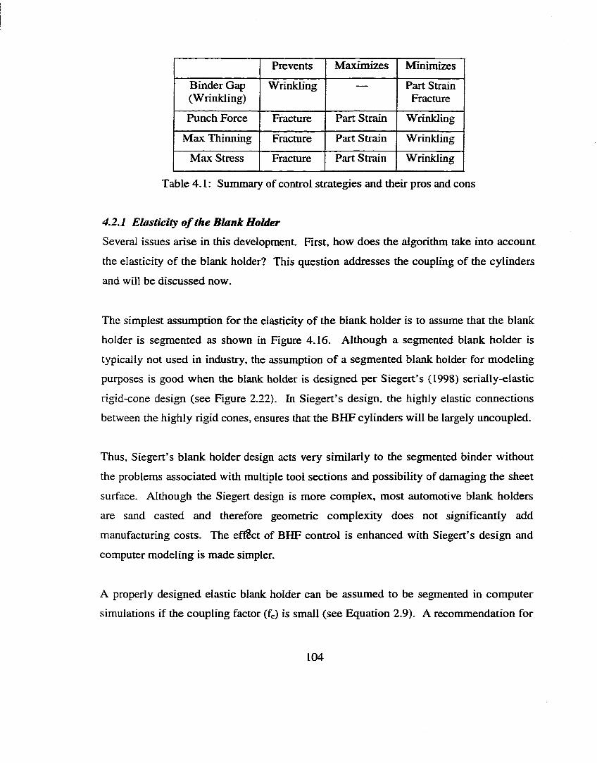
Prevents Maximizes Minimizes

Binder Gap (Wrinkling)

Wrinkling Part Strain Fracmre

Punch Force Fracture Part Strain Wrinkling

Max Thinning Fracmre Part Strain Wrinkling

Max Stress Fracture Part Strain Wrinkling

Table 4 .1 : Summary of control strategies and their pros and cons

4.2.1 Elasticity o f the B lank Holder

Several issues arise in this development. First, how does the algorithm take into account

the elasticity of the blank holder? This question addresses the coupling of the cylinders

and will be discussed now.

The simplest assumption for the elasticity of the blank holder is to assume that the blank

holder is segmented as shown in Figure 4.16. Although a segmented blank holder is

typically not used in industry, the assumption o f a segmented blank holder for modeling

purposes is good when the blank holder is designed per Siegert’s (1998) serially-elastic

rigid-cone design (see Figure 2.22). In Siegert’s design, the highly elastic connections

between the highly rigid cones, ensures that the BHF cylinders will be largely uncoupled.

Thus, Siegert’s blank holder design acts very similarly to the segmented binder without

the problems associated with multiple tool sections and possibility of damaging the sheet

surface. Although the Siegert design is more complex, most automotive blank holders

are sand casted and therefore geometric complexity does not significantly add

manufacturing costs. The effect of BHF control is enhanced with Siegert’s design and

computer modeling is made simpler.

A properly designed elastic blank holder can be assumed to be segmented in computer

simulations if the coupling factor (fc) is small (see Equation 2.9). A recommendation for

104

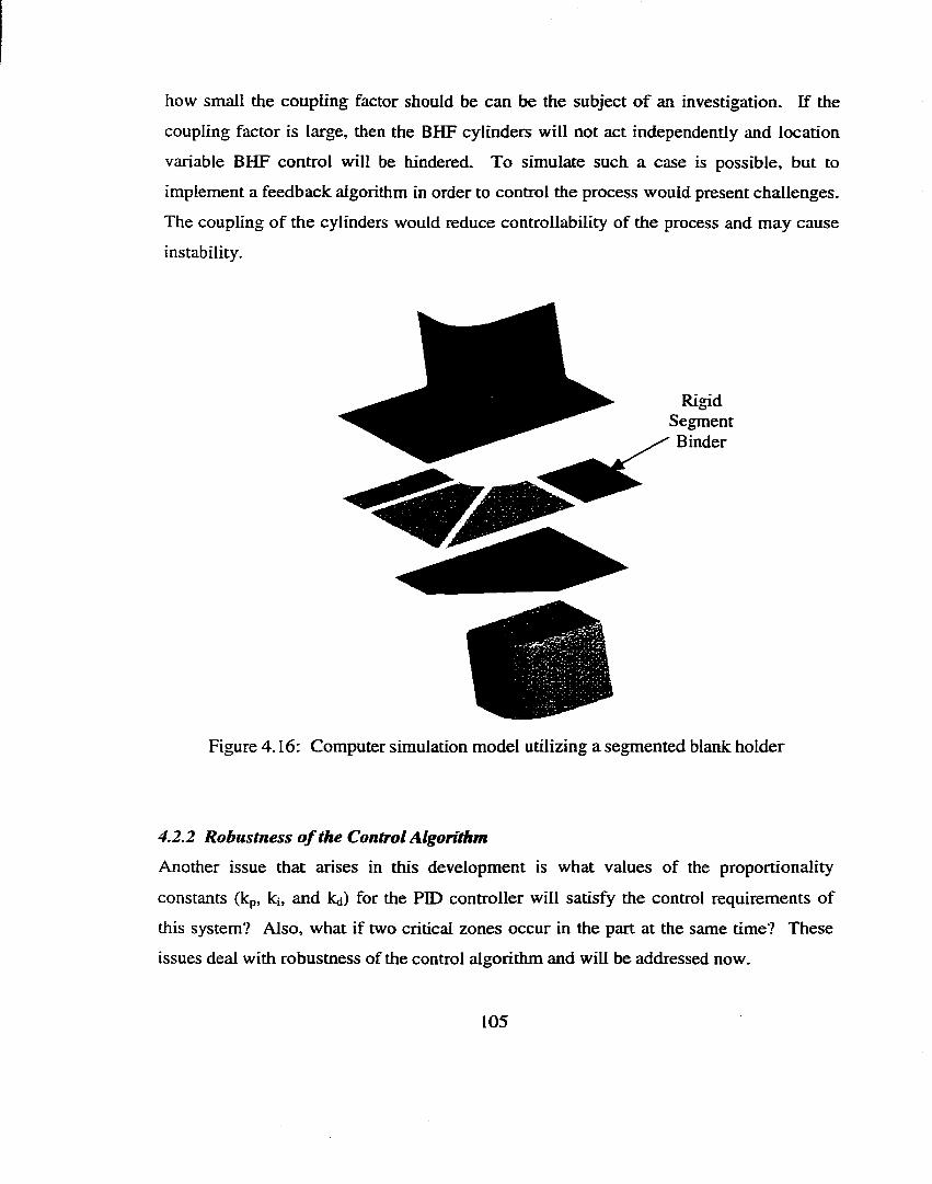
how small the coupling factor should be can be the subject o f an investigation. If the

coupling factor is large, then the BHF cylinders will not act independently and location

variable BHF control will be hindered. To simulate such a case is possible, but to

implement a feedback algorithm in order to control the process would present challenges.

The coupling of the cylinders would reduce controllability of the process and may cause

instability.

RigidSegmentBinder

Figure 4.16: Computer simulation model utilizing a segmented blank holder

4.2.2 Robustness o f the Control Algorithm

Another issue that arises in this development is what values of the proportionality

constants (kp, ki, and kd) for the FID controller will satisfy the control requirements of

this system? Also, what if two critical zones occur in the part at the same time ? These

issues deal with robustness of the control algorithm and will be addressed now.

105

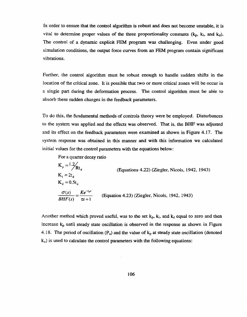
In order to ensure that the control algorithm is robust and does not become unstable, it is

vital to determine proper values of the three proportionality constants (kp, kj, and k^).

The control of a dynamic explicit FEM program was challenging. Even under good

simulation conditions, the output force curves from an FEM program contain significant

vibrations.

Further, the control algorithm must be robust enough to handle sudden shifts in the

location of the critical zone. It is possible that two or more critical zones will be occur in

a single part during the deformation process. The control algorithm must be able to

absorb these sudden changes in the feedback parameters.

To do this, the fundamental methods of controls theory were be employed. Disturbances

to the system was applied and the effects was observed. That is, the BHF was adjusted

and its effect on the feedback parameters were examined as shown in Figure 4.17. The

system response was obtained in this manner and with this information we calculated

initial values for the control parameters with the equations below:

For a quarter decay ratio K = 1 .2 /

(Equations 4.22) (Ziegler, Nicols, 1942, 1943)K i= 2 t,Kj =0.5tj

(Tis) Ke (Equation 4.23) (Ziegler, Nicols, 1942, 1943)

Another method which proved useful, was to the set kp, k,, and kj equal to zero and then

increase kp until steady state oscillation is observed in the response as shown in Figure

4.18. The period of oscillation (Pu) and the value o f kp at steady state oscillation (denoted

ku) is used to calculate the control parameters with the following equations:

106

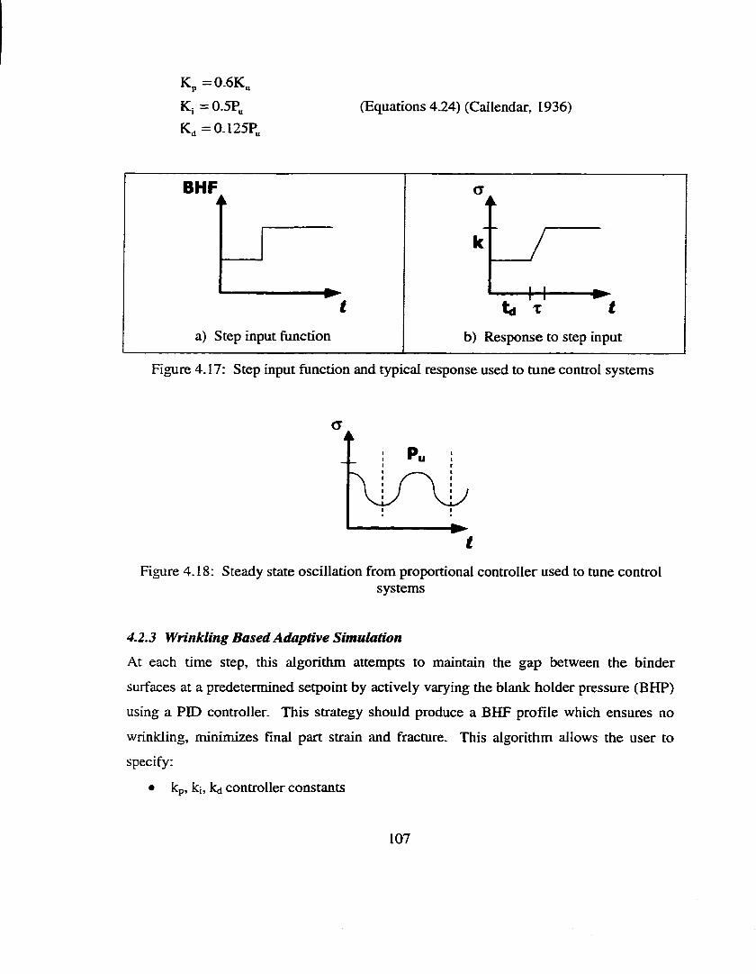
Kp =0.6K„ K, =0.5P„K , =0.125P„

(Equations 4J24) (Callendar, 1936)

BHFi i.

ai

k

I

_ v

t

a) Step input function

■■■ ' r I^ T t

b) Response to step input

Figure 4.17: Step input function and typical response used to tune control systems

t

Figure 4.18: Steady state oscillation from proportional controller used to tune controlsystems

4.2.3 Wrinkling Based Adaptive Simulation

At each time step, this algorithm attempts to maintain the gap between the binder

surfaces at a predetermined setpoint by actively varying the blank holder pressure (BHP)

using a PDD controller. This strategy should produce a BHF profile which ensures no

wrinkling, minimizes final part strain and fracture. This algorithm allows the user to

specify:

• kp, ki, kd controller constants

107

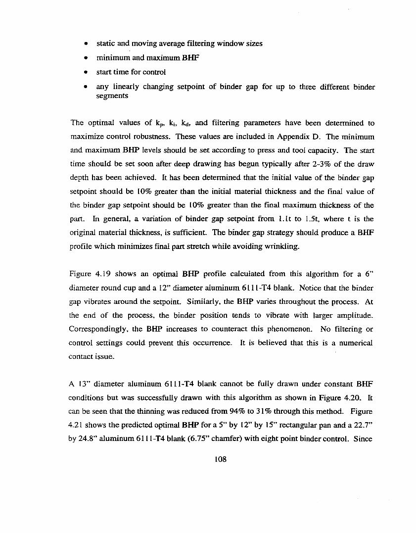
• static and moving average filtering window sizes

• minimum and maximum BHF

• start time for control

• any linearly changing setpoint of binder gap for up to three different binder segments

The optimal values of kp, ki, kd, and filtering parameters have been determined to

maximize control robustness. These values are included in Appendix D. The minimum

and maximum BHP levels should be set according to press and tool capacity. The start

time should be set soon after deep drawing has begun typically after 2-3% of the draw

depth has been achieved. It has been determined that the initial value of the binder gap

setpoint should be 1 0 % greater than the initial material thickness and the final value of

the binder gap setpoint should be 1 0 % greater than the final maximum thickness of the

part. In general, a variation of binder gap setpoint from L it to 1.5t, where t is the

original material thickness, is sufficient. The binder gap strategy should produce a BHF

profile which minimizes final part stretch while avoiding wrinkling.

Figure 4.19 shows an optimal BHP profile calculated from this algorithm for a 6 ”

diameter round cup and a 12” diameter aluminum 6111-T4 blank. Notice that the binder

gap vibrates around the setpoint. Similarly, the BHP varies throughout the process. At

the end of the process, the binder position tends to vibrate with larger amplitude.

Correspondingly, the BHP increases to counteract this phenomenon. No filtering or

control settings could prevent this occurrence. It is believed that this is a numerical

contact issue.

A 13” diameter aluminum 6111-T4 blank cannot be fully drawn under constant BHF

conditions but was successfully drawn with this algorithm as shown in Figure 4.20. It

can be seen that the thinning was reduced from 94% to 31% through this method. Figure

4.21 shows the predicted optimal BHP for a 5” by 12” by 15” rectangular pan and a 22.7”

by 24.8” aluminum 6111-T4 blank (6.75” chamfer) with eight point binder control. Since

108

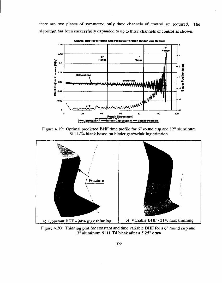
there are two planes of symmetry, only three channels o f control are required- The

algorithm has been successfully expanded to up to three channels of control as shown-

Optimal BHF for a Round Cup Prediclad Through Binder Gap Method0 .1 4

R a n g e0.12

- 4

R a n g e R a n g e0.1

S 0 .08

12 0 .0 6

S e tp o in t G ap- 0 «

Binder Gap

g 0 .04

0.02

BHF

400 SO20 80 100 120Punch Stroke (mm)

Optimal BHP — Binder Gap Setpoint —Binder Position |

Figure 4.19: Optimal predicted BHF time profile for 6 ” round cup and 12” aluminum 6111-T4 blank based on binder gap/wrinkling criterion

' Fracture

a) Constant BHF - 94% max thinning b) Variable BHF -31% max thinning

Figure 4.20: Thinning plot for constant and time variable BHF for a 6 ” round cup and 13" aluminum 6111-T4 blank after a 5.25" draw

109

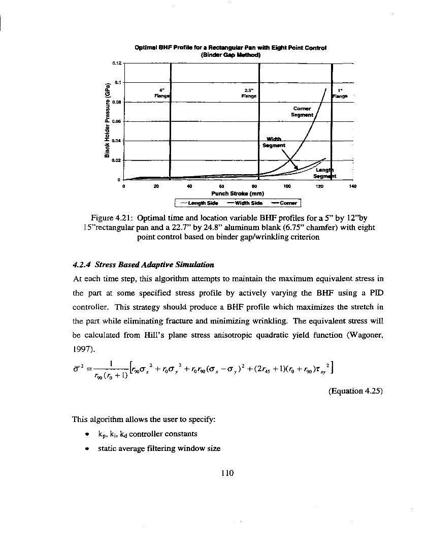
O p tim al B H F P ro file f o r a R e c ta n g u la r P a n w itti E ig lit P o in t C o n tro l (B in d e r G a p M ettiod )

0.12

0.1

£ 2S"R a n g e

1"R a n g eR a n g e

£ 0 .08

CornerSegment

z 0 .04Segment

0.02

Lengt i

0 20 40 60 80 100 140120

P unch S tro k e (m m )

-Length Side — Width Side — Comer

Figure 4.21: Optimal time and location variable BHF profiles for a 5” by I2”by I5”rectangular pan and a 22.7” by 24.8” aluminum blank (6.75” chamfer) with eight

point control based on binder gap/wrinkling criterion

4.2.4 Stress Based Adaptive Simulation

At each time step, this algorithm attempts to maintain the maximum equivalent stress in

the part at some specified stress profile by actively varying the BHF using a PID

controller. This strategy should produce a BHF profile which maximizes the stretch in

the part while eliminating fracture and minimizing wrinkling. The equivalent stress will

be calculated from Hill’s plane stress anisotropic quadratic yield function (Wagoner,

1997).

= --- +'c)'90(O'x ~ ^ y ) ‘ +(^^45 +U(/b + /bo ]90 \ Q V

(Equation 4.25)

This algorithm allows the user to specify:

• kp, ki, kd controller constants

• static average filtering window size

110

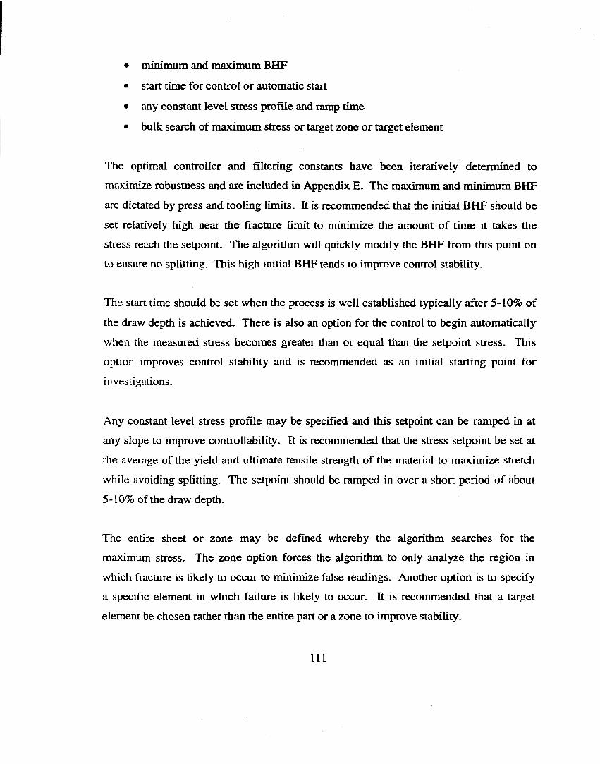
• minimum and maximum BHF

• start time for control or automatic start

• any constant level stress profile and ramp time

• bulk search of maximum stress or target zone or target element

The optimal controller and filtering constants have been iteratively determined to

maximize robustness and are included in Appendix E. The maximum and minimum BHF

are dictated by press and tooling limits. It is recommended that the initial BHF should be

set relatively high near the fracture limit to minimize the amount o f time it takes the

stress reach the setpoint. The algorithm will quickly modify the BHF from this point on

to ensure no splitting. This high initial BHF tends to improve control stability.

The start time should be set when the process is well established typically after 5-10% of

the draw depth is achieved. There is also an option for the control to begin automatically

when the measured stress becomes greater than or equal than the setpoint stress. This

option improves control stability and is recommended as an initial starting point for

investigations.

Any constant level stress profile may be specified and this setpoint can be ramped in at

any slope to improve controllability. It is recommended that the stress setpoint be set at

the average of the yield and ultimate tensile strength o f the material to maximize stretch

while avoiding splitting. The setpoint should be ramped in over a short period of about

5-10% of the draw depth.

The entire sheet or zone may be defined whereby the algorithm searches for the

maximum stress. The zone option forces the algorithm to only analyze the region in

which fracture is likely to occur to minimize false readings. Another option is to specify

a specific element in which failure is likely to occur. It is recommended that a target

element be chosen rather than the entire part or a zone to improve stability.

I l l

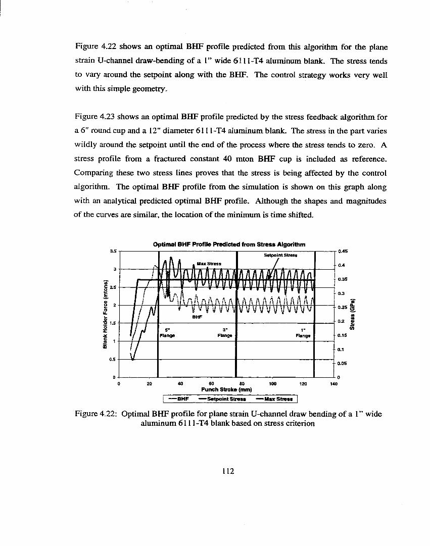
Figure 4.22 shows an optimal BHF profile predicted from this algorithm for the plane

strain U-channel draw-bending of a I” wide 6 1 11-T4 aluminum blank. The stress tends

to vary around the setpoint along with the BHF. The control strategy works very well

with this simple geometry.

Figure 4.23 shows an optimal BHF profile predicted by the stress feedback algorithm for

a 6 " round cup and a 12" diameter 6111-T4 aluminum blank. The stress in the part varies

wildly around the setpoint until the end of the process where the stress tends to zero. A

stress profile from a fractured constant 40 mton BHF cup is included as reference.

Comparing these two stress lines proves that the stress is being affected by the control

algorithm. The optimal BHF profile from the simulation is shown on this graph along

with an analytical predicted optimal BHF profile. Although the shapes and magnitudes

of the curves are similar, the location o f the minimum is time shifted.

O p tim a l B H F P ro f ile P re d ic te d fro m S t r e s s A lgorittim3 .5

M ax S t r e s s

2 1 .5oXjgS 1 m

0 .5

B H F

3>R a n g e

1“R a n g e

0 .4 5

0 .4

0 .3 5

-• 0 .3

s0.2 O

CO

0 .1 5

0.1

0 .0 5

20 4 0 6 0 80P u n ch S troke (mm)

100 120 140

— BHF Setpoint Stress — Max Strass

Figure 4.22: Optimal BHF profile for plane strain U-channel draw bending o f a 1” wide aluminum 6111-T4 blank based on stress criterion

112

Optimal BHF Profile from Stress Based Algorithm180 0 .7

160(C o n s ta n t BHF) - 0.6

2" O’R a n g *

S 120M eaau tad

S tr e s s(BtlF Cu im u l)

J 0.4 a.ç 100A naly tica l

B H F80 ■ - 0 .3 S

S t r e s sSetpoint

O p tim a lB H F

- 0.120

0 40 6020 100 14080 120Punct) Stroke (mm)

-O p tim a l B H F — A naly tica l BH F ^ — S t r e s s S e tp o in t-M e a s u r e d S t r e s s (B H F C o n tro l) M e a s u re d S tr e s s (C o n s ta n t BHF)_____________________

Figure 4.23: Optimal BHF time profile for a 6 ” round cup and 12” aluminum 6111-T4blank based on stress criterion

4.2.5 Strain Based Adaptive Simulation

At each time step, this algorithm attempts to maintain the maximum thinning in the part

at some specified thinning profile by actively varying the BHF using a PID controller.

This strategy should produce a BHF profile which eliminates fracture in the part and

minimizes wrinkling. The maximum thinning is defined as:

tr.maximum thinning 0 min (Equation 4.26)

Where tmin is the minimum thickness in the part.

This algorithm allows the user to specify:

• kp, ki, kd controller constants

• static average filtering window size

• minimum and maximum BHF

• start time for control

113

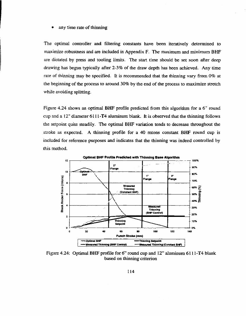
• any time rate of thinning

The optimal controller and filtering constants have been iteratively determined to

maximize robustness and are included in Appendix F. The maximum and minimum BHF

are dictated by press and tooling limits. The start time should be set soon after deep

drawing has begun typically after 2-3% of the draw depth has been achieved. Any time

rate of thinning may be specified. It is recommended that the thinning vary from 0% at

the beginning of the process to around 30% by the end of the process to maximize stretch

while avoiding splitting.

Figure 4.24 shows an optimal BHF profile predicted from this algorithm for a 6 " round

cup and a 12" diameter 6111-T4 aluminum blank. It is observed that the thinning follows

the setpoint quite steadily. The optimal BHF variation tends to decrease throughout the

stroke as expected. A thinning profile for a 40 mtons constant BHF round cup is

included for reference purposes and indicates that the thinning was indeed controlled by

this method.

O ptim al B H F P ro file P re d ic te d w ith T h in n in g B a s e A lgorithm12

10

'3Î*c

: =o2

VX

^ * m

2

2"R a n g e ' .......... ..

B H F \ 1"R a n g e

0"R a n g e

\ M easu redT h in n in g

\ (C o n s ta n t BHF)

--

A\

-•

\

M e a su re dT h in n in g

(B H F C on tro l)

" T h in n in g S e tp o in t

--

100%

80%

60% ^

g50% S

30%

20 4 0 60 BO

Punch Stroke (mm)100 120 140

— OpWmel B H F ' Men u m d T h tn n ln g (B H F C ontro l)

•T h in n in g S e tp o in t■ M eeeu red T h in n in g (C o n ita n t BHF)

Figure 4.24: Optimal BHF profile for 6 ” round cup and 12” aluminum 6111-T4 blankbased on thinning criterion

114

4.2.6 Force Based Adaptive Simulation

At each time step, this algorithm attempts to maintain the punch force of the process at

some specified force profile by actively varying the BHF using a PID controller. This

strategy should produce a BHF profile which eliminates fracture and minimizes

wrinkling in the part. This algorithm allows the user to specify:

• kp, kj, kd controller constants

• static average filtering window size

• minimum and maximum BHF

• start time for control o r automatic start

• any constant level force profile

The optimal controller and filtering constants have been iteratively determined to

maximize robustness and are included in Appendix G. The maximum and minimum

BHF are dictated by press and tooling limits. The initial value of the BHF should be set

relatively high (near the fracture limit) in order to minimize the time it takes to reach the

setpoint force. The controller will then modify the BHF to ensure that failure does not

occur. Control stability is improved by setting the initial BHF high.

The start time should be set when the process is well established typically after 5-10% of

the draw depth is achieved. There is also an option for the control to begin automatically

when the measured punch force becomes greater than or equal than the setpoint force.

This option improves control stability and is recommended as an initial starting point for

investigations.

Any constant level of punch force may be specified. It is recommended that the punch

force be set at 75% o f the minimum punch force that causes fracture in constant level

BHF trials. This should maximize final part stretch while avoiding splitting and

minimizing wrinkling.

115

Figure 4.25 shows an optimal BHF profile predicted from this algorithm for a 6 " round

cup and a 12" diameter 6111-T4 aluminum blank. Once control begins, the punch force

tends to vibrate around the setpoint. The optimal BHF profile tends to decrease then

increase to maintain the punch load at the setpoint. An analytically predicted BHF

profile is also shown in this figure. The shape and magnimde o f the BHF profiles are

similar in size and shape but are time shifted from one another.

Drawability is improved with the force algorithm as shown in Figure 4.26. A 13"

diameter 6H I-T 4 aluminum blank cannot be fully drawn into a 6 " round cup using

constant BHF, but is successfully drawn with the force control strategy. Figure 4.27

shows an optimal BHF profile predicted for a 5” by 12” by 15” rectangular pan drawn

from a 22.7” by 24.8” aluminum 6111-T4 blank (6.75” chamfer). The BHF profile

vibrates wildly but can be smoothed with a filtering function for use in a press.

Figure 4.28 shows a thinning contour plot of this rectangular panel. Note that this

maximum thinning is only 19%. The blank shape used for these rectangular simulations

was predicted with the one-step FEM code FastFormBD to have a uniform flange after a

5” draw. This was proposed to maximize strain uniformity and increase drawability and

part quality. It can be observed from this plot that the flange is relatively uniform. It is

believed that the blank shape played major role in permitting a full 5” draw from

aluminum.

116

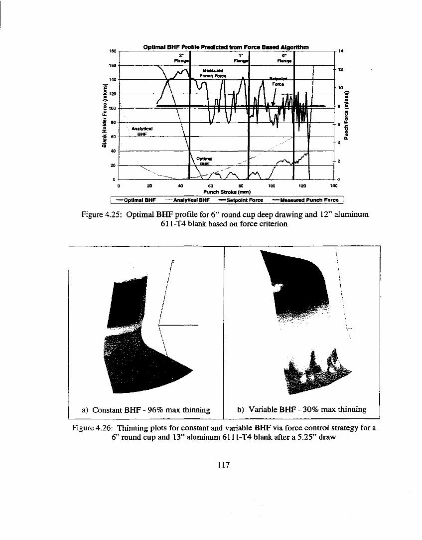
Optimal BHF Profile Predicted from Force Based Aloonthm

Flange

P u n c h F o rc eS e tp o in t

2 120

2 100

A n aly tica l

O p ttm alSHE

so 80Punch Stroke (mm)

— Optimal BHF - Analytical BHF ^ —Setpoint Force ’Measured Punch Force

Figure 4.25: Optimal BHF profile for 6 ” round cup deep drawing and 12” aluminum611-T4 blank based on force criterion

b) Variable BHF - 30% max thinninga) Constant BHF - 96% max thinning

Figure 4.26: Thinning plots for constant and variable BHF via force control strategy for a 6 ” round cup and 13” aluminum 6111-T4 blank after a 5.25” draw

117

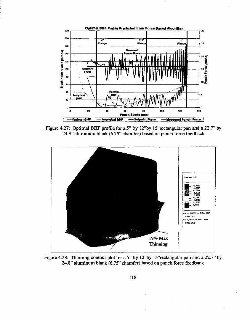
200 Optimal BHF Profile Predicted from Force Based Algorithm

M e a s u re d P un c h P a re #

20 CB

> e lp o in t

O p ttm alA naty tfcal

B H F

60 80 Punch Stroke (mm)

"Optimal BHF •Analytical BHF Setpoint Force "— Measured Punch Force

Figure 4.27: Optimal BHF profile for a 5” by I2”by I5”rectangular pan and a 22.7” by 24.8” aluminum blank (6.75” chamfer) based on punch force feedback

19% Max Thinning

Figure 4.28: Thinning contour plot for a 5” by 12”by 15”rectangular pan and a 22.7” by 24.8” aluminum blank (6.75” chamfer) based on punch force feedback

Thtmtn» O l

g -0.7888-0.6737-OJ5708-0.4S18-OJS29-0.20-OJ351-O.02S1

B F 0.0828

am -0.S37S33 in SKLL 2887 STBtE 20 j .

MX 0.l9t7? in 208 STftfE 20.1

118

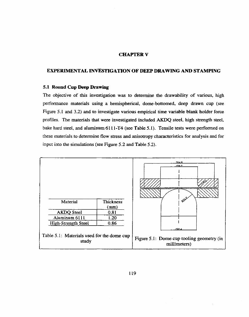
CHAPTER V

EXPERIMENTAL INVESTIGATION OF DEEP DRAWING AND STAMPING

5.1 Round Cup Deep DrawingThe objective of this investigation was to determine the drawability o f various, high

performance materials using a hemispherical, dome-bottomed, deep drawn cup (see

Figure 5.1 and 3.2) and to investigate various empirical time variable blank holder force

profiles. The materials that were investigated included AKDQ steel, high strength steel,

bake hard steel, and aluminum 6111-T4 (see Table 5.1). Tensile tests were performed on

these materials to determine flow stress and anisotropy characteristics for analysis and for

input into the simulations (see Figure 5.2 and Table 5.2).

Material Thickness(mm)

AKDQ Steel 0.81Aluminum 6111 1 . 2 0

High-Strength Steel 0 . 8 6

Table 5.1 : Materials used for the dome cup study Figure 5 .1 : Dome cup tooling geometry (in

millimeters)

119

It is interesting to note that the flow stress curves for bake hard steel and AKDQ steel

were very similar except for a 5% reduction in elongation for bake hard. Although, the

elongations for high strength steel and aluminum 6111-T4 were similar, the n-value for

aluminum 6111-T4 was twice as large. Also, the r-values for AKDQ was much bigger

than 1, while bake hard was nearly 1, and aluminum 6111-T4 was much less than 1.

The time variable BHF profiles used in this investigation included constant, linearly

decreasing, and pulsating (see Figure 5.3). The experimental conditions for AKDQ steel

were simulated using the incremental FEM code Pam-Stamp. Examples o f wrinkled,

fractured, and good laboratory cups are shown in Figures 2.14 and 2.15 as well as an

image of a simulated wrinkled cup.

Limits of drawability were experimentally investigated using constant BHF. The results

of this study are shown in Table 5.3. This table indicates that AKDQ had the largest

drawability window while aluminum had the smallest and bake hard and high strength

steels were average. The strain distributions for constant, ramp, and pulsating BHF are

compared experimentally in Figure 5.4 and are compared with simulations in Figure 5.5

for AKDQ. In both simulations and experiments, it was found that the ramp BHF

trajectory improved the strain distribution the best. Not only were peak strains reduced

by up to 5% thereby reducing the possibility of fracture, but low strain regions were

increased. This improvement in strain distribution can increase product stiffness and

strength, decrease springbuck and residual stresses, increase product quality and process

robustness.

Pulsating BHF, at the frequency range investigated, was not found to have an effect on

strain distribution. This was likely due to the fact the frequency of pulsation that was

tested was only 1 Hertz. It is known from previous experiments o f other researchers that

proper frequencies range from 5 to 25 Hertz (Siegert, 1995). A comparison of load-

stroke curves from simulation and experiments are shown in Figure 5.6 for AKDQ.

120

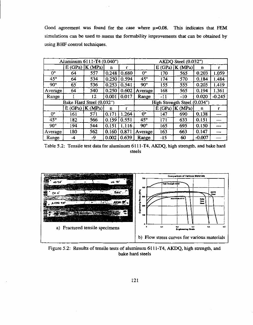
Good agreement was found for the case where ^=0.08. This indicates that FEM

simulations can be used to assess the formability improvements that can be obtained by

using BHF control techniques.

A uminum 6111-T4 (0.040") AKDQ Steel (0.032")E (GPa) K(MPa) n r E (GPa) K(MPa) n r

0 ° 64 557 0.248 0.680 0 ° 170 565 0.203 1.05945° 64 534 0.250 0.594 45° 174 570 0.184 1.48490° 65 536 0.253 0.541 90° 155 555 0.205 1.419

Average 64 540 0.250 0.602 Average 168 565 0.194 1.361Range 1 1 2 0 . 0 0 1 0.017 Range - 1 1 - 1 0 0 . 0 2 0 -0.245

Bake Hare Steel (0.032") t igh Strength Steel [0.034")E (GPa) K(MPa) n r E (GPa) K(MPa) n r

0 ° 161 571 0-171 1.264 0 ° 147 690 0.138 —

45° 182 566 0.159 0.551 45° 171 633 0.151 ---------

90° 194 544 0.151 1.116 90° 165 695 0.150 ---------

Average 180 562 0.160 0.871 Average 163 663 0.147 ---

Range -4 -9 0 . 0 0 2 0.639 Range -15 60 -0.007 ---

Table 5.2: Tensile test data for aluminum 6111-T4, AKDQ, high strength, and bake hardsteels

c

a) Fracmred tensile specimens

Comparison of Various Materials

High Stran«th St mi

engfnmhng Strain

b) Flow stress curves for various materials

Figure 5.2: Results of tensile tests of aluminum 6111-T4, AKDQ, high strength, andbake hard steels

121

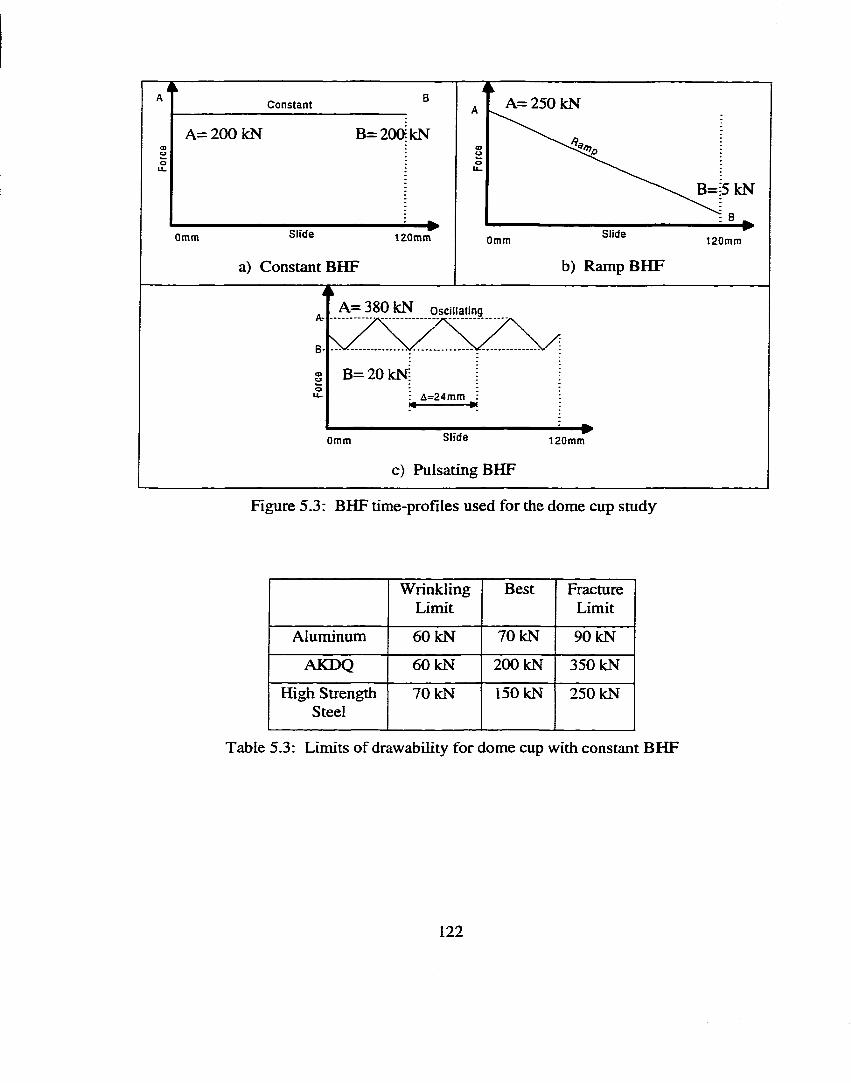
i iA= 250 kNConstant

A =200kN

Slide SlideQmm t 2 0 mm 0mm 120mm

b) Ramp BHFa) Constant BHF

A— 380 kN Oscillating

Slide0mm 120mm

c) Pulsating BHF

Figure 5.3: BHF time-profiles used for the dome cup study

WrinklingLimit

Best FractureLimit

Aluminum 60 kN 70 kN 90 kN

AKDQ 60 kN 200 kN 350 kN

High Strength Steel

70 kN 150 kN 250 kN

Table 5.3: Limits of drawabUity for dome cup with constant BHF

122

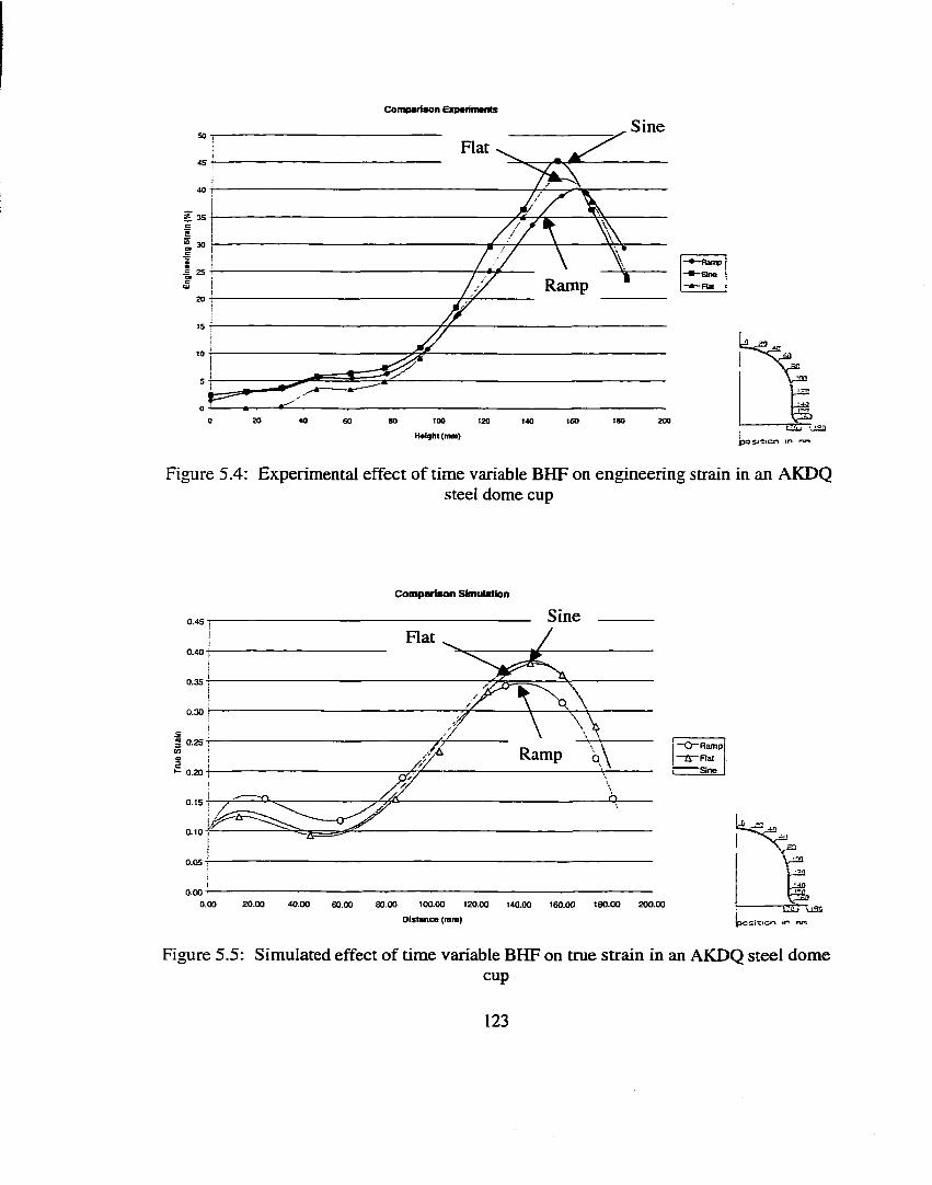
Comparison Exparimants

Sine50

Flata*.45

40

30

25

Ramp20

10

20 40 1000 80 120 160 180 200GO 140

-Ramp I “Sne I -Rai.

Height (nwn) lOSi'&cn in rw#

Figure 5.4: Experimental effect of time variable BHF on engineering strain in an AKDQsteel dome cup

C o m p a r i s o n S im u M fo n

Sine0.45

Flat0 .4 0 -j*

0 .30 t

5 0 .25 T

Ramp0.20 t

0.15

0.05

0.0020.000.00 40.00 100.00 120.00 180.0060.00 80.00 160.00 200.00

D istance (mm)%I4Q

Figure 5.5: Simulated effect of time variable BHF on true strain in an AKDQ steel domecup

123

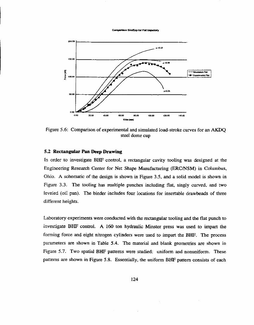
Comparison SinVExp for Flat trajactory

200.00

S 100.00

50.00

0.000.00 20.00 40.00 80.00 120.00 140.00100.00

SIM# (mm)

Figure 5.6: Comparison of experimental and simulated load-stroke curves for an AKDQsteel dome cup

5.2 Rectangular Pan Deep DrawingIn order to investigate BHF control, a rectangular cavity tooling was designed at the

Engineering Research Center for Net Shape Manufacturing (ERC/NSM) in Columbus,

Ohio. A schematic of the design is shown in Figure 3.5, and a solid model is shown in

Figure 3.3. The tooling has multiple punches including flat, singly curved, and two

leveled (oil pan). The binder includes four locations for insertable drawbeads of three

different heights.

Laboratory experiments were conducted with the rectangular tooling and the flat punch to

investigate BHF control. A 160 ton hydraulic Minster press was used to impart the

forming force and eight nitrogen cylinders were used to impart the BHF. The process

parameters are shown in Table 5.4. The material and blank geometries are shown in

Figure 5.7. Two spatial BHF patterns were studied: uniform and nonuniform. These

patterns are shown in Figure 5.8. Essentially, the uniform BHF pattern consists of each

124

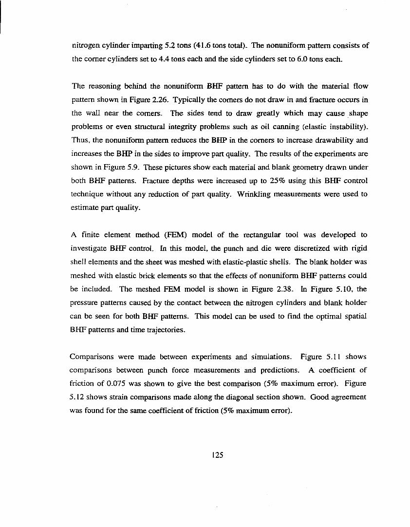
nitrogen cylinder imparting 5.2 tons (41.6 tons total). The nonuniform pattern consists of

the comer cylinders set to 4.4 tons each and the side cylinders set to 6.0 tons each.

The reasoning behind the nonuniform BHF pattern has to do with the material flow

pattern shown in Figure 2.26. Typically the comers do not draw in and fracture occurs in

the wall near the comers. The sides tend to draw greatly which may cause shape

problems or even stmctural integrity problems such as oil carming (elastic instability).

Thus, the nonuniform pattem reduces the BHP in the comers to increase drawabUity and

increases the BHP in the sides to improve part quality. The results of the experiments are

shown in Figure 5.9. These pictures show each material and blank geometry drawn under

both BHF pattems. Fracture depths were increased up to 25% using this BHF control

technique without any reduction of part quality. Wrinkling measurements were used to

estimate part quality.

A finite element method (FEM) model of the rectangular tool was developed to

investigate BHF control. In this model, the punch and die were discretized with rigid

shell elements and the sheet was meshed with elastic-plastic shells. The blank holder was

meshed with elastic brick elements so that the effects of nonuniform BHF pattems could

be included. The meshed FEM model is shown in Figure 2.38. In Figure 5.10, the

pressure pattems caused by the contact between the nitrogen cylinders and blank holder

can be seen for both BHF pattems. This model can be used to find the optimal spatial

BHF pattems and time trajectories.

Comparisons were made between experiments and simulations. Figure 5.11 shows

comparisons between punch force measurements and predictions. A coefficient of

friction of 0.075 was shown to give the best comparison (5% maximum error). Figure

5.12 shows strain comparisons made along the diagonal section shown. Good agreement

was found for the same coefficient of friction (5% maximum error).

125

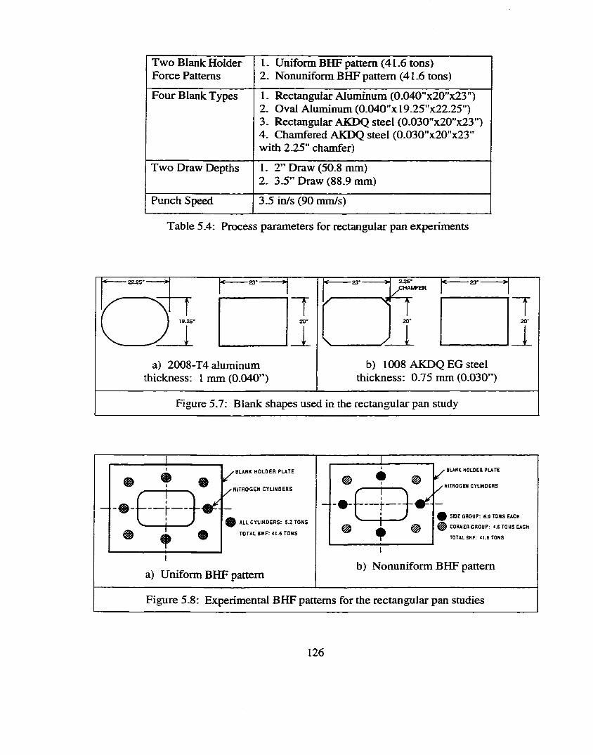
Two Blank Holder Force Pattems

1. Uniform BHF pattem (41.6 tons)2. Nonuniform BHF pattem (41.6 tons)

Four Blank Types 1. Rectangular Aluminum (0.040 "x20"x23")2. Oval Aluminum (0.040"xl9.25"x22.25")3. Rectangular AKDQ steel (0.030"x20 "x23")4. Chamfered AKDQ steel (0.030"x20"x23" with 2.25" chamfer)

Two Draw Depths 1. 2” Draw (50.8 mm)2. 3.5” Draw (88.9 mm)

Punch Speed 3.5 in/s (90 mm/s)

Table 5.4: Process parameters for rectangular pan experiments

225* 23* 23"CHAMFER

19.25*

b) 1008 AKDQ EG steel thickness: 0.75 mm (0.030”)

a) 2008-T4 aluminum thickness: I mm (0.040”)

Figure 5.7: Blank shapes used in the rectangular pan study

f 1 \

- h - WL j J

BLANK HOLDER PLATE

NITROGEN CYLINDERS

ALL CYLINDERS: 5.2 TONS

TOTAL SHF: 41.6 TONS

a) Uniform BHF pattem

z ' " 1- # - - - - - - -

V

N- - - - - - -

J® 1 1 #

/

BLANK holder PLATE

NITROGEN CYLINDERS

I SIDE GROUP: 6.0 TONS EACH

I CORNER GROUP: 4.6 TONS EACH

total BHF; 41.6 TONS

b) Nonuniform BHF pattem

Figure 5.8: Experimental B H F pattems for the rectangular pan studies

126

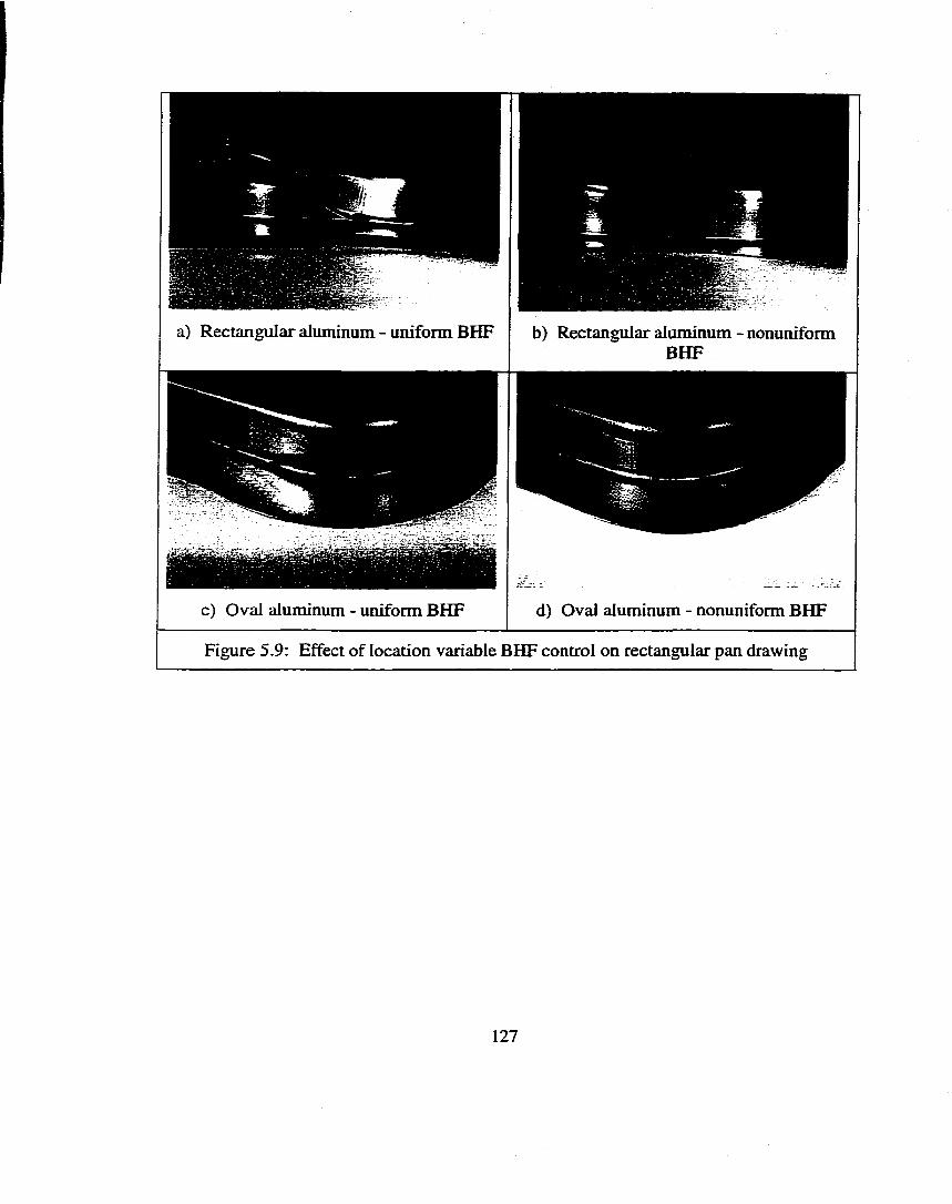
a) Rectangular aluminum - uniform BHF b) Rectangular aluminum - nonuniform BHF

c) Oval aluminum - uniform BHF d) Oval aluminum - nonuniform BHF

Figure 5.9: Effect of location variable BHF control on rectangular pan drawing

127

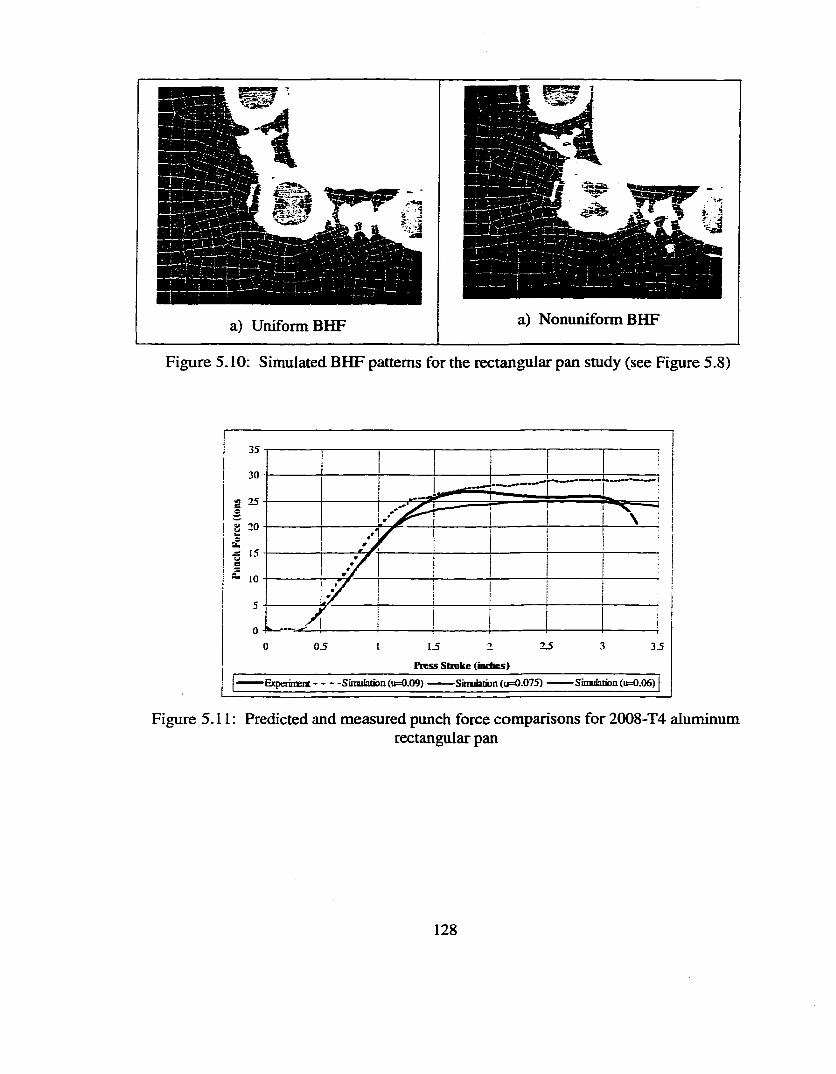
a) Uniform BHF a) Nonuniform BHF

Figure 5.10: Simulated BHF pattems for the rectangular pan study (see Figure 5.8)

S 20

- 10

Z5

Pnss Stroke (indies)

Experiment* - • -Siraifatk)n(u=0.09) — — SnnilanDn(u=0.075) — Sunulation(it=0.06)

Figure 5.11: Predicted and measured punch force comparisons for 2008-T4 aluminumrectangular pan

128

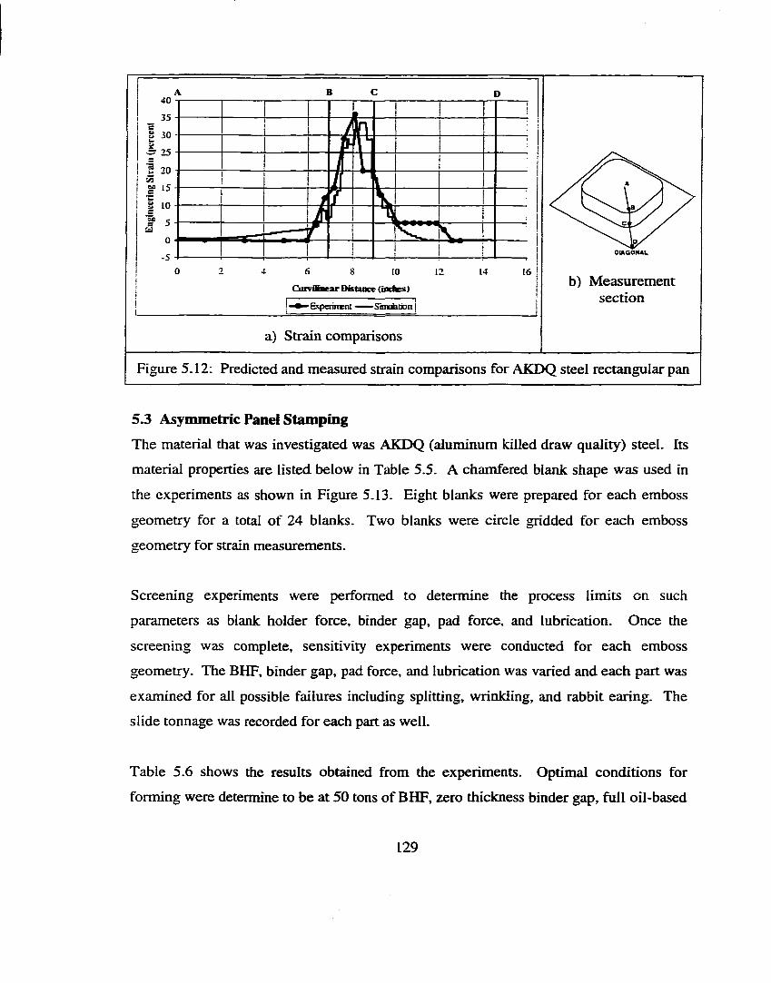
40

30

to -

DWGONAL

b) Measurement section

CmviMiiear Distance (oKhes)

Experiment Simulaoon |

a) Strain comparisons

Figure 5.12: Predicted and measured strain comparisons for AKDQ steel rectangular pan

5.3 Asymmetric Panel StampingThe material that was investigated was AKDQ (aluminum killed draw quality) steel. Its

material properties are listed below in Table 5.5. A chamfered blank shape was used in

the experiments as shown in Figure 5.13. Eight blanks were prepared for each emboss

geometry for a total of 24 blanks. Two blanks were circle gridded for each emboss

geometry for strain measurements.

Screening experiments were performed to determine the process limits on such

parameters as blank holder force, binder gap, pad force, and lubrication. Once the

screening was complete, sensitivity experiments were conducted for each emboss

geometry. The BHF, binder gap, pad force, and lubrication was varied and each part was

examined for all possible failures including splitting, wrinkling, and rabbit earing. The

slide tonnage was recorded for each part as well.

Table 5.6 shows the results obtained from the experiments. Optimal conditions for

forming were determine to be at 50 tons of BHF, zero thickness binder gap, full oil-based

129

water soluble lubrication, and 1250 psi pad pressure. Fracture was observed to occur at

75 and 100 tons of BHF and at fast press speeds (3.54 inches/second). Wrinkling was

observed to occur at 25 tons BHF and at binder gaps equal to one and two times the blank

thickness. Rabbit earing was not observed to occur on any o f the panels at any process

condition. Pad pressure was applied to the panel but did not have an observable effect on

the panel quality nor did it have a measurable effect on the strain distribution.

Figure 5.14 contains sample pictures of the asymmetric panel with the oval door emboss.

Similarly, Figure 5.15 shows sample pictures for the rectangular emboss and Figure 5.16

for the oblong emboss. In order to observe the history of deformation, a binder wrap

panel was formed as shown in Figure 5.17. A panel was formed one inch off bottom as

well and is shown in Figure 5.18. The history of deformation appeared to be good since

no gathering of material was observed.

Figure 5.19 indicates the locations and directions of strain measurements for each of the

asymmetric panels. Figure 5.20 is a graph of the major strain distribution versus original

blank position. This graph is indicated with positions A, B, C, and D which correspond

to the lettered positions in Figure 5.19. Essentially, A is located at the near panel wall

(header/sweeping curvature), B is at the beginning of the emboss, C is at the far edge of

the emboss and D is at the far panel wall (width side). It is observed that the oval emboss

distributes the strain the best while the oblong emboss distributes the strains the worst.

The initial design was confirmed using Pam-Stamp simulations. The model is shown in

Figure 5.21. It is important for the strain in the panel to exceed 3% so that springback

does not greatly effect final part geometry. The simulations showed that the asymmetric

part strain mostly exceeded the 3% minimum. Several attempts were made to maximize

this area including increasing the punch radius and increasing the blank holder force.

These methods helped but not significantly. Increasing the blank holder force does

increase the strain but it also increases the likelihood of fracture. Figure 5.22 is a strain

130

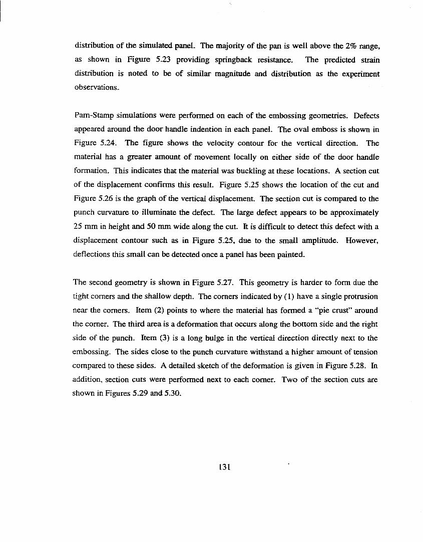
distribution of the simulated panel. The majority of the pan is well above the 2% range,

as shown in Figure 5.23 providing springback resistance. The predicted strain

distribution is noted to be of similar magnimde and distribution as the experiment

observations.

Pam-Stamp simulations were performed on each of the embossing geometries. Defects

appeared around the door handle indention in each panel. The oval emboss is shown in

Figure 5.24. The figure shows the velocity contour for the vertical direction. The

material has a greater amount of movement locally on either side o f the door handle

formation. This indicates that the material was buckling at these locations. A section cut

of the displacement confirms this result. Figure 5.25 shows the location of the cut and

Figure 5.26 is the graph of the vertical displacement. The section cut is compared to the

punch curvature to illuminate the defect. The large defect appears to be approximately

25 mm in height and 50 mm wide along the cut. It is difficult to detect this defect with a

displacement contour such as in Figure 5.25, due to the small amplimde. However,

deflections this small can be detected once a panel has been painted.

The second geometry is shown in Figure 5.27. This geometry is harder to form due the

tight comers and the shallow depth. The comers indicated by ( 1) have a single protrusion

near the comers. Item (2) points to where the material has formed a “pie crust" around

the comer. The third area is a deformation that occurs along the bottom side and the right

side of the punch. Item (3) is a long bulge in the vertical direction directly next to the

embossing. The sides close to the punch curvature withstand a higher amount of tension

compared to these sides. A detailed sketch of the deformation is given in Figure 5.28. In

addition, section cuts were performed next to each comer. Two of the section cuts are

shown in Figures 5.29 and 5.30.

131

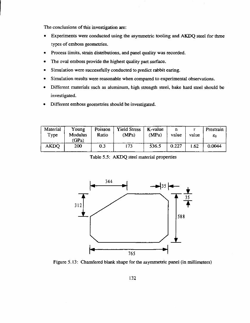
The conclusions of this investigation are:

• Experiments were conducted using the asymmetric tooling and AKDQ steel for three

types of emboss geometries.

• Process limits, strain distributions, and panel quality was recorded.

• The oval emboss provide the highest quality part surface.

• Simulation were successfiilly conducted to predict rabbit earing.

• Simulation results were reasonable when compared to experimental observations.

• Different materials such as aluminum, high strength steel, bake hard steel should be

investigated.

• Different emboss geometries should be investigated.

MaterialType

YoungModulus

(GPa)

PoissonRatio

Yield Stress (MPa)

K-value(MPa)

nvalue

rvalue

Prestrain£q

AKDQ 2 0 0 0.3 173 536.5 0.227 1.62 0.0044

Table 5.5: AKDQ steel material properties

34435

312

A35

T

588

HI 765

Figure 5.13: Chamfered blank shape for the asymmetric panel (in millimeters)

132

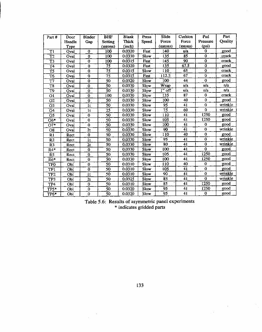
Part# DoorHandleType

BinderGap

BEIFSetting(mtons)

BlankThick(inch)

PressSpeed

SlideForce

(mtons)

CushionForce

(mtons)

PadPressure

(psi)

PartQuality

Tl Oval 0 100 0.0320 Fast 140 n/a 0 goodT2 Oval 0 100 0.0330 Slow 135 85 0 crackT3 Oval 0 100 0.0315 Fast 145 90 0 crackT4 Oval 0 75 0.0320 Fast 135 67.5 0 goodT5 Oval 0 75 0.0315 Slow 110 65 0 crackT6 Oval 0 75 0.0315 Fast 112.5 67 0 crackT7 Oval 0 50 0.0320 Slow 100 44 0 goodT8 Oval 0 50 0.0330 Slow Wrap n/a n/a n/aT9 Oval 0 50 0.0330 Slow I” off n/a n/a n/aOl Oval 0 100 0.0330 Slow 135 87 0 crack02 Oval 0 50 0.0330 Slow 100 40 0 good03 Oval It 50 0.0330 Slow 95 41 0 wrinkle04 Oval It 25 0.0330 Slow 75 60 0 wrinkle05 Oval 0 50 0.0330 Slow 110 41 1250 good06* Oval 0 50 0.0330 Slow 105 41 1250 good07* Oval 0 50 0.0330 Slow 100 41 0 good08 Oval 2t 50 0.0330 Slow 90 41 0 wrinkleR1 Rect 0 50 0.0330 Slow 110 40 0 goodR2 Reel It 50 0.0330 Slow 95 41 0 wrinkleR3 Rect 2t 50 0.0330 Slow 80 41 0 wrinkle

R4* Rect 0 50 0.0330 Slow 100 41 0 goodR5 Rect 0 50 0.0330 Slow 105 41 1250 good

R6* Rect 0 50 0.0330 Slow 100 41 1250 goodTPO Obi 0 50 0.0310 Slow 110 40 0 goodTPl Obi 0 50 0.0310 Slow 105 41 0 goodTP2 Obi It 50 0.0310 Slow 90 41 0 wrinkleTP3 Obi 2t 50 0.0325 Slow 85 41 0 wrinkleTP4 Obi 0 50 0.0310 Slow 85 41 1250 goodTPS* Obi 0 50 0.0320 Slow 95 41 1250 goodTP6* Obi 0 50 0.0320 Slow 95 41 0 good

Table 5.6: Results of asymmetric panel experiments * indicates gridded parts

133

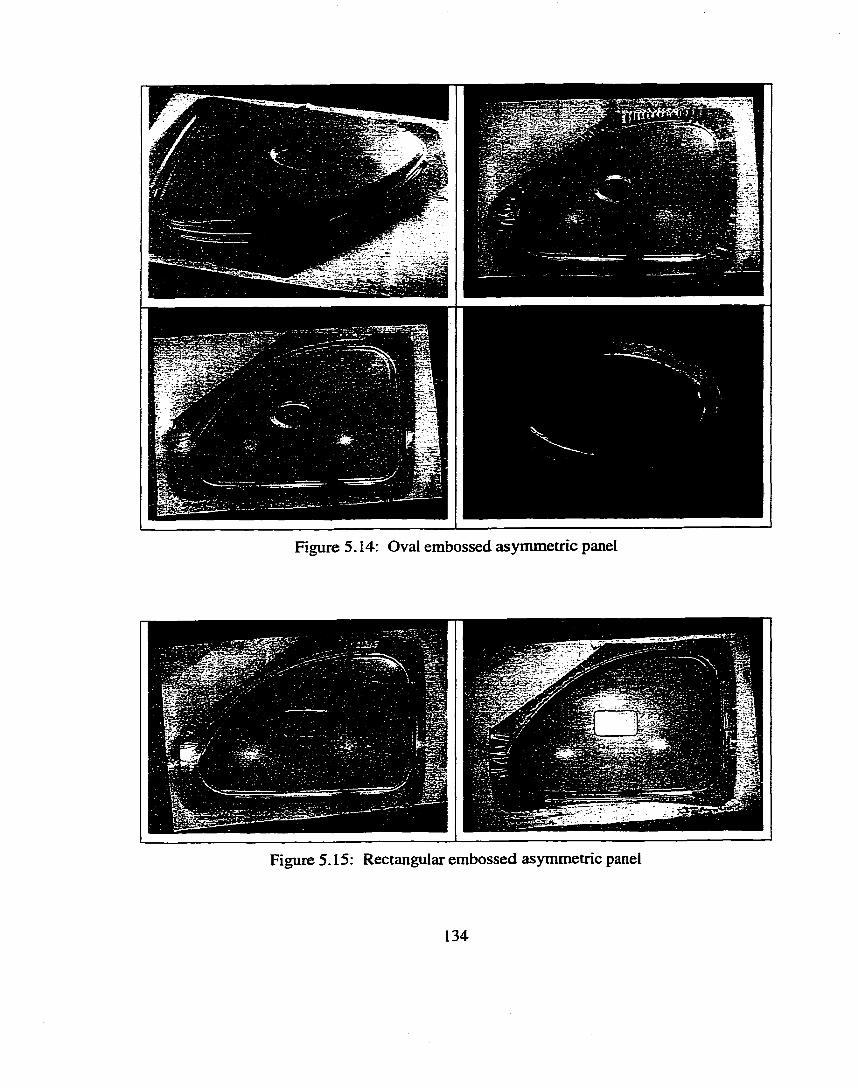
Figure 5.14: Oval embossed asymmetric panel

Figure 5.15: Rectangular em bossed asym m etric panel

134

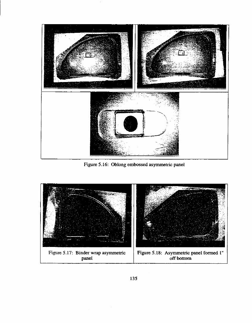
Figure 5.16: Oblong embossed asymmetric panel

Figure 5.17: Binder wrap asymmetric panel

Figure 5.18: Asymmetric panel formed I" off bottom

135

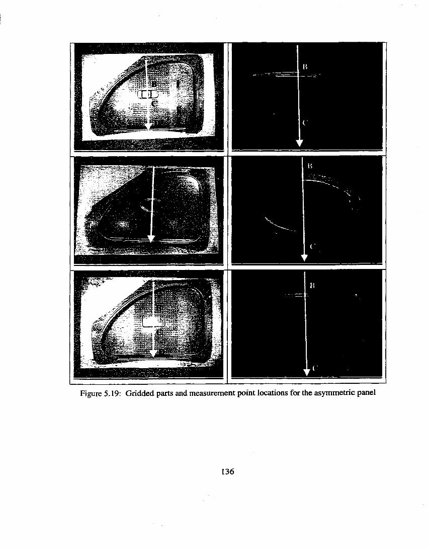
I

Figure 5.19: Gridded parts and measurement point locations for the asymmetric panel

136

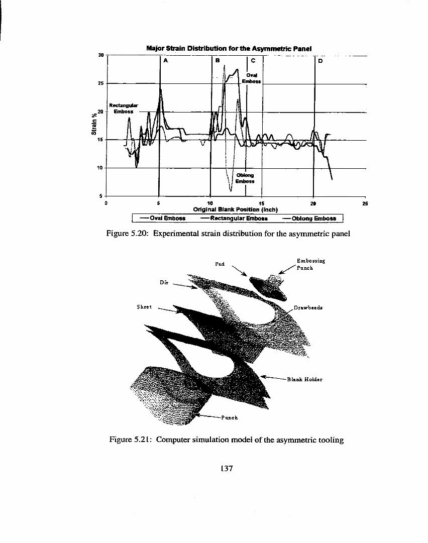
30 TMajor Strain Distribution for the Asymmetric Panel

A B

-l/\c

OvalniMss

D

RectanBUiar 111

r lII

^ A /1

\\ i mgOSS \

25

.20

c2

15

10

10 15O rig in a l B lan k P o s itio n (in ch )

20 25

— O val E m b o ss — R e c ta n g u la r E m b o ss — O b lo n g E m b o ss )

Figure 5.20: Experimental strain distribution for the asyrrunetric panel

Pad

Drawbeads

EmbossingPnnch.

Blank Holder

Figure 5 .2 L : Computer sim ulation m odel o f the asymmetric tooling

137

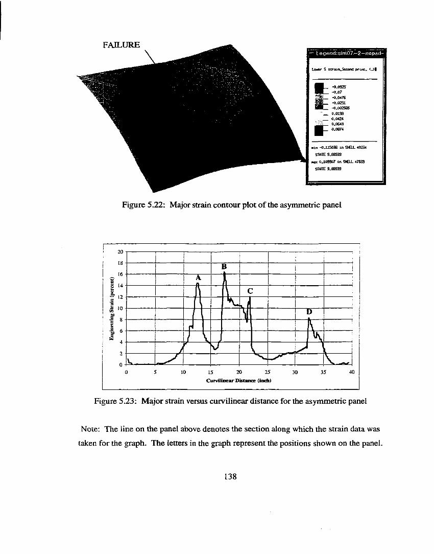
FAILUREL eg e n d :s im 0 7 —2 —n o p ad -

Lower S stratn_Seoond p rin c . < ^ |

-O.OS2S-0 07- 0.0476-0.0251-0.002565

0.0139 0.0424

0.0S430.0874

■m -0.115036 in SHELL 40234

STATE 9.88933

max 0a03907 in StCLL 47639

STATE 9.88939

Figure 5.22: Major strain contour plot o f the asymmetric panel

Î

20

18

16

14

12

10

8

6

4

2

0

5 20 25 35 400 10 15 30Curvilinear Distance (inch)

Figure 5.23: Major strain versus curvilinear distance for the asymmetric panel

Note: The line on the panel above denotes the section along which the strain data was

taken for the graph. The letters in the graph represent the positions shown on the panel.

138

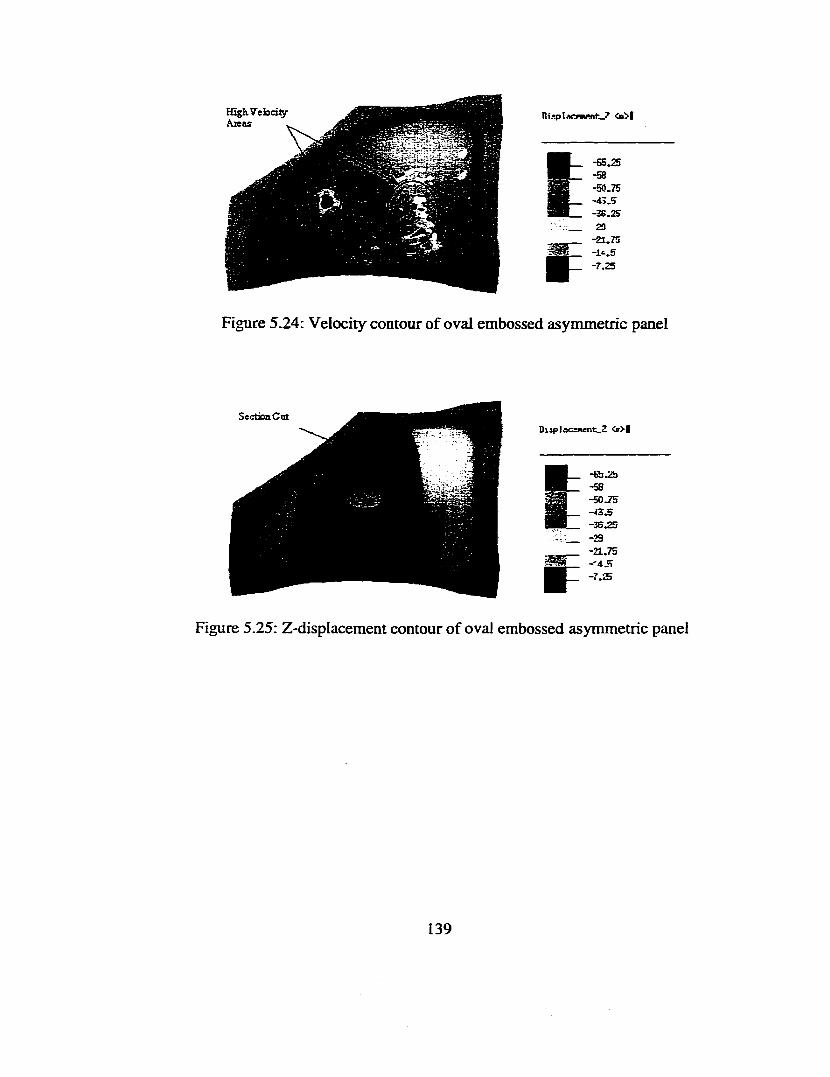
Hîgh.VeIoci^ Aie a s

-65.25-58-50-75-iîJS- 36.2523

- 21.75-L‘-.5-7.25

Figure 5.24: Velocity contour of oval embossed asymmetric panel

SectionCntDiiplacEinenC-Z <»>|

-55.25-58-50.75

-36.25-29-a .7 5

- 7.25

Figure 5.25: Z-dispIacement contour of oval embossed asymmetric panel

139

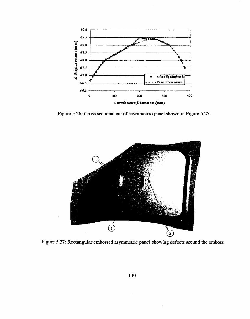
7 0 .0

I 9.0 S 6SS I 6 S .0

* 67.5

67.0 I— A fie r S ÿ n tg b a c k

- C w r a tw e

66.04000 200100 300

C urvilinear. D is tan ce (mm)

Figure 5.26: Cross sectional cut of asymmetric panel shown in Figure 5.25

Figure 5.27: Rectangular embossed asymmetric panel showing defects around the emboss

140

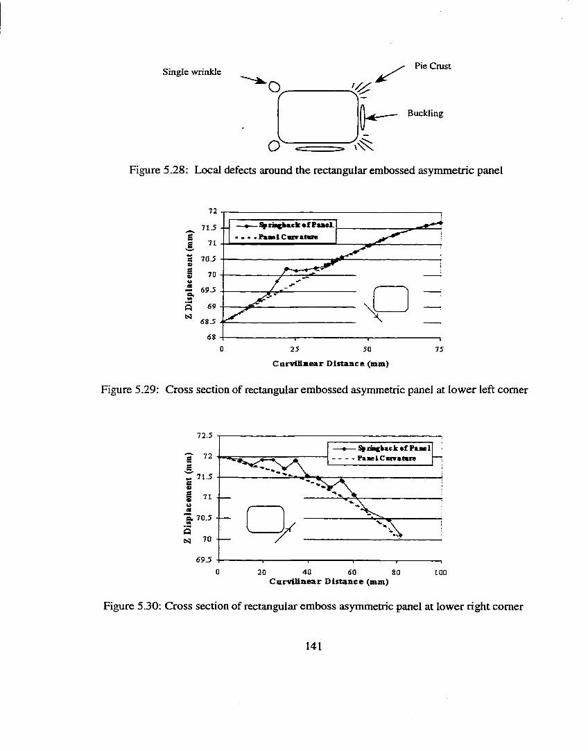
Single wrinkle Pie Crust

Buckling

Figure 5.28: Local defects around the rectangular embossed asymmetric panel

72

—•— Sÿxni(k»ck •£ Bamel - • • F u e l C a t r a t v e

_ 7 1 S -

1C 70^ - -9I

I 69.5

70

S'a 69

68.5

630 25 50 75

C u rv ilin e a r D istance (mm)

Figure 5.29: Cross section of rectangular embossed asymmetric panel at lower left comer

I— Sjpinckmck •£ Psmel - - PaBelCwateze72 ■

71.5

Bi 7 0 . 5 ------

7 0 ------

69.50 4020 60 80 100

C urv ilinear D istance (mm)

Figure 5.30: Cross section o f rectangular em boss asymmetric panel at low er right com er

141

CHAPTER VI

PART, DIE, AND PROCESS DESIGN METHODOLOGY FOR DEEP DRAWING AND STAMPING

6.1 Near Zero StampingIn 1994, the Auto Body Consortium (ABC) submitted the proposal entitled Near Zero

Stamping (NZS) to the National Institute of Science and Technology's (NIST) Motor

Vehicles Manufacturing Advanced Technology Program. In the NZS project, 26

automotive companies provided matching funds along with NIST funding to achieve a

total project budget of $ 18 million for 4 years. Five research instimtions were chosen to

conduct the technical work of the project which included the Engineering Research

Center for Net Shape Manufacturing (ERC/NSM) at the Ohio State University.

The author of this dissertation has managed this project as a full time engineer for the

ERC/NSM since kick off. Part of the intent of this work is to deliver this dissertation and

it contributions as part of the Near 2Iero Stamping project and to the members of the Auto

Body Consortium.

The Near Zero project was organized into four projects and eleven tasks of which the

ERC/NSM was involved in three tasks. This dissertation will largely concentrate on two

of these tasks whose primary goals are respectively:

• Task 1.2: Computer Simulation - To develop a methodology to implement

computer simulation into the auto body design process and to produce the

necessary technologies to make this possible/easier.

142

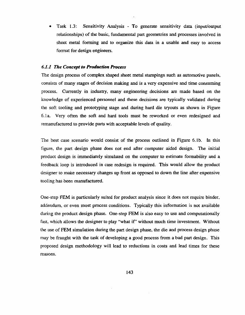
• Task 1.3: Sensitivity Analysis - To generate sensitivity data (input/output

relationships) of the basic, fundamental part geometries and processes involved in

sheet metal forming and to organize this data in a usable and easy to access

format for design engineers.

6.1.1 The Concept to Production Process

The design process o f complex shaped sheet metal stampings such as automotive panels,

consists of many stages of decision making and is a very expensive and time consuming

process. Currently in industry, many engineering decisions are made based on the

knowledge of experienced personnel and these decisions are typically validated during

the soft tooling and prototyping stage and during hard die tryouts as shown in Figure

6.1a. Very often the soft and hard tools must be reworked or even redesigned and

remanufactured to provide parts with acceptable levels of quality.

The best case scenario would consist of the process outlined in Figure 6.1b. In this

figure, the part design phase does not end after computer aided design. The initial

product design is immediately simulated on the computer to estimate formability and a

feedback loop is introduced in case redesign is required. This would allow the product

designer to make necessary changes up front as opposed to down the line after expensive

tooling has been manufactured.

One-step FEM is particularly suited for product analysis since it does not require binder,

addendum, or even most process conditions. Typically this information is not available

during the product design phase. One-step FEM is also easy to use and computationally

fast, which allows the designer to play “what i f ’ without much time investment. Without

the use of FEM simulation during the part design phase, the die and process design phase

may be fraught with the task of developing a good process from a bad part design. This

proposed design methodology will lead to reductions in costs and lead times for these

reasons.

143

Once the product has been designed and validated, the development project would enter

the time zero phase and would be passed onto the die designer. The die designer would

validate his/her design with an incremental FEM code and make necessary design

changes and perhaps even optimize the process parameters to ensure not just minimum

acceptability of part quality, but maximum achievable quality. This increases product

quality but also increases process robusmess. Incremental FEM is particularly suited for

die design analysis since it does require binder, addendum, and process conditions which

are either known dining die design or desired to be known.

The most common use o f FEM simulation in industry is to estimate the formability o f the

process and to determine the most optimal process conditions. The elimination of

splitting and wrinkling via BHF and drawbeads is not the only possible use. The

prediction of gravity/binder wrap conditions, impact line movement, surface distortions,

trimming/piercing, springback, ideal blank shape, and optimum BHF trajectory/pattern

may also be achieved. A proposed simulation methodology will be presented in the next

subsection for the design o f complex stampings which fully utilizes the potential of

computer simulation.

The validated die design would then be manufactured directly into the hard production

tooling and be validated with physical tryouts during which the prototype parts would be

made. Tryout time should be decreased due to the earlier numerical validations.

Redesign and remanufacturing of the tooling due to unforeseen forming problems should

be a thing of the past. The decrease in tryout time and elimination of

redes ign/remanufacturing should more than make up for the time used to numerically

validate the part, die, and process.

In Figure 6.1, notice that the experience of the engineer is not replaced with computerized

tools. On the contrary, the experience of the engineer is an integral part o f this process.

If the experience of an engineer is limited for whatever reason, then the educational

144

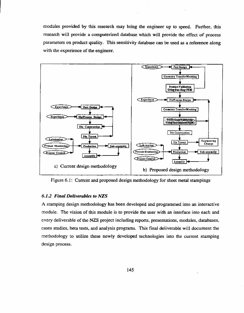
modules provided by this research may bring the engineer up to speed. Further, this

research will provide a computerized database which will provide the effect o f process

parameters on product quality. This sensitivity database can be used as a reference along

with the experience of the engineer.

[Experience

CCExpcri

^ X u b r i c a t i o n _

Monilor -

Process ControL "

Part Design

Die/Proccsy Design

I D i e C o n s t n i c t i o n

I Pie Tryout 1

Production H Sub-assem bly"l

I Assembly H

a) Current design methodology

ÇExpcriemcc >{~Tart

I G eom etry T ra a sfe r /M c sh ia g |TP raiticC V alMatfoa. aiiagOme SkpKKI

C T E x p e n e n c c ^ ^ # | D te/Process Dcsigo |4

I G eom etry T raosfer/M esh iiig I

7; Drt nccniValiifMK

IDie C an s tm c tio a

CTLubricaiiiiaZDie T ry o u t

Toceis Monitoria ^ CTProcess Comte»0 - 1

E n g in ee r in gC h an g e

Frodaction S n b -asse m b ly

A ssem bly |<

b) Proposed design methodology

Figure 6 . 1 : Current and proposed design methodology for sheet metal stampings

6.1.2 F inal Deliverables to N ZS

A stamping design methodology has been developed and programmed into an interactive

module. The vision of this module is to provide the user with an interface into each and

every deliverable of the NZS project including reports, presentations, modules, databases,

cases studies, beta tests, and analysis programs. This final deliverable will document the

methodology to utilize these newly developed technologies into the current stamping

design process.

145

The concept will be to outline the auto body design process using flowcharting

techniques and provide this user with a clickable exploding map of the process as shown

in Figures 6.2 through 6.4. On each page, clickable items may lead the user deeper into

the module or to related deliverables. In this way, a user who is searching for help may

find the information and tools in an environment which is familiar to them.

The highest level of final deliverable is shown in Figure 6.2. Here the auto body

realization methodology is outlined from concept to production. By clicking on the “Part

Design” box, the user is transported into the page shown in Figure 6.3, which outlines the

stamping part design methodology. If the user clicks on the “Die Build” box in Figure

6.2, he or she is taken to the page shown in Figure 6.4, which is the stamping die build

methodology. Please note that on each of these pages are clickable items which take the

user directly to related deliverables.

For example if the user is trying to solve a splitting problem, then he or she may click

into the "Stamping Die Build" section, then click "Splitting". The user will then find

pictures of split parts and methods to predict splitting including forming limit diagrams

and failure criteria. A list of possible solutions to splitting problems will be included

such as:

• Decrease BHF, drawbead restraint, and blank size.

• Increase lubrication, material thickness, material grade, n-value, r-value, and

part/die radii.

• Modify blank shape/location, binder and addendum geometry.

Each of the above solutions would be clickable to allow the user to understand how to

implement each of these. Furthermore, the user would have access to any reports, case

studies, databases, modules, and software that would contain useful information on

splitting. In this case the list of tools would be:

• Report "Evaluating Failiure Criteria Using Computer Simulation," by Sylvan Lemercier

146

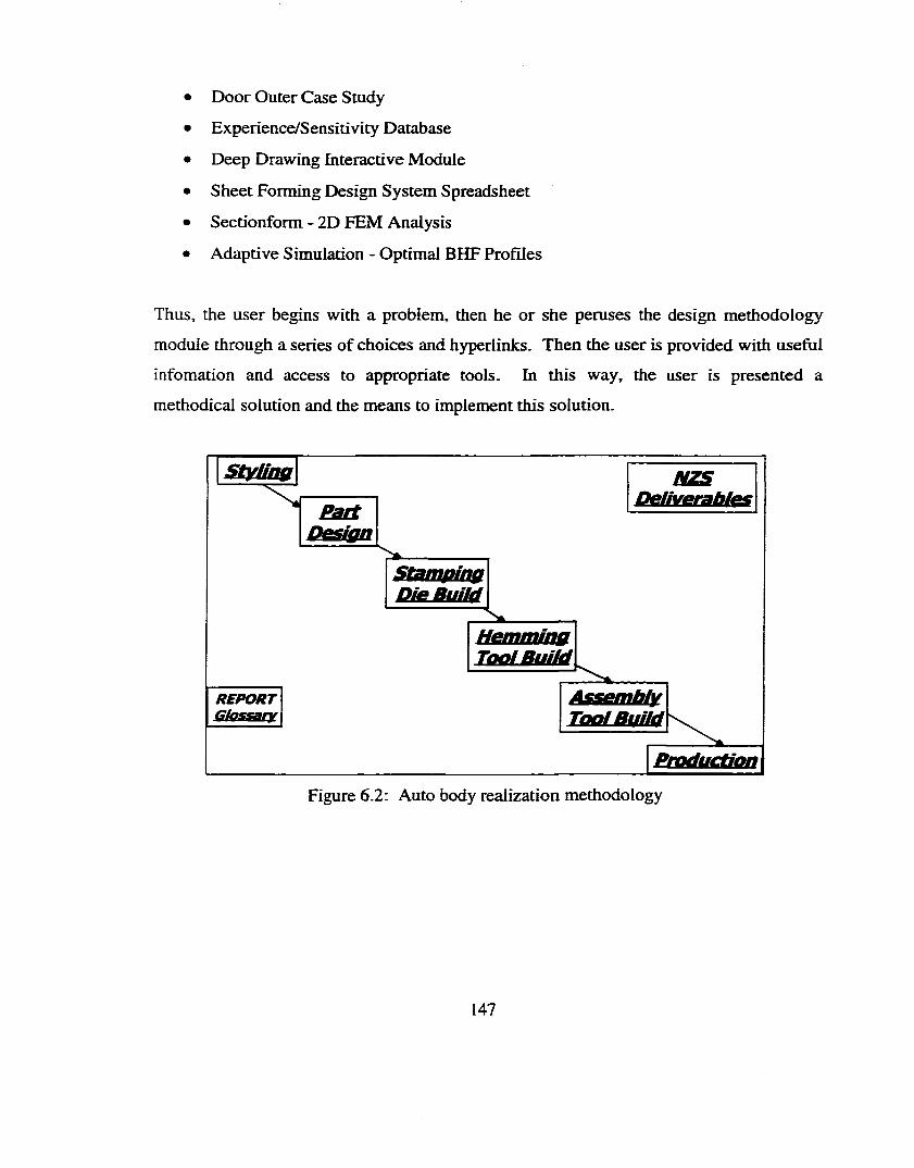
• Door Outer Case Study

• Experience/Sensitivity Database

• Deep Drawing Interactive Module

• Sheet Forming Design System Spreadsheet

• Sectionform - 2D FEM Analysis

• Adaptive Simulation - Optimal BHF Profiles

Thus, the user begins with a problem, then he or she peruses the design methodology

module through a series of choices and hyperlinks. Then the user is provided with useful

infomation and access to appropriate tools. In this way, the user is presented a

methodical solution and the means to implement this solution.

PartDesign

Stamping Die Buiid

HemmingTooi Buiid

ProductionFigure 6.2: Auto body realization methodology

147

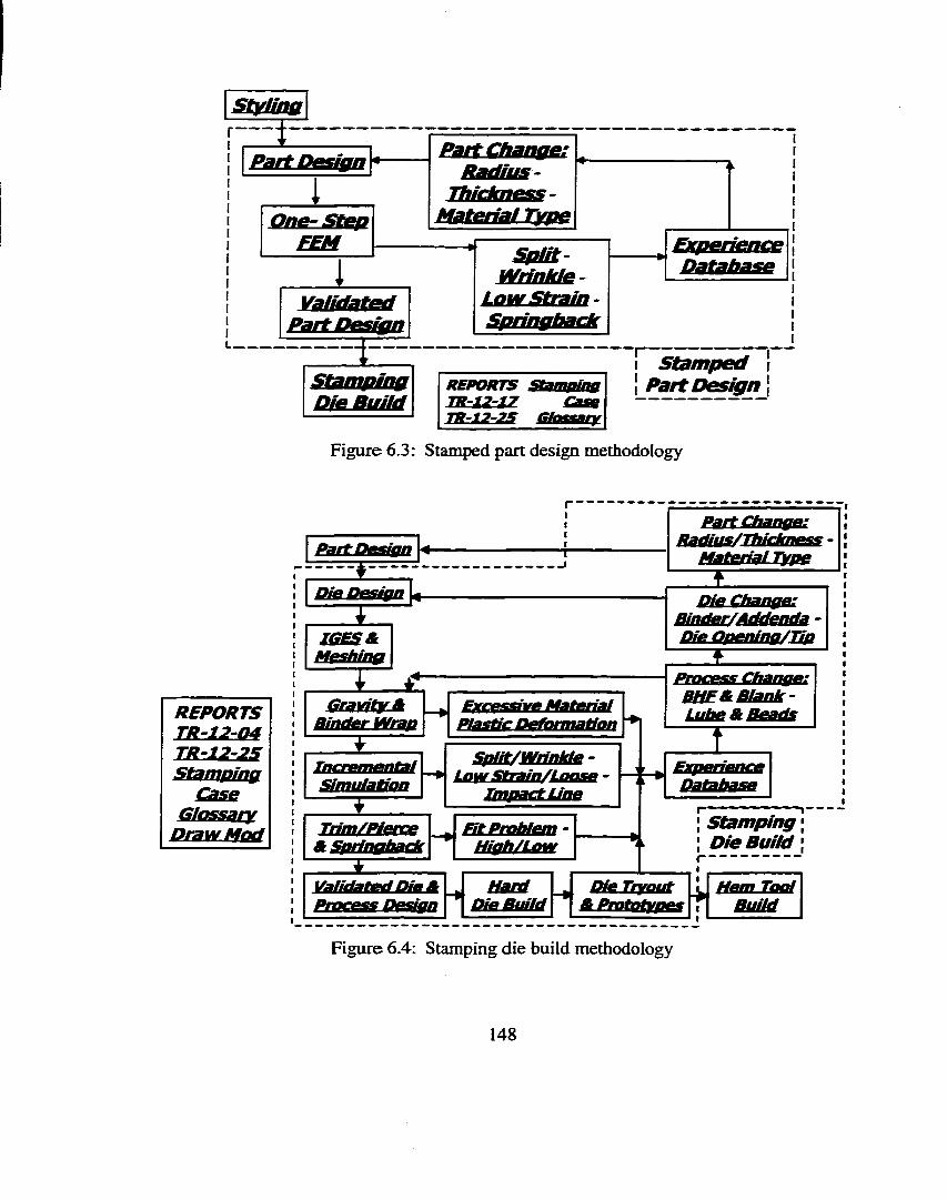
f stamped i I Part Design |

y r

Part Design

One- Step EEM Experience

DatabaseVaiidated

Part Design

REPORTS StampÎÊig TR-12-17 Cox TR-12~25 Gfossary

Spiit- Wrinkle-

Low strain-Springback

Part Change: R a d iu s-

T h lck n ess-Materiai Tÿpe

REPORTSTR-12-04T R zl2-25Stam ping

CaseG iossary

D raw M od

Figure 6.3: Stamped part design methodology

EoitDeaanr-IIII

T "

Part Change:B adius/Ibtdsaem -

MateriaLType

DieDesiBB «--------------------------------------------------_ T ------------

Binder/Addenda -IGESAMeshing

Die Opening/Tipf ....

T Z ^G a d ty n

Binder WrapExcesaxe M aterialPlastic Defomadan

Incranenta!Simulation

I : :

SpUt/W riDUe- Law strain/Lao^ -

Im padtU ne

Trim/Pierce & Sprittgbatic

M tP nM m n - H igh/Lew

Validated Die SProcnes Design

Hard Die Buiid

Process Change;BHF&Biank- Lube A Beads

Î ,ExperienceDatabase

f s m r n p ln g \ \ D ie B uiid ;I------------------------------I

Die Tryout A Prototypes

Hem Tool B uiid

Figure 6.4: Stamping d ie build methodology

148

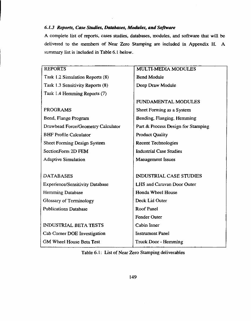
6.L3 Reports, Case Studies, Databases, Modules, and Software

A complete list of reports, cases studies, databases, modules, and software that will be

delivered to the members of Near Zero Stamping are included in Appendix H. A

summary list is included in Table 6 .1 below.

REPORTS MULTI MEDIA MODULES

Task 1.2 Simulation Reports (8 ) Bend Module

Task 1.3 Sensitivity Reports (8 ) Deep Draw Module

Task 1.4 Hemming Reports (7)

FUNDAMENTAL MODULES

PROGRAMS Sheet Forming as a System

Bend, Flange Program Bending, Flanging, Hemming

Drawbead Force/Geometry Calculator Part & Process Design for Stamping

BHF Profile Calculator Product Quality

Sheet Forming Design System Recent Technologies

SectionForm 2D FEM Industrial Case Studies

Adaptive Simulation Management Issues

DATABASES INDUSTRIAL CASE STUDIES

Experience/Sensitivity Database LHS and Caravan Door Outer

Hemming Database Honda Wheel House

Glossary of Terminology Deck Lid Outer

Publications Database Roof Panel

Fender Outer

INDUSTRIAL BETA TESTS Cabin Inner

Cab Comer DOE Investigation Instrament Panel

GM Wheel House Beta Test Truck Door - Hemming

Table 6 .1 : List of Near Zero Stamping deliverables

149

6.2 Industrial Case Studies6.2.1 Deck Lid Soft Tool Tryouts - Case Study

This section will discuss the results of a deck lid simulation Two materials were

simulated and formed in physical soft tool tryouts, 1004 AKDQ steel and 6111-T4

aluminum. The material properties are listed in Table 6.2. The process conditions used

in the simulations are listed in Table 6.3. The panel geometry was symmetrical, so only

half of the tooling was simulated.

The geometry for a rear deck lid draw die was obtained in IGES format and imported into

I DEAS, so that it could be cleaned and meshed. A coarse mesh was initially defined, so

that adaptive mesh refinement could later be used in regions of sharp geometry. The

meshed surfaces of the die, binder, sheet, and trim line were imported into Pam-Stamp’s

preprocessor module. The punch surface was created by offsetting the die surface by a

sheet thickness. The opposing binder surface was similarly created.

The first step in the forming process was binder wrap. This was simulated by orienting

the sheet between the binder surfaces and closing the binders together using a velocity

boundary condition. This process formed the initial blank shape shown in Figure 6.5a

into the binder wrap sheet shape shown in Figure 6.5b. The second step was to simulate

the stretch-draw operation. The appropriate binder force was applied and the punch was

assigned a velocity boundary condition. A typical drawbead restraining force was then

applied and the result is shown in Figure 6 . 6 for both materials. Severe wrinkling

occurred in the product area for the aluminum blank due to loose material in the die. The

steel blank does not exhibit the severe wrinkling but still exhibits less than 1 % strain in

the same region indicating a similar loose material condition. These predictions were

also observed during the soft tool tryouts. The loose material issue was resolved using a

drawbar in the addendum region as shown in Figure 6.7.

150

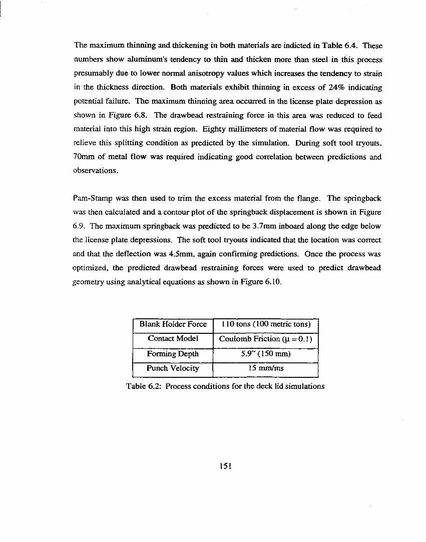
The maximum thinning and thickening in both materials are indicted in Table 6.4. These

numbers show aluminum's tendency to thin and thicken more than steel in this process

presumably due to lower normal anisotropy values which increases the tendency to strain

in the thickness direction. Both materials exhibit thinning in excess o f 24% indicating

potential failure. The maximum thinning area occurred in the license plate depression as

shown in Figure 6 .8 . The drawbead restraining force in this area was reduced to feed

material into this high strain region. Eighty millimeters of material flow was required to

relieve this splitting condition as predicted by the simulation. During soft tool tryouts,

70mm of metal flow was required indicating good correlation between predictions and

observations.

Pam-Stamp was then used to trim the excess material from the flange. The springback

was then calculated and a contour plot o f the springback displacement is shown in Figure

6.9. The maximum springback was predicted to be 3.7mm inboard along the edge below

the license plate depressions. The soft tool tryouts indicated that the location was correct

and that the deflection was 4.5mm, again confirming predictions. Once the process was

optimized, the predicted drawbead restraining forces were used to predict drawbead

geometry using analytical equations as shown in Figure 6.10.

Blank Holder Force 1 1 0 tons ( 1 0 0 metric tons)

Contact Model Coulomb Friction (p. = 0.1)

Forming Depth 5.9” (150 mm)

Punch Velocity 15 mm/ms

Table 6.2: Process conditions for the deck lid simulations

151

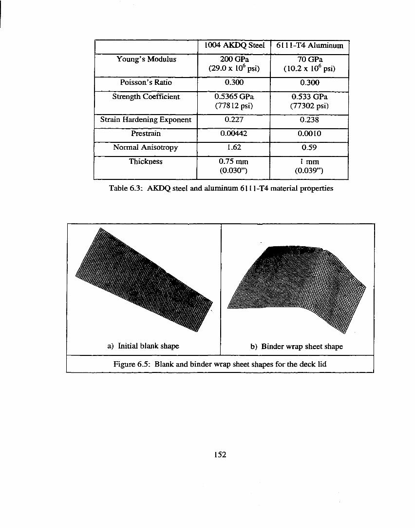
1004 AKDQ Steel 6 111-T4 Aluminum

Young’s Modulus 200 GPa (29.0 X 10® psi)

70 GPa (10.2 X 10® psi)

Poisson s Ratio 0.300 0.300

Strength Coefficient 0.5365 GPa (77812 psi)

0.533 GPa (77302 psi)

Strain Hardening Exponent 0.227 0.238

Prestrain 0.00442 0 . 0 0 1 0

Normal Anisotropy 1.62 0.59

Thickness 0.75 mm (0.030”)

1 mm (0.039”)

Table 6.3: AKDQ steel and aluminum 6111-T4 material properties

a) Initial blank shape b) Binder wrap sheet shape

Figure 6.5: Blank and binder wrap sheet shapes for the deck lid

152

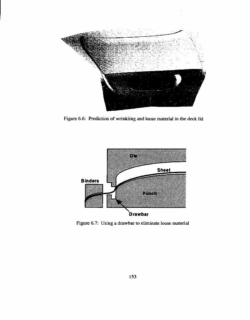
Figure 6 .6 : Prediction of wrinkling and loose material in the deck lid

Sheet

Binders

Drawbar

Figure 6.7: Using a drawbar to eliminate loose material

153

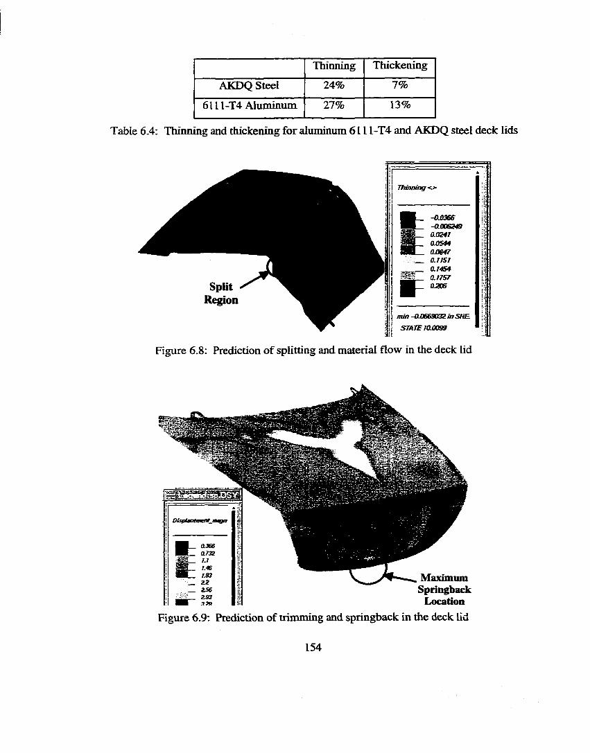
Thinning Thickening

AKDQ Steel 24% 7%

6111-T4 Aluminum 27% 13%

Table 6.4: Thinning and thickening for aluminum 6111-T4 and AKDQ steel deck lids

Thinning-K.

-a o s e s-aOQS249 0.0041 Q.OS44 0.084r

_ 0./757 a 74W

Q.nST aooB

m m -0.0b69O 3Z in SH B

STATE 10.0099

SplitRegion

Figure 6 .8 : Prediction o f splitting and material flow in the deck lid

Dtspiac tment m^gn

Maximum Springback

LocationFigure 6.9: Prediction of trimming and springback in the deck lid

154

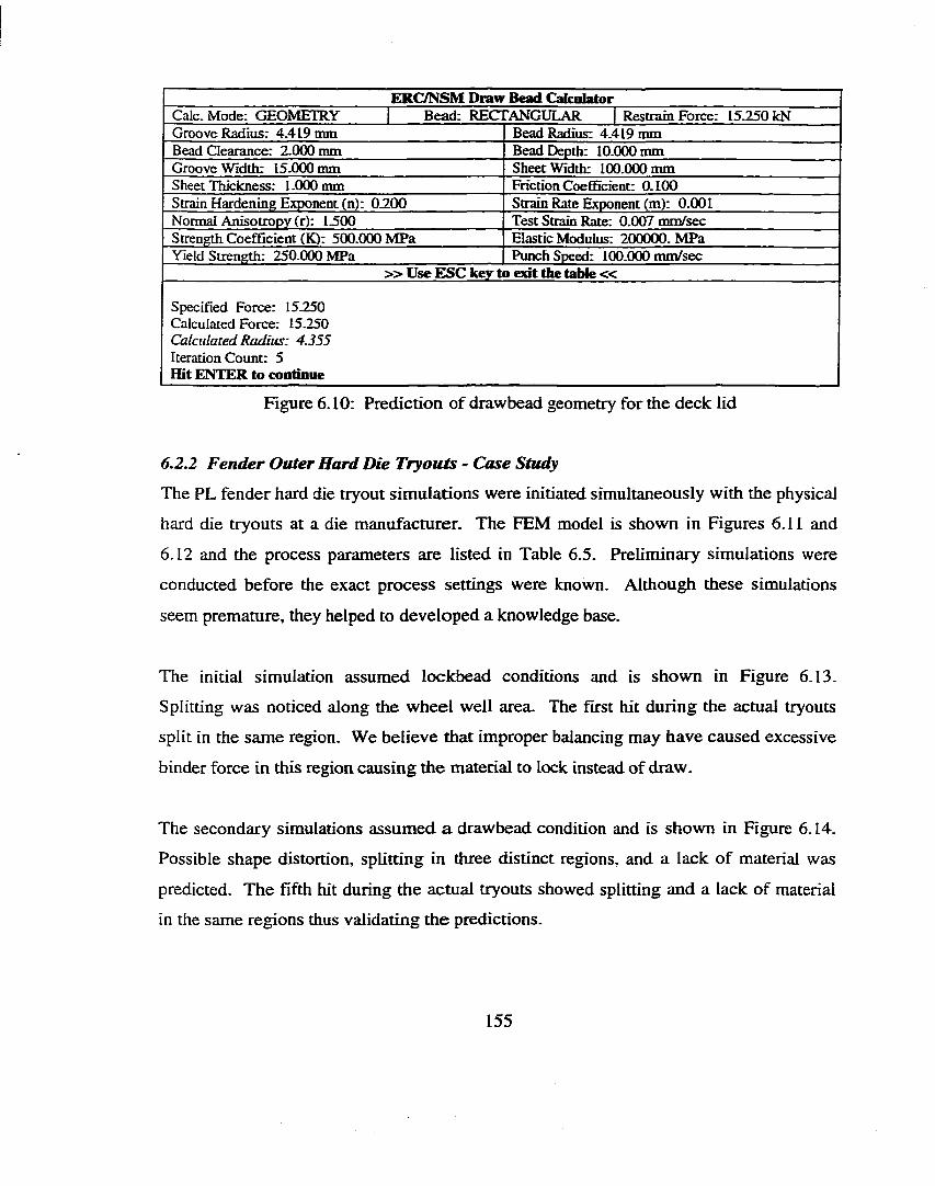
ERC/NSM Draw Bead CalculatorCalc. Mode: GEOMETRY Bead: RECTANGULAR Restrain Force: 15.250 kNGroove Radius: 4.419 mm Bead Radius: 4.419 mmBead Clearance: 2.000 mm Bead Depth: 10.000 mmGroove Width: 15.000 mm Sheet Width: 100.000 mmSheet Thickness: 1.000 mm Friction Coefficient: 0.100Strain Hardening Exponent (n): 0.200 Strain Rate Exponent (m): 0.001Normal Anisotropy (r): 1300 Test Strain Rate: 0.007 mm/secStrength Coefficient (K): 500.000 MPa Elastic Modulus: 200000. MPaYield Strength: 250.000 MPa Punch Speed: 100.000 mm/sec

» Use ESC key to exit the table «

Specified Force: 15.250 Calculated Force: 15.250 Calculated Radius: 4.355 Iteration Count: 5 Hit ENTER to continue

Figure 6 .10: Prediction of drawbead geometry for the deck lid

6.2.2 Fender Outer Hard Die Tryouts - Case Study

The PL fender hard die tryout simulations were initiated simultaneously with the physical

hard die tryouts at a die manufacturer. The FEM model is shown in Figures 6 . 11 and

6.12 and the process parameters are listed in Table 6.5. Preliminary simulations were

conducted before the exact process settings were known. Although these simulations

seem premature, they helped to developed a knowledge base.

The initial simulation assumed lockbead conditions and is shown in Figure 6.13.

Splitting was noticed along the wheel well area. The first hit during the actual tryouts

split in the same region. We believe that improper balancing may have caused excessive

binder force in this region causing the material to lock instead of draw.

The secondary simulations assumed a drawbead condition and is shown in Figure 6.14.

Possible shape distortion, splitting in three distinct regions, and a lack of material was

predicted. The fifth hit during the actual tryouts showed splitting and a lack of material

in the same regions thus validating the predictions.

155

We received the exact drawbead geometry and blank holder force and incorporated the

new information into the third set of simulations. Figure 6.15 shows the binder wrap and

shaded images of the deformation history of the fender. Figure 6.16 shows the draw-in

pattern after the draw stage which predicts a lack of material in the wheel well region.

Figure 6.17 shows a strain contour which predicts areas of low strain.

The combination of poor binder wrap, excessive material flow, and insufficient length o f

line caused the low strain problem in the simulation. After trimming the tryout fender,

the region o f low strain could not retain its geometry thus validating the predictions.

Gainers were added to the section between the left and right hand fenders as shown in

Figure 6.18 to eliminate the low strain condition.

Final process conditions were provided by the die manufacturer for the final fender

simulations. The blank, drawbeads, BHF, and balancing blocks were redesigned as

shown in Figure 6.19. The changes were implemented into the simulation, and final

simulation was run. Figure 6.20 shows that a good panel was obtained thus ending the

tryouts.

The simulated panel was trimmed as a final exercise and is shown in Figure 6.21. To aid

in the visualization of the simulated fender geometry, rapid prototypes were made of the

binder wrap, 75% draw, and 100% draw (Figure 6.22). Nodal and connectivity data were

obtained from Pam-Stamp and fed into a custom-made software developed by the

ERC/NSM to generate stereolithography (STL) files. The STLs were then downloaded

into a fused deposition machine (FDM) to create the models. This process is referred to

as virtual processing.

156

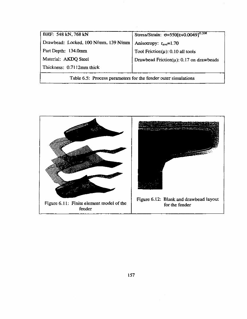
BHF: 548 kN, 768 kN

Drawbead: Locked, 100 N/mm, 139 N/mm

Part Depth: 134.0mm

Material: AKDQ Steel

Thickness: 0.7112mm thick

Stress/Strain: a=550[e+0.0049]°~°*

Anisotropy: rave=L70

Tool Friction(p): 0.10 all tools

Drawbead Friction(p): 0.17 on drawbeads

Table 6.5: Process parameters for the fender outer simulations

1%Figure 6 . 1 1 : Finite element model of the

fender

Figure 6.12: Blank and drawbead layout for the fender

157

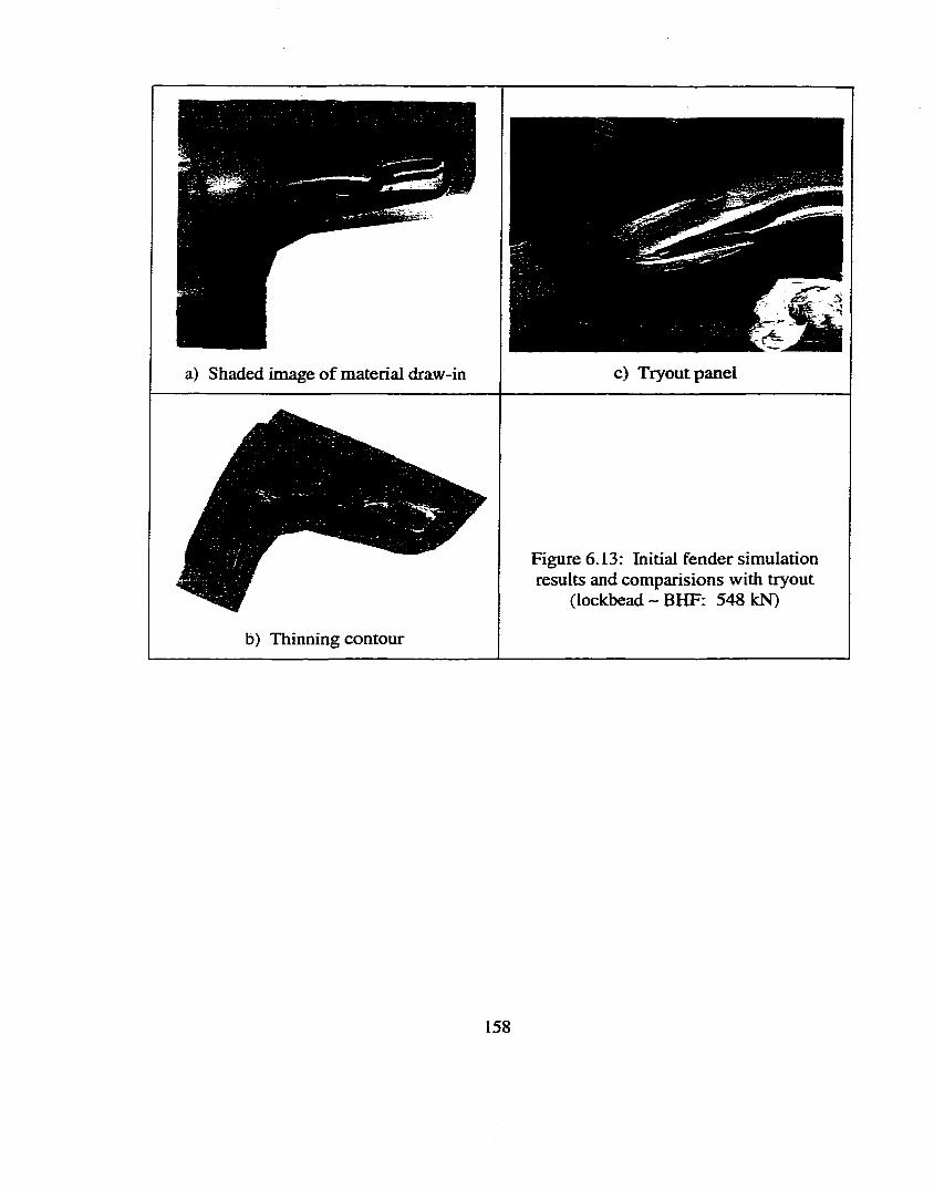
a) Shaded image o f material draw-in c) Tryout panel

Figure 6.13: Initial fender simulation results and comparisions with tryout

(lockbead - BHF: 548 kN)

b) Thinning contour

158

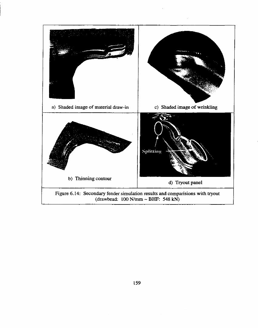
a) Shaded image of material draw-in

b) Thinning contour

c) Shaded image o f wrinkling

Spl itt injd

d) Tryout panel

Figure 6.14: Secondary fender simulation results and comparisions with tryout (drawbead: 100 N/mm ~ BHF: 548 kN)

159

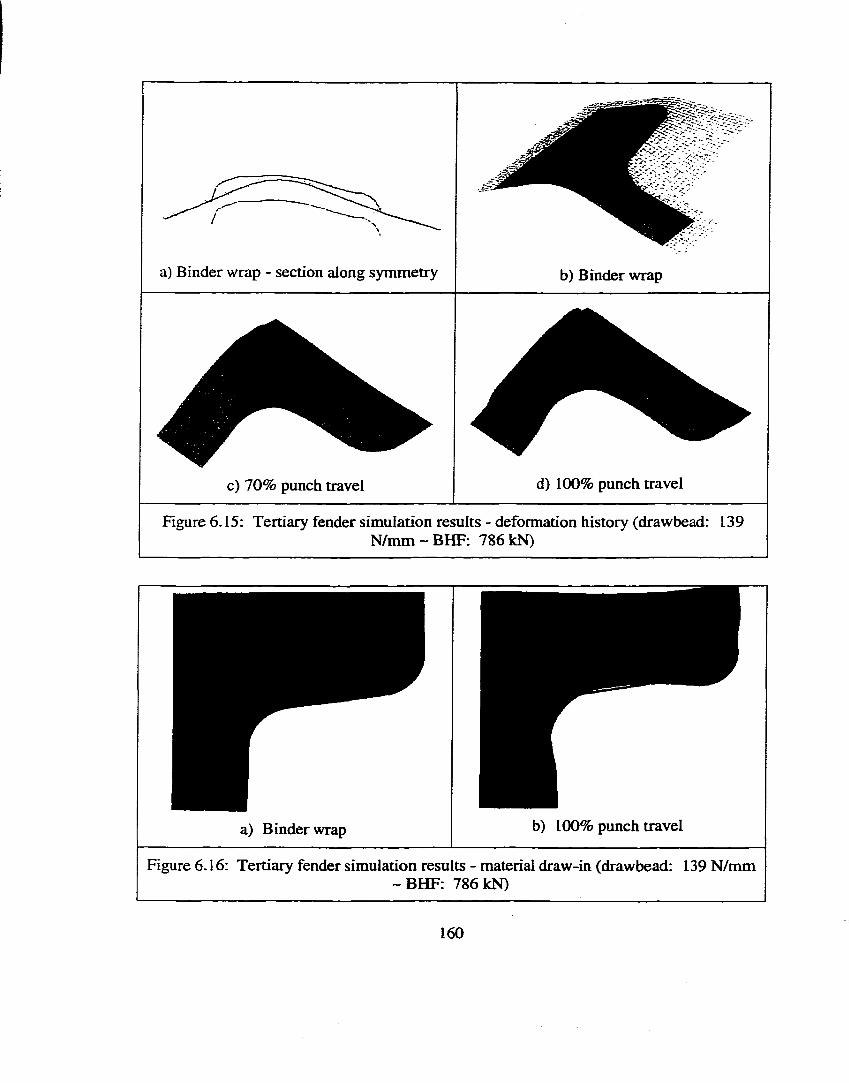
a) Binder wrap - section along symmetry b) Binder wrap

c) 70% punch travel d) 1 0 0 % punch travel

Figure 6.15: Tertiary fender simulation results - deformation history (drawbead: 139N/mm — BHF: 786 kN)

a) Binder wrap b) 1 0 0 % punch travel

Figure 6.16: Tertiary fender simulation results - material draw-in (drawbead: 139 N/mm-B H F : 7 86kN)

160

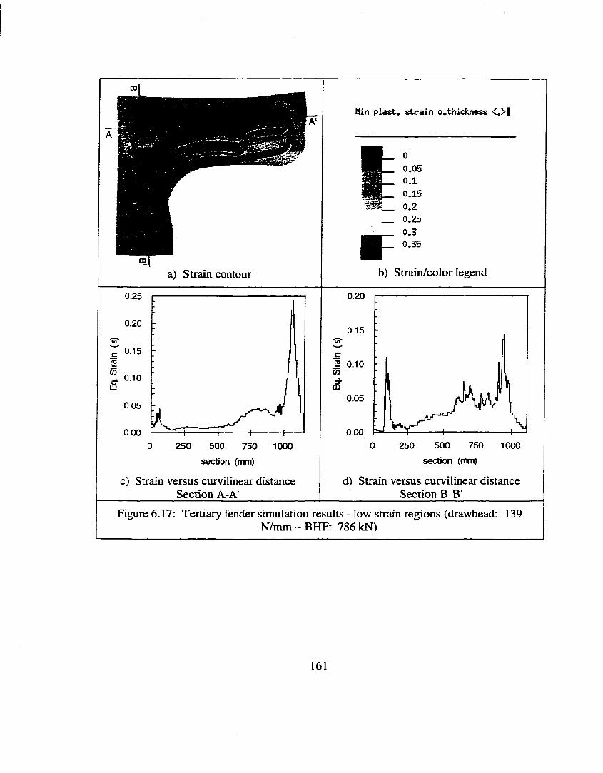
a) Strain contour

Min p last. strain o*thickness 0 |

00.050.10.150.20.250.30.35

b) Strain/color legend

0.25

0.20

0.15

- 0.10crLU

0.05

0.000 250 500 750 1000

0.20

0-15

S 0-10CO

0.05

0.00500 750 10000 250

section (mm)

c) Strain versus curvilinear distance Section A-A’

section (mm)

d) Strain versus curvilinear distance Section B-B

Figure 6-17: Tertiary fender simulation results - low strain regions (drawbead: 139N/mm ~ BHF: 786 kN)

161

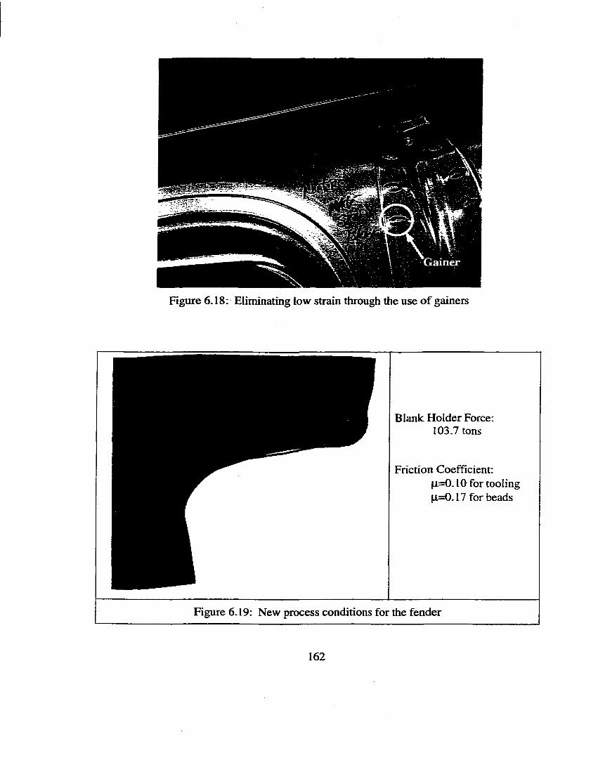
Figure 6.18: Eliminating low strain through the use o f gainers

Blank Holder Force: 103.7 tons

Friction Coefficient:(1 =0 . 1 0 for tooling (1=0.17 for beads

Figure 6.19: New process conditions for the fender

162

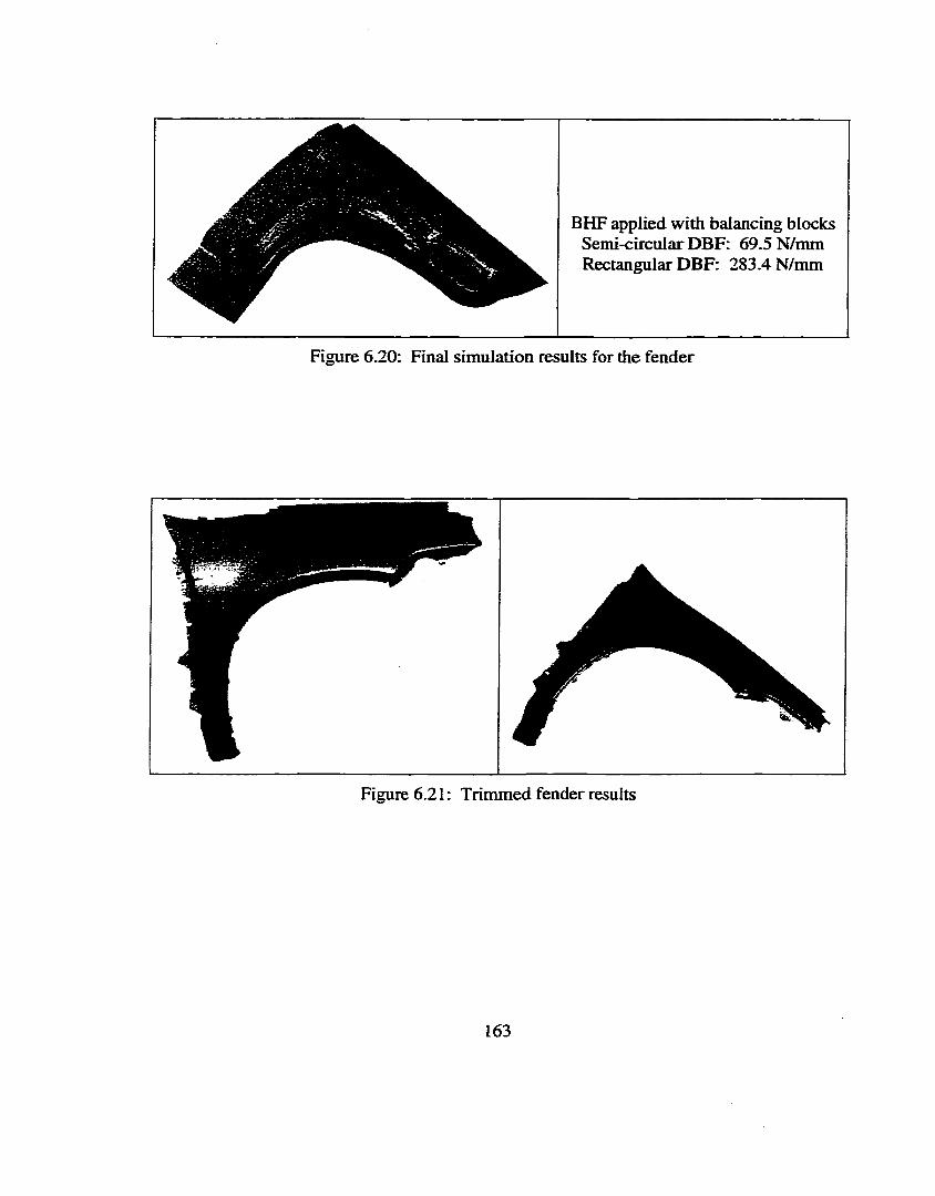
BHF applied with balancing blocks Semi-circular DBF: 69.5 N/mm Rectangular DBF: 283.4 N/mm

Figure 6.20: Final simulation results for the fender

Figure 6.21 : Trimmed fender results

163

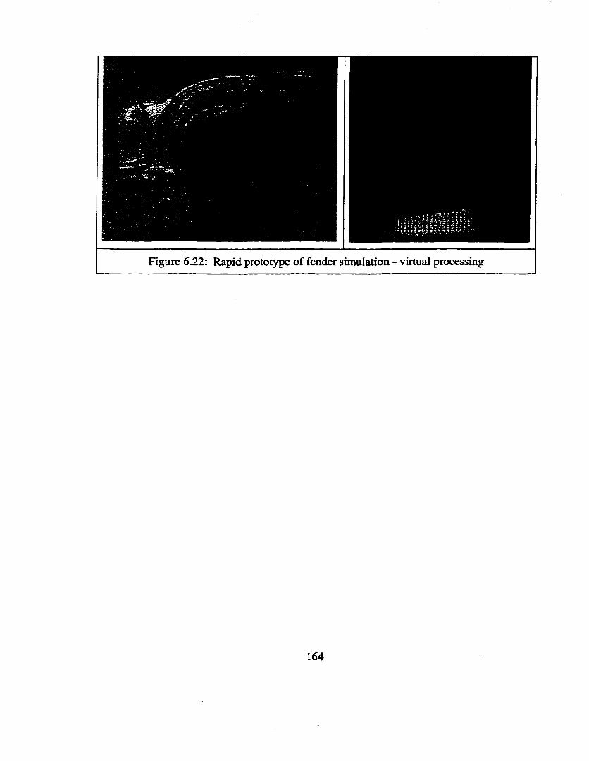
Figure 6.22: Rapid prototype of fender simulation - virtual processmg

164

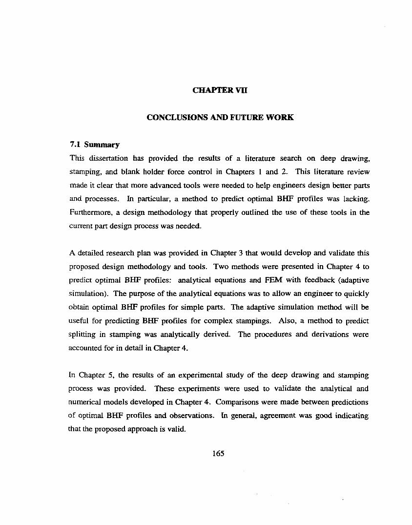
CHAPTER Vn

CONCLUSIONS AND FUTURE WORK

7.1 SummaryThis dissertation has provided the results of a literature search on deep drawing,

stamping, and blank holder force control in Chapters I and 2. This literature review

made it clear that more advanced tools were needed to help engineers design better parts

and processes. In particular, a method to predict optimal BHF profiles was lacking.

Furthermore, a design methodology that properly outlined the use of these tools in the

current part design process was needed.

A detailed research plan was provided in Chapter 3 that would develop and validate this

proposed design methodology and tools. Two methods were presented in Chapter 4 to

predict optimal BHF profiles: analytical equations and FEM with feedback (adaptive

simulation). The purpose of the analytical equations was to allow an engineer to quickly

obtain optimal BHF profiles for simple parts. The adaptive simulation method will be

useful for predicting BHF profiles for complex stampings. Also, a method to predict

splitting in stamping was analytically derived. The procedures and derivations were

accounted for in detail in Chapter 4.

In Chapter 5, the results of an experimental study of the deep drawing and stamping

process was provided. These experiments were used to validate the analytical and

numerical models developed in Chapter 4. Comparisons were made between predictions

of optimal BHF profiles and observations. In general, agreement was good indicating

that the proposed approach is valid.

165

A general description for the proposed design methodology was provided in Chapter 6.

This system outlines the current and proposed design methodology. The proposed design

methodology designates when in the design process does each tool or module enter in.

This design methodology provides the framework by which engineers may improve their

stamping designs. The analytical and empirical tools o f this research will allow engineers

to conduct their work more scientifically. The educational modules provided by this

dissertation will deliver these concepts and tools to engineers in an efficient manner. In

addition, the results and deliverables of the Near Zero Stamping project was described.

7.2 Research ResultsThe following research contributions to the state of the art were developed through this

dissertation:

• Part and process design methodology for the deep drawing and stamping of sheet

metal parts that will lead to a robust process with improved drawability.

• Computerized tools that provide engineers with the effect of process parameters

on part quality (sensitivity data) for various simple tool geometries from

laboratory experiments and computer simulations.

• Mathematical model and computer software that allows engineers to calculate

forming forces, formability limits, required tool geometry, and optimal BHF

profiles for simple part geometries such as round cups, rectangular pans, U-

channels, hemispherical shells, and asymmetric panels.

• Module for commercial finite element method (FEM) programs that implements a

feedback loop into the calculations (adaptive simulation) in order to determine

optimal process BHF time profiles and spatial patterns for general complex

geometries.

1 6 6

7.3 ConclusionsThe following conclusions are made based on the previously described dissertation work:

• Three new laboratory tools have been designed, built, and implemented through

this dissertation work including the rectangular pan tooling, the hydraulic BHF

control system, and the asymmetric panel tooling.

• The analytical and numerical models were successfiiUy validated through the use

of laboratory experiments on round, rectangular, and asymmetric parts.

• The analytical and numerical models successfully predict optimal time and

location variable BHF profiles for simple deep drawing and complex stamping.

• The proposed design methodology has been validated through a series of

industrial cases studies.

• A variety of tools has been developed for the sheet forming engineer including an

interactive module which guides the user through the proposed design

methodology and provides him or her with access to reports, cases studies,

databases, modules, and software developed through the NZS project.

• The results of this dissertation can be used to help implement light weight, less

formable materials into automotive products.

• The appendices at the end of this dissertation outline the detailed procedures to

develop the analytical and numerical tools and can be helpful to anyone who

wishes to follow this work.

7.4 Future WorkThe author of this dissertation proposes the following items as future work:

• Develop an analytical method to predict time and location variable BHF profiles

for rectangular and asymmetric panels.

• Continue the numerical investigation of implementing a feedback loop into

commercial FEM software (adaptive simulation) for the purpose of predicting

optimal time and location variable BHF profiles and vahdate with laboratory

experiments.

167

• Conduct adaptive simulations and experiments with the non-flat rectangular panel

tooling and hydraulic BHF control system.

• Conduct adaptive simulations on industrial parts and validate with industrial

experiments.

• Implement failiue criteria into a commercial FEM program and validate with

laboratory experiments.

• Beta test the proposed design methodology and interactive modules at an

industrial site and use the results to improve the methodology.

168

REFERENCES

Adamson, A.M., Ulsoy, A.G., Demeri, M. (1996) Dimensional Control in Sheet Metal Forming via Active Binder Force Adjustment. Transactions of the North American Manufacturing Research Institution o f SME. Vol. XXIV. pp. 167-172.

Ahmetoglu, Brouwers, D., Shuikin, L., Taupin L., Kinzel, GX., Altan, T. (1995) Deep Drawing of Round Cups from Tailor-Welded Blanks. Elsevier. Journal of Materials Processing Technology. Vol. 53. pp.684-694.

Ahmetoglu, M., Altan, T. (1996) Using Computer Simulations for Sheet Metal Forming. Stamping Quarterly. July/August, pp. 42.

Ahmetoglu, M., Broek, T.R., Kinzel, G., Altan, T. (1996) How to Improve Results when Deep Drawing Rectangular Parts Controlling BHF to Eliminate Wrinkling and Fracture. The Fabricator. October.

Ahmetoglu, M., Kinzel, G., Altan, T. (1996) Advanced Techniques to Improve the Formability of Aluminum Alloys. METALFORM '96 PMA Technical Symposium. March.

Aida Press Handbook (1992) Aida Engineering. Ltd.Aita, S., Khaldi, F., Fontaine, L., Tamada, T., Tamura, E. (1992) Numerical Simulation

of Stretch Drawn Autobody. Warrendale, PA; SAE International Congress and Exposition.

Altan, T., Oh, S., and Gegel, H. L. (1983) Metal Forming: Fundamentals and Applications. American Society for Metals.

Aluminum Association. (1997) Aluminum Standards and Data.

Antunez, H.J., Kleiber, M. (1996) Parameter Sensitivity of Metal Forming Processes. Computer Assisted Mechanics and Engineering Sciences, pp.263-282.

Arrieux, R. (1995) Determination and Use of the Forming Limit Stress Diagrams in Sheet Metal Forming. Journal of Materials Processing Technology. Vol. 53. pp. 47-56.

Asnafi, N. (1993) The Influence of In-Process Variation of Blank Holding Force on Deep-Drawability Swedish Institute for Metals Research. Sept. 27.

169

Auto Body Consortium. (1995) Near Zero Stamping Proposal to the Advance Technology Program (95-02) for the 1995 Motor Vehicle Manufacturing Technology.

Avitzur, B. (1983) Deep-Drawing. Handbook of Metal-Forming Processes, pp. 527- 579.

Badrinarayanan, S., Zabaras, N. (1996) A Sensitivity Analysis for the Optimal Design of Metal-forming Processes. Computer Methods in Applied Mechanics and Engineering, pp.319-348.

Balanethiram, V., Daehn, G. (1994) Hyperplasticity-Increased Forming Limits at High Workpiece Velocities. Scripta Metallurgica. Vol. 31.

Banabic, D., Achimas, G., Dorr, I.R. (1993) The Influence of Pulsatory Straining on the Forming Limit Diagrams. Advance Technology of Plasticity. Proceedings of the Fourth International Conference on Technology o f Plasticity, pp. 1923-1928.

Blickwede, D. (1968) Metals Progress. December, pp. 64-70.

Blurael, K.W., Hartmann, G., Heldbuchel, P. (1991) Computer Driven Variable Blankholder. International Deep Drawing Research Group.

Burk, T.G., Chandorkar, K.V., Story, JM ., Assempoor, A., Kolodziejski, J. (1996) Tool Design For Aluminum Stamping. Aluminum and Magnesium for Automotive Applications Proceedings TMS Materials Week 95 Symposium 1996. pp. 49-67.

Callendar, A., Hartree, D., Porter, A. (1936) Time Lag in a Control System. Philos. Transactions R. Soc. London. Cambridge University Press.

Cao, J., Bakkestuen, R., Jalkh, P., Boyce, M.C., Hardt, D.E. (1994) Improvement of Forming Height and Stability of Aluminum Parts Using Active Binder Control- International Deep Drawing Research Group.

Ceretti, E., Giardini, C., Maccarini, G. (1994) Theoretical and Experimental Analysis of Non-Axisymmetrical Deep Drawing. Journal of Materials Processing Technology. Vol. 54. pp. 375-384.

Cherril, A.P., Zhang, S., Ousterhout, K.B. (1996) A Variable Force Binder for a Draw Press. Journal of Materials Processing Technology. Vol. 73. pp. 7-17.

Chiang, D., Kobayashi, S. (1966) The Effect of Anisotropy and Work-Hardening Characteristics on the Stress and Strain Distribution in Deep Drawing. Journal of Engineering for Industry. November, pp. 443.

Crockroft, M., Latham, D. (1968) Ductility and the Workability of Metals. Journal Institute of Metallurgy. Vol. 96. pp. 33-39.

Crowley, C. (1998) Investigation of Process Variables in Deep Drawing of Round Cups and Asymmetric Stamping Design and Tryout. M.S. Thesis. The Ohio State University. Columbus, Ohio.

170

Decaillet, C., Millet, P., Saur, E. (1990) Recent Developments in Aluminum Sheet Manufacture for Car Body Panels. International Journal of Vehicle Design. Vol. 11. No. 3.

Diller, M. (1997) A Systematic Approach to Automotive Stamping Design with Finite Element Analysis. M.S. Thesis. The Ohio State University. Columbus, Ohio.

Doege, E., Sommer, N. (1987) Blank Holder Pressure and Blank Holder Layout in Deep Drawing of Thin Sheet Metal. Advanced Technology of Plasticity. Vol. 2. pp. 1305-1314.

Doege, E., Stock G. (1995) Locked Tool - Deep-Drawing Process and Examples of Operations with Elastic Blank-Holders. SAE Paper No. 950917.

Duncan, J.L., Sowerby, R. (1987) Review of Practical Modeling Methods for Sheet Metal Forming. 2nd International Conference on Technology of Plasticity, 1. pp. 615-624.

Eary, D., Reed, E. (1974) Techniques of Pressworking Sheet Metal: An Engineering Approach to Die Design Prentice Hall, Inc.

El Sabaie, M., Melior, P. (1972) Plastic Instability Conditions in the Deep Drawing of a Circular Blank of Sheet Metal. International Journal of Mechanical Sciences, pp. 535.

Esche, S., Kinzel, G., Altan, T. (1996) Review of Failure Analysis in Sheet Metal Forming Simulations. NUMISHEET.

Esche, S.K., Khamitkar, S., Kinzel, G.L., Altan, T. (1996) Process and Die Design for Multi-Step Forming of Round Parts from Sheet Metal. Journal of Materials Processing Technology. Vol. 59. pp. 24-33.

Feteke, J R. (1997) Overview of Sheet Metals for Stamping. SAE Papers. No 970715. pp. 125-137.

Forming Technologies Inc. (1994) Stampability of Aluminum Panels With Reference to Spotting of Blankholder and Selection of Drawbead. Oakville, Ontario.

Frankling, G., Powell, J., Emami-Neiini, A. (1994) Feedback Control o f Dynamic Systems. Addison-Wesley. 3"* Edition.

Gerdeen, J.C., Huang, M. (1992) Factors Affecting the Formability of Comers in Sheet Metal Parts. SAE Technical Paper Series. No. 920637. pp. 173-181.

Ghouati, O., Gelin, J.C. (1996) Sensitivity Analysis and Optimization o f Shape and Process Parameters in Metal Forming. PD-Vol.75. Engineering Systems Design and Analysis. Vol.3. ASME.

Goodwin, G.M. (1968) Application Of Strain Analysis To Sheet Metal Forming Problems In The Press Shop. SAE Paper No. 680093.

171

Gotoh, M-, Katoh, M., Yamasitha^ M. (1997) Studies of Stretch-Drawing Process of Sheet Metals. Journal of Materials Processing Technology. Vol. 63. pp. 123- 128.

Guida, M., Li, X., Messina, A., Strona, P. (1994) Industrial Integrated Methodology for Deep-Drawing Process Optimization by Numerical Simulation. Journal Material Processing Technology. Vol.45. pp.323-328.

Gunnarsson, L., Thilderkvist, P., Runesson, J. (1997) In-Process Control of the Blank Holder Force with Gas Springs Applied on a Modified Cup Test and a Muffler. Swedish Institute for Metals Research. Feb. 26.

Hancock, T. (1989) A Systems Approach to Sheet Metal Processing. Computers in Industry. Vol. 13. pp. 245-251.

Hardt, D., Fenn, R. (1993) Real-Time Control of Sheet Stability During Forming. Journal of Engineering Industry. Vol. 115. pp. 299-308.

Haug, E., Di Pasquale, E., Pickett, AJC., and Ulrich, D. (1991) Industrial Sheet Metal Forming Simulation using Explicit Finite Element Method. Int. VDI Conference, Zurich. May 14-16.

Haug, E., Lefebvre, D., Heath, A., Recke, L., Guida, M., Panico, F., Westerling, C., Felder, E., Levaillant, C„ Netsch, T., Mazilu, P. (1994) Investigation for an Innovative Methodology for Sheet Metal Stamping. Presented at Umformtechnisches KoUoquiura Darmstadt (U K D '94). March 16-17.

Hayashi, Y., Takatani, M. (1984) New Forming Method for Avoiding Geometrical Defects of Outer Auto-body Panels. IDDRG 13^ Beinnal Congress, pp. 63-72.

Hecker, S. (1974) Metallurgical Engineering Quarterly, v 14, #4, 30.

Herderich, M. (1990) Experimental Determination of the Blankholder Forces Needed for Stretch Draw Die Design. Warrendale, PA: Society of Automotive Engineers. No. 900281. pp. 53-61.

Hill, R. (1979) Theoretical Plasticity of Textured Aggregates. Math. Proc. Cambridge Phil. Soc. Vol.85. pp. 179-191.

Hill, R. (1980) Constitutive Modelling of Orthotropic Plasticity in Sheet Materials. Journal of Mech Phys Solids. Vol. 38. No. 3. pp. 405-417.

Hirose, Y., Hishida, Y., Furubayashi, T., Oshima, M. (1990) Research on Techniques for Controlling Body Wrinkles by Controlling the Blank Holder Force. Spring Conference on Plastic Working, pp. 1-11.

Hishida, Y., Ujihara, S., Furubayashi, T., Hirose, Y., Kojima, M. (1990) Development of Blank Holding Force Control Forming Method— Part I. Nissan Motor Co. Ltd. Sumitomo Metal Industries Ltd.

172

Hishida, Y., Wagoner. R. (1993) Analysis of Blank Holding Force Control Forming Using Hydraulic Forming Simulator. Advanced Technology o f Plasticity. Vol. 2. Proceedings of 4th International Conference on Technology o f Plasticity, pp. 1740-1746.

Hobbs, R. (1974) Section I: Classification of Sheet Metal Operations, Prediction and Analysis o f Press Performance for Sheet Steels. BPH Technical Bulletin. Vol. 18. pp. 1-13.

Holt, R. ( 1998) Advances in Forming o f Aluminum Sheet for Automotive Applications. 3rd International Conference on Sheet Metal Forming Technology. Fabricators & Manufacturers Association.

Hosford, W. (1985) Comments on Anisotropic Yield Criteria. International Journal of Mechanical Sciences. Vol. 27. No. 78. pp. 423-427

Hosford, W., Caddell, R. (1993) Metal Forming: Mechanics and Metallurgy. New Jersey: Prentice Hall.

Jirathearanat, S. (1998) Virtual Processing and Rapid Tooling Techniques in Sheet Metal Forming. M.S. Thesis. The Ohio State University. Columbus. Ohio.

Kalpakjian, S. (1984) Manufacmring Processes for Engineering Materials. Addison- Wesley.

Karaflllis, A., Cao, J., Boyce, M. (1994) Simulation and Control of Sheet Metal Forming. Proceedings of the 15th Riso International Symposium on Materials Science: Numerical Predictions of Deformation Processes and the Behavior of Real Materials. Riso National Laboratory, Denmark.

Karima, M. (1994) Practical Application of Process Simulation in Stamping. Journal of Materials Processing Technology. Vol. 46. pp. 309-320.

Karima, M., Donatelli, V. (1989) Understanding Blank Holder Effect on Formability of Sheet Metal Stampings. SAE Annual Congress and Exposition, pp. 1-10.

Kawai, N. (1961) Critical Conditions o f Wrinkling in Deep Drawing of Sheet Metals. Bulletin of Japan Society of Mechanical Engineers. Vol. 4. No. 13. Reports 1-3. pp. 169-192.

Keeler, S. (1965) Determination of Forming Limits in Automotive Stampings. Sheet Metal Industries, pp. 683.

Kergen, R. (1983) Closed Loop Control of Blankholder Force Based on Deep Drawing Parameters: Its Laboratory and Industrial Applications. International Deep Drawing Research Group. Helsinki.

Kergen, R. (1996) A Comparison of Different Blank Holder Force Control Principles Based on the Cup Test. International Deep Drawing Research Group.

173

Kergen, R., Dauby, B. (1995) Computerised Control of BHF in Deep Drawing: A System Allowing Independent Closed Loop Control of the Blank Holder Force on Several Zones of the Blank Holder. International Deep Drawing Research Group.

Kergen, R., Jodogne, P. (1992) Computerized Control o f the Blankholder Pressure on Deep Drawing Presses. SAE Technical Papers. No. 920433.

Kojima, N. (1986) Effects of Drawbead Geometry on Drawbead Forces in Sheet Metal Forming. Proceedings of Advance Technology of Plasticity, pp. 434-435.

Konieczny, A., Kolodziejski, J., Karima, M. (1996) On Feasibility Assessment Tools for Car Body Styling and Body/Product Design. IBEC Body Assembly and Manufacturing.

Korhonen, A. (1982) Drawing Force in Deep Drawing o f Cylindrical Cup with Flat- Nose Punch. Journal of Engineering for Industry. February. Vol. 104. pp. 29.

Kuehne, L., Wohnig, W. (1993) Design and Simulation o f Press Dies for Body Panels. IBEC. pp. 73-80.

Kurii, K-, Shinabe, M., Hirabayashi, Y., Akiyama M. (1995). Binding Force Control of Uni-Pressure Cushion in Automobile Panel Stamping. SAE Paper #950916.

Kusuda, H , Takasago, T., Natsumi, F. (1996) Formability o f Tailored Blanks. Proceedings of the 2nd International Conference & Exhibits on Sheet Forming Technology.

Lange, K. (1985) Handbook of Metal Forming (Lehrbuch der Umformtechnik). Berlin, Springer- Verlag.

Lee, C.H., Huh, H. (1997) Blank Design and Strain Prediction of Automobile Stamping Parts by an Inverse Finite Element Approach. Journal of Materials Processing Technology. January, pp. 645-650.

Leu, D.K. (1997) Prediction of the Maximum Drawing Load in the Cup-Drawing Process of Sheet Metals. Journal of Materials Processing Technology. Vol. 72. pp. 256-261.

Livatyali, H. (1998) Computer Aided Process Design of Selected Sheet Metal Bending Processes - Flanging and Hemming. Ph D. Dissertation. The Ohio State University. Columbus, Ohio.

Logan, R.W. (1996) Use of Non-Quadratic Yield Surfaces in Design of Optimal Deep- Draw Part Geometry. Society of Automotive Engineers. No. 960597. pp. 61-72.

Majlessi, S.A., Lee, D. (1993) Deep Drawing of Square-Shaped Sheet Metal Parts, Part 2: Experimental Study. Journal of Engineering for Industry. Vol. 115. pp. 110- 117.

Makinouchi, A. (1996) Sheet Metal Forming Simulation in Industry. Journal of Materials Processing Technology. Vol. 60. pp. 19-26

174

Manabe, K., Nishimura, H. (1987) An Improvement in Deep Drawability of Steel/Plastic Laminate Sheets by Control of Blank Holding Force. Advanced Technology of Plasticity. Vol. 2. pp. 1297-1304.

Manabe, K., S. Yoshihara, M. Yang, Nishimura, H. (1995) Fuzzy Controlled Variable Blank Holding Force Technique for Circular Cup Deep Drawing of Aluminum Alloy Sheet. Transactions o f the North American Manufacturing Research Institution of SME. No MF995-121. Vol. 13. pp. 41-46.

Manabe, K., Yang, M., Teramac, T., Nishimura, H. (1996) Development of a Square- Cup Deep-Drawing Simulator with Cellularly Divided Blank Holder Control System. 19th International Deep Drawing Research Group Biennial Congress.pp. 101-108.

Manabe, K., Yoshihara, S., Nishimura, H., Shibata, A. (1996) Theoretical Analysis of Punch Speed and Blank Holder Force Control in Deep Drawing Process of Strain- Rate-Sensitive Materials. Proceedings of AS ME International Mechanical Engineering Congress, Dynamic Systems and Control Division. DSC-Vol. 58. pp. 175-182.

Marciniak, Z., Duncan, J i . (1991) The Mechanics of Sheet Metal Forming. London: Edward Arnold.

McVay, G., Courtright, E., Jones, R., Smith, M., Pacific Northwest National Lab. (1998) Reducing Manufacturing Costs: Key to Increasing Light Metal Usage inAutomotive Applications. Light Metal Age. Vol. 56. No. 9, 10. Fellom Publishing. San Franscico, CA.

Michigan Technological University. (1994) International Workshop on the Application of Closed Loop Control in Metal-Forming Processes.

Michler, J., Weinmann, K. (1995) Experimental and Finite Element Study of Sheet Metal Flow in a Strip Test Apparatus with Controllable Drawbead Penetration. Transactions of NAMRJ/SME. Vol. XXIII. pp. 45-50.

Michler, J.R., Kashani, A.R., Bohn, M L., Weinmann, K.J. (1995) Feedback Control of the Sheet Metal Forming Process Using Drawbead Penetration as a Control Variable. Transactions of the North American Manufacturing Research Institution of SME. Vol. X X d . pp. 71-76.

Mielnik, E.M. (1991) Metalworking Science and Engineering. McGraw-Hill, NY.Moessle, E. (1983) Influence of Deep-Drawing on the Surface State of Aluminum

Materials. Aluminum. May. Vol. 59. No. 5. pp. 349-357.

Muderrisoglu, A., Livatyali, H., Ahmetoglu, M., Altan, T. (1997) Computer Aided Design for Bending, Flanging and Hemming of Steels and Aluminum Alloys. Proceedings of the PMA Metalform '97 Symposium. March 9-12. Chicago, IL. pp. 151.

175

Murata, A., Matsui, M. (1994) Effects o f Control of Local Blank Holding Forces on Deep Drawability of Square Shell. International Deep Drawing Research Group, pp. 503-512.

Nakagawa, T. (1993) Recent Developments in Auto Body Panel Forming Technology. Annals of CIRP. Vol. 42/2. pp. 717-722.

Nakagawa, T., Nakamura, K. (1996) Various Applications of Hydraulic Counter- Pressure Deep Drawing. Proceedings of the 2nd International Conference & Exhibits on Sheet Forming Technology.

Nine, H.D. (1978) Drawbead Forces in Sheet Metal Forming. Mechanics of Sheet Metal Forming. Ed. Koistinen, D. P., Wang, N. M. Plenum Press, pp. 179-211.

Obermeyer, E.J., Majlessi, S_A. (1998) A Review of Recent Advances in the Application of Blank-Holder Force Towards Improving the Forming Limits of Sheet Metal Parts. Journal of Engineering Materials and Technology. Vol. 75. pp. 222-234.

Oehler, G., Kaiser, F. (1973) Blanking, Punching, and Drawing Tools. Fertingungstech. U. Betr., 17.

Okamoto, L, Takahashi, A., Sugiiu'a, H., Hiramatsu, T., Yamada, N., Mori, T. (1988) Computer Aided Design and Evaluation System for Stamping Dies in Toyota. SAE Technical Paper Series. No. 880524. pp. 79-89.

Osakada, K., Wang, C., Mori, K. (1995) Controlled FEM Simulation for Determining History of Blank Holding Force in Deep Drawing. Annals of the CIRP. Vol. 44/1. pp. 243-246.

Pahl, K.J. (1996) New Developments in Multi-Point Die-Cushion Technology. Proceedings o f 2nd International Conference on Sheet Metal Forming Technology. Engineering Research Center for Net Shape Manufacmring, Columbus, Ohio.

Painter, M., Pearce, R. (1976) Metal Flow Though a Drawbead. Sheet Metal Industries, pp. 12-19.

Park, K., Kim, Y. (1995) The Effect of Material and Process Variables on the Stamping Formability of Sheet Materials. Journal of Materials Processing Technology. Vol. 51. pp. 64-78.

Prasad, A.V., Chamverdi, R.C. (1996) Deep Drawing o f Cylindrical Cups — An Improved Software for Industrial Use. Numisheet. pp. 94-101.

Ray, R., Berry, J. (1970) Prediction of Press Loads in Deep Drawing Ti-6Al-4V, Stainless Steel AISI 304 and Inconel X Alloy Under Various Conditions of Lubrication at Room Temperamre. Transactions of the ASME. May. pp. 412.

Rebeio, N., Nagtegaal, J.C., Hibbitt, H.D. (1989) Practical Aspects of Modeling Sheet Forming Processes. NUMIFORM.

176

Roll, K. (1995) Finite Element Simulation of Eitemal and External High Pressure Forming. Proceedings of the Sheet Forming Technology Conference. Technical University Stuttgart, pp. 421-434.

Ruger, H. (1989) Modem Control o f Deep Drawing Presses. Sheet Metal Industries. May. pp. 221-223.

Sachs, G. (1951) Deep Drawing o f Thin-Walled Cylindrical Cups. Principles and Methods of Sheet-Metal Fabricating. Reinhold Publishing Co., NY. pp. 185-186.

Saran, M. (1997) Sensitivity of Forming Process to Variation of Material and Process Parameters. Society of Automotive Engineers.

Saran, M.J. (1990) Numerical and Experimental Investigations of Deep Drawing of Metal Sheets. Journal of Engineering for Industry. August. Vol. 112. pp. 272- 277.

Schey, J.A. (1996) Friction and Lubrication in Drawing Coated Steel Sheets on Chromium-Coated Beads. Lubricating Engineering. Sept. Vol. 52. No. 9. pp. 667-681.

Schey, J.A. (1997) Friction in Sheet Metalworking. SAE Technical Paper Series. No. 970712. International Congress and Exposition. February.

Schlegel, M. (1994) Pressure Controlled Nitrogen Cylinders for Draw Dies. Journal of Materials Processing Technology. Vol. 46. pp. 505-518.

Schuler GmbH. (1998) Metal Forming Handbook. Springer-Verlag, Berlin.

Schunemann, M., Ahmetoglu, M.A., Altan, T. (1996) Prediction of Process Conditions in Drawing and Ironing of Cans. Journal of Materials Processing Technology. Vol. 59. pp. 1-9.

Sellin, W. (1931) Handbook of Drawing Technology. Berling: Springer.

Semiatin, S. (Ed.). (1988) Deep Drawing. Metals Handbook. Vol. 14: Forming and Forging. American Society of Metals, pp. 575-590.

Semiatin, S. (Ed.). (1988) Stretch Forming. Metals Handbook. Vol. 14: Forming and Forging. American Society o f Metals, pp. 591-598.

Shang, H.M., Qin, S., Mo, J. (1996) Combined Effect of Drawing and Stretching in Axisymmetrical Sheet Forming. Journal of Materials Processing Technology. Vol. 62. pp. 454-457.

Shiraya, S. (1993) A Study of the Estimation Method for Sheet Blank Shape. Toyota Technical Report. Vol.43.

Shulkin, L. (1998) Blank Holder Pressure (BHP) Control with Flexible Blank Holder in Sheet Metal Forming. Ph D. Dissertation. The Ohio State University. Columbus, Ohio.

177

Shulkin, L. Rowan, D-, Kinzel, G., Altan, T. (1996) A New Hydraulic/Nitrogen Blank Holder Force Control System. Proceedings o f the ICTP. pp. 813.

Siebel, E., Beisswanger, H. (1955) Deep Drawing. Munich: Carl Hanser.

Siegert, K. (1995) Closed- Loop Control System for Blank Holder Forces In Deep Drawing. Annals o f CIRP. Vol. 44/1/1995. page 251-254.

Siegert, K. (1998) Tendencies in Draw Dies. 3"* International Conference on Sheet Forming Technology. Columbus, Ohio. Fabricators & Manufacturers Association.

Siegert, K., Harthun, S., Engelmann, D. (1996) Binder Design for Automotive Body Panels. SAE Technical Papers. No. 960822.

Siegert, K., Klamser. (1991) Four Point Hydraulic Draw System for Single Acting Mechanical Presses. Proceedings of the Conference on Draw Systems for Single Action Presses for Sheet Metal Forming. Technical University Stuttgart, pp. 41.

Siegert, K., Knabe, E. (1995) Fundamental Research and Draw Die Concepts for Deep Drawing of Tailored Blanks. SAE Technical Paper Series. No. 950921. pp. 159-169.

Siegert, K., Ziegler, M. (1997) Pulsating Blankholder Force. SAE Technical Papers. Paper No 970987. pp. 249-259.

Siegert, K., Ziegler, M., Wagner, S. (1996) Closed Loop Control of the Friction Force. Proceedings of 2nd International Conference on Sheet Metal Forming Technology. Engineering Research Center for Net Shape Manufacturing, Columbus, Ohio.

Siekirk, J. (1986) Process Variable Effects on Sheet Metal Quality. Journal of Applied Metal Working. Vol. 4. No. 3. pp. 262-269.

Siekirk, J. (1988) A Systems Approach to Sheet Metal Forming Process Control. Proceedings of the International Deep Drawing Research Group, pp. 1-7.

Sklad, M., Siekirk J. (1990) Aspects of Process Variables in Sheet Forming Simulation. International Deep Drawing Research Group, pp. 1-9.

Smith, D. A. (1994) Fundamentals of Pressworking. Society of Manufacturing Engineers (SME). Dearborn, Michigan.

Smith, M., Dunn, J. (1993) Lubrication Considerations for Aluminum Automotive Sheet. Journal of the Society of Tribologists and Lubrication Engineers.

Sonuner, N. (1986) Blankholder Force and Design o f Blankholders in Deep Drawing. University of Hannover. IFUM, VDI VERLAG.

Spisak, E., Stachowicz, F. (1994) Deformation Analysis o f Large-Sized Autobody Panels. Journal of Materials Processing Technology, pp. 817-826.

178

Stasik, M.,. Wagoner R. (1999) Forming of Tailor-Welded Aluminum Blanks. International Journal of Forming Technology (accepted for publication).

Story, J., Heinemann, S., Naegeler, S., Fraunhofer, USA. (1998) Forming and Joining Issues and Processes for Aluminum Tailored Blank Applications. Light Metal Age. Vol. 56. No. 9, 10. Fellom Publishing. San Franscico, CA.

Stoughton, T 3 . (1988) Model o f Drawbead Forces in Sheet Metal Forming. 15th Congress of IDDRG. May 16-18. Dearborn, MI. pp. 205-215.

Takahashi, A., Okamoto, I. (1988) Computer Aided Design Engineering in Body Stamping. Annals of CIRP. Vol. 37. pp. 569-577.

Tang, D., Wang, X. (1996) A Study o f Overlapping Vibration on Blank Holder for Improving Deep Drawing. Advanced Technology of Plasticity. Vol. 2. Proceedings of 5th International Conference on Technology of Plasticity, pp. 819-822.

Tatenami, T., Seki, Y. (1993) Effect of Controlling Blank Holding Force in Suppressing Wrinkle in Sheet Metal Forming. Advanced Technology of Plasticity. Vol. 3. Proceedings of 4th International Conference on Technology of Plasticity, pp. 1917-1922.

Taupin, E., Breitling, J., Wu, W., Altan, T. (1996) Material Fracture and Burr Formation in Blanking Results of FEM Simulation and Comparison with Experiments. Journal of Materials Processing Technology. Vol. 59. pp. 68-78.

Taylor, B. (1988) Formability Testing of Sheet Metals. Metals Handbook, 14: Forming and Forging, American Society of Metals, 877-899.

Teledyne Hyson (Company). (1993) DRAG Reference Manual: Basic Principles, Dynamic Solutions. BrecksviUe, OH.

Thiruvarudchelvan, S. (1990) Deep Drawing with Blank Holder Force Approximately Proportional to the Punch Force. Journal of Engineering for Industry. Vol. 112. pp. 278-285.

Thiruvarudchelvan, S., Loh, N. (1993) Drawing of Cylindrical and Hemispherical Cups Using and Improved Tooling for Friction-Actuated Blank Holding. Journal of Materials Processing Technology. Vol. 37. pp. 267-280.

Thiruvarudchelvan, S., Travis, F. (1996) Experimental Investigations on the Forming of Regularly Spaced Deep Recesses on Aluminum Sheet Metal Panels. Journal of Materials Processing Technology. Vol. 57. pp. 121-128.

Thomas, W., Altan, T. (1998) Application of Computer Modeling in Part, Die, and Process Design for Manufacturing of Automotive Stampings. Steel Research. Vol. 69. No. 4, 5.

179

Thomas, W., Kinzel, G. and Altan, T. (1997) Improving The Deep Drawability Of 2008-T4 Aluminum and 1008 AKDQ EG Steel Sheet With Location Variable Blank Holder Force Control. M.S. Thesis. The Ohio State University. Columbus, OH.

Thomas, W., Oenoki, T., Altan, T. (1999) Implementing FEM Simulation into the Concept to Product Process. 1999 SAE International Congress. 12th Session on Sheet Metal Stamping (jointly sponsored by the NADDRG). March 1-4. Detroit. MI.

Thoms, V. (1996) New Modular Car Structure and the Constancy for an Automotive Press-Shop. Proceedings of the 2nd International Conference & Exhibits on Sheet Forming Technology.

Traversin, M., Kergen, R., Harlet, P. (1996) Finite Element Simulation of the Closed- Loop Control of the Blankholder Force in Deep Drawing. 19th IDDRG Biennial Congress. June.

Tufekci, S., Wang, C.T., Kinzel, G.L., Altan, T. (1994) Estimation and Control of Drawbead Forces in Sheet Metal Forming. Society o f Automotive Engineers. Analysis o f Autobody Stamping Technology, SP-1021. No. 940941. pp. 153- 162.

Ujihara, S., Hirose, Y. (1992) Formability of Automotive Blanks Using Variable BHF. Journal of JSTP. Vol. 33. pp. 373-378.

Van der Hoeven, J., Lundgren, K., Brattstmm, L., Andersson, K. (1991) AvoidingSurface Deflections on a Automobile Rear Fender. IDDRG Work GroupMeeting. Pisa, Italy.

Vemuri, K.R., Raghupathi, P.S., Hoang-Vu, K. (1986) A Computer-Aided Design System for Axisymmetric Deep Drawing Process. NAMRC Conference.

Verma, R., Friedman, P., Ghosh, A. (1995) Superplastic Forming Characteristics of Fine-Grained 5083 Aluminum. Journal of Materials Engineering andPerformance. Vol. 4. Oct. 1995. pp. 543-550.

Vreede, P., Roelofsen, M., B rocking, R., Kranendonk, W. (1996) Dent Resistance and Material Properties. International Body Engineering Committee, Material and Body Engineering.

Wagoner, R., Chenot, J. (1997) Fundamentals of Metal Forming. Wiley. New York.

Wagoner, R.H., Chan, K.S., Keeler, S.P., (1989) Forming Limit Diagram: Concepts, Methods, and Applications. Minerals, Metals and Materials Society. Warrendale, PA.

Wallace, D. (1998) Improvement and Evaluation of a Practical Method for the Measurement of Formability and Friction in Stamping. M.S. Thesis. The Ohio State University. Columbus, Ohio.

180

Wang, C.T., Kinzel, G.L., Altan, T. (1993) Mathematical Modeling of Pîane-Strain Bending of Sheet and Plate. Journal of Materials Processing Technology. Vol. 39. pp. 279-304.

Wang, N.M. (1982) A Mathematical Model of Drawbead Forces in Sheet Metal Forming. Journal of Applied Metalworking. Vol. 2. No. 3. pp. 193-199.

Wang, Y.W., Majlessi, S.A. ( 1994) The Design of an Optimum Binder Force System for Improving Sheet Metal Formability. International Deep Drawing Research Group, pp. 491-502.

Weidemann, C. (1978) The Blankholdlng Action of Drawbeads. Sheet Metal Industries. Sept. 1984. pp. 79-85.

Wenner, M.L. ( 1992) Elementary Solutions and Process Sensitivities for Plane-Strain Sheet-Metal Forming. Journal of Applied Mechanics, pp. 1-6.

Whiteley, R. L. (1960) The Importance of Directionality in Drawing Quality Steel Sheet. Transactions of the ASM. Vol. 52. pp. 155-169.

Wick C. (Ed.). (1984) Forming. Tool and Manufacturing Engineer’s Handbook. Vol. 2. Society of Manufacturing Engineers, pp. 1.1-1.33,4.33-4.68.

Wong, W., Publisher. ( 1968) Luders Lines in Cold Worked 5252.Xu, S.G., Bohn, M L., Weinmann, K.J. (1997) Drawbeads in Metal Stamping - A

Review. Society of Automotive Engineers, pp. 233-247.

Yellup, J.M. (1984) Modeling of Sheet Metal Flow Through a Drawbead. 13thCongress of the IDDRG. Feb. 20-25. Melbourne, Australia, pp. 167-177.

Yoshida, K. (1993) Handbook of Ease or Difficulty in Press Forming (Translated from Japanese). National Center for Manufacturing Sciences foe. Ann Arbor, Michigan.

Yoshida, K., Hayashi, Y. (1979) Developments in Research into Sheet Metal Forming Processes in Japan. Sheet Metal Industries, International Issue, pp. 261-270.

Yoshida, K., Miyauchi, K. (1978) Experimental Studies of Material Behavior as Related to Sheet Metal Forming. Mechanics of Sheet Metal Forming: Material Behavior and Deformation Analysis. New York. pp. 19-52.

Yoshihara, S., Manabe, K., Yang, M., Nishimura, H. (1996) Fuzzy Model Optimization Based on Learning Algorithm in the Variable Blank Holder Force Control of Circular Cup Deep Drawing. Proceedings o f 5th International Conference on Technology of Plasticity. Vol. 2. pp. 735-738.

Yu, T., Johnson, W. (1982) The Buckling of Annular Plates in Relation to the Deep Drawing Process. International Journal of Mechanical Sciences, pp. 729.

Ziegler, J., Nichols, N. (1942) Optimum Settings for Automatic Controllers. Transactions of ASME. Vol. 64. pp. 759-768.

181

Ziegler, J., Nichols, N. (1943) Process Lags in Automatic Control Circuits. Transactions of ASME. Vol. 65. No. 5. pp. 433-444.

Zunkler, X. (1973) Workhardening Influence on Drawing Force and Limit-Drawing Ratio during Deep Drawing. Blech Rohre Profile. Vol. 20. pp. 343-346.

Zuocheng, W., Xianjin, W., Di, T. (1993) Effect of Composition and Processing Parameters on Deep Drawing Properties of High Strength If Steel. Proceedings of 4th International Conference on Technology of Plasticity, pp. 1856-1860.

182

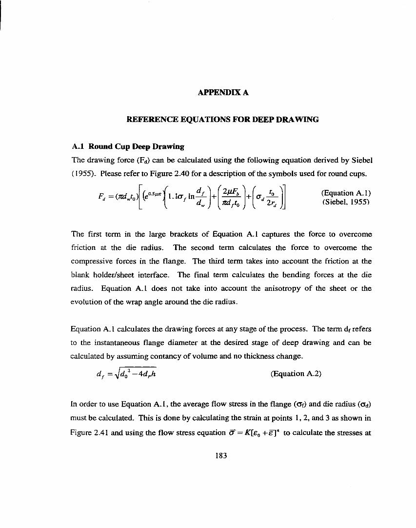
APPENDIX A

REFERENCE EQUATIONS FOR DEEP DRAWING

A .l Round Cup Deep DrawingThe drawing force (Fd) can be calculated using the following equation derived by Siebel

(1955). Please refer to Figure 2.40 for a description of the symbols used for round cups.

d . ) ^+ + (Equation A.1)

(Siebel, 1955)

The first term in the large brackets of Equation A.1 captures the force to overcome

friction at the die radius. The second term calculates the force to overcome the

compressive forces in the flange. The third term takes into account the friction at the

blank holder/sheet interface. The final term calculates the bending forces at the die

radius. Equation A.1 does not take into account the anisotropy of the sheet or the

evolution of the wrap angle around the die radius.

Equation A. 1 calculates the drawing forces at any stage of the process. The term df refers

to the instantaneous flange diameter at the desired stage of deep drawing and can be

calculated by assuming contancy of volume and no thickness change.

d^ — 4dph (Equation A.2)

In order to use Equation A.1, the average flow stress in the flange (<Tf) and die radius (cJd)

must be calculated. This is done by calculating the strain at points 1, 2, and 3 as shown in

Figure 2.41 and using the flow stress equation o ' = K[Sg -he]" to calculate the stresses at

183

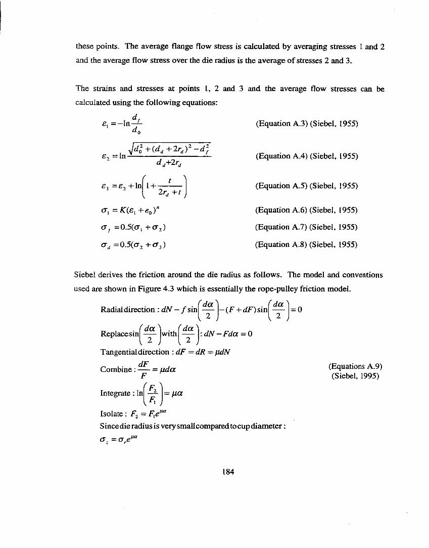
these points. The average flange flow stress is calculated by averaging stresses I and 2

and the average flow stress over the die radius is the average of stresses 2 and 3.

The strains and stresses at points I, 2 and 3 and the average flow stresses can be

calculated using the following equations:

£, ——In (Equation A.3) (Siebel, 1955)

- d jdu+2rj

1 +

C7, =AT(£, +eoV

(Ty =0.5((Ti -f-cr,)

a j =0.5(0", + 0 -3 )

(Equation A.4) (Siebel, 1955)

(Equation A.5) (Siebel, 1955)

(Equation A.6 ) (Siebel, 1955)

(Equation A.7) (Siebel, 1955)

(Equation A.8 ) (Siebel, 1955)

Siebel derives the friction around the die radius as follows. The model and conventions

used are shown in Figure 4.3 which is essentially the rope-pulley friction model.

f d a ^Radial direction : dN — / s i n f ^ ^

I 2 .-(F -t-d F )s in = 0

Replacesinf d a ^ . , f d a ^ with : dN — Fda = 0

Tangential direction : dF = d R = fJdN dFCombine :F

Integrate : In

fjda

fia

Isolate : F, = F^e^S ince die radius is very smallcompared to cup diameter :

cr. =

(Equations A.9) (Siebel, 1995)

184

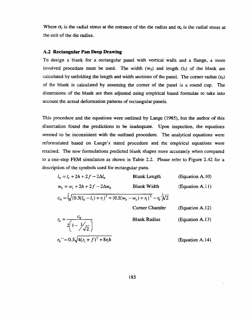
Where CTr is the radial stress at the entrance of the die radius and Oe is the radial stress at

the exit of the die radius.

A.2 Rectangular Pan Deep DrawingTo design a blank for a rectangular panel with vertical walls and a flange, a more

involved procedure must be used. The width (wq) and length (lo) of the blank are

calculated by unfolding the length and width sections o f the panel. The comer radius (ro)

of the blank is calculated by assuming the comer of the panel is a round cup. The

dimensions of the blank are then adjusted using empirical based formulas to take into

account the actual deformation patterns of rectangular panels.

This procedure and the equations were outlined by Lange (1985), but the author of this

dissertation found the predictions to be inadequate. Upon inspection, the equations

seemed to be inconsistent with the outlined procedure. The analytical equations were

reformulated based on Lange’s stated procedure and the empirical equations were

retained. The new formulations predicted blank shapes more accurately when compared

to a one-step FEM simulation as shown in Table 2.2. Please refer to Figure 2.42 for a

description of the symbols used for rectangular pans.

Iq = ly + 2 h -h 2 f — 2A/q Blank Length

Wq = vvj +2h + 2 f — 2AvVo Blank Width

Cq =(^{0.5(/(j —/,) + /]}“ -t-{0.5(Wo +

Comer Chamfer

(Equation A. 10)

(Equation A .11)

Blank Radius

To ■ ’ = 0.5-^4(ry+f)--i-Sryh

(Equation A. 12)

(Equation A. 13)

(Equation A. 14)

185

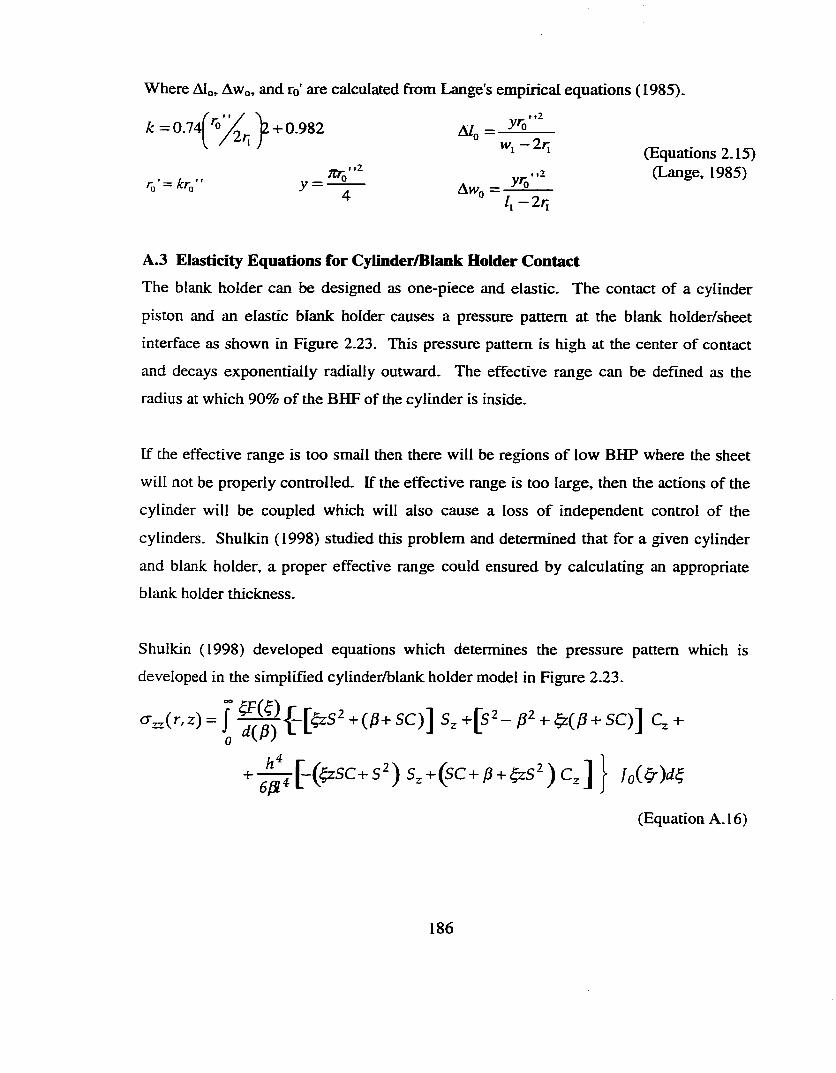
Where AIo, Awo, and ro' are calculated from Lange's empirical equations (1985).

k = 0.74 '■o Z b +0.982 A/o =(Equations 2.15)

a -g = .1 9 8 5 )

A.3 Elasticity Equations for Cylinder/Blank Holder ContactThe blank holder can be designed as one-piece and elastic. The contact of a cylinder

piston and an elastic blank holder causes a pressure pattern at the blank holder/sheet

interface as shown in Figure 2.23. This pressure pattern is high at the center of contact

and decays exponentially radially outward. The effective range can be defined as the

radius at which 90% of the BHF of the cylinder is inside.

If the effective range is too small then there will be regions of low BHP where the sheet

will not be properly controlled. If the effective range is too large, then the actions of the

cylinder will be coupled which will also cause a loss of independent control of the

cylinders. Shulkin (1998) studied this problem and determined that for a given cylinder

and blank holder, a proper effective range could ensured by calculating an appropriate

blank holder thickness.

Shulkin (1998) developed equations which determines the pressure pattern which is

developed in the simplified cylinder/blank holder model in Figure 2.23.

= [$ :S ^ + (/3 + S C )] S , + [ s 2 - ^ 2 + ^ ( ^ + SC )] Q +

+ - ^ [ - ( f ^ S C + s " ) S^+(SC +;3 + ^ z S ^ ) q ] I

(Equation A. 16)

186

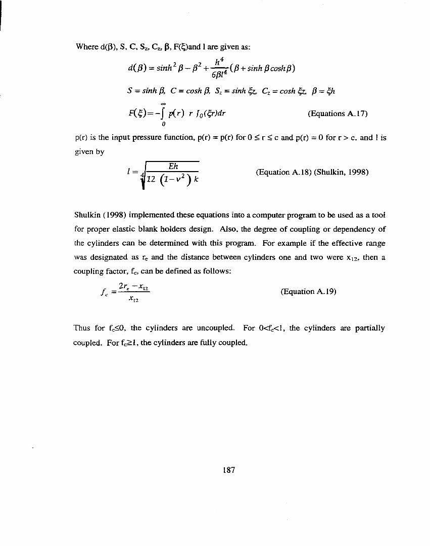
Where d(|3), S, C, S^, Cz, 3, F(^)and I are given as:

d ^ P ) = s i n h ^ p — + - ^ ^ { p - t s i n h P c o s h p )

S = sink P, C = cosh p, = sink Q = cosh P = ^h

F((^) = - J p{r) r [Q(^)dr (Equations A. 17)0

p(r) is the input pressure function, p(r) = p(r) for 0 < r < c and p(r) = 0 for r > c, and I is

given by

1= C Z E Z| l 2 ( I - v- ) A :

Eh(Equation A. 18) (Shulkin, 1998)

Shulkin ( 1998) implemented these equations into a computer program to be used as a tool

for proper elastic blank holders design. Also, the degree of coupling or dependency of

the cylinders can be determined with this program. For example if the effective range

was designated as r and the distance between cylinders one and two were Xi2 , then a

coupling factor, fc, can be defined as follows:

/ . = — (Equation A. 19)

Thus for fc<0, the cylinders are uncoupled. For 0<fc<l, the cylinders are partially

coupled. For fc^l, the cylinders are fully coupled.

187

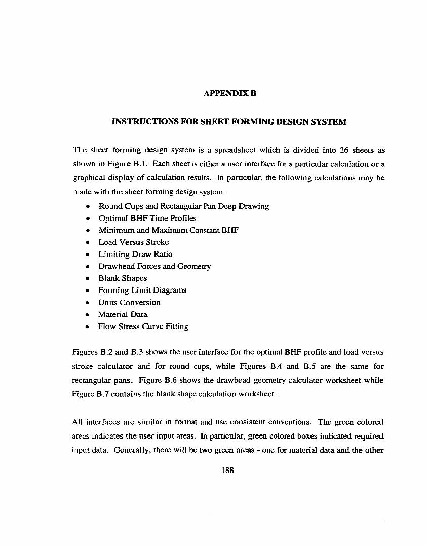
APPENDK B

INSTRUCTIONS FOR SHEET FORMING DESIGN SYSTEM

The sheet forming design system is a spreadsheet which is divided into 26 sheets as

shown in Figure B .L Each sheet is either a user interface for a particular calculation or a

graphical display o f calculation results. In particular, the following calculations may be

made with the sheet forming design system:

Round Cups and Rectangular Pan Deep Drawing Optimal BHF Time Profiles Minimum and Maximum Constant BHF Load Versus Stroke Limiting Draw Ratio Drawbead Forces and Geometry Blank Shapes Forming Limit Diagrams Units Conversion Material Data Flow Stress Curve Fitting

Figures B.2 and B.3 shows the user interface for the optimal BHF profile and load versus

stroke calculator and for round cups, while Figures B.4 and B.5 are the same for

rectangular pans. Figure B . 6 shows the drawbead geometry calculator worksheet while

Figure B.7 contains the blank shape calculation worksheet.

All interfaces are similar in format and use consistent conventions. The green colored

areas indicates the user input areas. In particular, green colored boxes indicated required

input data. Generally, there will be two green areas - one for material data and the other

188

for tool geometry. Useful values which are calculated by the spreadsheet are included in

red colored areas.

Grey areas indicate intermediate calculated values which are not necessary for the general

user. Important instructions are included in orange boxes and yellow boxes indicate

advanced solution techniques are required. The advance techniques are outlined in the

orange areas for the user’s convenience. The required units are always indicated and

schematics are included to explain the meaning of terminology used in the module. Each

sheet is formatted for easy printing and contains the current date and time for the

convenience of the user.

S h ee t Form ing DM ign Systm t SFD S

tn»tnieMon»onHmirtoU«»

birWiUiiiitTlwimsr>JanMiir2t,19M Engineering tlee—ichC nlir foe Met Slwpie llMiufacturing

O u tlin e o f t h e S h e e t Form ing D esign SystemThis module c on ta ins 2 4 différent woiftsheets - each containing various tools to allow the u s e r to design a s h e e t fomting process. You m ay switch betw een worksheet by clicking the b a r a t th e bottom of the Excel screen .

1. Instiuctions2 . BHF R ound Cup3. BHF Plot - R ound4 . Force Round Cup

5- Force Plot - R ound6 . Round Schem atic7. BHF Rect Pan a . BHF P lo t-R ec t9. Force R ect Pan10. Force Plot - R ect11. Rect Schem atic12. BHF Asym Panel13. BHF P lo t-A sym14. Force Asym P anel15. Force Plot - Asym IS .B H FU -C hannel17. Force U-Channel18. Drawbead Force19. OrawbeaO Geom etry20. Blank Design21. Row S tress22. R ow Curve23. Material24 . FLO25. FLO C hart26 . Units Convert

G ives the u se r an idea of th e organization and u se of this m odule.Calculates optimal blank holder force (BHF) profiles for round cup deep drawing. Predicts optimal BHF profile graph from 2 .Calculates the load versus stroke fo r round cup deep drawing.Also provides limiting d raw ratios, minimum and maximum BHF. and final cup geometry. Predicted load versus stroke g raph from 4.

Calculates optimal blank holder force (BHF) profiles for rectangular pan d eep drawing. Predicts optimal BHF profile graph from 6 .Calculates the load versus stroke fo r rectangular pan d eep drawing.Predicted load versus s troke graph from 8.

Calculates optimal blank holder force (BHF) profiles for asymmetric panel deep drawing. Predicts optimal BHF profile graph from 10.C alculates the load versus stroke fo r asymmetric panel d eep drawing.Predicted load versus s troke graph from 12.Calculates optimal blank holder force (BHF) profiles (or plane strain U-channels. Calculates the load versus stroke fo r plane strain U-channels.Calrxjlates restraining and binder hold down forces for drawbeatjs.Predicts the drawtiead geom etry required to provide specified restraining force. Calculates blank sh ap es fo r round and rectangular parts.Calculates How s tre ss relationship from raw tensile data.R ow cunre graph from 11.D atabase of various s h e e t material properiies.Calculates fomring limit curves fo r s te e ls based on n-value and thickness.Plots the calculated forming limit curves.Allows to u ser to convert betw een different units system s.

C o n v e n t io n s___________Each w orksheet contains a input area colored g reen .I y Enter th e requ ired values in the green outlined boxes.

' T /yca:T he calculated values a p p ea r in the red b o x e s- - ' T he g rey bo x es contain numerical information th a t is not necessarily important for the u ser.

Often o ran g e boxes contain important instructions on the u se of the module.Yellow colored b oxes require advanced solution terrimiques that m ust be exerxjted by th e user.The u s e r m ay print ou t any worksheet by clicking on the print button in the toolbar.

Figure B . 1 : Instruction page in the sheet forming design system

189

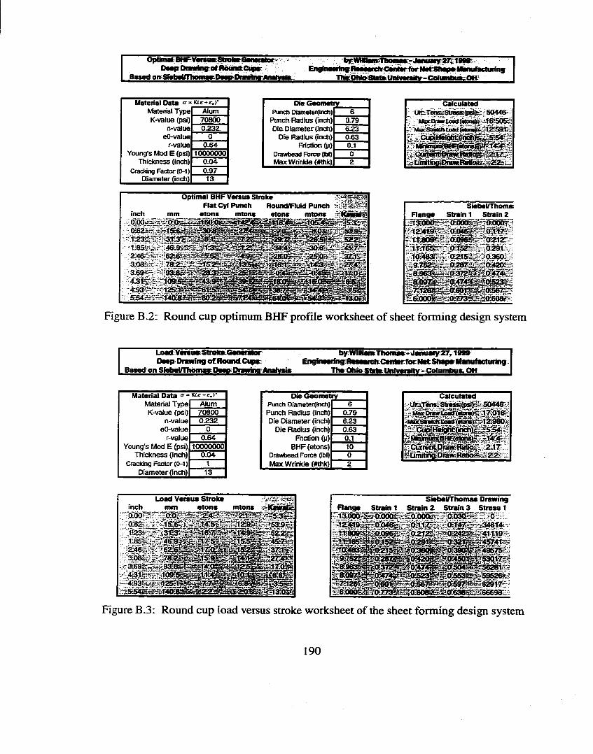
OpHmaiBHF-VeisueSiioteGeiw ' De#p Oimwln* of RowntCiîpm

. BMgd nJfcbgMnwnwrDiggiDwjjjhibKWH^^

Engfnairing n« tip cli CmiIm lurM>tStMip»lfcnuftcturinj

M aterial D ata o- - Kfr+c.)- Die G eo m etryMaterial Type Alum Punch DiameterOnch) 6K-value (psi) 70800 Punch Radius (inch) 0.79

n-value 0.232. Die Diameter (inch) 6.23eO-value 0 Die Radius (inch) 0.63

rvalue 0.64 Friction (p) 0.1Young's Mod E (psi) 10000000 Drawtiead Force (|bf) 0

Thickness (inch) 0.04 Max Wrinkle (#thk) 2Cracking Rictor(0-1) 0.97

Diameter (inch) 13

C a lc u la te dUKT«i%SÔâsm(p j 5044Ç MaxOiawUmt(«laai 2-f6'505;1

MaçârÉtchLc Cdôii: MÀârùlfl. q m # ^

ESS54

inch0’00~=a.62.—:23t"

laST ,2.46..308L369*--43Î" -4 93534-—

O p tim al BH F V e n u * S tro k eF la t Cyl P u n c h RoundlFlufd P u n c h

m m e to n s m to n e

.6263 -*J

—14«m#W8IE

e to n s m to n s - KeetMK

.-27:431

F la n g eSletaelTThoma:

S tra in 1 S tra in 2 :l3ÎOQ(R:: lKOOO= a«X t24i9i,T „ao^^^.o.ttn t t 6 ^ 0.096.*:--"0212 IT i f e S n ^ - 03t52= , 0:291 1&483h 02153" . 0.360. 9 7 5 ^ 02873% 0:420—

“8C963fc3 î0 3 7 ^p iÆ 4 7 ^ .^ 0 ^ 3 £ -

* - ‘ '

Figure B.2: Round cup optimum BHF profile worksheet of sheet forming design system

Load yofsi»Strol»6siionNor Deep OraMringoCRouiMf Cupsr

_BMedonSk*ginTMmgKgaegOggAngdga|g^

byWI8lamThoma#-JanwatyZ7,1999 EnginearingnaaaaicliCanlar.Ibr Nat Shap> Manufacturing

______TlmOh«o MglfahMmdgg _ColunggM OH_ _ _

M aterial D a ta » - K(£:--c.>-Material Type AlumK-value (psi) 70800

n-vaiue 0.232eO-vaiue 0

r-value 0.64Young's Mod E (psi) 10000000

Thickness (inch) 0.04Cracking Factor (0-1) 1

Diameter (inch) 13

D ie G e o m e tryPunch Diameteitkich) 6Punch Radius (inch) 0.79Die Diameter (inch) 623

Die Radius (inch) 0.63Friction (p) 0.1

BHF (etons) 10Drawtiead Force (Itil) 0Max Wrinkle (#thk) 2

C a lc u la te d

L o ad V e r s u s S tro k e . ' tm m e t o n s m to n s «^K àw aiâ

zjfkaxil

Siebein’homas D raw ing R a n g e S tra in 1 S tra in 2 S tra in 3 S t r e s s 1

i lm ,629#

Figure B.3: Round cup load versus stroke worksheet o f the sheet form ing design system

190

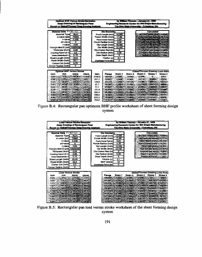
O p tim a l B H E V M su K S tra teO a iN fa iac : Deepr Drawihg:ief. B ee lan g u le r P a n e

_BaaaJpngftbaOT1wnwrDaag£majng i^^b y .w q » |n i îT h o ii ia * - J a n a a n r2 7 ,ie 9 e

E h g f n e e t6 ie F la a a a iè h C e n lB r fe c liÉ tS h a ^ lla n u ia e lie in g --

_______TheOhfeaijyii*m g£2£sS55Si!SSÊ£-—- ■

M aterial D a ta - K l t - r . r D ie G eom etryM aterial Type Alum Punch Length (inch) 1 4 346

K-value (psi) 70800 Punch W idth (inch) 1 1 3 9n-value 0 3 3 2 Pinch Conar Red Oi) 2 3 5

eO-value 0 P unch R ad iu s (inch) 0 3 9rv a lu e 0.64 Die L ength (inch) 15.098

Y oung's M od E (psi) 10000000 Die W idth (inch) 12:142T hickness (inch) 0 .04 D ie C o m er R ad (in) 3

Ccackkig c t o r (0-1) 0 3 D ie R a r tu s (inch) 0 3 9S n a sO iW tiU ia n (0 -1 ) 0.15 Draw D epth (inch) 5

Blank Length (inch) 24.8 Friction (p) 0.1Blank W idth (inrdi) 2 2 .7 □rawtwad Force (IbO 0

C o m er C u t (inch) 6 .75C om er R aifius (inch) 0

O ptim al BH F V arsu s S troke in ch m m e to iw m tons

aaa-.

b a rs2168.8SOt.7139.957.777.1151.8 264.4405.8 570.3753.8

S ieb e l/T h o m as D raw ing L oad Anaiy R a n g e Strain 1 S train 2 S t r a i n ) S t r e s s 1 S tre s s 2 2 4 5 1 0 - 0 .0 0 0 _.OLOOQ^ O O W _ 0 _ 83572 3 5 ^ ' a œ t f - 0 0 6 3 - O i l ï O ^ ~ , ^ 6 0 p ’’ 37233.23;irâ"_:ZL0r058E5- 0118 -= 0-teBg-.l36élE;f'SSISfK

Figure B.4: Rectangular pan optimum BHF profile worksheet o f sheet forming designsystem

L o a d V e rsu s S tro k e G e n e ra to r D e ep D raw ing o f R ec tan g u ia r P a n s

_BasedMBWePTImmasOeagOrawggdgl] ^b y WHHam T h o m a s • J a n u a ry 2 7 ,1 9 M

E ng ineering R ese a rch 'C e n te r f o r N a t S h a p e M anuC K turing ______ri»OW»SmieUnhj5tsit] ;Colunjbj«gOlf___

M aterial D ata <r- K t t» r . r D ie G eom etryM aterial Type Alum Punch Length (inch) 14.946K-value (psi) 70800 Punch W idth (inch) 1 139

n-vaiue 0 3 3 2 P is c h C om er Rad (n ) 2 9 5eO-vaiue 0 Punch R ad iu s (inch) 0.39

rv a lu e 0.64 Die Length (inch) 15.098Y oungs Mod E (psi) 10000000 Die W idth (inch) 1 2 1 4 2

T hickness (inch) 0 .04 Die C o m e r Had (in) 3Craddng Factor (0-1) 0.95 Die R ad ius (inch) 0.39

Stress D Btribulion(0-1) 0.15 Draw D epth (inch) 5Blank Length (inch) 2 5 3 4 Friction (p) 0.1Blank W idth (inch) 22.9 B H F(etons) 10

C om er C u t (inch) 6 3 [3rawbead Force OhI) 0C o m er R ad ius (inch) 0

C aieu la ted

m a s #

---- .a083j£|:' CùirîéiÆl»J‘ «050^

R a Ü W ô f P unch ,.-7 3 9 4

L o a d V e rsu s S tro k e inch m m e to n s0 0 0 „«o!dSgi^0 5 8 1.11

seesR a n g e S train 1

S ieb e l/T h o m as D raw ing L oad Analy S train 2 S tra in 3 S tr e s s 1 S tre s s 2

835Wmm=2321 fH4M34ÎS

B t9 i3 3

Figure B.5: Rectangular pan load versus stroke worksheet of the sheet forming designsystem

191

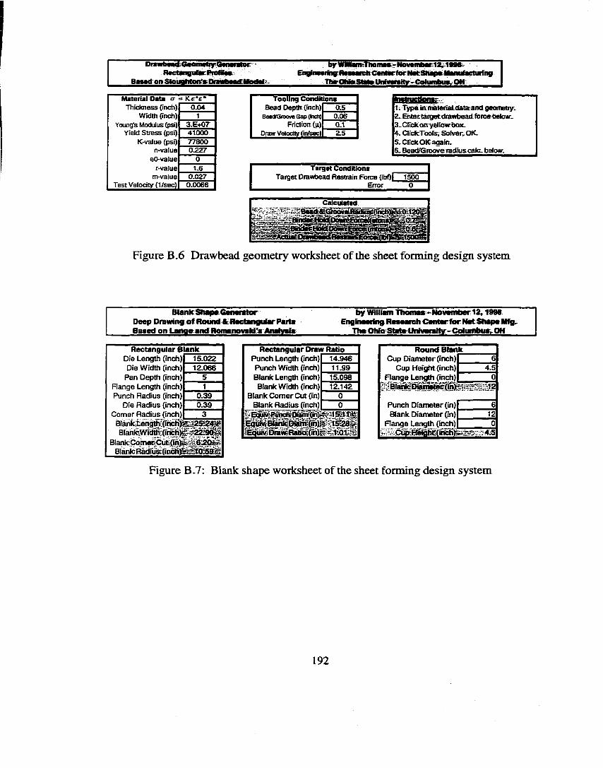
D re w b e e d iG e o m e tiy G e iw s lo c R a c ta n g u la c P io f iliK

_Ba##d KSIgggggiAçOgg###g*gd^Iiy-W«llimmieiiws:-Ne¥wiibetri2^19964!

E hgine«i«g:A w e*dt Center fo r NetiShapBiemiiteelurfng TlwOtifeSteletUnhieieitr-ColiiHibue^OH

M aterial D ata <r = Ke'É~Thickness (inch) 0.04

Width (inch) 1Young's Modulus (psi) 3.5*07

Yield Stress (psi) 41000K-value (psi) 77800

n-vaiue 0.227eO-value 0

rvalue 1.6m-value 0.027

Test Velocity (1/sec) 0.0066

T oo ling C ond itionaBead Depth (inch)|_ 0.5

Bead/Sroom Gap (kiOi)P 0.06Frictloatpjr 0.1

Draw Vetodtv (in/sec) P 25

Ine tn ic ttoiwÊt. Typftin materiaLdata; and geometiy. L te c targetdraiMbeactforça below. L Click OK yellow box:4. ClicfcTools,, Solver, OK.5. ClickOKagain.6. Bead/Groove radius calc, below.

T a rg e t C on d itio n sTarget Drawbead Restrain Force (IbO I 1500

Error 0

•mBmàtM

Figure B . 6 Drawbead geometry worksheet of the sheet forming design system

B lank S h a p e G w M fator Deep Drawing o f R ound A: R ec tan g u la r P a rts B ased o n L an q o an rt R om anoseldTf A nalysis

by William T h o m as -N o v em b er1 2 r 1998 Engm aaring R esea rch C e n la r f o r N et S h ap e Mtg

T heO h io S ta tsU n iv e rs ih f-C o lu m b u s OH

R ectangular B lankDie Length (inch) 15.022Die Width (inch) 1Z066

Pan Depth (inch) 5Range Length (inch) 1Punch Radius (inch) 0.39

Die Radius (inch) 059Comer Radius (inch) 3

Blanlc:Corher-Cuti(fnteBIW cRàdiüËfincAimSTOisa#

R ectangular Draw RatioPunch Length (inch) 14.946Punch Width (inch) 11.99Blank Length (inch) 15.098Blank Width (inch) 12.142

Blank Comer Cut (in) 0Blank Radius (inch) 0

m m

R ound B lankCup Diameter (inch) 6

Cup Height (inch) 4.5Flange Length (inch) 0

Punch Diameter (in) 6Blank Diameter (In) 12

Range Length (inch) 0

Figure B.7: Blank shape worksheet of the sheet forming design system

192

APPENDIX C

INSTRUCTIONS FOR COMPILING ROUTINES INTO THE FEM CODE PAM-STAMP

Engineering Systems International (ESI) has provided the author of this dissertation with

the means to implement subroutines into Pam-Stamp. This subroutine would be executed

at every timestep and allows the user the ability to modify any velocity or force profile

based on the forming conditions. The forming conditions that could be accessed through

the subroutine are:

L. current time 6 . elemental strain

2. nodal coordinates 7. elemental thitming

3. nodal displacement 8 . elemental stress

4. nodal velocity 9. contact force

5. nodal acceleration

The following files were provided by ESI.

1. Idcmod.f

2. v98.102.a

3. makefile

4. PC_INIT

The first file named "v98.102.a" is a library containing the Pam-Stamp core solver

program. The second file named "ldcmod.f is the user subroutine. The "makefile" is a

batch file which executes the commands to compile the core program with the user

subroutine. The "PC_INIT" file contains the license which will be required to run the

193

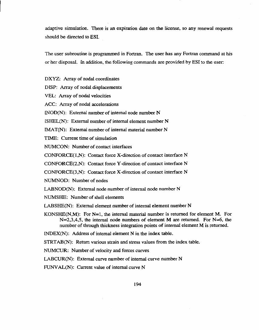
adaptive simulation. There is an expiration date on the License, so any renewal requests

should be directed to ESI.

The user subroutine is programmed in Fortran. The user has any Fortran command at his

or her disposal. In addition, the following commands are provided by ESI to the user:

DXYZ: Array of nodal coordinates

DISP: Array of nodal displacements

VEL: Array o f nodal velocities

ACC: Array of nodal accelerations

INOD(N): External number of internal node number N

ISHEL(N)- External number of internal element number N

IMAT(N)- External number of internal material number N

TIME: Current time of simulation

NUMCON: Number of contact interfaces

CONFORCE(l,N): Contact force X-direction of contact interface N

CONFORCE(2,N): Contact force Y-direction of contact interface N

CONFORCE(3,N): Contact force X-direction of contact interface N

NUMNOD: Number of nodes

LABNOD(N): External node number of internal node number N

NUMSHE: Number of shell elements

LABSHE(N): External element number of internal element number N

KONSHE(N,M): For N =l, the internal material number is returned for element M. For N=2,3,4,5, the internal node numbers of element M are returned. For N=6 , the number of through thickness integration points of internal element M is returned.

INDEX(N): Address of internal element N in the index table.

STRTAB(N): Return various strain and stress values from the index table.

NUMCUR: Number of velocity and forces curves

LABCUR(N): External curve number of internal curve number N

FUNVAL(N): Current value of internal curve N

194

MATTYP(N): Material type of internal material number N

CCM(N,M): For N=68,69,70, returns the G, F, and N values from Hill's Yield Function for internal element M.

ESI has also provided a routine which iteratively returns various strain and stress values

for each and every element successively in a DO loop. The various values and their

names are listed below.

THO: Original thickness

THK: Current thickness

THN: Current thinning

S 1(1): Normal stress in the X-direction for integration point I

S2(I): Normal stress in the Y-direction for integration point I

S3 (I): Shear stress integration point I

LSIGl I : Lower surface normal stress in the X-direction

LSIG22: Lower surface normal stress in the Y-direction

LSIGl2: Lower surface shear stress

USIGl I : Upper surface normal stress in the X-direction

USIG22: Upper surface normal stress in the Y-direction

USIG12: Upper surface shear stress

MSIGl 1: Middle surface normal stress in the X-direction

MSIG22: Middle surface normal stress in the Y-direction

M SIGl2: Middle surface shear stress

MSIG1 : Middle surface first principal stress

MSIG2: Middle surface second principal stress

MBPS PL: Middle surface plastic strain

LEPS11 : Lower surface normal strain in the X-direction

LEPS22: Lower surface normal strain in the Y-direction

LEPS 12: Lower surface shear strain

UEPS11 : Upper surface normal strain in the X-direction

195

UEPS22: Upper surface normal strain in the Y-direction

UEPS 12: Upper surface shear strain

STRESSEQ: Equivalent stress

Please note that the elemental values above correspond to the local coordinate system of

each element. ESI has also provided a routine which will find the maximum stress in the

sheet at every time step, the element number of this maximum stress, and the coordinates

of the center of gravity of this element. The variables used are:

STRESSMAX: Value of the maximum stress in the sheet

NBSHEMAX: Internal element number of the maximum stress

XCOG: Coordinate X of the center of gravity of the maximum stress element

YCOG: Coordinate Y of the center of gravity of the maximum stress element

ZCOG: Coordinate Z of the center of gravity of the maximum stress element

One thing to keep in mind is that Pam-Stamp renumbers nodes, elements, materials, and

curves internally. Therefore, if you want to get the stress of element 100. Then you must

find the internal numbering of the external element 100 by using the command "ISHEL".

Finally, ESI has provided a routine which accesses the current value of any force or

velocity curve and modifies it for the next timestep. The following variable is used in the

routine:

NCURSL: The external number of the curve to be modified.

Nuri Akgerman has provided the author with a subroutine which finds the next

uncommented line in a text file. This is very useful to read data from a configuration file.

The command structure is as follows:

196

GETNXTLN (LUN, CMNT_CHR, LINE_BUF, EOFLAG): Gets the next uncommented line number in the file "LUN” and returns the value in "LINE_BUF”. The character used as the comment indicator should be placed instead of "CMNTjCHR" and the end o f file flag should be placed instead of EOFLAG (typically "EOF").

The GETNXTLN routine is included below. This subroutine should be appended to

every user subroutine included in the next four appendices.

SUBROUTINE getnxCln ( LUN, CMNT_CHR, LINE_BUF, EOFLAG )CC Gets the next data line from LUN that is not a comment C Used by routines that read configuration files C N .Akgerman, Feb 1988 CC LUN : Logical unit numberC CMNT_CHR : Comment character, usually a # signC LXNE_BUF : Input line bufferC EOFLAG : End-Of-File flagC

LOGICAL EOFLAGINTEGER* 4 LUNCHARACTER* 1 CMNT_CHR CHARACTER* 80 LINE_BUF

CC------------------------------------------------------------C

EOFLAG = -FALSE.C DO 10 I = 1, 80

LINE_BUFCI:I) = • *10 CONTINUEC25 CONTINUE

READ ( LUN, 30, END=90 ) LINE_BUF 3 0 FORMAT ( A80 )

IF ( LINE_BUF(1:1) .EQ. CMNT_CHR ) GO TO 25C RETURNCC---------------------------------------------------C90 CONTINUE

EOFLAG = .TRUE.RETURNEND

CC

FUNCTION LLLEN ( STRNG )CC Determine the actual printable lengthC

CHARACTER* C *) STRNGC---------------------------------C

N = LEN ( STRNG )CC Search forward for a null byte

197

DO 2 5 I = 1 , N NN = r - 1I F { ST E N G C X rr) -E Q . CHARCO) } GO TO 3 0

2 5 CONTINDE NN = N

CC Eliminate any trailing spaces

3 0 DO 50 I = NN, 1 , - 1 LLLEN = II F ( ST H N G C IrX ) -N E . ' ' ) GO TO 9 0

5 0 CONTINDE LItLEN = 0

C9 0 CONTINUE

RETURN END

The author has added two more files to the adaptive simulation system as follows:

1. control.prm

2 . * .Io g

The "control.prm" file contains various configuration values for the adaptive simulation.

These values vary for each control strategy and will be discussed individually in the next

four appendices. The "control.prm" also provides the user with the opportunity to

designate the name of the output *.LOG file. The adaptive simulation will fill this output

log file with important values calculated during the adaptive simulation. Again, this will

be discussed in depth in the next four appendices.

In addition to this, the author o f this dissertation has defined several other variables that

are related to the specific control strategy. The common variables are listed here while

the specific control variables will be discussed in the next four appendices. We will

begin with the user specified variables:

STARTIME: User specified timestep value to begin control.

ENDTIME: User specified timestep value near the end of the simulation used todetermine the linear variation of the setpoint if specified.

N_TH: User specified static averaging window size.

MOVE: User specified moving averaging window size.

198

KP: User specified proportional constant for the PBD controller.

KI: User specified integral constant for the PID controller.

KD: User specified derivative constant for the PID controller.

MINBHF: User specified minimum BHF.

MAXBHF: User specified maximum BHF.

The following are the calculated common variables that have been designated by the

author.

TIMESTEP: Current timestep value (incremented every time the user subroutine is called).

NTMS: Static averaging window counter.

ERROR: Current error value or proportional value of the PID controller (=setpoint- measurement).

SUMERROR: Current summated error value or integral value of the PID controller (=summerror+error).

SLOPE: Current slope value or derivative value of the PID controller (= currentmeasurement - previous measurement).

AVGERROR: Current summated error value to be used for static averaging and is reset everytime the static averaging window is renewed.

DELTABHF: Current BHF modification as specified by the PID controller(=KP*ERROR+KI*SUMERROR+KD*SLOPE).

BHFHISTORY: The current summated DELTABHF to be used to modify theFUNVALCN) or BHF profile (=BHFHISTORY+DELTABHF).

BHF INITIAL: The initial value of the BHF used to ensure that the BHFHISTORY does not obtain a value which violates the MINBHF and MAXBHF.

PAMBHF: The current value of the BHF profile from Pam-Stamp used to output to the *.LOG file.

If a user want to develop his or her own control strategy, then he or she may develop a

new user subroutine "Idcmod.f. Once this new subroutine is created then it must be

compiled by executing an "Til" on the user subroutine and then compiling by executing

199

the make file. Thus make sure that the current directory contains the user subroutine, the

"makefile" and the Pam-Stamp core library. Thus the sequence of commands are:

f7 7 Id c m o d .fmakerm a .o u t:

No error should be indicated after any of these commands. Ignore any warnings as they

are permitted. This procedure will create an executable file named "v98.I02.x" which

contains the Pam-Stamp core solver embedded with the new user subroutine. Please

note, that the user subroutine variable "FUNVAL(N)" is the current value of the force

curve only. Thus, if the user is modifying these values as part of the control scheme, the

user must remember to modify these values every timestep as if from the starting value.

If a user wants to run an adaptive simulation on an existing Pam-Stamp input deck

(typically *.ps), then he or she must configure "control.prm" configiuration file as

necessary. Once this is complete, the adaptive simulation may be executed in C shell on

a Unix workstation. The environment variable "PCHOME" must be pointed to the

directory containing license file provided by ESI. Then adaptive simulation executable

file "v98.102.x" must be executed. Thus the sequence of commands are:

c s hset:env PCHOME p a .th ./v98.102.x <*.ps >* . out Sc

Please keep in mind, that the user must be aware of which control strategy he or she

would like to use, since all executable files have the same name but different control

methods. Typically, the directory which contains the executable has a descriptive name

indicating the control method.

200

There are several requirements for the adaptive simulation. First, the specified

"STARTIME " should be a value equal to or greater than the moving averaging window

size (MOVE) which should be in turn be greater than or equal to the static averaging

window size (N_TH). The "MINBHF" should not be less that zero and the "MAXBHF"

should not be larger than the maximum force allowable by the contact model. If a larger

"MAXBHF" is necessary then the user should input a larger contact penalty.

Also, there are several requirements for the setup o f the FEM model for an adaptive

simulation. First, the press must be double action. That is the die surface must be

stationary, the binder surface must apply a constant force onto the die, and the punch

must travel with a velocity boundary condition into the sheet and die cavity. The

stamping direction and punch movement must be in the positive Z-direction. The die

surface must be entirely in the positive Z space with the lowest portion of the die surface

at Z=0. The remaining tools are arranged accordingly from there. See Figure C. 1 for an

illustrated example.

Each of these feedback routines modify curve number 2. Therefore, the user should

make sure that the nodal force BHF boundary condition be defined with curve number 2,

or else the control will not work correctly. The scalar value of the nodal force should be

equal to one and curve 2 should contain the actual BHF values which should be of

constant value during the control sequence. The user should renumber the nodes,

elements, materials, curves, and contact interfaces sequentially beginning from one.

There are automatic routines in the Pam-Stamp preprocessor. Future, the user should

remember to set Eo greater than zero when using Krupkowski’s flow law, CT=K(e+eo)“.

The final restriction is that the adaptive simulation is developed only for sheet material

models 107 or 109 with reduced integration (see Pam-Stamp manuals).

201

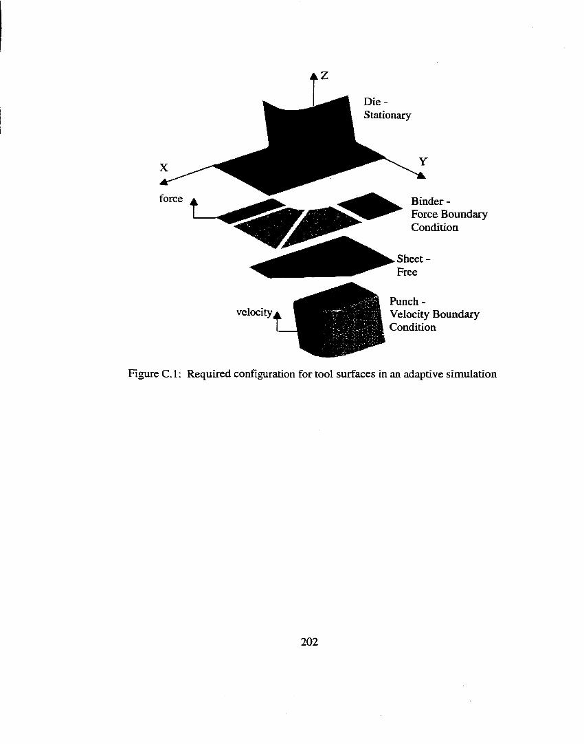
Die -Stationary

Sheet -

velocity

Binder - Force Boundary Condition

Punch -Velocity Boundary Condition

Figure C. I : Required configuration for tool surfaces in an adaptive simulation

202

APPENDIX D

INSTRUCTIONS FOR WRINKLING BASED ADAPTIVE SIMULATION

At each time step, this algorithm attempts to maintain the gap between the binder

surfaces at a predetermined setpoint by actively varying the blank holder pressure (BHF)

using a PID controller. This strategy should produce a BHF profile which ensures no

wrinkhng, minimizes final part strain and fracture. This algorithm allows the user to

specify:

• kp, ki, kd controller constants

• static and moving average filtering window sizes

• minimum and maximum BHF

• start time for control

• any linearly changing setpoint of binder gap for up to three different binder segments

The optimal values of kp, kj, kd, and filtering parameters have been determined to

maximize control robustness. They are as follows:

KP = 0.001

K1 = 0.0

KD = 0.0

N_TH = 100

MOVE = 100

The minimum and maximum BHP levels should be set according to press and tool

capacity. The start time should be set soon after deep drawing has begun typically after

203

2-3% of the draw depth has been achieved- It has been determined that the initial value

of the binder gap setpoint should be 1 0 % greater than the initial material thickness and

the final value of the binder gap setpoint should be 1 0 % greater than the final maximum

thickness of the part. In general, a variation of binder gap setpoint from L it to 1.51,

where t is the original material thickness, is sufficient. The binder gap strategy should

produce a BHF profile which minimizes final part stretch while avoiding wrinkling.

This is the only user routine which controls the blank holder pressure rather than the

blank holder force. It was found that the optimal values for the controller constants kp, ki,

kd were functions of the binder surface area. Thus, by controlling the BHP rather than the

BHF, control stability was improved and a unique set of kp, ki, kd were found. Thus the

user should keep in mind to define a static pressure to the binder surface or surfaces

rather than a nodal force. If only one binder segment is to be controlled, then the static

pressure for this segment should be defined with curve number 2. If two or more binder

segments are to be controlled, then define static pressures for binder segment 2 with

curve number 3 and binder segment 3 with curve number 4.

Thus the previously defined variable, MINBHF, MAXBHF, DELTABHF,

BHFHISTORY, BHF INITIAL, and PAMBHF are actually pressure instead of force. The

minimum and maximum BHP should be set to 0.0 and 1.0 GPa. Due to the intrinsic

nature of this control scheme, violent vibrations are imparted onto the system In order to

reduce contact problems, the penalty contact values for the binder-sheet and die-sheet

interfaces should be set to 0 . 1 .

The following user specified variables are defined for this control algorithm:

STARTGAP: User specified initial binder gap setpoint Z position.

ENDGAP: User specified final binder gap setpoint Z position.

NODEfN): User specified external node number contained in the binder segment N to be controlled.

204

POINTS: User specified number of binder segments to be controlled (up to three).

The following calculated variables are defined for this control algorithm:

GAP: Current binder gap setpoint distance calculated based on the line from the point (STARTGAP, STARTIME) to the point (ENDGAP, ENDTIME).

INODE(N): Internal node numbers corresponding to NODE(N)

ZPOS(N): Current Z coordinate position of the binder segment N.

AVG2TOS(N): Summated Z coordinate position o f binder segment N reset everytime static averaging window is renewed.

PREVZPOS(N) : Previous averaged Z position of binder segment N.

ALLZPOS(N,M) : An array of all Z positions for binder segment M for timestep N.

The configuration file "control.prm" takes the following format:

# Control Parameter file. The first line contains# KP, KI. KD, MINBHF, MAXBHF, N_TH, MOVE, NODE(l) (3F10.5, 2F10.1, 3110) #2345678901234567890123456789012345678901234557890123456789012345578901234567890

0.00100 0.00000 0.00000 0.0 1.0 100 100 1800# Extra Parameters# STARTGAP, ENDGAP, STARTIME, ENDTIME, POINTS, NODE{2), NODE(3) (2F10.3, 5110)#2345678901234567890123456789012345678901234567890123456789012345678901234567890

-1.100 -1.500 500 60000 3 2000 2300## This is the name of the output file, up to 40 characters rect3-p2.log

Please note that the format and positions of the numbers are precise and are indicated in

the commented areas. These number formats are standard Fortran number formats. For

example, a format "3F10.5" indicates that there are 3 floating point numbers which are 10

characters long (including decimal and sign) which have five digits after the decimal

place. The format "5110" indicates that there are five integers with 10 characters each

(including decimal and sign).

The output *.LOG file takes the following format:

205

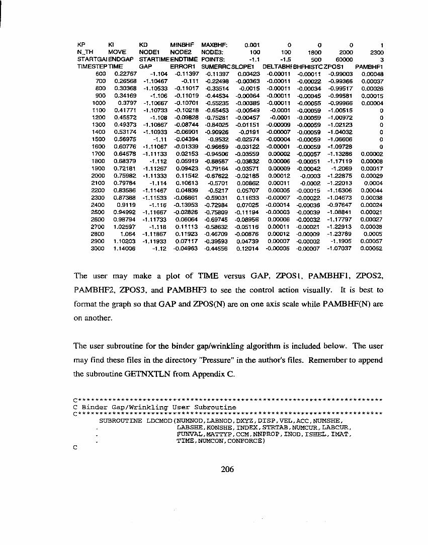
KP KI KD MINBHF MAXBHF: 0.001 0 0 0 1N_TH MOVE NODE1 NODE2 N0DE3: 100 100 1800 2000 2300STARTGAI ENDGAP STARTIME ENDTIME POINTS: -1.1 -1.5 500 60000 3TIMESTEP TIME GAP ERROR1 SUMERRCSLOPEl DELTABHF BHFHISTCZPOS1 PAMBHF1

600 0.22767 -1.104 -0.11397 -0.11397 0.00423 -0.00011 -0.00011 -0.99003 0.00048700 0.26568 -1.10467 -0.111 -0.22498 -0.00363 -0.00011 -0.00022 -0.99366 0.00037800 0.30368 -1.10533 -0.11017 -0.33514 -0.0015 -0.00011 -0.00034 -0.99517 0.00026900 0.34169 -1.106 -0.11019 -0.44534 -0.00064 -0.00011 -0.00045 -0.99581 0.00015

1000 0.3797 -1.10667 -0.10701 -0.55235 -0.00385 -0.00011 -0.00055 -0.99966 0.000041100 0.41771 -1.10733 -0.10218 -0.65453 -0.00549 -0.0001 -0.00059 -1.00515 01200 0.45572 -1.108 -0.09828 -0.75281 -0.00457 -0.0001 -0.00059 -1.00972 01300 0.49373 -1.10867 -0.08744 -0.84025 -0.01151 -0.00009 -0.00059 -1.02123 01400 0.53174 -1.10933 -0.06901 -0.90926 -0.0191 -0.00007 -0.00059 -1.04032 01500 0.56975 -1.11 -0.04394 -0.9532 -0.02574 -0.00004 -0.00059 -1.06606 01600 0.60776 -1.11067 -0.01339 -0.96659 -0.03122 -0.00001 -0.00059 -1.09728 01700 0.64578 -1.11133 0.02153 -0.94506 -0.03559 0.00002 -0.00057 -1-13286 0.000021800 0.68379 -1.112 0.05919 -0.88587 -0.03832 0.00006 -0.00051 -1.17119 0.000081900 0.72181 -1.11267 0.09423 -0.79164 -0.03571 0.00009 -0.00042 -1.2069 0.000172000 0.75982 -1.11333 0.11542 -0.67622 -0.02185 0.00012 -0.0003 -1.22875 0.000292100 0.79784 -1.114 0.10613 -0.5701 0.00862 0.00011 -0.0002 -1.22013 0.00042200 0.83586 -1.11467 0.04839 -0.5217 0.05707 0.00005 -0.00015 -1.16306 0.000442300 0.87388 -1.11533 -0.06861 -0.59031 0.11633 -0.00007 -0.00022 -1.04673 0.000382400 0.9119 -1.116 -0.13953 -0.72984 0.07025 -0.00014 -0.00036 -0.97647 0.000242500 0.94992 -1.11667 -0.02826 -0.75809 -0.11194 -0.00003 -0.00039 -1.08841 0.000212600 0.98794 -1.11733 0.06064 -0.69745 -0.08956 0.00006 -0.00032 -1.17797 0.000272700 1.02597 -1.118 0.11113 -0.58632 -0.05116 0.00011 -0.00021 -1.22913 0.000382800 1.064 -1.11867 0.11923 -0.46709 -0.00876 0.00012 -0.00009 -1.23789 0.00052900 1.10203 -1.11933 0.07117 -0.39593 0.04739 0.00007 -0.00002 -1.1905 0.000573000 1.14006 -1.12 -0.04963 -0.44556 0.12014 -0.00005 -0.00007 -1.07037 0.00052

The user may make a plot of TIME versus GAP, 2TOSI, PAMBHF I, ZPOS2,

PAMBHF2, ZPOS3, and PAMBHF3 to see the control action visually. It is best to

format the graph so that GAP and ZPOS(N) are on one axis scale while PAMBHF(N) are

on another.

The user subroutine for the binder gap/wrinkling algorithm is included below. The user

may find these files in the directory "Pressure" in the author's files. Remember to append

the subroutine GETNXTLN from Appendix C.

^ i c ' * c * i F i c i e - t r i c i r i e i e - i e i r ' i c i r i e i c i c i e i e i c i e i c i e i e i e ' i e i c i c i r i f * c i C ' i r i c i f i e i e i c i e i e i c - i c ' i e ' i e i c - t r i c i e i c i c i r i e ' i e i e ' i e i e * ' * e * * * * * * * * i c i e * *

C Binder Gap/Wrinkling User SubroutineSUBROUTINE LDCMOD (NUMNOD, LABNOD, DXYZ, DISP, VEL, ACC, NUMSHE,

LAB SHE, KONSHE, INDEX, STRTAB, NUMCUR, LABOUR,FUNVAL. MATTYP, COM, NNPRO P , INOD, ISHEL, IMAT,TIME, NUMCON, CONFORCE )

C

206

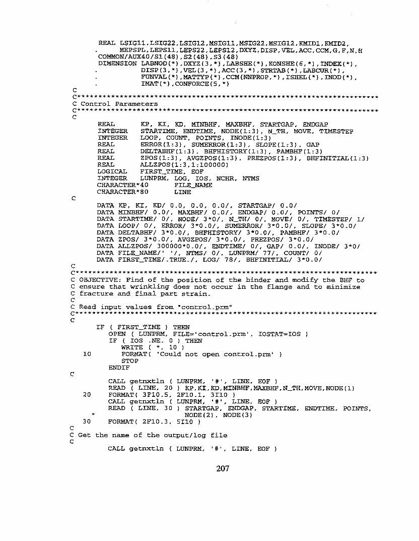
REAL LSIGll, LSIG22, LSIG12, MSIGll, MSIG22, MSLG12, KMTDL, KMID2,MEPSPL, LEPSll, LEPS22 , LEPS12 , DXYZ, DXSP, VEL, ACC, CCM, G , F, N , H

COMMON/AÜX40/SK48) , S2 (48) , S3 (48)DIMENSION LABNOD (*) ,DXYZ(3,*) ,LABSHE(*) ,K0NSHE(6, *) ,INDEX(*) ,

DISP(3,*),VEL(3,*),ACC(3,*),STRTAB(*),LABCUR(*),FUNVAL (*) ,MATTYP(*) ,CCM(NNPROP, *) , ISHEL (*) ,INOD(*) , IMAT (*),CONFORCE(5,*)C

C Control Parametersc

REAL KP, KI, KD, MINBHF, MAXBHF, STARTGAP, ENDGAPINTEGER STARTIME, ENDTIME, N0DE(L:3), N_TH, MOVE, TIMESTEPINTEGER LOOP, COUNT, POINTS, INODE(1:3)REAL ERROR(l:3), SUMERROR (1:3 ) , SLOPE (1:3) , GAPREAL DELTABHF(1:3) , BHFHISTORY( 1:3 ) , PAMBHF (1:3)REAL ZPOS(l:3), AVGZPOS(1:3), PREZPOS(1:3), BHFINITIAL(1:3)REAL ALLZPOS(1:3,1:100000)LOGICAL FIRST_TIME, EOFINTEGER LUNPRM, LOG, lOS, NCHR, NTMSCHARACTER*40 FILE_NAMECHARACTER* 80 LINE

CDATA KP, KI, KD/ 0.0, 0.0, 0.0/, STARTGAP/ 0.0/DATA MINBHF/ 0.0/, MAXBHF/ 0.0/, ENDGAP/ 0.0/, POINTS/ 0/DATA STARTIME/ 0/, NODE/ 3*0/, N_TH/ 0/, MOVE/ 0/, TIMESTEP/ 1/ DATA LOOP/ 0/, ERROR/ 3*0.0/, SUMERROR/ 3*0.0/, SLOPE/ 3*0.0/ DATA DELTABHF/ 3*0.0/, BHFHISTORY/ 3*0.0/, PAMBHF/ 3*0.0/DATA ZPOS/ 3*0.0/, AVGZPOS/ 3*0.0/, PREZPOS/ 3*0.0/DATA ALLZPOS/ 300000*0.0/, ENDTIME/ 0/, GAP/ 0.0/, INODE/ 3*0/ DATA FILE_NAME/' '/, NTMS/ 0/, LUNPRM/ 77/, COUNT/ 0/DATA FIRST_TIME/.TRUE./, LOG/ 78/, BHFINITIAL/ 3*0.0/C

C OBJECTIVE : Find of tiie position of the binder and modify the BHF to C ensure that wrinkling does not occur in the flange and to minimize C fracture and final part strain.CC Read input values from "control.prm"c

IF ( FIRST_TIME ) THENOPEN ( LUNPRM, FILE='control.prm ' , IOSTAT=IOS )IF ( lOS .NE. 0 ) THEN

WRITE ( *, 10 )10 FORMAT( 'Could not open control.prm' )

STOPENDIF

CCALL getnxtln ( LUNPRM, LINE, EOF )READ ( LINE, 20 ) KP,KI,KD,MINBHF,MAXBHF,N_TH,MOVE,NODE(1)

20 FORMAT( 3F10.5, 2F10.1, 3110 )CALL getnxtln ( LUNPRM, ' , LINE, EOF )READ ( LINE, 3 0 ) STARTGAP, ENDGAP, STARTIME, ENDTIME, POINTS,

* NODE(2), NODE(3)30 FORMAT( 2F10.3, 5110 )C

C Get the name of the output/log file CCALL getnxtln ( LUNPRM, '#', LINE, EOF )

207

NCHR = LLLEN ( LINE )FILE_NAME = LINE(L:NCHR) // CHAR(O)CCLOSE ( LUNPRM )FIRST_TIME = .FALSE.C

C Open the log file C

OPEN ( LOG, FILE=FILE_NAME, IOSTAT=IOS )WRITE { LOG, 40 ) KP, KI, KD, MINBHF, MAXBHF

40 FORMAT( 'KP, KI, KD, MINBHF, MAXBHF: ' , 3F10.5, 2F10.1 )WRITE{ LOG, 50 ) N_TH, MOVE, NODE(l), NODE(2), NODE(3)

50 FORMAT( 'N_TH, MOVE, NODEl, N0DE2, NODE3:', 5110)WRITE( LOG, 60 ) STARTGAP, ENDGAP, STARTIME, ENDTIME, POINTS

60 FORMAT ( ' STARTGAP, ENDGAP, STARTIME, ENDTIME, POINTS : ' , 2F10 .3 , 3110)WRITE( LOG, 70 )7 0 FORMAT ( ' , TIMESTEP, TIME, GAP, ERRORl, SDMERRORl, SLOPEl, DELTABHFl, ' ,

• BHFHISTORYl, ZPOSl, PAMBHFl, ERROR2 , SOMERROR2 , SLOPE2 , ' ,* • DELTABHF2, BHFHIST0RY2 , ZPOS2 , PAMBHF2, ERR0R3 , SUMERROR3 , ' ,

' SLOPES , DELTABHF3 , BHFHIST0RY3 , ZP0S3 , PAMBHF3 ' )ENDIFCC Get Z displacement of NODE c

DO 77 COUNT=l,NUMNOD DO 73 L00P=1,3

IF (INOD (COUNT) .EQ. NODE (LOOP) ) INODE (LOOP) = COUNT 73 CONTINUE 77 CONTINUE

CDO 80 LOOP = 1, POINTS

ALLZPOS(LOOP,TIMESTEP) = DXYZ(3,INODE(LOOP))80 CONTINUEC

* ie ie •ie ie ie ir * ic ie * * * * * * ic * -ie -k ir ie irir * ie -ie -ir -ie ir -te * * "ir ic ■iç ir * -tc* it -ie * ir -it ir ir ir ir icie it * * * * -icie * ie *■ ic * ie -k icic * ic *

C Proportional, Integral, Derivative Controller C

IF (TIMESTEP .GT. STARTIME) THEN NTMS = NTMS + 1 IF (NTMS .GE. N_TH) THEN

DO 100 COUNT = 1, POINTSDO 90 LOOP = (TIMESTEP-MOVE+1) , (TIMESTEP)

AVGZPOS (COUNT) = AVGZPOS (COUNT) + ALLZPOS (COUNT, LOOP)90 CONTINUEZPOS(COUNT) = AVGZPOS(COUNT) / MOVE

100 CONTINUEC

DO 175 COUNT = 1, POINTSIF (PREZPOS(COUNT) .EQ. 0.0) THEN AVGZPOS(COUNT) =0.0DO 150 LOOP = (TIMESTEP-MOVE-N_TH-i-l) , (TIMESTEP-N_TH) AVGZPOS (COUNT) = AVGZPOS (COUNT) + ALLZPOS (COUNT, LOOP)

150 CONTINUEPREZPOS(COUNT) = AVGZPOS(COUNT) / MOVE ENDIF

175 CONTINUEC

GAP = STA R TG A P+( ( (E N D G A P -S T A R T G A P )/E N D T IM E ) * T IM E S T E P )

208

IF ( ABS(GAP) .G T . ABS (ENDGAP) ) GAP = ENDGAPC

DO 200 COUNT = 1, POINTSERROR(COUNT) = GAP - ZPOS(COUNT)SUMERROR (COUNT) = SUMERROR (COUNT) + ERROR (COUNT)SLOPE(COUNT) = ZPOS(COUNT) - PREZPOS(COUNT)PREZPOS(COUNT) = ZPOS(COUNT)AVGZPOS(COUNT) = 0.0

200 CONTINUENTMS = 0

CC Now calculate the binder load adjustment DELTABHF.C

DO 225 COUNT = 1, POINTSDELTABHF (COUNT) = KP*ERROR(COUNT)+KI*SUMERROR(COUNT) +

KD*SLOPE(COUNT)BHFHISTORY (COUNT) = BHFHISTORY (COUNT) + DELTABHF (COUNT)

225 CONTINUECC Adjust the binder load curve #2 thru 4 by BHFHISTORY(N) .C

DO 275 LOOP = 1. POINTS NCURSL = LOOP + 1 DO 250 ICUR = 1, NUMCUR NCUR = LABCUR(ICUR)IF (NCUR .EQ. NCURSL) THEN IF ( TIMESTEP . EQ . ( STARTIME+N_TH) )

* BHFINITIAL(LOOP)=FUNVAL(ICUR)FUNVAL(ICUR) = BHFHISTORY(LOOP) + FUNVAL(ICUR)IF (FUNVAL(ICUR) .LT. MINBHF) THEN FUNVAL(ICUR) = MINBHFBHFHISTORY(LOOP) = MINBHF - BHFINITIAL(LOOP)

ENDIFIF (FUNVAL (ICUR) .GT. MAXBHF) THEN FUNVAL(ICUR) = MAXBHFBHFHISTORY(LOOP) = MAXBHF - BHFINITIAL(LOOP)

ENDIFIF (ZPOS(LOOP) .GT. 10) THEN FUNVAL(ICUR) =0.0BHFHISTORY (LOOP) = MINBHF - BHFINITIAL(LOOP)ENDIFPAMBHF(LOOP) = FUNVAL(ICUR)

ENDIF 250 CONTINUE275 CONTINUEC

C Output to Log File C

WRITE ( LOG, 300 ) TIMESTEP, TIME,GAP, ERROR( 1) , SUMERROR( 1) ,* SLOPE(1) ,DELTABHF(1),BHFHISTORY (1) ,ZP0S(1) ,PAMBHF(1) ,* ERR0R(2) ,SUMERR0R(2) ,SLOPE( 2 ) ,DELTABHF(2) ,BHFHISTORY (2) ,* ZPOS(2),PAMBHF(2),ERR0R(3),SUMERR0R(3),SLOPE(3),DELTABHF(3),

BHFHISTORY(3),ZPOS(3),PAMBHF(3)300 FORMAT( 110, 23 ( I h , F10.5) )

CENDIF

CC Adjust the binder load curve #2 by DELTABHF again.C

DO 350 LOOP = 1, POINTS NCURSL = LOOP + 1

209

c

DO 325 ICUR = 1, NUMCUR NCUR = LABCUR(ICUR)IF (NCUR-EQ.NCURSL) FUNVAL (ICUR) =BHFHISTORY(LOOP)+FDNVALCICUR) IF (ZPOS(LOOP) -GT. 10) THEN FUNVAL(ICUR) =0.0BHFHISTORY (LOOP) = MINBHF - BHFINITIAL (LOOP)

ENDIF 325 CONTINUE 3 50 CONTINUE

ENDIFT IM E S T E P = t i m e s t e p + 1

RETURNEND

210

APPENDIX E

INSTRUCTIONS FOR STRESS BASED ADAPTIVE SIMULATION

At each time step, this algorithm attempts to maintain the maximum equivalent stress in

the part at some specified stress profile by actively varying the BHF using a PID

controller. This strategy should produce a BHF profile which maximizes the stretch in

the part while eliminating fracture and minimizing wrinkling. The equivalent stress will

be calculated from Hill’s plane stress anisotropic quadratic yield function (Wagoner,

1997).

= --- :------— +'c)' 9o(‘ x +(2rt5 + 0 ( ^ 0''wC'b- < - 0

(Equation 4.25)

This algorithm allows the user to specify:

• kp, ki, kd controller constants

• static average filtering window size

• minimum and maximum BHF

• start time for control or automatic start

• any constant level stress profile and ramp time

• bulk search of maximum stress or target zone or target element

The optimal controller and filtering constants have been iteratively determined to

maximize robustness. They are as follows:

KP = 20

KI = 0.0

BCD = 0.0

211

N_TH = 250

The maximum and minimum BHF are dictated by press and tooling limits. It is

recommended that the initial BHF should be set relatively high near the fracture limit to

minimize the amount o f time it takes the stress reach the setpoint. The algorithm will

quickly modify the BHF from this point on to ensure no splitting. This high initial BHF

tends to improve control stability.

The start time should be set when the process is well established typically after 5-10% of

the draw depth is achieved. There is also an option for the control to begin automatically

when the measured stress becomes greater than or equal than the setpoint stress. This

option improves control stability and is recommended as an initial starting point for

investigations. To use automatic start, just enter a negative value for the STARTIME.

Any constant level stress profile may be specified and this setpoint can be ramped in at

any slope to improve controllability. It is recommended that the stress setpoint be set at

the average of the yield and ultimate tensile strength of the material to maximize stretch

while avoiding splitting. The setpoint should be ramped in over a short period of about

5-10% of the draw depth.

The entire sheet or zone may be defined whereby the algorithm searches for the

maximum stress. The zone option forces the algorithm to only analyze the region in

which fracture is likely to occur to minimize false readings. Another option is to specify

a specific element in which failure is likely to occur. It is recommended that a target

element be chosen rather than the entire part or a zone to improve stability.

The following user specified variables are defined for this control algorithm:

STRESSLIMTT: User specified stress setpoint target.

212

RAMPTIME: User specified timestep value for ramping in of die stress setpoint. The RAMPTIME should be less than ENDTIME and greater then STARTIME.

ELEMENT: User specified external element number for stress measurement.

The following calculated variables are defined for this control algorithm:

lELEM: Internal element number of ELEMENT.

STRESSMAX: Current Hill’s equivalent stress for ELEMENT.

AVGSTRESSMAX: Current summated STRESSMAX value to be used for the static averaging window and is reset everytime the static averaging window is renewed.

STRESSINrriAL: Equivalent stress value of ELEMENT at TIMESTEP=STARTIME. This is used to calculate the ramping of the stress setpoint.

STRESSRAMP: Current stress setpoint with ramping calculation. The STRESSRAMP begins at STARTIME or automatic start and takes on the value of the current STRESSMAX. The STRESSRAMP then ramps up to the STRESSLIMTT value by RAMPTIME. The STRESSRAMP is equivalent to STRESSLIMTT thereafter.

STRESSPREV: Value of STRESSMAX during the previous static averaging window.

The configuration file "control.prm" takes the following format:

# Control Parameter file. The first line contains# KP,KI,KD, STRESSLIMIT, MINBHF, MAXBHF, ELEMENT, N_TH in (4F10.5, 2F10.1, 2110) #234567890123456789012345678901234567890123456789012345678901234557890123455789020.00000 0.00000 0.00000 0.30000 0.0 200.0 585 250## Extra Parameters# STARTIME, RAMPTIME, ENDTIME (3F10.1)#2345678901234567890123456789012345678901234567890123456789012345678901234567890 2750 12500 51500## This is the name of the output file, up to 40 characters piel2-e3.log

Please note that the format and positions of the numbers are precise and are indicated in

the commented areas. These number formats are standard Fortran number formats. For

example, a format "3F10.5" indicates that there are 3 floating point numbers which are 10

characters long (including decimal and sign) which have five digits after the decimal

213

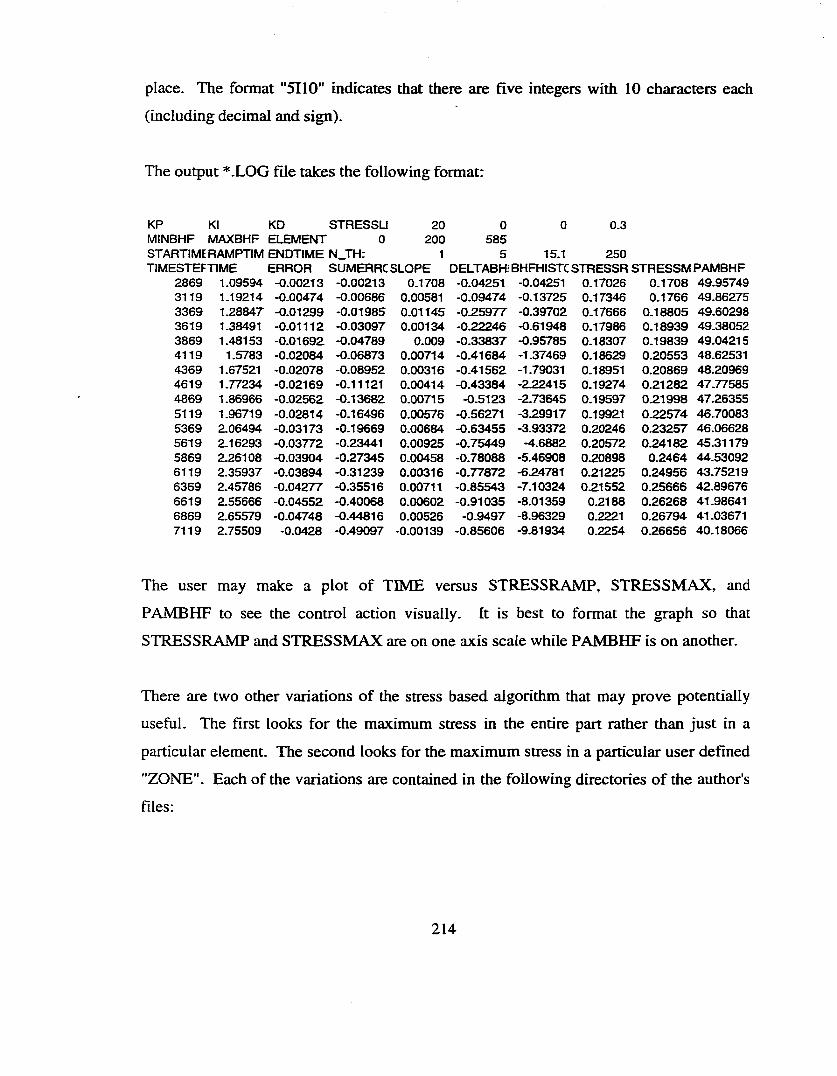
place. The format "5110" indicates that there are five integers with 10 characters each

(including decimal and sign).

The output *.LOG file takes the following format:

KP KI KD STRESSU 20 0 0 0.3MINBHF MAXBHF ELEMENT 0 200 585STARTIME RAMPTIM ENDTIME N_TH: 1 5 15.1 250TIMESTEFTIME ERROR SUMERRC SLOPE DELTABHIBHFHISTC STRESSR STRESSM PAMBHF

2869 1.09594 -0.00213 -0.00213 0.1708 -0.04251 -0.04251 0.17026 0.1708 49.957493119 1.19214 -0.00474 -0.00686 0.00581 -0.09474 -0.13725 0.17346 0.1766 49.862753369 1.28847 -0.01299 -0.01985 0.01145 -0.25977 -0.39702 0.17666 0.18805 49.602983619 1.38491 -0.01112 -0.03097 0.00134 -0.22246 -0.61948 0.17986 0.18939 49.380523869 1.48153 -0.01692 -0.04789 0.009 -0.33837 -0.95785 0.18307 0.19839 49.042154119 1.5783 -0.02084 -0.06873 0.00714 -0.41684 -1.37469 0.18629 0.20553 48.625314369 1.67521 -0.02078 -0.08952 0.00316 -0.41562 -1.79031 0.18951 0.20869 48.209694619 1.77234 -0.02169 -0.11121 0.00414 -0.43384 -222415 0.19274 0.21282 47.775854869 1.86966 -0.02562 -0.13682 0.00715 -0.5123 -273645 0.19597 0.21998 47.263555119 1.96719 -0.02814 -0.16496 0.00576 -0.56271 -3.29917 0.19921 0.22574 46.700835369 2.06494 -0.03173 -0.19669 0.00684 -0.63455 -3.93372 0.20246 0.23257 46.066285619 2.16293 -0.03772 -0.23441 0.00925 -0.75449 -4.6882 0.20572 0.24182 45.311795869 2.26108 -0.03904 -0.27345 0.00458 -0.78088 -5.46908 0.20898 0.2464 44.530926119 2.35937 -0.03894 -0.31239 0.00316 -0.77872 -6.24781 0.21225 0.24956 43.752196369 2.45786 -0.04277 -0.35516 0.00711 -0.85543 -7.10324 0.21552 0.25666 42.896766619 2.55666 -0.04552 -0.40068 0.00602 -0.91035 -8.01359 0.2188 0.26268 41.986416869 2.65579 -0.04748 -0.44816 0.00526 -0.9497 -8.96329 0.2221 0.26794 41.036717119 2.75509 -0.0428 -0.49097 -0.00139 -0.85606 -9.81934 0.2254 0.26656 40.18066

The user may make a plot of TIME versus STRESSRAMP, STRESSMAX, and

PAMBHF to see the control action visually. It is best to format the graph so that

STRESSRAMP and STRESSMAX are on one axis scale while PAMBHF is on another.

There are two other variations of the stress based algorithm that may prove potentially

useful. The first looks for the maximum stress in the entire part rather than just in a

particular element. The second looks for the maximum stress in a particular user defined

"ZONE". Each of the variations are contained in the following directories of the author's

files:

214

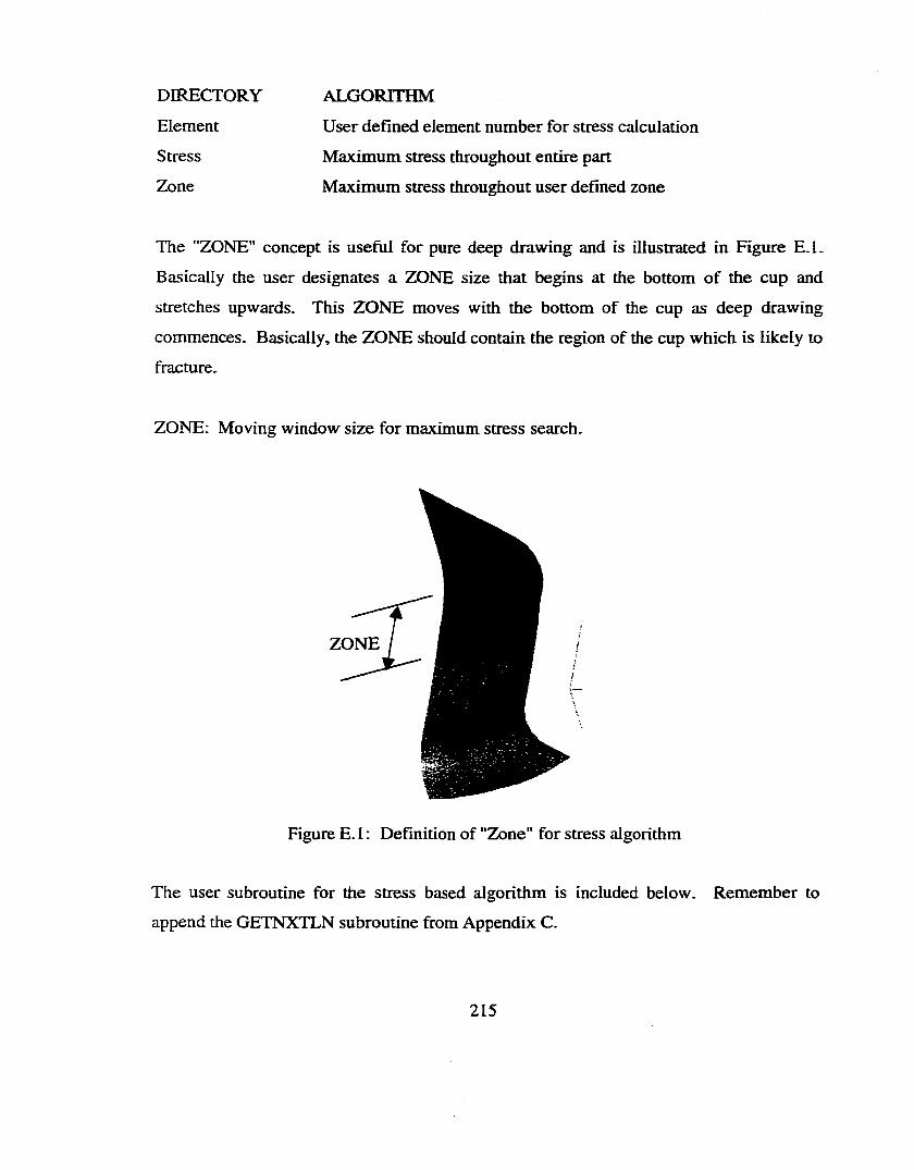
DIRECTORY

Element

Stress

Zone

ALGORITHM

User defined element number for stress calculation

Maximum stress throughout entire part

Maximum stress throughout user defined zone

The "ZONE" concept is useful for pure deep drawing and is illustrated in Figure E.L

Basically the user designates a ZONE size that begins at the bottom o f the cup and

stretches upwards. This ZONE moves with the bottom of the cup as deep drawing

commences. Basically, the ZONE should contain the region of the cup which is likely to

fracture.

ZONE: Moving window size for maximum stress search.

ZONE

Figure E. 1 : Definition of "Zone" for stress algorithm

The user subroutine for the stress based algorithm is included below. Remember to

append the GETNXTLN subroutine from Appendix C.

215

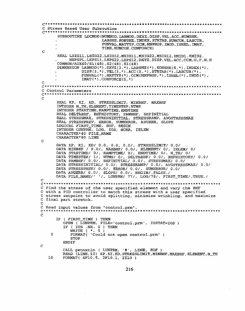
C Stress Based User SubroutineSUBROUTINE LDCMOD ( NUMNOD, LABNOD, DXYZ, DISP, VEL, ACC, NUMSHE,

LAB SHE, KONSHE, INDEX, STRTAB, NUMCUR. LABCUR, FUNVAL, MATTYP, CCM, NNPROP, INOD, ISHEL, IMAT,TIME, NUMCON, CONFORCE )C

REAL LSIGll, LSIG22 , LSIG12 ,MSIGll, MSIG22, MSIG12, KMIDl, KMID2 ,MEPSPL, LEPSll, LEPS22 , LEPS12 , DXYZ, DISP, VEL, ACC, CCM, G , F , N, H

COMMON/AUX40/Sl(48),S2(48),S3(48)DIMENSION LABNOD (*) .DXYZ (3, *) .LABSHEC*) .KONSHE(6.*) ,INDEX(*) .

DISP(3,*) ,VEL(3.*) .ACC(3,*} .STRTAB(*) ,LABCUR(*) ,FUNVAL ( * ) . MATTYP ( * ) . CCM (NNPROP, * ) . ISHEL ( * ) . INOD ( * ) . IMAT(*).CONFORCE(5 .*)C

C Control Parameters c

REAL KP. KI. KD, STRESSLIMIT. MINBHF, MAXBHFINTEGER N_TH, ELEMENT, TIMESTEP, NTMSINTEGER STARTIME, RAMPTIME, ENDTIMEREAL DELTABHF, BHFHISTORY, PAMBHF. BHFINITIALREAL STRESSMAX, STRESSINITIAL. STRESSRAMP. AVGSTRESSMAXREAL STRESSPREV. ERROR. SUMERROR. AVGERR. SLOPELOGICAL FIRST_TIME. EOF. BEGININTEGER LUNPRM. LOG, lOS. NCHR. lELEMCHARACTER*40 FILE_NAMECHARACTER*80 LINECDATA KP. KI. KD/ 0.0. 0.0. 0.0/. STRESSLIMIT/ 0.0/DATA MINBHF / 0.0/. MAXBHF/ 0.0/. ELEMENT/ 0/. lELEM/ 0/DATA STARTIME/ 0/. RAMPTIME/ 0/. ENDTIME/ 0/. N_TH/ 0/DATA TIMESTEP/ 1/. NTMS/ 0/. DELTABHF/ 0.0/. BHFHISTORY/ 0.0/DATA PAMBHF/ 0.0/. BHFINITIAL/ 0.0/. STRESSMAX/ 0.0/DATA STRESSINITIAL/ 0.0/, STRESSRAMP/ 0.0/. AVGSTRESSMAX/ 0.0/ DATA STRESSPREV/ 0.0/, ERROR/ 0.0/, SUMERROR/ 0.0/DATA AVGERR/ 0.0/, SLOPE/ 0.0/. BEGIN/.FALSE./DATA FILE_NAME/■ '/, LONPRM/ 77/. LOG/78/ , FIRST_TIME/.TRUE. /C

C Find the stress of the user specified element and vary the BHF C with a PID controller to match this stress with a user specified C stress setpoint to avoid splitting, minimize wrinkling, and maximize C final part stretch.CC Read input values from "control.prm".c

IF ( FIRST_TIME ) THENOPEN ( LUNPRM. FILE='control.prm ' . IOSTAT=IOS )IF ( 10S .NE. 0 ) THEN

WRITE ( *. 5 )5 FORMAT( 'Could not open control.prm' )

STOPENDIFCCALL getnxtln ( LUNPRM, '#', LINE, EOF )READ (LINE, 10) KP. KI. KD. STRESSLIMIT. MINBHF,MAXBHF. ELEMENT,N_TH

10 FORMAT( 4F10.5. 2F10.1. 2110 )

216

CALL getnxtln ( LDNPRM, LINE, EOF )READ ( LINE, 15 ) STARTIME, RAMPTIME, ENDTIME

15 FORMAT( 3110 )CC Get the name of the output/log file C

CALL getnxtln ( LONPRM, LINE, EOF )NCHR = LLLEN { LINE )FILE_NAME = LINE(1:NCHR) // CHAR(O)CCLOSE { LONPRM )NTMS = 0 AVGERR =0.0 FIRST_TIME = .FALSE.C

C Find Internal Element Number C

DO 100 ISHE=1,NOMSHEIF (ISHEL(ISHE) .EQ. ELEMENT) lELEM = ISHE

100 CONTINUECC Open the log file C

OPEN ( LOG, FILE=FILE_NAME, IOSTAT=IOS )CWRITE ( LOG, 20 ) KP, KI, KD, STRESSLIMIT

20 FORMAT( 'KP,KI,KD,STRESSLIMIT, 4F10.5 )WRITE( LOG, 25 ) MINBHF, MAXBHF, ELEMENT, lELEM

25 FORMAT( 'MINBHF, MAXBHF, ELEMENT, lELEM: ', 2F10.1, 2110 )WRITE( LOG, 3 0 ) STARTIME, RAMPTIME, ENDTIME, N_TH

3 0 FORMAT( 'STARTIME, RAMPTIME, ENDTIME, N_TH:’,4I10)WRITE( LOG, 35 }

3 5 FORMAT ( ' , TIMESTEP, TIME, ERROR, SUMERROR, SLOPE, DELTABHF, ' ,* ■ BHFHISTORY, STRESSRAMP, STRESSMAX, PAMBHF ' )ENDIF

CC Initialization of STRESSMAX CC STRESSLIMIT = 250

STRESSMAX = -1.0 NBSHEMAX = 0

CC Get element values of element number NSHESL c

ISHE=IELEMCC DO 200 ISHE=1,NUMSHEC NSHE = LABSHECISHE)C IF{NSHE.EQ.NSHESL) THENCC Define variables relative to element NSHE C

IGAUS = 0 1 Inteçrration type flagIN = INDEX { ISHE) - 1 1 Address of NSHE in INDEX tableIP = KONSHE(5,ISHE) 1 Number of through thickness

int. points CC Extract thickness and thinning values C

2 1 7

IF(IGAUS.EQ.l) THEN I Selective integration (Hughes-Tezd.)

CCCCCCCCCCCCCccccccc

ISTEP = 6ISFIX = 2 2lADD = 4c THO = STRTAB (IN4-21) I Initial thicknessc THK = STRTAB (IN4- 1) I Current thicknessc THN = (THO-THK)/THO i Thinning ratio

ELSE I Reduced integration (BelytISTEP = 6ISFIX = 18lADD - 4c THO = STRTAB(IN+17) I Initial thicknessc THK = STRTAB(IN+ 1) t Current thicknessc .THN = (THO-THK) /THO

c ENDIF

cccccccccccc

Get stresses at each, integration pointDO 210 1=1,IP

K = IN + ISFIX 4. (I-1)*ISTEP SKI) = STRTAB (K-f-l) !S2(I) = STRTAB (K-i-2) !S3 (I) = STRTAB (K+3) !

210 CONTINUEGet Lower/Upper surface stress tensor

SigmaSigmaSigma

112212

LSIGll = LSIG22 = LSIG12 = USIGll = USIG22 = USIG12 =

SKI) S2(l) S3 (1) SKIP) S2(IP) S3(IP)

Get Middle surface stress tensor151 = (IP+D/2152 = IP/2 + 1MSIGll = 0.5*(S1(IS1) 4- SKIS2) )MSIG22 = 0.5* (S2 (ISl) 4- S2(IS2) )MSIG12 = 0.5* (S3 (ISl) 4- S3 (IS2) )

Get Middle surface plastic strainKMIDl = IN + ISFIX 4- (ISl-1) *ISTEP 4- lADDKMID2 = IN 4- ISFIX 4- (IS2-1) *ISTEP 4- lADDMEPSPL = 0 .5* (STRTAB (KMIDl) 4-STRTAB (KMID2) )

Get Lower/Upper surface strain tensorK = IN 4- ISFIX - 8LEPSll = STRTAB (K4-4) LEPS22 = STRTAB (K4-5)' LEPS12 = .5*STRTAB(K4-6) UEPSll = STRTAB (K4-1)UEPS22 = STRTAB (K4-2) UEPS12 = .5*STRTAB(K4-3) ENDIF

Compute Equivalent Stress (Hill)

EpsilonEpsilonEpsilonEpsilonEpsilonEpsilon

11 Lower 22 Lower12 Lower11 Upper 22 Upper12 Upper

surfacesurfacesurfacesurfacesurfacesurface

218

ccccccccccccccccccccccccccccccccccccc

2 * HMSIGllMSIG22

C C C C C C C C C C C CC Check if che element is in the wall of the part C

NODEl = KONSHE(2. ISHE)N0DE2 = KONSHE(3,ISHE)NODE3 = KONSHE (4, ISHE)NODE4 = KONSHE(5, ISHE)

IF ( (MATTYP (KONSHE(1, ISHE) ) -EQ.107) -OR.(MATTYP(K0NSHE(1,ISHE) ) -EQ-109) ) THEN

G = CCM( 68, KONSHE (1, ISHE) )F = CCM( 69, KONSHE (1, ISHE) )N = CCM(70,KONSHE(1,ISHE) )H = 2 - GSTRESSAOX = 2 * N * MSIG12 STRESSAOX = STRESSAUX + (G STRESSAOX = STRESSAOX -t- (F STRESSAOX = SQRT (STRESSAOX STRESSEQ = STRESSAOX

2 -

H) * H) * 0-5)

* MSIGll * * 2

2

MSIG22

ZNODEl = DXYZ (3 ,NODEl)ZN0DE2 = DXYZ(3 ,N0DE2)ZNQDE3 = DXYZ (3 , N0DE3 )IF (NODE4 -NE- 0) THEN

ZNODE4 = DXYZ(3,NODE4)ELSEZNODE4 = DEPTH ENDIFIF (TIMESTEP -GT- STARTIME) THEN

ZONEPOS = (DEPTH/ENDTIME*TIMESTEP) - ZONE IF (ZONEPOS -LT- 0-0) ZONEPOS = 0.0IF (ZONEPOS -GT. (DEPTH-ZONE) ) ZONEPOS = DEPTH - ZONE IF ( (ZNODEl -GT- ZONEPOS) -AND- (ZNODE2 -GT- ZONEPOS) -AND.

(ZNODE3 -GT- ZONEPOS) -AND- (ZN0DE4 -GT- ZONEPOS) -AND- (STRESSEQ -GT. STRESSMAX) ) THEN

STRESSMAX = STRESSEQ NBSHEMAX = ISHE

ENDIF ELSE

IF (STRESSEQ -GT. STRESSMAX) THEN STRESSMAX = STRESSEQ NBSHEMAX = ISHE

ENDIF ENDIF

ENDIFCalculate Equivalent Stress of EILEMENT

IF (ISHEL (ISHE) -EQ- ELEMENT) THEN G = CCM (68, KONSHE (1, ISHE) )F = CCM(69, KONSHE (1, ISHE) )N = CCM(70, KONSHE (1, ISHE) )H = 2 - GSTRESSAUX = 2 * N * MSIG12 ** 2 - 2 * H ^STRESSAUX = STRESSAOX + (G + H) * MSIGllSTRESSAUX = STRESSAOX + (F + H) * MSIG22STRESSAUX = SQRT (STRESSAUX * 0.5)STRESSEQ = STRESSAOX STRESSMAX = STRESSEQ

MSIGll * * 2 * * 2

MSIG22

219

c ENDIFCC Calculated Major Stress of ELEMENT CC IF (ISHE .EQ. lELEM) THENC MSIGl = ((MSIG11+MSIG22)/2)C MSIGl = MSIGl + SQRT (CCMSIG11-MSIG22)/2)**2+MSIG12**2)C MSIG2 = MSIGl - SQRT ( C (MSIG11-MSIG22)/2) **2+MSIG12**2)C ENDIFCC 200 CONTINUE CC Get displacement of all nodes of element NBSHEMAXcc NODEl = KONSHE (2, NBSHEMAX)C N0DE2 = KONSHE ( 3 . NBSHEMAX)C N0DE3 = KONSHE (4. NBSHEMAX)C N0DE4 = KONSHE C 5, NBSHEMAX)C NDOF = 6C XNODEl = DXYZ(1,NODEl)C YNODEl = DXYZ(2,NODEl)C ZNODEl = DXYZ(3,NODEl)C XNODE2 = DXYZ(1,N0DE2)C YNODE2 = DXYZ(2,NODE2)C ZNODE2 = DXYZ(3,NODE2)C XNODE3 = DXYZ(1,N0DE3 )C YN0DE3 = DXYZ(2,NODE3)C ZN0DE3 = DXYZ(3,N0DE3 )C IF (NODE4 .NE. 0) THENC XN0DE4 = DXYZ(1,N0DE4)C YNODE4 = DXYZ(2,N0DE4)C ZN0DE4 = DXYZ{3,NODE4)c XCOG = (XNODEl XN0DE2 + XNODE3 + XN0DE4) / 4c YCOG = (YNODEl + YN0DE2 + YNODE3 + YN0DE4) / 4c ZCOG = (ZNODEl -r ZN0DE2 + ZN0DE3 + ZN0DE4) / 4c ELSEc XCOG = (XNODEl + XN0DE2 XNODE3 ) / 3c YCOG = (YNODEl -f- YN0DE2 YNODE3 ) / 3c ZCOG = (ZNODEl + ZN0DE2 +■ ZNODE3 ) / 3C ENDIFC

ie ie -X -ie * iç -k- ir -te -ie * ir * * ie * ir * * * * * * ie ie ie *icie * ir icie * * * * * -k-"te ie ie icir ie ir ie * -ie ic ic ie ir-ie ic * * * * * * ie-ie * * * * ir'*e *

C Proportional, Integral, Derivative ControllercC Checlc to see if it is time to begin control.CC Find the error (proportional), sum of previous errors (integral), and C slope (derivative)C

IF (STARTIME .LT. 0) THENIF (STRESSMAX .GE. STRESSLIMIT) BEGIN=.TRaE.

ELSEIF (TIMESTEP .GT. STARTIME) BEGIN=.TRUE.

ENDIFC

IF (BEGIN) THENIF ( ( TIMESTEP . LT. RAMPTDXE ) .AND. (STARTIME .GE. 0)) THEN

STRESSRAMP = STRESSINITIAL + (STRESSLIMIT - STRESSINITIAL)

2 2 0

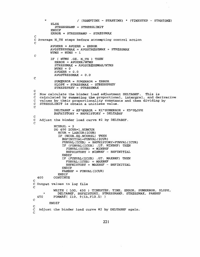
* / (RAMPTIME - STARTIME) * (TIMESTEP - STARTIME}ELSE

STRESSRAMP = STRESSLIMIT ENDIFERROR = STRESSRAMP - STRESSMAX

CC Average N_TH steps before attempting control action C

AVGERR = AVGERR + ERRORAVGSTRESSMAX = AVGSTRESSMAX + STRESSMAX NTMS = NTMS +■ 1

CIF ( NTMS .GE. N_TH ) THEN

ERROR = AVGERR/NTMS STRESSMAX = AVGSTRESSMAX/NTMS NTMS = 0 AVGERR =0.0 AVGSTRESSMAX = 0.0

CSUMERROR = SUMERROR + ERROR SLOPE = STRESSMAX - STRESSPREV STRESSPREV = STRESSMAX

CC Now calculate the binder load adjustment DELTABHF. This is C calculated by summating the proportional, intergral, and derivative C values by their proportionality constants and then dividing by C STRESSLIMIT is obtain a unitless value.C

DELTABHF = KP*ERROR + KI*SUMERROR + KD*SLOPE BHFHISTORY = BHFHISTORY +- DELTABHF

CC Adjust the binder load curve #2 by DELTABHF.C

NCURSL = 2DO 400 ICUR=1,NUMCUR

NCUR = LABCUR (ICUR)IF ( NCUR. EQ. NCURSL ) THEN

BHFIÎHTIAL=FUNVAL ( ICUR)FUNVAL (ICUR) = BHFHISTORY+FUNVAL (ICUR)IF (FUNVAL (ICUR) .LT. MINBHF) THEN

FUNVAL ( ICUR) = MINBHF BHFHISTORY = MINBHF - BHFINITIAL

ENDIFIF (FUNVAL (ICUR) .GT. MAXBHF) THEN

FUNVAL(ICUR) = MAXBHF BHFHISTORY = MAXBHF - BHFINITIAL

ENDIFPAMBHF = FUNVAL(ICUR)

ENDIF 400 CONTINUE

CC Output values to log file C

WRITE ( LOG, 450 ) TIMESTEP, TIME, ERROR, SUMERROR, SLOPE,* DELTABHF, BHFHISTORY, STRESSRAMP, STRESSMAX, PAMBHF

450 FORMAT( 110, 9 (lh,F10.5) )C

ENDIFCC Adjust the binder load curve #2 by DELTABHF again.C

221

NCDRSL = 2 DO 500 ICDR=1,N0MCDR

NCUR = LABOUR (XCUR)IF (NCUR.EQ.NCURSL) THEN

FUNVAL ( rCUR) = BHFHISTORY+FDNVAL ( ICUR) ENDIF

500 CONTINUEC

ELSESTRESSINITIAL = STRESSMAX

ENDIFTIMESTEP = TIMESTEP + 1

CR E T U R NEND

2 2 2

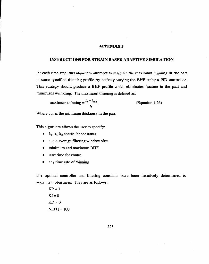
APPENDK F

INSTRUCTIONS FOR STRAIN BASED ADAPTIVE SIMULATION

At each time step, this algorithm attempts to maintain the maximum thinning in the part

at some specified thinning profile by actively varying the BHF using a FID controller.

This strategy should produce a BHF profile which eliminates fracture in the part and

minimizes wrinkling. The maximum thinning is defined as:

maximum thinning = —— (Equat i on 4.26)^0

Where tmin is the minimum thickness in the part.

This algorithm allows the user to specify:

• kp, ki, kd controller constants

• static average filtering window size

• minimum and maximum BHF

• start time for control

• any time rate of thinning

The optimal controller and filtering constants have been iteratively determined to

maximize robusmess. They are as follows:

KP = 3

KI = 0

KD = 0

N_TH = 100

223

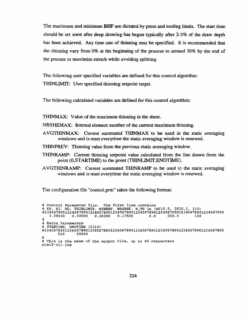
The maximum and minimum BHF are dictated by press and tooling limits. The start time

should be set soon after deep drawing has begun typically after 2-3% of the draw depth

has been achieved. Any time rate o f thiiming may be specified. It is recommended that

the thiiming vary from 0% at the beginning of the process to around 30% by the end of

the process to maximize stretch while avoiding splitting.

The following user specified variables are defined for this control algorithm:

THINLIMIT: User specified thinning setpoint target.

The following calculated variables are defined for this control algorithm:

THINMAX: Value of the maximum thinning in the sheet.

NBSHEMAX: Internal element number of the current maximum thinning.

AVGTHINMAX: Current summated THINMAX to be used in the static averaging windows and is reset everytime the static averaging window is renewed.

THINPREV: Thinning value from the previous static averaging window.

THINRAMP: Current thinning setpoint value calculated from the line drawn from the point (0,STARTIME) to the point (THINLIMIT^NDTTME).

AVGTHINRAMP: Current summated THINRAMP to be used in the static averaging windows and is reset everytime the static averaging window is renewed.

The configuration file "control.prm" takes the following format:

# Control Parameter file. The first line contains# KP, KX, KD, THINLIMIT, MINBHF, MAXBHF, N_TH in (4F10.5, 2F10.1, 110) #2345S7890123456789012345S7890123456789012345S789012345S789012345678901234567890

3.00000 0.00000 0.00000 0.17500 0.0 200.0 100## Extra Parameters# STARTIME, ENDTIME (2110)#2345578901234557890123455789012345578901234567890123455789012345578901234567890

500 20000## This is the name of the output file, up to 40 characters piel2-tll.log

224

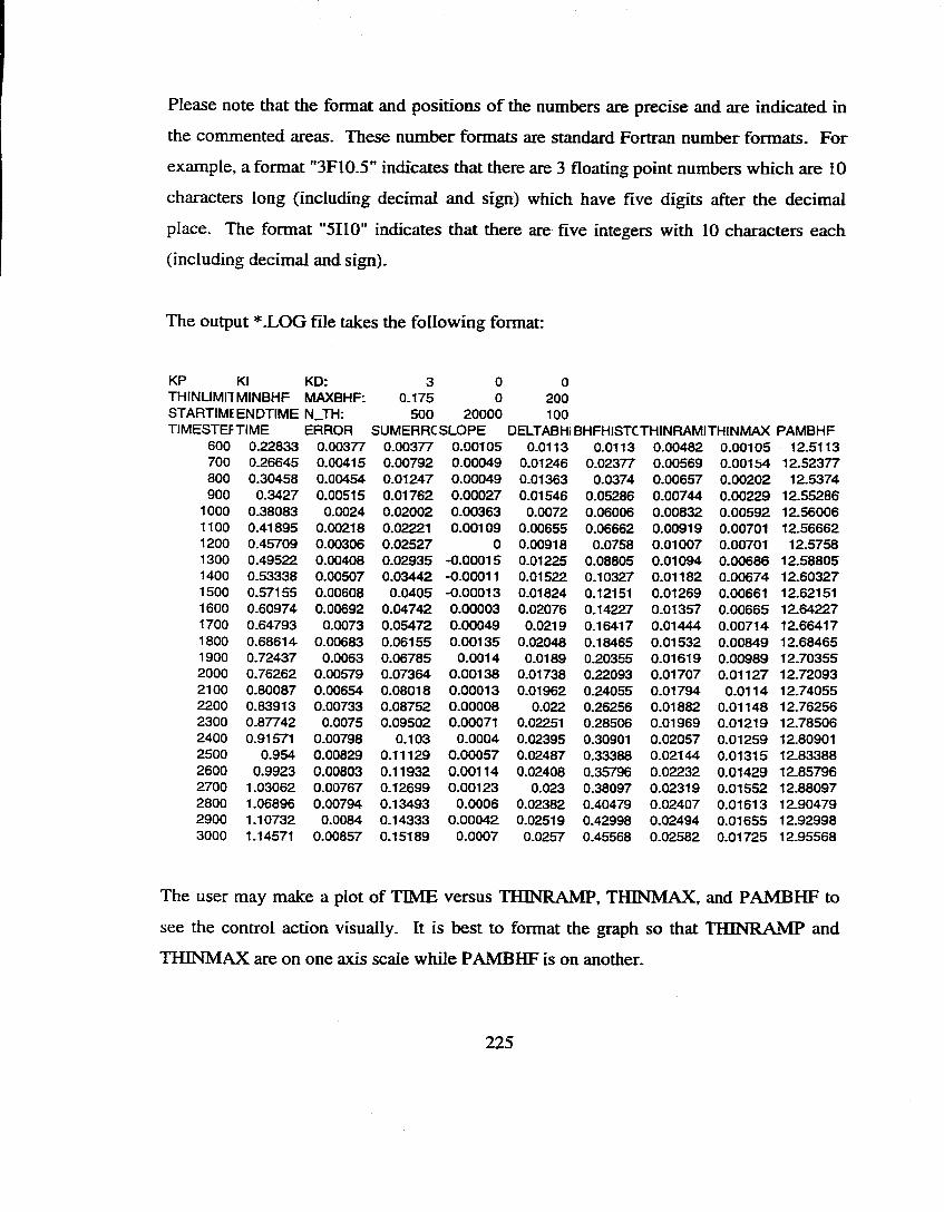
Please note that the format and positions of the numbers are precise and are indicated in

the commented areas. These number formats are standard Fortran number formats. For

example, a format "3F10.5" indicates that there are 3 floating point numbers which are 10

characters long (including decimal and sign) which have five digits after the decimal

place. The format "5110 " indicates that there are five integers with 10 characters each

(including decimal and sign).

The output *.LOG file takes the following format:

KP KI KD: 3 0 0THINLIMn MINBHF MAXBHF: 0-175 0 200STARTIME ENDTIME N_TH: 500 20000 100TIMESTEFTIME ERROR SUMERRC SLOPE DELTABHi BHFHISTCTHINRAMITHINMAX PAMBHF

600 0.22833 0.00377 0.00377 0.00105 0.0113 0.0113 0.00482 0.00105 12.5113700 0.26645 0.00415 0.00792 0.00049 0.01246 0.02377 0.00569 0.00154 12.52377800 0.30458 0.00454 0.01247 0.00049 0.01363 0.0374 0.00657 0.00202 12.5374900 0.3427 0.00515 0.01762 0.00027 0.01546 0.05286 0.00744 0.00229 12.55286

1000 0.38083 0.0024 0.02002 0.00363 0.0072 0.06006 0.00832 0.00592 12.560061100 0.41895 0.00218 0.02221 0.00109 0.00655 0.06662 0.00919 0.00701 12.566621200 0.45709 0.00306 0.02527 0 0.00918 0.0758 0.01007 0.00701 12.57581300 0.49522 0.00408 0.02935 -0.00015 0.01225 0.08805 0.01094 0.00686 12.588051400 0.53338 0.00507 0.03442 -0.00011 0.01522 0.10327 0.01182 0.00674 12.603271500 0.57155 0.00608 0.0405 -0.00013 0.01824 0.12151 0.01269 0.00661 12.621511600 0.60974 0.00692 0.04742 0.00003 0.02076 0.14227 0.01357 0.00665 12.642271700 0.64793 0.0073 0.05472 0.00049 0.0219 0.16417 0.01444 0.00714 12.664171800 0.68614 0.00683 0.06155 0.00135 0.02048 0.18465 0.01532 0.00849 12.684651900 0.72437 0.0063 0.06785 0.0014 0.0189 0.20355 0.01619 0.00989 12.703552000 0.76262 0.00579 0.07364 0.00138 0.01738 0.22093 0.01707 0.01127 12.720932100 0.80087 0.00654 0.08018 0.00013 0.01962 0.24055 0.01794 0.0114 12.740552200 0.83913 0.00733 0.08752 0.00008 0.022 0.26256 0.01882 0.01148 12.762562300 0.87742 0.0075 0.09502 0.00071 0.02251 0.28506 0.01969 0.01219 12.785062400 0.91571 0.00798 0.103 0.0004 0.02395 0.30901 0.02057 0.01259 12.809012500 0.954 0.00829 0.11129 0.00057 0.02487 0.33388 0.02144 0.01315 12.833882600 0.9923 0.00803 0.11932 0.00114 0.02408 0.35796 0.02232 0.01429 12.857962700 1.03062 0.00767 0.12699 0.00123 0.023 0.38097 0.02319 0.01552 12.880972800 1.06896 0.00794 0.13493 0.0006 0.02382 0.40479 0.02407 0.01613 12.904792900 1.10732 0.0084 0.14333 0.00042 0.02519 0.42998 0.02494 0.01655 12.929983000 1.14571 0.00857 0.15189 0.0007 0.0257 0.45568 0.02582 0.01725 12.95568

The user may make a plot of TIME versus THINRAMP, THINMAX, and PAMBHF to

see the control action visually. It is best to format the graph so that THINRAMP and

THINMAX are on one axis scale while PAMBHF is on another.

225

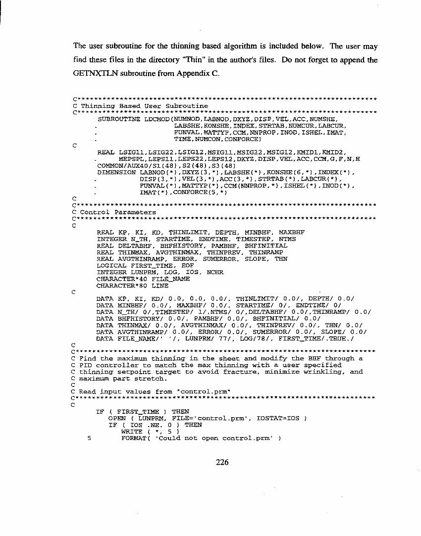
The user subroutine for the thinning based algorithm is included below. The user may

find these files in the directory "Thin" in the author's files. Do not forget to append the

GETNXTLN subroutine from Appendix C.

c * * * * * * * * * * * * * * * * * * * * * * * * * * * * * * * * * * * * * * * * * * * * * * * * * * * * * * * * * * * * * * * * * * * * * * *

C Thinning Based User SubroutineSUBROUTINE LDCMOD(NUMNOD,LABNOD,DXYZ,DISP,VEL,ACC,NUMSHE,

LABSHE, KONSHE, INDEX, STRTAB, NUMCUR, LABCUR,FUNVAD, MATTYP, CCM, NNPROP, INOD, ISHEL, IMAT,TIME, NUMCON, CONFORCE )

CREAL LSIGll, LSIG22 , LSIG12, MSIGll, MSIG22, MSIG12, KMIDl, KMID2,

MEPSPL, LEPSll, LEPS22, LEPS12 , DXYZ, DISP, VEL, ACC, CCM, G, F , N, H COMMON/AUX40/S1(48),S2(48),S3(48 )DIMENSION LABNOD(*),DXYZ(3,*),LABSHE(*),KONSHE(6,*),INDEX(*),

DISP(3, *) ,VEL(3,*) ,ACC(3,*),STRTAB(*) ,LABCUR(*),FUNVAL(*) ,MATTYP(*),CCM (NNPROP,*),ISHEL(*) ,INOD(*) ,IMAT(*),CONFORCE(5 ,*)C

C Control Parameters C

REAL KP, KI, KD, THINLIMIT, DEPTH, MINBHF, MAXBHF INTEGER N_TH, STARTIME, ENDTIME, TIMESTEP, NTMS REAL DELTABHF, BHFHISTORY, PAMBHF, BHFINITIAL REAL THINMAX, AVGTHINMAX, THINPREV, THINRAMP REAL AVGTHINRAMP, ERROR, SUMERROR, SLOPE, THN LOGICAL FIRST_TIME, EOF INTEGER LUNPRM, LOG, 10S, NCHR CHARACTER*40 FILE_NAME CEIARACTER*80 LINE

CDATA KP, KI, KD/ 0.0, 0.0, 0.0/, THINLIMIT/ 0.0/, DEPTH/ 0.0/DATA MINBHF/ 0.0/, MAXBHF/ 0.0/, STARTIME/ 0/, ENDTIME/ 0/DATA N_TH/ 0/,TIMESTEP/ 1/,NTMS/ 0/,DELTABHF/ 0.0/, THINRAMP/ 0.0/ DATA BHFHISTORY/ 0.0/, PAMBHF/ 0.0/, BHFINITIAL/ 0.0/DATA THINMAX/ 0.0/, AVGTHINMAX/ 0.0/, THINPREV/ 0.0/, THN/ 0.0/ DATA AVGTHINRAMP/ 0.0/, ERROR/ 0.0/, SUMERROR/ 0.0/, SLOPE/ 0.0/ DATA FILE_NAME/■ '/, LUNPRM/ 1 1 1 , LOG/78/, FIRST_TIME/.TRUE./

CC Find the maximum thinning in the sheet and modify the BHF through a C PID controller to match the majc thinning with a user specifiedC thinning setpoint target to avoid fracture, minimize wrinkling, andC maximum part stretch.CC Read input values from "control.prm" c

IF ( FIRST_TIME ) THENOPEN ( LUNPRM, FILE= ' control .prm’, IOSTAT=IOS )IF ( lOS .NE. 0 ) THEN

WRITE ( *, 5 )5 FORMAT( 'Could not open control.prm' )

226

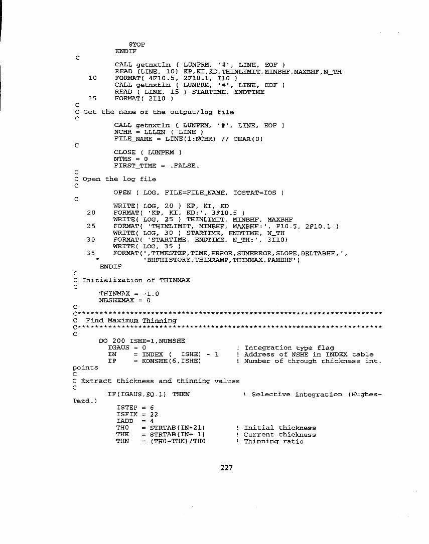
STOPENDIF

CCALL getnxtln ( LDNPRM, LINE, EOF )READ (LINE, 10) KP, KI, KD, THINLIMIT,MINBHF,MAXBHF,N_TH10 FORMAT( 4F10.5, 2F10.1, 110 )CALL getnxtln ( LUNPRM, LINE, EOF )READ ( LINE, 15 ) STARTIME, ENDTIME

15 FORMAT( 2110 )CC Get the name of the output/log file C

CALL getnxtln ( LUNPRM, '#', LINE, EOF )NCHR = LLLEN ( LINE )FILE_NAME = LINE(1:NCHR) // CHAR(O)

CCLOSE ( LUNPRM )NTMS = 0FIRST_TIME = .FALSE-C

C Open the log file C

OPEN ( LOG, FILE=FILE_NAME, IOSTAT=IOS )CWRITE( LOG, 20 } KP, KI, KD

20 FORMAT( 'KP, KI, KD:', 3F10.5 )WRITE( LOG, 25 ) THINLIMIT, MINBHF, MAXBHF

25 FORMAT( 'THINLIMIT, MINBHF, MAXBHF: ' , F10.5, 2F10.1 )WRITE( LOG, 3 0 } STARTIME, ENDTIME, N_TH

3 0 FORMAT{ ' STARTIME, ENDTIME, N_TH: ' , 3110)WRITE( LOG, 35 )

3 5 FORMAT ( ' , TIMESTEP, TIME, ERROR, SUMERROR, SLOPE, DELTABHF, ' ,* • BHFHISTORY, THINRAMP, THINMAX, PAMBHF ' )ENDIF

CC Initialization of THINMAX C

THINMAX = -1.0 NBSHEMAX = 0

C(2* * * * * * * * * * * * * * * * * * ie * ic * * * * * * * * ie * -ie ie icir ir * ie * * * * * icie -k- * * ie ie * ie icie *ie * * * * •tr * ir ie * -ie * ie * * ie

C Find Maximum Thinning c

DO 200 ISHE=1,NUMSHEIGAUS = 0 1 Integration type flagIN = INDEX ( ISHE) - 1 i Address of NSHE in INDEX tableIP = KONSHE (6, ISHE) I Number of through thickness int.

pointsCC Extract thickness and thinning values C

IF(IGAUS.EQ.l) THEN 1 Selective integration (Hughes-Tezd.)

ISTEP = 6ISFIX = 22lADD = 4THO = STRTAB(IN+21) 1 Initial thicknessTHK = STRTAB (IN-t- 1) I Current thicknessTHN = (THO-THK)/THO I Thinning ratio

227

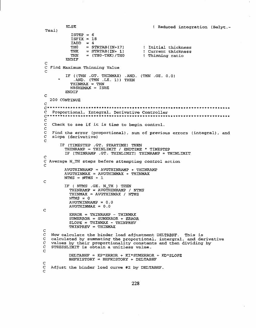
ELSE 1 Reduced, inCegration (Belyt.-Tsai)ISTEP = 6ISFIX = 18lADD = 4THO = STRTAB (m+17) L Initial thicknessTHK = STRTAB (IK+ 1) i Current thicknessTHN = (THO-THK) /THO I Thinning ratioENDIFC

C Find Maximum Thinning Value CIF ( (THN .GT. THINMAX) .AND. (THN .GE. 0.0)

* .AND. (THN .LE. 1)) THENTHINMAX = THN NBSHEMAX = ISHE

ENDIFC200 CONTINUE

CC Proportional, Integral, Derivative Controller cC Check to see if it is time to begin control.CC Find the error (proportional) , sum of previous errors (integral) , and C slope (derivative)C

IF (TIMESTEP .GT. STARTIME) THENTHINRAMP = THINLIMIT / ENDTIME * TIMESTEP IF (THINRAMP .GT. THINLIMIT) THINRAMP = THINLIMITC

C Average N_TH steps before attempting control action CAVGTHINRAMP = AVGTHINRAMP + THINRAMP AVGTHINMAX = AVGTHINMAX + THINMAX NTMS = NTMS + 1CIF ( NTMS .GE. N_TH ) THENTHINRAMP = AVGTHINRAMP / NTMS THINMAX = AVGTHINMAX / NTMS NTMS = 0AVGTHINRAMP = 0.0 AVGTHINMAX = 0.0CERROR = THINRAMP - THINMAX SUMERROR = SUMERROR + ERROR SLOPE = THINMAX - THINPREV THINPREV = THINMAXC

C Now calculate the binder load adjustment DELTABHF. This is C calculated by summating the proportional, intergral, and derivative C values by their proportionality constants and then dividing by C STRESSLIMIT is obtain a unitless value.C

DELTABHF = KP* ERROR + KI* SUMERROR + KD*SLOPE BHFHISTORY = BHFHISTORY + DELTABHFC

C Adjust the binder load curve #2 by DELTABHF.C

228

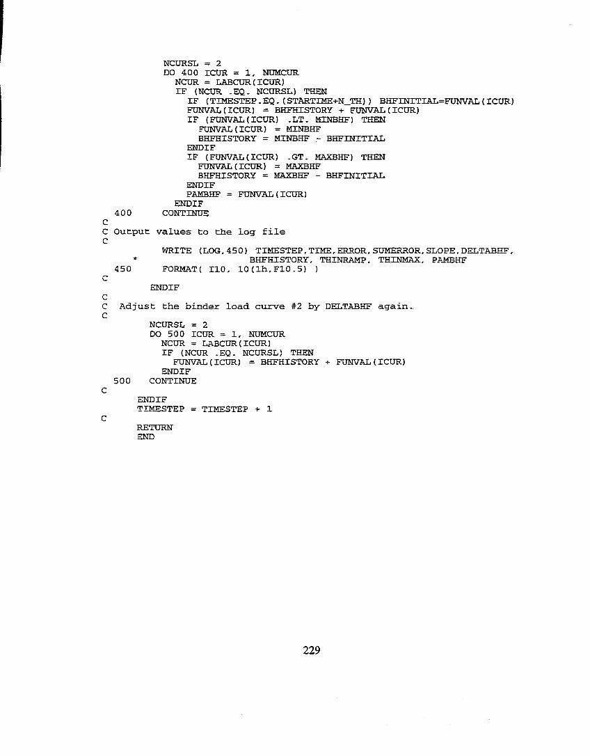
NCDRSL = 2DO 400 rCUR = 1, NDMCÜR

NCUR = LABCUR CICDR)IF (NCUR .EQ. NCURSL) THEN

IF (TIMESTEP.EQ. (STARTIMEh-N_TH) ) BHFINITIAL=FUNVAL (ICUR) FUNVAL (ICUR) = BHFHISTORY + FUNVAL (ICUR)IF (FUNVAL(ICUR) .LT. MINBHF) THEN

FUNVAL (ICUR) = MINBHF BHFHISTORY = MINBHF - BHFINITIAL

ENDIFIF (FUNVAL(ICUR) .GT. MAXBHF) THEN

FUNVAL(ICUR) = MAXBHF BHFHISTORY = MAXBHF - BHFINITIAL

ENDIFPAMBHF = FUNVAL(ICUR)

ENDIF 400 CONTINUE

CC Output values to the log file C

WRITE (LOG, 450) TIMESTEP, TIME, ERROR, SUMERROR, SLOPE, DELTABHF, * BHFHISTORY, THINRAMP, THINMAX, PAMBHF

450 FORMAT( 110, 10(lh,F10.5) )C

ENDIFCC Adjust the binder load curve #2 by DELTABHF again.C

NCURSL = 2DO 500 ICUR = 1, NUMCUR

NCUR = LABCUR (ICUR)IF (NCUR .EQ. NCURSL) THENFUNVAL (ICUR) = BHFHISTORY + FUNVAL (ICUR)ENDIF

500 CONTINUEC

ENDIFTIMESTEP = TIMESTEP + 1

CRETURNEND

229

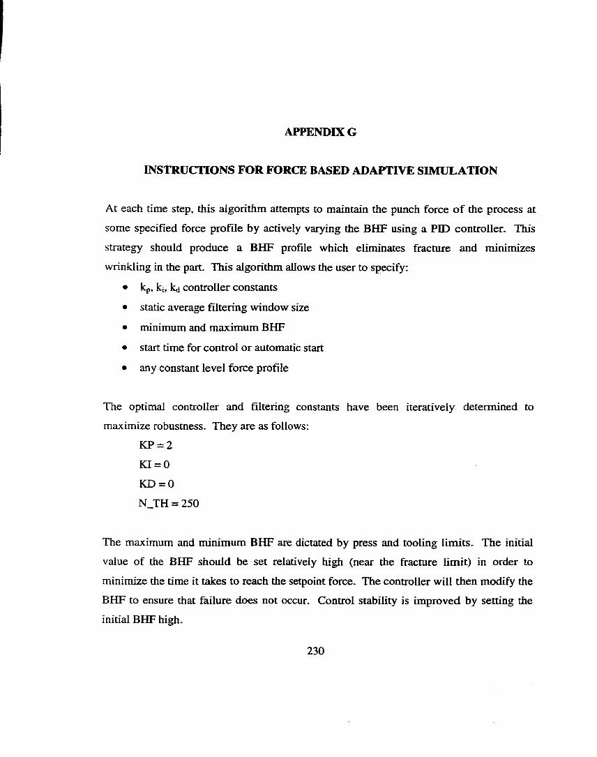
APPENDIX G

INSTRUCTIONS FOR FORCE BASED ADAPTIVE SIMULATION

At each time step, this algorithm attempts to maintain the punch force o f the process at

some specified force profile by actively varying the BHF using a FID controller. This

strategy should produce a BHF profile which eliminates fracture and minimizes

wrinkling in the part. This algorithm allows the user to specify:

• kp, ki, kd controller constants

• static average filtering window size

• minimum and maximum BHF

• start time for control or automatic start

• any constant level force profile

The optimal controller and filtering constants have been iteratively determined to

maximize robustness. They are as follows:

KP = 2

KI = 0

BCD = 0

N_TH = 250

The maximum and minimum BHF are dictated by press and tooling limits. The initial

value of the BHF should be set relatively high (near the fracture limit) in order to

minimize the time it takes to reach the setpoint force. The controller will then modify the

BHF to ensure that failure does not occur. Control stability is improved by setting the

initial BHF high.

230

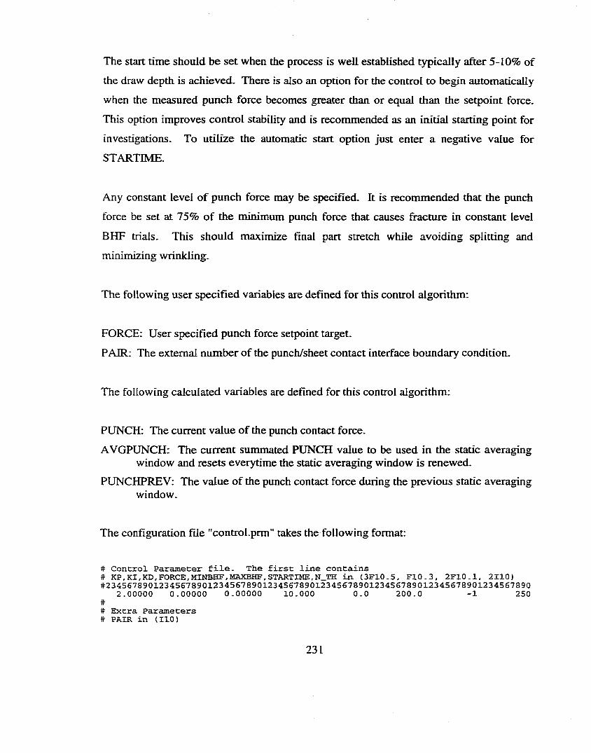
The start time should be set wheu the process is well established typically after 5-10% of

the draw depth is achieved. There is also an option for the control to begin automatically

when the measured punch force becomes greater than or equal than the setpoint force.

This option improves control stability and is recommended as an initial starting point for

investigations. To utilize the automatic start option just enter a negative value for

STARTIME.

Any constant level o f punch force may be specified. It is recommended that the punch

force be set at 75% of the minimum punch force that causes fracture in constant level

BHF trials. This should maximize final part stretch while avoiding splitting and

minimizing wrinkling.

The following user specified variables are defined for this control algorithm:

FORCE: User specified punch force setpoint target.

PAIR: The external number of the punch/sheet contact interface boundary condition.

The following calculated variables are defined for this control algorithm:

PUNCH: The current value of the punch contact force.

AVGPUNCH: The current summated PUNCH value to be used in the static averaging window and resets everytime the static averaging window is renewed.

PUNCHPREV: The value of the punch contact force during the previous static averaging window.

The configuration file "control.prm" takes the following format:

# Control Parameter file. The first line contains# KP,KI,KD,FORCE,MINBHF,MAXBHF,STARTIME,N_TH in. (3F10.5, F10.3, 2F10.1, 2110) #2345678901234567890123456789012345578901234567890123456789012345678901234567890

2.00000 0.00000 0.00000 10.000 0.0 200.0 -1 250## Extra Parameters# PAIR in (110)

231

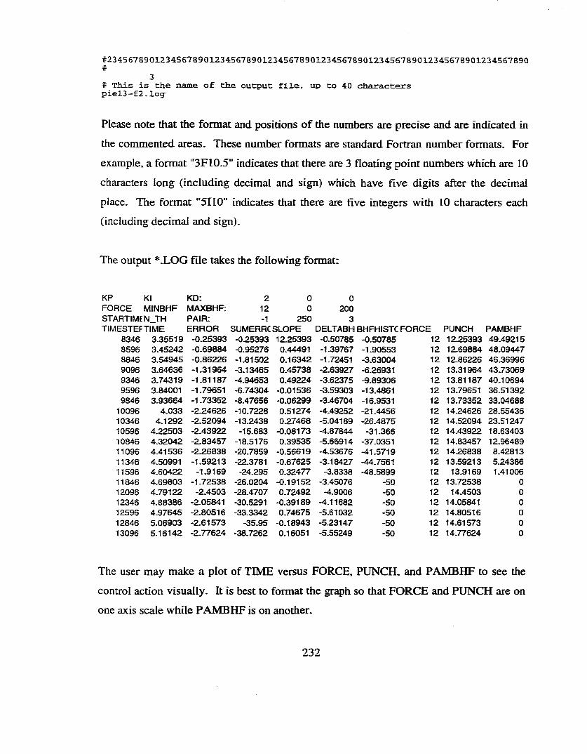
#2345678901234557890123456789012345678901234567890123456789012345678901234567890#

3# This is the name of the output file, up to 40 characters piel3-f2.log

Please note that the format and positions o f the numbers are precise and are indicated in

the commented areas. These number formats are standard Fortran number formats. For

example, a format "3FI0.5 " indicates that there are 3 floating point numbers which are 10

characters long (including decimal and sign) which have five digits after the decimal

place. The format "5110" indicates that there are five integers with 10 characters each

(including decimal and sign).

The output *.LOG file takes the following format:

KP KI KD: 2 0 0FORCE MINBHF MAXBHF: 12 0 200STARTIME N_TH PAIR: -1 250 3TIMESTEFTIME ERROR SUMERRC SLOPE DELTABHI BHFHISTC FORCE PUNCH PAMBHF

8346 3-35519 -0-25393 -0-25393 12-25393 -0.50785 -0-50785 12 12-25393 49-492158596 3.45242 -0-69884 -0-95276 0-44491 -1-39767 -1-90553 12 12-69884 48-094478846 3.54945 -0-86226 -1-81502 0-16342 -1-72451 -3-63004 12 12-86226 46-369969096 3-64636 -1-31964 -3-13465 0-45738 -2-63927 -6-26931 12 13-31964 43-730699346 3-74319 -1-81187 -4-94653 0-49224 -3-62375 -9-89306 12 13-81187 40.106949596 3-84001 -1.79651 -6-74304 -0-01536 -3-59303 -13-4861 12 13-79651 36-513929846 3-93664 -1-73352 -8-47656 -0-06299 -3-46704 -16-9531 12 13-73352 33.04688

10096 4-033 -2-24626 -10-7228 0-51274 -4-49252 -21-4456 12 14-24626 28-5543610346 4-1292 -2.52094 -13-2438 0-27468 -5-04189 -26-4875 12 14-52094 23-5124710596 4-22503 -2-43922 -15-683 -0-08173 -4.87844 -31-366 12 14-43922 18-6340310846 4-32042 -2-83457 -18-5176 0-39535 -5-66914 -37.0351 12 14-83457 12-9648911096 4-41536 -2-26838 -20-7859 -0-56619 -4-53676 -41-5719 12 14-26838 8-4281311346 4-50991 -1-59213 -22-3781 -0-67625 -3-18427 -44-7561 12 13.59213 5-2438611596 4-60422 -1-9169 -24-295 0-32477 -3-8338 -48-5899 12 13-9169 1-4100611846 4-69803 -1-72538 -26-0204 -0-19152 -3-45076 -50 12 13-72538 012096 4-79122 -2-4503 -28-4707 0-72492 -4-9006 -50 12 14-4503 012346 4-88386 -2.05841 -30-5291 -0.39189 -4-11682 -50 12 14-05841 012596 4-97645 -2-80516 -33-3342 0-74675 -5-61032 -50 12 14-80516 012846 5-06903 -2.61573 -35-95 -0-18943 -5-23147 -50 12 14-61573 013096 5-16142 -2.77624 -38-7262 0.16051 -5-55249 -50 12 14-77624 0

The user may make a plot of TIME versus FORCE, PUNCH, and PAMBHF to see the

control action visually. It is best to format the graph so that FORCE and PUNCH are on

one axis scale while PAMBHF is on another.

232

The user subroutine for the force based algorithm is included below The user may find

these files in the directory "Force" in the author's files. Please remember to append the

GETNXTLN subroutine from Appendix C.

C Force Based User SxibrouCineSUBROUTINE LDCMOD ( NUMNOD, LABNOD, DXYZ, DISP , VEL , ACC, NUMSHE,

LABSHE, KONSHE, INDEX, STRTAB, NUMCUR, LABCUR, FUNVAL, MATTYP, CCM, NNPROP, INOD, ISHEL, IMAT,TIME,NUMCON, CONFORCE)

CREAL LSIGll, LSIG22, LSIG12, MSIGll, MSIG22, MSIG12, KMIDl, KMID2,

MEPSPL, LEPSll, LEPS22 , LEPS12 , DXYZ, DISP, VEL, ACC, CCM, G , F, N, H COMMON/AUX40/SI{48) ,S2(48) ,S3(48)DIMENSION LABNOD (*) ,DXYZ(3,*) , LABSHE (*) ,KONSHE(6,*) ,INDEX(*) ,

DISPC3, *) ,VEL(3 , *) ,ACC{3, *) , STRTAB ( * ) ,LABCUR(*) , FUNVALC*) , MATTYP (*) , CCM (NNPROP, *) , ISHEL ( * ) , INOD ( * ) ,IMAT(*),CONFORCE(5,*)

CQie ie ie * ie -k -k -k -k * * * * * -k-k-k-k * ie icicie ir * ie ic ** ir ** icie ie ie ie ir * * * ie * ie ie * * * * ie ie * ie * ir ie * * ie * te ie ic ** ie *

C Control Parametersc

REAL KP, KI, KD, FORCE, MINBHF, MAXBHF INTEGER STARTIME, N_TH, PAIR, TIMESTEP, NTMS REAL DELTABHF, BHFHISTORY, PAMBHF, BHFINITIAL REAL PUNCH, AVGPUNCH, PUNCHPREV REAL ERROR, SUMERROR, SLOPE LOGICAL FIRST_TIME, EOF, BEGIN INTEGER LONPRM, LOG, lOS, NCHR, lELEM CHARACTER* 40 FILE_NAME CHARACTER* 80 LINE

CDATA KP, KI, KD/ 0.0, 0.0, 0.0/, FORCE/ 0-0/DATA MINBHF / 0.0/, MAXBHF/ 0.0/, BEGIN/. FALSE. /DATA STARTIME/ 0/, N_TH/ 0/, PAIR / 0/DATA TIMESTEP/ 1/, NTMS/ 0/, DELTABHF/ 0.0/, BHFHISTORY/ 0.0/DATA PAMBHF/ 0.0/, BHFINITIAL/ 0.0/, PUNCH/ 0.0/, AVGPUNCH/ 0.0/ DATA PUNCHPREV/ 0.0/, ERROR/ 0.0/, SUMERROR/ 0.0/, SLOPE/ 0.0/ DATA FILE_NAME/‘ '/, LUNPRM/ 77/, LOG/78/, FIRST_TIME/ . TRUE. /

CC Determine the punch contact force and modify the BHF through a PIDC controller to maintain the punch force at a user specified setpointC force to avoid splitting, minimize wrinkling, and maximize final C part stretch.CC Read input values from "control.prm" c

IF ( FIRST_TIME ) THENOPEN ( LUNPRM, FILE= ' control .prm', IOSTAT=IOS )IF ( 10S .NE. 0 ) THEN

WRITE ( *, 5 )5 FORMAT ( ' Could not open control .prm' )

233

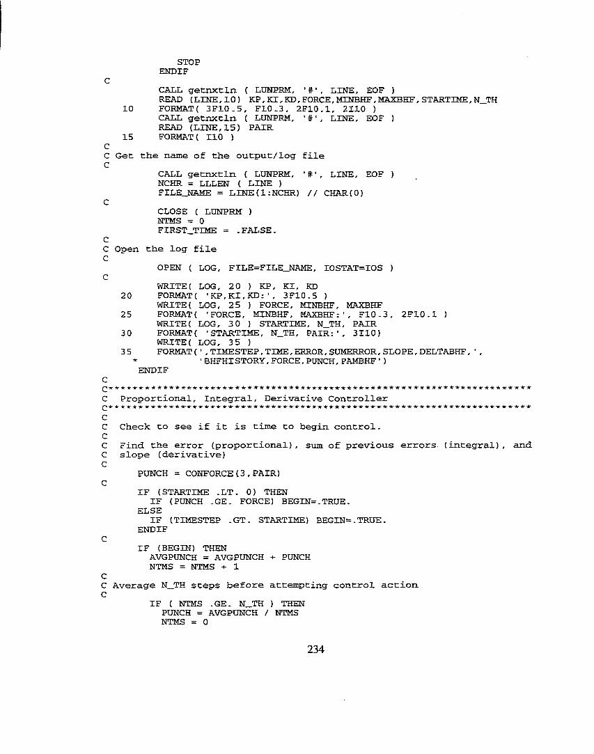
STOPENDIF

CCALL getnxtln ( LONPRM, LINE, EOF )READ (LINE,10) KP , KI, KD , FORCE, MINBHF, MAXBHF, STARTIME, N_TH

10 FORMAT( 3F10-5, FLO.3, 2F10.1, 2110 )CALL getnxtln ( LONPRM, LINE, EOF )READ (LINE, 15) PAIR

15 FORMAT ( n o )CC Get tiie name of the output/log file C

CALL getnxtln ( LONPRM, LINE, EOF )NCHR = LLLEN ( LINE )FILE_NAME = LINE(1:NCHR) // CHAR(O)

CCLOSE ( LONPRM )NTMS = 0FIRSTJTIME = .FALSE.

CC Open the log file C

OPEN ( LOG, FILE=FILE_NAME, IOSTAT=IOS )C

WRITE( LOG, 20 ) KP, KI, KD 20 FORMAT( 'KP,KI,KD:', 3F10.5 )

WRITE( LOG, 25 ) FORCE, MINBHF, MAXBHF 25 FORMAT( 'FORCE, MINBHF, MAXBHF:’, F10.3, 2F10.1 )

WRITE( LOG, 3 0 ) STARTIME, N_TH, PAIR 3 0 FORMAT ( ’STARTIME, N_TH, PAIR:’, 3110)

WRITE( LOG, 3 5 )3 5 FORMAT ( ’ , TIMESTEP, TIME, ERROR, SOMERROR, SLOPE, DELTABHF, ' ,

* ’ BHFHISTORY, FORCE, PONCH, PAMBHF ’ )ENDIFC

ie * -k * ie * ic * * -ie * ir ie ic *■ ic ie * ir *■ ie ie ie * ie * •kie ic-k ic ie "icie ir ie ir ie * "ifir * * ie *■ * * ic * * ip ip ie icie icie ie iç ie ie ie ie

C Proportional, Integral, Derivative Controller cC Check to see if it is time to begin control.CC Find the error (proportional) , sum of previous errors (integral) , and C slope (derivative)C

PUNCH = CONFORCE (3 , PAIR)C

IF (STARTIME .LT. 0) THENIF (PUNCH .GE. FORCE) BEGIN=.TRUE.

ELSEIF (TIMESTEP .GT. STARTIME) BEGIN=.’TRUE.

ENDIFC

IF (BEGIN) THENAVGPUNCH = AVGPUNCH + PUNCH NTMS = NTMS + 1

CC Average N_TH steps before attempting control action C

IF ( NTMS .GE. N_TH ) THEN PUNCH = AVGPUNCH / NTMS NTMS = 0

234

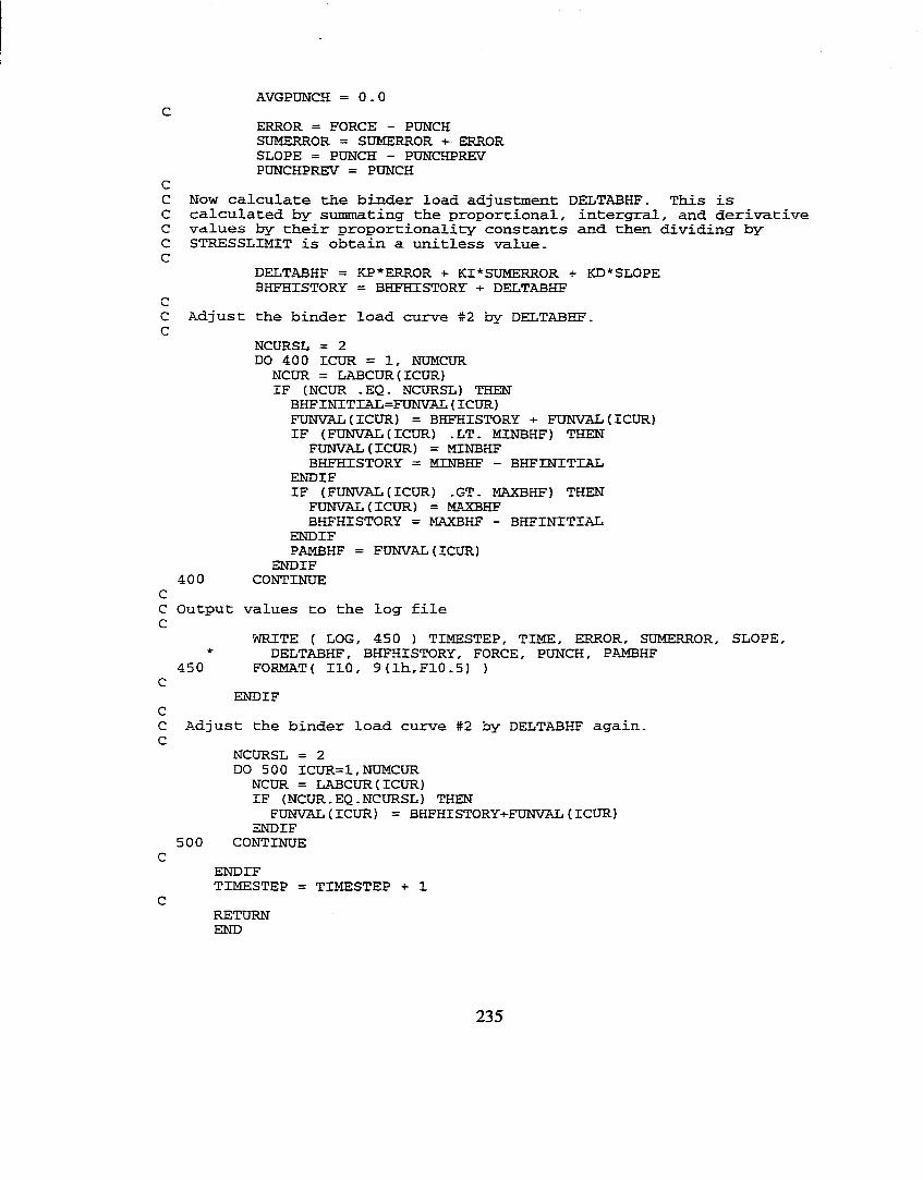
AVGPUNCH =0.0C

ERROR = FORCE - PUNCH SUMERROR = SUMERROR -t- ERROR SLOPE = PUNCH - PUNCHPREV PUNCHPREV = PUNCH

CC Now calculate the binder load adjustment DELTABHF. This is C calculated by summating the proportional, intergral, and derivative C values by their proportionality constants and then dividing by C STRESSLIMIT is obtain a unitless value.C

DELTABHF = KP*ERROR -t- KI*SUMERROR + KD*SLOPE BHFHISTORY = BHFHISTORY + DELTABHFC

C Adjust the binder load curve #2 by DELTABHF.C

NCURSL = 2DO 400 ICUR = 1, NUMCUR

NCUR = LABCUR (ICUR)IF (NCUR .EQ. NCURSL) THEN BHFINITIAL=FUNVAL ( ICUR)FUNVAL (ICUR) = BHFHISTORY + FUNVAL (ICUR)IF (FUNVAL (ICUR) .LT. MINBHF) THEN

FUNVAL (ICUR) = MINBHF BHFHISTORY = MINBHF - BHFINITIAL

ENDIFIF (FUNVAL (ICUR) .GT. MAXBHF) THEN

FUNVAL (ICUR) = MAXBHF BHFHISTORY = MAXBHF - BHFINITIAL

ENDIFPAMBHF = FUNVAL (ICUR)

ENDIF 400 CONTINUE

CC Output values to the log file C

WRITE ( LOG, 450 ) TIMESTEP, TIME, ERROR, SUMERROR, SLOPE,* DELTABHF, BHFHISTORY, FORCE, PUNCH, PAMBHF

450 FORMAT( 110, 9(lh,F10.5) )C

ENDIFCC Adjust the binder load curve #2 by DELTABHF again.C

NCURSL = 2DO 500 ICUR=1,NUMCUR

NCUR = LABCUR (ICUR)IF (NCUR.EQ.NCURSL) THENFUNVAL (ICUR) = BHFHISTORY-t-FUNVAL (ICUR)

ENDIF 500 CONTINUE

CENDIFTIMESTEP = TIMESTEP + 1

CR E T U R NEND

235

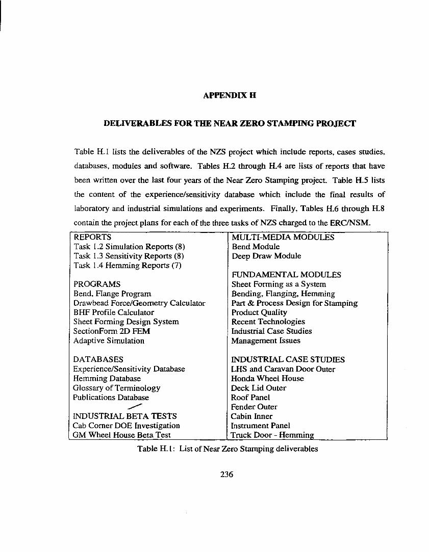
APPENDIX H

DELIVERABLES FOR THE NEAR ZERO STAMPING PROJECT

Table H.I lists the deliverables of the NZS project which include reports, cases studies,

databases, modules and software. Tables H.2 through H.4 are lists of reports that have

been written over the last four years of the Near Zero Stamping project. Table H.5 lists

the content of the experience/sensitivity database which include the final results of

laboratory and industrial simulations and experiments. Finally, Tables H . 6 through H . 8

contain the project plans for each of the three tasks of NZS charged to the ERC/NSM.

REPORTS MULTI-MEDIA MODULESTask 1.2 Simulation Reports (8 ) Bend ModuleTask 1.3 Sensitivity Reports (8 ) Deep Draw ModuleTask 1.4 Hemming Reports (7)

FUNDAMENTAL MODULESPROGRAMS Sheet Forming as a SystemBend, Flange Program Bending, Flanging, HemmingDrawbead Force/Geometry Calculator Part & Process Design for StampingBHF Profile Calculator Product QualitySheet Forming Design System Recent TechnologiesSectionForm 2D FEM Industrial Case StudiesAdaptive Simulation Management Issues

DATABASES INDUSTRIAL CASE STUDIESExperience/Sensitivity Database LHS and Caravan Door OuterHemming Database Honda Wheel HouseGlossary of Terminology Deck Lid OuterPublications Database Roof Panel

Fender OuterINDUSTRIAL BETA TESTS Cabin InnerCab Comer DOE Investigation Instrument PanelGM Wheel House Beta Test Truck Door - Hemming

Table H. 1 : List o f Near Zero Stam ping deliverables

236

# STATUS T IT L E /A U T H O R1 S-97-R-005 A Systematic Approach to Automotive Stamping Design With Finite

Element Analysis by Mark Oilier2 S-97-R-012 Evaluating Failure Criteria Using Computer Simulation by Sylvain

Lemercier3 S-98-R-012 Validation and Application o f FE Simulation for Stamping Process

Design by Toshi Oenoki4 S-98-018A Design, Validation, Machine Tool Path Plarming, Construction,

Simulation And Tryout o f an Asymmetric Stretch Draw Die Set by Carmen Crowley

5 S-98-R-23 Guidelines and Recommendation on the Use of the FEM Code Pam- Stamp With Explanation of Features by Thomas Schmidt

6 S-98-R-24 Simulation of the Effect of Blank Shape Geometry and Mesh Configuration on Deep Drawing Using the FEM Code Pam-Stamp by Thomas Schmidt

7 S-99-R-15 Product and Process Design Methodology for Deep Drawing and Stamping of Sheet Metal Parts by William Thomas

8 S-99-R-?? Industrial Case Studies on Deep Drawing and Stamping of Complex Shapes Using Steel and Aluminum by Tolga Uludag

Table H.2: List of reports for NZS Task 1.2 - Simulation

# STATUS T IT L E /A U T H O RI S-96-33 State o f the Art Review: Stamping Parameters and Their Effect on

Sheet Metal Formability by William Thomas2 S-97-R-007 Sensitivity Analysis of an AKDQ Steel Rectangular Deep Drawn

Panel by Carlos Alvarado3 S-97-08 Improving the Deep Drawability of 2008-T4 Aluminum and 1008

AKDQ EG Steel with Location Variable Blank Holder Force Control by William Thomas

4 S-98-R-10 Improving the Drawability of a Dome Cup Using Blank Holder Force Control by Peter Riegler

5 S-98-R-018 Investigation of Process Variables in Deep Drawing of Round Cups and Asynunetric Stamping Design and Tryout by Carmen Crowley

6 S-98-R-32 Determination of Optimal Process Conditions by Sensitivity Analysis and FEM Simulation by Shunping Li

7 S-99-R-36 Sheet Metal Forming and Stamping Glossary by Serhat Kaya8 S-99-R-35 Selected Technical Papers on Sheet Metal Forming by Serhat Kaya9 S-99-R-31 Part, Die, and Process Design for Sheet Metal Forming - An Eight

Part Modular Workshop by William Thomas

Table H.3: List of reports for NZS Task 1.3 - Sensitivity

237

# STATUS TITLE/AUTHORI S-97-R-015 Bending, Flanging and Hemming o f Steel and Aluminum Sheets -

Progress Report I by Attila Muderissoglu.2 S-97-R-017 Flanging and Hemming o f Steel and Aluminum Sheets - Progress

Report H by Haydar Livatyali.3 S-97-R-022 Flanging and Hemming o f Steel Sheets - Progress Report lH by

Thomas Laxhuber.4 S-99-R-16 Hanging And Hemming O f H at Surface-Straight Edge And

Convex Edge Steel Sheets Progress Report IV by Haydar Livatyali and Seth Larris.

5 S-99-R-13 Computer Aided Process Design of Selected Sheet Metal Bending Processes — Hanging and. Hemming by Haydar Livatyali.

6 S-99-R-30 Investigation o f Key Characteristics o f Hanging and Hemming of H at Surface - Curved Edge Sheet Metal by Seth Larris.

7 S-99-R-37 Analytical and Numerical Investigations of Sheet Metal Bending, Hanging and Hemming by Hsien-Chih Wu.

Table H.4: List for reports for NZS Task 1.4 - Hemming

PART GEOMETRIESBending INVESTIGATIVE METHODSHangingHemming Industrial Experiments

Drawbeads Computer SimulationsU-Channel Laboratory Experiment

Hemispherical Domes Analytical EquationsRound Cups

Rectangular Pans Forming Limit Diagrams

Asymmetric PanelCab Comer

Table H.5: Contents of experience/sensitivity database

238

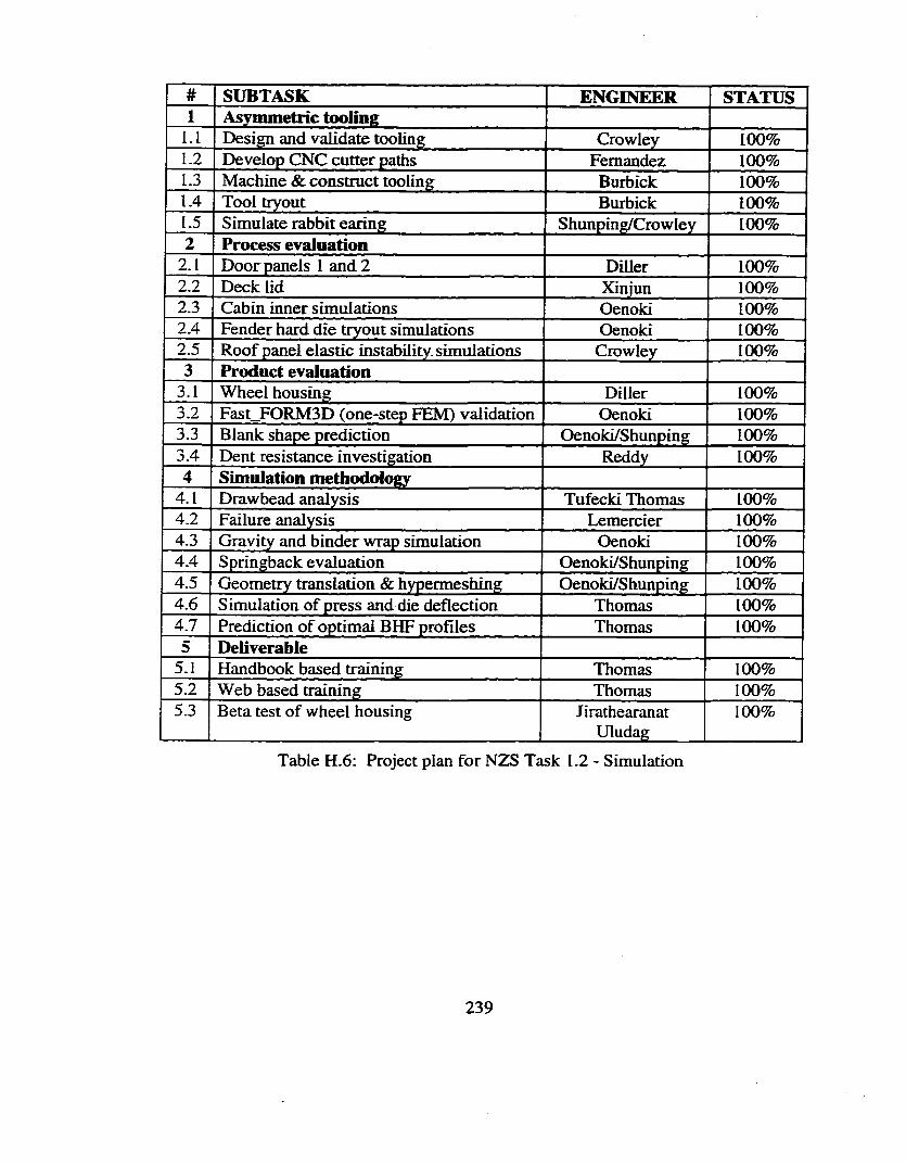
# SÜBTASK ENGINEER STATUS1 Asymmetric tooling

1.1 Design and validate tooling Crowley 100%1.2 Develop CNC cutter paths Fernandez 100%1.3 Machine & construct tooling Burbick 100%1.4 Tool tryout Burbick 100%1.5 Simulate rabbit earing Shunping/Crowley 100%2 Process evaluation

2.1 Door panels 1 and 2 Diller 100%2.2 Deck lid Xinjun 100%2.3 Cabin inner simulations Oenoki 100%2.4 Fender hard die tryout simulations Oenoki 100%2.5 Roof panel elastic instability, simulations Crowley 100%3 Product evaluation

3.1 Wheel housing Diller 100%3.2 Fast_FORM3D (one-step FEM) validation Oenoki 100%3.3 Blank shape prediction Oenoki/Shunping 100%3.4 Dent resistance investigation Reddy 100%4 Simulation methodology

4.1 Drawbead analysis Tufecki Thomas 100%4.2 Failure analysis Lemercier 100%4.3 Gravity and binder wrap simulation Oenoki 100%4.4 Springback evaluation Oenoki/Shunping 100%4.5 Geometry translation & hypermeshing Oenoki/Shunping 100%4.6 Simulation of press and die deflection Thomas 100%4.7 Prediction of optimal BHF profiles Thomas 100%5 Deliverable

5.1 Handbook based training Thomas 100%5.2 Web based training Thomas 100%5.3 Beta test of wheel housing Jirathearanat

Uludag100%

Table H.6: Project plan for NZS Task 1.2 - Simulation

239

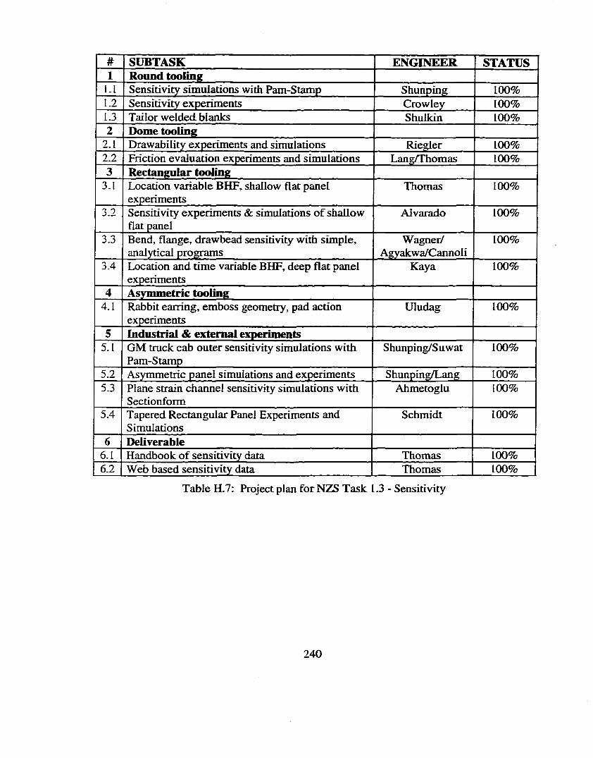
# SÜBTASK ENGINEER STATUS1 Round tooline

1.1 Sensitivity simulations with Pam-Stamp Shunping 100%1.2 Sensitivity experiments Crowley 100%1.3 Tailor welded blanks Shulkin 100%2 Dome tooling

2.1 Drawability experiments and simulations Riegler 100%2.2 Friction evaluation experiments and simulations Lang/Thomas 100%3 Rectangular tooling

3.1 Location variable BHF, shallow flat panel experiments

Thomas 100%

3.2 Sensitivity experiments & simulations o f shallow flat panel

Alvarado 100%

3.3 Bend, flange, drawbead sensitivity with simple, analytical programs

Wagner/Agyakwa/Cannoli

100%

3.4 Location and time variable BHF, deep flat panel experiments

Kaya 100%

4 Asymmetric tooling4.1 Rabbit earring, emboss geometry, pad action

experimentsUludag 100%

5 Industrial & external experiments5.1 GM truck cab outer sensitivity simulations with

Pam-StampShunping/Suwat 100%

5.2 Asymmetric panel simulations and experiments Shunping/Lang 100%5.3 Plane strain channel sensitivity simulations with

SectionformAhmetoglu 100%

5.4 Tapered Rectangular Panel Experiments and Simulations

Schmidt 100%

6 Deliverable6.1 Handbook of sensitivity data Thomas 100%6.2 Web based sensitivity data Thomas 100%

Table H.7: Project plan for NZS Task 1.3 - Sensitivity

240

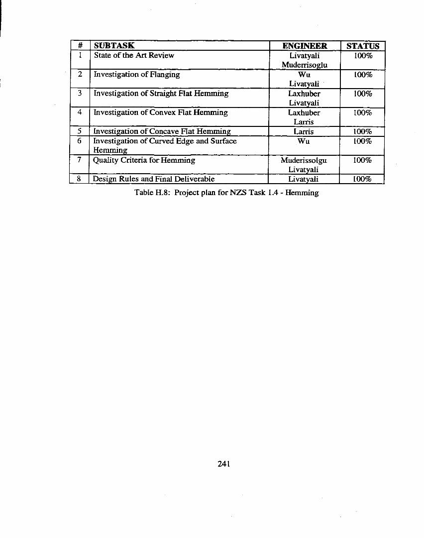
# SÜBTASK ENGINEER STATUSI State of the Art Review Livatyali

Muderrisoglu100%

2 Investigation of Flanging WuLivatyali

100%

3 Investigation of Straight Flat Hemming LaxhuberLivatyali

100%

4 Investigation of Convex Flat Hemming LaxhuberLarris

100%

5 Investigation of Concave Flat Hemming Larris 100%6 hivestigation of Curved Edge and Surface

HemmingWu 100%

7 Quality Criteria for Hermning MuderissolguLivatyali

100%

8 Design Rules and Final Deliverable Livatyali 100%

Table H.8: Project plan for NZS Task 1.4 - Hemming

241