INFORMATION TO USERS

This reproduction was made from a copy o f a document sent to us for microfilming. While the most advanced technology has been used to photograph and reproduce this document, the quality o f the reproduction is heavily dependent upon the quality o f the material submitted.

The following explanation o f techniques is provided to help clarify markings or notations which may appear on this reproduction.

1. The sign or “target” for pages apparently lacking from the document photographed is “Missing Page(s)” . If it was possible to obtain the missing page(s) or section, they are spliced into the film along with adjacent pages. This may have necessitated cutting through an image and duplicating adjacent pages to assure complete continuity.

2. When an image on the film is obliterated with a round black mark, it is an indication o f either blurred copy because of movement during exposure, duplicate copy, or copyrighted materials that should not have been filmed. For blurred pages, a good image o f the page can be found in the adjacent frame. If copyrighted materials were deleted, a target note will appear listing the pages in the adjacent frame.

3. When a map, drawing or chart, etc., is part o f the material being photographed, a definite method o f “sectioning” the material has been followed. It is customary to begin filming at the upper left hand comer o f a large sheet and to continue from left to right in equal sections with small overlaps. If necessary, sectioning is continued again-beginning below the first row and continuing on until complete.

4. For illustrations that cannot be satisfactorily reproduced by xerographic means, photographic prints can be purchased at additional cost and inserted into your xerographic copy. These prints are available upon request from the Dissertations Customer Services Department.

5. Some pages in any document may have indistinct print. In all cases the best available copy has been filmed.

Uni

international300 N. Zeeb Road Ann Arbor, Ml 48106

8311788

Pery, Ane

A THEORETICAL AND EXPERIMENTAL STUDY OF HYDRAULIC POWER SUPPLIES USING PRESSURE-COMPENSATED PUMPS, THEIR INFLUENCE ON SERVOSYSTEM DYNAMIC RESPONSE, AND THEIR UTILIZATION IN ENERGY-SAVING CONFIGURATIONS

The Ohio State University Ph.D. 1983

University Microfilms

Intern eti one! 300 N. zeeb Road, Ann Arbor, MI 48106

Copyright 1983

by

Pery, Arie

All Rights Reserved

A THEORETICAL AND EXPERIMENTAL STUDY OF HYDRAULIC POWER SUPPLIES USING PRESSURE-COMPENSATED

PUMPS, THEIR INFLUENCE ON SERVOSYSTEM DYNAMIC RESPONSE, AND TRIER UTILIZATION IN ENERGY-SAVING CONFIGURATIONS

DISSERTATIONPresented in Partial Fulfillment of the Requirements for

the Degree of Philosophy in the Graduate School of the Ohio State University

byArie Pery, B.Sc.,M.Sc.The Ohio State University

1983

Reading Committee:Professor E, 0. Doebelin Professor D. R. Houser Professor K, Srinivasan

Approved by

AdvisorDepartment of Mechanical Engineering

ACKNOWLEDGMENTS

„-I would like to thank all those who helped and contri­buted to my studies in Ohio State University.

First, I want to thank and express my appreciation to my advisor Professor Doebelin, for his guidance, help and encouragement throughout the entire program.

The support of department Chairman James E. A. John is gratefully acknowledged as is the technical support of Mr. Cecil Rhodes from the M. E. Electronics Laboratory and Mr. Robert A. Frank and all the staff in the M. E. Machine Shop.

My thanks are also to all the members of my family in Israel who have supported morally and financially my studies.

My appreciation should be indeed expressed to my daughters Tamar and Tal who spent the last three years "missing their dady" while I was concentrated on my work.

Last but not least, my special thanks is to my wife Dafna, for her support, help, encouragement, strength and love, without them my studies could not have been completed.

11

VITA

December 24, 1947 1970

19761970 - 1977

1977 - 1979

Born - Timisoara, Romania,B. Sc. Mechanical Engineering, Technion , Haifa, Israel.M, Sc., Technion, Haifa, Israel.Technical Staff Member,The Israely Navy.Israely Aircraft Industries,M. B. T. Division, R & D Department,

PUBLICATIONS

Sept. 1980Journal of Hydraulics and Pneumatics"Pressure Balanced, Variable Displacement Vane Pump"

FIELDS OF STUDY

Major Field: Mechanical EngineeringStudies in Feedback Control Systems, Measurements and

Systems Dynamics -Professor E. 0. Doebelin

111

TABLE OF CONTENTS

ACKNOWLEDGMENTS,

VITA..........LIST OF FIGURES, LIST OF TABLES, NOMENCLATURE--

INTRODUCTIONPART ONE

Theoretical and Experimental Study of the Effect of Pump Dynamics on the Response of Servosystems Supplied by Pressure Compensated Pumps .........

1.1 - General ....................... .1.2 - Historical Background ...........1.3 - Organizational Plan of the Study ,

1.3.1 - Frequency Domain Analysis1.3.2 - Time Domain Analysis ....

CHAPTER 2 - THEORETICAL ANALYSIS ..........2.1 - General ........... ............2,2 - Valve Controlled Rotary Actuator

Servosystem............... ...2.3 - Valve Controlled Linear Actuator

Servosystem ...................2.4 - Closed Loop Systems2.5 - Pump Servovalve - Rotary Actuator

Combination ....................

ii

iii

xii

x x i v

X XV i

CHAPTER 1 - INCLUDING PUMP DYNAMICS IN SERVOSYSTEMS - BACKGROUND ........................ 5

6 8

1212141616

22

3034

37

IV

2.6 - Generalized "Load Subsystem" Analysis .. 432.7 - "Supply Subsystem" Analysis ......... 472.8 - "Control Subsystem" Analysis ......... 512.9 - Valve Controlled Linear Actuator System 53

2.10 - Transfer Functions — (S); — (S) andp R R— -(S) Derivations ... . . .. . .. ...... 57^0

2.11 - Summary.............................. 62CHAPTER 3 - THE EXPERIMENTAL PROGRAM.............. 65

3.1 - Introduction.......................... 653.2 - Apparatus Description ................. 66

3.3 - The Experimental Program.............. 68

3.3.1 - System Parameters MeasurementOutline....................... 69

3.3.2 - System Dynamic Tests Outline ... 703.4 - System Parameters Measurement ......... 723.5 - System Dynamic Response Tests .......... 77

3.5.1 - Step Response Tests Outline(Time Domain) .................. 77

3.5.2 - Step Response Test Results ..... 803.5.3 - Frequency Response Tests Outline

(Frequency Domain) ............. 1093.5.4 - Frequency Response Test Results • 1123.5.5 - Accumulator Included

In Frequency Response Tests .... 1213.5.6 - Comments on the Results ........ 126

CHAPTER 4 - COMPUTER SIMULATION ................... 12 74.1 - Introduction ....................... 12 74.2 - CSMP - Time Domain Computer Program .... 129

4.2.1 - Nonlinear Computer Model........ 1314.2.2 - The Alternative Model .......... 132

4.2.3 - CSMP Inputs and Outputs....... 1374.2.4 - The CSMP Computer Program..... 1394.2.5 - CSMP Computer Program Graphical

Results ........................ 1464.3 - SPEAKEASY - Frequency Domain Computer

Program ................................ 1484.4 - Transfer Function - Frequency Domain

Computer Program ....................... 1674.4.1 - The Transfer Functions

Development......... 1694.4.2 - Numerical Values For The Transfer

Functions ...................... 174CHAPTER 5 - DISCUSSION AND CONCLUSIONS............ 181

5.1 - Computer and Experimental Results Compa­rison - Time Domain.................... 181

5.2 - Computer and Experimental Results Compa­rison - Frequency Domain ............... 194

5.3 - Program #20 and Experiment Comparison ... 2145.3.1 - The — ( S ) Transfer Function 214

RPg5.3.2 - The— ( S ) Transfer Function ..... 215RPq5.3.3 - The— ( S ) Transfer Function ..... 216^O

5.4 - Conclusion ............................. 220vi

PART TWOTheoretical Study of Proposed Energy Saving Hydraulic Control Configuration Based on Variable Displacement Pumps ........ 221CHAPTER 6 - LOAD SENSING - BACKGROUND............. 222

5.1 - General Background.................... 222

6.2 - The Definition of the Problem......... 22 36.3 - Historical Background................ 2256.4 - Load Sensing in Servovalve Actuator

Systems .............. 227CHAPTER 7 - DEVELOPMENT AND THEORETICAL ANALYSIS

OF PROPOSED ENERGY SAVINGCONFIGURATIONS....................... 230

7.1 - Maximum Power Transfer to Load With aServovalve (Merritt, page 226) ........ 230

7.2 - Maximum Power Transfer and Efficiency(Merritt, page 228) ................... 234

7.3 - The P^ = 2/3 Pg Scheme ............... 2 367.3.1 - Principle of Operation........ 2387.3.2 - Speed-Control and Pressure

Control Servosystem ........... 2417.3.3 - Position-Control and Pressure

Control Servosystem ........... 2447.3.4 - Feasibility Study............. 248

7.4 - Felicio's Scheme..................... 2547.4.1 - The Proposal Presented by

Felicio....................... 2547.4.2 - The Set of Governing

Differential Equations ........ 259

VI1

CHAPTER 8 - COMPUTER SIMULATION AND DISCUSSION OFTHE RESULTS .......................... 262

8.1 - General ............................... 2628.2 - Computer Simulation................... 264

8.2.1 - System Evaluation Method...... 2648.2.2 - The P_ = 2/3 P_ Computer Program 268

L i O

8.2.3 - Felicio's Scheme.............. 272

8.2.4 - Constant Pressure Configuration . 2 788.2.5 - The Computer Program........... 2808.2.6 - Inputs to the System R(t) and

T^(t) .......................... 287

8.3 - Analysis of the Results ............... 2928.3.1 - Energy Analysis ................ 2928.3.2 - Performance Analysis........... 2998.3.3 - "Supplementary Pressure Loop"

Analysis in Felicio's Scheme .... 3058.4 - Conclusions .............. 3088.5 - Summary ............................... 310

PART THREEFurther Study of Felicio's Model of a Variable Dis­placement Pressure Compensated Vane Pump.......... 314

CHAPTER 9 - "RE - DESIGN" OF VARIABLE DISPLACEMENTVANE PUMPS FOR FASTER RESPONSE........ 317

9.1 - General ............................... 3179.2 - Stability Analysis ................... 3199.3 - Disturbance Analysis .................. 3229.4 - "Speed of Response" Analysis ......... 324

viii

9.5 - Investigation of the Coefficient .... 3269.6 - The "New" Design...................... 331

9,6,1 - Explanation of the New Design ,,, 3339.7 - Quantitative Analysis ................. 336

CHAPTER 10 - EXPLANATION OF 12.5Hz PEAK IN PUMPDISCHARGE PRESSURE FREQUENCY SPECTRUM , 340

10.1- General ............................... 340

10.2 - Theoretical Analysis ............. 34310.2.1 - Describing Function Theory ,,, 34310.2.2 - Static Friction Nonlinearity

and Its Describing Function Analysis............. ...... 344

10.2.3 - Describing Function Analysisof the Pump With Static Fric­tion Nonlinearity........... 351

10.3 - Computer Simulation . . 35610.3.1 - CSMP Program .,,,......... 35610.3.2 - Frequency Response Computer

Program................. 35910.4 - Experimental Study............ 36110.5 - Conclusions ...................... 366

CONCLUSIONS AND SUGGESTIONSFor Further Study...... 357

CHAPTER 11 - CONCLUSIONS AND SUGGESTIONS FORFURTHER STUDY ....................... 368

11.1 - General Conclusions ................. 36811.2 - Specific Conclusions - Pump Dynamic Effects369

IX

11.3 - Specific Conclusions - Energy Saving .. 37211.4 - Suggestions for Further Study ........ 374

11.5 - Pump Analysis ....................... 376

APPENDICESA - REFERRING TO PART ONE IN THE TEXT CHAPTER 3 -

EXPERIMENTAL PROGRAM.........................A.l - Apparatus Physical Dimensions ........... 38 CA. 2 - Pressure Drop Pump - Valve Lines....... 382A.3 - Hydraulic Motor Parameters ............. 388

A.3.1 - Characteristics C__ and C. .... 390em imA.3.2 - Internal Coefficients C_ and

Seal Friction Torque T ^ ........ 394A.3.3 - Measurement of C^ Coefficient ... 397

A.4 - Servovalve Parameters .................. 399

A.4.1 - Flow Pressure Coefficient .... 402

A.4.2 - Servovalve "First Stage" Dynamics 407A.5 - Controller Compensation Network ........ 40 9A. 6 - System Gain Setting.................... 413A.7 - Step Response Test Instrumentation .... 415

C - REFERRING TO PART 3 IN THE T EXT..............C,1 - Chapter 10 - 12.5Hz Peak

Time History and Power Spectral Density Tests ...... 419

D--------- EXPLANATION OF TURBINE FLOW - METERDISCREPANCY DURING FLOW MEASUREMENTS .. 431

D,1 - The Definition of the Problem ......... 431D.2 - Instrumentation Used.................. 433

D.3 - The Proposed Program for the Study ofthe Problem.......................... 437

D.4 - Experimental Results ................. 438D.4.1 - The Repetition of the Original

Calibration configuration .... 43 8D.4.2 - Flow - meter Interchange .... 44.1D.4.3 - "Absolute" Calibration Results 4 44

D. 5 - Discussion of the Results ........... 447D. 5.1 - Pulsations Effects ......... 447D.5.2 - Pressure Level Effects ..... 447

D.6 - Explanation of the Cause of theDiscrepancy.......................... 44 8

E - LITERATURE REVIEIV SCHEME...................... 44 9LIST OF REFERENCES ........................ 459

XI

LIST OF FIGURES

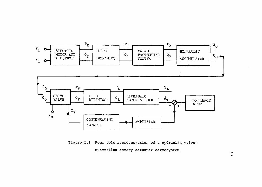
1.1 Four pole representation of a hydraulicvalve - controlled rotary actuator servosystem 13

2.1 Valve controlled rotary actuator servosystemin speed control configuration (General case) . 17

2.2 Valve controlled linear actuator positioncontrol servosystem .......................... 31

2.3 Linear actuator between points 8 and 9 ....... 322.4 V, D, Pump - Servovalve - Rotary actuator

combination .................................. 382.5 Hydraulic motor as a "two port" device ....... 392.6 Load Subsystem (Including pipe line. Hydraulic

motor and Load ) ...... 422.7 Equation 2.39 in block diagram form.......... 442.8 Four pole representation of a generalized

"Load Subsystem" ............................. 452.9 "Supply Subsystem" including electrical motor

(prime mover), pipe line, filter and accumulator.............................. 47

2.10 "Supply Subsystem" analyzed .................. 472.11 "Supply Subsystem" in block diagram form ..... 482.12 Generalized "Subsystem" configuration of a

hydraulic valve controlled rotary actuatorspeed control system......................... 52

2.13 Valve controlled linear actuator "Load Sub­system" ...................................... 53

2.14 V, D. Pump - Servovalve - Linear Actuatorcombination.............. 55

3.1 Experimental apparatus ....................... 673.2 Step response test - apparatus and

instrumentation .............................. 79xii

3.3 Step response - Pump Dynamics included -(Pg = Gp Qg ; Pg = SOOpsi, J^=0.00431b^sec in) 83

3.4 Step response - Constant supply pressure (Pg=const.; Pg=500psij J^=0.00431b^sec in) ,,, 84

3.5 Step response - Encoder Voltage (V )Comparison between P =const, and P_=G„Q_ .... 85

S o IT D

3.6 Step response - Valve current (I )Comparison between P = const, and P„ = G_Q_ , 85

o o ir o

3.7 Step response - Valve pressure (P ) and pump pressure (Pg) ............................. 86

3.8 Step response - Motor input pressure (P^^)Comparison between Pg = const, and ^s“®P®s 8?

3.9 Step response - Motor output pressure (P^^) Comparison between Pg=const, and Pg=GpOg

3.10 Step response - Pump dynamics included,( Pg=GpQg, Pg=730psi, J^=0.0043 Ib^sec^in )............ 89

3.11 Step response - Constant supply pressure (Pg=const., Pg=730psi, J^=0.0043 Ib^sec in) ... 90

3.12 Step response - Encoder Voltage (V )Comparison between Pg=const. and Pg=GpQg ... 91

3.13 Step response - Pump dynamics included ^(Pg = Gp Qg ,Pg = 950 psi, J^=0.0043 Ib^sec in) 92

3.14 Step response - Constant supply pressure (Pg=const., Pg=950psi, J^=0.0043 Ib^sec in) ,,, 93

943.15 Step response - Encoder Voltage (V^)

Comparison between Pg = const, and Pg = Gp Qg

3.16 Step response - Accumulator installed close to the pump, pump dynamics included (P =G_Q ,Pg = 730 psi, = 0,0043 Ib^sec in) . , 9 8

Xlll

3.17 Step response - Accumulator installed close to the pump, Constant supply pressure (P_=const., Pg=730psi, J^=0.00431bj^sec in)...... 99

3.18 Step response - Encoder Voltage (Vq )Accumulator close to the pumpComparison between P„ = Q„ and P = const. 100

O ir o b

3.19 Step response - Encoder Voltage (V ) Pg=GpQg,Comparison between accumulator close to pump and accumulator close to valve «(Pg = 730 psi, = 0.0043 Ib^sec in) ...... 101

3.20 Step response - Encoder Voltage (V ) Pg=constComparison between accumulator close to pumpand accumulator close to valve (P =730 psi,J = 0.0043 lb.sec in) ......... 102m r

3.21 Step response - Constant Supply pressure (Pg = const., Pg = 730psi, J = 0.00431b.*bg b 111 Xsec in) ................................... 105

3.22 Step response - Pump dynamics included (Pg =GpOg ,Pg=730psi, J^=0.00431b^sec^in )....... 105

3.23 Step response - Encoder Voltage (V^),Comparison between Pg=const. and Pg=GpQg (Pg=730psi, J^=0.0531b^sec^in) ............. 108

3.24 Frequency response test - apparatus and instrumentation ........................... Ill

Pg3.25 Frequency response - — ^(S) , open loop atR

50ma±12.5ma .............................. 114Pg3.26 Frequency response— (S), closed loop,R

at 25ma±12.5ma........................... 115

3.27 Frequency response - — ^(S), open loop,R

at 75mad=12.5ma........................... 116

XIV

3.28 Frequency response —(S), closed loop,R

at 75ma±12.5ma............................ 117Pg3.29 Frequency response ---- (S), open loop.

at 50ma:± 20m a .............................. 118Pg3.30 Frequency response (S), closed loop,

at 50ma±: 12,5ma..... ? .,, 119Pg3.31 Frequency response (S), Open loopVq

at 50ma± 12,5ma including accumulatordynamics ................................ 124Pg3.32 — (S)=KGp(S) Estimation by curve fitting ^0of accumulator frequency response .......... 125

4.1 Nonlinear Model - CSMP program flow chart .,, 1334.2 Alternative Model - CSMP program flow chart , 1364.3 CSMP output. Pump Supply Pressure (Pg) ..... 1494.4 CSMP output, Encoder Voltage (V ), comparison

= ;•••••••.... 15°4.5 CSMP output, Encoder Voltage (V^), comparison

(Pg =const. ) ............................... 151

4.6 CSMP output. Valve current (I ), comparison(Pg ~ Gp Qg) 152

4.7 CSMP output. Valve current (I ), comparison(Pg = const. ) .............................. 153

4.8 CSMP output. Encoder Voltage (V^) nonlinearmodel, Pg = Gp Qg - Pg const.......... 154

4.9 CSMP output. Encoder Voltage (V^), alterna­tive model, Pg = Gp Qg - Pg = const.......... 155

XV

4.10 CSMP output. Motor pressure (P-, P^), non­linear model Pg = Gp Q g .................... 156

4.11 CSMP output; Motor pressure (P , P.), non­linear model Pg = const..................... 157

4.12 CSMP output. Load Pressure (P ), comparison between the models ....................... 158

4.13 CSMP output, Load Flow (Q ), comparisonbetween the models ......................... 159

4.14 Open loop system matrix representation inletter form................................ 164

4.15 Closed loop system matrix representation inletter form ,,,........................ ,,,,, 165

Pg4.16 Pump frequency response -^( S) = Pump only P ^1— (S) = Pump + line + filter............... 175Q2

4.17 "Supply Subsystem" output impedance frequencvPgresponse ( iw) ........................... 179Vq

4.18 Comparison between theoretical and experimen­tal pump frequency response 180

5.1 Valve current - Step response (Pg=GpQg),Comparison between Experiment and CSMP ..... 184

5.2 Valve current - Step response (Pg = const,), Comparison between Experiment.and CSMP ..... 184

5.3 Encoder Voltage - Step response (Pg = Gp Qg), Comparison between Experiment.and CSMP ..... 186

5.4 Encoder Voltage- Step response (Pg = const,), Comparison between Experiment.and CSMP ..... 187

5.5 Valve Pressure P^ Step response. Comparison between Experiment and CSMP ................ 188

XVI

5.6 Motor input pressure - Step response (Pg=GpQg) Comparison between Experiment and CSMP .... 190

5.7 Motor input pressure - Step response(Pg=const) Comparison between Experiment and CSMP ...... 191

5.8 Motor output pressure - Step response - (Pg =G„Q_), Comparison between Experiment and CSMP 193

ir S

5.9 Motor output pressure - Step response (Pg =const,), Comparison between Experiment andCSMP ....................................... 193Pg5.10 — (iw) Open loop, at 50ma±l2,5roa RExperimental frequency response result ....... 202Pg .5.11 — (iw) Open loop, at 50ma±12,5ma,RComparison between Experiment and SPEAKEASY ,, 203

5.12 — (iw) Open loop, at 50ma± 12,5ma, Experimen- Rtal frequency response result............... 204

5.13 — (iw) Open loop, at 50ma±12,5ma, Comparison Rbetween Experiment and SPEAKEASY ............ 205Pg5.14 — -(iw) Open loop, at 50ma±12,5ma Experiment- ^0al frequency response result ................ 206Pg5.15 — (iw) Open loop, at 50mai: 12,5ma, Comparison ^0between Experiment and SPEAKEASY ............ 207

5.16 — (iw) Closed loop, at 50ma±12,5ma RExperimental frequency response result ..... 208

XVI1

5.17 — (iw) Closed loop, at 50ma± 12.5ma,RComparison between Experiment and SPEAKEASY .. 209

V,s5.18 — (iw) Closed loop, at 50ma±: 12.5ma Experimen-0tal frequency response result ............... 210Pg5.19 — (iw) Closed loop at 50ma± 12.5ma,^0Comparison between Experiment and SPEAKEASY «. 211Pg5.20 — (iw) Closed loop, at 50ma± 12.5ma Experimen- Rtal frequency response result ............... 212Pg5.21 — (iw) Closed loop, at 50ma±12.5ma,RComparison between Experiment and SPEAKEASY .. 213

5.22 Open loop at 50majtl2.5ma (Program #20)^0_ ^i ^ampl ^enco ^ ^m_______ ^ ^>'■ G (s) ....

w w U W PPV V h h5.23 Open loop at 50ma±12.5ma (Program #20)

218(4 + — + ^ ) Gpp(S,£0 UV V

5.24 Open loop at 50ma±12.5ma (Program #20)P_ „2 2LS— (S) = --- — G^(S) ( ^ + -— + 1)......... 219V K W0 enco h h

7.1 Normalized plot of power at load versus load pressure (Merritt) ......................... 2 32

7.2 The proposed Supply Pressure Optimalizingscheme (P^ = 2/3 Pg) ....................... 2 37

XVIXI

7.3 Pressure - Flow relation in a controlledcompensated p ump........................... 239

7.4 P_ versus P_ enforcing the P_=2/3 P_ rule ,, 240Q L i l i D

7.5 Speed - Control Servosystem with Supply -Pressure Optimization ...................... 243

7.6 Position - Control Servosystem with SupplyPressure Optimization ...................... 246

7.7 Pt = 2/3 P_ scheme in block diagram formJb O(Position - Control) ....................... 247

7.8 Felicio's - Energy saving scheme ........... 2587.9 Example showing a design for desired pressure

profile P^(t) .............................. 259

8.1 P_ = 2/3 P_ scheme in block diagram formL i o

Speed - Control - Pressure Control system ,,, 2 708.2 Felicio's scheme in block diagram form ..... 2 738.3 Constant - Pressure scheme in block diagram

form....................................... 2798.4 A typical input R^(t) and (t) combination 289

8.5 System supply pressure (comparison) ........ 2918.6 System efficiency (comparison) ............. 2948.7 Power loss reduction (comparison) .......... 2968.8 Energy loss (comparison) ................... 3008.9 System Error RMS (comparison) 3048.10 System Efficiency (without filtering) ...... 3128.11 Power Loss Reduction (without filtering) 3139.1 Block diagram of the perturbation dynamic

model for the proportional control type ofpump................................... 318

9.2 Linearized block diagram ................... 319xix

9.3 Linearized pump block diagram having thedisturbing variable as the input......... 322

9.4 Oil flow between parallel plates ........... 32 79.5 Pressure Compensated Pump of the Proportional

Control Type ................................ 3289.6 Cross section A - A .................... 3309.7 Pump ring - rotor configuration........ 3309.8 The "new" p ump......................... 3329.9 Side view of the ring .................... 334

10.1 Power spectral density of P^(t) for P^= g48psiQ = 1.75gpm and Qp = 0 (Plot obtained

from the NICOLET 660 A analyzer) ............ 34710.2 The forces on the ring................. 34510.3 Idealized friction characteristics ......... 34610.4 Equation 10.4 in block diagram form.... 34710.5 Viscous friction nonlinearity .............. 34810.6 Newton's law including coulomb friction .... 34910.7 Backlash nonlinearity ...................... 35010.8 Describing function for backlash (Merritt) ... 35110.9 Pump block diagram including coulomb friction

Ff ................................................ 35210.10 Describing function form of the system ..... 35210.11 The plot of -1/Gj and G(iw) on Nyguist diagram 35410.12 CSMP output. Limit cycle analysis .......... 35810.13 Measuring points ........................... 36110.14 Time history and Power Spectral density in

regulating region ........................... 363

XX

List of Figures in the Appendix

A.l Pressure drop measurements ................. 385A.2 Pipe pressure measurements .................. 386A, 3 Pipe flow resistance coefficient 387

A,4 Typical Leakage flow versus Forward pressure . 391A.5 Leakage measurement apparatus arrangement 391A.6 Leakage flow Q. and Q forward pressure P , 393ÜU €in «LA.7 Typical Torque - pressure curves for T and

measurement ......... 394A .8 and T^ measurement apparatus situation and

equipment ................................... 395

A. 9 Friction torque T^ versus supply pressure Pg . 395

A, 10 Typical curve for measurements ........... 397

A.11 Measurement of coefficient Forward pressureP^ versus Motor Speed 0m

A.15 Block diagram of a velocity control servo­system .................. ...............

400

A.12 Apparatus and instrumentation for constant(K^) measurement .......................... 403

A.13 Apparatus configuration for measurement ofvalve first stage speed of response .......

A,14 Valve first stage step response .............

408

408

410

A.16 Compensator frequency response test T = 49sec . 412

420C. 1 Time history and Power spectral density in

regulating region, PQ=280(psi), 0^=1.75(gpm) .C. 2 Time history and Power spectral density in

regulating region, P^sSOOCpsi), 0^=0(gpm) .... 421

XXI

C. 3 Time history and Power spectral density in re­gulating region, Pg=500(psi), QQ=1.75(gpm) ... 422

C. 4 Time history and Power spectral density in re­gulating region, PQ=700(psi), Qg=0(gpm) ..... 423

C. 5 Time history and Power spectral density in re­gulating region, P^=700(psi), QQ=1.75(gpm) ... 424

C. 5 Time history and Power spectral density in re­gulating region, Pj^=948(psi ), Qj^=0(gpm) ..... 425

C. 7 Time history and Power spectral density in re­gulating region, PQ=948(psi), QQ=1.75(gpm) ... 426

C. 8 Time history and Power spectral density in nonregulating region, P = 280(psi),Qq = 4.5(gpm) .............................. 427

C. 9 Time history and Power spectral density in nonregulating region, P = SOO(psi),Qq = 4.0(gpm) ....... V ..................... 428

C.IO Time history and Power spectral density innonregulating region, P = 700(psi),Qq = 3.75(gpm) ............................. 429

C.ll Time history and Power spectral density in nonregulating region, P. = 800(psi),Og = 3.54(gpm) ....... 430

D ,1 Instrumentation used for pump flowmetercalibration .............................. 432

D .2 A typical calibration flowmeter (C, F, M.)versus pump flowmeter (P. F. M.) calibration curve (From Felicio ) ...................... 436

D ,3 System configuration for P.F.M, - C.F.M,calibration ................................ 438

D .4 Calibration curves at four pressure settings,without accumulator................... 439

XXI1

D.5 Calibration curve at 900 psi with and withoutaccumulator ................................ 440

D.6 System configuration for C.F.M. - P.F.M.calibration ................................ 441

D.7 C.F.M. - P.F.M. calibration withoutaccumulator ................................ 442

D.8 C.F.M. - P.F.M. calibration with accumulator . 44 3D.9 System configuration for flow meters absolute

calibration ................................ 444D.IO Absolute calibration curve ......... 446

XXI11

LIST OF TABLESpage

3.1 Oil parameters...... 733.2 Pipe line parameters ....................... 743.3 Filter and accumulator parameters ........... 753.4 Hydraulic motor parameters ................. 753.5 Servovalve parameters............... 763.6 Gain Settings ........................... 76

R5,1 — (iw) Open loop, Figure 5.10 ............... 201

5.2 — (iw) Open loop. Figure 5.12 ............... 201R

5.3 — (iw) Closed loop. Figure 5.16...... 201R

Pg5.4 — (iw) Closed loop. Figure 5.20 ............ 201R

8.1 The power lost - Constant load.............. 2928.2 System efficiency - Constant load........... 2938.3 Power loss reduction - Constant load........ 2958.4 The power lost - Constant speed............. 2958.5 System efficiency - Constant speed .......... 2978.6 Power loss reduction - Constant speed ....... 2988.7 Energy loss ................................. 2998.8 Percentage error - Constant load............ 3018.9 System gain - Constant load ....... 301

XXIV

8.10 Percentage error - Constant Speed .......... 3028.11 System gain - Constant Speed............... 3038.12 Error RMS ................................ 303

10.1 Pump pressure levels...................... 365

List of Tables in the AppendixA.l Pump - Valve pipe line pressure drop

measurement .................... 382

A.2 Leakage flow Q. , Q measurement.......... 392 im' emA. 3 and C^ measurement experimental results . 395A.4 Measurement for C, coefficient Experimental

result....................... 398A.5 Experimental result for the measurement of

valve constant ......................... 405

A. 6 Flow - pressure measurements Experimentalresults ................................... 406

A.7 Gain setting measurementsPressure setting 730(psi) ................. 414

D.l "Free flow" measurements .................. 445

XXV

NOMENCLATURE

a A

A A

AP

A _ . ApiAmAP

®vf A

C AaccuAc

Cd A

^dv A

^em A

C Aep

Cfilt A

C . Af

^fl A

C, AimC. A

I P

C t, Ap

Ctm A

XXVI

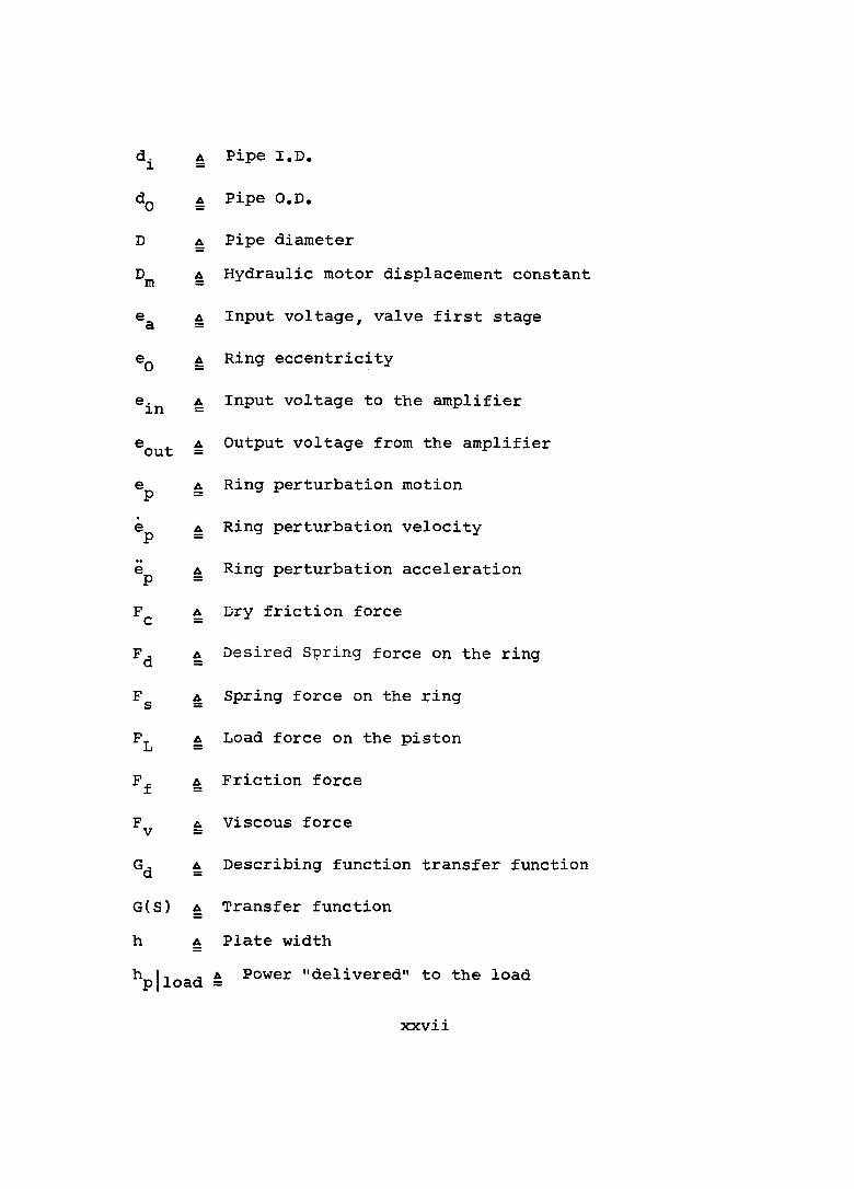
d. A1

d- A0

D A

D Ame Aae_ A0

e. Ain

®out A

e APê APë APF AcFj AdF As

Ft ALF. AfF AV

Gd A

G(S) A

h A

^pjload

A Plate widthA Power "delivered" to the load

xxvii

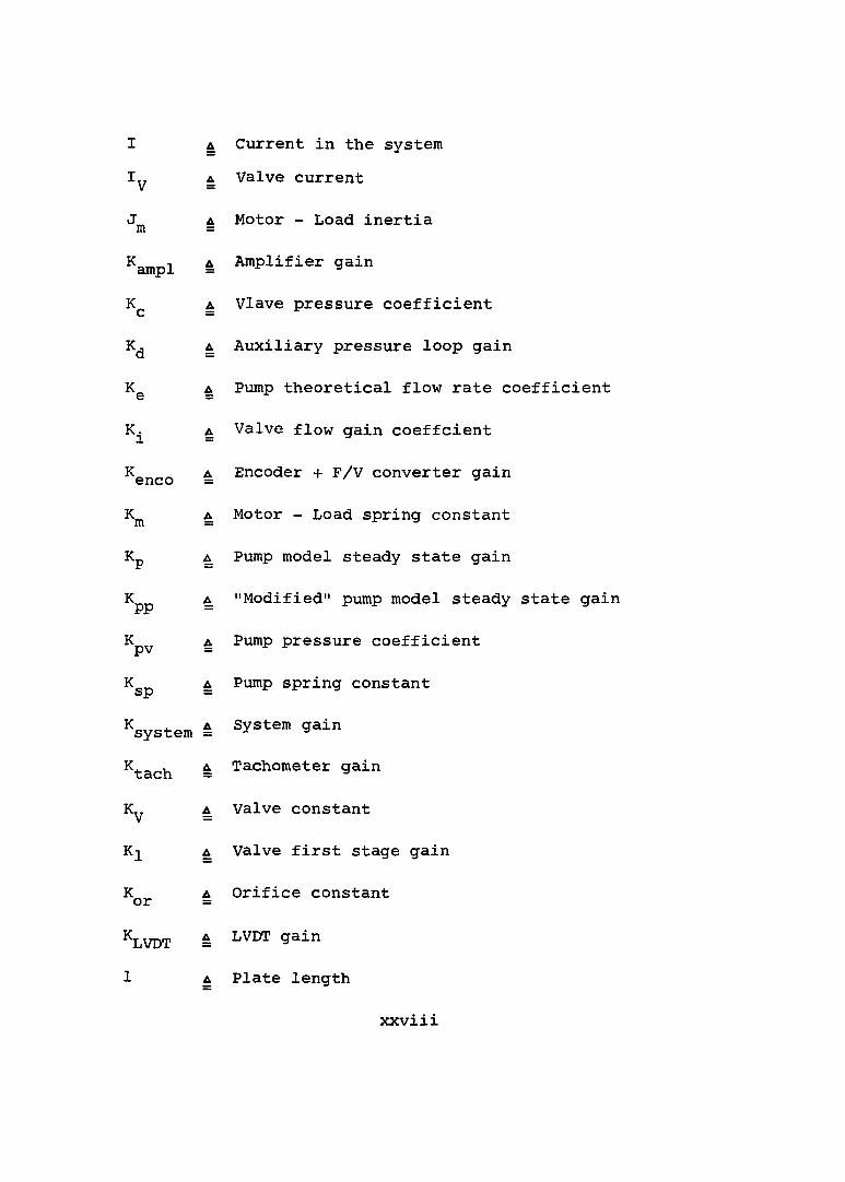
I A Current in the systemA Valve current

'"m A Motor - Load inertia

^ampl A Amplifier gain

A Vlave pressure coefficient

A Auxiliary pressure loop gain

A Pump theoretical flow rate coefficient

A Valve flow gain coeffcient

enco A Encoder + F/V converter gain

A Motor - Load spring constant

A Pump model steady state gain

^PP A "Modified" pump model steady state gain

^pv A Pump pressure coefficient

^sp A Pump spring constant

system A System gain

^tach A Tachometer gain

A Valve constant

Kl A Valve first stage gain

^or A Orifice constant

^VDT A LVDT gain

1 A Plate length

XXVIXI

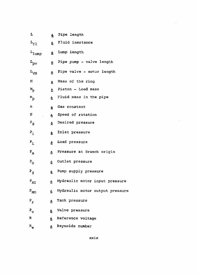
L A Pipe lengthA Fluid inertance

^limp A Lump length

A Pipe pump - valve length

^VM A Pipe valve - motor length

M A Mass of the ringMp A Piston - Load mass

■"p g Fluid mass in the pipe

n A Gas constantN A Speed of rotation

A Desired pressure

A Inlet pressure

A Load pressure

A Pressure at Branch origin

^0 A Outlet pressure

A Pump supply pressure

^MI A Hydraulic motor input pressure

^MO A Hydraulic motor output pressure

A Tank pressure

A Valve pressureR A Reference voltage

A Reynolds number

XXIX

A Fluid resistance

A Horizontal component of R^

Rq ^ Reference voltage sinusoidal amplitude

R^ A Resultant pressure force on the ring

Ry ^ Vertical component of R^

g Inlet flow rate

= Load flow rate

0^ A Branch away flow (Branch away component)

A Pipe flow (Built in component)

Qq a Outlet flow rate

Qp ^ Disturbing flowQg A Pump supply flow rate

A Valve flow

Qfh = theoretical flow rate

S A Laplace Transfer variableA Motor friction torque

A Thermocouple reading

T^ A Load torque

T^^ A Line propagation time

t_ A Time to maximum overshootP =Tp A Propagation time

XXX

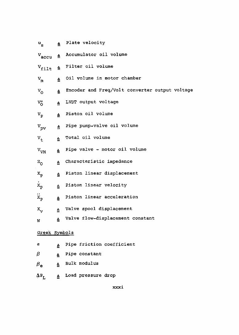
"s A Plate velocity

Vaccu A Accumulator oil volume

^filt A Filter oil volume

A Oil volume in motor chamber

^0 A Encoder and Freq/Volt converter output voltage

^0 A LVDT output voltage

A Piston oil volume

^pv A Pipe pump-valve oil volume

A Total oil volume

^VM A Pipe valve - motor oil volume

^0 A Characteristic impedance

^P A Piston linear displacement

^P A Piston linear velocity

^P A Piston linear acceleration

%v A Valve spool displacement

w A Valve flow-displacement constant

Greek Symbols

a A Pipe friction coefficientA Pipe constant

^e A Bulk modulus

A Load pressure drop

XXXI

Ai 6 Valve first stage differential current5 A Tolerance

f A Damping ratio(j A Natural frequency

6 A Hydraulic motor angular displacementK A Wave length

y- A Oil absolute viscosityTT A 3.14151692...

T A Time constantP A Oil density1/ A Oil dynamic viscosity

A EfficiencyA Phase angle

XXXll

INTRODUCTION

The basis of the art of oil hydraulics is in the science of fluid mechanics. Like all mechanical arts and sciences, oil hydraulics had its forerunners and pioneers, such asH. S.Hele - Shaw, Conrad M. Conradson, Renold Jenney,W, E. Megic, Walter Ferris, to mention only a few. But astonishing as it may sound to many, oil hydraulics as an industry dates back only about sixty years (1 )*.

The increasing amount of fluid power available to man that requires control and stringent demands of modern control systems have focused attention on the theory, efficiency, design, and applications of hydraulic control Systems.

Hydraulic control fills a substantial portion of the field of control. Hydraulic components and systems are found in many mobile, marine, airborne, and stationary applications (2 ).

The development of the electro-hydraulic servovalve was probably the most significant factor affecting the entire field. Hydraulic system dynamics became important

* See list of references, page 467.1

and it has been the subject of research for the past three decades.

Most valve - controlled servosystem analyses assume constant supply pressure irrespective of the type of power supply. When servo transients are large and fast enough, a pressure compensated pump type of supply, without accumulator, can no longer maintain reasonably constant supply pressure and pump dynamics become significant. This phenomenon was studied analytically for several types of systems and was experimentally tested for a speed control servosystem in Part one of the present dissertation.

Merritt states with respect to pressure variations in hydraulic power supplies; "Because of many variables and nonlinearities involved, prediction of those pressure transients is virtually impossible. Direct measurements in the evaluation program for the system is necessary",(p.343) (2) 1957. Today, with the highly developed modeling techniques and availability of computer simulation programs such as CSMP III, the prediction of those pressure transients should be possible. This was the first topic of this dissertation.

Efficient use of energy has recently become a subject for strong consideration in all facets of our lives. Ineffi­ciency in hydraulic systems can have many origins, but all

energy losses ultimately appear in two forms: heat and noise, therefore, fluid power manufacturers and users became actually aware of the oil and energy wasted in leaks, friction and inefficient design, A control philo­sophy that is rapidly gaining universal acceptance is to produce just the hydraulic energy actually required and produce it only when needed.

We studied for feasibility two schemes suggested as means to take advantage of the controllability of variable displacement pumps for energy saving operation of servo- systems. One scheme, suggested by Felicio, uses pre­knowledge of system duty cycle to program discharge pressure to meet the needs of the load without excessive power losses at the servovalve.

The second approach attempts to enforce the well known maximum power transfer rule (load pressure drop should be 2/3 of supply pressure) by sensing supply pressure and load AP and using these signals in a control scheme which adjusts pump discharge pressure so as to enforce maximum power transfer at "all" times.

The two schemes belong to the "Load-Responsive" family of hydraulic systems. The idea is to monitor the pressure drop (AP) across the actuator (load pressure) and to set up a pump controlling loop which will operate simultaneously with the velocity feedback loop. This was the second

subject studied in this dissertation.Finally, we performed further study of Felicio's model

of a variable displacement pressure compensated vane pump. In view of the fact that two questions in his research had not been complete answered, the third part of the disser­tation will be concerned with them,(1) The "Re-design" of Variable Displacement Vane Type

Pumps for Faster Response,(2) Explanation of 12,5Hz Peak in Pump Discharge Pressure

Frequency Spectrum during Pressure Measurements,

PART ONE

Theoretical and Experimental Study of the Effect of Pump Dynamics on the Response of Servosystems Supplied by Pressure Compen­sated Pumps

CHAPTER 1PUMP DYNAMICS TN SERVOSYSTEMS-BACKGROUND

1.1 General

Pressure transients frequently occur in hydraulic systems. These pressure peaks may become substantially higher than steady state values and generate noise and/or cause damage to system components if safe levels are exceeded. Therefore identification of physical situations that can cause pressure surges, computing the magnitude of such surges, and methods of limiting surges are an essential consideration in successful system design.Those transients occur when fluid flow is suddenly changed or stopped due to valve closure, when a sudden change in load speed is required and when hydraulic actuators are suddenly stopped or disturbed. Of course, it is possible for all situations to occur simultaneously, generating a complex transient (2 ).

There are basically two ways to control the flow of fluid power to a load:

(1) Varying some characteristics of the pump which generates fluid power from a prime mover source so that the rate at which fluid energy is generated is varied (pump control).

(2) Varying some characteristics of a valve so that the rate at which fluid energy is converted to useful energy at the load is varied, (valve control) (6 ).

Four configurations are available using valve or pump control, linear motor or rotary motor as actuators.

(1) Servovalve - Linear Motor (hydraulic piston)(2) Servovalve - Rotary Motor (hydraulic motor)(3) Servopump - Linear Motor (hydraulic piston)(4) Servopump - Rotary Motor (hydraulic motor)The four types of systems were studied by G. M, Swisher

(7), including pipe line dynamics using linearized analysis. He considered the supply pressure as constant.

An investigation of the assumption that a typical hydraulic power supply consisting of a constant displace­ment pump and unloader valve maintain constant pressure was performed by T, Comstock. His conclusion was that theassumption is valid at frequencies approaching the system'snatural frequency (8 ).

Servopump dynamics were investigated by Felicio (9) who developed a linearized dynamic model for a proportional

control type of variable displacement vane pump. When pump dynamics are considered and pressure transients exceed the ratio P^/Pg = 0.6 , linear analysis is invalid and additional linear and/or nonlinear fluid and mechanical details have to be included. Digital simulation becomes increasingly attractive as model complexity rises (lO).

This study will augment these developments by including an accumulator (located at selected points) in the system, including nonlinearities and using computer simulation CSMP III.

1.2 Historical Background

The two basic ways to control flow of fluid power to a load; valve control and pump control, were discussed by many investigators. As a historical background, a summary of the contributions of several authors in the field is presented. There are many books and articles on the subject and just a few which are the so called "bread and butter" of the domain were selected.

Historically, the book by J, F, Blackburn, G. Reethof and J, L.Shearer, "Fluid Power Control", published in 1960, could be regarded as the first and most comprehensive in the analysis of the dynamic performance of hydraulic systems in that period. This book has dominated the field

for the past two decades (6 ).Shortly after that, in 1963 A, C, Morse published the

book, "Electrohydraulic Servomechanisms", using material developed over twelve years of experience. This experience has spanned the period since the early appearance of the two-stage servovalve, maybe the most significant develop­ment affecting the entire field (1 2).

Probably the best book in tlie field, "Hydraulic Control Systems", was published by H. E. Merritt in 1967. It does not investigate pipe line dynamics or other attached components. Although it outlines the nonlinearities involved in hydraulic servosystems, the analysis is linearized and performed in frequency domain. This book is one of the main references in this dissertation (2 ).

The book, "Analysis, Synthesis and Design of Hydraulic Servosystems and Pipelines" by T, J. Viersma, published in 1980, deals almost exclusively with valve controlled linear actuators, emphasizing the design stage. The main contributions to the field are:

(1) The analysis of friction nonlinearity using describing function.

(2) The synthesis of pipeline dynamics and other hydraulic components.

(3) A detailed analysis on pump pressure pulsations and servovalve pressure transient suppression using

10

accumulators (13),A detailed study of hydraulic conduit dynamics, deve­

lopment of transfer functions for specified inlet and outlet conditions, consideration of fluid friction and pipe longitudinal vibration is given by E. O, Doebelin in his book "System Modeling and Response" published in 1980.The book is a useful guide in theoretical and experimental approaches as well as in Digital Computer Simulation CSMP III used in hydraulic systems (10).

The book by McCloy and H. R.Martin, "Control of Fluid Power, Analysis and Design", published in 1980, is also design oriented. Chapter 14 has a good discussion in the dynamics of pressure and speed control systems (14).

Two more sources in the subject of Computer Simulationare:

(1) The Ph.D. dissertation by Kropp, C, S.; "Digital Computer Simulation of Complex Hydraulic Systems Using Multiport Component Models" from Oklahoma State University, 1975 (15).

(2) The technical Report AF WAL-TR-80-2039 "Advanced Fluid System Simulation" written for the Air Force in April 1980. The purpose of the Advanced Fluid System Simulation (AFSS) program was to establish and validate, by test, the modeling required fora comprehensive dynamic simulation of aircraft

11hydraulic systems. In this report one can see for the first time an empirical model of a varia­ble displacement pressure compensated hydraulic pump included in the overall system model (16).

Many articles are related to the field of dynamics in hydraulic systems. Again I will mention a few that present different approaches.

NCFP - References: (20), (21), (22), (23), (24), (25),(26).

ASME - References: (36), (37), (38), (39), (40).AIEE - Reference: (42).ASAE - Reference: (45).SAE - References: (46), (47).Journal of Mechanical Engineering Science (53).Control Engineering: Reference (55).Bulletin of the JSME; References: (57), (58), (59),The dynamics of hydraulic systems have been investigated

since 1960 when the first papers appeared. The most recent papers deal with the use of digital computer simulation in hydraulic systems and with the introduction of modern control theory in the field.

12

1.3 Organizational Plan of the Study

We divided our study into three main parts:(1) Theoretical analysis(2) Experimental work(3) Computer simulation

1.3.1 Frequency Domain Analysis

Using the four pole and impedance coupling methods one can set up the system differential equations Laplaced Transformed for frequency domain analysis. This method provides good results for the linearized equations, but it would be difficult to include nonlinearities. To study the system using computer simulation, the approach would be to solve the set of equations as ordinary linear equations for specific frequencies using canned computer programs. (see Figure 1.1)

In the mechanical engineering department in OSU, there is available for example the digital computer program num­ber 24 (IBM 370/165), "Frequency Response From System Simultaneous Equations" using Speakeasy Matrix operations. One can use lumped parameter equations as well as distribu­ted parameter equations. This method was used in our frequency domain computer work and compared to the experi­mental frequency response test.

O—

SERVOVALVE

AMPLIFIER

PIPEDYNAMICS REFERENCE

INPUT

DYNAMICSPIPE

COMPENSATINGNETWORK

HYDRAULIC MOTOR & LOAD

ELECTRIC MOTOR AND V.D.PUMP

VALVEPROTECTINGFILTER ACCUMULATOR

HYDRAULIC

Figure 1.1 Four pole representation of a hydraulic valve- controlled rotary actuator servosystem

OJ

14

1.3.2 Time Domain Analysis

Using digital computer simulation IBM CSMP III, applied directly to the system differential equations, one can "solve" for any of the output variables for time domain analysis. The system models can be augmented with addition­al nonlinear fluid and mechanical details, which is the main advantage of this method. Different features of the system as well as stability problems can be easily inves­tigated just by changing the parameters and/or the initial conditions. A recent text book devoted entirely to CSMP III is; "A Guide to Using CSMP" by Speckhart, F. H. and Green, W. L, (17). This method was used in our time domain computer work and compared to the experimental step response tests.

Comparison between the step response tests was achieved, using the system in two different conditions:(1) Including pump dynamics and investigating its effects

on system response.(2) Suppressing pump dynamics by means of an accumulator,

to simulate a "Constant Supply Pressure System".The use of accumulators in hydraulic systems was

studied by Viersma, who gave some practical recommendations for the size and location of accumulators for suppression of pump flow pulsations and reduction of supply pressure

15

variations due to servovalve transients (13). A 1 din (61in ) volume accumulator (Viersuma's recommendation) was added to our set up in two possible locations: close to the pump and close to the servovalve input.

The study of the effect of pump dynamics on the respon­se of servosystems is understood to be the investigation of hydraulic motor shaft angular velocity (controlled variable) as well as valve input pressure (supply pressure) variations, as a function of servovalve operations (i.e., input current ) as input. Hydraulic motor inlet pressure P^ and outlet pressure P^ were investigated as well, in order to study load pressure (P = P - P^) variations.

CHAPTER 2 THEORETICAL ANALYSIS

2,1 General

The system of equations developed during the mathema­tical modeling of most hydraulic systems is composed of algebraic and ordinary differential equations. In general, the algebraic equations are nonlinear and may not be reduced analytically. The ordinary differential equations result­ing from the mathematical modeling are, in general, also nonlinear (15), The dynamic equations representing a servovalve controlled actuator including pump dynamics, will now be derived. The hydraulic power element of a servovalve rotary actuator is probably the most widely used combination in numerous applications, and our analysis will concentrate first on this type of system, Servovalve- linear actuator system will be considered next, concluding the analysis and presenting a useful, fundamental design tool.

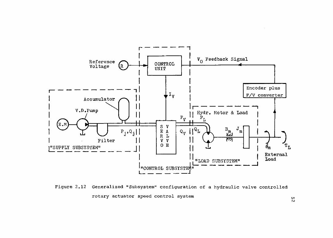
The most general case will be considered first, includ­ing all the typical hydraulic components in such a servo- Bystem pump, servovalve, control valves, actuator,

16

0R

0R

AccumulatorV.D.Pump Hydraulic

Motor & Load

Pipe © ‘P ip e © F ilte r

Pipe © I

HI

Encoder + F/V converterAmpl

SignalGenerator

Figure 2.1 Valve controlled rotary actuator servosystemin speed control configuration (General case)

18

accumulator, filter, and pipe line dynamics (Figure 2.1), As one can see the overall hydraulic system includes

several components "attached" to the pipe line, others "built into" the pipe line. In order to use the four pole representation of such a system, we will make the following clarifications;(1) Components branched away from the pipe line can be characterized by "branch away" flow as a function of the pressure at the origin of the branch (13).

Q„(S)G, (s) = n:— (2.1)

Pm'S)where ;

Gj (S) A Branch away transfer function.

A Branch away flow.A Pressure at branch origin.

Qm

I I ___________________

5i r.

"Branch away" component

19

= Qq + = Branch away flow. (2,2)

= Pg = A Uniform pressure. (2,3)

where :

^i ê Inlet pressure .

^0A Outlet pressure

0. A Inlet flow .1

Go à Outlet flow.

Transfer functions of a wide variety of branch away components such as accumulators or filters can be found in the literature,(2) Components built into the pipe line can be characterizedby "Pressure Drop" AP as a function of the flow rate Qm mthrough the element.

Kor

Qi I I Qq

"Built in" component

= Qq = = Incompressible flow, (2,4)

Q^ = (P^ - Pq )= Linearized orifice, (2,5)

20

where ;0^ = Pipe flow.

Orifice constant.

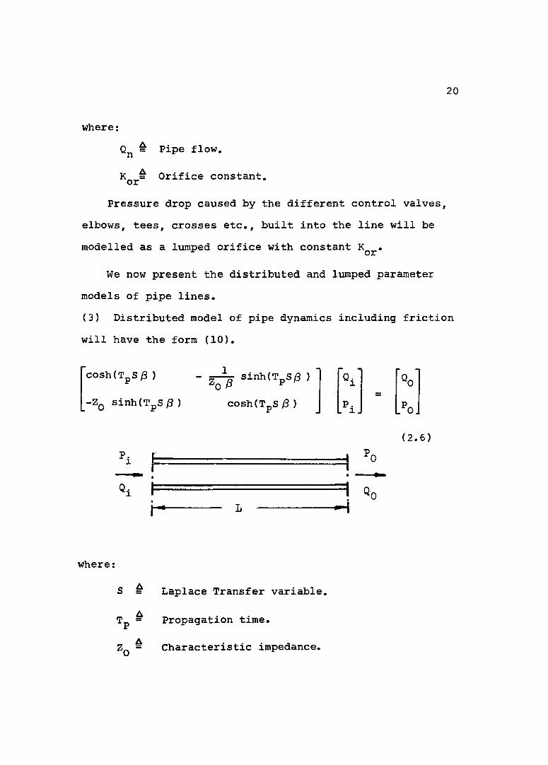
Pressure drop caused by the different control valves, elbows, tees, crosses etc., built into the line will be modelled as a lumped orifice with constant

We now present the distributed and lumped parameter models of pipe lines.(3) Distributed model of pipe dynamics including friction will have the form (1 0 ).

cosh(TpS /3 )

-Zq sinh(TpS/3)

sinh(T S/3 )

cosh(TpS 13 )'Oo'

7i. /o.

^i

Qi

(2.6)

where:

S à

Tp =

Laplace Transfer variable.

Propagation time.

Characteristic impedance.

21

The quantity B is a complicated, complex valued function of frequency, pipe radius,viscosity, and density that requires use of Bessel function in its calculation (10).

A more detailed analysis can be found in (13), where a rough approximation is given over a wide frequency range.

where

[iS(S) ] = — + 1 S

a = 32 /i

(2.7)

M = Absolute oil viscosity.D A Pipe diameter.

when friction is not included ) /3 = 1 .(4) Lumped parameter representation of pipe line dynamicscould be (1 0 );

(2.8)1 -(*fl+LfiS) P.1 "Po"

-Cfi s l+Rf^S+L^jCjlS^ _ _0i_where

Rfl A Fluid resistance •

Cfl A Fluid compliance .

^fl A Fluid inertance .

22

Neglecting fluid inertance = 0) :

1 - ^fl- Cfl s ^fl Cfi s _GiNeglecting fluid friction (Rfl

1 0 P.1 ^0

" ^fl 1 Oi °0

(2.9)

(2.10)

Expression (2.10) is often used for "short" connecting pipe lines.

2.2 Valve Controlled Rotary Actuator Servosystem

Having done this short introduction for the four pole method analysis, let us derive now the set of algebraic and differential equatian equations describing our system. The equations will be linearized models in terms of pertur­bations about an operating point. For simplicity we will omit the subscript "P" as the perturbation symbol.

We refer our analysis to Fig.2.1. Variable displacement vane type pump dynamics was investigated by Felicio and a useful linearized model was presented by him. Since in our experimental program we used the very same pump we will use the transfer function given by Felicio, which describes the dynamic relation between pump output pressure P(supply pressure), and pump flow rate Qg (supply flow rate)

23

Pump Transfer Function (Felicio)

P - K (T S + 1)G„(S) = — (S) = — -- (2.11)

Qg S 2 f SS -- + 1--- + 1^P

V.D.Pump Pipe LineSystem

Equation (2.11) can be seen as the input impedance to the pipe line connecting the pump with the system, where :

Gp(S) A Pump transfer function,A Pump supply pressure.

^P à Pump steady state gain,A Pump time constant.A Pump natural frequency.A Pump damping ratio.

Gs A Pump supply flow.

24

Pipe line connecting pump-valve (pipe No.l)

Using the distributed parameter model derived earlier we get:

cosh(T^ S /3 ) -- 1— sinh(T^ S /S) Qs

-Zq/3 sinh(T^S0 ) cosh(T^S0) / 2 _

(2.12)where

= Pipe No.l propagation time.

Qg =Q^ = Pipe No.l input flow.

Pg=P^= Pipe No.l input pressure .

Qg = Pipe No.l output flow .

Pg = Pipe No.l output pressure .

Pipe lines connecting valve-actuator

Similarly, the pipe lines connecting valve-motor inlet port and valve-motor outlet port have the form:Pipe line No.2

sinh(T_S0)cosh(T2S/S) ------- ---- 0? ^8

-Zq/3 sinh(T2SjS) coshiT^Sfi) / 7 _ _

(2.13)

25

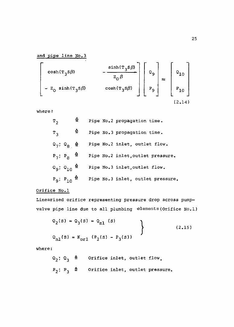
and pipe line No.3

coshCT^S/S)

- Zq sinhfTgSfü

sinhCT^S/S)

coshtTgS^)

Q9 Qio

^9 ^10

(2.14)where :

0?; Qg A

^7* ^8

®9' °10

^9' ^10 Orifice No.l

A

A

A

Pipe No.2 propagation time.

Pipe No.3 propagation time.

Pipe No.2 inlet, outlet flow.

Pipe No.2 inlet,outlet pressure.

Pipe No.3 inlet,outlet flow.

Pipe No.3 inlet, outlet pressure.

Linearized orifice representing pressure drop across pump- valve pipe line due to all plumbing elements(Orifice No.l)

Qgfs) = 0 3 (3 ) = (S)

Qnl'Sl = Korl IPz'Sl - Ps'S))}

(2.15)

where ;

®2' ®3

^2* ^3

Orifice inlet, outlet flow.

Orifice inlet, outlet pressure.

26

Valve protecting filterThe filter between pump and servovalve (13)

Pa'S) = 9 4(3 ) =

QjCS) = 0^(3) +

l i t e r = 7 ^Pml'S)

Vf i l t e r S = C 0. filter ^

(2.16)where:

Q3; Q4 #

P3 : P4 =

filter

^filter

Filter inlet, outlet flow.

Filter pressure ,

Filter volume (oil capacity).

Bulk Modulus,

Filter compliance .

The accumulator installed close to the valve, eliminates pressure fluctuations caused by sudden and large valve openings (10).

^4 (8) = 9 5(8 ) = 9*2(8)

Ojfs) = 0 5 (3 ) + 0^3(3)

Q„o(s) s v

(2.17)

27

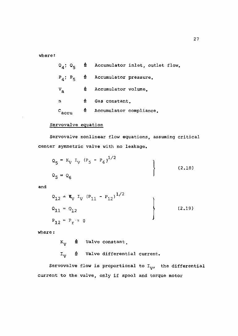
where :

®4* A Accumulator inlet, outlet flow

^4 : ^5 A Accumulator pressure.

^a A Accumulator volume.

n A Gas constant.Caccu A Accumulator compliance.

Servovalve equation

Servovalve nonlinear flow equations, assuming critical center symmetric valve with no leakage.

,1/2

and

where :

°12 “ «V 4

°11 " ^12

^12 = p - ~ r

A

à

121/2

Valve constant

(2.18)

(2.19)

Servovalve flow is proportional to the differentialcurrent to the valve, only if spool and torque motor

28

dynamics can be neglected. Actually, flow-current transfer function is given by the manufacturer (MOOG), for a known supply pressure.

Q»(s) K

^ ^ + — + 1

where;

Ù) OJV V

Qy - Valve flow.

= Valve natural frequency.

^ = Valve damping ratio .

Servovalve first stage dynamics (torque motor dynamics) was neglected, since it was found experimentally to have a "fast" time constant.If the linearized relations of the valve are used, one gets.

Q^(S) = Qg(S) 1

0.(3) = K. I„(S) G„(S) + K P.(S) - K P.(S).D I V V C D C O(2.21)

and

Ol2(S) = Qii(S)

OigfS) = K^I^(S)G^(S) + K^Pii(S) -

P^gtS) = Pj.(S) «0

where; A Valve flow gain .= Valve pressure coefficient.

. (2.22)

29

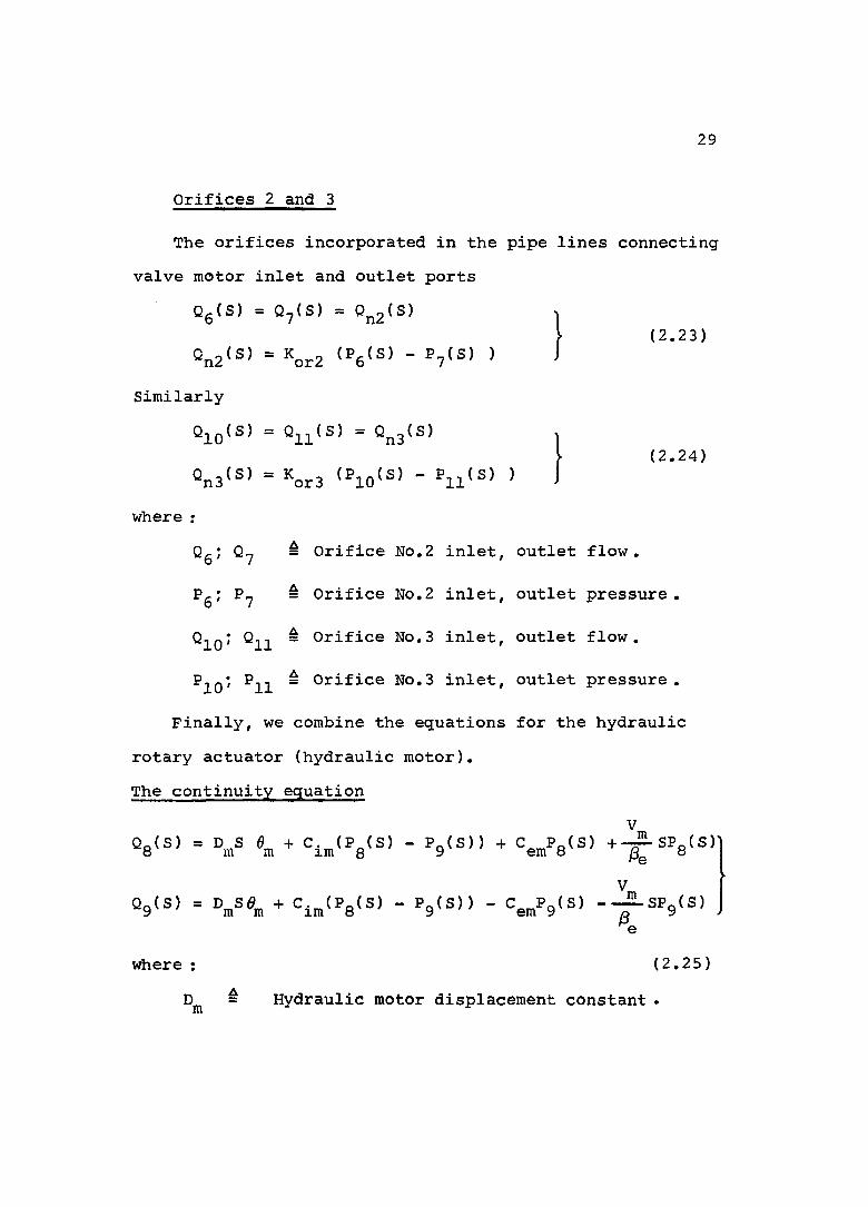
Orifices 2 and 3

The orifices incorporated in the pipe lines connecting valve motor inlet and outlet ports

Qg(S) = Q^(S) =

On2<S> = V 2 (Pe'S) - P,(S) )(2.23)

SimilarlyQlo(S) = OiilS, = Q„3(S)

° n 3 < S > = V s ( P l o ' S l - P l l ' S ) >

(2.24)

Where ;Qg; = Orifice No.2 inlet, outlet flow.

Pg; P.y = Orifice No.2 inlet, outlet pressure.

^10' ^11 Orifice No.3 inlet, outlet flow.

^10* ^11 Orifice No.3 inlet, outlet pressure.

Finally, we combine the equations for the hydraulic rotary actuator (hydraulic motor).The continuity equation

Os'S) = V % * Cim'Pg'S) - PgtSII + +-SPg(S)l

Og(S) = + Clm'Pg'S) " ‘ - ^ S W ^ ( S )e

where ; (2.25)= Hydraulic motor displacement constant .

30

^im à Hydraulic motor internal leakage coefficient.

*"em A Hydraulic motor external leakage coefficient ,

A Oil volume in motor chamber.

^eA Bulk modulus ,

mA Hydraulic motor angular motion.

Newton's law

“m [Pg'S' - fs'S'] = V^»n. + V « m + + ^l ' )(2.26)

where :J = Motor-Load inertia,mB = Motor-Load viscous friction coefficient,m

= Motor-Load spring constant.

( S ) = Load T orque .

2,3 Valve Controlled Linear Actuator Servosystem

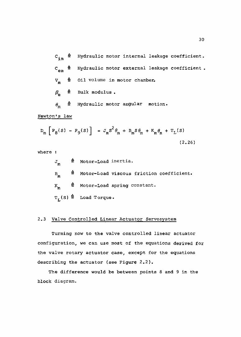
Turning now to the valve controlled linear actuator configuration, we can use most of the equations derived for the valve rotary actuator case, except for the equations describing the actuator (see Figure 2,2),

The difference would be between points 8 and 9 in the block diagram.

1 QçV.D.Pump

%

P i p e ©

0RIPICE □

Accumulator

Filter

è d )

é

s \rE kR LV V0 E

;4

Ampl,

SignalGenerator

ÜJ,£/i(,

E 0] I Pipe©,

LVDT

Figure 2.2 Valve controlled linear actuator position control servosystemCüH

32

Q-^(External Leakage)

Q. (Internal Leakage)

Figure 2.3 Linear actuator between points 8 and 9

where we install now a hydraulic piston replacing the hydraulic motor.The continuity equation

OgIS) = ApSXp + C.p [Pg(S) - Pg(S)] + CgpPg(S) + % P g ( S ,

Qio's' = V ^ p + =ip [Pe's) - Pg'sl] - <=ep^9< = > -ySPg(s)

(2.27)

33

where:

Apwhere

Piston area .

Piston internal leakage coefficient.

Piston external leakage coefficient.

''p é Piston oil volume .

I 's law

■g(S) - Pg(S)] = MpS^Xp + BpSXp + CpXp + Fj (S)

Mp A Piston-Load mass.

Bp ^ Piston-Load viscous friction coefficient.

Cp ^ Piston-Load spring constant,

Fp g Load force.

Equations (2,11) to (2,26) define the dynamic behaviour of a servovalve rotary actuator servosystem. Similarly, equations (2,11) to (2,24) and (2,27), (2,28) describe the valve linear actuator system. Using one of the methods mentioned earlier one can solve these equations for any of the variables, in time domain or in frequency domain, with the following exceptions:(1) Pipe dynamics representation for CSMP computer analysis has to be in lumped parameter configuration. If pipe lines are short, only compliance is significant and equation (2 .1 0)

34

can be used. Non linear-equations are allowed.(2) For Speakeasy Matrix Methods in frequency domain, servovalve and orifice flow-pressure equations have to be in the linearized form. Non-linear equations are not allowed in this type of analysis.

2.4 Closed Loop Systems

The two types of valve controlled actuators could be used in speed or position control configuration, depending on the specific application, although each type has its "usual" operating form.

The most widely used application of rotary actuator closed loop systems is in speed control due to the 360° rotation feature of the hydraulic motor. The controlled variable is or actually the encoder and F/V convertervoltage output V^. "Disturbance" to the system is load torque T^(t), a known function of time in a particular application. We define as the output of our system, the open loop input will be the input current to the servovalve I , which is the controller variable.

Linear actuators are used usually in position control applications due to physical construction of a piston having limited stroke. The controlled variable is Xp or LVDT voltage output V^. Similarly, F^(t) is the

35

"disturbance" to the system and it is the load force.Equations (2.11) to (2.28) are the "open loop" set of

equations describing rotary and linear actuator servosystems.Our final analysis refers to the "closed loop" represen­

tation of the two systems.(1) The servocontroiler output is the current input tothe valve I^. The input would be the error voltage R -of the closed loop, where = K 0 in the rotary0 enco mactuator speed control configuration or R - , where

the linear actuator position controlconfiguration.

Usually,a compensation network G^(S) is needed in feedback systems, obtaining the final "loop closing" equations.Iv = Kampl^c^^) (R - Vq ) for speed control (2.29)

= KampiG^fS) (R - V^) for position control (2.30)

where :

^ampl = Amplifier gain

G^(S) g Compensating network

R A Reference input voltage= Motor angular -velocity.

The "new" input to the system will be R, the reference voltage.

36

Before leaving this sectionna final comment concerning stability of the two types of systems would be appropriate.(1) A lag compensation network

G^(S) = 1/(t S + 1) installed before the servo­valve is usually enough to stabilize a speed control system.(2) In a position control system a lead-lag network could be tried G^(S) = (r^S + D/fTgS + 1 ), but a crossport (piston inlet/outlet) valve is more useful in most of the applications (see Fig.2.2 - by pass valve).

We now want to develop useful relations which will enable us to investigate the effect of pump dynamics on system performance. We restrict ourselves to the simplest closed loop pump-valve-actuator configuration, neglecting the dynamics of any other hydraulic component in the system. When we get to the experimental part of our study, we will justify numerically any simplification or assumption made towards this goal.

Let us now add pump dynamics to the well known valve controlled actuator dynamic relation found in many text­books (2 ).

37

2,5 Pump-Servovalve-Rotary Actuator Combination

It is desirable and possible to express the continuity equations of the motor chamber in a more useful form. In­troducing the term = (Q + Q2 )/2 , we add the two equations in eq.(2.25) and divide by 2 to obtain the equation

where :A Load flow .

P^ “ 1*2 — Load pressure ,

Ctm = =im + C«m/2 ê Leakage coefficient ,

\ = 2 V A Total m = oil volume ,

This equation is the basic form of the continuity equation for all hydraulic rotary actuators, without detailed consideration of the flows in each chamber.

Since - ?2 , the final basic equation of thetorque balance equation (Newton's law) for the motor will be

“m ''l = -Im S «m + + ?&(=) (2-32)Static and coulomb friction loads would also be

present to some degree but will be neglected in a lineari­zed analysis (2),

38

L n

HYDRAULICMOTOR

SERVOVALVE

RETURNSUPPLY

TANK

V. D. PUMP

Figure 2.4 V. D. Pump ' - Servovalve - Rotaryactuator combination

39

Since our analysis is based on the four pole approach it will be more useful to describe the rotary actuator in its four pole representation. The "new" forms of the continuity and torque balance equations allow us tovisualize the hydraulic motor as a "two->port device

111L_ J

Figure 2.5 Hydraulic motor as a "two port" device

where :A Input effort variable .

A Input flow variable .

T^ A Output effort variable .

A A Output flow variable . m —

The boundaries of our subsystem include the oil tank, the load, and the pipe line connecting the valve with the motor.

Rearranging equation (2,31) we get

«n, = V ' V > - (2.33)

and substituting eq.(2.33) into eq.(2.32)

40

J S S dj= Dm K_m Km

(Zl Jj I ).s + + fs ) g'L 4 A De m m

B_ C. K V.+ (1 + - 2— ÈÏ. + _IL_E , s +m "ge “m

‘tm

m

(2.34)A series of simplifications are possible due to

parameter relations and orders of magnitude. Becauseusual loads are often simpler, some special cases of

2eq.(2.34) are of interest. The quantity B C. /D can bem tm mneglected compared to unity, because usually B^ is "very" small and the leakage coefficient is small in practical applications.

Furthermore, let spring loads be absent, that is,= 0, for the present, so that eq.(2,34) reduces to

^t ^m

m°m

- ( — SL s + 1 ) — Q,B_m D, (2.35)

m

41

And now rewriting eq.(2,33) in terms of

4 =tm(2.35)

Equations ^2.35) and (2.36) can now be represented in the four pole form as follows:

2S+ 1) \ -(T^ S + 1)JS.

" -

’’l^h "h ^m

-(Tm S + 1) Ctm^m

1Dm

Ql 9m

(2.37)where :

à Hydraulic undamped natural frequency.

Bm ^t 1/2 a(----- ) = HydraulicDm damping ratio.

T = J /B A Rotary actuator time constant, h m m =7 = V^/(4 /3g A Hydraulic time constant.

Since the boundaries of the subsystem include the pipe line connecting the valve with the hydraulic motor, is the total oil volume of the "non active" oil in the motorchambers and the oil in the connecting lines.

42

Usually is the lowest natural frequency in a servo- system and limits its frequency response characteristics. Therefore, the designer should make an effort to minimize as much as possible the length of the connecting pipe line between valve and the actuator. Once the minimum pipe length is achieved in a particular application, obtaining the highest natural frequency .there is a common practice to neglect fluid friction and inertia. In cases where this goal can not be achieved pipe dynamics (including friction, inertia, and compliance) have to be considered (7).

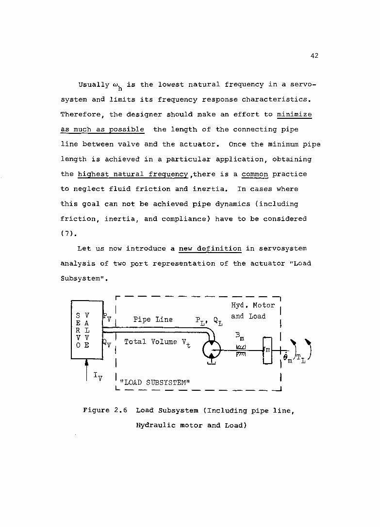
Let us now introduce a new definition in servosystem analysis of two port representation of the actuator "Load Subsystem".

s VE AR LV V0 E

Pipe Line

Total Volume V.

Hyd. Motor .-n n and load

«I IB.

"LOAD SUBSYSTEM"

P77TI m

Figure 2.6 Load Subsystem (Including pipe line. Hydraulic motor and Load)

43

Using four pole coupling methods the so called input Pwimpedance --- (S) of the Load Subsystem at the servovalveQy

upstream will be obtained.

2.6 Generalized "Load Subsystem" Analysis

We will derive now a generalized input impedance transfer function — (S) of the Load Subsystem including

Gypipe dynamics.

The four pole representation of the rotary actuatorderived earlier can be rewritten in terms of as afunction of T_ , d .L ' m

E(S) F(S)-1

’^l ' "^l 'G(S) H(S) êm Gl

where;

E(S) = (-(O

+ 1 ^ + 1) D0)

m

(2.38)

BF(S) A _ ( T: S + 1) m

mG(S) = - (T S + 1) Ct_/Dm tm mH(S) = 1/D,m

We recall now the four pole representation of pipe line dynamics (neglecting friction, /3= 1)

44

cosh K l ksinh (’’ll =)■

- 2q S j cosh(?^L s )

°in

^in

Qi Go

/ L _ ^i ^0

which will have the block diagram form.

(2.39)

Figure 2.7 Equation 2.39 in block diagram form

The inverse representation would be.Dt - B, Q.L L 0 1— C_ A_ P.L L 0 1

(2.40)

where;

T^^ g Propagation time (total line length).

45

cosh(Tj^S)

A - sinh(T^S) /Z^

Cl A - Zg

Dj A cosh(Tj^S)

The final "Load Subsystem" four pole representationusing the inverse of equation (2.38), and DET = EH-FG.

em

Tn

E L o . QL DDET+ <.

—G 1' T>DET ®L

1

-FDET L

+M

+k PL

DET

+---

Figure 2.8 Four pole representation of a generalized "Load Subsystem"

In most of the cases we take T^ = 0, thus G(S) and E(S) have no significance.

As discussed earlier when pipe line between valve and motor is short one can neglect friction and inertia i.e.,A^ = =1, = 0 and S as given in equation

46

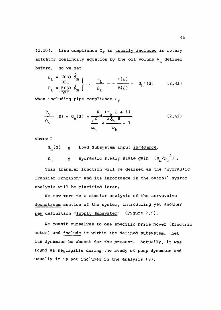
(2,10). Line compliance is usually included in rotary actuator continuity equation by the oil volume defined before. So we get

Elf) " m 1 P F(S)DET 1 . __L_ -------= G ' ( S) (2.41)

PL = F(S) Qt E(S)L -ÔËT ^

When including pipe compliance

P„ K (T S + 1)(S) = G, (S) = _ 2 _ h — ----------- (2.42)

«V Z 1 Z & Z 7 T' h %

where :G^(S) é Load Subsystem input impedance.

2A Hydraulic steady state gain (B^/D^ ) .

This transfer function will be defined as the "Hydraulic Transfer Function" and its importance in the overall system analysis will be clarified later.

We now turn to a similar analysis of the servovalve downstream section of the system, introducing yet another new definition "Supply Subsystem" (Figure 2,9).

We commit ourselves to one specific prime mover (Electric motor) and include it within the defined subsystem. Let its dynamics be absent for the present. Actually, it was found as negligible during the study of pump dynamics and usually it is not included in the analysis (9).

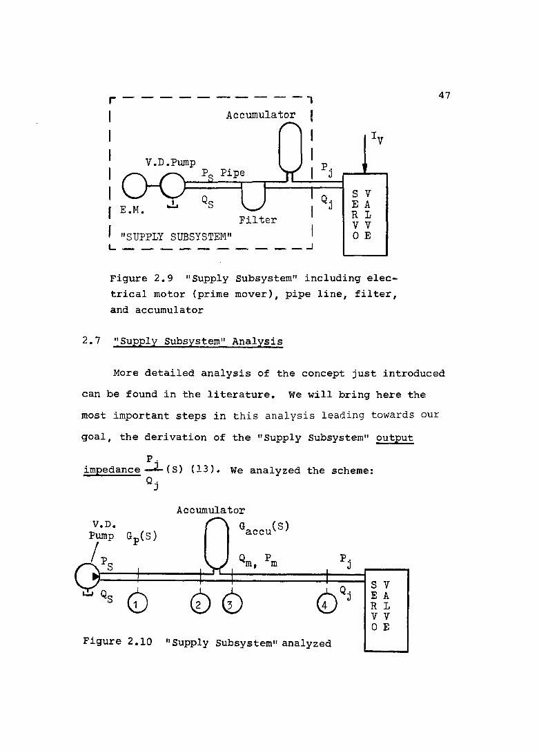
47Accumulator

V.D.PumpPq Pipe

E.M.

"SUPPLY SUBSYSTEM"

Figure 2.9 "Supply Subsystem" including elec­trical motor (prime mover), pipe line, filter, and accumulator

2.7 "Supply Subsystem" Analysis

More detailed analysis of the concept just introduced can be found in the literature. We will bring here the most important steps in this analysis leading towards our goal, the derivation of the "Supply Subsystem" output

P .impedance — (S) (13). we analyzed the scheme:

/o

V.D.Pump Gp(S)

Accumulator Gaccu (S)

( b ( b ( b ( b

Figure 2.10 "Supply Subsystem" analyzed

48

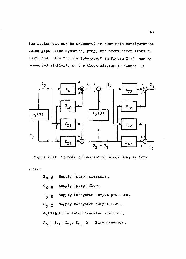
The system can now be presented in four pole configuration using pipe line dynamics, pump, and accumulator transfer functions. The "Supply Subsystem" in Figure 2.10 can be presented similarly to the block diagram in Figure 2.8.

L2

'L2

12

L2

Figure 2.11 "Supply Subsystem" in block diagram form

where ;

A Supply (pump) pressure ,

°s A Supply (pump) flow .

A Supply Subsystem output pressure

A Supply Subsystem output flow .

G^(S)A Accumulator Transfer Function .

^Li* ®Li' ^Li' ^Li = dynamics.

49

PcG (S) 4 Pump Transfer Function --- (S) which^ «s

is the "Supply Subsystem" input impedance.

The system in Fig.2.11 is the general representation of the supply subsystem. Using four pole methods (matrix multiplication) one could obtain the output impedance

P-i— — (S) in its most general form, as a function of pipe

line, accumulator and pump dynamics. In our case, since the accumulator is close to the valve, the pipe connection will be neglected and since the pipe line between the pump and the accumulator is short, fluid inertance and friction will be neglected, including only oil compliance using the lumped parameter representation (eq.2.10) and defining accumulator dynamics G^(S) = S (C^ = accumulator

compliance) we get :

P . - 1_2(s) ----------------------------------- (2.43)

1 + Ca ^0 ^LL + Zg S/Zg Gp(S)

■ LL = + l/%0 S ' ® ’

50

In the general case "Supply Subsystem" pipe length can not be shortened indefinitely because of constructional and physical dimensional constraint.

A filter to protect the servovalve is absolutely

necessary, and the accumulator is installed close to the valve to suppress sudden and large flow demands. In our particular application the absolute minimum pipe length was used. In the very same way as in the hydraulic motor analysis, where we included pipe line volume in motor compliance, filter and short pipe line volumes connecting pump with servovalve have been included in pump compliance.

Adding this oil volume to the compliance of the "original" "Felicio's Pump Model" used in our development, we realize an increase in damping ratio ^ and a decrease in

pump natural frequency w^.

Not including accumulator dynamics (i.e., G (S) = 0),P.the supply subsystem output impedance — = (S) (eq.2.43)

becomes just the "modified" pump linearized transferfunction G i s ) , i.e. P. = P and Q. = Q .P ] S J s

Pg - K (r s + 1) (S) = G (S) = ----2-- — (2.44)

"p “p

51

where co and are the "new" pump natural frequency and

damping ratio.As we can see, the Supply Subsystem output impedance

and the Load Subsystem input impedance have the same form. When combined via the servovalve the subsystem with the lowest natural frequency will dominate the whole system's natural frequency.

2,8 "Control Subsystem" Analysis

Finally, we define the last subsystem which combines the "Supply Subsystem" with the "Load Subsystem" and will call it the "Control Subsystem". This subsystem includes the control unit, (i.e., computer, servoamplifier, and compensating networks) the "brain" of the subsystem and the servovalve, the "muscle" of the subsystem. The equations modeling the "Control Subsystem", using P_=P_ and Q„=Qt oneV L i V J-iValve current G^(S) (R - Vq )

Valve flow

Valve dynamics G^Cs) =

(2.45)

The different variables were defined earlier. The

V-, Feedback SignalReferenceVoltage CONTROL

UNIT

Encoder plus F/V converter

Accumulator

V.D.Pump Hydr. Motor & Load

E.M

F ilte rI SUPPLY SUBSYSTEM"

ExternalLoad"LOAD SUBSYSTEM"

"CONTROL SUBSYSTEM"

Figure 2.12 Generalized "Subsystem" configuration of a hydraulic valve controlled rotary actuator speed control system Ln

53generalized "Subsystem" configuration of a valve controlled actuator speed control system is presented in Figure 2.12.

Using the "new" subsystem representation we will analyze now the valve controlled linear actuator system.

2.9 Valve Controlled Linear Actuator System

A completely identical analysis can be made for the valve controlled linear actuator combination. The only difference would be the "Load Subsystem" output variables which will become now Xp(t) and F^(t).

"LOAD SUBSYSTEM"

Q-X

J

Figure 2.13 Valve controlled linear actuator "Load Subsystem"

Another difference would be the usual presence of spring load 0 =4= 0 since the motion is now limited to the piston stroke.

54

Thus, all the above derived equations are valid in this case except the "Load Subsystem" four pole representation, which will have the following form:

=4ee*p‘

=tpCp

and

=

Ap^L ®p+ _i_s + 1 (2.46)S . =P Ap S

s) ''tp fL (2.47)ApS 4feCtp Ap SEquations (2.46) and (2.47) can be represented in four

pole configuration.

(2.48)A(S) B(S) ”^l ’ ~^l ’c(s) D(S) _Ql _ / p _

where .

A(S) =4%Ap'

■)s

4fgAp2 Ap2 Ap2

B(S) -- (-^ S + — S + 1)Ap S Cp

55XP HYDRAULIC PISTON

“H :

Cep Pi

X

7 ^

)1

V

T^iP

Pl=Pi-P2

V. ep

M„P11 I

-M:SERVOVALVE

Q;RETURN r- 0

SUPPLY

TANK

V. D. PUMP

Figure 2.14 v. d. pumn - servovalve - linear actuator combination

56

V. C.^ 1c(s) = - (— — s + —

"^e=tp S S

D(S) = l/(Ap S)

All the other derivations to achieve the Load Subsysteminput impedance are identical with the rotary actuationcase. A typical configuration is given in Figure 2.14.

Having presented a "new way" of looking at a valvecontrolled servosystem we now want to get actual transferfunction for different variables in the system as a functionof the input and possible disturbance. The subsystemconcept is a generalization of the analysis presented inthe liturature (13).

For the present, we assume no disturbing torque on thehydraulic motor shaft i.e., T^(t) = 0. Thus, the input tothe system will be a reference voltage R(t) to the servo-controller. If "open loop" transfer function are desired weneed no compensation network and neglecting amplifierdynamics we get = K , R.V ampi

The variables investigated during our study were:(1) Vq = - Encoder plus F/V converter

output voltage. This voltage was also used as thefeedback signal

(2) Pg - Supply subsystem pressure output (valve input pressure) •

57

At this point it would be appropriate to repeat the statement which ended the first chapter in this dissertation.

"The study of the effect of pump dynamics on the response of servosystems is understood to be the investigation of hydraulic motor shaft angular velocity (the controlled variable) as well as valve input pressure (supply pressure) variations as a function of reference input R".

Vo Pg Pg2,10 Transfer Functions — (S); -- (S); (S) DerivationR R

Let us now develop the appropriate transfer functions;V_ "Encoder voltage output— (S) =R Reference voltage inputP Valve input pressure— i s ) = ----------- ---------R Reference voltage inputP Valve input pressure__S (s) = -------------------------Vq Encoder voltage output

"Supply Subsystem" output impedance Pg - K (T S + 1)— i s ) = GL(S) --- 2— 2-------- (2.49)

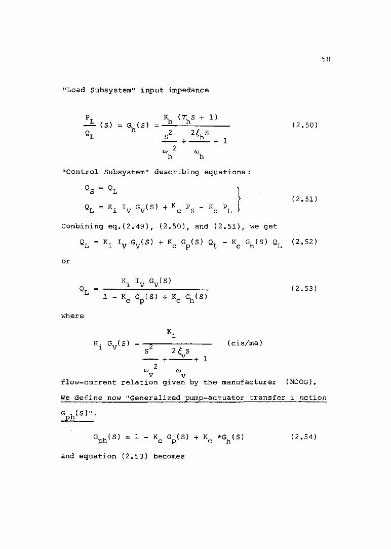
'Load Subsystem" input impedance

P K (T S + 1)— (S) = G, (S) -- ------Ob s2 . + 1

"Control Subsystem" describing equations :

58

(2.50)

Os = 0^

Ob = ^i ^s - ^b(2.51)

Combining eq.(2.49), (2.50), and (2.51), we getQy = K I G (S) + K G (S) - K G (S) (2,52)L I V V C p L- c n L

or

Ki Gy(S)1 - Gp(S) + Kp G^(S)

(2.53)

whereK.1

Gy(S) = (cis/ma)

Cl> O)V Vflow-current relation given by the manufacturer (MOOG).We define now "Generalized pump-actuator transfer i nction

Gph(S)".

Gph(S) = 1 - Kc Gp(S) + *G^(S) (2.54)

and equation (2.53) becomes

59

= T T (2.55)+ 1 Gph (S)

<0 Ù)V V

using Vq = Kencoder ' 4 = 4mpl ^ ^he transfer

function

1/D,e m ( S ) = m

we get finally for— — (S)R

(2.56)

Zl.s, = —R _2

^i ^ampl 4nco ^ 4 -(2.57)S“ 2f S S 2 A s(— — + — — -f- 1 ) ( - -t — + 1 ) G ( S )o 9 P h

% %

Deriving now the transfer function for (S) , we getR

°L = "i ly Gy'S) + %c ?s - ■'c

«S - =L

— = VyGy's> + Vs - Vh'G)-^ f,2.5e,Gp(E)

's[:-

V ~ ^ampl

K_G_(S) + K_G^(S)j = K^I„G„(S)G_(S)c p' ' ' c h ' j ■■i*V“V'”''p'= K_ R

and finally we have

— (S) = R

KamplG_, (S)

+ 1 PhÛ)V Ù)

Finally, the transfer function — (S)

Is _.fs /_Zo _ Ps 2R R R V,

f s (S, . Ki*amplGy(S)GplS,v_ Sph(S)

S h ' = > + -+ 1 )

Gv'S)%iKamplKen=o/ ">n,or

60

(2,59)

(2.60)

K.Gp(S)

enco (Ü CÜ(2.61)

h hEquation (2.61) is the most important transfer function from the point of view of investigation of pump dynamics. If one can get a "high" hydraulic natural frequency (as in our case) the term in the parentheses can be neglected compar­ed to pump natural frequency and we get finally

V,(S) = Gp(S, / (2.62)

The derivation of G (S)FhK_ K (r s + 1) K K (r S + 1)

G (s) = 1 :------- +_£_E---2------Ph 9

Cj. Ct>,

°Ph'=> =

2 2 ""p '"h

, ' 4 1 s' + P , % ' 4 4 1 g2 , 'fh 1

_ “> p \ _"p^ "h^

,

_"p "hS + 1

' S4 ' 4 V P ’s ,

w 2w 2 'I h p2

CO CO,_ p h2 2

"h * p

J - + - ^ +_:E_

L*p^ "h *p"h

K %h<y. (Ü CO,

IE0 ) _ CO

+ • — •■■' + — K_K^ „ + K_K^CO, co„

c P P c h h

Co

S + 1 + Kh - Kc KpL p h h “p

The "Generalized pump - actuator transfer function" <T>M

62

Rewriting G^^fS) in a more convenient form

Gp^(S) É (1 - Gp(S) + G^(S))

=ph'=> '

2 f S 2 £ SK, ( 7! S+1 ) ( + +1 ) + Kp ( 7L S+1 ) ( + —— — + 1)2 t r 2

l . K _______________ ■> ________________ Ü5____ "hc

(2.63)Whichever natural frequency ü) or is the lowest,

will be dominant in this transfer function. In our case(w, = 600 rad/sec and w = 115 rad/sec) and we can h p h P

assume that

orfS) = (1 - K G (S)) ph c p

G (S) = 1 - K G (S) (2.64)PP c pwhich is dominant in our application and will be defined as the "Generalized Pump Transfer Function"

2.11 Summary

We completed now our theoretical analysis of the pump- valve-actuator configuration. Including pump dynamics and

53

the "new" organization of "Subsystems" in servosystem analysis are two of the main contributions of this disser­tation to the hydraulic control field.

There are advantages of the "Subsystem Method" over the "Conventional Method", that is, organization in subsystems of complex hydraulic systems enables the use of two-port-impedance concept. Hydraulic systems are assem­bled of a variety of components from standard building blocks such as pumps, valves, filters, accumulators, and piping. Familiarity with the "subsystem-approach" and the use of the four-pole method is particulary helpful in the process of designing new systems. Rather than each time breaking down the system to the component-level, it may be more efficient to develop only once a subsystem model and couple these models to create an overall system.

Another important application area of the "subsystem concept" involves experimental testing. When lack of accu­rate theoretical models requires experimental testing,such testing is generally least expensive and most accurate in predicting overall system behavior if it is at a subsystem level rather than an element level (10).

During our experimental work we used a great deal the subsystem concept to obtain accurate models.

In order to validate any theoretical analysis, computer and experimental work are needed. BuL before a detailed

64

discussion of the computer analysis we present first our experimental work, since computer simulation is programed for a particular case, i.e., the different parameter have to get numerical values of the actual hardware.

CHAPTER 3 THE EXPERIMENTAL PROGRAM

3.1 Introduction

The theoretical analysis of earlier chapter provides a framework for understanding the general character of the dynamic response of a valve controlled actuator servosystem. Of major importance in such a study is physical testing of the actual system. Such an experimental work serves two major functions. First, when a theoretical model has been developed, its validity must be checked by actual experi­mental tests if a high level of confidence is desired. Second, if a computer simulation model is to be developed, one needs the actual system parameters, since computer models can be run for a particular case only. Once an adequate model has been verified against the experimental results it can simulate any other similar system by chang­ing its data parameters.

65

66

3.2 Apparatus Description

Our study included an extensive experimental program carried out on a pump-servovalve-rotary actuator combina­tion. The power supply has a pressure compensated variable displacement vane pump, the control unit is a two stage flow control servovalve with a D.C. servocontroller and finally, the actuator is a hydraulic Rol-Vane-Motor.

The apparatus was exclusively built for research pur­poses aiming at the study of the effect of pump dynamics on the response of the servosystem. Towards this goal, a variety of measuring devices have been included in the set up such as pressure gauges, pressure transducers, thermo­couples for temperature readings and an encoder and Freq/ Volt converter for motor shaft angular velocity reading.To make the rest of the system significantly faster than pump dynamics one has to minimize any static or dynamic effects such as pipe dynamics, unnecessary valving, and other attached components. As mentioned earlier, pump- valve connecting line has a minimum possible length inclu­ding only the valve protecting filter, an accumulator and measurement devices. Valve-actuator connecting lines have minimum possible length as well, enabling static and dynamic pressure measurements at motor inlet and outlet ports. The experimental apparatus is presented in Figures.1

Accumulator

V.D.Pump

Encoder F/V conv

lLi

ElectronicBoard

ControllerCompensator

SignalGeneratorampl

Figure 3.1 Experimental apparatus

68

where

© ' © ' © ' ©

Kampl

Pressure gauges for static pressure measurementsPressure transducers (piezoelectic type) for dynamic pressure measurements Thermocouple for temperature measure­ment of valve input oil temperature Encoder and Freq/Volt converter, volta­ge proportional to motor shaft angular velocity used also as feedback signal to the servocontroller Voltage proportional to current input

to the valve. Voltage across a 10.3ohm resistanceReference Voltage System input from the signal generator Measurement of the amplifier gain setting by measuring the value in Kohms of the gain setting potentiometer

3.3 The Experimental Program

The experimental program included;

69

3.3.1 System Parameters Measurement Outline

(1) Dimensions of pipe-lines connecting pump-valve and valve-actuator and filter oil volume for compliance calculations.

(2) Pressure drop in the pipe line connecting pump and valve, including the filter.

(3) Hydraulic motor parameters3.1 Internal leakage coefficient (C. ).im3.2 External leakage coefficient (C ).em3.3 Internal friction coefficient (C^).3.4 Friction torque (T^).3.5 The coefficient (C^).

(4) Servovalve parameters.4.1 Flow-pressure coefficient K^.4.2 Valve first stage dynamic response.

(5) Controller compensating network, step response and frequency response.

(6) System gain setting.Our task in the experimental work was to obtain dynamic

step response and frequency response results to validate our time domain and frequency domain computer simulation.

System parameters measurements were aimed to obtain the parameters needed in the computer modeling. In order not to interrupt the logical seqence of the dissertation.

70

the experimental procedure of the section "System parame­ters measurement" was placed in Appendix (A).

3,3.2 System Dynamic Response Tests Outline

3,3.2.1 Time domain- step response testsThe input to the system was the signal

generator-reference voltage R(t).As defined in the objectives of the study the two main

outputs investigated were:1.1) Encoder voltage-V^, proportional to shaft angular speed 6^, and1.2) Supply pressure- Pg at the input to the servovalve

In addition to these two points four other measurements have been taken simultaneously using a six channel recorder.

Pj Pump manifold pressurePg Hydraulic motor input pressureP^ Hydraulic motor output pressure

Servovalve input current The measurements were taken with the apparatus at the

two situations discussed earlier:1.3) Without accumulator, investigating the effects of pump dynamics1.4) With accumulator (at two different locations) elimi­nating pump dynamics, to simulate a constant supply pressure system.

71

Finally, the tests have been conducted at SOOpsi, 730 psi, 950psi pump pressure setting to study the effects of system pressure level on system response.

3.3,2.2 Frequency domain-Frequency response testsThe following transfer functions

have been recorded, using the t-FFT) NICOLET 660A analyzer: Encoder Voltage Output

° (S) =R Reference Voltage InputP Valve Pressure Input

( S ) -----------------------R Reference Voltage InputP Valve Pressure Input— (S) ----------------------

Encoder Voltage Output

The input sinusoidal voltage R(t) = Rq sinwt has been produced by the Wavetek Model 114 signal generator.

Pump pressure setting for all the tests was 730psi (medium range).

The tests were performed for both:* Open loop frequency response* Closed loop frequency response.

Three different operating points of valve opening were tested: 25% (25ma); 50% (50ma); 75% (75ma) to study the effect of changing the operating point in the highly non­linear component - the servovalve.

72

For the very same reason, three different amplitudes (Rq) of the input sinusoidal signal were checked, = 12.5 %' 20%; 40% of valve opening which are small, medium, and large signal amplitudes.

We recall that the maximum valve opening corresponds to = 100 ma input current.

The final scheme would be the following points:(1) 25ma±12.5ma(2) 50ma:tl2.5ma

50ma ± 20.Oma SOma ± 40.Oma

( 3 ) 75ma ±12. 5ma 75ma ±20.Oma

Finally, the highest frequency of interest was lOOHz, Actually system natural frequency is in the range of 20Hz but we extended our test frequency range to 5 times this value as recommended in the literature.

Let us turn now to the presentation of the experimental results. A more detailed discussion and conclusions will be given later in Chapter 5, when we will compare experi­mental results with the computer simulation results.

3.4 System Parameters Measurement

As stated earlier the experimental procedure of the different measurements will be presented in the appendix.

73

but it will prove useful to list the results in tabular form. The results are important at this point, for under­standing the dynamic tests, which are our main goal, as well as for the explanation of the computer simulation which follows this chapter.

Table 3.1 Oil parameters(Gulf Harmony 45AW, by GULF)

Parameter Value

Oil density p= 0.816 * ICT^fib sec^/in^

Oil absolute viscosity 5.976 * 10"G(lb sec/in^)

Oil dynamic viscosity V = 47.25 (est)(100*F )

*Oil bulk modulus = 10^ (Ib/in^)

*An approximate "working" value, includes the effect of enframed air and component elasticity.

74

Table 3.2 Pipe line parameters

Parameter Results

Pipe O.D. ^0 = 0.5(in)Pipe I.D. d.1 0.375(in)Pipe wall thickness ^w = 0.0625(in)Pipe cross section area A . pipe = 0.11045(in^)Pipe, pump-valve length ^pv = 16(in)Pipe, pump-valve oil volume ^PV = 1.767(in^)Pipe valve-motor length(each) ^VM = 16(in)Pipe valve-motor oil volume(total) ^VM = 3.5344(in^)

1 /2Propagation velocity a = O^/p ) a = 35000.0(in/secWave length at f = lOOHz A = a/f A = 350(in/cycle)Lump length " 10 lumps rule" ^lump = 35(in)

wave lengthMaximum flow rate Qmax = 15(cis)Reynolds number (laminar) Re = 695.7Maximum calculated pressure drop

_ 128 PL max . max

D^^max = 2.955(lb/in^)

Fluid mass in the pipe m^ = PLA = 11.82 * 10“ (lb sec^/in)

75

Table 3.3 Filter and accumulator parameters

Parameter Value

Filter oil volume

Filter compliance

Accumulator Volume

Accumulator compliance

V^._ = 6.102 (in^) flit

6.102 * 10” (in^/psi)

V = 61.03 (in^)

= 5 * 10~^( in^/psi )

Table 3.4 Hydraulic motor parameters

Parameter Value

Motor internal leakage (C. )imMotor external leakage (C )emMotor friction coefficient (C ) Motor damping coefficient

Motor friction torque (T )

C. = 13.0 * 10~^(cis/psi) im= 2.3 * 10”^(cis/psi)= 0.0213 (dimensionless)f 4= 41.8 * 10 (dimension-

less)T = 2.04 lb*in c

76

Table 3.5 Servovalve parameters

The characteristics given by MOOG First order dynamic model

12 cis-2_(s) =L 100100 ma S■V " ^ + 1

85Second order dynamic model

.0. ( 3 ) = 1-----ly 1100 ma J S___ 1277^ 277

Valve flow gain (at lOOOpsi supply pressure)

= 0.1925 (cis/ma)

Valve constant (Q = I^(AP) )

found experimentallyL= 0.00965 (cis/ma/(psi)^)

Table 3.6 Gain settings

Amplifier gain setting

System gain setting

"sYStem = «

77

3.5 System Dynamic Response Tests

Having found all the needed system steady state para­meters to be used later in the computer simulation, we now proceed to the system dynamic response tests. The dynamic experiments have been conducted in both, "Time domain" and "Frequency domain". From the various test methods we used the "classical" Step Response (in time domain) and Frequency Response (in frequency domain) methods.

Let us turn now to the presentation of the dynamic test program. Final discussion on the results will be made after comparison with the computer simulation in Chapter 5.

3.5.1 Step Response Tests Outline (Time Domain)

As stated before "Step Response" test is under­stood as the study of motor shaft rotation, as the output (controlled variable) as a function of reference voltage to the amplifier R, as the input. The amplifier reference input voltage was designed so as to open the valve from 0% to 95% in step fashion.

The accumulator was installed close to the valve, connected to the system via a shut off valve, which enables one to take measurements "with" and "without" accumulator. When operated without accumulator (shut off valve closed) pump dynamics is included in the servosystem

78

and when accumulator is connected (opening the shut off valve) it suppresses any pump flow pulsations, keeping actually a constant pressure at the valve input.

Originally, only the voltage proportional to shaft rotation and the voltage proportional to valve pressure input were recorded, using a two channel recorder. Since the apparatus was built to enable the dynamic measurement of pump manifold pressure, motor inlet and motor outlet pressure, as well as the current input to the valve, a six channel recorder was used. For details see Figure 3.2

The following voltages have been recorded.

^0 Encoder Freq/Volt converter output voltage

^i Voltage proportional to valve current input

Pump manifold pressure

Valve input pressure

Actuator inlet port pressure

^MO Actuator outlet port pressure

Details about the instrumentation used for these measurements can be found in Appendix A.8.

The step response tests have been conducted according to the following sequence;a) Accumulator close to the valve

1) Pump pressure setting SOOpsi (Test No. 1 )1.1) With accumulator-constant Supply Pressure

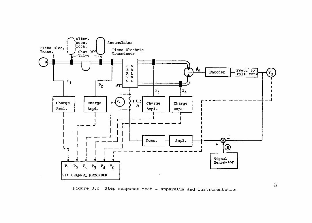
Alter. Accu, Loca,

\ / Shut OffT^Valve -

AccumulatorPiezo Elec. j Trans Piezo Electric

Transducer

Freq. to Volt convEncoder

I10.3ChargeAmpl.

ChargeAmpl.

ChargeAmpl.

ChargeAmpl.

I I J

AmplComp

SignalGenerator

SIX CHANNEL RECORDER-JVDFigure 3.2 Step response test — apparatus and instrumentation

80

(Pg = constant).1.2) Without accumulator-pump dynamics included

^ Gg)'2) Pump pressure setting 730psi (Test No. 2)

2.1) With accumulator (P^ = const)2.2) Without accumulator (P^ = G^Qg)

3) Pump pressure setting 950psi (Test No.3}3.1) With accumulator (Pg = const)3.2) Without accumulator (Pg = G^Qg)

In these tests , the effect of pressure setting on system behaviour was studied.

b) Accumulator close to the pump (Test No.4)At a pressure setting of 730psi step response tests were

taken with and without accumulator. This test was aimed to investigate the effect of accumulator location within the boundaries of the supply subsystem.c) Finally, in order to study how hydraulic system natural frequency variations affect the results, we increasedload inertia by a factor of 10:1 (Test No.5).

2Jm = 0.0043 lbg*sec *in (the original inertia)2J =0.05 lbr*sec *in (the "new" inertia) m f

3.5.2 Step Response Test ResultsThe six variables were recorded on the six

channel recorder as follows;

81

(1) Valve current - (ma)

(2) Encoder voltage - (Volt)

(3) Valve pressure - (psi)

(4) Pump pressure - P^ (psi)

(5) Motor input pressure - P^^ (psi)

(6) Motor output pressure P^^ (psi)

For tests 1, 2, 3 the accumulator was installed closeto the valve, and load moment of inertia was J = 0.0043 ' m2Ib^sec in, to obtain the highest hydraulic natural frequency.

3.5.2.1 Test No.lConditions

Pressure setting P^ = SOOpsi2Load inertia J = 0.0043 Ib^sec in m f

Fig.3.3 is for Pg = GpQg and Fig.3.4 is for Pg = const,

both the actual measurements on the recorder. Fig.3.5 to 3.9 are a magnification of 3:1 to make the comparison between the two cases easier.

The effect of pump dynamics is clearly observed in Fig. 3.5. There is almost a 100% increase in the time to peak itp) comparing between pump dynamics included and Constant

Supply pressure.

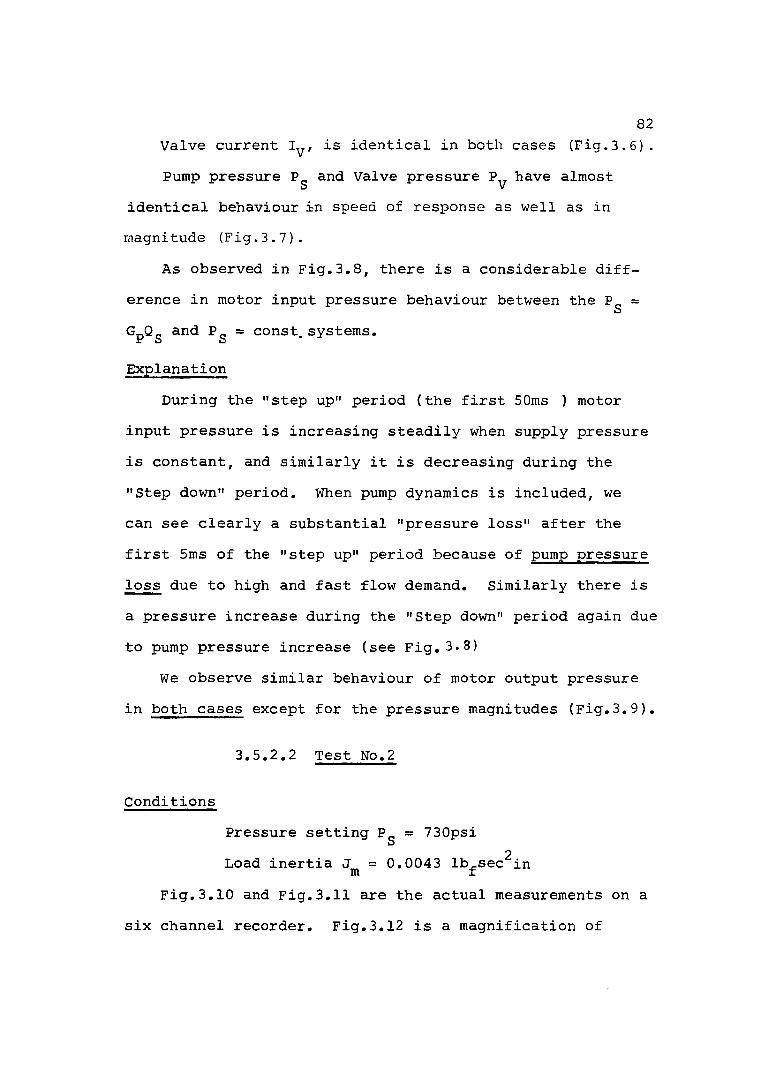
82Valve current is identical in both cases (Fig.3.6).Pump pressure Pg and Valve pressure P^ have almost

identical behaviour in speed of response as well as in magnitude (Fig.3.7).

As observed in Fig.3.8, there is a considerable diff­erence in motor input pressure behaviour between the Pg = GpQg and Pg = const, systems.

ExplanationDuring the "step up" period (the first 50ms ) motor

input pressure is increasing steadily when supply pressure is constant, and similarly it is decreasing during the "Step down" period. When pump dynamics is included, we can see clearly a substantial "pressure loss" after the first 5ms of the "step up" period because of pump pressure loss due to high and fast flow demand. Similarly there is a pressure increase during the "Step down" period again due to pump pressure increase (see F i g . 3.8)

We observe similar behaviour of motor output pressure in both cases except for the pressure magnitudes (Fig.3.9).

3.5.2.2 Test No.2

ConditionsPressure setting Pg = 730psi

2Load inertia J = 0.0043 Ikusec in m fFig.3.10 and Fig.3.11 are the actual measurements on a

six channel recorder. Fig.3.12 is a magnification of

MOTOR OUT PRESSURE

(psi)

MOTOR INPUT PRESSURE

PUMP PRESSUREVALVEPRESSURE

ENCODER VOLTAGE V„ (Volt)

VALVECURRENT

U)w M

O U1OO

-

H-

H-H-

200psi1OOpsi1Volt60ma SOOpsi00W

enCH

►dV3

oO3enrtW3rt

MOTOR INPUT MOTOR OUT PRESSURE PRESSURE

PUMPPRESSURE

ENCODER VOLTAGE VALVEPRESSURE

Vn (Volt) Py (psi)VALVECURRENT

w

wrt

*0Mment)O3enm

ooo U1(jO

no3enrtfu3rt

ro

en

M

SOOpsi 200psi60ma 1OOpsi1 Volt

85

P„=Constant

r4O

500 (psi)

0.0043 (lb sec in)

o

50msTIME

Figure 3.5 Encoder Voltage ( ) ' Comparison between Pg = const, and P^ = Qg

ciEP„=Constant

sec in)M

sI01g

50msTIME

Figure 3.6 Valve current (l^)^-Comparison between Pg=const. and Pg=GpQg

86

•HJ = 0.0043 (Ib^sec in)

CM•H

HcotoI

Pump Pressure P,

Valve Pressure P.

L ‘ ' T |50ms — ^TIME

Figure 3.7 Valve Pressure P^, Pump Pressure Pg

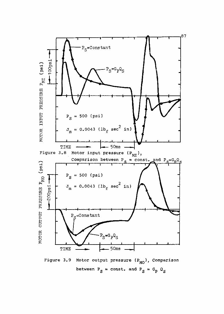
•Hm

H

HcocoHg

P4a

gg£

Pg=Constant

S P S

Pg = 500 (psi)

J = 0.0043 (Iku sec in) m ±

TIMEFigure 3.8 Motor input pressure (P^^),

Comparison between P = const, and P =G„Q

opf •HH

gFM P„=Constant

cgEMo£

TIME

Figure 3,9 Motor output pressure (P^^), Comparison between P = const, and P = G„

88

3:1 for comparison of the encoder output voltage (contro­lled variable). We did not present magnified figures of the other variables since one can see the same general behaviour as for the = SOOpsi pressure setting except for the magnitudes.

3.5.2.3 Test No.3Conditions

Pressure setting P^ = 950psi2Load inertia J = 0.0043 Ibusec in m f

Fig.3.13 and Fig.3.14 are the actual measurements on a six channel redorder. Fig.3.15 is a magnification of 3 : 1 for comparison of the encoder voltage (controlled variable). Again, only one variable was presented in its magnified form,from the very same reason.

Summary of the testsTests 1, 2, 3 were aimed to study system behaviour, as

measured by the six variables, at different pressure sett­ings, low, medium, and high pressure.

We conclude that there is consistency in system behaviour at all pressure levels. Pressure peaks increase as pressure setting iA increased and bocopie con­siderably high for high pressures.

VALVE CURRENT ly (ma)

ENCODER VOLTAGE V q (Volt)

VALVE PRESSURE Py (psi)

PUMP PRESSURE Pg (psi)

MOTOR INPUT MOTOR OUTPUTPRESSURE PRESSURE

^MI ^MO (psi)

wooow

H-M

N)

00U)6 Oma 200psi1 Volt 1OOpsiSOOpsi SOOpsiFigure 3.10 Step response - Pump dynamics included Pg = Gp Qg

4H-

'gMm

toc+mtiMmm0 301 wIo0 301 (+ SU3rt

ta3

■Smto01

•3to

IIootor+

VALVE CURRENT ly (ma)

ENCODER VOLTAGEVq (Volt)

VALVEPRESSUREV (psi)

PUHPPRESSURE Pn (psi)

MOTOR INPUTPRESSURE

"MI (psi)MOTOR OUT PRESSUREMO (psi)

o (jOOo

H-

H-

300psi 200psi60ma 200psi1Volt 1OOpsi

91

Pg GpQg

Pg= Constant

Pg = 730 (psi)

J = 0.0043 (Ibj. sec in) ra f

TIME — '— '— h50ms —

Figure 3.12 Encoder Voltage (V^) , Comparison between Pg = const, and Pg = Gp Qg

Y M jVE PRESSURE MOTOR INPUT PRESSURE MOTOR OUTPRESSURE

P_ (vsi) P»AT (psi) Pwin (psi)ENCODER VOLTAGEVALVE

CURRENTp .

mV^ (Volt)

WMWCOrt

hmCOtiooCOm

o U1

wH-

I03H-OCO

H-3Oh-'

CO 200psi1OOpsiIVolt60ma 300psilO

to

xn

MH-iQdh

oo3cort03rt

VALVE CURRENT ly (ma)

ENCODER VOLTAGE Vq (Volt)

VALVE PRESSURE Ey (psi)

PUMP PRESSURE Pg (psi)

MOTOR INPUTPRESSURE% (psi)

MOTOR OUT PRESSUREPpio (psi)m

w1 - 1

xnrt(D

MmcotJo3COm

o(jj

H-H*

Oo3COrtSrt

VJlH-

60ma IVolt 3 0 0 p s i P O O p si 1 O O p si 2 O O p si

cow

94

•ptHO> P„=Constant

o>

§Ü

950 (psi)

0.0043 (IbrSec in)

50msTIME

Figure 3.15 Encoder Voltage (V^), Comparisonbetween P = const, and P = G„ Q

95

Discussion of the results and conclusions The desired performance characteristics of a system of

any order are specified in terms of the transient response

to a unit step function input of the controlled variable.The variables we investigated were, the controlled

variable (Encoder voltage) and valve input pressure (Supply pressure).

The performance of the system may be evaluated in terms of the following quantities:(1) Maximum overshoot (Damping ratio)(2) Frequency of oscillations (u )(3) Time to maximum overshoot (t^)(4) Settling time (t ) (2% or 5%)

We will study the Effect of Pump Dynamics on the res­ponse of our system in these terms.

Let us perform now the comparison between the step response results obtained for the two conditions:(1) Pump dynamics is included (Pg = GpQg), when the accu­mulator is not connected to the system. (See Fig.3.3, 3.10, and 3.13).(2) Pump dynamics not included (P = constant), when the accumulator is connected to the system suppressing pump pulsations. One can observe clearly the "constant" pressure maintained at the pump manifold and at the valve input (See Fig.3.4, 3.11, and 3.14).

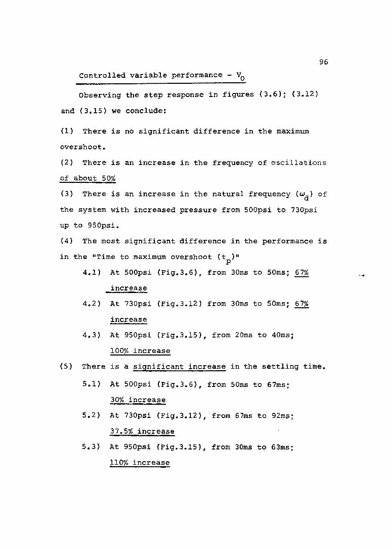
96Controlled variable performance - V_

Observing the step response in figures (3.6); (3,12) and (3,15) we conclude:

(1) There is no significant difference in the maximum overshoot,(2) There is an increase in the frequency of oscillations of about 50%(3) There is an increase in the natural frequency (w^) ofthe system with increased pressure from SOOpsi to 730psiup to 950psi,(4) The most significant difference in the performance is in the "Time to maximum overshoot (t^)"

4.1) At 500psi (Fig,3,6), from 30ms to 50ms; 67% increase

4.2) At 730psi (Fig,3,12) from 30ms to 50ms; 67% increase

4.3) At 950psi (Fig,3,15), from 20ms to 40ms;100% increase

(5) There is a significant increase in the settling time.

5.1) At SOOpsi (Fig,3.6), from 50ms to 67ms;30% increase

5.2) At 730psi (Fig,3,12), from 67ms to 92ms;37,5% increase

5.3) At 950psi (Fig,3,15), from 30ms to 63ms;110% increase

97

ConclusionExcept for the overshoot, we get a constant "worsening"

in system performance due to pump dynamics.3.5.2.4 Accumulator installed close to

the pump (Test No.4)In order to investigate the effect of

accumulator location on system behaviour, we installed the accumulator "close to the pump". The step response test was performed at 730psi pressure setting for both cases:(1) Pg = GpQg - Fig.3.16(2) Pg = const - Fig.3.17.

In the case when the accumulator was installed "close to the valve" the distance was about 2(in) from the valve upstream. When it was installed "close to the pump" the distance was about 2(in) from the pump downstream. The line connecting pump and servovalve is 16(in) long.

Discussion of the resultsIn order to compare the performances of the system for

the two accumulator locations, we present a superimposed, "magnified" version of the different variables investigated. (See Fig.3.19 and Fig.3.20).

For comparison of Pg=const. and Pg=GpQg, see Figure 3.18. Let us now discuss the behaviour of encoder voltage V^.Vg - Encoder output voltage

(1) For both cases, with pump dynamics (Fig,3.19) and with

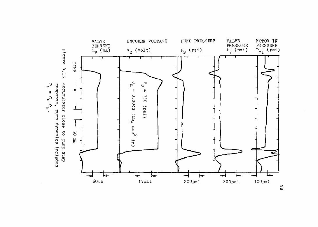
M Mm m Il >o

o►tjo -m 1

en

MH-iQfD

en>oo

o 3 (n m (ürtOtjoMoo, en tüa

3n ti

IH- 30 tn M rt

01 Wmo,

VALVE CURRENT ly (ma)

ENCODER VOLTAGE V q (Volt)

PTMP PRESSURE

P g ( p s i )

VALVE PRESSURE Py (psi)

MOTOR INPRESSURE

(psi)

o wow

H-

H-

60raa IVolt S O O p si 1 O O p siS O O p si

H-iQ3Hmwv->

o >o o0 nen 3rt 3(U 33 Hrt 0»

rten Oc h

tJt l oM Mo

m(D

hm rten OenC *3M

JDPI

w Wrt

II fD*3

Oo 3a (Den tort tJfU O3 3rt CO. (D

VALVE CURRENT ly (ma)

ENCODER VOLTAGEVq (Volt)

VALVE PRESSURE

VD.r (psi)MOTOR INPRESSURE

?MI (psi)

1 V o l t60m a S O O p si lOOpl

VD

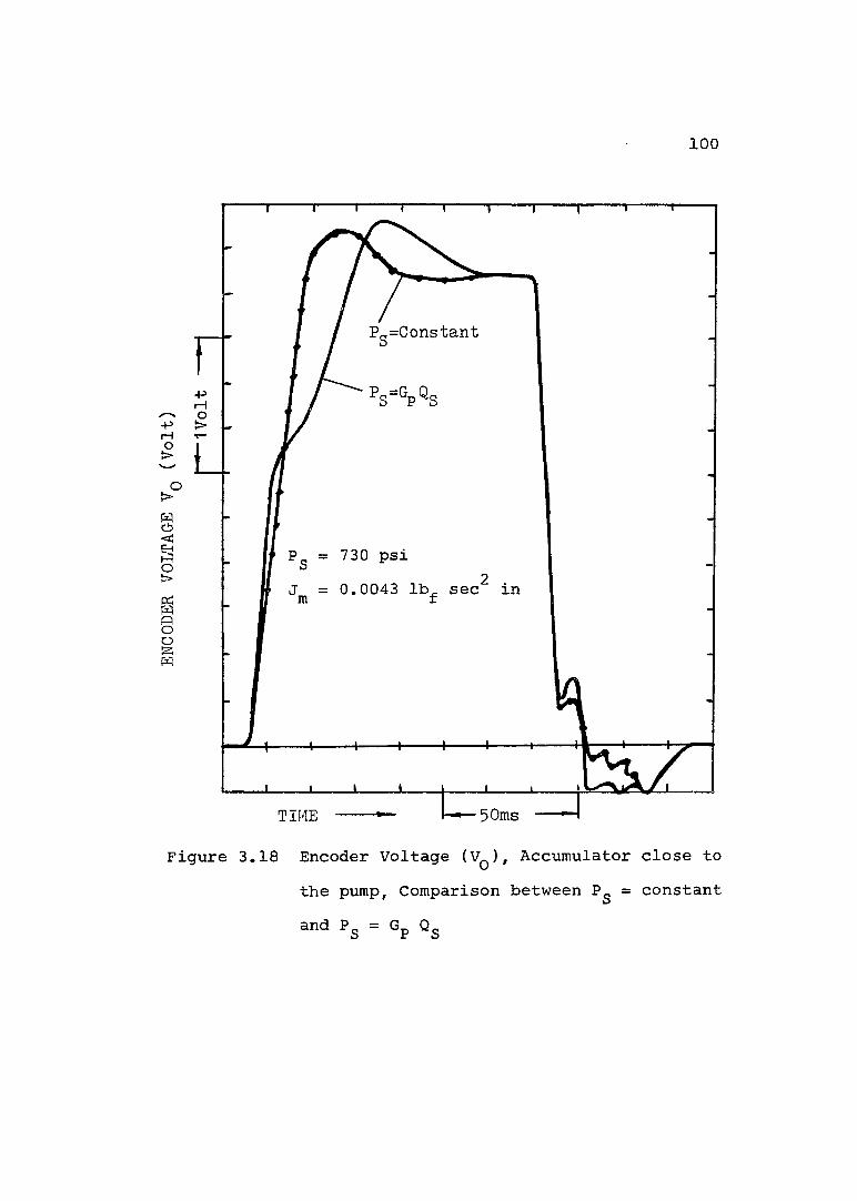
1 0 0

P„=Constant

-prHO>O>

730 psi0.0043 Ibj. sec in

Io!aH

50msTIME

Figure 3.18 Encoder Voltage (V^), Accumulator close to the pump. Comparison between Pg = constantand Pg = Gp Og

101

Accumulator Close to Pump

Accumulator Close to Valve

Pg = 730 psiJ = 0.0043 lb. sec in m f

TIME ^ j-*— 50ms' —Figure 3.19 Encoder Voltage (V^); Pg = Qg, Comparison

between accumulator close to pump and accumulator close to valve

1 0 2

Accumulator Close to Pump

Accumulator Close to Valve

■piHO>O

= 730 psi0.0043 Ib^ sec in

o

50msTIMEFigure 3.20 Encoder Voltage (V^); Pg = const.,

Comparison between accumulator close to pump and accumulator close to valve

103

constant supply pressure (Fig.3,20) we observe a slight increase in the maximum overshoot when the accumulator is located close to the pump. This result suggests that at this location the accumulator is "helping" the pump to deliver the needed flow.(2) There are no significant differences in the frequency

of Oscillations nor in settling time or the time to peak.Generally speaking, there is no major change in the

performance of the controlled variable V^. The main reason is probably because of the short connecting pipe line. We would expect larger differences when the pipe lines would be longer and more hydraulic components would be incorporated in the supply subsystem.

3.5.2.5 Increase of load inertia J = 0.05mIb^sec^/in^Fig.3.21^ 3.22 (Test No.5)

We recall that the reason for consider-2ing the smallest possible inertia = 0.0043 Ibsec in

in our experiments was to achieve the highest possible hydraulic natural frequency (w )

4)3 D ^<j =(— 22— As we can see, variations in the

value of the inertia are the main cause for frequency variations, since all the other parameters in the equation are constant for a given system.

104

However, such a small inertia is unrealistic in practi­cal applications, so, an inertia ten times larger J =' ' = mnew10 attached to the motor shaft and the test was

repeated. We decreased system natural frequency by a factor of (10) causing instability at system gain setting and for the compensating network used in the previous case.

The compensating network was replaced by G^(S) = 1/(0,1 S + 1) = 100ms) and in this case the highestpossible gain was = 100 (ma/V).

Again, a superimposed graph of encoder voltage (con­

trolled variable) of the constant pressure and pump dynamics included cases are presented (Figure 3.23),

The main difference once again is in the time to maxi­mum overshoot t ; there is an increase from 80ms to 100ms P(25%), Obviously, the difference is smaller as systemnatural frequency is decreasing, (It was 67% for =0,0043 Ibsec^in.)

If one would increase further load inertia J . them'hydraulic natural frequency will decrease and will dominate system natural frequency, making the effect of pump dynamics insignificant.

MOTOR OUTPUT PRESSURE

MOTOR INPUTPRESSURE

PUMPPRESSUREVALVE CURRENT ENCODER VOLTAGE

(ma) V_ (Volt)

wM

IIOo3COr+(U3rt

(A)

tn

H-

H-

60ma IVolt 200psi 200psi1OOpsi

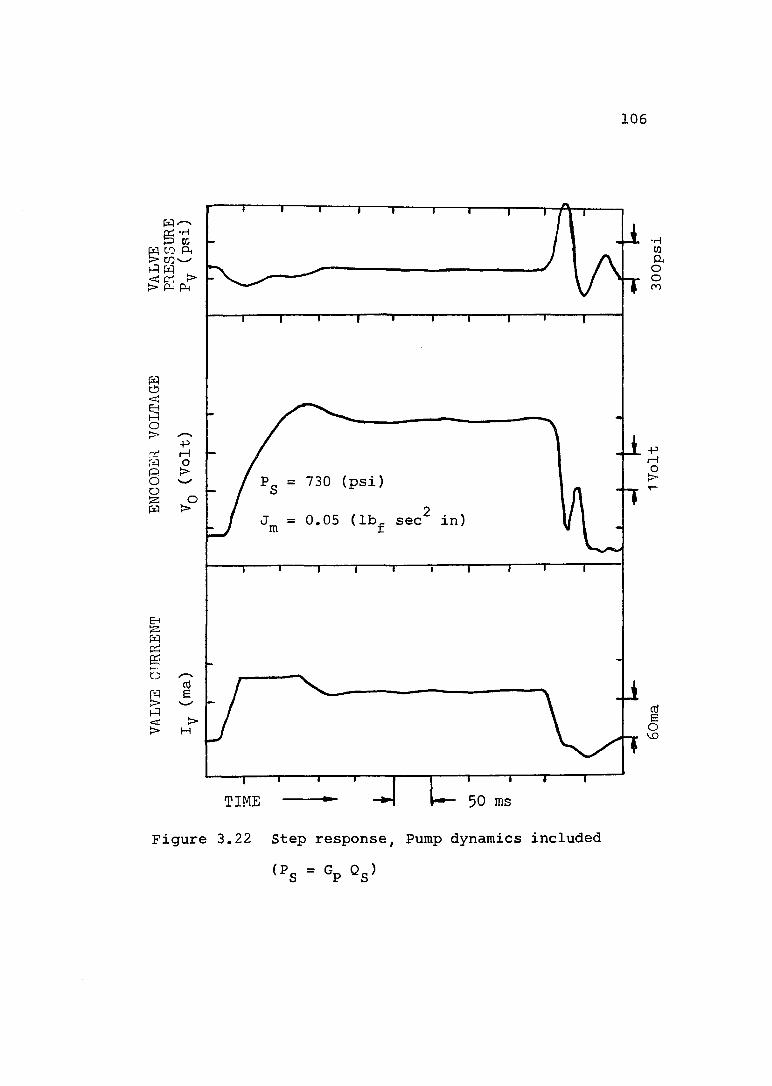
106

pi *H

O> 730 (psi)o>

in)

i>H

50 msTIME

•HWAooro

-PrHO

0}EOU)

Figure 3,22 Step response. Pump dynamics included

4H-iQCh

PUMP PRESSURE Pg (psi)

MOTOR OUTPUT PRESSURE

Pf O (psi)

MOTOR INPUTPRESSURE

i*MI (psi) 'w

H-

VJl

1OOpsi200psi200psi o

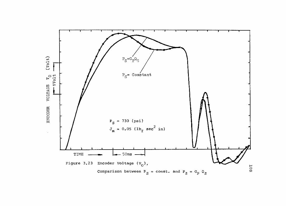
Po=Gt,Q

P^= Constant

P = 730 (psi)= 0.05 (Ib^ sec in)

TIME

Figure 3.2 3 Encoder Voltage ( ) ,Comparison between = const, and P„ =

109

3,5.3 Frequency Response Tests Outline (Frequency Domain)

Frequency response tests were designed to verify system behaviour in the frequency domain. The tests were

conducted using the NICOLET 560A analyzer in its frequency response mode up to a maximum of lOOHz range. Pump pressure setting for the frequency response tests was 730psi (medium range). A sinusoidal input signal was generated at the amplifier reference input voltage R = R^* sin(wt) by the Wavetek Model 114.

The transfer functions of interest:V Encoder Voltage output-2_(S) = ----------------------------------R Amplifier Reference Voltage inputP Valve Pressure input-_L(S) ------------------------------- ^R Amplifier Reference Voltage inputP Valve Pressure input— (S) = -------------------------^0 Encoder Voltage input' were derived in the theoretical part of this work.

The most important transfer function isP_

(S) — ■ Gp( S)^0 ^enco

110

Is''o ■'enco . ,V' M + ■“ + J*

t> Üp pbecause it does not include valve dynamics, compensation network dynamics nor hydraulic system and load dynamics (due to high natural frequency).

It enables us to investigate pump dynamics (in frequen­cy domain) for a valve controlled rotary actuator by moni­toring Valve input pressure and Motor shaft rotation while applying a sinusoidal voltage at the amplifier-reference

input. To achieve satisfactory results,load inertia has to be removed and the highest possible hydraulic natural frequency in the particular system has to be achieved.

To investigate system behaviour in frequency domain in several operating modes, frequency response curves for the three transfer functions have been produced both in open loop and closed loop configurations.

The frequency response test generated 12 sets of data for the three transfer functions.

3,5.3,1 Instrumentation used in Frequency

response tests (see Figure 3,24)The various sensors which are an inte­

gral part of the system were used to obtain the voltages

Accumulator

Piezo Elec- V.D. tr ie Trans- Pump duper

Piezo E lectr ic Transducer

F i l t e r

ChargeAmpl,

s VE AR LV V0 A

■valve

a,m

Gc(S)= 1

— Encoder — Preq / v o l t ——

TS+1 ampl

, VR

'0NICOLET 660A Analyzer

^ I n p u t Input R RSignalGenerator

Figure 3.24 Frequency Response test - Apparatus and instrumentation

1 1 2

needed for the analyzer input channels.The analyzer is the (FFT) NICOLET 660A type analyzer

used in its frequency response mode. The hard copy outputs include amplitude ratio and phase angle with linear y axis in dB and logarithmical frequency on x axis (Bode plots).

Transfer functions analyzed

Pg V P— (S); — (S) and— 2. (S).R R VoGain setting during the frequency response tests was

^ampl = (ma/V).

We will present now just a few curves from the results obtained during the frequency response tests. The sample curves in open loop and closed loop configuration, are for the three operating points 25ma, 50ma, and 75ma and for small and medium input amplitudes ±12.5ma and + 20ma.

In order to be able to estimate natural frequency and later on to compare the experimental results with computer results, numerical values for ampl. ratio AR and phase angle <p were taken from the (FFT) NICOLET 660A analyzer at several frequencies using the cursor. The results are pre­sented in tabular form attached to each frequency response curve.

3.5.4 Frequency Response Test Results

The frequency response curves and the attached

113

tabular results are as follows.Pc3,5,4.1 The transfer function— (S)

Ü ( s ) ! U l 2 ! ! E i _ . (3.2)^ . , Gph'S) — + + 1

1) Open loop. Fig.3.25, at the operating condition 50ma ± 12.5ma

2) Closed loop. Fig.3.26, at the operating condition 25ma 1 12.5ma

3.5,4.2 The transfer function— — (S)R

^0, ^i ^ampl ^enco ^-- = — —*----------------- K---------------------R S 2fs S 2£s

( + — "■ — + 1 ) ( y + — — + 1 ) ( S )V “v ^ “ h

(3,3)1) Open loop. Fig.3.2 7 at the operating condition 75ma

±12.5ma2) Closed loop. Fig.3.28 at the operating condition

75ma — 12.5maPc3.5.4.3 The transfer function (S)Vo

Pc D— (S) -- Gp(S) (3,4)* %enco

NICOLET SS0A 50.00000 HZ

1 35 . S DG VLN- 1 1 . 2 «dB C

W(HZ) AR(dB) 0(DG)

SFigure 3.25 — (i w ); Open loop, Operating pointR50m a ± 12.5ma

0.13 -10 .0 13.30.25 -10.0 - 12.70.38 - 9 .8 - 17.10.63 - 6.0 26.61.00 - 7.1 17.01.50 - 6.6 16.02.00 - 6.4 16.93.00 - 5.4 18.84.00 - 4.5 20.65.00 - 3.7 19.0

10.00 1.0 6.315.00 2.0 - 23.420.00 2.1 - 62.725.00 1.8 -107.630.00 1.2 -136.635.00 - 0 .8 —166.937.75 - 2.4 179.440.00 - 3.9 172.845.00 - 7 .4 152.450.00 -11.2 135.8

HM

NXCOL.ET 6S0A50.00000 HZ

5 4-S3

SS

DG VLNC

W(HZ) A R ( d B ) 0 ( D G )

50

Figure 3.26 — (i w ); Closed loop, Operating point R25ma±12.5ma

0.13 -23.9 67.90.25 -22.5 48.21 .00 -19.3 15.52.00 -18.8 14.93.00 -17.8 15.05.00 -15.7 13.08.00 -12.3 1.9

10.00 -10.5 - 11.012.00 - 9 .0 - 29.415.00 - 7.0 - 59.917.00 - 6.2 - 84.520.00 - 7.1 -121.925.00 -10.9 -174.125.62 -11.4 -178.527.00 -18.8 170.830.00 -15.4 152.835.00 -19.6 124.640.00 -24.2 100.945.0 -28.6 27.750.00 -33.8 54.8

(ji

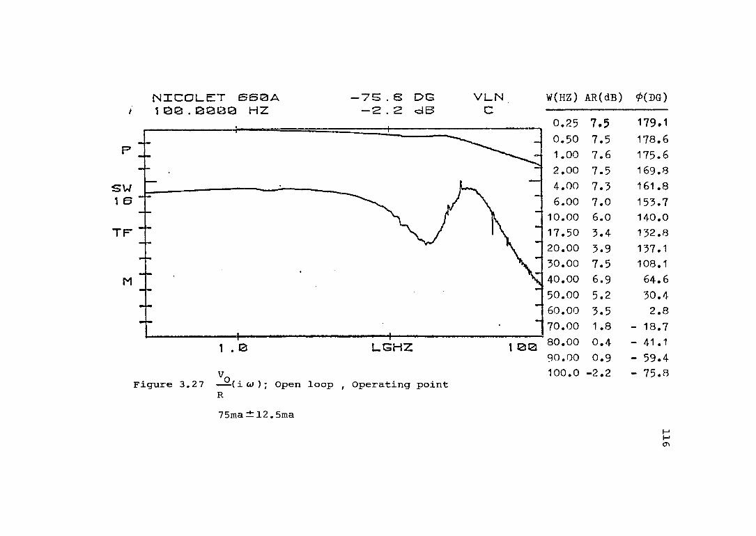
/NICOLET GS0A 100.0000 HZ

-75.S D0 - 2 . 2 d B

-------------\ , ■ -■ ,

VLNC

W(HZ) AR(dB) 0(DG)

0.25 7.5 179.10.50 7.5 178.6p 1.00 7.6 175.62.00 7.5 169.8

s w 4.00 7.3 161.81 G 6.00 7.0 155.7

10.00 6.0 140.0T F 17.50 3.4 152.8

20.00 5.9 157.150.00 7.5 108.1

M 40.00 6.9 64.650.00 5.2 50.460.00 5.5 2.8

■ 70.00 1.8 - 18.7

1 . 0 LGHZ 1 00 80.00 0.4 - 41.190.00 0.9 - 59.4100.0 -2 .2 - 75.8

Figure 3.2 7 --(i w ); Open loop , Operating pointR75ma ± 12.5ma

<T>

NICOLETT ee^A5 0 . 0 0 0 0 0 HZ

- 3 7- 1 e

5s

DGcjB

VLNC

0.S LGHZ

Figure 3.28 — ^ (i w ); Closed loop. Operating point R75mad:l2.5ma

W(HZ) AR(dB) 0(DG)

0.15 - 3.1 178.90.25 - 3.3 179.10.38 - 3.7 179.50.50 - 2.7 176.0

— 0.63 - 2 .6 172.50.75 - 2 .8 176.31.00 - 2 .7 171.92.00 - 2.9 165.33.00 - 2.9 157.84.00 - 3.0 150.95.00 - 3.1 143.1

10.00 - 4.5 100.9

\ c 15.00 - 9.5 71.520.00 -13.2 76.525.00 -11.7 67.3

0 30.00 -11.5 46.835.00 —12.6 18.440.00 -14.7 — 6.145.00 —16.6 - 25.350.00 —18.8 - 37.5

H

\

NXCOL.ET 6S0A50.00000 HZ

1 05 . 3 DG VL.N-25.S as C

0 .5 LGHZ S 0

Figure 3.29 -- (la»); Open loop.V,GOperating point 50ma±20ma

W(HZ) AR(dB) ^(DG)

0.13 -18.3 126.10.25 -26.2 -143.70.50 ' -19.0 -125.01 .00 -18.1 -134.02.00 -15.1 -131.05.00 -12.8 -132.68.50 -12.0 -135.5

10.25 -10.8 -144.815.00 - 9.0 —166.616.25 - 8 .4 -177.916.75 — 8.4 178.519.00 — 8.8 147.720.00 - 9.5 148.025.00 -11.8 116.130.00 -12.6 100.035.00 -14.1 93.140.00 -17.0 100.845.00 -20.1 106.550.00 -25 .8 105.3

MH00

MICOLET 6S0A 53.33333 HZ -25

07

DG V1_NC

W(HZ) A R ( d B ) 0 ( D G )

SW 1 e

T F

M

Figure 3.30 !i w ); Closed loop.

Operating point: 5 0 m a ± 12.5ma

0.25 -25.1 -103.40.50 -19.3 -147.60.75 -22.5 -149.41.50 -17.8 -157.25.00 -14.4 -145.07.00 -13.9 -142.8

10.00 -13.2 -147.213.00 -11.9 -155.415.00 - 9 .8 -164.516.50 — 8.8 -178.416.75 - 8.9 179.819.00 — 6.8 152.520.00 - 7 .6 143.824.00 - 7.6 111.925.00 - 7.3 104.530.00 -10.8 89.235.00 -14.6 85.940.00 -18.1 78.545.00 -21.7 83.250.00 -25.7 74.9

MKD

120

1) Open loop. Fig.3.29, at the operating condition 50ma ± 20ma

2) Closed loop. Fig.3.30, at the operating condition 50ma ± 12.5ma

Before going to discuss the next test results, we wishto point the readers attention to the "dotted" region inthe frequency response curves of Fig.3.29 and Fig.3.30.We observe discontinuities in the phase angle ( ) andmagnitude (M) curves at very low frequencies (0.1 to 0.25Hz). We performed further study into the cause of thisbehaviour, and came to the following aonclusions :(1) The discontinuities appear mostly in the frequency

response curves involving pressure as one of thePg Pgvariables i.e., in (iw) or (iw) transfer

' 0functions.

(2) Observing the variations of the pressure as a function of time we obtained a highly non, -sinusoidalbehaviour of the pressure.

(3) In the low frequency range, coulomb friction effects the pump and actuator are more significant.

We believe these findings are the explanation to the discontinuity phenomenon. Such low-frequency data cannot be considered very reliable.

1213,5.5 Accumulator Included In Frequency Response

Tests

In order to study the effect of an accumulator on system frequency response, several frequency response curves were produced with accumulator included in the system.

Let us perform now a short analysis to include accumu­lator in the system:

We would like to obtain the transfer function— — (in)Gv

including the accumulator

I II Accumulator

Ps = Pm = Pv

Qs = On + Qv 0.5)

Pq Q„— (S) = G-(S) ; — = G=(S) = sGs ^ "

122

So we get now

Qs = Ga(S) Pg + Oy (3.6)

Pg - G,(S) = Q„ (3.7)Gp(S) a S -V

Finally

Q,; - — + G^(S)V Gp(S)

(3.8)

whereaccumulator compliance = 5 * 10~^ in^/psi and

pump transfer function Gp(S) could be approximated

Gp(S) = -53.18 (-- -— + 1) (3.9)^ 23.72

neglecting the second order term in the denominator.PgDeriving— (S) and substituting numerical values will

give.

- 53.18 (— ^— + 1)— (S) = — T,------------ 23^J72----------- (3.10)Q,, S 2 * 1.256 * S

^ + + 19.45 9.45

which could be simplified to

(— ^ + 1)Pq 23.72— ^ (S) = - 53.18------------- (3.11)Ov JL+ 1

123

PgThe transfer function - (S) developed during theVotheoretical analysis is the most suitable for our purposes.

We found

P. D— (S) = — G (S) (3.12)Vo %enco

which is exactly the "pump transfer function" or the"Supply Subsystem - output impedance",

Thus, we produced several frequency response curves of

Pg— (iw) with the highest frequency at 50Hz including theVoaccumulator.

The transfer function just developed

53.18(---- + 1)(g) ________ 2 3 ^ _____

Os JL+ 14

is nothing else but the "Supply Subsystem - output impedan­ce" .

Enclosed is a sample of the experimental results (one of many curves produced) together with the numerical values of AR and 0 taken from the EFT. (Figure 3.31)

Finally, the experimental frequency response curve and the theoretical transfer function are presented superimpos­ed on Bode diagram showing an excellent agreement, (Fig.3.32)

NICOL-ET 660AS0.00000 HZ

W(HZ) AR(dBJ 0(DG)VLN-23.20.15 -36 .6-24.1 -39.9-23.7 -46.3-27.71 . 0 0 -58.4

-60.1-33.4-60.5-35.8

-39.2 -53.2-41.6 -47.1-45.2 -39.7-45.4 - 20.2-45.7 -13.4-45.1- 10.00

- 1 5 . 0 0 -42.9r 20.00 - 42.225.00 -41.530.00 -41 .035.00 - 42.1 -27.840.00 -43.8 -39.5

- 52.645.00 -45.2-64.450.00 -45.3

Figure 3.31 (i w ) Open loop. Operating point:V.50ma±: 12.5ma, Frequency response including accumulator dynamics

-20 Actual Measurment

Curve Pitting Asymptote-40

Accumulator Transfer Function

25.72

10.0 FREQUENCY(rad/sec)1 . 00.2Figure 3,32 --(i w ) = K G (S) Estimation, by curve fitting, of system

with an accumulator frequency response Ln

126

ConclusionThe output impedance of the supply subsystem including

the accumulator would be

53.18 (— ^ + 1)— (S) = ------------- (3.13)

1)For reference, the output impedance without accumulator

i.e., pump only was

53.18 (--§--- + 1)P_ 23.72— - ( S ) = — ——' ■ (3.14)

2 * 0.6 * S , ,■' + ' ' - + 1115.66^ 115.66

3.5.6 Comments On The Results

At this point we can not make any conclusion regarding the tests since we have not yet explained and developed the frequency response computer simulation.

A detailed discussion about frequency response results will be given in Chapter 5 after we will obtain computer results and superimposed graphs could be generated.

To summarize, this section of the experimental program was just a presentation of the results and an explanation of the frequency response test procedure.

CHAPTER 4 COMPUTER SIMULATION

4.1 Introduction

The earlier chapters presented the theoretical analysis for an overall hydraulic servosystem which includes pump dynamics and the results of an extensive experimental program, aiming at investigating the effect of pump dynamics on system performance. We now turn to the development of a computer simulation which can "duplicate" the behaviour of the real system. Computer simulation is an integral part of such a study and comparison of the experimental results with computer output will give us a high level of confidence in its validity and therefore in the whole study.

If computer model modeling is in its general form, it can simulate any such servosystem (including ones not yet built) simply by changing its parameters and/or initial conditions. Having tested the system in time domain and frequency domain, computer simulation will be developed to give results in both domains.

127

128

Historically, electric analog computer dominated the time domain analysis and the design of a variety of

engineering systems. Digital simulation languages have now largely replaced the analog approach. Probably, one of the more versatile and complete languages is CSMP, the Continuous System Modeling Program of IBM Corporation.It is widely used by engineers, and will be our simulation language in the time domain (10).

We used frequency-response methods in our experimental program and we wish to address the computer aids available to the engineer in the frequency domain in order to verify these tests.

Special purpose "canned" programs for evaluating and plotting W(iw) for a selected range of frequencies are widely available in computer libraries. We selected the frequency - response calculation method based on matrix techniques. This approach has certain features and advan­tages that make it of considerable practical interest.The Speakeasy language is particularly easy to use in these cases, and it can give tabular or graphical represen­tation of the results (10).

Finally, we wish to point out that both, the digital simulation technique CSMP for obtaining time response and the matrix method Speakeasy, for linear - system frequen­cy - response deal directly with the basic simultaneous

129

differential equations describing the system, and also produce information on all the system variables, not just a single output / input pair (10).

4.2 CSMP - Time Domain Computer Program

Let us now present the CSMP computer program that was developed to simulate our system in time domain. In our theoretical analysis we defined the basic hydraulic servo­system components; actuator, control unit and power source as; "Supply Subsystem", "Control Subsystem" and "Load Subsystem". By physical simplifications of the system and by numerical verification of parameters we showed earlier that our subsystems are dominated by the pump, servovalve, and rotary actuator connected by short pipe lines. Pump- valve pipe line compliance (neglecting inertia and friction) was included in Felicio's pump dynamic model. Similarly, valve - actuator pipe lines compliance (again neglecting friction and inertia) were included in the hydraulic motor model, which is a common practice in the literature (2).

It is known that linearized models are aimed at describ­ing the system when operating with small perturbations around an operating point. The most difficult component to be linearized in our system is the servovalve due to its flow- pressure characteristic which is highly nonlinear. Our

130

analysis involves large valve opening and therefore signi­ficant supply pressure variations, so we no longer can claim that we are operating with small perturbations around an operating point. Therefore, in our CSMP program we used the original nonlinear valve flow-pressure equations

Q = Ky Iy(Pg - P)^ (4.1)

where = 0,00965 (cis/ma/(psi)^).After completion of the program which included pump

dynamics (P^ = G^Qg), a second program, using different notations, was run using constant supply pressure Pg = constant = P^^^ (i*e., no pump dynamics). In order to compare the results and study the effect of pump dynamics on the response of servosystem the output variables were superimposed using the PAGE GROUP feature available in CSMP.

Two different models have been developed, each aimed for a specific purpose in our study, and their description will be given next.

Since CSMP simulation produces information on all system variables as a function of time, and having recorded six different variables during our experimental program, we compared them with the computer output of these same six variables. Discussion on these outputs and their correla­tion with experimental results will come later in Chapter 5,

131

when we superimpose the two results.

4.2.1 Nonlinear Computer Model

The program was based on the nonlinear represen­tation of:(1) Pump Dynamic model (Felicio) which includes the non­

linear term of dry friction F^.(2) Servovalve nonlinear flow-pressure equations

°1 = •'in In <I’s -and

«2 = Kin In (P2 ''Where K.^ = K^, and = I^.

(3) Hydraulic actuator (motor) torque equation including the nonlinear friction terms with the appropriate parameters , C^, T^ found experimentally.

“m - ^2> = \ 'L + Bm ^

+ A If 'h + ^2» +1 ml I m|

(4.2)where

®m = ^d^ °m +

K = 0.0 m

13 2

In the continuity equations, the flow rates into the valve Q^, out of the valve Qg well as the motor input pressure and the output pressure P^ appear as variables.Since P^ and Pg were recorded experimentally, we used these computer outputs in our evaluation of system and computer simulation correlation. The nonlinear model is regarded as the most adequate simulation of our system since it includes all the terms to the best of our knowledge.

Fig.4,1 is the presentation of the CSMP program in flow-chart form. The program including pump dynamics ( P^= GpQg) was named as RUN I and the program with constant supply pressure P^ = const was named as RUN II.

4.2.2 The Alternative Model

During the computer work we developed a second model, based on the more "compact" representation of the hydraulic motor continuity and torque equations explained in section 2.5, using the definitions for and P «

Ql = (Qj + Qgl/Z; = ?! - ?2 (4.3)

whereQ Load flow rate equal to pump flow rate

P^ Load pressure(pressure drop across the actuator).The main advantage is that we decrease the number of

variables from ; QgjP jPg to and P^ and pump flow rate

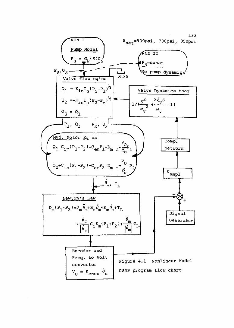
/^RUN IPump Model

133Pgg^=500psi, 730psi, 950psi

Ps'OsValve flow eq'ns

°1 = Kinln(Ps-Pl)'

0? =-KirI^(Po-P_)'

1

2 ^in^n'^2 r

Q n = Q

•Pr O

UN II— J#Pg=const

o pump dynamics

Valve Dynamics Moog s

1/ (— —7 4 Hi)

^1' ^1 ^2' ®2

Hyd. Motor Eq'nsV.

Newton s Law

^m Q

^m |"m|

Comp.Network

I Encoder and Freq. to Volt converter^0 “ *enco *m

Signal Generator

Figure 4.1 Nonlinear Model CSMP program flow chart

134

Qg = as well as pressure drop across the actuator =P^ - Pg are more often measured, rather than the individual flow rates and pressures in the pipe lines connecting the valve with the motor.

Another difference between the original nonlinear model and the "Alternative model" is that friction nonlinearities in the pump model and the motor torque equation have been neglected . By doing that, we studied the effect of the nonlinear friction forces on the behaviour of our system. These friction forces are known to have destabilizing effects when slow and small motions occur around an opera­ting point. The assumption was that these effects will be negligible in case of fast and large servosystem operation.

This assumption was confirmed during our numerous computer runs, leading to the conclusion that in future studies, when fast and large load motions are of interest coulomb and dry friction effects can be neglected.The hydraulic motor equations Continuity equation

Where ;

^tm ^im + = Leakage coefficient.

= (0 + A Load flow rate.

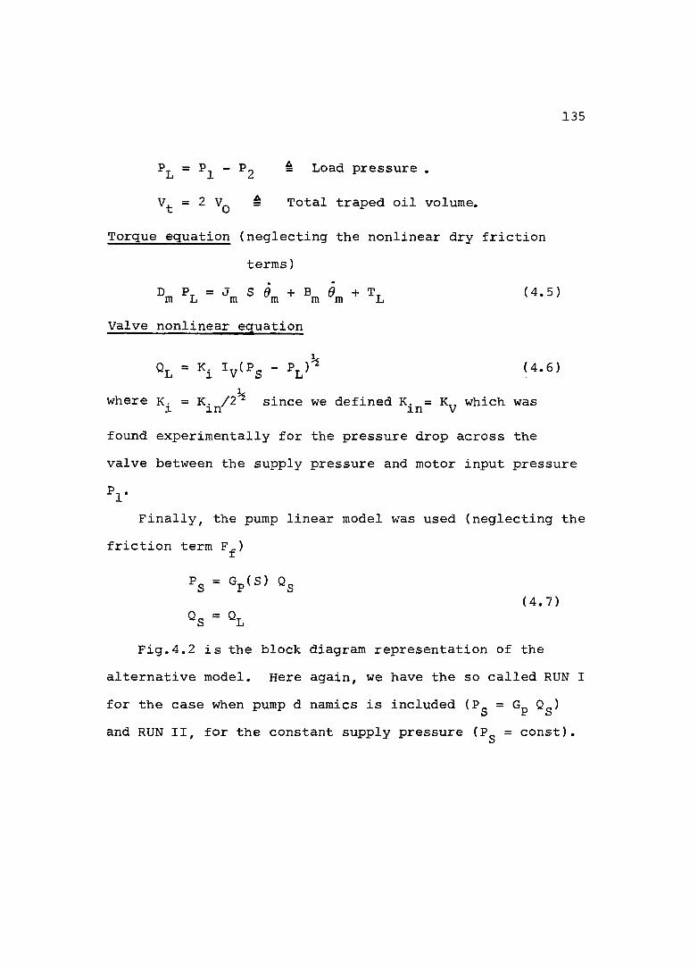
135

Pl = P, - P - Pg = Load pressure

= 2 Vq = Total traped oil volume.

Torque equation (neglecting the nonlinear dry frictionterms)

Valve nonlinear equation

°L = ■'i ly'Ps - '4-slpwhere k. = K. /2^ since we defined K. = K„ which was 1 in in V

found experimentally for the pressure drop across thevalve between the supply pressure and motor input pressure

Pi'Finally, the pump linear model was used (neglecting the

friction term F^)fPg = Gp(S) Og

(4.7)

Fig.4.2 is the block diagram representation of the alternative model. Here again, we have the so called RUN I for the case when pump d namics is included (Pg = Qg) and RUN II, for the constant supply pressure (P = const).

136= 500, 730, 950psi

RUN IPump

RUN IIP„=const

No pump dynamics

Valve dynamics

ÛJ Ci>

Comp

+C^_P, +T7î^ SP

ampl

Encoder+F/V ^O^^enco m Signal

Generator(output)

(Input)

Figure 4.2 Alternative Model - CSMP program flow chart

137

4.2.3. CSMP Input and Outputs

Let us now turn to the computer simulation output variables and results. As a first requirement we asked for the plot as a function of time of five from the six variables monitored in the experimental program.(1) - Encoder voltage(2) ly - Valve current(3) Py “ Valve pressure.

In our case it is identical to pump pressure since we included pipe and filter compliance in the pump equation.(4) P^ - Hydraulic motor input pressure(5) ^2 ” Hydraulic motor output pressure.

In order to differentiate between the various outputs (and variables) the letter "N" was used for all the variables in the nonlinear model, and no subscript for the variables of the alternative model. For example PSN and PS represent the nonlinear model and the alternative model pump pressure output respectively. The addition of the letter "C" will represent the variables when the supply pressure is constant (Pg = constant). Using the PAGE GROUP statement we superimposed the different outputs for comparison, analysis and conclusions. The output sequence and their explanation is given in the CSMP program. The input to the system, reference voltage R(t), was designed to obtain the largest and fastest valve opening.

138R = 0.7 + 4.12 * STEP(0.06) - 4.12 * STEP(0.2)

R(t)V 4-820L

0.7I

o.'oe 0.2 0.^2 t (sec)

This input will exercise the system in the two typical "Step up" and "Step down" situation in order to observe system behaviour in both cases. The same input was applied during the experimental program. The relative values 0.06 sec, 0.2 sec and the final value 0.32 sec were obtained from experiment and from the experience of numerous compu­ter runs, and leave enough time for the different variables to "settle down".

The input signal is "one sided" (only positive voltage), since the optical encoder operates for only C. W. (or only C. C. W. ) shaft rotation. The initial voltage 0.7V, was needed in order not to allow "negative" voltages to occur during the "step down" part (obtained experimentally).The maximum voltage 4.82V, was obtained experimentally as well and was aimed to achieve maximum valve opening.

The two models were developed to deal with "two sided" signals, which means C. W. and/or C. C. W, shaft rotation.

In the next section we will present the CSMP computer program, and the graphical "results".

139

4.2,4 The CSMP Computer ProgramTII l E p u m p d y n a m i c s INCLUDED IN A iERVO SYSTEM ANALYSISMETHOD RKSFXINIT* * * * * * * * * * * * * * * * * * * * ** PUMP p a r a m e t e r s* PUMP PARAMETERS PGR PSEF=730.0 PSI PARAM PSET=730.QPARAM XD0AR=0.15578 PARAM CGEFI=0.49I,C0EF2=3.l3l PARAM C0EF3=0.00299 PARAM C0EF4=65b.987 PARAM TAUP=8.696E-03 INCJN ICE=12.64E-03 INl ON ICPS=730.0 * * * * * * * * * * * * * * * * * * * * * * * * * * * * * * * ** HYDRAULIC MOTOR PARAMETERSPARAM CIM=13.0765E-05fC5M=2.2857E-C5,DM=15.9155E-02 PARAM KM=0.0PARAM CG=4l.7du0E04 , MIU=5 . 9 T6E-0t>, KH U = 0. bl6E-04 PARAM TC=2.0394,CF=0.0213 PARAM BL=0.0

8M=CD*MIU*DM+BL PARAM JM=0.0043

CTM=CIM+CEM/2.0* * * * * * * * * * * * * * * * * * * * * * * * * * * * * * * * * * * * * * * * * * * * * * ** PIPE LINE BETWEEN SERVOVALVE - HYD. MOTOR* COMPLIANCE INCLUDED IN HYD. MUTUR EQUATIONS PAKAM LVM=lo.0,DVM=0.375

V00=0.11045*LVM+0.5 VT=VUU*2.0

* * * * * * * * * * * * * * * * * * * * * * * * * * * * * * * * * * * * * * * * * ** PPIPE l i n e b e t w e e n p u m p - SERVOVALVE* COMPLIANCE INCLUDED IN PUMP EQUATIONS PAKAM LPV=15.3,DPV=0.375* FILTER VOLUME PARAM VFILT=6.1024 * * * * * * * * * * * * * * * * * * * * * * * * * * * * * * * * * * * * * * * * ** THE NEW PUMP COMPLIANCE - TAUPNEW - PAKAM TAUPN=21.9132E-03 * * * * * * * * * * * * * * * * * ** BULK MODULUS PARAM B£=100JD0.0 * * * * * * * * * * * * * * * * * * * * * * * * * * ** SERVOVALVE PARAMETERS PARAM KIN=0.00965)2

KI=KIN/SQRT(2.0)PARAM UMEG.AV=277.0, £ETAV = 1.0

NVSd*+7+ȣTO*0 = N01Xnv Ndd*Ntxnv=Ngynv

(O’T * 0*0*0*T-*irON03)MSNOd=N^XOV (N03*0*0)AI%30=i00N03

T3GDW N0Ii3I%3 - 0101133 ** * * * * * * * * * * * * * * * * * * * * * * * *

{MVT0d*C0-?ZeT6*lZ*Sd0I)1d1V3V=NV$d (Ntrd*fO-3ZET6'1Z*SdOI)1d1V3%=NSd

td300*NV03%0=NVTOd ty3O0*NO3%0=N1 Od

E31O0-N$0-NV0Wi0=NVn3d0 Ed300-NSO-NOHlD=N03dO

NV03*Z3300-t3300=NVAd% NC3+Z33 00-T3300=NAdV NVO3*iEET0P=NVGHlP)

N03*Affl*88=N0WiD (tvJVTr3*Z.TZ^0*O*30I )id1V3>i=NV03

(NTni*iLTZ*»r*0*30I)1d1V3d=M03 0*00EZ/( NVSd*NVAd?-0'00EZ*yV8aX)=NVt03

0*00EZ/(Nd3+NSd*NAdX-0'00EZ*%Vg0X)=NT03niOIlBd - SOIWVNAQ dWnd *

* * * * * * * * * * * * * * * * * * * * * * * * * * * * * * * * * * * * * * * * * * * * * * * * * * * * * * * * * * * * * * * * * * * * * * * * * * * * * * * * * * * * * * * * * * * * * * * * * * * * * * * * * * * * * * * * * * * * * * * * * * * * * * * * * * * * * * * * * * * * * * * * * * * * * * * * * * * * * * * * * * **%riOW "OAH - 3AlVAnA%3S - dWOd - 130rW dVINIINON ** * * * * * * * * * * * * * * * * * * * * * * * * * * * * * * * * * * * * * * * * * * * * * * * * * ** * * * * * * * * * * * * * * * * * * * * * * * * * * * * * * * * * * * * * * * * * * * * * * * * * * * * * * * * * * * * * * * * * * * * * * * * * * * * * * * * * * * * * * * * * * * * * * * * * * * * * * * * * * * * * * *

0 * 0=11(Z*0)d3iS*ZT*^-(90*0)d31S*ZT*>+i*0=d

W31SAS 3H1 Cl SindNI ** * * * * * * * * * * * * * * * * * * * * * * * * *

bVNAO0'S9E=0Zd NOON I0*Ç9C=0Td NOON I

0*0=001 NOONT0*0=01 NOONI

0*0=OV13i NOONI0*0=010031 NOONIo*r=oid NOONI

SNCIIIONTO 1VI1INI ** * * * * * * * * * * * * * * * * * * * * * * *

ZO-3111't=O0N3X kVWVd SV?i=wVdVd dPOl xoveo?3d ** * * * * * * * * * * * * * * * * * * * * * * * * * * * * * *

Eo-go'o?=zdOovi*eo-3o*T=Tdonvi wvwvdO'0tl=1dWVX KVdVd

S%313wvyvd WOlVSNPdWOO ONV d3IdI1dWV ** * * * * * * * * * * * * * * * * * * * * * * * * * * * * * * * * * * * * * * * * *

OfT

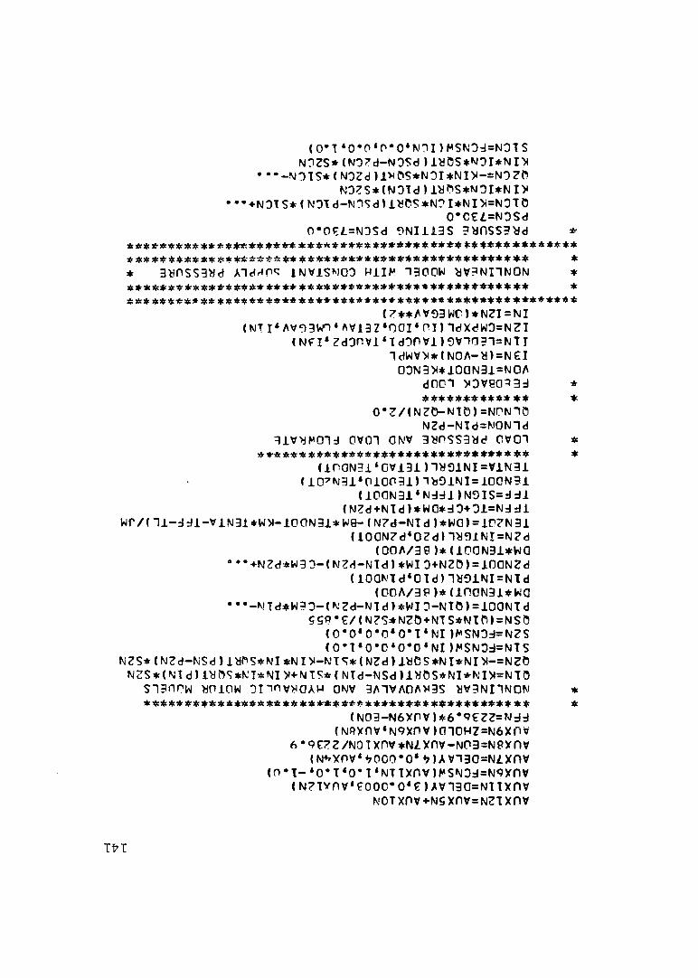
(0*1 *0*0‘0*0*N'1I )MSN'Od=NOTS N3ZS*(N37d-N3Sd)1%DS*N3I*NI%

•""-N3tS*(N3Zd)i%PS*N3I*NI%-=N3Zm N3Z$*(N3td)iynS*N3I*NI%

'"'+N3tS*(N3td-N3Sd1i%OS*N3I*NI>=N3tO0"CEi=N3Sd

n'0fl=N3Sd 3N I Ü 3 S ?aflSS3^d ********************** a********************************* a**********?************************************* ** 3%nSS3%d AldXpq 1NV1SM03 HilM 330DW %V3NHN0N ************************************************** ** * * * * * * * * * * * * * * * * * * * * * * * * * * * * * * * * * * * * * * * * * * * * * * * * * * * * * *

(?**AV93WC)*NZI=NI (NTI‘AV33W3*AV13Z*nOI*ni)1dXdW3=NZI

(NFI* Zd0r!Vl*Td3nVi)9V3n31=NTI 1dWVX*(N0A-a)=N€I 03N3»*10QN3i=NOA

dflOT %3Ve033d ** * * * * * * * * * * * * *

O*Z/(NZ0-NT0)=NI3N3C NZd-NTd=N0N3d

3iV%K01d OVOl ONV 3ynSS3dd CV03 ** * * * * * * * * * * * * * * * * * * * * * * * * * * * * * * * * *

(inaN3i*OVi3i n»91NI=VlN31 (iO^N3i*niOf'31) 3>j9iNI = 10GN3i

(iOON3i'Nddi)N9IS=ddi (NZd+NTd)*Wa*d3+01=Nddi

Wr/(3i-ddi-ViN3i$W%-i00N3i*W9-(N7d-NTd)*W0)=10ZN3i(100NZd*OZd)l%91NI=NZd

(OOA/39 )*(lD0N3i*WQ '"'+NZd*W33-(NZd-NTd)*WI3+NZO)=iOGNZd

(iOaNTd*OId)iy9iNI=NTd (CCA/3P)*(inON31*WG

•••-NTd*W33-(NZd-NTd)*WI3-NT0)=lDGNTd SSO"E/(NZS*NZ0+NTS*Nin)=NS0

(0*0‘0’0*OM*NI )PSN3d=NZS ( O M * 0*0*0*0* NI )MSN3d=NTS

NZS*(NZd-NSd)i%ms*NI*NI>-NTS*(NZd)i%BS*NI*NI%-=NZO NZS*(NId)i%BS*NI*NI%+NTS*(NTd-NSd)l%DS*NI*NI%=NTO

SIBHGW « m o w 3Iinv%0AW ONV 3A1VAOAX3S ÜV3NI3N0N ** * * * * * * * * * * * * * * * * * * * * * * * * * * * * * * * * * * * * * * * * * * * * * * *

(NG3-N6XrV)*6'9EZZ=Ndd (NQXnV*N9XnVIG10HZ=N6XnV

6"9Ezz/N0Txnv*NAxnv-N03=Nexnv (N^Xnv*t000"0't)AV13G=NlXnv

(O*T-*0*T*0* T*NTIXnV)MSN3d=N9Xnv (NZTynv*E0OC*O*E)AV33G=Nnxnv

NOTxnv+Nsxnv=NZTxnv

Tt T

142

S2CN=FCNSW(ICN,1.0tO.O,0.0)PiCNuO=(ülCN-CIM*(PlCN-P^CN)-CEM*PlCN-...DM*TECNOU)*(BE/VOO)P1CN=INTGRL(P10,P1CNDÜ)P2CNUÜ=(42CN+CIM*(P1CN-P2CN)-CEM*P2CN+...DM*TECNOO)*(BE/VOO)P2CN=INTGRL(P2ü,P2CNDD)TCN20T = (0M*(P1CN-P2CN)-BM*TECNUÜ-KM*TECNTA-TFFC-TL)/JMTFFNC=TC+CF*DÜ*(P1CN+P2UN)rFFC=SlGN(TFFNCtTcCNDÜ)TECND0=1NTGRL(TE00T0,TCN^0T)TECNTA=INTGRL(TETAO,TECNÜÜ)

» *************$***$*»**$*+*$**»*» LOAD PRESSURE AND LOAD FLOWRATc

PLCN0N=P1CN-P2CN QLCNUN=(QlCN-Q2CN)/2.0

* * * * * * * * * * * * * ** FEEDBACK LOOP

VOCN=TECNÛQ*KENCQ I3CN=(R-V0CN)*KAMPL IlCN=LEDLAG(TAUCPltTAuCP2tI3CN)I2CN=CMPXPL(lÜtlDUtZcTAV,ONEGA V,IICN) ICN=I2CN*(ÜMEGAV**2)**»*******************»***$****$***»******$******

**¥*******************«*** *«*41**** V*****W ¥***'91*** ******************$************************* ALTERNATIVE MODEL ** * * * * * * * * * * * * * * * * * * * * * * * * * * * * * * * * * * * * * * * * * * * * * * * * * * * * * * * * * * * * * * * * * * * * * * * * * * * * * * * * * * * * * * * * * * * * * * * * * * * * * * * * * * * * * * * * * * * * * * * * * * * * * * * * * * * * * * * * * * * * ** PUMP DYNAMICS - FELiLlO - LINEARIZED

E01=(XDBAR*23 00.ü-KPV*PS+FF)/2 300.0* * * * * * * * * * * * * * * * * ** NO FRICTION TERM

FF=O.ÜEO = R E A L P L ( I C E ,0.04217,EDI)QTrtO=8i.l337*EO KPV=C0EFl-C0EF2*tÜ QR Eü=QTHO-QS-CUE F3 P01=OREO*COEF4 PS=REALPL(ICPS,TAUP,POl»

* * * * * * * * * * * * * * * * * * * * ** CONTINUITY EQUATIONS

PLD0T=(QL-0M*TEDUT-CTM*PL)*(4.v*bE/VT)PL=INTGRL(PLO,PLDOT)

» NEWTON,S LAWTEDD0T=(DM»PL-BM*T£UJT-KM*TEl A-T L-TFE)/JM

143

* * * * * * * * * * * * * * * * *♦ NO FRICTION TERM

TFE=0.0TEDOT=IN rCRL(TEOOTO,TEDDQT) TETA=INTGRL(TETAU,TEÜüT)

* * * * * * * * * * * * * * * * * * * * * * * * ** VALVE - NONLINEAR EQUATIuN

WL=KI*I*SQRT(PS-bd*PL)QS=wL*SW/3.855 SW=FCNSW(I,“ I.OtO.0,1.0)

♦ **** * * * * * * * *♦ FEEDBACK LOOP

VO=TEDOr*KENCO I3=(R-V0)*KAMPL I1=L£DLAG(FAUCPl,TAJCP^,13)I22=CMPXPL(10,100,2E7AV,OMEGAV,11) I=I22*(0MEGAV**2)

* * * * * * * * * * * * * * * * * * * * * * * * * * * * * * * * * * * * * * * * * * * * * * * * * * * * ** ************************************************ a l t e r n a t i v e MODEL WITH CONST. SUPPLY PRESSURE »* * * * * * * * * * * * * * * * * * * * * * * * * * * * * * * * * * * * * * * * * * * * * * * * * * * * * * * * * * * * * * * * * * * * * * * * * * * * * * * * * * * * * * * * * * * * * * * * * * * * ** PRESSURE s e t t i n g PSC=730.0

PSC=730.Q* CONTINUITY EQUATION

PLCDOT=(QLC-DM*TtCDOT-CTM*PLC)*l4.0*BE/VT) PLC=INTGRL(PLO,PLCDOT)

* NEWTON,S LAW TEC20T=(DM*PLC-BM*TEC0UT-KM$TELTA-TL-TFEC)/JM

* * * * * * * * * * * * * * * * ** NO FRICTION TERM

TFEC=0.0TECDUT=INTGRL(TED0T0,TEC20T)TECTA=INTGRL(0.0,TEC0UT)

* * * * * * * * * * * * * * * * * * * * * * * * * * ** VALVE - NONLINEAR EQUATION

QLC=KI*IC*SQRT(PSC-SWC*PLC) SWC=FCNSW(IC,“1.0,0.0,1.0)

* * * * * * * * * * * * * ** FEEDBACK LOOP

VOC=TECDOT*KENCO I3C=(R-V0C)*KAMPL I1C=LE0LAG(TAUCP1,TAUCP2,I3C) I2C=CMPXPL(IO,IOO,2ET a V,UMEGAV,I1C)IC=12C$(0MEGAV**2)

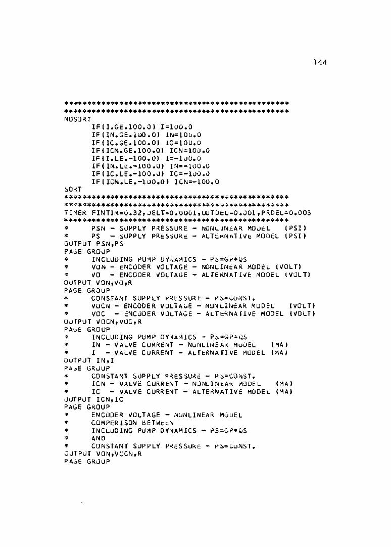
144

****$******$****+******$*****$**»»$*$**$**$***» ******$********************»**+****$***$***$*****NOSORT

I F d . G E . 100.0) 1=100.0 IF(IN.GE.100.0) 1N=100.0 I F {IC.GE.100.0) 1C=100.0 IF(ICN.GE.100.0) ICN=100.0 IF(I.LE.-100.0) i=-100.0 IF(IN.LE.-100.0) IN=-100.0 IF(IC.LE.-100.0) IC=-100.0 IF(ION.LE.-100.0) ICN=-100.0

SORT* * * * * * *

***************************************************TIMER FINTIH=0.32t JELT=0.0001,UUT0EL=0.001,PRDEL = 0.003 ***♦********************** ******** * * * * * * * * * * * * * * ** PSN - SUPPLY PRESSURE - NONLINEAR MOJEL ( P S D* PS - SUPPLY PRESSURE - ALTERNATIVE MODEL ( P S DOUTPUT PSN,PSPAuE GROUP* INCLUDING PUMP DYNAMICS - P S = G r *OS$ VON - ENCODER VOLTAGE - NONLINEAR MODEL (VOLT)* VO - ENCODER VOLTAGE - ALTERNATIVE MODEL (VOLT)OUTPUT VON,VO,RPAGE GROUP» CONSTANT SUPPLY PRESSURE - PS=CUNST.» VOCN - ENCODER VOLTAGE - NONLINEAR MUDÉL (VOLT)* voc - ENCODER VOLTAGE - ALTERNATIVE MODEL (VOLT)D j TPUT VOCN,VOC,RPAGE GROUP* INCLUDING PUMP DYNAMICS - PS=GP»QS* IN - V a l v e C u r r e n t - n o n l i n e a r m o d e l (m a )* I - VALVE CURRENT - ALTERNATIVE MODEL (MA)OUTPUT IN,IPAcE GROUP* CONSTANT SUPPLY PRESSURE - PS=CONST.* ICN - VALVE CURRENT - NONLINEAR MODEL (MA)* IC - VALVE CURRENT - ALTERNATIVE MODEL (MA)OUTPUT ICN,ICPAGE GROUP* ENCODER v o l t a g e - NONLINEAR MODEL* COMPARISON BETWctN* INCLUDING PUMP DYNAMICS - PS=GP*(jS* AND* CONSTANT SUPPLY PRESSURE - P S = l u NST.OUTPUT VON,VOCN,RPAGE GROUP

145

* ENCODER VOLTAGE - ALTERNATIVE MODEL* COMPARISON SETWEEN* INCLUDING PUMP DYNAMICS - PS=GP*WS* AND* CONSTANT SUPPLY PRESSURE - PS=LUNST.OUTPUT VU,VOC,RPAGE GROUP* i n c l u d i n g p u m p DYNAMICS - PS=GP*QS* PIN - MOTOR INPUT PRESSURE ( P S D* P2N - MOTOR OUTPUT PRESSURE ( P S D OUTPUT P1N,P2NPAGE GROUP* CONSTANT SUPPLY PRESSURE - PS=CONST.» PICN - MOTOR INPUT PRESSURE (PSIJ* P2CN - MOTOR OUTPUT PRESSURE ( P S D OUTPUT P1CN,P2CNPAuc GROUP» LOAD PRESSURE - PL$ INCLUDING PUMP DYNAMICS - PS=GP*QS* COMPARISON BETWEEN* NONLINEAR MODEL* AND* ALTERNATIVE MODEL OUTPUT PLNON,PLPAGE GROUP* LOAD PRESSURE - PL* CONSTANT SUPPLY PRESSURE - PS=CUNST.* COMPARISON BETWEtN* NONLINEAR MODEL* AND* a l t e r n a t i v e m o d e lOUTPUT PLCNON,PLCp a o e g r o u p* INCLUDING PUMP DYNAMICS - PS=GP*wS* QLNUN - LOAD FLOrtRATE - NONLINEAR MODEL (CIS)$ OL LOAD FLO w R A T c - ALTERNATIVE MODEL (CIS)uUTPUT QLNON,QLPAGE GROUP* CONSTANT SUPPLY PRESSURE - PS=CONST.* QLCNON - LOAD FLOWRATt - N u N l INEAR MODEL (CIS)* OLC - LOAD FLU-WRAIE - ALTERNATIVE MODEL (CIS)uUTPUT QLCNON,OLCPAGE GROUP END

146

4.2.5 CSMP Computer Program Graphical Results

CSMP computer simulation is aimed to "predict" system response in time domain. The "results" were presen­ted using the x-y PLOT mode available in CSMP and later in Chapter 5 these outputs will be compared to the actual step response experimental results described in the previous section.

As explained earlier the program is capable of simula­ting a "Constant Supply Pressure (P^ = const)" system as well as the system "Including Pump Dynamics (Pg = Q^)",and the variables (recorded experimentally) were plotted as a function of time in the following sequence.(1) PSN, P - Pump Supply Pressure (P ), Fig.4.3. A com­parison between the nonlinear and the alternative models. During the "step down" period the supply pressure in the alternative model has a higher frequency of oscillation and a higher pressure peak, since "Load flow Q^" demand is faster when no friction is included.(2) VON, VO, R_ Encoder Voltage (V^), Fig.4.4. A compari­son between the two models, related to the input reference voltage(R), when pump dynamics is included (Pg = Qg).

(3) VOCN, VOC, R - Encoder voltage (V^), Fig.4.5. A com­parison between the two models, related to the input refer­ence voltage (R), when Supply Pressure is constant

147

(Pg = const).There is good consistency in the voltage output for

both models in both cases.(4) IN, I - Valve current (ly), Fig.4.6. A comparison between the models, when pump dynamics is included (Pg =

S Os'-(5) ICN , IC - Valve current (ly), Fig.4.7. A comparison between the models, when Supply pressure is constant (Pg= const).

We observe an almost identical behaviour for both models in both cases, which suggests that there is no effect of the friction in the system on valve current (ly).(6) VON, VOCN, R - Encoder Voltage (V^), Fig.4.8. The Nonlinear model, a comparison between "constant pressure" and "pump dynamics".(7) VO ,VOC, R - Encoder Voltage (V ), Fig.4.9. The Alternative model, a comparison between "constant pressure" and "pump dynamics".

There is very good agreement between the two models in the voltage as well as current output of the CSMP program.

Next, we presented hydraulic motor input pressure P^ and hydraulic motor output pressure Pg with and without pump dynamics for the nonlinear model.

148

(8) PIN, P2n - Motor input and motor output pressure.Fig.4.10, the nonlinear model, with pump dynamics included.(9) PlCN, p2CN - Motor input and motor output pressure.Fig.4.11, the nonlinear model, with constant supply pressure.(10) PLNON, PL - Load pressure (P^), Fig.4.12. In order to be able to compare load pressure of the "Alternative model" and "Nonlinear model" we used the definition P^ = P^ - Pg, thus:

P Alternative modelPLNON = PIN - P2N; Nonlinear model.

(11) QL, QLNON - Load Flow rate (Qj ), Fig.4.13. For the comparison between load flowrate of the two models we used the definition = (Q^ + thus:

Qt A Alternative modeli j —

QLNON = (QlN + Q2N) /2 4 Nonlinear model One can observe good agreement between the two models in the Load Pressure and Load Flowrate.

4.3 SPEAKEASY - Frequency Domain Computer Program

Having shown the great utility of frequency - response methods in theoretical and experimental studies, we wish to discuss here the frequency domain computer "simulation" techniques used to "verify" their validity.

o

O

D.ID

S U P P L Y P R E S S U R EL E G E N DUl_

PSN

o_

.00 0.04 0.08 0.16 0.20 0.32TIMEFigure 4.3 CSMP output. Pump Supply pressure (Pg) H

ED

ID

OLD

OOm

oin

OC

ooo

otn

m

O>

E N C O D E R V O L T A G E - P S = G P x Q SL E G E N D

VON

ZJ-

0.00 0.04 0.08 0 . 1 2 0.16 0.20 0.28 0.32T I M EFigure 4.4 CSMP output. Encoder Voltage (Vq ), comparison (Po=GpQp)

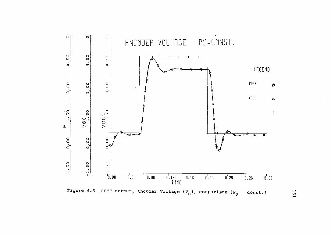
ID

■ O ID

OC

O

E N C O D E R V O L T A G E - P S = C O N S T

E G E N DVOCNo

VOC

ZIDOj-UJ-

ooo

0.08 G.20 0.24 0.28 0.32TIMEFigure 4.5 CSMP output. Encoder Voltage (V^), comparison (P^ = const.) LnM

o

ooinI

V A L V E C U R R E N T - P S = G P x Q So_

L E G E N D

o.

Z

0.00 0.08 0.20 0.28 0.32TIMEFigure 4.6 CSMP output. Valve current (I ), comparison (P_=GLQe)V s p o Ulro

u

oD_

OOmf\)j1

o_, VALVE C U R R E N T - P S = C O N S T

L E G E N DICNo.

U

0.00 0.08 0 . 1 2 0.16 0.20 0.28 0.32T I M E

0

Figure 4.7 CSMP output. Valve current (ly), comparison (P^ = const.) Hen(jü

(0

m

OC

m

oUJO>

o

E N C O D E R V O L T A G E - N O N L I N E A R M O D E L

L E G E N DVOW

VOCN

zj-

0.00 0.08 0 . 16 0.20 0 . 2 4 0 . 2 8 0.32TIM EFigure 4.8 CSMP output. Encoder Voltage (Vq ), nonlinear model,.

Pg = Gp.Qg (VON) - Pg = const.(VOCN)Ln

to" to"

o o oID ID IDzf =f

O o Oo o ocn cn cn

a o oID ID IDuj- •-

CC > >

o o oo o o'4o o o

o o oID ID LO1 1 'o

E N C O D E R V O L T A G E - A L T E R N A T I V E M O D E L

1------ r0 . 1 2 0 .T IME

L E G E N DVO 0

voc A

R +

Figure 4.9 CSMP output. Encoder VoltagefV^), alternative model, Pg=G .Q^ (VO) P^=Con3t. (VOL)

Ü1Ü1

oXo

1/ 1.=r

%tn.

M O T O R INPUT - O U T P U T PRESS. P S = G P x Q SL E G E N D

D.

PIN

P2N

o.

û-o

.00 0.04 0.08 0 . 1 2 0.16 0.20 0.28 0.32T I M E

0

Figure 4.10 CSMP output, Motor pressure (P^, Pg), nonlinear model Pg=3pQ, HUien

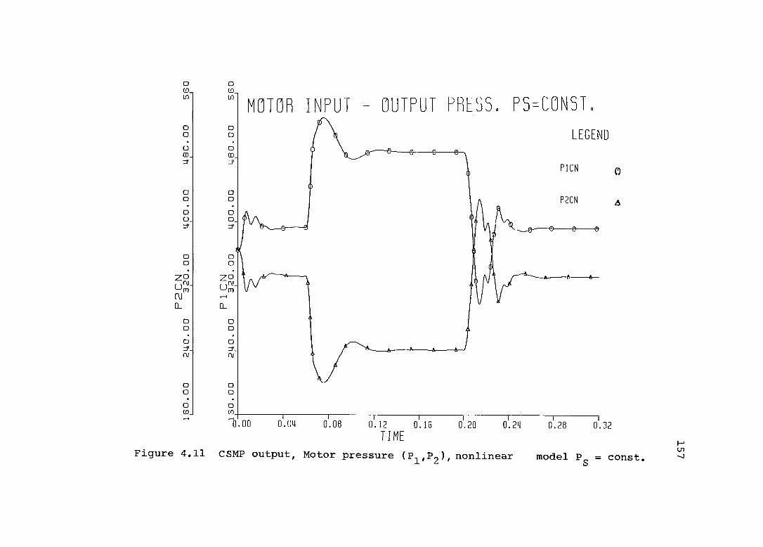
o o10_,Ln in

o Do oo oCD. 00.df d'

o oo oo oo_ o_

d*

o oo o

z °u:::-C\J

Z O

Q_ CL

D oo oo od*. d*.(V nj

o oo oo oID. ID

0

M O T O R INPUT O U T P U T PRESS. P S = C O N S T .L E G E N D

PlCN 0

0.04 0.08 0.12 0.16 T I M E 0.20 0.24 0.28 0.32

Figure 4.11 CSMP output. Motor pressure (P^,P2), nonlinear model P = const. U1

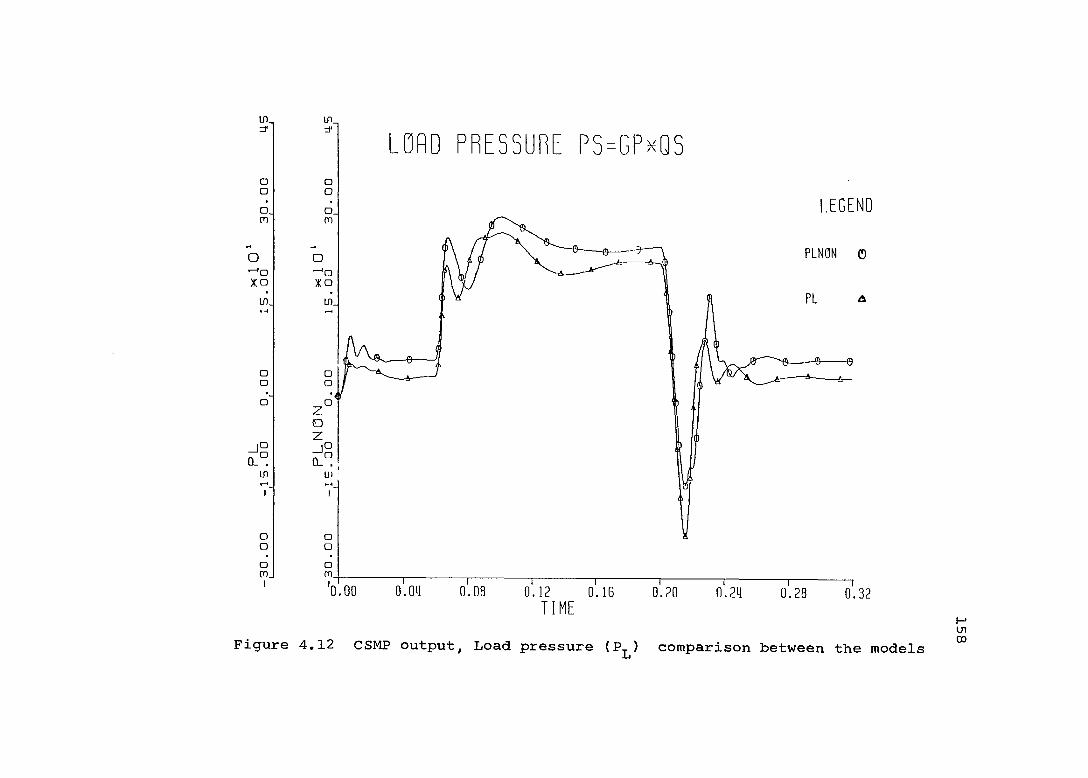
o*ouil

o

inr

oD0 mj1

L O R D P R E S S U R E P S = G P x Q SL E G E N DO.

PLNONxo

0.00 0.04 0.08 0.20 0.28 0.32TIMEFigure 4.12 CSMP output, Load pressure (P ) comparison between the models

I-»Ln00

_Jo

tn.

o.

in

o_, LO A D F L O W R A T E P S = G P ^ Q S

L E G E N DQLNONo.

Z oDO

0.00 0.08 0.16 0.20 0.24 0.28TI M EFigure 4.13 CSMP output, Load flow (Q^) comparison between the models ^

160

Frequency - response methods could be applied in app­roximation to nonlinear systems, using digital simulation such as CSMP in time domain. If nonlinearities are not extreme, the periodic steady state output, due to sinusoi­dal input will be close to sinusoidal and one can estimate its amplitude and phase angle relative to the input, thus getting one point on the system frequency response curves. Repetition of the procedure with increasing frequencies will produce the system frequency response curves, amplitu­de ratio and phase angle. Obviously, this method can lead to excessive computer costs, therefore is not justi­fied when the system is complicated and numerous variables are to be studied (10).

Let us now turn to the explanation of the Speakeasy computer program we used based on matrix techniques. The method is based on the fact that system models consist of sets of simultaneous differential equations. If one desires a transfer function relating a chosen output/input pair, it is necessary to use substitution and elimination, determinants, and so on to combine n equations with n un­knowns. These manipulations become increasingly tedious and subject to errors as n get larger. If the desired end result of such manipulations is only to obtain output/input frequency - response graphs for known numerical values of parameters, matrix computer operations on the original

151

set of n equations allow us to achieve this result with no manual manipulations whatever. The only restriction is that the set of differential equations describing the system have to be linear with constant coefficients (10).

Real systems are nonlinear, but usually most of the non- linearities are small such as in our system the friction nonlinearities in the pump and the motor. The servovalve is a highly nonlinear device, but its linearized model, about an operating point has to be used in the program.Since nonlinear systems response is sensitive to input amplitude, this may also have to be explored.

However, experimental studies showed insignificant differences in the frequency response curves when various amplitudes were used at one operating point. In our case the linearized valve equation was used at the 50% opening operating point with medium amplitudes.

In setting up the system differential equations we used the linearized valve model Q,. = K. 1.,+ K - K and

Li I V C S C L

the linear pump and actuator models, in order to achieve yet another compact useful frequency response model. Once verified experimentally the model could be used to study the system operation at various operating points and similar systems behaviour with different parameters.

The output/input pairs studied were selected according to our goal to investigate the effect of pump dynamics on

162

the response of servosysterns. The input to our system is R ■ Rq sin w t, the reference voltage input to the amplifier, whereas the outputs were; the Controlled Variable (V^) and Valve Input Pressure (Pg)»

Let us now set up the matrix technique described earlier for our system.(1) Pump dynamics (Felicio)

Pg K (r S + 1)— (S) E P------- (4.8)®s 2

T + —

This pump model includes pipe + filter compliance.(2) Servovalve linearized model

= ^i GytS) Pg - P^(4.9)

°S -

where1

G (S) -------------- Valve dynamics MOOGV 9

(3) Continuity equation

e

(4) Newton's Law

“m = Jm S «m + Ef + ’'l

163

(T = 0 in our case)(5) Encoder and Frequency to Voltage converter output

''o = "encc K (4-121(6) Open loop

Input current to the valve

^ampl ^( 7) Closed loop

Input current to the valve

l\r Gc(s) (« - Vq )

(4.13)

whereGc(5) = 0.001 S + 1

(4.14)

compensation network0.05 S + 1

The presentation of these differential equations in matrix form as required in our computer program will be

M

Outputs

Inputs

0 IU NT PP UU TT

QS' ' Ql ' m'R, T^ (T^ = 0 in our case)

We will present now the M matrix for open and Closed loop situation.

2CO COp p

Kp(TpS+l) 0 0 0 0 0 0

0 0 0 1 0 0 0 ^•^ampl

0 1 0 0 0 0 -1 0

0 0 0 0 Kenco -1 0 Iv = 0

0 0 s^ 4,%0 Dm 0 -1 < 0

0 0 - °m 0 JmS+Bm 0 0 -^L

0-

^i0 0 Ql 0

2CO CO V V

—1

Figure 4,14 Open loop system matrix representation in letter form Hcr>

s g +-^+1 K„(T^S+1)

2ÙJ (üP P

K

P P

0

0

48

-D_m

-K

0

2(O Cl)V V

K

JmS+Bm

0

K

enco

m

amplTj S+l

0

-1

-1

-1

0

-1

Q,

m

Q,

T s+iR— KT^S+l

0

ampl

0

-T,

Figure 4,15 closed loop system matrix representation in letter form mtn

166

The numerical values used in our Speakeasy program were; For the pump

Kp = 53.18 (psi/gpm) Wp = 115.66 (rad/sec)

Tp = 0,04217 sec ^p = 0.6

where and ^ are calculated including pump-valve line

and filter compliance.For the hydraulic motor

D = 0.159155 cis/rad m/3g = 100000 psi

= 14.22 * 10~^ cis/psi

= 3.52 in^2J = 0.0043 lb sec in m

= 0.3737 lb in/rad/sec

For the valve= 0.00800 cis/psi (at 50ma operating point)

= 0.1506 cis/ma (at =730psi pump pressure setting)

Valve dynamic characteristics2

Gy(S) = 1/ (— ---+ - ^ + 1) (from MOGG) (4.15)277^ 277

Feedback loop parameters(1) Encoder and Frequency to Volt converter

= 0.04777 V/rad/sec enco

167

(2) Amplifier gain

■'ampl ' 1== V/ma

(3) Compensation network G^(S) = (T^ S + l ) / ( S + 1)

G^(S) = -2i2°i_L+J:_ (4.16)0.05 S + 1

In order to save computer time and to compare open loop and closed loop frequency response results the two configurations were presented in one program using differ­ent notations.

The SPEAKEASY computer program has the form: (next page)

4.4 Transfer Function - Frequency Domain Computer Program

Before we end our discussion in the frequency domain computer analysis, we wish to compare the Speakeasy program in Matrix form with the Transfer Function form.

The Speakeasy Matrix Frequency Response program is probably the most useful when a complex system with a large number of equations is analyzed. Its disadvantage is being very expensive since it is using matrix manipulations (matrix inversions), which limits its use for final stages of system analysis. Therefore, in our theoretical analysis

Vo Pg Pgwe developed the transfer functions — (S); — (S) and— (S)R R Vo

HYDRAULIC SYSTEM - FREQUENCY RESPONSE - INCLUDING PUMP DYNAMICS DOMAIN COMPLEX;FREQ«A1D(I:)m a g p s » f r e q :m a g v o <f r e q ;m a g p v « f r e qh d b p s «f r e q :m o b v o «f r e q :m d b p v * f r e qPHASPS»FREQ;PHASVO»FREQ;PHASPV»FREQ MAGPSl=FREQ;MAGV01=FREQ:MAGPVI=FREQ HDBrSl=FREQ;MDBV01=FREQ;MDBPVI=FREQ PHSPS1=FREQ;PHSV01=FREQ;PHSPV1=FREQ FOR L=l,351,l;S=IL-l)*ll;J=IMAG(S)OPEN LOOP TRANSFER FUNCTION M=MATRIX(7,7)MI1)=0.0,0.0,0.0,1.0MI2)=S*S+138.792$S+13377.236,7779.929*15+23.721 Ml 31^0.0,1.0,0.0,0.0,0.0,0.0,"1.0 M(4I=0.0,0.0,0.0,0.0,0.04777,-1.0MI 51=0.0,0.0,0.87E-05*S+14.22E-05,0.0,0.159155,0.0,-1.0MI6)=0.0,0.0,-0.159155,0.0,0.0043*S+0.3887MI 71=0.008,0.0,-0.008,11969.724/1S*S+544.0*5+76729.0)0.0,0.0,—1.0INVMxINVERSEIN);RITSID=VECT0RI7:155.0);PROD=INVM*RIT5I0CLOSED LOOP TRANSFER FUNCTIONN*MATRIXI7,7IN(11=0.0,0.0,0.0,1.0,0.0,3.0*15+1000.01/IS+20.0)NI 21 =5*5+138.792*5+13377.236,7779.929*15+23.72)NI 31=0.0,1.0,0.0,0.0,0.0,0.0,— 1.0 NI41=0.0,0.0,0.0,0.0,0.04777,-1.0NI 51=0.0,0.0,0.87E-05*S+14.22E-05,0.0,0.159155,0.0,-1.0 NI 61 = 0.0,0.0,-0.159155,0.0,0.0043*5+0.3887 NI 71=0.008,0.0,-0.008,11969.724/15*5 + 544.0*5+76729.01 0.0,0.0,—1.0INVN=INVERSEI NIîRITSIT=V£CTOR17:3.*15+1000.1/15+20.11 PRGT=INVN*RITSITPS=PR0DI11;V0=PR0DI61;MPS=ABSIPS1;MV0=ABSIV01MDBPSIL1=20.0*L0G10(MPS1IMOBVQIL1=20.0*L0G10(MV01MDBPVIL1=20.0*LOG10IMPS/HV01MAGPSIL1=MPS;MAGV0(L1=MV0;MAGPVIL1=MPS/MV0PHP5=PHA5EIP51;PHVO=PHASEIVOl;PHPV=PHASEIPS1-PHASEIVO)DPHP5=57.3*PHPSî0PHVG=57.3*PHV0;DPHPV=57.3*PHPVPHASPSILI»OPHP5;PHASVO(L1=DPHVG;PHA5PVIL1=OPHPVPS1=PRGTI1I;VQ1=PRQTI61;MPS1=ABSIPS1);MV01=ABSIV011MDBPS1IL1=20.0*LGG10(MPS11;M0BV01ILl=20.0*LOG10IMV011M08PV1IL)=20.0*LOG10IMPS1/MV011MAGP51IL1«MPSI;MAGV01IL1=MV01;MAGPV1IL1=HPS>/MVQ1 PHPS1=PHA5E(P511;PHVG1=PHASEIVG11 PHPVl=PHASEIPSI1-PHASE IVGllDPHPS1»57.3*PHPS1;0PHV01=57.3*PHV01;DPHPV1=57.3*PHPV1 PHSPSICLl»0PHPSl;PHSV0lIL)=DPHVGl;PH5PVllLl=DPMPVl FREQIL1«J; HZ(L1=FREQIL1/6.28 ENDLOQP LTABULATE FREQ,HZ,MObPS ,PHASPS,H0BV0,PHASV0,f1DBPV,PHASPV TABULATE FREQ,HZ,MOBPS1,PHSPS1,MOBVG1,PHSVQl,MDBPVI,PHSPVI

169

in letter form, which are the working formulas if satisfac­torily verified.

The Transfer Function representation gives us a better insight into the system behaviour in frequency do­main. The development of the Transfer Function was based on the system of simultaneous differential equations, same as the Matrix method. In Ohio State University Mech. Eng. Dept, the computer program number 20 is a "canned" program using the Transfer Function Method, As far as computer cost is concerned, this program is about one tenth of the Speakeasy - Matrix Method program, which makes it useful and attractive in the initial stages of the system analysis.

4.4.1 The Transfer Functions Development

Let us now bring up again briefly the develop­ment of the Transfer Functions in letter form and then substitute numerical values to compare computer results with experimental results.P -K (T S + 1)— (S) = -- = G (S) (4.17)°S S S

+P P

Transfer Function representation of the hydraulic motorV,

^m = (Jm S + 6,

(4.18)

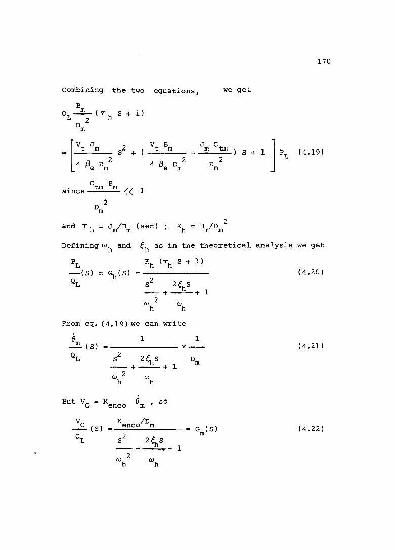
170

Combining the two equations, B

we get

m (r^ S + 1)m

+ -2— ) s + 14 fe Dm Dm

(4.19)

since — ^ — — << 1

m

""h = V ® m (sec) ; = B/D^'

Defining and as in the theoretical analysis we get

"V. (^h s + 1) ( S ) = G, ( S ) = ----------

2& S+ 1

(4.20)

^h ^hFrom eq. (4,19) we can write

d_m ( S ) =Dm

(4.21)

(li Oih h

'>0 = %encoK /D 2.(3) = ~ 2nco m

+ Z 2 1 + 1Gm'S) (4.22)

w.h w.h

171

Servovalve equation

°L = >'i V v < S > + %c Ps - ■'c '’l

= ° L

G„(S) -------------- Valve dynamics MOOG (4.23)V 9

"vOpen loop current equation

V ■'ampl K (4.241Closed loop current equation

=V= Kampl Gc(S> (R - Vo) (4.25)

Tn S + 1G (S) = ---------- Comp, network (4.26)^ T2 S + 1

Open loop Transfer FunctionsSubstituting eq.(4.17), (4.20), (4.24) into eq.(4.25)

we get

Ol = Ki GylS) E - Gp(S) G^(S)

and

.!k(s) = ^ l i E E L ! v l f ! (4.27)°ph'S>

whereGph(S) . 1 + Gp(S) + Gj (S)

which is the system characteristics equation. Transfer

172

Qrfunction (S) is now the basic equation from which we will

develop the desired transfer functions. To get the transferfunction— -(S) we will replace Q_ = V./G (S)R L 0 m

Z2(s) Gy(S) GJS) (4.28)* Gph<S)

PcTo get the transfer function— (S) we will replace Q =R ^

Pg/Gp(S) (since = Q^)

% S ) = Gy(S) Gp(S) (4.29)% Gph(S)

PgFinally, the transfer function (S) will be^0

VQ R R

Pg G (g)— (S) = — ------------------- (4.30)Vo Gm(S)

In our case the hydraulic natural frequency (w^^ is much higher than the pump natural frequency (CL ) so G^(S) is “negligible" in Gp^(S) which becomes

Gph<S)Sl + Gp(S)

orGpp(S) = 1 + Gp(S) (4.31)

173

Next we will substitute numerical values for the transfer functions.Pump dynamics from Felicio

P„ -53,18 (S/23.72 + 1)Gp(S) = ■ ( S) = -■■ ----------------------------

Qg (S/183.5) + 2 * 0.3778 S/183.5 + 1

(4.32)Pump dynamics including pipe + filter compliance

P_ -53.18 (S/23.72 + 1)G„ ( S ) = — ^ ( S ) =^ °S (S/115.66)^ + 2 * 0.6 S/115.66 + 1

(4.33)Developing now Gpp(S) for the case Iy= 50ma operating

point i.e., = 0.008

Gpp(S) = 1 + Gp(S) 4 Modified Pump T. F*

1.42544 (— ---+ -LjLill2iL_Ë. + 1)Gpp(S) ---------------------------------- (4.34)

-i. + + 1115.66^ 115.66

"ppG (S) = K -- ^ ------ — ---------------- (4.35)g2 2 f S (— + + 1 )<u 2 wP P

174

The two transfer functions eq,(4.32) and eq.(4.33) re­presenting pump dynamics for the cases discussed, were plotted on a Bode diagram using the tabular results from frequency response program No. 20,Fig.4.16. This theoreti­cal result of the pump transfer function will be compared later in Fig.4.17 and Fig.4.18 with the experimental fre­quency response test results of the "Supply subsystem" output impedance,

4.4.2 Numerical Values For The Transfer Functions

Substituting for:= 0.1506 (cis/ma); = 0.008 (cis/psi)

= 155 (ma/V); D = 0.159155 (CIS/rad)a lT ip j. in

PgWe get for the transfer function — (S)R

Is ,3 , , 3 W = >R G p p ( S )

or

Ps,_. %i Kampl Kp/Kpp (?P + 1)—— I a ) n — — — -R S 2 f S o2 2 S

( + — 1 ) ( _ ^ + 1)'"pp "v

(4.39)and after substituting for the numerical values

(s) =

(s) =

-90100,0 FREQUENCY(rad/sec)1 . 2 1 0 .0

r.Figure 4.16 Pump frequency response.— -(S) - 2Pump only, --(S) = Pump + line + filter

° 2

U1

176

10.8 * 10^ (S + 23.72)-lis) -------------------------------^ (S + 544.0 S + 76729) (S^ + 378.78 S + 19068.3)

(4.40)Finally

R— (S)

10.8 * 10^ (S + 23.72)+ 923.0 + 30.19 * 10^ + 39.5 * 10^ + 1.5 * 10^

(4.41)Now substituting for the— — (S) transfer function

: S (S, . ' - p i S l Ü f m 'i L R Gpp(S)

^2cs)

2 & SKampl Kenco/Om'--r-+

^P “p___________________

, f L n 1)% P ^PP *h

(4.43)We now neglect the hydraulic natural frequency term £o , substitute for the numerical values and get

(4.44)

1 7 7

:2(s,R

______ 43.36 * 10^ (S^ + 138 S + 13377.236)(S + 544.0 S + 76729) ( + 378.78 S + 19068.3)

and finally

— (S)R

43.36 * 10^ (S + 138.792 S + 13377.236)

+ 923.0 + 30.19 * lo" + 39.5 * 10® S + 1.5 * 10^(4.45)

PgFinally for (S) we get^0

Pg G (S)— (S) = -- (4.46)Vo G^/S)

or

,4.47,

en p

After substituting numerical values and neglecting hydraulic natural frequency we get

Pg 25.3 * 10^ (S + 23.72)—— (S) = — ' ' ... - — . (4.48)Vq (S + 138.79 S + 13.4 *10^)

1 7 8

Special attention should be focused on the Transfer Function

Pc D Tp S + 1 S— (S) = — Kp ---------- (--- + --— +1) (4.49)^0 ^enco 2 f S w + _ ^ + 1 h h

w w P P

which is the Supply Subsystem output impedance. In our case the hydraulic natural frequency is high and equa­tion (4.49) becomes:

Pc— (S) = -- G (S) (4.50)^0 ^enco

which is the pump transfer function times a constant D^/Kenco

The experimental frequency response result is presented in Fig.4.17. In the EODE diagram (Fig.4.18) we observe a good correlation between the computer program and the experimental frequency response result.

NTCOLET SS0A50.00000 HZ

7S■2-4

41

D G.cJB

VL-NC

T F

Figure 4,17 "Supply Subsystem" output impedancePgfrequency response — =(iw )

W(HZ) A R ( d B ) <^(DG)

0.13 -31.1 -144.30.25 -22.5 -122.40.50 -19 .6 -118.71.00 -19 .0 -129.32.00 - 15.8 - 131.85.00 -13 .3 -128.48.00 -12 .6 -128.4 2.00 - 10.8 - 140.3 5.00 - 8.2 -165.1 6.25 - 7 .8 -179.4

- 7.3- 6.4- 6.7- 6.8 — 8,2 -11.5 -15.1 -18 .0 - 2 1 . 5 - 24.2

179.3 169.6144.3 119.2 105,095.090.0 75.9 73.3 76.5

H*-JVO

Theoretical analysis

-53.18(3/23.72 + 1)45 -^(s) =S /115.66 + 2*0.6*3/115.66 + 1

Program #20pq

Experiment

Pump frequency response25

— (S)= —2.(3)enco

100.0 PREQUENCY(rad/sec)1 0 .01 . 2Figure 4.18 Comparison between theoretical and experimental

pump frequency response 00o

CHAPTER 5 DISCUSSION AND CONCLUSIONS

As stated earlier in several occasions, theoretical, experimental and computer work are interrelated in any practically oriented study. The computer simulation is based on the theoretical analysis, but it is limited in giving results related to a particular apparatus with specific hardware.

A good correlation between this specific computer simu­lation and the experimental results, both, in time domain and frequency domain validates the theoretical analysis. Therefore it will give a high level of confidence that the computer modeling in its general form, based upon the developed theory, can simulate any such system, including ones not yet built, simply by changing its parameters.

5.1 Computer and Experimental Results Comparison - Time Domain

Let us turn now to the comparison between the computer CSMP, and the experimental time domain step response results.

1 8 1

1 8 2

The six variables recorded simultaneously on the six channel GOULD Recorder were magnified by a factor of 3 : 1 transferring the results from the regular recorder paper to milimetric paper. (The procedure has been introduced al­ready in the experimental section.) Since CSMP graphic results include numerical values side by side with the TIME variable, these were used to plot point by point superimposed on the magnified experimental results.

The computer program was written for pump pressure sett­ing of Pg = 730psi and the variables compared were:(1) - Valve input current (ma)

(2) Vq - Encoder voltage (Volt)

(3) Pg - Pump pressure (psi)

( 4 ) PMI- Motor input pressure (psi)

(5) Pj o~ Motor output pressure (psi)

All these variables were tested experimentally and computer simulated for both cases:(1) ^ pressure supressing accumulator, i.e., pump dyna­

mics included (Pg = Qg)

(2) Accumulator connected, i.e., "constant" supply press­ure at valve input (Pg = constant)

1 8 3

Discussion of the compared results

Fig.5,1 to Fig,5.9 present the comparison between the experimental step response and the, CSMP results for P^ = constant and P^ = Gp Qg. Our discussion will cover each variable individually.

Valve current (1 ) - Fig.5.1 and 5.2

In the CSMP simulation we limited the valve current to lOOma, to simulate valve saturation, therefore there is no overshoot during the "step up" period as we observe in both figures. During the "step down" period, in both figures, the experimental current has a lower "under - shoot" and lower natural frequency. This behaviour is explained by a smaller actual valve natural frequency and damping ratio than the numerical values used in the model, given by MOOG.

Encoder Voltage (V ) Fig.5.3 and 5.4

There is a fairly good agreement between experiment and CSMP except for two phenomenan:(1) The computer model has a slightly higher overshoot

during the "step up" period, which suggests that there is a higher leakage flow in the motor than in the model, increasing damping ratio.

(2) The experimental voltage has a small high frequency "ripple" during the "step down" period, which was not

184

Experiment

iCSMP>M

Ü

L 50ms -""iTIME

Figure 5.1 Valve current - Step response (Pg = Gp Qg), Comparison between Experiment and CSMP

n5E>M 0)EH as VOH PdI u

CSMP

Pg = constant

i h A 1----1--- ^

J I I L

TIMEJ L

50msFigure 5.2 Valve current - Step response (Pg = const.).

Comparison between Experiment and CSMP

1 8 5

completely understood and could be further studied.(3) The behaviour of the encoder voltage as observed in

the dotted region in Fig.5.3 is due to pump dynamics and has the following explanation;Due to large flow demands, pump pressure drops and

reaches its lower peak about 10 to 15ms from the beginning of the step function. So, encoder voltage (which is a measure of shaft speed of rotation) "levels off" for about 10ms at this point and continues to increase as pump pres­sure "recovers" to the set pressure. See Fig.5.5 for pump pressure behaviour. In Fig.5.4 where pump pressure is maintained constant this phenomenon does not occur and shaft speed of rotation (encoder voltage) is increasingsteadily up to the peak.

This is exactly the cause and the explanation for the worsening in performance of the controlled variable (V^), which was studied numerically in the previous sections.

Supply pressure (P^) - Fig.5.5

Pump - supply pressure (Supply subsystem pressure)was defined as P^ = Gp(S) Qg, where Gp(S) is the supply sub­system (pump) transfer function which is fairly accurately known and Qg is flow demand by the servovalve (system).

There is a slightly lower "low peak" and higher "high peak" in the CSMP results during the "step up" and "step

186

CSMP

Experiment

■pf—Io!>O

II0.7

50ms' —JTIME

Figure 5.3 Encoder Voltage - Step response (Pg = Gp Qg), Comparison between Experiment and CSMP

187

Experiment

CSMP

constant

0.7

TIME

Figure 5.4 Encoder voltage - Step response (Pg = const.),Comparison between Experiment and CSMP

188

n

•HEQa Experiment

>

wcowg>2

CSMP

50msTIME

Figure 5.5 Valve pressure Step response.Comparison between Experiment and CSMP

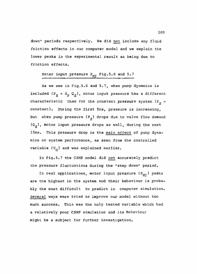
1 8 9

down" periods respectively. We did not include any fluid friction effects in our computer model and we explain the lower peaks in the experimental result as being due to friction effects.

Motor input pressure Fig.5.6 and 5.7

As we see in Fig.5.6 and 5.7, when pump dynamics is included (Pg = Gp Qg), motor input pressure has a different characteristic than for the constant pressure system (Pg = constant). During the first 5ms, pressure is increasing, but when pump pressure (Pg) drops due to valve flow demand (Qg), motor input pressure drops as well, during the next 15ms. This pressure drop is the main effect of pump dyna­mics on system performance, as seen from the controlled variable (V^) and was explained earlier.

In Fig.5.7 the CSMP model did not accurately predict the pressure fluctuations during the "step down" period.

In real applications, motor input pressure (P^^) peaks are the highest in the system and their behaviour is proba­bly the most difficult to predict in computer simulation. Several ways were tried to improve our model without too much success. This was the only tested variable which had a relatively poor CSMP simulation and its behaviour might be a subject for further investigation.

1 9 0

Experiment CSMP

•HCOA

COHg

H

ggS

1— '— '— t— 50ms ——1TIME

Figure 5.6 Motor input pressure - Step response, Comparison between Experiment and CSMP

1 9 1

Experiment

I 1-------\M 355

TIME 50ms

Figure 5,7 Motor input pressure - Step response, Comparison between Experiment and CSMP

1 9 2

Motor outlet pressure (P^^) Fig.5.8 and 5.9

In this case the CSMP and the experimental results compare fairly closely. The experimental peaks are slight­ly higher, the frequency however, is in good correlation.

CONCLUSIONS

A computer model is aimed to simulate system perfor­mance within certain limitations. The success of such a model depends obviously on how well does the programmer know the numerical values of the different parameters and the dynamic response of the components and subsystems.

We carried out an extensive experimental program to find system parameters using well developed and proved techniques in time domain and frequency domain.

Generally speaking, the comparison between CSMP and Experiment showed a good correlation, thus, we conclude that the CSMP model is a good time domain simulation of the servosystem.

It is known, from practical experience, that a time domain model of a complex system is difficult to predict analytically.

We turn now to the comparison between Experiment and Computer Simulation in frequency domain, where we will find a much better correlation in most of the cases.

121

Experiment

•Hopf

CM

^ -LM^ 365

oggs CSMP

I ' ' I'-^50ms — *TIME

Figure 5.8 Motor output pressure - Step response

•tHtoftopf

Experiment•H

H fte 8CO CM constant

CSMPo

TIME 50ms

Figure 5.9 Motor output pressure - Step response

1 9 4

5.2 Computer and Experimental Results Comparison - Frequency Domain

The next step in validating our confidence in the theoretical analysis would be the comparison between the Frequency Domain computer programs and the Frequency Response experimental results.

Let us look first at the SPEAKEASY computer program output which is in tabular form giving numerical values for amplitude ratio and phase angle as a function of frequency.

As mentioned earlier the program was developed for the 50% valve opening (50ma) operating point since the majority of the experimental tests were at that very same operating point.

In order to be able to compare between the computer tabular results and the FFT analyzer graphical results, we recorded during the frequency response tests numerical values at several frequencies (20 points) using the cursor on the frequency analyzer. Thus, each graph is accompanied by a table of amplitude ratio in dB and phase angle in degrees as a function of frequency. The tests were conduc­ted in both ,open and closed loop configuration at 50ma ± 12.5ma operating point, not including accumulator in order to exercise pump dynamics. We showed earlier that accumu­lator break frequency was at about 4rad/sec "killing" pump dynamics ( = 115.66rad/sec).

1 9 5

The Speakeasy Frequency Response computer program was explained in detail and presented in Chapter 4. The "results" of such a program are in tabular form as a func­tion of frequency and the number can be plotted in order to compare with experimental results.

Since the highest frequency of interest was 350(rad/sec), the computer generated 8 pages of results for each case with increments of 1 rad/sec. We will present here only a sample of one page of the tabular results in each, open and closed loop configuration in the following sequence:Open loopMDBPS - Supply pressure (P ) amplitude ratio (dB)PHASPS - Supply pressure (P ) phase angle (Degrees)MDBVO - Encoder Voltage (V ) amplitude ratio (dB)PHASVO - Encoder Voltage (V^) phase angle (Degree)MDBPV - Supply pressure (P ) / Encoder Voltage (V )

amplitude ratio (dB)PHASPV - Supply pressure (Pg) / Encoder Voltage (Vq )

phase angle (Degree)

196

FREQ HZ «« $**$**#*0 01 . 1 5 9 2 42 . 3 1 8 4 73 .477714 . 6 3 6 9 45 . 7 9 6 1 86 . 9 5 5 4 17 1 . 1 1 4 68 1 . 2 7 3 99 1 . 4 3 3 1

10 1 . 5 9 2 411 1 . 7 5 1 612 1 . 9 1 0 813 2 . 0 7 0 114 2 . 2 2 9 315 2 . 3 8 8 516 2 . 5 4 7 817 2 . 7 0 718 2 . 8 6 6 219 3 . 0 2 5 520 3 . 1 8 4 721 3 . 3 4 3 922 3 . 5 0 3 223 3 . 6 6 2 424 3 . 8 2 1 725 3 . 9 8 0 926 4 . 1 4 0 127 4 . 2 9 9 428 4 . 4 5 8 62 9 4 . 6 1 7 830 4 . 7 7 7 131 4 . 9 3 6 332 5 . 0 9 5 533 5 . 2 5 4 834 5 . 4 1 435 5 . 5 7 3 236 5 . 7 3 2 537 5 . 8 9 1 738 6 . 0 5 139 6 . 2 1 0 240 6 . 3 6 9 441 6 . 5 2 8 742 6 . 6 8 7 943 6 . 8 4 7 14 4 7 . 0 0 6 4

MDBPS******4 8 . 6 4 54 8 . 6 5 34 8 . 6 7 548.7124 8 . 7 6 24 8 . 8 2 64 8 . 9 0 44 8 . 9 9 34 9 , 0 9 44 9 . 2 0 44 9 . 3 2 54 9 . 4 5 44 9 . 5 94 9 . 7 3 44 9 . 8 8 35 0 . 0 3 75 0 . 1 9 45 0 . 3 5 65 0 . 5 25 0 . 6 8 65 0 . 8 5 35 1 . 0 2 15 1 . 1 8 95 1 - 3 5 85 1 . 5 2 65 1 . 6 9 35 1 . 8 5 95 2 . 0 2 45 2 . 1 8 75 2 . 3 4 95 2 . 5 0 85 2 . 6 6 65 2 . 8 2 15 2 . 9 7 45 3 . 1 2 45 3 - 2 7 25 3 . 4 1 75 3 . 5 65 3 . 75 3 . 8 3 85 3 - 9 7 25 4 . 1 0 45 4 . 2 3 45 4 . 365 4 . 4 8 4

PHASPS MDBVO PHASVO *************************

1 8 0 . 0 1 1 5 . 3 7 9 01 5 . 3 7 8 - . 6 4 0 3 61 5 . 3 7 7 - 1 . 2 8 0 61 5 . 3 7 4 - 1 . 9 2 0 61 5 . 3 7 1 - 2 . 5 6 0 21 5 . 3 6 7 - 3 . 1 9 9 41 5 . 3 6 1 - 3 . 8 3 7 91 5 . 3 5 5 - 4 . 4 7 5 71 5 . 3 4 8 - 5 . 1 1 2 71 5 . 3 4 - 5 . 7 4 8 71 5 . 3 3 1 - 6 . 3 8 3 61 5 . 3 2 1 - 7 . 0 1 7 21 5 . 3 1 - 7 . 6 4 9 61 5 . 2 9 8 - 8 . 2 8 0 41 5 . 2 8 6 - 8 . 9 0 9 71 5 . 2 7 2 - 9 . 5 3 7 2

- 1 7 8 . 8 2 - 1 7 7 . 6 5 - 1 7 6 . 4 8 - 1 7 5 . 3 4 - 1 7 4 . 2 4 - 1 7 3 . 1 7 - 1 7 2 . 1 5 - 1 7 1 . 1 8 - 1 7 0 . 2 7 - 1 6 9 . 4 1 - 1 6 8 . 6 2 - 1 6 7 . 8 9 - 1 6 7 . 2 3 - 1 6 6 . 6 3 - 1 6 6 . 1 - 1 6 5 . 6 3 - 1 6 5 . 2 3 - 1 6 4 . 9 - 1 6 4 . 6 3 - 1 6 4 . 4 1 - 1 6 4 . 2 6 - 1 6 4 . 1 6 - 1 6 4 . 1 2 - 1 6 4 . 1 3 - 1 6 4 . 1 9 - 1 6 4 . 3 - 1 6 4 . 4 6 —1 6 4 . 6 6 - 1 6 4 . 9 - 1 6 5 . 1 8 - 1 6 5 . 5 —1 6 5 . 8 6 - 1 6 6 . 2 5 —1 6 6 . 6 8 - 1 6 7 . 1 3 - 1 6 7 . 6 2 - 1 6 8 . 1 3 —1 6 8 . 6 7 - 1 6 9 . 2 4 - 1 6 9 . 8 3 - 1 7 0 . 4 5 - 1 7 1 . 0 8 - 1 7 1 . 7 4 - 1 7 2 . 4 2

1 5 . 2 5 7 - 1 0 . 1 6 3 1 5 . 2 4 2 - 1 0 . 7 8 7 1 5 . 2 2 5 - 1 1 . 4 0 8 1 5 . 2 0 8 - 1 2 . 0 2 81 5 . 1 8 9 - 1 2 . 6 4 5 1 5 . 1 7 - 1 3 . 2 5 91 5 . 1 5 - 1 3 . 8 7 11 5 . 1 2 9 - 1 4 . 4 8 1 5 . 1 0 7 - 1 5 . 0 8 6 1 5 . 0 8 4 - 1 5 . 6 8 9 1 5 . 0 6 1 - 1 6 . 2 8 91 5 . 0 3 6 - 1 6 . 8 8 6 1 5 . 0 1 1 - 1 7 . 4 7 91 4 . 9 8 5 - 1 8 . 0 6 9 1 4 . 9 5 8 - 1 8 . 6 5 5 1 4 . 9 3 - 1 9 . 2 3 71 4 . 9 0 1 - 1 9 . 8 1 5 1 4 . 8 7 1 - 2 0 . 3 8 8 1 4 . 8 4 1 - 2 0 . 9 5 8 1 4 . 8 1 - 2 1 . 5 2 31 4 . 7 7 8 - 2 2 . 0 8 4 1 4 . 7 4 6 - 2 2 . 6 3 91 4 . 7 1 2 - 2 3 . 1 9 1 4 . 6 7 8 - 2 3 . 7 3 6 1 4 . 6 4 4 - 2 4 . 2 7 71 4 . 6 0 8 - 2 4 . 8 1 3 1 4 . 5 7 2 - 2 5 . 3 4 3 1 4 . 5 3 5 - 2 5 . 8 6 8 1 4 . 4 9 8 - 2 6 . 3 8 7

MDBPV******3 3 . 2 6 73 3 . 2 7 53 3 . 2 9 83 3 . 3 3 73 3 . 3 9 13 3 . 4 63 3 . 5 4 23 3 . 6 3 83 3 - 7 4 5 3 3 . 8 6 43 3 . 9 9 4 3 4 . 1 3 3 3 4 . 2 83 4 - 4 3 5 3 4 . 5 9 7 3 4 . 7 6 5 3 4 . 9 3 7 3 5 . 1 1 4 3 5 . 2 9 4 3 5 . 4 7 8 3 5 . 6 6 3 3 5 . 8 5 1 3 6 . 0 3 9 3 6 . 2 2 9 3 6 . 4 1 93 6 . 6 0 9 3 6 . 7 9 93 6 . 9 8 8 3 7 . 1 7 7 3 7 . 3 6 4 3 7 . 5 5 1 3 7 . 7 3 6 3 7 . 9 2 3 8 . 1 0 2 3 8 . 2 8 3 3 8 . 4 6 23 8 . 6 3 9 3 8 . 8 1 53 8 . 9 8 8 3 9 . 1 5 9 3 9 . 3 2 9 3 9 - 4 9 6 3 9 . 6 6 2 3 9 - 8 2 53 9 . 9 8 6

PHASPV*******

1 8 0 - 0 1- 1 7 8 - 1 8 - 1 7 6 - 3 6 - 1 7 4 . 5 6 - 1 7 2 - 7 8 - 1 7 1 . 0 4 - 1 6 9 - 3 3 - 1 6 7 - 6 8 - 1 6 6 . 0 7 - 1 6 4 - 5 2 - 1 6 3 . 0 3 —1 6 1 . 6 - 1 6 0 . 2 4 - 1 5 8 - 9 5 - 1 5 7 . 7 2 - 1 5 6 . 5 6 - 1 5 5 . 4 7 —1 5 4 . 4 5 - 1 5 3 . 4 9 - 1 5 2 . 6 - 1 5 1 . 7 7 - 1 5 1 - 1 5 0 . 2 9 - 1 4 9 . 6 4 - 1 4 9 . 0 4 - 1 4 8 . 5 - 1 4 8 . 0 1 - 1 4 7 . 5 7 - 1 4 7 . 1 8 - 1 4 6 . 8 3 - 1 4 6 . 5 3 - 1 4 6 . 2 7 - 1 4 6 . 0 4 - 1 4 5 . 8 6 - 1 4 5 - 7 2 - 1 4 5 . 6 1 - 1 4 5 - 5 3 - 1 4 5 . 4 9 - 1 4 5 . 4 8 - 1 4 5 . 5 1 - 1 4 5 - 5 6 - 1 4 5 . 6 4 - 1 4 5 . 7 4 - 1 4 5 . 8 7 - 1 4 6 . 0 3

197

Closed loopMDBPSl - Supply pressure (PSl) amplitude ratio (dB) PHSPSl - Supply pressure (PSl) phase angle (DG)MDBVOl - Encoder Voltage (VOl) amplitude ratio (dB) PHSVOl - Encoder Voltage (VOl) phase angle (DG)MDBPVl - Supply pressure (PSl) / Encoder Voltage (VOl)

amplitude ratio (dB)PHSPVl - Supply pressure (PSl) / Encoder Voltage (VOl)

phase angle (DG)

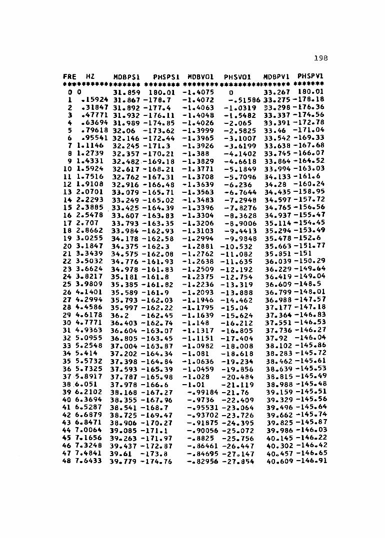
198

FRE HZ MDBPSl PHSPSl MDBVOl PHSVOl MDBPVl PHSPVl* * * * * * * * * * * * * * * * * * * * * * * * * * * * * * * * **********K****** *******

0 0 3 1 . 8 5 9 1 8 0 . 0 1 - 1 . 4 0 7 5 0 3 3 . 2 6 7 1 8 0 .0 11 . 1 5 9 2 4 3 1 . 8 6 7 - 1 7 8 . 7 - 1 . 4 0 7 2 - . 5 1 5 8 6 3 3 . 2 7 5 - 1 7 8 . 1 82 . 3 1 8 4 7 3 1 . 8 9 2 - 1 7 7 . 4 —1 . 4 0 6 3 - 1 . 0 3 1 9 3 3 . 2 9 8 - 1 7 6 . 3 63 . 4 7 7 7 1 3 1 . 9 3 2 - 1 7 6 . 1 1 - 1 . 4 0 4 8 - 1 . 5 4 8 2 3 3 . 3 3 7 - 1 7 4 . 5 64 . 6 3 6 9 4 3 1 . 9 8 9 - 1 7 4 . 8 5 - 1 . 4 0 2 6 - 2 . 0 6 5 3 3 . 3 9 1 - 1 7 2 . 7 85 - 7 9 6 1 8 3 2 . 0 6 - 1 7 3 . 6 2 - 1 . 3 9 9 9 - 2 . 5 8 2 5 3 3 . 4 6 - 1 7 1 . 0 46 . 9 5 5 4 1 3 2 . 1 4 6 - 1 7 2 . 4 4 - 1 . 3 9 6 5 - 3 . 1 0 0 7 3 3 . 5 4 2 - 1 6 9 . 3 37 1 . 1 1 4 6 3 2 . 2 4 5 - 1 7 1 . 3 - 1 . 3 9 2 6 - 3 . 6 1 9 9 3 3 . 6 3 8 - 1 6 7 . 6 88 1 . 2 7 3 9 3 2 . 3 5 7 - 1 7 0 . 2 1 - 1 . 3 8 8 - 4 . 1 4 0 2 3 3 . 7 4 5 - 1 6 6 . 0 79 1 . 4 3 3 1 3 2 . 4 8 2 - 1 6 9 . 1 8 - 1 . 3 8 2 9 - 4 . 6 6 1 8 3 3 . 8 6 4 - 1 6 4 . 5 2

10 1 . 5 9 2 4 3 2 . 6 1 7 - 1 6 8 . 2 1 - 1 . 3 7 7 1 - 5 . 1 8 4 9 3 3 . 9 9 4 - 1 6 3 . 0 3i l 1 . 7 5 1 6 3 2 . 7 6 2 - 1 6 7 . 3 1 - 1 . 3 7 0 8 - 5 . 7 0 9 6 3 4 . 1 3 3 - 1 6 1 . 612 1 . 9 1 0 8 3 2 - 9 1 6 - 1 6 6 . 4 8 - 1 . 3 6 3 9 - 6 . 2 3 6 3 4 . 2 8 - 1 6 0 . 2 413 2 . 0 7 0 1 3 3 . 0 7 9 - 1 6 5 . 7 1 - 1 . 3 5 6 3 - 6 . 7 6 4 4 3 4 . 4 3 5 - 1 5 8 . 9 514 2 . 2 2 9 3 3 3 . 2 4 9 - 1 6 5 . 0 2 - 1 . 3 4 8 3 - 7 . 2 9 4 8 3 4 . 5 9 7 - 1 5 7 . 7 215 2 . 3 8 8 5 3 3 . 4 2 5 - 1 6 4 . 3 9 - 1 . 3 3 9 6 - 7 . 8 2 7 6 3 4 . 7 6 5 —1 5 6 . 5 616 2 . 5 4 7 8 3 3 . 6 0 7 - 1 6 3 . 8 3 - 1 . 3 3 0 4 - 8 . 3 6 2 8 3 4 . 9 3 7 - 1 5 5 . 4 717 2 . 7 0 7 3 3 . 7 9 3 - 1 6 3 . 3 5 - 1 . 3 2 0 6 - 8 . 9 0 0 6 3 5 . 1 1 4 - 1 5 4 . 4 518 2 . 8 6 6 2 3 3 . 9 8 4 - 1 6 2 . 9 3 - 1 . 3 1 0 3 - 9 . 4 4 1 3 3 5 . 2 9 4 - 1 5 3 . 4 919 3 . 0 2 5 5 3 4 . 1 7 8 - 1 6 2 . 5 8 - 1 . 2 9 9 4 - 9 . 9 8 4 8 3 5 . 4 7 8 - 1 5 2 . 620 3 . 1 8 4 7 3 4 . 3 7 5 - 1 6 2 . 3 - 1 . 2 8 8 1 - 1 0 . 5 3 2 3 5 . 6 6 3 - 1 5 1 . 7 721 3 . 3 4 3 9 3 4 . 5 7 5 - 1 6 2 . 0 8 - 1 . 2 7 6 2 - 1 1 . 0 8 2 3 5 . 8 5 1 - 1 5 122 3 . 5 0 3 2 3 4 . 7 7 6 - 1 6 1 . 9 3 - 1 . 2 6 3 8 - 1 1 . 6 3 5 3 6 . 0 3 9 - 1 5 0 . 2 923 3 . 6 6 2 4 3 4 . 9 7 8 - 1 6 1 . 8 3 - 1 . 2 5 0 9 - 1 2 . 1 9 2 3 6 . 2 2 9 - 1 4 9 . 6 424 3 . 8 2 1 7 3 5 . 1 8 1 - 1 6 1 . 8 - 1 . 2 3 75 - 1 2 . 7 5 4 3 6 . 4 1 9 - 1 4 9 . 0 425 3 . 9 8 0 9 3 5 . 3 8 5 - 1 6 1 , 8 2 - 1 . 2 2 3 6 - 1 3 . 3 1 9 3 6 . 6 0 9 - 1 4 8 . 526 4 . 1 4 0 1 3 5 . 5 8 9 - 1 6 1 . 9 - 1 . 2 0 9 3 - 1 3 . 8 8 8 3 6 . 7 9 9 - 1 4 8 . 0 127 4 . 2 9 9 4 3 5 . 7 9 3 - 1 6 2 . 0 3 - 1 . 1 9 4 6 - 1 4 . 4 6 2 3 6 . 9 8 8 - 1 4 7 . 5 728 4 . 4 5 8 6 3 5 . 9 9 7 - 1 6 2 . 2 2 - 1 . 1 7 9 5 - 1 5 . 0 4 3 7 . 1 7 7 - 1 4 7 . 1 829 4 . 6 1 7 8 3 6 . 2 - 1 6 2 . 4 5 - 1 . 1 6 3 9 - 1 5 . 6 2 4 3 7 . 3 6 4 - 1 4 6 . 8 330 4 . 7 7 7 1 3 6 . 4 0 3 - 1 6 2 . 7 4 - 1 . 1 4 8 - 1 6 . 2 1 2 3 7 . 5 5 1 - 1 4 6 . 5 331 4 . 9 3 6 3 3 6 . 6 0 4 - 1 6 3 . 0 7 - 1 . 1 3 1 7 - 1 6 . 8 0 5 3 7 . 7 3 6 - 1 4 6 . 2 732 5 . 0 9 5 5 3 6 . 8 0 5 - 1 6 3 . 4 5 - 1 . 1 1 5 1 - 1 7 . 4 0 4 3 7 . 9 2 - 1 4 6 . 0 433 5 . 2 5 4 8 3 7 . 0 0 4 - 1 6 3 . 8 7 - 1 . 0 9 8 2 - 1 8 . 0 0 8 3 8 . 1 0 2 - 1 4 5 . 8 634 5 . 4 1 4 3 7 . 2 0 2 - 1 6 4 . 3 4 - 1 . 0 8 1 - 1 8 . 6 1 8 3 8 . 2 8 3 - 1 4 5 . 7 235 5 . 5 7 3 2 3 7 . 3 9 8 - 1 6 4 . 8 4 —1 •0 6 3 6 - 1 9 . 2 3 4 3 8 . 4 6 2 - 1 4 5 . 6 136 5 . 7 3 2 5 3 7 . 5 9 3 - 1 6 5 . 3 9 - 1 . 0 4 5 9 - 1 9 . 8 5 6 3 8 . 6 3 9 - 1 4 5 . 5 337 5 . 8 9 1 7 3 7 . 7 8 7 - 1 6 5 . 9 8 - 1 . 0 2 8 - 2 0 . 4 8 4 3 8 . 8 1 5 - 1 4 5 . 4 938 6 . 0 5 1 3 7 . 9 7 8 - 1 6 6 . 6 - 1 . 0 1 - 2 1 . 1 1 9 3 8 . 9 8 8 - 1 4 5 . 4 839 6 . 2 1 0 2 3 8 . 1 6 8 - 1 6 7 . 2 7 - . 9 9 1 8 4 - 2 1 . 7 6 3 9 . 1 5 9 - 1 4 5 . 5 140 6 . 3 6 9 4 3 8 . 3 5 5 - 1 6 7 . 9 6 - . 9 7 3 6 - 2 2 . 4 0 9 3 9 . 3 2 9 - 1 4 5 . 5 641 6 . 5 2 8 7 3 8 . 5 4 1 - 1 6 8 . 7 - . 9 5 5 3 1 - 2 3 . 0 6 4 3 9 - 4 9 6 - 1 4 5 . 6 442 6 . 6 8 7 9 3 8 . 7 2 5 - 1 6 9 . 4 7 - . 9 3 7 0 2 - 2 3 . 7 2 6 3 9 . 6 6 2 - 1 4 5 . 7 443 6 . 8 4 7 1 3 8 . 9 0 6 - 1 7 0 . 2 7 - . 9 1 8 7 5 - 2 4 . 3 9 5 3 9 . 8 2 5 - 1 4 5 . 8 744 7 . 0 0 6 4 3 9 . 0 8 5 - 1 7 1 . 1 - . 9 0 0 5 6 - 2 5 . 0 7 2 3 9 . 9 8 6 - 1 4 6 . 0 345 7 . 1 6 5 6 3 9 . 2 6 3 - 1 7 1 . 9 7 - . 8 8 2 5 - 2 5 . 7 5 6 4 0 - 1 4 5 —1 4 6 . 2 246 7 . 3 2 4 8 3 9 . 4 3 7 - 1 7 2 . 8 7 - . 8 6 4 6 1 - 2 6 . 4 4 7 4 0 . 3 0 2 - 1 4 6 . 4 247 7 . 4 8 4 1 3 9 . 6 1 - 1 7 3 . 8 - . 8 4 6 9 5 - 2 7 . 1 4 7 4 0 . 4 5 7 - 1 4 6 . 6 548 7 . 6 4 3 3 3 9 . 7 7 9 - 1 7 4 . 7 6 - . 8 2 9 5 6 - 2 7 . 8 5 4 4 0 . 6 0 9 - 1 4 6 . 9 1

199

In Fig.5.10 to 5,21 we will present the compared fre­quency response results. The six pairs of graphs include the FFT NICOLET 660A frequency analyzer output and the Bode diagrams for the open loop and closed loop configura­tion.

The experimental frequency response curves obtained using the frequency analyzer can be compared with computer output tabular results by taking numerical values for the amplitude ratio in (dB) and the phase angle in (degree) as a function of frequency at desired values. The comparison was made by "calibrating" both the amplitude ratio and phase angle values, on the Bode diagram, to the computer output numerical values.

The experimental amplitude ratio values obtained using the cursor in the analyzer are a result of the relative input sensitivity setting on both channels A and B and the calibration factors of the transducers used to obtain voltage signals during the test. To clarify the point we will derive for example the amplitude ratio relation for the pair -=— ( S) in Fig. 5.10. The computer amplitude ratio for low frequency was 48.645dB, where is in (psi), and the FFT analyzer value was -ll.SdB and Pg is in volts (since the analyzer relates voltages). The pressure to volt calibration of the piezo transducer and charge ampli­fier combination was lvolt/300psi, i.e., -49.5dB whereas

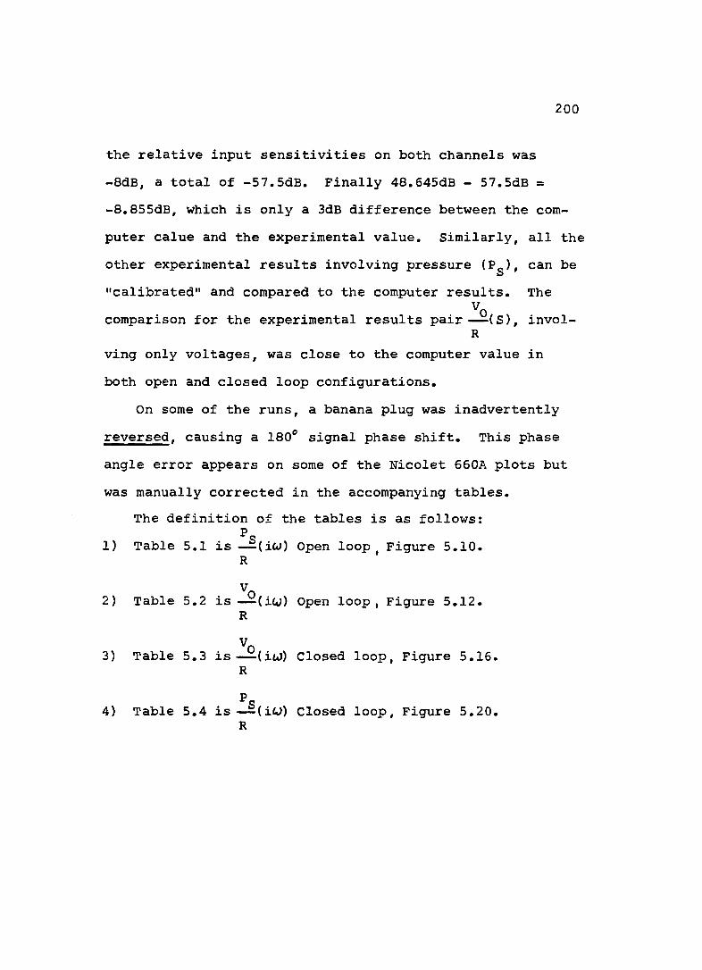
200

the relative input sensitivities on both channels was -8dB, a total of -57.5dB. Finally 48.645dB - 57.5dB = -8.855dB, which is only a 3dB difference between the com­puter calue and the experimental value. Similarly, all the other experimental results involving pressure (Pg), can be "calibrated" and compared to the computer results. Thecomparison for the experimental results pair— 2.(s), invol-

Rving only voltages, was close to the computer value inboth open and closed loop configurations.

On some of the runs, a banana plug was inadvertentlyreversed, causing a 180® signal phase shift. This phaseangle error appears on some of the Nicolet 660A plots butwas manually corrected in the accompanying tables.

The definition of the tables is as follows:Pg1) Table 5.1 is — (iw) Open loop Figure 5.10.RV

2) Table 5.2 is —^(iw) Open loop, Figure 5.12.RV

3) Table 5.3 is — ^(iw) Closed loop, Figure 5.16.R

Pg4) Table 5.4 is— (iU) Closed loop, Figure 5.20.R

Table 5.3 Table 5.4Table 5.1 Table 5.2 W(HZ) ^(DG) W(HZ) 0(DG)W(HZ) ^(DG) W(HZ) <*(DG) 0.13 - 1.1 0.13 -131.8

0.13 -101.5 0.13 62.0 0.25 - 0.9 1 .00 -160.50.25 -103.8 0.25 1.5 0.38 - 0.5 2.00 -163.10.50 -112.1 0.63 0.2 0.50 - 2.0 3.00 -165.01.00 -127.6 1 .00 - 3.8 0.63 - 7.5 4.00 -167.02.00 -133.5 2.00 - 6.5 0.75 - 3.7 6.00 -168.23.00 -132.5 3.50 - 14.0 1.00 - 8.7 8.00 -181.95.00 -133.8 5.00 - 20.0 2.00 - 14.7 10.00 -191.0

10.00 -159.3 10.00 - 37.7 3.00 - 22.2 15.00 -239.015.00 -190.0 15.00 - 43.6 4.00 - 29.1 17.00 -264.520.00 -230.7 20.00 - 45.3 5.00 - 36.9 20.00 -301.925.00 -279.6 25.00 - 53.4 10.00 - 79.1 24.00 -344.430.00 -319.3 30.00 - 72.5 15.00 -108.5 25.00 -354.135.00 -331.5 40.00 -122.7 20.00 -103.5 25.88 -359.539.00 -335.5 45.00 -142.9 25.00 -112.7 27.00 -369.239.25 -358.9 50.00 -158.1 30.00 -133.2 30.00 -387.240.00 -356.5 60.00 -184.5 35.00 -161.6 35.00 -415.445.00 -339.5 40.00 -186.1 40.00 -439.150.00 -324.6 45.00 -205.3 45.00 -462.3

50.00 -217.5 50.00 -485.2

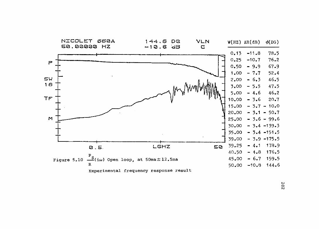
NICOLET O60AB0.00000 HZ

1 4 4- 1 0SS

DGd B

VLNC

0 S. LGHZ S0

Figure 5.10 — ^(iw) Open loop, at SOmal:12.5ma RExperimental frequency response result

W(HZ) AR(dB) #DG)

0.13 -11.8 78.50.25 -10.7 76.20.50 - 9.9 67.91.00 - 7.7 52.42.00 - 6.3 46.53.00 - 5.5 47.55.00 - 4.6 46.2

10.00 - 3.6 20.715.00 - 3.7 - 10.020.00 - 3.1 - 50.725.00 - 3.6 - 99.630.00 - 3.4 -139.335.00 - 3.4 -151.539.00 - 3.9 -175.539.25 - 4.1 178.940.50 - 4.8 176.545.00 - 6.7 159.550.00 —10.8 144.6

NJoI\3

60

Experiment

40

SpeakeasycbA

-360

100.0 FREQUENCY (rad/sec)10.01 . 2

Figure 5.11 — -(iw) Open loop, at 50ma±12.5maRComparison between Experiment and Speakeasy

tooU)

NICOLET SS0A100.0000 HZ

-80-0

74

DGd B

V L NC

W(HZ) A R ( d B ) <^(DG)

Figure 5,12 —^(iw) Open loop R

LGHZ at 50ma ±12.5ma

1 00

Experimental frequency response results

0.13 9.5 143.80.25 10.2 178.50.63 10.4 179.81.00 9.1 176.22.00 9.5 173.53.50 9.5 166.05.00 9.5 160.0

10.00 8.6 142.315.00 6.9 130.420.00 6.1 134.725.00 8.3 126.630.00 9.8 107.540.00 9.7 57.345.00 8.8 37.150.00 8.2 21.960.00 6.3 - 4.570.00 4.0 - 31.180.00 2.7 - 51.890.00 1.0 - 67.9100.0 -0 .4 - 80.7roo

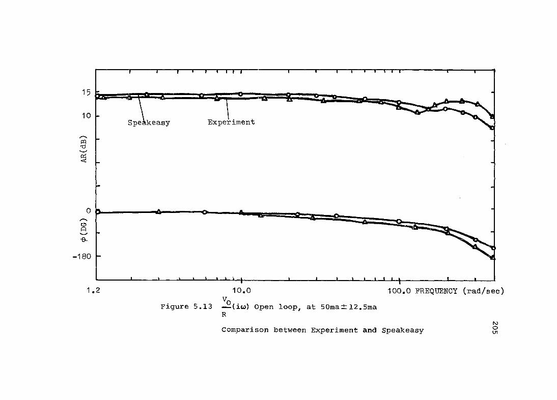
15

10 ExperimentSpeàkeasy

pq

0

-180

100.0 FREQUENCY (rad/sec)1 . 2 1 0 . 0

Figure 5.13 — (iw) Open loop, at 50ma±12.5maRComparison between Experiment and Speakeasy OUl

NXCOL.ET BSQiAS 0 .B00QQ HZ

33•2S

37

DGd3

VLNC

Figure 5.14 — (iw) Open loop, at 50ma±12.5ma

Experimental frequency response result

W(HZ) AR(dB) f(DG)

0.13 -22 ,6 .-150.40.25 -21.8 -152 .40.50 -20.3 -149.10.88 -19.0 -153.01.00 -17.9 -153.02.00 -16.6 -153.84.00 -14.2 -148.05.00 -12 .4 -144.3

10.00 - 8.1 -147.315.00 - 5.9 -169.716.00 - 5.3 -175.617.00 — 4.6 173.418.00 - 4.1 167.020.00 - 8.3 145.025.00 - 8.0 112.630.00 -12.8 96.135.00 -14.5 91.340.00 -18.2 88.145.00 -22.1 94.750.00 -26.0 93.7

o

40

Speakeasy

Experiment

- 180

-360

100.0 FREQUENCY (rad/sec)1 0 . 01 . 2

sFigure 5.15 (ico) Open loop at 50ma±: 12. 5maVoComparison between Experiment and Speakeasy

NICOLET SSQA50.00000 HZ

-37- 1 S

5S

DGdB

VLNC

W(HZ) AR(dB) 0(DG)

0.5Figure 5.16 — - (iw) Closed loop

R

LGHZ

at 50ma±12,5ma

50

Experimental frequency response result

0.13 - 3.1 178.90.25 - 3.3 179.10.38 - 3.7 179.50.50 - 2.7 176.00.63 — 2.6 172.50.75 - 2*8 176.31.00 - 2 .7 171.92.00 - 2.9 165.33.00 - 2.9 157.84.00 - 3 .0 150.95.00 - 3.1 143.1

10.00 - 4.5 100.915.00 - 9.5 71.520.00 -13.2 76.525.00 -11.7 67.330.00 -11.5 46.835.00 —12.6 18.440.00 -14.7 — 6.145.00 —16.6 - 25.350.00 —18.8 - 37.5 N3o

03

pqTJ

Speakeasy0

o-

Experiment

-10

ciA

-180

100.0 FREQUENCY (rad/sec)10.01 . 2

Figure 5,17 — -(iw) Closed loop at SOma it 12.5ma RComparison between Experiment and Speakeasy

N)OVO

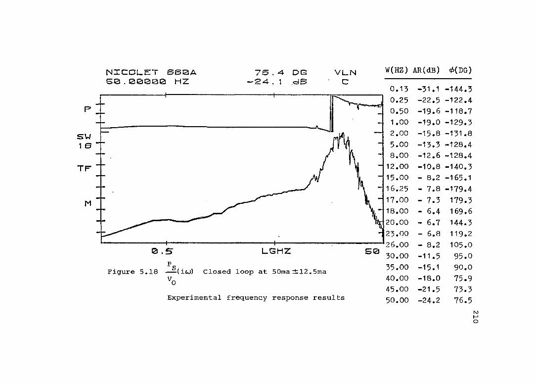
NICOLET eSQA50.00000 HZ

S W 1 G

T F

M

Figure 5.18

VLN

0.25

2.00

8.001 2 . 0 015.0016.2517.00

- 18.0020.00

- 23.0026.0030.0035.00Closed loop at SOma 12.Sma40.0045.005 0 . 0 0

W(HZ) A R ( d B ) 0 ( D G )

-31.1 -144.3 -22.5 -122.4 -19 .6 -118.7 -19.0 -129.3 -15 .8 -131.8 -13.3 -128.4 -12 .6 -128.4 -10 .8 -140.3- 8.2 -165.1- 7 .8 -179.4

Experimental frequency response results

179.3169.6144.3119.2105.0

-11.5-15.1—1 8 . 0

-21.5-24.2

MHO

Speakeasy

30Experiment

-360

100.0 FREQUENCY (rad/sec)1 0 . 01 . 2

S,..Figure 5.19 — (icj) Closed loop, at 50ma±12.5ma

Comparison between Experiment and Speakeasy

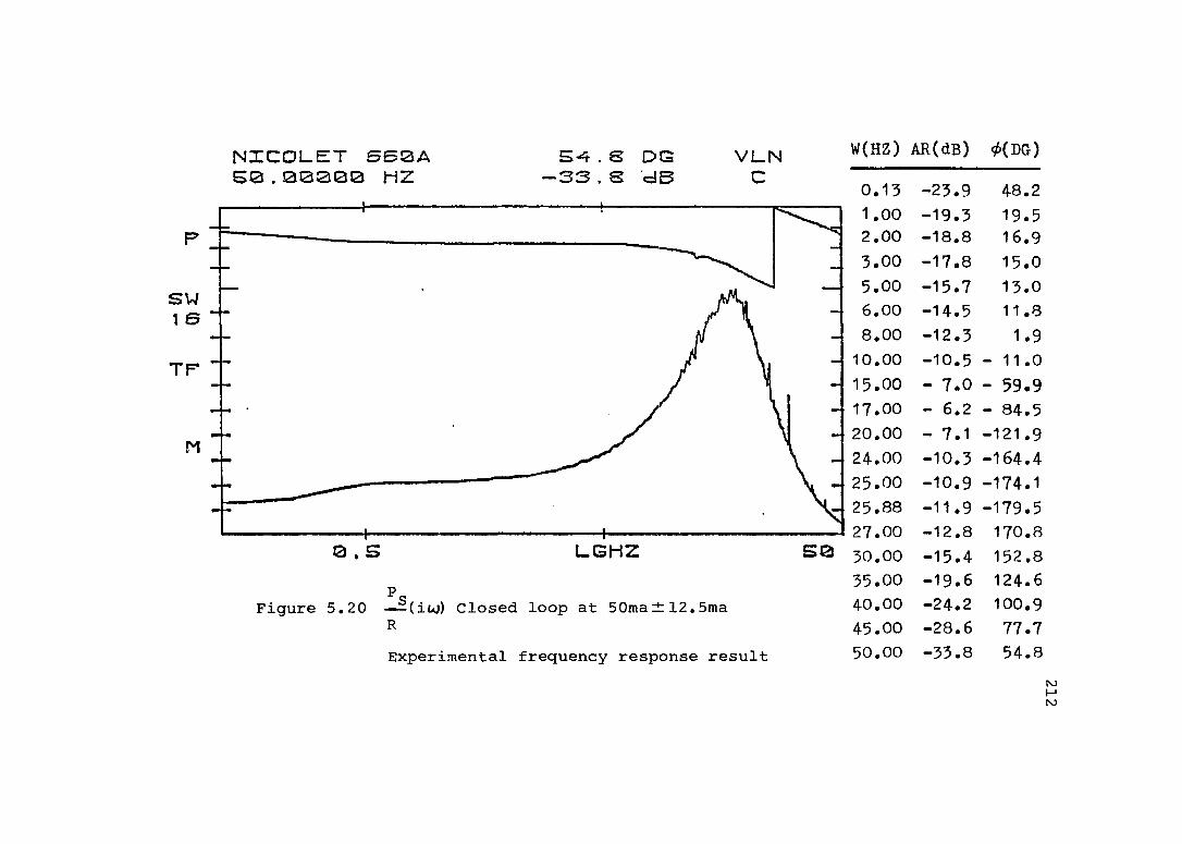
NICOLET SeSA50.00000 HZ

SW1 e

TP

M

VL-N

2.00

6.008.00

- 10.00- 15.00- 17.00- 20.00- 24.00- 25.00- 25.88

27.000 . S 30.00

35.0040.0045.005 0 . 0 0

W(HZ) A R ( d B ) <^(DG)

48.2 19.5 16.9 15.0 1 3 .0 1 1 . 8

1.9-10.5 - 11.0- 7.0 - 59.9— 6.2 — 84.5 - 7.1 -121.9 -10.3 -164.4 -10.9 -174.1 -11.9 -179.5 - 1 2 . 8 1 7 0 . 8

Figure 5.20 — (iw) Closed loop at 50ma± 12.5ma RExperimental frequency response result

-23.9-19.3-18.8-17.8-15.7-14.5-12.3

-15.4- 19.6- 24.2-28.6-33.8

152.81 24 . 6100.977.754.8

K)MK>

Speakeasy

Experiment

-180

-360

100,0 EREQUENCY(rad/sec)1 0 .01 . 2qFigure 5.21 — (iw) Closed loop at SOma— 12.5ma

RComparison between Experiment and Speakeasy N>

to

214

5.3 Program #20 and Experiment Comparison

An important outcome of our theoretical analysis was the derivation of the three transfer functions Pg V P— (S); -- (S); — (S) investigated in letter form. TheseR R VQ

transfer functions will become now tools in servosystem design, synthesis and analysis in frequency domain. The frequency response can be obtained fast using the OSU Mech, Eng. Dept. Frequency Response program #20 which is much less expensive than the previously described Speakeasy program

and much easier to use.We conclude our frequency domain analysis comparing

the experimental frequency response results used earlier with the output of program #20.

V5.3.1 The— (S) Transfer Function

The letter form is:

''o,., K, K (S; = n--------------- n----- --------------R s S'" 2^ 5

( T + — ' • + 1) (--T + ---- + 1) Gpp(S)" V ^v " h "h

(5.1)

215

Substituting numerical values we get

V- 43.3*10^ (s + 138.8 S + 13377.3)•(S) =

^ 5^ + 923.0 S^ + 30.19*10^ +39.5*10^5+1.5*10^(5.2)

Fig.5.22 is the comparison between the experiment and the computer program output.

Pg5.3.2 The— (S) Transfer Function R

In the letter form

-S,s) . , i (5.3)

%

And after substituting numerical values

P„ 10.8*10^ (S + 23.72)_ 5 ( s ) --------------------------------------------------^ + 923 + 30.19*10^s2 + 39.5*10^5 + 1.5*10^

(5.4)Fig.5,2 3 is the comparison between the experimental result and the computer program output.

Finally the third transfer function

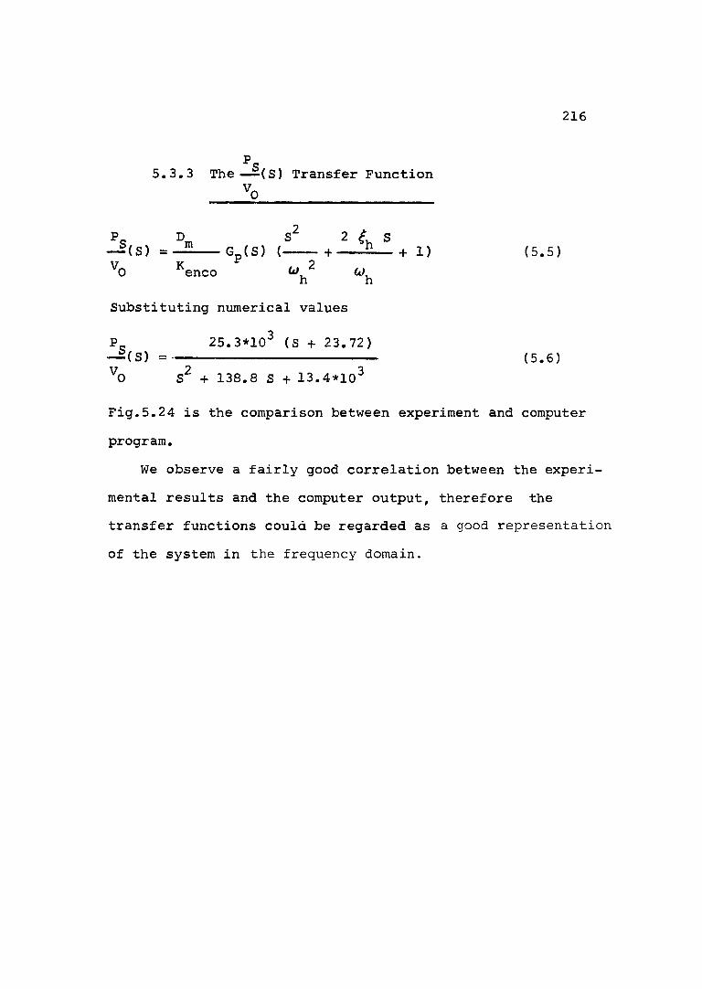
216

Pg5,3,3 The (S) Transfer Function^0________________________

Pq B 2 ^ S~(S) = -2 G (S) (---- + ----- + 1) (5,5)^0 ^enco W Cl>n nSubstituting numerical values

P„ 25,3*10^ (S + 23,72)— ( S ) = --- -- ■ ■ (5,6)^0 S + 138,8 S + 13,4*10^

Fig.5,24 is the comparison between experiment and computer program.

We observe a fairly good correlation between the experi­mental results and the computer output, therefore the transfer functions could be regarded as a good representation of the system in the frequency domain.

Program #20

Experiment

i ampl enco(S)

PP

-180

100.0 EREQUENCY(rad/sec)10.01 . 2

Figure 5.22 Open loop at 50d:12.5ma (Program #20)N)M

50 Program #20

ExperimentG„(S)

35 — (S)

PP

-180 [>

-360

100.0 FREQUENCY(rad/sec)1 0 . 01.2Figure 5.23 Open loop at 50d:l2,5ma (Program #20)

toH00

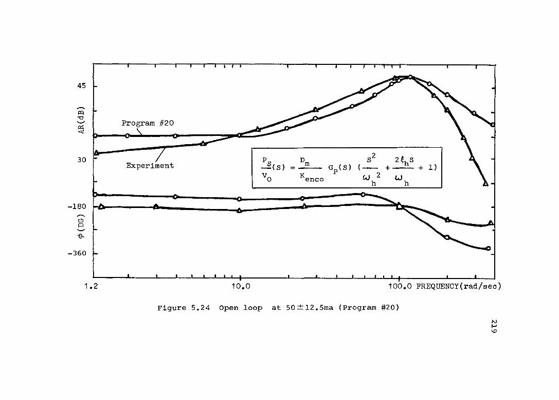
45

PPX)

Program #20

30 Experiment G_ ( S ) ( - +enco

-180ci)A

-360

100.0 FREQUENCY(rad/sec)1. 2 10.0

Figure 5.24 Open loop at 50±12.5ma (Program #20)

220

5.4 CONCLUSION

From the Bode diagrams comparing experimental results with the Speakeasy frequency response computer

output and program #20 output we conclude that in the frequency domain we get a good correlation.

Since our comparison between the CSMP output and the experimental step response results was satisfactory as well we summarize this chapter stating that computer simulation was validated with a fairly high level of confidence.

PART TWOTheoretical Study of Proposed Energy-

Saving Hydraulic Control Configuration Based on Variable Displacement Pumps

221

222

CHAPTER 6 LOAD SENSING - BACKGROUND

6.1 General Background

Efficiency or efficient use of energy has recently become a subject for strong consideration in all facets of our lives. The increasing amount of fluid power applied in industry, focused the attention of both the designers and the users of hydraulic systems on the improvement of device efficiency. Recently, every fluid power manufactur­er and user became actually aware of the oil and energy wasted in leaks, friction and inefficient designs. It always has been obvious that the popular method of "thrott­ling", to control pressure and flow is wasteful (64).

Pumps can also be great power wasters, and in order to improve efficiency, variable displacement pumps are used, controlled by various means to eliminate the dumped flow. There are six basic types of such controls (66):(1) Pressure Compensation.(2) Torque Compensation.(3) Flow Compensation.(4) Power Compensation,(5) Speed Compensation.

223

(6) Viscosity Compensation.Inefficiency in hydraulic systems can have many origins,

but all energy losses ultimately appear in two forms; heat and noise. A concept that is rapidly gaining universal acceptance is to produce just the hydraulic energy actually required and deliver it only when needed,

6.2 The Definition of the Problem

Fluid-power users are turning from brute-force methods toward Load-Sensing systems that hold down energy costs.The energy savers first appeared in mobile construction equipment, but are now making inroads in the general indus­trial market. Of special interest in this dissertation is the application of the Load-Sensing concept in valve con­trolled servosystems. The pressure-compensated variable displacement pump was and remains the basic component of such applications.

All fluid power systems take an energy source, transform mechanical energy to fluid energy, transfer it through the system, transform it back to mechanical energy, and deliver it to a load in the form of linear or rotary motion.

That is what fluid power does-and in essence that is what competing mechanical and electrical systems do. Diff­erences between the "new" and old generation of fluid power systems lie in the pumps, and more specifically, in

224

the pimp control package.We propose to study for feasibility two schemes suggest­

ed as means to take advantage of the controllability of variable-displacement pumps for energy-saving operation of servo-systems. One scheme, suggested by Felicio (9), uses pre-knowledge of system duty cycle to program pump discharge pressure to meet the needs of the load without excessive power losses at the servovalve. The second approach attempts to enforce the well-known maximum power transfer rule (load pressure drop should be 2/3 of supply pressure) by sensing supply pressure and load Ap and using these signals in a feedback scheme which adjusts pump discharge pressure so as the enforce maximum power transfer at "all" times.

The two proposed schemes belong to the "Load-Responsive" family of hydraulic systems. The idea is to monitor the pressure drop (AP) across the actuator (load pressure) and to set up a pump pressure controlling loop which will operate simultaneously with the velocity or (position) feedback loop on the servovalve.

In the near future we anticipate a "marriage" of elec­tronics and hydraulics, integrating microprocessors and highly reliable pressure and flow measuring devices into the hydraulic systems (65). Thus, the controllability of systems will be substantially improved, making energy- saving possible.

225

6.3 Historical Background

There are no books available in the field of "Energy- Saving in Hydraulic Systems" and literature on "Load- Responsive" or "Energy-Saving" hydraulic circuits could be found only in papers published in the last five or six years. Although this subject is very important, much of its technical development is being kept closed in the form of industrial secrets. Papers available today are published by manufacturing companies such as: Abex-Denison, Eaton, Parker-Hannifin, Rexroth, Sperry-Vickers and Sundstrand.

Load-sensing and energy savings in non-servo applica­tions is a rapidly growing concept in hydraulic systems and new information is available almost every month. From the many papers we have, we will summarize just a few.(1) Two-types of hydraulic systems, closed and open loop, are available to the designer. Both systems can be very efficient if properly used (49).(2) Three-systems of hydraulic control for open loop circuits are used in industry (75).

2.1 The Open-Center system.2.2 The Constant-Pressure-Closed Center System.

The open-center and closed center systems are the most often used.

226

2.3 A third type of system which is not as commonly used in the hydraulic field is one which permits the pump output pressure to drop to a relative low value when the closed- center valve is in the neutral position. In addition, this system changes both, the pump volume and pressure outputs according to the demands of work load. This system is known as :"Load-Sensing System".(3) There are two basic methods of load sensing, pump con­trol and valve control. Most commercial load sensing systems use pump control based on variable displacement pumps (63).(4) Finally, an outstanding article published by B. Ander­son, "A Survey of Load-Sensing Systems" in the BFPR Journal, 13 Feb. 1980, summarizes the subject giving 39 references including those mentioned earlier (77).

In Appendix B, several more papers have been mentioned as being related to the subject of "Load-Sensing" and "Energy-Saving".

NCFP - References: (27); (28); (29); (30); (31); (32).ASME - Reference: (46).SAE - References: (48); (50); (51); (52).Machine Design - References: (60); (61); (62); (63).Product Engineering - References: (64); (65); (66); (67)Hydraulic & Pneumatics - References: (68); (69); (70);

(71); (72); (73); (74).

227

Manufacturing Companies - References: (75); (76); (77)(78).

6.4 Load-Sensing in Servovalve-Actuator Systems

The primary components of the "Load-Sensing" system as used in non-servo applications are a special closed-center type directional control valve and a unique pressure com­pensated variable displacement pump with the "compensator" set to destroke the pump at a low-pressure. The control valve senses the work port pressure as the control valve spool is shifted from neutral to the working position to provide flow to move the load at some desired maximum speed. This pressure signal is sent to the spring biased pump compensator through a separate pilot line, adjusting the pump delivery to keep pump pressure between ISOpsi to 250psi higher than work pressure, so-called "standby pressure".The maximum standby pressure can normally be adjusted, however, an increased standby pressure represents a constant load that is imposed upon the pump at all times. Whenever the control valve is shifted to a work position, the pump will maintain this standby pressure at a higher level than that required to move the load. Load speed is defined by pump delivery and system response depends on pump speed of response which is the typical pump-control configuration.

228known as a "slow" responding system.

In servovalve-actuator systems a pressure compensated variable displacement pump is also often used. The pump provides maximum set pressure even if load can be moved at desired speed by a lower pressure. Pump delivery will be maximal at that pressure, thus pressure drop as well as flow rate across the valve needed for a desired load speed are provided at "all times". Therefore, a "fast" system is achieved, making the "Conventional Load Sensing" concept described earlier not suitable for servosystem applications. Pump stroke is regulated in this case under maximum pressure setting during servovalve operations. Excessive leakage, at high pressure (high energy loss) is caused when servo­valve is closed or when load is stalled, but servovalve is open.

"Load Sensing" in a servosystem must have a different logic. In this case the pump "flow" is compensated in such a way that the pressure drop across the valve port, which is needed to supply actuator flow (actuator speed), is main­tained at "all times."

Pump "pressure setting" is achieved by sensing supply pressure Pg, load pressure drop AP and using these signals in a control scheme to feed a pressure regulator. Keeping pump discharge pressure Pg, slightly higher (ISOpsi to 250 psi) than load pressure P^ plus servovalve pressure drop '^valve can minimize energy losses in the system caused

2 2 9

by leakages, since they occur at low pressure.We presented in this chapter a summary of the available

information on load sensing. Although somewhat lengthy for an introductory chapter, we feel it was necessary, since as we mentioned earlier the field is not yet covered in textbooks. The chapter was also .aimed to serve as a back­ground for the analysis of the two proposed energy saving schemes.

CHAPTER 7 DEVELOPMENT AND THEORETICAL ANALYSIS OF PROPOSED ENERGY-SAVING CONFIGURATIONS

As an introductory section to our explanation and analysis of the two proposed schemes, we will present now two paragraphs taken from literature (2). These few pages disclose the "heart" of the problem of power transfer and efficiency in valve controlled servosystems, which deals exactly with our analysis.

Statements were published in 1967, such as(1) "Efficiency is not a major consideration in hydraulic

servo design and operation."(2) "Factors such as accuracy, response and compliance are

considerations that outweigh efficiency in importance,"(3) "These facts are typical of control systems as a

discipline."Recent increases in energy costs make these statements

less valid today than in 1967 and are a motivation for deve­loping energy-saving schemes.

7.1 Maximum Power Transfer to Load with a Servovalve (Merritt, page 226)It will prove helpful to review the well known condi-

230

231

tions for maximum power transfer to the load with a servo­valve controlled actuator. For simplicity, let us assume a critical center valve for which the flow with a positivespool displacement has been shown to be,

1/2Ob = Cdv" (Pg - P^i/P (7.1)

where:0^ é "Load" flow rate (cis).

Orifice coefficient (= 0.61) . é Valve spool displacement (in).

P A Oil density (Ib-sec^/in).Pg A Supply pressure (psi).Pj A "Load" pressure (psi).

The horsepower supplied to the load is thenh p / l o a d . 0 ^ P l

hp/load = CgyXy w (Pg/Pl^/Z pg (1 . P;/Pg,l/2

(7.2)where : W a Valve flow coefficient (in^/in).

hp/load A Power "delivered" to the load (HP) . which is plotted in Fig.7.1.

The load horsepower is zero when P. = P_ because noLj Opressure drop remains across the servovalve orifices to yield a flow to cause actuator motion; the actuator is stalled. When P^ = 0 no horsepower is required by the load. Maximum horsepower occurs between these extremes

232

0.4

0.3

0.2

0.1P i => f P, for

maximum power / transfer

0.2 0.4 0.6 0.8 1.0PJP.

Figure 7.1 Normalized plot of power at load versus load pressure (Merritt)

and is found by forming dh^/dp^ = 0, and simplifying it to give the well-known result

î’l = 2/3 Pg (7.3)

Thus, maximum power is transferred to the load when the pressure across the load is two thirds- of. supply, pressure. However, because is usually changing during servo opera­tion, it will be at 2/3 only a small portion of the operating time. Hence power is usually transferred to the load in a less than optimum manner. Therefore this rela­tionship is not very useful in a design unless the load is relatively constant over a duty cycle.

However, as a general rule, power elements are sized such that P does not exceed 2/3 P„ for the maximum loads normally expected. Although this rule promotes efficiency by handling the largest expected load at the point of

233

maximum power transfer, this is not the most important reason for the rule. It should be apparent that as load is increased, approaches and the hydraulic actuatortends to stall. Because the pressure drop across the servo­valve approaches zero, the flow gain is decreased and the servo tends to lose control of the load. Hence, it is desirable to limit P so that the flow gain is high enoughJjfor the servo to maintain control. If it is limited to 2/3 Pg, then the flow gain is reduced to not more than

= 0.577 = 57.7% (7.4)

of the no load flow gain. Because servos are usually desi­gned to provide sufficient control if the loop gain drops by half to allow margin for gain changes in components due to tolerance, aging, temperature, loads, etc., then the 2/3 Pg rule seems adequate and should be disregarded with caution.

Although it is quite possible that high acceleration rates during rapid transients may cause P to exceed 2/3 Pg, such conditions are usually of short duration and need not to be taken into account.

234

7.2 Maximum Power Transfer and Efficiency (Merritt, pg.228)

Combining (7.2) and (7.3), the maximum power that can be transmitted to the load is

h /load = ^dv ^vmax (p /3)3/2 (7.5)Pmax ( p )l/2 s

where.h /load A Maximum power to the load (HP).^max

Xvmax = Maximum valve spool displacement(in)and occurs when = 2/3 Pg, The operating efficiency ofa servovalve controlled actuator may be stated as

h /load P Q P"op = K^TgiH- * = P ^ * 100 - pi * 100

(7.6 )where:

= Operating efficiency {%).

This equation assumes that the hydraulic power supply uses a variable delivery pump which adjusts its output flow to just meet the required load flow. Some additional pump flow, of course, would be required to meet leakage losses. The operating efficiency is zero at no load (for the obvious reason that no horsepower is required by the load) and increases to 100% with a stall load. Because P /P±j s

is normally limited to 2/3; the maximum operating efficiency is 67% for servovalve controlled actuators. The power

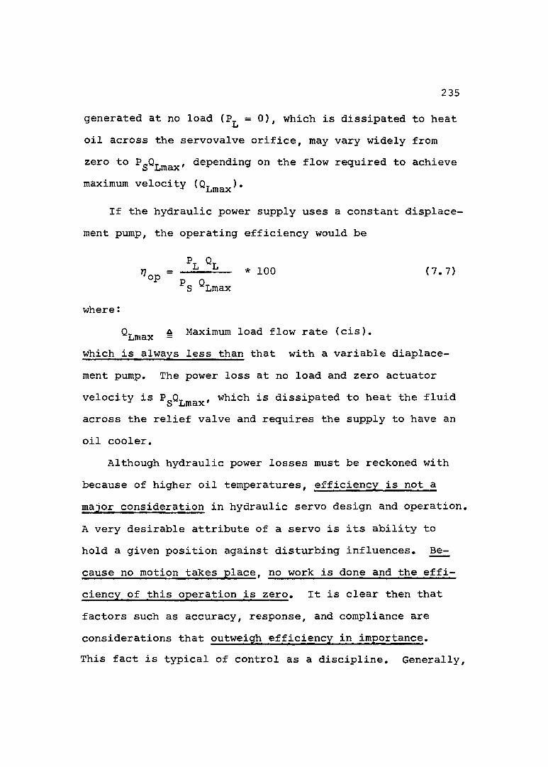
235

generated at no load (P^ = 0), which is dissipated to heat oil across the servovalve orifice, may vary widely from zero to PgQ^max' depending on the flow required to achieve maximum velocity (Q^max^'

If the hydraulic power supply uses a constant displace­ment pump, the operating efficiency would be

Pr Qrrj = — h— k — * 1 0 0 ( 7 . 7 )

P p QS Lmaxwhere :

A Maximum load flow rate (cis).ijITla.X —

which is always less than that with a variable displace­ment pump. The power loss at no load and zero actuator velocity is P Q , which is dissipated to heat the fluidD JjIUâXacross the relief valve and requires the supply to have an oil cooler.

Although hydraulic power losses must be reckoned with because of higher oil temperatures, efficiency is not a major consideration in hydraulic servo design and operation. A very desirable attribute of a servo is its ability to hold a given position against disturbing influences. Be­cause no motion takes place, no work is done and the effi­ciency of this operation is zero. It is clear then that factors such as accuracy, response, and compliance are considerations that outweigh efficiency in importance.This fact is typical of control as a discipline. Generally,

236

the power involved in the process under control i s much

larger than the power required for control purposes.

Therefore, improvements in e ff ic ie n c y of the process under

control would net greater return in o v er -a ll cost reduction.

- End of citation from Merritt - As we can see in this quotation from Merritt,efficiency

was of little interest in the 60's and poor efficiency of control systems was taken as acceptable.

System efficiency and energy saving are probably the main concerns in all sections of today's industry. There­fore, it is essential, if not required, to make an effort to develop a more efficient valve controlled servosystem in order to achieve the maximum theoretical efficiency (66.1%),

Having determined in detail the conditions for a maxi­mum power transfer to the load and the efficiency in a servovalve-controlled actuator system, we now turn to the actual explanation and analysis of the two proposed energy saving configurations.

7.3 The P_ = 2/3 P„ SchemeLi O

AP j = Load Pressure .Pg = Supply Pressure .

Figure 7.2 describes the proposed Pressure OptimizingScheme, based on the P = 2/3 P rule.If s

Pressure Control Loop Controlled Variable P_(t)

Velocity Control Loop Controlled Variable # ( t j

(t) = Pressure drop across the actuator

3/2

Ampl

PumpAmpl

ABS

RegulatorServoValve

D if f . Press Transducer

Hydr, Motor + Load

SpeedFeedbackSignal

S^(t) = Desired speed setting

Figure 7.2 The proposed Supply Pressure Optimalizing scheme (P^ = 2/3 P^)N)W'vl

2387.3,1 Principle of Operation

Our goal in this "Optimizing" configuration is to enforce the "Maximum Power Transfer Law" by adjusting the supply pressure Pg to be 3/2 P^ at "all times" during the duty cycle. It is assumed that the pressure compensated variable displacement pump is operating in the "regulating region" providing the flow rate needed by the system. The flow to move the load at a desired speed; is enforced bythe control loop closed around the servovalve.

In the P^ = 2/3 Pg concept, which we will name as"Supply Pressure Optimization ", configuration, the con­trolled variable is the Pump Supply Pressure Pg. The idea is to sense the pressure drop signal across the actuator APt (t) as it occurs and feed it back multiplied by 1.5 to the "Pump Pressure Adjusting Mechanism ", thus Pg(t) = 3/2 AP^(t) at all times.

Pressure compensated variable displacement pumps used today, with no variable pressure control capabilities, apply maximum set pressure Pg^ax if the load can bemoved at desired speed with lower pressure. The excess pressure drop, times the flow rate,is wasted power in the system. In order to reach a better understanding of the "new concept" let us follow the supply pressure control procedure observing the pressure - flow relation curve in a pressure compensated pump (Figure 7.3):

239

Max. Press. Operating Point

Press.=

Required PowerPower

Point

Desired FlowQ Q max pump

(c is )

Figure 7.3 Pressure flow relation in a controlled compensated pump

The desired flow rate is defined by the Speed Control Loop, assuming pump is set at With novariable control on the supply pressure P^, the pump pro­vides maximum pressure, point A on the diagram, even if the load can be moved at desired speed with a lower pressure Pg^ or Pg2* Let us say that the pressure required by thesystem is P^g, then the region between Pgg ^Smax the "Lost Power". Our proposed optimizing scheme will

is

eontinuously control the pressure Pg co the "Required Power Level", thereby saving energy.

240

The variable displacement vane-pump used in Felicio's apparatus (9), has regulation over the 600/1000psi range, however, other pumps(larger) have a regulating range of 300/1500psi (5 to 1), and therefore the possible energy saving is much higher. The regulating region could be best represented in the following diagram:

Pump P AP -Smax

Smin2/3 P loadSmax

Figure 7.4 Pg versus 4P2oad enforcing the = 2/3 Pg rule

Since the system has leakages even during the "Idle Position", to keep energy losses at the lowest possible level, the minimum pump pressure setting Pg^^^ is the best possible choice. This pressure is equivalent to the "Standby Pressure" in the "regular" load sensing system described earlier. The pump regulating limits, Pg^^^ and Pgmax' and ISOOpsi respectively, "connected"

241by the P^= 2/3 concept, are the "heart" of the proposed scheme. In computer simulation this curve can be generated using the P^= AFGEN(CURVE, 4P) function available in CSMP.In a practical case various means could be used to adjust pump pressure in response to the load 4P signal.

7.3.2 Speed Control and Pressure Control Servosystem

Let us turn now to the derivation of the set ofdifferential equations governing the new concept. As wecan see in Fig. 7.2, the two control loops-, the velocity loop,and the supply pressure adjusting loop are not independentand the interrelation occurs via the servovalve. Inorder to explain the logic behind the supply pressureoptimizing loop, we will present briefly the model ofthe pressure compensated variable displacement pump as afunction of the "desired pressure" P„/P,(S).

PgThe "disturbance" transfer function — (S), i.e. pumpQs

pressure as a function of system flow demand was given in chapter 2.

P -K (T S + 1)(S) = ----2---E------- (7.8)

242

and was used to investigate pump dynamics effects on servo­system response. During the experimental analysis in part one of this dissertation we found that "slow" changes in system flow demand have a negligible effect on pump pressure variations. So, in our case, the relation between the supply pressure Pg and the "Desired Pressure P^" is of im­portance (9).

Pq 1— (S) = ------------------- (7.9)

Usually is large (185 rad/sec in our case), and sincewe are interested in"slow changing" transients, much

Pbelow pump natural frequency, pump's _S (S) relation can be

simplified toPg 1— (S) = --------- (7.10)^d ?pl s + 1

This model will be used in the pressure control loop but if "fast" transients need to be accomodated, equation (7.8) could be used without changing the basic analysis approach.

The set of differential equations describing the block diagram in Figure 7.5 was derived in Chapter 2.

The pump model;■ Pq 1— (S) = --------- (7.11)

"d S + 1

Pg (p s i)

V.D.Pump 1500

300200 1000

GAINADJUSTINGBLOCKZZZZZPressure

RegulatorTorqueMotor Comp

i i

Ampl

A P Tach DesiredSpeedABS

Figure 7.5 Speed control Servosystem with Supply-Pressure Optimization N)to

244

(7.15 )

Servovalve nonlinear model

OL = Iv'Ps - (7-12)The continuity equation

OL = Dm »m + =tm ?L +

Newton'S lawS «m + «m + T'l (S) (7.14)

The velocity control feedback loop;

2v= K^,pl °comp<S) - Vq)

''o ' ''tach K

And finally the pressure control feedback loop= 1.5 (7.16)

7.3.3 Position Control - Pressure Control System

Before going into a "Feasibility Study" of the new concept we will mention the possibility of using the proposed scheme in position ssrvcsystsms as well.

The set of differential equation describing the posi­tion servo would be: (see chapter 2)

^S 1Pump model — (S) = ------------------- (7.17)

T-pi + 1

245

Valve nonlinear model = K^I^(Pg - (7.18)

Continuity equation

OL = Ap Xp + Ctp S (7.19)

Newton's law

= Jp Xp + Bp S Xp + Cp Xp + F^IS) ,,_20) The position control feedback

:v= Kampl (%v - Xp' (7-21)

And the pressure control feedbackP^ = Pj * 1.5 (7.22 )

where:

= ^cl - Per'A typical position control servosystem with Supply

pressure optimization is presented in Figure 7.6 and the appropriate block diagram is given in Figure 7,7.

When position control servosystems use large amounts of power, such as a moving gun turret or a searching radar our energy - saving scheme can save a significant amount of power.

Next, we will perform a "Feasibility Study" on the speed - control pressure - control system.

V.D.Pump

i L300

200Servo Valve Gain adjusting block

izzrz// ForceMotor

PressureRegulator Ampl

or

Piston

A p.

ABS

Figure 7.6 Position-Control Servosystem with Supply-Pressure OptimizationtVJCTi

3/2

Sqrt.(PRESSURE LOOP)

Pt(S) Loadvalve

ampl

(POSITION LOOP)

Figure 7.7 P^ = 2/3 P^ scheme in block diagram form (position control)

X„(S) Input

248

7.3.4 Feasibility Study

The new concept was qualitatively analyzed in several common situations to determine if it had any obvious flaws. The pressure control loop i.e. = 1.5P^^ will limit the maximum load that could be moved, using the new concept, as follows:

The differential pressure across the motor is:

\ - ^2> = «n, + I? -?]'

Neglecting compressibility and leakage, the continuity equation has the form:

«L = “n. i (7-24,

Using the nonlinear servovalve relations

(7.25)

we obtain:Ol = "V Pv'P2 - <Pr='»

Pg = Pi + Pz

the well known pressure relation in servo-systems.And enforcing Pg = 1.5 (P - P2), i.e. the P^ = 2/3 Pg

rule, we get P^ = 5/6 Pg and Pg = 1/6 Pg or finally

P^ = 5 Pg (7.26)

Equation (7.26) is the pressure relation in the actuator

249

defining the maximum load that could be moved, using the "Supply Pressure Optimizing" scheme.

Fast pressure transients may occur when this ratio is exceeded (due to disturbances), but since they are of short duration there is no need to take them into account.

The above short analysis is valid for position control as well, where will represent P j and P^ will be P^^.

Pel = 5 Per

where;P j & left side cylinder pressure.P^^ Ù right side cylinder pressure.

Steady state situation

Load at desired position, no external forces,P^ = Pg = Pg/2 = ISOpsi. Pump pressure is set at minimum value of 300psi, where the maximum pressure setting is ISOOpsi

Case I Load stalled (Q, = 0)

If is given a small step change, valve openspartially, P^^ starts to increase, P^^ starts to decrease. When AP j reaches 200psi pump pressure starts to adjust upward. This further increases P^; causing further increase in P until P_ = ISOOpsi is reached. P thenS oltlaX o

250

stops at this value and the pump is acting as a "Constant Pressure - Setting Pump".Since load is stalled (Xp=0), there is no work done and the only energy losses are the leakages under pressure in the system.

Case II Load allowed to move at "slow"constant velocity = constant

Situation

(1) No acceleration; Xp = 0(2) No spring; Cp = 0(3) Slow motion; Xp» 0(4) So coulomb friction is dominant and pres­

sure drop will be (F ” P )= F /A sign (X )OX 03T C P

If X^ is given a small step change APp_ willincrease, passing 200psi it will adjust Pg upwards untilthe desired pressure to move the load will be reached.The load will move with constant speed Xp and it will gradually close the valve, causing P^^ to decrease and P^^ to increase, thus APj will decrease and Pg as well. At thepoint where APp_ = 200psi, the pump will go back to theoriginal minimum setting SOOpsi.

251

ISOO(psi)(psi)

300psi

EL=200psi

Motion Delay MotionStarts Stops

Case II Pg versus time - Load is moving at a "slow" constant speed

Case III Load is allowed to move at "Fast" constant velocity

In this case the viscous friction force will be dominant and AP^ has the form:

(7.28)= (Pci - Per' = r '(p •

The situation in the system :(1) No external load; F^^t) = 0,(2) No acceleration; Xp = 0 ,(3) No spring; Cp = 0.

If is given a small step change, APp_ will increase until it reaches the needed value and we get a situationsimilar to Case II but faster.

252

Case IV Load accelerates at constant rate X.

Situation(1) No external force (t ) = 0(2) No spring Cp = 0 Actuator pressure drop will be;

= ^cl - Per = Xp *P

(7.29)

If is given a small step change, AP^ will increasePg to increase.suddenly to its maximum value causing

(assuming AP^ >200psi). If next we "ask" for a constant speed motion APj will drop to the level needed to overcome friction forces.

S(psi )

300psi

1—

Load Moves Const. Valve Speed Closed

Time

CASE IV Pg versus Time - Load is moving at a constant acceleration

253

Case V Load moving at constant speed Xp anddecelerated to stop.

Actuator pressure drop will be "Nega­tive" and system behaviour same as case IV.

Case VI Load at desired position, EXTERNAL FORCE F^(t) is applied causing dis­turbance, a small step change in Xp.

Situation(1) Xp = 0; No velocity.(2) Xp = 0; No acceleration.(3) Cp = o ;No spring.

will increase and "fight" against the external force disturbance, to the value

F,(t)P , - P = ---- (Neglecting friction) (7.30)

a

Assuming F^ ( t) is large enough such as APj > 2G0psi, Pg will adjust upward, piston will start to overcome the force and Xp will tend to decrease.

Valve will never close and flow rate will be equal to the leakages. Pg will stay at the final value defined by (P^i - Per) = Fj.(t)/Ap, i.e., Pg = 1.5 F^(t)/Ap.

254

Case VII Combination of all the cases men­tioned. System behaviour, Super­position of all the cases except Case I where the actuator was stalled.

Conclusions

According to this feasibility study we don't see any obvious qualitative flaws in the proposed "Supply Pressure Optimalizing" scheme for the typical situations studied.

The analytical study using computer simulation will give us quantitative information on the behaviour and performance of this system.

7.4 Felicio's Scheme

7.4.1 The Proposal Presented by Felicio

A second combination of pump, servovalve and hydraulic motor models, such that a fast and energy saving system is achieved, will be discussed next. Since it was proposed by Felicio as a subject for further investigation in his dissertation, this scheme will be called "Felicio's scheme". But before going into any analysis let us bring

255

the proposal as it was presented by Felicio (9):"In general, when a hydraulic system is composed of a

pressure compensated pump, a servovalve and a hydraulic motor there is always energy loss in the servovalve. For the cases where the motor torque is small and the motor speed is high the energy loss at the servovalve becomes large, since both the flow rate and the pressure drop across the servovalve are large. Therefore, a solution to reduce this energy loss is to decrease the pump outlet pressure in order to obtain a small pressure drop across the servovalve. The ideal solution would be the total elimination of the servovalve; however, such a procedure would degrade the speed of the motor response due to the pump dynamics. Thus, the combination shown in Figure 7.8 seems to be a solution for obtaining both a fast and an energy saving hydraulic system.

The system shown in Figure 7.8 is supposed to be working on a repetitive sequence of operations. A practi­cal application of the system could be, for example, the hydraulic system of an industrial robot.

It is assumed in this system that the needed torque to perform a determined task is known from past experience or by measurements. The speed of the hydraulic motor is a requirement,i.e., in terms of control theory, the motor's

256

actual speed is the controlled variable. Under these conditions the minimum pump pressure can be calculated based on the torque, speed, and leakage of the hydraulic motor. Since in a practical application the utilized torque and specified speed are functions of time, the minimum value for the pump pressure can also be found as a function of time. Then, changing this pressure profile to compensate the losses, transients, small disturbances and to anticipate the increases of power demand, a profile for the desired pump pressure can therefore be obtained, see Figure 7.9.

If the hydraulic system is part of a digital control system, the computer of the control system might be pro­grammed to obtain the desired pressure profile. The complementary information, such as torque and flow being used, which is needed for the pressure profile computation can be measured and fed directly to the computer. During the first cycle the desired pressure can be equal to its maximum value until the computer collects enough data to figure out the "best" profile for the desired pressure.

Feasibility StudyPresumably, the system shown in Figure 7,8 works as

follows.(1) In terms of control, the input is the desired speed

257

of the hydraulic motor and the output is the actual hydrau­lic motor speed.(2) If the hydraulic motor speed is at steady state, the servovalve will be almost fully open; therefore, energy losses in the servovalve will be small.(3) The "speed" of a transient response due to a tran­sient input will be governed by the servovalve and motor since at that instant of time the pump is already set to supply the needed power.(4) If the motor speed is at steady state and small dis­turbances occur, the corrective action will involve only the loop containing the servovalve and the motor. This can take place because of the method used to design the desired pressure profile.(5) If the motor speed is at steady state and "large" disturbances occur, the first reaction is to have the variable i input going toward its maximum possible value.If i input happens to be equal to i input max., then the system may lose control over the speed since the servo­valve is saturated. In order to prevent such a problem a feedback path from i input to the desired pressure is needed. This feedback information asks for additional power to be supplied by the pump.

(6) In an emergency situation, the hydraulic motor can bei tstopped by using the servovalve.

Maximum Desired Pressure 1500(psi)

Programmed P ro file for the Desired Pressure

U tilisedTorque

DisturbingTorque

PressureDesiredPressure

Time +Hydraulic Motor and Load

Pumpdl Speed

input L_ (current)d2

Low Pass F ilte r

(PRESSURE LOOP)(VELOCITY LOOP)

Maximum Desired Pressure (SOOpsi)

Voltage

ServovalveAmplifier Tachometer

VoltageMaximum Valve for i Gain

I Desired Speed

Figure 7,8 Felicio's - Energy saving scheme. cn03

259Programmed Pressure Profile P^(t)

Transients Leakage and Small Disturbances

-----------

Minimum Desired Pressure Transients

Power A nticipation Time

Figure 7.9 Example showing a design for the desired pressure profile P^(t)

Although the system given in Figure 7.8 has not been analyzed in detail by Felicio, it seems to be suitable for those applications where the desired pressure has variations slow enough to be met by the pump dynamic response.

7.4.2 The Set of Governing Differential Equations

Having presented the proposed scheme we will turn now to a detailed analysis, similar to the one per­formed for the "P = 2/3 P scheme",Li o

Pump model

— (S) = ?d T p i S + 1

( 7 . 3 1 )

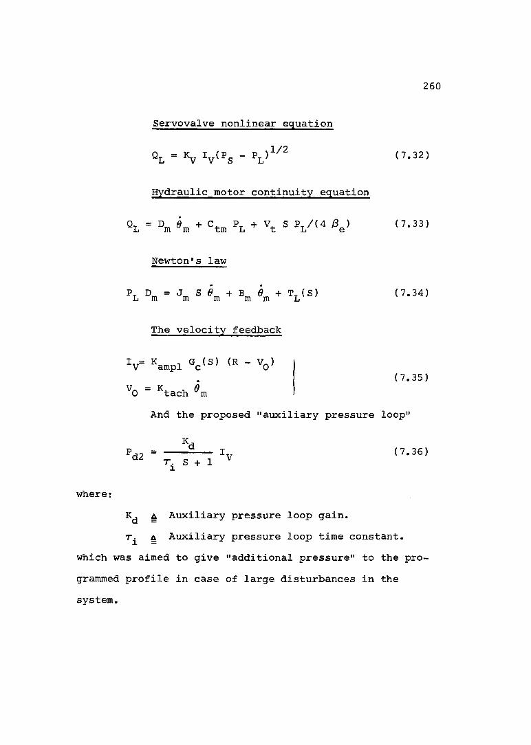
260

Servovalve nonlinear equation

0% = Ky Iv'Ps - (7-32)

Hydraulic motor continuity equation

Ol = «m + =tm \ S V ( ^ e> (7-331

Newton'S law

"L Dm = Jm S + ®m «m + ’’l (®> (7-341

The velocity feedback

Iv= Kampl Gc(S) (R - *0 )

^0 = %tach( 7 . 3 5 )

And the proposed "auxiliary pressure loop"

where:Kj 4 Auxiliary pressure loop gain.

A Auxiliary pressure loop time constant, which was aimed to give "additional pressure" to the pro­grammed profile in case of large disturbances in the system.

261

The final "Desired Pressure P^" to the pumppump ” (programmed) + P^^ (auxiliary ). (7.37)

This system can not be regarded as an "On line" energy saving configuration, when compared to the P^ = 2/3 P^ scheme, since one has to know the needed torque to per­form a task from past experience or by measurements. Once the desired pressure is determined, the system is not suitable to drive any other load, which may be a disad­vantage of Felicio's scheme compared to the P = 2/3 P _

Li O

configuration.We are leaving now this chapter to discuss the com­

puter simulation which was aimed at comparing several aspects of the two proposed schemes with a "standard" constant - supply - pressure type of system.

CHAPTER 8 COMPUTER SIMULATION AND DISCUSSION

OF THE RESULTS

8.1 General

The behaviour of the two proposed energy saving con­figurations iYas investioated in time domain using computer simulation CSMP. In order to compare the performance of the two schemes with a non-regulating system, a third model, with constant supply pressure(P^ = constant) was also investigated. The three models have been presented simultaneously in one computer program and the results were compared using different symbols for the desired parameters and the PAGE GROUP feature of the CSMP.

Before going into a detailed description of the com­puter program we would like to develope the criteria used to compareteria were defined, two relating to energy efficiency and one relating to servo system accuracy.

System efficiency

The major disadvantage of a system with constant

262

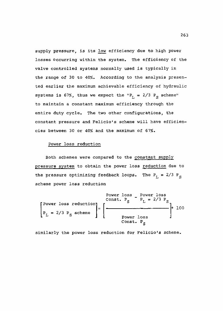
263

supply pressure, is its low efficiency due to high power losses occurring within the system. The efficiency of the valve controlled systems normally used is typically in the range of 30 to 40%. According to the analysis presen­ted earlier the maximum achievable efficiency of hydraulic systems is 67%, thus we expect the = 2/3 Pg scheme" to maintain a constant maximum efficiency through the entire duty cycle. The two other configurations, the constant pressure and Felicio's scheme will have efficien­cies between 30 or 40% and the maximum of 67%.

Power loss reduction

Both schemes were compared to the constant supply pressure system to obtain the power loss reduction due to the pressure optimizing feedback loops. The P^ = 2/3 Pg scheme power loss reduction

Const. P P. = 2/3 P'Power loss reduction"P = 2/3 P scheme

Power loss Power loss

* 100Power loss Const. P,S

similarly the power loss reduction for Felicio's scheme.

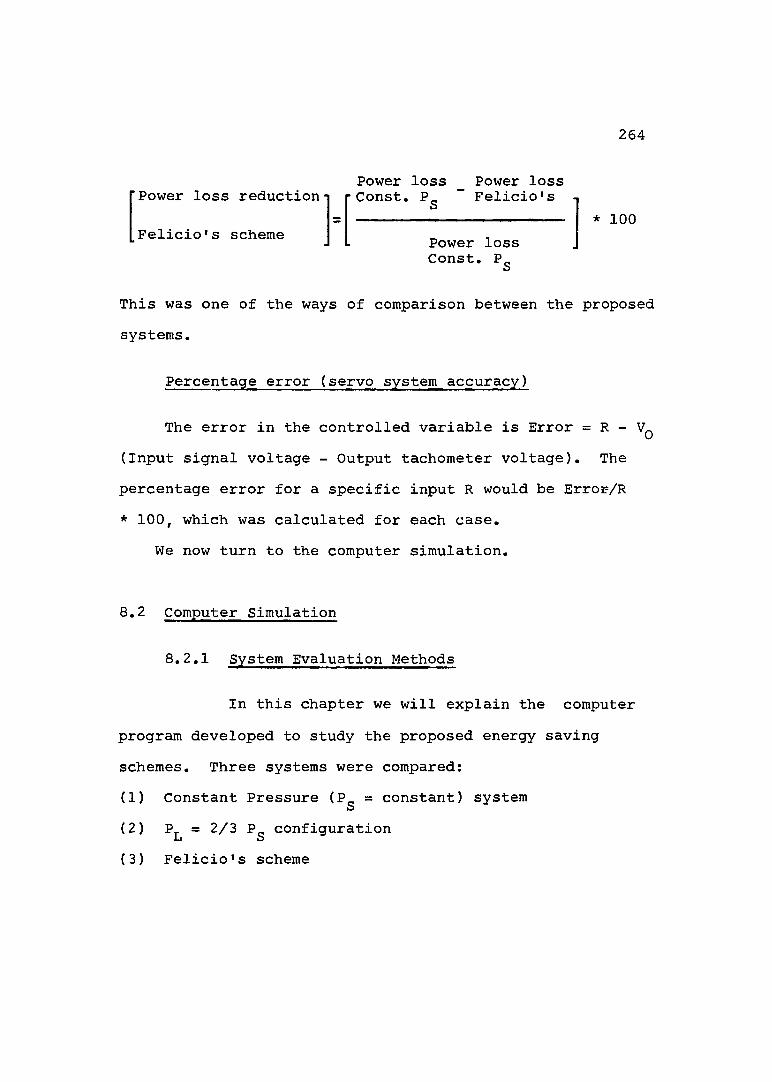
'Power loss reduction- ■Const. Pg ~ Felicio's ■

Felicio's scheme Power loss

264

Power loss Power loss

* 100

Const, Pg

This was one of the ways of comparison between the proposed systems.

Percentage error (servo system accuracy)

The error in the controlled variable is Error = R - (Input signal voltage - Output tachometer voltage). The percentage error for a specific input R would be Error/R * 100, which was calculated for each case.

We now turn to the computer simulation.

8.2 Computer Simulation

8.2.1 System Evaluation Methods

In this chapter we will explain the computer program developed to study the proposed energy saving schemes. Three systems were compared:(1) Constant Pressure (Pg = constant) system(2) P^ = 2/3 Pg configuration(3) Felicio's scheme

265

In comparing the schemes', we focused on system energy, efficiency and system performance.

Energy analysis

(1) Power generatedThe power generated by a hydraulic system is defined

by: Supply pressure (Pump pressure) times Flow rate (Pump flow)

Supply Press.(psi) * Flow rate(cis)Power generated(HP) =

Pg.QrPWGEN = — --—

6750.0

6750.0 ( 2 ) Load power

The hydraulic power delivered to the load is: Load Pressure times Flow rate

Load Pressure(psi) * Flow rate(cis)Load Power(HP) =

PWLOAD = — — —

6750.0

6750.0(3) The power lost in the system is the power generated minus the power delivered

Power lost = Power generated - Power delivered

266

P..Q, - F - Q (P - PL) * Q,PWLOST = -2— h----h— k =-— £--- k k (HP)

6750.0 6750.0(4) The energy lost during a duty cycle

.TENLOST = / PWLOST dt

0(5) System efficiency

Power generated - Power lost

Power generated

_ V = L - " “s -'■l> * «L V = ---------------------^s Ql

P,* 100

PsThese five variables are calculated and compared for

ail three systems.

Performance analysis

System performance was again analyzed from several aspects.(1) Error RMS

The most widely used measure of the magnitude of system error is the root - mean - squared (RMS) defined as

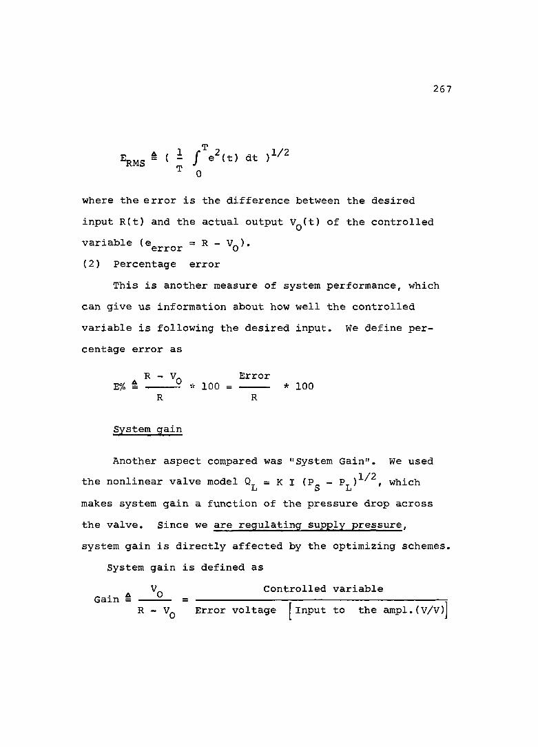
267

=RMS = ' ; )■0

where the error is the difference between the desired input R(t) and the actual output V^Ct) of the controlled variable = R - V^).(2 ) Percentage error

This is another measure of system performance, which can give us information about how well the controlled variable is following the desired input. We define per­centage error as

R - ErrorE% = ---------- * 100 = — ----- * 100

System gain

Another aspect compared was "System Gain". We usedthe nonlinear valve model Q = K I (P_ - which1j 5 Lmakes system gain a function of the pressure drop acrossthe valve. Since we are regulating supply pressure,system gain is directly affected by the optimizing schemes.

System gain is defined asV Controlled variable

Gain = = rR - Vq Error voltage fInput to the ampl.(V/V)I

2 6 8

P o w e r l o s s r e d u c t i o n

Power loss in a constant pressure (non regu­lating) system is the highest’ when compared with the power loss in the two proposed schemes. Thus, yet another excel­lent measure of the amount of energy saved will be the "Power Loss Reduction", which is defined as:PWLOSSRED = Power loss (Const. Press.) - Power lossCOpt.)

Power loss (Const. Press.)* 100

We will describe now the CSMP programs for the proposed energy saving schemes.

8.2.2 The P = 2/3 P Computer Program

The block diagram form of the P = 2/3 P scheme is given in Figure 8.1.

The "new" element in this block diagram is the "Pres­sure loop", where load pressure signal is measured by adifferential pressure transducer is fed back to "produce" the desired pressure P^. Pump pressure is limited between a minimum of 300psi up to the maximum of ISOOpsi. Apply­ing the "Pg = 2/3 P^ rule", the range of pressures between these two limits is governed by the curve:

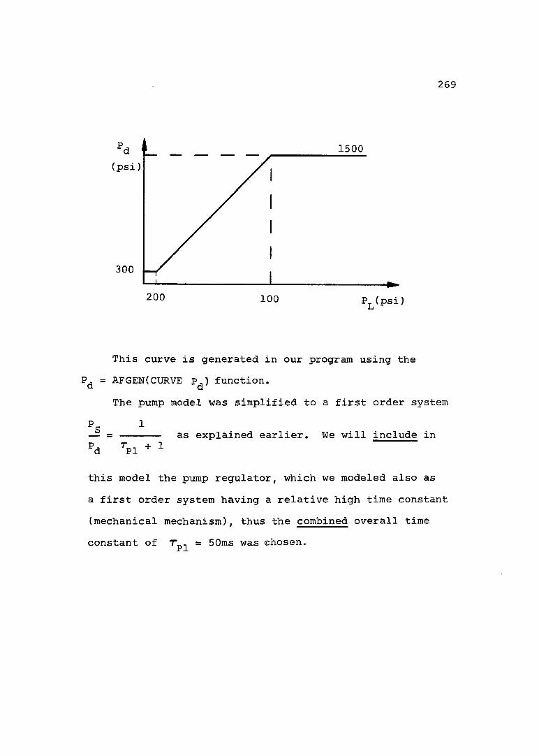
269

1500(psi)

300

200 100

This curve is generated in our program using theP, = AFGEN(CURVE p , ) function, a d

The pump model was simplified to a first order system

"■pi + 1as explained earlier. We will include in

this model the pump regulator, which we modeled also as a first order system having a relative high time constant (mechanical mechanism), thus the combined overall timeconstant of Tp^ = 50ms was chosen.

ABS 1500

300200 1000

(PRESSURE LOOP)Sqrt

Sqrt.

valve

(S)comp

ampl(VELOCITY LOOP)

tach

Figure 8,1 = 2/3 scheme in block diagram formSpeed Control - Pressure control systemR(S) Input

O

2 71

Gain adjustment

Another improvement added to the system was a "Gain Adjusting Block". We mentioned earlier that system gain is directly related to supply pressure(Pg)adjustment. In the = 2/3 Pg scheme, supply pressure starts at a low "Standby" pressure of BOOpsi, when there is no load pre­ssure ( P^ = 0) and system gain is lower by a factor of

1/2(5) compared with the constant pressure configuration^ worsening significantly system performance.

We introduced a gain adjusting block, relating gain to the constant pressure scheme gain.

1500 - P /2 K,, = (----------------------------------- (8.1)11

where ;A Adjusting gain.

Pt A Load Pressure.Jj —Pg A Supply Pressure.

Practically, the new block is a voltage proportional to adjusting valve current via the amplifier. Itis assumed that voltages proportional to P and P areS J-iavailable in our system, thus, the gain adjusting block can be easily constructed.

2 7 2

The flow - pressure valve equation will have now the form;

°L = S K. . ly (Pg - (8.2)

We found also that system compliance had to beincreased and signal low - pass filtering was needed toachieve a stable system, since high gain changes up to

1/2(5) times the original gain, caused the system to be too oscillatory. In our case, the compliance of the pipe line connecting the valve with the hydraulic motor was increased by using additional oil volume,which could be an accumulator.

Before turning to the discussion of the CSMP results let us describe Felicio's scheme in a similar way.

8.2.3 Felicio's Scheme

The scheme proposed by Felicio in block dia­gram form is presented in Fig.8.2. Once again, the velo­city loop is a conventional presentation of the continuity equation and Newton's law in block diagram form. The "improvement" is in the so called "pressure adjusting branch"(it is not a loop), which starts at the desired supply pressure programmed profile

The "supplementary" pressure loop added byFelicio is aimed to supply additional pressure to the

P^a(t) Programmed Pressure

1500ABS

Sqrt.valve 1500( PRESSURE LOOP )

Sqrt.

ampl( VELOCITY LOOP )

tach

R(S) Input Figure 8.2 Felicio's scheme in block diagram formrow

2 74

system when large disturbances occur. The loop "monitors" valve input current I^,and if it is close to its saturation level (100.Oma in our case) it will supply up to 300psi Pj^(t) increasing the actual desired pressure P^^t) as it is sensed by the pump.

The actual current - pressure curve is

(psi)300

95.0 100.0 I„(ma)

which was generated using the P^2 = AFGEN (CURVE,ly)

function available in CSMP. A low pass filter1

G(S) = ----------0.1 S + 1

was introduced in the loop to allow only "slow" signals to affect the system.

2 75

The pump model, was identical to that used in the = 2/3 Pg scheme.Finally, the sum of the signals P^ = P ^ + P^g was

sent through a "limiting block" to allow a maximum of ISOOpsi desired pressure setting in the system, thus mak­ing all three configurations identical in the upper limit.

Gain adjusting block

In order to obtain a similar effect as in the P = 2/3 Pg scheme we introduced in this scheme also a gain adjusting block which has the form

KFF = ( 15%) - )l/2 (8.3)PSFC - PLFC

where;KFF = Adjusting gain .PLFC = Load pressure (Felicio's scheme).PSFC = Supply pressure (Felicio's scheme).

The system behaviour was similar to the P^ = 2/3 Pg scheme and increased oscillations were observed. Therefore the measures mentioned earlier have been applied to obtain stability.

276

T h e p r o g r a m m e d p r e s s u r e P ^ ^ ( t )

It is assumed that the needed torque to perform a predetermined task and the speed of the actuator, which is a controlled variable, are known functions of time. The minimum pump pressure can be calculated based on the torque, speed, leakages, friction and load inertia, also as a function of time.

In order to find the necessary pressure, the allowed error between the controlled variable (V^) and the desired input (R^ has to be given. The decision has been made that output will follow the input (in the velocity loop) within 10% accuracy. Other values could be used, if desired, without changing the method of the analysis.

We will present now the developed program used to "find" the programmed pressure knowing the desiredinput (R^) and the needed torque (T^^). We will emphasize here that these "inputs" are used to "calculate" the pro­grammed pressure The "real" inputs to our system areT^ and R.

In our case, we will write the system differential equations and solve for the supply pressure Pg, which is usually a known value, having the information about R^,

Tli («1 - Vq ).

2 7 7

The system differential equations

Continuity equation

\ '®Lf ^mf ^tm ^Lf 4 ^ ^Lf (8.4)

Newton's law

^Lf = < 'm »mf + «mf + ^Ll>/ (8.51The servovalve equation

°Lf = (?sf -or

Qt f 2P = ( ---+ P (8.6)K.f I,

(where the symbol f is for Felicio's scheme)And the feedback loop

''o = «mf * Ktach (8.7)

If = ("l - '7o> "ampl We need two more equations in order to be able to

proceed to the actual finding ofP^^ = DERIV (0.0, P^^) (8.8 )

= DERIV (0.0, (8.9)Since we decided on the tracking accuracy (10%) we

can find and as a function of the desired input R ,

«mf = O'SKl/ "tach (8.101

2 7 8

and

:f = V a m p l (8.111So, equations (8.10)and (8.11)are now known function of time and we can find and using equations (8.4); (8.5); (8.7); (8,8) and (8.9) also as a function of time.

From equation (8.6) we get the desired pressure and deciding on 20% "safety factor" we multiply Pg^ by 1.2 to obtain the final programmed pressure Thesafety factor could be taken as any other value without changing the concept.

8.2,4 Constant Pressure Configuration

Finally, we will mention the "Constant Pre­ssure Configuration" which is our "Reference Scheme", where it is assumed that the supply pressure is maintained constant (Pg = 1500.Opsi).

In block diagram form it will be as presented in Figure 8.3.

So now we have three schemes which are actually compared using CSMP,(1) PSC = ISOOpsi (Constant pressure)(2) PS = 3/2 P^ (Max. power rule)(3) PSF = For Felicio's Scheme

The CSMP program will be presented next, wherein the parameters used are from system discussed in Part I,

Sqrt.( PRESSURE LOOP )

valve

J_S+B

(S)comp

ampl ( VELOCITY LOOP )

tach

R(S) Input

Figur 8.3 Constant Pressure scheme in block diagram formtokO

280

8.2.5 The CSMP Computer ProgramTITLE SUPPLY PRESSURE OPTIMIZING SCHEMESm e t h o d RKSFXINIT*******************************♦ HYDRAULIC MOTOR PARAMETERS PARAM CIM=13.0765E-05,CEM =2.2857E-05 PARAM DM=15.9155E-02,CD=41.78E04 PARAM JM=0.05PARAM BL=0.05

CTM=ClM+CEM/2.0BM=CD*DM*MIU+BL

****************************************♦ PIPE LINE VALVE - MOTOR PARAMETERS PARAM LVM=120.0

VT=0.11045*LVM******************♦ BULK MODULUS PARAM BE=100000.0 ******************************♦ HYDRAULIC OIL PARAMETERS PARAM MIU=5.976E-06,RHO=0.8I6E-04 ***************************♦ SERVOVALVE PARAMETERSPARAM KIFF=0.00683,KIC=0.00683,KI=0.00683 PARAM KIF=0.015 PARAM TAUV=11.67E-03 ******************************************♦ AMPLIFIER AND COMPENSATOR PARAMETERS PARAM KAMPL=95.0PARAM TAUCP=0.15 *******************************♦ FEEDBACK LOOP PARAMETERS PARAM KTACH=4.777E-02 ************************♦ INITIAL CONDITIONS INCON PL0=0.0INCON TEDOTO=0.0 INCON 10=0.0 DYNAM**************************************************************************♦ INPUT TO THE SYSTEM

R1=0.02+32.0*RAMP(0.0)-32.0*RAMP(0.05)*... 32.0*RAMP(0.5)-32.0»RAMP(0.55)+32.0*RAMP(1.0)-... 32.0*RAMP(1.0 5)+24.0*RAMP(1.5)-24.0*RAMP(1.55)-.. 30.0*RAMP(1.9)+30.0*RAMP(2.0)R=Rl

0"t/T3%%a=Z3%N3 (DS3%%3*0"0)l%9jNI=13%%3

Z**3%%3=0S3%%3 30A-y=3%%3

yoy)i3 39VlN33y3d ONV SWM yoy%3 ************$****$************* *

SISA1VNV 33NVW«0d«3d ********************* *

0'0t*3N3=S033N3 (SOH3Md'0'0)iy91NI=3N3

0"001*(3Sd/31d)=3333 0"0S19/(33B*(33d-3Sd))=S013Md

0"0S19/33D*33d=0033Md O'OSi9/330*3Sd=N393Md

SISAIVNV A9W3N3 **************** *

(3%%3)SgV/30A=NV93ASNIV9 W31SAS ************ *

< 3 1 I * A n V i * 0 I ) 1 d l V 3 « = 3 I (3€I*d3nvl‘0ind3V3d=3TI

ldWV%*(30A-y)=3CI H3Vi%*i0a331=30A

dOOl %3Vg033d *************

I0"0+(31d-3Sd)i%0S*3I*3I%=310 NOIlVnoa yV3NI3N0N 3A3VA0AW3S ***************************** (10Z331*010031)3V91NI=100331

Wr/(31-10O331*wg-31d*WO)=lOZ331HVl S*N01M3N

************* (10031d*01dl3%91NI=31d

(lA/39*0"t)*(31d*W13-100331*Wa-310)=10031dN0IlVn03 A1I0NI1N03 *******************

SN0I1V003 «010W •GAH ********************

0*00ST=3Sd*******************************************************************************************************************************************♦ lNVlSN03=Sd - dOOT 3«0993«d ON******************************************* ************************************************ ************************************************

ni»ii(l"E)dWV«*0"S19+(S"E)dWV«*0"519

"""-(S6"Z)dWV«*"00E-(9"Z)dWV«*"00E+(5E"Z)dWV«*"00E """-(Z'Z)dWV«*"00E+(ST"0)dWV«*'00E-(*0)dWV«*"00E=T31

T82

282

ERCRMS=SQRTIERRC2)ERCPER=(ERRC/R)*100.0

**********************$*****$$***$**********$***** ******$***********************$****$*****$** OPTIMIZING SCHEME - PL=2/3*PS ♦* ******************************************* ************************************************* ************************************************** ********************♦ HYD. MOTOR EQUATIONS* ********************♦ CONTINUITY EQUATIONS

PLD0T=(QL-DM*TED0T-CTM*PL)*(4.0*BE/VT) PL=lNTGRt(PLO,PLDOT)PL1=REALPL(0.0,0.04,PL)* *************

* NEWTON,S LAW TEDDOT=(DM*PL-BM*TEDOT-TL)/JM TEDOT=INTGRL(TEDOTO,TEDDOT)* *****************************

* SERVOVALVE NONLINEAR EQUATION KI1=SQRT((1500.0-PL1)/IPS-PL1)I QL=KI*KII*I*SQRT(PS-PL1)

* ************** FEEDBACK LOOP

VO=TEDOT*KTACH I3=IR-V0)*KAMPL I1=REALPL(I0,TAUCP.I3)I=REALPL(I0,TAUV,I1)

* ************ SYSTEM GAIN

SYSGAN=VO/ABS(ERROR>* *************♦ PRESSURE LOOP

P1=ABS(PL)P0=AFG6NtCURVE,Pl)

AFGEN CURVE=0. 0,300 .0,200. 0,300. 0,1000 .0,1500.O f * . 1300.0,1500.0 PS=REALPL(300.0,0.05,PD)* ***************

* ENERGY ANALYSISPWGEN=PS*QL/6750.0 PWLOAD=PL*QL/6750.0 PWLOST=((PS-PLl)*0LI/6750.0 EFF=(PL1/PS)*100.0 ENL=INTGRL(0.0,PWLOST)ENL0ST=ENL*10.0

283

* *************$****»** PERFORMANCE ANALYSIS* ******************************* ERROR RMS AND PERCENTAGE ERROR

ERROR=R-VO ERRSQR=ERR0R**2 ERRl=INTGRL(O.OtERRSQR)ERR2=ERRl/4.0ERRRMS=SQRT(ERR2)ERRPER=(ERROR/R)*100.0

* *****»$**********$*** POWER LOSS REDUCTION

PWLRED*((PWCLOS-PWLOST)*100.0)/PWCL0S*****************************************************,***$**#************************************** *******************$********$**$*$#**$****** FELICIO,S ENERGY SAVING SCHEME ** ********************$**********$******$**** **********************#*****$******#[**»#***$**$$* $***********************************#***#$*$****** FINDING PRESSURE SETTING FROM KNOWN RI AND T1

QLF=DM*TED0TF+CTM*PLF+(VT/(4.0*6E))*PLDOTF PLF=(JM*TE20TF+BM$TED0TF+TL1)/DM PLDOTF=DERIV(300.0,PLF)TE20TF=DERIV(0.0,TED0TF)* *******************************************

* OUTPUT FOLLOWS INPUT WITHIN 10? ACCURACY TED0TF=(0.90*Rl)/KTACH FI»0.10*KAMPL*R1PSF=(QLF/(KIF*FI))**2+PLF **********************

* FELICIO,S SCHEME* ********************♦ HYD. MOTOR EQUATIONS* *******************» CONTINUITY EQUATION

PLFCD0=(QLFC-DM*TEFCD0-CTM#PLFCI*(4.0*BE/VT)PLFC=INTGRL(PLO,PLFCDO)PLFCI=REALPL(0.0,0.04,PLFC)* *************

* NEWTON,S LAWTEFC2=(DM*PLFC-BM*TEFCDO-TL)/JM TEFCDO=INTGRL(TEDOTO,TEFC2)* *****************************

» SERVOVALVE NONLINEAR EQUATIONKFF=SQRT((1500.0-PLFC1»/(PSFC-PLFC1)» QLFC=KIFF*KFF♦IFC*SQRT(PSFC-PLFC i)

2 8 4

$ *************** FEEDBACK LOOP

VOFC=TEFCDO*KTACH13 FC* C R-VOFC)*KAHPL IlFC=REALPL(IO,TAUCPfI3FC»IFC=REALPH IQtTAUV» IIFC)* ***********

* SYSTEM GAIN SYFGAN=VOFC/ABS(ERRF)* ************************

* PRESSURE LOOP - FELICIO -PSFC1=1.2*PSF PSFC2=PSFCl+PSFC3 IFC1=REALPL(0.0,0.10,IFC)IFC2=ABS(IFCl>PSFC3=AFGEN(CURVE1,IFC2)

AFGEN CURVE1=0.0,0.0,95.0,0.0,105.0,300.0,150.,300.0 PSFC22=ABS(PSFC2)PSFC4=AFGEN(CURVE2,PSFC22)

AFGEN CURVE2=0.0,0.0,1500.0,1500.0,3500.0,1500.0 PSFC=REALPL(500.0,0.05,PSFC4)* ***************

* ENERGY ANALYSIS PWFGEN=PSFC*QLFC/6750.0 PWFLOO=PLFC*QLFC/6750.0 PWFLOS=( { PSFC-PLFCl)*QLFC)/6750.0 EFFF=(PLFC1/PSFC)*100.0 ENF=INTGRL(0.0,PWFLOS)e n f l o s = e n f * i o . o

* ********************* PERFORMANCE ANALYSIS* ******************************* ERROR RMS AND PERCENTAGE ERROR

ERRFsR-VOFC ERFSQR=ERRF**2 ERRF1=INTGRL(0.0,ERFSQR)ERRF2=ERRFl/4.0ERFRMS=SQRT(ERRF2>ERFPER=CERRF/R)*100.0

* ********************* POWER LOSS REDUCTION

PWLFRE=((PWCL0S-PWFLOS)*100.0)/PWCLOS******

I l S d ï 3 W 3 H 0 S S * 0 I 0 n 3 d ( I S d ) 3 W 3 H 0 S S d E / Z = l d ( I S d ) 3 W 3 H 3 S • l S N O O = S d

dnO%9 39Vd ddd3*0dd3*dd3 indino ( i } 3W 3H 3S S ‘0 I 0n 3d - A 0 N 3I D I d d 3= d d d 3 ♦( % ) 3W 3H 0S S d € /7 = l d - A 3N 3I 3 I d d 3 = d d 3 *( % ) 3W 3H 3S " i S N 03= S d - A 3N 3 I 3 I d d 3= 3 d d 3 *

dnOdO 39Vd S01dN3*S013N3*lS03N3 lOdinO

(WN) 3W3H3S S'0I3I13d - ISO! A9%3N3=S01dN3 *(WN) 3W3W3S Sd £/Z=ld - ISO! A9%3N3=iS03N3 *(WN) 3W3H3S •lSN03=Sd - ISO! A9%3N3=S013N3 ♦

d n O d 9 3 9 V ds o i d M d * s c n 3 M d ' i S o i M d i n d i n o

(dH) 3W3W3S S * 0 I 3 n 3 d - ISO! %3M0d=S03dMd *(dH) 3W3H3S Sd E/Z=ld - ISO"! %3M0d=lS01Md *(dH) 3W3H3S "iSN03=Sd - ISO! W3M0d=S013Md *

d n 0 d 9 3 9 V d 3 d i d ' 3 i d ' i d i n d i n o

3 « n S S 3 « d 0 V 0 1 = 3 d l d *3 d n S S 3 X d O V O l = l d *3 * n S S 3 % d O V O l = 3 1 d *

d n 0 W 9 3 9 V d 3 d S d * 3 S d * S d i n d i n o

( I S d ) 3 W 3 H 3 S S ' 0 I 3 I 1 3 d - 3 % n S S 3 % d A l d d O S = 3 d S d *( I S d ) 3 W 3 H 3 S S d E / Z = S d - 3 « n S S 3 « d A l d d O S = S d *( I S d ) 3 W 3 H 3 S " i S N 0 3 = S d - 3 % n S S 3 % d A l d d O S = 3 S d *dooyg 39Vd 3d I*31*1 indino iN3«an3 3AlVA=3dI * iN3%an3 3A1VA «I * iN3aan3 3Ai v a =3i *dno%9 39Vd a'3d0A'30A*0A iOdiOO (IIOA) 3W3H3S S*0I3I13d - 3 9 V Ü 0 A iOdinO=3dOA *(ilOA) 3W3H3S Sd Ç/Z=ld - 39VilOA iOdiOO =0A »(ilOA) 3W3H3S "iSN03=Sd - 3 9 V Ü 0 A iOdiOO =30A *

NoiiVNvidxg s%3i3wvyvd indino **************$**************$*********** ZO"O=13OinO*OIOO"O=il30*O"t=WIiNId b3WIi **************************************** ****************************************

i Ü O S* * * *0*S0T=3dI (0"S0I"39"3dI)dI 0-001=31 (O-00T-39-3I)dI 0-001=1 (0-00I-39-I)dI SilWIl NOIiVaniVS 3A1VA0A%3S

****************************

vwvwvw

3 W 3 H 3 S S * 0 I 3 I 1 3 d 3 W 3 H 3 S S d E / Z = l d 3 W 3 H 3 S - i S N 0 3 * S d

**

i d O S O N

5 8 2

2 8 6

PWLFRE=POWER LOSS REDUCTION - FELICIO,S SCHEME P W l RED=POWER LOSS REDUCTION - PL=2/3 PS SCHEME

OUTPUT PWLRED,PWLFRE AGE GROUP

ERCRMS=ERROR RMS - PS=CONST. SCHEME ERRRMS=ERROR RMS - PL=2/3 PS SCHEME ERFRMS=ERROR RMS - FELICIO,S SCHEME

OUTPUT ERRRMS,ERCRMS,ERFRMS AGE GROUP

ERCPER=PERCENTAGE ERROR - PS=CONST. SCHEME ( % ) ERRPER=PERCENTAGE ERROR - PL=2/3 PS SCHEME ( % ) ERFPER=PERCENTA6E ERROR - FELICIO,S SCHEME ( X )

UTPUT ERRPER,ERCPER,ERFPER AGE GROUP

SYCGAN=SYSTEM GAIN - PS=CONST. SCHEME SYSGAN=SYSTEM GAIN - PL=2/3 PS SCHEME SYFGAN=SYSTEM GAIN - FELICIO,S SCHEME

UTPUT SYCGAN,SYSGAN,SYFGAN AGE GROUP

PSFC1= PROGRAMMED PRESSURE C PSI)PSFC3= CURRENT LOOP PRESSURE ( PSI >PSFC2= PROG. PRESS. PLUS CURR. LOOP PRESS. ( PSI )

UTPUT PSFC1,PSFC2,PSFC3 AGE GROUP UTPUT PSF,PLF AGE GROUP

END

2 8 7

8.2.6 Inputs to the system R(t) and T^(t)

The inputs to the system are the desired velo­city R(t) and the load torque T^(t). Since maximum valve opening (lOOma) will give maximum velocity, and controlled variable V^(t) is directly related to percentage valve opening we choose valve current (ly) as the measure of speed control.

In order to compare the power level of the optimizing schemes with the constant pressure system, several duty cycles were designed to effectively exercise the systems and reveal their operating characteristics. From the numerous computer runs we can summarize the following features for both optimizing schemes.(1) Varying the servo speed, keeping the loads constant.In this case a considerable reduction in the power lossis observed when the servo is operating against small loads.(2) Varying the servo load, keeping the speeds constant. The reduction in the power loss is quite high when the servo is operating at low speed.

288

Therefore, the energy saving system will be most vigorously exercised for the cases where we have fast motion with small loads (High flow rate at relative low pressure), and slow motion with large load (low flow rate at high pressure). In order to obtain the needed infor­mation about the system performance and energy saving, we will present the results for the following inputs "applied" in one duty cycle:(1) Three levels of torque loads T^(t); small, medium and large(2) Four levels of controlled variable V^(t) speed, as measured by valve opening 25%; 50%; 75%; 100%,

The actual values of system input variables (Valve opening) and lL(t) (load torque) are expressed in non- dimensional form as

t/L = — — —

where

and

T,Lmax

T^* A Non - dimensional load .T^ ^ Actual applied load (lb*in) .Tt A Maximum load (150 lb*in) . Lmax =

I * = T / IV “V ' Vmax

2 8 9

where ;

'V g Non - dimensional valve current. A Actual valve current (ma).A Maximum valve current (lOOma). VrtlaX —

The inputs have the following form;(1) Keeping load torque constant

?L* 1/3 1/3 1/3 1/3

iv* 1/4 1/2 3/4 1Keeping speed constant

* 0 1/3 2/3 1*

4 1/2 1/2 1/2 1/2A typical set of inputs over a full duty cycle will be:

1.03/4

1/2 1/21/4

1.0

2/3

1/3

DUTY CYCLE TimeFigure 8.4 A tyyical input R^(t) and T^^(t) combination

2 9 0

System output variables and "Supplementary PressureLoop"The output variables in our model were explained and

listed earlier at the end of the computer program in sec­tion 8,2.4.

The behaviour of the supply pressure (Pg) in all threeschemes for the input in figure 8.4 is presented in figure8.5, which is the computer CSMP result.

Our second objective was to prove the principle of operation of the "Supplementary Pressure Loop" suggested in Felicio's scheme, which is aimed to supply additional pressure P^gft) to the programmed pressure P^^(t) in case of large disturbances and/or close to stalling situation. The P = 2/3 P_ scheme has no such a supplementary loopJj o ——since it is an "On line" scheme and supply pressure will increase "automatically" when disturbance occurs. Toward this goal, "disturbing" loads were Yadded" to the torque needed to "Activate the Supplementary Pressure Loop".

Let us turn now to the analysis of the results and to conclusions about the feasibility of the proposed schemes.

oin_

oom

□

oo _

oo

UU_

o_U)

oo

f\i

o

oomCM_

o

O

oo_

ooui-1

u5

o _in

ooinjOJ

S U P P L Y P R E S S U R E LEGEND

P3C

PSFCo.

Û-0o _ .

0.50 .50 2.50 3.00 3.50 y.ooT I M E roIDFigure 8.5 System supply pressure (comparison)

292

8.3 Analysis of the Results

The principle of operation of an "On - line - Continu­ous" optimizing scheme is based on sensing the variables needed at "all times" and controlling continuously power loss and system gain. Power loss is to be kept minimum during the entire duty cycle and the gain is kept about 6 (V/V), which is the recommended gain (2) in a velocity control system. In this section we will analyze the results in energy saving and performance as obtained from the CSMP computer program.

8.3.1 Energy Analysis

Let us analyze now the energy saving aspect of the two proposed schemes and the effects on the servo- controlled actuator configuration.(1) varying the servo speed, keeping the loads constant

Table 8.1 The Power Lost - Constant Load

m * _ * PWCLOS (HP) PWLOST (HP) PWFLOS(HP)^L V Pg = const, scheme P =2/3 P scheme •Li S Felicio's scheme

1/3 1/4 0.80 0.14 0.441/3 1/2 1.50 0.31 0.901/3 3/4 2.00 0.55 1.331/3 1 2.30 0.75 1.73

2 9 3

Examining the table we observe that the power lost isincreasing, in all three schemes as speed is increasing,since higher flow rate is transfered under constantpressure. The power lost is from 5.7 to 3.0 timeslower in the = 2/3 P_ scheme, and from 1,80 to 1.35 ij slower in Felicio's scheme, compared to the Constant Supply Pressure configuration. Therefore, there is a clear advantage for the P = 2/3 P scheme as expected.

Table 8.2 System efficiency - Constant Load

* * EFFC (%) Pg=const. scheme

EFF (%) P^=2/3 Pg scheme

EFFF (%)Felicio's scheme

1/3 1/4 24.35 63.15 40.70

1/3 1/2 29.75 65.80 45.201/3 3/4 35.00 66.70 44.601/3 1 39.00 66.50 46.55

System efficiency is maintained close to the maximum possible (67%), for all cases in the P^ = 2/3 Pg scheme, the task it was designed for (see Figure 8.6).

The efficiency is obviously very poor (about 30%) in the Constant Pressure scheme and it is higher (about 45%) for Felicio's scheme. (See Figure 8.6.)

-1 -1

o oo oo. o.10 ID

o Oo Qin. in.zf =r

o oo o

Ll • u •ü-°-Ll U_

LlI LlI

D oO oin. in.

D oo oo o

E F F I C I E N C Yo.

L E G E N D

EFFC Û

EfFf +

0.50 .00 2.00 2.50 3.00 3.50 4.00T I M EFigure 8.6 System efficiency (comparison)

VO4

295

Table 8.3 Power loss reduction - Constant Load

* * PWLRED (%)P. = 2/3 P_ scheme1j D

PWLFRE (%) Felicio's scheme

1/3 1/4 90.00 49.101/3 1/2 83.50 36.601/3 3/4 72.75 32.201/3 1 67.75 26.20

There is a decrease in power loss reduction, in bothconfigurations as speed is increasing. The reductionrange is from 90.0% to 67% in P = 2/3 P scheme whereas

l i S

only from 49.0% to 26% in Felicio's scheme. See Figure 8.7.

(2) Varying the servo loads, keeping the speed constant.

Table 8.4 The power lost - Constant Speed

* *:v

PWCLOS (HP) Pg=const. scheme

PWLOST (HP) Pj =2/3 Pg scheme

PWFLOS (HP) Felicio's scheme

0 1/2 1.80 0.23 0.731/3 1/2 1.50 0.31 0.902/3 1/2 1.00 0.46 0.901 1/2 0.62 0.62 0.62

o oo 0-0

o oo oUl_ in_r- r-

o oo oo_ D_in in

ïg P°LlIo

3Q- Q_

o oo oo' o'

o oo oin mnjJ rvj

P O W E R L O S S R E D U C T I O N

0.00 0.50 .00 1.50 2.00 2.50 3.00 3.50 4.T I M E

L E G E N DPWLRED 0

PWLFRE 6

Figure 8.7 Power loss reduction (comparison) VOcn

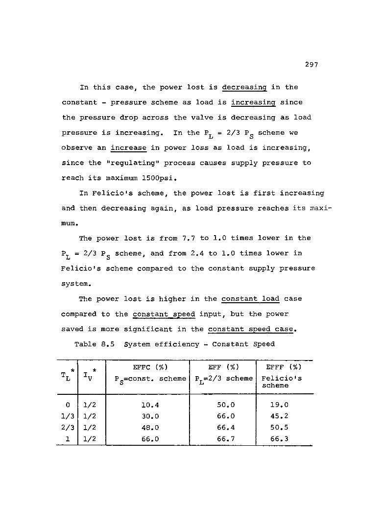
297

In this case, the power lost is decreasing in the constant - pressure scheme as load is increasing since the pressure drop across the valve is decreasing as load pressure is increasing. In the = 2/3 Pg scheme we observe an increase in power loss as load is increasing, since the "regulating" process causes supply pressure to reach its maximum ISOOpsi.

In Felicio's scheme, the power lost is first increasing and then decreasing again, as load pressure reaches its maxi­mum.

The power lost is from 7.7 to 1.0 times lower in the P^ = 2/3 Pg scheme, and from 2.4 to 1.0 times lower in Felicio's scheme compared to the constant supply pressure system.

The power lost is higher in the constant load case compared to the constant speed input, but the power saved is more significant in the constant speed case.

Table 8.5 System efficiency - Constant Speed

* *4

EFFC {%) Pg=const. scheme

EFF {%) P^=2/3 scheme

EFFF (%)Felicio's scheme

0 1/2 10.4 50.0 19.01/3 1/2 30.0 66.0 45.22/3 1/2 48.0 66.4 50.51 1/2 66.0 66.7 66.3

298

System efficiency is increasing in all three cases as load pressure is increasing since pressure drop across the valve is decreasing. Efficiency level is from 50% to 66.7% in the = 2/3 scheme, from 10% to 66.7% in the constant - pressure scheme and from 20% to 66.7% in Felicio's scheme. Again in this case the efficiency in P^ = 2/3 P^ scheme is the highest, kept close to 66.7% at all times (see

Figure 8.6).

Table 8.6 Power loss reduction - Constant Speed

* * PWLRED (%)P = 2/3 P„ scheme

PWLFRE (%) Felicio's scheme

0 1/2 88.3 56.71/3 1/2 83.5 36.62/3 1/2 55.0 11.61 1/2 2.0 0.1

We can see that there is a substantial decrease in power loss reduction as load is increasing for both schemes. It approaches almost zero for the limiting case of low speed (valve almost closed) and high load (system stalled), where no power is lost since there is no motion. Power loss reduction is significant (88%) when there is no

299

load and the system is moving at low speed in the = 2/3Pg scheme and (56%) in Felicio's scheme (see Figure 8.7).

Energy loss

Energy loss is a cumulative quantity over a period of time, so we will present its value at the end of the duty cycle.

Table 8.7 Energy loss

ENCLOS (NM) ENLOST (NM) ENFLOS (NM)Pg = const, scheme P^ = 2/3 scheme Felicio's scheme

53.0 17.0 36.5

The energy loss is lowest in the P = 2/3 P„ scheme.Jj sFinally, from the energy analysis comparing the two

schemes it reveals a clear and constant advantage to the P^ = 2/3 Pg scheme as expected. See Figure 8.8.

8.3.2 Performance Analysis

System performance is of great importance and the "gain adjusting block" which was introduced in both energy saving schemes had the purpose of keeping "constant" gain (6 V/V) to maintain a good performance.

r-

ooo_ID

OOin_ZÏ

Z LUooin.

ooo

in.

ooo.to

ooin_S’

COoDoU o_tn

LUooin.

oo

in., L E G E N DE N E R G Ï L O S To_

ENCLOS

ENFLOS

COq,o_

0.50 .00 2.00 2.50 3.00 3.50 4.00T I M EFigure 8.8 Energy loss (comparison)

woo

3 0 1

(1) Varying the servo speed, keeping the loads constant

Table 8.8 Percentage error - Constant Load

*^L

*"v

ERCPER (%) Pg=const. scheme

ERRPER (%) P_=2/3 P„ schemeLl o

ERFPERFelicio's scheme

1/3 1/4 13.4 10.8 10.51/3 1/2 13.7 14.7 11.61/3 3/4 14.0 14.0 14.31/3 1 14.4 14.5 14.3

The percentage error is fairly constant ( ~ 14%) in the constant pressure scheme. There is a slight increase in percentage error in the P = 2/3 P and Felicio's schemeLl oas speed is increasing suggesting that the system is less capable to track high speeds. Generaly speaking, the percentage error is uniform in all three schemes (~14%) thanks to the "gain" adjusting blocks" introduced.

Table 8.9 System gain - Constant Load

*^L

* SYCGAN (V/V) Pg=const. scheme

SYSGAN (V/V) P_=2/3 P_ schemeLj o

SYFGAN Felicio's scheme

1/3 1/4 6.50 5.75 5.751/3 1/2 6.30 6.30 6.301/3 3/4 6.00 6.00 6.001/3 1 5.90

- ... . ... - .. .. J 5.80...

5.80

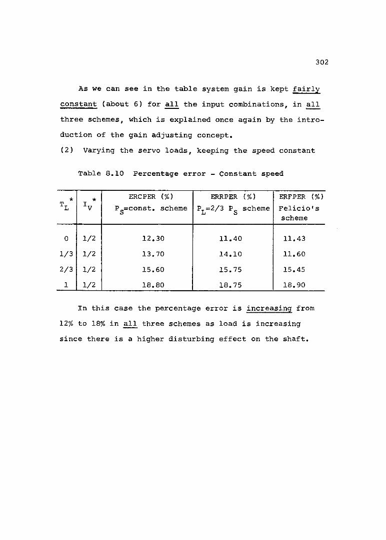
3 0 2

As we can see in the table system gain is kept fairly constant (about 6) for all the input combinations, in all three schemes, which is explained once again by the intro­duction of the gain adjusting concept,(2) Varying the servo loads, keeping the speed constant

Table 8.10 Percentage error - Constant speed

* *4

ERCPER (%) Pg=const. scheme

ERRPER (%) P_=2/3 P_ schemeJ_i o

ERFPER (%) Felicio's scheme

0 1/2 12.30 11.40 11.431/3 1/2 13.70 14.10 11.602/3 1/2 15.60 15.75 15.451 1/2 18.80 18.75 18.90

In this case the percentage error is increasing from 12% to 18% in all three schemes as load is increasing since there is a higher disturbing effect on the shaft.

3 0 3

T a b l e 8 . 1 1 S y s t e m g a i n - C o n s t a n t S p e e d

* * SYCGAN (V/V) Pg=const. scheme

SYSGAN (V/V) P =2/3 P_ schemelj O

SYFGAN(V/V) Felicio's scheme

0 1/2 7.10 7.90 7.751/3 1/2 6.30 6.30 6.302/3 1/2 5.40 5.50 5.451 1/2 4.30 4.30 4.30

System gain is varying from 7 to 4.3. As we can see the gain is less stable in the case where load torque is changing compared to the case where system gain is changing.

Error RMS

Similarly to the "Energy loss" term used in the energy analysis the Error RMS is a cumulative quantity over the period of the duty cycle.

Table 8.12 Error RMS

ERCRMS ERRRMS ERFRMSPg =const. scheme P =2/3 P_ scheme

l i OFelicio's scheme

0.5778 0.5718 0.5718

ow

in

enZomm

ÜJ

inQ

ooo

o

olûo

U)

enZoccm

LU

l/)o’

oo

E R R O R R M S

L E G E N DERRRMS

ERFRMS

0.50 2.00 2.50 3.00 3.50 4.00T I M EFigure 8.9 System Error RMS (comparison)

wo

3 0 5

Finally, since Error RMS is a value indicating system behaviour over the whole period of operation, it is a good measure of system performance. The Error RMS in all three schemes is identical proving the effectiveness and the necessity of the gain adjusting concept in energy saving configurations (see Figure 8.9).

8.3.3 "Supplementary Pressure Loop" Analysis in Felicio's Scheme

An input combination R(t) and T^(t) was design­ed to exercise the "Supplementary Pressure Loop - in order to test its feasibility. The duty cycle has the following form:(1) Fast motion of the system with a small load, in the first half of the duty cycle, and(2) slow motion with a large load in the second half of the duty cycle.

For this type of duty cycle the optimizing scheme will be maximum exercized and any disturbance in the load will cause large valve openings and "activation" of the pro­posed loop. The desired speed as a function of time was defined as R^(t):

306

Max. Valve openin'

50% Valve opening0.5

Time0.5 1.0

Duty cycle Duty cycle

and the load which was defined as T^^(t)

3/4 Load

1/4 Load

Time

0.5 1.0Duty cycle Duty cycle

3 0 7

The "new" load will present a small disturbance during the fast motion and stalling condition during the second half of the duty cycle (an obstacle simulation).

1.0

3/4

1/2The original desired T,.(t)

1/4Time

0.5 1.0Duty cycle Duty cycle

The results showed that during the small disturbance, the increase of the load to 1/2 the supplementarypressure loop "added" pressure to the originalPdi(t) to overcome the disturbance. During the stalling situation, when P^ = Pg, there is no motion and the pressure generated P^^(t) + P^^(t) becomes the maximum supply pressure ISOOpsi, so the additional pressure loop functions properly.

3 0 8

8 . 4 C o n c l u s i o n s

(1) The two energy saving schemes investigated were found to be applicable in servocontrolled actuator system applications. Energy saving seems feasible, and at the same time, keeping system performance equivalent to the nonregulating constant pressure configuration.

(2) The P = 2/3 P "Optimizing Scheme" is easier toij Oenforce as an "On line" energy saving application and it can be used in continuous systems.

(3) Felicio's scheme is applicable when a digital computer is used to generate the programmed pressure profile Pdi(t) and changes in system duty cycle could be easily reprogrammed. In the case of continuous systems a programmed supply pressure P^^(t) will be applicable only for one particular duty cycle. Load or speed changes will cause necessary changes in the programmed pressure, therefore the importance of the "Supplementary Pressure Loop" suggested by Felicio and successfully tested by us. Actually, this "pressure loop" has the features of an "On line" control except that it is limited to a certain valve opening range.

3 0 9

(4) Gain adjusting blockWe mentioned earlier that system performance was

worsened considerably by the "Pressure loop" which adjusted supply pressure, since system gain is a function of the pressure difference across the valve.

Therefore, the introduction of the gain adjusting blocks. keeping "constant" gain during the duty cycle, made energy saving schemes feasible in servosystems. The Error RMS values were identical for all three schemes proving the applicability of "On line" gain adjusting circuits,

(5) Percentage errorThe three systems maintain percentage error from

10% to 18% for all of the load - speed combinations investigated.

( 6) Energy saving analysisConstant Pressure System efficiency has an

average of 35%.Felicio's Scheme efficiency average is 45%, with

about 10% higher.The P^ = 2/3 Pg scheme maintains system efficiency

at 66.7% (maximum possible) at all times as designed for.

3 1 0

8 , 5 Summary

We analyzed a specific system, using for the para­meters numerical values taken from the servosystem studied in part one, however, the computer model was developed for the general case. To summarize our inves­tigation on the two proposed energy saving schemes, we will comment on general conclusions reached based on the results.(1) Energy saving schemes are applicable in valve con­trolled servosystems.(2) Gain adjusting is necessary to maintain desired system performance.(3) The introduction of "pressure loops" and "gain adjusting blocks" cause the system to be more oscillatory. Therefore, more damping and low pass filtering is needed. In figures (8.10) and (8.11) we presented the CSMP output for the system without low pass filters. One can observe clearly high oscillations, compared to the same outputs in figures (8.6) and (8.7) of the same variables.(4) System efficiency can be improved significantly, by up to 30%.(5) The energy saving schemes analyzed are suitable for those applications where the variations of the inputs

3 1 1

are slow enough to be met by pump dynamic response. The maximum bandwidth of the inputs used for the system stud­ied here was about 20(rad/sec).

U)(\J-

oooo_

oo

oo

IJLÜJo_-Ul

OOin_CM

oo

mCM_

oooo_

oo

oo

Ul

U.Li_ü_LUo_Ul

ooU)_CM

oo

E F F I C I E N C Y L E G E N DEFF

o_EFFC

EFFFUl.

mî>

llS-LlLU

Ul.

.00 0.50 .50 2.00 2.50 3.00 3.50T I M E

0

F i g u r e 8 . 1 0 S y s t e m e f f i c i e n c y ( w i t h o u t f i l t e r i n g )

WHM

of\!_

OOo_O)

ooo_ID

üJqCCou_

û_

oo

oo0 m_1

P O W E R L O S S R E D U C T0(1o_

O-

üJo|0 -

2.00 2.50 3.00 3.50 4.00.000.500.00 T I M E

L E G E N D PWLRED 0

PWLFRE ù

Figure 8,11 Power Loss Reduction (without filtering)WMW

3 1 4

PART THREEFurther Study of Felicio's Model of a

Variable Displacement Pressure Compensated Vane Pump

3 1 4

3 15

G e n e r a l

The pump model used in our study was originally deve­loped by Felicio. In view of the fact that three questions in his research had not been completely answered, this part of our study will be concerned with them.

(1) The dynamic behaviour of the pump is dominated by the ratio which is the pump time - constantTp explained in chapter 2, where is the viscous -friction force coefficient and is the regulating spring constant. When designing a pressure compensated pump with fast correction action, i.e., a fast capability of chang­ing its displacement due to disturbances, the ratioB^^/ Kgp (the time constant T^) should be as small as possible.

We will investigate how such pumps can possibly be 3re - designed to improve their speed of response (Chap. 9).

(2) A general characteristic of any positive dis­placement pump is the existence of pressure "ripples" at its outlet. As expected the pump used for the development of the model exhibited such pressure fluctuations. The power spectral density of these fluctuations showed a high peak at 12.5 Hz. No final conclusion was reached

316

by Felicio concerning this phenomenon, however, experimen­tal data indicated that the peak is caused by the pump (rather than tubing dynamics) since it occurs in the regu­lating region. This frequency component of the pressure signal is suspected to be a limit cycle effect.

We set up a theoretical and experimental program to study this phenomenon (Chap.10).

(3) Finally, since accurate measurements are vital in validating the theoretical models, and since some of the measurements were not routine, instrumentation pro­blems are considered an important part of the overall study. In Felicio's work, there was some discrepancy between the low and high pressure readings of the two tur­bine flow meters which was not completely resolved.

We performed additional analysis and tests to remove this uncertainty from the flow measurements (Appendix D) .

CHAPTER 9 "RE - DESIGN" OF VARIABLE DISPLACEMENT

VANE PUMPS FOR FASTER RESPONSE

9 . 1 G e n e r a l

Felicio's contribution in the field of Variable Displacement Vane Type Pressure Compensated Pump was, the development of a dynamic model of the pump. The "Speed of Response", in other words the speed in which the pump can build up pressure as a function of flow disturbances is very important. At the end of his dissertation, Felicio gave several suggestions how to decrease the pump regula­ting time constant.

Having had experience in Vane Pump design and construc­tion, since my master thesis was in the same field, namely "The Development of a Pressure Balanced Variable Displace­ment Vane Pump" we will suggest a possible way to improve the speed of response of such pumps. As stated earlier, the dynamic behaviour of the pump is dominated by the ratio Byf/Kgp, which are physical parameters, therefore the solution would be a "Re - Design" of the pump structure.

3 1 7

Ff-Ff(Pop» ®p» ®p^

pOPTD

^dp _

OP

1/KËE.

PV

^PV Kpv^^op'^p)

thp^ _ <

N K

Hydrau-1CLoad

1

‘OP

Ce D

KIK

Figure 9.1 Block diagram of the perturbation dynamic model for the proportional control type of pump

wM00

3 1 9

Let us turn now to the analysis of the parameters of vane pumps involved in such a possible "Re - Design",The main goal is to reduce the bad dynamic effects (supply pressure changes) in servosystems using such pumps as the power supply. These dynamic effects on the controlled variable of servo systems were described in Chapter 2.

A block diagram of the model developed by Felicio is given in Figure 9.1.

9.2 Stability Analysis

In order to study the effect of system parameters on the stability, an approximate, linearized analysis was performed, neglecting nonlinearities.

The pump regulating operation is a "feedback system" with the following linearized block diagram.

°thB_ 1

^C® ^IKgp

Figure 9.2 Linearized block diagram

320

PThe needed transfer f u n c t i o n S ) is then written direct-

^dply from the block diagram.Pop^dp

(S)

^ ^ ------------------ (9.1)

or in standard form Pop^dp

(S)

Kpv * %e

Kpv * %e + %sp %1K

^ _)s +( ---)g2+(^yf*lK*^spCc )cV^e + WlK V*®e+>'sp''lK %pv™e+VlK

(9.2)where :

Kp^ A Pressure coefficient (Ib^/psi).N A Speed of rotation (rpm).

A Flow coefficient (gpm/rpm in).Kgp A Spring constant (Ib^/in).M A Ring mass (Ib^).

A Friction coefficient (lb^/rad/sec).

3 2 1

A Compliance (gal/psi).A Leakage coefficient (gpm/psi).

Applying Routh Stability Criterion to equation (9.1) the following condition for stability is obtained

iBvf + « KlK* <=vf'^K + ■'sp =c> - “ ' V " ■'e +K^P Kpx) > 0 (9.3)

2and since B C =#= 0 then if we eliminate for K , vf c sp 'we get

V " - °vf' == " =vf ''IK

Equation (9,4) gives an approximate relationship between the spring constant and the other pump parameters for a stable pressure compensated pump.

According to the steady state analysis if the spring is softer, the pump pressure regulation is better since between points A and B in Fig.9.5 the curve tends to approach horizontal. The dynamic point of view, however, indicates that this goal must be compromised.

The open - loop gain of the feedback system is inverse­ly proportional to K . Therefore, too soft a spring willspcause system instability.

Practically, the transfer function P^p/Qp (S) becomes more important, since system flow demands act as a

322

d i s t u r b a n c e t o t h e p r e s s u r e r e g u l a t i n g f e e d b a c k s y s t e m .

9.3 Disturbance Analysis

When a pressure compensated pump is operating under normal conditions, the desired input (the set pressure) is usually kept constant. The pump dynamics are exercised by the "disturbing" input Qp according to the demand of the system connected to the pump. The pressure block diagram reduces to :

Kpv *Ms + +K

Figure 9.3 Linearized block diagram with the variable as an input

The transfer function -5-^ ( S ) is then obtain-P

ed directly from the block diagram.

3 2 3

-Î2E (S)Qp

- (M S + K^p)

MCpS^ + (BvfCc+MKix)s2 + ( B^jK^j.+K^pC^ ) S + C^yNX^+K^pK^^)

(9.5)or in the standard form

^op (S)°p

-%sp 2(nS

KpvBKe + KspKlK "n

c .,3 , ^ , V l K 5 f = ,3 , ,KpvB%e+KspKlK V' e+"sp''lK V^a-^VlK

(9.6)where ;

"n è M/Ksp •2M ^ Mass of the ring (Ib^ sec /in).

Stability analysis is identical with the previous analysis

^ o p / % (S'-steady state analysis carried out by Felicio shows a

strong relation between the K (spring constant) andsp

3 2 4

Kp^(vertical force coefficient) affecting steady state behaviour on the P - Q diagram (K = -1/(K NK /K +K^ ).

S S p V © s p -Lj!\

The above result suggests that the smaller the coeffi­cient Kgp the better is the pump as far as steady state error is concerned. However, as stated earlier, there must exist a trade off between the steady state error (small Kgp) and stability(large Kg^). Having done stabi­lity and disturbance analysis to obtain a better under­standing of the upper and lower limits of the spring con­stant K , we now turn to the investigation of the second spparameter of importance in our case the viscouscoefficient. In order to do so we will perform a "Speed of Response" analysis.

9.4 "Speed of Response" Analysis

By quick response we mean a "fast" pressure build­up due to flow demand disturbances. For a given operatingpoint the coefficients K , N, and K are constant.pv ' ' e

The feedback gain and dynamic behaviour of the ringare defined by the physical parameters M, and ofthe ring. The dynamic response of the ring is dominated

2by the rate B _/K , since M/K = l/cj was found tovx sp sp n

32 5

to be very small when compared to the other terms= 1068 rad/sec). The numerical values are: M=2.016*

10” lb_sec^/in; B ^=97 Ib^sec/in; K =2300 lb /in. TheX Vi I sp Idynamic model of the pump will have the final form Pop

(S)Qp

^sp ®vf( S + 1)

Kpv * %e + %sp %1K %sp

____________ ^vf ^c ^ 2 ^vf ^IK ^sp ^c g ^

Kpv * %e + XlK %sp Kpv * %e + %1K %sp

(9.7)which is actually used in our analysis in chapter 2 .

To get a fast response and assuming the coefficients K , N, K , C , are not largely controllable by the

p v G C .Lxv

designer, the coefficient should be as smallas possible,i.e., small and or large.

During our earlier analysis we found that too smallvalues of K will cause instability; on the other hand spa large value of K will degrade the accuracy of thesp"control system", i.e., will cause high steady errors.

3 2 6

The viscous - friction force coefficient is a quantity which depends on clearances, viscosity, pressure distribution inside the pump and leakage patterns, A smaller would be obtained by increasing the clearances, however, this solution decreases pump volumetric efficiency, which is undesirable due to a higher energy loss.

Therefore, when designing a pump, a balance of speed of response, energy loss and accuracy, must be established. Since we are limited to a relatively small range in spring constant - variations to "Re - Design" the pump(Fig,9.5) for a fast response requires minimizing B^^.But before turning to the actual re-design, let us study the parameters defining B^^.

9,5 Investigation of the B^^ Coefficient

The viscous - friction - force coefficient B^^ is a quantity which depends on clearances, viscosity, pressure distribution inside the pump, and leakage patterns.

32 7

Velocity ProfileAp=p. -P,leak

77777777777777Figure 9.4 Oil flow between parallel plates

Using the above picture to explain the variables on which the coefficient depends, we define

1 h(9.8)

(The derivation of can be found in any appropriatetextbook,)

3 2 8

= FsScrew to adjust the pressure

Spring Shoe

m

Thrust screwMaximum Volume Regulator

FLOW RATE max

é Spring force on the ring due to ring motion from its maximum eccentricity (when ring is max. eccentricity

fd = °>Fs A Spring preload force on the ring

Fh A Thrust screw force on the ring

Rr A Resultant pressure force on the ring

F-n A Horizontal component of RrFy A Vertical component of R

Figure 9,5 Pressure Compensated Pump of the Proportional Control Type

3 2 9

The leakage flow between the plates will be representedby

Oleak = AP (9.9)ieaK 12 M 1

which is sensitive to clearances ( 5^) and directly propor­tional to the pressure drop AP.

Assuming constant viscosity M , the coefficient is linearly dependent on 1 and h, and inversely dependent on5 .

To get a small we desire small h, 1, and large 5 ,which on the other hand causes substantial increase in leakage (Q <=< 5 ).

We will now refer to the actual construction of the pump to define the different parameters h, 1,5 , and AP. In order to do so let us look at the cross section A-A in Fig.9.6.

As we can see from the construction of the pump thering is "pressed" between two plates which actually sealthe "pumping" chamber. Leakage flow is proportionalto the pressure drop between the high pressure chamberP and the case pressure P ~ 0- and to theset case ' 3c l e a r a n c e 5 b e t w e e n t h e r i n g a n d t h e p l a t e c u b e d ( 5 ) .

3 30

Thrust screwPLATE

outlet

RingVaneSlot

— Rotor

Rotor•Vane/T

Inlet RingFigure 9,6 CROSS SECTION A-A

Plate PlateRotor

Case Chamber (Low Pressur^

Suction Port (Low Pressure)

Pressure Port(High Pressure)

Figure 9.7 Pump ring - rotor configuration

3 3 1

The dimensions h and 1 in equation (9.9) are represen­ted in Figure 9.7. where h = 7TR and 1 = t.

Now referring to the viscous coefficient in equa­tion (9.8), we see that it is directly proportional to the area = h * 1 of the parallel plates in Figure 9.7.This surface in the case of ring is

\ing =We conclude that is large since the surface

area of friction between the ring and the plates is large(47TR) and the clearance S is very small (the ring is"pressed" between the plates).

9.6 The "new" Design

Having done qualitative and quantitative analysis on the two parameters and B^^ affecting pump speed ofresponse, we came to the following conclusions:(1) The spring constant K is defined by stability -spaccuracy considerations and its value has to be defined once the desired trade off is achieved.(2) The friction coefficient B^^ which depends on physi­cal design parameters, B^^ = M h 1/S , could be modified by re-design.

332

Pressure setting Spring

Housing

Piston

DividingBlades

Figure 9.8 The "new" pump

3 3 3

We suggest the following re-design procedure:(1) Substantially increase the clearance 5 and decrease the friction surface area h*l, thus decreasing(2) Eliminate the pressure drop AP across the ring, thus eliminating leakage whatever the "new" clearance 8

would be.(3) Use of a piston to balance the pressure setting springand thus to achieve a higher flexibility in choosing thespring constant K .sp

Fig.9.8 describes the "New Pump". The design effort was concentrated on designing a new ring Fig.9.9 and a new way to balance the pressure adjusting spring.

9.6.1 Explanation of the New Design

Fig.9.8 shows a "frozen" moment where the chamber between the ring and the rotor has two parts; high pressure P^, outlet port, and low pressure P^, inlet port.

The "Dividing Blades" (A) separate the two case chambers into two equal 180° parts and move in slots in the housing with a tight tolerance. The blades and the ring are manu­factured in one piece. The rotor and the dividing blades have the same width H, and the ring has a width h = H - 25. The "clearance 5 " is now large and enables oil to enter the case chamber and equalize the pressure across the ring so Ap = 0 and = 0 (Fig.9.9).

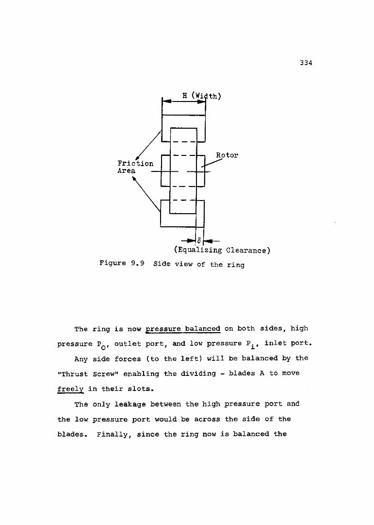
3 3 4

H (Width)

RotorFrictionArea

(Equalizing Clearance) Figure 9,9 Side view of the ring

The ring is now pressure balanced on both sides, high pressure P^, outlet port, and low pressure P^, inlet port.

Any side forces (to the left) will be balanced by the "Thrust Screw" enabling the dividing - blades A to move freely in their slots.

The only leakage between the high pressure port and the low pressure port would be across the side of the blades. Finally, since the ring now is balanced the

3 3 5

r e g u l a t i n g f o r c e i n F i g . 9 . 5 b a l a n c i n g t h e s p r i n g K^p,

is zero and regulating force is obtained by introducinga piston actuated by the pressure difference - P^.Thus, the coefficient is now replaced by the pistonarea A_.P

Before we perform a quantitative analysis of the improved pump under the new conditions, let us summarize what are the achievements of our re-design.(1) Ring is pressure balanced ( AP = 0) in both high and low pressure region and the only stresses would be due to the external spring force and piston force. Therefore, it could be manufactured with a much smaller thickness t, in the range of 0.2 in (instead of 0.375 in now) reducing mass M.(2) No case drain leakage, “ 0, i.e. there is no need for a case drain pipe, due to the pressure balance AP = 0, which means energy saving and overall higher pump efficiency. The leakage between the outside chamber across the side of the dividing blades is negligible, i.e., the leakage coefficient is decreased substantially.(3) The regulating method is now based on the force A^*(Pq - P^) balancing the spring force Fg + F^. We can "control" the regulating force by varying piston area A^,

3 3 6

which enables us more flexibility in choosing spring constant Ksp(4) Finally, we decrease substantially the "friction area" between the ring and the plates (the h*l term) at least by an order of magnitude. Earlier, the friction area was present on the two sides of the ring and now it is present only on the sides of the dividing blades.

The clearance 6 between the sides of the blades and the plate can be increased, without affecting the ovarall leakages. Therefore, the friction coefficient = ‘■ 1 h/8

can be decrease significantly.Let us turn now to the quantitative analysis of the

possible improvement in pump speed of response.

9.7 Quantitative Analysis

The dimensions of the present ring

ii

II f II7 2.0 FrictionArea

Tolerance 8 With Plate

1

old ring

T h e n e w p r o p o s e d r i n g

3 3 7

3/16

3/16 0.5

0.8 FrictionArea

_ Tolerance 8 '^with Plate

0.810*10"^ (Ib.sec^/in)Mnew

Afric.new = 0.5 in^ new ring

The tolerance = 2 5^ (for example). Improvements so far

®vf new - ®vf oldM.hew 1/2.3 Mold

The spring compression is controlled now by a pistonA, (it was before K „P_). p o pv o

The maximum value of the coefficient K from Feliciopv0.451(lb^/psi).

The steady state gain in the system is

3 3 8

-1K V

^spwhich is dominated by the ratio . Since in ourcase the piston surface area is replacing the constant

II 2Kp^, a piston diameter of 1 for example (A^ = 0.7859in ) will increase the spring constant

^sp new = ^gp oldThis method of balancing the pressure regulating spring

(piston) enabled an increase in the spring constant K ,spwhich was a constant, 2300 (lb/in) earlier, without any effect on the steady state error. It enables a second degree of design freedom in increasing the speed of res­ponse of the pump as well.

A "Pressure Balanced Variable Displacement Vane Pump" based on these principles, has been built and partially developed by the author as part of the master degree requirements (80).

Concluding the results of the proposed new design, weget

®vf new = °'°5 ®vf old

^sp new~^*^^ ^sp old

3 3 9

T ----- the time constant^sp

’’new - 0-02857

I, E,, we improved substantially the speed of response.

CHAPTER 1 0

EXPLANATION OF 12.5Hz PEAK IN PUMP DISCHARGE PRESSURE FREQUENCY SPECTRUM

10.1 General

We stated earlier that a pressure compensated variable displacement vane pump is a feedback system, when working in the regulating region, A general characteristic of any positive displacement pump is the existence of pressure "ripples" at its outlet. The problem was and remains a subject of investigation for many pump manufacturers and users, A few references have been gathered in the litera- tyre review on this subject, such as: NCFP; 33, 34, 35.As expected the pump used for the experimental program presented pulsations. A typical power spectral density of these pressure pulsations is given in Fig.10.1, and we observe two high peaks, at 12.5Hz and at 382.5Hz.

The peak at 382.5Hz is understood as that caused by the pump speed and the number of vanes (pump speed is 1765rpm) and the number of vanes (13). The basic frequency would be 29.42Hz and we can see clearly the peaks at the

3 4 0

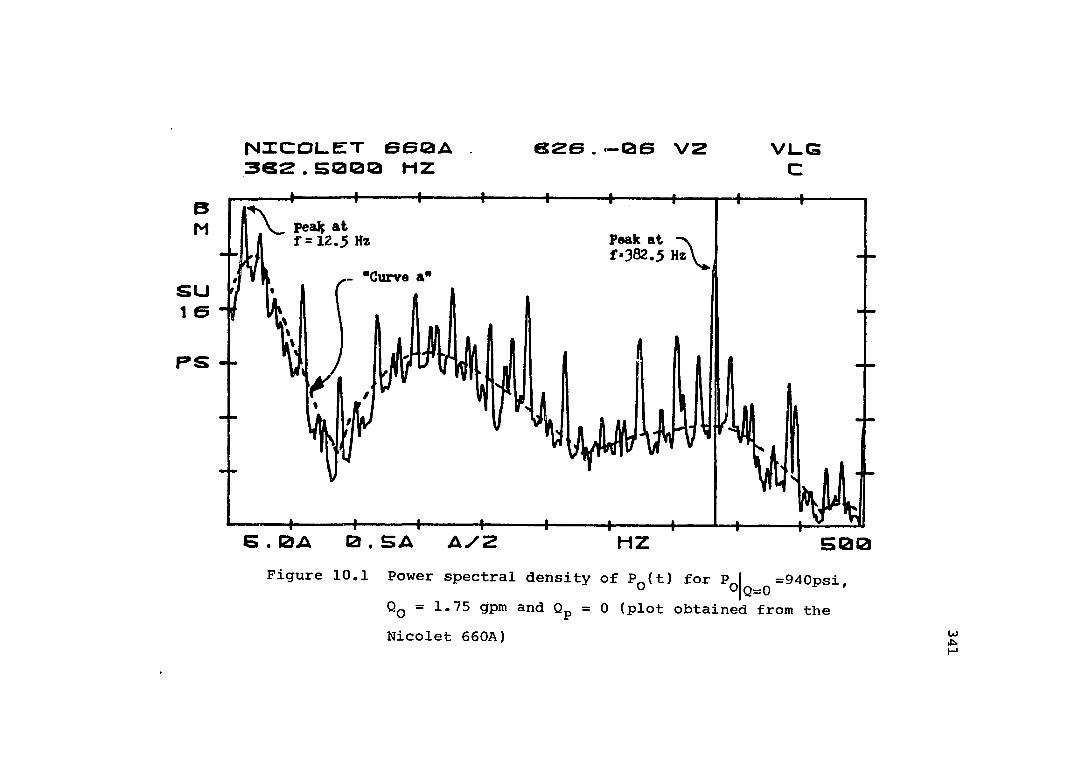
NICDL.ET 6S0A362.5000 HZ

626.—06 V2

Peak atf"382.5 Hz\^

5 . 0 A 0 . S A A / 2 H Z

VL.GC

Pealç at f = 12.5 Hz

- "Curve a"

5 0 0Figure 10.1 Power spectral density of P^(t) for P I =940psi° 0|q=0 '

Qq = 1.75 gpm Nicolet 660A)Qq “ 1*75 gpm and = 0 (plot obtained from the

w

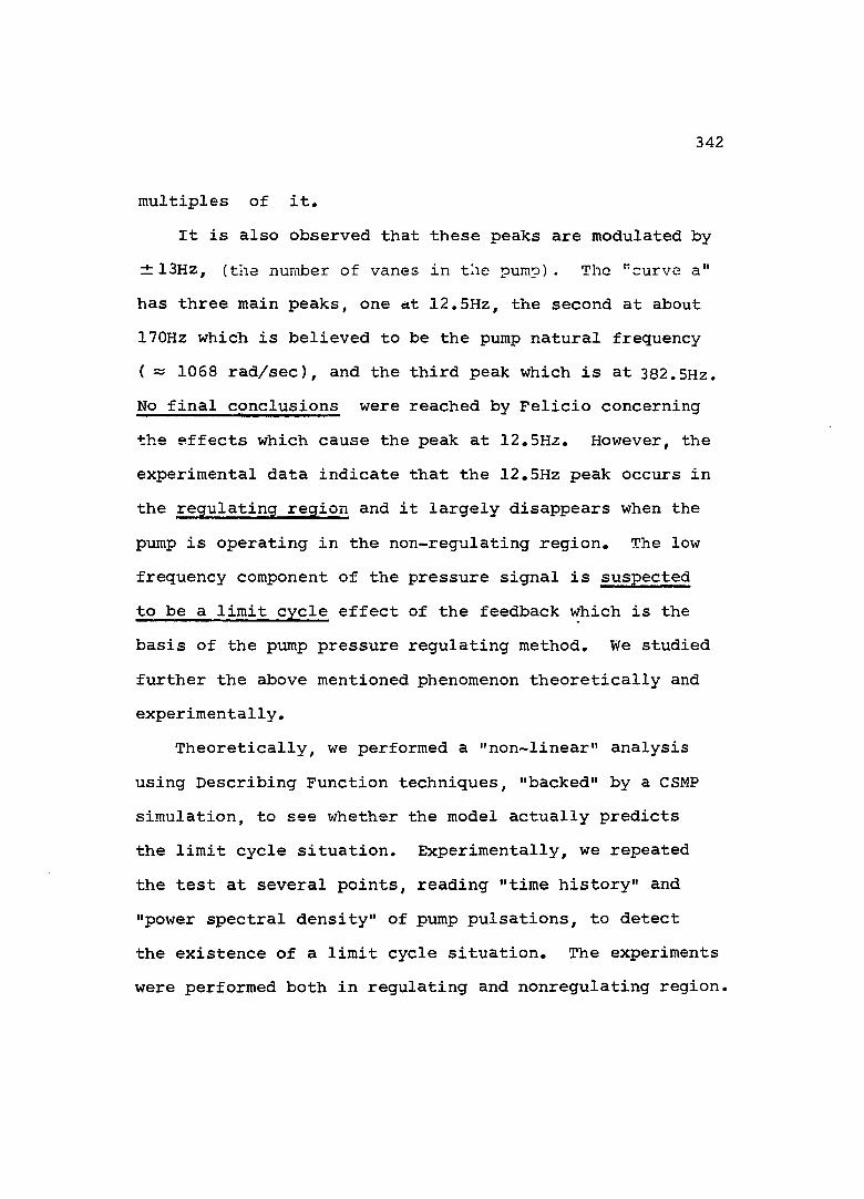
3 4 2

m u l t i p l e s o f i t .

It is also observed that these peaks are modulated by ±13Hz , (the number of vanes in the pump). The "curve a" has three main peaks, one at 12.5Hz, the second at about 170Hz which is believed to be the pump natural frequency ( ~ 1068 rad/sec), and the third peak which is at 382.5Hz. No final conclusions were reached by Felicio concerning the effects which cause the peak at 12.5Hz. However, the experimental data indicate that the 12.5Hz peak occurs in the regulating region and it largely disappears when the pump is operating in the non-regulating region. The low frequency component of the pressure signal is suspected to be a limit cycle effect of the feedback which is the basis of the pump pressure regulating method. We studied further the above mentioned phenomenon theoretically and experimentally.

Theoretically, we performed a "non-linear" analysis using Describing Function techniques, "backed" by a CSMP simulation, to see whether the model actually predicts the limit cycle situation. Experimentally, we repeated the test at several points, reading "time history" and "power spectral density" of pump pulsations, to detect the existence of a limit cycle situation. The experiments were performed both in regulating and nonregulating region.

343

1 0 , 2 T h e o r e t i c a l A n a l y s i s

10.2.1 Describing Function Theory

Before we turn to the nonlinear analysis of the pump, let us present a short review of the describing function theory. Although, it is well documented in the literature, it is brief enough to permit inclusion in this dissertation. Describing function analysis is based pri­marily on the assumption that the input to the nonlinear element is sinusoidal and that linear elements which follow in the loop have a "low pass filtering" effect on the output signal such that this signal becomes essentially the fundamental component of a Fourier series of its wave­form,

A restriction on the method is that there must be a possibility to concentrate in one block all the nonlineari­ties in a system.

Consider the loop:

m =M sin(wt) C = sin(wt+4^) + Cg sinfwt+fg) +••

----1

Nonlinear part

G(iw )

Linear part

3 4 4

with all the nonlinear elements lumped in and all the linear elements in G(io» ).

The closed loop expression is

C G , « G ( i Ù) )— = (10.1)R 1 + G^ « G(i w )

Stability of the system is dependent on the roots of the characteristic equation

1 + G^.GCiûj ) = 0 (10.2)

Solution of equations (10.2)are found easily by plott­ing both sides of equations (10.3)in the following form:

1G(i w ) ------------------ (10.3)

Gdon the customary Nyguist diagram. If àn intersection of the two loci exists, then limit cycle osillations will occur with the frequency given by the left side of equation (10.3) and the magnitude given by G .

10.2.2 Static Friction Nonlinearity and Its Describing Function Analysis

The pump, when operating in the regulatingregion is maintaining constant average pressure by keepinga force balance between the spring force F , viscoussp

345

force F^, the friction force F^, inertia "force" and the vertical pressure force R^.

SP SP

7771

1

Plate

EZZRing

Figure 10.2 The forces on the ring

The force F^ is due to the static friction between the ring and the plates. The viscous friction coefficient

dealt with in the previous chapter, was also strongly related to the "friction area" between the plates and the ring.

• Newton's law applied to our system will result in an equation of the form

''i = *v= " So + ®vf ®0 + >'sp ®0 + '■f

where :

346

(10.4)

F. A Input force (lb_).1 — X2M g Mass of the ring (Ib^ sec /in).

Fg A Friction force (Ib^) . e^ Ring eccentricites (in),

where F^ is the friction force and will be considered a sign dependent function of velocity as shown in Fig.10.3.

-F

Figure 10.3 Idealized friction characteristics

Static friction nonlinearity is common in servosystems and it has been studies by a number of investigators. An excellent analysis was presented by Merritt, who considered three describing functions, each having utility in differ­ent circumstances.

3 4 7

(1) Case a - Mass Force dominant (M large)(2) Case b - Viscous Force dominant (B large)(3) Case c - Spring Force dominant (K large).

In general, all the cases are valid in a certain com­bination because mass ^ present in all systems. If however, mass M is negligible compared to the significantviscous friction coefficient B _ and spring constant K ,vr spas is true in our case, we can present equation (10.4) in the following block diagram.

dl

sp

vfvf

Figure 10.4 Equation 10.4 in block diagram form

The derivation of a describing function of the element between and e^ will be explained in two steps.

3 4 8

(1) Let us analyze first the part in the dotted area and get a describing function = n/m representation.

As long as the time constant M/B^^ can be neglected

compared to the frequency of interest i.e., ^interest

is less than 0.2 the analysis becomes simple.In our case

B= vf 97

= 48115 rad/sec

O)

M 2.016*10 = 12.5 Hz = 78.54 rad/secof interest

78.54 rad/sec < <. 0.2 = 9623 rad/sec

therefore, in our case the time constant M/B^^ is negligi­ble.

Thus, the input output nonlinearity between points m, n becomes

n=Bvf 0

ra(input)

Figure 10.5 Viscous friction nonlinearity

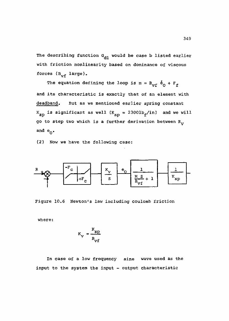
3 4 9

The describing function would be case b listed earlier with friction nonlinearity based on dominance of viscous forces large).

The equation defining the loop is m = e^ +

and its characteristic is exactly that of an element withdeadband. But as we mentioned earlier spring constantK is significant as well (K.^ = 23001bVin) and we will sp sp X

go to step two which is a further derivation between and e^.

(2) Now we have the following case:

sp

-F

+Fvf

Figure 10.6 Newton's law including coulomb friction

where;KB.spvf

In case of a low frequency sine wave used as the input to the system the input - output characteristic

3 5 0

between points e^ and would result in the following form.

Figure 10.7 Blacklash nonlinearity

The action is similar to that of a loop with dead band followed by an integration which is common analog compu­ter circuit for generating backlash.

3 5 1

1.0

0.8 - 20'

0.6 -40*

0.4 -60*

m0.2 -SO '

- 100'0.4 0.8 1.6 2.0

HIM

Figure 10.8 Describing function for blacklash(Merritt)

Thus, the static friction in our system introduces backlash, which is well known to be destabilizing.

10.2.3 Describing Function Analysis of the Pump With Static Friction Nonlinearity

The overall blockdiagram of the pump including the "hydraulic transfer function" has the form given in Fig.10.9 and will have the final describing function form given in Fig.10.10.

K . / 7 ' =0PV / // SB..^(MS/B ^+1)

Load

C0EF4T^S+1

P,

Figure 10.9 Pump block diagram including coulomb friction F.

G(S)

/S(T, S+1)(T\S+1)

F i g u r e 1 0 . 1 0 D e s c r i b i n g f u n c t i o n f o r m o f t h e s y s t e m

wUlN)

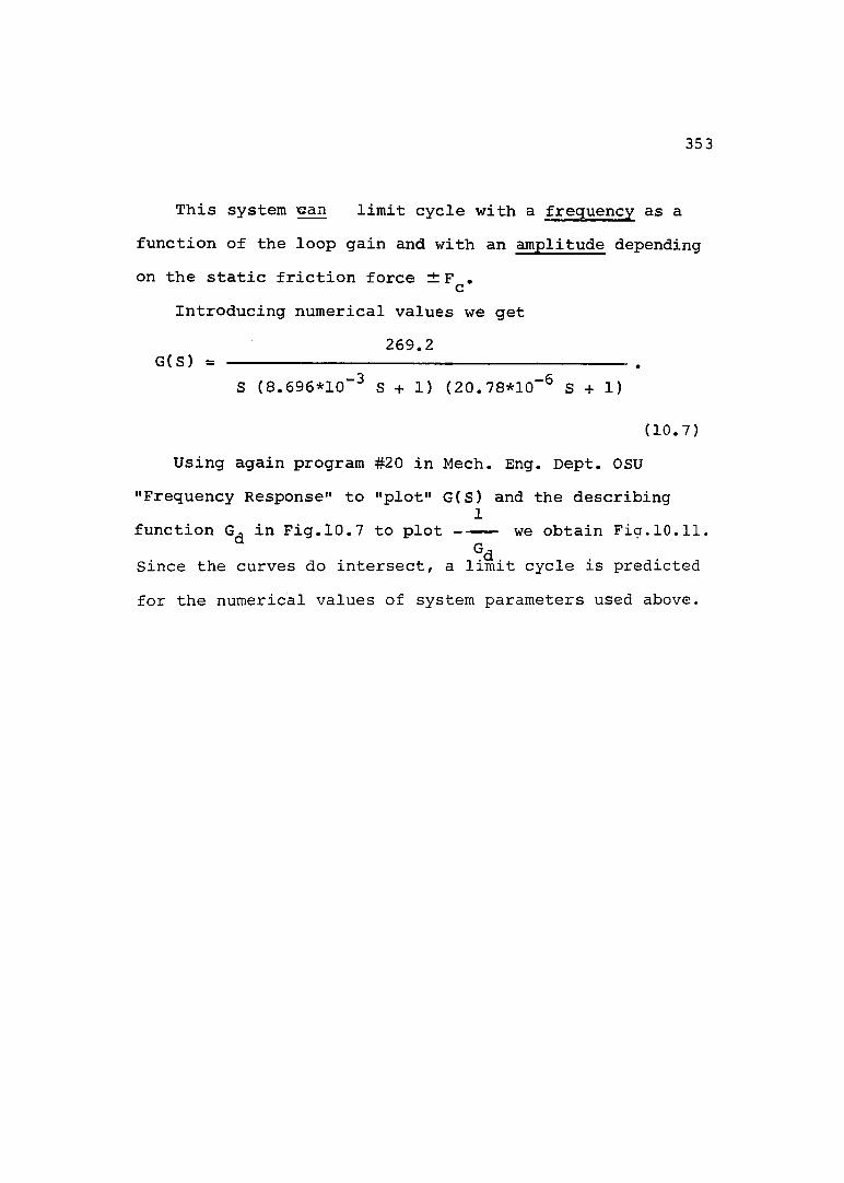
3 5 3

This system gan limit cycle with a frequency as afunction of the loop gain and with an amplitude dependingon the static friction force ± F .c

Introducing numerical values we get269.2

G(S) =S (8.696*10"^ S + 1) (20.78*10 S + 1)

(10.7)Using again program #20 in Mech. Eng. Dept. OSU

"Frequency Response" to "plot" G(S) and the describing1

function G^ in Fig.10.7 to plot ----- we obtain Fig.10.11.GdSince the curves do intersect, a limit cycle is predicted

for the numerical values of system parameters used above.

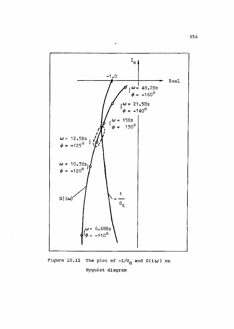
3 5 4

- 1 . 0

W = 4 8 . 2 H z

^ = —160^w = 2 1 . 5 H z

<f> = - 1 4 0 °

w = 1 5Hz

Ü) = 1 2 . 5 H z

<i> = - 1 2 5 °

w = 1 0 . 5 H z

d> = -120°

D= 6 . 6 8 H z

Figure 10.11 The plot of -1/G^ and G(i£j) onNyguist diagram

355

Limit cycles predicted by describing function analysis are most accurate when the two curves intersect nearly perpendicular. In our case the intersection near 12.5Hz is not very "clear", therefore, we can infer that accuracy of prediction may be relatively poor. Also, most of the parameters in the model such as compliance C^, the coeffi­cients K K_, the constant friction coefficient B and pv' e' vf'the static friction force are difficult to predict accurately and changes of ±50% in their values are not unrealistic. Only some of the parameters are reasonably well known constants, such as the spring constant Kspgiven by the manufacturer, and pump speed of rotation N. Thus, changes in the parameters will affect the loop gain which is the variable defining the limit cycle frequency.

In our digital computer simulation program we tried numerous models changing each and every parameter (within ± 50% range) to study the effect on the pump model. The change of number of parameters together, resulted often in a nonproportional change in the limit cycle frequency.As we can see in figure (10.11), we have to decrease gain in order to get the intersection between G(icj ) and -1/G^ at 1 2.5Hz. The conclusion of our study of parame­ters changes was that decreasing the gain factor COEF 4 will cause the system to limit cycle at 12.5Hz. At this

356

point changes in ±F^ resulted in changes of the limit cycle amplitude confirming the theoretical analysis.We will present now the model which gave satisfactory results.

10.3 Computer Simulation

10.3.1 CSMP Program

In the CSMP model we used the FCNSW function available, to present the friction force F^ which is a function of velocity.

After substituting numerical values we obtained a model which limit cycles at 12.5Hz. The changes in the parameters were "lumped" in the coefficient COEF 4, which is a gain factor in our model. As we see in Figure 10.11 the gain had to be decreased in order to get the cross over frequency at the correct value.

The amplitude of the oscillations was controlled by varying the magnitude of the static friction force F^,which is a function of pump pressure setting as follows:

F^ = 5.10 Ibg for 280 psiF = 9.10 Ib^ for 500 psic f ^

F =12.74 lb_ for 700 psic fF =17.25 Ibj. for 948 psic f ^

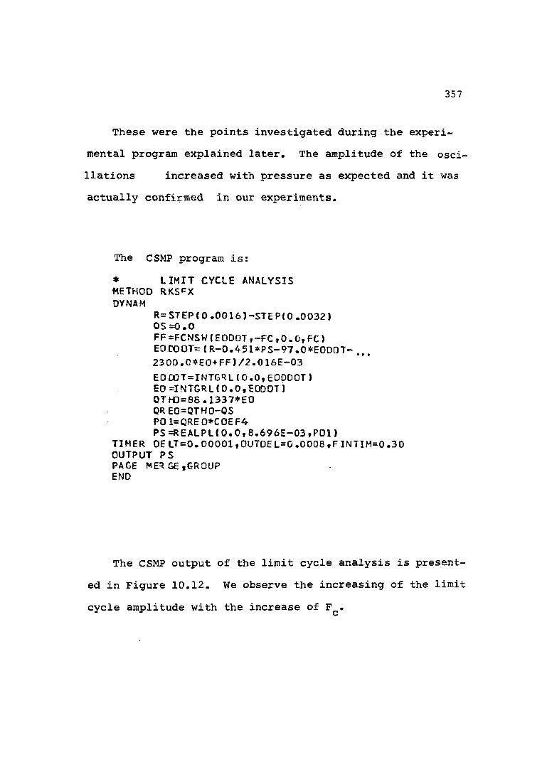
357

These were the points investigated during the experi­mental program explained later. The amplitude of the osci­llations increased with pressure as expected and it was actually confirmed in our experiments.

The CSMP program is:* LIMIT CYCLE ANALYSISM E T H O D R K S ^ XDYNAM

R= STEP (0.0016 )-STEP( 0.0032)0S=0.0FF=FCNSW(EOD0T,-FC,0.0,FC) B0DDOT=(R-0.451*PS-97.0*E0D0T- ... 2300.C*EO+FF)/2.016E-03EODOT=INTGRL(O.0,EODDOT)EO =INTGRL(0.0,E000T)0TH0=86.1337*E0 QREO=QTHO-QS PO 1=QRE0*C0EF4 PS=REALPL(0.0,8.696E-03,P01)

TIMER DE LT=0.00001,0UTDEL=0.0008,FINTIM=0.30OUTPUT PSPAGE MERGE,GROUPEND

The CSMP output of the limit cycle analysis is present­ed in Figure 10,12. We observe the increasing of the limit cycle amplitude with the increase of F^,

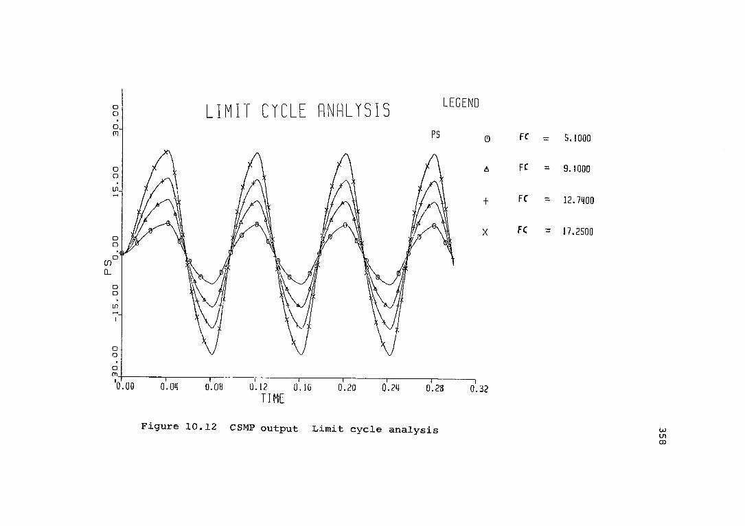
L I M I T C Y C L E A N A L Y S I S L E G E N D

0 FC = 5 . 1 0 0 0

A PC = 9 . 1 0 0 0

+ FC = 1 2 . 7 80 0

X FC = 17 .2 50 0

0.08 U. I 2 (hie OTo oITij ÔT23 0.32T I M EFigure 10.12 CSMP output Limit cycle analysis w

( j i00

359

10.3.2, Frequency Response Computer Program

The linear part of the describing function analysis was found to be

G(S) = --------------- 269^2--------------------S (8.696*10“ S + 1) (20.78*10"® S + 1)

and as mentioned earlier we used program #20, "Frequency Response" to "plot" G(S) on Nyguist diagram, see figure (10.7).

The computer program and the tabular results are pre­sented as follows.

Computer program #20 FREQUENCY RESPONSE DATAUSER SPECIFIED FREQUENCY RANGES AND INCREMENTSSYSTEM function INPUT DATA

NUMERATOR COEFFICIENTS DENOMINATOR COEFFICIENTS S**( 0) O.lOUOE+01 O.IQOOE+OIPOLES REAL PART IMaG. PART

-0.11506 + 03 0.Ü-0.4812E+05 0 JÜ

NUMBER OF DIFFERENTIATORS (PQS. INTEGER)OR INTEGRATORS (NEC. INTEGER )= -IDEADTIME = 0.0K = 0.I490E+1USTEADY-STATE GAIN = 0.2S93E+03STATIC LOOP SENSITIVITY = 0.1490E+IO

360

FREQUENCY AMPLITUDE RATIO PHASE(HZ. > (RAO./SEC.) (DEGREES)

0.159E+00 0.100 6+01 0.2 696+03 -0.9056+020.955E+00 G.6006+01 0.448 6+02 -0.9306+020.175E+01 0.1106+02 0.244 6+02 -0.9556+020.255E+01 0.1606 + 02 0.1676+02 -0.9796+020.334E+01 0.2106 + 02 0.126 6+02 -0.1006+030.4146+01 0.2606+C2 0.1016+02 -0.1036+030.493E+0I 0.3106+02 Ü.8396+01 -0.1056+030.573E+01 0.3606+02 0.7146+01 -0.1076+030.653E+0I 0.4106+02 0.619 6+01 -0.1106+030.732E+01 0.4606+02 0.5436+01 -0.1126+030.8I2E+01 0.5106 + 02 0.4836+01 -0.1146+030.891E+01 0.5606+02 0.432 6+01 -0.1166+030.971E+Q1 0.6106 + 02 0.3906+01 -0.1186+030.987E+01 0.6206+02 0.3826+01 -0.1186+03O.lOOE+02 0.6306+02 0.3 756+01 -0.1196+030.107E+Ü2 0.6706 + 02 0.3476+01 -0.1206+030.108E+02 0.6306+02 0.3416+01 -0.1216+030.1lOE+02 0.6906 + 02 0.335 6+01 -0.1216+03O.lllE+02 0.7006 + 02 0.3 296 + 01 -0,1216+030.113E+Û2 0.7106+02 0.3236+01 -0.1226+030.115E+02 0.720E+U2 0.317 6+01 -0.1226+030.116E+02 0 . 73 0 6 + 02 0.3116+01 -0.1236+030.118E+02 0.7406+02 0.306 6+01 -0.1236+030.119E+02 0.7506+02 0.301 6+01 -0.1236+030.121E+02 0.7606 + 02 0.296 6+01 -0.1246+030.123E+02 0.7706+02 0.2916+01 -0.1246+030.1246+02 0.7806+02 0.2boE+01 -0.1246+03I0.126E+02 0.7906+J2 0.2816+01 -0.1256 + 030.127E+02 0.6006 + C2 0.2766+01 -0.1256+030.1296+02 Ü.310E+U2 0.272 6+01 -0.1256+030.1316+02 0.8206 + 02 0.2676+01 -0.1266+030.1326+02 0.5306 + 02 0.263 6+01 -0.1266+030.1346+02 0.840E+C2 0.2596+01 -0.1266+030.I35E+02 0.6506+02 0.255 6+01 -0.1276+030.1376 + 02 0.8606+C2 0.2516+01 -0.1276+030.138E+02 0.8706 + 02 0.2476+01 -0.1276+030.140E+02 0.8806 + 02 0.2436+01 -0.1286+030.1426+02 0.8906 + 02 0.239 6+01 -0.1266+030.1436+02 0.9006 + 02 0.2366+01 -0.1286+030.1456+02 0.9106 + 02 0.232 6+01 -0.1286+030.22+6+02 0.1416 + 03 0.1216+01 -0.1416+030.3 0 46+ 02 0. 1916+0 0.727 6+00 -0.1496+030.3846+02 0.2416 + 03 0.4816+00 -0.1556+030.4636+02 0.2916+03 0.340 6+00 -0.1596+030.5436+02 0.3416+re 0.2526+00 -0.1626+030.6226+02 0.3916+U3 0.1946+00 —0.1646+030.7026+02 0.4416 + 03 0.154 6+00 -0.1666+030.7816+02 0.4916+03 0.1256+00 -0.1676 + 03RUN COMPLETE

361

10.4 Experimental Study

The experimental program included, recording of the "time history" and "power spectral density" at twelve different points on the P - Q curve.

^0(ps i )

948

700

500

280

Regulating Region I Nonregulating Region(948, 0) (948, 1.75)

(700, 0) (700, 1.75)

(500, 0) j (500, 1.75)

I(280, 0) j (280, 1.75)

(800, 3.54)

(700, 3.75)

(500, 4)

(280, 4.5)

1.75 5.54 4.76 QO(gpm)

Figure 10.13 Measuring points

362

As we can see the twelve points were carefully selected on the P - Q curve such as to test the pump in the regulating region (8 points) and several points (4) in the nonregula­ting region where the ring is on the volume regulating screw.

The tests were performed at the following points:(1) Qq = 0 gpm ^0 280 psi(2) Qq = 1.75 gpm ^0 280 psi(3) Qq = 0 gpm Pq 500 psi(4) Qq = 1.75 gpm ^0 = 500 psi(5) Qq = 0 gpm ^0 = 700 psi(6) Qq = 1.75 gpm ^0 = 700 psi(7) Qq = 0 gpm ^0 = 948 psi(8) Qq = 1.75 gpm ^0 = 948 psi(9) Qq = 4.5 gpm ^0 = 280 psi(10) % = 4 gpm ^0 = 500 psi(11) Qq = 3.75 gpm ^0 = 700 psi(12) Qq = 3.54 gpm Pq 800 psi

Regulatingregion

Nonregulatingregion

In each case we recorded the time-varying pressureon a Brush recorder and "Power Spectral

Density" using the FFT NICOLET 660A analyzer.A typical set of data are presented in Figure 10.14.

For the rest of the data see appendix C.

TimeHistory

•H

12.5 HzOp. Cond. jvjPq = 280 psi 12.5 Hz--°0 - 0 s u

1 S ■■■Power Spectral

P SDensity

2 . 0A H Z 5 0 0

Figure 10,14 Time history and Power spectral density in regulating region ww

364

Observing the power spectral density curves, we can see a consistant peak at 12.5 Hz as expected in the regulating region. For the nonregulating region, the peak decreases substantially and for low pressure (280 psi), it even disappears.

The frequency does not change with pressure setting, but the amplitude is decreasing as we increase pressure.

There are three dominant "low" frequencies in each curve at 12.5 Hz, 3 0 Hz, and 60 Hz. The 3 0 Hz and 6 0 Hz peaks are explained by 18 00 rpm pump speed. The 12.5 Hz peak is probably the limit cycle effect we are investi­gating. Observing now the "time function" data for each run, we can see very clearly the dominant 29 to 30 Hz and 58 tO 6 0 Hz oscillations. The 12.5 Hz component is not clearly visible here but becomes obvious in the spec­trum analysis.

Comparing the tests for zero flow rate at each pressure setting to the 1.75 gpm flow rate, we can see that the 12.5 Hz peak in the power spectral density is dominant for the 1.75 gpm flow rate.

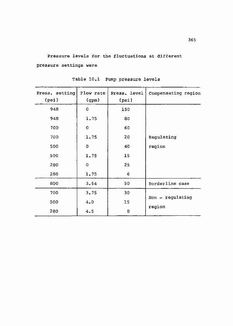
365

Pressure levels for the fluctuations at different pressure settings were

Table 10,1 Pump pressure levels

Press, setting (psi)

Flow rate (gpm)

Press, level (psi)

Compensating region

948 0 150948 1.75 80700 0 60700 1.75 20 Regulating500 0 40 region500 1.75 15280 0 25280 1.75 6

800 3.54 50 Borderline case700 3.75 30

Non - regulating500 4.0 15

region280 4.5 8

366

10.5 Conclusions

We performed a theoretical study, computer simulation and experimental tests to investigate the 12.5 Hz peak in the pump pulsation power spectral density data. Summariz­ing these efforts, we conclude that there is a limit cycle effect occurring when the pump is operating in the regulating region.

Looking back to Chapter 9, which discussed a possible "re-design" of such pumps, one can determine that the new proposed configuration will minimize possible limit cycle oscillations.

Decreasing the friction area, we actually reduce thestatic friction force F which is the cause of the limitccycle oscillations.

CONCLUSIONS and

SUGGESTIONS for further Study

367

CHAPTER 11CONCLUSIONS AND SUGGESTIONS FOR FURTHER STUDY

11.1 General Conclusions

Most valve-controlled servosystem analyses assume con­stant supply pressure. When servo transients are large and fast enough, a pressure compensated pump type of supply, without accumulator, can no longer maintain reasonably constant supply pressure and pump dynamics become signifi­cant. Combined pump/servosystem dynamics was studied analytically and experimentally tested. Both linearized and nonlinear system models were formulated. A useful subsystem modeling technique was developed. Computer programs were devloped in both time domain and frequency domain.

Experimentally, step response performance was evaluated in terms of controlled variable maximum overshoot, frequency of oscillations and time to peak. Frequency tests were performed investigating three transfer functions.

The comparison between the digital simulation time domain computer program and experiment shows a fairly good correlation. Comparison between the experimental results and the frequency response computer program gave good

368

369agreement. The models developed are thus felt to be sufficiently accurate for system preliminary design purposes.

Efficient use of fluid power has recently received much attention in non-servo applications. Servo applica­tions present unique problems and have not been extensively studied. We studied for feasibility two schemes designed to take advantage of the controllability of variable displacement pumps for energy-saving operation of servo- systems, using computer simulation.

One scheme uses preknowledge of system duty cycle to program pump discharge pressure. The second approach attempts to continuously enforce the well known maximum power transfer rule (actuator pressure drop should be 2/3 of supply pressure) by sensing load pressure and using these signals to adjust pump discharge pressure.

Computer simulation results showed that both schemes appear feasible, though for different types of applications. In comparison with a conventional system using constant supply pressure, servo performance was maintained while energy efficiency was improved as much as 30 percent.

11.2 Specific Conclusions - Pump Dynamic EffectsIn the process of the theoretical analysis of the

overall servosystem, a new concept has been introduced.

370that is, the organization of the system into subsystems according to their tasks.

1) The "Supply Subsystem," which includes all the hydraulic components (pump, filter, accumulator, and pipe line) up to the servovalve input.

2) The "Control Subsystem," including an analog or digital control unit, the "brain" of the servosystem, and the servovalve.

3) The "Load Subsystem," including all the hydraulic components (pipe line, actuator, etc.) from the servovalve downstream, and the load.

Including pump dynamics in servosystems is a contri­bution to the field, since previous analysis in literature (2) assumed constant supply pressure at the servovalve input.

The effect of pump dynamics on supply pressure and also on the controlled variable (load speed) was studied for

both step and sinusoidal commands. Observing the stepresponse of the controlled variable and comparing to asystem with constant supply pressure:

1) There is no significant difference in the maxi­mum overshoot.

2) With pump dynamics, there is an increase in thefrequency of oscillations of about 50%.

3) The most significant difference in the performance

371

is the "time to maximum overshoot," which increases by 67% when pump dynamics are present.

4) There is also a significant increase in the set­tling time.

5) Increasing load inertia, "Load Subsystem" natural frequency sufficently^ will make the effect of pump dynamics insignificant.

Observing supply pressure to the servovalve when pump dynamics is included we conclude;

1) Pressure peaks of + 80% of nominal supply pressure were observed for step commands corresponding to 95% of full scale valve openings.

Even though pressure compensated vane pump used in our experimental program was relatively "fast," the time to maximum overshoot and the settling time increased about 100% compared to the constant supply pressure system. In other systems of this type, having pumps with slower speed of response we would expect even greater degradation in system performance due to pump dynamics.

Since pressure compensated variable displacement pumps will in the future be dominant in hydraulic power supplies, one has to choose a pump "fast" enough to achieve system performance, or else use accumulators.

372It is a common practice in the design of a servosystem,

to select the servovalve such that its natural frequency is considerably higher than the highest system natural frequency, therefore its dynamics can be neglected. Thus, "Load Subsystem" or "Supply Subsystem" natural frequency, which even is smaller, will dominate system natural frequency.

A general conclusion of our study is that, unless accumulators are used, pump dynamics (supply subsystem dynamics) is significant in many of the applications. When this is the case, the models developed in this dissertation should be helpful to system designers in assessing overall system response.

11.3 Specific Conclusions - Energy Saving The = 2/3 Pç, Scheme

According to earlier studies (2), it has been found that the maximum power is transferred to the load when the pressure across the load (AP ) is two-thirds of supply pressure (P = 2/3 P_). The operating efficiency forij O

servovalve controlled actuators in this case turns out to be 67%.

A Gain Adjusting Block has been introduced to keep load gain fairly constant through the entire duty cycle.

373The presence of the "pressure loop" (P- = 2/3 PS) and

the introduction of the gain adjusting block caused the system to be more oscillatory. We found that system com­pliance had to be increased and signal low-pass filtering was needed to achieve a stable system.

The performance of the system was compared to the con­stant supply pressure system. The criteria used were:1) System efficiency, the power lost and total energy, from

energy point of view.2) System gain, percentage error and RMS Error analyzing

system performance.

System behavior was analyzed1) Keeping load torque constant, varying speed.2) Keeping speed constant, varying load torque.

Programmed Supply Pressure SchemeThe Programmed Supply Pressure Scheme is applicable

when the hydraulic system is a part of a digital control system and the computer might be programmed to obtain the desired pressure profile Pd, (t). Changes in the system duty cycle could easily be reprogrammed.

The gain adjusting block discussed in the P^ = 2/3 Pg scheme has been introduced in this system as well, main­taining percentage error very close to the constant supply pressure scheme.

374

Its average efficiency is about 45% compared to about 35% for the constant supply pressure system, but less than the efficiency of the P = 2/3 P„ scheme which is 67%.J_l b

This system showed similar stability problems.Analyzing the results from the energy point of view,

we observe that the power lost is increasing as speed is increasing, since more flow is needed via the servovalve under the same pressure drop. Power lost is decreasing as load is increasing, since the pressure drop across the valve is decreasing as load pressure is increasing.

Finallyjfrom the energy analysis comparing the two schemes, we see a clear and constant advantage to the P = 2/3 P„ scheme.

From system performance analysis in terms of RIIS Error we conclude that it is identical in all three schemes, proving the effectiveness and the necessity of the gain adjusting concept in energy saving configurations.

The conclusion is that the two energy saving schemes investigated were found to be applicable in servocontrolled actuator system applications. Energy saving seems feasible, and at the same time keeping system performance equivalent to the nonregulating constant pressure system.

375

11.4 Suggestions for Further Study(1) Our investigation was aimed to include pump dynamics and observe its effect on servosystem response. The pump tested by us was "too fast" (up = 183 rad/sec) to show strong pump dynamic effects in many cases. Therefore, in order to be able to perform our study, we had to practically eliminate pipe dynamics, having very short connecting lines and minimum necessary hydraulic components, accumulator, and filter. In a more practical system, pipe lines are long and several hydraulic components such as flow and pressure control valves are incorporated, having signifi­cant effect on system dynamics. In further studies, the use of a "slower" pump would make the pump dynamic effects more significant.

It is suggested to build a typical hydraulic servo­system (not just an experimental apparatus) using a "slow" pump and including all possible hydraulic components and run the same experiments. Along with that, the CSMP computer program should be extended to its more general configura­tion, using the governing differential equations presented in Chapter 2 in their most general form. Computer simula­tion and experimental tests will reveal the limits of pump dynamic effects on the system and provide added confidence in the validity of the predictions.

376

(2) It is suggested to repeat the described experimental program and computer simulation using a linear acutator (piston) in a position control configuration. The set of governing equations for this case are presented in Chapter 2, so the CSMP program could be easily developed. The only change in the experimental apparatus would be to replacethe hydraulic motor by a hydraulic cylinder and rewire the servocontroller as a position control system.(3) An investigation of several types of power supplies(pumps) as well as acutators and loads is suggested, inorder to obtain more complete results about "Supply Sub­system" - "Load-Subsystem" interrelation.

Suggestions for Further Study - Energy Saving(1) Develop and run CSMP computer program for the linear

actuator position control configuration. The govern­ing equations as well as the block diagram have been presented in Chapter 7.

(2) Modify the developed program and "test" the rotary acutator position control configuration.

(3) Finally, it is suggested to build the needed hardwareand actually enforce the proposed pressure controlloop along with the speed control loop to obtainpractical experience in both rotary and linear actuator systems.

377

(4) Study improved stabilization and compensation tech­niques to deal with the stability problems produced by the pressure-adjusting scheme.

11.5 Pump AnalysisWe will end our section of conclusions with several

comments on the work done on the variable displacement vane pump.(1) With proper redesign of the pump, it seems to be feasible to increase significantly the speed of response.We recommend to build a modified pump according to the design outline presented in Chapter 9 and actually test the "new" pump.(2) Supply pressure fluctuations at high frequencies, associated with pump speed of rotation and the number of vanes are well known in practice. Low frequency oscilla­tions, associated with the possible limit cycle conditions were not mentioned in the literature.

Our investigation, experimental and theoretical, revealed that the pump pressure regulating mechanism is affected by coulomb friction (F ) which creates a limit cycle condition at low frequency (12.5Hz). Our pump re-design recommendations seem to solve partially the problem by decreasing coulomb friction force F^, and therefore minimize the limit cycle amplitude.

APPENDIX

378

APPENDICES

The first section of the appendix was aimed to comple­te and clarify the subjects discussed in the body of the dissertation, which has three main parts. Therefore, we divided the first section of the appendix into three parts as well, each referring to one of the parts in the text.

(1) Appendix A - Part one(2) Appendix B - Part two{3) Appendix C - Part threeThe second section has two parts:

(4) Appendix D - Explanation of turbine flow - meter discrepancy during flow measurements

(5) Appendix E - Literature review scheme(6) References

379

APPENDIX A REFERRING TO PART ONE IN THE TEXT CHAPTER 3

- EXPERIMENTAL PROGRAM

A.l Apparatus Physical Dimensions

Pipe line dimensions arid oil parameters were given in Table 3.1 and Table 3,2, Let us now calculate the minimum pipe length needed in a lumped parameter analysis,

a = Propagation velocity

a = ( = ( 10^/8,16*10"^)^/^ = 35000,0 (in/sec)P

To choose an approximate number of lumps we need anestimate of the highest frequency up to which the computermodel is to be accurate. We will take f = lOOHz, sincemax 'this was the highest frequency in the frequency response test.

The wave length at lOOHz is

, _ 35000,0 (in/sec) ^50 in100 (cycle/sec) cycle

Using the "10 lumps per wave length rule", a lump lengthis 35 in, which is more than twice the length of the pipe

380

381

lines in our system. Thus, the lumped parameter approach in writing the equations describing pipe dynamics is ade­quate. We can also neglect friction and inertia, as it will be shown, considering compliance only (equation 2,10).

The highest flow rate delivered by the pump during our experiments was = IScis at a mean flow velocityof V = 135,8in/sec,The Reynolds number would be:

Re = Z_D = 135,8 * 0.375 Un/sec in) ^ ggs.?0,0732 (in /sec)

/. Re < 2100which is well into the laminar region. The maximum pressure drop in a 16in pipe line assuming fully developed laminar flow,

APmax = 'A'l'7T D

AP = 128 * 5.976*10-6 (lb sec/in^) * 16 (in) * in Vsec )max . .

(0,375)^ (inT)

AP^ax = 2,955 (Ib/in^)

which is negligible since our pressure range is 750psi, Considering now fluid inertia

m =P1 A = 8,16*10"^ (lb sec^/in^) * 16 (in) * 0,11045(in^)

m = 11,82 * 10 (lb sec^/ in)

382

which is again negligible.So we have justified the negligibility of friction

and inertia in our analysis.

A.2 Pressure Drop Pump - Valve Line

Having justified the negligibility of the steady state pressure drop in the pipes at the highest flow rate, we now turn to experimental results.

The steady state pressure drop between "Pump manifold pressure" and "Servovalve input pressure" as well as act­uator shaft angular velocity have been measured.

Accumulator

Shut Off ValvePump

Filter Tach

Pg A Pump manifold pressure Py A Valve input pressure Vq a Voltage proportional to 6^

Figure A.l Pressure drop measurements

383

Accumulator was not included using the shut off valve installed on the connecting line. Therefore, the main pressure drop source would be the valve protecting filter. A new filter was installed at the beginning of the experi­mental program, to keep pressure drop to a minimum. According to the manufacturer, the pressure drop at 7.0gpm is lOpsi, when clean assembled. The experiment has been conducted with three pressure settings: SOOpsi, 730psi, 950psi, the low, medium, and high pressure regulating range of the pressure compensated pump.

The leakage coefficients of the hydraulic motor were also measured and their contribution to the continuity equations for steady state situation will be

= Dm Pj . (A.2)

where :C. = 13.0765 * 10"^ cis/psi. im

= 2.2857 * 10"5 cis/psi,= C. + C /2 = 14.219 cis/psi * lO"^. tm im em

The highest P^ = P^ - Pg measured at any pump pressuresetting was 150psi which gives a maximum leakage flow

384

®leak “ 0.02133 cis. This is just 0.57% of the highest flow rate in our experiment.

Therefore, flow rate measurements by 6^ (i.e.,

Vq = K^ach m^ neglecting leakages is for all practical purposes justified.

To summarize, the pressure drop experiment was a steady state measurement of : Pump manifold pressure P^, Valve input pressure P^, and tachometer voltage at four

different valve openings (25%, 50%, 75%, 95%) and three pump pressure settings 500, 730, 950psi.

The results were summarized in Table A.l.

385

Table A.l Pump-Valve pipe line pressure drop measurements

Press Ppump Pvalve Tach. Volt Flow rate Press, dropSetting Pg (psi) Py(PSi) Vq (Volt) (cis) AP (psi)

500 500 0 0 0466 460 1.12 3.739 6

500 465 455 1.95 6.510 10psi 463 450 2.85 9.515 13

460 443 3.35 11.183 17

730 730 0 0 0730 722 1.49 4.974 8

730730 717 2.54 8.479 13

psi730 710 3.70 12.352 20

730 708 4.41 14.722 22

950 950 0 0 0

950 940 1.76 5.875 10950

942 926 2.97 9.915 16psi

940 918 4.28 14.288 22

860 835 4.69 15.657 25

386

If we plot the results on a vs. AP graph, we realizethat a linearized orifice model Q_ = K AP could be usedLi orin our theoretical analysis with a high level of confidence (see Fig.A.3).

= 0.64 (cis/psi)

Turning now to the pipes connecting the servovalve with the actuator inlet and outlet port, we see that they are free of restrictions. The static and dynamic pressure measurement equipment will not cause any pressure loss due to its physical construction.

Pressure gauge

From

ValvePiezoelectricPressure pickup

Figure A.2 Pipe pressure measurement

To the .motor

cis

or,pipe = 0-G4 c i s /p s i

Legend □ 500 psiO 730 psi A 950 psi

2 -

10 15 20 25 psi50

Figure A.3 Pipe flow resistance coefficient KorpipeW00•-J

388

A.3 Hydraulic Motor Parameters

A clear and simple way to measure the different para­meters of an hydraulic motor and its performance curves was described by Merritt. His methods were used in our experimental work of obtaining motor parameters.

The steady state continuity equations (i.e., without compressibility flow) for the motor chambers are

=1 - =em - =im 'h ' 2> ‘ ''m «m = °^ =im"'l - '2 > - =em ‘’2 - «2 = ° <*.4)

where ;A Ideal volumetric displacement of motor.

= 0.1591 (in^/rad) given by the manufacturer

A Motor shaft speed (rad/sec).

A Forward flow rate to motor (in /sec).3

@2 A Return flow rate from motor (in /sec).

and Pg è Inlet port and outlet port pressure respective­ly.

These two equations completely describe the flow in the hydraulic motor and

389

A Internal or cross port leakage coefficient (cis/psi).

^em - External (case drain) leakage coefficient (cis/psi).

These parameters have been found experimentally.Let us now consider the torques which act in a hydrau­

lic motor

’’l = “m - 2» - =d “m " % - VQ

(P-. + Pp ) — — — - T (A.5)m

where ;T^ A External load (in * lb).

Tg = D (Pj - Pg)^ Ideal generated torque (lb * in).A Torque proportional to

motor speed (lb*in).= Cg = Viscous damping coefficient (in*lb*sec)

A Dimensionless damping coefficient.2M ^ Absolute viscosity of fluid (lb * sec/ in ).

Cf (Pi + P2 ) /| #m| = friction torque

proportional to the motor speed and the sum of motor pressure (lb*in).

C_ & Internal friction coefficient (dimensionless).

390

'm T ^Torque required to overcome sealfriction (lb*in) .

So far we have analyzed the steady state behaviour of motors and defined useful performance parameters such as

^im' ^em' ^d'’c * ^ series of tests have beencarried out to establish these parameters.

A.3.1 Characteristics C and C.em im

The motor leakage characteristics are easilydetermined by locking the motor shaft and letting thereturn line be vented to atmosphere (i.e., P2 0).Pressure P^ is then applied to the forward chamber and theflows in the return and drain lines are measured. Underthese conditions the return line flow is the internalleakage flow Q. , am

“im = “im '^1 - ^2 ' = “im P j » » )(A.6)

and the drain flow is the external leakage flow of the forward chamber.

“em = “em 'l <*•’>The external leakage of the return chamber could also be obtained but is usually not necessary because the two chambers are nearly identical , so

Typical curves would look like:

391

2) Shaft locked 5) Temperature=const

w•H imV

Internal

Externalg em

FORWARD PRESSURE (psi)

Figure A,4 Typical Leakage flow versus Forward pressure

The apparatus arrangement enabled the measurement of oil volume over a known time period at each pressure sett­ing. The results are summarized in Table A.2

Return l in

Shaft Locked

Case Drain Line

Supply Pressure Measured at Motor Input

Figure A.5 Leakage measurement apparatus arrangement

392

Table A.2 Leakage flow Q. , Q measurement im' em

Pressureinput

(psi)

Return line Case drainTime(min) Volume(ml)

is! .10-3sec

Time(min) Volume(ml)

* 10“^sec

3005 min

166 ml33.7

7 min 42 ml

6.10

5002 min

122 ml62.0

6 min 62 ml

10.50

7002 min

180 ml91.5

4 min 61 ml

15.5

9001.5 min 186 ml

126.13 min

65 ml22.0

Calculating the slopes of the curves (see Fig.A.6), leakage versus pressure input, we obtain the following leakage coefficients.

C. = 13.0 * 10 im-5 cis/psi,-5= 2.28 * 10 cis/psiem

o0)a.3 1 2 0 - Ü

Shaft locked Temperature = constant

o

80-

= 13.0 *10~^ fcis/psi)ciJ3B 40-

im

0 200. 400. 600. 800. 1000 .FORWARD PRESSURE (psi)

Figure A.6 Leakage flow and versus forward pressure P wVDU>

394

A,3.2 Internal Friction Coefficient and Seal

Friction Torque T

A recommended method of measuring internal friction coefficient and the constant is to connect a line between both motor ports and apply test pressure In this manner the same pressure is applied to both ports (i.e., P^ = Pg = Pg) and no pressure drop exists across the motor. A load torque is then applied with a spring scale to rotate the shaft slowly. Because P^ - Pg = 0 and

0 the motor torque equation reduces to

-■'l = 2 Cf Dm Ps + T c (a.8)A series of readings of -T^ and Pg will give a plot fromwhich Cj. and T can be obtained from the slope and a f ctypical curve would be

•H*5

= Slope/2D

AEH

PRESSURE SETTING P, psi

Figure A.7 Typical Torque - pressure curvesfor T^ and measurement

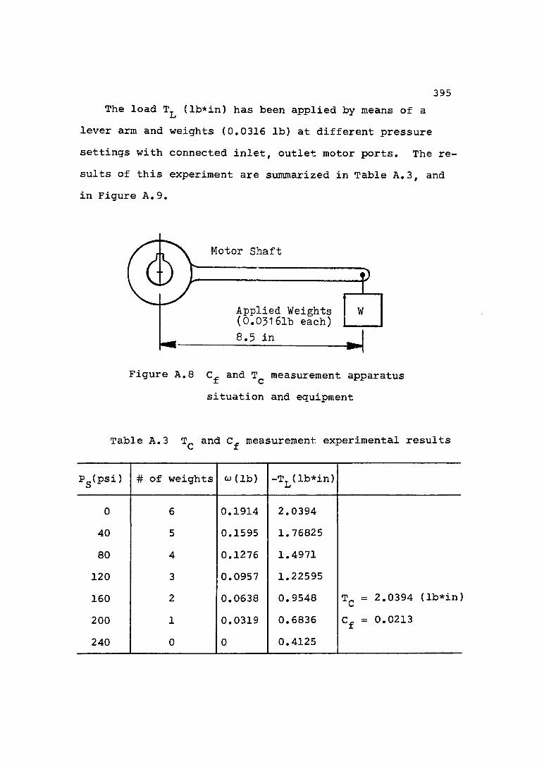
395The load T^ (lb*in) has been applied by means of a

lever arm and weights (0,0316 lb) at different pressure settings with connected inlet, outlet motor ports. The re­sults of this experiment are summarized in Table A,3, and in Figure A,9,

Motor Shaft

Applied Weights (0,03161b each)8,5 in

Figure A,8 and T^ measurement apparatus situation and equipment

Table A,3 T^ and measurement experimental results

Pg(psi) # of weights cj (lb) -Tj^(lb*in)

0 6 0,1914 2,039440 5 0,1595 1,7682580 4 0,1276 1,4971120 3 0,0957 1,22595160 2 0,0638 0,9548 T^ = 2,0394 (lb*in)200 1 0,0319 0,6836 = 0,0213240 0 0 0,4125

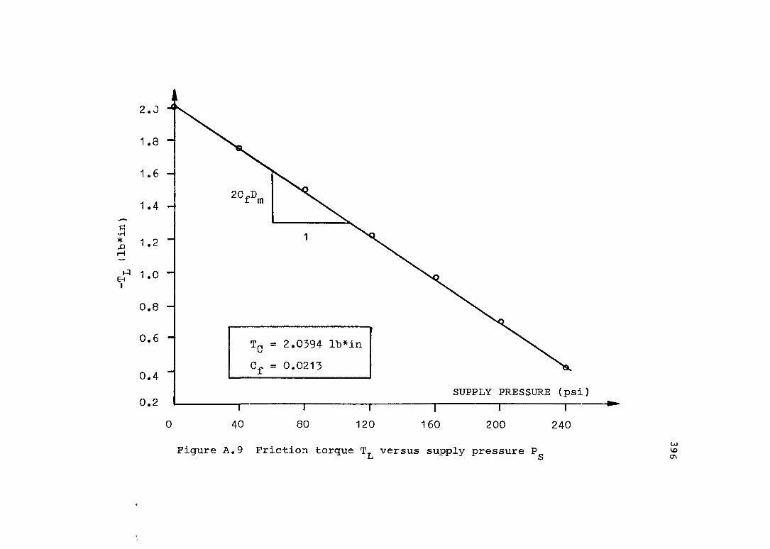
20.D,

AE4I

0.8

0.6 = 2.0394 lb*in

0.4SUPPLY PRESSURE (psi)

0.240 1600 80 120 200 240

Figure A.9 Friction torque T versus supply pressure P wVO

397

A, 3.3 Measurement of C, Coefficienta

The torque losses which depend on speed are found by measuring the forward pressure required to run the unloaded motor at various speeds with no return pressure (i.e., P2 » 0). A typical curve is illustrated

1-Ccns

psiptHMOTOR SPEED frad/sec')

Figure A.10 Typical curve for measurements

The equation governing this situation is

T_

“m - Cf)(A.9)

398

Knowing the coefficient C and absolute viscosity onecan find from the slope

^d -slope (1 - C^)

(A.10)

Table A.4 Measurements for coefficient Experimental results

(psi) Vq (Volt) ^m (rad/sec)

50 1.25 178.571 18.7000100 2.42 345.714 36.2030150 3.75 535.714 56.0994200 5.18 740.000 77.497

The intersection with y axis

2.0394 (lb*in)(1 - C^) 0.159155*(1 - 0.0213) in /rad

= 13.0928 (psi)The coefficient from the slope

Cd" 1501 - C , 77.497 - 18.700

= 2.55116 psi/rad/sec

399

The absolute viscosity calculation

I' = 47.25 est at 100*F (dynamic viscosity)I. = 0.0732375 in^/sec

Neglecting internal leakages at this low pressure , we take

^0 “ ^tachp = 0.816*10 lb sec^/in^ = oil density = y p = 5.976*10” lb sec/in^ = oil absolute

viscosityFinally, we can find from the slope in Fig.A.11.

2.55116 * (1 - 0.0214)^ d ------------------------

5.976 * 10"®

Cg = 41.78 * lo" (dimensionless )

A.4 Servovalve Parameters

Servovalves convert electrical signals into a hydraulic

output which controls the acceleration, velocity, and position of an actuator. Because servovalves occupy a unique position at the electric-hydraulic interface of systems and require some knowledge of both areas to under­stand their operation, they are often the focal point of attention in servo design. This has resulted in an

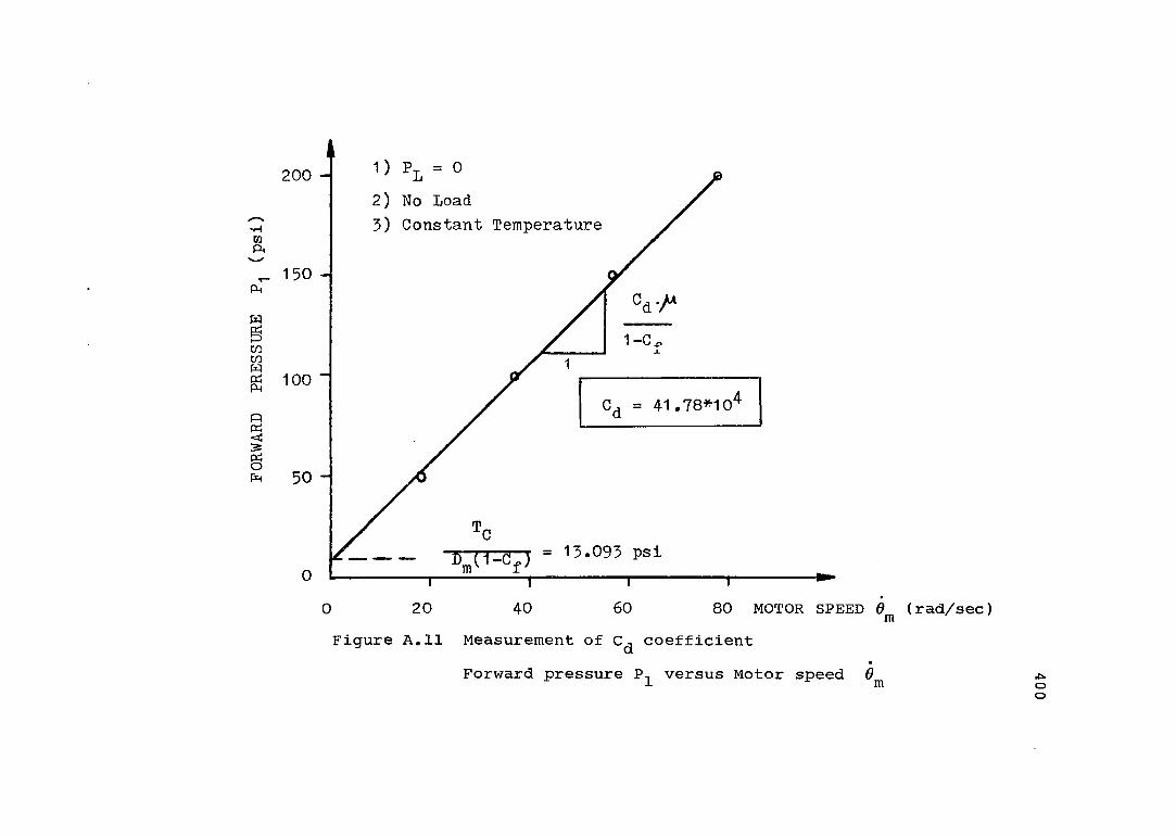
2002) No Load3) Constant Temperature

150Ph

WCOC/DWg 100

41.78*10ASg

= 13.093 psi

0 20 40 60 80 MOTOR SPEED (rad/sec)Figure A,11 Measurement of coefficient

Forward pressure P^ versus Motor speed 0m oo

401

extraordinarily long list of parameters which specify servovalve performance. However, there are some funda­mental static and dynamic performance characteristics which are useful for both designer and user in selecting and evaluating servovalves (2).

The two stage flow control servovalve used in our set­up is:

Manufacturer: MOOGModel: 77-223 Series 400Max. current: lOOma (coils in series)

The dynamic characteristics given by MooG is the valve second stage dynamics.First order model

-2_(s) = (19.25 CIS ---1---ji 100 ma S ^

85Second order model

2. (s) *(— ^100 ma S , 2S , , + ■■■'■"'■ + J.

277 277At lOOOpsi supply pressure.

So, the flow gain= 0.1925 cis/ma at lOOOpsi

402

is the only steady state parameter given by the manufac­turer and it will be verified experimentally.

The experimental verification of the dynamic performan­ce of the valve is much more involved. It can not be performed without special equipment and it is beyond the scope of this dissertation. We will show later that using the given dynamic transfer function in computer simulation in both time and frequency domain gave satisfactory results.

A.4.1 Flow Pressure Coefficient

As mentioned earlier, the flow gain of the valve was verified experimentally using the well known flow, squareroot of pressure valve relation

0 = Ky ly ( (A.11)1/2For a certain given supply pressure setting, = Ky( AP)

(cis/ma) which is the value given by MOOG. We will find experimentally the more fundamental parameter K„ of the given servovalve.

403

Apparatus configuration for this measurement

ProportionaltoTach

Proportional to current I

Input Reference Voltage 'Ampl

Figure A,12 Apparatus and instrumentation for constant (K ) measurement

The above system has been tested in steady state situation at the following pump pressure settings SOOpsi, 730psi, 950psi. Amplifier reference input voltages were chosen for 25%, 50%, 75%, and 95% valve opening (i.e., Oma, 25ma, 50ma, 75ma, 95ma), by means of measuring V^, a voltage

404

proportional to the valve input current. At each valve opening and pump pressure setting the following measurements were taken.

P. Valve input pressure (psi)

P, Actuator input pressure (psi)

'?2 Actuator output pressure (psi)

Voltage proportional to current (mv)

Vq Voltage proportional to shaft velocity (Volt)

R Amplifier reference input voltage (Volt)Here again, system flow rate has been calculated from

Vq measurement neglecting leakages. Amplifier gain was arbitrarily set at

l ampl =The experimental results were summarized in Tables

A.5 and A.6.

405

Table A,5 Experimental results for the measurement of valve constant K,V

Supply pressure SOOpsi

pvalvepsi

pmotor in psi

pmotor out psi

currentvolt

^ref volt Volt

V^tachVolt

460 265 200 303 0.28 1.12455 290 190 519 0.47 1.95450 290 170 780 0.70 2.85443 290 155 971 0.87 3.35

Supply pressure 730psi

722 415 340 308 0.28 1.49717 450 330 519 0.47 2.54710 440 300 780 0.70 3.70708 430 280 971 0.87 4.41

Supply pressure 950psi

940 540 470 321 0.28 1.76926 550 440 537 0.47 2.97918 540 400 780 0.70 4.28835 470 320 971 0.87 4.69

406

Evaluating the needed parameters for our purposes we get the following

Table A.6 Flow-Pressure measurements Experimental results

Supply pressure SOOpsi

Input curr amp psi

^valvecis

6 shaft mrad/sec

29.42 195 3.74 23.4550.38 165 6.51 40.8275.73 160 9.51 59.6694.27 153 11.18 74. 31

Supply pressure 730psi

29.41 307 4.97 31.1950.39 267 8.48 53.1775.73 270 12.35 77.4594.27 278 14.72 92.32

Supply pressure 950psi

31.17 400 5.88 36.8452.14 376 9.92 62.1775.73 378 14.29 89.6099.27 365 15.66 98.18

407

Using the usual valve flow-pressure equation Q =1/2(Py - ) and evaluating , the valve flow coefficient

we obtain an average from the 12 measurements in Table A.6,

Ky = 0.00965 (----— --- -)ma (psi)^/^

A.4.2 Servovalve "First Stage" Dynamics

In order to complete our test work on the servo­valve we performed a step response test to find valve first stage (torque motor) dynamic response.

Servovalve first stage dynamics relating output current to input voltage is

Ai K (S) = ---- ---- (A.14)e_ S/w + 1

where

^1 A Steady state gain .

COa A First stage break frequency

Ai A Output current .

®a A Input voltage .

which is a first order system with armature circuit break frequency. The current Ai was measured via a lO.Sohm resistance (e^^^). The input to the amplifier was a step input of a signal generator (e%^^. (See Figure A.13.)

408

SignalGenerator

o— —

®ino— —Amplifier(Nc Dynamics)

oul - T ------ 'Coils In Series

Valve F irs t Stage

Figure A.13 Apparatus configuration for measurement of valve first stage speed of response

As we can see the test included the amplifier and the valve first stage dynamics (Amplifier dynamics can be neglected).

Input Input to valve )

uoUJ

Figure A.14 Valve first stage step response

409

Set up situation and test conditions were:Pg = 730psi (pump pressure setting)

Input voltage to the amplifier: 0 — 0.536 (V)Current input to valve: 0— 92.23 (ma)

Gain setting 30ohm : K^mpl “ 1^8 (ma/V)Conclusion

The first stage (torque motor) dynamics is negligible (oj very large).

A.5 Controller Compensation Network

The theoretical part of the study was carried out for several types of systems, but because of time and budget limits, only the speed control configuration was experimen­tally tested. For two basic reasons it is often desirable to control velocity of a hydraulic actuator by sensing velocity and feeding it back to form a servo loop.(1) Velocity may be the principle output of the system,such as rate tables, radars,gun turrets etc..(2) Velocity may be fedback in a subsidiary or minor loopas a means of compensating the major control loop.

The advantages are increased loop stiffness, minimiza­tion of overall loop gain variations, and finally amplifier gain can be made high to reduce errors and increase speed of response.

410

However, the disadvantage is system stability problems. Stability of hydraulic velocity control loops demands that the crossover frequency be lower than the hydraulic natural frequency.

Valve dynamics Motor and load

tach

amplw

1/D

+1W

valve+1

Figure A=15 Block diagram of a velocity control servosystem

This is a type zero servosystem with the loop transfer function

K,G(S) =

2 A s S 2 f s(— + — — + 1) (--- + ----2— + X)

(A.12)

CO COV V

CÜh

where K^^lve "= 6 system open loop

Steady state gain.

411

Usually this type of system is unstable even for re­latively low gains, even though gains 5 are desirablein most of the cases. Therefore, electrohydraulic velocity control loops must always be compensated to achieve stabi- lity. The simplest method of compensation is to place an RC lag network in the electronic portion of the loop ahead of the servovalve (2).

The servocontroller from MOOG used in our apparatus had such a compensating possibility built in and only the installation of a Ifif capacitor together with 5OKohm resis­tance was necessary (Calculated value). The compensation network obtained

G(s) = 9-001 S + 1 (A.13)0.05 S + 1

which was verified experimentally.For all practical purposes the transfer function has

the form

G(S) =0.05 S + 1

where r = 50 m sec The frequency response test is presented in Figure A.16.

NICOL.ET 0 S 0 A3 . 2 5 0 0 0 HZ

- 1 . 0 d B VL.NC

M --

S W __

0.05*S + 1

TF —

0 . SA 0 . iSA Ay-4 LGHZFigure A,16 Compensator frequency response test T* = 50 sec 4

to

413

A.6 System Gain Setting

The gain in a velocity control servosystem is usually increased to be high enough to reduce errors but low enough to maintain the traditional 2.5 gain margin for stability. However, our apparatus was built to study the effect of pump dynamics on the response of the system which is under­stood as the measurement of v^, the controlled variable. Shortly speaking, we want to observe pressure variations in pump pressure Pg (t) affecting controlled variable perfor­mance (t). Thus, our goal was to cause the largest and fastest flow demand possible, by means of valve opening, to obtain the largest pump pressure variation. So, we conclude that we need the highest loop gain possible before unstability occurs.

The measurements were taken at Vq Voltage proportional to 6^ (Volt)

V^ Voltage proportional to I^^lve ( V)

R Reference Voltage (Volt)Pump pressure setting 730psi

Gain setting in our system was by means of a variable potentiometer from 0 to lOOkQ in the controller panel, enabling an amplifier gain range setting between 2.5ma/V to 250ma/V. The results are given in Table A.7.

414

Table A.7 Gain setting measurements Pressure setting 730psi

Gain potentiometer setting 2OKohmRef. Voltage

R (Volt)Input current

Vi(mv) (ma)

Encoder output V q (Volt)

Ampl. gainKampl(ma/V)

OverallgainKo(V/V)

1 . 1 1 995 96.6 3.91 87.00 3.500.86 773 75.0 3.31 87.20 3.800.57 515 50.0 2.37 87.72 4.160.28 258 25.0 1 . 2 1 89.28 4.32

Gain potentiometer setting 30Kohm

0.18 258 25 1.14 140.0 5.710.36 515 50 2.27 138.9 5.930.54 773 75 3.20 138.9 6.300.69 996 96.6 3.94 138.9 6.33

Gain potentiometer setting 40Kohm

0.14 258 25 1.17 178.6 8.350.27 515 50 2.30 185.2 8.520.41 773 75 3.22 182.9 7.850.53 996 96.6 3.94 182.3 7.43

415

Since the gain setting in our system is by means of the potentiometer which we are able to record in Kohms on the electronic board we will find a "rule" for gain setting.

Observing the 12 measurements and the calculated K.ampl(ma/v) and (V/V) we get

K

Kampi = (Kohm reading) * 4,5 (A,14)

^overall” (K°hm reading) / 5 (A.15)

ampl 180 (ma/V) was approximately the highest possi­ble ampl. gain or K . ~8 (V/V) and Gain = 40Kohm.system potThe actual gain used in our experimental work was

Kampl = ma/vThis value was used in the computer simulation as well. This gain setting for the amplifier gave the desired

Kq = 6 (V/V) in speed control systems.

A.7 Step Response Test Instrumentation (see Fig.3.2)

In this section the sensors and the measurement instru­mentation will be described.(1) Pressure measurements

The four pressures:P^ Pump manifold pressure

Pg Valve input pressure P^ Hydraulic motor inlet port pressure

416

Hydraulic motor outlet port pressure.

were measured both in static and dynamic situation. For static pressure measurements all four pressure mo­

nitoring points were connected via shut off valves to a central Pressure Gauge enabling separate pressure measure­ments.

Heise gauge number: H - 39818Manufacturer : Heise Bourdon Tube Co., Inc.

Maximum pressure: lOOOpsiMaximum hysteresis ; Ipsi

Resolution : 2psiFor dynamic pressure measurements piezo-electric

pressure pick ups were used.ModelTypeManufacturer

616 M2Piezo-electric Quartz Kistler Instrument Corporation

Pressure range: 30 to SOOOpsi Linearity : 1%

Freq. response: Flat from 1.6*10~^ to 10 K Hz Output : 1 pcb/psiIn order to obtain voltage outputs charge amplifiers

were used:Pressure P^ and Pg - Charge amplifiers Manufacturer: Kistler

417

Model : 5001Calibration : 1 V/ lOOpsiPressure and P^ - Charge amplifiers Manufacturer : Dynamic Instrumentation Co.Model : 730Calibration : I V / lOOpsi

( 2 ) Shaft rotation measurementShaft angular velocity has been measured using an

Optical Encoder.Manufacturer : TeledyneModel : 8605 #GN032 7

- photo diode outputs in quadrature- 2500 cycles per revolution- lamp voltage, 6Volt at 60ma- power supply ±18V

At lOOOrpm it gave about 42000Hz.The optical encoder was used for one directional rota­

tion measurements. To obtain voltage output a frequency to voltage converter was used.

AndexRangeFilterCalibration

Model PI608 51.2KHZ Low pass5.00Volt at 42000Hz

Encoder + converter calibration : 0.0477V/(rad/sec)

418

Frequency to voltage converter speed of response was tested and was found suitable for our experiments. The output voltage has been used as system feedback signal in the speed control configuration.(3) Valve input current measurement

The maximum current input to the valve was lOOma.The dc Servocontroller MooG, Model 82-300 had an optional current meter to monitor valve opening. In order to mea­sure the current in voltages a 10.3ohm resistor was install­ed in the valve inlet line and the voltage across it gave a Voltage measurement proportional to the current.

Calibration : 10.3mv/ma(4) Voltage measurements

The static voltages were recorded on digital voltmeters (DVM).

Dynamic voltages for step response tests were recordedon

1) Two channel recorder Brush Recorder-Mark 280

2) six channel recorder (Max. 5V Full scale)Gould Recorder - Mark 2600

(5) Signal generatorThe input voltage R to our system was generated by a

Wavetek - Model 114 ±16V max.

APPENDIX C REFERRING TO PART THREE IN THE TEXT

C.l Chapter 10 - 12.5Hz peak

During the explanation of the experimental program to investigate the 12.5Hz peak in the pump pressure power spectral density an example was given for the

(1) Time history and(2) Power spectral density

recorded during the tests. The case presented was for 280psi pump pressure setting and no flow situation.

We will present now the rest of the cases investigated (12 points).

419

0.1 secTimeHistory ■H

Op. Cond.P_ = 280 (psi)

12.5 HzS U

Power SpectralDensity

0 . S A - B / 1 6 H Z ' 5 0 0

Figure C #1 Time history and Power spectral density in regulating region

1— 13.1 sec

Time •H

History

Op. Cond.P_ = 500 (psi) S U

Power SpectralDensity

12.5 Hz

S . 0 A 5 . Q D “ 3 / 1 S H ZN)

Figure C.2 Time history and Power spectral density in regulating region

TimeHistory

Op. Cond.= 1.75 (gpm) S U

° 1 ePq = 500 (psi)

Power Spectral Density

r12.5 Hz

1 . ©A 1 G H Z S 0 3

Figure c . 3 Time history and Power spectral density in regulating region N)

0.1 secTime

•HHistory

VD

Op. Cond.= 700 (psi) S U

1 e --

P S --Power Spectral

Density12.5 Hz

M 2 NJU)Figure C.4 Time history and Power spectral density in regulating region

0.1 sec•H

Timet —

CMHistory

Op. Cond.Q-, = 1.75 (gpm)

12.5 HzS U

Power Spectral p s Density

— B / 1 O2 . 0 A H Z

Figure C.5 Time history and Power spectral density in regulating region

0.1 sec

Time •HHistory oin

Op. condS U 1 6948 (psi)

Power SpectralDensity

12.5 Hz

S . ©A H Z 5 0 0

Figure C.6 Time history and Power spectral density in regulating region4toUi

TimeHistory

Op» Cond.1.75 (gpm) g y

= 948 (psi)

Power Spectral Density

r

12.5 Hz

#S . 0 A — B y \ B H Z ' 5 0 0

C.7 Time history and Power spectral density in regulating regionnja\

TimeHistory

Op. Cond.Qq = 4.5 (gpm)

Power Spectral Density

12.5 Hz

L2 . B A —B / i e M 2 S 0 0

Figure C. 8 Time history and Power spectral density in non-regulating region

0.1 secTime History

•H

in

— ^12.5 HzOp. Cond

P- = 500 (psi)S U 1 © --

Power Spectral P SDensity

2 . O A S .0 D - B / 1S H ZFigureC.9 Time history and Power spectral density in nonregulating region

w00

0.1 secTime History

ro

Op. Cond 12.5 Hz700 (psi) 3.75 (gpm)

Power Spectral p g _„ Density

S . 0 A S . G D - S X 1 S H Z

Figure .C#10 Time history and Power spectral density in nonregulating regionN)V£>

Time History

Op. Cond.Qq = 3 .5 4 (gpm)

= 800 ( p s i ) S U

Power Spectral p s - Density

12.5 Hz

1 0 , A - B / Î 5 H Z 5 0 0

Figure C.ll Time history and Power spectral density in nonregulating region Wo

APPENDIX D

EXPLANATION OF TURBINE FLOW-METER DISCREPANCY DURING FLOW MEASUREMENTS

D. 1 The Definition of the Problem

During his study Felicio used a turbine type flow­meter installed close to the pump to measure pump flow rate (Pump Flow Meter - P.F.M,). Downstream, on the same line a second turbine type "auxiliary flow meter" was installed for calibration purposes through a shut off valve, with an opening to the atmosphere (Calibration Flow-Meter-C.F.M.). The C.F.M. was calibrated by actually collecting oil in a standard volume outside the hydraulic system, over a known period of time interval and measuring the number of pulses/ sec? produced by the turbine .

The primary reason for having this calibrated C.F.M. in a set up built for research purposes is to ease the calibration of any pump flow meter installed later in the system, without the need of collecting again the oil out of the system.

The P.F.M. calibration was performed by Felicio using the C.F.M.. Two voltages proportional to the pulse rates

431

432

of the two turbine flowmeters were plotted directly using a X - Y recorder. Fig, D.l shows the equipment configura­tion used by Felicio for this calibration. The details of the measurement instrumentation and the different calibrations are given in the next page.

AccumulatorValve

Pump Valve

TankPump Flowmeter (P.F.M.)

CalibrationFlowmeter(C.F.L.)

DC Component ConditionedSignal y-axis

x-axis

F VC #1F VC #2

FVC #5 x=y Recorder

Figure ,D.l Instrumentation used for the pump flowmeter calibration

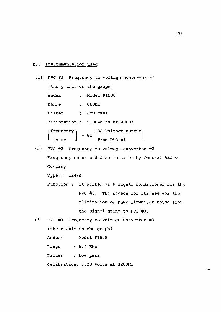
433

D. 2 Instrumentation used

(1) FVC #1 Frequency to voltage converter #1 (the y axis on the graph)Andex Range Filter Calibration •frequency in Hz

= 80

Model PI608 800Hz Low passS.OOVolts at 400Hz

■DC Voltage output- ■from FVC #1

(2) FVC #2 Frequency to voltage converter #2 Frequency meter and discriminator by General Radio CompanyType : 1142AFunction : It worked as a signal conditioner for the

FVC #3. The reason for its use was the elimination of pump flowmeter noise from the signal going to FVC #3.

(3) FVC #3 Frequency to Voltage Converter #3 (the X axis on the graph)Andex; Model PI608Range : 6.4 KHzFilter : Low passCalibration: 5.00 Volts at 3200Hz

434

= 540DC voltage outputfrom FVC #3

frequency in Hz

(4) X - y PlotterMetric plotter-Hewlett-Packard 7044A Sensitivities used;X - axis (pump flowmeter) = 0.25 V/cm y - axis (calibration flowmeter) = 0.25 V/cm

Flow - Meters - used

Manufacturer Pickoff Type Max. flow Linearity

(1) Pump Flow Meter (P.F.M.)Model : FT-6-8A5-LB, No.8602287

(Turbine flow transducer)Flow Technology Magnetic 5 gpm0.5% over normal 10:1

flow range (liquid)Frequency response

(2) Calibration Flow Meter (C.F.M.)Model : Turbine flow transducer No.1/2 5550Manufacturer : Potter Aero Corp.Maximum flow ; 9gpm

Flat up to 53Hz, first order behaviour

435

A typical calibration curve such as the one shown in Fig.D.2 was performed as follows:(1) Variation of the flow rate at low pressure was obtain­ed by changing the volume regulator from zero to maximum flow rate.(2) Leaving volume regulator where it was at the end of step(l), we closed the valve gradually (increasing the load on the pump, up to the highest pressure set) and flow rate was decreased to zero (valve completely closed).

The data obtained in Fig.D.2 is actually the reading of the pump flowmeter on the X axis plotted against the reading of the calibration flow meter on the Y axis.

The flowmeters have exactly the same flow rate since they are installed in series, thus we should get a "single" curve, rather than a "double" curve actually obtained.

This discrepancy between the readings was not comple­tely resolved by Felicio, but it was speculated that the two flowmeters might be effected by pulsations and that each meter is affected in a different way.

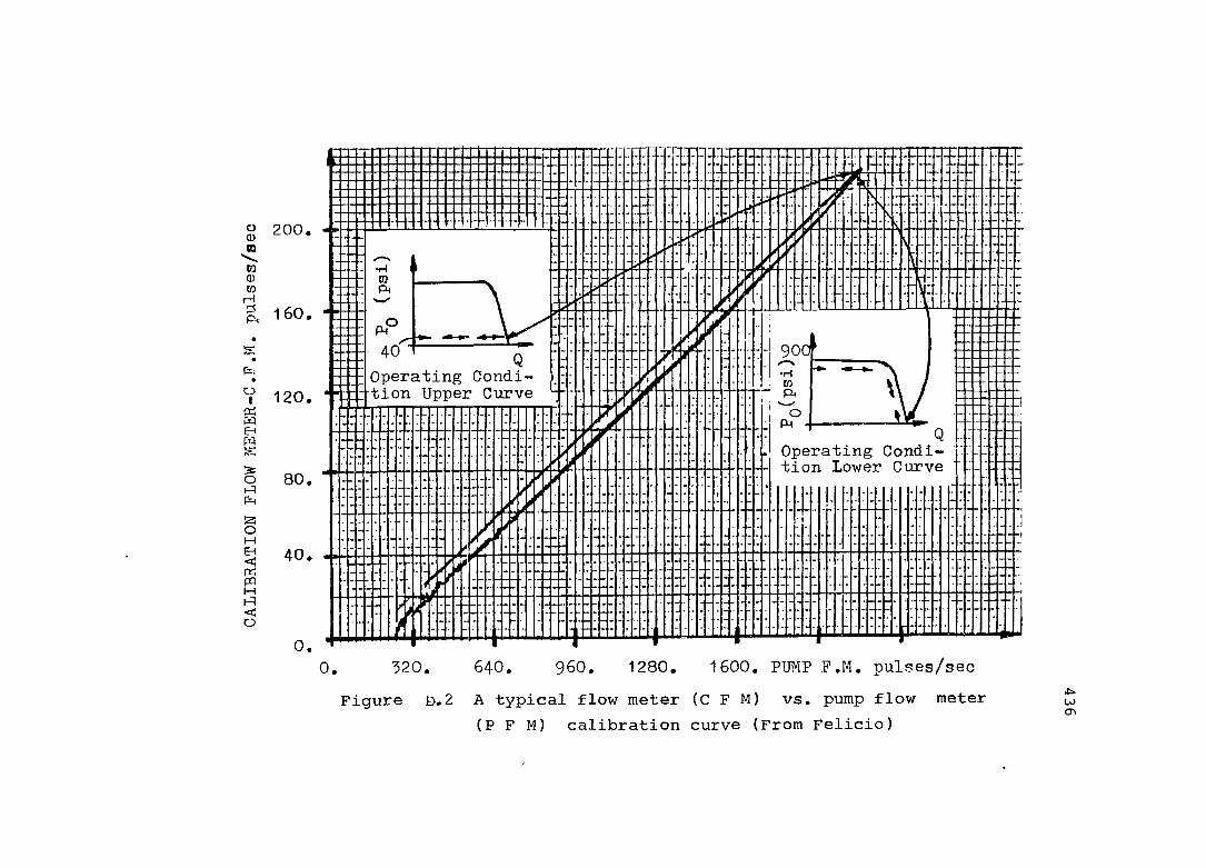
n

% 200.

160.god'

operating Condi­tion Upper CurveV 120.

Operating Condi­tion Lower Curve80.

M40.

0.1600. PUMP P.M. pulses/sec640. 960. 1280.0

Figure d.2 A typical flow meter (C F M) vs. pump flow meter (P F M) calibration curve (From Felicio)

Wo>

437

D.3 The Proposed Program for the Study of the Problem

In order to investigate the described discrepancy,we performed the following operations and experiments.(1) An accumulator was installed right at the pump mani­

fold to surpress pump pressure pulsations. The cali­bration procedure was repeated with and without the accumulator to study the effect of pump pulsationson the turbine flow meters.

(2) The calibrations were performed at four different pressure settings,350, 500, 700,900psi, to detect dependence on system pressure level.

(3) Interchanged the flow meters, i.e., the C.F.M. close to the pump and the P.F.M. downstream, to investigate the assumption that the two meters are affected in a different way.

(4) We performed again an "absolute" calibration on both flowmeters simultaneously. That is, we caught the outflow and measured the volume accumulated over a time period.

438

D.4 Experimental Results

D.4.1 The Repetition of the Original Calibration Configuration

The original configuration i.e., Pump Flow Meter first and Calibration Flow Meter second, was used to repeat the calibration procedure for four pressure sett­ings, 350psi, BOOpsi, 700psi, and 900psi. At the high pressure setting (900psi) the experiment was performed both with and without accumulator (see Fig.#.4 andFig.D.5).

Accumulator

PumpValve

t P.F.M. C.F.M,T

x-y Plotters Freq/VoIt converter

Valve

à = System

Figure Û.3 System configuration for P.F.M. calibration

- C.F.M.

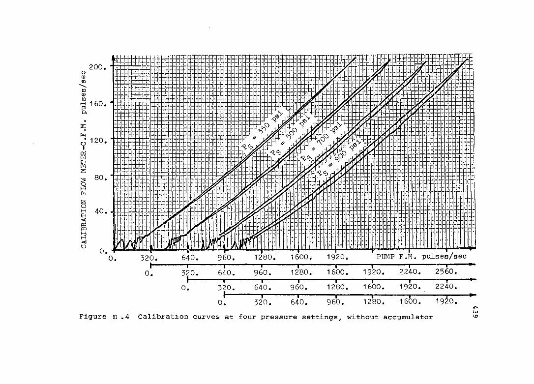
JXÜZI/200

rj 1 60

120

80

M

PUMP P.M. pulses/sec1600 1920960640 1280320h —1—

320— r—960 — I—

1280— I—1920 2240 2^-T—

640 16000. 320.

h -640. 960.

0. 320. 640. 960. 1280. 16&0. 19^0 . Figure b .4 Calibration curves at four pressure settings, without accumulator

640.

1280. T

1600. T

1920.16&0.

2240.

WKO

ü 200

^ 160

20

80o

40I—I

o

1920. PUMP P.M. pulses/sec640. 960. 1280. 1600.0. 520.— *—

0. 520. 640.Figure D.5 Calibration curve at 900psi with and without accumulator

I ' "I ' ' I I960, 1280. 1600. 1920.

o

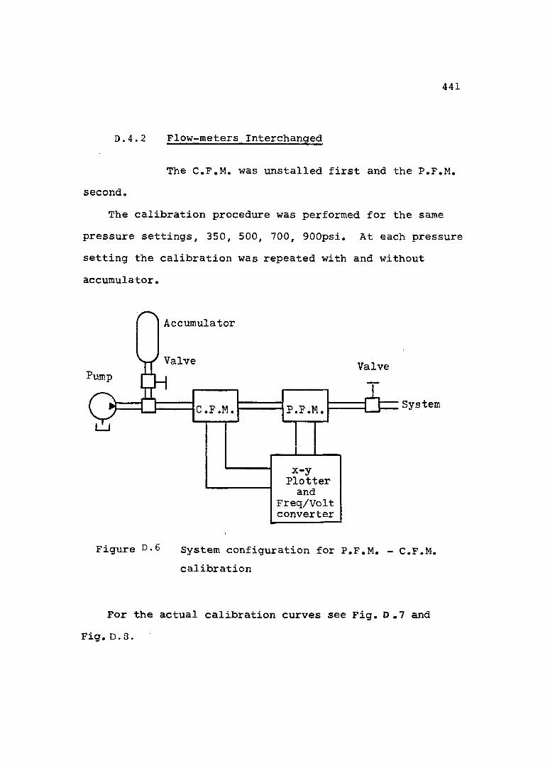
441

D.4.2 Flow-meters Interchanged

The C.F.M, was unstalled first and the P.F.M.second.

The calibration procedure was performed for the same pressure settings, 350, 500, 700, 900psi. At each pressure setting the calibration was repeated with and without accumulator.

Accumulator

Valve Valve

SystemC.F.M P.F.M

x-yPlotterand

Freq/Voltconverter

Figure D - 6 System configuration for P.F.M. calibration

- C.F.M.

For the actual calibration curves see Fig. D.7 and Fig. D.8.

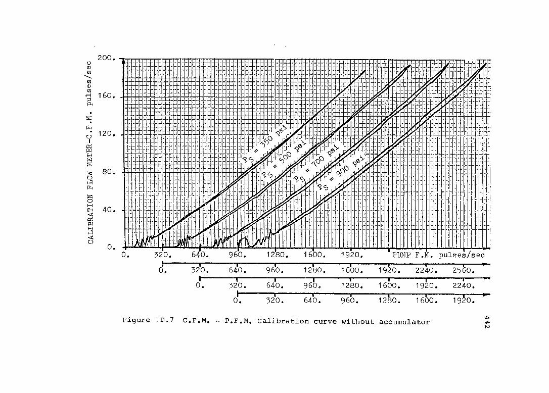
200ü0)entn<umr—IA

• 120oI

gE-tHS80ënq

H

OPUMP P.M. pulses/sec640 960 16001280 1920

640 960 1280 1600 1920 2240 25IÔ320

0. — I— 320.

h—0.640. 96^ T T1280. 1600. 1920. 2240.320. 640. 960. 1280. 1 6 0 0 . I92Ô7

Figure :d .7 C.F.M. - P.F.M. Calibration curve without accumulatorto

üCDCQCO<DtnrHA

pqa

I

gEHgoPHS0 HEH

1i-qco

2 0 0 .

160.

120.

r«80 .

40.

0 . PTMP P.M. pulses/sec1600640 960 19201280320H T T T T TT T T0 . 320.

I—0 .

640.— T--320.

I—

960.640. T

1280.960 .

1600.T

1 9 2 0 . I--------

2240. —I--- 2560.T1280. 1600. 1920. 2240.

Figure D.3 C.F.M. -

• I ' I I '0. 320. 640. 960. 1280. 1600.

P.F.M. calibration curves with accumulator

1920.

W

444

D.4.3 "Absolute" Calibration Results

The test was performed by measuring the out­put voltage from the two turbine flowmeters. In this test the servovalve was fully open and there was almost no load pressure. Hydraulic motor outlet port and case drain out­flow were measured.

Pump

Q ~ .P.F.M.

DVM #1

Pump P.M. Voltage

C.F.M

DVM #2

Calib. P.M. Voltage

s VE AR LV V0 E

Am pi.

CaseDrain

Oil Volume Measurement

Input

Figure d .9 System configuration for the flow meters absolute calibration

Three points were checked on the "upper" part of the 700psi (no accumulator) calibration curve. The test points

445

have been selected according to the P.F.M. voltage. 1.5Volt, Z.OVolt, 2.5Volt that is, low medium and high flow rates respectively.

Table D.l "Free flow" measurements

P.F.M.(Volt)

C.F.M.(Volt)

Flow rateVol (ml) Time (sec) CIS ml/sec

1.50 1.02 3500 22.3 9.6 156.92.00 1.39 3250 15.4 12.8 209.62.50 1 .83 3500 13.4 15.9 261.2

Two points, low and high flow rate have been checked on the "lower" part of the curve. The voltages on P.F.M. were selected again as calibration voltages, 1.40Volt and 2.40Volt, the voltages obtained from the C.F.M. were 0,83 Volt and 1.68Volt respectively. The constant load pressure 700psi (Pump pressure setting 700psi) was kept using the controller Voltage R. Fig. D. 10 shows tne result of the calibration measurements.

ü0)CQ

m0) CQ I— I 0 A

PAüIgEHH

Oi-qPHaOt-HEH<3ÎgM<O

200

: m i ,70V)— 136.

1600.1280.

n(1.85V) %4- -

(1.40V)T

(1.00V)(0.85V) 68.

1280. fPUMP P.M. pulses/sec

Figure D.IO Absolute calibration curve

a\

447

D, 5 Discussion of the Results

D.5.1 Pulsations Effects

(1) Focusing our attention to Fig.D.4 - D.3, we can see that there is no difference between the calibration curves at the four pressure settings, 350, 500, 700, 900psi, thus we can conclude that the two flow-meters respond the same way to pulsations. We observed Calibration curves for the original configuration (P.F.M,— C.F.M,) and the interchang­ed configuration (C.F.M, — P.F.M.) without accumulator,(2) When observing the calibration curves produced with accumulator which surpresses most of the pump pulsation, we can see almost identical curves, i.e., pump pulsations have no significant affect on the flow meters.

D.5.2 Pressure Level Effects (Fig. D.4, D .7, D .8)

In both cases P.F.M.— C.F.M. and C.F.M.-P.F.M. we can see that the distance between the curves is decreas­ing as load pressure is decreasing. This fact suggests that the flow meters are affected by pressure level in the system.

When we compare the results of the "absolute" calibra­tion at the three points, low, medium, and high flow rates.

448

at 730psi pressure setting, we observe good correlation with the calibration curve.

D.5 Explanation of the Cause of the Discrepancy

Having presented and discussed the results of our study, and justified the different experiments, let us turn now to the explanation of the discrepancy in the flow meters calibration curves.

The flow meters are apparently affected by pressure level in the system. Things like friction in the bearings and housing expansion at high pressure cause lower pulse rates (voltages). Our reading of the curves has to be: "The upper curve for low pressure, the lower curve for high pressure". That is why the vertical distance between the lines decreases as pressure decreases.

APPENDIX E LITERATURE REVIEW SCHEME

The following sources were used to perform the litera­ture search:1. - Engineering Index search,2. - ASME Transactions search.3. - SAE Transactions search.4. - NCFP Publications search.5. - JSME Transactions search.6. - Hydraulics & Pneumatics Publications search.7. - Product Engineering Publications search.8. - Machine Design Publications search.9. - Additional Papers have been searched in:

* Journal of Mechanical Engineering Science* Institute of Mechanical Engineers (London)* Control Engineering* ASAE Publications* AIEE Publications

10.- Computer search.11.- Search for publications by specific authors.12.- Publications by Manufacturing Companies.

449

450

E .1 Engineering Index

The reference, "Engineering Index", was examined for publications from Nov. 1981 back to 1971 in the following subject titles;

* Computer Simulation.* Control equipment, hydraulic.* Control systems, linear,* Control systems, nonlinear.* Dynamic, simulation.* Dynamics.* Energy conservation.* Hydraulic drives.

* Hydraulic machinary.* Hydraulic models.* Hydraulics.* Servomechanisms.* Servomotors.

30 articles were applicable.

451

E.2 ASME Transactions

The reference, "ASME Transactions", was examined for publications from 1981 back to 1970. From 1958 the "ASME Transactions" have been divided into the following journals:

* Journal of Engineering for Industry.* Journal of Engineering for Power.* Journal of Mechanical Design.* Journal of Basic Engineering.* Journal of Dynamic Systems.

The following subject titles were used:* Automatic Control.* Computer Simulation.* Dynamic Simulation.* Energy Conservation.* Energy Saving.* Fluid Power.* Fluid Systems.* Hydraulic Systems.

* Mathematical Systems.* Modeling.* Nonlinear Systems.* Perturbation analysis.* Servo systems.

452

* Servo valves.18 articles were copied and found applicable.

E. 3 SAE Transactions

The reference, "SAE Transactions", was examined for publications from 1981 back to 1971 using the following subject titles:

* Computer applications.* Computer simulations.* Energy conservation.* Fluid Power.* Hydraulic control.* Hydraulic drives.* Hydraulic motors.* Hydraulic systems.* Hydrostatic transmissions* Servomechanisms.

13 articles were applicable.

E.4 NCFP Publications

The reference, "NCFP Publications", was examined for publications from 1981 back to 1960.

The National Conference on Fluid Power meeting annually is probably the best reference in the field of

453

Fluid Power Control. 29 articles were found as applicable to the subjects of this dissertation.

g.5 JSME Transactions

The reference,""JSME Transactions", was examined according to the Computer Search results. 8 articles were applicable.

E.6 Hydraulics and Pneumatics Publications

The reference, "Hydraulics & Pneumatics", was examined for publications from 1981 back to 1970. Many articles were found but only a few were applicable. The articles are mostly descriptive.

E .7 Product Engineering (Recently Design Engineering) Publications

The reference, "Product Engineering", was examined for publications from 1980 back to 1975. About 10 applicable articles were found but they are mostly descriptive.

E.8 Machine Design Publications

The reference, "Machine Design", was examined for publi­cations from 1981 back to 1976. 17 articles were applicable.

454

E. 9 Additional Papers

10 more articles were applicable from the above mention­ed references. The search in this case was performed according to references recommended in books and other articles.

E.IO Computer Search

Three kinds of computer service were considered:- "Science Retrospective".- "Science Current Awareness".- Ph.D. dissertation titles.

E.10.1 "Science Retrospective"

The key words that were used are:(1) For the first search, performed on 11/07/81

* Sensing, Valve* Servo, Control* Flow, Control* Fluid, Power* Hydraulics, Dynamics* Hydraulics, Efficiency* Hydraulics, Save* Hydraulics, Systems

455

* Hydraulics, Control* Hydraulics, Energy* Load, Sensing* Load, Compensation* Load, Control* Load, Energy* Load, Power* Load, Pump* Pump, Sensing* Pump, Control* Transient, Pressure

(2) For the second search, performed on 11/20/81* Saving, Energy* Servo, Mechanism* Servo, Motor* Servo, Valve* Conservation, Energy* Robot, Industry* Hydraulics, Servo* Hydraulics, Drive* Hydraulics, Machine* Hydraulics, Mobile* Hydraulics, Noise* Hydraulics, Test* Hydraulics, Vibrations

456

(3) ]For the third search, performed on 12/01/81* Hydraulics, Dynamics* Hydraulics, System* Hydraulics, Computer* Hydraulics, Energy* Hydraulics, Load* Hydraulics, Pressure* Hydraulics, Pump* Hydraulics, Robot* Hydraulics, Simulation

Those three searches gave several hundred titles but most of the helpful information was just a double check with the search in journal 1 to 9.

B.10.2 "Science Current Awareness"

The key words that were used are:(1) For the first search, performed on 11/10/81 up to 11/24/81.

Same as E.10.1 (1)(2) For the second search, performed on 11/24/81

Combination between E.10.1 (1) and E.10.1 (2).No helpful material was found in this method.

E.IO.3 Ph.D. Dissertations Titles

This method searches the Ph.D. titles from the American and Canadian Universities.

457

The key words used here were the same as those inE.10.1 (3).

Eighty five titles were listed, but only four can be considered as important.

E .11 Search For Publications By Authors

The "Engineering Index" was the reference examined covering publications from 1981 back to 1973. The names for the search were chosen from the main reference books and from specific articles. The names are:ADAMS G. O. ANDERSON B, BLACKBURN J, F. BVDZICH T.CLAAR L, M. DECKER R. L. ERNST W.FITCH E. C.HENKE RUSS IYENGAR S. K. R. KHATT RAMKISHAN

MYERS ALLEN REETHOF G. SCHLOSSER W. M. J. SCOTT G.SCULTHORPE H. SHEARER J. L. TSCHIDA DONALD W. UNRUH DENNIS VIERSMA T. J. VERAAR R.MERRITT H. E.

458

E.12 Publications By Manufacturing Companies

Letters asking for material related to the topics of this dissertation were written to several manufacturing companies working in the field of hydraulic equipment such as :

Continental Hydraulics.Sundstrand Hydro-Transmission.Parker Hannifin Corporation.Rexroth-World Wide Hydraulics.I recieved several useful articles and new material

appears every month.

459

REFERENCES

1. Ernst, W,; "Oil Hydraulic Power and Its IndustrialApplications" McGraw-Hill; 1949.

2. Merritt, H. E.; "Hydraulic Control Systems". John Wiley& Sons, Inc.; 1967.

3. Fitch, E. C.; "Fluid Power Control Systems". McGraw-Hill; 1966.

4. Fox, J. A.; "Hydraulic Analysis of Unsteady Flow inPipe Networks". John Wiley & Sons, Inc.; 1977.

5. Wylie, E. B., and Streeter, V. L.; "Fluid Transients".McGraw-Hill; 1978.

6. Blackburn, J. F., G. Reethof, and J. L. Shearer;"Fluid Power Control", The Technology Press of M. I. T.; 1960.

7. Swisher, G. M.; "A Theoretical and ExperimentalInvestigation of the Dynamics of Hydraulic Control Systems Connected by Long Lines or Hoses". Ohio State University; 1969 (Ph.D. Diss.).

8. Comstock, T.; "A Theoretical Study of Hydraulic PowerSupply Dynamics". Ohio State University, 1962.(M. Sc. Thesis).

9. Felicio, L. C.; "A Theoretical and Experimental Studyof the Static and Dynamic Behavior of Vane-Type

460

Pressure Compensated Hydraulic Pumps with Propor­tional-Type Regulator". Ohio State University;1981 (Ph.D. Diss.).

10. Doebelin, E. 0,; "System Modeling and Response, Theore­tical and Experimental Approaches". John Wiley & Sons, Inc.; 1980.

11. Doebelin, E. O.; "Dynamic Analysis and Feedback Control'McGraw-Hill; 1962.

12. Morse, A. C.; "Electrohydraulic Servomechanisms".McGraw-Hill; 1963.

13. Viersma, T. J.; "Analysis, Synthesis and Design ofHydraulic Servosystems and Pipelines".Elsevier Scientific Publishing Company; 1980.

14. McCloy, D., and H, R. Martin; "Control of FluidPower, Analysis and Design". John Wiley & Sons,Inc.; 1980.

15. Kropp, C. S.; "Digital Computer Simulation of ComplexHydraulic Systems Using Multiport Component Models". Oklahoma State University; 1975.(Ph.D. Diss.).

16. DeGarcia, H., Deshazer, R. F., Levek, R. J., Pierce,N. J., Stevens, M. J.; "Advanced Fluid Systems Simulation". Technical Report AFWAL-TR-80-2039, McDonnell Aircraft Company; April 1980.

17. Speckhart, F. H., and Green, W. L.; "A Guide to UsingCSMP III". Prentice-Hall, Englewood Cliffs,N. J., 1976.

18. Keller, G, R,; "Hydraulic System Analysis".Published by Hydraulics & Pneumatics; 1969.

461

19. Johnson, J, E,; "Electrohydraulic Servosystems".Published by Hydraulics & Pneumatics; 1973.

N. C. F. P. - Proceedings of the National Conference on Fluid Power.

20. Houlihan, T, M.; "Modern Analysis of HydraulicControl Systems". NCFP, 1978, p. 87-91.

21. Gerry Amies; "Computer Simulation of HydraulicSystems Under Dynamic Conditions". NCFP,1967, p. 101-116.

22. S. K. R, Iyengar; "Application of Large-Scale Systems.Analysis Techniques to the Analysis and Design of Hydraulic Servomechanisms". NCFP, 1975, p.507-535.

23. P. Dransfield, and Rogers, K.J,; "Simulating HydraulicControl Systems". NCFP, 1972, p. 629-641.

24. J, J. Schachte and Bollinger, J, G.; "Analog ComputerSimulation Techniques for Analysis of a Machine Tool Hydraulic Drive". NCFP, 1972, p. 248-261.

25. D. R. Unruh, E. C. Fitch and H. R. Sebesta; "ComputerAided Identification of Fluid Power System Models". NCFP, 1970, p. 298-305.

26. G. 0. Adams, R. D. Bonnell and J. E. Funk; "ComputerSimulation of Fluid Power Systems", NCFP, 1968, p. 169-183.

27. Claar, L.M,; "Variable Displacement Pump and ControlsApplied to Variable Speed - Variable Torque Drive Systems" NCFP, 1974, p. 123-143.

28. Ram. N. Rathi; "A Load Sensing Hydraulic System asApplies to Hydraulic Lift Cranes". NCFP, 1975, p. 701-711.

462

29. Darrell P. Nelson; "Pump and Valve Combination forMaximum Energy Conservation on a Hydraulic Spindle Drive". NCFP, 1977, p. 211-214.

30. T, Budzich; "Load Responsive Pressure CompensatedDirection Control Valves for Use in Load Responsive Systems". NCFP, 1977, p. 182-188.

31. W, G. Holzback; "Energy-Saving ElectrohydraulicSystems". NCFP, 1977, p. 324-331.

32. R, H, Breeden; "A Load Sensing Hydraulic Valve forMobile Vehicles". NCFP, 1981, p. 203-207.

33. S. K, R. Iyengar; "Estimation of the 'Blacked Pressure'Ripple for a Fixed Displacement Pump". NCFP,1978, p. 21-28.

34. F. A, Stevens; "Pump Flow Variation Relationship toFluid Borne Noise". NCFP, 1977, p. 24-31.

35. D, R. Unruh; "Outlet Pressure Ripple Measurement ofPositive Displacement Hydraulic Pumps". NCFP,1975, p.727-762.

A. S. M. E. - American Society of Mechanical Engineering.36. D. J. Martin and C. R. Burrows; "The Dynamic Charac­

teristics of an Electro-Hydraulic Servovalve". Journal of Dynamic Systems, Measurement and Control; December 1976, p. 395-406.

37. A. F. D'Souza and R, Oldenburger; "Dynamic Responseof Fluid Lines". Journal of Basic Engineering; September 1964, p. 589-598,

38. J. L. Shearer; "Dynamic Characteristics of Valve-Controlled Hydraulic Servomotors". August 1954, p. 895-903.

463

39. Sanbar S., and M. O. M, Osman; "On the DynamicAccuracy of Machine-Tool Hydraulic Control Systems". ASME - Journal of Engineering for Industry; May 1974, p. 519-524.

40. J, L, Shearer; "Proportional Control of Rate-Type.Servomotors". ASME - August 1954, p. 889-894.

41. B, R, Singh; "Study of Critical Velocity of Stick-Slip Sliding". ASME - Journal of Engineering for Industry; Nov. 1960, p. 393-398.

A. I. E. E. - American Institute of Electrical Engineers42. D, V, Stalland; "Analysis and Performance of a Valve-

Controlled Hydraulic Servomechanism", AIEE, Vol.75, May 1956, p. 75-83.

43. M, Y. Siberberg; "A Note on the Describing Functionof an Element with Coulomb, Static, and Viscous Friction". AIEE, Vol. 76, January 1957, p. 423-425.

A. S. A. E. - American Society of Agriculture Engineers.44. G, R. McKennie and J, S. Cundiff; "Computer Aided

Design of Hydraulic Systems". ASAE; 1979, p. 1023-1028.

45. Khatti Rambishan; "Allis Chalmers Load SensitiveHydraulic System for Tractor-Implement Control". ASAE, 1974, p. 851-855.

S. A. E. - Society of Automotive Engineers.46. R, J, Levek; "Digital Computer Simulation of Aircraft

Hydraulic Systems". SAE Paper No. 801193,October 1980.

464

47. A. Klimaszenski; "Dynamic Consideration in theApplication of Hydraulic Motors". SAE Paper No. 720758, September 1972.

48. G, D, McConeghey and W. E. Hull; "Energy ConscionableApplication of Hydraulic Transmissions". SAE Paper No. 810909, September 1981.

49. Allen Myers; "Controlling Variable DisplacementHydraulic Pumps for Energy Conservation". SAE Paper No. 750807, September 1975.

50. Charles A. Kubilos; "Energy Conservation withVariable Displacement Pumps and Motors", SAE Paper No. 791054, January 1980.

51. O, W, Johnson; "Load Sensing Hydraulic Flow Control-A Versatile Controller". SAE Paper No. 780728, September 1978.

52. Khatti Rambishan; "Load Sensitive Hydraulic SystemFor Chalmers Models 7030 and 7050 Agricultural Tractors". SAE Paper No. 730860, September 1973.

JOURNAL - of Mechanical Engineering Science.53. H, A. Martin and D. McCloy; "Pressure Transients

Generated During the Rapid Braking of Asymmetric Hydraulic Actuators". Vol. 21, No. 2, 1979.

Institute of Mechanical Engineers (London).54. J. K, Royle; "Inherent Non-Linear Effects in Hydraulic

Control System with Inertia Loading". Vol. 173,No. 9, 1959, p. 257-269.

465

Control Engineering55. T, J, Viersma; "Designing Load-Compensated Fast

Response Hydraulic Servo". May 1962, p. 111-114.56. H, E, Merritt; "How to Find When Friction Causes

Instability". December 1966, p. 65-70.Bulletin - of the JSME - Japan Society of Mechanical

Engineers.57. Koji Takahashi and Yoneaki Takahashi; "Dynamic

Characteristics of a Spool-Valve-Controlled Servomotor with Non-symmetrical Cylinder".Paper No. 181-17. JSME, Vol. 23, No. 181, July 1980, p. 1155-1162.

58. H. Akashi, T. Nakagawa and T. Osumi; "Analysis ofVibration in Hydraulic Drive System". Paper No. 172-16, JSME, vol. 22, NO. 172, October 1979, p. 1471-1478.

59. Koji Takahashi and Yoneaki Takahashi; "TransientPhenomena Caused by Directional Control Valve in a Hydraulic Pipeline". JSME, Vol. 16, No. 102, December 1973, p. 1911-1917.

Machine Design60. Raymond P. Lambeck; "Energy-Saving Controls for Pumps"

Vol. 52, No. 3, February 7, p. 70-78.61. Richard C. Beercheck; "Curbing the Energy Appetite of

Hydraulic Systems". Vol. 52, No. 15, Jan. 26, p. 95-99.

62. Howard J. Sculthorpe; "Pump Controls that Save Energy"Vol. 49, No. 9, April 21, p. 255-259.

46663. Russ Henke; "Hydraulic Systems that Conserve Energy".

Vol. 48, No. 18, August 12, p. 81-85.Product Engineering64. Frank Yeaple; "load Sensing Hydraulics Save Energy".

March 1979, p. 62-63.65. Frank Yeaple; "Fluid Power is the Muscle of Industry".

April 1978, p. 29-38.66. Larry L. Boulden; "Those Energy-Scrimping Power-

Saving Hydraulic Systems". October 1975, p. 57-61.67. No Author Named - "Hydrostatic Drive Now Controlled

in Six Modes and Combinations". August 1977, p. 21-23.

Hydraulics and Pneumatics68. Russ Henke; "Demand Flow Circuits". November 1981,

p. 70-80. Chapter 7 of a book by Russ Henke,"Fluid Power Systems 4 Circuits" which will be available late in 1982.

69. E. Jacobs; "Energy Conservation Ideas for the 80's".January 1980, p. 97-104.

70. G, Scott; "Pilot Pressure Related Controls forImproved System Design".Part 1; October 1978, p. 155-159.Part 2; November 1978, p. 69-71.Part 3; February 1979, p. 58-61.Part 4; March 1979, p. 116-118.

71. Z, J, Lansky, and R. A, Olszewski; "Save Energy by Con­sidering Hydraulic Circuit Efficiency". September 1978, p. 88-89.

467

72. A, Myers; "Can the Efficiency of Open Circuit HydraulicSystems be Increased". October 1976, p. 148-152.

73. A. Zahid; "Can an Accumulator Help You Save HydraulicEnergy". July 1975, p. 82-84.

74. R, Veraar; "How to Design Load-Sensing HydraulicSystems". September 197 3, p. 195-197.

Hydraulic Components - Manufacturing Companies.75. Donald W. Tschida; "Load Sensing Hydraulic Systems".

Presented in M, M. D, S.; August 1978, Gresen Manufacturing Company.

76. Charles H. Whitmore; "Variable Volume Pump ControlsPressure & Volume to Save Energy". Presented to DIVTEC Meeting, October 1979, Parker Hannifin Corporation, Ind. Div.

77. B. Anderson; "A Survey of Load Sensing Systems".The BFPR Journal, February 13, 1980, p. 103-115.

78. T, Budzich and R, Veraar; "Hydrostatic, Load Responsive,Central Hydraulic Systems". Independent Engineering Consultant and Fluid Power Components, Inc. (Ohio)(No date).

79. B, N, Suresh, W. L. Green and D. J. Sangh; "On-lineControl for the Regulation of Power Source in Multiple-Servo Electro-Hydraulic Systems". ASME- November 1981.; 81-WA/DSC-3.

80. A, Pery; "Development of a Pressure Balanced VariableDisplacement Vane Pump". Techmion, Haifa, Isreal; 1976 (Master Thesis).