ProQuest Dissertations - OhioLINK ETD Center

INFORMATION TO USERS

This manuscript has been reproduced from the microfilm master. UMI films the text directly from the original or copy submitted. Thus, some thesis and dissertation copies are in typewriter face, while others may be from any type of computer printer.

The quality of this reproduction Is dependent upon the quality of the copy submitted. Broken or indistinct print, colored or poor quality illustrations and photographs, print bleedthrough, substandard margins, and improper alignment can adversely affect reproduction.

In the unlikely event that the author did not send UMI a complete manuscript and there are missing pages, these will be noted. Also, if unauthorized copyright material had to be removed, a note will indicate the deletion.

Oversize materials (e.g., maps, drawings, charts) are reproduced by sectioning the original, beginning at the upper left-hand comer and continuing from left to right in equal sections with small overlaps. Each original is also photographed in one exposure and is included in reduced form at the back of the book.

Photographs included in the original manuscript have been reproduced xerographically in this copy. Higher quality 6" x 9" black and white photographic prints are available for any photographs or illustrations appearing in this copy for an additional charge. Contact UMI directly to order.

uivriBell & Howell Information and Learning

300 North Zeeb Road, Ann Arbor. Ml 48106-1346 USA 800-521-0600

M odel B ased S ignal P ro cessing for C o m m unicatio ns a n d R a d a r

DISSERTATION

Presented in Partial Fulfillment of the Requirements for

the Degree Doctor of Philosophy in the

Graduate School of The Ohio State University

By

Ashutosh Sabharwal, B.Tech., M.S.

* * * * *

The Ohio State University

1999

Dissertation Committee:

Lee C. Potter, Adviser

Randolph Moses

Urbashi Mitra

Approved by

A d ^ er Departmeût of Electrical

Engineering

DMX Number: 9941423

Copyright 1999 by Sabharwal, Ashutosh

All rights reserved.

UMI Microform 9941423 Copyright 1999, by UMI Company. All rights reserved.

This microform edition is protected against unauthorized copying under Title 17, United States Code.

UMI300 North Zeeb Road Ann Arbor, MI 48103

© Copyright by

Ashutosh Sabharwal

1999

ABSTRACT

In this dissertation, we report results on three problems in statistical signal pro

cessing: model selection, cell sectorization and receiver design for multirate direct-

sequence code division multiple access (DS-CDMA) systems. All three problem for

mulations and their proposed solutions rely on parametric modeling of the systems

under study.

First, we propose a computationally efficient procedure based on the Wald statistic

for model order selection in nested models. The consistency of the proposed method is

proven and performance is studied via Monte-Carlo simulations. Second, we propose

a new criterion for cell sectorization in wireless cellular communication systems. The

non-convex design problem is reparametrized into a convex problem, which allows

computation of ail the optimal solutions, using simple numerical procedures. The

utility of the proposed technique to obtain lower bounds on antenna array sizes is

demonstrated with examples. Third, DS-CDMA systems with multiple data rates,

we derive linear receivers based on the minimum mean square error criterion. We show

that, in general, the optimal linear receiver is cyclically time-varying, in contrast to

time-invariant structures which have been widely studied in single rate DS-CDMA

systems. Performance analysis is performed both analytically and via simulations.

u

To Human Resilience

m

ACKNOWLEDGMENTS

Three things are certain: the uncertainity principle, speed of light and my grati

tude for my advisor, Prof. Lee Potter. His professional integrity and ethics, rigor in

research, and humility have always been inspiring. I would always be indebted to him

for his patience in carefully guiding me though all aspects of research.

I would also like to thank Prof. Randolph Moses, &om whom I ieamt two impor

tant things, accepting one’s ignorance and gaining insight from simple examples. I

would also like to thank Prof. Urbashi Mitra, who has unselfishly extended her help

more than once. Her contagious enthusiasm for research has helped me in the recent

year to gain focus.

Thanks are also due to all the faculty members in IPS Lab, including Prof. Michael

Fitz, Prof. Ashok Krishnamurthy and Prof. Stanley Ahalt, for creating an amiable

environment in the IPS Lab which has been extremely conducive to learning and

research.

I would also like to thank Dr. Dan Avidor of Lucent Technologies for his patience

in teaching me the engineering challenges of wireless system design.

Special thanks are due to all members of IPS Labaratory, especially .Jondee.

.Jayanth, BUI and Jaime for their generous help and support. I would also like to

thank my special Mend, Ya-Fen Lo, for her patience, cheerfulness and trust.

FinaUy, I would like to thank my famUy.

IV

VITA

1993 ......................................................................B. Tech. Electrical EngineeringIndian Institute of Technology New Delhi, India

1995 ......................................................................M.S. Electrical EngineeringThe Ohio State University Columbus OH

PUBLICATIONS

C. J. Ying, A. Sabharwal and R. Moses, “A combined order selection and parameter estimation algorithm for undamped exponentials,” to appear in IEEE Transactions on Signal Processing, 1999.

A. Sabharwal and L. Potter, ‘‘Convexly constrained linear inverse problems: iterative least-squares and regularization,” IEEE Transactions on Signal Processing, 46(9), pp. 2345-2352, Sep. 1998.

A. Sabharwal and L. Potter. “Set estimation via ellipsoid approximations: theory and algorithms,” IEEE Transactions on Signal Processing, 45(12). pp. 3107-3112. Dec. 1997.

FIELDS OF STUDY

Major Field: Electrical Engineering

Studies in:Topic 1 StatisticsTopic 2 MathematicsTopic 3 Control Engineering

TABLE OF CONTENTS

Page

A b strac t........................................................................................................................... ii

Dedication....................................................................................................................... iii

Acknowledgments.......................................................................................................... iv

V i t a ................................................................................................................................. V

List of T a b le s ................................................................................................................. viii

List of Figures .............................................................................................................. ix

Chapters:

1. In troduction.......................................................................................................... 1

1.1 Model Selection.......................................................................................... 31.2 Cell Sectorization....................................................................................... 71.3 Multirate DS-CDMA R eceivers............................................................. 101.4 C ontributions............................................................................................. 12

2. Wald Statistic for Model Selection in Nonlinear M odels............................. 14

2.1 Introduction ............................................................................................. 142.2 Nonlinear Superposition M odels............................................................. 162.3 Model Order S election ............................................................................. 202.4 Consistency of the Proposed Algorithm................................................ 262.5 Implementation Issues and Simulation R esu lts ................................... 35

2.5.1 Dynamic p r o g ra m ....................................................................... 352.5.2 Simulation results ....................................................................... 36

2.6 Conclusions................................................................................................ 37

vi

3. Sector Beam Synthesis for Cellular Systems using Phased Antenna Arrays 41

3.1 Introduction ............................................................................................. 413.2 Problem Formulation................................................................................ 43

3.2.1 The linear array p a t te rn ............................................................. 433.2.2 Inter-sector interference and beam efficiency.......................... 443.2.3 Maximizing beam efficiency....................................................... 453.2.4 Reparametrization (U L A ).......................................................... 473.2.5 Extensions : constrained S I R .................................................... 51

3.3 Numerical R e s u l t s ................................................................................... 513.3.1 Beam efficiency versus sector w id th .......................................... 523.3.2 Array size calculations................................................................ 53

3.4 Conclusions................................................................................................ 54

4. MMSE Receivers for Multirate DS-CDMA S y ste m s ..................................... 63

4.1 Introduction ............................................................................................. 634.2 Problem Formulation................................................................................ 654.3 MMSE Receiver ...................................................................................... 674.4 Effect of Front-End Filter Bandw idth.................................................... 694.5 Comparison with Time-invariant MMSE R eceiver............................ 704.6 Simulation R e s u lts ................................................................................... 724.7 Conclusions................................................................................................ 73

5. Future Work ........................................................................................................ 81

5.1 Critique of Parametric M o d e lin g ........................................................... 815.2 Possible Extensions................................................................................... 82

5.2.1 Model selection ............................................................................. 835.2.2 Cell sectorization.......................................................................... 855.2.3 Receivers for multirate sy s te m s ................................................ 86

B ib lio g ra p h y ................................................................................................................. 90

vu

LIST OF TABLES

Table Page

3.1 Average signal-to-interference ratio (= lO lo g io jï^ ) for a 3 dB insector peak-to-peak ripple and j = 0.5........................................ 60

3.2 Average signal-to-interference ratio (= 10 iog^o for a 3 dB insector peak-to-peak ripple and y = 0.5........................................ 60

vui

LIST OF FIGURES

Figure Page

1.1 A typical cellular system. A base-station, B, receives signals from thedesired user, T, and also interference from other active users................ 8

2.1 Notional geometry of the nested classes...................................................... 38

2.2 Probability of correct detection of model order as a function of SNR 39

2.3 Probability of correct detection of model order as a function of datalength at SNR/mode = -15 dB ................................................................. 39

2.4 Ratio of average computational complexity j as a functionof data length at SNR/mode = -15 d B .................................................... 40

3.1 A 90 degree cell sectorization with four anteima arrays serving onesector each......................................................................................................... 55

3.2 Maximally efficient beam pattern for AT = 16, j = 0.5. The in-sector peak-to-peak ripple is 38.61 dB and the efficiency of the beam patternis 99.94%............................................................................................................ 56

3.3 Radiation pattern of the antenna element used in simulation................. 57

3.4 Beam efficiency as a function of central sector width. The in-sectorpeak-to-peak ripple is 3 dB and j = 0.5..................................................... 58

3.5 Beam efficiency as a function of non-central sector width (0 , = [0,0„|).The in-sector peak-to-peak ripple is 3 dB and y = 0.5........................... 59

3.6 90 degree central sectors for y = 0.5,0.55 and AT = 16............................ 61

IX

3.7 Two 45 degree noa-central sectors for j = 0.55 generated using a single16-element a r r a y . .......................................................................................... 62

4.1 Receiver structure............................................................................................. 74

4.2 Decomposition of users into vitual users for a two class case, each withone user. User 11 of class 1 is decomposed into 3 virtual users, each with symbol period T, and User 12 is left undecomposed....................... 74

4.3 MMSE receiver for each virtual user............................................................. 75

4.4 Complete MMSE receiver for a user in the presence of multirate interference................................................................................................................ 76

4.5 Probability of error as a function of SNR for user 11............................... 77



4.8 Probability of error as a function of front-end filter bandwidth for user 13. 80

X

CHAPTER 1

INTRODUCTION

Models are often used in scientific inquiry to capture the relevant features of the

observed physical phenomenon. Models governed by parameters are often used, where

a parameterization is usually chosen to capture relevant physical features of the data.

Often, only a limited amount of finite precision, noise corrupted data is available,

which seldom allows precise deterministic modeling. A widely used paradigm is to

assume that the modeling error is an outcome of a random experiment. This leads to

parametric statistical modeling.

Parametric statistical modeling has been widely used in social, physical and en

gineering sciences. The primary reason for such a widespread success of parametric

modeling is its ability to compress large amounts of data into a convenient, parsimo

nious representation. Ebcperimenters, equipped with physically motivated models, can

use well understood methodologies to estimate and evaluate the unknown parameters

of the models.

An ubiquitous example of parametric modeling is the sample mean. The sample

mean is commonly reported instead of the entire data record with an aim to capture

the trend in the data, a value representative of “most” of the data. The author believes

that the reason for choosing a simple representation of the observed processes stems

1

from human belief^ that nature “does not play dice with humans” . This belief is so

strongly rooted that it is accepted as a logical principle, Occam’s Razor, attributed

to a fourteenth century philosopher, William of Ockham.

In this thesis, we restrict our attention to design and analysis of systems for

data communications and radar processing. The three seemingly different problem

areas considered here are components of a typical modem communication or radar

processing system. Specifically, the three problems studied in this thesis are model

selection, sectorization in cellular systems and receiver design for multiple data rate

communication systems.

The common theme of the three studies is the reliance on parametric modeling

to simplify design and mathematical analysis of systems. Even though simplifying

assumptions are made throughout the sequel, the effectiveness of the resulting pro

cedures is satisfying. The primary simplifying assumptions include models used for

the signals of interest, distortions introduced due to channels, and models of data

collection equipment {e.g., power amplifiers, frequency response of antennae).

The thesis is organized as follows. In Sections 1.1-1.3, we provide a brief outline

of the three reported studies. For each study, we start by motivating the problem fol

lowed by a discussion of the current trends and our contribution. For the convenience

of the reader, the contributions of this thesis are summarized in Section 1.4. In Chapi

ter 2, we present the proposed model order selection method, with complete proofs of

results. In Chapter 3, the new criterion for cell sectorization and its convex reparam

eterization is presented; several design examples are also presented. In Chapter 4. we

A discussion to understand the reasons for this belief is out of the scope of this document.

-An opinion held by Einstein [36].

present our results on minimum mean square error receiver design for multiple rate

direct sequence code division multiple access systems. Finally, conclusions with some

possible extensions to current work are given in Chapter 5.

1.1 Model Selection

Fisher [40-43], in his pioneering work, laid the mathematical foundations for a

branch of statistics commonly known as frequentist statistics. Fisher’s crowning

achievement was the convincing arguments for parametric modeling, which he de

scribed as a convenient way of data summarization. His results regarding the math

ematical accuracy of the maximum likelihood based procedures form the basis of the

frequentist statistics. The basic idea in maximum likelihood modeling is to use a

probability distribution function, p{x\9), which is believed to be the model of data

production. Given a finite number of observations, x = {xi,X 2 , - . . the objec

tive is to obtain an estimate of the unknown fixed parameter, 9. Fisher suggested

to use as an estimate a value, 9, which is most likely to have produced the observed

data. Mathematically, the parameter estimate 9 is chosen by maximizing p{x\9) over

the set of feasible parameter values.

Fisher not only formalized the design of parameter estimators, but also empha

sized the importance of performance analysis. In [43], he implicitly implied that an

estimator is not only a mapping firom data to the parameter, but also comes with

guarantees regarding its performance. An important performance bound, the Cramer-

Rao bound, for continuous parameter estimation was derived by extending Fisher’s

ideas [94].

Typically, in modeling physical phenomena, the dimension of the parameter is

also unknown. Motivating examples can be found in practically all physical system

modeling, where it cannot be decided a priori what subset of all possible eflfects were

active during data production. Increasing the number of parameters in the model

generally leads to a more accurate modeling of the data, but also increases the vari

ability of parameter estimates. On the other hand, decreasing the dimension of the

parameter leads to loss in modeling hdelity, thereby reducing the utility of estimates.

If the unknown dimension is estimated using maximum likelihood parameter estima

tion, then usually the largest hypothesized dimension is chosen. The reason for such

undesirable behaviour of maximum likelihood is that it only accounts for accuracy in

modeling the observed data and ignores the effect of dimension on reliability.

The problem of accounting for the unknown dimension was first addressed by

Akaike [2] in 1973. The proposed principle called Akaike Information Criterion (AIC)

was a generalization of the maximum likelihood principle via the KuUback-Liebler

information [67]. The work by Akaike generated considerable interest in the statistical

community. Soon, it was noted that AIC gives inconsistent results^ rrespective of the

number of data samples. In 1978, Rissanen [97] and Schwarz [111] independently

proposed new criteria with similar asymptotic forms, which provided consistent model

estimates. The two criteria were derived with different philosophies.

Schwarz appUed the well-known Bayesian principle and assumed regular exponen

tial families to arrive at Bayesian Information Criterion. Rissanen [97,99,100] pro

posed the minimum description length principle which was motivated by Kolmogorov

complexity [65]'*. The work also has strong connections with universal coding and

prediction [81,98]. Rissanen proceeded by noting that any estimator can be viewed

as a data compression scheme. Following Kolmogorov®, it was proposed to choose

the model that leads to shortest length codeword. Each parameter fixes a model for

the data, which leads to a source code. For the decoder to be able to reconstruct

the signal, not only the codeword but also the codebook is required. The resultant

codeword thus has two parts, one which specifies the codebook and the other specifies

the codeword in that codebook.

The minimum description length principle has been widely proposed [13,75.110,

128] in many applications where the parameter dimension is unknown. Several en

couraging asymptotic results have been proved [13,97,99,100], but the implementa

tion aspects of minimum description length based methods have received little atten

tion. Computational complexity has impeded widespread use of minimum description

length methods. For instance, minimum description length based methods require [33]

maximum likelihood estimates of model parameters for each of the hypothesized mod

els. However, numerous engineering problems involve nested models, where a simpler

model can be embedded in a more complex model to form a nesting. This fact has

been exploited in an ad hoc fashion [58,135] to avoid estimating parameters for all

hypothesized models.

The motivation of the method proposed in Chapter 2 comes from the differential

geometric structure of the hypothesized model class. Rao [94] in his landmark paper

not only provided the Cramer-Rao bound but also laid the foundation for differential

similar attempt was made in 1968 by Wallace and Boulton [127].

'’Kolmogorov complexity can be viewed as a mathematical formulation of Occam’s Razor [25].

geometric methods in statistics. Rao showed that the Fisher information matrix is

a Riemannian metric on the manifold of the parametric distributions [70j. But the

first breakthough in using differential geometry for design and analysis of estimators

is due to Efron [34,35]. The work by Efron generated considerable interest in the

mathematical statistics community. For example, Efron’s work was generalized to

multidimensional parametric families [3,5,8,10,11,62,83] to study nonlinear regres

sion [87,88], hypothesis testing [27-29], sequential estimation [7], linear systems [6],

ARMA models [96], and ancilliarity [4].

The geodesic statistic [29] has been proposed for hypothesis testing and we use its

asymptotic approximation, the Wald statistic, to propose a model selection procedure

for nested nonlinear model classes. The motivation is the computational simplicity

of the Wald statistic [125] and its asymptotic equivalence to the likelihood ratio

test [95,125]. The model classes considered are sufficiently general to include many

engineering models of interest. We restrict our attention to nested nonlinear superim

posed models ® in Gaussian noise; examples include estimating multipath components

in wireless com muni cations [93], estimating the mechanisms in inverse scattering [51],

and identification of new users in burst packet CDMA systems [134]. Use of the Wald

statistic for model selection has been previously proposed in [18,113,135].

The advantage in employing the Wald statistic is that model order can be esti

mated from the parameter estimates of only the most complex model. The Wald

statistic can be viewed as a '‘distance” of ML estimates from the parameter set of the

simpler model. This interpretation is exact for linear models with affine parameter

sets and is an asymptotic approximation for general nonlinear models [29].

^The proposed methods can be extended to general nonlinear model classes.

To prove the consistency of the proposed order selection procedure, we extend

the results in [60] to prove that ML parameter estimates are consistent when the

Fisher information matrix computed at the overparameterized true parameter is not

full rank. This consistency result is also applicable to the least-squares estimate for

non-identically distributed non-Gaussian noise. We also discuss the inclusion of the

proposed order estimate in a dynamic program to reduce the average complexity of

the order selection procedure. Representative simulation results are provided for an

inverse scattering application.

1.2 Cell Sectorization

The recent surge in the demand for the wireless communication has led to a need

to develop advanced signal processing techniques to serve more users in a limited

available spectrum. This growth has been furiously fueled by internet services, which

have created a demand for high data rate, low delay services.

To increase the capacity of any multiuser system, either the spectral allocation or

the transmitted power can be increased. Spectral resources are limited and govern

ment organizations generally regulate transmitted power^. With limitations on two

obvious resources for increasing system capacity, exploiting spatial diversity, due to

clijEferent physical location of the users, is being considered as the (last) most promising

avenue [86].

Most modem wireless systems rely on the cellular concept, in which the service

area is divided into small cells (Figure 1.1). Each cell is served by a base-station,

which can simultaneously support several users. The division into small cells leads to

In USA, Federal Communications Commission (FCC) is resposibie for standardization.

INTER-CELL INTERFERENCEIN-CELL INTERFERENCE

Figure 1.1: A typical cellular system. A base-station, B, receives signals from the desired user, T, and also interference from other active users.

a reduced power requirement for base-stations, cheaper and smaller handsets, and a

drastic increase in the system capacity. In a typical cellular system, the base-station

not only receives signal from the user of interest but also from other active users,

both inside and outside the cell (Figure 1.1).

Cell sectorization has been widely proposed for improving system capacity in

cellular systems [20,76,78]. The improvement in the system capacity is made possible

by the reduced inter-cell and intra-cell interference. Every cell is divided into multiple

sectors, and each sector is served by a dedicated antenna. With ideal sector antennas,

the increase in system capacity for both voice and data networks is propotional to the

number of sectors [59]. As an additional benefit, cell sectorization is reported to result

in a considerable decrease in delay spread in the received signal [115]. However, perfect

sectorization is not realizable. Non-ideal radiation patterns reduce the capacity of

sectorized cellular systems due to inter-sector interference [59,73,84].

Several approaches for sector beam synthesis have been proposed [17,39,66,108).

Most published methods are extensions of digital filter design techniques [39,66,108].

However, sector beam synthesis using antenna arrays is considerably different from

conventional filter design for the following reasons. First, the analogy between filter

design and sector synthesis holds only for A/2 inter-element spacing in uniform linear

arrays with isotropic elements. Second, the phase of the synthesized beam is irrelevant

for many array applications; in contrast, linear phase is an important requirement

in many filter design problems. Third, the minimax criterion widely used in filter

design is not well suited for multisector wireless applications because the criterion

does not appear to be directly related to any significant communication performance

parameter.

We propose a sector beam synthesis technique using phased antenna arrays to

minimize the total inter-sector interference. We assume that each cell is divided into

sectors of equal width and that each sector is served by an independent anteima array,

as depicted in Figure 1 for the case of six sectors. In addition to synthesizing the

desired pattern, the proposed technique allows us to quantify the relationships among

sector size, beam efficiency, signal-to-interference ratio, and capacity.

The proposed approach m inim izes the total inter-sector interference subject to a

ripple constraint on the in-sector power pattern. This is an example of power synthe

sis [17,79]. We show that the proposed non-convex problem can be converted into a

convex fractional linear programming problem via a suitable reparametrization [133].

The convex reparameterization guarantees that a globally optimal solution can be

computed using a numerically efficient algorithm. The proposed approach accomo

dates non-isotropic antenna elements, arbitrary element spacing, and non-central sec

tors®, but is limited to uniformly spaced linear (or planar) arrays.

1.3 Multirate DS-CDMA Receivers

The growth of wireless networks has resulted in systems offering heterogeneous

services, such as voice, video and data. Several system architectures based on Di

rect Sequence Code Division Multiple Access (DS-CDMA) signalling have been pro

posed recently [1,30,91,92]. These proposals include systems with multiple chipping

rates [1], variable spreading gain with constant chip rate [1] and multicode CDMA [82].

Another instance of a multiple chipping rate system is a wideband DS-CDMA system

operating in the presence of an existing narrowband DS-CDMA system.

Bursty data sources, like those encountered in ethemet, internet and file transfer

applications, favour statistical multiplexing schemes [15]. It is well known that for

(bursty) Markov sources, the throughput of the statistical multiplexing is higher [15]

than any fixed assignment multiplexing schemes, such as time or frequency division

multiple access. A packet-based DS-CDMA system [30,53,64,68,89,114,120] natu

rally allows statistical multiplexing, where multiple users can simultaneously transmit

packets and the spreading gain diversity allows resolution of multiple packets (as com

pared to slotted ALOHA, where multiple packets lead to a collision).

Multiuser receivers for single rate DS-CDMA systems have been extensively stud

ied following the seminal work by Verdii [121-123]. Both the implementation is

sues and performance analysis of single-rate systems have been widely studied (see

^The center of the sector is not normal to the plane of the array.

10

for example [124] and references therein). In contrast, multiple data rate multiuser

detection is a relatively new problem area without maturity in system design and

performance analysis. Receivers which truly exploit the nature of multi-rate signals

have focussed on synchronous and pseudo-synchronous systems in non-multipath en

vironments [19,21,22,82,109]. Designs which accomodate asynchronous or multipath

channels [116] do not fully take advantage of the multi-rate nature of the problem.

In the development of optimal linear receivers for multirate modulations, we ex

ploit the cyclostationarity of the modulation schemes. Cyclostationarity and its use

in communication can be largely attributed to Gardner [46-50]. The work by Gardner

clearly demonstrates the advantages of exploiting the cyclostationarity, or spectral re

dundancy, of the communication signals. Most of Gardner’s work is dedicated to the

problem of signal separation, rather than data demodulation. In signal separation,

the complete waveform of the signal of interest is estimated in the presence of inter

ference. The signal separation is thus in the same spirit as Wiener filtering [131], and

is not limited to communication systems. On the other hand, in data demodulation,

the data symbols, instead of the modulated signal, are of interest. In most practical

DS-CDMA systems, the data rate is less than the transmission bandwidth, which

implies that the two problems of data demodulation and signal separation are not

equivalent. This difference is also manifested in the linear least-squares solution for

the two problems. Consider, for example, a multiuser communication system where

each user transmits at the same data rate, and hence have the same period of cy

clostationarity. For signal separation using the MMSE criterion, the optimal linear

receiver is cyclically time-varying [50]. On the other hand, the optimal linear receiver

for data demodulation is time-invariant [77,124].

II

In this thesis, we derive linear multiuser receivers based on the minimum mean

squared error (MMSE) criterion, for multiuser systems where users with different sym

bol rates coexist. We first derive MMSE receivers without any causality constraints;

this extends the work in [16,46]. The non-causal structure proposed in this paper

provides a basis for more practical causal realizations and also provides a baseline for

comparison to other multi-rate receiver stuctures.

It is shown that the optimal linear MMSE receiver is, in general, time-varying. The

same observation was also independently made in [19] for a dual rate synchronous

DS-CDMA system; in [19], a non multipath environment with time-limited square

pulses was assumed. The receiver structure developed here is sufficiently general to

include the cases of arbitrary alphabet size, multipath channels and multiple band

width systems. Although the optimal linear demodulator for multirate systems is

time-varying in general, the nature of periodicity is different from that seen in cyclic

Wiener filtering [50].

In systems with multiple chipping rates, different user classes occupy different

bandwidths. The choice of bandwidth of the front-end filter for the smaller bandwidth

users determines the performance of their receivers, which is also intimately tied to

the total system capacity. The front-end filter bandwidth determines the sampling

rate which is one of the factors determining receiver cost for users with lesser spectral

resources. We study the effect of front-end filter bandwidth on the performance of

smaller bandwidth users.

1.4 Contributions

For the convenience of the reader, we summarize our contributions in this section.

12

1. Model Order Selection [105-107,135]

• Propose a computationally efficient model order selection procedure for

nested nonlinear models, based on the Wald statistic. The proposed algo

rithm extends our previous work on superimposed exponential model to

general superimposed models.

• Extend the results on the consistency of maximum likelihood estimates to

the case where the noiseless data can be generated by multiple parameters.

• Prove the consistency of the proposed model order selection procedure.

2. Cell Sectorization [101-103]

• Propose a new criterion for cell sectorization in cellular systems.

• Optimize the proposed non-convex criterion via a convex reparametrization

and a numerically efficient linear program m ing technique.

• Demonstrate the utility of the proposed approach by calculating the lower

bounds on array sizes for a DS-CDMA system.

3. MMSE Receivers for M ultirate Systems [104]

• Demonstrate that the linear MMSE receiver, in general, is time-varying.

• Derive the optimal time-varying and time-invariant MMSE receivers, and

compare their MSE performance.

• Analytically characterize the effect of front-end filter bandwidth on system

capacity.

13

CHAPTER 2

WALD STATISTIC FOR MODEL SELECTION IN NONLINEAR MODELS

2.1 Introduction

The maximum likelihood (ML) principle is commonly used to estimate unknown

fixed parameters when the dimension of the model is known. In applications where

the parameter dimension is also unknown, the minimum description length princi

ple [97] has been widely proposed [13,75,110,128]. Several encouraging asymptotic

results have been proved [13,97,99,100], but the implementation aspects of minimum

description length based methods have received little attention. Computational com

plexity has impeded the widespread use of minimum description length methods. For

instance, minimum description length based methods require [33] maximum likeli

hood estimates of model parameters for each of the hypothesized models. However,

numerous engineering problems involve nested models, where a simpler model can be

embedded in a more complex model to form a nesting. This fact has been exploited

in an ad hoc fashion [58,135] to avoid estimating parameters for all hypothesized

models.

14

Motivated by the computational simplicity of the Wald statistic [125] and its

asymptotic equivalence to the likelihood ratio test [95,125], we propose a model se

lection procedure based on the Wald statistic for nested nonlinear model classes. The

model classes considered are sufficiently general to include many engineering mod

els of interest. We restrict our attention to nested nonlinear superimposed models

in Gaussian noise; examples include estimating multipath components in wireless

communications [93], estimating the mechanisms in inverse scattering [51], and iden

tification of new users in burst packet CDMA systems [134]. Use of the Wald statis

tic for model selection has been previously proposed for .A.RMA model [18], linear

model [113], and undamped exponential model [135].

The advantage in employing the Wald statistic is that model order can be esti

mated from the parameter estimates of only the most complex model. The Wald

statistic can be viewed as a “distance” between ML estimates and the parameter

set of the simpler model. This interpretation is exact for linear models with affine

parameter sets and is an asymptotic approximation for general nonlinear models [29].

To prove the consistency of the proposed order selection procedure, we extend the

results in [60] to prove that ML parameter estimates are consistent when the Fisher

information m atrix a t the overparameterized true parameter is not full rank. This

consistency result is also applicable to the least-squares estimate for non-identically

distributed non-Gaussian noise.

In Section 2.2, we formulate the model selection problem and highlight, a rank

property of the Fisher information matrix for models under consideration. In Sec

tion 2.3, the proposed order selection procedure is given. The consistency of the

^The proposed methods can be extended to general nonlinear model classes.

15

proposed method is proven in Section 2.4. In Section 2.5, we discuss the inclusion of

the proposed order estimate in a dynamic program to reduce the average complexity

of the order selection procedure. Also, representative simulation results are provided

for an inverse scattering application.

2.2 Nonlinear Superposition Models

We consider a weighted sum of parametric signals in noise,

x{t) = g{t;p,y) +e{t), t = 1 , 2 , . . . ,W (2 .1 )p

= + e(t), (2 .2 )i=l

where s{t; 6) is a known parametric function of d and e(t) is zero-mean white circular

Gaussian noise. The unknown parameters are {p,7 } where 7 = {(oi,0i,^t)}f=i- The

choice of s{t; Û) is application dependent; two examples are given below.

Example 1 (Multipath propagation) : For high speed communication, parsimonious

channel modeling can be achieved by using the model in (2 .1) in place of the com

monly used FIR channel model. In (2.1), s{t;9i) = s(t — Oi) where di denotes the

time delay in receiving the multipath component and s{t) is the known training

waveform. For high definition television, where the effective delay spread can span

several hundred symbols [61], the reduction in the number of unknown parameters

is significant. A similar model is encountered in blind equalization based on second-

order statistics for high-speed communication systems [61).

16

Example 2 (Radar scattering) : For high frequency radar applications, the undamped

exponential model is an accurate approximation to radar scattering [52,90, Theo

rem 2]. For small relative bandwidths, the scattering model is s{t;9i) =

where di is distance to the scattering object, t indexes frequency, and c is the speed

of propagation.

We adopt the following terminology. Each parameter tuple is referred

to as a mode, with amplitude, phase and the location parameters, respectively. The

unknown parameter p is referred to as the model order. The real-valued vectors a, ç,

and 0 denote the amplitude, phase and location parameter subsets, respectively. The

bounded parameter sets for each model order, p > 0 , are defined as follows.

= {%€ (0, Umax)* X ( - 7T, 7r)* X (^nùn, ®max)* : /(%) is full rank} (2.3)

where / ( j ) is the Fisher information matrix (FIM). Note that the closure of F*, Ft,

contains parameters for all the model orders less than or equal to k. In the sequel,

Fp, p < t is used to denote two representations of the same set: first, as a subset of

and second, as a subset of F* C R^*. Particular usage will be clear from the

context.

We first characterize all the points in F t which belong to a lower model order

parameter set. We start by defining identifiability of a parameter.

D efin ition 1 (Iden tifiab ility ) A parameter 7 is identifiable i f and only I (7 ) is fu ll

rank.

The motivation for our terminology regarding identifiability of the modes comes from

inverse function theorem [31 j, and was also used by Wald [126]. A differentiable

17

mapping is uniquely invertible at any point if only if the FIM is full rank. This

implies if the FIM is not full rank then no unique inverse or equivalently no unique

parameter estimate exists for certain noiseless data records.

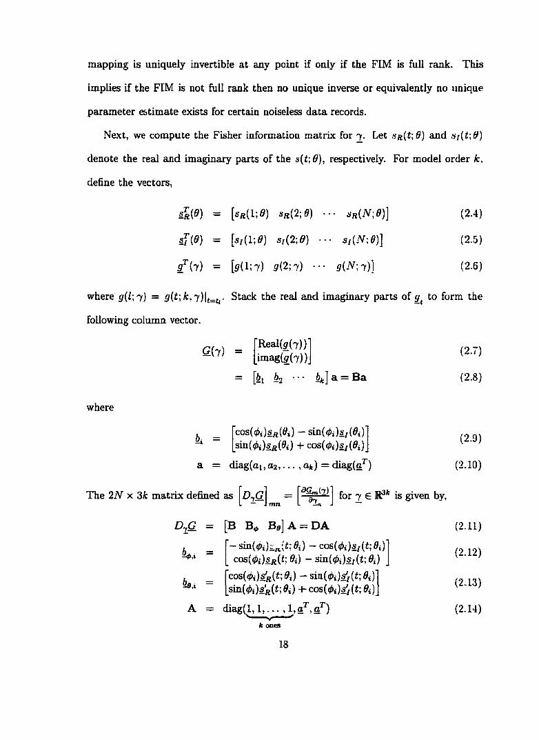
Next, we compute the Fisher information matrix for 7 . Let Sft{t\d) and Sf(t;0)

denote the real and imaginary parts of the s(t;0), respectively. For model order k,

define the vectors,

= [s« (l;0 ) Sr(2 ; 0 )

sf(0) = [s/(l;0) si(2;0) ••• Sf(N;0)]

3 ^ ( 7 ) = b ( l : 7 ) 3(2; 7 ) ••• '/(^V;7 )]

(2.4)

(2.5)

(2 .6 )

where = 3 ( t ;k , 7 )l^_ . Stack the real and imaginary parts of ^ to form the

following column vector.

Real(£(7 ))imag(^(7 ))G(7) =

= [hi hg a = B a

(2.7)

(24)

where

6v = cos(0 j)sft(0i) - sin(tf>i)sf(di) sin((^i)sji(0i) i - cos(^i)sf(0i)

a = diag(ai, 0 2 , . . . , a k ) = diag(a^)

(29)

(2-10)

The 2 N X 3k matrix defined as for 7 6 is given by.

DyG = [B B^ Bfl]A = D A

'-s in ((p i)r„ (t:0i) - cos(</»i)s^(t;0i) cos(0i)sfi(t; 0i) - sin{<f)i)s[{t;di)

cos(0 i)s'^(£; 0j) - 9i)sin(0i)s's(t; ffi) 4- cos(<pi)s'f(t; di)

A = diag(l, 1 , . . . , l ,g ^ ,a^ )

=

(2 . 11)

(2. 12)

(2.13)

(2.14)k ones

18

where is the column of and ^ is the column of Bg. Further,

and s’[ denote the derivatives of and with respect to 6. The FIM is given by

I { j ) = 7 € Ffc. We first state the Proposition for the complex data

case (2.1).

Proposition 1 {FIM under overparameterization) Assume that s{t;&) is dif

ferentiable with respect to 9, d E Q C R. Assume further that s(t;9) gives linearly

indepedent columns o /D for distinct . . . ,0*}. Also, let N > 3k. Then FIM

for any 7 € F* C is full rank if and only if

(a) none of the amplitudes are zero, and

(b) 9i 9j for all i j ^ j .

Proof o f Proposition 1 : Since 7 (7 ) = (^ 7^ ) , we have

piHl ) ) = p(D A ) = p (-D7Ç ) (2.13)

where p (/(7 )) denotes the rank of the matrix I{j ) . Suppose 6 is such that ^ 9j for

i # j . Then p{I) = 3 k — 2g, where g is the total number of zero elements of a^.

Conversely, suppose £ is such that 9i = 9j for some i < j . Then, s(t',9i) = s{t;9j)

and s'{t;9i) = s'{t;9j). This implies that p{I) < p{D) < 3Ar — 2. The elimination

of modes with nondistinct location parameters reduces the new set of modes to the

previous case. ■

Remark 1 The conditions in Proposition 1 are intuitively appealing: a parameter

7 e Ffc belongs to Ft_i if and only if at least one mode has zero energy (oi = 0 ) or

two modes have the same location parameter.

19

Remark 2 Let I be the number of unidentifiable modes, then for 7 6 f*, 3{k — I) <

< 3(A: — l + l).

Remark 3 {real data) If the data is real, i.e., éj = 0 , a € (—Umax, Umax), and s{t; 6)

is real for all t and 6, then DyG is given by

DyG = [s(0 i) ••• s{6k) ••• (2.16)

= [S(£) S'(0}]A (2.17)

= D A (2.18)

where ^ { 9 ) = [s(l; 9) s(2; 9) • • • s{N] 6)] and sf(9) is the derivative of s(9) with

respect to 9. Also, A = diag(l , 1 , .. . , l ,a^ ). Then, Proposition 1 applies for N > 2k.k ones

Furthermore, 2{k — I) < p{l{y)) < 2{k - I + 1).

Remark 4 In [60, 69], the consistency of the least-squares estimate is proven by

assuming the complete identifiability of the true parameter, i.e., the FIM is assumed

to be full rank a t the true parameter. If the model in (2.1) is overparametrized,

then the FIM is rank deficient. Existing results are extended in Corollary 1 below

to establish consistency for the case of singular FIM, thereby extending the results

in [60,69].

2.3 Model Order Selection

In this section, we present the proposed model order selection algorithm as an asymp

totic implementation of the likelihood ratio test. We start by briefly outlining order

selection based on the minimum description length (MDL) principle. Next, we appeal

to the geometry of the nested model classes and propose geodesic distance as a statis

tic for order selection. Motivated by Wald’s asymptotic approximations to geodesic

20

distance in [125], we propose an order selection algorithm using the generalized Wald

statistic.

The selection of model order can be written as a multiple hypothesis testing prob

lem

H k - p = k, k = l , . . . , K (2.19)

where K is the maximum candidate model order. The MDL and the maximum

aposteriori probability (MAP) [33] are well-known solutions for the A'-ary hypothesis

testing problem in (2.19). The MDL and MAP estimates of p are of the form

CkfP m d l = arg rnin - log + — — log N (2.20)

I , . , , y i\ 6

where 7 ^ T* is the maximum likelihood estimate of the parameter for model order

k. The parameter complexity term, logiV, depends on the model function

a{k) is derived for several linear and nonlinear models in [33,100]. Computation of

the MDL cost in (2.20) requires the computation of the maximum likelihood estimate

for each candidate model order.

To exploit the structure of nested classes under consideration, we appeal to the

notional geometry in Figure 2.1. The nested parameter sets are denoted by Fj and

Ft such that Fj C F* (in our case, this is equivalent to j < k ) . The noiseless data is

obtained by the transformation, g{t\ •). The noiseless data sequence, y = g{t; 7 ), lies in

for real data and R^^ for complex data. The least-squares estimate of the noiseless

data, y, assuming that the true model order is t , can be obtained by projecting the

noisy measurement x{t) onto the manifold giVk)- The least-squares estimate of the

parameter, 7 , is obtained by using the inverse image of g{t; •) (Corollary 1 makes

the inverse mapping precise). The shortest distance between any two points on the

21

manifold, g(Ft), is known as the geodesic distance [70]. Accordingly, we label the

geodesic distance between 5 (7 ) and ÿ(Fj) as the geodesic statistic, ^ (7 , Tj).

To motivate the use of geodesic distance as a relevant statistic for model selection,

we use a result proved in Section 2.4 regarding the consistency of the estimate, 7 € T*.

It is shown in Corollary 1 that if the FIM is continuous with respect to 7 , then as

iV —>■ 00,

. , _ , JO if j > the true model order ,in f/i(7 , 7 ) -> < (2 .2 1 )

I ^ r , 0 if j < the true model order

Furthermore, the hypothesis test (2.19) can be rewritten as follows.

: 2 € Ft, k = l , . . . , K (2.22)

Thus, detecting the correct model order is equivalent to finding the smallest parameter

set of which the given parameter is a member. This implies that a test of the following

form can be used to detect the correct model order.

acceptX l ,F j ) ^ Zj(7) (2.23)

reject

where the threshold, is chosen based on the conditional distribution of /u(7 , F^)

given that the true parameter 7 is an element of Fj. The gain in using the geodesic

statistic for order selection is that only one parameter estimate, 7 E F ^ , is required

for hypothesis testing as compared to the K estimates required for MDL test in (2.20).

However, computation of the geodesic statistic is computationally intensive; in gen

eral, it involves solving a multidimensional boundary value problem. A computation

ally simple alternative to the geodesic statistic is the Wald statistic [125], which is a

first order Taylor series approximation to the geodesic squared statistic [29].

22

The Wald statistic can be computed as follows. Assume that the following repre

sentation for the set f j is available for k > j:

= ( l ^ : r(2) = 0} (2.24)

where r( ) 6 is a differentiable restriction on the parameter set F^. Note that

r(-) characterizes the embedding of F, in Ft. Given the ML parameter estimate. 7 ,

the generalized Wald statistic [55] is given by,

w = d x f {R{x f l<( 2 )R{2 )] ' r(7 ) (2.25)

where (*)f the Moore-Penrose pseudo inverse, and ^ ( 7 ) is the matrix of first deriva

tives of £(7 ) with respect to 7

dr (7)p = l , . . . , ( & - ; ) , ç = l , . . . .Â:. (2.26)

The Wald statistic is asymptotically similar^° to the likelihood ratio test statis

tic (LRT) [95]; this similarity was also noted in [18] to use the Wald statistic for

order selection in ARMA models.

From Proposition 1 , the embedding of F in F t is equivalent to addition of {k —

j ) unidentifiable modes to any parameter 7 € Fj. Furthermore, the identifiability

conditions in Proposition 1 also provide the required restriction, r(-), on Ft to identify

the parameters in Fj. Note that the restrictions firom Proposition 1 are in two parts.

A mode is declared unidentifiable, if either

(i) its energy is zero, Oj = 0, or

(ii) its location parameter is identical to another mode, 0, = dj, j < i (oj = 0 ).

^°Two statistics are asymptotically similar if their asymptotic distributions are identical.

23

A mode is unidentifiable if it satisfies at least one of the above criteria. The

generalized Wald statistic (2.25) requires a unique embedding of the true parameter,

7 € Tj, in Ffc. The bipartite nature of the restrictions leads to a non-unique embedding

of the true parameter and hence does not allow a direct application of the Wald

statistic as given in [55,95,125]. Motivated by the results in [135], the asymptotic

equivalence of the generalized Wald statistic to the LRT [37] and the nature of the

restrictions, r(-), we propose the following order selection procedure.

1. Given the estimate of the parameter, 7 , or equivalently, the subparameters, a,

0 and £, form the order statistics, a and £. The order statistic a is formed

by reordering the elements of a such that > âi+i for all z = 1 , . . . , A' — 1:

the order statistic £ is formed similarly. For the location parameter, form the

order statistic of the first difference, A£, where A£ = \ — £j+i- The modes

are labeled to obtain two ordered sets, m“ and m®. corresponding to the order

statistics, à and A£, respectively.

2. The restrictions on the amplitude and the location parameters are constructed

as follows.

•4fcO — [0{/c-fc)xifc Û = 0 (2.27)

©ifcA£ = [0(K_fc_t)xA: A£ = 0 (2.28)

where Opx, is a p x q matrix of zeros, and ^ is a p x p identity matrix.

3. The generalized Wald statistic [55] can be written as follows,

W Î = {A ta )^ {A lP S )A t) 'i .A i,0 j (2.29)

< = ( e , Â | ) ’’ ( e î ' / t ( Â â e t ) ' ( 9 kÂé) (2.30)

24

where /(•) is the FIM.

4. The order estimate is obtained as follows

^ log(JV) (2.31)

f - 1 = arg^^ min log(iV) (2.32)

PwALD = |{m“ : Î = 1 , . . . , ^ } n {mf : i = I , . . . , ^ } | (2.33)

The idea underlying the proposed test is to reject unidentifiable modes, i.e., those

with small energy or identical location parameters. The first test (2.31) rejects modes

with small energies, and the second test (2.32) finds the subset of modes with unique

location parameters. Only the modes which are accepted by both tests are retained.

The model order estimate, Pwald) is obtained by counting the number of accepted

modes.

The penalty term in (2.31) and (2.32) is chosen to be identical to MDL (MAP),

because the number of unknown parameters per mode is same in both tests. While

the consistency of the order selection procedure is not critically dependent on this

particular choice of the penalty term, best performance was observed in the non-

asymptotic regime by choosing the same penalty term as in MDL (MAP).

Example : To clarify the steps of the proposed algorithm, consider the following

example. Let K = A with the following parameter estimates.

7 - ^ ( l - l . | . o ) . (2. j , l ) , ( l . ^ , l . l ) . (0.1, ^ . 2 ) (2.34)

mi m2 m3

where m, is used to denote the 3-tuple of the parameters, (o^,0i,a;i), of a mode.

Following the steps of the proposed algorithm, we obtain

25

1. Order statistics

a == [2 1.1 1 0 .1] (2.35)

£ == [2 1.1 1 0 ] (2.36)

K b == [1 0 .9 0.1] (2.37)

The corresponding relabeling of modes yields the following two ordered sets.

in" = {m2 , mi, m3 , m4} (2.38)

m® = {(m2 , m i), (m3, m4), (m3, m2 )} (2.39)

2. The restrictions are formed as in Step 2 of the proposed method. The order

estimates, ^ and are obtained following Steps 3 and 4 of the proposed

method. Consider the case where ^ = 3 and ^ — 1 = 2 . That is, mode m^ is

rejected by the amplitude test, and the location test rejects the pair, (m3, m2).

Since both m2 and m3 are accepted by the amplitude test, any one of the two

modes can be retained; we retain m2 since its energy is more than m3. Thus

the final model order estimate is

PWALD = I{mi, m2 ,m 3} n {m i,m 2 ,m 4 }| (2.40)

= |{m i,m 2 }| (2.41)

= 2 (2.42)

2.4 Consistency of the Proposed Algorithm

In this section, we establish that the proposed order selection procedure, (2.31)-

(2.33), is consistent. Ail asymptotics are in data length, but the results are also

applicable to the i.i.d. case, in the limit as the noise variance vanishes. The three

26

steps in the proof are as follows. First, we prove that the least-squares estimate of

the noiseless data, y 6 is a consistent estimator of y. Second, we show that the

least-squares estimate of the parameter, 7 G Ft, converges in the geodesic distance

to the true parameter 7 € F* (in the sense defined below). Third, equipped with

the strong law of large numbers and the convergence of Taylor series, we obtain the

desired consistency of a ld -

We first study the behaviour of the least-squares estimate (maximum likelihood

if the noise is i.i.d. Gaussian) when the FIM is singular at the true parameter. We

introduce some notation before stating the main result. Let 1 (7 ) = (^(t; 7 ) ) ^ u and

let y = ÿ(Ffc) C loo(Z) denote the set of noiseless data sequences generated by g. The

level sets of g define equivalence classes in the parameter space:

^{y) = { 7 € Ffc : 5r(7 ) = y}

The true parameter 7 G Fp C Ffc belongs to the equivalence class, £ = £{y). Complete

identifiability of 7 is equivalent to nonsingularity of FIM at 7 (Proposition I). Thus

the true mode, when overparameterized, can only be identified upto the equivalence

class, £. Any sequence z ' m y which minimizes

1 ^(2.43)

^ £=1

will be called the least squares estimator, , of g{£) = y. Under an assumption on

the function g, the consistency of the least squares estimator, , can be proved by

modifying a proof in [60].

T h e o rem 1 {ctynsistency in d a ta space) Let x{t) = y{t) -f e(t), vjith zero mean

and finite variance noise e{t). Let y ^ be the least squares estimate o f the data sequence

27

y = g{£). Assume that g((; 2 ) w a continuous function of j , and that the tail cross

product o f the function g{')) with itself exists and is non-zero. Further assume that

1 ^Q(^) = - 2 ( 0 P (2.44)

(=1

has a unique minimum at z = y, where y E y is the true data sequence. Then, {y^}

and ajif = Q^{y^ ) are strongly consistent estimators'^ of y and the noise variance,

a^.

Theorem 1 does not require the model g{t, •) to be a superposition model and hence

holds for more general nonlinear models.

Before proving Theorem 1, we briefly review the concept of tail product and

tail cross products for complex valued sequences and complex valued random vari

ables [69]; the case of real valued sequences was considered in [60]. Let u = (u(t))

and V = (v(t)) be two sequences of complex numbers and define

1(2.43)

t=l

If lim^v- oo [u, v\ff exists, its limit [u, u] is called the tail product of u and v. If u = v,

|]'u|j = [u, u] is called the tail norm of u. Let c and h be two sequences of complex

valued functions on F*, such that [c(7 “) ,h (y ’) j^ converges uniformly to a complex

number, [0 (7 “), h { Ÿ )] , for all 7 “, 7 * € Ffc. If (c, h) denotes the function on F* x Ft —>■

C which takes (7 “, 7 *) into [0(7 “), h(7 *)], then this function is called tail cross product

of c and h.

If c(t; 7 ) and h{t; 7 ) are continuous functions on F^ and both c(t; 7 ) and h{t; 7 ) are

uniformly bounded by a bounded function of t, then the tail cross product of c and

“ A sequence of estimators, 7^, is said to be strongly consistent for every 7 G F if P(UmAr->oo 7^ =7) = 1.

28

h exists [69]. We restate a strong law of large numbers for real noise sequences [24],

which directly applies to white circular complex noise sequences.

L em m a 1 I f t = (e(t)) is such that E(c(t)) = 0 and E(e^(t)) < oo J o t all t. and

if the ta il norm o f a sequence u o f real num bers exists, then [u, c]jv 0 fo r alm ost

every e.

P ro o f o f T h eo rem 1 : To begin, from the strong law of large numbers (Lemma 1),

we have

(=1

Next, rewrite (2.43) to observeN

(2.47)£=l

1 "= ; j ÿ E [ l ! '( ‘) - - ( ‘)i" + 2 R e { (îr ( () -z ( ( )) t;) + l«.l"] (248)

C=l

By hypothesis, the tail cross product of g with itself exists. Hence, the second term

in (2.48) goes uniformly to zero by Lemma 1 . Therefore

\im Q ^ { z ) = Q { z ) + a ^ (2.49)JV—»oo

uniformly for all z € y . Since g (t;7 ) € C is a continuous function of 7 for each

t, we have that ^(7 ) = { g { t ; j ) ) is also a continuous function of 7 . Since the set

Ffc C R?* is bounded and closed, it is also compact. Continuity of ^(7 ) implies that

the set y = g{Tk) is a compact subset of /oo(Z). Since y is compact, there exists a

subsequence y” of such that lim„_,oo y” = ÿ, where ÿ denotes the limit of

Note that Q is continuous and Q" converges uniformly to Q which implies

U m Q ^ i r ) = Q { V ) + ( ^ (2.50)n—foo

29

Since y” is a least squares estimator, we obtain

<3”(5” ) < « “{!/) = - Ê k(«)P = (2.51)

Therefore, as n - f oo,

Q ( ÿ ) + c r ^ < a ^ (2.52)

which implies that Q(ÿ) = 0. Since Q has a unique minimum at y, we obtain ÿ — y.

Note that the above conclusion holds for all the limit points of the sequence . Thus

1/ -)■ y-

Using the same arguments as above, we obtain that Q ^(y^) —> Q{y) + cr . Since

Q(y) = 0 , we conclude that Q^{y^ ) is a consistent estimator of a^. ■

The model in Example 2 satisfies all the hypotheses of Theorem 1 , and the model

in Example 1 satisfies the hypotheses if s{t) is a continuous function with non-zero

tail cross product^^.

Next, we prove that the least squares estimator is also consistent in the parameter

space in the following sense. If the least squares estimate of the data sequence,

is consistent, then the equivalence class defined by , comes arbitrarily close to

£. That is, if Q{y^) —>• 0, then

in f . | | 7 - 7 | | - ^ 0 . (2-53)1&S.Î&SN - -

If the Fisher information matrix is continuous with respect to 7 , then there exists a

constant C such that for any 7 € F^, /r(7 , Fp) < C inf2erp | |7 - 7 ||- Thus, the above

convergence of in 2-norm also implies the convergence in the geodesic distance.

^^Noa-zero tail cross product implies that s{t) is a finite power signal. In communication applications, s(t) is generally a finite energy continuous waveform, like a raised cosine pulse; in this case. Theorem 1 holds for a fixed iV as u -»• 0.

30

Corollary 1 {consistency in parameter space) Under the assumptions of The

orem 1, is a singleton set with probability 1 and as N —y oc converges almost

surely to some element of £ .

P roof of Corollary 1 : The Fisher information, / ( 7 ), is by hypothesis full rank

at all 7 6 ffc. Also, the set Ft \ F* has a measure zero. Thus, by inverse function

theorem [31], the inverse of g is unique a.e. on Ft, i.e., is a singleton set with

probability 1 .

Since F* is compact, g is uniformly continuous on F t. Further, since g is one-to-

one on Ffc, g~^ is uniformly continuous and unique almost everywhere on Ffc. Since

— >• J / , the sequence is Cauchy. From the uniform continuity of g~^, it follows

that ^ is Cauchy and hence converges. Assume 7 — 7 ^ 6 . Continuity of g implies

^(7 ) = t/^ —> ^(7 ) / y, which is a contradiction. Hence, 7 converges to a point in

£. ■

Thus the equivalence class estimates, are almost always singletons, and the

estimated parameter vector converges to an element in the true equivalence class, S.

All parameters in the equivalence class £ produce the same data y and hence are

indistinguishable using observations x{t) , t = I , . . . . for all N.

The limit point, Umisr-^oo^^ € f for a particular noise realization is algorithm

dependent. For example, in our simulations, we found tha t parameter estimates

computed using subspace based techniques for superimposed undamped exponential

models tend to converge to a point with p modes at the true locations and {K — p)

modes used to model the noise; the amplitudes of the extraneous modes converge

to zero such that no two location parameters are the same. On the other hand, the

31

limit points of a FFT-initiaiized method [135] converge to closely spaced equal energy

modes.

Since the least-squares estimate of the parameter converges to an element in the

equivalence class, S (Corollary 1), the expected value of may not converge to

a single parameter value. This implies that when the equivalence class E is not

a singleton, the asymptotic distribution of E ^ does not exist. Thus, the results

pertaining to the asymptotic distribution of Wetld statistic [125] are not applicable.

Instead, we rely on convergence of the Taylor series expansion and the law of large

numbers to prove the consistency of the proposed model order estimate.

T h e o rem 2 {m odel order co n sis ten cy ) Let the true model order be denoted by

p and the hypothesized maximum model order by K > p. Also assume that the

conditions for Proposition I and Theorem 1 hold. Further assume that f {x\y) is

at least twice continuously differentiable with respect to 7 . Finally, assume that the

Fisher information matrix satisfies the following rate conditions'^ for r ‘ {N), r^(:V) >

log(iV),

fo r nonnegative definite matrices, and T f. Then, Pwalo P-

^^These rate conditions are similar to the Assumption fi in [132].

32

P ro o f o f T h e o rem 2 : Since is assumed to be at least twice differentiable, the

loglikelihood, /(7 ) = log/(ar|7 ), can be expanded in the following Taylor series [129]

/(?) = /(7) + ( 7 - 7 )5 7

+ ( 7 — 7 ) i / ( 7 ) ( 7 — 7 ) + higher order terras2=2

where ^ ( 7 ) is the Hessian matrix with entries H,j(7 ) = By hypothesis, 1(7 ) is

continuous and 7 — 7 which implies ( 7 — 7 )^H^(7 ) ( 7 — 7 ) 0 [129]. From the strong

law of large numbers [118], it follows that / f ( 7 ) / ( 7 ). Also, from the assumed

continuity of FIM, 7 (7 ), we obtain that 7 (7 ) -+ 7 (7 ). Combining the above facts, we

obtain

(7 - %)^7 (7 ) (7 - 7 ) ->■ 0 (2.54)

Note that the Taylor series also converges for any bounded transform of the parame

ters. This implies that 7 and 7 in (2.54) can be replaced with a and S, respectively.

The transform 0^ is linear with bounded entries, and hence is a bounded transform.

Thus the convergence result in (2.54) can likewise be obtained with A£ replacing 7 .

We first demonstrate that asymptotically, ^ a ld < P- First consider the amplitude

test. From Proposition 1, it follows that there are (7l — p“) modes in 7 with zero

amplitudes, where p“ is the the number of modes with non-zero amplitude. For

k > p“, AkU = 0 and from (2.29) we have

= {Akà - AkO^'^I{Akà){Akà - Aka) (2.55)

From the convergence of Taylor series (2.54), we get lim^v-K» = 0 , for k > p“.

Thus,

lira ^ = lira [arg min Wu -I- log(iV) N- <x iV-»oo [ k=0,...,K ' 2

33

< P“ (2.56)

Thus, all modes with zero amplitudes are rejected by the amplitude test (2.31). Fol

lowing the same arguments, the location test (2.32) rejects mode pairs having zero

location differences. Thus, all the unidentifiable modes are rejected in (2.33) and

maybe more, i.e.,

lim PwALD ^ P (2-57)N-too

We next show that none of the identifiable modes are rejected, i.e., lim^_,oo a ld >

p. From the structure of the FIM and Proposition 1, it follows that if p modes are

identifiable, then the FIMs for amplitudes and location subparameters of the identi

fiable modes are also full rank. That is, /(Op) and I{Bp) are full rank where Op and

0p are parameters of the identifiable modes.

Again consider the amplitude test first. Let lim^_,oo H = a. Identifiability of each

subparameter implies that for all ^ < p, p{'£%) = 6 > 1 , where = lim/v-^oo

Consider the singular value decomposition of Eg = Cf[AkUk. Let = U j and

observe p{Lk) = p(Eg). The matrix Eg is FIM for the linearized model, LkAka + e.

where e is i.i.d. Gaussian. Thus,

jim = [ A , a f L l U (A,a) = > 0 (2.58)

with equality iff Aka is in the null space of Lk, which contradicts the fact that the

linearized model has non-zero energy. Thus limiv-»oo ^prfi7)^^k is bounded away from

zero. Combining the above with the Taylor series convergence (2.54), we obtain

that ~ 0(r®(iV)) for k < p. Since T“(iV)) > log(iV), we immediately obtain

limyv- oo > p. Using similar arguments, we obtain limAr_»c« > p. Thus, asymp

totically all the identifiable modes are retained, which implies,

lim ^ a l d > P (2.59)

34

Combining (2.57) and (2.59), we obtain iim/v_^ooP w a l d = V-

■Note that the model classes discussed in Examples 1 and 2 satisfy all the conditions

of Theorem 2. The rate of growth of submatrices of FIM for Example 2 can be found

in [117], where it was shown that r “(iV) = N and r^{N) = N^.

2.5 Implementation Issues and Simulation Results

In this section, we briefly discuss some implementation issues and present simu

lation results for the nested model class discussed in Example 2.

2.5.1 Dynamic program

Rather than estimate 7 for the maximum model order K, 7 € may be se

quentially estimated for j < k to minimize the expected computational cost. This

is conveniently achieved by embedding the proposed model order estimate in a dy

namic program [38,45]. Based on the a priori probability distributions of model order

and model parameters, and the cost of computing estimates for different candidate

models, a sequential procedure is obtained to selectively estimate candidate model

parameters. The complete dynamic program can be intractable since it requires dis

tribution of pwALDÎ a useful asymptotic approximation can be obtained by using the

consistency of a ld - Thus, the asymptotic dynamic program (ADP) is obtained by

using

■{Sp p < k

^ai.d (7 e r k ) = i ; " ^ . V 7 G FA: (2.60)6k p > k

where 6m is Kronecker delta.

35

Having obtained ^ ald, the parameters of the modes retained in (2.33) provide an

estimate for the unknown parameters of the modes; denote the parameter estimate so_ f 1 ^ALD ^

obtained as 7 = | (a,, ^i ) j . A n alternate parameter estimate, %, is obtained

by minimizing the cost (2.43) over the parameter set T^vald- The variance of the

parameter estimate, 7 , is higher than the variance of the parameter estimate 7^,

because 7 is a subset of a larger parameter 7 6 Ft, A: > Pwald- For large differences,

^-PwALD, the variance of 7 may be undesirably high. On the other hand, a complete

reestimation of the parameters to obtain 7 adds to computation. A low complexity

alternative is to use a gradient descent method with 7 as initial estimates [135].

2.5.2 Simulation results

The detection performance and computational complexity of the proposed method

is compared to MDL and MAP [33]. The penalty terms for the MDL and MAP

estimates are a{k) = 3k and a{k) = 5fc, respectively. The difference in the penalty

terms for the two rules arises from different asymptotic analyses. The asymptotic rule

for MDL is derived by considering i.i.d. data collection or equivalently as the noise

power vanishes. On the other hand, the penalty term for the MAP rule is obtained

as data length, N , increases unboundedly; for the model in Example 2, this implies

independent but non-indentically distributed data.

For the simulation results, a uniform distribution on model order for Ar = [1 . . . . ,7]

was assumed. The maximum hypothesized model order was chosen to be AT = 7, and

for each experiment, 1000 trials were performed. The ADP chooses^** to compute only

the ML estimate for K = 7.

‘‘‘For K — 15, for example, ADP computes ML estimate for Ar = 13. If a ld < 13, the procedure stops, else the ML estimate for t = 13 is computed. For large maximnm model order AT, the ADP can significantly reduce computation.

36

In Figure (2.2), the detection performance of Pwald is compared to Pmdl and Pmap

for TV = 64 samples. The probability of correct detection is shown as a function of

SNR/mode/Fbin, where the Fourier bin is defined as Fbin = 1 /AT.

In Figure (2.3) the detection performance is shown as a function of number of

samples, N, with SNR/mode = —15 dB. The ratio of the average computational cost

of MDL and MAP to the average computational cost of Pwald is shown in Figure (2.4).

as a function of the data length. The average computational cost of MDL and MAP

is more than three times the proposed method, with similar detection performance.

Note that the computational savings increase as either maximum model order. K, or

the data length, N, increases.

2.6 Conclusions

In this chapter, we presented a model order estimation procedure for superimposed

models, which are frequently encountered in engineering applications. The proposed

technique is consistent and is computationally more efficient than order selection

using the minimum description length principle. The consistency proof requires the

consistency of the overparameterized maximum likelihood estimates, for which the

existing results were extended to the case where the noiseless data can be generated

by multiple parameters.

37

geodesicstatistic Xc?

rFigure 2.1: Notional geometry of the nested classes.

38

0.9 //0.6

0.6

0.2

0.1

-20 -10 0 10 SNFVmodo/Fbln (In dB)

Figure 2.2: Probability of correct detection of model order as a function of SNR

MOLMAPWald

0.9

as

0.7

0.6

g 0.3

02

0.1

80 tooNumber O f samples

Figure 2.3: Probability of correct detection of model order as a function of data length at SNR/mode = -15 dB

39

4.5

igZ5a

1.5

0.5iO 60 7(Number O f samples

100

Figure 2.4: Ratio of average computational complexity as a function ofdata length at SNR/mode = -15 dB

40

CHAPTER 3

SECTOR BEAM SYNTHESIS FOR CELLULAR SYSTEMS USING PHASED ANTENNA ARRAYS

3.1 Introduction

Cell sectorizatioa has been widely proposed for improving system capacity in

cellular systems [20, 76,78]. Every cell is divided into multiple sectors, and each

sector is served by a dedicated antenna. With ideal sector antennas, the increase

in system capacity for both voice and data networks is propotional to the number

of sectors [59]. As an additional benefit, cell sectorization is reported to result in a

considerable decrease in delay spread in the received signal [115]. However, perfect

sectorization is not realizable. Non-ideal radiation patterns reduce the capacity of

sectorized cellular systems due to inter-sector interference [59,73,84].

In this chapter, we propose a sector beam synthesis technique using phased an

tenna arrays to minimize the total inter-sector interference. We assume that each cell

is divided into sectors of equal width and that each sector is served by an indepen

dent antenna array, as depicted in Figure 3.1. In addition to synthesizing the desired

pattern, the proposed technique allows us to quantify the relationships among sector

size, beam efficiency, signal-to-interference ratio, and capacity.

41

Several approaches for sector beam synthesis have been proposed [17,39,66,108].

Most published methods are extensions of digital filter design techniques [39,66,108].

However, sector beam synthesis using antenna arrays is considerably different from

conventional filter design for the following reasons. First, the analogy between filter

design and sector synthesis holds only for A/2 inter-element spacing in uniform linear

arrays (ULAs) with isotropic elements. Second, the phase of the synthesized beam

is irrelevant for many array applications; in contrast, linear phase is an important

requirement in many filter design problems. Third, the minimax criterion widely

used in filter design is not well suited for multisector wireless applications because

the criterion does not appear to be directly related to any significant communication

performance parameter.

In contrast, the proposed approach minimizes the total inter-sector interference

subject to a ripple constraint on the in-sector power pattern. This is an example of

power synthesis [17,79]. We show that the proposed non-convex problem can be con

verted into a convex fractional linear programming problem with linear constraints,

via a suitable reparametrization [133]. The convex reparameterization guarantees that

a globally optimal solution can be computed using a numerically efficient algorithm.

The proposed approach accomodates non-isotropic antenna elements, arbitrary ele

ment spacing, and non-central sectors^®, but is limited to uniformly spaced linear (or

planar) arrays.

^^The center of the sector is not normal to the plane of the array.

42

In Section 3.2, we motivate the design criterion of maximum beam efficiency sub

ject to a constraint on in-sector ripple. The optimization problem is solved by frac

tional linear programming by using a suitable reparametrization to yield convex con

straints. Some numerical results from the algorithm are presented in Section 3.3. To

illustrate the utility of proposed results, we compute the minimum size of the antenna

arrays required for the sectorized CDMA system analysed in [59].

A joint optimization involving all the cell antenna elements as a single array would

lead to a smaller inter-sector interference. However, we avoid a joint optimization for

two reasons. First, a design dividing the array elements to a number of disjoint

groups, one group for each sector antenna, allows distributed implementation of the

hardware for each sector. This simplifies the architecture of the base station. Second,

the commonly used antenna arrays employ directional antenna elements, and hence

the loss in a distributed optimization is small.

3.2 Problem Formulation

3.2.1 The linear array pattern

Consider a linear array of K antennas at locations xq, x i , . . . ,x /c-i € R. The

radiation pattern of each antenna element is t = 0 , . . . , K — 1. A plane wave

with wavelength A is incident from direction 9 and propagates across the array (which

we assume for simplicity does not change the field). The angle 9 is measured with

respect to the normal of the array. The K signal outputs are scaled by complex

weights Wi and summed to give the linear array beam pattern W{9)

/ 2-jr \= Gxp f sin(g) 1 = 5 ^ Wigi{9). (3.1)

1=0 ^ '' i=0

43

The weights, w = [u/o,Wi, . . . , wk - i^ -, are chosen to achieve a desired beam pattern

W{d). The power density emitted by the antenna array is given by P{6) = \ W[9)\^.

3.2.2 Inter-sector interference and beam efficiency

A terminal located in any sector {e.g., terminal T l in Sector 1, Figure 3.1) is

subjected to interference generated by the base station transmitters driving the re

maining N —l sectors. Assuming that all N transmitters are equal in power and emit

uncorrelated signals, then the total interference power density suffered by a terminal

located at angle 0 is

•/(«) = E ^ (3.2)n = l ' '

where J[6) and P{6) are, in this case, expressed in Watt/radian*®. Integrating J{d)

over one sector, we obtain the total interference power received by the sector from

other sectors in the same cell. With no loss of generality, we consider the sector

[O’ ■

/"wJ s = J[9)d9 (3.3)

Jo/ 97T \ f

j d g = P{9)d9 (3.4)

The beam efihciency, rj, is defined as the ratio of the power transmitted in the sector

of interest to the total power radiated by the array, i.e..

9 — r2v (3 5)f o ' m d e

P{e)de - P[e)de

= — T m S ---------- =

^^The antenna arrays considered allow beam pattern shaping only in the horizontal plane, thereby reducing the problem to a two-dimensional problem.

44

where P is the power transmitted by one transmitter. Hence, (1 —t] )P represents the

total interference power radiated within the boundaries of one sector. Thus, rj is an

important parameter in sectorized systems.

3.2.3 Maximizing beam efficiency

Consider a sector of interest 0 , = [di, 0„], —i r < d i < 9 ^ < n . The beam efficiency

is given by

The power transmitted by the antenna array to the sector spanning ©, is

P e . = r p { e ) d dJBi

= 5252 *"*^* / 9 i[^ )9 kW di=o k=o

= w ^A w (3.8)

where Aik = Jg ' 9i{9)gk(9)d9. By subsituting 9i = - t t and = n, the total power

radiated by the array can be computed as

Vq = w ^ M w (3.9)

where Mik = gi{9)gk(9)d9. The matrix >1 is Hermitian and positive definite for

all values of —t t < 9i <9.^ < t t . Furthermore, M is a symmetric and positive definite

matrix. The matrix M is real if Qi (9) is symmetric about 0 = 0 for all i = 0 , . . . , K —L

45

Using Equations (3.8) and (3.9), efficiency can be written as

Aui w ^ M w

v ^ T vv ^ v v ^v

(3.11)

where v = and is the matrix square root of M. From Equation (3.10),

it is evident that maximizing beam efficiency in absence of any constraints requires

finding an eigenvector corresponding to the maximum eigenvalue of the matrix T. The

m atrix T depends on the design variables, K, j , Qi{d) and ©„ but is independent

of the weight vector w. Thus, fixing the design variables fixes the maximally efficient

pattern (or the subspace of patterns if the maximum eigenvalue of T is non-unique).

A pattern thus obtained has a large in-sector peak-to-peak ripple, especially at

the end points of sectors. As an example, a maximally efficient pattern for a 30

degree central sector is shown in Figure 3.2 (for the array described in Section 3.3).

The high in-sector ripple, which is characteristic of the maximally efficient patterns,

is undesirable in cellular applications, for it leads to a wide distribution of the user

powers. This motivates a constraint on in-sector peak-to-peak ripple, p,

A ripple constraint, p < e for 0 < e < oo, can be expressed as a set constraint, C . on

the array weights, w.

= {w : p < t } (3.13)

For any w ^ C c with mingle, P{9) = 7 , the ripple constraint p < e imphes

7 < P{0) < lO '/^S, g E 0 ,. (3.14)

46

We arbitrarily assign 7 = 1, thereby fixing a scale for w, and define

V, = { w : l < P{B) < 9 e 0 „ and(3.15)

P (0 )> O , 0 6 e \ e , } .

where 0 = [—t t , t t ) and 0 \ 0 , = {0 : 0 6 © and 6 ^ Qj}. The positivity constraint,

P(0) > 0, always holds since P{9) is the power of the pattern W{6)-, the importance

of explicitly requiring positivity will become apparent in the next subsection. From

the definitions of p and the set Vf, we conclude that if n; 6 Cj, then aw 6 for some

O' > 0. Because efficiency is invariant to scaling of w, we can use D, to constrain

the in-sector ripple without any loss of generality. Thus, the proposed optimization

problem is

max 77 (3.16)wen.

The optimization problem in (3.16) is an example of power synthesis, in which no

phase requirements are prescribed [17]; therefore, all available degrees of freedom in

w are utilized to optimize the power pattern. Power synthesis generally leads to a

non-convex optimization problem (e.g. (3.16)), and is considered more complicated

than traditional convex design approaches [17]. However, power synthesis is very

important because pattern specifications for radar and com m unication systems are

often defined in terms of magnitude only [17,63,79]. Using the ideas in [133], we

show that for uniform linear arrays, a reparametrization of the power synthesis task

in (3.16) yields a convex optimization problem.

3.2.4 Reparametrization (ULA)

Consider the following reparametrization of P{6) assuming a uniform linear ar

ray (ULA), x.e., Qi{9) = Q{9), Xi = xA, for all x = 0 , . . . ,ü r — 1. The array power

47

pattern may be written

P{d) = \W{d)Ÿ (3.17)fr-i / ^ \ K-i

where

= \Q{ )? ^ u/fcexp ^j^^fcsin(0)^(3.18)

/ OttA \= IQ (^ )P X ^ X ^ ‘ i^ fcex p fj——(fc - i)s in (0 ) j (3.19)

i=0 t =0 ' '

= 5 1 Pn.exp f j^ ^ m s in ( 0 ) ^ |g (0 )p = ^ p (3.20)m = - ( K - i ) ' /

A '-l

Pm = 5 Z - ( ^ - 1 ) ,. .. ,AT - 1, (3.21)»=-(Ar-i)

= exp ^ j^ ^ m s in ( 0 )^ \Q{Q)? (3.22)

(3.23)

The constraint set can be rewritten in terms of p as

2?f = {p : 1 < d^p < 10'^^° V 6 € ©s, and

d^p > G V 0 € 0 \ 0 , }

The positivity constraint on power, P{6) = > 0, was redundant in (3.15)

but is required in (3.23) so that the optimization may be performed over the new

parameterization, p. This ensures that we consider only those p which represent a

valid autocorrelation sequence for some w ^ . The constraint set in (3.23) is

an infinite set of linear inequalities in p. Further, the beam efficiency can also be

rewritten in terms of p,

a^pn = ^ (3.24)

b p

where for m = —{K — 1 ) ,. . . , iv — 1

dm = I |Q (0)pexp ^ - j^ ^ m s i n ( ô ) ^ (3.25)

byn = 10(0)1^ exp ^ - j^ ^ m s i n ( 0 ) ^ (3.26)

48

Thus, the constrained optimization problem in (3.16) can be stated as a semi-infinite

fractional linear program (FLP) in terms of the new variable, p.

q^p(F): p* = a r g m ^ -jj= (3.27)

- gen. b p

Using the methods of [26], we show that the FLP in (3.27) can be converted to the

following linear program.

(L): (u*,t*) = arg max qû (3.28)

The set C, is given by

ICt = {(m, t) - t < dû < 9 6 0 ,;

> 0 , 0 € 6 \ 0 ,; (3.29)

£ > 0 ; bû = 1}

where u = tp and t = {bû)~'^. The equivalence of (F) and (L) can be demonstrated

as follows. If p € ■Pe, then with u = tp, £ > 0 , we obtain

i ^ do P ^ t dg u (3.30)

d^p < 10 ' / = > < £10 '/ '° (3.31)

do £ ^ 0 =>■ d^ M ^ 0 (3.32)

t = {b“p)~'- => bû = 1 (3.33)

which implies {u,t) 6 /Cj. Similarly, if (u ,£) 6 £ > 0 , then the converse is true

in (3.30)-(3.32). This implies that p = yu 6 P*. Lastly,

S = K = - - -(3.34)

Thus, we have established that if (u*, t*) is an optimal solution for Problem (L), then

pu* is an optimal solution for Problem (F) and vice versa.

49

Problem (L) is a semi-infinite linear program in AK — 1 real variables, and is there

fore a convex optimization problem. For convex optimization problems, a globally

optimal solution can be computed using numerically efficient methods.

A simple method to approximately solve (3.28) is to discretize the constraint set

JCi [54]. For instance, select a set of angles, —tt < di < 02 < ■ ■ • < 6i < tt and replace

ICf with the set

c r = {(«, d, e 0 ,;

& >5, 0 i6 0 \ 0 , : (3.35)

t > 0; = 1}.

where J > 0 is a small number chosen so that the spectral factorization condition^^

is met by the solution to the discretized problem**. The discretized constrained

problem is an outer approximation [54] to the original semi-infinite problem and can

be efficiently solved in practice*®. Further, as the discretization becomes finer, the

solution of the discretized problem approaches the solution of (3.28); a standard rule

of thumb is to choose L » 15AT for discretizing semi-infinite programs [133], but we

use L » 225K in our computed results for improved accuracy.

Having obtained the globally optimal solution, p*. a corresponding optimal array

weight vector w* can be obtained via spectral factorization [9]. There exist upto 2^

excitation vectors, w*, with autocorrelation p*, where 2M is the number of zeros of

p* with magnitude not equal to one. This provides an added degree of freedom in

the choice of the optimal weight vector. For example, from among all spectral factors

^^There exists an w € such that p is the autocorrelation of tu if and only if > 0 for ail 8 6 [-7T, ÏÏ-] [9].

‘*The parameter 5 is introduced to ensure that d^p > 0, for all Ô e t = 1, -. - , I. — 1,and hence p E d can be increased until the spectral factorization condition is met [133].

^^We use the Mathworks, Inc. M a t l a b routine Ip to solve the discretized problem (3.35).

50

of p*, an excitation vector with least difference between the power fed to adjacent

elements would reduce strong mutual coupling effects in the array.

3.2.5 Extensions : constrained SIR

The worst case signal-to-interference ratio (SIR) experienced by any terminal is

minog[@,,0 l This will typically happen at the sector boundaries, i.e., for 9 = 6i

ov 9 = 9ui and will be less than 1 (see the numerical results in the next section). In

some applications, it may be desirable to keep the worst case SIR above a criticial

value, (3, for most of the sector.

SIR(0) = 9 e B t C e , (3.36)

We assume that 0 j is a strict subset of 0 , and does not include the end points of the

sector. The semi-infinite constraint on SIR is also a linear constraint, for any 0 6 0 j .

as shown below.

m - '

< 2 S (3-38)n = l ' ’

f N-\. \ ^

2 ï 0 (839)

Thus, the linear program (L) in (3.28)-(3.29) can be readily extended to include the

constraint in (3.39) limiting worst-case SIR.

3.3 Numerical Results

In this section, we present some numerical results obtained using the proposed

synthesis technique. Specifically, we show how efficiency varies as a function of the

51

size of the array and sector size; both central and non-central sectors are considered.

Finally, we present an example to demonstrate the use of the proposed method in

calculating antenna array sizes for the DS-CDMA system analyzed in [59].

For all results in this section, we use e = 3 dB and a single element radiation

pattern, Q{6), that is an analytical approximation to the measured radiation pattern

of a prototype array element built by Lucent Technologies (see Figure 3.3).

3.3.1 Beam efficiency versus sector width

In Figure 3.4, beam efficiency as a function of sector width is shown for central

sectors. For a fixed array and a limit on the peak to peak ripple, the beam efficiency

decreases as the sector width decreases. This implies that the average signal-to-

interference ratio, lOlogjo decreases with a finer sectorization. In other words, to

maintain a desired SIR, a finer sectorization requires a larger array with an increased

cost. The same conclusions can be drawn for the non-central sectors, spanning [0 , 6^],

as shown in Figure 3.5. Because of the specific Q{d) in Figure 3.3, very large non

central sectors cannot be generated as efficiently as the smaller sectors. In Tables 1

and 2 , the corresponding average signal-to-interference ratios are shown.

In Figure 3.6, we compare two 90 degree central sectors generated using 16-element

arrays with y = 0.5 and y = 0.55. Finally, in Figure 3.7, two 45 degree non-central

sectors are generated using a single 16-element anteima array to cover a full 90 degree

sector with y = 0.55; this example demonstrates how finer sectorization can be

obtained without employing additional antenna arrays.

52

3.3.2 Array size calculations

To illustrate the utility of the proposed sector synthesis technique, we compute

the antenna array requirements for a sectorized DS-CDMA cellular system considered

in [59] for voice communication. Similar analysis can be performed for throughput of

data networks using the results in [59].

In [59], the imperfection in sectorization was modeled by considering an ideal

antenna with a beam covering the sector [O, ^ + 1/] where u is the overlap angle

between sectors. Capacity, throughput, and delay analysis was performed by varying

the overlap angle, u. The efficiency for such a pattern is t; = For overlap angle

f/ = 0, the efficiency is t) = I. k s u increases, the efficiency of the beam decreases.

Also, for a fixed u, the efficiency of the sector beam decreases as the sectorization is

made finer.

For N = 6 sectors, and using Q(d) in Figure 3.3, a 5-element array leads to 90%

efficiency (for a central sector with e = 3dB and y = 0.5), which implies a 6.66 degree

overlap between the sectors. Using the results in [59], u = 6.66 degree leads to 16%

loss in the capacity (in terms of the number of users) when compared against the

system with perfect sectorization (but with no voice activity monitoring). This loss

can be reduced to below 10% if the antenna array size is increased to 12 elements,

which corresponds to an efficiency of roughly 95%. We note that the above size

calculations should be considered as lower bounds on the antenna array size for a

given set of system parameters.

53

3.4 Conclusions

We presented a new method to synthesize sector beams using phased antenna

arrays. To realize the full capacity benefits of cell sectorization, it is important that

the sector antennas are designed to minimize the inter-sector interference. We pre

sented a simple procedure to maximize beam efficiency, or equivalently, to minimize

the inter-sector interference, with an in-sector ripple constraint on the power density.

The proposed technique allows the designer to quantify the tradeoffs involved in finer

sectorization, antenna array size, and system capacity.

54

ANTENNA ARRAY FOR SECTOR «1

SECTOR «4 SECTOR «1

• Tl

SECTOR «3 SECTOR «2

Figure 3.1: A 90 degree ceil sectorization with four antenna arrays serving one sector each.

55

-20

-40

-SO

-100

-120-100 -50 100 150-150

Angle (In degrees)

Figure 3.2: Maximally efficient beam pattern for A" = 16, j = 0.5. The in-sector peak-to-peak ripple is 38.61 dB and the efficiency of the beam pattern is 99.94%.

56

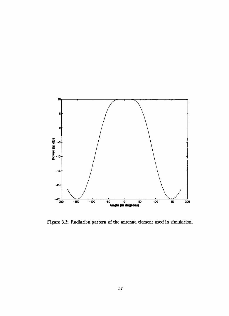
s 5

-15

-20

-2 5 '—-200 -150 - I O C 150-50 100 200

Angle (In degrees)

Figure 3.3: Radiation pattern of the antenna element used in simulation.

57

100

K=1

K=8

K=4

u 70

90Width of the central sector (In degrees)

Figure 3.4: Beam efficiency as a function of central sector width. The in-sector peak-A Ato-peak ripple is 3 dB and j = 0.5.

58

100K=16

K=8

K=4

40

20

20Width of the non-central sector (in degrees)

Figure 3.5: Beam efficiency as a function of non-central sector width (0 , = [0,0u]). The in-sector peak-to-peak ripple is 3 dB and y = 0.5.

59

Table 3.1: Average signal-to-interference ratio (= lOIogjo (î^ ) for a 3 dB in-sector peak-to-peak ripple and y = 0.5.

Central sector width (in degrees)

Average SIR (in dB)K = 4 K = 8 K = 16

15 -0.29 5.48 8.7330 5.52 8.74 11.8245 6.47 10.44 13.4760 8.91 11.53 14.5790 10.22 12.35 15.78

Table 3.2: Average signal-to-interference ratio (= 10 log Q for a 3 dB in-sectorpeak-to-peak ripple and y = 0.5.

Non-central sector width (in degrees)

(0 , = [O,0«])

Average SIR (in dB)

K = 4 K = 8 AT = 1615 -0.21 5.47 8.6830 5.48 8.52 11.5445 5.93 9.71 12.8360 6.04 9.31 12.9175 -8.54 4.08 9.26

60

-10

-20

-50

-60

-70

-80

-90150100-150 -100 -50

Angle (In degrees)

Figure 3.6: 90 degree central sectors for j = 0.5,0.55 and K = 16.

61

-10

I 'I

e -20

a. -30

-40

-50

-60-150 -100 -50 too 150

Angle (In degrees)

Figure 3.7: Two 45 degree non-central sectors for j = 0.55 generated using 16-element array.

a single

62

CHAPTER 4

MMSE RECEIVERS FOR MULTIRATE DS-CDMASYSTEMS

4.1 Introduction

The growth of wireless networks has resulted in systems offering heterogeneous

services, such as voice, video and data. Several system architectures based on Di

rect Sequence Code Division Multiple Access (DS-CDMA) signalling have been pro

posed recently [1,30,91,92]. These proposals include systems with multiple chipping

rates [1], variable spreading gain with constant chip rate [ij and multicode CDMA [82].

Another instance of a multiple chipping rate system is a wideband DS-CDMA system

operating in the presence of an existing narrowband DS-CDMA system.

Receivers which truly exploit the nature of multi-rate signals have focussed on

synchronous and pseudo-synchronous systems in non-multipath environments [19,21,

22,82,109]. Designs which accomodate asynchronous or multipath channels [116] do

not fully take advantage of the multi-rate nature of the problem.

In this chapter, we derive linear multiuser receivers based on the minimum mean

squared error (MMSE) criterion, for multiuser systems where users with different sym

bol rates coexist. We first derive MMSE receivers without any causality constraints;

this extends the work in [16,46]. The proposed non-causal structure provides a basis

63

for more practical causal realizations and also provides a baseline for comparison to

other multi-rate receiver stuctures. We show that the optimal linear MMSE receiver

is, in general, time-varying. The same observation was also independently made in [19]

for a dual rate synchronous DS-CDMA system; a non multipath environment with

time-limited square pulses was assumed. The reciever structure developed herein is

sufficiently general to include the cases of arbitrary alphabet size, multipath channels

and multiple bandwidth systems. As the work in [19] and the current work both

exploit the cyclostationarity of the multirate signals, there is a similarity in some of

our conclusions.

In systems with multiple chipping rates, different user classes occupy different

band widths. The choice of bandwidth of the front-end filter for the smaller bandwidth

users determines the performance of their receivers. This performance, and hence

total bandwidth, is a determining function in the total system capacity. Also, the

front-end filter bandwidth determines the sampling rate which is one of the factors

determining receiver cost for users with lesser spectral resources.

This chapter is organized as follows. In Section 4.2, the system model is described.

The time-varying MMSE receiver is developed in Section 4.3. The effect of front-end

filter bandwidth on the performance of smaller bandwidth users is studied in Sec

tion 4.4. The optimal time-invariant MMSE receiver is derived in Section 4.5 and its

mean-squared error is compared to that of the time-varying MMSE receiver. Simula

tion results for a three class system are provided in Section 4.6; to gain insight, only

a non-multipath environment is considered. The analytical predictions on relative

performance and the effect of filter bandwidth are verified by the numerical results.

64

4.2 Problem Formulation

We consider multiuser multiple rate transmission. For simplicity of presentation,

we assume that all users have the same carrier frequency. It is noted that for practical

multiple bandwidth systems, some form of frequency planning and thus multiple

carriers will improve the efficiency of the system [116]. The methods considered in

the current work are easily extended to multiple carrier systems.

The received baseband signal is

C P k

:c(() = 5 3 ^ Akrikit) + n{t) (4.1)k=i i=i

oorik{t) = ^ bik{l)sik{t - ITk - Tik) (4.2)

1 = —OO

where C is the number of service classes. There are Pk users in class k; each user in

a particular class transmits at the same rate, and employs the spreading gain of

Lik. Users are indexed by two variables: k indicates the rate/class and i indicates the

user number within rate k. The received signal for user ik is denoted by r,t(t). The

corresponding received amplitude is .4,*. Each user ik is received after a propagation

delay of The additive noise process, n{t), is assumed to be white and Gaussian

with zero mean and power The information stream for user ik is denoted by

6iifc(0- For simplicity of presentation, binary phase shift keying (BPSK) modulation

is assumed. The information bits are independent from user to user and in time.

The spreading waveform is denoted by Sik{t) and is formed by modulating a pseudo

random noise sequence by the pulse shape (l>k{t)

L,kSik{t) = ^ Oik{n)<l)k (t - nTcJ (4.3)

11= I

65

where a^(n) is the pseudo-random code for user ik. The pulse is the convolution

of the pulse shaping filter {e.g., raised cosine) and the channel response. Arbitrary

pulse shapes are considered herein. In particular, we wish to consider bandwidth

efficient pulses. Such bandlimitation is essential to our examination of the effect

of the bandwidth of the front-end filter in smaller bandwidth user performance in

Section 4.4

To motivate the methods employed, we first investigate the second order statistics

of a single spread spectrum signal in the absence of the noise. Consider a CDMA

signal with symbol period T and spreading gain L, r(t) = - IT), where

s{t) is the symbol waveform; we assume periodic modulation. The covariance function

of r(t), Rr{t, u), is

{ 00 OO "j

A ^ b{l)s{t - IT)A b{k)s{u - kT) I (4.4)

/ = —OO fc= —OO )oo 00

= A^ Y 1 ^ E{6( l)6(A)}s(t - /T)s(u -tT) (4.5)f = —OO CO

oo OO

= .4 ^ Rt,{mT) ^ s{t — lT)s{u — IT — mT) (4.6)m =—oo (= —00

where RbimT) is the correlation of the stationary data sequence. For uncoded data.

Rb{mT) = 5m, where 6m is the Dirac delta. The summation in Z is periodic with

period T. If the support of s{t) is time limited to [0, T'], then R{t, u) is zero for

\t — u| > T '. Since R{t, u) is a periodic function with period T, its Fourier series

expansion exists with fundamental frequency as 1/T . For the raised cosine pulse,

0(t), the non-zero cyc/e frequencies of r{t) are 0 ,1 /T ,. . . , L / T [47].

‘"Rectangular pulse shapes and thus very wide bandwidth front end filters are assumed in [19].

66

Given the prior discussion, we can determine the autocorrelation of the received

multirate signal, x{t) in (4.1)

C P k

= Y ^ ' ^ A ^ k R i k i t , u ) + Rn{t - u). (4.7)t=i *=i

The periodicity of Rx{t,u) depends on the ratios of individual symbol periods, T*. If

any ratio ^ is an irrational number, the function R^{t,u) is not periodic. For the rest

of the chapter, we confine our attention to the case where all ratios ^ are rational.

This implies that Rx{t, u) is periodic with period pTi where p is the smallest integer

such that ^ for all 1 < A: < C.

Based on the results in [16,44] for single rate systems, the optimal linear MMSE

receiver will be periodic with period pTi. This observation was also made in [19]. This

is because the cyclostationary process x(t) can be converted into a vector stationary

process (for bandlimited systems), with vector lengths a multiple of pTi. Thus for

symbol-by-symbol MMSE detection, the linear filter will be time-varying.

4.3 MMSE Receiver

Without loss of generality, assume that the user of interest has symbol period

Ti- Further, we assume that the covariance is periodic with period pTi where p is

the smallest integer such that ^ 6 Z"*" for all 1 < A: < C. Since the symbols for

each user are uncorrelated, the signal of interest can be decomposed into p virtual

users (Figure 4.2), each with symbol period pTi. Similarly, each of the interfering

users can be decomposed into ^ virtual users. This effectively maps the original

multirate problem onto a single rate problem, and we need to find p optimal MMSE

receivers, one for each virtual user of interest. The optimal MMSE receiver for each

of the p virtual user is time-invariant and can be computed using the results in [16]

67

as follows. The desired linear receiver structure is shown in Figure 4.1, where h{t) is

the front-end filter.

Let T = pTi and define % = each user in class k can be decomposed into Vk

virtual users. The received signal for user ik is written as

u* —1 oo

^ — IT — Tik).5=0 i= -oo

(4.8)

Note that the original multirate problem has Pk users and is equivalent to a

single rate problem with P = Yik=i virtual users. The only difference is that the

symbol period of each virtual user is longer than its original symbol period. Define

Sikif) =

f iU)S ik( f )mf)SikU)e- ^ rr.(4.9)

where Sikif) is the Fourier transform of the spreading waveform Sik{t — Tik) and H{f )

is the Fourier transform of the front end filter h{t). Further define

Qïif) = [.%(/)

S^ (/) = [Sfl7)

(4.10)

(4.11)

and the normalized matrix

n=-oo(4.12)

\H i f - #) PiV„/2

where A is a diagonal matrix with powers of each virtual user and I is an identity

matrix. For each of the p virtual users of interest, we define a column vector B. with

only one non-zero entry at the location, equal to the power of the z‘ virtual user.

A?, - With the above notation, the time-invariant optimal linear filter for each of the

68

z virtual users is [16]

where Qz{f) = R "X /)^ z and we have assumed that all P virtual users have linearly

independent signaling waveforms. Further simplification of (4.13) yields the structure

of the optimal linear receiver for virtual user in Figure 4.3, and the complete time-

varying optimal solution is seen in Figure 4.4. The filter Kik{f) is defined as follows,

K..mU) = E (4.14)1=0

where M = {i— l)Pfc + The receiver for virtual user z is comprised of the

front end matched filter, followed by a bank of filters matched to each user’s spreading

waveform, a bank of interference suppresion filters and then combining.

4.4 Effect of Front-End Filter Bandwidth

In a system with multiple chipping rates, users with smaller bandwidth will poten

tially be provided with low complexity (i.e. low cost) receivers. This motivates us to

investigate the effect of front-end filter bandwidth on the receiver performance, since

the sampling rate is an important factor in the cost of the receiver. Furthermore, the

same analysis will also indicate the effect of the front-end filter on system capacity in

terms of the number of active users. Note that the subsequent analysis allows us to

draw conclusions without having to resort to any assumptions about the correlation

between user codes; for the same reason, the conclusions only provide trends.

Consider a multirate system with two user classes with symbol periods, Ti > Tj.

chipping periods, 7^ > Tc, and spreading gains, Li and Lj. Let the number of users

in each class be Pi and 7%, respectively.

69

First consider detection of users in class 2. The observation interval is T2 and

bandwidth of the front end filter is B = The approximate number of dimensions

for the low rate users is L[ = [112] and for the high rate users is L-j =

[112]. A sufficient condition to guarantee identifiability of all users is that the

total number of users is less than the total number of dimensions per symbol. Thus,

the number of users in the system is governed by

■p + < 1 (4.15)L2 Li

For demodulating the low rate users, the observation interval is and B is such that

2 < < 2 - The approximate number of dimensions for each low rate user is

2 g ^ T = Li. Each high rate user contributes at most g = + 1 virtual users and

each virtual user has approximately L' = [Z,22Brc,J dimensions. Thus,

^ ^ < 1 (4.16)Li L2

Therefore, the total number of dimensions increases linearly with bandwidth. This

implies that the interference suppression capabilities for the low rate users increases

linearly with bandwidth, B.

4.5 Compeirisoii with Time-invariant MMSE Receiver

In this section, we derive and study the performance of the time-invariant MMSE

(TI-MMSE) receiver for the user of interest. As shown in Section 4.3, the optimal

linear MMSE receiver may be time-varying for the multirate DS-CDMA signal (4.1).

For the cases where the optimal linear receiver is time-varying, the time-varying

receiver has higher computational complexity compared to a time-invariant structure.

Further, if a wideband DS-CDMA system is being overlaid on an existing narrowband

70

system, then the analysis of the time-invariant receivers is required to quantify the

loss in performance for the existing users employing time-invariant MMSE receivers^^.

By inspection of (4.8), it is clear the optimal linear receiver will be time-invariant

for class k if and only if % = 1. For the general case, the time-invariant receiver

can be found as follows. Again consider demodulation of user II . Since the received

signal is wide-sense cyclostationary, the symbols 6u(/ui) and bn{lvi + k) for a fixed

k € [0 ,... ,ui], encounter the same interference. Since the receiver is time-invariant,

it has to suppress the interference encountered by each of the vi virtual users of

interest. In other words, even though the interference environment is periodically

time-varying, a time-invariant processing requires simultaneous suppression of inter

ference encountered by all virtual users. Hence the effective symbol periods of each

interfering virtual user is T\ instead of T. Equivalently, we have a single rate problem

with covariance of the received signal as R{t, u) = + zTi, u + iTi), which is

periodic with period Ti. Define

âf(/) = [S „ (/) S p ,,(/)] (4.17)

= [ s f ( / ) s r ( / ) 9 Î ( / ) ] (4.18)

The TI-MMSE can be found as

W ) = Q ( / ) | / ï - ( / ) |2 /V J2

where G if) = R where the first entry Bi is the power of user 11 and the

rest are all zero. The matrix R (/) is obtained by replacing T with Ti and Q (/)

^Note that the need for time-varying receivers can be completely obviated by appropriate spectral shaping of the user pulses to resemble an FDMA system [116]. In a multirate FDMA system, where users with different symbol periods occupy diqoint portions of the spectrum, time-invariant receivers are optimal linear MMSE receivers. This is because interference from other rate users can be completely suppressed by a front bandpass filter followed by a time-invariant receiver to suppress users with same symbol periods.

71

with Q (/) in the expression for R ( /) . The mean-squared error (MSE) for the two

receivers, assuming E{|6xip} = 1, is given by

Note that MMSE receiver designed for the virtual user has the lowest MSE among

all linear receivers, i.e., ^ M S E t i > M S E ^ for all z = 1 , .. . , vi. This implies, that

M S E t i > M S E ^y = M SE rv- The TI-MMSE is designed to suppress more

users than the TV-MMSE, and hence achieves a higher MSE.

4.6 Simulation Results

First, we study the performance of the proposed receivers for the following three

class system. The symbol periods of the three classes are assumed to h^Tk = k, k =

1 ,2,3. All users in all three classes employ the same spreading gain, L = 16. There

are three users in class 1 and four each in classes 2 and 3, i.e.. Pi = 3, P2 = 4, Pj = 4.

Further, Aik = 1 for A = 1,2,3 and Aik = 3 for i = 2 , . . . , Pk, k = 1 ,2 ,3. The codes

for all users were chosen at random and a half-cosine pulse was chosen as <pk(t) for

simplicity. Finally, a pseudo-synchronous situation is assumed, i.e., Tik = 0 for i, k.

The probability of error as a function of SNR for the matched filter, time-invariant

MMSE (TI-MMSE) and the proposed time-varying MMSE (TV-MMSE) receivers is

studied. In Figures 4.5, 4.6, 4.7, the three receivers are compared for users 11, 12.

13 respectively; the single user bound is also shown. For probability of error equal to

10“^, the loss incurred by the TI-MMSE receiver as compared to the TV-MMSE varies

from 1 dB (user 13) to 4 dB (user 12). Finally, the user with smallest bandwidth,

72

user 13, has the poorest performance as compared to the single user bound. These

trends were also observed in [116].

The effect of varying front-end filter bandwidth on probability of error for class 3

users is shown in Figure 4.8; a ^ sampling of the input signal was used. From

Figure 4.8, a linear decrease in probability of error as a function of front-end filter

bandwidth is observed. Furthermore, if the front-end filter for user 13 is matched

to its own bandwidth, the loss in performance is approximately 8 dB for an error

probability of 10“ .

4.7 Conclusions

In this chapter, the optimal linear MMSE receiver and the optimal linear time-

invariant receiver for multirate DS-CDMA systems were derived and compared. It

was shown that the optimal linear MMSE filter is periodically time-varying and its

period depends on the symbol periods of the interfering users. Using simulations, it

was shown that time-invariant MMSE can incur a large loss in probability of error

performance compared to the optimal time-varying MMSE receiver. Also, TV-MMSE

receivers for users with more bandwidth had a lower probability of error as compared

to the coexisting smaller bandwidth users.

The effect of the front-end bandwidth on smaller bandwidth user's receiver per

formance was studied both analytically and via simulations. It was observed that a

loss in to tal system capacity and a degradation in probability of error is incurred, if

the sampling frequency is less than the Nyquist frequency of any of the interfering

users.

73

x(t)Front End

Filterh(t)

MMSE Receiver

u(t,l)6.(1)

Figure 4.1: Receiver structure.

User 11

User 12

Decomposition into virtual users

Virtual User 1

Virtual User 2

Virtual User 3

User 12

Figure 4.2: Decomposition of users into vitual users for a two class case, each with one user. User 11 of class 1 is decomposed into 3 virtual users, each with symbol period T, and User 12 is left undecomposed.

74

r - s,VO

— H(0 —

V

K-(f)

kL(0

Figure 4.3: MMSE receiver for each virtual user.

75

x(t)

u / f )

u,(f)é 1

È

T

Figure 4.4: Complete MMSE receiver for a user in the presence of multirate interference.

76

Matched Filter TI-MMSE TV-MMSE Single-User Bound

P 10

£ 10

2014SNR (in dB)

Figure 4.5: Probability of error as a function of SNR for user 11.

77


,.2

d: 10

-5

SNR (îndB)


78


10-’

§O

(QI

SNR fin dB)


79

TI-MMSE (4 dB) TV-MMSE (4 dB) TI-MMSE (12 dB) TV-MMSE (12 dB)

10" '

0.7 0.80.5B a n d w id t h o ( t h e f r o n t - e n d f it t e r

0.60.3 0.40.1B a n d w id t h

Figure 4.8: Probability of error as a function of front-end filter bandwidth for user 13.

80

CHAPTER 5

FUTURE WORK

In this concluding chapter, we suggest directions for future work. In Section 5.1,

we examine the challenges of parametric modeling. We conclude this thesis with

possible extensions in Section 5.2.

5.1 Critique of Parametric Modeling

In Chapter 1, the concept of parametric modeling was promoted on the grounds of

simplicity and widespread applicability. A significant research effort in engineering,

statistics and mathematics is geared towards developing techniques by assuming that

the hypothesized model is exact, an assumption which is, more often than not, sus

pect. Parametric techniques, in general, perform poorly under slight perturbation in

the assumed model [57,130]. Even though no formal analysis is available, the author

believes that the techniques developed using the higher order differential geometric

structures [5,11,62] are increasingly sensitive to the accuracy of the assumptions. To

the best of author’s knowledge, most of the research effort in analysis with model

ing errors, barring the work by White [130], is for linear models. Furthermore, the

modeling errors are also assumed to be linear in most statistical research.

81

Nonlinear parametric models are also fraught with numerical problems. Most es

timators for nonlinear parameters require solving a computationally hard non-convex

problem (for example, computation of maximum likelihood estimates in Examples 1

and 2, Chapter 2).

In the light of the above discussion, the utility of the results proved in Chapters 2-4

becomes questionable. For example, the definition of the parameter and model order

consistency relies on the fact that the true model belongs to the set of hypothesized

models. The concerns regarding the utility of the usually accepted statistical perfor

mance measures (consistency, efficiency, unbiasedness etc) and attempts to address

them are not new [12,99,130]. Although significant progress has been made in uni

versal modeling and coding [12], these generalizations come at a price. In practice,

the rate of convergence of the estimators to their asymptotic values is significantly

slower than the case where the true distribution is assumed [25]. This is expected

since lesser knowledge is assumed regarding the observed process. The result of slow

convergence rate is that the universal coding and modeling techniques perform poorly

for practical sample sizes [25].

This leads to a dilemma in the choice of concepts, for they affect the resulting

procedures^. That is, conceptually appealing schemes may perform poorly in practice

and practically useful schemes seem to rely on questionable assumptions.

5.2 Possible Extensions

In this section, we suggest potential extensions to the results reported in Chap

ters 2-4. We choose to continue our future efforts primarily in the context of classical

"A possible solution is to choose a philosophy which “works.” Then the theoretician and practitioner would differ on the definition of what they think is “working.”

82

statistics and information theory, i.e., the hypothesized model is assumed to exactly

represent the true distribution.

5.2.1 Model selection

In Chapter 2, no connections with universal coding [25,32] were explored. If

the composite source model is assumed to be nested, then the proposed scheme also

provides a universal coding scheme in the same spirit as MDL [12,98]. Optimal rates

of convergence for universal coding procedures have been reported in [12]. Since

both MDL and the proposed Wald statistic procedure are consistent, it remains to

be determined if they perform differently in terms of rate of convergence. The author

conjectures that for nested classes, the proposed procedure has the same rate of

convergence, and hence is a lower complexity procedure that performs as well as

MDL. Note that MDL is applicable for all model classes, nested or non-nested, but

the Wald statistic based procedure applies to only nested model classes.

The cost of computation can be directly included into the problem formulation

to yield a constrained optimization problem; the optimization is performed over all

procedures with a bounded average cost. This possibility has been explored [38,45]

and generally leads to dynamic programming based procedures. But the resultant

procedures are generally intractable for most practical cases [38,106]. Nonetheless,

the study of optimal procedures is useful to provide lower bounds on the achievable

performance. A useful problem formulation is to study universal coding and model

ing with complexity constraints. The constrained universal coding problem becomes

more meaningful since new results in time and memory constrained Kolmogorov com

plexity [74] have been reported^.

Recall that the motivation for MDL was the unconstrained Kolmogorov complexity.

83

In [61], MDL was proposed to estimate the number of multipaths with the channel

model given in Example 1, Chapter 2, for equalization in HDTV. In digital modems,

complexity of equalization forms the bulk of total computation. Thus an accurate

determination of the model order is important to reduce the average complex!ty^^

and guarantee a minimum desired performance level. Furthermore, as the data rate

increases in multipath rich environments, the cost of the equalization also increases.

Also, typically large data lengths {N > 10'*) and large maximum model orders (K >

15) are encountered in high speed communications. Thus, the computational savings

of the proposed Wald statistic over MDL can be significant to allow the design of

equalizers with reasonable complexity.

Statistical signal processing is extensively used in the physical layer of commu

nication systems. Yet, very little published work has aimed to establish explicit

connections between physical layer performance bounds {e.g., Cramer-Rao bound)

and information theoretic quantities {e.g., channel capacity). These connections are

particularly relevant for time-varying channels. For instance, choice of equalization

method (blind vs. non-blind) and choice of training sequence length, can potentially

be made analytically if the role of statistical bounds is made explicit in the commu

nication bounds.

We outline a procedure to determine information theoretically optimal training

sequence. Consider a block fading channel [85], where the fading coefficients are

assumed to be constant for every block of fixed size T ; the following scheme can be

easily extended to frequency selective channels. Each block sufiers an independent

fade. Assume the com m on packet transmission scheme, where a training sequence is

•‘‘Average complexity directly affects the battery life.

84

transmitted in the header of each packet. The traning sequence is used to estimate

the channel, which is then used in data detection. To compute the capacity of such a

scheme, the inaccuracy of the channel estimates needs to be modeled. The Cramer-

Rao bound provides a resolution bound and thus can be used to define a compound

channel as follows. Let h denote the channel estimate, and J iih ) denote the Cramer-

Rao bound computed at h for a training sequence of length L. Note that for fading

channels, /£,(h) depends only on the length of the training sequence. The compound

channel can be defined as

Ci = | / i : h ± kJ^lh) , k = 1,2,. . . , £ / | (5.1)

where U is chosen such that Prob(|h -t- UJi{h) - ho\ < e) > I — e. The capacity

of the above compound channel can be found using the results in [71,72]; denote

it by C i. As L increases, the reliability of the channel estimates increases, which

implies that the volume of the compound channel, Ct, decreases. The decrease in

the volume of the compound channel implies that C i should increase. But increasing

L also implies that the efiective channel usage decreases, since only (T — L) of the

transmitted symbols per block are information bearing symbols. Hence, C i is not

monotonically increasing. We conjecture that it will be concave in L and the extremal

point provides the information theoretically optimum value of the training sequence.

5.2.2 Cell sectorization

The algorithm for cell sectorization given in Chapter 3 was specifically designed

for uniform linear arrays. Non-uniformly spaced arrays (circular, cylindrical) and two

dimensional planar arrays have also been proposed for wireless cellular and satellite

systems. Although the criterion proposed in Chapter 3 is applicable for an arbitrary

85

antenna array, the design technique is applicable only for uniformly spaced linear

arrays. The key difiBculty in using the reparametrization in Chapter 3 appears to

be unavailability of the spectral factorization theorem for the non-uniformly sampled

and multidimensional linear systems. To the authors’ best knowledge, only tools from

algebraic geometry, Grobner basis [14] in particular, seem to provide some hope in

this direction.

5.2.3 Receivers for multirate systems

The development and analysis of receivers for multiple data rate systems is still

in its infancy. The specific issues of future interest are

• Suboptimal Receivers ; In Chapter 4, it was shown that the optimal linear

MMSE receiver is in general cyclically time-varying with a period p. Thus the

implementation of the optimal time-varying receiver requires p time-invariant

receivers of the same length. For multicarrier systems, the period p may be

prohibitively large, thus creating the need for (suboptimal) low complexity re

ceivers. A possible method of reducing the complexity is as follows.

Since the optimal receiver is periodic, it admits a Fourier series expansion.

Y{f , l ) = y { f J + p ) (5.2)

= (5.3)n = 0

where V{f , l ) = I = kp-\-i,Q < i < p, and I is the symbol number

to be demodulated. Note that the alternate representation of the optimal re

ceiver also requires p time-invariant filters. The output of each of the p filters is

sampled every Ti seconds and weighted by an appropriate Fourier coefficient. A

86

low-complexity suboptimal receiver can be designed by choosing a time-varying

receiver with I Fourier coefficients, where I p.

• Choice of Suboptimal Receivers : For a given choice of 1, there are choices

of suboptimal receivers, with the same computational complexity. To choose the

best suboptimal receiver from possible suboptimal receivers, we suggest

the following procedure. The mean square error of the optimal receiver admits

the following series representation,

p= (5.4)

where is the contribution due to the Fourier coefficient. The I coef

ficients can be chosen such that the increase in MSE of the resulting filter is

minimum. Alternately, the filter coefficients can be ordered based on their

values and I coefficients with the highest values can be retained.

• Code Design : Code design for multirate systems can be done to allow the

use of suboptimal receivers with minimal performance loss as compared to the

optimal receiver. Again, we resort to the Fourier series expansion to heuristicaUy

explain the problem of code design. The zeroth coefficient of the Fourier series

represents the ^DC” component of the optimal time-varying filter. For the

cases where the interference does not vary significantly over p symbols of the

user of interest, the zeroth Fourier coefficient is dominant. This implies that

the performance loss in using the time-invariant receiver is small as compared

to the optimal receiver.

• Frequency Planning and Power Control : One of the main objectives of a cel

lular system designer is to accomodate as many users as possible, in a fixed

87

spectrum, while mantaining a minimum level of quality of service. This objec

tive can be achieved by adapting both the transmission rates and powers of the

users. An information theoretically optimal power and rate control for a fixed

number of users was presented in [56,119]. But for practical systems, the scheme

in [56,119] provides guidelines, at best, for practical system design. The assump

tion regarding complete channel knowledge at both transm itter and receiver is

unrealistic and generally not applicable. For the same reason, the increase in

capacity due to additional transmit and receive antennae are unrealistic, since

they do not account for inaccuracies in channel estimation . For a more re

alistic capacity analysis for fading channels, the recent work by Marzetta and

Hochwald [80] is more relevant to practical systems. An information theoretic

analysis under the following setup will be a desirable next step.

1. Users can occupy difierent bandwidths.

2. At first, flat fading is assumed for simplicity. A more realistic assumption

is to model the channels as multipath channels. It is worth mentioning that

fading channels are commonly assumed in information theoretic analysis

because they lead to convex multiuser rate regions [119], while the same

is not true for multipath charmels [23]. The convexity of the rate regions

is exploited to obtain simple capacity achieving power control methods

in [119].

3. The fading coefficients are assumed to be constant over a fixed size block

of data (block fading channel [85]).

88

4. Both transmitter and receiver are assumed to have no knowledge of the

fading coefficients and no ad-hoc training schemes are assumed.

5. Both transmitter and receiver are equipped with one antenna; extensions

to multiple antenna case should follow from the results in [80].

Based on the capacity analysis for the above system, the effect of a specific

frequency plan can be better understood. Further, optimal power and rate

control methods can be derived in a more realistic setting.

89

BIBLIOGRAPHY

[1] F. Adachi, M. Sawahashi, and H. Suda. Wideband DS-CDMA for next generation mobile communication systems. IEEE Communications Magazine, pages 56-69, September 1998.

[2] H. .\kaike. Information theory and an extension of the maximum likelihood principle. In B. N. Petrov and F. Caski, editors, Proc. 2nd Int. Symp. Inform. Theory, 1973.

[3] S. Amari. Differential geometry of curved exponential families—curvatures and information loss. The Annals o f Statistics, 10(2):357-385, 1982.

[4] S. Amari. Geometrical theory of asymptotic ancillarity and conditional inference. Biometrika, 69(1):1-17, 1982.

[5] S. Amari. Differential Geometrical Methods in Statistics, volume 28 of Lecture Notes in Statistics. Springer Verlag, New York, 1985.

[6] S. Amari. Differential geometry of a parametric family of invertible linear systems - Riemannian metric, dual affine connections, and divergence. Math. Systems Theory, 20:53-82, 1987.

[7] S. Amari. Asymptotic theory of sequential estimation: differential geometrical approach. The Annals o f Statistics, 19(2):961-981, 1991.

[8] S. Amari and M. Kumon. Differential geometry of edgeworth expansions in curved exponential family. Ann. Inst. Statist. Math., 35(A):1-24, 1983.

[9] B- Anderson and J. B. Moore. Optimal Filtering. Prentice-Hall, 1979.

[10] 0 . E. Bamdorff-Nielson. Likelihood and observed geometries. Ann. Stat.. 14(3):856-873, 1986-

[11] O. E. Bamdorff-Nielson, D. R. Cox, and N. Reid. The role of differential geometry in statistical theory. Int. Statist. Rev., 54(l):83-96, 1986.

90

[12] A.. Barron, J. Rissanen, and B. Yu. The minimum description length principle in coding and modeling. IEEE Trans. Info. Th., 44(6):2743-2760, Oct. 1998.

[13] A. R. Barron and T. M. Cover. Minimum complexity density estimation. IEEE Trans. Info. Th., 37(4):1034-1054, July 1991.

[14] T. Becker and V. Weispfenning. Grobner Bases: A Computational Approach to Commutative Algebra. Springer Verlag, 1993.

[15] D. Bertsekas and R. Gallager. Data Networks. Prentice Hall, 1992.

[16] E. Biglieri, M. Elia, and L. Lopresti. The optimal linear receiving filter for digital transmission over nonlinear channels. IEEE Trans. Info. Th., 35(3), May 1989.

[17] 0 . M. Bucci, G. D’elia, G. Mazzarella, and G. Panariello. Antenna pattern synthesis : A new general approach. Proc. IEEE, 82(3):358-371, March 1994.

[18] D. Burshtein and E. Weinstein. On the application of the Wald statistic to order estimation of ARMA models. IEEE Auto. Control, 36(9):1091-1096, Sep. 1991.

[19] S. Buzzi, M. Lops, and A. M. Tulino. MMSE multiuser detection for asynchronous dual-rate direct sequence CDMA communications. In the Ninth IEEE Int. Symp. Personal, Indoor and Mob. Radio Comm., volume 1, pages 223-227,1998.

[20] G. K. Chan. Effects of sectorization on the spectrum efficiency of cellular radio systems. IEEE Trans. Veh. Tech., 41(3):217-225, Aug. 1992.

[21] J. Chen and U. Mitra. Analysis of decorrelator-based receivers for multi-rate CDMA com m unications, to appear tn IEEE Trans. Veh. Tech., 1999.

[22] J. Chen and U. Mitra. Dual-rate MMSE recivers for DS-CDMA signals: Analysis and comparisons, to appear in IEEE Trans. Info. Th., 1999.

[23] R. S. Cheng and S. Verdii. Gaussian multiaccess channels with ISl - capacity region and multiuser water-filling. IEEE Trans. Info. Th., 39(3):773-785, 1993.

[24] Y. S. Chow. On a strong law of large numbers for martingales. Ann. Math. S ta t, 38:660, 1967.

[25] Thomas M. Cover and Joy A. Thomas. Elements o f Information Theory. John Wiley & Sons, 1991.

[26] B. D. Craven and B. Mond. The dual of a fractional linear program. J. Math. Anal. Appl., 42:507-512, 1973.

91

[27] F. Critchley, P. Maxriot, and M. Salmon. Preferred point geometry and statistical manifolds. Ann. Statist, 21(3):1197-1224, 1993.

[28] F. Critchley, P. Marriot, and M. Salmon. Preferred point geometry and the local diSerential geometry of the Kullback-Leibler divergence. Ann. S tatist, 22(3):1587-1602, 1994.

[29] F. Critchley, P. Marriot, and M. Salmon On the differential geometry of the Wald test with nonlinear restrictions. Econometrica, 64(5):1213-1222, Sep. 1996.

[30] E. Dahlman, B. Gudmundson, M. Nilsson, and J. Skoid. UMTS/IMT20GO based on wideband CDMA. IEEE Communications Magazine, pages 70-80. September 1998.

[31] R. W. R. Darling. Differential Forms and Connections. Cambridge University Press, 1994.

[32] L. D. Davisson. Universal noiseless coding. IEEE Trans. Info. Th., IT-19:783- 795, 1973.

[33] P. M. Djuric. Asymptotic MAP criteria for model selection. IEEE Trans. Sig. Proc., 46(10):2726-2735, Oct. 1998.

[34] B. Efron. Defining the curvature of a statistical problem (with applications to second order efficiency). The Annals o f Statistics, 3(6):1189-1242, 1975.

[35] B. Efron. The geometry of exponential families. The Annals o f Statistics, 6(2^362-376, 1978.

[36] Albert Einstein and Max Bom. Bom-Einstein Letters: correspondence between Albert Einstein and Max and Hedwig B om from 1916-1955. Commentaries by Max Bom . Translated from the German by Irene Bom . London: Macmillan. 1971.

[37] A. T. El-Helbawy and T. Hassan. A note on the Wald, Lagrangian multiplier and likelihood ratio tests when the information matrix is singular. Egyptian Statist. J., 32(2):135-152, 1988.

[38] E. Ertin. Polarimetric Processing and Sequential Detect '.on for Automatic Target Recognition Systems. PhD thesis, The Ohio State U niversity, 1999.

[39] J. E. Evans. Synthesis of equiripple sector antenna patterns. IEEE Trans. Ant. Prop., pages 347-353, May 1967.

92

[40] R. A. Fisher. On the mathematical foundations of theoretical statistics. Phil. Trans. Royal Sac. London, A222:309-368, 1922.

[41] R. A. Fisher. Theory of statistical estimation. Proc. Cambridge Philos. Soc.. 122:700-725, 1925.

[42] R. A. Fisher. Two new properties of mathematical likelihood. Proc. R. Soc. A, 144:285-307, 1934.

[43] R. A. Fisher. Statistical Methods and Scientific Inference. H aber, New York. 1959.

[44] L. E. Franks. Signal Theory. Prentice-Hall, Inc., 1969.

[45] K-S. Fu, Y. T. Chen, and G. P. Cardillo. A dynamic programming approach to sequential pattern recoginition. IEEE Trans. Patt. Anal. Mach. IntelL, PAMI- 8(3^313-326,1986.

[46] W. A. Gardner. The structure of least-mean-square linear estiimators for synchronous M-ary signals. IEEE Trans. Info. Th., pages 240-243, March 1973.

[47] W. A. Gardner. Statistical Spectral Analysis : A Nonprobabilistic Theory. Prentice-Hall, 1988.

[48] W. A. Gardner. Exploitation of spectral redundancy in cyclostationary signals. IEEE SP Mag., pages 14-36, April 1991.

[49] W. A. Gardner. A new method for chaimel identification. IEEE Trans. Comm.. 39(6):813-817, June 1991.

[50] W. A. Gardner. Cyclic Wiener filtering : theory and method. IEEE Trans. Comm., 41(1):151-163, Jan. 1993.

[51] M. Gerry. Two-dimensional Inverse Scattering Based on the GTD Model. PhD thesis. The Ohio State University, Columbus, OH, 1997.

[52] M. J. Gerry, L. C. Potter, I. J. Gupta, and A. van der Merwe. A parametric model for synthetic aperture radar measurements. IEEE Trans. Ant. Prop.. 47(7), July 1999.

[53] S. Glisic and J. Vikstedt. Effect of wireless link characteristics on packet-level QoS in CDMA/CSMA networks. IEEE J. Se i Areas Comm., 16(6):875-889.1998.

[54] M. A. Gobema and M. A. Lopez. Linear Semi-infinite Optimization. John Wiley and Sons, 1998.

93

[55] A. S. Hadi and M. T. Wells. A note on geneialized Wald’s method. Metrika, 37:309-315, 1990.

[56] S. V. Hanly and D. N. C. Tse. Multiaccess fading channels-Part II: delay-limited capacities. IEEE Trans. Info. Th., 44(7):2816-2831, Nov. 1998.

[57] P. J. Huber. Robust Statistical Procedures. SIAM, 1977.

[58] J.-K. Hwang and Y.-C. Chen. A combined detection-estimation algorithm for the harmonic-retrieval problem. Sig. Proc., 30:177-197, 1993.

[59] M. G. Jansen and R. Prasad. Capacity, rhroughput, and delay analysis of a cellular DS CDMA system with imperfect power control and imperfect sectorization. IEEE Trans. Veh. Tech., 44(l):67-75, Feb. 1995.

[60] R. I. Jennrich. Asymptotic properties of non-linear lease squares estimators. Ann. Math. S ta t, 40(2):633-643, 1969.

[61] I. Kang, M. Fitz, and S. Gelfand. Blind estimation of multipath channel parameters: A modal analysis approach. IEEE Trans, on Comm.. 47(8):1140-1150. 1999.

[62] R. E. Kass. The geometry of asymptotic inference. Stat. Sc., 4(3):188-234, 1989.

[63] Y. U. Kim and R. S. Elliot. Shaped-pattem synthesis using pure real distribution. IEEE Trans. Ant. Prop., 36(ll):1645-49, Nov. 1988.

[64] D. N. Knisely, S. Kumar, S. Laha, and S. Nanda. Evolution of wireless data services: IS-95 to cdma2000. IEEE Comm. Mag., 36(10):140-14£). 1998.

[65] A. N. Kolmogorov. Three approaches to the quantitative definition of information. Problems of Information Transmission, 1:4-7, 1965.

[66] A. Ksienski. Maximally flat and quasi-smooth sector beams. IRE Trans. Ant. Prop., pages 476-484, September 1960.

[67] S. KuUback. Information Theory and Statistics. Wiley, 1968.

[68] S. Kumar and S. Nanda. High data-rate packet communications for cellular networks using CDMA: algorithms and performance. IEEE J. Sel. Areas Comm.. 17(3):472-492, 1999.

[69] D. Kundu. Asymptotic properties of the complex valued non-linear regression model. Commun. S tatist- Theory Meth., 20(12):3793-3803, 1991.

94

[70] S. Lang. Fundamentals of Differential Geometry. Springer, Fourth edition,1999.

[71] A. Lapidoth and I. E. Telatar. The compound channel capacity of a class of finite-state channels. IEEE Trans. Info. Th., 44(3):973-983, May 1998.

[72] A. Lapidoth and P. Narayan. Reliable communication under channel uncertainity. IEEE Trans. Info. Th., 44(6):2148-2177, Oct. 1998.

[73] D. Lee and C. Xu. The efifect of narrowbeam antenna and multiple tiers on system capacity in CDMA wireless local loop. IEEE Comm. Mag., pages 110- 114, Sept. 1997.

[74] Ming Li and Paul Vitanyi. An Introduction to Kolmogorov Complexity and its Applications. Springer-Verlag, 1993.

[75] G. Liang, M. D. Wilkes, and J. A. Cadzow. ARMA model order estimation based on the eigenvalues of the covariance matrix. IEEE Trans. Sig. Proc., 41:3003-9, Oct. 1993.

[76] A. S. Macedo and E. S. Sousa. Antenna-sector time-division multiple access for broadband indoor wireless systems. IEEE J. Sel. Areas Comm., 16(6):937-952, Aug. 1998.

[77] U. Madhow and M. L. Honig. MMSE inteference suppression for direct-sequence spread-spectrum CDMA. IEEE Trans. Comm., 42(12):3178-3188, 1994.

[78] A. S. Mahmoud, D. D. Falconer, and S. A. Mahmoud. A multiple access scheme for wireless access to a broadband ATM LAN based on polling and sectored antennas. In PIM RC’95, volume 3, pages 1047-1051, Toronto, Canada, Sept.1995.

[79] R. Mailloux. Phased Array Antenna Handbook. Artech House, 1994.

[80] T. L. Marzetta and B. M. Hochwald. Capacity of a mobile multiple-antenna communication link in rayleigh flat fading. IEEE Trans. Info. Th., 45(1):139- 157, 1999.

[81] N. Merhav and M. Feder. A strong version of the redundancy-capacity theorem of universal coding. IEEE Trans. Info. Th., 41(3):714-722, May 1995.

[82] U. Mitra. Comparison of maximum-likelihood based detection for two multirate access schemes for CD NIA signals. IEEE Trans. Comm., 47(l):64-77. Jan.1999.

95

[83] Michael K. Murray and John W. Rice. Differential Geometry and Statistics. Number 48 in Monographs on statistics and applied probability. Chapman & Hall, 1993.

[84] P. Newson and M. R. Heath. The capacity of a spread spectrum CDMA system for cellular mobile radio with consideration of system imperfections. IEEE J. Sel. Areas Comm., 12(4):673-684, May 1994.

[85] L. H. Ozarow, S. Shamai, and A. D. Wyner. Information theoretic considerations for cellular mobile radio. IEEE Trans. Info. Th., 43(2):359-378, May 1994.

[86] A. J. Paulraj and C. B. Papadias. Space-time processing for wireless communications. IEEE Sig. Proc. Mag., 14(6):49-83, 1997.

[87] A. Pazman. Some statistical consequences of the geometry of nonlinear regression. In Proc. 5th Pannonian Symp. on Math. Stat., pages 273-283, Visegrad. Hungary, 1985.

[88] A. Pazmeui. Small-sample distributional properties of nonlinear regression estimators (a geometric approach). Statistics, 21(3):323-367, 1989.

[89] R. Pichna and Q. Wang. A medium-access control protocol for a cellular packet CDMA carrying multirate traflBc. IEEE J. Sel. Areas Comm., 14(9):1728-1736,1996.

[90] L. C. Potter and R. L. Moses. Attributed scattering centers for SAR ATR. IEEE Transactions on Image Processing, 6(1):79-91, Jan. 1997.

[91] R. Prasad. CDMA for Wireless Personal Communications. Artech House. Boston, 1996.

[92] R. Prasad. Universal Wireless Personal Communications. Artech House, Boston, 1998.

[93] J. G. Proakis. Digital Communications. McGraw-Hill, 1983.

[94] C. R. Rao. Information and the accuracy attainable in the estimation of statistical parameters. Bull. Calcutta Math. Soc., 37:81-91, 1945.

[95] C. R. Rao. Linear Statistical Inference and its Applications. Wiley, New York, 1973.

[96] N. Ravishankar, E. L. Melnick, and C-L. Tsai. Differential geometry of ARMA models. J. Time Ser. Anal., ll(3):259-274, 1990.

96

[97] J. Rissanen. Modeling by the shortest data description. Automatical 14:465- 471, 1978.

[98] J. Rissanen. Universal coding, information, prediction, and estimation. IEEE Trans. Info. Theory, 30(4):629-636, 1984.

[99] J. Rissanen. Stochastic Complexity in Statistical Inquiry. World Scientific. Singapore, 1989.

[100] J. Rissanen. Fisher information and stochastic complexity. IEEE Trans. Info. Theory, 42(l):40-47, 1996.

[101] A. Sabharwal and D. Avidor. Synthesizing a system of sector beams with linear phased arrays. U.S. Patent Application, 1998.

[102] A. Sabharwal, D. Avidor, and L. Potter. Sector beam synthesis for cellular systems using phased antenna arrays, submitted to IEEE Trans. Veh. Tech., 1998.

[103] A. Sabharwal, D. Avidor, and L. Potter. Sector beam synthesis for cellular systems using phased antenna arrays. In Proc. of IEEE WCNC, New Orleans. LA, Sept. 1999.

[104] A. Sabharwal, U. Mitra, and R. Moses. Cyclic Wiener filtering based multirate DS-CDMA receivers. In Proc. of IEEE WCNC, New Orleans, LA, Sept. 1999.

[105] A. Sabharwal and L. Potter. A fast order selection algorithm for nested model classes. In Ninth IEEE Sig. Proc. Workshop on Stat. Sig. and Array Proc., Portland, Oregon, Sep. 1998.

[106] A. Sabharwal and L. Potter. Wald statistic for selection of nested nonlinear models, submitted to IEEE Trans. Info. Th.. Aug. 1999.

[107] A. Sabharwal, C. J. Ying, L. Potter, and R. Moses. Model order selection for summation models. In Proceedings of the Thirtieth Asilomar Conference on Signals, Systems, and Computers, Pacific Grove, CA, November 1996.

[108] A. Safaai-Jazi. A new formulation for the design of Chebyshev arrays. IEEE Trans. Ant. Prop., 42(3):439-443, March 1994.

[109] M. Saquib, R. Yates, and N. Mandayam. Decorrelating detectors for a dual rate synchronous DS-CDMA channel. In Proc. IEEE Veh. Tech. Conf., Atlanta, G A. May 1996.

[110] L. L. Scharf. Statistical Signal Processing, Detection, Estimation, and Time Series Analysis. Addison Wesley, 1991.

97

[111] G. Schwarz. Estimating the dimension of a model. Ann. Stat., 6(2):461 -464, 1978.

[112] D. Slepian. On bandwidth. Proc. IEEE, 64(3):292-300, March 1976.

[113] S. Sommer and R. M. Huggins. Variables selection using the Wald test and a robust Cp. Appl. Statist, 45(l):15-29, 1996.

[114] M. Soroushnejad and E. Geraniotis. Multi-access strategies for an integrated voice/data CDMA packet radio network. IEEE Trans. Comm., 43(2-4, Pt. 3):934-945, 1995.

[115] E. S. Sousa, V. M. Jovanovic, and C. Daigneault. Delay spread measurements for the digital cellular channel in Toronto. IEEE Trans. Veh. Tech., 43(4):837- 847, Nov. 1994.

[116] R. Srinivasan, U. Mitra, and R. Moses. Design and analysis of receiver filters for multiple chip-rate DS-CDMA systems, to appear in IEEE JSAC, 1999.

[117] Petre Stoica, Randolph L. Moses, Benjamin Friedlander, and Torsten Soderstrom. Maximum likelihood estimation of the parameters of multiple sinusoids from noisy measurements. IEEE Transactions on Acoustics, Speech, and Signal Processing, ASSP-37(3):378-392, March 1989.

[118] R. L. Taylor. Stochastic Convergence of Weighted Sums o f Random Elements in Linear Spaces. Springer-Verlag, 1978.

[119] D. N. C. Tse and S. V. Hanly. Multiaccess fading channels-Part I: polymatroid structure, optimal resource allocation and throughput capacities. IEEE Trans. Info. Th., 44(7):2796-2815, Nov. 1998.

[120] R. D. J. van Nee, R. N. van Wolfswinkel, and R. Prasad. Slotted ALOHA and code division multiple access techniques for land-mobile satellite personal communications. IEEE J. Sel. Areas Comm., 13(2):382-388, 1995.

[121] S. Verdû. Optimum Multiuser Signal Detection. PhD thesis, University of Illinois at Urbana-Champaign, Aug. 1984.

[122] S. Verdû. Optimum multiuser asymptotic efficiency. IEEE Trans. Comm.. 34(9):89Q-897, Sept. 1986.

[123] S. Verdû. Computational complexity of optimum multiuser detection. Algorith- mtca, 4:303-312, '989.

[124] S. Verdû. Multiuser Detection. Cambridge University Press, 1998.

98

[125] A. Wald. Tests of statistical hypothesis concerning several parameters when the number of observations is large. Trans. Amer. Math. Soc., 54{3):426-482, Nov. 1943.

[126] A. Wald. Note on the consistency of the maximum likelihood estimate. Ann. Math. S ta t, 20:595-601, 1949.

[127] C. S. Wallace and D. M. Boulton. An information measure for classification. Comp. J., 11(2):185-195, 1968.

[128] M. Wax and T. Kailath. Detection of signals by information theoretic criteria. IEEE Trans. Acoust. Speech, Sig. Proc., ASSP-33:387-392, Apr. 1985.

[129] .J. R. L. Webb. Functions of Several Real Variables. Ellis Horwood, 1991.

[130] H. White. Estimation, Inference, and Specification Analysis. Cambridge University Press, 1994.

[131] N. Wiener. Extrapolation, Interpolation and Smoothing o f Stationary Time- Series. New York: The Technology Press of MIT and John Wiley & Sons. 1949.

[132] C-F. Wu. Asymptotic theory of nonlinear least squares estimation. Ann. S ta t. 9(3):501-513, 1981.

[133] S. Wu, S. Boyd, and L. Vandenberghe. FIR filter design via spectral factorization and convex optimization. In B. Dutta, editor. Applied Computational Control, Signal and Communications. Birkhauser, 1997.

[134] A. Yener and R. 0 . Yates. Multiuser access detection for CDMA systems. In Proc. of CISS ’98. Princeton. March 1998.

[135] C-H. Ying, A. Sabharwal, and R. Moses. .\n order selective maximum likelihood algorithm, accepted for publication in IEEE Trans. Sig. Proc., 1999.

99

ProQuest Dissertations - OhioLINK ETD Center

Documents

Transcript of ProQuest Dissertations - OhioLINK ETD Center