C

Sm

L

p©

GEOPHYSICS, VOL. 72, NO. 5 SEPTEMBER-OCTOBER 2007; P. B113–B120, 10 FIGS., 3 TABLES.10.1190/1.2754249

ase History

tudy of riverine deposits using electromagneticethods at a low induction number

uigi Sambuelli1, Salvatore Leggieri1, Corrado Calzoni1, and Chiara Porporato1

cbeetStst

o

Cmdsdfhs

mqpeisv

t receivrio, dell@polito

ABSTRACT

We conducted electromagnetic EM profiles along the PoRiver in Turin, Italy. The aim of this activity was to verify theapplicability of low-induction-number EM multifrequencysoundings carried out from a boat in riverine surveys and todetermine whether this technique, which is cheaper than air-carried surveys, could be used effectively to define the typol-ogy of sediments and to estimate the stratigraphy below a ri-verbed. We used a GEM-2 handheld broadband EM sensoroperating with six frequencies to survey the investigatedarea. Ground-penetrating radar GPR, a conductivity meter,and a time-domain reflectometer were used to estimate thebathymetry and to measure the EM properties of the water. Aglobal positioning system, working in real-time kinematicmode, tracked the route of the boat with centimetric accuracy.We analyzed the induction number, the depth of investigationDOI, and the sensitivity of our experimental setup by for-ward modeling — varying the water depth, frequency, andbottom-sediment resistivity. The simulations optimized thechoice of the frequencies that could be used reliably for theinterpretation. The 3406-Hz signal had a DOI in the Po Riverwater 27 m of 2.5 m and provided sediment resistivitieshigher than 100 m. We applied a bathymetric correction tothe conductivity data using the water depths obtained fromthe GPR data. We plotted a map of the river bottom resistivityand compared this map to the results of a direct sedimentsampling campaign. The resistivity values 120–240 mwere compatible with the saturated gravel and pebbles in asandy matrix, which resulted from direct sampling and withthe known geology.

Manuscript received by the Editor September 15, 2006; revised manuscrip1Politecnico di Torino, DITAG Dipartimento di Ingegneria del Territo

olito.it; todi.leggieri@libero.it; corrado.calzoni@polito.it; chiara.porporato2007 Society of Exploration Geophysicists.All rights reserved.

B113

INTRODUCTION

Inland waters can be of great interest from several points of view:ivil water supplies, waterways, resort activities, material dredging,ridge scours, river bar monitoring, harbor and river engineering,nvironmental interactions with shallow aquifers, recharge areas,rosion, submerged unexploded ordnance UXO in bombed indus-rial cities, or disaster planning flood prevention and mitigation.ome usual shallow-water geophysics techniques and some other

echniques borrowed from near-surface geophysics can help to re-olve problems such as bathymetry mapping, riverbed characteriza-ion, and UXO detection.

Boat-carried ground-penetrating radar GPR and seismic meth-ds have been used for inland riverine surveys. Beres and Haeni1991 have used GPR to study selected stratified-drift deposits inonnecticut. Dudley and Giffen 1999 ran a GPR survey along 50iles of the Penobscot River, Maine, in the spring of 1999 to pro-

uce maps describing the composition and distribution of streambedediments. Webb et al. 2000 have used GPR to estimate waterepths and identify infilled fluvial scour features, acquired at 10 dif-erent bridge sites in southeastern and central Missouri. Toth 2004

as used a newly designed GPR combined with seismic methods tourvey the Danube River in the center of Budapest, Hungary.

The aim of our research was to verify the applicability of electro-agnetic EM dipole-dipole methods with a handheld multifre-

uency GEM-2 broadband sensor Won et al., 1996 to define the ty-ology of the streambed sediments. Up to now, frequency-domainlectromagnetic FDEM systems have rarely been utilized in river-ne soundings because of EM interference between the transmittedignal and the boat engine. Butler et al. 2004 have conducted a sur-ey concerning these applications to delineate the recharge area to a

ed March 20, 2007; published online July 27, 2007.’Ambiente e delle Geotecnologie, Turin, Italy. E-mail: luigi.sambuelli@.it.

rsirsdI

ia

••

•

•

•

Oogtap

cke

bscgmHsrr

fiatsti

sptanuwoob

fptbt

npfWbarl==as

ssosste

m

Ft

Ftm

B114 Sambuelli et al.

iver valley aquifer on the Saint John River Fredericton, New Brun-wick using a combination of three geophysical surveys: resistivitymaging along the shoreline, seismic surveys, and EM methods car-ied above the water subsurface. The results of the research wereuccessful, and the geophysical interpretations were confirmed by-rilling. We acquired GEM-2 multifrequency data on the Po River intaly, mainly according to the method used by Butler et al. 2004.

METHODS

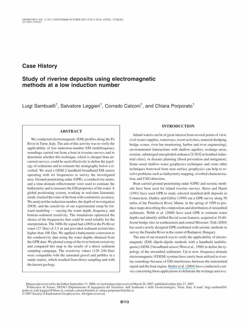
The measurements were conducted along a stretch of the Po Rivern Turin near Valentino Park, using the following instruments aboardmotorboat Figure 1:

a Geophex GEM-2 handheld broadband conductivity meteran IDS RIS/0 k2 georadar with a TR200 antenna 200-MHz cen-tral frequencya Tektronix 1502c time-domain reflectometer, or TDR to mea-sure water permittivitya ProfiLine-197 conductivity meter to measure water conductivi-ty and temperaturetwo LEICASystem 1200 GPS L1 + L2 receivers

In the first survey, two GPS receivers were placed aboard a boat.ne of the antennas was positioned at the stern, the other at the prowf the boat; both were fixed atop a 50-cm wooden pole to ensurereater visibility of the antennas and to reduce multiple paths. Thewo receivers were needed 1 to determine the bearing of the boatnd provide a second-by-second geographical reference of the geo-hysical instruments in an absolute reference system and 2 to cal-

A1

6.50

1.10

RadarGEM-2

A2

igure 1. Layout of the motorboat used for the survey: A1 and A2 arehe DGPS antennas; the dimensions are in meters.

4990250

4990000

4989750

4989500

4989264.85

East - WGS84 (m)

Nor

th -

WG

S84

(m

)

396276.25 396500

B

Turin

396750 397000 397250 397500

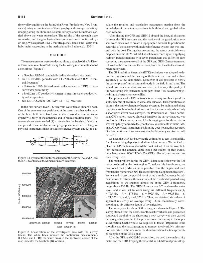
igure 2. Localization of the investigated area with the surveyracks. The white lines indicate the continuous measurementsGEM-2 and GPR; the white cross in the northwest corner of theap indicates the borehole B location.

ulate the rotation and translation parameters starting from thenowledge of the antenna positions in both local and global refer-nce systems.

After placing the GPR and GEM-2 aboard the boat, all distancesetween the GPS antennas and the vertices of the geophysical sen-ors were measured to create a topographic network to position theentroids of the sensors within a local reference system that was inte-ral with the boat. During data processing, the sensor centroids wereapped onto the UTM-WGS84 absolute reference system applyingelmert transformations with seven parameters that differ for each

urveying instant to move all of the GPR and GEM-2 measurements,eferred to the centroids of the sensors, from the local to the absoluteeference system.

The GPS real-time kinematic RTK technique was adopted to de-ne the trajectory and the bearing of the boat in real time and with anccuracy of a few centimeters. Moreover, it was possible to verifyhe carrier phases’ initialization directly in the field in real time. Thetored raw data were also postprocessed; in this way, the quality ofhe positioning was tested and some gaps in the RTK data from phys-cal signal obstructions were filled.

The presence of a GPS network is necessary to obtain good re-ults, in terms of accuracy in wide-area surveys. This condition alsoermits the same coherent reference system to be maintained alongrajectories of hundreds of kilometers. For the case study, where onlyshort river stretch was surveyed, the Politecnico di Torino perma-ent GPS station, located almost 2 km from the surveying area, wassed as the RTK master station.A1-Hz logging rate for the receiversas set up to synchronize the geophysical instruments with the GPSnes. Geophysical instrument positioning does not need an accuracyf a few centimeters, so low-cost, single-frequency receivers coulde used.

We used the GPR for bathymetric estimation to test its suitabilityor characterizing deposits in shallow inland waters. We decided tolace the GPR antennas aboard the boat instead of on the river bot-om because the antenna cable could get caught in tree trunks,ranches, or even WWII UXO. The GPR collected, on average, onerace every 3 cm.

The main problem during the GEM-2 data acquisition was the EMoise produced by the boat engine. To reduce this interference, weositioned the GEM-2 as far as possible from the engine and usedrequencies higher than 500 Hz according to Geophex indications.

e wanted to test the possibility of using a multifrequency broad-and sensor to estimate the resistivity of the riverbed deposits duringcquisition, so we spanned almost the entire GEM-2 frequencyange above 500 Hz. The GEM-2 sensor was 0.7 m above the waterevel, and it was set to work using six different frequencies: f1

775 Hz, f2 = 1175 Hz, f3 = 3925 Hz, f4 = 9825 Hz, f5

21,725 Hz, and f6 = 47,025 Hz. Thus, we obtained six values ofpparent resistivity on average every 0.8 m, theoretically corre-ponding to six different depths of investigation.

The survey tracks, about 300 m long, are shown in Figure 2. Theurvey started from the north, near the east riverbank, and proceededouthward parallel to the shoreline; a new survey was then carriedut along a line parallel to the previous one, but sailing in the oppo-ite direction. On the whole, we acquired 11 tracks 10 parallel to thehoreline and the last zigzagging to transect the river. No informa-ion was taken in the areas near the shoreline where the trees prevent-d reception of the GPS signal.

After the GPR and GEM-2 acquisition, we used the conductivityeter and the TDR, keeping the boat still in 14 different points Fig-

uptms

tespmtpa

trHeadct

n

um1vv

sstrtaFg

Gpab−ce

tnlafc

Tl

D

1

1

1

1

1

1

2

2

2

2

3

6Fp

Riverine deposits mapped by broadband EM B115

re 3 to conduct punctual measurements of the conductivity, tem-erature, and dielectric constant of the water at different depths. Inhis second survey, the LEIKAGPS allowed us to locate the punctual

easurements in points close to the tracks followed in the firsturvey.

In April 2006, almost five months after the geophysical surveys,he riverbed was sampled with a Van Veen grab bucket. No floodvent had occurred during the elapsed time from the geophysicalurvey until the day of the direct sampling survey. Twelve samplingoints Figure 3 were chosen according to the previous geophysicaleasurements, with the aim of recovering direct information where

he geophysical survey had failed. We positioned the samplingoints with a Garmin GPSMAP 60CS, a GPS system that providedn accuracy of the point locations of about 5 m.

We took two or four sediment samples at each selected point to ob-ain an average estimate and to overcome the difficulty of samplingiverbed deposits that were mainly made up of coarse material.owever, because of the nature of the deposits, it was impossible to

nsure enough material for a complete particle-size analysis. Welso obtained some geologic data from a borehole Figure 2, point Brilled about 300 m away on the west bank. This borehole reportedoarse gravel, pebbles, gravel, and sand Table 1 from 4 m abovehe level of the river surface to 17 m below it.

DATA PROCESSING

The water conductivity meter and the TDR measurements gaveearly constant water resistivity, temperature, and permittivity val-

4989850

4989800

4989750

4989700

4989650

4989600

3.0

2.5

2.0

1.5

1.0

East UTM WGS-84 (m)

Nor

th U

TM

WG

S-8

4 (m

)

396600

12

9

7

65

4

3

8

P11

P10

P1

P2

P3

Depth (m)

P4

P5 P6

P7

P8

P9

P12

N

S

E W

P13

P14

2 1

10

11

396650 396700 396750

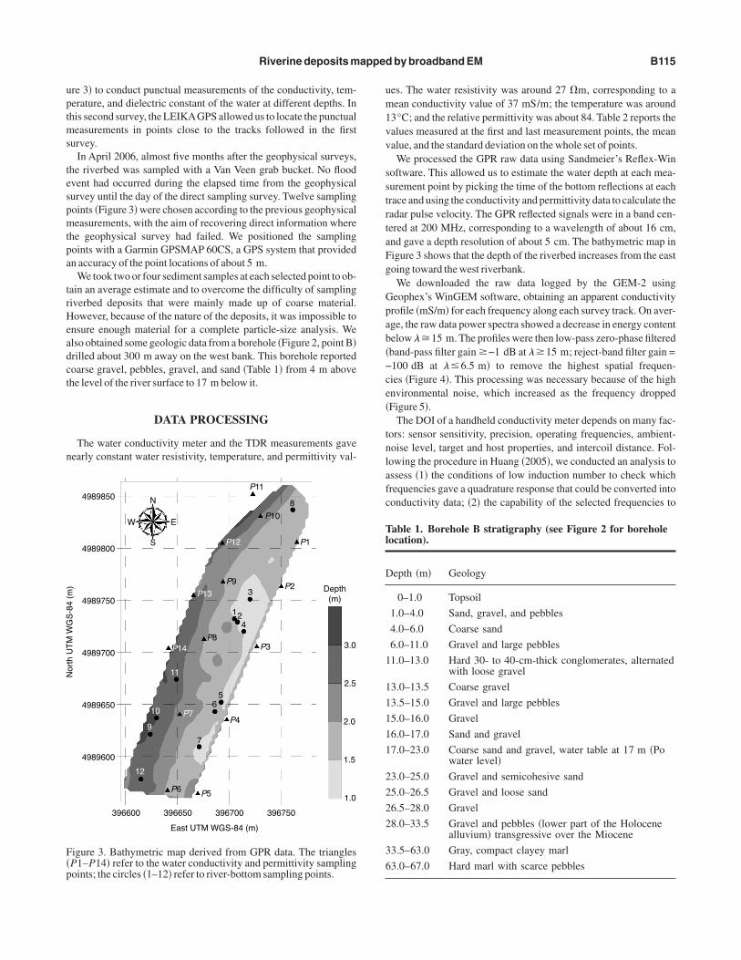
igure 3. Bathymetric map derived from GPR data. The trianglesP1–P14 refer to the water conductivity and permittivity samplingoints; the circles 1–12 refer to river-bottom sampling points.

es. The water resistivity was around 27 m, corresponding to aean conductivity value of 37 mS/m; the temperature was around

3°C; and the relative permittivity was about 84. Table 2 reports thealues measured at the first and last measurement points, the meanalue, and the standard deviation on the whole set of points.

We processed the GPR raw data using Sandmeier’s Reflex-Winoftware. This allowed us to estimate the water depth at each mea-urement point by picking the time of the bottom reflections at eachrace and using the conductivity and permittivity data to calculate theadar pulse velocity. The GPR reflected signals were in a band cen-ered at 200 MHz, corresponding to a wavelength of about 16 cm,nd gave a depth resolution of about 5 cm. The bathymetric map inigure 3 shows that the depth of the riverbed increases from the eastoing toward the west riverbank.

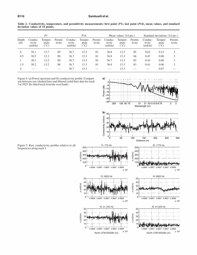
We downloaded the raw data logged by the GEM-2 usingeophex’s WinGEM software, obtaining an apparent conductivityrofile mS/m for each frequency along each survey track. On aver-ge, the raw data power spectra showed a decrease in energy contentelow 15 m. The profiles were then low-pass zero-phase filteredband-pass filter gain −1 dB at 15 m; reject-band filter gain =100 dB at 6.5 m to remove the highest spatial frequen-ies Figure 4. This processing was necessary because of the highnvironmental noise, which increased as the frequency droppedFigure 5.

The DOI of a handheld conductivity meter depends on many fac-ors: sensor sensitivity, precision, operating frequencies, ambient-oise level, target and host properties, and intercoil distance. Fol-owing the procedure in Huang 2005, we conducted an analysis tossess 1 the conditions of low induction number to check whichrequencies gave a quadrature response that could be converted intoonductivity data; 2 the capability of the selected frequencies to

able 1. Borehole B stratigraphy (see Figure 2 for boreholeocation).

epth m Geology

0–1.0 Topsoil

1.0–4.0 Sand, gravel, and pebbles

4.0–6.0 Coarse sand

6.0–11.0 Gravel and large pebbles

1.0–13.0 Hard 30- to 40-cm-thick conglomerates, alternatedwith loose gravel

3.0–13.5 Coarse gravel

3.5–15.0 Gravel and large pebbles

5.0–16.0 Gravel

6.0–17.0 Sand and gravel

7.0–23.0 Coarse sand and gravel, water table at 17 m Powater level

3.0–25.0 Gravel and semicohesive sand

5.0–26.5 Gravel and loose sand

6.5–28.0 Gravel

8.0–33.5 Gravel and pebbles lower part of the Holocenealluvium transgressive over the Miocene

3.5–63.0 Gray, compact clayey marl

3.0–67.0 Hard marl with scarce pebbles

Td

D

Fs3

Ff

B116 Sambuelli et al.

able 2. Conductivity, temperature, and permittivity measurements: first point (P1), last point (P14), mean values, and standardeviation values of 14 points.

P1 P14 Mean values 14 pts. Standard deviations 14 pts.epth

mConduc-

tivitymS/m

Temper-ature°C

Permit-tivity

Conduc-tivity

mS/m

Temper-ature°C

Permit-tivity

Conduc-tivity

mS/m

Temper-ature°C

Permit-tivity

Conduc-tivity

mS/m

Temper-ature°C

Permit-tivity

0 39.1 13.7 89 36.7 13.3 81 36.8 13.3 85 0.62 0.12 3

0.5 38.5 13.3 90 36.7 13.3 81 36.8 13.3 84 0.47 0.06 3

1 38.3 13.2 90 36.7 13.3 83 36.7 13.3 85 0.43 0.06 3

1.5 38.2 13.2 88 36.7 13.3 81 36.8 13.3 83 0.41 0.06 3

2 — — — 36.7 13.3 — — 13.3 — — 0.07 —

a)

Wavelength (m) P

ower

(dB

) 209 126 90 70 31 21 1613 10 9 8 76 3 2

0

–6

–12

–18

–24

–30

–36

b)

Distance (m)

Con

duct

ivity

(m

S/m

)

0 50 100 150 200 250 300

50

40

30

20

10

0

igure 4. a Power spectrum and b conductivity profile. Compari-on between raw dashed line and filtered solid line data for trackat 3925 Hz third track from the west bank.

f1: 775 Hz

σ (m

S/m

)

4.9896 4.9897 4.9897 4.9897 4.9898x 106

500

400

300

200

100

0

f2: 1775 Hz

σ (m

S/m

)

4.9896 4.9897 4.9897 4.9897 4.9898x 106

500

400

300

200

100

0

f5: 21,725 Hz

σ (m

S/m

)

4.9896 4.9897 4.9897 4.9897 4.9898x 106

50

40

30

20

10

0

f6: 47,025 Hz

North UTM-WGS84 (m) North UTM-WGS84 (m)

σ (m

S/m

)

4.9896 4.9897 4.9897 4.9897 4.9898x 106

50

40

30

20

10

0

f3: 3925 Hz

σ (m

S/m

)

4.9896 4.9897 4.9897 4.9897 4.9898x 106

50

40

30

20

10

0

f4: 9825 Hz

σ (m

S/m

)

4.9896 4.9897 4.9897 4.9897 4.9898x 106

50

40

30

20

10

0

igure 5. Raw conductivity profiles relative to allrequencies along track 3.

dcr

5a1wWssio2p4

qiHbscn

Gpmcir

to2

ws

Fnq21t

FamdctfMrt

Riverine deposits mapped by broadband EM B117

etect the river bottom sediment reliably, that is, the DOI; and 3 theapability to discriminate reliably among sediments having differentesistivity, i.e., sensitivity.

For this purpose, we conducted a set of simulations that spanned a00-Hz to 50-kHz frequency range with six frequencies per decade,water resistivity of 27 m, a 1- to 3-m water depth range, and a3.5- to 532-m sediment resistivity range. The latter two rangesere selected on the basis of the bathymetric and the geologic data.e conducted this analysis using the Anderson 1979 modeling

oftware. We obtained 25 synthetic apparent conductivities corre-ponding to five depths in the 1- to 3-m range, as well as five resistiv-ty values in the 13.5- to 532-m range using this simulation at eachf the following frequencies: 733.9; 1077.22; 3406; 10,772.2;3,208; and 50,000 Hz. We used these results to compare with ex-erimental data at, respectively, 775; 1175; 3925; 9825; 21,725; and7,025 Hz.

The apparent conductivity can be calculated only from theuadrature response of the conductivity meter when it operates at annduction number much lower than one McNeill, 1980. Moreover,uang and Won 2003 demonstrate that the induction number muste larger than 0.02; otherwise, the EM response is small and has amall dependence on the frequency. Therefore, it is possible to onlyonsider reliable those EM responses obtained when the inductionumber is included in the following range:

0.02 B =s

= i0

2s 1. 1

iven the GEM-2 intercoil spacing s = 1.66 m and the magneticermeability of free space 0 = 410−7 H/m, we calculated theean and standard deviation of the induction numbers relative to the

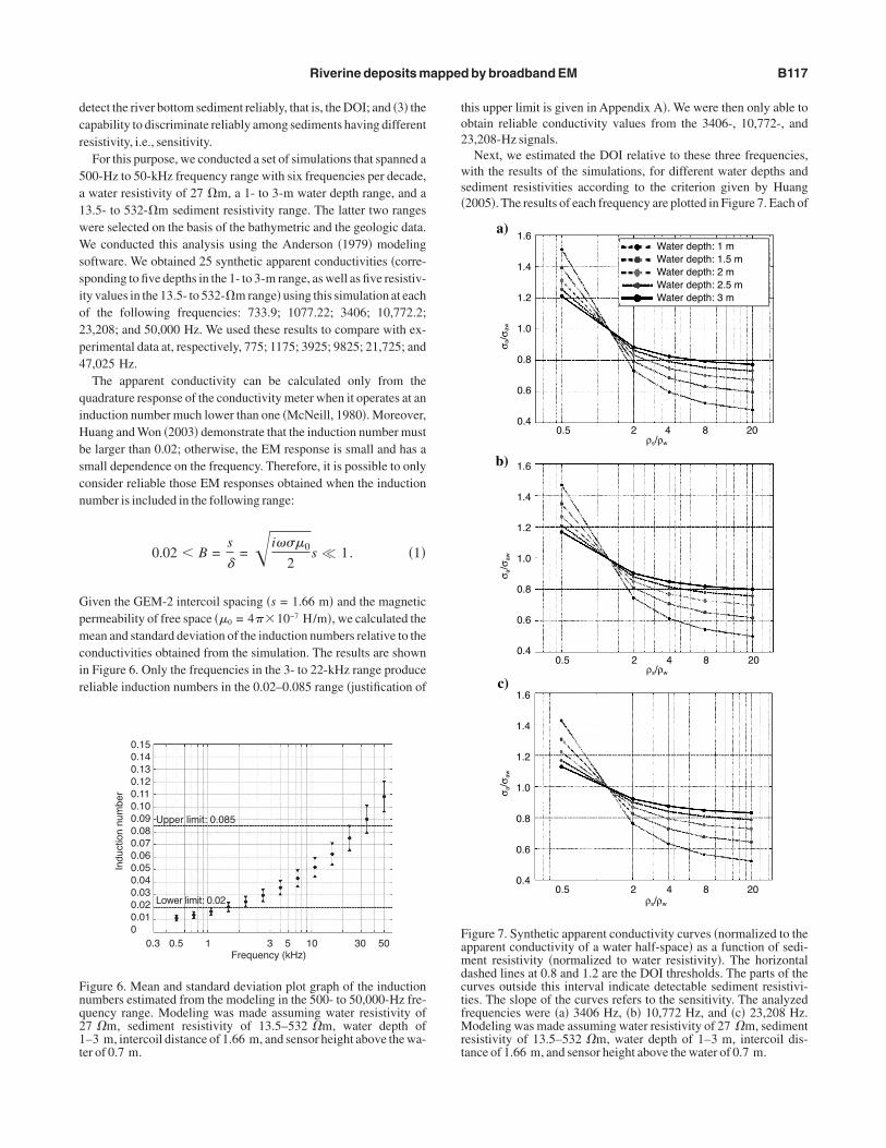
onductivities obtained from the simulation. The results are shownn Figure 6. Only the frequencies in the 3- to 22-kHz range produceeliable induction numbers in the 0.02–0.085 range justification of

Frequency (kHz)

Indu

ctio

n nu

mbe

r

0.3 0.5 1

Upper limit: 0.085

Lower limit: 0.02

3 5 10 30 50

0.15 0.14 0.13 0.12 0.11 0.10 0.09 0.08 0.07 0.06 0.05 0.04 0.03 0.02 0.01 0

igure 6. Mean and standard deviation plot graph of the inductionumbers estimated from the modeling in the 500- to 50,000-Hz fre-uency range. Modeling was made assuming water resistivity of7 m, sediment resistivity of 13.5–532 m, water depth of–3 m, intercoil distance of 1.66 m, and sensor height above the wa-er of 0.7 m.

his upper limit is given in Appendix A. We were then only able tobtain reliable conductivity values from the 3406-, 10,772-, and3,208-Hz signals.

Next, we estimated the DOI relative to these three frequencies,ith the results of the simulations, for different water depths and

ediment resistivities according to the criterion given by Huang2005. The results of each frequency are plotted in Figure 7. Each of

ρs/ρw

σ a/σ

aw

0.5 2 84 20

1.6

1.4

1.2

1.0

0.8

0.6

0.4

Water depth: 1 mWater depth: 1.5 mWater depth: 2 mWater depth: 2.5 mWater depth: 3 m

a)

ρs/ρw

σ a/σ

aw

0.5 2 84 20

1.6

1.4

1.2

1.0

0.8

0.6

0.4

b)

ρs/ρw

σ a/σ

aw

0.5 2 84 20

1.6

1.4

1.2

1.0

0.8

0.6

0.4

c)

igure 7. Synthetic apparent conductivity curves normalized to thepparent conductivity of a water half-space as a function of sedi-ent resistivity normalized to water resistivity. The horizontal

ashed lines at 0.8 and 1.2 are the DOI thresholds. The parts of theurves outside this interval indicate detectable sediment resistivi-ies. The slope of the curves refers to the sensitivity. The analyzedrequencies were a 3406 Hz, b 10,772 Hz, and c 23,208 Hz.

odeling was made assuming water resistivity of 27 m, sedimentesistivity of 13.5–532 m, water depth of 1–3 m, intercoil dis-ance of 1.66 m, and sensor height above the water of 0.7 m.

totraAopd—s

ttTc

t3lmcotocemib

mbtt2ao

mpmi

wa

Tf

wcf

tesmatds

Tb

3l12im

ctmt

FTp

B118 Sambuelli et al.

he views plots the ratio of the apparent conductivity of a water layerver sediments a to the apparent conductivity of an indefinite wa-er layer aw versus the ratio of the sediment resistivity s to the wateresistivity w. The two horizontal lines represent the 20% thresholds,nd the curved lines represent a/aw at five different water depths.ccording to the results of these simulations, if we accept a thresh-ld value of 20% — i.e., we can detect a sediment if the measured ap-arent conductivity differs by more than 20% from the apparent con-uctivity one would have measured above water alone a/aw = 1

then the following considerations can be drawn concerning theensitivity and the DOI.

All of the graphs show there is quite a low sensitivity to the resis-ivity of the sediments, particularly if the sediments are more resis-ive than the water the curves have a very weak slope when s w.he sensitivity grows as the frequency and the riverbed depth de-rease.

We obtained only a very rough capability to discriminate be-ween coarse 100 m and finer 100 m sediments from the406-Hz signal down to a depth of 2.5 m. When the water depth wasower than 1.5 m, we were also able to discriminate between sedi-

ents with different resistivities. We obtained only a very roughapability to discriminate between coarse 100 m and finer100 m sediments from the 10,772-Hz signal down to a depthf 2 m. When the water depth was lower than 1 m, we were also ableo discriminate between sediments with different resistivities. Webtained only a very rough capability to discriminate betweenoarse 100 m and finer 100 m sediments from the high-st frequency 23,208 Hz down to a depth of 1 m, which was theinimum water depth we encountered in the survey. This means the

nformation carried by this latter signal is mainly relative to theathymetry.

4989850

4989800

4989750

4989700

4989650

4989600

400

300

200

100

East UTM WGS-84 (m)

Nor

th U

TM

WG

S-8

4 (m

)

396600

79

10

11

12

65

4

3

8Ωm

21

396650 396700 396750

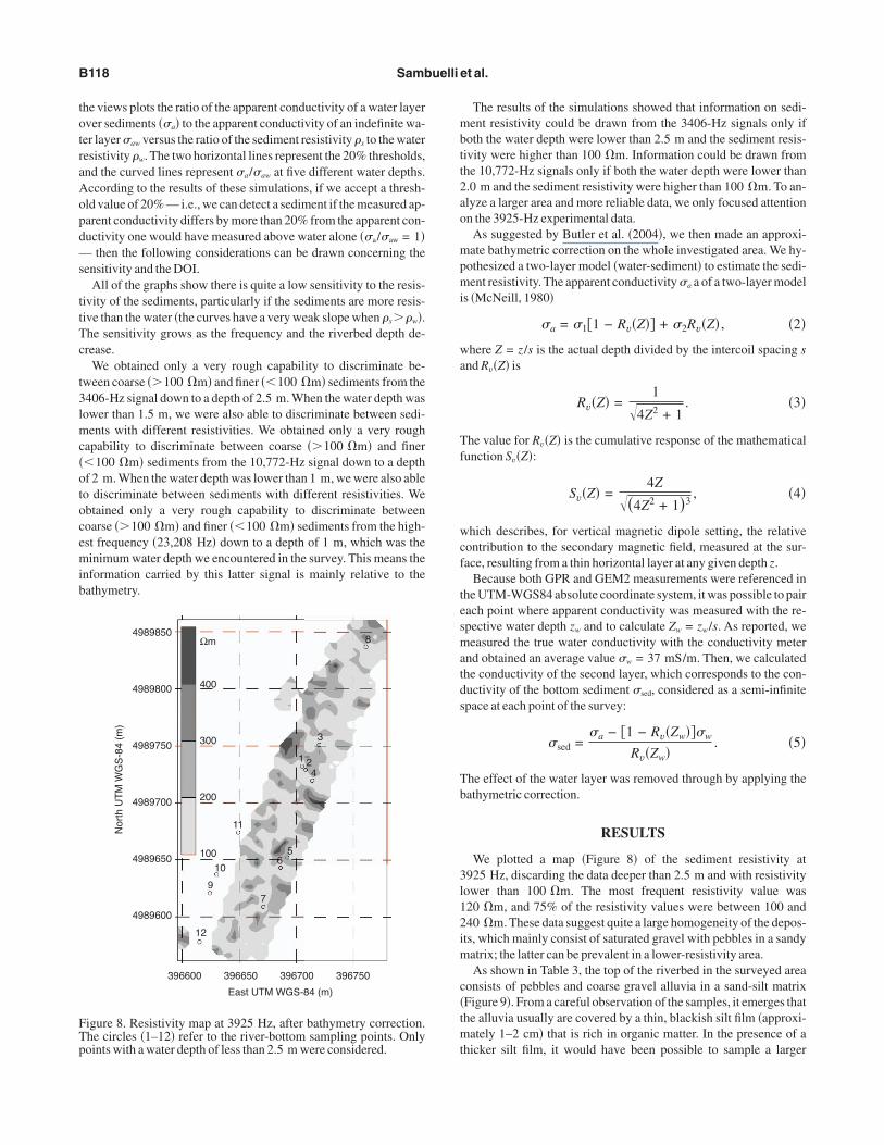
igure 8. Resistivity map at 3925 Hz, after bathymetry correction.he circles 1–12 refer to the river-bottom sampling points. Onlyoints with a water depth of less than 2.5 m were considered.

The results of the simulations showed that information on sedi-ent resistivity could be drawn from the 3406-Hz signals only if

oth the water depth were lower than 2.5 m and the sediment resis-ivity were higher than 100 m. Information could be drawn fromhe 10,772-Hz signals only if both the water depth were lower than.0 m and the sediment resistivity were higher than 100 m. To an-lyze a larger area and more reliable data, we only focused attentionn the 3925-Hz experimental data.

As suggested by Butler et al. 2004, we then made an approxi-ate bathymetric correction on the whole investigated area. We hy-

othesized a two-layer model water-sediment to estimate the sedi-ent resistivity. The apparent conductivity a a of a two-layer model

s McNeill, 1980

a = 11 − RvZ + 2RvZ , 2

here Z = z/s is the actual depth divided by the intercoil spacing snd RvZ is

RvZ =1

4Z2 + 1. 3

he value for RvZ is the cumulative response of the mathematicalunction SvZ:

SvZ =4Z

4Z2 + 13, 4

hich describes, for vertical magnetic dipole setting, the relativeontribution to the secondary magnetic field, measured at the sur-ace, resulting from a thin horizontal layer at any given depth z.

Because both GPR and GEM2 measurements were referenced inhe UTM-WGS84 absolute coordinate system, it was possible to pairach point where apparent conductivity was measured with the re-pective water depth zw and to calculate Zw = zw/s. As reported, weeasured the true water conductivity with the conductivity meter

nd obtained an average value w = 37 mS/m. Then, we calculatedhe conductivity of the second layer, which corresponds to the con-uctivity of the bottom sediment sed, considered as a semi-infinitepace at each point of the survey:

sed =a − 1 − RvZww

RvZw. 5

he effect of the water layer was removed through by applying theathymetric correction.

RESULTS

We plotted a map Figure 8 of the sediment resistivity at925 Hz, discarding the data deeper than 2.5 m and with resistivityower than 100 m. The most frequent resistivity value was20 m, and 75% of the resistivity values were between 100 and40 m. These data suggest quite a large homogeneity of the depos-ts, which mainly consist of saturated gravel with pebbles in a sandy

atrix; the latter can be prevalent in a lower-resistivity area.As shown in Table 3, the top of the riverbed in the surveyed area

onsists of pebbles and coarse gravel alluvia in a sand-silt matrixFigure 9. From a careful observation of the samples, it emerges thathe alluvia usually are covered by a thin, blackish silt film approxi-

ately 1–2 cm that is rich in organic matter. In the presence of ahicker silt film, it would have been possible to sample a larger

amc

bat

mcor

pcpqpinst

ses

sabb

Tamw

Sp

1

2

3

4

5

6

7

8

9

1

1

1

Fp

Riverine deposits mapped by broadband EM B119

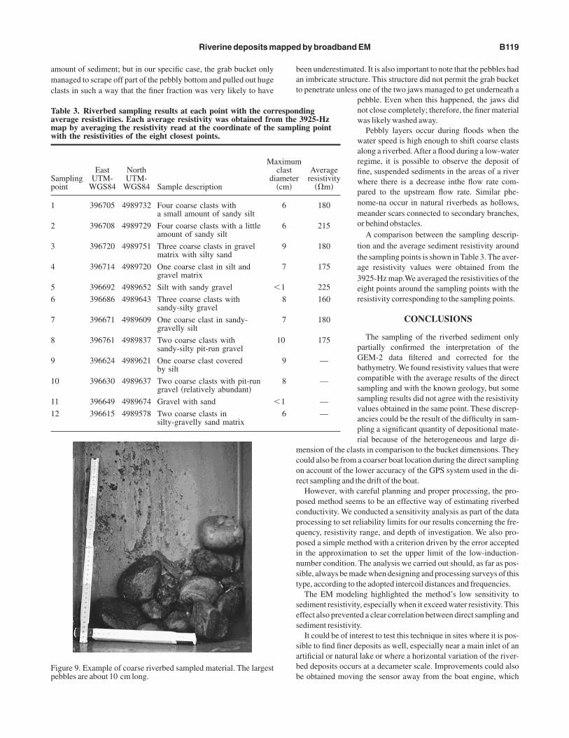
mount of sediment; but in our specific case, the grab bucket onlyanaged to scrape off part of the pebbly bottom and pulled out huge

lasts in such a way that the finer fraction was very likely to have

able 3. Riverbed sampling results at each point with the corverage resistivities. Each average resistivity was obtained froap by averaging the resistivity read at the coordinate of theith the resistivities of the eight closest points.

amplingoint

EastUTM-

WGS84

NorthUTM-

WGS84 Sample description

M

d

396705 4989732 Four coarse clasts witha small amount of sandy silt

396708 4989729 Four coarse clasts with a littleamount of sandy silt

396720 4989751 Three coarse clasts in gravelmatrix with silty sand

396714 4989720 One coarse clast in silt andgravel matrix

396692 4989652 Silt with sandy gravel

396686 4989643 Three coarse clasts withsandy-silty gravel

396671 4989609 One coarse clast in sandy-gravelly silt

396761 4989837 Two coarse clasts withsandy-silty pit-run gravel

396624 4989621 One coarse clast coveredby silt

0 396630 4989637 Two coarse clasts with pit-rungravel relatively abundant

1 396649 4989674 Gravel with sand

2 396615 4989578 Two coarse clasts insilty-gravelly sand matrix

igure 9. Example of coarse riverbed sampled material. The largestebbles are about 10 cm long.

een underestimated. It is also important to note that the pebbles hadn imbricate structure. This structure did not permit the grab bucketo penetrate unless one of the two jaws managed to get underneath a

pebble. Even when this happened, the jaws didnot close completely; therefore, the finer materialwas likely washed away.

Pebbly layers occur during floods when thewater speed is high enough to shift coarse clastsalong a riverbed.After a flood during a low-waterregime, it is possible to observe the deposit offine, suspended sediments in the areas of a riverwhere there is a decrease inthe flow rate com-pared to the upstream flow rate. Similar phe-nome-na occur in natural riverbeds as hollows,meander scars connected to secondary branches,or behind obstacles.

A comparison between the sampling descrip-tion and the average sediment resistivity aroundthe sampling points is shown in Table 3. The aver-age resistivity values were obtained from the3925-Hz map.We averaged the resistivities of theeight points around the sampling points with theresistivity corresponding to the sampling points.

CONCLUSIONS

The sampling of the riverbed sediment onlypartially confirmed the interpretation of theGEM-2 data filtered and corrected for thebathymetry. We found resistivity values that werecompatible with the average results of the directsampling and with the known geology, but somesampling results did not agree with the resistivityvalues obtained in the same point. These discrep-ancies could be the result of the difficulty in sam-pling a significant quantity of depositional mate-rial because of the heterogeneous and large di-

ension of the clasts in comparison to the bucket dimensions. Theyould also be from a coarser boat location during the direct samplingn account of the lower accuracy of the GPS system used in the di-ect sampling and the drift of the boat.

However, with careful planning and proper processing, the pro-osed method seems to be an effective way of estimating riverbedonductivity. We conducted a sensitivity analysis as part of the datarocessing to set reliability limits for our results concerning the fre-uency, resistivity range, and depth of investigation. We also pro-osed a simple method with a criterion driven by the error acceptedn the approximation to set the upper limit of the low-induction-umber condition. The analysis we carried out should, as far as pos-ible, always be made when designing and processing surveys of thisype, according to the adopted intercoil distances and frequencies.

The EM modeling highlighted the method’s low sensitivity toediment resistivity, especially when it exceed water resistivity. Thisffect also prevented a clear correlation between direct sampling andediment resistivity.

It could be of interest to test this technique in sites where it is pos-ible to find finer deposits as well, especially near a main inlet of anrtificial or natural lake or where a horizontal variation of the river-ed deposits occurs at a decameter scale. Improvements could alsoe obtained moving the sensor away from the boat engine, which

ding3925-Hz

ling point

Averageresistivity

m

180

215

180

175

225

160

180

175

—

—

—

—

responm thesamp

aximumclast

iametercm

6

6

9

7

1

8

7

10

9

8

1

6

co

cwmwptG

smdGmg

natcf

4c

wis

T

Wi

WAo

A

B

B

D

H

H

M

T

W

W

Fbcde

B120 Sambuelli et al.

ould result in a better signal-to-noise ratio but also in a larger spreadf the equipment and more difficult positioning.

The GPS measurements were very useful, as they ensured smoothomparisons and overlaps between the GEM-2 and GPR responses,hich was crucial to perform the bathymetric correction. Further-ore, the RTK mode made it possible for us to obtain the coordinatesith centimetric accuracy in real time, allowing the location ofunctual measurements, taken with the conductivity meter, near theracks followed during the continuous measurements GPR andEM-2.

ACKNOWLEDGMENTS

The authors thank the Reale Società Canottieri Cerea of Turin forupplying the boat and the steersman, Alberto Godio for the TDReasurements and fruitful discussions, Stefano Stocco for the con-

uctivity meter measurements, Emanuele Pesenti for help in thePS operations, and Hydrodata S.p.A. for sampling the bottom sedi-ents. The authors also thank the reviewers, whose observations

reatly improved the manuscript.

APPENDIX A

JUSTIFICATION OF THE SELECTEDUPPER LIMIT OF THE LOW-INDUCTION-

NUMBER CONDITION

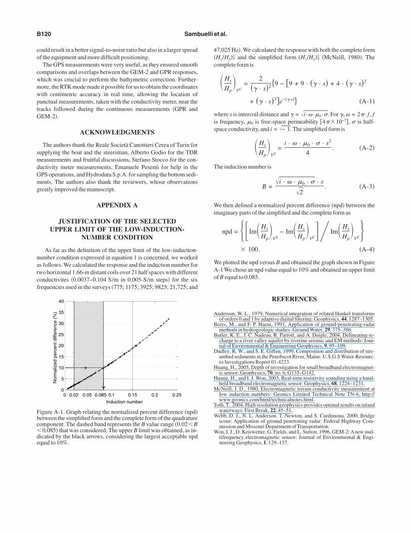
As far as the definition of the upper limit of the low-induction-umber condition expressed in equation 1 is concerned, we workeds follows. We calculated the response and the induction number forwo horizontal 1.66-m distant coils over 21 half spaces with differentonductivites 0.0037–0.104 S/m in 0.005-S/m steps for the sixrequencies used in the surveys 775; 1175; 3925; 9825; 21,725; and

40

35

30

25

20

15

10

5

0

Induction number

Nor

mal

ized

per

cent

diff

eren

ce (

%)

0 0.02 0.05 0.085 0.1 0.15 0.2 0.25

igure A-1. Graph relating the normalized percent difference npdetween the simplified form and the complete form of the quadratureomponent. The dashed band represents the B value range 0.02B0.085 that was considered. The upper B limit was obtained, as in-

icated by the black arrows, considering the largest acceptable npd

qual to 10%.

7,025 Hz. We calculated the response with both the complete formHx/HpV

C and the simplified form Hz/HpVS McNeill, 1980. The

omplete form is

Hs

Hp

VC=

2

· s29 − 9 + 9 · · s + 4 · · s2

+ · s3e−·s A-1

here s is intercoil distance and = i · ·0 ·. For , = 2 · f , fs frequency, 0 is free-space permeability 410−7, is half-pace conductivity, and i = − 1. The simplified form is

Hs

Hp

VS=

i · · 0 · · s2

4. A-2

he induction number is

B =i · · 0 · · s

2. A-3

e then defined a normalized percent difference npd between themaginary parts of the simplified and the complete form as

npd = ImHs

Hp

VS− ImHs

Hp

VC ImHs

Hp

VC

100. A-4

e plotted the npd versus B and obtained the graph shown in Figure-1 We chose an npd value equal to 10% and obtained an upper limitf B equal to 0.085.

REFERENCES

nderson, W. L., 1979, Numerical integration of related Hankel transformsof orders 0 and 1 by adaptive digital filtering: Geophysics, 44, 1287–1305.

eres, M., and F. P. Haeni, 1991, Application of ground-penetrating-radarmethods in hydrogeologic studies: Ground Water, 29, 375–386.

utler, K. E., J. C. Nadeau, R. Parrott, and A. Daigle, 2004, Delineating re-charge to a river valley aquifer by riverine seismic and EM methods: Jour-nal of Environmental & Engineering Geophysics, 9, 95–109.

udley, R. W., and S. E. Giffen, 1999, Composition and distribution of stre-ambed sediments in the Penobscot River, Maine: U.S.G.S Water-Resourc-es Investigations Report 01-4223.

uang, H., 2005, Depth of investigation for small broadband electromagnet-ic sensor: Geophysics, 70, no. 6, G135–G142.

uang, H., and I. J. Won, 2003, Real-time resistivity sounding using a hand-held broadband electromagnetic sensor: Geophysics, 68, 1224–1231.cNeill, J. D., 1980, Electromagnetic terrain conductivity measurement atlow induction numbers: Geonics Limited Technical Note TN-6, http://www.geonics.com/html/technicalnotes.html.

oth, T., 2004, High resolution geophysics provides optimal results on inlandwaterways: First Break, 22, 45–51.ebb, D. J., N. L. Anderson, T. Newton, and S. Cardimona, 2000, Bridgescour: Application of ground penetrating radar: Federal Highway Com-mission and Missouri Department of Transportation.on, I. J., D. Keiswetter, G. Fields, and L. Sutton, 1996, GEM-2:Anew mul-tifrequency electromagnetic sensor: Journal of Environmental & Engi-

neering Geophysics, 1, 129–137.