Studies of Millimeter-wave Atmospheric Noise above Mauna Kea

The Astrophysical Journal, 708:1674–1691, 2010 January 10 doi:10.1088/0004-637X/708/2/1674C© 2010. The American Astronomical Society. All rights reserved. Printed in the U.S.A.

STUDIES OF MILLIMETER-WAVE ATMOSPHERIC NOISE ABOVE MAUNA KEA

J. Sayers1,6

, S. R. Golwala2, P. A. R. Ade

3, J. E. Aguirre

3,4, J. J. Bock

1, S. F. Edgington

2, J. Glenn

5, A. Goldin

1, D. Haig

3,

A. E. Lange2, G. T. Laurent

5, P. D. Mauskopf

3, H. T. Nguyen

1, P. Rossinot

2, and J. Schlaerth

51 Jet Propulsion Laboratory, California Institute of Technology, 4800 Oak Grove Drive, Pasadena, CA 91109, USA; [email protected]

2 Division of Physics, Mathematics, & Astronomy, California Institute of Technology, Mail Code 59-33, Pasadena, CA 91125, USA3 Physics and Astronomy, Cardiff University, 5 The Parade, P. O. Box 913, Cardiff CF24 3YB, Wales, UK

4 University of Pennsylvania, 209 South 33rd Street, Philadelphia, PA 19104, USA5 Center for Astrophysics and Space Astronomy & Department of Astrophysical and Planetary Sciences, University of Colorado, 389 UCB, Boulder, CO 80309, USA

Received 2009 April 24; accepted 2009 November 24; published 2009 December 23

ABSTRACT

We report measurements of the fluctuations in atmospheric emission (atmospheric noise) above Mauna Kea recordedwith Bolocam at 143 and 268 GHz from the Caltech Submillimeter Observatory. The 143 GHz data were collectedduring a 40 night observing run in late 2003, and the 268 GHz observations were made in early 2004 and early2005 over a total of 60 nights. Below �0.5 Hz, the data time-streams are dominated by atmospheric noise inall observing conditions. The atmospheric noise data are consistent with a Kolmogorov–Taylor turbulence modelfor a thin wind-driven screen, and the median amplitude of the fluctuations is 280 mK2 rad−5/3 at 143 GHz and4000 mK2 rad−5/3 at 268 GHz. Comparing our results with previous ACBAR data, we find that the normalizationof the power spectrum of the atmospheric noise fluctuations is a factor of �80 larger above Mauna Kea than abovethe South Pole at millimeter wavelengths. Most of this difference is due to the fact that the atmosphere abovethe South Pole is much drier than the atmosphere above Mauna Kea. However, the atmosphere above the SouthPole is slightly more stable as well: the fractional fluctuations in the column depth of precipitable water vaporare a factor of �√

2 smaller at the South Pole compared to Mauna Kea. Based on our atmospheric modeling,we developed several algorithms to remove the atmospheric noise, and the best results were achieved when wedescribed the fluctuations using a low-order polynomial in detector position over the 8′ field of view. However, evenwith these algorithms, we were not able to reach photon-background-limited instrument photometer performanceat frequencies below �0.5 Hz in any observing conditions. We also observed an excess low-frequency noise thatis highly correlated between detectors separated by � (f/#)λ; this noise appears to be caused by atmosphericfluctuations, but we do not have an adequate model to explain its source. We hypothesize that the correlationsarise from the classical coherence of the electromagnetic field across a distance of �(f/#)λ on the focal plane.

Key words: atmospheric effects – site testing – techniques: photometric

Online-only material: color figures

1. INTRODUCTION

A number of wide-field ground-based millimeter/submillimeter imaging arrays have been commissioned dur-ing the past 15 years, including SCUBA (Holland et al. 1999),MAMBO (Kreysa et al. 1998), Bolocam (Glenn et al. 1998),SHARC II (Dowell et al. 2003), APEX-SZ (Dobbs et al. 2006),LABOCA (Kreysa et al. 2003), ACT (Kosowsky 2003), andSPT (Ruhl et al. 2004). Since these cameras are operated atground-based telescopes, they all see emission from water va-por in the atmosphere. In almost all cases, the raw data fromthese cameras are dominated by atmospheric noise caused byfluctuations in this emission.7 All of these cameras make useof the fact that the atmospheric water vapor is in the near field,and therefore most of the fluctuations in the atmospheric emis-sion are recorded as a common-mode signal among all of thedetectors (Jenness et al. 1998; Borys et al. 1999; Reichertz et al.

6 NASA Postdoctoral Program Fellow.7 The column depth of oxygen in the atmosphere also produces anon-negligible amount of emission, a factor of a few less than the emissionfrom water vapor under typical conditions at Mauna Kea. However, the oxygenin the atmosphere is well mixed, and therefore fluctuations in the emission areminimal. In contrast, the temperature of the atmosphere tends to be close to thecondensation point of the water vapor, and causes the water vapor to be poorlymixed in the atmosphere. Therefore, there are, in general, significantfluctuations in the emission from water vapor (Masson 1994).

2001; Weferling et al. 2002; Archibald et al. 2002). Most of theatmospheric noise can be removed from the data by subtract-ing this common-mode signal, and this method has been shownto be at least as effective as the traditional beam-switching orchopping techniques (Conway et al. 1965; Weferling et al. 2002;Archibald et al. 2002).

However, this subtraction does not allow recovery ofphoton-background-limited instrument photometer (BLIP) per-formance on scales where the atmospheric signal is largest(i.e., at low frequencies in the time-stream data). In the caseof Bolocam, the majority of the atmospheric fluctuations canbe removed by subtraction of the common-mode signal; but theresidual atmospheric noise still limited the sensitivity of ourdata, thus motivating further study of these atmospheric fluctu-ations. This study focused on two main topics: (1) determiningthe phenomenology of the atmospheric noise (i.e., could it bemodeled in a simple and robust way); and (2) finding moreeffective ways to remove the atmospheric noise based on thismodeling.

1.1. Instrument Description

Bolocam is a large format, millimeter-wave camera designedto be operated at the Caltech Submillimeter Observatory (CSO),and �115 optical detectors were used for the observationsdescribed in this paper. Cylindrical waveguides and a metal-

1674

http://dx.doi.org/10.1088/0004-637X/708/2/1674

mailto:[email protected]

No. 2, 2010 BOLOCAM ATMOSPHERIC NOISE 1675

mesh filter are used to define the passbands for the detectors,which can be centered at either 143 or 268 GHz with a �15%fractional bandwidth. Note that, for either configuration, theentire focal plane uses the same passband. A cold (4 K) Lyot stopis used to define the illumination of the 10.4 m primary mirrorwith a diameter of �8 meters, and the resulting far-field beamshave full width at half-maximums (FWHMs) of 60′′ or 30′′ (143or 268 GHz). The detector array, which utilizes silicon nitridemicromesh (spider-web) bolometers (Mauskopf et al. 1997), hasa hexagonal geometry with nearby detectors separated by 40′′,and the field of view (FOV) is approximately 8′.

The optical efficiency from the cryostat window to thedetectors is 8% at 143 GHz and 19% at 268 GHz; at eachfrequency approximately half of the loss in efficiency is dueto coupling to the Lyot stop and half is due to inefficiencies(reflection, standing waves, or loss) in the metal-mesh filterstack. At 143 GHz, the typical optical load from the atmosphereis relatively small (�0.5 pW or 10 K), but the total optical load is�4 pW (80 K), most of which is sourced by warm surfaces insidethe relay optics box. The atmosphere contributes an optical loadof 5–15 pW (20–60 K) per detector at 268 GHz, and there isan additional load of �10 pW (40 K) due to the warm and coldoptics. Optical shot and Bose noise contribute in roughly equalamounts to the total photon noise at each observing frequency,with the BLIP NEPγ � 1.5 mK/

√Hz (2.3 mKCMB/

√Hz) at

143 GHz and the BLIP NEPγ � 0.8 mK/√

Hz (4.5 mKCMB/√Hz) at 268 GHz.8 More details of the Bolocam instrument can

be found in Glenn et al. (1998); Glenn et al. (2003); Haig et al.(2004); and Sayers (2007).

The data we describe in this paper were collected duringthree separate observing runs at the CSO: a 40 night run at143 GHz in late 2003, a 10 night run at 268 GHz in early2004, and a 50 night run at 268 GHz in early 2005. For the143 GHz observations, we focused on two science fields, onecentered on the Lynx field at 08h49m12s, +44d50m24s (J2000)and one coinciding with the Subaru/XMM-Newton Deep Survey(SXDS or SDS1) centered at 02h18m00s, −5d00m00s (J2000).The 268 GHz observations were all focused on the COSMOSfield at 10h00m29s, +2d12m21s (J2000). All three of these fieldsare blank, which means they contain very little astronomicalsignal. Therefore, our data are well suited to measure the signalcaused by emission from the atmosphere. To map these fields,we raster-scanned the telescope parallel to the R.A. or decl. axisat 4 arcmin s−1 for the 143 GHz observations and 2 arcmin s−1

for the 268 GHz observations.9 Throughout this paper, we willrefer to single scans and single observations; a scan is oneraster across the field and is �15 s (�30′–60′) in length andan observation is a set of �15–20 scans that completely mapthe science field, which takes �10 minutes. Our total data setcontains approximately 1000 observations at each observingfrequency, with the 143 GHz data split evenly among Lynx and

8 The subscript cosmic microwave background (CMB) is used throughoutthis paper to denote CMB temperatures; all temperatures given without asubscript refer to Rayleigh–Jeans temperatures.9 Slower scan speeds improve our observing efficiency by reducing thefractional amount of time spent turning the telescope around between scans(the CSO turnaround time is approximately 10 s regardless of scan speed), butfaster scan speeds improve the instantaneous sensitivity of the camera bymoving the signal band to higher frequencies where there is less atmosphericnoise. Several scan speeds were tried at each observing frequency to find thebest combination of observing efficiency and instantaneous sensitivity, and wefound that 4 arcmin s−1 is optimal for 143 GHz observations and 2 arcmin s−1

is optimal for 268 GHz observations. Note that it may be possible to optimizethe CSO telescope drive servo to improve the turnaround time, but this has notbeen attempted.

SDS1. Flux calibration was determined from observations ofUranus, Neptune, and Mars, and nearby quasars were used forpointing reconstruction. A more detailed description of the datais given in Sayers et al. (2009) and J. E. Aguirre et al. (2010, inpreparation).

1.2. Typical Observing Conditions

Since atmospheric noise from water vapor is generally thelimiting factor in the sensitivity of broadband, ground-based,millimeter-wave observations, the premier sites for these ob-servations, which include Mauna Kea, Atacama, and the SouthPole, are extremely dry. On Mauna Kea, the CSO continuouslymonitors the atmospheric opacity with a narrowband, hetero-dyne τ -meter that measures the optical depth at 225 GHz (τ225)(Chamberlin 2004). Since τ225 is a monotonically increasingfunction of the column depth of precipitable water vapor in theatmosphere, these τ225 measurements can be used to quantifythe dryness of the atmosphere above Mauna Kea. Historically,the median value of τ225 is 0.091 during winter nights, whichcorresponds to a column depth of precipitable water vapor ofCPW = 1.68 mm (Pardo et al. 2001a, 2001b, 2005; Figure 1).The 25th and 75th centiles at Mauna Kea are 1.00 and 2.92 mm,respectively. Note that the 25th, 50th, and 75th centiles of ourdata sets closely match these historical averages, so our data area fair representation of the average conditions on Mauna Kea.For comparison, the median value of CPW at the ALMA site inAtacama is �1.00 mm during winter nights, while the medianvalue at the South Pole is around 0.25 mm during the winter(Radford & Chamberlin 2000; Lane 1998; Peterson et al. 2003;Stark et al. 2001).10

2. KOLMOGOROV–TAYLOR (K–T)/THIN-SCREENATMOSPHERIC MODEL

The K–T model of turbulence provides a good descriptionof air movement in the atmosphere (Kolmogorov 1941; Taylor1938; Tatarskii 1961). According to the model, processes suchas convection and wind shear inject energy into the atmosphereon large length scales, of order several kilometers (Kolmogorov1941; Wright 1996). This energy is transferred to smallerscales by eddy currents, until it is dissipated by viscous forcesat Kolmogorov microscales, corresponding to the smallestscales in turbulent flow and of order several millimeters forthe atmosphere (Kolmogorov 1941). For a three-dimensionalvolume, the model predicts a power spectrum for the fluctuationsfrom this turbulence that is proportional to |�q|−11/3, where �q is athree-dimensional spatial frequency with units of 1/length. Thesame spectrum holds for particulates that are passively entrainedin the atmosphere, such as water vapor (Tatarskii 1961).

For our analysis, we adopted the two-dimensional thin-screenmodel described by Lay & Halverson (2000), and a schematic ofthis thin-screen model is given in Figure 2. This model assumesthat the fluctuations in water vapor occur in a turbulent layer ata height hav with a thickness Δh, where hav � Δh. This layeris moved horizontally across the sky by wind at an angularvelocity �w. Given these assumptions and following the notationof Bussmann et al. (2005), the three-dimensional Kolmogorov–Taylor power spectra reduces to

P (�α) = B2ν (sin ε)(1−b)|�α|−b, (1)

10 Note that the scaling between CPW and opacity is different at the three sitesdue to the different atmospheric conditions at each location (see Figure 1).

1676 SAYERS ET AL. Vol. 708

Figure 1. Atmospheric opacity as a function of CPW for Mauna Kea, the SouthPole, and the ALMA site. The opacity is shown at 150 GHz and 275 GHz,the approximate centers of the Bolocam/ACBAR observing bands. All of thescalings were derived using the Pardo ATM algorithm (Pardo et al. 2001a,2001b, 2005).

(A color version of this figure is available in the online journal.)

where B2ν is the amplitude of the power spectrum at zenith, ε is

the elevation angle of the telescope, �α is the two-dimensionalangular frequency with units of 1/radians, and b is the powerlaw of the model (equal to 11/3 for the K–T model). Note thatB2

ν has units of mK2 rad−5/3 for b = 11/3.

3. FITTING BOLOCAM DATA TO THE K–T THEORY

3.1. Calculating the Wind Velocity

If the angular wind velocity, �w, is assumed to be constantand the spatial structure of the turbulent layer is static on thetimescales required for the wind to move the layer past ourbeams (Taylor 1938), then detectors aligned with the angularwind velocity will see the same atmospheric emission, but atdifferent times (Church 1995). Making reasonable assumptionsfor the wind speed (10 m s−1) and height of the turbulent layer(1 km) yields an angular speed of approximately 30 arcmin s−1

for the layer. Note that this is much faster than our maximumscan speed of 4 arcmin s−1. Since the diameter of the Bolocamfocal plane is 8′, the angular wind velocity and spatial structuresonly need to be stable for a fraction of a second to make ourassumption valid. To look for these time-lagged correlations,we computed the relative cross power spectrum between everypair of bolometers, described by

xPSDi,j (fm) = Di(fm)∗Dj (fm)√|Di(fm)|2√|Dj (fm)|2

,

where xPSDi,j (fm) is the relative cross power spectral density(PSD) between bolometers i and j, Di(fm) is the Fouriertransform of the data time-stream for bolometer i at Fourierspace sample m, and fm is the frequency (in Hz) of sample m.

If two bolometers see the same signal at different times, thenthe cross PSD of these bolometers will have a phase angledescribed by

tan−1(xPSD) = Θf = 2πf Δt,

Figure 2. Diagram of the thin-screen turbulence model described by Lay &Halverson (2000) that is used throughout this paper.

where f is the frequency in Hz and Δt is the time difference(in s) between the signal recorded by the two bolometers.Therefore, the slope of a linear fit to Θf versus f will beproportional to Δt . If the simple atmospheric model that wehave assumed is correct, then Δt/θpair should be a sinusoidallyvarying function of the relative angle on the focal plane betweenthe bolometer pair, φpair, where θpair is the angular separation ofthe two bolometers (i.e., if one bolometer is located at position(x1, y1) and another bolometer is located at position (x2, y2),then φpair = tan−1( y2−y1

x2−x1) and θpair =

√(x2 − x1)2 + (y2 − y1)2).

Some examples of 2πΔt/θpair versus φpair are given in Figure 3.In general, the model provides an excellent fit for roughly halfof our data (typically the data collected in better weather asquantified by the time-stream rms). The remaining data tendto contain several outliers and/or features in addition to theunderlying sinusoid given by the model.

The model fits also provide an estimate of the angular windspeed, with

| �w| = θpair/Δt,

where θpair � 40′′ for adjacent detectors on the Bolocam focalplane. Histograms showing the angular wind speed for all of ourobservations at both 143 and 268 GHz are given in Figure 4.Note that the median angular wind speed is 31 arcmin s−1 for the143 GHz data and 35 arcmin s−1 for the 268 GHz data, whichis approximately what we expected for a physically reasonablemodel of the atmosphere.

3.2. Instantaneous Correlations

Equation (1) can be converted from a power spectrum inangular frequency space to a correlation function as a functionof angular separation. Since the power spectrum is azimuthallysymmetric, we can write P (�α) as P (α), where α = |�α|. Thispower spectrum will produce a correlation function accordingto

C(θ ) = 2π

∫ ∞

αmin

dα α P (α) J0(2παθ ), (2)

where θ is the angular separation in radians, αmin is themaximum length scale of the turbulence, and J0 is the zeroth-order Bessel function of the first kind.

To compare our data to this model, we calculated thecorrelation between the time-streams of every bolometer pairaccording to

Cij = 1

N

∑n

dindjn,

where Cij is the correlation between bolometer i and bolometerj in mK2, N is the number of time-stream samples, and din is


Figure 3. Plots of (ΔΘf /Δf )θpair

averaged over all bolometer pairs and all scans for a single observation. This slope is binned according to φpair, and the sinusoidal fit

predicted from the thin-screen K–T model is overlaid in red. In general, roughly half of our data are well described by this model, with a typical example shown inthe left-hand plot. The other half of the data tend to contain outliers and/or additional features; the right-hand plot shows an example of one of these data sets.


Figure 4. Angular wind speed of the turbulent layer for every observation atboth 143 GHz and 268 GHz. Note that the median value of the distributionsis 31 and 35 arcmin s−1, respectively. This corresponds to a linear speed of10 m s−1 if the layer is at a height of 1 km, which is physically reasonable.


the time-stream data for bolometer i at time sample n. A singlecorrelation value for each pair was calculated for each �15-s-long scan made while observing one of the science fields, andthen averaged over the twenty scans in one complete observationof the field. Therefore, we have assumed that the atmosphericnoise conditions do not change over the �10-minute-longobservation and are independent of the scan direction, whichis reasonable given that the typical angular wind speed is muchlarger than our scan speed. The Cij were then binned as a functionof angular separation between bolometer i and bolometer j togive correlation as a function of θ .

Ideally, we would like to compare our data directly to thetheoretical model using Equation (2). However, evaluatingthe integral in Equation (2) is non-trivial, especially whenthe effects of Bolocam’s finite beams, data processing, etc.,are included. Therefore, we have determined the theoreticalcorrelation function based on the K–T model via simulation.First, we generate 50 two-dimensional projections (i.e., maps)of the atmospheric fluctuation signal according to the powerspectrum given in Equation (1). In each of these realizations,

the phases of the different spatial frequency components aretaken to be random. Next, we convolve each map with theprofile of a Bolocam beam.11 Then, we generate time-streamdata by moving the atmospheric fluctuation map across ourdetector array at a rate given by the angular wind speed wecalculated in Section 3.1. These simulated time-streams are thenprocessed in the same way as our real data, including removingthe mean signal level from each �15-s-long scan. Finally, wedetermine the values of Cij for the simulated data, averaging overall 50 realizations, and bin these Cij as a function of bolometerseparation.

The shape of the theoretical C(θ ) determined from thesesimulations will depend not only on the value of the power-law index, b, but also on the height of the turbulent layer, h.Any reasonable value of h will be in the near field for Bolocam,so the physical size of the beam profiles (in meters) will beapproximately independent of h, which means that the angularsize of the beams in the turbulent layer will be a function ofh. Therefore, a change in the height of the turbulent layer willcause a change in the way that the angular emission profileof the atmosphere is smoothed by the Bolocam beams, whichwill result in a different profile for C(θ ). Thus, in principle,our measured correlation profiles as a function of separationare sensitive to both b and h (along with B2

ν ). However, as weexplain below and show in Figure 6, we obtain no meaningfulconstraint on h because our measurement uncertainty on C(θ )is large compared to the variations in C(θ ) with h.

Initially, we assumed that both the height h and the power-lawindex b were unknown, and ran simulations over a grid of valuesfor each parameter. In our grid, the values of b ran from 2/3 to20/3 in steps of 1/2, and the values of h were 375, 500, 750,1000, 1500, 2000, 3000, 4000, and 6000 m. Note that we used anirregular step size for h because the beam size is proportional to1/h. Since the computation time required for our simulation issubstantial, we were only able to run the full grid of 121 differentparameter values over a randomly selected subset of 96 143 GHzobservations (approximately 10% of our 143 GHz data). Aftercomputing the best-fit value of B2

ν for each observation and each

11 Since the far-field distance for Bolocam is tens of kilometers, we assumethat the atmospheric fluctuations occur in the near field. Therefore, theBolocam beams can be well approximated by the primary illumination pattern,which is approximately a top hat with a diameter of 8 m. This means that theangular size of the beam will depend on the height of the turbulent layer.


Figure 5. Plots of the average correlation between bolometer pairs as a function of separation between the bolometers. The top row shows data from a 143 GHzobservation taken when the amplitude of the atmospheric noise is better than average, and the bottom row shows data from a 143 GHz observation taken when theamplitude of the atmospheric noise is worse than average. The model fits overlaid on the left plots show a range of power-law indices, b, at the best-fit value of h forthe data set. The model fits overlaid on the right plots show a range of heights, h, at the best-fit value of b for the data set. The χ2 value of the model fit for these twoobservations is similar, and is at roughly the 30th centile of our complete set of data (i.e., 1/3 of our observations produce a better fit to the K–T model, and 2/3 ofour observations produce a worse fit to the K–T model). Therefore, the quality of the model fit for these observations is fairly typical. Note the degeneracy between band h in the general shape of the model fits, which makes it difficult to constrain either value precisely for a single observation, especially h. These plots clearly showthe excess correlation among adjacent bolometers, and note that the adjacent bolometer correlations are discarded when fitting the K–T model to the data.


grid point, we determined what values of h and b provided thebest fit to the data. Note that the data from adjacent bolometerpairs are discarded before fitting a model, due to the excesscorrelations between these pairs (see Section 5.1). Additionally,the constraints on b or h for a single observation are not veryprecise because there is a wide range of combinations of b and hthat will produce very similar model profiles. Some examples ofdata with model fits overlaid are given in Figure 5. We found theaverage best-fit value of the power law b is 3.3 with a standarddeviation of 1.1, indicating that our data are consistent with theK–T model prediction of b = 11/3. Note that Bussmann et al.(2005) previously found the atmosphere above the South Poleto be consistent with the K–T model (b = 3.9 ± 0.6 when onlyhigh signal-to-noise scans are included, b = 4.1 ± 0.8 when allscans are included) using ACBAR data that were sensitive tomuch different physical scales in the atmosphere (�1.5 m beamsand a �1◦ FOV).12 Figure 6 shows that the best-fit values of hwere uniformly distributed over the allowed range, indicatingour data do not meaningfully constrain h.

12 For ACBAR, the primary mirror is �1.5 m in diameter and adjacentdetectors are separated by 16′. As a result, the typical separation betweenACBAR beams is larger than the diameter of a single beam as they passthrough the water vapor in atmosphere (i.e., each ACBAR beam passesthrough a different column of atmosphere). In contrast, the �10 m primary atthe CSO and 40′′ separation between adjacent Bolocam detectors means thatthere is significant overlap between the beams as they pass through the watervapor in the atmosphere.

We have so far assumed that the beams have a top-hat profilewhile passing through the atmosphere. If the profile is not atop hat and/or varies among pixels, then our simulation willpredict a C(θ ) that is too flat. However, given that the data areconsistent with the K–T model prediction of b = 11/3, there isno indication that such an effect is significant.

3.3. Atmospheric Noise Amplitude

After showing that our data are consistent with the K–Tmodel, we repeated the analysis of Section 3.2 for all of our data.For each observation, we generated 50 simulated atmosphericnoise maps with the value of b fixed at 11/3 and the value ofh fixed at 1000 m. We set b = 11/3 because this is the powerlaw predicted by the theory and is consistent with our data.The value of h was chosen based on independent measurementsof the water vapor profile above Mauna Kea (e.g., Pardo et al.(2001b), estimated from Hilo radiosonde data). Note that ourprimary result, a measurement of the distribution of B2

ν , doesnot depend strongly on the choice of h because the best-fit valueof B2

ν is fairly insensitive to h.13 For the 143 GHz data, thequartile values of B2

ν are 100, 280, and 980 mK2 rad−5/3, and

13 Varying h over the physically reasonable range that we allowed inSection 3.2 (375–6000 m) causes B2

ν to vary by ±15% compared to the valueof B2

ν at h = 1000 m. This variation is comparable to the uncertainty in B2ν due

to our flux calibration uncertainty.


Figure 6. Histogram on the left shows the best-fit value of the power-law exponent b for the K–T model of the atmosphere for a randomly selected subset of 96143 GHz observations. The mean is 3.3 and the standard deviation is 1.1, indicating that our data are consistent with the K–T model prediction of b = 11/3, whichis shown as a red vertical line. The histogram on the right shows the best-fit value for the height of the turbulent layer. The uniform distribution of h over the allowedrange indicates that we do not meaningfully constrain h.


Figure 7. Plots of the cumulative distribution function of B2ν at both 143 and

268 GHz.


for the 268 GHz data the quartile values are 1100, 4000, and14000 mK2 rad−5/3. Note that the uncertainty in these valuesdue to our flux calibration is approximately 12%. Plots of thecumulative distribution function of B2

ν at each frequency aregiven in Figure 7.

A reasonable phenomenological expectation is that the frac-tional fluctuations in the column depth of water vapor are in-dependent of the amount of water vapor (i.e., δCPW ∝ CPW ).Since

B2ν ∝ (δετ )2B2

atm,

where ετ = 1 − eτν is the emissivity of the atmosphere andBatm = 2ν2

c2 kBTatm is the brightness of the atmosphere in theRayleigh–Jeans limit, this means that

B2ν ∝

(dετ

dCPW

δCPW

)2

B2atm ∝

(dετ

dCPW

CPW

)2

B2atm.

Note that τν is the total opacity of the atmosphere at observingfrequency ν. To test the validity of this expectation, we firstconsidered the data in each observing band separately. The data

sets for each observing band spanned a wide range of weatherconditions, and in general our predicted scaling fit the data fairlywell over the entire range14 (see Figure 8). Additionally, we cantest our assumption that δCPW ∝ CPW by comparing the valuesof B2

ν at 143 GHz to the values at 268 GHz. For our bands, the

median value of(

dετ

dCPWCPW

)2B2

atm, based on the Pardo ATM

model (Pardo et al. 2001a, 2001b, 2005), is approximately 16times larger for the 268 GHz data compared to the 143 GHzdata. The ratio of the values of B2

ν for the two frequencies is11, 14, and 14 for the three quartiles, indicating that most of theobserved difference in B2

ν between the two observing bands canbe accounted for by assuming that δCPW ∝ CPW .

3.4. Comparing Mauna Kea to the South Pole and Atacama

At the South Pole, the median column depth of precipitablewater vapor is �0.25 mm, roughly 6–7 times lower than themedian value at Mauna Kea. Therefore, the amplitude of theatmospheric noise at the South Pole is expected to be much lowerthan the amplitude at Mauna Kea. Using our data, along withACBAR data collected at the South Pole, we can make a directcomparison of the amplitude of the atmospheric noise betweenthe two locations. ACBAR had observing bands centered at 151and 282 GHz, very close to the Bolocam bands, along with athird band centered at 222 GHz. For the 2002 observing season,Bussmann et al. (2005) determined that the quartile values ofB2

ν for the 151 GHz band are 3.7, 10, and 37 mK2 rad−5/3, andthe quartile values of B2

ν for the 282 GHz band are 28, 74, and230 mK2 rad−5/3. Therefore, the amplitude of the atmosphericnoise is a factor of �25 different for the Bolocam and ACBARbands at �150 GHz, and a factor of �50 different for the bands at�275 GHz. Additionally, the ratio of B2

ν between Bolocam andACBAR is similar for all three quartiles in both observing bands,indicating that the relative variations in B2

ν are comparable atboth locations (see Table 1).

Our phenomenological expectation of constant fractionalfluctuations in CPW (i.e., δCPW

CPWis on average the same at both

14 During the course of our observations 0.5 � CPW � 3.5 mm, and the value

of(

dετdCPW

CPW

)2B2

atm varies by almost 2 orders of magnitude over this range

of CPW .


Figure 8. Plots of the amplitude of the atmospheric noise, B2ν , as a function

of column depth of precipitable water vapor, CPW . The data points show themedian value of B2

ν and the error bars give the uncertainty on this median value;the light shaded region spans the 10th–90th centile values of B2

ν , and the darkershaded region spans the 25th–75th centile values of B2

ν . The top plot showsBolocam data collected at 143 GHz and the bottom plot shows Bolocam datacollected at 268 GHz. Overlaid on the plots is a fit to the data assuming that thefractional fluctuations in the column depth of precipitable water are constant

(i.e., that B2ν is proportional to

(dετ

dCPWCPW

)2B2

atm).


locations) implies that the ratio of ( dετ

dCPWCPW )2B2

atm should

predict the ratio of B2ν . This prediction, again based on the Pardo

ATM model (Pardo et al. 2001a, 2001b, 2005),15 is that the ratioof B2

ν should be 12 for the �150 GHz bands and 21 for the

15 Note that by adjusting the input parameters, the Pardo ATM model can bematched to the conditions at the South Pole.

�275 GHz bands.16 These predicted scalings are much lowerthan the observed scalings of 25 and 50, indicating that the valueof ( δCPW

CPW)2 is a factor of �2 lower at the South Pole compared to

Mauna Kea. Consequently, in addition to the South Pole beingon average much drier than Mauna Kea, we conclude that thefractional fluctuations in the column depth of water vapor arealso lower by a factor of �√

2.Thus, because ( δCPW

CPW)2 is a factor of �2 larger at Mauna Kea

compared to the South Pole, and because the median valueof C2

PW is a factor of �40 larger at Mauna Kea compared tothe South Pole, we find that B2

ν is a factor of �80 larger atMauna Kea compared to the South Pole for millimeter-waveobservations. Additionally, Bussmann et al. (2005), using theresults in Lay & Halverson (2000), found that the value of B2

ν

is a factor of �30 lower at the South Pole compared to theALMA site in Atacama. Therefore, we can infer that B2

ν is afactor of �3 lower at the ALMA site compared to Mauna Kea.Since the value of ( dετ

dCPWCPW )2B2

atm is a factor of �3.5 lowerat the ALMA site than Mauna Kea for the median observingconditions at each location, we find that the value of ( δCPW

CPW)2

is similar for Mauna Kea and the ALMA site.17 Therefore, thefractional fluctuations in the column depth of precipitable watervapor appear to be the same at Mauna Kea and the ALMAsite, but they are significantly lower at the South Pole; theselower fluctuations at the South Pole may be due to the lackof diurnal variations at that site. We emphasize that these arestatements about the fluctuations in CPW , and thus relate onlyto atmospheric noise. In shorter wavelength bands with higheropacity, it may be that signal attenuation and photon noise dueto the absolute opacity are more important than atmosphericnoise in determining the quality of a given site.

16 We have used the measured Bolocam and ACBAR bandpasses, along withthe Pardo ATM model (Pardo et al. 2001a, 2001b, 2005), to determine thevalue of ( dετ

dCPWCPW )2B2

atm for each instrument for the median observingconditions at their respective sites. Although the Bolocam and ACBAR bandsare similar, there are important differences; not only are the Bolocam bandscentered at lower frequencies than the ACBAR bands, but the �150 GHzBolocam band is significantly narrower as well. Since the value of ( dετ

dCPW)2 is,

in general, a strong function of observing frequency, these subtle differences inthe observing bands produce noticeable differences in the predicted value ofB2

ν . Additionally, differences in the atmosphere above each location can causesignificant differences in the value of ( dετ

dCPW)2 for a given value of CPW .

Specifically, the ratio of ( dετdCPW

)2 between Bolocam and ACBAR is �0.30 forthe �150 GHz bands and �0.45 for the �275 GHz bands.17 The median value of CPW at the Cerro Chajnantor site under considerationfor the Cornell–Caltech Atacama Telescope (CCAT) is approximately0.83 mm, so the median value of B2

ν should be about 30% lower at the CCATsite compared to the ALMA site.

Table 1Atmospheric Noise Amplitude (B2

ν )

Instrument Frequency Quartile 1 Quartile 2 Quartile 3

Bolocam 143 GHz 100 mK2 rad−5/3 280 mK2 rad−5/3 980 mK2 rad−5/3

ACBAR 151 GHz 3.7 mK2 rad−5/3 10 mK2 rad−5/3 37 mK2 rad−5/3

Bolocam/ACBAR 27 28 26

Bolocam 268 GHz 1100 mK2 rad−5/3 4000 mK2 rad−5/3 14000 mK2 rad−5/3

ACBAR 282 GHz 28 mK2 rad−5/3 74 mK2 rad−5/3 230 mK2 rad−5/3

Bolocam/ACBAR 39 54 61

Notes. The observed quartile values of B2ν for the two Bolocam observing bands from Mauna Kea and two of the ACBAR observing

bands from the South Pole. The ratio of B2ν for the two instruments is given for each of the bands (�150 and �275 GHz).


3.5. Map Variance as a Function of Atmospheric Conditions

Although it is useful to determine the amplitude of the fluc-tuations in atmospheric emission, the quality of our data ischaracterized by the residual noise level after removing asmuch atmospheric noise as possible. We will use the dif-ference between the measured map variance, σ 2

map, and theexpected map variance in the absence of atmospheric noise,σ 2

white, as a proxy for this residual noise level. Note that thesemaps are produced after removing most of the atmosphericnoise using the average subtraction algorithm given in Sec-tion 4.1, and σ 2

white is estimated from the noise level of themap at high spatial frequency where the atmospheric noise isnegligible.

As expected, we find a correlation between σ 2map − σ 2

white

and B2ν , although there is quite a bit of scatter in the amount of

residual atmospheric noise for a given value of B2ν (see Figure 9).

Most of this scatter is likely due to the fact that the residualnoise is inversely proportional to the amount of correlation inthe atmospheric signal over our FOV; this correlation dependsnot only on the value of B2

ν , but also on the height and angularwind speed of the turbulent layer. Since the atmosphere is inthe near field for Bolocam, an increase in the height of theturbulent layer reduces the overlap of the beams from individualdetectors. Thought of in a different way, a decrease in the heightof the turbulent layer implies that the beam smoothing of theatmospheric signal is extended to larger spatial scales, makingthe atmospheric signal more uniform over the fixed angularscale of our FOV. Therefore, for a fixed value of B2

ν , there willbe less correlation in the atmospheric signal over the FOV as theheight of the turbulent layer increases. Additionally, the angularwind speed of the turbulent layer will influence the amount ofatmospheric noise in the data because our scan speed is muchslower than the angular wind speed. This means that a higherangular wind speed will modulate the atmospheric noise tohigher frequencies in the time-stream data; at higher frequenciesmore of the atmospheric noise will be in our signal band and lessof the noise will be removed using the subtraction algorithmsdescribed in Section 4. Also, note that, in the best conditions,our data approach the white noise limit, and these conditions canoccur over a relatively wide range of values for B2

ν . Thus, wefind that while B2

ν (and also CPW based on our assumption thatB2

ν ∝ ( dετ

dCPWCPW )2B2

atm) is not a precise predictor of σ 2map−σ 2

white,there is a general trend of less residual map noise at lower valuesof B2

ν (CPW ).

3.6. Summary

In summary, the K–T thin-screen model appears to providean adequate description of the atmospheric signal in our data.We find the angular speed of the thin screen to be approximately30 arcmin s−1, although roughly half of our data contain somefeatures that cannot be explained with a single angular windvelocity. The turbulent layer has a power-law exponent ofb = 3.3 ± 1.1, consistent with the K–T prediction of b = 11/3.If we assume that b = 11/3, then the median amplitude ofthe atmospheric fluctuations is 280 mK2 rad−5/3 at 143 GHzand 4000 mK2 rad−5/3 at 268 GHz. These amplitudes are �80times larger than the amplitudes found at similar observingfrequencies at the South Pole using ACBAR (Bussmann et al.2005). Most of the scaling in B2

ν between observing frequenciesand locations can be accounted for by assuming that thefractional fluctuations in the column depth of precipitable

Figure 9. Top plot shows the 143 GHz single-observation residual map varianceafter subtracting the white noise level as a function of the amplitude of theatmospheric noise, B2

ν . Note that the typical white noise level of the maps isσ 2

white � 5 mK2CMB. The error bars represent the error on the median value for

each data point; the light shaded region spans the 10th–90th centile values andthe dark shaded region spans the 25th–75th centile values. Note that most of theatmospheric noise has been removed from the data using the average subtractionalgorithm described in Section 4.1. The red line shows the prediction assumingthat the residual map variance is proportional to B2

ν . The bottom plot showscumulative distribution of residual map variance for the 143 GHz data.


water vapor, δCPW

CPW, are constant. However, the data indicate

that δCPW

CPWis a factor of �√

2 smaller at the South Polecompared to Mauna Kea. We thus find that the bulk of thereduction in atmospheric noise at the South Pole is due tothe consistently low value of CPW at that site, and the lowerfractional fluctuations in the precipitable water vapor onlyreduce the rms of the atmospheric noise by an additional factorof �√

2. Additionally, after removing as much atmosphericnoise as possible, we find a correlation between the value ofB2

ν and the amount of residual atmospheric noise in our data,although it is likely that the height and angular speed of theturbulent layer also influence the amount of residual atmosphericnoise.

4. ATMOSPHERIC NOISE: REMOVAL

In this section, we describe various atmospheric noise re-moval techniques, including one based on the relatively un-sophisticated common-mode assumption and several based onthe properties of the atmospheric noise determined from ourfits to the K–T model. Additionally, we summarize the resultsof subtracting the atmospheric noise using adaptive principlecomponent analysis (PCA). Note that in this section, alongwith Section 5, our analysis focuses entirely on the 143 GHzdata.


Figure 10. Plots of 143 GHz time-stream PSDs averaged over all scans and all bolometers for a single observation. The left column shows data from an observationmade in relatively good weather, and the right column shows an observation made in relatively poor weather. For each plot, the atmospheric subtraction algorithmapplied to the data is given in the legend. Overlaid as a dotted line in each plot is the profile of the Bolocam beam, and the approximate BLIP limit is shown as adashed line.


4.1. Average Template Subtraction

Our most basic method for removing atmospheric noise isto subtract the signal that is common to all of the bolometers.Initially, a template is constructed according to

Tn =∑i=Nb

i=1 c−1i din∑i=Nb

i=1 c−1i

, (3)

where n is the sample number, Nb is the number of bolometers,ci is the relative responsivity of bolometer i, din is the signalrecorded by bolometer i at sample number n, and Tn is thetemplate. The relative responsivity is required to account forthe fact that the bolometer response (in nV) to a given signal(in mK) is slightly different from one bolometer to the next. Aseparate template is computed for each �15-s-long scan. Afterthe template is computed, it is correlated with the signal from

each bolometer to determine the correlation coefficient, with

c̃i =∑j=Ns

j=1 Tndin∑j=Ns

j=1 T 2n

. (4)

c̃i is the correlation coefficient of bolometer i, and Ns is thenumber of samples in the �15-s-long scan.18 Next, the ci inEquation (1) are set equal to the values of c̃i found fromEquation (1), and a new template is computed. The processis repeated until the values of ci stabilize. We generally iterateuntil the average fractional change in the cis is less than 1×10−8,which takes five to ten iterations. If the cis fail to converge after100 iterations, then the scan is discarded from the data. Thisalgorithm generally removes the majority of the atmosphericnoise, as shown in Figure 10.

18 The best-fit correlation coefficients change from one scan to the next,typically by a couple percent.


4.2. Wind Model

Since the moving screen atmospheric model given inSection 3.1 provided a fairly good description of our data, we at-tempted to improve our atmospheric noise removal algorithm byapplying the appropriate time delay/advance to every bolometerprior to average subtraction. The angular wind velocity for eachobservation was determined using the formalism described inSection 3.1, and from this angular wind velocity we computedthe time delay/advance for each bolometer based on its locationon the focal plane. If the spatial structure of the atmosphericemission is static on the timescales of the delay/advance, thenthe shifted beam centers will be pointed at the same location inthe turbulent layer for bolometers aligned parallel to the angularwind velocity. Therefore, the atmospheric signal in these shiftedtime-streams will be identical for these bolometers, modulo un-certainties in the angular wind velocity, slight differences in thebeam profiles, etc. See Section 3.2 for a discussion of the impactof the latter. For the typical angular speeds of the turbulent layer,the shifts are of order 1 sample, and we used a linear interpo-lation to account for shifts that are a fraction of a sample. Notethat this linear interpolation acts as a low-pass filter on our data;to preserve the PSDs of our time-streams, we correct for thisattenuation in frequency space (see the appendix). We appliedthe appropriate shift to the time-stream of each bolometer beforeperforming average subtraction, but this did not seem to reducethe post-subtraction noise PSD relative to time-instantaneousaverage subtraction (see Figure 10). Therefore, we abandonedthis atmospheric noise subtraction algorithm.

4.3. Higher Order Template Subtraction

Based on the K–T model fits, we were able to determinewhich spatial Fourier modes cause the atmospheric emission tobecome uncorrelated over our 8′ FOV. Our time-stream PSDsshow that most of the atmospheric noise signal is at frequenciesbelow 0.1 Hz, and the atmospheric noise becomes negligible atfrequencies above 0.5 Hz. Therefore, most of the atmosphericfluctuations occur on long timescales, which correspond to largespatial scales. To convert these temporal frequencies to angularfrequencies, we divide by the angular wind speed we determinedfor the thin-screen model, which we found in Section 3.1 tobe approximately 30 arcmin s−1. This means that most ofthe atmospheric noise is at small angular frequencies withα < 300−1 arcmin−1, and the atmospheric noise is negligiblefor angular frequencies larger than α = 60−1 arcmin−1. We cantherefore conclude that very little atmospheric signal is sourcedby spatial modes with wavelengths smaller than our FOV. Notethat Jenness et al. (1998), based on the atmospheric noise inSCUBA data and making reasonable assumptions for the heightand angular speed of the turbulent layer, found a similar scalefor the atmospheric fluctuations.

Since most of the atmospheric signal is caused by power inspatial modes with wavelengths much larger than our FOV, thesignal will be slowly varying over our focal plane. Therefore, wedecided to model the atmospheric fluctuations using a low-ordertwo-dimensional polynomial in detector position. This is similarto the method used by SHARC II to remove atmospheric noise(Kovacs 2008). Additionally, Borys et al. (1999) attempted asimilar planar subtraction with SCUBA, although with limitedsuccess.

For planar and quadratic subtraction, including the specialcase of average subtraction described in Section 4.1, the algo-rithm is implemented as follows. The data are modeled accord-

ing to�dn = CS �pn,

where �dn is a vector with nb elements representing the bolometerdata at time sample n, C is a diagonal nb×nb element matrix withthe relative responsivity of each bolometer, S is an nb × nparamselement matrix, and �pn is a vector with nparams elements. nb isthe number of bolometers, n is the sample number within the�15-s-long scan, and nparams is the number of fit parameters. S isbased on the geometry of the focal plane, with nparams = 1/3/6for average/planar/quadratic subtraction and

Si1 = 1, Si2 = xi, Si3 = yi,

Si4 = xiyi, Si5 = x2i , Si6 = y2

i ,

where �x and �y are vectors with nb elements that contain the xand y coordinate of each bolometer on the focal plane. The �pn

are the nparams atmospheric noise templates, which are obtainedby minimizing

χ2n = ( �dn − CS �pn)T ( �dn − CS �pn) (5)

with respect to �pn.19 For a given time sample n, the values of �pn

give the coefficients for each term in the polynomial expansionof the atmospheric signal over the focal plane at that particulartime. A single element in the vector �pn, when considered overall the samples in a scan, gives the time dependence of thatparticular coefficient. Essentially, each element in �pn can bethought of as a data time-stream that gives the amplitude of theatmospheric signal with a particular spatial dependence over thefocal plane. Minimizing Equation (1) yields

�pn = (ST S)−1ST C−1 �dn. (6)

Once �pn is known, we can construct an atmospheric templateanalogous to Equation (1) for each bolometer according to

�Tn = S �pn. (7)

Note that �Tn varies from bolometer to bolometer as prescribedby the assumed two-dimensional polynomial form and the best-fit polynomial coefficients �pn. A correlation coefficient is thencomputed for each bolometer according to Equation (1), a newmatrix C is computed according to these correlation coefficients,and a new template is computed according to Equations (6) and(7). The process is repeated until the fractional change in thevalues of the correlation coefficients is less than one part in 108.

In general, the PSDs of the higher order templates are �5times smaller than the PSD of the zeroth-order template forbolometers halfway between the center and the edge of the focalplane. As expected, the ratio of the higher order templates to the

19 We have assumed that the individual bolometer intrinsic (i.e.,non-atmospheric) noises at time sample n are not correlated with each other sothat the covariance matrix is diagonal. The noises of the different bolometersare sufficiently similar, once corrected for relative responsivity via C, that thenoise covariance matrix can, in fact, be taken to be a multiple of the identitymatrix. The χ2 statistic is thus proportional to a statistically rigorous χ2,though it is not normalized correctly. The normalization is unimportant for ourpurposes. If these assumptions are incorrect, then our estimators of theatmospheric templates will not be minimum variance estimators; they will,however, be unbiased. We also have implicitly assumed that we shoulddetermine �pn at each point in time independently, which relies on theassumption that the intrinsic noise of a given bolometer is uncorrelated withitself in time (i.e., white in frequency space). This is also a reasonably validassumption, and, again, if it is incorrect, then our estimators are not maximallyefficient but remain unbiased.


Figure 11. Power spectra for the templates generated by the quadratic sky subtraction algorithm for 143 GHz data. The plot on the left represents data collected inrelatively good weather, and the plot on the right shows data collected in relatively poor weather. All six elements of �pi are plotted, with labels given in the upperright of each plot. The higher order elements in �pi are shown for a bolometer approximately halfway between the array center and the edge of the array. Note that themagnitude of the higher order templates in bad weather is a factor of �2 larger than the magnitude of the higher order templates in good weather.


zeroth-order template increases as the weather becomes worse.Some typical power spectra of the �pi are shown in Figure 11.

Compared to average sky subtraction, a slight reduction innoise, most noticeable at low frequencies, can be seen in thetime-streams (see Figure 10). However, the difference in thenoise level of a map made from co-adding all �500 observationsof the Lynx science field is far more dramatic (see Figure 12).The reason such a small change in the time-stream PSDsproduces such a large change in the map PSDs is becauseplanar and quadratic subtraction reduce the amount of residualatmospheric noise correlations remaining in the time-streams ofthe bolometers. Figures 13 and 14 illustrate this reduction in thebolometer–bolometer correlations with quadratic subtraction.

However, the higher order templates also remove moreastronomical signal compared to average subtraction. Therefore,a single observation of a given astronomical source shape willhave an optimal subtraction algorithm based on the noise levelof the data and the amount of signal attenuation. For an extendedsource, (e.g., a CMB anisotropy, which is usually modeled asflat in C��(� + 1)/2π at large �, where � is angular multipole),20

we found that average subtraction was optimal for �50% of theobservations, planar subtraction was optimal for �42% of theobservations, and quadratic subtraction was optimal for �8% ofthe observations. Average and planar subtraction provide verysimilar sensitivity to a flat CMB power spectrum, likely becausethe CMB signal is nearly indistinguishable from the atmosphericnoise signal for linear variations over our 8′ FOV (see Figure 12).For point-like sources, we found that average subtraction wasoptimal for �37% of the observations, planar subtraction wasoptimal for �49% of the observations, and quadratic subtractionwas optimal for �14% of the observations. Most observationswere optimally processed with the same algorithm for bothpoint-like and extended objects, indicating that weather is theprimary factor in determining which subtraction algorithm willbe optimal for a given observation. However, observations of

20 A flat CMB anisotropy signal profile is used throughout this paper toquantify the sensitivity of our data and to test our subtraction algorithms. Thissignal shape was chosen because: (1) the 143 GHz data were collectedprimarily to look for CMB anisotropies (Sayers et al. 2009); (2) it has a similarpower spectrum to the atmospheric noise, making it a good indicator of theamount of atmospheric noise; and (3) several large-format instruments havealso been commissioned at millimeter wavelengths to study the CMBanisotropies at the South Pole (e.g., SPT; Ruhl et al. 2004) and at Atacama(APEX-SZ and ACT—Dobbs et al. 2006; Kosowsky 2003).

point sources show a slight preference for planar and quadraticsubtraction compared to extended sources. This is because thehigher order subtraction algorithms attenuate signal primarilyon large scales, so extended objects are more sensitive to thesignal loss caused by these algorithms.

4.4. Adaptive PCA

We have also used an adaptive PCA algorithm to removeatmospheric noise from Bolocam data (Laurent et al. 2005;Murtagh & Heck 1987). The motivation for this algorithmis to produce a set of statistically independent modes, whichhopefully convert the widespread spatial correlations into asmall number of high variance modes. First, consider the mean-subtracted bolometer data for a single scan to be a matrix, d,with nb × ns elements. As usual, nb denotes the number ofbolometers and ns denotes the number of samples in a scan.For our adaptive PCA algorithm, we first calculate a covariancematrix, C, with nb × nb elements according to

C = ddT .

Next, C is diagonalized in the standard way to produce aset of eigenvalues (λi) and eigenvectors ( �φi), where i is theindex of the eigenvector and �φ contains nb elements. The jthelement of the ith eigenvector, (φi)j , indicates the contributionof the jth bolometer to the ith eigenvector. The ith eigenvaluegives the contribution of the ith eigenvector to the total varianceof the data. Eigenvectors with large eigenvalues thus carry mostof the noise in the time-stream data. A transformation matrix,R, is then formed from the eigenvectors according to

R = ( �φ1, �φ2, ..., �φnb

).

This transformation matrix is used to decompose the data intoeigenfunctions, �Φi , with

( �Φ1, �Φ2, ..., �Φnb)T = Φ = dRT .

These eigenfunctions are the time-dependent amplitude of thecorresponding eigenvector in the time-stream data; the eigen-value λi is the variance of that time-dependent eigenfunction. Atthis point, we compute the logarithm for all of the eigenvalues,


Figure 12. Plot in the top left shows the map PSD for all of the 143 GHz Lynx field data processed using average subtraction, planar subtraction, quadratic subtraction,or the optimal subtraction for each observation. The plot in the top right shows the same data divided by the window function for each subtraction algorithm and thewindow function of the beam. This plot shows the relative sensitivity per unit Δ log(�) to a flat band power CMB power spectrum in C��(� + 1)/2π . The bottom plotsshow the cumulative sensitivity to a flat band power CMB power spectrum including all of the data at multipoles > �. The two curves for each data set representthe uncertainty based on the rms variations in each �-bin. Note that the sensitivity, including all �-bins, is consistent for the average, planar, and optimal data sets.Therefore, our sensitivity to a CMB signal is largely independent of whether average or planar subtraction is used. This result implies that the CMB signal andthe atmospheric noise signal are nearly indistinguishable if they are modeled as linearly varying over our 8′ FOV. However, since quadratic subtraction reduces oursensitivity, we can infer that the CMB signal shows more correlation on small scales than the atmospheric noise signal, which is reasonable since the power spectrumof the atmosphere goes like α−11/3 and the power spectrum of the CMB goes like α−2.


and then determine the standard deviation of that distribution.All of the eigenvalues with a logarithm more than three standarddeviations from the mean are cut, and then a new standard de-viation is calculated. The process is repeated until there are nomore outliers with large eigenvalues. Next, all of the eigenvectorcolumns �φi in R that correspond to the cut eigenvalues are setto zero, yielding a new transformation matrix, R′. When recon-structing the data, setting these columns in R equal to zero isequivalent to discarding the cut eigenvectors. Finally, we trans-form back to the original basis, with the adaptive PCA cleaneddata, d′, computed according to

d′ = ΦR′.

In general, the eigenfunction, �Φi , corresponding to the largesteigenvalue is nearly equal to the template created for averagesky subtraction. Therefore, the physical interpretation of theleading order eigenfunction is fairly well understood. However,it is not obvious what signal(s) the lower order eigenfunctionscorrespond to.

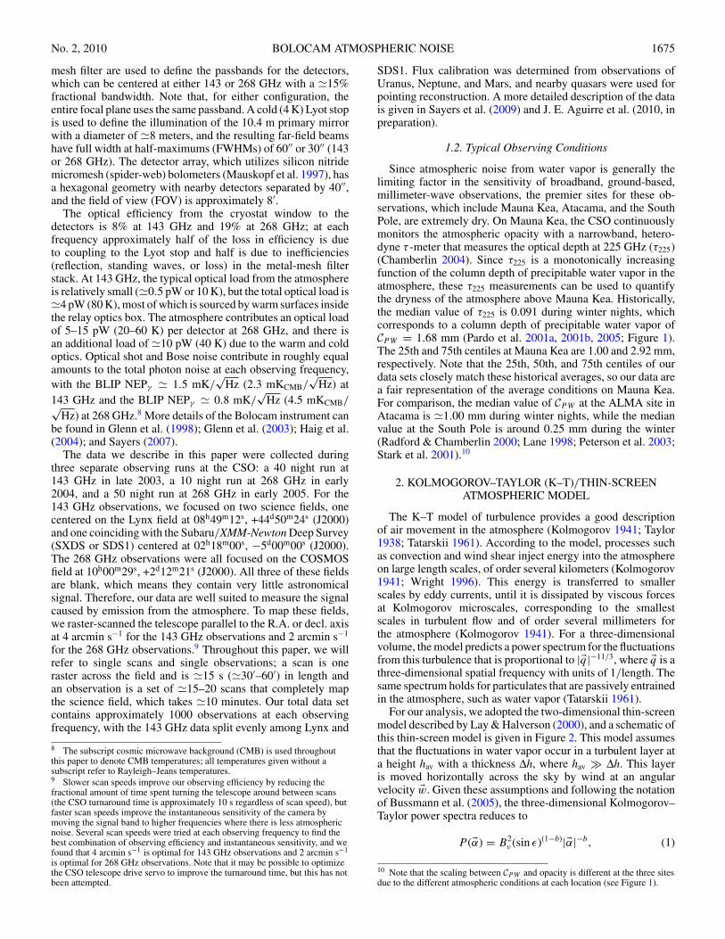
Typically, adaptive PCA only removes one or two eigenvec-tors from the 143 GHz data. In good weather, adaptive PCAproduces slightly better time-stream noise PSDs than averagesubtraction, while average subtraction produces slightly betternoise PSDs in bad weather (see Figure 15). However, adaptivePCA attenuates much more signal than average subtraction at

low frequencies, which means that average subtraction producesa better post-subtraction signal-to-noise ratio (S/N) comparedto adaptive PCA subtraction in all conditions. Therefore, adap-tive PCA was never the optimal subtraction algorithm for ouranalysis of blankfield data. Note that for observations of brightsources an iterative map-making technique can be used to re-cover a substantial amount of the signal that is lost in the processof subtracting the atmospheric noise (Enoch et al. 2006). Suchflux recovery may change which subtraction algorithm that isoptimal for a given observation.

4.5. Prospects for Improving Atmospheric Noise Subtraction

Although none of our subtraction algorithms allow usto reach BLIP-limited performance with Bolocam below�0.5 Hz, this does not mean that BLIP performance is impossi-ble from Mauna Kea. SuZIE I.5 was able to achieve instrument-limited performance21 down to 10 mHz at 150 GHz at the CSOby subtracting a combination of spatial and spectral common-mode signals (Mauskopf 1997). The initial subtraction of thespatial common-mode signal was obtained by differencing de-tectors separated by �4′ and removed the atmospheric noise towithin a factor of 2 of the instrument noise level below a couple

21 For reference, SuZIE I.5’s BLIP limit was a factor of �3 below theinstrument noise limit at 100 mHz and a factor of �6 below the instrumentnoise limit at 10 mHz.


Figure 13. Histograms of the magnitude of the bolometer–bolometer correlations at frequencies below 1 Hz for both adjacent and non-adjacent bolometer pairs at143 GHz. The plots on the left show data processed with average subtraction, and the plots on the right show data processed with quadratic subtraction. The top rowshows adjacent bolometer correlations, and the bottom row shows non-adjacent bolometer correlations. Quadratic subtraction removes almost all of the atmosphericnoise from the data; the residual atmospheric noise in the average subtracted data is the reason for the much higher correlations compared to quadratic subtracted data.Adjacent bolometers are still significantly correlated even after quadratic subtraction, this correlation is primarily due to the excess low-frequency noise described inSection 5.1.

hundred mHz. In addition, SuZIE I.5 had three observing bands(143, 217, and 269 GHz) per spatial pixel, which allowed de-termination of the correlated signal over a range of frequencies.The remaining atmospheric noise at low frequency was removeddown to the instrument noise level by subtracting this spectralcommon-mode signal.

SuZIE II was able to employ a similar subtraction method,using observing bands at 143, 221, and 355 GHz for each spatialpixel (Benson 2004). Additionally, SuZIE II had a much lowerinstrument noise level at 150 GHz compared to SuZIE I.5, within50% of the BLIP limit. Similar to Bolocam, SuZIE II reachedthe instrument noise level at frequencies above a couple hundredmHz by subtracting a spatial common-mode signal. However,by subtracting the spectral common-mode signal, SuZIE IIachieved instrument noise limited performance below 100 mHz,and was within a factor of 1.5 of the instrument noise limit at10 mHz. Therefore, spectral subtraction of the atmospheric noisedoes provide a method to achieve nearly BLIP performancefrom the CSO. The MKIDCam CSO facility camera, due tobe deployed in 2010, will make use of these lessons; it will have576 pixels each sensing four colors, thus providing the ability toperform both spatial and spectral subtraction of the atmosphericnoise (Glenn et al. 2008).

Additionally, scanning the telescope more quickly can in-crease the amount of astronomical signal band that is free from

Figure 14. Plots of median bolometer–bolometer correlation fraction as afunction of bolometer separation for time-stream data below 1 Hz. The datahave been averaged over all bolometer pairs and all 143 GHz observations. Theresidual atmospheric noise can be easily seen in the average subtracted data asan excess correlation at small separations and an excess anti-correlation at largeseparations. In contrast, there is very little residual correlation in the quadraticsubtracted data for non-adjacent bolometers, indicating that the atmosphericnoise can be removed quite well with quadratic subtraction. The large spike inthe correlation for adjacent bolometers is due to the excess low-frequency noisedescribed in Section 5.1.



Figure 15. Plots of 143 GHz time-stream PSDs averaged over all scans and all bolometers for a single observation for average subtraction and PCA subtraction. Theleft plot shows data from an observation made in relatively good weather, and the right plot shows an observation made in relatively poor weather. Overplotted asdotted lines is the S/N for each subtraction method (in arbitrary units), calculated by dividing the window function for a CMB shaped signal by the noise PSD. Notethat the S/N is significantly higher for average subtraction compared to PCA subtraction at low frequencies because average subtraction attenuates much less signal.


atmospheric noise. As long as the telescope scan speed is slowerthan the angular wind speed of the turbulent layer, the atmo-spheric noise power spectrum will remain unchanged in thetime-stream data as the telescope scan speed is increased. ForBolocam at the CSO, this means that the atmospheric noise willremain below �0.5 Hz for scan speeds below the average angu-lar wind speed of �30 arcmin s−1. Increasing the scan speed forBolocam observations from 2–4 arcmin s−1 to 30 arcmin s−1

would increase the half-width of the beam profile from �1–2 Hzto �10–20 Hz, significantly increasing the amount of astronom-ical signal band that is at frequencies above the atmosphericnoise. Unfortunately, we are not able to collect Bolocam data atthese fast scan speeds because it is impossible/inefficient to scanthe CSO telescope faster than a few arcmin s−1 (see footnote 9).

5. RESIDUAL TIME-STREAM CORRELATIONS

5.1. Adjacent Bolometer Correlations

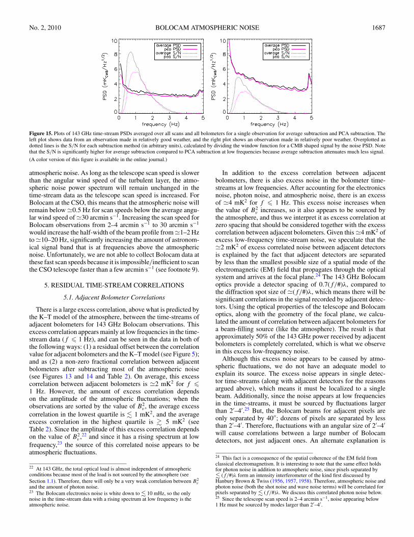
There is a large excess correlation, above what is predicted bythe K–T model of the atmosphere, between the time-streams ofadjacent bolometers for 143 GHz Bolocam observations. Thisexcess correlation appears mainly at low frequencies in the time-stream data (f � 1 Hz), and can be seen in the data in both ofthe following ways: (1) a residual offset between the correlationvalue for adjacent bolometers and the K–T model (see Figure 5);and as (2) a non-zero fractional correlation between adjacentbolometers after subtracting most of the atmospheric noise(see Figures 13 and 14 and Table 2). On average, this excesscorrelation between adjacent bolometers is �2 mK2 for f �1 Hz. However, the amount of excess correlation dependson the amplitude of the atmospheric fluctuations; when theobservations are sorted by the value of B2

ν , the average excesscorrelation in the lowest quartile is � 1 mK2, and the averageexcess correlation in the highest quartile is � 5 mK2 (seeTable 2). Since the amplitude of this excess correlation dependson the value of B2

ν ,22 and since it has a rising spectrum at lowfrequency,23 the source of this correlated noise appears to beatmospheric fluctuations.

22 At 143 GHz, the total optical load is almost independent of atmosphericconditions because most of the load is not sourced by the atmosphere (seeSection 1.1). Therefore, there will only be a very weak correlation between B2

νand the amount of photon noise.23 The Bolocam electronics noise is white down to � 10 mHz, so the onlynoise in the time-stream data with a rising spectrum at low frequency is theatmospheric noise.

In addition to the excess correlation between adjacentbolometers, there is also excess noise in the bolometer time-streams at low frequencies. After accounting for the electronicsnoise, photon noise, and atmospheric noise, there is an excessof �4 mK2 for f � 1 Hz. This excess noise increases whenthe value of B2

ν increases, so it also appears to be sourced bythe atmosphere, and thus we interpret it as excess correlation atzero spacing that should be considered together with the excesscorrelation between adjacent bolometers. Given this �4 mK2 ofexcess low-frequency time-stream noise, we speculate that the�2 mK2 of excess correlated noise between adjacent detectorsis explained by the fact that adjacent detectors are separatedby less than the smallest possible size of a spatial mode of theelectromagnetic (EM) field that propagates through the opticalsystem and arrives at the focal plane.24 The 143 GHz Bolocamoptics provide a detector spacing of 0.7(f/#)λ, compared tothe diffraction spot size of �(f/#)λ, which means there will besignificant correlations in the signal recorded by adjacent detec-tors. Using the optical properties of the telescope and Bolocamoptics, along with the geometry of the focal plane, we calcu-lated the amount of correlation between adjacent bolometers fora beam-filling source (like the atmosphere). The result is thatapproximately 50% of the 143 GHz power received by adjacentbolometers is completely correlated, which is what we observein this excess low-frequency noise.

Although this excess noise appears to be caused by atmo-spheric fluctuations, we do not have an adequate model toexplain its source. The excess noise appears in single detec-tor time-streams (along with adjacent detectors for the reasonsargued above), which means it must be localized to a singlebeam. Additionally, since the noise appears at low frequenciesin the time-streams, it must be sourced by fluctuations largerthan 2′–4′.25 But, the Bolocam beams for adjacent pixels areonly separated by 40′′; dozens of pixels are separated by lessthan 2′–4′. Therefore, fluctuations with an angular size of 2′–4′will cause correlations between a large number of Bolocamdetectors, not just adjacent ones. An alternate explanation is

24 This fact is a consequence of the spatial coherence of the EM field fromclassical electromagnetism. It is interesting to note that the same effect holdsfor photon noise in addition to atmospheric noise, since pixels separated by� (f/#)λ form an intensity interferometer of the kind first discussed byHanbury Brown & Twiss (1956, 1957, 1958). Therefore, atmospheric noise andphoton noise (both the shot noise and wave noise terms) will be correlated forpixels separated by � (f/#)λ. We discuss this correlated photon noise below.25 Since the telescope scan speed is 2–4 arcmin s−1, noise appearing below1 Hz must be sourced by modes larger than 2′–4′.


Table 2143 GHz Data, f < 1 Hz

Parameter Bin 1 Bin 2 Bin 3 Bin 4 All Data

B2ν (mK2 rad−5/3) 46 ± 2 170 ± 10 580 ± 20 4000 ± 400 280 ± 60

Raw atmosphere (mK2) 77 ± 11 131 ± 22 310 ± 60 1060 ± 150 240 ± 50Adj. corr. noise (mK2) 0.8 ± 0.1 1.1 ± 0.1 1.9 ± 0.2 5.8 ± 0.3 1.9 ± 0.1Adj. corr. fraction 0.39 ± 0.04 0.52 ± 0.04 0.42 ± 0.07 0.53 ± 0.03 0.46 ± 0.03

Notes. Description of the excess low-frequency noise that appears in the 143 GHz time-stream data and is likely sourced by theatmosphere. The first four columns give the median value, and uncertainty on the median value, of the data when they are binnedas a function of the amplitude of the atmospheric fluctuations, B2

ν . The final column gives the median values, and uncertaintieson the median values, for the full data set. From top to bottom, the rows give the value of B2

ν ; the raw atmospheric noise below1 Hz prior to subtraction; the excess correlated noise between adjacent detectors below 1 Hz after accounting for residual atmosphericnoise, and correlated photon/white noise; and the correlation fraction between adjacent detectors below 1 Hz after accounting forthe correlations expected from residual atmospheric noise and photon/white noise. The excess noise rises at low frequency andincreases as a function of B2

ν , indicating that it is sourced by the atmosphere. Additionally, the excess noise is �50% correlatedbetween adjacent detectors; we hypothesize that this correlation is a consequence of the 0.7(f/#)λ spacing between these detectors.

motivated by the fact that the median amount of excess low-frequency noise (�4 mK2) is much less than the total amount ofatmospheric noise in the Bolocam data below 1 Hz (�240 mK2).Therefore, this excess noise could be explained by atmosphericfluctuations at a reasonable height if there is an optical non-ideality that couples 1%–2% of the beam to the atmosphere ina manner that is uncorrelated across the array, excluding theadjacent bolometer correlations discussed above.

This excess correlated noise is difficult to remove becauseit is only correlated among bolometers that are close to eachother on the focal plane. We have attempted to remove thisnoise by constructing localized templates using the data from abolometer and the �6 bolometers that are adjacent to it on thefocal plane. We have removed these localized templates fromthe data both before and after applying our atmospheric noiseremoval algorithm to the data. Unfortunately, subtracting thesetemplates from the data resulted in an unacceptable amount ofsignal attenuation, and not all of the locally correlated noise wasremoved.

Additionally, as a consequence of the Bolocam detector spac-ing, we expect the atmospheric photon noise will also be �50%correlated between adjacent detectors. Since the photon noisehas a white spectrum, these correlations will have a larger ef-fect at high frequencies in the time-stream data where thereis almost no contamination from atmospheric noise. For Bolo-cam, the median white noise of 5 mK2 Hz−1 is composed of2.5 mK2 Hz−1 of detector plus electronics noise and 2.5 mK2

Hz−1 of photon noise. At frequencies above 2.5 Hz, well abovethe sky noise, the median correlation between adjacent bolome-ter time-streams is 5%, which means the median correlated noiseis 5 × 0.05 = 0.3 mK2 Hz−1. As mentioned above, EM-fieldoverlap between adjacent pixels implies that 50% of the photonnoise should be correlated, yielding an expectation of 1.3 mK2

Hz−1 of correlated white noise, roughly 4 times the observedvalue.

We speculate that this deficit of correlation in the photonnoise is explained by the fact that high-angle scattering towarm surfaces in the relay optics is the dominant source ofoptical loading.26 Such scattering does not necessarily preservethe correlation of the EM field between adjacent pixels in theway that it is preserved for the transmitted beam. The EM-field

26 Physical optics calculations with ZEMAX indicate that overillumination ofthe relay optics is negligible, and optical tests with a cold source indicate veryhigh-angle scattering, not mirror spillover, produces most of our observedoptical load.

correlations between adjacent pixels are only guaranteed to bepreserved for the 10% of our optical loading that is received fromthe atmosphere via the transmitted beam. However, we cautionthat we have no positive evidence supporting this scatteringhypothesis for the observed deficit of correlated photon noisebetween adjacent detectors.

Finally, our hypothesis of EM-field overlap between adjacentdetectors implies that the atmospheric noise will also be �50%correlated between adjacent detectors as a result of our spacing.However, since most of the fluctuation power in the atmosphereis at large scales, the atmospheric noise in these detectors is al-ready highly correlated. Therefore, the excess adjacent bolome-ter correlations will only appear in the atmospheric noise thatthe K–T model predicts will be uncorrelated (i.e., the differencebetween the K–T model prediction for adjacent bolometers andbolometers with zero separation). The median amount of noisepredicted by the K–T model to be uncorrelated between adjacentbolometers is �0.2 mK2, which means there will be �0.1 mK2

of correlated noise between adjacent bolometers that is not pre-dicted by the K–T model. This means that the atmospheric noisewill only cause an excess correlated noise signal of �0.1 mK2

between adjacent detectors.In summary, there is an excess noise that appears at low

frequencies in the Bolocam time-stream data. The amount ofexcess noise depends on the amplitude of the atmosphericfluctuations, and it is approximately �50% correlated betweenadjacent detectors. We hypothesize that this correlation is due tothe EM-field overlap engendered by the geometry of the opticalsystem and the physical separation between adjacent detectors.The available evidence suggests that this excess noise is dueto the atmosphere, but we emphasize that we do not have aphysical model to explain it, nor do we have direct evidence forour EM-field overlap hypothesis.

5.2. Sensitivity Losses Due to Residual Atmospheric Noise andAdjacent Bolometer Correlations

Ideally, the noise in our data would be uncorrelated betweenbolometers and have a white spectrum. This is approximatelywhat we would expect if instrumental or photon noise was thedominant source of unwanted signal in our data time-streams.However, our data contain a significant amount of noise witha rising spectrum at low frequency. Some of this noise is dueto residual atmospheric noise, and some is due to the excesslow-frequency noise described in Section 5.1. As mentionedin Section 5.1, the excess low-frequency noise (along with


>

Figure 16. Map PSDs for actual and simulated time-streams. The solid blackline shows the map PSD for all of the 143 GHz Lynx data. The red dotted lineshows the map PSD for simulated data generated using the noise spectrum ofour actual time-streams, except that the simulated data are uncorrelated betweendetectors. The green dashed line shows the map PSD for uncorrelated simulateddata that have a flat frequency spectrum and is based on the white noise levelof our actual data. The blue dot-dashed line shows the map PSD for a mapmade from our actual data, after masking out some detectors so that the spacingbetween all detectors is � 1.3(f/#)λ. This reduces the number of detectors from115 to 36, but it discards the highly correlated data between adjacent detectorpairs. Note that this spectrum has been multiplied by

√36/115 to account for the

change in the number of detectors. Since this PSD overlaps with the uncorrelatedsimulated PSD, we can conclude that most of the correlations between detectortime-streams are among adjacent detector pairs, and these residual correlationshave a significant impact on the noise of the resulting maps.


some residual atmospheric noise and photon noise) is highlycorrelated among adjacent bolometers. Additionally, there arecorrelations between all bolometer pairs on the focal planedue to the residual atmospheric noise. Finally, the atmospherictemplate used in our subtraction algorithms is constructed as asuperposition of all the bolometer time-streams, so removingthis template from each bolometer time-stream will cause it tobe slightly correlated with every other bolometer time-stream.

To understand how these non-idealities affect our data, wehave generated two sets of simulated data. A different simulateddata set was generated for each detector for each �10-minute-long observation, based on the measured PSD of each bolometerfor each observation. One simulated data set contains randomlygenerated data with the same noise PSD as our actual data,except the simulated data are completely uncorrelated betweenbolometers. The second set was generated using a flat noisespectrum (i.e., white noise), based on the white noise levelobserved in our actual data at high frequency. This simulateddata set provides a best-case scenario for Bolocam. For eachsimulation, we generated data corresponding to all of the143 GHz observations of the Lynx science field, and the resultsare shown in Figure 16. Additionally, we made a map fromour actual data after masking off 79 of the 115 detectors. Thisdata set includes 36 detectors, all of which are separated by� 1.3(f/#)λ, allowing us to test if the time-stream correlationsare isolated to adjacent bolometer pairs. The results from thisdata set are also shown in Figure 16.

At high spatial frequency (� � 10000), the simulated data setsproduce noise levels that are similar to our actual data, whichimplies that the correlations between detectors occur at lowfrequency and are caused by the atmospheric noise. However,

Table 3Lynx Data

Data Type Data Spectrum CMB Amplitude Uncertainty

Actual data Actual data 270 μK2CMB

Simulated Actual data 170 μK2CMB

Simulated White 100 μK2CMB

Actual data, > (f/#)λ Actual data 170 (550) μK2CMB

Notes. The estimated uncertainty on measuring the amplitude of a flat CMBpower spectrum for all of the 143 GHz Lynx observations. The four data setsinclude: our actual data, simulated data using our actual time-stream noisespectra, simulated data using our actual time-stream white noise level, and ouractual data after masking off 79 of our 115 detectors so that the spacing betweenall detectors is � 1.3(f/#)λ. For the two simulated data sets, the bolometertime-streams are uncorrelated. The results for the second and fourth data setsare similar, after accounting for the reduction in detector number in the fourthset, indicating that the majority of the correlations between our detector time-streams are between adjacent detector pairs. The results show that our sensitivityto a CMB amplitude is reduced by a factor of �1.6 due to these correlations,and by another factor of �1.7 due to the residual atmospheric noise in our dataat low frequencies.

both simulated data sets have a much lower noise level than ouractual data at low spatial frequencies. To quantify the differencebetween the simulated data sets and our actual data set, wehave estimated the uncertainty in determining the amplitude ofa flat CMB power spectrum (see Sayers et al. (2009) for detailsof the calculation). Additionally, we estimated the uncertaintyin determining the amplitude of a flat CMB power spectrumfor the data set that contains our actual data for 36 detectors.This uncertainty was multiplied by 36/115 to account for thedegradation caused by masking off 79 detectors. The resultsare shown in Table 3. The simulated data indicate that ouruncertainty on the amplitude of a flat CMB power spectrumwould be improved by a factor of �1.6 if the detector time-streams were uncorrelated, and by another factor of �1.7 if thetime-streams had a white spectrum instead of a rising spectrumat low frequency due to the residual atmospheric noise.

Additionally, after correcting for the loss of 79 detectors,the data set with 36 detectors produces a similar result tothe simulated data set based on our actual noise spectra. Thisindicates that the correlations between time-streams of non-adjacent bolometers are negligible. The implication is that, if wehad used larger horns (in (f/#)λ) while maintaining the samenumber of detectors, we would have improved our sensitivityin μK2

CMB by a factor of 1.6. By going to larger horns, wewould also have had a larger FOV, which would have had bothpositive (e.g., sensitivity to larger scales) and negative (e.g., lessuniform map coverage) effects on our data.27 It seems likelythat these negative effects would have been small compared tothe large gain in sensitivity that we would have obtained byeliminating the excess correlations between adjacent bolometertime-streams. Another implication is that, at fixed detectorcount, it is more advantageous from the atmospheric noise pointof view to use � (f/#)λ pixel spacing and increase the FOVthan it is to hold the FOV fixed and sample it more finely with� (f/#)λ pixel spacing. Increasing the Bolocam FOV was not

27 Additionally, there would be less correlation in the atmospheric noise signalover a larger FOV. However, given how well the K–T model describes thecorrelations as a function of separation in our data (see Figure 5), thecorrelation over an 8′ subregion of the FOV would be approximately equal towhat we observed. Therefore, similar atmospheric noise removal could beobtained by performing the atmospheric noise subtraction algorithms onsubregions of the larger FOV and/or subtracting higher order polynomials.


possible by the time this effect was observed, but this lesson isbeing applied for MKIDCam.

6. CONCLUSIONS

We have studied the atmospheric noise above Mauna Kea atmillimeter wavelengths from the CSO using Bolocam. Underall observing conditions, the data time-streams are dominatedby atmospheric noise at frequencies below �0.5 Hz. The dataare consistent with a K–T turbulence model for a thin wind-driven screen, and the median amplitude of the fluctuations is280 mK2 rad−5/3 at 143 GHz and 4000 mK2 rad−5/3 at 268 GHz.Based on a comparison to the ACBAR data in Bussmann et al.(2005), we conclude that these atmospheric noise fluctuationamplitudes are a factor of �80 larger than they would be at theSouth Pole for identical observing bands. This large differencein atmospheric noise amplitudes is due primarily to the SouthPole being a much drier site than Mauna Kea, with a small factorof �2 arising from the fact that the fractional fluctuations in thecolumn depth of water vapor are a factor of �√

2 lower at theSouth Pole. Based on our atmospheric modeling, we developedseveral algorithms to remove atmospheric noise, and the bestresults were achieved when we described the fluctuations usinga low-order polynomial in detector position over the 8′ focalplane. However, even with these algorithms, we were not ableto obtain BLIP performance at frequencies below �0.5 Hz inany observing conditions. Therefore, we conclude that BLIPperformance is not possible from Mauna Kea below �0.5 Hzfor broad band �1–2 mm receivers with subtraction of a spatialatmospheric template on scales of several arcminutes. We alsoobserved an excess low-frequency noise that is highly correlatedbetween detectors separated by � (f/#)λ; this noise appears tobe caused by atmospheric fluctuations, but we do not have anadequate model to explain its source. We hypothesize that thecorrelations arise from the classical coherence of the EM fieldacross a distance of �(f/#)λ on the focal plane.

We acknowledge the assistance of the following: Minhee Yunand Anthony D. Turner of NASA’s Jet Propulsion Laboratory,who fabricated the Bolocam science array; Toshiro Hatake ofthe JPL electronic packaging group, who wirebonded the array;Marty Gould of Zen Machine and Ricardo Paniagua and theCaltech PMA/GPS Instrument Shop, who fabricated much ofthe Bolocam hardware; Carole Tucker of Cardiff University,who tested metal-mesh reflective filters used in Bolocam; BenKnowles of the University of Colorado, who contributed to thesoftware pipeline, the day crew and Hilo staff of the CaltechSubmillimeter Observatory, who provided invaluable assistanceduring commissioning and data-taking for this survey data set;high school teacher Tobias Jacoby and high school studentsJonathon Graff, Gloria Lee, and Dalton Sargent, who helped assummer research assistants; and Kathy Deniston, who providedeffective administrative support at Caltech. We thank W. L.Holzapfel for his many useful comments as referee of ourmanuscript. Bolocam was constructed and commissioned usingfunds from NSF/AST-9618798, NSF/AST-0098737, NSF/AST-9980846, NSF/AST-0229008, and NSF/AST-0206158. J.S. andG.L. were partially supported by NASA Graduate StudentResearch Fellowships, J.S. was partially supported by a NASAPostdoctoral Program Fellowship, J.A. was partially supportedby a Jansky Postdoctoral Fellowship, and S.G. was partiallysupported by a R. A. Millikan Postdoctoral Fellowship atCaltech. The research described in this paper was carried

out at the Jet Propulsion Laboratory, California Institute ofTechnology, under a contract with the National Aeronauticsand Space Administration.

Facility: CSO

APPENDIX

APPENDIX MATERIAL

In order to account for the time lags and advances betweenbolometer time-streams that are described by the K–T thin-screen model, we in general have to shift the time-streams by afractional number of samples. For example, if a given bolometertime-stream is advanced by Δtb seconds, then we will accountfor this advance by shifting the time-stream according to

d ′n =

(1 −

∣∣∣∣Δtb

Δt

∣∣∣∣)

dn +

∣∣∣∣Δtb

Δt

∣∣∣∣ dn+Δtb/Δt , (A1)

where d ′n is the interpolated data time-stream, dn is the original

data time-stream, Δt is the time between samples, and n is thesample number. Note that we have assumed that Δtb < Δt , sinceshifts by integer multiples of Δt are trivial. Alternatively, thisshift can be performed in frequency space by applying

Sm =(

1 −∣∣∣∣Δtb

Δt

∣∣∣∣ +

∣∣∣∣Δtb

Δt

∣∣∣∣ e−sign(Δtb)i2πfmΔt

)(A2)

to the Fourier transform of the time-stream data, where fm isfrequency in Hz and m is the frequency-space index. Sm acts likea filter, and, for all non-zero frequencies, |Sm| < 1. Therefore, topreserve the noise properties of our data, we divide the Fouriertransform of the shifted time-stream by |Sm|. In summary, weshift the time-stream data according to Equation (1), then correctfor the filtering effects of this shift in frequency space by dividingby |Sm|.

REFERENCES

Archibald, E. N., et al. 2002, MNRAS, 336, 1Benson, B. A. 2004, PhD thesis, Stanford Univ.Borys, C., et al. 1999, MNRAS, 308, 527Bussmann, R. S., Holzapfel, W. L., & Kuo, C. L. 2005, ApJ, 622, 1343Chamberlin, R. A. 2004, PASA, 21, 264Church, S. E. 1995, MNRAS, 272, 551Conway, R. G., et al. 1965, MNRAS, 131, 159Dobbs, M., et al. 2006, New Astr. Rev., 50, 960Dowell, C. D., et al. 2003, Proc. SPIE, 4855, 73Enoch, M., et al. 2006, ApJ, 638, 293Glenn, J., et al. 1998, Proc. SPIE, 3357, 326Glenn, J., et al. 2003, Proc. SPIE, 4855, 30Glenn, J., et al. 2008, Proc. SPIE, 7020, 10Haig, D. J., et al. 2004, Proc. SPIE, 5498, 78Hanbury Brown, R., & Twiss, R. Q. 1956, Nature, 178, 1046Hanbury Brown, R., & Twiss, R. Q. 1957, Proc. R. Soc. A, 242, 300Hanbury Brown, R., & Twiss, R. Q. 1958, Proc. R. Soc. A, 243, 291Holland, W. S., et al. 1999, MNRAS, 303, 659Jenness, T., et al. 1998, Proc. SPIE, 3357, 638Kolmogorov, A. N. 1941, Dokl. Akad. Nauk SSSR, 30, 301Kosowsky, A. 2003, New Astr. Rev., 47, 939Kovacs, A. 2008, Proc. SPIE, 7020, 45Kreysa, E., et al. 1998, Proc. SPIE, 3357, 319Kreysa, E., et al. 2003, Proc. SPIE, 4855, 41Lane, A. P. 1998, in ASP Conf. Ser. 141, Astrophysics from Antarctica, ed. G.

Novak & R. Landsberg (San Francisco, CA: ASP), 289Laurent, G. T., et al. 2005, ApJ, 623, 742Lay, O. P., & Halverson, N. W. 2000, ApJ, 543, 787Masson, C. R. 1994, in ASP Conf. Ser. 59, Astronomy with Millimeter and

Submillimeter Wave Interferometry, IAU Colloquium 140, ed. M. Ishiguro& J. Welch (San Francisco, CA: ASP), 87

Mauskopf, P. D. 1997, PhD thesis, Univ. California at BerkeleyMauskopf, P. D., et al. 1997, Appl. Opt., 36, 765

http://dx.doi.org/10.1046/j.1365-8711.2002.05582.x

http://adsabs.harvard.edu/cgi-bin/bib_query?2002MNRAS.336....1A

http://adsabs.harvard.edu/cgi-bin/bib_query?2002MNRAS.336....1A

http://dx.doi.org/10.1046/j.1365-8711.1999.02753.x

http://adsabs.harvard.edu/cgi-bin/bib_query?1999MNRAS.308..527B

http://adsabs.harvard.edu/cgi-bin/bib_query?1999MNRAS.308..527B

http://dx.doi.org/10.1086/427935

http://adsabs.harvard.edu/cgi-bin/bib_query?2005ApJ...622.1343B

http://adsabs.harvard.edu/cgi-bin/bib_query?2005ApJ...622.1343B

http://adsabs.harvard.edu/cgi-bin/bib_query?2004PASA...21..264C

http://adsabs.harvard.edu/cgi-bin/bib_query?2004PASA...21..264C

http://adsabs.harvard.edu/cgi-bin/bib_query?1995MNRAS.272..551C




http://dx.doi.org/10.1016/j.newar.2006.09.029

http://adsabs.harvard.edu/cgi-bin/bib_query?2006NewAR..50..960D

http://adsabs.harvard.edu/cgi-bin/bib_query?2006NewAR..50..960D

http://dx.doi.org/10.1117/12.459360

http://adsabs.harvard.edu/cgi-bin/bib_query?2003SPIE.4855...73D

http://adsabs.harvard.edu/cgi-bin/bib_query?2003SPIE.4855...73D

http://dx.doi.org/10.1086/498678

http://adsabs.harvard.edu/cgi-bin/bib_query?2006ApJ...638..293E

http://adsabs.harvard.edu/cgi-bin/bib_query?2006ApJ...638..293E

http://dx.doi.org/10.1117/12.317418

http://adsabs.harvard.edu/cgi-bin/bib_query?1998SPIE.3357..326G

http://adsabs.harvard.edu/cgi-bin/bib_query?1998SPIE.3357..326G

http://dx.doi.org/10.1117/12.459369

http://adsabs.harvard.edu/cgi-bin/bib_query?2003SPIE.4855...30G

http://adsabs.harvard.edu/cgi-bin/bib_query?2003SPIE.4855...30G

http://dx.doi.org/10.1117/12.553154

http://adsabs.harvard.edu/cgi-bin/bib_query?2004SPIE.5498...78H

http://adsabs.harvard.edu/cgi-bin/bib_query?2004SPIE.5498...78H

http://dx.doi.org/10.1038/1781046a0

http://adsabs.harvard.edu/cgi-bin/bib_query?1956Natur.178.1046H

http://adsabs.harvard.edu/cgi-bin/bib_query?1956Natur.178.1046H

http://dx.doi.org/10.1098/rspa.1957.0177

http://adsabs.harvard.edu/cgi-bin/bib_query?1957RSPSA.242..300B





http://dx.doi.org/10.1046/j.1365-8711.1999.02111.x

http://adsabs.harvard.edu/cgi-bin/bib_query?1999MNRAS.303..659H

http://adsabs.harvard.edu/cgi-bin/bib_query?1999MNRAS.303..659H

http://dx.doi.org/10.1117/12.317420

http://adsabs.harvard.edu/cgi-bin/bib_query?1941DoSSR..30..301K

http://adsabs.harvard.edu/cgi-bin/bib_query?1941DoSSR..30..301K

http://dx.doi.org/10.1016/j.newar.2003.09.003

http://adsabs.harvard.edu/cgi-bin/bib_query?2003NewAR..47..939K

http://adsabs.harvard.edu/cgi-bin/bib_query?2003NewAR..47..939K

http://adsabs.harvard.edu/cgi-bin/bib_query?2008SPIE.7020E..45K

http://adsabs.harvard.edu/cgi-bin/bib_query?2008SPIE.7020E..45K

http://dx.doi.org/10.1117/12.317367

http://adsabs.harvard.edu/cgi-bin/bib_query?1998SPIE.3357..319K

http://adsabs.harvard.edu/cgi-bin/bib_query?1998SPIE.3357..319K

http://dx.doi.org/10.1117/12.459176

http://adsabs.harvard.edu/cgi-bin/bib_query?2003SPIE.4855...41K

http://adsabs.harvard.edu/cgi-bin/bib_query?2003SPIE.4855...41K

http://adsabs.harvard.edu/cgi-bin/bib_query?1998ASPC..141..289L

http://dx.doi.org/10.1086/428823

http://adsabs.harvard.edu/cgi-bin/bib_query?2005ApJ...623..742L


http://dx.doi.org/10.1086/317115



http://adsabs.harvard.edu/cgi-bin/bib_query?1994IAUCo.140...87M

http://dx.doi.org/10.1364/AO.36.000765

http://adsabs.harvard.edu/cgi-bin/bib_query?1997ApOpt..36..765M

http://adsabs.harvard.edu/cgi-bin/bib_query?1997ApOpt..36..765M


Murtagh, F., & Heck, A. 1987, Multivariate Data Analysis (Boston: Kluwer)Pardo, J. R., Cernicharo, J., & Serabyn, E. 2001a, IEEE Trans. Antennas Propag.,

49, 1683Pardo, J. R., Serabyn, E., & Cernicharo, J. 2001b, J. Quant. Spectrosc. Radiat.

Transfer, 68, 419Pardo, J. R., et al. 2005, J. Quant. Spectrosc. Radiat. Transfer, 96, 537Peterson, J. B., et al. 2003, Publ. Astron. Soc. Pac., 115, 383Radford, S. J., & Chamberlin, R. A. 2000, ALMA Memo, 334Reichertz, L. A., et al. 2001, A&A, 379, 735

Ruhl, J., et al. 2004, Proc. SPIE, 5498, 11Sayers, J. 2007, PhD thesis, CaltechSayers, J., et al. 2009, ApJ, 690, 1597Stark, A. A., et al. 2001, Publ. Astron. Soc. Pac., 113, 567Tatarskii, V. I. 1961, Wave Propagation in a Turbulent Medium (New York:

McGraw-Hill)Taylor, G. I. 1938, Proc. R. Soc. A, 164, 476Weferling, B., et al. 2002, A&A, 383, 1088Wright, M. C. H. 1996, Publ. Astron. Soc. Pac., 108, 520

http://dx.doi.org/10.1109/8.982447

http://adsabs.harvard.edu/cgi-bin/bib_query?2001ITAP...49.1683P

http://adsabs.harvard.edu/cgi-bin/bib_query?2001ITAP...49.1683P

http://adsabs.harvard.edu/cgi-bin/bib_query?2001JQSRT..68..419P


http://dx.doi.org/10.1016/j.jqsrt.2005.04.005



http://dx.doi.org/10.1086/368101

http://adsabs.harvard.edu/cgi-bin/bib_query?2003PASP..115..383P

http://adsabs.harvard.edu/cgi-bin/bib_query?2003PASP..115..383P

http://dx.doi.org/10.1051/0004-6361:20011227

http://adsabs.harvard.edu/cgi-bin/bib_query?2001A&A...379..735R

http://adsabs.harvard.edu/cgi-bin/bib_query?2001A&A...379..735R

http://dx.doi.org/10.1117/12.552473

http://adsabs.harvard.edu/cgi-bin/bib_query?2004SPIE.5498...11R

http://adsabs.harvard.edu/cgi-bin/bib_query?2004SPIE.5498...11R

http://dx.doi.org/10.1088/0004-637X/690/2/1597

http://adsabs.harvard.edu/cgi-bin/bib_query?2009ApJ...690.1597S

http://adsabs.harvard.edu/cgi-bin/bib_query?2009ApJ...690.1597S

http://dx.doi.org/10.1086/320281

http://adsabs.harvard.edu/cgi-bin/bib_query?2001PASP..113..567S

http://adsabs.harvard.edu/cgi-bin/bib_query?2001PASP..113..567S


http://adsabs.harvard.edu/cgi-bin/bib_query?1938RSPSA.164..476T

http://adsabs.harvard.edu/cgi-bin/bib_query?1938RSPSA.164..476T

http://dx.doi.org/10.1051/0004-6361:20011617

http://adsabs.harvard.edu/cgi-bin/bib_query?2002A&A...383.1088W

http://adsabs.harvard.edu/cgi-bin/bib_query?2002A&A...383.1088W

http://dx.doi.org/10.1086/133757

http://adsabs.harvard.edu/cgi-bin/bib_query?1996PASP..108..520W

http://adsabs.harvard.edu/cgi-bin/bib_query?1996PASP..108..520W

http://dx.doi.org/10.1016/S0022-4073(00)00034-0

http://dx.doi.org/10.1016/S0022-4073(00)00034-0

Studies of Millimeter-wave Atmospheric Noise above Mauna Kea

Documents

Transcript of Studies of Millimeter-wave Atmospheric Noise above Mauna Kea