arX

iv:2

203.

0089

2v1

[ee

ss.S

P] 2

Mar

202

21

Joint Localization and Orientation Estimation in

Millimeter-Wave MIMO OFDM Systems via

Atomic Norm MinimizationJianxiu Li, Graduate Student Member, IEEE, Maxime Ferreira Da Costa, Member, IEEE,

and Urbashi Mitra, Fellow, IEEE

Abstract—Herein, an atomic norm based method for accu-rately estimating the location and orientation of a target frommillimeter-wave multi-input-multi-output (MIMO) orthogonalfrequency-division multiplexing (OFDM) signals is presented. Anovel virtual channel matrix is introduced and an algorithm toextract localization-relevant channel parameters from its atomicnorm decomposition is designed. Then, based on the extendedinvariance principle, a weighted least squares problem is pro-posed to accurately recover the location and orientation usingboth line-of-sight and non-line-of-sight channel information. Theconditions for the optimality and uniqueness of the estimate andtheoretical guarantees for the estimation error are characterizedfor the noiseless and the noisy scenarios. Theoretical resultsare confirmed via simulation. Numerical results investigate therobustness of the proposed algorithm to incorrect model orderselection or synchronization error, and highlight performanceimprovements over a prior method. The resultant performancenearly achieves the Cramer-Rao lower bound on the estimationerror.

Index Terms—Atomic norm minimization, localization, orien-tation estimation, millimeter-wave MIMO OFDM systems.

I. INTRODUCTION

M ILLIMETER-wave (mmWave) communications are of

strong interest for fifth generation multi-input-multi-

output (MIMO) systems due to the significant bandwidth

afforded by small wavelengths [2]. One challenge with these

systems is path loss; however, this effect can be mitigated by

beamforming [3]. In addition to large bandwidth, mmWave

MIMO also experiences limited multipath, thus making this

signaling a natural candidate for localization [4]–[11]. In [7],

[8], localization based on classic compressed sensing is pur-

sued by exploiting multipath sparsity. However, the perfor-

mance is limited by quantization error and grid resolution.

In [8], a space-alternating generalized expectation maximiza-

tion algorithm is proposed to refine the channel estimates for

localization, initialized with the channel parameters that are

coarsely estimated via a modified distributed compressed sens-

ing simultaneous orthogonal matching pursuit (DCS-SOMP)

J. Li, M. Ferreira Da Costa, and U. Mitra are with the Department ofElectrical and Computer Engineering, University of Southern California, LosAngeles, CA 90089, USA (e-mails: jianxiul, mferreira, ubli@usc.edu).

This paper will be presented in part at the 2022 IEEE InternationalConference on Acoustics, Speech and Signal Processing (ICASSP 2022) [1].This work has been funded in part by one or more of the following: CiscoFoundation 1980393, ONR N00014-15-1-2550, ONR 503400-78050, NSFCCF-1410009, NSF CCF-1817200, NSF CCF-2008927, Swedish ResearchCouncil 2018-04359, ARO W911NF1910269, and DOE DE-SC0021417.

scheme [12]. However, this method suffers from local minima

when the signal-to-noise ratio (SNR) is low or when the

initialization is not sufficiently accurate. To address the grid

mismatch, sparse Bayesian learning based methods [9], [10]

are designed for mmWave MIMO localization, relying on the

knowledge of the prior distribution of the channel coefficients.

For a more realistic, band-limited, frequency selective channel

model, a weighted orthogonal matching pursuit strategy is

proposed in [11], which operates in parallel in the angular

and delay domains to improve the localization accuracy with

lower requirement on the grid resolution.

In contrast, atomic norm minimization (ANM) [13], also

known as total variation minimization, has emerged as a useful

convex optimization framework for estimating continuous val-

ued parameters without relying on discretization. Of late, this

method has been actively studied in the context of recovering

the parameters of a sparse sum of complex exponentials [14],

as we do herein. ANM is known to achieve near-optimal

denoising rates in the signal space in that context [15],

and to recover the correct model-order under a separation

condition on the parameters [16], [17]. Error-bounds on the

parameter estimates have been derived under a Gaussian noise

assumption [18]. Furthermore, this framework has also been

successfully generalized to recover multi-dimensional signals

[19], [20] as we do herein. In [19], the two-dimensional case is

studied and a higher dimensional case is discussed in [20]. We

observe that our semi-definite program formulation is different

from that suggested in [20].

The ANM framework has previously been employed for

the purpose of localization [21]–[24], but in the absence

of multipath. In [20], [25], [26], ANM is used for channel

estimation, but can not be used for localization as the time-

of-arrival (TOA) is not considered in the model. In contrast

to [25]–[27] that focus on the estimation of one-dimensional

signals, this paper considers high-accuracy estimation of the lo-

calization and orientation from signals using mmWave MIMO

orthogonal frequency-division multiplexing (OFDM) signaling.

A multi-dimensional ANM based estimator is proposed to si-

multaneously recover all the relevant parameters by harnessing

the structure of a novel virtual channel matrix. We underscore

that our methods herein do not require the prior, Bayesian

model information for [9], [10] and we have considered other

atomic norm based schemes [25]–[27] which can exploit the

effect of practical pulse shapes in [11].

The main contributions of this paper are:

2

1) A novel virtual channel matrix capturing the geometry of

the paths is designed for mmWave MIMO OFDM channels.

2) Based on the sparse structure of the virtual channel matrix,

a multi-dimensional atomic norm channel estimator is pro-

posed to simultaneously estimate the TOAs, angle-of-arrivals

(AOA), and angle-of-departures (AOD) with super-resolution,

i.e. without relying on a discretization of the search space.

3) Sufficient conditions for exact recovery of the parameters

are given in Propositions 1 and 2 for the noiseless case; in the

presence of noise, an upper bound is derived for the estimation

errors in Proposition 3, suggesting the appropriate value of a

key regularization parameter to improve performance.

4) Location and orientation are accurately inferred from the

solution of ANM through a weighted non-linear least squares

scheme, where the designed weight matrix is compatible with

the ANM channel estimator.

5) The theoretical analyses for the proposed scheme are

validated via simulation, and the comparisons with the DCS-

SOMP method [8] are presented. It is shown that the proposed

scheme offers more than 7dB gain with respect to the root-

mean-square error (RMSE) of estimation when a small number

of antennas are employed; furthermore, the proposed method

nearly achieves the Cramer-Rao lower bound (CRLB) [8] in

the studied cases.

6) The effects of incorrect model order selection and syn-

chronization error on the estimation accuracy are numerically

investigated to show the robustness of the proposed scheme.

The present work completes our previous work [1] with

an analysis of the optimality and uniqueness of the estimate

in the noiseless case. Furthermore, we derive an expression

for the regularization parameter under a white Gaussian noise

assumption as a function of the pilot signals to achieve near-

optimal denoising rates, with extended derivations and proofs.

The robustness of the proposed method to incorrect model

order selection and synchronization error is also studied via

simulation; the proposed approach is shown to be durable to

such mismatch.

The rest of this paper is organized as follows. Section II-A

introduces the signal model for the mmWave MIMO OFDM

systems. Section II-B presents the design of a novel virtual

channel matrix, which captures geometric parameters of the

signal model. In Section III, the structure of the proposed

virtual channel matrix is explicitly exploited for the design

of a multi-dimensional atomic norm based channel estimator.

Sufficient conditions for exact recovery in absence of noise is

investigated in Section III-A, and a denoising bound is derived

in Section III-B under a white Gaussian noise assumption.

Section III-C presents a semidefinite representation of ANM

that can be solved using off-the-shelf convex solvers. Section

III-D and III-E propose a high accuracy method to recover

the location and orientation of the target from the solution of

the ANM program based on the Vandermonde factorization of

Toeplitz matrices [28] and the extended invariance principle

(EXIP) [29]. Numerical results are given in Section IV to

verify the theoretical analyses and highlight the performance

improvements with respect to the previous method. Finally, a

conclusion is drawn in Section V. Appendices A and B provide

The scatterer of the k-thh path ((h ((skskkkkkk)

..

..

.

d

1

2

Nt

Tx ((x ((q(((qqq) Rx ((x ((p(((ppp(((((( )

θTx,0

θTx,k

θRx,0

θRx,k

θo

Figure 1. System model.

the proofs of two propositions of this work.

Scalars are denoted by lower-case letters, x and column

vectors by bold letters x. The ith element of x is denoted

by x[i]. Matrices are denoted by bold capital letters, X . xl

denotes the lth column of X and X[i, j] is the (i, j)th element.

The operators ⌊x⌋, |x|, ‖x‖1,‖x‖2, sign(x), Re(x), diag(A)represent the largest integer that is less than x, the magnitude

of x, the ℓ1 norm of x, the ℓ2 norm of x, the complex

sign of x defined as sign(x) = x‖x‖2

, the real part of x,

a diagonal matrix whose diagonal elements are given by A.

‖X‖F is the Frobenius norm of X . 〈A,X〉 stands for the

usual matrix inner product while 〈A,X〉R , Re(〈A,X〉).Id and 0d stand for a d × d identity matrix and a d × d

zero matrix, respectively. The notations ⊗ and E{·} denote the

Kronecker product and the expectation of a random variable.

The operators rank(·),Tr(·), (·)T, and (·)H are defined as the

rank of a matrix, the trace of a matrix, the transpose of a

matrix or vector, and the conjugate transpose of a vector or

matrix, respectively.

II. MMWAVE MIMO OFDM NARROWBAND CHANNELS

A. Signal Model

We adopt the narrowband channel model of [8], where

a single base station (BS) is equipped with Nt antennas

and a target has Nr antennas. The locations of the BS

and the target are denoted by q = [qx, qy]T ∈ R2 and

p = [px, py]T ∈ R

2, respectively, where q is known while p

is to be estimated. In addition, there is an unknown orientation

of the target’s antenna array, denoted by θo. Assume that

one line-of-sight (LOS) path and K non-line-of-sight (NLOS)

paths exist in the mmWave MIMO OFDM channel. The k-th

NLOS path is produced by a scatterer at an unknown location

sk = [sk,x, sk,y]T ∈ R2. Denoting by Ns the number of the

sub-carriers, we transmit G OFDM pilot signals with carrier

frequency fc and bandwidth B ≪ fc. Given the g-th pilot

signal over the n-th sub-carrier x(g,n) 1, the g-th received

1The pilot signals x(g,n) ∈ CNt is a general expression that permits theincorporation of the beamforming matrix, the design of which is beyond thescope of this paper.

3

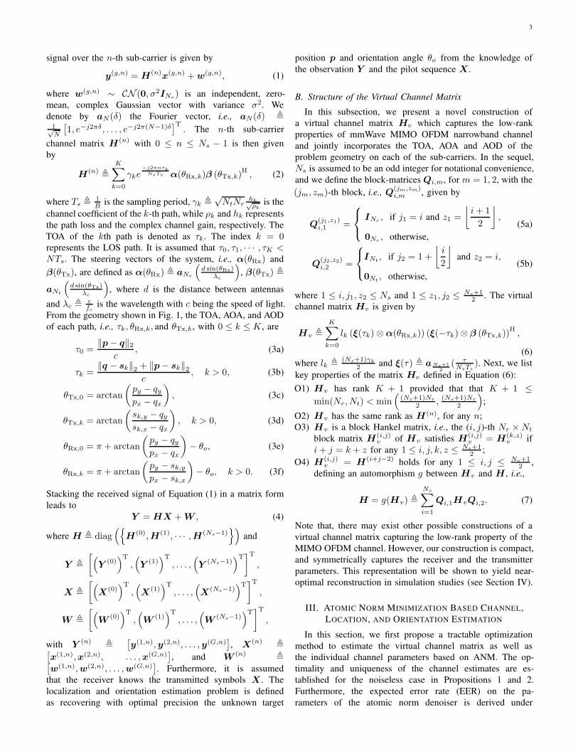
signal over the n-th sub-carrier is given by

y(g,n) = H(n)x(g,n) +w(g,n), (1)

where w(g,n) ∼ CN (0, σ2INr) is an independent, zero-

mean, complex Gaussian vector with variance σ2. We

denote by aN (δ) the Fourier vector, i.e., aN(δ) ,1√N

[1, e−j2πδ, . . . , e−j2π(N−1)δ

]T. The n-th sub-carrier

channel matrix H(n) with 0 ≤ n ≤ Ns − 1 is then given

by

H(n),

K∑

k=0

γke−j2πnτk

NsTs α(θRx,k)β (θTx,k)H, (2)

where Ts ,1B is the sampling period, γk ,

√NtNr

hk√ρk

is the

channel coefficient of the k-th path, while ρk and hk represents

the path loss and the complex channel gain, respectively. The

TOA of the kth path is denoted as τk. The index k = 0represents the LOS path. It is assumed that τ0, τ1, · · · , τK <

NTs. The steering vectors of the system, i.e., α(θRx) and

β(θTx), are defined as α(θRx) , aNr

(d sin(θRx)

λc

), β(θTx) ,

aNt

(d sin(θTx)

λc

), where d is the distance between antennas

and λc ,cfc

is the wavelength with c being the speed of light.

From the geometry shown in Fig. 1, the TOA, AOA, and AOD

of each path, i.e., τk, θRx,k, and θTx,k, with 0 ≤ k ≤ K , are

τ0 =‖p− q‖2

c, (3a)

τk =‖q − sk‖2 + ‖p− sk‖2

c, k > 0, (3b)

θTx,0 = arctan

(py − qy

px − qx

), (3c)

θTx,k = arctan

(sk,y − qy

sk,x − qx

), k > 0, (3d)

θRx,0 = π + arctan

(py − qy

px − qx

)− θo, (3e)

θRx,k = π + arctan

(py − sk,y

px − sk,x

)− θo, k > 0. (3f)

Stacking the received signal of Equation (1) in a matrix form

leads to

Y = HX +W , (4)

where H , diag({

H(0),H(1), · · · ,H(Ns−1)})

and

Y ,

[(Y (0)

)T,(Y (1)

)T, . . . ,

(Y (Ns−1)

)T]T,

X ,

[(X(0)

)T,(X(1)

)T, . . . ,

(X(Ns−1)

)T]T,

W ,

[(W (0)

)T,(W (1)

)T, . . . ,

(W (Ns−1)

)T]T,

with Y (n),

[y(1,n),y(2,n), . . . ,y(G,n)

], X(n)

,[x(1,n),x(2,n), . . . ,x(G,n)

], and W (n)

,[w(1,n),w(2,n), . . . ,w(G,n)

]. Furthermore, it is assumed

that the receiver knows the transmitted symbols X . The

localization and orientation estimation problem is defined

as recovering with optimal precision the unknown target

position p and orientation angle θo from the knowledge of

the observation Y and the pilot sequence X .

B. Structure of the Virtual Channel Matrix

In this subsection, we present a novel construction of

a virtual channel matrix Hv which captures the low-rank

properties of mmWave MIMO OFDM narrowband channel

and jointly incorporates the TOA, AOA and AOD of the

problem geometry on each of the sub-carriers. In the sequel,

Ns is assumed to be an odd integer for notational convenience,

and we define the block-matrices Qi,m, for m = 1, 2, with the

(jm, zm)-th block, i.e., Q(jm,zm)i,m , given by

Q(j1,z1)i,1 =

INr, if j1 = i and z1 =

⌊i+ 1

2

⌋,

0Nr, otherwise,

(5a)

Q(j2,z2)i,2 =

INt

, if j2 = 1 +

⌊i

2

⌋and z2 = i,

0Nt, otherwise,

(5b)

where 1 ≤ i, j1, z2 ≤ Ns and 1 ≤ z1, j2 ≤ Ns+12 . The virtual

channel matrix Hv is given by

Hv ,

K∑

k=0

lk (ξ(τk)⊗α(θRx,k)) (ξ(−τk)⊗ β (θTx,k))H,

(6)

where lk ,(Ns+1)γk

2 and ξ(τ) , aNs+12

( τNsTs

). Next, we list

key properties of the matrix Hv defined in Equation (6):

O1) Hv has rank K + 1 provided that that K + 1 ≤min(Nr, Nt) < min

((Ns+1)Nr

2 ,(Ns+1)Nr

2

);

O2) Hv has the same rank as H(n), for any n;

O3) Hv is a block Hankel matrix, i.e., the (i, j)-th Nr ×Nt

block matrix H(i,j)v of Hv satisfies H(i,j)

v = H(k,z)v if

i+ j = k + z for any 1 ≤ i, j, k, z ≤ Ns+12 ;

O4) H(i,j)v = H(i+j−2) holds for any 1 ≤ i, j ≤ Ns+1

2 ,

defining an automorphism g between Hv and H , i.e.,

H = g(Hv) ,

Ns∑

i=1

Qi,1HvQi,2. (7)

Note that, there may exist other possible constructions of a

virtual channel matrix capturing the low-rank property of the

MIMO OFDM channel. However, our construction is compact,

and symmetrically captures the receiver and the transmitter

parameters. This representation will be shown to yield near-

optimal reconstruction in simulation studies (see Section IV).

III. ATOMIC NORM MINIMIZATION BASED CHANNEL,

LOCATION, AND ORIENTATION ESTIMATION

In this section, we first propose a tractable optimization

method to estimate the virtual channel matrix as well as

the individual channel parameters based on ANM. The op-

timality and uniqueness of the channel estimates are es-

tablished for the noiseless case in Propositions 1 and 2.

Furthermore, the expected error rate (EER) on the pa-

rameters of the atomic norm denoiser is derived under

4

a white Gaussian noise assumption in Proposition 3. Fi-

nally, given the mappings in Equations (3a)-(3f) between

η , {{τ0, θTx,0, θRx,0}, · · · , {τK , θTx,K , θRx,K}} and η ,

{q, θo, s1, s2, · · · , sK}, we estimate the orientation and lo-

cation of the target via a non-linear weighted least squares

problem based on the EXIP [29], which is compatible with

our proposed ANM based channel estimator. The proposed

strategy is denoted as Location-Orientation-Channel estima-

tion via Multi-dimensional Atomic Norm (LOCMAN).

A. Exact Recovery in Noiseless Settings

The virtual channel matrix Hv in Equation (6) is a sparse

summation of rank-one matrices lying in the atomic set A

defined by{A (τ, θRx, θTx, φ) , ejφχ(τ, θRx)ζ(τ, θTx)

H | φ ∈ [0, 2π),

d sin (θRx)

λc,d sin (θTx)

λc∈ (−1

2,1

2],

τ

NsTs∈ (0, 1]

},

(8)

where χ(τ, θ) , ξ(τ) ⊗ α (θ) and ζ(τ, θ) , ξ(−τ) ⊗ β (θ) .The atomic norm of Hv, denoted as ‖Hv‖A, is defined as the

Minkowski functional associated with A and is given by

‖Hv‖A = inft>0

{Hv ∈ t conv(A)}

= inf

{∑

k

∣∣∣lk∣∣∣ | Hv =

∑

k

∣∣∣lk∣∣∣A (τk, θRx,k, θTx,k, φk)

}

(9)

The theory of atomic norm minimization [13] enables the

estimation of parameters in the sparse decomposition of Hv

via the atomic decomposition {τk, θRx,k, θTx,k, φk} realizing

the infimum of Equation (9).

In absence of noise, atomic norm minimization consists

of estimating the virtual channel matrix by the matrix with

minimal atomic norm which is consistent with the observation

model in Equation (4), yielding the convex program

Hv = argminHv

‖Hv‖As.t. Y = g(Hv)X .

(10)

Of crucial interest is to understand when exact recovery

is achieved i.e. when Hv = Hv. This property is well-

understood to be related to the existence of a dual solution

satisfying certain interpolation properties ( i.e. the dual cer-

tificate). The following proposition provides the conditions

to ensure the optimality and uniqueness of the solution of

Equation (10).

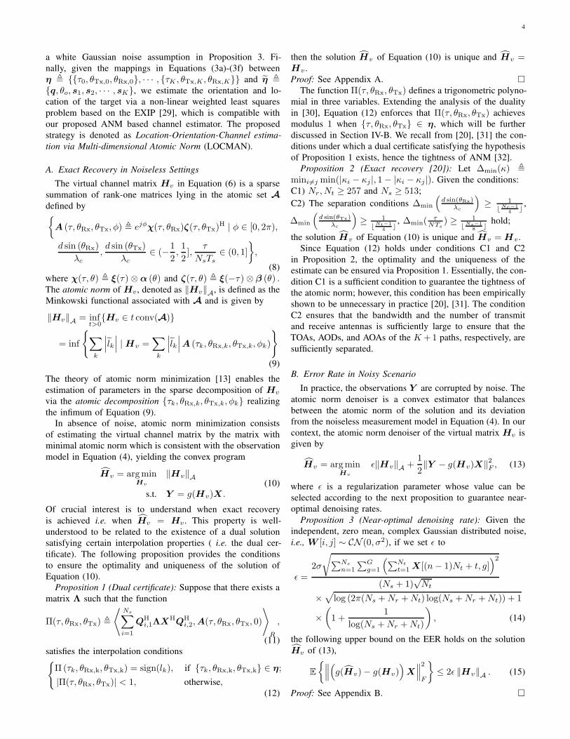
Proposition 1 (Dual certificate): Suppose that there exists a

matrix Λ such that the function

Π(τ, θRx, θTx) ,

⟨Ns∑

i=1

QHi,1ΛXHQH

i,2,A(τ, θRx, θTx, 0)

⟩

R

,

(11)

satisfies the interpolation conditions{Π(τk, θRx,k, θTx,k) = sign(lk), if {τk, θRx,k, θTx,k} ∈ η;

|Π(τ, θRx, θTx)| < 1, otherwise,

(12)

then the solution Hv of Equation (10) is unique and Hv =Hv .

Proof: See Appendix A. �

The function Π(τ, θRx, θTx) defines a trigonometric polyno-

mial in three variables. Extending the analysis of the duality

in [30], Equation (12) enforces that Π(τ, θRx, θTx) achieves

modulus 1 when {τ, θRx, θTx} ∈ η, which will be further

discussed in Section IV-B. We recall from [20], [31] the con-

ditions under which a dual certificate satisfying the hypothesis

of Proposition 1 exists, hence the tightness of ANM [32].

Proposition 2 (Exact recovery [20]): Let ∆min(κ) ,

mini6=j min(|κi − κj |, 1− |κi − κj |). Given the conditions:

C1) Nr, Nt ≥ 257 and Ns ≥ 513;

C2) The separation conditions ∆min

(d sin(θRx)

λc

)≥ 1

⌊Nr−14 ⌋ ,

∆min

(d sin(θTx)

λc

)≥ 1

⌊Nt−14 ⌋ , ∆min(

τNTs

) ≥ 1⌊Ns−1

8 ⌋ hold;

the solution Hv of Equation (10) is unique and Hv = Hv.

Since Equation (12) holds under conditions C1 and C2

in Proposition 2, the optimality and the uniqueness of the

estimate can be ensured via Proposition 1. Essentially, the con-

dition C1 is a sufficient condition to guarantee the tightness of

the atomic norm; however, this condition has been empirically

shown to be unnecessary in practice [20], [31]. The condition

C2 ensures that the bandwidth and the number of transmit

and receive antennas is sufficiently large to ensure that the

TOAs, AODs, and AOAs of the K+1 paths, respectively, are

sufficiently separated.

B. Error Rate in Noisy Scenario

In practice, the observations Y are corrupted by noise. The

atomic norm denoiser is a convex estimator that balances

between the atomic norm of the solution and its deviation

from the noiseless measurement model in Equation (4). In our

context, the atomic norm denoiser of the virtual matrix Hv is

given by

Hv = argminHv

ǫ‖Hv‖A +1

2‖Y − g(Hv)X‖2F , (13)

where ǫ is a regularization parameter whose value can be

selected according to the next proposition to guarantee near-

optimal denoising rates.

Proposition 3 (Near-optimal denoising rate): Given the

independent, zero mean, complex Gaussian distributed noise,

i.e., W [i, j] ∼ CN (0, σ2), if we set ǫ to

ǫ =2σ

√∑Ns

n=1

∑Gg=1

(∑Nt

t=1 X[(n− 1)Nt + t, g])2

(Ns + 1)√Nt

×√log (2π(Ns +Nr +Nt) log(Ns +Nr +Nt)) + 1

×(1 +

1

log(Ns +Nr +Nt)

), (14)

the following upper bound on the EER holds on the solution

Hv of (13),

E

{∥∥∥(g(Hv)− g(Hv)

)X∥∥∥2

F

}≤ 2ǫ ‖Hv‖A . (15)

Proof: See Appendix B. �

5

The bound in Equation (15) is obtained by selecting the

smallest ǫ that is greater than or equal to the expectation of

the dual norm of∑Ns

i=1 QHi,1WXHQH

i,2 (see Equation (23) for

the definition of the dual norm). Note that, as the noise W

is added to g(Hv)X in our measurement model instead of

Hv , the theoretical results derived in [33] cannot be directly

applied to our setting.

In contrast to [20], which selects the regularization parame-

ter ǫ ∝ σ

√(Ns+1

2

)2NrNt log

((Ns+1

2

)2NrNt

), Proposition

3 takes the structure of the virtual channel matrix and the en-

ergy of the pilot signal into consideration. Numerical evidence

of the benefits of the choice of ǫ provided in Proposition 3 will

be given in Section IV-B.

C. Semidefinite Approximation of the Atomic Norm

Given a (2r1−1)×(2r2−1) matrix U , we define by T2(U)the r1r2 × r1r2 2-level block Toeplitz matrix [28] as

T2(U) =

T (u0) T (u1) · · · T (ur1−1)T (u−1) T (u0) · · · T (ur1−2)

......

. . ....

T (u−r1+1) T (u−r1+2) · · · T (u0)

(16)

where T (u) is defined for any a 2r2−1 vector u as the r2×r2Toeplitz matrix with first row [u[0],u[1], . . . ,u[r2 − 1]] and

first column [u[0],u[1], . . . ,u[−r2 + 1]]T

.

Although Equations (10) and (13) are both convex programs

involving multi-dimensional polynomial constraints, comput-

ing their optimal solution requires resolving a Lasserre hier-

archy of semidefinite programs (SDP) [34]. In fact, it can be

shown that the first Lasserre approximation is tight provided

that the number of paths is small enough, which is the subject

of Proposition 4.

Proposition 4 (Semidefinite representation): The atomic

norm ‖Hv‖A defined in Equation (9) is equivalent to the SDP

minV ,U ,Hv

1

2Tr (J)

s.t. J ,

[ T2(U ) Hv

HHv T2(V )

]� 0,

H(i,j)v = H(k,z)

v , if i+ j = k + z, ∀i, j, k, z,(17)

provided that rank(T2(U)) < min(Ns+1

2 , Nr

)and

rank(T2(V )) < min(Ns+1

2 , Nt

), where U and V are the

estimates for U and V , respectively.

Proof: Let ‖Hv‖ be the objective value in Equation (17) and

define SDP(Hv) as in [20, Equation (35)] that is,

SDP(Hv) , minV ,U ,Hv

1

2Tr (J)

s.t. J ,

[ T2(U ) Hv

HHv T2(V )

]� 0.

(18)

The inequality ‖Hv‖ ≥ SDP(Hv) holds based on the defini-

tions of the key quantities. It can be shown from [20, Lemma

1] that ‖Hv‖ ≤ ‖Hv‖A. Furthermore, given rank(T2(U)) <

min(Ns+1

2 , Nr

)and rank(T2(V )) < min

(Ns+1

2 , Nt

), T2(U )

and T2(V ) admit the unique 2-level Vandermonde decompo-

sition [28]. Then, [31, Theorem 3] can be applied to the two-

dimensional case, which, combined with [20, Lemma 2] yields

the equality SDP(Hv) = ‖Hv‖A, yielding on the desired

result. �

While the 2-level Vandermonde decompositions of the so-

lutions T2(U) and T2(V ) of Equation (18) need to exist for

the SDP equivalence to hold, the rank conditions are simple

sufficient conditions to ensure their existence. In addition, we

remark that the conditions C1 and C2 in Proposition 2 are not

necessary for the equivalence of SDP(Hv) and ‖Hv‖A to

hold.

Note that, a Toeplitz-Hankel formulation is proposed in

[35] for the recovery of one-dimensional signals, which is

shown to be equivalent to the atomic norm when the Hankel

matrix therein admits a Vandermonde decomposition. Though

the formulation in [35] might be extended for the multi-

dimensional case, their extended formulation still does not fit

our signal model since Hv is not a Hankel matrix.

D. Estimation of Individual Channel Parameters

Proposition 1 suggests that it is possible to estimate the

TOAs, AOAs, and AODs (τk, θTx,k, and θRx,k) by identifying

the values where the modulus of the dual trigonometric

polynomial achieves unity. For computational efficiency, we

estimate these channel parameters from the 2-level Vander-

monde decomposition of the solution of Equation (10) or (13)

in the sequel. Specifically, the individual channel parameters

are estimated via the matrix pencil and pairing (MaPP) algo-

rithm [28]. The estimates corresponding to the same path are

paired, which presupposes the total number of the paths to be

known by the receiver. If the total number of the paths K is

unknown by the receiver, it can be estimated by the rank of the

solution Hv of the program in Equation (10) or (13) which

can be computed regardless of the model order. In practice, it

is sufficient to count the number of eigenvalues of Hv that

are greater than a threshold to get a reliable estimate of

K before applying the MaPP algorithm. We assume that the

channel coefficient γ0 associated to the LOS path is the one

with largest modulus when K is to be estimated. The choice

of is empirically discussed in Section IV-D.

E. Localization and Orientation Estimation

Although the estimated location and orientation can be

directly estimated from the geometry of the LOS path, more

accurate estimates can be achieved by leveraging the geom-

etry of the NLOS paths [8]. Once the parameter η, which

parametrizes Equation (13) given the channel coefficients

{γ0, γ1, · · · γK}, is estimated through the procedure presented

in Section III-D, the final step consists of recovering the loca-

tion and orientation parameters from the geometric mapping

in Equation (3).

Since we make no assumptions on the path loss model in

the signal model, knowledge of the channel coefficients do not

improve the accuracy of the localization and orientation es-

timation. In addition, {p, θo, s1, s2, · · · , sK , γ0, γ1, · · · , γK}can be used to re-parametrize the optimization problem in

6

Equation (13). Therefore, we fix the estimated channel co-

efficients2 and propose a weighted least squares problem to

achieve an accurate localization and orientation estimation,

with the estimates of all the paths, i.e., η, exploited,

η = argminη

(η − f(η))TD (η − f(η)) , (19)

where the mapping f(η) = η integrates the geometric map-

ping in Equation (3). Inspired by the EXIP [8], [29], the weight

matrix D in Equation (19) is set to the Hessian of the objective

function L(η) of the program in Equation (13) at the estimated

channel parameters η, i.e.,

D ,

∂2L(η)∂τ0∂τ0

∂2L(η)∂τ0∂θTx,0

· · · ∂2L(η)∂τ0∂θRx,L

∂2L(η)∂θTx,0∂τ0

∂2L(η)∂θTx,0∂θTx,0

· · · ∂2L(η)∂θTx,0∂θRx,L

......

. . ....

∂2L(η)∂θRx,L∂τ0

∂2L(η)∂θRx,L∂θTx,0

· · · ∂2L(η)∂θRx,L∂θRx,L

,

(20)

which depends on the channel parameters estimated via the

proposed ANM based method of Section III-B3.

The non-linear least squares problem in Equation (19)

can be solved via the Levenberg-Marquard-Fletcher algo-

rithm [36]. The parameters in η are initialized with the

values pLOS, θo,LOS, {s1,y,LOS, s2,y,LOS, · · · , sK,y,LOS}, and

{s1,x,LOS, s2,x,LOS, · · · , sK,x,LOS}, which are derived in the

following set of equations,

pLOS = q + cτ0[cos(θTx,0), sin(θTx,0)]T, (21a)

θo,LOS = π + θTx,0 − θRx,0, (21b)

sk,y,LOS = tan(θTx,k)(sk,x − qx) + qy, (21c)

sk,x,LOS =

tan(θTx,k)qx − tan(θRx,k + θo,LOS)pLOS,x + pLOS,y − qy

tan(θTx,k)− tan(θRx,k + θo,LOS)

.

(21d)

Note that, Equation (19) implicitly depends on the received

signal via η and D. Essentially, the non-linear weighted

least squares problem in Equation (19) is a second-order

Taylor expansion of the cost function in Equation (13) re-

parametrized by {p, θo, s1, s2, · · · , sK , γ0, γ1, · · · , γK} at the

global optimum [29], which is different from more typical

indirect localization methods with multilateration [37].

IV. SIMULATION RESULTS

In this section, we evaluate the performance of our pro-

posed scheme , i.e., LOCMAN. First, the theoretical analyses

presented in Propositions 1-3 are numerically validated in

Section IV-B. Then, in Section IV-C, our LOCMAN scheme

is compared with DCS-SOMP [8], [12] to the show the

performance improvements over the estimation accuracy of

individual channel parameters, orientation and location. Fi-

nally, the effects of the incorrect model order selection as

2We can substitute the estimated η into Equation (4) to achieve a systemof linear equations to compute the estimates of channel coefficients [27].

3We note that the derivative of the term ǫ ‖Hv‖A in Equation (13) withrespect to the parameters in η is 0, so Equation (20) reduces to the Hessian

of the quadratic loss function 12‖Y − g(Hv)X‖2F at η.

well as synchronization errors are studied via simulation in

Section IV-D.

A. Signal Parameters

In all of the numerical results, we set fc = 60GHz,

B = 100MHz, Ns = 15, Nr = 16, Nt = 16, G = 16, K = 2,

and d = λc

2 . The pilot signals are random complex values

uniformly distributed on the unit circle. Unless otherwise

stated, the total number of paths is known at the receiver and

the channel coefficients are generated based on the free-space

path loss model [38] in the simulation. The BS is placed at

[0m, 0m]T while the target is at [20m, 5m]T with an orienta-

tion θo = 0.2 rad. The scatterers corresponding to two NLOS

paths are placed at [7.45m, 8.54m]T and [19.89m,−6.05m]T.

We solve the optimization problem in Equations (10) and (13)

for the channel estimation in the noiseless and noisy cases,

where the semidefinite representation of the atomic norm in

Proposition 4 is adopted. For the atomic norm denoiser in

Equation (13), the regularization parameters ǫ is set according

to Proposition 3. In the presence of independent, zero mean,

complex Gaussian distributed noise, the SNR is defined as

SNR =‖HX‖2

F

‖W‖2F

.

B. Validation of Propositions 1-3

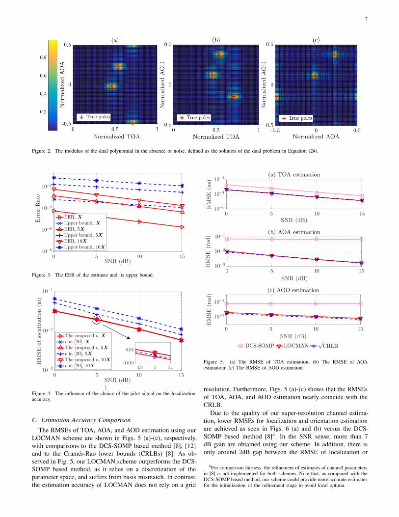
Fig. 2 shows the modulus of the dual polynomial for the

noiseless case. Recall that, the dual polynomial is a trigono-

metric function with respect to TOAs, AOAs, and AODs.

For better visualization, the modulus of the dual polynomial

is projected on the TOA-AOA, TOA-AOD, and AOA-AOD

axes in Fig. 2 (a), (b), and (c), respectively. Consistent with

our analysis for Proposition 1, from Fig. 2, we can observe

that the modulus of dual polynomial nearly equals 1 when

{τ, θRx, θTx} ∈ η even though condition C1 of Proposition 2

is not satisfied given the values of N , Nr, and Nt selected in

our experiments.

For the noisy scenario, the EER of the estimate

and its theoretical bound are shown in Fig. 3. We

can verify that that 2ǫ ‖Hv‖A is an upper bound of

E

{∥∥∥(g(Hv)− g(Hv)

)X∥∥∥2

F

}, as stated in Proposition 3.

Though the bound is not sharp, Proposition 3 suggests a

good choice of the regularization parameter ǫ. To show the

benefits of setting ǫ according to Equation (14), we present

in Fig. 4 the RMSEs of localization, with different choices of

pilot signals, i.e., X , 5X , 10X, when ǫ is selected according

to Proposition 3 and according to [20] for comparison. We

observe that the localization accuracy using our design of

ǫ yield near constant RMSEs as the energy of pilot signal

increases while the performance degrades with the choice

suggested in [20]. This strong improvement can be explained

by the fact that our proposed choice of the regularization

parameter ǫ incorporates the energy of the pilot signals and the

structure of the virtual channel matrix, leading to a dynamic

penalization of the atomic norm in Equation (13).

7

Figure 2. The modulus of the dual polynomial in the absence of noise, defined as the solution of the dual problem in Equation (24).

0 5 10 15SNR (dB)

10−8

10−6

10−4

10−2

ErrorRate

EER, XUpper bound, XEER, 5XUpper bound, 5XEER, 10XUpper bound, 10X

Figure 3. The EER of the estimate and its upper bound.

0 5 10 15SNR (dB))

10−3

10−2

10−1

RMSE

oflocalization(m

)

The proposed ǫ, Xǫ in [20], XThe proposed ǫ, 5Xǫ in [20], 5XThe proposed ǫ, 10Xǫ in [20], 10X 4.9 5 5.1

0.019

0.02

Figure 4. The influence of the choice of the pilot signal on the localizationaccuracy.

C. Estimation Accuracy Comparison

The RMSEs of TOA, AOA, and AOD estimation using our

LOCMAN scheme are shown in Figs. 5 (a)-(c), respectively,

with comparisons to the DCS-SOMP based method [8], [12]

and to the Cramer-Rao lower bounds (CRLBs) [8]. As ob-

served in Fig. 5, our LOCMAN scheme outperforms the DCS-

SOMP based method, as it relies on a discretization of the

parameter space, and suffers from basis mismatch. In contrast,

the estimation accuracy of LOCMAN does not rely on a grid

0 5 10 15SNR (dB)

10−5

10−4

10−3

RMSE

(us)

(a) TOA estimation

DCS-SOMP LOCMAN√

CRLB

0 5 10 15

SNR (dB)

10−3

10−2

10−1

RMSE

(rad)

(b) AOA estimation

0 5 10 15

SNR (dB)

10−3

10−1

RMSE

(rad)

(c) AOD estimation

Figure 5. (a) The RMSE of TOA estimation; (b) The RMSE of AOAestimation; (c) The RMSE of AOD estimation.

resolution. Furthermore, Figs. 5 (a)-(c) shows that the RMSEs

of TOA, AOA, and AOD estimation nearly coincide with the

CRLB.

Due to the quality of our super-resolution channel estima-

tion, lower RMSEs for localization and orientation estimation

are achieved as seen in Figs. 6 (a) and (b) versus the DCS-

SOMP based method [8]4. In the SNR sense, more than 7dB gain are obtained using our scheme. In addition, there is

only around 2dB gap between the RMSE of localization or

4For comparison fairness, the refinement of estimates of channel parametersin [8] is not implemented for both schemes. Note that, as compared with theDCS-SOMP based method, our scheme could provide more accurate estimatesfor the initialization of the refinement stage to avoid local optima.

8

0 5 10 15SNR (dB)

10−4

10−2

100

RMSE

(rad)

(a) Orientation estimation

DCS-SOMP LOCMAN√

CRLB

0 5 10 15

SNR (dB)

10−4

10−2

100

RMSE

(m)

(b) Localization

Figure 6. (a) The RMSE of orientation estimation; (b) The RMSE oflocalization.

orientation estimation using our LOCMAN scheme and the

CRLB curves, verifying the efficacy of our design.

D. Model Order Selection and Synchronization Error

We next study the scenario where the total number of

paths K is unknown at the receiver. The efficiency of the

thresholding-based model order selection proposed in Section

III-D is investigated. To show the effect of the choices of

on the performance degradation, we fix l0, l1, and l2 in

Equation (6) to 0.0025 0.0011, and 0.0014, while we vary

the value of . Figure 7 presents the RMSE of orientation

estimation and localization for = 0.0005, = 0.0013and = 0.002, respectively, from which a similar estimation

accuracy for different choices of can be observed. Since we

assume that the LOS path is that with the largest modulus of

channel coefficient in Section III-A when K is unknown at the

receiver, the channel parameters associated with the LOS path

are always available for localization5 and the loss caused by

the estimation error of the model order is less than 1 dB with

respect to the RMSE of localization or orientation estimation.

Finally, the performance degradation caused by synchroniza-

tion errors is investigated though synchronization errors are not

considered in our signal model. Specifically, denoting by τ the

unknown synchronization error, we define AOAs and AODs

according to Equations (3c)-(3f) while re-express the TOA of

5This is achievable unless the value of is so large that the estimated totalnumber of paths is 0.

0 5 10 15

SNR (dB)

10−3

10−2

RMSE

(rad)

(a) Orientation estimation

4.5 5 5.5

8

10

×10-4

0 5 10 15SNR (dB)

10−2

10−1

RMSE

(m)

(b) Localization

= 0.0005 = 0.0013 = 0.002

4.9 5 5.1

0.019

0.02

0.021

Figure 7. The influence of incorrect model order selection on localizationand orientation estimation.

each path as

τ0 =‖p− q‖2

c+ τ , (22a)

τk =‖q − sk‖2 + ‖p− sk‖2

c+ τ , k > 0. (22b)

We still exploit the LOCMAN proposed in Section III for

channel estimation as well as localization. The RMSEs of

orientation estimation and localization are presented in Figs.

8 (a) and (b), respectively. Since the definitions of AOAs

and AODs in Equations (3c)-(3f) are maintained, the syn-

chronization error has negligible influence on the AOA or

AOD estimation and correspondingly, the RMSE of orientation

estimation is nearly constant with the increase of the value of

τ , as observed in Fig. 8 (a). In addition, the synchronization

error has a minor effect on the TOA estimation as the value

of τ is quite small as compared with the TOA of each

path in the simulation6. In contrast, the synchronization error

degrades the localization accuracy, according to Fig. 8 (b).

However, as compared with the DCS-SOMP based method,

the centimeter-level localization accuracy is still attained using

our scheme when τ ≤ 1× 10−3 µs. The estimation design of

the synchronization error is left as the future work.

V. CONCLUSIONS

In this paper, a multi-dimensional atomic norm based

method is proposed for high-accuracy localization and ori-

entation estimation in mmWave MIMO OFDM systems. To

6Note that, for a localization problem, the synchronization error is generallyat ns-level[39].

9

10−6 10−5 10−4 10−3τ (us)

10−4

10−2

RMSE

(rad)

(a) Orientation estimation

LOCMAN, 0 dB√

CRLB, 0 dB LOCMAN, 5 dB

10−6 10−5 10−4 10−3

τ (us)

10−2

10−1

100

RMSE

(m)

(b) Localization

data5 data6 data7 data8 DCS-SOMP, 15 dB

√

CRLB, 5 dB LOCMAN, 10 dB√

CRLB, 10 dB

LOCMAN, 15 dB√

CRLB, 15 dB

Figure 8. The influence of synchronization error on localization and orienta-tion estimation.

effectively estimate all of the location-relevant channel param-

eters with super-resolution, a novel virtual channel matrix is

introduced and an atomic norm based channel estimator is

proposed. Theoretical performance guarantees are derived for

both the noiseless and noisy cases. Using the estimates of all

the paths, a weighted least squares problem is proposed based

on the extended invariance principle to accurately recover

the location and orientation. The new method offers strong

improvements with respect to the RMSE of estimation over

prior work [8] (more than 7 dB gain) and exhibits high

robustness in terms of the incorrect model order selection

or synchronization errors. Furthermore, with the proposed

method, the RMSEs of channel estimation, localization and

orientation estimation nearly achieve the CRLBs.

APPENDIX A

PROOF OF PROPOSITION 1

To derive the optimality and uniqueness conditions, we

follow the proof structure of [14], [30], and define the dual

norm as

‖Z‖∗A = sup‖Hv‖A≤1

〈Z, Hv〉R

= supτ,θRx,θTx,φ

〈Z ,A(τ, θRx, θTx, φ)〉R,

= supτ,θRx,θTx

|〈Z,A(τ, θRx, θTx, 0)〉| .

(23)

The Lagrange dual problem of Equation (10) is given by

argminΛ

〈Λ,Y 〉R

s.t.

∥∥∥∥∥Ns∑

i=1

QHi,1ΛXHQH

i,2

∥∥∥∥∥

∗

A

≤ 1.(24)

It can be verified that any Λ satisfying Equation (12) is dual

feasible. Next, we have that

‖Hv‖A(a)

≥ ‖Hv‖A∥∥∥∥∥

Ns∑

i=1

QHi,1ΛXHQH

i,2

∥∥∥∥∥

∗

A(b)

≥⟨

Ns∑

i=1

QHi,1ΛXHQH

i,2,Hv

⟩

R

=

⟨Ns∑

i=1

QHi,1ΛXHQH

i,2,

K∑

k=0

lkA(τk, θRx,k, θTx,k, 0)

⟩

R

=K∑

k=0

Re

(l∗k

⟨Ns∑

i=1

QHi,1ΛXHQH

i,2,A(τk, θRx,k, θTx,k, 0)

⟩)

=

K∑

k=0

Re (l∗kΠ(τk, θRx,k, θTx,k, 0))(c)=

K∑

k=0

|lk| ≥ ‖Hv‖A ,

(25)

where (a) and (c) hold because of Equation (12) while (b)results from Holder inequality. Therefore, 〈Λ,Y 〉R = ‖Hv‖Aand strong duality holds. Then, Hv is a primal optimal

solution and Λ is a dual optimal solution.

We show the uniqueness by contradiction by assuming the

existence of a distinct optimal solution Hv such that

Hv =

K∑

k=0

lkA(τk, θRx,k, θTx,k, 0

)(26)

with ‖Hv‖A =∑K

k=0 |lk|. From Equation (12), we have

Equation (27), which contradicts the strong duality. Hence,

the optimal solution is unique, concluding the proof.

APPENDIX B

PROOF OF PROPOSITION 3

For the proof of Proposition 3, we first extend [33, Lemma1

and Theorem 1] to our atomic norm denoising formulation.

Lemma 1: If Hv is the solution of Equation (13), it holds

that∥∥∥∥∥

Ns∑

i=1

QHi,1

(Y − g(Hv)X

)XHQH

i,2

∥∥∥∥∥

∗

A

≤ ǫ, (28a)

⟨Y − g(Hv)X , g(Hv)X

⟩R= ǫ

∥∥∥Hv

∥∥∥A. (28b)

Proof: Define a(Hv) ,

∥∥∥Y − g(Hv)X∥∥∥ + ǫ

∥∥∥Hv

∥∥∥A. The

subdifferential ∂a(Hv) of the previous writes

∂a(Hv) =

Ns∑

i=1

QHi,1

(g(Hv)X − Y

)XHQH

i,2 + ǫZ, (29)

10

where Z ∈ ∂∥∥∥Hv

∥∥∥A. Since Hv is the solution of Equa-

tion (13), 0 ∈ ∂a(Hv) holds which leads to the equality

Ns∑

i=1

QHi,1

(Y − g(Hv)X

)XHQH

i,2 = ǫZ. (30)

Furthermore, the properties of the subdifferential of norms

imply that ‖Z‖∗A ≤ 1, and⟨Hv,Z

⟩R

=∥∥∥Hv

∥∥∥A

. One

concludes on Lemma 1 by applying these properties to Equa-

tion (30).

�

Lemma 2: If E

{∥∥∥∑Ns

i=1 QHi,1WXHQH

i,2

∥∥∥∗

A

}≤ ǫ, the

solution of Equation (13), i.e., Hv satisfies

E

{∥∥∥(g(Hv)− g(Hv)

)X∥∥∥2

2

}≤ 2ǫ ‖Hv‖A . (31)

Proof: Considering Y = g(Hv)X +W , we have∥∥∥(g(Hv)− g(Hv)

)X∥∥∥2

F

=⟨g(Hv)X − g(Hv)X, g(Hv)X − g(Hv)X

⟩

=⟨g(Hv)X − g(Hv)X, g(Hv)X − (Y −W )

⟩

=⟨g(Hv)X − g(Hv)X,W − (Y − g(Hv)X)

⟩

=⟨g(Hv)X − g(Hv)X,W − (Y − g(Hv)X)

⟩R

=⟨g(Hv)X ,Y − g(Hv)X

⟩R− 〈g(Hv)X,W 〉R

+⟨g(Hv)X,W

⟩R−⟨g(Hv)X ,Y − g(Hv)X

⟩R

(d)

≤ 2ǫ ‖Hv‖A . (32)

if

∥∥∥∑Ns

i=1 QHi,1WXHQH

i,2

∥∥∥∗

A≤ ǫ. Note that, (d) holds with

Equation (28) and the Holder inequality as optimality implies

that ⟨g(Hv)X,Y − g(Hv)X

⟩R≤ ǫ ‖Hv‖A , (33a)

−〈g(Hv)X,W 〉R ≤ ǫ ‖Hv‖A , (33b)⟨g(Hv)X,W

⟩R≤∥∥∥Hv

∥∥∥A, (33c)

⟨Y − g(Hv)X, g(Hv)X

⟩R= ǫ‖Hv‖A. (33d)

We restrict the derivation of the previous to Equation (33a) as

the others can be shown analogously⟨g(Hv)X,Y − g(Hv)X

⟩R

=

⟨Hv,

Ns∑

i=1

QHi,1

(Y − g(Hv)X

)XHQH

i,2

⟩

R

(e)

≤ ‖Hv‖A

∥∥∥∥∥Ns∑

i=1

QHi,1

(Y − g(Hv)X

)XHQH

i,2

∥∥∥∥∥

∗

A(f)

≤ ǫ ‖Hv‖A , (34)

where (e) and (f) follow from Holder inequality and

Equation (28). We conclude on Equation (31) given

E

{∥∥∥∑Ns

i=1 QHi,1WXHQH

i,2

∥∥∥∗

A

}≤ ǫ. �

Proof of Proposition 3: The goal of Proposition 3 is to give an

upper bound on the EER. Based on Lemma 2, we need to de-

rive a proper upper bound on E

{∥∥∥∑Ns

i=1 QHi,1WXHQH

i,2

∥∥∥∗

A

}.

To that end, we start by introducing the quantity W as

W ,2

(Ns + 1)√NrNt

Ns∑

i=1

QHi,1WXHQH

i,2. (36)

Next, let Γ = (0, 1]× (− 12 ,

12 ]× (− 1

2 ,12 ], δ = [δ1, δ2, δ3] ∈ Γ

with δ1 , τNTs

, δ2 ,d sin(θRx)

λc, δ3 ,

d sin(θTx)λc

, and let δ =

[δ1, δ2, δ3] = [ei2πδ1 , ei2πδ2 , ei2πδ3 ]. We define the function

Ξ(δ) ,∑

z=1,...,Nr

t=1,...,Nt

i=1,...,Ns

W [(i−1)Nt+t, (i−1)Nr+z]δi−11 δz−1

2 δt−13 .

(37)

From Equation (23),

∥∥∥∑Ns

i=1 QHi,1WXHQH

i,2

∥∥∥∗

Acan be sim-

plified as given in Equation (35). Note that, (g) and (h) hold

with Equation (5) and Equation (8). To clarify the proof, we

introduce the quantity

‖Ξ‖∞ , supδ∈Γ

∣∣∣Ξ(δ)∣∣∣ =

∥∥∥∥∥Ns∑

i=1

QHi,1WXHQH

i,2

∥∥∥∥∥

∗

A

.

Next, for any pair(δ(1), δ(2)

)∈ Γ× Γ, we have that

∣∣∣Ξ(δ(1)

)∣∣∣−∣∣∣Ξ(δ(2)

)∣∣∣ ≤∥∥∥∥δ

(1) − δ(2)∥∥∥∥2

supδ∈T3

∥∥∥∥∂Ξ

∂δ

∥∥∥∥2

⟨Ns∑

i=1

QHi,1ΛXHQH

i,2, Hv

⟩

R

=

⟨Ns∑

i=1

QHi,1ΛXHQH

i,2,

K∑

k=0

lkA(τk, θRx,k, θTx,k, 0

)⟩

R

=∑

(τk,θ

Rx,k,θ

Tx,k)∈η

Re

(l∗k

⟨Ns∑

i=1

QHi,1ΛXHQH

i,2,A(τk, θRx,k, θTx,k, 0)

⟩)

+∑

(τk,θ

Rx,k,θ

Tx,k)/∈η

Re

(l∗k

⟨Ns∑

i=1

QHi,1ΛXHQH

i,2,A(τk, θRx,k, θTx,k, 0)

⟩)

<∑

(τk,θ

Rx,k,θ

Tx,k)∈η

|l∗k|+

∑

(τk,θ

Rx,k,θ

Tx,k)/∈η

|l∗k| = ‖Hv‖A. (27)

11

∥∥∥∥∥Ns∑

i=1

QHi,1WXHQH

i,2

∥∥∥∥∥

∗

A

= supτ,θRx,θTx

∣∣∣∣⟨W ,

(Ns + 1)√NrNt

2A(τ, θRx, θTx, 0)

⟩∣∣∣∣

(g)= sup

δ∈Γ

∣∣∣∣∣∣

Nr∑

z=1

Nt∑

t=1

Ns∑

i=1

Ns+12∑

o=1

W [(o− 1)Nr + z, (i− o)Nt + t]δi−11 δz−1

2 δt−13

∣∣∣∣∣∣

(h)= sup

δ∈Γ

∣∣∣∣∣Nr∑

z=1

Nt∑

t=1

Ns∑

i=1

W [(i − 1)Nr + z, (i− 1)Nt + t]δi−11 δz−1

2 δt−13

∣∣∣∣∣ = supδ∈Γ

∣∣∣Ξ(δ)∣∣∣

(35)

(i)

≤ (Ns +Nr +Nt)

∥∥∥∥δ(1) − δ

(2)∥∥∥∥2

‖Ξ‖∞

≤ (Ns +Nr +Nt)

∥∥∥∥δ(1) − δ

(2)∥∥∥∥1

‖Ξ‖∞

≤ 2π(Ns +Nr +Nt)∥∥∥δ(1) − δ(2)

∥∥∥1‖Ξ‖∞ , (38)

where (i) holds according to the multi-dimensional Bernstein

inequality [40]. To find the proper upper bound on ‖Ξ‖∞,

we extend [33, Appendix C] to our model. Define the three-

dimensional regular grid G ⊂ Γ as

G =1

NTOA

{0, . . . , NTOA

}

× 1

NAOA

{−NAOA

2+ 1, . . . ,

NAOA

2

}

× 1

NAOD

{−NAOD

2+ 1, . . . ,

NAOD

2

}(39)

From Equation (38), we can derive the inequality

‖Ξ‖∞ ≤ maxδ(2)∈G

∣∣∣Ξ(δ(2)

)∣∣∣

+ π(Ns +Nr +Nt)

(1

NTOA+

1

NAOA+

1

NAOD

)‖Ξ‖∞ .

(40)

Therefore, it comes that

‖Ξ‖∞

≤(1− π(Ns +Nr +Nt)

(1

NTOA+

1

NAOA+

1

NAOD

))−1

× maxδ(2)∈G

∣∣∣Ξ(δ(2)

)∣∣∣(j)

≤(1 + 2π(Ns +Nr +Nt)

(1

NTOA+

1

NAOA+

1

NAOD

))

× maxδ(2)∈G

∣∣∣Ξ(δ(2)

)∣∣∣ ,(41)

where we assume that π(Ns + Nr +

Nt)(

1NTOA

+ 1NAOA

+ 1NAOD

)< 1. The inequality (j)

can be verified with some algebra.

Then, finding the upper bound on E {‖Ξ‖∞} amounts

to evaluating the expectation of the right-hand side of

Equation (41). Recalling that W [i, j] ∼ CN (0, σ2), we

have from the definitions of Qi,1 and Qi,2 in Equa-

tion (5) that Ξ(δ(2)

)∼ CN

(0, σ2

), with σ2 ,

4σ2 ∑Nsn=1

∑Gg=1(

∑Ntt=1 X[(n−1)Nt+t,g])

2

Nt(Ns+1)2 . By [33, Lemma 5] the

expectation of maxδ(2)∈G

∣∣∣Ξ(δ(2)

)∣∣∣ can be bounded by,

E

{max

δ(2)∈G

∣∣∣Ξ(δ(2)

)∣∣∣}

≤ σ√log(NTOANAOANAOD) + 1

(42)

By substituting Equation (42) into Equation (41), we can

obtain the upper bound

E {‖Ξ‖∞}

≤(1 + 2π(Ns +Nr +Nt)

(1

NTOA+

1

NAOA+

1

NAOD

))

× σ√log(NTOANAOANAOD) + 1. (43)

Furthermore, using the harmonic mean-geometric mean in-

equality, we have

E {‖Ξ‖∞} ≤ σ

(1 + 2π(Ns +Nr +Nt)

1

N

)√log(N) + 1,

(44)

where N , NTOA = NAOA = NAOD. Setting N = 2π(Ns +Nr+Nt) log(Ns+Nr+Nt) [33, Appendix D] in Equation (44)

yields the desired statement. �

REFERENCES

[1] J. Li, M. Ferreira Da Costa, and U. Mitra, “Atomic Norm BasedLocalization and Orientation Estimation for Millimeter-Wave MIMOOFDM Systems”, in ICASSP 2022 - 2022 IEEE International Con-

ference on Acoustics, Speech and Signal Processing (ICASSP), 2022.[2] T. S. Rappaport, S. Sun, R. Mayzus, H. Zhao, Y. Azar, K. Wang,

G. N. Wong, J. K. Schulz, M. Samimi, and F. Gutierrez, “MillimeterWave Mobile Communications for 5G Cellular: It Will Work!”, IEEE

Access, vol. 1, pp. 335–349, 2013.[3] S. Hur, T. Kim, D. J. Love, J. V. Krogmeier, T. A. Thomas, and

A. Ghosh, “Millimeter Wave Beamforming for Wireless Backhauland Access in Small Cell Networks”, IEEE Transactions on Commu-

nications, vol. 61, no. 10, pp. 4391–4403, 2013.[4] F. Lemic, J. Martin, C. Yarp, D. Chan, V. Handziski, R. Brodersen,

G. Fettweis, A. Wolisz, and J. Wawrzynek, “Localization as afeature of mmWave communication”, in 2016 International Wireless

Communications and Mobile Computing Conference (IWCMC), 2016,pp. 1033–1038.

[5] H. Deng and A. Sayeed, “mm-wave MIMO channel modeling anduser localization using sparse beamspace signatures”, in 2014 IEEE

15th International Workshop on Signal Processing Advances in Wire-

less Communications (SPAWC), 2014, pp. 130–134.[6] B. Zhou, R. Wichman, L. Zhang, and Z. Luo, “Simultaneous Lo-

calization and Channel Estimation for 5G mmWave MIMO Commu-nications”, in 2021 IEEE 32nd Annual International Symposium on

Personal, Indoor and Mobile Radio Communications (PIMRC), 2021,pp. 1208–1214.

[7] J. Saloranta and G. Destino, “On the utilization of MIMO-OFDMchannel sparsity for accurate positioning”, in 2016 24th European

Signal Processing Conference (EUSIPCO), 2016, pp. 748–752.

12

[8] A. Shahmansoori, G. E. Garcia, G. Destino, G. Seco-Granados,and H. Wymeersch, “Position and Orientation Estimation ThroughMillimeter-Wave MIMO in 5G Systems”, IEEE Transactions on

Wireless Communications, vol. 17, no. 3, pp. 1822–1835, 2018.[9] F. Zhu, A. Liu, and V. K. N. Lau, “Channel Estimation and

Localization for mmWave Systems: A Sparse Bayesian LearningApproach”, in ICC 2019 - 2019 IEEE International Conference on

Communications (ICC), 2019, pp. 1–6.[10] J. Fan, X. Dou, W. Zou, and S. Chen, “Localization Based on Im-

proved Sparse Bayesian Learning in mmWave MIMO Systems”, IEEE

Transactions on Vehicular Technology, vol. 71, no. 1, pp. 354–361,2022.

[11] W. Zheng and N. Gonzalez-Prelcic, “Joint Position, Orientation ANDChannel Estimation in Hybrid mmWAVE MIMO Systems”, in 2019

53rd Asilomar Conference on Signals, Systems, and Computers, 2019,pp. 1453–1458.

[12] M. Duarte, S. Sarvotham, D. Baron, M. Wakin, and R. Baraniuk,“Distributed Compressed Sensing of Jointly Sparse Signals”, in Con-

ference Record of the Thirty-Ninth Asilomar Conference onSignals,

Systems and Computers, 2005., 2005, pp. 1537–1541.[13] Y. Chi and M. Ferreira Da Costa, “Harnessing Sparsity Over the

Continuum: Atomic norm minimization for superresolution”, IEEE

Signal Processing Magazine, vol. 37, no. 2, pp. 39–57, 2020.[14] E. J. Candes and C. Fernandez-Granda, “Towards a Mathematical

Theory of Super-Resolution”, Communications on pure and applied

Mathematics, vol. 67, no. 6, pp. 906–956, 2014.[15] G. Tang, B. N. Bhaskar, and B. Recht, “Near Minimax Line Spectral

Estimation”, IEEE Transactions on Information Theory, vol. 61, no. 1,pp. 499–512, 2015.

[16] V. Duval, “A characterization of the Non-Degenerate Source Condi-tion in super-resolution”, Information and Inference: A Journal of the

IMA, vol. 9, no. 1, pp. 235–269, 2020.[17] M. Ferreira Da Costa and Y. Chi, “On the Stable Resolution Limit

of Total Variation Regularization for Spike Deconvolution”, IEEE

Transactions on Information Theory, vol. 66, no. 11, pp. 7237–7252,2020.

[18] Q. Li and G. Tang, “Approximate support recovery ofatomic line spectral estimation: A tale of resolution andprecision”, Applied and Computational Harmonic Analysis,vol. 48, no. 3, pp. 891–948, 2020. [Online]. Available:https://www.sciencedirect.com/science/article/pii/S1063520318300824.

[19] Y. Chi and Y. Chen, “Compressive Two-Dimensional HarmonicRetrieval via Atomic Norm Minimization”, IEEE Transactions on

Signal Processing, vol. 63, no. 4, pp. 1030–1042, 2014.[20] Y. Tsai, L. Zheng, and X. Wang, “Millimeter-Wave Beamformed Full-

Dimensional MIMO Channel Estimation Based on Atomic Norm Min-imization”, IEEE Transactions on Communications, vol. 66, no. 12,pp. 6150–6163, 2018.

[21] R. Heckel, “Super-resolution MIMO radar”, in 2016 IEEE Interna-

tional Symposium on Information Theory (ISIT), 2016, pp. 1416–1420.

[22] X. Wu and W.-P. Zhu, “Single Far-Field or Near-Field Source Local-ization With Sparse or Uniform Cross Array”, IEEE Transactions on

Vehicular Technology, vol. 69, no. 8, pp. 9135–9139, 2020.[23] X. Wu, W.-P. Zhu, and J. Yan, “Atomic Norm Based Localization

of Far-Field and Near-Field Signals with Generalized SymmetricArrays”, in ICASSP 2020 - 2020 IEEE International Conference on

Acoustics, Speech and Signal Processing (ICASSP), 2020, pp. 4762–4766.

[24] W.-G. Tang, H. Jiang, and Q. Zhang, “Range-Angle Decoupling andEstimation for FDA-MIMO Radar via Atomic Norm Minimizationand Accelerated Proximal Gradient”, IEEE Signal Processing Letters,vol. 27, pp. 366–370, 2020.

[25] S. Beygi, A. Elnakeeb, S. Choudhary, and U. Mitra, “Bilinear MatrixFactorization Methods for Time-Varying Narrowband Channel Esti-mation: Exploiting Sparsity and Rank”, IEEE Transactions on Signal

Processing, vol. 66, no. 22, pp. 6062–6075, 2018.[26] A. Elnakeeb and U. Mitra, “Bilinear Channel Estimation for MIMO

OFDM: Lower Bounds and Training Sequence Optimization”, IEEE

Transactions on Signal Processing, vol. 69, pp. 1317–1331, 2021.[27] J. Li and U. Mitra, “Improved Atomic Norm Based Time-Varying

Multipath Channel Estimation”, IEEE Transactions on Communica-

tions, vol. 69, no. 9, pp. 6225–6235, 2021.[28] Z. Yang, L. Xie, and P. Stoica, “Vandermonde Decomposition of

Multilevel Toeplitz Matrices With Application to MultidimensionalSuper-Resolution”, IEEE Transactions on Information Theory, vol. 62,no. 6, pp. 3685–3701, 2016.

[29] P. Stoica and T. Soderstrom, “On reparametrization of loss functionsused in estimation and the invariance principle”, Signal Processing,vol. 17, no. 4, pp. 383–387, 1989.

[30] G. Tang, B. N. Bhaskar, P. Shah, and B. Recht, “Compressed SensingOff the Grid”, IEEE Transactions on Information Theory, vol. 59,no. 11, pp. 7465–7490, 2013.

[31] Z. Yang and L. Xie, “Exact Joint Sparse Frequency Recovery viaOptimization Methods”, IEEE Transactions on Signal Processing,vol. 64, no. 19, pp. 5145–5157, 2016.

[32] M. Ferreira Da Costa and W. Dai, “A Tight Converse to the SpectralResolution Limit via Convex Programming”, in 2018 IEEE Interna-

tional Symposium on Information Theory (ISIT), 2018, pp. 901–905.[33] B. N. Bhaskar, G. Tang, and B. Recht, “Atomic Norm Denoising

With Applications to Line Spectral Estimation”, IEEE Transactions

on Signal Processing, vol. 61, no. 23, pp. 5987–5999, 2013.[34] J. B. Lasserre, “Global Optimization with Polynomials

and the Problem of Moments”, SIAM Journal on

Optimization, vol. 11, no. 3, pp. 796–817, 2001. eprint:https://doi.org/10.1137/S1052623400366802. [Online]. Available:https://doi.org/10.1137/S1052623400366802.

[35] M. Cho, J.-F. Cai, S. Liu, Y. C. Eldar, and W. Xu, “Fast alternatingprojected gradient descent algorithms for recovering spectrally sparsesignals”, in 2016 IEEE International Conference on Acoustics, Speech

and Signal Processing (ICASSP), 2016, pp. 4638–4642.[36] R. Fletcher, “A Modifidied Marquart Subroutine for Nonlinear Least

Squares”, Harwell Report, 1971.[37] R. Zekavat and R. M. Buehrer, “Handbook of Position Location:

Theory, Practice, and Advances”, in Wiley-IEEE Press, 2019, pp. 435–465.

[38] A. Goldsmith, Wireless Communications. Cambridge University Press,2005.

[39] K. Zhao, T. Zhao, Z. Zheng, C. Yu, D. Ma, K. Rabie, and R. Kharel,“Optimization of Time Synchronization and Algorithms with TDOABased Indoor Positioning Technique for Internet of Things”, Sensors,vol. 20, no. 22, 2020.

[40] S. H. Tung, “Bernstein’s Theorem for the Polydisc”, Proceedings of

the American Mathematical Society, vol. 85, no. 1, pp. 73–76, 1982.