arX

iv:2

005.

0096

8v1

[cs

.IT

] 3

May

202

01

Millimeter-Wave Beam Search with Iterative

Deactivation and Beam Shifting

Chunshan Liu, Min Li, Lou Zhao, Philip Whiting, Stephen V. Hanly,

Iain B. Collings

Abstract

Millimeter Wave (mmWave) communications rely on highly directional beams to combat severe

propagation loss. In this paper, an adaptive beam search algorithm based on spatial scanning, called

Iterative Deactivation and Beam Shifting (IDBS), is proposed for mmWave beam alignment. IDBS

does not require advance information such as the Signal-to-Noise Ratio (SNR) and channel statistics,

and matches the training overhead to the unknown SNR to achieve satisfactory performance. The

algorithm works by gradually deactivating beams using a Bayesian probability criterion based on a

uniform improper prior, where beam deactivation can be implemented with low-complexity operations

that require computing a low-degree polynomial or a search through a look-up table. Numerical results

confirm that IDBS adapts to different propagation scenarios such as line-of-sight and non-line-of-sight

and to different SNRs. It can achieve better tradeoffs between training overhead and beam alignment

accuracy than existing non-adaptive algorithms that have fixed training overheads.

Index Terms

Beamforming, beam alignment, beam training, Bayesian, millimeter wave communications.

I. INTRODUCTION

Millimetre wave (mmWave) wireless communications represent one of the most promising

means of introducing new high bandwidth services as anticipated for 5G and beyond (such as

This work will be presented in part in Proceedings of the 54th IEEE International Conference on Communications, ICC’20,

Dublin, Ireland, June 7-11, 2020 [1]. Chunshan Liu and Lou Zhao are with the School of Communication Engineering,

Hangzhou Dianzi University, Hangzhou, 310018, China (email: {chunshan.liu, lou.zhao}@hdu.edu.cn). Min Li is with College

of Information Science and Electronic Engineering, Zhejiang University, Hangzhou, 310027, China (e-mail: min.li@zju.edu.cn).

Philip Whiting, Stephen V. Hanly and Iain B. Collings are with the School of Engineering, Macquarie University, Sydney,

Australia (email: {philip.whiting, stephen.hanly, iain.collings}@mq.edu.au). (Corresponding author: Min Li)

2

high-definition video, V2X communications [2]–[8], mobile edge computing [9] and surveil-

lance [10]). With strongly directional beams implemented by the antenna arrays equipped at the

base station (BS) and the user equipment (UE) to compensate for the high propagation loss [11],

high data rate mmWave communications can be achieved over distances of hundreds of metres.

However, to align the directional beams to dominant propagation paths requires beam direction

searches, which are challenging [12] because they often have to take place over a large search

space and within a very short time period. The former is due to the requirement of highly

directional beams, hence requiring a large number of beams to cover all possible directions. The

latter is due to the short coherence time of mmWave channels which can be on the order of

fractions of a millisecond in mobile scenarios [13].

Spatial scanning is a widely adopted approach for mmWave beam search [14]–[22] and has

drawn considerable attention due to its simplicity and high performance. In spatial scanning, pre-

synthesised beams covering the angular intervals of interest are examined so as to determine the

best possible BS-UE beam pair that aligns with the dominant path of the channel.1 Once this BS-

UE beam pair has been found, it can be used immediately for subsequent data transmission, and

thus explicit estimate of the channel coefficients is not needed. Due to the sparsity of mmWave

channels, such beams, upon correct identification, can provide spectrum efficiencies very close

to that from the optimal BS-UE beams constructed with perfect channel knowledge [24].

Much effort has been devoted to developing beam search algorithms that attain satisfactory

performance (e.g., the achievable spectrum efficiency using the beams identified) with short train-

ing time [15]–[17], [20], [21], [25]. The ability to achieve satisfactory beam search performance

with less training time is clearly a desirable goal as it gives more time for data transmission.

Such algorithms also reduce access delay caused by beam search, which is helpful in meeting

low latency targets in 5G and future networks. They also extend the coverage range of mmWave

BSs, as more efficient algorithms give better chances for users further away from BSs to find

their optimal beam pair within a limited training time.

Hierarchical Search (HS) is a classical approach to beam alignment [14], [15]. It uses tree-

search in conjunction with hierarchical multi-resolution codebooks to reduce the number of beam

measurements and hence search time. (The beam search method specified in IEEE 802.11ad

1If prior knowledge of the direction of the dominant path is available, spatial scanning can be performed in a reduced space,

e.g., over path skeletons [23]. In this work, we focus on initial alignment where there is no such prior knowledge.

3

shares a similar spirit to HS, where searches are performed in two hierarchical levels at the

sector level and the beam level [22].) Subsequent investigations into HS [20], [21] proposed

advanced multi-resolution codebook designs. Recent research has shown that HS incurs signif-

icant performance loss and is inferior to Exhaustive Search (ES) when the pre-beamforming

signal-to-noise ratio (SNR) of the dominant channel path is low [17]. In addition, more recent

study [25] has proposed a generalised ES algorithm called optimised two-stage search (OTSS) to

further enhance ES. During the first stage of OTSS, beam combinations unlikely to be optimal

are eliminated using only a fraction of the training time, leaving the best beam combination to

be identified from a small set of candidates in the second stage. A similar algorithm is proposed

in [16]. Both methods achieve the same beam search performance as ES within shorter time.

All the above algorithms are non-adaptive as they require the amount of training time to be

optimised prior to search. This is problematic because different SNR scenarios require different

amounts of time to attain satisfactory search accuracy, e.g., a high SNR scenario requires less

time than a low SNR scenario to reach the same search accuracy. And the SNR necessary to

obtain the optimised training time is unknown in initial beam search and varies across different

users. The drawback of using a fixed overhead for all scenarios is clear: If the training time is

set to ensure the performance for low-SNR users, it will lead to unnecessarily large overhead

for high-SNR users; if the training time is chosen to ensure only high-SNR users, then low-SNR

users will experience poor beam search performance.

To overcome the above shortcoming, we propose a new spatial-scanning beam search algorithm

called Iterative Deactivation and Beam Shifting (IDBS). Our proposed IDBS algorithm is an

adaptive approach in the sense that it uses a suitable amount of training time in all cases to

achieve satisfactory beam search performance: In low SNR, IDBS uses longer training times

to achieve good beam search accuracy, while in high SNR, IDBS uses shorter training time

leaving more time for data transmission and reducing access delay. IDBS achieves this goal by

adopting a Bayesian criterion, which does not require prior knowledge of the SNR or of the

fading statistics.

Our proposed IDBS differs from conventional non-adaptive algorithms that have a fixed

training time, which limits their flexibility in achieving good balances between beam search

accuracy and the overhead spent in different scenarios. IDBS also differs from other iterative

algorithms with variable training time [26], [27], because IDBS makes no assumptions as to

4

the underlying channel statistics and does not require prior knowledge of the channel. As

a comparison, [26] uses a reference SNR value and a multiple hypothesis testing method to

calculate the initial required training time, which is then updated based on channel estimates

made during beam search. The authors in [27] assume i.i.d. complex Gaussian statistics for the

path gains with known variance, from which the successful beam alignment probability was

derived and an adaptive algorithm was developed.

IDBS owes its adaptivity to the use of a Bayesian criterion together with an improper prior.

As we will show, this leads to a low complexity, robust and transparent algorithm. The best

beams are thus identified using a probabilistic criterion which rejects beams unlikely to be the

best when compared with the likelihood score for the current maximum. Only a single parameter

in the form of an acceptance probability is needed. As our empirical results will show, the same

parameter choice gives satisfactory performance across a wide range of channels.

Another important feature of IDBS is that it can achieve higher spatial resolution than the

original codebook used for training via a procedure we call beam shifting. This feature does

not require any additional training overhead, including the use of an oversampled codebook

for spatial scanning, a method suggested by [20]. In fact, by allowing beam shifting, IDBS

makes an overhead saving by avoiding the excessive overhead needed to distinguish between

two comparable beams.

The remainder of the paper is as follows. Section II presents the problem formulation and

the system model which is followed by a detailed description of IDBS in Section III. Extensive

numerical results are presented in Section IV and Section V which are used to examine the

algorithm features and to show its superior performance as compared to non-adaptive approaches.

Conclusions are drawns in Section VI. Some theoretical results are deferred to the Appendices.

II. SYSTEM MODEL AND PROBLEM FORMULATION

We consider a mmWave communications system where Uniform Linear Arrays (ULAs) are

equipped at both BS and UE. In this system, BS and UE cooperatively send and measure pilot

signals with different narrow beams pre-synthesised to jointly cover the angular intervals of

interest at BS and UE. By searching through the pre-synthesised codebooks, the goal is to

find the BS-UE beamformers that align well to the strongest channel path, i.e., maximising the

effective channel gain after beamforming.

5

Let NT be the number of antennas at BS and NR the number of antennas at UE. Denote

L = {u1, . . . ,uL} as the UE codebook and S = {w1, . . . ,wS} as the BS codebook. In this

work, we consider DFT beamformers in L and S:

ul =1√NR

[

1, e−i2πdλψcl , . . . , e−i

2πdλ

(NR−1)ψcl

]T

, (1)

ws =1√NT

[

1, e−i2πdλφcs , . . . , e−i

2πdλ

(NT−1)φcs

]T

. (2)

Here ψcl.= sin(ψcl ) ∈ [−1, 1] (φcs

.= sin(φcs) ∈ [−1, 1]) and ψcl ∈ [−90◦,+90◦] (φcs ∈ [−90◦,+90◦])

is the beam centre of ul (ws). We also consider that the beams are evenly spaced in the

angular space of interest with inter-beam distance 2/NR at the UE (2/NT at the BS): ψcl+1 =

ψcl + 2/NR (φcs+1 = φcs + 2/NT ). Denote also Ψℓ = [ψcℓ − 1/NR, ψcℓ + 1/NR], ℓ = 1, . . . , L

(Φs = [φcs− 1/NT , φcs+1/NT ], s = 1, . . . , S) as the intended coverage intervals of the UE (BS)

beams. The beamforming gain of beamformer uℓ (ws) at a direction within its intended coverage

interval, i.e., ψ ∈ Ψℓ (φ ∈ Φs) is typically much stronger than the gain of other beams:

GRℓ(ψ).= |u†

ℓaR(ψ)|2 ≫ |u†jaR(ψ)|2, ∀ ψ ∈ Ψℓ, ℓ 6= j,

GTs(φ).= |w†

saT (φ)|2 ≫ |w†paT (φ)|2, ∀ φ ∈ Φs, s 6= p, (3)

where aR(ψ) ∈ CNR×1 and aT (φ) ∈ CNT×1 are the array response vectors of BS and UE,

respectively.2

With the DFT beams at both BS and UE, the total number of beam pairs, S×L, is proportional

to NT × NR, which can be very large. Instead of performing a direct search over the S × L

BS-UE beam pairs [14], we propose an alternative beam alignment protocol which we call two-

phase spatial scanning, as illustrated in Fig. 1. In the first phase, the BS transmits pilot signals

in the downlink using a wide beam covering its entire angular interval of interest and the UE

measures the pilots using beams in L. Upon finding the best beam at UE, the UE sends a signal

informing the BS that phase 1 has ended. In the second phase, the UE transmits pilot signals

in the uplink using the beam identified in Phase 1 and the BS measures the pilots using beams

2Note that when the direction ψ is close to the boundary of uℓ, e.g., φℓ, the beamforming gain of ul+1 may be comparable to

uℓ, which depends on the number of antennas and the beam synthesis technique used. Note also that although we have assumed

DFT beams that have the peak gain equal to the number of antennas, the proposed beam search method to be presented can

also be applied to other beams that satisfy the property in (3). There is a rich literature [20], [21], [28]–[30] in designing beam

synthesis techniques that produce beam patterns with flexible beam width and the properties specified by (3).

6

Pilots

BS UE

Phase 1

Phase 1 ends BS UE

Scan

Phase 2

Phase 2 ends(Tx) (Rx) (Tx)(Rx)(feedback)

Scan

Pilots

(feedback)

Fig. 1. An illustration of two-phase search for beam alignment: In Phase 1, BS is the transmitter (Tx) while UE is the receiver

(Rx). In Phase 2, BS is the Rx while UE is the Tx.

from S. Once the best BS beam is identified, the BS sends a signal to the UE that Phase 2 has

ended. This completes beam alignment. The two-phase protocol reduces the number of beams

examined from S × L to S + L. We note that the two-phase protocol requires a dedicated

feedback channel to exchange the completion message at each phase, which may be realised

using low-frequency carriers. For instance, in 5G non-standalone (5G NSA) implementation, 5G

radios use LTE channels to transmit control signalling. We also note that this two-phase protocol

has been considered by several existing works in the literature, see [31] for an example.

We assume a block fading model where the channel remains unchanged during spatial scanning

and consider that the BS and UE are synchronised (see [32], [33] for possible mmWave synchro-

nisation techniques). We also consider that spatial scanning is performed via pilots transmitted in

a coherent frequency band, which can be a few tens of MHz or higher [34]. Denote H ∈ CNR×NT

as the channel matrix between BS and UE. Let the unit-norm vector w ∈ CNT×1 be the wide

beam that the BS adopts in Phase 1 and define u∗ and w∗ as

u∗ .= argmax

uℓ∈L|u†ℓHw|, w∗ .

= arg maxws∈S

|u∗†Hws|. (4)

Clearly, w∗ and u∗ are the best BS-UE beams that will be selected in the two-phase search

when there is no noise. In practice beam search has to find a pair of BS and UE beams which

achieve good spectrum efficiency compared to that of the best beams w∗ and u∗, using noisy

measurements provided by pilot signals. As we will discuss in the next section, this outcome

can be obtained by adopting a Bayesian criterion for the unknown channel.

7

III. BEAM SEARCH WITH ITERATIVE DEACTIVATION AND BEAM SHIFTING

The beam search problems in Phase 1 and Phase 2 are equivalent, i.e., identifying the best

beam from a set of noisy measurements of the candidate beams. The Iterative Deactivation and

Beam Shifting (IDBS) algorithm is designed to solve this general beam search problem, and

will be applied to both Phase 1 and Phase 2. In this section, we will focus on Phase 1 to explain

the details of IDBS. We note that in both phases it is the receiver that does the beam search.

The transmitter (Tx) sends pilot symbols and does not need to know the beam selections made

at the receiver (Rx). In phase 1 the Rx is the UE, in phase 2 the Rx is the BS.

A. IDBS Sketch and Signal Model

IDBS is an iterative algorithm and it works by maintaining two sets of beams, namely the

active set and the inactive set. In each iteration, training measurements are collected at the Rx

using beams in the active set.3 After collecting the measurements (in each iteration), both the

active and inactive set are updated. The updates are performed at the Rx by moving the active

beams that are deemed to be relatively weak in comparison with the other active beams from

the active set to the inactive set - we call this step “beam deactivation”. Thus the active set

reduces progressively in size until a stopping point is reached and the algorithm terminates. At

this point final beam selection is made. Note that sometimes the active set can grow, since the

algorithm allows for a deactivated beam to be placed back in the active set under exceptional

circumstances- we call this step “inactive beam restoration”. IDBS thus has the following key

components which will be discussed in detail below: 1) Beam deactivation; 2) Inactive beam

restoration; 3) Stopping criteria and 4) Final beam selection.

Of these four components, the one at the heart of the algorithm is “Beam deactivation”. Here

a Bayesian prior, reflecting the uncertainty of the unknown channel gain, is used in calculating

the a posteriori probability that one beam has a stronger gain than another. Beams which are

seen as unlikely to be the strongest according to a given probability threshold are deactivated

and no longer measured. The idea is that at high SNR the best beam returns large measurement

values with high probability and weak beams are thus quickly deactivated, saving search time.

On the other hand, at low SNR, the same criterion will act to retain all the beams, as their

3Note that IDBS is applied to both Phase 1 and Phase 2. Thus in each phase, there are multiple IDBS iterations.

8

measured values are all similar, until sufficient measurements are taken to discriminate between

them.

In most cases the algorithm will stop as a result of only one beam being left in the active set.

However, it will also halt when there are two beams left covering adjacent angular intervals, to

deal with the case that the dominant path of the channel falls between two beams.

The benefit of the beam search outlined in this section comes from finding the best Rx beam

more quickly than with exhaustive search. This not only saves time, but also energy since the

Tx can stop sending pilots earlier. This benefit would disappear in a fully digital system where

all the receiver beams could be tested simultaneously. However, in analog beamforming (as

considered at mm-wave) the beams are switched, and hence tested one at a time.

Before describing the four key components of the algorithm in detail, we first define some

necessary notations for Phase 1 as follows.

Let L(t) ⊆ L be the active set at iteration t (t = 1, 2, · · · ), and nℓ(t) be the accumulated

number of pilot symbols for beam ℓ from iteration 1 to iteration t. At each iteration, each active

beam is sampled once such that at iteration t, the number of accumulated pilot symbols for all

the active beams are the same: nℓ(t) = tn0, ℓ ∈ L(t), where n0 is the number of pilot symbols

in each measurement. Denote hℓ.= u

†ℓHw as the effective channel after Tx beam w and Rx

beam uℓ and let sℓ(t) ∈ Cnℓ(t)×1 be the vector containing all the pilot symbols used to measure

beam uℓ from iteration 1 to iteration t in Phase 1, with ‖sℓ(t)‖22 = PTnℓ(t) and PT being the

transmission power. The measured signal at Rx, yℓ(t) ∈ Cnℓ(t)×1, can then be represented as:

yℓ(t) = hℓsℓ(t) + zℓ(t). (5)

Here zℓ(t) is the additive noise vector whose elements are assumed to be independent circularly

symmetric Gaussian random variables with known variance σ2. The combined matched filter

output is

rℓ(t) =1

‖sℓ(t)‖22s†ℓ(t)yℓ(t). (6)

It can be seen that rℓ(t) follows a complex Gaussian distribution with mean hℓ and variance

σ2/‖sℓ(t)‖22, therefore

Tℓ(t).= 2nℓ(t)PT |rℓ(t)|2/σ2 ∼ χ2

2(ηℓ(t)), (7)

9

i.e., Tℓ(t) follows a non-central chi-square distribution with Degree of Freedom (DoF) equal to

2 and a non-centrality parameter ηℓ(t) given by:

ηℓ(t) = 2nℓ(t)PT |hℓ|2/σ2. (8)

B. Beam Deactivation

At each iteration, the set of beams to be deactivated, defined as LE(t) ⊆ L(t), are identified

according to a single test function f(·), which makes a comparison between pairs of beams and

deactivates the one that appears to be much weaker. As mentioned briefly in Section I, this test

function is obtained according to the posterior probability that a beam has a smaller underlying

channel gain than another.

We now present the derivation of the test function f(·) by deriving the posterior probability

f(·) that beam ℓ has a stronger underlying effective channel than beam j, given observations

Tℓ(t) and Tj(t). f(Tℓ(t), Tj(t)) can be represented as:

f(Tℓ(t), Tj(t)).= Pr

{|hℓ| > |hj |

∣∣(Tℓ(t), Tj(t))

}

= Pr

{ηℓnℓ(t)

>ηjnj(t)

∣∣(Tℓ(t), Tj(t))

}

(9)

= Pr{ηℓ > ηj

∣∣(Tℓ(t), Tj(t))

}, (10)

where (9) follows from (8), and (10) is due to the fact that nj(t) = nℓ(t), ∀ ℓ, j ∈ L(t).To calculate (10), we need to know p(ηℓ, ηj|Tℓ(t), Tj(t)), the probability density of (ηℓ, ηj)

given observations (Tℓ(t), Tj(t)). Since there is no prior knowledge as to which beam is stronger

than another one, nor the strengths of the effective channels for the beams to be searched in

initial alignment, it is reasonable to treat them equally. For this reason, we suppose that the

non-centrality parameters are i.i.d. random variables that are uniformly distributed in [0, η+]. We

further suppose that η+ → ∞ as ηℓ can be large due to the possibility of high-SNR and large

nℓ. We note that the uniform prior with η+ → ∞ is often referred as “improper prior”, which

is commonly adopted in statistical inference when there is lack of knowledge as to which prior

distribution to choose.

10

With the above assumptions, p(ηℓ, ηj|Tℓ(t), Tj(t)) can be represented as

p(ηℓ, ηj|Tℓ(t), Tj(t)) = p(ηℓ|Tℓ(t))p(ηj|Tj(t)) (11)

=p(Tℓ(t)|ηℓ)pηℓp(Tℓ(t))

p(Tj(t)|ηj)pηjp(Tj(t))

, (12)

where p(ηj|Tj(t)) is the probability density of ηj given observation Tj(t), pηj = 1/η+ is the

prior probability density of ηj , p(Tj(t)|ηj) is the likelihood and p(Tj(t)) is the density of Tj(t).

Eq. (11) follows from the fact that the measurements of the various beams are independent as

they are collected at different times, while (12) is due to Bayes’ theorem.

Now denote gη(x) as the probability density function of χ22(η),

gη(x) =1

2exp(−x+ η

2)I0(√ηx), (13)

where I0(x) is the modified Bessel function of the first kind of zero-order [35].

Since the non-centrality parameters ηℓ’s are drawn uniformly from [0, η+], it follows that

p(ηℓ|Tℓ) =p(Tℓ|ηℓ)pηℓp(Tℓ)

=1/η+gηℓ(Tℓ)

p(Tℓ)

=1/η+gTℓ(ηℓ)

1/η+∫ η+

0gTℓ(η)dη

(14)

=gTℓ(ηℓ)

1−Q1(√Tℓ,√η+)

(15)

where Q1 is the Marcum Q-function [35], and to obtain (14) we have used the reciprocity

relationship gη(x) = gx(η).

To reflect the dependence on η+, we rewrite f of (10) as fη+ which can be obtained as:

fη+(Tℓ(t), Tj(t)) =

∫

η+≥η>ν≥0

gTℓ(t)(η)(

1−Q1(√

Tℓ(t),√η+)) × gTj(t)(ν)

(

1−Q1(√

Tj(t),√η+))dηdν. (16)

By taking η+ →∞, we can obtain the test function f = limη+→∞ fη+ as follows:

f(Tℓ(t), Tj(t)) =

∫

η>ν

gTℓ(t)(η)gTj(t)(ν)dηdν. (17)

which is the posterior probability of error under an improper (uniform) prior.

The test function f(Tk(t), Tj(t)) is compared against a fixed threshold α ∈ (0, 1). By com-

11

paring all possible pairs in the active set L(t), the deactivation set LE(t) can be identified as:

LE(t) = {j : j ∈ L(t), maxk 6=j,k∈L(t)

f(Tk(t), Tj(t)) > α}. (18)

We now present some properties of f(Tℓ(t), Tj(t)) which are used to simplify the deactivation

step.

Theorem 1. Function f(Tℓ(t), Tj(t)) is monotonically increasing with respect to Tℓ(t) and

monotonically decreasing with respect to Tj(t).

Theorem 2. The set of beams being eliminated at iteration t, i.e., LE(t) in (18), can be

equivalently identified by:

LE(t) = {j : j ∈ L(t) \ ℓ∗(t), f(Tℓ∗(t)(t), Tj(t)) > α}, (19)

where ℓ∗(t) = argmaxℓ∈L(t) Tℓ(t). Further, LE(t) = ∅ if f(Tℓ∗(t)(t), Tℓ−(t)(t)) ≤ α, where

ℓ−(t) = argminℓ∈L(t) Tℓ(t).

Theorem 1 is proved in Appendix A. Theorem 2 follows directly from the monotonicity of

function f(·) in Theorem 1. Theorem 2 shows that it is sufficient to compare beam ℓ∗(t) =

argmaxℓ∈L(t) Tℓ(t), the one with the strongest measurement, against the other |L(t)| − 1 beams.

Lemma 1. Function f(x, y) has the following closed-form representation:

f(x, y) = 1− 1

2exp

(

−x2− y

4

) +∞∑

m=1

(1

2

)m

Lm(−y

4)

m−1∑

k=0

(x2)k

k!. (20)

where Lm(a) is the Laguerre polynomial of order m.

Proof. See Appendix B.

Lemma 1 provides a tractable way to numerically evaluate function f(x, y), in which a finite

number of summands can be used to approximate the infinite sum of (20). The number of

summands M required to reach good accuracy depends on the value x and y. M can be high

when both x and y are large and comparable, making it difficult to compute in real time.

Fortunately, due to the monotonicity properties proved in Theorem 1, evaluating f(x, y) and

making a comparison with the threshold α to identify LE(t) can be alternatively realised by

12

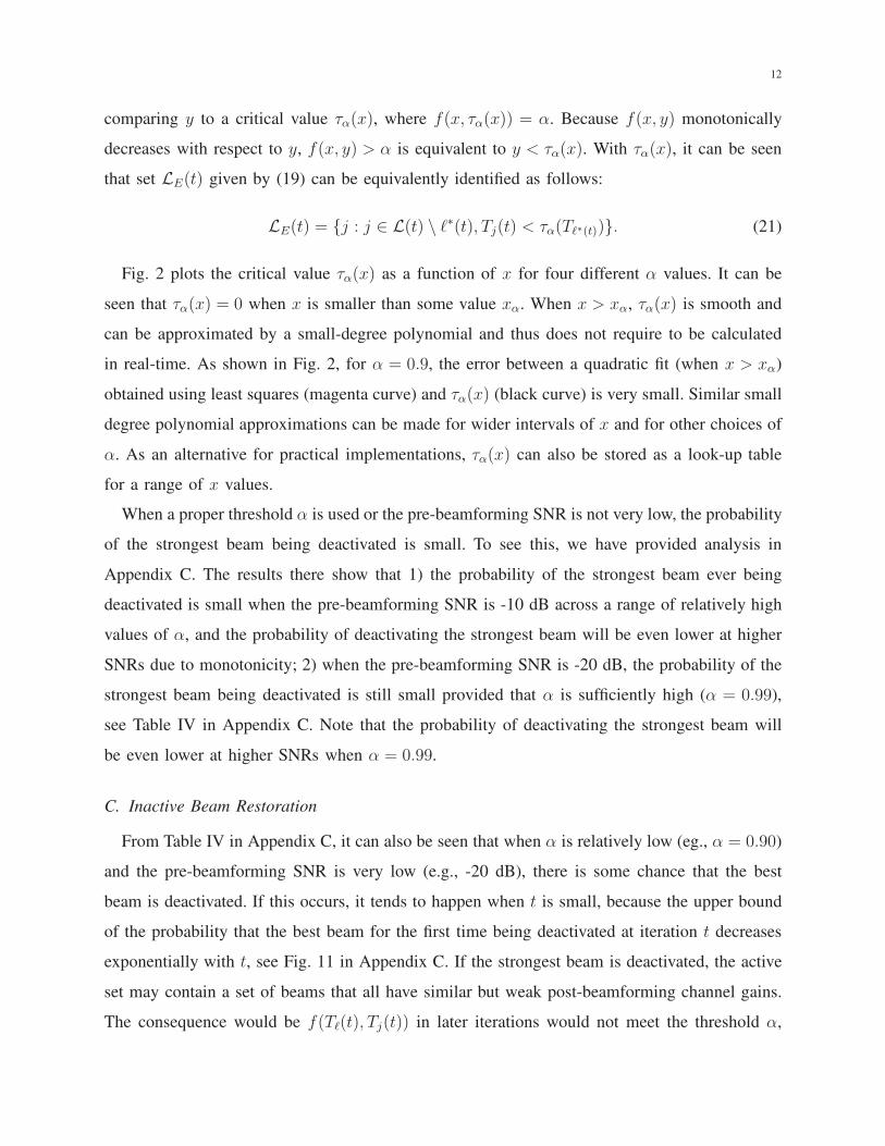
comparing y to a critical value τα(x), where f(x, τα(x)) = α. Because f(x, y) monotonically

decreases with respect to y, f(x, y) > α is equivalent to y < τα(x). With τα(x), it can be seen

that set LE(t) given by (19) can be equivalently identified as follows:

LE(t) = {j : j ∈ L(t) \ ℓ∗(t), Tj(t) < τα(Tℓ∗(t))}. (21)

Fig. 2 plots the critical value τα(x) as a function of x for four different α values. It can be

seen that τα(x) = 0 when x is smaller than some value xα. When x > xα, τα(x) is smooth and

can be approximated by a small-degree polynomial and thus does not require to be calculated

in real-time. As shown in Fig. 2, for α = 0.9, the error between a quadratic fit (when x > xα)

obtained using least squares (magenta curve) and τα(x) (black curve) is very small. Similar small

degree polynomial approximations can be made for wider intervals of x and for other choices of

α. As an alternative for practical implementations, τα(x) can also be stored as a look-up table

for a range of x values.

When a proper threshold α is used or the pre-beamforming SNR is not very low, the probability

of the strongest beam being deactivated is small. To see this, we have provided analysis in

Appendix C. The results there show that 1) the probability of the strongest beam ever being

deactivated is small when the pre-beamforming SNR is -10 dB across a range of relatively high

values of α, and the probability of deactivating the strongest beam will be even lower at higher

SNRs due to monotonicity; 2) when the pre-beamforming SNR is -20 dB, the probability of the

strongest beam being deactivated is still small provided that α is sufficiently high (α = 0.99),

see Table IV in Appendix C. Note that the probability of deactivating the strongest beam will

be even lower at higher SNRs when α = 0.99.

C. Inactive Beam Restoration

From Table IV in Appendix C, it can also be seen that when α is relatively low (eg., α = 0.90)

and the pre-beamforming SNR is very low (e.g., -20 dB), there is some chance that the best

beam is deactivated. If this occurs, it tends to happen when t is small, because the upper bound

of the probability that the best beam for the first time being deactivated at iteration t decreases

exponentially with t, see Fig. 11 in Appendix C. If the strongest beam is deactivated, the active

set may contain a set of beams that all have similar but weak post-beamforming channel gains.

The consequence would be f(Tℓ(t), Tj(t)) in later iterations would not meet the threshold α,

13

5 10 15 20 25 30 35 40 45 50

x

0

5

10

15

20

25

30

(x)

= 0.90

= 0.95

= 0.97

= 0.99

Quadratic fit: = 0.90

Fig. 2. Rejection region area below τα(x) vs x.

because the underlying channels are all comparable (note that f(x, y)∣∣x=y

= 0.5), leading to

excessive training time wasted, as well as a failure to find the best beam.

This issue is addressed by the Inactive Beam Restoration step which restores the best beam

to the active set if it happens to be deactivated. This step is thus performed when an inactive

beam has the strongest matched filter output, i.e., ℓ∗ 6= ℓ∗(t), where ℓ∗ = argmaxl∈L |rℓ(t)| is

the beam that has the strongest matched filter output from all candidate beams L, including the

active beams and the inactive beams. (We remind the reader that ℓ∗(t) is the beam that has the

strongest matched filter output from the active beams L(t), which is not necessarily the same

to ℓ∗.) If this condition is triggered, beam ℓ∗ is required to be measured again such that its

accumulated number of pilot symbols is nℓ∗(t) = n0t before it can be moved back to the active

set. We pause to note that this is due to the requirement that all active beams must have the

same number of measurements such that beam deactivations can be realised by low-complexity

operations using a single look-up table.4 After collecting the additional measurements, beam ℓ∗

is then added to the active set as: L(t)← L(t) ∪ {ℓ∗}.As we will show in Section V-B, the restoration step can reduce average overhead and improve

spectrum efficiency when relatively low values of α (such as α = 0.90) are used. The inclusion

of this step increases the chance that the best beam is retained in the active set, thus increasing

4It is possible to drop the restriction that nℓ(t) = n0t, ∀ℓ ∈ L(t) and to derive a generalisation to (20). However, under

this circumstance, it is required to store many look-up tables for different pairs of (nℓ(t), nj(t)), or to compute the generalised

form of (20) in real time. This would either require much larger memory space or higher computational complexity and would

render the algorithm less attractive from a practical point of view.

14

the chance that the best beam is selected at the end of the search and also that the weak beams

are deactivated more rapidly. The performance improvement from beam restoration becomes

negligible for larger values of α as the chance that the strongest beam is deactivated is low.

Inactive beam restoration makes IDBS more robust to the choice of α, which may be chosen

differently to achieve different tradeoffs between overhead and spectrum efficiency (see Sec. V).

D. Stopping Criteria

At each iteration, IDBS checks against the following three stopping conditions to decide

whether it should terminate.

I. Only one beam remains active:

|L(t)| = 1. (22)

II. Two adjacent beams are active

|L(t)| = 2, |ℓ∗(t)− j| = 1, ∀ j ∈ L(t), j 6= ℓ∗(t), (23)

and they have comparable statistics Tℓ(t)’s:

maxℓ∈L(t)

Tℓ(t)/minℓ∈L(t)

Tℓ(t) < 2 (24)

III. There is not enough training time to collect measurements for an additional iteration:

N(t).=∑

l∈Lnℓ(t) > N1 − n0|L(t)|, (25)

where N1 is the maximum number of pilot symbols, available to Phase 1.

Condition I in (22) means that all but one beam has been deactivated from further consideration.

Condition II in (23)–(24) is an early stopping criterion which is proposed to deal with the

possibility that a dominant path falls close to the boundary of two adjacent beams.5 Condition

III in (25) means that the remaining time is not enough to scan the active beams for an additional

iteration. Without the early stopping condition, i.e., Condition II, IDBS can take longer search

time to reach Condition I or even use up all the available time, as we will show in Section IV.

5Note that Condition II requires both (23) and (24) to be met. If only (23) is met, IDBS will not terminate.

15

E. Decision Rule

The fact that IDBS terminates due to Condition II also provides an opportunity for IDBS

to select a beam that is better than any of the two active beams, namely the beam centred

at the boundary of the two adjacent beams. Motivated by this consideration, we propose the

following decision rule for IDBS. When IDBS terminates, a beam is selected for subsequent

data transmission. The selected beam could either be one from the original codebook used for

spatial scanning, or a shifted version of one of the original beams, according to the following

decision rules:

A. If iterations are terminated when Condition I or Condition III is met, then choose beam ℓ∗(t)

as the beam for subsequent use.

B. If iterations are terminated when Condition II is met, then shift beam ℓ∗(t) by half a beam

width towards the other active beam j. For ULA, the shifted beamforming vector can be

obtained by [20]:

u′ℓ∗(t) = uℓ∗(t) ⊙ [1, e−i

2πdλδψ , . . . , e−i

2πdλ

(NR−1)δψ ]T , (26)

where δψ = ψj − ψcℓ∗(t) and ⊙ is the Hadamard product.

We emphasise that the beam shifting operation due to Condition II requires no extra training

time but provides an opportunity for IDBS to select a better beam than any of the original

beams used for spatial scanning, i.e., an opportunity to even outperform the best beams from the

original codebook given by (4). This benefit will be confirmed by numerical results in Sec. IV

and Sec. V.

The IDBS algorithm is summarised in Table I. Note that IDBS in Table I is applied first to

Phase 1 and then to Phase 2. The same threshold α is adopted for the two phases. Suppose

the maximum training time available for beam alignment, measured by the number of pilot

symbols, is N+. To apply IDBS to both phases, the maximum overhead of Phase 1 is set to

N1 < N+ − n0S so that there is enough time for the Tx to scan its entire codebook, recalling

that S is the number of Tx candidate beams. The maximum overhead available to Phase 2 varies

as it depends on how much resource is spent at Phase 1. However, it is at least N+ −N1.

We finally note that IDBS requires one feedback each at the end of Phase 1 and Phase 2. As

discussed earlier, these messages can be exchanged using low-frequency carriers, similarly to

16

TABLE I

IDBS FOR BEAM ALIGNMENT

Input: Beam codebook L; Total overhead budget N1; Threshold α; Look-up table (τα(y), y)Initialisation: t← 0; L(t)← L, N(t)← 0, nℓ(t)← 0, ∀ ℓ ∈ L(t), flag ← 0

While flag = 0

Step 1): collect one additional measurement for each of the beams

l ∈ L(t), compute rℓ(t) and Tℓ(t) as in (6) and (7)

Step 2):

2.1) Identify LE(t),the set of beams to deactivate, according to (21)

2.2) Update the active set L(t)← L(t) \ LE(t)Step 3): ℓ∗ = argmaxℓ∈L |rℓ(t)| and ℓ∗(t) = argmaxℓ∈L(t) |rℓ(t)|.

If l∗ 6= l∗(t):3.1) Collect extra measurements for beam ℓ∗ such that nℓ∗(t) = n0t3.2) Update the active set as L(t)← L(t) ∪ {ℓ∗}

Step 4): Update N(t) and Check Stopping Criteria

I. If N(t) + |L(t)| > N1 & |LA(t)| > 1, flag ← 1

II. If |LA(t)| = 1, flag ← 2

III. If (23) and (24) are satisfied, flag ← 3

Decision:

If flag = 1 or flag = 2, choose beam uℓ∗(t)If flag = 3, shift beam uℓ∗(t) according to (26)

5G NSA where low-frequency channels are used to transmit control signalling. The termination

messages are not required to contain the beam index identified in each phase nor the indices of

the deactivated beams. This is because the beam measurements and deactivation are performed

by the Rx (e.g., UE in Phase 1) while the Tx is only required to keep transmitting the pilots

(e.g., BS in Phase 1), as explained at the start of Section III. Therefore, the number of bits to

feedback in each message can be as small as 1 bit. IDBS requires fast beam switching, due to the

iterative beam examination where each beam is scanned using a short pilot sequence. However,

this fast beam switching can be supported by state-of-the-art technologies. For instance, IBM

has reported beam switching speeds of < 4 ns [36].

IV. EXAMPLES TO EXPLAIN CONDITION II OF THE STOPPING CRITERIA AND BEAM

SHIFTING OF THE DECISION RULE

In this section, we use two simple examples to explain the motivation of adopting Condition

II of the stopping criteria and the beam shifting operation as presented in Section III. In the two

examples, we consider a single-path channel, a UE equipped with a single antenna and a BS

with a ULA of NT = 32 antennas. In this setup, beam scanning only occurs at BS in Phase 2.

The BS codebook consists of DFT vectors as given by (2). We also consider that the angular

17

interval of BS is a 60◦-sector, i.e., φ ∈ [−30◦,+30◦] or equivalently φ ∈ [−1/2, 1/2], thus the

codebook has S = 16 beams. With this setup, φcs = −12+ (s−1/2)

16, s = 1, . . . , 16, and the effective

channel gain

|hs|2 = |Hws|2 = |γ|2|w†saT (φ)|2 ∝ GTs(φ), (27)

where we recall that GTs(φ).= |w†

saT (φ)|2 is the beamforming gain of ws at angle φ. Fig. 3 (a)

and (b) plots GTs(φ) with respect to beam index s, in Example 1 and Example 2, respectively.

It can be seen that in Example 1, beam 9 has a much stronger channel than all other beams,

as the channel path falls nearly in the centre of its intended coverage interval. In comparison,

in Example 2, both beam 9 and 10 have much stronger channels than the other beams, as the

channel path falls close to the boundary between the intended coverage intervals of beam 9 and

10. However, the beamforming gains of beam 9 and 10 in Example 2 are much weaker than

that of beam 9 in Example 1.

The results to be presented in this section are averaged over 5 × 103 trials with H fixed

for Example 1 and Example 2 but noises generated randomly. The training budget is set to

N+ = 1024 symbols and α = 0.97.

Fig. 4 is the average of the total number of pilot symbols when IDBS terminnates, with and

without Condition II as specified in (23) and (24). The horizontal axis is the pre-beamforming

SNR, which equalsPT |γ|2σ2

. As expected, in Example 1, there is no discernible difference with

and without Condition II of the stopping criterion. In Example 2, significantly lower overhead

is observed across SNRs when Condition II is included in the stopping criteria.

Fig. 5 illustrates how training time is spent on each beam in Example 2. The vertical axis is

the average number of pilot symbols spent on each beam, i.e., E{ns(t)}, at termination. It can

be seen that for both the pre-beamforming SNR values presented, −20 dB for Fig. 5(a) and 0

dB for Fig. 5 (b), IDBS without Condition II spends much longer time attempting to make a

decision between beam 9 and beam 10, which have comparable effective channel strengths.

Fig. 4 and Fig. 5 show that Condition II indeed leads to significant reduction of training

time when the dominant path falls near the boundary of two adjacent beams. We next show

that the reduction of training time, due to the adoption of Condition II, does not come at the

price of sacrificing the performance of subsequent data transmission. In fact, the combined use

of Condition II and the beam shifting rule can lead to noticeable performance improvement in

18

1 2 3 4 5 6 7 8 9 10 11 12 13 14 15 16Beam index s

-30

-20

-10

0

10

20B

eam

gai

ns G

Ts(

) (d

B)

(a)

1 2 3 4 5 6 7 8 9 10 11 12 13 14 15 16Beam index s

-10

-5

0

5

10

15

Bea

m g

ains

GT

s()

(dB

)

(b)

Fig. 3. (a) Example 1: Only one dominant beam (beam 9). sin(φ) = 0.0141 (b) Example 2: Two comparable beams (beam 9 and

10). sin(φ) = 0.0297. The intended coverage of beam 9 is [0, 0.0313]. The intended coverage of beam 10 is [0.0313, 0.0626].

-20 -18 -16 -14 -12 -10 -8 -6 -4 -2 0

Pre-beamforming SNR (dB)

0

100

200

300

400

500

600

700

800

900

Ave

rage

tota

l num

ber

of p

ilot s

ymbo

ls

Example 2: Full Stopping Criterion - Condition I-IIIExample 2: Stopping Criteria without Condition IIExample 1: Full Stopping Criterion - Condition I-IIIExample 1: Stopping Criteria without Condition II

Example 1: One dominant beam

Example 2: Two comparable beams

Fig. 4. Average total number of pilot symbols when different stopping criteria are adopted.

scenarios like Example 2.

Fig. 6 presents the average spectrum efficiency after beam search in Example 2. The curve

labeled as “IDBS” is obtained when the full version IDBS as described in Section III is adopted

for beam selection. The curve labeled as “IDBS: no beam shifting” assumes that IDBS is

adopted with all the three stopping conditions (Condition I-III) but without the beam shifting

given. In other words, it always chooses the active beam that has the strongest measurement

for data transmission. The comparison between IDBS with and without beam shifting is to

demonstrate the effectiveness of beam shifting. The curve labeled as “IDBS: no Condition II

no beam switching” is obtained assuming IDBS with only Condition I and Condition III as the

stopping criteria and without beam shifting. The final curve labeled as “Best beam from scanning

codebook” corresponds to the rate calculated using (28) below assuming the best beams given

19

1 2 3 4 5 6 7 8 9 10 11 12 13 14 15 16

Beam index

20

40

60

80

100

120

140

160

180A

vera

ged

num

ber

of p

ilot s

ymbo

ls

SNR = -20 dB

Stopping Criteria of IDBSStop iteration when only one beam active

(a)

1 2 3 4 5 6 7 8 9 10 11 12 13 14 15 16

Beam index

0

10

20

30

40

50

60

70

Ave

rage

d nu

mbe

r of

pilo

t sym

bols

SNR = 0 dB

Stopping Criteria of IDBSStop iteration when only one beam active

(b)

Fig. 5. Example 2 - two comparable beams. Average number of pilot symbols when different stopping criteria are adopted: (a)

SNR = -20 dB; (b) SNR = 0 dB

-20 -18 -16 -14 -12 -10 -8 -6 -4 -2 0

Pre-beamforming SNR (dB)

0

1

2

3

4

5

Ave

rage

spe

ctru

m e

ffici

ency

(bp

s/H

z) IDBS

IDBS: no Condition II no beam shifting

Best beam from scanning codebook

IDBS: no beam shifting

Fig. 6. Example 2: Average spectrum efficiency after beam alignment, with or without beam switching.

in (4) are selected. For all these four cases, the spectrum efficiency is calculated assuming that

the same transmission power is adopted by beam training and data transmission. Therefore, the

spectrum efficiency is given by:

R = log2

(

1 +PT∣∣u†Hw

∣∣2

σ2

)

(28)

where the UE beam u equals one (since a single antenna is assumed at UE) and w is the beam

selected under each scheme considered.

It can be seen from Fig. 6 that “IDBS with no Condition II and no beam shifting” does have

slightly higher average spectrum efficiencies than “IDBS without beam shifting”. This is because

the former spends much more time on measuring beam 9 and beam 10, and thus can choose

20

the slightly better beam more reliably. However, the performance differences are not significant

across the SNR range and they come from significantly longer training time.

In can also be seen from Fig. 6 that both “IDBS with no Condition II and no beam shifting”

and “IDBS without beam shifting” have similar average spectrum efficiencies to that of the best

beams from the original codebook, across the entire SNR range. This means that IDBS can

almost always find the best beam in this example across the entire SNR range. IDBS improves

upon “IDBS without beam shifting” and even outperforms the best beams from the original

codebook. This is because the beam shifting operation in IDBS allows it to choose a beam that

is outside the original codebook used for scanning and which offers a stronger beamforming

gain.

To summarise, the examples in this section demonstrate that the introduction of Condition

II can help reduce training overhead when the dominant path falls close to the boundary of

two adjacent beams. The beam shifting operation performed after stopping on Condition II can

provide better rate performance.6

V. NUMERICAL RESULTS

In this section, we evaluate the performance of IDBS and investigate the impact of parameter

choices on its performance. Throughout this section, we suppose that ULAs are equipped at both

BS and UE, and that the number of antennas at BS is NT = 64 and the number of antennas at UE

is NR = 16. The angular interval of interest for BS is [−30◦,+30◦], i.e., φ ∈ [−1/2, 1/2], and

the angular interval of interest for UE is [−90◦, 90◦], i.e., ψ ∈ [−1, 1]. This setup corresponds

to the initial beam alignment stage where a UE is synchronised to a BS, whose coverage is a

60◦-sector. The wide beam w used by the BS to cover the 60◦-sector in phase 1 is synthesised

using the algorithm in [30]. The narrow beams used by the BS and UE are DFT beams with

inter-beam distances 2/NT , 2/NR and peak gains NT and NR, respectively. Because the BS

covers interval φ ∈ [−1/2, 1/2], there are S = 32 narrow beams in the BS codebook. The UE

codebook has L = NR = 16 beams because the UE angular interval of interest is ψ ∈ [−1, 1].In what follows, we assume the same transmit power in beam training and data transmission

6It is noted that in the rare occasion that two or more paths falling to the centres of adjacent beams, beam shifting may lead

to worse rate performance. However, for IDBS to suffer from this problem, not only must this situation occur, but the paths

must also have comparable path strengths such that neither of the beams that cover these two paths is deactivated. This makes

it even rarer and thus is not considered in the design of IDBS.

21

(when evaluating the spectrum efficiency). We also consider the same noise variance σ2 at BS

and UE and n0 = 1.

Following [17], we consider two scenarios, namely line-of-sight (LOS) and non-line-of-sight

(NLOS) scenarios. In the LOS scenarios, a Rician channel model is considered where there is

one dominant path from angle φ and ψ with respect to the BS and UE. The Rician K-factor (i.e.,

the ratio of the power of the dominant path to the sum of the power of the scattering components)

is set to 13.2 dB [37] and both φ ∈ [−30◦,+30◦] and ψ ∈ [−90◦, 90◦] are uniformly distributed.

In the NLOS scenairo, the channel is modelled as the sum of I paths, each with φi and ψi

uniformly drawn from [−30◦,+30◦] and [−90◦, 90◦], respectively. Each path is again assumed

to be Rician, with K-factor set to 6 dB [38]. The number of paths is I = max{1, ζ}, where ζ is

a Poisson random variable with mean 1.8 and the power fractions of the I paths are generated

by the method in [11]. In what follows, the results presented are obtained by averaging over

2× 104 random channel realisations. The average pre-beamforming SNR is defined as the ratio

between the average sum power from all paths and the average noise power at the receiver.

A. Impact of the threshold α

We first investigate the impact of the threshold α on the training overhead of IDBS and the

spectrum efficiency. Two maximum overhead levels N+ = {3072, 1024} are considered. In either

case, the maximum budget for Phase 1 is set to N1 = N+ − 32 × 4 to ensure that the beam

searching time left for Phase 2 is not too short.

Fig. 7(a) and (b) respectively present the average overhead and the average spectrum efficiency

in the LOS case. The results for the NLOS case are not presented for brevity, as the insights

are the same as in the LOS case.

As can be seen from Fig. 7(a), the average overhead is lower when the average pre-beamforming

SNR is higher, at all α values. As expected, a higher α increases the average overhead at both N+

values. This overhead increase is more significant at lower SNRs. For instance, when N+ = 3072,

increasing α from 0.90 to 0.99 increases the average overhead by (898.6/524.5−1) = 71% when

the SNR is -20 dB, while only by (51.1/49.1− 1) = 4% when the SNR is 0 dB.

A higher α also tends to provide better spectrum efficiency, as one would expect and also

shown in Fig. 7(b). Similar to the observations on the overhead, the improvement in spectrum

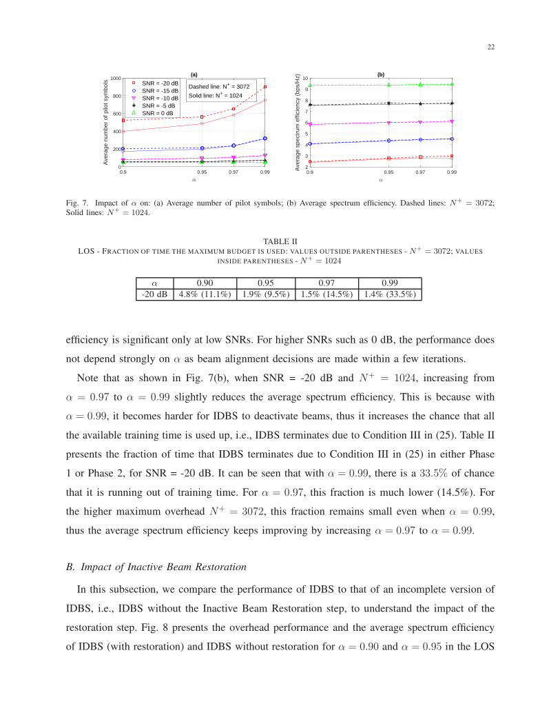
22

0.9 0.95 0.97 0.990

200

400

600

800

1000

Ave

rage

num

ber

of p

ilot s

ymbo

ls

(a)

SNR = -20 dBSNR = -15 dBSNR = -10 dBSNR = -5 dBSNR = 0 dB

0.9 0.95 0.97 0.992

3

4

5

6

7

8

9

10

Ave

rage

spe

ctru

m e

ffici

ency

(bp

s/H

z) (b)

Dashed line: N+ = 3072

Solid line: N+ = 1024

Fig. 7. Impact of α on: (a) Average number of pilot symbols; (b) Average spectrum efficiency. Dashed lines: N+ = 3072;

Solid lines: N+ = 1024.

TABLE II

LOS - FRACTION OF TIME THE MAXIMUM BUDGET IS USED: VALUES OUTSIDE PARENTHESES - N+ = 3072; VALUES

INSIDE PARENTHESES - N+ = 1024

α 0.90 0.95 0.97 0.99

-20 dB 4.8% (11.1%) 1.9% (9.5%) 1.5% (14.5%) 1.4% (33.5%)

efficiency is significant only at low SNRs. For higher SNRs such as 0 dB, the performance does

not depend strongly on α as beam alignment decisions are made within a few iterations.

Note that as shown in Fig. 7(b), when SNR = -20 dB and N+ = 1024, increasing from

α = 0.97 to α = 0.99 slightly reduces the average spectrum efficiency. This is because with

α = 0.99, it becomes harder for IDBS to deactivate beams, thus it increases the chance that all

the available training time is used up, i.e., IDBS terminates due to Condition III in (25). Table II

presents the fraction of time that IDBS terminates due to Condition III in (25) in either Phase

1 or Phase 2, for SNR = -20 dB. It can be seen that with α = 0.99, there is a 33.5% of chance

that it is running out of training time. For α = 0.97, this fraction is much lower (14.5%). For

the higher maximum overhead N+ = 3072, this fraction remains small even when α = 0.99,

thus the average spectrum efficiency keeps improving by increasing α = 0.97 to α = 0.99.

B. Impact of Inactive Beam Restoration

In this subsection, we compare the performance of IDBS to that of an incomplete version of

IDBS, i.e., IDBS without the Inactive Beam Restoration step, to understand the impact of the

restoration step. Fig. 8 presents the overhead performance and the average spectrum efficiency

of IDBS (with restoration) and IDBS without restoration for α = 0.90 and α = 0.95 in the LOS

23

-20 -15 -10 -5 0

Average pre-beamforming SNR at Rx (dB)

0

100

200

300

400

500A

vera

ge to

tal n

umbe

r of

sym

bols = 0.95: No Restoration

= 0.95: With Restoration = 0.90: No Restoration = 0.90: With Restoration

(a)

-20 -15 -10 -5 0Average pre-beamforming SNR at Rx (dB)

2

4

6

8

10

Ave

rage

spe

ctru

m e

ffici

ency

(bp

s/H

z)

= 0.95: No Restoration = 0.95: With Restoration = 0.90: No Restoration = 0.90: With Restoration

(b)

Fig. 8. Impact of the Inactive Beam Restoration on: (a) Average number of pilot symbols (overhead); (b) Average spectrum

efficiency for α = 0.90 and α = 0.95, in LOS scenario.

case. The maximum overhead is set to N+ = 1024.

For α = 0.90, it can be seen from Fig. 8 (a) that Inactive Beam Restoration reduces the average

overhead of IDBS. The overhead reduction is more significant at low SNRs, as the chance that

the best beam being deactivated is higher in these scenarios (see the analysis in Appendix C).

Fig. 8 (b) shows that with α = 0.90, the adoption of Inactive Beam Restoration also increases

the average spectrum efficiency. Both key aspects of performance are seen to improve.

As also shown by Fig. 8 (a) and (b), with α = 0.95, the performance improvement by using

Inactive Beam Restoration becomes less significant. This is because the algorithm is less likely

to deactivate the best beam when α is high, as explained in Appendix C, thus restoration is

triggered much less frequently.

C. Performance Evaluation of IDBS

In this subsection, we evaluate the average spectrum efficiency and the average overhead

of IDBS in different SNRs and fading scenarios to demonstrate its capability of adapting to

the unknown scenarios to achieve good tradeoffs between the two metrics. For illustration, we

consider N+ = 1024.

Fig. 9 and Fig. 10 plots the average spectrum efficiency versus the average overhead of IDBS in

LOS and NLOS, respectively. Two pre-beamforming SNRs are considered: −15 dB and −5 dB.

The four red points for IDBS in each plot correspond to α = [0.90, 0.95, 0.97, 0.99] from left

to right. As benchmarks to the spectrum efficiency, we have added “best beam pair of scanning

codebook” (magenta dashed curve) and “infinite-resolution beamforming” (black solid curve)

24

in the figures. The “best beam pair of scanning codebook” is obtained by searching over the

original codebooks assuming the knowledge of channel, as given by (4). The “infinite-resolution

beamforming” benchmark is obtained by searching over the entire angular space at both the UE

and the BS, i.e., ψ ∈ [−1, 1] and φ ∈ [−1/2, 1/2]:

u∗ = arg maxψ∈[−1,1]

|u†(ψ)Hw|,

w∗ = arg maxφ∈[−1/2,1/2]

|u∗†Hw(φ)|, (29)

where u(ψ) and w(φ) are the UE and BS DFT beams centred at ψ and φ, respectively. Because

the search of “infinite-resolution beamforming” is in the continuous space as opposed to “best

beam pair of scanning codebook” that is over a set of discretised angles, the former has higher

spectrum efficiencies than the latter, and is also an upper bound to the spectrum efficiency that

can be achieved by directional analog beamforming.

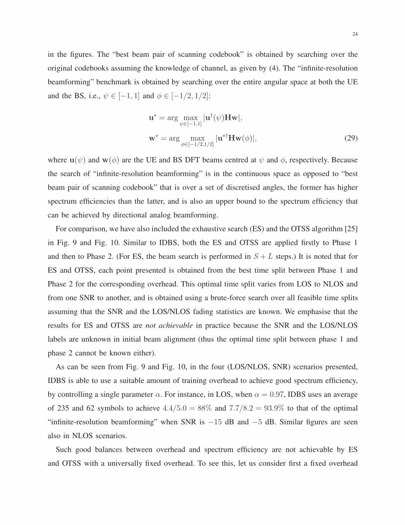
For comparison, we have also included the exhaustive search (ES) and the OTSS algorithm [25]

in Fig. 9 and Fig. 10. Similar to IDBS, both the ES and OTSS are applied firstly to Phase 1

and then to Phase 2. (For ES, the beam search is performed in S +L steps.) It is noted that for

ES and OTSS, each point presented is obtained from the best time split between Phase 1 and

Phase 2 for the corresponding overhead. This optimal time split varies from LOS to NLOS and

from one SNR to another, and is obtained using a brute-force search over all feasible time splits

assuming that the SNR and the LOS/NLOS fading statistics are known. We emphasise that the

results for ES and OTSS are not achievable in practice because the SNR and the LOS/NLOS

labels are unknown in initial beam alignment (thus the optimal time split between phase 1 and

phase 2 cannot be known either).

As can be seen from Fig. 9 and Fig. 10, in the four (LOS/NLOS, SNR) scenarios presented,

IDBS is able to use a suitable amount of training overhead to achieve good spectrum efficiency,

by controlling a single parameter α. For instance, in LOS, when α = 0.97, IDBS uses an average

of 235 and 62 symbols to achieve 4.4/5.0 = 88% and 7.7/8.2 = 93.9% to that of the optimal

“infinite-resolution beamforming” when SNR is −15 dB and −5 dB. Similar figures are seen

also in NLOS scenarios.

Such good balances between overhead and spectrum efficiency are not achievable by ES

and OTSS with a universally fixed overhead. To see this, let us consider first a fixed overhead

25

50 100 150 200 250 300 350 400 450 500

Total number of pilot symbols

1

2

3

4

5A

vera

ge s

pect

rum

effi

cien

cy (

bps/

Hz)

Infinite-resolution beamformingIDBS (Proposed)Best beam pair from scanning codebookOTSSES

(0.90,0.95,0.97,0.99)

(a)

50 60 70 80 90 100 110 120

Total number of pilot symbols

5

5.5

6

6.5

7

7.5

8

Ave

rage

spe

ctru

m e

ffici

ency

(bp

s/H

z)

Infinite-resolution beamforming

IDBS (Proposed)

Best beam pair from scanning codebook

OTSS

ES

(b)

Fig. 9. LOS: Beam search performance tradeoff - average spec-

trum efficiency vs. overhead. (a) pre-beamforming SNR = -15

dB; (b) pre-beamforming SNR = -5 dB. The four red points of

IDBS represent four values of α, i.e., {0.90, 0.95, 0.97, 0.99}from left to right.

50 100 150 200 250 300 350 400 450 500Total number of pilot symbols

0

1

2

3

4

5

Ave

rage

spe

ctru

m e

ffici

ency

(bp

s/H

z)

Infinite-resolution beamforming

IDBS (Proposed)

Best beam pair from scanning codebook

OTSS

ES

(a)

50 60 70 80 90 100 110 120

Total number of pilot symbols

4.5

5

5.5

6

6.5

7

7.5

8

Ave

rage

spe

ctru

m e

ffici

ency

(bp

s/H

z)

Infinite-resolution beamforming

IDBS (Proposed)

Best beam pair from scanning codebook

OTSS

ES

(b)

Fig. 10. NLOS: Beam search performance tradeoff - av-

erage spectrum efficiency vs. overhead. (a) pre-beamforming

SNR = -15 dB; (b) pre-beamforming SNR = -5 dB. The

four red points of IDBS represent four values of α, i.e.,

{0.90, 0.95, 0.97, 0.99} from left to right.

at 300 for ES. In LOS and SNR = -15 dB, see Fig. 9 (a), this overhead allows the ES to

achieve 4.0/5.0 ≈ 80% of the “infinite-resolution beamforming”. However, the overhead at 300

is unnecessarily large for SNR = -5 dB, as there is hardly any improvement of spectrum efficiency

by increasing the overhead beyond 100. For SNR = -5 dB and LOS, a more suitable overhead

level appears around 60, with which ES approaches “best beam pair of scanning codebook”

and achieves 7.3/8.2 = 89% of the optimal “infinite-resolution beamforming”. But again, this

overhead around 60 will be a rather poor choice for SNR = -15 dB, as the spectrum efficiency

achieved will be very poor, i.e., only 1.4/5.0 = 28% of the “infinite-resolution beamforming”.

It can also be seen that the amount of overhead required by ES (and OTSS) differs from LOS

to NLOS, with longer time required in NLOS. This fact further demonstrates the drawback of

the non-adaptive approach with a universally fixed overhead.

26

We remark that IDBS can achieve higher spectrum efficiencies than the best beam pair from

the scanning codebook. This is because IDBS, with beam shifting, is allowed to select a beam

that is outside the original scanning codebook, providing it an opportunity to select a better

beam. The benefit of beam shifting will be smaller if oversampled codebooks, with more beams

placed closer to achieve higher spatial resolution, are used in spatial scanning. However, using

oversampled codebooks will significantly increase the training overhead, as there are more beams

to examine. A more effective way to gain higher spatial resolution is to refine the beams after the

initial alignment, using beam refinement algorithms such as [39], instead of using an extremely

fine resolution codebook for initial scanning.

We also remark that there are other alternative performance metrics to the average spectrum

efficiency. For instance, an effective spectrum efficiency that takes account for the overhead

spent in beam search: R′ = R × (1 − Ntraining/Nmax), may be used, where Nmax is the total

number of symbols in a coherent block and Ntraining is the number of symbols used for beam

search. Another valid metric is the outage probability that captures the fraction of time that the

achieved spectrum efficiency is lower than one of the benchmarks by a certain amount. Using

these metrics do not change the overall insights drawn above, we thus omit them due to the

page limit.

We finally note that the overhead of IDBS varies even for the same SNR due to random

channel realisations and noise. The overhead variations tend to be more significant when the

pre-beamforming SNR is lower. To see this, we present in Table III the 90-th percentile of the

overhead, along with the average overhead, where the 90-th percentile is used to illustrate the

overhead consumed by IDBS in “worst-case” realisations. As can be seen from Table III, for

SNR at −5 dB, LOS and α = 0.95, the 90-th percentile is 71 which is only 71 − 58.9 = 12.1

larger than the average or 12.1/58.9 = 20.5% larger in relative terms. The overhead consumed

is relatively concentrated around the average. For SNR of −15 dB, LOS and α = 0.95, the

90-th percentile of the overhead is 314, which is 314 − 200 = 114 larger than the average or

114/200 = 57% larger in relative terms.

VI. CONCLUSIONS

In this paper, we presented a new algorithm for mmWave beam search called Iterative De-

activation and Beam Shifting (IDBS). IDBS does not require any prior information such as

27

TABLE III

IDBS OVERHEAD - VALUES OUTSIDE PARENTHESES: 90-PERCENTILE OF THE OVERHEAD UPON TERMINATION. VALUES

INSIDE PARENTHESES:AVERAGE OVERHEAD UPON TERMINATION. OVERHEAD IS MEASURED BY THE TOTAL NUMBER OF

PILOTS. N+ = 1024.

α = 0.90 α = 0.95 α = 0.97 α = 0.99

LOS -15 dB 263 (171.0) 314 (200.0) 379 (235.1) 507 (314.4)

LOS -5 dB 64 (54.6) 71 (58.9) 78 (62.3) 91 (70.2)

NLOS -15 dB 461 (232.2) 606 (300.3) 778 (358.9) 950 (478.0)

NLOS -5 dB 81 (65.1) 105 (76.3) 127 (84.8) 166 (101.0)

SNR references and channel fading statistics in order to operate. It automatically adapts its

overhead to the unknown SNR and fading statistics to obtain beam alignment performance

close to that achieved by the best beams from the codebooks used for beam search, but with

minimal overhead. Simulations over LOS and NLOS fading channel models extracted from

NYU’s measurements [11] have confirmed that IDBS can achieve good balances between training

overhead and beam search accuracy in different SNRs and in different fading scenarios. This

makes the algorithm attractive for outdoor mmWave cellular mobile communications where the

SNR and channel fading statistics vary significantly.

APPENDIX A

PROOF OF THEOREM 1

f(Tℓ(t), Tj(t)) =

∫

ηℓ>ηj

gTℓ(t)(ηℓ)gTj(t)(ηj)dηℓdηj =

∫ +∞

η

gTℓ(t)(ηℓ)[1−Q1(

√

Tj(t),√η)]dηℓ,

(30)

where Q1(a, b) is the Marcum Q-function with DoF = 1. Since Q1(a, b) is monotonically

increasing with respect to a [40], it follows that f(Tℓ(t), Tj(t)) is monotonically decreasing

with respect to Tj(t).

Since∫

ηℓ,ηjgTℓ(t)(ηℓ)gTj(t)(ηj)dηℓdηj = 1, it follows that

f(Tℓ(t), Tj(t)) = 1−∫

+∞≥ηj>ηℓ≥0

gTℓ(t)(ηℓ)gTj(t)(ηj)dηℓdηj

= 1−∫ +∞

η

gTj(t)(ηj)[1−Q1(

√

Tℓ(t),√η)]dηj. (31)

28

Therefore, f(Tℓ(t), Tj(t)) is monotonically increasing with respect to Tℓ(t).

APPENDIX B

PROOF OF LEMMA 1

Following (17), f(x, y) can be represented as:

f(x, y) =

∫ +∞

0

gx(η1)

∫ η1

0

gy(η2)dη2dη1 = 1−∫ +∞

0

gx(η)Q1 (√y,√η) dη, (32)

where we have used the fact that∫ x

0gy(η)dη = 1−Q1(

√x,√η) to obtain the second equation.

Substituting gx(η) of (13) into (32), it can be obtained that

f(x, y) = 1−∫ +∞

0

1

2exp(−x+ η

2)I0(√ηx)Q1(

√y,√η)dη

= 1−+∞∑

k=0

exp(−x2)xk

2× 4k × (k!)2

∫ +∞

0

ηk exp(−η2)Q1(√y,√η)dη

︸ ︷︷ ︸

F (k,η,y)

, (33)

where we have used the fact that the modified Bessel function of the first kind with zero-order

can be represented as [41, Eq. 9.6.12 on Page 375], I0(z) =∑∞

k=0

( 1

4z2)

k

(k!)2to obtain (33). To

further compute F (k, η, y) in (33), we use the following fact [42, Eq. (15)]:

Ra,b(M, p, 1) =Γ(M)

pM×[

1− b2

b2 + 2pexp

(

− a2p

b2 + 2p

)M−1∑

m=0

(2p

b2 + 2p

)m

Lm

(

− a2p

b2 + 2p

)]

(34)

where Ra,b(k, p, v).=∫ +∞0

xk−1 exp(−px)Qv(a, b√x)dx, and Γ(M) = (M − 1)! is the gamma

function. It is easy to see that F (k, η, y) = R√y,1(k + 1, 1

2, 1), with a =

√y, b = 1, p = 1

2and

M = k + 1 in (34), thus F (k, η, y) can be represented as:

F (k, η, y) =Γ(k + 1)

(12)k+1

[

1− 1

2exp

(

−y4

) k∑

m=0

(1

2

)m

Lm

(

−y4

)]

. (35)

Substituting (35) into (33), it can be obtained that

f(x, y) =1

2exp

(

−x2− y

4

) +∞∑

k=0

(x2)k

k!

k∑

m=0

1

2mLm

(

−y4

)

︸ ︷︷ ︸

G

, (36)

29

where the G term can be further computed as:

G =exp(x

2

) +∞∑

m=0

(1

2

)m

Lm

(

−y4

)

−+∞∑

m=1

(1

2

)m

Lm

(

−y4

)m−1∑

k=0

(x2)k

k!, (37)

=2× exp(x

2+y

4

)

−+∞∑

m=1

(1

2

)m

Lm

(

−y4

)m−1∑

k=0

(x2)k

k!, (38)

since the Laguerre polynomial has the following property [43, Pg. 242]:

+∞∑

m=0

Lm(z)ωm =

1

1− ω exp

(ωz

ω − 1

)

, |ω| < 1. (39)

This completes the proof.

APPENDIX C

SOME ANALYSIS OF BEAM DEACTIVATION

We now present some performance results of IDBS. As we aim to gain insights on the

deactivation operation, we only consider one phase of search, e.g., Phase 1. Consider in this

case the Tx omnidirectional transmit the pilot signals and the Rx scans [0◦, 360◦] using M

ideal beams, with the same beam widths, the same uniform gain with the intended coverage

interval, and zero-leakage outside this interval [25]. Suppose also that the channel has a single

path with some fixed angle φ at the Rx. Then there is only one true beam that has non-zero

beamforming gain to the channel and this gain is M . Without loss of generality, we assume

the true beam is beam 1. Consequently, T1(t) is a sequence of χ22(η1(t)) random variables with

η1(t) = 2tPT |h1|2/σ2 = 2tPTM |γ|2/σ2, where γ is the complex path coefficient (see (27)) and

the pre-beamforming SNR is PT |γ|2/σ2.

Lemma 2. Consider the event E(t) that the true beam is first deactivated at the iteration t

under the algorithm. It holds that

Pr{E(t)} ≤ Pr{f(Y (t), T1(t)) > α} = Pr{τα(Y (t)) > T1(t)} .= q(t), (40)

where Y (t) is the maximum of all the false beam measurements at iteration t which are supposed

taken, irrespective of whether they have been deactivated.

Proof. Let Z(t) be the maximum of the false beams active at step t and Y (t) the maximum of

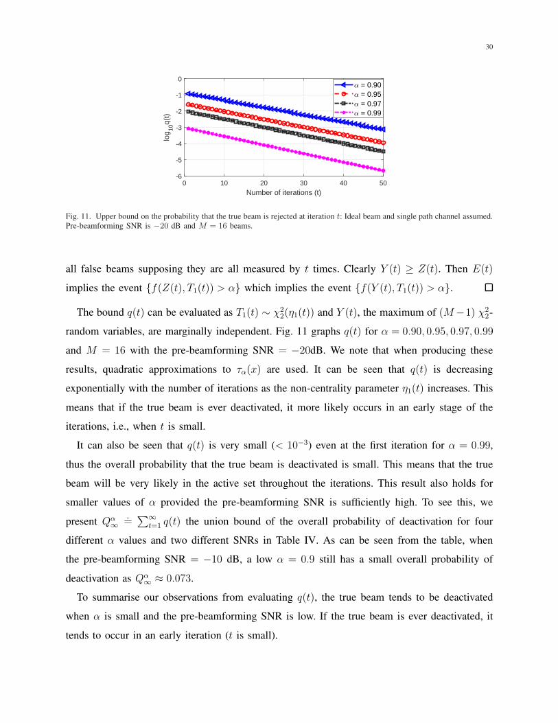
30

0 10 20 30 40 50

Number of iterations (t)

-6

-5

-4

-3

-2

-1

0

log 10

q(t)

= 0.90 = 0.95 = 0.97 = 0.99

Fig. 11. Upper bound on the probability that the true beam is rejected at iteration t: Ideal beam and single path channel assumed.

Pre-beamforming SNR is −20 dB and M = 16 beams.

all false beams supposing they are all measured by t times. Clearly Y (t) ≥ Z(t). Then E(t)

implies the event {f(Z(t), T1(t)) > α} which implies the event {f(Y (t), T1(t)) > α}.

The bound q(t) can be evaluated as T1(t) ∼ χ22(η1(t)) and Y (t), the maximum of (M−1) χ2

2-

random variables, are marginally independent. Fig. 11 graphs q(t) for α = 0.90, 0.95, 0.97, 0.99

and M = 16 with the pre-beamforming SNR = −20dB. We note that when producing these

results, quadratic approximations to τα(x) are used. It can be seen that q(t) is decreasing

exponentially with the number of iterations as the non-centrality parameter η1(t) increases. This

means that if the true beam is ever deactivated, it more likely occurs in an early stage of the

iterations, i.e., when t is small.

It can also be seen that q(t) is very small (< 10−3) even at the first iteration for α = 0.99,

thus the overall probability that the true beam is deactivated is small. This means that the true

beam will be very likely in the active set throughout the iterations. This result also holds for

smaller values of α provided the pre-beamforming SNR is sufficiently high. To see this, we

present Qα∞

.=∑∞

t=1 q(t) the union bound of the overall probability of deactivation for four

different α values and two different SNRs in Table IV. As can be seen from the table, when

the pre-beamforming SNR = −10 dB, a low α = 0.9 still has a small overall probability of

deactivation as Qα∞ ≈ 0.073.

To summarise our observations from evaluating q(t), the true beam tends to be deactivated

when α is small and the pre-beamforming SNR is low. If the true beam is ever deactivated, it

tends to occur in an early iteration (t is small).

31

TABLE IV

UNION BOUND ON PROBABILITY OF DEACTIVATIONQα∞

.

α 0.90 0.95 0.97 0.99

γ = −20 dB - 0.2443 0.0836 0.0073

γ = −10 dB 0.0734 0.0142 0.0047 0.000397

REFERENCES

[1] C. Liu, M. Li, L. Zhao, P. Whiting, S. V. Hanly, and I. B. Collings, “An adaptive algorithm for millimetre-wave beam

alignment with iterative beam-deactivation,” 2020, accepted and to appear in Proc. IEEE ICC, Dublin, Ireland.

[2] Z. Pi and F. Khan, “An introduction to millimeter-wave mobile broadband systems,” IEEE Commun. Mag., vol. 49, no. 6,

2011.

[3] J. G. Andrews, S. Buzzi, W. Choi, S. V. Hanly, A. Lozano, A. C. Soong, and J. C. Zhang, “What will 5G be?” IEEE J.

Sel. Areas Comms., vol. 32, no. 6, pp. 1065–1082, 2014.

[4] M. Xiao, S. Mumtaz, Y. Huang, L. Dai, Y. Li, M. Matthaiou, G. K. Karagiannidis, E. Bjornson, K. Yang, I. Chih-Lin

et al., “Millimeter wave communications for future mobile networks,” IEEE J. Sel. Areas Commun., vol. 35, no. 9, pp.

1909–1935, 2017.

[5] L. Zhao, D. W. K. Ng, and J. Yuan, “Multi-user precoding and channel estimation for hybrid millimeter wave systems,”

IEEE Journal on Selected Areas in Communications, vol. 35, no. 7, pp. 1576–1590, July 2017.

[6] J. Lee et al., “Spectrum for 5G: Global status, challenges, and enabling technologies,” IEEE Commun. Mag., vol. 56, no. 3,

pp. 12–18, 2018.

[7] Y. Niu, Y. Li, D. Jin, L. Su, and A. V. Vasilakos, “A survey of millimeter wave communications (mmwave) for 5g:

opportunities and challenges,” Wireless Networks, vol. 21, no. 8, pp. 2657–2676, 2015.

[8] Z. Wei, D. W. K. Ng, and J. Yuan, “Noma for hybrid mmwave communication systems with beamwidth control,” IEEE

Journal of Selected Topics in Signal Processing, vol. 13, no. 3, pp. 567–583, June 2019.

[9] C. Zhao, Y. Cai, A. Liu, M. Zhao, and L. Hanzo, “Mobile edge computing meets mmwave communications: Joint

beamforming and resource allocation for system delay minimization,” IEEE Transactions on Wireless Communications,

vol. 19, no. 4, pp. 2382–2396, April 2020.

[10] Y. Cai, C. Zhao, Q. Shi, G. Y. Li, and B. Champagne, “Joint beamforming and jamming design for mmwave information

surveillance systems,” IEEE Journal on Selected Areas in Communications, vol. 36, no. 7, pp. 1410–1425, July 2018.

[11] M. Akdeniz, Y. Liu, M. Samimi, S. Sun, S. Rangan, T. Rappaport, and E. Erkip, “Millimeter wave channel modeling and

cellular capacity evaluation,” IEEE J. Sel. Areas Comms., vol. 32, no. 6, pp. 1164–1179, June 2014.

[12] M. Giordani, M. Polese, A. Roy, D. Castor, and M. Zorzi, “A tutorial on beam management for 3gpp nr at mmwave

frequencies,” IEEE Communications Surveys Tutorials, vol. 21, no. 1, pp. 173–196, 2019.

[13] V. Va, J. Choi, and R. W. Heath, “The impact of beamwidth on temporal channel variation in vehicular channels and its

implications,” IEEE Transactions on Vehicular Technology, vol. 66, no. 6, pp. 5014–5029, 2016.

[14] S. Hur, T. Kim, D. J. Love, J. V. Krogmeier, T. A. Thomas, and A. Ghosh, “Millimeter wave beamforming for wireless

backhaul and access in small cell networks,” IEEE transactions on communications, vol. 61, no. 10, pp. 4391–4403, 2013.

[15] A. Alkhateeb, O. El Ayach, G. Leus, and R. W. Heath, “Channel estimation and hybrid precoding for millimeter wave

cellular systems,” IEEE J. Sel. Sig. Processing, vol. 8, no. 5, pp. 831–846, 2014.

32

[16] Z. Tang, J. Wang, J. Wang, and J. Song, “A high-accuracy adaptive beam training algorithm for mmwave communication,”

in 2018 IEEE Globecom Workshops (GC Wkshps). IEEE, 2018, pp. 1–6.

[17] C. Liu, M. Li, S. V. Hanly, I. B. Collings, and P. Whiting, “Millimeter wave beam alignment: Large deviations analysis

and design insights,” IEEE J. Sel. Areas Commun., vol. 35, no. 7, pp. 1619–1631, July 2017.

[18] 3GPP-R1-167672, “Synchronization in NR considering beam sweeping,” 2016.

[19] 3GPP-R1-167543, “Beam management considerations for above 6 GHz NR,” 2016.

[20] Z. Xiao, T. He, P. Xia, and X. G. Xia, “Hierarchical codebook design for beamforming training in millimeter-wave

communication,” IEEE Trans. Wireless Commun., vol. 15, no. 5, pp. 3380–3392, 2016.

[21] J. Zhang, Y. Huang, Q. Shi, J. Wang, and L. Yang, “Codebook design for beam alignment in millimeter wave communication

systems,” IEEE Transactions on Communications, vol. 65, no. 11, pp. 4980–4995, 2017.

[22] “IEEE standard for Information Technology-Telecommunications and information exchange between systems-local and

metropolitan area networks-specific requirements-part 11: Wireless LAN Medium Access Control (MAC) and Physical

Layer (PHY) Specifications Amendment 3: Enhancements for very high throughput in the 60 Ghz band,” IEEE Std

802.11ad-2012, pp. 1–628, Dec. 2012.

[23] S. Khosravi, H. Shokri Ghadikolaei, and M. Petrova, “Efficient beamforming for mobile mmwave networks,” in The

International Symposium on Modeling and Optimization in Mobile, Ad Hoc, and Wireless Networks (WiOpt), 2019.

[24] V. Raghavan, J. Cezanne, S. Subramanian, A. Sampath, and O. Koymen, “Beamforming tradeoffs for initial ue discovery

in millimeter-wave mimo systems,” IEEE J. Sel. Topics in Signal Processing, vol. 10, no. 3, pp. 543–559, 2016.

[25] M. Li, C. Liu, S. V. Hanly, I. B. Collings, and P. Whiting, “Explore and eliminate: Optimized two-stage search for

millimeter-wave beam alignment,” IEEE Trans. Wireless Comms., vol. 18, no. 9, pp. 4379–4393, 2019.

[26] T. Kadur, W. Rave, and G. Fettweis, “Application of multiple hypothesis testing for beam selection,” in 2019 IEEE ICC,

May, Shanghai, China, 2019.

[27] M. Kokshoorn, H. Chen, P. Wang, Y. Li, and B. Vucetic, “Millimeter wave MIMO channel estimation using overlapped

beam patterns and rate adaptation,” IEEE Trans. Signal Process., vol. 65, no. 3, pp. 601–616, 2017.

[28] Z. Xiao, P. Xia, and X.-G. Xia, “Codebook design for millimeter-wave channel estimation with hybrid precoding structure,”

IEEE Trans. Wireless Comms., vol. 16, no. 1, pp. 141–153, 2017.

[29] Z. Xiao, H. Dong, L. Bai, P. Xia, and X.-G. Xia, “Enhanced channel estimation and codebook design for millimeter-wave

communication,” IEEE Trans. Veh. Technol., vol. 67, no. 10, pp. 9393–9405, 2018.

[30] W. Fan, C. Zhang, and Y. Huang, “Flat beam design for massive mimo systems via riemannian optimization,” IEEE

Wireless Commun. Lett., vol. 8, no. 1, pp. 301–304, 2019.

[31] J. Palacios, D. De Donno, and J. Widmer, “Tracking mm-wave channel dynamics: Fast beam training strategies under

mobility,” in IEEE INFOCOM. IEEE, 2017, pp. 1–9.

[32] C. Liu, M. Li, I. B. Collings, S. V. Hanly, and P. Whiting, “Design and analysis of transmit beamforming for millimeter

wave base station discovery,” IEEE Trans. Wireless Commun., vol. 16, no. 2, pp. 797–811, 2017.

[33] C. Barati Nt., S. Hosseini, S. Rangan, P. Liu, T. Korakis, S. Panwar, and T. Rappaport, “Directional cell discovery in

millimeter wave cellular networks,” IEEE Trans. Wireless Comms., vol. 14, no. 12, pp. 6664–6678, 2015.

[34] T. S. Rappaport, G. R. MacCartney, M. K. Samimi, and S. Sun, “Wideband millimeter-wave propagation measurements

and channel models for future wireless communication system design,” IEEE Transactions on Communications, vol. 63,

no. 9, pp. 3029–3056, 2015.

33

[35] D. A. Shnidman, “The calculation of the probability of detection and the generalized marcum q-function,” IEEE

Transactions on Information Theory, vol. 35, no. 2, pp. 389–400, March 1989.

[36] A. Valdes-Garcia, “Millimeter-wave phased array for 5g,” http://www.winlab.rutgers.edu/iab/2018-01/Slides/04%20-

%20IBM 5G PAWR June 1st.pdf.

[37] Z. Muhi-Eldeen, L. P. Ivrissimtzis, and M. Al-Nuaimi, “Modelling and measurements of millimetre wavelength propagation

in urban environments,” IET microwaves, antennas and propagation, vol. 4, no. 9, pp. 1300–1309, 2010.

[38] M. K. Samimi, G. R. MacCartney, S. Sun, and T. S. Rappaport, “28 ghz millimeter-wave ultrawideband small-scale fading

models in wireless channels,” in Proc. IEEE 83rd Veh. Technol. Conf., 2016, pp. 1–6.

[39] D. Zhu, J. Choi, Q. Cheng, W. Xiao, and R. W. Heath, “High-resolution angle tracking for mobile wideband millimeter-wave

systems with antenna array calibration,” IEEE Trans. Wireless Comms., vol. 17, no. 11, pp. 7173–7189, 2018.

[40] Y. Sun, A. Baricz, and S. Zhou, “On the monotonicity, log-concavity, and tight bounds of the generalized marcum and

nuttall q-functions,” IEEE Transactions on Information Theory, vol. 56, no. 3, pp. 1166–1186, March 2010.

[41] M. Abramowitz and I. A. Stegun, Handbook of mathematical functions: with formulas, graphs, and mathematical tables.

Courier Corporation, 1965, vol. 55.

[42] G. Cui, L. Kong, X. Yang, and D. Ran, “Two useful integrals involving generalised marcum q-function,” Electronics letters,

vol. 48, no. 16, pp. 1017–1018, 2012.

[43] W. Magnus, F. Oberhettinger, and R. P. Soni, Formulas and theorems for the special functions of mathematical physics.

Springer-Verlag, 1966.