UNIVERSITY OF HERTFORDSHIRE

AeroelasticityStructural Dynamics Coursework

Dr Y Xu

11/29/2013

10227333 APS5

This is a simple modal analysis of a beam simulating a modelairplane wing as shown below. The solid cantilever beam ofrectangular cross-section is tapered in both the chord-wise andspan-wise directions across its length of 1.5m. The depth of thebeam tapers from 0.02m at its fixed end to 0.005m at its free end. Thewidth of the beam tapers from 0.3m at the fixed end to 0.1m at thefree end. The beam is made of a high strength aluminium alloy withthe Young’s modulus E=70 GPa, Poisson’s ratio =0.33, and the materialdensity =2700kg/m3.

Rayleigh-Ritz method

(1) Use the Rayleigh-Ritz method to obtain approximate values forthe first and second natural frequencies of the beam under flexuralfree vibrations. Choose a polynomial function given in the lecturenotes for “Structural Dynamics” as the assumed modes for thecalculation. The beam will be divided evenly along its length. Theminimum number of segments for the task is five. Trapezoidal rule,Simpson’s rule, and Lagrange’s interpolation formula are equallyvalid in deriving the weighting matrix for this task.

Dividing the beam evenly along its length in 5 segments

Interval between each segments (d) = 1.55 = 0.3m

Let the distance from the fixed end to the tip of the beam be (x)

Then, x0 = 0, x1 = 0.3, x2 = 0.6, x3 = 0.9, x4 = 1.2, x5 = 1.5

Rayleigh-Ritz method involves the use of assumed modes

Let us select as the assumed modes the polynomial function given by:

V1(x) = 2(xl)

2 - 43(xl)

3 + 13(xl)

4

1

V2(x) = 103 (xl)

3 - 103 (xl) 4+ (xl)

5

2

1

10227333 APS5

If the beam is divided into 5 equal segments, we have 6 spanwisestations, including the root, and the assumed lateral displacementat any given time may be represented by the matrix equation:

{Φ} = {V1}q1 + {V2}q2 3

Where Φ, V1 and V2 are the column matrices with 6 elementsrepresenting values Φ(x), V1(x) and V2(x) at 6 spanwise stationsrespectively. Substituting the value of (x) in the polynomial

function gives: {V1} = [0

0.069860.243200.475200.733386

1] {V1} = [

00.021650.138240.365760..66901

1]

The matrix [V] is formed as:

[V] = [0 0.06986 0.24320 0.47520 0.733896 10 0.02170 0.13824 0.36576 0.669013 1 ]

The transpose of above function is given by [V]T

[V]T = [0 0

0.06986 0.021700.24320 0.138240.47520 0.365760.733896 0.669013

1 1]

Now,

[d2v1dx2

] = 1l2

¿(4 – 8(xl) + 4(xl)

2 ]

4

2

10227333 APS5

[d2v2dx2

] = 1l2 [20 (

xl) – 40(

xl)

2 + 20(xl)3]

5

[d2v1(x)

dx2 ] = [1.71.1370.640.2840.0710

] [d2v2(x)

dx2 ] =[0

1.1371.280.8530.2840

]The matrix of [d

2Vdx2] is formed as:

[d2Vdx2] = [1.7 1.137 0.64 0.284 0.071 0

0 1.137 1.28 0.853 0.284 0]

The transpose matrix of [d2Vdx2] is given by [

d2Vdx2]

T

[d2Vdx2]

T = [1.7 01.137 1.1370.64 1.280.284 0.8530.071 0.2840 0

]The mass matrix [m] is a diagonal matrix representing the mass perunit length at the 6 spanwise stations. To calculate the mass of thebeam at each section, the cross section area (A) of the station ismultiplied by the density of the beam (ρ).

[m] = A x ρ 6

To calculate the Cross section area of the beam, the depth and thewidth of the beam is needed which varies due to the beam beingdouble tapered. Since the beam is divided equally in 5 segments

3

10227333 APS5

creating 6 spanwise stations, we calculate the depth of each stationas:

Interval = 0.02−0.055=0.003

The depth of the beam is decreasing at 0.003m interval spanwise at(xn)

Therefore, the depth of the beam at each station = 0.02 - 0.003n7

Where (n) = the no of station, In this case n = 0,1,2,3,4,5,6

Using equation 7, we can calculate the depth of each substation at0.003m interval

d0 = 0.02m, d1 = 0.017m, d2 = 0.014m, d3 = 0.011m, d4 =0.008m, d5

= 0.005m

Similarly, we calculate the base of the stations as:

Interval = 0.3−0.15 = 0.04m

The base of the beam is decreasing at 0.04m interval spanwise at(xn)

Therefore, the base of the beam at each station = 0.3-0.04n8

Using equation 8, we calculate the base of each substation at 0.04minterval

b0 = 0.3m, b1 = 0.26m, b2 = 0.22m, b3 = 0.18m, b4 = 0.14m, b5 =0.1m

Now, to calculate the cross section area (A)

An = bn x dn 9

Therefore,

A0 = 0.006m2 A3 = 0.00198m2

A1 = 0.00442m2 A4 = 0.00112m2

4

10227333 APS5

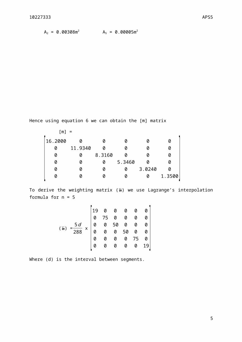
A2 = 0.00308m2 A5 = 0.00005m2

Hence using equation 6 we can obtain the [m] matrix

[m] =

[16.2000 0 0 0 0 0

0 11.9340 0 0 0 00 0 8.3160 0 0 00 0 0 5.3460 0 00 0 0 0 3.0240 00 0 0 0 0 1.3500

]To derive the weighting matrix (w) we use Lagrange’s interpolationformula for n = 5

(w) = 5d288 x [

19 0 0 0 0 00 75 0 0 0 00 0 50 0 0 00 0 0 50 0 00 0 0 0 75 00 0 0 0 0 19

]Where (d) is the interval between segments.

5

10227333 APS5

(w) = [0.0990 0 0 0 0 0

0 0.3906 0 0 0 00 0 0.2604 0 0 00 0 0 0.2604 0 00 0 0 0 0.3906 00 0 0 0 0 0.0990

]The rigidity matrix (EI) is a product of the Young’s modulus ofelasticity (E) and the second moment of area of the beam (I) aboutits neutral axis at six spanwise stations:

I = bndn

3

12 10

Where (bn) is the base and (dn) is the depth of each station

EI = [14000 0 0 0 0 00 7451.38 0 0 0 00 0 3521.5 0 0 00 0 0 1397.6 0 00 0 0 0 4181.02 00 0 0 0 0 7291.67

]The characteristics equation is given by:

ω2 [V ] [m ][w ][V]T{q} = [d2vdx2

][EI][w] [d2vdx2

] {q} 11

Now, substituting all the values of matrix in the equation 11 weget:

ω2[1.1502 0.96850.9685 0.8374] [

q1

q2] = [8.1725×103 4.6056×103

4.6056×103 5.5434×103][q1

q2]

[1.1502ω2−8172.5 0.9685ω2−4605.60.9685ω2−4605.6 0.8374ω2−5543.4]¿] = 0 12

6

10227333 APS5

The only non-trivial solution for the above equation 12 is when q ≠0

Therefore, taking the determinant of the above equation:

¿)×(0.8374ω2−5543.4) – (0.9685ω2−4605.6)×(0.9685ω2−4605.6) = 0

0.02518523ω4 – 4298.62298ω2 + 24091885.14 = 0 13

Using the quadratic equation:

ω2=−b±√b2−4ac

2a14

ω2 =−(−4298.62298)±√(−4298.62298)2−4(0.02518523)(24091885.14)

2(0.02518523)

ω2 = 4298.62298±4006.385010.05037046

The first two natural frequencies of the beam are:

ω12 = 5801.772904 ω2

2 = 164875.5417

ω1=√5801.772904 ω2= √164875.5417

ω1=76.16936985 ω2= 406.0486938

Converting in hertz by diving with 2π

ω1=76.16936985

2πω2=

406.04869382π

ω1=12.12 Hz ω2= 64.62 Hz

Mode of shapes

(2) Determine and plot the first two mode shapes of the beam corresponding to the first two natural frequencies obtained in Question (1). Substituting the values of ω2in equation 12

7

10227333 APS5

[1.1502ω2−8172.5 0.9685ω2−4605.60.9685ω2−4605.6 0.8374ω2−5543.4]¿]

Using ω12 we get

[−1499.200806 1013.4170581013.417058 −684.9953702 ] ¿] = 0

q1

q2 = 0.6759

The column matrix which represents the first mode shape at sixstations is obtained by substituting in equation 3

q1 = 0.6759 and q2 = 1

{φ1} = q1 {V1} + q1{V2}

{φ1} = 0.6759[0

0.069860.24320.47520.73386

1] + [

00.0216530.138240.365760.669013

1] = [

00.068870.302620.686951.165031.6759

]Normalising the final column for {φ1} =1.6759 [

00.041090.180570.40990.69517

1]

Again, Using ω22we get

[−1499.200806 1013.4170581013.417058 −684.9953702 ] ¿] = 0

8

10227333 APS5

q1

q2 = - 0.8546

The column matrix which represents the first mode shape at sixstations is obtained by substituting

q1 = -0.8546 and q2 = 1

{φ2} = q1 {V1} + q1{V2}

{φ2} = -0.8546[0

0.069860.24320.47520.73386

1] + [

00.0216530.138240.365760.669013

1] = [

0−0.03805−0.0696−0.040350.041860.1454

]Normalising the final column for {φ2} =0.1454 [

0−0.26169−0.47868−0.277510.2879

1]

Plotting the graph of φ1 and φ2 against x/L

9

10227333 APS5

0 0.2 0.4 0.6 0.8 1 1.20

0.20.40.60.81

1.2

First mode shape

x/L

φ1

Figure 1 Graph of φ1 against x/L

0 0.2 0.4 0.6 0.8 1 1.2

-1

-0.5

0

0.5

1

1.5

Second mode shape

x/L

φ2

Figure 2 Graph of φ2 against x/L

10

10227333 APS5

ANSYS Modal Analysis(3) Use the finite element method to obtain approximate values for the first and second natural frequencies of the beam under flexural free vibrations. Refer to the ANSYS Modal Analysis Tutorial for more information if ANSYS is used for this task.

The first step is to choose the type of analysis to be carried. In this case structural.

11

10227333 APS5

The beam is added next which is later defined by adding constrains

The properties of the model can then be defined thorough Material

Props

12

10227333 APS5

Since the beam is elastic, we can now add the value of Young’s Modulus = 70Gpa and the density of the beam = 2700 kg/m3

13

10227333 APS5

The beam is then defined by adding the cross section area of the each side through Common sections under Beam. The root 0.3mx 0.02m and the tip 0.1mx0.005m

14

10227333 APS5

The length of the beam is then defined

15

10227333 APS5

Once points appear in the window, Modelling can be done by adding key points to make a straightline

16

10227333 APS5

Meshing attributes is then defined by selecting taper from the drop down option

The size of meshing is then defined by the adding number of elements. The higher the number, the accurate the result will be. In this case we used 1000.

17

10227333 APS5

Line for mesh is added

Now we can begin by selecting the type of analysis to conduct

18

10227333 APS5

Upon selecting the type of analysis, the sub menu changes to enter relevant options. The number of natural frequency to be obtained is added which is two in our case.

The type of load that the structure will experience is defined in the next step

19

10227333 APS5

The Degree of freedom for the beam regarding displacement is then added

The final step is to run the simulation by clicking solve

20

10227333 APS5

The values obtained for the first and second natural frequency are 11.393 Hz and 37.336 Hz

21

10227333 APS5

Comparison between Results

(4) Compare the results from the Rayleigh-Ritz method and the finiteelement method. Discuss sources of errors in results from the two methods and propose any measures which can be employed to improve the results.

Rayleigh-Ritz Finite Elementω1 12.12Hz 11.939Hzω2 64.62Hz 37.336Hz

The results obtained by using Rayleigh-Ritz method and Fineelement method are similar for the first mode of natural frequencybut a huge difference for the second natural frequency. TheRayleigh-Ritz approach to calculate the natural frequency of the

22

10227333 APS5

beam was by using an assumed polynomial function and assuming thedeflection curve of the beam. The beam was discretised evenly in 5segments to make it suitable for evaluation as it is in smallerchunks. However since the approach is more through assumptions and aset of universal equation, the findings may not be very accurate. Ifthe beam were to be discretised into smaller parts such as 20 or 50,the approximation can be improved. However, the calculation wouldhave been very complex needing software to perform calculation whichwould make the finite element method more feasible.

Finite element method is a systematic process where thediscretization was more physical. The structures behaviour can beknown by simplifying the object. This technique takes into accountof boundary conditions of the variables. Also the different types ofload, material, size dynamics are taken into account which givebetter approximation. During the operation of ANSYS, the meshingsize was used as 1000 which meant the beam was discretised equallyinto small 1000 parts and structural test was carried out. Byseparating models into fine smaller parts, more accurate results andfindings could be achieved. If the accuracy of the result were to beimproved, the meshing size could be further increased. Also thereare various parameters that can be added to make the object asclosely defined to the real object the loads experienced. Alsocomplex parts and objects can be modelled to produce simulationwhich increases the accuracy and prediction.

23