Analysis on Structural Modeling for Recycled Asphalt ...
342
ANALYSIS OF STRUCTURAL MODELING FOR RECYCLED ASPHALT PAVEMENT USED AS A BASE LAYER A Dissertation Submitted to the Graduate Faculty of the North Dakota State University of Agriculture and Applied Science By Ehab Magdy Salah Noureldin In Partial Fulfillment of the Requirements for the Degree of DOCTOR OF PHILOSOPHY Major Department: Civil and Environmental Engineering September 2015 Fargo, North Dakota
-
Upload
khangminh22 -
Category
Documents
-
view
1 -
download
0
Transcript of Analysis on Structural Modeling for Recycled Asphalt ...

ANALYSIS OF STRUCTURAL MODELING FOR RECYCLED ASPHALT PAVEMENT
USED AS A BASE LAYER
A Dissertation
Submitted to the Graduate Faculty
of the
North Dakota State University
of Agriculture and Applied Science
By
Ehab Magdy Salah Noureldin
In Partial Fulfillment of the Requirements
for the Degree of
DOCTOR OF PHILOSOPHY
Major Department:
Civil and Environmental Engineering
September 2015
Fargo, North Dakota
North Dakota State University
Graduate School
Title
ANALYSIS OF STRUCTURAL MODELING FOR RECYCLED
ASPHALT PAVEMENT USED AS A BASE LAYER
By
Ehab Magdy Salah Noureldin
The Supervisory Committee certifies that this disquisition complies with North
Dakota State University’s regulations and meets the accepted standards for the
degree of
DOCTOR OF PHILOSOPHY
SUPERVISORY COMMITTEE:
Dr. Magdy Abdelrahman
Chair
Dr. Dinesh Katti
Dr. Ying Huang
Dr. Yarong Yang
Approved:
11/19/2015 Dr. Dinesh Katti
Date Department Chair
iii
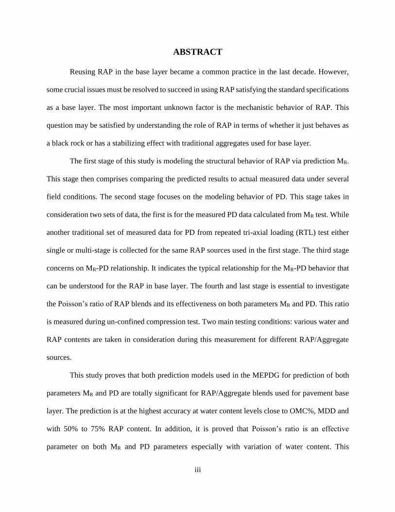
ABSTRACT
Reusing RAP in the base layer became a common practice in the last decade. However,
some crucial issues must be resolved to succeed in using RAP satisfying the standard specifications
as a base layer. The most important unknown factor is the mechanistic behavior of RAP. This
question may be satisfied by understanding the role of RAP in terms of whether it just behaves as
a black rock or has a stabilizing effect with traditional aggregates used for base layer.
The first stage of this study is modeling the structural behavior of RAP via prediction MR.
This stage then comprises comparing the predicted results to actual measured data under several
field conditions. The second stage focuses on the modeling behavior of PD. This stage takes in
consideration two sets of data, the first is for the measured PD data calculated from MR test. While
another traditional set of measured data for PD from repeated tri-axial loading (RTL) test either
single or multi-stage is collected for the same RAP sources used in the first stage. The third stage
concerns on MR-PD relationship. It indicates the typical relationship for the MR-PD behavior that
can be understood for the RAP in base layer. The fourth and last stage is essential to investigate
the Poisson’s ratio of RAP blends and its effectiveness on both parameters MR and PD. This ratio
is measured during un-confined compression test. Two main testing conditions: various water and
RAP contents are taken in consideration during this measurement for different RAP/Aggregate
sources.
This study proves that both prediction models used in the MEPDG for prediction of both
parameters MR and PD are totally significant for RAP/Aggregate blends used for pavement base
layer. The prediction is at the highest accuracy at water content levels close to OMC%, MDD and
with 50% to 75% RAP content. In addition, it is proved that Poisson’s ratio is an effective
parameter on both MR and PD parameters especially with variation of water content. This

iv
conclusion recommends to take in consideration Poisson’s ratio as an effective parameter in MR
and PD prediction models used in MEPDG software.
v
ACKNOWLEDGEMENTS
First, I wish to thank my main advisor Dr. Magdy Abdelrahman for his guidance and
academic support during my study. Also, I would like to thank my committee members: Dr. Dinesh
Katti, Dr. Ying Huang from Civil and Environmental Engineering Department, and Dr. Yarong
Yang from Statistics Department for their help and patience during my study. I would like to
acknowledge Dr. Mohammed Attia for his measured data collected during his Ph.D work at NDSU
and used here in the modeling part of this study. An additional acknowledgement to my previous
committee members: Dr. Frank Yazdani from Civil and Environmental Engineering Department
and Dr. Vlodymyr Melnykov from Statistics Department in the beginning of my study.
Furthermore, I would like to thank the Minnesota Department of Transportation
(MN/DOT) for supplying the needed materials used in this research. Also, I would like to thank
the Civil and Environmental Engineering Department at NDSU, and National Science Foundation
(NSF) for financial support during this research. Additional thanks to Mechanical Engineering
Department at NDSU for renting the load cells needed to complete the experimental stage of this
research. Special thanks to Rob Sailor in Mechanical Engineering department for helping in this
issue.
Finally, thanks for all the team research members in CEE materials lab: Mohyeldin Ragab,
Anthony Waldenmaier and Amir Ghavibazoo, who helped the author during his work to complete
this research. Special thanks to my close friends: Ahmed El Fatih and his wife Nesreen El Doliefy,
Amr Salem and Ahmed El Ghazaly, who supported me here during my life in US. I would like to
extend my gratitude to all my close family members and old friends in Egypt who kept caring and
supporting during my Ph.D progress.

vi
DEDICATION
Thanks for God’s support and blessings during my whole life and studying here in US, which
without it I cannot achieve my goal.
I dedicate this work to my dear father for his help and guidance during my whole personal and
career life.
Additional dedication to my dear mother and sister for their deep concern and caring.
Finally, a special dedication to my beloved home country Egypt, hoping a brilliant future to
achieve its goals.

vii
TABLE OF CONTENTS
ABSTRACT ................................................................................................................................... iii
ACKNOWLEDGEMENTS ............................................................................................................ v
DEDICATION ............................................................................................................................... vi
LIST OF TABLES ........................................................................................................................ xii
LIST OF FIGURES ..................................................................................................................... xiii
LIST OF ABBREVIATIONS ..................................................................................................... xvii
LIST OF APPENDIX TABLES ................................................................................................ xviii
LIST OF APPENDIX FIGURES............................................................................................... xxiv
CHAPTER 1. INTRODUCTION ................................................................................................... 1
1.1. General Overview ................................................................................................................ 1
1.2. Problem Statement ............................................................................................................... 2
1.3. Research Objectives ............................................................................................................. 3
1.4. Thesis Organization ............................................................................................................. 4
CHAPTER 2. LITERATURE REVIEW ........................................................................................ 6
2.1. Background on RAP ............................................................................................................ 6
2.2. RAP Used in HMA .............................................................................................................. 7
2.3. RAP Aging Characteristics ................................................................................................ 10
2.4. RAP Used in Base Layer ................................................................................................... 13
2.5. Environmental Impacts of Using RAP .............................................................................. 18
2.5.1. RAP leaching characteristics (Townsend, 1998) ........................................................ 19
2.5.2. Inorganic contaminant leaching (Kang, Gupta, Bloom, et al., 2011) ......................... 23
2.6. Main Design Base Layer Parameters ................................................................................. 24
2.6.1. Resilient modulus (MR)............................................................................................... 24
2.6.2. Permanent deformation (PD) ...................................................................................... 31
viii
2.6.3. Poisson’s ratio ............................................................................................................. 38
CHAPTER 3. METHODOLOGY AND EXPERIMENTAL WORK .......................................... 43
3.1. Main Research Tasks ......................................................................................................... 43
3.1.1. MR modeling task ........................................................................................................ 43
3.1.2. PD modeling task ........................................................................................................ 47
3.1.3. MR and PD correlation task......................................................................................... 48
3.1.4. Poisson’s ratio task ..................................................................................................... 51
3.2. Experimental Program ....................................................................................................... 53
3.2.1 Sieve analysis gradation test ........................................................................................ 53
3.2.2. Asphalt extraction test................................................................................................. 53
3.2.3. Moisture content-dry density relationship .................................................................. 54
3.2.4. Tri-axial shear test....................................................................................................... 54
3.2.5. Resilient modulus test ................................................................................................. 54
3.2.6. Permanent deformation test ........................................................................................ 55
3.2.7. Un-confined compression test..................................................................................... 56
3.3. RAP Index Properties Data ................................................................................................ 57
CHAPTER 4. RESILIENT MODULUS MODELING ................................................................ 60
4.1. Introduction ........................................................................................................................ 60
4.2. Experimental Considerations ............................................................................................. 61
4.3. Statistical Analysis ............................................................................................................. 62
4.4. Sensitivity Analysis ........................................................................................................... 69
4.4.1. Witczak model parametric analysis ............................................................................ 69
4.4.2. MEPDG model parameter analysis ............................................................................. 70
4.4.3. Pezo model parameter analysis ................................................................................... 71
4.5. Parametric Analysis ........................................................................................................... 76

ix
4.5.1. Analysis of K1 ............................................................................................................. 77
4.5.2. Analysis of K2 ............................................................................................................. 82
4.5.3. Analysis of K3 ............................................................................................................. 83
4.5.4. RAP-aggregate combination analysis ......................................................................... 87
4.6. MR Modeling Task Summary ............................................................................................ 93
CHAPTER 5. PERMANENT DEFORMATION MODELING .................................................. 95
5.1. Introduction ........................................................................................................................ 95
5.2. PD-MEPDG Prediction Model .......................................................................................... 96
5.3. Modeling Methodology ..................................................................................................... 97
5.3.1. Stage I ......................................................................................................................... 97
5.3.2. Stage II ........................................................................................................................ 98
5.3.3. Stage III ....................................................................................................................... 98
5.4. Analysis of Results ............................................................................................................ 99
5.4.1. PD from resilient modulus test ................................................................................... 99
5.4.2. Single-stage RTL test ................................................................................................ 110
5.4.3. Multi-stage RTL test ................................................................................................. 116
5.5. PD Modeling Task Summary........................................................................................... 121
CHAPTER 6. CORRELTION OF RESILIENT MODULUS AND PERMANENT
DEFORMATION ....................................................................................................................... 123
6.1. Introduction ...................................................................................................................... 123
6.2. Correlation Approach....................................................................................................... 123
6.3. Stages of Work ................................................................................................................. 124
6.4. Analysis of Results .......................................................................................................... 126
6.4.1 Resilient modulus test ................................................................................................ 126
6.4.2. Single-stage RTL test ................................................................................................ 135
6.4.3. Multi-stage RTL test ................................................................................................. 138
x
6.5. Correlation Task Summary .............................................................................................. 144
6.5.1. Resilient modulus testing .......................................................................................... 144
6.5.2. Single-Stage RTL Testing......................................................................................... 145
6.5.3. Multi-Stage RTL Testing .......................................................................................... 145
CHAPTER 7. POSSOIN’S RATIO MEASUREMENT ............................................................ 146
7.1. Introduction ...................................................................................................................... 146
7.2. Scope of Task ................................................................................................................... 147
7.3. Stages of Analysis ............................................................................................................ 148
7.3.1. Analysis versus RAP content .................................................................................... 148
7.3.2. Analysis versus water content ................................................................................... 152
7.3.3. Correlation between lateral strain and compressive stress ....................................... 158
7.4. MR Relationship with Un-confined Compression Test Parameters ................................. 162
7.5. PD Relationship with Un-confined Compression Test Parameters ................................. 167
7.6. Poisson’s Ratio Task Summary ....................................................................................... 171
CHAPTER 8. CONCLUSIONS AND RECOMMENDATIONS .............................................. 173
8.1. RAP Effectiveness on MR Modeling ............................................................................... 173
8.2. RAP Effectiveness on PD Modeling................................................................................ 174
8.3. Correlation for Both MR and PD Parameters ................................................................... 175
8.4. Poisson’s Ratio Effectiveness on RAP behavior ............................................................. 176
8.5. Final Summary ................................................................................................................. 176
8.6. Recommendations for Future Research ........................................................................... 177
REFERENCES ........................................................................................................................... 178
APPENDIX A. RESILIENT MODULUS DATA MODELING ............................................... 188
APPENDIX B. PERMANENT DEFORMATION DATA MODELING .................................. 213
APPENDIX C. CORRELATION DATA OF MR AND PD ...................................................... 303

xi
APPENDIX D. POISSON’S RATIO MEASURED DATA ...................................................... 306

xii
LIST OF TABLES
Table Page
2.1. Resilient Modulus Predictive Models (M. I. E.-S. Attia, 2010) ............................................ 29
2.2. Typical Values of Poisson’s Ratio (Maher & Bennert, 2008) ............................................... 41
3.1. Index Properties for RAP TH 10/Class 5 Blends (M. I. E.-S. Attia, 2010) ........................... 58
3.2. Index Properties for Other Tested RAP/Aggregate Blends ................................................... 59
4.1. R2 for the Six Rejected Models .............................................................................................. 67
4.2. R2 for Water Content (W.C) Variation on RAP Approved Models ...................................... 68
4.3. R for 90% Maximum Dry Density (MDD) on RAP Approved Models ................................ 68
4.4. R2 for Freezing-Thawing (F-T) Cycles on RAP Approved Models ...................................... 68
5.1. R2 for Multi-Stage RTL Test ............................................................................................... 117
6.1. R2 for MR-PD Relation of Resilient Modulus Test for RAP TH 10 .................................... 130
6.2. R2 for MR-PD Relation of Resilient Modulus Test for All RAP Sources ............................ 134
6.3. R2 for MR-PD relation of Multi-Stage RTL Test for RAP TH 10 ....................................... 143
xiii
LIST OF FIGURES
Figure Page
2.1. Conventional Flexible Pavement Design (Huang, 1993) ...................................................... 15
2.2. Loading Shape of MR Testing ................................................................................................ 25
2.3. Permanent Deformation Stages (Werkmeister, 2004) ........................................................... 32
2.4. Poisson's Ratio for Cylinder during Un-Confined Compression Test ................................... 39
3.1. Research Hierarchy Flow Chart ............................................................................................. 44
3.2. MR Modeling Flow Chart....................................................................................................... 45
3.3. Experimental Data Collection ................................................................................................ 46
3.4. PD Modeling Flow Chart ....................................................................................................... 49
3.5. MR and PD Correlation Flow Chart ....................................................................................... 51
3.6. Poisson’s Ratio Flow Chart ................................................................................................... 52
4.1. Measured versus Predicted MR Values of Witczak Model .................................................... 64
4.2. Measured versus Predicted MR of MEPDG Model ............................................................... 65
4.3. Measured versus Predicted MR Values of Pezo Model ......................................................... 66
4.4. Analysis of K Parameters for Witczak Model under Tested Factors..................................... 73
4.5. Analysis of K Parameters for MEPDG Model under Tested Factors .................................... 74
4.6. Analysis of K Parameters for Pezo Model under Tested Factors .......................................... 75
4.7. K1 versus Water Content Variation........................................................................................ 79
4.8. K1 versus Maximum Dry Density Variation .......................................................................... 80
4.9. K1 versus Freeze and Thaw Cycles ........................................................................................ 81
4.10. K2 versus Water Content Variation...................................................................................... 84
4.11. K2 versus Maximum Dry Density Variation ........................................................................ 85
4.12. K2 versus Freeze and Thaw Cycles ...................................................................................... 86
4.13. K3 versus Water Content Variation...................................................................................... 88
xiv
4.14. K3 versus Maximum Dry Density Variation ........................................................................ 89
4.15. K3 versus Freeze and Thaw Cycles ...................................................................................... 90
4.16. Analysis of MEPDG Model versus RAP Concentration ..................................................... 91
5.1. Measured versus Predicted PD for Class 5 (0% RAP) ........................................................ 101
5.2. Measured versus Predicted PD for 50% RAP TH 10 + 50% Class 5 .................................. 102
5.3. Measured versus Predicted PD for 75% RAP TH 10 + 25% Class 5 .................................. 103
5.4. Measured versus Predicted PD for 100% RAP TH 10 ........................................................ 104
5.5. Measured versus Predicted PD for RAP TH 19-101 ........................................................... 106
5.6. Measured versus Predicted PD for RAP TH 19-104 ........................................................... 107
5.7. Measured versus Predicted PD for RAP TH 22................................................................... 108
5.8. Measured versus Predicted PD for Cell 18 .......................................................................... 109
5.9. Measured versus Predicted PD of Single-stage RTL for Class 5 ........................................ 112
5.10. Measured versus Predicted PD of Single-stage RTL for 50% RAP TH 10
+ 50% Class 5 at OMC% ................................................................................................... 113
5.11. Measured versus Predicted PD of Single-stage RTL for 50% RAP TH 10
+ 50% Class 5 at OMC+2% ............................................................................................... 114
5.12. Measured versus Predicted PD of Single-stage RTL for 50% RAP TH 10
+ 50% Class 5 with 6% Added Fines ................................................................................ 115
5.13. Measured versus Predicted PD of Multi-stage RTL for Class 5 ........................................ 118
5.14. Measured versus Predicted PD of Multi-stage RTL for 50% RAP TH 10 + 50% Class 5 .................................................................................................................... 119
5.15. Measured versus Predicted PD of Multi-stage RTL for 50% RAP TH 10
+ 50% Class 5 with 3.5% Added Fines ............................................................................. 120
6.1. MR versus PD for RAP TH 10 at Several Confining Pressure Levels ................................. 128
6.2. MR versus PD for RAP TH 10 at Several RAP Percentages ................................................ 129
6.3. MR versus PD for all RAP Sources at 50% RAP ................................................................. 132
6.4. MR versus PD for all RAP Sources at 100% RAP ............................................................... 133

xv
6.5. MR versus PD for Single-stage RTL at OMC%................................................................... 136
6.6. MR versus PD for Single-stage RTL at OMC+2% .............................................................. 137
6.7. MR versus PD for Multi-stage RTL of Class 5 .................................................................... 140
6.8. MR versus PD for Multi-stage RTL of 50% RAP TH 10/50% Class 5 ............................... 141
6.9. MR versus PD for Multi-stage RTL of 50% RAP TH10/50% Class 5
+ 3.5% Plastic Fines ............................................................................................................ 142
7.1. Poisson’s Ratio for RAP TH 29/New Class 5 Blends versus RAP Content ........................ 149
7.2. Poisson’s Ratio for RAP TH 10/Old Class 5 Blends versus RAP Content ......................... 150
7.3. Comparison between Ultimate Compressive Strength and Poisson’s Ratio for
RAP/Aggregate blends versus RAP Content ...................................................................... 151
7.4. Poisson’s Ratio for RAP TH 29 + New Class 5 Blends versus Water Content .................. 154
7.5. Poisson’s Ratio for RAP TH 10 + Old Class 5 Blends versus Water Content .................... 155
7.6. Poisson’s Ratio for Field RAP Blends versus Water Content ............................................. 156
7.7. Ultimate Compressive Strength for RAP Blends versus Water Content ............................. 157
7.8. Comparison between Lateral Strain and Compressive Stress for RAP TH 29 + New Class 5 Blends ......................................................................................................... 159
7.9. Comparison between Lateral Strain and Compressive Stress for RAP TH 10 + Old Class 5 Blends ........................................................................................................... 160
7.10. Lateral Strain versus Compressive Stress for Field RAP Blends ...................................... 161
7.11. Comparison between MR and Un-confined Compression Parameters versus RAP Content for RAP TH 10 + Old Class 5 Blends ......................................................... 164
7.12. Comparison between MR and Un-confined Compression Parameters versus
Water Content for RAP TH 10 + Old Class 5 Blends ....................................................... 165
7.13. Comparison between MR and Un-confined Compression Parameters versus
Water Content for Other Field RAP Blends ...................................................................... 166
7.14. Comparison between PD and Un-confined Compression Parameters versus RAP Content for RAP TH 10 + Old Class 5 Blends ......................................................... 168
7.15. Comparison between PD and Un-confined Compression Parameters versus
Water Content for RAP TH 10 + Old Class 5 Blends ....................................................... 169

xvi
7.16. Comparison between PD and Un-confined Compression Parameters versus
Water Content for Other Field RAP Blends ...................................................................... 170
xvii
LIST OF ABBREVIATIONS
AASHTO………………... American Association of State Highway and Transportation Officials
AC……………………...... Asphalt Concrete
ASTM…………………..... American Society of Testing and Materials
CBR……………………… California Bearing Ratio
FDR…………………….... Full Depth Reclamation
FWD……………………... Falling Weight Deflectometer
F-T………………………. Freeze-Thaw cycles
HMA…………………….. Hot Mix Asphalt
MEPDG………………….. Mechanistic-Empirical Pavement Design Guide
MDD…………………….. Maximum Dry Density
MN/DOT……………….... Minnesota Department of Transportation
MR……………………….. Resilient Modulus
NCHRP………………….. National Cooperative Highway Research Program
OMC……………………... Optimum Moisture Content
PD……………………….. Permanent deformation
RAP……………………… Recycled Asphalt Pavement
RLT……………………… Repeated Load Tri-axial test
TH……………………….. Trunk Highway
WC………………………. Water Content
xviii
LIST OF APPENDIX TABLES
Table Page
A1. MR data for Class 5 versus Water Content Variation........................................................... 188
A2. MR data for Class 5 at 90% Maximum Dry Density ............................................................ 190
A3. MR data for Class 5 after Two Freeze-Thaw Cycles ............................................................ 191
A4. MR data for 50% Old Class 5/50% RAP TH 10 versus Water Content Variation ............... 192
A5. MR data for 50% Class 5 + 50% RAP TH 10 at 90% Maximum Dry Density .................... 194
A6. MR data for 50% Class 5 + 50% RAP TH 10 after Two Freeze-Thaw Cycles .................... 195
A7. MR data for 25% Class 5 + 75% RAP TH 10 versus Water Content Variation................... 196
A8. MR data for 25% Class 5 + 75% RAP TH 10 after Two Freeze-Thaw Cycles .................... 198
A9. MR data for 100% RAP TH 10 versus Water Content Variation ......................................... 199
A10. MR data for 100% RAP TH 10 at 90% Maximum Dry Density ........................................ 201
A11. MR data for 100% RAP TH 10 after Two Freeze-Thaw Cycles ........................................ 202
A12. K’s Parameters versus Water Content Variation ............................................................... 203
A13. K’s Parameters versus 90% Maximum Dry Density ......................................................... 204
A14. K’s Parameters versus Two Freeze-Thaw Cycles .............................................................. 204
A15. K’s Parameters versus Water Content Variation for Class 5 at Different Confining
Pressure Levels .................................................................................................................. 205
A16. K’s Parameters versus Water Content Variation for 50% RAP TH 10 + 50% Class 5
at Different Confining Pressure Levels .............................................................................. 206
A17. K’s Parameters versus Water Content Variation for 75% RAP TH 10 + 25% Class 5
at Different Confining Pressure Levels .............................................................................. 207
A18. K’s Parameters versus Water Content Variation for 100% RAP TH 10 at Different
Confining Pressure Levels ................................................................................................. 208
A19. K’s Parameters versus 90% Maximum Dry Density for Class 5 at Different Confining
Pressure Levels .................................................................................................................. 209
A20. K’s Parameters versus 90% Maximum Dry Density for 50% RAP TH 10 + 50% Class 5
at Different Confining Pressure Levels .............................................................................. 209

xix
A21. K’s Parameters versus 90% Maximum Dry Density for 100% RAP TH 10 at Different
Confining Pressure Levels ................................................................................................. 210
A22. K’s Parameters versus Two Freeze-Thaw Cycles for Class 5 at Different Confining
Pressure Levels .................................................................................................................. 210
A23. K’s Parameters versus Two Freeze-Thaw Cycles for 50% Class 5 + 50% RAP TH 10
at Different Confining Pressure Levels .............................................................................. 211
A24. K’s Parameters versus Two Freeze-Thaw Cycles for 25% Class 5 + 75% RAP TH 10
at Different Confining Pressure Levels .............................................................................. 211
A25. K’s Parameters versus Two Freeze-Thaw Cycles for 100% RAP TH 10 at Different
Confining Pressure Levels ................................................................................................. 212
B1. PD Measured Data from MR Test for Class 5 (OMC-2%) ................................................... 213
B2. PD Measured Data from MR Test for Class 5 (OMC%) ...................................................... 214
B3. PD Measured Data from MR Test for Class 5 (OMC+2%) .................................................. 215
B4. PD Measured Data from MR Test for 50% RAP TH 10 (OMC-2%) ................................... 216
B5. PD Measured Data from MR Test for 50% RAP TH 10 (OMC%) ...................................... 217
B6. PD Measured Data from MR Test for 50% RAP TH 10 (OMC+2%) .................................. 218
B7. PD Measured Data from MR Test for 75% RAP TH 10 (OMC-2%) ................................... 219
B8. PD Measured Data from MR Test for 75% RAP TH 10 (OMC%) ...................................... 220
B9. PD Measured Data from MR Test for 75% RAP TH 10 (OMC+2%) .................................. 221
B10. PD Measured Data from MR Test for 100% RAP TH 10 (OMC-2%) ............................... 222
B11. PD Measured Data from MR Test for 100% RAP TH 10 (OMC%) .................................. 223
B12. PD Measured Data from MR Test for 100% RAP TH 10 (OMC+2%) .............................. 224
B13. PD Measured Data from MR Test for Extracted 100% RAP TH 10 (OMC%) .................. 225
B14. PD Measured Data from MR Test for RAP TH 19-101 (OMC-2%) .................................. 226
B15. PD Measured Data from MR Test for RAP TH 19-101 (OMC%) ..................................... 227
B16. PD Measured Data from MR Test for RAP TH 19-101 (OMC+2%) ................................. 228
B17. PD Measured Data from MR Test for RAP TH 19-104 (OMC-2%) .................................. 229

xx
B18. PD Measured Data from MR Test for RAP TH 19-104 (OMC%) ..................................... 230
B19. PD Measured Data from MR Test for RAP TH 19-104 (OMC+2%) ................................. 231
B20. PD Measured Data from MR Test for RAP TH 22 (OMC-2%) ......................................... 232
B21. PD Measured Data from MR Test for RAP TH 22 (OMC%)............................................. 233
B22. PD Measured Data from MR Test for RAP TH 22 (OMC+2%) ........................................ 234
B23. PD Measured Data from MR Test for Cell 18 (OMC-2%) ................................................. 235
B24. PD Measured Data from MR Test for Cell 18 (OMC%) .................................................... 236
B25. PD Measured Data from MR Test for Cell 18 (OMC+2%) ................................................ 237
B26. PD Measured Data from Single-stage RTL Test for Class 5 at OMC% (σd = 17 psi) ....... 238
B27. PD Measured Data from Single-stage RTL Test for Class 5 at OMC% (σd = 24 psi) ....... 240
B28. PD Measured Data from Single-stage RTL Test for Class 5 at OMC+2% (σd = 12 psi) ... 242
B29. PD Measured Data from Single-stage RTL Test for Class 5 at OMC+2% (σd = 17 psi) ... 244
B30. PD Measured Data from Single-stage RTL Test for 50% Class 5 + 50% RAP TH 10
at OMC% (σd = 17 psi) ...................................................................................................... 246
B31. PD Measured Data from Single-stage RTL Test for 50% Class 5 + 50% RAP TH 10
at OMC% (σd = 24 psi) ...................................................................................................... 248
B32. PD Measured Data from Single-stage RTL Test for 50% Class 5 + 50% RAP TH 10
at OMC% (σd = 37 psi) ...................................................................................................... 250
B33. PD Measured Data from Single-stage RTL Test for 50% Class 5 + 50% RAP TH 10
at OMC+2% (σd = 12 psi) .................................................................................................. 251
B34. PD Measured Data from Single-stage RTL Test for 50% Class 5 + 50% RAP TH 10
at OMC+2% (σd = 17 psi) .................................................................................................. 253
B35. PD Measured Data from Single-stage RTL Test for 50% Class 5 + 50% RAP TH 10
+ 6% Fines at OMC% (σd = 17 psi) ................................................................................... 255
B36. PD Measured Data from Single-stage RTL Test for 50% Class 5 + 50% RAP TH 10
+ 6% Fines at OMC% (σd = 24 psi) ................................................................................... 257
B37. PD Measured Data from Single-stage RTL Test for 50% Class 5 + 50% RAP TH 10
+ 6% Fines at OMC+2% (σd = 12 psi) ............................................................................... 259

xxi
B38. PD Measured Data from Single-stage RTL Test for 50% Class 5 + 50% RAP TH 10
+ 6% Fines at OMC+2% (σd = 17 psi) ............................................................................... 261
B39. PD Measured Data from Multi-stage RTL Test for Class 5 at OMC-2% (σd = 6 psi) ....... 263
B40. PD Measured Data from Multi-stage RTL Test for Class 5 at OMC-2% (σd = 12 psi) ..... 264
B41. PD Measured Data from Multi-stage RTL Test for Class 5 at OMC-2% (σd = 17 psi) ..... 265
B42. PD Measured Data from Multi-stage RTL Test for Class 5 at OMC-2% (σd = 24 psi) ..... 266
B43. PD Measured Data from Multi-stage RTL Test for Class 5 at OMC% (σd = 17 psi) ........ 267
B44. PD Measured Data from Multi-stage RTL Test for Class 5 at OMC% (σd = 24 psi) ........ 268
B45. PD Measured Data from Multi-stage RTL Test for Class 5 at OMC% (σd = 37 psi) ........ 268
B46. PD Measured Data from Multi-stage RTL Test for Class 5 at OMC+2% (σd = 6 psi) ...... 269
B47. PD Measured Data from Multi-stage RTL Test for Class 5 at OMC+2% (σd = 12 psi) .... 270
B48. PD Measured Data from Multi-stage RTL Test for Class 5at OMC+2% (σd = 17 psi) ..... 271
B49. PD Measured Data from Multi-stage RTL Test for Class 5 at OMC+2% (σd = 24 psi) .... 272
B50. PD Measured Data from Multi-stage RTL Test for 50% Class 5 + 50% RAP TH 10
at OMC-2% (σd = 17 psi) ................................................................................................... 273
B51. PD Measured Data from Multi-stage RTL Test for 50% Class 5 + 50% RAP TH 10
at OMC-2% (σd = 24 psi) ................................................................................................... 274
B52. PD Measured Data from Multi-stage RTL Test for 50% Class 5 + 50% RAP TH 10
at OMC-2% (σd = 37 psi) ................................................................................................... 275
B53. PD Measured Data from Multi-stage RTL Test for 50% Class 5 + 50% RAP TH 10
at OMC-2% (σd = 53 psi) ................................................................................................... 276
B54. PD Measured Data from Multi-stage RTL Test for 50% Class 5 + 50% RAP TH 10
at OMC-2% (σd = 63 psi) ................................................................................................... 277
B55. PD Measured Data from Multi-stage RTL Test for 50% Class 5 + 50% RAP TH 10
at OMC-2% (σd = 73 psi) ................................................................................................... 278
B56. PD Measured Data from Multi-stage RTL Test for 50% Class 5 + 50% RAP TH 10
at OMC% (σd = 24 psi) ...................................................................................................... 279
B57. PD Measured Data from Multi-stage RTL Test for 50% Class 5 + 50% RAP TH 10
at OMC% (σd = 37 psi) ...................................................................................................... 280
xxii
B58. PD Measured Data from Multi-stage RTL Test for 50% Class 5 + 50% RAP TH 10
at OMC% (σd = 53 psi) ...................................................................................................... 281
B59. PD Measured Data from Multi-stage RTL Test for 50% Class 5 + 50% RAP TH 10
at OMC% (σd = 63 psi) ...................................................................................................... 281
B60. PD Measured Data from Multi-stage RTL Test for 50% Class 5 + 50% RAP TH 10
at OMC+2% (σd = 6 psi) .................................................................................................... 282
B61. PD Measured Data from Multi-stage RTL Test for 50% Class 5 + 50% RAP TH 10
at OMC+2% (σd = 12 psi) .................................................................................................. 283
B62. PD Measured Data from Multi-stage RTL Test for 50% Class 5 + 50% RAP TH 10
at OMC+2% (σd = 17 psi) .................................................................................................. 284
B63. PD Measured Data from Multi-stage RTL Test for 50% Class 5 + 50% RAP TH 10
at OMC+2% (σd = 24 psi) .................................................................................................. 285
B64. PD Measured Data from Multi-stage RTL Test for 50% Class 5 + 50% RAP TH 10
at OMC+2% (σd = 37 psi) .................................................................................................. 286
B65. PD Measured Data from Multi-stage RTL Test for 50% Class 5 + 50% RAP TH 10
at OMC+2% (σd = 53 psi) .................................................................................................. 286
B66. PD Measured Data from Multi-stage RTL Test for 50% Class 5 + 50% RAP TH 10
+ 3.5% Plastic Fines at OMC-2% (σd = 17 psi) ................................................................. 287
B67. PD Measured Data from Multi-stage RTL Test for 50% Class 5 + 50% RAP TH 10
+ 3.5% Plastic Fines at OMC-2% (σd = 24 psi) ................................................................. 288
B68. PD Measured Data from Multi-stage RTL Test for 50% Class 5 + 50% RAP TH 10
+ 3.5% Plastic Fines at OMC-2% (σd = 37 psi) ................................................................. 289
B69. PD Measured Data from Multi-stage RTL Test for 50% Class 5 + 50% RAP TH 10
+ 3.5% Plastic Fines at OMC-2% (σd = 53 psi) ................................................................. 290
B70. PD Measured Data from Multi-stage RTL Test for 50% Class 5 + 50% RAP TH 10
+ 3.5% Plastic Fines at OMC-2% (σd = 63 psi) ................................................................. 291
B71. PD Measured Data from Multi-stage RTL Test for 50% Class 5 + 50% RAP TH 10
+ 3.5% Plastic Fines at OMC-2% (σd = 73 psi) ................................................................. 292
B72. PD Measured Data from Multi-stage RTL Test for 50% Class 5 + 50% RAP TH 10
+ 3.5% Plastic Fines at OMC% (σd = 17 psi) .................................................................... 293
B73. PD Measured Data from Multi-stage RTL Test for 50% Class 5 + 50% RAP TH 10
+ 3.5% Plastic Fines at OMC% (σd = 24 psi) .................................................................... 294

xxiii
B74. PD Measured Data from Multi-stage RTL Test for 50% Class 5 + 50% RAP TH 10
+ 3.5% Plastic Fines at OMC% (σd = 37 psi) .................................................................... 295
B75. PD Measured Data from Multi-stage RTL Test for 50% Class 5 + 50% RAP TH 10
+ 3.5% Plastic Fines at OMC% (σd = 53 psi) .................................................................... 296
B76. PD Measured Data from Multi-stage RTL Test for 50% Class 5 + 50% RAP TH 10
+ 3.5% Plastic Fines at OMC% (σd = 63 psi) .................................................................... 297
B77. PD Measured Data from Multi-stage RTL Test for 50% Class 5 + 50% RAP TH 10
+ 3.5% Plastic Fines at OMC% (σd = 73 psi) .................................................................... 298
B78. PD Measured Data from Multi-stage RTL Test for 50% Class 5 + 50% RAP TH 10
+ 3.5% Plastic Fines at OMC+2% (σd = 6 psi) .................................................................. 299
B79. PD Measured Data from Multi-stage RTL Test for 50% Class 5 + 50% RAP TH 10
+ 3.5% Plastic Fines at OMC+2% (σd = 12 psi) ................................................................ 300
B80. PD Measured Data from Multi-stage RTL Test for 50% Class 5 + 50% RAP TH 10
+ 3.5% Plastic Fines at OMC+2% (σd = 17 psi) ................................................................ 301
B81. PD Measured Data from Multi-stage RTL Test for 50% Class 5 + 50% RAP TH 10
+ 3.5% Plastic Fines at OMC+2% (σd = 24 psi) ................................................................ 302
B82. PD Measured Data from Multi-stage RTL Test for 50% Class 5 + 50% RAP TH 10
+ 3.5% Plastic Fines at OMC+2% (σd = 37 psi) ................................................................ 302
C1. PD Data Collected from MR test at Different Confining Pressure Levels ........................... 303
C2. MR Measured Data from MR test at Different Confining Pressure Levels........................... 304
C3. MR Versus PD data for 50% RAP Blends at Different Confining Pressure Levels ............. 305
C4. MR Versus PD data for 100% RAP Blends at Different Confining Pressure Levels ........... 305
D1. Summary of Poisson’s Ratio Results for All RAP/Aggregate Tested Samples .................. 318
xxiv
LIST OF APPENDIX FIGURES
Figure Page
D1. Stress- Strain Biaxial Relationship for New Class 5 ............................................................ 306
D2. Stress- Strain Biaxial Relationship for New Class 5 (Replicate) ......................................... 307
D3. Stress- Strain Biaxial Relationship for Old Class 5 ............................................................. 308
D4. Stress- Strain Biaxial Relationship for 50% New Class 5 + 50% RAP TH 29.................... 309
D5. Stress- Strain Biaxial Relationship for 50% New Class 5 + 50% RAP TH 29 (Replicate) . 310
D6. Stress- Strain Biaxial Relationship for 50% Old Class 5 + 50% RAP TH 10 ..................... 311
D7. Stress- Strain Biaxial Relationship for 100% RAP TH 29 .................................................. 312
D8. Stress- Strain Biaxial Relationship for 100% RAP TH 29 (Replicate) ................................ 313
D9. Stress- Strain Biaxial Relationship for 100% RAP TH 10 .................................................. 314
D10. Stress- Strain Biaxial Relationship for RAP TH 19-101 ................................................... 315
D11. Stress- Strain Biaxial Relationship for RAP TH 19-104 ................................................... 316
D12. Stress- Strain Biaxial Relationship for RAP TH 22 ........................................................... 317

1
CHAPTER 1. INTRODUCTION
1.1. General Overview
Nowadays the worldwide paving industry is facing tremendous problems due to the severe
shortage of suitable aggregates in general and/or the high cost of virgin aggregates used in different
pavement layers. Therefore, utilizing the recycled asphalt pavement (RAP) concept to construct
an adequate granular base course layer is an excellent alternative especially in cases where lack of
suitable aggregates exists. The Federal Highway Administration (FHWA) reported in 2007 that
about 100 million tons of RAP are produced each year during pavement rehabilitation activities
(M. Attia, Abdelrahman, Alam, Section, & Department, 2009), which presents a major solid waste
concern, and consequently several environmental pollution and hazards. RAP has already become
one of the most widely used recycled materials in the United States now. Nationally, the use of
RAP in new pavement layers is expected to be doubled by 2014, compared to its recorded annual
usage of 60 million tons in 2009 (Zahid Hossain, 2012).
RAP is collected when asphalt pavements are removed for reconstruction, resurfacing, or
to obtain access to buried utilities. Rehabilitation projects of old asphalt pavements produce a huge
amount of RAP. FHWA reported that at least 13 state agencies (Arizona, Illinois, Louisiana,
Maine, Nebraska, New Hampshire, North Dakota, Oregon, Rhode Island, South Dakota, Texas,
Virginia, and Wisconsin) had used RAP as an aggregate in the base layer (M. I. E.-S. Attia, 2010).
Many mechanical tests are currently used to investigate the strength parameters of the base layer,
such as the resilient modulus (MR) and/or repeated loading tri-axial (RLT) for measuring the
permanent deformation (PD). It is recommended to measure both parameters MR and PD by the
mechanistic empirical pavement design guide (MEPDG) for the granular unbound base layer. A

2
prediction model for each is available in the MEPDG software if testing is not possible (Guide,
2008).
These tests were performed on RAP and/or RAP/Aggregate blends to compare its
performance with traditionally granular aggregates used for base layer. In general, it was found
that using RAP alone in the base layer did not achieve the standard specifications required for this
layer. Contrary, when RAP was mixed with various qualities granular aggregates especially at
50/50 percentage, the RAP behavior in the blend became similar to that of the unbound granular
aggregates (M. I. E.-S. Attia, 2010). Accordingly, RAP/Aggregate blend well achieved the
required specifications for base layer in several previous studies covering this research area.
However, there is a need to investigate the structural modeling parameters for RAP/Aggregate
blends used as a base layer.
1.2. Problem Statement
Using RAP in the base layer is facing many challenges nowadays. One of the most
important ones is the uncertainty concerning structural behavior of RAP in the base layer and
whether it behaves just as a black rock or has a stabilization effect on traditional aggregates used
as a base layer. Modeling the structural behavior of RAP blends, especially the resilient modulus,
can solve this key question of RAP behavior in base layer. Many parameters should be taken into
consideration in resilient modulus behavior modeling, such as different testing conditions, RAP
components, permanent deformation and Poisson’s ratio of base layer. Firstly, the need is apparent
to investigate previous constitutive models in terms of assessing the prediction of structural
capacity of base layer. This assessment would yield significant conclusions in terms of goodness
to fit of these models for RAP behavior under different testing conditions, such as moisture
contents, densities, freeze-thaw cycles and percentages of RAP in blends.
3
In addition, the permanent deformation (PD) is important to be investigated with respect
to describing the structural modeling behavior of RAP as a base layer. Previous studies on PD for
RAP blends in base layer construction had contradictive results. Some studies proved that PD
increased with higher RAP contents and others were vice versa. The MR results were more directly
proportional with percentage of RAP in the blend. On the other hand, PD contradictive values
resulted in not being able to determine the optimum percentage of RAP that can be used in the
base layer. Therefore, there is a need for a further study on PD modeling behavior of
RAP/Aggregate blends and its relation to MR modeling of the base layer under different testing
conditions. Also, it is essential to take into consideration the PD as an effective parameter on the
structural modeling of RAP as a base layer expressed by the resilient modulus MR.
Finally, the Poisson’s ratio was not considered in previous studies as an important
parameter affecting the structural capacity for granular base layer, especially when measured
during the resilient modulus test. Usually, Poisson’s ratio was estimated during all methods of
pavement design including the MEPDG. However, effect of Poisson’s ratio on both MR and PD
modeling behavior for RAP blends is essential to be studied to investigate its effectiveness on the
structural capacity of base layer. This stage of study is needed to confirm the difference in behavior
of RAP blends from granular aggregates, especially under variation of water content.
1.3. Research Objectives
Results of literature survey, yielded that the effectiveness of aged RAP components
characteristics would be minimal on the measured MR and PD values. Also, no environmental
hazards are expected from using RAP in the granular base layer blends. Therefore, there is no need
to investigate both factors in this study. Main objectives of this research are concluded in the
following points:
4
Comparing RAP/Aggregate blends to granular aggregate through constitutive prediction
models of the main effective parameters (MR and PD) previously used for granular base
layer.
Investigating the structural modeling behavior of RAP/Aggregate base layer blends by
prediction of MR and PD.
Investigating the relation between permeant deformation and resilient modulus for
different RAP blends as a base Layer.
Determine the effectiveness of Poisson’s ratio on measured MR and PD values for RAP
base layer blends.
Reassessing the prediction models of MR and PD to assess the need for additional
parameters to be taken in consideration.
1.4. Thesis Organization
This thesis is divided into 8 chapters as follows:
Chapter 1: Introduction
It explains the problem statement, main objectives and organization of this research.
Chapter 2: Literature Review
This chapter presents the previous work related to using of RAP in pavement construction
generally and base layer specifically, and its effect on the surrounding environment. Also, it
focuses on the main design parameters and the previous prediction models used for unbound base
layer.
Chapter 3: Methodology and Experimental Work
This chapter describes the main tasks that achieve the research objectives. In addition, it
presents testing procedures and materials tested to collect the data analyzed in this research.

5
Chapter 4: Resilient Modulus Modeling
This chapter concerns the adequacy of several previous resilient modulus prediction
models used for unbound granular base layer on RAP/aggregate blends at different testing
conditions.
Chapter 5: Permanent Deformation Modeling
This chapter focuses on the rutting MEPDG model used in permanent deformation
prediction for unbound granular base layer on RAP/aggregate blends at different testing
conditions.
Chapter 6: Correlation of Resilient Modulus and Permanent Deformation
This chapter explains the correlation between both parameters MR and PD for
RAP/aggregate blends under the most expected field conditions that could happen for base layer.
Chapter 7: Poisson’s Ratio Measurement
This chapter describes the relation between Poisson’s ratio and ultimate compressive
strength values for RAP/aggregate blends and its effectiveness on the main design parameters of
the base layer.
Chapter 8: Conclusions and Recommendations
This chapter presents summary of the research results, conclusions and recommended
future work.
6
CHAPTER 2. LITERATURE REVIEW
2.1. Background on RAP
Three most common asphalt pavement removal processes are milling, full-depth
reclamation (FDR) and asphalt plant waste. In first process, the top pavement surface only is
removed using a milling machine, which can remove up to a 2 in. thickness in a single pass. FDR
involves ripping and breaking the pavement using a rhino horn on a bulldozer and/or pneumatic
pavement breakers. This process removes both the top old pavement surface and the underlying
base or sub-base layers. Asphalt plant waste is generated as all asphalt plant operations
accumulates some waste during plant start-up, transition between mixes, and clean-out. When
these accumulated materials are properly crushed and screened, the RAP consists of high-quality,
well-graded aggregates coated by asphalt. After collecting the RAP, material characterization is
performed with respect to aggregate gradation and asphalt content.
In the early 1970’s pavement recycling became of interest as a result of severe price
inflation in the oil market due to decrease supplies from the oil producing and exporting countries
(OPEC) caused from 1973 war in the Middle East. FHWA initiated a project to demonstrate the
technical viability of asphalt recycling as a rehabilitation technique. This effort resulted in
materials, mix design and construction guidelines for implementing an asphalt recycling project.
States and paving contractors began making extensive use of RAP and over the years a number of
applications were developed including: addition to hot-mix asphalt (HMA); aggregate in cold-mix
asphalt; granular or stabilized base and sub-base course; fill or embankment material. In 2000,
FHWA reported that in the United States 33 million metric tons RAP were used in highway
construction applications out of 41 million metric tons RAP produced amounting to some 80%

7
reuse (P. J. Cosentino, Kalajian, Dikova, Patel, & Sandin, 2008). Lately, FHWA reported that
presently all 50 states are using RAP (P. J. Cosentino et al., 2008).
As large quantities of RAP are produced during highway maintenance and construction,
some can be used in new HMA, while the surplus RAP is still frequently available. If this material
could be reused on site as a sub-base or base material, it would reduce the environmental impact,
reduce the waste stream, and reduce the materials transportation costs associated with road
maintenance and construction. There are an estimated 90 million tons of RAP milled yearly with
80% to 90% being reused in roadway repaving, translating into 18 million tons of RAP being
available for other uses (P. Cosentino et al., 2003). Using RAP as recycle material was developed
through a combination of environmental, economic and technological factors. Recycling
eliminates the disposal and the concurrent hauling and transportation costs, provides a source of
readily available aggregate as a substitute for limited natural resources, and finally takes advantage
of the technological advancements brought about by inexpensive material processing techniques.
The clear conclusion from the expansion test results was that RAP materials have much
lower tendencies to expand or swell when compared to the high expansion potentials of especially
the virgin steel slag aggregates (Deniz, Tutumluer, & Popovics, 2009). As it is well known, RAP
has both elastic and viscous properties. An elastic material can be modeled as a spring. For a
spring, the deformation is proportional to the applied force. A viscous material can be modeled as
a dashpot. For the dashpots, force is proportional to velocity (stress is proportional to rate of strain).
2.2. RAP Used in HMA
One recurring question regarding RAP is whether it acts like a “black rock”. If RAP acts
like a black rock, the aged binder will not combine to any appreciable extent with the virgin binder
added and will not change the total binder properties (R. McDaniel & Anderson, 2001). To remedy

8
the situation of using RAP in HMA layer, the Federal Highway Administration’s Superpave
mixtures expert task group used past experience to develop interim guidelines for the use of RAP
in the Superpave method. These guidelines reflect the fact that the effect of aged binder from RAP
on the performance properties of the virgin binder depends upon the level of RAP in the HMA.
When the level is low, the effect is minimal, and the RAP is likened to a “black rock” that
influences the mix volumetric and performance through its aggregate gradation and properties. As
the level of RAP in the HMA increases, the black rock analogy breaks down as the aged binder
blends with the virgin material in sufficient quantity to significantly affect its performance
properties (R. McDaniel & Anderson, 2001).
During the construction and service life of the roadway from which the RAP was obtained,
the asphalt binder in the roadway became aged or hardened by reacting with oxygen in the air. If
a high percentage of RAP is used in HMA (greater than 15 to 30 percent), the RAP binder will
have to be considered when choosing the virgin asphalt grade added. Because of variability
concerns, some states limit the amount of RAP that can be included in new mixtures. Some states
allow the use of higher percentages of RAP, if the material is milled off the same project where
the new mix will be placed. Nevertheless, if RAP is used from a stockpile that includes material
from several projects, smaller RAP content may be used.
RAP materials are not as likely to segregate as aggregates because the asphalt binder in
RAP helps keep coarse and fine aggregate bound together (R. S. McDaniel, Soleymani, Anderson,
Turner, & Peterson, 2000). The moisture-holding capability of RAP is negligible, because there is
little minus No. 200 fraction, and most RAP aggregates are coated with asphalt (Puppala, Saride,
& Williammee, 2011). The effect of introducing RAP into the binder course mix was evaluated
through a series of laboratory tests including the Marshall test, the indirect tensile stiffness
9
modulus test, the indirect tensile fatigue test and the water sensitivity test. The laboratory tests
have shown that the introduction of RAP to the binder course mix resulted in an improvement in
all mechanical properties. In particular, it was found that the mix containing up to 30% RAP,
displayed improved fatigue resistance relative to the control mix manufactured from virgin
materials (Tabaković, Gibney, McNally, & Gilchrist, 2010).
The description of the process of extracting, recovering and testing the RAP aged binder
properties when needed, shows that for low RAP contents (<15%) it is not necessary to do this
testing because there is not enough of the old, hardened RAP binder present to change the total
binder properties. However, at higher RAP contents (>25%), the RAP aged binder will have a
noticeable effect, and it must be accounted for by using a softer grade of binder. For intermediate
ranges of RAP (15-25%), the virgin binder grade can simply be dropped one grade. For higher
percentages of RAP, there is a need to extract and recover the RAP binder and determine its
properties. These results provide compelling evidence that RAP does not act like a black rock. It
seems unreasonable to suggest that total blending of the RAP binder and virgin binder ever occurs,
but partial blending apparently occurs to a significant extent. The findings also support the concept
of a tiered approach to RAP usage because the effects of the RAP binder are negligible at low RAP
contents (R. S. McDaniel et al., 2000).
These findings mean that in general, conventional equipment and testing protocols can be
used with RAP binders. The tiered approach allows for the use of up to 15 to 30 percent RAP
without extensive testing. Higher RAP contents can also be used when additional testing is
conducted. The significance of these results is that the concept of using a softer virgin binder with
higher RAP contents is supported. A tiered approach to the use of RAP is found to be appropriate.
The advantage of this tiered approach is that relatively low levels of RAP can be used without
10
extensive testing of the RAP binder. If the use of higher RAP contents is desirable, conventional
Superpave binder tests can be used to determine how much RAP can be added or which virgin
binder to use (R. McDaniel & Anderson, 2001).
2.3. RAP Aging Characteristics
Asphalt for pavement construction is called asphalt cement. Asphalt cement is often added
to aggregate to make asphalt concrete or asphalt mix for construction of flexible asphalt pavements
for highways and parking lots. When these asphalt pavements are removed from a road surface,
the by-product is commonly called reclaimed asphalt pavement (RAP). RAP mostly consists of
ground up old asphalt pavement that stayed for its lifetime until it completely distressed. As asphalt
ages and is exposed to various waste elements, it tends to harden and become brittle. As a result
the viscosity of the asphalt cement increases and elasticity decreases (Huesemann, Hausmann, &
Fortman, 2005).
Asphalt binder originally consists largely of hydrocarbons, along with other molecules and
molecular structures. These molecules generally consist of carbon, hydrogen, sulfur, oxygen and
nitrogen, as well as a traceable amount of metals (Bennert & Dongré, 2010). To understand the
asphalt chemistry and its components especially for aged binder as the case in using RAP, many
tests are recommended for the extracted asphalt binder collected from RAP.
The role of the aged binder in the RAP was studied before in several researches especially
in the case of reusing RAP in HMA mixtures as mentioned before. As it is important to understand
the blending probability of the aged asphalt binder in RAP with the virgin asphalt added to restore
its original properties. One of the main issues to determine appropriate levels of RAP in asphalt
mixtures was that it assumes an ideal condition that the RAP aged asphalt binder fully blends with
the virgin asphalt binder added. However, different researches had shown that this is not most

11
likely the case and may be less than originally assumed (Bennert & Dongré, 2010). Many
researchers proved that the mechanical blending with the virgin asphalt added to the RAP in HMA
mixtures interact only with a small portion of the RAP asphalt binder (Bennert & Dongré, 2010).
This result agree partially with the assumption that RAP will behave just as a black rock if it is
used in HMA mixes especially if the RAP content is below 15% (R. S. McDaniel & Shah, 2003).
However, the extraction and recovery process for collecting the aged binder with PG
grading tests indicated that the asphalt binder did not stiffen linearly with increasing RAP content
in HMA mixtures (Bennert & Dongré, 2010). That means that the aged binder has indirect relation
with the stiffness and has partially blending effect with the virgin asphalt added. Therefore, it is
important to study the role of the aged binder in RAP if it is used as a base layer especially that it
is usually used in higher contents (50% or more) than HMA layer (25% or less). Most probably
there will be an effect of aged binder on stiffness parameters of base layers with the variation of
different field conditions, such as moisture content, density, fine contents, etc.
The definition of asphalt aging refers to a series of changes in asphalt concrete such as
evaporation, oxidation, polymerization, and changes of the internal structure of asphalt. In the
aging process of asphalt, the asphalt binder is exposed to the temperature, water and oxygen in the
air which causes the aromatics, resins and asphaltenes partially oxidize to produce
dehydrogenation of water (Zhang & Sun, 2012). Then, the remaining parts of heavy oil component
of active groups will polymerize or shrink and produce higher molecular weight substances (Zhang
& Sun, 2012). And, during this process, it was seen that its softening point will increase, and its
penetration will lower, the insoluble heptane’s will increase, and its mobility is also greatly
reduced (Zhang & Sun, 2012).

12
The Abson method was used frequently to recover asphalt binder from RAP, but several
studies have warned that it may cause excessive hardening of the extracted binder. This excessive
oxidative hardening of the recovered binder is partly due to chemical and physical hardening
processes which the asphalt binder experiences during the removal process of the solvent (Zahid
Hossain, 2012). Therefore, it is recommended to use the rotary evaporator instead. This practice is
intended to recover asphalt from a solvent using the rotary evaporator to ensure that changes in the
asphalt properties during the recovery process are minimized.
Gel permeation chromatography (GPC), also known as size exclusion chromatography
(SEC), is used to separate the molecules of a solution into its various sizes, yielding a clear
depiction of the molecular weight distribution within the medium. Jennings et al. (Jennings et al.,
1980) found that, based on a primitive asphalt rating system, the worse the asphalt pavement was
with respect to damage, the higher the number of large molecules (LMS) present in the asphalt.
The concept of large molecular size (LMS) increase with respect to the stiffening of asphalt binder
due to oxidation and aging is a popular one.
Fourier transform infrared spectroscopy (FTIR) is a method of determining chemical
functional groups within a medium. Chemical functional groups are groups of atoms responsible
for different reactions within a compound. Bowers et al. (Bowers, Huang, Shu, & Miller, 2014)
explore the blending efficiency of RAP within asphalt paving mixtures by considering GPC and
FTIR to investigate each layer collected from the stage extraction of asphalt and determine the
binder blending that occurs in HMA mixtures on the basis of the molecular and chemical
characteristics defined by the aging processes.
As stated in this research by Bowers et al. (Bowers et al., 2014), it was found that the
carbonyl and sulfoxide functional group’s increased with aging time. However, the sulfoxide
13
group decreased after 507 hours of aging. An increase in the carbonyl is characteristic of an
increase in the oxidation, or aging of the asphalt binder. The carbonyl component found in the
aged binder is well known to be sensitive to moisture level variation. This issue may be very
important factor in analysis of mechanical testing results for RAP blends used as a base layer.
Based on the comparison between GPC and FTIR in the previous study, the FTIR yielded a higher
differentiation in ratio than the GPC. This leads to the belief that the FTIR may be more effective
for determining asphalt aging properties in a layered system such as the stage extraction. On the
other hand, GPC is considered as a gradation test for asphalt components while the FTIR is used
to measure the percentage of the molecular compounds present in the aged binder such as carbonyl.
Therefore, both tests are important to investigate the aged asphalt characteristics.
2.4. RAP Used in Base Layer
The old asphalt pavement is often recycled and processed in the same place to produce a
granular pavement base. Hot in-place and cold in-place are the two methods of in-place recycling
of asphalt pavement. Sometimes this recycling is performed by adding some additives, for
example, cement or foamed asphalt to produce a stabilized base layer (M. Attia et al., 2009).
Many State Departments of Transportation allow the use of recycled asphalt pavement
(RAP) to be blended with mineral aggregates to produce a composite base course material. An
increased percentage of RAP in base course materials could offer potential economic and
environmental benefits. However, as more RAP material is incorporated into the base course
material, concerns are being raised by the agencies, such as the impact of a high percentage RAP
on pavement, appropriate compaction requirements, and drainage characteristics, all of which may
affect the overall long-term performance of both flexible and rigid pavement structures (Wen &
Wu, 2011).
14
Base and sub-base layers are often the load-bearing layers of the pavement whereas
subgrade is the underlying ground where the excavation stops and construction begins. Main
functions of base layer in flexible pavements can be summarized as follows:
Distribution of the wheel load over larger surface area by building up relatively thick layer
to protect the subgrade layer underneath.
Provide support and stability to the top surface asphalt concrete (AC) layers.
Provide drainage of water from pavement layers especially during thawing periods in cold
climates.
Gives additional protection against frost action if necessary during cold climates.
Improving structural support or resistance to deformation by reducing the thickness. This
may be more desirable and economic by stabilizing the base course with asphalt or cement,
or to reinforce it with geo-synthetics.
Materials for base and sub-base layers are selected such that they provide maximum
drainage, stiffness, and strength. Material strength helps in prevention of rutting for the top asphalt
layer as base layer is responsible for carrying traffic loads on traditional flexible pavement as
shown in Figure 2.1. Drainage is important because increased water content decreases material
strength and thus pavement failure. In cold climate, increased water content in the base and sub-
base layers can also lead to pavement heaving and fracturing. Water retention characteristics and
hydraulic conductivity are surrogates for drainage characteristics whereas resilient modulus is a
surrogate of material stiffness and rutting. And cohesion and friction angle are surrogates for
material shear strength (Kang, Gupta, Ranaivoson, Siekmeier, & Roberson, 2011).

15
Figure 2.1. Conventional Flexible Pavement Design (Huang, 1993)
Reclaimed asphalt pavement (RAP) can be used as granular base or sub-base material in
virtually all pavement types, including paved and unpaved roadways, parking areas, bicycle paths,
gravel road rehabilitation, shoulders, residential driveways, trench backfill, engineered fill, pipe
bedding, and culvert backfill. RAP that has been properly processed and in most cases blended
with conventional aggregates has demonstrated satisfactory performance as granular road base for
more than 20 years and is now considered standard practice in many areas.
At least 13 state agencies (Arizona, Illinois, Louisiana, Maine, Nebraska, New Hampshire,
North Dakota, Oregon, Rhode Island, South Dakota, Texas, Virginia, and Wisconsin) have used
RAP as aggregate in base course. In addition at least four state agencies (Alaska, New York, Ohio,
and Utah) have used RAP as unbound aggregate in sub-base, and at least two states (California
and Vermont) have experience with RAP use in stabilized base course.
Compacted Subgrade
1-2 in.
in. 2-4 in.
4-12 in.
4-12 in.
6 in.
16
In addition to the states listed above, it has also been reported that RAP has been used as a
base course additive in Idaho and New Mexico. Some of the positive features of RAP aggregates
that have been properly incorporated into granular base applications include adequate bearing
capacity, good drainage characteristics, and very good durability. However, non-properly
processed RAP or blended to design specification requirements may result in poor pavement
performance (Chesner, Collins, & MacKay, 1997).
The most common RAP applications as base materials are mixed RAP and granular
aggregate blends, full-depth reclamation and cold in-place recycling. Researchers described initial
trials of RAP as a base layer as satisfactory but recommended further research in two main areas:
(i) the structural capacity of RAP-aggregate blends considering fundamental engineering
properties and (ii) the possibility of using RAP at higher content. Strain is an important structural
factor for base material in fatigue analysis. The base layer is designed specially to resist fatigue
cracking (Alam, Abdelrahman, & Schram, 2010). Finding innovative ways to incorporate RAP
into highway base course applications will provide both environmental and economic benefits by
allowing in situ recycling of material for projects such as widening or shoulder addition. RAP is a
well-drained granular material which is already on site. However, 100% RAP has low bearing
strength and creeps under load.
Two main problems limit the reuse of RAP in a roadway base course; relatively low
strength and tendency to creep under a constant stress. In general, adding RAP to lime-rock blends
for example increased the soaked retained strength and improved permeability compared to 100%
lime-rock. Also, the FHWA found that properly processed RAP and in most cases blended with
conventional aggregates has demonstrated satisfactory performance as granular road base for more
than 30 years. However, most reclaimed asphalt pavement materials, when used as a total
17
substitute for natural aggregates in base applications, do not often meet the minimum stiffness
property requirements set by AASHTO (Puppala, Hoyos, & Potturi, 2011).
To use RAP as a base layer, different engineering properties need to be investigated.
Gradation is a very important material property for a pavement base layer because it influences the
base stability. In an aggregate plus RAP blend, the gradation also depends on the characteristics
of the virgin aggregate. It was found that the addition of RAP to the virgin materials resulted in an
increase in the amount of particles passing the upper sieves, and a decrease in the percentage of
particles passing the lower sieves. A final report of Florida DOT (P. J. Cosentino et al., 2012)
collects a group of several researches that concludes the effect of different RAP/Aggregate blends
on different physical and mechanical properties.
Generally, it was found that the resilient modulus increases with adding RAP to base layer,
however CBR decreases which is another measure of stiffness but under static load. While the
results coming from compaction curves gave lower optimum moisture content and maximum dry
densities for RAP/Aggregate blends. Permeability results were contradictory as Mac George et al.
(MacGregor, Highter, & DeGroot, 1999) declared no change and Bennert & Maher et al. (Bennert
& Maher, 2005) declared it decreased while Taha et al. (Taha, Ali, Basma, & Al-Turk, 1999)
declared it increased.
It is well known that granular pavement layers show a nonlinear and time-dependent
elastic-plastic response under traffic loading. To deal with this nonlinearity and to differentiate
from the traditional elasticity theories, the resilient response of granular materials is usually
defined by resilient modulus (MR) and Poisson’s ratio. Previous investigations, from the early
studies reported that stress level is the factor that has the most significant impact on resilient
properties of granular materials (Lekarp, Isacsson, & Dawson, 2000a). Compared to the resilient
18
modulus, very few studies have aimed at characterizing Poisson’s ratio. Determination of
Poisson’s ratio requires very accurate measurement of radial strain, which in practice has proved
to be much more difficult than measuring axial strain. Therefore, it is common to assume a constant
value, for instance, 0.35, for the resilient Poisson’s ratio of granular materials (Lekarp et al.,
2000a). However, there is a need to measure Poisson’s ratio at various testing conditions to
investigate the relation between both parameters MR and Poisson’s ratio.
Several researchers (Garg & Thompson, 1996; Jeon, Steven, & Harvey, 2009; Kim &
Labuz, 2007; MacGregor et al., 1999) have investigated permanent deformation for RAP under
cyclic loading when compared to several typical base layers but they got different results. While
RAP had higher MR so it should have lower permanent deformation, which was found in (M. I.
E.-S. Attia, 2010; Bennert & Maher, 2005; MacGregor et al., 1999; Papp, Maher, Bennert, &
Gucunski, 1998). Through this literature review, a full project was found in Illinois which
consisted of the construction of the pavement base and then the observation of the performance of
the roadway. In 1993, the Lincoln Avenue of Urbana, Illinois, was constructed with RAP base.
The overall structural response and the field performance were monitored; in the conclusion the
author mentioned that RAP can be successfully used as a conventional flexible pavement base
material (Garg & Thompson, 1996).
2.5. Environmental Impacts of Using RAP
Recycling of RAP has both environmental and economic benefits. Environmentally,
recycling of RAP saves natural resources and landfill space. Economically, recycling of RAP saves
the asphalt facility owner money. In comparison, there are two different types of environmental
concerns related to leaching of pollutants from RAP. The first is the leachate produced when
rainfall infiltrates the RAP stockpiles. The second environmental concern is the use of RAP as fill
19
material, either in a beneficial reuse option such as construction of pavement layer or simply as
mono-fill disposal. RAP used as fill material could potentially leach off contaminants when rainfall
infiltrates the waste in an unsaturated condition. In some instances, the RAP material could be
placed below the water table in a saturated condition. In both situations, the leachate produced
could potentially be contaminated with trace amounts of hazardous chemicals, namely organic
compounds or heavy metals.
Clean fill is defined as “any solid waste virtually inert, not a pollution threat to ground
water or surface waters, not a fire hazard, and is likely to retain its physical and chemical structure
under expected conditions of disposal or use”. Many states have already determined that asphalt
road waste should classified as clean fill. Under most current waste management policies, the
evaluation of leaching risk is performed by determining the concentration of a pollutant that would
occur in the groundwater after leaching from a waste, and comparing that concentration to the
applicable groundwater guidance concentration. The researchers concluded that reclaimed asphalt
pavement (RAP) should give no concern if used as a clean fill material. There were two studies
concerned with RAP in general as a fill material as follows:
2.5.1. RAP leaching characteristics (Townsend, 1998)
This study investigated the leaching characteristics of RAP in thorough laboratory
investigation program. The results lead to the conclusion that RAP poses minimal risk to
groundwater because of pollutant leaching under normal land disposal or beneficial reuse. It is
observed that there was a loss of asphalt content over time. However, the research indicates that
old asphalt pavement is not a hazardous waste and does not leach chemicals greater than typical
groundwater standards.

20
One limitation to using RAP as fill material stems from the unknown risks of pollutants
leaching from the waste to the environment. Data regarding the composition of leachate from RAP
is limited. It has been suggested that chemical compounds, such as polycyclic aromatic
hydrocarbons (PAH’s) and heavy metals, might be present in RAP and therefore leach from RAP.
A series of leaching tests were performed at both batch-scale and in leaching columns.
This study focused on leachable pollutants and did not attempt to characterize the total
concentration of pollutants in the RAP. The primary chemicals investigated were volatile organic
compounds (VOC’s), polycyclic aromatic hydrocarbons (PAH’s), and heavy metals. The results
of the toxicity characteristic leaching procedure (TCLP) tests performed indicated that the RAP
tested was not a hazardous waste.
Volatile organic compounds (VOC’s) were not expected to be a major concern in regard
to leaching from RAP. Because of their volatility, most of these compounds would tend to
evaporate quickly when spilled on the roadway or be expected to leave the RAP samples in the
field. Polycyclic aromatic hydrocarbons (PAH’s) are a group of chemicals formed primarily during
the incomplete burning of coal, oil and gas, or other organic substances. It has been reported that
sources of PAH’s have included vehicle exhaust, weathered material from asphalt roads,
lubricating oils, gasoline, diesel fuel, and tire particles. The results indicated that there was no
PAH occurrence greater than the groundwater guidance concentrations in the extracted leachate.
Heavy metals are often cited as a concern when dealing with materials from roadways.
Vehicle wear, fuel emissions, and fuel leakage could all result in contamination with heavy metals.
Leachate samples were analyzed on both the flame atomic absorption spectrometer and graphite
furnace atomic absorption spectrometer in order to reach a detection limit below the groundwater

21
guidance. These results indicate that the older samples likely contained more lead because of
longer exposure to vehicle traffic and emissions.
A few chemicals were observed to leach from asphalt road waste. The primary chemicals
encountered were the heavy metals lead, chromium, and barium. The asphalt tested by TCLP was
never found to be hazardous. Some concentrations in the TCLP leachate were greater than drinking
water standards. The TCLP test is an aggressive test designed to simulate the interior of an
anaerobic landfill. Other leaching tests are likely more suitable to measure actual leaching in non-
landfilled environments.
The first tests were typical batch-leaching tests including the TCLP, synthetic precipitation
leaching procedure (SPLP), and de-ionized water leaching procedure. The second test was a
column-leaching test performed to simulate a more realistic environmental condition. Leachate
samples obtained from the batch experiments and column experiments were analyzed for the same
parameters. The primary chemicals investigated were volatile organic compounds (VOC’s),
polycyclic aromatic hydrocarbons (PAH’s), and heavy metals. The total concentrations of
pollutants in the RAP were not measured. Batch tests were performed on all six RAP samples.
In the leachate generated during the TCLP batch test, measurements of volatile organic
compounds (VOC’s), polycyclic aromatic hydrocarbons (PAH’s), and heavy metals all were below
detection limit (BDL) and below any applicable TCLP limits. The RAP samples evaluated were
therefore not a hazardous waste. The TCLP test is a somewhat aggressive test that represents the
conditions inside an anaerobic landfill. Less aggressive tests were therefore also conducted in this
study (SPLP and deionized water). Previous studies regarding asphalt road waste also found trace
amounts of lead in some circumstances. Since lead was encountered in greater concentrations in
older samples, the source of lead was likely prolonged exposure to vehicle traffic and emissions.
22
Most of the previous studies regarding RAP leaching were consistent with the results found
in this study. Organic compounds do not leach from typical RAP under the conditions tested.
Heavy metals are sometimes encountered. The literature indicated the presence of chromium, lead,
and barium. Only lead was detected in this study and was ascribed to prolonged exposure to traffic
and vehicle emissions. The literature often referred to chromium resulting from slag used as
aggregate. It should be noted that the aggregate used in the asphalt
As discussed previously, the batch tests were more dilute than the column test. This
condition helps to explain why lead concentrations were observed in the column study but not in
the batch test. In a real world situation, rainfall and other surface water runoff would ultimately
dilute leachate produced from a stockpile before it reaches the groundwater table or a nearby
receiving body of water. This phenomenon is commonly referred to as dilution attenuation.
Possible conditions of risk would be from RAP used as fill below the groundwater table in
areas with little dilution. Lead was observed in the greatest concentrations in the oldest RAP
samples. This indicated that the lead was not a result of the aggregate or asphalt cement, but rather
a result of vehicle traffic and emissions. Lead was used for many years in leaded gasoline and in
crankcase oil. Since vehicle accidents and accidental spills contribute to this contamination, there
is a possibility that this contamination was site specific. Previous studies regarding asphalt road
waste also found trace amounts of lead in some circumstances. Lead was encountered in greater
concentrations in older samples, indicating that the source of lead was prolonged exposure to
vehicle traffic and emissions.
Only lead was detected in this study and was attributed to prolonged exposure to traffic
and vehicle emissions. The literature often referred to chromium resulting from slag used as
aggregate. It should be noted that the aggregate used in the asphalt samples collected for this study
23
was assumed to be natural aggregate (e.g. lime rock). If other materials, especially waste materials
such as slag, spent sandblast grit and ash, are used as aggregate, the results gathered here may not
be applicable. It should also be noted that fresh asphalt was not tested, nor were extremes in
temperatures evaluated.
2.5.2. Inorganic contaminant leaching (Kang, Gupta, Bloom, et al., 2011)
Another study was under taken to evaluate the suitability of fly ash (FA), reclaimed asphalt
pavement (RAP), recycled cement material (RCM), and foundry sand (FS) mixed in with virgin
aggregates as base and sub-base materials. In this research, the results on inorganic contaminants
leaching from six mixtures of FA–RAP aggregates under batch and flow through conditions were
reported. The concentrations of most inorganic chemicals in both batch and flow through modes
from all six mixtures were either below the detection limit of the instrument or less than the EPA
drinking water standard. Briefly, from other literature researches, these leaching tests showed that
lead concentrations were higher than the drinking water standard for some of the RAP and RCM
mixtures with aggregates. For a couple of mixtures of RAP with aggregates, cadmium
concentrations in the leachate were also higher than the drinking water standards.
Maximum concentration of inorganic chemicals in the leachate from the flow through tests
was generally lower than the corresponding concentration in the batch test. This is expected
considering that the reaction time of water with particles in a flow through tests will be limited
compared to 18 h in a batch mode, that is, likely insufficient reaction time to completely dissolve
or desorb in a flow through set-up. Since flow in column tests is closer to field conditions, results
from breakthrough are more realistic in terms of field applications rather than results from the
leaching test in batch mode.
24
The results from this study showed that addition of up to 5% FA and 75% RAP in virgin
aggregates will lead to some leaching of aluminum but not any substantial leaching of other
inorganic chemicals to the surrounding environment. All mixtures in the batch mode and mixtures
containing 15% FA in the flow through set-up showed significant leaching at least initially (<1
pore volume) of several inorganic contaminants thus suggesting that increased residence time of
water in contact with the mixture may lead to higher elution of these chemicals above the EPA
drinking water standards. There is slight risk that dissolved inorganic chemicals at concentrations
higher than the EPA drinking water standards could laterally move to the surface water bodies if
mixtures containing 15% FA are used in base and sub-base layers.
2.6. Main Design Base Layer Parameters
2.6.1. Resilient modulus (MR)
Resilient modulus (MR) is the main mechanistic design parameter of the base layer as it is
used to characterize the elastic stiffness of the pavement materials rather than Young's modulus
(Christopher, Schwartz, & Boudreau, 2006; Huang, 1993; Tutumluer & Meier, 1996). Resilient
modulus is directly related to the stiffness of the base layer and is mainly associated with the
fatigue behavior that happens for hot mix asphalt layer (Itani, 1990; Seed, Chan, & Lee, 1962).
Achieving a proper modulus for an unbound base course is important for pavement performance.
One commonly used parameter to define material stiffness is the resilient modulus (MR) similar to
Young’s modulus, based on the cyclic axial loading as shown in Figure 2.2. MR is the ratio of
imposed axial (deviator) stress (σd) and recoverable axial strain (εr) after frequent number of
loading cycles as shown in Equation 2.1:
MR = σd
εr (2.1)
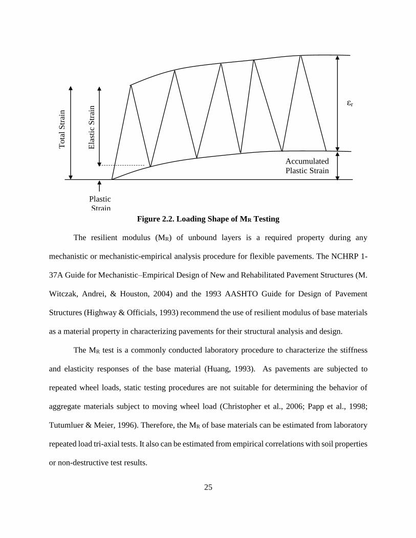
25
Figure 2.2. Loading Shape of MR Testing
The resilient modulus (MR) of unbound layers is a required property during any
mechanistic or mechanistic-empirical analysis procedure for flexible pavements. The NCHRP 1-
37A Guide for Mechanistic–Empirical Design of New and Rehabilitated Pavement Structures (M.
Witczak, Andrei, & Houston, 2004) and the 1993 AASHTO Guide for Design of Pavement
Structures (Highway & Officials, 1993) recommend the use of resilient modulus of base materials
as a material property in characterizing pavements for their structural analysis and design.
The MR test is a commonly conducted laboratory procedure to characterize the stiffness
and elasticity responses of the base material (Huang, 1993). As pavements are subjected to
repeated wheel loads, static testing procedures are not suitable for determining the behavior of
aggregate materials subject to moving wheel load (Christopher et al., 2006; Papp et al., 1998;
Tutumluer & Meier, 1996). Therefore, the MR of base materials can be estimated from laboratory
repeated load tri-axial tests. It also can be estimated from empirical correlations with soil properties
or non-destructive test results.
Ela
stic
Str
ain
Tota
l S
trai
n
Plastic
Strain
Accumulated
Plastic Strain
εr
26
The MRtest is conducted in the laboratory by maintaining constant confining pressure
within a conventional tri-axial cell and applying a cyclic axial stress to simulate traffic loading.
There are a number of methods to perform the resilient modulus testing. The most common
protocols for this testing are: AASHTO T 292-91, AASHTO T 294- 92, AASHTO T-307,
AASHTO T P46-94, LTPP protocol P46 (Protocol, 1996) and NCHRP 1-28A (M. W. Witczak,
2003). During the MR test, the sample is subjected to different levels of confining pressures and
deviator stresses.
The NCHRP 1-28A (M. W. Witczak, 2003) test protocol is the most updated standard for
measuring MR after all required modifications of the other previous standards. This standard for
unbound granular materials, consists of 30 loading sequences, but the protocol loading involves
conditioning stage, which attempts to establish steady state or resilient behavior, through the
application of 1000 cycles of 30-psi deviator stresses at 15-psi confining pressure. The cycles are
then repeated 100 times for 30 loading sequences with different combinations of deviator stress
and confining pressure. The MR value is calculated as the mean of the last five cycles of each
sequence from the recoverable axial strain and cyclic axial stress.
The resilient modulus (MR) of unbound granular material is affected by several factors
including: the state of stress, moisture content, dry density and freeze-thaw action. Several
researchers have tried to understand and model the effect of these factors on the resilient modulus
of different granular materials. A limited effort was conducted to understand the effect of those
factors on MR of RAP and RAP/aggregate blends as a pavement base course layer (Mohamed Attia
& Abdelrahman, 2011). From the literature survey of MR for base layer, it was found that MR is
more dependent on confining pressure than deviator stress levels (Huang, 1993).
27
Several constitutive MR models were studied for base layer, especially in case of using
RAP without taking in consideration all factors mentioned before and the effective confining
pressure levels at different state of stresses. The MEPDG model was found to be the best suitable
prediction model for MR (Mohamed Attia & Abdelrahman, 2011). This prediction model is called
mechanistic-empirical because of the mechanistic calculation of stresses, strains, and deflections
properties of a pavement structure. These properties are the fundamental pavement responses
under repeated traffic loadings. The relation of these responses to field distresses and performance
is determined using existing empirical relationships, widely known as transfer functions. This
design process is an iterative procedure that starts with a trial design and ends when predicted
distresses meet the acceptable limits based on the level of statistical reliability desired (Chehab &
Daniel, 2006).
Based on the literature review, Attia et al. (M. I. E.-S. Attia, 2010) collected nine prediction
models were previously used for granular base materials and, tested on RAP and RAP/aggregate
blends but only under the effect of different state of stresses. A summary of the investigated models
is presented in Table 2.1. The MR for granular material was found to increase with the increase in
the confining pressure, as presented in the first model (Kim & Labuz, 2007). Several researchers
reported that the MR value was dependent on the bulk stress θ (first stress invariant) applied to the
sample. The K-θ model (Huang, 1993) was used to describe the resilient behavior of unbound
material, as presented in the second model at Table 2.1. In reality, most soils are affected by both
the confining pressure and shear stress. Uzan proposed a model which accounted for the shear
stress effects (Uzan, 1985). Uzan's model is presented as the third model in Table 2.1.
Later the octahedral shear stress was used instead of deviator stress, as presented in the
fourth model (M. Witczak & Uzan, 1988). The MR was also modeled based on both the deviator

28
stress and confining pressure by Pezo et al. (Pezo, 1993), as presented in the fifth model. Tam and
Brown (Tam & Brown, 1988) suggested modeling the MR of granular material using the mean
stress to the deviator stress ratio, as presented in the sixth model. Itani (Itani, 1990) developed a
model that included bulk stress, shear stress and an additional confining pressure component, as
presented in the seventh model in Table 2.1.
A modified form of Uzan's equation is used by the mechanistic-empirical pavement design
guide (MEPDG) (Lekarp et al., 2000a), as presented the eights model in Table 2.1. Witczak
evaluated 14 constitutive models (M. Witczak, Andrei, & Houston, 2000) in both log-log and semi-
log forms for their capabilities of predicting the resilient behavior of different granular material
and recommended a five-parameter model as the model that statistically has the overall goodness
of fit. Witczak's model is presented the ninth model in Table 2.1. Several researchers proposed
correlations of the resilient modulus with the stress state (Mohammad, Herath, Rasoulian, &
Zhongjie, 2006).
The influence of stress state on unbound material stiffness has long been recognized in
pavement engineering. For coarse-grained granular soils as base layer, an increase in stiffness with
increasing confining stress is usually the dominant effect. In reality, most soils exhibit both effects
of increasing stiffness with increasing confinement and decreasing stiffness with increasing shear
(Andrei, Witczak, Schwartz, & Uzan, 2004). Witczak and Uzan (M. Witczak & Uzan, 1988) have
proposed a “universal” model that combined both effects into a single Equation 2.2:
MR = K1. Pa(θ
Pa)K2 (
σd
Pa)K3 (2.2)
Where K1> 0, K2 ≥ 0 and K3 ≤ 0 and each K parameter is a multiple regression constant
calculated from resilient modulus test.
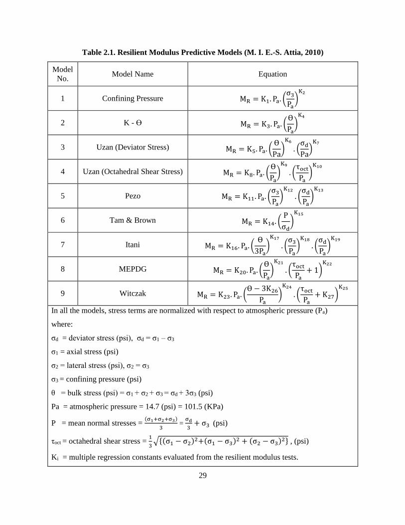
29
Table 2.1. Resilient Modulus Predictive Models (M. I. E.-S. Attia, 2010)
Model
No. Model Name Equation
1 Confining Pressure MR = K1. Pa. (σ3
Pa)
K2
2 K - ϴ MR = K3. Pa. (Ɵ
Pa)
K4
3 Uzan (Deviator Stress) MR = K5. Pa. (Ɵ
Pa)
K6
. (σd
Pa)
K7
4 Uzan (Octahedral Shear Stress) MR = K8. Pa. (Ɵ
Pa)
K9
. (τoct
Pa)
K10
5 Pezo MR = K11. Pa. (σ3
Pa)
K12
. (σd
Pa)
K13
6 Tam & Brown MR = K14. (P
σd)
K15
7 Itani MR = K16. Pa. (Ɵ
3Pa)
K17
. (σ3
Pa)
K18
. (σd
Pa)
K19
8 MEPDG MR = K20. Pa. (Ɵ
Pa)
K21
. (τoct
Pa+ 1)
K22
9 Witczak MR = K23. Pa. (Ɵ − 3K26
Pa)
K24
. (τoct
Pa+ K27)
K25
In all the models, stress terms are normalized with respect to atmospheric pressure (Pa)
where:
σd = deviator stress (psi), σd = σ1 – σ3
σ1 = axial stress (psi)
σ2 = lateral stress (psi), σ2 = σ3
σ3 = confining pressure (psi)
θ = bulk stress (psi) = σ1 + σ2 + σ3 = σd + 3σ3 (psi)
Pa = atmospheric pressure = 14.7 (psi) = 101.5 (KPa)
P = mean normal stresses = (σ1+σ2+σ3)
3 =
σd
3+ σ3 (psi)
τoct = octahedral shear stress = 1
3√{(σ1 − σ2)2+(σ1 − σ3)2 + (σ2 − σ3)2} , (psi)
Ki = multiple regression constants evaluated from the resilient modulus tests.
30
The modification of previous Equation 2.2 has been adopted for the new national
pavement design guide being finalized in NCHRP Project 1-37A (M. Witczak et al., 2004):
MR = K1. Pa(θ
Pa)K2 (
τoct
Pa+ 1)K3 (2.3)
Where the 1 in the (τoct) term is to avoid numerical problems when (τoct) approaches zero.
As the model presented in Equation 2.3 shows a clear improvement for some materials and tests
while for others it actually diminishes model accuracy. After some trials and errors in NCHRP 1-
28A (M. W. Witczak, 2003), it was found that adding K4 (as Equation 2.4) to the previous model
increases accuracy generally but the model remains inconsistent. For some materials, it shows
improvement and for some others it shows less accuracy. Because the (+1) model were not
consistent in showing improvement on all tests or for all materials, it was obvious that 1 was not
always the right value. Hence, in the last model as presented in Equation 2.4, a regression constant
K5 was introduced instead of (+1). As expected, the analysis showed that the model exhibits the
best overall goodness-of-fit statistics (Andrei et al., 2004).
MR = K1. Pa(θ−3K4
Pa)K2 (
τoct
Pa+ K5)K3 (2.4)
The MR is a primary input to any mechanistically-oriented pavement design procedure. The
pavement design computer code must be adapted to support the specific predictive equation
selected for MR. Upon completion of NCHRP Project 1-28A (M. W. Witczak, 2003), no
recommendation was made about the final form for the MR model. It was obvious that the selection
of the final model had to be coordinated with the pavement design method or code in which it was
to be implemented. Development of the AASHTO 2002 “Guide for the Design of New and
Rehabilitated Pavement Structures” was just getting under way when NCHRP Project 1-28A (M.
W. Witczak, 2003) was being completed.

31
After a thorough review of the results of Witczak & Uzan (Andrei et al., 2004) and other
studies from the literature dealing with prediction of the resilient response of unbound materials,
the NCHRP Project 1-37A (M. Witczak et al., 2000) team selected the model presented in Equation
(2.3) as the recommended MR model to be implemented and used in the 2002 design guide. This
model was deemed the best compromise between accuracy, ease of implementation, and
computational stability (for the case of τoct = 0). The model form given in Equation 2.3 was
implemented successfully in the AASHTO 2002 design guide software.
2.6.2. Permanent deformation (PD)
The mechanistic pavement design requires proper understanding of the properties and
performance of the materials used. Strain is carried into a material when it is loaded and this strain
is divided into two parts resilient and permanent. The resilient strain part from the applied load
can be recovered when the material is unloaded. The rest of the strain not recovered is the
permanent capable of doing stress behavior on the material (Adu-Osei, 2000). Permanent
deformation (PD) in unbound granular base and/or sub-base layers was generally assumed to be
negligible. But this assumption proved to be false, because serious rutting can occur within those
layers if they are not properly designed, constructed or characterized (Park, 2000). PD happens in
all layers of pavement structure; top asphalt mix, base and/or sub-base layer and subgrade soil.
Therefore, PD became a key factor in the failure of the whole pavement structure as
accumulation of PD in base layer causes rutting failure for the top asphalt layer (Erlingsson &
Rahman, 2013). The plastic deformations of different pavement layers contribute to the surface
rutting in flexible pavements. However, rutting in flexible pavements is often associated with
permanent deformation of the unbound granular layer (Erlingsson & Rahman, 2013). PD has
always been considered as one of the most important distresses in flexible pavements, and unbound
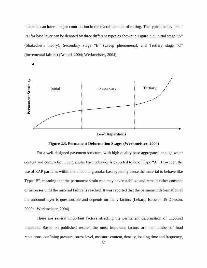
32
materials can have a major contribution in the overall amount of rutting. The typical behaviors of
PD for base layer can be denoted by three different types as shown in Figure 2.3: Initial stage “A”
(Shakedown theory), Secondary stage “B” (Creep phenomena), and Tertiary stage “C”
(incremental failure) (Arnold, 2004; Werkmeister, 2004).
Figure 2.3. Permanent Deformation Stages (Werkmeister, 2004)
For a well-designed pavement structure, with high quality base aggregates, enough water
content and compaction, the granular base behavior is expected to be of Type “A”. However, the
use of RAP particles within the unbound granular base typically cause the material to behave like
Type “B”, meaning that the permanent strain rate may never stabilize and remain either constant
or increases until the material failure is reached. It was reported that the permanent deformation of
the unbound layer is questionable and depends on many factors (Lekarp, Isacsson, & Dawson,
2000b; Werkmeister, 2004).
There are several important factors affecting the permanent deformation of unbound
materials. Based on published results, the most important factors are the number of load
repetitions, confining pressure, stress level, moisture content, density, loading time and frequency,
Load Repetitions
Perm
an
ent
Str
ain
εp
Initial Secondary Tertiary

33
and stress history (Bani Hashem & Zapata, 2013). Usually in base layer, most of the stress goes
into permanent strain that accumulates with repeated loading and unloading of traffic flow. It is
this accumulating permanent strain in an aggregate base course that creates rutting.
The measurement of permanent deformation characteristics of unbound aggregates has
received relatively less experimental attention than resilient modulus, as MR considered the main
engineering design parameter in base layer. Some notable contributions were made on the testing
procedure for permanent deformation of base layer such as repeated load tri-axial (RLT) which
have two types: single-stage and multi-stage of loading. This is partly because this experiment is
inherently destructive and require many specimens to be tested compared to the lower stress level,
essentially non-destructive, resilient strain tests (Adu-Osei, 2000). The RLT test involves imposing
cyclic stresses, similar to the stress conditions in the field, on a prepared cylindrical specimen
where the corresponding deformations are measured.
A multi-stage (MS) testing approach has been introduced where a number of consecutive
stress paths are applied to the same specimen reducing considerably the effort needed to test the
material. This approach is also more realistic since it takes into account the effect of stress history
as the same specimen is subject to different stress paths of varying magnitudes. The drawback of
this method, on the other hand, is the complexity of modeling the accumulation of permanent
deformation compared to single-stage RLT tests (Erlingsson & Rahman, 2013). The MS testing
procedure is very close to the situation of resilient modulus testing except that MS testing change
the deviator stress levels without changing the confining pressure levels. The MR testing apply 30
sequences by changing both deviator and confining stress with lower number of load repetitions
(100 cycles) than MS test (5000 cycles).
34
Huge efforts of research on granular base layer were focused on modeling the resilient
behavior of these materials. On the other hand, less research was done focusing on their permanent
behavior. This because permanent deformation tests are more difficult to perform than resilient
modulus tests. These permanent deformation tests are time consuming and a new sample should
be prepared for each stress condition as mentioned before. Therefore, greater achievements were
accomplished with the resilient behavior of granular base layer materials rather than the long-term
rutting distress of granular materials (El-Badawy, 2006).
Utilizing recycled asphalt pavements (RAP) as a base layer is questionable by many state
agencies and researchers. This is mainly due to the PD accumulated when using RAP. Many
researchers had several contradictive results. Few studies (M. I. E.-S. Attia, 2010; Jeon et al., 2009)
proved that PD decreases when increasing percentage of RAP in the base layer blend and more
studies (Bennert & Maher, 2005; Garg & Thompson, 1996; Kim & Labuz, 2007) proved opposite
result. However, resilient modulus (MR) results were more significant than PD. MR values were
directly proportional to the percentage of RAP in the blend. This result yields that modeling of MR
for RAP in base layer is much an easier process than modeling PD. Modeling the PD for RAP used
in base layer was not extensively studied before. Also, there are no specific models for prediction
of PD for RAP base layer.
Two main design methods were used by most of the design agencies to control permanent
deformation. The first is to control the vertical compressive strain on the top of the subgrade and
the second is to limit the total accumulated permanent deformation on the top pavement surface
based on the permanent deformation of each individual layer within the whole pavement matrix to
a tolerable amount (Huang, 1993; Yoder & Witczak, 1975). The second method follows the
concept taken in consideration during implementation of the mechanistic-empirical pavement
35
design guide (MEPDG) (Guide, 2008). This concept was based on prediction of accumulated
deformation in each pavement layer through predictive models. Therefore, prediction of permanent
strain for unbound granular materials is essential but it requires constitutive relationships or
mathematical models.
It is well known that the two most important factors affecting the PD accumulated in the
base layer, are the number of load repetitions and stress condition. Therefore, both parameters are
taken in consideration in order to model the permanent deformation of granular base layer. Several
models were presented in previous researches to model permanent deformation in unbound base
layer and subgrade based on both field and laboratory data. Researchers found and documented
the importance of the number of load cycles on PD. Therefore, the number of load cycles is a main
component in all permanent deformation models.
Badawy and Lekarp et al. (El-Badawy, 2006; Lekarp et al., 2000b) had summarized the
permanent deformation models established several years ago. Generally they differentiate these
models as relationships describing the influence of number of load applications and relationships
describing the influence of applied stresses. In addition, almost all researchers pointed that the
moisture content plays a critical role in accumulation of permanent deformation for unbound
materials. Until now, there is a limited number of models that take the moisture content as a
primary predictor. In order to estimate the permanent deformation of unbound materials when
using Level 3 analysis of MEPDG, a PD model was established as a function of the number of
repetitions, the groundwater table depth and CBR of the soil (Lekarp et al., 2000b).
Finally MEPDG permanent deformation model for granular base layer takes effect of load
repetitions, water content, stress levels and resilient deformation. However, the resilient modulus
prediction model in MEPDG does not take the effect of permanent deformation (PD). This effect
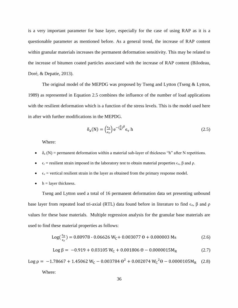
36
is a very important parameter for base layer, especially for the case of using RAP as it is a
questionable parameter as mentioned before. As a general trend, the increase of RAP content
within granular materials increases the permanent deformation sensitivity. This may be related to
the increase of bitumen coated particles associated with the increase of RAP content (Bilodeau,
Doré, & Depatie, 2013).
The original model of the MEPDG was proposed by Tseng and Lytton (Tseng & Lytton,
1989) as represented in Equation 2.5 combines the influence of the number of load applications
with the resilient deformation which is a function of the stress levels. This is the model used here
in after with further modifications in the MEPDG.
δa(N) = (ϵo
ϵr) e−(
ρ
N)β
ϵv h (2.5)
Where:
δa (N) = permanent deformation within a material sub-layer of thickness “h” after N repetitions.
ϵr = resilient strain imposed in the laboratory test to obtain material properties ϵo, β and ρ.
ϵv = vertical resilient strain in the layer as obtained from the primary response model.
h = layer thickness.
Tseng and Lytton used a total of 16 permanent deformation data set presenting unbound
base layer from repeated load tri-axial (RTL) data found before in literature to find ϵo, β and ρ
values for these base materials. Multiple regression analysis for the granular base materials are
used to find these material properties as follows:
Log(ϵo
ϵr) = 0.80978 - 0.06626 WC+ 0.003077 ϴ + 0.000003 MR (2.6)
Log β = −0.919 + 0.03105 WC + 0.001806 ϴ − 0.0000015MR (2.7)
Log ρ = −1.78667 + 1.45062 WC − 0.003784 ϴ2 + 0.002074 WC2ϴ − 0.0000105MR (2.8)
Where:

37
MR = resilient modulus of base layer (psi).
WC = water content (%).
ϴ = bulk stresses (psi).
A sensitivity study was achieved later on this model by El-Basyouny (M. M. El-Basyouny,
2004) using the same data that Tseng and Lytton used before in establishing this model. This study
showed unusable trends and predictions of permanent deformation using this model. Therefore,
El-Basyouny & Witczak (M. El-Basyouny, Witczak, & Kaloush, 2005) modified this model for
calculation of PD for unbound granular materials. The modified model was implemented in the
MEPDG software.
The final form of the modified model by El-Basyouny & Witczak for granular base layer
recommended to the MEPDG and used for this study as follows:
δa(N) = βs1K1hϵv (
ϵo
ϵr) [e−(
ρ
N)β
] (2.9)
Logβ = −0.61119 − 0.017638(WC) (2.10)
ρ = 109 [Co
(1−(109)β]
1
β (2.11)
Co = ln (a1MR
b1
a9MRb9
) = ln (0.0075) = -4.893 (2.12)
Where:
δa (N) = permanent deformation of the base layer (inches).
N = number of load repetitions.
ϵr = resilient strain (in. /in.).
ϵv = primary response model (assumed to be equal to ϵr in this study).
h = thickness of the layer (inches).
ϵo, ρ, β = material properties.

38
K1 (granular materials) = 1.673 (natural calibration).
βs1 = field calibration factor = 1 (unless there are field data).
MR = resilient modulus of base layer (psi).
WC = water content (%).
a1, b1, a2, b2 = regression constants = 0 (natural calibration).
(ϵo/ϵr) is calculated from the previous Equation 2.6 suggested by Tseng and Lytton as no new
prediction equations were instead suggested by the MEPDG software.
The natural calibration values were taken from the manual of practice of MEPDG.
This study focuses on the rutting performance model in the MEPDG, as it is the last model
established for PD of unbound base layer. Attia et. al. (M. I. E.-S. Attia, 2010) results reflected
that permanent deformation of RAP can be modeled like a typical granular material. The analysis
of his study focused on six different models which reflected that both the exponential function,
currently used in the MEPDG, and the power model (log-log relation between number of load
cycles and permanent strain) are suitable functions to be used to model the permanent deformation
of RAP/aggregate blends.
2.6.3. Poisson’s ratio
This ratio is an essential factor used in analytical pavement design theories based on stress-
strain relationship. For base, sub-base and subgrade layers, the Poisson’s ratio is affected with
other parameters by several factors; elastic modulus of material, temperature, cohesion, saturation
degree, coarseness and roughness of material particles. When a compressive force acts on a
cylinder body, the force causes the sample to contract in the direction of the force and expand
laterally. Within the elastic range of the material, the ratio of these strains is a constant for that
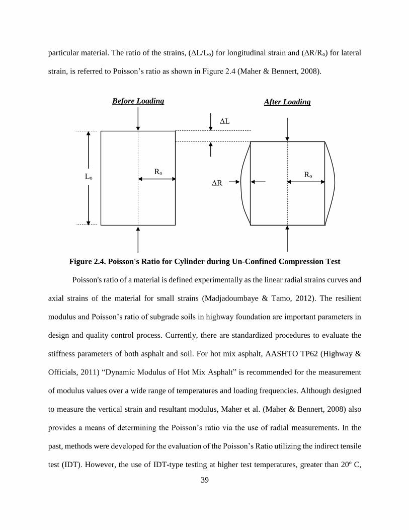
39
particular material. The ratio of the strains, (ΔL/Lo) for longitudinal strain and (ΔR/Ro) for lateral
strain, is referred to Poisson’s ratio as shown in Figure 2.4 (Maher & Bennert, 2008).
Figure 2.4. Poisson's Ratio for Cylinder during Un-Confined Compression Test
Poisson's ratio of a material is defined experimentally as the linear radial strains curves and
axial strains of the material for small strains (Madjadoumbaye & Tamo, 2012). The resilient
modulus and Poisson’s ratio of subgrade soils in highway foundation are important parameters in
design and quality control process. Currently, there are standardized procedures to evaluate the
stiffness parameters of both asphalt and soil. For hot mix asphalt, AASHTO TP62 (Highway &
Officials, 2011) “Dynamic Modulus of Hot Mix Asphalt” is recommended for the measurement
of modulus values over a wide range of temperatures and loading frequencies. Although designed
to measure the vertical strain and resultant modulus, Maher et al. (Maher & Bennert, 2008) also
provides a means of determining the Poisson’s ratio via the use of radial measurements. In the
past, methods were developed for the evaluation of the Poisson’s Ratio utilizing the indirect tensile
test (IDT). However, the use of IDT-type testing at higher test temperatures, greater than 20º C,
Before Loading
LoRo
ΔL
Ro
ΔR
After Loading
40
for stiffness determination is not recommended due to excessive deformations that may occur in
the vicinity of the loading platens, as well as the inappropriateness of using linear elastic theory in
the diametric loading position (Tayebali, Tsai, & Monismith, 1994).
In addition, the currently used techniques include CBR (California Bearing Ratio) test,
resilient modulus test, DCP (Dynamic Cone Penetrometer), and FWD (Falling Weight
Deflectometer) tests. However, these techniques have certain limitations and sometimes fail to
satisfy the requirement and accuracy for design purposes (Zeng & Hu, 2013). Nowadays, Poisson’s
ratio is estimated rather than measured directly in most soil tests especially the CBR which cannot
be used in measuring Poisson’s Ratio because the loading conditions in a CBR test is different
compared with those happen in the field. Usually these estimated values are assumed depending
on the soil type as shown in Table 2.2. As for each soil type there is a range for the linear elastic
stress-strain relationship and an average value is taken to represent the midpoint of this linear
relationship. This procedure will be used in this research depending on the linear elastic region
measured for each sample.
The ASTM standard method C469/C469M-14 (Astm, 2014) for measuring Poisson’s Ratio
of concrete samples in compression test uses a rate of loading 1 mm/min in loading. However, this
rate may be too high in case of using RAP because it is much weaker than concrete. In addition,
this standard recommends measuring Poisson’s ratio at 40% from the ultimate compressive
strength of the samples to be confident that the result in the linear elastic region. For unbound
materials, the MEPDG only allows the user to estimate a constant value for the Poisson’s Ratio,
thereby; neglecting any effect of applied stress or change in resilient modulus may have on
Poisson’s Ratio. However, for the case of RAP, the variation in several testing conditions have a
huge effect on the structural capacity, especially permanent deformation. This effect may be

41
related to the relation of strength parameters MR and PD with Poisson’s ratio. This prediction was
estimated from the falling weight deflectometer FWD sensitivity analysis (Maher & Bennert,
2008). As it appears that both the Poisson’s Ratio of the asphalt layer and the unbound aggregates
layer (base layer) have an influence on the back-calculated modulus values.
Table 2.2. Typical Values of Poisson’s Ratio (Maher & Bennert, 2008)
Material Range of
Values
Typical
Value
Hot Mix Asphalt 0.3 – 0.4 0.35
Portland Cement Concrete 0.15 – 0.2 0.15
Untreated Granular Materials 0.3 - 0.4 0.35
Cement Treated Granular Materials 0.1 - 0.2 0.15
Cement Treated Fine Grained Soils 0.15 – 0.35 0.25
Lime Stabilized Materials 0.10 – 0.25 0.20
Lime Fly Ash Mixtures 0.10 – 0.15 0.15
Loose Sand or Silty Sand 0.20 – 0.40 0.30
Dense Sand 0.30 - 0.45 0.35
Fine Grained Soils 0.30 -0.50 0.40
Saturated Soft Clays 0.40 – 0.50 0.45
Maher et al. (Maher & Bennert, 2008) research project encompassed the evaluation of
whether or not the Poisson’s Ratio can be measured using the same test procedures commonly
used to obtain the modulus values for flexible pavement design (i.e. dynamic modulus test for
asphalt and resilient modulus test for unbound materials). The research concluded that the
Poisson’s Ratio can be measured during the dynamic modulus test for asphalt mixtures but should
not be measured during the resilient modulus (MR) test for unbound materials. This is mainly
because the MR test does not typically test the material in its natural linear elastic state, where the

42
Poisson’s Ratio concept is valid. The Poisson’s Ratio parameter is only valid with testing materials
within their linear elastic range. This means that, theoretically, there should be no permanent
deformation accumulated during any of the loading cycles and the vertical strain should be in the
low strain range (< 0.001%). Poisson’s ratio is an important characteristic that enters into the
pavement design process. Usually this parameter is estimated instead of measuring according to
typical values for each pavement material. The flexible asphalt pavement is a three-component
system consisting of stone aggregates, pores filled by air and asphalt binder. Nowadays, this
system is characterized as elastic in pavement design practice which means that the ideal state for
measuring Poisson’s ratio at the linear elastic stress-strain relationship (Zak et al., 2014).
As mentioned before, there is almost 13 states nowadays in the field that adds RAP within
base layer up to 50%, but most of researchers are trying to investigate the effects by exceeding this
critical content. From this strategy, it will be more economical and beneficial to use more than
50% RAP within base layer without any defects or effectiveness on pavement lifetime. Therefore
this study will focus on studying the RAP with contents varying from 50% to 100%.
43
CHAPTER 3. METHODOLOGY AND EXPERIMENTAL WORK
3.1. Main Research Tasks
The objectives of this study are achieved via four main tasks, as shown in the flow chart
represented in Figure 3.1. The first task of the research is concerned with modeling the structural
behavior of RAP in the base layer utilizing measured data collected for MR of RAP/Aggregate
blends in base layer (M. I. E.-S. Attia, 2010). This task is implemented taking into consideration
several testing conditions describing the possible circumstances that may be encountered in the
field for RAP in base layer. The second task concerns modeling behavior of the permanent
deformation of RAP blends utilizing values measured by MR and single & multi-stage RTL tests
through MEPDG rutting model. The third stage is also essential to correlate values of MR with
permanent deformation accumulated during stages of loading of MR tests for the same RAP blends
tested in the first task under identical testing conditions, especially three water content levels.
Finally, the last task comprises measuring Poisson’s ratio for the same RAP/Aggregate
blends to evaluate its effectiveness on the modeling behavior of both parameters MR and PD. Based
on literature review results, this ratio cannot be measured during the MR test. Therefore, the un-
confined compression test is used to determine the respective results. This test is more suitable and
practical to implement in measuring the lateral deformation without any effect of confining
pressure like MR or RTL tests.
3.1.1. MR modeling task
The main objective of this research task is to assess the nine constitutive models previously
tested by Attia et. al.(M. I. E.-S. Attia, 2010), as represented in Table 2.1, for RAP as a base layer
under the effect of different actual environmental and field conditions other than the state of
stresses. This objective is fulfilled in three stages as described in the flow chart represented at
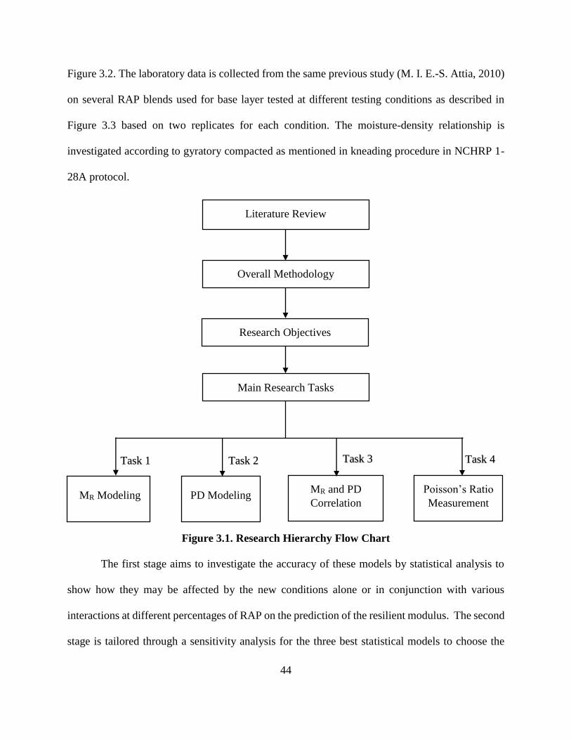
44
Figure 3.2. The laboratory data is collected from the same previous study (M. I. E.-S. Attia, 2010)
on several RAP blends used for base layer tested at different testing conditions as described in
Figure 3.3 based on two replicates for each condition. The moisture-density relationship is
investigated according to gyratory compacted as mentioned in kneading procedure in NCHRP 1-
28A protocol.
Figure 3.1. Research Hierarchy Flow Chart
The first stage aims to investigate the accuracy of these models by statistical analysis to
show how they may be affected by the new conditions alone or in conjunction with various
interactions at different percentages of RAP on the prediction of the resilient modulus. The second
stage is tailored through a sensitivity analysis for the three best statistical models to choose the
Task 2 Task 1 Task 3 Task 4
MR Modeling PD Modeling Poisson’s Ratio
Measurement
MR and PD
Correlation
Literature Review
Overall Methodology
Research Objectives
Main Research Tasks

45
best-fit one and its suitability in predicting the resilient modulus of RAP. This stage also assesses
the adequacy of these factors in representing most of the field conditions affecting the base layer.
Then, this stage is important to investigate the need for more future laboratory measurements
and/or more, environmental and field conditions in predicting the resilient modulus such as
leaching components or Poisson’s ratio. In the third stage, a parametric analysis is achieved for
the MR-MEPDG model by using the measured MR values under different measured testing
parameters used in this model. This stage is considered to calculate each K parameter under five
different levels of confining pressure (3, 6, 10, 15 and 20 psi) using the Excel solver software. Six
replicates are considered for each level of confining pressure.
Figure 3.2. MR Modeling Flow Chart
Nine Collected MR
Prediction Models (M. I.
E.-S. Attia, 2010)
Experimental Data
Collection (Figure 3.3)
Nine MR
Prediction
Models
Three Best-fit
MR Prediction
Models
MEPDG MR
Prediction
Model
Statistical
Analysis
Sensitivity
Analysis
Parametric
Analysis
Stage 2
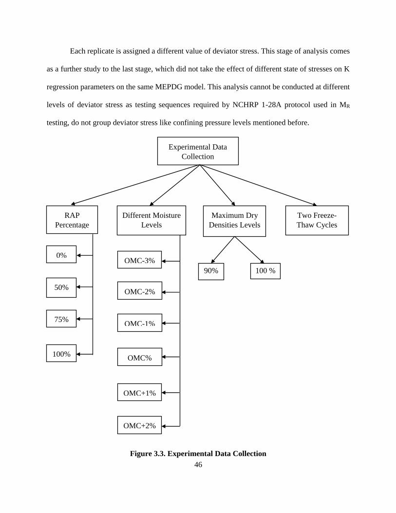
46
Each replicate is assigned a different value of deviator stress. This stage of analysis comes
as a further study to the last stage, which did not take the effect of different state of stresses on K
regression parameters on the same MEPDG model. This analysis cannot be conducted at different
levels of deviator stress as testing sequences required by NCHRP 1-28A protocol used in MR
testing, do not group deviator stress like confining pressure levels mentioned before.
Figure 3.3. Experimental Data Collection
0%
50%
75%
100%
OMC-3%
OMC-2%
OMC-1%
OMC+1%
OMC+2%
OMC%
Experimental Data
Collection
Different Moisture
Levels
Maximum Dry
Densities Levels
Two Freeze-
Thaw Cycles
RAP
Percentage
90% 100 %

47
3.1.2. PD modeling task
The MR modeling task yielded that the MR-MEPDG model is the best-fit model that works
for RAP base layer. Also, Attia et al.(M. I. E.-S. Attia, 2010) found that the PD-MEPDG model
was the best-fit model for RAP base layer. Therefore, this task comprises investigating the ability
of predicting the permanent deformation for RAP using the MEPDG rutting prediction model.
This task concentrates on how the major factors (state of stresses, moisture content, load repetitions
and stress history) affect permanent deformation modeling behavior of RAP and RAP/aggregate
blends.
To achieve this objective, PD data collected from both resilient modulus (MR) and repeated
tri-axial (RTL) loading tests are taken into consideration. Each test is responsible on investigation
one of the major factors affecting PD accumulated from using RAP. The MR takes in consideration
the stress history of different successive stages of loading, while the single-stage RTL is
responsible on measuring PD after frequent number of load repetitions (20,000 or more). The
multi-stage RTL is close to the trend of the MR test than single-stage RTL test. Different stages of
loading were applied with equal number of load repetitions (5000) and different deviator stress
levels but with same confining pressure (3 psi).
The comparison between predicted and measured PD values using the rutting MEPDG
model is achieved on three main stages, as described in Figure 3.4. In the first stage, a comparison
is made between PD values measured from the MR test to predicted PD values using PD-MEPDG
prediction model on the main RAP source (TH 10). This comparison is achieved on three major
testing conditions; four RAP contents (0%, 50%, 75% and 100%), three water content levels
(OMC-2%, OMC% and OMC+2%) and three base layer thickness (6, 9 and 12 inches). Also, this
stage focuses on the same comparison of measured and predicted PD of other four field RAP
48
sources. Three RAP sources (TH 19-101, TH 19-104 and TH 22) contain 50% RAP and 50%
granular aggregates. The fourth RAP source (Cell 18) contains 100% RAP. This comparison of
RAP sources is achieved on PD measured values collected from MR test at the same testing
conditions. The first number of each source refers to the Trunk Highway location in Minnesota
State, while the other number refers to the mile location
The second stage focuses on the comparison of PD values with those measured in the
single-stage RTL. This test is more reliable for measuring PD taking into consideration the effect
of several load repetitions (20,000 or more). The comparison is achieved for RAP TH10 on two
levels of water contents (OMC% and OMC+2%) and two contents of RAP (0% and 50%). Also,
this comparison takes in consideration the effect of adding 6% fines on PD modeling for 50% RAP
blend. The third stage focuses on the comparison of PD values versus those measured in the multi-
stage RTL. This test is important for measuring PD taking into consideration the effect of stress
history. The comparison is achieved for RAP TH 10 on three levels of water contents (OMC-2%,
OMC% and OMC+2%), two contents of RAP (0% and 50%). In addition, this comparison takes
in consideration the effect of adding 3.5% fines on PD modeling for 50% RAP blend.
3.1.3. MR and PD correlation task
This study focuses on MR-PD relationship for different sources of RAP under variable
confining pressure, moisture content and RAP levels. The confining pressure is the most effective
state of stresses on the structural behavior of the base layer. Firstly, this relation is important to be
investigate in terms of how the PD affects MR values under the variation of all mentioned testing
conditions. Also, it shall indicate if there is a typical relation for the MR-PD behavior that can be
understood for the RAP in base layer or not. Secondly, this stage helps to decide the optimum RAP
content that can be used in base layer blends. This content will result in achieving the highest MR
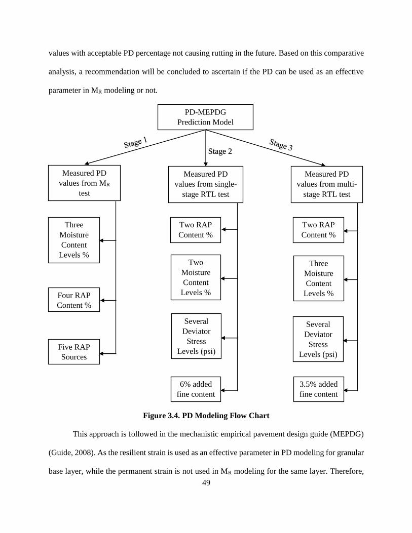
49
values with acceptable PD percentage not causing rutting in the future. Based on this comparative
analysis, a recommendation will be concluded to ascertain if the PD can be used as an effective
parameter in MR modeling or not.
Figure 3.4. PD Modeling Flow Chart
This approach is followed in the mechanistic empirical pavement design guide (MEPDG)
(Guide, 2008). As the resilient strain is used as an effective parameter in PD modeling for granular
base layer, while the permanent strain is not used in MR modeling for the same layer. Therefore,
Measured PD
values from MR
test
Measured PD
values from single-
stage RTL test
Measured PD
values from multi-
stage RTL test
PD-MEPDG
Prediction Model
Three
Moisture
Content
Levels %
Four RAP
Content %
Five RAP
Sources
Two RAP
Content %
Two
Moisture
Content
Levels %
6% added
fine content
Several
Deviator
Stress
Levels (psi)
Two RAP
Content %
3.5% added
fine content
Three
Moisture
Content
Levels %
Several
Deviator
Stress
Levels (psi)
Stage 2
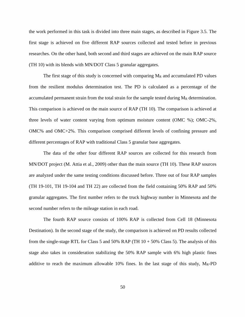
50
the work performed in this task is divided into three main stages, as described in Figure 3.5. The
first stage is achieved on five different RAP sources collected and tested before in previous
researches. On the other hand, both second and third stages are achieved on the main RAP source
(TH 10) with its blends with MN/DOT Class 5 granular aggregates.
The first stage of this study is concerned with comparing MR and accumulated PD values
from the resilient modulus determination test. The PD is calculated as a percentage of the
accumulated permanent strain from the total strain for the sample tested during MR determination.
This comparison is achieved on the main source of RAP (TH 10). The comparison is achieved at
three levels of water content varying from optimum moisture content (OMC %); OMC-2%,
OMC% and OMC+2%. This comparison comprised different levels of confining pressure and
different percentages of RAP with traditional Class 5 granular base aggregates.
The data of the other four different RAP sources are collected for this research from
MN/DOT project (M. Attia et al., 2009) other than the main source (TH 10). These RAP sources
are analyzed under the same testing conditions discussed before. Three out of four RAP samples
(TH 19-101, TH 19-104 and TH 22) are collected from the field containing 50% RAP and 50%
granular aggregates. The first number refers to the truck highway number in Minnesota and the
second number refers to the mileage station in each road.
The fourth RAP source consists of 100% RAP is collected from Cell 18 (Minnesota
Destination). In the second stage of the study, the comparison is achieved on PD results collected
from the single-stage RTL for Class 5 and 50% RAP (TH 10 + 50% Class 5). The analysis of this
stage also takes in consideration stabilizing the 50% RAP sample with 6% high plastic fines
additive to reach the maximum allowable 10% fines. In the last stage of this study, MR-PD

51
comparison is achieved on PD values collected from multi-stage RTL for the same samples tested
before in the previous stage but with 3.5% normal fines only.
Figure 3.5. MR and PD Correlation Flow Chart
3.1.4. Poisson’s ratio task
The last task of this study is an experimental program to measure Poisson’s ratio for
different RAP/Aggregate blends. This program is described in the flow chart shown in Figure 3.6.
Identical cylindrical samples (6-inches diameter and 12-inches height) are prepared similar to
Resilient Modulus
Test
Four RAP
Content %
Three
Moisture
Content
Levels %
Five RAP
Sources
Five
Confining
Pressure
Levels (psi)
Single-stage RTL
Test
Two RAP
Content %
Two
Moisture
Content
Levels %
6% added
fine content
Several
Deviator
Stress
Levels (psi)
Multi-stage RTL
Test
Two RAP
Content %
3.5% added
fine content
Three
Moisture
Content
Levels %
Several
Deviator
Stress
Levels (psi)
Data Collected for MR and
PD from several tests
Stage 2
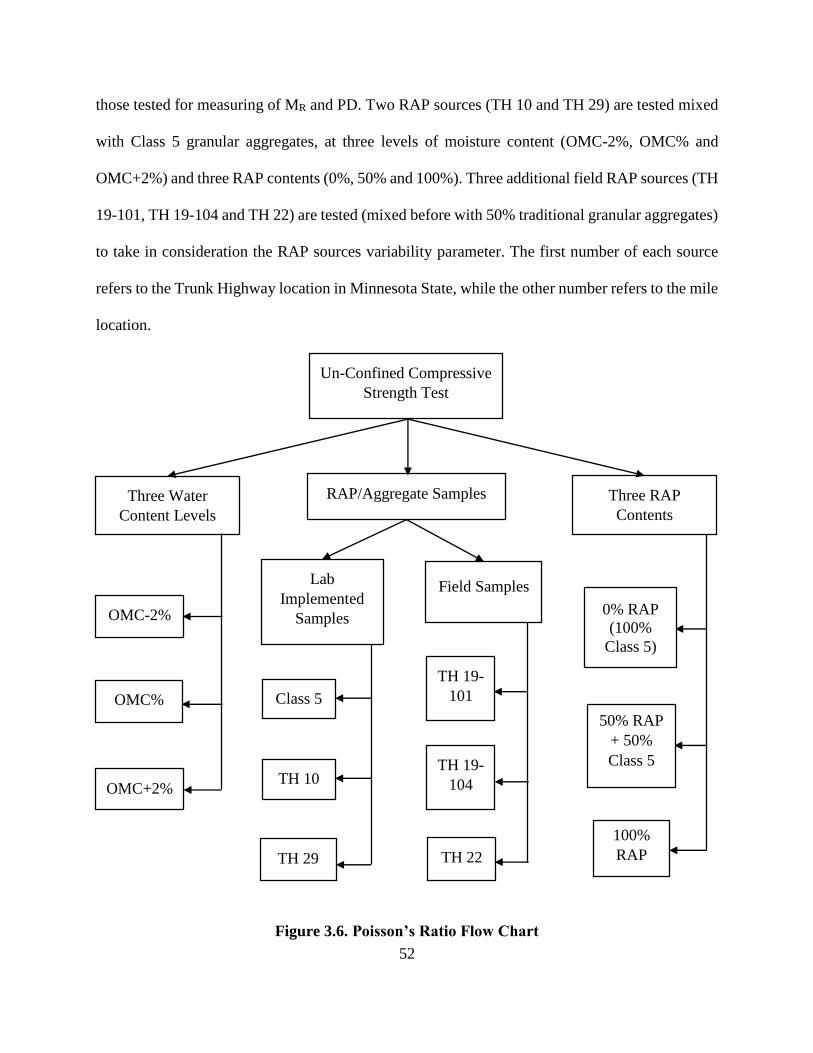
52
those tested for measuring of MR and PD. Two RAP sources (TH 10 and TH 29) are tested mixed
with Class 5 granular aggregates, at three levels of moisture content (OMC-2%, OMC% and
OMC+2%) and three RAP contents (0%, 50% and 100%). Three additional field RAP sources (TH
19-101, TH 19-104 and TH 22) are tested (mixed before with 50% traditional granular aggregates)
to take in consideration the RAP sources variability parameter. The first number of each source
refers to the Trunk Highway location in Minnesota State, while the other number refers to the mile
location.
Figure 3.6. Poisson’s Ratio Flow Chart
Three Water
Content Levels
OMC-2%
OMC%
OMC+2%
Three RAP
Contents
0% RAP
(100%
Class 5)
50% RAP
+ 50%
Class 5
100%
RAP
TH 10
TH 29
Lab
Implemented
Samples
Class 5
Field Samples
TH 19-
101
TH 19-
104
TH 22
RAP/Aggregate Samples
Un-Confined Compressive
Strength Test

53
This test aims at measuring ultimate compressive strength and Poisson’s ratio of these
samples. Both axial and lateral strains are measured during the whole test and recorded at the linear
axial stress-strain relationship to calculate the Poisson’s Ratio. Two digital dial gauges
simultaneously measure lateral strains, then the average of both readings is considered in
calculating the Poisson’s ratio.
3.2. Experimental Program
This section includes the procedures used for testing the physical and/or mechanical
properties of RAP/Aggregate blends investigated in this research even for collecting the data used
in the modeling section of both design parameters MR and PD or measuring Poisson’s ratio and
ultimate compressive strength values.
3.2.1 Sieve analysis gradation test
Gradation is a very important material property for the pavement construction layers in
general because it influences on each layer stability strength and drainage characteristics. Dry sieve
analysis is done based on ASTM C 136 standard. Representative material of each sample is
collected and oven dried at a temperature less than 140° F for 2 days. Then, the material of each
sample is put on soil sieve shaker and the mass retained on each sieve is measured after 10 minutes
of shaking. While, the material finer than 0.075 mm is determined by washing the material on 4.75
mm sieve using ASTM C 117 standard.
3.2.2. Asphalt extraction test
Asphalt content is one of the criteria that are normally considered by the highway agencies
when trying to utilize RAP material. In this research, asphalt extraction is done by reflux extraction
following ASTM D 2172 (Method B) standard.

54
3.2.3. Moisture content-dry density relationship
For RAP/aggregate blends tested for collecting MR and PD data, the relation between the
dry density and moisture content is achieved by gyratory compactor. All material greater than 12.5
mm is replaced by material passing 12.5 mm and retained on sieve no. 4 (4.75 mm) for material
homogeneity. The optimum moisture content and maximum dry density are based on samples
compacted by the gyratory compactor at a pressure equal to 600 Kpa, the number of gyrations
equal to 50, the machine is set to conduct 30 revolutions per minute and the angle of gyration was
set to 1.25 degrees. While for RAP/aggregate blends tested by un-confined compression test to
collect Poisson’s ratio and ultimate strength values, the relation between dry density and moisture
content is achieved by modified proctor hammer using ASTM D 1557 standard to determine the
optimum moisture content (OMC %) at maximum dry density level.
3.2.4. Tri-axial shear test
Shear strength is an important property for materials used as a base layer. The tri-axial
shear test is achieved after the resilient modulus testing on the same sample, unless the sample
failed during MR test. The shear test is conducted in strain controlled mode, at a loading rate of
0.03 mm/sec (0.6% strain /minute) and confining pressure of 4 and 8 psi. The results are used to
calculate the friction angle and cohesion for the tested materials.
3.2.5. Resilient modulus test
The resilient modulus test is achieved based on NCHRP 1-28A (M. W. Witczak, 2004)
testing protocol and MN/DOT requirements. The resilient modulus is the ratio of axial cyclic
deviator stress to the recoverable strain. Generally for base layer, cyclic stress of fixed magnitude
for 0.1 second is applied to the specimen followed by a 0.9 second rest period, in order to determine
the resilient modulus. The specimen is subjected to a confining stress provided by means of a tri-
55
axial pressure chamber. The sample is subject to 30 different sequences stages of loading, unless
it failed early in the test. The samples are dried first at 150º F for 24 hours before adding determined
water content. Gyratory compactor is used for compacting the samples into two molds 6 inches
height each. Then the surface between the two molds, is scratched and the two molds are
compacted with vibratory hammer in split mold. No visual lateral movement was found between
the top and bottom samples in any of the tested samples. Details regarding the testing system and
the calibration process can be found in Attia et al. (M. I. E.-S. Attia, 2010).
3.2.6. Permanent deformation test
For PD test, the sample is prepared exactly like the MR sample, with one exception in the
loading sequences. The effects of moisture content and fine content on PD are evaluated based on
repeated load tri-axial (RTL) testing. The effect of those factors on permanent deformation (PD)
of base layer containing RAP is evaluated using both single-stage and multi-stage PD testing. In
the single-stage PD test, the sample is subject to cyclic loading at one level of stress up to
predetermined number of cycles or failure of the sample. In this research the number of cycles is
selected to be 20,000 cycles, except for limited number of samples where the number of cycles is
only 10,000 cycles. The single-stage PD test has the advantage of avoiding the effect of stress
history on the material. However, single stage PD test is very time consuming and it incorporates
the variability of the material, sample preparation and testing.
For the multi-stage PD test, each load is applied to the sample for 5000 cycles, then the
deviator stress is increased and another 5000 cycles are applied to the sample and so on until the
sample failed (more than 5% strain is achieved). The advantage of the multi-stage testing is that
the behavior of the material under different states of stress can be evaluated from one sample,
which saves time and money. The disadvantage is the possible effect of stress history on material
56
response. Samples at OMC+2% showed much higher PD and fails very early in the test when
subject to high levels of deviator stresses. For this reason, samples at OMC+2% are tested at lower
deviator stresses. The selection of the confining pressure to be 3 psi is based on earlier work in the
literature for base layer (Kim & Labuz, 2007; Song & Ooi, 2010).
3.2.7. Un-confined compression test
Each sample specimen is prepared according to NCHRP 1-28A (M. Witczak, 2003), which
was the same testing procedure used before in MR and PD determination. Gradation of each
specimen is modified by replacing particles retained on sieve ¾ in. (19 mm) with particles passing
the same sieve and retained on sieve No. 4 (4.75 mm). Each sample is compacted with modified
proctor hammer manually on 6 layers with same modified proctor compaction energy which results
in 123 blows per each layer according to Equation 3.1.
E = WHNn
V (3.1)
Where:
E = compaction energy equals to 56000 ibs.ft/ft3.
H = hammer drop equals to 18 inches (1.5 ft).
W = weight of hammer equals to 10 ibs.
V = volume of mold equals to 339.29 in3 (0.1964 ft3).
n = number of layers equals to 6.
N = number of blows per layer equal to 123.
After trial and error of testing several specimens varying the loading rate from 1 to 0.25
mm/min, the analyzed samples are tested by un-confined compression test at strain rate 0.25
mm/min until reaching failure. This rate is found the most suitable allowing enough time for
accumulating lateral strain at the mid-height of the tested specimen. Both axial and lateral strains

57
are measured during the whole test period every 30 seconds and recorded at the linear elastic axial
stress-strain relationship to calculate the Poisson’s Ratio. Two digital dial gauges simultaneously
measure lateral strains, then the average of both readings is considered in calculating the Poisson’s
ratio.
3.3. RAP Index Properties Data
All the data of MR, single and multi-stage RTL testing of all RAP/aggregate blends used
in this research were tested in MN/DOT previous report (M. Attia et al., 2009). While all the data
of the unconfined compression test for Poisson’s ratio measurement is collected in the last task of
this research. Group of preliminary tests are performed prior to actual measuring MR, PD and
Poisson’s ratio, such as gradation, compaction, shear parameters, etc. A list of the index properties
for RAP TH 10 is given in Table 3.1, while the index properties of the other field RAP sources are
given in Table 3.2.
A concern is taken in this study on the shear strength properties, therefore a tri-axial test is
done by the MN/DOT project on the same RAP samples tested before for MR. Shear strength is an
important property especially if the base layer was constructed under a thin HMA layer, for this
case the base will be subjected to high shear stresses. Previous research on MN-ROAD Cell 26
(Mulvaney & Worel, 2001) presents one of the full depth reclamation cases where the material
had enough resilient modulus but failed due to high shear stress in the base layer that exceeded the
material shear strength. The maximum deviator stress carried by all RAP samples changed
between 85 to 135 psi at 8 psi confining pressure and between 70 to 110 psi at 4 psi confining
pressure. Garg & Thompson reported that granular base materials carried more than 90 psi deviator
stress at 15 psi confining pressure had low rutting potential in the field (Garg & Thompson, 1997).
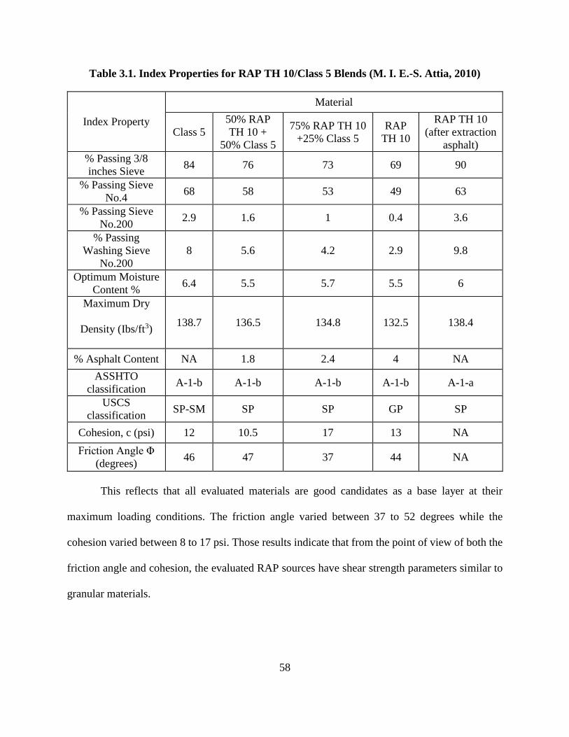
58
Table 3.1. Index Properties for RAP TH 10/Class 5 Blends (M. I. E.-S. Attia, 2010)
This reflects that all evaluated materials are good candidates as a base layer at their
maximum loading conditions. The friction angle varied between 37 to 52 degrees while the
cohesion varied between 8 to 17 psi. Those results indicate that from the point of view of both the
friction angle and cohesion, the evaluated RAP sources have shear strength parameters similar to
granular materials.
Index Property
Material
Class 5
50% RAP
TH 10 +
50% Class 5
75% RAP TH 10
+25% Class 5
RAP
TH 10
RAP TH 10
(after extraction
asphalt)
% Passing 3/8
inches Sieve 84 76 73 69 90
% Passing Sieve
No.4 68 58 53 49 63
% Passing Sieve
No.200 2.9 1.6 1 0.4 3.6
% Passing
Washing Sieve
No.200
8 5.6 4.2 2.9 9.8
Optimum Moisture
Content % 6.4 5.5 5.7 5.5 6
Maximum Dry
Density (Ibs/ft3) 138.7 136.5 134.8 132.5 138.4
% Asphalt Content NA 1.8 2.4 4 NA
ASSHTO
classification A-1-b A-1-b A-1-b A-1-b A-1-a
USCS
classification SP-SM SP SP GP SP
Cohesion, c (psi) 12 10.5 17 13 NA
Friction Angle Φ
(degrees) 46 47 37 44 NA
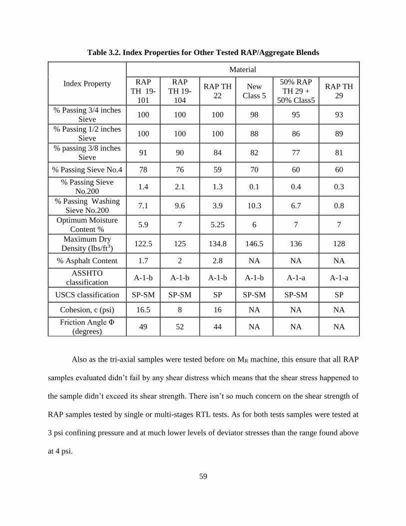
59
Table 3.2. Index Properties for Other Tested RAP/Aggregate Blends
Also as the tri-axial samples were tested before on MR machine, this ensure that all RAP
samples evaluated didn’t fail by any shear distress which means that the shear stress happened to
the sample didn’t exceed its shear strength. There isn’t so much concern on the shear strength of
RAP samples tested by single or multi-stages RTL tests. As for both tests samples were tested at
3 psi confining pressure and at much lower levels of deviator stresses than the range found above
at 4 psi.
Index Property
Material
RAP
TH 19-
101
RAP
TH 19-
104
RAP TH
22
New
Class 5
50% RAP
TH 29 +
50% Class5
RAP TH
29
% Passing 3/4 inches
Sieve 100 100 100 98 95 93
% Passing 1/2 inches
Sieve 100 100 100 88 86 89
% passing 3/8 inches
Sieve 91 90 84 82 77 81
% Passing Sieve No.4 78 76 59 70 60 60
% Passing Sieve
No.200 1.4 2.1 1.3 0.1 0.4 0.3
% Passing Washing
Sieve No.200 7.1 9.6 3.9 10.3 6.7 0.8
Optimum Moisture
Content % 5.9 7 5.25 6 7 7
Maximum Dry
Density (Ibs/ft3) 122.5 125 134.8 146.5 136 128
% Asphalt Content 1.7 2 2.8 NA NA NA
ASSHTO
classification A-1-b A-1-b A-1-b A-1-b A-1-a A-1-a
USCS classification SP-SM SP-SM SP SP-SM SP-SM SP
Cohesion, c (psi) 16.5 8 16 NA NA NA
Friction Angle Φ
(degrees) 49 52 44 NA NA NA

60
CHAPTER 4. RESILIENT MODULUS MODELING
4.1. Introduction
The main objective of this research task is to assess the constitutive models previously
tested for RAP as a base layer as presented in Table 2.1 under the effect of different actual
environmental and field conditions other than the state of stresses. This objective is fulfilled in
three stages. The first stage aims to investigate the accuracy of these models by statistical analysis
to show how they may be affected by the new conditions alone or in conjunction with various
interactions at different percentages of RAP on the prediction of the resilient modulus.
Then, the second stage is tailored by a sensitivity analysis for the best statistical models
known from the first stage in order to choose the best-fit one and its suitability in predicting the
resilient modulus of RAP. Otherwise, determine the need if any, to establish a new prediction
model in the future. The study also assesses the adequacy of these factors in representing most of
the field conditions affecting the base layer. Then to investigate the need for more laboratory
measurements in the future to take the effect of other and/or more, environmental and field
conditions in predicting the resilient modulus for the RAP mixes to be utilized in the base course
layers such as the leaching contents of RAP.
From the first two stages, the MEPDG model is proved to be the most reliable and best-fit
model for predicting the MR of RAP as a base layer under different field conditions. However, it
is found that there is no exact relationship between each K parameter and the studied field
conditions individually. These field conditions include various water contents, decreased dry
density and applied freeze-thaw cycles at different RAP concentrations. Therefore, the third
parametric analysis stage is needed to assess the physical meaning of each constant in the model
especially from the point of view of state of stresses representing the most influencing parameter

61
on MR for base layer. In addition, this stage is important to check the model suitability for
traditional base course aggregates and RAP-Aggregate mixes depending on the behavior of each
constant parameter of MEPDG model at different state of stresses.
4.2. Experimental Considerations
This study is conducted on one source of RAP (RAP-TH 10 - Trunk Highway at 10 miles
location) collected by the Minnesota Department of Transportation (MN/DOT) in previous
researches. This decision is taken to avoid the problem of RAP variability if it collected from
several sources or sites. This material is mixed with Class 5 of base aggregates with 50%, 75%,
and 100% of RAP. For sample homogeneity, the maximum particle size is recommended to be
less than 10% of the mold size; therefore all material greater than 12.5 mm is replaced by other
materials passing the 12.5 mm sieve and retained on sieve No.4 (4.75 mm). This is the only
adjustment for aggregate gradation in this stage of the research (Kim & Labuz, 2007). For this
kind of RAP, the OMC% is 5.5% and MDD 2,124 kg/m3, and for Class 5, the OMC% is 6.4% and
MDD 2,223 kg/m3 (Mohamed Attia & Abdelrahman, 2011).
The MR test is conducted immediately after sample compaction. The target sample size is
6 inches in diameter and 12 inches in height. In addition, the sample is subjected to 1000 load
cycles for pre-conditioning followed by the 30-load sequences, as specified by the NCHRP 1-28A
protocol, procedure 1A. The resilient modulus test is conducted inside a tri-axial pressure chamber,
capable of maintaining the required confining pressure. These results of the measured resilient
modulus were produced before by the NDSU research team with the cooperation of MN/DOT
which supplied the material samples. These results are used in this study to compare the measured
and predicted values of MR for the constitutive models under consideration.
62
The nine prediction models for MR shown in Table 2.1, previously used for prediction of
MR for granular base course layer, are considered in this study. The comparison between measured
and predicted MR values at various percentages of RAP is taken under consideration of different
factors. These factors are: water content varying from OMC-3% to OMC+2%, dry density of the
sample changing from 100% to 90% of the maximum dry density (MDD) and finally the freeze-
thaw (F-T) cycling, never studied before for the RAP behavior. For the purpose of freeze-thaw,
the samples are subjected to two cycles of freeze-thaw prior to testing for determining the MR
values. The freezing-thawing limits are freezing samples at -12° F for 24 hours then thawing for
24 hours again at 75°F (M. I. E.-S. Attia, 2010). All these factors are compared under the effect of
different percentages of RAP to the equivalent measured MR samples at the same conditions.
4.3. Statistical Analysis
The known constitutive models for granular material are investigated for their suitability
in modeling MR behavior of RAP materials and mixtures. Each predictive model is run to predict
the measured MR values from laboratory tests conducted on RAP at different conditions and
percentages. For each model, a multiple regression comparison is utilized for all state of stresses
at various testing conditions and different RAP percentages together with their interactions to
determine the multiple regression factors (K’s constants) using the Excel Solver. Then, a linear
regression comparison is made using the Minitab software for each model between the predicted
and measured MR at all tested conditions. This procedure is used to calculate all regression-related
parameters, such as R2. Each prediction model is evaluated at a different RAP percentages varying
from 50% to 100% for each tested condition or interactions between these conditions.
From the comparison between the predicted and measured values of MR, it is obvious that
six models are rejected as shown in Table 4.1. Only three can be considered applicable for the
63
RAP behavior. These are: the Pezo, MEPDG, and Witczak models. This result is attributed to the
relative closeness of the regression lines, obtained from these models, to the equity line. This
implies that the best prediction of the MR values may be obtained with these models as shown in
Figures 4.1, 4.2, and 4.3. This finding is confirmed by results of the calculated R2 as these three
models yield the highest values for all the tested conditions as shown in Tables 4.2, 4.3 and 4.4.
Finally, the summary of this statistical analysis involves the nine resilient modulus (MR)
prediction models previously used for granular materials to study the effect of the RAP under some
field and environmental conditions (water content, dry density, and freeze-thaw cycles) and at
three different percentages of RAP (50%, 75% and 100%). The analysis in this first stage is
achieved by comparing the predicted and measured MR values under the above mentioned testing
conditions.
This analysis is proceeded with calculating dimensionless multiple regression constants K
parameters in each model to know their value. From these comparisons, three models are chosen
as shown in Figures 4.1, 4.2 and 4.3 based on the criteria of higher R2 and less deviation from the
equity line of measured and predicted MR values. The two following stage analysis will focus on
measuring these K parameters under the variation of previous testing conditions and taking in
consideration the most influential factor on MR which is the state of stresses. Those two extra
analysis stages are needed to choose the best-fit model for predicting MR for RAP base layer under
all possible field conditions.
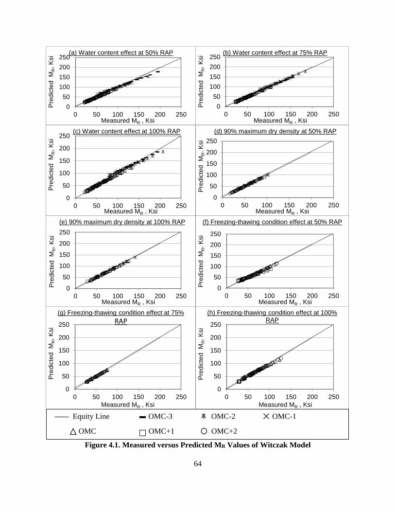
64
Figure 4.1. Measured versus Predicted MR Values of Witczak Model
0
50
100
150
200
250
0 50 100 150 200 250
Pre
dic
ted
MR,
Ksi
Measured MR , Ksi
(b) Water content effect at 75% RAP
0
50
100
150
200
250
0 50 100 150 200 250
Pre
dic
ted
MR,
Ksi
Measured MR , Ksi
(c) Water content effect at 100% RAP
0
50
100
150
200
250
0 50 100 150 200 250P
redic
ted
MR,
Ksi
Measured MR , Ksi
(d) 90% maximum dry density at 50% RAP
0
50
100
150
200
250
0 50 100 150 200 250
Pre
dic
ted
MR,
Ksi
Measured MR , Ksi
(e) 90% maximum dry density at 100% RAP
0
50
100
150
200
250
0 50 100 150 200 250
Pre
dic
ted
MR,
Ksi
Measured MR , Ksi
(f) Freezing-thawing condition effect at 50% RAP
0
50
100
150
200
250
0 50 100 150 200 250
Pre
dic
ted
MR,
Ksi
Measured MR , Ksi
(g) Freezing-thawing condition effect at 75%
RAP
0
50
100
150
200
250
0 50 100 150 200 250
Pre
dic
ted
MR,
Ksi
Measured MR , Ksi
(h) Freezing-thawing condition effect at 100% RAP
0
50
100
150
200
250
0 50 100 150 200 250
Pre
dic
ted
MR,
Ksi
Measured MR , Ksi
(a) Water content effect at 50% RAP
Equity Line OMC-3 OMC-2 OMC-1
OMC OMC+1 OMC+2
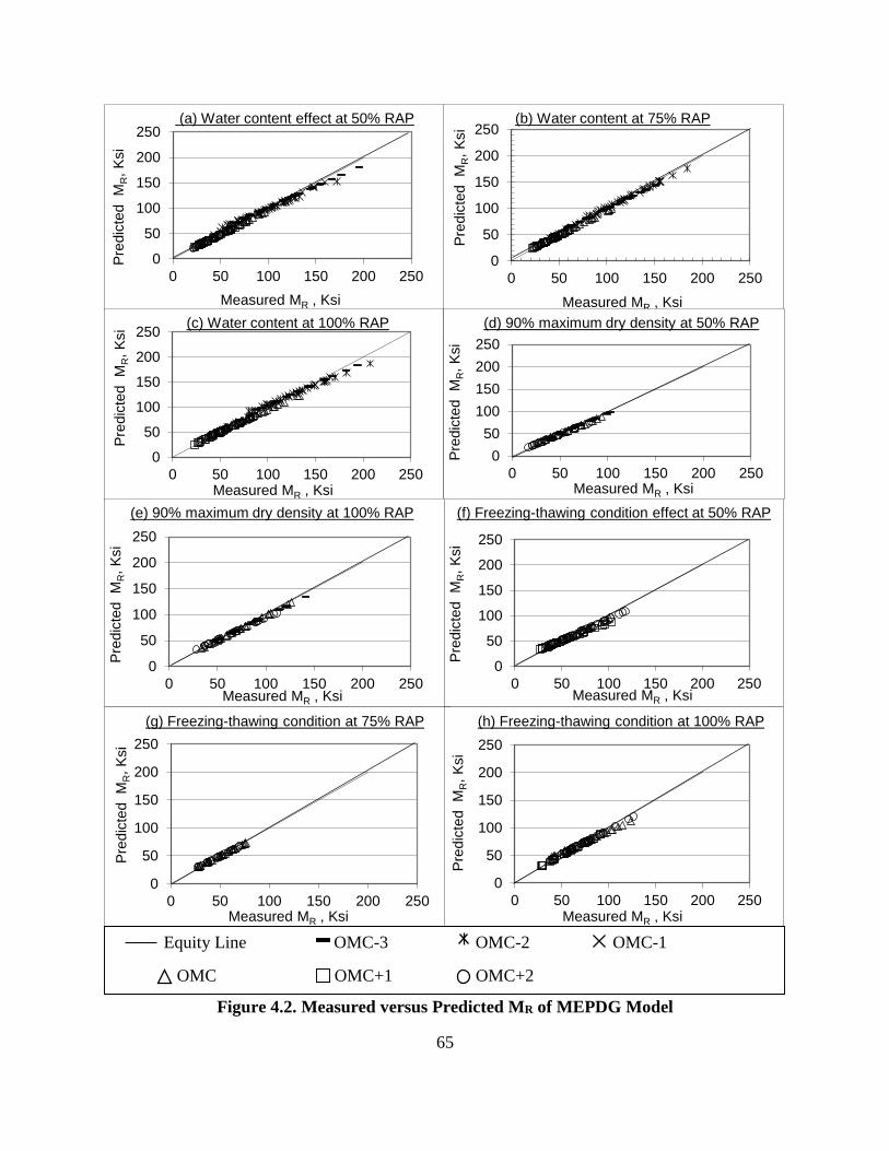
65
Figure 4.2. Measured versus Predicted MR of MEPDG Model
0
50
100
150
200
250
0 50 100 150 200 250
Pre
dic
ted
MR,
Ksi
Measured MR , Ksi
(a) Water content effect at 50% RAP
0
50
100
150
200
250
0 50 100 150 200 250
Pre
dic
ted
MR,
Ksi
Measured MR , Ksi
(b) Water content at 75% RAP
0
50
100
150
200
250
0 50 100 150 200 250
Pre
dic
ted
MR,
Ksi
Measured MR , Ksi
(c) Water content at 100% RAP
0
50
100
150
200
250
0 50 100 150 200 250
Pre
dic
ted
MR,
Ksi
Measured MR , Ksi
(d) 90% maximum dry density at 50% RAP
0
50
100
150
200
250
0 50 100 150 200 250
Pre
dic
ted
MR,
Ksi
Measured MR , Ksi
(e) 90% maximum dry density at 100% RAP
0
50
100
150
200
250
0 50 100 150 200 250
Pre
dic
ted
MR,
Ksi
Measured MR , Ksi
(f) Freezing-thawing condition effect at 50% RAP
0
50
100
150
200
250
0 50 100 150 200 250
Pre
dic
ted
MR,
Ksi
Measured MR , Ksi
(g) Freezing-thawing condition at 75% RAP
0
50
100
150
200
250
0 50 100 150 200 250
Pre
dic
ted
MR,
Ksi
Measured MR , Ksi
(h) Freezing-thawing condition at 100% RAP
Equity Line OMC-3 OMC-2 OMC-1
OMC OMC+1 OMC+2
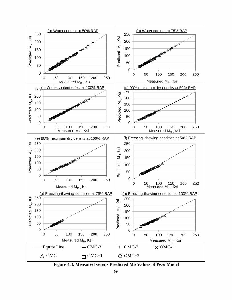
66
Figure 4.3. Measured versus Predicted MR Values of Pezo Model
0
50
100
150
200
250
0 50 100 150 200 250
Pre
dic
ted
MR,
Ksi
Measured MR , Ksi
(a) Water content at 50% RAP
0
50
100
150
200
250
0 50 100 150 200 250
Pre
dic
ted
MR,
Ksi
Measured MR, Ksi
(b) Water content at 75% RAP
0
50
100
150
200
250
0 50 100 150 200 250
Pre
dic
ted
MR,
Ksi
Measured MR , Ksi
(c) Water content effect at 100% RAP
0
50
100
150
200
250
0 50 100 150 200 250
Pre
dic
ted
MR,
Ksi
Measured MR , Ksi
(d) 90% maximum dry density at 50% RAP
0
50
100
150
200
250
0 50 100 150 200 250
Pre
dic
ted
MR,
Ksi
Measured MR , Ksi
(e) 90% maximum dry density at 100% RAP
0
50
100
150
200
250
0 50 100 150 200 250
Pre
dic
ted
MR,
Ksi
Measured MR , Ksi
(f) Freezing -thawing condition at 50% RAP
0
50
100
150
200
250
0 50 100 150 200 250
Pre
dic
ted
MR,
Ksi
Measured MR, Ksi
(g) Freezing-thawing condition at 75% RAP
0
50
100
150
200
250
0 50 100 150 200 250
Pre
dic
ted
MR,
Ksi
Measured MR , Ksi
(h) Freezing-thawing condition at 100% RAP
Equity Line OMC-3 OMC-2 OMC-1
OMC OMC+1 OMC+2
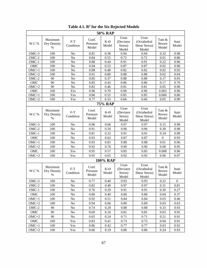
67
Table 4.1. R2 for the Six Rejected Models
50% RAP
W.C %
Maximum
Dry Density
%
F-T
Condition
Conf.
Pressure
Model
K-ϴ
Model
Uzan
(Deviator
Stress)
Model
Uzan
(Octahedral
Shear Stress)
Model
Tam &
Brown
Model
Itani
Model
OMC-3 100 No 0.81 0.38 0.94 0.94 0.32 0.98
OMC-2 100 No 0.84 0.55 0.72 0.72 0.01 0.86
OMC-1 100 No 0.88 0.44 0.91 0.91 0.22 0.96
OMC 100 No 0.94 0.53 0.87 0.87 0.02 0.96
OMC+1 100 No 0.88 0.48 0.82 0.82 0.02 0.92
OMC+2 100 No 0.91 0.80 0.88 0.88 0.02 0.04
OMC-2 90 No 0.85 0.37 0.88 0.88 0.17 0.95
OMC 90 No 0.85 0.43 0.86 0.86 0.17 0.70
OMC+2 90 No 0.82 0.46 0.81 0.81 0.05 0.90
OMC 100 Yes 0.96 0.70 0.90 0.90 0.003 0.96
OMC+1 100 Yes 0.86 0.55 0.85 0.85 0.006 0.80
OMC+2 100 Yes 0.77 0.33 0.66 0.66 0.05 0.90
75% RAP
W.C %
Maximum
Dry Density
%
F-T
Condition
Conf.
Pressure
Model
K-ϴ
Model
Uzan
(Deviator
Stress)
Model
Uzan
(Octahedral
Shear Stress)
Model
Tam &
Brown
Model
Itani
Model
OMC-3 100 No 0.96 0.66 0.97 0.97 0.15 0.98
OMC-2 100 No 0.91 0.50 0.96 0.96 0.30 0.98
OMC-1 100 No 0.81 0.32 0.91 0.91 0.34 0.98
OMC 100 No 0.93 0.62 0.87 0.87 0 0.93
OMC+1 100 No 0.93 0.81 0.88 0.88 0.01 0.96
OMC+2 100 No 0.92 0.76 0.90 0.90 0.08 0.95
OMC 100 Yes 0.95 0.57 0.85 0.85 0.008 0.96
OMC+2 100 Yes 0.95 0.65 0.92 0.92 0.06 0.97
100% RAP
W.C %
Maximum
Dry Density
%
F-T
Condition
Conf.
Pressure
Model
K-ϴ
Model
Uzan
(Deviator
Stress)
Model
Uzan
(Octahedral
Shear Stress)
Model
Tam &
Brown
Model
Itani
Model
OMC-3 100 No 0.77 0.40 0.93 0.93 0.22 0
OMC-2 100 No 0.82 0.40 0.97 0.97 0.31 0.81
OMC-1 100 No 0.76 0.29 0.91 0.91 0.30 0.27
OMC 100 No 0.86 0.40 0.86 0.86 0.04 0.37
OMC+1 100 No 0.92 0.51 0.84 0.84 0.03 0.46
OMC+2 100 No 0.94 0.66 0.89 0.89 0.03 0.63
OMC-2 90 No 0.74 0.29 0.88 0.88 0.33 0.93
OMC 90 No 0.69 0.16 0.81 0.81 0.03 0.92
OMC+2 90 No 0.65 0.24 0.71 0.71 0.21 0.91
OMC 100 Yes 0.83 0.41 0.73 0.73 0.04 0.91
OMC+1 100 Yes 0.86 0.42 0.77 0.77 0.03 0.92
OMC+2 100 Yes 0.66 0.19 0.86 0.86 0.24 0.93

68
Table 4.2. R2 for Water Content (W.C) Variation on RAP Approved Models
Table 4.3. R for 90% Maximum Dry Density (MDD) on RAP Approved Models
Table 4.4. R2 for Freezing-Thawing (F-T) Cycles on RAP Approved Models
W.C %
50 % RAP 75 % RAP 100% RAP
Pezo
Model
(Fig.
4.3-a)
MEPDG
Model
(Fig. 4.2-
a)
Witczak
Model
(Fig. 4.1-
a)
Pezo
Model
(Fig.
4.3-b)
MEPDG
Model
(Fig. 4.2-
b)
Witczak
Model
(Fig. 4.1-
b)
Pezo
Model
(Fig.
4.3-c)
MEPDG
Model
(Fig. 4.2-
c)
Witczak
Model
(Fig.
4.1-c)
OMC-3 0.99 0.90 0.89 0.98 0.93 0.93 0.95 0.89 0.87
OMC-2 0.84 0.78 0.80 0.98 0.92 0.90 0.96 0.82 0.79
OMC-1 0.96 0.94 0.95 0.97 0.96 0.95 0.97 0.94 0.92
OMC 0.96 0.95 0.97 0.93 0.96 0.98 0.96 0.91 0.91
OMC+1 0.91 0.86 0.91 0.94 0.94 0.97 0.93 0.95 0.98
OMC+2 0.91 0.92 0.96 0.92 0.89 0.93 0.94 0.89 0.90
W.C %
50 % RAP 100% RAP
Pezo
Model
(Fig. 4.3-
d)
MEPDG
Model
(Fig. 4.2-
d)
Witczak
Model
(Fig. 4.1-
d)
Pezo
Model
(Fig. 4.3-
e)
MEPDG
Model
(Fig. 4.2-e)
Witczak
Model
(Fig. 4.1-
e)
OMC-2 0.95 0.94 0.96 0.93 0.94 0.96
OMC 0.93 0.91 0.95 0.94 0.91 0.94
OMC+2 0.89 0.87 0.90 0.83 0.81 0.88
W.C %
50% RAP 75% RAP 100% RAP
Pezo
Model
(Fig.
4.3-f)
MEPDG
Model
(Fig. 4.2-f)
Witczak
Model
(Fig.
4.1-f)
Pezo
Model
(Fig.
4.3-g)
MEPDG
Model
(Fig. 4.2-
g)
Witczak
Model
(Fig.
4.1-g)
Pezo
Model
(Fig.
4.3-h)
MEPDG
Model
(Fig. 4.2-
h)
Witczak
Model
(Fig.
4.1-h)
OMC 0.96 0.93 0.96 0.96 0.94 0.97 0.87 0.80 0.82
OMC+1 0.88 0.82 0.80 NA NA NA 0.90 0.95 0.98
OMC+2 0.83 0.85 0.91 0.96 0.93 0.87 0.93 0.93 0.87
69
4.4. Sensitivity Analysis
A second stage is performed to assess the best-fit of the three models chosen on RAP
behavior considering all the interactions taken in the study at the three different concentrations of
RAP. This second stage is carried out by comparing each multiple regression constant K values of
each model under the effect of tested conditions at different RAP percentages in order to
understand the possible change(s), if any, of each K value with the tested conditions.
4.4.1. Witczak model parametric analysis
Based on the Witczak model equation, it is obvious that K23 is directly related to MR. From
Figure 4.4, K23 increases for 75% and 100% of RAP and it reaches its maximum value at the
optimum moisture content (OMC%). Also, it hugely increases when the maximum dry density
(MDD) decreases from 100% to 90% for all RAP percentages. However, K23 value differs
completely under the effect of freeze-thaw as it decreases in general for all RAP percentages and
increases after exceeding the OMC%. In general, K23 is usually at its highest values at 100% RAP
under the effect of all tested conditions resulting in an increase in the MR.
For K24, the same K23 behavior is noticed under the effect of the water content as it reaches
its maximum value at the OMC% for all RAP percentages. There is no general trend for K24 under
the effect of freeze-thaw and its values are almost the same for all RAP percentages, but with
different behavior for each percent. The effect of decreasing MDD increases slightly the K24
values. This increase continues with increasing the water content. However, the percentage of RAP
does not have a remarkable significance on the K24 values in general under the effect of all the
factors studied. The effect of K24 on the MR differs according to the value under the power as MR
may increase or decrease, as shown in Witczak model equation in Table 2.1.
70
Concerning K25, its effect on MR is directly proportional, as the lower the K25 the lower is
the MR as shown in the equation in Table 2.1. Under the effect of water content, it reaches its
minimum value at the OMC especially for the 75% and 100% RAP cases. There is no noticeable
difference in the K25 under the effect of decreasing MDD level. However, it tends to show a rather
linear trend with water content variations. On the other hand, the effect of freeze-thaw on K25
showed a significant increase for all RAP percentages without a definite behavior for water content
variations. So, in general K25 affects negatively on MR especially under the effects of water content
and decreasing MDD. However, this negative effect is minimized with the effect of freeze-thaw.
The study does not consider the effect of the tested factors for both parameters K26 and K27.
This is attributed to the fact that, after trial and error assumptions of different values for both
parameters at various percentages of RAP, it is found that at K26 = -5 and K27 = 5 yield the highest
R2 for the linear comparison between predicted and measured MR values. Therefore, it is assumed
that K26 = -5 and K27 = 5 for all interactions of tested factors at all percentages of RAP.
4.4.2. MEPDG model parameter analysis
From the equation of MEPDG model, it is clear that K20 is directly related to MR. In general,
as shown in Figure 4.5, K20 decreases with increasing the water content for all RAP percentages
with slight higher values at 100% RAP. The effect of decreasing MDD decreases K20 slightly
especially at water content less than OMC%. In addition, it has the higher values at higher
percentage of RAP. Furthermore, freeze-thaw cycles negatively affect K20 especially at OMC-1%
for all percentages of RAP. In general, K20 negatively affects all results of the tested conditions
especially when water content exceeds OMC%. On the contrary it has a positive effect when the
RAP percent increases.

71
For K21, Figure 4.5 shows that for all RAP percentages, K21 reaches its maximum value
when the water content is much close to the OMC%. The percent of RAP does not have a large
effect on K21 values. Also, in terms of the effect of the other two factors, 90% MDD and freeze-
thaw cycles are not significant on K21 values. Furthermore, there is no general trend for the
interaction between these factors and water content. In addition, K21 is almost the same for all
RAP contents. So, it seems that this parameter is affected only by varying the water content. In
addition, the effect of K21 on MR is not clearly obvious, as it depends on the value under the power,
as shown in MEPDG model equation in Table 2.1.
For K22 parameter, it reaches is its minimum values when water content approaches the
OMC% irrespective of the percent of RAP. But, the absolute values of K22 slightly increases under
the effect of decreasing MDD with increases at higher percent of RAP especially at lower water
contents. There is no a significant effect of the freeze-thaw cycles on K22 for all RAP percentages.
Therefore, in general the parameters of this model are affected more by the water content variation
with small effect of decreasing MDD and almost no effect of freeze-thaw cycles at all RAP
contents. Also, the parameters are not remarkably affected by increasing the percentage of RAP.
4.4.3. Pezo model parameter analysis
K11 is directly proportional to MR. Figure 4.6 shows that K11 decreases at increased water
content and increased percent of RAP. Both factors, 90% MDD and freeze-thaw cycles, negatively
affect K11 with varying the water content especially for 90% MDD. Its interaction with water
content is more obvious than that of the freeze-thaw cycles with water content variation. In general,
all the tested factors negatively affect K11 values with consequently negative effects on the MR
values, as shown in Pezo model equation in Table 2.1.
72
For K12 parameter, Figure (4.6-c) indicates that it reaches its maximum values at the OMC
irrespective to the percent of RAP. For both other two factors, K12 increases slightly especially for
the interaction of 90% MDD and water content, as shown in Figure (4.6-d). Almost no significant
effects may be noticed for applying freeze-thaw cycles on K12 parameter alone. For K13, as shown
in Figure (4.6-e), is affected by water content as it reaches its minimum value when water content
approaches to the OMC%. Also, the percent of RAP has a little significance. Decreasing MDD
slightly, decreases K13 also slightly with significance of the percent of RAP. Freeze-thaw cycles
have almost no significance on K13 at all RAP percent’s. Therefore, in general, parameters of this
model do not show a well-defined behavior trend under the effect of the tested factors, except only
that K11 factor is negatively affected by the tested conditions and therefore, negatively affect the
MR values.
Finally, these three models are considered the best-fit for RAP behavior under tested
conditions. However, another analysis is felt needed in a second stage to confirm the results of the
first one and choose the best-fit model for RAP behavior. Therefore, this second sensitivity
analysis is carried out on the three models to compare each K under the effect of each condition of
the tested factors. Figures 4.4, 4.5, and 4.6, show that the MEPDG model gives the best physical
meanings of the obtained results when compared to the other two models. In general, the
parameters of this model are highly affected by the water content variation, slightly affected when
decreasing the MDD, almost not affected by freeze-thaw cycles at all RAP contents. This model’s
parameters are not highly affected by increasing the percentage of RAP. This model in general,
gives the best prediction MR values at 75% RAP.
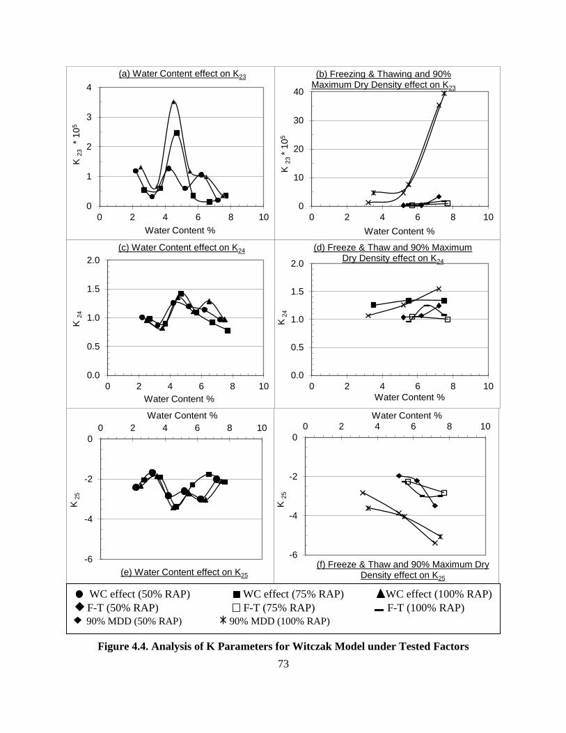
73
Figure 4.4. Analysis of K Parameters for Witczak Model under Tested Factors
0
1
2
3
4
0 2 4 6 8 10
K 2
3*
10
5
Water Content %
(a) Water Content effect on K23
0.0
0.5
1.0
1.5
2.0
0 2 4 6 8 10
K 2
4
Water Content %
(c) Water Content effect on K24
-6
-4
-2
0
0 2 4 6 8 10
K25
Water Content %
(e) Water Content effect on K25
0
10
20
30
40
0 2 4 6 8 10
K 2
3 *
10
5
Water Content %
(b) Freezing & Thawing and 90% Maximum Dry Density effect on K23
0.0
0.5
1.0
1.5
2.0
0 2 4 6 8 10
K24
Water Content %
(d) Freeze & Thaw and 90% Maximum Dry Density effect on K24
-6
-4
-2
0
0 2 4 6 8 10
K 2
5
Water Content %
(f) Freeze & Thaw and 90% Maximum Dry Density effect on K25
WC effect (50% RAP) WC effect (75% RAP) WC effect (100% RAP)
F-T (50% RAP) F-T (75% RAP) F-T (100% RAP)
90% MDD (50% RAP) 90% MDD (100% RAP)
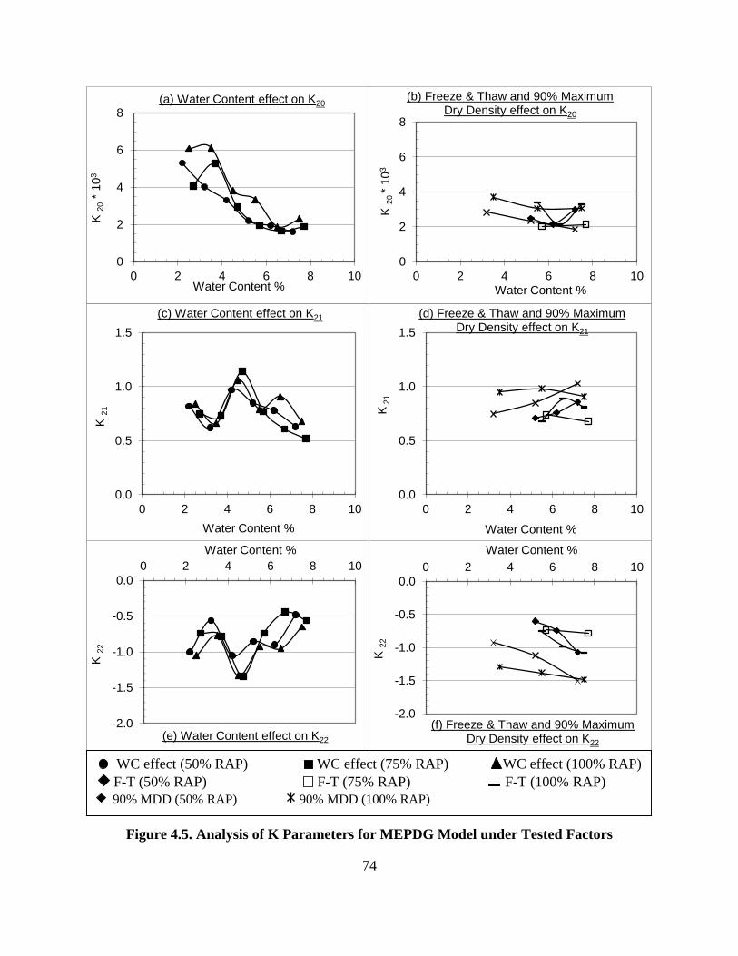
74
Figure 4.5. Analysis of K Parameters for MEPDG Model under Tested Factors
0
2
4
6
8
0 2 4 6 8 10
K 2
0 *
10
3
Water Content %
(b) Freeze & Thaw and 90% Maximum Dry Density effect on K20
0
2
4
6
8
0 2 4 6 8 10
K 2
0*
10
3
Water Content %
(a) Water Content effect on K20
0.0
0.5
1.0
1.5
0 2 4 6 8 10
K 2
1
Water Content %
(c) Water Content effect on K21
0.0
0.5
1.0
1.5
0 2 4 6 8 10
K21
Water Content %
(d) Freeze & Thaw and 90% Maximum Dry Density effect on K21
-2.0
-1.5
-1.0
-0.5
0.0
0 2 4 6 8 10
K 2
2
Water Content %
(e) Water Content effect on K22
-2.0
-1.5
-1.0
-0.5
0.0
0 2 4 6 8 10
K 2
2
Water Content %
(f) Freeze & Thaw and 90% Maximum Dry Density effect on K22
WC effect (50% RAP) WC effect (75% RAP) WC effect (100% RAP)
F-T (50% RAP) F-T (75% RAP) F-T (100% RAP)
90% MDD (50% RAP) 90% MDD (100% RAP)
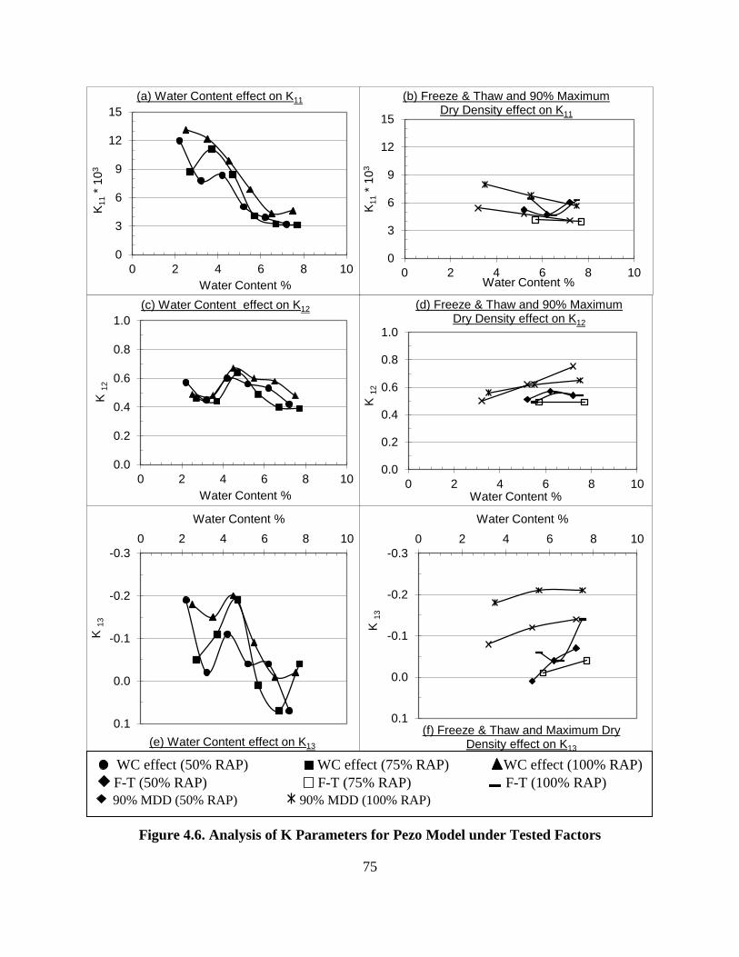
75
Figure 4.6. Analysis of K Parameters for Pezo Model under Tested Factors
0
3
6
9
12
15
0 2 4 6 8 10
K11
* 10
3
Water Content %
(a) Water Content effect on K11
0
3
6
9
12
15
0 2 4 6 8 10
K11
* 10
3
Water Content %
(b) Freeze & Thaw and 90% Maximum Dry Density effect on K11
0.0
0.2
0.4
0.6
0.8
1.0
0 2 4 6 8 10
K 1
2
Water Content %
(c) Water Content effect on K12
0.0
0.2
0.4
0.6
0.8
1.0
0 2 4 6 8 10
K 1
2
Water Content %
(d) Freeze & Thaw and 90% Maximum Dry Density effect on K12
-0.3
-0.2
-0.1
0.0
0.1
0 2 4 6 8 10
K 1
3
Water Content %
(e) Water Content effect on K13
-0.3
-0.2
-0.1
0.0
0.1
0 2 4 6 8 10
K 1
3
Water Content %
(f) Freeze & Thaw and Maximum Dry Density effect on K13
WC effect (50% RAP) WC effect (75% RAP) WC effect (100% RAP)
F-T (50% RAP) F-T (75% RAP) F-T (100% RAP)
90% MDD (50% RAP) 90% MDD (100% RAP)
76
4.5. Parametric Analysis
This third stage analysis is focused on the MEPDG model which is proved to be the best
prediction model from the previous two stages. But, this analysis is focused on the different state
of stresses applied during the resilient modulus test under the same testing conditions taken in
consideration before. The state of stresses was proved from different researches in the literature
survey to be the most important effective parameter on the MR of the base layer. This factor is
needed to be studied to be more confident for using the MEPDG model for RAP in base layer.
At first, multiple regression analysis is achieved for the MEPDG model by utilizing the
measured MR values under different measured testing parameters inside this model. This stage
comprises calculating each K parameter under five different levels of confining pressure (3, 6, 10,
15 and 20 psi) using the Excel solver software. Six replicates are considered for each level of
confining pressure. Each replicate is assigned a different value of deviator stress. This analysis
cannot be done at different levels of deviator stress as testing sequences required by NCHRP 1-
28A protocol used in MR testing, do not group deviator stress at the grouped levels of confining
pressure mentioned before. This regression is repeated under four different field conditions:
i. Percentages of RAP (0%, 50%, 75% and 100%).
ii. Six different moisture contents, ranging from OMC-3% to OMC+2% with 1% increments.
iii. Two different levels of compaction, 100% and 90% Maximum Dry Density (MDD).
iv. Two cycles of Freeze-Thaw (F-T).
MEPDG model: MR = K1. Pa(θ
Pa)K2 (
τoct
Pa+ 1)K3 (4.1)
Where:
MR = Resilient modulus (psi)
Ki = multiple regression constants evaluated from the resilient modulus tests.

77
Pa = atmospheric pressure = 14.7 psi = 101.5 kPa.
θ = bulk stress (psi) = σ1 + σ2 + σ3 = σd+ 3σ3 (psi).
σd = deviator stress (psi), σ3 = confining pressure (psi).
τoct = octahedral shear stress (psi) =1
3√{(σ1 − σ2)2+(σ1 − σ3)2 + (σ2 − σ3)2}.
Review of previous literature with respect to the MR-MEPDG model showed that K1 > 0
and refers to the Young’s Modulus of the material. Also, K2 > 0 which refers to stress stiffening
and K3 < 0 refers to shear softening (Andrei et al., 2004). Most of the results collected satisfy the
trend concluded from literature at different confining pressure levels and various field conditions
tested, which includes water content, dry density and freeze-thaw cycles at different RAP
percentages in the blend. In the following sections, the analysis of each K parameter in the model
at those different testing conditions is presented.
4.5.1. Analysis of K1
The variation of this parameter is considerably high under the variation of confining
pressure at different testing conditions. Therefore, the data collected for this parameter is shown
on semi-log charts in Figures 4.7, 4.8 and 4.9 to represent K1 under the variation of confining
pressure factor for all testing conditions at different RAP concentrations. Firstly, confining
pressure levels can be divided into three categories: low (3&6 psi), intermediate (10 psi) and high
(15&20 psi). Under the variation of water content at different levels of confining pressure and
different percentages of RAP (Figure 4.7), K1 increases with increasing the percentage of RAP
exceeding the original values before using RAP (0%). This relation is obvious at low confining
pressure levels (3&6 psi) and most of water content levels except OMC-3%.
At intermediate confining pressure level (10 psi), K1 decreases dramatically approaching
zero on granular coarse aggregates before using RAP (0%). In case of using RAP at different water

78
content levels, K1 also approaches zero except at 100% RAP and water content levels ranging from
OMC-2% to OMC.
At high confining pressure levels (15&20 psi), K1 increases dramatically at 0% RAP and
the case is the same when using RAP. However, it does not exceed the original values at 0% RAP.
There is an exception for this relation at low water content levels OMC-2 and OMC-3% as K1 does
not increase dramatically like the other water content levels and it decreases with increasing
percentage of RAP.
For the case of decreasing MDD from 100% to 90% (Figure 4.8), at low confining pressure
category, K1 increases with increasing percentage of RAP exceeding the original values of K1 at
granular base coarse aggregates (0% RAP). At intermediate confining pressure, K1 decreases
remarkably to approach zero for all percentages of RAP. At high confining pressure levels, K1
increases dramatically for all percentages of RAP. In general, K1 values at 90% MDD are higher
than 100% MDD in the same other testing conditions.
Finally, for the last case of freeze-thaw cycles (Figure 4.9) at low confining pressure levels,
K1 increases with increasing percentage of RAP exceeding the original K1 values at 0% RAP. This
relation is clearer at 3 psi confining pressure than 6 psi. At intermediate confining pressure, K1
decreases approaching zero except at 100% RAP in OMC+2%. At high confining pressure
category, K1 increases dramatically except at high percentage of RAP and water content
concentration. Generally, K1 values are not affected significantly by freeze-thaw cycles at the same
testing field conditions.
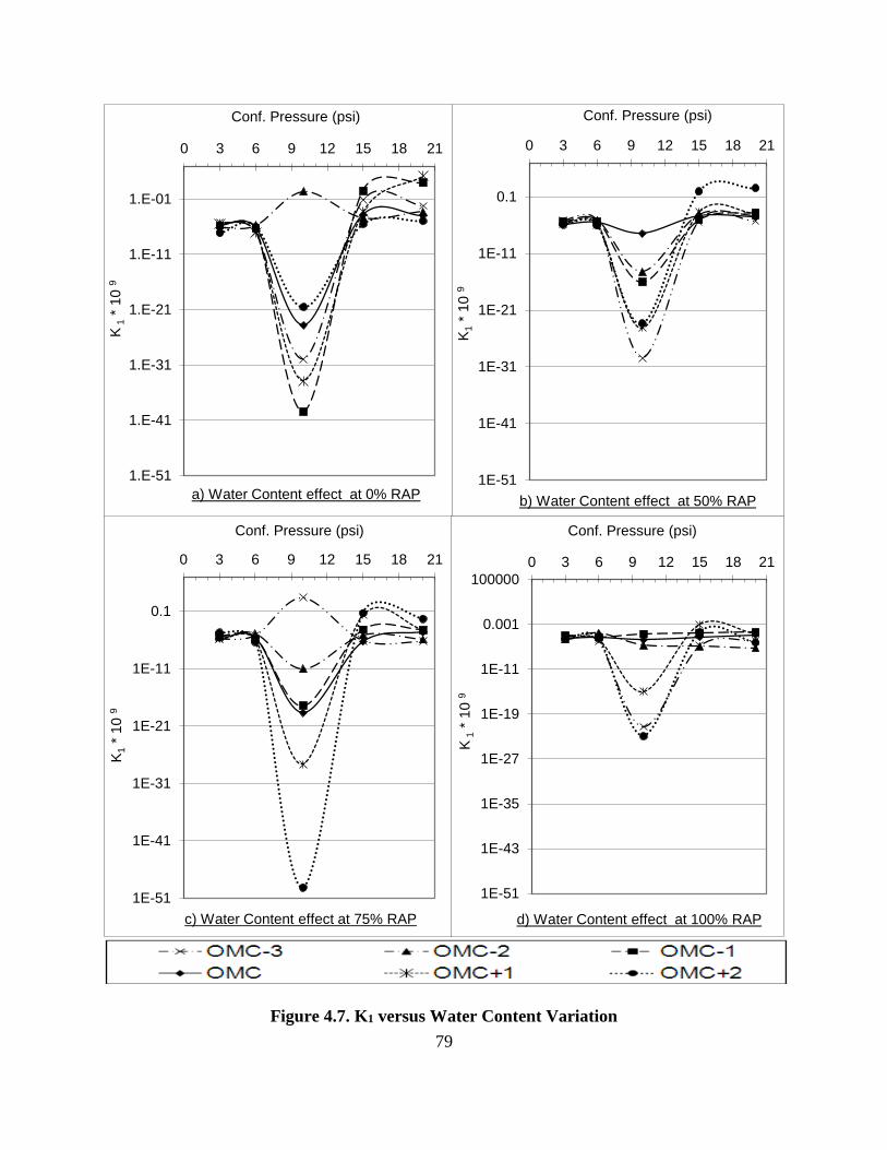
79
Figure 4.7. K1 versus Water Content Variation
1.E-51
1.E-41
1.E-31
1.E-21
1.E-11
1.E-01
0 3 6 9 12 15 18 21
K1
* 10 9
Conf. Pressure (psi)
a) Water Content effect at 0% RAP1E-51
1E-41
1E-31
1E-21
1E-11
0.1
0 3 6 9 12 15 18 21
K1
* 10 9
Conf. Pressure (psi)
b) Water Content effect at 50% RAP
1E-51
1E-41
1E-31
1E-21
1E-11
0.1
0 3 6 9 12 15 18 21
K1
* 10 9
Conf. Pressure (psi)
c) Water Content effect at 75% RAP
1E-51
1E-43
1E-35
1E-27
1E-19
1E-11
0.001
100000
0 3 6 9 12 15 18 21
K1
* 10 9
Conf. Pressure (psi)
d) Water Content effect at 100% RAP

80
Figure 4.8. K1 versus Maximum Dry Density Variation
1.E-79
1.E-64
1.E-49
1.E-34
1.E-19
1.E-04
1.E+11
0 3 6 9 12 15 18 21
K1
* 10 9
Conf. Pressure (psi)
a) 90% Maximum Dry Density effect at 0% RAP
1E-79
1E-64
1E-49
1E-34
1E-19
0.0001
1E+11
0 3 6 9 12 15 18 21
K1
* 10 9
Conf. Pressure (psi)
b) 90% Maximum Dry Density effect at 50% RAP
1E-79
1E-64
1E-49
1E-34
1E-19
0.0001
1E+11
0 3 6 9 12 15 18 21
K1
* 10 9
Conf. Pressure (psi)
c) 90% Maximum Dry Density effect at 100% RAP

81
Figure 4.9. K1 versus Freeze and Thaw Cycles
1.E-34
1.E-26
1.E-18
1.E-10
1.E-02
0 3 6 9 12 15 18 21
K1
* 10 9
Conf. Pressure (psi)
a) F-T effect at 0% RAP
1.E-34
1.E-26
1.E-18
1.E-10
1.E-02
0 3 6 9 12 15 18 21
K1
* 10
9
Conf. Pressure (psi)
b) F-T effect at 50% RAP
1E-34
1E-26
1E-18
1E-10
0.01
0 3 6 9 12 15 18 21
K1
* 10 9
Conf. Pressure (psi)
c) F-T effect at 75% RAP
1E-34
1E-26
1E-18
1E-10
0.01
0 3 6 9 12 15 18 21
K1
* 10 9
Conf. Pressure (psi)
d) F-T effect at 100% RAP
82
4.5.2. Analysis of K2
It is obvious for all testing conditions that K2 is positive at most confining pressure levels
and reaches its maximum values for most of the testing conditions at confining pressure of 10 psi.
Therefore, K2 seems to be more reliable at intermediate confining pressure than others. As it is
shown in Figures 4.10, 4.11 and 4.12, K2 values are very close to zero and sometimes negative.
This result satisfies those of the literature for this model and confirmed that K2 values should be
positive for base layer. This describes the behavior of stress stiffening (Andrei et al., 2004).
For water content variation (Figure 4.10), the maximum values of K2 are usually reached
when water content is far-away from the optimum moisture content (at OMC-3% and OMC+2%)
especially at 50% and 100% of RAP where K2 values at OMC are the lower than 0% and 75% of
RAP. But, this relation is not the same for granular base aggregates as shown at 0% RAP (Class
5), the maximum values reached at OMC-1% and OMC+1%. The comparison between different
RAP concentrations and granular base aggregates shows that the trend of K2 seems to be very close
at 75% RAP. Generally, maximum K2 values are reached in far-away water contents than OMC%
and ranged between 50 to 80 at 50% RAP, while it is in between 70 to 140 at 75% RAP and around
50 at 100% RAP. Nevertheless, for granular base aggregates, it ranges in between 75 to 100 at
water contents close to OMC%.
By decreasing MDD to 90% (Figure 4.11), K2 values increases reaching 170 for 50% and
100% RAP and 250 for 0% RAP. These optimum values are reached especially with high water
content levels such as OMC+2%. However, K2 values at OMC-2% for 50% and 100% RAP
remarkably decrease and reach non-realistic negative values for K2. This behavior is not the same
for granular base aggregates (0% RAP) at high water content.
83
After applying freeze-thaw cycles (Figure 4.12) at different water contents, K2 values range
between 65 to 75 especially at OMC+2% for 50% and 75% RAP. However, at 100% RAP, K2
values decrease to 55 at OMC+1%. For granular base aggregates (0% RAP), optimum K2 values
reach 80 at OMC+2% and 65 at OMC%. This is much higher than 50% and 100% RAP.
Application of freeze-thaw cycles affects K2 values positively as it increases after F-T cycles at
the same water content levels for all percentages of RAP.
4.5.3. Analysis of K3
As shown in Figures 4.13, 4.14 and 4.15 for all testing conditions, K3 is negative at most
confining pressure levels and reaches its minimum values for most of the testing conditions at a
confining pressure of 10 psi. This result satisfies those shown in previous literature that K3 values
should be negative for base layer. Thus, describes the behavior of shear softening (Andrei et al.,
2004). In the case of water content variation (Figure 4.13), K3 values reach their minimum values
at water content levels away from OMC% such as OMC-3% and OMC+2%. This trend is obvious
at 50%, 75% and 100% of RAP. Approximately, the lowest K3 values are around -80, -140 and -
60 for cases of 50%, 75% and 100% RAP respectively. At 0% RAP, the lowest K3 value reaches
-110 at water content level of OMC-1%. By comparing both percentages 0% and 100% RAP, it
seems to be that the general trend of K3 values at 0% is much lower than 100%, which means that
this model is more suitable for granular base aggregates than RAP.
For the case of decreasing MDD to 90% (Figure 4.14), K3 values are lower than 100%
MDD reaching -170 especially at OMC+2% for 50% and 100% RAP. In the case of 0% RAP,
K3values are lower than those for all percentages of RAP (50% and 100%) at the three different
water contents of OMC-2%, OMC% and OMC+2%. At 0% RAP, K3 reaches -250 in the case of
OMC+2% compared to -170 at both RAP percentages 50% and 100%.
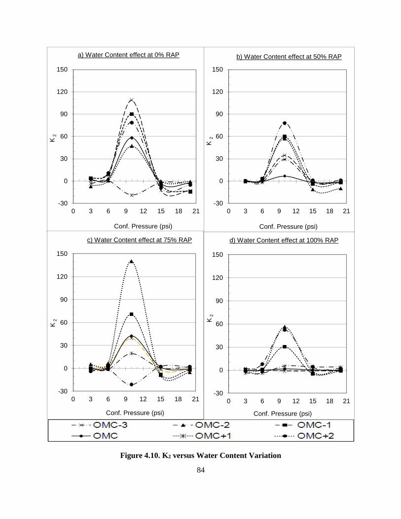
84
Figure 4.10. K2 versus Water Content Variation
-30
0
30
60
90
120
150
0 3 6 9 12 15 18 21
K2
Conf. Pressure (psi)
a) Water Content effect at 0% RAP
-30
0
30
60
90
120
150
0 3 6 9 12 15 18 21K
2
Conf. Pressure (psi)
b) Water Content effect at 50% RAP
-30
0
30
60
90
120
150
0 3 6 9 12 15 18 21
K2
Conf. Pressure (psi)
c) Water Content effect at 75% RAP
-30
0
30
60
90
120
150
0 3 6 9 12 15 18 21
K2
Conf. Pressure (psi)
d) Water Content effect at 100% RAP
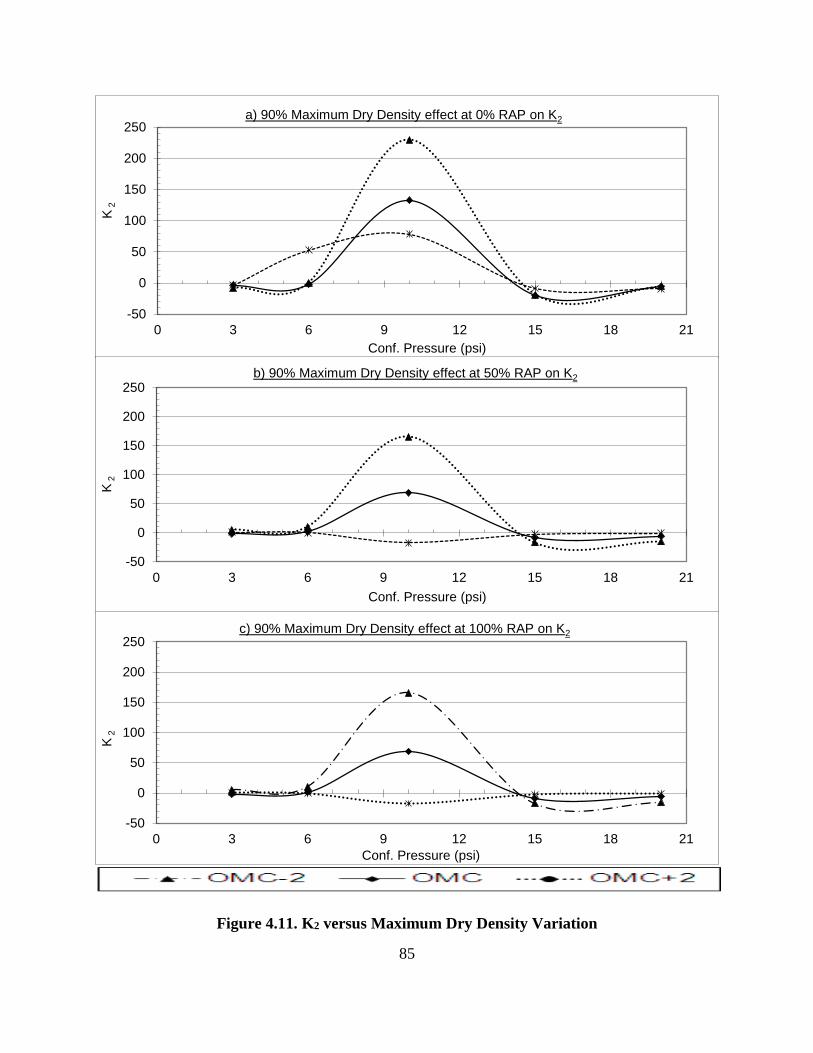
85
Figure 4.11. K2 versus Maximum Dry Density Variation
-50
0
50
100
150
200
250
0 3 6 9 12 15 18 21
K2
Conf. Pressure (psi)
a) 90% Maximum Dry Density effect at 0% RAP on K2
-50
0
50
100
150
200
250
0 3 6 9 12 15 18 21
K2
Conf. Pressure (psi)
b) 90% Maximum Dry Density effect at 50% RAP on K2
-50
0
50
100
150
200
250
0 3 6 9 12 15 18 21
K2
Conf. Pressure (psi)
c) 90% Maximum Dry Density effect at 100% RAP on K2

86
Figure 4.12. K2 versus Freeze and Thaw Cycles
-20
0
20
40
60
80
100
0 3 6 9 12 15 18 21
K2
Conf. Pressure (psi)
a) F-T effect at 0% RAP
-20
0
20
40
60
80
100
0 3 6 9 12 15 18 21
K2
Conf. Pressure (psi)
b) F-T effect at 50% RAP
-20
0
20
40
60
80
100
0 3 6 9 12 15 18 21
K2
Conf. Pressure (psi)
C) F-T effect at 75% RAP
-20
0
20
40
60
80
100
0 3 6 9 12 15 18 21
K2
Conf. Pressure (psi)
d) F-T effect at 100% RAP

87
Decreasing MDD to 90% result matches with the same conclusion in the case above of water
content variation.
After applying freeze-thaw cycles (Figure 4.15) at different water contents, K3 reaches -80
at OMC+2% for 50% RAP compared to -60 at the same field conditions before F-T cycles. K3
reaches -65 at OMC+2% for 75% RAP and reaches -50 at 100% RAP and OMC+1%. For the case
of granular coarse aggregates (0% RAP), K3 reaches -80 at OMC+2% compared to -50 at the same
case before applying F-T cycles. Then, F-T cycles affect more positively on K3 absolute values.
Therefore, by comparing granular coarse aggregates (0%) and RAP (100%), traditional coarse
aggregates are more suitable to the model as K3 absolute values are higher which describes shear
softening behavior for base layer better than RAP.
4.5.4. RAP-aggregate combination analysis
After the analysis of each K parameter with different confining pressure levels under
various testing conditions, it is felt necessary to assess the variation of each K parameter with
different RAP concentrations for all confining pressure levels studied before. In this case, testing
conditions are only concerned with OMC% and 100% MDD without freeze-thaw cycles as these
are the most frequent field conditions probable to happen at early life stages of pavement section.
This stage of analysis is achieved to differentiate between the behaviors of each K parameter when
granular base coarse aggregates or RAP are used. The following paragraph present the analyses
included as shown in (Figure 4.16):
K1 values are low for granular base coarse aggregates and RAP concentrations (50%, 75% and
100%) at low and intermediate confining pressure levels (Figure 4.16-a). However, K1 increases
dramatically at high confining pressure levels (15 and 20 psi) especially for base coarse
aggregates. It remarkably increases by increasing RAP concentration.

88
Figure 4.13. K3 versus Water Content Variation
-150
-120
-90
-60
-30
0
30
0 3 6 9 12 15 18 21
K3
Conf. Pressure (psi)
a) Water Content effect at 0% RAP
-150
-120
-90
-60
-30
0
30
0 3 6 9 12 15 18 21
K3
Conf. Pressure (psi)
b) Water Content effect at 50% RAP
-150
-120
-90
-60
-30
0
30
0 3 6 9 12 15 18 21
K3
Conf. Pressure (psi)
c) Water Content effect at 75% RAP
-150
-120
-90
-60
-30
0
30
0 3 6 9 12 15 18 21
K3
Conf. Pressure (psi)
d) Water Content effect at 100% RAP
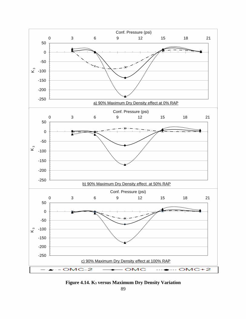
89
Figure 4.14. K3 versus Maximum Dry Density Variation
-250
-200
-150
-100
-50
0
50
0 3 6 9 12 15 18 21
K3
Conf. Pressure (psi)
a) 90% Maximum Dry Density effect at 0% RAP
-250
-200
-150
-100
-50
0
50
0 3 6 9 12 15 18 21
K3
Conf. Pressure (psi)
b) 90% Maximum Dry Density effect at 50% RAP
-250
-200
-150
-100
-50
0
50
0 3 6 9 12 15 18 21
K3
Conf. Pressure (psi)
c) 90% Maximum Dry Density effect at 100% RAP
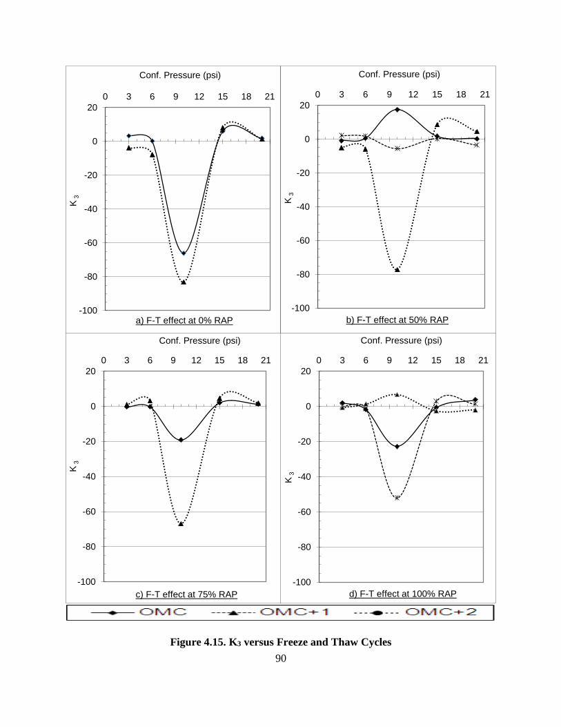
90
Figure 4.15. K3 versus Freeze and Thaw Cycles
-100
-80
-60
-40
-20
0
20
0 3 6 9 12 15 18 21
K3
Conf. Pressure (psi)
a) F-T effect at 0% RAP
-100
-80
-60
-40
-20
0
20
0 3 6 9 12 15 18 21
K3
Conf. Pressure (psi)
b) F-T effect at 50% RAP
-100
-80
-60
-40
-20
0
20
0 3 6 9 12 15 18 21
K3
Conf. Pressure (psi)
c) F-T effect at 75% RAP
-100
-80
-60
-40
-20
0
20
0 3 6 9 12 15 18 21
K3
Conf. Pressure (psi)
d) F-T effect at 100% RAP

91
Figure 4.16. Analysis of MEPDG Model versus RAP Concentration

92
K2 values are almost zero for all RAP concentrations (Figure 4.16-b) at both low and high
confining pressure levels, except for intermediate level (10 psi). It has high positive value at
granular coarse aggregates (0% RAP) compared to the other percentages (50%, 75% and
100%). For 75% RAP, K2 values' seem to be unreasonable compared to those at the other two
percentages of RAP (50% and 100%).
K3 values are almost zero for all RAP concentrations (Figure 4.16-c) at both low and high
confining pressure levels except for intermediate level (10 psi). It has high negative value at
granular coarse aggregates (0% RAP) compared to those of the other percentages of RAP
(50%, 75% and 100%). The 75% RAP values seem to be unreasonable compared to those of
the other two percentages of RAP (50% and 100%).
The behavior of this model seems to be approximately the same for both granular base coarse
aggregates and RAP when used in base layer. On the other hand, by increasing the confining
pressure levels up to 10, 15 and 20 psi, the model seems to better fit for the case of granular
base coarse aggregates. In this case, the values of each K parameter are reasonable and agree
more with those shown in the literature for the MR-MEPDG model.
To prove the variation of K2 and K3 at 10 psi for 75% RAP, Figure (4.16-d) shows that the
general trend of the original measured MR data for 75% RAP were lower than both percentages
50% and 100% RAP at all confining pressure levels tested. These results were much lower
than expected for 75% RAP as the general trend that MR increases when percentage of RAP
increases.
93
4.6. MR Modeling Task Summary
By comparing each dimensionless K regression parameter in the MR-MEPDG prediction
model versus confining pressure levels and different RAP concentrations at various testing field
conditions such as water content, maximum dry density and freeze-thaw cycles, few important
points are analyzed as following:
K1 is dramatically affected by confining pressure levels for both base course layer cases; RAP
and granular coarse aggregates. However, this variation is minimized at water contents close
to OMC% for the case of RAP. Generally, K1 increases by increasing percentage of RAP at
confining pressure levels below 10 psi.
K1 values at 90% MDD are higher than those of 100% MDD at all the other same testing
conditions for RAP and granular coarse aggregates. But, they are not significantly affected by
freeze-thaw cycles under the other testing conditions.
General trend of K2, it decreases with increasing percentage of RAP at low confining pressure
levels (< 10 psi) and vice versa at high confining pressure (> 10 psi). Water content variation
is an effective factor on K2 values for the case of RAP. However, this effect diminishes when
reaching the OMC%.
K2 values increase at 90% MDD for both cases of RAP and granular coarse aggregates. Freeze-
thaw cycles do not negatively affect K2 for both cases. Generally K2 values decrease at 90%
MDD and F-T cycles by increasing percentage of RAP in base layer.
K2 values at high confining pressure levels above 10 psi are below zero which contradicts with
the concept of stress stiffening related to this parameter confirmed by the literature survey.

94
K3 values are affected by confining pressure variation especially at intermediate level (10 psi).
Nevertheless, this variation is the least at water content levels close to OMC% when using
RAP.
K3 value is negative at low confining pressure levels (<10 psi) and water contents close to
OMC%. This finding seems to be reasonable and satisfy the concept of shear softening related
to this parameter, as confirmed in the literature. K3 values are almost the same for the two cases
of with or without RAP in the base course.
90% MDD is an effective factor on K3 values for both cases of granular coarse aggregates and
RAP, as the absolute values increased compared to 100% MDD at the same testing conditions.
However, F-T cycles are not effective on K3 parameter for both cases of with or without RAP
in base layer.
The resilient modulus prediction by MEPDG model fits the two base course cases studied, the
traditional base coarse aggregates and three different concentrations of RAP-Aggregate
combination (50%, 75% and 100%) for confining pressure levels below 10 psi.
The case of 75% RAP in the base layer has some extreme absolute values related to the trend
of the other two percentages (50% and 100%). This result is found repeated in several other
testing conditions.
95
CHAPTER 5. PERMANENT DEFORMATION MODELING
5.1. Introduction
The permeant deformation (PD) parameter is essential for evaluating the adequacy of using
RAP as a base layer. To measure PD, regularly using repeated tri-axial loading test (RTL), is very
time consuming and un-economic in most cases. Then, prediction of PD for RAP used as a base
layer is an essential step. However, studying the significance of previous PD prediction models of
granular base layer for RAP is insufficient. The MR prediction model in MEPDG is found from
previous task to be the most significant model for predicting MR for RAP base layer.
Therefore, this study task is focusing on MEPDG rutting prediction model of granular base
layer when RAP is used. From previous researches on this topic, it was found that the MEPDG
model for PD was highly significant in predicting the PD values compared to repeated tri-axial
loading (RTL) measured values. But, there is no sufficient research on prediction of PD from data
collected from the resilient modulus test. The PD-MEPDG model takes into consideration the
resilient strain calculated from the resilient modulus test. This proves that both parameters are
related to each other in evaluating the base layer characteristics. Survey of several previous
researches indicates that the most effective parameters on PD are load repetitions, moisture content
and stress condition. However, there are other factors needed to be investigated especially for the
case of using RAP in a base layer. These factors are stress history, RAP content and different RAP
sources which are easier to be investigated from the resilient modulus test.
The main objective of the modeling in this research task is to develop an understanding of
RAP behavior as compared to typical granular material. In addition, it concentrates on how the
major factors (state of stresses, moisture content, load repetitions and stress history) affect
permanent deformation modeling behavior of RAP and/or RAP/aggregate blends. Therefore, this
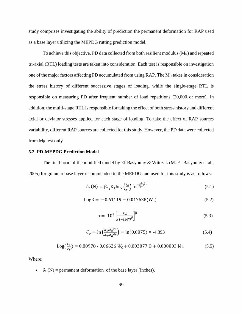
96
study comprises investigating the ability of prediction the permanent deformation for RAP used
as a base layer utilizing the MEPDG rutting prediction model.
To achieve this objective, PD data collected from both resilient modulus (MR) and repeated
tri-axial (RTL) loading tests are taken into consideration. Each test is responsible on investigation
one of the major factors affecting PD accumulated from using RAP. The MR takes in consideration
the stress history of different successive stages of loading, while the single-stage RTL is
responsible on measuring PD after frequent number of load repetitions (20,000 or more). In
addition, the multi-stage RTL is responsible for taking the effect of both stress history and different
axial or deviator stresses applied for each stage of loading. To take the effect of RAP sources
variability, different RAP sources are collected for this study. However, the PD data were collected
from MR test only.
5.2. PD-MEPDG Prediction Model
The final form of the modified model by El-Basyouny & Witczak (M. El-Basyouny et al.,
2005) for granular base layer recommended to the MEPDG and used for this study is as follows:
δa(N) = βs1K1hϵv (
ϵo
ϵr) [e−(
ρ
N)β
] (5.1)
Logβ = −0.61119 − 0.017638(WC) (5.2)
ρ = 109 [Co
(1−(109)β]
1
β (5.3)
𝐶𝑜 = ln (𝑎1𝑀𝑅
𝑏1
𝑎9𝑀𝑅𝑏9
) = ln (0.0075) = -4.893 (5.4)
Log(𝜖𝑜
𝜖𝑟) = 0.80978 - 0.06626 𝑊𝐶+ 0.003077 ϴ + 0.000003 MR (5.5)
Where:
δa (N) = permanent deformation of the base layer (inches).
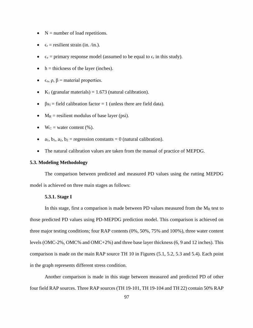
97
N = number of load repetitions.
ϵr = resilient strain (in. /in.).
ϵv = primary response model (assumed to be equal to ϵr in this study).
h = thickness of the layer (inches).
ϵo, ρ, β = material properties.
K1 (granular materials) = 1.673 (natural calibration).
βs1 = field calibration factor = 1 (unless there are field data).
MR = resilient modulus of base layer (psi).
WC = water content (%).
a1, b1, a2, b2 = regression constants = 0 (natural calibration).
The natural calibration values are taken from the manual of practice of MEPDG.
5.3. Modeling Methodology
The comparison between predicted and measured PD values using the rutting MEPDG
model is achieved on three main stages as follows:
5.3.1. Stage I
In this stage, first a comparison is made between PD values measured from the MR test to
those predicted PD values using PD-MEPDG prediction model. This comparison is achieved on
three major testing conditions; four RAP contents (0%, 50%, 75% and 100%), three water content
levels (OMC-2%, OMC% and OMC+2%) and three base layer thickness (6, 9 and 12 inches). This
comparison is made on the main RAP source TH 10 in Figures (5.1, 5.2, 5.3 and 5.4). Each point
in the graph represents different stress condition.
Another comparison is made in this stage between measured and predicted PD of other
four field RAP sources. Three RAP sources (TH 19-101, TH 19-104 and TH 22) contain 50% RAP
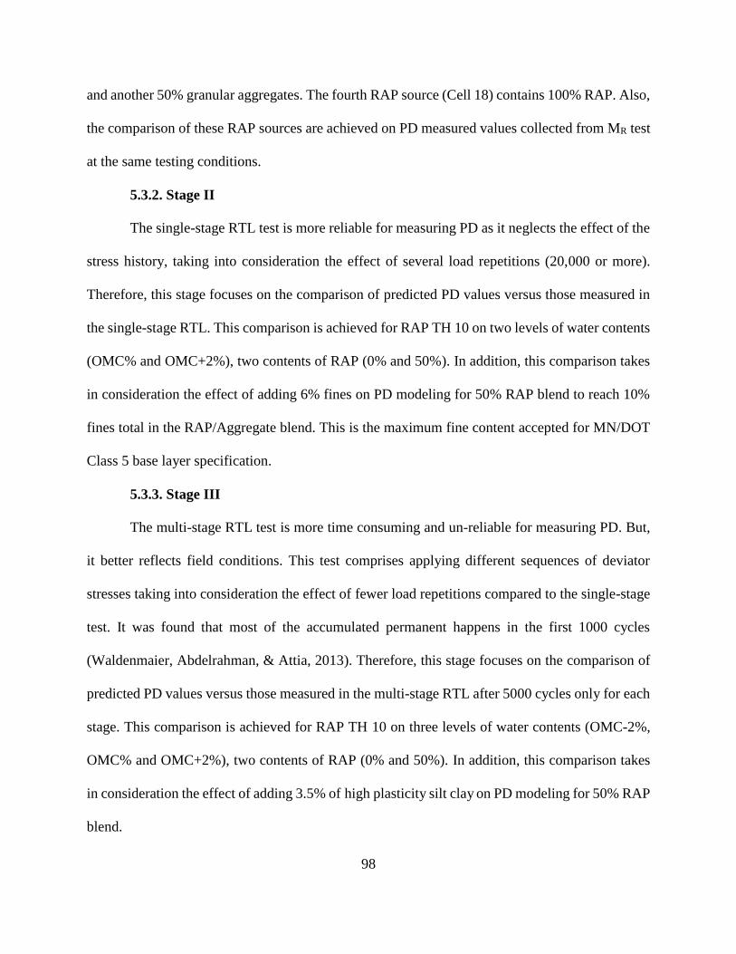
98
and another 50% granular aggregates. The fourth RAP source (Cell 18) contains 100% RAP. Also,
the comparison of these RAP sources are achieved on PD measured values collected from MR test
at the same testing conditions.
5.3.2. Stage II
The single-stage RTL test is more reliable for measuring PD as it neglects the effect of the
stress history, taking into consideration the effect of several load repetitions (20,000 or more).
Therefore, this stage focuses on the comparison of predicted PD values versus those measured in
the single-stage RTL. This comparison is achieved for RAP TH 10 on two levels of water contents
(OMC% and OMC+2%), two contents of RAP (0% and 50%). In addition, this comparison takes
in consideration the effect of adding 6% fines on PD modeling for 50% RAP blend to reach 10%
fines total in the RAP/Aggregate blend. This is the maximum fine content accepted for MN/DOT
Class 5 base layer specification.
5.3.3. Stage III
The multi-stage RTL test is more time consuming and un-reliable for measuring PD. But,
it better reflects field conditions. This test comprises applying different sequences of deviator
stresses taking into consideration the effect of fewer load repetitions compared to the single-stage
test. It was found that most of the accumulated permanent happens in the first 1000 cycles
(Waldenmaier, Abdelrahman, & Attia, 2013). Therefore, this stage focuses on the comparison of
predicted PD values versus those measured in the multi-stage RTL after 5000 cycles only for each
stage. This comparison is achieved for RAP TH 10 on three levels of water contents (OMC-2%,
OMC% and OMC+2%), two contents of RAP (0% and 50%). In addition, this comparison takes
in consideration the effect of adding 3.5% of high plasticity silt clay on PD modeling for 50% RAP
blend.

99
5.4. Analysis of Results
Each stage of work in this task is analyzed separately and compared to the previous stage.
So, this comparison may lead to which test data is more significant for prediction using MEPDG
model. This analysis also compares different RAP sources to show if they have similar relation as
the main source TH 10. It is proved from all stages of work that both measured and predicted PD
values increase with the increase of the base layer thickness. Almost no change is found in the
regression parameter R2 at each thickness (6, 9 and 12 inches) for all testing conditions.
5.4.1. PD from resilient modulus test
It is obvious from Figure 5.1 of Class 5-MN/DOT granular aggregates that increasing the
water content from OMC-2% to OMC+2% results in an increase in the measured PD values. The
largest increase happens between OMC-2% to OMC%. However, it seems that the predicted PD
values at the three water content levels are much lower than the measured values.
It is proved from literature review that this prediction model fits for the granular base
aggregates layer. However, this finding was achieved on data collected from repeated tri-axial
loading test. This result most probably is related to the effect of stress history and low number of
repetitions of the resilient modulus test. Each point on the graph is for each water content level
and only represents the PD accumulated after 100 load repetitions. This number of load repetitions
is much lower compared to those obtained from the RTL test either single (20,000) or multi stage
(5000 per each stage). However, it seems that the variation of both measured and predicted values
have high correlation as R2 values varied from 0.74, 0.78 and 0.87 at OMC+2%, OMC% and
OMC-2% respectively.
After adding 50% RAP to the base layer blend, as shown in Figure 5.2, the measured PD
values slightly decrease than those Class 5 aggregates before adding RAP (Figure 5.1). However,
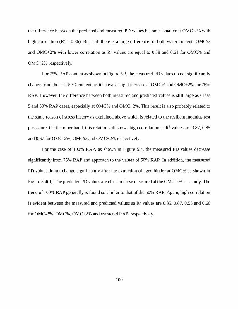
100
the difference between the predicted and measured PD values becomes smaller at OMC-2% with
high correlation (R2 = 0.86). But, still there is a large difference for both water contents OMC%
and OMC+2% with lower correlation as R2 values are equal to 0.58 and 0.61 for OMC% and
OMC+2% respectively.
For 75% RAP content as shown in Figure 5.3, the measured PD values do not significantly
change from those at 50% content, as it shows a slight increase at OMC% and OMC+2% for 75%
RAP. However, the difference between both measured and predicted values is still large as Class
5 and 50% RAP cases, especially at OMC% and OMC+2%. This result is also probably related to
the same reason of stress history as explained above which is related to the resilient modulus test
procedure. On the other hand, this relation still shows high correlation as R2 values are 0.87, 0.85
and 0.67 for OMC-2%, OMC% and OMC+2% respectively.
For the case of 100% RAP, as shown in Figure 5.4, the measured PD values decrease
significantly from 75% RAP and approach to the values of 50% RAP. In addition, the measured
PD values do not change significantly after the extraction of aged binder at OMC% as shown in
Figure 5.4(d). The predicted PD values are close to those measured at the OMC-2% case only. The
trend of 100% RAP generally is found so similar to that of the 50% RAP. Again, high correlation
is evident between the measured and predicted values as R2 values are 0.85, 0.87, 0.55 and 0.66
for OMC-2%, OMC%, OMC+2% and extracted RAP, respectively.

101
Figure 5.1. Measured versus Predicted PD for Class 5 (0% RAP)
R² = 0.8729
0
0.001
0.002
0.003
0.004
0.005
0 0.05 0.1 0.15 0.2 0.25 0.3 0.35 0.4 0.45
Pre
dic
ted P
D (
inches)
Measured PD (inches)
a) WC = OMC-2%
6" Base
9" Base
12" Base
6" Base
9" Base
12" Base
R² = 0.7745
0
0.0005
0.001
0.0015
0.002
0 0.05 0.1 0.15 0.2 0.25 0.3 0.35 0.4 0.45
Pre
dic
ted P
D (
inches)
Measured PD (inches)
b) WC = OMC%
6" Base
9" Base
12" Base
6" Base
9" Base
12" Base
R² = 0.7413
0
4E-10
8E-10
1.2E-09
1.6E-09
0 0.05 0.1 0.15 0.2 0.25 0.3 0.35 0.4 0.45
Pre
dic
ted P
D (
inches)
Measured PD (inches)
c) WC = OMC+2%
6" Base
9" Base
12" Base
6" Base
9" Base
12" Base

102
Figure 5.2. Measured versus Predicted PD for 50% RAP TH 10 + 50% Class 5
R² = 0.8618
0
0.005
0.01
0.015
0.02
0.025
0 0.05 0.1 0.15 0.2 0.25 0.3 0.35 0.4 0.45
Pre
dic
ted P
D (
inches)
Measured PD (inches)
a) WC = OMC-2%
6" Base
9" Base
12" Base
6" Base
9" Base
12" Base
R² = 0.5758
0
0.0004
0.0008
0.0012
0.0016
0 0.05 0.1 0.15 0.2 0.25 0.3 0.35 0.4 0.45
Pre
dic
ted P
D (
inches)
Measured PD (inches)
b) WC = OMC%
6" Base
9" Base
12" Base
6" Base
9" Base
12" Base
R² = 0.6131
0
0.0000002
0.0000004
0.0000006
0.0000008
0.000001
0 0.05 0.1 0.15 0.2 0.25 0.3 0.35 0.4 0.45
Pre
dic
ted P
D (
inches)
Measured PD (inches)
c) WC = OMC+2%
6" Base
9" Base
12" Base
6" Base
9" Base
12" Base
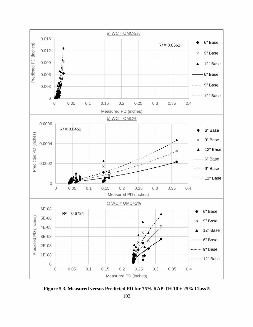
103
Figure 5.3. Measured versus Predicted PD for 75% RAP TH 10 + 25% Class 5
R² = 0.8661
0
0.003
0.006
0.009
0.012
0.015
0 0.05 0.1 0.15 0.2 0.25 0.3 0.35 0.4
Pre
dic
ted P
D (
inches)
Measured PD (inches)
a) WC = OMC-2%
6" Base
9" Base
12" Base
6" Base
9" Base
12" Base
R² = 0.8452
0
0.0002
0.0004
0.0006
0 0.05 0.1 0.15 0.2 0.25 0.3 0.35 0.4
Pre
dic
ted P
D (
inches)
Measured PD (inches)
b) WC = OMC%
6" Base
9" Base
12" Base
6" Base
9" Base
12" Base
R² = 0.6724
0
1E-08
2E-08
3E-08
4E-08
5E-08
6E-08
0 0.05 0.1 0.15 0.2 0.25 0.3 0.35 0.4
Pre
dic
ted P
D (
inches)
Measured PD (inches)
c) WC = OMC+2%
6" Base
9" Base
12" Base
6" Base
9" Base
12" Base
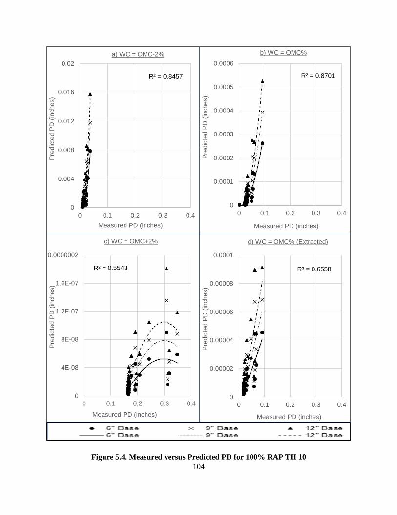
104
Figure 5.4. Measured versus Predicted PD for 100% RAP TH 10
R² = 0.8457
0
0.004
0.008
0.012
0.016
0.02
0 0.1 0.2 0.3 0.4
Pre
dic
ted P
D (
inches)
Measured PD (inches)
a) WC = OMC-2%
R² = 0.8701
0
0.0001
0.0002
0.0003
0.0004
0.0005
0.0006
0 0.1 0.2 0.3 0.4
Pre
dic
ted P
D (
inches)
Measured PD (inches)
b) WC = OMC%
R² = 0.5543
0
4E-08
8E-08
1.2E-07
1.6E-07
0.0000002
0 0.1 0.2 0.3 0.4
Pre
dic
ted P
D (
inches)
Measured PD (inches)
c) WC = OMC+2%
R² = 0.6558
0
0.00002
0.00004
0.00006
0.00008
0.0001
0 0.1 0.2 0.3 0.4
Pre
dic
ted P
D (
inches)
Measured PD (inches)
d) WC = OMC% (Extracted)
105
Then, it can be concluded from the resilient modulus test, that the PD-MEPDG model is
found highly significant in two cases only: 50% and 100% RAP at OMC-2% as predicted values
are so close to those measured. However, the predicted values for the other RAP contents are
significantly less than those measured at different water contents. These results are expect to be
related to the stress history of resilient modulus test procedure used for collecting PD data.
To assure the results collected for the main RAP source (TH 10), other RAP sources are
analyzed in this stage using the same MR testing procedure and same testing conditions. First, the
study begins with the 50% field RAP sources: TH19-101, TH 19-104 and TH 22. For RAP TH 19-
101, as shown in Figure 5.5, similar relation is found as RAP TH 10 for the three studied water
content levels. Still the predicted PD values are much less than measured ones. Nevertheless, the
correlation trend at this case is higher as R2 values vary between 0.75 to 0.92 for OMC+2% and
OMC%, respectively. For RAP TH 19-104, as shown in Figure 5.6, the same trend is found for
both RAP’s TH 10 and TH 19-101. For the three water content levels, the predicted PD values are
far away from the measured ones and the correlation is worse than before as R2 values are 0.49,
0.64 and 0.55 for OMC-2%, OMC% and OMC+2%, respectively.
For RAP TH 22, as shown in Figure 5.7, the trend is almost the same as RAP TH 10. The
predicted values are close to those measured at OMC-2% (Figure 5.7-a) and far away in the other
two water content levels. Expectedly, this behavior is similar to TH 10 and PD measured values
for both RAP’s are so close to each other without a significant difference in MR values too,
especially at OMC-2%. Finally, from comparing the fourth 100% RAP source (Cell 18), as shown
in Figure 5.8, the same trend exists as the other field RAP sources TH 19-101 and TH 19-104. The
predicted PD values are much less than the measured ones with reasonable R2 values of 0.54, 0.83
and 0.91 at OMC-2%, OMC% and OMC+2%, respectively.

106
Figure 5.5. Measured versus Predicted PD for RAP TH 19-101
R² = 0.9016
0
0.003
0.006
0.009
0.012
0 0.05 0.1 0.15 0.2
Pre
dic
ted P
D (
inches)
Measured PD (inches)
a) WC = OMC-2%
6" Base
9" Base
12" Base
6" Base
9" Base
12" Base
R² = 0.915
0
0.00005
0.0001
0.00015
0.0002
0.00025
0 0.05 0.1 0.15 0.2
Pre
dic
ted P
D (
inches)
Measured PD (inches)
b) WC = OMC%
6" Base
9" Base
12" Base
6" Base
9" Base
12" Base
R² = 0.7486
0
2E-08
4E-08
6E-08
8E-08
0 0.05 0.1 0.15 0.2
Pre
dic
ted P
D (
inches)
Measured PD (inches)
c) WC = OMC+2%
6" Base
9" Base
12" Base
6" Base
9" Base
12" Base

107
Figure 5.6. Measured versus Predicted PD for RAP TH 19-104
R² = 0.4928
0
0.0002
0.0004
0.0006
0.0008
0.001
0 0.05 0.1 0.15 0.2 0.25 0.3 0.35 0.4 0.45
Pre
dic
ted P
D (
inches)
Measured PD (inches)
a) WC = OMC-2%
6" Base
9" Base
12" Base
6" Base
9" Base
12" Base
R² = 0.6428
0
0.000001
0.000002
0.000003
0.000004
0.000005
0 0.05 0.1 0.15 0.2 0.25 0.3 0.35 0.4 0.45
Pre
dic
ted P
D (
inches)
Measured PD (inches)
b) WC = OMC%
6" Base
9" Base
12" Base
6" Base
9" Base
12" Base
R² = 0.5461
0
4E-12
8E-12
1.2E-11
1.6E-11
0 0.05 0.1 0.15 0.2 0.25 0.3 0.35 0.4 0.45
Pre
dic
ted P
D (
inches)
Measured PD (inches)
c) WC = OMC+2%
6" Base
9" Base
12" Base
6" Base
9" Base
12" Base

108
Figure 5.7. Measured versus Predicted PD for RAP TH 22
R² = 0.8629
0
0.005
0.01
0.015
0.02
0.025
0 0.03 0.06 0.09 0.12 0.15 0.18
Pre
dic
ted P
D (
inches)
Measured PD (inches)
a) WC = OMC-2%
6" Base
9" Base
12" Base
6" Base
9" Base
12" Base
R² = 0.6648
0
0.0001
0.0002
0.0003
0.0004
0.0005
0.0006
0 0.03 0.06 0.09 0.12 0.15 0.18
Pre
dic
ted P
D (
inches)
Measured PD (inches)
b) WC = OMC%
6" Base
9" Base
12" Base
6" Base
9" Base
12" Base
R² = 0.5635
0
0.0000002
0.0000004
0.0000006
0.0000008
0 0.03 0.06 0.09 0.12 0.15 0.18
Pre
dic
ted P
D (
inches)
Measured PD (inches)
c) WC = OMC+2%
6" Base
9" Base
12" Base
6" Base
9" Base
12" Base
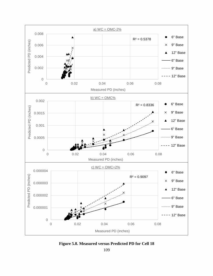
109
Figure 5.8. Measured versus Predicted PD for Cell 18
R² = 0.8336
0
0.0005
0.001
0.0015
0.002
0 0.02 0.04 0.06 0.08
Pre
dic
ted P
D (
inches)
Measured PD (inches)
b) WC = OMC%
6" Base
9" Base
12" Base
6" Base
9" Base
12" Base
R² = 0.5378
0
0.002
0.004
0.006
0.008
0 0.02 0.04 0.06 0.08
Pre
dic
ted P
D (
inches)
Measured PD (inches)
a) WC = OMC-2%
6" Base
9" Base
12" Base
6" Base
9" Base
12" Base
R² = 0.9097
0
0.000001
0.000002
0.000003
0.000004
0 0.02 0.04 0.06 0.08
Pre
dic
ted P
D (
inches)
Measured PD (inches)
c) WC = OMC+2%
6" Base
9" Base
12" Base
6" Base
9" Base
12" Base

110
Therefore, all of the field RAP sources studied using the PD data collected from MR test in
this stage have the same insignificant prediction trend of RAP TH 10 with more similarity with
RAP TH 22. Generally, the PD predicted values are much lower than the measured values at
different testing conditions such as RAP content and water content level. This result is due to the
low load repetitions (100 cycles) applied in each sequence and the effect of stress history from
successive sequences of loading. Both RAP’s TH 10 and TH 22, are the only sources that give a
significant prediction but at OMC-2% water content only. The RAP content for both RAP sources
is 50% mixed with another 50% traditional granular aggregate sources. Regression analysis from
comparing predicted and measured PD values gives high correlation. However, it does not give an
accurate prediction of PD as MR test proved that it cannot be used in measuring PD during the 30
sequences of loading of the test due to the stress history.
5.4.2. Single-stage RTL test
In this stage, a single-stage repeated tri-axial loading (RTL) test procedure is followed.
This test is the typical or standard technique used to measure permanent deformation for granular
base layer. This test procedure can measure the PD accumulated in the sample after high number
of load repetitions (20,000 or more) expected from traffic loads. The multi-stage test is another
type of this RTL technique. However, the single-stage test has the advantage of not including the
effect of the stress history of previous stages. Therefore, it is expected to find accurate prediction
of PD values when using this model for single-stage RTL test data.
In Figure 5.9, prediction of PD is achieved on Class 5 aggregates before adding RAP. A
comparison is made between measured and predicted PD. This comparison is achieved at two
water content levels; OMC% & OMC+2% and two levels of deviator stress (σd); 17 & 24 psi for
OMC% content and 12 & 17 psi for OMC+2% content. As shown in Figure (5.9-a), the PD

111
predicted values are very accurate and close to the measured ones. However, by increasing the
deviator stress level to 24 psi (Figure 5.9-b), the accuracy becomes weaker, as the predicted values
are lower than those measured. By increasing the water content level at both deviator stress levels
(12 and 17 psi), the prediction accuracy is still weak. But, from the high regression parameter R2
for all testing conditions for this Class 5 aggregates, the MEPDG model is still quietly efficient for
PD prediction.
Both Figures 5.10 and 5.11, show the comparison between predicted and measured PD
values for 50% RAP TH10 blends with Class 5 at OMC% and OMC+2%, respectively. At OMC%
(Figure 5.10), the comparison is achieved at three deviator stress levels; 17, 24 and 37 psi. At both
deviator stress levels 17 and 37 psi, the prediction accuracy is relatively high as the PD predicted
values are too close to the measured ones. However, the accuracy decreased slightly for the 24 psi
deviator stress level. But for this case, the predicted values are higher than the measured ones. At
OMC+2% (Figure 5.11), the comparison is achieved at two deviator stress levels; 12 and 17 psi.
The prediction accuracy decreases significantly especially at 17 psi. Generally, the PD prediction
accuracy for the 50% RAP TH10 blend is significantly high and even better than the previous case
for Class 5 aggregates tested with the same procedure single-stage RTL test.
The same comparison of 50% RAP is repeated again in Figure 5.12 but with the addition
of 6% fines. This percent of fines is selected to reach 10% (maximum allowable fine content for
base layer) to investigate its effectiveness on the PD accumulated. The comparison is achieved at
two deviator stress levels 17 & 24 psi for OMC% and 12 & 17 psi for OMC+2%. Results indicate
that addition of fines increase PD values. The prediction for these samples decrease slightly
especially at OMC+2%. Generally, the prediction is under-estimating the PD values. Contrary, the
predicted values are over-estimated at OMC% with the 17 psi deviator stress.
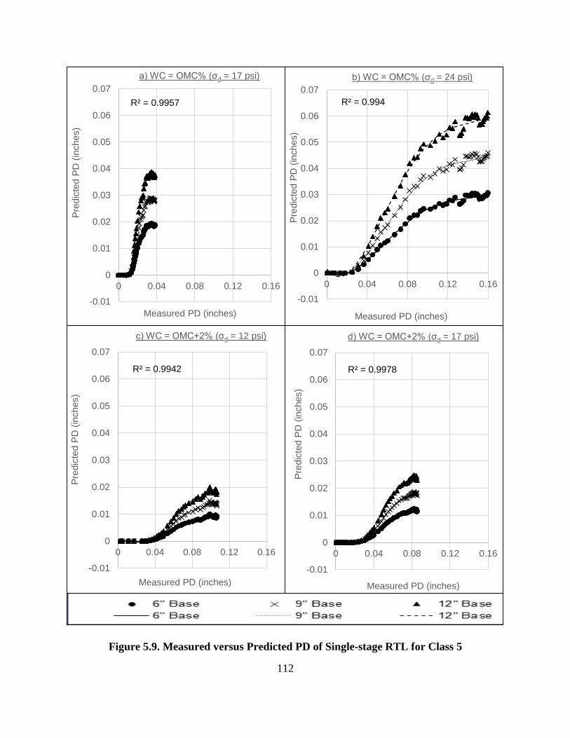
112
Figure 5.9. Measured versus Predicted PD of Single-stage RTL for Class 5
R² = 0.9957
-0.01
0
0.01
0.02
0.03
0.04
0.05
0.06
0.07
0 0.04 0.08 0.12 0.16
Pre
dic
ted P
D (
inches)
Measured PD (inches)
a) WC = OMC% (σd = 17 psi)
R² = 0.994
-0.01
0
0.01
0.02
0.03
0.04
0.05
0.06
0.07
0 0.04 0.08 0.12 0.16P
redic
ted P
D (
inches)
Measured PD (inches)
b) WC = OMC% (σd = 24 psi)
R² = 0.9942
-0.01
0
0.01
0.02
0.03
0.04
0.05
0.06
0.07
0 0.04 0.08 0.12 0.16
Pre
dic
ted P
D (
inches)
Measured PD (inches)
c) WC = OMC+2% (σd = 12 psi)
R² = 0.9978
-0.01
0
0.01
0.02
0.03
0.04
0.05
0.06
0.07
0 0.04 0.08 0.12 0.16
Pre
dic
ted P
D (
inches)
Measured PD (inches)
d) WC = OMC+2% (σd = 17 psi)

113
Figure 5.10. Measured versus Predicted PD of Single-stage RTL for 50% RAP TH 10 +
50% Class 5 at OMC%
R² = 0.955
-0.02
0
0.02
0.04
0.06
0.08
0.1
0 0.01 0.02 0.03 0.04 0.05 0.06
Pre
dic
ted P
D (
inches)
Measured PD (inches)
c) WC = OMC% (σd = 37 psi)
6" Base
9" Base
12" Base
6" Base
9" Base
12" Base
R² = 0.9875
-0.02
0
0.02
0.04
0.06
0.08
0.1
0 0.01 0.02 0.03 0.04 0.05 0.06
Pre
dic
ted P
D (
inches)
Measured PD (inches)
a) WC = OMC% (σd = 17 psi)
6" Base
9" Base
12" Base
6" Base
9" Base
12" Base
R² = 0.9824
-0.02
0
0.02
0.04
0.06
0.08
0.1
0 0.01 0.02 0.03 0.04 0.05 0.06
Pre
dic
ted P
D (
inches)
Measured PD (inches)
b) WC = OMC% (σd = 24 psi)
6" Base
9" Base
12" Base
6" Base
9" Base
12" Base
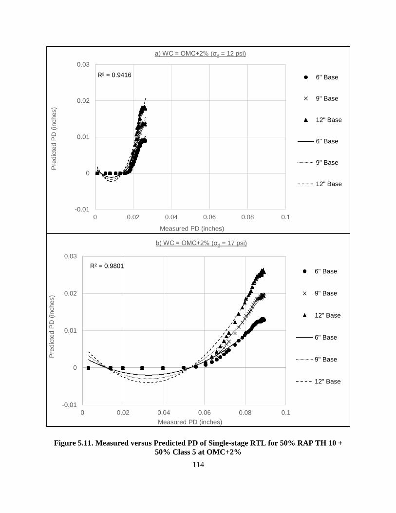
114
Figure 5.11. Measured versus Predicted PD of Single-stage RTL for 50% RAP TH 10 +
50% Class 5 at OMC+2%
R² = 0.9416
-0.01
0
0.01
0.02
0.03
0 0.02 0.04 0.06 0.08 0.1
Pre
dic
ted P
D (
inches)
Measured PD (inches)
a) WC = OMC+2% (σd = 12 psi)
6" Base
9" Base
12" Base
6" Base
9" Base
12" Base
R² = 0.9801
-0.01
0
0.01
0.02
0.03
0 0.02 0.04 0.06 0.08 0.1
Pre
dic
ted P
D (
inches)
Measured PD (inches)
b) WC = OMC+2% (σd = 17 psi)
6" Base
9" Base
12" Base
6" Base
9" Base
12" Base
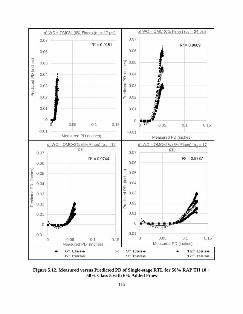
115
Figure 5.12. Measured versus Predicted PD of Single-stage RTL for 50% RAP TH 10 +
50% Class 5 with 6% Added Fines
R² = 0.9151
-0.01
0
0.01
0.02
0.03
0.04
0.05
0.06
0.07
0 0.05 0.1 0.15
Pre
dic
ted P
D (
inches)
Measured PD (inches)
a) WC = OMC% (6% Fines) (σd = 17 psi)
R² = 0.9689
-0.01
0
0.01
0.02
0.03
0.04
0.05
0.06
0.07
0 0.05 0.1 0.15P
redic
ted P
D
(inches)
Measured PD (inches)
b) WC = OMC (6% Fines) (σd = 24 psi)
R² = 0.9744
-0.01
0
0.01
0.02
0.03
0.04
0.05
0.06
0.07
0 0.05 0.1 0.15
Pre
dic
ted P
D
(inches)
Measured PD (inches)
c) WC = OMC+2% (6% Fines) (σd = 12 psi)
R² = 0.9737
-0.01
0
0.01
0.02
0.03
0.04
0.05
0.06
0.07
0 0.05 0.1 0.15
Pre
dic
ted P
D
(inches)
Measured PD (inches)
d) WC = OMC+2% (6% Fines) (σd = 17 psi)

116
Finally, the PD-MEPDG model seems better than the resilient modulus test in terms of
predicting PD for data collected from single-stage RTL test. It is highly significant for the case of
using RAP in base layer blends as shown in 50% RAP samples. However, there is a need to achieve
this model on test data collected from multi-stage RTL for RAP samples used as a base layer taking
in consideration the effect of stress history as MR test. This high accurate prediction is found also
for Class 5 granular aggregate in OMC% at 17 psi deviator stress level. Best results of the high
accuracy of the PD prediction is shown in 50% RAP blend at OMC% water content level under
17 and 37 psi deviator stress levels. By adding 6% fines to the 50% RAP blend, the prediction
accuracy is affected significantly. As the prediction under-estimates the PD values except at
OMC% under 17 psi deviator stress level it is overestimated.
5.4.3. Multi-stage RTL test
In this stage, a comparison also is made between measured and predicted PD values for
data collected from multi-stage RTL test. This test is more reflecting the field situation by applying
different deviator stresses for each stage of loading for 5000 loading cycles. Nevertheless, it has
the same problem of stress history as MR test coming from the previous loading stages. This
comparison is achieved at three water contents: OMC-2%, OMC% and OMC+2% for Class 5,
50% RAP TH 10 + 50% Class 5 and 50% RAP case with 3.5% high plasticity clay fines. This fine
content and type are chosen to avoid the problem of PD increase, while at the same time gains the
advantage of MR increase. From the comparison in Class 5, as shown in Figure 5.13, for all water
content levels, the measured PD values are much higher than the predicted PD values at all deviator
stress levels. However, all R2 values are high exceeding 0.9 and approaching to 1 as shown in
Table 5.1. This model is not accurate in predicting PD values for granular base layer for measured
data from multi-stage RTL test.
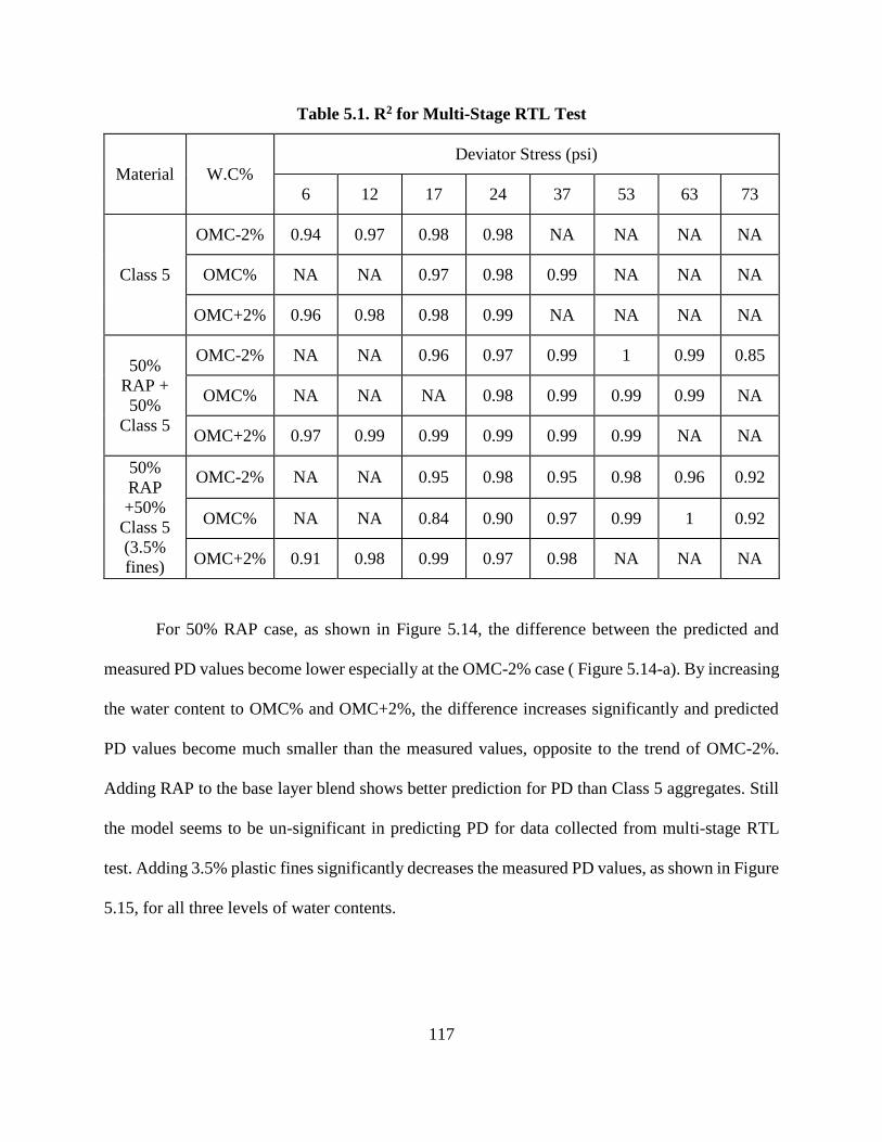
117
Table 5.1. R2 for Multi-Stage RTL Test
For 50% RAP case, as shown in Figure 5.14, the difference between the predicted and
measured PD values become lower especially at the OMC-2% case ( Figure 5.14-a). By increasing
the water content to OMC% and OMC+2%, the difference increases significantly and predicted
PD values become much smaller than the measured values, opposite to the trend of OMC-2%.
Adding RAP to the base layer blend shows better prediction for PD than Class 5 aggregates. Still
the model seems to be un-significant in predicting PD for data collected from multi-stage RTL
test. Adding 3.5% plastic fines significantly decreases the measured PD values, as shown in Figure
5.15, for all three levels of water contents.
Material W.C%
Deviator Stress (psi)
6 12 17 24 37 53 63 73
Class 5
OMC-2% 0.94 0.97 0.98 0.98 NA NA NA NA
OMC% NA NA 0.97 0.98 0.99 NA NA NA
OMC+2% 0.96 0.98 0.98 0.99 NA NA NA NA
50%
RAP +
50%
Class 5
OMC-2% NA NA 0.96 0.97 0.99 1 0.99 0.85
OMC% NA NA NA 0.98 0.99 0.99 0.99 NA
OMC+2% 0.97 0.99 0.99 0.99 0.99 0.99 NA NA
50%
RAP
+50%
Class 5
(3.5%
fines)
OMC-2% NA NA 0.95 0.98 0.95 0.98 0.96 0.92
OMC% NA NA 0.84 0.90 0.97 0.99 1 0.92
OMC+2% 0.91 0.98 0.99 0.97 0.98 NA NA NA

118
Figure 5.13. Measured versus Predicted PD of Multi-stage RTL for Class 5
-0.02
0
0.02
0.04
0.06
0.08
0.1
0 0.1 0.2 0.3 0.4
Pre
dic
ted P
D (
inches)
Measured PD (inches)
b) WC = OMC%
17 psi
24 psi
37 psi
17 psi
24 psi
37 psi
-0.02
0
0.02
0.04
0.06
0.08
0.1
0 0.1 0.2 0.3 0.4
Pre
dic
ted P
D (
inches)
Measured PD (inches)
c) WC = OMC+2%
6 psi
12 psi
17 psi
24 psi
6 psi
12 psi
17 psi
24 psi
-0.02
0
0.02
0.04
0.06
0.08
0.1
0 0.1 0.2 0.3 0.4
Pre
dic
ted P
D (
inches)
Measured PD (inches)
a) WC = OMC-2%
6 psi
12 psi
17 psi
24 psi
6 psi
12 psi
17 psi
24 psi

119
Figure 5.14. Measured versus Predicted PD of Multi-stage RTL for 50% RAP TH 10
+ 50% Class 5
0
0.05
0.1
0.15
0.2
0.25
0.3
0 0.1 0.2 0.3 0.4 0.5
Pre
dic
ted P
D (
inches)
Measured PD (inches)
a) WC = OMC-2% 17 psi
24 psi
37 psi
53 psi
63 psi
73 psi
17 psi
24 psi
37 psi
53 psi
63 psi
73 psi
0
0.05
0.1
0.15
0.2
0.25
0.3
0 0.1 0.2 0.3 0.4 0.5
Pre
dic
ted P
D (
inches)
Measured PD (inches)
b) WC = OMC%
24 psi
37 psi
53 psi
63 psi
24 psi
37 psi
53 psi
63 psi
0
0.05
0.1
0.15
0.2
0.25
0.3
0 0.1 0.2 0.3 0.4 0.5
Pre
dic
ted P
D (
inches)
Measured PD (inches)
c) WC = OMC+2% 6 psi
12 psi
17 psi
24 psi
37 psi
53 psi
6 psi
12 psi
17 psi
24 psi
37 psi
53 psi
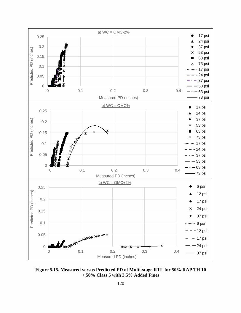
120
Figure 5.15. Measured versus Predicted PD of Multi-stage RTL for 50% RAP TH 10
+ 50% Class 5 with 3.5% Added Fines
0
0.05
0.1
0.15
0.2
0.25
0 0.1 0.2 0.3 0.4
Pre
dic
ted P
D (
inches)
Measured PD (inches)
a) WC = OMC-2% 17 psi
24 psi
37 psi
53 psi
63 psi
73 psi
17 psi
24 psi
37 psi
53 psi
63 psi
73 psi
0
0.05
0.1
0.15
0.2
0.25
0 0.1 0.2 0.3 0.4
Pre
dic
ted P
D (
inches)
Measured PD (inches)
b) WC = OMC% 17 psi
24 psi
37 psi
53 psi
63 psi
73 psi
17 psi
24 psi
37 psi
53 psi
63 psi
73 psi
0
0.05
0.1
0.15
0.2
0.25
0 0.1 0.2 0.3 0.4
Pre
dic
ted P
D (
inches)
Measured PD (inches)
c) WC = OMC+2%6 psi
12 psi
17 psi
24 psi
37 psi
6 psi
12 psi
17 psi
24 psi
37 psi
121
This result is expected from the literature survey results on the effect of adding clay on PD
for base layer in general. In addition, the predicted PD values become too close to the measured
ones only in the OMC% case. Nevertheless, by changing the water contents to the other two levels
OMC-2% and OMC%, the difference between predicted and measured PD values significantly
increases. In the OMC-2%, the model is over-estimating PD significantly, while in OMC+2% the
model is underestimating the PD significantly.
Finally, it is obvious that PD-MEPDG model is significant in prediction for the measured
PD data by single-stage RTL test only while very un-significant for the other two tests, MR and
multi-stage RTL tests. This finding is attributed to the effect of the stress history from applying
successive stages of loading on base layer blends in both tests. The model is highly accurate for
single-stage RTL test at water contents close to OMC% and at deviator stresses lower than 24 psi.
5.5. PD Modeling Task Summary
Several points are concluded from prediction of permanent deformation for RAP using the
rutting MEPDG for the two measured laboratory data sets included in this task. It can be concluded
from the resilient modulus test, that the PD-MEPDG model is found highly significant in two cases
only: 50% and 100% RAP at OMC-2% as predicted values are so close to those measured.
However, the predicted values for the other RAP contents are significantly less than those
measured at different water contents. These results are expect to be related to the stress history of
resilient modulus test procedure used for collecting PD data. All of the field RAP sources studied
using the PD data collected from MR test in this task have the same insignificant prediction trend
of RAP TH 10 with more similarity with RAP TH 22. Generally, the PD predicted values are much
lower than the measured values at different testing conditions such as RAP content and water
content level. This result is due to the low load repetitions (100 cycles) applied in each sequence
122
and the effect of stress history from successive sequences of loading. Both RAP’s TH 10 and TH
22, are the only sources that give a significant prediction but at OMC-2% water content only. The
RAP content for both RAP sources is 50% mixed with another 50% traditional granular aggregate
sources. Regression analysis from comparing predicted and measured PD values gives high
correlation. However, it does not give an accurate prediction of PD.
For the single-stage RTL testing, the PD-MEPDG model seems better than the resilient
modulus test in terms of predicting PD for data collected from single-stage RTL test. It is highly
significant for the case of using RAP in base layer blends as shown in 50% RAP samples.
However, same insignificance is found for this model on test data collected from multi-stage RTL
for RAP samples used as a base layer due to the effect of stress history as MR test. This high
accurate prediction is found also for Class 5 granular aggregate in OMC% at 17 psi deviator stress
level. Best results of the high accuracy of the PD prediction is shown in 50% RAP blend at OMC%
water content level under 17 and 37 psi deviator stress levels. By adding 6% fines to the 50% RAP
blend, the prediction accuracy is affected significantly. As the prediction under-estimates the PD
values except at OMC% under 17 psi deviator stress level it is overestimated.
Finally, it is found from this task that the PD-MEPDG model is statistically significant in
prediction PD compared to the measured PD values from the single-stage RTL test especially at
OMC% condition with different stress levels. While the predicted PD values are much below the
corresponding measured PD values from the resilient modulus and multi-stage RTL tests due to
the effect of stress history from subsequent sequences or stages of loading.
123
CHAPTER 6. CORRELTION OF RESILIENT MODULUS AND
PERMANENT DEFORMATION
6.1. Introduction
Previous researches summarized in the literature survey on RAP used as a base layer
concluded that no exact optimum content of RAP to be in the granular blend. The previous results
showed that increasing RAP content in granular layer blends, leads to increased MR values.
However PD results were different. Both parameters MR and PD, are very important in the design
process of the base layer and choosing the optimum RAP content. MR is the responsible parameter
of estimating the stiffness of the base layer blend under repetitive loads. The PD represents the
accumulation of the permanent strain that happens in the base layer and participates in the rutting
distress that will occur in the top asphalt layer.
Therefore, there is a need to correlate between both parameters under the most expected
field conditions that could happen for base layer. Previous studies concluded that the state of
stresses is the most effective parameter on the strength of the base layer. The moisture content
variation was the second main effective parameter. In addition, this MR-PD correlation was never
studied before assuming MR as the response of base layer blend and PD as an effective parameter
on MR values under the variation of different testing conditions. Therefore, correlating between
these two parameters is highly required to study RAP behavior in base layer. The study focuses on
the effect of main parameters on MR, including accumulated permanent deformation after several
load cycles responsible of rutting of the whole pavement section.
6.2. Correlation Approach
This task focuses on studying MR-PD relationship for different sources of RAP used as a
base layer under the variable confining pressure, moisture content and RAP contents. The
124
confining pressure is the most effective state of stresses on the structural behavior of the base layer.
Firstly, this relation is important to be investigate in terms of how the PD affects MR values under
the variable testing conditions mentioned above. In addition, this task shall indicate whether a
typical relation for the MR-PD behavior is understood or not for the RAP in base layer. Secondly,
this task aims at deciding the optimum RAP content, which has the highest MR values with
acceptable PD percentage not causing rutting in the future. Finally, it is important to recommend
if the PD can be used as an effective parameter in MR modeling or not. This approach is followed
in the mechanistic empirical pavement design guide (MEPDG) (Guide, 2008). As the resilient
strain is used as an effective parameter in PD modeling for granular base layer, while the
permanent strain is not used in MR modeling for the same layer.
6.3. Stages of Work
The first stage of this task is concerned with PD accumulated from the resilient modulus
determination test. The PD is calculated as a percentage of the accumulated permanent strain from
the total strain for the sample tested during MR determination. Almost all other previous studies,
measure PD by performing the repeated tri-axial loading (RTL) test either single or multiple stage
as a separate test. However, this test was found very time consuming to cover all data previously
measured for MR through the project with MN/DOT (M. Attia et al., 2009). Firstly, the comparison
between MR and PD is achieved on the main RAP source (TH 10). The comparison is achieved at
three levels of water content varying from optimum moisture content (OMC %); OMC-2%,
OMC% and OMC+2%. This comparison comprised different levels of confining pressure which
is well-known before as the most effective parameter on MR. Each point on the same graph has a
different percent of RAP (0, 50, 75 and 100%) in the blend with MN/DOT Class 5 granular
aggregates. This aggregates type is used traditionally before as unbound granular base layer. The
125
comparison for this RAP source is divided into two steps. The first is under same confining
pressure level (Figure 6.1) and the second under the same RAP content (Figure 6.2). Therefore,
each factor is individually studied for each moisture content. For each condition in both steps,
there is a best-fit regression to compare R2 values.
It is important to achieve the comparison between MR and PD on different RAP sources to
take into consideration the RAP variability factor, one of the main problems facing the reuse of
RAP as a base layer. Therefore, the data of the other four different RAP sources tested in MN/DOT
project (M. Attia et al., 2009) are collected for this research in addition to the main source TH 10.
These RAP sources are analyzed under the same testing conditions discussed before. Three from
those four RAP samples (TH 19-101, TH 19-104 and TH 22) are collected from the field
containing 50% RAP and 50% granular aggregates, as shown in Figure 6.3.
The first number refers to the truck highway number in Minnesota and the second number
refers to the mileage station in each road. The fourth RAP source consists of 100% RAP collected
from Cell 18 (Minnesota Destination) as shown in Figure 6.4. All four RAP sources are compared
with TH 10 (main RAP source) at the equivalent percentage, 50% RAP (Figure 6.3) or 100%
(Figure 6.4). This approach is followed to avoid the problem of different gradations, which may
have effect on both measured parameters MR and PD. For both Figures 6.3 and 6.4, each point on
the graph is for a different confining pressure level (3, 6, 10, 15 and 20 psi). Also, for each RAP
in both figures there is a best-fit regression to compare between R2 values.
In the second stage, the comparison is achieved on PD results collected from the single-
stage RTL for Class 5 and 50% RAP TH 10 + 50% Class 5. The analysis of this stage is shown in
two figures (6.5 and 6.6) with an emphasis on stabilizing the 50% RAP sample with adding plastic
fines. Figure 6.5 is for both blends at OMC% and Figure 6.6 is for both blends at OMC+2%. In

126
the third and last stage of this task, MR-PD comparison is achieved on PD values collected from
multi-stage RTL for the same samples tested before in the previous stage. Figure 6.7 is for the
Class 5 aggregates and Figure 6.8 is for 50% RAP TH 10 + 50% Class 5 blends and Figure 6.9 for
50% RAP blend with added fines. Therefore, finally the work performed in this task is divided
into three main stages. The first stage is achieved on five different RAP sources collected and
tested before in previous researches. On the other hand, both second and third stages are performed
on the main RAP source TH 10 with its blends with MN/DOT Class 5 granular aggregates.
6.4. Analysis of Results
6.4.1 Resilient modulus test
Firstly, the comparison between MR and PD is achieved on RAP TH 10, as shown in
Figures 6.1 and 6.2. In Figure 6.1, the comparison is accomplished at different confining pressure
levels and each point on the same graph has a different content of RAP (0, 50, 75 and 100%) in
the blend with Class 5 aggregates. On the other hand in Figure 6.2, the comparison is performed
at different RAP concentrations and the relation is reversed as each point on the same graph has a
different confining pressure level (3, 6, 10, 15 and 20 psi). The regression values R2 for both figures
are shown in Table 6.1.
From Figure 6.1, there is an obvious relation that appears at OMC% (Figure 6.1-b), as MR
decreases by increasing PD until a certain point for all confining pressure levels, except at 20 psi
which has the opposite relation. This certain point at 0% RAP blends for 3, 6, 10 and 15 confining
pressure (C.P). However, for 20 psi the highest point at 100% RAP. This relation shows that as
the percentage of RAP exceeds 50%, MR increases and PD decreases, a result that may be
recommended for base layer design considerations. Also, this relation works well on confining
pressure levels less than 15 psi with highest correlation R2.

127
By decreasing the moisture level to OMC-2% (Figure 6.1-a), as may be expected, MR
values generally increase and PD decrease. On the other hand, the typical relation found before at
OMC% almost disappears from most of confining pressure levels except at 3 psi. In addition, PD
increases when RAP content increases and MR does not markedly increase after exceeding 75%
RAP for all confining pressure levels, except for 20 psi. By increasing the moisture level to
OMC+2% (Figure 6.1-c), generally MR values decrease and PD increase approaching the failure
limit 5% accumulated PD (M. I. E.-S. Attia, 2010), which is also expected. The typical relation for
OMC% also disappears except at 6 psi confining pressure level with the highest correlation (R2 =
0.71). But, the only exception at this moisture level is that the PD values at 75% RAP are higher
than those at 50% and 100% RAP.
For the same data analyzed before in Figure 6.1, but at different RAP contents as in Figure
6.2, it is obvious at OMC% (Figure 6.2-b) that both 100% and extracted (without aged binder)
RAP’s have the highest MR and lowest PD values with higher correlation to 100% RAP (R2 =
0.92). The removal of aged binder affected MR negatively and the effect on PD was minimal. For
other RAP contents, MR has lowest values at 3 and 6 psi, and increases with the increase of
confining pressure levels with high contribution on PD at 20 psi. By decreasing the moisture level
to OMC-2% (Figure 6.2-a), the relation is more clear with high correlation and close to the trend
of 100% RAP at OMC%, MR increases with increasing confining pressure levels and PD also
increases. On the other hand, by increasing the moisture level to OMC+2% (Figure 6.2-c), the
relation is not clear and the correlation is too weak. Both 50% and 100% RAP blends have the
highest MR and lowest PD values.

128
Figure 6.1. MR versus PD for RAP TH 10 at Several Confining Pressure Levels
0
30
60
90
120
150
0 0.5 1 1.5 2
MR
(ksi)
PD %
b) WC = OMC%3 psi
6 psi
10 psi
15 psi
20 psi
3 psi
6 psi
10 psi
15 psi
20 psi
0
50
100
150
200
0 0.1 0.2 0.3 0.4 0.5
MR
(ksi)
PD %
a) WC = OMC-2%
3 psi
6 psi
10 psi
15 psi
20 psi
3 psi
6 psi
10 psi
15 psi
20 psi
0
20
40
60
80
100
2.5 3 3.5 4 4.5
MR
(ksi)
PD %
c) WC = OMC+2%3 psi
6 psi
10 psi
15 psi
20 psi
3 psi
6 psi
10 psi
15 psi
20 psi
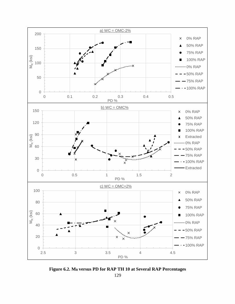
129
Figure 6.2. MR versus PD for RAP TH 10 at Several RAP Percentages
0
50
100
150
200
0 0.1 0.2 0.3 0.4 0.5
MR
(ksi)
PD %
a) WC = OMC-2%
0% RAP
50% RAP
75% RAP
100% RAP
0% RAP
50% RAP
75% RAP
100% RAP
0
30
60
90
120
150
0 0.5 1 1.5 2
MR
(ksi)
PD %
b) WC = OMC%0% RAP
50% RAP
75% RAP
100% RAP
Extracted
0% RAP
50% RAP
75% RAP
100% RAP
Extracted
0
20
40
60
80
100
2.5 3 3.5 4 4.5
MR
(ksi)
PD %
c) WC = OMC+2%
0% RAP
50% RAP
75% RAP
100% RAP
0% RAP
50% RAP
75% RAP
100% RAP
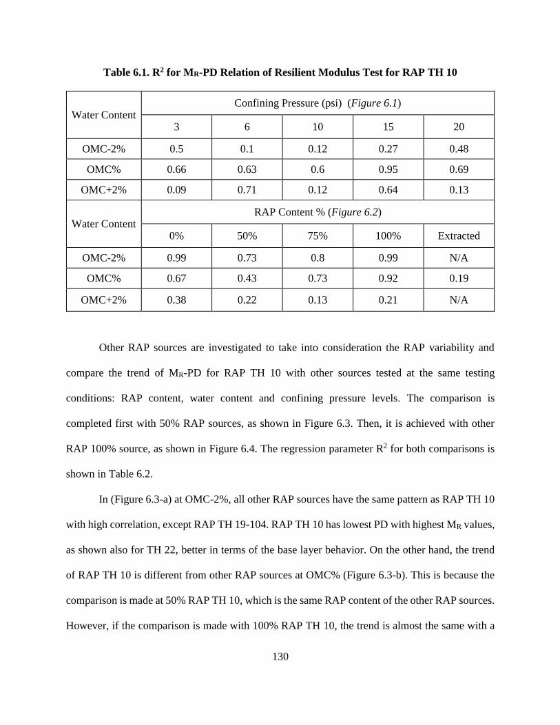
130
Table 6.1. R2 for MR-PD Relation of Resilient Modulus Test for RAP TH 10
Other RAP sources are investigated to take into consideration the RAP variability and
compare the trend of MR-PD for RAP TH 10 with other sources tested at the same testing
conditions: RAP content, water content and confining pressure levels. The comparison is
completed first with 50% RAP sources, as shown in Figure 6.3. Then, it is achieved with other
RAP 100% source, as shown in Figure 6.4. The regression parameter R2 for both comparisons is
shown in Table 6.2.
In (Figure 6.3-a) at OMC-2%, all other RAP sources have the same pattern as RAP TH 10
with high correlation, except RAP TH 19-104. RAP TH 10 has lowest PD with highest MR values,
as shown also for TH 22, better in terms of the base layer behavior. On the other hand, the trend
of RAP TH 10 is different from other RAP sources at OMC% (Figure 6.3-b). This is because the
comparison is made at 50% RAP TH 10, which is the same RAP content of the other RAP sources.
However, if the comparison is made with 100% RAP TH 10, the trend is almost the same with a
Water Content Confining Pressure (psi) (Figure 6.1)
3 6 10 15 20
OMC-2% 0.5 0.1 0.12 0.27 0.48
OMC% 0.66 0.63 0.6 0.95 0.69
OMC+2% 0.09 0.71 0.12 0.64 0.13
Water Content RAP Content % (Figure 6.2)
0% 50% 75% 100% Extracted
OMC-2% 0.99 0.73 0.8 0.99 N/A
OMC% 0.67 0.43 0.73 0.92 0.19
OMC+2% 0.38 0.22 0.13 0.21 N/A
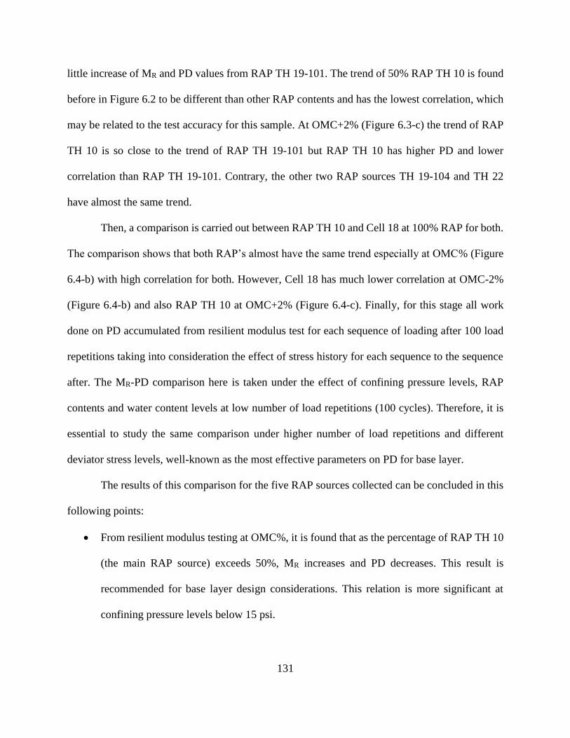
131
little increase of MR and PD values from RAP TH 19-101. The trend of 50% RAP TH 10 is found
before in Figure 6.2 to be different than other RAP contents and has the lowest correlation, which
may be related to the test accuracy for this sample. At OMC+2% (Figure 6.3-c) the trend of RAP
TH 10 is so close to the trend of RAP TH 19-101 but RAP TH 10 has higher PD and lower
correlation than RAP TH 19-101. Contrary, the other two RAP sources TH 19-104 and TH 22
have almost the same trend.
Then, a comparison is carried out between RAP TH 10 and Cell 18 at 100% RAP for both.
The comparison shows that both RAP’s almost have the same trend especially at OMC% (Figure
6.4-b) with high correlation for both. However, Cell 18 has much lower correlation at OMC-2%
(Figure 6.4-b) and also RAP TH 10 at OMC+2% (Figure 6.4-c). Finally, for this stage all work
done on PD accumulated from resilient modulus test for each sequence of loading after 100 load
repetitions taking into consideration the effect of stress history for each sequence to the sequence
after. The MR-PD comparison here is taken under the effect of confining pressure levels, RAP
contents and water content levels at low number of load repetitions (100 cycles). Therefore, it is
essential to study the same comparison under higher number of load repetitions and different
deviator stress levels, well-known as the most effective parameters on PD for base layer.
The results of this comparison for the five RAP sources collected can be concluded in this
following points:
From resilient modulus testing at OMC%, it is found that as the percentage of RAP TH 10
(the main RAP source) exceeds 50%, MR increases and PD decreases. This result is
recommended for base layer design considerations. This relation is more significant at
confining pressure levels below 15 psi.
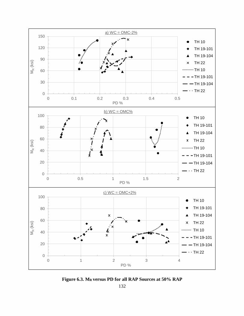
132
Figure 6.3. MR versus PD for all RAP Sources at 50% RAP
0
30
60
90
120
150
0 0.1 0.2 0.3 0.4 0.5
MR
(ksi)
PD %
a) WC = OMC-2%
TH 10
TH 19-101
TH 19-104
TH 22
TH 10
TH 19-101
TH 19-104
TH 22
0
20
40
60
80
100
0 0.5 1 1.5 2
MR
(ksi)
PD %
b) WC = OMC%
TH 10
TH 19-101
TH 19-104
TH 22
TH 10
TH 19-101
TH 19-104
TH 22
0
20
40
60
80
100
0 1 2 3 4
MR
(ksi)
PD %
c) WC = OMC+2%
TH 10
TH 19-101
TH 19-104
TH 22
TH 10
TH 19-101
TH 19-104
TH 22

133
Figure 6.4. MR versus PD for all RAP Sources at 100% RAP
0
50
100
150
200
0 0.1 0.2 0.3 0.4 0.5
MR
(ksi)
PD %
a) WC = OMC-2%
TH 10
Cell 18
TH 10
Cell 18
0
50
100
150
200
0 0.2 0.4 0.6 0.8 1
MR
(ksi)
PD %
b) WC = OMC%
TH 10
Cell 18
TH 10
Cell 18
0
30
60
90
120
150
0 1 2 3 4
MR
(ksi)
PD %
c) WC = OMC+2%
TH 10
Cell 18
TH 10
Cell 18
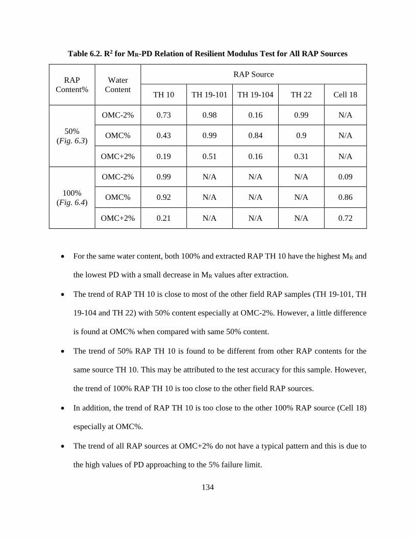
134
Table 6.2. R2 for MR-PD Relation of Resilient Modulus Test for All RAP Sources
For the same water content, both 100% and extracted RAP TH 10 have the highest MR and
the lowest PD with a small decrease in MR values after extraction.
The trend of RAP TH 10 is close to most of the other field RAP samples (TH 19-101, TH
19-104 and TH 22) with 50% content especially at OMC-2%. However, a little difference
is found at OMC% when compared with same 50% content.
The trend of 50% RAP TH 10 is found to be different from other RAP contents for the
same source TH 10. This may be attributed to the test accuracy for this sample. However,
the trend of 100% RAP TH 10 is too close to the other field RAP sources.
In addition, the trend of RAP TH 10 is too close to the other 100% RAP source (Cell 18)
especially at OMC%.
The trend of all RAP sources at OMC+2% do not have a typical pattern and this is due to
the high values of PD approaching to the 5% failure limit.
RAP
Content%
Water
Content
RAP Source
TH 10 TH 19-101 TH 19-104 TH 22 Cell 18
50%
(Fig. 6.3)
OMC-2% 0.73 0.98 0.16 0.99 N/A
OMC% 0.43 0.99 0.84 0.9 N/A
OMC+2% 0.19 0.51 0.16 0.31 N/A
100%
(Fig. 6.4)
OMC-2% 0.99 N/A N/A N/A 0.09
OMC% 0.92 N/A N/A N/A 0.86
OMC+2% 0.21 N/A N/A N/A 0.72
135
6.4.2. Single-stage RTL test
In this testing method, both parameters MR and PD are measured during 5000 load
repetitions. As load repetitions increases, both parameters increase, as shown in Figures 6.5 and
6.6. As deviator stress increases for both Class 5 and 50% RAP blends, PD increases without a
significant difference in MR values. It is very clear from comparing both Figures (6.5-a) and (6.5-
b) that by adding 50% RAP, PD decreases and MR increases. This finding is very useful for the
base layer behavior.
From comparing both Figures (6.5-b) and (6.5-c), it is obvious that modifying the 50%
RAP blend by adding 6% fines have a negative behavior on base layer characteristics. As for both
levels of deviator stress 17 and 24 psi, MR decreases and PD increases. This comparison is
repeated but at OMC+2%, as shown in Figure 6.6. From Figure (6.6-a), it is obvious that as
deviator stress increases from 12 to 17 psi, PD decreases without significant change in MR contrary
to the OMC% case. For the 50% RAP at OMC+2% (Figure 6.6-b), the increase of deviator stress
increases the PD and negatively decreases MR. From comparing both Figures (6.6-b) and (6.6-c),
no significant difference is found after adding fines to the 50% RAP blend. However, there is a
little decrease in MR especially at the low deviator stress level of 12 psi.
In this testing method, both parameters MR and PD were measured during 5000 load
repetitions. As load repetitions increase, both parameters increase, as shown in Figures 6.5 and
6.6. It is obvious from Figure 6.5 that as deviator stress increases for both Class 5 and 50% RAP
blends, PD increase without a significant difference in MR values. It is very clear from comparing
both Figures (6.5-a) and (6.5-b) that by adding 50% RAP to the blend, PD decreases and MR
increases. Again, this conclusion is very useful to the base layer behavior.

136
Figure 6.5. MR versus PD for Single-stage RTL at OMC%
R² = 0.9312 R² = 0.7461
0
20
40
60
80
0 0.5 1 1.5 2 2.5 3
MR
(ksi)
PD %
a) WC = OMC% (Class 5)
17 psi
24 psi
17 psi
24 psi
R² = 0.9157
R² = 0.9328
R² = 0.9765
0
20
40
60
80
0 0.5 1 1.5 2 2.5 3
MR
(psi)
PD %
b) WC = OMC% (50% RAP)
17 psi
24 psi
37 psi
17 psi
24 psi
37 psi
R² = 0.9728 R² = 0.8319
0
20
40
60
80
0 0.5 1 1.5 2 2.5 3
MR
(psi)
PD %
c) WC = OMC% (50% RAP + 6% Fines)
17 psi
24 psi
17 psi
24 psi
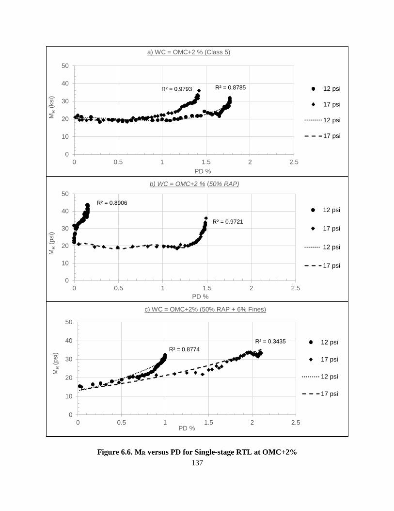
137
Figure 6.6. MR versus PD for Single-stage RTL at OMC+2%
R² = 0.8785R² = 0.9793
0
10
20
30
40
50
0 0.5 1 1.5 2 2.5
MR
(ksi)
PD %
a) WC = OMC+2 % (Class 5)
12 psi
17 psi
12 psi
17 psi
R² = 0.8906
R² = 0.9721
0
10
20
30
40
50
0 0.5 1 1.5 2 2.5
MR
(psi)
PD %
b) WC = OMC+2 % (50% RAP)
12 psi
17 psi
12 psi
17 psi
R² = 0.8774
R² = 0.3435
0
10
20
30
40
50
0 0.5 1 1.5 2 2.5
MR
(psi)
PD %
c) WC = OMC+2% (50% RAP + 6% Fines)
12 psi
17 psi
12 psi
17 psi
138
From comparing both Figures (6.5-b) and (6.5-c), modifying the 50% RAP blend by adding
6% fines have a negative behavior on base layer characteristics. As for both levels of deviator
stress 17 and 24 psi, MR decreases and PD increases. This comparison is repeated but at OMC+2%,
as shown in Figure 6.6. From Figure (6.6-a), it is obvious that as deviator stress increases from 12
to 17 psi, PD decreases without significant change in MR contrary to the OMC% case. For the 50%
RAP at OMC+2% (Figure 6.6-b), the increase of deviator stress, increases the PD and negatively
decreases MR. From comparing both Figures (6.6-b) and (6.6-c), no significant difference is found
after adding fines to the 50% RAP blend. However, there is a little decrease in MR especially at
the low deviator stress level of 12 psi.
Finally, it can be concluded from the data analysis for single-stage RTL test that, as the
deviator stress increases for both Class 5 and 50% RAP blends, PD increases without a significant
difference in MR values for both water content levels OMC-2% and OMC%. Adding RAP to the
base layer has a positive effect for base layer by decreasing PD and increasing MR values.
Modifying the 50% RAP blends by 6% plastic fines does not have any positive effects on base
layer performance for both water content levels OMC-2% and OMC%.
6.4.3. Multi-stage RTL test
In this stage, the same effort is repeated but on different type of RTL testing. This stage is
more close to the methodology of resilient modulus testing by applying stages of loading with
different deviator stresses (D.S) but at higher number of load repetitions (5000 compared to 100
cycles). Confining pressure is kept the same (3 psi for all stages of loading). Figures 6.7, 6.8 and
6.9 show the MR-PD trend for different RAP TH 10/Class 5 blends at three different water content
levels: OMC-2%, OMC% and OMC+2% and the regression parameter R2 for this relation is shown
in Table 6.3. For Class 5 aggregates (Figure 6.7), the general trend is that both parameters MR and

139
PD increase with the increase of deviator stress until reaching the highest stage of loading where
the sample fails when reaching 5% PD and the MR decreases when increasing PD. It is obvious
that for all water content levels (Figures 6.7-a, 6.7-b and 6.7-c), Class 5 aggregates begin to fail
when deviator stress reaches 24 psi without a significant difference in MR values.
By adding 50% RAP to Class 5 aggregates (Figure 6.8), MR values increase while PD
values decrease. This finding proves that adding RAP is better for base layer performance.
However, the trend shown before with Class 5 changes with adding RAP at low water content
level of OMC-2% (Figure 6.8-a). The MR values change un-expectedly with the increase of PD.
On the other hand, the trend shown before with Class 5 is almost the same for the other two water
content levels OMC% and OMC+2% (Figures 6.8-b and 6.8-c). Nevertheless, in this case the
samples fails at higher deviator stress levels 59 and 48 psi for OMC% and OMC+2% respectively.
From comparing both Figures 6.8 and 6.9 for both cases of 50% RAP, the general trend of
MR-PD is almost the same. However, the significant result from this comparison is that adding
3.5% fines to the 50% RAP samples has remarkably positive effect on the behavior of the samples.
It is found for all water content levels that PD values do not reach the 5% failure limit. The MR
values are significantly higher than those samples shown before stabilization. This result is
completely different to samples tested before by single-stage RTL test with 6% fines added.

140
Figure 6.7. MR versus PD for Multi-stage RTL of Class 5
0
10
20
30
40
0 1 2 3 4 5 6 7
MR
(ksi)
PD %
a) WC = OMC-2%
6 psi
12 psi
17 psi
24 psi
6 psi
12 psi
17 psi
24 psi
0
10
20
30
40
0 1 2 3 4 5 6 7
MR
(ksi)
PD %
b) WC = OMC%
17 psi
24 psi
37 psi
17 psi
24 psi
37 psi
0
10
20
30
40
0 1 2 3 4 5 6 7
MR
(ksi)
PD %
c) WC = OMC+2%
6 psi
12 psi
17 psi
24 psi
6 psi
12 psi
17 psi
24 psi
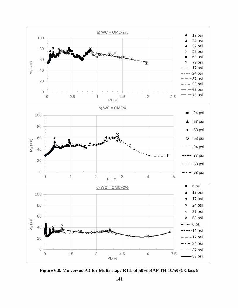
141
Figure 6.8. MR versus PD for Multi-stage RTL of 50% RAP TH 10/50% Class 5
0
20
40
60
80
100
0 0.5 1 1.5 2 2.5
MR
(ksi)
PD %
a) WC = OMC-2%17 psi
24 psi
37 psi
53 psi
63 psi
73 psi
17 psi
24 psi
37 psi
53 psi
63 psi
73 psi
0
20
40
60
80
100
0 1 2 3 4 5
MR
(ksi)
PD %
b) WC = OMC%
24 psi
37 psi
53 psi
63 psi
24 psi
37 psi
53 psi
63 psi
0
20
40
60
80
100
0 1.5 3 4.5 6 7.5
MR
(ksi)
PD %
c) WC = OMC+2% 6 psi
12 psi
17 psi
24 psi
37 psi
53 psi
6 psi
12 psi
17 psi
24 psi
37 psi
53 psi
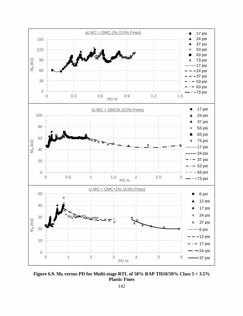
142
Figure 6.9. MR versus PD for Multi-stage RTL of 50% RAP TH10/50% Class 5 + 3.5%
Plastic Fines
0
30
60
90
120
150
0 0.3 0.6 0.9 1.2 1.5
MR
(ksi)
PD %
a) WC = OMC-2% (3.5% Fines) 17 psi
24 psi
37 psi
53 psi
63 psi
73 psi
17 psi
24 psi
37 psi
53 psi
63 psi
73 psi
0
20
40
60
80
100
0 0.5 1 1.5 2 2.5 3
MR
(ksi)
PD %
b) WC = OMC% (3.5% Fines) 17 psi
24 psi
37 psi
53 psi
63 psi
73 psi
17 psi
24 psi
37 psi
53 psi
63 psi
73 psi
0
10
20
30
40
50
0 1 2 3 4 5 6
MR
(ksi)
PD %
c) WC = OMC+2% (3.5% Fines)
6 psi
12 psi
17 psi
24 psi
37 psi
6 psi
12 psi
17 psi
24 psi
37 psi
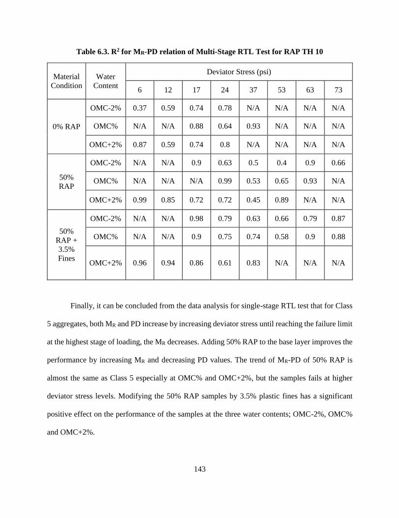
143
Table 6.3. R2 for MR-PD relation of Multi-Stage RTL Test for RAP TH 10
Finally, it can be concluded from the data analysis for single-stage RTL test that for Class
5 aggregates, both MR and PD increase by increasing deviator stress until reaching the failure limit
at the highest stage of loading, the MR decreases. Adding 50% RAP to the base layer improves the
performance by increasing MR and decreasing PD values. The trend of MR-PD of 50% RAP is
almost the same as Class 5 especially at OMC% and OMC+2%, but the samples fails at higher
deviator stress levels. Modifying the 50% RAP samples by 3.5% plastic fines has a significant
positive effect on the performance of the samples at the three water contents; OMC-2%, OMC%
and OMC+2%.
Material
Condition
Water
Content
Deviator Stress (psi)
6 12 17 24 37 53 63 73
0% RAP
OMC-2% 0.37 0.59 0.74 0.78 N/A N/A N/A N/A
OMC% N/A N/A 0.88 0.64 0.93 N/A N/A N/A
OMC+2% 0.87 0.59 0.74 0.8 N/A N/A N/A N/A
50%
RAP
OMC-2% N/A N/A 0.9 0.63 0.5 0.4 0.9 0.66
OMC% N/A N/A N/A 0.99 0.53 0.65 0.93 N/A
OMC+2% 0.99 0.85 0.72 0.72 0.45 0.89 N/A N/A
50%
RAP +
3.5%
Fines
OMC-2% N/A N/A 0.98 0.79 0.63 0.66 0.79 0.87
OMC% N/A N/A 0.9 0.75 0.74 0.58 0.9 0.88
OMC+2% 0.96 0.94 0.86 0.61 0.83 N/A N/A N/A
144
6.5. Correlation Task Summary
By comparing the two most important parameters (MR and PD) in the RAP base layer
performance, several findings are concluded from the three different testing procedures included
in this study resilient modulus, single-stage RTL and multi-stage RTL tests. These findings may
be summarized as follows:
6.5.1. Resilient modulus testing
From resilient modulus testing at OMC%, it was found that as the percentage of RAP TH 10
(the main RAP source) exceeds 50%, MR increases and PD decreases. This result is positive
for base layer strength. This relation is more significant at confining pressure levels below 15
psi.
For the same water content, both 100% and extracted RAP TH 10 have the highest MR and the
lowest PD with a small decrease in MR values after extraction.
The trend of RAP TH10 is close to most of the other field RAP samples (TH 19-101, TH 19-
104 and TH 22) with 50% content especially at OMC-2%. However, a little difference is found
at OMC% when compared with same 50% content.
The trend of 50% RAP TH 10 is found to be different than other RAP contents for the same
source TH10. This may be attributed to the test accuracy for this sample. However, the trend
of 100% RAP TH 10 is too close to the other field RAP sources.
Also, the trend of RAP TH 10 is too close to the other 100% RAP source (Cell 18) especially
at OMC%.
The trend of all RAP sources at OMC+2% do not have a typical pattern and this is due to the
approach of the PD from the failure limit (5%) and the lowest correlation found (R2 is low) as
shown in Tables 3 and 4. This behavior is changed for single and multi-stage RTL test, because
145
the effect of stress history in resilient modulus test by applying 30 different sequences of
loading with variable deviator and confining stresses.
6.5.2. Single-Stage RTL Testing
As the deviator stress increases for both Class 5 and 50% RAP blends, PD increases without a
significant difference in MR values for both water content levels OMC-2% and OMC%.
Adding RAP to the base layer has a positive effect for base layer by decreasing PD and
increasing MR values.
Modifying the 50% RAP blends by 6% plastic fines do not have any positive effects on base
layer performance for both water content levels OMC-2% and OMC%.
6.5.3. Multi-Stage RTL Testing
For Class 5 aggregates, both MR and PD increase by increasing deviator stress until reaching
the failure limit at the highest stage of loading, the MR decreases.
Adding 50% RAP to the base layer improves the performance by increasing MR and decreasing
PD values.
The trend of MR-PD of 50% RAP is almost the same as Class 5 especially at OMC% and
OMC+2% but the samples fails at higher deviator stress levels.
Modifying the 50% RAP samples by 3.5% plastic fines has a significant positive effect on the
performance of the samples at the three water contents; OMC-2%, OMC% and OMC+2%.

146
CHAPTER 7. POSSOIN’S RATIO MEASUREMENT
7.1. Introduction
Based on the results of Maher et. al. (Maher & Bennert, 2008) study, Poisson’s ratio
measured values during the dynamic modulus test are very close to the MEPDG predicted values
for several HMA mixes tested at this study. However, this study showed that unbound granular
aggregates used for base layer have identical resilient modulus at different levels of Poisson’s
Ratio values. For example, a Poisson’s ratio value of approximately 0.15 occurred at all five
confining pressures and had resilient modulus values that ranged from 22,000 to almost 90,000 psi
(Maher & Bennert, 2008). In addition, it is not accurate to measure Poisson’s ratio for confined
materials during uniaxial loading as the confining pressure applied to samples during testing affect
on the real lateral strain that happens to the sample. Even if there is a confining pressure in the
field, but in this study the material is assumed totally elastic especially in the linear stress-strain
relationship to measure accurate Poisson’s ratio value and avoid the variation found from the above
mentioned study.
Therefore, there is a need to measure Poisson’s ratio for RAP/Aggregate blends in a base
layer with another testing procedure, especially when it is still in elastic region just before failure
or permanent deformation accumulation. The un-confined compression test seems to be the most
suitable procedure to measure the lateral deformation of RAP samples during axial loading. Lateral
strain gauges can be used to measure this deformation simultaneously with axial deformation
measured without any confining pressure, which may affect on the accuracy of lateral deformation
measurement. This test was used before in evaluating the stiffness of cement treated base as by
adding cement a pozzlanic reaction happens which changes the layer from elasto-plastic material
147
to totally elastic brittle material. In this case the treated material cannot be measured with the same
methods used for granular base materials
Finally, the Poisson’s ratio was not considered in previous studies as an important
parameter affecting the structural capacity for granular base layer, especially during measuring
any stiffness parameter either under dynamic or static loading. Usually, Poisson’s ratio was
estimated during all methods of pavement design including the MEPDG. However, effect of
Poisson’s ratio on both MR and PD modeling behavior for RAP blends is essential to be studied to
investigate its effectiveness on the structural capacity of base layer. This study is essentially needed
to confirm the difference in behavior of RAP blends from granular aggregates, especially under
variation of water content. Usually the accepted variation of water content in the field is 2% from
the OMC%, therefore Poisson’s ratio is measured within this range for all investigated
RAP/Aggregate blends.
7.2. Scope of Task
The main objective of this task focuses on measuring Poisson’s ratio and ultimate
compressive strength for several RAP/Aggregate blends, tested before in the previous research
tasks on resilient modulus and repeated tri-axial loading (RTL) tests to determine the values of
both parameters MR and PD, at various testing conditions. The target of this task is to evaluate the
Poisson’s ratio and compressive strength relationship, and its future effectiveness on the main
design parameters of RAP blends used in base layer such as MR and PD. Based on literature review
results, this ratio cannot be measured during the MR test. Therefore, the un-confined compression
test is used to determine the respective results. This test is more suitable and practical to implement
in measuring the lateral deformation without any effect of confining pressure like MR or RTL tests.

148
7.3. Stages of Analysis
According to the literature review collected in this study, for each tested specimen an axial
stress-strain curve is drawn and the linear elastic region is calculated as a range percentage from
the ultimate compressive strength as shown in appendices. Generally, this linear relationship is
varied from 15% to 90%, while the average midpoint for this relation varied from 40% to 65% of
the ultimate compressive strength for analyzed samples. Usually, the Poisson’s ratio should be
constant in this linear elastic for homogenous specimens. However, these tested specimens are not
truly homogenous due to many reasons such as; gradation, compaction, aggregate properties, aging
characteristics and etc. Therefore, the Poisson’s ratio is considered as the average midpoint of this
linear elastic region for each sample condition. For all analyzed samples, the Poisson’s ratio varied
from 0.07 to 0.47, while the ultimate compressive strength varied from 1.92 to 32.83 psi. The
analysis of this task is divided into three main stages according to the different testing conditions
investigated.
7.3.1. Analysis versus RAP content
This stage is focusing on the condition of percentage of RAP with traditional Class 5
granular aggregates on Poisson’s ratio and ultimate compressive strength values. Two RAP
sources TH 29 and TH 10 are analyzed in this stage with the two different sources of Class 5 at
three water content levels OMC-2%, OMC% and OMC+2%. The new Class 5 source used for this
study is mixed with RAP TH 29, as shown in Figure 7.1. The old Class 5 source used before in
MN/DOT project (M. Attia et al., 2009) is mixed with RAP TH 10, as shown in Figure 7.2.
For Figure 7.1 the general trend of both OMC-2% and OMC% is almost the same, as
Poisson’s ratio values increases significantly at 50% RAP then decreases significantly at 100%
RAP with a little higher values at OMC% condition.
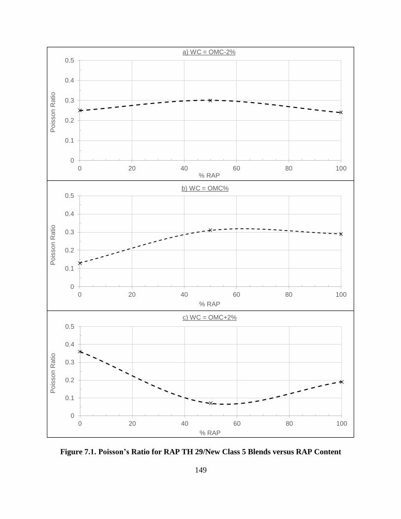
149
Figure 7.1. Poisson’s Ratio for RAP TH 29/New Class 5 Blends versus RAP Content
0
0.1
0.2
0.3
0.4
0.5
0 20 40 60 80 100
Pois
son R
atio
% RAP
a) WC = OMC-2%
0
0.1
0.2
0.3
0.4
0.5
0 20 40 60 80 100
Pois
son R
atio
% RAP
b) WC = OMC%
0
0.1
0.2
0.3
0.4
0.5
0 20 40 60 80 100
Pois
son R
atio
% RAP
c) WC = OMC+2%

150
Figure 7.2. Poisson’s Ratio for RAP TH 10/Old Class 5 Blends versus RAP Content
0
0.1
0.2
0.3
0.4
0.5
0 20 40 60 80 100
Pois
son R
atio
% RAP
a) WC = OMC-2%
0
0.1
0.2
0.3
0.4
0.5
0 20 40 60 80 100
Pois
son R
atio
% RAP
b) WC = OMC%
0
0.1
0.2
0.3
0.4
0.5
0 20 40 60 80 100
Pois
son R
atio
% RAP
c) WC = OMC+2 %

151
Figure 7.3. Comparison between Ultimate Compressive Strength and Poisson’s Ratio for
RAP/Aggregate blends versus RAP Content
0
5
10
15
20
0 20 40 60 80 100
Com
pre
ssiv
e S
trength
(psi)
% RAP
a) New Class 5 + RAP TH 29
OMC-2%
OMC%
OMC+2%
0
5
10
15
20
0 20 40 60 80 100
Com
pre
ssiv
e S
trength
(psi)
% RAP
c) Old Class 5 + RAP TH 10
OMC-2%
OMC%
OMC+2%
0
0.1
0.2
0.3
0.4
0.5
0 20 40 60 80 100
Pois
son's
Ratio
% RAP
b) New Class 5 + RAP TH 29
OMC-2%
OMC%
OMC+2%
0
0.1
0.2
0.3
0.4
0.5
0 20 40 60 80 100
Pois
son's
Ratio
% RAP
d) Old Class 5 + RAP TH 10
OMC-2%
OMC%
OMC+2%
152
This trend changes at OMC+2% as Poisson’s ratio value is the lowest at 50% RAP. In
Figure 7.2 the trend is obvious at OMC%, as Poisson’s ratio increases with the increase of
percentage of RAP significantly. However, the trend is opposite at OMC+2% as it decreases
significantly with RAP content increase. And the change in Poisson’s ratio is not significant at
OMC-2% water content. In addition, a general comparison is achieved between the trend of both
the ultimate compressive strength and Poisson’s ratio values, at the three water content levels for
both RAP/Class 5 blends versus RAP content, as shown in Figure 7.3.
Generally, the ultimate compressive strength decreases with the increase of RAP content
for new Class 5 + RAP TH 10 blends. While on the other hand, the trend is opposite for old Class
5 + RAP TH 29 at all water content levels. This conclusion can be explained as new Class 5 (6-18
psi) is much stronger than the old Class 5 (3-9 psi). However, RAP TH 29 (2-3 psi) is much weaker
than RAP TH 10 (5-13 psi), as this source of RAP is much older which means that more age
hardening effect on the asphalt binder. This means that for the first case softening effect happens
by increasing the RAP TH 29 content and the opposite for the second case by increasing RAP TH
10 content. Contrary, there is no typical shape from the Poisson’s ratio relationship for both RAP
blends. At OMC%, the Poisson’s ratio increases from 0.13 to 0.29 for RAP TH 29 blend, and also
it increases from 0.16 to 0.45 for RAP TH 10 blend with increasing RAP content. At OMC+2%,
the trend of both blends is almost the same as Poisson’s ratio decreases significantly from 0.4 to
0.2 approximately. On the other hand at OMC-2%, there isn’t significant variation in Poisson’s
ratio values.
7.3.2. Analysis versus water content
In this stage, Poisson’s ratio parameter is analyzed versus water content variation for the
three main RAP/Aggregate blends. New Class 5/ RAP TH 29 blends are shown in Figure 7.4,
153
while old Class 5/RAP TH 10 are shown in Figure 7.5 and the other field RAP sources are shown
in Figure 7.6. In addition, ultimate compressive strength parameter is analyzed also versus water
content variation for the same RAP/Aggregate blends, as shown in Figure 7.7.
For Class 5, Poisson’s ratio is are in its lowest value (0.15 approximately) at OMC% level,
as shown in Figures (7.4-a) and (7.5-a) for both types. At 50% RAP TH 29, Poisson’s ratio
decreases significantly from 0.3 to 0.07 (Figure 7.4-b) by increasing water content, while it
increases slightly from 0.19 to 0.35 (Figure 7.5-b) for 50% RAP TH 10. At 100% RAP, Poisson’s
ratio increases at OMC% then decreases at the other two water contents for both RAP blends with
more significance for RAP TH 10 blend by comparing both Figures (7.4-c) and (7.5-c). As
Poisson’s ratio for 100% RAP TH 10 reaches 0.45 corresponding to 0.29 for 100% TH 29.
For the other field RAP sources, Poisson’s ratio values almost has no significant change
for RAP TH 19-101 (Figure 7.6-a) by increasing water content. However, for the other two RAP
sources, Poisson’s ratio for RAP TH 19-104 reaches its lowest value 0.15 (Figure 7.6-b), while for
RAP TH 22 it reaches its optimum value 0.47 (Figure 7.6-c), both at OMC% level. On the other
hand, for the ultimate compressive strength parameter (Figure 7.7), it decreases significantly for
both RAP/Class 5 blends by increasing water content from 15 psi to 3 psi approximately especially
for Class 5 blends, as shown in Figures (7.7-a) and (7.7-b).
Also for the other field RAP sources, RAP TH 22 is the only one which have the same
behavior as RAP/Class 5 blends as its ultimate strength decreases significantly from 16 to 6 psi
approximately (Figure 7.7-c). While for the other two RAP sources, their ultimate strength reach
its optimum values 32 and 25 psi at OMC% for RAP’s TH 19-101 and TH 19-104 respectively, as
shown in Figure (7.7-c).
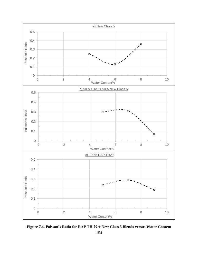
154
Figure 7.4. Poisson’s Ratio for RAP TH 29 + New Class 5 Blends versus Water Content
0
0.1
0.2
0.3
0.4
0.5
0 2 4 6 8 10
Pois
son's
Ratio
Water Content%
a) New Class 5
0
0.1
0.2
0.3
0.4
0.5
0 2 4 6 8 10
Pois
son's
Ratio
Water Content%
b) 50% TH29 + 50% New Class 5
0
0.1
0.2
0.3
0.4
0.5
0 2 4 6 8 10
Pois
son's
Ratio
Water Content%
c) 100% RAP TH29
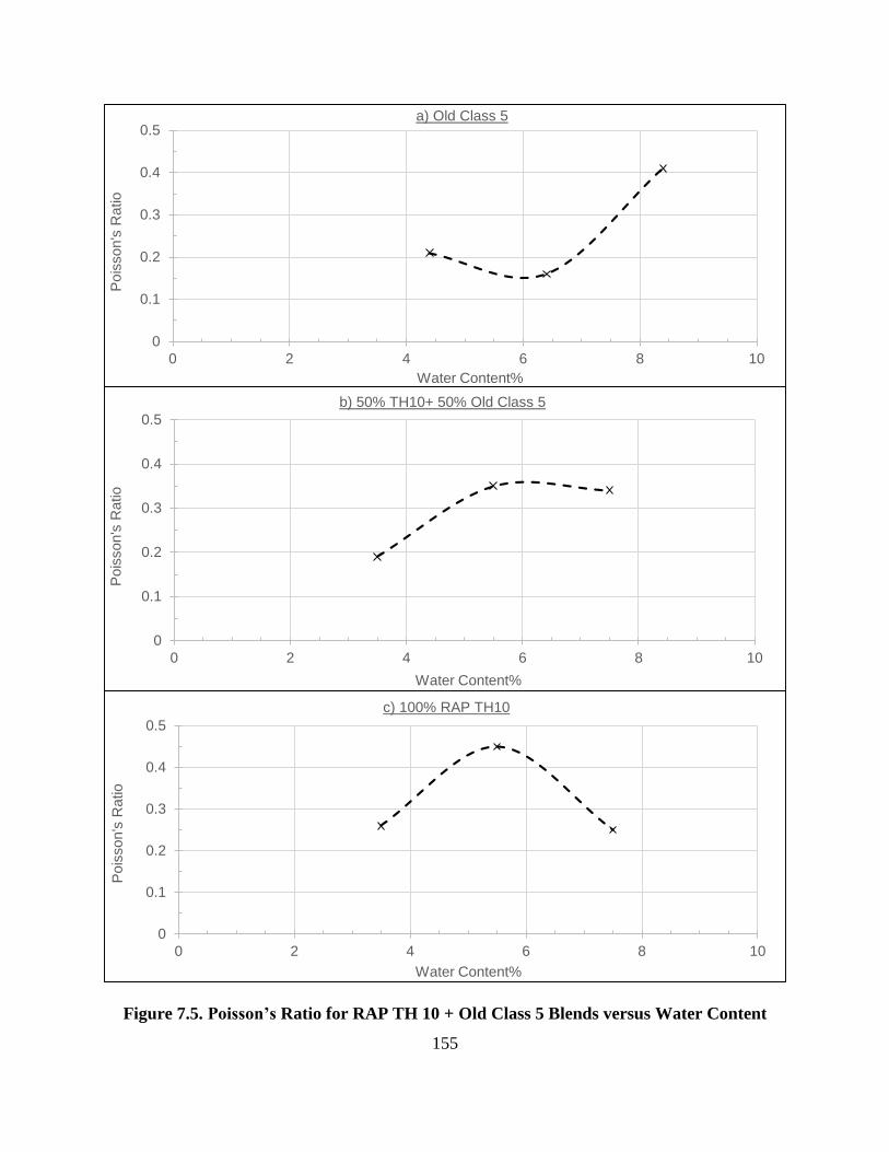
155
Figure 7.5. Poisson’s Ratio for RAP TH 10 + Old Class 5 Blends versus Water Content
0
0.1
0.2
0.3
0.4
0.5
0 2 4 6 8 10
Pois
son's
Ratio
Water Content%
a) Old Class 5
0
0.1
0.2
0.3
0.4
0.5
0 2 4 6 8 10
Pois
son's
Ratio
Water Content%
b) 50% TH10+ 50% Old Class 5
0
0.1
0.2
0.3
0.4
0.5
0 2 4 6 8 10
Pois
son's
Ratio
Water Content%
c) 100% RAP TH10
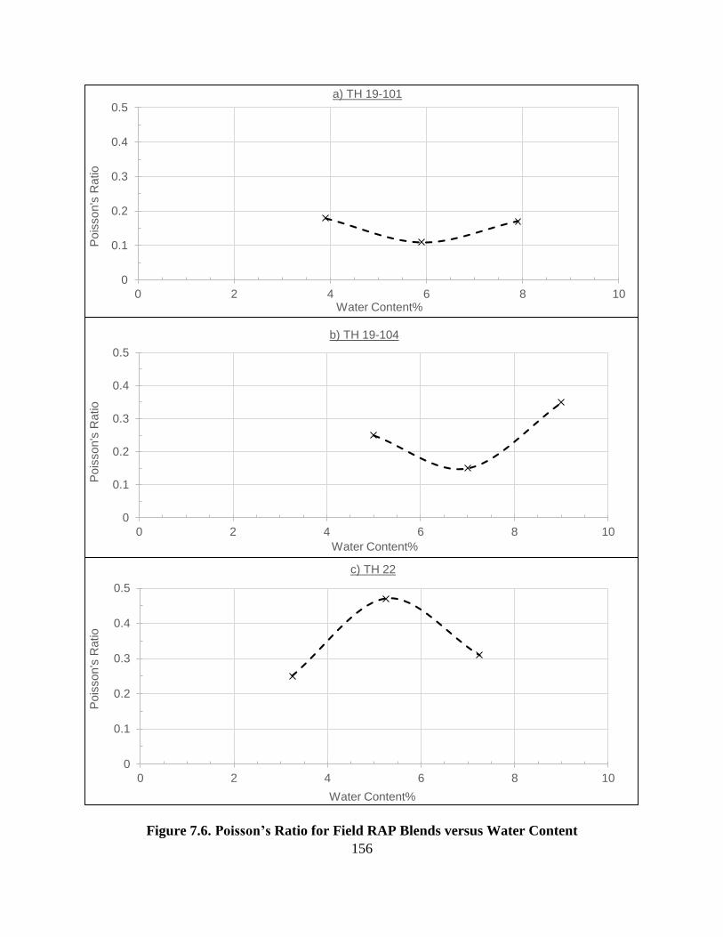
156
Figure 7.6. Poisson’s Ratio for Field RAP Blends versus Water Content
0
0.1
0.2
0.3
0.4
0.5
0 2 4 6 8 10
Pois
son's
Ratio
Water Content%
a) TH 19-101
0
0.1
0.2
0.3
0.4
0.5
0 2 4 6 8 10
Pois
son's
Ratio
Water Content%
b) TH 19-104
0
0.1
0.2
0.3
0.4
0.5
0 2 4 6 8 10
Pois
son's
Ratio
Water Content%
c) TH 22

157
Figure 7.7. Ultimate Compressive Strength for RAP Blends versus Water Content
0
10
20
30
40
0 2 4 6 8 10
Com
pre
ssiv
e S
trength
(psi)
Water Content%
a) New Class 5 + RAP TH 29
Class 5
50% RAP
100% RAP
0
10
20
30
40
0 2 4 6 8 10
Com
pre
ssiv
e S
trength
(psi)
Water Content%
b) Old Class 5 + RAP TH 10
Class 5
50% RAP
100% RAP
0
10
20
30
40
0 2 4 6 8 10
Com
pre
ssiv
e S
trength
(psi)
Water Content%
c) Field Samples
TH 19-101
TH 19-104
TH 22

158
7.3.3. Correlation between lateral strain and compressive stress
At this third stage, a comparison is made between lateral strain to the compressive stress
directly at four levels (25%, 50%, 75% and 100%) of the ultimate compressive strength for all
RAP blends tested at investigated testing conditions. This stage is important to show the lateral
strain increase during whole compression test. RAP TH 29/Class 5 blends are shown in Figure 7.8,
RAP TH 10/Class 5 blends are shown in Figure 7.9 and field RAP blends are shown in Figure
7.10. The general trend is that increasing the compressive stress increases lateral strain. By
decreasing water content, same lateral strain values are achieved at higher compressive stresses
except for 50% RAP TH 29 (Figure 7.8-b) and field RAP’s TH 19-101 & TH 19-104 (Figure 7.10-
b & 7.10-c) blends. For those RAP blends, the highest stress values are achieved at OMC%. One
sample is tested as a trial for RAP TH 10 by retesting the sample at OMC% after extracting the
aged asphalt binder, as shown in Figure (7.9-c).
The extracted sample has slightly higher stress levels and smaller lateral strain than the
original sample but the variation is insignificant. It is obvious from most of RAP blends tested that
variation of water content have more effect on the compressive stress than lateral strain values. On
the other hand, the RAP contents have contradicting effects on both parameters depending on the
RAP source, aging characteristics, granular aggregate gradation and strength parameters.

159
Figure 7.8. Comparison between Lateral Strain and Compressive Stress for RAP TH 29
+ New Class 5 Blends
0
0.5
1
1.5
2
0 5 10 15 20
Late
ral S
train
%
Compressive Strength (psi)
a) New Class 5
OMC-2%
OMC%
OMC+2%
0
0.5
1
1.5
2
0 5 10 15 20
Late
ral S
train
%
Compressive Strength (psi)
b) 50% TH29 + 50% New Class 5
OMC-2%
OMC%
OMC+2%
0
0.5
1
1.5
2
0 5 10 15 20
Late
ral S
train
%
Compressive Strength (psi)
c) 100% RAP TH29
OMC-2%
OMC%
OMC+2%

160
Figure 7.9. Comparison between Lateral Strain and Compressive Stress for RAP TH 10
+ Old Class 5 Blends
0
0.5
1
1.5
2
0 3 6 9 12 15
Late
ral S
train
%
Compressive Strength (psi)
a) Old Class 5
OMC-2%
OMC%
OMC+2%
0
0.5
1
1.5
2
0 3 6 9 12 15
Late
ral S
train
%
Compressive Strength (psi)
b) 50% TH10 + 50% Old Class 5
OMC-2%
OMC%
OMC+2%
0
0.5
1
1.5
2
0 3 6 9 12 15
Late
ral S
train
%
Compressive Strength (psi)
c) 100% RAP TH10
OMC-2% OMC%
OMC+2% Ext. (OMC%)

161
Figure 7.10. Lateral Strain versus Compressive Stress for Field RAP Blends
0
0.5
1
1.5
2
0 5 10 15 20 25 30 35
Late
ral S
train
%
Compressive Strength (psi)
a) TH 19-101
OMC-2%
OMC%
OMC+2%
0
0.5
1
1.5
2
0 5 10 15 20 25 30 35
Late
ral S
train
%
Compressive Strength (psi)
b) TH 19-104
OMC-2%
OMC%
OMC+2%
0
0.5
1
1.5
2
0 5 10 15 20 25 30 35
Late
ral S
train
%
Compressive Strength (psi)
c) TH 22
OMC-2%
OMC%
OMC+2%
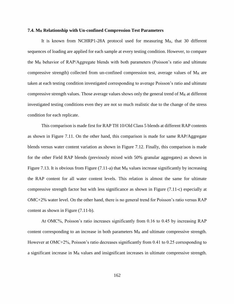
162
7.4. MR Relationship with Un-confined Compression Test Parameters
It is known from NCHRP1-28A protocol used for measuring MR, that 30 different
sequences of loading are applied for each sample at every testing condition. However, to compare
the MR behavior of RAP/Aggregate blends with both parameters (Poisson’s ratio and ultimate
compressive strength) collected from un-confined compression test, average values of MR are
taken at each testing condition investigated corresponding to average Poisson’s ratio and ultimate
compressive strength values. Those average values shows only the general trend of MR at different
investigated testing conditions even they are not so much realistic due to the change of the stress
condition for each replicate.
This comparison is made first for RAP TH 10/Old Class 5 blends at different RAP contents
as shown in Figure 7.11. On the other hand, this comparison is made for same RAP/Aggregate
blends versus water content variation as shown in Figure 7.12. Finally, this comparison is made
for the other Field RAP blends (previously mixed with 50% granular aggregates) as shown in
Figure 7.13. It is obvious from Figure (7.11-a) that MR values increase significantly by increasing
the RAP content for all water content levels. This relation is almost the same for ultimate
compressive strength factor but with less significance as shown in Figure (7.11-c) especially at
OMC+2% water level. On the other hand, there is no general trend for Poisson’s ratio versus RAP
content as shown in Figure (7.11-b).
At OMC%, Poisson’s ratio increases significantly from 0.16 to 0.45 by increasing RAP
content corresponding to an increase in both parameters MR and ultimate compressive strength.
However at OMC+2%, Poisson’s ratio decreases significantly from 0.41 to 0.25 corresponding to
a significant increase in MR values and insignificant increases in ultimate compressive strength.

163
At OMC-2%, there isn’t a significant increase (0.21-0.25) corresponding to an increase in both
parameters MR and ultimate compressive strength.
The same comparison is achieved between MR behavior and un-confined strength
parameters with water content variation for each RAP/Aggregate blend as shown in Figure 7.12.
Both MR and ultimate compressive strength have the same trend as each parameter decreases
significantly with water content increase as shown in both figures (7.12-a) and (7.12-c). For
Poisson’s ratio parameter as shown in Figure (7.12-b), both RAP blends have the same behavior
as it reaches their maximum values 0.35 and 0.45 for 50% and 100% RAP respectively then
decreases significantly at the other two water contents. While Class 5 have an opposite trend as it
reaches its lowest value 0.16 at OMC%.
For the other three field RAP’s, the same comparison is conducted with water content
variation only as those RAP’s were already mixed with 50% granular aggregates. For MR results
as shown in Figure (7.13-a), the trend is the same for all RAP sources as MR decreases by
increasing water content. However, this trend is not the same for ultimate compressive strength
parameter (Figure 7.13-c) as both RAP sources TH 19-101 and TH 19-104 reaches their maximum
values 25 and 33 psi respectively at OMC%. Also, it is obvious for both RAP’s that they have the
same behavior for Poisson’s ratio parameter (Figure 7.13-b). As they reach their lowest values
0.11 and 0.15 for RAP TH 19-101 and RAP TH 19-104 respectively. While for RAP TH 22, the
Poisson’s ratio behavior is more close to its MR behavior than ultimate compressive strength. As
it reaches its maximum value 0.47 at OMC%.
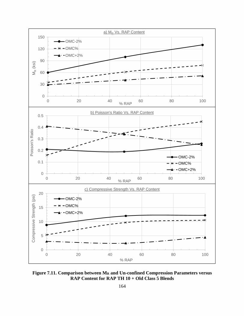
164
Figure 7.11. Comparison between MR and Un-confined Compression Parameters versus
RAP Content for RAP TH 10 + Old Class 5 Blends
0
30
60
90
120
150
0 20 40 60 80 100
MR
(ksi)
% RAP
a) MR Vs. RAP Content
OMC-2%
OMC%
OMC+2%
0
0.1
0.2
0.3
0.4
0.5
0 20 40 60 80 100
Pois
son's
Ratio
% RAP
b) Poisson's Ratio Vs. RAP Content
OMC-2%
OMC%
OMC+2%
0
5
10
15
20
0 20 40 60 80 100
Com
pre
ssiv
e S
trength
(psi)
% RAP
c) Compressive Strength Vs. RAP Content
OMC-2%
OMC%
OMC+2%

165
Figure 7.12. Comparison between MR and Un-confined Compression Parameters versus
Water Content for RAP TH 10 + Old Class 5 Blends
0
30
60
90
120
150
0 2 4 6 8 10
MR
(ksi)
Water Content%
a) MR Vs. Water Content
Class 5
50% RAP
100% RAP
0
0.1
0.2
0.3
0.4
0.5
0 2 4 6 8 10
Pois
son's
Ratio
Water Content%
b) Poisson's Ratio Vs. Water Content
Class 5
50% RAP
100% RAP
0
5
10
15
20
0 2 4 6 8 10
Com
pre
ssiv
e S
trength
(psi)
Water Content%
c) Compressive Strength Vs. Water Content
Class 5
50% RAP
100% RAP
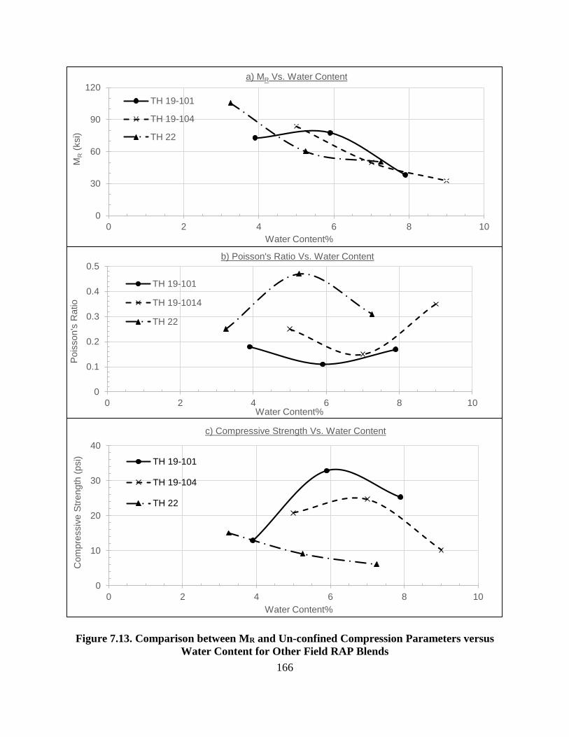
166
Figure 7.13. Comparison between MR and Un-confined Compression Parameters versus
Water Content for Other Field RAP Blends
0
30
60
90
120
0 2 4 6 8 10
MR
(ksi)
Water Content%
a) MR Vs. Water Content
TH 19-101
TH 19-104
TH 22
0
0.1
0.2
0.3
0.4
0.5
0 2 4 6 8 10
Pois
son's
Ratio
Water Content%
b) Poisson's Ratio Vs. Water Content
TH 19-101
TH 19-1014
TH 22
0
10
20
30
40
0 2 4 6 8 10
Com
pre
ssiv
e S
trength
(psi)
Water Content%
c) Compressive Strength Vs. Water Content
TH 19-101
TH 19-104
TH 22

167
7.5. PD Relationship with Un-confined Compression Test Parameters
During the resilient modulus test for collecting MR values of RAP/Aggregate blends
investigated, PD is accumulated for every sequence of loading. Those values are calculated as a
percentage from whole sample height then an average value is taken for each sample as an indicator
for PD values. PD values collected from both single-stage and multi-stage RTL test cannot be used
as it didn’t cover all the investigated testing conditions such as RAP content and water content for
tested RAP/Aggregate blends analyzed in this chapter.
Generally, it seems that the RAP content is not significantly affect PD as water content by
comparing both Figures (7.14-a) and (7.15-a). As increasing water content, increases PD
accumulated for all RAP/Aggregate blend. However, increasing RAP content do not change PD
accumulated significantly except at OMC%. At OMC% by increasing RAP content, PD decreases
from 1.4% to 0.5% while Poisson’s ratio increases significantly from 0.16 to 0.45. At OMC+2%,
PD decreases insignificantly from 3.4% to 3.8% corresponding to a significant decrease for
Poisson’s ratio from 0.41 to 0.25. At OMC-2%, both parameters PD and Poisson’s ratio do not
change significantly by increasing RAP content.
By increasing water content, PD increases significantly for all RAP/Aggregate blends as
shown in Figure (7.15-a). While the Poisson’s ratio for both 50% and 100% RAP/Aggregate blends
reach its maximum values 0.35 and 0.45 respectively, however Class 5 has an opposite trend
(Figure 7.15-b). For the field RAP blends, increasing water content increases PD significantly as
shown in Figure (7.16-a). And both RAP’s TH 19-101 and TH 19-104 have a similar behavior for
Poisson’s ratio while RAP TH 22 have an opposite trend (Figure 7.16-b).

168
Figure 7.14. Comparison between PD and Un-confined Compression Parameters versus
RAP Content for RAP TH 10 + Old Class 5 Blends
0
1
2
3
4
5
0 20 40 60 80 100
PD
%
% RAP
a) PD vs RAP Content
OMC-2%
OMC%
OMC+2%
0
0.1
0.2
0.3
0.4
0.5
0 20 40 60 80 100
Pois
son's
Ratio
% RAP
b) Poisson's Ratio Vs. RAP Content
OMC-2%
OMC%
OMC+2%
0
5
10
15
20
0 20 40 60 80 100
Com
pre
ssiv
e S
trength
(psi)
% RAP
c) Compressive Strength Vs. RAP Content
OMC-2%
OMC%
OMC+2%

169
Figure 7.15. Comparison between PD and Un-confined Compression Parameters versus
Water Content for RAP TH 10 + Old Class 5 Blends
0
5
10
15
20
0 2 4 6 8 10
Com
pre
ssiv
e S
trength
(psi)
Water Content%
c) Compressive Strength Vs. Water Content
Class 5
50% RAP
100% RAP
0
1
2
3
4
5
0 2 4 6 8 10
PD
%
Water Content %
a) PD vs Water Content %
Class 5
50% RAP
100% RAP
0
0.1
0.2
0.3
0.4
0.5
0 2 4 6 8 10
Pois
son's
Ratio
Water Content%
b) Poisson's Ratio Vs. Water Content
Class 5
50% RAP
100% RAP
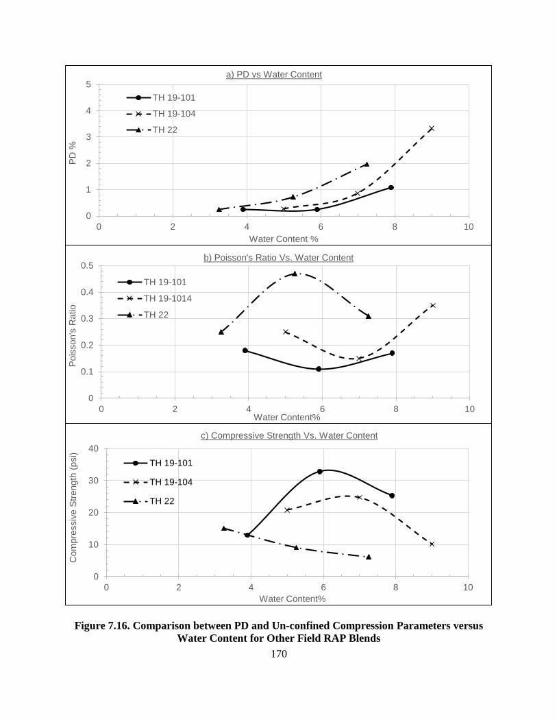
170
Figure 7.16. Comparison between PD and Un-confined Compression Parameters versus
Water Content for Other Field RAP Blends
0
1
2
3
4
5
0 2 4 6 8 10
PD
%
Water Content %
a) PD vs Water Content
TH 19-101
TH 19-104
TH 22
0
0.1
0.2
0.3
0.4
0.5
0 2 4 6 8 10
Pois
son's
Ratio
Water Content%
b) Poisson's Ratio Vs. Water Content
TH 19-101
TH 19-1014
TH 22
0
10
20
30
40
0 2 4 6 8 10
Com
pre
ssiv
e S
trength
(psi)
Water Content%
c) Compressive Strength Vs. Water Content
TH 19-101
TH 19-104
TH 22
171
7.6. Poisson’s Ratio Task Summary
By studying three different testing conditions for RAP/Aggregate blends on both measured
parameters Poisson’s ratio and ultimate compressive strength, several outcomes can be concluded
for each condition. The first testing condition is the RAP content, it is proved that increasing RAP
content affects positively or negatively on the compressive strength depending on the RAP aging
characteristics and granular aggregate properties. No typical standard shape can be concluded for
the Poisson’s ratio relationship with RAP content. However, it seems to be that the 50% RAP
content is a critical point in most cases, as Poisson’s ratio reaches its maximum or minimum value
at this point.
Water content variation is the second testing condition investigated. In most cases, it is
found that increasing water content affects negatively on the compressive strength. However, two
of the field RAP sources (TH19-101 & TH 19-104) achieved their ultimate compressive strength
at OMC% level. Strength of RAP TH 29 blends is found to be un-affected by water content
variation at both RAP contents 50% and 100%. Poisson’s ratio for granular aggregates is found to
be in its lowest value at OMC% level.
After adding RAP, Poisson’s ratio have two main trends; as it reaches its highest optimum
values at OMC% level as for RAP’s TH 29, TH 10, TH 22 or lowest values at OMC% for TH 19-
101 and TH 19-104 which the same trend of both types of Class 5 used. This can be explained by
the role of the aged binder in the RAP. If it is still effective so it will cause softening effect to the
whole blend by adding water. While if it is completely aged, RAP behaves the same as granular
aggregate reaching its strongest point at OMC% with high strength and low Poisson’s ratio values.
It can be concluded that aging of RAP and aggregate material strength properties have a
significant and very important role for both tested parameters. When RAP is more aged it behaves
172
normally like granular aggregates, depending on its material strength compared to the aged RAP.
At this case there is insignificant effect on Poisson’s ratio and normal decreasing effect on
compressive strength by increasing water content. And when RAP is not completely aged, it affects
drastically on the compressive strength causing significant increase in Poisson’s ratio. An
additional conclusion can be understood that aging of RAP is related to the asphalt binder
percentage. As field samples has higher strength than lab implemented samples with lower asphalt
content as shown in Tables 3.1 and 3.2. This means that the ultimate compressive strength is
indirect proportional to the percentage of aged asphalt binder in RAP/Aggregate blends.
Generally by comparing MR with un-confined compression parameters, MR has the same
behavior with ultimate compressive strength as expected. As both parameters increase by
increasing RAP content while they decrease by increasing water content. While on the other hand,
no general trend is found from MR and Poisson’s ratio comparison especially with RAP content
increase. However the variation with water content shows that OMC% level is a critical condition
for Poisson’s ratio parameter.
Finally by comparing PD with un-confined strength parameters, a typical direct relation is
found for both parameters PD and Poisson’s ratio with RAP content increase at three water
contents investigated. This relation is significant for RAP content up to 50% then reversed to
indirect relationship especially at OMC% and OMC+2% water levels. On the other hand, by
comparing both parameters as PD was increasing with water content increase, Poisson’s ratio has
critical condition at OMC% level. From comparing PD with ultimate compressive strength, an
indirect relation is found that as PD increase with water content increase, the compressive strength
decreases. While a direct relationship is found for both parameters with RAP content increase.
173
CHAPTER 8. CONCLUSIONS AND RECOMMENDATIONS
8.1. RAP Effectiveness on MR Modeling
From comparing the predicted and measured values of MR for different prediction models,
it is obvious that the MEPDG is considered the best-fit for RAP behavior under tested conditions.
This result is understood to the relative closeness of the regression lines, obtained from this model,
to the equity line. In addition, this conclusion is confirmed by results of the calculated R2 as this
model yield the highest values for all the tested conditions
This model is proceeded with an extra study for calculating dimensionless multiple
regression constants K parameters. Generally, the parameters of this model are highly affected by
the water content variation, slightly affected by decreasing the maximum dry density level and
almost not affected by freeze-thaw cycles at all RAP contents. This model parameters (K’s for
Equation 4.1) are not highly affected by increasing the percentage of RAP. Also this model in
general, gives the best prediction MR values at 50% to 75% RAP in the base layer blend.
This model fits all four concentrations of RAP-Aggregate combinations (0%, 50%, 75%
and 100%) especially for confining pressure levels below10 psi. As K1 is dramatically affected by
confining pressure levels however, this variation is minimized at water contents close to OMC%.
Generally, K1 increases by increasing percentage of RAP at confining pressure levels below 10
psi. While K2 decreases with increasing percentage of RAP at low confining pressure levels (< 10
psi) and vice versa at high confining pressure (> 10 psi). Water content variation is an effective
factor on K2 values for the case of RAP. However, this effect diminishes when reaching the
OMC%. K2 values at high confining pressure levels above 10 psi are below zero which contradicts
with the concept of stress stiffening related to this parameter confirmed by the literature survey.

174
The K3 values are affected by confining pressure variation especially at intermediate level
(10 psi). Nevertheless, this variation is the least at water content levels close to OMC% when using
RAP. K3 value is negative at low confining pressure levels (< 10 psi) and water contents close to
OMC%. This finding seems to be reasonable and satisfy the concept of shear softening related to
this parameter, as confirmed in the literature. K3 values are almost the same for the two cases of
with or without RAP in the base course.
8.2. RAP Effectiveness on PD Modeling
By studying the rutting model effectiveness in MEPDG on measured PD data from several
tests, it can be concluded from the resilient modulus test, that this model is found highly significant
in two cases only: 50% and 100% RAP at OMC-2% as predicted values are so close to those
measured. However, the predicted values for the other RAP contents are significantly less than
those measured at different water contents. These results are expect to be related to the stress
history of resilient modulus test procedure used for collecting PD data.
The PD-MEPDG model seems better in terms of predicting PD for data collected from
single-stage RTL test than the resilient modulus test. It is highly significant for the case of using
RAP in base layer blends especially for 50% RAP content. This high accurate prediction is found
also for Class 5 granular aggregate in OMC% at 17 psi deviator stress level. Best results of the
high accuracy of the PD prediction is shown in 50% RAP blend at OMC% water content level
under 17 and 37 psi deviator stress levels. By adding 6% fines to the 50% RAP blend, the
prediction accuracy is affected significantly. As the prediction under-estimates the PD values
except at OMC% under 17 psi deviator stress level it is overestimated.
For PD data collected from the multi-stage RTL test, it is obvious that PD-MEPDG model
is more significant in prediction for the measured PD data by single-stage RTL test other than the
175
multi-stage. This finding is concluded to the effect of the stress history from applying successive
stages of loading on base layer blends as the MR test. Finally, it is found that the PD-MEPDG
model is highly accurate for data measured by single-stage RTL test at water contents close to
OMC% and at deviator stresses lower than 24 psi.
8.3. Correlation for Both MR and PD Parameters
By achieving this comparison on data collected from several tests, few conclusions can be
considered from each test individually. From resilient modulus testing, at OMC% it is found that
as the percentage of RAP exceeds 50%, MR increases and PD decreases which is recommended
for base layer design considerations. While the trend at OMC+2% do not have a typical pattern
and this is due to the approach of the PD from the failure limit. By increasing RAP content to
100%, MR reaches its highest value while PD reaches its lowest.
For data collected of both parameters in RTL testing, as the deviator stress increases for
both granular aggregates and RAP/Aggregate blends, PD increases without a significant difference
in MR values at both water content levels OMC-2% and OMC%. While adding 50% RAP to the
base layer improves the performance by increasing MR and decreasing PD values. For single-stage
RTL test, modifying the 50% RAP blends by 6% plastic fines do not have any positive effects on
base layer performance at both water content levels OMC-2% and OMC%. However for multi-
stage RTL test, modifying the 50% RAP samples by 3.5% plastic fines has a significant positive
effect on the performance of the samples at the three water contents; OMC-2%, OMC% and
OMC+2%.

176
8.4. Poisson’s Ratio Effectiveness on RAP behavior
It is proved that increasing RAP content affects on the compressive strength depending on
the RAP aging characteristics and granular aggregate properties. For RAP/Aggregate blends, it is
found that Poisson’s ratio reaches its highest optimum values at OMC% level then decreases by
varying water content from this level. On the other hand for granular aggregates, it is found to be
in its lowest value at OMC% level. In most cases, it is found that increasing water content affects
negatively on the compressive strength.
Generally by comparing MR with Poisson’s ratio, no general trend is found from this
comparison especially with RAP content increase. However the variation against water content
shows that OMC% level is a critical condition for Poisson’s ratio parameter. While by comparing
PD with Poisson’s ratio parameter, a typical direct relation is found for both parameters PD and
Poisson’s ratio with RAP content increase at three water contents investigated. This relation is
significant for RAP content up to 50% then reversed to indirect relationship especially at OMC%
and OMC+2% water levels. On the other hand, by comparing both parameters with water content
increase, PD increases while Poisson’s ratio has critical condition at OMC% level.
8.5. Final Summary
Both models used in the MEPDG for prediction of both parameters MR and PD are totally
significant for RAP/Aggregate blends used for pavement base layer. The prediction is at the
highest accuracy at water content levels close to OMC%, MDD and with 50% to 75% RAP content.
Poisson’s ratio is an effective parameter on both parameters especially with variation of water
content as a typical relation is found between investigated parameters with this factor. The ultimate
compressive strength have the same behavior like MR parameter, which is expected as both
177
parameters evaluate strength of samples, the first is under static loading while the second is under
dynamic loading.
8.6. Recommendations for Future Research
A further study is needed to investigate the aged properties of RAP before mixing with
traditional granular aggregates. As there is a need to focus especially on aged binder to know if it
is still effective or not. This point is very important with water content variation as the reaction
between aged binder and water content may cause stress stiffening or shear softening depending
on the chemical properties of the aged binder.
Also there is a need to evaluate statistical significance for both MR and PD prediction
models on stabilized RAP/Aggregate blends. These RAP blends are stabilized by modifying the
gradation through adding fines and/or by adding different rejuvenating agents such as virgin binder
or used motor oil. Stabilization of RAP blends is important to reactive the properties of the original
asphalt mixes.

178
REFERENCES
Adu-Osei, A. (2000). Characterization of unbound granular layers in flexible pavements Research
Project Title: Evaluation of Superpave Aggregate Specifications. (pp. 260 p.). Washington,
DC.
Alam, T. B., Abdelrahman, M., & Schram, S. A. (2010). Laboratory characterisation of recycled
asphalt pavement as a base layer. International Journal of Pavement Engineering, 11(2),
123-131.
Andrei, D., Witczak, M. W., Schwartz, C. W., & Uzan, J. (2004). Harmonized resilient modulus
test method for unbound pavement materials. Transportation Research Record: Journal of
the Transportation Research Board, 1874(1), 29-37.
Arnold, G. K. (2004). Rutting of granular pavements. (Ph.D.), University of Nottingham.
Astm, C. (2014). 469/469M Standard test method for static modulus of elasticity and Poisson’s
ratio of concrete in compression. West Conshohochen: American Society for Testing and
Materials.
Attia, M., & Abdelrahman, M. (2011). Effect of state of stress on the resilient modulus of base
layer containing reclaimed asphalt pavement. Road Materials and Pavement Design, 12(1),
79-97.
Attia, M., Abdelrahman, M., Alam, T., Section, M. D. o. T. R. S., & Department, N. D. S. U. C.
E. (2009). Investigation of Stripping in Minnesota Class 7 (RAP) and Full-depth
Reclamation Base Materials: Minnesota Department of Transportation, Research Services
Section.
Attia, M. I. E.-S. (2010). Characterization of the structural behavior of reclaimed asphalt
pavement as pavement base layer: North Dakota State University.

179
Bani Hashem, E., & Zapata, C. E. (2013). Enhancement of Permanent Deformation Model for
Unbound Materials Used by DARwin-ME. Paper presented at the Transportation Research
Board 92nd Annual Meeting.
Bennert, T., & Dongré, R. (2010). Backcalculation method to determine effective asphalt binder
properties of recycled asphalt pavement mixtures. Transportation Research Record:
Journal of the Transportation Research Board, 2179(1), 75-84.
Bennert, T., & Maher, A. (2005). The development of a performance specification for granular
base and subbase material (C. f. A. I. T. (CAIT), Trans.). Piscataway, NJ 08854-8014:
Rutgers, The State University
Bilodeau, J.-P., Doré, G., & Depatie, J. (2013). Mitigation of permanent deformation in base layer
containing recycled asphalt aggregates. Canadian Journal of Civil Engineering, 40(2),
181-187.
Bowers, B. F., Huang, B., Shu, X., & Miller, B. C. (2014). Investigation of Reclaimed Asphalt
Pavement blending efficiency through GPC and FTIR. Construction and Building
Materials, 50, 517-523.
Chehab, G. R., & Daniel, J. S. (2006). Evaluating recycled asphalt pavement mixtures with
mechanistic-empirical pavement design guide level 3 analysis. Transportation Research
Record: Journal of the Transportation Research Board, 1962(1), 90-100.
Chesner, W., Collins, R., & MacKay, M. (1997). User Guidelines for Waste and By-product
Materials in Pavement Construction, US Department of Transportation, Federal Highway
Administration, Publication No: FHWA-RD-97-148.
180
Christopher, B., Schwartz, C., & Boudreau, R. (2006). Geotechnical aspects of pavements. Report
No. FHWA NHI-05-037. Washington, DC, US Department of Transportation, Federal
Highway Administration.
Cosentino, P., Kalajian, E., Shieh, C., Mathurin, W., Gomez, F., Cleary, E., & Treeratrakoon, A.
(2003). Developing specifications for using recycled asphalt pavement as base, subbase or
general fill materials, phase II (C. Engineering, Trans.) (pp. 272): Florida Institute of
Technology.
Cosentino, P. J., Kalajian, E. H., Bleakley, A. M., Diouf, B. S., Misilo, T. J., Petersen, A. J., . . .
Sajjadi, A. M. (2012). Improving the properties of reclaimed asphalt pavement for roadway
base applications (C. Engineering, Trans.) (pp. 605): Florida Institute of Technology.
Cosentino, P. J., Kalajian, E. H., Dikova, D., Patel, M., & Sandin, C. (2008). Investigating the
Statewide Variability and Long Term Strength Deformation Characteristics of RAP and
RAP-Soil Mixtures (C. Engineering, Trans.) (pp. 411): Florida Institute of Technology.
Deniz, D., Tutumluer, E., & Popovics, J. S. (2009). Expansive characteristics of reclaimed asphalt
pavement (RAP) used as base materials (I. C. f. Transportation, Trans.) (pp. 92): University
of Illinois at Urbana-Champaign
El-Badawy, S. M. A. (2006). Development of a Mechanistic Constitutive Model for the Repeated
Load Permanent Deformation Behavior of Subgrade Pavement Materials. Arizona State
University.
El-Basyouny, M., Witczak, M., & Kaloush, K. (2005). Development of the permanent deformation
models for the 2002 design guide. Paper presented at the Proc., Transportation Research
Board 84th Annual Meeting.
181
El-Basyouny, M. M. (2004). Calibration and validation of asphalt concrete pavements distress
models for 2002 design guide. Arizona State University.
Erlingsson, S., & Rahman, M. S. (2013). Evaluation of Permanent Deformation Characteristics of
Unbound Granular Materials from Multi-Stage Repeated Load Triaxial Test. in Transport
Research Records: Journal of the Transportation Research Board.
Garg, N., & Thompson, M. R. (1996). Lincoln Avenue reclaimed asphalt pavement base project.
Transportation Research Record: Journal of the Transportation Research Board, 1547(1),
89-95.
Garg, N., & Thompson, M. R. (1997). Triaxial characterization of Minnesota road research project
granular materials. Transportation Research Record: Journal of the Transportation
Research Board, 1577(1), 27-36.
Guide, M. E. P. D. (2008). A Manual of Practice. American Association of State Highway and
Transportation Officials.
Highway, A. A. o. S., & Officials, T. (1993). AASHTO Guide for Design of Pavement Structures,
1993 (Vol. 1): AASHTO.
Highway, A. A. o. S., & Officials, T. (2011). Standard specifications for transportation materials
and methods of sampling and testing: AASHTO.
Huang, Y. H. (1993). Pavement analysis and design: Prentice Hall.
Huesemann, M. H., Hausmann, T. S., & Fortman, T. J. (2005). Leaching of BTEX from aged crude
oil contaminated model soils: Experimental and modeling results. Soil & Sediment
Contamination, 14(6), 545-558.
Itani, S. Y. (1990). Behavior of base materials containing large sized particles. (Ph.D.), Georgia
Institute of Technology.

182
Jennings, P., Pribanic, P., Campbell, W., Dawson, K., Shane, S., & Taylor, R. (1980). High
pressure liquid chromatography as a method of measuring asphalt composition (D. o.
Chemistry, Trans.) (pp. 82). Bozeman, MT: Montana State University.
Jeon, E., Steven, B., & Harvey, J. (2009). Laboratory testing and performance evaluation of
recycled pulverized hot-mix asphalt material. Transportation Research Record(2014), 42-
52.
Kang, D.-H., Gupta, S. C., Bloom, P., Ranaivoson, A. Z., Roberson, R., & Siekmeier, J. (2011).
Recycled materials as substitutes for virgin aggregates in road construction: II. Inorganic
contaminant leaching. Soil Science Society of America Journal, 75(4), 1276-1284.
Kang, D.-H., Gupta, S. C., Ranaivoson, A. Z., Siekmeier, J., & Roberson, R. (2011). Recycled
materials as substitutes for virgin aggregates in road construction: I. Hydraulic and
mechanical characteristics. Soil Science Society of America Journal, 75(4), 1265-1275.
Kim, W., & Labuz, J. (2007). Resilient modulus and strength of base course with recycled
bituminous material (C. Engineering, Trans.) (pp. 270). Minneapolis, MN: University of
Minnesota.
Lekarp, F., Isacsson, U., & Dawson, A. (2000a). State of the art. I: Resilient response of unbound
aggregates. Journal of transportation engineering, 126(1), 66-75.
Lekarp, F., Isacsson, U., & Dawson, A. (2000b). State of the art. II: Permanent strain response of
unbound aggregates. Journal of transportation engineering, 126(1), 76-83.
MacGregor, J. A., Highter, W. H., & DeGroot, D. J. (1999). Structural numbers for reclaimed
asphalt pavement base and subbase course mixes. Transportation Research Record:
Journal of the Transportation Research Board, 1687(1), 22-28.
183
Madjadoumbaye, J., & Tamo, T. (2012). Influence of Poisson's Ratio on the Stresses, Strains and
Deflections in Pavement Design. Electronic Journal of Geotechnical Engineering, 17.
Maher, A., & Bennert, T. A. (2008). Evaluation of Poisson’s ratio for use in the mechanistic
empirical pavement design guide (MEPDG) (C. E. Engineering, Trans.) (pp. 60): Center
for Advanced Infrastructure & Transportation (CAIT), Rutgers, The State University.
McDaniel, R., & Anderson, R. M. (2001). Recommended use of reclaimed asphalt pavement in
the superpave mix design method: guidelines: Transportation Research Board, National
Research Council.
McDaniel, R. S., & Shah, A. (2003). Use of reclaimed asphalt pavement (RAP) under Superpave
specifications. Asphalt Paving Technology, 72, 226-252.
McDaniel, R. S., Soleymani, H., Anderson, R. M., Turner, P., & Peterson, R. (2000).
Recommended use of reclaimed asphalt pavement in the Superpave mix design method.
NCHRP Web document, 30.
Mohammad, L. N., Herath, A., Rasoulian, M., & Zhongjie, Z. (2006). Laboratory evaluation of
untreated and treated pavement base materials: Repeated load permanent deformation test.
Transportation Research Record: Journal of the Transportation Research Board, 1967(1),
78-88.
Mulvaney, R., & Worel, B. (2001). MnROAD Cell 26 Forensic Investigation. Commercially
Unpublished Report to the Office of Materials and Road Research. Minnesota Department
of Transportation.
Papp, W., Maher, M., Bennert, T., & Gucunski, N. (1998). Behavior of construction and
demolition debris in base and subbase applications. Paper presented at the Recycled
Materials in Geotechnical Applications.
184
Park, S.-W. (2000). Evaluation of accelerated rut development in unbound pavement foundations
and load limits on load-zoned pavements. Texas A & M University.
Pezo, R. F. (1993). A general method of reporting resilient modulus tests of soils, a pavement
engineer’s point of view. Paper presented at the 72nd Annual Meeting of the Transportation
Research Board, Washington, DC.
Protocol, L.-T. P. P. (1996). P46, Resilient Modulus of Unbound Granular Base/Subbase Materials
and Subgrade Soils. Long-Term Pavement Performance.
Puppala, A. J., Hoyos, L. R., & Potturi, A. K. (2011). Resilient moduli response of moderately
cement-treated reclaimed asphalt pavement aggregates. Journal of Materials in Civil
Engineering, 23(7), 990-998.
Puppala, A. J., Saride, S., & Williammee, R. (2011). Sustainable reuse of limestone quarry fines
and RAP in pavement base/subbase layers. Journal of Materials in Civil Engineering,
24(4), 418-429.
Seed, H. B., Chan, C., & Lee, C. E. (1962). Resilience characteristics of subgrade soils and their
relation to fatigue failures in asphalt pavements. Paper presented at the International
Conference on the Structural Design of Asphalt Pavements. Supplement.
Song, Y., & Ooi, P. (2010). Interpretation of shakedown limit from multistage permanent
deformation tests. Transportation Research Record: Journal of the Transportation
Research Board(2167), 72-82.
Tabaković, A., Gibney, A., McNally, C., & Gilchrist, M. D. (2010). Influence of recycled asphalt
pavement on fatigue performance of asphalt concrete base courses. Journal of Materials in
Civil Engineering, 22(6), 643-650.

185
Taha, R., Ali, G., Basma, A., & Al-Turk, O. (1999). Evaluation of reclaimed asphalt pavement
aggregate in road bases and subbases. Transportation Research Record: Journal of the
Transportation Research Board, 1652(1), 264-269.
Tam, W., & Brown, S. (1988). Use of the falling weight deflectometer for insitu evaluation of
granular materials in pavements. Paper presented at the Australian Road Research Board
(ARRB) Conference, 14th, 1988, Canberra.
Tayebali, A. A., Tsai, B.-w., & Monismith, C. L. (1994). Stiffness of asphalt-aggregate mixes:
Strategic Highway Research Program, National Research Council Washington DC.
Townsend, T. (1998). Leaching characteristics of asphalt road waste (E. E. Sciences, Trans.) (pp.
77). Gainesville, FL: University Of Florida.
Tseng, K.-H., & Lytton, R. L. (1989). Prediction of permanent deformation in flexible pavement
materials. Implication of Aggregates in the Design, Construction, and Performance of
Flexible Pavements, ASTM STP, 1016, 154-172.
Tutumluer, E., & Meier, R. W. (1996). Attempt at resilient modulus modeling using artificial
neural networks. Transportation Research Record: Journal of the Transportation Research
Board, 1540(1), 1-6.
Uzan, J. (1985). Characterization of granular material. Transportation Research Record(1022).
Waldenmaier, A. J., Abdelrahman, M., & Attia, M. (2013). Strain Response of Reclaimed Asphalt
Pavement Material Blends under Extended Loading Testing. Journal of Materials in Civil
Engineering, 25(11), 1674-1681.
Wen, H., & Wu, M. (2011). Evaluate high percentage recycled asphalt pavement as base materials
(T. N. R. C. X. (TransNow), Trans.) (pp. 142). Seattle, Washington: University of
Washington.
186
Werkmeister, S. (2004). Permanent deformation behaviour of unbound granular materials in
pavement constructions: Techn. Univ., Fak. Bauingenieurwesen.
Witczak, M. (2003). NCHRP 1-28A: Harmonized Test Method for Laboratory Determination of
Resilient Modulus for Flexible Pavement Design: Final Report. TRB, National Research
Council, Washington, DC.
Witczak, M., Andrei, D., & Houston, W. (2000). Guide for mechanistic-empirical design of new
and rehabilitated pavement structures. Appendix DD-1: Resilient modulus as function of
soil moisture—Summary of predictive models. Final report to National Cooperative
Highway Research Program, Report(1-37A).
Witczak, M., Andrei, D., & Houston, W. (2004). Guide for Mechanistic–Empirical Design of New
and Rehabilitated Pavement Structures. Transportation Research Board of the National
Research Council, 1-91.
Witczak, M., & Uzan, J. (1988). The universal airport pavement design system. Report I of V:
granular material characterization, Department of Civil Engineering, University of
Maryland, College Park, MD.
Witczak, M. W. (2003). Harmonized Test Methods for Laboratory Determination of Resilient
Modulus For Flexible Pavement Design (N. C. H. R. Program, Trans.).
Witczak, M. W. (2004). Laboratory determination of resilient modulus for flexible pavement
design: Transportation Research Board.
Yoder, E. J., & Witczak, M. W. (1975). Principles of pavement design: John Wiley & Sons.
Zahid Hossain, P. S., Musharraf Zaman, Sharon Lewis and Kenneth Habson. (2012). Influence of
Recovery Processes on Properties of Binders and Aggregates Recovered from Recycled
Asphalt Pavement (Vol. 9, No. 2).
187
Zak, J., Stastna, J., Vavricka, J., Milackova, K., Kasek, L., & Zanzotto, L. (2014). Poisson's Ratio
of Hot Asphalt Mixtures Determined by Relaxation and Small Amplitude Oscillation Tests.
Paper presented at the Design, Analysis, and Asphalt Material Characterization for Road
and Airfield Pavements.
Zeng, X., & Hu, R. (2013). Developing an Economical and Reliable Test for Measuring the
Resilient Modulus and Poisson’s Ratio of Subgrade Soils. Bridges, 10,
9780784413128.9780784413006.
Zhang, X. Y., & Sun, D. Y. (2012). The Aging Rules of Asphalt and General Study on RAP.
Applied Mechanics and Materials, 105, 1211-1214.
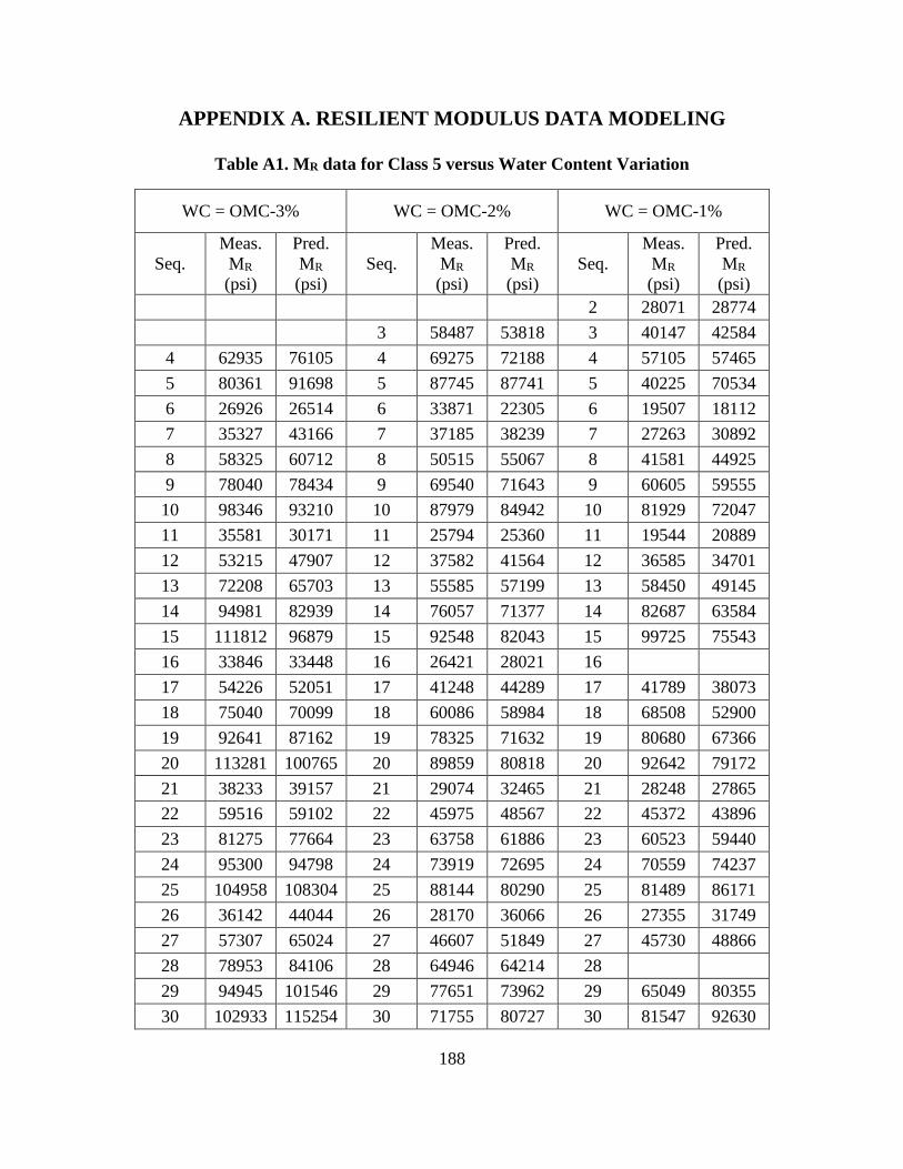
188
APPENDIX A. RESILIENT MODULUS DATA MODELING
Table A1. MR data for Class 5 versus Water Content Variation
WC = OMC-3% WC = OMC-2% WC = OMC-1%
Seq.
Meas.
MR
(psi)
Pred.
MR
(psi)
Seq.
Meas.
MR
(psi)
Pred.
MR
(psi)
Seq.
Meas.
MR
(psi)
Pred.
MR
(psi)
2 28071 28774
3 58487 53818 3 40147 42584
4 62935 76105 4 69275 72188 4 57105 57465
5 80361 91698 5 87745 87741 5 40225 70534
6 26926 26514 6 33871 22305 6 19507 18112
7 35327 43166 7 37185 38239 7 27263 30892
8 58325 60712 8 50515 55067 8 41581 44925
9 78040 78434 9 69540 71643 9 60605 59555
10 98346 93210 10 87979 84942 10 81929 72047
11 35581 30171 11 25794 25360 11 19544 20889
12 53215 47907 12 37582 41564 12 36585 34701
13 72208 65703 13 55585 57199 13 58450 49145
14 94981 82939 14 76057 71377 14 82687 63584
15 111812 96879 15 92548 82043 15 99725 75543
16 33846 33448 16 26421 28021 16
17 54226 52051 17 41248 44289 17 41789 38073
18 75040 70099 18 60086 58984 18 68508 52900
19 92641 87162 19 78325 71632 19 80680 67366
20 113281 100765 20 89859 80818 20 92642 79172
21 38233 39157 21 29074 32465 21 28248 27865
22 59516 59102 22 45975 48567 22 45372 43896
23 81275 77664 23 63758 61886 23 60523 59440
24 95300 94798 24 73919 72695 24 70559 74237
25 104958 108304 25 88144 80290 25 81489 86171
26 36142 44044 26 28170 36066 26 27355 31749
27 57307 65024 27 46607 51849 27 45730 48866
28 78953 84106 28 64946 64214 28
29 94945 101546 29 77651 73962 29 65049 80355
30 102933 115254 30 71755 80727 30 81547 92630
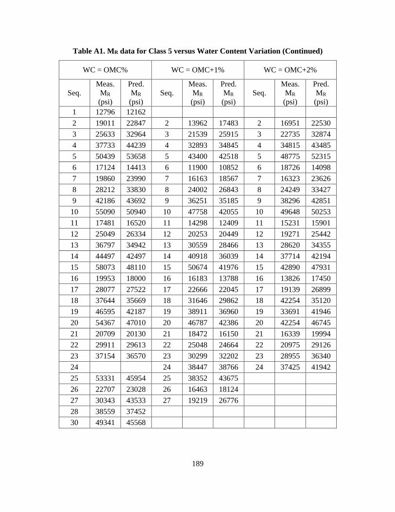
189
Table A1. MR data for Class 5 versus Water Content Variation (Continued)
WC = OMC% WC = OMC+1% WC = OMC+2%
Seq.
Meas.
MR
(psi)
Pred.
MR
(psi)
Seq.
Meas.
MR
(psi)
Pred.
MR
(psi)
Seq.
Meas.
MR
(psi)
Pred.
MR
(psi)
1 12796 12162
2 19011 22847 2 13962 17483 2 16951 22530
3 25633 32964 3 21539 25915 3 22735 32874
4 37733 44239 4 32893 34845 4 34815 43485
5 50439 53658 5 43400 42518 5 48775 52315
6 17124 14413 6 11900 10852 6 18726 14098
7 19860 23990 7 16163 18567 7 16323 23626
8 28212 33830 8 24002 26843 8 24249 33427
9 42186 43692 9 36251 35185 9 38296 42851
10 55090 50940 10 47758 42055 10 49648 50253
11 17481 16520 11 14298 12409 11 15231 15901
12 25049 26334 12 20253 20449 12 19271 25442
13 36797 34942 13 30559 28466 13 28620 34355
14 44497 42497 14 40918 36039 14 37714 42194
15 58073 48110 15 50674 41976 15 42890 47931
16 19953 18000 16 16183 13788 16 13826 17450
17 28077 27522 17 22666 22045 17 19139 26899
18 37644 35669 18 31646 29862 18 42254 35120
19 46595 42187 19 38911 36960 19 33691 41946
20 54367 47010 20 46787 42386 20 42254 46745
21 20709 20130 21 18472 16150 21 16339 19994
22 29911 29613 22 25048 24664 22 20975 29126
23 37154 36570 23 30299 32202 23 28955 36340
24 24 38447 38766 24 37425 41942
25 53331 45954 25 38352 43675
26 22707 23028 26 16463 18124
27 30343 43533 27 19219 26776
28 38559 37452
30 49341 45568

190
Table A2. MR data for Class 5 at 90% Maximum Dry Density
WC = OMC-2% WC = OMC% WC = OMC+2%
Seq.
Meas.
MR
(psi)
Pred.
MR
(psi)
Seq.
Meas.
MR
(psi)
Pred.
MR
(psi)
Seq.
Meas.
MR
(psi)
Pred.
MR
(psi)
1 11431 8518
2 29536 27893 2 28073 26237 2 11858 13898
3 36935 40102 3 34731 37680 3 17103 19767
4 48448 52342 4 45425 48670 4 26439 25955
5 61459 62307 5 56418 57140 5 36067 31331
6 23610 17671 6 19812 16255 6 9672 9234
7 27104 29034 7 24516 26712 7 12704 14913
8 36491 40374 8 33882 36567 8 20324 20975
9 50965 50940 9 45241 44986 9 30237 27227
10 65642 58988 10 56875 50761 10 37025 32562
11 20243 19748 11 18765 17836 11 10408 10553
12 28233 30863 12 26054 27277 12 15516 16759
13 42564 40806 13 38362 34728 13 24490 23174
14 56424 49154 14 46339 39972 14 31277 29614
15 63947 54992 15 49935 42923 15 35306 35007
16 20172 21497 16 17988 19070 16 11621 11754
17 30088 32269 17 25895 27523 17 17486 18414
18 43427 41140 18 33013 33255 18 22166 25151
19 46967 48083 19 35170 36651
20 54518 52693 20 43446 38204
21 20647 24292 21 20398 20829
22 33524 34303 22 25681 27532
23 38112 41639 23 24252 31000
24 43318 46898
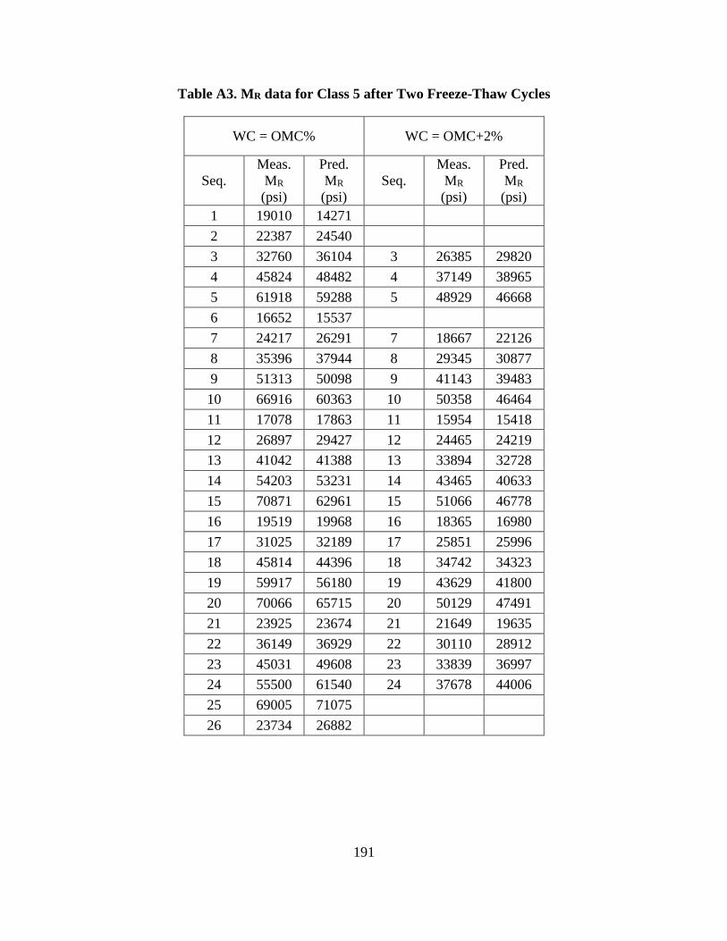
191
Table A3. MR data for Class 5 after Two Freeze-Thaw Cycles
WC = OMC% WC = OMC+2%
Seq.
Meas.
MR
(psi)
Pred.
MR
(psi)
Seq.
Meas.
MR
(psi)
Pred.
MR
(psi)
1 19010 14271
2 22387 24540
3 32760 36104 3 26385 29820
4 45824 48482 4 37149 38965
5 61918 59288 5 48929 46668
6 16652 15537
7 24217 26291 7 18667 22126
8 35396 37944 8 29345 30877
9 51313 50098 9 41143 39483
10 66916 60363 10 50358 46464
11 17078 17863 11 15954 15418
12 26897 29427 12 24465 24219
13 41042 41388 13 33894 32728
14 54203 53231 14 43465 40633
15 70871 62961 15 51066 46778
16 19519 19968 16 18365 16980
17 31025 32189 17 25851 25996
18 45814 44396 18 34742 34323
19 59917 56180 19 43629 41800
20 70066 65715 20 50129 47491
21 23925 23674 21 21649 19635
22 36149 36929 22 30110 28912
23 45031 49608 23 33839 36997
24 55500 61540 24 37678 44006
25 69005 71075
26 23734 26882

192
Table A4. MR data for 50% Old Class 5/50% RAP TH 10 versus Water Content Variation
WC = OMC-3% WC = OMC-2% WC = OMC-1%
Seq.
Meas.
MR
(psi)
Pred.
MR
(psi)
Seq.
Meas.
MR
(psi)
Pred.
MR
(psi)
Seq.
Meas.
MR
(psi)
Pred.
MR
(psi)
3 79563 93197
4 96009 115717
5 115888 133289 5 158978 158039
6 59511 48291 6
7 72912 72232 7 69655 65970
8 106606 94318 8 89025 95677
9 166865 165353 9 128302 113703 9 118361 123676
10 195384 187132 10 172143 127986 10 147467 144873
11 88891 65093 11 68694 52756 11 56183 42121
12 106162 101246 12 75931 76859 12 69736 69676
13 120887 128830 13 103232 96162 13 90312 94579
14 155937 149476 14 116191 111406 14 114471 115047
15 176834 162548 15 132801 122069 15 148128 128804
16 79977 70908 16 57896 57623 16 50241 46106
17 98114 103494 17 68726 80619 17 65285 72337
18 124789 125288 18 89029 97447 18 93446 93610
19 146299 139778 19 109153 110403 19 108086 109446
20 153902 147853 20 121372 119177 20 135837 119252
21 74100 79567 21 51533 65029 21 50479 52354
22 93177 105139 22 68081 85221 22 73252 75809
23 115324 119668 23 89777 99370 23 90690 91981
24 126536 127403 24 104853 109666 24 100607 102442
25 143773 130595 25 123227 116331 25 117701 108209
26 63177 84464 26 57400 69801 26 43848 56999
27 81690 105391 27 77143 88457 27 65268 77882
28 106859 115980 28 98471 100810 28 84960 90654
29 128328 119512 29 117858 109596 29 97607 98112
30 132044 120495 30 127251 115172 30 103679 101861
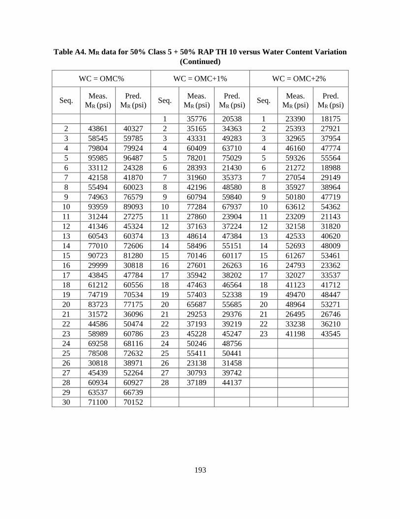
193
Table A4. MR data for 50% Class 5 + 50% RAP TH 10 versus Water Content Variation
(Continued)
WC = OMC% WC = OMC+1% WC = OMC+2%
Seq. Meas.
MR (psi)
Pred.
MR (psi) Seq.
Meas.
MR (psi)
Pred.
MR (psi) Seq.
Meas.
MR (psi)
Pred.
MR (psi)
1 35776 20538 1 23390 18175
2 43861 40327 2 35165 34363 2 25393 27921
3 58545 59785 3 43331 49283 3 32965 37954
4 79804 79924 4 60409 63710 4 46160 47774
5 95985 96487 5 78201 75029 5 59326 55564
6 33112 24328 6 28393 21430 6 21272 18988
7 42158 41870 7 31960 35373 7 27054 29149
8 55494 60023 8 42196 48580 8 35927 38964
9 74963 76579 9 60794 59840 9 50180 47719
10 93959 89093 10 77284 67937 10 63612 54362
11 31244 27275 11 27860 23904 11 23209 21143
12 41346 45324 12 37163 37224 12 32158 31820
13 60543 60374 13 48614 47384 13 42533 40620
14 77010 72606 14 58496 55151 14 52693 48009
15 90723 81280 15 70146 60117 15 61267 53461
16 29999 30818 16 27601 26263 16 24793 23362
17 43845 47784 17 35942 38202 17 32027 33537
18 61212 60556 18 47463 46564 18 41123 41712
19 74719 70534 19 57403 52338 19 49470 48447
20 83723 77175 20 65687 55685 20 48964 53271
21 31572 36096 21 29253 29376 21 26495 26746
22 44586 50474 22 37193 39219 22 33238 36210
23 58989 60786 23 45228 45247 23 41198 43545
24 69258 68116 24 50246 48756
25 78508 72632 25 55411 50441
26 30818 38971 26 23138 31458
27 45439 52264 27 30793 39742
28 60934 60927 28 37189 44137
29 63537 66739
30 71100 70152
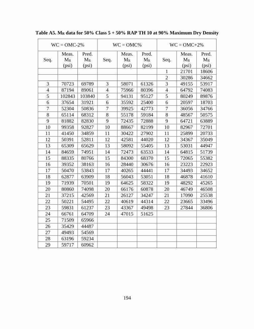
194
Table A5. MR data for 50% Class 5 + 50% RAP TH 10 at 90% Maximum Dry Density
WC = OMC-2% WC = OMC% WC = OMC+2%
Seq.
Meas.
MR
(psi)
Pred.
MR
(psi)
Seq.
Meas.
MR
(psi)
Pred.
MR
(psi)
Seq.
Meas.
MR
(psi)
Pred.
MR
(psi)
1 21701 18606
2 30286 34662
3 70723 69789 3 58071 61326 3 49155 53917
4 87194 89061 4 75966 80396 4 64792 74083
5 102843 103840 5 94131 95127 5 80249 89876
6 37654 31921 6 35592 25400 6 20597 18703
7 52304 50836 7 39925 42773 7 36056 34766
8 65114 68312 8 55178 59184 8 48567 50575
9 81882 82830 9 72435 72888 9 64721 63889
10 99358 92827 10 88667 82199 10 82967 72701
11 41450 34859 11 30422 27902 11 25899 20733
12 50391 52811 12 42581 44020 12 34367 35049
13 65309 65629 13 58092 55405 13 53031 44947
14 84659 74951 14 72473 63533 14 64815 51739
15 88335 80766 15 84300 68370 15 72065 55382
16 39352 38163 16 28440 30676 16 23223 22923
17 50470 53843 17 40265 44441 17 34493 34652
18 62877 63909 18 56043 53051 18 46878 41610
19 71939 70501 19 64625 58322 19 48292 45265
20 80860 74098 20 66176 60878 20 46749 46508
21 37215 42569 21 26127 34247 21 17090 25538
22 50221 54495 22 40619 44314 22 23665 33496
23 59831 61237 23 43367 49498 23 27844 36806
24 66761 64709 24 47015 51625
25 71509 65966
26 35429 44487
27 49493 54569
28 63196 59234
29 59717 60962

195
Table A6. MR data for 50% Class 5 + 50% RAP TH 10 after Two Freeze-Thaw Cycles
WC = OMC% WC = OMC+1% WC = OMC+2%
Seq.
Meas.
MR
(psi)
Pred.
MR
(psi)
Seq.
Meas.
MR
(psi)
Pred.
MR
(psi)
Seq.
Meas.
MR
(psi)
Pred.
MR
(psi)
1 36017 28731 1 35676 24497
2 47589 44081 2 38718 38693 2 49043 53934
3 60123 61635 3 52507 55083 3 70379 79364
4 77780 79179 4 73641 71513 4 95321 104854
5 95899 93428 5 93414 84754 5 110984 124897
6 36195 28875 6 32053 24621 6 38980 32398
7 44413 45851 7 38070 40072 7 51546 55173
8 57127 62843 8 51968 55441 8 71177 77271
9 78098 78141 9 74277 69113 9 96035 96189
10 98444 89803 10 95546 79311 10 114944 109424
11 34778 32034 11 29182 27312 11 43002 35799
12 44056 50008 12 39837 43177 12 57017 57476
13 63201 65026 13 54654 56028 13 77194 73506
14 78809 77345 14 62114 66310 14 102103 85371
15 100978 86368 15 85198 73564 15 117643 92804
16 33592 35873 16 28923 30526 16 41300 39655
17 47657 53197 17 38436 45412 17 59240 58624
18 67089 66434 18 55428 56373 18 81779 71116
19 83996 77259 19 64236 64887 19 87890 79334
20 92174 84902 20 72881 70568 20 101777 83771
21 35735 41744 21 28663 35286 21 41864 44828
22 50460 57009 22 41134 47894 22 61971 59248
23 65505 68660 23 51649 56872 23 69400 67443
24 82197 77692 24 58499 63292 24 71749 71668
25 91564 83862 25 69082 67310 25 74638 73222
26 34629 45067 26 27154 37875 26 34136 47292
27 51489 59827 27 44500 49583 27 50571 59174
28 73622 70406 28 55466 57230 28 57099 64674
29 80864 78389 29 51955 62442 29 51234 66806
30 79660 83789 30 102696 65586

196
Table A7. MR data for 25% Class 5 + 75% RAP TH 10 versus Water Content Variation
WC = OMC-3% WC = OMC-2% WC = OMC-1%
Seq.
Meas.
MR
(psi)
Pred.
MR
(psi)
Seq.
Meas.
MR
(psi)
Pred.
MR
(psi)
Seq.
Meas.
MR
(psi)
Pred.
MR
(psi)
8 10936 103661 8 89404 92430 8
9 128288 127606 9 118157 123266 9 154995 157328
10 150974 145406 10 144571 146652 10 184287 177427
11 71570 54444 11 11
12 78169 81280 12 67480 63488 12 111107 102048
13 94936 104289 13 86265 89194 13 124774 128672
14 127254 122996 14 114569 110071 14 156141 149398
15 141336 135755 15 134157 123608 15 169112 162916
16 62853 58707 16 49572 39430 16 91355 74726
17 78284 84436 17 67910 65462 17 105293 105104
18 103645 104751 18 90060 86527 18 126319 127903
19 121942 120139 19 104688 101516 19 145161 144199
20 134855 130090 20 117046 110119 20 155363 154108
21 59781 65410 21 45437 45121 21 82022 82341
22 78279 88907 22 63114 67621 22 97430 109115
23 101465 105401 23 78569 82325 23 117910 126579
24 114535 116817 24 91278 90781 24 137711 137649
25 135427 123755 25 102785 94649 25 154741 143754
26 62136 70462 26 40943 49228 26 79147 87889
27 80766 91936 27 57509 68510 27 93406 111553
28 98511 105850 28 72403 79104 28 115071 125478
29 124183 114968 29 85481 84096 29 139389 133577
30 30 89540 85769 30 148916 137724

197
Table A7. MR data for 25% Class 5 + 75% RAP TH 10 versus Water Content Variation
(Continued)
WC = OMC% WC = OMC+1% WC = OMC+2%
Seq.
Meas.
MR
(psi)
Pred.
MR
(psi)
Seq.
Meas.
MR
(psi)
Pred.
MR
(psi)
Seq.
Meas.
MR
(psi)
Pred.
MR
(psi)
1 26966 21991 1 1
2 33280 35841 2 27011 28766 2 32093 32125
3 44446 50203 3 34310 38846 3 37805 40149
4 62711 64288 4 46366 48209 4 45991 47197
5 79137 75583 5 56210 55897 5 54698 52393
6 27311 23468 6 22278 20168 6 27865 24159
7 34446 37206 7 28671 29892 7 31095 32785
8 46866 50532 8 37793 39719 8 37163 40029
9 65424 62711 9 49047 48379 9 46757 45951
10 78845 71871 10 59616 54994 10 56237 50035
11 27500 26020 11 23858 22033 11 28125 25775
12 37779 39387 12 34051 32792 12 34413 33774
13 53117 51056 13 45151 41984 13 41475 39806
14 58882 60704 14 53433 49068 14 46241 44238
15 76771 67388 15 59243 54518 15 53560 47021
16 28121 28156 16 24291 25232 16 25330 27061
17 39001 41060 17 34160 34994 17 30141 34472
18 52827 51463 18 44477 4123 18 34166 39607
19 62438 59503 19 51553 49778 19 41633 43096
20 67080 64803 20 59055 54762
21 28235 31546 21 27315 28104
22 39024 43477 22 35755 37751
23 48530 52072 23 42791 45251
24 24 43615 51250
25 64106 61993
26 28914 34132
27 43056 45155
28 51380 52523
30 58588 60538
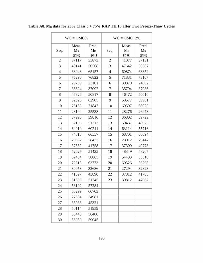
198
Table A8. MR data for 25% Class 5 + 75% RAP TH 10 after Two Freeze-Thaw Cycles
WC = OMC% WC = OMC+2%
Seq.
Meas.
MR
(psi)
Pred.
MR
(psi)
Seq.
Meas.
MR
(psi)
Pred.
MR
(psi)
2 37117 35873 2 41077 37131
3 49141 50568 3 47642 50587
4 63043 65157 4 60874 63352
5 75290 76822 5 71831 73107
6 29709 23101 6 30870 24802
7 36624 37092 7 35794 37986
8 47826 50817 8 46472 50010
9 62825 62905 9 58577 59981
10 76165 71847 10 69597 66925
11 28194 25538 11 28276 26973
12 37996 39816 12 36802 39722
13 52193 51212 13 50437 48925
14 64910 60241 14 63114 55716
15 74813 66557 15 68701 60094
16 28562 28432 16 28912 29442
17 37552 41758 17 37300 40778
18 52627 51435 18 48349 48207
19 62454 58865 19 54433 53310
20 72315 63773 20 60526 56298
21 30053 32686 21 27294 32823
22 41597 43890 22 37812 41705
23 51698 51745 23 39812 47062
24 58102 57284
25 65299 60703
26 27584 34981
27 38936 45321
28 50114 51959
29 55448 56408
30 58959 59045
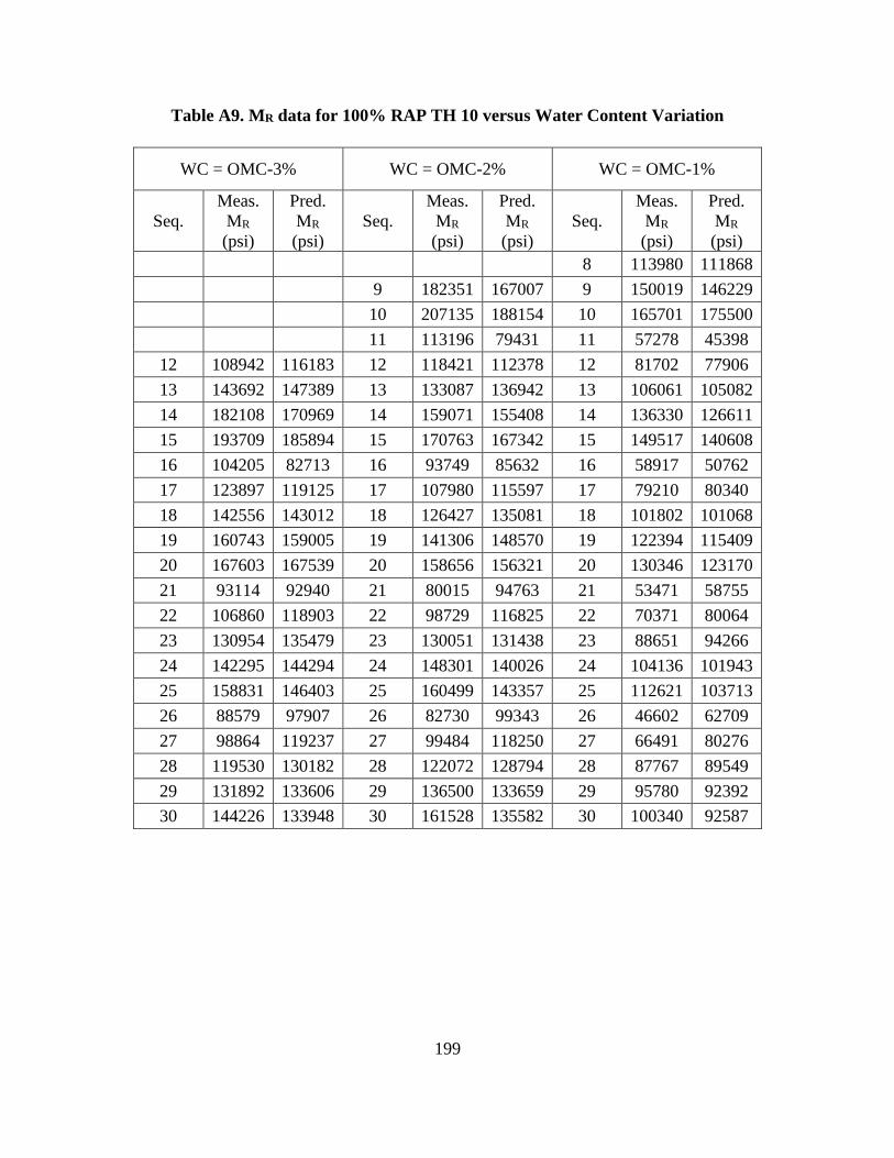
199
Table A9. MR data for 100% RAP TH 10 versus Water Content Variation
WC = OMC-3% WC = OMC-2% WC = OMC-1%
Seq.
Meas.
MR
(psi)
Pred.
MR
(psi)
Seq.
Meas.
MR
(psi)
Pred.
MR
(psi)
Seq.
Meas.
MR
(psi)
Pred.
MR
(psi)
8 113980 111868
9 182351 167007 9 150019 146229
10 207135 188154 10 165701 175500
11 113196 79431 11 57278 45398
12 108942 116183 12 118421 112378 12 81702 77906
13 143692 147389 13 133087 136942 13 106061 105082
14 182108 170969 14 159071 155408 14 136330 126611
15 193709 185894 15 170763 167342 15 149517 140608
16 104205 82713 16 93749 85632 16 58917 50762
17 123897 119125 17 107980 115597 17 79210 80340
18 142556 143012 18 126427 135081 18 101802 101068
19 160743 159005 19 141306 148570 19 122394 115409
20 167603 167539 20 158656 156321 20 130346 123170
21 93114 92940 21 80015 94763 21 53471 58755
22 106860 118903 22 98729 116825 22 70371 80064
23 130954 135479 23 130051 131438 23 88651 94266
24 142295 144294 24 148301 140026 24 104136 101943
25 158831 146403 25 160499 143357 25 112621 103713
26 88579 97907 26 82730 99343 26 46602 62709
27 98864 119237 27 99484 118250 27 66491 80276
28 119530 130182 28 122072 128794 28 87767 89549
29 131892 133606 29 136500 133659 29 95780 92392
30 144226 133948 30 161528 135582 30 100340 92587
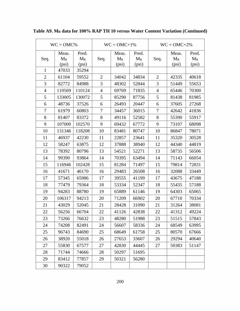
200
Table A9. MR data for 100% RAP TH 10 versus Water Content Variation (Continued)
WC = OMC% WC = OMC+1% WC = OMC+2%
Seq.
Meas.
MR
(psi)
Pred.
MR
(psi)
Seq.
Meas.
MR
(psi)
Pred.
MR
(psi)
Seq.
Meas.
MR
(psi)
Pred.
MR
(psi)
1 47033 35294
2 61104 59552 2 34042 34834 2 42335 40618
3 82772 84988 3 48302 52844 3 51449 55653
4 110569 110124 4 69769 71835 4 65446 70300
5 133005 130072 5 85290 87756 5 81438 81985
6 48736 37526 6 26493 20447 6 37605 27268
7 61979 60803 7 34457 36015 7 42642 41836
8 81407 83372 8 49116 52582 8 55390 55917
9 107000 102570 9 69432 67772 9 73107 68098
10 131346 118208 10 83481 80747 10 86847 78071
11 46937 42230 11 22857 23641 11 35320 30528
12 58247 63875 12 37888 38940 12 44340 44819
13 78392 80796 13 54521 52271 13 58735 56506
14 99390 93864 14 70395 63494 14 71143 66054
15 116946 102428 15 81284 71497 15 79814 72831
16 41671 46170 16 29483 26508 16 32088 33449
17 57345 65986 17 39555 41199 17 43675 47188
18 77479 79364 18 53334 52347 18 55435 57188
19 94283 88780 19 65889 61146 19 64303 65065
20 106317 94213 20 71209 66902 20 67710 70334
21 43029 52045 21 28428 31090 21 31264 38081
22 56256 66704 22 41126 42838 22 41312 49224
23 73266 76632 23 48280 51988 23 51515 57843
24 74208 82491 24 56607 58336 24 68549 63995
25 96743 84690 25 68649 61758 25 80570 67666
26 38920 55018 26 27653 33607 26 29294 40640
27 55830 67577 27 42830 44445 27 50383 51147
28 71744 74666 28 50297 51695
29 83412 77857 29 50321 56280
30 90322 79052

201
Table A10. MR data for 100% RAP TH 10 at 90% Maximum Dry Density
WC = OMC-2% WC = OMC% WC = OMC+2%
Seq.
Meas.
MR
(psi)
Pred.
MR
(psi)
Seq.
Meas.
MR
(psi)
Pred.
MR
(psi)
Seq.
Meas.
MR
(psi)
Pred.
MR
(psi)
2 52982 54169
3 71500 79938
4 104845 116980 4 89577 104664
5 5 111323 122729
6 126540 141088 6 41330 31690
7 65045 56798 7 50636 54120
8 91811 98265 8 78758 81638 8 68106 73852
9 121412 123402 9 103176 102598 9 89613 88969
10 141241 140526 10 123110 116651 10 108537 97963
11 52704 42626 11 44883 34724 11 40339 34306
12 69134 70434 12 58919 57745 12 51726 52953
13 89548 90354 13 81406 73892 13 74628 63859
14 113458 104586 14 96105 85184 14 91764 70366
15 120596 112892 15 103270 91510 15 97520 73055
16 49224 47207 16 42721 38388 16 36786 36905
17 65315 70752 17 53769 57557 17 50370 51137
18 86038 85513 18 73254 69222 18 65301 58086
19 93383 94285 19 79265 75756 19 70056 60531
20 114781 98260 20 88221 78377 20 63228 60347
21 50956 53027 21 36497 42901 21 28246 39500
22 70623 69954 22 50309 56292 22 37273 48015
23 82280 78322 23 60353 62388 23 36771 49980
24 82142 81268 24 69525 63972 24 41374 48544
25 91311 81085 25 74013 63156
26 47507 55353 26 33519 44617
27 63326 68697 27 46369 54818
28 69369 73172 28 51455 57569
29 66513 73107 29 52624 56675

202
Table A11. MR data for 100% RAP TH 10 after Two Freeze-Thaw Cycles
WC = OMC% WC = OMC+1% WC = OMC+2%
Seq.
Meas.
MR
(psi)
Pred.
MR
(psi)
Seq.
Meas.
MR
(psi)
Pred.
MR
(psi)
Seq. Meas.
MR (psi)
Pred.
MR
(psi)
2 60213 58920 2 37245 38948 2 59966 58140
3 78561 80410 3 52637 58516 3 87038 83309
4 114685 100920 4 73732 78789 4 121139 107732
5 87678 116721 5 91473 95322 5 126666 126346
6 53852 39347 6 29256 22960 6 44833 35996
7 61912 60408 7 39627 40245 7 61146 59086
8 76197 79844 8 55737 57991 8 78417 80383
9 98624 96139 9 74932 73964 9 94213 97868
10 123736 107641 10 90946 85770 10 106751 109587
11 53186 42888 11 29662 25705 11 48835 39329
12 65876 63525 12 40909 42997 12 58287 60583
13 83981 78737 13 63186 56966 13 75230 75229
14 102446 90141 14 74528 68017 14 89670 85521
15 110186 97653 15 84286 75548 15 94250 91545
16 42409 46957 16 28338 28947 16 42272 42992
17 59400 65529 17 41365 44792 17 54239 61010
18 77940 77983 18 59874 56269 18 70635 72024
19 91874 86793 19 68169 64752 19 80106 78612
20 104330 92139 20 76895 70042 20 78643 81712
21 41521 52628 21 29990 33615 21 38057 47640
22 58387 67448 22 43038 46533 22 50841 60680
23 75585 76752 23 54378 55132 23 65392 67188
24 81462 82558 24 61532 60680 24 70377 69827
25 95872 85658 25 66594 63700 25 78791 70194
26 39938 55509 26 29071 36050 26 38365 49690
27 57875 68517 27 42299 47514 27 55447 59852
28 72617 75767 28 53037 54228 28 62055 63612
29 81247 79889 29 55717 58147 29 65471 64251
30 56496 60026 30 71097 63017
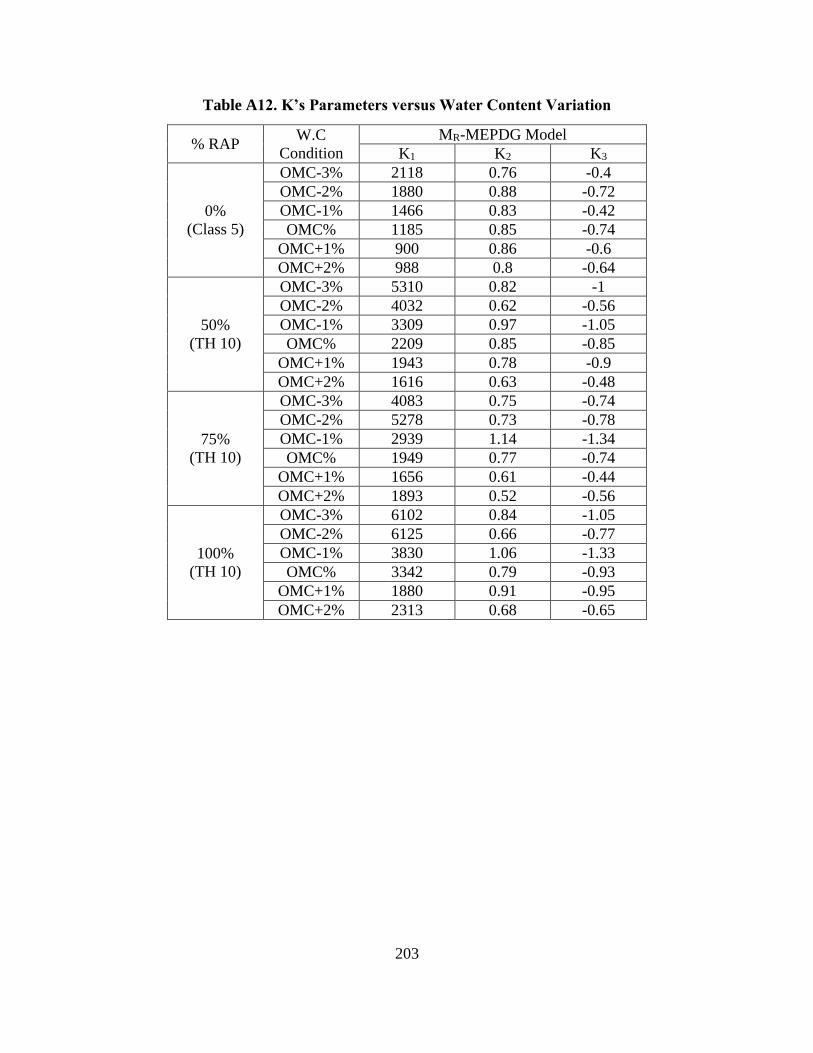
203
Table A12. K’s Parameters versus Water Content Variation
% RAP W.C
Condition
MR-MEPDG Model
K1 K2 K3
0%
(Class 5)
OMC-3% 2118 0.76 -0.4
OMC-2% 1880 0.88 -0.72
OMC-1% 1466 0.83 -0.42
OMC% 1185 0.85 -0.74
OMC+1% 900 0.86 -0.6
OMC+2% 988 0.8 -0.64
50%
(TH 10)
OMC-3% 5310 0.82 -1
OMC-2% 4032 0.62 -0.56
OMC-1% 3309 0.97 -1.05
OMC% 2209 0.85 -0.85
OMC+1% 1943 0.78 -0.9
OMC+2% 1616 0.63 -0.48
75%
(TH 10)
OMC-3% 4083 0.75 -0.74
OMC-2% 5278 0.73 -0.78
OMC-1% 2939 1.14 -1.34
OMC% 1949 0.77 -0.74
OMC+1% 1656 0.61 -0.44
OMC+2% 1893 0.52 -0.56
100%
(TH 10)
OMC-3% 6102 0.84 -1.05
OMC-2% 6125 0.66 -0.77
OMC-1% 3830 1.06 -1.33
OMC% 3342 0.79 -0.93
OMC+1% 1880 0.91 -0.95
OMC+2% 2313 0.68 -0.65

204
Table A13. K’s Parameters versus 90% Maximum Dry Density
Table A14. K’s Parameters versus Two Freeze-Thaw Cycles
% RAP W.C
Condition
MR-MEPDG Model
K1 K2 K3
0% OMC% 1257 0.82 -0.43
OMC+2% 1105 0.77 -0.51
50%
OMC% 2484 0.71 -0.6
OMC+1% 2165 0.76 -0.74
OMC+2% 2994 0.86 -1.07
75% OMC% 2019 0.74 -0.73
OMC+2% 2140 0.68 -0.78
100%
OMC% 3388 0.68 -0.75
OMC+1% 2126 0.89 -0.98
OMC+2% 3284 0.81 -1.08
% RAP W.C
Condition
MR-MEPDG Model
K1 K2 K3
0%
OMC-2% 1491 0.83 -0.8
OMC% 1436 0.88 -1.15
OMC+2% 724 0.73 -0.27
50%
OMC-2% 2834 0.75 -0.92
OMC% 2349 0.85 -1.12
OMC+2% 1864 1.03 -1.5
100%
OMC-2% 3700 0.95 -1.29
OMC% 3059 0.98 -1.38
OMC+2% 3053 0.91 -1.48
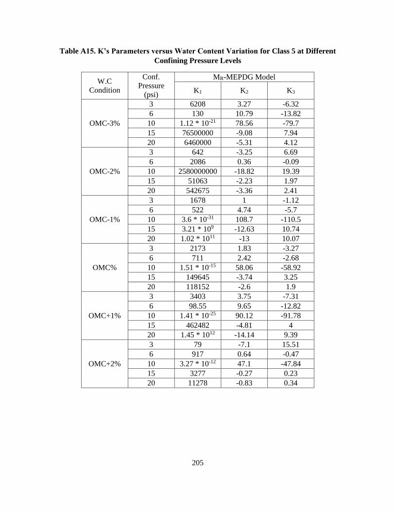
205
Table A15. K’s Parameters versus Water Content Variation for Class 5 at Different
Confining Pressure Levels
W.C
Condition
Conf.
Pressure
(psi)
MR-MEPDG Model
K1 K2 K3
OMC-3%
3 6208 3.27 -6.32
6 130 10.79 -13.82
10 1.12 * 10-21 78.56 -79.7
15 76500000 -9.08 7.94
20 6460000 -5.31 4.12
OMC-2%
3 642 -3.25 6.69
6 2086 0.36 -0.09
10 2580000000 -18.82 19.39
15 51063 -2.23 1.97
20 542675 -3.36 2.41
OMC-1%
3 1678 1 -1.12
6 522 4.74 -5.7
10 3.6 * 10-31 108.7 -110.5
15 3.21 * 109 -12.63 10.74
20 1.02 * 1011 -13 10.07
OMC%
3 2173 1.83 -3.27
6 711 2.42 -2.68
10 1.51 * 10-15 58.06 -58.92
15 149645 -3.74 3.25
20 118152 -2.6 1.9
OMC+1%
3 3403 3.75 -7.31
6 98.55 9.65 -12.82
10 1.41 * 10-25 90.12 -91.78
15 462482 -4.81 4
20 1.45 * 1012 -14.14 9.39
OMC+2%
3 79 -7.1 15.51
6 917 0.64 -0.47
10 3.27 * 10-12 47.1 -47.84
15 3277 -0.27 0.23
20 11278 -0.83 0.34
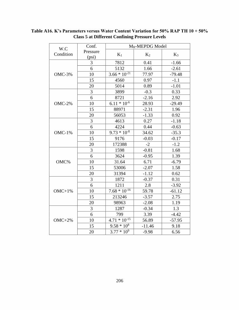
206
Table A16. K’s Parameters versus Water Content Variation for 50% RAP TH 10 + 50%
Class 5 at Different Confining Pressure Levels
W.C
Condition
Conf.
Pressure
(psi)
MR-MEPDG Model
K1 K2 K3
OMC-3%
3 7812 0.41 -1.66
6 5132 1.66 -2.61
10 3.66 * 10-21 77.97 -79.48
15 4560 0.97 -1.1
20 5014 0.89 -1.01
OMC-2%
3 3899 -0.3 0.33
6 8721 -2.16 2.92
10 6.11 * 10-6 28.93 -29.49
15 88971 -2.31 1.96
20 56053 -1.33 0.92
OMC-1%
3 4613 0.27 -1.18
6 4224 0.44 -0.63
10 9.73 * 10-8 34.62 -35.3
15 9176 -0.03 -0.17
20 172388 -2 -1.2
OMC%
3 1598 -0.81 1.68
6 3624 -0.95 1.39
10 31.64 6.71 -6.79
15 53006 -2.07 1.58
20 31394 -1.12 0.62
OMC+1%
3 1872 -0.37 0.31
6 1211 2.8 -3.92
10 7.68 * 10-16 59.78 -61.12
15 213246 -3.57 2.75
20 98963 -2.08 1.19
OMC+2%
3 1287 -0.34 1.3
6 799 3.39 -4.42
10 4.71 * 10-15 56.89 -57.95
15 9.58 * 108 -11.46 9.18
20 3.77 * 109 -9.98 6.56
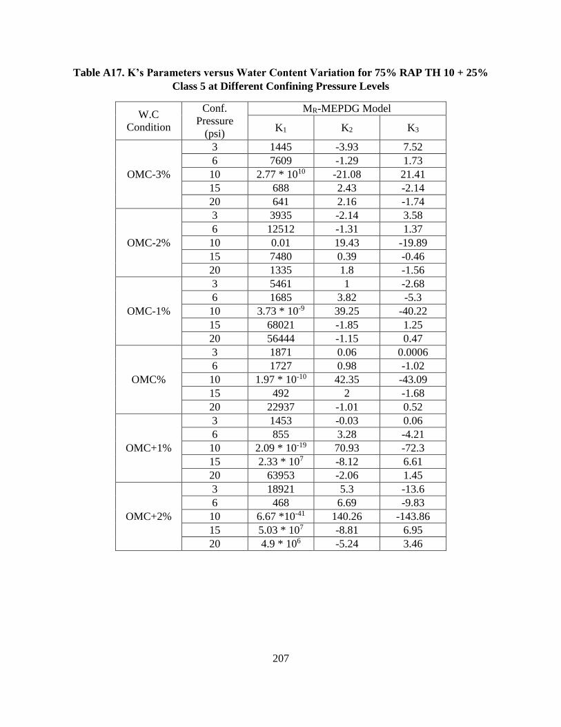
207
Table A17. K’s Parameters versus Water Content Variation for 75% RAP TH 10 + 25%
Class 5 at Different Confining Pressure Levels
W.C
Condition
Conf.
Pressure
(psi)
MR-MEPDG Model
K1 K2 K3
OMC-3%
3 1445 -3.93 7.52
6 7609 -1.29 1.73
10 2.77 * 1010 -21.08 21.41
15 688 2.43 -2.14
20 641 2.16 -1.74
OMC-2%
3 3935 -2.14 3.58
6 12512 -1.31 1.37
10 0.01 19.43 -19.89
15 7480 0.39 -0.46
20 1335 1.8 -1.56
OMC-1%
3 5461 1 -2.68
6 1685 3.82 -5.3
10 3.73 * 10-9 39.25 -40.22
15 68021 -1.85 1.25
20 56444 -1.15 0.47
OMC%
3 1871 0.06 0.0006
6 1727 0.98 -1.02
10 1.97 * 10-10 42.35 -43.09
15 492 2 -1.68
20 22937 -1.01 0.52
OMC+1%
3 1453 -0.03 0.06
6 855 3.28 -4.21
10 2.09 * 10-19 70.93 -72.3
15 2.33 * 107 -8.12 6.61
20 63953 -2.06 1.45
OMC+2%
3 18921 5.3 -13.6
6 468 6.69 -9.83
10 6.67 *10-41 140.26 -143.86
15 5.03 * 107 -8.81 6.95
20 4.9 * 106 -5.24 3.46

208
Table A18. K’s Parameters versus Water Content Variation for 100% RAP TH 10 at
Different Confining Pressure Levels
W.C
Condition
Conf.
Pressure
(psi)
MR-MEPDG Model
K1 K2 K3
OMC-3%
3 6476 -0.78 0.96
6 831 7.9 -10.55
10 5.32 * 10-13 52.18 -53.33
15 175 4.37 -4.21
20 1075 2.2 -2.06
OMC-2%
3 2424 -3.62 6.63
6 29932 -4.14 5.08
10 191 5.41 -5.59
15 128 4.36 -3.94
20 66 4.15 -3.35
OMC-1%
3 9915 2.41 -5.5
6 5243 0.68 -1.28
10 18909 -1.11 0.82
15 27178 -0.74 0.2
20 37911 -0.76 0.15
OMC%
3 3232 -0.06 -0.26
6 4803 -0.53 0.6
10 1670 1.73 -1.9
15 5060 0.43 -0.65
20 15364 -0.32 -0.05
OMC+1%
3 2164 0.63 -1.11
6 1835 0.88 -0.92
10 1.06 * 10-6 30.53 -31.15
15 891795 -4.75 3.71
20 18347 -0.8 0.37
OMC+2%
3 1970 -0.72 1.05
6 3913 -1.31 1.93
10 1.16 * 10-14 56.27 -57.57
15 38269 -1.93 1.56
20 547 1.75 -1.34
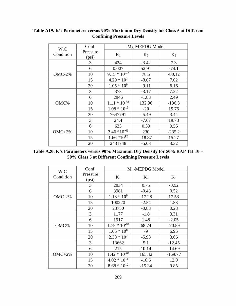
209
Table A19. K’s Parameters versus 90% Maximum Dry Density for Class 5 at Different
Confining Pressure Levels
Table A20. K’s Parameters versus 90% Maximum Dry Density for 50% RAP TH 10 +
50% Class 5 at Different Confining Pressure Levels
W.C
Condition
Conf.
Pressure
(psi)
MR-MEPDG Model
K1 K2 K3
OMC-2%
3 424 -3.42 7.3
6 0.007 52.91 -74.1
10 9.15 * 10-22 78.5 -80.12
15 4.29 * 107 -8.67 7.02
20 1.05 * 109 -9.11 6.16
OMC%
3 378 -3.17 7.22
6 2846 -1.83 2.49
10 1.11 * 10-38 132.96 -136.3
15 1.08 * 1013 -20 15.76
20 7647791 -5.49 3.44
OMC+2%
3 24.4 -7.67 19.73
6 633 0.39 0.56
10 3.46 *10-69 230 -235.2
15 1.66 *1012 -18.87 15.27
20 2431748 -5.03 3.32
W.C
Condition
Conf.
Pressure
(psi)
MR-MEPDG Model
K1 K2 K3
OMC-2%
3 2834 0.75 -0.92
6 3981 -0.43 0.52
10 1.13 * 109 -17.28 17.53
15 100220 -2.54 1.83
20 23750 -0.83 0.28
OMC%
3 1177 -1.8 3.31
6 1917 1.48 -2.05
10 1.75 * 10-18 68.74 -70.59
15 1.05 * 108 -9 6.95
20 2.38 * 107 -5.93 3.66
OMC+2%
3 13662 5.1 -12.45
6 215 10.14 -14.69
10 1.42 * 10-48 165.42 -169.77
15 4.02 * 1011 -16.6 12.9
20 8.68 * 1012 -15.34 9.85

210
Table A21. K’s Parameters versus 90% Maximum Dry Density for 100% RAP TH 10 at
Different Confining Pressure Levels
Table A22. K’s Parameters versus Two Freeze-Thaw Cycles for Class 5 at Different
Confining Pressure Levels
W.C
Condition
Conf.
Pressure
(psi)
MR-MEPDG Model
K1 K2 K3
OMC-2%
3 3435 -0.16 0.14
6 2921 1.7 -2.3
10 5.44 * 10-9 38.79 -39.81
15 563883 -3.72 2.61
20 97375 -1.58 0.72
OMC%
3 4222 0.58 -1.99
6 5489 -0.6 0.35
10 4.58 * 10-19 71.02 -72.87
15 3.62 * 106 -5.6 4.15
20 94065 -1.65 0.7
OMC+2%
3 5960 1.58 -4.72
6 791 6.59 -9.74
10 2.24 * 10-50 171.75 -176.34
15 3.93 * 1012 -18.39 14.38
20 7.92 * 1011 -13.36 8.49
W.C
Condition
Conf.
Pressure
(psi)
MR-MEPDG Model
K1 K2 K3
OMC%
3 694 -1.2 3.37
6 1244 0.4 0.29
10 1.15 * 10-17 65.08 -66.07
15 5.96 * 106 -7 6
20 138456 -2.61 2
OMC+2%
3 1929 2.43 -3.75
6 217 6.25 -7.67
10 6.92 * 10-23 81.62 -83.09
15 1.08 * 108 -9.8 8.12
20 50304 -2 1.43
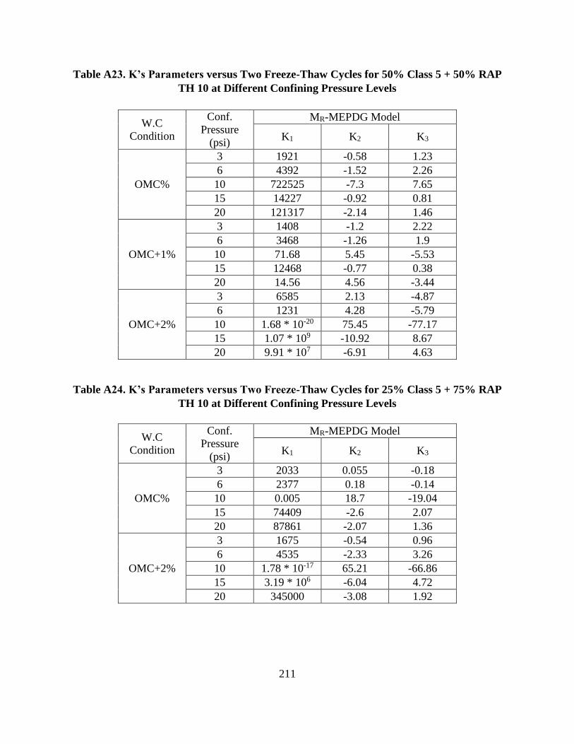
211
Table A23. K’s Parameters versus Two Freeze-Thaw Cycles for 50% Class 5 + 50% RAP
TH 10 at Different Confining Pressure Levels
Table A24. K’s Parameters versus Two Freeze-Thaw Cycles for 25% Class 5 + 75% RAP
TH 10 at Different Confining Pressure Levels
W.C
Condition
Conf.
Pressure
(psi)
MR-MEPDG Model
K1 K2 K3
OMC%
3 1921 -0.58 1.23
6 4392 -1.52 2.26
10 722525 -7.3 7.65
15 14227 -0.92 0.81
20 121317 -2.14 1.46
OMC+1%
3 1408 -1.2 2.22
6 3468 -1.26 1.9
10 71.68 5.45 -5.53
15 12468 -0.77 0.38
20 14.56 4.56 -3.44
OMC+2%
3 6585 2.13 -4.87
6 1231 4.28 -5.79
10 1.68 * 10-20 75.45 -77.17
15 1.07 * 109 -10.92 8.67
20 9.91 * 107 -6.91 4.63
W.C
Condition
Conf.
Pressure
(psi)
MR-MEPDG Model
K1 K2 K3
OMC%
3 2033 0.055 -0.18
6 2377 0.18 -0.14
10 0.005 18.7 -19.04
15 74409 -2.6 2.07
20 87861 -2.07 1.36
OMC+2%
3 1675 -0.54 0.96
6 4535 -2.33 3.26
10 1.78 * 10-17 65.21 -66.86
15 3.19 * 106 -6.04 4.72
20 345000 -3.08 1.92
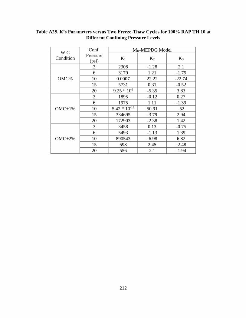
212
Table A25. K’s Parameters versus Two Freeze-Thaw Cycles for 100% RAP TH 10 at
Different Confining Pressure Levels
W.C
Condition
Conf.
Pressure
(psi)
MR-MEPDG Model
K1 K2 K3
OMC%
3 2308 -1.28 2.1
6 3179 1.21 -1.75
10 0.0007 22.22 -22.74
15 5731 0.31 -0.52
20 9.25 * 106 -5.35 3.83
OMC+1%
3 1895 -0.12 0.27
6 1975 1.11 -1.39
10 5.42 * 10-13 50.91 -52
15 334695 -3.79 2.94
20 172903 -2.38 1.42
OMC+2%
3 3458 0.13 -0.75
6 5493 -1.13 1.39
10 890543 -6.98 6.82
15 598 2.45 -2.48
20 556 2.1 -1.94

213
APPENDIX B. PERMANENT DEFORMATION DATA MODELING
Table B1. PD Measured Data from MR Test for Class 5 (OMC-2%)
Seq. Measured
MR (psi)
Measured
PD (inches)
Pred. PD (inches)
H = 6 in. H = 9 in. H = 12 in
4 63010 0.0096 7.4931E-05 0.0001124 0.00014986
5 80403 0.01008 0.00010066 0.00015098 0.00020131
6 26926 0.00612 3.4574E-05 5.1862E-05 6.9149E-05
7 34455 0.00858 6.2239E-05 9.3358E-05 0.00012448
8 46727 0.00912 9.3779E-05 0.00014067 0.00018756
9 64814 0.00984 0.00013334 0.00020002 0.00026669
10 83747 0.01038 0.00018198 0.00027297 0.00036396
11 24551 0.00822 6.9856E-05 0.00010478 0.00013971
12 42634 0.00846 0.00010181 0.00015272 0.00020362
13 61387 0.00924 0.00015545 0.00023317 0.0003109
14 82326 0.01002 0.00024157 0.00036235 0.00048313
15 98613 0.01104 0.00036178 0.00054267 0.00072356
16 25425 0.00912 0.00010083 0.00015125 0.00020166
17 44821 0.0096 0.00014922 0.00022383 0.00029844
18 63824 0.01062 0.0002374 0.00035611 0.00047481
19 80972 0.01242 0.0003936 0.00059041 0.00078721
20 94180 0.01488 0.00061572 0.00092359 0.00123145
21 30261 0.0126 0.00014852 0.00022279 0.00029705
22 48693 0.01434 0.00024959 0.00037439 0.00049919
23 67823 0.0174 0.00043002 0.00064503 0.00086003
24 80901 0.02214 0.00079139 0.00118709 0.00158278
25 95115 0.0276 0.00132384 0.00198575 0.00264767
26 29988 0.02508 0.00021612 0.00032419 0.00043225
27 50503 0.02682 0.00036734 0.00055101 0.00073467
28 71442 0.02958 0.00066778 0.00100167 0.00133557
29 81753 0.03696 0.00134908 0.00202362 0.00269815
30 89707 0.05202 0.00248566 0.00372849 0.00497132

214
Table B2. PD Measured Data from MR Test for Class 5 (OMC%)
Seq. Measured
MR (psi)
Measured
PD (inches)
Pred. PD (inches)
H = 6 in. H = 9 in. H = 12 in
1 18235 0.0573 2.7139E-07 4.0709E-07 5.4278E-07
2 19011 0.0573 5.6625E-07 8.4938E-07 1.1325E-06
3 25633 0.0576 8.1371E-07 1.2206E-06 1.6274E-06
4 37734 0.0582 1.0277E-06 1.5415E-06 2.0553E-06
5 50439 0.0585 1.2758E-06 1.9138E-06 2.5517E-06
6 17124 0.0573 4.9689E-07 7.4534E-07 9.9379E-07
7 19860 0.0576 9.5477E-07 1.4321E-06 1.9095E-06
8 28212 0.0579 1.3367E-06 2.0051E-06 2.6734E-06
9 42186 0.0585 1.7137E-06 2.5706E-06 3.4274E-06
10 55090 0.0588 2.2197E-06 3.3296E-06 4.4395E-06
11 17481 0.0579 9.1379E-07 1.3707E-06 1.8276E-06
12 25050 0.0585 1.5009E-06 2.2513E-06 3.0017E-06
13 36798 0.0591 2.14E-06 3.21E-06 4.2801E-06
14 44497 0.0597 3.3659E-06 5.0489E-06 6.7318E-06
15 58073 0.0618 4.5408E-06 6.8111E-06 9.0815E-06
16 19954 0.0609 1.2099E-06 1.8149E-06 2.4199E-06
17 28077 0.0621 2.0752E-06 3.1129E-06 4.1505E-06
18 37644 0.0645 3.2854E-06 4.928E-06 6.5707E-06
19 46596 0.069 5.2755E-06 7.9133E-06 1.0551E-05
20 54368 0.0744 7.9234E-06 1.1885E-05 1.5847E-05
21 20709 0.0747 1.9871E-06 2.9806E-06 3.9741E-06
22 29911 0.078 3.4903E-06 5.2355E-06 6.9807E-06
23 37155 0.0873 6.2114E-06 9.3171E-06 1.2423E-05
24 38398 0.114 1.2158E-05 1.8237E-05 2.4317E-05
25 53331 0.1497 1.7302E-05 2.5953E-05 3.4604E-05
26 22707 0.1512 2.6546E-06 3.9819E-06 5.3091E-06
27 34553 0.1557 4.7032E-06 7.0548E-06 9.4064E-06
28 41748 0.1773 9.1037E-06 1.3656E-05 1.8207E-05
29 49341 0.2538 3.3443E-05 5.0165E-05 6.6887E-05
30 18235 0.0573 2.7139E-07 4.0709E-07 5.4278E-07
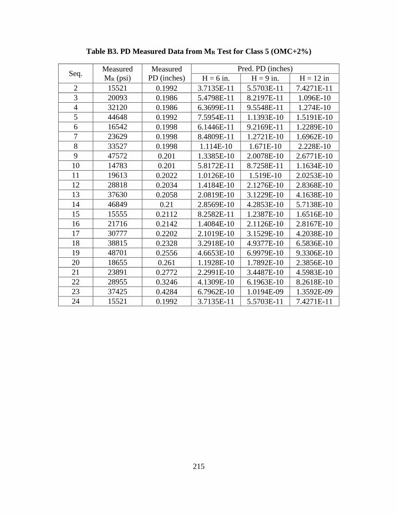
215
Table B3. PD Measured Data from MR Test for Class 5 (OMC+2%)
Seq. Measured
MR (psi)
Measured
PD (inches)
Pred. PD (inches)
H = 6 in. H = 9 in. H = 12 in
2 15521 0.1992 3.7135E-11 5.5703E-11 7.4271E-11
3 20093 0.1986 5.4798E-11 8.2197E-11 1.096E-10
4 32120 0.1986 6.3699E-11 9.5548E-11 1.274E-10
5 44648 0.1992 7.5954E-11 1.1393E-10 1.5191E-10
6 16542 0.1998 6.1446E-11 9.2169E-11 1.2289E-10
7 23629 0.1998 8.4809E-11 1.2721E-10 1.6962E-10
8 33527 0.1998 1.114E-10 1.671E-10 2.228E-10
9 47572 0.201 1.3385E-10 2.0078E-10 2.6771E-10
10 14783 0.201 5.8172E-11 8.7258E-11 1.1634E-10
11 19613 0.2022 1.0126E-10 1.519E-10 2.0253E-10
12 28818 0.2034 1.4184E-10 2.1276E-10 2.8368E-10
13 37630 0.2058 2.0819E-10 3.1229E-10 4.1638E-10
14 46849 0.21 2.8569E-10 4.2853E-10 5.7138E-10
15 15555 0.2112 8.2582E-11 1.2387E-10 1.6516E-10
16 21716 0.2142 1.4084E-10 2.1126E-10 2.8167E-10
17 30777 0.2202 2.1019E-10 3.1529E-10 4.2038E-10
18 38815 0.2328 3.2918E-10 4.9377E-10 6.5836E-10
19 48701 0.2556 4.6653E-10 6.9979E-10 9.3306E-10
20 18655 0.261 1.1928E-10 1.7892E-10 2.3856E-10
21 23891 0.2772 2.2991E-10 3.4487E-10 4.5983E-10
22 28955 0.3246 4.1309E-10 6.1963E-10 8.2618E-10
23 37425 0.4284 6.7962E-10 1.0194E-09 1.3592E-09
24 15521 0.1992 3.7135E-11 5.5703E-11 7.4271E-11

216
Table B4. PD Measured Data from MR Test for 50% RAP TH 10 (OMC-2%)
Seq. Measured
MR (psi)
Measured
PD (inches)
Pred. PD (inches)
H = 6 in. H = 9 in. H = 12 in
3 79563 0.00162 0.00020217 0.00030325 0.00040433
4 96009 0.00234 0.00032097 0.00048145 0.00064194
5 115888 0.00288 0.0004637 0.00069555 0.0009274
6 106606 0.00372 0.00032303 0.00048454 0.00064605
7 128302 0.00432 0.00054273 0.00081409 0.00108546
8 172143 0.00684 0.00084724 0.00127086 0.00169447
9 68694 0.00312 0.00017599 0.00026399 0.00035199
10 87005 0.0042 0.00035224 0.00052835 0.00070447
11 112236 0.00606 0.00062775 0.00094163 0.00125551
12 130895 0.00546 0.00110425 0.00165638 0.0022085
13 148482 0.00642 0.00176205 0.00264308 0.00352411
14 66120 0.00444 0.00026688 0.00040032 0.00053376
15 79487 0.00498 0.00055554 0.00083331 0.00111108
16 102830 0.00576 0.00100249 0.00150374 0.00200498
17 122593 0.00702 0.00180095 0.00270142 0.0036019
18 132155 0.00882 0.00296412 0.00444618 0.00592824
19 61594 0.00672 0.00047081 0.00070622 0.00094163
20 77286 0.0075 0.0009956 0.0014934 0.00199121
21 98436 0.009 0.00190221 0.00285331 0.00380441
22 79106 0.01218 0.00415394 0.00623091 0.00830788
23 132971 0.01638 0.00639151 0.00958727 0.01278302
24 61665 0.01392 0.00067975 0.00101963 0.00135951
25 80782 0.01482 0.001471 0.0022065 0.00294201
26 104740 0.01632 0.00297907 0.0044686 0.00595813
27 124768 0.01986 0.00618289 0.00927434 0.01236578
28 133546 0.0276 0.01174529 0.01761793 0.02349058
29 79563 0.00162 0.00020217 0.00030325 0.00040433
30 96009 0.00234 0.00032097 0.00048145 0.00064194
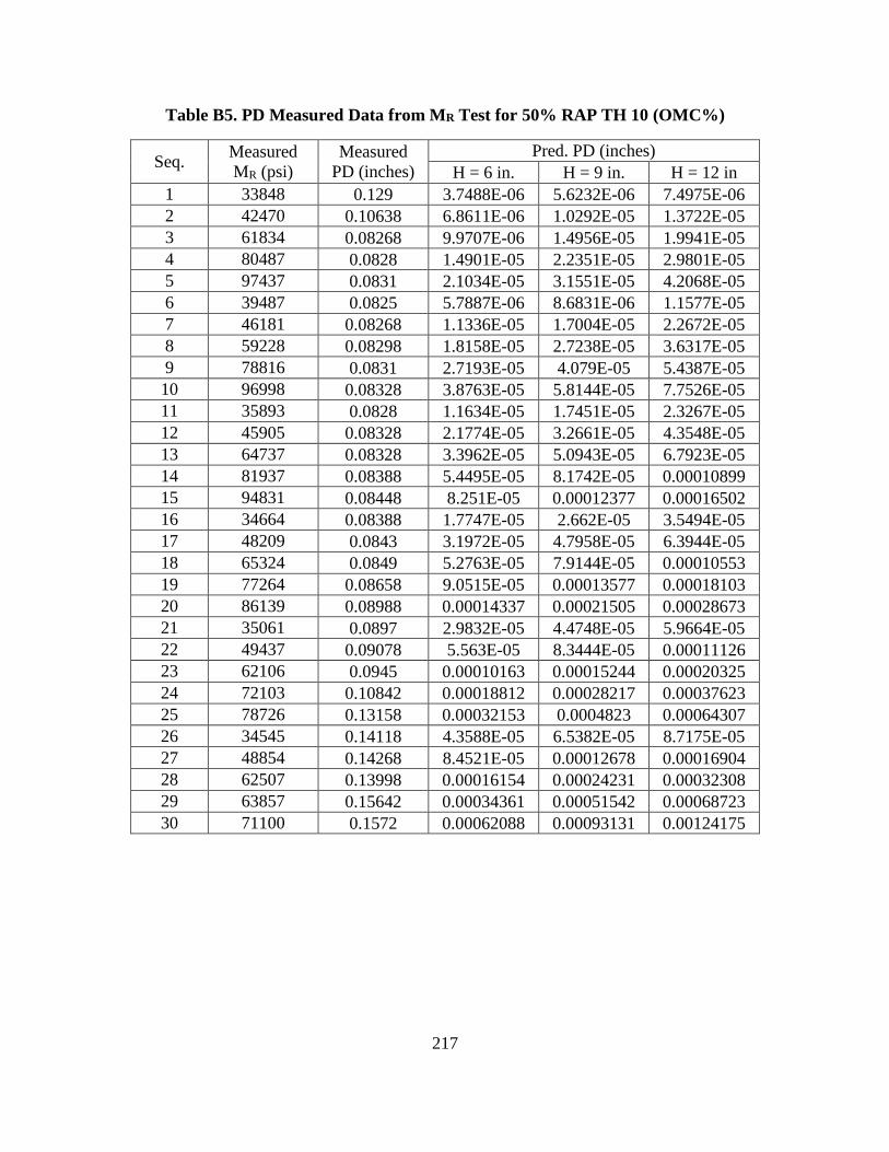
217
Table B5. PD Measured Data from MR Test for 50% RAP TH 10 (OMC%)
Seq. Measured
MR (psi)
Measured
PD (inches)
Pred. PD (inches)
H = 6 in. H = 9 in. H = 12 in
1 33848 0.129 3.7488E-06 5.6232E-06 7.4975E-06
2 42470 0.10638 6.8611E-06 1.0292E-05 1.3722E-05
3 61834 0.08268 9.9707E-06 1.4956E-05 1.9941E-05
4 80487 0.0828 1.4901E-05 2.2351E-05 2.9801E-05
5 97437 0.0831 2.1034E-05 3.1551E-05 4.2068E-05
6 39487 0.0825 5.7887E-06 8.6831E-06 1.1577E-05
7 46181 0.08268 1.1336E-05 1.7004E-05 2.2672E-05
8 59228 0.08298 1.8158E-05 2.7238E-05 3.6317E-05
9 78816 0.0831 2.7193E-05 4.079E-05 5.4387E-05
10 96998 0.08328 3.8763E-05 5.8144E-05 7.7526E-05
11 35893 0.0828 1.1634E-05 1.7451E-05 2.3267E-05
12 45905 0.08328 2.1774E-05 3.2661E-05 4.3548E-05
13 64737 0.08328 3.3962E-05 5.0943E-05 6.7923E-05
14 81937 0.08388 5.4495E-05 8.1742E-05 0.00010899
15 94831 0.08448 8.251E-05 0.00012377 0.00016502
16 34664 0.08388 1.7747E-05 2.662E-05 3.5494E-05
17 48209 0.0843 3.1972E-05 4.7958E-05 6.3944E-05
18 65324 0.0849 5.2763E-05 7.9144E-05 0.00010553
19 77264 0.08658 9.0515E-05 0.00013577 0.00018103
20 86139 0.08988 0.00014337 0.00021505 0.00028673
21 35061 0.0897 2.9832E-05 4.4748E-05 5.9664E-05
22 49437 0.09078 5.563E-05 8.3444E-05 0.00011126
23 62106 0.0945 0.00010163 0.00015244 0.00020325
24 72103 0.10842 0.00018812 0.00028217 0.00037623
25 78726 0.13158 0.00032153 0.0004823 0.00064307
26 34545 0.14118 4.3588E-05 6.5382E-05 8.7175E-05
27 48854 0.14268 8.4521E-05 0.00012678 0.00016904
28 62507 0.13998 0.00016154 0.00024231 0.00032308
29 63857 0.15642 0.00034361 0.00051542 0.00068723
30 71100 0.1572 0.00062088 0.00093131 0.00124175

218
Table B6. PD Measured Data from MR Test for 50% RAP TH 10 (OMC+2%)
Seq. Measured
MR (psi)
Measured
PD (inches)
Pred. PD (inches)
H = 6 in. H = 9 in. H = 12 in
1 23390 0.1449 1.1205E-08 1.6808E-08 2.241E-08
2 25394 0.1458 2.2642E-08 3.3963E-08 4.5284E-08
3 32965 0.1458 3.4017E-08 5.1025E-08 6.8034E-08
4 46160 0.1455 4.5508E-08 6.8261E-08 9.1015E-08
5 59323 0.1455 5.8949E-08 8.8424E-08 1.179E-07
6 21272 0.1455 2.1037E-08 3.1556E-08 4.2074E-08
7 27054 0.1461 3.7645E-08 5.6468E-08 7.5291E-08
8 35926 0.1464 5.6584E-08 8.4876E-08 1.1317E-07
9 50180 0.147 7.7811E-08 1.1672E-07 1.5562E-07
10 63612 0.1473 1.042E-07 1.5631E-07 2.0841E-07
11 23209 0.1473 3.6595E-08 5.4893E-08 7.319E-08
12 32158 0.1491 6.2758E-08 9.4137E-08 1.2552E-07
13 42533 0.1503 9.8448E-08 1.4767E-07 1.969E-07
14 52693 0.1533 1.5373E-07 2.3059E-07 3.0746E-07
15 61266 0.1584 2.2488E-07 3.3732E-07 4.4976E-07
16 24793 0.159 5.1459E-08 7.7188E-08 1.0292E-07
17 32027 0.1623 9.5551E-08 1.4333E-07 1.911E-07
18 41123 0.1686 1.5744E-07 2.3616E-07 3.1488E-07
19 49470 0.1839 2.5905E-07 3.8857E-07 5.1809E-07
20 53365 0.2124 4.0971E-07 6.1456E-07 8.1941E-07
21 24158 0.2163 8.9154E-08 1.3373E-07 1.7831E-07
22 33238 0.2664 1.6426E-07 2.4639E-07 3.2852E-07
23 41198 0.3084 2.944E-07 4.416E-07 5.8881E-07
24 67781 0.4146 4.3123E-07 6.4684E-07 8.6246E-07

219
Table B7. PD Measured Data from MR Test for 75% RAP TH 10 (OMC-2%)
Seq. Measured
MR (psi)
Measured
PD (inches)
Pred. PD (inches)
H = 6 in. H = 9 in. H = 12 in
8 166416 0.00342 0.00016887 0.0002533 0.00033774
9 174602 0.00666 0.00029646 0.00044468 0.00059291
10 202458 0.00708 0.00047951 0.00071926 0.00095902
11 123215 0.003 7.7198E-05 0.0001158 0.0001544
12 119481 0.00606 0.0001733 0.00025995 0.0003466
13 132315 0.00648 0.00033025 0.00049537 0.0006605
14 166513 0.00702 0.00059936 0.00089904 0.00119873
15 182814 0.00792 0.00097943 0.00146914 0.00195886
16 95941 0.0063 0.00012201 0.00018302 0.00024402
17 108771 0.00666 0.00026831 0.00040247 0.00053663
18 130924 0.0075 0.00051613 0.00077419 0.00103225
19 153410 0.00822 0.0009613 0.00144195 0.0019226
20 164140 0.01002 0.00160699 0.00241048 0.00321398
21 85771 0.0081 0.00021571 0.00032357 0.00043142
22 101500 0.00864 0.00048379 0.00072568 0.00096758
23 121174 0.00978 0.00097613 0.0014642 0.00195227
24 136311 0.01254 0.00193218 0.00289827 0.00386435
25 151939 0.0165 0.00344261 0.00516392 0.00688523
26 77600 0.01422 0.00032556 0.00048834 0.00065111
27 91835 0.01482 0.000754 0.001131 0.001508
28 113448 0.01602 0.00157693 0.0023654 0.00315386
29 135549 0.01944 0.00331005 0.00496508 0.0066201
30 147222 0.02664 0.00632183 0.00948275 0.01264367

220
Table B8. PD Measured Data from MR Test for 75% RAP TH 10 (OMC%)
Seq. Measured
MR (psi)
Measured
PD (inches)
Pred. PD (inches)
H = 6 in. H = 9 in. H = 12 in
1 26966 0.0405 1.4184E-06 2.1276E-06 2.8368E-06
2 33281 0.0414 2.5974E-06 3.8961E-06 5.1948E-06
3 44446 0.042 3.8886E-06 5.8328E-06 7.7771E-06
4 62712 0.0426 5.3467E-06 8.02E-06 1.0693E-05
5 79137 0.0432 7.2143E-06 1.0821E-05 1.4429E-05
6 27311 0.0411 2.4322E-06 3.6483E-06 4.8645E-06
7 34446 0.0417 4.43E-06 6.6451E-06 8.8601E-06
8 46866 0.0426 6.6603E-06 9.9904E-06 1.3321E-05
9 65424 0.0435 9.4405E-06 1.4161E-05 1.8881E-05
10 78845 0.0441 1.3298E-05 1.9947E-05 2.6595E-05
11 27500 0.0417 4.5295E-06 6.7942E-06 9.059E-06
12 37779 0.0429 7.9068E-06 1.186E-05 1.5814E-05
13 53117 0.0438 1.2075E-05 1.8112E-05 2.415E-05
14 58882 0.0447 2.0442E-05 3.0663E-05 4.0884E-05
15 76771 0.0477 2.8439E-05 4.2658E-05 5.6878E-05
16 28121 0.0453 6.6095E-06 9.9143E-06 1.3219E-05
17 39001 0.0468 1.1723E-05 1.7584E-05 2.3445E-05
18 52828 0.0489 1.8918E-05 2.8377E-05 3.7836E-05
19 62439 0.0534 3.1959E-05 4.7939E-05 6.3919E-05
20 67081 0.0615 5.1016E-05 7.6524E-05 0.00010203
21 28236 0.0603 1.117E-05 1.6755E-05 2.234E-05
22 39025 0.0642 2.0731E-05 3.1096E-05 4.1461E-05
23 48530 0.0732 3.7431E-05 5.6147E-05 7.4862E-05
24 64106 0.1443 0.00011283 0.00016924 0.00022566
25 28915 0.1437 1.5833E-05 2.375E-05 3.1666E-05
26 43057 0.1479 2.9125E-05 4.3687E-05 5.8249E-05
27 51381 0.1608 5.7526E-05 8.6289E-05 0.00011505
28 58588 0.3651 0.00021845 0.00032768 0.00043691
29 26966 0.0405 1.4184E-06 2.1276E-06 2.8368E-06
30 33281 0.0414 2.5974E-06 3.8961E-06 5.1948E-06
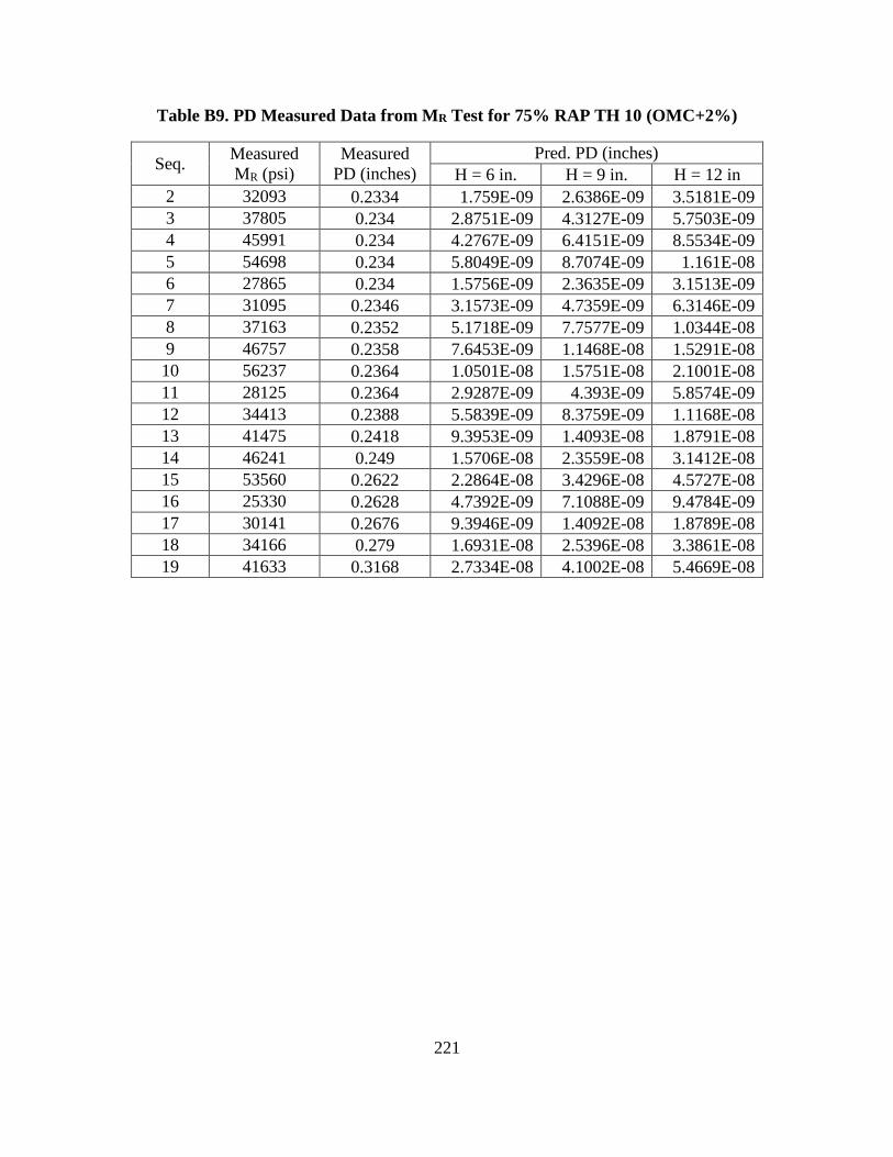
221
Table B9. PD Measured Data from MR Test for 75% RAP TH 10 (OMC+2%)
Seq. Measured
MR (psi)
Measured
PD (inches)
Pred. PD (inches)
H = 6 in. H = 9 in. H = 12 in
2 32093 0.2334 1.759E-09 2.6386E-09 3.5181E-09
3 37805 0.234 2.8751E-09 4.3127E-09 5.7503E-09
4 45991 0.234 4.2767E-09 6.4151E-09 8.5534E-09
5 54698 0.234 5.8049E-09 8.7074E-09 1.161E-08
6 27865 0.234 1.5756E-09 2.3635E-09 3.1513E-09
7 31095 0.2346 3.1573E-09 4.7359E-09 6.3146E-09
8 37163 0.2352 5.1718E-09 7.7577E-09 1.0344E-08
9 46757 0.2358 7.6453E-09 1.1468E-08 1.5291E-08
10 56237 0.2364 1.0501E-08 1.5751E-08 2.1001E-08
11 28125 0.2364 2.9287E-09 4.393E-09 5.8574E-09
12 34413 0.2388 5.5839E-09 8.3759E-09 1.1168E-08
13 41475 0.2418 9.3953E-09 1.4093E-08 1.8791E-08
14 46241 0.249 1.5706E-08 2.3559E-08 3.1412E-08
15 53560 0.2622 2.2864E-08 3.4296E-08 4.5727E-08
16 25330 0.2628 4.7392E-09 7.1088E-09 9.4784E-09
17 30141 0.2676 9.3946E-09 1.4092E-08 1.8789E-08
18 34166 0.279 1.6931E-08 2.5396E-08 3.3861E-08
19 41633 0.3168 2.7334E-08 4.1002E-08 5.4669E-08

222
Table B10. PD Measured Data from MR Test for 100% RAP TH 10 (OMC-2%)
Seq. Measured
MR (psi)
Measured
PD (inches)
Pred. PD (inches)
H = 6 in. H = 9 in. H = 12 in
9 182351 0.00978 0.00037049 0.00055574 0.00074098
10 207135 0.01038 0.00059888 0.00089832 0.00119776
11 113196 0.00876 9.7009E-05 0.00014551 0.00019402
12 118421 0.00906 0.00021474 0.00032212 0.00042949
13 133087 0.0096 0.00040838 0.00061257 0.00081675
14 159071 0.01098 0.00073731 0.00110597 0.00147462
15 170763 0.0123 0.00119362 0.00179043 0.00238724
16 93750 0.01026 0.00015216 0.00022824 0.00030431
17 107980 0.01074 0.00033256 0.00049884 0.00066512
18 126428 0.01152 0.00064102 0.00096154 0.00128205
19 141306 0.01302 0.0011876 0.0017814 0.00237519
20 158656 0.0162 0.00198038 0.00297057 0.00396076
21 80016 0.01428 0.00027492 0.00041237 0.00054983
22 98729 0.01518 0.00060366 0.0009055 0.00120733
23 130051 0.0168 0.00119637 0.00179456 0.00239274
24 148301 0.0204 0.0023869 0.00358035 0.0047738
25 160499 0.02532 0.00427756 0.00641633 0.00855511
26 82730 0.0228 0.00039142 0.00058713 0.00078285
27 99484 0.02358 0.00090783 0.00136174 0.00181566
28 122072 0.0252 0.0019244 0.0028866 0.00384881
29 136500 0.0297 0.00409338 0.00614006 0.00818675
30 161528 0.03774 0.00786894 0.01180341 0.01573788

223
Table B11. PD Measured Data from MR Test for 100% RAP TH 10 (OMC%)
Seq. Measured
MR (psi)
Measured
PD (inches)
Pred. PD (inches)
H = 6 in. H = 9 in. H = 12 in
1 35765 0.0015 1.6876E-06 2.5314E-06 3.3752E-06
2 48278 0.0252 2.9492E-06 4.4238E-06 5.8984E-06
3 84285 0.0237 4.0097E-06 6.0145E-06 8.0194E-06
4 122364 0.0243 6.1441E-06 9.2162E-06 1.2288E-05
5 152522 0.0249 9.2282E-06 1.3842E-05 1.8456E-05
6 45733 0.0225 2.4496E-06 3.6744E-06 4.8992E-06
7 59907 0.0231 4.51E-06 6.765E-06 9.0199E-06
8 84111 0.024 7.1278E-06 1.0692E-05 1.4256E-05
9 111785 0.0249 1.1302E-05 1.6953E-05 2.2604E-05
10 139704 0.0258 1.6968E-05 2.5453E-05 3.3937E-05
11 46111 0.0234 4.5617E-06 6.8426E-06 9.1235E-06
12 59317 0.024 8.6777E-06 1.3017E-05 1.7355E-05
13 80740 0.0252 1.4276E-05 2.1414E-05 2.8553E-05
14 53423 0.0264 3.2219E-05 4.8329E-05 6.4439E-05
15 122797 0.0282 3.6285E-05 5.4427E-05 7.2569E-05
16 41514 0.0252 7.293E-06 1.094E-05 1.4586E-05
17 58550 0.0258 1.3272E-05 1.9908E-05 2.6545E-05
18 80368 0.0276 2.2336E-05 3.3504E-05 4.4672E-05
19 97320 0.0297 3.8745E-05 5.8118E-05 7.749E-05
20 109269 0.033 6.2244E-05 9.3366E-05 0.00012449
21 42211 0.0303 1.222E-05 1.8331E-05 2.4441E-05
22 56228 0.0318 2.4062E-05 3.6093E-05 4.8124E-05
23 74831 0.0351 4.323E-05 6.4845E-05 8.646E-05
24 99678 0.0519 0.00013777 0.00020665 0.00027554
25 39445 0.0486 1.8536E-05 2.7804E-05 3.7072E-05
26 56349 0.0507 3.6226E-05 5.4338E-05 7.2451E-05
27 73487 0.0546 6.9582E-05 0.00010437 0.00013916
28 96697 0.06 0.00013364 0.00020046 0.00026728
29 90323 0.0912 0.000262 0.000393 0.000524
30 35765 0.0015 1.6876E-06 2.5314E-06 3.3752E-06

224
Table B12. PD Measured Data from MR Test for 100% RAP TH 10 (OMC+2%)
Seq. Measured
MR (psi)
Measured
PD (inches)
Pred. PD (inches)
H = 6 in. H = 9 in. H = 12 in
2 45187 0.1644 3.0816E-09 4.6224E-09 6.1632E-09
3 51199 0.1644 5.2475E-09 7.8713E-09 1.0495E-08
4 59162 0.165 8.205E-09 1.2307E-08 1.641E-08
5 70708 0.165 1.1302E-08 1.6953E-08 2.2604E-08
6 44102 0.1656 2.5095E-09 3.7643E-09 5.0191E-09
7 47283 0.1656 5.2323E-09 7.8484E-09 1.0465E-08
8 55026 0.1662 8.9042E-09 1.3356E-08 1.7808E-08
9 67053 0.1668 1.3821E-08 2.0731E-08 2.7642E-08
10 74242 0.1674 2.0297E-08 3.0445E-08 4.0594E-08
11 39975 0.1674 5.0391E-09 7.5587E-09 1.0078E-08
12 45928 0.1686 1.0208E-08 1.5312E-08 2.0417E-08
13 54139 0.1704 1.7701E-08 2.6552E-08 3.5403E-08
14 64733 0.177 2.8725E-08 4.3088E-08 5.7451E-08
15 66262 0.1914 4.5463E-08 6.8194E-08 9.0925E-08
16 34883 0.1914 8.2834E-09 1.2425E-08 1.6567E-08
17 44083 0.195 1.5937E-08 2.3906E-08 3.1875E-08
18 47731 0.207 2.9991E-08 4.4986E-08 5.9982E-08
19 52918 0.243 5.2387E-08 7.8581E-08 1.0477E-07
20 49955 0.3072 9.03E-08 1.3545E-07 1.806E-07
21 29747 0.312 1.5896E-08 2.3844E-08 3.1792E-08
22 36612 0.3186 3.2242E-08 4.8364E-08 6.4485E-08
23 44434 0.348 5.8962E-08 8.8444E-08 1.1792E-07
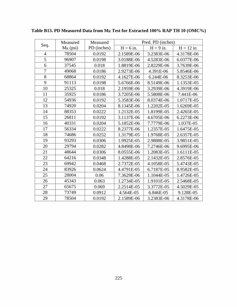
225
Table B13. PD Measured Data from MR Test for Extracted 100% RAP TH 10 (OMC%)
Seq. Measured
MR (psi)
Measured
PD (inches)
Pred. PD (inches)
H = 6 in. H = 9 in. H = 12 in
4 78504 0.0192 2.1589E-06 3.2383E-06 4.3178E-06
5 96907 0.0198 3.0188E-06 4.5283E-06 6.0377E-06
6 37545 0.018 1.8819E-06 2.8229E-06 3.7639E-06
7 49068 0.0186 2.9273E-06 4.391E-06 5.8546E-06
8 68864 0.0192 4.1627E-06 6.244E-06 8.3253E-06
9 91113 0.0198 5.6766E-06 8.5149E-06 1.1353E-05
10 25325 0.018 2.1959E-06 3.2939E-06 4.3919E-06
11 35925 0.0186 3.7205E-06 5.5808E-06 7.441E-06
12 54936 0.0192 5.3583E-06 8.0374E-06 1.0717E-05
13 74920 0.0204 8.1345E-06 1.2202E-05 1.6269E-05
14 88353 0.0222 1.2132E-05 1.8199E-05 2.4265E-05
15 26811 0.0192 3.1137E-06 4.6705E-06 6.2273E-06
16 40331 0.0204 5.1852E-06 7.7779E-06 1.037E-05
17 56334 0.0222 8.2377E-06 1.2357E-05 1.6475E-05
18 74686 0.0252 1.3179E-05 1.9768E-05 2.6357E-05
19 93293 0.0306 1.9925E-05 2.9888E-05 3.9851E-05
20 29794 0.0282 4.8498E-06 7.2746E-06 9.6995E-06
21 48644 0.0306 8.0555E-06 1.2083E-05 1.6111E-05
22 64216 0.0348 1.4288E-05 2.1432E-05 2.8576E-05
23 69942 0.0468 2.7372E-05 4.1058E-05 5.4743E-05
24 83926 0.0624 4.4791E-05 6.7187E-05 8.9582E-05
25 28004 0.06 7.3629E-06 1.1044E-05 1.4726E-05
26 45343 0.063 1.2734E-05 1.9101E-05 2.5468E-05
27 65675 0.069 2.2514E-05 3.3772E-05 4.5029E-05
28 73749 0.0912 4.564E-05 6.846E-05 9.128E-05
29 78504 0.0192 2.1589E-06 3.2383E-06 4.3178E-06

226
Table B14. PD Measured Data from MR Test for RAP TH 19-101 (OMC-2%)
Seq. Measured
MR (psi)
Measured
PD (inches)
Pred. PD (inches)
H = 6 in. H = 9 in. H = 12 in
3 90464 0.01032 7.88E-05 0.000118 0.000158
4 105556 0.01116 0.000128 0.000192 0.000256
5 124349 0.01188 0.000188 0.000282 0.000377
6 72609 0.00942 3.75E-05 5.63E-05 7.51E-05
7 71999 0.00984 8.24E-05 0.000124 0.000165
8 79246 0.01056 0.000148 0.000222 0.000296
9 93611 0.01362 0.000241 0.000361 0.000481
10 108745 0.01224 0.000356 0.000534 0.000711
11 58879 0.00954 7.88E-05 0.000118 0.000158
12 60720 0.01008 0.000173 0.000259 0.000346
13 68176 0.01098 0.000313 0.00047 0.000627
14 87061 0.012 0.000504 0.000756 0.001008
15 95112 0.01344 0.000782 0.001173 0.001564
16 51518 0.0102 0.000127 0.000191 0.000255
17 56342 0.01092 0.000274 0.000412 0.000549
18 66878 0.01194 0.000494 0.000741 0.000988
19 79211 0.0135 0.000849 0.001273 0.001698
20 85637 0.01608 0.001363 0.002045 0.002726
21 48981 0.0126 0.000223 0.000335 0.000446
22 51488 0.01326 0.000514 0.000771 0.001028
23 61123 0.01488 0.000973 0.001459 0.001946
24 70208 0.0186 0.001809 0.002713 0.003617
25 80041 0.02568 0.003027 0.004541 0.006054
26 45535 0.02088 0.000338 0.000508 0.000677
27 48973 0.0216 0.0008 0.001201 0.001601
28 58857 0.02322 0.001587 0.00238 0.003174
29 70782 0.02724 0.003085 0.004627 0.006169
30 81916 0.0369 0.005508 0.008263 0.011017
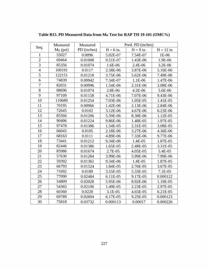
227
Table B15. PD Measured Data from MR Test for RAP TH 19-101 (OMC%)
Seq. Measured
MR (psi)
Measured
PD (inches)
Pred. PD (inches)
H = 6 in. H = 9 in. H = 12 in
1 55027 0.0096 5.02E-07 7.54E-07 1E-06
2 69464 0.01008 9.51E-07 1.43E-06 1.9E-06
3 85356 0.01074 1.6E-06 2.4E-06 3.2E-06
4 100191 0.0117 2.58E-06 3.87E-06 5.16E-06
5 122151 0.01218 3.75E-06 5.62E-06 7.49E-06
6 74839 0.00942 7.34E-07 1.1E-06 1.47E-06
7 82031 0.00996 1.54E-06 2.31E-06 3.08E-06
8 88696 0.01074 2.8E-06 4.2E-06 5.6E-06
9 97109 0.01158 4.71E-06 7.07E-06 9.43E-06
10 110689 0.01254 7.03E-06 1.05E-05 1.41E-05
11 70195 0.00966 1.42E-06 2.13E-06 2.84E-06
12 72645 0.0102 3.12E-06 4.67E-06 6.23E-06
13 85566 0.01206 5.59E-06 8.38E-06 1.12E-05
14 90406 0.01224 9.86E-06 1.48E-05 1.97E-05
15 97478 0.01386 1.54E-05 2.31E-05 3.08E-05
16 66045 0.0105 2.18E-06 3.27E-06 4.36E-06
17 68163 0.0111 4.89E-06 7.33E-06 9.77E-06
18 73441 0.01212 9.34E-06 1.4E-05 1.87E-05
19 82446 0.01386 1.65E-05 2.48E-05 3.31E-05
20 85986 0.01674 2.7E-05 4.05E-05 5.4E-05
21 57630 0.01284 3.99E-06 5.99E-06 7.99E-06
22 59392 0.01362 9.34E-06 1.4E-05 1.87E-05
23 66793 0.01524 1.84E-05 2.76E-05 3.67E-05
24 71692 0.0189 3.55E-05 5.33E-05 7.1E-05
25 77090 0.02484 6.11E-05 9.17E-05 0.000122
26 54809 0.02028 5.95E-06 8.92E-06 1.19E-05
27 54365 0.02106 1.49E-05 2.23E-05 2.97E-05
28 60360 0.0228 3.1E-05 4.65E-05 6.21E-05
29 69789 0.02694 6.17E-05 9.25E-05 0.000123
30 75818 0.03732 0.000113 0.00017 0.000226

228
Table B16. PD Measured Data from MR Test for RAP TH 19-101 (OMC+2%)
Seq. Measured
MR (psi)
Measured
PD (inches)
Pred. PD (inches)
H = 6 in. H = 9 in. H = 12 in
2 35693 0.04098 5.49E-10 8.24E-10 1.1E-09
3 49109 0.04584 8.1E-10 1.22E-09 1.62E-09
4 56813 0.04758 1.26E-09 1.9E-09 2.53E-09
5 70762 0.04896 1.7E-09 2.55E-09 3.4E-09
6 30247 0.04038 5E-10 7.5E-10 9.99E-10
7 36703 0.04494 9.42E-10 1.41E-09 1.88E-09
8 36383 0.0465 1.78E-09 2.67E-09 3.56E-09
9 46059 0.04836 2.62E-09 3.92E-09 5.23E-09
10 57518 0.04998 3.51E-09 5.26E-09 7.02E-09
11 29831 0.04488 9.46E-10 1.42E-09 1.89E-09
12 26581 0.04602 2.32E-09 3.48E-09 4.64E-09
13 31976 0.04776 3.86E-09 5.8E-09 7.73E-09
14 44109 0.05016 5.49E-09 8.24E-09 1.1E-08
15 55032 0.05334 7.61E-09 1.14E-08 1.52E-08
16 24684 0.04752 1.64E-09 2.46E-09 3.28E-09
17 24969 0.04872 3.71E-09 5.56E-09 7.41E-09
18 32387 0.05124 5.97E-09 8.96E-09 1.19E-08
19 41268 0.05598 9.31E-09 1.4E-08 1.86E-08
20 46693 0.06486 1.42E-08 2.13E-08 2.84E-08
21 22117 0.05856 3.05E-09 4.57E-09 6.1E-09
22 25023 0.06006 6.54E-09 9.82E-09 1.31E-08
23 31609 0.06606 1.14E-08 1.71E-08 2.28E-08
24 40556 0.08658 1.9E-08 2.84E-08 3.79E-08
25 43746 0.13566 3.2E-08 4.8E-08 6.41E-08
26 24602 0.11574 4.03E-09 6.04E-09 8.05E-09
27 33565 0.1377 1.74E-08 2.6E-08 3.47E-08
28 41571 0.18432 3.19E-08 4.78E-08 6.38E-08
29 35693 0.04098 5.49E-10 8.24E-10 1.1E-09
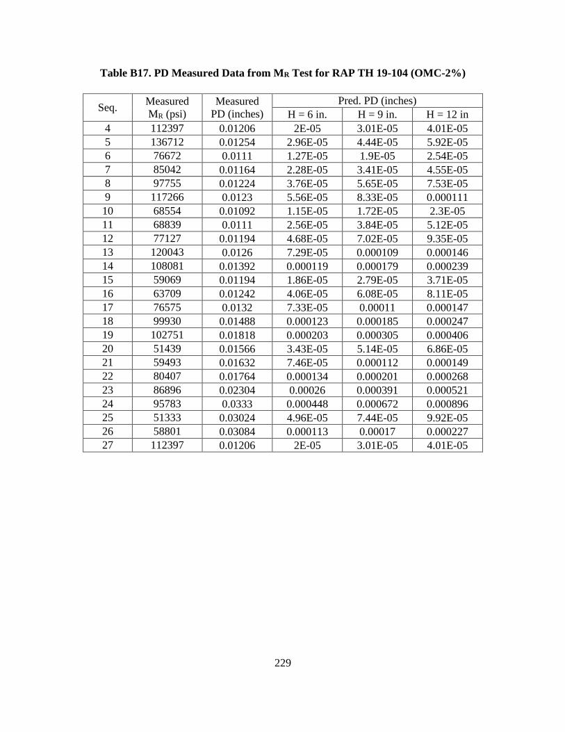
229
Table B17. PD Measured Data from MR Test for RAP TH 19-104 (OMC-2%)
Seq. Measured
MR (psi)
Measured
PD (inches)
Pred. PD (inches)
H = 6 in. H = 9 in. H = 12 in
4 112397 0.01206 2E-05 3.01E-05 4.01E-05
5 136712 0.01254 2.96E-05 4.44E-05 5.92E-05
6 76672 0.0111 1.27E-05 1.9E-05 2.54E-05
7 85042 0.01164 2.28E-05 3.41E-05 4.55E-05
8 97755 0.01224 3.76E-05 5.65E-05 7.53E-05
9 117266 0.0123 5.56E-05 8.33E-05 0.000111
10 68554 0.01092 1.15E-05 1.72E-05 2.3E-05
11 68839 0.0111 2.56E-05 3.84E-05 5.12E-05
12 77127 0.01194 4.68E-05 7.02E-05 9.35E-05
13 120043 0.0126 7.29E-05 0.000109 0.000146
14 108081 0.01392 0.000119 0.000179 0.000239
15 59069 0.01194 1.86E-05 2.79E-05 3.71E-05
16 63709 0.01242 4.06E-05 6.08E-05 8.11E-05
17 76575 0.0132 7.33E-05 0.00011 0.000147
18 99930 0.01488 0.000123 0.000185 0.000247
19 102751 0.01818 0.000203 0.000305 0.000406
20 51439 0.01566 3.43E-05 5.14E-05 6.86E-05
21 59493 0.01632 7.46E-05 0.000112 0.000149
22 80407 0.01764 0.000134 0.000201 0.000268
23 86896 0.02304 0.00026 0.000391 0.000521
24 95783 0.0333 0.000448 0.000672 0.000896
25 51333 0.03024 4.96E-05 7.44E-05 9.92E-05
26 58801 0.03084 0.000113 0.00017 0.000227
27 112397 0.01206 2E-05 3.01E-05 4.01E-05
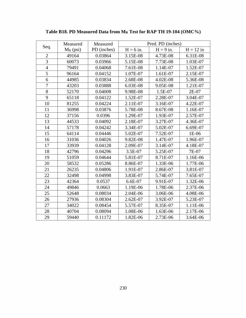
230
Table B18. PD Measured Data from MR Test for RAP TH 19-104 (OMC%)
Seq. Measured
MR (psi)
Measured
PD (inches)
Pred. PD (inches)
H = 6 in. H = 9 in. H = 12 in
2 49164 0.03864 3.15E-08 4.73E-08 6.31E-08
3 60073 0.03966 5.15E-08 7.73E-08 1.03E-07
4 79491 0.04068 7.61E-08 1.14E-07 1.52E-07
5 96164 0.04152 1.07E-07 1.61E-07 2.15E-07
6 44985 0.03834 2.68E-08 4.02E-08 5.36E-08
7 43203 0.03888 6.03E-08 9.05E-08 1.21E-07
8 52170 0.04008 9.98E-08 1.5E-07 2E-07
9 65118 0.04122 1.52E-07 2.28E-07 3.04E-07
10 81255 0.04224 2.11E-07 3.16E-07 4.22E-07
11 36998 0.03876 5.78E-08 8.67E-08 1.16E-07
12 37156 0.0396 1.29E-07 1.93E-07 2.57E-07
13 44533 0.04092 2.18E-07 3.27E-07 4.36E-07
14 57178 0.04242 3.34E-07 5.02E-07 6.69E-07
15 64114 0.04446 5.02E-07 7.52E-07 1E-06
16 31036 0.04026 9.82E-08 1.47E-07 1.96E-07
17 33939 0.04128 2.09E-07 3.14E-07 4.18E-07
18 42796 0.04296 3.5E-07 5.25E-07 7E-07
19 51059 0.04644 5.81E-07 8.71E-07 1.16E-06
20 58532 0.05286 8.86E-07 1.33E-06 1.77E-06
21 26235 0.04806 1.91E-07 2.86E-07 3.81E-07
22 32498 0.04998 3.83E-07 5.74E-07 7.65E-07
23 42364 0.0537 6.6E-07 9.91E-07 1.32E-06
24 49846 0.0663 1.19E-06 1.78E-06 2.37E-06
25 52648 0.08034 2.04E-06 3.06E-06 4.08E-06
26 27936 0.08304 2.62E-07 3.92E-07 5.23E-07
27 34022 0.08454 5.57E-07 8.35E-07 1.11E-06
28 40704 0.08094 1.08E-06 1.63E-06 2.17E-06
29 59440 0.11172 1.82E-06 2.73E-06 3.64E-06

231
Table B19. PD Measured Data from MR Test for RAP TH 19-104 (OMC+2%)
Seq. Measured
MR (psi)
Measured
PD (inches)
Pred. PD (inches)
H = 6 in. H = 9 in. H = 12 in
3 36595 0.16698 4.12E-13 6.18E-13 8.24E-13
4 41426 0.16776 6.44E-13 9.66E-13 1.29E-12
5 50277 0.168 8.57E-13 1.29E-12 1.71E-12
6 32494 0.16644 1.95E-13 2.93E-13 3.9E-13
7 25072 0.16716 5.26E-13 7.88E-13 1.05E-12
8 29407 0.16806 8.67E-13 1.3E-12 1.73E-12
9 37943 0.1689 1.24E-12 1.86E-12 2.48E-12
10 48145 0.16962 1.62E-12 2.43E-12 3.25E-12
11 23022 0.16794 4.83E-13 7.25E-13 9.67E-13
12 24912 0.16932 1.01E-12 1.52E-12 2.02E-12
13 35033 0.17136 1.49E-12 2.23E-12 2.98E-12
14 38336 0.17568 2.51E-12 3.77E-12 5.02E-12
15 43522 0.1884 3.67E-12 5.51E-12 7.35E-12
16 18414 0.18684 8.7E-13 1.3E-12 1.74E-12
17 24539 0.1905 1.55E-12 2.33E-12 3.11E-12
18 29577 0.19986 2.65E-12 3.98E-12 5.3E-12
19 36197 0.2418 4.24E-12 6.36E-12 8.47E-12
20 37910 0.34356 6.8E-12 1.02E-11 1.36E-11
21 17001 0.34518 1.58E-12 2.37E-12 3.16E-12
22 24520 0.35574 2.75E-12 4.13E-12 5.5E-12
23 29218 0.4191 5.01E-12 7.52E-12 1E-11
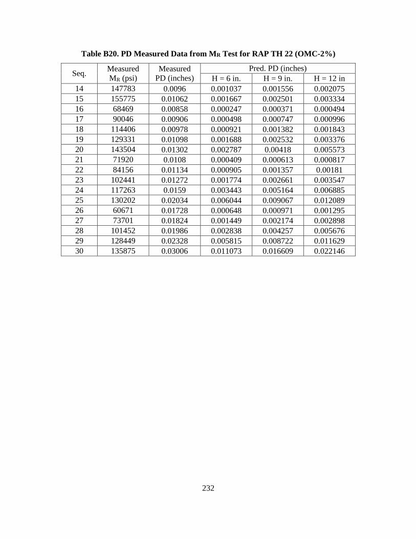
232
Table B20. PD Measured Data from MR Test for RAP TH 22 (OMC-2%)
Seq. Measured
MR (psi)
Measured
PD (inches)
Pred. PD (inches)
H = 6 in. H = 9 in. H = 12 in
14 147783 0.0096 0.001037 0.001556 0.002075
15 155775 0.01062 0.001667 0.002501 0.003334
16 68469 0.00858 0.000247 0.000371 0.000494
17 90046 0.00906 0.000498 0.000747 0.000996
18 114406 0.00978 0.000921 0.001382 0.001843
19 129331 0.01098 0.001688 0.002532 0.003376
20 143504 0.01302 0.002787 0.00418 0.005573
21 71920 0.0108 0.000409 0.000613 0.000817
22 84156 0.01134 0.000905 0.001357 0.00181
23 102441 0.01272 0.001774 0.002661 0.003547
24 117263 0.0159 0.003443 0.005164 0.006885
25 130202 0.02034 0.006044 0.009067 0.012089
26 60671 0.01728 0.000648 0.000971 0.001295
27 73701 0.01824 0.001449 0.002174 0.002898
28 101452 0.01986 0.002838 0.004257 0.005676
29 128449 0.02328 0.005815 0.008722 0.011629
30 135875 0.03006 0.011073 0.016609 0.022146

233
Table B21. PD Measured Data from MR Test for RAP TH 22 (OMC%)
Seq. Measured
MR (psi)
Measured
PD (inches)
Pred. PD (inches)
H = 6 in. H = 9 in. H = 12 in
2 30670 0.04458 7.87E-06 1.18E-05 1.57E-05
3 59994 0.0306 9.12E-06 1.37E-05 1.82E-05
4 82447 0.03144 1.33E-05 1.99E-05 2.65E-05
5 103832 0.0321 1.85E-05 2.78E-05 3.71E-05
6 31386 0.0294 6.19E-06 9.28E-06 1.24E-05
7 42192 0.03024 1.08E-05 1.63E-05 2.17E-05
8 58394 0.03108 1.65E-05 2.47E-05 3.29E-05
9 79278 0.03198 2.44E-05 3.66E-05 4.88E-05
10 98688 0.03282 3.46E-05 5.2E-05 6.93E-05
11 31478 0.03 1.16E-05 1.73E-05 2.31E-05
12 413215 0.03102 2.75E-05 4.12E-05 5.5E-05
13 61425 0.03204 3.14E-05 4.72E-05 6.29E-05
14 79852 0.03336 4.95E-05 7.43E-05 9.91E-05
15 91948 0.0351 7.5E-05 0.000112 0.00015
16 30835 0.03192 1.75E-05 2.62E-05 3.49E-05
17 43152 0.03312 3.1E-05 4.65E-05 6.2E-05
18 60279 0.03468 4.96E-05 7.44E-05 9.93E-05
19 75120 0.03726 8.24E-05 0.000124 0.000165
20 85665 0.04128 0.000129 0.000194 0.000258
21 31436 0.03804 2.92E-05 4.37E-05 5.83E-05
22 44345 0.04032 5.38E-05 8.07E-05 0.000108
23 59650 0.04422 9.35E-05 0.00014 0.000187
24 72687 0.05322 0.000168 0.000253 0.000337
25 85193 0.06516 0.000279 0.000419 0.000559
26 31642 0.06192 4.19E-05 6.29E-05 8.38E-05
27 46566 0.06408 7.85E-05 0.000118 0.000157
28 62425 0.06864 0.000145 0.000218 0.000291
29 74845 0.08346 0.000284 0.000426 0.000569
30 81380 0.11724 0.000523 0.000785 0.001047
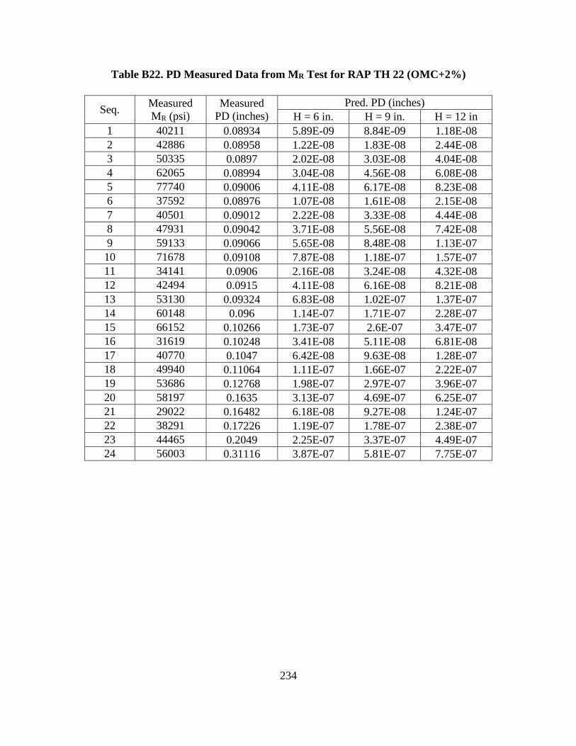
234
Table B22. PD Measured Data from MR Test for RAP TH 22 (OMC+2%)
Seq. Measured
MR (psi)
Measured
PD (inches)
Pred. PD (inches)
H = 6 in. H = 9 in. H = 12 in
1 40211 0.08934 5.89E-09 8.84E-09 1.18E-08
2 42886 0.08958 1.22E-08 1.83E-08 2.44E-08
3 50335 0.0897 2.02E-08 3.03E-08 4.04E-08
4 62065 0.08994 3.04E-08 4.56E-08 6.08E-08
5 77740 0.09006 4.11E-08 6.17E-08 8.23E-08
6 37592 0.08976 1.07E-08 1.61E-08 2.15E-08
7 40501 0.09012 2.22E-08 3.33E-08 4.44E-08
8 47931 0.09042 3.71E-08 5.56E-08 7.42E-08
9 59133 0.09066 5.65E-08 8.48E-08 1.13E-07
10 71678 0.09108 7.87E-08 1.18E-07 1.57E-07
11 34141 0.0906 2.16E-08 3.24E-08 4.32E-08
12 42494 0.0915 4.11E-08 6.16E-08 8.21E-08
13 53130 0.09324 6.83E-08 1.02E-07 1.37E-07
14 60148 0.096 1.14E-07 1.71E-07 2.28E-07
15 66152 0.10266 1.73E-07 2.6E-07 3.47E-07
16 31619 0.10248 3.41E-08 5.11E-08 6.81E-08
17 40770 0.1047 6.42E-08 9.63E-08 1.28E-07
18 49940 0.11064 1.11E-07 1.66E-07 2.22E-07
19 53686 0.12768 1.98E-07 2.97E-07 3.96E-07
20 58197 0.1635 3.13E-07 4.69E-07 6.25E-07
21 29022 0.16482 6.18E-08 9.27E-08 1.24E-07
22 38291 0.17226 1.19E-07 1.78E-07 2.38E-07
23 44465 0.2049 2.25E-07 3.37E-07 4.49E-07
24 56003 0.31116 3.87E-07 5.81E-07 7.75E-07

235
Table B23. PD Measured Data from MR Test for Cell 18 (OMC-2%)
Seq. Measured
MR (psi)
Measured
PD (inches)
Pred. PD (inches)
H = 6 in. H = 9 in. H = 12 in
5 170163 0.01272 0.000574 0.000861 0.001149
7 91074 0.01134 0.000226 0.000339 0.000452
8 117018 0.01188 0.000395 0.000593 0.000791
9 139380 0.01248 0.000674 0.001011 0.001348
10 162839 0.01314 0.00105 0.001575 0.0021
11 69136 0.01128 0.000219 0.000329 0.000438
12 87987 0.01176 0.000438 0.000657 0.000877
13 108490 0.01638 0.000791 0.001186 0.001582
14 132867 0.01338 0.001378 0.002068 0.002757
15 150656 0.01482 0.002203 0.003305 0.004407
16 66983 0.0126 0.000331 0.000497 0.000662
17 85440 0.01326 0.000673 0.00101 0.001346
18 108358 0.01422 0.001235 0.001853 0.002471
19 134056 0.01602 0.002228 0.003342 0.004456
20 144556 0.01872 0.00369 0.005535 0.00738
21 70996 0.01638 0.000545 0.000817 0.00109
22 88361 0.0174 0.001175 0.001762 0.00235
23 108337 0.01944 0.002313 0.00347 0.004626
24 124396 0.02418 0.004514 0.006772 0.009029
25 130925 0.03138 0.008 0.012 0.015999
26 61272 0.02844 0.000853 0.001279 0.001706
27 80080 0.0297 0.001846 0.002769 0.003691
28 100975 0.03228 0.003763 0.005645 0.007526

236
Table B24. PD Measured Data from MR Test for Cell 18 (OMC%)
Seq. Measured
MR (psi)
Measured
PD (inches)
Pred. PD (inches)
H = 6 in. H = 9 in. H = 12 in
4 138283 0.0183 1.95E-05 2.92E-05 3.89E-05
5 170158 0.01872 3E-05 4.5E-05 6E-05
7 77267 0.01758 1.26E-05 1.9E-05 2.53E-05
8 104081 0.01746 2.12E-05 3.18E-05 4.24E-05
9 135208 0.01794 3.52E-05 5.29E-05 7.05E-05
10 160721 0.01854 5.47E-05 8.21E-05 0.000109
11 55714 0.01692 1.29E-05 1.94E-05 2.59E-05
12 78125 0.0174 2.41E-05 3.61E-05 4.81E-05
13 106273 0.018 4.15E-05 6.23E-05 8.3E-05
14 131834 0.0189 7.2E-05 0.000108 0.000144
15 149020 0.02028 0.000115 0.000172 0.00023
16 54460 0.01842 1.95E-05 2.93E-05 3.9E-05
17 70738 0.01896 3.83E-05 5.75E-05 7.67E-05
18 104029 0.01998 6.52E-05 9.78E-05 0.00013
19 122728 0.0219 0.000117 0.000176 0.000235
20 138843 0.02496 0.000193 0.000289 0.000386
21 52780 0.0228 3.37E-05 5.06E-05 6.75E-05
22 77642 0.02412 6.48E-05 9.72E-05 0.00013
23 104116 0.027 0.000122 0.000183 0.000244
24 117729 0.03294 0.000238 0.000357 0.000476
25 139599 0.04068 0.000416 0.000624 0.000832
26 50588 0.04032 5.01E-05 7.51E-05 0.0001
27 74971 0.04182 9.94E-05 0.000149 0.000199
28 102947 0.04518 0.000195 0.000293 0.000391
29 119916 0.05496 0.000406 0.000609 0.000812
30 119071 0.07584 0.000778 0.001167 0.001556
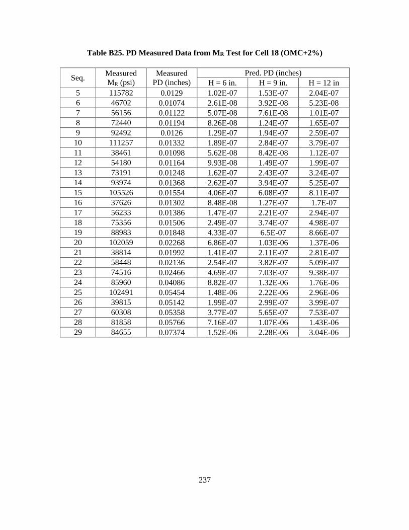
237
Table B25. PD Measured Data from MR Test for Cell 18 (OMC+2%)
Seq. Measured
MR (psi)
Measured
PD (inches)
Pred. PD (inches)
H = 6 in. H = 9 in. H = 12 in
5 115782 0.0129 1.02E-07 1.53E-07 2.04E-07
6 46702 0.01074 2.61E-08 3.92E-08 5.23E-08
7 56156 0.01122 5.07E-08 7.61E-08 1.01E-07
8 72440 0.01194 8.26E-08 1.24E-07 1.65E-07
9 92492 0.0126 1.29E-07 1.94E-07 2.59E-07
10 111257 0.01332 1.89E-07 2.84E-07 3.79E-07
11 38461 0.01098 5.62E-08 8.42E-08 1.12E-07
12 54180 0.01164 9.93E-08 1.49E-07 1.99E-07
13 73191 0.01248 1.62E-07 2.43E-07 3.24E-07
14 93974 0.01368 2.62E-07 3.94E-07 5.25E-07
15 105526 0.01554 4.06E-07 6.08E-07 8.11E-07
16 37626 0.01302 8.48E-08 1.27E-07 1.7E-07
17 56233 0.01386 1.47E-07 2.21E-07 2.94E-07
18 75356 0.01506 2.49E-07 3.74E-07 4.98E-07
19 88983 0.01848 4.33E-07 6.5E-07 8.66E-07
20 102059 0.02268 6.86E-07 1.03E-06 1.37E-06
21 38814 0.01992 1.41E-07 2.11E-07 2.81E-07
22 58448 0.02136 2.54E-07 3.82E-07 5.09E-07
23 74516 0.02466 4.69E-07 7.03E-07 9.38E-07
24 85960 0.04086 8.82E-07 1.32E-06 1.76E-06
25 102491 0.05454 1.48E-06 2.22E-06 2.96E-06
26 39815 0.05142 1.99E-07 2.99E-07 3.99E-07
27 60308 0.05358 3.77E-07 5.65E-07 7.53E-07
28 81858 0.05766 7.16E-07 1.07E-06 1.43E-06
29 84655 0.07374 1.52E-06 2.28E-06 3.04E-06
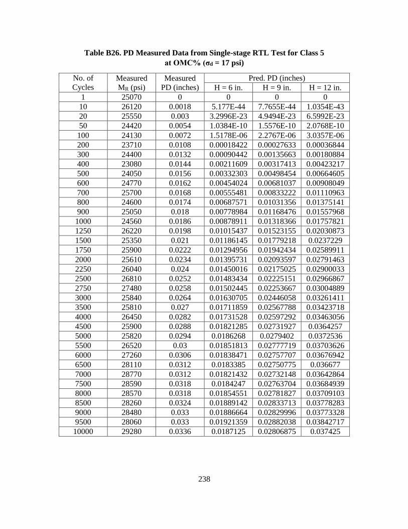
238
Table B26. PD Measured Data from Single-stage RTL Test for Class 5
at OMC% (σd = 17 psi)
No. of
Cycles Measured
MR (psi)
Measured
PD (inches)
Pred. PD (inches)
H = 6 in. H = 9 in. H = 12 in.
1 25070 0 0 0 0
10 26120 0.0018 5.177E-44 7.7655E-44 1.0354E-43
20 25550 0.003 3.2996E-23 4.9494E-23 6.5992E-23
50 24420 0.0054 1.0384E-10 1.5576E-10 2.0768E-10
100 24130 0.0072 1.5178E-06 2.2767E-06 3.0357E-06
200 23710 0.0108 0.00018422 0.00027633 0.00036844
300 24400 0.0132 0.00090442 0.00135663 0.00180884
400 23080 0.0144 0.00211609 0.00317413 0.00423217
500 24050 0.0156 0.00332303 0.00498454 0.00664605
600 24770 0.0162 0.00454024 0.00681037 0.00908049
700 25700 0.0168 0.00555481 0.00833222 0.01110963
800 24600 0.0174 0.00687571 0.01031356 0.01375141
900 25050 0.018 0.00778984 0.01168476 0.01557968
1000 24560 0.0186 0.00878911 0.01318366 0.01757821
1250 26220 0.0198 0.01015437 0.01523155 0.02030873
1500 25350 0.021 0.01186145 0.01779218 0.0237229
1750 25900 0.0222 0.01294956 0.01942434 0.02589911
2000 25610 0.0234 0.01395731 0.02093597 0.02791463
2250 26040 0.024 0.01450016 0.02175025 0.02900033
2500 26810 0.0252 0.01483434 0.02225151 0.02966867
2750 27480 0.0258 0.01502445 0.02253667 0.03004889
3000 25840 0.0264 0.01630705 0.02446058 0.03261411
3500 25810 0.027 0.01711859 0.02567788 0.03423718
4000 26450 0.0282 0.01731528 0.02597292 0.03463056
4500 25900 0.0288 0.01821285 0.02731927 0.0364257
5000 25820 0.0294 0.0186268 0.0279402 0.0372536
5500 26520 0.03 0.01851813 0.02777719 0.03703626
6000 27260 0.0306 0.01838471 0.02757707 0.03676942
6500 28110 0.0312 0.0183385 0.02750775 0.036677
7000 28770 0.0312 0.01821432 0.02732148 0.03642864
7500 28590 0.0318 0.0184247 0.02763704 0.03684939
8000 28570 0.0318 0.01854551 0.02781827 0.03709103
8500 28260 0.0324 0.01889142 0.02833713 0.03778283
9000 28480 0.033 0.01886664 0.02829996 0.03773328
9500 28060 0.033 0.01921359 0.02882038 0.03842717
10000 29280 0.0336 0.0187125 0.02806875 0.037425
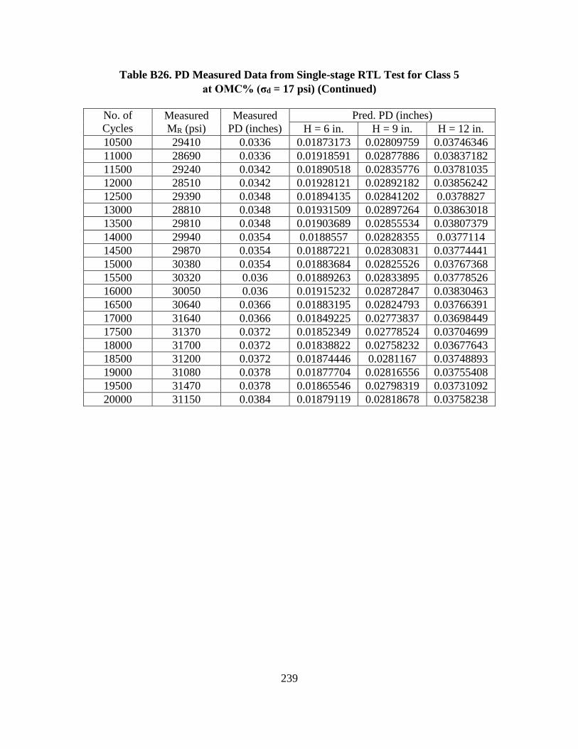
239
Table B26. PD Measured Data from Single-stage RTL Test for Class 5
at OMC% (σd = 17 psi) (Continued)
No. of
Cycles Measured
MR (psi)
Measured
PD (inches)
Pred. PD (inches)
H = 6 in. H = 9 in. H = 12 in.
10500 29410 0.0336 0.01873173 0.02809759 0.03746346
11000 28690 0.0336 0.01918591 0.02877886 0.03837182
11500 29240 0.0342 0.01890518 0.02835776 0.03781035
12000 28510 0.0342 0.01928121 0.02892182 0.03856242
12500 29390 0.0348 0.01894135 0.02841202 0.0378827
13000 28810 0.0348 0.01931509 0.02897264 0.03863018
13500 29810 0.0348 0.01903689 0.02855534 0.03807379
14000 29940 0.0354 0.0188557 0.02828355 0.0377114
14500 29870 0.0354 0.01887221 0.02830831 0.03774441
15000 30380 0.0354 0.01883684 0.02825526 0.03767368
15500 30320 0.036 0.01889263 0.02833895 0.03778526
16000 30050 0.036 0.01915232 0.02872847 0.03830463
16500 30640 0.0366 0.01883195 0.02824793 0.03766391
17000 31640 0.0366 0.01849225 0.02773837 0.03698449
17500 31370 0.0372 0.01852349 0.02778524 0.03704699
18000 31700 0.0372 0.01838822 0.02758232 0.03677643
18500 31200 0.0372 0.01874446 0.0281167 0.03748893
19000 31080 0.0378 0.01877704 0.02816556 0.03755408
19500 31470 0.0378 0.01865546 0.02798319 0.03731092
20000 31150 0.0384 0.01879119 0.02818678 0.03758238
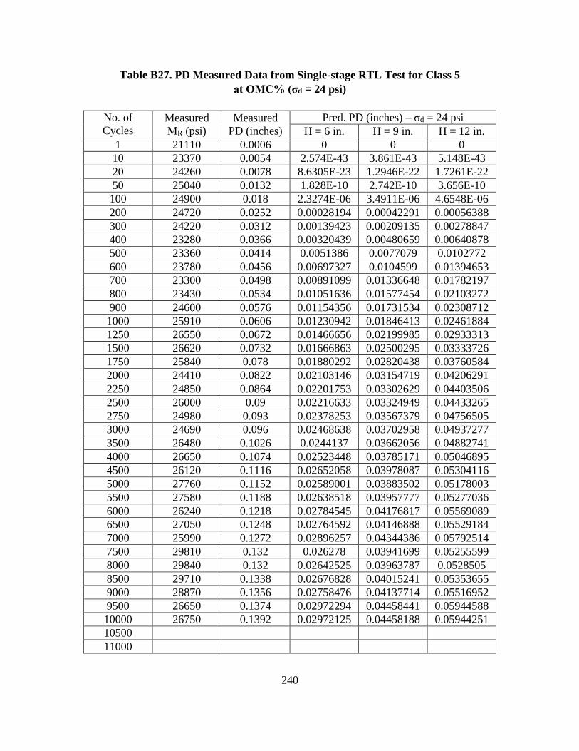
240
Table B27. PD Measured Data from Single-stage RTL Test for Class 5
at OMC% (σd = 24 psi)
No. of
Cycles Measured
MR (psi)
Measured
PD (inches)
Pred. PD (inches) – σd = 24 psi
H = 6 in. H = 9 in. H = 12 in.
1 21110 0.0006 0 0 0
10 23370 0.0054 2.574E-43 3.861E-43 5.148E-43
20 24260 0.0078 8.6305E-23 1.2946E-22 1.7261E-22
50 25040 0.0132 1.828E-10 2.742E-10 3.656E-10
100 24900 0.018 2.3274E-06 3.4911E-06 4.6548E-06
200 24720 0.0252 0.00028194 0.00042291 0.00056388
300 24220 0.0312 0.00139423 0.00209135 0.00278847
400 23280 0.0366 0.00320439 0.00480659 0.00640878
500 23360 0.0414 0.0051386 0.0077079 0.0102772
600 23780 0.0456 0.00697327 0.0104599 0.01394653
700 23300 0.0498 0.00891099 0.01336648 0.01782197
800 23430 0.0534 0.01051636 0.01577454 0.02103272
900 24600 0.0576 0.01154356 0.01731534 0.02308712
1000 25910 0.0606 0.01230942 0.01846413 0.02461884
1250 26550 0.0672 0.01466656 0.02199985 0.02933313
1500 26620 0.0732 0.01666863 0.02500295 0.03333726
1750 25840 0.078 0.01880292 0.02820438 0.03760584
2000 24410 0.0822 0.02103146 0.03154719 0.04206291
2250 24850 0.0864 0.02201753 0.03302629 0.04403506
2500 26000 0.09 0.02216633 0.03324949 0.04433265
2750 24980 0.093 0.02378253 0.03567379 0.04756505
3000 24690 0.096 0.02468638 0.03702958 0.04937277
3500 26480 0.1026 0.0244137 0.03662056 0.04882741
4000 26650 0.1074 0.02523448 0.03785171 0.05046895
4500 26120 0.1116 0.02652058 0.03978087 0.05304116
5000 27760 0.1152 0.02589001 0.03883502 0.05178003
5500 27580 0.1188 0.02638518 0.03957777 0.05277036
6000 26240 0.1218 0.02784545 0.04176817 0.05569089
6500 27050 0.1248 0.02764592 0.04146888 0.05529184
7000 25990 0.1272 0.02896257 0.04344386 0.05792514
7500 29810 0.132 0.026278 0.03941699 0.05255599
8000 29840 0.132 0.02642525 0.03963787 0.0528505
8500 29710 0.1338 0.02676828 0.04015241 0.05353655
9000 28870 0.1356 0.02758476 0.04137714 0.05516952
9500 26650 0.1374 0.02972294 0.04458441 0.05944588
10000 26750 0.1392 0.02972125 0.04458188 0.05944251
10500
11000
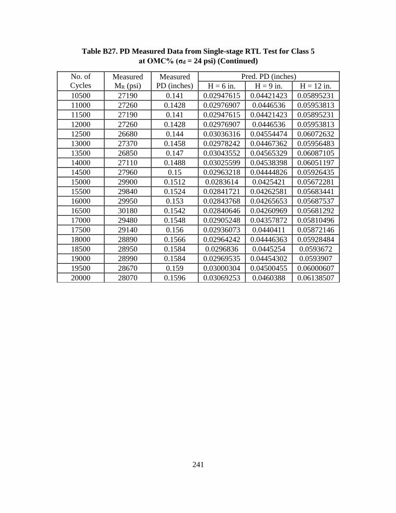
241
Table B27. PD Measured Data from Single-stage RTL Test for Class 5
at OMC% (σd = 24 psi) (Continued)
No. of
Cycles Measured
MR (psi)
Measured
PD (inches)
Pred. PD (inches)
H = 6 in. H = 9 in. H = 12 in.
10500 27190 0.141 0.02947615 0.04421423 0.05895231
11000 27260 0.1428 0.02976907 0.0446536 0.05953813
11500 27190 0.141 0.02947615 0.04421423 0.05895231
12000 27260 0.1428 0.02976907 0.0446536 0.05953813
12500 26680 0.144 0.03036316 0.04554474 0.06072632
13000 27370 0.1458 0.02978242 0.04467362 0.05956483
13500 26850 0.147 0.03043552 0.04565329 0.06087105
14000 27110 0.1488 0.03025599 0.04538398 0.06051197
14500 27960 0.15 0.02963218 0.04444826 0.05926435
15000 29900 0.1512 0.0283614 0.0425421 0.05672281
15500 29840 0.1524 0.02841721 0.04262581 0.05683441
16000 29950 0.153 0.02843768 0.04265653 0.05687537
16500 30180 0.1542 0.02840646 0.04260969 0.05681292
17000 29480 0.1548 0.02905248 0.04357872 0.05810496
17500 29140 0.156 0.02936073 0.0440411 0.05872146
18000 28890 0.1566 0.02964242 0.04446363 0.05928484
18500 28950 0.1584 0.0296836 0.0445254 0.0593672
19000 28990 0.1584 0.02969535 0.04454302 0.0593907
19500 28670 0.159 0.03000304 0.04500455 0.06000607
20000 28070 0.1596 0.03069253 0.0460388 0.06138507

242
Table B28. PD Measured Data from Single-stage RTL Test for Class 5
at OMC+2% (σd = 12 psi)
No. of
Cycles Measured
MR (psi)
Measured
PD (inches)
Pred. PD (inches) – σd = 12 psi
H = 6 in. H = 9 in. H = 12 in.
10 21900 0.0024 0 0 0
20 21240 0.0048 2.6806E-43 4.0209E-43 5.3612E-43
50 21130 0.0114 6.0125E-19 9.0187E-19 1.2025E-18
100 18350 0.0174 9.3238E-11 1.3986E-10 1.8648E-10
200 19470 0.0258 1.0542E-06 1.5813E-06 2.1084E-06
300 18950 0.03 2.4608E-05 3.6913E-05 4.9217E-05
400 18700 0.033 0.0001195 0.00017924 0.00023899
500 18730 0.036 0.00030531 0.00045796 0.00061062
600 19170 0.039 0.00056362 0.00084543 0.00112724
700 19510 0.042 0.0008679 0.00130185 0.00173581
800 20280 0.0444 0.00117549 0.00176323 0.00235098
900 20640 0.0468 0.00149625 0.00224437 0.0029925
1000 20230 0.0492 0.00187347 0.0028102 0.00374693
1250 19310 0.0534 0.00285745 0.00428617 0.00571489
1500 19370 0.057 0.00367103 0.00550654 0.00734205
1750 19850 0.06 0.00428091 0.00642136 0.00856181
2000 19230 0.063 0.00508004 0.00762007 0.01016009
2250 19070 0.0654 0.0056188 0.0084282 0.0112376
2500 20040 0.0684 0.0059272 0.0088908 0.0118544
2750 19950 0.0708 0.00634911 0.00952366 0.01269822
3000 20610 0.0726 0.00660023 0.00990034 0.01320046
3500 21180 0.0762 0.00700515 0.01050772 0.0140103
4000 21860 0.0804 0.00731199 0.01096799 0.01462399
4500 21780 0.084 0.00777255 0.01165883 0.0155451
5000 21800 0.0864 0.0081366 0.0122049 0.01627319
5500 24320 0.0888 0.00774747 0.01162121 0.01549495
6000 23490 0.0912 0.00821254 0.01231882 0.01642509
6500 23120 0.093 0.00850746 0.01276119 0.01701492
7000 22610 0.0942 0.00891041 0.01336562 0.01782082
7500 23300 0.0966 0.00893159 0.01339738 0.01786318
8000 23210 0.0966 0.00910126 0.01365189 0.01820251
8500 22750 0.0978 0.00943001 0.01414501 0.01886002
9000 21620 0.099 0.01002527 0.01503791 0.02005054
9500 23270 0.0996 0.00945976 0.01418965 0.01891953
10000 23880 0.1002 0.00949526 0.01424289 0.01899052
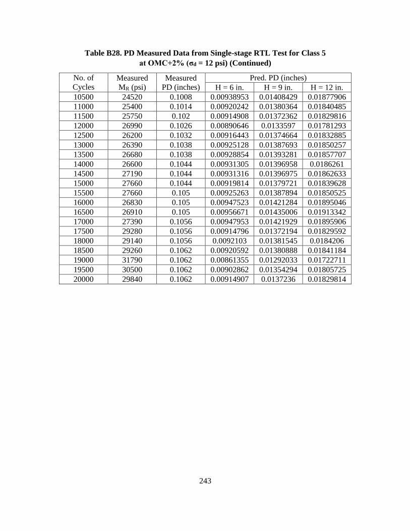
243
Table B28. PD Measured Data from Single-stage RTL Test for Class 5
at OMC+2% (σd = 12 psi) (Continued)
No. of
Cycles Measured
MR (psi)
Measured
PD (inches)
Pred. PD (inches)
H = 6 in. H = 9 in. H = 12 in.
10500 24520 0.1008 0.00938953 0.01408429 0.01877906
11000 25400 0.1014 0.00920242 0.01380364 0.01840485
11500 25750 0.102 0.00914908 0.01372362 0.01829816
12000 26990 0.1026 0.00890646 0.0133597 0.01781293
12500 26200 0.1032 0.00916443 0.01374664 0.01832885
13000 26390 0.1038 0.00925128 0.01387693 0.01850257
13500 26680 0.1038 0.00928854 0.01393281 0.01857707
14000 26600 0.1044 0.00931305 0.01396958 0.0186261
14500 27190 0.1044 0.00931316 0.01396975 0.01862633
15000 27660 0.1044 0.00919814 0.01379721 0.01839628
15500 27660 0.105 0.00925263 0.01387894 0.01850525
16000 26830 0.105 0.00947523 0.01421284 0.01895046
16500 26910 0.105 0.00956671 0.01435006 0.01913342
17000 27390 0.1056 0.00947953 0.01421929 0.01895906
17500 29280 0.1056 0.00914796 0.01372194 0.01829592
18000 29140 0.1056 0.0092103 0.01381545 0.0184206
18500 29260 0.1062 0.00920592 0.01380888 0.01841184
19000 31790 0.1062 0.00861355 0.01292033 0.01722711
19500 30500 0.1062 0.00902862 0.01354294 0.01805725
20000 29840 0.1062 0.00914907 0.0137236 0.01829814

244
Table B29. PD Measured Data from Single-stage RTL Test for Class 5
at OMC+2% (σd = 17 psi)
No. of
Cycles Measured
MR (psi)
Measured
PD (inches)
Pred. PD (inches)
H = 6 in. H = 9 in. H = 12 in.
1 21000 0.0006 0 0 0
10 19380 0.0036 0 0 0
20 19510 0.0054 4.7686E-43 7.1529E-43 9.5372E-43
50 19200 0.0084 1.072E-18 1.6079E-18 2.1439E-18
100 19640 0.0114 1.3695E-10 2.0543E-10 2.7391E-10
200 19730 0.0162 1.5714E-06 2.3571E-06 3.1428E-06
300 19490 0.0198 3.5613E-05 5.342E-05 7.1226E-05
400 19610 0.0234 0.00016871 0.00025307 0.00033742
500 19620 0.027 0.00042758 0.00064136 0.00085515
600 19500 0.0306 0.00080496 0.00120744 0.00160992
700 19350 0.033 0.00126437 0.00189656 0.00252875
800 18390 0.036 0.00186181 0.00279272 0.00372362
900 19250 0.0384 0.0023141 0.00347114 0.00462819
1000 20700 0.0402 0.00269943 0.00404914 0.00539886
1250 20140 0.0444 0.00402799 0.00604199 0.00805598
1500 20050 0.048 0.00520297 0.00780445 0.01040594
1750 20820 0.0504 0.00606323 0.00909484 0.01212645
2000 20980 0.0528 0.00691428 0.01037141 0.01382855
2250 21550 0.0552 0.00754145 0.01131218 0.0150829
2500 21660 0.057 0.00811703 0.01217554 0.01623405
2750 22260 0.0594 0.00852623 0.01278935 0.01705247
3000 22150 0.0612 0.00908749 0.01363123 0.01817498
3500 23320 0.0642 0.00953222 0.01429832 0.01906443
4000 23240 0.0666 0.01024937 0.01537405 0.02049873
4500 23900 0.069 0.01052979 0.01579468 0.02105957
5000 24490 0.0708 0.01085002 0.01627503 0.02170004
5500 25280 0.072 0.0109416 0.0164124 0.0218832
6000 26700 0.0732 0.01079347 0.0161902 0.02158693
6500 27310 0.0744 0.01090104 0.01635155 0.02180207
7000 27730 0.0756 0.01097461 0.01646191 0.02194921
7500 27760 0.0768 0.01126684 0.01690026 0.02253368
8000 27630 0.0768 0.01146245 0.01719367 0.02292489
8500 28510 0.0774 0.0114777 0.01721655 0.02295541
9000 28520 0.078 0.01153291 0.01729937 0.02306583
9500 28750 0.0786 0.01171744 0.01757615 0.02343487
10000 29110 0.0792 0.01169109 0.01753663 0.02338217

245
Table B29. PD Measured Data from Single-stage RTL Test for Class 5
at OMC+2% (σd = 17 psi) (Continued)
No. of
Cycles Measured
MR (psi)
Measured
PD (inches)
Pred. PD (inches)
H = 6 in. H = 9 in. H = 12 in.
10500 28950 0.0798 0.01183084 0.01774626 0.02366168
11000 28850 0.0804 0.01202802 0.01804204 0.02405605
11500 29080 0.0804 0.01205749 0.01808624 0.02411499
12000 29070 0.081 0.01215131 0.01822697 0.02430262
12500 29580 0.0816 0.01208437 0.01812655 0.02416874
13000 29910 0.0816 0.01210685 0.01816028 0.02421371
13500 29310 0.0822 0.01234321 0.01851481 0.02468642
14000 29490 0.0822 0.01233531 0.01850297 0.02467063
14500 30480 0.0828 0.01213998 0.01820998 0.02427997
15000 30270 0.0828 0.01223327 0.0183499 0.02446654
15500 31210 0.0834 0.01196495 0.01794743 0.02392991
16000 32260 0.0834 0.01178611 0.01767917 0.02357223
16500 32230 0.0834 0.01183645 0.01775468 0.0236729
17000 31980 0.084 0.01199825 0.01799738 0.02399651
17500 33640 0.084 0.01159015 0.01738522 0.0231803
18000 33070 0.084 0.01174569 0.01761854 0.02349139
18500 31670 0.0846 0.01230005 0.01845008 0.0246001
19000 32790 0.0846 0.01202897 0.01804346 0.02405795
19500 33390 0.0846 0.0118754 0.0178131 0.0237508
20000 36000 0.0852 0.0114442 0.01716631 0.02288841
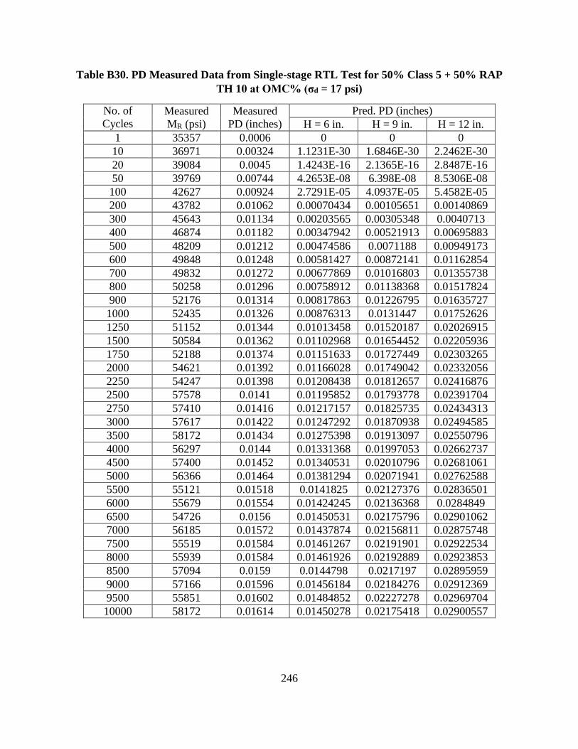
246
Table B30. PD Measured Data from Single-stage RTL Test for 50% Class 5 + 50% RAP
TH 10 at OMC% (σd = 17 psi)
No. of
Cycles Measured
MR (psi)
Measured
PD (inches)
Pred. PD (inches)
H = 6 in. H = 9 in. H = 12 in.
1 35357 0.0006 0 0 0
10 36971 0.00324 1.1231E-30 1.6846E-30 2.2462E-30
20 39084 0.0045 1.4243E-16 2.1365E-16 2.8487E-16
50 39769 0.00744 4.2653E-08 6.398E-08 8.5306E-08
100 42627 0.00924 2.7291E-05 4.0937E-05 5.4582E-05
200 43782 0.01062 0.00070434 0.00105651 0.00140869
300 45643 0.01134 0.00203565 0.00305348 0.0040713
400 46874 0.01182 0.00347942 0.00521913 0.00695883
500 48209 0.01212 0.00474586 0.0071188 0.00949173
600 49848 0.01248 0.00581427 0.00872141 0.01162854
700 49832 0.01272 0.00677869 0.01016803 0.01355738
800 50258 0.01296 0.00758912 0.01138368 0.01517824
900 52176 0.01314 0.00817863 0.01226795 0.01635727
1000 52435 0.01326 0.00876313 0.0131447 0.01752626
1250 51152 0.01344 0.01013458 0.01520187 0.02026915
1500 50584 0.01362 0.01102968 0.01654452 0.02205936
1750 52188 0.01374 0.01151633 0.01727449 0.02303265
2000 54621 0.01392 0.01166028 0.01749042 0.02332056
2250 54247 0.01398 0.01208438 0.01812657 0.02416876
2500 57578 0.0141 0.01195852 0.01793778 0.02391704
2750 57410 0.01416 0.01217157 0.01825735 0.02434313
3000 57617 0.01422 0.01247292 0.01870938 0.02494585
3500 58172 0.01434 0.01275398 0.01913097 0.02550796
4000 56297 0.0144 0.01331368 0.01997053 0.02662737
4500 57400 0.01452 0.01340531 0.02010796 0.02681061
5000 56366 0.01464 0.01381294 0.02071941 0.02762588
5500 55121 0.01518 0.0141825 0.02127376 0.02836501
6000 55679 0.01554 0.01424245 0.02136368 0.0284849
6500 54726 0.0156 0.01450531 0.02175796 0.02901062
7000 56185 0.01572 0.01437874 0.02156811 0.02875748
7500 55519 0.01584 0.01461267 0.02191901 0.02922534
8000 55939 0.01584 0.01461926 0.02192889 0.02923853
8500 57094 0.0159 0.0144798 0.0217197 0.02895959
9000 57166 0.01596 0.01456184 0.02184276 0.02912369
9500 55851 0.01602 0.01484852 0.02227278 0.02969704
10000 58172 0.01614 0.01450278 0.02175418 0.02900557
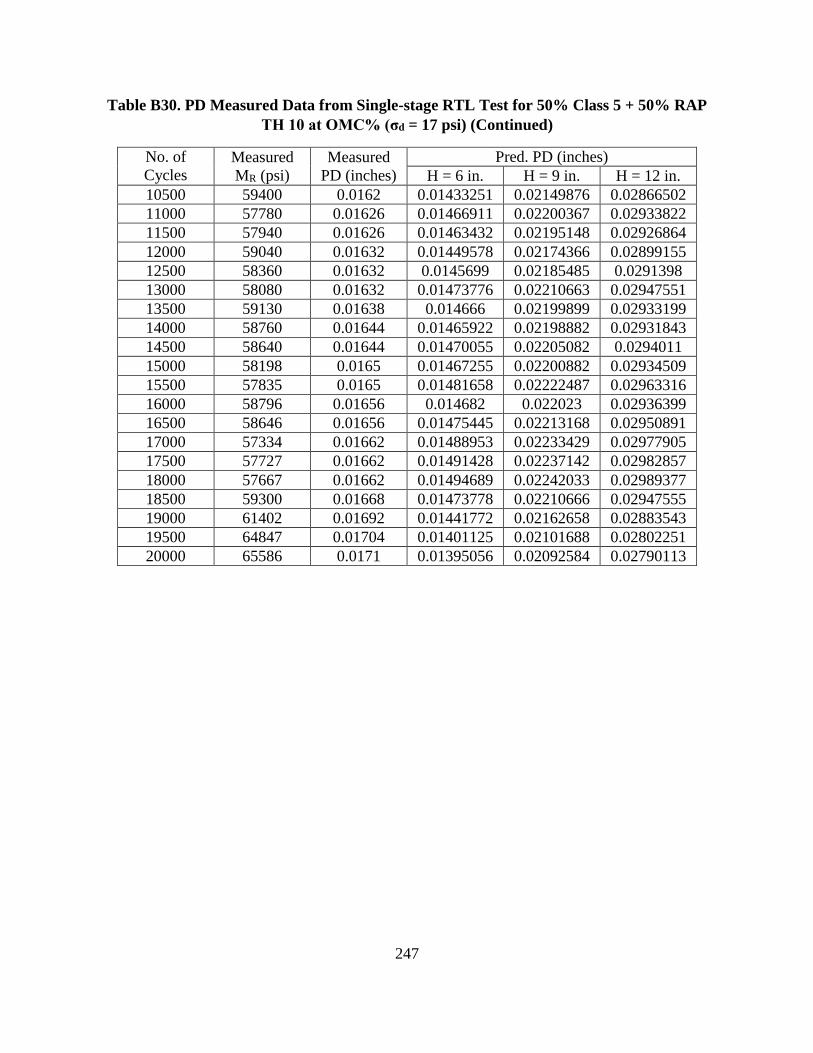
247
Table B30. PD Measured Data from Single-stage RTL Test for 50% Class 5 + 50% RAP
TH 10 at OMC% (σd = 17 psi) (Continued)
No. of
Cycles Measured
MR (psi)
Measured
PD (inches)
Pred. PD (inches)
H = 6 in. H = 9 in. H = 12 in.
10500 59400 0.0162 0.01433251 0.02149876 0.02866502
11000 57780 0.01626 0.01466911 0.02200367 0.02933822
11500 57940 0.01626 0.01463432 0.02195148 0.02926864
12000 59040 0.01632 0.01449578 0.02174366 0.02899155
12500 58360 0.01632 0.0145699 0.02185485 0.0291398
13000 58080 0.01632 0.01473776 0.02210663 0.02947551
13500 59130 0.01638 0.014666 0.02199899 0.02933199
14000 58760 0.01644 0.01465922 0.02198882 0.02931843
14500 58640 0.01644 0.01470055 0.02205082 0.0294011
15000 58198 0.0165 0.01467255 0.02200882 0.02934509
15500 57835 0.0165 0.01481658 0.02222487 0.02963316
16000 58796 0.01656 0.014682 0.022023 0.02936399
16500 58646 0.01656 0.01475445 0.02213168 0.02950891
17000 57334 0.01662 0.01488953 0.02233429 0.02977905
17500 57727 0.01662 0.01491428 0.02237142 0.02982857
18000 57667 0.01662 0.01494689 0.02242033 0.02989377
18500 59300 0.01668 0.01473778 0.02210666 0.02947555
19000 61402 0.01692 0.01441772 0.02162658 0.02883543
19500 64847 0.01704 0.01401125 0.02101688 0.02802251
20000 65586 0.0171 0.01395056 0.02092584 0.02790113
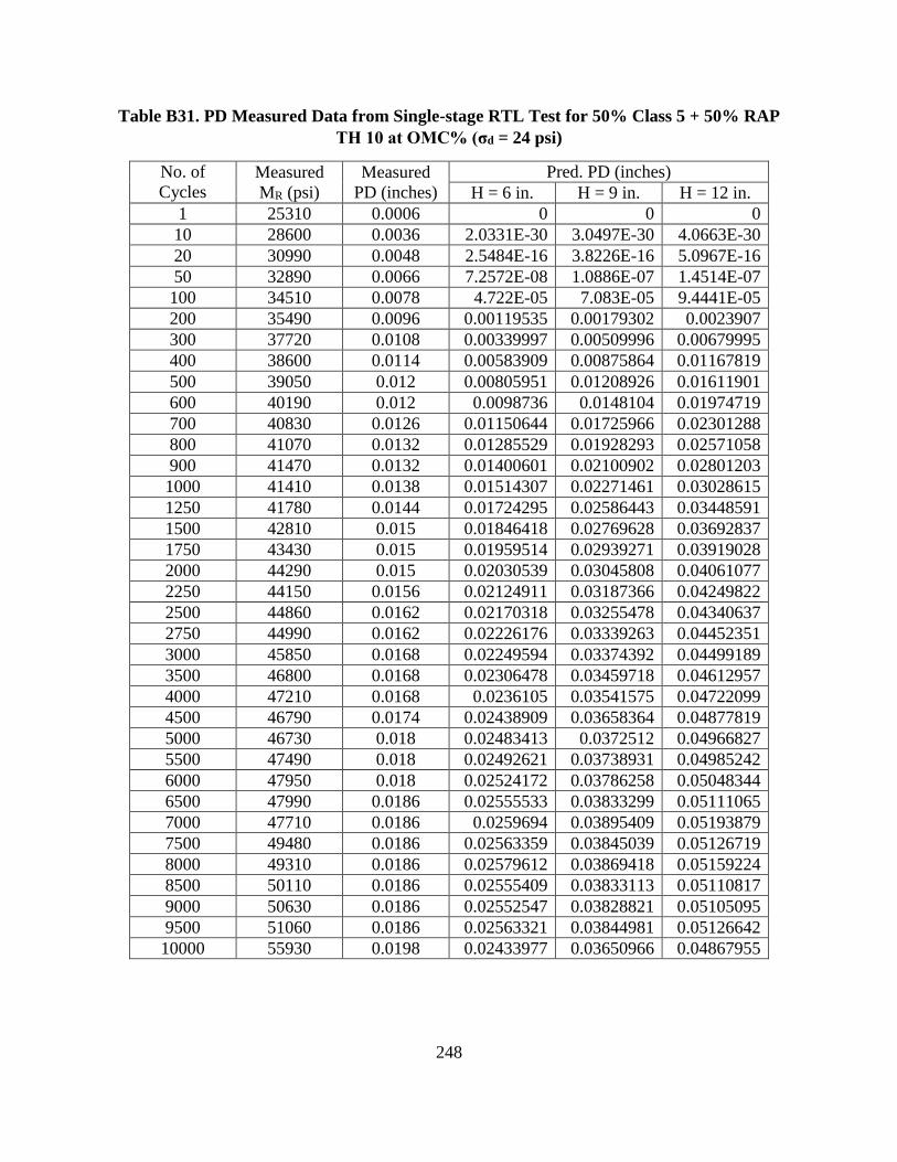
248
Table B31. PD Measured Data from Single-stage RTL Test for 50% Class 5 + 50% RAP
TH 10 at OMC% (σd = 24 psi)
No. of
Cycles Measured
MR (psi)
Measured
PD (inches)
Pred. PD (inches)
H = 6 in. H = 9 in. H = 12 in.
1 25310 0.0006 0 0 0
10 28600 0.0036 2.0331E-30 3.0497E-30 4.0663E-30
20 30990 0.0048 2.5484E-16 3.8226E-16 5.0967E-16
50 32890 0.0066 7.2572E-08 1.0886E-07 1.4514E-07
100 34510 0.0078 4.722E-05 7.083E-05 9.4441E-05
200 35490 0.0096 0.00119535 0.00179302 0.0023907
300 37720 0.0108 0.00339997 0.00509996 0.00679995
400 38600 0.0114 0.00583909 0.00875864 0.01167819
500 39050 0.012 0.00805951 0.01208926 0.01611901
600 40190 0.012 0.0098736 0.0148104 0.01974719
700 40830 0.0126 0.01150644 0.01725966 0.02301288
800 41070 0.0132 0.01285529 0.01928293 0.02571058
900 41470 0.0132 0.01400601 0.02100902 0.02801203
1000 41410 0.0138 0.01514307 0.02271461 0.03028615
1250 41780 0.0144 0.01724295 0.02586443 0.03448591
1500 42810 0.015 0.01846418 0.02769628 0.03692837
1750 43430 0.015 0.01959514 0.02939271 0.03919028
2000 44290 0.015 0.02030539 0.03045808 0.04061077
2250 44150 0.0156 0.02124911 0.03187366 0.04249822
2500 44860 0.0162 0.02170318 0.03255478 0.04340637
2750 44990 0.0162 0.02226176 0.03339263 0.04452351
3000 45850 0.0168 0.02249594 0.03374392 0.04499189
3500 46800 0.0168 0.02306478 0.03459718 0.04612957
4000 47210 0.0168 0.0236105 0.03541575 0.04722099
4500 46790 0.0174 0.02438909 0.03658364 0.04877819
5000 46730 0.018 0.02483413 0.0372512 0.04966827
5500 47490 0.018 0.02492621 0.03738931 0.04985242
6000 47950 0.018 0.02524172 0.03786258 0.05048344
6500 47990 0.0186 0.02555533 0.03833299 0.05111065
7000 47710 0.0186 0.0259694 0.03895409 0.05193879
7500 49480 0.0186 0.02563359 0.03845039 0.05126719
8000 49310 0.0186 0.02579612 0.03869418 0.05159224
8500 50110 0.0186 0.02555409 0.03833113 0.05110817
9000 50630 0.0186 0.02552547 0.03828821 0.05105095
9500 51060 0.0186 0.02563321 0.03844981 0.05126642
10000 55930 0.0198 0.02433977 0.03650966 0.04867955
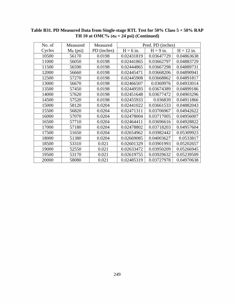
249
Table B31. PD Measured Data from Single-stage RTL Test for 50% Class 5 + 50% RAP
TH 10 at OMC% (σd = 24 psi) (Continued)
No. of
Cycles Measured
MR (psi)
Measured
PD (inches)
Pred. PD (inches)
H = 6 in. H = 9 in. H = 12 in.
10500 56170 0.0198 0.02431819 0.03647729 0.04863638
11000 56050 0.0198 0.02441865 0.03662797 0.04883729
11500 56590 0.0198 0.02444865 0.03667298 0.04889731
12000 56660 0.0198 0.02445471 0.03668206 0.04890941
12500 57270 0.0198 0.02445908 0.03668862 0.04891817
13000 56670 0.0198 0.02466507 0.0369976 0.04933014
13500 57450 0.0198 0.02449593 0.03674389 0.04899186
14000 57620 0.0198 0.02451648 0.03677472 0.04903296
14500 57520 0.0198 0.02455933 0.036839 0.04911866
15000 58120 0.0204 0.02441022 0.03661533 0.04882043
15500 56820 0.0204 0.02471311 0.03706967 0.04942622
16000 57070 0.0204 0.02478004 0.03717005 0.04956007
16500 57710 0.0204 0.02464411 0.03696616 0.04928822
17000 57180 0.0204 0.02478802 0.03718203 0.04957604
17500 51650 0.0204 0.02654962 0.03982442 0.05309923
18000 51380 0.0204 0.02669085 0.04003627 0.0533817
18500 53310 0.021 0.02601329 0.03901993 0.05202657
19000 52550 0.021 0.02633472 0.03950209 0.05266945
19500 53170 0.021 0.02619755 0.03929632 0.05239509
20000 58080 0.021 0.02485319 0.03727978 0.04970638

250
Table B32. PD Measured Data from Single-stage RTL Test for 50% Class 5 + 50% RAP
TH 10 at OMC% (σd = 37 psi)
No. of
Cycles Measured
MR (psi)
Measured
PD (inches)
Pred. PD (inches)
H = 6 in. H = 9 in. H = 12 in.
1 23551 0.006 0 0 0
10 30791 0.0186 3.1287E-30 4.693E-30 6.2574E-30
20 31910 0.0234 4.1526E-16 6.2288E-16 8.3051E-16
50 33779 0.0294 1.2305E-07 1.8457E-07 2.4609E-07
100 36671 0.0342 7.9279E-05 0.00011892 0.00015856
200 38861 0.0378 0.0020024 0.00300361 0.00400481
300 40968 0.0402 0.00577222 0.00865833 0.01154444
400 41968 0.042 0.00985129 0.01477693 0.01970258
500 42745 0.0432 0.01355967 0.0203395 0.02711934
600 42649 0.0438 0.016882 0.025323 0.03376401
700 43127 0.0444 0.0196817 0.02952255 0.0393634
800 43998 0.045 0.02186784 0.03280176 0.04373568
900 44152 0.0456 0.02390619 0.03585929 0.04781238
1000 44401 0.0462 0.02563768 0.03845652 0.05127536
1250 44085 0.0468 0.02945585 0.04418377 0.05891169
1500 46259 0.048 0.03132924 0.04699386 0.06265849
1750 47403 0.0486 0.03291078 0.04936616 0.06582155
2000 47806 0.0492 0.03434553 0.0515183 0.06869106
2250 47680 0.0492 0.03592556 0.05388833 0.07185111
2500 48478 0.0498 0.03641716 0.05462574 0.07283433
2750 48463 0.0498 0.03736788 0.05605182 0.07473576
3000 49414 0.0504 0.03780626 0.05670939 0.07561253
3500 50041 0.051 0.03871016 0.05806523 0.07742031
4000 50777 0.0516 0.03939535 0.05909303 0.07879071
4500 51233 0.0516 0.0398684 0.0598026 0.07973679
5000 52284 0.0522 0.04016788 0.06025182 0.08033576
5500 52763 0.0522 0.04022879 0.06034319 0.08045759
6000 53434 0.0528 0.04026418 0.06039627 0.08052836
6500 53657 0.0528 0.04072888 0.06109332 0.08145776
7000 54304 0.0534 0.04075262 0.06112893 0.08150524
7500 54503 0.0534 0.04089897 0.06134845 0.08179794
8000 54253 0.0534 0.0411601 0.06174016 0.08232021
8500 55163 0.054 0.04103636 0.06155454 0.08207272
9000 55618 0.054 0.04106809 0.06160214 0.08213619
9500 55933 0.054 0.04121286 0.06181929 0.08242573
10000 55296 0.054 0.04160694 0.06241041 0.08321388

251
Table B33. PD Measured Data from Single-stage RTL Test for 50% Class 5 + 50% RAP
TH 10 at OMC+2% (σd = 12 psi)
No. of
Cycles Measured
MR (psi)
Measured
PD (inches)
Pred. PD (inches)
H = 6 in. H = 9 in. H = 12 in.
1 31700 0.0012 0 0 0
10 24620 0.0054 7.7265E-57 1.159E-56 1.5453E-56
20 23020 0.0078 1.0117E-29 1.5176E-29 2.0234E-29
50 22110 0.0108 1.94E-13 2.91E-13 3.88E-13
100 24290 0.0132 4.805E-08 7.2076E-08 9.6101E-08
200 26540 0.0156 2.3462E-05 3.5193E-05 4.6924E-05
300 27130 0.0168 0.00019126 0.00028689 0.00038253
400 29870 0.018 0.00050979 0.00076469 0.00101959
500 29800 0.0186 0.00096197 0.00144295 0.00192393
600 30810 0.0186 0.00143477 0.00215216 0.00286954
700 32200 0.0192 0.00187585 0.00281377 0.00375169
800 32910 0.0198 0.00231096 0.00346644 0.00462192
900 33030 0.0198 0.00275314 0.00412971 0.00550627
1000 33560 0.0204 0.00312963 0.00469444 0.00625926
1250 34330 0.021 0.00396176 0.00594265 0.00792353
1500 34990 0.0216 0.00470142 0.00705213 0.00940284
1750 34340 0.0216 0.0053114 0.0079671 0.01062281
2000 34890 0.0222 0.00576297 0.00864446 0.01152594
2250 34940 0.0222 0.00621514 0.00932271 0.01243028
2500 35940 0.0222 0.00638379 0.00957568 0.01276757
2750 38250 0.0228 0.00642447 0.0096367 0.01284894
3000 37810 0.0228 0.00671059 0.01006589 0.01342118
3500 39270 0.0228 0.00701489 0.01052234 0.01402979
4000 39100 0.0234 0.00741104 0.01111656 0.01482208
4500 39230 0.0234 0.00765371 0.01148056 0.01530741
5000 37350 0.0234 0.00810676 0.01216014 0.01621352
5500 36670 0.024 0.00839925 0.01259887 0.01679849
6000 37350 0.024 0.00850448 0.01275673 0.01700897
6500 39120 0.024 0.00835958 0.01253937 0.01671916
7000 37610 0.024 0.00866874 0.01300311 0.01733748
7500 38990 0.0246 0.00859705 0.01289558 0.01719411
8000 38690 0.0246 0.00872823 0.01309234 0.01745646
8500 39140 0.0246 0.00878961 0.01318441 0.01757921
9000 39400 0.0246 0.00878727 0.0131809 0.01757453
9500 39090 0.0246 0.00893473 0.0134021 0.01786946
10000 39050 0.0246 0.00910529 0.01365794 0.01821059

252
Table B33. PD Measured Data from Single-stage RTL Test for 50% Class 5 + 50% RAP
TH 10 at OMC+2% (σd = 12 psi) (Continued)
No. of
Cycles Measured
MR (psi)
Measured
PD (inches)
Pred. PD (inches)
H = 6 in. H = 9 in. H = 12 in.
11000 39890 0.0246 0.00895504 0.01343256 0.01791009
11500 40060 0.0252 0.00895553 0.0134333 0.01791107
12000 40350 0.0252 0.00900567 0.0135085 0.01801133
12500 40960 0.0252 0.00895412 0.01343118 0.01790824
13000 41400 0.0252 0.00896791 0.01345186 0.01793582
13500 41600 0.0258 0.00907271 0.01360906 0.01814541
14000 41100 0.0258 0.00897182 0.01345773 0.01794364
14500 41620 0.0258 0.00905527 0.01358291 0.01811054
15000 40750 0.0258 0.0091379 0.01370685 0.0182758
15500 41080 0.0258 0.00918285 0.01377428 0.01836571
16000 41290 0.0258 0.00913991 0.01370986 0.01827981
16500 43040 0.0258 0.0088959 0.01334385 0.01779181
17000 43580 0.0258 0.00894046 0.01341069 0.01788093
17500 42950 0.0258 0.00901927 0.0135289 0.01803853
18000 42370 0.0258 0.00914841 0.01372262 0.01829683
18500 43030 0.0258 0.00898632 0.01347948 0.01797264
19000 43690 0.0264 0.00899391 0.01349087 0.01798783
19500 43590 0.0264 0.00888847 0.01333271 0.01777694
20000 43810 0.0264 0.00891899 0.01337848 0.01783797

253
Table B34. PD Measured Data from Single-stage RTL Test for 50% Class 5 + 50% RAP
TH 10 at OMC+2% (σd = 17 psi)
No. of
Cycles Measured
MR (psi)
Measured
PD (inches)
Pred. PD (inches)
H = 6 in. H = 9 in. H = 12 in.
1 23720 0.003 0 0 0
10 23980 0.0138 1.1139E-56 1.6708E-56 2.2277E-56
20 25910 0.0198 1.3443E-29 2.0164E-29 2.6885E-29
50 28700 0.0294 2.292E-13 3.438E-13 4.584E-13
100 28490 0.0396 6.2154E-08 9.3231E-08 1.2431E-07
200 28460 0.0498 3.2704E-05 4.9056E-05 6.5408E-05
300 27480 0.0558 0.00027396 0.00041094 0.00054792
400 26420 0.0606 0.00081003 0.00121504 0.00162005
500 27260 0.0636 0.00149086 0.00223629 0.00298172
600 28790 0.066 0.0021817 0.00327255 0.0043634
700 29790 0.0678 0.00287699 0.00431549 0.00575399
800 29910 0.0696 0.00359559 0.00539339 0.00719118
900 30470 0.0708 0.00422198 0.00633297 0.00844396
1000 31830 0.072 0.00471846 0.00707769 0.00943693
1250 31330 0.075 0.00617263 0.00925895 0.01234526
1500 31480 0.0768 0.00728685 0.01093027 0.0145737
1750 32270 0.0786 0.00809259 0.01213889 0.01618519
2000 32680 0.0798 0.0087722 0.01315831 0.01754441
2250 33530 0.0804 0.00932343 0.01398515 0.01864686
2500 34180 0.0816 0.00972391 0.01458586 0.01944782
2750 35010 0.0822 0.01002443 0.01503664 0.02004885
3000 35310 0.0828 0.01034346 0.01551519 0.02068692
3500 35980 0.0834 0.01087257 0.01630885 0.02174514
4000 35940 0.084 0.01137726 0.0170659 0.02275453
4500 37070 0.0846 0.01163927 0.01745891 0.02327854
5000 36920 0.0852 0.01201837 0.01802755 0.02403673
5500 36870 0.0858 0.0122577 0.01838656 0.02451541
6000 37590 0.0858 0.01234595 0.01851892 0.0246919
6500 38320 0.0864 0.01244171 0.01866257 0.02488343
7000 38940 0.0864 0.01244125 0.01866188 0.02488251
7500 40310 0.087 0.01239093 0.01858639 0.02478186
8000 40300 0.087 0.01250624 0.01875936 0.02501248
8500 41200 0.087 0.01245525 0.01868287 0.0249105
9000 41650 0.087 0.01240326 0.01860489 0.02480652
9500 42450 0.0876 0.01240735 0.01861102 0.02481469
10000 41760 0.0876 0.01265976 0.01898963 0.02531951
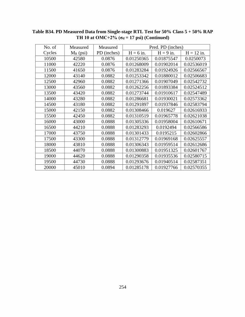
254
Table B34. PD Measured Data from Single-stage RTL Test for 50% Class 5 + 50% RAP
TH 10 at OMC+2% (σd = 17 psi) (Continued)
No. of
Cycles Measured
MR (psi)
Measured
PD (inches)
Pred. PD (inches)
H = 6 in. H = 9 in. H = 12 in.
10500 42580 0.0876 0.01250365 0.01875547 0.0250073
11000 42220 0.0876 0.01268009 0.01902014 0.02536019
11500 41650 0.0876 0.01283284 0.01924926 0.02566567
12000 43140 0.0882 0.01253342 0.01880012 0.02506683
12500 42960 0.0882 0.01271366 0.01907049 0.02542732
13000 43560 0.0882 0.01262256 0.01893384 0.02524512
13500 43420 0.0882 0.01273744 0.01910617 0.02547489
14000 43280 0.0882 0.01286681 0.01930021 0.02573362
14500 43180 0.0882 0.01291897 0.01937846 0.02583794
15000 42150 0.0882 0.01308466 0.019627 0.02616933
15500 42450 0.0882 0.01310519 0.01965778 0.02621038
16000 43000 0.0888 0.01305336 0.01958004 0.02610671
16500 44210 0.0888 0.01283293 0.0192494 0.02566586
17000 43750 0.0888 0.01301433 0.0195215 0.02602866
17500 43300 0.0888 0.01312779 0.01969168 0.02625557
18000 43810 0.0888 0.01306343 0.01959514 0.02612686
18500 44070 0.0888 0.01300883 0.01951325 0.02601767
19000 44620 0.0888 0.01290358 0.01935536 0.02580715
19500 44730 0.0888 0.01293676 0.01940514 0.02587351
20000 45010 0.0894 0.01285178 0.01927766 0.02570355
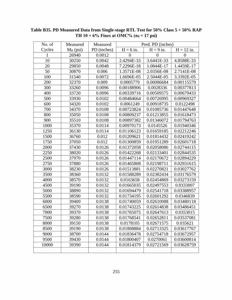
255
Table B35. PD Measured Data from Single-stage RTL Test for 50% Class 5 + 50% RAP
TH 10 + 6% Fines at OMC% (σd = 17 psi)
No. of
Cycles Measured
MR (psi)
Measured
PD (inches)
Pred. PD (inches)
H = 6 in. H = 9 in. H = 12 in.
1 26940 0.0012 0 0 0
10 30250 0.0042 2.4294E-33 3.6441E-33 4.8588E-33
20 29850 0.0048 7.2296E-18 1.0844E-17 1.4459E-17
50 30870 0.006 1.3571E-08 2.0356E-08 2.7141E-08
100 31540 0.0072 1.6696E-05 2.5044E-05 3.3392E-05
200 32370 0.009 0.0005779 0.00086684 0.00115579
300 33260 0.0096 0.00188906 0.0028336 0.00377813
400 33720 0.0096 0.00339716 0.00509575 0.00679433
500 33930 0.0102 0.00484664 0.00726995 0.00969327
600 34320 0.0102 0.0061249 0.00918735 0.0122498
700 34370 0.0108 0.00723824 0.01085736 0.01447648
800 35050 0.0108 0.00809237 0.01213855 0.01618473
900 35510 0.0108 0.00897382 0.01346072 0.01794763
1000 35370 0.0114 0.00970173 0.0145526 0.01940346
1250 36130 0.0114 0.01106123 0.01659185 0.02212246
1500 36760 0.012 0.01209621 0.01814432 0.02419242
1750 37050 0.012 0.01300859 0.01951289 0.02601718
2000 37430 0.0126 0.01372058 0.02058086 0.02744115
2250 38020 0.0126 0.01422268 0.02133401 0.02844535
2500 37970 0.0126 0.01447114 0.02170672 0.02894229
2750 37880 0.0126 0.01465808 0.02198711 0.02931615
3000 38230 0.0126 0.01513881 0.02270821 0.03027762
3500 38360 0.0132 0.01588289 0.02382434 0.03176579
4000 38570 0.0132 0.0163658 0.02454869 0.03273159
4500 39190 0.0132 0.01665035 0.02497553 0.0333007
5000 38890 0.0132 0.01694479 0.02541718 0.03388957
5500 38590 0.0132 0.01734195 0.02601292 0.0346839
6000 39400 0.0138 0.01740059 0.02610088 0.03480118
6500 39270 0.0138 0.01743225 0.02614838 0.03486451
7000 39370 0.0138 0.01765075 0.02647613 0.0353015
7500 39280 0.0138 0.01768541 0.02652811 0.03537081
8000 39150 0.0138 0.0178105 0.02671575 0.035621
8500 39190 0.0138 0.01808884 0.02713325 0.03617767
9000 38700 0.0144 0.01836478 0.02754718 0.03672957
9500 39430 0.0144 0.01800407 0.0270061 0.03600814
10000 39390 0.0144 0.01814379 0.02721569 0.03628759

256
Table B35. PD Measured Data from Single-stage RTL Test for 50% Class 5 + 50% RAP
TH 10 + 6% Fines at OMC% (σd = 17 psi) (Continued)
No. of
Cycles Measured
MR (psi)
Measured
PD (inches)
Pred. PD (inches)
H = 6 in. H = 9 in. H = 12 in.
11000 40940 0.0144 0.01794373 0.0269156 0.03588747
11500 40580 0.0144 0.01800412 0.02700618 0.03600824
12000 40520 0.0144 0.01806986 0.02710478 0.03613971
12500 41240 0.0144 0.01796619 0.02694929 0.03593239
13000 40910 0.0144 0.01807455 0.02711182 0.03614909
13500 41670 0.015 0.01798981 0.02698471 0.03597961
14000 41820 0.015 0.01794311 0.02691466 0.03588622
14500 41990 0.015 0.01803805 0.02705708 0.03607611
15000 42080 0.015 0.01798255 0.02697382 0.03596509
15500 42120 0.015 0.01789426 0.02684138 0.03578851
16000 42430 0.015 0.01795347 0.0269302 0.03590693
16500 42450 0.015 0.01790272 0.02685408 0.03580544
17000 42520 0.015 0.0179966 0.02699489 0.03599319
17500 43090 0.015 0.0178043 0.02670645 0.0356086
18000 42890 0.015 0.01787137 0.02680706 0.03574274
18500 43370 0.015 0.01780815 0.02671223 0.0356163
19000 42730 0.015 0.01802489 0.02703734 0.03604979
19500 43190 0.0156 0.01802138 0.02703207 0.03604275
20000 43080 0.0156 0.01795534 0.02693301 0.03591067
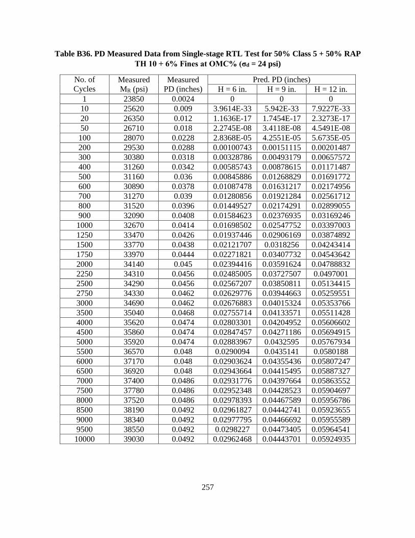
257
Table B36. PD Measured Data from Single-stage RTL Test for 50% Class 5 + 50% RAP
TH 10 + 6% Fines at OMC% (σd = 24 psi)
No. of
Cycles Measured
MR (psi)
Measured
PD (inches)
Pred. PD (inches)
H = 6 in. H = 9 in. H = 12 in.
1 23850 0.0024 0 0 0
10 25620 0.009 3.9614E-33 5.942E-33 7.9227E-33
20 26350 0.012 1.1636E-17 1.7454E-17 2.3273E-17
50 26710 0.018 2.2745E-08 3.4118E-08 4.5491E-08
100 28070 0.0228 2.8368E-05 4.2551E-05 5.6735E-05
200 29530 0.0288 0.00100743 0.00151115 0.00201487
300 30380 0.0318 0.00328786 0.00493179 0.00657572
400 31260 0.0342 0.00585743 0.00878615 0.01171487
500 31160 0.036 0.00845886 0.01268829 0.01691772
600 30890 0.0378 0.01087478 0.01631217 0.02174956
700 31270 0.039 0.01280856 0.01921284 0.02561712
800 31520 0.0396 0.01449527 0.02174291 0.02899055
900 32090 0.0408 0.01584623 0.02376935 0.03169246
1000 32670 0.0414 0.01698502 0.02547752 0.03397003
1250 33470 0.0426 0.01937446 0.02906169 0.03874892
1500 33770 0.0438 0.02121707 0.0318256 0.04243414
1750 33970 0.0444 0.02271821 0.03407732 0.04543642
2000 34140 0.045 0.02394416 0.03591624 0.04788832
2250 34310 0.0456 0.02485005 0.03727507 0.0497001
2500 34290 0.0456 0.02567207 0.03850811 0.05134415
2750 34330 0.0462 0.02629776 0.03944663 0.05259551
3000 34690 0.0462 0.02676883 0.04015324 0.05353766
3500 35040 0.0468 0.02755714 0.04133571 0.05511428
4000 35620 0.0474 0.02803301 0.04204952 0.05606602
4500 35860 0.0474 0.02847457 0.04271186 0.05694915
5000 35920 0.0474 0.02883967 0.0432595 0.05767934
5500 36570 0.048 0.0290094 0.0435141 0.0580188
6000 37170 0.048 0.02903624 0.04355436 0.05807247
6500 36920 0.048 0.02943664 0.04415495 0.05887327
7000 37400 0.0486 0.02931776 0.04397664 0.05863552
7500 37780 0.0486 0.02952348 0.04428523 0.05904697
8000 37520 0.0486 0.02978393 0.04467589 0.05956786
8500 38190 0.0492 0.02961827 0.04442741 0.05923655
9000 38340 0.0492 0.02977795 0.04466692 0.05955589
9500 38550 0.0492 0.0298227 0.04473405 0.05964541
10000 39030 0.0492 0.02962468 0.04443701 0.05924935

258
Table B36. PD Measured Data from Single-stage RTL Test for 50% Class 5 + 50% RAP
TH 10 + 6% Fines at OMC% (σd = 24 psi) (Continued)
No. of
Cycles Measured
MR (psi)
Measured
PD (inches)
Pred. PD (inches)
H = 6 in. H = 9 in. H = 12 in.
10500 38930 0.0492 0.02984813 0.0447722 0.05969627
11000 38780 0.0492 0.03010598 0.04515897 0.06021195
11500 39280 0.0498 0.02989621 0.04484432 0.05979242
12000 39720 0.0498 0.02985182 0.04477773 0.05970363
12500 39560 0.0498 0.02993 0.044895 0.05986001
13000 39440 0.0498 0.03015639 0.04523459 0.06031278
13500 39280 0.0498 0.03040217 0.04560325 0.06080434
14000 39980 0.0498 0.03012495 0.04518743 0.0602499
14500 40330 0.0498 0.02984134 0.04476201 0.05968268
15000 39720 0.0498 0.03031636 0.04547453 0.06063271
15500 40210 0.0504 0.03014826 0.04522239 0.06029652
16000 41310 0.0504 0.02946662 0.04419993 0.05893325
16500 40790 0.0504 0.02984203 0.04476305 0.05968406
17000 40820 0.0504 0.03002439 0.04503659 0.06004879
17500 42530 0.0504 0.02915555 0.04373333 0.05831111
18000 42350 0.0504 0.02923703 0.04385555 0.05847406
18500 41530 0.0504 0.02974381 0.04461571 0.05948762
19000 44250 0.051 0.02844842 0.04267263 0.05689685
19500 45840 0.051 0.027705 0.0415575 0.05541
20000 44770 0.051 0.02833509 0.04250264 0.05667019
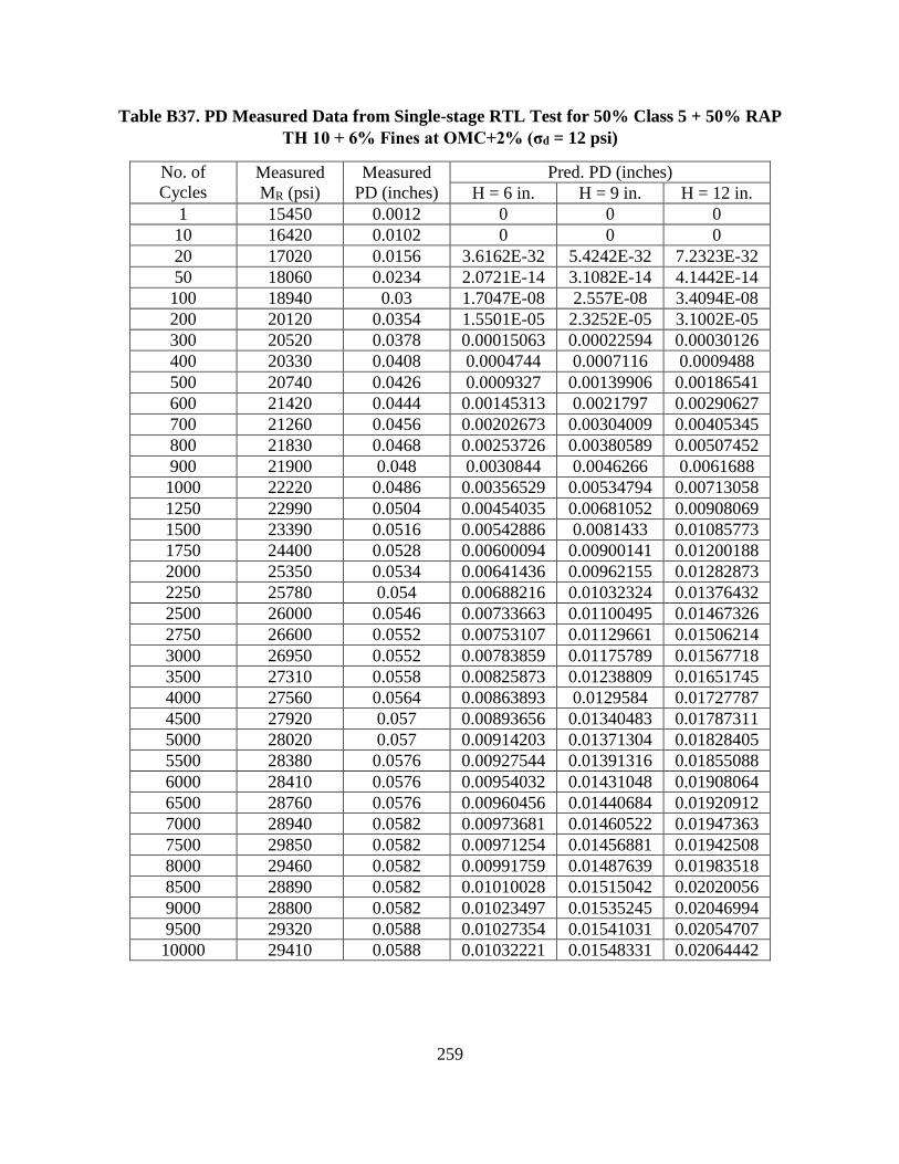
259
Table B37. PD Measured Data from Single-stage RTL Test for 50% Class 5 + 50% RAP
TH 10 + 6% Fines at OMC+2% (σd = 12 psi)
No. of
Cycles Measured
MR (psi)
Measured
PD (inches)
Pred. PD (inches)
H = 6 in. H = 9 in. H = 12 in.
1 15450 0.0012 0 0 0
10 16420 0.0102 0 0 0
20 17020 0.0156 3.6162E-32 5.4242E-32 7.2323E-32
50 18060 0.0234 2.0721E-14 3.1082E-14 4.1442E-14
100 18940 0.03 1.7047E-08 2.557E-08 3.4094E-08
200 20120 0.0354 1.5501E-05 2.3252E-05 3.1002E-05
300 20520 0.0378 0.00015063 0.00022594 0.00030126
400 20330 0.0408 0.0004744 0.0007116 0.0009488
500 20740 0.0426 0.0009327 0.00139906 0.00186541
600 21420 0.0444 0.00145313 0.0021797 0.00290627
700 21260 0.0456 0.00202673 0.00304009 0.00405345
800 21830 0.0468 0.00253726 0.00380589 0.00507452
900 21900 0.048 0.0030844 0.0046266 0.0061688
1000 22220 0.0486 0.00356529 0.00534794 0.00713058
1250 22990 0.0504 0.00454035 0.00681052 0.00908069
1500 23390 0.0516 0.00542886 0.0081433 0.01085773
1750 24400 0.0528 0.00600094 0.00900141 0.01200188
2000 25350 0.0534 0.00641436 0.00962155 0.01282873
2250 25780 0.054 0.00688216 0.01032324 0.01376432
2500 26000 0.0546 0.00733663 0.01100495 0.01467326
2750 26600 0.0552 0.00753107 0.01129661 0.01506214
3000 26950 0.0552 0.00783859 0.01175789 0.01567718
3500 27310 0.0558 0.00825873 0.01238809 0.01651745
4000 27560 0.0564 0.00863893 0.0129584 0.01727787
4500 27920 0.057 0.00893656 0.01340483 0.01787311
5000 28020 0.057 0.00914203 0.01371304 0.01828405
5500 28380 0.0576 0.00927544 0.01391316 0.01855088
6000 28410 0.0576 0.00954032 0.01431048 0.01908064
6500 28760 0.0576 0.00960456 0.01440684 0.01920912
7000 28940 0.0582 0.00973681 0.01460522 0.01947363
7500 29850 0.0582 0.00971254 0.01456881 0.01942508
8000 29460 0.0582 0.00991759 0.01487639 0.01983518
8500 28890 0.0582 0.01010028 0.01515042 0.02020056
9000 28800 0.0582 0.01023497 0.01535245 0.02046994
9500 29320 0.0588 0.01027354 0.01541031 0.02054707
10000 29410 0.0588 0.01032221 0.01548331 0.02064442
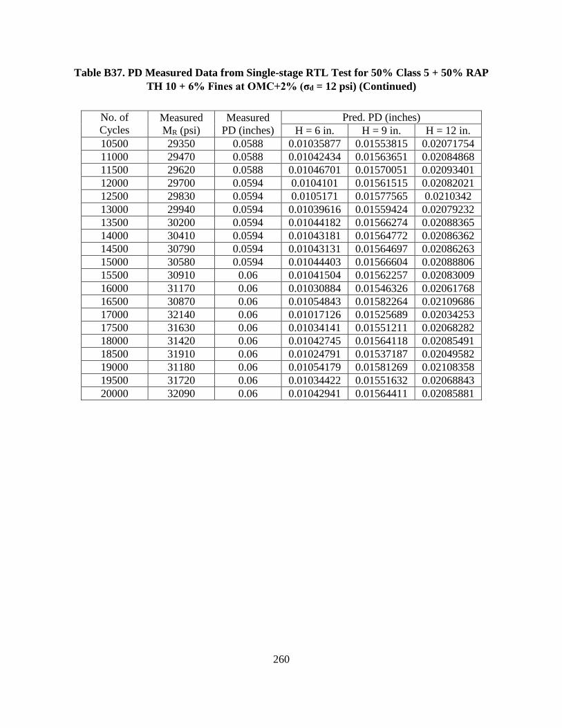
260
Table B37. PD Measured Data from Single-stage RTL Test for 50% Class 5 + 50% RAP
TH 10 + 6% Fines at OMC+2% (σd = 12 psi) (Continued)
No. of
Cycles Measured
MR (psi)
Measured
PD (inches)
Pred. PD (inches)
H = 6 in. H = 9 in. H = 12 in.
10500 29350 0.0588 0.01035877 0.01553815 0.02071754
11000 29470 0.0588 0.01042434 0.01563651 0.02084868
11500 29620 0.0588 0.01046701 0.01570051 0.02093401
12000 29700 0.0594 0.0104101 0.01561515 0.02082021
12500 29830 0.0594 0.0105171 0.01577565 0.0210342
13000 29940 0.0594 0.01039616 0.01559424 0.02079232
13500 30200 0.0594 0.01044182 0.01566274 0.02088365
14000 30410 0.0594 0.01043181 0.01564772 0.02086362
14500 30790 0.0594 0.01043131 0.01564697 0.02086263
15000 30580 0.0594 0.01044403 0.01566604 0.02088806
15500 30910 0.06 0.01041504 0.01562257 0.02083009
16000 31170 0.06 0.01030884 0.01546326 0.02061768
16500 30870 0.06 0.01054843 0.01582264 0.02109686
17000 32140 0.06 0.01017126 0.01525689 0.02034253
17500 31630 0.06 0.01034141 0.01551211 0.02068282
18000 31420 0.06 0.01042745 0.01564118 0.02085491
18500 31910 0.06 0.01024791 0.01537187 0.02049582
19000 31180 0.06 0.01054179 0.01581269 0.02108358
19500 31720 0.06 0.01034422 0.01551632 0.02068843
20000 32090 0.06 0.01042941 0.01564411 0.02085881
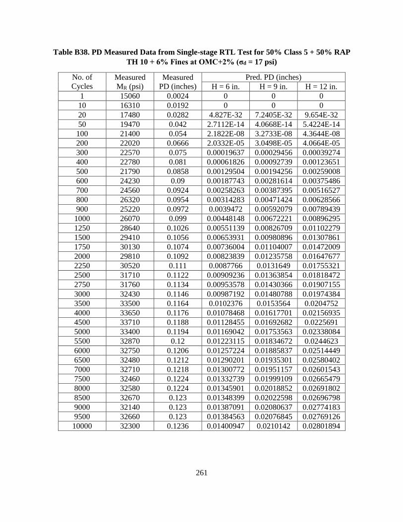
261
Table B38. PD Measured Data from Single-stage RTL Test for 50% Class 5 + 50% RAP
TH 10 + 6% Fines at OMC+2% (σd = 17 psi)
No. of
Cycles Measured
MR (psi)
Measured
PD (inches)
Pred. PD (inches)
H = 6 in. H = 9 in. H = 12 in.
1 15060 0.0024 0 0 0
10 16310 0.0192 0 0 0
20 17480 0.0282 4.827E-32 7.2405E-32 9.654E-32
50 19470 0.042 2.7112E-14 4.0668E-14 5.4224E-14
100 21400 0.054 2.1822E-08 3.2733E-08 4.3644E-08
200 22020 0.0666 2.0332E-05 3.0498E-05 4.0664E-05
300 22570 0.075 0.00019637 0.00029456 0.00039274
400 22780 0.081 0.00061826 0.00092739 0.00123651
500 21790 0.0858 0.00129504 0.00194256 0.00259008
600 24230 0.09 0.00187743 0.00281614 0.00375486
700 24560 0.0924 0.00258263 0.00387395 0.00516527
800 26320 0.0954 0.00314283 0.00471424 0.00628566
900 25220 0.0972 0.0039472 0.00592079 0.00789439
1000 26070 0.099 0.00448148 0.00672221 0.00896295
1250 28640 0.1026 0.00551139 0.00826709 0.01102279
1500 29410 0.1056 0.00653931 0.00980896 0.01307861
1750 30130 0.1074 0.00736004 0.01104007 0.01472009
2000 29810 0.1092 0.00823839 0.01235758 0.01647677
2250 30520 0.111 0.0087766 0.0131649 0.01755321
2500 31710 0.1122 0.00909236 0.01363854 0.01818472
2750 31760 0.1134 0.00953578 0.01430366 0.01907155
3000 32430 0.1146 0.00987192 0.01480788 0.01974384
3500 33500 0.1164 0.0102376 0.0153564 0.0204752
4000 33650 0.1176 0.01078468 0.01617701 0.02156935
4500 33710 0.1188 0.01128455 0.01692682 0.0225691
5000 33400 0.1194 0.01169042 0.01753563 0.02338084
5500 32870 0.12 0.01223115 0.01834672 0.0244623
6000 32750 0.1206 0.01257224 0.01885837 0.02514449
6500 32480 0.1212 0.01290201 0.01935301 0.02580402
7000 32710 0.1218 0.01300772 0.01951157 0.02601543
7500 32460 0.1224 0.01332739 0.01999109 0.02665479
8000 32580 0.1224 0.01345901 0.02018852 0.02691802
8500 32670 0.123 0.01348399 0.02022598 0.02696798
9000 32140 0.123 0.01387091 0.02080637 0.02774183
9500 32660 0.123 0.01384563 0.02076845 0.02769126
10000 32300 0.1236 0.01400947 0.0210142 0.02801894

262
Table B38. PD Measured Data from Single-stage RTL Test for 50% Class 5 + 50% RAP
TH 10 + 6% Fines at OMC+2% (σd = 17 psi) (Continued)
No. of
Cycles Measured
MR (psi)
Measured
PD (inches)
Pred. PD (inches)
H = 6 in. H = 9 in. H = 12 in.
10500 31780 0.1236 0.01440413 0.0216062 0.02880827
11000 31680 0.1236 0.01449611 0.02174417 0.02899223
11500 31420 0.1242 0.01467836 0.02201754 0.02935672
12000 31670 0.1242 0.0146501 0.02197515 0.0293002
12500 31780 0.1242 0.01472577 0.02208866 0.02945155
13000 31720 0.1242 0.01481928 0.02222891 0.02963855
13500 319200 0.1248 0.01077018 0.01615526 0.02154035
14000 32880 0.1248 0.01450051 0.02175076 0.02900101
14500 33030 0.1248 0.01461367 0.0219205 0.02922734
15000 33030 0.1254 0.0145533 0.02182995 0.0291066
15500 33740 0.1254 0.01445435 0.02168153 0.02890871
16000 32950 0.1254 0.01482901 0.02224351 0.02965802
16500 32990 0.1254 0.01480462 0.02220692 0.02960923
17000 33120 0.1254 0.01479564 0.02219346 0.02959128
17500 33260 0.126 0.01482038 0.02223056 0.02964075
18000 33240 0.126 0.01484957 0.02227436 0.02969914
18500 32980 0.126 0.01498022 0.02247033 0.02996044
19000 32950 0.126 0.01503958 0.02255937 0.03007915
19500 33630 0.126 0.01482236 0.02223354 0.02964472
20000 33350 0.126 0.01497346 0.02246019 0.02994692

263
Table B39. PD Measured Data from Multi-stage RTL Test for Class 5
at OMC-2% (σd = 6 psi)
No. of
Cycles Measured
MR (psi)
Measured
PD (inches)
Pred. PD (inches)
H = 6 in. H = 9 in. H = 12 in.
1 19220 0.0012 0 0 0
10 17980 0 4.72E-25 7.07E-25 9.43E-25
20 18340 0 6.63E-14 9.95E-14 1.33E-13
50 17390 0 3.34E-07 5.02E-07 6.69E-07
100 17260 0.0006 5.77E-05 8.65E-05 0.000115
200 17710 0.0006 0.000749 0.001123 0.001497
300 17250 0.0012 0.001806 0.002708 0.003611
400 17140 0.0012 0.002798 0.004196 0.005595
500 16920 0.0012 0.003674 0.005512 0.007349
600 16680 0.0018 0.004436 0.006654 0.008873
700 16780 0.0018 0.004986 0.007479 0.009972
800 16890 0.0018 0.005538 0.008307 0.011076
900 17090 0.0018 0.005927 0.008891 0.011854
1000 17120 0.0024 0.006265 0.009397 0.01253
1250 17160 0.0024 0.007058 0.010587 0.014116
1500 16840 0.0024 0.007577 0.011366 0.015155
1750 17080 0.0024 0.007969 0.011953 0.015937
2000 16800 0.003 0.008368 0.012552 0.016736
2250 16710 0.003 0.008651 0.012976 0.017302
2500 16930 0.003 0.00881 0.013214 0.017619
2750 16820 0.003 0.008986 0.013478 0.017971
3000 16810 0.003 0.009068 0.013601 0.018135
3500 17200 0.0036 0.009297 0.013945 0.018594
4000 17160 0.0036 0.009466 0.0142 0.018933
4500 17030 0.0036 0.009578 0.014367 0.019156
5000 16990 0.0036 0.00982 0.014731 0.019641

264
Table B40. PD Measured Data from Multi-stage RTL Test for Class 5
at OMC-2% (σd = 12 psi)
No. of
Cycles Measured
MR (psi)
Measured
PD (inches)
Pred. PD (inches)
H = 6 in. H = 9 in. H = 12 in.
1 26330 0.0054 0 0 0
10 18830 0.0066 1.28E-24 1.92E-24 2.56E-24
20 17130 0.0078 1.82E-13 2.73E-13 3.64E-13
50 16170 0.0096 9.26E-07 1.39E-06 1.85E-06
100 12750 0.0126 7.32E-05 0.00011 0.000146
200 16580 0.0126 0.001984 0.002976 0.003968
300 16180 0.0168 0.004791 0.007187 0.009582
400 16100 0.0204 0.007456 0.011185 0.014913
500 16280 0.0228 0.009481 0.014221 0.018962
600 17400 0.0252 0.010707 0.01606 0.021414
700 17130 0.0276 0.012394 0.018591 0.024788
800 17320 0.0294 0.013675 0.020512 0.02735
900 16690 0.0306 0.014955 0.022433 0.02991
1000 16720 0.0324 0.015823 0.023735 0.031646
1250 17220 0.0354 0.017206 0.025809 0.034412
1500 17880 0.0372 0.017953 0.02693 0.035906
1750 18070 0.039 0.018621 0.027931 0.037241
2000 18910 0.0414 0.018546 0.027818 0.037091
2250 18810 0.0426 0.019209 0.028814 0.038418
2500 19110 0.0444 0.019384 0.029075 0.038767
2750 19800 0.0456 0.01921 0.028815 0.03842
3000 21190 0.0474 0.018558 0.027837 0.037115
3500 21870 0.0492 0.018587 0.027881 0.037174
4000 22190 0.0504 0.018945 0.028418 0.03789
4500 21530 0.0522 0.019657 0.029485 0.039313
5000 23600 0.054 0.018529 0.027793 0.037057
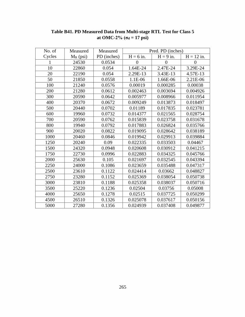
265
Table B41. PD Measured Data from Multi-stage RTL Test for Class 5
at OMC-2% (σd = 17 psi)
No. of
Cycles Measured
MR (psi)
Measured
PD (inches)
Pred. PD (inches)
H = 6 in. H = 9 in. H = 12 in.
1 24530 0.0534 0 0 0
10 22860 0.054 1.64E-24 2.47E-24 3.29E-24
20 22190 0.054 2.29E-13 3.43E-13 4.57E-13
50 21850 0.0558 1.1E-06 1.66E-06 2.21E-06
100 21240 0.0576 0.00019 0.000285 0.00038
200 21280 0.0612 0.002463 0.003694 0.004926
300 20590 0.0642 0.005977 0.008966 0.011954
400 20370 0.0672 0.009249 0.013873 0.018497
500 20440 0.0702 0.01189 0.017835 0.023781
600 19960 0.0732 0.014377 0.021565 0.028754
700 20590 0.0762 0.015839 0.023758 0.031678
800 19940 0.0792 0.017883 0.026824 0.035766
900 20020 0.0822 0.019095 0.028642 0.038189
1000 20460 0.0846 0.019942 0.029913 0.039884
1250 20240 0.09 0.022335 0.033503 0.04467
1500 24320 0.0948 0.020608 0.030912 0.041215
1750 22730 0.0996 0.022883 0.034325 0.045766
2000 25630 0.105 0.021697 0.032545 0.043394
2250 24000 0.1086 0.023659 0.035488 0.047317
2500 23610 0.1122 0.024414 0.03662 0.048827
2750 23280 0.1152 0.025369 0.038054 0.050738
3000 23810 0.1188 0.025358 0.038037 0.050716
3500 25220 0.1236 0.02504 0.03756 0.05008
4000 25650 0.1278 0.02515 0.037725 0.050299
4500 26510 0.1326 0.025078 0.037617 0.050156
5000 27280 0.1356 0.024939 0.037408 0.049877
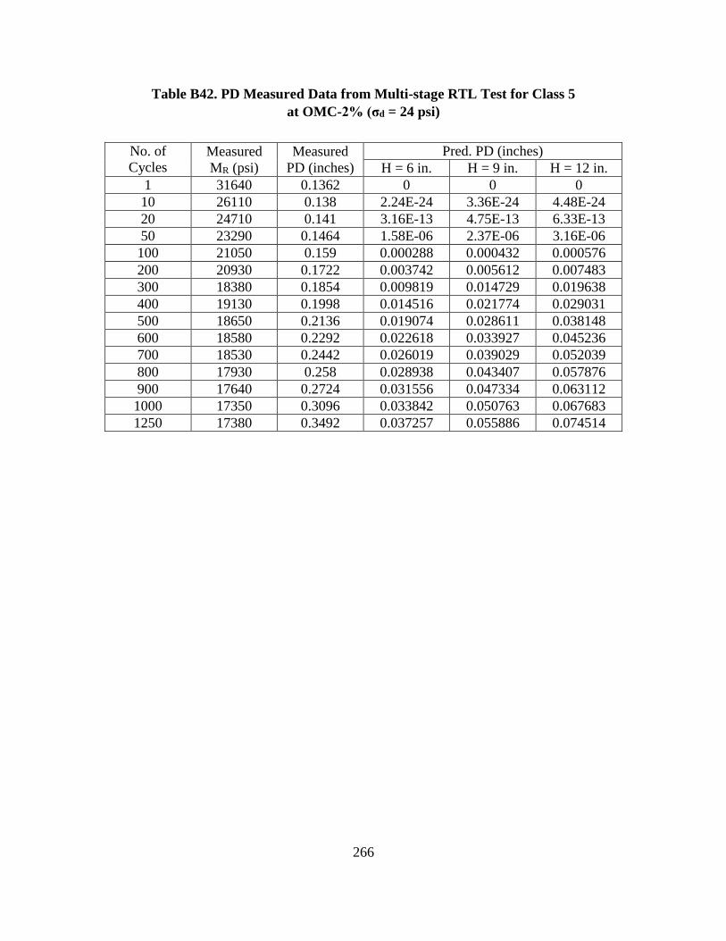
266
Table B42. PD Measured Data from Multi-stage RTL Test for Class 5
at OMC-2% (σd = 24 psi)
No. of
Cycles Measured
MR (psi)
Measured
PD (inches)
Pred. PD (inches)
H = 6 in. H = 9 in. H = 12 in.
1 31640 0.1362 0 0 0
10 26110 0.138 2.24E-24 3.36E-24 4.48E-24
20 24710 0.141 3.16E-13 4.75E-13 6.33E-13
50 23290 0.1464 1.58E-06 2.37E-06 3.16E-06
100 21050 0.159 0.000288 0.000432 0.000576
200 20930 0.1722 0.003742 0.005612 0.007483
300 18380 0.1854 0.009819 0.014729 0.019638
400 19130 0.1998 0.014516 0.021774 0.029031
500 18650 0.2136 0.019074 0.028611 0.038148
600 18580 0.2292 0.022618 0.033927 0.045236
700 18530 0.2442 0.026019 0.039029 0.052039
800 17930 0.258 0.028938 0.043407 0.057876
900 17640 0.2724 0.031556 0.047334 0.063112
1000 17350 0.3096 0.033842 0.050763 0.067683
1250 17380 0.3492 0.037257 0.055886 0.074514

267
Table B43. PD Measured Data from Multi-stage RTL Test for Class 5
at OMC% (σd = 17 psi)
No. of
Cycles Measured
MR (psi)
Measured
PD (inches)
Pred. PD (inches)
H = 6 in. H = 9 in. H = 12 in.
1 21590 0.0012 0 0 0
10 20380 0.0054 1.99E-43 2.99E-43 3.98E-43
20 19550 0.0078 6.93E-23 1.04E-22 1.39E-22
50 19040 0.0126 1.47E-10 2.21E-10 2.94E-10
100 19150 0.0186 1.87E-06 2.81E-06 3.75E-06
200 18290 0.0264 0.000222 0.000334 0.000445
300 18880 0.0324 0.001059 0.001589 0.002118
400 17880 0.0372 0.002519 0.003778 0.005038
500 19050 0.042 0.003872 0.005808 0.007744
600 17920 0.0462 0.005659 0.008489 0.011319
700 18550 0.0504 0.006907 0.010361 0.013814
800 18460 0.054 0.00826 0.01239 0.01652
900 18940 0.057 0.009251 0.013877 0.018502
1000 19600 0.06 0.010048 0.015071 0.020095
1250 19860 0.066 0.012123 0.018184 0.024246
1500 20530 0.0696 0.013576 0.020364 0.027151
1750 21550 0.0732 0.01418 0.021271 0.028361
2000 21240 0.0756 0.015348 0.023022 0.030696
2250 21380 0.0786 0.016166 0.024248 0.032331
2500 21420 0.081 0.016868 0.025302 0.033736
2750 21480 0.0834 0.017553 0.026329 0.035105
3000 21440 0.0858 0.018078 0.027118 0.036157
3500 22880 0.0894 0.018113 0.027169 0.036225
4000 22290 0.0924 0.019099 0.028648 0.038197
4500 22220 0.096 0.019797 0.029695 0.039593
5000 25390 0.0984 0.018223 0.027335 0.036446
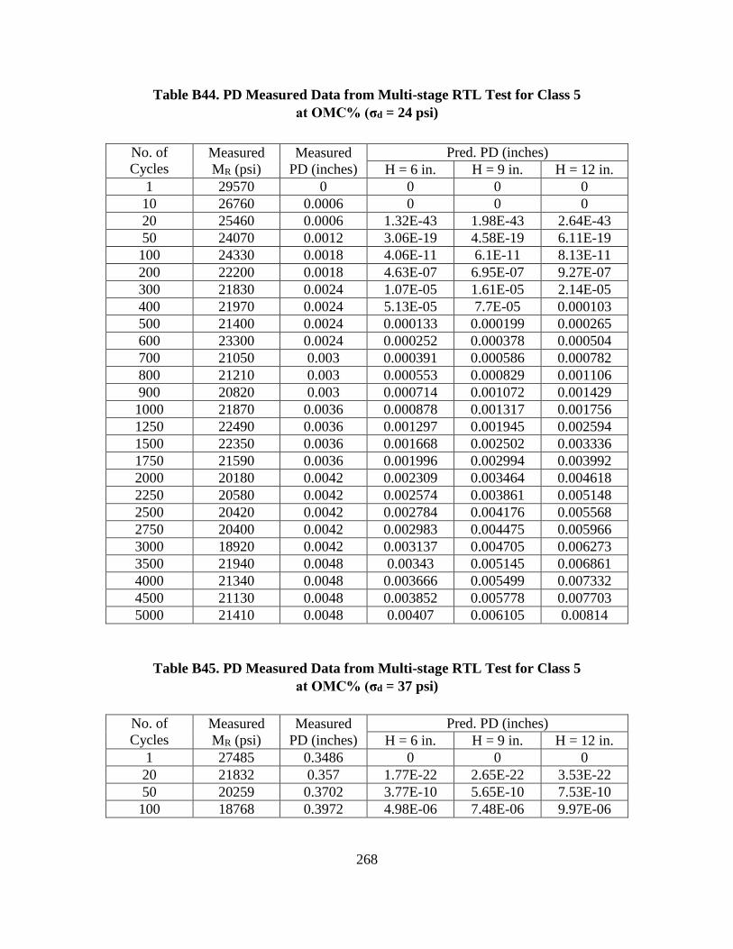
268
Table B44. PD Measured Data from Multi-stage RTL Test for Class 5
at OMC% (σd = 24 psi)
Table B45. PD Measured Data from Multi-stage RTL Test for Class 5
at OMC% (σd = 37 psi)
No. of
Cycles Measured
MR (psi)
Measured
PD (inches)
Pred. PD (inches)
H = 6 in. H = 9 in. H = 12 in.
1 29570 0 0 0 0
10 26760 0.0006 0 0 0
20 25460 0.0006 1.32E-43 1.98E-43 2.64E-43
50 24070 0.0012 3.06E-19 4.58E-19 6.11E-19
100 24330 0.0018 4.06E-11 6.1E-11 8.13E-11
200 22200 0.0018 4.63E-07 6.95E-07 9.27E-07
300 21830 0.0024 1.07E-05 1.61E-05 2.14E-05
400 21970 0.0024 5.13E-05 7.7E-05 0.000103
500 21400 0.0024 0.000133 0.000199 0.000265
600 23300 0.0024 0.000252 0.000378 0.000504
700 21050 0.003 0.000391 0.000586 0.000782
800 21210 0.003 0.000553 0.000829 0.001106
900 20820 0.003 0.000714 0.001072 0.001429
1000 21870 0.0036 0.000878 0.001317 0.001756
1250 22490 0.0036 0.001297 0.001945 0.002594
1500 22350 0.0036 0.001668 0.002502 0.003336
1750 21590 0.0036 0.001996 0.002994 0.003992
2000 20180 0.0042 0.002309 0.003464 0.004618
2250 20580 0.0042 0.002574 0.003861 0.005148
2500 20420 0.0042 0.002784 0.004176 0.005568
2750 20400 0.0042 0.002983 0.004475 0.005966
3000 18920 0.0042 0.003137 0.004705 0.006273
3500 21940 0.0048 0.00343 0.005145 0.006861
4000 21340 0.0048 0.003666 0.005499 0.007332
4500 21130 0.0048 0.003852 0.005778 0.007703
5000 21410 0.0048 0.00407 0.006105 0.00814
No. of
Cycles Measured
MR (psi)
Measured
PD (inches)
Pred. PD (inches)
H = 6 in. H = 9 in. H = 12 in.
1 27485 0.3486 0 0 0
20 21832 0.357 1.77E-22 2.65E-22 3.53E-22
50 20259 0.3702 3.77E-10 5.65E-10 7.53E-10
100 18768 0.3972 4.98E-06 7.48E-06 9.97E-06

269
Table B46. PD Measured Data from Multi-stage RTL Test for Class 5
at OMC+2% (σd = 6 psi)
No. of
Cycles Measured
MR (psi)
Measured
PD (inches)
Pred. PD (inches)
H = 6 in. H = 9 in. H = 12 in.
1 19220 0 0 0 0
10 17980 0.0006 0 0 0
20 18340 0.0006 1.32E-43 1.98E-43 2.64E-43
50 17390 0.0012 3.06E-19 4.58E-19 6.11E-19
100 17260 0.0018 4.06E-11 6.1E-11 8.13E-11
200 17710 0.0018 4.63E-07 6.95E-07 9.27E-07
300 17250 0.0024 1.07E-05 1.61E-05 2.14E-05
400 17140 0.0024 5.13E-05 7.7E-05 0.000103
500 16920 0.0024 0.000133 0.000199 0.000265
600 16680 0.0024 0.000252 0.000378 0.000504
700 16780 0.003 0.000391 0.000586 0.000782
800 16890 0.003 0.000553 0.000829 0.001106
900 17090 0.003 0.000714 0.001072 0.001429
1000 17120 0.0036 0.000878 0.001317 0.001756
1250 17160 0.0036 0.001297 0.001945 0.002594
1500 16840 0.0036 0.001668 0.002502 0.003336
1750 17080 0.0036 0.001996 0.002994 0.003992
2000 16800 0.0042 0.002309 0.003464 0.004618
2250 16710 0.0042 0.002574 0.003861 0.005148
2500 16930 0.0042 0.002784 0.004176 0.005568
2750 16820 0.0042 0.002983 0.004475 0.005966
3000 16810 0.0042 0.003137 0.004705 0.006273
3500 17200 0.0048 0.00343 0.005145 0.006861
4000 17160 0.0048 0.003666 0.005499 0.007332
4500 17030 0.0048 0.003852 0.005778 0.007703
5000 16990 0.0048 0.00407 0.006105 0.00814
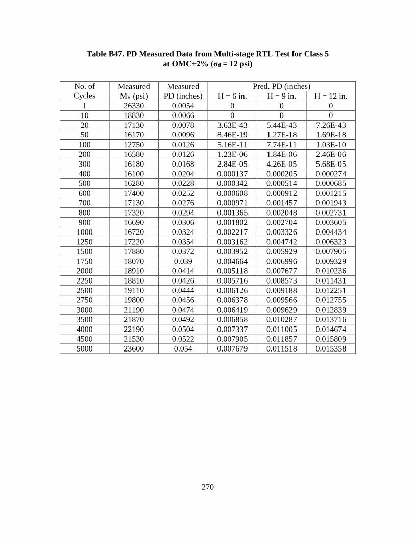
270
Table B47. PD Measured Data from Multi-stage RTL Test for Class 5
at OMC+2% (σd = 12 psi)
No. of
Cycles Measured
MR (psi)
Measured
PD (inches)
Pred. PD (inches)
H = 6 in. H = 9 in. H = 12 in.
1 26330 0.0054 0 0 0
10 18830 0.0066 0 0 0
20 17130 0.0078 3.63E-43 5.44E-43 7.26E-43
50 16170 0.0096 8.46E-19 1.27E-18 1.69E-18
100 12750 0.0126 5.16E-11 7.74E-11 1.03E-10
200 16580 0.0126 1.23E-06 1.84E-06 2.46E-06
300 16180 0.0168 2.84E-05 4.26E-05 5.68E-05
400 16100 0.0204 0.000137 0.000205 0.000274
500 16280 0.0228 0.000342 0.000514 0.000685
600 17400 0.0252 0.000608 0.000912 0.001215
700 17130 0.0276 0.000971 0.001457 0.001943
800 17320 0.0294 0.001365 0.002048 0.002731
900 16690 0.0306 0.001802 0.002704 0.003605
1000 16720 0.0324 0.002217 0.003326 0.004434
1250 17220 0.0354 0.003162 0.004742 0.006323
1500 17880 0.0372 0.003952 0.005929 0.007905
1750 18070 0.039 0.004664 0.006996 0.009329
2000 18910 0.0414 0.005118 0.007677 0.010236
2250 18810 0.0426 0.005716 0.008573 0.011431
2500 19110 0.0444 0.006126 0.009188 0.012251
2750 19800 0.0456 0.006378 0.009566 0.012755
3000 21190 0.0474 0.006419 0.009629 0.012839
3500 21870 0.0492 0.006858 0.010287 0.013716
4000 22190 0.0504 0.007337 0.011005 0.014674
4500 21530 0.0522 0.007905 0.011857 0.015809
5000 23600 0.054 0.007679 0.011518 0.015358

271
Table B48. PD Measured Data from Multi-stage RTL Test for Class 5
at OMC+2% (σd = 17 psi)
No. of
Cycles Measured
MR (psi)
Measured
PD (inches)
Pred. PD (inches)
H = 6 in. H = 9 in. H = 12 in.
1 24530 0.0534 0 0 0
10 22860 0.054 0 0 0
20 22190 0.054 4.56E-43 6.83E-43 9.11E-43
50 21850 0.0558 1.01E-18 1.51E-18 2.02E-18
100 21240 0.0576 1.34E-10 2.01E-10 2.68E-10
200 21280 0.0612 1.52E-06 2.29E-06 3.05E-06
300 20590 0.0642 3.54E-05 5.31E-05 7.08E-05
400 20370 0.0672 0.00017 0.000254 0.000339
500 20440 0.0702 0.000429 0.000644 0.000859
600 19960 0.0732 0.000816 0.001224 0.001632
700 20590 0.0762 0.001241 0.001862 0.002483
800 19940 0.0792 0.001785 0.002678 0.003571
900 20020 0.0822 0.002301 0.003452 0.004603
1000 20460 0.0846 0.002794 0.004191 0.005588
1250 20240 0.09 0.004104 0.006156 0.008208
1500 24320 0.0948 0.004537 0.006805 0.009074
1750 22730 0.0996 0.005732 0.008598 0.011464
2000 25630 0.105 0.005987 0.008981 0.011975
2250 24000 0.1086 0.007039 0.010559 0.014079
2500 23610 0.1122 0.007715 0.011573 0.01543
2750 23280 0.1152 0.008422 0.012633 0.016844
3000 23810 0.1188 0.008772 0.013157 0.017543
3500 25220 0.1236 0.009239 0.013859 0.018478
4000 25650 0.1278 0.00974 0.01461 0.01948
4500 26510 0.1326 0.010085 0.015127 0.02017
5000 27280 0.1356 0.010335 0.015503 0.020671
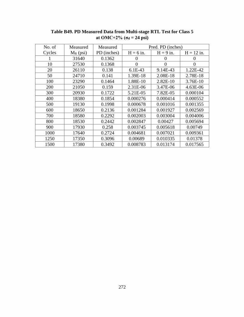
272
Table B49. PD Measured Data from Multi-stage RTL Test for Class 5
at OMC+2% (σd = 24 psi)
No. of
Cycles Measured
MR (psi)
Measured
PD (inches)
Pred. PD (inches)
H = 6 in. H = 9 in. H = 12 in.
1 31640 0.1362 0 0 0
10 27530 0.1368 0 0 0
20 26110 0.138 6.1E-43 9.14E-43 1.22E-42
50 24710 0.141 1.39E-18 2.08E-18 2.78E-18
100 23290 0.1464 1.88E-10 2.82E-10 3.76E-10
200 21050 0.159 2.31E-06 3.47E-06 4.63E-06
300 20930 0.1722 5.21E-05 7.82E-05 0.000104
400 18380 0.1854 0.000276 0.000414 0.000552
500 19130 0.1998 0.000678 0.001016 0.001355
600 18650 0.2136 0.001284 0.001927 0.002569
700 18580 0.2292 0.002003 0.003004 0.004006
800 18530 0.2442 0.002847 0.00427 0.005694
900 17930 0.258 0.003745 0.005618 0.00749
1000 17640 0.2724 0.004681 0.007021 0.009361
1250 17350 0.3096 0.00689 0.010335 0.01378
1500 17380 0.3492 0.008783 0.013174 0.017565

273
Table B50. PD Measured Data from Multi-stage RTL Test for 50% Class 5 + 50% RAP
TH 10 at OMC-2% (σd = 17 psi)
No. of
Cycles Measured
MR (psi)
Measured
PD (inches)
Pred. PD (inches)
H = 6 in. H = 9 in. H = 12 in.
1 54265 0.00078 0 0 0
10 55576 0.00162 2.66E-18 3.99E-18 5.32E-18
20 55145 0.0018 2.4E-10 3.6E-10 4.8E-10
50 56430 0.0021 1.41E-05 2.12E-05 2.83E-05
100 57135 0.0024 0.000551 0.000827 0.001103
200 58618 0.00276 0.003419 0.005128 0.006837
300 59051 0.00294 0.006307 0.009461 0.012615
400 60091 0.00306 0.00854 0.012809 0.017079
500 60322 0.00312 0.010275 0.015412 0.020549
600 60279 0.00318 0.011672 0.017508 0.023345
700 61105 0.00324 0.012595 0.018892 0.02519
800 60993 0.0033 0.013537 0.020305 0.027073
900 60283 0.0033 0.014277 0.021415 0.028554
1000 61205 0.00336 0.014782 0.022173 0.029563
1250 62120 0.00342 0.01593 0.023895 0.031861
1500 61260 0.00342 0.016811 0.025217 0.033622
1750 61048 0.00348 0.017482 0.026224 0.034965
2000 65940 0.00354 0.017149 0.025723 0.034298
2250 66536 0.00354 0.017566 0.02635 0.035133
2500 66282 0.0036 0.017707 0.026561 0.035415
2750 66773 0.00366 0.018031 0.027047 0.036063
3000 67271 0.00366 0.01811 0.027165 0.03622
3500 67524 0.00372 0.01841 0.027615 0.03682
4000 68689 0.00378 0.018495 0.027742 0.03699
4500 69923 0.00384 0.018616 0.027924 0.037232
5000 67063 0.00384 0.019077 0.028615 0.038153
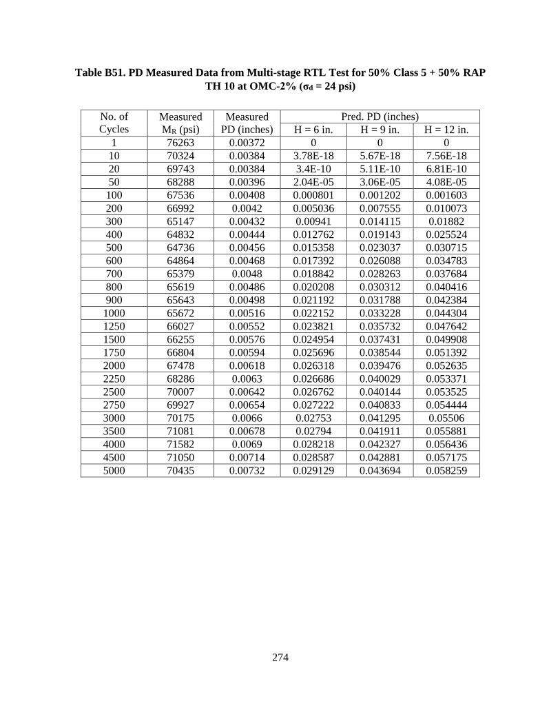
274
Table B51. PD Measured Data from Multi-stage RTL Test for 50% Class 5 + 50% RAP
TH 10 at OMC-2% (σd = 24 psi)
No. of
Cycles Measured
MR (psi)
Measured
PD (inches)
Pred. PD (inches)
H = 6 in. H = 9 in. H = 12 in.
1 76263 0.00372 0 0 0
10 70324 0.00384 3.78E-18 5.67E-18 7.56E-18
20 69743 0.00384 3.4E-10 5.11E-10 6.81E-10
50 68288 0.00396 2.04E-05 3.06E-05 4.08E-05
100 67536 0.00408 0.000801 0.001202 0.001603
200 66992 0.0042 0.005036 0.007555 0.010073
300 65147 0.00432 0.00941 0.014115 0.01882
400 64832 0.00444 0.012762 0.019143 0.025524
500 64736 0.00456 0.015358 0.023037 0.030715
600 64864 0.00468 0.017392 0.026088 0.034783
700 65379 0.0048 0.018842 0.028263 0.037684
800 65619 0.00486 0.020208 0.030312 0.040416
900 65643 0.00498 0.021192 0.031788 0.042384
1000 65672 0.00516 0.022152 0.033228 0.044304
1250 66027 0.00552 0.023821 0.035732 0.047642
1500 66255 0.00576 0.024954 0.037431 0.049908
1750 66804 0.00594 0.025696 0.038544 0.051392
2000 67478 0.00618 0.026318 0.039476 0.052635
2250 68286 0.0063 0.026686 0.040029 0.053371
2500 70007 0.00642 0.026762 0.040144 0.053525
2750 69927 0.00654 0.027222 0.040833 0.054444
3000 70175 0.0066 0.02753 0.041295 0.05506
3500 71081 0.00678 0.02794 0.041911 0.055881
4000 71582 0.0069 0.028218 0.042327 0.056436
4500 71050 0.00714 0.028587 0.042881 0.057175
5000 70435 0.00732 0.029129 0.043694 0.058259
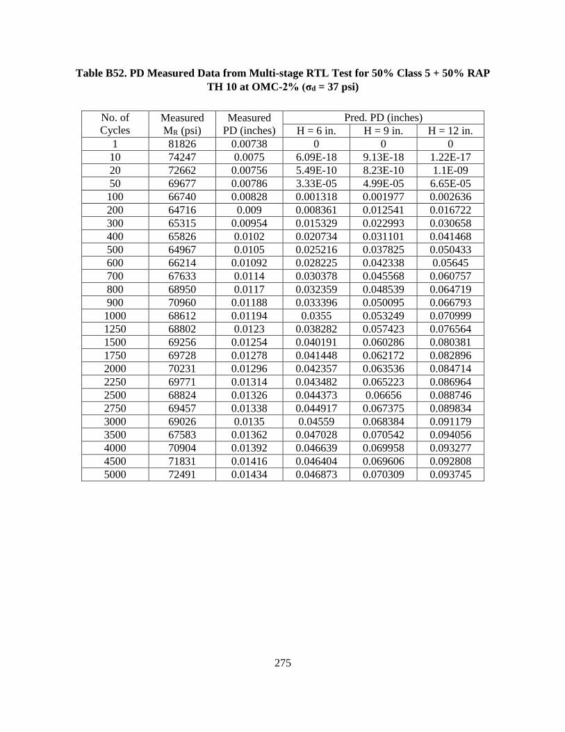
275
Table B52. PD Measured Data from Multi-stage RTL Test for 50% Class 5 + 50% RAP
TH 10 at OMC-2% (σd = 37 psi)
No. of
Cycles Measured
MR (psi)
Measured
PD (inches)
Pred. PD (inches)
H = 6 in. H = 9 in. H = 12 in.
1 81826 0.00738 0 0 0
10 74247 0.0075 6.09E-18 9.13E-18 1.22E-17
20 72662 0.00756 5.49E-10 8.23E-10 1.1E-09
50 69677 0.00786 3.33E-05 4.99E-05 6.65E-05
100 66740 0.00828 0.001318 0.001977 0.002636
200 64716 0.009 0.008361 0.012541 0.016722
300 65315 0.00954 0.015329 0.022993 0.030658
400 65826 0.0102 0.020734 0.031101 0.041468
500 64967 0.0105 0.025216 0.037825 0.050433
600 66214 0.01092 0.028225 0.042338 0.05645
700 67633 0.0114 0.030378 0.045568 0.060757
800 68950 0.0117 0.032359 0.048539 0.064719
900 70960 0.01188 0.033396 0.050095 0.066793
1000 68612 0.01194 0.0355 0.053249 0.070999
1250 68802 0.0123 0.038282 0.057423 0.076564
1500 69256 0.01254 0.040191 0.060286 0.080381
1750 69728 0.01278 0.041448 0.062172 0.082896
2000 70231 0.01296 0.042357 0.063536 0.084714
2250 69771 0.01314 0.043482 0.065223 0.086964
2500 68824 0.01326 0.044373 0.06656 0.088746
2750 69457 0.01338 0.044917 0.067375 0.089834
3000 69026 0.0135 0.04559 0.068384 0.091179
3500 67583 0.01362 0.047028 0.070542 0.094056
4000 70904 0.01392 0.046639 0.069958 0.093277
4500 71831 0.01416 0.046404 0.069606 0.092808
5000 72491 0.01434 0.046873 0.070309 0.093745
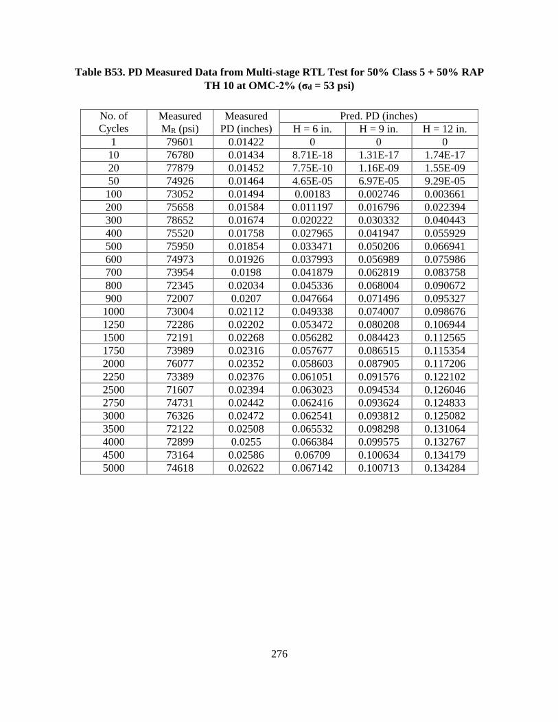
276
Table B53. PD Measured Data from Multi-stage RTL Test for 50% Class 5 + 50% RAP
TH 10 at OMC-2% (σd = 53 psi)
No. of
Cycles Measured
MR (psi)
Measured
PD (inches)
Pred. PD (inches)
H = 6 in. H = 9 in. H = 12 in.
1 79601 0.01422 0 0 0
10 76780 0.01434 8.71E-18 1.31E-17 1.74E-17
20 77879 0.01452 7.75E-10 1.16E-09 1.55E-09
50 74926 0.01464 4.65E-05 6.97E-05 9.29E-05
100 73052 0.01494 0.00183 0.002746 0.003661
200 75658 0.01584 0.011197 0.016796 0.022394
300 78652 0.01674 0.020222 0.030332 0.040443
400 75520 0.01758 0.027965 0.041947 0.055929
500 75950 0.01854 0.033471 0.050206 0.066941
600 74973 0.01926 0.037993 0.056989 0.075986
700 73954 0.0198 0.041879 0.062819 0.083758
800 72345 0.02034 0.045336 0.068004 0.090672
900 72007 0.0207 0.047664 0.071496 0.095327
1000 73004 0.02112 0.049338 0.074007 0.098676
1250 72286 0.02202 0.053472 0.080208 0.106944
1500 72191 0.02268 0.056282 0.084423 0.112565
1750 73989 0.02316 0.057677 0.086515 0.115354
2000 76077 0.02352 0.058603 0.087905 0.117206
2250 73389 0.02376 0.061051 0.091576 0.122102
2500 71607 0.02394 0.063023 0.094534 0.126046
2750 74731 0.02442 0.062416 0.093624 0.124833
3000 76326 0.02472 0.062541 0.093812 0.125082
3500 72122 0.02508 0.065532 0.098298 0.131064
4000 72899 0.0255 0.066384 0.099575 0.132767
4500 73164 0.02586 0.06709 0.100634 0.134179
5000 74618 0.02622 0.067142 0.100713 0.134284

277
Table B54. PD Measured Data from Multi-stage RTL Test for 50% Class 5 + 50% RAP
TH 10 at OMC-2% (σd = 63 psi)
No. of
Cycles Measured
MR (psi)
Measured
PD (inches)
Pred. PD (inches)
H = 6 in. H = 9 in. H = 12 in.
1 81984 0.02616 0 0 0
10 80780 0.02628 1.16E-17 1.73E-17 2.31E-17
20 81092 0.02634 1.04E-09 1.56E-09 2.07E-09
50 77488 0.0264 6.21E-05 9.32E-05 0.000124
100 76607 0.0267 0.002426 0.003639 0.004851
200 77729 0.02766 0.014982 0.022473 0.029965
300 76043 0.02898 0.027626 0.041439 0.055251
400 71078 0.02988 0.038715 0.058073 0.077431
500 70830 0.03102 0.046356 0.069534 0.092713
600 67222 0.0321 0.053894 0.080842 0.107789
700 65591 0.0333 0.059405 0.089107 0.118809
800 64824 0.03432 0.064461 0.096692 0.128923
900 64139 0.03516 0.067712 0.101568 0.135424
1000 68137 0.03606 0.068161 0.102241 0.136322
1250 66732 0.03798 0.074421 0.111632 0.148843
1500 63735 0.03936 0.080145 0.120217 0.160289
1750 61891 0.04062 0.084531 0.126797 0.169063
2000 59391 0.0417 0.088978 0.133467 0.177957
2250 61513 0.04296 0.089037 0.133555 0.178073
2500 67391 0.04446 0.086083 0.129124 0.172166
2750 70822 0.04602 0.085192 0.127788 0.170384
3000 71419 0.0471 0.085739 0.128608 0.171478
3500 74967 0.0492 0.085568 0.128352 0.171136
4000 76433 0.05016 0.086013 0.129019 0.172025
4500 77041 0.05082 0.086891 0.130336 0.173782
5000 75520 0.05148 0.088679 0.133018 0.177357
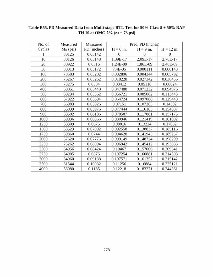
278
Table B55. PD Measured Data from Multi-stage RTL Test for 50% Class 5 + 50% RAP
TH 10 at OMC-2% (σd = 73 psi)
No. of
Cycles Measured
MR (psi)
Measured
PD (inches)
Pred. PD (inches)
H = 6 in. H = 9 in. H = 12 in.
1 80125 0.05142 0 0 0
10 80126 0.05148 1.39E-17 2.09E-17 2.78E-17
20 80922 0.0516 1.24E-09 1.86E-09 2.48E-09
50 80013 0.05172 7.4E-05 0.000111 0.000148
100 78583 0.05202 0.002896 0.004344 0.005792
200 76267 0.05262 0.018228 0.027342 0.036456
300 73275 0.0534 0.03412 0.05118 0.06824
400 69051 0.05448 0.047488 0.071232 0.094976
500 69234 0.05562 0.056721 0.085082 0.113443
600 67922 0.05694 0.064724 0.097086 0.129448
700 66083 0.05826 0.07151 0.107265 0.14302
800 65039 0.05976 0.077444 0.116165 0.154887
900 68502 0.06186 0.078587 0.117881 0.157175
1000 69936 0.06366 0.080946 0.121419 0.161892
1250 68309 0.0675 0.08816 0.13224 0.17632
1500 68523 0.07092 0.092558 0.138837 0.185116
1750 69860 0.0744 0.094628 0.141943 0.189257
2000 67620 0.07776 0.099149 0.148724 0.198299
2250 73262 0.08094 0.096942 0.145412 0.193883
2500 64956 0.08424 0.10467 0.157006 0.209341
2750 64005 0.0876 0.107254 0.160881 0.214508
3000 64960 0.09138 0.107571 0.161357 0.215142
3500 61544 0.10032 0.11256 0.16884 0.225121
4000 53080 0.1185 0.12218 0.183271 0.244361

279
Table B56. PD Measured Data from Multi-stage RTL Test for 50% Class 5 + 50% RAP
TH 10 at OMC% (σd = 24 psi)
No. of
Cycles Measured
MR (psi)
Measured
PD (inches)
Pred. PD (inches)
H = 6 in. H = 9 in. H = 12 in.
1 28980 0.0015 0 0 0
10 31200 0.00534 1.98E-30 2.97E-30 3.96E-30
20 31866 0.00684 2.56E-16 3.85E-16 5.13E-16
50 32873 0.00894 7.58E-08 1.14E-07 1.52E-07
100 34429 0.01074 5.01E-05 7.52E-05 0.0001
200 35327 0.01254 0.001292 0.001938 0.002584
300 36505 0.01374 0.003785 0.005678 0.00757
400 37492 0.01458 0.006448 0.009672 0.012896
500 37988 0.0153 0.008901 0.013352 0.017803
600 38328 0.01584 0.011138 0.016707 0.022276
700 39009 0.01632 0.01286 0.01929 0.02572
800 39420 0.0168 0.014474 0.02171 0.028947
900 40501 0.01722 0.01548 0.02322 0.030961
1000 40626 0.01758 0.016586 0.02488 0.033173
1250 40651 0.01824 0.019108 0.028662 0.038217
1500 41595 0.01884 0.020524 0.030786 0.041047
1750 42067 0.01926 0.021672 0.032508 0.043344
2000 42375 0.01956 0.022625 0.033938 0.045251
2250 43047 0.01986 0.023322 0.034983 0.046643
2500 42897 0.0201 0.02402 0.036029 0.048039
2750 43551 0.02034 0.02451 0.036764 0.049019
3000 44178 0.02058 0.024675 0.037012 0.04935
3500 44950 0.02094 0.025221 0.037832 0.050443
4000 46032 0.02136 0.025534 0.0383 0.051067
4500 46056 0.02166 0.026086 0.039128 0.052171
5000 46400 0.0219 0.02634 0.039509 0.052679

280
Table B57. PD Measured Data from Multi-stage RTL Test for 50% Class 5 + 50% RAP
TH 10 at OMC% (σd = 37 psi)
No. of
Cycles Measured
MR (psi)
Measured
PD (inches)
Pred. PD (inches)
H = 6 in. H = 9 in. H = 12 in.
1 59644 0.02226 0 0 0
10 52377 0.02232 2.68E-30 4.02E-30 5.36E-30
20 53576 0.02322 3.02E-16 4.54E-16 6.05E-16
50 45379 0.02334 1.1E-07 1.65E-07 2.2E-07
100 44402 0.02508 7.33E-05 0.00011 0.000147
200 43610 0.02856 0.001911 0.002867 0.003823
300 43831 0.03144 0.005636 0.008455 0.011273
400 44000 0.03396 0.009674 0.014511 0.019348
500 42999 0.03606 0.013657 0.020486 0.027315
600 42950 0.0378 0.01699 0.025486 0.033981
700 41527 0.03918 0.02039 0.030585 0.04078
800 45959 0.04074 0.021435 0.032152 0.042869
900 44446 0.04176 0.023991 0.035986 0.047982
1000 44219 0.04278 0.025854 0.038781 0.051708
1250 45415 0.04488 0.029041 0.043562 0.058082
1500 45665 0.04662 0.031701 0.047552 0.063403
1750 45092 0.04806 0.034114 0.05117 0.068227
2000 45873 0.04914 0.035454 0.053181 0.070909
2250 47467 0.05028 0.035971 0.053956 0.071942
2500 46573 0.05112 0.037701 0.056551 0.075402
2750 46598 0.05196 0.038668 0.058001 0.077335
3000 46953 0.05274 0.039328 0.058992 0.078656
3500 47933 0.05382 0.040158 0.060238 0.080317
4000 47190 0.05472 0.041569 0.062354 0.083138
4500 48284 0.0555 0.041859 0.062788 0.083717
5000 46973 0.05616 0.043446 0.065169 0.086891
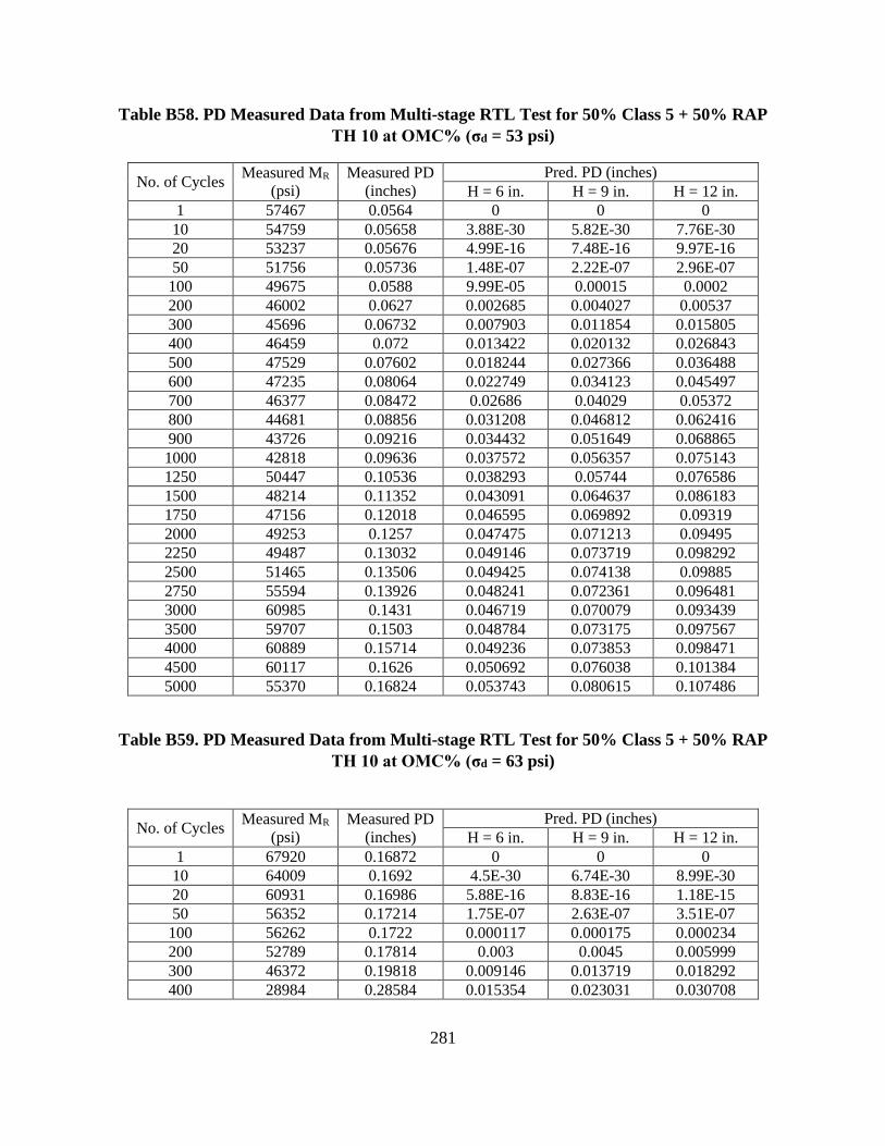
281
Table B58. PD Measured Data from Multi-stage RTL Test for 50% Class 5 + 50% RAP
TH 10 at OMC% (σd = 53 psi)
Table B59. PD Measured Data from Multi-stage RTL Test for 50% Class 5 + 50% RAP
TH 10 at OMC% (σd = 63 psi)
No. of Cycles Measured MR
(psi)
Measured PD
(inches)
Pred. PD (inches)
H = 6 in. H = 9 in. H = 12 in.
1 57467 0.0564 0 0 0
10 54759 0.05658 3.88E-30 5.82E-30 7.76E-30
20 53237 0.05676 4.99E-16 7.48E-16 9.97E-16
50 51756 0.05736 1.48E-07 2.22E-07 2.96E-07
100 49675 0.0588 9.99E-05 0.00015 0.0002
200 46002 0.0627 0.002685 0.004027 0.00537
300 45696 0.06732 0.007903 0.011854 0.015805
400 46459 0.072 0.013422 0.020132 0.026843
500 47529 0.07602 0.018244 0.027366 0.036488
600 47235 0.08064 0.022749 0.034123 0.045497
700 46377 0.08472 0.02686 0.04029 0.05372
800 44681 0.08856 0.031208 0.046812 0.062416
900 43726 0.09216 0.034432 0.051649 0.068865
1000 42818 0.09636 0.037572 0.056357 0.075143
1250 50447 0.10536 0.038293 0.05744 0.076586
1500 48214 0.11352 0.043091 0.064637 0.086183
1750 47156 0.12018 0.046595 0.069892 0.09319
2000 49253 0.1257 0.047475 0.071213 0.09495
2250 49487 0.13032 0.049146 0.073719 0.098292
2500 51465 0.13506 0.049425 0.074138 0.09885
2750 55594 0.13926 0.048241 0.072361 0.096481
3000 60985 0.1431 0.046719 0.070079 0.093439
3500 59707 0.1503 0.048784 0.073175 0.097567
4000 60889 0.15714 0.049236 0.073853 0.098471
4500 60117 0.1626 0.050692 0.076038 0.101384
5000 55370 0.16824 0.053743 0.080615 0.107486
No. of Cycles Measured MR
(psi)
Measured PD
(inches)
Pred. PD (inches)
H = 6 in. H = 9 in. H = 12 in.
1 67920 0.16872 0 0 0
10 64009 0.1692 4.5E-30 6.74E-30 8.99E-30
20 60931 0.16986 5.88E-16 8.83E-16 1.18E-15
50 56352 0.17214 1.75E-07 2.63E-07 3.51E-07
100 56262 0.1722 0.000117 0.000175 0.000234
200 52789 0.17814 0.003 0.0045 0.005999
300 46372 0.19818 0.009146 0.013719 0.018292
400 28984 0.28584 0.015354 0.023031 0.030708
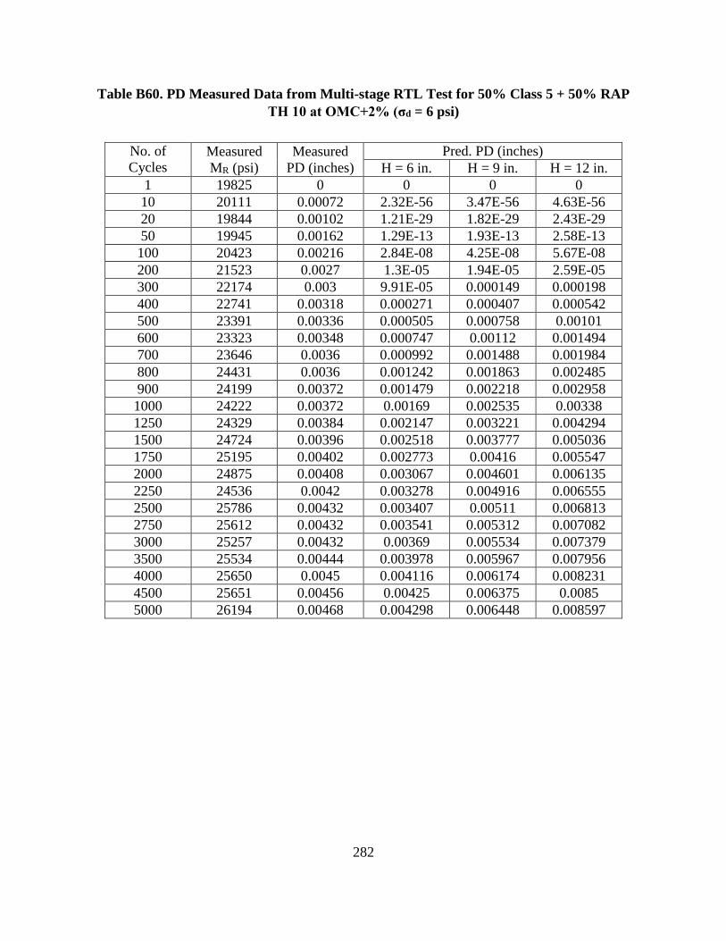
282
Table B60. PD Measured Data from Multi-stage RTL Test for 50% Class 5 + 50% RAP
TH 10 at OMC+2% (σd = 6 psi)
No. of
Cycles Measured
MR (psi)
Measured
PD (inches)
Pred. PD (inches)
H = 6 in. H = 9 in. H = 12 in.
1 19825 0 0 0 0
10 20111 0.00072 2.32E-56 3.47E-56 4.63E-56
20 19844 0.00102 1.21E-29 1.82E-29 2.43E-29
50 19945 0.00162 1.29E-13 1.93E-13 2.58E-13
100 20423 0.00216 2.84E-08 4.25E-08 5.67E-08
200 21523 0.0027 1.3E-05 1.94E-05 2.59E-05
300 22174 0.003 9.91E-05 0.000149 0.000198
400 22741 0.00318 0.000271 0.000407 0.000542
500 23391 0.00336 0.000505 0.000758 0.00101
600 23323 0.00348 0.000747 0.00112 0.001494
700 23646 0.0036 0.000992 0.001488 0.001984
800 24431 0.0036 0.001242 0.001863 0.002485
900 24199 0.00372 0.001479 0.002218 0.002958
1000 24222 0.00372 0.00169 0.002535 0.00338
1250 24329 0.00384 0.002147 0.003221 0.004294
1500 24724 0.00396 0.002518 0.003777 0.005036
1750 25195 0.00402 0.002773 0.00416 0.005547
2000 24875 0.00408 0.003067 0.004601 0.006135
2250 24536 0.0042 0.003278 0.004916 0.006555
2500 25786 0.00432 0.003407 0.00511 0.006813
2750 25612 0.00432 0.003541 0.005312 0.007082
3000 25257 0.00432 0.00369 0.005534 0.007379
3500 25534 0.00444 0.003978 0.005967 0.007956
4000 25650 0.0045 0.004116 0.006174 0.008231
4500 25651 0.00456 0.00425 0.006375 0.0085
5000 26194 0.00468 0.004298 0.006448 0.008597
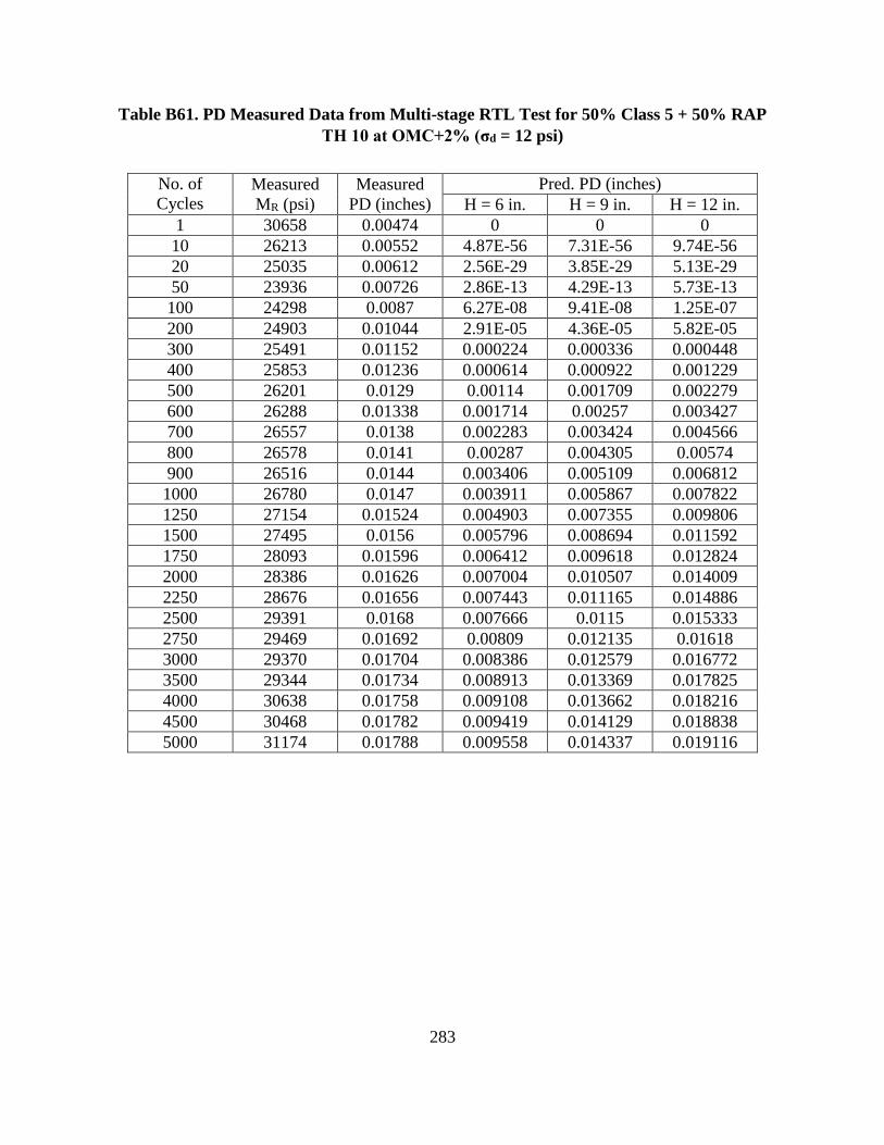
283
Table B61. PD Measured Data from Multi-stage RTL Test for 50% Class 5 + 50% RAP
TH 10 at OMC+2% (σd = 12 psi)
No. of
Cycles Measured
MR (psi)
Measured
PD (inches)
Pred. PD (inches)
H = 6 in. H = 9 in. H = 12 in.
1 30658 0.00474 0 0 0
10 26213 0.00552 4.87E-56 7.31E-56 9.74E-56
20 25035 0.00612 2.56E-29 3.85E-29 5.13E-29
50 23936 0.00726 2.86E-13 4.29E-13 5.73E-13
100 24298 0.0087 6.27E-08 9.41E-08 1.25E-07
200 24903 0.01044 2.91E-05 4.36E-05 5.82E-05
300 25491 0.01152 0.000224 0.000336 0.000448
400 25853 0.01236 0.000614 0.000922 0.001229
500 26201 0.0129 0.00114 0.001709 0.002279
600 26288 0.01338 0.001714 0.00257 0.003427
700 26557 0.0138 0.002283 0.003424 0.004566
800 26578 0.0141 0.00287 0.004305 0.00574
900 26516 0.0144 0.003406 0.005109 0.006812
1000 26780 0.0147 0.003911 0.005867 0.007822
1250 27154 0.01524 0.004903 0.007355 0.009806
1500 27495 0.0156 0.005796 0.008694 0.011592
1750 28093 0.01596 0.006412 0.009618 0.012824
2000 28386 0.01626 0.007004 0.010507 0.014009
2250 28676 0.01656 0.007443 0.011165 0.014886
2500 29391 0.0168 0.007666 0.0115 0.015333
2750 29469 0.01692 0.00809 0.012135 0.01618
3000 29370 0.01704 0.008386 0.012579 0.016772
3500 29344 0.01734 0.008913 0.013369 0.017825
4000 30638 0.01758 0.009108 0.013662 0.018216
4500 30468 0.01782 0.009419 0.014129 0.018838
5000 31174 0.01788 0.009558 0.014337 0.019116

284
Table B62. PD Measured Data from Multi-stage RTL Test for 50% Class 5 + 50% RAP
TH 10 at OMC+2% (σd = 17 psi)
No. of
Cycles Measured
MR (psi)
Measured
PD (inches)
Pred. PD (inches)
H = 6 in. H = 9 in. H = 12 in.
1 36404 0.01788 0 0 0
10 35031 0.01794 6.23E-56 9.34E-56 1.25E-55
20 33652 0.018 3.26E-29 4.89E-29 6.52E-29
50 32400 0.01824 3.56E-13 5.35E-13 7.13E-13
100 31388 0.0186 8.02E-08 1.2E-07 1.6E-07
200 30210 0.01938 3.88E-05 5.82E-05 7.76E-05
300 29762 0.02022 0.000303 0.000454 0.000605
400 29611 0.02088 0.000852 0.001277 0.001703
500 29744 0.02166 0.001572 0.002358 0.003144
600 29665 0.02226 0.002371 0.003557 0.004742
700 29677 0.0228 0.003172 0.004758 0.006344
800 29942 0.02328 0.003949 0.005923 0.007897
900 29956 0.02376 0.00469 0.007035 0.009379
1000 30050 0.02418 0.005342 0.008014 0.010685
1250 30322 0.02508 0.006824 0.010237 0.013649
1500 30501 0.0258 0.008017 0.012026 0.016034
1750 30957 0.0264 0.008963 0.013445 0.017927
2000 31569 0.02688 0.00966 0.014489 0.019319
2250 31385 0.02724 0.010377 0.015565 0.020754
2500 31647 0.02748 0.010984 0.016476 0.021968
2750 31392 0.02778 0.011535 0.017303 0.02307
3000 31621 0.02802 0.011918 0.017877 0.023837
3500 31713 0.0285 0.012633 0.018949 0.025266
4000 32335 0.02886 0.013023 0.019535 0.026046
4500 32722 0.02922 0.013462 0.020194 0.026925
5000 32803 0.02946 0.013779 0.020669 0.027559
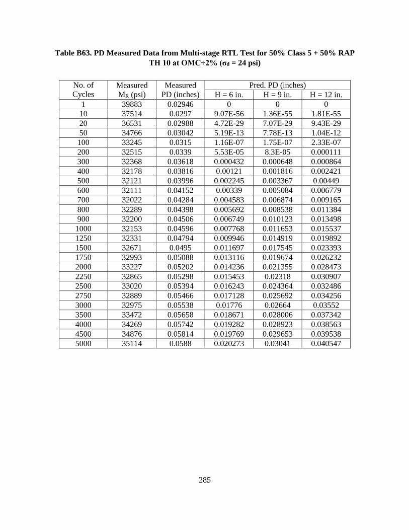
285
Table B63. PD Measured Data from Multi-stage RTL Test for 50% Class 5 + 50% RAP
TH 10 at OMC+2% (σd = 24 psi)
No. of
Cycles Measured
MR (psi)
Measured
PD (inches)
Pred. PD (inches)
H = 6 in. H = 9 in. H = 12 in.
1 39883 0.02946 0 0 0
10 37514 0.0297 9.07E-56 1.36E-55 1.81E-55
20 36531 0.02988 4.72E-29 7.07E-29 9.43E-29
50 34766 0.03042 5.19E-13 7.78E-13 1.04E-12
100 33245 0.0315 1.16E-07 1.75E-07 2.33E-07
200 32515 0.0339 5.53E-05 8.3E-05 0.000111
300 32368 0.03618 0.000432 0.000648 0.000864
400 32178 0.03816 0.00121 0.001816 0.002421
500 32121 0.03996 0.002245 0.003367 0.00449
600 32111 0.04152 0.00339 0.005084 0.006779
700 32022 0.04284 0.004583 0.006874 0.009165
800 32289 0.04398 0.005692 0.008538 0.011384
900 32200 0.04506 0.006749 0.010123 0.013498
1000 32153 0.04596 0.007768 0.011653 0.015537
1250 32331 0.04794 0.009946 0.014919 0.019892
1500 32671 0.0495 0.011697 0.017545 0.023393
1750 32993 0.05088 0.013116 0.019674 0.026232
2000 33227 0.05202 0.014236 0.021355 0.028473
2250 32865 0.05298 0.015453 0.02318 0.030907
2500 33020 0.05394 0.016243 0.024364 0.032486
2750 32889 0.05466 0.017128 0.025692 0.034256
3000 32975 0.05538 0.01776 0.02664 0.03552
3500 33472 0.05658 0.018671 0.028006 0.037342
4000 34269 0.05742 0.019282 0.028923 0.038563
4500 34876 0.05814 0.019769 0.029653 0.039538
5000 35114 0.0588 0.020273 0.03041 0.040547
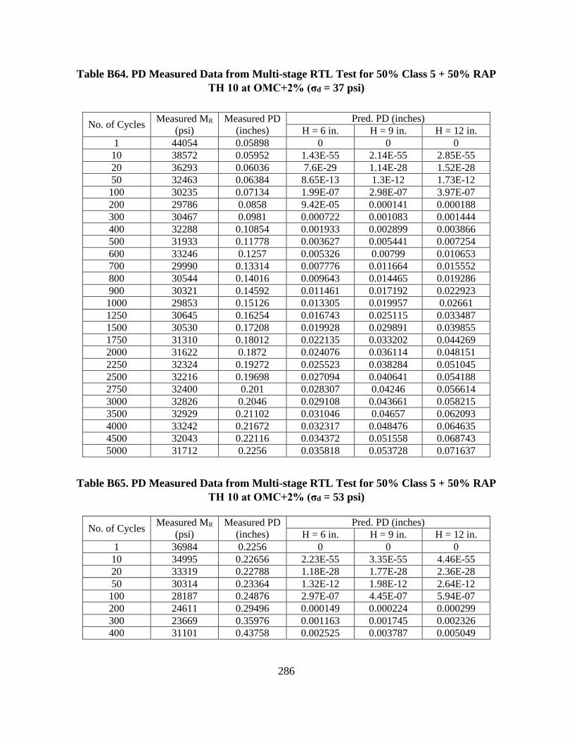
286
Table B64. PD Measured Data from Multi-stage RTL Test for 50% Class 5 + 50% RAP
TH 10 at OMC+2% (σd = 37 psi)
Table B65. PD Measured Data from Multi-stage RTL Test for 50% Class 5 + 50% RAP
TH 10 at OMC+2% (σd = 53 psi)
No. of Cycles Measured MR
(psi)
Measured PD
(inches)
Pred. PD (inches)
H = 6 in. H = 9 in. H = 12 in.
1 44054 0.05898 0 0 0
10 38572 0.05952 1.43E-55 2.14E-55 2.85E-55
20 36293 0.06036 7.6E-29 1.14E-28 1.52E-28
50 32463 0.06384 8.65E-13 1.3E-12 1.73E-12
100 30235 0.07134 1.99E-07 2.98E-07 3.97E-07
200 29786 0.0858 9.42E-05 0.000141 0.000188
300 30467 0.0981 0.000722 0.001083 0.001444
400 32288 0.10854 0.001933 0.002899 0.003866
500 31933 0.11778 0.003627 0.005441 0.007254
600 33246 0.1257 0.005326 0.00799 0.010653
700 29990 0.13314 0.007776 0.011664 0.015552
800 30544 0.14016 0.009643 0.014465 0.019286
900 30321 0.14592 0.011461 0.017192 0.022923
1000 29853 0.15126 0.013305 0.019957 0.02661
1250 30645 0.16254 0.016743 0.025115 0.033487
1500 30530 0.17208 0.019928 0.029891 0.039855
1750 31310 0.18012 0.022135 0.033202 0.044269
2000 31622 0.1872 0.024076 0.036114 0.048151
2250 32324 0.19272 0.025523 0.038284 0.051045
2500 32216 0.19698 0.027094 0.040641 0.054188
2750 32400 0.201 0.028307 0.04246 0.056614
3000 32826 0.2046 0.029108 0.043661 0.058215
3500 32929 0.21102 0.031046 0.04657 0.062093
4000 33242 0.21672 0.032317 0.048476 0.064635
4500 32043 0.22116 0.034372 0.051558 0.068743
5000 31712 0.2256 0.035818 0.053728 0.071637
No. of Cycles Measured MR
(psi)
Measured PD
(inches)
Pred. PD (inches)
H = 6 in. H = 9 in. H = 12 in.
1 36984 0.2256 0 0 0
10 34995 0.22656 2.23E-55 3.35E-55 4.46E-55
20 33319 0.22788 1.18E-28 1.77E-28 2.36E-28
50 30314 0.23364 1.32E-12 1.98E-12 2.64E-12
100 28187 0.24876 2.97E-07 4.45E-07 5.94E-07
200 24611 0.29496 0.000149 0.000224 0.000299
300 23669 0.35976 0.001163 0.001745 0.002326
400 31101 0.43758 0.002525 0.003787 0.005049
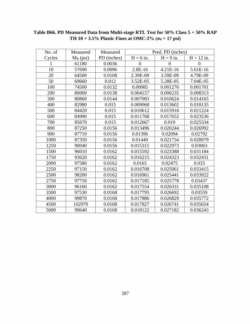
287
Table B66. PD Measured Data from Multi-stage RTL Test for 50% Class 5 + 50% RAP
TH 10 + 3.5% Plastic Fines at OMC-2% (σd = 17 psi)
No. of
Cycles
Measured
MR (psi)
Measured
PD (inches)
Pred. PD (inches)
H = 6 in. H = 9 in. H = 12 in.
1 61180 0.0036 0 0 0
10 57690 0.0096 2.8E-16 4.21E-16 5.61E-16
20 64500 0.0108 2.39E-09 3.59E-09 4.79E-09
50 69660 0.012 3.52E-05 5.28E-05 7.04E-05
100 74500 0.0132 0.00085 0.001276 0.001701
200 80000 0.0138 0.004157 0.006235 0.008313
300 80860 0.0144 0.007083 0.010624 0.014165
400 82980 0.015 0.009068 0.013602 0.018135
500 84420 0.015 0.010612 0.015918 0.021224
600 84990 0.015 0.011768 0.017652 0.023536
700 85670 0.015 0.012667 0.019 0.025334
800 87250 0.0156 0.013496 0.020244 0.026992
900 87710 0.0156 0.01396 0.02094 0.02792
1000 87350 0.0156 0.01449 0.021734 0.028979
1250 90040 0.0156 0.015315 0.022973 0.03063
1500 96010 0.0162 0.015592 0.023388 0.031184
1750 93620 0.0162 0.016215 0.024323 0.032431
2000 97580 0.0162 0.0165 0.02475 0.033
2250 97150 0.0162 0.016708 0.025061 0.033415
2500 98200 0.0162 0.016961 0.025441 0.033922
2750 97750 0.0162 0.017185 0.025778 0.03437
3000 96160 0.0162 0.017554 0.026331 0.035108
3500 97530 0.0168 0.017795 0.026692 0.03559
4000 99870 0.0168 0.017886 0.026829 0.035772
4500 102970 0.0168 0.017827 0.026741 0.035654
5000 99640 0.0168 0.018122 0.027182 0.036243
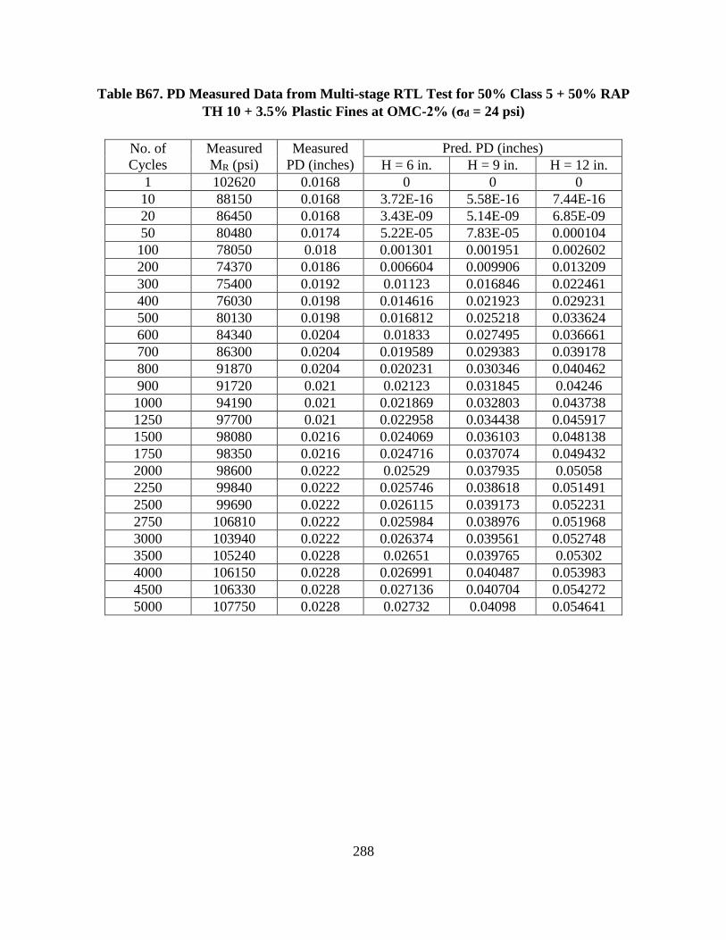
288
Table B67. PD Measured Data from Multi-stage RTL Test for 50% Class 5 + 50% RAP
TH 10 + 3.5% Plastic Fines at OMC-2% (σd = 24 psi)
No. of
Cycles
Measured
MR (psi)
Measured
PD (inches)
Pred. PD (inches)
H = 6 in. H = 9 in. H = 12 in.
1 102620 0.0168 0 0 0
10 88150 0.0168 3.72E-16 5.58E-16 7.44E-16
20 86450 0.0168 3.43E-09 5.14E-09 6.85E-09
50 80480 0.0174 5.22E-05 7.83E-05 0.000104
100 78050 0.018 0.001301 0.001951 0.002602
200 74370 0.0186 0.006604 0.009906 0.013209
300 75400 0.0192 0.01123 0.016846 0.022461
400 76030 0.0198 0.014616 0.021923 0.029231
500 80130 0.0198 0.016812 0.025218 0.033624
600 84340 0.0204 0.01833 0.027495 0.036661
700 86300 0.0204 0.019589 0.029383 0.039178
800 91870 0.0204 0.020231 0.030346 0.040462
900 91720 0.021 0.02123 0.031845 0.04246
1000 94190 0.021 0.021869 0.032803 0.043738
1250 97700 0.021 0.022958 0.034438 0.045917
1500 98080 0.0216 0.024069 0.036103 0.048138
1750 98350 0.0216 0.024716 0.037074 0.049432
2000 98600 0.0222 0.02529 0.037935 0.05058
2250 99840 0.0222 0.025746 0.038618 0.051491
2500 99690 0.0222 0.026115 0.039173 0.052231
2750 106810 0.0222 0.025984 0.038976 0.051968
3000 103940 0.0222 0.026374 0.039561 0.052748
3500 105240 0.0228 0.02651 0.039765 0.05302
4000 106150 0.0228 0.026991 0.040487 0.053983
4500 106330 0.0228 0.027136 0.040704 0.054272
5000 107750 0.0228 0.02732 0.04098 0.054641
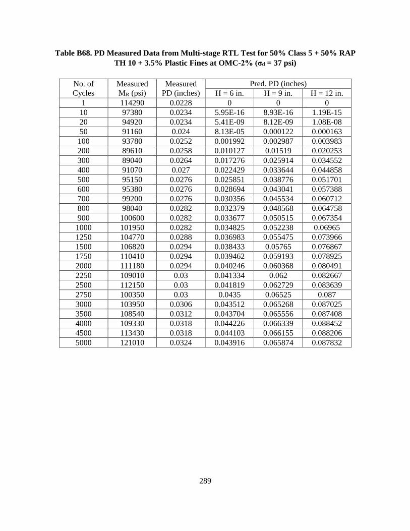
289
Table B68. PD Measured Data from Multi-stage RTL Test for 50% Class 5 + 50% RAP
TH 10 + 3.5% Plastic Fines at OMC-2% (σd = 37 psi)
No. of
Cycles
Measured
MR (psi)
Measured
PD (inches)
Pred. PD (inches)
H = 6 in. H = 9 in. H = 12 in.
1 114290 0.0228 0 0 0
10 97380 0.0234 5.95E-16 8.93E-16 1.19E-15
20 94920 0.0234 5.41E-09 8.12E-09 1.08E-08
50 91160 0.024 8.13E-05 0.000122 0.000163
100 93780 0.0252 0.001992 0.002987 0.003983
200 89610 0.0258 0.010127 0.01519 0.020253
300 89040 0.0264 0.017276 0.025914 0.034552
400 91070 0.027 0.022429 0.033644 0.044858
500 95150 0.0276 0.025851 0.038776 0.051701
600 95380 0.0276 0.028694 0.043041 0.057388
700 99200 0.0276 0.030356 0.045534 0.060712
800 98040 0.0282 0.032379 0.048568 0.064758
900 100600 0.0282 0.033677 0.050515 0.067354
1000 101950 0.0282 0.034825 0.052238 0.06965
1250 104770 0.0288 0.036983 0.055475 0.073966
1500 106820 0.0294 0.038433 0.05765 0.076867
1750 110410 0.0294 0.039462 0.059193 0.078925
2000 111180 0.0294 0.040246 0.060368 0.080491
2250 109010 0.03 0.041334 0.062 0.082667
2500 112150 0.03 0.041819 0.062729 0.083639
2750 100350 0.03 0.0435 0.06525 0.087
3000 103950 0.0306 0.043512 0.065268 0.087025
3500 108540 0.0312 0.043704 0.065556 0.087408
4000 109330 0.0318 0.044226 0.066339 0.088452
4500 113430 0.0318 0.044103 0.066155 0.088206
5000 121010 0.0324 0.043916 0.065874 0.087832
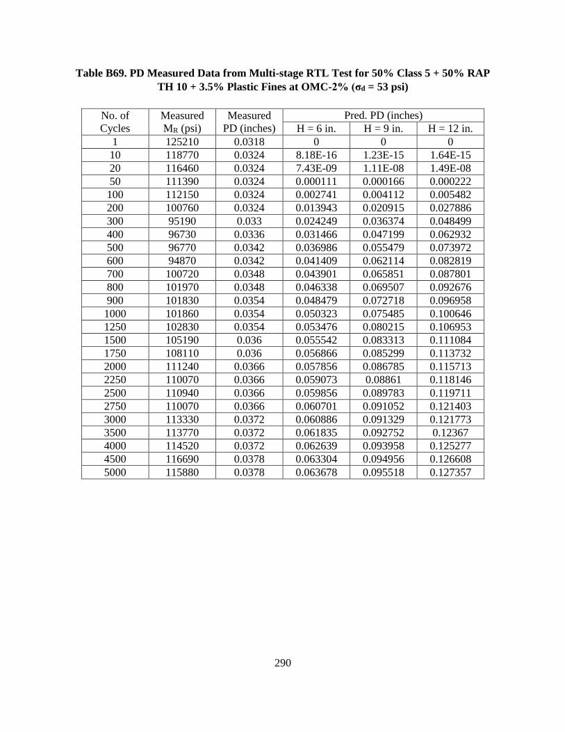
290
Table B69. PD Measured Data from Multi-stage RTL Test for 50% Class 5 + 50% RAP
TH 10 + 3.5% Plastic Fines at OMC-2% (σd = 53 psi)
No. of
Cycles
Measured
MR (psi)
Measured
PD (inches)
Pred. PD (inches)
H = 6 in. H = 9 in. H = 12 in.
1 125210 0.0318 0 0 0
10 118770 0.0324 8.18E-16 1.23E-15 1.64E-15
20 116460 0.0324 7.43E-09 1.11E-08 1.49E-08
50 111390 0.0324 0.000111 0.000166 0.000222
100 112150 0.0324 0.002741 0.004112 0.005482
200 100760 0.0324 0.013943 0.020915 0.027886
300 95190 0.033 0.024249 0.036374 0.048499
400 96730 0.0336 0.031466 0.047199 0.062932
500 96770 0.0342 0.036986 0.055479 0.073972
600 94870 0.0342 0.041409 0.062114 0.082819
700 100720 0.0348 0.043901 0.065851 0.087801
800 101970 0.0348 0.046338 0.069507 0.092676
900 101830 0.0354 0.048479 0.072718 0.096958
1000 101860 0.0354 0.050323 0.075485 0.100646
1250 102830 0.0354 0.053476 0.080215 0.106953
1500 105190 0.036 0.055542 0.083313 0.111084
1750 108110 0.036 0.056866 0.085299 0.113732
2000 111240 0.0366 0.057856 0.086785 0.115713
2250 110070 0.0366 0.059073 0.08861 0.118146
2500 110940 0.0366 0.059856 0.089783 0.119711
2750 110070 0.0366 0.060701 0.091052 0.121403
3000 113330 0.0372 0.060886 0.091329 0.121773
3500 113770 0.0372 0.061835 0.092752 0.12367
4000 114520 0.0372 0.062639 0.093958 0.125277
4500 116690 0.0378 0.063304 0.094956 0.126608
5000 115880 0.0378 0.063678 0.095518 0.127357

291
Table B70. PD Measured Data from Multi-stage RTL Test for 50% Class 5 + 50% RAP
TH 10 + 3.5% Plastic Fines at OMC-2% (σd = 63 psi)
No. of
Cycles
Measured
MR (psi)
Measured
PD (inches)
Pred. PD (inches)
H = 6 in. H = 9 in. H = 12 in.
1 117520 0.0378 0 0 0
10 110280 0.0378 1.12E-15 1.67E-15 2.23E-15
20 108630 0.0378 1.02E-08 1.52E-08 2.03E-08
50 107590 0.0378 0.000152 0.000228 0.000304
100 104170 0.0384 0.003766 0.005649 0.007532
200 96650 0.0384 0.019012 0.028518 0.038025
300 93230 0.039 0.032878 0.049317 0.065756
400 88290 0.0396 0.043761 0.065642 0.087522
500 88080 0.0396 0.051412 0.077118 0.102823
600 87670 0.0402 0.057324 0.085986 0.114648
700 84850 0.0408 0.062662 0.093994 0.125325
800 86010 0.0408 0.066311 0.099467 0.132623
900 86200 0.0414 0.069033 0.10355 0.138066
1000 85410 0.0414 0.071884 0.107827 0.143769
1250 86490 0.042 0.076457 0.114686 0.152914
1500 86900 0.0426 0.079553 0.11933 0.159106
1750 94260 0.0438 0.07979 0.119686 0.159581
2000 97390 0.0444 0.080741 0.121111 0.161481
2250 96530 0.045 0.082524 0.123787 0.165049
2500 98510 0.0456 0.083118 0.124676 0.166235
2750 99360 0.0462 0.083694 0.125541 0.167387
3000 100900 0.0468 0.08466 0.12699 0.16932
3500 106880 0.0474 0.084498 0.126748 0.168997
4000 109140 0.048 0.085285 0.127928 0.17057
4500 110880 0.0486 0.085779 0.128668 0.171558
5000 113940 0.0486 0.085964 0.128946 0.171928

292
Table B71. PD Measured Data from Multi-stage RTL Test for 50% Class 5 + 50% RAP
TH 10 + 3.5% Plastic Fines at OMC-2% (σd = 73 psi)
No. of
Cycles
Measured
MR (psi)
Measured
PD (inches)
Pred. PD (inches)
H = 6 in. H = 9 in. H = 12 in.
1 114820 0.0486 0 0 0
10 110390 0.0486 1.37E-15 2.06E-15 2.74E-15
20 111700 0.0486 1.24E-08 1.86E-08 2.48E-08
50 112380 0.0486 0.000184 0.000276 0.000369
100 110180 0.0492 0.004538 0.006807 0.009076
200 109220 0.0492 0.022595 0.033893 0.04519
300 103720 0.0492 0.038959 0.058438 0.077917
400 104510 0.0498 0.050699 0.076049 0.101398
500 103110 0.0498 0.059808 0.089713 0.119617
600 104660 0.0504 0.06616 0.09924 0.13232
700 100530 0.0504 0.072128 0.108192 0.144256
800 97560 0.051 0.077388 0.116082 0.154776
900 97220 0.051 0.080835 0.121253 0.16167
1000 99110 0.0516 0.083213 0.124819 0.166425
1250 98880 0.0528 0.088638 0.132957 0.177276
1500 99040 0.0534 0.092554 0.138832 0.185109
1750 97110 0.054 0.09597 0.143956 0.191941
2000 94980 0.0546 0.098785 0.148177 0.19757
2250 96570 0.0552 0.10016 0.150241 0.200321
2500 95720 0.0558 0.10192 0.15288 0.20384
2750 96990 0.0564 0.10264 0.153959 0.205279
3000 102020 0.0564 0.102246 0.153369 0.204492
3500 98690 0.057 0.10501 0.157515 0.21002
4000 109340 0.0582 0.10317 0.154755 0.20634
4500 109710 0.0588 0.104199 0.156299 0.208399
5000 111210 0.0594 0.104843 0.157265 0.209687

293
Table B72. PD Measured Data from Multi-stage RTL Test for 50% Class 5 + 50% RAP
TH 10 + 3.5% Plastic Fines at OMC% (σd = 17 psi)
No. of
Cycles
Measured
MR (psi)
Measured
PD (inches)
Pred. PD (inches)
H = 6 in. H = 9 in. H = 12 in.
1 46870 0.0012 0 0 0
10 45440 0.0018 9.33E-27 1.4E-26 1.87E-26
20 44890 0.0024 1.35E-14 2.03E-14 2.7E-14
50 44920 0.003 2.67E-07 4.01E-07 5.34E-07
100 45980 0.0036 7.14E-05 0.000107 0.000143
200 48640 0.0042 0.001138 0.001706 0.002275
300 49030 0.0042 0.002889 0.004334 0.005779
400 50650 0.0042 0.00453 0.006795 0.00906
500 51250 0.0042 0.005971 0.008956 0.011941
600 51400 0.0042 0.007177 0.010766 0.014354
700 51810 0.0042 0.008195 0.012293 0.016391
800 51520 0.0042 0.009054 0.013582 0.018109
900 51640 0.0048 0.009797 0.014696 0.019594
1000 52090 0.0048 0.010368 0.015552 0.020736
1250 52350 0.0048 0.011649 0.017474 0.023298
1500 52480 0.0048 0.012451 0.018677 0.024902
1750 53290 0.0048 0.01309 0.019635 0.026181
2000 54230 0.0048 0.013345 0.020018 0.02669
2250 53340 0.0048 0.01411 0.021164 0.028219
2500 54350 0.0048 0.014277 0.021416 0.028555
2750 54130 0.0048 0.014627 0.02194 0.029253
3000 54160 0.0048 0.014767 0.02215 0.029533
3500 55340 0.0048 0.015128 0.022692 0.030256
4000 56540 0.0054 0.015251 0.022877 0.030503
4500 56610 0.0054 0.015449 0.023173 0.030898
5000 56810 0.0054 0.015679 0.023518 0.031358

294
Table B73. PD Measured Data from Multi-stage RTL Test for 50% Class 5 + 50% RAP
TH 10 + 3.5% Plastic Fines at OMC% (σd = 24 psi)
No. of
Cycles
Measured
MR (psi)
Measured
PD (inches)
Pred. PD (inches)
H = 6 in. H = 9 in. H = 12 in.
1 63630 0.0048 0 0 0
10 59790 0.0054 1.27E-26 1.91E-26 2.55E-26
20 59820 0.0054 1.81E-14 2.72E-14 3.63E-14
50 57960 0.0054 3.6E-07 5.4E-07 7.2E-07
100 57930 0.0054 9.81E-05 0.000147 0.000196
200 56780 0.0054 0.001624 0.002435 0.003247
300 56730 0.006 0.004112 0.006168 0.008224
400 55630 0.006 0.006665 0.009998 0.013331
500 55850 0.006 0.00878 0.01317 0.017561
600 56580 0.006 0.010615 0.015923 0.02123
700 55870 0.006 0.012126 0.01819 0.024253
800 56570 0.006 0.013355 0.020033 0.02671
900 56910 0.006 0.014336 0.021503 0.028671
1000 56620 0.0066 0.015331 0.022997 0.030663
1250 56750 0.0066 0.017147 0.025721 0.034295
1500 56820 0.0066 0.018419 0.027629 0.036839
1750 56900 0.0066 0.019447 0.029171 0.038895
2000 56840 0.0066 0.020338 0.030507 0.040676
2250 56920 0.0066 0.020914 0.031371 0.041828
2500 57570 0.0072 0.021225 0.031838 0.042451
2750 57760 0.0072 0.021759 0.032639 0.043519
3000 57950 0.0072 0.022098 0.033147 0.044197
3500 58300 0.0072 0.022603 0.033905 0.045206
4000 60970 0.0072 0.022533 0.033799 0.045066
4500 61850 0.0072 0.022719 0.034078 0.045437
5000 62220 0.0078 0.022946 0.034419 0.045892

295
Table B74. PD Measured Data from Multi-stage RTL Test for 50% Class 5 + 50% RAP
TH 10 + 3.5% Plastic Fines at OMC% (σd = 37 psi)
No. of
Cycles
Measured
MR (psi)
Measured
PD (inches)
Pred. PD (inches)
H = 6 in. H = 9 in. H = 12 in.
1 70970 0.0078 0 0 0
10 65680 0.0078 1.99E-26 2.98E-26 3.98E-26
20 63520 0.0078 2.88E-14 4.31E-14 5.75E-14
50 60540 0.0078 5.79E-07 8.69E-07 1.16E-06
100 58420 0.0084 0.00016 0.00024 0.00032
200 57000 0.009 0.002661 0.003992 0.005323
300 56480 0.0096 0.006823 0.010235 0.013646
400 56200 0.0102 0.010944 0.016416 0.021888
500 56220 0.0102 0.014494 0.021741 0.028989
600 56130 0.0108 0.01756 0.02634 0.03512
700 56020 0.0108 0.020074 0.030111 0.040148
800 55800 0.0108 0.022289 0.033434 0.044579
900 55850 0.0114 0.024102 0.036153 0.048204
1000 56080 0.0114 0.025618 0.038427 0.051235
1250 56120 0.0114 0.028763 0.043144 0.057526
1500 55670 0.012 0.031166 0.046748 0.062331
1750 56120 0.012 0.032872 0.049308 0.065743
2000 56010 0.0126 0.034479 0.051718 0.068958
2250 56420 0.0126 0.035375 0.053062 0.07075
2500 56900 0.0126 0.036221 0.054332 0.072443
2750 56690 0.0132 0.036904 0.055356 0.073808
3000 57240 0.0132 0.037402 0.056103 0.074804
3500 57670 0.0132 0.038227 0.05734 0.076453
4000 58250 0.0138 0.038943 0.058414 0.077885
4500 58510 0.0138 0.039332 0.058998 0.078665
5000 58690 0.0138 0.039908 0.059862 0.079815
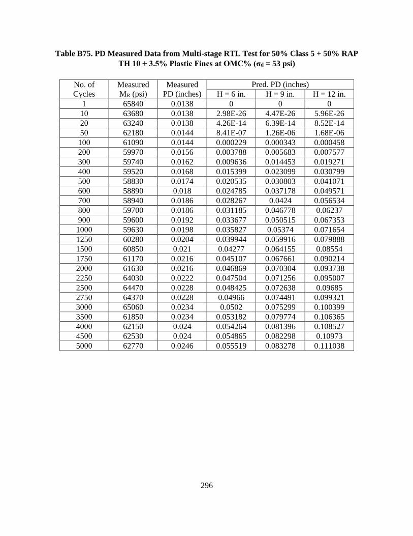
296
Table B75. PD Measured Data from Multi-stage RTL Test for 50% Class 5 + 50% RAP
TH 10 + 3.5% Plastic Fines at OMC% (σd = 53 psi)
No. of
Cycles
Measured
MR (psi)
Measured
PD (inches)
Pred. PD (inches)
H = 6 in. H = 9 in. H = 12 in.
1 65840 0.0138 0 0 0
10 63680 0.0138 2.98E-26 4.47E-26 5.96E-26
20 63240 0.0138 4.26E-14 6.39E-14 8.52E-14
50 62180 0.0144 8.41E-07 1.26E-06 1.68E-06
100 61090 0.0144 0.000229 0.000343 0.000458
200 59970 0.0156 0.003788 0.005683 0.007577
300 59740 0.0162 0.009636 0.014453 0.019271
400 59520 0.0168 0.015399 0.023099 0.030799
500 58830 0.0174 0.020535 0.030803 0.041071
600 58890 0.018 0.024785 0.037178 0.049571
700 58940 0.0186 0.028267 0.0424 0.056534
800 59700 0.0186 0.031185 0.046778 0.06237
900 59600 0.0192 0.033677 0.050515 0.067353
1000 59630 0.0198 0.035827 0.05374 0.071654
1250 60280 0.0204 0.039944 0.059916 0.079888
1500 60850 0.021 0.04277 0.064155 0.08554
1750 61170 0.0216 0.045107 0.067661 0.090214
2000 61630 0.0216 0.046869 0.070304 0.093738
2250 64030 0.0222 0.047504 0.071256 0.095007
2500 64470 0.0228 0.048425 0.072638 0.09685
2750 64370 0.0228 0.04966 0.074491 0.099321
3000 65060 0.0234 0.0502 0.075299 0.100399
3500 61850 0.0234 0.053182 0.079774 0.106365
4000 62150 0.024 0.054264 0.081396 0.108527
4500 62530 0.024 0.054865 0.082298 0.10973
5000 62770 0.0246 0.055519 0.083278 0.111038
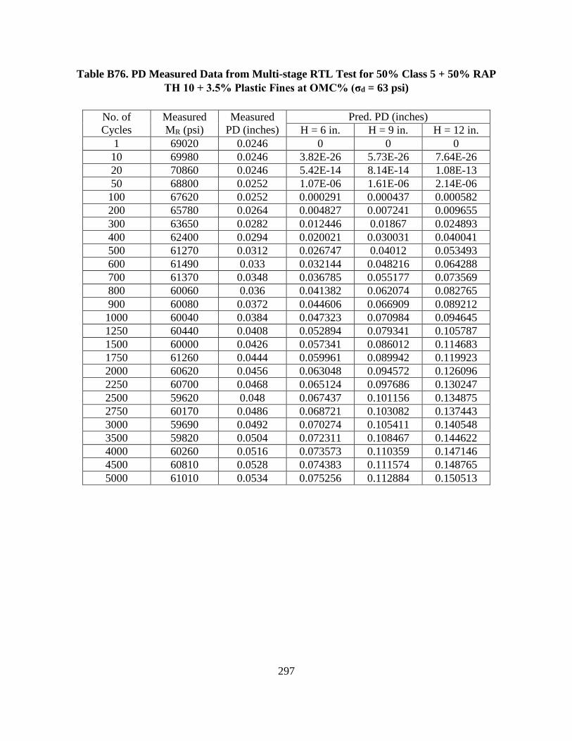
297
Table B76. PD Measured Data from Multi-stage RTL Test for 50% Class 5 + 50% RAP
TH 10 + 3.5% Plastic Fines at OMC% (σd = 63 psi)
No. of
Cycles
Measured
MR (psi)
Measured
PD (inches)
Pred. PD (inches)
H = 6 in. H = 9 in. H = 12 in.
1 69020 0.0246 0 0 0
10 69980 0.0246 3.82E-26 5.73E-26 7.64E-26
20 70860 0.0246 5.42E-14 8.14E-14 1.08E-13
50 68800 0.0252 1.07E-06 1.61E-06 2.14E-06
100 67620 0.0252 0.000291 0.000437 0.000582
200 65780 0.0264 0.004827 0.007241 0.009655
300 63650 0.0282 0.012446 0.01867 0.024893
400 62400 0.0294 0.020021 0.030031 0.040041
500 61270 0.0312 0.026747 0.04012 0.053493
600 61490 0.033 0.032144 0.048216 0.064288
700 61370 0.0348 0.036785 0.055177 0.073569
800 60060 0.036 0.041382 0.062074 0.082765
900 60080 0.0372 0.044606 0.066909 0.089212
1000 60040 0.0384 0.047323 0.070984 0.094645
1250 60440 0.0408 0.052894 0.079341 0.105787
1500 60000 0.0426 0.057341 0.086012 0.114683
1750 61260 0.0444 0.059961 0.089942 0.119923
2000 60620 0.0456 0.063048 0.094572 0.126096
2250 60700 0.0468 0.065124 0.097686 0.130247
2500 59620 0.048 0.067437 0.101156 0.134875
2750 60170 0.0486 0.068721 0.103082 0.137443
3000 59690 0.0492 0.070274 0.105411 0.140548
3500 59820 0.0504 0.072311 0.108467 0.144622
4000 60260 0.0516 0.073573 0.110359 0.147146
4500 60810 0.0528 0.074383 0.111574 0.148765
5000 61010 0.0534 0.075256 0.112884 0.150513

298
Table B77. PD Measured Data from Multi-stage RTL Test for 50% Class 5 + 50% RAP
TH 10 + 3.5% Plastic Fines at OMC% (σd = 73 psi)
No. of
Cycles
Measured
MR (psi)
Measured
PD (inches)
Pred. PD (inches)
H = 6 in. H = 9 in. H = 12 in.
1 65810 0.0534 0 0 0
10 65100 0.0534 4.85E-26 7.27E-26 9.7E-26
20 64590 0.0534 6.92E-14 1.04E-13 1.38E-13
50 63570 0.054 1.36E-06 2.04E-06 2.72E-06
100 62470 0.054 0.00037 0.000555 0.00074
200 60220 0.0552 0.00617 0.009254 0.012339
300 58870 0.057 0.015803 0.023704 0.031605
400 57570 0.0588 0.02542 0.03813 0.05084
500 56530 0.0618 0.033916 0.050875 0.067833
600 54660 0.0654 0.041544 0.062316 0.083088
700 53160 0.0702 0.048068 0.072101 0.096135
800 52190 0.0762 0.05386 0.08079 0.107721
900 48890 0.0828 0.060101 0.090152 0.120202
1000 50180 0.09 0.062858 0.094287 0.125716
1250 46630 0.1104 0.073493 0.110239 0.146986
1500 47660 0.1362 0.076951 0.115426 0.153902
1750 46400 0.1794 0.080093 0.12014 0.160187

299
Table B78. PD Measured Data from Multi-stage RTL Test for 50% Class 5 + 50% RAP
TH 10 + 3.5% Plastic Fines at OMC+2% (σd = 6 psi)
No. of
Cycles
Measured
MR (psi)
Measured
PD (inches)
Pred. PD (inches)
H = 6 in. H = 9 in. H = 12 in.
1 22940 0 0 0 0
10 21840 0.003 2.44E-48 3.65E-48 4.87E-48
20 21580 0.0042 1.13E-25 1.69E-25 2.25E-25
50 21840 0.0054 4.38E-12 6.58E-12 8.77E-12
100 22030 0.0066 1.54E-07 2.3E-07 3.07E-07
200 23490 0.0078 2.8E-05 4.2E-05 5.6E-05
300 23530 0.0084 0.000159 0.000239 0.000318
400 23270 0.009 0.000391 0.000586 0.000781
500 23940 0.009 0.000653 0.00098 0.001307
600 24150 0.0096 0.000936 0.001404 0.001872
700 24110 0.0096 0.001201 0.001802 0.002403
800 24180 0.0096 0.001458 0.002187 0.002915
900 24300 0.0096 0.001686 0.002529 0.003372
1000 23960 0.0096 0.00191 0.002866 0.003821
1250 24650 0.0102 0.002364 0.003547 0.004729
1500 25120 0.0102 0.002637 0.003956 0.005274
1750 26180 0.0108 0.002815 0.004222 0.00563
2000 25700 0.0108 0.003144 0.004717 0.006289
2250 26140 0.0108 0.003286 0.004929 0.006571
2500 25640 0.0108 0.00348 0.00522 0.00696
2750 26130 0.0114 0.003542 0.005313 0.007085
3000 26690 0.0114 0.003618 0.005427 0.007237
3500 26860 0.0114 0.003783 0.005674 0.007565
4000 27660 0.0114 0.003869 0.005804 0.007739
4500 28220 0.012 0.00391 0.005865 0.00782
5000 28440 0.012 0.004023 0.006034 0.008046
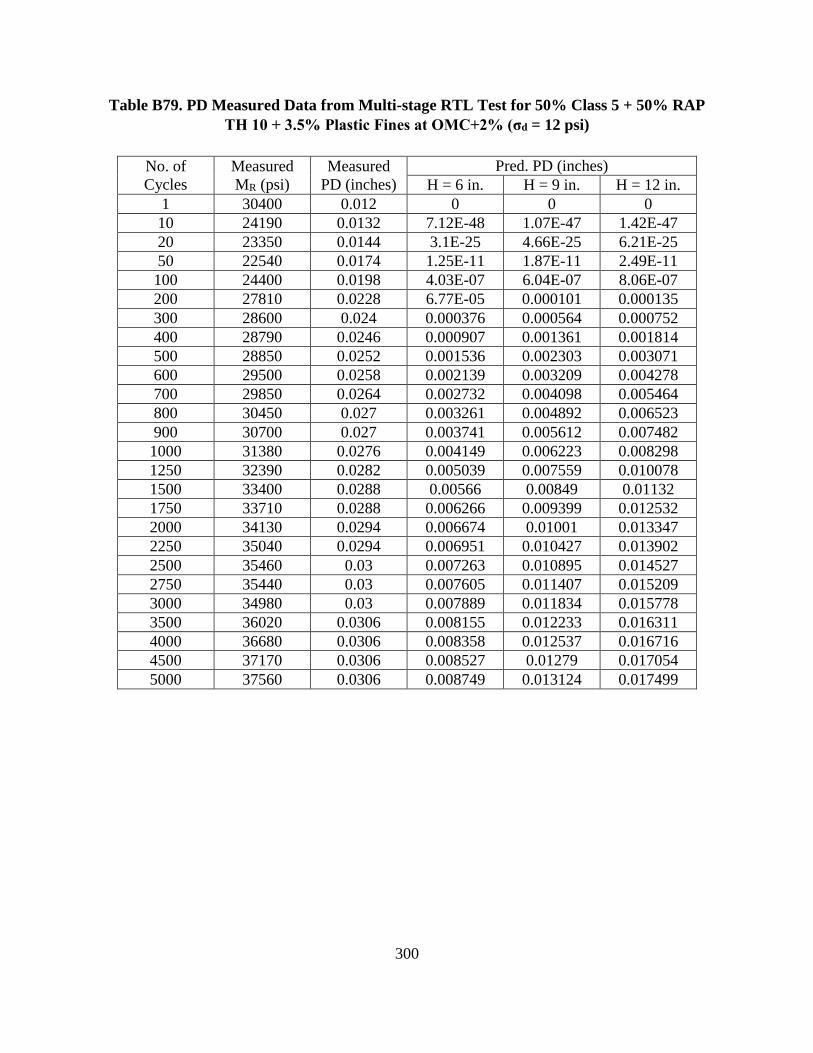
300
Table B79. PD Measured Data from Multi-stage RTL Test for 50% Class 5 + 50% RAP
TH 10 + 3.5% Plastic Fines at OMC+2% (σd = 12 psi)
No. of
Cycles
Measured
MR (psi)
Measured
PD (inches)
Pred. PD (inches)
H = 6 in. H = 9 in. H = 12 in.
1 30400 0.012 0 0 0
10 24190 0.0132 7.12E-48 1.07E-47 1.42E-47
20 23350 0.0144 3.1E-25 4.66E-25 6.21E-25
50 22540 0.0174 1.25E-11 1.87E-11 2.49E-11
100 24400 0.0198 4.03E-07 6.04E-07 8.06E-07
200 27810 0.0228 6.77E-05 0.000101 0.000135
300 28600 0.024 0.000376 0.000564 0.000752
400 28790 0.0246 0.000907 0.001361 0.001814
500 28850 0.0252 0.001536 0.002303 0.003071
600 29500 0.0258 0.002139 0.003209 0.004278
700 29850 0.0264 0.002732 0.004098 0.005464
800 30450 0.027 0.003261 0.004892 0.006523
900 30700 0.027 0.003741 0.005612 0.007482
1000 31380 0.0276 0.004149 0.006223 0.008298
1250 32390 0.0282 0.005039 0.007559 0.010078
1500 33400 0.0288 0.00566 0.00849 0.01132
1750 33710 0.0288 0.006266 0.009399 0.012532
2000 34130 0.0294 0.006674 0.01001 0.013347
2250 35040 0.0294 0.006951 0.010427 0.013902
2500 35460 0.03 0.007263 0.010895 0.014527
2750 35440 0.03 0.007605 0.011407 0.015209
3000 34980 0.03 0.007889 0.011834 0.015778
3500 36020 0.0306 0.008155 0.012233 0.016311
4000 36680 0.0306 0.008358 0.012537 0.016716
4500 37170 0.0306 0.008527 0.01279 0.017054
5000 37560 0.0306 0.008749 0.013124 0.017499
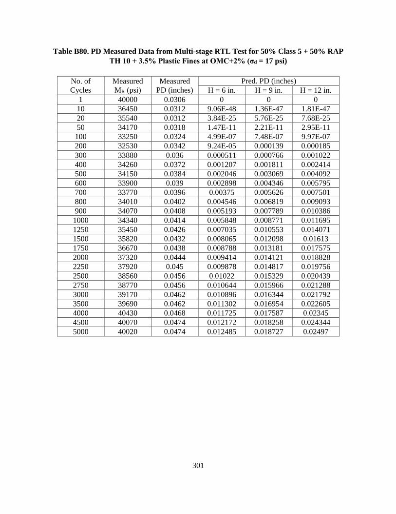
301
Table B80. PD Measured Data from Multi-stage RTL Test for 50% Class 5 + 50% RAP
TH 10 + 3.5% Plastic Fines at OMC+2% (σd = 17 psi)
No. of
Cycles
Measured
MR (psi)
Measured
PD (inches)
Pred. PD (inches)
H = 6 in. H = 9 in. H = 12 in.
1 40000 0.0306 0 0 0
10 36450 0.0312 9.06E-48 1.36E-47 1.81E-47
20 35540 0.0312 3.84E-25 5.76E-25 7.68E-25
50 34170 0.0318 1.47E-11 2.21E-11 2.95E-11
100 33250 0.0324 4.99E-07 7.48E-07 9.97E-07
200 32530 0.0342 9.24E-05 0.000139 0.000185
300 33880 0.036 0.000511 0.000766 0.001022
400 34260 0.0372 0.001207 0.001811 0.002414
500 34150 0.0384 0.002046 0.003069 0.004092
600 33900 0.039 0.002898 0.004346 0.005795
700 33770 0.0396 0.00375 0.005626 0.007501
800 34010 0.0402 0.004546 0.006819 0.009093
900 34070 0.0408 0.005193 0.007789 0.010386
1000 34340 0.0414 0.005848 0.008771 0.011695
1250 35450 0.0426 0.007035 0.010553 0.014071
1500 35820 0.0432 0.008065 0.012098 0.01613
1750 36670 0.0438 0.008788 0.013181 0.017575
2000 37320 0.0444 0.009414 0.014121 0.018828
2250 37920 0.045 0.009878 0.014817 0.019756
2500 38560 0.0456 0.01022 0.015329 0.020439
2750 38770 0.0456 0.010644 0.015966 0.021288
3000 39170 0.0462 0.010896 0.016344 0.021792
3500 39690 0.0462 0.011302 0.016954 0.022605
4000 40430 0.0468 0.011725 0.017587 0.02345
4500 40070 0.0474 0.012172 0.018258 0.024344
5000 40020 0.0474 0.012485 0.018727 0.02497

302
Table B81. PD Measured Data from Multi-stage RTL Test for 50% Class 5 + 50% RAP
TH 10 + 3.5% Plastic Fines at OMC+2% (σd = 24 psi)
Table B82. PD Measured Data from Multi-stage RTL Test for 50% Class 5 + 50% RAP
TH 10 + 3.5% Plastic Fines at OMC+2% (σd = 37 psi)
No. of Cycles Measured MR
(psi)
Measured PD
(inches)
Pred. PD (inches)
H = 6 in. H = 9 in. H = 12 in.
1 46570 0.0474 0 0 0
10 41890 0.048 1.25E-47 1.87E-47 2.49E-47
20 39720 0.048 5.37E-25 8.05E-25 1.07E-24
50 35490 0.0498 2.15E-11 3.22E-11 4.29E-11
100 32370 0.0534 7.62E-07 1.14E-06 1.52E-06
200 30870 0.06 0.000145 0.000217 0.000289
300 30360 0.0654 0.000833 0.00125 0.001667
400 29490 0.0702 0.00205 0.003075 0.004099
500 30980 0.0744 0.003332 0.004999 0.006665
600 29800 0.078 0.004861 0.007291 0.009721
700 30260 0.081 0.006182 0.009273 0.012364
800 30150 0.084 0.007528 0.011292 0.015057
900 30860 0.087 0.008551 0.012826 0.017101
1000 30640 0.09 0.009708 0.014562 0.019416
1250 31020 0.0966 0.011824 0.017736 0.023647
1500 31080 0.1032 0.013606 0.020409 0.027212
1750 29710 0.1086 0.015578 0.023367 0.031156
2000 29330 0.1146 0.016971 0.025457 0.033943
2250 28700 0.12 0.018288 0.027433 0.036577
2500 29270 0.1254 0.018856 0.028284 0.037713
2750 29460 0.1308 0.019474 0.029211 0.038948
3000 29340 0.1362 0.020225 0.030337 0.040449
3500 28060 0.1464 0.022071 0.033107 0.044142
4000 27950 0.1578 0.022889 0.034334 0.045778
4500 27170 0.1692 0.024011 0.036017 0.048022
5000 25870 0.1824 0.025424 0.038136 0.050848
No. of Cycles Measured MR
(psi)
Measured PD
(inches)
Pred. PD (inches)
H = 6 in. H = 9 in. H = 12 in.
1 29470 0.2286 0 0 0
10 24760 0.2352 2.69E-47 4.04E-47 5.38E-47
20 27390 0.2424 9.49E-25 1.42E-24 1.9E-24
50 23040 0.2568 4.54E-11 6.81E-11 9.08E-11
100 22290 0.2796 1.59E-06 2.39E-06 3.18E-06
200 21230 0.3138 0.000305 0.000457 0.000609
300 19940 0.354 0.001821 0.002732 0.003643

303
APPENDIX C. CORRELATION DATA OF MR AND PD
Table C1. PD Data Collected from MR test at Different Confining Pressure Levels
W.C
Condition
Conf.
Pressure
(psi)
% RAP Extracted
RAP 0 50 75 100
OMC-2%
3 0.2 0.12 0.13 0.23
NA
6 0.23 0.13 0.15 0.24
10 0.25 0.12 0.14 0.26
15 0.28 0.14 0.18 0.28
20 0.35 0.19 0.23 0.34
OMC%
3 1.28 1.69 1.04 0.42 0.52
6 1.3 1.64 1.07 0.5 0.5
10 1.4 1.58 1.14 0.53 0.55
15 1.2 1.67 0.77 0.55 0.62
20 1.83 1.75 1.96 0.71 0.52
OMC+2%
3 3.74 2.71 4.07 3.49
NA
6 3.64 2.9 4.06 2.89
10 3.82 3.07 4.13 3.52
15 4.22 3.48 4.32 3.67
20 3.61 2.77 4.07 3.46
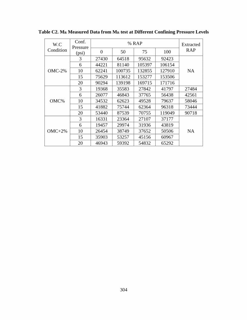
304
Table C2. MR Measured Data from MR test at Different Confining Pressure Levels
W.C
Condition
Conf.
Pressure
(psi)
% RAP Extracted
RAP 0 50 75 100
OMC-2%
3 27430 64518 95632 92423
NA
6 44221 81140 105397 106154
10 62241 100735 132855 127910
15 75629 113612 153277 153506
20 90294 139198 169715 171716
OMC%
3 19368 35583 27842 41797 27484
6 26077 46843 37765 56438 42561
10 34532 62623 49528 79637 58046
15 41882 75744 62364 96318 73444
20 53440 87539 70755 119049 90718
OMC+2%
3 16331 23364 27107 37177
NA
6 19457 29974 31936 43819
10 26454 38749 37652 50506
15 35903 53257 45156 60967
20 46943 59392 54832 65292
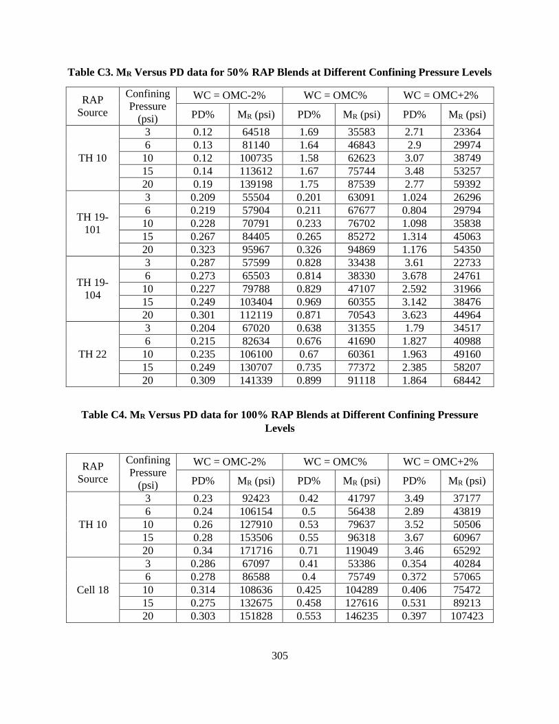
305
Table C3. MR Versus PD data for 50% RAP Blends at Different Confining Pressure Levels
Table C4. MR Versus PD data for 100% RAP Blends at Different Confining Pressure
Levels
RAP
Source
Confining
Pressure
(psi)
WC = OMC-2% WC = OMC% WC = OMC+2%
PD% MR (psi) PD% MR (psi) PD% MR (psi)
TH 10
3 0.12 64518 1.69 35583 2.71 23364
6 0.13 81140 1.64 46843 2.9 29974
10 0.12 100735 1.58 62623 3.07 38749
15 0.14 113612 1.67 75744 3.48 53257
20 0.19 139198 1.75 87539 2.77 59392
TH 19-
101
3 0.209 55504 0.201 63091 1.024 26296
6 0.219 57904 0.211 67677 0.804 29794
10 0.228 70791 0.233 76702 1.098 35838
15 0.267 84405 0.265 85272 1.314 45063
20 0.323 95967 0.326 94869 1.176 54350
TH 19-
104
3 0.287 57599 0.828 33438 3.61 22733
6 0.273 65503 0.814 38330 3.678 24761
10 0.227 79788 0.829 47107 2.592 31966
15 0.249 103404 0.969 60355 3.142 38476
20 0.301 112119 0.871 70543 3.623 44964
TH 22
3 0.204 67020 0.638 31355 1.79 34517
6 0.215 82634 0.676 41690 1.827 40988
10 0.235 106100 0.67 60361 1.963 49160
15 0.249 130707 0.735 77372 2.385 58207
20 0.309 141339 0.899 91118 1.864 68442
RAP
Source
Confining
Pressure
(psi)
WC = OMC-2% WC = OMC% WC = OMC+2%
PD% MR (psi) PD% MR (psi) PD% MR (psi)
TH 10
3 0.23 92423 0.42 41797 3.49 37177
6 0.24 106154 0.5 56438 2.89 43819
10 0.26 127910 0.53 79637 3.52 50506
15 0.28 153506 0.55 96318 3.67 60967
20 0.34 171716 0.71 119049 3.46 65292
Cell 18
3 0.286 67097 0.41 53386 0.354 40284
6 0.278 86588 0.4 75749 0.372 57065
10 0.314 108636 0.425 104289 0.406 75472
15 0.275 132675 0.458 127616 0.531 89213
20 0.303 151828 0.553 146235 0.397 107423

306
APPENDIX D. POISSON’S RATIO MEASURED DATA
Figure D1. Stress- Strain Biaxial Relationship for New Class 5
0
5
10
15
20
0 0.5 1 1.5 2 2.5 3
Str
ess (
psi)
Strain%
a) WC = OMC-2%
Axial
Lateral
0
5
10
15
20
0 0.5 1 1.5 2 2.5 3
Str
ess (
psi)
Strain%
b) WC = OMC%
Axial
Lateral
0
5
10
15
20
0 0.5 1 1.5 2 2.5 3
Str
ess (
psi)
Strain%
c) WC = OMC+2%
Axial
Lateral
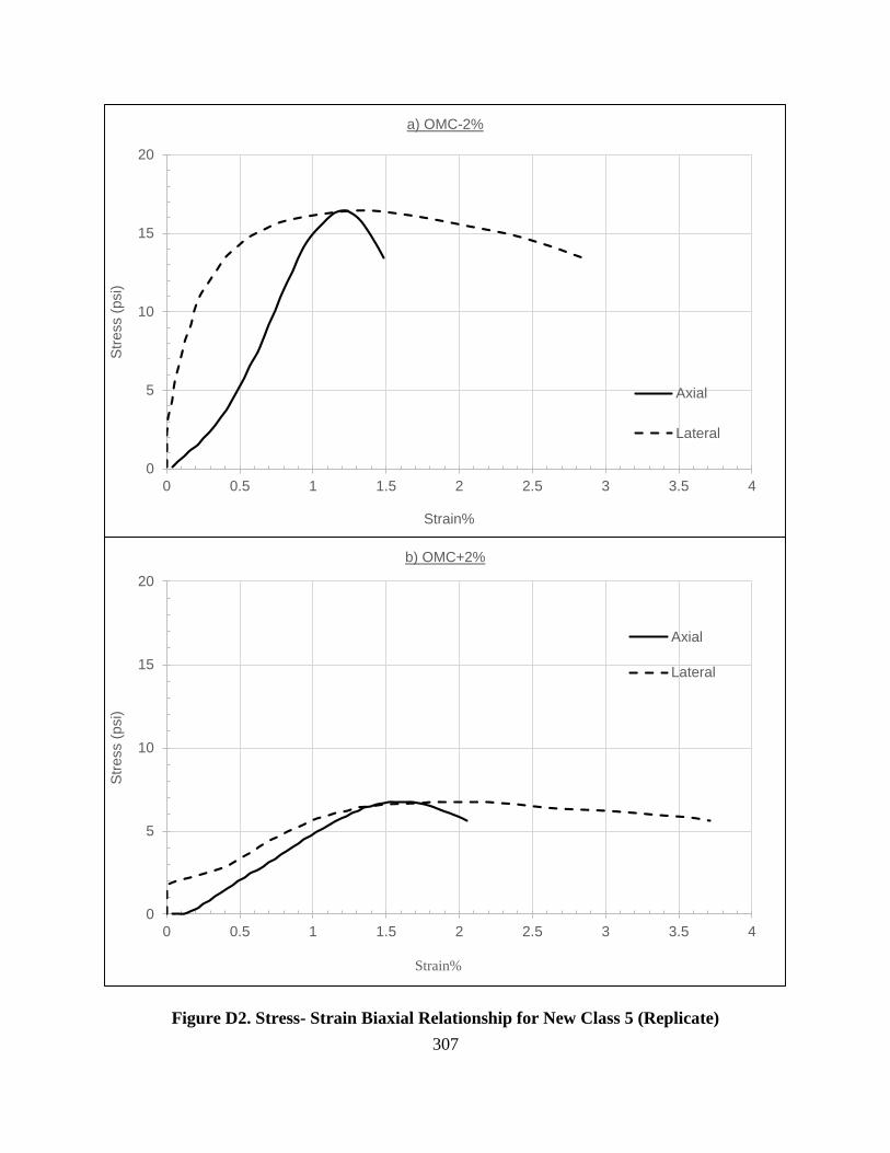
307
Figure D2. Stress- Strain Biaxial Relationship for New Class 5 (Replicate)
0
5
10
15
20
0 0.5 1 1.5 2 2.5 3 3.5 4
Str
ess (
psi)
Strain%
a) OMC-2%
Axial
Lateral
0
5
10
15
20
0 0.5 1 1.5 2 2.5 3 3.5 4
Str
ess (
psi)
Strain%
b) OMC+2%
Axial
Lateral
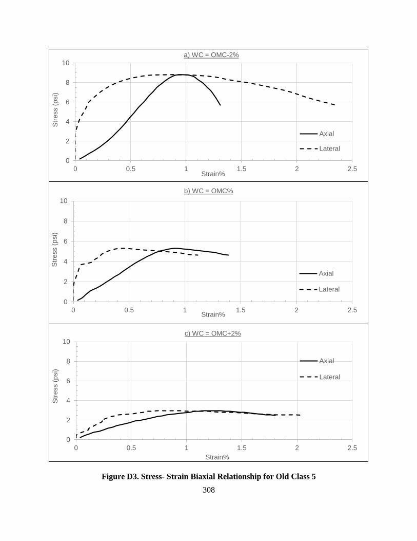
308
Figure D3. Stress- Strain Biaxial Relationship for Old Class 5
0
2
4
6
8
10
0 0.5 1 1.5 2 2.5
Str
ess (
psi)
Strain%
a) WC = OMC-2%
Axial
Lateral
0
2
4
6
8
10
0 0.5 1 1.5 2 2.5
Str
ess (
psi)
Strain%
b) WC = OMC%
Axial
Lateral
0
2
4
6
8
10
0 0.5 1 1.5 2 2.5
Str
ess (
psi)
Strain%
c) WC = OMC+2%
Axial
Lateral

309
Figure D4. Stress- Strain Biaxial Relationship for 50% New Class 5 + 50% RAP TH 29
0
1
2
3
4
5
6
0 0.5 1 1.5 2 2.5 3
Str
ess (
psi)
Strain%
a) WC = OMC-2%
Axial
Lateral
0
1
2
3
4
5
6
0 0.5 1 1.5 2 2.5 3
Str
ess (
psi)
Strain%
b) WC = OMC%
Axial
Lateral
0
1
2
3
4
5
6
0 0.5 1 1.5 2 2.5 3
Str
ess (
psi)
Strain%
c) WC = OMC+2%
Axial
Lateral

310
Figure D5. Stress- Strain Biaxial Relationship for 50% New Class 5 + 50% RAP TH 29
(Replicate)
0
1
2
3
4
5
0 0.5 1 1.5 2 2.5 3 3.5 4
Str
ess (
psi)
Strain%
a) WC = OMC-2%
Axial
Lateral
0
1
2
3
4
5
0 0.5 1 1.5 2 2.5 3 3.5 4
Str
ess (
psi)
Strain%
b) WC = OMC%
Axial
Lateral

311
Figure D6. Stress- Strain Biaxial Relationship for 50% Old Class 5 + 50% RAP TH 10
0
3
6
9
12
15
0 1 2 3 4
Str
ess (
psi)
Strain%
a) WC = OMC-2%
Axial
Lateral
0
2
4
6
8
10
0 1 2 3 4
Str
ess (
psi)
Strain%
b) WC = OMC%
Axial
Lateral
0
1
2
3
4
5
0 1 2 3 4
Str
ess (
psi)
Strain%
c) WC = OMC+2%
Axial
Lateral

312
Figure D7. Stress- Strain Biaxial Relationship for 100% RAP TH 29
0
1
2
3
0 1 2 3 4 5
Str
ess (
psi)
Strain%
a) WC = OMC-2%
Axial
Lateral
0
1
2
3
0 1 2 3 4 5
Str
ess (
psi)
Strain%
b) WC = OMC%
Axial
Lateral
0
1
2
3
0 1 2 3 4 5
Str
ess (
psi)
Strain%
c) WC = OMC+2%
Axial
Lateral
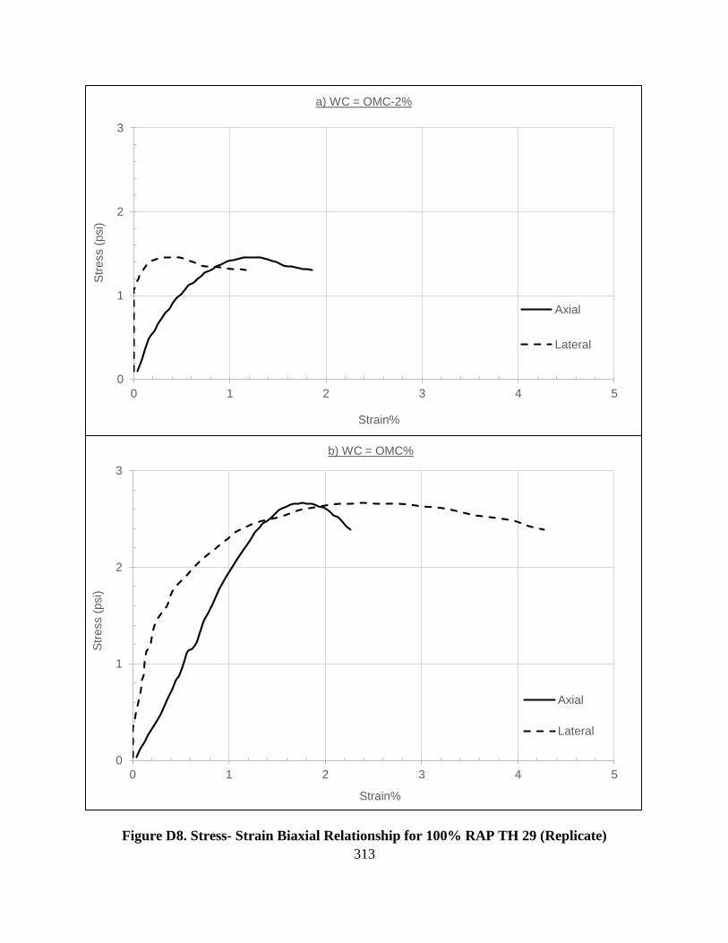
313
Figure D8. Stress- Strain Biaxial Relationship for 100% RAP TH 29 (Replicate)
0
1
2
3
0 1 2 3 4 5
Str
ess (
psi)
Strain%
a) WC = OMC-2%
Axial
Lateral
0
1
2
3
0 1 2 3 4 5
Str
ess (
psi)
Strain%
b) WC = OMC%
Axial
Lateral

314
Figure D9. Stress- Strain Biaxial Relationship for 100% RAP TH 10
0
3
6
9
12
15
0 1 2 3 4
Str
ess (
psi)
Strain%
a) WC = OMC-2%
Axial
Lateral
0
3
6
9
12
15
0 1 2 3 4
Str
ess (
psi)
Strain%
b) WC =OMC+2%
Axial
Lateral
0
3
6
9
12
15
0 1 2 3 4
Str
ess (
psi)
Strain%
c) WC = OMC%
Axial
Lateral
0
3
6
9
12
15
0 1 2 3 4
Str
ess (
psi)
Strain%
d) WC = OMC% Extracted
Axial
Lateral
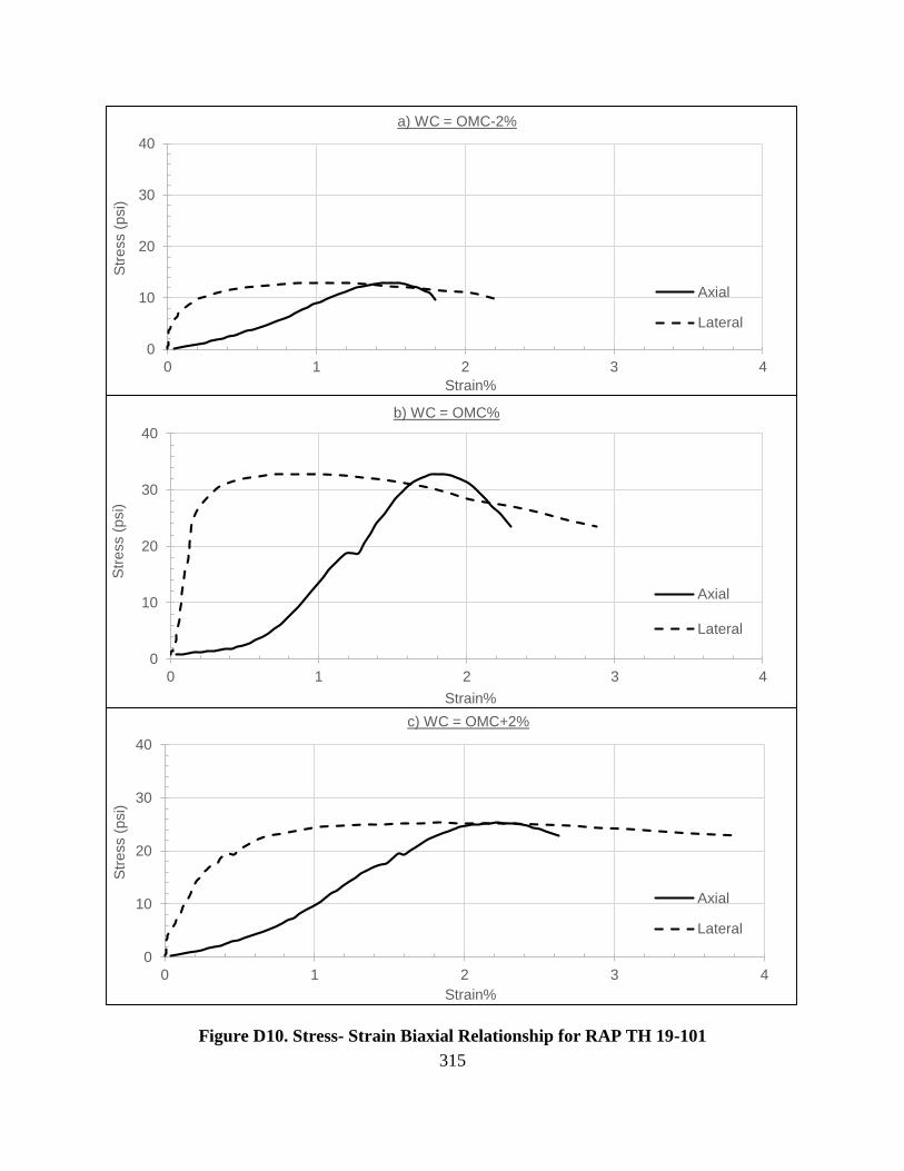
315
Figure D10. Stress- Strain Biaxial Relationship for RAP TH 19-101
0
10
20
30
40
0 1 2 3 4
Str
ess (
psi)
Strain%
a) WC = OMC-2%
Axial
Lateral
0
10
20
30
40
0 1 2 3 4
Str
ess (
psi)
Strain%
b) WC = OMC%
Axial
Lateral
0
10
20
30
40
0 1 2 3 4
Str
ess (
psi)
Strain%
c) WC = OMC+2%
Axial
Lateral

316
Figure D11. Stress- Strain Biaxial Relationship for RAP TH 19-104
0
10
20
30
0 1 2 3 4 5
Str
ess (
psi)
Strain%
a) WC = OMC-2%
Axial
Lateral
0
10
20
30
0 1 2 3 4 5
Str
ess (
psi)
Strain%
b) WC = OMC%
Axial
Lateral
0
10
20
30
0 1 2 3 4 5
Str
ess (
psi)
Strain%
c) WC = OMC+2%
Axial
Lateral

317
Figure D12. Stress- Strain Biaxial Relationship for RAP TH 22
0
4
8
12
16
0 1 2 3 4
Str
ess (
psi)
Strain%
a) WC = OMC-2%
Axial
Lateral
0
4
8
12
16
0 1 2 3 4
Str
ess (
psi)
Strain%
b) WC = OMC%
Axial
Lateral
0
4
8
12
16
0 1 2 3 4
Str
ess (
psi)
Strain%
c) WC = OMC+2%
Axial
Lateral
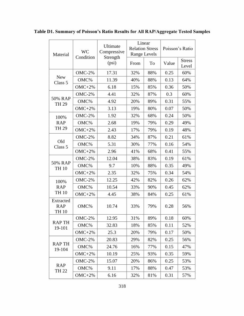
318
Table D1. Summary of Poisson’s Ratio Results for All RAP/Aggregate Tested Samples
Material
WC
Condition
Ultimate
Compressive
Strength
(psi)
Linear
Relation Stress
Range Levels
Poisson’s Ratio
From To Value Stress
Level
New
Class 5
OMC-2% 17.31 32% 88% 0.25 60%
OMC% 11.39 40% 88% 0.13 64%
OMC+2% 6.18 15% 85% 0.36 50%
50% RAP
TH 29
OMC-2% 4.41 32% 87% 0.3 60%
OMC% 4.92 20% 89% 0.31 55%
OMC+2% 3.13 19% 80% 0.07 50%
100%
RAP
TH 29
OMC-2% 1.92 32% 68% 0.24 50%
OMC% 2.68 19% 79% 0.29 49%
OMC+2% 2.43 17% 79% 0.19 48%
Old
Class 5
OMC-2% 8.82 34% 87% 0.21 61%
OMC% 5.31 30% 77% 0.16 54%
OMC+2% 2.96 41% 68% 0.41 55%
50% RAP
TH 10
OMC-2% 12.04 38% 83% 0.19 61%
OMC% 9.7 10% 88% 0.35 49%
OMC+2% 2.35 32% 75% 0.34 54%
100%
RAP
TH 10
OMC-2% 12.25 42% 82% 0.26 62%
OMC% 10.54 33% 90% 0.45 62%
OMC+2% 4.45 38% 84% 0.25 61%
Extracted
RAP
TH 10
OMC% 10.74 33% 79% 0.28 56%
RAP TH
19-101
OMC-2% 12.95 31% 89% 0.18 60%
OMC% 32.83 18% 85% 0.11 52%
OMC+2% 25.3 20% 79% 0.17 50%
RAP TH
19-104
OMC-2% 20.83 29% 82% 0.25 56%
OMC% 24.76 16% 77% 0.15 47%
OMC+2% 10.19 25% 93% 0.35 59%
RAP
TH 22
OMC-2% 15.07 20% 86% 0.25 53%
OMC% 9.11 17% 88% 0.47 53%
OMC+2% 6.16 32% 81% 0.31 57%