Structural Analysis in Multi-Relational Social Networks

Bing Tian Dai ∗ Freddy Chong Tat Chua ∗ Ee-Peng Lim ∗

Abstract

Modern social networks often consist of multiple rela-tions among individuals. Understanding the structureof such multi-relational network is essential. In soci-ology, one way of structural analysis is to identify dif-ferent positions and roles using blockmodels. In thispaper, we generalize stochastic blockmodels to General-ized Stochastic Blockmodels (GSBM) for performing po-sitional and role analysis on multi-relational networks.Our GSBM generalizes many different kinds of Multi-variate Probability Distribution Function (MVPDF) tomodel different kinds of multi-relational networks. Inparticular, we propose to use multivariate Poisson dis-tribution for multi-relational social networks. Our ex-periments show that GSBM is able to identify the struc-tures for both synthetic and real world network data.These structures can further be used for predicting re-lationships between individuals.

1 Introduction

There are often different kinds of interactions co-existing with one another in social networks. For ex-ample in Facebook1, one can write on others’ wall,poke her friends, or tag her friends in her own pho-tos. When single relational network model is used torepresent such a social network, the different interac-tion types are treated the same making them indistin-guishable. As information is lost in the network rep-resentation, we may not be able to model the networkaccurately.

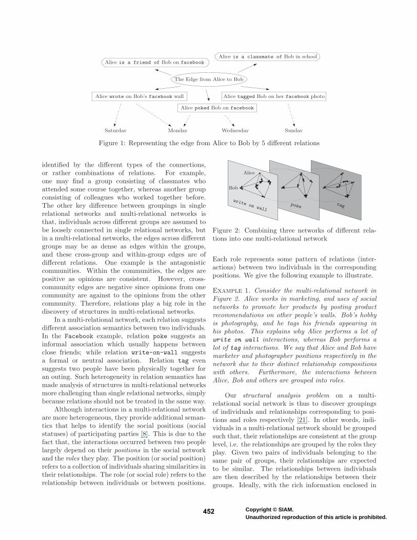
A multi-relational network, on the other hand, al-lows multiple relations to exist in the network and evenexist between two individuals. A relation represents asocial connection or a set of interactions of the samekind between two individuals. For example, Figure 1indicates 5 different relations from Alice to Bob onFacebook. The top two are social connections, i.e., Aliceis a classmate of Bob, and also a friend of Bob. Thereare also 5 interactions between Alice and Bob, as shownin the lower part of Figure 1. For instance, Alice pokedBob on Monday and Wednesday, which contributes two

∗Living Analytics Research Centre (LARC), School of Infor-mation Systems, Singapore Management University

1http://www.facebook.com

interactions of the same kind. Thus the 5 interactionsdescribe three different relations, i.e, write-on-wall,poke and tag. In other words, each interaction is un-derstood as a relation instance and multiple interactionsof the same kind between a pair of individuals representinstances of the same relation.

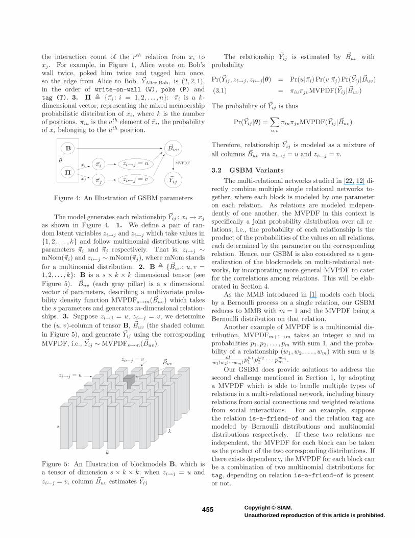
Each relation defines a single relational network.As shown in Figure 2, the multi-relational network inFacebook consists of multiple single relational networks,shown in different planes. The single relational networkscorrespond to relations write-on-wall, poke and tagrespectively. Since Alice wrote on Bob’s wall, there isa directed interaction edge from Alice to Bob in thewrite-on-wall network.

We can then define a multi-relational network asa merger of multiple single relational networks. Fig-ure 2 represents a multi-relational network constructedby combining the three single relational networks to-gether. Dotted lines in Figure 2 indicate vertices rep-resenting the same individuals, which are merged intoone vertex in the multi-relational network. An edge be-tween two nodes in a multi-relational network is alsocalled a relationship, which consists of all relations andinteractions between the two individuals.

Various structural analyses have been studiedon single relational network. For example, givena single relational network constructed by relationis-a-friend-of, plenty of clustering methods groupthe individuals based on how densely they are con-nected, i.e., individuals within the same group are morelikely to be friends, while individuals across differentgroups are less likely. The grouping of the individu-als provides a structural summary for the entire net-work and also determines the communities formed. Thecommunity affiliations of the individuals help in learningtheir behavior patterns, e.g. one would like to buy itemswhich many others in her community have bought. Dis-covery of structural information is thus essential to bet-ter understanding of all kinds of social networks, includ-ing multi-relational networks.

However, multi-relational networks are much moredifficult to analyze than single relational networks.In a single relational network, grouping of nodes areidentified by the density of the connections among them.In a multi-relational networks, such groupings can be

236 Copyright © SIAM.Unauthorized reproduction of this article is prohibited.

451 Copyright © SIAM.Unauthorized reproduction of this article is prohibited.

The Edge from Alice to Bob

Alice is a friend of Bob on facebookAlice is a classmate of Bob in school

Alice wrote on Bob’s facebook wall

Alice poked Bob on facebook

Alice tagged Bob on her facebook photo

SundayMondaySaturday Wednesday

Figure 1: Representing the edge from Alice to Bob by 5 different relations

identified by the different types of the connections,or rather combinations of relations. For example,one may find a group consisting of classmates whoattended some course together, whereas another groupconsisting of colleagues who worked together before.The other key difference between groupings in singlerelational networks and multi-relational networks isthat, individuals across different groups are assumed tobe loosely connected in single relational networks, butin a multi-relational networks, the edges across differentgroups may be as dense as edges within the groups,and these cross-group and within-group edges are ofdifferent relations. One example is the antagonisticcommunities. Within the communities, the edges arepositive as opinions are consistent. However, cross-community edges are negative since opinions from onecommunity are against to the opinions from the othercommunity. Therefore, relations play a big role in thediscovery of structures in multi-relational networks.

In a multi-relational network, each relation suggestsdifferent association semantics between two individuals.In the Facebook example, relation poke suggests aninformal association which usually happens betweenclose friends; while relation write-on-wall suggestsa formal or neutral association. Relation tag evensuggests two people have been physically together foran outing. Such heterogeneity in relation semantics hasmade analysis of structures in multi-relational networksmore challenging than single relational networks, simplybecause relations should not be treated in the same way.

Although interactions in a multi-relational networkare more heterogeneous, they provide additional seman-tics that helps to identify the social positions (socialstatuses) of participating parties [8]. This is due to thefact that, the interactions occurred between two peoplelargely depend on their positions in the social networkand the roles they play. The position (or social position)refers to a collection of individuals sharing similarities intheir relationships. The role (or social role) refers to therelationship between individuals or between positions.

pokewrite on wall

tag

Alice

Bob

Figure 2: Combining three networks of different rela-tions into one multi-relational network

Each role represents some pattern of relations (inter-actions) between two individuals in the correspondingpositions. We give the following example to illustrate.

Example 1. Consider the multi-relational network inFigure 2. Alice works in marketing, and uses of socialnetworks to promote her products by posting productrecommendations on other people’s walls. Bob’s hobbyis photography, and he tags his friends appearing inhis photos. This explains why Alice performs a lot ofwrite on wall interactions, whereas Bob performs alot of tag interactions. We say that Alice and Bob havemarketer and photographer positions respectively in thenetwork due to their distinct relationship compositionswith others. Furthermore, the interactions betweenAlice, Bob and others are grouped into roles.

Our structural analysis problem on a multi-relational social network is thus to discover groupingsof individuals and relationships corresponding to posi-tions and roles respectively [21]. In other words, indi-viduals in a multi-relational network should be groupedsuch that, their relationships are consistent at the grouplevel, i.e. the relationships are grouped by the roles theyplay. Given two pairs of individuals belonging to thesame pair of groups, their relationships are expectedto be similar. The relationships between individualsare then described by the relationships between theirgroups. Ideally, with the rich information enclosed in

237 Copyright © SIAM.Unauthorized reproduction of this article is prohibited.

452 Copyright © SIAM.Unauthorized reproduction of this article is prohibited.

a multi-relational network, structural analysis is ableto group individuals by their social positions, and therelationships are then determined by the social roles be-tween such social positions. As in the above example,the relationship from Alice to Bob is determined by therole from the position of marketer to the position of pho-tographer. Such positions can be explicit or implicit.For instance, in Example 1, one’s occupation is an ex-plicit position while one’s hobbies determine an implicitposition.

A

B

C

D

E

{A}

{B,C}

{D,E}

Figure 3: By clipping vertices B, C together, vertices D,E together, the left figure is reduced to its core structureon the right, which preserves all edges

One direct application of our structural analysis isto provide a structural view of the entire social network,which describes how these positions are related to oneanother. For example, in Figure 3, by merging Band C to {B,C}, and D and E to {D,E}, we have a3-node structural view over the 5-node graph ABCDE,where all directed and undirected edges among ABCDEare preserved by the edges between the groups of thevertices. We often call such a reduced graph a corestructure of the original graph. We can apply ourstructural analysis to identify the core structure whereeach node in the core structure represents a particularposition and each edge represents the role from oneposition to the other. Core structure provides a goodvisualization of the entire network, as well as a tool tointerpret relationships between individuals.

Other applications of structural analysis include theuse of core structures to predict relationships. Forexample, we can predict a negative link exists betweentwo individuals who join two different groups having anantagonistic relationship. It is also interesting to studykey changes in the graph that cause changes to the corestructure. With the core structure, we can generatesynthetic graphs that up-size or downsize the originalgraph easily for performance study, or anonymize datathrough structural similarity [11].

Although structural analysis is widely applicable,it is however challenging due to the following threereasons. First, individuals in social networks do notalways have a definite position. For instance, one can bea sales executive at work, a part-time student at school,

and a husband or even a father at home. Thus, it is notreasonable to restrict one to have a single position inthe core structure. Instead, an individual should havea mixture of the positions. This general challenge ofmixed membership on single relational networks hasbeen solved in [1], and we will extend the solutionfurther for multi-relational networks.

The second challenge is brought by the multi-relational aspect. Single relational networks are mostlymodeled as a binary graph where an edge either existsor not, or a weighted graph where an edge is associatedwith a value. For multi-relational networks, the chal-lenge is therefore to model multiple relations simultane-ously as a relationship between nodes may be character-ized by a combination of relations. For instance, relationis-a-friend-of is a binary relation, the relation tagon Facebook is a weighted relation where the numberof times one tags another is a signal on how strong therelation is between them. When these two relations co-exist in the multi-relational network, our model shouldbe able to model them together, not separately.

The third challenge is that, relations are oftencorrelated, especially in social networks. Modeling ofa multi-relational network by directly combining singlerelational networks without considering the correlationamong relations will likely compromise the accuracy ofmodeling network positions and roles. For example,relation dine-together and relation drink-togetherare very likely to be correlated between two friends wholike to hang out together. Therefore, our model ought tohandle the challenging task of modeling the correlationsamong relations.

The contributions of this paper are summarized asfollows.• We propose Generalized Stochastic Blockmodels

(GSBM) as a novel framework to perform struc-tural analysis on multi-relational networks. Theframework is designed to model multiple rela-tions corresponding to different types of net-works and to capture the correlations among rela-tions. The framework can also accommodate differ-ent multivariate probability distribution functions(MVPDF) for generating interactions of differentrelations between a pair of individuals based ontheir positions.

• Multivariate Poisson Distribution (MVPois) is in-troduced as a MVPDF in the GSBM framework soas to derive network structures from interactionsin social networks, since MVPois incorporates thecorrelations between relations. We estimate the pa-rameters of the GSBM with MVPois using Maxi-mum Likelihood Estimation (MLE) for learning themodel parameters.

238 Copyright © SIAM.Unauthorized reproduction of this article is prohibited.

453 Copyright © SIAM.Unauthorized reproduction of this article is prohibited.

• Finally, we demonstrate that our blockmodel candiscover the ground truth grouping in syntheticnetwork and predict relationships in real (IMDb)networks. We also show the results of structuralanalysis using a case study.The remainder of the paper is organized as follows.

We will first give a review on blockmodels in Section 2.The framework of our GSBM is then introduced in Sec-tion 3.1, which is followed by the discussion about con-nections between our GSBM and other various block-models in Section 3.2. A basic MVPDF, multiple Pois-son (mPois) distribution, is examined first with GSBMto model multi-relational social networks in Section 4.1.It is then extended to multivariate Poisson (MVPois)distribution to capture correlations among relations inSection 4.2. Together with this particular modeling ofsocial networks, we then apply MLE and EM algorithmto build a blockmodel from a given multi-relational so-cial network in Section 5. Finally, we experimentallyvalidate our GSBM in Section 6.

2 Related Works

Positional and role analysis receives a lot of atten-tion from sociology researchers. White, Boorman andBreiger [22] introduced the concept of blockmodel tostudy roles and positions as parts of social structure.They also developed blockmodels for networks withmultiple ties. Wasserman and Faust [21] defined ablockmodel as a partition of individuals into k posi-tions, and the blockmodel also specifies m different tiesbetween and within the positions. A blockmodel is rep-resented by a tensor B = {bruv}, m × k × k, with eachentry bruv (called a role block) indicating the presence orabsence of tie r from position u to position v. bruv = 1represents a oneblock, meaning there exists tie r fromeach individual in position u to everyone in position v.bruv = 0 indicates a zeroblock, meaning there is no con-nection between individuals in positions u and v.

Doreian, Batagelj and Ferligoj [7] generalized theblockmodel in [22]. Instead of allowing only oneblocksand zeroblocks, they also considered modeling networksby other types of role blocks, e.g., dominant blockswhere at least one individual from one position isconnected to everyone in the other position, and regularblocks where everyone in one position is connectedto at least one individual from the other position.Ziberna [19] further generalized this idea to valuednetworks, which aims to minimize the inconsistencyamong edges grouped into each role block.

Another direction to generalize the original block-models is to make blockmodels stochastic, i.e., associateone or more probability distributions to each block asstudied in [12, 20]. However, most stochastic block-

models assign every individual to one position only,except Airoldi, Blei, Fienberg and Xing’s [1] mixedmembership blockmodels (MMB) on single relationalbinary networks. MMB describes (i) each individualby a mixed membership probabilistic distribution indi-cating her different position with probabilities; and (ii)a stochastic blockmodel by a probability matrix whereeach probability induces a Bernoulli process on the ex-istence of the single relation for its corresponding roleblock. In MMB, the existence of the edge from one in-dividual to another is then modeled as a mixture on allBernoulli processes via position variables following boththeir membership distributions.

However, the basic MMB only considers binarygraphs and does not capture the “relationship strength”in social networks [23]. Gallagher [10] further ex-tended the stochastic blockmodel from binary graphsto weighted networks. In his model, the weight of anedge is the number of observations of such edge, e.g.,the number of messages. Thus instead of modeling eachrole block using a Bernoulli distribution, it is modeled asa Poisson distribution. We shall see that the two afore-mentioned blockmodels are special cases of our general-ized framework in Section 3.1.

Multi-relational networks have attracted much at-tention in recent years [5, 16, 3]. Many works fo-cus on finding communities in multi-relational net-works [6, 18, 2, 17]. However, these works revolvearound modeling the relations within the communitiesand neglect the relations between different communi-ties. Although blockmodels on multi-relational net-works have been discussed in [22, 12, 9], mixed mem-bership stochastic blockmodel has not been studied onmulti-relational networks. In this paper, our main fo-cus is to generalize stochastic blockmodels to multi-relational networks.

3 Generalized Stochastic Blockmodel

3.1 The Framework

Relationships in a multi-relational network are vec-tors of occurrences of a set of ordered relations. Basedon the stochastic blockmodels [1] mentioned in Sec-tion 2, we propose the generalized stochastic blockmod-els (GSBM): θ � (Π,B) on a multi-relational networkG = (X, Y ).

We first define the following notations. 1. X �{xi : i = 1, 2, . . . , n}: the set of vertices, where n isthe total number of vertices. 2. Y � {�Yij : i �= j}:the observed relationships; each �Yij is a m-dimensionalvector representing the relationship from xi to xj ,where m is the number of relations in the multi-relational network. The rth element of �Yij , Yijr, denotes

239 Copyright © SIAM.Unauthorized reproduction of this article is prohibited.

454 Copyright © SIAM.Unauthorized reproduction of this article is prohibited.

the interaction count of the rth relation from xi toxj . For example, in Figure 1, Alice wrote on Bob’swall twice, poked him twice and tagged him once,so the edge from Alice to Bob, �YAlice,Bob, is (2, 2, 1),in the order of write-on-wall (W), poke (P) andtag (T). 3. Π � {�πi : i = 1, 2, . . . , n}: �πi is a k-dimensional vector, representing the mixed membershipprobabilistic distribution of xi, where k is the numberof positions. πiu is the uth element of �πi, the probabilityof xi belonging to the uth position.

B

θMVPDFxi

xj

Π

�πi

�πj

zi→j = u

zi←j = v

�Buv

�Yij

Figure 4: An Illustration of GSBM parameters

The model generates each relationship �Yij : xi → xj

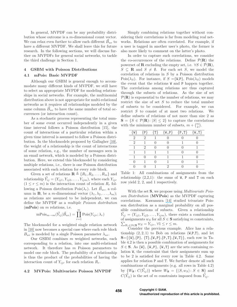
as shown in Figure 4. 1. We define a pair of ran-dom latent variables zi→j and zi←j which take values in{1, 2, . . . , k} and follow multinomial distributions withparameters �πi and �πj respectively. That is, zi→j ∼mNom(�πi) and zi←j ∼ mNom(�πj), where mNom standsfor a multinomial distribution. 2. B � { �Buv : u, v =1, 2, . . . , k}: B is a s × k × k dimensional tensor (seeFigure 5). �Buv (each gray pillar) is a s dimensionalvector of parameters, describing a multivariate proba-bility density function MVPDFs→m( �Buv) which takesthe s parameters and generates m-dimensional relation-ships. 3. Suppose zi→j = u, zi←j = v, we determinethe (u, v)-column of tensor B, �Buv (the shaded columnin Figure 5), and generate �Yij using the correspondingMVPDF, i.e., �Yij ∼ MVPDFs→m( �Buv).

zi→j = u

zi←j = v �Buv

sk

k

Figure 5: An Illustration of blockmodels B, which isa tensor of dimension s × k × k; when zi→j = u andzi←j = v, column �Buv estimates �Yij

The relationship �Yij is estimated by �Buv withprobability

Pr(�Yij , zi→j , zi←j |θ) = Pr(u|�πi) Pr(v|�πj) Pr(�Yij | �Buv)

= πiuπjvMVPDF(�Yij | �Buv)(3.1)

The probability of �Yij is thus

Pr(�Yij |θ) =∑

u,v

πiuπjvMVPDF(�Yij | �Buv)

Therefore, relationship �Yij is modeled as a mixture ofall columns �Buv via zi→j = u and zi←j = v.

3.2 GSBM Variants

The multi-relational networks studied in [22, 12] di-rectly combine multiple single relational networks to-gether, where each block is modeled by one parameteron each relation. As relations are modeled indepen-dently of one another, the MVPDF in this context isspecifically a joint probability distribution over all re-lations, i.e., the probability of each relationship is theproduct of the probabilities of the values on all relations,each determined by the parameter on the correspondingrelation. Hence, our GSBM is also considered as a gen-eralization of the blockmodels on multi-relational net-works, by incorporating more general MVPDF to caterfor the correlations among relations. This will be elab-orated in Section 4.

As the MMB introduced in [1] models each blockby a Bernoulli process on a single relation, our GSBMreduces to MMB with m = 1 and the MVPDF being aBernoulli distribution on that relation.

Another example of MVPDF is a multinomial dis-tribution, MVPDFm+1→m takes an integer w and mprobabilities p1, p2, . . . , pm with sum 1, and the proba-bility of a relationship (w1, w2, . . . , wm) with sum w is

n!w1!w2!···wm!p

w11 pw2

2 · · · pwmm .

Our GSBM does provide solutions to address thesecond challenge mentioned in Section 1, by adoptinga MVPDF which is able to handle multiple types ofrelations in a multi-relational network, including binaryrelations from social connections and weighted relationsfrom social interactions. For an example, supposethe relation is-a-friend-of and the relation tag aremodeled by Bernoulli distributions and multinomialdistributions respectively. If these two relations areindependent, the MVPDF for each block can be takenas the product of the two corresponding distributions. Ifthere exists dependency, the MVPDF for each block canbe a combination of two multinomial distributions fortag, depending on relation is-a-friend-of is presentor not.

240 Copyright © SIAM.Unauthorized reproduction of this article is prohibited.

455 Copyright © SIAM.Unauthorized reproduction of this article is prohibited.

In general, MVPDF can be any probability distri-bution whose outcome is a m-dimensional count vector.We can relax even further to allow each different �Buv tohave a different MVPDF. We shall leave this for futureresearch. In the following sections, we will discuss fur-ther on MVPDFs for general social networks, to tacklethe third challenge in Section 1.

4 GSBM with Poisson Distributions

4.1 mPois: Basic MVPDF

Although our GSBM is general enough to accom-modate many different kinds of MVPDF, we still haveto select an appropriate MVPDF for modeling relation-ships in social networks. For example, the multinomialdistribution above is not appropriate for multi-relationalnetworks as it requires all relationships modeled by thesame column �Buv to have the same number of total oc-currences (or interaction count).

As a stochastic process representing the total num-ber of some event occurred independently in a giventime interval follows a Poisson distribution [15], thecount of interactions of a particular relation within agiven time interval is assumed to follow a Poisson distri-bution. In the blockmodels proposed by Gallagher [10],the weight of a relationship is the count of interactionsof some relation, e.g., the number of messages seen inan email network, which is modeled by a Poisson distri-bution. Here, we extend this blockmodel by consideringmultiple relations, i.e., there is one Poisson distributionassociated with each relation for every role block.

Given a set of relations R � {R1, R2, . . . , Rm} andrelationship �Yij = (Yij1, Yij2, . . . , Yijm), where each Yijr

(1 ≤ r ≤ m) is the interaction count of relation Rr fol-lowing a Poisson distribution Pois(λr). Let �Buv, a col-umn in B, be a m-dimensional vector (λ1, λ2, . . . , λm);as relations are assumed to be independent, we candefine the MVPDF as a multiple Poisson distribution(mPois) on m relations, i.e.

mPoism→m(�Yij | �Buv) =m∏

r=1

Pois(Yijr; λr)

The blockmodel for a weighted single relation networkin [10] now becomes a special case where each role blockBuv is modeled by a single Poisson parameter λuv.

Our GSBM combines m weighted networks, eachcorresponding to a relation, into one multi-relationalnetwork. It therefore has m Poisson parameters tomodel one role block. The probability of a relationshipis thus the product of the probabilities of having theinteraction count of Yijr for each relation Rr.

4.2 MVPois: Multivariate Poisson MVPDF

Simply combining relations together without con-sidering their correlations is far from modeling real net-works. Relations are often correlated. For example, ifa user is tagged in another user’s photo, the former isalso more likely to comment on the latter’s photo.

In order to capture such correlations, we considerthe co-occurrences of the relations. Define P(R) thepowerset of R excluding the empty set, i.e. ∀S ∈ P(R),S ⊆ R and S �= ∅. For each set S, we model thecorrelation of relations in S by a Poisson distributionPois(λS). For instance, if S ={W,P}, Pois(λS) modelsthe event that the relations W and P happen together.The correlations among relations are thus capturedthrough the subsets of relations. As the size of setP(R) is exponential to the number of relations, we mayrestrict the size of set S to reduce the total numberof subsets to be considered. For example, we canrestrict S to consist of at most two relations. Wedefine subsets of relations of not more than size 2 asS = {S ∈ P(R) : |S| ≤ 2} to capture the correlationswith the minimum number of subsets, m +

(m2

).

{W} {P} {T} {W,P} {P,T} {W,T}2 2 1 0 0 02 1 0 0 1 01 2 0 0 0 11 1 1 1 0 01 0 0 1 1 00 1 0 1 0 10 0 1 2 0 0

Table 1: All combinations of assignments from therelationship (2,2,1): the sums of W, P and T on eachrow yield 2, 2, and 1 respectively.

With the set S, we propose using Multivariate Pois-son Distribution (MVPois) as the MVPDF capturingcorrelations. Kawamura [14] studied trivariate Pois-son distribution as a marginal probability on all pos-sible combinations of subsets. Given a relationship�Yij = (Yij1, Yij2, . . . , Yijm), there exists a combinationof assignments wS for all S ∈ S satisfying m constraints,∑

Rr∈S∈S wS = Yijr, ∀1 ≤ r ≤ m.Consider the previous example. Alice has a rela-

tionship (2, 2, 1) to Bob on relations (W,P,T), and letS={{W},{P}, {T},{W,P},{P,T},{W,T}}, each row in Ta-ble 4.2 is then a possible combination of assignments forS ∈ S. As {W}, {W,P}, {W,T} are the sets containing re-lation W, the constraint that their assignments sum upto be 2 is satisfied for every row in Table 4.2. Sameapplies for relation P and T. We further denote all suchcombinations of assignments (e.g. all rows in Table 4.2)by {WS : C(�Yij)} where WS = {〈S, wS〉 : S ∈ S} andC(�Yij) is the set of m constraints imposed from �Yij .

241 Copyright © SIAM.Unauthorized reproduction of this article is prohibited.

456 Copyright © SIAM.Unauthorized reproduction of this article is prohibited.

The probability of each combination of assignmentscan be obtained by the mPois distribution on set S,since correlations among relations are now captured bysets in S and the independence is assumed among setsin S. So the probability of an observed relationship �Yij

is the sum of the probabilities of all combinations WS

with constraint C(�Yij). For example, the probability ofthe relationship (2, 2, 1) can be obtained by summingup all probabilities of the rows in Table 4.2.

Hence, we formulate the MVPois as follows.

MVPois|S|→m(�Yij | �Buv)

=∑

{WS : C(�Yij)}

∏

S∈S

Pois(wS ; λS)(4.2)

Each column �Buv is a vector of |S| Poisson parameters,each λS models the correlation of relations in set S.Our GSBM can therefore incorporate the MVPois tomodel correlations among relations in a multi-relationalnetwork. The choice of MVPois is our belief for socialnetworks with correlated relations. There may be othermore complicated multivariate functions that betterdescribe multi-relational networks. A detailed study ofthese MVPDF functions will be a topic for our futurework. In the next section, we will turn our attentionto GSBM model estimation for a given multi-relationalsocial network.

5 GSBM Model Estimation

We now describe how to build a good GSBM for socialnetworks to discover roles and positions. We use Max-imum Likelihood Estimation (MLE), a popular statis-tical method, to learn the parameters of the mixturemodel [13].

Given the blockmodel θ = (Π,B) and relationship�Yij , suppose the two latent variables zi→j and zi←j fol-low distribution qij , i.e., qij(u, v|�Yij , θ) is the probabilityof zi→j = u and zi←j = v. The expected complete loglikelihood for �Yij is

〈lc(θ|�Yij)〉qij�

∑

u,v

qij(u, v|�Yij ,θ) log Pr(�Yij , u, v|θ)

where∑

u,v qij(u, v|�Yij , θ) = 1. An EM algorithm isthen adopted to maximize the log likelihood in theabove equation. In E-step, by Jensen’s Inequality [4],the choice of qij(u, v|�Yij , θ) = Pr(u, v|�Yij , θ) maxi-mizes the above log likelihood. As in Equation 3.1,Pr(�Yij , u, v|θ) = πiuπjvMVPDF(�Yij | �Buv),

Pr(u, v|�Yij , θ) =Pr(�Yij , u, v|θ)

Pr(�Yij |θ)

=πiuπjvMVPDF(�Yij | �Buv)

Pr(�Yij |θ)

In M-step, we optimize the expected complete loglikelihood for all relationships, i.e. lc(θ|Y) �∑

�Yij∈Y〈lc(θ|�Yij)〉qijwith respect to model θ. By set-

ting ∂lc(θ|Y)∂πiu

= 0 with the constraint∑

u πiu = 1 for alli, we have

πiu =

∑�Yij ,v qij(u, v|�Yij ,θ) +

∑�Yji,v

qji(v, u|�Yji, θ)

|{�Yij ∈ Y}| + |{�Yji ∈ Y}|To optimize the blockmodel B, we first prove:

Theorem 5.1. A multiple Poisson distribution isequivalent to a joint probability distribution of a uni-variate Poisson distribution and a multinomial distribu-tion, where the univariate Poisson distribution modelsthe sum of all variables, and the multinomial distribu-tion models the variables, i.e.

mPois(λ1, λ2, . . . , λm) = Pois(λ) �� mNom(p1, p2, . . . , pm)

where λi = λpi ∀1 ≤ i ≤ m.Proof. Given �w = (w1, w2, . . . , wm) and n =

∑i wi

Pois(n; λ) �� mNom(�w; p1, p2, . . . , pm)

=λne−λ

n!· n!∏

i wi!

∏

i

pwii =

∏

i

(λpi)wie−λpi

wi!(5.3)

= mPois(�w; λp1, λp2, . . . , λpm)

Equation 5.3 makes use of the condition∑

i pi = 1.

By the above theorem, Equation 4.2 can be revised to anequivalent definition. Define each block �Buv by |S| + 1parameters, with one Poisson parameter λuv and |S|probabilities puvS satisfying

∑S∈S puvS = 1.

MVPois|S|+1→m(�Yij | �Buv)

=∑

{WS : C(�Yij)}Pois(

∑

S∈S

wS ; λuv) · mNom(WS; puvS)

We now optimize the expected complete log likelihoodlc(θ|Y) with respect to the above formulation. Bysetting ∂lc(θ|Y)

∂λuv= 0, λuv is the root to the polynomial

∑

�Yij∈Y

qij(u, v|�Yij , θ)∑

α1α! · (βα+1 − βα) · λα

uv∑α

1α! · βα · λα

uv

= 0

where βα =∑P

S∈S wS=α

{WS : C(�Yij)} mNom(WS; puvS) is a param-

eter with respect to a pair of (�Yij , �Buv). λuv is thusobtained by Newton-Raphson method.

Setting ∂lc(θ|Y)∂puvS

to a Lagrange multiplier [4] since∑S∈S puvS = 1, for a particular S0 ∈ S, we have puvS0

proportional to

∑

�Yij∈Y

qij(u, v|�Yij , θ)

∑{WS : C(�Yij)} wS0

∏S∈S

(λuvpuvS)wS

wS !∑

{WS : C(�Yij)}∏

S∈S(λuvpuvS)wS

wS !

242 Copyright © SIAM.Unauthorized reproduction of this article is prohibited.

457 Copyright © SIAM.Unauthorized reproduction of this article is prohibited.

k = 4 k = 6 k = 8 k = 10 k = 12

Vertices Grouped byGround Truth Posi-tions

Vertices in RandomOrder

Vertices Grouped byPredicted Positionsusing GSBM+mPois

Vertices Grouped byPredicted Positions us-ing GSBM+MVPois

Figure 6: Blockmodels on synthetic data (if not printed in color, please refer to the electronic version)

With all the above formulae, EM algorithm iteratesfor the MLE, which will be validated in the laterexperimental study.

6 Experimental Study

In this section, we evaluate our proposed GSBM by us-ing both synthetically generated networks and multi-relational networks extracted from the IMDb dataset.In Section 6.1, we aim to show that GSBM togetherwith MVPois can perform well on recovering the hiddenpositions by visualizing such positions. We use GSBMwith mPois as the baseline method to demonstrate thedifferent results produced by ignoring the correlationsamong relations. Section 6.2 then focuses on validatingour GSBM by relationship prediction on real world net-works. A GSBM with MVPois is trained from a networkin an earlier period, and then predicts relationships fora later period. Finally, we present a case study thatreveals interesting positions discovered from the IMDbnetwork in Section 6.3.

6.1 Evaluation using Synthetic Data

We first developed a strategy to generate syntheticmulti-relational networks with vertices of known posi-tions. By hiding the position labels, we performed po-sition and role analysis using GSBM with mPois andMVPois, which were denoted by GSBM+mPois andGSBM+MVPois respectively. The predicted posi-tions by GSBM+mPois and GSBM+MVPois were thencompared with the ground truth positions and their ac-curacies were measured.

Synthetic network generation. For easy visu-alization, we assumed the multi-relational networks in-volved 3 relations represented by primary colors, i.e.,red(R), green(G) and blue(B). These networks had 1000vertices divided into k positions. Our experiment usedk = 4, 6, 8, 10 and 12. We only considered correlationfor at most 2 relations and this gave rise to S = {R, G,B, RG, RB, GB} as the possible relation co-occurrences.

For each of the k×k role blocks of relationships, wegenerated the Poisson parameter for each S ∈ S. Each

243 Copyright © SIAM.Unauthorized reproduction of this article is prohibited.

458 Copyright © SIAM.Unauthorized reproduction of this article is prohibited.

block contained about 1000k vertices2. We randomly

generated a Poisson parameter for each S from theuniform distribution U [0.2, 1.0). Hence, each role blockhad a unique set of Poisson parameters. Next, wedetermined the relation occurrences of the relationshipbetween every vertex i and vertex j in role block (u,v)respectively by first generating an integer value for eachS ∈ S using the Poisson parameters assigned to (u, v).The red relation occurrence count of relationship (i, j)was the sum of the values on R, RG and RB; the greenrelation occurrence count was the sum of the values onG, RG and GB; the blue relation occurrence count wasthe sum of the values on B, RB and GB. The bitmapsin the first row of Figure 6 depicted the colors generatedfor each of the k × k role blocks based on ground truthpositions of vertices when the vertices were sorted byposition. Note that each bitmap image had blocksassigned with distinctive color and block boundaries.

Position prediction. To ensure that verticesof different positions were well mixed before applyingGSBM, we randomly shuffled the vertices as shownin the second row, leading to indistinguishable po-sitions. We then applied the GSBM+mPois andGSBM+MVPois on the multi-relational networks ofshuffled vertices. Once the positions of vertices werelearned, we grouped them by position as shown in thelast two rows in Figure 6. Note the positions were rear-ranged to make the bitmap most similar to that of theground truth.

Results. Visually, vertices with correctly pre-dicted positions when grouped together should have thebitmap of relationships look identical to that of rela-tionships of vertices grouped by ground truth positions.GSBM+mPois which did not consider correlations wasbuilt on the three relations only. The bitmaps generatedby GSBM+mPois had some resemblance with those ofground truth especially when k was small. As k in-creased, the resemblance became less distinct.

GSBM+MVPois that considered the correlationsup to two relations, i.e. R, G, B, RG, RB and GB,demonstrated significantly better results. It generatedbitmaps very similar to those of ground truth. Thisshowed that the GSBM with MVPois can predict thepositions with good accuracy.

6.2 Evaluation Using Real Dataset

IMDb network. We applied our GSBM+MVPoison IMDb3 dataset. The IMDb dataset had sev-eral types of nodes and relations. We included

2The bitmaps were drawn based on 13

of the vertices due tothe large file size of 1000 × 1000 bitmaps

3http://www.imdb.com

actors/actresses, directors and producers. Threerelations were included, i.e., collaborate (among ac-tors/actresses, among directors, or among produc-ers), direct (from directors to actors/actresses) andwork for (from actors/actresses to producers and fromdirectors to producers). We extracted a connectedIMDb Network as follows.

We started from a set of movies between 2003 and2006 (inclusive) which are directed by eleven directors,James Cameron, Chris Columbus, Jon Favreau, RonHoward, Doug Liman, Christopher Nolan, Guy Ritchie,Martin Scorsese, Steven Soderbergh, Steven Spielbergand David Yates. We then expanded the set of movietwice by the following way. Among the set of movies,we selected actors, actresses and producers who partic-ipated in at least two movies. Then, we obtained a newset of movies in which at least two of the above actors,actresses and producers participated. Within this setof movies, we chose those directors and those actors,actresses or producers who participated in at least twomovies. We thus obtained a set of 1530 users, and a net-work was build from this set of users with the relationsmentioned above.

Performance measures. We measured the accu-racy of relationship prediction by precisions. For a pairof individuals (xi, xj), �Yij denote the actual relation-ship from xi to xj . Let the set of relationships in thetest data be E = {�Yij : ∃r, Yijr > 0}, i.e., E is the setof individual pairs where a certain relationship exists.Let Yij be the predicted relationship from xi to xj thatmaximizes the probability, i.e., Yij = arg max�e�=0 p(�e |θ, i, j). The precision is measured by

Precision =|{�Yij : Yij = �Yij ∧ (xi, xj) ∈ E}|

|E|However, if there is only one edge type in the test

edge set E, prediction Yij is trivial. Thus edge typeswhich appear more frequently should be penalized,compared to edge types that are less frequent. Wehave therefore considered the soft precision, which is theprecision weighted by the negative log of its probability,i.e.

Soft Precision =−∑

Yij=�Yij∧(xi,xj)∈E log p(�Yij)

|E| · H(E)

Given edge type �e appears with probability p(�e) in thetest set E, every correct prediction Yij = �Yij , where �Yij

is of type �e, will carry a score of [− log p(�e)] to the softprecision. The maximum is thus |E| ·H(E), where |E| isthe total number of the edges and H(E) is the entropyof the edges. Soft precision is thus normalized by themaximum, as given in the above equation.

244 Copyright © SIAM.Unauthorized reproduction of this article is prohibited.

459 Copyright © SIAM.Unauthorized reproduction of this article is prohibited.

xi xi

xj xj

xs1

xs2xt1

xt2

xs3

xs4xt3

xt4

direct work for

Figure 7: An illustration of modified common neighbormethod on relations direct and work for from xi toxj

Baseline Method. As there hardly exists amethod that predicts relationships between two indi-viduals, we modified the well-known common neighbormethod in the context of directed network. When com-mon neighbor method is applied on an undirected net-work, a pair of vertices with more common neighborsis more likely to form a link than a pair with less com-mon neighbors. In a directed network, if the relation isnot transitive, there may not be any common neighborbetween a pair of potential vertices. For example, as-sume a network derived by direct relation is a bipartitegraph with one side all directors and the other side allactors or actresses (i.e., assume no overlapping betweendirectors and actors/actresses); between a director andan actress, which potentially forms a direct edge, thereis no common neighbor since all edges from the directorare connected to actors/actresses, while all edges fromthe actress are connected to directors. Therefore, wedefine the number of paths of length 3 as the modifiedcommon neighbor in a directed network constructed byrelation Rr, i.e.,

MCN(i, j; Rr) = |{(s, t) : ∃Yisr > 0∧Ytsr > 0∧Ytjr > 0}|The definition of modified common neighbor can beconsidered as an analogue of the original definition, inthe sense that, the number of common neighbors in theoriginal definition is the number of paths of length 2connecting i and j, while MCN is the number of pathsof length 3 with the middle edge having the oppositedirection in the definition of modified common neighbor.

As shown in Figure 7, there are three pairs ofindices served as “common neighbor” from xi to xj

on relation direct, namely, MCN(i, j; direct) ={(s1, t1), (s2, t1), (s2, t2)}. But there are only twopairs between xi and xj on relation work for:MCN(i, j; work for) = {(s3, t3), (s4, t4)}.

The baseline method assumes the relationship fromi to j is a pair {〈R0, 1〉}, where R0 is the relationwhich gives maximum |MCN|, i.e., |MCN(i, j; R0)| ≥

|MCN(i, j; Rr)|∀1 ≤ r ≤ m. In Figure 7, thebaseline method will not predict {〈work for, 1〉} since|MCN(i, j; direct)| > |MCN(i, j; work for)|. As com-mon neighbor method is pretty accurate for link pre-diction, the precision for modified common neighbormethod on relationship prediction can reach more than80% as we shall see in the next paragraph.

0.2

0.3

0.4

0.5

0.6

0.7

0.8

0.9

1

1.1

[03,06][02,06][01,06][00,06][99,06]P

reci

sion

[xx,06]: Training Data from Year xx to Year 06

Prediction of the Relationship in Year 07 as Training Data Vary

Baseline PrecisionGSBM Precision

Baseline Soft PrecisionGSBM Soft Precision

Figure 8: Relationship predictions in IMDb network forthe year 07 with different sets of training data

0.2

0.3

0.4

0.5

0.6

0.7

0.8

0.9

1

1.1

[07,11][07,10][07,09][07,08][07,07]

Pre

cisi

on

[07,yy]: Test Data From Year 07 to Year yy

Varying Prediction Time Frame with Training Data [03,06]

Baseline PrecisionGSBM Precision

Baseline Soft PrecisionGSBM Soft Precision

Figure 9: Relationship predictions in IMDb networkover different time frames with the same set of trainingdata

Results. In Figure 8 and Figure 9, we comparedour GSBM model (using MVPois) applied on the IMDbnetwork with the baseline method. As most of theedges have the count of 1 on one relation and 0 onthe other two relations, the baseline method can reachmore than 80% precision. Figure 8 showed the precisionresults on Task 1, i.e., predicting the relationship inthe year of 2007 with training data on various timeframes before 2007. Our model improved the precision

245 Copyright © SIAM.Unauthorized reproduction of this article is prohibited.

460 Copyright © SIAM.Unauthorized reproduction of this article is prohibited.

to 90%, almost one quarter of the maximum possibleimprovement. On the measure of soft precision, GSBMoutperformed the baseline by about 20% in all cases,as the additional edges predicted correctly by GSBMcarried heavier weights than those predicted correctlyby the baseline method. The precision do not alwaysimprove with more training data. This could be dueto outdated data for a long period of training data.For task 2, as shown in Figure 9, our GSBM modelagain outperformed baseline in all the test periods. Wealso observed the decrease in both precision and softprecision as longer time period of test data was involved.This was expected since the information obtained fromthe training data became more outdated for the recentrelationships.

These results on networks extracted from IMDbdataset confirmed the usefulness of the positions inpredicting future relationships.

6.3 A Case Study

We also gave a case study to show that the positionsfound by our GSBM are sound. From the elevendirectors mentioned in our IMDb dataset, we selectedtheir 73 movies directed by them from year 2000 to2010. 486 directors, producers and actors/actressesinvolved in at least two of these movies. For this smallerIMDb network, we learned the model using GSBM andMVPois with k = 6.

The clusters formed by the learned positions areshown in Figure 10. The green edges are undirected,representing the collaborative relation, whereas theblue edges and the red edges are directed, representingthe direct and work for relations respectively. Thethicker an edge (relation) is, the more interactions itcarries.

Out of the 11 directors, 10 directors were togetherin block A, except James Cameron, who acted in 2movies, directed 3 movies and also produced 4 movies.His position as a director was not so obvious as otherdirectors, he was thus outside the director block, i.e.,block A.

There was also a producer block D, consisting of 6active producers, who produced up to 10 movies. Otherproducers did not produce so many movies, and manyof them acted in the movies they produced.

There were two interesting actors/actresses blocks,B and F. Block B included the actors/actresses inOcean’s Eleven/Twelve/Thirteen Series, e.g., GeorgeClooney (Danny), Brad Pitt (Rusty), and Matt Damon(Linus). Block F included the actors/actresses in HarryPotter Series, e.g., Daniel Radcliffe (Harry), EmmaWatson (Hermione), and Rupert Grint (Ron). As thisIMDb network was dominated by the collaboration

relation, actors/actresses played in a series of moviesare grouped together.

The remaining two blocks, although not as notableas the previous, can also be explained. Block C had113 people who were mostly producers with relativelyfewer movies as compared to block D, which includedactive producers. Block E has 145 people who wereactors/actresses not involved in any special series, orseries that did not see many overlapping actors, e.g.the Da Vinci Code and Angles & Demons.

This case study demonstrated that the blocks dis-covered by our proposed model matches well with the in-tuition. We therefore conclude that GSBM with multi-variate Poisson is an effective method for conducting po-sition and role analysis on a multi-relational network.

7 Conclusion

We presented a generalized stochastic blockmodels(GSBM) that discover structures on multi-relationalnetworks. For multi-relational social networks, we pro-posed to use multivariate Poisson distribution as theMVPDF for our GSBM. Using the sets formed by rela-tions, we are able to accurately capture the correlationamong the relations. We then demonstrated an instanceof our GSBM using multivariate Poisson modeling andestimated its parameters using EM algorithm. Exper-imental studies on both synthetic and real data showthat our GSBM is effective for discovering structuresand predicting the relationship of future links.

8 Acknowledgment

We will like to thank Agus Trisnajaya Kwee for helpingus with the visualization of multi-relational networks.

This work is supported by Singapore’s NationalResearch Foundation’s research grant, NRF2008IDM-IDM004-036.

References

[1] Edoardo M. Airoldi, David M. Blei, Stephen E. Fien-berg, and Eric P. Xing. Mixed membership stochasticblockmodels. Journal of Machine Learning Research,9:1981–2014, June 2008.

[2] Michele Berlingerio, Michele Coscia, and Fosca Gian-notti. Finding and characterizing communities in mul-tidimensional networks. In ASONAM, pages 490–494,2011.

[3] Michele Berlingerio, Michele Coscia, Fosca Giannotti,Anna Monreale, and Dino Pedreschi. Foundationsof multidimensional network analysis. In ASONAM,pages 485–489, 2011.

[4] Stephen Boyd and Lieven Vandenberghe. ConvexOptimization. Cambridge University Press, 2004.

246 Copyright © SIAM.Unauthorized reproduction of this article is prohibited.

461 Copyright © SIAM.Unauthorized reproduction of this article is prohibited.

Chris ColumbusJon FavreauRon HowardDoug Liman

Christopher NolanGuy Ritchie

Martin ScorseseSteven SoderberghSteven Spielberg

David Yates

David BarronFrederic W. Brost

David HeymanGregory JacobsLorne OrleansLionel Wigram

Daniel RadcliffeEmma WatsonRupert GrintBonnie Wright

Michael GambonAlan Rickman

George ClooneyBrad Pitt

Matt DamonBernie Mac

Elliott Gould

Tom HanksLeonardo DiCaprio

Russel CroweRobert Downey Jr.

Tom Hardy

James CameronDan Brown

Chris BrighamJordan Goldberg

Kevin Feige

AB

C

D E

F

Figure 10: A case study on the blockmodel constructed on 73 movies with k = 6

[5] Sergey V. Buldyrev, Roni Parshani, Gerald Paul,H. Eugene Stanley, and Shlomo Havlin. Catastrophiccascade of failures in interdependent networks. Nature,464(7291):1025–1028, April 2010.

[6] Deng Cai, Zheng Shao, Xiaofei He, Xifeng Yan, andJiawei Han. Community mining from multi-relationalnetworks. In PKDD, pages 445–452, 2005.

[7] Patrick Doreian, Vladimir Batagelj, and AnuskaFerligoj. Generalized Blockmodeling. Cambridge Uni-versity Press, 2005.

[8] Joan Ferrante. Sociology: a global perspective. Thom-son Wadsworth, 2008.

[9] Stephen E. Fienberg, Michael M. Meyer, and Stanley S.Wasserman. Statistical analysis of multiple sociometricrelations. Journal of the American Statistical Associa-tion, 80(389):51–67, March 1985.

[10] Ian Gallagher. Bayesian block modelling for weightednetworks. In MLG, pages 55–61, 2010.

[11] Michael Hay, Gerome Miklau, David Jensen, DonTowsley, and Philipp Weis. Resisting structural re-identification in anonymized social networks. Proc.VLDB Endow., 1:102–114, August 2008.

[12] Paul W. Holland, Kathryn Blackmond Laskey, andSamuel Leinhardt. Stochastic blockmodels: Firststeps. Social Networks, 5(2):109–137, June 1983.

[13] Michael I. Jordan. An Introduction to ProbabilisticGraphical Models. in preparation, 2002.

[14] Kazutomo Kawamura. The structure of trivariatepoisson distribution. Kotai Mathematical SeminarReports, 28(1):1–8, 1976.

[15] Sheldon M. Ross. Stochastic Processes. John Wiley &Sons, 1996.

[16] Michael Szell, Renaud Lambiotte, and Stefan Thurner.Multirelational organization of large-scale social net-works in an online world. Proceedings of the Na-tional Academy of Sciences, 107(31):13636–13641, Au-gust 2010.

[17] Lei Tang, Huan Liu, and Jianping Zhang. Identify-ing evolving groups in dynamic multimode networks.IEEE Trans. Knowl. Data Eng., 24(1):72–85, 2012.

[18] Lei Tang, Huan Liu, Jianping Zhang, and ZohrehNazeri. Community evolution in dynamic multi-modenetworks. In KDD, pages 677–685, 2008.

[19] Ales Ziberna. Generalized blockmodeling of valuednetworks. Social Networks, 29(1):105–126, January2007.

[20] Yuchung J. Wang and George Y. Wong. Stochasticblockmodels for directed graphs. Journal of the Amer-ican Statistical Association, 82(397):8–19, March 1987.

[21] Stanley Wasserman and Katherine Faust. Social Net-work Analysis: Methods and Applications. CambridgeUniversity Press, 1994.

[22] Harrison C. White, Scott A. Boorman, and Ronald L.Breiger. Social structure from multiple networks. i.blockmodels of roles and positions. The AmericanJournal of Sociology, 81(4):730–780, January 1976.

[23] Rongjing Xiang, Jennifer Neville, and Monica Rogati.Modeling relationship strength in online social net-works. In WWW, pages 981–990, 2010.

247 Copyright © SIAM.Unauthorized reproduction of this article is prohibited.

462 Copyright © SIAM.Unauthorized reproduction of this article is prohibited.