Evaluating Structural Engineering Finite Element Analysis Data Using Multiway Analysis

2014 IEEE International Conference on BigData (IEEE BigData 2014), Washington DC

Evaluating Structural Engineering Finite Element Analysis Data

Using Multiway Analysis

Matija Radovic

Civil Engineering Department

University of Delaware

Newark, DE.

[email protected]

Jennifer McConnell

Civil Engineering Department

University of Delaware

Newark, DE.

[email protected]

Abstract- The scope of this paper is to introduce multiway

analysis into structural engineering research and to outline

methodology used in tensor decomposition of finite element

analysis (FEA) data. More specifically, the example evaluated

herein evaluates the stress distribution of two different highway

bridge structural components (girders and cross frames), being

subjected to incrementally increasing forces. Additionally, the

paper shows potential advantages of using multiway methods in

interpretation of FEA data and makes recommendations for

future investigations on the use of multiway methods in FEA post-

processing of structural engineering data.

Keywords—Multiway analysis, finite element analysis, bridge

engineering, structural engineering, Tucker3 model.

I. INTRODUCTION

In current structural engineering practice, finite element analysis (FEA) is commonly used to predict the structural behavior of various structural members, of assemblies of structural members, and / or of entire structures. For example, FEA can be used to determine the maximum strength or displacements of a structural member under various loading scenarios or to investigate the distribution of stress between various members. It is routinely used to design unique structures such as bridges and buildings and as a research tool.

FEA is based on a discretization of structural parts into geometric shapes (elements) that are bounded at their corners or edges with points (nodes). Each element has assigned material properties. The grid lines seen in the left of Fig. 1 denote the element boundaries for an I-shaped member. The response of these elements to an input loading is calculated via a system of partial differential equations with each element containing multiple unknown quantities that are calculated by the FEA method [1]. Since the solution for the set of the partial differential equations is based on numerical approximations, a more detailed set (a finer FEA mesh with a larger number of elements) will theoretically yield more accurate solutions up to a point where the influence of mesh size converges to a common solution.

The number of elements in a typical model could vary anywhere from hundreds to millions. As a result of a typical FEA, displacements, stresses, and strains in multiple directions are computed for each element. Furthermore, one FEA may

Fig. 1. Finite element model (FEM) of a steel bridge I-girder (on the left)

shows the element mesh, where rectangles represent discretized geometrical shapes (elements) that can be numerically modeled with a system of partial

differential equations. Stress contours (on the right) the spatial variation of

stress magnitudes due to imposed loads. Red colored elements are elements with the largest stresses, while the green colored elements are the elements with

the lowest stresses.

realistically contain anywhere from one to hundreds of loading conditions, producing a unique data set for each loading. Thus, the potential output from these analyses is immense. Fig 2. shows a subset of potential FEA data, showing one type of output (von Mises stresses) for one part (bottom flange) of one highway bridge member (one girder) that was subjected to 60 load increments.

In current practice, only a small fraction of this available data is quantitatively analyzed. For example, it is often the case that only the extreme values in the data set (such as minimum and maximum stresses or maximum displacements) at a particular region of interest are analyzed. A possible exception to this statement are contour plots showing the spatial distribution of the magnitudes of a specific output variable that can be produced by some FEA post-processing software (as seen in Fig 1. on the right). However, an approach for performing a rigorous quantitative analysis of the data has yet to be applied in any published works that could be identified by the authors.

For these reasons, this paper explores the use of “big data” applications to analyze a large data set resulting from the FEA of a representative civil engineering structure, a steel bridge. The general goal of this effort is to first determine a methodology using big data analysis techniques to improve upon the current practice of using isolated subsets of the available data and/ or visual data contours that lack a means to readily conduct

Center for Innovative Bridge Engineering (CIBrE),

University of Delaware, Newark, DE.


Fig. 2. FEA output of bottom flange element stresses from bridge girder,

subjected to 60 load increments. Each line represents a single bottom flange

element and each point on the line represents the stress value measured at

increasing load increments.

quantitative data analysis. Secondly, it is desired to assess the

practical significance of this data, it being anticipated that a

more rigorous quantitative analysis will have the potential to

reveal a greater understanding of the structural response, for

complex structures in particular. Another benefit in more

comprehensive analysis of the large FEA data sets is envisioned

as being a means to compare and contrast similarities and

differences in competing design options.

Therefore the scope of this paper is to explore the use of multiway data analysis techniques in analyzing structural engineering FEA output. More specifically, the example evaluated herein assesses the stress distribution of two different structural components (girders and cross frames) in highway bridges that are subjected to incremental loading. Tucker3 tensor decomposition is used as an analytics tool to explore the dataset resulting from the FEA of such a steel I-girder highway bridge. This paper outlines the methodology used in Tucker3 tensor decomposition to propose a new methodology for interpreting FEA data in structural engineering, compares the outputs of traditional interpretation of FEA analysis to interpretation of FEA analysis based on multiway models, and makes recommendation for future use of multiway tools in bridge engineering practice.

II. BACKGROUND

Generally, “big data” is a term used to describe large and complex data sets. The main benefit in using large data sets is that larger data sets may lead to more accurate and insightful understanding of a particular phenomenon. Typically, engineers and analysts usually impose a 2-dimensional structure on data analysis which has diminished capability to reveal valuable patterns and trends in the data. Due to the sheer volume and complexity of a large data set, sophisticated analytical tools are necessary to fully utilize it.

Multiway data analysis is one such tool that has become popular as an exploratory analysis tool in discovering the latent structures in higher-order datasets [2,3]. Higher-order data sets are data sets with more than two modes (i.e., dimensions), with

a mode representing a set of data arranged in matrix form. Conventional data analysis deals with analyzing data in the form of two dimensional matrixes. The addition of a third mode will result in the data being in the form of a data cuboid, which is a typical example of a higher-order data set. For example, in the present situation of interest, consider a data set that consists of stress values along the length of a structural member. If we assume that the member consists of a top flange (TF), a bottom flange (BF), and a web, then mode 1 in the data matrix will be the elements comprising these member components in each cross-section of the member (with mode 1 usually organized as the row variables) and mode 2 will be the distances along the length of the girder (usually organized as the column variable). The data inside the matrix would consist of stresses at each cross-section element at each distance. If behavior under increasing magnitudes of load is of interest, then a third mode could consist of load magnitudes (usually the third mode is called a “tube” in 3-D array). In models with increasing complexity, additional modes can be added. For example, the influence of temperature fluctuations on the structural member’s stresses, during incremental loading, could serve as a 4th mode in the present example. Depending of the complexity of the problem as many modes as needed can be added.

Clearly, multiway or higher-order data is ubiquitous and there are several methods for analyzing such data. One of the methods available for the analysis of multiway data is higher order singular value decomposition (HOSVD), also known as Tucker tensor decompositions [4]. If the data set is in a three-way format, Tucker3 tensor decomposition is a special case of HOSVD used for analyzing the data. Tucker3 tensor decomposition is mathematically expressed in matrix (1) and element form (2), which show this to be a trilinear decomposition method, decomposes the three-dimensional array into sets of scores (or loadings) that potentially describe the data in a more condensed form than the original data array.

(1)

Here X is a three-way data set; G is the core tensor array whose

entries show the level of interaction between the different

loading matrices; A, B, and C are loading matrixes and E is

an error array.

(2)

Consequently, in element form, g is the core tensor array entry; a, b, and c are the loading matrix element entries; e is an entry from the error array; and P, Q, and R are the numbers of components in the loading matrices A, B, and C, respectively. Tucker3 decomposition of the structural engineering example discussed in the previous paragraph is conceptually presented in Fig. 3.

Load increments

Stresses (psi)


In order to properly decompose three-wayarray using Tucker3 method, several core tensors (arrays) must be fitted in order to find the most appropriate one, given the dataset under analysi

s.

In order to properly decompose three-way array using Tucker3 method, several core tensors (arrays) must be fitted in order to find the most appropriate one, given the dataset under analysis. The biggest advantage of using Tucker3 tensor decomposition method is its ability to compress variation, extract features, explore data, and generate parsimonious models, especially from highly correlated data sets [5]. The biggest disadvantage of using Tucker3 tensor decomposition method is that it sometimes requires complex data interpretation before optimal model parameters are chosen. Parameters in questions are the size of the core tensor G (p x q x r); core tensor and loading matrix constraints, such as orthogonality or non-negativity; and the selection of an optimization algorithm based on the data structure and / or software used. Due to these restrictions, the user must be familiar with the practical significance of the data set of interest in order to interpret and conduct the analysis in meaningful and accurate manner.

III. METHODOLOGY

The investigation and results presented in this paper are based on the FEA of a representative civil engineering structure, a steel I-girder highway bridge. This structure, the description of the corresponding FEA model, and the loading conditions applied to the model are first described below in Sections A through C, respectively. Section D then describes the post-processing of the FEA data that was needed as pre-processing for executing the tensor decomposition. This methodology section concludes with explaining the use of the Tucker3 method in tensor decomposition.

A. FEA Subject Bridge Description

The FEA results which will be presented in the following sections of this paper were based on a representative highway bridge, labeled Bridge 7R. A photograph of this structure can be seen at the top of Fig. 4. This bridge is selected due the extensive prior evaluation of the behavior of this structure, including in-service and destructive testing and corresponding FEA [6]. The bridge is a three-span, 63° skewed steel I-girder bridge, with the span of interest being 105ft. long. The bridge has 4 plate girders spaced 8 ft. on center. All four plate girders were fabricated from A7 steel having a web depth of 60 in. and a web thickness of 3/8 in.

The top flange dimensions were 20 x 1 in. for the exterior girders and 18 x 7/8 in. for the interior girders. The effective dimensions of the bottom flanges at mid-span, including the cover plates that existed in this location, were 20 x 3-1/8 in. for the exterior girders and 20 x 2-1/2 in. for the interior girders. The web was stiffened with double-sided transverse stiffeners on the interior girders, in addition to single-sided transverse stiffeners and single-sided longitudinal stiffeners on the exterior girders. The composite 8 in.-thick concrete deck and 2 in. haunch were connected to the girder with shear connectors. Lateral bracing consisted of K-frames that were spaced at 20 ft. along the length of the girders, with the first cross-frame being offset 22.5 ft. from the supports. These were composed of 4” x 3 ½” x 3/8” angles and connected to gusset plates, with four bolts at the end of each member, which were in turn bolted to transverse stiffeners welded to the girders. Additionally, end diaphragms were used to connect the girders at each end of the member. These diaphragms were steel I-sections of equal depth to the girders.

B. FEA Description

Previous work [6] has validated a FEA of Bridge 7R. In this

FEA, all bridge components were modeled using a relatively

fine mesh of reduced-integration shell elements. Longitudinal

and transverse deck reinforcement was modeled using a built-

in function in the finite element software. Full composite

action between the reinforced concrete deck and the steel

girder was developed by using a beam-type multipoint

constraint that assures nodal compatibility between the girder

top flange and the deck at these locations. The cross-frame-to-

girder connection is modeled by merging nodes on the cross-

frames and transverse stiffeners serving as connection plates.

Merged nodes are also used to connect the connection plates,

webs, and flanges. Linear elastic properties are used to model

the concrete deck while for the steel, a multi-linear

constitutive response is used, simulating the linear elastic,

yield plateau, strain hardening, and ultimate regimes, based on

the von Mises yield criterion [7]. The bottom section of Fig. 4

shows a cross-sectional view of the finite element model

(FEM) used in the FEA of Bridge7R.

Fig. 3. Graphic representation of three-way tensor decomposition using Tucker3 method.

[G]pxqxr


C. FEA Loading Conditions

The structural response of Bridge 7R was examined using

the modified Riks method. The basic function of this method

is that it applies progressively larger magnitudes of load until

an ultimate capacity is reached while searching for a

combination of forces and displacements (and thus other

C. FEA Loading Conditions

The basic function of the modified Riks method is that it

associated structural response metrics such as stress) that

satisfy equilibrium at each magnitude of loading. The Riks

method is ideally suited to analyzing the behavior after such a

peak loading is reached. Such algorithms exist in commercial

FEA software, such as Abaqus 6.12 [7], which is used in this

work. In this case, the load is expressed in terms of load

proportionality factors (a multiple of the input load). For this

study, the input load is a HS-20 vehicle load commonly used

in bridge design and evaluation [8]. Since each LPF is a

multiple of the input load and the input load is a HS-20 loading

vehicle, the results of the Riks method are expressed in terms

of number of these design vehicles. For the scenario being

described here, for which non-linear geometry was prescribed,

the maximum LPF at which convergence is obtained is 17.

D. Data Preprocessing for Tensor Decomposition

In order to carry out Tucker3 decomposition, the data must

be organized in a specific three-way format. In this work, the

goal was to investigate the stresses in different element

groups representing different structural members under

increasing loads. Since the girders of Bridge 7R were simply

supported composite beams, their bottom flanges will

experience the highest stress. Thus, only the bottom flange

element stresses were considered for the girders in this

example. It follows that girder bottom flange and cross-frame

element groups, stress magnitude (expressed in terms of the

number of elements experiencing the same range of stress at a

given load) and increasing loads were selected to represent the

dimensions in the array. Stress ranges were used because it

would be impractical to capture all possible stress values of

each element in the structure. In this way, the data emulates

the form of stress histograms for each loading increment.

The data extracted from the FEA was organized into

element groups representing different structural members of

the bridge in different locations in the bridge structure. For

example, cross-frame elements that are connecting Girder 1

and Girder 2 (see Fig. 4) are labeled XG1; cross-frame

elements that are connecting Girder 2 and Girder 3 are labeled

XG2; and cross-frame elements that are connecting Girder 3

and Girder 4 are labeled XG3. Girder 1 bottom flange

elements are labeled G1BF, Girder 2 bottom flange elements

are labeled G2BF, and so on. At the end of this step, a total of

7 element groups are formed (X1G, X2G, X3G, G1BF, G2BF,

G3BF and G4BF), each one containing histogram data for 51

stress ranges and 17 load magnitudes, representing data from

280,976 locations in the structure.

The optimum histogram bin size was determined using the

mean integrated squared error procedure [9]. Mean integrated

square error algorithm is used to measure the goodness-of-the-

fit of a histogram by computing the estimated errors for

several candidate bin sizes, and the bin size that yields the

smallest estimated error is selected. The stress ranges

(histogram bins) were kept constant for all element groups as

well as being constant between load increments. As a result,

for the data set presented in this paper, the optimal bin size

was determined to be 733 psi and a total of 51 bins were used.

Note that von Mises stresses [7] are used in this work, so all

stress values have a positive sign.

Because the girder bottom flanges and cross-frames have

significantly different numbers of elements, comparing counts

of the frequencies of elements in each stress bin would not

reveal the desired information. Therefore, the number of

elements in each stress range in each element group is

normalized (divided) by the number of elements in the

corresponding group. For example, if 665 is the number of

bottom flange elements in Girder 4 that are in a given stress

range and because the total number of elements in the bottom

flange of Girder 4 is 3838, then the resulting value in this

stress range (bin) would be 0.173 (665/3838). The procedure

is repeated for each element group and for each loading.

This preprocessing results in creating element group stress

histograms as shown in Fig. 5. All preprocessing was executed

by a custom-made Matlab code [10].

Fig. 4. Bridge 7R: photograph of actual structure on the top and cross-

sectional view of FEA on the bottom.


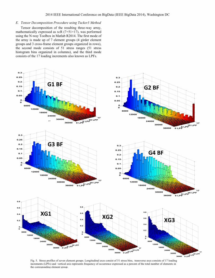
E. Tensor Decomposition Procedure using Tucker3 Method

Tensor decomposition of the resulting three-way array,

mathematically expressed as xϵR (7×51×17), was performed

using the N-way Toolbox in Matlab R2014. The first mode of

the array is made up of 7 element groups (4 girder element

groups and 3 cross-frame element groups organized in rows),

the second mode consists of 51 stress ranges (51 stress

histogram bins organized in columns), and the third mode

consists of the 17 loading increments also known as LPFs.

0 LPF5 LPF

10 LPF

17 LPF

0

6000

12000

18000

24000

30000

36000

0

0.05

0.1

0.15

0.2

0.25

0.3

G1 BF

psi

% o

f tot

al e

lem

ents

0 LPF5 LPF

10 LPF

17 LPF

0

6000

12000

18000

24000

30000

36000

0

0.05

0.1

0.15

0.2

0.25

0.3

0 LPF5 LPF

10 LPF

17 LPF

0

6000

12000

18000

24000

30000

36000

0

0.2

0.4

0.6

0.8

0 LPF5 LPF

10 LPF

17 LPF

0

6000

12000

18000

24000

30000

36000

0

0.05

0.1

0.15

0.2

0.25

0.3

% o

f tot

al e

lem

ents

0 LPF5 LPF

10 LPF

17 LPF

0

6000

12000

18000

24000

30000

36000

0

0.05

0.1

0.15

0.2

0.25

0.3

Fig. 5. Stress profiles of seven element groups. Longitudinal axes consist of 51 stress bins, transverse axes consists of 17 loading

increments (LPFs) and vertical axis represents frequency of occurrence expressed as a percent of the total number of elements in the corresponding element group.

0 LPF5 LPF

10 LPF

17 LPF

0

6000

12000

18000

24000

30000

36000

0

0.2

0.4

0.6

0.8

G1 BF

G3 BF

XG1 XG2

G2 BF

G4 BF

0 LPF

5 LPF10 LPF

17 LPF

0

6000

12000

18000

24000

30000

36000

0

0.2

0.4

0.6

0.8

XG3


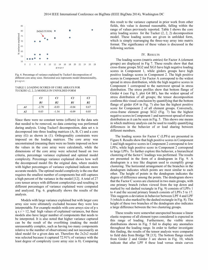
Fig. 6. Percentage of variance explained by Tucker3 decomposition of

different core array sizes. Horizontal axis represents model dimensionality, p x q x r.

TABLE I. LOADING SCORES OF CORE ARRAYS FOR

TUCKER3 (2, 2, 2) MODELS IN UNFOLDED FORM

C1 C1 C2 C2

B1 B2 B1 B2

A1 -2.70 -0.03 -0.04 0.67

A2 0.03 -1.54 -0.09 0.05

Since there were no constant terms (offsets) in the data sets

that needed to be removed, no data centering was performed

during analysis. Using Tucker3 decomposition, data set x is

decomposed into three loading matrices (A, B, C) and a core

array (G) as shown in (1). Orthogonality constraints were

imposed on the loading matrices. The core array was

unconstrained (meaning there were no limits imposed on how

the values in the core array were calculated), while the

dimensions of the core array were selected based on two

criteria, percentage variance explained and optimal model

complexity. Percentage variance explained shows how well

the decomposed model fits the original data, where models

with higher percentages of variance explained indicate more

accurate models. The optimal model complexity is the one that

requires the smallest number of components but still captures

a high percent of the variance in the model [12]. A total of 27

core tensor arrays with different complexities and resulting in

different percentages of variance explained were computed

and analyzed. Fig. 6. graphically shows the results of the

analysis.

Models with large variance explained but with larger core array size were ultimately excluded because they were less interpretable. For example models with core arrays size of p x q x r > 12, had high values of explained variances, but these models also have larger number of components that needs to be interpreted. It is also noted that higher variance captured can be the result of the overfitting (making the model unreasonably complex, such as having too many components relative to the number of observations) and not necessarily an ideal model for a given data set. Therefore the 2x2x2 model was selected because it captured 72.91% of variance with the least degree of complexity (core array size is 8). Comparing

this result to the variance captured in prior work from other fields, this value is deemed reasonable, falling within the range of values previously reported. Table I shows the core array loading scores for the Tucker (2, 2, 2) decomposition model. These loading scores are given in unfolded form, which is simply rearranging the three-way array into matrix format. The significance of these values is discussed in the following section.

IV. RESULTS

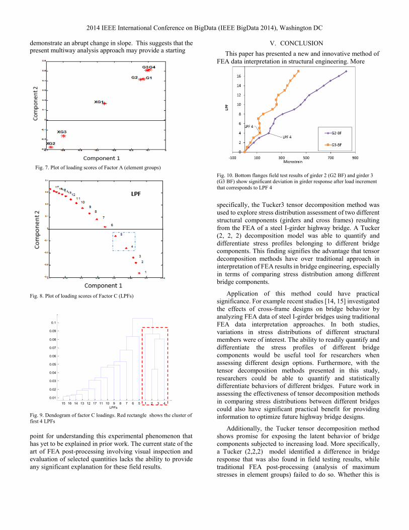
The loading scores (matrix entries) for Factor A (element groups) are displayed in Fig 7. These results show that that cross-frame groups XG2 and XG3 have high negative loading scores in Component 1, while girders groups have high positive loadings scores in Component 2. The high positive scores in Component 2 for Factor A correspond to the widest spread in stress distribution, while the high negative scores in Component 1 correspond to the narrowest spread in stress distribution. The stress profiles show that bottom flange of Girder 4 (see Fig 5, plot G4 BF), has the widest spread of stress distribution of all groups; the tensor decomposition confirms this visual conclusion by quantifying that the bottom flange of girder (G4 in Fig. 7) also has the highest positive score for Component 2 of all element groups. Conversely, cross-frame element group XG2 (Fig. 7) has the highest negative scores in Component 1 and narrowest spread of stress distribution as it can be seen in Fig. 5. This shows one means in which multiway analysis can be used to readily quantifying differences in the behavior of or load sharing between different members.

The loading scores for Factor C (LPFs) are presented in Figure 8. Results show that high positive scores in Component 1 and high negative scores in Component 2 correspond to low LPFs, while high positive score in Component 2 correspond to large LPFs. To further explore this behavior, a hierarchical clustering of the factor C loadings was performed. The results are presented in the form of a dendogram in Fig. 9. A dendogram is a tree like diagram used to exemplify group clustering. The horizontal arrangement of the branches in the dendogram indicates which points are most similar to each other. The height of points in the dendogram indicates the degree of difference among the points. The dendogram shows that the Factor C scores are clustered in two main groups, with one primary branch (when viewed from the top down and marked by red dashed rectangle in Fig. 9) consists of LPFs 1 to 4 and the second primary branch consists of LPFs 5 to 17. This suggests a deviation in behavior between LPF 4 and LPF 5 (which is also marked by the dashed rectangle in Fig. 8). The height of these two branches of the dendogram also indicates a large difference between the two clustering groups.

These results were somewhat unexpected because a linear elastic response of all element types considered is expected in this range of loading. Furthermore, the visible stress distributions shown in Fig. 5 fail to display any anomalies throughout the loading range. In order to further investigate this finding, the results of the tensor analysis were compared to field data from Bridge 7R [13]. The bottom flange results from Girder 2 and Girder 3 are shown in Fig. 10, which indicate that after LPF 4 these load versus strain curves

(72.91%)


demonstrate an abrupt change in slope. This suggests that the present multiway analysis approach may provide a starting

Fig. 7. Plot of loading scores of Factor A (element groups)

Fig. 8. Plot of loading scores of Factor C (LPFs)

Fig. 9. Dendogram of factor C loadings. Red rectangle shows the cluster of first 4 LPFs

point for understanding this experimental phenomenon that

has yet to be explained in prior work. The current state of the

art of FEA post-processing involving visual inspection and

evaluation of selected quantities lacks the ability to provide

any significant explanation for these field results.

V. CONCLUSION

This paper has presented a new and innovative method of

FEA data interpretation in structural engineering. More

Fig. 10. Bottom flanges field test results of girder 2 (G2 BF) and girder 3 (G3 BF) show significant deviation in girder response after load increment

that corresponds to LPF 4

specifically, the Tucker3 tensor decomposition method was

used to explore stress distribution assessment of two different

structural components (girders and cross frames) resulting

from the FEA of a steel I-girder highway bridge. A Tucker

(2, 2, 2) decomposition model was able to quantify and

differentiate stress profiles belonging to different bridge

components. This finding signifies the advantage that tensor

decomposition methods have over traditional approach in

interpretation of FEA results in bridge engineering, especially

in terms of comparing stress distribution among different

bridge components.

Application of this method could have practical

significance. For example recent studies [14, 15] investigated

the effects of cross-frame designs on bridge behavior by

analyzing FEA data of steel I-girder bridges using traditional

FEA data interpretation approaches. In both studies,

variations in stress distributions of different structural

members were of interest. The ability to readily quantify and

differentiate the stress profiles of different bridge

components would be useful tool for researchers when

assessing different design options. Furthermore, with the

tensor decomposition methods presented in this study,

researchers could be able to quantify and statistically

differentiate behaviors of different bridges. Future work in

assessing the effectiveness of tensor decomposition methods

in comparing stress distributions between different bridges

could also have significant practical benefit for providing

information to optimize future highway bridge designs.

Additionally, the Tucker tensor decomposition method

shows promise for exposing the latent behavior of bridge

components subjected to increasing load. More specifically,

a Tucker (2,2,2) model identified a difference in bridge

response that was also found in field testing results, while

traditional FEA post-processing (analysis of maximum

stresses in element groups) failed to do so. Whether this is

15 16 14 13 12 17 11 10 9 8 7 6 5 1 2 3 4

0.01

0.02

0.03

0.04

0.05

0.06

0.07

0.08

0.09

0.1

LPFs


coincidence or pointing to an underlying change in structural

response that is possible to detect via multiway analysis

requires further evaluation to determine.

REFERENCES

[1] Bathe, K.-J. (1982). Finite element procedures in engineering analysis. Englewood Cliffs, N.J: Prentice-Hall.

[2] Comon, P. (2009). Tensor decompositions, state of the art and applications. ArXiv Preprint arXiv :0905.0454.

[3] Acar, E., Bro, R., & Schmidt, B. (2008). New exploratory clustering tool. Journal of Chemometrics, 22(1), 91-100.

[4] Kolda, T. G., & Bader, B. W. (2009). Tensor decompositions and applications. SIAM Review, 51(3), 455-500.

[5] Bro, R. (1998). Multi-Way Analysis in the Food Industry: Models, Algorithms, and Applications, Doctoral Dissertation, Københavns

Universitet Københavns, Universitet.

[6] McConnell, J., Chajes, M., & Michaud, K. (2014). Field testing of a

decommissioned skewed steel I–Girder bridge: Analysis of system effects.

ASCE Journal of Structural Engineering, in press.

[7] ABAQUS 6.12 User Documentation. (2014). Simulia.

[8] American Association of State Highway and Transportation Officials.

(2012). AASHTO LRFD Bridge Design Specifications, 5th Edition.

American Association of State Highway and Transportation Officials, Washington, D.C.

[9] Shimazaki, H., & Shinomoto, S. (2007). A method for selecting the bin size of a time histogram. Neural Computation, 19(6), 1503-1527.

[10] Van, V. L. H. (1970). Materials science for engineers. Reading, Mass: Addison-Wesley Pub. Co.

[11] Matlab R2014. (2014) Mathworks.

[12] Singh, K. P., Malik, A., Singh, V. K., & Sinha, S. (2006). Multi-way

data analysis of soils irrigated with wastewater–A case study. Chemometrics and Intelligent Laboratory Systems, 83(1), 1-12.

[13] Michaud, K (2011). “Evaluating Reserve Bridge Capacity Through Destructive Testing of a Decommissioned Bridge”, Master Thesis,

University of Delaware.

[14] Radovic, M., McConnell, J. (2014). Evaluation of Cross -frame

Designs for Highly Skewed Steel I-Girder Bridges. Proceedings of 31st Annual International Bridge Conference. IBC 14-47, 407-415.

[15] McConnell, J., Radovic, M., and Ambrose, K. (2014). Cross-Frame Forces in Skewed Steel I-Girder Bridges: Field Measurements and Finite

Element Analysis. University of Delaware Center for Bridge Engineering,

Final Report to Delaware Department of Transportation.

Evaluating Structural Engineering Finite Element Analysis Data Using Multiway Analysis

Documents

Transcript of Evaluating Structural Engineering Finite Element Analysis Data Using Multiway Analysis