Advances in Water Resources 29 (2006) 1341–1350

www.elsevier.com/locate/advwatres

Stochastic modelling of DO and BOD components in a streamwith random inputs

Fulvio Boano *, Roberto Revelli, Luca Ridolfi

Department of Hydraulics, Transports, and Civil Infrastructures—Politecnico di Torino, Corso Duca degli Abruzzi 24, 10129 Turin, Italy

Received 9 September 2005; received in revised form 7 October 2005; accepted 16 October 2005Available online 1 December 2005

Abstract

A stochastic model for the evolution of DO and BOD components along a river with independent BOD point inputs has beendeveloped. The model examines the case in which the initial conditions and the concentrations of the inputs are affected by uncer-tainty. The uncertain quantities are modelled as random variables, for which any kind of probability distribution can be adopted.The possibility of separately analysing the different components of BOD (e.g., CBOD and NBOD) is included. A semi-analyticalexpression for the joint probability density function (pdf) of the concentrations is derived. The application of this relationshipgreatly reduces the computation efforts compared to Monte-Carlo methods. A procedure for the analytical determination of theconcentration moments is also described.� 2005 Elsevier Ltd. All rights reserved.

PACS: 92.40.Qk

Keywords: River pollution; BOD; Dissolved oxygen; Stochastic modelling; Uncertain inputs

1. Introduction

One of the most important anthropogenic impacts onthe environment is the disposal of wastes that originatefrom human activities. Among liquid wastes, wastewa-ters contaminated by biodegradable pollutants consti-tute a common by-product of both civil settlementsand industrial facilities. This class of substances isknown as biochemical oxygen demand (BOD), as it ismade up of carbonaceous and nitrogenous matter thatis oxidized by aerobic microorganisms, resulting in adeficit in the concentration of dissolved oxygen (DO)in the water body. Since small quantities of suchcontaminants are often present even in pristine environ-ments, the discharge of BOD contaminated wastewaters

0309-1708/$ - see front matter � 2005 Elsevier Ltd. All rights reserved.doi:10.1016/j.advwatres.2005.10.007

* Corresponding author. Fax: +39 011 564 5698.E-mail addresses: fulvio.boano@polito.it (F. Boano), roberto.

revelli@polito.it (R. Revelli), luca.ridolfi@polito.it (L. Ridolfi).

into natural rivers has become a consolidated habit.However, excessive BOD loads are detrimental for thequality of river water, as the resulting low DO concen-tration makes the river unsuitable for the life of floraand fauna. Consequently, a number of models for theprediction of water quality modifications due to BODdischarges have been formulated.

The first models, starting from the basic work byStreeter and Phelps [1], adopted a deterministicapproach. The main feature of deterministic models isthat all the characteristics of the system are consideredto be known, that is, boundary and initial conditionsand model parameters are assigned a unique value,which is considered to be exact. The value of contami-nant concentration C along the river at any time canthen be computed. However, it is commonly recognizedthat there are many sources of uncertainty that affectcontaminant dynamics. This uncertainty is mainly dueto three aspects: firstly, the natural heterogeneity of real

1342 F. Boano et al. / Advances in Water Resources 29 (2006) 1341–1350

rivers is often difficult to synthesize in a single value of aparameter, and uncertainty on the values of initial andboundary conditions (e.g., source terms) is often pres-ent. Secondly, calibration measurements that are usedfor the estimation of the values of parameters are alwaysaffected by experimental errors. Finally, simple modelscan be inadequate to describe the complexity of theactual physical phenomena that occur in rivers.

In order to consider these approximations, probabi-listic methods have been developed over the last twodecades, that describe the uncertain initial and boundaryconditions and parameters as random variables or sto-chastic processes. These kinds of models can be groupedinto three main typologies: first-order error analysis,Monte-Carlo methods, and stochastic differential equa-tions. First-order error analysis is a simple approachthat gives an estimate of the variance of the concentra-tion as a function of the moments of the uncertainparameters (e.g., [2–4]). The limit of this approach isthat its results are not valid for non-linear models andthat only the concentration variance is provided. TheMonte-Carlo method is a popular numerical techniquethat is often used to evaluate the probability densityfunction (pdf) of the concentration C (e.g., [2,5–7]);however, it often requires great computational efforts,and its results are generally valid only for the specificsimulated case. Stochastic differential equations derivefrom deterministic models in which model parameters,initial and boundary conditions are described by ran-dom variables or stochastic processes [8,9]. Even thoughthis approach implies greater analytical difficulties thanthe previous methods, it allows—at least for simplemodels—analytic expressions to be obtained for thepdf and moments of the concentrations (e.g., [10–19]).A review on the various applications of stochastic mod-els to contaminant fate problems can be found in [20].

This paper describes a stochastic model for the studyof the evolution of DO and BOD components in a riverwith BOD point inputs. Such inputs can represent dis-charges from wastewater treatment plants or industrialfacilities, as well as small, polluted tributaries. The casein which the main sources of uncertainty are the BODconcentration of the inputs and the concentrations ofboth BOD and DO at the initial section of the modelledreach is addressed. The uncertainties due to oversimpli-fications of the actual physical processes are notaddressed. This model represents the extension of a pre-vious work [20] in which only the total BOD evolutionwas described, and it is based on a system of stochasticdifferential equations with random boundary condi-tions. The model allows (i) any kind of probabilisticdistribution of the random inputs to be chosen, (ii)semi-analytical expressions of the pdf of the BOD andDO concentrations to be obtained, and (iii) differenttypes of BOD components (e.g., carbonaceous andnitrogenous BOD) to be considered. The possibility of

choosing any statistical distribution for the random con-centrations is important because greater flexibility—with respect to the often adopted Gaussian distribu-tion—is thus obtained. The semi-analytical solutionconsists of a multiple integral, which can be evaluatedthrough numerical methods (when the analytical resolu-tion is not attainable) in a very fast way. Finally, it canbe important to separately analyse the different classesof substances (e.g., carbonaceous and nitrogenous) thatBOD is composed of, since they play different roles asnutrients in the river ecosystem [21,22].

2. Description of the model

The river is approximated as a uniform, steady, tur-bulent open channel flow with constant discharge, Q,and mean velocity, U. A reference axis, x, that coincideswith the stream direction, is defined. It is assumed thatthe effects of dispersion are negligible compared withthose of advection and reactions, so that the river canbe modelled as a plug-flow system [21]. If a Lagrangianpoint of view is adopted, it is possible to follow a genericslice X of infinitesimal width as it moves along thestream; let t = x/U be the travel time of X, and C(t)and O(t) its section-averaged concentrations of BODand DO, respectively. Position, x, is therefore replacedby travel time, t. It should be noted that, since disper-sion is neglected, each flow element can be regarded asindependent of the other elements.

Let us assume that n independent point inputs ofBOD are located at xi, i = 1, . . . ,n; for the sake of sim-plicity, let x1 = 0. The BOD concentration of the genericith input is assumed to be uncertain, and is thereforedescribed as a random variable with known pdf pi(Ci).In fact, in several cases the concentration of an inputvaries in time in a non-deterministic way. This can bethe case, for instance, of a sewer as well as an industrialdischarge. The concentration pdf should be determinedon the basis of the specific production cycle and technol-ogies. It should be noticed that no restriction is set to theshape of the pdfs pi(Ci), and non-Gaussian distributionscan thus be chosen to describe skewed and/or non-neg-ative valued pdfs.

The initial river concentrations of BOD and DO atx = 0, namely C0 and O0, are also treated as randomvariables, with joint pdf p(C,O, t = 0) = p0(C0,O0). Theinputs pi(Ci) are considered to be independent, i.e., nocorrelation exists among the random variables Ci,i = 1, . . . ,n. On the contrary, some degree of correlationgenerally exists between the initial concentrations C0 andO0. The water discharge Qi of each input is assumed to bemuch smaller than the river discharge Q, so that the riverdischarge remains constant along the examined reach.

When the element X passes the ith input, at timeti = xi/U, it receives a random amount of BOD that

x x x xDistance

BO

D

(a)

Δ1

1

x x x x

Distance

DO

(b)

Δ4Δ3

Δ2

2 3 4

1 2 3 4

=0

=0

Fig. 1. Qualitative evolution of BOD (a) and DO (b) concentrationalong the stream.

F. Boano et al. / Advances in Water Resources 29 (2006) 1341–1350 1343

causes an increment DCi in the river BOD concentration.

This random increment can therefore be related to theBOD concentration of the input Ci

DCi ¼

Qi

QCi ð1Þ

as long as Qi� Q, and the corresponding pdf piðDCi Þ of

the random increment can be defined. In this work, theconcentrations Ci have therefore been replaced by thecorresponding random jumps DC

i .The resulting situation is sketched in Fig. 1a: when-

ever the element X passes an input, it ‘‘samples’’ a valuefrom the pdf piðDC

i Þ, and eventually undergoes a series ofrandom jumps.

It is assumed that the river receives no DO from theinputs. This simplification is acceptable because the DOconcentration is limited by the saturation concentrationOsat (which is a function of the water temperature, and isassumed to be constant); as shown by Eq. (1), the DOinput concentration would be further reduced by thedilution factor Qi/Q� 1. As a result, the river wouldreceive a very small amount of DO, which can thereforebe neglected. This assumption also leads to a prudentialunderestimation of the river DO concentration.

Let us now define the ith subreach as the river seg-ment between two consecutive inputs located at xi andxi+1, that is, x 2 [xi,xi+1]. As the element X moves alongthe ith subreach, BOD and DO undergo a series of bio-logical reactions and reaeration phenomena that aredescribed by the well-known model proposed by [1]

dCdt¼ �kC

i C; ð2Þ

dDdt¼ kC

i C � kAi D; ð3Þ

where the DO is replaced by the river DO deficitD(t) = Osat � O(t), C(t) is the river BOD concentration,t is the travel time, kC

i is the first-order decay constantfor the ith subreach, and kA

i is the reaeration constantfor the ith subreach. Even though simple, the Streeter-Phelps model is recognized as being able to describethe main features of BOD and DO dynamics in rivers.More complex versions of the model have been pro-posed to consider other possible sources, sinks andchemical components. An extension of the model thatis considered in this paper (see, e.g., [21,23–25]) is

dCdt¼ �kC

i C; ð4Þ

dNdt¼ �kN

i N ; ð5Þ

dDdt¼ kC

i C þ kNi N � kA

i D; ð6Þ

where C(t) and N(t) are now the carbonaceous (CBOD)and nitrogenous (NBOD) components of BOD, respec-tively, and kC

i and kNi the respective decay constants for

the ith subreach. It should be understood that the totalBOD concentration is now given by the sum of C and N,whereas in Eqs. (2) and (3), the total BOD concentrationis simply given by C. This subdivision can be of interestbecause the two species are important as macronutrientsin the stream ecology [21,22]. The extension of the mod-el to subdivisions into more components—e.g., fast- andslow-decaying BOD—is straightforward, and is notshown here.

The qualitative behaviour of DO along a subreach isshown in Fig. 1b. While the BOD concentration under-goes a monotonic decay (compare Fig. 1b with a), afteran initial phase of decay the concentration of DOreaches a minimum (provided that the subreach is longenough), after which the reaeration process leads to anasymptotic increase towards the saturation concentra-tion Osat.

The overall dynamics of BOD and DO (i.e., model(2)–(3)), with the addition of the random source term(1), can be described by the system of stochastic differen-tial equations

dX!ðtÞdt¼ K!

X!ðtÞ þ P

!ðtÞ; t > 0 ð7Þ

in which

X!ðtÞ ¼

CðtÞDðtÞ

� �; K!¼ �kC

i 0

kCi �kA

i

" #;

P!ðtÞ ¼

Pni¼1dðt � tiÞDC

i

0

" #;

where d( Æ ) is the Dirac delta function, and P!ðtÞ repre-

sents the point source term corresponding to the inputsat t = ti, i = 1, . . . ,n. In this paper, it is assumed that the

1344 F. Boano et al. / Advances in Water Resources 29 (2006) 1341–1350

input pdfs piðDCi Þ, i = 1, . . . ,n and the joint pdf of the ini-

tial concentrations p(C0,D0) � p0(C,D) at t = 0 areknown. It should be noticed that the initial concentra-tions C0 and D0 can be correlated. The aim of the paperis to solve Eq. (7) for the joint probability density func-tion pðX!; tÞ ¼ pðC;D; tÞ at a generic travel time t.

For the case of three chemical components (i.e.,model (4)–(6)), Eq. (7) holds together with

X!ðtÞ ¼

CðtÞ

NðtÞ

DðtÞ

2664

3775; K

!¼�kC

i 0 0

0 �kNi 0

kCi kN

i �kAi

2664

3775;

P!ðtÞ ¼

Pni¼1dðt � tiÞDC

iPni¼1dðt � tiÞDN

i

0

2664

3775;

where DCi and DN

i are, respectively, the random incre-ments in CBOD and NBOD due to the ith input,i = 1, . . . ,n. In this case, the input pdfs piðDC

i ;DNi Þ and

the initial pdf p(C0,N0,D0) � p0(C,N,D) are assumedto be known. Since each input discharges both CBODand NBOD, the random jumps DC

i and DNi are expected

to be correlated.

3. Solutions

The steps to determine the pdf pðX!; tÞ and themoments of the concentration distribution are presentedin this section. Since, from a mathematical point of view,model (4)–(6) is similar to the simpler model (2)–(3),with only the addition of the independent equation (5),the solutions are derived for the simpler case of twocomponents. The results for three components are givenmore briefly.

3.1. Probability density functions

3.1.1. Two component model

Let us consider the generic point downstream to thenth input. The formal solution of the linear stochasticdifferential Eq. (7) can be written as

CðtÞ ¼ C0e�c1;nþ1 þXn

j¼1

DCj e�cj;nþ1 ; ð8Þ

DðtÞ ¼ D0e�a1;nþ1 þ C0uC1;n þ

Xn

j¼1

DCj uC

j;n; ð9Þ

where t > tn, and with

cj;i ¼Xi�2

‘¼j

kC‘ ðt‘þ1 � t‘Þ þ ð1� di;nþ1ÞkC

i�1ðti � ti�1Þ

þ di;nþ1kCi�1ðt � ti�1Þ; ð10Þ

aj;i ¼Xi�2

‘¼j

kA‘ ðt‘þ1 � t‘Þ þ ð1� di;nþ1ÞkA

i�1ðti � ti�1Þ

þ di;nþ1kAi�1ðt � ti�1Þ; ð11Þ

uCj;i ¼

Xi

‘¼j

qC‘ e�cj;‘þ1�a‘þ1;iþ1 � e�cj;‘�a‘;iþ1ð Þ; ð12Þ

qCi ¼

kCi

kAi � kC

i

; ð13Þ

where di,j is the Kronecker delta function. It should benoticed that ci,i = ai,i = 0.

In order to derive the concentration pdf at a generictravel time, it is more straightforward to split Eqs. (8)and (9) into two parts, that correspond to two distinctphases of the travelling of an element X along the river:(i) the movement in the subreaches between two consec-utive inputs and (ii) the passages in correspondence tothe inputs.

Let us first consider the generic ith subreach betweenthe ith and the (i + 1)th inputs and define pðC;D; t�i Þ andpðC;D; tþi Þ as the joint pdf of the BOD and DO deficitimmediately upstream and downstream to the ith input.In this subreach, the dynamics of C(t) and D(t) is deter-ministic and is governed by Eqs. (2) and (3), whose solu-tion is

X!ðtÞ ¼ A

!ðtÞ � X!

0; t 2 ½tþi ; t�iþ1�; ð14Þ

where

X!ðtÞ ¼

CðtÞDðtÞ

� �; X!

0 ¼Cðtþi ÞDðtþi Þ

� �;

A!ðtÞ ¼ e�kC

i ðt�tiÞ 0

qCi ðe�kC

i ðt�tiÞ � e�kAi ðt�tiÞÞ e�kA

i ðt�tiÞ

" #.

ð15Þ

Eq. (14) establishes a deterministic link between the up-stream concentration vector, X

!0, and the downstream

one, X!ðtÞ. It is then possible to write [8]

pðX!; tÞ ¼ jA!�1

j � pðX!0 ¼ A!�1

X!Þ. ð16Þ

Eq. (16) can be applied to derive the concentration pdfat a generic t 2 ½tþi ; t�iþ1�, given the pdf at tþi . Fort ¼ t�iþ1, in particular, it provides the relationship be-tween pðX!; tþi Þ and pðX!; t�iþ1Þ, that is, the overall effecton the concentration pdf of the travelling of X throughthe ith subreach. The introduction of (15) into (16) leadsto

pðC;D; t�iþ1Þ ¼ eci;iþ1þai;iþ1

� p Ceci;iþ1 ;Deai;iþ1 þ CqCi ðeci;iþ1 � eai;iþ1Þ; tþi

� �;

ð17Þ

where cj,i, aj,i, and qCi have been defined by (10), (11),

and (13), respectively.Eq. (17) provides the desired link between the concen-

tration pdfs at the upstream and downstream ends of the

F. Boano et al. / Advances in Water Resources 29 (2006) 1341–1350 1345

ith subreach. A relationship between the two concentra-tion pdfs at t�i and tþi is now sought for the second step.When the element X passes the ith input, its BOD con-centration increases by a random quantity DC

i which isextracted from the corresponding distribution piðDC

i Þ,while the DO concentration remains unchanged:

X!ðtþi Þ ¼ X

!ðt�i Þ þ D!

i; ð18Þ

in which

D!

i ¼DC

i

0

" #.

The resulting downstream joint pdf is given by the con-volution of all the possible upstream concentrations to-gether with all the possible random jumps, that is,

pðC;D; tþi Þ ¼Z C

0

pðC � DCi ;D; t

�i ÞpiðDC

i ÞdDCi . ð19Þ

It is now possible to recursively apply (for i = 1, . . . ,n)Eqs. (17) and (19), thus obtaining the analytical solutionat a generic travel time. The solution at the generic t > tn

is

pðC;D; tÞ ¼ ec1;nþ1þa1;nþ1

Z fn

0

� � �Z f1

0

p0½f1 � DC1 ; h1�

� p1ðDC1 ÞdDC

1 � � � pnðDCn ÞdDC

n ; ð20Þ

where

fj ¼Cecj;jþ1 ; j ¼ n;

ðfjþ1 � DCjþ1Þecj;jþ1 ; j ¼ n� 1; . . . ; 1

(ð21Þ

hj ¼CqC

j ðecj;jþ1 � eaj;jþ1Þ þ Deaj;jþ1 ; j ¼ n;

ðfjþ1 � DCjþ1ÞqC

j ðecj;jþ1 � eaj;jþ1Þ þ eaj;jþ1 hjþ1;

j ¼ n� 1; . . . ; 1;

8><>: ð22Þ

and cj,i, aj,i, and qCi are given by (10), (11), and (13),

respectively.The convolution integrals in Eq. (20) can only be ana-

lytically solved for certain distributions (see [20]). Whenanalytical resolution is not possible, the numerical reso-lution of Eq. (20) is very fast, and is generally consider-ably quicker than the application of a Monte-Carlomethod. This happens because the contribution of then inputs is simply evaluated by n convolutions, whilethe number of required Monte-Carlo samples wouldbe equal to cn, where c is the number of samples for eachinput pdf. Moreover, FFT-based algorithms exist thatare extremely efficient in solving convolution integrals[26].

3.1.2. Three component model

The case of three substances is analogous: the formalsolution of Eq. (7) at the generic t > tn is

CðtÞ ¼ C0e�c1;nþ1 þXn

j¼1

DCj e�cj;nþ1 ; ð23Þ

NðtÞ ¼ N 0e�m1;nþ1 þXn

j¼1

DNj e�mj;nþ1 ; ð24Þ

DðtÞ ¼ D0e�a1;nþ1 þ C0uC1;n þ N 0u

N1;n

þXn

j¼1

DCj uC

j;n þXn

j¼1

DNj uN

j;n; ð25Þ

where cj,i, aj,i, uCj;i, and qC

i are still given by (10)–(13), and

mj;i ¼Xi�2

‘¼j

kN‘ ðt‘þ1 � t‘Þ þ ð1� di;nþ1ÞkN

i�1ðti � ti�1Þ

þ di;nþ1kNi�1ðt � ti�1Þ; ð26Þ

uNj;i ¼

Xi

‘¼j

qN‘ ðe�mj;‘þ1�a‘þ1;iþ1 � e�mj;‘�a‘;iþ1Þ; ð27Þ

qNi ¼

kNi

kAi � kN

i

; ð28Þ

where dj,i is the Kronecker delta function. It should benoticed that mi,i = 0.

For the ith subreach, the solution of (4)–(6) is stillgiven by Eq. (14) with

X!ðtÞ¼

CðtÞNðtÞDðtÞ

264

375; X!

0¼Cðtþi ÞNðtþi ÞDðtþi Þ

264

375;

A!ðtÞ¼

e�ci;iþ1 0 0

0 e�mi;iþ1 0

qCi ðe�ci;iþ1 � e�ai;iþ1Þ qN

i ðe�mi;iþ1 � e�ai;iþ1Þ e�ai;iþ1

264

375;ð29Þ

where t 2 ½tþi ; t�iþ1�. The introduction of (29) into (16)gives

pðX!; t�iþ1Þ ¼ eci;iþ1þmi;iþ1þai;iþ1 � p Ceci;iþ1 ;Nemi;iþ1 ;Deai;iþ1½þCqC

i ðeci;iþ1 � eai;iþ1Þ þ NqNi ðemi;iþ1 � eai;iþ1Þ; tþi

�;

ð30Þ

which is analogous to (17).At the ith input, Eq. (18) still holds with

D!

i ¼DC

i

DNi

0

264

375.

The pdf immediately downstream of the ith input istherefore given by

pðX!; tþi Þ ¼Z C

0

Z N

0

pðC � DCi ;N � DN

i ;D; t�i Þ

� piðDCi ;D

Ni ÞdDC

i dDNi . ð31Þ

1346 F. Boano et al. / Advances in Water Resources 29 (2006) 1341–1350

Finally, from (30) and (31), the analytical solution forthe joint pdf of the concentrations at t > tn can be foundas

pðC;N ;D; tÞ ¼ ec1;nþ1þm1;nþ1þa1;nþ1

�Z fn

0

Z gn

0

� � �Z f1

0

Z g1

0

p0½f1�DC1 ;g1�DN

1 ;h1�

� p1ðDC1 ;D

N1 ÞdDC

1 dDN1 � � �pnðDC

n ;DNn ÞdDC

n dDNn ;

ð32Þ

where fj is still given by Eq. (21), and

gj ¼Nemj;jþ1 ; j ¼ n;

ðgjþ1 � DNjþ1Þemj;jþ1 ; j ¼ n� 1; . . . ; 1;

(ð33Þ

hj ¼

CqCj ðecj;jþ1 � eaj;jþ1Þ þ NqN

j ðemj;jþ1 � eaj;jþ1Þ

þDeaj;jþ1 ; j ¼ n;

ðfjþ1 � DCjþ1ÞqC

j ðecj;jþ1 � eaj;jþ1Þ

þ ðgjþ1 � DNjþ1ÞqN

j ðemj;jþ1 � eaj;jþ1Þ

þ eaj;jþ1 hjþ1; j ¼ n� 1; . . . ; 1.

8>>>>>>>><>>>>>>>>:

ð34Þ

3.2. Moment analysis

3.2.1. Two component model

The linearity of Eq. (7) allows the moments of theconcentration distribution to be obtained. The momentsprovide less information than the joint pdf pðX!; tÞ, butthey synthesize the main features of the concentrationdistributions and can thus be useful for practical pur-poses. The method herein described allows the momentsto be analytically derived in a straightforward way.

Eqs. (8) and (9) show how each input DCi and the ini-

tial concentrations C0 and D0 give independent contri-butions to the final concentrations C(t) and D(t). Inorder to explicit these contributions, Eqs. (8) and (9)can be rewritten as

CðtÞ ¼ Y C0þXn

j¼1

Y DCj; ð35Þ

DðtÞ ¼ ZD0þ ZC0

þXn

j¼1

ZDCj; ð36Þ

where

Y C0¼ C0e�c1;nþ1 ; Y DC

j¼ DC

j e�cj;nþ1

and

ZD0¼ D0e�a1;nþ1 ; ZC0

¼ C0uC1;n; ZDC

j¼ DC

j uCj;n.

The terms in Eqs. (35) and (36) are independent randomvariables whose distributions can be evaluated as

pðY C0Þ ¼ ec1;nþ1 p0ðC0ec1;nþ1Þ; ð37Þ

pðY DCjÞ ¼ ecj;nþ1 pjðDC

j ecj;nþ1Þ; j ¼ 1; . . . ; n; ð38Þ

pðZD0Þ ¼ ea1;nþ1 p0ðD0ea1;nþ1Þ; ð39Þ

pðZC0Þ ¼ 1

uC1;n

p0

C0

uC1;n

!; ð40Þ

pðZDCjÞ ¼ 1

uCj;n

pj

DCj

uCj;n

!; j ¼ 1; . . . ; n; ð41Þ

where p0ðCÞ ¼Rþ1

0p0ðC;DÞdD and p0ðDÞ ¼

Rþ10

pðC;DÞdC are the marginal distributions of C0 andD0, respectively, and cj,i, aj,i, and uC

j;i are still definedby (10)–(12).

Since C(t) and D(t) are given by the sum of indepen-dent random variables, their distributions can be foundas the convolution integral of the pdfs defined in (37)–(41). Let us now define the Laplace transform

L½pðCÞ� ¼ P CðsÞ ¼Z 1

0

pðCÞe�sC dC;

and recall the well-known theorem [27]

L½pðaCÞ� ¼ 1

aP C

sa

� �; ð42Þ

where a is a real number. The application of the Laplacetransform to Eqs. (35) and (36), together with (37)–(42),gives

P CðsÞ ¼ P C0ðse�c1;nþ1Þ �

Yn

j¼1

PDCjðse�cj;nþ1Þ; ð43Þ

P DðsÞ ¼ P D0ðse�a1;nþ1Þ � P C0

ðsuC1;nÞ �

Yn

j¼1

PDCjðsuC

j;nÞ; ð44Þ

where cj,i, aj,i, and uCj;i are still given by (10)–(12).

Even though the Laplace antitransform of Eqs. (43)and (44) can seldom be evaluated, the moments of themarginal pdfs of C(t) and D(t) can be derived, providedthe involved distributions can be Laplace transformed.First, we recall that

lCj ðtÞ �

Z þ1

0

CjðtÞpðC; tÞdC ¼ ð�1ÞjdjP C

dsj

����s¼0

; ð45Þ

lDj ðtÞ �

Z þ1

0

DjðtÞpðD; tÞdD ¼ ð�1ÞjdjP D

dsj

����s¼0

; ð46Þ

where lCj ðtÞ and lD

j ðtÞ are the jth order non-central mo-ments of C(t) and D(t), respectively, at the generic traveltime t.

It is also possible to derive the corresponding centralmoments, mj(t), as (e.g., [28])

m2 ¼ r2 ¼ l2 � l21; ð47Þ

m3 ¼ l3 � 3l1l2 þ 2l31; ð48Þ

m4 ¼ l4 � 4l1l3 þ 6l21l2 � 3l4

1; ð49Þ

and so on.

Table 1Locations and mean values of the initial concentrations (p0) and of therandom jumps (p1,p2,p3,p4)

x (km) lC (mg/L) lN (mg/L) lD (mg/L)

p0 0 2 1 2p1 0 4 2 –p2 30 3 2.5 –p3 40 2 3 –p4 60 2 3 –

F. Boano et al. / Advances in Water Resources 29 (2006) 1341–1350 1347

3.2.2. Three component model

The same passages can be repeated for the case ofthree components, thus obtaining the Laplace trans-forms of the three concentration pdfs. The equationfor PC(s) is formally identical to (43), while the otherexpressions are

P N ðsÞ ¼ P N0ðse�m1;nþ1Þ �

Yn

j¼1

PDNjðse�mj;nþ1Þ; ð50Þ

P DðsÞ ¼ P D0ðse�a1;nþ1Þ � P C0

ðsuC1;nÞ � P N0

ðsuN1;nÞ

�Yn

j¼1

½PDCjðsuC

j;nÞPDNjðsuN

j;nÞ�; ð51Þ

where aj,i, uCj;i, mj,i, and uN

j;i are still defined as in (11),(12), (26), and (27), respectively.

The non-central moments of the concentrations canbe derived according to (45), (46), and

lNj ðtÞ ¼ ð�1Þjd

jP N

dsj

����s¼0

; ð52Þ

and the central moments can be evaluated with (47)–(49).

4. Examples

In this section, the proposed solution has beenapplied to a hypothetical stream with a cross-sectionallyaveraged velocity U = 0.2 m/s. The three-componentmodel was used, and the total BOD was split into its car-bonaceous and nitrogenous components C and N,respectively. Two different situations were considered:first, the case of three independent BOD inputs was ana-lyzed. The inputs were separated by a constant distanceof 30 km, with the first input located at x1 = 0 km. Sec-ondly, a fourth input was added at 40 km. Each inputwas assumed to have a bivariate lognormal distributionpiðDC

i ;DNi Þ, i = 1, . . . ,n, for the random increments [29].

A correlation coefficient q = 0.9 was chosen to considerthe simultaneous discharge of CBOD and NBOD. Forboth cases, a trivariate lognormal distributionp0(C,N,D) has been adopted for the in-stream concen-trations at x = 0. Again, a correlation coefficientq = 0.9 between CBOD and NBOD was assumed. Themean values for each distribution have been summarizedin Table 1, while the same coefficient of variationCV = 0.2 was adopted for all the components of eachdistribution. The value Osat = 11 mg/L for the DO satu-ration concentration was used; it approximately corre-sponds to a water temperature of 10 �C. Finally, thedecay rates kC

i ¼ 5� 10�6 s�1 and kNi ¼ 2� 10�6 s�1

were chosen for the CBOD and the NBOD, respectively,while the reaeration rate kA

i ¼ 10�5 s�1 was adopted. Forthe sake of simplicity, kC

i , kNi and kA

i were considered tobe constant along the whole examined length of the

stream. It should be worth noting that the describedproblem could also be solved using a Monte-Carloapproach, but not without great computational efforts;for instance, if each component is sampled 102 times(which is the minimum for a significant statistical anal-ysis), then a total of 1018 simulations would be required.

Eqs. (30) and (31) were recursively applied to find thepdf of the concentrations of the three chemical compo-nents along the stream. The joint pdf p(C,N,D) wasevaluated every 1.5 km, and it was used to derive themarginal distributions and the values of the moments.The marginal pdfs of the three concentrations atx = 50 km have been reported in Fig. 2a and b, for thethree and four inputs cases, respectively. These pdfscan be useful to evaluate the uncertainty in the in-streamconcentration due to the ensemble of all the possibleinputs. The effects of the introduction of the fourthinput at x = 40 km can be observed from a comparisonof the two figures: at the considered location, both theCBOD and, to a greater extent, the NBOD pdfs shiftedtowards higher mean concentrations and have increasedtheir variances, while the DO pdf has shifted towardslower concentrations without any appreciable modifica-tion of its variance.

The CBOD evolution along the river is shown inFig. 3a and b; the series of jumps and decays describedin the previous sections can be appreciated. The overalluncertainty in the CBOD concentration is representedby the 80% confidence interval, that is given by the 0.1and 0.9 quantiles. It should be noticed that the inputsact as sources of uncertainty for the CBOD concentra-tion, since the width of the confidence interval suddenlyincreases in correspondence to them. On the other hand,the uncertainty gradually decreases along each subreach,since the concentration asymptotically tends to the (cer-tain) zero value. A comparison of the two figures showsthat the CBOD concentration increased in the centralpart of the examined reach, while only small differencescan be observed between the two cases at the end of thereach, where most of the CBOD had already been oxi-dized by the microorganisms. It should also be noticedthat the uncertainty was not substantially modified bythe presence of the new input at 40 km.

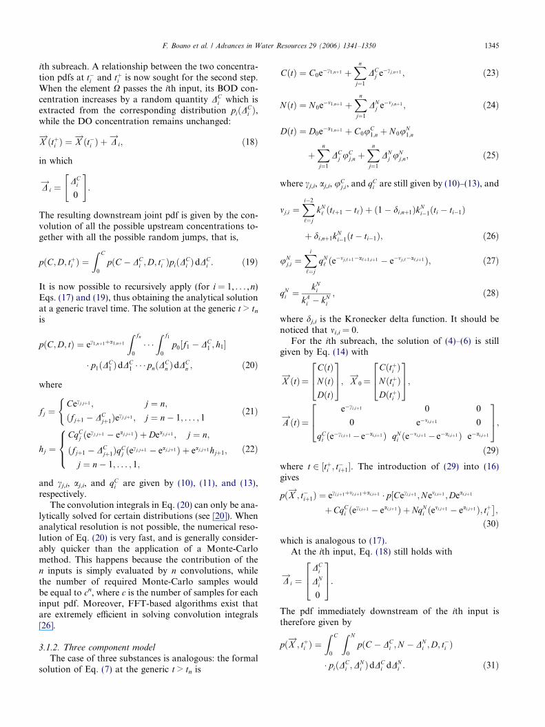
Fig. 4a and b shows the evolution of NBOD concen-tration along the stream. The qualitative behaviour is

0 2 4 6 8 10 120

0.2

0.4

0.6

0.8

1

1.2

1.4

Concentration (mg/L)

pdf

(a)

0 2 4 6 8 10 120

0.2

0.4

0.6

0.8

1

1.2

1.4

Concentration (mg/L)

pdf

(b)

Fig. 2. Marginal probability density functions of CBOD (continuousline), NBOD (dashed line), and DO (dash-dotted line) concentrationsat x = 50 km. Case of three (a) and four (b) point inputs.

0 20 40 60 80 100 1200

1

2

3

4

5

6

7

8

x (km)

CB

OD

(mg/

L)

(a)

0 20 40 60 80 100 1201

2

3

4

5

6

7

8

x (km)

CB

OD

(mg/

L)

(b)

Fig. 3. CBOD mean value (continuous line), 0.1 and 0.9 quantiles(dashed lines) along the stream. Case of three (a) and four (b) pointinputs.

1348 F. Boano et al. / Advances in Water Resources 29 (2006) 1341–1350

similar to that of the CBOD, but the impact of theadded input on the water quality is greater than in theCBOD case, due to the combined effect of the higher dis-charged mass and of the slower decay reactions.

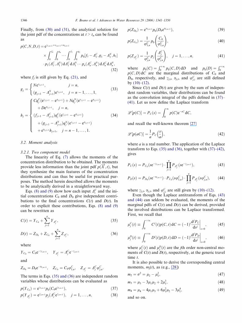
The mean DO concentration along the river, with itsconfidence interval, has been represented in Fig. 5a andb. The sequence of DO microbial consumption and rea-eration is evident; both the mean concentration and thewidth of the confidence interval are continuous, buttheir spatial derivatives are discontinuous in correspon-dence to the inputs. It should be noticed how the addi-tion of the fourth input at x = 40 km affects the DOconcentration to a great extent, increasing the overallmass of nutrients and thus the rate of oxygen consump-tion by the microorganisms. It should also be observedthat the non-monotonic behaviour of the width of theconfidence interval leads to high uncertainty levels incorrespondence to the local minima, which representthe most critical points for the water quality.

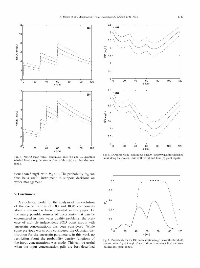
Since the availability of dissolved oxygen is of crucialimportance for an ecosystem, a useful tool for the anal-ysis of river water quality is the probability Pth that theDO goes below a critical threshold Oth or, equivalently,the probability that the DO deficit exceeds the thresholdvalue Dth = (Osat � Oth)

P thðtÞ ¼Z þ1

Dth

pðD; tÞdD. ð53Þ

This probability can easily be evaluated from the mar-ginal DO pdf, and it has been represented in Fig. 6 forthe investigated cases. The threshold value Oth = 8 mg/L was chosen. The particular, non-trivial shape of thesefunctions is due to the combined effect of the oxygenconsumption and of the reaeration process. Fig. 6 showsthat the introduction of the fourth input would lead along segment of the river to have lower DO concentra-

0 20 40 60 80 100 1200

2

4

6

8

10

12

x (km)

NB

OD

(mg/

L)

(a)

0 20 40 60 80 100 1200

2

4

6

8

10

12

x (km)

NB

OD

(mg/

L)

(b)

Fig. 4. NBOD mean value (continuous line), 0.1 and 0.9 quantiles(dashed lines) along the stream. Case of three (a) and four (b) pointinputs.

0 20 40 60 80 100 1206

6.5

7

7.5

8

8.5

9

9.5

x (km)

DO

(mg/

L)

(a)

0 20 40 60 80 100 1206

6.5

7

7.5

8

8.5

9

9.5

x (km)

DO

(mg/

L)

(b)

Fig. 5. DO mean value (continuous line), 0.1 and 0.9 quantiles (dashedlines) along the stream. Case of three (a) and four (b) point inputs.

1

F. Boano et al. / Advances in Water Resources 29 (2006) 1341–1350 1349

tions than 8 mg/L with Pth ’ 1. The probability Pth canthus be a useful instrument to support decisions onwater management.

0 20 40 60 80 100 1200

0.2

0.4

0.6

0.8

x (km)

Pth

Fig. 6. Probability for the DO concentration to go below the thresholdconcentration Oth = 8 mg/L. Case of three (continuous line) and four(dashed line) point inputs.

5. Conclusions

A stochastic model for the analysis of the evolutionof the concentrations of DO and BOD componentsalong a stream has been presented in this paper. Ofthe many possible sources of uncertainty that can beencountered in river water quality problems, the pres-ence of multiple independent BOD point inputs withuncertain concentrations has been considered. Whilesome previous works only considered the Gaussian dis-tribution for the uncertain parameters, in this work norestriction about the probability density functions ofthe input concentrations was made. This can be usefulwhen the input concentration pdfs are best described

1350 F. Boano et al. / Advances in Water Resources 29 (2006) 1341–1350

by skewed distributions. Moreover, non-negative valuedpdfs can be chosen, thus avoiding the problem of thenegative tails of Gaussian distributions with high coeffi-cients of variation. Correlations among the differentBOD components that are released by each input werealso included.

The joint DO and BOD concentration pdf can bederived from the proposed semi-analytical expressions.This joint pdf provides complete knowledge about theevolution of the concentrations. For instance, the prob-ability of having a DO concentration below a thresholdlevel can be inferred, thus determining the actual risk ofcritical conditions for the river ecosystem. When thesemi-analytic relationships cannot be analytically evalu-ated and a numerical resolution is needed, our modelallows to take advantage of the properties of convolu-tion, which can be quickly solved using FFT-based algo-rithms. Since each input requires a convolution integral,the computation time grows linearly with the number ofinputs. When the number of inputs is great, the presentmethod may be preferred to a Monte-Carlo approach,for which the computation time exponentially increaseswith the number of inputs to be sampled.

A procedure for the evaluation of the moments ofany order has also been presented. This procedure per-mits analytical expressions to be obtained for themoments of the concentration pdf, provided the lattercan be Laplace transformed. Even though the momentsprovide less information than the joint pdf, the use ofthese analytical relationships provides an adequatedescription of the problem in a straightforward way.

The proposed examples have shown a possible appli-cation of the model as a support tool for the analysis ofthe overall effect of several point inputs on water qual-ity. The evaluation of both the concentrations and thecorresponding uncertainty of the DO and BOD compo-nents was attained. The adoption of a stochasticapproach thus provides a practical method to deriveinformation on the overall uncertainty, which is partic-ularly useful to foresee possible events with low DOconcentrations.

Acknowledgements

This research was partially financed by the CRCFoundation (Fondazione Cassa di Risparmio di Cuneo).

References

[1] Streeter HW, Phelps EB. A study on the pollution and natu-ral purification of the Ohio river. Public Health Bull 1925;146.

[2] Burges SJ, Lettenmaier DP. Probabilistic methods in streamquality management. Water Resour Bull 1975;11(1):115–30.

[3] Tung YK, Hathhorn WE. Assessment of probability distributionof dissolved oxygen deficit. J Environ Eng Div Am Soc Civ Eng1988;114(6):1421–35.

[4] Song Q, Brown LB. DO model uncertainty with correlated inputs.J Environ Eng Div Am Soc Civ Eng 1990;116(6):1164–80.

[5] Scavia D, Powers WF, Canale RP, Moody JL. Comparison offirst-order error analysis and Monte Carlo simulation in time-dependent lake eutrophication models. Water Resour Res1981;17(4):1051–9.

[6] Dewey RJ. Application of stochastic dissolved oxygen model. JEnviron Eng Div Am Soc Civ Eng 1984;110(2):412–29.

[7] Canale RP, Effler SW. Stochastic phosphorus model for Onon-daga Lake. Water Res 1989;23:1009–16.

[8] Soong TT. Random differential equations in science and engi-neering. San Diego, CA: Academic; 1973.

[9] Gardiner CW. Handbook of stochastic methods: for physics,chemistry and the natural sciences. Berlin: Springer; 1983.

[10] Padgett WJ, Schultz G, Tsokos CP. A random differentialequation approach to the probability distribution of BOD andDO in streams. Appl Math SIAM 1977;32(2):467–83.

[11] Finney BA, Bowles DS, Windham MP. Random differentialequations in river water quality modeling. Water Resour Res1982;18(1):122–34.

[12] Papadopoulos AS. A stochastic model for BOD and DO withrandom initial conditions and distance dependent velocity. MathBiosci 1983;67:19–31.

[13] Leduc RT, Unny TE, McBean EA. Stochastic models for first-order BOD kinetics. Water Res 1986;20(5):625–32.

[14] Leduc RT, Unny TE, McBean EA. Stochastic models for first-order kinetics of biochemical oxygen demand with random initialconditions, inputs and coefficients. Appl Math Modell1988;12:565–72.

[15] Zielinski PA. Stochastic dissolved oxygen model. J Environ EngDiv Am Soc Civ Eng 1988;114(1):74–90.

[16] Zielinski PA. On the meaning of randomness in stochasticenvironmental models. Water Resour Res 1991;27(7):1611–70.

[17] Ouldali S, Leduc R, Van Nguyen V-T. Uncertainty modeling offacultative aerated lagoon systems. Water Res 1989;23(4):451–9.

[18] Papadopoulos AS, Tiwari RC. Bayesian Approach for BOD andDO When the Discharged Pollutants are Random. Ecol Modell1994;71:245–57.

[19] Stijnen JW, Heemink AW, Ponnambalam K. Numerical treat-ment of stochastic river quality models driven by coloured noise.Water Resour Res 2003;39(3):1053. doi:10.1029/2001WR001054.

[20] Revelli R, Ridolfi L. Stochastic dynamics of BOD in a stream withrandom inputs. Adv Water Resour 2004;27:943–52.

[21] Schnoor JL. Environmental modeling. New York: Wiley; 1996.[22] Hemond HF, Fechner-Levy EJ. Chemical fate and transport in

the environment. 2nd ed. San Diego: Academic; 2000.[23] Thibodeaux LJ. Environmental chemodynamics. New York: Wi-

ley; 1996.[24] Leduc R, McBean EA, Unny TE, Karmeshu K. Comment on

‘‘Random differential equations in river water quality modeling’’by B.A. Finney et al.. Water Resour Res 1983;19(5):1334–6.

[25] Finney BA, Bowles DS, Windham MP. Reply to ‘‘Comment on�Random differential equations in river water quality modeling� byB.A. Finney et al.’’. Water Resour Res 1983;19(5):1337–8.

[26] Press WH, Teukolsky SA, Vetterling WT, Flannery BP. Numer-ical recipes in Fortran: the art of scientific computings. Cam-bridge: Cambridge University Press; 1992.

[27] Arfken GB, Weber HJ. Mathematical methods for physicists. 5thed. Amsterdam: Harcourt Academic Press; 2001.

[28] Van Kampen NG. Stochastic processes in physics and chemis-try. Amsterdam: North-Holland; 1992.

[29] Kotz S, Balakrishnan N, Johnson NL. Continuous multivariatedistributions, vol. 1, 2nd ed.. New York: Wiley; 2000.