Annals of Operations Research 100, 251–272, 2000 2001 Kluwer Academic Publishers. Manufactured in The Netherlands.

Stochastic Lagrangian Relaxation Applied to PowerScheduling in a Hydro-Thermal System underUncertainty

MATTHIAS P. NOWAK and WERNER RÖMISCH romisch@mathematik.hu-berlin.deHumboldt University Berlin, Institute of Mathematics, 10099 Berlin, Germany

Abstract. A dynamic (multi-stage) stochastic programming model for the weekly cost-optimal generationof electric power in a hydro-thermal generation system under uncertain demand (or load) is developed.The model involves a large number of mixed-integer (stochastic) decision variables and constraints linkingtime periods and operating power units. A stochastic Lagrangian relaxation scheme is designed by assigning(stochastic) multipliers to all constraints coupling power units. It is assumed that the stochastic load processis given (or approximated) by a finite number of realizations (scenarios) in scenario tree form. Solving thedual by a bundle subgradient method leads to a successive decomposition into stochastic single (thermal orhydro) unit subproblems. The stochastic thermal and hydro subproblems are solved by a stochastic dynamicprogramming technique and by a specific descent algorithm, respectively. A Lagrangian heuristics thatprovides approximate solutions for the first stage (primal) decisions starting from the optimal (stochastic)multipliers is developed. Numerical results are presented for realistic data from a German power utilityand for numbers of scenarios ranging from 5 to 100 and a time horizon of 168 hours. The sizes of thecorresponding optimization problems go up to 200 000 binary and 350 000 continuous variables, and morethan 500 000 constraints.

Keywords: multistage stochastic programming, mixed-integer, Lagrangian relaxation, power management,stochastic unit commitment

1. Introduction

Mathematical models for the efficient operation of electric power generation systemsoften lead to rather complex optimization problems. In particular, they are character-ized by combinations of challenges like mixed-integer decisions, nonlinear costs, largedimensions and data uncertainty. The latter aspect mostly concerns uncertainties of elec-trical load forecasts, of generator failures, of flows to hydro reservoirs or plants, and offuel or electricity prices (cf. [12,13,18,29] for earlier relevant work). The present paperaims at treating power optimization in a hydro-thermal system under uncertain electricalload. More precisely, a generation system comprising thermal units and pumped hydrostorage plants as encountered at the German utility VEAG Vereinigte Energiewerke AGBerlin is considered. The relevant mathematical optimization model contains a largenumber of binary and continuous variables, constraints and uncertainty appearing in theload constraints. The time horizon is about 7 days as it is needed for the efficient weeklyoperation of hydro-thermal systems involving weekly load and pumping cycles.

252 NOWAK AND RÖMISCH

The machinery of stochastic programming offers modelling and solution tech-niques for such optimization problems under uncertainty. In the present paper, a multi-stage stochastic programming model in which the expected production costs are mini-mized and stages refer to the availability of further observations of the load is developed.In particular, the first stage refers to the time period for which a reliable load forecast isavailable. The attention is focused on the (deterministic) first-stage scheduling decisions(on/off and outputs), which are obtained by minimizing the total expected generationcosts and, hence, hedge against uncertainty. Since the stochastic programming modelcontains mixed-integer decisions in all stages and is large-scale, new questions on thedesign of solution algorithms are raised.

Nowadays, solution methods are well developed for linear multi-stage stochasticprograms without integrality constraints (cf. the monographs [3,16,17,38] and the state-of-the-art surveys [2,34]). Recently, progress has been made for mixed-integer stochasticprogramming models and applications to power optimization. The following algorithmicapproaches for mixed-integer multi-stage models appear in the literature:

(a) stochastic branch and bound methods [26],

(b) scenario decomposition by splitting methods combined with suitable heuristics [25,32,36,37],

(c) scenario decomposition combined with branch and bound [6,7], and

(d) stochastic (augmented) Lagrangian relaxation of coupling constraints [8,10,30,33].

The approaches in (b) and (c) are based on a successive decomposition of the sto-chastic program into finitely many deterministic (or scenario) programs, which may besolved by available conventional techniques. The idea of (d) is a successive decompo-sition into finitely many smaller stochastic subproblems for which (efficient) solutiontechniques have to be developed eventually. Due to the nonconvexity of the underlyingstochastic program, the successive decompositions in (b)–(d) have to be combined withcertain global optimization techniques (branch-and-bound, heuristics, etc.).

The approach followed in the present paper consists in a stochastic version of theclassical Lagrangian relaxation idea [23], which is very popular in power optimiza-tion [1,11,14,24,35,39,40]. Since the corresponding coupling constraints contain ran-dom variables, stochastic multipliers are needed for the dualization, and the dual prob-lem represents a nondifferentiable stochastic program. Subsequently, the approach isbased on the same, but stochastic, ingredients as in the classical case: a solver forthe nondifferentiable dual, subproblem solvers, and a Lagrangian heuristics. It turnsout that, with a state-of-the-art bundle method for solving the dual, efficient stochasticsubproblem solvers based on a specific descent algorithm and stochastic dynamic pro-gramming, respectively, and a specific Lagrangian heuristics for determining a nearlyoptimal first-stage solution, this stochastic Lagrangian relaxation algorithm becomesefficient.

The paper is organized as follows. In Section 2 a detailed description of the hydro-thermal generation system is given and the stochastic programming model is devel-

STOCHASTIC LAGRANGIAN 253

oped. Section 3 describes the stochastic Lagrangian relaxation approach together withits components: algorithms for solving the stochastic dual, single-unit and economicdispatch problems, and the Lagrangian heuristics. Numerical experience is provided forall (sub)algorithms. Finally, numerical results for the stochastic Lagrangian relaxationbased algorithm are reported in Section 4 for realistic data of the VEAG system.

2. Model

We consider a power generation system comprising (coal-fired and gas-burning) thermalunits, pumped hydro storage plants and delivery contracts, and describe a model for itsweekly cost-optimal generation under uncertainty on the electrical load (cf. [10,28]).Let T denote the number of time intervals obtained from a uniform discretization of theoperation horizon. Let I and J denote the number of thermal and pumped hydro storageunits in the system, respectively. Delivery contracts are regarded as particular thermalunits. The decision variables in the model correspond to the outputs of units, i.e., theelectric power generated or consumed by each unit of the system. They are denoted byuti , pt

i , i = 1, . . . , I, and stj , wtj , j = 1, . . . , J, t = 1, . . . , T , where ut

i ∈ {0, 1} and pti

are the on/off decisions and the production levels of the thermal unit i during the timeperiod t . Thus, ut

i = 0 and uti = 1 mean that the unit i is off-line and on-line during

period t , respectively. stj , wtj are the generation and pumping levels of the pumped

hydro storage plant j during the period t , respectively. Further, by ltj we denote thestorage level (or volume) in the upper reservoir of plant j at the end of the interval t . Allvariables mentioned above have finite upper and lower bounds representing unit limitsand reservoir capacities of the generation system:

pmini ut

i � pti � pmax

i uti , ut

i ∈ {0, 1}, i = 1, . . . , I, t = 1, . . . , T ,0 � stj � smax

j , 0 � wtj � wmax

j ,

0 � ltj � lmaxj , j = 1, . . . , J, t = 1, . . . , T .

(1)

The constants pmini , pmax

i , smaxj , wmax

j , and lmaxj denote the minimal/maximal outputs of

the units and the maximal storage levels in the upper reservoirs, respectively. The dy-namics of the storage level, which is measured in electrical energy, is modelled by theequations:

ltj = lt−1j − stj + ηjwt

j , t = 1, . . . , T ,l0j = linj , lTj = lend

j , j = 1, . . . , J.(2)

Here, linj and lendj denote the initial and final levels in the upper reservoir, respectively,

and ηj is the cycle (or pumping) efficiency of plant j . The cycle efficiency is definedas the quotient of the generation and of the pumping load that correspond to the sameamount of water. The equalities (2) show, in particular, that there occur no in- or outflowsin the upper reservoirs and, hence, that the storage plants of the system operate witha constant amount of water. Together with the upper and lower bounds for ltj Eqs. (2)mean that certain reservoir constraints have to be maintained for all storage plants during

254 NOWAK AND RÖMISCH

the whole time horizon. Further single-unit constraints are minimum up- and down-times and possible must-on/off constraints for each thermal unit. Minimum up- anddown-time constraints are imposed to prevent thermal stress and high maintenance costsdue to excessive unit cycling. Denoting by τi the minimum down-time of unit i, thecorresponding constraints are described by the inequalities:

ut−1i − ut

i � 1 − uτi , τ = t + 1, . . . ,min{t + τi − 1, T }, t = 1, . . . , T . (3)

Analogous constraints can be formulated describing minimum up-times. The next con-straints are coupling across power units: the load and reserve constraints. The firstconstraints are essential for the operation of the power system and express that the sumof the output powers is greater than or equal to the load demand in each time period.Denoting by dt the electrical load (or demand) during period t , the load constraints aredescribed by the inequalities:

I∑i=1

pti +

J∑j=1

(stj − wt

j

)� dt , t = 1, . . . , T . (4)

In order to compensate unexpected events (e.g., sudden load increases or decreases,outages of units) within a specified short time period, a spinning reserve describing thetotal amount of generation available from all units synchronized on the system minusthe present load is prescribed. The corresponding constraints are given by the followinginequalities:

I∑i=1

(pmaxi ut

i − pti

)� rt , t = 1, . . . , T , (5)

where rt > 0 is the spinning reserve in period t , which is assumed to be proportionalto dt . The objective function is given by the total costs for operating the thermal units.These costs consist of the sum of the costs of each individual unit over the whole timehorizon, i.e.,

I∑i=1

T∑t=1

[Ci

(pti ,ut

i

)+ Sti (ui)], (6)

where Ci are the fuel costs for the operation of the thermal unit i during period t and Stiare the start-up costs for getting the unit on-line in this period. We assume that each Ci

is piecewise linear convex, strictly monotonically increasing and of the form

Ci(p,u) = maxl=1,...,L

{ailp + bilu}, (7)

where ail and bil are fixed cost coefficients. The start-up costs Sti (ui) may vary froma maximum cold-start value to a much smaller value when the unit i is still relatively

STOCHASTIC LAGRANGIAN 255

close to its operation temperature. The following description of start-up costs reflectsthis dependence on the down-time:

Sti (ui) = maxτ=0,...,τ ci

cτi

(uti −

τ∑κ=1

ut−κi

),

where c0i = 0 and cτi , τ = 0, . . . , τ ci , are fixed increasing cost coefficients, τ ci is the

time the unit i needs to cool down, and cτcii its maximum cold-start costs. Altogether,

minimizing the objective function (6) subject to the constraints (1)–(5) leads to a cost-optimal schedule for all units of the power system during the specified time horizon.It is worth mentioning that a cost-optimal schedule has the following two interestingproperties, which are both a consequence of the strict monotonicity of the fuel costs. If aschedule (u,p, s,w) is optimal, then the load constraints (4) are typically satisfied withequality and we have stjwt

j = 0 for all j = 1, . . . , J, t = 1, . . . , T , i.e., generation andpumping do not occur simultaneously (cf. [15]).

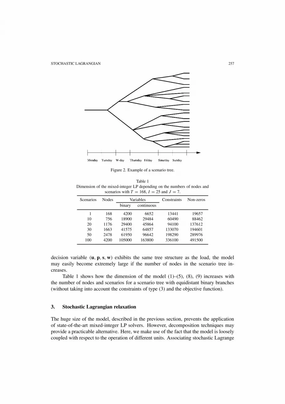
The minimization problem (1)–(6) represents a mixed-integer program with linearconstraints, and IT binary and (I+2J )T continuous decision variables, respectively. Fora typical configuration of the VEAG-owned generation system with I = 25 (thermal),J = 7 (hydro) and T = 168 (i.e., 7 days with hourly discretization), the dimension ofthe model is shown in the first row of Table 1.

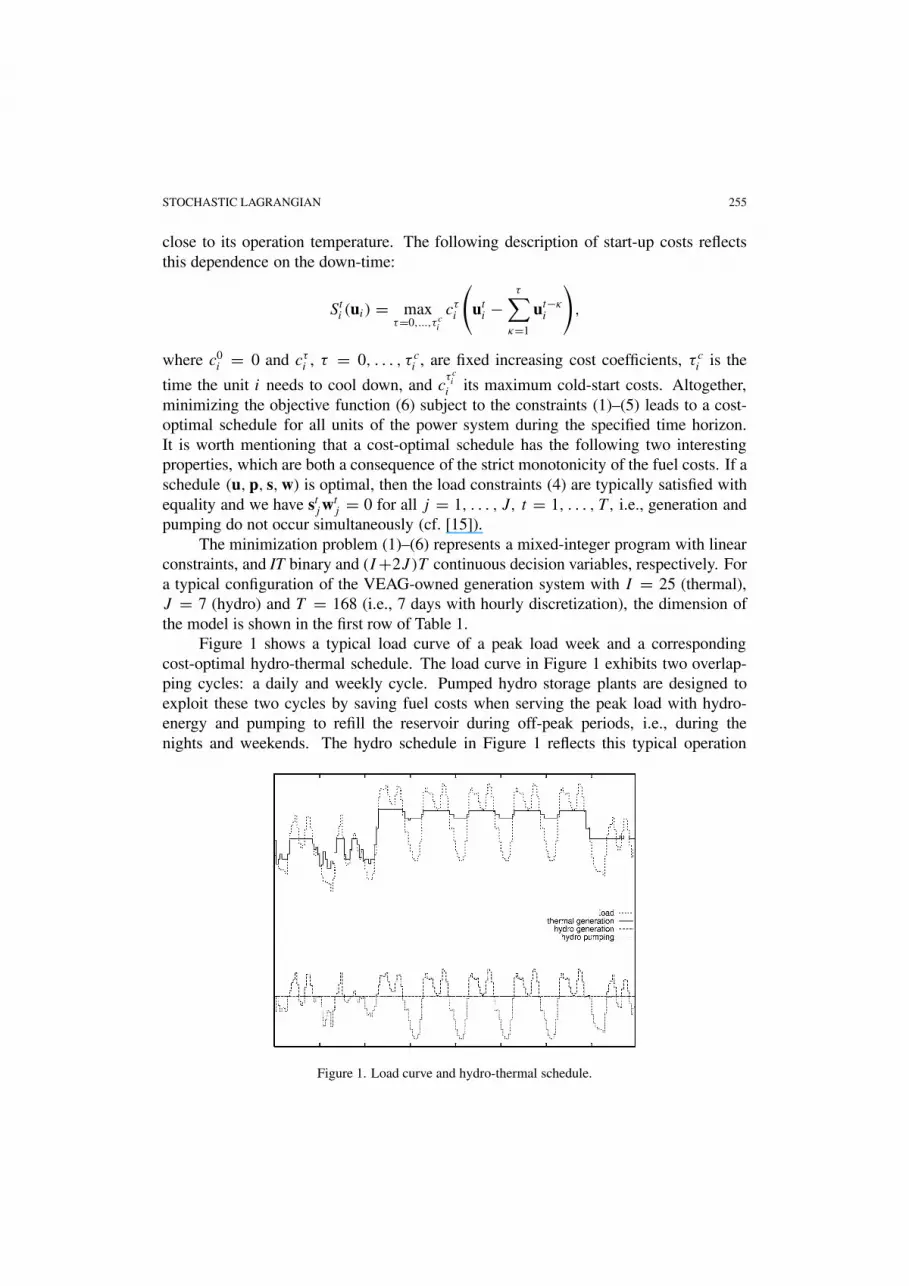
Figure 1 shows a typical load curve of a peak load week and a correspondingcost-optimal hydro-thermal schedule. The load curve in Figure 1 exhibits two overlap-ping cycles: a daily and weekly cycle. Pumped hydro storage plants are designed toexploit these two cycles by saving fuel costs when serving the peak load with hydro-energy and pumping to refill the reservoir during off-peak periods, i.e., during thenights and weekends. The hydro schedule in Figure 1 reflects this typical operation

Figure 1. Load curve and hydro-thermal schedule.

256 NOWAK AND RÖMISCH

of pumped hydro storage plants. The remaining load, i.e., the difference between theoriginal system load and the hydro schedule, shows a more uniform structure thanthe original load. This portion of the load is covered by the total output of thermalunits. So far we have tacitly assumed that the electrical load is given and determinis-tic over the whole time horizon. In electric utilities, schedulers forecast the electricalload for each time period of the day or week in advance. But, clearly, the actual elec-trical load may deviate from the predicted load at any time period due to various un-foreseeable (random) influences (temperature, daylight, switch off of local consumers,etc.). This gives rise to a stochastic model of the electrical load {dt : t = 1, . . . , T }as a (discrete-time) stochastic process on some probability space (�,A,P) reflectingthat the information on the load is complete for t = 1, and that the uncertainty in-creases with growing t . Let {At}Tt=1 be the filtration generated by the load process,i.e., At is the σ -field generated by the random vector (d1, . . . ,dt ). Hence, we have{∅,�} = A1 ⊆ A2 ⊆ · · · ⊆ At ⊆ · · · ⊆ AT ⊆ A. The sequence of schedulingdecisions {(ut ,pt , st ,wt ): t = 1, . . . , T } also forms a stochastic process on (�,A,P),which is assumed to be adapted to the filtration of σ -fields, i.e., non-anticipative. Thelatter condition means that the decision (ut ,pt , st ,wt ) depends only on the data history(d1, . . . ,dt ) or, equivalently, that (ut ,pt , st ,wt ) is At -measurable. Since all decisionvariables are uniformly bounded, we may restrict our attention to decisions (u,p, s,w)belonging to L∞(�,A,P; R

m), where m := 2(I + J )T . Then the non-anticipativitycondition can be formulated equivalently as

(u,p, s,w) ∈ T×t=1

L∞(�,At ,P; R2(I+J )

), (8)

and the (stochastic) optimization problem consists in minimizing the expected costs

E

{I∑

i=1

T∑t=1

[Ci

(pti ,ut

i

)+ Sti (ui)]}

(9)

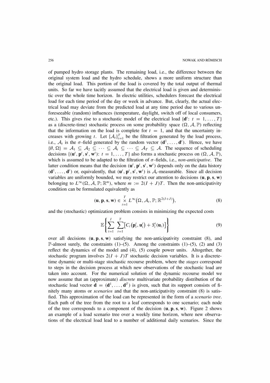
over all decisions (u,p, s,w) satisfying the non-anticipativity constraint (8), andP-almost surely, the constraints (1)–(5). Among the constraints (1)–(5), (2) and (3)reflect the dynamics of the model and (4), (5) couple power units. Altogether, thestochastic program involves 2(I + J )T stochastic decision variables. It is a discrete-time dynamic or multi-stage stochastic recourse problem, where the stages correspondto steps in the decision process at which new observations of the stochastic load aretaken into account. For the numerical solution of the dynamic recourse model wenow assume that an (approximate) discrete multivariate probability distribution of thestochastic load vector d = (d1, . . . ,dT ) is given, such that its support consists of fi-nitely many atoms or scenarios and that the non-anticipativity constraint (8) is satis-fied. This approximation of the load can be represented in the form of a scenario tree.Each path of the tree from the root to a leaf corresponds to one scenario; each nodeof the tree corresponds to a component of the decision (u,p, s,w). Figure 2 showsan example of a load scenario tree over a weekly time horizon, where new observa-tions of the electrical load lead to a number of additional daily scenarios. Since the

STOCHASTIC LAGRANGIAN 257

Figure 2. Example of a scenario tree.

Table 1Dimension of the mixed-integer LP depending on the numbers of nodes and

scenarios with T = 168, I = 25 and J = 7.

Scenarios Nodes Variables Constraints Non-zerosbinary continuous

1 168 4200 6652 13441 1965710 756 18900 29484 60490 8846220 1176 29400 45864 94100 13761230 1663 41575 64857 133070 19460150 2478 61950 96642 198290 289976

100 4200 105000 163800 336100 491500

decision variable (u,p, s,w) exhibits the same tree structure as the load, the modelmay easily become extremely large if the number of nodes in the scenario tree in-creases.

Table 1 shows how the dimension of the model (1)–(5), (8), (9) increases withthe number of nodes and scenarios for a scenario tree with equidistant binary branches(without taking into account the constraints of type (3) and the objective function).

3. Stochastic Lagrangian relaxation

The huge size of the model, described in the previous section, prevents the applicationof state-of-the-art mixed-integer LP solvers. However, decomposition techniques mayprovide a practicable alternative. Here, we make use of the fact that the model is looselycoupled with respect to the operation of different units. Associating stochastic Lagrange

258 NOWAK AND RÖMISCH

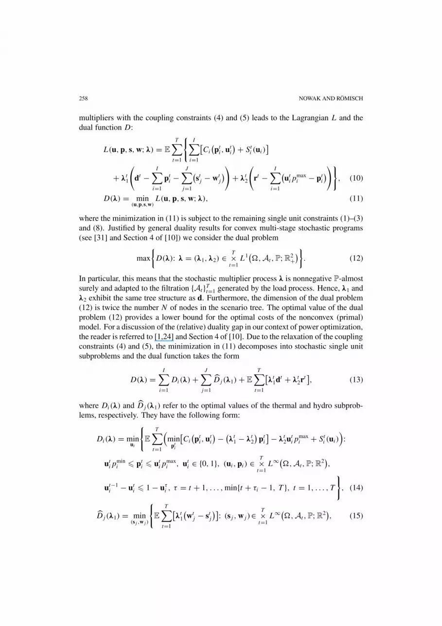
multipliers with the coupling constraints (4) and (5) leads to the Lagrangian L and thedual function D:

L(u,p, s,w;λ) = E

T∑t=1

{I∑

i=1

[Ci

(pti ,ut

i

)+ Sti (ui)]

+ λt1

(dt −

I∑i=1

pti −

J∑j=1

(stj − wt

j

))+ λt2

(rt −

I∑i=1

(utip

maxi − pt

i

))}, (10)

D(λ) = min(u,p,s,w)

L(u,p, s,w;λ), (11)

where the minimization in (11) is subject to the remaining single unit constraints (1)–(3)and (8). Justified by general duality results for convex multi-stage stochastic programs(see [31] and Section 4 of [10]) we consider the dual problem

max

{D(λ): λ = (λ1,λ2) ∈ T×

t=1L1(�,At ,P; R

2+)}. (12)

In particular, this means that the stochastic multiplier process λ is nonnegative P-almostsurely and adapted to the filtration {At}Tt=1 generated by the load process. Hence, λ1 andλ2 exhibit the same tree structure as d. Furthermore, the dimension of the dual problem(12) is twice the number N of nodes in the scenario tree. The optimal value of the dualproblem (12) provides a lower bound for the optimal costs of the nonconvex (primal)model. For a discussion of the (relative) duality gap in our context of power optimization,the reader is referred to [1,24] and Section 4 of [10]. Due to the relaxation of the couplingconstraints (4) and (5), the minimization in (11) decomposes into stochastic single unitsubproblems and the dual function takes the form

D(λ) =I∑

i=1

Di(λ) +J∑

j=1

Dj (λ1) + E

T∑t=1

[λt

1dt + λt2rt], (13)

where Di(λ) and Dj (λ1) refer to the optimal values of the thermal and hydro subprob-lems, respectively. They have the following form:

Di(λ) = minui

{E

T∑t=1

(min

pti

[Ci

(pti ,ut

i

)− (λt

1 − λt2

)pti

]− λt2ut

ipmaxi + Sti (ui)

):

utip

mini � pt

i � utip

maxi , ut

i ∈ {0, 1}, (ui ,pi) ∈ T×t=1

L∞(�,At ,P; R2),

ut−1i − ut

i � 1 − uτi , τ = t + 1, . . . ,min{t + τi − 1, T }, t = 1, . . . , T

}, (14)

Dj (λ1) = min(sj ,wj )

{E

T∑t=1

[λt

1

(wtj − stj

)]: (sj ,wj )∈

T×t=1

L∞(�,At ,P; R2), (15)

STOCHASTIC LAGRANGIAN 259

0 � stj � smaxj , 0 � wt

j � wmaxj , 0 � ltj � lmax

j , t = 1, . . . , T , (16)

ltj = lt−1j − stj + ηjwt

j , t = 1, . . . , T , l0j = linj , lTj = lendj

}. (17)

The thermal subproblem (14) for unit i is a mixed-integer multi-stage stochastic pro-gram. But, it reduces to a combinatorial multi-stage stochastic program, since the innerminimization with respect to the one-dimensional continuous variable pt

i can be carriedout explicitly by examining the kinks of the fuel costs Ci . The hydro subproblem (15)for plant j is a linear multi-stage stochastic program. Altogether, the dual function D isconcave and nondifferentiable on R

2N , and polyhedral due to (7).Similar to the deterministic case, the stochastic Lagrangian relaxation algorithm

for solving the model in Section 2 consists of the following ingredients:

(a) Maximization of the dual function D by a proximal bundle method using functionand subgradient information (Section 3.1);

(b) Efficient solvers for the stochastic single unit subproblems: stochastic dynamic pro-gramming (Section 3.2) and a specific descent algorithm (Section 3.3);

(c) Lagrangian heuristics for finding a feasible first-stage decision (Section 3.4);

(d) Economic dispatch for determining a nearly optimal first-stage decision (Sec-tion 3.5).

In the remaining part of this section we provide a description of these ingredients.

3.1. Proximal bundle method

We consider the maximization of the dual concave function D on the set R2N+ , and

assume that the set of maximizers is nonempty. Function values D(λ) are evalu-ated according to (13) and a corresponding subgradient g(λ) ∈ ∂D(λ) is given by(g1(λ), . . . , gN(λ), gN+1(λ), . . . , g2N(λ)), where gn(λ) for n = 1, . . . , N is equal tothe value of the stochastic process{

dt −I∑

i=1

pti(λ) −

J∑j=1

(stj (λ)− wt

j (λ))}T

t=1

at node n and gN+n(λ) for n = 1, . . . , N is equal to the value of the stochastic process{rt −

I∑i=1

(uti(λ)p

maxi − pt

i(λ))}T

t=1

at node n. Here, (u(λ),p(λ), s(λ),w(λ)) is a Lagrangian solution, i.e., it belongs toarg min(u,p,s,w) L(u,p, s,w;λ).

260 NOWAK AND RÖMISCH

The proximal bundle method [19,21] generates a sequence (λk) in R2N+ converging

to some maximizer, and trial points λk ∈ R2N+ starting with λ1 = λ1 for evaluating

subgradients g(λk) of D and its polyhedral upper approximation

Dk(λ) = minj∈J k

{D(λj)+ ⟨

g(λj),λ − λj

⟩}, (18)

where J k is a subset of {1, . . . , k}. In iteration k the next trial point λk+1 is selected by

λk+1 ∈ arg max

{Dk(λ) − 1

2uk∥∥λ − λk

∥∥2: λ ∈ R

2N+

}, (19)

where uk is a proximity weight. A descent step to λk+1 = λk+1 occurs if D(λk+1) �D(λk) + κδk, where κ ∈ (0, 1) is fixed and δk = Dk(λ

k+1) − D(λk) � 0. If δk = 0,then λk is optimal. Otherwise, a null step λk+1 = λk improves the next polyhedralfunction Dk+1. Strategies for updating uk and choosing J k+1 are discussed in [19,21].The method is implemented such that the cardinality of J k is bounded (by some naturalnumber NGRAD) and that it terminates if δk is less than a given (relative) optimalitytolerance opt.tol.

Our computational experience with the proximal bundle code NOA 3.0 [20] forsolving (12) is very encouraging (cf. Section 4). In our test runs, for instance, NOA 3.0applied to solving (12) performed in 300 iterations as good as a standard subgradientmethod (with step lengths 1/k) in 10.000 iterations.

3.2. Stochastic dynamic programming

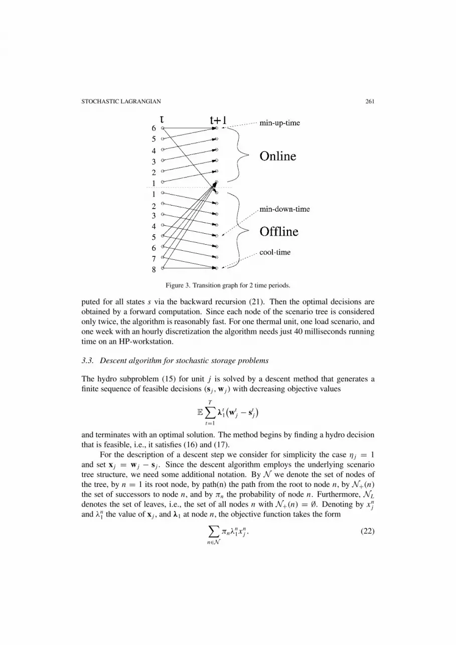
In order to solve the thermal subproblem (14) by dynamic programming, the state spaceis extended by including the recent history such that minimum up/down-times and start-up costs depend just on the current and the previous state. Figure 3 shows a part ofthe state transition graph of a thermal unit having a minimum up-time of 6 hours, aminimum down-time of 5 hours, and a cooling down-time of 8 hours. It shows possibleand feasible transitions on some fixed arc of the scenario tree, where the arrows refer tofeasible transitions. Let αt

i (s) denote the node weight at time t and state s and Si(s, s)

the arc weight for the arc from state s to state s in the state transition graph. The nodeweights αt

i (s) are equal to 0 for off-line states s and it holds

αti (s) = min

pi

{Ci(pi, 1) − (

λt1 − λt

2

)pi − λt

2pmaxi : pmin

i � pi � pmaxi

}(20)

for on-line states s. The arc weights Si(s, s) describe start-up costs for the thermal unit.They are independent of λ, and are non-zero only for arcs leading from off-line states toon-line states. The cost-to-go functions are given by

γ ti (s) = αt

i (s) + E

(mins

{Si(s, s) + γ t+1

i (s)}|At

), (21)

where E(·|At ) denotes the conditional expectation w.r.t. the σ -field At . Now, the dy-namic programming algorithm works as follows. First the cost-to-go functions are com-

STOCHASTIC LAGRANGIAN 261

Figure 3. Transition graph for 2 time periods.

puted for all states s via the backward recursion (21). Then the optimal decisions areobtained by a forward computation. Since each node of the scenario tree is consideredonly twice, the algorithm is reasonably fast. For one thermal unit, one load scenario, andone week with an hourly discretization the algorithm needs just 40 milliseconds runningtime on an HP-workstation.

3.3. Descent algorithm for stochastic storage problems

The hydro subproblem (15) for unit j is solved by a descent method that generates afinite sequence of feasible decisions (sj ,wj ) with decreasing objective values

E

T∑t=1

λt1

(wtj − stj

)and terminates with an optimal solution. The method begins by finding a hydro decisionthat is feasible, i.e., it satisfies (16) and (17).

For the description of a descent step we consider for simplicity the case ηj = 1and set xj = wj − sj . Since the descent algorithm employs the underlying scenariotree structure, we need some additional notation. By N we denote the set of nodes ofthe tree, by n = 1 its root node, by path(n) the path from the root to node n, by N+(n)the set of successors to node n, and by πn the probability of node n. Furthermore, NL

denotes the set of leaves, i.e., the set of all nodes n with N+(n) = ∅. Denoting by xnjand λn1 the value of xj , and λ1 at node n, the objective function takes the form∑

n∈Nπnλ

n1x

nj . (22)

262 NOWAK AND RÖMISCH

The next feasible iterate xj is chosen such that the objective (22) decreases and thatxnj = xnj holds for each node n ∈ N \ ({nG} ∪ GL), i.e.,∑

n∈Nπnλ

n1

(xnj − xnj

) =∑

n∈{nG}∪GL

πnλn1

(xnj − xnj

)< 0, (23)

where nG and GL denote the root node and the set of leaves of a subtree with a set G ofnodes contained in N , i.e., it holds that {nG} ∪ GL ⊆ G, nG ∈ path(n) for each n ∈ G,N+(n)∩G = ∅ for each n ∈ GL and N+(n) ⊆ G for each n ∈ G\GL. A subtree havingthese properties is called d-subtree. It is shown in [27] that for each nonoptimal feasiblehydro decision xj , a d-subtree and a feasible decision xj exist such that (23) is satisfied.Moreover, the conditions on a node n to form a root node of a d-subtree are as follows:

• Case of increasing the level lnj : min{xmaxj − xnj , d

upn }{λn1πn + r

upn } � 0,

• Case of decreasing the level lnj : min{xnj − xminj , ddown

n }{λn1πn + rdownn } � 0,

where lnj denotes the value of lj at node n, xmaxj = wmax

j , xminj = −smax

j and dupn , ddown

n ,r

upn and rdown

n are for each n ∈ N defined by

dupn =

xnj − xmin

j if bupn = 1,

min{lmaxj − lnj , min

n+∈N+(n)d

upn+

}if bup

n = 0,

ddownn =

xmaxj − xnj if bdown

n = 1,

min{lnj , min

n+∈N+(n)ddownn+

}if bdown

n = 0,

rupn =

λn1πn if bup

n = 1,∑n+∈N+(n)

rupn+ if bup

n = 0,

rdownn =

λn1πn if bdown

n = 1,∑n+∈N+(n)

rdownn+ if bdown

n = 0.

Here, bupn and bdown

n are binary decisions at node n ∈ N . All superscripts up/down referto cases of an increased/decreased level lnj for n ∈ G \GL. In case of an increased level,the correspondence of binary decisions to the tree G is determined by

n ∈ GL ⇔ bupn = 1 and n ∈ G \GL ⇔ bup

n = 0.

The decision to reduce the storage is denoted by bupn = 1, while b

upn = 0 refers to the

decision to keep the additional amount. Similarly, the notations bdownn = 1 and bdown

n = 0are used.Now, the descent algorithm EXCHA works as follows:

Step 1: Input and initialization;

Step 2: Determine a feasible point;

STOCHASTIC LAGRANGIAN 263

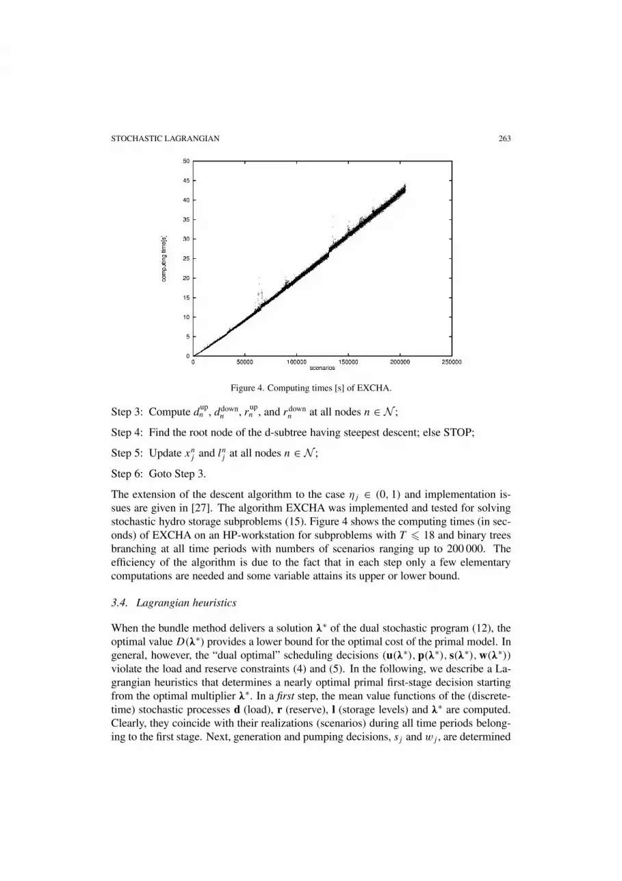
Figure 4. Computing times [s] of EXCHA.

Step 3: Compute dupn , ddown

n , rupn , and rdown

n at all nodes n ∈ N ;

Step 4: Find the root node of the d-subtree having steepest descent; else STOP;

Step 5: Update xnj and lnj at all nodes n ∈ N ;

Step 6: Goto Step 3.

The extension of the descent algorithm to the case ηj ∈ (0, 1) and implementation is-sues are given in [27]. The algorithm EXCHA was implemented and tested for solvingstochastic hydro storage subproblems (15). Figure 4 shows the computing times (in sec-onds) of EXCHA on an HP-workstation for subproblems with T � 18 and binary treesbranching at all time periods with numbers of scenarios ranging up to 200 000. Theefficiency of the algorithm is due to the fact that in each step only a few elementarycomputations are needed and some variable attains its upper or lower bound.

3.4. Lagrangian heuristics

When the bundle method delivers a solution λ∗ of the dual stochastic program (12), theoptimal value D(λ∗) provides a lower bound for the optimal cost of the primal model. Ingeneral, however, the “dual optimal” scheduling decisions (u(λ∗),p(λ∗), s(λ∗),w(λ∗))violate the load and reserve constraints (4) and (5). In the following, we describe a La-grangian heuristics that determines a nearly optimal primal first-stage decision startingfrom the optimal multiplier λ∗. In a first step, the mean value functions of the (discrete-time) stochastic processes d (load), r (reserve), l (storage levels) and λ∗ are computed.Clearly, they coincide with their realizations (scenarios) during all time periods belong-ing to the first stage. Next, generation and pumping decisions, sj and wj , are determined

264 NOWAK AND RÖMISCH

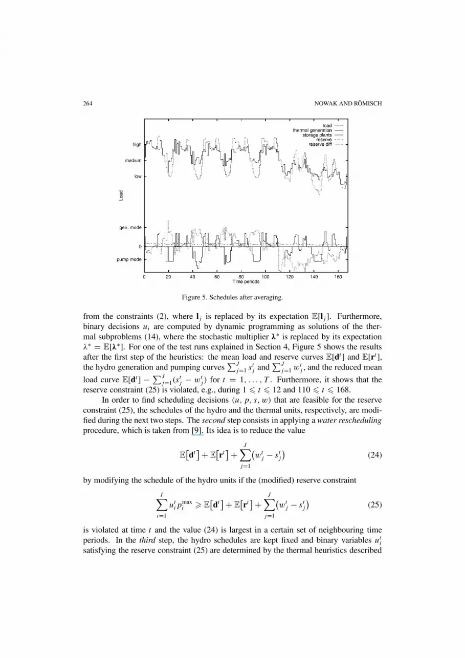
Figure 5. Schedules after averaging.

from the constraints (2), where lj is replaced by its expectation E[lj ]. Furthermore,binary decisions ui are computed by dynamic programming as solutions of the ther-mal subproblems (14), where the stochastic multiplier λ∗ is replaced by its expectationλ∗ = E[λ∗]. For one of the test runs explained in Section 4, Figure 5 shows the resultsafter the first step of the heuristics: the mean load and reserve curves E[dt ] and E[rt ],the hydro generation and pumping curves

∑Jj=1 s

tj and

∑Jj=1 w

tj , and the reduced mean

load curve E[dt] − ∑Jj=1(s

tj − wt

j ) for t = 1, . . . , T . Furthermore, it shows that thereserve constraint (25) is violated, e.g., during 1 � t � 12 and 110 � t � 168.

In order to find scheduling decisions (u, p, s,w) that are feasible for the reserveconstraint (25), the schedules of the hydro and the thermal units, respectively, are modi-fied during the next two steps. The second step consists in applying a water reschedulingprocedure, which is taken from [9]. Its idea is to reduce the value

E[dt]+ E

[rt]+

J∑j=1

(wtj − stj

)(24)

by modifying the schedule of the hydro units if the (modified) reserve constraint

I∑i=1

utipmaxi � E

[dt]+ E

[rt]+

J∑j=1

(wtj − stj

)(25)

is violated at time t and the value (24) is largest in a certain set of neighbouring timeperiods. In the third step, the hydro schedules are kept fixed and binary variables utisatisfying the reserve constraint (25) are determined by the thermal heuristics described

STOCHASTIC LAGRANGIAN 265

in [40]. Its main idea consists in determining the time t , where the constraint (25) ismost violated, and in increasing λ∗t

2 as much as necessary to switch on (by dynamicprogramming) just as many thermal units as needed to satisfy (25) at t . This is repeateduntil the reserve constraint (25) is satisfied in all time periods. Since this technique doesnot distinguish between identical units that appear quite often in real-life power systems,the start-up costs of such units are slightly modified. In our numerical experiments thismodification led to improved results (cf. Section 4).

3.5. Economic dispatch

The Lagrangian heuristics ends with a binary schedule uti for the thermal units such thata feasible schedule (u, p, s,w) exists for the primal model in Section 2 when replacingthe stochastic load d and reserve r by their expected values. In a final step, a cost-optimalschedule (p, s,w) is determined for fixed u by solving the corresponding primal model(with fixed start-up costs). The aim of this section is to develop an algorithmic approachfor solving this economic dispatch problem. The approach also applies to multi-stagestochastic power scheduling models with fixed stochastic binary decisions u. Since thismay be of independent interest, we consider the model:

min(p,s,w)

{E

I∑i=1

T∑t=1

Ci

(pti ,ut

i

): (p, s,w) ∈ T×

t=1L∞(�,At ,P; R

I+2J), (26)

utip

mini � pt

i � utip

maxi , t = 1, . . . , T , i = 1, . . . , I, (27)

0 � stj � smaxj , 0 � wt

j � wmaxj , 0 � ltj � lmax

j , (28)

ltj = lt−1j − stj + ηjwt

j , t = 1, . . . , T ,

l0j = linj , lTj = lendj , j = 1, . . . , J, (29)

I∑i=1

pti +

J∑j=1

(stj − wt

j

)� dt , t = 1, . . . , T , (30)

I∑i=1

(utip

maxi − pt

i

)� rt , t = 1, . . . , T

}. (31)

The structure of the stochastic program (26)–(31) is partly similar to (15) exceptingthe thermal units. This motivates the idea to apply the same technique as in Section 3.3.Thermal and hydro units are coupled by the constraints (30). Moving the sum

∑Jj=1(s

tj−

wtj ) to the right-hand side in (30) and taking the right-hand side as a parameter, the

optimization problem (26), (27), (30) decomposes into parametric programs for eachtime period t and scenario ω. Denoting the parameter by θ , the parametric programs andtheir optimal value functions φt,ω(·) have the form:

266 NOWAK AND RÖMISCH

φt,ω(θ) = minpt

{I∑

i=1

Ci

(pti ,ut

i(ω)): ut

i(ω)pmini � pt

i � uti(ω)p

maxi , i = 1, . . . , I,

dt (ω) − θ �I∑

i=1

pti �

I∑i=1

uti(ω)p

maxi − rt (ω)

}.

Such optimal value functions may be evaluated by efficient algorithms (see, e.g., [4,5,22]for the case of (piecewise) linear and quadratic costs). Now, the economic dispatchproblem (26)–(31) can be reformulated as

min(s,w)

{E

T∑t=1

φt,.

(J∑

j=1

(stj − wt

j

)): (28), (29)

}. (32)

This reformulation allows to study how the objective function varies when altering theoperation of the hydro units. If the functions φt,ω were differentiable, the linearizationof the model (32) takes the form

J∑j=1

min(sj ,wj )

E

T∑t=1

dφt,.dθ

(J∑

j=1

(stj − wt

j

))(stj − wt

j

), (33)

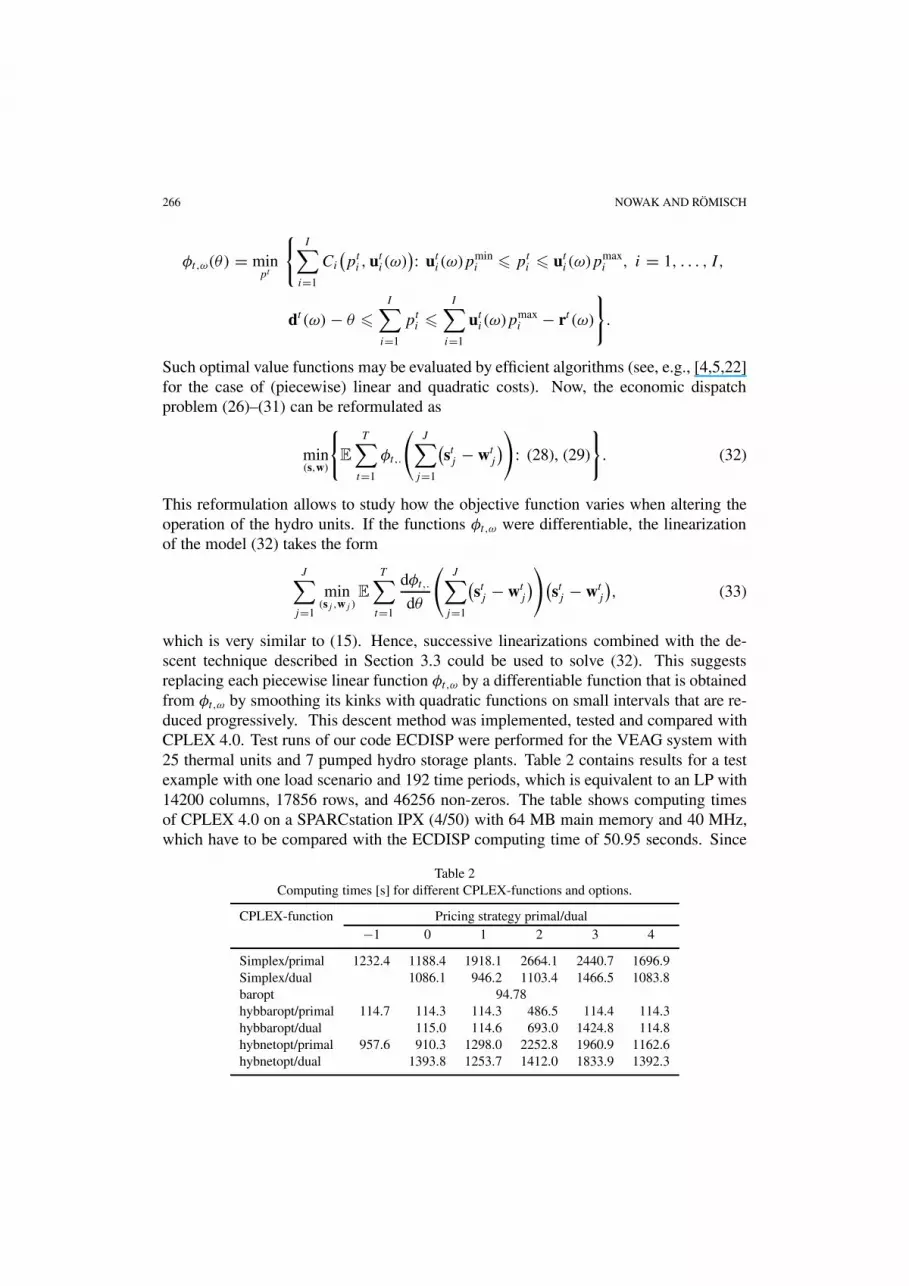
which is very similar to (15). Hence, successive linearizations combined with the de-scent technique described in Section 3.3 could be used to solve (32). This suggestsreplacing each piecewise linear function φt,ω by a differentiable function that is obtainedfrom φt,ω by smoothing its kinks with quadratic functions on small intervals that are re-duced progressively. This descent method was implemented, tested and compared withCPLEX 4.0. Test runs of our code ECDISP were performed for the VEAG system with25 thermal units and 7 pumped hydro storage plants. Table 2 contains results for a testexample with one load scenario and 192 time periods, which is equivalent to an LP with14200 columns, 17856 rows, and 46256 non-zeros. The table shows computing timesof CPLEX 4.0 on a SPARCstation IPX (4/50) with 64 MB main memory and 40 MHz,which have to be compared with the ECDISP computing time of 50.95 seconds. Since

Table 2Computing times [s] for different CPLEX-functions and options.

CPLEX-function Pricing strategy primal/dual−1 0 1 2 3 4

Simplex/primal 1232.4 1188.4 1918.1 2664.1 2440.7 1696.9Simplex/dual 1086.1 946.2 1103.4 1466.5 1083.8baropt 94.78hybbaropt/primal 114.7 114.3 114.3 486.5 114.4 114.3hybbaropt/dual 115.0 114.6 693.0 1424.8 114.8hybnetopt/primal 957.6 910.3 1298.0 2252.8 1960.9 1162.6hybnetopt/dual 1393.8 1253.7 1412.0 1833.9 1392.3

STOCHASTIC LAGRANGIAN 267

Table 3Comparison of ECDISP with CPLEX.

Scen’s Nodes Columns Rows Non-zeros ECDISP[s] CPLEX[s] Adv’

3 336 24840 31248 80944 18.69 97.61 5.225 462 34148 42966 111294 29.48 162.47 5.517 588 43456 54684 141644 47.93 206.00 4.309 687 50766 63891 165487 43.09 305.43 7.09

11 792 58520 73656 190776 67.17 500.30 7.4513 930 68716 86490 224018 86.73 461.54 5.3215 1035 76470 96255 249307 98.04 569.18 5.8117 1036 76528 96348 249532 117.42 620.65 5.2919 1120 82728 104160 269760 91.63 1720.33 18.721 1232 91000 114576 296736 131.94 243.27 1.8422 1260 93064 117180 303476 128.18 794.93 6.20

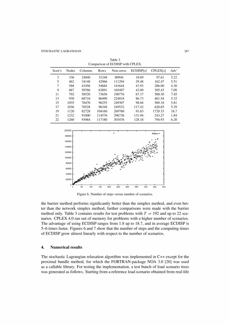
Figure 6. Number of steps versus number of scenarios.

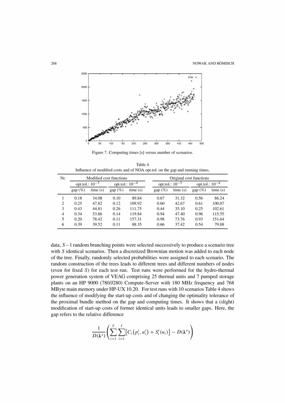
the barrier method performs significantly better than the simplex method, and even bet-ter than the network simplex method, further comparisons were made with the barriermethod only. Table 3 contains results for test problems with T = 192 and up to 22 sce-narios. CPLEX 4.0 ran out of memory for problems with a higher number of scenarios.The advantage of using ECDISP ranges from 1.8 up to 18.7, and in average ECDISP is5–6 times faster. Figures 6 and 7 show that the number of steps and the computing timesof ECDISP grow almost linearly with respect to the number of scenarios.

4. Numerical results

The stochastic Lagrangian relaxation algorithm was implemented in C++ except for theproximal bundle method, for which the FORTRAN-package NOA 3.0 [20] was usedas a callable library. For testing the implementation, a test bunch of load scenario treeswas generated as follows. Starting from a reference load scenario obtained from real-life

268 NOWAK AND RÖMISCH

Figure 7. Computing times [s] versus number of scenarios.

Table 4Influence of modified costs and of NOA opt.tol. on the gap and running times.

Nr. Modified cost functions Original cost functions

opt.tol.: 10−3 opt.tol.: 10−4 opt.tol.: 10−3 opt.tol.: 10−4

gap (%) time (s) gap (%) time (s) gap (%) time (s) gap (%) time (s)

1 0.18 34.08 0.10 89.84 0.67 31.32 0.56 86.242 0.25 47.82 0.12 109.92 0.60 42.67 0.61 100.073 0.43 44.81 0.26 111.75 0.44 35.10 0.25 102.614 0.34 53.86 0.14 119.84 0.94 47.40 0.96 115.555 0.20 78.42 0.11 157.31 0.98 73.76 0.93 151.646 0.39 39.52 0.11 88.35 0.66 37.42 0.54 79.88

data, S−1 random branching points were selected successively to produce a scenario treewith S identical scenarios. Then a discretized Brownian motion was added to each nodeof the tree. Finally, randomly selected probabilities were assigned to each scenario. Therandom construction of the trees leads to different trees and different numbers of nodes(even for fixed S) for each test run. Test runs were performed for the hydro-thermalpower generation system of VEAG comprising 25 thermal units and 7 pumped storageplants on an HP 9000 (780/J280) Compute-Server with 180 MHz frequency and 768MByte main memory under HP-UX 10.20. For test runs with 10 scenarios Table 4 showsthe influence of modifying the start-up costs and of changing the optimality tolerance ofthe proximal bundle method on the gap and computing times. It shows that a (slight)modification of start-up costs of former identical units leads to smaller gaps. Here, thegap refers to the relative difference

1

D(λ∗)

(T∑t=1

I∑i=1

[Ci

(pti , u

ti

)+ Sti (ui)]− D(λ∗)

)

STOCHASTIC LAGRANGIAN 269

of the cost of the scheduling decision (u, p, s,w) and the optimal value of the dual prob-lem. Moreover, improving optimality tolerances leads to smaller gaps paid by increasedcomputing times.

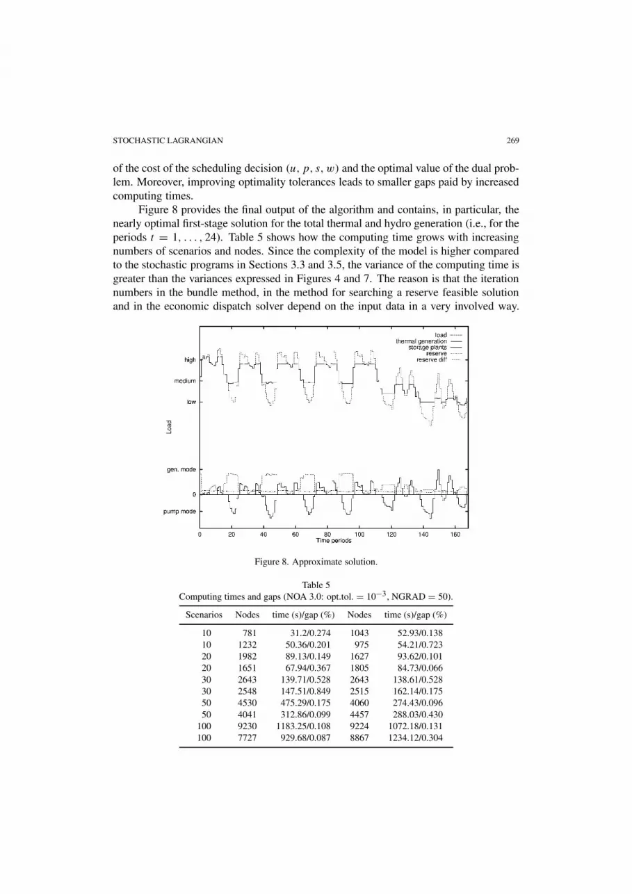
Figure 8 provides the final output of the algorithm and contains, in particular, thenearly optimal first-stage solution for the total thermal and hydro generation (i.e., for theperiods t = 1, . . . , 24). Table 5 shows how the computing time grows with increasingnumbers of scenarios and nodes. Since the complexity of the model is higher comparedto the stochastic programs in Sections 3.3 and 3.5, the variance of the computing time isgreater than the variances expressed in Figures 4 and 7. The reason is that the iterationnumbers in the bundle method, in the method for searching a reserve feasible solutionand in the economic dispatch solver depend on the input data in a very involved way.

Figure 8. Approximate solution.

Table 5Computing times and gaps (NOA 3.0: opt.tol. = 10−3, NGRAD = 50).

Scenarios Nodes time (s)/gap (%) Nodes time (s)/gap (%)

10 781 31.2/0.274 1043 52.93/0.13810 1232 50.36/0.201 975 54.21/0.72320 1982 89.13/0.149 1627 93.62/0.10120 1651 67.94/0.367 1805 84.73/0.06630 2643 139.71/0.528 2643 138.61/0.52830 2548 147.51/0.849 2515 162.14/0.17550 4530 475.29/0.175 4060 274.43/0.09650 4041 312.86/0.099 4457 288.03/0.430

100 9230 1183.25/0.108 9224 1072.18/0.131100 7727 929.68/0.087 8867 1234.12/0.304

270 NOWAK AND RÖMISCH

Another observation is that the gap seems to be (almost) independent of the number ofscenarios.

5. Conclusions

We have elaborated a mixed-integer multi-stage stochastic programming model forpower scheduling in a hydro-thermal generation system under uncertainty on the elec-trical load. Due to the huge size of the model, an application of state-of-the-art mixed-integer LP solvers is prevented. Therefore, we have developed a novel approach based onstochastic Lagrangian relaxation of coupling constraints. It consists of proximal bundleiterations for solving a stochastic dual followed by a Lagrangian heuristics to determinea nearly optimal primal first-stage solution. The stochastic dual decomposes into sto-chastic thermal and hydro subproblems, which are solved by specific fast algorithms.Our computational experience indicates that the stochastic Lagrangian relaxation algo-rithm is able to produce good approximate first-stage solutions for medium-size realisticpower systems and 20 (100) load scenarios within less than 2 (20) minutes on a mod-ern HP-workstation. It also indicates that the algorithm bears potential for solving morecomplex real-life power scheduling models under uncertainty in reasonable time.

Acknowledgments

The authors are grateful to K.C. Kiwiel (Polish Academy of Sciences, Warsaw) forthe permission to use the NOA 3.0 package and for valuable comments, to DarinkaDentcheva (Humboldt-University Berlin) for useful discussions on the Lagrangianheuristics described in Section 3.4 and to G. Schwarzbach and J. Thomas (VEAG Verein-igte Energiewerke AG) for providing us with the data used in our test runs. We extendour gratitude to two anonymous referees for their suggestions which led to an improvedpresentation of the material. This research was supported by the SchwerpunktprogrammEchtzeit-Optimierung großer Systeme of the Deutsche Forschungsgemeinschaft and bythe Graduiertenkolleg Geometrie und Nichtlineare Analysis at the Humboldt-UniversityBerlin.

References

[1] D.P. Bertsekas, G.S. Lauer, N.R. Sandell Jr. and T.A. Posbergh, Optimal short-term scheduling oflarge-scale power systems, IEEE Transactions on Automatic Control AC-28 (1983) 1–11.

[2] J.R. Birge, Stochastic programming computations and applications, INFORMS Journal on Computing9 (1997) 111–133.

[3] J.R. Birge and F. Louveaux, Introduction to Stochastic Programming (Springer, New York, 1997).[4] P.P.J. van den Bosch, Optimal static dispatch with linear, quadratic and nonlinear functions of the fuel

costs, IEEE Transactions on Power Apparatus and Systems PAS-104 (1985) 3402–3408.[5] P.P.J. van den Bosch and F.A. Lootsma, Scheduling of power generation via large-scale nonlinear

optimization, Journal of Optimization and Applications 55 (1987) 1684–1690.

STOCHASTIC LAGRANGIAN 271

[6] C.C. Carøe and R. Schultz, Dual decomposition in stochastic integer programming, Operations Re-search Letters 24 (1999) 37–45.

[7] C.C. Carøe and R. Schultz, A two-stage stochastic program for unit commitment under uncertainty ina hydro-thermal power system, DFG-Schwerpunktprogramm Echtzeit-Optimierung großer Systeme,Preprint 98-13 (1998).

[8] P. Carpentier, G. Cohen, J.-C. Culioli and A. Renaud, Stochastic optimization of unit commitment:a new decomposition framework, IEEE Transactions on Power Systems 11 (1996) 1067–1073.

[9] D. Dentcheva, R. Gollmer, A. Möller, W. Römisch and R. Schultz, Solving the unit commitmentproblem in power generation by primal and dual methods, in: Progress in Industrial Mathematics atECMI 96, eds. M. Brøns, M.P. Bendsøe and M.P. Sørensen (Teubner, Stuttgart, 1997) pp. 332–339.

[10] D. Dentcheva and W. Römisch, Optimal power generation under uncertainty via stochastic program-ming, in: Stochastic Programming Methods and Technical Applications, eds. K. Marti and P. Kall,Lecture Notes in Economics and Mathematical Systems, Vol. 458 (Springer, Berlin, 1998) pp. 22–56.

[11] S. Feltenmark and K.C. Kiwiel, Dual applications of proximal bundle methods, including Lagrangianrelaxation of nonconvex problems, SIAM Journal on Optimization 10 (2000) 697–721.

[12] S.-E. Fleten, S.W. Wallace and W.T. Ziemba, Portfolio management in a deregulated hydropowerbased electricity market, in: Hydropower ’97, eds. E. Broch, D.K. Lysne, N. Flatabø and E. Helland-Hansen (Balkema, Rotterdam, 1997).

[13] A. Gjelsvik, T.A. Røtting and J. Røynstrand, Long-term scheduling of hydro-thermal power systems,in: Hydropower ’92, eds. E. Broch and D.K. Lysne (Balkema, Rotterdam, 1992) pp. 539–546.

[14] R. Gollmer, A. Möller, W. Römisch, R. Schultz, G. Schwarzbach and J. Thomas, Optimale Block-auswahl bei der Kraftwerkseinsatzplanung der VEAG, in: Optimierung in der Energieversorgung II,VDI-Berichte, Vol. 1352 (Düsseldorf, 1997) pp. 71–85.

[15] N. Gröwe, W. Römisch, R. Schultz, A simple recourse model for power dispatch under uncertaindemand, Annals of Operations Research 59 (1995) 135–164.

[16] J.L. Higle and S. Sen, Stochastic Decomposition—A Statistical Method for Large Scale StochasticLinear Programming (Kluwer, Dordrecht, 1996).

[17] G. Infanger, Planning Under Uncertainty—Solving Large-Scale Stochastic Linear Programs (Boydand Fraser, 1994).

[18] J. Jacobs, G. Freeman, J. Grygier, D. Morton, G. Schultz, K. Staschus and J. Stedinger, SOCRATES:A system for scheduling hydroelectric generation under uncertainty, Annals of Operations Research59 (1995) 99–133.

[19] K.C. Kiwiel, Proximity control in bundle methods for convex nondifferentiable optimization, Mathe-matical Programming 46 (1990) 105–122.

[20] K.C. Kiwiel, User’s Guide for NOA 2.0/3.0: A Fortran package for convex nondifferentiable opti-mization, Polish Academy of Sciences, Systems Research Institute, Warsaw, Poland (1993/94).

[21] K.C. Kiwiel, Approximations in proximal bundle methods and decomposition of convex programs,Journal of Optimization Theory and Applications 84 (1995) 529–548.

[22] P. Kleinmann and R. Schultz, A simple procedure for optimal load dispatch using parametric pro-gramming, ZOR—Methods and Models of Operations Research 34 (1990) 219–229.

[23] C. Lemaréchal, Lagrangian decomposition and nonsmooth optimization, in: Nonsmooth OptimizationMethods and Applications, ed. F. Gianessi (Gordon and Breach, 1992) pp. 201–216.

[24] C. Lemaréchal and A. Renaud, A geometric study of duality gaps, with applications, MathematicalProgramming (to appear).

[25] A. Løkketangen and D.L. Woodruff, Progressive hedging and tabu search applied to mixed integer(0,1) multi-stage stochastic programming, Journal of Heuristics 2 (1996) 111–128.

[26] V.I. Norkin, G. Pflug and A. Ruszczynski, A branch and bound method for stochastic global optimiza-tion, Mathematical Programming 83 (1998) 425–450.

[27] M.P. Nowak, A fast descent method for the hydro storage subproblem in power generation, Interna-tional Institute for Applied Systems Analysis, Laxenburg, Austria, Working Paper WP-96-109 (1996).

272 NOWAK AND RÖMISCH

[28] M.P. Nowak and W. Römisch, Optimal power dispatch via multistage stochastic programming, in:Progress in Industrial Mathematics at ECMI 96, eds. M. Brøns, M.P. Bendsøe and M.P. Sørensen(Teubner, Stuttgart, 1997) pp. 324–331.

[29] M.V.F. Pereira and L.M.V.G. Pinto, Multi-stage stochastic optimization applied to energy planning,Mathematical Programming 52 (1991) 359–375.

[30] A. Renaud, Optimizing short-term operation of power generation: a new stochastic model, Lecturepresented at the VIII International Conference on Stochastic Programming, Vancouver, Canada (Au-gust 1998).

[31] R.T. Rockafellar and R.J.-B. Wets, The optimal recourse problem in discrete time: L1-multipliers forinequality constraints, SIAM Journal on Control and Optimization 16 (1978) 16–36.

[32] R.T. Rockafellar and R.J.-B. Wets, Scenarios and policy aggregation in optimization under uncer-tainty, Mathematics of Operations Research 16 (1991) 119–147.

[33] W. Römisch and R. Schultz, Decomposition of a multi-stage stochastic program for power dispatch,ZAMM—Zeitschrift für Angewandte Mathematik und Mechanik 76(Suppl. 3) (1996) 29–32.

[34] A. Ruszczynski, Decomposition methods in stochastic programming, Mathematical Programming,Series B 79 (1997) 333–353.

[35] G.B. Sheble and G.N. Fahd, Unit commitment literature synopsis, IEEE Transactions on Power Sys-tems 9 (1994) 128–135.

[36] S. Takriti, J.R. Birge and E. Long, A stochastic model for the unit commitment problem, IEEE Trans-actions on Power Systems 11 (1996) 1497–1508.

[37] S. Takriti, B. Krasenbrink and L.S.-Y. Wu, Incorporating fuel constraints and electricity spot pricesinto the stochastic unit commitment problem, Operations Research 48 (2000) 268–280.

[38] R.J.-B. Wets, Stochastic Programming, in: Handbooks in Operations Research and ManagementScience, Vol. 1, Optimization, eds. G.L. Nemhauser, A.H.G. Rinnooy Kan and M.J. Todd (North-Holland, Amsterdam, 1989) pp. 573–629.

[39] A.J. Wood and B.F. Wollenberg, Power Generation, Operation, and Control, 2nd edn. (Wiley,New York, 1996).

[40] F. Zhuang and F.D. Galiana, Towards a more rigorous and practical unit commitment by Lagrangianrelaxation, IEEE Transactions on Power Systems 3 (1988) 763–773.