POWER MANAGEMENT IN A HYDRO-THERMALSYSTEM UNDER UNCERTAINTY BY LAGRANGIANRELAXATIONNICOLE GR�OWE-KUSKA�, KRZYSZTOF C. KIWIELy,MATTHIAS P. NOWAKz, WERNER R�OMISCHx, AND ISABEL WEGNER{Abstract. We present a dynamic multistage stochastic programming model for thecost-optimal generation of electric power in a hydro-thermal system under uncertainty inload, in ow to reservoirs and prices for fuel and delivery contracts. The stochastic loadprocess is approximated by a scenario tree obtained by adapting a SARIMA model tohistorical data, using empirical means and variances of simulated scenarios to constructan initial tree, and reducing it by a scenario deletion procedure based on a suitable prob-ability distance. Our model involves many mixed-integer variables and individual powerunit constraints, but relatively few coupling constraints. Hence we employ stochasticLagrangian relaxation that assigns stochastic multipliers to the coupling constraints.Solving the Lagrangian dual by a proximal bundle method leads to successive decom-position into single thermal and hydro unit subproblems that are solved by dynamicprogramming and a specialized descent algorithm, respectively. The optimal stochasticmultipliers are used in Lagrangian heuristics to construct approximately optimal �rststage decisions. Numerical results are presented for realistic data from a German powerutility, with a time horizon of one week and scenario numbers ranging from 5 to 100. Thecorresponding optimization problems have up to 200,000 binary and 350,000 continuousvariables, and more than 500,000 constraints.Key words. Stochastic programming, Lagrangian relaxation, unit commitment,bundle methods, scenario generation.AMS(MOS) subject classi�cations. 90C15, 90C90, 90C11, 90C25, 65K051. Introduction. Many issues motivate a growing interest in mathe-matical modeling and optimization techniques for operating power systemsand trading electricity. Some of them are related to the ongoing liberal-ization of electricity markets: electric utilities generate power in a compet-itive environment, generating and trading activities must be coordinated,electricity portfolios for spot and option markets become important, andthe electrical load as well as electricity prices become increasingly unpre-dictable. Further issues are related to the complex nature of mathemat-ical models for the e�cient generation, transmission and distribution ofelectric power. They often lead to optimization problems characterizedby combinations of challenges such as mixed-integer decisions, nonlinear�Institute of Mathematics, Humboldt University Berlin, Berlin, Germany. E-mail:nicole@mathematik.hu-berlin.de.ySystems Research Institute, Warsaw, Poland. E-mail: kiwiel@ibspan.waw.pl.zInstitute of Mathematics, Humboldt University Berlin, Berlin, Germany. E-mail:mefju@mathematik.hu-berlin.de.xInstitute of Mathematics, Humboldt University Berlin, Berlin, Germany. E-mail:romisch@mathematik.hu-berlin.de.{Institute of Mathematics, Humboldt University Berlin, Berlin, Germany. E-mail:wegner@mathematik.hu-berlin.de. 1

2 GR�OWE-KUSKA, KIWIEL, NOWAK, R�OMISCH, WEGNERcosts and constraints, huge dimensions and data uncertainty. The latteraspect mostly concerns uncertainty in electric load forecasts, generator fail-ures, stream ows to hydro reservoirs, and fuel and electricity prices (see[20, 22, 24, 31, 44] for relevant earlier work).The present paper aims at optimizing generation and trading of anelectric hydro-thermal based utility under data uncertainty. More speci�-cally, we consider a power system comprising thermal units, pumped hydrostorage plants and contracts for delivery and purchase. The relevant un-certain data comprise electric load, stream ows to hydro units, and fueland electricity prices.We develop a dynamic stochastic programming model where the ex-pected production costs are minimized subject to operational constraints.Since the model contains stochastic mixed-integer decisions and is large-scale, new questions are raised on designing solution algorithms and gener-ating approximate scenario-based data processes. Our model and solutiontechniques are validated on the system of the German utility VereinigteEnergiewerke AG (VEAG). The VEAG generation system consists of 25(coal-�red or gas-burning) thermal units and 7 pumped hydro units. Itstotal capacity is about 13,000 megawatts (MW) including a hydro capacityof 1,700 MW; the system peak loads are about 8,600 MW.Nowadays, solution methods are well developed for linear dynamic(multistage) stochastic programs without integrality constraints (see themonographs [4, 26, 57] and the surveys [3, 52]). Most of them are basedon discrete approximations of the stochastic data process in the form ofscenario trees. Recently, some algorithmic progress has also been achievedin mixed-integer stochastic programming models and applications to poweroptimization. The following algorithmic approaches to mixed-integer sto-chastic programs appear in the literature: (a) stochastic branch and boundmethods [40], (b) scenario decomposition by splitting methods combinedwith suitable heuristics [50, 38, 54, 55], (c) scenario decomposition com-bined with branch and bound [7, 6], (d) stochastic (augmented) Lagrangianrelaxation of coupling constraints [1, 8, 9, 48, 11, 51]. The approaches in(b) and (c) are based on a successive decomposition of the stochastic pro-gram into �nitely many deterministic (or scenario) programs that may besolved by available conventional techniques. The approach of (d) hinges ona successive decomposition into �nitely many smaller stochastic subprob-lems for which (e�cient) solution techniques must be developed eventually.Due to the nonconvexity of the underlying stochastic program, the succes-sive decompositions in (b){(d) have to be combined with certain globaloptimization techniques (branch-and-bound, heuristics, etc.).The solution approach pursued in the present paper consists in astochastic version of classical Lagrangian relaxation [36], which is verypopular in power optimization [2, 18, 23, 37, 53, 59, 61]. Since the couplingconstraints contain random variables, stochastic multipliers are needed fortheir dualization, and the dual problem is a nondi�erentiable stochastic

POWER MANAGEMENT IN A HYDRO-THERMAL SYSTEM 3program. Consequently, this approach is based on the same, but stochas-tic, ingredients as in the classical case: a solver for the nondi�erentiabledual, subproblem solvers, and a Lagrangian heuristic. With a state-of-the-art bundle method for solving the dual, specialized subproblem solvers andLagrangian heuristics, this stochastic Lagrangian relaxation algorithm be-comes rather e�cient. Our numerical results indicate that the algorithmbears potential for solving complex real-life power scheduling models underuncertainty in reasonable time.Generation of representative scenario trees is presently an active �eldof research; see the survey [14]. Known scenario generation methods mayessentially be classi�ed into two categories: (a) approaches that are embed-ded in the solution procedure of stochastic programs [10, 30, 27, 21, 17], and(b) approaches that generate optimal scenario trees for classes of stochas-tic optimization problems [45, 29, 60, 39]. For power management underuncertainty discrete time stochastic models are calibrated from historicaltime series for the load and stream ows [20, 55]. The calibrated modelscan be used to simulate or select a large number of sample paths. Theseindependently generated data trajectories are combined into scenario trees.The algorithmic approaches in (a) allow possible updates of the scenariotree structure as part of the solution procedure in the case of linear or con-vex stochastic programs without integrality constraints. Since a sequenceof stochastic programs corresponding to subsequent approximations haveto be solved, the computational e�ort of all these methods is high. Thetree building procedures in (b) control the goodness-of-�t of the approx-imation by certain distances. An optimal scenario tree is de�ned as thetree-structured discrete distribution that minimizes the selected distance.The resulting scenario trees can be tested within postoptimality analysis[12, 13]. The iterative procedure in [45] is based on the Wasserstein dis-tance of probability measures. A weighted least-squares criterion is usedin [29] to obtain a scenario tree that preserves certain moments or otherstatistical properties of the true multivariate distribution; the scenario treeis obtained by solving highly nonlinear nonconvex programs. [60] proposesa scenario reduction technique (nonrandom sampling) for the expectationof path-dependent discount functions.In our approach to load scenario tree generation, simulation scenariosare drawn from a SARIMA model for the load. Their empirical means andstandard deviations enter a tree building scheme for the initial (binary)load scenario tree. In a �nal step the number of load scenarios is reducedby a scenario deletion procedure based on a suitable probability distance.The paper is organized as follows. In x2 we give a description of ahydro-thermal generation system and develop our stochastic programmingmodel. In x3 we describe the stochastic Lagrangian relaxation approachtogether with its components and report on numerical results for the VEAGsystem with uncertain load. In x4 we present our procedure for generatingscenario trees of the electrical load process and report on numerical tests.

4 GR�OWE-KUSKA, KIWIEL, NOWAK, R�OMISCH, WEGNER2. Power system modeling. We consider a power generation sys-tem comprising thermal units, pumped storage plants and contracts fordelivery and purchase, and describe a model for its cost-optimal operationunder uncertainty in electrical load (i.e., demand), stream ows in hydrounits and prices for fuel or electricity.The scheduling horizon for unit commitment is typically discretizedinto uniform (e.g., hourly) intervals. Accordingly, the load, stream owsand prices are assumed to be constant within each time period. Thescheduling decisions for thermal units are: which units to commit in eachperiod, and at what generating capacity. The decision variables for hydroplants are the generation and pumping levels for each period. Contractsfor delivery and purchase are regarded as special thermal units. The sched-ule should minimize the total generation costs, subject to the operationalrequirements.We use the following notation. There are T time periods. I and Jare the numbers of thermal and hydro units, respectively. For a thermalunit i in period t, uit 2 f0; 1g is its commitment (1 if on, 0 if o�), and pitits production, with pit = 0 if uit = 0, pit 2 [pminit ; pmaxit ] if uit = 1, wherepminit and pmaxit are the minimum and maximum capacities. Additionally,there are minimum up/down-time requirements : when unit i is switchedon (o�), it must remain on (o�) for at least ��i (� i, resp.) periods. For ahydro plant j, vjt and wjt are its generation and pumping levels in periodt, with upper bounds vmaxjt and wmaxjt respectively, and ljt is the storagevolume in the upper dam at the end of period t, with upper bound lmaxjt .The water balance relates ljt with lj;t�1, vjt, wjt and the water in ow jt,using the pumping e�ciency �j . The initial and �nal volumes are speci�edby linj and lendj .The basic system requirement is to meet the electric load. Anotherimportant requirement is the spinning reserve constraint. To maintainreliability (compensate sudden load peaks or unforeseen outages of units)the total commited capacity should exceed the load in every period by acertain amount (e.g., a fraction of the demand). The load and the spinningreserve during period t are denoted by dt and rt, respectively.Figure 1 shows a typical load curve and a corresponding cost-optimalhydro-thermal schedule. The load curve exhibits a daily cycle; also weeklycycles may occur (see, e.g., Fig. 5 in x4.1). E�cient operation of pumpedstorage hydro plants exploits such cycles by generating during peak loadperiods and pumping during o�-peak periods.Since the operating costs of hydro plants are usually negligible, thetotal system cost is given by the sum of startup and operating costs ofall thermal units over the whole scheduling horizon. The fuel cost Cit foroperating thermal unit i during period t has the formCit(pit; uit) := maxl=1:�l f ailtpit + biltuit g ;(2.1)

POWER MANAGEMENT IN A HYDRO-THERMAL SYSTEM 5

-2000

0

2000

4000

6000

8000

10000

0 20 40 60 80 100 120 140 160 180

therm. generation hydro generation loadFig. 1. Typical load curve and hydro-thermal schedulewith coe�cients ailt, bilt such that Cit(�; 1) is convex and increasing onR+ ; note that Cit(0; 0) = 0. The startup cost of unit i depends on itsdowntime; it may vary from a maximum cold-start value to a much smallervalue when the unit is still relatively close to its operating temperature.This is modeled by the startup costSit(ui) := max�=0:�ci ci� uit � �X�=1ui;t��! ;(2.2)where 0 = ci0 < : : : < ci�ci are �xed cost coe�cients, � ci is the cool-downtime of unit i, ci�ci is its maximum cold-start cost, ui := (uit)Tt=1, andui� 2 f0; 1g for � = 1� � ci : 0 are given initial values.2.1. Stochastic model. In electric utilities, schedulers forecast theelectric load for the required time span. Since the load is mainly drivenby meteorological parameters (temperature, cloud cover, etc.), the actualload deviates from its prediction. Of course, the load uncertainty increaseswith the length of the planning horizon. Other sources of uncertaintyare generator outages, stream ows in hydro units, and prices of fuel andelectricity.To formulate a power generation model that incorporates uctuationsin stream in ows in hydro plants, and fuel and electricity prices in additionto the load uncertainty, we use a probabilistic description of uncertainty.

6 GR�OWE-KUSKA, KIWIEL, NOWAK, R�OMISCH, WEGNERThus f�t := (dt; rt; t;at; bt; ct) gTt=1(2.3)is assumed to be a discrete-time stochastic process on some probabilityspace (;F ;P), where dt, rt and t represent the load, the spinning reserveand the water in ows in period t, while at, bt and ct collect the costcoe�cients of (2.1) and (2.2) (we use bold characters to emphasize randomelements).The scheduling decisions for period t are made after learning the re-alization of the stochastic variables for that period. Denote by Ft � F the�-�eld generated by f��gt�=1, i.e., the events observable till period t. Sincethe information on �1 is complete, F1 = f;;g, i.e., �1 is deterministic. Byassuming FT = F we require that full information be available at the end ofthe planning horizon. The sequence of scheduling decisions fut;pt;vt;wtgalso forms a stochastic process on (;F ;P), which is assumed to be adaptedto the �ltration of �-�elds, i.e., nonanticipative. Nonanticipativity meansthat the decisions (ut;pt;vt;wt) may depend only on the data observabletill period t, or equivalently that (ut;pt;vt;wt) is Ft-measurable.In a stochastic programming framework, an optimal schedule is ob-tained by minimizing the expectation of the costs caused by all nonanti-cipative decisions while meeting the operational constraints. Formally, ourstochastic problem is stated as:min E ( TXt=1 IXi=1 [Cit(pit;uit) + Sit(ui) ]) s.t.(2.4) pminit uit � pit � pmaxit uit; uit 2 f0; 1g; t = 1:T; i = 1: I;(2.5a) ui� � ui;��1 � uit; � = t� ��i + 1: t� 1; t = 1:T; i = 1: I;(2.5b) ui;��1 � ui� � 1� uit; � = t� � i + 1: t� 1; t = 1:T; i = 1: I;(2.5c) 0 � vjt � vmaxjt ; 0 � wjt � wmaxjt ; 0 � ljt � lmaxjt ; t = 1:T; j = 1: J;(2.6a) ljt = lj;t�1 � vjt + �jwjt + jt; t = 1:T; j = 1: J;(2.6b) lj0 = linj ; ljT = lendj ; j = 1: J;(2.6c) IXi=1 pit + JXj=1(vjt �wjt) � dt; t = 1:T;(2.7a)

POWER MANAGEMENT IN A HYDRO-THERMAL SYSTEM 7

1 t1 t2 tK TFig. 2. Example of a scenario treeIXi=1(uitpmaxit � pit) � rt; t = 1:T;(2.7b) (u;p;v;w) 2 T�t=1L1 �;Ft;P ;R2(I+J)� ;(2.8)where (2.4) is the expected cost (cf. (2.1)){(2.2)), (2.5) describes the oper-ating ranges and minimum up/down-time requirements of thermal units,(2.6) models the operating ranges and dynamics of hydro units, (2.7) im-poses the load and reserve requirements, (2.8) expresses the nonanticipativ-ity constraint (since all decision variables are uniformly bounded, we mayrestrict attention to decisions in L1(;F ; P ;R2(I+J) )), and for�ini := 1� maxi=1:I f � ci ; ��i � 1; � i � 1 g(2.9)and � = �ini: 0, ui� in (2.4) (cf. (2.2)) and (2.5b){(2.5c) are replaced by�xed initial values ui� 2 f0; 1g, i = 1: I .2.2. Scenario tree model. To develop algorithms for problem (2.4){(2.8), we now assume that we have a discrete distribution of the data pro-cess f�tgTt=1 (cf. (2.3)). Its support consists of scenarios (i.e., realizationsof f�tgTt=1) that form a scenario tree based on a �nite set of nodes N (cf.Fig. 2). The root node n = 1 stands for period t = 1. Every other node nhas a unique predecessor node n� and a transition probability �n=n� > 0,which is the probability of n being the successor of n�. The successors tonode n form the set N+(n); their transition probabilities add to 1. Theprobability �n of each node n is generated recursively by�1 = 1; �n = �n=n��n� for n 6= 1:

8 GR�OWE-KUSKA, KIWIEL, NOWAK, R�OMISCH, WEGNERNodes n with N+(n) = ; are called leaves; they constitute the terminalset NT . A scenario corresponds to a path from the root node to a leaf.The probabilities f�ngn2NT provide a distribution for the set of all scenar-ios. Conversely, given such scenario probabilities, the remaining node andtransition probabilities are generated recursively by�n = Xn+2N+(n)�n+ ; �n+=n = �n+=�n for n+ 2 N+(n):Let path(n) denote the path from the root to node n. Then noden corresponds to a set of realizations of f�tgTt=1 that coincide until theperiod t(n) := j path(n)j associated with node n; their common value �t(n)is denoted by �n := (dn; rn; n; an; bn; cn). Let the decisions for period t bemade after learning the realization of f�tgt�=1. The scheduling decisions(un; pn; vn; wn) assigned to nodes n in Nt := fn : t(n) = tg are realizationsof the stochastic decisions (ut;pt;vt;wt); note that Pn2Nt �n = 1.Let upath(n)i := (u�i )�2path(n). We use the following notation for thesequence of predecessors of any node n 2 N n f1g: n�1 := n�, n�(�+1) :=(n��)� if t(�) > 1; note that t(n��) = t(n)�� for � = 1: t(n)�1. To handlethe initial values u�i = ui� with � = �ini: 0 (cf. (2.9)), we let n� := �� t(n)for � = t(n) + �ini: t(n) (as if the original tree were augmented with nodes� = �ini: 0 with associated periods t(�) = �). Then (cf. (2.1) and (2.2))Cni (pni ; uni ) := maxl=1:�l f anilpni + bniluni gand Sni �upath(n)i � := max�=0:�ci cni� uni � �X�=1un��i !(2.10)are the fuel and startup costs of unit i at node n.The scenario-tree form of the stochastic problem (2.4){(2.8) reads:min Xn2N �n IXi=1 hCni (pni ; uni ) + Sni �upath(n)i �i s.t.(2.11) pminit(n)uni � pni � pmaxit(n)uni ; uni 2 f0; 1g; n 2 N ; i = 1: I;(2.12a) un��i � un�(�+1)i � uni ; � = 1: ��i � 1; n 2 N ; i = 1: I;(2.12b) un�(�+1)i � un��i � 1� uni ; � = 1: � i � 1; n 2 N ; i = 1: I;(2.12c) 0 � vnj � vmaxjt(n); 0 � wnj � wmaxjt(n); 0 � lnj � lmaxjt(n); n 2 N ; j = 1: J;(2.13a)

POWER MANAGEMENT IN A HYDRO-THERMAL SYSTEM 9Table 1Size of the scenario-tree model (2.11){(2.14) depending on the numbers of scenariosand nodes for T = 168, I = 25 and J = 7S N Variables Constraints Nonzerosbinary continuous1 168 4200 6652 13441 1965720 1176 29400 45864 94100 13761250 2478 61950 96642 198290 289976100 4200 105000 163800 336100 491500lnj = ln�j � vnj + �jwnj + nj ; n 2 N ; j = 1: J;(2.13b) l0j = linj ; lnj = lendj ; n 2 NT ; j = 1: J;(2.13c) IXi=1 pni + JXj=1(vnj � wnj ) � dn; n 2 N ;(2.14a) IXi=1(uni pmaxit(n) � pni ) � rn; n 2 N ;(2.14b)Note that the objective and constraints of (2.11){(2.14) correspond directlyto (2.4){(2.7), whereas the nonanticipativity constraint (2.8) is handledimplicitly (i.e., it is ensured automatically) by the tree-based model.The tree-based form (2.11){(2.14) for N := jN j nodes involves INbinary and (I + 2J)N continuous decision variables. In contrast, thestochastic program (2.4){(2.8) for S := jNT j scenarios has ITS binary and(I + 2J)TS continuous decision variables; note that typically N � TS.Table 1 shows how the size of a mixed-integer LP formulation of thescenario-tree model (2.11){(2.14) increases with the number of nodes (with-out taking into account the constraints of type (2.12b){(2.12c) and theobjective function).3. Stochastic Lagrangian relaxation. In this section we developLagrangian duals of the stochastic program (2.4){(2.8) and its tree-basedversion (2.11){(2.14). We also describe the structure of Lagrangian relax-ation, the bundle method used for solving the dual problem, the algorithmsfor solving subproblems and two Lagrangian heuristics for recovering pri-mal solutions. Finally, we give numerical results.3.1. Dual stochastic problem. Problem (2.4){(2.8) is almost sep-arable with respect to units, since only constraints (2.7) couple di�erentunits. This structure allows us to apply a stochastic version of Lagrangian

10 GR�OWE-KUSKA, KIWIEL, NOWAK, R�OMISCH, WEGNERrelaxation by associating a stochastic Lagrange multiplier � with the cou-pling constraints (2.7). For convex multistage stochastic programs, thisapproach is justi�ed by the general duality theory of [49]. Hence supposemomentarily the constraint uit 2 f0; 1g of (2.5a) is relaxed to uit 2 [0; 1],so that problem (2.4){(2.8) becomes convex. Then (cf. [11, x4]) with mul-tipliers � = (�1;�2) belonging to �Tt=1 L1(;Ft;P ;R2+), the LagrangianL(u;p;v;w;�) := E TXt=1( IXi=1[Cit(pit;uit) + Sit(ui) ](3.1)+ �1t hdt � IXi=1 pit � JXj=1(vjt �wjt)i+ �2t hrt � IXi=1(uitpmaxit � pit)i9=; ;and the dual functionD(�) := min(u;p;v;w)L(u;p;v;w;�) s.t. constraints (2.5){(2.6);(3.2)the dual problem readsmax�D(�) : � 2 T�t=1L1(;Ft;P ;R2+)� :(3.3)In particular, this means that the stochastic multiplier process f�tgTt=1 isnonnegative P-almost surely and adapted to the �ltration fFtgTt=1. In thegeneral case of integrality constraints in (2.5a), the optimal value of thedual problem (3.3) only provides a lower bound for the optimal cost of thenonconvex primal problem (the duality gap is discussed in [11, x4]).The minimization in (3.2) decomposes into stochastic single unit sub-problems. Speci�cally, the dual functionD(�) = IXi=1Di(�) + JXj=1 D̂j(�1) + E TXt=1(�1tdt + �2trt)(3.4)may be evaluated by solving the thermal subproblemsDi(�) := minui (E TXt=1[ minpit fCit(pit;uit)� (�1t � �2t )pitg(3.5)� �2tuitpmaxit + Sit(ui)] s.t. (ui;pi) 2 T�t=1L1(;Ft;P ;R2 ) and (2:5)�(where we used separability and exchanged expectation with minimizationover pi) and the hydro subproblemsD̂j(�1) := min(vj ;wj)(E TXt=1 �1t (wjt � vjt) s.t.(3.6) (vj ;wj) 2 T�t=1L1(;Ft;P ;R2) and (2:6)� :

POWER MANAGEMENT IN A HYDRO-THERMAL SYSTEM 11Both subproblems represent multistage stochastic programming models forthe operation of a single unit. While the thermal subproblem (3.5) isa combinatorial multistage program involving stochastic costs, the hydrosubproblem (3.6) is a linear multistage model with stochastic costs andstochastic right-hand sides.3.2. Dual scenario-based problem. Let us now assume that a dis-crete distribution of the data process f�tgTt=1 is given in the scenario treeform discussed in x2.2. Then f�tgTt=1, being adapted to the �ltrationfFtgTt=1 generated by f�tgTt=1, has the tree structure of f�tgTt=1, and isnonnegative P-almost surely. Accordingly, the multipliers �n 2 R2+ as-signed to nodes n in Nt := fn : t(n) = tg are realizations of the stochasticmultipliers �t, for t = 1:T . Letting � := (�n)n2N =: (�1; �2) 2 RN+ � RN+ ,where N := jN j, we may rewrite the dual problem (3.3), the decomposeddual objective (3.4) and the Lagrangian subproblems (3.5){(3.6) as follows:max�D(�) : � 2 R2N+ ;(3.7) D(�) = IXi=1 Di(�) + JXj=1 D̂j(�1) + Xn2N �n (�n1 dn + �n2 rn) ;(3.8) Di(�) = minui (Xn2N �n �minpni fCni (pni ; uni )� (�n1 � �n2 )pni g(3.9) � �n2uni pmaxit(n) + Sni �upath(n)i �� s.t. (2:12));D̂j(�1) = min(vj ;wj)(Xn2N �n�n1 (wnj � vnj ) s.t. (2:13)) :(3.10)Alternatively, these expressions may be derived from the LagrangianL(u; p; v; w;�) := Xn2N �n( IXi=1 Cni (pni ; uni ) + IXi=1 Sni �upath(n)i �(3.11)+ �n1 hdn � IXi=1 pni � JXj=1(vnj � wnj )i+ �n2 hrn � IXi=1(uni pmaxit(n) � pni )i9=; ;and the de�nition of the dual functionD(�) := min(u;p;v;w)L(u; p; v; w;�) s.t. constraints (2.12){(2.13):(3.12)The dual function D is concave and polyhedral, since the fuel costs(2.1) are polyhedral.

12 GR�OWE-KUSKA, KIWIEL, NOWAK, R�OMISCH, WEGNERsolution of the dual problem(proximal bundle method)?Lagrange heuristics?6(stochastic) economic dispatch-� -� solution of subproblems(stochastic dynamic programming)(descent algorithm)

Fig. 3. Structure of the stochastic Lagrangian relaxation method3.3. Structure of the solution method. Extending Lagrangianrelaxation approaches for deterministic power management models, ourmethod for solving the tree-based model (2.11){(2.14) consists of the fol-lowing ingredients:(a) Solving the dual problem (3.7) by a proximal bundle method usingfunction and subgradient information;(b) E�cient solvers for the single unit subproblems: dynamic pro-gramming for (3.9) and a special descent algorithm for (3.10);(c) Lagrangian heuristics for determining a nearly optimal �rst-stagedecision that employ economic dispatch.These components are discussed in the following subsections; their interac-tion is illustrated in Fig. 3.3.4. Proximal bundle method. The tree-based problem (2.11){(2.14) has the following form: min0 := min 0(z) s.t. l(z) � 0; l = 1:L; z 2 Z(3.13)with z := (z1; : : : ; zI+J) and Z := Z1 � � � � � ZI+J , where Zi is the set ofpoints zi := (uni ; pni )n2N satisfying (2.12) for i = 1: I , ZI+j is the set ofpoints zI+j := (vnj ; wnj )n2N satisfying (2.13) for j = 1: J , L := 2N , and 0(z) := IXi=1 Xn2N �n nCni (pni ; uni ) + Sni �upath(n)i �o ;(3.14a) n(z) := dn � IXi=1 pni � JXj=1(vnj � wnj ); n = 1:N;(3.14b) N+n(z) := rn � IXi=1(uni pmaxit(n) � pni ); n = N + 1: 2N:(3.14c)Note that each function l, l = 0:L, is continuous on the compact set Z.

POWER MANAGEMENT IN A HYDRO-THERMAL SYSTEM 13Let � denote the dual space RL of multipliers � = (�1; �2) 2 RN �RNequipped with the probabilistic inner producth�; �i� := NXn=1�n (�n1�n1 + �n2�n2 ) = h��; �i ;(3.15)where � 2 RL�L is a diagonal matrix with entries �nn := �N+n;N+n :=�n, n = 1:N , and h�; �i is the standard inner product on RL . Then, withthe constraint function := ( 1; : : : ; L), the Lagrangian (3.11) becomesL(z;�) := 0(z) + h�; (z)i�(3.16)(cf. (3.14)). Thus the dual function (3.12) of problem (3.13)D(�) := minz2Z L(z;�) = minz2Z f 0(z) + h�; (z)i�gmay be evaluated at � by �nding a partial Lagrangian solutionz(�) 2 Z(�) := Argminz2Z L(z;�) = Argminz2Z f 0(z) + h�; (z)i�g ;(3.17)which provides a subgradient gD(�) := (z(�)) of D at �, i.e.,D(�) � L(z(�);�) = D(�) + h�� �; gD(�)i� 8�:(3.18)Clearly, gD(�) is bounded, since is continuous on the compact Z.Suppose the primal problem (3.13) (�(2.11){(2.14)) is feasible. Thenit has a nonempty solution set Z� (by Weierstrass). Further, the lowerbound D� := supRL+D � min0 (weak duality) yields D� < 1, so the dualoptimal set �� := maxRL+D is nonempty (since D is polyhedral).In e�ect, the proximal bundle method [32], [28, xXV.3] may be used forsolving the dual problem [18]. This method generates a sequence f�kcg1k=1 �RL+ converging to some �� 2 ��, and trial points �k 2 RL+ for evaluating theLagrangian solutions zk := z(�k) (cf. (3.17)), the subgradients gkD := (zk)of D and its linearizations (cf. (3.18))Dk(�) := D(�k) + � � �k ; gkD�� � D(�);starting from an arbitrary point �1c = �1 2 RL+ . Iteration k uses thepolyhedral model of DDk(�) := minl2LkDl(�) with k 2 Lk � f1: kg(3.19)for �nding the next trial point�k+1 := argmax�Dk(�)� 12ukj�� �kc j2� : � 2 RL+ ;(3.20)

14 GR�OWE-KUSKA, KIWIEL, NOWAK, R�OMISCH, WEGNERwhere the proximity weight uk > 0 and the penalty term j � j2� := h�; �i�should keep �k+1 close to the prox-center �kc . An ascent step to �k+1c =�k+1 occurs if �k+1 is signi�cantly better than �kc as measured byD(�k+1) � D(�kc ) + ��k;(3.21)where � 2 (0; 1) is a �xed Armijo-like parameter and�k := Dk(�k+1)�D(�kc ) � 0is the predicted ascent (if �k = 0 then �kc 2 D� and the method may stop).Otherwise, a null step �k+1c = �kc improves the next model Dk+1 with thenew linearization Dk+1 (cf. (3.19)).The choice of weights uk is discussed in [18, 32]. For choosing Lk+1,subgradient selection exploits the fact that the QP method of [34] for solv-ing subproblem (3.20) produces multipliers �kl � 0 of the linear pieces Dl in(3.19) such thatPl2Lk �kl = 1 and the set L̂k := fl 2 Lk : �kl > 0g satis�esjL̂kj � L+1. To save storage without impairing convergence, it su�ces tochoose Lk+1 � L̂k [ fk + 1g, i.e., we may drop inactive linearizations Dlwith �kl = 0. (The multipliers �kl could be used for constructing a general-ized solution to a relaxed version of problem (3.13), and for recovering goodprimal feasible solutions; this idea is exploited for deterministic unit com-mitment in [18], but its stochastic extension requires further work.) Sincesubgradient selection may require too much storage (up to L+2 lineariza-tions), alternatively one may employ subgradient aggregation [32], in whichgroups of past linearizations are replaced by their convex combinations sothat at most NGRAD � 2 linearizations are stored.The proximal bundle method has very strong convergence properties.First, because D is polyhedral, for subgradient selection the convergenceis �nite [33] (i.e., �k = 0 and �kc 2 �� for some k) if the dual problem(3.7) satis�es a mild technical condition, or \su�ciently many" iterationsrequire an exact ascent step, i.e., (3.21) with � = 1. For subgradientaggregation, �nite convergence need not occur, but �kc ! �� 2 �� and fzkgconverges to Z(��) (cf. (3.17)). In particular, the thermal unit schedulesu(k)i of zki = (u(k)i ; p(k)i ) converge to \dual optimal" schedules; this maybe exploited in Lagrangian heuristics for recovering a good primal feasiblesolution. Further, �k ! 0, so that for any optimality tolerance opt tol > 0,the method eventually meets the stopping criterion�k � opt tol � 1 + jD(�kc )j � :(3.22)Usually, when opt tol = 10�m is used, upon termination the dual objectivevalue D(�kc ) has m correct digits [18].We may add that using the probabilistic inner product (3.15) andnorm j � j� := h�; �i1=2� in the Lagrangian (3.16) and the bundle subproblem

POWER MANAGEMENT IN A HYDRO-THERMAL SYSTEM 15(3.20) is natural in the stochastic setting. It may also enable faster conver-gence. Namely, in a similar context [1] reports poor bundle performancefor � replaced by the identity matrix in (3.16) and (3.20), and much betterperformance for � replaced by �1=2 in (3.16) and by the identity matrixin (3.20); the latter version corresponds to ours (expressed in variables�� = �1=2�).3.5. Descent algorithm for stochastic hydro units and eco-nomic dispatch. The hydro subproblem (3.10) for unit j is solved bya specialized descent method that generates a �nite sequence of feasiblehydro decisions (vj ; wj) with decreasing objective values(vj ; wj) := Xn2N �n�n1 (vnj � wnj )and terminates with an optimal solution. The method begins by �ndinga feasible hydro decision (vj ; wj) that satis�es (2.13). The next feasibleiterate (~vj ; ~wj) with (~vj ; ~wj) < (vj ; wj) is chosen so that the di�erence(~vnj ; ~wnj )� (vnj ; wnj ) is nonzero only for n belonging to a rather small subsetNG of N . Here the subscript G refers to a subset of N with the followingproperties: There exist nG 2 G and LG � G such that nG 2 path(n) foreach n 2 G, N+(n) \ G = ; for each n 2 LG, and N+(n) � G for eachn 2 GnLG. Since such a subset G corresponds to a subtree with root nodenG and leaves in LG, it is called d-subtree in what follows.It is shown in [42] that for each nonoptimal feasible hydro decision(vj ; wj) there exist a d-subtree G and a hydro decision (~vj ; ~wj) such that~vnj = vnj and ~wnj = wnj for each node n 2 N n NG with NG = fnGg [ LG,and Xn2NG �n�n1 (~vnj � vnj � ( ~wnj � wnj )) < 0;which implies (~vj ; ~wj) < (vj ; wj). Moreover, there exists a constant�G 6= 0 such that ~lnj = lnj +�G for n 2 GnLG and ~lnj = lnj for n 2 Nn(GnLG),where ~lj and lj are the corresponding storage volumes. If �G > 0 then~vnGj < vnGj or ~wnGj > wnGj , and ~wnj < wnj or ~vnj > vnj for each n 2 LG, andsimilarly for �G < 0. For a precise description of the iterative scheme werefer to [42]. It is also shown there that for each nonoptimal feasible hydrodecision, a d-subtree leading to steepest descent of can be determinedwith complexity that grows linearly with N . Implementation issues andnumerical results of the descent algorithm are given in [41, 42].When the binary decisions uni are �xed, the tree-based model (2.11){(2.14) becomes an economic dispatch problem. This problem can be refor-mulated as min Xn2N �n�n0@ JXj=1(vnj � wnj )1A s.t. (2:13);(3.23)

16 GR�OWE-KUSKA, KIWIEL, NOWAK, R�OMISCH, WEGNERwhere �n are the optimal value functions of the following one-parametricthermal subproblems�n(�) := minp ( IXi=1 Cni (pi; uni ) : pminit(n)uni � pi � pmaxit(n)uni ; i = 1: I;dn � � � IXi=1 pi � IXi=1 pmaxit(n)uni � rn) :Such piecewise linear functions may be evaluated via e�cient algorithms(e.g., [56]). If the functions �n were di�erentiable, successive linearizationcombined with the above descent technique could be used to solve (3.23).This suggests replacing each �n by a di�erentiable function ~�n that isobtained from �n by smoothing its kinks with quadratic functions on smallintervals. Then successive linearization and descent may be combined withprogressive reduction of the smoothing intervals. More information on thiseconomic dispatch algorithm and its numerical performance may be foundin [42, 43].3.6. Dynamic programming for stochastic thermal units. Tosolve the thermal subproblem (3.9) for unit i by dynamic programming,the startup costs (2.2) and the minimum up/down-times (2.12b){(2.12c)are incorporated in its state space Si := f��̂i:�1g [ f1: ��ig with �̂i :=maxf� ci ; � ig. Unit i is in state s > 0 (s < 0) if it has been up (down) forat least s (�s, resp.) time periods. The set Ti � Si � Si of feasible statetransitions of unit i is given byTi := f(s; s+ 1) for s = 1: ��i � 1; (��i; ��i); (��i;�1); (��̂i;��̂i);(s; s� 1) for s = ��̂i � 1:�1; (s; 1) for s = ��̂i:�� ig :To formulate the dynamic programming recursion, we set for all nodesn 2 N and integers s; ~s�ni (s) := ( 0 if s < 1;minpminit(n)�p�pmaxit(n)[Cni (p; 1)� (�n1 � �n2 )p]� �n2 pmaxit(n) else,�ni (s; ~s) := � cni;�s if s 2 f�� ci :�1g and ~s > 0;0 otherwise;where cni� are the startup cost coe�cients of (2.10). Thus �ni (s) is theweight of node n in state s, and �ni (s; ~s) is the weight for the arc from states to state ~s at node n in the dynamic programming graph. Then we haveDi(�) = minui Xn2N �n "�ni (uni ) + max�=0:�ci cni� uni � �X�=1un��i !#

POWER MANAGEMENT IN A HYDRO-THERMAL SYSTEM 17= min(Xn2N �n [�ni (sn) + �ni (sn� ; sn)] : (sn� ; sn) 2 Ti; n 2 N)= �0i (s0i );where s0i is the initial state determined by the given fui�g0�=�ini, and �0i (s)is determined by the backward recursion�ni (s) = �ni (s) + Xn+2N+(n)�n+=n min(s;~s)2Ti ��n+i (s; ~s) + �n+i (~s) ; s 2 Si;for n 2 N [ f0g with �0i (s) � 0, N+(0) = f1g, �1=0 = 1. Now, the dy-namic programming algorithm works as follows. First the cost-to-go �ni (s)is computed for all states s 2 Si and nodes n 2 N via the backward re-cursion, which also yields �0i (s0i ). Then the optimal scheduling decisionsf(uni (�); pni (�))gn2N are obtained by forward tracing the tree. Implemen-tation issues are discussed in more detail in [42].3.7. Lagrangian heuristics. When the bundle method delivers anoptimal multiplier ��, the optimal value D(��) provides a lower boundfor the optimal cost of the model (2.11){(2.14). In general, however, the\dual optimal" scheduling decisions z(��) = (u(��); p(��); v(��); w(��))(cf. (3.17)) violate the load and reserve constraints (2.14).In practice the data forecast may be reliable until some period t1 2f1:T�1g, so that the data process f�tgt1t=1 is deterministic. Thus it is usefulto distinguish the deterministic �rst stage comprising periods t = 1: t1. Thenodes of the �rst stage form the set N�rst := [t1t=1Nt (see also Fig. 2).In the following, we describe two Lagrangian heuristics that determinenearly optimal �rst stage decisions f(un; pn; vn; wn)gn2Nfirst starting fromthe optimal multiplier �� and z(��). While the �rst heuristics provides anearly optimal decision only at nodes n 2 N�rst, the result of the secondone is a nearly optimal solution at every node in N .Our �rst heuristic LH1 starts by computing mean values of the scena-rio-based stochastic processes �, �� and lj = lj(��), j = 1: J , i.e., wedetermine �� = E [�], ��� = E [�� ] and �lj = E [lj ]. For instance, we have( �dt; �rt; � t; �at;�bt; �ct) = ��t = Xn2Nt �n�n = Xn2Nt �n(dn; rn; n; an; bn; cn):Next, replacing N by f1:Tg and � by ��, we consider deterministic single-scenario versions of the model (2.11){(2.14) and the thermal subproblems(3.9). Then we �nd deterministic generation and pumping decisions vj andwj that satisfy the constraints (2.13) with lj and j replaced by �lj and � j ,respectively. Furthermore, deterministic on/o� decisions ui are computedby dynamic programming as solutions of the thermal subproblems (3.9)with the multiplier � and the cost coe�cients a, b and c replaced by ���, �a,

18 GR�OWE-KUSKA, KIWIEL, NOWAK, R�OMISCH, WEGNER�b and �c. In the next step, the hydro decisions vj and wj are rescheduled inorder to meet, as much as possible, the modi�ed reserve constraintIXi=1 uitpmaxit � �dt + �rt + JXj=1(wjt � vjt) t = 1:T;(3.24)i.e., the sum of the load and reserve constraints (2.14a) and (2.14b) withd and r replaced by �d and �r. To this end our procedure reduces the right-hand side of (3.24) by modifying the hydro schedules at those t where theconstraint is violated and its right-hand side is largest in a certain set ofneighboring time periods. This procedure is repeated several times (seealso [23]). In the next step the hydro variables are �xed, and following [61]we search for binary variables ui that satisfy the constraint (3.24). Themain idea is to select the period t where (3.24) is most violated and toincrease ���t as much as necessary to switch on in the thermal subproblemsjust as many units as needed to satisfy (3.24) at t. This is repeated untilthe constraint (3.24) is satis�ed in all periods. Since this technique does notdistinguish between identical units that appear quite often in practice, thestartup costs of such units are slightly modi�ed. Once the binary decisionsui are �xed, the economic dispatch algorithm (see x3.5 and [43]) completesLH1 by providing (deterministic) scheduling decisions fpt; vt; wtg for thewhole planning horizon t = 1:T .The second Lagrangian heuristic LH2 is based on the observation thatusually the binary decisions in u(�� + "1) change signi�cantly relative tou(��) even for small " > 0, and ensure feasibility for " large enough. (Here1 denotes the L-vector with unit components.) Hence, LH2 starts by �nd-ing some " > 0 such that z(�� + "1) satis�es all constraints (2.12){(2.14).Then taking u(�� + "1) as a starting point, a �nite sequence of binarydecisions is constructed such that their components are decreasing. Thisis done by selecting a node n 2 N where the available reserve capacityPIi=1(uni pmaxit(n) � pni ) � rn is maximal, and switching some unit i o� at nand some predecessor and successor nodes. This unit i and the neighbor-ing nodes of n are detected by stochastic dynamic programming. Next,a stochastic economic dispatch problem is solved by the descent methoddescribed in x3.5 and [43]. This procedure, which generates a sequence ofscheduling decisions at all nodes, is continued until infeasibility is detectedduring economic dispatch. The heuristic terminates with the schedulingdecision having minimal cost (2.11).3.8. Numerical results. The stochastic Lagrangian relaxation algo-rithm was implemented in C++ except for the proximal bundle method, forwhich the Fortran package NOA 3.0 [35] was used as a callable library. Fornumerical tests we considered the hydro-thermal power system of VEAG(with T = 168, I = 25 and J = 7) under uncertain load (i.e., the remainingdata were deterministic). A bunch of load scenario trees was constructed

POWER MANAGEMENT IN A HYDRO-THERMAL SYSTEM 19Table 2Computing times and gaps with LH1 (NOA 3.0: opt tol = 10�3, NGRAD = 50)S N time[s] gap[%] N time[s] gap[%]20 1982 89 0.15 1627 94 0.1020 1651 68 0.37 1805 85 0.0750 4530 475 0.18 4060 274 0.1050 4041 313 0.10 4457 288 0.43100 9230 1183 0.11 9224 1072 0.13100 7727 930 0.09 8867 1234 0.30Table 3Computing times and gaps with LH2 (NOA 3.0: opt tol = 10�5, NGRAD = 200)S N NOA time[s] total time[s] gap[%]1 168 10 16 0.205 542 65 101 0.1910 983 128 230 0.7121 2098 351 531 0.3924 2175 374 695 0.8327 2208 380 8349 0.7332 2173 359 3337 0.6634 3043 497 1499 0.9539 3848 874 4092 0.82as follows. Starting with a reference load scenario obtained from real-lifedata, S� 1 random branching points were selected successively to producea scenario tree with S identical scenarios. Then a (discretized) Brownianmotion was added to each node of the scenario tree. The test runs wereperformed on an HP 9000 (780/J280) computer with 180 MHz frequencyand 768 MByte main memory under HP-UX 10.20.First we consider the Lagrangian relaxation algorithm based on LH1.Table 2 shows computing times and gaps for di�erent numbers of scenarios(S) and four randomly generated scenario trees, each having a di�erentnumber of nodes (N). The gap refers to the relative di�erence1D� TXt=1 IXi=1 [Cit(pit; uit) + Sit(ui)]�D�!of the cost of the scheduling decision (u; p; v; w) and the optimal value D�of the dual problem. We note that, in general, this gap does not providea quality measure for the approximate �rst stage solution (it may evenbecome nonpositive). When reading the computing times in Table 2, it isworth recalling that N = 4000 and N = 8000 correspond to 100; 000 and200; 000 binary variables in the model (2.11){(2.14), respectively.Table 3 reports computing times and gaps for the Lagrangian relax-ation algorithm based on LH2 applied to test problems with di�erent num-bers S and N of scenarios and nodes of randomly generated load scenario

20 GR�OWE-KUSKA, KIWIEL, NOWAK, R�OMISCH, WEGNERtrees. Here the gap refers to the following bound of the relative duality gap1D� Xn2N �n IXi=1 hCni (pni ; uni ) + Sni �upath(n)i �i�D�! :Clearly, this bound provides an accuracy certi�cate for the approximateprimal-feasible solution f(un; pn; vn; wn))gn2N .While the \deterministic" Lagrangian heuristics LH1 requires onlyshort computing times, this becomes quite di�erent for the \stochastic"heuristics LH2. Table 3 gives more insight into the (total) computingtimes of di�erent test runs. Higher computing times are always due tovery many economic dispatches required by LH2. It is worth mentioninghere that LH2 is quite sensitive to the accuracy of the dual solution, i.e.,to the optimality tolerance of the proximal bundle method. The advantageof using LH1 consists in low running times even for mid-size scenario trees,while its drawbacks are that only �rst-stage solutions are provided with noaccuracy bounds. The advantage of LH2 is that it produces a \stochastic"solution together with a guaranteed accuracy bound, but at the expense ofhigher computing times even for scenario trees of smaller size. For furtherinformation the interested reader is referred to [42].Another test employed a load scenario tree with sixteen scenarios and912 nodes that was generated from real-life VEAG data by the techniquedescribed in x4.4. As before, we had T = 168, I = 25, J = 7. In e�ect,the scenario tree formulation of our optimization model had 22,800 binaryand 41,952 continuous variables, 92,224 constraints and 242,704 nonzeros.Figure 4 provides the �nal output of the Lagrangian relaxation algorithmusing LH2. It presents 16 realizations of load and generation levels.4. Generation of load scenario trees. Our generation of load sce-nario trees for the stochastic power generation model (2.11){(2.14) proceedsaccording to the following steps:1. Identify a statistical (time series or regression) model of the load,and use it for generating a large number of simulation scenarios.2. Determine an initial structure of the load tree. Compute scenariovalues, using the sample means and standard deviations of the simulatedscenarios.3. Reduce the number of scenarios in the tree optimally.These steps are explained in the following subsections.4.1. Identi�cation of a time series for the electric load. Forthe identi�cation of a statistical model we got from the VEAG utility anhourly load pro�le for one year. We could not �t regression models becauseof missing meteorological parameters.To select a suitable class of models for the set of observed load datafdtgt2I with I � Z := f0;�1;�2; : : :g, fdtgt2I is considered as part of arealization of the stochastic load process fdtgt2Z. A time series model for

POWER MANAGEMENT IN A HYDRO-THERMAL SYSTEM 21

-2000

0

2000

4000

6000

8000

10000

0 20 40 60 80 100 120 140 160 180

therm. generation hydro generation loadFig. 4. Optimal stochastic solution for one weekfdtgt2I is a speci�cation of the joint distributions of fdtgt2Z. We now recallsome concepts of time series analysis.A complete time series model for a stochastic process fXtgt2Z shouldspecify the distribution of any random vector (Xi1 ; : : : ; Xil). Often theanalysis focuses on the second-order properties of fXtg: the expected val-ues EXt and the covariances cov(Xt; Xs) := E [(Xt � EXt )(Xs � EXs )] forall t; s. In the particular case of Gaussian time series all random vari-ables Xt are normally distributed. Therefore all the joint distributionsare multivariate normal and completely characterized by the second-orderproperties of fXtg. Classical time series analysis relies on the concept ofstationarity. Recall that fXtg is stationary if EX2t < 1, EXt is constantand cov(Xr; Xs) = cov(Xr+t; Xs+t), 8r; s; t 2 Z.To select an appropriate model for observed data, their properties areanalyzed �rst. In particular, the data graph is searched for any seasonal(periodic) or trend (nonconstant mean) components, outlying observationsor sharp changes in behavior. Then suitable transformations are appliedto the data to get a new stationary series (residuals) with zero mean andunit variance. The trend and seasonal components may be removed byestimating these components and subtracting them from the data; this isthe classical decomposition model incorporating trend, a seasonal compo-nent and random noise. Another transformation is called di�erencing ; itreplaces fXtg by fYt := Xt �Xt�sg for some lag s 2 N, thus eliminatinga seasonal component of period s.

22 GR�OWE-KUSKA, KIWIEL, NOWAK, R�OMISCH, WEGNER24 168

4000

5000

6000

7000

168 672

4000

5000

6000

7000

Fig. 5. Time plot of the load pro�le for one week (left) and for one month (right)2000 4000 6000 8000

4000

5000

6000

7000

8000

Fig. 6. Time plot of the load pro�le for one yearFigures 5 and 6 highlight the periodic components of our historicaldata. In the week and month load data there is clearly a recurring patternwith the seasonal period of 24 (one day). There are further periodic com-ponents of length 168 (one week) and change points in the year data dueto the start/end of the daylight saving time.Most approaches for �tting a time series to the deseasonalized datarely on linear models. Autoregressive moving average (ARMA) modelsare characterized by �nite-order linear di�erence equations with constantcoe�cients. The process fXtg is called ARMA(p; q) if it is stationary andXt � �1Xt�1 � : : :� �pXt�p = Zt + �1Zt�1 + : : :+ �qZt�q 8t;(4.1)where (�k)pk=1 and (�l)ql=1 are real coe�cients and fZtgt2Z is the whitenoise process WN(0; �2) with zero mean and variance �2, i.e., EZt = 0,EZ2t = �2, 8t 2 Z, and EZrZt = 0 if r 6= t. Using the backward shiftoperator B de�ned by B`Xt := Xt�` for t; ` 2 Z, the ARMA equations(4.1) can be rewritten as�(B)Xt = �(B)Zt; 8t 2 Z; fZtg �WN(0; �2);where � and � denote the polynomials �(z) = 1 � �1z � : : : � �pzp,�(z) = 1 + �1z + : : : + �qzq. An ARMA(p; q) process fXtgt2Z is said tobe causal (or future-independent) if there exists a real sequence f `g suchthat P1̀=0 ` <1 and Xt = 1X̀=0 `Zt�`; 8t 2 Z:

POWER MANAGEMENT IN A HYDRO-THERMAL SYSTEM 23If the di�erenced series fYt = (1 � Bs)Xtgt2Z is an ARMA(p; q) processthen the model for the original series fXtg reads �(B)(1�Bs)Xt = �(B)Zt;further, fXtg belongs to the class of seasonal autoregressive integrated mov-ing average (SARIMA) processes if fYtg is causal. General SARIMAprocesses are de�ned as follows. The process fXtgt2Z is said to be aSARIMA(p; d; q)� (P;D;Q)S process with period s if the di�erenced pro-cess Yt := (1�B)d(1�BS)DXt is the causal ARMA process�(B)�(Bs)Yt = �(B)�(Bs)Zt; fZtg �WN(0; �2);where �(z) = 1�: : :��pzp; �(z) = 1�: : :��P zP , �(z) = 1+: : :+�qzq and�(z) = 1+ : : :+�QzQ. Then the model for fXtgt2Z reads �(B)�(BS)(1�B)d(1�BS)DXt = �(B)�(BS)Zt.There is no single systematic approach to identifying SARIMA mod-els of higher order; see, e.g., [5]. To determine a suitable SARIMA modelfor a given time series, the di�erencing orders d, D and the length S ofthe seasonal component must be identi�ed. Characteristics of the origi-nal time series like trend and substantial periodic components are re ectedin the empirical autocorrelation function, the empirical counterpart of theautocorrelation function cov(X`; X0)= var(X0), ` 2 Z. The length of theseasonal component S can be discovered by inspecting the periodicity of theempirical autocorrelation function, and the seasonal components are elimi-nated by di�erencing the data D times with lag S. Next, d is chosen so thatdi�erencing d times with lag 1 gives residuals Yt := (1�B)d(1�BS)DXtthat are stationary in appearance. The behavior of the di�erenced (desea-sonalized) series is described by two coupled ARMA models. The modelorders P and Q should to be chosen so that the empirical autocorrelationfunction is consistent with that of an ARMA(P;Q) model for multiples ofthe period S. The orders p and q should be selected so that the empiricalautocorrelation function within the period S shows the same behavior asthe autocorrelation function of an ARMA(p; q) process. Finally, the modelcoe�cients (�`)p̀=1, (�`)P̀=1, (�`)q̀=1, (�`)Q̀=1 and the white noise vari-ance �2 can be estimated via parameter estimation procedures for ARMAprocesses. If the white noise process fZtg is Gaussian, the most e�cientestimates are produced by the maximum likelihood method. Since suchestimates are found as optimal solutions to a highly nonlinear nonconvexoptimization problem, good initial values for the model coe�cients areneeded. They can be obtained by the Hannan-Rissanen algorithm (cf. [5,x5]) that solves the problem of order selection and parameter estimationfor ARMA processes simultaneously.In our case, di�erencing the hourly load pro�le with lag 168 (one week)gave residuals that were stationary in appearance. The residuals weretreated as part of a realization of the stochastic process fYt := dt�dt�168g.The Hannan-Rissanen algorithm from the Mathematica Time Series Pack[58] selected for fYtg an ARMA(7,9) model that served as an initial model

24 GR�OWE-KUSKA, KIWIEL, NOWAK, R�OMISCH, WEGNERfor the maximum likelihood method. For the resulting maximum likelihoodestimates (�̂`)7̀=1 and (�̂`)9̀=1, the time series model for fYtg readsYt � �̂1Yt�1 � : : :� �̂7Yt�7 = Zt + �̂1Zt�1 + : : :+ �̂9Zt�9; t 2 Z;where the estimated model coe�cients and random noise process are(�̂1; : : : ; �̂7) = (2:79;�4:35; 5:16;�4:88; 3:67;�1:92; 0:50);(�̂1; : : : ; �̂9) = (�1:27; 1:53;�1:35; 0:88;�0:31;�0:06; 0:18; 0:11; 0:07);fZtg � N(0; 11729:02); t 2 Z:Accordingly, the time series model for the load process fdtgt2Z is theSARIMA(7; 0; 9)� (0; 1; 0)168 modeldt = �̂1dt�1 + : : :+ �̂7dt�7 � dt�168 � �̂1dt�169 � : : :� �̂7dt�175(4.2) + Zt + �̂1Zt�1 + : : :+ �̂9Zt�9; t 2 Z:Suppose there is a reliable load prediction fdtgt1t=1 for the �rst-stage(deterministic) time span t = 1: t1, t1 < T . A large number (M) of sim-ulated load scenarios ~d` = ( ~dt̀)Tt=t1+1, ` = 1:M , may be generated usingthe SARIMA equation (4.2) with M i.i.d. realizations of fZtgTt=t1�8, andstarting values fdtgt1t=t1�174 (supplied by the power utility). The empiricalmeans �dt and standard deviations ��t of the simulated load scenarios arede�ned by�dt = 1M MX̀=1 ~dt̀ ; ��2t = 1M � 1 MX̀=1( ~dt̀ � �dt)2; t = t1 + 1:T:(4.3)4.2. The initial load scenario tree. An important initial decisionis the choice of the number of stages and of the branching scheme for thescenario tree, i.e., the number and positions of branching levels and thebranching degree in every node. We choose the following initial structureof the load scenario tree:� A balanced tree with K branching periods tk, k = 1:K. Thebranching periods tk, k = 2:K, are equidistant within the timespan t = t1:T , i.e., tk := t1 + (T � t1)(k � 1)=K, k = 2:K.� jN+(n)j = � 2; n 2 Ntk = fn : t(n) = tkg; k = 1:K;1; otherwise:Thus, the tree consists of S := 2K scenarios ds = (dst )Tt=1, s = 1:S. Thebranching points tk, k = 2:K, should correspond to the (normally �xed)times when already observable meteorological and load data provide theopportunity to re-adjust the unit commitment. For the planning horizonof one week with an hourly discretization, tk = 12 + 12k for k = 1: 12 is areasonable choice for the generation system of the utility VEAG. For longerscheduling periods, non-equidistant branching points would be preferable

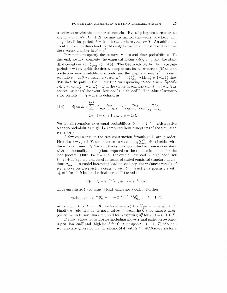
POWER MANAGEMENT IN A HYDRO-THERMAL SYSTEM 25in order to restrict the number of scenarios. By assigning two successors toany node n in Ntk , k = 1:K, we may distinguish the events \low load" and\high load" for periods t = tk + 1: tk+1, where tK+1 := T . An additionalevent such as \medium load" could easily be included, but it would increasethe scenario number to S = 3K .It remains to specify the scenario values and their probabilities. Tothis end, we �rst compute the empirical means f �dtgTt=t1+1 and the stan-dard deviations f��tkgK+1k=2 (cf. (4.3)). The load predicted for the �rst-stageperiods t = 1: t1 yields the �rst t1 components for all scenarios. (If no loadprediction were available, one could use the empirical means.) To eachscenario s = 1:S we assign a vector !s = (!sk)Kk=1 with !sk 2 f�1; 1g thatdescribes the path in the binary tree corresponding to scenario s. Speci�-cally, we set !sk = �1 (!sk = 1) if the values of scenario s for t = tk+1: tk+1are realizations of the event \low load" (\high load"). The value of scenarios for periods t = t1 + 1:T is de�ned asdst := �dt + k�1Xi=1 !si ��ti+12(K+1�i)=2 + !sk ��tk+12(K+1�k)=2 t� tktk+1 � tk(4.4) for t = tk + 1: tk+1; k = 1:K:We let all scenarios have equal probabilities S�1 = 2�K . (Alternativescenario probabilities might be computed from histograms of the simulatedscenarios.)A few comments on the tree construction formula (4.4) are in order.First, for t = t1 + 1:T , the mean scenario value 1S PSs=1 dst coincides withthe empirical mean �dt. Second, the symmetry of the load tree is consistentwith the normality assumptions imposed on the time series model for theload process. Third, for k = 1:K, the events \low load" (\high load") fort = tk + 1: tk+1 are expressed in terms of scaled empirical standard devia-tions ��tk+1 . To model increasing load uncertainty, the variances var(dt) ofscenario values are strictly increasing with t. The extremal scenario s with!sk = 1 for all k has in the �nal period T the valuedsT = �dT + 2�K=2��t2 + � � �+ 2�1=2��T :Thus unrealistic (\too large") load values are avoided. Further,var(dtk+1) = 2�K��2t2 + � � �+ 2�(K+1�k)��2tk+1 ; k = 1:K;so for ��tk+1 � ��, k = 1:K, we have var(dT ) � ��2( 12K + � � � + 12 ) � ��2.Finally, we add that the scenario values between the tk's are linearly inter-polated so as to save work required for computing ��2t for all t = t1 + 1:T .Figure 7 shows ten scenarios (including the extremal paths correspond-ing to \low load" and \high load" for the time span t = t1+1 : T ) of a loadscenario tree generated via the scheme (4.4) with 212 = 4096 scenarios for a

26 GR�OWE-KUSKA, KIWIEL, NOWAK, R�OMISCH, WEGNER

24 168

3000

4000

5000

6000

7000

8000

Fig. 7. Ten selected scenarios of a load scenario tree for one weekplanning horizon of one week with an hourly discretization and branchingpoints tk = 12 + 12k, k = 1: 12.Calibration of scenario trees generated by the scheme (4.4) is studiedin the forthcoming paper [25].4.3. Optimal reduction of the scenario tree. As shown in x4.2,the probability distribution of the load may be approximated by a dis-crete probability distribution with a �nite number of scenarios. Since themixed-integer model (2.11){(2.14) is large even for relatively few nodes, acompromise between acceptable computing times and the quality of the ap-proximate scenario tree is unavoidable. Therefore, one often has to reducethe number of scenarios of the initial scenario tree.Our reduction argument is based on certain probability metrics thatmeasure the distance between the initial discrete approximation and thereduced one. Quantitative stability results for stochastic programs (cf.[16, 19, 47]) indicate which probability metric is canonically associated toa given model and/or to a speci�c type of approximation. In particular,the results in [15, 16, 47] suggest considering the Fortet-Mourier metrics�h, h � 1, for a multistage stochastic program like (3.3).For h � 1 we denote by Gh the class of functions g : RT ! R satisfyingthe Lipschitzian propertyjg(!)� g(!0)j � ch(!; !0) for all !; !0 2 RT ;where ch(!; !0) := maxf1; k!kh�1; k!0kh�1gk! � !0k and k � k is the Eu-clidean norm on RT . Furthermore, we denote by Mh the set of all (Borel)

POWER MANAGEMENT IN A HYDRO-THERMAL SYSTEM 27probability measures � such that RRT k!kh�(d!) < 1. Then the Fortet-Mourier metric �h of (Borel) probability measures �; � 2 Mh is�h(�; �) := sup���� ZRT g(!)�(d!)� ZRT g(!)�(d!)��� : g 2 Gh� :(4.5)For h = 1, �1 is also known as the (L1-) Wasserstein or Kantorovich met-ric. The metric �h enjoys a well developed duality theory and convergenceanalysis (cf. [46, Chap. 5]).Let �! denote the probability measure on RT having unit mass at! 2 RT . Consider now two discrete probability measures� := SXs=1 �s�!s and � := ~SXs=1 ~�s�~!swith supports f!sgSs=1, f~!�g ~S�=1, and nonnegative weights �s, ~�� such thatPs �s =P� ~�� = 1. Then the dual transportation problem�h(�; �) = sup8<: SXs=1 �s�s + ~SX�=1 ~�� ~�� : �s + ~�� � ch(!s; ~!�)9=;is the �nite-dimensional analogue of (4.5). When the two measures � and� have the same support f!sgSs=1, but di�erent weights, upper and lowerbounds for �h(�; �) can be derived [15].Now, let � = PSs=1 �s�!s be a discrete probability distribution onRT that is regarded as a good initial approximation for the probabilitydistribution entering a given stochastic program. For ` = 1:S, let�`(�) := min(�h �; SXs=1 ~�s�!s! : ~�s � 0; SXs=1 ~�s = 1; ~�` = 0) :Thus �`(�) is the distance of � to a closest probability distribution havingsupport f!s : s = 1:S; s 6= `g, i.e., corresponding to deleting scenario ` of�. Then we have (cf. [15])�`(�) � �`mins6=` ch(!`; !s) for every ` 2 f1:Sg;(4.6)with the upper bounds attained if ch satis�es the triangle inequality, i.e.,for h = 1.An optimal rule for deleting one scenario of � may be stated as:Remove scenario !k with k 2 Arg min`=1:S �`(�):Replacing �`(�) above by the upper bounds of (4.6) yields the more easilyimplementable deletion rule:Delete scenario !k with k 2 Arg min`=1:S��`mins6=` ch(!`; !s)� :

28 GR�OWE-KUSKA, KIWIEL, NOWAK, R�OMISCH, WEGNER

1 24 36 48 60 72 84 96 108 120 132 144 156 168

-1000

-500

0

500

1000

Fig. 8. Shifted supports of the reduced scenario treeThen, roughly speaking, deletion occurs where scenarios are close as mea-sured by the distance ch or where probabilities are small. The reduceddiscrete probability measurePSs=1;s6=k �s�!s has S � 1 scenarios, where�sk := �sk + �k for some sk 2 Argmins6=k ch(!k; !s);�s := �s for all s =2 fsk; kg:This reduction procedure may be repeated until a prescribed number ~S ofscenarios in the reduced measure is attained.4.4. Example of scenario reduction. To test our approach, wegenerated a load scenario tree via the scheme (4.4) for an hourly discretizedtime horizon of one week (T = 168) with branching points tk = 12 + 12k,k = 1: 12 (cf. Fig. 7). The initial number of scenarios S = 4096 was reducedto 16 by applying the scenario reduction rule of x4.3.Figure 8 shows the position of the shifted supports (dst � �dt)168t=1, s =1: 16, of the reduced scenario tree within the extremal paths of the initialscenario tree indicated by dashed lines, with grey levels proportional toscenario probabilities. The probabilities �s, s = 1: 16, assigned to scenariosin the reduced tree vary between 0.04 and 0.11.The reduction technique of x4.3 produces a discrete approximationwhose moments di�er in general from those of the initial approximationgenerated by (4.4). For example, Figure 9 shows the di�erence betweenthe mean scenario value P16s=1 �sdst of the reduced tree and the empiricalmean �dt of the simulation scenarios for t = t1 + 1:T . Figure 10 comparesthe standard deviation at the branching periods tk, k = 1: 12, for the initialapproximation and the reduced scenario tree.

POWER MANAGEMENT IN A HYDRO-THERMAL SYSTEM 2924 36 48 60 72 84 96 108 120 132 144 156 168

-25

0

25

Fig. 9. Di�erence of mean values of the reduced and initial scenario trees24 168

100200300400500

24 168

100200300400500

Fig. 10. Standard deviations of the initial (left) and reduced (right) scenario treesAcknowledgment. The authors are grateful to Darinka Dentcheva(Lehigh University; formerly Humboldt-University Berlin), Svetlozar T.Rachev (University of California at Santa Barbara and University Karls-ruhe) and R�udiger Schultz (Gerhard-Mercator University Duisburg) foruseful discussions on the material of this paper, and to G. Schwarzbach,J. Thomas and J. Krause (VEAG Vereinigte Energiewerke AG, Berlin)for providing us with the data used in our test runs. This research wassupported by the Schwerpunktprogramm Echtzeit-Optimierung gro�er Sys-teme of the Deutsche Forschungsgemeinschaft, the Alexander von Hum-boldt Foundation and the Graduiertenkolleg Geometrie und NichtlineareAnalysis at the Humboldt-University Berlin.REFERENCES[1] L. Bacaud, C. Lemar�echal, A. Renaud, and C. Sagastiz�abal, Disaggregatedbundle methods in stochastic optimal power management, Research Report,INRIA, Rocquencourt, 1999.[2] D. Bertsekas, G. S. Lauer, N. R. Sandell, and T. A. Posberg, Optimal short-term scheduling of large-scale power systems, IEEE Trans. Automat. Control,AC-28 (1983), pp. 1{11.[3] J. R. Birge, Stochastic programming computation and applications, INFORMS J.Comput., 9 (1997), pp. 111{133.[4] J. R. Birge and F. Louveaux, Introduction to Stochastic Programming, Springer,New York, 1997.[5] P. J. Brockwell and R. A. Davies, Introduction to Time Series and Forecasting,Springer, New York, 1996.[6] C. C. Car�e and R. Schultz, A two-stage stochastic program for unit commitmentunder uncertainty in a hydro-thermal power system, Preprint 98-13, Konrad-

30 GR�OWE-KUSKA, KIWIEL, NOWAK, R�OMISCH, WEGNERZuse-Zentrum f�ur Informationstechnik, Berlin, Germany, 1998.[7] , Dual decomposition in stochastic integer programming, Oper. Res. Lett., 24(1999), pp. 37{45.[8] P. Carpentier, G. Cohen, and J.-C. Culioli, Stochastic optimal control anddecomposition-coordination methods, part II: Application, in Recent Develop-ments in Optimization, R. Durier and C. Michelot, eds., Lecture Notes in Eco-nomics and Mathematical Systems 429, Springer-Verlag, Berlin, 1995, pp. 88{103.[9] P. Carpentier, G. Cohen, J.-C. Culioli, and A. Renaud, Stochastic optimiza-tion of unit commitment: A new decomposition framework, IEEE Trans. PowerSystems, 11 (1996), pp. 1067{1073.[10] G. Consigli and M. A. H. Dempster, Dynamic stochastic programming for asset-liability management, Ann. Oper. Res., 81 (1998), pp. 131{161.[11] D. Dentcheva and W. R�omisch, Optimal power generation under uncertainty viastochastic programming, in Stochastic Programming Methods and TechnicalApplications, K. Marti and P. Kall, eds., Lecture Notes in Economics andMathematical Systems 458, Springer-Verlag, Berlin, 1998, pp. 22{56.[12] J. Dupa�cov�a, Scenario-based stochastic programs: Resistance with respect to sam-ple, Ann. Oper. Res., 64 (1996), pp. 21{38.[13] , Portfolio optimization via stochastic programming: Methods of output anal-ysis, Math. Methods Oper. Res., 50 (1999), pp. 245{270.[14] J. Dupa�cov�a, G. Consigli, and S. W. Wallace, Scenarios for multistage stochas-tic programs, Ann. Oper. Res. To appear.[15] J. Dupa�cov�a, N. Gr�owe-Kuska, and W. R�omisch, Scenario reduction: Anapproach using probability metrics, manuscript, Institut f�ur Mathematik,Humboldt-Univ. Berlin, Berlin, Germany, 2000. Forthcoming.[16] J. Dupa�cov�a and W. R�omisch, Quantitative stability of scenario-based stochasticprograms, in Prague Stochastics '98, M. H. et al., ed., JCMF, Prague, 1998,pp. 119{124.[17] N. C. P. Edirisinghe, Bound-based approximations in multistage stochastic pro-gramming: Nonanticipativity aggregation, Ann. Oper. Res., 85 (1999), pp. 173{192.[18] S. Feltenmark and K. C. Kiwiel, Dual applications of proximal bundle meth-ods, including Lagrangian relaxation of nonconvex problems, SIAM J. Optim.(1999). To appear.[19] O. Fiedler and W. R�omisch, Stability in multistage stochastic programming, Ann.Oper. Res., 56 (1995), pp. 79{93.[20] S.-E. Fleten, S. W. Wallace, and W. T. Ziemba, Portfolio management in aderegulated hydropower-based electricity market, in Hydropower '97, E. Broch,D. K. Lysne, N. Flatab�, and E. Helland-Hansen, eds., Balkema, Rotterdam,1997, pp. 197{204.[21] K. Frauendorfer, Barycentric scenario trees in convex multistage stochastic pro-gramming, Math. Programming, 75 (1996), pp. 277{293.[22] A. Gjelsvik, T. A. R�tting, and J. R�ynstrand, Long-term scheduling of hydro-thermal power systems, in Hydropower '92, E. Broch and D. K. Lysne, eds.,Balkema, Rotterdam, 1992, pp. 539{546.[23] R. Gollmer, A. M�oller, W. R�omisch, R. Schultz, G. Schwarzbach, andJ. Thomas, Optimale Blockauswahl bei der Kraftwerkseinsatzplanung derVEAG, in Optimierung in der Energieversorgung II, VDI-Berichte 1352, VDI,D�usseldorf, 1997, pp. 71{85.[24] N. Gr�owe, W. R�omisch, and R. Schultz, A simple recourse model for powerdispatch under uncertain demand, Ann. Oper. Res., 59 (1995), pp. 135{164.[25] N. Gr�owe-Kuska and I. Wegner, Generating scenario trees for multistagestochastic programs: A time series approach, manuscript, Institut f�ur Mathe-matik, Humboldt-Univ. Berlin, Berlin, Germany, 2000. Forthcoming.[26] J. L. Higle and S. Sen, Stochastic Decomposition; A Statistical Method for Large

POWER MANAGEMENT IN A HYDRO-THERMAL SYSTEM 31Scale Stochastic Linear Programming, Kluwer, Dordrecht, 1997.[27] , Statistical approximations for stochastic linear programming problems, Ann.Oper. Res., 85 (1998), pp. 173{192.[28] J.-B. Hiriart-Urruty and C. Lemar�echal, Convex Analysis and MinimizationAlgorithms, Springer-Verlag, Berlin, 1993.[29] K. H�yland and S. W. Wallace, Generating scenario trees for multi-stage deci-sion problems, Management Sci. (1999). To appear.[30] G. Infanger,Monte Carlo (importance) sampling within a Bender's decompositionfor stochastic linear programs, Ann. Oper. Res., 39 (1992), pp. 69{95.[31] J. Jacobs, G. Freeman, J. Grygier, D. Morton, G. Schultz, K. Staschus, andJ. Stedinger, SOCRATES: A system for scheduling hydroelectric generationunder uncertainty, Ann. Oper. Res., 59 (1995), pp. 99{133.[32] K. C. Kiwiel, Proximity control in bundle methods for convex nondi�erentiableminimization, Math. Programming, 46 (1990), pp. 105{122.[33] , Exact penalty functions in proximal bundle methods for constrained convexnondi�erentiable minimization, Math. Programming, 52 (1991), pp. 285{302.[34] , A Cholesky dual method for proximal piecewise linear programming, Numer.Math., 68 (1994), pp. 325{340.[35] , User's guide for NOA 3.0: A Fortran package for convex nondi�erentiableoptimization, tech. rep., Systems Research Institute, Warsaw, 1994.[36] C. Lemar�echal, Lagrangian decomposition and nonsmooth optimization: Bundlealgorithm, prox iteration, augmented Lagrangian, in Nonsmooth Optimization,Methods and Applications, F. Giannessi, ed., Gordon and Breach, Philadel-phia, 1992, pp. 201{216.[37] C. Lemar�echal and A. Renaud, Dual-equivalent convex and nonconvex problems,Research Report, INRIA, Rocquencourt, 1996.[38] A. L�kketangen and D. L. Woodruff, Progressive hedging and tabu search ap-plied to mixed integer (0; 1) multi-stage stochastic programming, J. Heuristics,2 (1996), pp. 111{128.[39] A. C. Miller and T. R. Rice, Discrete approximations of probability distributions,Management Sci., 29 (1983), pp. 352{362.[40] V. I. Norkin, G. Pflug, and A. Ruszczy�nski, A branch and bound method forstochastic global optimization, Math. Programming, 83 (1998), pp. 425{450.[41] M. P. Nowak, A fast descent method for the hydro storage subproblem in powergeneration, WP-96-109, International Institute for Applied Systems Analysis,Laxenburg, Austria, 1996.[42] , Stochastic Lagrangian Relaxation in Power Scheduling of a Hydro-ThermalSystem Under Uncertainty, PhD thesis, Institut f�ur Mathematik, Humboldt-Univ. Berlin, Berlin, Germany, 1999. Submitted.[43] M. P. Nowak and W. R�omisch, Stochastic Lagrangian relaxation applied to powerscheduling in a hydro-thermal system under uncertainty, Preprint 98-36, Insti-tut f�ur Mathematik, Humboldt-Univ. Berlin, Berlin, Germany, 1998. Submit-ted to Ann. Oper. Res.[44] M. V. F. Pereira and L. M. V. G. Pinto, Multi-stage stochastic optimizationapplied to energy planning, Math. Programming, 52 (1991), pp. 359{375.[45] G. C. Pflug and A. �Swietanowski, Optimal scenario tree generation for mul-tiperiod �nancial optimization, AURORA TR 1998-22, Univ. Wien, Vienna,Austria, 1998.[46] S. T. Rachev, Probability Metrics and the Stability of Stochastic Models, Wiley,Chichester, 1991.[47] S. T. Rachev and W. R�omisch, Quantitative stability in stochastic program-ming: The method of probability metrics, manuscript, Institut f�ur Mathematik,Humboldt-Univ. Berlin, Berlin, Germany, 2000. Forthcoming.[48] A. Renaud, Optimizing short-term operation of power generation: A new stochas-tic model. Lecture presented at the VIII International Conference on StochasticProgramming, Vancouver (Canada), Aug. 1998.

32 GR�OWE-KUSKA, KIWIEL, NOWAK, R�OMISCH, WEGNER[49] R. T. Rockafellar and R. J.-B. Wets, The optimal recourse problem in discretetime: L1-multipliers for inequality constraints, SIAM J. Control Optim., 16(1978), pp. 16{36.[50] , Scenarios and policy aggregation in optimization under uncertainty, Math.Oper. Res., 16 (1991), pp. 119{147.[51] W. R�omisch and R. Schultz, Decomposition of a multi-stage stochastic programfor power dispatch, Z. Angew. Math. Mech., 76 (1996), pp. 29{32. Suppl. 3.[52] A. Ruszczy�nski, Decomposition methods in stochastic programming, Math. Pro-gramming, 1{3 (1997), pp. 333{353.[53] G. B. Shebl�e and G. N. Fahd, Unit commitment literature synopsis, IEEE Trans.Power Systems, 9 (1994), pp. 128{135.[54] S. Takriti, J. R. Birge, and E. Long, A stochastic model for the unit commitmentproblem, IEEE Trans. Power Systems, 11 (1996), pp. 1497{1508.[55] S. Takriti, B. Krasenbrink, and L. S.-Y. Wu, Incorporating fuel constraints andelectricity spot prices into the stochastic unit commitment problem, ResearchReport RC 21066, Mathematical Sciences Dept., IBM Research Division, T.J.Watson Research Center, Yorktown Heights, New York, 1997. To appear inAnn. Oper. Res.[56] P. P. J. van den Bosch and F. A. Lootsma, Scheduling of power generation vialarge-scale nonlinear optimization, J. Optim. Theory Appl., 55 (1987), pp. 313{326.[57] R. J.-B. Wets, Stochastic programming, in Optimization, G. L. Nemhauser,A. H. G. Rinnooy-Kan, and M. J. Todd, eds., vol. 1 of Handbooks in Oper-ations Research and Management Science, North-Holland, Amsterdam, 1989,pp. 573{629.[58] Wolfram Research, Mathematica Time Series Pack: Reference and User'sGuide, Champaign, IL, 1995.[59] A. J. Wood and B. F. Wollenberg, Power Generation, Operation, and Control,Wiley, New York, second ed., 1996.[60] S. A. Zenios and M. S. Shtilman, Constructing optimal samples from a binomiallattice, J. Inform. Optim. Sci., 14 (1993), pp. 125{147.[61] G. Zhuang and F. D. Galiana, Towards a more rigorous and practical unitcommitment by Lagrangian relaxation, IEEE Trans. Power Systems, 3 (1988),pp. 763{773.