Semi-Lagrangian relaxation applied to the uncapacitated facility location problem

Comput Optim Appl (2012) 51:387–409DOI 10.1007/s10589-010-9338-2

Semi-Lagrangian relaxation appliedto the uncapacitated facility location problem

C. Beltran-Royo · J.-P. Vial · A. Alonso-Ayuso

Received: 24 July 2009 / Published online: 29 June 2010© Springer Science+Business Media, LLC 2010

Abstract We show how the performance of general purpose Mixed Integer Pro-gramming (MIP) solvers, can be enhanced by using the Semi-Lagrangian Relaxation(SLR) method. To illustrate this procedure we perform computational experimentson large-scale instances of the Uncapacitated Facility Location (UFL) problems withunknown optimal values. CPLEX solves 3 out of the 36 instances. By combiningCPLEX with SLR, we manage to solve 18 out of the 36 instances and improve thebest known lower bound for the other instances. The key point has been that, on av-erage, the SLR approach, has reduced by more than 90% the total number of relevantUFL variables.

Keywords Lagrangian relaxation · Mixed integer programming · Uncapacitatedfacility location (UFL) problem

This work has been partially supported by the Spanish government subsidyMTM2009-14039-C06-03 and by the ‘Comunidad de Madrid’ subsidy S2009/esp-1594.

C. Beltran-Royo (�) · A. Alonso-AyusoStatistics and Operations Research, Rey Juan Carlos University, Madrid, Spaine-mail: [email protected]

A. Alonso-Ayusoe-mail: [email protected]

J.-P. VialUniversity of Geneva, Geneva, Switzerland

J.-P. VialORDECSYS, Geneva, Switzerlandurl: www.ordecsys.com

mailto:[email protected]

mailto:[email protected]

http://www.ordecsys.com

388 C. Beltran-Royo et al.

1 Introduction

Implementing an exact method for large scale MIP problems usually requires devis-ing efficient cuts, efficient branching strategies, etc. to exploit the special structure ofthe problem at hand. In this paper we explore another possibility: to solve large scaleMIP problems by combining the SLR approach with a general MIP solver. The ideais to take advantage of the steadily increasing power of general MIP codes. The aimof combining a general MIP solver with SLR is not to obtain the fastest procedureto solve a problem, but to enhance the performance of the MIP solver at low pro-gramming cost. Here we use the UFL problem, as a benchmark to illustrate the SLRapproach. In order to obtain the best performance, one should use Erlenkotter typealgorithms [14], which are especially designed for the UFL problem.

The Semi-Lagrangian Relaxation (SLR) method was introduced in [5] to solve thep-median problem. In order to solve a combinatorial problem, the SLR method hastwo main advantages compared to the Lagrangian relaxation (LR): The SLR methodcloses the duality gap and gives an optimal integer solution as a byproduct. The dis-advantage of the SLR method is that the relaxed problem is more difficult to solvethan in the case of the LR.

SLR applies to problems with equality constraints. Like Lagrangian Relaxation(LR), the equality constraints are relaxed, but the definition of the semi-Lagrangiandual problem incorporates those constraints under the weaker form of inequalities.On combinatorial problems with positive coefficients, it has the strong property ofachieving a zero duality gap. The method has been used with success to solve largeinstances of the p-median problem. In this paper we revisit the method and apply itto the celebrated Uncapacitated Facility Location (UFL) problem. We perform com-putational experiments on two main collections of UFL problems with unknown op-timal values. CPLEX solves 3 out of the 36 instances. On one collection, we manageto solve to optimality 16 out of the 18 problems. On the second collection we solve 2out of 18 instances. Nevertheless, we are able to improve the Lagrangian lower boundin this collection and thereby confirm that the Hybrid Multistart heuristic of [32] pro-vides near optimal solutions (over 99% optimal in most cases).

The UFL problem (also called the simple plant location problem) is a basic but im-portant problem in location science [31]. See [29] for a survey. [27] and [24] improvethe famous dual-based procedure of Donald Erlenkotter [14], where the condenseddual of the LP relaxation for the UFL problem is heuristically maximized by the co-ordinate ascent method. This procedure is followed by a Branch-and-Bound if nec-essary. [11] propose an projection method to improve the coordinate ascent methodin order to compute an exact optimum of the condensed dual problem. [15] adaptErlenkotter’s method to effectively solve the so called two-echelon location problem,which generalizes the UFL problem.

On the other hand, after 1990 contributions to the UFL problem mainly dealt withheuristic methods. Some of the most successful methods are: Tabu search in [16, 33],a combination of Tabu search, Genetic Algorithm and Greedy Randomized Adapta-tive Search in [26] and Hybrid Multistart heuristic in [32]. Other contributions haveinvestigated enhanced versions of the UFL problem, as the two-stage UFL [28] orhave investigated new computational techniques applied to the UFL problem, as par-allel interior point methods [12].

Semi-Lagrangian relaxation applied to the uncapacitated facility 389

Lagrangian relaxation [20] has also been used to solve the UFL problem, thoughwith less success than the LP dual-based procedures. For example [19] proposes tostrengthen the Lagrangian relaxation (equivalent to the LP relaxation) by using Ben-ders inequalities. From a more theoretical point of view, [30] studies the duality gapof the UFL problem. A complete study of valid inequalities, facets and lifting theo-rems for the UFL problem can be found in [8–10].

This paper is organized as follows: In Sect. 2 we review the main properties ofthe SLR and discuss two algorithms to solve its associated dual problem: Proximal-ACCPM and the dual ascent algorithm. In Sect. 3, we apply the SLR to the UFLproblem, develop some related theoretical properties and detail a specialization ofthe dual ascent algorithm for the UFL case. Section 4 reports our empirical study.Our conclusions are given in a last section.

2 Semi-Lagrangian relaxation

The concept of semi-Lagrangian relaxation was introduced in [5]. In this section, wesummarize the main results obtained in that paper and simplify the proofs given there.

Consider the problem, to be named “primal” henceforth.

z∗ = minx

cT x

s.t. Ax = b, (1a)

x ∈ S ⊂ X ∩ Nn. (1b)

Assumption 1 The components of A ∈ Rm × R

n, b ∈ Rm and c ∈ R

n are nonnega-tive.

Assumption 2 X is a polyhedral set, 0 ∈ S and (1) is feasible.

Assumptions 1 and 2 together imply that (1) has an optimal solution.The semi-Lagrangian relaxation consists in adding the inequality constraint Ax ≤

b and relaxing Ax = b only. We thus obtain the dual problem

maxu∈Rm

L(u), (2)

where L(u) is the semi-Lagrangian dual function defined as

L(u) = minx

cT x + uT (b − Ax) (3a)

s.t. Ax ≤ b, (3b)

x ∈ S. (3c)

Note that with our assumptions the feasible set of (3) is bounded. We also have thatx = 0 is feasible to (3); hence (3) has an optimal solution. L(u) is well-defined, butthe minimizer in (3) is not necessarily unique. With some abuse of notation, we write

x(u) = arg minx

{cT x + uT (b − Ax) | Ax ≤ b, x ∈ S} (4)


to denote one such minimizer. With this notation we may write L(u) = (c −AT u)T x(u) + bT u. We denote U∗ the set of optimal solutions of problem (2). Fi-nally, given two sets S1 and S2, its addition corresponds to S1 + S2 = {s1 + s2 : s1 ∈S1 and s2 ∈ S2}.Theorem 1 The following statements hold [5].

1. L(u) is concave and b − Ax(u) is a subgradient at u.2. L(u) is monotone and L(u′) ≥ L(u) if u′ ≥ u, with strict inequality if u′ > u and

u′ ∈ U∗.3. U∗ + R

m+ = U∗; thus U∗ is an unbounded (convex) set.4. If x(u) is such that Ax(u) = b, then u ∈ U∗ and x(u) is optimal for problem (1).5. Conversely, if u ∈ int(U∗), then any minimizer x(u) is optimal for problem (1).6. The SLR closes the duality gap for problem (1).

Now, we simplify the proof given in [5].

Proof From the definition of the SLR function as a pointwise minimum, the inequal-ity

L(u′) ≤ cT x(u) + (u′)T (b − Ax(u))

= L(u) + (b − Ax(u))T (u′ − u), (5)

holds for any pair u,u′. This shows that L(u) is concave and that (b − Ax(u)) is asubgradient at u. This proves statement 1.

To prove statement 2, we note, in view of b −Ax(u′) ≥ 0 and u′ ≥ u, that we havethe chain of inequalities

L(u′) = cT x(u′) + (b − Ax(u′))T u′,

= cT x(u′) + (b − Ax(u′))T u + (b − Ax(u′))T (u′ − u),

≥ cT x(u′) + (b − Ax(u′))T u,

≥ cT x(u) + (b − Ax(u))T u = L(u).

This proves the first part of the third statement. If u′ /∈ U∗, then 0 /∈ ∂L(u′), thesubdifferential of L at u′ [22], and one has (b − Ax(u′))j > 0 for some j . Thus,u < u′ implies (b − Ax(u′))T (u′ − u) > 0. Hence, L(u′) > L(u).

The third statement is an immediate consequence of the monotone property ofL(u). Furthermore, U∗ is convex since it is the optimal set of a concave function [22].

To prove the fourth statement, we note that Ax(u) = b implies 0 ∈ ∂L(u), a nec-essary and sufficient condition of optimality for problem (2). Hence u ∈ U∗. Finally,since x(u) is feasible to (1) and optimal for the relaxation (3) of problem (1), it isalso optimal for (1).

To prove the fifth statement, assume now u ∈ int(U∗). In this case there existsu′ ∈ U∗ such that u′ < u; thus (b − Ax(u))T (u − u′) ≥ 0, with strict inequality ifb − Ax(u) = 0. In view of (5),

0 ≥ (b − Ax(u))T (u′ − u) ≥ L(u′) − L(u).


Thus Ax(u) = b, and x(u) is optimal to (1). It follows that the original problem(1) and the semi-Lagrangian dual problem (2) have the same optimal value (the laststatement). �

To close this section we present the two methods we use to solve the SLR dualproblem (2): The proximal analytic center cutting plane method (proximal-ACCPM)and dual ascent method. The first one consists in choosing a theoretically and prac-tically efficient general method for solving the semi-Lagrangian dual problem. Asfor the p-median problem [5] we select the proximal analytic center cutting planemethod (proximal-ACCPM). This ensures a small number of iterations, and seemsto keep the oracle subproblem simple enough during the solution process. The othermethod is a variant of the dual ascent method (e.g., [6]) based on finite increasesof the components of u. In fact, the dual ascent algorithm we use is in essence thedual multi-ascent procedure used in [27] to solve the Erlenkotter’s ‘condensed’ dualof the UFL problem [14]. In the case of LR, the dual multi-ascent method does notnecessarily converge. In the case of the SLR we prove finite convergence.

2.1 The proximal analytic center cutting plane method

Function L(u) in problem (2) is by construction, concave and nonsmooth (it is implic-itly defined as the pointwise minimum of linear functions in u). Extensive numericalexperience shows that Proximal-ACCPM, is an efficient tool for solving (2). See, forinstance, [18] and references therein included; see also [5] for experiments with thep-median problem.

In the cutting plane procedure, we consider a sequence of points {uk}k∈K in thedomain of L(u). We consider the linear approximation to L(u) at uk , given by

Lk(u) = L(uk) + sk · (u − uk)

and have

L(u) ≤ Lk(u)

for all u.The point uk is referred to as a query point, and the procedure to compute the

objective value and subgradient at a query point is called an oracle. Furthermore, thehyperplane that approximates the objective function L(u) at a feasible query pointand defined by the equation z = Lk(u), is referred to as an optimality cut.

A lower bound to the maximum value of L(u) is provided by:

θl = maxk

L(uk).

The localization set is defined as

LK = {(u, z) ∈ Rn+1 | u ∈ R

n, z ≤ Lk(u) ∀k ≤ K, z ≥ θl}, (6)

where K is the current iteration number. The basic iteration of a cutting plane methodcan be summarized as follows:


1. Select (u, z) in the localization set LK .2. Call the oracle at u. The oracle returns one or several

optimality cuts and a new lower bound L(u).3. Update the bounds:

(a) θl ← max{L(u), θl}.(b) Compute an upper bound θu to the optimum of problem (2).

4. Update the lower bound θl and add the new cuts in thedefinition of the localization set (6).

These steps are repeated until a point is found such that θu − θl falls below aprescribed optimality tolerance. The first step in the above algorithm sketch is notcompletely defined. Actually, cutting plane methods essentially differ in the way onechooses the query point. For instance, the intuitive choice of the Kelley point (u, z)

that maximizes z in the localization set [25] may prove disastrous, because it over-emphasizes the global approximation property of the localization set. Safer methods,as for example bundle methods [21] or Proximal-ACCPM [2, 13, 17, 18], introduce aregularizing scheme to avoid selecting points too “far away” from the best recordedpoint. In this paper we use Proximal-ACCPM (Proximal Analytic Center CuttingPlane Method) which selects the proximal analytic center of the localization set. For-mally, the proximal analytic center is the point (u, z) that minimizes the logarithmicbarrier function of the localization set plus a quadratic proximal term which ensuresthe existence of a unique minimizer. This point is relatively easy to compute usingthe standard artillery of Interior Point Methods. Furthermore, Proximal-ACCPM isrobust, efficient and particularly useful when the oracle is computationally costly—as is the case in this application.

2.2 A dual ascent method

We state the algorithm first and then prove finite convergence. This algorithm, at eachiteration, increases some or all of the coordinates of the dual iterate uk , by at least� > 0.

Algorithm 1 Dual ascent algorithm (basic iteration)

1. Solve the oracle: Compute

xk = arg minx

{cT x + (uk)T (b − Ax) | Ax ≤ b, x ∈ S},

where uk is the current dual iterate.2. Stopping criterion: If sk := b − Axk = 0, stop.

(xk, uk) is an optimal primal-dual point.3. Update the dual iterate: For j = 1, . . . , n, set

uk+1j =

{uk

j + δkj if sk

j > 0,

ukj otherwise,

where δkj ≥ �.


We now prove finite convergence of the above algorithm.

Theorem 2 The following statements hold.

1. Algorithm 1 is a dual ascent method when applied to solve the SLR dual problem:for any two consecutive iterates uk and uk+1 we have L(uk+1) > L(uk).

2. Let us suppose that u0 ≥ 0 and that U∗ = ∅. Algorithm 1 converges to an optimaldual point u ∈ U∗ after finitely many iterations.

Proof Let us prove statement 1 first. The updating procedure of Algorithm 1 consistsin increasing some components of the current dual point uk (step 3). Thus, uk+1 > uk

and by Theorem 1.2 we have that L(uk+1) > L(uk).The proof of statement 2 goes as follows. Let us consider the sequence {sk} of

subgradients generated by the algorithm. We have two exclusive cases.Case 1: There exists k0 such that sk0 = 0. Then 0 ∈ ∂L(uk0) and uk0 ∈ U∗.Case 2: At least for one component of sk , say the 1st, there exists a subsequence

{ski

1 } ⊂ {sk1 } such that s

ki

1 = 0 for all i = 0,1,2, . . . . We will prove by contradictionthat this case cannot happen.

By definition of the algorithm we will have:

uki

1 ≥ uk01 + i�. (7)

Let us show that the subsequence {L(uki )} is unbounded from above which con-tradicts the hypothesis U∗ = ∅. Let us define J ki = {j | s

ki

j > 0}. Since x is a binaryvector, it implies, by Assumption 1, that there exists an absolute constant η > 0 suchthat

minj

minx

{sj = (b − Ax)j | (b − Ax)j > 0} = η.

Thus ski

j ≥ η for all j ∈ J ki and for all i.

Using the fact that cT x ≥ 0 and that uki ≥ 0, we have

L(uki ) = cT x(uki ) + (b − Ax(uki ))T uki

= cT x(uki ) + (ski )Tuki

≥ (ski )Tuki

=∑

j∈J ki

ski

j uki

j

≥ uki

1 η

≥ (uk01 + i�)η.

Thus limi→∞ L(uki ) = +∞. �


3 SLR applied to the UFL problem

In the Uncapacitated Facility Location (UFL) problem we have a set of ‘facilities’indexed by I = {1, . . . ,m} and a set of ‘clients’ indexed by J = {1, . . . , n}. The pur-pose is to open facilities relative to the set of clients, and to assign each client toa single facility. The cost of an assignment is the sum of the shortest distances cij

from a client to a facility plus the fixed costs of opened facilities fi . The distanceis sometimes weighed by an appropriate factor, e.g., the demand at a client node.The objective is to minimize this sum. The UFL problem is NP-hard [29] and can beformulated as follows.

z∗ = minx,y

z(x, y) (8a)

s.t.m∑

i=1

xij = 1, j ∈ J, (8b)

xij ≤ yi, i ∈ I, j ∈ J, (8c)

xij , yi ∈ {0,1}, (8d)

where

z(x, y) =m∑

i=1

n∑j=1

cij xij +m∑

i=1

fiyi . (9)

xij = 1 if facility i serves the client j , otherwise xij = 0 and yi = 1 if we open facilityi, otherwise yi = 0.

Following the ideas of the preceding section, we formulate the semi-Lagrangianrelaxation of the UFL problem. We obtain the dual problem

maxu∈Rn

L(u) (10)

and the oracle (note that, now, we keep the equality constraint (8b) as an inequality)

L(u) = minx,y

f (u, x, y) (11a)

s.t.m∑

i=1

xij ≤ 1, j ∈ J, (11b)

xij ≤ yi, i ∈ I, j ∈ J, (11c)

xij , yi ∈ {0,1}, (11d)

where

f (u, x, y) =m∑

i=1

n∑j=1

cij xij +m∑

i=1

fiyi +n∑

j=1

uj

(1 −

m∑i=1

xij

)

=m∑

i=1

n∑j=1

(cij − uj )xij +m∑

i=1

fiyi +n∑

j=1

uj . (12)


As in the previous section, we denote (x(u), y(u)) an optimal point for the oracle(11). The associated Lagrangian relaxation that we use in this paper, corresponds toformulation (11) without constraints (11b).

3.1 Properties of the SLR dual problem

In this section we show that, in order to solve the SLR dual problem, we can re-strict our dual search to a box. To this end, we define for each client j , its bestcombined costs as c̃j := mini{cij + fi}. The vector of best combined costs is thusc̃ := (c̃1, . . . , c̃n). Furthermore, for each client j , we sort its costs cij , and get thesorted costs

c1j ≤ c2

j ≤ · · · ≤ cmj .

Theorem 3 u ≥ c̃ ⇒ u ∈ U∗ and u > c̃ ⇒ u ∈ int(U∗).

Proof Consider the oracle

minx

m∑i=1

(fiyi +n∑

j=1

(cij − uj )xij ) +n∑

j=1

uj

m∑i=1

xij ≤ 1, ∀j

xij ≤ yi, ∀i, j

xij , yi ∈ {0,1}.Assume u ≥ c̃. If there exists an optimal solution of the oracle such that

∑i xij =

1, ∀j , then, by Theorem 1, this solution is optimal for the original problem. Assumewe have an oracle solution with

∑i xij = 0 for some j . Let ik be such that c̃j =

fik + cikj . By hypothesis, c̃j − uj ≤ 0. Thus, fik + (cikj − uj ) ≤ 0 and one can setxikj = 1 and yik = 1 without increasing the objective value. The modified solution isalso optimal. Hence, there exists an optimal oracle solution with

∑i xij = 1, ∀j and

u ∈ U∗. The second statement of the theorem follows from c̃ ∈ U∗ and statement 3of Theorem 1. �

Theorem 4 If u ∈ int(U∗), then u ≥ c1.

Proof Let us assume that uj0 < c1j0

for some j0 ∈ J and see that this contradicts

u ∈ int(U∗). If uj0 < c1j0

then ckj0

− uj0 > 0 for all k ∈ I . Any optimal solution x(u)

is such that xij0(u) = 0, for all i ∈ I . Hence, 1 − ∑i∈I xij0(u) = 1 and by Theorem

1, u is not in int(U∗). �

Corollary 1 Let us consider the scalar ε > 0, the vector ε̄, where each component isequal to ε, and the box

B := {u ∈ Rn | c1 < u ≤ c̃ + ε̄}.


Then, for the UFL problem one has

int(U∗) ∩ B = ∅.

This corollary implies that the search for an optimal dual point can be confinedto a box. In particular, taking u = c̃ + ε̄ and solving the oracle for u, yields a primaloptimal solution in one step. As pointed out earlier, it is likely to be impracticalbecause the oracle is too difficult at that u. It is also, likely that there is a smalleru∗ ∈ U∗, for which the oracle subproblem would be easier (with less binary variables)and hopefully tractable by an integer programming solver. This justifies the use ofdual methods that increase the dual iterates in small steps.

3.2 Structure of the oracle: the core subproblem

In this section, we study the structure of the UFL oracle as a function of the dualvariable u. We shall show how some primal variables xij can be set to zero when uj issmall enough. This operation, which reduces the size of the oracle, is quite commonin Lagrangian relaxation applied to combinatorial optimization. There, using someappropriate argument, one fixes some variables of the oracle and obtains a reduced-size oracle called the core subproblem. (See, for instance, [1, 7].)

We now define the core UFL subproblem in the SLR case. Let c(u) be the matrixof reduced costs such that c(u)ij = cij − uj . Let G = (V × W,E) be the bipartitegraph associated to the UFL problem, such that each node in V (W ) represents afacility (client) and the edge eij exists if facility i can serve client j . c(u)ij is thusthe reduced cost associated to eij . Let E(u) ⊂ E be the subset of edges with strictlynegative reduced cost for a given dual point u. Let V (u) ⊂ V and W(u) ⊂ W be theadjacent vertices to E(u). Let G(u) = (V (u) × W(u),E(u)) be the induced bipartitesubgraph. We call G(u) the core graph.

It is easy to see that for any c(u)ij ≥ 0 there exists x(u) such that x(u)ij = 0.Therefore, we can restrict our search to the core graph G(u) to compute x(u). Theadvantage of solving oracle (11) with core graph G(u) is that in G(u) we may havemuch less edges (variables xij ) and facility nodes (variables yj ), as we will see inSect. 4.6. A further advantage of solving the core subproblem is that, even though G

is usually a connected graph, G(u) may be decomposable into independent subgraphsand then we can decompose the core subproblem into smaller (easier) subproblems.

We now study the inverse image of the mapping G(u). In other words, we wish todescribe the set of u’s that have the graph G as a common image through the mappingG(u). It is easy to see that it is a simple box.

To define an elementary box, we use the sorted costs to partition the domain ofeach coordinate uj into intervals of the form ]ck

j , ck+1j ], with the convention that

cm+1j = +∞. Note that some boxes may be empty (if ck

j = ck+1j ). These coordinate

partitions induce a partition of the box B into elementary boxes. It is not difficultto show that, there is a bijection between core graphs G(u) and elementary boxes.Therefore, it is enough to restrict the dual search to one representative point per el-ementary box. The dual ascent algorithm to be presented in the next section willexploit this structure.


3.3 The dual ascent algorithm to solve the SLR dual problem

We now present a specialized version of the dual ascent method (Algorithm 1) for theUFL problem. We know by Corollary 1, that the dual search can be confined to thebox B. The discussion of the previous section shows that B can be partitioned intoelementary boxes and that it is enough to restrict the dual search to one representativepoint per elementary box. Our choice is to take this representative point, as small aspossible within each elementary box. Since an elementary box is determined by theintervals ]ck

j , ck+1j ], we choose the representative point to be uj = c

l(j)j + ε (j =

1, . . . , n), for some fixed ε > 0.Our algorithmic scheme is as follows: Take a small ε > 0 and for each client j ,

take some l(j) ∈ I (see Sect. 4.1 for details). Start the dual search at u0j := c

l(j)j + ε

(each client node will have exactly l(j) core edges). Query the oracle, and if thecurrent dual iterate is not optimal, update it. To maintain the number of core edgesas low as possible, at each iteration, we add at most one edge per client, that is,we update uj from c

l(j)j + ε to c

l(j)+1j + ε, for some l(j) ∈ I . We only update the

coordinates of the dual iterate uk whose corresponding subgradient coordinate is notnull. The details of this simple procedure are as follows.

Algorithm 2 Dual ascent algorithm (UFL case)

1. Initialization: Set k = 0 and ε > 0. For each client j ∈ J = {1, . . . , n}, set(a) u0

j = cl(j)j + ε for some l(j) ∈ I = {1, . . . ,m},

(b) c̃j = mini{cij + fi},(c) cm+1

j = +∞.

2. Oracle call: Compute L(uk), (x(uk), y(uk)) and sk where

skj = 1 −

m∑i=1

xkij ,

for all j ∈ J . (Note that skj ∈ {0,1}.)

3. Stopping criterion: If sk = 0 then stop. The pair (uk; (x(uk), y(uk)) is a primal-dual optimal point.

4. Multiplier updating: For each j ∈ J such that skj = 1, set

uk+1j = min{cl(j)+1

j , c̃j } + ε and l(j) = min{l(j) + 1, n}.5. Set k = k + 1 and go to Step 2.

By construction, the iterates are monotonic with at least one strictly increasingcoordinate. The algorithm converges in a finite number of iterations. The semi-Lagrangian dual function is also monotonic, which makes the algorithm a dual-ascent.


4 Computational experiments

The objective of our numerical test is twofold: first, we study the quality of the so-lution given by the semi-Lagrangian relaxation (SLR) and second we study the SLRperformance in terms of CPU time. The CPU time limit is set to 7200 seconds. First,we compare our combined SLR-CPLEX approach to the plain CPLEX. Second, wecompare our results to the results reported in [32] and in the Uncapacitated FacilityLocation Library (UflLib) [23].

4.1 Parameter setting for the algorithms

Programs have been written in MATLAB 7.0 and run on a PC (Pentium-IV, 3.0 GHz,with 3 GB of RAM memory) under the Windows XP operating system. The readershould bear in mind that results reported in [32] were found on a different machine(SGI Challenge with 28 196-MHz MIPS R10000 processors, although each executionwas limited to a single processor) and programs were implemented in C++.

In our context and using the terminology of oracle based optimization [2], to callor to solve an oracle means to compute L(uk): Oracle 1 for the Lagrangian relax-ation and Oracle 2 for the semi-Lagrangian relaxation. To solve Oracle 2 (a large-scale mixed integer program) we have intensively used CPLEX 9.1 (default settings)interfaced with MATLAB [3].

The dual ascent algorithm is implemented as stated in the previous section with-out parameter tuning (ε = 10−3). Proximal-ACCPM is used in its generic form asdescribed in [2] with some tuning. We use Proximal-ACCPM in a two phase scheme:in the first phase we solve the Lagrangian relaxation (LR) dual problem. In the secondphase we solve the semi-Lagrangian relaxation (SLR) dual problem. The Proximal-ACCPM parameter setting is as follows: In the LR phase, we use a proximal weightρ that at each Proximal-ACCPM iteration is updated within the range [10−6,104]and the required precision is 10−6. In the SLR phase, we choose to fix the referenceproximal point at the initial point u0. As pointed out in [5], an optimal LR dual pointu∗

LR is a good starting point u0 for the SLR method. To be more precise, in our UFL

computational experiments, for each client j , we take the cl(j)j which is the closest to

u∗LRj

and define u0j := c

l(j)j + ε, for some small ε > 0 (as we saw in Algorithm 2).

The proximal weight ρ has been fixed, by tuning, to 10−4 for the Barahona-Chudakinstances and to 10−3 for the Koerkel-Ghosh instances.

4.2 Instance description

For our test we use 36 unsolved UFL instances that can be obtained in the UFL libraryUflLib (see Table 1). The first set, with 18 instances, is called Barahona-Chudak [4].In the Euclidian plane n points are randomly generated in the unit square [0,1] ×[0,1]. Each point simultaneously represents a facility and a client (m = n), withn = 500,1000, . . . ,3000. The connection costs cij are determined by the Euclidiandistance. In each instance all the fixed costs fi are equal and calculated by

√n/l

with l = 10,100 or 1000. All values are rounded up to 4 significant digits and madeinteger [23]. We use the label n − l to name these instances.


Table 1 Instance description: For the Barahona-Chudak instances, the fixed cost is the same for all facil-ities. For the Koerkel-Ghosh instances the fixed cost is randomly chosen for each facility according to auniform distribution

Barahona-Chudak Nb. of Fix Koerkel-Ghosh Nb. of Fix

instances clients cost instances clients cost

500-1000 500 224 gs00250a-1 250 U [100,200]

500-100 500 2236 gs00250b-1 250 U [1000,2000]

500-10 500 22361 gs00250c-1 250 U [10000,20000]

1000-1000 1000 316 gs00500a-1 500 U [100,200]

1000-100 1000 3162 gs00500b-1 500 U [1000,2000]

1000-10 1000 31623 gs00500c-1 500 U [10000,20000]

1500-1000 1500 387 gs00750a-1 750 U [100,200]

1500-100 1500 3873 gs00750b-1 750 U [1000,2000]

1500-10 1500 38730 gs00750c-1 750 U [10000,20000]

2000-1000 2000 447 ga00250a-1 250 U [100,200]

2000-100 2000 4472 ga00250b-1 250 U [1000,2000]

2000-10 2000 44721 ga00250c-1 250 U [10000,20000]

2500-1000 2500 500 ga00500a-1 500 U [100,200]

2500-100 2500 5000 ga00500b-1 500 U [1000,2000]

2500-10 2500 50000 ga00500c-1 500 U [10000,20000]

3000-1000 3000 548 ga00750a-1 750 U [100,200]

3000-100 3000 5477 ga00750b-1 750 U [1000,2000]

3000-10 3000 54772 ga00750c-1 750 U [10000,20000]

The second set of UFL instances is called Koerkel-Ghosh. In these instances,the connection costs cij are drawn uniformly at random from [1000,2000]. Thefixed costs fi are drawn uniformly at random from [100, 200] in class ‘a’, from[1000,2000] in class ‘b’ and from [10000,20000] in class ‘c’. Furthermore symmet-ric and asymmetric connection matrices are created. UflLib provides instances of the3 largest sizes presented in [16] with n = m = 250,500 and 750. Of the 90 instancesproposed in the UflLib, we took 18 representative ones. We use the label gX00YZ-1to name these instances, where X can be either ‘s’ or ‘a’ for the symmetric or asym-metric case respectively. Y is equal to ‘n’ and Z is the class (a, b or c).

4.3 CPLEX performance

In Table 2 we report the results obtained with CPLEX 9.1 (default settings and 7200seconds as CPU time limit). Barahona-Chudak instances: We observe that CPLEXhas solved the first three instances. However, the remaining 15 instances have becometoo large, even to solve their LP relaxation. Koerkel-Gosh instances: CPLEX hasgiven an integer solution and a lower bound in most of the cases. Cases gs00750a-1and ga00750a-1 have become too large at the beginning of the B&B process (CPLEXhas been able to solve their LP relaxation and compute an integer solution). For theother 4 instances with 750 points, CPLEX has not even solved the LP relaxationwithin 7200 seconds.


Table 2 CPLEX performance: ‘UB’ stands for upper bound, ‘LB’ for lower bound. Larger instances haveproduced an ‘Out of memory’ either before CPLEX solved the LP relaxation or after (‘Before LP’ and‘After LP’)

Instance UB LB B&B gap (%) CPLEX time (sec.) Out of memory

500-1000 99169 99169 0.00 12

500-100 326790 326790 0.00 4

500-10 798577 798577 0.00 35

1000-1000 – – – – Before LP

1000-100 – – – – Before LP

1000-10 – – – – Before LP

1500-1000 – – – – Before LP

1500-100 – – – – Before LP

1500-10 – – – – Before LP

2000-1000 – – – – Before LP

2000-100 – – – – Before LP

2000-10 – – – – Before LP

2500-1000 – – – – Before LP

2500-100 – – – – Before LP

2500-10 – – – – Before LP

3000-1000 – – – – Before LP

3000-100 – – – – Before LP

3000-10 – – – – Before LP

gs00250a-1 257999 257803 0.08 7200

gs00250b-1 276892 274324 0.94 7200

gs00250c-1 332935 324142 2.71 7200

gs00500a-1 512237 510446 0.35 7200

gs00500b-1 654860 533027 22.86 7200

gs00500c-1 746506 601986 24.01 7200

gs00750a-1 785232 762565 2.97 5023 After LP

gs00750b-1 – – – 7200

gs00750c-1 – – – 7200

ga00250a-1 257991 257778 0.08 7200

ga00250b-1 276556 274112 0.89 7200

ga00250c-1 334735 324892 3.03 7200

ga00500a-1 512071 510614 0.29 7200

ga00500b-1 649226 533339 21.73 7200

ga00500c-1 747626 602861 24.01 7200

ga00750a-1 783973 762464 2.82 5707 After LP

ga00750b-1 – – – 7200

ga00750c-1 – – – 7200


4.4 Dual solution quality

In Table 3 we report the dual solution quality. We observe an important result: thesemi-Lagrangian relaxation closes the duality gap (if convergence is reached). Col-umn (3.a) reports the best known upper bound (UB) to the optimal primal cost. Inthe remaining 6 columns we report the results concerning the Lagrangian relaxation(LR) and the semi-Lagrangian relaxation (SLR) bounds.

In column (3.b) we have the LR lower bound (obtained with Proximal-ACCPM).In column (3.c) we give the LR duality gap (in fact we give an upper bound to thetrue duality gap since in some cases we do not know the true primal optimum but anupper bound). In the remaining 4 columns (3.d–g), we report the SLR lower boundinformation, obtained either with the dual ascent method o with Proximal-ACCPM.We also give the optimality gap of these dual values. Optimal SLR dual bounds havebeen written in boldface. In the remaining cases, the SLR procedure was stoppedbefore reaching optimality because of the CPU time limit (7200 seconds).

4.5 Primal solution quality

In Table 4 we report the primal solution quality. Column (4.a) reports the best knownlower bound. In column (4.b), we have the upper bounds (UB) to the UFL optima,reported in literature. In the first half of this column, we have the results for theBarahona-Chudak instances reported in [32], (they were obtained as the average ofseveral runs). In the second half of this column, we have the results for the Koerkel-Ghosh instances as reported in UflLib (the results reported in [32] for these instancesdo not correspond to single instances but for groups of 5 instances). In columns (4.d)and (4.f) we have the UB obtained in the framework of the dual ascent method andProximal-ACCPM, respectively.

In this section, the important result is that the SLR approach has been able tosolve 18 instances of the 36 previously unsolved ones. These 18 instances have beensolved by Proximal-ACCPM. On the other hand, the dual ascent method has beenable to solve 16 UFL instances.

For the unsolved instances we have reported the upper bound obtained by the fol-lowing simple heuristic which computes a primal feasible solution. At each iterationof the SLR method the oracle solution y(uk) proposes to open a set of facilities. Tocomplete the solution, each client is assigned to its closest open facility. If the SLRmethod fails to converge, we take the best heuristic solution as the primal SLR so-lution. In general, the sophisticated heuristic used in [32] performs better than oursimple primal heuristic. At the same time, the SLR procedure combined with thissimple heuristic, has given better primal solutions than CPLEX.

4.6 Instance reduction

Very often, Lagrangian relaxation is used to decompose difficult problems. The de-composition induced by SLR is more coarse-grained than the Lagrangian relaxationone. Thus for example, in the UFL problem, after Lagrangian relaxation, one has onesubproblem per facility. However, after SLR, one may have from several to only one


Table 3 Dual solution quality: ‘UB’ stands for upper bound, ‘LB’ for lower bound, ‘PACCPM’ forProximal-ACCPM, ‘DA’ for dual ascent. Optimal lower bounds are in boldface

Instance UB LB

Lagrangian Semi-Lagrangian Semi-Lagrangian

(PACCPM) (Dual ascent) (PACCPM)

Bound Dual Bound Optimality Bound Optimality

gap (%) gap (%) gap (%)

(3.a) (3.b) (3.c) (3.d) (3.e) (3.f) (3.g)

500-1000 99169 99160 0.0091 99169 0 99169 0

500-100 326790 326790 0 326790 0 326790 0

500-10 798577 798577 0 798577 0 798577 0

1000-1000 220560 220559 0.0003 220560 0 220560 0

1000-100 607878 607814 0.0105 607878 0 607878 0

1000-10 1434154 1433389 0.0534 1434154 0 1434154 0

1500-1000 334962 334944 0.0054 334962 0 334962 0

1500-100 866454 866453 0.0001 866454 0 866454 0

1500-10 2000801 1999284 0.0758 2000696 0.0052 2000801 0

2000-1000 437686 437678 0.0018 437686 0 437686 0

2000-100 1122748 1122746 0.0002 1122748 0 1122748 0

2000-10 2558118 2557753 0.0143 2558118 0 2558118 0

2500-1000 534405 534395 0.0019 534405 0 534405 0

2500-100 1347516 1347494 0.0016 1347516 0 1347516 0

2500-10 3100225 3096856 0.1087 3097647 0.0831 3097647 0.0831

3000-1000 643463 643432 0.0048 643463 0 643463 0

3000-100 1602335 1601652 0.0426 1602063 0.0170 1602120 0.0134

3000-10 3570766 3570752 0.0004 3570766 0 3570766 0

Partial average 1200367.0 1199985 0.0184 1200203 0.0059 1200212 0.0054

gs00250a-1 257964 257639 0.1259 257899 0.0252 257964 0

gs00250b-1 276761 273693 1.1085 275363 0.5051 275574 0.4289

gs00250c-1 332935 322696 3.0753 329135 1.1414 330559 0.7137

gs00500a-1 511229 510408 0.1606 510408 0.1606 510408 0.1606

gs00500b-1 537931 533020 0.913 534029 0.7254 533477 0.8280

gs00500c-1 620041 601962 2.9158 607260 2.0613 609333 1.7270

gs00750a-1 763671 762562 0.1453 762562 0.1452 762562 0.1452

gs00750b-1 797026 790334 0.8396 790917 0.7665 790917 0.7665

gs00750c-1 900454 875340 2.789 879430 2.3348 879343 2.3445

ga00250a-1 257957 257618 0.1315 257882 0.0291 257957 0

ga00250b-1 276339 273296 1.1012 275080 0.4556 275200 0.4122

ga00250c-1 334135 322958 3.3451 329839 1.2857 331171 0.8871

ga00500a-1 511422 510587 0.1632 510587 0.1633 510587 0.1633

ga00500b-1 538060 533334 0.8784 534416 0.6772 533837 0.7849

ga00500c-1 621360 602852 2.9787 608518 2.0668 609975 1.8323

ga00750a-1 763576 762462 0.1459 762462 0.1459 762462 0.1459

ga00750b-1 796480 790112 0.7995 790631 0.7344 790630 0.7345

ga00750c-1 902026 875593 2.9304 880301 2.4085 879601 2.4861

Partial average 555520.4 547581 1.3637 549818 0.8795 550087 0.8089

Global average 877943.7 873783 0.6910 875010 0.4427 875149 0.4071


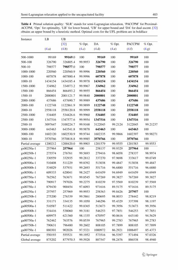
Table 4 Primal solution quality: ‘SLR’ stands for semi-Lagrangian relaxation, ‘PACCPM’ for Proximal-ACCPM, ‘Opt.’ for optimality, ‘LB’ for lower bound, ‘UB’ for upper bound and ‘DA’ for dual ascent. [32]obtains an upper bound by a heuristic method. Optimal costs for the UFL problem are in boldface

Instance LB UB

[32] % Opt. DA % Opt. PACCPM % Opt.

(4.a) (4.b) (4.c) (4.d) (4.e) (4.f) (4.g)

500-1000 99169 99169.0 100 99169 100 99169 100

500-100 326790 326805.4 99.9953 326790 100 326790 100

500-10 798577 798577.0 100 798577 100 798577 100

1000-1000 220560 220560.9 99.9996 220560 100 220560 100

1000-100 607878 607880.4 99.9996 607878 100 607878 100

1000-10 1434154 1434185.4 99.9978 1434154 100 1434154 100

1500-1000 334962 334973.2 99.9967 334962 100 334962 100

1500-100 866454 866493.2 99.9955 866454 100 866454 100

1500-10 2000801 2001121.7 99.9840 2000801 100 2000801 100

2000-1000 437686 437690.7 99.9989 437686 100 437686 100

2000-100 1122748 1122861.9 99.9899 1122748 100 1122748 100

2000-10 2558118 2558120.8 99.9999 2558118 100 2558118 100

2500-1000 534405 534426.6 99.9960 534405 100 534405 100

2500-100 1347516 1347577.6 99.9954 1347516 100 1347516 100

2500-10 3097647 3100224.7 99.9168 3122045 99.2124 3122045 99.21237

3000-1000 643463 643541.8 99.9878 643463 100 643463 100

3000-100 1602120 1602530.9 99.9744 1602335 99.9866 1602397 99.98271

3000-10 3570766 3570818.8 99.9985 3570766 100 3570766 100

Partial average 1200212 1200420.0 99.9903 1201579 99.9555 1201583 99.9553

gs00250a-1 257964 257964 100 258137 99.9329 257964 100

gs00250b-1 275574 276761 99.5693 279416 98.6058 278337 98.9974

gs00250c-1 330559 332935 99.2812 337270 97.9698 333617 99.0749

gs00500a-1 510408 511229 99.8392 513038 99.4847 513038 99.4847

gs00500b-1 534029 537931 99.2693 551716 96.6880 551716 96.6880

gs00500c-1 609333 620041 98.2427 641659 94.6949 641659 94.6949

gs00750a-1 762562 763671 99.8545 767269 99.3827 767269 99.3827

gs00750b-1 790917 797026 99.2275 810239 97.5569 810239 97.5569

gs00750c-1 879430 900454 97.6093 971616 89.5175 971616 89.5175

ga00250a-1 257957 257969 99.9953 258363 99.8426 257957 100

ga00250b-1 275200 276339 99.5861 280695 98.0033 278442 98.8219

ga00250c-1 331171 334135 99.1050 346296 95.4329 337398 98.1197

ga00500a-1 510587 511422 99.8365 513673 99.3956 513673 99.3956

ga00500b-1 534416 538060 99.3181 546253 97.7851 546253 97.7851

ga00500c-1 609975 621360 98.1335 670597 90.0616 643140 94.5629

ga00750a-1 762462 763576 99.8539 767965 99.2783 767965 99.2783

ga00750b-1 790631 796480 99.2602 808105 97.7899 808105 97.7899

ga00750c-1 880301 902026 97.5321 1000972 86.2921 1008497 85.4373

Partial average 550193 555521 99.1952 573516 96.5397 571494 97.0326

Global average 875202 877970.5 99.5928 887547 98.2476 886538 98.4940


subproblem. Furthermore, the number of subproblems usually is different for eachSLR iteration. For this reason, we do not report the number of subproblems at eachiteration, but its average. In Table 5, we have the average number of subproblems(ANS) per SLR iteration. More specifically, columns (5.a) and (5.b) report the ANSfor the dual ascent method and for Proximal-ACCPM respectively. For example, ininstance 500-1000 the ANS value is 108 and 84 for the dual ascent method and forProximal.ACCPM, respectively. This means that the SLR method has managed todecomposed this instance. In other 30 instances (instance 500-100 for example) theSLR does not decompose the instance (ANS = 1). Note that the decomposition isslightly better with the dual ascent method than with Proximal-ACCPM.

An important advantage of the SLR is that usually it drastically reduces the num-ber of relevant variables (otherwise said, we can fix to 0 many variables). In column(5.c) we have the total number of xij variables. For example, instance 500-1000 has250000 xij variables, but, as we can see in column (5.d) only 0.3% are relevant inthe SLR combined with the dual ascent method (the remaining 99.7% are fixed to0). The number of relevant xij variables in the case of Proximal-ACCPM is reportedin (5.e). The analogous results for the yi variables can be found in columns (5.f–h).Note that the number of variables is different for each SLR iteration and therefore wegive average figures corresponding to all the SLR iterations.

On average, in this test, the SLR only uses 2.5% of the xij variables and 46% ofthe yi variables when we use the dual ascent algorithm (columns (5.d) and (5.g)). Inthe Proximal-ACCPM case we use a slightly higher number of variables (columns(5.e) and (5.h)).

4.7 Performance

Finally, in Table 6 we report the performance of the dual ascent method and Proximal-ACCPM in terms of the number of SLR iterations and CPU time. The CPU time limitis set as follows: we stop the SLR algorithm after the first completed SLR iterationthat produces a cumulated CPU time above 7200 seconds. If that iteration, say the kthone, goes beyond 10000 seconds, we stop the SLR procedure and report the resultsof the (k − 1)th iteration.

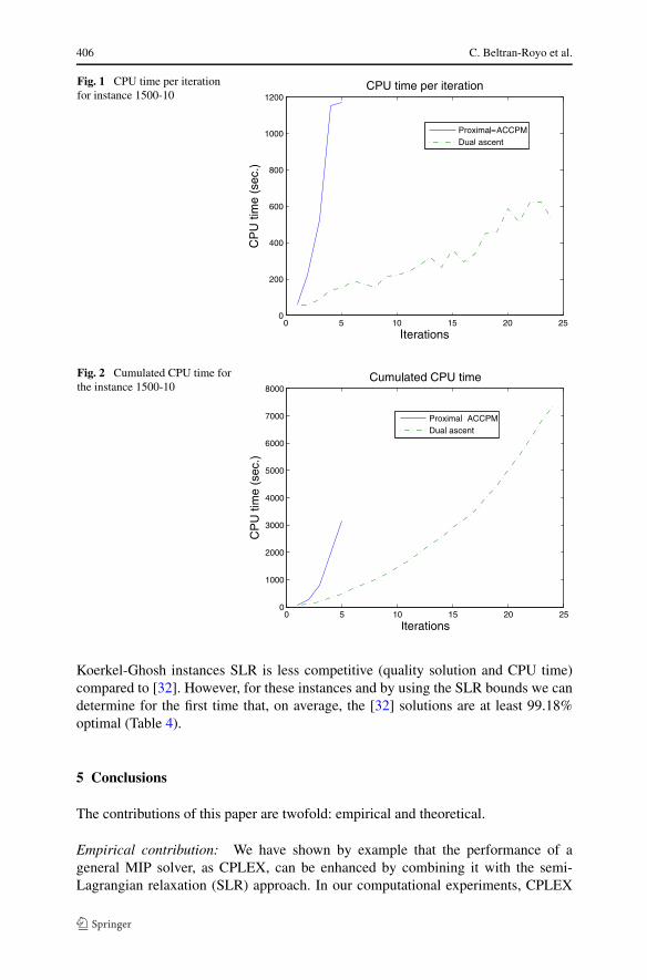
Proximal-ACCPM reduces by 60% the average number of dual ascent iterations.One would expect a similar reduction in the CPU time, instead of the mentioned35%. The reason for this mismatch, as we can see in (6.e) and (6.f), is that the av-erage CPU time per SLR iteration is greater for Proximal-ACCPM than for the dualascent algorithm. This is because Proximal-ACCPM perform a faster increase of theLagrange multiplier values, which produces a faster increase in the number of rele-vant variables, as observed in Table 5. This produces harder (CPU time consuming)Oracle 2’s. (See Fig. 1 and Fig. 2.)

As usual, a heuristic method reduces the CPU time of an exact method at the priceof no information about the solution quality. If we compare the best SLR results(column (6.f)) versus the results reported in [32] (column (6.g)) we observe that: forthe Barahona-Chudak instances, the SLR CPU time is very competitive, since at theprice of an extra 64% of CPU time, we solve up to optimality 16 instances. For the2 remaining instances we can evaluate its quality by the SLR lower bound. For the


Table 5 Semi-Lagrangian reduction and decomposition: ‘ANS’ stands for average number of subprob-lems per SLR iteration, ‘DA’ for dual ascent, ‘PACCPM’ for proximal-ACCPM, ‘ANX’ for average num-ber of relevant xij variables per SLR iteration (in %) and ‘ANY’ for average number of relevant yi variablesper SLR iteration (in %)

Instance ANS Total ANX (%) Total ANY (%)

DA PACCPM Nb. of xij DA PACCPM Nb. of yi DA PACCPM

(5.a) (5.b) (5.c) (5.d) (5.e) (5.f) (5.g) (5.h)

500-1000 108 84 250000 0.3 0.5 500 56 98

500-100 1 1 250000 1.2 1.2 500 66 66

500-10 1 1 250000 2.8 2.8 500 35 35

1000-1000 106 29 1000000 0.3 0.3 1000 89 94

1000-100 1 1 1000000 0.8 0.9 1000 55 61

1000-10 1 1 1000000 2.6 3.4 1000 39 51

1500-1000 11 7 2250000 0.3 0.3 1500 86 87

1500-100 1 1 2250000 0.6 0.6 1500 50 50

1500-10 1 1 2250000 1.8 2.6 1500 30 44

2000-1000 2 2 4000000 0.2 0.2 2000 82 82

2000-100 1 1 4000000 0.6 0.6 2000 50 50

2000-10 1 1 4000000 1.2 2.2 2000 25 42

2500-1000 3 3 6250000 0.2 0.2 2500 80 80

2500-100 1 1 6250000 0.5 0.6 2500 46 58

2500-10 1 1 6250000 1.7 1.7 2500 35 35

3000-1000 2 2 9000000 0.2 0.2 3000 78 78

3000-100 1 1 9000000 0.5 0.6 3000 53 56

3000-10 1 1 9000000 1.0 1.0 3000 23 23

Partial average 14 8 3791667 0.9 1.1 1750 54 61

gs00250a-1 1 1 62500 2.4 4.6 250 60 87

gs00250b-1 1 1 62500 5.6 6.3 250 50 54

gs00250c-1 1 1 62500 14.4 18.4 250 43 52

gs00500a-1 1 1 250000 1.3 1.3 500 48 48

gs00500b-1 1 1 250000 1.8 2.2 500 24 30

gs00500c-1 1 1 250000 5.1 6.1 500 23 27

gs00750a-1 1 1 562500 1.0 1.0 750 48 48

gs00750b-1 1 1 562500 1.6 1.6 750 26 26

gs00750c-1 1 1 562500 3.0 3.0 750 17 17

ga00250a-1 1 1 62500 2.5 4.3 250 62 85

ga00250b-1 1 1 62500 5.5 5.9 250 48 50

ga00250c-1 1 1 62500 13.5 16.9 250 40 47

ga00500a-1 1 1 250000 1.4 2.4 500 53 31

ga00500b-1 1 1 250000 2.4 1.4 500 31 24

ga00500c-1 1 1 250000 5.2 6.3 500 23 30

ga00750a-1 1 1 562500 1.0 1.0 750 44 44

ga00750b-1 1 1 562500 1.3 1.5 750 23 24

ga00750c-1 1 1 562500 2.9 2.7 750 16 15

Partial average 1 1 291667 4.0 4.8 500 38 41

Global average 7 4 2041667 2.5 3.0 1125 46 51


Fig. 1 CPU time per iterationfor instance 1500-10

Fig. 2 Cumulated CPU time forthe instance 1500-10

Koerkel-Ghosh instances SLR is less competitive (quality solution and CPU time)compared to [32]. However, for these instances and by using the SLR bounds we candetermine for the first time that, on average, the [32] solutions are at least 99.18%optimal (Table 4).

5 Conclusions

The contributions of this paper are twofold: empirical and theoretical.

Empirical contribution: We have shown by example that the performance of ageneral MIP solver, as CPLEX, can be enhanced by combining it with the semi-Lagrangian relaxation (SLR) approach. In our computational experiments, CPLEX


Table 6 Performance: ‘PACCPM’ stands for proximal-ACCPM and ‘DA’ for dual ascent. [32] uses anheuristic method

Instance Nb. of completed iterations Total CPU time (sec.)

LR SLR LR LR + SLR [32]

PACCPM DA PACCPM PACCPM DA PACCPM

(6.a) (6.b) (6.c) (6.d) (6.e) (6.f) (6.g)

500-1000 128 1 1 2.7 3 4 33

500-100 100 1 1 1.9 2 2 33

500-10 177 1 1 4.1 5 5 24

1000-1000 121 1 1 3.5 6 6 174

1000-100 276 2 2 11.8 16 19 149

1000-10 535 29 5 46.1 4024 1061 142

1500-1000 128 1 1 5.0 9 10 348

1500-100 311 1 1 19.0 22 22 379

1500-10 327 24 5 19.3 7438 3156 387

2000-1000 137 1 1 7.0 12 12 718

2000-100 245 1 1 16.7 23 23 651

2000-10 408 40 4 37.7 2256 661 760

2500-1000 136 1 1 9.4 18 18 1420

2500-100 342 2 2 36.1 55 89 1128

2500-10 754 1 1 177.7 8214 8214 1309

3000-1000 160 5 3 14.0 76 63 1621

3000-100 427 10 8 64.1 7355 8428 1978

3000-10 413 1 1 60.5 90 90 2081

Partial average 285 7 2 29.8 1646 1216 741

gs00250a-1 209 11 5 7.1 8173 5765 6

gs00250b-1 165 11 3 2.9 9145 3845 8

gs00250c-1 252 37 13 5.2 7831 7929 7

gs00500a-1 195 0 0 9.5 10 10 40

gs00500b-1 191 2 1 10.2 2771 515 52

gs00500c-1 143 14 5 7.1 7241 7573 57

gs00750a-1 192 0 0 12.9 13 13 118

gs00750b-1 143 1 1 11.3 5436 5234 127

gs00750c-1 140 8 2 10.7 7274 1868 137

ga00250a-1 177 9 4 5.9 7389 6567 5

ga00250b-1 229 12 3 4.6 7283 2223 8

ga00250c-1 156 36 13 2.5 7675 7804 8

ga00500a-1 233 0 0 9.9 10 10 44

ga00500b-1 229 3 1 4.6 8899 478 53

ga00500c-1 150 16 5 5.3 7936 6604 51

ga00750a-1 199 0 0 14.1 14 14 113

ga00750b-1 137 1 1 10.6 3134 3181 126

ga00750c-1 126 10 2 7.7 9018 1554 130

Partial average 181 10 3 7.9 5514 3399 61

Global average 233 8 3 18.8 3580 2307 401


solved 3 out of 36 Uncapacitated Facility Location (UFL) unsolved instances fromthe UflLib. In contrast, by using the SLR together with two standard optimizationtools, CPLEX and Proximal-ACCPM, we solved 18 instances. For the remaining 18still unsolved UFL instances, we have improved the best known lower bound andconfirmed, for the first time, that the Hybrid Multistart heuristic of [32] provides nearoptimal solutions (over 99% optimal). The reason for this good result is that, the SLRdrastically reduced the number of UFL relevant variables. Roughly speaking, on theaverage number of relevant xij variables was reduced to 3% and the average numberof relevant yi variables, was reduced to 50%.

Also from an empirical point of view, we have compared two dual optimizationmethods: Proximal-ACCPM and a dual ascent method. Proximal-ACCPM has showna better performance than the dual ascent: it has produced similar and sometimesbetter solutions with a CPU time reduction of 35%. Within the 2 hours of CPU timelimit, Proximal-ACCPM and the dual ascent method have fully solved 18 and 16 UFLinstances, respectively (from a pool of 36 unsolved instances). The advantage of thedual ascent method is its extreme simplicity compared to Proximal-ACCPM.

Theoretical contribution: From a theoretical point of view, this paper has proposedan extension of the Koerkel dual multi-ascent method to solve the SLR dual problemand we have proved (finite) convergence. Furthermore, We have studied the theoreti-cal properties of the SLR dual problem in the UFL case. We have shown that for theUFL problem we can restrict our dual search to a box whose definition depends onthe problem costs. This property has not shown to be very useful for the dual ascentmethod. In contrast, in the case of Proximal-ACCPM the explicit use of this box hasslightly improved the dual search.

Acknowledgements We are thankful: To Mato Baotic (Swiss Federal Institute of Technology) for itsMatlab/Cplex interface [3], to Martin Hoefer (Max Planck Institut Informatik) for the UFL data from theUflLib [23], and to the anonymous referees for their constructive comments and suggestions.

References

1. Avella, P., Sassano, A., Vasil’ev, I.: Computational study of large-scale p-median problems. Math.Program. 109(1), 89–114 (2007)

2. Babonneau, F., Beltran, C., Haurie, A.B., Tadonki, C., Vial, J.-Ph.: Proximal-ACCPM: a versatile or-acle based optimization method. In: Kontoghiorghes, E.J., Gatu, C. (eds.) Advances in ComputationalEconomics, Finance and Management Science. Advances on Computational Management Science,pp. 200–224. Springer, Berlin (2006)

3. Baotic, M.: Matlab interface for CPLEX (2004). http://control.ee.ethz.ch/hybrid/cplexint.php4. Barahona, F., Chudak, F.: Near-optimal solutions to large scale facility location problems technical

report. Technical Report RC21606, IBM Watson Research Center (1999)5. Beltran, C., Tadonki, C., Vial, J.-Ph.: Solving the p-median problem with a semi-Lagrangian relax-

ation. Comput. Optim. Appl. 35(2), 239–260 (2006)6. Beltran-Royo, C.: A conjugate Rosen’s gradient projection method with global line search for piece-

wise linear concave optimization. Eur. J. Oper. Res. 182(2), 536–551 (2007)7. Briant, O., Naddef, D.: The optimal diversity management problem. Oper. Res. 52(4), 515–526 (2004)8. Canovas, L., Landete, L., Marin, A.: On the facets of the simple plant location packing polytope.

Discrete Appl. Math. 124, 27–53 (2002)9. Cho, D.Ch., Johnson, E.L., Padberg, M.W., Rao, M.R.: On the uncapacitated facility location problem

I: Valid inequalities and facets. Math. Oper. Res. 8(4), 590–612 (1983)

http://control.ee.ethz.ch/hybrid/cplexint.php


10. Cho, D.Ch., Padberg, M.W., Rao, M.R.: On the uncapacitated facility location problem II: Facets andlifting theorems. Math. Oper. Res. 8(4), 590–612 (1983)

11. Conn, A.R., Cornuéjols, G.: A projection method for the uncapacitated facility location problem.Math. Program. 46, 373–398 (1990)

12. de Silva, A., Abramson, D.: A parallel interior point method and its application to facility locationproblems. Comput. Optim. Appl. 90(3), 249–273 (1998)

13. du Merle, O., Vial, J.-Ph.: Proximal-ACCPM, a cutting plane method for column generation and La-grangian relaxation: application to the p-median problem. Technical report, Logilab, HEC, Universityof Geneva (2002)

14. Erlenkotter, D.: A dual-based procedure for uncapacitated facility location. Oper. Res. 26, 992–1009(1978)

15. Gao, L.-L., Robinson, E.P.: Uncapacitated facility location: General solution procedure and computa-tional experience. Eur. J. Oper. Res. 76(3), 410–417 (1994)

16. Ghosh, D.: Neighborhood search heuristics for the uncapacitated facility location problem. Eur. J.Oper. Res. 150, 150–162 (2003)

17. Goffin, J.-L., Haurie, A., Vial, J.-Ph.: Decomposition and nondifferentiable optimization with theprojective algorithm. Manag. Sci. 37, 284–302 (1992)

18. Goffin, J.-L., Vial, J.-Ph.: Convex nondifferentiable optimization: A survey focussed on the analyticcenter cutting plane method. Optim. Methods Softw. 179, 805–867 (2002)

19. Guignard, M.: A Lagrangean dual ascent algorithm for simple plant location problems. Eur. J. Oper.Res. 35, 193–200 (1988)

20. Guignard, M.: Lagrangian relaxation. TOP 11(2), 151–228 (2003)21. Hiriart-Urruty, J.B., Lemaréchal, C.: Convex Analysis and Minimization Algorithms, vols. I, II.

Springer, Berlin (1996)22. Hiriart-Urruty, J.-B., Lemaréchal, C.: Fundamentals of Convex Analysis. Springer, Berlin (2000)23. Hoefer, M.: Ufllib (2006). http://www.mpi-inf.mpg.de/departments/d1/projects/benchmarks/UflLib/24. Janacek, J., Buzna, L.: An acceleration of Erlenkotter-Koerkel’s algorithms for the uncapacitated fa-

cility location problem. Ann. Oper. Res. 164, 97–109 (2008)25. Kelley, J.E.: The cutting-plane method for solving convex programs. J. SIAM 8, 703–712 (1960)26. Kochetov, Y., Ivanenko, D.: Computationally difficult instances for the uncapacitated facility location

problem. In: Ibaraki, T., Nonobe, K., Yagiura, M. (eds.) Metaheuristics: Progress as Real Solvers.Springer, Berlin (2005)

27. Koerkel, M.: On the exact solution of large-scale simple plant location problems. Eur. J. Oper. Res.39(2), 157–173 (1989)

28. Landete, M., Marin, A.: New facets for the two-stage uncapacitated facility location polytope. Com-put. Optim. Appl. 44(3), 487–519 (2009)

29. Mirchandani, P., Francis, R.: Discrete Location Theory. Wiley, New York (1990)30. Mladenovic, N., Brimberg, J., Hansen, P.: A note on duality gap in the simple plant location. Eur. J.

Oper. Res. 174(1), 11–22 (2006)31. Nemhauser, G.L., Wolsey, L.A.: Integer and Combinatorial Optimization. Wiley, New York (1988)32. Resende, M.G.G., Werneck, R.F.: A hybrid multistart heuristic for the uncapacitated facility location

problem. Eur. J. Oper. Res. 174(1), 54–68 (2006)33. Sun, M.: Solving uncapacitated facility location problems using tabu search. Comput. Oper. Res. 33,

2563–2589 (2006)

http://www.mpi-inf.mpg.de/departments/d1/projects/benchmarks/UflLib/

Semi-Lagrangian relaxation applied to the uncapacitated facility location problem

Documents

Transcript of Semi-Lagrangian relaxation applied to the uncapacitated facility location problem