arX

iv:0

809.

4850

v2 [

cond

-mat

.sta

t-m

ech]

25

Aug

200

9

Spectral and Dynamical Properties in Classes of Sparse Networks with

Mesoscopic Inhomogeneities

Marija Mitrovic⋆,⋄ and Bosiljka Tadic⋄⋆ Scientific Computing Laboratory; Institute of Physics; 11000 Belgrade; Serbia

⋄Department for Theoretical Physics; Jozef Stefan Institute; P.O. Box 3000; SI-1001 Ljubljana; Slovenia,

We study structure, eigenvalue spectra and random walk dynamics in a wide class of networkswith subgraphs (modules) at mesoscopic scale. The networks are grown within the model with threeparameters controlling the number of modules, their internal structure as scale-free and correlatedsubgraphs, and the topology of connecting network. Within the exhaustive spectral analysis for boththe adjacency matrix and the normalized Laplacian matrix we identify the spectral properties whichcharacterize the mesoscopic structure of sparse cyclic graphs and trees. The minimally connectednodes, clustering, and the average connectivity affect the central part of the spectrum. The numberof distinct modules leads to an extra peak at the lower part of the Laplacian spectrum in cyclicgraphs. Such a peak does not occur in the case of topologically distinct tree-subgraphs connectedon a tree. Whereas the associated eigenvectors remain localized on the subgraphs both in trees andcyclic graphs. We also find a characteristic pattern of periodic localization along the chains on thetree for the eigenvector components associated with the largest eigenvalue λL = 2 of the Laplacian.Further differences between the cyclic modular graphs and trees are found by the statistics of randomwalks return times and hitting patterns at nodes on these graphs. The distribution of first returntimes averaged over all nodes exhibits a stretched exponential tail with the exponent σ ≈ 1/3 fortrees and σ ≈ 2/3 for cyclic graphs, which is independent on their mesoscopic and global structure.

PACS numbers: 89.75.Hc, 05.40.Fb, 02.70.-c

I. INTRODUCTION

Complex dynamical systems and network mesoscopicstructure. In recent years a lot of attention has been de-voted to the problem of representing the complex dynam-ical systems by networks and investigating their struc-tural and dynamical properties [1]. These networks of-ten exhibit inhomogeneity at all scales, from the locallevel (individual nodes), to mesoscopic (groups of nodes)and global network level. The mesoscopic inhomogene-ity of networks may be defined as topologically distinctgroupings of nodes in a range from few nodes to largemodules, communities, or different interconnected sub-networks. These subgraphs play an important role in thenetwork’s complexity along the line from the local inter-actions to emergent global behavior, both in the structureand the function of networks [1, 2]. Hence, the charac-teristic subgraphs can be defined not only topologicallybut also dynamically, and different subgraphs appear tocharacterize different functional networks. In particu-lar, communities are often studied in social networks [3],topological modules [4] and characteristic dynamical mo-tifs [5] are found in genetic interactions and communi-cation networks, whereas paths and trees appear as rel-evant subgraphs in the networks representing biochemi-cal metabolic processes and neural networks [6]. Chains,representing a special type of motifs, have been observedin networks of words in books and the power grid net-works, [7]. In these examples the mesoscopic topologyis related to dynamics of the whole network. On theother side, we have multi-networks consisting of a few

interconnected networks in which the internal structureand possibly also dynamics might be different [8]. Thenthe interaction between such diverse networks leads toemergent global behavior, as for instance in the networksrepresenting interacting eco-systems [9].

Understanding the mesoscopic structure of networksin both topological and dynamical sense is, therefore,of paramount importance in the quantitative study ofcomplex dynamical systems. Recently much attentionwas devoted to network’s topological modularity, such ascommunity structure [3, 10, 11, 12, 13, 14, 15], where awide range of methods are designed to find the appro-priate network partitioning. Mostly these methods usethe centrality measures (i.e., a topological [10] or a dy-namical [11] flow) based on the maximal-flow-minimal-cut theorem [16]. Further effective approaches for graphpartitioning utilize the statistical methods of maximum-likelihood [12, 13], occurrence of different time scales inthe dynamic synchronization [14] and eigenvector local-ization [15] in mesoscopically inhomogeneous structures.In more formal approaches, the definitions of differentmesoscopic structures in terms of simplexes and theircombinations, simplicial complexes, are well known in thegraph theory [17]. This approach has been recently ap-plied [18] to scale-free (SF) graphs and some other real-world networks.

Spectral analysis of networks. Properties of the eigen-values and eigenvectors of the adjacency matrix of a com-plex network and of other, e.g., Laplacian matrices re-lated to the network structure, contain important infor-mation that interpolates between the network structure

2

and dynamic processes on it. One of the well studied ex-amples is the synchronization of phase-coupled oscillatorson networks [1, 14, 19, 20], where the smallest eigen-value of the Laplacian matrix corresponds to the fullysynchronized state. The synchronization between nodesbelonging to better connected subgraphs (modules) oc-curs at somewhat smaller time scale [14, 21] correspond-ing to lowest nonzero eigenvalues of the Laplacian, andthe positive/negative components of the correspondingeigenvectors are localized on these modules [1, 15]. Thespreading of diseases [22] and random walks and navi-gated random walks [2, 23, 24, 25] are other type of thediffusive processes on networks which are related to theLaplacian spectra.

Compared to the well known semicircular law for therandom matrices [26], the spectra of binary and struc-tured graphs have additional prominent features, whichcan be related to the graph structure [15, 19, 27, 28,29, 30, 31]. Particularly, some of the striking differencesfound in the scale-free graphs are the appearance of thecentral peak or a ’triangular form’ [27] and the power-law tail [28, 32] in the spectral density of the adjacencymatrix, which is related to the node connectivity. Inthe classical paper Samukhin et al. [30] elucidated therole of the minimally-connected nodes on the Laplacianspectra of trees and uncorrelated tree-like graphs. Theyderived analytical expression for the spectral density ofthe Laplacian matrix. Other topological features of thegraph, particularly the finite clustering [19] and the pres-ence of modules [15], have been also found to affect theLaplacian spectra. Attempts to classify the graphs ac-cording to their spectral features were presented recently[31].

In this paper we study systematically the spectralproperties of a large class of sparse networks with meso-scopic inhomogeneities. The topology of these networksat all scales may lead to qualitative differences in thespectra both of the adjacency and Laplacian matrix.Having well controlled structure of the networks by themodel parameters, we are able to quantitatively relatethe spectral properties of the networks to their structure.As explained below, we identify different regions of thespectra in which certain structural features are mainlymanifested. We further explore these networks by simu-lating the random walk dynamics on them. We focus onlyon two properties of random walks: hitting patterns andfirst-return time distribution, which are closely relatedto graph structure and spectrum of the Laplacian. Inthis way we would like to emphasise deeper interconnec-tions between the structure and the dynamics of complexnetworks and their spectra, features which often remainfragmented in numerous studies of complex networks.

In Section II we represent model of growing networkswith controlled number of modules and their internalstructure. We then briefly study the spectral density ofthe adjacency matrix of modular networks in Section III.Section IV is devoted to detailed analysis of the spectraof the normalized Laplacian matrix, which is related to

the diffusive dynamics on these networks. The simula-tions of random walks on trees and on sparse modulargraphs with minimal connectivity M ≥ 2 is presented inSection V. Finally, a short summary and the discussionof the results is given in Section VI.

II. GROWING MODULAR NETWORKS

We first present the model for growing networks withstatistically defined modularity. It is based on the modelfor growing clustered scale-free graphs originally intro-duced in Ref. [33]. The preferential-attachment andpreferential-rewiring during the graph growth leads tothe correlated scale-free structure, which is statisticallysimilar to the one in real WWW [33]. Two parameters,α and M as explained below, fully control the emergentstructure. Here we generalize the model in a nontrivialmanner by allowing that a new module starts growingwith probability P0. The added nodes are attached pref-erentially within the currently growing module, whereasthe complementary rewiring process is done between allexisting nodes in the network. The growth rules are ex-plained in detail below.

At each time step t we add a new node i and Mnew links. With probability Po a new group (module)is started and the current group index is assigned to theadded node (first node belong to the first group). Thegroup index plays a crucial role in linking of the nodeto the rest of the network. Note that each link is, inprinciple, directed, i.e., emanating from the origin nodeand pointing to the target node. For each link the targetnode, k, is always searched within the currently growingmodule (identified by its group index gk). The targetis selected preferentially according to its current numberof incoming links qin(k, t). The probability pin(k, t) isnormalized according to all possible choices at time t

pin(k, t) =Mα + qin(k, t)

MNgk(t)α + Lgk

(t). (1)

where Ngk(t) and Lgk

(t) stand for, respectively, the num-ber of nodes and links within the growing module gk. Thelink i → k is fixed with the probability α. If α < 1, thereis a finite probability 1 − α that the link from the newadded node i → k is cut (rewired) and a new origin noden is searched from which the link n → k established andfixed. The new origin node n is searched within all nodesin the network present at the moment t. The search isagain preferential but according to the current numberof outgoing links qout(n, t)[33]:

pout(n, t) =Mα + qout(n, t)

MN(t)α + L(t), (2)

where N(t) = t and L(t) ≤ MN(t) are total number ofnodes and links in the entire network at the moment t.Note that the number of added links is smaller than Mfor the first few nodes in the modul until M −1 nodes are

3

(a) (b)

Pajek Pajek

Pajek Pajek

(c) (d)

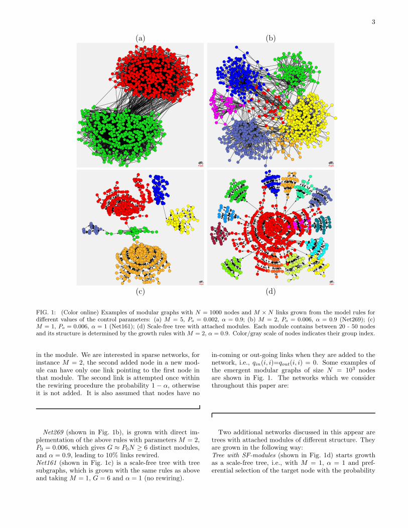
FIG. 1: (Color online) Examples of modular graphs with N = 1000 nodes and M × N links grown from the model rules fordifferent values of the control parameters: (a) M = 5, Po = 0.002, α = 0.9; (b) M = 2, Po = 0.006, α = 0.9 (Net269); (c)M = 1, Po = 0.006, α = 1 (Net161); (d) Scale-free tree with attached modules. Each module contains between 20 - 50 nodesand its structure is determined by the growth rules with M = 2, α = 0.9. Color/gray scale of nodes indicates their group index.

in the module. We are interested in sparse networks, forinstance M = 2, the second added node in a new mod-ule can have only one link pointing to the first node inthat module. The second link is attempted once withinthe rewiring procedure the probability 1 − α, otherwiseit is not added. It is also assumed that nodes have no

in-coming or out-going links when they are added to thenetwork, i.e., qin(i, i)=qout(i, i) = 0. Some examples ofthe emergent modular graphs of size N = 103 nodesare shown in Fig. 1. The networks which we considerthroughout this paper are:

Net269 (shown in Fig. 1b), is grown with direct im-plementation of the above rules with parameters M = 2,P0 = 0.006, which gives G ≈ P0N ≥ 6 distinct modules,and α = 0.9, leading to 10% links rewired.Net161 (shown in Fig. 1c) is a scale-free tree with treesubgraphs, which is grown with the same rules as aboveand taking M = 1, G = 6 and α = 1 (no rewiring).

Two additional networks discussed in this appear aretrees with attached modules of different structure. Theyare grown in the following way:Tree with SF-modules (shown in Fig. 1d) starts growthas a scale-free tree, i.e., with M = 1, α = 1 and pref-erential selection of the target node with the probability

4

pin(k, t) = α+qin(k,t)N(t)α+L(t) . A random integer r in the inter-

val [20, 50] is selected and at rth node a module of sizer is started to grow. The module rules are preferentiallinking and preferential rewiring within the same modulewith the parameters M = 2 and α = 0.9. Subsequentlya new integer r is selected and the tree resumes to growfor the following r steps, after which a module of thethe same size is added and so on. Now the nodes in themodules are excluded as potential targets for the resumedtree growth. The relative size of the tree and modularstructure can be controled in different ways, e.g., by theparameter P0 as above. For the purpose of the presentstudy we keep full balance between the size of the treeand total number of nodes included in the modules.Tree with cliques is grown as a random tree, i.e., targetnode k is selected with probability pin(k, t) = 1/N(t)from all nodes present at time t. With probability P0 aclique of size n is selected and attached to a randomlyselected node. Then the tree resumes growth and so on.

The structural properties of these networks dependcrucially on three control parameters: the average con-nectivity M , the probability of new group P0, and theattractivity of node α. By varying these parameters wecontrol the internal structure of groups (modules) andthe structure of the network connecting different mod-ules. Here we explain the role of these parameters. Notethat for P0 = 0 no different modules can appear and themodel reduces to the case of the clustered scale-free graphof Ref. [33] with a single giant component. In particular,for M = 1 and Po = 0 and α < 1 the emergent struc-ture is clustered and correlated scale-free network. Forinstance, the case α = 1/4 corresponds to the statisti-cal properties measured in the WWW with two differentscale-free distributions for in- and out-degree and non-trivial clustering and link correlations (disassortativity)[33]. On the other hand, for M = 1 and Po = 0, α = 1a scale-free tree is grown with the power-law in-degreewith the exponent τ = 3 exactly.

Here we consider the case P0 > 0, which induces differ-ent modules to appear statistically. The number of dis-tinct groups (modules) is given by G ∼ P0N . By varyingthe parameters M and α appropriately, and implement-ing the linking rules as explained above with the proba-bilities given in Eqs. (1-2), we grow the modular graphswith G connected modules of different topology. In par-ticular for α < 1 the scale-free clustered and correlatedsubgraphs appear (cf. Fig. 1a,b). Whereas for α = 1the emergent structure is a tree of (scale-free) trees ifM = 1 (Fig. 1c). Another limiting case is obtained whenα = 1 and M ≥ 2, resulting in a scale-free tree connect-ing the unclustered uncorrelated scale-free subgraphs. Inorder to systematically explore the role of topology bothof modules and connecting networks in the spectral anddynamical properties of sparse modular graphs, we willstudy in parallel two network types shown in Fig. 1b andc, referred as Net269 and Net161, respectively.

Note that the growth rule as explained above lead to adirected graph with generally different connectivity pat-

terns for in-coming and out-going links. Each modulealso tends to have a central node (local hub), throughwhich it is connected with the rest of the network. Thepattern of directed connections of the nodes within mod-ules and the role of the connecting node can be nicelyseen using the maximum-likelihood method for graphpartitioning, as shown in our previous work [13]. Forthe purpose of the present work, in this paper we analizeundirected binary graphs, which have symmetric form ofthe adjacency matrix and the normalized Laplacian ma-trix. Therefore, the total degree of a node q = qin + qout

is considered as a relevant variable, for which we find apower-law distribution according to

P (q) ∼ q−τ . (3)

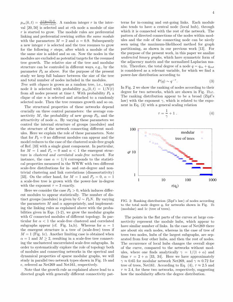
In Fig. 2 we show the ranking of nodes according to theirdegree for two networks, which are shown in Fig. 1b,c.The ranking distribution appear to be a broad (Zipf’slaw) with the exponent γ, which is related to the expo-nent in Eq. (3) with a general scaling relation

τ =1

γ+ 1 . (4)

1

10

100

1 10 100 1000

qi

r(qi)

modular

tree of trees

FIG. 2: Ranking distribution (Zipf’s law) of nodes accordingto the total node degree qi for networks shown in Fig. 1b(modular) and 1c (tree of trees).

The points in the flat parts of the curves at large con-nectivity represent the module hubs, which appear tohave similar number of links. In the case of Net269 thereare about six such nodes, whereas in the case of tree oftrees two nodes, hubs of the largest subgraphs, are sep-arated from four other hubs, and then the rest of nodes.The occurrence of local hubs changes the overall slopeof the curve, compared to the networks without mod-ules, where one finds analytically γ = 1/(1 + α) andthus τ = 2 + α [33, 34]. Here we have approximatelyγ ≈ 0.65 for modular network Net269, and γ ≈ 0.72 fortree of trees, Net161. According to Eq. (4), τ ≈ 2.5 andτ ≈ 2.4, for these two networks, respectively, suggestinghow the modularity affects the degree distribution.

5

III. EIGENVALUE SPECTRUM OF GROWING

MODULAR NETWORKS

The sparse network of size N is defined with an N ×Nadjacency matrix A with binary entries Aij = (1, 0),representing the presence or the absence of a link be-tween nodes i and j. For the sparse binary networksthe eigenvalue spectral density of the adjacency matrix isqualitatively different from the well known random ma-trix semi-circular law [28]. Moreover, in a large num-ber of studies it was found that the eigenvalue spec-tra differ for different classes of structured networks[1, 15, 19, 27, 28, 29, 30, 31]. We study the spectralproperties of the adjacency matrix A and the relatedLaplacian matrix L (see Sec. IV) of different networkswith mesoscopic inhomogeneity using the complete solu-tion of the eigenvalue problem:

AV Ai = λA

i V Ai . (5)

Here the set {λAi } denotes eigenvalues and {V A

i } a set ofthe corresponding eigenvectors, i = 1, 2 · · ·N , of the ad-jacency matrix A. For the modular networks grown withthe algorithms in Section II we focus on the effects thatthe network mesoscopic structure has on (i) the spectraldensity, (ii) the eigenvalues ranking, and (iii) the struc-ture and localization of the eigenvectors.

As stated above, we use the undirected networks. Thusthe adjacency matrix is symmetric, which is compatiblewith the real eigenvalues and the orthonormal basis of theeigenvector. We use the networks of the size N = 1000and solve the eigenvalue problem numerically. Particu-larly, we use the numerical routines in C from NumericalRecipes [35] for calculation of eigenvalues and eigenvec-tors of adjacency matrix with the precision 10−6. Thespectral densities are calculated with a large resolution,typically ∆λ = 0.05, and averaged over 500 networks.

A. Change of the spectrum with network growth

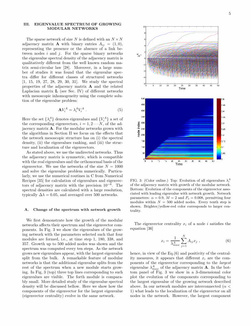
We first demonstrate how the growth of the modularnetworks affects their spectrum and the eigenvector com-ponents. In Fig. 3 we show the eigenvalues of the grow-ing network with the parameters selected such that fourmodules are formed, i.e., at time step 1, 180, 338, and357. Growth up to 500 added nodes was shown and thespectrum was computed every ten steps. As the networkgrows new eigenvalues appear, with the largest eigenvaluesplit from the bulk. A remarkable feature of modularnetworks is that the additional eigenvalue splits from therest of the spectrum when a new module starts grow-ing. In Fig, 3 (top) three top lines corresponding to sucheigenvalues are visible. The forth module is compara-bly small. More detailed study of the eigenvalue spectraldensity will be discussed bellow. Here we show how thecomponents of the eigenvector for the largest eigenvalue(eigenvector centrality) evolve in the same network.

0 5 10 15 20 25 30 35 40 45 50−8

−6

−4

−2

0

2

4

6

8

10

Time

λA i

FIG. 3: (Color online.) Top: Evolution of all eigenvalues λA

i

of the adjacency matrix with growth of the modular network.Bottom: Evolution of the components of the eigenvector asso-ciated with leading eigenvalue with network growth. Networkparameters: α = 0.9, M = 2 and Po = 0.008, permitting fourmodules within N = 500 added nodes. Every tenth step isshown. Brighter/yellow-red color corresponds to larger cen-trality.

The eigenvector centrality xi of a node i satisfies theequation [36]

xi =1

λAmax

N∑

j=1

Aijxj , (6)

hence, in view of the Eq.(6) and positivity of the central-ity measures, it appears that different xi are the com-ponents of the eigenvector corresponding to the largesteigenvalue λA

max of the adjacency matrix A. In the bot-tom panel of Fig. 3 we show in a 3-dimensional colorplot the evolution of the components corresponding tothe largest eigenvalue of the growing network describedabove. In our network modules are interconnected (α <1) what leads to the localization of the eigenvector on allnodes in the network. However, the largest component

6

corresponds to the hub of the first module. When a newmodule is added to the network, the strongest componentis eventually shared among the hubs of the two modules.During the growth of the module, however, the centralityxi of the nodes in that module remains small until themodule grows large enough (cf. Fig. 3).

B. Spectral density of clustered modular networks

0

0.1

0.2

0.3

0.4

0.5

0.6

0.7

0.8

0.9

1

-10 -5 0 5 10

ρ(λA

)

λA

G=1

G=2

G=6

0

0.002

0.004

0.006

0.008

0.01

0.012

0.014

0.016

0.018

12 14 16 18 20 22

0

0.5

1

1.5

2

2.5

3

-10 -5 0 5 10

ρ(λΑ

)

λΑ

α=1

α=0.9

α=0.6

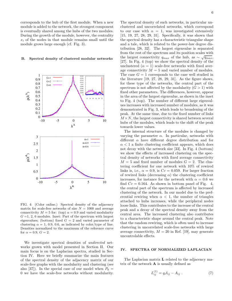
FIG. 4: (Color online.) Spectral density of the adjacencymatrix for scale-free networks of size N = 1000 and averageconnectivity M = 5 for: (top) α = 0.9 and varied modularityG =1, 2, 6 modules. Inset: Part of the spectrum with largesteigenvalues; (bottom) fixed G = 2 and varied parameter ofclustering α = 1, 0.9, 0.6, as indicated by color/type of line.Densities normalized to the maximum of the reference curvefor α = 0.9, G = 2.

We investigate spectral densities of undirected net-works grown with model presented in Section II. Ourmain focus is on the Laplacian spectra, studied in Sec-tion IV. Here we briefly summarize the main featuresof the spectral density of the adjacency matrix of ourscale-free graphs with the modularity and clustering (seealso [37]). In the special case of our model when P0 =0 we have the scale-free networks without modularity.

The spectral density of such networks, in particular un-clustered and uncorrelated networks, which correspondto our case with α = 1, was investigated extensively[15, 19, 27, 28, 29, 31]. Specifically, it was shown thatthe spectral density has a characteristic triangular shapeand a tale, which is related to the power-law degree dis-tribution [28, 32]. The largest eigenvalue is separatedfrom the rest of the spectrum and its position scales withthe largest connectivity qmax of the hub, as ∼ √

qmax,[27]. In Fig. 4 (top) we show the spectral density of theunclustered (α = 1) scale-free networks with fixed aver-age connectivity M = 5 and varied number of modules.The case G = 1 corresponds to the case well studied inthe literature [19, 27, 28, 29, 31]. As the figure shows,for these type of the networks, the central part of thespectrum is not affected by the modularity (G > 1) withfixed other parameters. The differences, however, appearin the area of the largest eigenvalue, as shown in the insetto Fig. 4 (top). The number of different large eigenval-ues increases with increased number of modules, as it wasdemonstrated in Fig. 3, which leads to broadening of thepeak. At the same time, due to the fixed number of linksM×N , the largest connectivity is shared between severalhubs of the modules, which leads to the shift of the peaktowards lower values.

The internal structure of the modules is changed byvarying the parameter α. In particular, networks withdifferent α have different degree distribution and forα < 1 a finite clustering coefficient appears, which doesnot decay with the network size [33]. In Fig. 4 (bottom)we show the effects of increased clustering on the spec-tral density of networks with fixed average connectivityM = 5 and fixed number of modules G = 2. The clus-tering coefficient for one network with 10% of rewiredlinks is, i.e., α = 0.9, is Cc = 0.059. For larger fractionof rewired links (decreasing α) the clustering coefficientincreases, for instance for the network with α = 0.6 wefind Cc = 0.164. As shown in bottom panel of Fig. 4,the central part of the spectrum is affected by increasedclustering of the network. In our model due to the pref-erential rewiring when α < 1, the number of trianglesattached to hubs increases, while the peripheral nodesloose links. This contributes to the increase of the centralpeak and a decay of the spectral density away from thecentral area. The increased clustering also contributesto a characteristic shape around the central peak. Notethat the random rewiring, which is often used to increaseclustering in uncorrelated scale-free networks with largeaverage connectivity, M = 20 in Ref. [19], may generateuncontrolable effects.

IV. SPECTRA OF NORMALIZED LAPLACIAN

The Laplacian matrix L related to the adjacency ma-trix of the network A is usually defined as

L(1)ij = qiδij − Aij . (7)

7

For the dynamics of the random walks on networks otherforms of the Laplacian matrices have been discussed inthe literature [30, 31]. Generally, for a random or navi-gated walker [38, 39, 40] one can define the basic proba-bility piℓ for walker to jump from node i → ℓ in a discretetime unit (one time step). Then the probability Pij(n)that the walker starting at node i arrives to node j in nsteps is given by

Pij(n) =∑

l1...ln−1

pil1 . . . pln−1j . (8)

Consequently, the change of the transition probabilityPij(n) in one time step can be written via

Pij(n + 1) −Pij(n) = (9)

=∑

ln

[∑

l1...ln−1

pil1 . . . pln−1lln](plnj − δlnj)

≡ −∑

ln

Piln(n)Llnj ,

which defines the components of the Laplacian matrixLij in terms of the basic transition probability pij of thewalker. For the true random walk from node i equalprobability applies for all qi links, i.e., pij = 1

qiwhen the

link Aij is present. Thus the Laplacian matrix suitablefor the true random walk on the network is given by

L(2)ij = δij −

1

qi

Aij , (10)

and satisfies the conservation law for diffusion dynamicson graph [31]. We consider the symmetrical Laplacian

L3ij = δij −

1√

qiqj

Aij , (11)

which is a normalized version of the Laplacian for therandom walks [30]. (It can be related with the transitionprobability chosen as pij = 1

√qiqj

.) The Laplacian matrix

in Eq. (11) has a limited spectrum in the range λLi ∈

[0, 2] and an orthogonal set of the associated eigenvectorsV (λL

i ), i = 1, 2 · · ·N , which makes it suitable for thenumerical study. As already pointed out in Ref. [30],the operators (10) and (11) are connected by a diagonalsimilarity transformation Sij = δij

√qi. Hence they have

the same spectrum [30].

A. Spectral density of the normalized Laplacian of

modular networks

As mentioned above, the spectrum of the Laplacian(11) is bounded within the interval [0, 2], regardless ofthe size of network. The maximum value λL

max = 2 isfound only in bipartite graphs and trees. Whereas formonopartite graphs with cycles the maximum eigenvalue

0

10

20

30

40

50

0 0.5 1 1.5 2

ρ(λL

)

λL

G=1G=6

0

1

2

3

4

5

6

7

8

0 0.5 1 1.5 2

ρ(λL

)

λL

G=1G=6

0

2

4

6

8

10

12

0 0.2 0.4 0.6 0.8 1 1.2 1.4 1.6

ρ(λL

)

λL

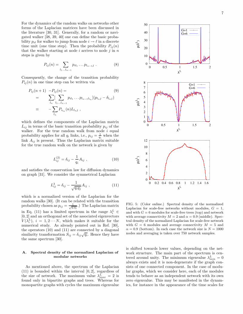
FIG. 5: (Color online.) Spectral density of the normalizedLaplacian for scale-free networks without modules, G = 1,and with G = 6 modules for scale-free trees (top) and networkwith average connectivity M = 2 and α = 0.9 (middle). Spec-tral density of the normalized Laplacian for scale-free networkwith G = 6 modules and average connectivity M = 5 andα = 0.9 (bottom). In each case the network size is N = 1000nodes and averaging is taken over 750 network samples.

is shifted towards lower values, depending on the net-work structure. The main part of the spectrum is cen-tered around unity. The minimum eigenvalue λL

min = 0always exists and it is non-degenerate if the graph con-sists of one connected component. In the case of modu-lar graphs, which we consider here, each of the modulestends to behave as an independent network with its ownzero eigenvalue. This may be manifested in the dynam-ics, for instance in the appearance of the time scales for

8

0

0.5

1

1.5

2

0 200 400 600 800 1000

λLi

r(λLi)

0

0.5

1

1.5

2

0 200 400 600 800 1000

λLi

r(λLi)

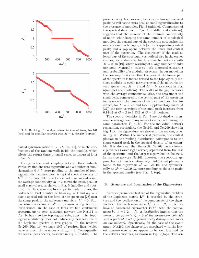
FIG. 6: Ranking of the eigenvalues for tree of trees, Net161(top) and for modular network with M = 2, Net269 (bottom).

partial synchronization ti ∼ 1/λi [14, 41], or in the con-finement of the random walk inside the module, whichaffects the return times at small scale, as discussed laterin Sec. V.

Owing to the weak coupling between these subnet-works, we find one zero eigenvalue and a number of smalleigenvalues 0 . λ corresponding to the number of topo-logically distinct modules. A typical spectral density ofL(3) of an ensemble of networks with six modules andthe average connectivity M ≥ 2 shows the extra peak atsmall eigenvalues, as shown in Fig. 5 (middle) and (bot-tom) . In the sparse graphs and particularly in trees, thenodes with least number of links qm = 1 and qm = 2play a special role in the form of the spectrum [28] nearthe sharp peak in the adjacency matrix at λA = 0. Sim-ilar situation occurs at λL = 1, shown in Fig. 5 (top).Furthermore, in the case of trees we find continuousspectrum up to zero, although network like Net161 inFig. 1c has tree-like topological subgraphs. The topo-logical modularity does not induce any new features ofthe Laplacian spectra in tree graphs. In the networkNet269, Fig. 1b, we have 10% of rewired links, whichleave as much of the nodes with qm = 1. Consequently,the central peak occurs, as shown in Fig. 5 (middle). The

presence of cycles, however, leads to the two symmetricalpeaks as well as the extra peak at small eigenvalues due tothe presence of modules, Fig. 5 (middle). Comparison ofthe spectral densities in Figs. 5 (middle) and (bottom),suggests that the increase of the minimal connectivityof nodes while keeping the same number of topologicalmodules, the central part of the spectrum approaches theone of a random binary graph (with disappearing centralpeak) and a gap opens between the lower and centralpart of the spectrum. The occurrence of the peak atlower part of the spectrum was noticed also in the earlierstudies, for instance in highly connected network withM = 20 in [19], where rewiring of a large number of linksper node eventually leads to both increased clusteringand probability of a modular structure. In our model, onthe contrary, it is clear that the peak at the lowest partof the spectrum is indeed related to the topologically dis-tinct modules in cyclic networks even if the networks arevery sparse, i.e., M = 2 and M = 5, as shown in Fig.5(middle) and (bottom). The width of the gap increaseswith the average connectivity. Also, the area under thesmall peak, compared to the central part of the spectrumincreases with the number of distinct modules. For in-stance, for M = 2 we find (see Supplementary material[37]) the relative weight of the small peak increases from0.144% at G = 2 to 1.53% at G = 16 modules.

The spectral densities in Fig. 5 are obtained with en-semble average over many networks grown with using thesame parameters P0, α, M . For the individual networkrealization, particularly the Net161 and Net269 shown inFig. 1b,c, the eigenvalues are shown in the ranking orderin Fig. 6. Within the numerical precision, the centralplateau in the ranking distribution corresponds to thesharp central peak in the spectral density of an ensem-ble. It is also clear that the cyclic Net269 has six lowesteigenvalues (lower right corner) separated from the restof the spectrum, and the largest eigenvalue lies below 2.In the tree network Net161, however, the spectrum ap-proaches both ends continuously. Additional plateau isfound at the eigenvalue λL = 1.707107 and symmetri-cally at λL = 0.292893, corresponding to the side peaksin the spectral density (see Fig. 5, top).

B. Structure and Localization of the Eigenvectors

Another prominent feature of the eigenvalue problemof the Laplacian matrix L

(3) is revealed by the struc-ture and the localization of the components of the eigen-vectors. For each eigenvalue λL

i , i = 1, 2, · · · , N , wehave an associated eigenvector V (λL

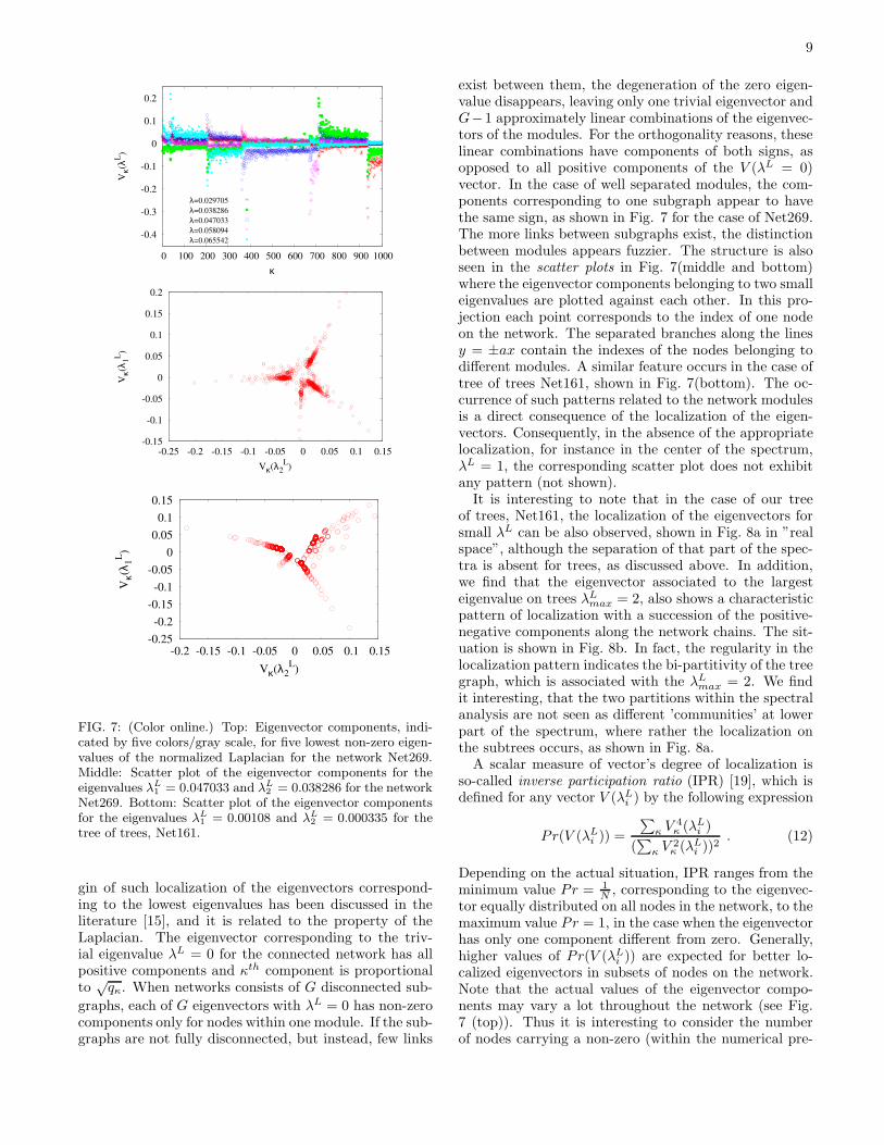
i ) with the compo-nents Vκ, κ = 1, 2, · · ·N . A localization implies that thenonzero components Vκ 6= 0 of the eigenvector coincidewith a particular set of geometrically distinguished nodeson the network. Specifically, for the case of the cyclicgraph, Net269, the eigenvectors associated with the low-est nonzero eigenvalues appear to be well localized onthe network modules, as shown in Fig. 7(top). The ori-

9

-0.4

-0.3

-0.2

-0.1

0

0.1

0.2

0 100 200 300 400 500 600 700 800 900 1000

Vκ(

λL)

κ

λ=0.029705

λ=0.038286

λ=0.047033

λ=0.058094

λ=0.065542

-0.15

-0.1

-0.05

0

0.05

0.1

0.15

0.2

-0.25 -0.2 -0.15 -0.1 -0.05 0 0.05 0.1 0.15

Vκ(

λ 1L)

Vκ(λ2L)

-0.25

-0.2

-0.15

-0.1

-0.05

0

0.05

0.1

0.15

-0.2 -0.15 -0.1 -0.05 0 0.05 0.1 0.15

Vκ(

λ 1L)

Vκ(λ2L)

FIG. 7: (Color online.) Top: Eigenvector components, indi-cated by five colors/gray scale, for five lowest non-zero eigen-values of the normalized Laplacian for the network Net269.Middle: Scatter plot of the eigenvector components for theeigenvalues λL

1 = 0.047033 and λL2 = 0.038286 for the network

Net269. Bottom: Scatter plot of the eigenvector componentsfor the eigenvalues λL

1 = 0.00108 and λL2 = 0.000335 for the

tree of trees, Net161.

gin of such localization of the eigenvectors correspond-ing to the lowest eigenvalues has been discussed in theliterature [15], and it is related to the property of theLaplacian. The eigenvector corresponding to the triv-ial eigenvalue λL = 0 for the connected network has allpositive components and κth component is proportionalto

√qκ. When networks consists of G disconnected sub-

graphs, each of G eigenvectors with λL = 0 has non-zerocomponents only for nodes within one module. If the sub-graphs are not fully disconnected, but instead, few links

exist between them, the degeneration of the zero eigen-value disappears, leaving only one trivial eigenvector andG−1 approximately linear combinations of the eigenvec-tors of the modules. For the orthogonality reasons, theselinear combinations have components of both signs, asopposed to all positive components of the V (λL = 0)vector. In the case of well separated modules, the com-ponents corresponding to one subgraph appear to havethe same sign, as shown in Fig. 7 for the case of Net269.The more links between subgraphs exist, the distinctionbetween modules appears fuzzier. The structure is alsoseen in the scatter plots in Fig. 7(middle and bottom)where the eigenvector components belonging to two smalleigenvalues are plotted against each other. In this pro-jection each point corresponds to the index of one nodeon the network. The separated branches along the linesy = ±ax contain the indexes of the nodes belonging todifferent modules. A similar feature occurs in the case oftree of trees Net161, shown in Fig. 7(bottom). The oc-currence of such patterns related to the network modulesis a direct consequence of the localization of the eigen-vectors. Consequently, in the absence of the appropriatelocalization, for instance in the center of the spectrum,λL = 1, the corresponding scatter plot does not exhibitany pattern (not shown).

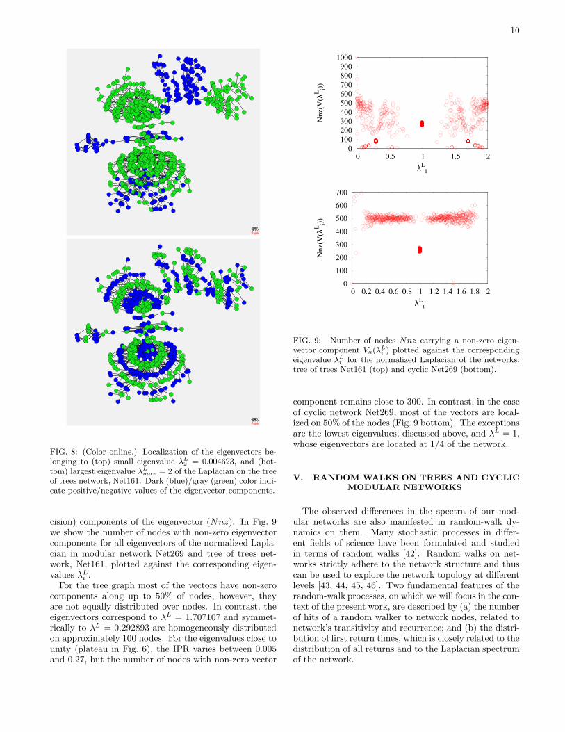
It is interesting to note that in the case of our treeof trees, Net161, the localization of the eigenvectors forsmall λL can be also observed, shown in Fig. 8a in ”realspace”, although the separation of that part of the spec-tra is absent for trees, as discussed above. In addition,we find that the eigenvector associated to the largesteigenvalue on trees λL

max = 2, also shows a characteristicpattern of localization with a succession of the positive-negative components along the network chains. The sit-uation is shown in Fig. 8b. In fact, the regularity in thelocalization pattern indicates the bi-partitivity of the treegraph, which is associated with the λL

max = 2. We findit interesting, that the two partitions within the spectralanalysis are not seen as different ’communities’ at lowerpart of the spectrum, where rather the localization onthe subtrees occurs, as shown in Fig. 8a.

A scalar measure of vector’s degree of localization isso-called inverse participation ratio (IPR) [19], which isdefined for any vector V (λL

i ) by the following expression

Pr(V (λLi )) =

∑κ V 4

κ (λLi )

(∑

κ V 2κ (λL

i ))2. (12)

Depending on the actual situation, IPR ranges from theminimum value Pr = 1

N, corresponding to the eigenvec-

tor equally distributed on all nodes in the network, to themaximum value Pr = 1, in the case when the eigenvectorhas only one component different from zero. Generally,higher values of Pr(V (λL

i )) are expected for better lo-calized eigenvectors in subsets of nodes on the network.Note that the actual values of the eigenvector compo-nents may vary a lot throughout the network (see Fig.7 (top)). Thus it is interesting to consider the numberof nodes carrying a non-zero (within the numerical pre-

10

Pajek

Pajek

FIG. 8: (Color online.) Localization of the eigenvectors be-longing to (top) small eigenvalue λL

2 = 0.004623, and (bot-tom) largest eigenvalue λL

max = 2 of the Laplacian on the treeof trees network, Net161. Dark (blue)/gray (green) color indi-cate positive/negative values of the eigenvector components.

cision) components of the eigenvector (Nnz). In Fig. 9we show the number of nodes with non-zero eigenvectorcomponents for all eigenvectors of the normalized Lapla-cian in modular network Net269 and tree of trees net-work, Net161, plotted against the corresponding eigen-values λL

i .For the tree graph most of the vectors have non-zero

components along up to 50% of nodes, however, theyare not equally distributed over nodes. In contrast, theeigenvectors correspond to λL = 1.707107 and symmet-rically to λL = 0.292893 are homogeneously distributedon approximately 100 nodes. For the eigenvalues close tounity (plateau in Fig. 6), the IPR varies between 0.005and 0.27, but the number of nodes with non-zero vector

0

100

200

300

400

500

600

700

800

900

1000

0 0.5 1 1.5 2

Nnz(

V(λ

Li)

)

λLi

0

100

200

300

400

500

600

700

0 0.2 0.4 0.6 0.8 1 1.2 1.4 1.6 1.8 2

Nnz(

V(λ

Li)

)

λLi

FIG. 9: Number of nodes Nnz carrying a non-zero eigen-vector component Vκ(λL

i ) plotted against the correspondingeigenvalue λL

i for the normalized Laplacian of the networks:tree of trees Net161 (top) and cyclic Net269 (bottom).

component remains close to 300. In contrast, in the caseof cyclic network Net269, most of the vectors are local-ized on 50% of the nodes (Fig. 9 bottom). The exceptionsare the lowest eigenvalues, discussed above, and λL = 1,whose eigenvectors are located at 1/4 of the network.

V. RANDOM WALKS ON TREES AND CYCLIC

MODULAR NETWORKS

The observed differences in the spectra of our mod-ular networks are also manifested in random-walk dy-namics on them. Many stochastic processes in differ-ent fields of science have been formulated and studiedin terms of random walks [42]. Random walks on net-works strictly adhere to the network structure and thuscan be used to explore the network topology at differentlevels [43, 44, 45, 46]. Two fundamental features of therandom-walk processes, on which we will focus in the con-text of the present work, are described by (a) the numberof hits of a random walker to network nodes, related tonetwork’s transitivity and recurrence; and (b) the distri-bution of first return times, which is closely related to thedistribution of all returns and to the Laplacian spectrumof the network.

11

(a) (b)

100

101

102

103

104

105

∆t

10−3

10−2

10−1

100

101

102

103

104

105

P(∆

t)

tree with cliques tree of trees scale−free treey=238x

−0.23exp(−(x/120)

0.338)

100

101

102

103

104

105

∆t

10−3

10−2

10−1

100

101

102

103

104

105

P(∆

t)

Net569 Net269 SFM2 50:50 tree & modulesy=230x

−0.06exp(−(x/540)

0.66)

y=25x−0.06

exp(−(x/140)0.33

) Slope: −1.0

10−2

10−1

100

101

102

<hi>

10−1

100

101

102

σ i

Net269 slope: 0.62 tree of trees Slope: 0.71

100

101

102

103

ri

100

101

102

<h i>

Net269 tree of trees scale−free tree slope −0.5 slope −0.45

(c) (d)

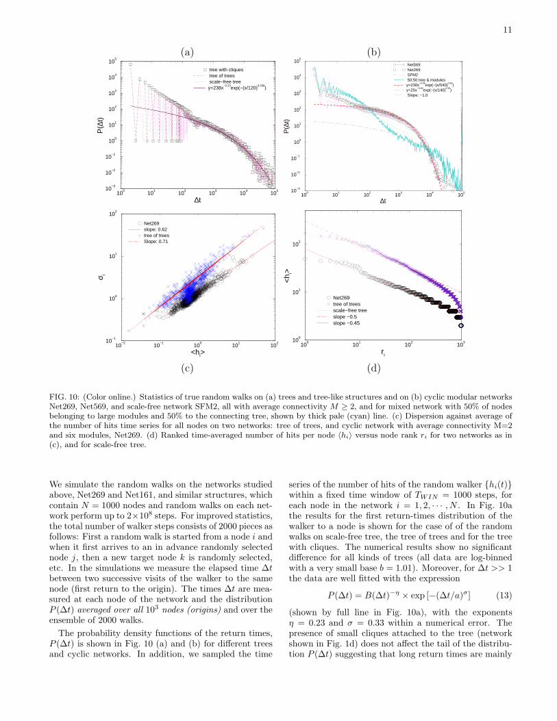
FIG. 10: (Color online.) Statistics of true random walks on (a) trees and tree-like structures and on (b) cyclic modular networksNet269, Net569, and scale-free network SFM2, all with average connectivity M ≥ 2, and for mixed network with 50% of nodesbelonging to large modules and 50% to the connecting tree, shown by thick pale (cyan) line. (c) Dispersion against average ofthe number of hits time series for all nodes on two networks: tree of trees, and cyclic network with average connectivity M=2and six modules, Net269. (d) Ranked time-averaged number of hits per node 〈hi〉 versus node rank ri for two networks as in(c), and for scale-free tree.

We simulate the random walks on the networks studiedabove, Net269 and Net161, and similar structures, whichcontain N = 1000 nodes and random walks on each net-work perform up to 2×108 steps. For improved statistics,the total number of walker steps consists of 2000 pieces asfollows: First a random walk is started from a node i andwhen it first arrives to an in advance randomly selectednode j, then a new target node k is randomly selected,etc. In the simulations we measure the elapsed time ∆tbetween two successive visits of the walker to the samenode (first return to the origin). The times ∆t are mea-sured at each node of the network and the distributionP (∆t) averaged over all 103 nodes (origins) and over theensemble of 2000 walks.

The probability density functions of the return times,P (∆t) is shown in Fig. 10 (a) and (b) for different treesand cyclic networks. In addition, we sampled the time

series of the number of hits of the random walker {hi(t)}within a fixed time window of TWIN = 1000 steps, foreach node in the network i = 1, 2, · · · , N . In Fig. 10athe results for the first return-times distribution of thewalker to a node is shown for the case of of the randomwalks on scale-free tree, the tree of trees and for the treewith cliques. The numerical results show no significantdifference for all kinds of trees (all data are log-binnedwith a very small base b = 1.01). Moreover, for ∆t >> 1the data are well fitted with the expression

P (∆t) = B(∆t)−η × exp [−(∆t/a)σ] (13)

(shown by full line in Fig. 10a), with the exponentsη = 0.23 and σ = 0.33 within a numerical error. Thepresence of small cliques attached to the tree (networkshown in Fig. 1d) does not affect the tail of the distribu-tion P (∆t) suggesting that long return times are mainly

12

determined by the tree structure of the underlying graph.Note also that there are no significant difference betweenthe random walks on the random tree and the scale-freetree, as well as the tree of trees (network in Fig. 1c). Inone of the early works considering the diffusion on ran-dom graphs [47] the exponent 1/3 for the case of randomwalk on a tree was derived by heuristic arguments.

A similar expression fits the distribution in the caseof random walks on cyclic graphs, however, with differ-ent exponents. The fit suggests the stretching exponentσ ≈ 0.66, that is twice larger compared with the caseof trees. The simulations of random walks on variouscyclic networks, also shown in Fig. 10b, suggest that,within the numerical accuracy, the tail of the distributionP (∆t) is practically independent on the size of cycles in-cluding triangles. A short region with very small slope isfound in the intermediate part of the curve, in agreementwith Eq. (13) with very small η. For short return times∆t < 102 we find tendency to a power-law dependence asP (∆t) ∼ (∆t)−1, which is more pronounced in networkswith increased clustering and modularity. For the treewith attached modules, described in Sec. II and shownin Fig. 1d, the tail of return-time distribution P (∆t) onthis network are also shown in Fig. 10b: the tail tendsto oscillate between the curves for the trees (long-dashedline) and the cyclic graphs, with a pronounced crossoverat short times.

Analysis of the time series {hi(t)} of the number of hitsof the random walker to each node reveals additional reg-ularity in the dynamics, which underly the return-timedistribution. In Fig. 10c we show the scatter plot of thedispersion σi of the time series hi(t) against the aver-age < hi(t) >t for each node i = 1, 2, · · · , N representedby a point. As shown in Fig. 10c, long-range correla-tions in the diffusion processes on networks lead to anon-universal scaling relation [25]

σi = const × 〈hi〉µt , (14)

where the averaging over all time windows is taken. Theexponent µ depends on the network structure and thesize of the time window. The origin of scaling in diffusiveprocesses on networks has been discussed in detail in [25]and references therein. Here we stress the differencesof the underlying networks for the fixed time windowTWIN = 1000: we find µ = 0.7 and µ = 0.62 for tree oftrees and modular network Net269, respectively. In thisplots the groups of nodes that are most often visited canbe identified at the top-right region of the plot.

Ranking distribution of the average number of hits <hi(t) >t at nodes is shown in Fig. 10d for the same tworepresentative networks. Generally, the number of hitsof true random walker to a node is proportional to nodeconnectivity [43] and thus, the ranking distribution is apower-law with the slope γ which is directly related to theranking distribution of degree in Fig. 2. In the presence ofnetwork modularity we realize the flat part of the curve,representing most visited nodes. In our modular network,like Net269, these nodes are roots of different modules.

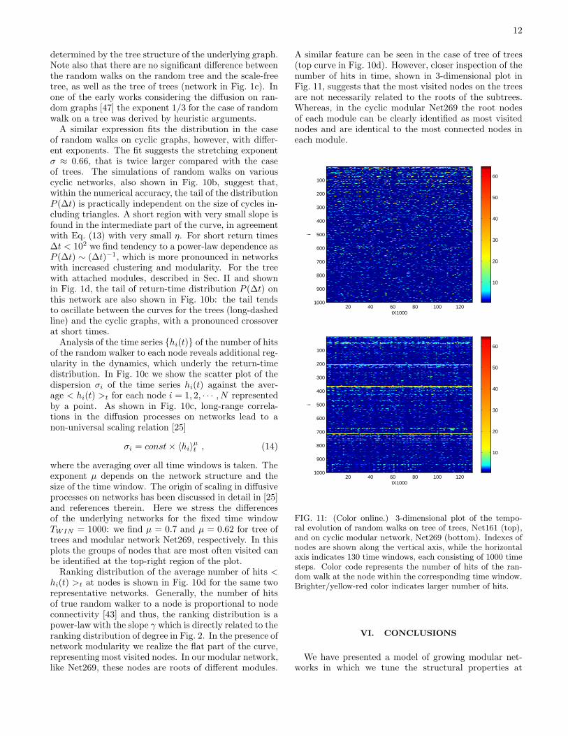
A similar feature can be seen in the case of tree of trees(top curve in Fig. 10d). However, closer inspection of thenumber of hits in time, shown in 3-dimensional plot inFig. 11, suggests that the most visited nodes on the treesare not necessarily related to the roots of the subtrees.Whereas, in the cyclic modular Net269 the root nodesof each module can be clearly identified as most visitednodes and are identical to the most connected nodes ineach module.

tX1000i

20 40 60 80 100 120

100

200

300

400

500

600

700

800

900

1000

10

20

30

40

50

60

tX1000

i

20 40 60 80 100 120

100

200

300

400

500

600

700

800

900

1000

10

20

30

40

50

60

FIG. 11: (Color online.) 3-dimensional plot of the tempo-ral evolution of random walks on tree of trees, Net161 (top),and on cyclic modular network, Net269 (bottom). Indexes ofnodes are shown along the vertical axis, while the horizontalaxis indicates 130 time windows, each consisting of 1000 timesteps. Color code represents the number of hits of the ran-dom walk at the node within the corresponding time window.Brighter/yellow-red color indicates larger number of hits.

VI. CONCLUSIONS

We have presented a model of growing modular net-works in which we tune the structural properties at

13

all scales by varying the respective control parameters.Specifically, the parameter P0 controls the number oftopologically distinct subgraphs (modules); the param-eter α is directly related to the number of rewired linkswhich, in turn, determine the clustering inside the scale-free subgraphs and connections between different mod-ules; the parameter M is the average number of linksper node, which can be varied independently on the clus-tering and modularity. The wide class of mesoscopicallyinhomogeneous networks grown by varying these param-eters includes the sparse modular graphs with variety oftopological features, both within the modules and at thelevel of the connecting network. Two limiting cases arethe interacting scale-free networks with finite clusteringand correlations, at one end, and a scale-free tree sup-porting a large number of cyclic modules, on the other(see Fig. 1).

We further study the spectral properties of these net-works by focusing on the normalized Laplacian matrixwhich is related to the diffusion (random walk) processeson these networks. We have also explored these net-works by simulating random walks on them. The sys-tematic analysis of the spectra while the network growsand by varying the control parameters enabled us topoint out the role played by a specific topological prop-erty of the network (controlled by different parameter)in their spectra and the dynamics. Two prototype mod-ular networks—tree connecting scale-free tree subgraphs(Net161) and the cyclic graph connecting scale-free clus-tered subgraphs (Net269), exhibit systematic differencesat the level of spectra and the random-walk dynamics.

Our complete spectral analysis reveals the firm connec-tion between the structure and spectra. We have foundseveral new results and also demonstrated clearly howsome expected results for this type of graphs are relatedto the structure. Specifically, we point out:

• the role of most connected nodes as opposed to therole of the underlying tree graph;

• the role that least connected nodes play in the ap-pearance of the central peak;

• how the increased clustering changes the shape ofthe spectrum near the central peak;

• the appearance of the extra peak at small eigenval-ues of the normalized Laplacian; In view of our finetunning of the structure, this peak is related to thenumber of distinct modules even if the graphs arevery sparse, as long as they are cyclic; Increasedclustering does not affect this peak;

• the Laplacian spectra of trees are different, partic-ularly, they do not show extra peak related withthe (tree) subgraphs;

• the eigenvector components show the expected pat-tern of localization on modules in the case of smallnonzero eigenvalues of the Laplacian. In spite of thedifferences in the spectral density, we find a similarlocalization pattern in trees with tree subgraphs.In addition, we find a robust localization along thenetwork chains of the eigenvectors for largest eigen-value of the Laplacian λL = 2, occurring only intrees and bipartite graphs;

• the simulation results for the first return-time dis-tribution of the random walks, averaged over net-work nodes, on different tree graphs exhibits apower-law with stretching exponential cut-off withσ ≈ 1/3 in agreement with Eq. (13) and heuristicarguments [47];

• when the graph contains cycles, the distribution be-longs to another class of behavior with twice largerstretching exponent. The numerical results do notdependent on the clustering coefficient. The pres-ence of modules and increased clustering affect thebehavior at small times, where a power-law decayoccurs before the cutoff.

Our systematic numerical study along the linestructure–spectra–random-walks quantifies the relation-ships between different structural elements of the net-work and their spectra and the dynamics. We hope thatthe presented results contribute to better understand-ing of the diffusion processes on the sparse graphs withcomplex topology. Potentially, some of our findings maybe used for fine differentiation between classes of graphswith respect their spectral and dynamical properties.

Acknowledgments

Research supported in part by the program P1-0044(Slovenia) and national project OI141035 (Serbia), bi-lateral project BI-RS/08-09-047 and MRTN-CT-2004-005728. The numerical results were obtained on theAEGIS e-Infrastructure, supported in part by EU FP6and FP7 projects EGEE-III, SEE-GRID-SCI and CX-CMCS.

[1] S. Boccaletti, V. Latora, Y. Moreno, M. Chavez, and D.-U. Hwang, Physics Reports 424, 175 (2006).

[2] B. Tadic, G. J. Rodgers, and S. Thurner, InternationalJournal of Bifurcation and Chaos 17(7), 2363 (2007).

[3] A. Arenas, L. Danon, A. Dıaz-Guilera, P. M. Gleiser,and R. Guimera, European Physical Journal B 38, 373(2004).

[4] E. Ravasz, A. L. Somera, D. A. Mongru, Z. N. Oltvai,

14

and A. L. Barabasi, Science 297, 1551 (2002).[5] R. Milo, S. Shen-Orr, S. Itzkovitz, N. Kashtan,

D. Chklovskii, and U. Alon, Science 298, 824 (2002).[6] R. Graben, C. Zhou, M. Thiel, and J. Kurths, Lectures

in Supercomputational Neuroscience: Dynamics in Com-plex Brain Networks (Understanding Complex Systems(Springer-Verlafg, Berlin Heidelberg, 2008).

[7] P. R. Villas Boas, F. A. Rodrigues, G. Travieso, and L. daFontoura Costa, Phys. Rev. E 77(2), 026106 (2008).

[8] A. Aleksiejuk, J. A. Holyst, and D. Stauffer, PhysicaA Statistical Mechanics and its Applications 310, 260(2002).

[9] J. M. Olesen, J. Bascompte, Y. L. Dupont, and P. Jor-dano, Proceedings of the National Academy of Science104, 19891 (2007).

[10] L. Danon, A. Dıaz-Guilera, and A. Arenas, Journalof Statistical Mechanics: Theory and Experiment 11,P11010 (2006).

[11] S. Fortunato, V. Latora, and M. Marchiori, Phys. Rev.E 70(5), 056104 (2004).

[12] M. E. J. Newman and E. A. Leicht, Proceedings of theNational Academy of Sciences 104(23), 9564 (2007).

[13] M. Mitrovic and B. Tadic, Lecture Notes in ComputerScience 5102, 551 (2008).

[14] A. Arenas, A. Dıaz-Guilera, and C. J. Perez-Vicente,Physical Review Letters 96(11), 114102 (2006).

[15] L. Donetti and M. A. Munoz, Journal of Statistical Me-chanics: Theory and Experiment 10, P10012, (2004).

[16] T. H. Cormen, C. E. Leiserson, R. L. Rivest, and C. Stein,Introduction to Algorithms, 2nd edn. (MIT Press andMcGraw-Hil, 2001).

[17] A. Hatcher, Algebraic Topology (Cambridge UniversityPress, 2002).

[18] S. Maletic, M. Rajkovic, and D. Vasiljevic, Lecture Notesin Computer Science 5102, 568 (2008).

[19] P. N. McGraw and M. Menzinger, Phys. Rev. E 77(3),031102 (2008).

[20] C. Zhou and J. Kurths, Chaos 16(1), 015104 (2006).[21] J. Almendral and A. Diaz-Guilera, New Journal of

Physics 9(6), 187 (2007).[22] D. Bell, J. Atkinson, and C. J.W., Social Networks 21(1),

1 (1999).[23] B. Tadic, European Physical Journal B 23, 221 (2001).[24] J. D. Noh and H. Rieger, PRL 92(11), 118701 (2004).[25] B. Kujawski, B. Tadic, and G. J. Rodgers, New Journal

of Physics 9, 154 (2007).[26] S. F. Edwards and R. C. Jones, Journal of Physics A:

Mathematical and General 9(10), 1595 (1976).[27] I. J. Farkas, I. Derenyi, A.-L. Barabasi, and T. Vicsek,

Phys. Rev. E 64(2), 026704 (2001).[28] S. N. Dorogovtsev, A. V. Goltsev, J. F. Mendes, and

A. N. Samukhin, Phys. Rev. E 68(4), 046109 (2003).[29] K.-I. Goh, B. Kahng, and D. Kim, Phys. Rev. E 64(5),

051903 (2001).[30] A. N. Samukhin, S. N. Dorogovtsev, and J. F. F. Mendes,

Phys. Rev. E 77(3), 036115 (2008).[31] A. Banerjee and J. Jost, Networks and Heterogeneous

Media 3(2), 395 (2008).[32] G. J. Rodgers, K. Austin, B. Kahng, and D. Kim, Journal

of Physics A: Mathematical and General 38(43), 9431(2005).

[33] B. Tadic, Physica A Statistical Mechanics and its Appli-cations 293, 273 (2001).

[34] S. N. Dorogovtsev, J. F. F. Mendes, and A. N. Samukhin,Phys. Rev. Lett. 85(21), 4633 (2000).

[35] W. Press, S. Teukolsky, W. Vetterling, and B. Flannery,Numerical Recipes in C-The Art of Scientific Computing,2nd edn. (Cambridge University Press, 1992).

[36] M. E. J. Newman, Phys. Rev. E 70(5), 056131 (2004).[37] M. Mitrovic, http://www.scl.rs/papers/supplemetray.pdf

(2008).[38] R. Guimera, A. Dıaz-Guilera, F. Vega-Redondo,

A. Cabrales, and A. Arenas, Physical Review Letters89(24), 248701 (2002).

[39] B. Tadic and S. Thurner, Physica A 346, 183 (2005).[40] A. Fronczak and P. Fronczak, arXiv:0709.2231 (2007).[41] A. Diaz-Guilera, J. Phys. A: Math. Theor. 41, 224007

(2008).[42] V. A. Kaymanovich, Random Walks and Geometry: Pro-

ceedings of a Workshop at the Erwin Schrdinger Institute,Vienna (Walter de Gruyter, 2004).

[43] B. Tadic, in AIP Conf. Proc. 661: Modeling of ComplexSystems (2003).

[44] M. Newman, Social networks 27, 39 (2005).[45] H. Zhou, Phys. Rev. E 67(6), 061901 (Jun 2003).[46] J. Huang, T. Zhu, and D. Schuurmans, Lecture Notes in

Computer Science 4213, 187 (2006).[47] A. Bray and G. Rodgers, Physical Review B 38, 11461

(1988).