Spatial Patterns of Species Diversity in Kenya

Boniface Oluoch Oindo

CENTRALE LANDBOUWCATALOGUS

0000 0873 5504

Promotoren Prof. Dr. Herbert H.T. Prins Professor of Tropical Nature Conservation and Vertebrate Ecology

Prof. Dr. Andrew K. Skidmore Professor of Vegetation and Agricultural Land Survey, ITC, Enschede

Co-promotor Dr. Jan de Leeuw Senior Scientist, ITC, Enschede

Promotie commissie:

Prof. Dr. R. Leemans Prof. Dr. Ir. A. Stein Prof. Dr. P.J. Curran Prof. Dr. J. van Andel

Wageningen University Wageningen University Southampton University Groningen University

r..^?ol,3l0D ,vVO.

Spatial Patterns of Species Diversity in Kenya

Boniface Oluoch Oindo

Thesis to fulfill the requirements for the degree of doctor on the authority of the Rector Magnificus of Wageningen University, Prof. Dr. Ir. L. Speelman to be publicly defended on Wednesday 12th December 2001 at four o'clock afternoon in the auditorium of ITC, Enschede

;^v^ V £ ^ \ M ^

Doctoral thesis (2001) ISBN 90-5808-495-7 Wageningen University, The Netherlands

2001 Oindo, B.O

ITC Dissertation No. 85

This study was carried out at the International Institute for Aerospace Survey and Earth Sciences (ITC)

P.O. Box 6 7500AA Enschede The Netherlands.

ru S!?o». 3 / 0 ^ yO/^Oi ?o ' ,

Propositions

Oindo, B.O. (2001) Spatial Patterns of Species Diversity in Kenya. Ph.D. Thesis, Wageningen University and ITC.

1. The satellite-derived vegetation index can measure environmental factors influencing species diversity of a given region (TTzz's Tlwsis).

2. A reliable measure of herbivore species diversity can be derived from the inverse relationship between the body size of species and its local abundance (Tltis Jliesis).

3. An understanding of the species concept is fundamental to measuring biological diversity.

4. Species diversity can change in response to both natural processes and human actions (Johnson NC, Mark A], Szaro RC & Sexton WT, 1999, Ecological Stewardship. A common reference for ecosystem management, Vol. 1, Elsevier Science Ltd).

5. Planning of conservation priorities requires understanding of interaction between historical and ecological processes (Fjeldsa J, 1994, Biodiversity and Conservation 3: 207-226).

6. A thing is right when it tends to preserve the integrity, stability, and beauty of the biotic community. It is wrong when it tends otherwise (Aldo Leopold, 1949, A Sand County Almanac, and Sketches Here and Tliere, Oxford University Press, New York).

7. The one who possesses intellectual honesty is characterized by a readiness to challenge what one believes to be true and to pay attention to other evidence available.

8. The most important limit you must know is your own.

To my parents and brothers, who supported and encouraged me to pursue education

Acknowledgements

During the three and half year period I have been doing this Ph.D. research, I can confidently say that it has really helped me improve my understanding of scientific method. It is my humble feeling that this is my major academic achievement during this period. The completion of this thesis would have not been possible without the support and cooperation of many individuals and institutions. I highly appreciate the generous financial support extended to me from the Netherlands Fellowship Programme through ITC for the success of this research.

I wish to express my gratitude to my promoter Prof. Andrew Skidmore who facilitated and encouraged me to undertake this Ph.D. research immediately after my M. Sc. degree course at ITC. During the entire course of my study, he was very understanding and ready to provide constructive suggestions to my research. I acknowledge his motivating scientific support during my studies, his critical review of submitted papers and his stimulating confidence in my abilities. I greatly benefited from the Ph.D. tutorials he introduced in ACE Division. I learnt a lot from these tutorials and they improved my approach and thinking on many issues related to scientific research, social, economic and management of resources. His wife, Eva, son Ben and daughter Tansy were also friendly and hospitable to my family and me.

I am very grateful to Prof. Herbert H.T. Prins for accepting to supervise my study. I greatly benefited from his perspective on what science is. He was very supportive, friendly and promptly reviewed my papers and gave me useful suggestions and constructive criticisms.

Many thanks go to Dr. Jan de Leeuw for being my co-promoter. I benefited from his effective guidance during my M. Sc. degree research that gave me a good foundation for Ph.D. research. I also thank him for helping me during my Ph.D. qualifying phase to select good research questions that greatly contributed to the success of this thesis. I acknowledge many publications on biodiversity I received from him.

I wish to thank Dr. Rolf A. de By for accepting to be in my Ph.D. supervisory committee. I sincerely appreciated the support I got from him and consistent friendship. My Ph.D. research really benefited from his computer programming skills and knowledge on bird species in general, which contributed greatly to successful publications of two chapters of this thesis. I also thank him for translating my summary to Dutch.

I thank my employer, Department Resource Surveys and Remote Sensing (DRSRS), Ministry of Environment and Natural Resources, for allowing me to take study leave and pursue this research. My sincere gratitude goes to the Director Mr. Hesbon Mwendwa Aligula of DRSRS for the encouragement, support and a good letter of recommendation, which enabled me to get the Ph.D. scholarship. I am indeed grateful to all members of Aerial Survey Section and support staff who participated in the collection of data from 1977 to 1997. I am also grateful to all members of Data Management Section who helped in data processing. In this respect, I highly acknowledge the help of Mr. Evanson C. Njuguna and Mrs. Mary Stella Barasa.

I am very grateful to Dr. Elisabeth Kosters and Ms. Loes Colenbrander for their support and consistent friendship. I also received considerable support from Messrs. Job Duim, Benno Masselink, Gerard Leppink, Bert Riekerk as well as Daniella Semeraro, Carla Gerritsen, Marga Koelen, Fely de Boer, Ronnie Geerdink, Ceciel Wolters.

In connection with my accommodation in ITC International Hotel, I acknowledge the support of Ms. Bianca Haverkate, Saskia, among others. Support from my long-term officemates, Dr. Liu Xuehua and Mr. Laurent Sedogo are highly appreciated. I must also acknowledge the moral support I received from friends Dr. Iris van Duren, Dr. Wilber Ottichilo and Messrs. Eric Timponjones, Henk van Oosten, Charles Situma, Dan Kithinji Marangu, Charles Ataya, Patrick Chege Kariuki, Connel Oduor, Joseph Gathua and Felix Mugambi. I also thank Dr. Wietske Bijker for organizing our Ph.D. tutorials as well as those who participated for their nice contributions.

I would like to express my heartfelt appreciation for the spiritual, moral and material support that I received from the Enschede English Congregation of Jehovah's Witnesses. The congregation contributed a lot to my spiritual progress as well as that of my family and I really enjoyed the congregation's privileges and responsibilities. I thank all brothers and sisters for the love they extended to my family and special thanks go to Sister Chrissie Johnson and Brothers John Ton, Alexander Gathier, Joop Buitenhuis and Rueben Chetty for being always ready to take my family and me to the meetings and assemblies. Finally, I wish to thank my wife Isabel and sons Brian and Eric for their love, cooperation and patience during the period of my study.

via

Table of Contents

Acknowledgements vii Contents ix

Chapter 1 1 General introduction

Chapter 2 6 Body size and abundance relationship: An index of diversity for herbivores B.O. Oindo, A.K. Skidmore & H.H.T. Prins (Biodiversity and Conservation 10: 1921-1929(2001)

Chapter 3 17 Body size and measurement of species diversity in large grazing mammals B.O. Oindo (in press, African Journal of Ecology)

Chapter 4 32 Interannual variability of NDVI and species richness in Kenya B.O. Oindo & A.K. Skidmore (in press, International Journal of Remote Sensing)

Chapter 5 49 Predicting mammal species richness and abundance using multi-temporal NDVI B.O. Oindo (in press, Photogrammetric Engineering & Remote Sensing)

Chapter 6 64 Mapping habitat and biological diversity in the Maasai Mara Ecosystem B.O. Oindo, A.K. Skidmore & P. De Salvo (in press, International Journal of Remote Sensing)

Chapter 7 85 Environmental factors influencing bird species diversity in Kenya B.O. Oindo, R.K. deBy & A.K. Skidmore (African Journal of Ecology 39(3): 295-302(2001)

ix

Chapter 8 98 Interannual variability of NDVI and bird species diversity in Kenya B.O. Oindo, R.K. deBy & A.K. Skidmore (International Journal of Applied Earth Observation & Geoinformation, Vol. 2-Issue 3/4- 2000)

Chapter 9 114 Patterns of herbivore species richness and current ecoclimatic stability B.O. Oindo (in press, Biodiversity and Conservation)

Chapter 10 136

Synthesis: patterns and theories of species diversity

Summary 147

Samenvatting 149

Curriculum Vitae 151

Appendix 1 152

CHAPTER 1

GENERAL INTRODUCTION

The extinctions of species resulting from human activities throughout the world have caused great concern in the scientific community and among the general public. This disappearance of species has been decried as a loss of plants and animals with potential agricultural and economic value, as a loss of medical cures not yet discovered, as a loss of the Earth's genetic diversity, as a threat to the global climate and the environment for human existence, and as a loss of species that have as much inherent right to exist as does Homo sapiens (Huston, 1994). The attention given this issue has led to the addition of a new word, biodiversity (a contraction of 'biological diversity'). Diversity is a concept that refers to the range of variation or differences among some set of entities; biodiversity is commonly used to describe the number, variety and variability of living organisms (Groombridge, 1992).

There is little hope of understanding any phenomena with as many complex components and scales of spatial and temporal variability as biological diversity, unless it can be divided into components within which repeatable patterns and consistent behavior occurs. Moreover, management of natural resources requires measurement, and measures of diversity only become possible when some quantitative value can be ascribed to them and these values can be compared (Groombridge, 1992). It is thus necessary to try and disentangle some of the separate elements of which biodiversity is composed. Hence, it has become a widespread practice to define biodiversity in terms of genes, species and ecosystems, corresponding to three fundamental and hierarchically related levels of biological organization. Perhaps because the living world is most widely considered in terms of species, biodiversity is very commonly used as a synonym of species diversity, in particular of 'species richness', which is the number of species in a site or habitat (Groombridge, 1992).

Biodiversity is best defined by patterns we see in the world around us and these patterns are the raw material for understanding biological diversity (Huston, 1994). Patterns of species diversity have long been of interest to biogeographers and ecologists, but explanation of these patterns remains unresolved scientific issue (Brown, 1988). Today, scientific interest in patterns of species diversity can be related directly to three goals common to all branches of science that are interested in improving our understanding of the Earth. These goals are to: (1) better understand the functioning of the Earth as a planetary system; (2) predict global changes resulting from human use of environment; (3) derive practical benefits from scientific knowledge. Among the practical applications, scientists are being asked to propose biologically defensive policies for sustainable development that include preservation of biological diversity (Stoms and Estes, 1993). Spatial patterns of species diversity are urgently required (Soule and Kohm, 1989; Lubchenco et al., 1991) to formulate short-term resource management strategies, to develop and test scientific hypotheses, and to serve as baseline data in monitoring (Stoms and Estes, 1993).

Describing the great variety of species diversity patterns on the Earth is relatively simple in comparison with understanding and explaining those patterns. Associated with almost every pattern of variation in species diversity are patterns of variation in many different physical and biological factors that could conceivably influence biological diversity. In order to understand patterns of species diversity, it is prerequisite to determine what factors are correlated with species diversity, independent of whether or not there is a spatial pattern such as zonation. Environmental factors correlated with species diversity are, therefore, the raw materials for identifying and potentially understanding the mechanisms that produce the diversity patterns. However, it is the theory or theories of the regulation of species diversity that will be the basis of understanding, and not simply the correlations themselves (Huston, 1994).

In practice, biodiversity is commonly measured by counting the number of species in an area (species richness). However, this simple count gives equal weight to all taxa, whether they occur repeatedly in a sample or are represented by a single individual (Schluter and Ricklefs, 1993). Ecologists often wish to include information on commonness and rarity, by calculating one or more indices that combine measures of the number of species in a sample together with the relative abundance of those species (Peet, 1974). However, relative abundance of species varies widely in space and time (Groombridge, 1992; Pielou, 1995) and requires massive sampling efforts. Moreover, these measures of biodiversity treat all species as taxonomically equivalent, or as equal units. In view of these, we consider it highly desirable to find effective

means of measuring biodiversity over large areas, by which the sampling effort is reduced and species are treated as essentially different. The focus of this thesis is on species component of biological diversity of better-known taxa, mainly birds and large mammals (herbivores), and to a lesser extent plants, because they tend to be of considerable direct importance to humanity. In addition, data on these taxa are readily available. Therefore, the main objectives of this thesis are:

1. To evaluate existing biodiversity indices and propose new indices for quantifying large herbivore species diversity.

2. To integrate remote sensing and Geographical Information System (GIS), as well as statistical analysis, to address the question whether environmental factors can be used to predict spatial patterns of species diversity.

3. To investigate whether areas of high species diversity can be mapped from remotely sensed data.

The Study Area

Kenya is situated between latitudes 5° 40' north and 4° 4' south and between longitudes 33° 50' and 41° 45' east (Figure 1). It covers an area of 583,000 km2 and has diverse landforms ranging from coastal plains to savanna grasslands to highland moors. The pattern of drainage is influenced by the country's topography. The main rivers drain radially from the central highlands into the Rift Valley and eastwards into the Indian Ocean. Rivers to the west of the Rift Valley drain westwards into Lake Victoria. The climate of Kenya is controlled by the movement of the inter-tropical convergence zone (ITCZ) that is then modified by altitudinal differences, giving rise to varied climatic regimes. The country's equatorial location and its position on the Indian Ocean seaboard also influence the climate. The land cover/land use types can broadly be grouped into two main categories, namely: those occurring in the medium to high rainfall with a high potential for agriculture and those occurring in arid and semi-arid lands (ASALs). The latter occupy about 80% of the total land area of Kenya and support up to 20% of the country's population, and 50% of the national livestock herd. ASALs contribute more than 3% of the annual agricultural output and 7% commercial production. The medium and high rainfall areas cover approximately 165,243 km2. Land use is primarily agriculture, including dairy farming.

Kenya's biological diversity is all of its plants, animals and microorganisms, the genes they contain and the ecosystems of which they are part. The country has about 35,000 known species of animals, plants and microorganisms. These are fundamental to human well being because they are the source of food, fuel, medicine, shelter and income. Tourism is a key foreign exchange earner, which is largely based on the

presence of wildlife and seashores. Economic development in Kenya, which is and will continue to be largely dependent on exploitation of biological resources, is presently unsustainable, precisely, because many of the biological resources are being mismanaged and cannot sustain their present rates of use. Biodiversity conservation is therefore vital to sustainable economic growth (Government of Kenya, 1994).

SOMALIA

TANZANIA

Figure 1. Location of Kenya in Africa. The boundaries represent administrative districts.

Outline of the Thesis

This thesis basically presents a collection of 8 research papers that have been accepted for publication in five different international peer-reviewed journals. I have tried as much as possible to maintain the content of each paper to reflect what was presented to the journal, however, some standardization in the layout is necessary for consistency of the thesis. Chapter 1 provides a brief general introduction on biological diversity, objectives of the study and description of the study area. Chapters 2 and 3 review the species diversity measures with the help of a case study on large herbivore species data. The chapters propose two diversity indices based on animal body size.

Chapter 4 explores the relationship between interannually integrated maximum NDVI variables (viz. average, standard deviation and coefficient of variation) and species richness of large mammals (nine districts) and plants (two districts) at a landscape scale. The influence of remotely sensed derived ecosystem productivity on variation of species richness and number of individuals is given in chapter 5.

Chapter 6 deals with the mapping of areas with high large mammal species richness using high resolution remotely sensed imagery (Landsat TM). Chapter 7 investigates environmental correlates of avian species richness at regional scale. While chapter 8 assesses the extent to which vegetation index time series data can be used to predict the avian species richness at regional scale. In this chapter the relations between bird species richness and interannually integrated NDVI variables (viz. average, standard deviation and coefficient of variation) are explored. Chapter 9 compares regional patterns of large herbivore species richness with remotely sensed data reflecting current ecoclimatic stability. Finally, chapter 10 provides an overview of the findings of the research in relation to the theories of species diversity.

References

Brown JH (1988) Species Diversity. In: Myers AA and Giller PS (eds) Analytical Biogeography. An integrated approach to the study of animal and plant distributions, pp 57-89. Chapman and Hall, London

Government of Kenya (1994) The Kenya National Environment Action Plan Report, Ministry of Environment and Natural Resources, Nairobi

Groombridge B (1992) Global Biodiversity. Status of the Earth's Living Resources, World Conservation Monitoring Centre

Huston MA (1994) Biological Diversity. The coexistence of species on changing landscapes, Cambridge University Press, Cambridge

Lubchenco J, Olson AM, Bubaker LB, Carpenter SR, Holland MM, Hubell SP, Levin SA, MacMahon JA, Matson PA, Melillo JM, Mooney HA, Peterson CH, Pulliam HR, Real LA, Regal PJ and Risser PG (1991) The sustainable biosphere initiative: An ecological research agenda. Ecology 72: 371-412

Schluter D and Ricklefs R (1993) Species diversity in ecological communities. Historical and Geographical perspectives. University of Chicago, Chicago

Soule ME and Kohm KA (1989) Research priorities for conservation biology, Island Press, Washington DC

Stoms DM and Estes JE (1993) A remote sensing research agenda for mapping and monitoring biodiversity. International Journal of Remote Sensing 14:1839-1860

Peet RK (1974) The measurement of species diversity. Annual review of ecology and systematics 5: 285-307

Pielou EC (1995) Biodiversity versus old-style diversity: Measuring biodiversity for conservation. In: Boyle TJB and Boontawee B (eds) Measuring and monitoring biodiversity in tropical and temperate forests, pp 5-17. Center for International Forestry Research, Bogor, Indonesia

CHAPTER 2

BODY SIZE AND ABUNDANCE RELATIONSHIP: AN INDEX OF DIVERSITY FOR HERBIVORES

Abstract

It is evident to any biologist that small-bodied species within a given higher taxon (order, class, phylum, etc) tend to be represented by more individuals. Hence small-bodied species are generally more abundant than large-bodied species. We analyzed large herbivore species data collected in Kenyan rangelands. An index of biological diversity derived from the negative relation between animal species body size and its local abundance is proposed. We compared the new index with species abundances at landscape scale (10 x 10 km) in individual districts, as well as in the combined regional data. The results show a consistently strong positive relation between the new diversity index and species abundances. The proposed diversity index has the advantage of incorporating information on species abundances without the need for time-consuming surveys.

Key words: animal abundance, biodiversity indices, body size, large herbivores, species diversity

Introduction

Biodiversity is the sum total of all biotic variation from the level of genes to ecosystems. The challenge comes in measuring such a broad concept in ways that are useful. The most commonly considered facet of biodiversity is species richness — the number of species in a site or habitat. Hence, species are an obvious choice of unit when trying to measure diversity (Purvis and Hector, 2000). Many diversity indices have been developed to convey the extent to which individuals are distributed evenly among species. Species diversity indices usually combine two distinct statistical components, species richness and the distribution of individuals among the species (Huston, 1994). The best known of these composite statistics are the Shannon-Wiener (H1) and Simpson's indices (D) (Mcintosh, 1967; Peet, 1974; Pielou, 1975; Magurran, 1988).

H ' = - Z p i l n p i (1)

D = l / I P i 2 (2)

where p, is the proportion of the total sample (i.e., of the total number of individuals) composed of species i. Communities with the same species richness may differ in diversity depending upon the distribution of the individuals among the species. Although as a heterogeneity measure H takes into account the evenness of the abundance of species, Peet (1974) proposed an additional measure of evenness. Since the maximum diversity (Hmax) results if individuals are distributed equally among species, the ratio of observed diversity (H) to maximum diversity can be taken as a measure of evenness (E) (Peet, 1974; Pielou, 1975; Magurran, 1988).

E = H'/Hmax (3)

In mammal assemblages, the relationship between body size and population abundance is characteristically negative, that is, larger species have a lower abundance (Damuth, 1981; Fa and Purvis, 1997). Indeed, across a variety of habitats from different continents, large-bodied mammal species occur at lower densities than small-bodied species, with regression slopes of approximately -0.75 on logarithmically transformed scales (Damuth, 1981; Peters and Raelson, 1984).

Now assume the number of individuals in each species of a mammal assemblage is sampled. Plotting one point for each species on a graph of abundance against size yields an approximate universal form (Damuth, 1981):

A = kW-°-75 (4)

where A is the abundance of a species, W is the average body mass of the species, and different guilds have different values of k, even if they all share a common slope.

Furthermore, it has been noted that the species diversity of any group of taxa generally increases as the abundance of the taxa increases (Diamond, 1988). A new diversity index (B) is therefore proposed where species diversity is estimated using body mass (Equation 5).

n B = X Wf0'75 (5)

The performance of the proposed biodiversity index was tested by correlating it with species abundances from ecological communities. This comparison indicates whether the use of body size as a surrogate for diversity is adequate. Moreover, the proposed index was correlated with species richness, evenness, Shannon-Wiener and Simpson indices to assess which component of diversity it measures (Magurran, 1988). The proposed diversity index was tested at a landscape scale because most management decisions concerning the conservation of species are made at this scale (Bohning-Gaese, 1997).

Methods

Study area and animal species data Kenya is situated between latitudes 5° 40' north and 4° 4' south and between longitudes 33° 50' and 41° 45' east. The study area covered five districts, namely, Kajiado, Laikipia, Narok, Samburu, and Taita Taveta (Figure 1). The major national parks and reserves are situated in four of these districts such as Tsavo National Park (Taita Taveta), Amboseli National Park (Kajiado), Masai Mara National Reserve (Narok) and Samburu, Shaba and Buffalo Springs reserves (Samburu). Although Laikipia district does not have game reserves, most ranches carry abundant wild herbivore species (Mizutani, 1999).

The large herbivore species were observed from 1981 to 1997 across the five districts in Kenya. The data were obtained from Department of Resource Surveys and Remote Sensing (DRSRS), Ministry of Environment and Natural Resources, Kenya. The systematic reconnaissance flight methodology used by DRSRS for aerial census of animals is well documented (Norton-Griffiths, 1978). Statistical analyses to validate DRSRS survey methodology have proved the method and data to be reliable (De

Leeuw et ah, 1998; Ottichilo and Khaemba, 2001). Topographic maps of scale 1:250,000 were used for flight planning and all transects conform to the UTM coordinate system. The aerial surveys were carried out along transects oriented in east-west direction and spaced at 5 km intervals.

Figure 1. The location of Kenya and the study districts, Samburu (a), Laikipia (b), Narok (c), Kajiado (d) and Taita Taveta (e).

The standard flying height and aircraft speed were 120 m and 190 km/hr respectively. Two experienced and well-trained observers (Dirschl et ah, 1981) occupied the rear seats of a high wing aircraft (Cessna 185 or Partenevia) and counted animals that appeared between two rods attached to the wing struts. The field of vision between these rods was calibrated by flying repeatedly across ground markers of known spacing (Ottichilo and Sinange, 1985). The number of animals falling within the survey strips on either side of the aircraft along each 5 km transect segment were counted and recorded onto tape recorders by the two rear seat observers. Groups of animals more than ten in number were also photographed. After every survey the tape-recorded observations were transcribed to data sheets, which together with processed photographs, were interpreted for animal species using 10 * binocular microscope and overhead projector. Since our study was executed at landscape scale, the processed data at 5 x 5 km spatial resolution were converted to 10 * 10 km grid cells. The study focuses on a group of species exploiting the same class of environmental resource in a similar way —such a group has been termed a guild (Begon et ah, 1990). Examples of such classes of environmental resources for herbivores are fruits, seeds, tree leaves, herbs and grasses (Prins and Olff, 1998). We have limited our investigation to herbivores heavier than 10 kg and native to Kenya. The average

body mass of each species is defined as the midpoints of quoted weight ranges and averaged male and female body weights (Prins and Olff, 1998). Body mass data were obtained from Haltenorth and Diller (1980).

Analysis The sum of the species abundances was calculated in every quadrat (10 x 10) across the five districts, Kajiado, Laikipia, Narok, Samburu and Taita Taveta. The number of herbivore species present was also counted to give a value for total species richness. In addition, in every quadrat the Shannon-Wiener and Simpson's indices as well as Shannon evenness were calculated (Equation 1-3). The expected abundance (A) of every species was calculated from their average body mass (W) as:

A =W-°-75 (6)

The abundance (A) is higher in smaller species (e.g., steinbok (Raphicerus campestris) 11.1 kg (A = 0.164) than larger species (e.g., elephant (Loxodonta africana) 3550 kg (A = 0.002). Since the estimated species abundance values are fractions, calculating the total (Equation 5) in every quadrat gives a single value (the new diversity index) that lies between 0 and 1. For smaller species with body masses less than 1 kg, the diversity index will have values greater than 1, for example, by including shrews (2g) —the diversity index will range from 0 to approximately 106. The highest values occur in ecosystems with numerous species of small body mass; large body mass species contribute relatively less to the proposed diversity index (Equation 5). The Pearson correlations between the new diversity index and species abundance as well as species richness, Shannon evenness, Shannon-Wiener and Simpson's indices were then calculated at 95% confidence intervals.

Results

The response of the proposed diversity index to species abundance is quite good. Table 1 shows that the new index is strongly related to the abundance of individuals compared to diversity measures based on proportional abundances of species such as Shannon evenness, Shannon-Wiener and Simpson's indices. A comparison of diversity indices (i.e., for two districts known to be rich in large herbivore species, Narok and Laikipia) reveals that biodiversity indices are highly correlated (Table 2). The proposed diversity index yields a stronger correlation with measures of richness (i.e., species richness and Shannon-Wiener index) than with a measure of dominance (Simpson's index) or evenness.

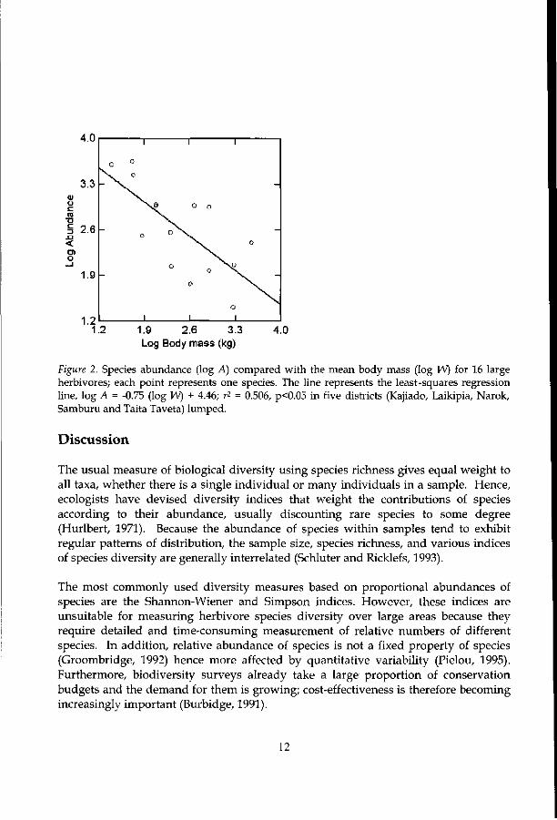
Figure 2 shows the negative relation of herbivores abundance to body size — abundance declines with body mass according to the -0.75-power law. The least squares fit for the relations between body mass and species abundance accounts for 51% of the variance. The proposed diversity index shows a very strong correlation wi th species abundance. The straight-line (Figure 3) relationships between species abundance and the proposed diversity index accounts for 63% of the variance.

Table 1. Coefficient of correlation (r2) between log-species abundances and diversity indices, species richness (S), Shannon-Wiener index (H1), Simpson's index (D), Evenness (£) and proposed diversity index (B) across five districts in Kenya. N stands for number of sample points

Kajiado Laikipia Narok Samburu Taita Taveta Lumped

S

0.473 0.586 0.720 0.493 0.562 0.677

H'

0.273 0.396 0.152 0.283 0.313 0.374

D

0.180 0.219 0.021 0.193 0.153 0.210

E

0.224 0.410 0.130 0.218 0.306 0.279

B

0.392 0.552 0.703 0.336 0.400 0.633

N

215 81 129 83 157 665

Table 2. Coefficient of correlation (r2) between diversity measures. The diversity of large herbivore species in two districts were correlated for five diversity indices, species richness (S), Shannon-Wiener index (H'), Simpson's index (D), Evenness (E), and proposed diversity index (B). La and Na stand for Laikipia and Narok districts respectively

H'

S 0.443 H'

Na

D

0.198 0.842 D

E

0.403 1.000 0.796 E

B

0.892 0.523 0.264 0.483 B

S

La

H'

0.817 H'

D

0.596 0.851 D

E

0.816 1.000 0.849 E

B

0.767 0.592 0.382 0.565 B

11

1.9 2.6 3.3 Log Body mass (kg)

4.0

Figure 2. Species abundance (log A) compared with the mean body mass (log W) for 16 large herbivores; each point represents one species. The line represents the least-squares regression line, log A = -0.75 (log W) + 4.46; r2 = 0.506, p<0.05 in five districts (Kajiado, Laikipia, Narok, Samburu and Taita Taveta) lumped.

Discussion

The usual measure of biological diversity using species richness gives equal weight to all taxa, whether there is a single individual or many individuals in a sample. Hence, ecologists have devised diversity indices that weight the contributions of species according to their abundance, usually discounting rare species to some degree (Hurlbert, 1971). Because the abundance of species within samples tend to exhibit regular patterns of distribution, the sample size, species richness, and various indices of species diversity are generally interrelated (Schluter and Ricklefs, 1993).

The most commonly used diversity measures based on proportional abundances of species are the Shannon-Wiener and Simpson indices. However, these indices are unsuitable for measuring herbivore species diversity over large areas because they require detailed and time-consuming measurement of relative numbers of different species. In addition, relative abundance of species is not a fixed property of species (Groombridge, 1992) hence more affected by quantitative variability (Pielou, 1995). Furthermore, biodiversity surveys already take a large proportion of conservation budgets and the demand for them is growing; cost-effectiveness is therefore becoming increasingly important (Burbidge, 1991).

12

For rapid appraisals suitable diversity indices should be based on presence or absence data. Such binary data must be easy to measure and capable of capturing the degree of difference between species. A potential animal species attribute that meets this condition is body size. Animal body size is easy to measure and it is related to many other species characteristics such as longevity, reproductive success, predation, competition and dispersal (Dunham et al., 1978; Siemann et al., 1996).

3.6

0.0

. . . 0 o o o i") nr. no co c o

0.0 01 0 2 0.3 0.4 Proposed diversity index

Figure 3. Scatter plots of relation between proposed diversity index (B) and species abundance (log A), log A = 4.23B + 0.83; r2 = 0.634, n = 665, p<0.05, in five districts (Kajiado, Laikipia, Narok, Samburu and Taita Taveta) lumped.

The proposed diversity index is based on a different kind of community pattern, that is, the inverse relationship between the body size of species and its local abundance (Figure 2). This pattern may be explained by the fact that within an assemblage of animals, or a taxonomic group (e.g., birds, mammals, fish), larger-bodied species tend to be rarer (Diamond, 1988). Since body size is positively correlated with generation time, large-bodied species will tend to have higher extinction rates resulting in lower speciation rates (Begon et al., 1990). In contrast, smaller-bodied species have lower extinction rates, probably due to high reproductive rates; hence the rate of speciation will be higher (Begon et al, 1990). Moreover, smaller species have a wider range of

13

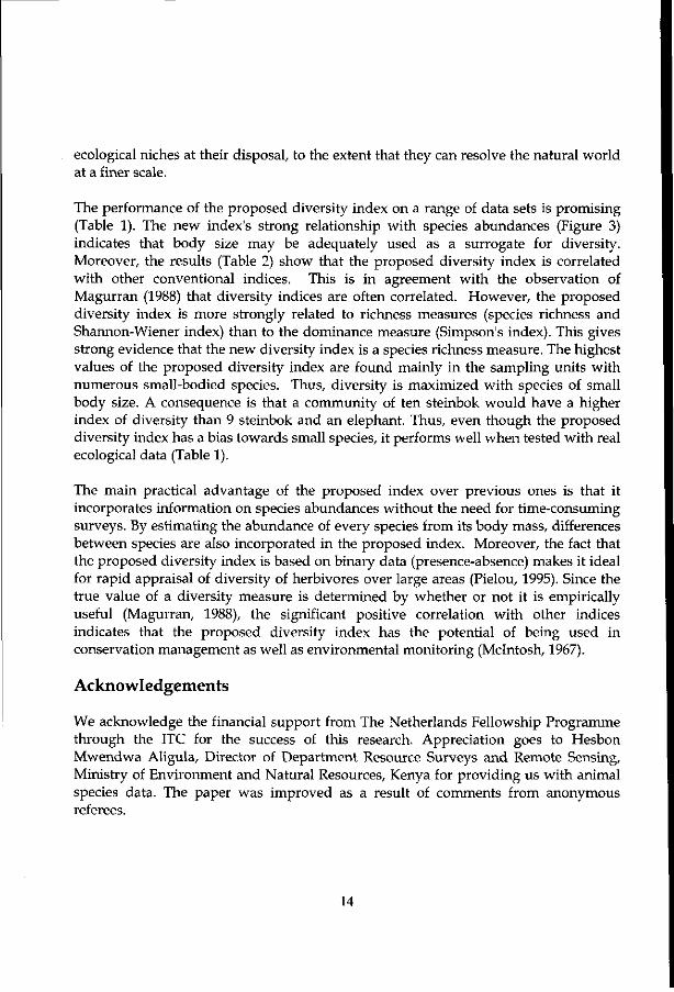
ecological niches at their disposal, to the extent that they can resolve the natural world at a finer scale.

The performance of the proposed diversity index on a range of data sets is promising (Table 1). The new index's strong relationship with species abundances (Figure 3) indicates that body size may be adequately used as a surrogate for diversity. Moreover, the results (Table 2) show that the proposed diversity index is correlated with other conventional indices. This is in agreement with the observation of Magurran (1988) that diversity indices are often correlated. However, the proposed diversity index is more strongly related to richness measures (species richness and Shannon-Wiener index) than to the dominance measure (Simpson's index). This gives strong evidence that the new diversity index is a species richness measure. The highest values of the proposed diversity index are found mainly in the sampling units with numerous small-bodied species. Thus, diversity is maximized with species of small body size. A consequence is that a community of ten steinbok would have a higher index of diversity than 9 steinbok and an elephant. Thus, even though the proposed diversity index has a bias towards small species, it performs well when tested with real ecological data (Table 1).

The main practical advantage of the proposed index over previous ones is that it incorporates information on species abundances without the need for time-consuming surveys. By estimating the abundance of every species from its body mass, differences between species are also incorporated in the proposed index. Moreover, the fact that the proposed diversity index is based on binary data (presence-absence) makes it ideal for rapid appraisal of diversity of herbivores over large areas (Pielou, 1995). Since the true value of a diversity measure is determined by whether or not it is empirically useful (Magurran, 1988), the significant positive correlation with other indices indicates that the proposed diversity index has the potential of being used in conservation management as well as environmental monitoring (Mcintosh, 1967).

Acknowledgements

We acknowledge the financial support from The Netherlands Fellowship Programme through the ITC for the success of this research. Appreciation goes to Hesbon Mwendwa Aligula, Director of Department Resource Surveys and Remote Sensing, Ministry of Environment and Natural Resources, Kenya for providing us with animal species data. The paper was improved as a result of comments from anonymous referees.

14

References

Begon M, Harper J L and Townsend CR (1990) Ecology: Individuals, populations and communities. Blackwell Scientific Publications, Oxford

Bohning-Gaese K (1997) Determinants of avian species richness at different spatial scales. Journal of Biogeography 24: 49-60

Burbidge AA (1991) Cost constraints on surveys for nature conservation. In: Margules CR and Austin MP (eds) Nature conservation: cost effective biological surveys and data analysis, pp 3-6. CSIRO, Canberra

Damuth J (1981) Population density and body size in mammals. Nature 290: 699-700 De Leeuw J, Prins HHT, Njuguna EC, Said MY and De By R (1998) Interpretation of

DRSRS animal counts (1977-1997) in the rangeland districts of Kenya. Ministry of Planning and National Development, Nairobi

Diamond J (1988) Factors controlling species diversity: Overview and synthesis. Annals of the Missouri Botanical Garden 75:117-129

Dirschl HJ, Norton-Griffiths M and Wetmore SP (1981) Training observers for aerial surveys of herbivores. The Wildlife Society Bulletin 9(2)

Dunham AE, Tinkle DW and Gibbons JW (1978) Body size in island lizards: A cautionary tale. Ecology 59:1230-1238

Fa JE and Purvis A (1997) Body size, diet and population density in Afrotropical forest mammals: A comparison with neotropical species. Journal of Animal Ecology 66: 98-112

Groombridge B (1992) Global Biodiversity. Status of the Earth's Living Resources. World Conservation Monitoring Centre, London

Halternorth T and Diller H (1980) Mammals of Africa including Madagascar. HarperCollins, London

Hurlbert SH (1971) The non-concept of species diversity: A critique and alternative parameters. Ecology 52: 577-586

Huston AH (1994) Biological Diversity. The coexistence of species on changing landscapes. Cambridge University Press, Cambridge

Mcintosh RP (1967) An index of diversity and the relation of certain concepts of diversity. Ecology 48: 392-404

Magurran AE (1988) Ecological Diversity and its Measurement. Croom Helm, London Mizutani F (1999) Biomass density of wild and domestic herbivores and carrying

capacity on a working ranch in Laikipia District, Kenya. African Journal of Ecology 37: 226-240

Norton - Griffiths M (1978) Counting animals. Handbook no.l. Africa Wildlife Leadership Foundation, Nairobi

15

Ottichilo WK and Khaemba W (2001) Validation of observer and aircraft calibration for aerial animal surveys: A case study of the Department of Resource Surveys and Remote Sensing (DRSRS), Kenya. African Journal of Ecology 39: 45-50

Ottichilo WK and Sinange RK (1985) Differences in the visual and photographic measurements in the estimation of strip widths for aerial censuses of animal populations. DRSRS, Ministry of Planning and National Development, Nairobi

Peters RH and Raelson JV (1984) Relations between individual size and mammalian population density. American Naturalist 124: 498-517

Peet RK (1974) The measurement of species diversity. Annual review of ecology and Systematics 5: 285-307

Pielou EC (1975) Ecological Diversity. John Wiley and Sons, New York Pielou EC (1995) Biodiversity versus old-style diversity: Measuring biodiversity for

conservation. In: Boyle TJB and Boontawee B (eds) Measuring and monitoring biodiversity in tropical and temperate forests, pp 5-17. Center for International Forestry Research, Bogor, Indonesia

Prins HHT and Olff H (1998) Species-Richness of African grazer assemblages: Towards A functional explanation. In: Newbery DM, Prins HHT and Brown ND (eds) Dynamics of Tropical Communities, pp 449-490. Blackwell Science, Oxford

Purvis A and Hector A (2000) Getting the measure of biodiversity. Nature 405: 212-219 Schluter D and Ricklefs R (1993) Species diversity in ecological communities. Historical

and Geographical perspectives. University of Chicago, Chicago Siemann E, Tilman D and Haarstad J (1996) Insect species diversity, abundance and

body size relationships. Nature 380: 704-706

16

CHAPTER

3

BODY SIZE AND MEASUREMENT OF SPECIES DIVERSITY IN LARGE GRAZING MAMMALS

Abstract

Species are by definition different from each other. This fact favours ranking rather than additive indices. However, ecologists have measured species diversity in terms of species richness, or by combining species richness with the relative abundance of species within an area. Both methods raise problems: species richness treats all species equally, while relative abundance is not a fixed property of species but varies widely temporally and spatially, and requires a massive sampling effort. The functional aspect of species diversity measurement may be strengthened by incorporating differences between species such as body size as a component of diversity. An index of diversity derived from a measure of variation in body size among species is proposed for large grazing mammals. The proposed diversity index related positively to species abundance indicating that the use of body size as a surrogate for diversity is adequate. Since the proposed index is based on presence or absence data, the expensive and time consuming counting of individuals per species in each sampling unit is not necessary.

Key words: biodiversity index, body size, grazers, mammals, species diversity

17

Introduction

To prioritize conservation efforts, differences in biodiversity across an area often need to be assessed (Groombridge, 1992). There has been controversy over the meaning of biological diversity, over methods for measuring and assessing diversity as well as the ecological interpretation of different levels of diversity. In the ensuing confusion, Hurlbert (1971) despaired, declaring diversity to be a non-concept. However, his despair proved premature, and when carefully defined according to an appropriate notation, diversity can be as unequivocal as any other ecological parameter (Hill, 1973). The controversy was largely the result of an unreasonable expectation that a single statistic should contain all the information about the assembly of objects that it represents (Huston, 1994). Unfortunately, when we look for a suitable numerical definition, we find that no particular formula has pre-eminent advantage, and that different authors have plausibly proposed different indices (Hill, 1973; Magurran, 1988). Since no single statistic can ever be an adequate description of the diversity of a collection, several statistics should always be provided to represent the collection more completely (Huston, 1994). Regardless of the statistics that are chosen to describe diversity, it is critical that the sample be collected using a statistical design that will allow a reliable estimate of the properties of the community that are relevant to the diversity issue being studied (Magurran, 1988).

The concept of diversity has two statistical properties and two unavoidable value judgments. The statistical properties are the number of species in a given sample and the relative numbers (individuals) of each different type of species. The value judgments are whether the species are different enough to be considered distinct and whether the individuals are similar enough to be considered the same. The number of species in a sample (species richness) can provide a good definition of biological diversity. However, the great range of diversity indices and models, which go beyond species richness, is evidence of the importance of the relative abundance of species (Magurran, 1988). The relative number of individuals comprising each species is usually referred to as 'evenness', since the more even the number of individuals, the greater the perceived diversity (Huston, 1994). Thus, ecologists have devoted considerable effort to developing various indices of diversity that combine two distinct statistical components, species richness and their relative population densities, in a single number (Brown, 1988). The most frequently used are the Shannon-Wiener index (H) and the Simpson's index (D):

H ' = - I P i l n P i (1)

D = 1/ IP i2 (2)

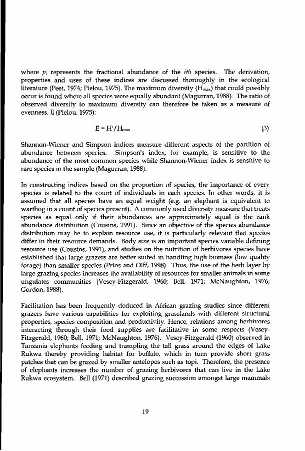
where p, represents the fractional abundance of the ith species. The derivation, properties and uses of these indices are discussed thoroughly in the ecological literature (Peet, 1974; Pielou, 1975). The maximum diversity (Hmax) that could possibly occur is found where all species were equally abundant (Magurran, 1988). The ratio of observed diversity to maximum diversity can therefore be taken as a measure of evenness, E (Pielou, 1975):

E = H'/Hnax (3)

Shannon-Wiener and Simpson indices measure different aspects of the partition of abundance between species. Simpson's index, for example, is sensitive to the abundance of the most common species while Shannon-Wiener index is sensitive to rare species in the sample (Magurran, 1988).

In constructing indices based on the proportion of species, the importance of every species is related to the count of individuals in each species. In other words, it is assumed that all species have an equal weight (e.g. an elephant is equivalent to warthog in a count of species present). A commonly used diversity measure that treats species as equal only if their abundances are approximately equal is the rank abundance distribution (Cousins, 1991). Since an objective of the species abundance distribution may be to explain resource use, it is particularly relevant that species differ in their resource demands. Body size is an important species variable defining resource use (Cousins, 1991), and studies on the nutrition of herbivores species have established that large grazers are better suited in handling high biomass (low quality forage) than smaller species (Prins and Olff, 1998). Thus, the use of the herb layer by large grazing species increases the availability of resources for smaller animals in some ungulates communities (Vesey-Fitzgerald, 1960; Bell, 1971; McNaughton, 1976; Gordon, 1988).

Facilitation has been frequently deduced in African grazing studies since different grazers have various capabilities for exploiting grasslands with different structural properties, species composition and productivity. Hence, relations among herbivores interacting through their food supplies are facilitative in some respects (Vesey-Fitzgerald, 1960; Bell, 1971; McNaughton, 1976). Vesey-Fitzgerald (1960) observed in Tanzania elephants feeding and trampling the tall grass around the edges of Lake Rukwa thereby providing habitat for buffalo, which in turn provide short grass patches that can be grazed by smaller antelopes such as topi. Therefore, the presence of elephants increases the number of grazing herbivores that can live in the Lake Rukwa ecosystem. Bell (1971) described grazing succession amongst large mammals

19

of the Serengeti ecosystem. In certain areas when the dry season starts, zebra eat the tough tall grass stems, thereby making basal leaves more available to wildebeest as well as topi, and these in turn prepare the grass sward for Thomson's gazelle.

McNaughton (1976) suggested that migrating Thomson's gazelle prefer to feed in areas already grazed by wildebeest because these areas produce young green regrowth not found in ungrazed areas. Another good example of facilitation is provided in Ngorongoro Crater where cattle, donkeys and small stock were removed in 1974. Since that time, plains zebra, common wildebeest, common eland, hunter's hartebeest and Grant's gazelle all declined in numbers. However, buffalo sharply increased in numbers after livestock removal (Runyoro et ah, 1995). The interpretation might be that cattle and buffalo showed competitive exclusion while the other herbivores were favoured by facilitation (Prins and Olff, 1998). The evidence suggests that the presence of large grazers in ecosystems enhances the nutritive value of forage and facilitates for more selective smaller grazers. Thus when facilitation takes place, small species is prevented from going extinct and such areas are likely to have more species because both selective and unselective grazers coexist (Table 1). Consequently, species richness of grazers should be highest where such facilitation interactions are strongest (Prins and Olff, 1998). Hence, facilitation interactions may form a basis for developing a new diversity measure.

The main objective of this study was to develop a new diversity index for large grazing mammal species that incorporates body size as a component of diversity. The study was carried out at landscape scale (10 * 10 km) because it is at this scale where the consequences of human activities such as ecosystem modification and fragmentation are most dramatic (Halffter, 1998). Hence, most management decisions concerning the conservation of species diversity are made at landscape scale (Bohning-Gaese, 1997).

Methods

The study area and animal species data Kenya is situated between latitudes 5° 40' north and 4° 4' south and between longitudes 33° 50' and 41° 45' east. The study area covered five rangeland districts, namely, Kajiado, Laikipia, Narok, Samburu and Taita Taveta. The natural vegetation types of these districts are as follows: Kajiado district consists of wooded grassland, open grassland, semi-desert bush land and scrub. Wildlife is an important feature of the district and is found within Amboseli and Chyulu game conservation area, as well as within defined dispersal areas that consist of group and individual ranchers (Republic of Kenya, 1990). Laikipia district has mainly dry forms of woodland and savanna with no game reserves but most ranches carry abundant wild herbivore

20

species (Mizutani, 1999). Narok district carries variable vegetation cover, that is, moist woodland, bush land or savanna and has one of the world's famous wildlife sanctuaries, Masai Mara National reserve. Samburu and Taita Taveta districts are dominated by Commiphora, Acacia trees or woodland and perennial grasses such as Cenchrus ciliaris and Chloris roxburghiana. Samburu has three game reserves, Samburu, Shaba and Buffalo Springs while Taita Taveta district covers a large portion of Tsavo National Park.

The source of large grazing mammal species (body mass greater than 10 kg) data (1981 to 1997) was the Department of Resource Surveys and Remote Sensing (DRSRS), Ministry of Environment and Natural resources, Kenya. The systematic reconnaissance flight methodology used by DRSRS for aerial census of animals is fully described by Norton-Griffiths (1978). Statistical analyses to validate DRSRS survey methodology have proved the method to be efficient and the data to be reliable (De Leeuw et al., 1998; Ottichilo and Khaemba, 2001). Topographic maps of scale 1: 250,000 were used for flight planning and all transects conform to the Universal Transverse Mercator (UTM) coordinate system. The aerial surveys were carried out along transects oriented in east-west direction and spaced at 5 km intervals. The standard flying height and aircraft speed were 120 m and 190 km/h respectively. Two experienced and well-trained observers occupied the rear seats of a high wing aircraft (Cessna 185 or Partenevia) and counted animals that appeared between two rods attached to the wing struts. The field of vision between these rods was calibrated by flying repeatedly across ground markers of known spacing (Ottichilo and Sinange, 1985). The number of animals falling within the survey strips on either side of the aircraft along each 5 km transect segment were counted and recorded into tape recorders by the two rear seat observers. Groups of animals more than ten in number were also photographed. After every survey the tape-recorded observations were transcribed to data sheets, which together with processed photographs, were interpreted for herbivore species using 10 x binocular microscopes and overhead projector. Since our study was executed at landscape scale, the processed data at 5 x 5 km spatial resolution were converted to 10 x 10 km grid cells by averaging. The study focuses on large mammal species that have grass as an important component in their diet and native in rangeland districts with at least four years of survey during the 16-year period (1981-1997).

Explanation of the proposed diversity index The proposed diversity index is based on the hypothesis that grazer species richness will be highest where large grazers are prevalent. From such a basis, high species richness should be expected where both small and large grazers coexist. Hence, a positive relationship between richness and any measure of variation in body size among species is expected. Therefore, two measures of variability, coefficient of

21

variation (i.e. variation relative to the average body weight) and the ratio between the median average body weight and interquartile range were compared in order to identify which measure of variability correlate strongly with species richness and total average abundance.

Table 1. The average body mass of grazing mammals larger than 10 kg, occurring in Kenyan rangeland. Average body mass of each species is defined as the midpoints of quoted weight ranges and averaged male and female body weights. The grazer species may be categorized from selective to unselective grazers (Caughley and Sinclair, 1994). Small size (<50 kg) species are selective feeders on leaves of bushes and grass while medium species (>100 kg) select high quality grass leaves. Mixed feeders change from grazing in rainy season to browsing in dry season. Unselective feeders prefer low quality grass (i.e. high biomass). Body mass (kg) data were obtained from Haltenorth and Diller (1980)

Common name Steinbok Thomson's gazelle Reedbuck Impala Grant's gazelle Warthog Topi Wildebeest Hunter's hartebeest Waterbuck Grevy's zebra Oryx Burchell's zebra Eland Buffalo Hippopotamus Elephant

Scientific name Raphicerus campestris Gazella thomsoni Redunca redunca Aegyceros melampus Gazella granti Phacocheorus aethiopicus Damaliscus korrigum Connochaetes taurinus Alcelaphus buselaphus Kobus ellipsiprymnus Equus grevyi Oryx gazella Equus burchelli Taurotragus oryx Syncerus caffer Hippopotamus amphibius Loxodonta africana

Body mass 11.1 24.9 44.8 52.5 55.0 73.5 119 132.3 134 211 408 203 235 471.3 631 1900 3550

Feeding method Selective Selective Selective Mixed Mixed Mixed Selective Selective Selective Selective Selective Unselective Unselective Unselective Unselective Unselective Unselective

Prior to calculation of coefficient of variation, average body weight (A) and s tandard deviation (S) were calculated as:

A = 1 2 > (4)

22

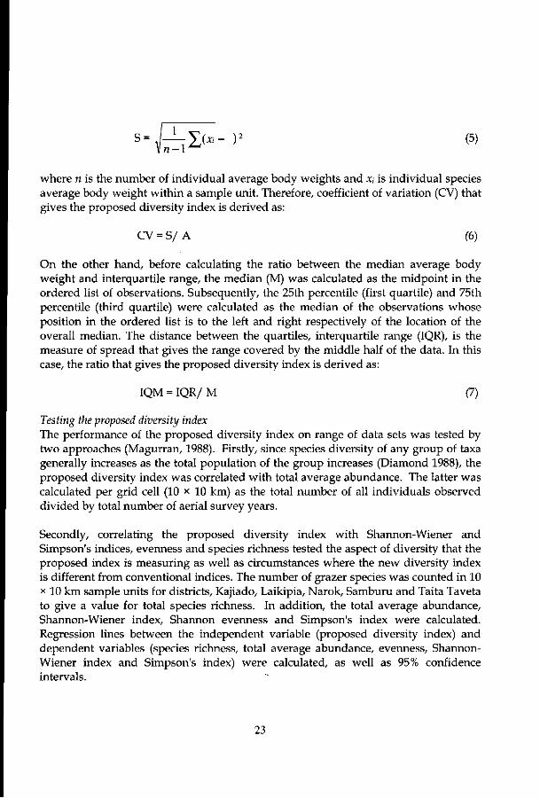
s = n-\ 5 > - )2 (5)

where n is the number of individual average body weights and x, is individual species average body weight within a sample unit. Therefore, coefficient of variation (CV) that gives the proposed diversity index is derived as:

CV = S/ A (6)

On the other hand, before calculating the ratio between the median average body weight and interquartile range, the median (M) was calculated as the midpoint in the ordered list of observations. Subsequently, the 25th percentile (first quartile) and 75th percentile (third quartile) were calculated as the median of the observations whose position in the ordered list is to the left and right respectively of the location of the overall median. The distance between the quartiles, interquartile range (IQR), is the measure of spread that gives the range covered by the middle half of the data. In this case, the ratio that gives the proposed diversity index is derived as:

IQM = IQR/ M (7)

Testing the proposed diversity index The performance of the proposed diversity index on range of data sets was tested by two approaches (Magurran, 1988). Firstly, since species diversity of any group of taxa generally increases as the total population of the group increases (Diamond 1988), the proposed diversity index was correlated with total average abundance. The latter was calculated per grid cell (10 x 10 km) as the total number of all individuals observed divided by total number of aerial survey years.

Secondly, correlating the proposed diversity index with Shannon-Wiener and Simpson's indices, evenness and species richness tested the aspect of diversity that the proposed index is measuring as well as circumstances where the new diversity index is different from conventional indices. The number of grazer species was counted in 10 x 10 km sample units for districts, Kajiado, Laikipia, Narok, Samburu and Taita Taveta to give a value for total species richness. In addition, the total average abundance, Shannon-Wiener index, Shannon evenness and Simpson's index were calculated. Regression lines between the independent variable (proposed diversity index) and dependent variables (species richness, total average abundance, evenness, Shannon-Wiener index and Simpson's index) were calculated, as well as 95% confidence intervals.

23

A 55 50 103 100 203 176 189 175

M 53 52 55 64 73 54 119 96

S IQ

10.5 10

15.6 10

82.5 22

73 81

214 184

236 28

194 158

191 160

IQMCV 0.19 0.19

0.19 0.31

0.40 0.80

1.27 0.73

2.52 1.05

0.52 1.34

1.33 1.03

1.67 1.09

Table 2. Example of the grazers' species individual body weights observed in sample units in Narok district. The average body weight (A), median (M), standard deviation (S) and interquartile range (IQ) were calculated per sample unit (10 x 10 km). The proposed diversity index is calculated as average body weight divided by standard deviation, coefficient of variation (CV) or interquartile range divided by median (IQM)

Grazer species body weights 45 51 53 55 73

25 45 51 53 55 73

45 51 53 55 73 211 235 25 45 51 53 55 73 119 132 211 235

45 51 53 55 73 211 235 471 631 25 45 51 53 55 73 471 631

45 51 53 55 73 119 132 211 235 471 631

25 45 51 53 55 73 119 132 211 235 471 631 45 51 53 55 73 119 132 211 235 471 631 1900 3550 579 132 1026418 3.17 1.77

25 45 51 53 55 73 119 132 211 235 471 631 1900 3550 539 126 996 418 3.33 1.85

Results

The two measures of variation in body size among species, coefficient of variation and the ratio between median and interquartile range correlated positively with species richness and total average abundance (Table 3). However, with exception of Samburu district, species richness and total average abundance correlated strongly with coefficient of variation than with the ratio between median and interquartile range. Hence, coefficient of variation may be taken as an appropriate measure of grazer diversity in the study districts than the ratio between median and interquartile range.

Although the proposed diversity index is not based on relative abundance of species, its correlation with total average abundance is moderately strong and comparable to conventional indices based on proportional abundance of species such as Shannon evenness, Shannon-Wiener and Simpson's indices (Table 4). Moreover, in Narok district with the highest species richness and abundance of individuals (Table 3) the new index yields stronger correlation with total average abundance than Shannon evenness, Shannon-Wiener and Simpson's indices (Table 4).

24

Table 3. The coefficient of correlation (r) between measures of variation in body size among species and species richness as well as abundance of individuals: Species richness (S) versus (vs.) coefficient of variation (CV); species richness versus the ratio between median and interquartile range (IQM); log-total average abundance (I) versus coefficient of variation; log-total average abundance versus the ratio between median and interquartile range across five range land districts. Logab and rich represent the maximum log-total average abundance and maximum species richness in 10 x 10 km respectively while n stands for number of sample points. Significant at p<0.001 is represented by ** while* represents significant at p<0.05, ns stands for not significant at p<0.05

District Kajiado Laikipia Narok

Samburu Taita Taveta

Pooled data

S vs. CV

0.525**

0.649** 0.749** 0.332**

0.566**

0.508**

S vs. IQM

ns

0.486** 0.429** 0.524**

0.328**

0.363**

I vs. CV

0.384** 0.471** 0.637**

ns

0.519** 0.361**

I vs. IQM

ns

0.280* 0.299** 0.460**

0.318** 0.268**

Logab

6.0 5.3

8.0 4.3

5.0 8.0

Rich

11

12 13 7

11 13

n

204

81 122 87

161 655

Table 4. Coefficient of correlation (r) between log-total average species abundance and diversity indices, species richness (S), Shannon-Wiener index (H'), Simpson's index (D), evenness (E), proposed diversity index (CV) across five rangeland districts in Kenya. With exception of ns which represents not significant at p<0.05, all other correlations are significant at p<0.001, n stands for number of sample points

District S H1 D E CV n

Kajiado 0 .650 0.505 0.374 0.486 0.384 204

Laikipia 0.779 0.676 0.495 0.657 0.471 81

Narok 0 .820 0.586 0.443 0.585 0.637 122

Samburu 0 .714 0.548 0.429 0.489 ns 87 Taita Taveta 0.747 0.567 0.403 0.561 0.519 161 Pooled data 0.805 0.637 0.517 0.572 0.361 655

The relations between diversity indices were compared in two districts wi th different levels of species richness and total average abundance (Table 5), that is, Narok district wi th the highest species richness and abundance of individuals, and Samburu district wi th the lowest species richness and abundance of individuals (Table 3). The results (Table 5) reveal that the proposed diversity index is strongly associated with conventional indices in the district (Narok) with the highest species richness and

25

abundance than in the district (Samburu) with the lowest species richness and abundance. Moreover, the proposed diversity measure gives stronger correlation with measures of richness (species richness and Shannon-Wiener index) than with a measure of dominance (Simpson's index). This indicates that the new index is a species richness measure that takes variation in body size among species into account as opposed to conventional indices. Figure 1 shows that straight-line relationship between the proposed diversity index and total average abundance in Narok, which account for 47% of the variance.

Table 5. Coefficient of correlation (r) between diversity measures. The diversity of grazer species in two districts were correlated for five diversity indices, species richness (S), Shannon-Wiener index (H1), Evenness (E), Simpson's index (D) and proposed diversity index (CV). Significant at p<0.05 is represented by* while ns stands for not significant at p<0.05, and other correlations are significant at p<0.001. Na and Sa stand for Narok and Samburu districts respectively

s I

0.820 I

Na

H'

0.761 0.581

H'

D E CV

0.644 0.760 0.749 0.443 0.585 0.637

0.899 1 0.436

D 0.898 0.368 E 0.435

CV

I

S 0.714 I

Sa

H' D E CV

0.863 0.717 0.713 0.332 0.548 0.429 0.488 ns

H' 0.951 0.842 0.240* D 0.803 ns

E 0.240* CV

Discussion

The proposed diversity index has values ranging between 0 and 3 across the five districts studied. The lowest values (Table 2) are found mainly in the sampling units with less variation in body size among species (i.e. low coefficient of variation). In essence, low values of the proposed diversity index reflect a community where grazer species are more or less similar in body mass. Consequently, resource competition is expected to prevail over facilitation interactions leading to low species diversity (Prins and Olff, 1998). Conversely, high values of the proposed diversity index occur in sampling units with high variation in body size among species (Table 2). This reflects a community where all species with different body weights are represented (i.e. small, medium and large species). In this case, grazing succession is expected to occur where large grazers that are unselective feeders, remove the tough tall grass thereby making basal leaves available to medium grazers. The medium size grazers in turn prepare the grass sward for highly selective feeders (small species).

26

0.6 1.2 1.8 Proposed diversity index

2.4

Figure 1. The relationship between proposed diversity index (CV) and log-total average abundance (I) in Narok district (I = 2.803 + 2.056CV, r? = 0.469, p < 0.001).

However, in some cases the high values of the proposed diversity index cannot be attributed to facilitation. For instance, smaller species may join larger grazers to dilute individual predation risks and not to benefit from grazing facilitation. In addition, grazers are water-dependent so the proposed diversity index is expected to be high near water bodies, again independently of grazing facilitation. Furthermore, there tend to be more species of small-bodied species than of large-bodied species (Diamond, 1988) and hence the variations in body size among smaller species are lower than among larger species (Table 2). As a consequence, two large species will give a higher value of the proposed diversity index than two small species even though the richness is not different.

The results (Figure 1) show that the proposed diversity index increases with increase in total average species abundance, which is consistent with the ecological rule that species diversity of any higher-level taxon generally increases with the group's total population size (Diamond, 1988). This demonstrates that body size may be adequately used as a surrogate for diversity. The proposed diversity index seems to have good performance in the districts with high species richness and high numbers of individuals than in the districts with low species richness and low numbers of individuals. In Narok district with the highest grazers' species richness and highest abundance of individuals, the new index yields a stronger correlation (Table 5) with total average abundance than Shannon evenness, Shannon-Wiener and Simpson's indices. Moreover, Table 5 reveals that the proposed diversity index is strongly

27

correlated with conventional indices in the district with the highest numbers of species and individuals. This provides evidence that the proposed diversity index better reflects grazer diversity in areas where species richness and abundance of individuals are higher than in areas where species richness and abundance of individuals are lower. Generally, quantification of biodiversity using indices based on proportional abundance of species in areas with high species richness and high abundance of individuals requires expensive and time consuming counting of individuals per species in each sampling unit. In such areas the new diversity measure may be useful because it is derived from presence-absence data that require relatively less sampling efforts.

The significant positive correlation between the new index and conventional indices (Table 5) shows that the proposed diversity index has a potential of being used in environmental monitoring. For example, adverse effects of pollution will be reflected in a reduction in values of the proposed diversity index because species with higher body weights are reduced in polluted communities (Magurran, 1988). Moreover, since the new index is based on a measure of variation in body size among species, the degree of difference between species is included in the index. This property has given the proposed diversity index an advantage over species richness and proportional abundances of species indices (Shannon-Wiener and Simpson's indices) that treat species as taxonomically equal. Furthermore, Shannon-Wiener and Simpson's indices combine species richness and relative abundance of species, which is more affected by quantitative variability (Pielou, 1995). Since population sizes of grazer species fluctuate enormously from year to year in the study areas, a diversity index based on body size that requires presence-absence data may provide a more effective estimate of biodiversity than diversity indices based on quantitative data that require massive sampling efforts.

Body size is one of the most studied attributes of animal species because it is related to many other species attributes such as longevity, reproductive success, predation, competition and dispersal (Dunham et ah, 1978; Siemann et ah, 1996). In addition, body size is easy to measure, so it is a convenient surrogate for these other elusive variables. Hence, knowing the distribution of body size can thus give insights into how other variables might be distributed within taxa or assemblages. Body weights definitely differ between adults and youngsters, but possibly for some species between males and females as well. This is extremely difficult to spot when carrying out aerial survey on a small aircraft, although for elephants it may be possible, and may influence the quantification of biodiversity. However, it is assumed that taking average body weight of each species as the median of quoted weight ranges (young to

28

adult) and averaged male and female body weights (Prins and Olff, 1998) are of sufficient precision for yielding a reliable biodiversity index.

Conclusion

In developing the new diversity index it has been assumed that larger grazer species facilitate for smaller species and hence species richness is expected to be higher in areas where both smaller and larger species coexist. From such a basis, an index derived from measures of variation in body size among species seems to be an appropriate measure of biodiversity because it correlates positively with species abundance from ecological communities (Table 3) as well as other conventional indices (Table 4 and 5). The fact that the proposed diversity index is based on presence-absence data makes it ideal for rapid appraisal of diversity of herbivores over large areas (Pielou, 1995).

It is known for many groups of animal—birds, mammals and fish—that the distribution of body sizes is skewed, so there are more relatively small species than large ones (Brown, 1995; Nee and Lawton, 1996). In addition, this right skewness has been observed in five orders of insects where basic patterns link species richness, relative abundances and body size (Siemann et al., 1996). Seemingly, the most abundant species among birds, mammals, fish and insects tend to be relatively small in size. Apparently, larger species have larger home ranges and lower densities (Peters, 1983) resulting in smaller local populations. On the contrary, smaller species take up less space than larger species and individuals of smaller species can live in very tiny places, filling ecological niches that would be unsuitable for larger spaces. Moreover, small individuals need only small amounts of food to reproduce quickly, and so large numbers can exist in restricted places. As a consequence, smaller species are generally more diverse than larger species (Diamond, 1988). However, for a given taxonomic group (e.g. birds, mammals, fish and insects) species richness should be expected to be high in areas where both small and large species coexist. In view of this, the proposed diversity index may be useful for quantification biodiversity for other taxonomic groups. However, more experiments need to be done to establish the possible merit of the proposed diversity index for other taxa.

Acknowledgement

We gratefully acknowledge the Netherlands Ministry of Development Co-operation and Ministry of Education for funding the research under the Netherlands Fellowship Programme. Appreciation goes to H. Mwendwa, Director of Department Resource Surveys and Remote Sensing (DRSRS) for providing animal species data.

29

References

Bell RHV (1971) A grazing ecosystem in the Serengeti. Scientific American 225: 86-93 Bohning-Gaese K (1997) Determinants of avian species richness at different spatial

scales. Journal of Biogeography 24:49-60 Brown JH (1988) Species Diversity. In: Myers AA and Giller PS (eds) Analytical

Biogeography. An integrated approach to the study of animal and plant distributions, pp 57-89. Chapman & Hall, London

Brown JH (1995) Macroecology. University of Chicago Press, Chicago Caughley G and Sinclair ARE (1994) Wildlife ecology and Management. Blackwell

Science, Cambridge Cousins SH (1991) Species diversity measurement: Choosing the right index. Trends in

Ecology and Evolution 6:190-192 De Leeuw J, Prins HHT, Njuguna EC, Said MY and De By R (1998) Interpretation of

DRSRS animal counts (1977-1997) in the rangeland districts of Kenya. Ministry of Planning and National Development, Nairobi, Kenya

Diamond J (1988) Factors controlling species diversity: Overview and synthesis. Annual Missouri Botanical Garden 75:117-129

Dunham AE, Tinkle DW and Gibbons JW (1978) Body size in island lizards: A cautionary tale. Ecology 59:1230-1238

Gordon IJ (1988) Facilitation of red deer grazing by cattle and its impact on red deer performance. Journal of Applied Ecology 25:1-10

Groombridge B (1992) Global Biodiversity. Status of the Earth's Living Resources. World Conservation Monitoring Centre, London

Halffter G (1998) A strategy for measuring landscape biodiversity. Biology International 36: 3-17

Haltenorth T and Diller H (1980) Mammals of Africa including Madagascar. HarperCollins, London

Hill MO (1973) Diversity and Evenness: A unifying notation and its consequences. Ecology 54: 427- 432

Hurlbert SH (1971) The non-concept of species diversity: A critique and alternative parameters. Ecology 52: 577-586

Huston AH (1994) Biological Diversity. The coexistence of species on changing landscapes. Cambridge University Press, Cambridge

Magurran AE (1988) Ecological Diversity and its Measurement. Princeton University Press, Princeton

Mcintosh RP (1967) An index of diversity and the relation of certain concepts of diversity. Ecology 48: 392-404

McNaughton SJ (1976) Serengeti migratory wildebeest: facilitation of energy flow by

30

grazing. Science 191: 92-94 Mizutani F (1999) Biomass density of wild and domestic herbivores and carrying

capacity on a working ranch in Laikipia District, Kenya. African Journal of Ecology 37: 226-240

Norton-Griffiths M (1978) Counting animals. Handbook no. 1. Africa Wildlife Leadership Foundation, Nairobi, Kenya

Ottichilo WK and Khaemba, W (2001) Validation of observer and aircraft calibration for aerial animal surveys: A case study of the Department of Resource Surveys and Remote Sensing (DRSRS), Kenya. African Journal of Ecology 39: 45-50

Ottichilo WK and Sinange RK (1985) Differences in the visual and photographic measurements in the estimation of strip widths for aerial censuses of animal populations. DRSRS, Ministry of Planning and National Development, Nairobi, Kenya

Peet RK (1974) The measurement of species diversity. Annual review of ecology and systematics 5: 285-307

Peters RH (1983) The ecological implications of body size. Cambridge University Press, Cambridge

Pielou EC (1975) Ecological Diversity. John Wiley & Sons, New York Pielou EC (1995) Biodiversity versus old-style diversity: In: Boyle TJB and Boontawee

B (eds) Measuring and monitoring biodiversity in tropical and temperate forests, pp 5-17. Center for International Forestry Research, Bogor, Indonesia

Prins HHT and Olff H (1998) Species-Richness of African grazer assemblages: Towards a functional explanation. In: Newbery DM, Prins HHT and Brown ND (eds) Dynamics of Tropical Communities, pp 449-490. Blackwell Science, Oxford

Republic of Kenya (1990) Kajiado District Atlas. Ministry of Reclamation and Development of Arid, Semi-arid areas and wastelands. ASAL Programme Kajiado, Kajiado, Kenya

Runyoro VA, Hofer H, Chausi EB and Moehlman PD (1995) Long-term trends in the herbivore populations of the Ngorongoro Crater, Tanzania. In: Sinclair ARE and Arcese P (eds) Serengeti II: Dynamics, Management and Conservation of an Ecosystem, pp 146-158. Chicago University Press, Chicago

Siemann E, Tilman D and Haarstad J (1996) Insect species diversity, abundance and body size relationships. Nature 380: 704-706

Vesey-Fitzgerald DF (1960) Grazing succession among East Africa game animals. Journal of Mammology 41:161-172

31

CHAPTER 4

INTERANNUAL VARIABILITY OF NDVI AND SPECIES RICHNESS IN KENYA

Abstract

Ecologists have long recognized the spatial variability of species richness. In an attempt to identify the factors responsible for this variability, ecologists have traditionally used environmental data obtained from sparse point samples (such as meteorological stations). However, remotely sensed data also provide a means of estimating relevant environmental factors and thereby improving predictions of species richness. The Advanced Very High Resolution Radiometer-Normalized Difference Vegetation Index (AVHRR-NDVI) has been shown to be related to net primary productivity (NPP) and actual evapotranspiration (AET) for many vegetation types. NPP and AET have frequently been used as surrogate measures for species richness. Local spatial variability of NPP and AET that indicates habitat heterogeneity is hypothesized as another influence on species richness. We examined the relationship between interannual maximum NDVI variables and species richness of vascular plants and large mammals. The study was done at a landscape scale, which matches the scale of data collection. Statistical analyses revealed that higher average NDVI results in lower species richness, whereas standard deviation and coefficient of variation correlated positively with species richness. Thus, NDVI variables appear to represent environmental factors influencing species richness. Hence, by utilizing remote sensing, our understanding of the spatial variability of species richness was improved.

Key words: AVHRR-NDVI, large mammals, mapping, plants, productivity, spatial heterogeneity, species richness, time series analysis

32

Introduction

Biological diversity is defined as the variability among living organisms from all sources including inter alia, terrestrial, marine, and other aquatic ecosystems, and the ecological complexes of which they are part; this includes diversity within species, between species, and of ecosystems. As the living world is mostly considered in terms of species, biological diversity is commonly used as a synonym of species diversity, in particular of 'species richness', which is the number of species in a site or habitat (Groombridge, 1992). Explaining patterns of species diversity at the species level is one of the most complex problems in ecology. This is because diversity is usually the outcome of many contributing factors whose relative importance varies with spatial and temporal scale (Diamond, 1988). At spatial scales of landscapes, the species pool can be attributed to three independent components of diversity, namely alpha, beta and gamma. Alpha diversity refers to the number of species in small, homogeneous community samples. Beta diversity refers to species turnover along habitat or environment gradients. Gamma diversity is the species turnover among similar habitats along geographical gradients (Cody, 1983). The size of landscape species pool is a function of the interactions between these three independent diversity components (Cowling, 1990).

The relationship between diversity and productivity has been the subject of a long­standing debate in ecology (Groombridge, 1992). The productivity hypothesis predicts that when resources are abundant and reliable, species become more specialized, allowing more species per unit area. However, empirical evidence shows that higher productivity can be either negatively or positively correlated with species richness. In fact, in many systems a unimodal pattern is found, with highest species richness at intermediate levels of productivity; above the point of central tendency species richness decreases as productivity increases, while below the point of central tendency species richness increases as productivity increases (Grime, 1979). A number of explanations of this apparent paradox have appeared (Rosenzweig and Abramsky, 1993), but no single theory has been accepted by ecologists. NDVI has been related to NPP at broad spatial scales (Box et ah, 1989; Prince, 1991). The chain of relationships from NDVI to NPP and NPP to species richness encouraged us to investigate whether a relationship could be established between NDVI and species richness.

Spatial heterogeneity is another popular hypothesis use to explain pattern of species richness (Stoms and Estes, 1993). The heterogeneity hypothesis states that diverse ecosystems support richer assemblages of biological species compared with simple ecosystems (Podolsky, 1994). The within-region variability of NDVI values, for

33

instance defined as the standard deviation of maximum NDVI, should relate to the heterogeneity of habitats, and consequently should have a positive relationship with species richness of mammals and plants.

Research at landscape (or gamma) scale (10 * 10 km) (Stoms and Estes, 1993) is needed in order to bridge the gap between the results obtained at the widely different scales of habitats and regions (Bohning-Gaese, 1997). It is essential to identify factors that determine species richness at landscape scale because most management decisions concerning the conservation of species are made at this scale. The aim of this paper is to examine the relationships between the species richness of vascular plants and large mammals with interannually integrated maximum NDVI variables (viz. average, standard deviation and coefficient of variation) at a landscape scale.

Function of NDVI

Net primary productivity and NDVI NDVI is based on the spectral properties of green vegetation contrasting with its soil background. This index has been found to provide a strong vegetation signal and good spectral contrast from most background materials (Tucker, 1979; Tucker and Sellers, 1986). NDVI also strongly reduces the impact of varying illumination conditions and shadowing effects caused by variations in solar and viewing angle (Kimes et al., 1984). NDVI is a measure derived by dividing the difference between near-infrared and red reflectance measurements by their sum (Sellers, 1989):

NDVI = (NIR-R) / (NIR + R) (1)

where NIR = near-infrared measurements and R = visible red measurements. High positive values of NDVI correspond to dense vegetation cover that is actively growing, whereas negative values are usually associated with bare soil, snow, clouds or non-vegetated surfaces. A number of studies have shown that NDVI provides an effective measure of photosynthetically active biomass (Tucker and Sellers, 1986; Asrar, 1989). NDVI has been shown to be well correlated with climate variables including rainfall and evapotranspiration in a wide range of environmental conditions (Justice et al, 1986; Cihlar et al, 1991). NDVI may therefore be considered to represent the integration of climatic variables at a given location and time (Anyamba and Eastman, 1996).

Productivity and related variables such as biomass, leaf area index and crop stage have been mapped over large areas with remote sensing (Wylie et al, 1991; Lewis et al, 1998). Box et al, (1989) confirmed a strong relationship between NDVI and NPP with a

34

predictive accuracy for annual NPP comparable to that of climate-based NPP models. The NDVI-productivity relationship appears to be consistent over most ecosystems worldwide. NDVI is least reliable in complex terrain (due to the frequency of mixed pixels) and arid zones or snow packs (Box et al., 1989). In these environments vegetation biomass is low, so measures of NPP are poorly estimated including estimates using NDVI.

Interannual variability of vegetation and NDVI Seasonal variations in climate are responsible for differences in species growth and establishment patterns, leading to changes in species composition and distributions (Hobbs, 1990). Thus large variations in species composition and general vegetative growth are seen in arid and semi-arid areas where rainfall is sporadic and the response of vegetation to such rainfall is rapid (Griffin and Friedal, 1985).

National Oceanic and Atmospheric Administration (NOAA) AVHRR data have been used to document interannual variation in vegetation in Sub-Saharan Africa (Tucker et al., 1986). Interannual comparisons of NDVI data incorporating data for more than one year is desirable because of the substantial variations from year to year that occur in the extent and timing of photosynthetic activity (Townshend and Justice, 1986). Although the AVHRR-NDVI data are normally of low spatial resolution (1 km at best, but more typically 7.6 km), they possess a remarkably high temporal resolution. Images are available twice per day, but with compositing to reduce cloud cover, images are commonly dekadal (every ten days) or monthly; they thus provide a very effective source for the examination of intra- and interannual climatic variations (Anyamba and Eastman, 1996). Yearly variations in vegetation can take the form of changes in the spatial distribution of plant growth (Tucker et al., 1986), or may involve differences in species dominance from year to year (Pitt and Heady, 1978).

The interannual variation of the maximum NDVI (per month, per season) can be used to assess whether vegetation cover over a number of years is actually stable in an area, or highly variable. For example, calculating the standard deviation for a number of years describes the variability of vegetation cover for an AVHRR-NDVI image pixel. Pixels with high standard deviations correspond to areas with large variations in vegetation composition and growth. Such areas are likely to have diverse habitats that may support richer assemblages of species (Podolsky, 1994). However, there are numerous examples of communities with high species diversity in environments with large variation in vegetation composition and growth. Such environments have lower productivity and are unpredictable, unstable or frequently disturbed (Huston, 1994).

35

A case study

Study area and species data Kenya is situated between latitudes 5° 40' north and 4° 4' south and between longitudes 33° 50' and 41° 45' east (Figure 1). With its diverse ecological communities, Kenya is a challenging yet promising location to observe whether a significant relationship exists between AVHRR-NDVI and species richness of plants as well as mammals. The country is challenging because of its diverse landforms ranging from coastal plains to savanna grasslands to highland moors.

Both mammal species (body mass greater than 4kg) and plant species data for the years 1982 to 1993 were obtained from Department of Resource Surveys and Remote Sensing (DRSRS), Ministry of Environment and Natural Resources, Kenya. The systematic reconnaissance flight methodology for animal census used by DRSRS is fully described by Norton-Griffiths (1978). The animal census data were at a spatial resolution of 5 * 5 km.

Figure 1. Location of study areas within Kenya. The study focussed on the shaded districts that include: Samburu (a), Baringo (b), Laikipia (c), Nyandarua (d), Nyeri (e), Narok (f), Kajiado (g), Taita Taveta (h), Kwale (i), Kilifi (j) and Lamu (k).

A clustered random sampling technique was used to collect plant species data (Mclntyre, 1978). Cluster points were randomly generated. Samples of plants species were taken in ten different sites within a distance of 2 km from the main cluster. Since clusters were 10 km apart, the plant species data were recorded at a 10 x 10 km resolution.

36

NDVI dekads data The NDVI was derived from data collected by NOAA satellites, and processed by the Global Inventory Monitoring and Modeling Studies (GIMMS) at the National Aeronautics and Space Administration (NASA). The GIMMS group developed the GIMMS NDVI first generation dataset (Holben, 1986). A complete record for Africa exists from August 1981 until the present at 7.6 km resampled resolution (Los, 1998). Cloud contamination and other atmospheric effects, along with some effects of sensor geometry, attenuate the value of NDVI and contribute to a greater error in the signal. To minimize the effect of cloud and atmospheric contamination, dekadal temporal composites of NDVI are developed by choosing the maximum NDVI value for each individual pixel location. The 10-day maximum value composite procedure selects the 'greenest' value (Lewis et al., 1998), which generally represents the least cloud contaminated pixel for each dekad period (Holben, 1986).

When vegetation cover is low, the spectrum observed by remote sensing is generally dominated by soil. Differences of bare soil reflectance may cause large NDVI variations. This results from differences in colour and brightness arising from soil properties as iron amount and organic matter amount (Richard and Poccard, 1998). In the districts studied, the average annual rainfall is in the range 600-1200 mm, mostly 700-1100 mm (Pratt and Gwynne, 1977). This is adequate to maintain vegetation cover in the grasslands of tropical East Africa, except in cases of severe drought condition (e.g., in 1983-84). Since Kenya experiences a bimodal rainfall distribution with peaks in April and November, it has two growing seasons. The interannual maximum NDVI used in this study generally represents NDVI at the height of the growing seasons (Lewis et al., 1998). Moreover, differences in soil reflectance were presumed to cause less variations of NDVI values because time series data were analyzed for the same pixel area. Thus, the effect of soil background is minimized by using annual time series data as well as the fact that vegetation cover is present and adequate (on an annual basis) across the study area.

Analysis of the data Historical image products of Kenya comprising 396 dekads of maximum NDVI were downloaded from the ADDS (1999) website (http://edcsnw4.cr.usgs. gov/bin/ satform/a=ndvi/ b=ke, 30 July 1999). These historical NDVI products are statistical summaries (i.e., maximum average NDVI) for the historical time period. Thus, there is no significant influence from cloud contamination. Since dekads span from the 1st to the 10th, the 11th to the 20th, and the 21st to month end, a year has 36 dekads (i.e., 3 dekads multiplied by 12 months). Hence, 396 dekads (i.e., 36 dekads multiplied by 11 years) correspond to an 11- year time period (1982-1993). By using Windisp 3.5

37

software image list builder (Pfirman et a\., 1999), a 396 dekad maximum NDVI image list was created. The NDVI variable images, comprising average (Figure 2a) and standard deviation (Figure 2b), were generated from the 396 dekad maximum NDVI image list using Windisp 3.5 time series data processor. The time series data processor calculates integrated maximum average NDVI (IV) as:

IV=J>v ) /n (2)

where pv is the individual pixel values (i.e., for all 396 dekads maximum NDVI images) and n is the number of dekads. The standard deviation of maximum NDVI (SD) was calculated as:

-l^>> S D = J - ^ - Y ( j c / - ) 2 (3)

where n is the number of observations (i.e., 396 dekads), x, is the deviations from the average and is the average NDVI for individual pixels.

The sample units (5><5 km) for large mammal species data for the districts Baringo, Kajiado, Kilifi, Kwale, Laikipia, Lamu, Narok, Samburu and Taita Taveta with at least four years of survey were summed over 10 * 10 km sample units to give a value for total species richness. Reliable plant species data for the period of 1982 to 1993 were only available for Mount Kenya-Aberdare region covering two districts (Nyandarua and Nyeri). As for large mammal species, the number of plant species was counted in every sample unit (10 x 10 km) to give a value for total species richness.

The coordinates of the sample units containing species were then conformed to the same geographic coordinate system as the NDVI images. Since the spatial resolution of the species data (10 x 10 km) was different from NDVI data (7.6 x 7.6 km), point maps representing species data were overlaid on NDVI variable raster images. For every sample unit (10 x 10 km) of species data overlaid on the maximum average NDVI and standard deviation of maximum NDVI images, the mean values of average NDVI as well as standard deviation were computed. The two NDVI variables were extracted using lower left corner coordinates of the sample unit. The coefficient of variation was calculated by dividing the standard deviation by average NDVI, expressed as a percentage. Thus each sample unit finally contained four variables: NDVI variables (average, standard deviation and coefficient of variation) and species richness (plants or mammals). The Pearson correlation between species richness (mammals) and interannually integrated NDVI variables was calculated for Baringo,

38

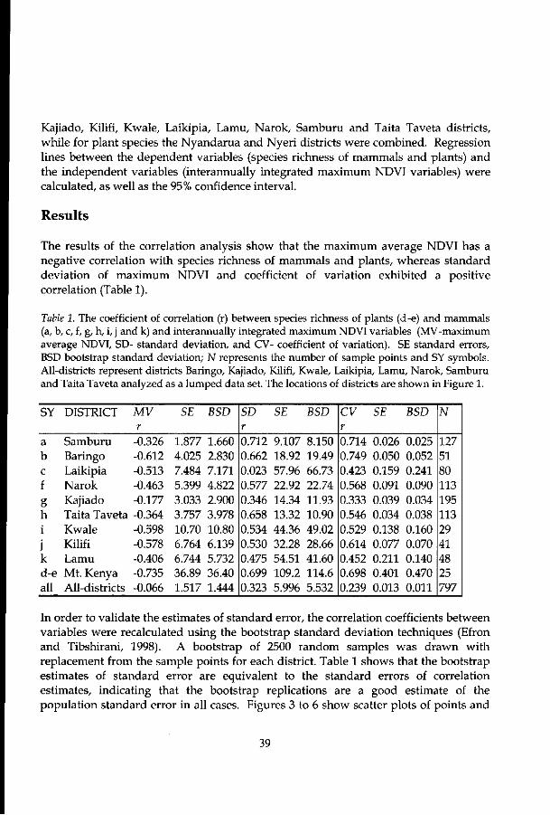
Kajiado, Kilifi, Kwale, Laikipia, Lamu, Narok, Samburu and Taita Taveta districts, while for plant species the Nyandarua and Nyeri districts were combined. Regression lines between the dependent variables (species richness of mammals and plants) and the independent variables (interannually integrated maximum NDVI variables) were calculated, as well as the 95% confidence interval.

Results

The results of the correlation analysis show that the maximum average NDVI has a negative correlation with species richness of mammals and plants, whereas standard deviation of maximum NDVI and coefficient of variation exhibited a positive correlation (Table 1).

Table 1. The coefficient of correlation (r) between species richness of plants (d-e) and mammals (a, b, c, f, g, h, i, j and k) and interannually integrated maximum NDVI variables (MV-maximum average NDVI, SD- standard deviation, and CV- coefficient of variation). SE standard errors, BSD bootstrap standard deviation; N represents the number of sample points and SY symbols. All-districts represent districts Baringo, Kajiado, Kilifi, Kwale, Laikipia, Lamu, Narok, Samburu and Taita Taveta analyzed as a lumped data set. The locations of districts are shown in Figure 1.

SY DISTRICT

a Samburu b Baringo c Laikipia f Narok g Kajiado h Taita Taveta i Kwale j Kilifi k Lamu d-e Mt. Kenya all All-districts

MV r -0.326 -0.612 -0.513 -0.463 -0.177 -0.364 -0.598 -0.578 -0.406 -0.735 -0.066

SE

1.877 4.025 7.484 5.399 3.033 3.757 10.70 6.764 6.744 36.89 1.517

BSD

1.660 2.830 7.171 4.822 2.900 3.978 10.80 6.139 5.732 36.40 1.444

SD r 0.712 0.662 0.023 0.577 0.346 0.658 0.534 0.530 0.475 0.699 0.323

SE

9.107 18.92 57.96 22.92 14.34 13.32 44.36 32.28 54.51 109.2 5.996

BSD

8.150 19.49 66.73 22.74 11.93 10.90 49.02 28.66 41.60 114.6 5.532

CV r 0.714 0.749 0.423 0.568 0.333 0.546 0.529 0.614 0.452 0.698 0.239

SE

0.026 0.050 0.159 0.091 0.039 0.034 0.138 0.077 0.211 0.401 0.013

BSD

0.025 0.052 0.241 0.090 0.034 0.038 0.160 0.070 0.140 0.470 0.011

N

127 51 80 113 195 113 29 41 48 25 797

In order to validate the estimates of standard error, the correlation coefficients between variables were recalculated using the bootstrap standard deviation techniques (Efron and Tibshirani, 1998). A bootstrap of 2500 random samples was drawn with replacement from the sample points for each district. Table 1 shows that the bootstrap estimates of standard error are equivalent to the standard errors of correlation estimates, indicating that the bootstrap replications are a good estimate of the population standard error in all cases. Figures 3 to 6 show scatter plots of points and

39

the least-squares fit for the relationships between species richness (mammals and plants) and interannually integrated maximum NDVI variables (average and coefficient of variation) for Narok, Samburu, Mt. Kenya-Aberdare area and the districts Baringo, Kajiado, Kilifi, Kwale, Laikipia, Lamu, Narok, Samburu and Taita Taveta analyzed concurrently.

Legend • Water • 0.10 0 0.20 10.30 10.40 • 0.50 • 0.00

Legend -£? • Water r D 0.02

Figure 2. Spatial distribution of interannually integrated maximum NDVI variables in Kenya 1982-1993 (a) Average NDVI image, (b) Standard deviation image.

Figure 7 shows that the numbers of species of mammals are high in areas where the maximum average NDVI is less than 0.33 and standard deviation of maximum NDVI more than 0.05. Since net primary productivity is directly related to average NDVI (Box et ah, 1989), highly productive areas seem to lower species richness of mammals. On the contrary, areas with a high standard deviation of maximum NDVI have higher mammal species richness.

Discussion

Interannually integrated maximum average NDVI and species richness In order to test the productivity hypothesis of species richness (see introduction), better information on the distribution of NPP is required over large areas. Currently, the most accessible and promising source of data on NPP is AVHRR-NDVI (Stoms and Estes, 1993). The relationship between interannually integrated maximum average NDVI and species richness was negative and moderately strong for selected individual regions (Table 1).

40

In the 1960s and 1970s, a number of examples in which species diversity was negatively correlated with productivity perplexed many ecologists (Huston, 1994). Available evidence, especially for plants, suggests that a decrease in species richness with resource enrichment is most common, or at least that a parabola (hump-shaped) curve of species richness will be found if the whole productivity range is examined (Begon et al, 1990). Our results confirmed the decrease of species richness of plants with increase of productivity (Figure 4a). However, since only one region was analyzed at a time, a parabola curve of species richness could not be realized. So, why does enhanced productivity tend to reduce plant species richness? One possible explanation is that as nutrients increase, light availability becomes more and more of a problem for competing plants (Newman, 1973); thus higher productivity is associated with increasingly intense competition for light (Huston, 1994). However, at very low levels of productivity, diversity increases with increasing productivity (Huston, 1979).

For a number of districts in Kenya, the maximum average NDVI, which is directly related to NPP (Box et al., 1989), is negatively correlated with species richness of mammals (Table 1). Figures 3, 5 and 6 provide evidence for the hypothesis that higher productivity, i.e., increasing NDVI, depresses tropical mammal species richness at a landscape scale; these results support the findings of Rosenzweig and Abramsky (1993).

10

a o o c o c o

0.15 0.25 0.35 0.45 0.55 0.65 Integrated maximum average NDVI 1982-1993

9 16 23 Coefficient of variation

(a) (b)

Figure 3. Mammal species richness versus interannual maximum NDVI variables (a) average (r2

=0.106, p<0.001) and (b) coefficient of variation (r2 = 0.600, p<0.001) in Samburu district.

41

50

40

•a 30

20

ra Q_ 10

0

ey

-

~

-

I

e a o J

i

i

\ e o

eo

i

1 e

a8eoe

oa

ok e

a8a °% oe

i

-

-

oa -

W

50

40

£ 30

I 20

ra 10-

0.0

e a

I

a o e o e

ea>o

wo

©olSesj-o

®8

i

oe .

oe

i

1 . ^

1 6.5 13.0 19.5 Coefficient of variation

26.0 0.38 0.44 0.50 0.56 0.62 Integrated maximum average NDVI 1982-1993

(a) (b) Figure 4. Plant species richness versus interannual maximum NDVI variables (a) average (r2 = 0.541, p<0.0001) and coefficient of variation (r2 = 0.487, p<0.0001) in Aberdare-Mt. Kenya region (Nyeri (e) and Nyandarua (a) districts).

As with plants, the parabola curve of diversity in relation to productivity has been reported for tropical mammals (Rosenzweig and Abramsky, 1993). However, the increase phase may be obscured in some districts due to few sample points (Figure 5), because when there are many sample points, a parabola curve may be observed (Figures 3 and 6).

18

12 -_ a a-

O jS* Sf Q

a

1^

o o

Q

0

Q

1

o o o o

o o

o

1

o o a

^ o 0 $, o

1

c o o o G

*° o s

& o

o

1

o

o o

o s o

0 s

G

Q O

t

a

a o Q

I

0

a 0

0 1

_

V °

0.36 0.42 0.48 0.54 0.60 0.66 Integrated maximum average NDVI 1992-1993

(a) (b)

10 14 Coefficient of variation

18

Figure 5. Mammal species richness and interannual maximum NDVI variables (a) average (r2 :

0.215, p<0.0001) and (b) coefficient of variation (r2 = 0.322, p<0.0001) in Narok district.

42

Furthermore, why do maximum levels of species richness of mammals occur at intermediate levels of productivity (maximum average NDVI)? One possibility is that under conditions of low primary productivity in natural ecosystems, there is not much habitat or resource heterogeneity — the landscape is uniformly barren. As productivity rises, the average variety of micronutrient combinations in fertile soils increases (Rosenzweig and Abramsky, 1993). This leads to a more diverse community of plants that can support a greater number of herbivore species (Begon et al., 1990). But go beyond a certain point on the productivity gradient and the habitat heterogeneity that support mammalian diversity declines (Rosenzweig and Abramsky, 1993). This leads to increased production of woody species, which in turn reduces the primary production of grass resources (because of shading by trees). Hence the scarcity and low quality of graminaceous resource in forest gaps result in decrease of species richness of mammals (Prins and Olff, 1998).

18

12 o o c c

} O OO r, o QC C

c o j a 0 o c

18

12

0.15 0.25 0.35 0,45 0.55 0.65

integrated maximum average NDV11982-1993

O OCOQO 5 OOOOC GOO O

OOQO Q o oa

QOOCQ CDOO ODOOO OC Q

CO QCD ooo oooog ooo

OOOOCOOTO OOQOC'O oo

oocoa iooanooooaoooooo ooooooo ooooooa

a o ocaiog.fi wsr-'ISS&oo o o a o oa o OOOGOOOOOCoooooooo

OOOOOOOGOOOQQO ODOOO

oooooatoo GO COO ODD ooo o c o o o a o c o c o o o o o o o o

OOfflOMCOOOO GO O

(a) (b) 8 16 24

Coefficient of variation

32

Figure 6. Mammal species richness versus interannual maximum NDVI variables (a) average (r2

=0.004, not significant at p<0.05) and coefficient of variation (r2 =0.057, p<0.0001) in the districts Baringo, Kajiado, Kilifi, Kwale, Laikipia, Lamu, Narok, Samburu and Taita Taveta analyzed as a lumped data set.

Standard deviation of maximum NDVI, Coefficient of variation and species richness For all the districts studied (Table 1), there was a positive correlation between species richness and the indices of habitat heterogeneity (standard deviation of maximum NDVI and coefficient of variation). This confirms that highly variable areas are endowed with more species. In addition, the positive relationships provide evidence that the standard deviation of maximum NDVI is related to variability of vegetation cover for selected individual regions. The finding is in agreement with the spatial heterogeneity hypothesis of species richness (Walker et al., 1992).

43

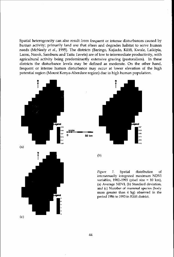
Spatial heterogeneity can also result from frequent or intense disturbances caused by human activity; primarily land use that alters and degrades habitat to serve human needs (McNeely et al., 1995). The districts (Baringo, Kajiado, Kilifi, Kwale, Laikipia, Lamu, Narok, Samburu and Taita Taveta) are of low to intermediate productivity, with agricultural activity being predominantly extensive grazing (pastoralism). In these districts the disturbance levels may be defined as moderate. On the other hand, frequent or intense human disturbance may occur at lower elevation of the high potential region (Mount Kenya-Aberdare region) due to high human population.

»« scale C X X I

50 km

(b)

Figure 7. Spatial distribution of interannually integrated maximum NDVI variables, 1982-1993 (pixel size = 10 km), (a) Average NDVI, (b) Standard deviation, and (c) Number of mammal species (body mass greater than 4 kg) observed in the period 1986 to 1993 in Kilifi district.

44

Conclusion

This study has illustrated that the multi-temporal data of vegetation reflectance can serve as a good surrogate for studying patterns of species richness. Remotely sensed images with a high temporal variation appear to model factors of resource quality and quantity associated with species richness (Diamond, 1988). The results suggest that maximum average NDVI as well as the standard deviation of maximum NDVI relate to important environmental factors that influence species richness of mammals and plants. Given the assumptions of the close relationship of maximum average NDVI to NPP, and standard deviation of maximum NDVI to heterogeneity (Podolsky, 1994), our results indicate that both the productivity and habitat heterogeneity hypotheses are important if we are to understand the potential of remotely sensed information for explaining patterns of species richness.

The patterns of plant species could be similar to mammals but comparative studies for a number of districts need to be done for a better comparison. Moreover, plant species data were collected at a few scattered sampling points, and could be biased. Nonetheless, the results for the mammal and plant species provide evidence, which support the suggestion of Stoms and Estes (1993), i.e., that multi-temporal NDVI may be used to monitor changes in productivity, and in turn could be used to model trends in species richness.

Acknowledgement

The financial support of The Netherlands government Fellowship Program through the International Institute for Aerospace Surveys and Earth Science (ITC) is highly acknowledged for the success of this research. Appreciation goes to H. Mwendwa, Director of Department Resource Surveys and Remote Sensing, Ministry of Environment, Kenya (DRSRS) for providing us with animal species data. The USAID/FEWS Project provided the AVHRR-NDVI time series images, which were accessed through the Internet.

References

ADDS, 1999, Africa Data Dissemination Service, EROS Data Center, U.S. Geological Survey Sioux Falls, South Dakota, US 57198. http://edcsnw4.cr.usgs.gov/ adds/adds.html.

Anyamba A and Eastman JR (1996) Interannual variability of NDVI over Africa and its relation to El Nino/Southern Oscillation. International Journal of Remote Sensing 17: 2533-2548

45

Asrar G (1989) Theory and Applications of Optical Remote Sensing. Wiley Series in Remote Sensing, John Wiley and Sons, New York

Begon M, Harper JL and Townsend CR (1990) Ecology. Individuals, Populations and Communities, Blackwell Scientific Publications, Oxford

Bohning-Gaese K (1997) Determinants of avian species richness at different spatial scales. Journal of Biogeography 24: 49-60

Box EO, Holben BN and Kalb V (1989) Accuracy of the AVHHRR Vegetation Index as a predictor of biomass, primary productivity and net C02 flux. Vegetatio 80: 71-89

Cihlar J, St Laurent L and Dyer JA (1991) The relation between normalized differences vegetation index and ecological variables. Remote Sensing of Environment 35: 279-298

Cody ML (1983) Continental diversity patterns and convergent evolution in bird communities. In: Kruger FJ, Mitchell DT and Jarvis JUM (eds) Mediterranean-type ecosystems: The role of nutrients, pp 357- 391. Springer-Verlag, Berlin

Cowling RM (1990) Diversity components in a species-rich area of the Cape Floristic Region. Journal of Vegetation Science 1: 699-710

Diamond J (1988) Factors controlling species diversity: Overview and synthesis. Annals of the Missouri botanical Garden 75:117-129

Efron B and Tibshirani RJ (1998) An introduction to the Bootstrap. Monographs on Statistics and Applied probability 57,Chapman and Hall/CRC, London

Griffin GF and Friedal MH (1985) Discontinuous change in central Australia: some major implications of ecological events for land management. Journal of Arid Environment 9: 63-82

Grime JP (1979) Plant strategies and vegetation processes, John Wiley and Sons, New York

Groombridge B (1992) Global Biodiversity. Status of the Earth's Living Resources, World Conservation Monitoring Centre

Hobbs RJ (1990) Remote sensing of spatial and temporal dynamics of vegetation. In: Hobbs RJ and Mooney HA (eds) Remote Sensing of Biosphere Functioning, Ecological Studies 79, pp 203-219. Springer- Verlag, New York

Holben BN (1986) Characteristics of maximum-value composite images for temporal AVHRR data. International Journal of Remote Sensing 7:1435-1445

Huston MA (1979) A general hypothesis of species diversity. American Naturalist 113: 81-101

Huston MA (1994) Biological Diversity. The coexistence of species on changing landscapes, Cambridge University Press, Cambridge

Justice C, Holben BN and Gwynne MD (1986) Monitoring East African vegetation using AVHRR data. International Journal of Remote Sensing 7:1453-1474

Kimes DS, Holben BN, Tucker CJ and Newcomb WW (1984) Optimal Directional View angles for Remote-Sensing Missions. International Journal of Remote Sensing 5:

46

887-908 Lewis JE, Rowland J, and Nadeau A (1998) Estimating maize production in Kenya

using NDVI: Some statistical considerations. International Journal of Remote Sensing 19: 2609-2617

Los SO (1998) Linkages between Global Vegetation and Climate. An analysis based on NOAA Advanced Very High Resolution Radiometer Data. GSFC/CR-1998-206852, National Aeronautics and Space Administration, Goddard Space Flight Center, Greenbelt, Maryland

Mcintyre GA (1978) Statistical aspects of vegetation sampling. In: 't Mannetje L (ed) Measurement of grassland vegetation and animal production, pp 8-21. Commonwealth Agricultural Bureax, England

McNeely JA, Gadgil M, Leveque C, Padoch C and Redford K (1995) Human influences on biodiversity. In: Heywood VH and Watson RT (eds) Global Biodiversity Assessment, pp 711- 821. Cambridge University Press, Cambridge

Newman EI (1973) Competition and diversity in herbaceous vegetation. Nature 244: 310-311

Norton-Griffiths M (1978) Counting animals. Handbook no.l. Africa Wildlife Leadership Foundation, Nairobi

Pfirman E, Hogue J and See L (1999) Windisp3.5. Map and image display system version 990217. UN Food and Agriculture Organization, US AID Famine Early Warning System, Southern Africa Development Community, US Forest Service and US Geological Survey

Pitt MD and Heady HF (1978) Responses of annual vegetation to temperature and rainfall patterns in northern California. Ecology 59: 336-350

Podolsky R (1994) Ecological Hot spots. A method for estimating biodiversity directly from digital Earth imagery. Earth Observation Magazine, June 30-36

Pratt DJ and Gwynne MD (1977) Rangeland Management and Ecology in East Africa, Hodder and Stoughton, London

Prince SD (1991) Satellite remote sensing of primary production: comparison of results for Sahelian grasslands 1981-1988. International Journal of Remote Sensing 12: 1301-1311

Prins HHT and Olff H (1998) Species-Richness of African grazer assemblages: Towards a functional explanation. In: Newbery DM, Prins HHT and Brown ND (eds) Dynamics of Tropical Communities, pp 449-490. Blackwell Science, Oxford

Richard Y and Poccard I (1998) A statistical study of NDVI sensitivity to seasonal and interannual rainfall variations in Southern Africa. International Journal of Remote Sensing 19: 2907-2920

Rosenweig ML and Abramsky Z (1993) How are diversity and productivity related? In: Ricklefs RE and Schluter D (eds) Species diversity in ecological communities. Historical and geographical perspectives, pp 52-65. University of Chicago Press,

47

Chicago Sellers PJ (1989) Vegetation-Canopy spectral reflectance and biophysical processes. In:

Asrar G (ed) Theory and Applications of Optical Remote Sensing, pp 279-335. Wiley, New York

Stoms DM and Estes JE (1993) A remote sensing research agenda for mapping and monitoring biodiversity. International Journal of Remote Sensing 14:1839-1860

Townshend JRG and Justice CO (1986) Analysis of the dynamics of African vegetation using NDVI. International Journal of Remote Sensing 7:1435-1445

Tucker CJ (1979) Red and Photographic infrared linear combinations for monitoring vegetation. Remote Sensing of the Environment 8: 681-698

Tucker CJ, Justice CO and Prince SD (1986) Monitoring the grasslands of the Sahel 1984-1985. International Journal of Remote Sensing 7:1715-1731

Tucker CJ and Sellers PJ (1986) Satellite remote sensing of primary production. International Journal of Remote Sensing 7:1133-1135

Walker RE, Stoms DM, Estes JE and Cayocca KD (1992) Relationships between biological diversity and multi-temporal vegetation index data in California. Technical Papers of the 1992 Annual Meeting of ASPRS/ACSM held in Albuquerque, New Mexico, 3-7 March 1992, pp 562-571. American Society for Photogrammetry and Remote Sensing, Bethesda,MD

Wylie BK, Harrington JA, Prince SD and Denda I (1991) Satellite and ground-based pasture production assessment in Niger: 1986-1988. International Journal of Remote Sensing 12:1281-1300

48

CHAPTER 5

PREDICTING MAMMAL SPECIES RICHNESS AND ABUNDANCE USING MULTI-TEMPORAL NDVI

Abstract

There is need to map indicators of biodiversity such as species richness and abundance of individuals in order to predict where species loss is occurring. Species richness and abundance have been hypothesized to increase with ecosystem productivity. Moreover, productivity of ecosystems varies in space and time, and this heterogeneity is also hypothesized to influence species richness and abundance of individuals. Ecosystem productivity may be estimated using remotely sensed data, and researchers have specifically proposed the Advanced Very High Resolution Radiometer-Normalized Difference Vegetation Index (AVHRR-NDVI). Interannual average NDVI and its variability (standard deviation) were correlated with large mammal species richness and abundance of individuals at a landscape scale in Kenya. The biodiversity indicators associated negatively with interannual average NDVI and positively with variability of NDVI. Understanding these relationships can help in estimating changes in mammalian species richness and abundance in response to global climate change.

Key words: abundance of individuals, AVHRR-NDVI, large mammals, mapping, productivity, species richness, temporal heterogeneity, time series analysis

49

Introduction

Biodiversity, the totality of genes, species and ecosystems in a region (Stoms and Estes, 1993), is distributed heterogeneously across the Earth. Some regions teem with more biological variation (for example, moist tropical forests and coral reefs) (Morin, 2000), others support lesser assemblages of biological species (for example, some deserts and polar regions), and most fall somewhere in between (Gaston, 2000). Patterns of species richness have been of inherent interest to biogeographers and ecologists (Brown, 1988). Hence, many studies have attempted to explain the geographical variation in the numbers of species that inhabit the Earth (Owen, 1990; Currie, 1991). Today, scientific interests in patterns of species richness are twofold. First, it reflects increased opportunity provided by improvements in available data and analytical tools (Gaston, 2000), and the use of remote sensing technology (to measure vegetation and other environmental variables) (Stoms and Estes, 1993; Gaston, 2000; Walker et ah, 1992). Second, it reflects concern over the future of biodiversity, and the resultant need to determine its current status, to predict its likely response to global environmental change (Gaston, 2000; Walker et al, 1992).

Species diversity is an emergent property that results from the interaction of the biotic and abiotic elements in the landscape. Consequently, species diversity co-varies with the biotic and abiotic factors that regulate the distribution and abundance of species (Sankaran and McNaughton, 1999). A key factor is 'ecosystem productivity' defined as the amount of energy captured and transformed into living matter per unit area (Morin, 2000). Since abundance of individuals increases with ecosystem productivity, species diversity may also increase with productivity (Diamond, 1988). However, this does not always follow logically because there could simply be lots of individuals of a few species (Legendre and Legendre, 1998). In regional biodiversity studies, productivity is usually calculated from weather station records collected at scattered (and often biased) sampling points —these points are extrapolated in order to characterize productivity over a large region (Owen, 1990; Currie, 1991). Such climate-based models assume that the vegetation cover is 'natural1, and ipso facto is under the control of climate (Box et al., 1989). However, at a landscape scale, vegetation productivity is also influenced by non-climatic factors including soil nutrient and structure, topography, disturbance and land use. In view of the fact that satellite remote sensing provides synoptic coverage with more intensive sampling, the maximum NDVI derived from satellite data should provide a more accurate index of actual or current ecosystem productivity compared with climate-based models (Box et al., 1989).

The heterogeneity of an area is strongly (positively) correlated with the number of species that are found in that particular area (Huston, 1994). Factors contributing to the

50

environmental heterogeneity are the spatial or temporal variation in the physical, chemical or biological features of the environment that create different conditions (or niches) that species can preferentially exploit (Morin, 2000). Hence, species diversity increases with niche or resource diversity because each species must occupy a distinct niche (Stoms and Estes, 1993). Since species diversity of any given group of taxa generally increases with the group's total population size (Diamond, 1988), it follows that abundance of individuals also increases with niche or resource diversity. It has been proposed that the within region variability of NDVI values, as defined by standard deviation of NDVI, may be used to estimate heterogeneity of ecosystem productivity (Walker et al, 1992).

Seasonal variations in climate are responsible for differences in plant species growth and establishment patterns, leading to changes in species composition and distributions (Hobbs, 1990). Thus, yearly variations in vegetation can take the form of changes in the spatial distribution of plant growth (Tucker et al., 1986). The interannual variation of the maximum NDVI (per month, per season) can be used to assess whether vegetation cover over the years is seasonally changing or constant. For example, calculating the standard deviation for a number of years may describe the seasonal variation of vegetation cover for an AVHRR-NDVI image pixel. Hence, image pixels with high standard deviation within a geographic area would likely contain high temporal niche differentiation (Begon et al., 1990), and should therefore have a positive relationship with species richness and number of individuals. Therefore, this paper aims to examine the relationships between interannual maximum NDVI variables (average and standard deviation) and species richness of large mammals as well as abundance of individuals in Kenya. The study was executed at landscape scale (10 * 10 km) — a scale appropriate for management decisions concerning the conservation of species diversity (Bohning-Gaese, 1997).

Methods

Study area and animal species data Kenya is situated between latitudes 5° 40' north and 4° 4' south and between longitudes 33° 50' and 41° 45' east (Figure 1). The study area encompasses five rangeland districts of Kenya with diverse landforms ranging from highland moors to savanna grasslands to coastal plains, and the analyses were carried out on individual district, as well as on the combined regional data.

The mammal species (herbivores with body weight greater than 4 kg) data collected from 1982 to 1993 were obtained from Department of Resource Surveys and Remote Sensing (DRSRS), Ministry of Environment and Natural Resources, Kenya. The aerial

51

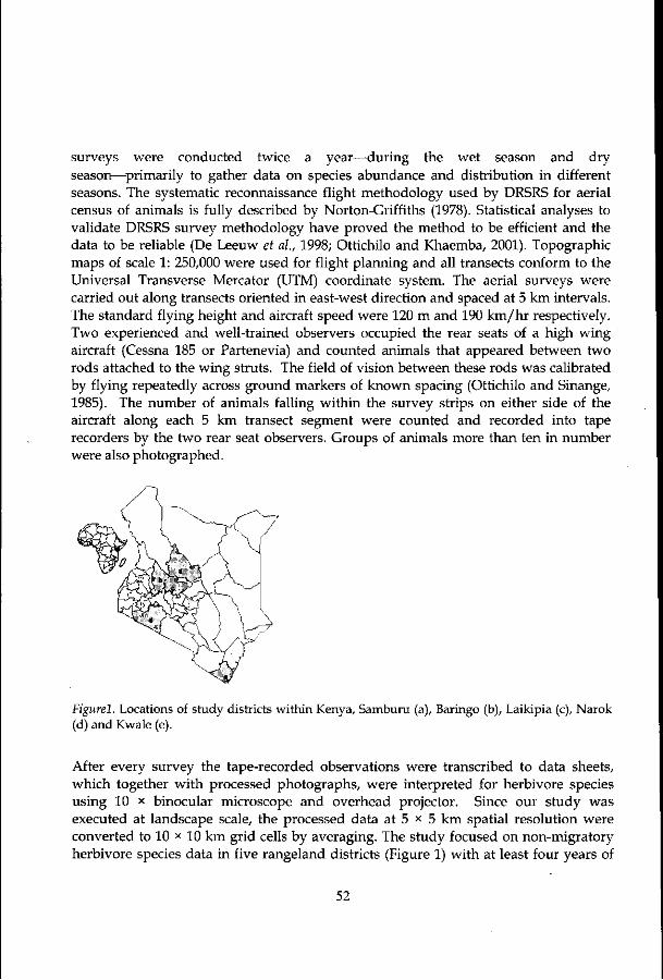
surveys were conducted twice a year—during the wet season and dry season—primarily to gather data on species abundance and distribution in different seasons. The systematic reconnaissance flight methodology used by DRSRS for aerial census of animals is fully described by Norton-Griffiths (1978). Statistical analyses to validate DRSRS survey methodology have proved the method to be efficient and the data to be reliable (De Leeuw et ah, 1998; Ottichilo and Khaemba, 2001). Topographic maps of scale 1: 250,000 were used for flight planning and all transects conform to the Universal Transverse Mercator (UTM) coordinate system. The aerial surveys were carried out along transects oriented in east-west direction and spaced at 5 km intervals. The standard flying height and aircraft speed were 120 m and 190 km/hr respectively. Two experienced and well-trained observers occupied the rear seats of a high wing aircraft (Cessna 185 or Partenevia) and counted animals that appeared between two rods attached to the wing struts. The field of vision between these rods was calibrated by flying repeatedly across ground markers of known spacing (Ottichilo and Sinange, 1985). The number of animals falling within the survey strips on either side of the aircraft along each 5 km transect segment were counted and recorded into tape recorders by the two rear seat observers. Groups of animals more than ten in number were also photographed.

Figurel. Locations of study districts within Kenya, Samburu (a), Baringo (b), Laikipia (c), Narok (d) and Kwale (e).

After every survey the tape-recorded observations were transcribed to data sheets, which together with processed photographs, were interpreted for herbivore species using 10 x binocular microscope and overhead projector. Since our study was executed at landscape scale, the processed data at 5 x 5 km spatial resolution were converted to 10 x 10 km grid cells by averaging. The study focused on non-migratory herbivore species data in five rangeland districts (Figure 1) with at least four years of

52

survey during the 11-year period (1982-1993). The number of large mammal species was counted in every grid cell (10 * 10 km) to give a value for total species richness. In addition, within each grid cell of 10 x 10 km the average number of individuals was estimated as the total number of individuals observed divided by total number of survey years.

NDVI dekads data The AVHRR-NDVI data were derived from images collected by the National Oceanic and Atmospheric Administration (NOAA) satellites, and processed by the Global Inventory Monitoring and Modeling Studies (GIMMS) at the National Aeronautics and Space Administration (NASA). A complete record for Africa exists from August 1981 until the present at 7.6 km resampled resolution (Los, 1998). NDVI is a measure derived by dividing the difference between near-infrared and red reflectance measurements by their sum (Sellers, 1989):

NDVI = (NIR- R) / (NIR + R) (1)

where NIR = near-infrared measurements and R = visible red measurements. High positive values of NDVI correspond to dense vegetation cover that is actively growing, whereas negative values are usually associated with bare soil, snow, clouds or non-vegetated surfaces. Cloud contamination and other atmospheric effects, along with some effects of sensor geometry, attenuate the value of NDVI and contribute to a greater error in the signal. To minimize the effect of cloud and atmospheric contamination, dekad (10 days) temporal composites of NDVI are developed by choosing the maximum NDVI value for each individual pixel location (Holben, 1986). Additionally, differences of bare soil reflectance may cause large NDVI variations. However, differences in soil reflectance were presumed to cause less variation of NDVI values because time series data were analyzed for the same pixel area. Moreover, since Kenya experiences a bimodal rainfall distribution with peaks in April and November, it has two growing seasons. The interannual maximum NDVI used in this study generally represents NDVI at the height of the growing seasons (Lewis et al., 1998) when vegetation cover is present and adequate across the study area.

The interannual comparisons of AVHRR-NDVI data incorporating data for more than one year is desirable because of the substantial variations from year to year that occur in the extent and timing of photosynthetic activity (Townshend and Justice, 1986). Hence, the study aims at measuring ecological variations within pixels in such a way that regions affected by occasional droughts or erratic changes in the timing and strength of rains, could be separated from those where the impact of such anomalies is slight. Since the total species richness and abundance of a region may be constrained by distinct dry or cold seasons (Fjeldsa et al., 1997), it is important to quantify the

53

anomalous events such as droughts or interannual differences in the timing and strength of rains. This was done by aggregating dekads to their appropriate months, calculating standard deviation of maximum NDVI for each month over the 11 year period, and then averaged the standard deviations for all 12 monthly NDVI values over the 11 year period (same for average NDVI). Thus, the variability over an 11-year period (1982 to 1993) of monthly NDVI values represents temporal variation of productivity.

OP: N

K. p \/\

*>> V Nrf*

• .

•y Legend D Water • 0.02 • 0.04 • 0 06 • 0.08 • 0.10

(a) (b)

Figure 2. Spatial distribution of interannual (1982-1993) maximum NDVI variables in Kenyan rangeland districts: (a) Average NDVI image, (b) Standard deviation image.

The historical image products of Kenya (ADDS, 2000) comprising 396 dekads of maximum NDVI were downloaded from website (http://edcsnw4.cr.sgs.gov/bin/ staform/a=ndvi/b=ke, 24th February 2000). These historical NDVI products are statistical summaries (i.e., average or maximum NDVI) for the historical time period (1982-1993) and hence there is no significant influence from cloud contamination. Since dekads span from the 1st to the 10th, the 11th to the 20th, and the 21st to month end, a year has 36 dekads (i.e., 3 dekads multiplied by 12 months). Hence, 396 dekads (i.e., 36 dekads multiplied by 11 years) correspond to an 11-year time period. This implies that each month over an 11-year period has 33 dekads (i.e., 3 dekads multiplied by 11 years). By using Windisp 3.5 time series data processor (Pfirman et ah, 1999), average NDVI (VIm) was computed for each of the 12 months over 11-year period as:

54

33 1

VI.. n

71 = 1

1 33

= -^Lp (2)

where p is the individual pixel values (i.e., for all 33 dekads maximum NDVI images) and n is the number of dekads. Calculating the average NDVI for all 12 monthly values produced the interannual average NDVI image (Figure 2a). The monthly standard deviation of NDVI (SDm) was also calculated for each of the 12 months over 11-year period as:

i=fci2>-v i S D m = J — : > J > - v i ) 2 (3)

where n is the number of observations (i.e., 33 dekads), xt is the observe value for pixel i and vi is the average NDVI for individual pixels. Calculating the average standard deviation for all 12 monthly NDVI values produced the standard deviation of NDVI image (Figure 2b).

The coordinates of the sample units containing species were then geometrically conformed to the same geographic coordinate system as the NDVI images. Since the spatial resolution of the species data (10 * 10 km) was different from NDVI data (7.6 x 7.6 km), the point maps representing species data were overlaid on the NDVI raster images. For every grid cell of 10 * 10 km of species data overlaid on the interannual average NDVI image (Figure 2a) and standard deviation of NDVI image (Figure 2b), the mean values of average NDVI as well as standard deviation were computed. The interannual maximum NDVI variables (viz. average NDVI and standard deviation) were extracted using lower left corner coordinates of the sample unit. Thus each sample unit finally contained four variables —NDVI variables (average and standard deviation) and biodiversity indicators (number of individuals and species richness). Regression lines between the dependent variables (biodiversity indicators) and the independent variables (NDVI variables) were calculated, as well as the 95% confidence interval.

Results

Table 1 shows that interannual average NDVI has a negative correlation with species richness, and number of individuals, whereas standard deviation of NDVI showed a positive correlation with biodiversity indicators. Plots of interannual average NDVI against species richness, and number of individuals reveal unimodal pattern (Figure

55

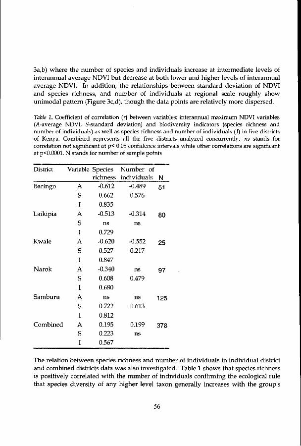
3a,b) where the number of species and individuals increase at intermediate levels of interannual average NDVI but decrease at both lower and higher levels of interannual average NDVI. In addition, the relationships between standard deviation of NDVI and species richness, and number of individuals at regional scale roughly show unimodal pattern (Figure 3c,d), though the data points are relatively more dispersed.

Table 1. Coefficient of correlation (r) between variables: interannual maximum NDVI variables (A-average NDVI, S-standard deviation) and biodiversity indicators (species richness and number of individuals) as well as species richness and number of individuals (J) in five districts of Kenya. Combined represents all the five districts analyzed concurrently, ns stands for correlation not significant at p< 0.05 confidence intervals while other correlations are significant at p<0.0001. N stands for number of sample points

District

Baringo

Laikipia

Kwale

Narok

Samburu

Combined

Variable

A S I A

S I A

S I A

S I

A

S I A S I

Species richness

-0.612 0.662 0.835

-0.513

ns 0.729 -0.620 0.527 0.847

-0.340 0.608 0.680

ns

0.722 0.812

0.195 0.223 0.567

Number of individuals

-0.489

0.576

-0.314

ns

-0.552 0.217

ns

0.479

ns

0.613

0.199 ns

N

51

80

25

97

125

378

The relation between species richness and number of individuals in individual district and combined districts data was also investigated. Table 1 shows that species richness is positively correlated with the number of individuals confirming the ecological rule that species diversity of any higher level taxon generally increases with the group's

56

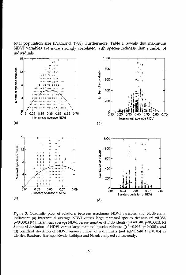
total populat ion size (Diamond, 1988). Furthermore, Table 1 reveals that max imum NDVI variables are more strongly correlated wi th species richness than number of individuals.

1000r

2 12 -

_

-

I

GO

O GO

C GO

O C/O

OCT OO

pc oo /OO 0 0

I

I

o

o

o

/So

GO

o o

o o

oo I

o

o o

o o

o o

o o

o o

o o

0 0

I

o

0

o o

o o

" o o "

o

OGL

o o

oo

o o I

y o

OO

o o

o

CO

o o

CO

o o

CO

o

o o

o o

GO

o o

I

o

0

o

oo

a

oo

o

o

o

I

i

oo.

o \

o o \

o o \

o o o \

to

0)

£ 3

z

Ql_£ 1 1 1 1 1 i_J

0.15 0.25 0.35 0.45 0.55 0.65 0.75 Interannual average NDVI

800

600 -

400

200

(a)

0.15 0.25 0.35 0.45 0.55 0.65 0.75 Interannual average NDVI

(b)

(c)

0.01 0,03 0.05 0.07 Standard deviation of NDVI

0.09

1000

800

600

400

200

0.01 0.03 0.05 0.07 Standard deviation of NDVI

0,09

(d)

Figure 3. Quadratic plots of relations between maximum NDVI variables and biodiversity indicators: (a) Interannual average NDVI versus large mammal species richness (r2 =0.038, p<0.0001) (b) Interannual average NDVI versus number of individuals ((r2 =0.040, p<0.0001), (c) Standard deviation of NDVI versus large mammal species richness ((r2 =0.052, p<0.0001), and (d) Standard deviation of NDVI versus number of individuals (not significant at p<0.05) in districts Samburu, Baringo, Kwale, Laikipia and Narok analyzed concurrently.

57

Presumably, in assemblages of biological species, there are generally several species represented by a few individuals, and a few species that are very abundant (Legendre and Legendre, 1998). This could have contributed to the dispersion of data points that most likely reduced the strength of association between number of individuals and NDVI variables (Figure 3b and d). The three dimensional plots (Figure 4a, b) demonstrate that at regional scale species richness and number of individuals are higher at intermediate levels of interannual average NDVI and standard deviation of NDVI. The species richness and number of individuals are high in regions where interannual average NDVI is less than 0.55 and the standard deviation of NDVI is more than 0.03 (Figure 3a,b, c, d). While in Kwale district, Figure 5 illustrates that species richness and abundance of individuals are higher in areas where interannual average NDVI is less than 0.40 and the standard deviation of NDVI is more than 0.03.

Discussion

The species diversity of natural communities is hypothesized to either increase or decrease monotonically with ecosystem productivity or to be unimodally related to productivity, with maximum diversity occurring at intermediate levels of productivity (Tilman, 1982; Rosenzweig and Abramsky, 1993). Plots of interannual average NDVI, which is an index of ecosystem productivity, against species richness, and number of individuals (Figure 3a, b) demonstrate unimodal relationship. The species richness and number of individuals are highest at the intermediate levels of interannual maximum average NDVI. Apparently, intermediate levels of average NDVI coincide with environments with intermediate levels of productivity (Box et ah, 1989) that support high production of grass resources. In turn, this enables more individual organisms to coexist, and thus more species at abundances that make it possible for them to maintain viable populations, that over time allows an increase in species richness and number of individuals (Gaston, 2000).

Moreover, at intermediate levels of productivity, predators (carnivores) can maintain diversity among prey by reducing interspecific competition (Morin, 2000). This mechanism breaks down in low- and high- productivity environments, where predators are respectively too infrequent to thin their prey or so numerous that only the best defended prey persist (Morin, 2000). Furthermore, natural ecosystems with low productivity environments lack niche or resource diversity to allow various species to coexist (Stoms and Estes, 1993), encouraging species adapted to the more productive niche to dominate the community, thereby decreasing overall species diversity (Kassen et al., 2000) and hence abundance of individuals. In higher productivity areas, resource diversity declines due to increased production of woody

58

species, which in turn reduces the primary production of grass resources (because of shading by trees) (Prins and Olff, 1998). Consequently, the reduced variety of resources results in more individuals per few species (Begon et ah, 1990) rather than more herbivore species.

Figure 4. Three dimensional relationships among variables in the districts (Baringo, Kwale, Laikipia, Narok and Samburu) analysed as lumped data set: Interannual average NDVI (INDVI) versus standard deviation of NDVI versus (a) large mammal species richness, and (b) number of individuals.

Although the unimodal patterns suggest that productivity is a primary factor determining species richness and number of individuals, productivity could simply be correlated with factors that actually generate diversity. One such factor may be temporal variation of productivity (Morin, 2000), in this case estimated from the standard deviation of NDVI. Presumably, variability in maximum NDVI represents seasonally changing environment where different species may be suited to conditions at different times of the year. Hence, more numbers of species and individuals might be expected to coexist in a seasonal environment than in a completely constant one (Begon et al, 1990).

Some investigators suggested that, when the entire range of productivity is considered, species richness is highest at intermediate levels. Tilman (1982) proposed an asymmetrical hump-shaped (unimodal) model of the number of plant species that can

59

coexist competitively on a limited resource base. Abramsky and Rosenzweig (1984), using rainfall as an index of productivity, was consistent with Tilman's (1982) model for the relationship between species richness of rodents and productivity in the Isreali arid lands. They showed that species richness of rodents reached a peak at moderately low productivity then declined as resources continued to increase. Tilman's (1982) model offers a way to reconcile the conflicting findings reported in the literature on the relationship between productivity and species richness. Both positive and negative responses of richness to productivity may be expected among different ranges, perhaps taxon specific, of productivity values (Owen, 1990).

Legend Legend

(a) (b)

Legend Legend

ffijCj

(c) (d)

Figure 5. Maps of Kwale district at spatial resolution of 10 x 10 km showing the distribution of (a) number of large mammal species, (b) average number of individuals, (c) interannual average NDVI and (d) standard deviation of NDVI in the period 1982 to 1993.

If the hump-shaped model of Tilman (1982) is general in scope, then the differing relationship between richness and productivity reported in the literature may reflect

60

only sampling from different slopes of a fundamental richness-productivity function (Owen, 1990). In the present study where the range of interannual average NDVI (productivity) represented is 0.20 to 0.63, the response of large mammal species richness and abundance to ecosystem productivity is at least consistent with the predictions of Tilman's (1982) model.

Conclusion

This study has provided an assessment of multi-temporal reflectance data for the purpose of predicting large mammal species richness and abundance of individuals. The results demonstrate that AVHRR-NDVI data can provide temporal quantitative information on vegetation reflectance that can be used to estimate relevant environmental factors influencing patterns of species richness and abundance of individuals. However, the predictive power of NDVI variables was relatively weak—with a few exceptions (Table 1). In addition, only a relatively small number of mammals were studied. It is believed that using finer pixel resolution imagery and increasing sample size of the number of species studied may improve the accuracy of the results. In the future, as finer pixel resolution satellite images become available at a frequency similar to NOAA AVHRR imagery, the mix of surface types in each pixel will be reduced (Box et al., 1989), thereby increasing the accuracy of results at the landscape level. Until then, AVHRR-NDVI data remain the most useful imagery available for monitoring vegetation (Tucker and Sellers, 1986) and predicting mammal species richness as well as abundance of individuals at a landscape scale in Kenya.

Acknowledgement

The financial support of The Netherlands government Fellowship Program through the International Institute for Aerospace Surveys and Earth Science (ITC) is highly acknowledged for the success of this research. Appreciation goes to H. Mwendwa, Director of Department Resource Surveys and Remote Sensing, Ministry of Environment, Kenya (DRSRS) for providing us with animal species data. The USAID/FEWS Project provided the AVHRR-NDVI time series images, which were accessed through the Internet.

References

Abramsky Z and Rosenzweig ML (1984) Tilman's predicted productivity-diversity relationship shown by desert rodents. Nature 309:150-151

ADDS (2000) Africa Data Dissemination Service, EROS Data Center, U.S. Geological Survey Sioux Falls, South Dakota, US 57198. http://edcsnw4.cr.usgs.gov/

61

adds/adds.html. Begon M, Harper JL and Townsend CR (1990) Ecology: Individuals, populations and

Communities, Blackwell Scientific Publications, Cambridge Bohning-Gaese K (1997) Determinants of avian species richness at different spatial

scales. Journal of Biogeography 24: 49-60 Box EO, Holben BN and Kalb V (1989) Accuracy of the AVHRR Vegetation Index as a

predictor of biomass, primary productivity and net CO2 flux. Vegetatio 80: 71-89 Brown JH (1988) Species Diversity. In: Myers AA and Giller PS (eds) Analytical

Biogeography. An integrated approach to the study of animal and plant distributions, pp 57-89. Chapman & Hall, London

De Leeuw J, Prins HHT, Njuguna EC, Said MY and De By R (1998) Interpretation of DRSRS animal counts (1977-1997) in the rangeland districts of Kenya. Ministry of Planning and National Development, Nairobi, Kenya

Currie DJ (1991) Energy and large-scale patterns of animal and plant species richness. American Naturalist 137: 27-49

Diamond J (1988) Factors controlling species diversity: Overview and synthesis. Annals of the Missouri Botanical Garden 75:117-129

Fjeldsa J, Ehrlich D and Lambin E (1997) Are biodiversity 'hotspots' correlated with current ecoclimatic stability? A pilot study using the NO AA-AVHRR remote sensing data. Biodiversity and Conservation 6: 401-422

Gaston KJ (2000) Global patterns in biodiversity. Nature 405: 220-227 Hobbs RJ (1990) Remote sensing of spatial and temporal dynamics of vegetation. In:

Hobbs RJ and Mooney HA (eds) Remote Sensing of Biosphere Functioning, Ecological Studies 79, pp 203-219. Springer- Verlag, New York

Holben BN (1986) Characteristics of maximum-value composite images for temporal AVHRR data. International Journal of Remote Sensing 7:1417-1434

Huston MA (1994) Biological Diversity. The coexistence of species on changing landscapes, Cambridge University Press, Cambridge

Kassen R, Buckling, A, Bell G and Rainey PB (2000) Diversity peaks at intermediate productivity in a laboratory microcosm. Nature 406: 508-512

Legendre P and Legendre L (1998) Numerical Ecology, Elsevier Science BV, Amsterdam

Lewis JE, Rowland J and Nadeau A (1998) Estimating maize production in Kenya using NDVI: Some statistical considerations. International Journal of Remote Sensing 19: 2609-2617

Los SO (1998) Linkages between Global Vegetation and Climate. An analysis based on NO AA-AVHRR data. GSFC/CR-1998-206852, National Aeronautics and Space Administration, Goddard Space Flight Center, Greenbelt, Maryland

Morin PJ (2000) Biodiversity's ups and downs. Nature 406: 463- 464 Norton-Griffiths M (1978) Counting animals, Handbook no.l, Africa Wildlife

62

Leadership Foundation, Nairobi Ottichilo WK and Khaemba W (2001) Validation of observer and aircraft calibration for

aerial animal surveys: A case study of the Department of Resource Surveys and Remote Sensing (DRSRS), Kenya. African Journal of Ecology 39: 45-50

Ottichilo WK and Sinange RK (1985) Differences in the visual and photographic measurements in the estimation of strip widths for aerial censuses of animal populations. DRSRS, Ministry of Planning and National Development, Nairobi

Owen JG (1990) Patterns of mammalian species richness in relation to temperature, productivity and variance in elevation. Journal of Mammalogy 71:1-13

Pfirman E, Hogue J and See L (1999) Windisp 3.5. Map and image display system version 990217. UN Food and Agriculture Organization, US AID Famine Early Warning System, Southern Africa Development Community, US Forest Service and US Geological Survey

Prins HHT and Olff H (1998) Species-richness of African grazer assemblages: Towards a functional explanation. In: Newbery DM, Prins HHT and Brown ND (eds) Dynamics of Tropical Communities, pp 449-490. Blackwell Science, Oxford

Rosenzweig ML and Abramsky Z (1993) How are diversity and productivity related? In: Ricklefs RE and Schluter D (eds) Species diversity in ecological communities. Historical and geographical perspectives, pp 52-65. University of Chicago Press, Chicago

Sankaran M and McNaughton SJ (1999) Determinants of biodiversity regulate compositional stability of communities. Nature 401: 691-693

Sellers PJ (1989) Vegetation-Canopy spectral reflectance and biophysical processes. In: Asrar G (ed) Theory and Applications of Optical Remote Sensing, pp 279-335. John Wiley & Sons, New York

Stoms DM and Estes JE (1993) A remote sensing research agenda for mapping and monitoring biodiversity. International Journal of Remote Sensing 14:1839-1860

Tilman D (1982) Resource competition and community structure, Princeton University Press, Princeton, New Jersey

Townshend JRG and Justice CO (1986) Analysis of the dynamics of African vegetation using NDVI. International Journal of Remote Sensing 7:1435-1445

Tucker CJ, Justice CO and Prince SD (1986) Monitoring the grasslands of the Sahel 1984-1985. International Journal of Remote Sensing 7:1715-1731

Tucker CJ and Sellers PJ (1986) Satellite remote sensing of primary production. International Journal of Remote Sensing 7:1133-1135

Walker RE, Stoms DM, Estes JE and Cayocca KD (1992) Relationships between biological diversity and multi-temporal vegetation index data in California. Technical Papers of the 1992 Annual Meeting of ASPRS/ACSM held in Albuquerque, New Mexico, 3-7 March 1992, pp 562-571. American Society for Photogrammetry and Remote Sensing, Bethesda

63

CHAPTER 6

MAPPING HABITAT AND BIOLOGICAL DIVERSITY IN THE MAASAI MARA ECOSYSTEM, KENYA

Abstract

There is need to identify ecosystems that support richer assemblages of biological species in order to preserve habitats and protect the greatest number of species. Remotely sensed data hold tremendous potential for mapping species habitats and indicators of biological diversity, such as species richness. Landscape level habitat analysis using remotely sensed data and Geographical Information Systems (GIS) has the potential to aid in explaining species richness patterns at fine-scale resolutions. We used Landsat Thematic Mapper (TM) image and GIS as well as field data to classify habitat types in the Masai Mara ecosystem, Kenya. The accuracy of the resulting habitat map was assessed and indices of habitat diversity computed. We then determined the relationship between large mammal species richness and habitat diversity indices, and investigated whether this relationship is sensitive to changes in spatial scale (extent and grain size). Statistical analyses show that species richness is positively correlated with habitat diversity indices and changes of scale in calculations of habitat diversity indices influenced the strength of the correlation. The results demonstrate that mammalian diversity can be predicted from habitat diversity derived from satellite remotely sensed data.

Key words: large mammals, mapping, habitats, diversity, remote sensing, scale, species richness

64

Introduction

Biodiversity is commonly used to describe the number, variety and variability of living organisms. As the living world is mostly considered in terms of species, the number of species in a site or habitat (species richness) is commonly used as an indicator of biodiversity (Groombridge, 1992). The general perception of conservation biologists and ecologists is that, all things being equal, diverse ecosystems are more important to preserve than low diversity systems (Podolsky, 1994). The reason for this is that diverse ecosystems support richer assemblages of biological species than do simple ones (Diamond, 1988; Podolsky, 1994). However, it must be pointed out that many low diversity ecosystems support rare or endangered species whose protection is also critical (Podolsky et al, 1992).

Mapping species richness and distributions is an important aspect of conservation and land use planning (Spellerberg, 1991; Miller and Allen, 1994). For example, maps can help identify areas of special biodiversity importance where conservation resources should be focused. Such areas include 'hot spots' of high species richness as well as places where species assemblages of particular interest occur (Cardillo et al., 1999). As the current rate of species extinction causes increasing concern (Wilson, 1988), land managers and biologists have sought to identify habitats important to the preservation of species diversity (Debinski et al., 1999). To identify and conserve areas with high biological importance, remote sensing technology can provide information concerning many variables useful for inventorying, modeling and monitoring species richness (Stoms and Estes, 1993). Coupled with GIS, remote sensing can provide information about landscape history, topography, soil, rainfall, temperature and other climatic conditions, as well as about present day habitat and soil coverage—factors on which the distribution of species depend (Noss, 1996). Relationships between species distribution patterns and remotely sensed/GIS data, if known, can be used to predict the distribution of single species or sets of species over large areas (Debinski and Humphrey, 1997). However, the utility of remotely sensed data to biological preservation is a function of the extent to which these data correlate with various biological resources (Podolsky et al., 1992).

Spatial heterogeneity is one of the most popular hypotheses used to explain patterns of species richness. The heterogeneity hypothesis states that diverse ecosystems support richer assemblages of biological species than simple ecosystems (Diamond, 1988). Researchers have examined the spatial configuration of habitat variables to predict species richness (Stoms and Estes, 1993). Measures of spatial patterning include a diversity index from information theory based on number and proportions of

65

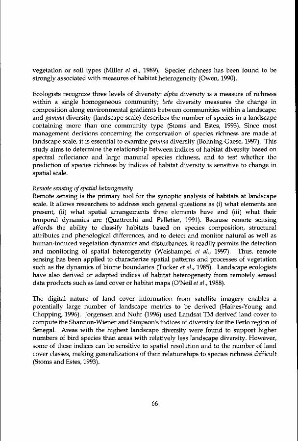
vegetation or soil types (Miller et al., 1989). Species richness has been found to be strongly associated with measures of habitat heterogeneity (Owen, 1990).

Ecologists recognize three levels of diversity: alpha diversity is a measure of richness within a single homogeneous community; beta diversity measures the change in composition along environmental gradients between communities within a landscape; and gamma diversity (landscape scale) describes the number of species in a landscape containing more than one community type (Stoms and Estes, 1993). Since most management decisions concerning the conservation of species richness are made at landscape scale, it is essential to examine gamma diversity (Bohning-Gaese, 1997). This study aims to determine the relationship between indices of habitat diversity based on spectral reflectance and large mammal species richness, and to test whether the prediction of species richness by indices of habitat diversity is sensitive to change in spatial scale.

Remote sensing of spatial heterogeneity Remote sensing is the primary tool for the synoptic analysis of habitats at landscape scale. It allows researchers to address such general questions as (i) what elements are present, (ii) what spatial arrangements these elements have and (iii) what their temporal dynamics are (Quattrochi and Pelletier, 1991). Because remote sensing affords the ability to classify habitats based on species composition, structural attributes and phenological differences, and to detect and monitor natural as well as human-induced vegetation dynamics and disturbances, it readily permits the detection and monitoring of spatial heterogeneity (Weishampel et al., 1997). Thus, remote sensing has been applied to characterize spatial patterns and processes of vegetation such as the dynamics of biome boundaries (Tucker et al., 1985). Landscape ecologists have also derived or adapted indices of habitat heterogeneity from remotely sensed data products such as land cover or habitat maps (O'Neil et al., 1988).

The digital nature of land cover information from satellite imagery enables a potentially large number of landscape metrics to be derived (Haines-Young and Chopping, 1996). Jorgensen and Nohr (1996) used Landsat TM derived land cover to compute the Shannon-Wiener and Simpson's indices of diversity for the Ferlo region of Senegal. Areas with the highest landscape diversity were found to support higher numbers of bird species than areas with relatively less landscape diversity. However, some of these indices can be sensitive to spatial resolution and to the number of land cover classes, making generalizations of their relationships to species richness difficult (Stoms and Estes, 1993).

66

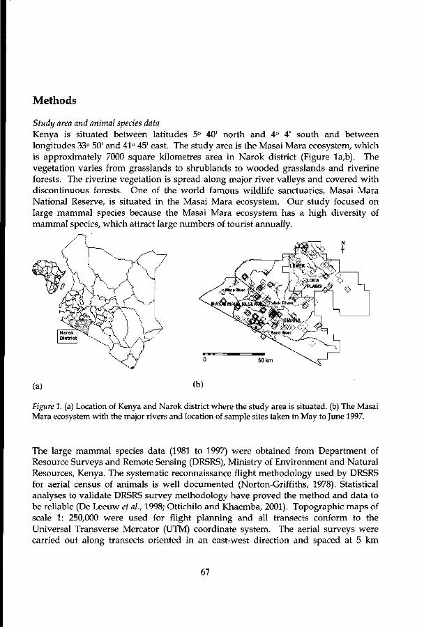
Methods

Study area and animal species data Kenya is situated between latitudes 5° 40' north and 4° 4' south and between longitudes 33° 50' and 41° 45' east. The study area is the Masai Mara ecosystem, which is approximately 7000 square kilometres area in Narok district (Figure la,b). The vegetation varies from grasslands to shrublands to wooded grasslands and riverine forests. The riverine vegetation is spread along major river valleys and covered with discontinuous forests. One of the world famous wildlife sanctuaries, Masai Mara National Reserve, is situated in the Masai Mara ecosystem. Our study focused on large mammal species because the Masai Mara ecosystem has a high diversity of mammal species, which attract large numbers of tourist annually.

(a) (b)

Figure 1. (a) Location of Kenya and Narok district where the study area is situated, (b) The Masai Mara ecosystem with the major rivers and location of sample sites taken in May to June 1997.

The large mammal species data (1981 to 1997) were obtained from Department of Resource Surveys and Remote Sensing (DRSRS), Ministry of Environment and Natural Resources, Kenya. The systematic reconnaissance flight methodology used by DRSRS for aerial census of animals is well documented (Norton-Griffiths, 1978). Statistical analyses to validate DRSRS survey methodology have proved the method and data to be reliable (De Leeuw et ah, 1998; Ottichilo and Khaemba, 2001). Topographic maps of scale 1: 250,000 were used for flight planning and all transects conform to the Universal Transverse Mercator (UTM) coordinate system. The aerial surveys were carried out along transects oriented in an east-west direction and spaced at 5 km

67

intervals. The standard flying height and aircraft speed were 120 m and 190 km/hr respectively. Two experienced and well-trained observers occupied the rear seats of a high wing aircraft (Cessna 185 or Partenevia) and counted animals that appeared between two rods attached to the wing struts. The field of vision between these rods was calibrated by flying repeatedly across ground markers of known spacing (Ottichilo and Sinange, 1985). The number of animals falling within the survey strips on either side of the aircraft along each 5 km transect segment were counted and recorded into tape recorders by the two rear seat observers. Groups of animals more than ten in number were also photographed. After every survey the tape-recorded observations were transcribed to data sheets, which together with processed photographs, were interpreted for animal species using 10 x binocular microscope and overhead projector. Since we carried out the study also at other spatial scales, the processed data at 5 * 5 km quadrats were converted to 10 * 10 km, 15 * 15 km, 20 x 20 km, 25 x 25 km and 30 * 30 km quadrats by spatial aggregation. The analyses focused on large mammal species that are non-migratory. Hence, animal species that were consistently observed over 17 years period were presumed to be resident to the study area.

GIS and remote sensing analysis The methodology for this study was directed toward producing a map of spectrally distinct habitat types as a basis for measuring habitat diversity of the study. Since the study focused on non-migratory large mammal species richness, single date imagery was considered appropriate for measuring habitat diversity. The Landsat 5 TM image (pixel size = 30 m) of the study area for 2nd January 1995 was georeferenced to plus or minus 0.5 pixel (15m) accuracy and resampled to a UTM coordinate system to match topographic maps of the region. A colour composite image was created to serve as a background image during sampling and subsequent supervised classification. The combination of bands 4, 3 and 2 (red: near infrared band 4, green: red visible band 3, and blue: green visible band 2) at ratio 1:1:1 was the best that allowed the identification of different habitat types in the study area.

An Iterative Self-Organizing Data Analysis (ISODATA) clustering algorithm was applied to the three-band image file to identify spectrally similar pixels. The ISODATA algorithm operates by initially seeding a specified number of cluster centroids in spectral feature space. The euclidean distance between each pixel and each cluster centroid is calculated, and the pixel assigned to a cluster centroid (class). The process of pixel evaluation-centroid recomputation continues iteratively until a threshold percentage (typically 95%) of pixels no longer change cluster centroid assignment. Ten initial clusters were specified for the ISODATA clustering, producing a map of ten classes, which enabled us to discriminate habitat types present in the study area.

68

Field vegetation mapping The field vegetation mapping was carried out from mid-May to mid-June 1997 at the height of growing season when the vegetation cover was present and adequate. This enabled us to get a good discrimination of the vegetation structure especially herbaceous layer in order to prepare a classification scheme that is hierarchical in nature (Table 1). A clustered random sampling design (Mclntyre, 1978) was used to collect data in the field. Computer generated cluster points randomly as well as six secondary sample sites, each within a distance of a kilometer from the main cluster. Sample sites were located in the field using Global Positioning System, topographic map (scale: 1: 250,000) and the Landsat TM 1995 image. Once the sample site was located (Figure lb), a quadrat of 20 m by 50 m was established, the height (in metres) and the total cover percentage of each habitat type was visually estimated.

Table 1. Criteria used to classify habitat types from the field data

Habitat type Cultivated/fallow/ bare land Dwarf shrubs/ short grassland Forest Tall grassland Shrubland Woody/ shrubby grassland

Sample size 22 103 4 39 16 38

Woody species -

15-50% (< 0.5 m) >50% (>6 m) <15% >50% (>0.5-4 m) 15-50% ((>0.5-<6m)

Non-woody species wheat farms/fallow >50% (< 0.25 m) <15% >50% (>0.25 m) <15% >50%

Since multiple layering of vegetation will often result in total cover values of well over 100 per cent, Braun-Blanquet scale was used where the range 0-100 per cent was partitioned into five classes (Kent and Coker, 1992). The field data were further processed in a spreadsheet and habitat types were categorized into six distinct classes, cultivated/ fallow/ bare land, dwarf shrubs/ short grassland, forest, tall grassland, shrubland and woody/shrubby grassland (Table 1). The field data were divided into training and testing samples (Table 2).

Supervised classification and accuracy assessment Representative or prototype pixels from each of the habitat type were chosen which form training data. The training pixels for each habitat type lied in a training field, 3 x 3 window (9 pixels). The training data estimated the parameters of the classifier algorithm to be used—these parameters are the properties of the probability model used or equations that define partitions in the multispectral space.

69

Table 2. Sample sizes for each habitat type used for training classifier and testing the accuracy of the supervised classification

Habitat type Cultivated/ fallow/ bare land Dwarf shrubs/ short grassland Forest Tall grassland Shrubland Woody/shrubby grassland

Training 9 50 2 18 7 18

Testing 13 53 2 21 9

20

Using the trained maximum likelihood classifier, every pixel in the image was classified into one of the desired habitat types. A majority filter was applied on the classified image to smooth classification results. An accuracy assessment was then performed on filtered habitat map (Figure 5). Test samples were selected from every cluster sampled in the field for each habitat type class (Table 2). They were carefully located on the habitat map using the UTM coordinates and since each test sample lies in the center of 3 x 3 window, the latter was considered to be a homogeneous test area representing a single habitat type class. Therefore, every classified pixel in the window was checked for correctness by comparing image class and the field habitat type class in the reference data. From the field checked data an error matrix table was constructed (Table 5).

Calculation of the TM-based habitat diversity index and species richness The large mammal species richness and habitat diversity index were estimated in six quadrats of different sizes, 5><5 km, 10 x 10 km, 15 x 15 km, 20 * 20 km, 25 x 25 km and 30 * 30 km. The size of the smallest quadrat ( 5 x 5 km) was determined by the aerial sampling method used by DRSRS and described in the previous section. In each quadrat the number of species was counted to give a value for total species richness. Prior to calculation of habitat diversity indices for these six quadrats, two point maps were created for each quadrat. The two point maps were then rasterized to two different pixel sizes (25 m and 75 m) with appropriate point sizes (Table 3). For example, point size 200 means that each sample unit in a point map will be represented by 200 x 200 pixels in the output raster map. Thus, all 40,000 pixels had the same identity as the sample unit.

70

Table 3. The quadrat sizes (km) with corresponding distance (m) between quadrats, point sizes and total number of pixels for pixel sizes 25 m and 75 m in a quadrat

Quadrat

5x5 10x 10 15x15 20x20 25 x25 30x30

Distance

5000

10000

15000

20000

25000

30000

Point

25 m

200 400 600 800 1000

1200

size

75 m

67 133 200 267 333 400

Total pixels

25 m 75 m

40000 4489

160000 17689

360000 40000

640000 71289

1000000 110889

1440000 160000

Integrating habitat map (pixel size = 30 m) and quadrat raster maps (pixel size = 25 m or 75 m) requires compatible pixel sizes. By using Nearest Neighbour resampling method, the habitat map was resampled twice to pixel sizes of 25 m and 75 m and then crossed with each of the six quadrat raster maps of 25 m and 75 m pixel sizes respectively. Table 4 shows an example of the resulting output table for an individual sample unit.

The habitat diversity was calculated for every sample unit based on habitat map of fine spatial scale (pixel size = 25 m) and relatively coarse spatial scale (pixel size = 75 m). The two commonly used diversity indices for quantifying landscape structure (Haines-Young and Chopping, 1996); Shannon-Wiener index (H1) and Simpson's index (D) were employed:

H' = - Spi In pi

D = 1/ IP i2

(1)

(2)

where p, represents the fractional abundance of each habitat type in a quadrat (i.e. number of pixels of specific habitat type ;' divided by total number of pixels in a quadrat).

Shannon-Wiener index is based on information theory that tries to measure the amount of uncertainty (Krebs, 1989) in every quadrat. Thus, measuring the amount of uncertainty in a quadrat can provide a measure of diversity. Hence, a quadrat with only one habitat type has no uncertainty (no diversity) in it, H'= 0, so the larger the value of H', the greater the uncertainty (diversity). Whereas Simpson's index is based on the probability that two habitat types are similar (Simpson, 1949).

71

Table 4. Cross table resulting from crossing a quadrat (15 x 15 km) raster map and habitat map of pixel size 25 m for a single sample unit. The number of pixels was used to compute habitat diversity using Shannon-Wiener and Simpson's indices

Sample unit 60095 60095 60095 60095 60095 60095 Total

Habitat type Woody/shrubby grassland Forest Dwarf shrubs/ short grassland Tall grassland Shrubland Cultivated/ fallow/ bare lands

No. of pixels 212125 18860 69191 53095 2872 3857

360000

Regression lines between the dependent variables (species richness) and the independent variables (Shannon and Simpson's habitat diversity indices) were calculated along with 95% confidence interval for different quadrat sizes. The correlation coefficients for the relations between large mammal species richness and habitat diversity indices calculated at two different pixel sizes were compared at different quadrat sizes. In addition, the relationship between the number of classes in the image classification and habitat diversity indices was calculated.

Results

Table 5 shows the error matrix resulting from classifying training set pixels and testing the accuracy. The overall accuracy is computed by dividing the total correct sum of the major diagonal by the total number of pixels in the error matrix (Jensen, 1996). The producer accuracy indicates the probability of a reference pixel being correctly classified and it is calculated by dividing diagonal value for each category by its column total. Conversely, user accuracy is the probability that a pixel classified on the map actually represents that category on the ground and it is calculated by dividing diagonal value for each category by its row total (Story and Congalton, 1986).

KAPPA analysis is a discrete multivariate technique of use in accuracy assessment (Congalton and Mead, 1983). It yields a KHAT statistic (an estimate of KAPPA) that is a measure of agreement between image data and the reference data or accuracy (Congalton, 1991). The KHAT statistic is computed as:

' r r

Khat = N £ xu - £ ( * „ • x x,) )/NP- £ ( x , x xc) (3)

72

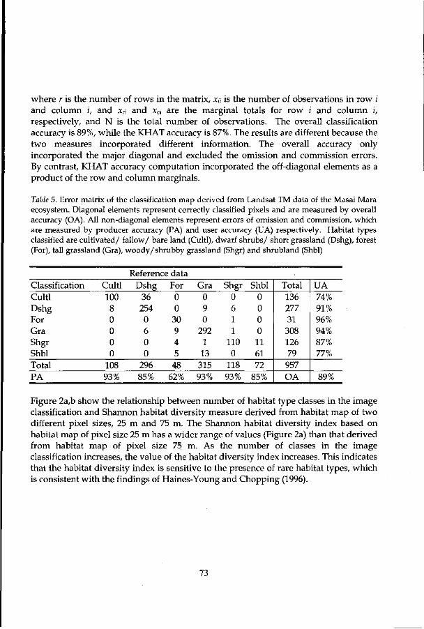
where r is the number of rows in the matrix, x„ is the number of observations in row i and column ;, and XH and xCi are the marginal totals for row ;' and column i, respectively, and N is the total number of observations. The overall classification accuracy is 89%, while the KHAT accuracy is 87%. The results are different because the two measures incorporated different information. The overall accuracy only incorporated the major diagonal and excluded the omission and commission errors. By contrast, KHAT accuracy computation incorporated the off-diagonal elements as a product of the row and column marginals.

Table 5. Error matrix of the classification map derived from Landsat TM data of the Masai Mara ecosystem. Diagonal elements represent correctly classified pixels and are measured by overall accuracy (OA). All non-diagonal elements represent errors of omission and commission, which are measured by producer accuracy (PA) and user accuracy (UA) respectively. Habitat types classified are cultivated/ fallow/ bare land (Cultl), dwarf shrubs/ short grassland (Dshg), forest (For), tall grassland (Gra), woody/shrubby grassland (Shgr) and shrubland (Shbl)

Classification Cultl Dshg For Gra Shgr Shbl Total PA

Cultl 100 8 0 0 0 0

108 93%

Reference data Dshg

36 254 0 6 0 0

296 85%

For 0 0

30 9 4 5 48

62%

Gra 0 9 0

292 1 13 315 93%

Shgr 0 6 1 1

110 0

118 93%

Shbl 0 0 0 0 11 61 72

85%

Total 136 277 31 308 126 79 957 OA

UA 74% 91% 96% 94% 87% 77%

89%

Figure 2a,b show the relationship between number of habitat type classes in the image classification and Shannon habitat diversity measure derived from habitat map of two different pixel sizes, 25 m and 75 m. The Shannon habitat diversity index based on habitat map of pixel size 25 m has a wider range of values (Figure 2a) than that derived from habitat map of pixel size 75 m. As the number of classes in the image classification increases, the value of the habitat diversity index increases. This indicates that the habitat diversity index is sensitive to the presence of rare habitat types, which is consistent with the findings of Haines-Young and Chopping (1996).

73

s T3

.1 T3

tfi

(a)

1 3 5 7 No. of classes in the image classification

(b)

3 5 7 No. of classes in the image classification

Figure 2. The influence of the number of habitat type classes in the image classification on Shannon habitat diversity measure based on (a) habitat map of 25 m pixel size (r2 = 0.365), and (b) habitat map of 75 m pixel size (r2 = 0.237) at quadrat size, 5><5 km. The correlation coefficients are significant at p< 0.05. The straight lines were fitted because residuals tend not to vary in a systematic fashion between positive and negative.

The habitat diversity indices (Shannon-Wiener and Simpson) based on habitat map of pixel size 25 m have significant correlation with mammalian species richness at all spatial scales (Table 6). On the other hand, habitat diversity indices based on habitat map of pixel size 75 m do not have significant correlation at quadrat sizes, 25 x 25 km and 30 x 30 km (Table 6). Generally, Shannon-Wiener habitat diversity index has a stronger correlation with species richness than Simpson's habitat diversity index. At quadrat sizes 5 x 5 km and 10 x 10 km, habitat diversity indices based on habitat map of pixel sizes 25 m and 75 m have more or less similar correlation with species richness. However, at quadrat sizes 15 x 15 km and 20 x 20 km habitat diversity indices based on habitat map of pixel size 25 m have a stronger correlation with species richness than habitat diversity indices derived from habitat map of pixel size 75 m (Table 6).

The coefficient of correlation is so low for the base quadrat size (5 x 5 km) because of the presence of few outlier quadrats, which have relatively high number of species but have low habitat diversity (Figure 3a). However, the strength of correlation increases as quadrat size increases (Table 6) because the outlier quadrats ( 5 x 5 km) are eliminated with increasing spatial aggregation. The highest correlation between species richness and habitat diversity indices based on habitat map of pixel sizes 25 m

and 75 m were obtained at intermediate quadrat size (20 * 20 km) with revalues of 0. 862 and 0. 618 respectively (Table 6).

Table 6. Coefficient of correlation (r2) for the relations between large mammal species richness and habitat diversity indices (Shannon-Wiener and Simpson) based on habitat map at 25 m and 75 m pixel sizes at different quadrat sizes (km), ns stands for not significant at p<0.05 while other correlations are significant at p <0.0001 and n represents sample size

Quadra t Shannon Simpson n_

25 m 75 m 25 m 75 m

5 x 5

10x10 15x15

20x20

25x25 30x30

0.119 0.554 0.854

0.862 0.855

0.833

0.104 0.552

0.315 0.618

ns ns

0.090 0.494

0.831 0.819

0.810 0.775

0.087 0.492

0.258 0.415

ns

ns

182

43 21 13

8 7

16

» 12 ™

— Q

I

>E>

£—-"' GO

0

o

I

I I

OO 5SO CO C

o o o o om> a cc

OQ3 a Q SS COOT o o o

<s> o c GO o o3co$a®"45a OTO

<a-

0

O C D i > « r * o i » C CD EGD3IS OO

S3 3SB2DO OO-SS O QCS G H 0 3 9

!JBDO O O CXCB1 OO

o a o o o o c o

0 0 0 0 0

1 1

~

-

4 -

0.2 0.5 0.8 1.1 Shannon Habitat diversity

1.4 0.9 1.2 Shannon Habitat diversity

1.5

(b)

Figure 3. Scatter plot of large mammal species richness (S) versus Shannon habitat diversity index (H') based on habitat map of pixel size 25 m calculated at quadrat sizes (a) 5 x 5 km (S =5.968 + 3.865H'), and (b) 20 x 20 km (S = 3.095 + 8.375H'). The least-squares fit for the relations in both a and b were fitted with straight lines because residuals tend not to vary in a systematic fashion between positive and negative.

Figure 3a,b show that mammal ian species richness increases with increase in habitat diversity at 5 x 5 km and 20 x 20 km quadrats which account for 12% and 86%

75

respectively of the observed variation of species richness. When the coefficient of correlation between species richness and habitat diversity base maps (pixel size = 25), with different resolutions (i.e. side length of squares used for habitat diversity calculations) are plotted. Figure 4 shows that the coefficient of correlation increases exponentially with increase in side length of squares and level off at a side length of 15, 000 m (360000 pixels).

0.0 4000 12000 20000 28000 36000

Side of square (m)

Figure 4. The change in coefficient of correlation (r2) between the number of species and different side lengths in squares used for calculation of habitat diversity index based on Shannon-Wiener (H1) and Simpson's indices (D).

Figure 6a shows that the highest habitat diversity is associated with two ecological units of the Masai Mara ecosystem, namely, Mara (including Mara Reserve) and Sianna (Figure 5). On the other hand, low values of habitat diversity are found in the northern part of the ecosystem (i.e. Loita region), associated with areas covered mainly with cultivated/fallow/ bare land and dwarf shrubs/ short grassland (Figure 5). Figure 6b shows that large mammal species richness is relatively high in the southern parts of the Masai Mara ecosystem, which have diverse habitats (Figure 5).

76

Discussion

Relation between habitat diversity and species richness An interesting question is which features in the Masai Mara ecosystem give high habitat diversity. The major rivers, namely, Mara, Talek and Sand (Figure lb) and their tributaries, drain Mara (including Mara reserve) and Sianna, hence there are variety of habitat types such as riverine forests, tall grassland, dwarf shrubs/ short grassland, shrubland and woody/shrubby grassland (Figure 5). In addition, there are no significant human activities that may cause large-scale habitat destruction. Consequently, Mara and Sianna regions support greater numbers of large mammal species (compare Figures 5 & 6b). By contrast, the Loita region has low number of species probably due to extensive habitat destruction caused by mainly large-scale wheat farming. As a consequence, the most common habitat types are dwarf shrubs/short grassland and cultivated/fallow/bare land (Figure 5). The results (Table 6) show that large mammal species richness is positively correlated with habitat diversity, confirming that highly diverse habitats are endowed with more species (Figure 3a,b). So, why does higher habitat diversity increase the species richness of mammals? One possibility is that a particular species tends to occur only in certain habitats and not others. Thus, as one proceeds along a habitat gradient, one accumulates more and more species, and the accumulated number of species increases with the diversity of habitats encountered (Diamond, 1988).

Habitat types

H I Cultivated/ Fallow/ Bare lands H I Dwarf shrubs/Short grassland H I Forest H I Tall grassland H I Shrubland H i Woody/shrubby grassland Q § Q ^ m

Figure 5. Habitat map based on Landsat TM of January 1995 — six categories of habitat types important for mammal species were classified.

77

Habitat diversity-species richness relationship and scale The main prerequisite for using satellite images for mapping of biodiversity is that habitat features important to higher animals, in this case large mammal species, can be detected on the images. This is mainly a question about scale of study—extent as well as grain (Allen and Starr, 1982). Extent refers to the size of the study area investigated, while grain is the resolution of the remote sensor—radiometric, spatial, spectral and temporal. As extent increases, the level of detail (grain) that can be maintained, given constraints on time, effort and money, will decrease, and vice versa. The amount of information that can be retrieved on numbers of habitat types depends on these factors (Nagendra, 2001). In view of these, the scale of the satellite image is important when analysing habitat diversity in relation to species richness (Jorgensen and Nohr, 1996).

Our results (Table 6) show that the changes of scale in estimation of habitat diversity influence the correlation with large mammal species richness. The latter has a stronger correlation with habitat diversity indices derived from habitat map of fine spatial resolution (25 m pixel size) at quadrat sizes of 15, 20, 25 and 30 km resolutions than relatively coarse resolution (75 m pixel size). Apparently, the choice of raster map pixel size (grain) has important implications for diversity indices that depend on the number of habitat types (Figure 2a,b). The loss of information associated with relatively coarser resolution (75 m pixel size) particularly at quadrat sizes of 15, 20, 25 and 30 km resolutions leads to the disappearance of habitat types represented by the least extensive and least compact patches (Haines-Young and Chopping, 1996). Consequently, Shannon-Wiener and Simpson's habitat diversity indices calculated from reduced number of habitat types have narrow range of values (Figure 2b) that weaken the strength of correlation with species richness.

The strengths of association between species richness and habitat diversity indices derived from habitat maps of pixel sizes 25 m and 75 m increase as quadrat size increases and peak at intermediate scale (20 x 20 km) then decline. Presumably, as quadrat size increases the species richness is increased by the presence of uncommon habitat types such as riverine forests and shrubland with unique set of species. However, as the quadrat size increases further, the number of habitat types mapped within quadrats tends to decrease with corresponding decline in number of species predicted. Because small patches are no longer mapped due to generalization, some habitat types and their associated species are no longer predicted to occur in a given quadrat (Stoms, 1992). Figure 4 illustrates the correlation between habitat diversity calculated with different sizes of squares and number of species observed. The curves level off at side length of square 15,000 m (15 x 15 km) — this may be recommended as

78

the minimal area for assessing the relationship between Landsat TM image (25 m pixel size) derived habitat diversity and large mammal species richness in the study area.

No. of species observed

14

(a) (b)

Figure 6. (a) Habitat diversity map derived by computing Shannon-Wiener index at 10 x 10 km quadrat of the habitat map (pixel size = 25). (b) Spatial distribution of the number of large mammal species observed at 10 x 10 km quadrat size.

Habitat map classification and accuracy assessment In ecological systems, local heterogeneity can play a comparably central role in regulating stability and diversity (Weishampel et al., 1997). Heterogeneity among patches is believed to generally increase species coexistence (Czaran and Bartha, 1992). Differences among climates, soils, hydrological conditions and disturbance histories are thought to produce repeatable differences among vegetation patches (Mcintosh, 1985). This view provides a rationale for vegetation (habitat) classification schemes and for the generation of thematic maps showing the spatial disposition of areas of different habitat types (Weishampel et al., 1997). To generate signatures that accurately represent habitat types during supervised classification of the Landsat TM image, training samples were repeatedly selected, and the signatures generated from samples were evaluated or manipulated by merging or deleting. The spectral separability between the data sets was studied and the training sets that were overlapping were either merged or deleted.

79

A classification is not complete until it has been assessed and that is when the decisions made based on that information have any validity. It is obvious that in order to adequately assess the accuracy of the remotely sensed classification, accurate ground or reference data must be collected. In addition, selection of the proper sampling scheme is absolutely critical to generating an error matrix that is representative of the entire classified image (Congalton, 1991). During the field surveys the choice of sampling scheme was influenced by cost and time effectiveness, good sample distribution throughout the study area and accessibility of the terrain. The clustered random sampling was employed which involved clustering of mapping units which ensured survey efficiency. The clusters were distributed throughout the accessible parts of the study area (Figure lb) so that all habitat types were sampled. Multiple samples for all habitat types were taken to ensure evenness of the spread of observations over whole of the Masai Mara ecosystem. Moreover, the sample parameters were accurately estimated. Due to inaccessibility fewer samples were taken in categories such as forest and shrubland (Table 1). Although Congalton (1991) suggested that a minimum of 50 samples for each habitat type category in the error matrix should be collected, we failed to reach the minimum samples for all categories, except dwarf shrubs/ short grassland (Table 1), because of inaccessibility, time and money constraints. Since sufficient effort should also be given to the classification scheme to be used (Congalton 1991), we used classification scheme that is hierarchical in nature and included every habitat type surveyed in the study area (Table 1).

The overall classification accuracy is 89%, which is above 85% proposed by Anderson et al. (1976). However, such a non site-specific accuracy assessment yields very high accuracy but misleading results when all the errors balance out in a region (Jensen, 1996). To correctly perform classification accuracy assessment, it is necessary to compare two sources of information: the remote sensing derived classification map and reference test information. Therefore, an error matrix (Table 5) is a standard method to represent accuracy because the accuracy of each category is clearly described, along with both the errors of inclusion (commission errors) and errors of exclusion (omission errors). If we were primarily interested in the ability to classify just cultivated/fallow/bare land, the producer's accuracy of this category was 93%, which is quite good. However, only 74% (user's accuracy) of the areas called cultivated/fallow/bare land are actually cultivated/fallow/bare land. A careful evaluation of the error matrix reveals that there was confusion when discriminating cultivated/fallow/bare land from dwarf shrubs/short grassland. Therefore, although the producer of this map can claim that 93% of the time an area that was cultivated/fallow/bare land was identified as such, a user of this map will find that only 74% of the time an area is visited in the field using the map actually be cultivated

80

/fallow/bare land. On the other hand, the producer's accuracy of forest is only 62% because there was confusion when discriminating forest from tall grassland, woody/shrubby grassland and shrubland as shown in the error matrix (Table 5). Even though, the producer of this map can claim that only 62% of the time an area that was forest was identified as such, a user of this map will find that 96% of the time an area is visited in the field using the map actually be forest.

Conclusion

The study has provided an assessment of high resolution Landsat TM image for the purpose of predicting and mapping large mammal species richness. The results underscore the importance of spatial scales (extent and grain size) in understanding the relationship between species richness and habitat diversity indices derived using spectral reflectance. Changes of spatial scales in calculations of habitat diversity indices influence the strength of correlation with species richness. However, the influence does not change the direction of the correlation between habitat diversity and species richness.

The study has practical implications for the use of habitat diversity indices derived from a remotely sensed data for predicting large mammal species richness. The diversity indices (Shannon-Wiener and Simpson's) are sensitive both to the number of habitat types and to grain size, so care must be exercised when defining the nature of the landscape mosaic which forms the object of study (Haines-Young and Chopping, 1996). Moreover, the strength of association between species richness and habitat diversity indices varies at different spatial scales. Hence, before starting to manage for high levels of species richness it is necessary to determine at which spatial scale species richness and habitat diversity should be protected. The study further reveals that the association between species richness and habitat diversity indices is strongest at a relatively intermediate scale (20 x 20 km). Thus, protecting the diversity of habitats at this spatial scale may ensure high levels of species richness in the study area.

Acknowledgement

We acknowledge the financial support of The Netherlands government Fellowship Programme through the ITC for the success of this research. The financial support from Leonardo da Vinci Project in collaboration with European Community, University Roma Tre and International Institute for Aerospace Surveys and Earth Sciences is also acknowledged. We thank H. Mwendwa, Director of Department Resource Surveys and Remote Sensing (DRSRS) for providing the animal species data.

References

Allen TFH and Starr TB (1982) Hierarchy: Perspectives for ecological complexity, University of Chicago Press, Chicago

Anderson JR, Hardy EE, Roach JT and Witmer RE (1976) A land use and land cover classification system for use with remote sensor data. Geological survey professional paper 964, US Government printing office, Washington

Bohning-Gaese K (1997) Determinants of avian species richness at different spatial scales. Journal of Biogeography 24: 49-60

Cardillo M, Macdonald DW and Rushton SP (1999) Predicting mammal species richness and distributions: Testing the effectiveness of satellite-derived land cover data. Landscape Ecology 14: 423-435

Congalton RG (1991) A review of assessing the accuracy of classification of remotely sensed data. Remote Sensing of Environment 37: 35-46

Congalton RG and Mead RA (1983) A quantitative method to test for consistency and correctness in photointerpretation. Photogrammetric Engineering and Remote Sensing 49: 69-74

Czaran T and Bartha S (1992) Spatio-temporal dynamic models of plant populations and communities. Trends in Ecology and Evolution 7: 38-42

Debinski DM, Kindscher K and Jakubauskas ME (1999) A remote sensing and GIS-based model of habitats and biodiversity in the Greater Yellowstone Ecosystem. International Journal of Remote Sensing 20: 3281-3291

De Leeuw J, Prins HHT, Njuguna EC, Said MY and De By R (1998) Interpretation of DRSRS animal counts (1977-1997) in the rangeland districts of Kenya. Ministry of Planning and National Development, Nairobi, Kenya

Diamond J (1988) Factors controlling species diversity: Overview and synthesis. Annals of the Missouri Botanical Garden 75:117-129

Haines-Young R and Chopping M (1996) Quantifying landscape structure: a review of landscape indices and their application to forested landscapes. Progress in Physical Geography, 20: 418-445

Jensen JR (1996) Introductory Digital Image Processing: A Remote Sensing Perspective, 2nd edn, Prentice Hall, New Jersey

Jorgensen AF and Nohr H (1996) The use of satellite images for mapping of landscape and biological diversity in Sahel. International Journal of Remote Sensing 17: 91-109

Kent M and Coker P (1992) Vegetation description and analysis: A practical approach, John Wiley & Sons, New York

Krebs CJ (1989) Ecological Methodology, HarperCollins Publishers, New York Mcintosh RP (1985) The background of ecology: Concept and theory, Cambridge

University Press, Cambridge Mclntyre GA (1978) Statistical aspects of vegetation sampling. In: 't Mannetje L (ed)

82

Measurement of grassland vegetation and animal production, pp 8-21. Commonwealth Agricultural Bureax, England

Miller RI, Stuart SN and Howell KM (1989) A methodology for analyzing rare species distribution patterns utilizing GIS technology: The rare birds of Tanzania. Landscape Ecology 2:173-189

Miller RI and Allen JH (1994) Mapping the elements of biodiversity: The rare species of Madagascar. In: Miller RI (ed) Mapping the Diversity of Nature, pp 37-50. Chapman and Hall, London

Nagendra H (2001) Using remote sensing to assess biodiversity. International Journal of Remote Sensing 22: 2377-2400

Norton-Griffiths M (1978) Counting animals. Handbook no.l, 2nd edn, Africa Wildlife Leadership Foundation, Nairobi

Noss RF (1996) Ecosystems as conservation targets. Trends in Ecology and Evolution 11: 351

O'Neil RV, Krummel JR, Gardener RH, Sugihara G, Jackson B, Deangelis DL, Milne BT, Turner MG, Zygmunt B, Christensen SW, Dale VH and Graham RL (1988) Indices of Landscape Pattern. Landscape Ecology 1:153-162

Ottichilo WK and Khaemba, W (2001) Validation of observer and aircraft calibration for aerial animal surveys: A case study of the Department of Resource Surveys and Remote Sensing (DRSRS), Kenya. African Journal of Ecology 39: 45-50

Ottichilo WK and Sinange RK (1985) Differences in the visual and photographic measurements in the estimation of strip widths for aerial censuses of animal populations. DRSRS, Ministry of Planning and National Development, Nairobi,

Owen JG (1990) Patterns of mammalian species richness in relation to temperature, productivity, and variance in elevation. Journal of Mammalogy 71:1-13

Podolsky R, Freilich J and Knehr R (1992) Predicting plant species richness from remotely sensed data in a high desert ecosystem. Technical Papers of the 1992 Annual meeting of ASPRS/ACSM/RT held in Washington DC, 3-8 August 1992, pp 57-63. Remote sensing and data acquisition

Quattrochi DA and Pelletier RE (1991) Remote sensing for analysis of landscapes: An introduction. In: Turner MG and Gardner RH (eds) Quantitative Methods in Landscape, pp 51-76. Springer-Verlag, New York

Simpson EH (1949) Measurement of diversity. Nature 163: 688 Spellerberg IF (1991) Monitoring Ecological Change, Cambridge University Press,

Cambridge Stoms DM (1992) Effects of habitat map generalization in biodiversity assessment.

Photogrammetric Engineering and Remote Sensing 58:1587-1591 Stoms DM and Estes JE (1993) A remote sensing research agenda for mapping and

monitoring biodiversity. International Journal of Remote Sensing 14:1839-1860 Story M and Congalton R (1986) Accuracy Assessment: A user's perspective.

83

Photogrammetric Engineering and Remote Sensing 52: 397-399 Tucker CJ, Townshend JRG and Goff TE (1985) African land-cover classification using

satellite data. Science 227: 369-375 Weishampel JF, Knox RG, Ranson KJ, Williams DL, and Smith JA (1997) Integrating

remotely sensed spatial heterogeneity with a three-dimensional forest succession model. In: Gholz HL, Nakane K and Shimoda H (eds) The use of Remote Sensing in the modeling of forest productivity, pp 109-134. Kluwer Academic Publishers, Dordrecht

Wilson EO (1988) Biodiversity, National Academy Press, Washington DC

84

CHAPTER 7

ENVIRONMENTAL FACTORS INFLUENCING BIRD SPECIES DIVERSITY IN KENYA

Abstract

Sustainable resource management requires understanding the factors that increase or decrease species richness. Regional species richness patterns may be predicted by analyzing patterns of variation in the environment. A number of studies have shown that bird species richness at a regional scale is influenced by climatic variables. We examined environmental correlates of bird species richness at a quarter degree square scale (55 x 55 km). Mean annual potential evapotranspiration accounts for 46% of the observed variation in species richness while mean annual temperature and range annual potential evapotranspiration are significantly correlated with species richness and together account for a further 5% of the observed variation. The results are consistent with the hypothesis that environmentally available energy limits regional species richness.

Key words: abiotic factors, birds, regional scale, species richness

85

Introduction

Biological diversity is the variety and variability among living organisms, the ecological complexes in which they live, encompassing genetic, species and ecosystems in a region (Stoms and Estes, 1993). Maintenance of biodiversity has become one of the principal goals of conservation (Williams and Gaston, 1994). Currently, there is a huge interest in conserving biological diversity due to a sharp increase of species extinctions, as habitats are becoming more fragmented and degraded worldwide (Walker et al, 1992). The search for factors determining the number of species in diverse habitats or regions is an important step toward understanding the spatial distribution of species richness and its ecological determinants (Stoms and Estes, 1993) as well as predicting the response of ecosystems functions to global change. As a practical measure of biodiversity, conservationists use species richness, which is the number of species in a site or habitat (Mcintosh, 1967).

Species diversity is not determined in all cases by the same single factor but is the outcome of many contributing factors (Diamond, 1988). Associated with almost every pattern of variation in species diversity are patterns of variation in many different biophysical factors, as well as anthropogenic processes that could conceivably influence biological diversity (Huston, 1994). Ecologists have searched for environmental factors that may limit biological 'diversity (Currie and Paquin, 1987; Currie, 1991). However, physical environmental factors may predict biodiversity, and are potentially attractive as they are already available or may be relatively inexpensive to acquire (Williams and Gaston, 1994). Patterns and processes are strongly scale dependent (Levin, 1992). In other words, patterns in species diversity are influenced by the spatial and temporal scale at which both a group of organisms and the factors that possibly determine the species richness of this group operate (Bohning-Gaese, 1997). Research on factors influencing avian biodiversity has been conducted mainly at within-habitat (alpha) diversity and regional (epsilon) diversity. Studies about within-habitat diversity, traditionally conducted by ecologists have revealed the importance of foliage-height diversity and horizontal habitat heterogeneity in predicting species richness (Karr and Roth, 1971; Roth, 1976). Conversely, regional studies have pointed to the importance of climatic variables such as potential evapotranspiration, mean annual temperature, and solar radiation in predicting species richness of birds (Rabinovich and Rapoport, 1975; Wright, 1983; Turner et al., 1988; Currie, 1991). These variables are highly correlated among themselves and reflect the availability of energy to be partitioned among different species (Currie, 1991).

This study aims to identify environmental variables that correlate with species richness of birds. The relationship between species richness and climatic variables, range and

86

mean annual rainfall, percentage moisture availability, range and mean elevation, range and mean annual temperature, as well as range and mean annual potential evapotranspiration were examined. The study sought to establish the factors that are generally most important at a regional scale. As a consequence, the study was performed at a quarter degree scale (55 x 55 km) that matches the scale of the distribution maps in the bird's atlas of Kenya (Lewis and Pomeroy, 1989).

Methods

The study area Kenya is situated between latitudes 5° 40' north and 4° 4' south and between longitudes 33° 50' and 41° 45' east. Kenya has diverse landforms ranging from the coastal plains through the dry Nyika Plateau to the savanna grasslands and the highlands on both sides of the Rift Valley. The region at the east of the Rift Valley lies at about 2000 m above sea level and is dominated by Mount Kenya (5,230 m) and Aberdare Range, reaching almost 4000 m. In the west, the country slopes toward Lake Victoria, but also has mountainous areas (the Mau Range and Mount Elgon (4,320 m) on the border with Uganda). The highlands, forming most of the southwest and central parts of the country, have an elevation varying 1400 m to 2800 m above sea level. Altitude exerts the greatest influence on temperature in Kenya. There is a wide range between the maximum and minimum temperatures; from below freezing point on the snow-capped Mount Kenya to over 40°C in some parts of the north and northeastern parts of the country. Generally, the low-lying northern plains are the hottest areas with maximum temperatures commonly exceeding 35°C. Annual rainfall follows a strong seasonal pattern. These seasonal variations are most pronounced in the dry lowlands and the north as well as east, but weakest in the humid highlands of the Central and Rift areas. There are three main regions of heavy rainfall. A relatively wet belt extends along the Indian Ocean coast. A second area of high rainfall covers western Kenya just east of Lake Victoria. A third type of region receiving heavy rainfall coincides with the main mountain ranges. Valley barriers tend to stand out as dry areas (UNEP, 1987).

Bird species data The Bird Atlas of Kenya (Lewis and Pomeroy, 1989) mapped the distribution of 871 species in Kenya (there are about 200 more, but they had too few records to be worth mapping). However, at the time of publication, it was estimated that only 40% of the possible records had been obtained, despite the rather large size of the mapping units used (quarters of degree squares). Since then, additional records (Oyugi, 1994) have increased this to about 42% (Pomeroy and Dranzoa, 1997). The atlas maps (Lewis and Pomeroy, 1989) use symbols to indicate the nine categories of records. However, only

87

species of birds recorded in Kenya since 1970 were included in this analysis. Vagrant species and those represented only by anecdotal records were excluded.

The distribution maps (Lewis and Pomeroy, 1989) for 871 of the 1065 species of Kenyan birds were photocopied and scanned in 256 gray scales and then saved as Tagged image file format (Tiff). An algorithm was developed for extracting the mapping symbols for the following status of birds from the scanned tiff maps: (1) confirmed breeding after 1/1/1970; (2) present and probable breeding after 1/1/1970; and (3) records after 1/1/1970 (but no confirmation of breeding). The algorithm rectified the images to obtain standard northing by identifying the location of two pixel patterns that appear in all images, and from their positions computed the orientation of the map. Finally, the algorithm translated and rotated the image to obtain a rectified image. For each status, the maps use a specific pattern. After rectification, the position of each block (55X55 km) was approximately known. For each block position, the algorithm computed a slightly wider buffer and then tried to find the best match for all three patterns. For some block positions, we found that lake and country boundaries obscured the recognition of patterns. We corrected for this at specific block positions by cross-checking the pattern against the original map in the bird atlas. In addition, we looked at trends in histograms per pattern that helped to identify problems where the algorithm erroneously identified patterns. Thus, all errors caused by translating the analogue database to a digital database were removed by the operator intervention.

Analysis of data The calculation of species richness was based on combination of the status of birds recorded since 1970, namely, confirmed breeding after 1/1/1970, present and probable breeding after 1/1/1970 and records after 1/1/1970 (but no confirmation of breeding). In each grid cell (55 x 55 km), the number of species present was counted to give a value for total species richness. The climatic variables for the 55 * 55 km grid cells were estimated from the agro-climatic zone map of Kenya 1980 (Sombroek et al., 1982). The calculations of the environmental variables are presented in Table 1.

Each grid cell was georeferenced onto a geographic coordinate system, which served as the baseline reference map for both the Kenya environmental data and bird species richness data. The environmental data were stored as many individual layers of grid cells. For each layer, the grid cells contained single values representing each variable class. The series of environmental variable grids conformed to the same geographic coordinate system as the grid cells representing bird species richness. Thus, each grid cell finally contained nine climatic variables (Table 1) and bird species richness. Forward stepwise multiple regression and regression lines between the dependent variables (bird species richness) and the independent variables (environmental) were

calculated, as well as 95% confidence intervals. In addition, the Pearson correlations between environmental variables were calculated.

Table 1. Measures of grid cell environmental variation used in correlation and regression analyses of bird species richness and environmental variables

Climatic variable Calculation Mean annual rainfall (mm)

Range annual rainfall (mm)

Mean annual temperature (°C)

Range annual temperature (°C)

Mean annual potential evapotranspiration (mm)

Range annual potential evapotranspiration (mm) Mean elevation (m) Range elevation (m) Moisture availability (%)

the mean of mean annual rainfall for agroclimatic zones found in the grid cell the highest minus the lowest value extracted for mean annual rainfall the mean of mean annual temperature for agroclimatic zones found in the grid cell the highest minus the lowest value extracted for mean annual temperature the mean of mean annual potential evapotranspiration for agroclimatic zones found in the grid cell the highest minus the lowest value extracted for mean annual potential evapotranspiration the mean of elevation classes the highest minus the lowest elevation the ratio of mean annual rainfall to mean annual potential evapotranspiration expressed as percentage (Sombroek et al., 1982)

Results

The results (Table 2) show that the highest positive correlation is observed with percentage moisture availability, which accounts for 45% of the variability in bird species richness in Kenya. However, bird species diversity declines in areas with the highest percentage moisture availability (Figure 2a). Figure lb shows that the map of bird species richness predicted by the regression model that includes percentage moisture availability (Figure 2a) roughly matches the map of observed species richness (Figure la). Moreover, climatic variables related to moisture availability such as mean annual rainfall and mean elevation, also have strong positive correlation with bird species richness (Table 2). However, measures of environmental variation such as range annual temperature, range annual potential evapotranspiration, range annual rainfall, and range elevation have a relatively weak positive correlation with species

89

richness. Conversely, mean annual potential evapotranspiration and mean annual temperature are negatively correlated with bird species richness (Table 2). The least squares fit for the relationship between bird species richness and mean annual potential evapotranspiration (Figure 2b) shows that higher potential evapotranspiration reduces bird species richness.

No. ofobMrved bird (pacta ^ ^ ^ ^ ^ ^ ^ ^ ^ ^ ^ ^ ^ ^ ^ ^ ^ | No. of predicted

UfdspsciM 477

400

(a) (b) Figure 1. The spatial distribution of bird species richness, (a) Number of bird species recorded in Kenya since 1970 (Lewis and Pomeroy 1989), (b) Number of bird species as predicted by percentage moisture availability.

As standard error is the most common way of indicating statistical accuracy (Efron and Tibshirani, 1998), the standard error of the correlation coefficients (Table 2) was estimated by bootstrapping standard deviation. The bootstrap is a recently developed technique for making certain kinds of statistical inferences. It is a computer-based method for estimating the standard error, confidence intervals, and distributions for any statistic (Efron and Tibshirani, 1998). Bootstrap samples consisted of 2500 points selected at random and with replacement from the actual sample points in every climatic variable. Table 2 shows that the bootstrap performed fairly well in estimating the standard error of the correlation coefficients. Note that the standard errors for the correlations are fairly close to bootstrap standard deviations in all climatic variables. This implies that the empirical standard deviation approaches the population standard deviation with large number of bootstrap replications.

In the stepwise multiple regression analysis of bird species richness versus all climatic variables, only mean annual potential evapotranspiration, mean annual temperature and range annual potential evapotranspiration were significant independent variables

90

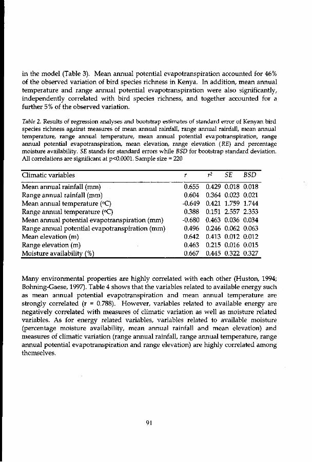
in the model (Table 3). Mean annual potential evapotranspiration accounted for 46% of the observed variation of bird species richness in Kenya. In addition, mean annual temperature and range annual potential evapotranspiration were also significantly, independently correlated with bird species richness, and together accounted for a further 5% of the observed variation.

Table 2. Results of regression analyses and bootstrap estimates of standard error of Kenyan bird species richness against measures of mean annual rainfall, range annual rainfall, mean annual temperature, range annual temperature, mean annual potential evapotranspiration, range annual potential evapotranspiration, mean elevation, range elevation (RE) and percentage moisture availability. SE stands for standard errors while BSD for bootstrap standard deviation. All correlations are significant at p<0.0001. Sample size = 220

Climatic variables r r2 SE BSD

Mean annual rainfall (mm) Range annual rainfall (mm) Mean annual temperature (°C) Range annual temperature (°C) Mean annual potential evapotranspiration (mm) Range annual potential evapotranspiration (mm) Mean elevation (m) Range elevation (m) Moisture availability (%)

Many environmental properties are highly correlated with each other (Huston, 1994; Bohning-Gaese, 1997). Table 4 shows that the variables related to available energy such as mean annual potential evapotranspiration and mean annual temperature are strongly correlated (r = 0.788). However, variables related to available energy are negatively correlated with measures of climatic variation as well as moisture related variables. As for energy related variables, variables related to available moisture (percentage moisture availability, mean annual rainfall and mean elevation) and measures of climatic variation (range annual rainfall, range annual temperature, range annual potential evapotranspiration and range elevation) are highly correlated among themselves.

0.655 0.604 -0.649 0.388 -0.680 0.496 0.642 0.463 0.667

0.429 0.364 0.421 0.151 0.463 0.246 0.413 0.215 0.445

0.018 0.023 1.759 2.557 0.036 0.062 0.012 0.016 0.322

0.018 0.021 1.744 2.353 0.034 0.063 0.012 0.015 0.327

91

550 r

•so

350

250

ISO

SO

° o

0

I l

8

G,

!

^ 8

1 9

8

9.

c

o

c

t 8

°

3 ©--

s 3

e

° °o ' ; " °

S c

cP

3a ..

. 0

o

• • - - . . . .

;J

c •>

8. ° i

i

(a) Percentage moisture availability

100 1^00 1600 1700 1800 1900 2000 2100 2200 2300 2400 Mean annual potential evapoErarvspiratiort (mm)

(b)

Figure 2. (a) Relation between species richness (S) and percentage moisture availability (M), fitted with 4* order polynomial function, S = 9.56 + 8.62M - 0.15M2 + 0.003M3 + 2.04M*. (b) Mean annual potential evapotranspiration (P) versus species richness, fitted with 4 th order polynomial function, S = -1.02 + 200.3P - 0.15P2 + 4.66P3 -5.58P1

Discussion

Bird species richness is strongly correlated with mean annual rainfall, percentage moisture availability and mean elevation (Table 2). Mean annual rainfall and percentage moisture availability account for 43% and 45% of the observed variation of bird species richness respectively. These results are consistent with the hypothesis that benign conditions permit more species (Currie, 1991). In Kenya such areas have abundant trees, which are important as sources of food, nesting or perching for bird species (Lewis and Pomeroy, 1989). The high rainfall areas are mainly situated in high altitudes (highlands) with greater topographic and habitat diversity that support several bird species endemic to forests and grasslands (Muriuki et ah, 1997). Our results agree with this finding because mean elevation accounts for 41% of the variability in bird species. On the other hand, altitudinal range accounts for only 22% of the observed variation of species richness, as many bird species, both aquatic and terrestrial, are restricted to certain altitude ranges (Lewis and Pomeroy, 1989).

Some studies indicate that species richness increases as climatic variation decreases (MacArthur, 1975). However, our results (Table 2) show that the bird species richness increases with measures of climatic variation such as range annual rainfall, range annual temperature and range annual potential evapotranspiration. What could be the reason? The effects of climatic variation on species richness depend on whether the variation is predictable or unpredictable. In a predictable, seasonally changing environment, different species may be suited to conditions at different times of the year. Hence, more species might be expected to coexist in a seasonal environment than

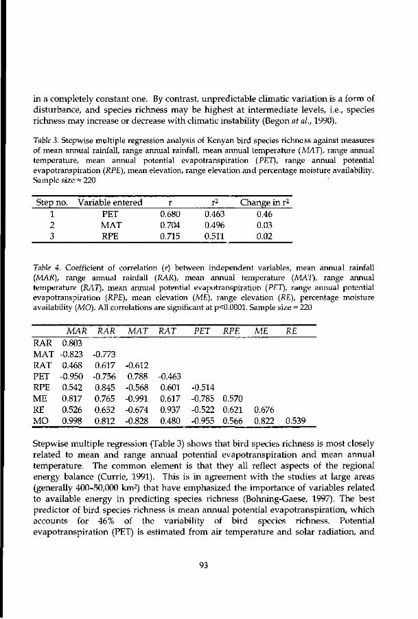
in a completely constant one. By contrast, unpredictable climatic variation is a form of disturbance, and species richness may be highest at intermediate levels, i.e., species richness may increase or decrease with climatic instability (Begon at al., 1990).

Table 3. Stepwise multiple regression analysis of Kenyan bird species richness against measures of mean annual rainfall, range annual rainfall, mean annual temperature (MAT), range annual temperature, mean annual potential evapotranspiration (PET), range annual potential evapotranspiration (RPE), mean elevation, range elevation and percentage moisture availability. Sample size = 220

Step no. Variable entered r r2 Change in r2

1 PET 0.680 0.463 0.46 2 MAT 0.704 0.496 0.03 3 RPE 0.715 0.511 0.02

Table 4. Coefficient of correlation (r) between independent variables, mean annual rainfall (MAR), range annual rainfall (RAR), mean annual temperature (MAT), range annual temperature (RAT), mean annual potential evapotranspiration (PET), range annual potential evapotranspiration (RPE), mean elevation (ME), range elevation (RE), percentage moisture availability (MO). All correlations are significant at p<0.0001. Sample size = 220

RAR MAT RAT PET RPE ME RE MO

MAR 0.803 -0.823 0.468 -0.950 0.542 0.817 0.526 0.998

RAR

-0.773 0.617 -0.756 0.845 0.765 0.652 0.812

MAT

-0.612 0.788 -0.568 -0.991 -0.674 -0.828

RAT

-0.463 0.601 0.617 0.937 0.480

PET

-0.514 -0.785 -0.522 -0.955

RPE

0.570 0.621 0.566

ME

0.676 0.822

RE

0.539

Stepwise multiple regression (Table 3) shows that bird species richness is most closely related to mean and range annual potential evapotranspiration and mean annual temperature. The common element is that they all reflect aspects of the regional energy balance (Currie, 1991). This is in agreement wi th the studies at large areas (generally 400-50,000 km2) that have emphasized the importance of variables related to available energy in predicting species richness (Bohning-Gaese, 1997). The best predictor of bird species richness is mean annual potential evapotranspiration, which accounts for 46% of the variability of bird species richness. Potential evapotranspiration (PET) is estimated from air temperature and solar radiation, and

93

represents the maximum amount of water that would be lost by evaporation from surfaces and transpiration of plant leaves when evapotranspiration is not limited by water availability (Huston, 1994). It is highly correlated with terrestrial primary productivity and is thus a measure of community energy use (Currie and Paquin, 1987). This observation is consistent with the hypothesis that energy is partitioned among species such that the total available energy limits species richness (Currie, 1991). Other factors induce variability around the limits determined by energy: for example, physically complex environments, like mountains, may favour more equal energy partitioning among species, and thus permit relatively more species to occur together (Currie and Paquin, 1987). Thus, for a given level of PET in Kenya, bird species richness is greater in moist mountainous areas that can support the growth of trees thereby providing nesting habitat and food for bird populations.

The authenticity of the regional data layers needs to be confirmed. Often coarse scale data coverages are useful for visual demonstration purposes but are worthless for scientific analysis (Miller et ah, 1989). The high correlations between mean annual rainfall and mean annual potential evapotranspiration, mean annual temperature as well as mean elevation (Table 4) provide strong evidence for the ecological validity of these data. The strong negative correlation between mean elevation and mean annual temperature (r = -0.991) reflects the notion that the higher you go the cooler it becomes. However, predicting bird species richness requires precise environmental data. Thus, the regional perspective requires the sacrifice of ecological precision for the sake of the generality, as well as the provision of more data thereby allowing statistical predictions. Environmental and species diversity relationships, documented by regression statistics, can be used to identify areas more likely characterized by high species diversity. These areas will be recognizable only on the regional scale, and field observations will be required for precise boundary determination (Miller et ah, 1989).

The results provide strong evidence that environmental factors do influence species richness (Tables 2 and 3). However, bird species richness is undoubtedly influenced by many other factors not considered in this study. Generally, it is the interaction of many factors that leads to extinction and thus to a decrease in species richness (Stoms and Estes, 1993). Phylogenetic analysis of montane African greenbuls identified speciation events due to isolation in different montane areas in eastern Africa (Roy et ah, 1998). Moreover, regional bird populations are affected by human activities such as clearing forests, removing mangroves, draining swamps, and the proliferation of agricultural chemicals, which destroy or pollute the habitat of both resident and migrant birds. Habitat loss caused by deforestation and replacing natural woody vegetation with plantations of exotic tree lead to loss of bird species diversity (Pomeroy and Dranzoa, 1997).

94

Conclusion

The study shows that bird species richness increases with moisture availability hence the moistest region in Kenya —the central and western highlands —support the highest species richness (Figure lb). However, most Kenya's agriculture and populace are also concentrated in this region, and most of the existing protected areas are small. The small size of these protected areas, their scattered location, their progressive isolation through the loss of connecting habitat and increasing edge to area ratios, are cause for concern (Muriuki et ah, 1997). Therefore, management plans are needed to prevent a confrontation between conservation and human interests. Planning of conservation priorities does not only require detailed knowledge of patterns of species richness but also an understanding of interaction between historical and ecological processes (Fjeldsa, 1994).

Biodiversity indicator such as species richness is only one of several criteria used for conservation evaluation (Margules and Usher, 1981). In particular are issues such as was the species there in viable numbers, and how many of the species were rare. Moreover, different taxonomic groups may show different patterns —even within groups, patterns of species richness may be different for different guild of species. The challenge is to develop predictive statistical models for many groups of species, establishing patterns in their distributions in such a way as to indicate clearly the conservation potential of different localities (Braithwaite et ah, 1989).

Acknowledgement

We acknowledge the financial support from The Netherlands Fellowship Programme through the ITC for the success of this research. The paper was improved as a result of comments from anonymous referees.

References

Begon M, Harper JL and Townsend CR (1990) Ecology: Individuals, populations and Communities. Blackwell Scientific Publications, Oxford

Bohning-Gaese K (1997) Determinants of avian species richness at different spatial scales. Journal of Biogeography 24: 49-60

Braithwaite LW, Austin MP, Clayton M, Turner J and Nicholls AO (1989) On predicting the presence of birds in Eucalyptus forest types. Biological Conservation 50: 33-50

Currie DJ (1991) Energy and large-scale patterns of animal and plant species richness. American Naturalist 137: 27-49

95

Currie DJ and Paquin V (1987) Large-scale biogeographical patterns of species richness of trees. Nature 329: 326-327

Diamond J (1988) Factors controlling species diversity: Overview and synthesis. Annals of the Missouri Botanical Gardens 75:117-129

Efron B and Tibshirani RJ (1998) An introduction to the bootstrap. Monographs on statistics and applied probability 57, Chapman and Hall/ CRC, London

Feldsa J (1994) Geographical patterns for relict and young species of birds in Africa and South America and implications for conservation priorities. Biodiversity and Conservation 3: 207- 226

Huston AH (1994) Biological Diversity. The coexistence of species on changing landscapes. Cambridge University Press, Cambridge

Karr JR and Roth RR (1971) Vegetation structure and avian diversity in several New World areas. American Naturalist 105: 423-435

Levin SA (1992) The problem of pattern and scale in ecology. Ecology 73:1943-1967 Lewis A and Pomeroy D (1989) A bird atlas of Kenya. Rotterdam, AA Balkema MacArthur JW (1975) Environmental fluctuations and species diversity. In: Cody ML

and Diamond JM (eds) Ecology and Evolution of communities, pp 74-84. Belknap, Cambridge

Margules C and Usher MB (1981) Criteria used in assessing wildlife conservation potential: A review. Biological Conservation 21: 79-109

Mcintosh RP (1967) An index of diversity and the relation of certain concepts to diversity. Ecology 48: 392-404

Miller RI, Stuart SN and Howell KM (1989) A methodology for analyzing rare species distribution patterns utilizing GIS technology: The rare birds of Tanzania. Landscape Ecology 2:173-189

Muriuki JN, de Klerk HM,Williams PH, Bennun LA, Crowe TM and Van den Berge E (1997) Using patterns of distribution and diversity of Kenyan birds to select and prioritize areas for conservation. Biodiversity and Conservation 6:191-210

Oyugi JO (1994) New records for the Bird Atlas of Kenya, 1984-1994. Centre for Biodiversity Research Report 15. National Museum, Kenya

Pomeroy D and Dranzoa C (1997) Methods of studying the distribution, diversity and abundance of birds in East Africa —some quantitative approaches. African Journal of Ecology 35:110-123

Rabinovich JE and Rapoport EH (1975) Geographical variation of diversity in Argentine passerine birds. Journal of Biogeography 2:141-157

Roth RR (1976) Spatial heterogeneity and bird species diversity. Ecology 57: 773-782 Roy MS, Arctander P and Fjeldsa J (1998) Speciation and taxonomy of montane

greenbuls of the genus Andropadus (Aves: Pycnonotidae). Steenstrupia 24: 51-66

96

Sombroek WG, Braun HMH and van der Pouw BJW (1982) Exploratory soil map and Agro-climatic zone map of Kenya, 1980 scale 1:1,000,000. Exploratory Soil Survey Report No. El, Kenya Soil Survey, Nairobi

Stoms DM and Estes JE (1993) A remote sensing research agenda for mapping and monitoring biodiversity. International Journal of Remote Sensing 14:1839-1860

Turner JRG, Lennan JJ and Lawrenson J A. (1988) British bird species distributions and the energy. Nature 335: 539-541

UNEP (1987) Kenya. National State of the Environment Report 2, United Nations Environmental Programme, Nairobi

Walker RE, Stoms DM, Estes JE and Cayocca KD (1992) Relationships between biological diversity and multi-temporal vegetation index data in California. Technical Papers of the 1992 Annual Meeting of ASPRS/ACSM held in Albuquerque, New Mexico, 3-7 March 1992, pp 562-571. American Society for Photogrammetry and Remote Sensing, Bethesda

Williams PH and Gaston DKJ (1994) Measuring more of biodiversity: Can higher-taxon richness predict wholesale species richness? Biological Conservation 67: 211-217

Wright DH (1983) Species-energy theory: an extension of species-area theory. Oikos 41: 496-506

97

CHAPTER

8

INTERANNUAL VARIABILITY OF NDVI AND BIRD SPECIES DIVERSITY IN KENYA

Abstract

Species richness or simply the number of species in a given area is commonly used as an important indicator of biological diversity. Spatial variability in species richness has been postulated to depend upon environmental factors such as climate and climatic variability, which in turn may affect net primary productivity. The Advanced Very High Resolution Radiometer (AVHRR) derived Normalized Difference Vegetation Index (NDVI) has been shown to be correlated with climatic variables including rainfall, actual evapotranspiration and net primary productivity. To determine factors favoring high species richness, we examined the relationship between interannual NDVI variables and species richness of birds at a quarter degree scale (55X55 km). Results revealed a strong positive correlation between species richness and maximum average NDVI. Conversely, species richness showed negative correlation with standard deviation of maximum NDVI and the coefficient of variation. Though these relationships are indirect, they apparently operate through the green vegetation cover. Understanding such relationships can help in mapping and monitoring biological diversity, as well as in estimating changes in species richness in response to global climatic change.

Key words: AVHRR-NDVI, birds, mapping, species richness, Kenya, time series analysis

98

Introduction

Biological diversity can be defined as the totality of genes, species and ecosystems in a region. The species component is certainly the most convenient level to consider whole-organism diversity. Species are also the primary focus of evolutionary mechanisms, and the extinction of species is the principal agent governing biological diversity (Groombridge, 1992). Among ecologists, the quest for an understanding of species diversity remains one of the cornerstones of community ecology because of the degree to which it summarizes the effects of so many processes of interest. Theoretical explorations seek to establish a general synthesis, while empirical characterizations strive to determine general relationships and to uncover underlying mechanisms. Thus, diversity continues to attract the interest of community ecologists and stimulate further study (Grace, 1999).

A challenge exists for scientists to propose biologically defensible policies for sustainable development that include preservation of biological diversity (Stoms and Estes, 1993). This requires a better understanding of the temporal and spatial scale of the processes that naturally maintain species within particular areas and habitats (Ricklefs, 1995). Avian communities have been the focus of many studies about the factors determining species richness (Bohning-Gaese, 1997). One reason is that birds have long been popular with naturalists, amateur and professional, and consequently their systematics and distributions are better known than from any other comparable group of animals, with the possible exception of the larger mammals (Pomeroy and Dranzoa, 1997). However, the problem with birds is that they fly around, often over large distances.

Studies of factors influencing avian biodiversity yield very different results depending on the area over which species richness is calculated. Ecological studies over small areas (i.e., 0.0025-0.4 km2) emphasize the importance of habitat diversity, whereas biogeographical studies over large areas (i.e., 400-50,000 km2) emphasize variables related to available energy (Bohning-Gaese, 1997). Primary productivity, the solar energy that is captured by plants and converted to carbon compounds, is the basic resource that fuels life on Earth (Huston, 1994). Productivity increases with increasing rainfall or temperature (Lieth, 1975). Since the number of consumer individuals increases with productivity, species diversity also increases with productivity (Diamond, 1988). Productivity and related variables have been mapped over large areas with remote sensing (Stoms and Estes, 1993). The Normalized Difference Vegetation Index (NDVI) has been related to net primary productivity (NPP) at coarse spatial scales (Box et ah, 1989). If a strong relationship can be shown between NDVI and NPP, then NDVI should have a direct relationship with species richness.

99

Climatic stability permits specialization (Currie, 1991) and hence high species diversity because populations would be stable and extinction rates due to population fluctuations would be low (Sanders and Hessler, 1969). However, there are many examples of low diversity communities in stable environments, such as tropical forests dominated by cativo (Prioria copifera), Mora, Gilbertiodendron, and other species in central Africa (Hart et ah, 1989). On the other hand, communities with high diversity are often found in environments that seem to be severe, unpredictable, or unstable, such as the Sonoran desert (Whittaker and Niering, 1965). The fire-maintained sclerophyll shrub communities of the Mediterranean climate regions of southern Africa and Australia may have higher species diversity than some rainforests (Huston, 1994).

NDVI has been shown to be highly sensitive to rainfall anomalies such as drought (Henricksen, 1986), allowing NDVI to be used as a good proxy of interannual climate variability (Richard and Poccard, 1998). Interannual variability in vegetation takes place as a result of climatic variability affecting germination and growth (Hobbs, 1990). Large variations in vegetation composition and growth are seen in arid and semi-arid areas where rainfall is sporadic and the response of vegetation to such rainfall is rapid (Griffin and Friedel, 1985). Therefore, the vegetation index time series give us a possibility to assess the climatic variability over the season and over the years (interannual variation). The interannual variability of NDVI values, as calculated using standard deviation of maximum NDVI, may indicate unstable and unpredictable environments. Consequently, high values of standard deviation of maximum NDVI should relate to areas with variable climate over a number of years and hence low species richness.

In this paper, we assess the extent to which vegetation index time series data can be used to predict the species richness of birds in Kenya. Specifically, we investigated the relationships between species richness and interannually integrated NDVI variables, average, standard deviation of NDVI as well as coefficient of variation. The study was executed at a quarter degree scale (55 X 55 km), which corresponds to the scale of the distribution maps in the bird atlas of Kenya (Lewis and Pomeroy, 1989).

Methods

Study area and bird species data Kenya is situated between latitudes 5° 40' north and 4° 4' south and between longitudes 33° 50' and 41° 45' east (Figure la). The wide range of habitats in Kenya is a reflection of the great altitudinal range and distinct regional patterns of rainfall. The diverse community assemblages range from montane forest habitats in the central

100

west to semi-arid scrub in the north and mangrove forests in the southeast. Consequently, most bird species have well-defined distributions (Lewis and Pomeroy, 1989). The Kenyan avifauna is one of the richest in Africa (Pomeroy and Lewis, 1987). The importance of conserving Kenyan birds is emphasized by the fact that bird watching is an important component of African tourism (Muriuki et ah, 1997).

34* ' • 36' " . ' . ' . 38* 40"

4 . 1 " ^ ' - - ' m

m\:H •'•••"

v

t » • " • — • •

(b)

Figure 1. (a) Geographical location of Kenya in Africa, (b) A sample species distribution map showing the distribution of Ostrich (Struthio camelus) in Kenya used in our study.

The distribution maps (Lewis and Pomeroy, 1989) for 871 breeding species in Kenya as well as the 194 migrant species (mostly northern winter visitors) were photocopied (Figure lb) and scanned in 256 gray scales and then saved as Tagged image file format (Tiff). An algorithm was developed for extracting the mapping symbols for the following status of birds from the scanned tiff maps: (1) confirmed breeding after 1/1/1970; (2) present and probable breeding after 1/1/1970; (3) recent presence and earlier confirmed breeding; (4) recent presence and earlier probable breeding; (5) recent probable breeding and earlier confirmed breeding; and (6) records after 1/1/1970 (but no confirmation of breeding). The algorithm rectified the images to obtain standard northing by identifying the location of two pixel patterns that appear in all images, and from their positions computed the orientation of the map. Finally, the algorithm translated and rotated the image to obtain a rectified image. For each status, the maps use a specific pattern (pattern 1 to 6). After rectification, the position of each block (55X55 km) was approximately known. For each block position, the algorithm computed a slightly wider buffer and then tried to find the best match for all six patterns. For some block positions, we found that lake and country boundaries obscured the recognition of patterns. We corrected for this at specific block positions by cross-checking the pattern against the original map in the bird atlas. In addition,

101

we looked at trends in histograms per pattern that helped to identify problems where the algorithm erroneously identified patterns. Thus, all errors caused by translating the analogue database to a digital database were removed by the operator intervention.

NDVI time series data The Normalized Difference Vegetation Index (NDVI) is a measure of vegetation vigor. The magnitude of NDVI is related to the level of photosynthetic activity in the observed vegetation (Tucker and Sellers, 1986). In general, higher values of NDVI indicate vigor and quantity of vegetation (ADDS, 1999). The NDVI data were obtained from the data collected by the National Oceanic and Atmospheric Administration (NOAA) satellites, and processed by the Global Inventory Monitoring and Modeling Studies (GIMMS) at the National Aeronautics and Space Administration (NASA). The GIMMS group at NASA Goddard Space Flight Center developed the GIMMS NDVI first generation dataset (Holben, 1986).

The processing chain of the GIMMS mapping system begins with stratification by continent in order to reduce the amount of data that must be processed. Suspect data are eliminated by discarding the 45 outer pixels on either side of a scan to reduce the variation in NDVI as a result of viewing geometry. The threshold of 45 pixels corresponds to a scan angle of approximately 42 degrees off-nadir (Los, 1998). In addition, data with a channel 5 brightness temperature below 288 K is assumed to be clouds and are eliminated. This cloud screening technique does not discriminate between warm clouds or partially cloud covered or "mixed" pixels (Eck and Kalb, 1991). Digital counts of channels 1 and 2 are then converted to radiances, and then normalized for incoming solar radiation with the preflight calibration coefficient from NOAA (Kidwell, 1995). NDVI is computed as the normalized ratio of the difference between near-infrared and red reflectance measurements by their sum (Sellers, 1989):

NDVI = (NIR - R) / (NIR + R)

where MR = near-infrared measurements and R = visible red measurements. Normalization reduces differences due to overall brightness of sunlight or of surfaces (e.g., shadows) that can strongly influence the image. High positive values of NDVI correspond to dense vegetation cover, whereas negative values are usually associated with bare soil, snow, clouds or non-vegetated surfaces.

Global Area Coverage NDVI data are mapped to the Hammer-Aitoff projection and resampled to 7.638 km in order to display the Africa continent on a 1024 by 1280 screen. In cases where pixels overlap, the value of the pixel with the highest NDVI is used (Los, 1998). Geo-registration is accomplished using the orbital parameters

102

provided by NOAA. Registration checks are made by comparing coasts and rivers in the image with those of the Central Intelligence Agency (CIA) World Data Bank II (Gorny, 1977). When a mismatch between features is found, the entire image is shifted over a whole number of pixels, which reduces the registration error to approximately 4 - 8 km (Los, 1998).

The daily images show large areas of missing data, resulting from gaps between mapped orbits. The effects of clouds, atmosphere, viewing and illumination geometry further reduce the utility of the data. To obtain complete cover of the land surface and to reduce the impact of these effects, a 10-day maximum value composite is obtained from the daily images by selecting the maximum NDVI value for each pixel. The 10-day maximum value composite procedure selects the 'greenest' value, which generally represents the least cloud contaminated pixel for each dekad period (Holben, 1986). Compositing does not account for changes in NDVI as a result of sensor degradation, solar zenith angle and/or soil background.

The spectral response of vegetated areas presents a complex mixture of vegetation, soil brightness, environmental effects, shadow, soil color and moisture. Hence, the effect of soil brightness exerts considerable influence on the computation of vegetation indices (Bannari et al., 1995). The soil background reflectance usually affects low and intermediate NDVI values more than high NDVI values because the increased vegetation cover tends to mask the soil (Huete et al, 1985). Since Kenya experiences a bimodal rainfall distribution with peaks in April and November, it has two growing seasons. The interannual maximum NDVI used in this study generally represents NDVI at the height of the growing seasons (Lewis et al., 1998). Moreover, differences in soil reflectance were presumed to cause less variation of NDVI values because time series data were analyzed for the same pixel area. Thus, the effect of soil background is minimized by using maximum NDVI as derived from the annual time series data, as well as the fact that vegetation cover is present and adequate (on an annual basis), across the study area.

Analysis of the data The historical image products of Kenya comprising 396 dekads of maximum NDVI were downloaded from ADDS1 (1999) website (http://edcsnw4.cr.usgs.gov/bin/ staform/a=ndvi/ b=ke, 24th February 2000). These historical NDVI products are statistical summaries (i.e., average or maximum NDVI) for the historical time period, and hence there is no significant influence from cloud contamination. Since a year has 36 dekads (i.e., 3 dekads multiplied by 12 months), 396 dekads (i.e., 36 dekads multiplied by 11 years) correspond to an 11-year time period (1982-1993). By using Windisp3.5 software image list builder (Pfirman et al., 1999), a 36 dekad maximum NDVI image list was created. The NDVI variable images, comprising the average

103

NDVI (Figure 2a) and standard deviation of NDVI (Figure 2b), were generated from the 36 dekads maximum NDVI image list.

The calculation of species richness was based on combinations of the status of birds recorded since 1970, namely, confirmed breeding after 1/1/1970, present and probable breeding after 1/1/1970, and records after 1/1/1970 (but no confirmation of breeding). In each sample unit (55 X 55 km), the number of species present was counted to give a value for total species richness. The coordinates of the sample units (55X55 km) containing bird species were then conformed to the same geographic coordinate system as the NDVI images. Since the spatial resolutions of the species data were different from NDVI data (7.6 X 7.6 km), the sample points representing species data were overlaid on NDVI images. For every sample unit the mean values of maximum average NDVI as well as standard deviation of maximum NDVI were computed. The two NDVI images were extracted using lower left corner coordinates of the sample unit. The coefficient of variation was calculated by dividing the standard deviation by average NDVI, expressed as a percentage. Thus, each sample unit finally contained NDVI variables (average, standard deviation and coefficient of variation) as well as the species richness of birds. The Pearson correlation between species richness and interannually integrated NDVI variables were calculated. Since correlation coefficients calculated on a grid cell by grid cell basis are often biased by spatial autocorrelation (Odland, 1988), a random sample of grid cells were selected for the correlation analysis, rather than the entire population. Regression lines between the dependent variable (bird species richness) and the independent variables (interannually integrated NDVI variables) were calculated.

Results

The interannually integrated average NDVI exhibits a distinct pattern in Kenya (Figure 2a). Predictably, the semi-humid to humid zones such as the Lake Victoria region, central highlands and the coastal strip have the highest maximum average NDVI. The standard deviation of maximum NDVI (Figure 2b) also shows regional patterns. High values occur in arid and semi-arid zones where large environmental gradients are present within a region, as for example from the northeast to the southeast of Kenya (excluding the coastal strip). Very arid areas (e.g., the northwest around Lake Turkana) exhibit low values, consistent with low average NDVI values. Since the higher the value of NDVI the more photosynthetically active the cover type (Sellers, 1985), low average NDVI values indicate that these areas have less photosynthetically active cover types.

104

The correlation analyses between NDVI variables and bird species richness were performed separately in areas with mean annual rainfall: less than 650 mm (arid to semi-arid zones); 650 mm and above (semi-humid to humid zones); and combination of all zones (arid to humid). These analyses were performed to investigate the extent to which NDVI variables can predict species richness under different agro-climatic zones. The results (Table 1) reveal that in semi-humid to humid zones, NDVI variables have weak relationship with bird species richness. On the contrary, both average NDVI and coefficient of variation have moderately strong association with species richness in arid and semi-arid zones. When arid to humid zones were analyzed as a lumped data set, both average NDVI and coefficient of variation had stronger correlation with species richness than standard deviation of NDVI.

Figure 3a shows that the spatial distribution of number of bird species recorded in Kenya since 1970 (Lewis and Pomeroy, 1989) roughly corresponds to that of interannual average NDVI (Figure 2a). The regression model (Figure 4a) (note r = 0. 708 for p < 0. 05), shows that species richness increases as the NDVI increases, and also accounted for 50% of the variance (Table 1). For mapping bird diversity in the study area, the results from the regression analyses were used to convert the maximum average NDVI image (Figure 2a) to a map of species richness.

(a) (b) Figure 2. Spatial distribution of interannually integrated maximum NDVI variables in Kenya: (a) Average NDVI image, (b) Standard deviation image.

The bird species richness map (Figure 3b) was computed using the equation (richness = -98.10 + 745. 66 * maximum average NDVI). This map roughly matches the observed species richness map (Figure 3a), as well as the map of bird species richness in tropical Africa mapped at the scale of a one degree square (Burgess et ah, 1997). The major differences between species richness and predicted species occur in areas

105

occupied by the two large lakes of Kenya, namely Victoria and Turkana as well as the Rift Valley, with its lakes (Figure 3c). Within the lake areas, large numbers of bird species were observed but NDVI values are zero (i.e., water), so the model prediction is low. On the other hand, the largest differences (i.e., negative) between observed species richness and predicted species richness occur in areas where few or no bird species were observed, but due to high NDVI values in these areas the model prediction is high. These areas correspond mainly to isolated humid areas in northern Kenya and the upper part of coastal strip bordering Somalia (Figure 3c).

No. of obsorvod bird ipoeiot

SOS

No. of prodlctod bird tpoclos

Figure 3. (a) Number of bird species recorded in Kenya since 1970 (Lewis and Pomeroy, 1989), (b) Number of bird species as predicted by interannually integrated maximum average NDVI, (c) The difference between the observed and the predicted species richness.

The standard deviation of maximum NDVI and coefficient of variation should reflect the degree of drought risk in a region. Our analysis shows that the variable has a weak negative relationship with species richness (Table 1) with an r-value of - 0.290 that accounts for only 8% of the variation of bird species richness. Plots of the coefficient of variation reveal a moderately strong negative association with bird species richness, with a correlation coefficient of r = - 0.613 (Figure 4b) which accounts for 38% of the observed variation in Kenyan bird species richness (Table 1).

Many studies have shown that plant growth and production are closely correlated to both temperature and rainfall (Leith, 1972). NDVI has been shown to be correlated with climate variables including rainfall and evapotranspiration over a wide range of environmental conditions (Justice et al., 1986). To establish the environmental factors that are related to NDVI variables, we correlated climatic variables (rainfall, temperature, potential evapotranspiration and moisture index) with NDVI variables (Table 2). Data for these climatic variables were taken from Sombroek et al., (1982) and

106

the relations between these climatic variables and bird species richness have been explained in Oindo et al., (2001). The moisture index (S) was calculated us ing the Bailey (1979) equation (S = 0.18p/ 1.045'), where p equals mean annual precipitation and t equals mean annual temperature in degrees centigrade. The results (Table 2) show that average NDVI is positively associated wi th rainfall and moisture availability, whereas s tandard deviation and coefficient of variation have a positive correlation with temperature as well as potential evapotranspiration.

Table 1. Coefficients of correlation between bird species richness and NDVI variables. The analyses were executed separately for arid and semi-arid zones (mean annual rainfall < 650mm), semi-humid to humid zones (mean annual rainfall > 650mm) and in case of combined zones (i.e., arid to humid), randomly selected sample of grid cells were analyzed and n represents the sample size. Underlined means not significant at p<0.05

NDVI variables

Average NDVI Standard deviation Coefficient of variation

Combined n=91

r 0.708 -0.290 -0.613

r2

0.501 0.084 0.376

<650 mm n=118

r 0.570 -0.058 -0.335

r2

0.326 0.003 0.112

> 650 mm n=80

r 0.221 -0.200 -0.205

r2

0.049 0.040 0.042

Table 2. The results of correlation analyses between climatic and NDVI variables in all agro-climatic zones combined. Potevapo stands for potential evapotranspiration and the sample size = 193. All correlations are significant at p<0.05

Climatic variables (average annual)

Rainfall (mm) Temperature (°C) Potevapo (mm) Moisture index

Average NDVI

r 0.820 -0.595 -0.800 0.757

r2

0.678 0.354 0.639 0.557

Standard deviation

r -0.477 0.405 0.404 -0.442

r2

0.227 0.164 0.163 0.193

Coefficient of variation

r -0.707 0.576 0.678 -0.649

r2

0.499 0.321 0.451 0.408

107

500 500

4 0 0 -

9 300 i_ <n

S. 200 in

CO

0.25 0.40 0.55 0.70 Integrated maximum average NDVI

\

-

" 0

o

sR

o 0

< : •

0

1

o > ^

u 0

0

p> \ C 0

0

-'

1

"• > V

0 6 -

1

'J O ^ -

fl° 1

-100

0 0.10 0.25 0.40 0.55 0.70 0

D 10 20 3D 40 Coefficient of variation

(a) (b) Figure 4. Scatter plots of relation between species richness and interannual NDVI variables: (a) Maximum average NDVI versus bird species richness, (b) Coefficient of variation (relative variability of NDVI) versus bird species richness.

Discussion

Productivity is the rate at which energy flows through an ecosystem (Rosenzweig and Abramsky, 1993). Ecologists normally use an index of productivity rather than measuring it directly. In arid and semi-arid landscapes, precipitation is often used as a proxy for the index (Rosenzweig and Abramsky, 1993). Actual evapotranspiration is also a suitable index for terrestrial systems with a wide variety of temperature and precipitation regimes (Rosenzweig, 1968). It has been shown that Normalized Difference Vegetation Index (NDVI) is closely related to net primary productivity as well as actual evapotranspiration, for many vegetation types (Box et al., 1989). Hence, the annual maximum average NDVI (1982-1993) was integrated as an index for productivity. The strong positive correlation between maximum average NDVI and climatic variables, mean annual rainfall and moisture availability (Table 2) indicates that maximum average NDVI is associated with variables related to vegetation growth (Nicholson et al, 1990). Consequently, high maximum average NDVI should represent high productivity. Table 1 shows that higher maximum average NDVI results in higher species richness.

So, why does high productivity tend to increase bird species richness? One explanation could be that, in natural habitats, bird populations are positively correlated with the

amount of woody vegetation (Pomeroy and Dranzoa, 1997). Since there is increased production of woody species in highly productive ecosystems (Prins and Olff, 1998), bird species richness too increases with woody vegetation (Pomeroy and Dranzoa, 1997). Apparently, the greatest bulk of woody vegetation is to be found in forests, which in the tropics are extraordinarily rich in insect species. These in turn support a rich diversity of birds, almost all of them breeding in the forest (Lewis and Pomeroy, 1989). Moreover, many species of land birds use trees as a source of food, or for nesting or as a perch; even many water birds nest or perch in trees.

While semi-arid woodlands may support as many species of birds as a forest, far fewer birds breed in woodland so the overall diversity of species is lower where diversity is measured in terms of breeding population (Pomeroy and Lewis, 1987). Figure 3a, b shows that western and southern Kenya supports the highest number of bird species. The west of Kenya has high topographic and habitat diversity supporting endemic species in forests and high altitude grasslands. On the other hand, the south of Kenya is characterized by shore and seabirds as well as species with ranges restricted to coastal forests (Muriuki et ah, 1997).

When the coefficient of variation of NDVI over an eleven year period is considered, the major aspects of climate that affect plant growth are variation in rainfall, evaporation and temperature (Sombroek et ah, 1982). There is often a striking decrease in productivity with aridity; especially in relatively dry environments where water supply may limit plant growth (Begon et ah, 1990). Thus, regions receiving low rainfall with high evaporation (due to high temperatures) have drier soil conditions, which minimize the potential for plant growth. Table 2 shows that standard deviation of maximum NDVI and coefficient of variation are positively correlated with mean annual temperature and potential evapotranspiration. Since these NDVI variables have a negative correlation with mean annual rainfall, drought risk (unstable) areas can be characterized by rather low maximum average NDVI and relatively high standard deviation of maximum NDVI and high coefficient of variation. By contrast, productive (stable) areas are characterized by a low coefficient of variation with rather high maximum average NDVI and relatively low standard deviation of maximum NDVI (Figure 2a, b). The negative association between NDVI variables (viz. standard deviation and coefficient of variation) and species richness (Table 1) is characteristic of arid areas with erratic rainfall; conditions that limit the growth of woody species. Since bird species diversity is correlated with the amount of woody vegetation in natural habitats (Pomeroy and Dranzoa, 1997), the lack of woody species in arid areas reduces bird species richness.

109

Conclusion

A satellite-derived vegetation index can provide both spatial and temporal quantitative information on vegetation reflectance, which can be translated into a measure of environmental factors that influence the biodiversity of a region. Our study reveals that interannually integrated maximum NDVI variables are strongly related to bird species richness. This indicates that NDVI represents the integration of climatic variables (Anyamba and Eastman, 1996) that are important for distribution of bird species. The results establish that maximum average NDVI relates to environmental factors favoring the bird species richness (i.e., quantity and vigor of vegetation), whereas standard deviation of maximum NDVI and coefficient of variation represent factors limiting the distribution of birds (i.e., amount of woody vegetation). Moreover, the results confirm that high bird species diversity occurs in stable and predictable environments in Kenya.

The importance of identifying centers of species richness and endemism in Africa has been emphasized at the Forum on Biodiversity in the U.S. (Huntley, 1988). Maps of bird distribution are fundamental for assessing the distribution of avian biodiversity (Burgess et ah, 1997). A bird species richness map, modeled from the positive correlation between bird species richness and average NDVI, was produced (Figure 3b). As the correlation is not perfect, the map cannot be used as a definitive and exact measurement of species in Kenya, but may indicate areas of high species diversity and conservation interest. These areas can become the foundation of a conservation, which can then be integrated into the prevailing economic, political, and social environment of a region.

Acknowledgement

Our appreciation goes to the Netherlands Ministry of Development Co-operation and Ministry of Education for funding the research under the Netherlands Fellowship Programme. The authors are grateful to USAID/FEWS Project for providing valuable NDVI time series images through the Internet.

References

ADDS (1999) Africa Data Dissemination Service, EROS Data Center, U.S. Geological Survey Sioux Falls, S. Dakota, US 57198. http://edcsnw4.cr.usgs.gov/adds/ adds.html

Anyamba A and Eastman JR (1996) Interannual variability of NDVI over Africa and its relation to El Nino/Southern Oscillation. International Journal of Remote Sensing

110

17: 2533-2548 Bailey HP (1979) Semi-Arid Climates: Their Definition and Distribution. In: Hall AE,

Cannell GH and Lawton HW (eds) Agriculture in Semi-Arid Environments, pp 73-97. Springer-Verlag, Berlin

Bannari A, Morin D and Bonn F (1995) A Review of vegetation indices. Remote Sensing Reviews 13: 95-120

Begon M, Harper JL and Townsend CR (1990) Ecology: Individuals, populations and Communities. Blackwell Scientific Publications, Oxford

Bohning-Gaese K (1997) Determinants of avian species richness at different spatial scales. Journal of Biogeography 24:49-60

Box EO, Holben BN and Kalb V (1989) Accuracy of the AVHRR Vegetation Index as a predictor of biomass, primary productivity and net CO2 flux. Vegetatio 80: 71-89

Burgess N, de Klerk H, Fjeldsa J, Crowe T and Rahbek C (1997) Mapping Afrotropical birds: links between atlas studies and conservation priority analyses. African Bird Club 4: 93-98

Currie DJ (1991) Energy and large-scale patterns of animal- and plant- species richness. American Naturalist 137: 27-49

Diamond J (1988) Factors controlling species diversity: Overview and synthesis. Annals of the Missouri Botanical Gardens 75:117-129

Eck TF and Kalb VL (1991) Cloud screening for Africa using geographically and seasonally variable infrared threshold. International Journal of Remote Sensing 12: 1205-1221

Grace JB (1999) The factors controlling species density in herbaceous plant communities: an assessment. Perspectives in plant ecology. Evolution and Systematics 2:1-28

Griffin GF and Friedal MH (1985) Discontinuous change in central Australia: Some major implications of ecological events for land management. Journal of Arid Environment 9: 63-82

Groombridge B (1992) Global Biodiversity. Status of the Earth's Living Resources. World Conservation Monitoring Centre, London

Hart TB, Hart JA and Murphy PG (1989) Monodominant and species-rich forests of the humid tropics: causes for their co-occurrence. American Naturalist 133: 613-633

Henricksen BL (1986) Reflections on drought: Ethiopia 1983-1984. International Journal of Remote Sensing 7:1447-1451

Hobbs RJ (1990) Remote sensing of spatial and temporal dynamics of vegetation. In: Hobbs RJ and Mooney HA (eds) Remote Sensing of Biosphere Functioning. Ecological Studies 79, pp 203-219. Springer-Verlag, New York

Holben BN (1986) Characteristics of maximum-value composite images for temporal AVHRR data. International Journal of Remote Sensing 7:1435-1445

111

Huete AR, Jackson RD and Post DF (1985) Spectral response of a plant canopy with different soil backgrounds. Remote Sensing of Environment 17: 37-53

Huntley BJ (1988) Conserving and monitoring biotic diversity: Some African examples. In: Wilson EO (ed) Biodiversity, pp 248-260. National Academy Press, Washington

Huston AH (1994) Biological Diversity. The coexistence of species on changing landscapes. Cambridge University Press, Cambridge

Justice C, Holben BN and Gwynne MD (1986). Monitoring East African vegetation using AVHRR data. International Journal of Remote Sensing 7:1453-1474

Kidwell KB (1995) Polar orbiter data user guide. U.S. Dept. of Commerce, NO A A/National Environmental Satellite Data and Information Service, National Climatic Data Center, Satellite Data Services Division, Washington DC

Leith H (1972) Modeling the primary productivity of the world. Nature and Resources 8: 5-10

Leith H (1975) Modeling the primary productivity of the world. In: Lieth H and Whittaker RH (eds), Primary productivity of the Biosphere. Ecological Studies 14, pp 237-263. Springer-Verlag, Berlin

Lewis A and Pomeroy D (1989) A bird atlas of Kenya. AA Balkema, Rotterdam Lewis JE, Rowland J and Nadeau A (1998) Estimating maize production in Kenya

using NDVI: Some statistical considerations. International Journal of Remote Sensing 19: 2609-2617

Los SO (1998) Linkages between Global Vegetation and Climate. An analysis based on NOAA Advanced Very High Resolution Radiometer Data. GSFC/CR-1998-206852, National Aeronautics and Space Administration, Goddard Space Flight Center, Greenbelt, Maryland

Muriuki JN, de Klerk HM,Williams PH, Bennun LA, Crowe TM and Van den Berge E (1997) Using patterns of distribution and diversity of Kenyan birds to select and prioritize areas for conservation. Biodiversity and Conservation 6:191-210

Nicholson SE, Davenport ML and Malo AR (1990) A comparison of the vegetation response to rainfall in the Sahel and East Africa, using normalized difference vegetation index from NO A A-AVHRR. Climate Change 17: 209-242

Odland J (1988) Spatial autocorrelation. In: Thrall GI (ed) Sage University Scientific Geography Series 9. Sage Publications, Beverly Hills

Oindo BO, de By RA, Skidmore AK (2001). Environmental factors controlling bird species diversity in Kenya. African Journal of Ecology 39: 295-302

Pfirman E, Hogue J and See L (1999) Windisp3.5. Map and image display system version 990217. UN Food and Agriculture Organization, US AID Famine Early Warning System, Southern Africa Development Community, US Forest Service and US Geological Survey

:12

Pomeroy D and Dranzoa C (1997) Methods of studying the distribution, diversity and abundance of birds in East Africa —some quantitative approaches. African Journal of Ecology 35:110-123

Pomeroy D and Lewis A (1987) Bird species richness in tropical Africa: some comparisons. Biology Conservation 40:11-28

Prins HHT and Olff H (1998) Species-Richness of African grazer assemblages: Towards a functional explanation. In: Newbery DM, Prins HHT and Brown ND (eds) Dynamics of tropical communities, pp 449-490. Blackwell Science, Oxford

Richard Y and Poccard I (1998) A statistical study of NDVI sensitivity to seasonal and interannual rainfall variations in Southern Africa. International Journal of Remote Sensing 19: 2907-2920

Ricklefs RE (1995) Distribution of biodiversity. In: Heywood VH and Watson RT (eds) Global Biodiversity Assessment, pp 139-166. Cambridge University Press, Cambridge

Rosenzweig ML (1968) Net primary productivity of terrestrial environments: Predictions from climatological data. America Naturalist 102: 67-84

Rosenzweig ML and Abramsky Z (1993) How are diversity and productivity related? In: Ricklefs RE and Schluter D (eds) Species diversity in ecological communities. Historical and geographical perspectives, pp 52-65. University of Chicago Press, Chicago

Sanders HL and Hessler RR (1969) Ecology of the deep sea benthos. Science 163:1419-1424

Sellers PJ (1985) Canopy reflectance, Photosynthesis and transpiration. International Journal of Remote Sensing 6:1335

Sellers PJ (1989) Vegetation-Canopy spectral reflectance and biophysical processes. In: Asrar G (ed) Theory and Applications of Optical Remote Sensing, pp 279-335. John Wiley and Sons, New York

Sombroek WG, Braun HMH and van der Pouw BJW (1982) Exploratory soil map and Agro-climatic zone map of Kenya, 1980 scale 1:1,000,000. Exploratory Soil Survey Report No. El, Kenya Soil Survey, Nairobi

Stoms DM and Estes JE (1993) A remote sensing research agenda for mapping and monitoring biodiversity. International Journal of Remote Sensing 14:1839-1860

Tucker CJ and Sellers PJ (1986) Satellite remote sensing of primary production. International Journal of Remote Sensing 7:1133-1135

Whittaker RH and Niering WA (1965) Vegetation of the Santa Catalina Mountains, Arizona (II). A gradient analysis of the south slope. Ecology 46: 429-452

113

CHAPTER

9

PATTERNS OF HERBIVORE SPECIES RICHNESS IN KENYA AND CURRENT ECOCLIMATIC STABILITY

Abstract

The increased attention to biodiversity worldwide has stimulated interest in understanding biophysical factors associated with indicators of biodiversity such as species richness. Although levels of biodiversity may seem to be equivalent in different areas, high species richness may be caused by accumulation of species over a long time in places where environmental conditions remained stable and predictable. The Advanced Very High Resolution Radiometer (AVHRR)-Normalized Difference Vegetation Index (NDVI) has been established to be a good proxy for studying interannual climate variability as well as regional drought condition. In this study, we examined the relationship between large herbivore species richness and AVHRR-NDVI derived climatic-variability indices, interannual average NDVI and coefficient of variation of NDVI at a regional spatial scale in Kenya. Regions with relatively low coefficient of variation of NDVI and high interannual average NDVI characterize current ecoclimatic stability. By contrast, high coefficient of variation of NDVI and relatively low interannual average NDVI characterize ecoclimatic instability (drought risk). Statistical analyses revealed that high interannual average NDVI increases species richness, whereas high coefficient of variation of NDVI lowers species richness. This indicates that maximum numbers of species are found in regions with current ecoclimatic stability. Understanding such relationships can help in explaining spatial distribution of species richness and predicting global changes resulting from human impacts on the environment.

Key words: AVHRR-NDVI, climatic variability, ecoclimatic stability, large herbivores, regional scale, species richness

114

Introduction

Patterns of species richness at local, regional and global scales have been of continual interest to biogeographers and ecologists (Brown, 1988). Since extant ecological patterns are the transient results of historical processes (Rohde, 1999), any complete explanation of patterns of species diversity must involve both historical events and current ecological processes (Groombridge, 1992). However, in the search for general patterns of variation in species richness (e.g., Currie and Paquin, 1987; Gaston, 1994; Rosenzweig, 1995) the influence of the past is largely ignored, despite substantial evidence for a strong impact of history (Ricklefs, 1989). Historical constraints may range from major events in the earth history to short-term disturbance (e.g., climatic instability) promoting invasions by opportunistic species and increased species turnover in some areas (Fjeldsa et ah, 1999).

It has been postulated that accumulation of species over a long time in places where environmental conditions remained stable and predictable causes high species diversity (Sanders and Hessler, 1969; Fjeldsa and Lovett, 1997). This is due to the fact that areas with predictable and stable climates may permit a more constant influx of resources and the evolution of greater specialization of niches (Pianka, 1983). By contrast, the exploitation of areas with unstable climate may require evolution of broad tolerances to deal with a wide range of environmental conditions (Owen, 1990). This should lead to decrease in the number of species as the amplitude of periodic climatic fluctuations increases (Pianka, 1983).

Ecoclimatic changes are highly complex, ranging from changing weather, inter-annual differences, among others to the general global cooling in the Pleistocene (Shackleton et ah, 1990). Considering that atmospheric and oceanic flows near the equator are regulated by the earth's rotation, topographic structures which moderate specific impacts today could also affect ecoclimatic stability on other time scales (Fjeldsa et ah, 1997; Fjeldsa et ah, 1999). Thus, identification of current modifiers of extreme weather could also provide a key to identifying places that were protected against polar impacts over substantial periods of evolutionary time (Fjeldsa et al., 1999).

Unfortunately, ecoclimatic data with high spatial resolution exist only from a short time period, compared with the evolutionary time perspective, since 1980 when a system of high resolution meteorological satellites was established. AVHRR-NDVI has been shown to be highly sensitive to rainfall anomalies such as drought (Henricksen, 1986), allowing NDVI to be used as a good proxy of interannual climate variability (Richard and Poccard, 1998). A pilot study comparing interannual variability of NDVI and patterns of endemism in Africa (Fjeldsa et ah, 1997) provided some evidence

115

linking local endemism with local ecoclimatic stability, thereby suggesting a link between short-term and long-term stability (Fjeldsa et al, 1999). The aim of this paper is to evaluate the role of stability (and instability) by comparing regional patterns of large herbivore species richness with remotely sensed data reflecting current ecoclimatic stability. More specifically, we examine the hypothesis that more species accumulate over time in regions where present-day climatic conditions remained predictable and stable.

Methods

Study area and herbivore species data Kenya is situated between latitudes 5° 40' north and 4° 4' south and between longitudes 33° 50' and 41° 45' east. The study area covered 19 rangeland districts (Figure 1) and the descriptions of these districts climatic conditions as well as vegetation types (Table 1) are based on Sombroek et al, (1982). While the source of land use/wildlife conflicts and conservation areas information are Aligula et ah, (1997).

The herbivore species (body weight greater than 10 kg) data were obtained from Department of Resource Surveys and Remote Sensing (DRSRS), Ministry of Environment and Natural Resources, Kenya. The systematic reconnaissance flight methodology used by DRSRS for aerial census of animals is well-documented (Norton-Griffiths, 1978). Statistical analyses to validate DRSRS survey methodology have proved the method and data to be reliable (De Leeuw et al., 1998; Ottichilo and Khaemba, 2001). Topographic maps of scale 1: 250,000 were used for flight planning and all transects conform to the Universal Transverse Mercator (UTM) coordinate system. The aerial surveys were carried out along transects oriented in east-west direction and spaced at 5 km intervals. The standard flying height and aircraft speed were 120 m and 190 km/hr respectively. Two experienced and well trained observers (Dirschl et al., 1981) occupied the rear seats of a high wing aircraft (Cessna 185 or Partenevia) and counted animals that appeared between two rods attached to the wing struts. The field of vision between these rods was calibrated by flying repeatedly across ground markers of known spacing (Ottichilo and Sinange, 1985). The number of animals falling within the survey strips on either side of the aircraft along each 5 km transect segment were counted and recorded into tape recorders by the two rear seat observers. Groups of animals more than ten in number were also photographed. After every survey the tape-recorded observations were transcribed to data sheets, which together with processed photographs, were interpreted for herbivore species using 10 x binocular microscope and overhead projector. The sample units (5 x 5 km) for species data for each of the 19 districts (Figure 1) were summed over the whole area of every district to give a value for total species richness. The study focused on resident

116

herbivore species (Table 2) and the descriptions of the home range of each species are based on Haltenorth and Diller (1980).

Figure 1. Location of Kenya and study districts, Mandera (a), Wajir (b), Marsabit (c), Turkana (d), West Pokot (e), Baringo (f), Laikipia (g), Samburu (h), Isiolo (i), Garissa (j), Lamu (k), Tana River (1), Kilifi (m), Kwale (n), Taita Taveta (o), Kitui (p), Machakos (q), Kajiado (r) and Narok (s).

AVHRR- NDVI time series data AVHRR-NDVI was derived from data collected by the National Oceanic and Atmospheric Administration (NOAA) satellites, and processed by the Global Inventory Monitoring and Modeling Studies (GIMMS) at the National Aeronautics and Space Administration (NASA). The GIMMS group developed the GIMMS NDVI first generation dataset (Holben, 1986). A complete record for Africa exists from August 1981 until the present at 7.6 km resampled resolution (Los, 1998). NDVI is a ratio derived by dividing the difference between near-infrared and red reflectance measurements by their sum:

NDVI = (NIR-R) / (NIR + R) (1)

where MR = near-infrared measurements and R = visible red measurements. Normalization reduces differences due to overall brightness of sunlight or of surfaces (e.g., shadows) that can strongly influence the image.

117

Table 1. Descriptions of the districts' area (km2), average annual rainfall (Rain), average annual temperature (Temp), average annual potential evaporation (Peva), agro-climatic zone (Acz), major vegetation types (Veg), presence of land use/wildlife conflicts (Luc) and conservation areas for large mammals. Agro-climatic zones include semi-arid to semi-humid (sah), arid to semi-arid (asa), very arid to arid (pad) and very arid (pa). Dominant vegetation types include dry woodland and bush land (daub), bush land and scrubland (bs), desert scrub and bush land (dsb), desert scrub and dwarf shrubs (dsd)

District Lamu

Kilifi Kwale

Laikipia

Narok Baringo

West Pokot Machakos

Taita Taveta Samburu

Kajiado

Kitui

Isiolo Marsabit

Tana River Garissa

Turkana Mandera Wajir

Area 6506

12414 8257

9718

16115 9885

9090 14178

16959 17521

19605

29388

25605 73952

38674 43931

61768 26470 56501

Rain 638

638 888

763

888 763

763 875

550 550

550

550

463 338

338 338

338 250 250

Temp 27

27 27

18

18 21

20 21

25 20

21

25

25 25

27 27

25 27 27

Peva 2040

2040 1905

1930

1905 1930

1930 1892

2090 2090

2090

2090

2140 2100

2100 2100

2100 2300 2300

Acz sah

sah sah

sah

sah sah

sah sah

asa asa

asa

asa

vaa vaa

vaa vaa

vaa va va

Veg dwb

dwb dwb dwb

dwb dwb

dwb dwb

bs bs

bs

bs

dsb dsb

dsb dsb

dsb dsd dsd

Luc no

no yes

yes

yes yes

yes yes

yes yes

no

yes

no no

no no

no no no

Conservation areas Dodori and Kiunga National reserves, private ranches No gazetted park Shimba Hills National Reserve

Private ranches, no gazetted park

Masai Mara National Reserve Lake Bogoria and lake Kamnarok game reserves No gazetted park Ol Donyo Sabuk National Park, private ranches Tsavo National Park Samburu, Shaba and Buffalo Springs reserves Amboseli National Park and Chyulu game reserve Tsavo West/ Chyulu Hills National Park No gazetted park Marsabit and Sibiloi National Parks, Losai game reserve Tana River Primate reserve Rahole, Arawale and Boni reserves No gazetted park Malkamari game reserve No gazetted park

The magni tude of NDVI is related to the level of photosynthetic activity in the observed vegetation (Tucker and Sellers, 1986). Generally, higher positive values of NDVI indicate vigor and quantity of vegetation (ADDS, 2000) whereas negative values are usually associated with bare soil, snow, clouds or non-vegetated surfaces.

118

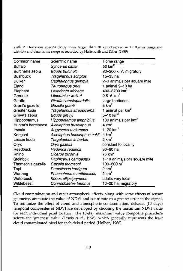
Table 2. Herbivore species (body mass larger than 10 kg) observed in 19 Kenya rangeland districts and their home range as recorded by Haltenorth and Diller (1980)

Common name Scientific name Home range Buffalo Burchell's zebra Bushbuck Duiker Eland Elephant Gerenuk Giraffe Grant's gazelle Greater kudu Grevy's zebra Hippopotamus Hunter's hartebeest Impala Kongoni Lesser kudu Oryx Reedbuck Rhino Steinbok Thomson's gazelle Topi Warthog Waterbuck Wildebeest

Syncerus caffer Equus burchelli Tragelaphus scriptus Cephalophus grimmia Taurotragus oryx Loxodonta africana Litocranius walleri Giraffa camelopardalis Gazella granti Tragelaphus strepsiceros Equus grevyi Hippopotamus amphibius Alcelaphus buselaphus Aegyceros melampus Alcelaphus buselaphus cokii Tragelaphus imberbis Oryx gazella Redunca redunca Diceros bicornis Raphicerus campestris Gazella thomsoni Damaliscus korrigum Phacocheorus aethiopicus Kobus ellipsiprymnus Connochaetes taurinus

50 knr 80-200 km2, migratory 15-35 ha 2-3 animals per square mile 1 animal 9-10 ha 400-3700 km2

2.5-6 km2

large territories 5 km2

1 animal per km2

5-10 km2

100 animals per km2

4 km2

1-20 km2

4 km2

2 km2

constant to locality 30-60 ha 75 km2

1-10 animals per square mile 100-300 m2

2 km2

2 km2

adults very local 10-20 ha, migratory

Cloud contamination and other atmospheric effects, along with some effects of sensor geometry, attenuate the value of NDVI and contribute to a greater error in the signal. To minimize the effect of cloud and atmospheric contamination, dekadal (10 days) temporal composites of NDVI are developed by choosing the maximum NDVI value for each individual pixel location. The 10-day maximum value composite procedure selects the 'greenest' value (Lewis et al., 1998), which generally represents the least cloud contaminated pixel for each dekad period (Holben, 1986).

119

When vegetation cover is low, the spectrum observed by remote sensing is generally dominated by soil. Differences of bare soil reflectance may cause large NDVI variations. This results from differences in colour and brightness arising from soil properties as iron amount and organic matter amount (Richard and Poccard, 1998). Since Kenya experiences a bimodal rainfall distribution with peaks in April and November, it has two growing seasons. The interannual maximum NDVI used in this study generally represents NDVI at the height of the growing seasons (Lewis et ah, 1998). Moreover, differences in soil reflectance were presumed to cause minor variations of NDVI values because time series data were analyzed for the same pixel area. Thus, the effect of soil background is minimized by using annual time series data as well as the fact that vegetation cover is present and adequate (on an annual basis) across the study area.

Analysis of data The aim of this analysis was to measure ecological variations within pixels in such a way that regions affected by occasional droughts or erratic changes in the timing and strength of rains, could be separated from those where the impact of such anomalies is slight. Since the total species richness of a region may be constrained by distinct dry or cold seasons (Fjeldsa et ah, 1997), it is important to quantify the anomalous events such as droughts or interannual differences in the timing and strength of rains. This was done month by month, by calculating coefficient of variation of NDVI between years. The variability over an 11-year period (1982 to 1993) of monthly NDVI values was assumed a better index of stability than the amplitudes of variation or summed changes.

The historical image products of Kenya comprising 396 dekads of maximum NDVI were downloaded from ADDS1 (2000) website (http://edcsnw4.cr.sgs.gov/bin/ staform/a=ndvi/b=ke, 24th February 2000). These historical NDVI products are statistical summaries (i.e., average or maximum NDVI) for the historical time period (1982-1993), and hence there is no significant influence from cloud contamination. Since dekads span from the 1st to the 10th, the 11th to the 20th, and the 21st to month end, a year has 36 dekads (i.e., 3 dekads multiplied by 12 months). Hence, 396 dekads (i.e., 36 dekads multiplied by 11 years) correspond to an 11-year time period. This implies that each month over an 11-year period has 33 dekads (i.e., 3 dekads multiplied by 11 years). By using Windisp 3.5 time series data processor (Pfirman et ah, 1999), average NDVI (VIm) was computed for each of the 12 months over 11-year period as:

120

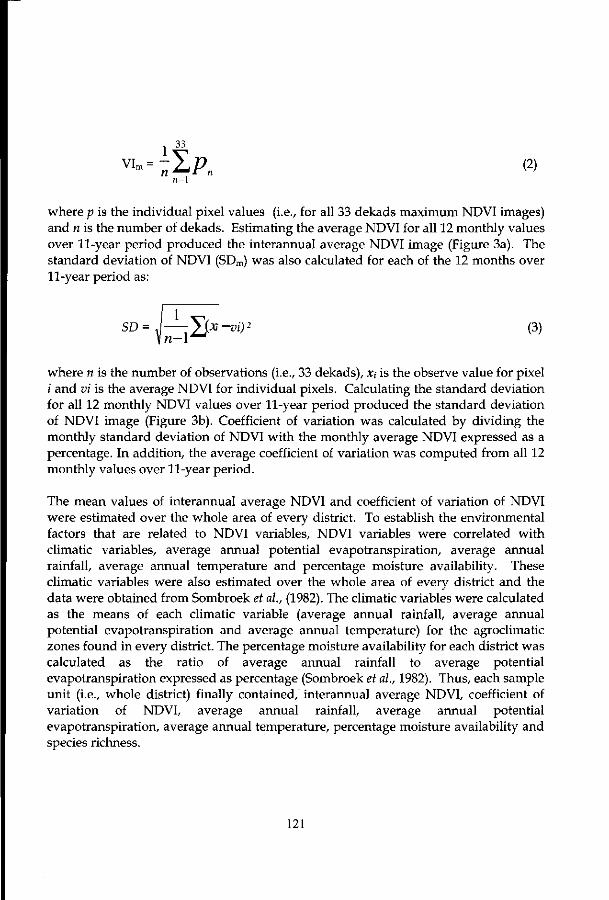
1 33

v i m = - y p (2) n=\

where p is the individual pixel values (i.e., for all 33 dekads maximum NDVI images) and n is the number of dekads. Estimating the average NDVI for all 12 monthly values over 11-year period produced the interannual average NDVI image (Figure 3a). The standard deviation of NDVI (SDm) was also calculated for each of the 12 months over 11-year period as:

SD=j—y%x-vi)2 (3)

where n is the number of observations (i.e., 33 dekads), x, is the observe value for pixel ;' and vi is the average NDVI for individual pixels. Calculating the standard deviation for all 12 monthly NDVI values over 11-year period produced the standard deviation of NDVI image (Figure 3b). Coefficient of variation was calculated by dividing the monthly standard deviation of NDVI with the monthly average NDVI expressed as a percentage. In addition, the average coefficient of variation was computed from all 12 monthly values over 11-year period.

The mean values of interannual average NDVI and coefficient of variation of NDVI were estimated over the whole area of every district. To establish the environmental factors that are related to NDVI variables, NDVI variables were correlated with climatic variables, average annual potential evapotranspiration, average annual rainfall, average annual temperature and percentage moisture availability. These climatic variables were also estimated over the whole area of every district and the data were obtained from Sombroek et ah, (1982). The climatic variables were calculated as the means of each climatic variable (average annual rainfall, average annual potential evapotranspiration and average annual temperature) for the agroclimatic zones found in every district. The percentage moisture availability for each district was calculated as the ratio of average annual rainfall to average potential evapotranspiration expressed as percentage (Sombroek et ah, 1982). Thus, each sample unit (i.e., whole district) finally contained, interannual average NDVI, coefficient of variation of NDVI, average annual rainfall, average annual potential evapotranspiration, average annual temperature, percentage moisture availability and species richness.

121

Since the districts are highly unequal by area and habitat complexity, the area factor alone will probably account for a considerable part of the variation of large herbivore species richness. Therefore, the influence of area was investigated by creating a species/area curve for the study area (Figure 4a). In addition, species richness was estimated for equal areas (10 x 10 km) in each district. In this case, sample units ( 5 * 5 km) for species data for every district were summed over 10 * 10 km grid cell to give a value for total species richness. Since correlation coefficients calculated on a grid cell by grid cell basis are often biased by spatial autocorrelation (Odland, 1988), a sample of grid cells with the highest number of species in every district were selected for the correlation analysis, rather than the entire population. Additionally, NDVI variables (annual average NDVI and coefficient of variation in NDVI) were computed over 10 x 10 km grid cells containing species richness for every district.

Regression lines between the dependent variable (species richness) and the independent variables (interannual average NDVI, coefficient of variation of NDVI, average annual rainfall, average annual potential evapotranspiration, average annual temperature, average annual moisture availability) were calculated as well as the 95% confidence intervals at regional scale. Moreover, at landscape scale (10 x 10 km) the regression lines between species richness and NDVI variables (annual average NDVI and coefficient of variation in NDVI) were calculated. The regression line was also calculated between regional (unequal areas) and landscape (equal areas) species richness. Finally, Pearson correlations between climatic variables and interannual NDVI variables were calculated.

Path- analysis Path-analysis was used to quantify the effects of different independent variables (predictors) on herbivore species richness (criterion variable). In path-analysis, the path-diagrams (Figure 2) formalize the hypothesized direct and indirect effects (respectively causal and non-causal effects) of predictors on criterion variable. The direct effects of a predictor is indicated by a path-coefficient (or standardized partial regression coefficient), and an arrow, which indicates the direction of the causal connection between predictor and criterion variable. The indirect effect occurs when the given predictor is correlated with another predictor, which has a direct effect on the criterion variable. It is calculated as the correlation coefficient times the path-coefficient for the direct effect of the correlated predictor. Thus, path-analysis indicates the change in the criterion variable (expressed in units standard deviation) as a result of a change of one unit standard deviation in each of its predictors, both direct and indirect (for calculations of direct and indirect effects, see Sokal and Rohlf, 1994).

For the path-analysis of this study, it is hypothesized (Figure 2) that each ecoclimatic variable (average annual rainfall, average annual potential evapotranspiration,

122

interannual average NDVI and coefficient of variation of NDVI) has significant direct effects on species richness. However indirect effects on species richness are also suggested; average annual rainfall affects interannual average NDVI and coefficient of variation of NDVI that in turn affect species richness. Average annual potential evapotranspiration affects both interannual average NDVI and coefficient of variation of NDVI that in turn affect species richness. Interannual average NDVI affects coefficient of variation of NDVI that in turn affects species richness.

Average annual

A A

Interannual average NDVI Herbivore

species richness

Average annual potential evapotranspiration

Figure 2. Hypothesized direct and indirect effects of predictor variables on criterion variable (species richness) at regional scale, presented as path-models. The sign refer to the expected direction of the effect, either positive (+) or negative (-). Only predictor variables with statistically significant correlation with species at p<0.05 were selected for path-analysis (See Table 3).

Results

The interannual average NDVI exhibits distinct regional patterns in Kenya (Figure 3a). Predictably, among the rangeland districts studied, semi-arid to semi-humid districts have high values of interannual average NDVI and low values of standard deviation of NDVI (Figure 3b) and hence low coefficient of variation. In general, higher values

123

of standard deviation of NDVI occur in very arid to semi-arid districts with much interannual differences and hence risk prone (i.e., drought risk). Since very arid to semi-arid districts have relatively low interannual average NDVI and high standard deviation of NDVI (Figure 3a), the coefficient of variation is very high.

Legend D Water

(a) (b) Figure 3. Spatial distribution of interannual (1982-1993) maximum NDVI variables in Kenyan rangeland districts: (a) Average NDVI image, (b) Standard deviation image.

Table 3 shows linear regressions of species richness on seven explanatory variables, each of which might be expected to influence number of large herbivore species. The linear regression function was strongly suggested by the residual plot against predicted values because residuals tend not to vary in a systematic fashion between positive and negative.

Table 3. Coefficients of correlation between species richness and a single explanatory variable at regional scale. Underlined means not significant at p<0.05, sample size = 19

Variables Species richness

Area (km2) Interannual average NDVI Coefficient of variation of NDVI Average annual rainfall (mm) Percentage moisture availability Average annual temperature (°C) Average annual potential evapotranspiration (mm)

r -0. 459 0.661

-0. 476 0.500 0.420

r2-0.211 0.437 0.226 0.251 0.177

-0.319 0.102 -0. 557 0. 310

124

The results (Table 3) show that five variables were significantly correlated with species richness —the highest level of significance was achieved by interannual average NDVI. Figure 4a shows a weak negative relationship between area and species richness, which accounts for 21 % of the observed variation in large herbivore species richness in Kenya. This suggests that factors other than size are influencing species richness.

In exploring regional variation in species richness, we need to understand how diversity at one scale might relate to that at another (Gaston, 2000). Hence, species richness estimated for equal areas (landscape scale) were compared to species richness calculated for unequal areas (regional scale). Figure 4b shows that landscape richness is directly proportional to, but less than, regional richness.

17000 34000 51000 68000 85000 Area (square km)

5 10 15 20 25 Regional species richness

(a) (b)

Figure 4. (a) Large herbivore species richness (S) recorded from 19 Kenyan rangeland districts, compared to their size (A), S = 18.106 - 0.0001A, r2=0.211, p<0.05. (b) Relations between landscape (equal areas) richness (SL) and regional (unequal areas) richness (SR), SL= -1.601 + 0.637SR, statistically significant (r2 =0.555, p<0.0001). The least-squares fit for the relations in both a and b were fitted with straight lines because residuals tend not to vary in a systematic fashion between positive and negative. Symbols for districts are given in Figure 1.

The relationships between species richness and NDVI variables were also examined at both regional and landscape scales. Figure 5a,b show that species richness increase as interannual average NDVI increase at both regional and landscape scales which account for 44% and 35% of observed species richness respectively. On the contrary, the coefficient of variation of NDVI shows a negative correlation with species richness. The straight-line (Figure 6a,b) relationships between species richness and coefficient of

125

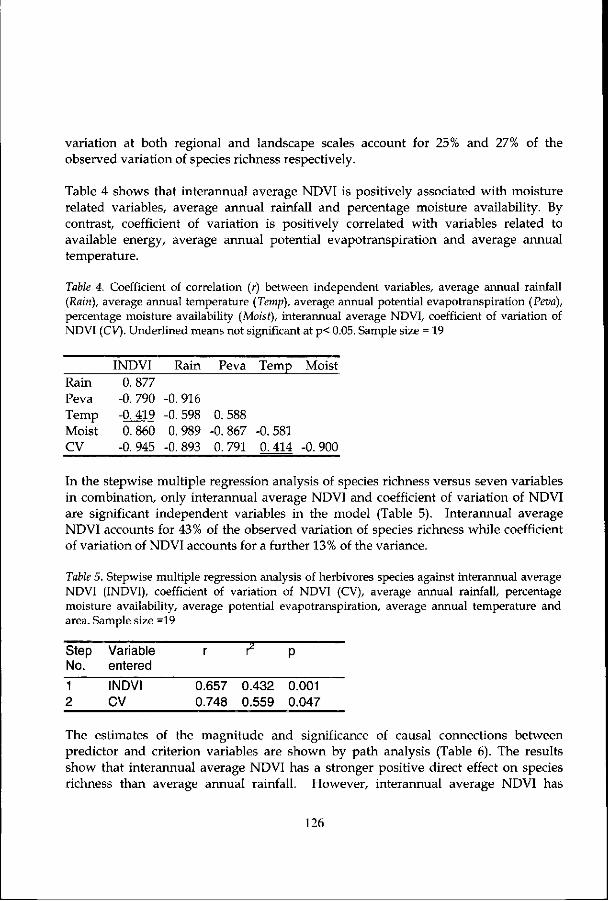
variation at both regional and landscape scales account for 25% and 27% of the observed variation of species richness respectively.

Table 4 shows that interannual average NDVI is positively associated with moisture related variables, average annual rainfall and percentage moisture availability. By contrast, coefficient of variation is positively correlated with variables related to available energy, average annual potential evapotranspiration and average annual temperature.

Table 4. Coefficient of correlation (r) between independent variables, average annual rainfall (Rain), average annual temperature (Temp), average annual potential evapotranspiration (Peva), percentage moisture availability (Moist), interannual average NDVI, coefficient of variation of NDVI (CV). Underlined means not significant at p< 0.05. Sample size = 19

INDVI Rain Peva Temp Moist

Rain Peva Temp Moist CV

0.877 -0. 790 -0. 419 0.860

-0. 945

-0. 916 -0. 598 0.989

-0. 893

0.588 -0.867 -0.581 0.791 0.414 -0.900

In the stepwise multiple regression analysis of species richness versus seven variables in combination, only interannual average NDVI and coefficient of variation of NDVI are significant independent variables in the model (Table 5). Interannual average NDVI accounts for 43% of the observed variation of species richness while coefficient of variation of NDVI accounts for a further 13% of the variance.

Table 5. Stepwise multiple regression analysis of herbivores species against interannual average NDVI (INDVI), coefficient of variation of NDVI (CV), average annual rainfall, percentage moisture availability, average potential evapotranspiration, average annual temperature and area. Sample size =19

Step Variable No. entered

1 INDVI 0.657 0.432 0.001 2 CV 0.748 0.559 0.047

The estimates of the magni tude and significance of causal connections between predictor and criterion variables are shown by pa th analysis (Table 6). The results show that interannual average NDVI has a stronger positive direct effect on species richness than average annual rainfall. However, interannual average NDVI has

126

slightly smaller total effects on species richness compared to average annual rainfall. Conversely, potential evapotranspiration has slightly larger negative direct and total effects on species richness compared to coefficient of variation of NDVI.

Table 6. Effects of predictor variables on species richness at regional scale. Direct, indirect and total effects are presented. All effects are significant at p<0.05. However, for indirect and total effects significance levels cannot be calculated (see Sokal and Rohlf, 1994)

Predictor variables Effects on species richness

Average annual rainfall (mm) Average annual potential evapotranspiration (mm) Interannual average NDVI Coefficient of variation of NDVI

Direct Indirect Total 0.49

-0.56 0.65

-0.53

1.51 -1.35 1.33 -1.36

2.10 -1.91 1.98

-1.89

0.6 0.20 0.27 0.34 0.41 interannual average NDVI

0.48 0.3 0.4 0.5 Interannual average NDVI

(a) (b) Figure 5. Relation between interannual average NDVI (VI) and (a) Regional (unequal areas) species richness (SR), SR = 2.468 + 32.87VI, r2 = 0.432, (b) Landscape (equal areas) species richness (SL), SL = -1.028 + 34.059VI, r2 = 0.346, both relations in a and b are statistically significant at p<0.05. The least-squares fit for the relations in both a and b were fitted with straight lines because residuals tend not to vary in a systematic fashion between positive and negative. Symbols for districts are given in Figure 1.

Discussion

Ecologists have shown interest in community stability mainly because man is per turbing natural and agricultural communities at ever-increasing rate. Hence, it is essential to know how communities respond to such perturbations and how they are

127

likely to respond in future. The stability of a community measures its sensitivity to disturbance (Begon et ah, 1990). Thus, a system is deemed stable if the variables all return to the initial equilibrium following their being perturbed from it. A system is locally stable if this return is known to apply only certainly for small perturbations and globally stable if the system returns from all possible perturbations (Pimm, 1984). There are terms that have been used to describe different aspects of stability such as variability, persistence, resilience, resistence, local stability and global stability (Begon et ah, 1990; Pimm, 1991). This study focuses on one aspect of stability, that is variability which describes how much the different variables of a system change in time.

The interannual variability in vegetation takes place as a result of climatic variability affecting germination and growth (Hobbs, 1990). Hence, large variations in vegetation composition and growth are seen in arid and semi-arid areas where rainfall is sporadic and the response of vegetation to such rainfall is rapid (Griffin and Friedel, 1985). Thus, the vegetation index time series give us a possibility to assess the climatic variability over the season and over the years (Oindo et al., 2000). For instance, calculating the coefficient of variation of NDVI for a number of years may describe the relative variability of vegetation cover for a given region. Consequently, regions with high coefficient of variation of NDVI should reflect regions with large variations in vegetation composition and growth. Such regions are likely to have unstable and unpredictable climatic conditions over a number of years. On the other hand, regions with low coefficient of variation of NDVI should depict regions with small variations in vegetation composition and growth. The results (Figure 5a,b) show that higher interannual average NDVI increases species richness, whereas higher coefficient of variation of NDVI decreases (Figure 6a,b) species richness.

Apparently, large herbivore species richness is low in regions with unstable and unpredictable climatic conditions. Hence, regions with current ecoclimatic instability may be characterized by high coefficient of variation of NDVI and relatively low interannual average NDVI. By contrast, high interannual average NDVI and relatively low coefficient of variation of NDVI characterize regions with current ecoclimatic stability. Both linear and multiple regression results (Table 3 and 5) reveal that the best predictor of species richness is interannual average NDVI. In addition, path-analysis (Table 6) shows that interannual average NDVI has the highest direct effect on species richness. So, why does interannual average NDVI emerge as the overriding variable? One possible explanation is that interannual average NDVI stands for environmental resources which may be utilized by herbivores species such as green-leaf biomass, photosynthetically active biomass and biomass of green vegetation (Holben et ah, 1980; Tucker and Sellers, 1986; Asrar, 1989).

128

25

20

15

10

I

eCipq

f "

i

i

h

c

i

i

i O 0

/ 1

ab

i

2

6

n

ko

i

sp go

n^

i

of oe

i

OQ

WI com ^ < 3 q csr

d

i

5 10 15 Coefficient of variation of NDVI

20 0 10 20 30 Coefficient of variation of NDVI

40

(a) (b)

Figure 6. Relation between coefficient of variation of NDVI (CV) and (a) Regional (unequal areas) species richness (SR), SR = 21.56-0. 608CV, r2 = 0.226, (b) Landscape (equal areas) species richness (SL), SL = 14.167-0. 202CV, r2 = 0.269 both the relations in a and b are statistically significant at p<0.05. The least-squares fit for the relations in both a and b were fitted with straight lines because residuals tend not to vary in a systematic fashion between positive and negative. Symbols for districts are given in Figure 1.

Moreover, Table 4 shows that interannual average NDVI is strongly associated with climatic variables (average annual rainfall and percentage moisture availability) related to vegetation growth (Nicholson et ah, 1990). Therefore, higher interannual average NDVI should represent high above-ground biomass. Consequently, herbivore species richness should be high in districts with higher interannual average NDVI due to abundance of above-ground biomass (Prins and Olff, 1998). Since interannual average NDVI is influenced by average annual rainfall, it has slightly lower total effects on species richness compared to that of average annual rainfall (Table 6).

When the coefficient of variation of NDVI over an eleven-year period is considered, districts with highest coefficient of variation have the lowest number of herbivore species (Figure 6a,b). Table 4 shows that coefficient of variation is positively associated with average annual temperature and average annual potential evapotranspiration but negatively correlated with average annual rainfall and percentage moisture availability. It appears that regions with high coefficient of variation have high average annual temperature and high potential evapotranspiration that reduce biomass production (Roberts, 1987). Furthermore, the negative correlation between coefficient of variation of NDVI and interannual average NDVI indicates that regions with high coefficient of variation of NDVI have low above-ground biomass.

129

The relationship between species diversity and area has a long history in ecological studies. The traditional approach to species-area relationships derives from island biogeography, where the relationship S = cAz has found wide application: S is the number of species on an island of area A, c is a constant and the exponent z reflects the rate at which number of species increase with island size (MacArthur and Wilson, 1967). The equation can be resolved into a linear regression by the use of logarithms, when z becomes the slope: log S = z log A + k. Here k is also a constant-the intercept. Although derived from island faunas and more recently floras, the same formula has also been applied to many mainland situations, and for various taxa (Pomeroy and Lewis, 1987). However, when we look at the herbivore species richness in Kenya, there is a relatively weak negative correlation between the size of a district and its number of species (Figure 4a) with z value of about -0.0001. In this case the z value reflects the rate at which the number of species decrease with district's size indicating that smaller districts have high species richness than larger districts. Evidently, more herbivore species are found in the smaller (southern and coastal) districts, which are currently much wetter, greener and contain more national parks (Table 1). On the contrary, herbivore species are low in larger districts because they are found in northern arid and semi-arid regions of Kenya (with few national parks) where interannual average NDVI is low and coefficient of variation of NDVI is high.

The authenticity of the regional data layers need to be confirmed because often coarse scale data coverages are useful for visual demonstration purposes but are worthless for scientific analysis (Miller et al., 1989). The districts are highly unequal by area and habitat heterogeneity. Hence, the spatial variance of NDVI data within a district may be quite high. The high correlations between interannual NDVI variables and average annual rainfall as well as average annual potential evapotranspiration (Table 4) provide strong evidence for the ecological validity of these data. These relationships are consistent with previous studies, which have proved NDVI to be well correlated with rainfall and evapotranspiration (Nicholson et al, 1990; Cihlar et ah, 1991). Furthermore, Figure 4b shows that regional (unequal areas) species richness is strongly correlated with landscape (equal areas) species richness. Consequently, the prediction of species richness by interannual average NDVI and coefficient of variation of NDVI at regional (unequal areas) scale roughly matches the prediction at landscape (equal areas) scale (see Figures 5a,b and 6a,b). However, predicting herbivore species richness requires precise environmental data. Thus, the regional perspective requires the sacrifice of ecological precision for the sake of the generality, as well as the provision of more data thereby allowing statistical predictions. Environmental and species richness relationships, documented by regression statistics, can be used to identify areas more likely characterized by high species diversity (Miller et al., 1989). Path-analysis has

130

some advantages over multiple regression analysis. In this study, it helped to determine the major paths by which environmental variables affect species richness. In addition, path-analysis quantifies the effects of a given environmental variable on different environmental variables and species richness. Thus, indicating the various ecological consequences of a change in one environmental variable.

Although the NOAA-AVHRR data are the best current available data now for this kind of analysis, there are limitations inherent to the data and to the approach used. The variability in vegetation cover measured from AVHRR data is the result of multiple influences: interannual variability in rainfall and temperature due to intrinsic characteristics of the climate, climate trends which exceed the 11-year period, vegetation successions, anthropogenic land-cover changes, and variability in the state of the atmosphere (Fjeldsa et ah, 1997). In this study, we simply regarded any region that is characterized by high interannual average NDVI and relatively low coefficient of variation as providing stable conditions for the herbivore species living there. A more comprehensive analysis requires investigation of other characteristics of time variability in surface conditions such as Fourier transform, amplitude of the variations, summed changes between neighboring months, among others (Fjeldsa et ah, 1997).

Conclusion

The study reveals that interannual maximum NDVI variables are strongly related to herbivore species richness at regional scale. This indicates that NDVI variables represent the integration of climatic variables at a given region and time (Anyamba and Eastman, 1996) important for the distribution of herbivore species. Moreover, the results establish that interannual average NDVI relates to environmental factors favorable to the distribution of the herbivore species. Conversely, coefficient of variation represents factors limiting the distribution of herbivore species.

Because of the multitude of current and historical factors affecting herbivore species richness, we can hardly expect to make precise predictions from remote sensing data alone. However, our study certainly provides general support to the hypothesis (Sanders and Hessler, 1969; Fjeldsa and Lovett, 1997) that high species diversity occurs in stable and predictable environments. It is of particular interest that persistence of stable regional conditions that permitted species specialization (Currie, 1991) and hence high species diversity may also have enhanced development of stable human cultures and agricultural development (Fjeldsa and Lovett, 1997). Therefore, the pressure on nature is often particularly great in the biologically most unique regions (Fjeldsa and Lovett, 1997). Since the late 1970's agriculture has encroached rangeland districts such as Narok, Laikipia, Taita Taveta, Kitui, Machakos, Kwale, Baringo, West

131

Pokot and Samburu (Aligula et ah, 1997). The current conservation strategy of reserving areas with few people therefore needs to be supplemented with actions to secure sustainable land use in these districts with numerous cases of human-wildlife conflicts (Table 1). Although biodiversity should be managed in a sustainable way in Kenya, the distinction made between stable and unstable regions suggests that distinctions must also be made concerning conservation priorities and management approaches (Fjeldsa and Lovett, 1997).

Acknowledgement

We have gratefully acknowledged the financial support of the government of The Netherlands through International Institute for Aerospace Surveys and Earth Science (ITC) for the success of this research. Appreciation goes to H. Mwendwa, Director of Department Resource Surveys and Remote Sensing (DRSRS) for providing animal species data. The USAID/FEWS Project provided valuable AVHRR-NDVI time series images through the Internet.

References

ADDS (2000) Africa Data Dissemination Service, EROS Data Center, U.S. Geological Survey Sioux Falls, S. Dakota, US 57198. http://edcsnw4.cr.usgs.gov/adds/ adds.html

Aligula HM, Said MY, Njuguna EC, de Leeuw J and Skidmore AK (1997) Geo-Information for sustainable rangeland management: A case study of the arid and semi-arid lands in Kenya. In: Beek KJ, de Bie CA and Driessen P (eds), Proceedings of the International Conference on Geo- Information for sustainable land management, Enschede, ITC, 17-21 August 1997, CD-ROM, ITC, The Netherlands

Anyamba A and Eastman JR (1996) Interannual variability of NDVI over Africa and its relation to El Nino/Southern Oscillation. International Journal of Remote Sensing 17: 2533-2548

Asrar G (1989) Theory and Applications of Optical Remote Sensing. Wiley Series in Remote Sensing. John Wiley and Sons, New York

Begon M, Harper JL and Townsend CR (1990) Ecology: Individuals, populations and Communities. Blackwell Scientific Publications, Cambridge

Brown JH (1988) Species Diversity. In: Myers AA and Giller PS (eds) Analytical Biogeography. An integrated approach to the study of animal and plant distributions, pp 57-89. Chapman and Hall, London

Cihlar J, ST Laurent L and Dyer JA (1991) The relation between normalized differences vegetation index and ecological variables. Remote Sensing of Environment 35: 279-298

132

Currie DJ (1991) Energy and Large-scale patterns of animal- and plant- species richness. American Naturalist 137: 27-49

Currie DJ and Paquin V (1987) Large-scale biogeographical patterns of species richness of trees. Nature 329: 326-327

De Leeuw J, Prins HHT, Njuguna EC, Said MY and De By R (1998) Interpretation of DRSRS animal counts (1977-1997) in the rangeland districts of Kenya. Ministry of Planning and National Development, Nairobi

Dirschl HJ, Norton-Griffiths M and Wetmore SP (1981) Training observers for aerial surveys of herbivores. The Wildlife Society Bulletin 9(2)

Eck TF and Kalb VL (1991) Cloud screening for Africa using geographically and seasonally variable infrared threshold. International Journal of Remote Sensing 12:

1205-1221 Fjeldsa J, Ehrlich D and Lambin E (1997) Are biodiversity 'hotspots' correlated with

current ecoclimatic stability? A pilot study using the NOAA-AVHRR remote sensing data. Biodiversity and Conservation 6: 401-422

Fjeldsa J, Lambin E and Mertens B (1999) Correlation between endemism and local ecoclimatic stability documented by comparing Andean bird distributions and remotely sensed land surface data. Ecography 22: 63-78

Fjeldsa J and Lovett JC (1997) Biodiversity and environmental stability. Biodiversity and Conservation 6: 315-323

Gaston KJ (1994) Rarity. Chapman and Hall, London Gaston KJ (2000) Global patterns in biodiversity. Nature 405: 220-227 Griffin GF and Friedal MH (1985) Discontinuous change in central Australia: some

major implications of ecological events for land management. Journal of Arid Environment 9: 63-82

Groombridge B (1992) Global Biodiversity. Status of the Earth's Living Resources. World Conservation Monitoring Centre, London

Halternorth T and Diller H (1980) Mammals of Africa including Madagascar. HarperCollins, London

Henricksen BL (1986) Reflections on drought: Ethiopia 1983-1984. International Journal of Remote Sensing 7:1447-1451

Hobbs RJ (1990) Remote sensing of spatial and temporal dynamics of vegetation. In: Hobbs RJ and Mooney HA (eds), Remote Sensing of Biosphere Functioning. Ecological Studies 79, pp 203-219. Springer-Verlag, New York

Holben BN, Tucker CJ and Fan CJ (1980) Spectral assessment for soybean leaf area and leaf biomass. Photogrametry Engineering and Remote Sensing 46: 651-656

Holben BN (1986) Characteristics of maximum-value composite images for temporal AVHRR data. International Journal of Remote Sensing 7:1435-1445

Lewis JE, Rowland J and Nadeau A (1998) Estimating maize production in Kenya using NDVI: Some statistical considerations. International Journal of Remote

133

Sensing 19: 2609-2617 Los SO (1998) Linkages between Global Vegetation and Climate. An analysis based on

NOAA-AVHRR data. GSFC/CR-1998-206852, National Aeronautics and Space Administration, Goddard Space Flight Center, Greenbelt, Maryland

MacArthur RM and Wilson EO (1967) The theory of island biogeography. Princeton University Press, Princeton

Miller RI, Stuart SN and Howell KM. (1989) A methodology for analyzing rare species distribution patterns utilizing GIS technology: The rare birds of Tanzania. Landscape Ecology 2:173-189

Nicholson SE, Davenport ML and Malo AR (1990) A comparison of the vegetation response to rainfall in the Sahel and East Africa, using Normalized Difference Vegetation Index from NOAA-AVHRR. Climate Change 17: 209-242

Norton-Griffiths M (1978) Counting animals. Handbook no.l. Africa Wildlife Leadership Foundation, Nairobi

Odland J (1988) Spatial autocorrelation. In: Thrall GI (ed) Sage University Scientific Geography Series 9. Sage Publications, Beverly Hills

Oindo BO, de By RA, Skidmore AK (2000) Interannual variability of NDVI and bird species diversity. International Journal of Applied Earth observation and Geoinformation 2:172-180

Ottichilo WK and Khaemba, W (2001) Validation of observer and aircraft calibration for aerial animal surveys: A case study of the Department of Resource Surveys and Remote Sensing (DRSRS), Kenya. African Journal of Ecology 39: 45-50

Ottichilo WK and Sinange RK (1985) Differences in the visual and photographic measurements in the estimation of strip widths for aerial censuses of animal populations. DRSRS, Ministry of Planning and National Development, Nairobi

Owen JG (1990) Patterns of mammalian species richness in relation to temperature, productivity and variance in elevation. Journal of Mammalogy 71:1-13

Pfirman E, Hogue J and See L (1999) Windisp 3.5. Map and image display system version 990217. UN Food and Agriculture Organization, USAID Famine Early Warning System, Southern Africa Development Community, US Forest Service and US Geological Survey

Pianka ER (1983) Evolutionary ecology. Harper and Row, Publishers, Inc., New York Pimm SL (1984) The complexity and stability of ecosystems. Nature 307: 321- 326 Pimm SL (1991) The Balance of Nature? Ecological issues in the conservation of species

and communities. University of Chicago Press, Chicago Pomeroy D and Lewis A (1987) Bird species richness in tropical Africa: some

comparisons. Biology Conservation 40:11-28 Prins HHT and Olff H (1998) Species-richness of African grazer assemblages: Towards

a functional explanation. In: Newbery DM, Prins HHT and Brown ND (eds) Dynamics of tropical communities, pp 449-490. Blackwell Science, Oxford

134

Rohde K (1999) Latitudinal gradients in species diversity and Rapoport's rule revisited: a review of recent work and what can parasites teach us about the causes of the gradients? Ecography 22: 593-613

Richard Y and Poccard I (1998) A statistical study of NDVI sensitivity to seasonal and interannual rainfall variations in Southern Africa. International Journal of Remote Sensing 19: 2907-2920

Ricklefs RE (1989) Speciation and diversity: Integration of local and regional processes. In: Otte D and Endler J (eds) Speciation and its consequences, pp 599-622. Sinauer Associates, Sunderland

Roberts BR (1987) The availability of herbage. In: Hacker JB and Ternouth JH (eds) The nutrition of herbivores, pp 47-64. Academic Press Australia, Sydney

Rosenzweig ML (1995) Species diversity in space and time. Cambridge University Press, Cambridge

Sanders HL and Hessler RR (1969) Ecology of the deep sea benthos. Science 163:1419-1424

Shackleton NJ, Berger A and Peltier WR (1990) An alternative astronomical calibration of the lower pleistocene timescale based on ODP site 677. Trans. Royal Society Edinburgh: Earth Sciences 81: 251-261

Sokal RR and Rohlf FJ (1994) Biometry: the principles and practice of statistics in biological research. W.H. Freeman and Company, New York

Sombroek WG, Braun HMH and van der Pouw BJW (1982) Exploratory soil map and Agro-climatic zone map of Kenya, 1980 scale 1:1,000,000. Exploratory Soil Survey Report No. El, Kenya Soil Survey, Nairobi

Tucker CJ and Sellers PJ (1986) Satellite remote sensing of primary production. International Journal of Remote Sensing 7:1133-1135

135

CHAPTER 10

SYNTHESIS:

PATTERNS AND THEORIES OF SPECIES DIVERSITY

Introduction

The explanation of spatial and temporal variation in species diversity is one of the central problems of biology (Groombridge, 1992). The problem has stimulated much discussion and numerous hypotheses have been advanced to account for species diversity patterns — these hypotheses often operate at different levels of explanation and much confusion has arisen as a result (Huston, 1979). At the outset, let us be clear why the problem of understanding species diversity is complicated. In the first place, species diversity is surely not determined in all cases by the same single factor but is the outcome of many contributing factors (Diamond, 1988). Secondly, while one can formulate 'rules' about species diversity, each rule has many exceptions. For example, it has been hypothesized that species diversity is high in stable environments (Sanders and Hessler, 1969; Fjeldsa and Lovett, 1997). However, there are examples of low diversity communities in stable environments, such as tropical forests dominated by cativo (Prioria copifera), Mora, Gilbertiodendron, and other species in central Africa (Hart et al., 1989). Furthermore, some communities with high species diversity are often found in environments that seem to be severe, unpredictable or unstable, such as the Sonoran desert (Whittaker and Niering, 1965). The exceptions to rules based on a single factor arise in part for the obvious reason that species diversity is influenced by many different interacting factors and processes, so the effect of one factor may be overridden by others (Diamond, 1988).

136

It is evident, however, that any complete explanation of patterns of species diversity must involve both historical events and current ecological processes —the former implicit in any explanation of the origin of diversity, the latter in explanations of its maintenance, these being two separate, although intimately linked processes (Groombridge, 1992). The progress in the understanding of ecological systems has been achieved by the awareness that patterns and processes are strongly scale dependent (Levin, 1992). Thus, patterns in species diversity are influenced by the spatial and temporal scale at which both a group of organisms and the factors that possibly determine the species richness of this group operate (Bohning-Gaese, 1997). Hence, an important step towards a more general understanding of species diversity might be to emphasize the spatial scale or quadrat size at which species richness is estimated (Cody, 1975).

The main aim of this thesis was to provide explanation of spatial patterns of species diversity in Kenya based on current ecological processes. Our research was motivated by the fact that an understanding of the importance of biological diversity should rest on an understanding of how and why it has the form that it does (Groombridge, 1992). Moreover, Kenya needs the formulation of strategy to maintain, use and preserve biodiversity (Government of Kenya, 1994) that depends on understanding ecological processes that naturally maintain species within particular areas and habitats (Ricklefs, 1995). Since landscape scale is appropriate for management decisions concerning the conservation of species diversity (Bohning-Gaese, 1997), we carried out many studies at landscape scale (Chapters 2-6). In addition, studies (Chapters 7-9) were performed at regional scale because the pressure on biodiversity is often particularly great in the biologically most unique regions (Fjeldsa and Lovett, 1997).

Getting the measure of species diversity

To proceed very far with the study of biodiversity, it is necessary to pin the concept down. We cannot even begin to look at how biodiversity is distributed, or how fast it is disappearing, unless we can put units on it (Purvis and Hector, 2000). However, any attempt to measure biodiversity quickly runs into the problem that it is a fundamentally multidimensional concept —it cannot be reduced sensibly to a single number (Magurran, 1988). Rather, different facets of biodiversity can each be quantified. The most commonly considered facet of biodiversity is species richness — the number of species in a site or habitat. Hence, species are an obvious choice unit when trying to measure diversity. A site containing a hundred species might not seem particularly diverse if 99.9% of individuals belong to the same species. As a result many diversity indices have been developed to convey the extent to which individuals

137

are distributed evenly among species (Magurran, 1988). Hence, the number of species and the evenness of relative abundance are the two statistical properties used to quantify species diversity. The best known composite statistics that combine these two statistical components of biodiversity are Shannon-Wiener and Simpson's indices. Thus, species diversity may be defined as a measure of species composition, in terms of both the number of species and their relative abundances. It is a synthetic biotic index that captures multidimensional information relative to the species composition of an assemblage or a community (Legendre and Legendre, 1998).

In deriving Shannon-Wiener and Simpson's indices including species richness, data for each species are added together. The two assumptions that are of interest here are (1) that the index is limited to one taxonomic group, i.e., birds rather than birds plus insects, and (2) that all species are equal (a buffalo is equivalent to a warthog in a count of species present). It is ironic that species are treated as equal in conventional indices when the very basis of the identification of species is that they are different from each other. The saying that 'you can't add apples and pears' alerts us to this problem (Cousins, 1991). Furthermore, Shannon-Wiener and Simpson's indices combine species richness and relative abundance of species, which is not a fixed property of species, but vary widely temporally and spatially (Groombridge, 1992). Hence, relative abundance of species is more affected by quantitative variability (Pielou, 1995) and requires massive sampling efforts (Chapters 2, 3). Since biodiversity surveys already take a large proportion of conservation budgets and the demand for them is growing, cost-effectiveness is becoming increasingly important (Burbidge, 1991). Consequently, conservationists face the problem of how to identify the most important areas for biodiversity quickly and cheaply (Williams and Gaston, 1994). For rapid appraisals of biodiversity over large areas, suitable diversity indices should be based on binary (presence-absence) data that must be easy to measure and capable of capturing the degree of difference between species. A potential solution is to measure diversity based on body size which is easy to measure and it is related to many other species characteristics such as longevity, reproductive success, predation, competition and dispersal (Dunham et ah, 1978; Siemann et al., 1996). In addition to the conventional Shannon-Wiener and Simpson's indices, we proposed (chapters 2 and 3) two new indices of diversity for large herbivore species based on their body size that take into account the degrees of difference between species and require less sampling effort.

Species-energy relationships

Perhaps the greatest unsolved ecological riddle is why some natural habitats are home to more species than others. Why, for instance, tropical rainforest contains some ten times more tree species than forests in temperate regions (Morin, 2000)? One factor

138

thought to be important in modulating any effect on the physical structure of the Earth in determining species richness is the relationship between the number of species in an area and ambient available ('usable') environmental energy. This energy is usually estimated from models or indirectly from other variables, and often used interchangeably with 'net primary productivity' (Gaston, 2000). Net primary productivity (NPP) is a difficult variable to measure directly, especially at landscapes or regional scales. Consequently, in regional biodiversity studies, NPP is typically derived from climatic data collected at scattered (and often biased) sampling points — these points are extrapolated in order to characterize productivity over a large region (Owen, 1990; Currie, 1991). Such climate-based models assume that the vegetation cover is 'natural', and ipso facto is under the control of climate (Box et al, 1989). However, at landscape and regional scales, vegetation productivity is also influenced by non-climatic factors including soil nutrient and structure, topography, disturbance and land use. Thus, the maximum Normalized Difference Vegetation Index (NDVI) derived from satellite data provides a more accurate index of ecosystem productivity compared with climate-based models, by virtue of being spatially explicit (Box et al., 1989).

The form and cause of diversity-productivity relations are hotly debated in the study of patterns of species diversity, with many fundamental issues as yet unresolved. Much of the discussion centres on the influence of spatial scale on diversity-productivity relationship (Gaston, 2000). At a relatively local scale, there is a marked tendency for general unimodal (hump-shaped) relationship between species richness and productivity, with species richness increasing from low to moderate levels of productivity and then declining again towards high levels of productivity when a sufficient range of productivity values is sampled (Rosenzweig and Abramsky, 1993). By contrast, at geographical scales diversity generally increases with productivity (Currie and Paquin, 1987; Currie, 1991). In our studies investigating diversity-productivity relations (Chapters 4, 5, 8), the interannual maximum average NDVI (1982-1993) was integrated as an index for productivity. Consequently, high maximum average NDVI should represent high productivity. Statistical analyses revealed that at a landscape scale high productivity results in lower species richness of large mammals and plants (Chapter 4). The unimodal (hump-shaped) relationship was observed between productivity and large mammal species richness, and abundance of individuals — highest number of species and individuals occurred at intermediate levels of productivity (Chapters 4, 5). Conversely, at regional scale species richness of birds (Chapter 8) and large herbivores (Chapter 9) increase with productivity. Thus, we confirmed previous cited findings on diversity-productivity relations. In addition, mean annual potential evapotranspiration emerged as the overriding environmental factor influencing bird species richness at regional scale (Chapter 7). Potential

139

evapotranspiration is highly correlated with terrestrial primary productivity (Rosenzweig, 1968; Leith, 1975) and is thus a measure of the net atmospheric energy balance, independent of water availability (Currie, 1991).

The positive relationship between species richness and productivity (energy availability) at regional scale and low-to-moderate energy levels at landscape scale may be explained by the fact that increasing productivity is assumed to support high production of grass resources. In turn, this enables more individual organisms to coexist, and thus more species at abundances that make it possible for them to maintain viable populations, that over time allows an increase in species richness and number of individuals (Gaston, 2000). Our results support this more-individuals hypothesis at landscape scale because mammal species richness and number of individuals increase with productivity at low-to-moderate energy levels (Chapter 5). This provides evidence as to how variation of species richness and abundance of individuals may change with productivity in animal systems.

Environmental heterogeneity and species diversity

Environmental heterogeneity broadly means the spatial or temporal variation in the physical, chemical or biological features of the environment that create different conditions (or niches) that different species can exploit preferentially (Morin, 2000). Environments which are more spatially heterogeneous can be expected to accommodate extra species because they provide a greater variety of microhabitats, a greater range of microclimates, more places to hide from predators, and so on. Thus, whether spatial heterogeneity arises intrinsically from the abiotic environment, or from the other biological components of the community, it is capable of promoting an increase in species richness (Begon et ah, 1990). Time also serves as a niche dimension that can be partitioned, so that temporal variability provides opportunities for differentiation absent in an environment that is constant with time (Diamond, 1988).

Heterogeneity is contributed by plants most significantly by the vertical structure and complexity produced by the roots, stems, branches and leaves of woody plants, as well as the non-woody plants growing with them (Huston, 1994). One of the classic generalizations of ecology is based on MacArthur and MacArthur's (1961) observation that bird species diversity is positively correlated with the structural complexity of the vegetation. Since this observation, similar patterns have been reported for the diversity of many different kinds of animals in relation to vegetation structure or other aspects of environmental heterogeneity (Recher, 1969; Tonn and Magnuson, 1982). Animals themselves can further increase the heterogeneity created by plants by eating or killing

140

plants, by disturbing the soil with burrows, trails and wallows, by defecating, and by dying (Huston, 1994).

It has been proposed that the within region variability of NDVI values, as defined by standard deviation of maximum NDVI, may be used to measure heterogeneity (Walker et al, 1992). At landscape scale, we demonstrated that high values of standard deviation of maximum NDVI and coefficient of variation (i.e., relative variability of vegetation cover) result in high species richness of mammals and plants (Chapter 4). Thus, our results confirmed that areas with high spatial heterogeneity are endowed with more species. In addition, temporal heterogeneity may be estimated from variability of multitemporal NDVI values. The positive correlation between biodiversity indicators (species richness and number of individuals) and standard deviation of maximum NDVI demonstrates that the variability of multitemporal NDVI values is related to temporal heterogeneity of vegetation cover for selected individual regions (Chapter 5). However, at regional scale image pixels with high standard deviation of maximum NDVI and high coefficient of variation reflect drought risk (unstable) regions that support low species richness of birds (Chapter 8) and large herbivores (Chapter 9).

Researchers have examined the spatial configuration of habitat variables to predict species richness (Stoms and Estes, 1993). Measures of spatial patterning include a diversity index from information theory (Shannon-Wiener and Simpson's indices) based on number and proportions of vegetation or soil types (Miller et al., 1989). Landscape ecologists have also derived or adapted indices of habitat heterogeneity from remotely sensed data products such as land cover or habitat maps (O'Neil et ah, 1988). We used Landsat TM derived habitat map to compute the Shannon-Wiener and Simpson's indices of diversity for the Masai Mara ecosystem, Narok district. Areas with the highest habitat diversity were found to support higher number of large mammal species than areas with less habitat diversity (Chapter 6). Moreover, our results demonstrated that changes of scale in calculations of habitat diversity influence the strength of the correlation with species richness. However, the influence does not change the direction of the relationship between habitat diversity and species richness. Our study further revealed that mammal species richness is more strongly associated with habitat diversity at relatively intermediate scale (20 x 20 km). This implies that protecting the diversity of habitats at this scale ensures high levels of species diversity.

Ecoclimatic stability and species diversity

Spatial patterns of species diversity have been hypothesized to depend upon climatic stability and predictability. High species diversity may be caused by accumulation of

141

species over a long time in places where environmental conditions remained predictable and stable (Fjeldsa and Lovett, 1997). This is because populations would be stable and extinction rates due to population fluctuations would be low (Sanders and Hessler, 1969). Conversely, unpredictable and severe environments may have low species diversity because unpredictability forces organisms to have broader niches which allow fewer species to be 'packed in' as well as causing a greater chance of extinction for marginal populations (Slobodkin and Sanders, 1969; Pielou, 1975). However, some communities with high species diversity are often found in environments that seem to be severe, unpredictable or unstable (Whittaker and Niering, 1965).

Predictability and stability in particular are defined in a variety of ways and are difficult to measure, especially on the evolutionary time scale (Huston 1979). However, Fjeldsa et ah, (1997) linked local species endemism with local environmental stability using remotely sensed data, thereby suggesting a link between short-term and long-term stability (Fjeldsa et ah, 1999). In view of this, remotely sensed data —Advanced Very High Resolution Radiometer-Normalized Difference Vegetation Index (AVHRR-NDVI) — can serve as a good proxy for studying current interannual climatic variability (Richard and Poccard, 1998). Hence with remotely sensed derived climatic variability indices, we demonstrated at regional scale that high species richness of birds (Chapter 8) and large herbivores (Chapter 9) occur in regions in Kenya where present-day climatic conditions remained predictable and stable. The bird species diversity is high because the greatest bulk of woody vegetation is found in stable, productive and predictable environments (Prins and Olff, 1998), which in the tropics are extraordinarily rich in insect species that support a rich diversity of birds (Lewis and Pomeroy, 1989). On the other hand, large herbivore species diversity is high in regions with current ecoclimatic stability due to abundance of high forage quantity and quality (Van Soest, 1985) leading to high carrying capacity (Roberts, 1987).

Remote sensing and species diversity research

Satellite images of the Earth have been commercially available since the early 1970's. Despite long standing scientific interest, the potential of remote sensing technology to measure, map, monitor and model spatial patterns as well as trends in species diversity have been little explored (Stoms and Estes, 1993). However, such data are important and needed if we are to manage our resource base to preserve species diversity to the maximum extent possible (Walker et ah, 1992). To monitor or predict the trends in species richness patterns, it is necessary to identify biophysical variables that are measurable with remote sensing instruments and whose change in magnitude is significant enough to be detected (Stoms and Estes, 1993).

142

Setting biologically defensible conservation priorities demands sound information concerning the locations of species. The capabilities of remote sensing are greater than simply mapping habitat types. Our results demonstrate that habitat heterogeneity (Chapters 4-6) and net primary productivity (Chapters 4, 5) associated with species richness and abundance of individuals (Chapter 5) may be estimated from remotely sensed data. In addition, factors reflecting current ecoclimatic stability related to patterns of species diversity may be derived from remotely sensed data (Chapters 8, 9). Furthermore, remote sensing provides synoptic coverage with more intensive spatial sampling than the sparse point samples traditionally used in testing species richness hypotheses. Global coverage from space-borne sensors also means we can obtain estimates of biophysical factors that are consistent between regions, allowing comparative studies across the entire gradient of climate and productivity (Stoms and Estes, 1993). Thus, with remote sensing technology, we are able to make real progress in understanding why more species occur in some places than in others (Chapters 4, 5, 8, 9) and in identifying the most critical places that must be protected to preserve the maximum number of species (Chapter 6).

References

Begon M., Harper JL and Townsend CR (1990) Ecology: Individuals, populations and Communities. Blackwell Scientific Publications, Cambridge

Bohning-Gaese K (1997) Determinants of avian species richness at different spatial scales. Journal of Biogeography 24: 49-60

Box EO, Holben BN and Kalb V (1989) Accuracy of the AVHRR Vegetation Index as a predictor of biomass, primary productivity and net CO2 flux. Vegetatio 80: 71-89

Burbidge AA (1991) Cost constraints on surveys for nature conservation. In: Margules CR and Austin MP (eds) Nature conservation: Cost effective biological surveys and data analysis, pp 3-6. CSIRO, Canberra

Cody ML (1975) Towards a theory of continental species diversities: bird distributions over Mediterranean habitat gradients. In: Cody ML and Diamond JM (eds) Ecology and Evolution of communities, pp 214-57. Cambridge, Massachusetts: Belknap Press

Cousins SH (1991) Species diversity measurement: Choosing the right index. Trends in Ecology and Evolution 6:190-192

Currie DJ (1991) Energy and large-scale patterns of animal- and plant- species richness. American Naturalist 137: 27-49

Currie DJ and Paquin V (1987) Large-scale biogeographical patterns of species richness of trees. Nature 329: 326-327

Diamond J (1988) Factors controlling species diversity: Overview and synthesis.

143

Annals of the Missouri botanical Garden 75:117-129 Dunham AE, Tinkle DW and Gibbons JW (1978) Body size in island lizards: A

cautionary tale. Ecology 59:1230-1238 Fjeldsa J, Ehrlich D and Lambin E (1997) Are biodiversity 'hotspots' correlated with

current ecoclimatic stability? A pilot study using the NOAA-AVHRR remote sensing data. Biodiversity and Conservation 6: 401-422

Fjeldsa J, Lambin E and Mertens B (1999) Correlation between endemism and local ecoclimatic stability documented by comparing Andean bird distributions and remotely sensed land surface data. Ecography 22: 63-78

Fjeldsa J and Lovett JC (1997) Biodiversity and environmental stability. Biodiversity and Conservation 6: 315-323

Gaston KJ (2000) Global patterns in biodiversity, Nature 405:220-227 Government of Kenya (1994) The Kenya National Environment Action Plan Report,

Ministry of Environment and Natural Resources, Nairobi Groombridge B (1992) Global Biodiversity. Status of the Earth's Living Resources.

World Conservation Monitoring Centre, London Hart TB, Hart JA and Murphy PG (1989) Monodominant and species-rich forests of the

humid tropics: Causes for their co-occurrence. American Naturalist 133: 613-633 Huston MA (1979) A general hypothesis of species diversity. American Naturalist 113:

81-101 Legendre P and Legendre L (1998) Numerical Ecology, Elsevier Science BV,

Amsterdam Leith H (1975) Modeling the primary productivity of the world. In: Lieth H and

Whittaker RH (eds) Primary productivity of the Biosphere, Ecological Studies 14, pp 237-263. Springer-Verlag, Berlin

Levin SA (1992) The problem of pattern and scale in Ecology. Ecology 73:1943-1967 Lewis A and Pomeroy D (1989) A bird atlas of Kenya. Balkema AA, Rotterdam Magurran AE (1988) Ecological Diversity and its Measurement. Croom Helm, London Miller RI, Stuart SN and Howell KM (1989) A methodology for analyzing rare species

distribution patterns utilizing GIS technology: The rare birds of Tanzania. Landscape Ecology 2:173-189

Morin PJ (2000) Biodiversity's ups and downs. Nature 406: 463- 464 O'Neil RV, Krummel JR, Gardener RH, Sugihara G, Jackson B, Deangelis DL, Milne

BT, Turner MG, Zygmunt B, Christensen SW, Dale VH and Graham RL (1988) Indices of Landscape Pattern. Landscape Ecology 1:153-162

Owen JG (1990) Patterns of mammalian species richness in relation to temperature, productivity and variance in elevation. Journal of Mammalogy 71:1-13

Pielou EC (1975) Ecological Diversity. John Wiley and Sons, New York Pielou EC (1995) Biodiversity versus old-style diversity: In: Boyle TJB and Boontawee

B (eds) Measuring and monitoring biodiversity in tropical and temperate forests,

144

pp 5-17. Center for International Forestry Research, Bogor, Indonesia Prins HHT and Olff H (1998) Species-Richness of African grazer assemblages: Towards

a functional explanation. In: Newbery DM, Prins HHT and Brown ND (eds) Dynamics of tropical communities, pp 449-490. Blackwell Science, Oxford

Purvis A and Hector A (2000) Getting the measure of biodiversity. Nature 405: 212-219 Recher HF (1969) Bird species diversity and habitat diversity in Australia and North

America. American Naturalist 103: 75-80 Richard Y and Poccard I (1998) A statistical study of NDVI sensitivity to seasonal and

interannual rainfall variations in Southern Africa. International Journal of Remote Sensing 19: 2907-2920

Ricklefs RE (1995) Distribution of biodiversity. In: Heywood VH and Watson RT (eds) Global Biodiversity Assessment, pp 139-166. Cambridge University Press, Cambridge

Roberts BR (1987) The availability of herbage. In: Hacker JB and Ternouth JH (eds) The nutrition of herbivores, pp 47-64. Academic Press Australia, Sydney

Rosenzweig ML (1968) Net primary productivity of terrestrial environments: Predictions from climatological data. America Naturalist 102: 67-84

Rosenzweig ML and Abramsky Z (1993) How are diversity and productivity related? In: Ricklefs RE and Schluter D (eds) Species diversity in ecological communities. Historical and geographical perspectives, pp 52-65. University of Chicago Press, Chicago

Sanders HL and Hessler RR (1969) Ecology of the deep sea benthos. Science 163:1419-1424

Siemann E, Tilman D and Haarstad J (1996) Insect species diversity, abundance and body size relationships. Nature 380: 704-706

Slobodkin LB and Sanders HL (1969) On the contribution of environmental predictability to species diversity. Brookhaven Symp. Biology 22: 82-93

Stoms DM and Estes JE (1993) A remote sensing research agenda for mapping and monitoring biodiversity. International Journal of Remote Sensing 14:1839-1860

Tonn WM and Magnuson JJ (1982) Patterns in the species composition and richness of fish assemblages in northern Wisconsin lakes. Ecology 63:1149-66

Van Soest PJ (1985) Composition, Fiber Quality, and Nutritive Value of Forages. In: Heath ME, Barnes RF and Metcalfe DS (eds) Forages: The Science of Grassland Agriculture, pp 412-421. Iowa State University Press, Iowa

Walker RE, Stoms DM, Estes JE and Cayocca KD (1992) Relationships between biological diversity and multi-temporal vegetation index data in California. Technical Papers of the 1992 Annual meeting of ASPRS/ACSM held in Albuquerque, New Mexico, 3-7 March 1992, pp 562-571.Bethesda, MD: American Society for Photogrammetry and Remote Sensing

Williams PH and Gaston KJ (1994) Measuring more of Biodiversity: Can higher-taxon

145

richness predict wholesale species richness? Biological Conservation 67: 211-217 Whittaker RH and Niering WA (1965) Vegetation of the Santa Catalina Mountains,

Arizona. (II) A gradient analysis of the south slope. Ecology 46: 429-452

146

Summary

The most striking feature of Earth is the existence of life and the most striking feature of life is its diversity. Explaining patterns of species diversity is one of the most complex problems in ecology. This is because diversity is usually the outcome of many contributing factors whose relative importance varies with spatial and temporal scales. However, carefully framed questions about species diversity can provide insight into a wide variety of processes on spatial and temporal scales. This doctoral thesis investigates ecological processes responsible for the spatial variability of mainly species richness of birds and large mammals, and to a lesser extent plants in Kenya.

Chapter 1 gives a brief general introduction on biological diversity, the aim of the study, description of the study area and the outline of the thesis. Chapters 2 and 3 introduce two new indices of diversity based on animal body size. In chapter 2, an index of diversity for large herbivores is derived from the inverse relationship between the body size of species and its local abundance. This diversity index has an advantage of incorporating information on species abundances without the need for time-consuming surveys. In addition, by estimating the abundance of every species from its body mass, differences between species are also incorporated in the proposed index. Chapter 3 proposes an index of diversity for large grazing mammals derived from a measure of variation in body size among species. This diversity index also has an advantage of treating species of different sizes as being essentially different. Practically, the two proposed indices (Chapters 2 and 3) may be ideal for rapid appraisal of large herbivore species diversity over large areas because species sampling is on the basis of presence and absence within a sampling unit.

Chapters 4 and 5 focus on the use of Advanced Very High Resolution Radiometer-Normalized Difference Vegetation Index (AVHRR-NDVI) as a means of estimating relevant environmental factors influencing patterns of species richness at landscape scale. In chapter 4, species richness of vascular plants and large mammals were correlated with interannually integrated maximum average NDVI and its variability (standard deviation and coefficient of variation). Species richness correlated negatively with maximum average NDVI and positively with variability of NDVI. Chapter 5 demonstrates the relations between net primary productivity (NPP) derived from maximum average NDVI and biodiversity indicators (species richness and number of individuals). The biodiversity indicators related positively to variability of NDVI (standard deviation) and unimodally to maximum average NDVI, with highest number of species and individuals occurring at intermediate levels of maximum average NDVI (productivity). Given assumptions of the close relationship of NDVI to

147

NPP and variability of NDVI to heterogeneity, this study concludes that both the productivity and spatial heterogeneity hypotheses are important in understanding the potential of remotely sensed data for explaining patterns of species richness.

Chapter 6 explores the relationship between large mammal species richness and indices of habitat diversity derived using spectral reflectance from high resolution satellite (Landsat TM). The influence of spatial scale on the relation between species richness and indices of habitat diversity was also tested. Species richness related positively to habitat diversity and changes of spatial scale in calculations of habitat diversity influence the strength of the correlation with species richness. However, the influence does not change the direction of the relationship between habitat diversity and species richness. This implies that before starting to manage for high levels of species diversity, the spatial scale at which species richness are to be protected must be determined.

Chapter 7 examines environmental correlates of bird species richness at regional (a quarter degree) scale. Mean annual potential evapotranspiration emerged as the overriding environmental factor influencing bird species richness confirming the hypothesis that energy is partitioned among species such that environmentally available energy limits regional species richness. In chapter 8, bird species richness is predicted from multi-temporal data of vegetation reflectance (AVHRR-NDVI) at regional scale. Species richness was correlated with interannually integrated maximum average NDVI and its variability (standard deviation and coefficient of variation). Species richness related positively to maximum average NDVI and negatively to variability of NDVI. Hence, the study establishes that maximum average NDVI relates to environmental factors favoring high bird species richness whereas variability of NDVI represent factors limiting the distribution of bird species. Since high maximum average NDVI may reflect stable vegetation cover, the study concludes that high bird species diversity occurs in stable and predictable environments in Kenya.

Chapter 9 relates regional patterns of large herbivore species richness to remotely sensed data reflecting current ecoclimatic stability. The study reveals that high large herbivore species richness occurs in regions with current ecoclimatic stability. However, persistence of stable regional conditions may also have enhanced development of stable human cultures and agricultural development. Consequently, the pressure on nature is often particularly great in the biologically most unique regions. In view of this, distinctions must be made between stable and unstable regions concerning conservation priorities and management approaches.

148

Samenvatting

Het meest opvallende aan planeet Aarde is de aanwezigheid van leven, en net meest opvallende aan dat leven is de grote diversiteit ervan. Het verklaren van patronen in soortenrijkdom is een van de grote vraagstukken in de ecologie. De reden hiervoor is dat deze rijkdom het resultaat is van een groot aantal factoren, waarvan het relatieve belang varieert met de ruimtelijke en tijdsschaal waarop de soortenrijkdom beschouwd wordt. Zorgvuldig geformuleerde vragen ten aanzien van biodiversiteit kunnen echter leiden tot een verbeterd inzicht in de figerende processen op verschillende ruimtelijke en tijdsschaal. Dit proefschrift rapporteert over ons onderzoek aan ecologische processen die verantwoordelijk lijken voor biodiversiteit van voornamelijk vogels en zoogdieren, in minder mate ook planten, in Kenia.

Hoofdstuk 1 verschaft een korte, algemene inleiding in biodiversiteit, in de doelstellingen van ons onderzoek, verschaft een beschrijving van het studiegebied en geeft een overzicht van het proefschrift. In de hoofdstukken 2 en 3 worden twee nieuwe indices van biodiversiteit geintroduceerd die zijn gebaseerd op lichaamsgrootte. Een index voor grote herbivoren wordt afgeleid in hoofdstuk 2; de index is gebaseerd op het inverse verband tussen lichaamsgrootte en lokale abundantie. Hoofdstuk 3 beschrijft een andere index van diversiteit van grote grazers, afgeleid van de variatie in lichaamsgrootte tussen soorten. Het voordeel hiervan is dat soorten van verschillende grootte ook verschillend behandeld worden. In de praktijk kunnen beide indices handige gereedschappen zijn voor de vaststelling van diversiteit van grote grazers in grotere gebieden omdat zulke inventarisaties geschieden op basis van aan- en afwezigheid binnen inventarisatie-eenheden.

Hoofdstukken 4 en 5 richten zich op het gebruik van de Advanced Very High Resolution Radiometer-Normalized Difference Vegetation Index (AVHRR-NDVI) voor het schatten van omgevingsinvloeden op soortenrijkdom op landschapsschaal. In hoofdstuk 4 wordt de soortenrijkdom van vasculaire planten en grote zoogdieren gecorreleerd met meerjarig, maximum gemiddeld NDVI (mmNDVI) en de variabiliteit ervan (in de vorm van standaardafwijking en variatiecoefficient). Soortenrijkdom vertoont een negatieve correlatie met mmNDVI, en een positieve correlatie met de variabiliteit ervan. In hoofdstuk 5 wordt het verband gelegd tussen netto primaire productie (NPP) zoals afgeleid van mmNDVI en indicatoren van biodiversiteit (als soortenrijkdom en aantallen individuen). Deze indicatoren vertonen een positieve correlatie met de standaardafwijking van NDVI, en unimodaal met mmNDVI, waarbij de hoogste aantallen soorten en individuen optreden bij middelmatige niveaus van mmNDVI. Gegeven de aanname van een nauw verband tussen NDVI en NPP en tussen variabiliteit van NDVI en ruimtelijke heterogeniteit, kunnen we concluderen dat beide hypotheses belangrijk zijn voor ons begrip van de mogelijkheden die remote sensing gegevens ons bieden ter verklaring van patronen van soortenrijkdom.

149

Hoofdstuk 6 onderzoekt het verband tussen soortenrijkdom van grote zoogdieren en indicatoren van variatie in habitat, zoals afgeleid van spectrale reflectiegegevens uit hoog-resolutie satellietbeelden (Landsat TM). De invloed van ruimtelijke schaal tussen de twee wordt ook onderzocht. Een positief verband wordt aangetoond, en verandering in ruimtelijke schaal blijkt van invloed op de sterkte van dat verband, dat overigens op iedere schaal positief blijft. Dit betekent dat voordat maatregelen genomen worden ter bevordering van soortenrijkdom, de ruimtelijke schaal, waarvoor deze rijkdom bevorderd moet worden, bepaald dient te worden. Hoofdstuk 7 onderzoekt de invloed van omgeving op rijkdom aan vogelsoorten op regionale, dat wil zeggen een kwart graad, schaal. De gemiddelde, jaarlijkse potentiele evapotranspiratie blijkt de overwegende factor te zijn. Dit is een bevestiging van de veronderstelling dat in de omgeving beschikbare energie wordt verdeeld tussen soorten, daarmee een beperkende factor vormend voor een regionale maat van soortenrijkdom.

Hoofdstuk 8 tracht te voorspellen wat de vogelsoortenrijkdom is middels tijdsseries van vegetatiereflectie (AVHRR-NDVI) op regionale schaal. Soortenrijkdom blijkt te correleren met meerjarig, maximum gemiddeld NDVI en de variabiliteit daarvan: de correlatie is positief met de eerste, negatief met de tweede factor. Een hoge mmNDVI maakt dus een hoge soortenrijkdom mogelijk, terwijl veel variatie daarin juist een beperkende factor op de rijkdom (en soortverspreiding) blijkt te zijn. Aangezien een hoge mmNDVI een indicatie kan zijn van een stabiele vegetatiebedekking, lijkt hoge soortenrijkdom dus op te treden in gebieden met stabiele en voorspelbare klimaten.

Hoofdstuk 9, tenslotte, onderzoekt regionale patronen van soortenrijkdom onder grote grazers in gebieden met huidige ecoklimatologische stabiliteit, zoals afgeleid uit satellietbeelden. Deze studie toont wederom een positieve correlatie tussen beide aan: hoge soortenrijkdom in gebieden met hoge stabiliteit. Een voortdurende klimatologische stabiliteit kan ook geleid hebben tot de ontwikkeling van stabiele menselijke activiteit, zoals bewoning en landbouw. Het gevolg daarvan is dat de bedreiging van natuurlijke bronnen vaak het grootst is in regio's die qua biodiversiteit het belangrijkst zijn. In dit kader is het van belang een onderscheid te maken tussen stabiele en instabiele gebieden wanneer beleid geformuleerd wordt en prioriteiten gesteld aangaande natuurbescherming.

150

Curriculum vitae

Boniface Oluoch Oindo was born on 18th February 1965 in Kisumu District, Kenya. Between 1980 and 1984 he attended secondary school in Wang'apala and City high school. After completing his advanced level in Njiiri's high school, he joined University of Nairobi to study Botany and Zoology in 1987. He graduated in 1990 with a B. Sc. (Hons) and employed as a Research Officer in the Department of Resource Surveys and Remote Sensing (DRSRS), Ministry of Environment and Natural Resources as from July 1991. In 1996, he was awarded a Scholarship under the Netherlands Fellowship Programme to pursue M. Sc. degree in Rural and Land Ecology in ITC. After obtaining his degree in 1998, he continued with Ph.D. research in Spatial Patterns of species Diversity in Kenya.

151

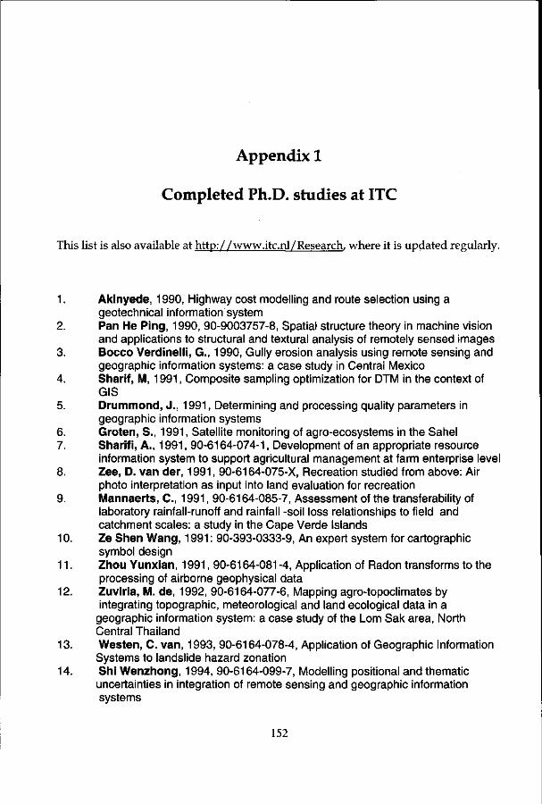
Appendix 1

Completed Ph.D. studies at ITC

This list is also available at http://www.itc.nl/Research, where it is updated regularly.

1. Akinyede, 1990, Highway cost modelling and route selection using a geotechnical information system

2. Pan He Ping, 1990, 90-9003757-8, Spatial structure theory in machine vision and applications to structural and textural analysis of remotely sensed images

3. Bocco Verdinelli, G., 1990, Gully erosion analysis using remote sensing and geographic information systems: a case study in Central Mexico

4. Sharif, M, 1991, Composite sampling optimization for DTM in the context of GIS

5. Drummond, J., 1991, Determining and processing quality parameters in geographic information systems

6. Groten, S., 1991, Satellite monitoring of agro-ecosystems in the Sahel 7. Sharifi, A., 1991, 90-6164-074-1, Development of an appropriate resource

information system to support agricultural management at farm enterprise level 8. Zee, D. van der, 1991, 90-6164-075-X, Recreation studied from above: Air

photo interpretation as input into land evaluation for recreation 9. Mannaerts, C, 1991, 90-6164-085-7, Assessment of the transferability of

laboratory rainfall-runoff and rainfall -soil loss relationships to field and catchment scales: a study in the Cape Verde Islands

10. Ze Shen Wang, 1991: 90-393-0333-9, An expert system for cartographic symbol design

11. Zhou Yunxian, 1991, 90-6164-081 -4, Application of Radon transforms to the processing of airborne geophysical data

12. Zuviria, M. de, 1992, 90-6164-077-6, Mapping agro-topoclimates by integrating topographic, meteorological and land ecological data in a

geographic information system: a case study of the Lorn Sak area, North Central Thailand

13. Westen, C. van, 1993, 90-6164-078-4, Application of Geographic Information Systems to landslide hazard zonation

14. Shi Wenzhong, 1994, 90-6164-099-7, Modelling positional and thematic uncertainties in integration of remote sensing and geographic information systems

152

15. Javelosa, R., 1994, 90-6164-086-5, Active Quaternary environments in the Philippine mobile belt

16. Lo King-Chang, 1994, 90-9006526-1, High Quality Automatic DEM, Digital Elevation Model Generation from Multiple Imagery

17. Wokabi, S., 1994, 90-6164-102-0, Quantified land evaluation for maize yield gap analysis at three sites on the eastern slope of Mt. Kenya

18. Rodriguez, O., 1995, Land Use conflicts and planning strategies in urban fringes: a case study of Western Caracas, Venezuela

19. Meer, F. van der, 1995, 90-5485-385-9, Imaging spectrometry & the Ronda peridotites

20. Kufoniyi, O., 1995, 90-6164-105-5, Spatial coincidence: automated database updating and data consistency in vector GIS

21. Zambezi, P., 1995, Geochemistry of the Nkombwa Hill carbonatite complex of Isoka District, north-east Zambia, with special emphasis on economic minerals

22. Woldai, T., 1995, The application of remote sensing to the study of the geology and structure of the Carboniferous in the Calanas area, pyrite belt, SW Spain

23. Verweij, P., 1995, 90-6164-109-8, Spatial and temporal modelling of vegetation patterns: burning and grazing in the Paramo of Los Nevados National Park, Colombia

24. Pohl, C, 1996, 90-6164-121-7, Geometric Aspects of Multisensor Image Fusion for Topographic Map Updating in the Humid Tropics

25. Jiang Bin, 1996, 90-6266-128-9, Fuzzy overlay analysis and visualization in GIS

26. Metternicht, G., 1996, 90-6164-118-7, Detecting and monitoring land degradation features and processes in the Cochabamba Valleys, Bolivia. A synergistic approach

27. Hoanh Chu Thai, 1996, 90-6164-120-9, Development of a Computerized Aid to Integrated Land Use Planning (CAILUP) at regional level in irrigated areas: a case study for the Quan Lo Phung Hiep region in the Mekong Delta, Vietnam

28. Roshannejad, A., 1996, 90-9009284-6, The management of spatio-temporal data in a national geographic information system

29. Terlien, M., 1996, 90-6164-115-2, Modelling Spatial and Temporal Variations in Rainfall-Triggered Landslides: the integration of hydrologic models, slope

stability models and GIS for the hazard zonation of rainfall-triggered landslides with examples from Manizales, Colombia

30. Mahavir, J., 1996, 90-6164-117-9, Modelling settlement patterns for metropolitan regions: inputs from remote sensing

31. Al-Amir, S., 1996, 90-6164-116-0, Modern spatial planning practice as supported by the multi-applicable tools of remote sensing and GIS: the Syrian case

32. Pilouk, M., 1996, 90-6164-122-5, Integrated modelling for 3D GIS 33. Duan Zengshan, 1996, 90-6164-123-3, Optimization modelling of a river-

aquifer system with technical interventions: a case study for the Huangshui

153

river and the coastal aquifer, Shandong, China 34. Man, W.H. de, 1996, 90-9009-775-9, Surveys: informatie als norm: een

verkenning van de institutionalisering van dorp - surveys in Thailand en op de Filippijnen

35. Vekerdy, Z., 1996, 90-6164-119-5, GIS-based hydrological modelling of alluvial regions: using the example of the Kisafold, Hungary

36. Pereira, Luisa, 1996, 90-407-1385-5, A Robust and Adaptive Matching Procedure for Automatic Modelling of Terrain Relief

37. Fandino Lozano, M., 1996, 90-6164-129-2, A Framework of Ecological Evaluation oriented at the Establishment and Management of Protected Areas: a case study of the Santuario de Iguaque, Colombia

38. Toxopeus, B., 1996, 90-6164-126-8, ISM: an Interactive Spatial and temporal Modelling system as a tool in ecosystem management: with two case studies: Cibodas biosphere reserve, West Java Indonesia: Amboseli biosphere reserve, Kajiado district, Central Southern Kenya

39. Wang Yiman, 1997, 90-6164-131 -4, Satellite SAR imagery for topographic mapping of tidal flat areas in the Dutch Wadden Sea

40. Asun Saldana-Lopez, 1997, 90-6164-133-0, Complexity of soils and Soilscape patterns on the southern slopes of the Ayllon Range, central Spain: a GIS assisted modelling approach

41. Ceccarelli, T., 1997, 90-6164-135-7, Towards a planning support system for communal areas in the Zambezi valley, Zimbabwe; a multi-criteria evaluation linking farm household analysis, land evaluation and geographic information systems

42. Peng Wanning, 1997, 90-6164-134-9, Automated generalization in GIS 43. Lawas, C, 1997, 90-6164-137-3, The Resource Users' Knowledge, the

neglected input in Land resource management: the case of the Kankanaey farmers in Benguet, Philippines

44. Bijker, W., 1997, 90-6164-139-X, Radar for rain forest: A monitoring system for land cover Change in the Colombian Amazon

45. Farshad, A., 1997, 90-6164-142-X, Analysis of integrated land and water management practices within different agricultural systems under semi-arid conditions of Iran and evaluation of their sustainability

46. Orlic, B., 1997, 90-6164-140-3, Predicting subsurface conditions for geotechnical modelling

47. Bishr, Y., 1997, 90-6164-141 - 1 , Semantic Aspects of Interoperable GIS 48. Zhang Xiangmin, 1998, 90-6164-144-6, Coal fires in Northwest China:

detection, monitoring and prediction using remote sensing data 49. Gens, R., 1998, 90-6164-155-1, Quality assessment of SAR interferometric

data 50. Turkstra, J., 1998, 90-6164-147-0, Urban development and geographical

information: spatial and temporal patterns of urban development and land values using integrated geo-data, Villaviciencia, Colombia

51. Cassells, C, 1998, Thermal modelling of underground coal fires in northern

154

China 52. Naseri, M., 1998, 90-6164-195-0, Characterization of Salt-affected Soils for

Modelling Sustainable Land Management in Semi-arid Environment: a case study in the Gorgan Region, Northeast, Iran

53. Gorte B.G.H., 1998, 90-6164-157-8, Probabilistic Segmentation of Remotely Sensed Images

54. Tenalem Ayenew, 1998, 90-6164-158-6, The hydrological system of the lake district basin, central main Ethiopian rift

55. Wang Donggen, 1998, 90-6864-551-7, Conjoint approaches to developing activity-based models

56. Bastidas de Calderon, M., 1998, 90-6164-193-4, Environmental fragility and vulnerability of Amazonian landscapes and ecosystems in the middle Orinoco river basin, Venezuela

57. Moameni, A., 1999, Soil quality changes under long-term wheat cultivation in the Marvdasht plain, South-Central Iran

58. Groenigen, J.W. van, 1999, 90-6164-156-X, Constrained optimisation of spatial sampling: a geostatistical approach

59. Cheng Tao, 1999, 90-6164-164-0, A process-oriented data model for fuzzy spatial objects

60. Wolski, Piotr, 1999, 90-6164-165-9, Application of reservoir modelling to hydrotopes identified by remote sensing

61. Acharya, B., 1999, 90-6164-168-3, Forest biodiversity assessment: A spatial analysis of tree species diversity in Nepal

62. Akbar Abkar, AM, 1999, 90-6164-169-1, Likelihood-based segmentation and classification of remotely sensed images

63. Yanuariadi, T., 1999, 90-5808-082-X, Sustainable Land Allocation: GIS-based decision support for industrial forest plantation development in Indonesia

64. Abu Bakr, Mohamed, 1999, 90-6164-170-5, An Integrated Agro-Economic and Agro-Ecological Framework for Land Use Planning and Policy Analysis

65. Eleveld, M., 1999, 90-6461-166-7, Exploring coastal morphodynamics of Ameland (The Netherlands) with remote sensing monitoring techniques and dynamic modelling in GIS

66. Yang Hong, 1999, 90-6164-172-1, Imaging Spectrometry for Hydrocarbon Microseepage

67. Mainam, Felix, 1999, 90-6164-179-9, Modelling soil erodibility in the semiarid zone of Cameroon

68. Bakr, Mahmoud, 2000, 90-6164-176-4, A Stochastic Inverse-Management Approach to Groundwater Quality

69. Zlatanova, Z., 2000, 90-6164-178-0, 3D GIS for Urban Development 70. Ottichilo, Wilber K., 2000, 90-5808-197-4, Wildlife Dynamics: An Analysis of

Change in the Masai Mara Ecosystem 71. Kaymakci, Nuri, 2000, 90-6164-181 -0, Tectono-stratigraphical Evolution of

the Cankori Basin (Central Anatolia, Turkey) 72. Gonzalez, Rhodora, 2000, 90-5808-246-6, Platforms and Terraces: Bridging

155

participation and GIS in joint-learning for watershed management with the Ifugaos of the Philippines

73. Schetselaar, Ernst, 2000, 90-6164-180-2, Integrated analyses of granite-gneiss terrain from field and multisource remotely sensed data. A case study from the Canadian Shield

74. Mesgari, Saadi, 2000, 90-3651 -511 -4, Topological Cell-Tuple Structure for Three-Dimensional Spatial Data

75. Bie, Cees A.J.M. de, 2000, 90-5808-253-9, Comparative Performance Analysis of Agro-Ecosystems

76. Khaemba, Wilson M., 2000, 90-5808-280-6, Spatial Statistics for Natural Resource Management

77. Shrestha, Dhruba, 2000, 90-6164-189-6, Aspects of erosion and sedimentation in the Nepalese Himalaya: highland-lowland relations

78. Asadi Haroni, Hooshang, 2000, 90-6164-185-3, The Zarshuran Gold Deposit Model Applied in a Mineral Exploration GIS in Iran

79. Raza, Ale, 2001, 90-3651 -540-8, Object-oriented Temporal GIS for Urban Applications

80. Farah, Hussein, 2001, 90-5808-331-4, Estimation of regional evaporation under different weather conditions from satellite and meteorological data. A case study in the Naivasha Basin, Kenya

81. Zheng, Ding, 2001, 90-6164-190-X, A Neural - Fuzzy Approach to Linguistic Knowledge Acquisition and Assessment in Spatial Decision Making

82. Sahu, B.K. 83. Alfasatwi, Y., 2001, 90-6164-198-5, The structural, paleogeographical and

hydrocarbon systems analysis of the Ghadamis and Murzuq Basins, West Libya, with emphasis on their relation to the intervening Al Qarqaf Arch

156

Printed by FEBODRUK BV, Enschede

Cover design by Dr. Iris van Duren

157