Spatial modelling of the fraction of photosynthetically active radiation absorbed by a boreal...

$: Spatial modelling of the fraction of photosynthetically active radiation absorbed by a boreal mixedwood forest using a lidar–hyperspectral approach$
www.elsevier.com/locate/agrformet

Agricultural and Forest Meteorology 140 (2006) 287–307

Spatial modelling of the fraction of photosynthetically

active radiation absorbed by a boreal mixedwood

forest using a lidar–hyperspectral approach

V. Thomas a,*, D.A. Finch a, J.H. McCaughey a, T. Noland b, L. Rich b, P. Treitz a

a Department of Geography, Faculty of Arts and Science, Queen’s University, Kingston, Ont., Canada K7L 3N6b Ontario Ministry of Natural Resources, Ontario Forest Research Institute, 1235 Queen St. East,

Sault Ste. Marie, Ont., Canada P6A 2E5

Received 16 November 2005; accepted 17 April 2006

Abstract

The spatial variability of the fraction of photosynthetically active radiation absorbed by the canopy (fPAR) was characterized for

a heterogeneous boreal mixedwood forest site located in northern Ontario, Canada, based on relationships found between fPAR and

light detection and ranging (lidar) data over different canopy architectures. Estimates of fPAR were derived from radiation

measurements made above the canopy at a flux tower and below-canopy radiation was measured across a range of species

compositions and canopy architectures. Airborne lidar data were used to characterize spatial variability of canopy structure around

the flux tower and a map of mean canopy chlorophyll concentration was derived from airborne hyperspectral imagery. Different

volumes of lidar points for the locations directly above each photosynthetically active radiation (PAR) sensor were examined to

determine if there is an optimal method of relating lidar returns to estimated fPAR values.

The strongest correlations between mean lidar height and fPAR occurred when using points that fell within a theoretical cone

which originated at the PAR sensor having a solid angle a = 558. For diffuse conditions, the correlation (r) between mean lidar

height versus fPAR � chlorophyll was stronger than between mean lidar height versus fPAR by 8% for mean daily fPAR and from

10 to 20% for diurnal fPAR, depending on solar zenith angle. For direct light conditions, the relationship was improved by 12% for

mean daily fPAR and 12–41% for diurnal relationships.

Linear regression models of mean daily fPAR � chlorophyll versus mean lidar height were used in conjunction with gridded

lidar data and the canopy chlorophyll map to generate maps of mean daily fPAR for direct and diffuse sunlight conditions. Site

average fPAR calculated from these maps was 0.79 for direct light conditions and 0.78 for diffuse conditions. When compared to

point estimates of mean daily fPAR calculated on the tower, the average fPAR was significantly lower than the point estimate.

Subtracting the direct sunlight fPAR map from the diffuse sunlight fPAR map revealed a distinct spatial pattern showing that areas

with open canopies and relatively low chlorophyll (e.g., black spruce patches) have a higher fPAR under direct sunlight conditions,

while closed canopies with higher chlorophyll (e.g., deciduous species) absorb more PAR under diffuse conditions. These findings

have implications for scaling from point measurements at flux towers to larger resolution satellite imagery and addressing local

scale heterogeneity in flux tower footprints.

# 2006 Elsevier B.V. All rights reserved.

Keywords: fPAR; Canopy structure; Spatial variability; Lidar; Hyperspectral; Chlorophyll

* Corresponding author. Tel.: +1 613 533 6000x75101; fax: +1 613 533 6122.

E-mail addresses: [email protected] (V. Thomas), [email protected] (D.A. Finch),

[email protected] (J.H. McCaughey), [email protected] (T. Noland), [email protected] (P. Treitz).

0168-1923/$ – see front matter # 2006 Elsevier B.V. All rights reserved.

doi:10.1016/j.agrformet.2006.04.008

mailto:<ce:author

mailto:[email protected]




http://dx.doi.org/10.1016/j.agrformet.2006.04.008

V. Thomas et al. / Agricultural and Forest Meteorology 140 (2006) 287–307288

1. Introduction

To better understand the exchanges of energy, water

and carbon dioxide between the forest and the

atmosphere, a detailed knowledge of the shortwave

radiation regime within the forest canopy is essential.

The architecture of the forest canopy strongly influ-

ences the spatial and temporal variability of shortwave

radiation transfer therein and depends upon tree species,

size and location of canopy gaps (Hardy et al., 2004).

FPAR is a key structural variable in national and global

models of net primary production, climate, hydrology,

biogeochemistry and ecology (e.g., Bonan, 1998;

Dickinson et al., 1986; Running and Coughlan, 1988;

Sellers et al., 1996).

The solar radiation regimes of various forest types

have been studied using sensors located at and near

meteorological towers (e.g., Baldocchi et al., 1984; Eck

and Deering, 1992; Chen et al., 1997; Hardy et al.,

2004). Meteorological measurements of total and

diffuse PAR from sensors located above and total

PAR below the canopy allow for the estimation of fPAR.

However, point estimates of fPAR are not necessarily

representative of forest canopies that exhibit a high

degree of spatial variability, such as boreal mixedwood

stands. In these environments, the spatial arrangement

of tree species and variability in canopy structure and

physiology will have a significant impact on the light

regime and the total capacity for photosynthesis in a

stand.

Remote sensing data can offer valuable perspectives

on the spatial variability of fPAR and photosynthetic

capacity across the landscape. Algorithms have been

developed for the retrieval of fPAR and LAI from

MODIS and other relatively low resolution satellite

platforms (Huemmerich et al., 2005; Knyazikhin et al.,

1998a,b). However, the pixel size of these systems is

very large (i.e., individual cell widths may range from

250 m to 1 km) and therefore do not address the spatial

variability that may exist within the footprint of a flux

tower. Further, in situ validation of coarse and moderate

resolution estimates is difficult, due spatial hetero-

geneity within the cell size of the models. Chen et al.

(2003) describe the traditional remote sensing

approaches to fPAR estimation as crude approximations

and discuss the need for alternative approaches that

consider the variability of clumping and LAI. Varia-

bility of fPAR is also highlighted by Shabanov et al.

(2003), who demonstrate that the spatial variability is at

least as large as the diurnal variability due to solar

zenith angle and stress the need to address ‘sub-pixel’

fPAR heterogeneity in current models.

High resolution hyperspectral and light detection and

ranging (lidar) sensors can provide considerable

information about canopy photosynthetic capacity

and structure, which may improve local estimates of

fPAR over point estimates derived from meteorological

towers or from large cell sizes available from traditional

remote sensing models. Lidar systems have the ability

to penetrate the forest canopy from above. This provides

a measure of canopy shape and structure, as opposed to

an assumption of simple crown shapes (i.e., conical or

spherical) (e.g., Arp et al., 1982; Aldred and Bonner,

1985; Nilsson, 1996; Næsset, 1997; Lefsky et al., 1997;

Magnussen and Boudewyn, 1998; Lefsky et al., 1999;

Thomas et al., 2006). Further, the ability to penetrate

into the canopy provides an opportunity to characterize

light transmittance through the canopy (e.g., Parker

et al., 2001; Todd et al., 2003). This, in turn, provides

information regarding the light available for photo-

synthesis and its variation throughout the depth of the

canopy (i.e., variations in fPAR).

The relationships between canopy photosynthetic

capacity and spectral reflectance have been observed in

the laboratory using spectroradiometers. There has been

some success developing hyperspectral indices that are

directly related to leaf and canopy chlorophyll content,

which has been shown to be related to photosynthetic

capacity (Waring et al., 1995). Very strong relationships

(r2 > 0.85) have been reported when comparing leaf

chlorophyll to leaf spectra measured with a spectro-

radiometer in laboratory or field conditions (Blackburn,

1998; Curran et al., 1990; Zarco-Tejada et al., 2000,

2001). Hyperspectral remote sensing potentially allows

for the expansion of these leaf relationships to the

canopy scale, by providing a more complete spectral

signature than what is possible with traditional remote

sensing platforms (e.g., Landsat or SPOT). Results of

canopy-scale studies of chlorophyll content of forests

and crops generally show moderate to strong correla-

tions of leaf samples to airborne hyperspectral data

(Yoder and Pettigrew-Crosby, 1995; Datt, 1998; Zarco-

Tejada et al., 2001; Blackburn, 2002).

In addition to the amount of PAR available

throughout the canopy and the concentration of

chlorophyll in the leaves, recent publications have

demonstrated that the ability to photosynthesize is also

influenced by the amount of diffuse versus direct PAR

available. Gu et al. (2003) demonstrated an increase in

diffuse PAR observed under cloudless conditions

immediately after the Pinatubo volcanic eruption which

translated into an increase in gross photosynthesis and a

resulting CO2 sink. Authors have also shown an

increase in CO2 uptake under cloudy conditions with

V. Thomas et al. / Agricultural and Forest Meteorology 140 (2006) 287–307 289

diffuse PAR conditions as opposed to clear conditions

(e.g., Gu et al., 2002; Freedman et al., 2001). At a

minimum, models of photosynthesis must separate the

diffuse and direct components of PAR in their

calculations to assess the impacts of varying fractions

of diffuse and direct PAR conditions.

The objective of this research is to integrate lidar and

hyperspectral data, as well as above- and below-canopy

quantum measurements of direct and diffuse PAR and

field measures of leaf chlorophyll, to model the spatial

variability of fPAR for a boreal mixedwood forest

located in northern Ontario, Canada.

2. Background

Although lidar technology and data characteristics

have been well described in the literature, some

discussion of lidar data characteristics is helpful to

contextualize the research presented in this paper.

While traditional multispectral and hyperspectral

sensors are described as passive remote sensing

technology (i.e., they measure the intensity of the sun’s

reflectance off surfaces), lidar sensors are referred to as

active technology (similar in concept to radar and SAR

technologies). Here, high energy laser pulses emitted in

short intervals are directed towards the ground and the

time of pulse return is measured. Because the velocity

of light is a constant (i.e., 3 � 108 m/s), the elapsed time

between emission and receiving of the pulse can be used

to determine the distance between the sensor and object

or the ground, a process known as pulse ranging (Wehr

and Lohr, 1999; Lim et al., 2003b). The lidar system

used in this research is categorized as a discrete ‘‘first-

and last-return’’ system, which records the first and last

energy response above a specified noise threshold for

each laser pulse (this is in contrast to a full waveform

system, which would capture an amplitude versus time

waveform). Using this concept, x, y and z measures can

be obtained in the form of a three-dimensional point

cloud, with horizontal accuracies of 50 cm and vertical

accuracies of 10 cm (Baltsavias, 1999; Wehr and Lohr,

1999; Lim et al., 2003b).

There are some distinct differences between discrete

lidar datasets and the more traditional multispectral or

hyperspectral images that have a significant impact on the

way data are analyzed and the types of information that

can be extracted from the dataset. First, lidar datasets are

not images and the raw data cannot be easily visualized

from the traditional planar perspective. Rather, the first-

and last-return coordinates are most easily viewed as

points in a three-dimensional scatterplot or in a software

package capable of redendering point clouds. For

example, Fig. 1 illustrates the first-return points

contained within a circular white birch plot with an

11.3 m radius (400 m2). Most points are clustered

between 8 and 15 m above ground and are representative

of the forest canopy. A few points have penetrated

through gaps in the canopy and reached the ground (note

that if last returns were also displayed, the majority of

them would be at ground level). The ‘bumps’ along the

top of the scatterplot illustrate different tree crowns

within the plot. If one were to examine the entire lidar

dataset for the 1 km radius around the flux tower it would

look like a very large scatterplot, containing more than 16

million points. For the purpose of this research, the 1 km

radius dataset is referred to the ‘original point cloud’.

Points that fall within the area of the sample plots were

subset from the original point cloud and analyzed to

determine correlations with fPAR.

Another key difference between lidar datasets and

traditional multispectral and hyperspectral remotely

sensed images is that there is no measurement of solar

reflectance and therefore no relationship between a

coordinate point and solar zenith angle. For each lidar

data point, the scan angle from the sensor would have

some effect on how deep into the canopy the lidar pulse

would penetrate, mainly due to the spatial configuration

of leaves and branches at that specific location.

However, because the scan angle rapidly changes

within a 408 field of view and because there are multiple

flight lines over the study site to increase the point

density, it can be assumed that there is no consistent

directional bias to the dataset (i.e., each 11.3 m radius

plot contains over 1000 first returns; the canopy would

have been scanned from many angles).

To date, lidar forestry research has been largely

empirical, focusing on strong relationships between tree

height, biomass, volume and other structural metrics.

Lim et al. (2003a) reported success using lidar to predict

several structural variables, including canopy closure,

LAI, basal area, volume, above ground biomass and

height. The reader is referred to Baltsavias (1999), Wehr

and Lohr (1999), St-Onge et al. (2003) and Lim et al.

(2003b) for more detailed overviews of the technology

and its particular application to forestry.

3. Site description

The experiment was conducted during the growing

season of 2004 at the Groundhog River Flux Station

(GFRS), which is part of the Fluxnet-Canada Research

Network. The GRFS is a boreal mixedwood stand,

located approximately 80 km southwest of Timmins,

Ontario, Canada (Fig. 2). At the site, there is a 41-m-tall


Fig. 1. Example of a lidar point cloud for an 11.3 m radius white birch plot. Lidar height above ground is presented on the vertical axis, with UTM

eastings and northings on the bottom.

micrometeorological flux tower where eddy covariance

(EC) measurements of turbulent fluxes (e.g., sensible

heat, latent heat, carbon and momentum), in addition to

climate data (e.g., air temperature, humidity, solar and

terrestrial radiation, and soil moisture) have been made

on a continuous basis since August 2003. The area of

the research site extends in a circular arrangement with

a 1 km radius centered on the flux tower.

The GRFS can be described as a heterogeneous

mixture of five primary tree species including:

trembling aspen [Populus tremuloides Michx.] (TA);

white birch [Betula papyrifera Marsh.] (WB); white

spruce [Picea glauca (Moench) Voss] (WS); black

spruce [Picea mariana (Mill.) BSP] (BS); and balsam

fir [Abies balsamea (L.) Mill.] (BF). There are also

distinct patches of northern white cedar [Thuja

occidentalis (L.)] (C) in a few wet locations within

the site. The canopy is characterized as under-mature,

with an average tree age of approximately 75 years.

There are 29 circular large-tree plots (radius = 11.3 m,

area = 400 m2) distributed across the range of species

associations, which were sampled in 2003 for structural

characteristics. Six of these plots were chosen for the

below-canopy PAR experiment, based on their species

composition. These included plots dominated by: (1)

white birch; (2) medium-sized aspen (i.e., tree

height < 25 m); (3) large aspen (i.e., tree height < 35 m)

m) with a balsam fir sub-canopy; (4) black spruce; (5)

cedar; (6) mixedwood (i.e., TA, WB, WS and BF)

(Fig. 2).

4. Methods

4.1. Mensurational data

Mensurational data for the 29 large tree plots

(including the 6 plots where under-canopy PAR was

measured) were collected during the summers of 2003

and 2004 in accordance with Fluxnet-Canada protocols,

which are derived from the Canadian National Forest

Inventory (NFI) protocols (Fluxnet-Canada, 2003).

Collected data includes diameter-at-breast height

(DBH), stem density, mean tree height, dominant tree

height, crown closure (%), species and leaf area index

(LAI) (for further details, the reader is referred to

Thomas et al., 2006). Plot coordinates were collected at


Fig. 2. Groundhog River Flux Site (80 km SW of Timmins, Ontario). Latitude/longitude: 48.217N, 82.156W.

decimeter-level accuracy using a survey-grade differ-

entially corrected global positioning system (DGPS).

4.2. PAR measurements

In this experiment, global PAR was measured as

photosynthetic photon flux density (PPFD) by quantum

PAR sensors (model LI-190SA, LI-COR, Lincoln, NE,

USA). Each sensor is composed of a silicon photodiode

that produces a linear current signal proportional to the

total photon flux density in the spectral waveband 400–

700 nm. A millivolt adapter (model 2290S, LI-COR)

converted each current signal to a voltage. The millivolt

signal is converted into PPFD (in mmol m�2 s�1) by use

of a sensor-specific calibration coefficient. The sensor is

cosine corrected to an 808 angle from vertical. In

addition to global PAR, downwelling diffuse PAR was

measured with a sunshine sensor (model BF2, Delta-T

Devices, Burwell, Cambridge, UK). This device uses an

array of silicon photodiodes and a unique shading

pattern on the radiometer dome to determine down-

welling diffuse PAR (as PPFD). The accuracies of these

sensors are �5 and �15% for the LI-190SA and BF2,

respectively (Delta-T Devices, 2005; LI-COR, 2005).

The calibrations of these sensors are checked once a

year using a factory-standard LI-190SA quantum sensor

calibrated by LI-COR Inc. (Fluxnet-Canada, 2003). The

GRFS calibration strategy also involves sensor inter-

comparison with a network ‘‘roving’’ standard LI-

190SA, which is part of Fluxnet-Canada’s site inter-

calibration program. This program entails the periodic

deployment of network standard meteorological and

eddy covariance sensors to evaluate the performance of

the site’s sensors and to ensure comparability of

measurements between stations in the network.

4.2.1. Above- and below-canopy PAR measured at

the flux tower

Above-canopy downwelling global PAR (ACP),

above-canopy upwelling global PAR (ACPup), above-

canopy downwelling diffuse PAR (ACPdiff) and below-

canopy downwelling global PAR (BCP) are measured

continuously at the flux tower as part of the Fluxnet-

Canada measurement program. The sensors are located

at 1.5 and 37 m above the ground, on south-facing

booms that are levelled and extended from the tower

approximately 5 m. Data from the above- and below-

canopy PAR sensors are recorded by dataloggers (i.e.,

model CR23X and CR7X for above- and below-canopy

PAR, respectively; Campbell Scientific, Logan, UT,

USA). Data are measured at a scan rate of 1 s, with

statistics (i.e., mean, maximum, minimum, standard


deviation) calculated by the datalogger at 1- and 30-min

intervals for above-canopy PPFD and 5- and 30-min

intervals for BCP.

4.2.2. Spatially variable below-canopy PAR

measurements

In addition to the measurements of PAR at the tower, a

small, self-contained and portable system of PAR sensors

was serially deployed at the six large tree plots to measure

spatial variability in fPAR (from June 12, 2004 (after leaf-

out) to August 14, 2004). The system consisted of six LI-

190SAs (named PAR1–PAR6), a Campbell Scientific

CR10 datalogger, a Campbell Scientific SM4M storage

module and a 12 V dc battery power supply. The

datalogger, storage module and power supply were

housed in a Campbell Scientific ENC12/14 fiberglass

enclosure to protect them from the elements. The sensors

measured every second, with 1-min statistics calculated

by the datalogger. The output data were stored on the

storage module until it was downloaded manually to a

computer. This datalogger’s internal clock was synchro-

nized to on-tower datalogger clocks before each

deployment to ensure synchronization between measure-

ments and accuracy of the fPAR calculations.

Within the six large tree plots selected for the BCP

measurements, the six PAR sensors were distributed

with 10 m spacing along north–south and east–west

transects. The placement of the sensors coincided with

the locations of hemispherical photographs which have

been repeatedly taken at the site in 2003 and 2004. The

hemispherical photographs provide a second, indepen-

dent source of information on canopy structure and leaf

area index within the approximate field of view of the

Fig. 3. Below-canopy PAR sensor

PAR sensor. Depending on which sensor is considered,

the distance between the sensors is 10, 14, 20, 30 or

31 m (Fig. 3). Each sensor was mounted on a tripod and

levelled at a height of 1.2 m above the ground. This

placement ensured that the sensors were above the

understory vegetation. The sensors were left in place for

at least 1 week at each large tree plot to capture as much

variability in solar radiation conditions as possible. The

diffuser surfaces on the LI-190SAs were regularly

checked and cleaned of any debris that may have

accumulated during the deployment.

To minimize differences in the sensitivity between

each sensor, all of the sensors were compared to one

standard LI-190SA (PAR1), which had been calibrated

at the factory by LI-COR. The sensor inter-comparison

was performed before and after the field experiment, at

Queen’s University in Kingston, Ontario, using the

same measurement system as in the field. The sensors

were deployed on the rooftop of a building with a

largely unobstructed hemispherical view of the sky.

They were mounted side-by-side, to minimize sensor

separation as much as possible (ASTM D4430-00e1,

2000), atop a tripod and individually levelled. The

sensors were left for over 1 week to capture a range of

conditions. From the data used in this comparison,

statistics were calculated between each sensor and

PAR1 (i.e., mean absolute error (MAE), mean bias error

(MBE), root mean square error (RMSE), the standard

deviation of the difference (ESOD), linear regression

and the coefficient of determination (r2)). The results of

the comparison were used to evaluate the performance

of each sensor and to derive sensor-specific corrections

for those sensors that did not match that of PAR1.

layout at the GRFS in 2004.


4.2.3. Estimation of fPAR

For each experiment plot, fPAR was estimated on a

half-hourly basis using the above-canopy PAR sensors

located on the tower and the six below-canopy PAR

sensors mounted on tripods beneath the canopy

(described above). Because the PAR reflectance over

each of the plot areas was unknown, the above-canopy

upwelling PAR (ACPup) measured at the flux tower was

used as a general canopy reflectance correction for all

plots. The canopy around the tower is mixed, with white

birch, trembling aspen and black spruce trees present

and a canopy height of approximately 20 m. The canopy

may be more open near the tower than in other mixed-

species locations, due to some tree loss during tower

construction. This has an impact on the general

reflectance correction, by increasing the ground

component of upwelling PAR as compared to some

other locations across the site. Thus, the calculation of

fPAR is considered to be an estimation of the true value.

The half-hour fPAR for each below-canopy sensor

was estimated using the following formula:

fPARi ¼�

1� BCPi

ACP

��

ACPup

ACP

�(1)

where BCPi: below-canopy total PAR for sensor i (i = 1,

. . ., 6); ACP: above-canopy downwelling PAR at the

flux tower; ACPup: above-canopy upwelling PAR at the

flux tower.

Mean daily fPAR for each sensor was also calculated

by averaging the half-hourly fPAR values over daylight

hours (i.e., 1200–2400 UTC).

To determine if the spatial variability in fPAR at the

GRFS would cause a significant change in the average

fPAR for the site based on tower measurements, the

same method of fPAR calculation was also completed

for the below-canopy PAR sensor mounted on the

tower as part of the Fluxnet-Canada measurement

protocol.

4.2.4. Direct versus diffuse PAR

A classification scheme based on sky condition was

devised to examine the influence of varying solar

radiation conditions on fPAR. This was accomplished

by comparing the fraction of ACPdiff and ACP (ACPdiff/

ACP) for the timeframe of the experiment. Values

approaching 1 for the entire day indicate overcast

(diffuse sunlight) conditions (i.e., ratio > 0.8), while

those approaching zero indicate sunny (direct sunlight)

conditions (i.e., ratio < 0.3). For the experiment at each

plot, the most sunny day and the most overcast day were

selected for model development.

4.3. Lidar data

The discrete lidar data collection for this study was

completed by Airborne 1 Corp. (a commercial data

provider based in El Segundo, CA, USA) using the

ALTM 2050 (Optech Inc., Toronto, Ontario, Canada).

This sensor operates at a wavelength of 1067 nm, with a

pulse rate of 50 kHz, a beam divergence setting of

0.3 mrad and a variable scan angle which ranges from

nadir to �208. The data were collected during the first

week of August 2003 at an approximate flying altitude

of 800 ft (244 m). The point spacing of the data across

the site ranged from approximately 3–8 pulses/m2 (i.e.,

3–8 first returns and 3–8 last returns), with a mean point

spacing of 4 pulses/m2 for the study plots. The

estimated positional accuracy at this flight altitude is

approximately 12.5 cm in the x–y direction, with an

error of less than 15 cm in the z direction.

4.3.1. Lidar analysis

In theory, the entire sphere of the sky above the PAR

sensor can have some influence on its recorded values.

When the PAR sensor is placed below the forest canopy,

significant portions of the sky are obstructed by trees

and no longer contribute to the below-canopy PAR

values. If one is trying to relate the below-canopy PAR

values to some calculation derived from lidar data, the

question arises about which portion of the forest canopy

above the sensor is most influencing the below-canopy

PAR values. This will affect the subsetting of lidar

points from the original point cloud for the canopy

above the PAR sensor.

Although there is currently no standard procedure for

analyzing lidar data in this context, some guidance can

be gained by examining results of fPAR and leaf area

index calculated from hemispherical photographs

situated below the canopy. When examining these

photographs, taken using a fish-eye lens, the sky can be

divided into a series of rings based on the angle from the

zenith of the sensor (i.e., directly overhead is 08). By

examining different rings, relative light availability and

canopy gaps can be investigated at specific zenith

angles (e.g., Nicotra et al., 1999). A similar approach

can be adopted for lidar data analysis, by creating a

theoretical cone which originates from the below-

canopy PAR sensor and extends skywards. By creating

theoretical lidar cones with different solid angles (or

theoretical lidar cone angle ‘‘a’’; Fig. 4) it is possible to

determine whether there exists a volume of lidar points

located above the PAR sensor that is most closely

related to fPAR (i.e., which portion of the forest canopy

above the sensor is most influencing the below-canopy


Fig. 4. Variable canopy volumes within a theoretical lidar cone located directly above a below-canopy PAR sensor and opening towards the sky.

fPAR values). The optimal a is unknown, and mainly a

function of canopy height and density in the vicinity of

the sensor.

To determine whether an optimal a exists, multiple

lidar cones of increasing a were extracted over each

PAR sensor location (i.e., a = 9.158, 158, 208, 258, 308,358, 408, 458, 508, 558, 608, 658, 708, 758 and 808).Analyzing each a separately, the average lidar height

was calculated within each cone for every PAR sensor

location. These lidar heights, while not a direct measure

of canopy height or density, are a positive function of

both (Thomas et al., 2006). The lidar heights were

correlated to measures of fPAR over each below-canopy

PAR sensor. Result of each a was compared to

determine the optimal cone.

It should be noted here that as a increases, the

potential for overlap between lidar cones also increases,

particularly in the upper canopy. Whether or not this

actually causes overlap in the cone lidar data depends on

the physical structure of the canopy at the sensor

locations (i.e., whether or not there are lidar returns in

the area of overlap). If there is significant overlap

between two lidar cones (particularly for sensors closest

together), it is not statistically valid to consider them as

independent data points in a correlation analysis.

Therefore, the amount of overlap between the lidar

cones was tested for each a. Where necessary (i.e., for

large a), the ‘‘middle’’ sensors were removed from the

analysis to increase the distance between sensors (i.e.,

Fig. 3) and make them statistically independent.

In addition to mean lidar height within the cone,

several other measures of canopy height and density

were calculated and correlated to fPAR. Several authors

have demonstrated the utility of examining different

lidar percentiles ( p), where the pth percentile is defined

as the lidar height above the ground such that at least p%

of the lidar returns are at or below this height (Miller

et al., 1990; Lim and Treitz, 2004; Næsset, 2004;

Thomas et al., 2006). Therefore, the higher the

percentile, the higher the value of mean lidar height

will be. Previous work at the GRFS, demonstrated that

the 50th and 75th percentiles of lidar data are strongly

related to mean dominant height, basal area, crown

closure and above-ground biomass (R2 = 0.89, 0.86,

0.75 and 0.79, respectively) (Thomas et al., 2006). For

this analysis, the mean, maximum, minimum and

median were calculated for the 25th, 50th and 75th

percentiles and correlated to fPAR. A canopy density


function described in Næsset (2004) was also calcu-

lated, which involved dividing the height into equal

intervals and determining the proportions of lidar hits

above this height interval to the total number of pulses.

4.3.2. Estimation of vertical foliage profile

To facilitate interpretation of lidar relationships to

fPAR, a vertical foliage profile was estimated for each

species. This was done by generating vertical histo-

grams of all lidar returns contained in the 11.3 m radius

plots (e.g., the vertical histogram derived from the data

presented in Fig. 1 would be the representative

histogram for white birch) (Thomas et al., 2006).

4.4. Chlorophyll analysis

The ability of a canopy to absorb PAR is not only a

function of canopy architecture, but also of the inherent

capacity of the leaf to photosynthesize. Many factors

contribute to this, including the physiological status and

the chlorophyll concentration in the leaf (Waring et al.,

1995). Consider the scenario of a large black spruce tree

compared to a large white spruce tree. If the trees are of

a similar physical structure (i.e., height, shape, branch

architecture, etc.), they will appear very similar in the

lidar data. However, their inherent capacity to photo-

synthesize may be quite different, depending on the

chlorophyll concentration within the needles for each

species. This difference will affect the amount of PAR

absorbed by the canopy, but will not be represented by

the lidar data alone. To address variability in

chlorophyll concentration between species, field mea-

surements of leaf total chlorophyll (a + b) (mg/cm2)

were made and incorporated into the statistical

correlation analysis. The fPAR values were multiplied

by average leaf total chlorophyll (a + b) concentrations

(i.e., fPAR � chlorophyll) and compared with the lidar

data within the theoretical cones. Scatterplots and

regression analyses were used to determine the

correlation between fPAR � chlorophyll versus mean

lidar height and the predictive linear regression

equations for direct and diffuse sunlight. A map of

chlorophyll was generated to enable the application of

the linear regression model to the entire site.

4.4.1. Field measures of leaf chlorophyll

Leaf samples were collected from the top of the

canopy (by shooting the upper branches with a shotgun)

for analysis of canopy chlorophyll (e.g., O’Neill et al.,

2002; Zarco-Tejada et al., 2001). Thirty trees (five trees

per each of the six species) were sampled four times

throughout the growing season (i.e., leaf-out, just after

leaf-out, leaf flush and senescence). For trembling

aspen, white birch and cedar, branches from the north

and south side of the trees were sampled (with each

sample consisting of multiple leaves). Black spruce,

white spruce and balsam fir were further stratified into

old and new leaf samples. Mean leaf total chlorophyll

(Chl(a + b)) (mg/cm2) was determined using standard

laboratory spectrophotometric analysis of pigments

(e.g., Zarco-Tejada et al., 2000).

Average values of leaf total chlorophyll (a + b)

concentration (mg/cm2) were determined for each of the

major species at the site. An interspecies comparison

was completed using the difference of means test (i.e., F

test, based on mean, standard deviation and number of

samples) to demonstrate statistical significance in the

chlorophyll concentration differences between species.

4.4.2. Mapping chlorophyll with airborne

hyperspectral data

Hyperspectral data collection was completed over

the GRFS on August 15, 2004, using a Compact

Airborne Spectrographic Imager (CASI, Itres Research

Limited, Calgary, Alberta) at an altitude of approxi-

mately 1900 m. Seventy-two channels with an approx-

imate bandwidth of 7.5 nm were collected over the

wavelength range of 400–940 nm. The CAM5S atmo-

spheric model was used to pre-process the data to at-

sensor radiance and then to ground reflectance (Zarco-

Tejada et al., 2001; Freemantle, 2005). The 1 km radius

around the flux tower was imaged in three flight swaths,

which were georeferenced using a sub-metre digital

elevation model of the site and validated with

differentially corrected GPS data collected by a

survey-grade receiver. The pixel size of the georefer-

enced reflectance image was 4 m � 4 m.

Many authors have discussed the potential utility of

the ‘red edge’ of the spectral reflectance curve (i.e., the

wavelengths between maximum chlorophyll reflectance

in the red and high reflectance in the near infrared,

approximately 680–750 nm) for the prediction of

chlorophyll and other pigments (e.g., Filella et al.,

1995; Gitelson et al., 1996; Boochs et al., 1990; Curran

et al., 1990; Danson and Plummer, 1995; Munden et al.,

1994; Pinar and Curran, 1996). The first and second

derivatives of the spectral reflectance curve (dR and

ddR), particularly along the red edge, are thought to

mitigate the confounding variability of background

reflectance and illumination (Curran et al., 1991;

Elvidge and Chen, 1995; Zarco-Tejada et al., 2000,

2001). This is particularly important when moving from

laboratory measurement of spectral reflectance to

airborne and satellite hyperspectral imagery.


For the work reported here, the maximum first

derivative over the red edge (i.e., max[dR680–750]) was

calculated from the casi hyperspectral data. Average

values were then extracted from 11 large tree plots

which were composed of either a single dominant

species or a relatively simple species mixture. These

values were compared to the average chlorophyll

concentration for the species present in the plot based

on the field measurements of leaf chlorophyll. The

linear regression model generated from these two

variables was applied to the entire image to produce a

map of total chlorophyll (a + b) for the site.

4.5. Effect of solar zenith angle

To determine the effect of variations in solar zenith

angle on fPAR and corresponding model performance,

the analysis was completed on both a diurnal and mean

daily basis. Diurnal variations in fPAR were examined

for each species for both direct and diffuse conditions.

The effect of increasing solar zenith angle on cor-

relations between fPAR (and fPAR � Chl) and mean

lidar height was also calculated.

4.6. Spatial modelling of mean daily fPAR

The best relationships between below-canopy PAR

and lidar under direct and diffuse sunlight conditions

were used to generate raster base maps showing the

spatial distribution of mean daily fPAR for the entire

GRFS. The map cell size was determined by calculating

the average H tan a (Fig. 4, where H is the canopy

height and a is optimal theoretical lidar cone angle). By

imposing a grid over the lidar data set, a cone of lidar

points was extracted over the centre of each grid cell and

the mean lidar height above the ground within that cone

was calculated for each cell. This resulting map was

used in conjunction with the chlorophyll map to solve

for fPAR in the linear regression model. Once maps of

fPAR were generated for the month of August for direct

Table 1

Plot mensuration data

TA/BF TA (medium) WB

DBH(quadratic) (cm) 25.7 21.8 15.6

Stem density (#/ha) 1400 1350 122

Mean height (m) 18.2 16.8 13.9

Mean dominant height (m) 32 25.2 16.6

Crown closure (m2/m2) 2.06 2.61 1.89

Species (%) TA-86, BF-10 TA-85, WB-13 WB

LAI (m2/m2) 2.27 1.72 2.42

Species codes—TA: trembling aspen; BF: balsam fir; WB: white birch; M

and diffuse conditions, descriptive statistics were then

generated for the entire GRFS and compared to

estimates of fPAR generated from the tower sensors

alone.

5. Results and discussion

A summary of mensurational data for the experiment

plots is provided in Table 1. It is evident that each plot is

quite distinct in terms of its physical structure and

species composition. The largest trees are found the

in TA/BF plot, which has two layers of canopy. The

upper layer is composed of large trembling aspen

(height > 30 m) with overlapping crowns. The lower

layer is composed mainly of smaller balsam fir, which

greatly increases the stem density of the plot, but does

not contribute to the upper canopy. The smallest trees

are located in the C/BS plot, which could be described

as a cedar thicket. In contrast, the BS plot can be

described as a thin black spruce bog, which extends well

beyond the plot boundary and can be seen as a large

distinct patch within the overall study site. WB, the

most commonly occurring species at the site, are

medium-sized, with less crown overlap than exists with

the TA. However, the crowns are fuller, with larger

leaves, than those in the aspen trees, resulting in a higher

LAI for the plot.

5.1. PAR and fPAR results

The calibration statistics for the below-canopy PAR

sensors are shown in Table 2 (where the calibration

sensor is the independent variable (x) and the other PAR

sensors are the dependent variables (y)). The high

correlation and minimal scatter for all sensors, as well

as the very low MAE, MBE, RMSE and ESOD

(Table 1), suggests that the only significant source of

error requiring correction is a systematic underestima-

tion of PAR for some sensors. Sensors 3 and 4 are within

the stated accuracy of the sensor (<5%). PAR2, PAR5

MW C/BS BS

17.1 16.0 12.1

5 1400 1725 575

16.3 8.8 9.7

22.6 18.1 13

1.63 0.97 0.16

-99 WB-52, TA-25, WS-15, BS-7 C-66, BS-29 BS-100

2.49 3.03 2.41

W: mixedwood; C: cedar; BS: black spruce.


Table 2

Pre-experiment calibration statistics for below-canopy PAR sensors

Sensor Regression equation R2 MAE (mV) MBE (mV) RMSE (mV) ESOD (mV)

Pre-experiment

2 Y = 0.92x + 0.002 0.99 0.23 0 0.04 0.04

3 Y = 0.97x + 2e�05 0.99 0.01 0 0.03 0.03

4 Y = 0.98x + 0.002 0.99 0.02 0 0.03 0.03

5 Y = 0.74x + 0.001 0.99 0.01 0 0.02 0.02

6 Y = 0.81x + 0.004 0.99 0.02 0 0.02 0.02

Post-experiment

2 Y = 1.01x + 0.001 0.99

3 Y = 0.98x + 0.001 1

4 Y = 0.99x + 0.002 0.99

5 Y = 0.97x + 3e�05 0.99

6 Y = 1.07x + 0.009 0.99

and PAR6 were corrected using the slope of the

regression equation as the calibration factor. Post-

experiment calibration statistics were also calculated to

identify any sensor drift throughout the experiment.

Table 2 demonstrates slight drift by the end of the

experiment for PAR6 (i.e., 2% beyond the accuracy of

the sensor). Therefore, values from this sensor were

ignored for August dates. High correlations and

accuracies are demonstrated for all other sensors as

compared to the original pre-experiment calibration

standard.

5.1.1. Direct versus diffuse PAR

Examination of the half-hour average above-canopy

direct and diffuse PAR measurements provides insight

Fig. 5. Half-hour incident above-canopy total and diffuse PAR (lower plots) a

experiment.

into the sunlight conditions throughout the various

experiments. Fig. 5 shows a sample time series of the

daily PAR regime above the canopy for the medium-

sized trembling aspen experiment, along with the fPAR

estimated from each of the below-canopy sensors. From

these data, it can be seen how sky conditions (i.e.,

cloudless or overcast) affects the radiation regime above

and below the canopy. For example, day of year (DOY)

164 (i.e., June 12, 2004) is a cloudless day, with a mean

daily ratio of ACPdiff/ACP of 0.27 (i.e., direct sunlight

conditions). There is a high degree of spatial and

temporal variability in fPAR between the six sensors,

with some low half-hourly values of fPAR (<0.4). This

is because during certain half-hourly periods (especially

around midday), the direct component of ACP was able

nd estimated fPAR (upper plots) for the medium-sized trembling aspen


to penetrate the canopy through gaps and reach the

below-canopy sensors. The increase in fPAR and the

reduction in variability at the beginning and end of the

day can be explained by the fact that direct solar

radiation cannot penetrate as far into the canopy from an

oblique angle, and thus the radiation reaching the senor

is mainly diffuse during these times.

In contrast, DOY 169 (June 17) is mainly overcast,

with a mean daily ratio of ACPdiff/ACP of 0.97 (i.e.,

diffuse sunlight conditions). The even distribution of

PAR throughout the canopy causes a reduction in the

variability in fPAR throughout the day. DOYs 165–168

show mixed conditions and consequently mixed

variability in fPAR and ACPdiff/ACP.

5.1.2. Influence of solar zenith angle, species and

canopy architecture on fPAR

Differences in estimated fPAR for the various species

configurations are shown for both direct (Fig. 6) and

diffuse (Fig. 7) sunlight conditions. The highest

estimated fPAR occurs in the large trembling aspen plot

(with balsam fir understory) for both cloudless and

overcast conditions. This plot demonstrates an insensi-

Fig. 6. Estimated fPAR and incoming total PAR for each of the experim

Trembling aspen (medium size); (B) black spruce; (C) mixedwood; (D) tre

tivity of fPAR to solar zenith angle, with a very slight

decrease in fPAR at around solar noon under cloudless

conditions. The maximum estimated fPAR (0.99) occurs

in the morning and late afternoon (i.e., large zenith

angles), with a minimum value (0.96) at around solar

noon (Fig. 6D). The vertical foliage profile calculated

from lidar data (Fig. 8) demonstrates high amounts of

lidar returns from the upper canopy. This suggests that the

large branches and foliage of the trembling aspen canopy

are preventing lidar penetration of these trees. A similar

effect would occur with the direct sunlight, causing

multiple scattering and reflection from the canopy. This

would increase the amount of diffuse light within the

canopy, reducing the sensitivity of fPAR to solar zenith

angle under cloudless conditions. Further contributing to

the higher estimated fPAR values is the larger volume of

canopy that is visible to the PAR sensors as a result of the

taller trees (Fig. 4), providing more opportunities for

foliage to absorb the PAR during photosynthesis.

The black spruce bog has the lowest value of fPAR

and the highest degree of sensitivity to solar zenith

angle shows a high degree of sensitivity to solar zenith

angle for both direct and diffuse conditions (Figs. 6B

ent plots under direct sunlight conditions at the GRFS in 2004. (A)

mbling aspen and balsam fir; (E) white birch; (F) cedar/black spruce.


Fig. 7. Estimated fPAR and incoming total PAR for each of the experiment plots under diffuse sunlight conditions at the GRFS in 2004. (A)

Trembling aspen (medium size); (B) black spruce; (C) mixedwood; (D) trembling aspen and balsam fir; (E) white birch; (F) cedar/black spruce.

and 7B). The vertical foliage profile (Fig. 8) is markedly

different for these species, showing three heights of

significant lidar returns, all lower than 10 m above

ground. The mean tree height for this plot is 10 m and

Fig. 8. Vertical foliage profiles estimated from lidar for PAR experi-

ment plots at the GRFS in 2004.

the maximum height is 16 m. The highest of the three

lobes of lidar returns corresponds to slightly less than

the mean height, likely because of the improbability of

the lidar pulse striking the apex of the crown. The lower

lobe indicates that many of the lidar returns reached the

ground (which suggests a significant component of the

direct sunlight would also reach the ground, lowering

fPAR for the plot under cloudless conditions). Lower

fPAR for diffuse conditions may result from a relatively

small amount of canopy falling within the field of view,

meaning considerably less foliage available for photo-

synthesis (note the very low value for canopy closure,

0.16; Table 1).

Low lidar heights (<10 m) are also evident for the

cedar/black spruce plot (Fig. 8). Once again, the cedar/

black spruce plot has a relatively open canopy (canopy

closure is 0.97; Table 1), although there is a much higher

stem density than exists for the black spruce bog

(1725 ha�1 as compared to 575 ha�1; Table 1). Although

there is not a significant lobe of lidar returns near the

ground level, the foliage profile demonstrates lidar

returns for the entire vertical distribution of the canopy,


Fig. 9. Seasonal mean total chlorophyll by species at the GRFS in

2004.

including the lower trunks. Again, this suggests a high

probability for direct sunlight to penetrate the canopy.

At first glance, the medium-sized TA, mixedwood

and WB plots show similar foliage distributions to the

large aspen/balsam fir plot and to each other. However,

upon consideration of the true canopy structure and tree

height for these plots, it becomes evident that the lidar

pulses are behaving differently for each case (Note:

mean height = 17, 16 and 14 m for medium-sized TA,

mixedwood and WB, respectively). In the case of the

medium-sized aspen, most of the lidar pulses are

returned from dominant trees (height > 20 m), whereas

the white birch allows greater penetration into the

canopy, with the maximum lidar returns occurring at

approximately 11 m. The white birch also has a slightly

lower fPAR for diffuse conditions, suggesting a

relationship between tree height and fPAR. The

mixedwood plot falls in the middle of these two cases,

with the height of maximum lidar return being

approximately the same as the mean tree height. There

is no notable difference in fPAR between the medium-

sized aspen and mixedwood plots under diffuse

conditions, but there is a slight decrease in mean fPAR

for the medium-sized aspen under direct conditions.

5.2. Lidar and fPAR

All of the lidar metrics calculated for this analysis are

a function of canopy height and density and were found

to be moderately-to-strongly correlated to fPAR and

fPAR � chlorophyll. Given that the strongest and most

consistent correlation to fPAR and fPAR � chlorophyll

is with mean lidar height, the discussion will focus on

this variable. Across all of the tested theoretical lidar

cone angles (‘‘a’’), the linear correlation coefficient

between mean daily fPAR and mean lidar height for the

cone of extraction ranges from r = 0.53 to 0.79 for direct

sunlight conditions and from r = 0.69 to 0.87 for diffuse

conditions (Fig. 11). A lidar cone with a = 558 clearly

showed the best correlation under both direct and

diffuse conditions. At this angle, data is included from

16 sensors (i.e., no overlap between lidar cones for these

16 sensors). Examination of the mean daily fPAR

scatterplots (Fig. 13A and B) reveals stronger relation-

ships and less variability for the diffuse model (for a

simple linear relationship, R2 = 0.75 and 0.62 for direct

and diffuse models, respectively).

Using a = 558, the diurnal relationships between

lidar and fPAR are demonstrated for diffuse light

(Fig. 12A) and direct light (Fig. 12B). For diffuse

conditions, there is a relatively small effect of solar

zenith angle on the performance of the fPAR–lidar

relationships (i.e., Spearman r correlation values range

from 0.74 to 0.85). The relationship is non-linear, which

peaks at 558 and tapers off for higher solar zenith angles.

Under clear sky conditions, there is more variability

with increasing solar zenith angle. This is due to the

relatively open canopy of the large homogenous black

spruce patch, which allows for a high amount of light

penetration through gaps. This causes a decrease in

correlation with fPAR for certain sensor locations,

depending on the relative position of neighbouring trees

and the sun. At very large zenith angles (i.e., >558),trees along the periphery of the sensor reduce the effect

of large gaps and the result is a relatively constant

relationship between lidar and fPAR (r > 0.70).

Because the lidar volume is constant, there is a

decrease in the strength of the relationship between

lidar and fPAR (as well as an increase it the variability

of the relationship) for smaller zenith angles.

5.3. Measured chlorophyll

Seasonal mean chlorophyll per species is shown in

Fig. 9. For most dates, TA has the highest chlorophyll

concentration. As expected, the chlorophyll concentra-

tions of the deciduous species increase throughout the

growing season and decrease as senescence begins. There

is no consistent trend for the coniferous species, although

WS, BS and BF do show variability throughout the

growing season. This variability is mainly a function of

the new needles, which begin to grow at approximately

mid-June and increase in chlorophyll throughout the

season. The old needles were found to have a relatively

constant chlorophyll concentration throughout the

season. Although the new needles cause an apparent

decrease in chlorophyll concentration for the spruce

trees, they are important to consider because they are the


Fig. 10. Mean canopy chlorophyll for PAR experiment plots at the

GRFS in 2004. Note: WS—white spruce.

Fig. 12. Effects of solar zenith angle on fPAR and fPAR � Chl

relationships with lidar for: (A) overcast (diffuse light) conditions

and (B) sunny (direct light) conditions.

most visible needles to the hyperspectral sensor. BS has

the lowest leaf chlorophyll of all species tested.

Mean chlorophyll per plot is presented in Fig. 10.

Chlorophyll samples from the sampling date closest to

the date of the below-canopy PAR experiment at each

plot were used for the calculations. The mixedwood

value was determined by averaging the chlorophyll

values for TA, WB, WS and BF. The two values

reported for the TA/BF plot represent the species

composition surrounding each of the sensors (i.e.,

sensors 2, 4, 5 and 6 are surrounded by an even mixture

of TA/BF, while sensors 1 and 3 are surrounded by

mainly BF). As expected, BS has the lowest chlorophyll

value, while TA/BF has the highest. Shapiro–Wilks

statistics of the plot chlorophyll concentrations demon-

strate normality of the distribution (n = 7, W = 95,

p = 0.75), meaning that parametric statistics can be

applied with confidence (e.g., linear regression statis-

tics, etc.) (Shapiro et al., 1968).

Fig. 11. Correlation curves for mean daily fPAR and fPAR � chlorophyll

theoretical lidar cone angles.

5.3.1. Influence of chlorophyll on fPAR–lidar

relationships

Both the mean daily (Fig. 11) and diurnal (Fig. 12A

and B) analysis show an increase in the strength and a

decrease in the variability of the relationships between

(Chl) vs. lidar return for direct and diffuse conditions with varying


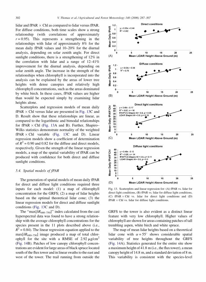
Fig. 13. Scatterplots and linear regression for: (A) fPAR vs. lidar for

direct light conditions, (B) fPAR vs. lidar for diffuse light conditions,

(C) fPAR � Chl vs. lidar for direct light conditions and (D)

fPAR � Chl vs. lidar for diffuse light conditions.

lidar and fPAR � Chl as compared to lidar versus fPAR.

For diffuse conditions, both time scales show a strong

relationship (with correlations of approximately

r = 0.95). This represents a strengthening in the

relationships with lidar of approximately 8% for the

mean daily fPAR values and 10–20% for the diurnal

analysis, depending on solar zenith angle. For direct

sunlight conditions, there is a strengthening of 12% in

the correlation with lidar and a range of 12–41%

improvement for the diurnal analysis, depending on

solar zenith angle. The increase in the strength of the

relationships when chlorophyll is incorporated into the

analysis can be explained by the areas of lower tree

heights with dense canopies and relatively high

chlorophyll concentrations, such as the areas dominated

by white birch. In these cases, fPAR values are higher

than would be expected simply by examining lidar

heights alone.

Scatterplots and regression models of mean daily

fPAR � Chl versus lidar are presented in Fig. 13C and

D. Result show that these relationships are linear, as

compared to the logarithmic and bimodal relationships

for fPAR � Chl (Fig. 13A and B). Further, Shapiro–

Wilks statistics demonstrate normality of the weighted

fPAR � Chl variable (Fig. 13C and D). Linear

regression models show a coefficient of determination

of R2 = 0.90 and 0.82 for the diffuse and direct models,

respectively. Given the strength of the linear regression

models, a map of the spatial variability of fPAR can be

produced with confidence for both direct and diffuse

sunlight conditions.

5.4. Spatial models of fPAR

The generation of spatial models of mean daily fPAR

for direct and diffuse light conditions required three

inputs for each model: (1) a map of chlorophyll

concentration for the GRFS; (2) a map of lidar heights

based on the optimal theoretical lidar cone; (3) the

linear regression models for direct and diffuse sunlight

conditions (Fig. 13C and D).

The ‘‘max[dR680–750]’’ index calculated from the casi

hyperspectral data was found to have a strong relation-

ship with the average chlorophyll concentrations for the

species present in the 11 plots described above (i.e.,

R2 = 0.84). The linear regression equation applied to the

max[dR680–750] image produced a map of total chlor-

ophyll for the site with a RMSE of 2.92 mg/cm2

(Fig. 14B). Patches of low canopy chlorophyll concen-

trations are evident for large areas of black spruce located

south of the flux tower and in linear swaths to the east and

west of the tower. The trail running from outside the

GRFS to the tower is also evident as a distinct linear

feature with very low chlorophyll. Higher values of

chlorophyll are shown for areas containing patches of tall

trembling aspen, white birch and white spruce.

The map of mean lidar heights based on a theoretical

lidar cone with a = 558 shows considerable spatial

variability of tree heights throughout the GRFS

(Fig. 14A). Statistics generated for the entire site show

a maximum height of 41.8 m (i.e., the flux tower), a mean

canopy height of 14.8 m, and a standard deviation of 8 m.

This variability is consistent with the species-level


Fig. 14. Characteristics of the GRFS in 2004. (A) Mean lidar heights optimal theoretical lidar cone of a = 558 (20 m cell size), (B) mean canopy total

chlorophyll (a + b) modelled from casi hyperspectral data (4 m cell size), (C) estimated fPAR for August for sunny (direct light) conditions, (D)

estimated fPAR for August for overcast (diffuse light) conditions and (E) spatial differences between fPAR for direct and diffuse light conditions.

mensuration data (Table 1) which show a range of mean

dominant heights from 13 to 32 m.

Integration of the lidar and chlorophyll maps with

the linear regression models result in a map of the

spatial variability of fPAR for direct and diffuse

conditions for the month of August (Fig. 14C and

D). Considerable spatial variability is evident through-

out the site, although the spatial patterns are not as


Table 3

Spatially modelled mean daily fPAR data compared with tower calculated fPAR

Reflectance up Tower data Modelled data

Fraction diffuse Mean daily fPAR S.D. (temporal) Mean daily fPAR S.D. (spatial)

Direct (cloudless) 0.034 0.243 0.882 0.008 0.787 0.131

Diffuse (overcast) 0.033 1.066 0.846 0.009 0.783 0.136

distinct. Statistics were generated for the entire site and

compared to values of fPAR estimated for the month of

August (Table 3).

Examination of the standard deviations of the tower

estimate fPAR (Table 3) reveals low temporal variability

in fPAR throughout the month of August for both direct

and diffuse conditions (i.e., standard deviation < 1%).

However, no information about the spatial variability of

fPAR can be gleaned from the tower results. In contrast,

the modelled data standard deviations show significant

variability in fPAR within the 1 km radius (i.e., standard

deviation > 13% with a range of more than 0.8 for both

sunny and overcast conditions). Depending on the wind

speed and direction (and resulting tower footprint), this

could have a significant impact on modelled photo-

synthesis as compared to estimates of fPAR from the

tower. Further, when comparing tower-measured versus

modelled mean fPAR, the tower results are approxi-

mately 9% higher for direct conditions and 6% higher for

diffuse conditions. This is most likely because of to the

large areas of black spruce within the GRFS with

relatively open canopies (resulting in a lower lidar height

estimate for the cone of extraction) and with relatively

low canopy chlorophyll, which is a very different canopy

configuration than what exists at the tower.

The modelled results of mean fPAR suggest very

little sensitivity to sunny versus diffuse light conditions.

However, examination of the spatial distribution of

these differences (Fig. 14E) reveals a distinct spatial

pattern. Direct sunlight conditions show a greater fPAR

than diffuse conditions for the large areas of black

spruce and other areas with relatively low chlorophyll or

open canopies. However, more PAR is absorbed under

diffuse conditions for areas containing more deciduous

trees, which have higher canopy chlorophyll concen-

trations and fewer gaps. This is likely because under

diffuse conditions, light reaches all parts of the canopy

equally well because it is coming from all directions,

whereas under direct sunlight conditions, some portions

of the closed canopy will be in shade (e.g., Gu et al.,

2003, 2002; Freedman et al., 2001).

The models described above are based on the

assumption that canopy structure and physiology (i.e.,

chlorophyll available for photosynthesis) are two of the

main factors affecting fPAR. Canopy structure, parti-

cularly lidar metrics based on height, will not change

significantly throughout the growing season for a

mature stand (unless there is significant structural

damage caused by a major event, such as a tornado or

fire). Therefore, the major temporal differences in fPAR

are likely to be caused by changes in canopy

physiology. The very low variability in fPAR over

the month of August, calculated from the tower sensors

(Table 3), suggests that a single base map for the month

of August is sufficient (i.e., there is not a significant

change in canopy physiology for the month of August).

Examination of the months of June and July show that

fPAR increases from 0.80 to 0.89, while the standard

deviation decreases from 0.03 to 0.01. This suggests

that most of the temporal variability in fPAR occurs in

June, during leaf-out and the period directly after leaf-

out when the leaves are maturing. Therefore, capturing

the change in canopy chlorophyll during leaf-out and

after leaf-out, as well as monthly throughout the rest of

the growing season, should be sufficient to model the

temporal variability in fPAR. This information, in

conjunction with continuous measurements of the

temperature and total incoming direct/diffuse PAR

(measured above the canopy at the tower) will allow for

the modelling of photosynthesis at the site throughout

the growing season which incorporates the spatial

variability at the site.

6. Conclusions

The strong relationship between lidar and fPAR once

species chlorophyll concentrations are included suggest

that if lidar data and chlorophyll maps are available, local

spatial variability in fPAR can be mapped for hetero-

geneous forests. This has important implications for at

least two related streams of research: (1) these data may

help fill the ‘‘missing link’’ in scaling efforts from point

measurements at flux towers to larger resolution satellite

imagery such as MODIS (e.g., Huemmerich et al., 2005;

Chen et al., 2003; Knyazikhin et al., 1998a,b), and (2)

addressing local scale heterogeneity for mixedwoods

and its impact on light absorption and photosynthesis

(e.g., Shabanov et al., 2003).


The multiple species present at the GRFS provide the

ideal scenario to characterize species structural differ-

ences and their impact on the spatial pattern of mean

daily fPAR. The analysis reveals a number of key

findings in this regard:

1. T
here are distinct structural differences between
the major species present at the GRFS. These

differences are evident in the apparent foliage

profiles estimated from airborne lidar measure-

ments.

2. S
trong correlations (r, R2) exist between fPAR and
mean lidar heights (a function of canopy height and

density). Solar zenith angle has an impact on the

relationship between fPAR and mean lidar heights,

particularly under direct sunlight conditions. This is

most prevalent in more open canopies, such as the

homogenous black spruce bog. In this patch,

correlations decrease for certain sensor locations,

depending on the relative position of the sensor,

neighbouring trees, and the sun.

3. H
yperspectral remote sensing data and field
sampling indicate that there are significant differ-

ences in canopy chlorophyll concentrations

between the major species at the GRFS.

4. f
PAR � chlorophyll has stronger correlations with
lidar than fPAR alone. For diffuse conditions,

correlation (r) is stronger by 8% for mean daily

fPAR and from 10 to 20% for diurnal fPAR,

depending on solar zenith angle. For sunny (direct

light) conditions, correlation to lidar is improved by

12% for mean daily fPAR and 12–41% for diurnal

relationships, depending on solar zenith angle.

Chlorophyll also reduces diurnal variability caused

by the solar zenith angle and makes the relation-

ships to lidar more linear.

5. S
imulation of multiple theoretical lidar cones
located above the below-canopy PAR sensor reveals

consistently stronger relationships with fPAR when

using lidar points falling within a cone defined by

a = 558.
6. W ith a theoretical lidar cone angle of a = 558, linear
regression models were developed with 90% of the

variance explained for diffuse sunlight conditions

and 82% of the variance explained for direct

conditions.

7. f
PAR calculated from above and below-canopy
PAR sensors mounted on the tower shows very low

variation over the month of August. Average fPAR

was 0.88 for direct sunlight conditions and 0.85 for

diffuse conditions with standard deviation less than

1% for both direct and diffuse conditions. No

information about the spatial variability can be

gleaned from these data.

8. T
he fPAR maps developed for the month of August
for the entire GRFS show a site average fPAR of

0.79 for direct light conditions and 0.78 for diffuse

conditions. This is lower than the point estimate of

fPAR derived by tower measures of above and

below-canopy PAR by 9% for direct conditions and

7% for diffuse conditions.

9. S
tatistics calculated over the spatial extent of the
site demonstrate standard deviation of fPAR of

approximately 0.13 and a range of approximately

0.80 for both direct and diffuse sunlight conditions.

This represents a spatial variability that is much

larger than the temporal variability for the month of

August.

10. M
apping of fPAR for direct and diffuse sunlight
conditions allows for a spatial comparison (i.e.,

subtraction of the maps) that reveals a distinct

spatial pattern showing that areas with open

canopies and relatively low chlorophyll (e.g., black

spruce patches) have a higher fPAR under direct

sunlight conditions, while closed canopies with

higher chlorophyll (e.g., deciduous species) absorb

more PAR under diffuse conditions.

11. D
epending on the wind direction, wind speed and
spatial extent of the flux footprint (i.e., the source-

area for scalar fluxes with respect to the eddy

covariance system), modelled photosynthesis based

on fPAR derived from tower-mounted PAR sensors

could deviate significantly from those derived from

fPAR calculated from the area within the tower

footprint.

Future work evolving from the analysis described in

this paper will involve the expansion of the model to

incorporate changes in canopy chlorophyll over the

growing season. These will be used in conjunction with

total incoming direct and diffuse PAR, along with

continuous measurements of temperature, wind speed,

wind direction, etc., to model photosynthesis within the

variable tower footprint throughout the entire year of

2004. Modelled results will be compared to estimates of

gross ecosystem productivity calculated from tower

measurements.

Acknowledgements

The authors would like to thank the anonymous

reviewers for their insights and helpful comments

which, we feel, have greatly strengthened this manu-

script. We also gratefully acknowledge the field efforts


of Denzil Irving, Bob Oliver, David Atkinson, BjOrn

Prenzel, Chris Hopkinson, Laura Chasmer, Brock

McLeod, Lauren MacLean and Adam Thompson. We

would also like to thank Al Cameron and Lincoln

Rowlinson for establishing cruise-line trail and on-site

assistance with tree species identification. Garry

Koteles provided valuable information regarding tree

and understory species and did all of the field

measurements for the NFI validation plots. The Ontario

Forest Research Institute (OFRI) provided technical

expertise for sampling and processing of leaves, use of

laboratory facilities, and performed the pigment

concentration analysis. Financial assistance for this

work was provided by the Natural Sciences and

Engineering Research Council of Canada (NSERC),

Fluxnet-Canada (NSERC, BIOCAP Canada, and the

Canadian Foundation for Climate and Atmospheric

Sciences (CFCAS)), the Ontario Graduate Scholarship

Program (OGS), the Centre for Research in Earth and

Space Technology (CRESTech), and Queen’s Univer-

sity.

References

Aldred, A., Bonner, M., 1985. Application of Airborne Lasers to

Forest Surveys. Canadian Forestry Service, Petawawa National

For. Inst. Inf. Rep. PI-X-51, 62 pp.

Arp, H.J., Griesbach, J., Burns, J., 1982. Mapping in tropical forests: a

new approach using the laser APR. ISPRS J. Photogram. Rem.

Sens. 48, 91–100.

ASTM D4430-00e1, 2000. Standard Practice for Determining the

Operational Comparability of Meteorological Measurements.

ASTM International, www.ASTM.org.

Baldocchi, D.D., Hutchinson, B.A., Matt, D.R., McMillen, R.T., 1984.

Solar radiation in an oak–hickory forest: an evaluation of extinc-

tion coefficients for several radiation components during full-

leafed and leafless periods. Agric. For. Meteorol. 32, 317–322.

Baltsavias, E.P., 1999. A comparison of between photogrammetry and

laser scanning. ISPRS J. Photogram. Rem. Sens. 54, 83–94.

Blackburn, G.A., 2002. Remote sensing of forest pigments using

airborne imaging spectrometer and LIDAR imagery. Rem. Sens.

Environ. 82, 311–321.

Blackburn, G.A., 1998. Quantifying chlorophylls and caroteniods at

leaf and canopy scales: an evaluation of some hyperspectral

approaches. Rem. Sens. Environ. 66, 273–285.

Bonan, G.B., 1998. The land surface climatology of the NCAR land

surface model coupled the NCAR community climate model. J.

Clim. 11, 1307–1327.

Boochs, F., Dockter, K., Kupfer, G., Kuhbauch, W., 1990. Shape of the

red edge as a vitality indicator for plants. Int. J. Rem. Sens. 11,

1741–1754.

Chen, J.M., Blanken, P., Black, T.A., Guilbeault, M., Chen, S., 1997.

Radiation regime and canopy architecture of a boreal aspen forest.

Agric. For. Meteorol. 86, 107–125.

Chen, J.M., Liu, J., Leblanc, S.G., Lacaze, R., Roujean, J.-L., 2003.

Multi-angular optical remote sensing for assessing vegetation

structure and carbon absorption. Rem. Sens. Environ. 84, 516–

525.

Curran, P.J., Dungan, J.L., Golz, H.L., 1990. Exploring the relation-

ship between reflectance red edge and chlorophyll content in slash

pine. Tree Physiol. 7, 33–48.

Curran, P.J., Dungan, J.L., Macler, B.A., Plummer, S.E., 1991. The

effect of a red leaf pigment on the relationship between red-

edge and chlorophyll concentration. Rem. Sens. Environ. 35,

69–75.

Danson, F.M., Plummer, S.E., 1995. Red-edge response to forest leaf

area index. Int. J. Rem. Sens. 16, 183–188.

Datt, B., 1998. Remote sensing of chlorophyll a, chlorophyll b,

chlorophyll a + b and total carotenoid content in eucalyptus

leaves. Rem. Sens. Environ. 66, 111–121.

Delta-T Devices, 2005. Product News, Light Measurement and

Canopy Analysis, Sunshine Sensor Type BF-2. Delta-T Devices,

Ltd., Burwell, Cambridge, England. Available from http://

www.delta-t.co.uk [cited 3 October 2005].

Dickinson, R.E., Henderson-Sellers, A., Kennedy, P.J., Wilson, M.F.,

1986. Biosphere–Atmosphere Transfer Scheme (BATS) for the

NCAR CCM, NCAR/TN-275-STR. NCAR Research, Boulder,

CO.

Eck, T.F., Deering, D.W., 1992. Canopy albedo and transmittance in

spruce-hemlock forest in mid-September. Agric. For. Meteorol.

59, 237–248.

Elvidge, C.D., Chen, Z., 1995. Comparison of broad-band and nar-

rowband red and near-infrared vegetation indices. Rem. Sens.

Environ. 54, 38–48.

Filella, I., Serrano, L., Serra, J., Penuelas, J., 1995. Evaluating wheat

nitrogen status with canopy reflectance indices and discriminant

analysis. Crop Sci. 35, 1400–1405.

Fluxnet-Canada, 2003. Fluxnet-Canada Measurement Protocols,

Working Draft Version 1.3 [online]. Fluxnet Canada Network

Management Office, Laval, Quebec. Available from http://

www.fluxnet-canada.ca [cited 3 February 2005].

Freedman, J.M., Fitzjarrald, D.R., Moore, K.E., Sakai, R.K., 2001.

Boundary layer clouds and vegetation–atmosphere feedbacks. J.

Clim. 14, 180–197.

Freemantle, J., 2005. CASI Data Collection Report, Sudbury 2004,

Groundhog River. York University, Unpublished document.

Gitelson, A.A., Kaufman, Y.J., Merzlyak, M.N., 1996. Use of a green

channel in remote sensing of vegetation from EOS-MODIS. Rem.

Sens. Environ. 58, 289–298.

Gu, L., Baldocchi, D., Verma, S.B., Black, T.A., Vesala, T., Falge,

E.M., Dowty, P.R., 2002. Advantages of diffuse radiation for

terrestrial ecosystem productivity. J. Geophys. Res. 107, 1–23.

Gu, L., Baldocchi, D.B., Wofsy, S.C., Munger, J.W., Michalsky, J.J.,

Urbanski, S.P., Boden, T.A., 2003. Response of a deciduous forest

to the mount Pinatubo eruption: enhanced photosynthesis. Science

299, 2035–2038.

Hardy, J.P., Melloh, R., Koenig, G., Marks, D., Winstral, A., Pomeroy,

J.W., Link, T., 2004. Solar radiation transmission through conifer

canopies. Agric. For. Meteorol. 126, 257–270.

Huemmerich, K.F., Privette, J.L., Mukelabai, M., Myneni, R.B.,

Knyazikhin, Y., 2005. Time-series validation of MODIS land

biophysical products in a Kalahari Woodland, Africa. Int. J.

Rem. Sens. 26, 4381–4398.

Knyazikhin, Y., Martonchik, J.V., Diner, D.J., Myneni, R.B., Ver-

straete, M., Pinty, B., Gobron, N., 1998a. Estimation of vegetation

canopy leaf area index and fraction of absorbed photosynthetically

active radiation from atmosphere-corrected MISR data. J. Geo-

phys. Res. 103, 32239–32257.

http://www.astm.org/

http://www.delta-t.co.uk/

http://www.delta-t.co.uk/

http://www.fluxnet-canada.ca/

http://www.fluxnet-canada.ca/


Knyazikhin, Y., Martonchik, J.V., Myneni, R.B., Diner, D.J., Running,

S.W., 1998b. Synergistic algorithm for estimating vegetation

canopy leaf area index and fraction of absorbed photosynthetically

active radiationfrom MODIS and MISR data. J. Geophys. Res.

103, 32257–32277.

Lefsky, M.A., Cohen, W.B., Acker, S.A., Spies, T.A., Parker, G.G.,

Harding, D., 1997. Lidar Remote Sensing of Forest Canopy

Structure and Related Biophysical Parameters at the H.J. Andrews

Experimental Forest, Oregon, USA. In Natural Resources Man-

agement Using Remote Sensing and GIS. ASPRS, Washington,

DC, pp. 79–91.

Lefsky, M.A., Cohen, W.B., Acker, S.A., Parker, G.G., Spies, T.A.,

Harding, D., 1999. Lidar remote sensing of the canopy structure

and biophysical properties of Douglas-fir western hemlock forests.

Rem. Sens. Environ. 70, 339–361.

LI-COR, 2005. LI-190 Specifications. LI-COR Biosciences 4421

Superior St. Lincoln, NE 68504, USA. Available from http://

www.licor.com [cited 3 October 2005].

Lim, K.S., Treitz, P.M., 2004. Estimation of above ground forest

biomass from airborne discrete return laser scanner data using

canopy-based quantile estimators. Scand. J. For. Res. 19, 558–570.

Lim, K., Treitz, P., Baldwin, K., Morrison, I., Green, J., 2003a. LiDAR

remote sensing of biophysical properties of tolerant northern

hardwood forests. Can. J. Rem. Sens. 29, 658–678.

Lim, K., Treitz, P., Wulder, M., St-Onge, B., Flood, M., 2003b. Lidar

remote sensing of forest structure. Prog. Phys. Geogr. 27, 88–106.

Magnussen, S., Boudewyn, P., 1998. Derivations of stand heights from

airborne laser scanner data with canopy-based quantile estimators.

Can. J. For. Res. 28, 1016–1031.

Miller, I., Freund, J.E., Johnson, R.A., 1990. Probability and Statistics

for Engineers, fourth ed. Prentice Hall, Englewood Cliffs.

Munden, R., Curran, P.J., Catt, J.A., 1994. The relationship between

red edge and chlorophyll concentration in the Broadbalk winter

wheat experiment at Rothamsted. Int. J. Rem. Sens. 15, 705–709.

Næsset, E., 1997. Determination of mean tree height of forest stands

using airborne laser scanner data. ISPRS J. Photogram. Rem. Sens.

52, 49–56.

Næsset, E., 2004. Effects of different flying altitudes on biophysical

stand properties estimated from canopy height and density mea-

sured with a small-footprint airborne scanning laser. Rem. Sens.

Environ. 91, 243–255.

Nicotra, A.B., Chazdon, R.L., Iriarte, S.V.B., 1999. Spatial hetero-

geneity of light and woody seedling regeneration in tropical wet

forests. Ecology 80, 1908–1926.

Nilsson, M., 1996. Estimation of tree heights and stand volume using

an airborne lidar system. Rem. Sens. Environ. 56, 1–7.

O’Neill, A.L., Kupiec, J.A., Curran, P.J., 2002. Biochemical and

reflectance variation throughout a Sitka spruce canopy. Rem.

Sens. Environ. 80, 134–142.

Parker, G.G., Lefsky, M.A., Harding, D.J., 2001. Light transmittance

in forest canopies determined using airborne laser altimetry and

in-canopy quantum measurements. Rem. Sens. Environ. 76, 298–

309.

Pinar, A., Curran, P.J., 1996. Grass chlorophyll and the reflectance red

edge. Int. J. Rem. Sens. 17, 351–357.

Running, S.W., Coughlan, J.C., 1988. A general model of forest

ecosystem processes for regional applications. Ecol. Model. 42,

124–154.

Sellers, P.J., Randall, D.A., Collatz, G.J., Berry, J.A., Field, C.B.,

Dazlich, D.A., Zhang, C., Collelo, G.D., Bounoua, L., 1996. A

revised land surface parameterization (SIB2) for atmospheric

GCMs: Part I. Model formulation. J. Clim. 9, 676–705.

Shabanov, N.V., Wang, Y., Buermann, W., Dong, J., Hoffman, S.,

Smith, G.R., Tian, Y., Knyazikhin, Y., Myneni, R.B., 2003. Effect

of foliage spatial heterogeneity in the MODIS LAI and FPAR

algorithm over broadleaf forests. Rem. Sens. Environ. 85, 410–

423.

Shapiro, S.S., Wilk, M.B., Chen, H.J., 1968. A comparative study of

various tests of normality. J. Am. Stat. Assoc. 63, 1343–1372.

St-Onge, B., Treitz, P., Wulder, M., 2003. Tree and canopy height

estimation with scanning lidar (light detection and ranging). In:

Franklin, S., Wulder, M. (Eds.), Remote Sensing of Forest Envir-

onments: Concepts and Case Studies. Kluwar Academic

Publishers, pp. 489–509.

Thomas, V., Treitz, P., McCaughey, J.H., Morrison, I., 2006. Mapping

stand-level forest biophysical variables for a mixedwood boreal

forest using lidar: an examination of scanning density. Can. J. For.

Res. 36, 34–47.

Todd, K.W., Csillag, F., Atkinson, P.M., 2003. Three-dimensional

mapping of light transmittance and foliage distribution using lidar.

Can. J. Rem. Sens. 29, 544–555.

Waring, R.H., Law, B.E., Goulden, M.L., Bassow, S.L., McCreight,

R.W., Wofsy, S.C., Bazzaz, F.A., 1995. Scaling gross ecosystem

production at Harvard Forest with remote sensing: a comparison of

estimates from a constrained quantum use efficiency model and

eddy correlation. Plant Cell Environ. 18, 1201–1213.

Wehr, A., Lohr, U., 1999. Airborne laser scanning—an introduction

and overview. ISPRS J. Photogram. Rem. Sens. 54, 68–82.

Yoder, B.J., Pettigrew-Crosby, R.E., 1995. Predicting nitrogen and

chlorophyll content and concentrations from reflectance spectra

(400–2500 nm) at leaf and canopy scales. Rem. Sens. Environ. 53,

199–211.

Zarco-Tejada, P.J., Miller, J.R., Noland, T.L., Mohammad, G.H.,

Sampson, P.H., 2000. Chlorophyll fluorescence effects on vegeta-

tion apparent reflectance: II laboratory and airborne canopy-level

measurements with hyperspectral data. Rem. Sens. Environ. 74,

596–608.

Zarco-Tejada, P.J., Miller, J.R., Noland, T.L., Mohammad, G.H.,

Sampson, P.H., 2001. Scaling-up and model inversion methods

with narrowband optical indices for chlorophyll estimation in

closed forest canopies with hyperspectral data. IEEE Trans.

Geosci. Rem. Sens. 39, 1491–1507.

http://www.licor.com/

http://www.licor.com/

Spatial modelling of the fraction of photosynthetically active radiation absorbed by a boreal...

Documents

Transcript of Spatial modelling of the fraction of photosynthetically active radiation absorbed by a boreal...