
Commodity cluster-based parallel processing of hyperspectral imagery
Upload
khangminh22Category
view
1download
0
Application of chemometrics to hyperspectral imaging analysis of environmental
and agricultural samples
Xin Zhang
ADVERTIMENT. La consulta d’aquesta tesi queda condicionada a l’acceptació de les següents condicions d'ús: La difusió d’aquesta tesi per mitjà del servei TDX (www.tdx.cat) i a través del Dipòsit Digital de la UB (diposit.ub.edu) ha estat autoritzada pels titulars dels drets de propietat intel·lectual únicament per a usos privats emmarcats en activitats d’investigació i docència. No s’autoritza la seva reproducció amb finalitats de lucre ni la seva difusió i posada a disposició des d’un lloc aliè al servei TDX ni al Dipòsit Digital de la UB. No s’autoritza la presentació del seu contingut en una finestrao marc aliè a TDX o al Dipòsit Digital de la UB (framing). Aquesta reserva de drets afecta tant al resum de presentació de la tesi com als seus continguts. En la utilització o cita de parts de la tesi és obligat indicar el nom de la persona autora.
ADVERTENCIA. La consulta de esta tesis queda condicionada a la aceptación de las siguientes condiciones de uso: La difusión de esta tesis por medio del servicio TDR (www.tdx.cat) y a través del Repositorio Digital de la UB (diposit.ub.edu) ha sido autorizada por los titulares de los derechos de propiedad intelectual únicamente para usos privados enmarcados en actividades de investigación y docencia. No se autoriza su reproducción con finalidades de lucro ni su difusión y puesta a disposición desde un sitio ajeno al servicio TDR o al Repositorio Digital de la UB. No se autoriza la presentación de su contenido en una ventana o marco ajeno a TDR o al Repositorio Digital de la UB (framing). Esta reserva de derechos afecta tanto al resumen de presentación de la tesis como a sus contenidos. En la utilización o cita de partes de la tesis es obligado indicar el nombre de la persona autora.
WARNING. On having consulted this thesis you’re accepting the following use conditions: Spreading this thesis by the TDX (www.tdx.cat) service and by the UB Digital Repository (diposit.ub.edu) has been authorized by the titular of the intellectual property rights only for private uses placed in investigation and teaching activities. Reproduction with lucrativeaims is not authorized nor its spreading and availability from a site foreign to the TDX service or to the UB Digital Repository. Introducing its content in a window or frame foreign to the TDX service or to the UB Digital Repository is not authorized (framing). Those rights affect to the presentation summary of the thesis as well as to its contents. In the using orcitation of parts of the thesis it’s obliged to indicate the name of the author.
�
�
�
�
Application�of�chemometrics�to�hyperspectral�
imaging�analysis�of�environmental�and�
agricultural�samples�
�
�
Xin�Zhang�
�
�
�
�
�
�
�
�

� �

�
Doctoral�program:�
Química�Analítica�del�Medi�Ambient�i�la�Pol.lució�
�
Application�of�chemometrics�to�hyperspectral�
imaging�analysis�of�environmental�and�
agricultural�samples�
�
�
�
Xin�Zhang�
�
�
�
�
Director:�Dr.�Roma�Tauler�Ferré�(Institute�of�Environmental�Assessment�and�Water���Council�for�Scientific�Research�IDAEA��CSIC)�
Tutor:�Dr.�Anna�de�Juan�(Department�of�Analytical�Chemistry,�University�of�Barcelona)�

� �

Acknowledgements�
During� the� work� in� this� thesis,� many� people� have� contributed� or� been� helped� me� in�different�ways.�I�am�very�grateful�to�all�of�you�and�would�like�to�thank�everybody�for�your�time�and�support.�There�are�some�in�particular�that�I�would�like�to�take�the�opportunity�to�express�my�gratitude.�
First�of�all,� I�would� like�to�thank�my�supervisor,�Professor�Roma�Tauler,�who�offered�me�the�possibility�to�do�this�PhD.�He�supported�me�for�sharing�his�knowledge�and�for�guiding�me�throughout�this�work�all�these�years.�Thanks�for�reading�all�the�papers�and�thesis�with�much�care,�and�a�lot�of�times�of�revises.�Thanks�a�lot�for�always�taking�the�time�to�discuss�the� work,� even� when� he� is� very� busy.� His� scientific� guidance,� his� generous� way� of�unconstrained� research� activities� and� his� great� enthusiasm� created� the� optimal� working�environment.�He�has�not�only�helped�me�to�develop�as�a�new�chemometritionist,�but�also�helped�me�to�become�a�better�person�with�his�unique�character.��
I�would�like�to�thank�my�tutor,�Dr.�Anna�de�Juan�for�accepting�to�supervise�this�thesis�but�also�for�helping�me�with�her�valuable�experience�and�advice.�Thanks�for�her�much�valued�feedback�on�my�papers�and�thesis�that�improved�this�work.�Thanks�for�always�to�help�me�and�for�sharing�her�knowledge.��
I�would�like�to�thank�Professor�Duponchel,�for�allowing�me�participated�projects�using�EPR,�SIMS,� XPS� analysis�and� for�guiding�me� to�visit�many� interesting�groups�when� I� stayed� in�Lille.�The�experience�enriched�my�knowledge�and�broad�my�horizons� in� the�area�we�are�studying.��
Thanks� to� all� staff� and� all� who� have� come� to� stay� for� a� good� working� in� group� of�chemometrics�of� IDAEA�CSIC,� I�want�to�thank�all�my�colleagues�and�friends�for�the�good�times� we� spent� together,� for� their� kindness,� friendship,� help� and� interesting� discussions�inside�and�beyond�the�field�of�Chemometircs.�Special�thanks�to�S.�Platikanov,�J.Jaumot,�M.�Farrés�et�al.�for�their�help�with�various�practical�problems.��
Even�though�we�did�not�spend�much�time�together�I�would�like�to�thank�my�PhD�student�colleagues�at�Lille�1�University�for�always�making�me�feel�welcome�during�my�short�visits�to�Lille.�
Special�thanks�to�my�wonderful�friends,�those�Chinese�students�studying�in�Barcelona,�give�me�an�incredible�amount�of�energy�and�happiness.�You�all�inspire�me,�both�professionally�and�socially.��
I� also� thank� China� Scholarship� Committee,� for� supporting� me� to� finish� my� work� in�Barcelona.�

Last� but� not� least,� I� am� deeply� grateful� to� my� parents� and� to� my� brother� for� their� long�lasting�help,�love�and�support�throughout�my�entire�life.�
�
�
� �
Abbreviation��
�
2�D� two�dimensional3�D� three�dimensionalAFS� Area�of�Feasible�Solutions�ALS� Alternating�Least�SquaresAsLS� Asymmetric�Least SquaresAVIRIS� Airborne�Visible�Infrared�Imaging�Spectrometer�(sensor)�CCD� Charge�Coupled�DeviceCLS� Classical�Least�SquaresFA�� Factor�AnalysisFT� Fourier�TransformGPS� Global�Positioning�SystemHPLC� High�Performance�Liquid�ChromatographyICA� Independent�Component�AnalysisIR� Infrared�MCR� Multivariate�Curve�ResolutionMSC� Multiplicative�Scatter�CorrectionMVSA� Minimum�Volume�Simplex�AnalysisNIR� Near�Infrared�NMF� Nonnegative�Matrix�Factorization�NMR� Nuclear�Magnetic�ResonancePCA� Principal�Component�AnalysisPLS� Partial�Least�SquaresSIMPLISMA� Simple�to�use�Interactive�Self�Modeling�Mixture�Analysis�SNR� Signal�to�Noise�RatioSVD� Singular�Value�DecompositionTOF�SIMS� Time�of�Flight�Secondary�Ion�Mass�SpectrometryUV� Ultraviolet�VCA� Vertex�Component�Analysis�

� �

�
Content�Abstract�...............................................................................................................................................�1�
Chapter�1�.............................................................................................................................................�3�
Objectives�and�structures�of�the�Thesis�..............................................................................................�3�
1.1�Objectives�..................................................................................................................................�5�
1.2�Structure�of�the�Thesis�..............................................................................................................�7�
1.3.�List�of�scientific�papers�presented�in�this�Thesis�......................................................................�8�
Chapter�2�.............................................................................................................................................�9�
Introduction�........................................................................................................................................�9�
2.1�Hyperspectral�imaging�applied�to�environmental�and�food�analysis�......................................�11�
2.2�Chemometric�methods�............................................................................................................�33�
Chapter�3�...........................................................................................................................................�69�
Application�of�MCR�ALS�on�remote�sensing�hyperspectral�imaging�.................................................�69�
Introduction�..................................................................................................................................�71�
Discussion�....................................................................................................................................�104�
Chapter�4�.........................................................................................................................................�107�
Application�of�hyperspectral�imaging�combined�with�chemometrics�on�food�analysis�.................�107�
Introduction�................................................................................................................................�109�
Discussion�....................................................................................................................................�130�
Chapter�5�.........................................................................................................................................�133�
Measuring�and�comparing�the�resolution�performance�and�the�extend�of�rotation�ambiguities�in�bilinear�modelling�methods�............................................................................................................�133�
Introduction�................................................................................................................................�135�
Discussion�....................................................................................................................................�160�
Chapter�6�.........................................................................................................................................�161�
Distribution�of�Dissolved�Organic�Matter�in�freshwaters�using�Excitation�Emission�fluorescence�and�Multivariate�Curve�Resolution�........................................................................................................�161�
Introduction�................................................................................................................................�163�
Discussion�....................................................................................................................................�178�
Chapter�7�.........................................................................................................................................�181�

Conclusion�.......................................................................................................................................�181�
Resumen�de�la�Tesis�........................................................................................................................�187�
Resumen�......................................................................................................................................�189�
Objetivos�generales�de�la�Tesis�...................................................................................................�191�
Introducción�................................................................................................................................�195�
Resúmenes�..................................................................................................................................�199�
Conclusiones�...............................................................................................................................�207�
References�.......................................................................................................................................�211�
�
�
� �
1��
�
AbstractHyperspectral� imaging� is� an� active� research� area� in� food� and� environment� analysis.�Hyperspectral�images�allow�obtaining�accurate�and�reliable�knowledge�about�the�chemical�composition� and� distribution� of� the� chemical� components� on� the� investigated� sample�surface.� Results� of� hyperspectral� image� analysis� can� be� used� to� acquire� fundamental�understanding� of� complex� chemical� systems� for� research� and� development,� for�commercial� testing� and� adulteration� studies,� in� particular� in� food� and� environment�analysis�and�in�industrial�process�analysis�and�control.�Hyperspectral�imaging�datasets�are�challenging� because� of� their� very� large� size� and� complexity.� Chemometric� methods� are�proposed�to�reveal�the�information�contained�in�the�analyzed�images�as�much�as�possible.�
This�Thesis�deals�with�the�resolution�of�hyperspectral�imaging�data�by�using�chemometric�methods,� in� particular� by� using� appropriate� data� pretreatment� methods� and� by� using�Multivariate� Curve� Resolution� (MCR)� methods.� The� main� contribution� of� the� present�Thesis� is� the� study� and� implementation� of� the� MCR�ALS� (Multivariate� Curve� Resolution�Alternating�Least�Squares)�method�for�the�resolution�of�hyperspectral�images,�collected�by�remote� sensing� (airborne� or� space� borne� Earth� observation� instrument)� and� by� micro�spectroscopy� imaging.� Specifically,� in� this� Thesis� work,� we� explore� the� combination� of�chemometric�and�hyperspectral�imaging�methods�for�the�resolution�of�spectra�(signatures)�and�spatial�distribution�maps�of�the�chemical�constituents�of�a�sample.�The�ultimate�goal�of�this�study�is�to�improve�the�analysis�and�interpretation�of�hyperspectral�imaging�data�by�taking� advantage� of� different� chemometric� powerful� tools.� Local� rank/selectivity�properties� describing� the� spatial� information� of� spectroscopic� images� can� be� used� as� a�constraint�to�increase�the�performance�of�MCR�methods�significantly,�decreasing�rotation�ambiguity�uncertainties.�Different�multivariate�resolution�methods�were�compared,�such�as�MCR�ALS,�Independent�Component�Analysis�(ICA),�Principal�Component�Analysis�(PCA),�and� Minimum� Volume� Simplex� Analysis� (MVSA),� Multivariate� Curve� Resolution�Function�Minimization� (MCR�FMIN),� MCR�BANDS� and� FAC�PACK.� All� these� approaches� have� been�used�for�the�evaluation�of�the�extension�of�rotation�ambiguities�remaining� in�the�results�after� their� application.� Several� hyperspectral� images� provided� by� standard� and� widely�used� instruments� such� as� NASA’s� Airborne� Visible� Infra�Red� Imaging� Spectrometer�(AVIRIS),�Raman�hyperspectral�imaging�Spectrometer,�and�Infrared�hyperspectral�imaging�Spectrometer� have� been� used� as� example� of� data� sets� to� test� the� different�methods,� in�particular� to� test� the� MCR�ALS� method.� The� effectiveness� of� MCR�ALS� is� illustrated� by�providing� exhaustive� comparisons� with� state�of�the�art� methods� for� spectral� unmixing�using�both�simulated�and�real�hyperspectral�data�sets.�

2��
� �

3��
�
�
�
�
�
Chapter 1
Objectives and structures of the Thesis �
� �

4��
� �
Objectives�and�structures�of�the�Thesis�
5��
1.1�Objectives�The� main� objective� of� this� Thesis� has� been� the� development� and� implementation� of�chemometric� methods� for� the� analysis� of� hyperspectral� images� obtained� from� remote�sensing� or� from� micro�imaging� for� the� analysis� of� environment� and� food� samples.�Different�simulated�and�experimental�data�sets�obtained�from�public�remote�sensing�data�repositories�and�from�experimental�measurements�have�been�studied�in�detail.�Especially�important� has� been� the� extension� and� application� of� the� MCR�ALS� method� for� the�resolution�of�hyperspectral� imaging�data�with� the�goal�of�obtaining� the�signatures� (pure�spectra)�and�distribution�maps�of�the�constituents�of�the�analyzed�samples.�
�
Objectives�of�the�analysis�of�hyperspectral�imaging�
� Apply� MCR�ALS� to� the� analysis� of� hyperspectral� image� from� simulated� dataset,�experiment� datasets� including� remote� sensing� hyperspectral� image� from�environment,� and� micro�hyperspectral� image� of� food� commercial� sample� from�chocolate.�In�all�these�cases,�MCR�ALS�was�proposed�to�resolve�the�spectra�of�the�components� in� the� mixture� for� their� characterization� and� to� estimate� their�contributions�and�distribution�maps.�
� Apply�MCR�ALS�method�to�hyperspectral�remote�sensing�image�to�resolve�different�objects�in�the�studied�image,�such�as�lakes,�hard�ground,�vegetation,�buildings�etc.�and�to�determine�their�locations�in�the�images�studied.�
� Apply� MCR�ALS� method� to� analyze� hyperspectral� image� of� the� chocolate� for�resolution� of� their� particle� shape� and� size� at� the� micro� level,� which� are� the�important�factor�related�to�the�product�quality�control�in�the�case�of�food�study.�
� Apply� the� MCR�ALS� method� to� the� analysis� of� fluorescence� data� to� track� the�sources� of� Dissolved� Organic� Matter� (DOM)� in� the� Ter� river� for� resolving� their�various� contributions,� concentrations,� geographical� distribution� and� the�relationship�between�human�activity�along�the�river�and�its�reservoirs.�
�
�
�
�
Objectives�of�the�chemometric�analysis�
� Develop�and�apply�MCR�ALS�method�for�data�analysis�on�hyperspectral�imaging�to�obtain�pure�spectral�and�constituent�distribution�in�the�image.�

Objectives�and�structures�of�the�Thesis�
6��
� Adapt� MCR�ALS� method� with� selectivity/local� rank� constraints� to� improve� the�results�resolution.�FSIW�EFA�and�correlation�coefficient�method�was�proposed�for�the�application�of�the�selectivity�constraint�in�spectroscopic�images.�
� Apply� spectral/signature� pretreatment� methods� to� reduce� the� light� scattering�influence� in� NIR,� the� fluorescence� background� in� Raman� spectroscopy� when� the�sample� is� irradiated,� the� presence� of� noise� contributions� in� background� and� the�baseline�contribution.��
� Apply� MCR�ALS� method� to� simultaneously� analyze� multiple� data� set� arranged� in�arrays� or� increased� multidirectional� structures� (multiway)� and� application� of� the�associated�constraint�to�trilinear�models.��
� Discuss� and� compare� different� ways� of� calculating� the� extension� of� rotation�ambiguity�of�MCR�methods,�such�as�MCR�BANDS�and�FAC�PACK�approaches,�which�allow�the�evaluation�of�the�quality�of�the�results�obtained�by�MCR�ALS.�
�
�
� �

Objectives�and�structures�of�the�Thesis�
7��
1.2�Structure�of�the�Thesis�The� Thesis� is� presented� in� two� sections.� In� the� first� introductory� part,� hyperspectral�imaging� technique,� their� application� in� different� area� and� chemometric� methods� are�introduced.� In�the�second�part,�discussion�part�of�the�results,�scientific�articles�and�their�detail�background�introduction�and�result�dissection,�and�finally,�references�employed�are�included.�This�Thesis�consists�of�seven�chapters�that�are�described�below.�
� In� the� first� chapter,� the� objectives� of� the� Thesis� are� presented.� Furthermore,�detailed�structure�and�relationship�of�scientific�work�of�this�report�are�given.�
� In� the� second� chapter,� introduction� part,� background� and� state� of� the� art�techniques�of�hyperspectral�imaging�and�their�application�in�environment�and�food�area�are�reviewed.�The�development�of�chemometric�in�hyperspectral�imaging�and�theories�of�chemometric�methods�applied�in�the�Thesis�are�introduced.�
� The�third�chapter,�the�application�of�MCR�ALS�methods�is�demonstrated�on�remote�sensing�hyperspectral�imaging.�The�simulated�data�using�spectra�from�USGS�library�and� the� public� remote� sensing� data� (AVIRIS,� Airborne� Visible/Infrared� Imaging�Spectrometer)�from�NASA�are�applied�for�evaluating�the�chemometric�models.�The�second�part�shows�the�effect�of�using� local�rank�and�selectivity�constraints�based�on� spatial� information� of� spectroscopic� images� to� increase� MCR� methods�performance�and�to�decrease�ambiguity.��
� In�Chapter�4,�it�shows�the�application�of�Raman�and�Infrared�hyperspectral�imaging�combined�with�pretreatment�methods�and�MCR�with�selectivity�constraint�to�the�analysis�of�the�constituents�of�commercial�chocolate�samples.��
� In� Chapter� 5,� several� chemometric� resolution� methods� using� bilinear� models�describing� the� data� are� compared.� Various� ways� to� calculate� the� extension� of�rotation�ambiguities�of�MCR�are�discussed�and�compared.��
� In�Chapter�6,�MCR�ALS�with�the�trilinearity�constraint�is�proposed�for�the�analysis�of�excitation–emission�fluorescence�data�from�Dissolved�Organic�Matter�(DOM)�in�fresh� water� natural� systems,� and� the� results� obtained� are� compared� with� those�obtained�with�PARAFAC.��
� In�Chapter�7,�the�conclusions�of�the�Thesis�are�presented.�
�
�
� �

Objectives�and�structures�of�the�Thesis�
8��
1.3.�List�of�scientific�papers�presented�in�this�Thesis�� Zhang,�X.;�Tauler,�R.,�Application�of�multivariate�curve�resolution�alternating�least�
squares� (MCR�ALS)� to� remote� sensing� hyperspectral� imaging.� Analytica� Chimica�Acta�2013,�762,�25�38.��
� Zhang,� X.;� Marcé,� R.;� Armengol,� J.;� Tauler,� R.,� Distribution� of� dissolved� organic�matter� in� freshwaters� using� excitation� emission� fluorescence� and� Multivariate�Curve�Resolution.�Chemosphere�2014,�111,�120�128.��
� Zhang,� X.;� Juan,� A;� Tauler,� R,� Multivariate� Curve� Resolution� applied� to�hyperspectral�imaging�analysis�of�chocolate�samples.�Applied�Spectroscopy.�2015,�69(8).�
� Zhang,�X.;�Juan,�A;�Tauler,�R,�Local�rank�based�spatial�information�for�improvement�of�remote�sensing�hyperspectral�imaging�resolution.�Submitted�to�Talanta.�
� Zhang,�X.;�R.�Tauler.�Measuring�and�comparing�the�resolution�performance�and�the�extend�of�rotation�ambiguities�in�bilinear�modelling�methods.�Submitted�to�Journal�of�Chemometrics.�
�

�
9��
�
�
�
�
Chapter 2
Introduction �
� �

�
10��
� �

Introduction�
11��
�
This�introductory�chapter�of�the�Thesis�has�two�main�parts.�In�the�first�part,�the�theoretical�background�and�applications�of�hyperspectral�imaging�are�introduced.�In�the�second�part�the�chemometric�methods�used�in�this�Thesis�are�introduced.�
�
2.1�Hyperspectral�imaging�applied�to�environmental�and�food�analysis�The�theoretical�concepts�corresponding�to�hyperspectral� imaging�and�an�overview�of�the�applications�of�hyperspectral�imaging�on�food�and�environment�analysis�are�introduced�in�this�first�part.�
Hyperspectral� imaging� is� an� integrated� technology� composed� of� detector� and� optical�instrumentation� on� one� side,� and� of� computer� technology� and� data� processing� on� the�other� side� 1.� It� is� also� known� as� chemical� or� spectroscopic� imaging,� and� it� integrates�conventional� imaging� and� spectroscopy� to� attain� both� spatial� and� spectral� information�from�an�object�or�sample�2.�
Spectroscopic� methods� can� provide� detailed� fingerprints� of� the� analyzed� food� and�environment� samples� using� the� physical� and� chemical� characteristics� of� the� interaction�between�electromagnetic� radiation� and� the� material�of� the� sample,� such� as� reflectance,�transmittance,�absorbance,�phosphorescence,�fluorescence,�and�radioactive�decay3,�which�are� either� absorbed� or� emitted.� Spectroscopic� analysis� can� provide� qualitative� and�quantitative�chemical�and�physical�information�4,�5.�By�scrutinizing�the�changes�in�spectra,�one� can� obtain� physical,� chemical,� and� biological� information� of� the� analyzed� products.�However,�direct�application�of�spectrometers� to�samples�can�only�usually�detect�a�small�portion� of� them;� therefore,� the� spectra,� strictly� speaking,� are� sometimes� not�representative� of� the� whole� sample,� especially� when� the� ingredients� are� not� evenly�distributed.�
In� 1985,� the� term� ‘hyperspectral� imaging’� originated� from� works� in� remote� sensing� (the�observation� of� a� target� by� a� device� without� physical� contact).� It� was� also� called�spectroscopic�imaging�6.�It�was�used�to�make�a�direct�identification�of�surface�materials�in�the� form� of� images.� Hyperspectral� imaging� studies� began� with� the� mapping� analysis� of�airborne�minerals� in� the� late�1970s�and�early�1980s.�The� invention�of� the�CCDs� (charge�coupled� device)� in� 1969� by� George� Smith� and� Willard� Boyle� was� the� foundation� of�hyperspectral� technology� who� made� its� initial� development7.� Progress� occurred� in� the�development�of�the�required�electronics,�hardware,�computing,�and�software�throughout�the�1980s�and�until�the�1990s.�At�the�beginning�of�the�1980s,�hyperspectral�imaging�was�introduced�with� the� airborne� imaging�spectrometer� (AIS)�developed�by�Alexander� Goetz�
Introduction�
12��
and� his� colleagues� at� NASA’s� Jet� Propulsion� Laboratory� (JPL),� California� Institute� of�Technology,� Pasadena,� California8.� In� 1983,� JPL� proposed� and� developed� the� Airborne�Visible/Infrared� Imaging� Spectrometer� (AVIRIS)� to� extend� ground�based� spectrometers�into�the�air�on�moving�platforms.�AVIRIS�measured�the�first�spectral�images�in�1987�and�it�was�the�first�imaging�spectrometer�to�measure�the�solar�reflected�spectrum�from�400�nm�to�2500�nm�with�10�nm�intervals9.�Improvements�in�sensor,�calibration,�and�data�systems�were� developed� to� introduce� other� multispectral� and� hyperspectral� instruments� in�ground�based�and�airborne�systems�during�the�next�years.�Although�it�was�first�developed�for� remote� sensing� applications,� hyperspectral� imaging� has� been� applied� to� other� areas�such�as�agriculture10,�biology11,�environmental12�and�other�earth�scientific�fields13.�
�
Hyperspectral� images� can� be� considered� to� be� an� extension� of� the� concept� of� digital�images� but� differently� to� the� later,� they� collect� full� spectral� information� on� the� spatial�dimension.�Digital�images�have�a�finite�number�of�digital�values,�called�pixels,�arranged�in�certain�order�to�describe�the�color�or�grayscale�information�on�a�surface.�The�digital�image�contains�a�fixed�number�of�rows�and�columns�of�pixels.�Pixels�are�the�smallest�individual�elements� in� an� image,� holding� quantized� values� that� represent� the� brightness� of� the�object14.�Therefore,�a�digital�image�is�an�array�of�I�rows�and�J�columns,�with�I��J�intensity�values,�also�called�pixels.�A�pixel�is�an�intensity�value�with�an�associated�coordinate�in�the�image.�An� I�� J� image�having�K�detected� features� (variables,�wavelengths)�would� form�a�three�way�data�array�of�size�I��J��K.�The�I��J��K�image�can�be�represented�as�K�slices,�where�each�slice�is�an�image�at�a�single�feature.�The�I��J��K�image�can�also�be�presented�as� a� two�way� array� of� vectors.� In� special� cases,� these� vectors� can� be� shown� and�interpreted�as�spectra.�
In� a� hyperspectral� image,� each� pixel� has� not� the� same� single� discrete� value,� but� it� may�have� a� wide� range� of� values� recorded� by� a� sensor� or� spectroscopy� instrument.� Like� in�ordinary� spectroscopy,� hyperspectral� imaging� also� collects� and� processes� information�from� across� the� electromagnetic� spectrum.� The� only� difference� is� that� hyperspectral�imaging�collects�the�data�points�in�an�order�as�pixels�of�an�image�which�show�the�spatial�information.� Hyperspectral� imaging� provides� much� more� detailed� information� on� the�scene�than�a�color�camera.�An�ordinary�color�camera�only�acquires�three�different�spectral�channels�corresponding�to�the�visual�primary�colors,�red,�green�and�blue.�On�the�contrary,�a�hyperspectral�image�is�made�up�of�hundreds�of�contiguous�wavebands�for�each�spatial�position�of�a�target�sample.�Each�pixel�in�a�hyperspectral�image�contains�the�spectrum�of�a�specific�spatial�position.�
�

Introduction�
13��
Two�aspects�characterize�hyperspectral�images:��
� They�can�have�many�wavelengths�(hundreds�or�thousands).�
� Every�pixel�has�a�spectrum�which�can�provide�chemical�information.��
�
Nowadays,� different� techniques� exist� for� acquiring� hyperspectral� data� which� depend� on�the�specific�application.�Spatial�and�spectral�scanning�were�mostly�used�in�the�previously�reported�studies15.�Spatial�scanning�obtains�slit�spectra�by�projecting�a�strip�of�the�scene�onto� a� slit� and� dispersing� the� slit� image� with� a� prism� or� a� grating.� With� these� line�scan�systems,� the� spatial� dimension� is� collected� by� platform� movement� or� scanning.� Spectral�scanning�is�typically�based�on�optical�band�pass�filters.�The�scene�is�spectrally�scanned�by�exchanging� the� filter� to� change� the� wavelength� of� the� scanning� systems� in� the�spectrometer16.�Apart�from�spatial�and�spectral�scanning,�non�scanning�procedures�are�in�development�at�present.�Non�scanning�methods�using�a�single�2�D�sensor�output�produce�simultaneously� spatial� and� spectral� data.� The� most� important� benefit� of� snapshot�hyperspectral�imaging�is�the�higher�light�throughput�and�the�shorter�acquisition�time.�The�tremendous� amount� of� memory� needed� to� store� the� entire� dataset� makes� the�computational�effort�and�manufacturing�cost�high17,�18.��
�
Hyperspectral� imaging� techniques� based� on� Raman,� infrared,� near� infrared� and�fluorescence� spectroscopy� are� useful� methods� in� different� areas,� such� as� polymer�research,� material� science,� biomedical� diagnostic,� pharmaceutical� industry,� analytical�chemistry,�process�control�and�environmental�analysis19,�20.�Materials�or�processes�can�be�also� analyzed� using� multiple� imaging� techniques� across� all� wavelength� and� time� scales.�Hyperspectral�imaging�can�also�be�used�to�gain�a�fundamental�understanding�of�complex�chemical� systems� in� industrial� processes� and� use� this� knowledge� to� control� them.�Nowadays,�application�of�hyperspectral� imaging�is�developing�very�fast,�and�it�allows�the�in�situ�acquisition�of�hyperspectral�images�(for�example,�inside�the�human�body,�or�inside�high�pressure�chemical�reactors).�The�ability�to�control�complex�processes�in�food�industry�or�in�environmental�monitoring�studies�will�require�the�same�techniques�to�those�used�for�imaging�analysis�in�other�fields�21�23.�
For� research,� development,� commercial� testing,� or� adulteration� validation,� reference�methods� for� food� or� environment� samples� are� necessary.� Reference� methods� for� food�safety� and� quality� control� analysis� often� have� limitations,� in� terms� of� their� adequacy� of�implementation� at� the� different� steps� of� the� food� chain24.� In� the� traditional� analytical�chemistry� approach,� sampling,� sample� preparation,� measuring� procedures,� and� waste�

Introduction�
14��
disposals� are� necessary� steps.� Normally,� these� works� include� laboratory� sample�pretreatment,� dissolution,� digestion,� separation,� enrichment,� and� other� slow� and�laborious� steps.� Traditional� analytical� chemistry� methods� have� the� following�disadvantages:�
� They� are� time�consuming.� Natural� samples� are� usually� mixtures� and� have� many�complex� constituents;� therefore� they� usually� need� many� pretreatment� steps�before� pure� components� are� isolated.� However� there� are� some� alternative�analytical� techniques�that�can�produce� instantaneous�results�with�good�accuracy,�but�they�need�the�simultaneous�application�of�powerful�data�analysis�techniques�25;�
� They� are� expensive.� For� example,� chromatographic� determinations� need� many�different� sensors� or� expensive� columns� to� analyze� different� constituents� in� one�sample.�Moreover,�the�control�at�any�crucial�link�in�the�process�chain�may�require�a�large�number�of�independent�analyses�to�be�performed26�and�a�lot�of�samples�for�analysis;�
� They� should� be� performed� in� the� laboratory.� Because� of� the� laborious� and� fine�operations� needed� for� sample� treatment� or� because� of� the� size� of� the� analytical�instruments� or� because� they� require� instrument� stability,� the� analytical�determinations�should�be�done�in�the�laboratory.�However�in�many�circumstances,�measurements�control�and�management��should�be�on�line��or�in�field;�
� They�are�not�flexible�and�they�are�only�useful�as�a�single�purpose�(one�method/one�parameter�analytical�tools�corresponding�for�a�particular�analyte);�
� They� are� not� always� respectful� with� the� environment� (toxic� reagents).� Usually,�sample� is� destroyed.� Also,� for� example,� mobile� phases� and� solvents� in�chromatography�are�usually�toxic.�They�contaminate�the�environment�and�they�are�harmful�to�the�health�of�laboratory�workers.��
In� recent� years,� the� international� community� is� paying� more� attention� on�environmental� issues� and� on� green� chemistry.� Green� chemistry� is� the� design� of�chemical�products�and�processes�that�reduce�or�eliminate�the�use�and�generation�of�hazardous�substances27.�Analytical�laboratories�are�essential�to�the�implementation�of�the�principles�of�green�analytical�chemistry�as�illustrated�in�27:��
� Elimination�of�reagents�and�solvents�from�the�analytical�laboratory.�
� Reduction�of�the�amounts�of�the�reagents�used.�
� Elimination�or�reduction�of�the�amount�of�solvents�used�in�analytical�procedures.�
� Reduction�of�emission�of�vapors�and�gases.�
Introduction�
15��
� Reduction�of�labor�and�energy�consumption.�
�
Hyperspectral�imaging�instruments��
Considering� the� limitations� of� classical� analytical� reference� methods� mentioned� above,�researchers�have�developed�new�analytical�methods�that�try�to�avoid�these�disadvantages,�many�of�them�based�on�spectroscopic�technologies,�such�as�fluorescence�spectroscopy28,�near�infrared� spectroscopy� (NIR)29,� mid�infrared� spectroscopy� (MID)30� and� Raman�spectroscopy31.� Spectroscopic� methods� enable� a� much� higher� level� and� frequency� of�sample�analysis�for�quality�control�in�industry�and�in�real�time�outdoor�monitoring,�leading�to�an�improved�food�safety�and�environment�quality�control�system32,�33.�The�development�of� robust� and� flexible� spectroscopic� instrumentations� adapted� for� on�line� or� in�field�control�of�the�production�chain�is�well�suited�for�the�continuous�monitoring�of�processes�from�raw�materials�to�finished�products,�and�also�suited�for�fluid�continuous�flow�in�rivers�or�air34.�Such�systems�provide�the�possibility�for�real�time�analyses,�and�they�are�feasible�for� large�amounts�of�sample�throughput�analysis.�The�other�advantages�of�spectroscopic�techniques�are�their�ability�to�determine�multiple�parameters�or�analytes�simultaneously,�reducing�considerably�the�use�of�reagents�and�sample�preparation�steps.�
Because�these�methods�provide�detailed�spectral�data,�hyperspectral�imaging�instruments�can�be�considered�an�extension�of�classical�spectrometric� instruments,�allowing�also�the�extraction� of� quantitative� information� such� as� the� concentration� or� relative� amounts� of�material� constituents.� Even� more,� hyperspectral� imaging� spectrometers� can� also� be�considered� as� a� particular� type� of� spectrometers,� so� that� image�specific� data� analytical�issues�can�be�addressed�as�well.�Analyzed�objects�will�be� shown� in�a� very�different� way�compared� to� ordinary� spectroscopy� techniques.� Hyperspectral� imaging� can� provide�spectral� measurements� of� the� whole� surface� area� of� the� product� while� conventional�spectrometers� only� can� give� point� measurements.� Hyperspectral� imaging� technology�contributes�to�improve�the�quality�of�analysis�in�environmental�monitoring�studies�and�in�food�processing�industry.�In�addition,�it�represents�a�huge�increase�of�the�speed�of�analysis�and�therefore,�a�drastically�reduction�in�their�costs.��
The� most� used� hyperspectral� imaging� instruments� are� based� on� Raman,� mid�infrared,�near�infrared�and�fluorescence.�They�are�briefly�introduced�here.�The�state�of�the�art�and�recent�applications�are�also�given�for�each�one�of�these�applications.�
Raman�hyperspectral�imaging��
Raman� hyperspectral� imaging� was� already� proposed� by� Delhaye� &� Dhamelincourt� in�197535.�But� this� technique�did�not�become�really� feasible�as�a�chemical� imaging�method�

Introduction�
16��
until�cooled�slow�scan�CCD�cameras�became�available.�Now,�the�Raman�microscope�is�one�of� the� most� used� instruments� of� imaging.� It� normally� includes� a� standard� optical�microscope,� and� adds� an� excitation� laser,� laser� rejection� filters,� a� spectrometer,� and� an�optical�sensitive�detector�such�as�a�charge�coupled�device�(CCD),�or�photomultiplier�tube,�(PMT).��
Raman�imaging�techniques�have�improved�and�transformed�in�recent�years�because�of�a�growing� interest� for� acquiring� multidimensional� analytical� information.� Also,� Raman�spectroscopy,� a� complementary� vibrational� spectroscopic� technique� for� molecular�analyses,� continues� to� benefit� enormously� from� advances� in� laser� and� array� detector�developments36.�Raman�imaging�has�the�advantage�of�its�high�selectivity,�low�sensitivity�to�water,�and�minimal�sample�preparation�requirements.��
The� low� sensitivity� of� conventional� Raman� techniques� has� led� to� recent� advances� in�nonlinear� Raman� microscopic� methodologies.� Coherent� Raman� scattering� techniques,�which� include� coherent� anti�Stokes� Raman� scattering� (CARS)� and� stimulated� Raman�scattering� (SRS)� microscopy,� have� become� more� prolific� in� recent� years;� therefore,� the�methodologies,� instrumentation,�and�technology� involved�continues�evolving�at�present.�The� inherently� low� scattering� cross� section� of� Raman� spectroscopy,� as� well� as� its�diffraction� limited� lateral� resolution,� has� been� overcome� by� new� Raman� microscopy�techniques.� Nonlinear� methods� such� as� coherent� anti�Stokes� Raman� spectroscopy� and�stimulated� Raman� spectroscopy� reduce� measurement� times� and� improve� resolution,�allowing�for�three�dimensional�spectroscopic�imaging.�Tip�enhanced�Raman�spectroscopy,�offered�by�surface�enhanced�Raman�scattering,�enables�Raman�spectroscopic�imaging�far�below�the�optical�diffraction�limit37.�
Yookyung�Jung�et�al.�(38)�reported�recently�a�longitudinal,�real�time�alternative�for�the�in�vivo,�label�free�imaging�of�sebaceous�glands�using�Coherent�Anti�Stokes�Raman�Scattering�(CARS)� microscopy,� which� has� been� used� for� selectively� visualize� lipids38.� Anti�Stokes�Raman�scattering�(CARS)�microscopy�provides�a�label�free�means�for�visualizing�biological�samples,� but� it� can� suffer� from� a� strong� non�resonant� background� in� samples� that� are�prepared�using�aldehyde�based�fixatives39.�
Label�Free�biomedical� imaging�with�high�sensitivity�was�performed�by�stimulated�Raman�scattering� microscopy� (SRS)� 40.� A� variety� of� biology� and� medical� applications� have� been�reported,� such� as� differentiating� distributions� of� omega�3� fatty� acids� and� of� saturated�lipids�in�living�cells,�imaging�of�brain�and�skin�tissues�based�on�intrinsic�lipid�contrast,�and�monitoring�drug�delivery�through�the�epidermis�41,�42.�

Introduction�
17��
The�ability�to�control�the�size,�shape,�and�material�of�a�surface�has�been�developed�in�the�field� of� surface�enhanced� Raman� spectroscopy� (SERS).� Surface�enhanced� Raman�scattering� (SERS)� imaging� has� widely� applied� on� rapid� and� sensitive� analysis� of� material�surfaces43,� phenotypical� marker� detection,� cancer� cells44,� 45,� organisms46,� nanocubes� of�metal47� and� so� on.� Excitation� of� the� localized� surface� plasmon� resonance� of� a�nanostructured� surface� or� nanoparticle� lies� at� the� heart� of� SERS.� The� ability� to� reliably�control� the� surface� characteristics� has� taken� SERS� from� an� interesting� surface�phenomenon�to�a�rapidly�developing�analytical�tool�with�many�possible�applications.�
Raman� can� also� be� applied� to� the� detection� of� chemical� threat� agents� from� a� marked�stand�off� distance48.� A� modern� Raman� technique� that� enables� recording� spectra� from�layers�several�millimeters�below�the�sample�surface�is�spatially�offset�Raman�spectroscopy�(SORS).� Spatially� offsets� hyperspectral� stand�off� Raman� imaging� was� used� for� explosive�detection� inside� containers49,� 50.� SORS� also� is� a� powerful� new� technique� for� the� non�invasive�detection�and�identification�of�packaged�products�and�drugs51.�
In� this� Thesis� (Chapter� 4)� Raman� hyperspectral� imaging� has� been� used� in� analysis� of�chocolate�ingredients�to�investigate�the�features�and�distribution�of�these�constituents�in�chocolate�products.�The�details�of�this�application�will�be�discussed�in�Chapter�4�and�in�the�associated�published�paper52.��
�
Mid�Infrared�hyperspectral�imaging��
Mid�infrared�(MIR,�3�20��m)�spectroscopy� is�associated�with�most�organic�and� inorganic�molecules� absorbing� MIR� photons,� and� it� provides� inherent� molecular� selectivity.� It� was�already�applied�commercially�in�the�early�1990s53.��
Waveguide�based�MIR�sensing�systems�generally�comprise�four�major�components:�1)�an�MIR� radiation� source,� 2)� waveguides� for� propagating� the� radiation� and� frequently� also�serving�as�the�transducer,�3)�a�wavelength�selection�device,�and�4)�an�MIR�detector.�In�its�most� common� form,� an� interferometer� is� coupled� to� a� multichannel,� liquid� nitrogen�cooled�mercury�cadmium�telluride�(MCT)�detector54.�The�detector�in�commercial�imaging�spectrometers�is�typically�a�linear�array�(LA)�or�a�focal�plane�array�(FPA).�
The� combination� of� an� infrared� focal�plane� array� detector� and� a� step�scanning� Fourier�transform�infrared�(FT�IR)�microscope�has�proven�to�be�a�powerful�approach�for�obtaining�spectroscopic� images� with� unprecedented� image� fidelity.� Today,� the� most� popular�configuration� for� IR� chemical� imaging� is� the� Fourier� transform� infrared� (FT�IR)� imaging�spectrometer,�which�employs�multiplex�detection�of�wavelengths�via�interferometry.�

Introduction�
18��
Today,�FT�IR�microscopes�are�designed�to�allow�the�spectra�of�physically�small�samples,�or�regions�of�small�samples,�to�be�measured�as�quickly�and�easily�as�possible.�Using�the�new�FT�IR� instrument� (HYPERION)� of� Bruker� as� an� example�(https://www.bruker.com/products.html),� the� recent� development� of� FTIR� spectroscopic�imaging� has� enhanced� our� capability� to� examine,� on� a� microscopic� scale,� the� spatial�distribution�components� in�physical,�chemical�and�biomedical�samples.�Recent�activity� in�this�emerging�area�has�concentrated�on�instrument�development,�theoretical�analyses�to�provide� guidelines� for� imaging� practice,� novel� data� processing� algorithms,� and� on� the�introduction�of�this�technique�to�new�application�fields.�
L.�M.�Kehlet�et�al.�has�developed�a�new�hyperspectral�imaging�spectrometer�in�the�mid�IR�spectral� region� which� is� based� on� nonlinear� frequency� up�conversion� and� subsequent�imaging� using� a� standard� Si�based� CCD� camera.� A� series� of� up�converted� images� are�acquired� with� different� phase� match� conditions� for� the� nonlinear� frequency� conversion�process.� From� this,� a� sequence� of� monochromatic� images� in� the� 3.2–3.4� �m� range� are�generated55.�
Kevin�Yeh�et�al.�published�fast�infrared�chemical�imaging�with�a�quantum�cascade�laser56.�The� advent� of� high�intensity,� broadly� tunable� quantum� cascade� lasers� (QCL)� has� now�accelerated� IR� imaging,� but� using� a� fundamentally� different� type� of� instrument� and�approach,�namely�discrete�frequency�IR�(DFIR)�spectral�imaging.�These�advances�offer�new�opportunities�for�high�throughput�IR�chemical�imaging,�especially�for�the�measurement�of�cells�and�tissues.�
In�this�Thesis,�Infrared�hyperspectral�imaging�has�been�used�for�the�analysis�of�chocolate�samples� and� its� constituents.� Different� from� Raman� hyperspectral� imaging,� infrared�hyperspectral� imaging� can� provide� the� ingredients� and� distribution� of� milk� chocolate�constituents� without� the� undesired� effect� of� strong� interference� of� fluorescent�contributions.�The�details�of�this�application�will�be��discussed�in�Chapter�4�and�published�paper52.��
�
Near�Infrared�Hyperspectral�imaging��
Near�infrared�(NIR,�900–1700�nm)�spectroscopy�has�been�proposed�after� the�NIR�region�was�discovered� in�1800,� revived�and�developed� in� the�early�1950s�and�put� into�practice�later�in�the�1970s57.�NIR�spectroscopy�is�now�a�very�prominent�major�analytical�technology.�In� this� instrument,� the� radiation� from� a� broadband� source� of� NIR� radiation� is� passed�through�a�liquid�crystal�tunable�filter�(LCTF)�so�that�a�narrow�region�of�the�NIR�spectrum�is�isolated58.�The� instruments� for�NIR�hyperspectral� imaging�are�more�versatile�and�rugged�

Introduction�
19��
than� the� corresponding� instruments� used� to� measure� mid�IR� and� Raman� spectra.� The�initial�imaging�systems�required�the�samples�to�be�stationary.�Newer�systems�(push�broom)�collect�images�from�moving�samples,�enabling�online�analysis.��
The�use�of�NIR�hyperspectral�imaging�has�been�and�it�is�still�being�improved�extensively�for�the�determination�of�quality�and�safety�of�agricultural�and�food�products.�Other�fields�of�interest� and� research� areas� where� NIR� hyperspectral� imaging� is� increasingly� applied�include�pharmaceuticals,�medical�applications,�archaeology�and�forensic.�
Increasing� processing� capacity� of� industrial� lines� raises� the� demand� for� strict� quality�control� and� optimization� of� the� analyzed� samples� and� for� product� inspection.� Rapid�quality�assessment�for�on�line�analysis�of�some�food�products�has�been�established�using�NIR� based� equipment� 59.� The� potential� application� of� NIR� hyperspectral� imaging� in� this�approach�is�still�under�investigation.��
In�this�Thesis,�in�Chapter�3,�the�remote�sensing�data�from�AVIRIS�satellite�from�NASA�were�analyzed.�Hyperspectral� solar� reflected�ground� images�were�measured�between�400�nm�and�2500�at�10�nm�intervals.�Most�of�these�wavelengths�are�located�in�the�near�infrared�region� (Near� infrared� is� from� about� 800� nm� to� 2500� nm).� In� this� case� near� infrared�hyperspectral� imaging�was�used�for�remote�sensing�of�ground�objects�analysis�(including�minerals,�airport,�and�lakes).�
�
Secondary�ion�mass�spectrometry�(SIMS)�
Secondary�ion�mass�spectrometry�(SIMS)�is�a�imaging�technique�for�surface�and�thin�film�analysis�with�already�a�long�history�and�a�mature�instrumental�base,�dating�from�the�early�1960s60.� It� is�an�analytical�technique�which�detects� ions�ejected�from�a�surface�after�the�surface�has�been�bombarded�with�high�energy� ions.�Bombarding� ions�are� referred�to�as�primary� ions� or� probing� ions� and� the� ions� ejected� from� the� surface� are� referred� to� as�secondary�ions.�These�secondary�ions�contain�analytical�information�about�the�sample�and�they�are�detected�and�measured�based�on�their�mass/charge�ratio61.��
It�is�a�fast�analytical�methodology�and�it�has�been�used�extensively�to�characterize�a�range�of� materials� including� electronics,� metallic,� polymers� and� biological� samples.� SIMS� has�been�used�extensively�to�examine�a�wide�range�of�samples�and�it�is�routinely�used�in�the�micro�electronics�industry�for�probing�the�distribution�of�dopants�in�silicon62.�In�materials�science� area,� in� 1970s,� there� were� already� many� reports� about� application� of� SIMS� on�sputtering� process� of� a� silicon� carbide� surface63.� Its� capability� has� had� a� revolutionary�improved� by� development� of� TOF�SIMS.� And� still� at� present� there� are� many� reports�

Introduction�
20��
published� in� SIMS� materials� surface� analysis.� A� recent� paper� about� surface�characterization�of�dialyzer�polymer�membranes�using�imaging�TOF�SIMS�and�quantitative�XPS�(X�ray�photoelectron�spectroscopy)�line�scans�has�been�recently�published�64.�
Application�of�SIMS�to�medical�and�biological�research�is�a�relatively�new�field.�SIMS�can�be�used� in�biometrical�and�tissue�analysis,�and�many�papers�have�been�published�about�these� applications� in� the� two� last� years.� For� example,� Louise� Carlred� et� al.� reported� the�spatial�localization�of�the�major�component�of�senile�plaques�in�Alzheimer’s�disease�(AD),�which�were�mapped� in� transgenic�AD�mouse�brains�using�TOF�SIMS65.�SIMS� imaging�has�been�proposed�by�C.�Bich�et�al.�as�a�tool�for�micrometric�histology�of�lipids�in�tissues66.�N�Desbenoit� et� al.� reported� using� TOF�SIMS� imaging� for� localization� and� quantification� of�benzalkonium�chloride�in�eye�tissue67.�
�
Electron�paramagnetic�resonance�(EPR)�spectroscopy�imaging�
Electron�paramagnetic�resonance�(EPR)�spectroscopy�is�a�technique�for�studying�materials�with� unpaired� electrons.� EPR� was� first� observed� in� Kazan� State� University� by� Soviet�physicist� Yevgeny� Zavoisky� in� 194468,� and� it� was� developed� independently� at� the� same�time�by�Brebis�Bleaney�at�the�University�of�Oxford69.� In�comparison�to�nuclear�magnetic�resonance� (NMR)� spectroscopy,� EPR� is� expected� to� show� a� higher� sensitivity� per� unit�volume�due�to�the�higher�gyromagnetic� ratio�of�electron�spins�due�to�roughly� ten�times�smaller�skin�depth�of�EPR�microwaves�in�comparison�to�NMR�radio�waves.�
Although�EPR�is�a�technique�developed�many�years�ago,�recently�it�has�been�extended�to�spectroscopic�imaging.�In�chemical�industry,�electron�paramagnetic�resonance�imaging�has�been�used�for�real�time�monitoring�of�Li�ion�batteries70.�This�is�an�efficient�way�to�locate�‘electron’�related� phenomena� and� opens� a� new� area� in� the� field� of� battery�characterization�that�should�enable�future�breakthroughs� in�battery�research.� In�medical�area,�P.� Kuppusamy’s� research� has� demonstrated� that� electron� paramagnetic� resonance�imaging� can� perform� noninvasive� anatomical� analysis� as� well� as� functional� imaging�analysis� and� that� it� provides� in� vivo� physiological� information� regarding� cellular�metabolism�in�tumor�and�normal�tissues.�It�is�not�a�popular�technique�in�environmental�or�food�sample�analysis�yet.��
Using�EPRI�to�identifying�defects�on�a�CaF2�surfaces�due�to�a�laser�beam�was�reported�in�71.�In� this� work,� MCR�ALS� has� been� proposed� to� identify� the� spectral� signatures� of� all�components�present�in�the�CaF2�samples�and�locate�the�distribution�maps�of�them�in�the�acquired�EPR�images.��

Introduction�
21��
�
Fast� detection� imaging� instruments� based� on� other� concepts� and� current� progress� of�them�
Fluorescence�spectral�imaging�was�not�applied�in�this�Thesis,�although�it�could�have�been�a� good� choice� as� an� alternative� technique� other� than� Raman� or� Infrared� techniques� in�future�research.�Hyperspectral�fluorescence�imaging�or�fluorescence�spectroscopy�has�not�received� much� attention� in� research� until� recently� 72� apart� from� kinetic� analysis.�Continuous� development� of� advanced� microscopy� systems� provides� fluorescence�spectroscopy� imaging� data� with� very� high� spatial�temporal� resolution� and� multiplexing�capabilities.�
During� the� last� decade,� fluorescence� microscopy� has� evolved� as� a� fundamental� tool� in�basic� and� applied� biomedical� research,� due� to� its� optical� sensitivity� and� molecular�specificity73.�Guido�Zavattini�et�al.�have�developed�a�hyperspectral�fluorescence�system�for�3D�in�vivo�optical� imaging,�which�generates�surface�contour�maps�of�animal�tissues.�This�system�is�flexible�enough�to�allow�the�testing�of�a�wide�range�of�illumination�and�detection�geometries.�74.�Wim�F.�J.�Vermaas�et�al.�have�used�hyperspectral�fluorescence�systems�to�determine�localization�and�distribution�of�pigments�in�cyanobacterial�cells�in�vivo75.�Seong�G.� et� al.� presented� a� hyperspectral� fluorescence� imaging� system� with� a� fuzzy� inference�scheme�for�detecting�skin�tumors�on�poultry�carcasses76.�Technical�developments�in�near�infrared�fluorescence�(NIRF)�imaging�and�tomography�have�enabled�recent�applications�on�humans.�Future�NIRF�imaging�agents,�which�consist�of�bright�fluorescent�dyes�conjugated�to� disease�targeting� moieties,� can� be� used� for� molecular� imaging� and� image�guided�surgery�77.��
Hyperspectral� imaging� techniques� are� developing� fast;� some� new� instrument� can� cope�with�the�problem�of�long�data�collection�time.�Snapshot�hyperspectral�imaging�is�a�class�of�hyperspectral�imaging�systems,�which�utilize�a�novel�optical�processor�that�provides�video�rate�hyperspectral�data�cubes78.�These�systems�have�no�moving�parts�and�do�not�operate�by�scanning�in�either�the�spatial�or�in�spectral�dimension.�They�are�capable�of�recording�a�full� three�dimensional� (two� spatial,� one� spectral)� hyperspectral� datacubes� in� each� video�frame,�ideal�for�recording�data�on�transient�events,�or�from�unstabilized�platforms79.�They�provide��new�real�time�hyperspectral�image�instruments80.�
Acousto�optic� tunable� filter� (AOTF)� is� a� novel� device� for� spectrometers.� Their� electronic�tunability�qualifies�them�with�the�most�compelling�advantages�of�higher�wavelength�scan�rate� over� conventional� spectrometers� that� are� mechanically� tuned,� and� the� feature� of�large� angular� aperture� makes� the� AOTF� system� particularly� suitable� in� imaging�
Introduction�
22��
applications81.� New� e� applications� of� these� instruments� have� been� reported� in� nerve�morphometry82,�tenderness�assessment�of�meat83,�skin�stratum�configuration,�citrus�fruit�decay84�and�some�other�areas.��
Imaging� techniques� are� not� limited� to� previously� mentioned� Raman,� Infrared,� near�infrared�and�fluorescence�spectroscopies,�but�also�to�some�other�principles,�such�as�those�given�bellow:�
Functional� near�Infrared� Spectroscopy� imaging� (fNIRI� or� fNIRSI)� is� a� technique� involving�the�quantification�of�chromophore�concentration�resolved�from�the�measurement�of�near�infrared�(NIR)�light�attenuation,�temporal�or�phasic�changes.�It�was�initially�introduced�by�F.� Scholkmann,� and� it� is� based� in� the� use� of� NIRS� (near�infrared� spectroscopy)� for� the�purpose�of� functional�neuroimaging.�Using� fNIR,�brain�activity�can�be�measured�through�hemodynamic�responses�associated�with�neuron�behavior85.��
Second�order� nonlinear� optical� imaging� of� chiral� crystals� (SONICC)� is� an� emerging�technique� for� crystal� imaging� and� characterization86� SONICC� images� can� be� used� to�determine� the� presence� or� absence� of� protein� crystals� through� both� manual� inspection�and�automated�analysis.�
Real�Time,� Subwavelength� Terahertz� Imaging� is� based� on� the� electro�optic� (EO)� imaging�combined� with� the� brightness� of� recently� developed� intense� THz� sources.� It� has� been�reported�that�permits�the�imaging�of�subwavelength�size�samples�without�compromising�spatial�resolution�or�acquisition�time87.�
M.� A.� Fadel� et� al.� have� reported� the� extraction� of� pure� spectral� signatures� and�corresponding�chemical�maps�from�electron�paramagnetic�resonance�(EPR)� imaging�data�sets88.�
�
�
Remote�sensing�hyperspectral�imaging�in�environment�monitoring�
�
Remote� sensing� is� the� technique� for� acquisition� information� from� an� object� or�phenomenon� without� making� physical� contact� with� the� object89.� In� the� narrow� sense,�remote�sensing�is�defined�as�the�measurement�of�object�properties�on�the�earth’s�surface�using�data�acquired�from�aircraft�and�satellites.�It� is�necessary�to�rely�on�the�propagated�signals�like�optical,�acoustical�or�microwave90.�The�acquisition�of�image�data�uses�cameras�and�other�sensors.�

Introduction�
23��
�
�
Figure�2��1�Illustration�of�remote�sensing�
Figure� 2�� 1� is� an� example� for� illustration� of� remote� sensing.� Reflected� sunlight� is� the�common� source� of� radiation� measured� by� satellite� or� airplane.� Normally,� the� sensor�includes�photography,�infrared�spectroscopy�or�radiometers.�In�this�Thesis,�the�interest�is�on�data�obtained�by�hyperspectral�imaging�spectroscopy.�
Remote� sensing� data� provides� either� discrete� point� measurements� or� a� profile� of�measurements�along�a�flight�path.�In�this�work,�we�are�mostly�interested�in�data�acquired�along� a� two� dimensional� spatial� grid,� which� is� an� image.� Remote� sensing� systems,� like�those�installed�on�satellites,�provide�information�for�monitoring�short�term�and�long�term�changes� on� earth,� and� possible� impacts� from� human� activates� on� a� particular� area91.�Sensor�data�provide�instrument�views�of�the�physical�objects�by�recoding�electromagnetic�radiation� emitted� or� reflected� from� them� and� surrounding� landscape.� Remote� sensing�images� can� provide� information� about� position,� size,� and� interrelationships� between�objects.� By� their� nature,� spectral� signature� profiles� can� be� recognized� and� used� for�description�of�the�objects.�
Hyperspectral�remote�sensing� is�a�useful�technology� in�many�scientific�and�technological�fields�and�it�has�been�proposed�also�in�the�environment�area�from�years�ago.�Since�1960s,�multispectral� imagery� has� been� used� as� data� source� for� environment� observational�remote� sensing� from� airborne� and�satellite� systems92.� Initially,� only� three� to� six� spectral�bands�were�used�in�a�single�observation�from�the�visible�and�near�infrared�regions�of�the�spectrum.�Recently,�advances� in�sensor� technology�have�overcome�this� limitation�of� the�data�collecting�systems,�with�the�development�of�new�hyperspectral�sensor�technologies.�It� is�now�possible�to�apply�this�technique�to�acquire�land�surface�information,�using�high�resolution� spectra.� Remote� sensing� can� play� a� unique� and� essential� role� because� of� its�ability�to�acquire�synoptic�information�at�different�time�and�space�scales.��
Introduction�
24��
The�first�Landsat�Multispectral�Scanner�System�(MSS)�was�launched�in�197293.�The�concept�of� imaging� spectroscopy� originated� in� the� 1980’s� at� NASA’s� Jet� Propulsion� Laboratory,�when�a�revolution�in�remote�sensing�began�with�the�introduction�of�the�Airborne�Visible�Infra�Red�Imaging�Spectrometer.�In�this�Thesis,�this�type�of�remote�sensing�is�an�important�topic� and� it� is� the� object� for� evaluation� of� the� performance� of� the�MCR�ALS� method� on�hyperspectral�imaging�(Chapter3�and�papers�94,�95).�
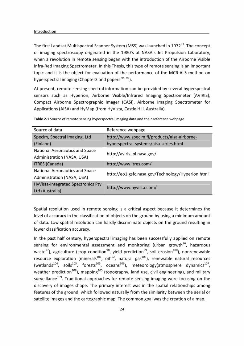
At�present,�remote�sensing�spectral�information�can�be�provided�by�several�hyperspectral�sensors� such� as� Hyperion,� Airborne� Visible/Infrared� Imaging� Spectrometer� (AVIRIS),�Compact� Airborne� Spectrographic� Imager� (CASI),� Airborne� Imaging� Spectrometer� for�Applications�(AISA)�and�HyMap�(from�HyVista,�Castle�Hill,�Australia).��
Table�2�1�Source�of�remote�sensing�hyperspectral�imaging�data�and�their�reference�webpage.�
Source�of�data� Reference�webpageSpecim,�Spectral�Imaging,�Ltd�(Finland)�
http://www.specim.fi/products/aisa�airborne�hyperspectral�systems/aisa�series.html�
National�Aeronautics�and�Space�Administration�(NASA,�USA)�
http://aviris.jpl.nasa.gov/�
ITRES�(Canada)� http://www.itres.com/�National�Aeronautics�and�Space�Administration�(NASA,�USA)�
http://eo1.gsfc.nasa.gov/Technology/Hyperion.html�
HyVista�Integrated�Spectronics�Pty�Ltd�(Australia)�
http://www.hyvista.com/�
�
Spatial� resolution� used� in� remote� sensing� is� a� critical� aspect� because� it� determines� the�level�of�accuracy�in�the�classification�of�objects�on�the�ground�by�using�a�minimum�amount�of�data.�Low�spatial�resolution�can�hardly�discriminate�objects�on�the�ground�resulting�in�lower�classification�accuracy.�
In� the�past�half�century,�hyperspectral� imaging�has�been�successfully�applied�on�remote�sensing� for� environmental� assessment� and� monitoring� (urban� growth96,� hazardous�waste97),� agriculture� (crop� condition98,� yield� prediction99,� soil� erosion100),� nonrenewable�resource� exploration� (minerals101,� oil102,� natural� gas103),� renewable� natural� resources�(wetlands104,� soils105,� forests105,� oceans106),� meteorology(atmosphere� dynamics107,�weather�prediction108),�mapping105� (topography,� land�use,�civil�engineering),�and�military�surveillance109.�Traditional�approaches� for� remote�sensing� imaging�were� focusing�on�the�discovery� of� images� shape.� The� primary� interest� was� in� the� spatial� relationships� among�features�of�the�ground,�which�followed�naturally�from�the�similarity�between�the�aerial�or�satellite�images�and�the�cartographic�map.�The�common�goal�was�the�creation�of�a�map.��
Introduction�
25��
As� mentioned� above,� hyperspectral� remote� sensors� acquire� images� across� narrow�contiguous� spectral� bands,� mainly� including� the� visible,� near�infrared� and� mid�infrared�portions� of� the� electromagnetic� spectrum� 110.� Typically,� hyperspectral� sensors� measure�the� reflected� spectrum� at� wavelengths� between� 350� and� 2500� nm� using� 150–300�contiguous� bands� with� 5� to� 10nm� bandwidths111.� Recent� scanners� support� even� higher�spectral�resolutions�in�the�sub�nanometer�range.�Although�hyperspectral�remote�sensing�has�a�relatively�short�history�compared�with�other�types�of�remote�sensing�such�as�aerial�photographs,� hyperspectral� sensors� have� been� very� effective� for� mapping� the� spatial�extent�of�native�and�non�native�species�across�all�types�of�communities�and�ecosystems112.�Recent�advances�in�materials�and�optics�have�allowed�the�development�of�smaller,�more�stable,� accurately� calibrated� imaging� spectrometers� that� can� quantify� properties� of� the�investigated� land� surface� using� absorbing� and� scattering� characteristics..� Hyperspectral�imaging� is� becoming� more� widely� available� from� government� and� commercial� sources;�thus,� it� is� increasingly� feasible�to�use�data�from�imaging�spectroscopy�for�environmental�research�purposes111.�
Previous� studies� have� shown� that� from� remote� measurements,� direct� identification� of�surface� materials� can� be� obtained.� Remote� sensing� instruments� can� provide� detailed�information�on�the�mineralogy�and�geochemistry�of�the�rock�types�comprising�the�Earth’s�surface.�Based�on�that,�remote�sensing�has�been�used�for�decades�to�map�rocks,�mineral�assemblages�and�weathering�characteristics�8,�113,�114.��
In�environmental�monitoring�analysis,�for�example,�for�air�protection,�people�require�the�continuous�monitoring�of� the�emissions�produced�by�coal�or�oil�power�plants,�municipal�and�hazardous�waste�incinerators�cement�plants,�as�well�as�many�other�industrial�source�pollutions.� These� monitoring� studies� are� usually� performed� using� extractive� sampling�systems� coupled� with� spectroscopy� techniques.� Environmental� monitoring� describes� the�processes,� and� activities� taken� place� in� the� environment.� Hyperspectral� imaging� can� be�used� for� environment� impact� assessment� as� well� as� in� many� other� circumstances� of�human�activates�assessment.��
The� application� of� hyperspectral� imaging� to� natural� resources,� vegetation� and� surface�water�is�an�important�field�in�environmental�monitoring�studies115.�The�spectral�signatures�of� vegetation� are� influenced� by� the� presence� of� pigments� (mainly� chlorophyll�a,�chlorophyll�b,� xanthophyll� and� carotenoids),� and� by� the� physical� structure� and� water�content� of� leaves116.� Hyperspectral� analysis� of� surface� water� bodies� (lakes,� rivers� and�coastal�waters�with�riparian�zones)�provides�information�on�key�water�quality�parameters�and�on�its�trophic�state.��
The�enhanced�capability�of�hyperspectral�technologies�in�environmental�monitoring�using�remote�sensing�allows�managers�to�take�correct�decisions�with�the�necessary�detail�and�in�
Introduction�
26��
an�efficient�time�frame.�With�the�fast�development�of�space�borne�and�airborne�sensors,�better�hyperspectral�data�are�more�frequently�and�conveniently�received.�As�a�result,�data�storage�and�proper�management,�and�effective�information�extraction�are�becoming�key�challenges�to�hyperspectral�remote�sensing�science�and�technology.�Especially,�automatic�or� semi�automatic� information� extraction� is� expected� to� be� growing� in� hyperspectral�investigations�and�applications.�
Some� recent� studies� have� used� hyperspectral� remote� sensing� to� assess� current� spatial�distribution� and� future� dispersion� of� invasive� plants� at� local,� regional� and� global� scales.�With� a� hyperspectral� sensor,� many� narrow� bands� can� capture� a� range� of� absorption�features� including� leaf� or� biochemical� constitutes� such� carotenes,� water,� nitrogen,�cellulose� and� lignin117.� As� leaves� and� plant� species� vary� in� the� concentration� of� their�biochemical� constitutes,� the� reflectance� spectra� vary� as� well118.� Kate� S.� He� et� al.� have�reported�hyperspectral�remote�sensing�results�for�detecting,�mapping�and�predicting�the�spatial�spread�of�invasive�species119.�Herold,�M.�evaluated�how�spectral�resolution�of�high�spatial�resolution�optical�remote�sensing�data�influences�detailed�mapping�of�urban�land�cover.� A� comprehensive� regional� spectral� library� and� low� altitude� data� from� the� AVIRIS�were�used�to�characterize�the�spectral�properties�of�urban�land�cover120.�
At� the� Laboratory� of� Hydraulics� of� DICEA�Sapienza� University� of� Rome,� an� effective�methodology�for�hyperspectral�monitoring�has�been�developed115.� It� is�based�on�the�use�of�two�innovative�experimental�devices�for�acquiring�hyperspectral�images,�one�based�on�the�use�of�tunable�interference�filters,�the�other�on�the�use�of�spectrometers121,�122.�In�L.�G.�Olmanson’s�work,�airborne�hyperspectral�remote�sensing�was�applied�to�assess�the�spatial�distribution� of� water� quality� features� in� large� rivers,� the� Mississippi� River� and� its�tributaries�in�Minnesota.�All�these�results�show�that�hyperspectral�imaging�can�be�used�to�distinguish�and�map�key�variables�under�complex�conditions,�particularly�to�separate�and�map�inorganic�suspended�sediments�independently�of�chlorophyll�levels123.�
F� Salem� reported� a� case� study� about� a� prototype� of� oil� spill� leaks� in� Patuxent� River� in�Maryland,� and� the� associated� image� analysis� for� detecting� oil� spills� using� hyperspectral�imagery�and�the�effect�on�soil,�water,�wetland,�a�vegetation�contaminated�by�oil�spill123.�F�Salem� et� al.� in� another� work,� reported� hyperspectral� allowed� precise� identification� of�grass�stress�and�soil�(oil�contaminated�wetland)�damaged�by�oil�polluted�water124.��
Space�borne�and�airborne� images,�are�the�main�source�for�getting�real�time�data.� In�the�event�of�an�oil�spill,�this�information�can�be�retrieved�in�short�time�to�help�authorities�to�plan� the�quickest� route�to�the�spill�and�formulate�an�effective�environmental�protection�plan.�That�could�be�a�way�to�reduce�damages.��

Introduction�
27��
In�chapter�3�of�this�Thesis,�remote�sensing�hyperspectral� imaging�(AVIRIS�data�sets�from�NASA)�data�has�been�analyzed�and�different�physical�objects,�such�as�buildings,�vegetation,�soil,�water,�etc.�were�properly�resolved.�
�
�
Hyperspctral�imaging�in�food�analysis�
�
More�and�more�food�species�are�supplied�by�food�industry�nowadays.�Food�can�be�a�very�complex�product�for�consumption.�It�can�have�a�plant�or�an�animal�origin,�and�it�consists�of� carbohydrates,� fats,� proteins,� vitamins� or� minerals.� Assessment� of� food� quality�parameters�like�meat,�vegetable�has�always�been�a�big�concern�in�all�processes�of�the�food�industry�because�consumers�are�always�demanding�high�quality�of�food�raw�materials�and�products.�Analysis�of�food�products�in�industry�is�a�complex�task.��
Food� quality� is� an� important� requirement,� which� can� usually� be� defined� in� terms� of�consumer� appreciation� of� texture� and� flavor,� and� of� food� safety,� which� includes� health�implications� from� both� compositional� and� microbiological� properties125.� Food� quality�assurance�plays�an�important�role,�because�it�is�directly�related�to�the�consumer�health.�In�the�food�industry,�the�producers�need�to�be�able�to�guarantee�the�quality�of�the�product�they� produce126.� When� consumers� choose� food,� they� always� take� care� about� its� visual�appearance,� textural� patterns,� geometrical� features� and� color.� Food� quality� assessment�can� use� methods� like� sensory� analysis,� nutrition� analysis,� bacteriological� and� chemical�analysis.� These� methods� give� judgments� based� on� taste,� healthiness,� convenience,�appropriate�packaging,�environmental�friendliness,�and�so�on127.�For�example,�people�can�use� some� chemical� properties� for� evaluation,� such� as� water� holding� capacity,� freshness,�content�in�proteins,�and�vitamins�128.�
The� other� important� aspect� to� consider� especially� concerned� by� producers,� distributors�and� consumers� is� product� authenticity� and� authentication.� Food� adulteration� has� been�practiced�since�thousands�years�ago,�but�it�has�become�more�sophisticated�in�the�recent�years.�Food�ingredients�most�likely�to�be�targets�for�adulteration�include�those�which�are�of�expensive�and/or�undergo�a�number�of�processing�steps�before�they�can�appear�in�the�market.� All� these� frequent� situations� require� the� use� of� appropriate� methods� and�technologies�for�food�analysis.�
To� analyze� a� particular� food� sample,� there� are� different� possibilities,� using� different�techniques,� depending� on� the� information� that� the� analyzer� wishes� to� obtain.�Conventional�methods�of�food�analysis�rely�on�a�subjective�visual�judgment�and�on�the�use�
Introduction�
28��
of� laboratory� chemical� tests.� In� addition,� traditional� grading� routines� and� quality�evaluation� methods� are� time� consuming,� destructive� and� associated� with� inconsistency�and� variability� due� to� human� subjectivity� 129.� Therefore,� evaluation� of� food� quality� in�recent�food�processing�lines�requires�the�use�of�new�analytical�instrumentation�that�is�fast,�specific,�robust,�and�durable�enough�for�the�harsh�environments�in�food�processing�plants�and�overcome�all�disadvantages�of�traditional�methodology130.�This� instrumentation�also�has�to�be�cost�effective�to�reflect�their�competitiveness�in�food�and�agriculture�markets.�
Food� industry� is� currently� undergoing� dramatic� changes� in� applying� the� most� advanced�technological� innovations,� and� it� has� gained� acceptance� and� respect� in� handling,�quality�control�and�assurance,�packaging�and�distribution.�Many�different�methods�for�measuring�food� quality� are� available,� which� are� based� on� different� principles,� procedures� or�instruments.� Over� the� past� few� years,� a� number� of� methods� have� been� developed� to�measure�food�quality.�
Analytical�techniques�most�commonly�used�for�food�analysis�are�the�following:�
� Spectroscopic�techniques�(IR,�NIR,�Raman,�UV�VIS,�fluorescence):�They�study�the�interaction� between� radiation� and� molecules.� Molecular� vibrations� give� spectral�signatures,� which� characterize� food� composition� and� may� be� considered� as�fingerprints�of�food�samples.�They�can�be�used�in�image�analysis.��
� Chromatography� (GC,� LC):�They�are�applied� to� the�detection�and�quantitation�of�particular� analytes� of� interest� in� food� samples.� It� is� based� on� the� interaction� of�analytes� (in� mixtures)� with� a� stationary� phase� when� they� travel� with� different�speeds� in�a�mobile�phase.�Chromatographic�methods�can�be�used� in�conjunction�with� different� detectors.� Usually,� UV� absorption� molecular� spectroscopy� (via� a�diode�array�detector,�DAD)�or�mass�spectroscopy�(MS),�can�be�used�as�detectors.�
� Mass� spectroscopy� (MS,�MS/MS):� Mass� spectroscopy� can� be� used� not� only� as� a�detector� for� Chromatography,� but� also� it� may� be� used� efficiently� for� direct�detection� and� quantitation� of� elements� and� other� constituents� of� food� samples�and�for�structure�analysis.��
� Nuclear�magnetic�resonance�(NMR):�It�can�be�applied�to�a�wide�range�of�liquid�and�solid�samples�to�elucidate�the�structure�of�organic�molecules�and�constituents,�and�to� perform� their� semiquantitation� in� food� samples.� It� can� be� used� in� imaging�analysis�of�food�samples.�
� Thermal� Analysis:� foods� can� be� submitted� to� variations� in� temperature� during�production,�transport,�storage,�preparation�or�consumption.�Temperature�changes�cause� alteration� of� the� physical� and� chemical� properties� of� the� food� products.�Thermal� analysis� is� the� measurement� of� changes� with� temperature� in� mass,�density,�heat�capacity�and�other�physical�properties�of�foods.��

Introduction�
29��
� Rheology�analysis:�measures� flow�or�changes� in� shape� of� food�materials�when�a�force�is�applied.�
�
In� the� food� industry,� quality� evaluation� and� control� are� still� performed� in� many�complicated� ways.� In� the� traditional� way,� the� analysis� work� is� tedious,� laborious,� costly�and�time�consuming.�Sometimes�human�errors�and�inconsistency�may�happen.�This�is�the�reason� why� there� is� a� great� interest� to� work� on� hyperspectral� imaging� systems� for�evaluation�of�food�quality.�Nowadays,�the�analysis�of�agricultural�products�is�also�based�on�automation� or� semi�automation� of� measurements,� and� therefore� there� is� also� a� high�demand�for�application�of�hyperspectral�imaging.�
Hyperspectral�imaging�is�a�fast�growing�area�in�food�analysis,�which�expands�and�improves�the� capabilities� of� traditional� spectral� analysis.� It� has� the� flexibility� to� tackle� all� type� of�samples,� whatever� their� size.� For� example,� it� is� able� to� deal� with� microscopic� particles,�with�a�single�kernel�or�with�the�whole�sample�(for�example,�with�a�fruit�or�with�a�piece�of�meat)�in�order�to�study�the�distribution�of�a�wide�range�of�chemical�compounds.�Research�on� application� of� hyperspectral� imaging� in� food� analysis� was� already� starting� in� 1990s2.�With� the� fast� development� of� imaging� and� computer� technologies,� hardware� of�hyperspectral� imaging�applied�to�food� industry�updates�at�a�rather�rapid�speed,�and�the�cost�of�hardware�decreases�correspondingly.�
�
Figure�2��2�Scheme�of�a�hyperspectral�imaging�instrument�
Camera
�
Spectrograph
Lens
Illunination�unit
Translation�stage
� Sample
Introduction�
30��
As� it� can� be� seen� from� Figure� 2�� 2,� hyperspectral� imaging� system� for� food� analysis�normally�consists�of�the�following�parts:�a�light�dispersion�device�and�an�imaging�unite�to�function� as� an� eye;� a� decision�making� component� such� as� computer� and� software.� The�light�provided� by� the� light� source� interacts�with� the� food�samples,�and� its�environment.�Light�interaction�with�physical�and�chemical�features�of�the�sample�will�be�dispersed�and�projected�onto�the�detector.��
The�illumination�unit�provides�light�to�the�sample.�This�part�makes�a�significant�impact�on�the� performance� and� reliability� of� the� system.� Tungsten� halogen� lamps,� which� add�halogen� elements� (F,� Cl,� Br,� I)� into� quartz� tubes,� are� widely� used� as� illuminators� in�hyperspectral� imaging� systems131,� 132.� Tungsten�halogen� lamps� have� higher� luminous�efficiency�compared�to�normal�light�bulbs.�Furthermore,�halogen�frequency�can�guarantee�sustained� glow� and� long� lifetime,� which� is� four� times� more� than� normal� light� bulbs.� In�addition,� other� kinds� of� durable� lamps� such� as� HgAr� lamps� or� LED� source� have� been�applied�as�well133.�
The�sensor�is�the�most�important�part�of�the�hyperspectral�imaging�systems,�which�helps�in� generating� a� spectrum� for� each� point� on� the� scanned� line.� With� the� development� of�sensor� technology,� many� different� types� of� sensors� have� been� developed,� which� can�acquire�images�in�different�spatial�resolution,�temporal�resolution�and�spectral�resolution.�
CCD�(Charged�Couple�Device)�or�CMOS�(Complementary�metal–oxide–semiconductor)�are�two�widely�used�image�sensors�that�have�been�developed�rapidly�in�recent�years.�The�role�of�CMOS�Image�Sensors�since�their�birth�around�the�1960s�has�been�changing�a�lot.�Unlike�the� past,� current� CMOS� Image� Sensors� are� becoming� competitive� with� regard� to� CCD�technology.� They� offer� many� advantages� with� respect� to� CCD,� such� as� lower� power�consumption,�lower�voltage�operation,�on�chip�functionality�and�lower�cost.�Nevertheless,�they�are�still�too�noisy�and�less�sensitive�than�CCDs134.�
The�computers’�memory,�hard�disk�capacity�as�well�as�the�processor�makes�data�storage,�and� data� processing� enhanced� a� lot.� In� the� near� future,� hyperspectral� hardware,� in�particular,�for�optical�devices,�will�be�more�intelligent�due�to�the�increasing�development�of�computer�technologies,�which�facilitate�operational�control�automatic�and�intelligent.�
Sometimes,�for�online�monitoring,�the�light�is�transmitted�through�optical�fibers�towards�a�line� light� reflector.� Nowadays,� many� kinds� of� fiber� optic� sensors� are� developed� such� as�Bragg� grating� optical� sensors135,� fiber� optic� Febry–Perot� temperature� sensors136� and�intensity�modulated�sensors.��
Discrimination� and� classification� for� constituents� detection� have� been� the� key� quality�control� stages� in� food� industry2.� Hyperspectral� imaging� has� already� shown� a� great�
Introduction�
31��
capability� to� quantify� and� control� quality� parameters� in� food� industry� with� high�precision137.��
In� fruits� and� vegetables,� hyperspectral� imaging� has� been� successfully� applied� to� the�detection� of� contaminates,� bruises� and� chilling� injury� in� apples138,� to� the� estimation� of�quality�parameters�in�strawberry139�and�cucumbers140.�The�results�of�these�previous�works�in�fruits�and�vegetables�emphasized�the�fact�that�hyperspectral�imaging�techniques�have�a�notable� performance� for� estimating� physical� and� chemical� attributes� such� as� firmness,�presence�of�bruises,�dry�matter,�soluble�solids�content,�pH,�and�sugar�contents�in�addition�to� displaying� their� spatial� distribution141.� This� enables� early� sorting� of� products� and�thereby�they�improved�significantly�quality�management�operations.�
Meat� tenderness� is� the�primary� determinant� for�consumer�satisfaction�which�affects�his�decision� to� purchase� certain� sort� of� meat.� Hyperspectral� imaging� was� applied� to� meat�products� such� as� decal� and� tumor142� detection� in� chicken� carcass143,� pork� quality�classification144,� tenderness� assessment� of� beef145,� fish� quality� evaluation3,� lamb�muscles146.�Both�reflectance�and�scattering�modes�have�been�used.�Researchers�should�be�careful�when�using�scattering�mode.�Scatter�effects�in�the�spectra�resulting�from�physical�sample�variations�may�pose�more�or�less�severe�analytical�problems147.�
There� are� few� publications� in� utilizing� hyperspectral� imaging� systems� for� quality�evaluation�of�dairy�products.�Commercially�produced�cheeses�containing�varying�amounts�of� protein,� fat,� and� carbohydrate� have� been� tested� using� a� hyperspectral� imaging�system148.� Similarly,� Gowen� et� al.� acquired� a� hyperspectral� images� of� high� and� low� fat�cheese�slices�using�a�pushbroom�hyperspectral�imaging�system148.��
The�various�applications�outlined�above�have�shown�the�benefits�of�hyperspectral�imaging�technique� for� sample� characterization� and� chemical� species� distribution.� Hyperspectral�imaging� has� proven� to� be� a� very� valuable� tool� for� a� wide� range� of� applications� in� food�analysis.�It�provides�attractive�analytical�solutions�to�meeting�consumer�demands�for�food�quality�and�safety.��
Right� now,� in� most� of� the� cases,� hyperspectral� imaging� systems� are� still� not� directly�implemented�in�online�systems�for�quality�evaluation�because�of�the�long�time�needed�for�image� acquisition� and� subsequent� data� treatment.� Anyway,� hyperspectral� imaging�technologies�can�be�a�very�useful�as�a�research�tool�for�determining�key�wavelengths�with�the�help�of�chemometric�methods.�When�only�a�reduced�number�of�key�wavelengths�are�used,� the� technology� can� be� implemented� in� a� real�time� multispectral� imaging� system.�These�optimum�wavelengths� should�not�only�contain� the�physical/chemical� information,�but�also�maintain�the�successive�decimation�and�classification�efficiency.��

Introduction�
32��
Chapter� 4� of� this� Thesis� shows� the� application� of� Raman� and� Infrared� hyperspectral�imaging�to�the�analysis�of�the�constituents�of�commercial�chocolate�samples.�
�
� �

Introduction�
33��
�
2.2�Chemometric�methods��
This�part�introduces�the�chemometric�methods�used�in�this�Thesis�and�their�application�to�the�analysis�of�hyperspectral�images.�
�
Chemometrics�was�first�introduced�in�early�1970s�as�computers�became�increasingly�used�in� analytical� chemistry� experiments� and� other� scientific� fields149.� The� international�chemometrics�society�was�established�by�Svante�Wold�and�Bruce�R.�Kowalski�in�1974149,�150.�Since� then,� chemometrics� has� been� developing� steadily,� and� now� it� is� widely� spread� to�different�fields�of�chemistry,�especially�analytical�chemistry.�According�to�the�International�Chemometrics�Society,�chemometrics�can�be�defined�as�the�chemical�discipline�that�uses�the�theory�and�methods�from�mathematics,�statistics,�computer�science�and�other�related�disciplines�to�optimize�the�procedure�of�chemical�measurement,�and�to�extract�as�much�as�possible�chemical�information�from�chemical�data151.�
Chemometrics� is� used� for� the� treatment� of� chemical� data,� for� the� evaluation� of�instrumental�signals,�for�the�extraction�of�useful�information,�and�for�decision�making��in�analytical� chemistry152.� Well�known� approaches� for� multivariate� calibration,� chemical�resolution,� and� pattern� recognition� have� been� developed� in� analytical� studies153.�Chemometrics�now�has�two�aspects,�1)�the�development�of�new�theoretical�principles�and�algorithms� for�manipulating�chemical�data,�and� 2)� the�applications�of� the�chemometrics�techniques� to� different� disciplines� of� chemistry� such� as� environmental� chemistry,� food�chemistry,� agricultural,� medicinal,� or� chemical� engineering,� and� more� recently� to� the�analytical�omics�(genomics,�transcriptomics,�metabonomics,�proteomics)�field�etc.��
During� years,� chemical� laboratories� introduced� many� new� instrumental� analytical�techniques� in� all� kinds� of� fields,� in� particular� in� many� instrumental� methods� like� those�based�on�spectroscopy�(UV�VIS,�IR,�NIR,�fluorescence,�etc.)�and�those�called�hyphenated,�such� as� High� Performance� Liquid� Chromatography� with� a� Diode� Array� Detector� (HPLC�DAD)154,� Gas� Chromatography� combined� with� a� Mass� Spectroscopic� detector(GC�MS)155,�Gas�Chromatography�with�an�Infrared�spectroscopic�detector(GC�IR)156,�High�Performance�Liquid� Chromatography� with� a� Mass� Spectroscopic� detector(HPLC�MS)157,� or� Capillary�Electrophoresis�with�a�Diode�Array�Detector(CE�DAD)158�among�other.�These�hyphenated�instruments�can�give�more�precise,�accurate,�sensitive�results�and�allow�for�the�qualitative�and�quantitative�determination�of�multiple�compounds�even�at� trace� levels.�All� the�data�produced� by� these� instruments,� like� spectra,� chromatograms,� voltammograms,� kinetic�curves,� titration� curves,� and� other� type� of� responses� can� be� stored� as� data� vectors� or�
Introduction�
34��
matrices159.�Univariate�deterministic�methods�cannot�solve�complex�chemical�and�physical�systems� that� appear� in� nature� or� in� the� laboratory.� Mathematical� tools,� such� as�classification�models,�calibration�models,�or� regression�models�can�be�applied�to�extract�the�information�that�analytical�signals�contain�and�solve�the�problems�being�investigated.�Alternatively,�multivariate�data�analysis�methods�can�be�chosen�to�solve�these�problems,�and� in� particular,� chemometric� methods� should� be� considered� for� this� purpose.�Chemometric� methods� allow� for� the� analysis� of� high� dimensional� complex� datasets�obtained�from�modern�analytical�instruments.�
The�use�of�chemometric�tools�in�hyperspectral�image�analysis�is�crucial�to�take�advantage�of� the� full� experimental� measurement.� Hyperspectral� images� provide� a� tremendous�amount�of�information�stored�in�large�data�sets.�At�each�pixel�of�the�image,�there�is�one�spectrum� at� multiple� wavelengths� 160.� Hyperspectral� images� usually� include� redundant�information.�Like�for�other�spectroscopic�methods,�hyperspectral�data�also�suffer�from�the�problem� of� multi�collinearly.� The� characterization� of� multicomponent� systems� by�hyperspectral� imaging� requires� to� cope� with� big� datasets� obtained� in� experimental�analysis161.� A� typical� hyperspectral� imaging� includes� thousands� of� spectra,� and� each�spectrum�can�contain�a�large�number�of�spectral�bands.�This�information�can�vary�due�to�the�composition,�structure,�position�and�orientation�of�the�species.�The�huge�amount�of�data�from�the�two�directions�of�the�sample�surface�and�from�the�spectral�direction�poses�considerable� computational� challenges.� To� fully� use� the� information� of� hyperspectral�datasets,� different� data� analysis� methods� such� as� classification,� resolution� or�segmentation�are�needed.�
�
In� the� late� 1980s,� chemometrics� and� other� communities� began� to� analyze� and� use�hyperspectral�images�on�a�pixel�basis,�taking�benefit�of�all�the�work�already�developed�in�conventional� spectrometric� data,� and� giving� rise� to� the� concept� of� Multivariate� Image�Analysis�(MIA)34.�In�this�approach,�the�image�cube�is�unfolded�into�a�data�matrix�on�which�multivariate� exploration,� regression� or� resolution� techniques� are� then� applied.� By� using�these�methods�to�hyperspectral�images,�the�following�aspects�should�be�considered:�
� Hyperspectral� image� compression.� It� is� usually� necessary� to� reduce� the�memory� requirements� by� removing� redundant� information� present� in� the�images.�
� Image�analysis,�including�classification�and�resolution.��� Speeding�up�the�process�of�collection�of�hyperspectral�imaging�data.�� Increasing�the�resolution�of�the�hyperspectral�imaging.�
Introduction�
35��
This� thesis� is� mainly� focused� on� the� resolution� of� the� pure� spectra� (signatures)� and�distribution� map� of� the� constituents� present� in� hyperspectral� images.� In� addition,� some�pretreatment� methods� are� discussed� to� improve� the� results� of� the� analysis.� They� are�introduced�first.�
�
�
Data�pretreatment�chemometrc�methods�
Data�pretreatment�methods�usually�try�to�reduce�large�baseline�variations,�physical�effects�(like�scattering),�detector�drifts�and�non�linearities,�dimensionality,�collinearity�and�noise�levels� from�observed�spectra162.�Usually�spectra�obtained�by�hyperspectral� imaging�have�the� problem� of� noisy� signatures,� baseline� drift,� and� surface� scattering.� Moreover,�sometimes� they� have� the� problem� of� having� different� constituents� at� different� scales.�Many� reasons� can� cause� these� problems.� Different� spectroscopic� techniques� are�influenced� by� different� factors,� for� example,� light� scattering� in� NIR,� or� fluorescence�background� in� Raman� spectroscopy,� when� samples� are� irradiated.� Correction� of� optical�errors� may� be� induced� by� lenses� and� atmospheric� disturbances.� Scattering� effects� are�often�encountered�when�measuring�diffuse�reflectance�objects�in�hyperspectral�imaging.�
Spectral� preprocessing� techniques� should� be� considered� a� key� step� for� the� successful�analysis� of� hyperspectral� data.� Hyperspectral� imaging� preprocessing� improves� the� visual�quality�of�images�and�makes�the�image�analysis�steps�more�reliable�by�reducing�noise,�and�easing� the� edge� detection.� To� deal� with� the� problems� above� mentioned,� different�methods�have�been�proposed�for�different�aims.��
�
Dead�pixels�and�spikes�
In�hyperspectral�images,�the�presences�of�dead/bad�pixels�having�zero�or�maximum�signal�values,�and/or�of�non�informative�background,�can�be�caused�by�several�sources.�Most�of�the� measuring� systems� are� based� on� diode� array� detectors� or� tunable� filters.� The�dysfunction�of�one�of�the�diodes�in�the�detector�array�may�generate�dead�pixels�(missing�or� zero� values),� unexpected� spectral� readings� (extreme� values)� or� spiked� points� in� one�specific�wavelength.�Dead�pixels�can�distort�multivariate�models.�Many�of�the�routines�for�multivariate�data�analysis�(e.g.�PCA)�can�handle�a�limited�amount�of�missing�values.�Once�the�dead�pixels�have�been�located,�the�best�choice�is�replacing�them�by�interpolation�with�neighbor�pixels,�due�to�their�evident�connection�in�structure�and�correlation�163.�
Spikes�can�be�defined�as�a�sudden�and�sharp�signal�rise�followed�by�a�sharp�signal�decline�in� the� spectrum� intensity164.� Spikes� can� appear� due� to� an� abnormal� behavior� of� the�
Introduction�
36��
detector,�imperfections�of�electronic�circuits�or�environmental�conditions,�like�cosmic�ray�events� when� instruments� like� Charge�Coupled� Device� detectors� (CCDs)� are� used� for�Raman� imaging165.� Approaches� based� on� the� derivatives� of� the� signal,� median� and�Median�Modified� Wiener� Filters� (MF� and� MMWF,� respectively)166,� or� Wavelet�Transforms(WT)165�have�been�proposed�to�remove�spikes.�
The�geometry�of�the�samples�in�the�acquisition�of�the�images�plays�an�essential�role�in�the�selection�of�the�Regions�of�Interest�(ROI).�Hyperspectral�techniques�usually�acquire�square�images.�If�the�sample�does�not�cover�all�the�scanned�area,�the�area�left�outside�the�sample�must� be� eliminated,� since� this� area� is� usually� composed� by� highly� noisy� spectra.� By� the�selection� of� ROI,� only� the� desired� area� will� be� analyzed.� Selecting� a� threshold� value�obtained�from�the�scores�of�a�previous�PCA�model,�background�removal�can�be�performed�as�another�common�practice.�
�
Baseline�correction�
Pre�treatments�that�can�correct�spectra�for�offset�and�changes�in�the�baseline�include�de�trending,�derivatives�and�Asymmetric�Least�Square�baseline�correction�(AsLS).�
De�trending:� The� trend� of� the� baseline� is� estimated� by� least� squares,� adjusting� each�spectrum� with� a� first� or� second� order� polynomial� and� then� subtracting� this� adjusted�spectrum� from� the� original� to� obtain� the� corrected� spectrum.� Higher� order� polynomials�can�be�used,�but�then�there�is�the�associated�risk�of�removing�relevant�information.�
Derivatives:� First� order� derivatives� may� reduce� spectral� offset;� additionally,� the� second�derivative�may�remove�a�uniform�slope�from�the�baseline.��
Asymmetric� least� squares� (AsLS):� This� method� calculates� complex� baseline� shapes� by�adjusting� two�parameters:� the�asymmetry�parameter�which� is� related� to� the�position�of�the�baseline,�and�the�smoothness�parameter�related�to�the�flexibility�in�the�shape�of�the�baseline.��
The�AsLS�method�has�been�proposed�by�H.�C.� Eilers� 167.� It� reduces� the�possible�baseline�and� background� contributions,� especially� when� it� changes� over� time.� It� estimates� a�baseline/background� contribution� by� minimizing� the� penalized� least� squares� function�based�on�the�Whittaker�smoother�168.�
Assume�that�m�spectra�s1,�s2,...,�sm�are� in�column�vectors,�and�that�z1,�z2,...,�zm�are�their�corresponding� baselines� to� be� estimated.� In� order� to� fit� a� smooth� series� z� to� s� the�following�optimization�is�performed�:��

Introduction�
37��
��������� � ��� � ���� � �� ��������� ��������������Equation�2��1�
where�����is�the�considered�spectrum,�
���� � ��� � ����� � ����� � ����� � �� � ����� � ����,��������Equation�2��2�
Weights�� �are� chosen� asymmetrically:�� � � �if��� � �� ,� otherwise�� � � � � .� The�values�of�w�should�be�set�to�1�where�si�is�observed�or�allowed�to�influence�z.�In�all�other�places,� the� values� of� w� were� set� to� 0,� z� values� are� smoothly� interpolated).���is� a�regularization�parameter,�which�sets�the�weight�of�the�second�term�and�acts�as�roughness�penalty,�the�larger��,�the�smoother�z�will�be.�Experience�shows�that�star�ng�from�w�1�and�iterating�between�the�two�computations�of��� � ��if��� � ��,�otherwise�� � � � �,�leads�to�a�solution�in�about�10�iterations.�With�p�near�to�zero�and�a�rather�large��,�z�will�tend�to�follow� the� valleys� of� s.� In� the� work� of� analysis� chocolate� using� Raman� and� Infrared�hyperspectral� imaging� in� Chapter� 4,� the� parameters� p� and���are� set� to� 0.001� and� 1×10⁷�respectively.�
�
Scattering�effects�correction�
When� analyzing� solid� and� heterogeneous� samples,� they� may� exhibit� sample�to�sample�variability�using�spectroscopic� instrumentation.�These�variations�come�from�the�changes�in� optical� path� length� due� to� physical� differences� between� samples,� due� to� particle� size�and� shape,� sample� packing,� and� sample� surface.� It� may� result� in� the� multiplicative� light�scattering�effect�masking� the�spectral�variations� relating� to�the�differences�between�the�chemical�compounds�within�a�sample.�Multiplicative�scattering�effects�present�in�spectra�are�commonly�corrected�by�the�following�methods:�
Scaling:� Multiplicative� effects� in� spectra� are� suppressed� by� dividing� each� spectrum� by�some�attribute�such�as�its�mean,�median,�minimum,�maximum�or�norm.��
Multiplicative�Scatter�Correction�(MSC):�The�best�line�fitting�each�spectrum�to�a�reference�spectrum�is�calculated,�and�each�value�in�the�spectrum�is�then�adjusted�by�subtracting�the�offset�and�dividing�by�the�slope�of�the�line�of�best�fit;�commonly,�the�reference�spectrum�is�the�mean�spectrum�of�the�data�set.�
MSC� is� a� general� signal� treatment� method� which� has� been� applied� for� eliminating� the�effect�of�scattering�produced�by�physical�effects,�and�also�as�a�preprocessing�to�linearize�spectral�data.�Multivariate�linear�statistical�regression�methods�can�give�better�predictions�when�applied�to�MSC�corrected�data.�It�corrects�for�the�scatter�level�of�a�group�of�sample�spectra� to� the� level� of� a� preselected� spectrum,� which� usually� is� the� sample� average�spectrum169.�Each�spectrum�is�fitted�to�this�average�spectrum�by�least�squares:�
Introduction�
38��
�� � �� � ��!" � #�������������������������������������������Equation�2��3�
where� � �is� an� individual� spectrum,� �!$ �the� mean� spectrum� of� the� group,� and��# �the� residual� spectrum,� which� ideally� represents� the� chemical� information� of� the�spectrum� related� to� the� specific� concentration� changes� of� the� different� constituents� of�this� particular� sample.� The� corrected� spectrum�� %&'( �is� calculated� using� the� fitted�constants�� �and� :�
��%)*+ � ��� � ���, �������������������������������������������Equation�2��4�
In�this�thesis,�in�the�Chapter�4�about�the�analysis�of�chocolate�samples�using�Raman�and�Infrared�hyperspectral� imaging,�the�preselected�spectrum�for�MSC�pretreatment�was�the�average�of�the�raw�spectra.��
Baseline� drift� always� blurs� or� even� swamps� signals� and� ruin� analytical� results.� Correct�baseline� drift� will� help� performing� further� data� analysis.� A� typical� baseline� correction�based�on�linear�models�or�on�more�complex�mathematical� functions,�can�be�performed.�Other�strategies,�such�as�working�with�derivative�spectra�instead�of�with�the�raw�spectra,�can�help� to�eliminate� instrumental�variations�such�as�offsets�or� linear�baselines� that�are�unrelated�to�the�chemical�composition�of�the�image.�
Extended� Multiplicative� Signal� Correction� (EMSC)170� is� an� extension� of� MSC� that� can� be�used�to�remove�additional�unwanted�interferences�in�the�signal,�correct�for�the�square�of�the�reference�spectrum�or�first�or�second�order�polynomial�of�the�spectra.�Therefore�this�method� cannot� only� correct� the� spectra� for� multiplicative� effects� but� can� also�simultaneously� correct� the� baseline� of� the� spectra� and� suppress� the� effect� of� know�interfering�compounds.�This�method�outperforms�MSC�in�some�cases171.�
Standard�Normal�Variate�(SNV):�Offset�and�multiplicative�effects�are�removed�from�each�individual� spectrum� by� mean� centering� and� scaling� by� its� own� standard� deviation.� This�method� has� been� applied� to� hyperspectral� imaging,� and� has� been� demonstrated� to�improve� performance� of� PLS� models� developed� by� using� raw� spectra� and� other� pre�treatments172.�
Robust�Normal�Variate�(RNV):�Selection�of�a�predefined�percentile,�and�calculation�of�the�standard�deviation�of�the�values�lower�than�the�selected�percentile�have�been�proposed�as� improvements� of� the� SNV� method� to� increase� its� robustness� against� extreme� values�and�to�solve�the�closure�problem173.�Selection�of�the�proper�percentile�may�be�decided�by�testing�different�values.�
Noise� to� signal� ratio� may� be� increased� by� multiplicative� correction,� especially� when� the�spectrum� is� divided� by� a� very� small� attribute.� This� can� overcome� benefits� gained� by�reduction�or�removal�of�the�multiplicative�effects.�On�the�other�hand,�model�performance�
Introduction�
39��
may�be�unimproved�if�the�component�being�modeled�(response�variable)�is�related�to�the�scattering�of�the�sample.�
�
Smoothing�
In� recent� years,� many� possible� methods� have� been� designed� to� de�noise� spectroscopic�datasets,�and�they�can�be�also�applied�to�hyperspectral� images.�Some�of�these�methods�rely� on� smoothing� procedures,� whether� by� averaging� or� by� fitting� neighboring� spectral�channels� to� a� polynomial� function,� or� also� based� on� mathematical� signal� filtering�procedures.�
Savitzky�Golay�(SG)�smoothing�174,�175is�a�very�popular�technique,�which�uses�convolution�arrays� derived� from� the� polynomial� coefficients� of� least� squares� fit� formulas� 176.� The�convolution�can�be�understood�as�a�weighted�moving�average�filter�with�weights�from�a�polynomial� of� a� certain� degree.� Instead� of� simply� using� the� averaging� technique,� the�Savitsky�Golay� filter� employs� the� regression� fitting� capacity� to� improve� the� smoothing�results.�It�has�been�used�in�this�work�to�remove�large�noise�contributions�of�Raman�signals.��
Selection�of�the�window�size�of�the�Savitsky�Golay�filter� is� important.�When�the�window�size� increases,� the� smoothing� effect� becomes� more� significant,� but� the� signal� resolution�decreases.�When�Savitzky�Golay�smoothing�is�applied,�the�span�of�the�moving�average�and�the�smoothing�polynomial�degree�has�to�be�set.��
�
Kramers�Kronig�transformation�
Infrared� active� photons,� both� longitudinal� and� transverse,� are� mostly� determined� from�reflection�spectra� in�the�infrared�spectral�range.�These�spectra�do�not�reveal�the�photon�frequencies� directly.� Kramers�Kronig� spectra� pretreatment� is� a� powerful� tool� enabling� a�calculation�of�absorption�spectra�in�case�only�reflectance�spectra�can�be�measured.�
The� complex� reflectance� spectrum� is� mathematically� decomposed� into� two� separate�spectra�� the� extinction� coefficient� and� refractive� index� spectrum.� The� extinction�coefficient�spectrum�can�be�then�used�to�calculate�the�absorption�spectrum.��
The�real�(n�=�refractive�index)�and�imaginary�(k�=�extinction)�parts�of�the�complex�index�of�refraction�are�calculated�from�the�reflectance�spectrum�using�the�following�formulas:�
�-� � .�/�0�.1/�0��23/�0�456��7�0�������������������������������������Equation�2��5�
8�-� � �23/�0�456�7�0��.1/�0��23/�0�456��7�0�������������������������������������������Equation�2��6�

Introduction�
40��
�
where�R�is�the�reflectance,�n�is�wavenumber,���is�phase�shift�angle�of�the�sample.�
For�a�given�wavenumber,�the�phase�shift�is�calculated�using�the�equation:�
9�-:� � 20;< = >?3/�0�@0
0A�0;ABC ����������������������������������������������Equation�2��7�
The� Kramers�Kronig� transform� algorithm� assumes� that� the� reflectance� spectra� are�measured�at�incidence�angles�close�to�zero.�
In� this� thesis,� in� the� work� about� Raman� hyperspctral� imaging� analysis� of� � chocolate�constituents,� Multiplicative� Scatter� Correction� (MSC)� 177,� 178,� Asymmetric� Least� Squares�(AsLS)�179,�180�and�Savitzky�Golay�smoothing�176�were�used�as�signal�pretreatment�methods�to�eliminate�undesired�light�scattering,�instrumental�and�background�effects.�In�the�third�Chapter,�infrared�hypespectral�imaging�used�the�Kramers�Kronig�transform.��
�
�
Chemometric�data�analysis�methods�
�
Bilinear�method�
Depending� on� the� structure� presenting� data� to� analyze,� it� may� apply� different� types� of�models� and� chemometric� methods.� Bilinear� chemometric� methods� can� be� used� in�hyperspectral�imaging�data�analysis.�To�describe�the�bilinear�decomposition�of�a�two�way�dataset,�the�following�expression�is�used:�
D $ � � E ?F?$ � G $H?I. ���������������������������������������������Equation�2��8�
and�the�reproduction�of�data�can�be�expressed�in�way�of�the�matrix:�
J � +*K � L�����������������������������������������������������Equation�2��9�
where�D $represents�the�ijth�element�in�the�two�way�dataset�J�(i=1,�...�,�I,and��j=1,�...�,�J).�E ?,�F?$,� and�G $are� the� elements� of�+,�*M�and�L.� N(n=1,� ...� ,� N)� is� the� number� of� considered�components,� (chemical� species� contributing� to� the� signal);� I� is� the� number� of� rows� (for�spectroscopic�data,�I�is�the�number�of�samples�spectra/profiles)�in�the�data�matrix�J;�and�J�is� the�number�of�columns�(for�spectroscopic�data,� J� is� the�number�of�bands)� in� the�data�matrix�J.�+�is�the�matrix�describing�how�the�contributions�of�the�N�species�change�in�the�I�different�rows�of�the�data�matrix�(concentration�profiles).�*M�is�the�matrix�describing�how�
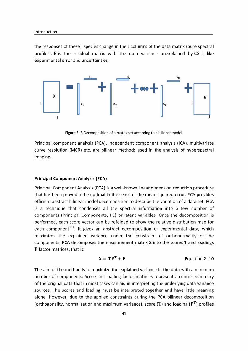
Introduction�
41��
the�responses�of�these�I�species�change�in�the�J�columns�of�the�data�matrix�(pure�spectral�profiles).�L �is� the� residual� matrix� with� the� data� variance� unexplained� by�+*M ,� like�experimental�error�and�uncertainties.�
�
Figure�2��3�Decomposition�of�a�matrix�set�according�to�a�bilinear�model.�
Principal� component� analysis� (PCA),� independent� component� analysis� (ICA),� multivariate�curve� resolution� (MCR)� etc.� are� bilinear� methods� used� in� the� analysis� of� hyperspectral�imaging.�
�
Principal�Component�Analysis�(PCA)�
Principal�Component�Analysis�(PCA)�is�a�well�known�linear�dimension�reduction�procedure�that�has�been�proved�to�be�optimal�in�the�sense�of�the�mean�squared�error.�PCA�provides�efficient�abstract�bilinear�model�decomposition�to�describe�the�variation�of�a�data�set.�PCA�is� a� technique� that� condenses� all� the� spectral� information� into� a� few� number� of�components� (Principal� Components,� PC)� or� latent� variables.� Once� the� decomposition� is�performed,�each� score� vector� can� be� refolded� to� show� the� relative� distribution� map� for�each� component181.� It� gives� an� abstract� decomposition� of� experimental� data,� which�maximizes� the� explained� variance� under� the� constraint� of� orthonormality� of� the�components.�PCA�decomposes�the�measurement�matrix�J�into�the�scores�K�and�loadings�N�factor�matrices,�that�is:�
J � KNK � L������������������������������������������������������Equation�2��10�
The�aim�of�the�method�is�to�maximize�the�explained�variance�in�the�data�with�a�minimum�number�of�components.�Score�and�loading�factor�matrices�represent�a�concise�summary�of�the�original�data�that�in�most�cases�can�aid�in�interpreting�the�underlying�data�variance�sources.� The� scores� and� loading� must� be� interpreted� together� and� have� little� meaning�alone.� However,� due� to� the� applied� constraints� during� the� PCA� bilinear� decomposition�(orthogonality,�normalization�and�maximum�variance),�score�(K)�and�loading�(NM)�profiles�
Introduction�
42��
are� not� providing� the� profiles� of� the� true� variance� sources,� but� a� linear� combination� of�them� fulfilling� the� applied� constraints.� True� variance� source� profiles� for� instance� do� not�fulfill� the� requirement� of� orthogonality� and� they� are� overlapped,� and� in� many� chemical�and�physical�systems�profiles�should�be�non�negative.��
In�this�thesis,�PCA�is�used�as�a�data�compression�noise�filtering�method�and�to�investigate�the� number� of� variance� sources,� as� a� first� step� of� the� other� image� resolution� methods.�Scores�and�loadings�obtained�by�PCA�facilitate�also�the�interpretation�of�the�behavior�and�description� of� the� sources� of� data� variance,� but� it� does� resolve� adequately� their� true�natural�profiles.�
Although� PCA� is� a� widely� used� approach� for� feature� extraction� and� data� reduction,� PCA�suffers� from� high� computational� cost,� large� memory� requirement� and� low� efficacy� in�dealing�with�large�dimensional�datasets�such�as�Hyperspectral�Imaging�(HSI).�J.�Zabalza�et�al.� proposed� Folded�PCA� for� improved� feature� extraction� and� data� reduction� with�hyperspectral�imaging182.�
In� Chapter� 6,� bilinear� methods� of� image� resolution� were� assessed,� and� the� comparison�between�MCR�ALS,�PCA,�and�other�related�methods�were�shown.�
�
Independent�Component�Analysis�(ICA)�
Independent� component� analysis� (ICA)� is� a� statistical� method� for� finding� underlying�factors�or�components�from�multivariate�data,�which�can�be�proposed�to�solve�the�blind�source� separation� problem183.� ICA� is� used� to� find� a� mathematical� transformation� of� the�data�into�a�linear�combination�of�statistically�independent�components.�The�difference�of�ICA� to� other� methods,� is� that� it� looks� for� components� that� are� both� statistically�independent�and�non�Gaussian184.�Bilinear�decomposition�ICA�constraints�are�more�severe�than�PCA�constraints,�since�statistical�independence�is�a�stronger�condition�than�the�linear�independence�(orthogonality�constraints)�assumed�by�PCA�(Orthogonality�is�a�special�case�of�linear�independence)185.�
ICA�assumes�that�the�data�is�a�linear�combination�of�non�Gaussian,�mutually�independent�latent�variables�in�an�unknown�mixing�matrix.�ICA�reveals�hidden�independent�sources�and�their� relative� contributions.� The� aim� of� ICA� is� the� decomposition� of� multivariate� signals�into�statistically�independent�component�contributions�with�minimum�loss�of�information.�Given� a� set� of� observations� represented� by� a� data� matrix�J�(I,J),�having� I� measurement�vectors,�the�ICA�bilinear�model�can�be�written�as�following:�
J � O* � L�����������������������������������������������Equation�2��11�

Introduction�
43��
where�*�(N,J)is� the� N� dimensional� vector� of� independent� sources� and�O�(I,N)� is� the�unknown� basis� matrix.�L(I,J)� is� the� error� matrix.� Then,� ICA� searches� for� the� linear�transformation�of�the�data�P,�such�that�the�projected�variables:�
PJ � *���������������������������������������������Equation�2��12�
are�as�independent�as�possible.�It�has�been�shown�that�the�model�is�completely�identical�if�the�sources�are�statistically�independent�and�at�least�N�1�of�them�are�non�Gaussian.�If�the�sources� are� Gaussian,� the� ICA� transformation� can� be� estimated� up� to� an� orthogonal�transformation.� Estimation� of� mixing� and� un�mixing� matrices� can� be� done� maximizing�diverse�objective�functions,�among�the�non�gaussianity�of�the�sources�and�the�likelihood�of�the�sample.��
Principal� Component� Analysis� (PCA),� Independent� Component� Analysis� (ICA)� can� be�considered�to�share�the�same�overall�objective:�the�decomposition�of�a�data�matrix�into�a�reduced�number�of�components.�
ICA� is� an� increasingly� popular� method� to� resolve� complex� data� sets,� like� hyperspectral�image� data,� into� component� signatures� (spectra)� and� their� distribution� maps.�Unfortunately,�the�pre�requisite�of�statistical�independence�severely�limits�the�application�of�ICA.�W.�Windig�and�M.�R.�Keenan�proposed�a�pre�processing�method�to�extend�the�use�of� ICA.� For� a� certain� class� of� data,� increasing� the� sparsity� of� a� data� set,� increases� the�independence�of�the�components,�and�thus�enables�the�successful�application�of�ICA.�The�sparsity� can� be� increased� by� simply� adding� zeros� to� the� data� set� or� by� applying� a� Haar�wavelet�transform186.�
In�Chapter�6�comparisons�between�ICA�and�other�methods� like�PCA�or�MCR�ALS�(below)�are�shown�for�some�specific�cases.�
�
Vertex�Component�Analysis�(VCA)�
VCA�(Vertex�Component�Analysis)�is�an�unsupervised�method�based�on�the�geometry�of�a�convex� data� set� which� considers� that� the� pure� image� constituents� are� located� at� the�vertices� of� a� simplex.� It� is� a� method� that� is� well� known� in� remote� sensing� area� for�endmember� (pure� component)� extraction.� For� example,� in� a� mixture� defined� by� three�constituents,� the� simplex� boundaries� built� by� VCA� are� a� triangle,� whose� vertices�correspond�to�the�estimations�of�the�pure�constituents�or�endmembers.�VCA�assumes�that,�for�every�constituent,�exists�one�or�more�pixels�in�the�image�where�only�this�constituent�exists� (pure� pixels).� If� this� condition� is� fulfilled,� VCA� will� find� these� vertex� pixels� and�therefore� the� corresponding� pure� components.� To� find� out� these� pure� pixels� and� the�spectral�signatures�associated�to�them,�VCA�iteratively�projects�the�data�onto�a�direction�
Introduction�
44��
which�is�orthogonal�to�the�subspace�spanned�by�the�endmembers�already�estimated.�The�new� endmember� signatures� are� located� at� the� extreme� of� the� new� projection.� This�iteration� procedure� goes� on� until� all� the� endmember� signatures� are� estimated.� A� more�detailed�description�of�the�method�can�be�found�in187.�
�
Minimum�Volume�Simplex�Analysis�(MVSA)�
MVSA� (Minimum� Volume� Simplex� Analysis),� also� considers� that� the� underlying� mixing�model�is�bilinear,�i.e.�that�the�mixed�hyperspectral�vectors�are�a�linear�combination�of�the�signatures� (spectra)� of� pure� components.� MVSA� is� a� method� that� finds� the� pure�components�(end�members)�in�hyperspectral�image�by�fitting�a�minimum�volume�simplex�to�the�hyperspectral�data,�under�some�constraint�such�as�for�every�pixel�no�less�than�zero�(non�negativity� constraint)� abundance� fractions� and� of� sum� is� equal� to� one� (closure).�MVSA� does� not� use� a� least� squares� approach,� but� a� Sequential� Quadratic� Programming�(SQP)�method,�based�on�a�quasi�Newton�non�linear�optimization�procedure�under� linear�constraints.�In�order�to�prevent�local�minima�and�to�achieve�a�faster�speed,�VCA�is�usually�applied� as� the� initial� step� to� provide� an� inflated� version� of� the� initial� simplex188.� More�details�about�the�MVSA�can�be�seen�in�references�and�the�original�paper�189.�
Geometrical�based� data� analysis� approaches� are� based� into� two� main� categories,� Pure�Pixel�(PP)�or�Minimum�Volume�(MV).�Pixel�Purity�Index�(PPI)190,�191,�Iterative�Error�Analysis�(IEA)� 192,� Vertex� Component� Analysis� (VCA)� and� Simplex� Growing� Algorithm� (SGA)193� are�pure� pixel� based� algorithms.� The� Minimum� Volume� Simplex� Analysis� (MVSA)189,� the�Minimum�Volume�Enclosing�Simplex�(MVES)194�and�the�Simplex�Identification�via�variable�Splitting�And�Augmented�Lagrangian�(SISAL)195�are�minimum�volume�approaches�which�fit�a� minimum� volume� simplex� to� the� hyperspectral� data.� In� this� thesis,� VCA� and� MVSA�methods� were� compared� with� MCR�ALS� for� the� resolution� of� remote� sensing�hyperspectral�images�in�Chapter�3.��
�
�
Other�recently�developed�image�resolution�methods��
When�considering�the�problem�of�hyperspectral�image�resolution,�most�of�the�literature�in�the� image� processing� areas� relies� on� the� widely� used� Linear� Mixing� Model� (LMM).�However,� this� model� may� be� not� valid� and� other� nonlinear� models� can� be� considered.�When�there�are�strong�multi�scattering�effects�or�intimate�interactions,�several�significant�contributions�have�been�proposed�to�overcome�the�limitations�of�linear�model.��
Introduction�
45��
Altmann,�Y.�etc.�have�reported�a�Bayesian�algorithm�to�estimate�the�parameters�involved�in� the�model� yielding�an�unsupervised�nonlinear�unmixing�algorithm� 196.�This� group�also�studied� a� linear� Radial� Basis� Function� Network� (RBFN)� for� unmixing� hyperspectral�images197.�They�proposed�to�estimate�the�model�abundances�using�a�linear�combination�of�radial�basis�functions�whose�weights�are�estimated�using�training�samples.�Yoann�Altmann�et� al.� reported� a� nonlinear� method� using� Gaussian� processes.� The� first� step� is� using� the�Bayesian� estimation� of� the� abundance� vectors� for� all� the� image� pixels� and� the� use� of� a�nonlinear�function�to�relate�the�abundance�vectors�to�the�experimental�observations.�The�pure� components� (endmembers)� are� subsequently� estimated� using� a� Gaussian� process�regression� 198.� Jie� Chen� etc.� formulated� a� new� kernel�based� paradigm� that� relies� on� the�assumption� that� the� mixing� mechanism� can� be� described� by� a� linear� mixture� of� pure�component�(endmember)�spectra,�with�additive�nonlinear�fluctuations�defined� in�Hilbert�space199.�� �

Introduction�
46��
�
Multivariate�Curve�Resolution�Alternating�Least�Squares�(MCR�ALS)�
�
Multivariate�Curve�Resolution�(MCR)�has�been�chosen�in�this�thesis�as�the�main�strategy�for�the�resolution�of�hyperspectral�images.�MCR�is�defined�as�a�group�of�techniques,�which�help� to� resolve� mixtures� by� determining� the� number� of� constituents,� their� response�profiles� (spectra),� and� their� estimated� concentrations,� when� no� prior� information� is�available�about�the�nature�and�composition�of�them200.�
The� basic� theory� of� MCR� is� that� the� bilinear� model� is� valid� for� the� investigated�spectroscopic�system�(i.e.�the�extended�multicomponent�multiwavelength�Lambert�Beer’s�law).�For�a�mixture�with�component�i=�1,2,…,N,:�
�
Q � +*K � � R�S�I� ��K��������������������������������Equation�2��13�
�
Here�N�is�the�number�of�absorbing�components�coexisting�in�the�system,�and�the�R �and�� �(i=1,�2,...,�N)�are�the�pure�concentration�profiles�and�spectra�respectively.�The�problem�to�be�solved�is�from�the�measurements�matrix�Q,�we�need�to�determine:�
� The�number�of�absorbing�chemical�components�is�N;��� The�spectrum�of�each�chemical�component�� (i=1,�2,...,�N);��� The�concentration�profile�of�each�chemical�component�R (i=1,�2,...,�N).��
�
�
MCR�methods�are�widespread�and�powerful�methodologies�for�the�analysis�and�modeling�of� multivariate� data� in� many� different� application� fields.� MCR� methods� have� been�successfully� used� to� analyze� data� coming� from� UV�vis� spectroscopy201,� infrared�spectroscopy202,�chromatography203,�mass�spectroscopy204,�nuclear�magnetic�resonance205,�hyperspectral� imaging206,� voltammetry207,� microarray208,� LC�MS� metabolomics209.� MCR� is�at�present�well�developed�both�from�a�theoretical�and�the�applied�point�of�view,�and�it�is�still�expanding�its�range�of�applications.��
The� wide� applicability� of� MCR� can� be� related� to� the� versatility� of� the� design� and�implementation�of�data�specific�constraints.�The�adequate�formulation�and�application�of�different� constraints� based� on� the� chemical� and� physical� features� of� the� component�
Introduction�
47��
profiles� (spectra� and� concentration� when� analyzing� hyperspectral� imaging� data)� to� be�resolved�are�the�reason�of�its�success.�
�
MCR�ALS� has� developed� very� fast� during� the� last� years.� An� updated� version� of� the�graphical�user�friendly� interface�related�to�the�Multivariate�Curve�Resolution�Alternating�Least�Squares� (MCR�ALS)�algorithm�has�been�published210.� It� includes� recently�published�advances�of�this�algorithm,�including�the�implementation�of�additional�constraints,�such�as�kinetic�hard�modeling�and�calibration,�as�well�as�constraints�linked�to�model�structure�for�multiset�and�multi�way�data�analysis,�and�the�possibility�to�use�fully�or�partially�multilinear�models�to�describe�the�data�set.�
Recently,� the� performance� and� validation� of� the� extension� of� MCR�ALS� with� the�quadrilinear� constraint� in� the� analysis� of� noisy� datasets� was� studied.� Results� suggested�that�MCR�ALS�with�the�quadrilinear�constraint�can�be�used�efficiently� for� the�analysis�of�four�way� quadrilinear� environmental� datasets211.� A� Non�Linear� Multivariate� Curve�Resolution� Alternating� Least� Squares� (NL�MCR�ALS)� method� has� been� proposed� and�applied� for� the� calibration� of� spectral� data� that� includes� the� so�called� saturated� peaks,�which� are� flattened� because� of� samples� with� ultrahigh� absorbance.� In� spite� of� serious�violations� of� the� Lambert–Beer� law,� the� NL�MCR�ALS� prediction� results� were� quite�satisfactory,�and�the�accuracy�achieved�is�better�than�using�other�competing�methods212.�In�another�example,�the�photodegradation�of�carbofuran�deposited�on�TiO2�film�under�UV�light�exposure�was�analyzed�using�a�Hard–Soft�Multivariate�Curve�Resolution�Alternating�Least�Squares�(HS�MCR�ALS)213.��
MCR�ALS� can� be� extended� to� the� analysis� of� multi�set� data� (via� column�� and� row�wise�augmented�data�matrices),�and�application�of�multilinear/multiset�constraints�to�profiles�to� be� resolved.� MCR�ALS� has� been� used� rather� extensively� also� to� the� analysis� of�environmental� monitoring� data� tables,� for� example,� to� explore� the� possible� interaction�between� O3� and� NOx� pollution� patterns214.� MCR�ALS� has� been� also� applied� to� the�resolution� of� concentration� and� spectral� profiles� of� the� azo�dyes� photodegradation�reactions�by�UV–visible�DAD�and�1H�NMR�spectroscopy�data�fusion�215.�M.J.�Culzoni�et�al.�have� developed� a� liquid� chromatographic� method� with� fast� scan� fluorimetric� detection�with� MCR�ALS� in� the� simultaneous� determination� of� five� marker� pteridines� in� urine�samples216.�Keshav�Kumar�et�al.�have�shown�that�the�synchronous�fluorescence�spectra�of�the� mixture� constituents� at� various� wavelength� offsets� using� Total� Synchronous�Fluorescence�Spectroscopy�(TSFS)�data�set�can�be�extracted�using�MCR�ALS217.�
Although�second��and�higher�order�data�sets�are�the�natural�type�of�data�to�be�analyzed�with�MCR�ALS,�recently�this�method�has�been�also�extended�for�the�analysis�of�first�order�

Introduction�
48��
data� using� a� correlation� constraint� 218.� In� this� case,� MCR�ALS� can� be� used� for� first�order�multivariate�calibration,�and�the�estimations�of�analyte�concentration�are�correct.��
MCR�ALS� has� been� recently� applied� to� the� identification� of� the� different� paramagnetic�centers� from� � complex� mixtures� of� them� analyzed� by� Electron� Paramagnetic� Resonance�(EPR)� spectroscopy� 219.� In� another� study,� the� analytical� data� obtained� from� a�chronoamperometric� experiment� for� the� analysis� of� a� weak� host–guest� complexation�system�was�also�analyzed�by�MCR�ALS.�The�data�matrices�collected�at�different�potentials�were� simultaneously� analyzed� by� MCR�ALS� to� recover� the� thermodynamic� parameters�(e.g.,�stoichiometric�ratio�and�formation�constant)�of�cyclodextrin–dopamine�complex220.�
�
MCR�ALS�has�been�applied� in�biology,� food�and�medicine� industry� in�recent�years.�MCR�ALS�has�been�proposed�to�investigate�biological�pathways�in�metabolic�networks.�By�using�this�method,�different�constraints�can�be� included�in�the�model,�and�the�same�source�of�variability� can� be� present� in� different� pathways,� which� is� reasonable� from� a� biological�standpoint221.� Silvia� Grassi� et� al.� have� used� MCR�ALS� to� model� milk� lactic� acid�fermentation�processes.�MCR�ALS�applied�to�FT�NIR�spectroscopy�can�be�used�as�a�control�system� which� can� also� be� implemented� in�line,� as� a� reliable� management� method� for�fermentation�process�monitoring�and�to�estimate�coagulation�profiles,�no�matter�what�are�the�operative�conditions�adopted�for�the�process222.�Maha�A�Hegazy�et�al.�have�used�MCR�ALS�to�estimate�and�quantify�spectrally�overlapped�Vitamin�B1,�Vitamin�B6,�benfotiamine�and�diclofenac�sodium�quaternary�mixtures�222,�223.�
�
Based�on�the�previous�experience�and�advantages�of�the�MCR�ALS�method,�in�this�Thesis,�this�method�has�been�extended�to�the�resolution�of�hyperspectral�imaging�data�sets.�The�goal� of� multivariate� image� analysis� is� to� identify� and� estimate� the� distribution� of� the�chemical�constituents�on�the�scanned�sample.�Hyperspectral�imaging�systems�coupled�to�MCR�ALS� have� already� been� already� applied� for� the� resolution� of� different� type� of�problems�95,�224.��
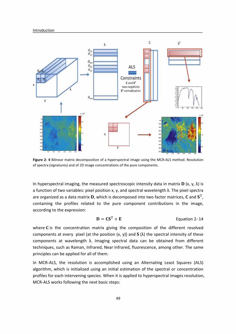
Introduction�
49��
�Figure�2��4�Bilinear�matrix�decomposition�of�a�hyperspectral�image�using�the�MCR�ALS�method.�Resolution�of�spectra�(signatures)�and�of�2D�image�concentrations�of�the�pure�components.�
�
In�hyperspectral�imaging,�the�measured�spectroscopic�intensity�data�in�matrix�Q�(x,�y,�)�is�a�function�of�two�variables:�pixel�position�x,�y,�and�spectral�wavelength�.�The�pixel�spectra�are�organized�as�a�data�matrix�Q,�which�is�decomposed�into�two�factor�matrices,�+�and�*M,�containing� the� profiles� related� to� the� pure� component� contributions� in� the� image,�according�to�the�expression:�
Q � +*M � L����������������������������������������������������Equation�2��14�
where�+�is� the� concentration� matrix� giving� the� composition� of� the� different� resolved�components�at�every��pixel�(at�the�position�(x,�y))�and�*�()�the�spectral�intensity�of�these�components� at� wavelength� .� Imaging� spectral� data� can� be� obtained� from� different�techniques,�such�as�Raman,�Infrared,�Near�Infrared,�fluorescence,�among�other.�The�same�principles�can�be�applied�for�all�of�them.��
In� MCR�ALS,� the� resolution� is� accomplished� using� an� Alternating� Least� Squares� (ALS)�algorithm,�which� is� initialized�using�an� initial�estimation�of� the�spectral�or�concentration�profiles�for�each�intervening�species.�When�it�is�applied�to�hyperspectral�images�resolution,�MCR�ALS�works�following�the�next�basic�steps:�

Introduction�
50��
(1)�Determination�of�the�number�of�constituents�in�the�raw�image�(Q).�
(2)�Generation�of� initial�estimates�(*M)�based�of�the�selection�of�the�purest�pixel�spectra�(SIMPLISMA).�
(3)�Given�Q�and�*M,�calculation�of�+�under�constraints.�
(4)�Given�Q�and�+,�calculation�of�*M,�under�constraints.�
(5)�Reproduction�of�Q�from�the�product�of�+�and�*M.�
(6)�Go�to�step�3�until�convergence�is�achieved.�
(7)�Recovering�spectral�information�from�ST�and�identification�of�image�constituents.�
(8)� Recovering� spatial� information� from� refolded� C� matrix,� and� mapping� of� the� image�constituents.��
The� number� of� image� constituents� can� be� either� known� beforehand� based� on� the�knowledge�of�the�samples�analyzed,�or�be�determined�by�PCA�or�SVD�on�the�whole�image.�The� alternating� optimization� should� always� start� by� using� the� original� preprocessed�measurement,�Q,� and� an� initial� guess� of� either� the�+�or� the�*Mmatrices.� Typically,� in�images,� the� initial� estimate� is� a�*M�matrix� formed� by� pixel� spectra� picked� up� from� the�image�according�to�previous�knowledge�(from�pixels�in�areas�of�interest)�or�as�a�result�of�applying�chemometric�tools�for�purest�pixel�selection,�such�as�SIMPLISMA�(Simple�to�use�Interactive�Self�modeling�Mixture�Analysis)�225.�
During�the�iterative�optimization�process�(steps�4�and�5),�the�unconstrained�least�squares�solution�for�the�concentration�profiles�can�be�calculated�by�the�following�equation:�
+ � Q�*K�1,�under�constraints������������������������������������Equation�2��15�
where��*M�1�is�the�pseudoinverse�of�the�spectral�matrix�*K,�and�it�is�equal�to�T*�*M*��.U�when�*M�is�full�rank.�The�new�estimation�of�the�+�matrix�can�be�then�used�to�recalculate�by�lest�squares�a�new�estimation�of�the�*M�matrix:�
*K � +1Q,�under�constraints�������������������������������������Equation�2��16�
where�+1�is� the� pseudoinverse� of�+,�+1 � �+M+��.+M�when�+�is� full� rank.� Each� of� these�two� equations,� are� solved� under� constraints.� Constraints� are� defined� as� chemical� or�mathematical�properties�that�should�hold�the�resolved�profiles.�For�example,�constraints�like�non�negativity�which�is�based�on�chemical�or�physical�assumptions�on�the�data�can�be�applied� during� the� iteration226.� Similarly,� constraints� like� local� rank� for� selectivity�
Introduction�
51��
constraints� which� are� not� necessary� in� relation� to� the� chemistry� or� the� physics� of� the�system� but� related� to� mathematical� properties� can� be� applied.� Constraints� are� used� to�have�profiles�with�shapes�that�are�physically�meaningful�and�to�approximate�the�solutions�to�the�true�ones�(see�below).�The�proper�application�of�constraints�is�the�more�important�aspect� in� the� application� of� the� MCR�ALS� method� (see� below� for� a� more� detailed�description�of�constraints).��
At�each�iteration�step,�a�new�estimation�of�the�+�and�*M�matrices�is�obtained�and�used�as�a� new� estimation� for� the� next� iteration.� Thus� the� alternating� least� squares� process�continues�until�convergence�is�reached�(There�is�no�significant�variation�among�the�fitting�results� nor� profiles� in� consecutive� cycles.).� If� the� applied� constraints� are� fulfilled� by� the�data,� the� final� solutions� are� close� or� equal� to� the� real� solution.� In� order� to� avoid� scale�indeterminacies�during�the�ALS�optimization,�usually�it�is�necessary�to�apply�normalization�either� to�+�or� to�*M�profiles.� In� this� thesis,� usually,� the� pure� spectra� of� the� resolved�components� have� been� normalized� 225.� Equal� vector� length� /� area� normalizations� are�selected�in�this�Thesis�for�hyperspectral�imaging�resolution�(Loadings�*�are�divided�by�the�square�root�of�the�sum�of�the�squares�of�all�the�elements�of�the�considered�spectra�profile,�so� that� all� components� have� the� same� spectral� contribution,� and� the� quantitative�information�is�contained�in�C�matrix).�
�

Introduction�
52��
�Figure�2��5�Processes�of�MCR�ALS�for�experimental�data�resolution�
+�and�*Kare�optimized�iteratively�using�an�Alternating�Least�Squares�(ALS)�algorithm�until�convergence�is�reached.�External�application�of�constraints�during�ALS�iterations�of�the�has�some� advantages:� it� has� the� flexibility� to� cope� with� many� kinds� of� data� structures� and�chemical�problems�and�the�ability�to�accommodate�external�information�in�the�resolution�process.� Both� soft� and� hard� constraints� can� be� applied� during� the� ALS� optimization�process.��
Constraints�are�essential�to�drive�the�iterative�resolution�process�to�chemically�meaningful�solutions� and� to� decrease� the� rotational� ambiguity� inherent� to� the� multivariate� curve�resolution�results�(see�below).�The�following�constraints�can�be�considered:�
Non�negativity�constraints:�Non�negativity�concentration�constraint�is�a�general�constraint�used�in�curve�resolution�methods.227.�Physical�concentrations�can�only�be�positive�or�zero�(+0),� and� in� many� spectroscopies,� for� example� Raman,� Infrared� applied� in� this� Thesis,�
VD�G���GW�X�Y�W����W��D
D
Z�W��X�VFW���W�[\]Z^_`Z]^ab
STinit
a`]
VFW���W�[�[c�d�eG��[c�E[��[GWF
]fY
g[FW���WF
]�GEW��ST
g[EGW��W�[_�[c�XGF
C
][X-���D=CST+E�h[��C��i�ST
ZWG��W�-GXj�dF���a`]
kd�W�W�W�-G��c[���W�[\g�X�e��W�[%�f�X�i�W�[%�_�Gi�EW�[b
kd�X�W�W�-G��c[���W�[\ZiGW�c�E�W�[b
�
Introduction�
53��
spectral�values�also�can�be�only�positive�or�zero�(*K0).�In�all�the�cases�of�this�Thesis,�non�negativity� concentration� constraints� and� non�negativity� spectra� constraints� have� been�applied� for� hyperspectral� imaging� resolution.� There� are� different� ways� to� apply� this�constraint,�such�as,�direct� replacement�of�negative�vales�to�zero,�or�using�more�rigorous�iterative�methods�based�on�non�negative� least�squares� (eg.�Non�negative�Least�Squares,�(NNLS)228,� and� Fast� Non�Negative� Least� Squares� (FNNLS)229).� In� this� Thesis,� FNNLS� have�been�applied�for�non�negative�constraint.�
Unimodality� constraints:� In� a� wide� variety� of� situations,� concentration� profiles� have� a�unimodal�shape,�for�example�they�only�have�a�maximum.�This�is�the�case�for�instance�for�chromatographic�elution�profiles.�In�contrast,�spectral�profiles�are�usually�not�unimodal�in�the� general� case.� Some�other� types� of� instrumental� signals� may� also� be� unimodal,� as� in�electrochemistry.�Whenever�the�shape�of�the�profiles�is�unimodal,�unimodality�is�a�useful�additional� constraint.� In� this� case,� the� algorithm� intends� to� avoid� the� formation� of�secondary� maxima.� First� the� highest� maximum� is� detected� and� then� all� the� departures�from� the� unimodal� condition� are� constrained,� discarding� left� and� right� maxima.� This�constraint� is�not�suitable�for�the�cases�of�hyperspectral� imaging�resolution� in�this�thesis.�See�reference230for�more�detailed�descriptions�of�the�unimodality�constraint.�
Closure� constraints:� This� case� is� frequently� encountered� for� instance� in� reaction�based�systems,� where� a� mass� balance� equation� is� obeyed� by� the� concentration� profiles� of� the�species� present� in� the� system.� With� this� constraint,� the� sum� of� the� concentrations� or�fractions�of�all�of�the�species�involved�in�the�reaction�or�mixture�(the�suitable�elements�in�each�row�of�the�C�matrix)�is�forced�to�be�equal�to�a�constant�value�(the�total�concentration�or�fractions)�at�each�stage� in�the�reaction�or� in�the�mixture.�The�closure�constraint� is�an�example� of� an� equality� constraint.� This� constraint� is� not� suitable� for� the� cases� of�hyperspectral� imaging� resolution� in� this� Thesis.� See� reference230for� more� detailed�descriptions�of�the�closure�constraint.�
Selectivity/local�rank�constraints�
Selectivity/local�rank�constraints�use�the�information�related�to�the�presence�or�absence�of�certain�components�in�particular�pixels.�Selectivity�and�local�rank�constraints�are�among�the� most� powerful� constraints� to� decrease� rotational� ambiguities� (see� below)� in� curve�resolution�studies231.�
The� rank� of� a� data� matrix� is� equal� to� the� number� of� linearly� independent� rows� or�columns232�of�the�considered�data�matrix.�Assuming�concentration�profiles�and�spectra�to�be� linearly� independent� and� noiseless,� the� rank� of� the� data� equals� the� number� of� pure�components.�This�number�can�be�estimated�from�Singular�Value�Decomposition�(SVD)�as�the�number�of�singular�values�which�are�larger�than�a�threshold�value�associated�to�noise�

Introduction�
54��
contributions.� In� general,� it� is� practical� to� define� a� ‘chemical� rank’� counting� only� the�number�of�singular�values�that�are�greater� than�a�cut�off�determined�by�the�noise� level.�This� implies� that� only� major� sources� of� variance� are� considered,� those� related� with� the�physical� phenomena� under� study,� for� instance� the� number� of� chemical� species� in� a�chemical�reaction�or�the�number�of�eluted�components�in�a�chromatographic�separation.��
When�analyzing�a�complex�chemical�imaging�system,�the�‘chemical�rank’�evaluated�by�SVD�equals�to�the�number�of�chemical�component�in�the�sample233.�Local�rank�detects�the�rank�in�a�small�area�of�the�image.�From�chemical� local�rank�information,� it� is�possible�to�infer�the�presence�or�absence�of�particular�constituents�in�the�image234.�Local�rank�constraints�use�this�rank�information�for�improve�the�MCR�resolution�results.�
Local�rank�analysis�methods�have�been�used�in�the�study�of�evolving�processes,�where�the�concentration�profiles�of�the�different�components�evolve�smoothly�and,�often�following�a�sequential� pattern235.� Using� gradually� growing� size� windows,� imitating� the� stepwise�progress�of�a�process,�the�evolution�of�the�number�of�significant�components�indicates�the�number� of� different� components� emerging� and� decaying.� In� sequential� processes,� the�proper� use� of� this� information� can� provide� concentration� windows.� For� example,� it� can�indicate� where� a� particular� component� is� present,� and� give� approximate� concentration�profiles�for�the�different�components.�Evolving�Factor�Analysis� (EFA)236�was�the�principal�method�used�for�local�rank�analysis�of�chemically�evolving�processes.�Modified�versions�of�this� method� were� oriented� to� confirm� the� sequential� evolution� of� components� in�unknown� processes,� to� improve� the� setting� of� concentration� windows� and� to� overcome�problems�linked�to�the�analysis�of�rank�deficient�processes.��
Local�rank�analysis�methods�are�based�on�the�use�of�fixed�size�moving�windows�covering�the�whole�data�set.�The�results�obtained�by�the�application�of�local�rank�analysis�methods�inform�about�the�local�complexity�of�the�data�set.�They�give�information�about�how�many�components�overlap�in�the�different�data�set�regions�enclosed�by�the�selected�windows.�They�can�be�used�to�locate�selective�regions�in�the�data�set,� i.e.,�windows�with�only�one�component,�which�are�critical�to�achieve��resolution�without�ambiguities�237.��
To�adapt�these�methods�to�the��hyperspectral�imaging�data�structures,�a�modified�FSMW�EFA� methodology� was� developed,� called� Fixed� Size� Image� Window–Evolving� Factor�Analysis� (FSIW�EFA)234(See� figure� 2�6).� It� has� been� adapted� to� the� structure� of� image�datasets�with�spatial� information�and�it�provides�the�information�to�be�used�as�MCR�ALS�constraints.� Hyperspectral� imaging� scans� material� surface� pixel� by� pixel,� covering� the�whole� surface� of� the� object.� Local� rank� maps� describe� the� pixels� where� local� rank�constraints�can�be�potentially�applied.�The�absence�of�a�particular�component�can�be�used�as� a� constraint� in� pixels� where� the� chemical� rank� is� lower� than� the� total� number� of�compounds� in� the� image.� From� a� rank� analysis� of� the� appropriate� data� windows�

Introduction�
55��
(submatrices)� it� is�possible�to�find�out�the�number�of�components�(constituents)�present�in�the�corresponding�pixel.��
�Figure�2��6�How�fixed�size�moving�windows�are�used�to�detect�local�ranks�
Identification� of� the� compounds� absent� in� these� pixels� requires� the� use� of� additional�information.� For� example,� comparison� of� the� pixel� spectrum� with� known� pure� spectra,�when�available�or�with�the�purest�selected�spectra�of�the�image.��
In� Chapter� 3,� when� analyzing� remote� sensing� image� datasets,� USGS� spectral� library� was�used�for�spectral�identification.�Also,�if�available,�the�spectra�from�external�samples�or�for�reference�spectra�can�be�used�during�the� image�resolution.� In�Chapter�4,�an�example�of�application�of�local�rank�constraints�is�shown�for�chocolate�analysis.�In�food�industry,�it�is�usual�to�have�some�previous�knowledge�about�the�possible�chemical�constituents�of�food�products�and�it�is�relatively�easy�to�have�their�pure�spectra.�
�
�
MCR�ALS�applied�to�the�simultaneous�analysis�of�multiple�data�matrices��
MCR�ALS� can� be� extended� to� the� analysis� of� multiset� and� multiway� data� structures.� A�single�data�matrix�can�be�row�wise,�column�wise,�or�row�and�column�wise�augmented�to�
� � � ��
�
SVD
Pixel�area(1,�1)
SVD
Pixel�area(n,�n)

Introduction�
56��
form�a�multiset�data�structure�when�other�matrices�have�either�the�same�variables�are�in�their� rows,� in� their� columns,� or� in� both.� In� these� cases� they� can� be� � appended� in� the�appropriate�direction�(see�Figure�2��7)238.�
�
�Figure�2��7�Extension�of�the�MCR�model�to�multiset�data�analysis�arranged�in�augmented�data�matrices.�a)�MCR�ALS�of�a�row�wise�augmented�data�matrix,�b)�MCR�ALS�of�a�column�wise�augmented�data�matrix,�c)�MCR�ALS�of�a�column��and�row�wise�augmented�data�matrix.�
To�have�a�new�meaningful�data�structure,�all�individual�data�matrices�(slices)�in�this�type�of�data�set�should�share�some� information�with�the�other�appended�matrices;�otherwise� it�does� not� make� any� sense� to� build� such� a� new� data� arrangement.� Different� ways� of�building� row�wise,� column�wise,� and� column�� and� row�wise� augmented� matrices� are�shown�in�Figure�2��7.��
Different� data� augmentation� arrangements� are� possible� and� they� may� be� written� in� a�more�concise�way.�For�instance,�in�the�work�of�Chapter�4,�experimental�data�of�chocolate�samples� and� reference� data� share� the� same� pure� spectra,� and� column�wise� augmented�matrices� were� used� (where� reference� spectra� of� pure� component� were� added� at� the�bottom� of� the� experiment� data� matrix� to� use� selectivity� constraints).� Column�wise�
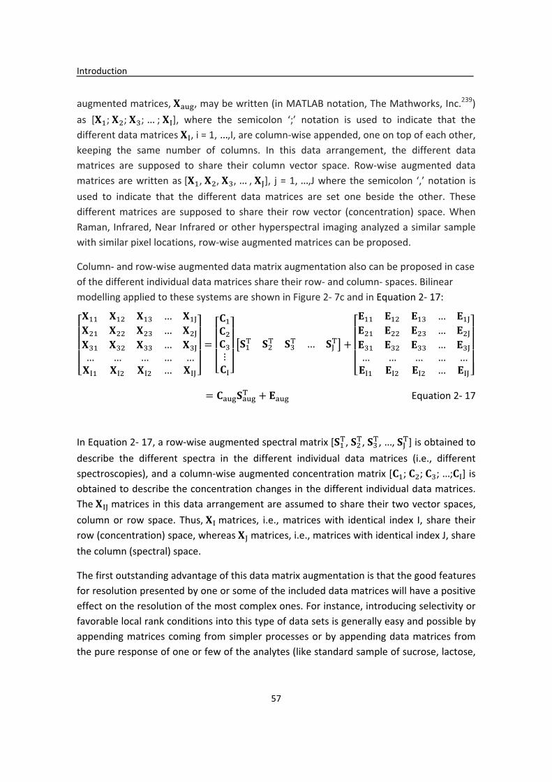
Introduction�
57��
augmented�matrices,�Jlmn,�may�be�written�(in�MATLAB�notation,�The�Mathworks,�Inc.239)�as� [J.;�J2;�Jo;�p�;�Jq],� where� the� semicolon� ‘;’� notation� is� used� to� indicate� that� the�different�data�matrices�Jq,�i�=�1,�p,I,�are�column�wise�appended,�one�on�top�of�each�other,�keeping� the� same� number� of� columns.� In� this� data� arrangement,� the� different� data�matrices� are� supposed� to� share� their� column� vector� space.� Row�wise� augmented� data�matrices�are�written�as [J.,�J2,�Jo,�p�,�Jr],� j�=�1,�p,J�where� the�semicolon� ‘,’�notation� is�used� to� indicate� that� the� different� data� matrices� are� set� one� beside� the� other.� These�different� matrices� are� supposed� to� share� their� row� vector� (concentration)� space.� When�Raman,�Infrared,�Near�Infrared�or�other�hyperspectral� imaging�analyzed�a�similar�sample�with�similar�pixel�locations,�row�wise�augmented�matrices�can�be�proposed.��
Column��and�row�wise�augmented�data�matrix�augmentation�also�can�be�proposed�in�case�of�the�different�individual�data�matrices�share�their�row��and�column��spaces.�Bilinear�modelling�applied�to�these�systems�are�shown�in�Figure�2��7c�and�in�Equation�2��17:�
stttuJ.. J.2 J.o p J.rJ2. J22 J2o p J2rJo. Jo2 Joo p Jorp p p p pJq. Jq2 Jq2 p Jqr v
wwwx�
stttu+.+2+oy+q vwwwxz*.M *2M *oM p *rM{ �
stttuL.. L.2 L.o p L.rL2. L22 L2o p L2rLo. Lo2 Loo p Lorp p p p pLq. Lq2 Lq2 p Lqr v
wwwx�
� +lmn*lmnM � Llmn��������������������������������������������������Equation�2��17�
�
In�Equation�2��17,�a�row�wise�augmented�spectral�matrix�[*.M,�*2M,�*oM,�p,�*rM]�is�obtained�to�describe� the� different� spectra� in� the� different� individual� data� matrices� (i.e.,� different�spectroscopies),�and�a�column�wise�augmented�concentration�matrix�[+.;�+2;�+o;�p;+q]�is�obtained�to�describe�the�concentration�changes�in�the�different�individual�data�matrices.�The�Jqr�matrices� in�this�data�arrangement�are�assumed�to�share�their�two�vector�spaces,�column� or� row� space.� Thus,�Jq�matrices,� i.e.,� matrices� with� identical� index� I,� share� their�row�(concentration)�space,�whereas�Jr�matrices,�i.e.,�matrices�with�identical�index�J,�share�the�column�(spectral)�space.�
The�first�outstanding�advantage�of�this�data�matrix�augmentation�is�that�the�good�features�for�resolution�presented�by�one�or�some�of�the�included�data�matrices�will�have�a�positive�effect�on�the�resolution�of�the�most�complex�ones.�For�instance,�introducing�selectivity�or�favorable�local�rank�conditions�into�this�type�of�data�sets�is�generally�easy�and�possible�by�appending�matrices�coming�from�simpler�processes�or�by�appending�data�matrices� from�the�pure�response�of�one�or�few�of�the�analytes�(like�standard�sample�of�sucrose,�lactose,�
Introduction�
58��
butter�and�whey�which�were�used�in�the�work�introduce�in�chapter�4)�present�in�a�much�more�complex�mixture�data�matrix.��
�
MCR�ALS�applied�to�multiway�data�using�multilinear�models��
Multivariate� Curve� Resolution� (MCR)� methods� can� be� extended� also� to� the� analysis� of�multi�way� data.� According� to� Sanchez� and� Kowalski,� the� analytical� data� generated� by�instrumental�techniques�can�be�classified�as�follows:�zero�order�data�(e.g.�a�univariate�or�single�data�per�analyte),�first�order�data�(e.g.�a�data�vector�per�sample),�second�order�data�(e.g.� a� data� matrix� per� sample)240.� Correspondingly,� zero�,� first�� and� second�order�calibration�methods�have�been�developed�for�extracting�chemical� information�from�each�type�of�data.�The�trilinear/PARAFAC�241model�are�gaining�widespread�acceptance�among�the� analytical� chemistry� area.� A� range� of� analytical� instrumentation� is� available� that�enables�high�dimensionality�data�to�be�resolved�and�explained.�Chemometric�techniques�for�treating�second�order�data�are�well�developed�at�present.�The�second�order�methods�have� the� so�called� “second�order� advantage”.� For� example,� they� can� predict� the�concentration�of�the�analysts�of�interest�even�in�the�presence�of�unknown�interferes.�This�also�enables�several�analytes�to�be�determined�simultaneously.�MCR�has�been�extended�to�the�study�of�second�order�data�arranged�in�three�way�data�cubes�242.�As�stated�before,�MCR�is�based�on�the�bilinear�decomposition�given�by�Equation�2��17.�Although�MCR�ALS�was�initially�designed�for�the�analysis�of�individual�and�augmented�two�way�data�matrices�under� the� assumption� of� a� bilinear� model,� MCR�ALS� was� extended� very� soon� to� the�investigation� of� three�way� data� with� the� trilinearity� which� forces� the� fulfillment� of� the�trilinear� model� also.� Analysis� of� a� three�way� data� set� using� a� trilinear� model� generates�three�sets�of�component�profiles�with�equal�number�of�components�in�the�three�modes.��
�
In� the� multiway�data�analysis� field,� the� more�stablished�method�of�analysis� is�PARAFAC.�PARAFAC�is�a�generalization�of�PCA�to�higher�order/multiway�data�arrays.�Three�way�data�analyzed�by�PARAFAC�are�characterized�by�several�sets�of�variables�that�are�measured�in�a�crossed�fashion�and�arranged�in�a�data�cube.�Chemical�examples�of�three�way�data�are�for�instance� Emission� Excitation� Matrix� (EEM)� fluorescence� spectra� for� analysis� DOM� in�several�samples�(see�Figure2�8)�river�Ter�(Details�in�Chapter�6).��

Introduction�
59��
�
Figure�2�8�Decomposition�of�the�data�cube�of�EEM�data�for�DOM�analysis�giving�the�profiles�corresponding�to�three�data�directions�using�a�trilinear�model.��
�
PARAFAC� decomposes� the� data� cube� in� three� factor� matrices� described� the� three� data�modes/way/directions�243.�In�the�case�of�EEM�dataset�J�is�a�data�cube�I�|J|K,�where�K�is�the�number�of�the�samples,�and�I�and�J�are�the�number�of�wavenumbers�of�the�emission�and� excitation� spectra.�The� trilinear�model�used� by�PARAFAC�can�be� expressed� for�each�data�slice�of�the�cube,�J}�as:�
J} � +~}*M � L}������������������������������������������Equation�2��18�
where� every/slice� data� matrix,�J},� is� decomposed�+(I,N),�*(J,N),� and�~}(N,N).�+�is� the�matrix�of�loadings�in�the�first�mode/way/direction�and�*�Mis�the�matrix�of�loadings�in�the�second�mode/way/direction.�And�the�factor�matrix�~}�of�loadings�in�the�third�direction�or�mode� is� a� diagonal� matrix� giving� the� relative� amounts� of� every� component� in� each�considered�data�matrix�J}.�Lk�is�the�residual�term�for�slice�J}.��
As� described� by� the� matrix� notation� in� Equation� 2�18,�~}�changes� for� the� different�matrices�J}.�+�and�*�M�matrices� are� the� same� (unique,� invariant)� in� all� simultaneously�analyzed�matrices�J}.��
This�is�a�strong�constraint�that�enforces�trilinear�decompositions�to�give�unique�solutions�for� the� three�factor� matrices� (apart� from� scale� and� trivial� permutation� rotation�ambiguities),� and� avoids� the� presence� of� rotational� ambiguities� associated� with� lower�structured�bilinear�models.�
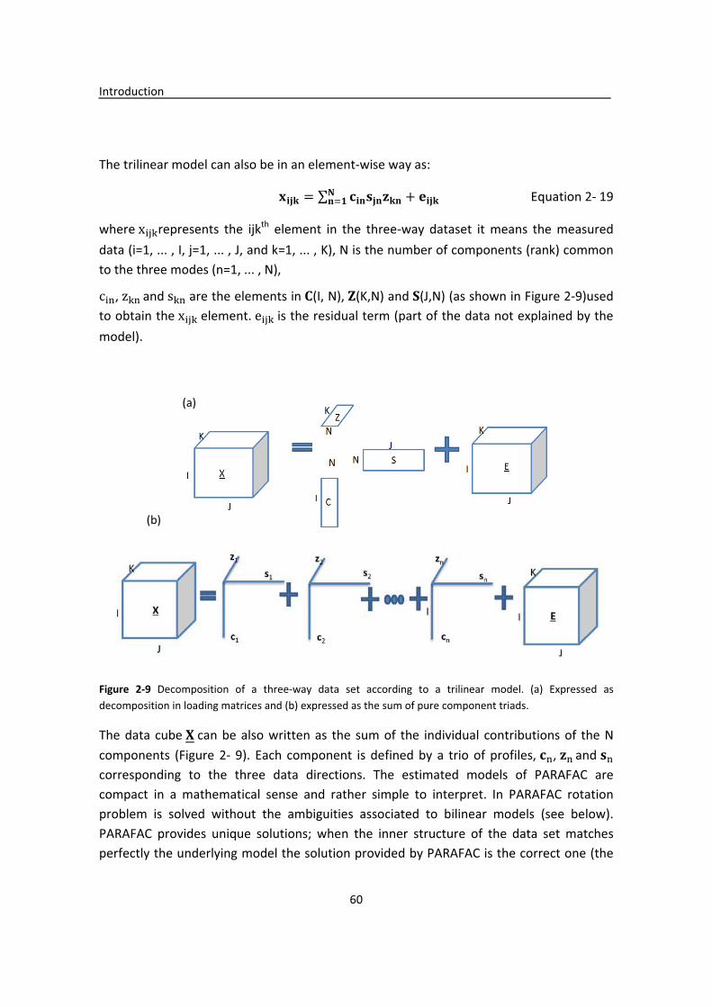
Introduction�
60��
�
The�trilinear�model�can�also�be�in�an�element�wise�way�as:�
��"� � � R���"���� � #�"�S�I� �����������������������������Equation�2��19�
where�D $}represents� the� ijkth� element� in� the� three�way� dataset� it� means� the� measured�data�(i=1,�...�,�I,�j=1,�...�,�J,�and�k=1,�...�,�K),�N�is�the�number�of�components�(rank)�common�to�the�three�modes�(n=1,�...�,�N),�
E ?,��}? �and�F}?�are�the�elements�in�+(I,�N),�~(K,N)�and�*(J,N)�(as�shown�in�Figure�2�9)used�to�obtain�the�D $}�element.�G $}�is�the�residual�term�(part�of�the�data�not�explained�by�the�model).�
�Figure� 2�9� Decomposition� of� a� three�way� data� set� according� to� a� trilinear� model.� (a)� Expressed� as�decomposition�in�loading�matrices�and�(b)�expressed�as�the�sum�of�pure�component�triads.�
The�data�cube�J�can�be�also�written�as� the�sum�of� the� individual� contributions�of� the�N�components� (Figure� 2�� 9).� Each� component� is� defined� by� a� trio� of� profiles,�R?,��?�and��?�corresponding� to� the� three� data� directions.� The� estimated� models� of� PARAFAC� are�compact� in� a� mathematical� sense� and� rather� simple� to� interpret.� In� PARAFAC� rotation�problem� is� solved� without� the� ambiguities� associated� to� bilinear� models� (see� below).�PARAFAC� provides� unique� solutions;� when� the� inner� structure� of� the� data� set� matches�perfectly�the�underlying�model�the�solution�provided�by�PARAFAC�is�the�correct�one�(the�
(a)�
(b)�

Introduction�
61��
true� one).� In� Chapter� 6,� PARAFAC� is� compared� with� MCR�ALS� with� the� trilinearity�constraint�that�is�described�immediately�below.�
�
In� MCR�ALS,� the� trilinear� model� described� above� can� be� implemented� as� a� constraint�during�ALS�for�each�resolved�component�separately.�This�is�achieved�algorithmically�by�a�constraint� during� the� ALS� optimization� and� it� has� been� described� in� detail� elsewhere244.�The� trilinear� constraint� forces� profiles� of� the� same� component� in� the� different� data�matrices� for� a� particular� direction� to� be� the� same� (to� have� the� same� shape)� and� only�change�in�scale/intensity.��
�
�
Figure�2��10�Implementation�of�the�trilinear�constraint�in�the�MCR�ALS�(see�text�for�details�of�the�procedure).�
The�first�step�in�the�MCR�ALS�method�is�the�determination�of�the�number�of�components.�Next,�as�shown�in�Figure�2��10,�initial�estimates�of�+lmn��and�*M�as�the�following�steps:�
1�First� it� is�needed�to�reshape�the�three�way�date�set�J�as�a�two�way�one�Jlmn,� leave�*M�as�the�spectral�from�which�will�obtain�the�pure�spectral�as�the�initial�data�for�the�iteration�calculation�of�ALS.�
2�Estimation�of�the�purest�(more�different)�spectra�from�the�raw�data�set�(SIMPLISMA)225.��

Introduction�
62��
3� Given� Qlmn �and� initial �*M estimation� of� +lmn under� non�negative� and� trilinearity�constraints� (trilinearity� is� introduced� below). �+lmn � Qlmn�*M�1 ,� �*M�1� is� the�pseudoinverse�of�the�spectral�matrix�*M,�and�it�is�equal�to�T*�*M*��.U�when�*M�is�full�rank.�The�new�estimation�of�the�+lmn�matrix�can�be�then�used�to�recalculate�by� lest�squares�a�new�estimation�of�the�*M�matrix:�
4�Given�Qlmn�and�+lmn�estimation�of�*M�under�non�negative�and�normalization�constraints.�*K � +lmn1 Q ,� under� constraints,� where� +lmn1 �is� the� pseudoinverse� of� +lmn ,� +lmn1 ��+lmnM +lmn��.+lmnM �when�+lmn�is�full�rank.�
5�Reproduction�of�Qlmn�from�+lmn�and�*M.��
6� Back� to� step� 3,� until� convergence� is� achieved.� To� end� the� optimization� process,�maximum�numbers�of�iterations�and�the�convergence�criterion�have�been�set.�
7�Decompose�+lmn��in�~�and�+.�
In�Figure�2��10,�when�the�trilinear�constraint� is�applied,�the�concentration�profiles�of�the�same� component� in� the� different� sub� matrices�+}�in�+lmn�are� forced� to� have� the� same�shape� during� iterations�of� the�ALS� optimization.� To� do� this,� in� step� 3,�a� one�component�concentration� profile� matrix,�+�� >%?�is� built� with� I� rows� (number� of� rows� of� each� data�matrix)�and�K�columns� (number�of�matrices�simultaneously�analyzed).�For�a� full� trilinear�model,�every�component�has�a�+�� >%?�matrix�(n=1,�...�,�N),�which�is�approximated�by�their�related�one�component�bilinear�decomposition� (using� for� instance�PCA�or�singular�value�decomposition�(SVD)).�R�is�the�one�column�vector,�which�contains�the�common�(average)�concentration�profile�of�the�component�n�in�the�different�sub�matrices�in�+lmn,�and��M�is�a�row�vector�with�the�relative�amounts�of�this�concentration�profile.�+�� >%? � R�M(See�figure�2�10).�After�this,�the�full�concentration�+lmn�augmented�matrix� is�rebuilt�and�updated�by�replacing�their�initial�profiles�by�the�+�� >%?�profiles,�obtained�from�the�different�individual.��
At�the�end�of�the�MCR�ALS�optimization,�only�the�recovered�spectral�information�in�*M�can�be� straight� forwardly� matched� with� one� of� the� three� PARAFAC� modes.� The� matrix�+lmn�contains�implicitly�the�information�related�to�matrices�+�and�~�in�the�other�two�PARAFAC�modes.� MCR�ALS� has� complete� freedom� in� the� correspondence� of� profiles� among�different� components� and� modes,� in� different� way� than� PARAFAC.� It� models� also�situations�where�two�or�more�components�have�common�profiles�in�one�of�the�modes,�in�what� is� called� interaction� models� 200� or� situations� where� one� component� should� be�described�with�more�than�one�profile�in�one�of�the�modes.��
In� the� work� of� using� EEM� to� analysis� DOM� in� water� system,� MCR�ALS� method� with� the�trilinearity�constraint�is�proposed.�More�details�are�explained�in�Chapter�6.�
Introduction�
63��
�
Uncertainties�in�MCR�results��
�
Bilinear�model�decompositions�differ�in�the�way�how�the�data�decomposition�is�performed.�PCA� and� ICA� apply� very� strong� constraints� which� produce� unique� solutions,� but� their�solutions�may�not�have�direct�physical�meaning.�MCR�methods�use�softer�constraints�but�with� more� physical� meaning,� like� non�negativity,� unimodality,� closure� or� local� rank� and�selectivity�(see�previous�section�2.2).�These�constraints�are�following�the�known�physical�and�chemical�(natural)�features�of�the�profiles�of�the�constituents�of�the�analyzed�samples.�200.�However�profiles�recovered�by�MCR�methods�may�be�affected�by�intensity�(or�scale�)�and�rotation�ambiguities245,�246.��
MCR�model�of�Equation�2��20�can�also�be�written�as:��
Q� � �+KK��*K � +�*�K�����������������������������������������Equation�2��20�
where�T�stands�for�any�transformation�matrix�and:�
� � � � +� � +K�and�*�M � K�.*M� ����������������������������������������Equation�2��21�This� is� the� mathematical� formulation� of� the� rotational� ambiguity,� which� means� that� the�same�lack�of�fit�can�be�obtained�in�the�description�of�the�data�set�Q�using�different�sets�of�profiles�(+��and�*�M),�shaped�differently�from�the�true�ones�(+�and�*M).��
Another� source� of� ambiguity� different� from�the� rotation�ambiguity� is� the� scale/intensity�ambiguity,�which�can�be�expressed�as:�
Q � � ���� R�� �����K���I� ���������������������������������Equation�2��22�
The�resolved�profiles�(R %�� )�for�each�pure�component�can�present�profiles�with�the�same�shape�but�with�one�of�them�8 �times�smaller�and�the�other�8 �times�larger�than�expected,�without� changing� the� final� result.� This� is� the� reason� why� in� MCR,� if� no� additional� scale�information�(like�mass�balance�or�closure),�a�normalization�constraint�is�usually�applied�to�one� of� the� two� set� of� profiles� of� every� component,� either� to� the� concentration� (like�closure)�or�to�the�spectra�(normalization�to�equal�length/area/intensity)��
The�extent�of�rotation�ambiguities� in�MCR�results�can�be�significantly�decreased�or�even�suppressed� by� the� use� of� constraints.� The� more� constrained� a� system� is,� the� fewer� the�number�of�possible�solutions�(profile�combinations)�can�fulfill�the�required�data�patterns�with�the�same�fit.�The�use�of�constraints�forces�results�to�be�closer�to�the�true�profiles�and�fit� optimally� the� data� set�Q�(only� constraints� that� are� fulfilled� by� the� data� should� be�applied).� The� presence� of� rotation� ambiguities� in� MCR� results� has� been� compelled�
Introduction�
64��
somewhat� the� wide� spread� use� of� MCR� methods.� Recently� there� have� been� some�attempts� to� evaluate� the� extent� of� rotation� ambiguities� in� MCR� solutions� 246�250.� Since�rotation�ambiguity�is�component�and�profile�dependent�and,�within�the�same�data�set,�we�may� find� components� or� profiles� with� low� ambiguity� and� others� that� have� it� in� a� larger�extent.�Due�to�the�presence�of�rotation�ambiguities,�instead�of�unique�solutions,�a�range�of� feasible� solutions� that� fit� the� data� giving� the� same� data�fitting� values� and� fulfill� the�same�applied�set�of�constraints�can�be�obtained�in�all�resolution�methods.�In�these�cases,�there� is� no� one� better� solution� than� others,� because� they� are� undistinguishable�considering�the�previous�knowledge�of�the�system.�MCR�results�from�hyperspectral�image�analysis�can�show�the�presence�of�rotation�and�intensity�ambiguities.�
�
�
Calculation�of�Rotation�ambiguities�and�Area�of�Feasible�Solutions�(AFS)�
Lawton� and� Sylvestre� proposed� a� first� algorithm� for� determining� the� AFS� of� two�component�systems�under�non�negative�constraints�in�spectra�and�concentration�profiles�in�early�1980s227.�In�1985�Borgen�et�al.251�developed�an�analytical�solution�of�the�feasible�ranges� of� the� pure� component� spectra� from� mixture� spectra� and� extended� it� for� three�component� systems� using� a� tangent� and� simplex� rotation� algorithms.� Low� dimensional�representation�of�this�continuum�of�solutions�is�also�called�the�Area�of�Feasible�Solutions�(AFS)252,�253.�
Henry� and� Kim� proposed� a� procedure� to� calculate� the� outer� boundary� of� the� region� of�feasible� solutions� by� using� linear� programming� methods� and� determine� all� its� vertices.�These�methods�require�the�use�of�non�negativity�and�other�physical�constraints,�to�restrict�feasible� solutions� to� single� points� (unique� solutions)� and� not� to� regions� (non�unique�solutions)254.�Leger�and�Wentzell�developed�a�dynamic�Monte�Carlo�SMCR�(Self�Modelling�Curve� Resolution)� method255� which� seeks� to� define� the� boundaries� of� feasible� pure�component� profiles.� The� algorithm� employs� a� directed� Monte� Carlo� approach� to� search�for�valid�solutions�with�high�efficiency.�The�parameters�for�the�search�(direction,�step�size)�are�set�through�bootstrap�estimates�of�the�geometry�of�the�solution�space.�However�this�method�suffers�from�large�instabilities�in�the�calculations.��
Rajkó�and�István256�revised�Borgen’s�study.�They�considered�that�the�normalized�feasible�solu�ons�are�embraced�in�a�(N�1)�dimensional�simplex�(N�is�the�number�of�components)�with� the� vertices� being� the� N�normalized� pure� profiles.� Computational� geometry� tools�were�used� instead�of� the� linear�programming� tools�used� to� draw�Borgen� plots�of� three�component�systems.�The�Borgen�plot�(BP)�method�used�for�these�calculations�is�based�on�SVD/PCA�and�it�is�highly�sensitive�to�noise.��

Introduction�
65��
H.�Abdollahi,�M.�Maeder�and�R.�Tauler�have�proposed�a�systematic�grid�search�method�for�all�feasible�solutions�and�the�results�have�been�displayed�in�appropriate�mesh�and�contour�plots�which�reveal�their�boundaries249.� In�2013,�A.�Golshan,�M.�Maeder�and�H.�Abdollahi�have� developed� the� method� using� the� simplex� volume� of� feasible� solutions� for�determination�and�visualization�of�rotational�ambiguity�of�four�components�mixture257.�
Recently,� Sawall� et� al.� suggested� a� fast� and� accurate� algorithm� to� find� AFS� in� two� and�three�component�systems�using�the�inflation�of�polygons�as�a�searching�method�258.�This�procedure�starts�with�an�initial�triangle�located�in�a�topologically�connected�subset�of�the�AFS,� and� an� automatic� extrusion� algorithm� is� then� used� to� form� a� sequence� of� growing�polygons�that�approximate�the�AFS�from�the�interior.�For�a�three�component�system�(s�=�3),�the�AFS�is�a�two�dimensional�geometric�region.�For�a�numerical�computation�of�the�AFS�two� methods� have� been� developed:� the� triangle� boundary�enclosure� scheme� and� the�polygon� inflation� method.� FAC�PACK� is� a� MATLAB� toolbox� for� the� computation� of� non�negative�multi�component�factorizations�and�for�the�numerical�approximation�of�the�Area�of� Feasible� Solutions� (AFS)� using� the� inflation� polygon� algorithm258.� Effective� tools�included� in�FAC�PACK�are�the�reduction�of�the�AFS�by�a�factor�locking�approach�and�the�use�of� the�complementarity� (duality)� theory.�This� software�comes�with�a�Graphical�User�Interface�(GUI)�in�MATLAB.�The�software�implements�the�polygon�inflation�algorithm�and�the� generalized� Borgen� plots.� Non�negative� Matrix� Factorization� (NMF)� is� used� as� the�starting� point� for� the� polygon� inflation� algorithm� in� FAC�PACK.� It� supplies� two� or� three�points�within�the�AFS�depending�on�the�number�of�components�of�the�system.�From�these�points�an�initial�polygon�can�be�constructed,�which�is�a�first�approximation�of�the�AFS.�The�initial� polygon� is� inflated� to� the� AFS� by� means� of� an� adaptive� algorithm.� This� algorithm�allows�computing�all�three�segments�of�an�AFS�separately.�
�
�
MCR�BANDS�
�
Gemperline255� presented� years� ago� an� alternative� method� which� can� be� applied� to� any�multivariate� data� set,� irrespective� of� the� level� of� overlap� and� of� the� number� of�components.�This�method�is�the�basis�of�the�MCR�BANDS�method�used�in�this�Thesis�for�the�evaluation�of�the�extent�of�the�rotation�ambiguities.� �MCR�BANDS�method�has�been�proposed�by�R.�Tauler�255�and�it�estimates�the�extent�of�rotation�ambiguities�producing�a�range�of�feasible�solutions�based�on�a�fast�maximization�and�minimization�of�the�relative�signal� component� contribution� of� each� component� (SCCF).� MCR�BANDs� method� has� no�limitation�to�a�number�of�components�and�uses�the�same�constraints�as�those�applied�to�

Introduction�
66��
find� the� MCR� solution.� It� gives� a� simple� evaluation� of� the� extent� of� rotation� ambiguity�from� the� difference� of� the� value� of� the� optimization� function� giving� maximum� and�minimum�values.�
�
MCR�BANDS� evaluates� for� each� component� the� minimum� and� maximum� the� relative�signal�contribution�function�(SCCF)�246.�This�method�can�be�used�to�evaluate�the�extent�of�rotation�ambiguities�associate�to�a�particular�MCR�solution�and�under�a�set�of�constraints.�The� method� is� based� on� the� maximization� and� minimization� of� the� signal� component�contribution�function,�SCCF,�which�is�defined�for�component�n�as:�
*++�� � �R���K��+*K� ��������������������������������������������Equation�2��23
�SCCFn�is�a�scalar�value�between�0�and�1,�which�gives�the�relative�signal�contribution�of�a�certain�component�in�relation�to�the�whole�signal�due�to�the�mixture�of�N�components�(n=1…N).�+�and�*M�are� as� defined� above;�R?�and��?�are� the� nth� column� and� row� of�+�and� * �matrices� respectively.� ��� �is� the� Frobenious� norm� �+*M� �gives� the� signal�contribution� of� all� the� components� present� in� the� whole� image� and��R?�?K��only� the�contribution�of�component�n�259.��
For�every� component,� SCCF� is� maximized� and�minimized�under� the�set�of� considered�constraints�and�equal�data�fitting.�When�the�maximum�and�minimum�values�of�SCCF�of�a�particular�component�N�are�practically�equal,�it�means�that�for�this�component�there�is�practically�no�ambiguity�remaining.�On�the�contrary�when�this�difference�is�large�and�close� to� one� (SCCF� is� scaled� between� 0� and� 1),� then� there� is� a� large� amount� of�ambiguity.�See�references246�for�more�details�about�how�this�procedure�is�implemented�and�works.�MCR�BANDS�performs�the�minimization�and�maximization�of�SCCF�using�a�general� sequential� quadratic� programming� procedure� to� solve� the� non�linear�optimization�of�SCCF�under�non�linear�constraints�246,�259,�260.�The�amount�of�ambiguity�resting� for� a� particular� solution� can� be� evaluated� from� the� differences� between� the�maximum�and�minimum�values�of�the�SCCF�function259.�
�
The�general�idea�of�MCR�BANDS�is�finding�the�boundary�of�SCCF�function�that�provides�the�maximum�and�the�minimum�relative�contribution�of�the�considered�component�signal�to�the� overall� signal� measured.� The� maximum� and� minimum� boundaries� of� this� function�should�correspond�to�profiles�that�fulfill�the�constraints�and�should�reproduce�the�data�set�with� the� optimal� fit.� This� approach� is� valid� for� data� sets� with� unlimited� number� of�components.�The�following�equations�can�be�written:�
Introduction�
67��
�
Q � + ? 4* ? 4M � + ? 4K: ?K�: ?�� * ? 4M � +: ?%?*: ?%?
M � + ? 4K:l�%�K�:l�%?�� �* ? 4M �+:l�%?*:l�%?M �������������������������������������������������������������������������Equation�2��24�
�
It� is� clear� that� if� no� constraints� are� considered,� there� is� an� infinite� number� of� possible�solutions�of�Equation�2��24�for�any�non�singular�matrix�K.� It� is�usually�possible�to�reduce�considerably� this� infinite� number� of� possible� solutions� by� means� of� constraints� derived�from�the�physical�nature�and�previous�knowledge�of�the�problem�under�study.�
The� boundaries� will� be� related� to� specific� rotation� matrices�K�for� every� component� n,�which� are� called�K:l�%?�and�K: ?%?.� Consider� a� particular� set� of� solutions� fulfilling� the�constraints� defined� by� the� problem,�+ ? 4�and�* ? 4M .� Feasible� solutions�+ ? 4�and�* ? 4M �can�be�initially�postulated�or�found�using�the�MCR�ALS�under�a�set�of�preselected�constraints.�The�maximum�band�boundaries�+:l�%?�(for�the�concentration�profiles)�and�*:l�%?M �(for�the�spectral�profiles)�and�the�minimum�band�boundaries�+: ?%?�(for�the�concentration�profiles)�and�*: ?%?
M �(for�the�spectral�profiles)�can�be�defined�by�the�Equation�2��24.�The�goal�of�the�method� described� here� is� to� find� a� way� to� calculate� these� values� of�K:l�%?�and�K: ?%?�which�define�the�maximum�and�minimum�boundaries�of�the�SCCF�function�which�define�feasible� solutions� of� the� component� profiles� under� a� set� of� constraints� defined� for� a�particular�data�set.�
�
MCR�BANDS� has� been� applied� to� the� evaluation� of� the� extent� of� rotation� ambiguities�associated� to� MCR�ALS� solutions� obtained� in� the� analysis� of� hyperspectral� images� (see�Chapters�5�of�this�Thesis).�In�the�general�case�of�the�analysis�of�complex�multi�component�hyperspectral� images� with� soft� constraints� like� non�negativity,� unique� solutions� are� not�guarantee�and�rotation�ambiguities�may�be�present.�Because�of�these�ambiguities,�a�set�of�feasible�solutions,�fulfilling�the�applied�constraints�(e.g.�non�negativity�constraints)�fitting�equally�well�the�analyzed�data�are�possible.��
MCR�BANDS�code�can�be�downloaded�from�the�http://www.mcrals.info/�
� �

Introduction�
68��
� �

�
69��
�
�
�
Chapter 3
Application of MCR-ALS on remote sensing hyperspectral imaging �
�
� �

�
70��
� �

Application�of�MCR�ALS�on�remote�sensing�hyperspectral�imaging�
71��
Introduction�In� this� chapter,� different� simulated� datasets� and� other� data� sets� (free� AVIRIS,� Airborne�Visible/Infrared� Imaging� Spectrometer� data� sets)� from� NASA� (The� National� Aeronautics�and�Space�Administration)�were�analyzed�by�means�of�MCR�ALS.��
The� simulated� data� sets� were� prepared� using� pure� spectra� (signatures)� from� USGS� (The�U.S.� Geological� Survey)� library.� This� spectra� library� includes� samples� of� minerals,� rocks,�soils,�physically�reconstructed,�as�well�as�mathematically�computed�mixture�spectra,�and�spectra�from�plants,�vegetation�communities,�microorganisms,�and�man�made�materials.�The�spectra�collected�from�this�dataset�were�assembled�in�this�Thesis�with�the�purpose�of�simulating�the�use�of�spectral�features�from�remote�sensing�detection�of�these�and�similar�materials261.�
AVIRIS�is�a�proven�instrument�in�the�realm�of�Earth�Remote�Sensing.�It�is�a�unique�optical�sensor�that�delivers�calibrated�images�of�the�upwelling�spectral�radiance�in�224�contiguous�spectral� channels� (bands)� with� wavelengths� from� 400� to� 2500� nanometers.� AVIRIS� has�been� installed� on� four� aircraft� platforms:� NASA's� ER�2� jet,� Twin� Otter� International's�turboprop,� Scaled� Composites'� Proteus,� and� NASA's� WB�57.� The� ER�2� jet� flies� at�approximately�20�km�above�sea�level,�at�about�730�km/hr.�The�Twin�Otter�aircraft�flies�are�acquired� at� 4� km� above� ground� level� at� 130� km/hr.� AVIRIS� has� flown� North� America,�Europe,�portions�of�South�America,�and�Argentina.�The�dataset�we�used�in�this�Thesis�was�obtained�by�NASA's�ER�2�jet.�
The�main�objective�of�the�AVIRIS�project�is�to�identify,�measure,�and�monitor�constituents�of� the� Earth's� surface� and� atmosphere� based� on� molecular� absorption� and� particle�scattering� signatures.� Research� with� AVIRIS� data� is� predominantly� focused� on�understanding�processes�related�to�the�global�environmental�and�climate�change.�
The�first�dataset�we�have�used�from�AVIRIS� is�a�hyperspectral� image�of�the�geographical�region�of�Cuprite,�Nevada,�USA,�obtained�in�1997262.�In�this�case,�the�analysis�was�limited�to�a�614��512�pixels�sub�image.�The�Cuprite�area�is�an�arid�area�with�a�small�amount�of�vegetation� cover,� and� it� has� an� excellent� rock� exposure,� comprising� alteration� zones�characterized� by� the� occurrence� of� key� indicator� minerals.� In� this� area,� the� use� of�hyperspectral� remote� sensing� of� minerals� is� well� documented.� Many� minerals� can� be�identified� from� airborne� images,� and� their� correlation� with� the� presence� of� valuable�minerals� has� been� established.� NASA� has� catalogued� several� of� the� possible� minerals�present�in�this�area,�as�well�as�their�spectral�signatures.�This�spectroscopic�image�has�been�widely� used� for� remote� sensing� experiments� and� for� development� and� application� of�imaging� data� analysis� methods.� Goetz� and� Srivastava� (1985)� were� the� first� to� use�hyperspectral�data�for�mineral�mapping�at�Cuprite263.�
Application�of�MCR�ALS�on�remote�sensing�hyperspectral�imaging�
72��
Dataset� 2� is� extracted� from� the� hyperspectral� image� of� a� naval� airport� in� San� Diego,�California,�collected�by�AVIRIS�sensor.�In�this�case,�the�analysis�was�limited�to�a�200��200�pixels�sub�image.�This�image�has�195�useful�spectral�bands.��
Dataset�3�was�acquired�over�Moffett�Field,�CA,�in�1997�by�the�AVIRIS�sensor.�In�this�case,�the�analysis�was� limited�to�a�400��400�pixels� sub�image,�and�this� image�has�199�useful�spectral� bands.� The� investigated� area� is� mainly� composed� of� water,� building,� soil,� and�vegetation.��
Methods�for�analyzing�hyperspectral�data�were�discussed�in�Chapter�2�of�this�Thesis�(see�Chapter� 2,� section� 2.2).� Many� methods� have� been� proposed� for� remote� sensing�hyperspectral� imaging,� such� as� the� Pixel� Purity� Index� (PPI)� 114,� the� Vertex� Component�Analysis�(VCA)�264,�the�Minimum�Volume�Simplex�Analysis�(MVSA)�188�,�and�others265,�We�propose� in� this� Thesis� the� use� of� MCR�ALS� for� the� resolution� of� remote� sensing�hyperspectral�imaging�datasets.�
The� way� MCR�ALS� has� been� used� to� resolve� hyperspectral� imaging� data� obtained� from�remote�sensing�was�described�in�Chapter�2�of�this�Thesis.�Two�research�papers�have�been�written� in� the� frame� of� this� Thesis� describing� the� application� of� Multivariate� Curve�Resolution�Alternating�Least�Squares�(MCR�ALS)�to�remote�sensing�hyperspectral�imaging,�emphasizing� the� use� of� local� rank�based� spatial� information� and� of� constraints� for� the�improvement�of�remote�sensing�hyperspectral�imaging�resolution.�Remote�sensing�has�its�own� characteristics� and� differences� compared� to� ordinary� hyperspectral� imaging.�Normally,� in� remote� sensing� hyperspectral� imaging� is� possible� to� find� out� some� purest�pixels� that� can� be� used� for� the� application� of� local� rank� constraint.� In� this� work,� a� new�procedure�based�on�the�use�of�correlation�coefficients�with�known�reference�spectra�was�proposed�to�detect�pure�pixels.�Details�about�how�local�rank�constraints�are�applied�have�been� described� in� the� Part� 2� of� this� Thesis� and� and� in� the� methods� section� of� the� two�papers:�
�
The�two�published�papers�of�this�chapter�are:�
�
Paper�1:�Zhang,�X.;�Tauler,�R.,�Application�of�multivariate�curve�resolution�alternating�least�squares�(MCR�ALS)�to�remote�sensing�hyperspectral�imaging.�Analytica�chimica�acta.�2013,�762,�25�38.�
Paper� 2:� Zhang,� X.;� Juan,� A.;� Tauler,� R.,� Local� rank�based� spatial� information� for�improvement�of�remote�sensing�hyperspectral�imaging�resolution.�Submitted�to�Talanta.�

Application�of�MCR�ALS�on�remote�sensing�hyperspectral�imaging�
73��
�
� �

Application�of�MCR�ALS�on�remote�sensing�hyperspectral�imaging�
74��
�
� �
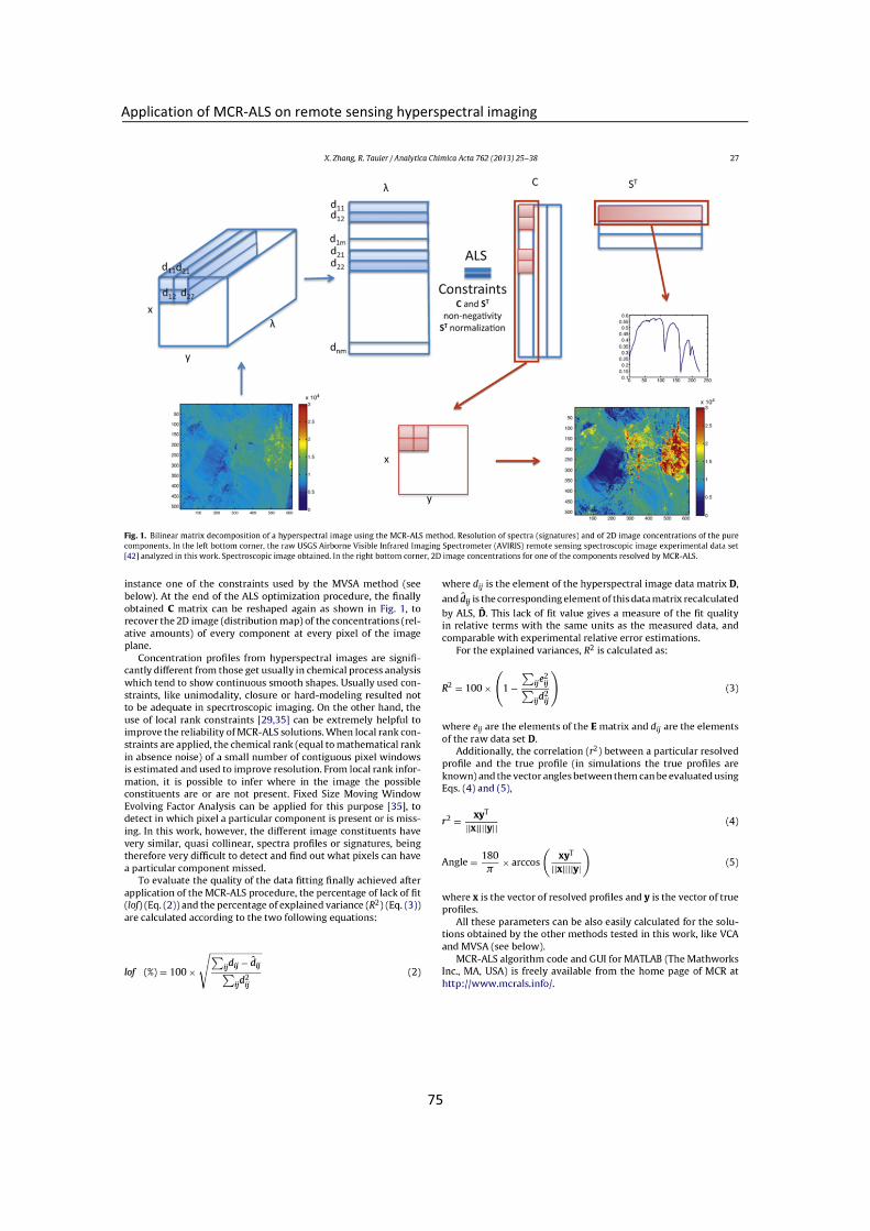
Application�of�MCR�ALS�on�remote�sensing�hyperspectral�imaging�
75��
�
� �

Application�of�MCR�ALS�on�remote�sensing�hyperspectral�imaging�
76��
�
� �
Application�of�MCR�ALS�on�remote�sensing�hyperspectral�imaging�
77��
�
� �

Application�of�MCR�ALS�on�remote�sensing�hyperspectral�imaging�
78��
�
� �

Application�of�MCR�ALS�on�remote�sensing�hyperspectral�imaging�
79��
�
� �
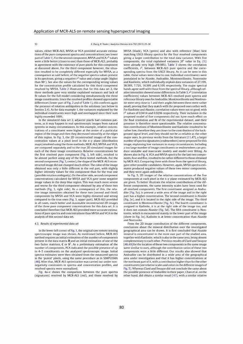
Application�of�MCR�ALS�on�remote�sensing�hyperspectral�imaging�
80��
�
� �

Application�of�MCR�ALS�on�remote�sensing�hyperspectral�imaging�
81��
�
� �

Application�of�MCR�ALS�on�remote�sensing�hyperspectral�imaging�
82��
�
� �

Application�of�MCR�ALS�on�remote�sensing�hyperspectral�imaging�
83��
�
� �

Application�of�MCR�ALS�on�remote�sensing�hyperspectral�imaging�
84��
�
� �
Application�of�MCR�ALS�on�remote�sensing�hyperspectral�imaging�
85��
�
� �

Application�of�MCR�ALS�on�remote�sensing�hyperspectral�imaging�
86��
�
� �

Application�of�MCR�ALS�on�remote�sensing�hyperspectral�imaging�
87��
�
� �
Application�of�MCR�ALS�on�remote�sensing�hyperspectral�imaging�
88��

Application�of�MCR�ALS�on�remote�sensing�hyperspectral�imaging�
89��
Application�of�MCR�ALS�on�remote�sensing�hyperspectral�imaging�
90��

Application�of�MCR�ALS�on�remote�sensing�hyperspectral�imaging�
91��

Application�of�MCR�ALS�on�remote�sensing�hyperspectral�imaging�
92��

Application�of�MCR�ALS�on�remote�sensing�hyperspectral�imaging�
93��

Application�of�MCR�ALS�on�remote�sensing�hyperspectral�imaging�
94��
Application�of�MCR�ALS�on�remote�sensing�hyperspectral�imaging�
95��
�
� �

Application�of�MCR�ALS�on�remote�sensing�hyperspectral�imaging�
96��

Application�of�MCR�ALS�on�remote�sensing�hyperspectral�imaging�
97��

Application�of�MCR�ALS�on�remote�sensing�hyperspectral�imaging�
98��

Application�of�MCR�ALS�on�remote�sensing�hyperspectral�imaging�
99��
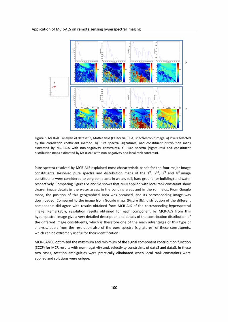
Application�of�MCR�ALS�on�remote�sensing�hyperspectral�imaging�
100��

Application�of�MCR�ALS�on�remote�sensing�hyperspectral�imaging�
101��
�
� �
Application�of�MCR�ALS�on�remote�sensing�hyperspectral�imaging�
102��
Application�of�MCR�ALS�on�remote�sensing�hyperspectral�imaging�
103��
�
�
� �

Application�of�MCR�ALS�on�remote�sensing�hyperspectral�imaging�
104��
�
Discussion�The� first� paper266� shows� how� MCR�ALS� allowed� the� resolution� of� pure� spectra� and�concentration� distribution� of� the� constituents� present� in� the� analyzed� remote� sensing�hyperspectral� imaging� simulated� datasets� and� in� the� remote� sensing� datasets� obtained�from�NASA,�AVIRIS�(Airborne�Visible/Infrared�Imaging�Spectrometer).��
Effective� use� of� remote� sensor� data� requires� the� analysis� and� interpretation� of� the�acquired� data� and� interprets� the� recovered� information� to� address� practical� problems,�such� as� the� position� of� landfills� or� searching� for� mineral� deposits.� Different� objects� are�discriminated�according�their�spectra�resolved�by�MCR�ALS.�
In� this� Thesis,� MVSA� and� VCA� endmember� (pure� component)� methods� were� compared�with�MCR�ALS� in� the�analysis�of�hyperspectral� remote�sensing�data.�Table�1� in�paper� 266�shows�how�similar�are�the�component�true�profiles�and�MCR�ALS,�MVSA�and�VCA�resolved�profiles,�in�the�analysis�of�two�different��simulated�data�sets.�Table�4�in�paper�266�gives�the�signal�component�contribution�function�SCCF�obtained�by�MCR�ALS,�VCA,�MVSA�and�MCR�BANDS�(maximum�and�minimum�values)�methods.�These�results�showed�that�MVSA�and�VCA� are� not� as� good� as� MCR�ALS� for� hyperspectral� imaging� resolution.� MVSA� produced�negative� spectra� values� in� some� circumstances,� which� are� not� physically� meaningful,�whereas� MCR�ALS� with� non�negative� constraints� always� obtained� results� with� a� clear�chemical�and�physical�meaning.��
MCR�BANDS� method� has� been� proposed� to� ascertain� the� extent� of� rotation� ambiguity�associated� to� MCR�ALS� resolved� spectra� profiles.� In� the� situation� of� remote� sensing�hyperspectral�imaging,�since�the�data�have�high�level�of�noise,�and�some�constituents�are�highly�collinear�(overlapped),�the�extent�of�rotation�ambiguity�of�MCR�ALS�(or�of�any�other�MCR�method)�resolved�profiles�can�be�rather�high.��
Local�rank�information�can�be�used�as�a�constraint�in�MCR�ALS�methods�to�reduce�rotation�ambiguity� significantly� and� to� obtain� unique� resolution� results� in� some� particular� cases�(see�Chapter�2�section�2.2�and�papers�266�94).�From�the�resolved�results�for�the�airport�of�San� Diego� dataset,� and� for� the� Moffett� Field� (California)� data� set,� shown� in� the� other�paper�of�this�chapter�94,�it�is�concluded�that�appropriate�use�of�local�rank�and�of�selectivity�constraints�can�improve�significantly�the�quality�of�the�pure�spectra�(signatures)�and�of�the�constituent� distribution� maps� resolved� by� MCR�ALS� in� the� analysis� of� hyperspectral�remote�sensing�images�
To� apply� local� rank� constraints� in� MCR�ALS,� the� FSIW�EFA� method� (see� Paper� 234,� and�Chapter� 2� of� section� 2.2)� is� preferred� for� the� general� situation,� when� one� or� more�components� are� absent� in� certain� pixels.� It� doesn’t� matter� whether� there� is� complete�

Application�of�MCR�ALS�on�remote�sensing�hyperspectral�imaging�
105��
selectivity� (only� one� component)� or� not.� When� FSIW�EFA� is� applied� singular� values�obtained� from� SVD� are� used� to� set� the� threshold� values� for� local� rank� analysis.� This�information�have�been�used�during�the�ALS�resolution�of�the�hyperspectral�images�in�the�work�of�this�chapter94.�
In�contrast,� the�correlation�coefficient�method�94�can�be�proposed�as�a�as�an�alternative�and�efficient�way�to� look�for�pixels�where�only�a�single�constituent�or�component�exists.�These�pixels�can�then�be�used�advantageously�for�the�application�of�selectivity�constraints�(pixels�with�only�one�component�present).��
For�the�analysis�of�Cuprite,�Nevada�dataset�(the�first�dataset�analyzed�in�this�chapter�and�paper267),�several�individual�constituents�were�preliminary�identified�as�Alunite,�Andradite,�Montmorillonite,�Nontronite�and�Kaolinite.� In�previous�studies�194,�268,�269,�apart�from�VCA�and� MVSA� methods� mentioned� in� this� chapter� and� the� paper52,� the� Automated�Morphological� Endmember� Extraction� (AMEE)� method,� the� Minimum� Volume� Enclosing�Simplex� (MVES)� method� and� the� Simplex� Identification� via� variable� Splitting� and�augmented� Lagrangian� (SISAL)� method,� were� also� applied� by� the� people� working� on�remote� sensing� to� the� analysis� of� this� similar� dataset� in� previously� published� papers.�Mainly,�these�methods�were�used�to�obtain�the�pure�spectra�(endmembers,�signatures)�of�the�different�objects�or�constituents�present�in�the�image.�In�contrast,�the�application�of�MCR�ALS�provided�both,�the�resolution�of�the�pure�spectra�(signatures)�and�the�estimation�of� the� concentration� distribution� maps� at� the� same� time.� This� information� can� be� used�supplementary� to� take� decisions� about� mineral� distribution� in� mining� studies.�Independent� Component� Analysis� (ICA)� also� has� been� used� for� the� resolution� on�hyperspectral�imaging�of�exactly�the�same�geographical�area�270(see�Chapter�2�Section�2.2�for� the� description� of� this� method).� In� the� paper267,� it� is� shown� that� ICA� can� provide�unique� results�but� that� they� may�not�be� the� true� solutions.� In� contrast,�using� local� rank�constraints� in�MCR�is�a�way�to�provide�unique�resolutions�which�are�coincident�with�the�true� physically� meaningful� ones.� In� Chapter� 5� a� more� detailed� comparison� between� ICA�and�MCR�is�given.�
�
The� second� experimental� data� set� example� (hyperspectral� images� from� San� Diego,�California� and� Moffett� Field,� CA,� in� 1997)� resulted� easier� to� analyze� because� it� was�possible� to� find�pixels�with�some�components�absent�and�suitable� for� the�application�of�local� rank� constraints� during� MCR�ALS.� In� the� analysis� of� hyperspectral� images� obtained�from�the�San�Diego�airport�and�of� the�Moffet� field,�MCR�ALS� results� showed�clearly� the�presence� of� different� objects� in� the� image,� like� airplanes,� green� plant� areas,� lakes,� hard�ground� field� and� other� related� objects.� By� appropriate� use� of� local� rank� constraints,�objects�in�the�rebuilt�images�were�defined�more�sharply�(and�more�easily�recognized).��

Application�of�MCR�ALS�on�remote�sensing�hyperspectral�imaging�
106��
In�other� studies� 271,�272� Anomaly� detection� (AD)� or� target�detection� (TD)�were�applied� to�hyperspectral� imaging� data� analysis� of� the� airport� in� San� Diego,� California� (the� second�dataset� used� in� this� chapter� and� paper94).� Their� results� could� identify� the� presence� of�airplanes�in�the�airport�directly.�K.C.�Tiwari�etc.�compared�different�methods�with�ICA�for�the�detection�of�these�airplane�targets.�These�models�performed�differently�depending�on�the� spectral� variability273.� Inverse� Euclidean� distance� based� super�resolution� mapping�method� was� reported� to� make� better� detection� of� those� airplanes274.� From� the� results�obtained�by�us�in�the�application�of�MCR�ALS�to�the�same�hyperspectral�images,�airplanes�could� be� detected� successfully� from� the� resolved� distribution� map.� Other� objects� with�very�similar�signatures�to�those�of�the�airplane�were�also�located�in�the�distribution�map�obtained�by�MCR�ALS.�
Physical�objects,�such�as�buildings,�vegetation,�soil,�water,�etc.(Moffett�Field,�CA�dataset�in�this� chapter� and� paper94)� studied� in� paper� 94� are� usually� investigated� in� remote� sensing�applications� such� as� geology,� forestry,� soil� science,� geography,� and� urban� planning275.�Resolution�of�distribution�maps�involves�to�locate�where�these�particular�objects�are,�and�to� identify� the� spectral� features� of� them.� For� example,� rivers,� geologic� structures� and�vegetation� may� be� mapped� for� environmental� applications.� Airports,� troop� convoys� or�missile� sites� are� for� special� interest� for� military� purposes.� The� analysis� of� the� objects�located� at� a� surface� of� the� ground� can� be� examined� from� the� MCR�ALS� resolved�distribution� maps.� This� technique� would� allow� taking� decisions� from� the� detailed�information�contained�in�these�images.�
�
�
�

�
107��
�
�
�
�
Chapter 4
Application of hyperspectral imaging combined with chemometrics on food analysis � �

�
108��
� �
Application�of�hyperspectral�imaging�combined�with�chemometrics�on�food�analysis�
109��
Introduction��
Spectroscopic�analysis�alone�cannot�provide�information�about�the�spatial�distribution�of�food�constituents.�Hyperspectral�imaging�integrates�spectroscopic�and�imaging�techniques,�providing�both�spectral�and�spatial�information�simultaneously�to�cope�with�the�increasing�demand� for� safe� foods.� Hyperspectral� imaging� techniques� are� also� applied� for� visual�evaluation�of�food�quality2.�
The� use� of� hyperspectral� imaging� technique� is� increasing� owing� to� its� high� speed,�simplicity�and�safety,�as�well�as�its�capacity�to�measure�multiple�attributes�simultaneously�without� the�need�of�slow�sample�preparation.�NIR,� IR�and�Raman�hyperspectral� imaging�are�the�most�successful�techniques�used�in�food�industry.�They�enable�the�qualitative�and�quantitative�assessment�of�chemical�and�physical�features.��
PCA,�Neural�network�classification,�fuzzy�logic,�or�SIMCA�chemometric�methods�have�been�applied� for� food� sample� classification� and� analysis� using� hyperspectral� imaging� data276.�These� methods� can� provide� information� about� texture,� color,� shape,� or� size� features� of�food�samples.�More�details�of�chemometric�methods�applied�in�hyperspectral�imaging�can�be�found�in�Chapter�2�of�this�Thesis.�
In� this� Thesis,� we� propose� the� use� of� Multivariate� Curve� Resolution� Alternating� Least�Squares�(MCR�ALS)�for�the�hyperspectral�imaging�analysis�of�chocolate�samples�as�a�case�study� of� food� analysis,� and� to� recover� the� spectra� of� its� constituents� and� their�corresponding�distribution�maps�on�the�analyzed�chocolate�samples.�
Chocolate� is� a� well� appreciated� food� which� is� made� of� a� complex� emulsion� of� different�constituents.� It� is� a� semi�solid� suspension� of� fine� solid� particles� containing� sugar,� butter�and� cocoa277.� Primary� chocolate� categories� are� dark,� milk� and� white.� They� differ� in� the�content� of� cocoa� solid,� milk� fat� and� cocoa� butter278.� Different� kinds� of� chocolate� have�varying� proportions� of� carbohydrates,� fat� and� proteins.� Chocolate� manufacturing�processes�differ�due�to�variation�in�national�consumer�preferences�and�company�practices.�
The�flavor�of�a�piece�of�chocolate�can�be�affected�by�the�type�and�amount�of�ingredients�present,�as�well�as�by�the�processing�techniques�used279.�In�processing�ordinary�chocolate,�it�is�conventional�to�grind�a�mixture�of�chocolate�liquor�and�sugar�to�the�desired�degree�of�fineness� using� ordinary� roll� refiners,� thereafter,� to� incorporate� the� desired� amount� of�cocoa�butter.�The�chocolate�mixture�and�cocoa�butter�is�then�placed�in�a�suitable�device�capable�of�agitating�or�working�the�mixture.�Because�of�the�need�of�continued�agitation�which�usually�involves�further�grinding,�the�sugar�and�skim�milk�solids�become�completely�coated�with�fat280.�

Application�of�hyperspectral�imaging�combined�with�chemometrics�on�food�analysis�
110��
Particle�size�distribution�and�ingredient�composition�influence�perception�of�primary�taste�and�oral�volatiles�release�of�chocolate281,�282.�Research279�also�supports�that�differences�in�the� flavor� of� milk� chocolate� tend� to� arise� from� processing� changes� rather� than� from�differences�in� ingredients.�Highly�skilled�chocolate�manufacturers�are�able�to�manipulate�flavors�in�the�chocolate279.�The�use�of�hyperspectral�imaging�to�analyze�the�particulars�of�chocolate�constituents�can�help�to�monitor�the�quality�of�chocolate,�and�it�can�reveal�the�existing�relation�between�chocolate�taste�and�product�processing.�
The�applicability�of�Raman�micro�spectroscopy�mapping�(imaging)�to�the�analysis�of�both�white�and�milk�chocolate�samples�was�reported�in�reference283.�In�this�report,�they�failed�to� analyze� milk� chocolate� because� of� the� strong� fluorescence� signal� from� cocoa� solids.�Infrared� hyperspectral� imaging� has� lower� spatial� resolution� than� Raman� but� it� does� not�suffer�from�the�effect�of�fluorescence,�and�it�has�faster�scanning�speeds�because�it�does�not� require� so� much� focus� at� the� sample� surface.� Moreover,� infrared� hyperspectral�imaging� has� many� common� features� to� Raman,� which� also� can� be� used� for� spatial� and�spectral�information�detection.�
For�Raman�spectra�acquisition,�a�HORIBA�JobinYvon�Raman�microscope�(HORIBA,�Ltd.)�was�used�using�a�532�nm�radiation� laser.�For� Infrared�spectra�acquisition�and�high�resolution�mapping,�the�Nicolet�iN10�MX�Infrared�Imaging�Microscope�with�MCT�(Mercury�cadmium�telluride)� detector� was� used.� The� instruments� used� in� the� experimental� determinations�are�shown�in�Figure�4�1.�
�
�Figure� 4�1� Hyperspectral� image� collection� instruments� used� in� the� experimental� analysis� of� chocolate�samples�
�
Hyperspectral� imaging� instruments� for� research� are� developing� very� fast.� For� example,�Bruker� Corporation� developed� a� new� Raman� system:� SENTERRA� Dispersive� Raman�Microscope,�which�can�scan�at�multiple�wavelengths,�(1064�nm,�785�nm,�633�nm,�532�nm�

Application�of�hyperspectral�imaging�combined�with�chemometrics�on�food�analysis�
111��
and�488�nm),�with�high�confocal�depth�profiling�performance.�It�has�an�open�architecture�version�for�the�study�of� large�size�samples�(e.g.� in�art�works)�with�high�lateral�resolution�for�the�investigation�of�living�cells,�etc.�All�of�these�features�have�been�improved�a�lot�in�comparison�with�the�instrument�we�have�applied�in�the�experimental�work�of�this�Thesis.�Collecting� the� dataset� of� the� same� sample� with� similar� pixel� numbers� needed� 24� hours�with� the� old� instruments,� while� the� new� instruments� only� need� about� 30min.�For�FT�IR,�Bruker�Corporation�has�also�developed�two�new�series�of�instruments,�named�LUMOS�and�HYPERION.� LUMOS� is� a� fully� automated� stand�alone� FT�IR� microscope.� HYPERION� is� an�instrument� with� highest� measuring� sensitivity� and� better� spatial� resolution.� Now,� these�instruments�can�only�work�at� laboratory�for�research.�But� it� is�no�doubt�that� in�the�near�future� more� hyperspectral� instruments� will� be� developed� suitable� for� online� and� inline�industry�applications.��
To� develop� the� analysis� of� chocolate� samples� using� hyperspectral� imaging,� Raman� and�Infrared�hyperspectral�imaging�were�used�combined�with�MCR�ALS�method.�The�following�research�paper�has�been�written�and�published�on�Applied�Spectroscopy.�
The�published�paper�in�this�chapter�
Zhang,� X.;� Juan,� A.;� Tauler,� R.,� Multivariate� Curve� Resolution� applied� to� hyperspectral�imaging�analysis�of�chocolate�samples.�Applied�Spectroscopy.�2015,�69(8).��
� �
Application�of�hyperspectral�imaging�combined�with�chemometrics�on�food�analysis�
112��

Application�of�hyperspectral�imaging�combined�with�chemometrics�on�food�analysis�
113��
Application�of�hyperspectral�imaging�combined�with�chemometrics�on�food�analysis�
114��

Application�of�hyperspectral�imaging�combined�with�chemometrics�on�food�analysis�
115��

Application�of�hyperspectral�imaging�combined�with�chemometrics�on�food�analysis�
116��
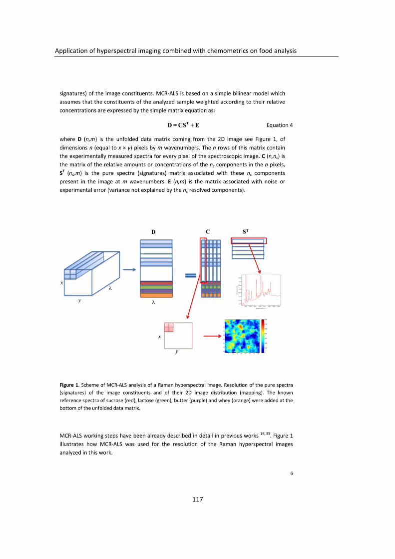
Application�of�hyperspectral�imaging�combined�with�chemometrics�on�food�analysis�
117��
Application�of�hyperspectral�imaging�combined�with�chemometrics�on�food�analysis�
118��

Application�of�hyperspectral�imaging�combined�with�chemometrics�on�food�analysis�
119��

Application�of�hyperspectral�imaging�combined�with�chemometrics�on�food�analysis�
120��

Application�of�hyperspectral�imaging�combined�with�chemometrics�on�food�analysis�
121��
Application�of�hyperspectral�imaging�combined�with�chemometrics�on�food�analysis�
122��
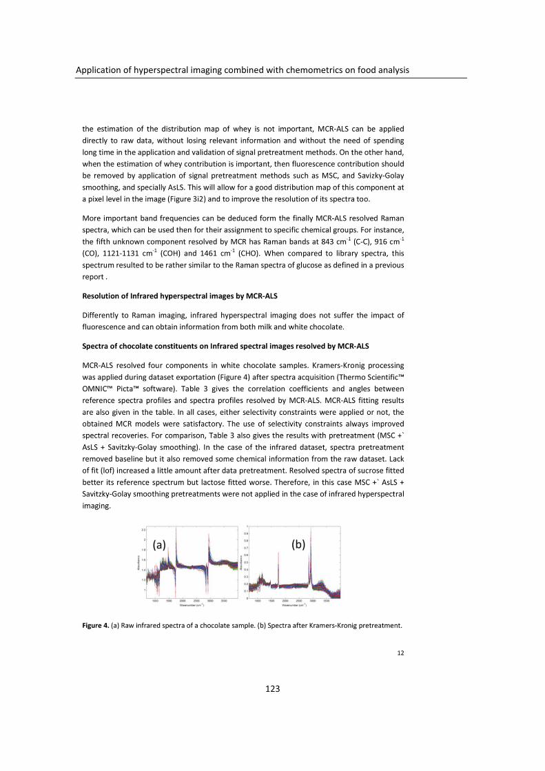
Application�of�hyperspectral�imaging�combined�with�chemometrics�on�food�analysis�
123��

Application�of�hyperspectral�imaging�combined�with�chemometrics�on�food�analysis�
124��

Application�of�hyperspectral�imaging�combined�with�chemometrics�on�food�analysis�
125��

Application�of�hyperspectral�imaging�combined�with�chemometrics�on�food�analysis�
126��
Application�of�hyperspectral�imaging�combined�with�chemometrics�on�food�analysis�
127��

Application�of�hyperspectral�imaging�combined�with�chemometrics�on�food�analysis�
128��

Application�of�hyperspectral�imaging�combined�with�chemometrics�on�food�analysis�
129��
�
� �
Application�of�hyperspectral�imaging�combined�with�chemometrics�on�food�analysis�
130��
Discussion��
In� this� chapter,� the� application� of� Raman� and� infrared� hyperspectral� imaging� combined�with� MCR�ALS� chemometric� data� analysis� is� shown� in� the� analysis� of� chocolate�constituents� as� a� case� of� study.� In� contrast� to� the� applications� of� hyperspectral� remote�sensing� in�previous�chapter,�the�hyperspectral� imaging�analysis�of�food�samples,� like�the�chocolate,� has� the� advantage� of� having� easily� available� reference� spectra� of� the� sample�constituents,� obtained� either� by� independent� experiments� in� the� laboratory� or� from�libraries� of� reference� spectra.� On� the� other� side,� food� samples� can� have� different�constituents� with� very� similar� chemical� structure� and� spectra,� which� makes� more�challenging�their�resolution�and�identification.�
Reviews�of�hyperspectral� imaging�applied�to�food�analysis�are�given� in�references�276,�284,�
285� and� in� the� Chapter� 2� of� this� Thesis.� In� these� previous� review� papers,� chemometric�methods� have� been� applied� to� the� area� of� hyperspectral� image� analysis,� mainly� for�regression�(linear�and�non�linear)�and�classification�(supervised�or�unsupervised)�purposes.�MCR�ALS�is�a�powerful�chemometrics�method�which�was�already�applied�for�hyperspectral�imaging�resolution�more�than�ten�years�ago.�However,� it� is�not�a�popular�method�in�the�food� hyperspectral� imaging� analysis� filed.� The� analysis� of� chocolate� samples� from� this�chapter�is�a�good�example�of�application�of�MCR�ALS�for�food�analysis.��
In�this�chapter,�different�pretreatment�methods�such�as�Multiplicative�Scatter�Correction�(MSC),� Asymmetric� Least� Squares� (AsLS)� and� Savitzky�Golay� data� smoothing� have� been�used.� In� the� Chapter� 2� of� this� Thesis,� these� methods� were� described.� Hyperspectral�imaging� analysis� can� be� performed� at� ambient� conditions,� without� requiring� special�sample�preparation.�Chemical�organic�molecules�can�produce�strong�fluorescence�signals�when� Raman� is� used.� Infrared� spectroscopic� technique� can� be� applied� instead� when�Raman�suffers�from�fluorescence�and�there�is�a�high�risk�of�sample�heating�form�the�laser.�Spectral� preprocessing� data� pretreatment� techniques� are� a� key� step� for� the� successful�analysis�of�hyperspectral�data�sets.��
In�the�case�of�chocolate�analysis�of�this�work,�the�use�of�data�pretreatment�methods�such�as�MSC,�AsLS�and�Savitzky�Golay�smoothing�methods,�either�separately�or�in�combination,�can� facilitate� the� extraction� of� chemical� information� contained� from� the� analyzed�spectroscopic� image� data.� Specifically,� the� undesired� strong� impact� of� fluorescence� on�Raman�spectra�can�be�removed�significantly.��
The� results� of� this� work� show� that� using� non�negativity� and� local� rank� constraints,� MCR�could�resolve�appropriately�most�of�the�chocolate�constituents�of�white�chocolate�such�as�sucrose,�lactose,�butter�and�whey�from�Raman�hyperspectral�imaging�data.�Concentration�

Application�of�hyperspectral�imaging�combined�with�chemometrics�on�food�analysis�
131��
distribution�maps�of�these�constituents�were�displayed�separately.�Compared�to�Raman,�infrared� hyperspectral� images� did� not� suffer� from� the� effect� of� fluorescence,� and� the�application� of� the� Kramers�Kronig� transformation� data� pretreatment� was� enough� in� this�case,� to� facilitate� the� extraction� of� the� chemical� information� contained� in� the� analyzed�images.� Constituents� of� milk� chocolate� could� be� well� resolved� by� infrared� hyperspectral�imaging�technique,�in�contrast�to�what�was�happening�with�Raman�hyperspectral�imaging�technique.��
Resolved� spectra� of� sucrose,� lactose,� butter� and� whey� were� compared� with� reference�spectra� obtained� experimentally.� Correlation� coefficients� between� reference� and�extracted�spectra�were�satisfactory.�Physical�composition�of�chocolate�constituents�could�be�displayed�adequately.�Homogeneity�of�chocolate�samples�could�be�validated�too�(see�in�paper52).��
Results� obtained� in� this� work� show� that� hyperspectral� imaging� technique� can� be� an�efficient� way� for� chocolate� quality� control,� and� that� it� also� can� be� used� for� chocolate�product� research� and� development.� The� surface� topography,� fat� crystallization� are�possible� obtained� by� using� resolved� concentration� distribution� map� of� Raman�hyperspectral� image� or� the� improved� IR� hyperspectral� image� mentioned� in� Chapter� 4�section�4.1�(Bruker’s�new�IR�instruments�have�better�pixel�size�resolution�and�faster�data�collection� capability).� These� parameters� have� a� relation� with� texture� and� color� of� the�products286.� Other� hyperspectral� imaging� analysis� of� important� ingredients� (like�polyphenols,�cocoa�butter�and�alternative�fats)�can�be�tried�in�the�future�for�the�chocolate�product�quality�monitor.��
In� the� paper52� of� this� chapter,� the� micro�scope� imaging� instrument� used� for� the�measurements� had� pixel� resolution� in� �m� scale� which� provides� more� details� of� the�constituent�and�reaction�information�in�the�food�samples��
Raman�or�infrared�hyperspectral�imaging�techniques�combined�with�MCR�ALS�as�proposed�in� this� Thesis� can� be� extended� to� homogeneity� analysis� of� other� type� samples� in�pharmaceutical� tablets287,� powders,� or� suspensions,� which� is� important� for� to�pharmaceutical�process�monitoring�and�quality�control288.��
� �

Application�of�hyperspectral�imaging�combined�with�chemometrics�on�food�analysis�
132��
� �

�
133��
�
�
�
Chapter 5
Measuring and comparing the resolution performance and the extend of rotation ambiguities in bilinear modelling methods �
� �

�
134��
� �

Measuring�and�comparing�the�resolution�performance�and�the�extend�of�rotation�ambiguities�in�bilinear�modelling�methods�
135��
Introduction��
Different� bilinear� methods� have� been� widely� applied� for� hyperspectral� image� analysis,�apart� from� MCR�ALS,� such� as� Independent� Component� Analysis� (ICA)289,� Principal�Component� Analysis� (PCA)2,� and� Minimum� Volume� Simplex� Analysis� (MVSA)189.� The�theories�of�these�methods�have�been�introduced�in�Chapter�2.�In�this�chapter�(Paper�267).�These�methods�are�compared�using�Mutual�Information�(MI),�Amari�Index�(AI)�and�lack�of�fit� (lof)� parameters.� This� comparison� can� help� to� understand� the� performance� of� these�bilinear�models�when�different�constraints�are�applied.�
In� Chapter� 3� and� Chapter� 4,� hyperspectral� imaging� resolution� results� have� be� shown� to�have� associated� a� certain� amount� of� rotation� ambiguity� 246� when� only� non�negativity�constraints� (apart� from� spectra� normalization)� were� used.� MCR�BANDS� method� was�applied� to�evaluate�the�extension�of� rotation�ambiguity� in� the�results�obtained�by�MCR�ALS.� Apart� from� MCR�BANDS,� methods� that� attempt� to� calculate� the� whole� Area� of�Feasible�Solutions� (AFS)�can�also�be�used�for�evaluate�the�effect�of�rotation�ambiguities,�and��different�algorithm�have�been�proposed227,�251,�255,�256,�290.��
The�gridding�search�method�was�proposed�by�Rajko�and�Abdollahi.�A.�Golshan,�et�al.�have�developed� an� AFS� method� using� a� simplex� grid� search� of� the� area� of� feasible� solutions�which� allows� the� visualization� of� rotational� ambiguity� in� mixtures� of� up� to� four�components249,�257.�
Rajkó�and�István256�used�computational�geometry�tools�instead�of�the�linear�programming�tools�used� to�draw�Borgen�plots�of� three�component�systems.�They�considered�that� the�normalized� feasible� solu�ons� are� embraced� in� a� (N�1)�dimensional� simplex� (N� is� the�number�of�components)�with�the�vertices�being�the�N�normalized�pure�profiles.�
R.�Tauler�developed�the�MCR�BANDS�method�259�based�on�a�previous�idea�of�P.Gemperline�104,� for� the� calculation� of� the� extension� of� rotation� ambiguities,� based� on� the� fast�maximization� and� minimization� of� a� function� defined� by� the� relative� Signal� Component�Contribution�(SCCF)�of�each�component�246,�255.�
Recently,� Sawall� et� al.� proposed� algorithm� to� find� AFS� in� two� and� three�component�systems�using� the� inflation�of�polygons� as�a� searching�method� 258.�This�procedure�starts�with� an� initial� triangle� located� in� a� topologically� connected� subset� of� the� AFS,� and� an�automatic�extrusion�algorithm�is�then�used�to�form�a�sequence�of�growing�polygons�that�approximate� the� AFS� from� the� interior.� FAC�PACK� is� a� MATLAB� toolbox� developed� by�Sawall�et�al.�for�the�computation�of�non�negative�multi�component�factorizations�and�for�the� numerical� approximation� of� the� Area� of� Feasible� Solutions� (AFS)� using� the� inflation�

Measuring�and�comparing�the�resolution�performance�and�the�extend�of�rotation�ambiguities�in�bilinear�modelling�methods�
136��
polygon� algorithm258.� In� this� chapter(Paper� 267),� the� results� of� MCR�BANDS� and� of� FAC�PACK�method�are�compared.��
�
Figure�5�1.�Profiles�used�for�Simulation�of�reaction�and�chromatographic�data�systems�with�two,�three,�and�four�components.�(a�i)�are�the�concentration�profiles,�and�(j�l)�are�the�pure�spectra.��
�
Reaction� and� chromatographic� type� of� data� systems� with� two,� three,� and� four�components�were�simulated�for�the�purposed�of�this�Chapter�(Paper�267).�For�the�first�data�(Figure� 5�1a)� set,� concentration� profiles� were� obtained� from� a� simple� first� order� kinetic�chemical�reac�on�or�process:�X�Y,�with�two�components�and�spectra�pro�les�(Figure�5�1j).� For� the� second� data� set,� the� elution� profiles� (Figure� 5�1b)� and� component� spectra�(Figure�5�1k)�of� three�co�eluting�components� in�a�single�HPLC�DAD�chromatographic�run�are�used.�For�the�third�data�set,�elution�profiles�(Figure�5�1c)�from�a�signal�HPLC�DAD�run�with�four�co�eluting�components�are�used.�Component�spectra�for�them�are�given�(Figure�5�1l).�
Datasets� 4�8� LC� are� elution� profiles� with� different� overlap� (coelution)� from� two�component� systems.� They� have� the� same� component� spectra� (Figure� 5�1j),� whereas� the�extent� of� chromatographic� resolution� decreased.� The� peak� overlap� increased� makes� the�system�more�challenging�for�curve�resolution�(Figure1�d,�e,�f,�g,�and�h).�

Measuring�and�comparing�the�resolution�performance�and�the�extend�of�rotation�ambiguities�in�bilinear�modelling�methods�
137��
In� the� last� dataset,� three� random� concentration� profiles� were� considered� for� the� data�simulation�(Figure�5�1i).�Spectra�of�the�components�for�this�simulate�dataset�are�given�in�Figure�5�1k.��
�
The�paper�in�this�chapter�
X.�Zhang,�R.�Tauler.�Measuring�and�comparing�the�resolution�performance�and�the�extend�of�rotation�ambiguities�in�bilinear�modelling�methods.�2015.��

Measuring�and�comparing�the�resolution�performance�and�the�extend�of�rotation�ambiguities�in�bilinear�modelling�methods�
138��

Measuring�and�comparing�the�resolution�performance�and�the�extend�of�rotation�ambiguities�in�bilinear�modelling�methods�
139��
Measuring�and�comparing�the�resolution�performance�and�the�extend�of�rotation�ambiguities�in�bilinear�modelling�methods�
140��

Measuring�and�comparing�the�resolution�performance�and�the�extend�of�rotation�ambiguities�in�bilinear�modelling�methods�
141��

Measuring�and�comparing�the�resolution�performance�and�the�extend�of�rotation�ambiguities�in�bilinear�modelling�methods�
142��
Measuring�and�comparing�the�resolution�performance�and�the�extend�of�rotation�ambiguities�in�bilinear�modelling�methods�
143��
Measuring�and�comparing�the�resolution�performance�and�the�extend�of�rotation�ambiguities�in�bilinear�modelling�methods�
144��

Measuring�and�comparing�the�resolution�performance�and�the�extend�of�rotation�ambiguities�in�bilinear�modelling�methods�
145��

Measuring�and�comparing�the�resolution�performance�and�the�extend�of�rotation�ambiguities�in�bilinear�modelling�methods�
146��

Measuring�and�comparing�the�resolution�performance�and�the�extend�of�rotation�ambiguities�in�bilinear�modelling�methods�
147��
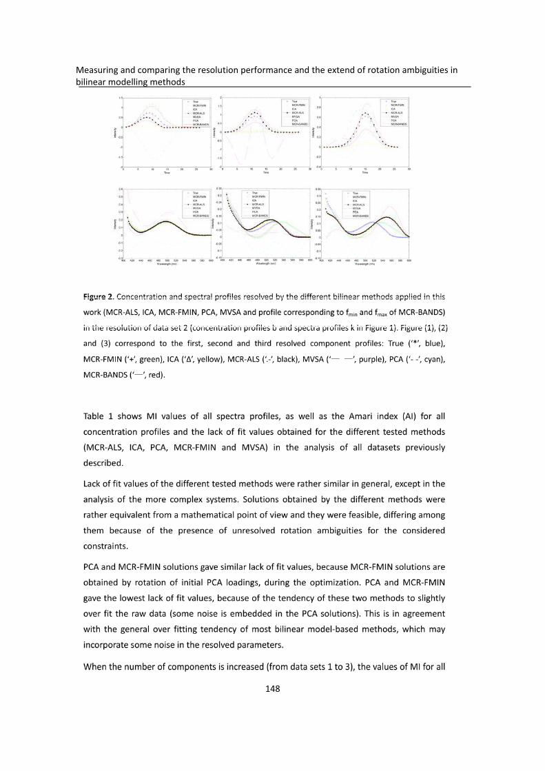
Measuring�and�comparing�the�resolution�performance�and�the�extend�of�rotation�ambiguities�in�bilinear�modelling�methods�
148��

Measuring�and�comparing�the�resolution�performance�and�the�extend�of�rotation�ambiguities�in�bilinear�modelling�methods�
149��

Measuring�and�comparing�the�resolution�performance�and�the�extend�of�rotation�ambiguities�in�bilinear�modelling�methods�
150��

Measuring�and�comparing�the�resolution�performance�and�the�extend�of�rotation�ambiguities�in�bilinear�modelling�methods�
151��

Measuring�and�comparing�the�resolution�performance�and�the�extend�of�rotation�ambiguities�in�bilinear�modelling�methods�
152��

Measuring�and�comparing�the�resolution�performance�and�the�extend�of�rotation�ambiguities�in�bilinear�modelling�methods�
153��

Measuring�and�comparing�the�resolution�performance�and�the�extend�of�rotation�ambiguities�in�bilinear�modelling�methods�
154��
�
� �
Measuring�and�comparing�the�resolution�performance�and�the�extend�of�rotation�ambiguities�in�bilinear�modelling�methods�
155��

Measuring�and�comparing�the�resolution�performance�and�the�extend�of�rotation�ambiguities�in�bilinear�modelling�methods�
156��

Measuring�and�comparing�the�resolution�performance�and�the�extend�of�rotation�ambiguities�in�bilinear�modelling�methods�
157��
�
� �

Measuring�and�comparing�the�resolution�performance�and�the�extend�of�rotation�ambiguities�in�bilinear�modelling�methods�
158��
�
� �

Measuring�and�comparing�the�resolution�performance�and�the�extend�of�rotation�ambiguities�in�bilinear�modelling�methods�
159��
�
� �

Measuring�and�comparing�the�resolution�performance�and�the�extend�of�rotation�ambiguities�in�bilinear�modelling�methods�
160��
Discussion��
Results�of�Mutual� Information�(MI)�and�of�Amari� Index�(AI)�showed�that�resolved�results�with�independence�and�orthogonality�constraints�usually�do�not�match�the�profiles�of�the�pure� component� in� the� experiment.� Profiles� independence� or� orthogonality� makes� the�profiles�of�the�components�to�differ�as�much�as�possible,�but�this�does�not�mean�that�they�correspond�to�the�true�profiles�causing�the�observed�data�variance.� In�the�real�situation,�especially� in� the� analysis� of� hyperspectral� imaging� of� this� Thesis,� independence� or�orthogonality�conditions�are�not� fulfilled�by�spectra�profiles� in�general.�Pure�component�spectral� in� the�hyperspectral� imaging�are�neither� independent�nor�orthogonal,�and� they�may�be�overlapped.�ICA�and�PCA�obtain�good�mathematical�models,�but�these�models�are�different�form�the�true�ones.�MVSA�method�provided�the�better�estimations�of�the�pure�spectra�(endmembers)�of�the�hyperspectral� imaging.�However�concentration�profiles�are�obtained� by� least� squares� post� processing� when� using� MVSA.� And� this� operation� was�always�giving�negative�values�for�them,�which�will�make�results�non�realistic.�Closure�(sum�to� 1)� constraint� in� MVSA� is� not� an� adequate� constraint� for� the� estimation� of�concentrations� (distribution� maps)� since� they� do� not� match� the� true� situation� of�hyperspectral�imaging.�
Bilinear� models� evaluated� in� this� chapter� can� be� applied� as� preprocessing,� exploration,�classification,� regression� and� resolution� tools.� All� of� them� can� be� considered� as� an�alternative� tool� for� the� analysis� of� mixed� signals� on� certain� cases.� However,�implementation� of� physical� constraints,� such� as� non�negativity� in� resolved� spectra� and�concentration�profiles�is�more�flexible�and�reliable�in�MCR�methods�like�in�MCR�ALS.�This�is� also� the� reason� why� MCR�ALS� is� a� more� adequate� method� for� hyperspectral� imaging�analysis.�
MCR�BANDS�delivers�an�approximation�to�the�extension�of�rotation�ambiguity.�AFS�represent�all�feasible�solutions�geometrically�and�can�be�depicted�by�a�method�like�FAC�PACK.�The�results�of�this�chapter�(Paper�267)�have�shown�that�the�extension�of�rotation�ambiguity�calculated�by�MCR�BANDS�and�the�AFS�calculated�by�a�method�like�FAC�PACK�are�concordant.�This�is�an�important�conclusion�for�future�work�and�applications�of�the�different�methods�evaluating�the�rotation�ambiguity�extension.�� �

�
161��
�
�
�
Chapter 6
Distribution of Dissolved Organic Matter in freshwaters using Excitation Emission fluorescence and Multivariate Curve Resolution�
� �

�
162��
� �

Distribution�of�Dissolved�Organic�Matter�in�freshwaters�using�Excitation�Emission�fluorescence�and�Multivariate�Curve�Resolution�
163��
Introduction��
Dissolved�Organic�Matter�(DOM)�analysis�in�surface�waters�
River� flows� include� all� the� material� flowing� through� the� river,� not� only� water,� but� also�sediments,� nutrients,� organic� debris� and� biomass.� These� flows� are� a� key� aspect� in�monitoring�studies�for�the�environmental�quality�assessment�of�the�flowing�area�near�to�the�river.291�They�have�strong�seasonal�patterns�and�display�strong�changes�due�to�natural�droughts.�River�water�quality�assessment�is�usually�based�on�the�comparison�of�measured�values�of�particular�physicochemical�parameters�with�threshold�values�defined�in�national�or�international�directives292.�
In� the� surface� water� systems,� the� dissolved� organic� matter� (DOM)� is� a� key� parameter�which� is� formed� by� a� mixture� of� aromatic� and� aliphatic� hydrocarbon� structures� with�different� attached� functional� groups.� These� functional� groups� have� different� structures�with�a�wide�range�of�molecular�weights293.�In�the�past,�DOM�in�surface�water�systems�has�been� considered� an� important� element� for� water� quality� assessment.� Its� composition�varies�in�time�and�space�depending�on�the�proximity�to�the�sources�and�on�the�exposure�to� degradation� processes294.� In� natural� environments,� concentration� and� composition�changes�of�DOM�have�a�potential�effect�on� the�health�of�ecosystems�through�processes�like�light�attenuation,�nutrient�availability,�and�contamination�transport295.��
As�the�chemical�nature�of�DOM�defines�its�optical�properties,�optical�measurements�have�been� applied� for� tracing� its� variability� in� natural� waters296.� The� two� major� DOM�components� that� have� been� found� to� fluoresce� are� humic� materials� (giving� blue�fluorescence)� and� protein� fractions� (giving� UV� fluorescence).� The� most� common�fluorescent� peaks� identified� in� natural� water� included� humic� and� fulvic�like� matter� with�fluorescence� patterns� called� as� fluorescence� A� (237�260/400�500� nm)� and� C� (300�370/400�500�nm),�and�protein�like�material�fluorescence�centers,�such�as�fluoreophores�T�(225�237/340�381�nm�and�275/340�nm)and�B� (225�237/390�321�and�275�310�nm).297,�298�They�are�respectively�written�as�UVA,�UVC,�UVT�and�UVB�for�short.�Additionally,�there�are�moleculars�with�fluorescence�patterns�called�UVD�(soil�fulvic�acid,�390/509�nm),�UVE�(soil�fulvic� acid,� (455/521� nm)),� UVM� (marine� humic�like,� (312/380�420� nm))� in� natural�environments�294.�
�
Excitation�Emission�Matrix�(EEM)�fluorescence�combined�with�chemometric�methods�for�DOM�analysis�and�water�quality�assessment�

Distribution�of�Dissolved�Organic�Matter�in�freshwaters�using�Excitation�Emission�fluorescence�and�Multivariate�Curve�Resolution�
164��
It�is�difficult�to�trace�changes�in�the�structure�of�DOM�in�natural�water�systems�because�of�the� complexity� and� non�conservative� behavior� of� the� composition� of� DOM� in� natural�environments�299,�300.��
Molecular�fluorescence�spectroscopy�is�a�particularly�useful�technique�for�the�study�of�the�chemical�properties�of�fluorescent�molecules.�It� is�a�highly�sensitive�analytical�technique,�allowing�nondestructive�direct�measurements�at�natural�environmental�concentrations301.�Molecular� fluorescence� is� a� very� sensitive� technique� for� the� analysis� of� the� chemical�environment�of�fluorophors302,�like�those�present�in�DOM.�The�excitation–emission�matrix�(EEM)�of�fluorescence�generates�multidimensional�data�structures�suitable�for�this�type�of�analysis.� The� utilization� of� EEM� fluorescence� can� be� used� in� the� characterization� of� the�properties� and� reactivity� of� DOM.� EEM� allows� DOM� analysis� and� monitoring� in� surface�waters� and� other� natural� systems303.� In� the� next� Figure,� EEM� experimental� measures� of�DOM�in�river�water�are�shown.�
�
Figure�6��1�EEM�data�matrix�structure�of�the�water�samples�obtained�from�Ter�River.�
In� this� Thesis� the� basic� EEM� data� matrix� structure� for� the� analysis� of� one� single� water�sample� was� composed� by� 76� rows� (76� excitation� bands)� and� 76� columns� (76� emission�bands),� giving� a� data� matrix,�Q�(76,� 76),� which� contains� the� fluorescence� spectra� of� the�considered� water� sample.� Excitation� and� emission� spectra� of� the� compounds� studied� in�individual�samples�can�be�arranged�in�data�tables�or�data�matrices.�In�this�study�only�the�fraction�of�the�raw�EEM�that�did�not�contain�scattering�bands�(from�227�450nm,�avoiding�the�region�between�200�and�225nm)�was�selected.��
As�said�before�EEM�spectra�can�be�arranged�in�a�data�cube�or�three�way,�three�mode�data�structure.�Totally�122�water�samples�were�collected�at�62�stations�along�the�Sau�Reservoir�system� and� its� tributary,� the� Ter� River.� When� the� EEM� data� of� 122� samples� were�considered,� then� a� new� data� structure� was� obtained� which� can� be� arranged� in� a� long�column�wise� data� matrix�Qlmn�(122×76,� 76)� which� can� be� arranged� by� setting� individual�
240 260 280 300 320 340 360 380 400 420 4400
0.1
0.2
0.3
0.4
0.5
wavelength(nm)240 260 280 300 320 340 360 380 400 420 440
0
0.1
0.2
0.3
0.4
0.5
wavelength(nm)
10 20 30 40 50 60 70
10
20
30
40
50
60
70 0.05
0.1
0.15
0.2
0.25
0.3
0.35
0.4
0.45
0.5
0.55

Distribution�of�Dissolved�Organic�Matter�in�freshwaters�using�Excitation�Emission�fluorescence�and�Multivariate�Curve�Resolution�
165��
data�matrices�from�every�sample,�one�on�the�top�of�the�other�and�keeping�the�emission�wavelength�axis�in�common.��
Chemometric�analysis�of�data�sets�obtained�in�large�environmental�monitoring�studies�of�natural�fresh�water�systems�by�EEM�fluorescence�spectra�(such�as�those�shown�in�previous�Figure� 6�1)� provide� a� powerful� and� convenient� way� to� investigate� DOM� source�contributions�of�the�investigated�watersheds304�306.��
Appropriate� three�way� chemometric� data� analysis� methods,� including� so�called� second�order�calibration�methods�and�those�based�on�trilinear�modeling�200�have�been�proposed�for� the� analysis� of� EEM� datasets.� The� high� analytical� potential� of� EEM� coupled� to�chemometric�methods�has�long�ago�been�recognized.�Due�to�the�intrinsic�structure�of�EEM�data,� the� Parallel� Factor� Analysis� (PARAFAC)� method� 241� based� on� the� trilinear� model� is�adequate�and�it�can�be�successfully�apply�for�their�decomposition.�PARAFAC�decomposes�directly�the�three�way�data�set�or�data�cube�into�components�using�and�alternative�least�squares�method.�In�Chapter�2,�these�methods�were�described.��
Alternatively� the� Multivariate� Curve� Resolution� Alternating� Least� Squares� (MCR�ALS),�method�can�be�used�also�for�the�analysis�of�three�way�data�fulfilling�the�premises�of�the�trilinear�model�200.�MCR�ALS�was�used�in�this�Thesis�to�analyze�the�EEM�dataset�(paper307).��
The� bilinear� decomposition� of� the� data� matrix�Q����can� be� described� by� the� following�equation:�
Q��� � *L��+*L�K � L�����������������������������������Equation�6��1�
where�*�:�(76,n)� is� the� matrix� of� excitation� spectra� (n� is� the� number� of� considered�bilinear� components� contributing� to� the� observed� fluorescence� signal),�*L��(Excitation�Profiles)�and�+�(Contribution�Profiles)�are�mixed�in�the�augmented�*L��+�matrix� (122×76,�n),�and�L�is�the�residual�matrix�describing�the�variance�not�explained�by�the�bilinear�model�(*L��+*�:M ).��
When�the�trilinear�model�308,�309�holds,�every�individual�data�matrix,�Q},�is�decomposed�by�the�following�equation�
Q} � *��+}*�:M � L����������������������������������Equation�6��2�
where�k�refers�to�slice�k�and�+}�is�a�diagonal�concentration�matrix�referring�to�the�relative�amounts� of� the� components� in� slice/matrix� k.�*L��and�*�:M �matrices� are� the� same� for� all�Q} �simultaneously� analyzed.� Only� the� new�+} �diagonal� matrix� of� dimensions� (n,� n),�changes� from� sample� to� sample� and� it� gives� in� its� diagonal� the� relative� spectral�contributions�of�the�n�components�to�the�fluorescence�signal�of�sample�matrix�k.��

Distribution�of�Dissolved�Organic�Matter�in�freshwaters�using�Excitation�Emission�fluorescence�and�Multivariate�Curve�Resolution�
166��
Alternating� Least� Squares� optimization� of� both�*���(,� estimation� of�*�:�is� performed�iteratively� under� non�negative,� trilinearity� and� normalization� constraints� until�convergence� is� achieved.� According� to� Figure� 6�2,� when� trilinearity� constraint� is� applied�during�the�ALS�optimization,�*���(�is�first�decomposed�by�SVD�for�each�component.�Only�the�first�singular�value�is�considered�in�this�decomposition.�For�this�component,�the�shape�of�its�excitation�spectrum�will�be�exactly�the�same�for�all�the�considered�samples�and�that�it�only�will�change�its�relative� intensity.�After�this�decomposition,�the�full�*���(�is�rebuilt�and� updated� for� the� next� ALS� iteration.� Apart� from� forcing� the� shape� of� the� excitation�spectrum� of� the� considered� component� to� be� the� same� for� all� different� samples,� this�procedure�captures�the�relative�intensity�variation�of�this�component,�which�is�stored�in�a�contribution� or� concentration�+�matrix� (loading� of� the� third� mode),� giving� therefore� the�relative�contribution�of� this�component� in� the�different�samples.�*���(Excitation�spectra)�and�+�(Contribution� Profiles)� in*���(�matrices� are� finally� obtained,� together� with�*�:�(emission�spectra)�matrix�obtained�directly�during�the�ALS�procedure�(Equation�6�2).��
�
�Figure�6�2�Decomposition�of�the�three�way�excitation–emission�fluorescence�data�set�using�the�trilinearity�constraint�during�the�Alternating�Least�Squares�optimization�in�MCR�ALS.�

Distribution�of�Dissolved�Organic�Matter�in�freshwaters�using�Excitation�Emission�fluorescence�and�Multivariate�Curve�Resolution�
167��
�
�
Compared�to�PARAFAC,�the�main�advantage�of�MCR�ALS�is�that�the�trilinearity�constraint�can� be� applied� independently� on� each� component,� in� contrast� to� PARAFAC� where� all�resolved�components�should�fulfill�the�sought�trilinear�condition.�
�
The�dataset�investigated�in�this�work�
The�study�area�investigated�in�this�work�was�the�middle�Ter�River�flow,�which�supplied�55%�of�the�raw�water�for�drinking�purposes�to�Barcelona�city�and�its�surroundings.�With�a�3010�km2�surface�basin�and�208�km�long,�it�originates�in�the�middle�of�the�Catalan�more�oriental�range�of�the�Pyrenees�(at�2400�m�high)�and�it�passes�through�Girona�city,�and�leads�to�the�Mediterranean�Sea310,�see�Figure�6�3�311and�Figure�6�4(From�google�map).�Most�of�the�Ter�river�basin�is�characterized�by�a�medium�population�density;�Girona�and�Vic�are�the�most�populous�cities.�In�terms�of�the�use�of�the�river�water,�53%�of�the�total�water�is�assigned�to� agricultural� irrigation� and� golf� courses,� 24%� to� domestic� use,� and� the� rest� is� for�industrial� (17%)�and�livestock�farmer�(7%)�use312.�This�river�receives�the�direct� impact�of�some�metallurgic,�pulp�mill,�textile�and�tannery�industries�313.�As�a�result�in�the�river�have�found� alkylphenols,� alkylphenol� ethoxylates,� aliphatic� and� aromatic� hydrocarbons,� fatty�acids,� plasticizers,� alkylbenzenes� and� pesticides,� the� discharge� of� urban� and� industrial�waters,�and�of�agricultural�runoff�314.�
�
Figure�6��3�The�location�of�Ter�River�basin�in�Catalunya,�Spain.�
Main� source� and� transformation� processes� of� the� DOM� in� Ter� river� system� were�characterized� and� located,� in� middle� course� of� Ter� river� (which� is� a� rather� populated�area)is�described,�several�kilometers�before�entering�its�main�reservoirs�in�Susqueda�and�

Distribution�of�Dissolved�Organic�Matter�in�freshwaters�using�Excitation�Emission�fluorescence�and�Multivariate�Curve�Resolution�
168��
Sau�(see�Figure�6�4),�during� its�travel�throughout�the� lentic�ambient�until�reaching�these�two� dams.� Results� obtained� in� this� study� support� the� hypothesis� that� the� different�fractions�of�DOM�are�differentially�processed�along�the�river�reservoir�system307.�
�
�
�
Figure�6��4�The�upper�part�is�the�terrain�map�of�Ter�river�basins�and�the�lower�part�is�the�main�reservoirs�in�Susqueda�and�Sau�(The�figure�was�obtained�from�online�Google�map).�
�
The�published�paper�in�this�chapter�
ZHANG,�Xin.,�Marcé,�R.,�Armengol,�J.,�&�Tauler,�R.�Distribution�of�dissolved�organic�matter�in�freshwaters�using�excitation�emission�fluorescence�and�Multivariate�Curve�Resolution.�Chemosphere,�2014,�111,�120�128�� �

Distribution�of�Dissolved�Organic�Matter�in�freshwaters�using�Excitation�Emission�fluorescence�and�Multivariate�Curve�Resolution�
169��
�
� �

Distribution�of�Dissolved�Organic�Matter�in�freshwaters�using�Excitation�Emission�fluorescence�and�Multivariate�Curve�Resolution�
170��
�
� �
Distribution�of�Dissolved�Organic�Matter�in�freshwaters�using�Excitation�Emission�fluorescence�and�Multivariate�Curve�Resolution�
171��
�
� �
Distribution�of�Dissolved�Organic�Matter�in�freshwaters�using�Excitation�Emission�fluorescence�and�Multivariate�Curve�Resolution�
172��
�
� �
Distribution�of�Dissolved�Organic�Matter�in�freshwaters�using�Excitation�Emission�fluorescence�and�Multivariate�Curve�Resolution�
173��
�
� �

Distribution�of�Dissolved�Organic�Matter�in�freshwaters�using�Excitation�Emission�fluorescence�and�Multivariate�Curve�Resolution�
174��
�
� �

Distribution�of�Dissolved�Organic�Matter�in�freshwaters�using�Excitation�Emission�fluorescence�and�Multivariate�Curve�Resolution�
175��
�
� �

Distribution�of�Dissolved�Organic�Matter�in�freshwaters�using�Excitation�Emission�fluorescence�and�Multivariate�Curve�Resolution�
176��
�
� �

Distribution�of�Dissolved�Organic�Matter�in�freshwaters�using�Excitation�Emission�fluorescence�and�Multivariate�Curve�Resolution�
177��
�
� �
Distribution�of�Dissolved�Organic�Matter�in�freshwaters�using�Excitation�Emission�fluorescence�and�Multivariate�Curve�Resolution�
178��
Discussion�DOM�sources�have�different�fluorophore�groups�which�can�be�identified�and�characterized.�in� this� Thesis,� Parallel� Factor� Analysis� (PARAFAC)� and� Multivariate� Curve� Resolution�Alternating� Least� Squares� (MCR�ALS)� have� been� satisfactory� applied� to� the� EEM� data�obtained� from� the� Ter� River�Reservoir� system.� The� results� obtained� in� this� work� can� be�useful�for�establishing�analytical�methodologies�protocols�for�DOM�monitoring�in�surface�water�systems.�
According�to�PARAFAC�and�MCR�ALS�results,�three�major�DOM�fluorescence�sources�(UVC,�UVA,� and� UVT)� were� resolved.� The� first� fluorescence� source� consisted� of� UVC� humic�derived�group�type�of�DOM�fraction.�Humic�substances�(HS)�are�natural�macromolecular,�heterogeneous�substances�with�a�high�degree�of�polydispersity.�They�occur�ubiquitously�in�soil,� aquatic� environment� and� certain� sediments.� They� are� known� to� contain� similar�functional�groups�i.e.�C=C,�COOH,�OH,�OCH3,�C=O,�NH�or�NH2,�arrangements�such�as�redox�quinone�semiquinone�hydroquinone,�charge�transfer�planar�complexes�etc.315.��
The�second�fluorescence�source�consisted�of�UVA�humic/fulvic�type�of�DOM�fraction.� Its�presence�is�associated�with�organic�matter�generated�within�the�stream�by�decomposition�of� organic� matter.� It� can� be� considered� to� fulvic� acid� fluorophone� groups� present� in� all�environments316.
And� the� third� fluorescence� source� consisted� of� mixed� contributions� of� UVT� protein�like�type�of�fraction,�with�tryptophan�groups.�The�agreement�between�the�results�(wavelength�of� UVC,� UVA,� and� UVT)� obtained� in� this� work� with� those� previously� obtained� in� other�studies� (introduced� in� the� first� section� of� this� chapter)� confirmed� the� identification� of�different�DOM�sources.��
Moreover�their�distribution�over�the�monitoring�area�under�study�was�also�estimated.�The�concentration� distributions� have� been� illustrated� on� the� map� using� MATLAB� mapping�toolbox� (MATLAB� R2013a.� The� MathWorks,� Inc.).� When� the� MCR�ALS� resolved�contributions�are�examined,� it� is�observed�that�UVC�and�UVT�contributions�describe� the�increase�of�DOM�concentrations�at�Manlleu�(large�town),�Roda�de�Ter�(WWTP)�and�Riera�de�Sant�Marti�(tributary�river).�After�these�three�locations�and�along�the�river�flow,�DOM�concentrations�revealed�by�UVA�showed�a�gradual�decreasing�trend.�The�main�difference�of�UVA�to�the�others�is�that�after�the�station�23�(where�river�flows�slower�from�this�station�than� upstream),� it� decreased� sharply� and� should� be� related� mostly� to� organic� matter�caused�by�human�(population)�impact.�
Hydroxy�benzoic� acids� (like� in� salicylic� acid),� �naphthol,� aromatic� nitrogen� rings,�tryptophan,�amino�acids�and�proteins�can�be�present�in�DOM�of�the�fresh�water�systems�and�are�responsible�of�most�of�the�fluorescence�properties�investigated�in�this�work.�Main�

Distribution�of�Dissolved�Organic�Matter�in�freshwaters�using�Excitation�Emission�fluorescence�and�Multivariate�Curve�Resolution�
179��
trends� of� the� organic� matter� processes� taking� place� along� the� fresh� water� system� were�described�in�detail�in�the�results�section�of�paper307.�
The� results� of� this� work� show� that� EEM� fluorescence� spectra� provide� a� powerful� and�convenient� way� to� investigate� DOM� source� contributions� in� watersheds.� Major� DOM�source�contributions�in�watershed�can�be�obtained�by�means�of�EEM�fluorescence�spectra�combined�with�chemometric�methods,�such�as�MCR�ALS�with�the�trilinearity�constraint�or�PARAFAC.�Increasing�and�decreasing�relative�contributions�of�DOM�in�river�can�be�related�with�factors�like�river�flow,�DOM�natural�sources�origin,�human�activities�in�the�area�and�population� input� sources� along� the� river.� MCR�ALS� with� the� trilinear� constraint� is� an�effective� way� to� characterize� and� resolve� DOM� sources� in� natural� fresh� water� systems�from�EEM�data.�
�
�
�
� �

Distribution�of�Dissolved�Organic�Matter�in�freshwaters�using�Excitation�Emission�fluorescence�and�Multivariate�Curve�Resolution�
180��
� �

�
181��
�
�
�
�
�
Chapter 7
Conclusion�
� �

�
182��
� �
Conclusions�
183��
Conclusions�of�the�application�of�chemometric�methods�
�
1)�The�results�obtained�in�this�Thesis�show�that�MCR�ALS�method�can�be�successfully�used�for� hyperspectral� image� resolution� purposes.� The� spectra� signatures� of� the� pure�constituents� present� in� hyperspectral� images� and� their� concentration� distribution� at� a�pixel� level� can� be� estimated.� Constituents� identification� can� be� performed� using� the�resolved�pure�spectra�signatures�and�comparing�them�to�reference�spectra�from�spectral�libraries�or�from�experimental�spectra�of�reference�samples.��
�
2)� Application� of� image� data� pretreatment� methods� such� as� Multiplicative� Scatter�Correction� (MSC),� Asymmetric� Least� Squares� (AsLS)� and� Savitzky�Golay� (SG)� smoothing�reduce� significantly� the� presence� of� strong� fluorescence� background� in� Raman�hyperspectral� images.� In� contrast,� infrared� hyperspectral� imaging� is� not� affected� by�fluorescence.� Kramers�Kronig� transform� enables� to� calculate� absorption� spectra� in� case�only�reflectance�spectra�can�be�measured�for�infrared�spectra.�
�
3)�The�extent�of�rotation�ambiguity�associated�to�MCR�ALS�and�other�resolution�methods�(like�VCA�(Vertex�Component�Analysis)�or�MVSA�(Minimum�Volume�Simplex�Analysis))�can�be�rather�high�when�they�are�applied�for�hyperspectral�image�resolution�with�high�noise.�The� correct� resolution� of� hyperspectral� images� can� only� be� guaranteed� if� additional�constraints� are� applied,� such� as� those� providing� information� about� the� local� rank�properties�of�the�image,�i.e.�about�the�presence�or�absence�of�the�different�constituents�(components)�in�the�image�pixels.�Only�in�this�way�it�is�possible�to�increase�the�reliability�of�the�solutions�provided�by�MCR�methods�and�decrease�the�uncertainties�associated�to�them.� Appropriate� use� of� local� rank� and� selectivity� constraints� can� improve� significantly�the� quality� of� the� pure� spectra� (signatures)� and� of� the� constituent� distribution� maps�resolved�by�MCR�ALS�analysis�of�hyperspectral�images�in�remote�sensing�studies.�
�
4)� Use� of� correlation� coefficients� between� selected� spectra� and� image� pixel� spectra� is�shown� to� provide� an� alternative� way� for� the� application� of� the� selectivity� constraint� in�hyperspectral�images�for�the�first�time.�This�alternative�method�resulted�to�be�satisfactory�when�pure�pixels�exist.�
�
5)� MCR�BANDS� method� can� be� used� to� get� estimations� of� the� extension� of� rotation�ambiguities� in� MCR� resolved� results.� The� Area� of� Feasible� Solutions� (AFS)� represents�

Conclusions�
184��
feasible� solutions� geometrically.� The� range� of� rotation� ambiguity� calculated� by� MCR�BANDS�and�AFS�are�in�agreement.�
�
6)�MCR�ALS�with�the�trilinearity�constraint�is�an�effective�way�to�characterize�and�resolve�Excitation�Emission� Matrix� fluorescence� spectra� (EEM).� Georeferenced� mapping� using�MATLAB� is� an� adequate� method� to� visualize� graphically� and� geographical� distribution�maps�of�the�constituents�resolved�by�MCR�ALS�analysis�of�environmental�monitoring�data�sets�using�fluorescence�EEM�data.��
�
Conclusions�from�environmental�and�food�samples�analysis�using�hyperspectral�imaging�and�Multivariate�Curve�Resolution�methods�
1)�In�the�analysis�of�remote�sensing�NIR�hyperspectral�images�obtained�from�the�region�of�Cuprite�in�Nevada,�in�the�San�Diego�airport�and�in�the�Moffet�field�in�California,�MCR�ALS�results� showed� clearly� the� presence� of� multiple� objects� such� as� airplanes,� green� plant�areas,� lakes,� hard� ground� field� and�other� related� objects� in� the� image.�Decisions� can� be�taken� from�the�detailed� information� (distribution�maps)�contained� in�these� images�after�examining�them�by�MCR�ALS.���
2)� Micro�hyperspectral� imaging� coupled� to� MCR�ALS� is� confirmed� to� be� an� appropriate�tool�for�the�direct�analysis�of�the�constituents�of�chocolate�samples,�and�by�extension,�it�is�proposed� for� the� analysis� of� other� mixture� constituents� in� commercial� food� samples.�Results� achieved� in� this� work� are� representative� of� the� possibilities� offered� by�hyperspectral� imaging� analysis� of� food� samples,� and� confirmed� the� potential� use� of� the�MCR�ALS� as� a� complementary� tool� method� for� this� type� of� analysis.� Application� of� this�combination� of� methods� (hyperspectral� imaging� and� MCR�ALS)� can� be� proposed� for�testing� samples� from� other� similar� fields� including� the� analysis� of� material� surfaces,�agriculture�products�as�well�as�biological�tissue�analysis�in�medicine.�
�
3)�Environmental�monitoring�studies�of�natural�fresh�water�systems�by�Excitation�Emission�Matrix�(EEM)�fluorescence�spectra�provide�a�powerful�and�convenient�way�to�investigate�Dissolved� Organic� Matter� (DOM)� source� contributions� in� watersheds.� Major� DOM�fluorescence� sources� were� resolved,� and� assigned� to� UVC� humic� type� of� fraction,� UVA�humic/fulvic� type� of� fraction,� UVT,� protein�like,� and� tryptophan�like� type� of� fraction.�Resolved� geographical� distribution� of� these� three� different� DOM� sources� over� the�investigated� area� showed� increasing� and� decreasing� relative� contributions� of� these�

Conclusions�
185��
sources�according�to�different�factors�like�river�flow,�DOM�natural�sources�origin,�human�activities�in�the�area�and�population�in�input�sources.�
�
�
� �

Conclusions�
186��
� �
�
187��
�
�
�
�
�
�
Resumen de la Tesis � �

�
188��
� �
Resumen�de�la�Tesis�
189��
�
Resumen��
El�análisis�de� imágenes�hiperespectrales�está� relativamente�avanzado�dentro�del�análisis�de�alimentos�y�de�medio�ambiente.�Las� imágenes�hiperespectrales�permiten�obtener�un�conocimiento� preciso� y� fiable� sobre� la� composición� química� y� la� distribución� de� los�componentes� químicos� en� la� superficie� de� una� muestra� a� investigar.� Los� resultados� del�análisis� de� imágenes� hiperespectrales� pueden� utilizarse� para� adquirir� una� comprensión�fundamental� de� los� sistemas� químicos� complejos� en� investigación� y� desarrollo,� con�repercusiones�comerciales,�como�métodos�de�validación�de�la�adulteración�en�el�análisis�de�alimentos�y�derivados,�y�en�el�análisis�de� los�procesos� industriales�y�de�su�control.�El�análisis�de�los�datos�de�imágenes�hiperespectrales�son�un�gran�reto�debido�a�su�tamaño�y�complejidad.� En� esta� Tesis� se� propone� el� desarrollo� y� utilización� de� métodos�quimiométricos� que� permitan� revelar� la� información� contenida� en� las� imágenes�espectrales�analizadas�tanto�como�sea�posible.�
Esta� Tesis� trata� de� la� resolución� de� datos� de� imágenes� hiperespectrales� utilizando�métodos�quimiométricos,�en�particular�mediante�el�uso�de�métodos�de�pretratamiento�de�datos� y� utilizando� métodos� de� resolución� multivariante� de� curvas� (MCR).� La� principal�contribución� de� la� presente� Tesis� es� el� estudio� y� la� aplicación� del� método� MCR�ALS�(resolución� multivariante� de� curvas� mediante� mínimos� cuadrados� alternados)� para� la�resolución�de� imágenes�hiperespectrales,�adquiridas�mediante� técnicas�de� teledetección�(en�el�aire�o�en�el�espacio,�transmitidas�a�la�Tierra�mediante�instrumentos�de�observación)�y�mediante�técnicas�de�micro�espectroscopia.�Específicamente,�en�el�trabajo�de�esta�Tesis,�se�explora�la�combinación�de�los�métodos�quimiométricos�y�de�los�métodos�de�análisis�de�imágenes�hiperespectrales,�para�la�resolución�de�los�espectros�(firmas)�y�de�los�mapas�de�distribución�de�los�componentes�químicos�de�la�muestra.�El�objetivo�final�de�este�estudio�es� mejorar� el� análisis� y� la� interpretación� de� los� datos� de� imágenes� hiperespectrales�mediante�el�aprovechamiento� de�diferentes�herramientas� quimiométricas�poderosas.� La�detección�del�rango��local�y�las�propiedades�de�selectividad�que�describen�la�información�espacial�de�los�componentes�presentes�en�las�imágenes�espectroscópicas�se�puede�utilizar�como� restricción� para� aumentar� significativamente� el� rendimiento� del� método� MCR,�disminuyendo� las� incertidumbres� asociadas� a� las� ambigüedades� rotacionales.� Se� han�comparado� diferentes� métodos� de� resolución,� tales� como� MCR�ALS,� ICA� (Análisis� de�Componentes� Independientes),� MVSA� (Mínimo� Volumen� Simplex� Análisis),� PCA� (Análisis�de�Componentes�Principales),�y�MCR�FMIN.�Los�métodos�MCR�BANDS�y�FAC�PACK�se�han�utilizado�para� la�evaluación�de� la�extensión�de� las�ambigüedades�rotacionales�existentes�en�los�resultados�después�de�la�aplicación�de�estos�métodos�de�resolución�multivariante.�

Resumen�de�la�Tesis�
190��
En� esta� Tesis� se� han� analizado� diversos� conjuntos� de� datos� compuestos� por� varias�imágenes� hiperespectrales� proporcionadas� por� instrumentos� estándar� tales� como� el�espectrómetro�de� imágenes�hiperespectrales�en�el�visible�y�en�el� infrarrojo�AVIRIS�de� la�NASA,� y� diversos� espectrómetros� de� imágenes� hiperespectrales� Raman� y� infrarrojo� de�laboratorio.� La� eficacia� del� procedimiento� MCR�ALS� se� ilustra� proporcionando�comparaciones� exhaustivas� con� otros� métodos� de� resolución� de� mezclas� espectrales� a�partir�de�conjuntos�de�datos�hiperespectrales�simulados�y�reales.�
� �

Resumen�de�la�Tesis�
191��
Objetivos�generales�de�la�Tesis��
El� objetivo� principal� de� esta� Tesis� ha� sido� el� desarrollo� y� la� aplicación� de� métodos�quimiométricas� para� el� análisis� de� imágenes� hiperespectrales� obtenidos� a� partir� de�técnicas�de�teledetección�o�de�micro�espectroscopia�de�muestras�de�medio�ambiente�y�de�alimentos.� Se� han� estudiado� en� detalle� diferentes� conjuntos� de� datos� simulados� y�experimentales,�obtenidos�bien�a�partir�de�repositorios�de�datos�de�teledetección�públicos,�o� a� partir� de� medidas� experimentales.� Se� han� analizado� y� caracterizado� diferentes�conjuntos� de� datos� simulados� y� experimentales� obtenidos� a� partir� de� repositorios� de�datos�de�teledetección�públicos�y�a�partir�de�mediciones�experimentales.��
Especialmente�importante�ha�sido�la�extensión�y�aplicación�del�método�de�MCR�ALS�para�la� resolución� de� datos� de� imágenes� hiperespectrales� obtenidas� mediante� teledetección,�con�el�objetivo�de�obtener�los�espectros�y�mapas�de�distribución�de�los�constituyentes�de�las�imágenes�analizadas.�
�
Objetivos�en�el�análisis�de�imágenes�hiperespectrales�
�
� Aplicar�el�método�MCR�ALS�al�análisis�de�imágenes�hiperespectrales�a�partir�de�conjuntos� de� datos� simulados� y� de� conjuntos� de� datos� experimentales,� que�incluyen� imágenes� obtenidas� a� partir� de� procedimientos� de� teledetección� del�medio�ambiente,�y�de� imágenes�obtenidas�a�partir�de�microespectroscopia�de�alimentos� de� muestras� comerciales� de� chocolate.� También� se� realiza� la��aplicación� el� método� MCR�ALS� al� análisis� fluorimétrico� de� muestras� de� aguas�superficiales�del�rio�Ter�y�de�sus�embalses�en�su�curso�medio�(embalses�de�Sau�y�Susqueda).�En�todos�estos�casos,�se�propone�la�aplicación�del�método�MCR�ALS�para� la� resolución� de� los� espectros� de� los� componentes� de� las� mezclas�analizadas,� para� su� � caracterización� y� estimación� de� sus� correspondientes�contribuciones�y�mapas�de�distribución.��
� Aplicar� el� método� MCR�ALS� a� las� imágenes� hiperespectrales� obtenidas� por�teledetección,� para� resolver� os� diferentes� objetos� presentes� en� las� imágenes�estudiadas,� tales� como� lagos,� suelos,� vegetación,� edificios,� etc.,� y� la�determinación�de�su�ubicación�en�la�imagen�estudiada.��
Resumen�de�la�Tesis�
192��
� Aplicar� el� método� MCR�ALS� al� análisis� hiperespectral� de� los� componentes� del�chocolate� para� su� resolución� a� nivel� micro� según� su� tamaño� de� partícula,�aspecto�importante�relacionado�con�el�control�de�la�calidad�del�producto�en�el�caso�de�estudio�de�alimentos.�
� Aplicar� el� método� MCR�ALS� al� análisis� de� los� datos� de� fluorescencia� para� el�seguimiento� de� las� fuentes� de� materia� orgánica� (DOM)� en� el� rio� Ter� para� la�resolución� de� sus� diferentes� contribuciones,� sus� niveles� de� concentración,� su�distribución� geográfica� y� la� relación� que� existen� entre� ellas� y� la� actividad�humana�a�lo�largo�del�cauce�del�río�y�de�sus�embalses.�
�
Objetivos�de�los�análisis�quimiométricso�
� Desarrollar�y�aplicacar�el�método�MCR�ALS�para�el�análisis�de�datos�de�imágenes�hiperespectrales,� para� obtener� los� espectros� puros� y� la� distribución� de� los�constituyentes�de�las�imágenes.��
� Adaptar� el� método� de� MCR�ALS� con� las� restricciones� de� selectividad/rango�locales� para� la� mejora� de� los� resultados� de� resolución.� Utilización� del�procedimiento� FSIW�EFA� y� del� método� del� coeficiente� de� correlación� para� la�aplicación�de�la�restricción�de��selectividad�en�imágenes�espectroscópicas.��
� Aplicar�los�métodos�de�pretratamiento�espectral�para�reducir�la�influencia�de�la��dispersión� (scattering)� de� luz� en� NIR,� de� la� fluorescencia� de� fondo� en� la�espectroscopia� Raman� cuando� se� irradia� la� muestra,� y� de� la� presencia� de�contribuciones�de�ruido�de�fondo�y�de�cambios�de�su�contribución�(linea�base).��
� Aplicar� el� método� MCR�ALS� al� análisis� simultaneo� de� conjuntos� múltiples� de�datos,� dispuestos� en� matrices� aumentadas� o� en� estructuras� multidireccionles�(multiway),�y�aplicación�de�la�restricción�asociada��a�modelos�trilineales.��
� Discutir� y� comparar� las� diferentes� formas� de� calcular� la� extensión� de� las�ambigüedades�rotacionales�de�los�métodos�MCR,�como�las�que�se�proponen�en�los� procedimiento� MCR�BANDS� y� FAC�PACK,� que� permiten� la� evaluación� de� la�calidad�de�los�resultados�obtenidos�por�MCR�ALS.��
� �

Resumen�de�la�Tesis�
193��
Estructura�de�la�Tesis�
Esta� Tesis� se� presenta� en� dos� grandes� apartados.� En� la� primera� parte� introductoria� se�incluye� la� descripción� de� las� técnicas� de� análisis� de� imágenes� hiperespectrales,� su�aplicación�en�diferentes�áreas,�y�los�métodos�quimiométricos�utilizados�para�su�aálisis.�En�la�segunda�parte�se�presentan�los�resultados�y�su�discusión�de�los�resultados,�en�la�que�se�incluyen� los� artículos� científicos� publicados� a� lo� largo� dela� Tesis� y� las� referencias�bibliográficas� consideradas.� Estas� dos� grandes� partes� de� la� Tesis� se� subdividen� en� siete�capítulos�que�describen�a�continuación�de�forma�concisa.��
� En� el� primer� capítulo� se� presentan� los� objetivos� de� la� Tesis.� Además,� se�describe�su�estructura�y�se�relaciona�con�el�trabajo�científico�de�este�informe.��
� En� el� segundo� capítulo,� se� revisan� las� técnicas� de� imágenes� hiperespectrales�más� recientes,� su� introducción,� antecedentes� y� � su� aplicación� en� medio�ambiente�y�en�el�área�del�análisis�de�alimentos.�Se� introduce� la�parte�teórica�de� los� métodos� quimiométricos� aplicados� al� análisis� de� imágenes�hiperespectrales.��
��
� En� el� tercer�capítulo,� se�muestra� la�aplicación�de� los�métodos�de�MCR�ALS�a�imágenes� obtenidas� por� teledetección� hiperespectral.� Se� describen� los� datos�generados� utilizando� espectros� de� la� biblioteca� de� la� USGS� y� de� datos� de�teledetección� pública� (AVIRIS,� Airborne� Visible� /� Infrared� Imaging�Spectrometer)� de� la� NASA.� Se� muestra� también� el� efecto� del� uso� de� las�restricciones� de� rango� local� y� de� selectividad� basadas� en� la� información�espacial�de�los�componentes�presentes�en�las�imágenes�espectroscópicas,�para�así�aumentar�el�rendimiento�de�los�métodos�MCR�y�disminuir�su�ambigüedad.��
� En� el� capítulo�cuarto,� se�muestra� la�aplicación�de� la�espectroscopia�Raman�y�infrarroja� de� imágenes� hiperespectrales� combinadas� con� los� métodos� de�pretratamiento� y� de� resolución� multivariante� de� curvas� (MCR)� con� la�restricción� de� selectividad� para� el� análisis� de� los� constituyentes� de� las�muestras�de�chocolate�comerciales�estudiadas.�
��
� En� el� quinto� capítulo,� se� comparan� diversos� métodos� quimiométricas� de�resolución� que� utilizan� modelos� bilineales� de� descripción� de� los� datos.� Se�
Resumen�de�la�Tesis�
194��
discuten� y� comparan� diversas� formas� de� calcular� la� extensión� de� las�ambigüedades�de�rotación.��
� En�el�Capítulo�sexto,�se�aplica�el�procedimiento�MCR�ALS�con�la�restricción�de�trilinealidad� y� se� propone� su� utilización� para� datos� de� fluorescencia� de�excitación�emisión� para� el� análisis� de� la� materia� orgánica� disuelta� (DOM)� en�sistemas�naturales�de�agua�dulce,�y�los�resultados�obtenidos�se�comparan�con�los�obtenidos�con�PARAFAC.�
��
� En�el�capítulo�séptimo�se�presentan�las�conclusiones�de�esta�Tesis.�
� �

Resumen�de�la�Tesis�
195��
�
Introducción��
La� utilización� de� las� espectroscopia� de� imágenes� representa� un� gran� avance� para� la�tecnología�de�teledetección317,�que� incluyen� la�utilización�de� las�espectroscopias�Raman,�infrarroja�y�de�fluorescencia318.�Representa�una�metodología�útil�que�puede�aplicarse�con�fines�analíticos�en�la�agricultura10,�la�biología11,�los�estudios�ambientales�12,�las�ciencias�de�la� tierra�y�en�otros�campos13.�Se�ha�convertido�en�una�disciplina�muy� importante�en� los�últimos�años89.�
El� análisis� de� imágenes� hiperespectrales� proporciona� grandes� conjuntos� de� datos� en�general,� integrados� en� 100� a� 200� bandas� espectrales� con� anchuras� de� banda�relativamente� estrechas,� de� aproximadamente� entre� 5� y� 10� nm.� Las� imágenes�hiperespectrales� se� pueden� representar� en� forma� de� cubos� de� datos.� La� información�espacial�se�recoge�en�el�plano�X�Y,�y�la�información�espectral�se�representa�en�la�dirección�Z.� El� análisis� de� estos� conjuntos� de� datos� multidimensionales� requiere� ordenadores�rápidos�y�grandes�capacidades�de�almacenamiento,�superiores�a�cientos�de�megabytes.�
Para� la� investigación,� desarrollo,� utilización� comercial,� validación,� y� comprobación� de�adulteración,� son� necesarios� métodos� de� referencia� adecuados.� Existen� métodos� de�referencia�para� la�seguridad�alimentaria,�pero�el�análisis�y�el�control�de�calidad�tienen�a�menudo� limitaciones,� debido� a� su� adecuación� a� las� diferentes� etapas� de� la� cadena�alimentaria.� Las� diversas� aplicaciones� desarrolladas� han� demostrado� claramente� los�beneficios� de� la� utilización� de� la� técnica� de� imagenes� hiperespectrales� para� la�caracterización� de� muestras� y� para� la� investigación� de� la� distribución� de� las� especies�químicas� presentes� en� las� imágenes� analizadas.� El� análisis� de� imágenes� hiperespectrales�ha�demostrado�ser�una�herramienta�muy�valiosa�para�una�amplia�gama�de�aplicaciones�en�el� análisis� de� alimentos� y� en� estudios� de� medio� ambiente.� La� mayor� capacidad� de� las�tecnologías� hiperespectrales� en� el� seguimiento� ambiental� utilizando� técnicas� de�teledetección� permite� a� los� gestores� ambientales� tomar� decisiones� correctas� con� el�detalle� necesario� y� en� un� marco� de� tiempo� eficiente.� Proporciona� soluciones� analíticas�atractivas� para� satisfacer� las� demandas� de� los� consumidores� en� relación� a� la� calidad� y�inocuidad�de�los�alimentos.�
�
Debido�al�enorme�tamaño�y�complejidad�de�los�datos�espectrales�obtenidos�en�el�análisis�de� imágenes� hiperespectrales,� los� métodos� quimiométricos� son� una� buena� opción� para�extraer� la� información�acerca�de�la�naturaleza,�cantidad�y�ubicación�de�los�componentes�
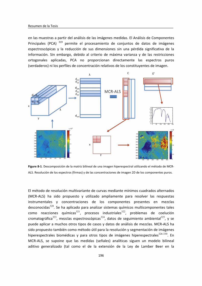
Resumen�de�la�Tesis�
196��
en�las�muestras�a�partir�del�análisis�de�las�imágenes�medidas.�El�Análisis�de�Componentes�Principales� (PCA)� 319� permite� el� procesamiento� de� conjuntos� de� datos� de� imágenes�espectroscópicas� y� la� reducción� de� sus� dimensiones� sin� una� pérdida� significativa� de� la�información.� Sin� embargo,� debido� al� criterio� de� máxima� varianza� y� de� las� restricciones�ortogonales� aplicadas,� PCA� no� proporcionan� directamente� las� espectros� puros�(verdaderos)�ni�los�perfiles�de�concentración�relativos�de�los�constituyentes�de�imagen.�
�
Figure�8�1.�Descomposición�de�la�matriz�bilineal�de�una�imagen�hiperespectral�utilizando�el�método�de�MCR�
ALS.�Resolución�de�los�espectros�(firmas)�y�de�las�concentraciones�de�imagen�2D�de�los�componentes�puros.�
�
El�método�de�resolución�multivariante�de�curvas�mediante�mínimos�cuadrados�alternados�(MCR�ALS)� ha� sido� propuesto� y� utilizado� ampliamente� para� resolver� las� respuestas�instrumentales� y� concentraciones� de� los� componentes� presentes� en� mezclas�desconocidas320.�Se�ha�aplicado�para�analizar�sistemas�químicos�multicomponentes�tales�como� reacciones� químicas321,� procesos� industriales322,� problemas� de� coelución�cromatográfica323,� mezclas� espectroscópicas324,� datos� de� seguimiento� ambiental325,� y� se�puede�aplicar�a�muchos�otros�tipos�de�casos�y�datos�de�análisis�de�mezclas.�MCR�ALS�ha�sido�propuesto�también�como�método�útil�para�la�resolución�y�segmentación�de�imágenes�hiperespectrales� biomédicas� y� para� otros� tipos� de� imágenes� hiperespectrales326-330.� En�MCR�ALS,� se� supoine� que� las� medidas� (señales)� analíticas� siguen� un� modelo� bilineal��aditivo� generalizado� (tal� como� el� de� la� extensión� de� la� Ley� de� Lamber� Beer� en� la�
Resumen�de�la�Tesis�
197��
espectroscopia� de� absorción331 para análisis multicomponente a múltiples longitudes de ona).�La�contribución�de�cada�componente�a�la�señal�medida�depende�de�su�concentración�y�de�su�propia�sensibilidad�espectral�(espectro�puro).�MCR�ALS�también�se�puede�aplicar�para� obtener� información� cuantitativa� y� proporciona� soluciones� con� significado� físico� y�químico�(Figura�8�1).�Esto�se�consigue�logra�porque�en�MCR�ALS,�las�restricciones�que�se�aplican� se� cumplen� de� forma� natural� en� las� soluciones� que� se� buscan,� como� son� por�ejemplo� la� no� negatividad229, 332,� la� unimodalidad333, 334,� el� rango� local335, 336,� y� la�trilinealidad244, 333.�
Sin� embargo,� aunque� las� soluciones� MCR� tienen� un� significado� más� físico� y� una�interpretación�más�fácil�que�los�obtenidos�por�PCA,�no�son�soluciones�únicas�en�general,�y�tienen�un�cierto�grado�de�ambigüedad.�La�ambigüedad�más�crítica�y�difícil�de�evitar�es�la�ambigüedad�de�rotación�o�rotacional.�En�este�caso,�un�conjunto�de�soluciones�diferentes�(y�combinaciones�lineales�de�las�mismas),�se�ajusta�a�los�datos�experimentales�igualmente�bien.� Por� lo� tanto� estas� soluciones� serán� equivalentes� desde� un� punto� de� vista�matemático�aunque�serán�completamente�diferentes�desde�un�punto�de�vista�físico.�Una�manera� para� reducir� este� tipo� de� ambigüedad� es� por� medio� de� la� aplicación� de� más�restricciones�a�las�soluciones,�pero�esto�debe�realizarse�manteniendo�la�plausibilidad�física�de�las�soluciones.��
Además� de� las� restricciones� naturales,� las� estrategias� más� poderosas� para� evitar� la�presencia� de� las� ambigüedades� rotacionales� en� los� métodos� de� MCR� son� el� uso� de� la�información�del�rango�local�y�de�la�selectivad,�la�extensión�MCR�para�el�análisis�simultáneo�de�múltiples�conjuntos�de�datos�y�de�datos�multidireccionales,�el�uso�de�modelos�basados�en�principios�físico�químicos�(determinista).�Usando�apropiadamente�estas�estrategias,�se�consigue� la�obtención�de�soluciones�únicas�como�se�ha�demostrado�en�diversos�trabajos�anteriores.�
Entre� todas� estas� posibilidades,� el� uso� de� la� restricción� de� tri�linealidad� en� el� análisis�simultáneo� de� múltiples� conjuntos� de� datos� es� la� mejor� opción� para� el� análisis� de�conjuntos� de� datos� que� cumplen� con� este� tipo� de� modelo.� Se� estudia� también� a�continuación�la�obtención�de�las�mismas�soluciones�a�partir�del�método�PARAFAC.�
Cuando�se�reconoce�que�las�soluciones�MCR�pueden�tener�un�cierto�grado�de�ambigüedad,�la�pregunta�es�cómo�se�puede�evaluar�este�grado�de�ambigüedad.�Diferentes�métodos�han�sido�propuestos�en� la� literatura�para�su�evaluación,� incluyendo�el�desarrollo�de�métodos�para�el�cálculo�de�los�límites�de�las�denominadas�bandas�posibles�o�factibles�y�de�sus�areas�de�existencia�(area�of�feasible�solutions,�AFS).�

Resumen�de�la�Tesis�
198��
Con� el� fin� de� evaluar� la� presencia� de� las� ambigüedades� de� rotación� asociados� a� una�solución�MCR�particular�y�para�medir�sus�efectos,�se�han�propuesto�diferentes�métodos�en�los�papeles249,�257�259.�
� �
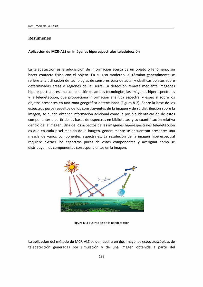
Resumen�de�la�Tesis�
199��
Resúmenes��
Aplicación�de�MCR�ALS�en�imágenes�hiperespectrales�teledetección�
�
La� teledetección� es� la� adquisición� de� información� acerca� de� un� objeto� o� fenómeno,� sin�hacer� contacto� físico� con� el� objeto.� En� su� uso� moderno,� el� término� generalmente� se�refiere�a�la�utilización�de�tecnologías�de�sensores�para�detectar�y�clasificar�objetos�sobre�determinadas� áreas� o� regiones� de� la� Tierra.� La� detección� remota� mediante� imágenes�hiperespectrales�es�una�combinación�de�ambas�tecnologías,�las�imágenes�hiperespectrales�y� la� teledetección,� que� proporciona� información� analítica� espectral� y� espacial� sobre� los�objetos�presentes�en�una�zona�geográfica�determinada�(Figura�8�2).�Sobre�la�base�de�los�espectros�puros�resueltos�de�los�constituyentes�de�la�imagen�y�de�su�distribución�sobre�la�imagen,� se�puede� obtener� información� adicional� como� la� posible� identificación� de� estos�componentes�a�partir�de�las�bases�de�espectros�en�bibliotecas,�y�su�cuantificación�relativa�dentro�de�la�imagen.�Una�de�los�aspectos�de�las�imágenes�hiperespectrales�teledetección�es� que� en� cada� píxel� medido� de� la� imagen,� generalmente� se� encuentran� presentes� una�mezcla� de� varios� componentes� espectrales.� La� resolución� de� la� imagen� hiperespectral�requiere� extraer� los� espectros� puros� de� estos� componentes� y� averiguar� cómo� se�distribuyen�los�componentes�correspondientes�en�la�imagen.�
�
Figure�8��2�Ilustración�de�la�teledetección�
�
La�aplicación�del�método�de�MCR�ALS�se�demuestra�en�dos�imágenes�espectroscópicas�de�teledetección� generadas� por� simulación� y� de� una� imagen� obtenida� a� partir� del�
Resumen�de�la�Tesis�
200��
espectrómetro�de�teledetección�de�imágenes�hiperespectrales�en�el�infrarrojo�AVIRIS�de�la�NASA.� Por� aplicación� de� MCR�ALS,� se� estiman� los� espectros� puros� de� los� componentes��presentes� en� la� imagen� y� su� distribución� a� nivel� de� píxel� de� la� imagen.� Los� resultados�obtenidos�por�MCR�ALS�se�comparan�con�los�obtenidos�por�otros�métodos�utilizados�con�frecuencia� en� el� estudio� de� imágenes� obtenidas� por� espectroscopia� infrarroja� de�teledetección�como�son�VCA�y�MVSA.�
En� el� caso� del� análisis� de� los� datos� experimentales,� los� espectros� puros� resueltos� se�compararon�con�espectros�de�referencia�de�la�biblioteca�del�USGS�para�su�identificación.�En� todos� los� casos,� también� se� evaluaron� los� resultados� sobre� la� posible� presencia� de�ambigüedades�rotacionales�utilizando�el�método�de�MCR�BANDS.�
Los�resultados�obtenidos�confirmaron�que�el�método�de�MCR�ALS�puede�ser�utilizado�con�éxito� para� fines� de� resolución� de� imagenes� hiperespectrales� de� teledetección.� Sin�embargo,� la� presencia� de� ambigüedad� rotacional� en� las� soluciones� obtenidas� por� los�diferentes�métodos�de�resolución�(como�VCA�o�MVSA)�puede�ser�en�algunos�casos�grande�y�debe�ser�evaluados�con�cuidado,�tratando�de�reducir�sus�efectos�mediante�la�selección�de�las�restricciones�más�apropiadas.�Sólo�de�esta�manera�es�posible�aumentar�la�fiabilidad�de�las�soluciones�aportadas�por�estos�métodos�y�disminuir�las�incertidumbres�asociadas�a�su�uso.�
�
Los�dos�artículos�publicados�en�el�presente�capítulo�son:�
Zhang,�X.;�Tauler,�R.,�Application�of�multivariate�curve�resolution�alternating�least�squares�(MCR�ALS)� to� remote� sensing� hyperspectral� imaging.� Analytica� chimica� acta.� 2013,� 762,�25�38.�
Zhang,� X.;� Juan,� A.;� Tauler,� R.,� Local� rank�based� spatial� information� for� improvement� of�remote�sensing�hyperspectral�imaging�resolution.�Submitted�to�Talanta.�
�
� �
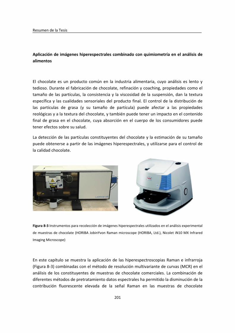
Resumen�de�la�Tesis�
201��
�
Aplicación�de�imágenes�hiperespectrales�combinado�con�quimiometría�en�el�análisis�de�alimentos�
�
El� chocolate� es� un� producto� común� en� la� industria� alimentaria,� cuyo� análisis� es� lento� y�tedioso.�Durante�el�fabricación�de�chocolate,�refinación�y�coaching,�propiedades�como�el�tamaño�de� las�partículas,� la�consistencia�y� la�viscosidad�de� la�suspensión,�dan� la� textura�específica�y� las�cualidades�sensoriales�del�producto� final.�El�control�de� la�distribución�de�las� partículas� de� grasa� (y� su� tamaño� de� partícula)� puede� afectar� a� las� propiedades�reológicas�y�a�la�textura�del�chocolate,�y�también�puede�tener�un�impacto�en�el�contenido�final� de� grasa� en� el� chocolate,� cuya� absorción� en� el� cuerpo� de� los� consumidores� puede�tener�efectos�sobre�su�salud.�
La�detección�de�las�partículas�constituyentes�del�chocolate�y�la�estimación�de�su�tamaño�puede�obtenerse�a�partir�de�las�imágenes�hiperespectrales,�y�utilizarse�para�el�control�de�la�calidad�chocolate.�
�
Figura�8�3�Instrumentos�para�recolección�de�imágenes�hiperespectrales�utilizados�en�el�análisis�experimental�
de�muestras�de�chocolate�(HORIBA�JobinYvon�Raman�microscope�(HORIBA,�Ltd.),�Nicolet� iN10�MX�Infrared�
Imaging�Microscope)�
�
En�este�capítulo�se�muestra� la�aplicación�de� las�hiperespectroscopias�Raman�e� infrarroja�(Figura�8�3)�combinadas�con�el�método�de�resolución�multivariante�de�curvas�(MCR)�en�el�análisis�de� los�constituyentes�de�muestras�de�chocolate�comerciales.� La� combinación�de�diferentes�métodos�de�pretratamiento�datos�espectrales�ha�permitido�la�disminución�de�la�contribución� fluorescente� elevada� de� la� señal� Raman� en� las� muestras� de� chocolate�
Resumen�de�la�Tesis�
202��
investigados.�A�partir�del�uso�de�las�restricciones�de�igualdad�(tales�como�de�rango�local�y�de� selectividad)� durante� el� análisis� de� MCR,� se� mejoraron� apreciablemente� las�estimaciones�de�los�espectros�puros�de�los�constituyentes�de�la�muestra�de�chocolate,�así�como� sus� contribuciones� relativas� y� su� distribución� espacial� en� las� muestras� analizadas.�Además,� componentes� desconocidos� de� la� muestra� podían� ser� también� resueltos.� La�distribución� de� los� constituyentes� del� chocolate� blanco� resueltos� a� partir� de� imágenes�hiperespectrales�Raman�indican�que�a�escala�macro,�la�sacarosa,�la�lactosa,�la�grasa�y��son�constituyentes�que�fueron�mezclados�en�forma�de�partículas.�
Las�omágenes�hiperespectrales� infrarrojas�no�sufren�de�fluorescencia�y�se�podian�utilizar�para� el� análisis� de� muestras� de� chocolate� blanco� y� de� chocolate� con� leche.� Como�conclusión�de�este�estudio,�las�imágenes�micro�hiperespectrales�analizadas�con�el�método�de� MCR� se� confirman� como� una� herramienta� adecuada� para� el� análisis� directo� de� los�constituyentes�de�muestras�de�chocolate�y,�por�extensión,�se�propone�el�análisis�de�otros�componentes�de�mezclas�de�alimenatos�en�productos�comerciales.��
�
El�artículo�publicado�en�el�presente�capítulo�es:�
Zhang,� X.;� Juan,� A.;� Tauler,� R.,� Multivariate� Curve� Resolution� applied� to� hyperspectral�imaging�analysis�of�chocolate�samples.�Applied�Spectroscopy.�2015,�69(8).��
� �

Resumen�de�la�Tesis�
203��
�
Medir�y�comparar�el�rendimiento�de�resolución�y�la�extensión�de�las�ambigüedades�de�rotación�en�los�métodos�de�modelado�bilineales��
�
Los�métodos�basados�en� modelos�bilineales� se�utilizan� frecuentemente� en�el�análisis�de�conjuntos� de� datos� de� espectroscopia� y� de� cromatografía.� Cuando� se� aplican� estos�métodos� de� modelización� bilineales,� las� ambigüedades� rotacionales� se� encuentran�presentes� y� deben� ser� consideradas.� En� este� trabajo,� se� examinan� los� resultados�obtenidos�por�la�aplicación�de�diferentes�métodos,�tales�como�el�análisis�de�componentes�independientes� (Independent� Component� Analysis,� ICA),� el� análisis� de� componentes�principales� (PCA),�y�el�Minimum�Volum�Simplex�Analysis� (MVSA),�y�se�comparan�con� los�obtenidos�por�el�método�de�resolución�multivariante�de�curvas�(MCR).�Con�el�fin�de�hacer�esta�comparación,�se�utilizan�diversos�parámetros�tales�como�el�que�mide�la�información�mutua�(Mutual�Information,�MI)�el�índice�de�Amari�(AI)�y�el�de�falta�de�ajuste�(lack�of�fit,�lof)�para�la�evaluación�de�los�rsultados�obtenidos�por�los�diferentes�métodos.�Las�áreas�o�regiones�de�soluciones�posibles�(AFS)�y�sus�límites�son�evaluados�por�diferentes�métodos�que� investigan�el�problema�ambigüedad�rotacional�a�partir�de�diferentes�conceptos.�Los�resultados�obtenidos�por�el�método�de�MCR�BANDS�en�el�cálculo�de� la�extensión�de� las�ambigüedades�rotacionales�se�analizan�y�se�comparan�con�los�recientemente�propuestos�para�la�estimación�de�toda�la�gama�de�soluciones�posibles�y�para�la�definición�del�área�de�soluciones�posibles�(AFS).�
Los� métodos� basados� en� modelos� de� descomposición� bilineal,� como� por� ejemplo,� MCR�ALS,� MCR�FMIN,� ICA,� PCA,� o� MVSA� (todos� ellos� utilizados� en� este� trabajo)� son� métodos�adecuados� para� la� resolución� multivariante� de� curvas.� Pero� no� todos� ellos� realizan� la�descomposición� de� la� misma� manera.� Cuando� estos� métodos� se� aplican� a� datos� en� dos�direcciones�(two�way)�y�no�existen�condiciones�de�resolución�única�(por�ejemplo�de�rango�local�o��de�selectividad),�no�hay�forma�en�general�de�saber�si�estos�métodos�proporcionan�la� solución� verdadera.� Diferentes� métodos� de� resolución� darán� una� de� las� soluciones�posibles�equivalentes�para�el�problema�en�estudio.�
Los� resultados� obtenidos� a� partir� de� todos� estos� métodos� muestran� que� es� posible�obtener� un� rango� de� soluciones� posibles� que� pueden� describir� y� ajustar� los� datos�igualmente� bien,� sin� dejar� de� cumplir� el� modelo� bilineal� y� las� restricciones� del� sistema�estudiado.�No�es�posible�por�lo�tanto�decir�que�un�método�es�mejor�que�otro�a�partir�de�los�resultados�obtenidos�por�los�diferentes�métodos.�Todos�ellos�pueden�ser�considerados�como� una� herramienta� alternativa� para� la� resolución� de� las� señales� espectroscópicas�
Resumen�de�la�Tesis�
204��
(espectros�puros)�en�ciertos�casos.�Sin�embargo,�la�aplicación�de�restricciones�físicas�como�son�la�no�negatividad�en�los�perfiles�espectrales�y�de�concentración�es�más�flexible�y�fiable�en�métodos�de�MCR�como�el�MCR�ALS.�
El�método�MCR�BANDS�ofrece�una�primera�aproximación�al�cálculo�de�la�región�o�área�de�todas� las� soluciones� MCR� posibles,� AFS.� La� representación� geométrica� de� todas� las�soluciones�posibles�puede�realizarse�a�partir�de�métodos�como�FAC�PACK�ara�un�número�limitado�de�componentes.�Es�interesante�remarcar�que�la�extensión�de�las�ambigüedades�rotacionales� calculada� por� el� método� MCR�BANDS� y� las� regiones� AFS� calculados� por� un�método�como�FAC�PACK�son�concordantes.�
�
El�artículo�en�el�presente�capítulo�es:�
X.�Zhang,�R.�Tauler.�Measuring�and�comparing�the�resolution�performance�and�the�extend�of� rotation� ambiguities� in� bilinear� modelling� methods.� Submitted� to� Journal� of�Chemometrics.�
� �
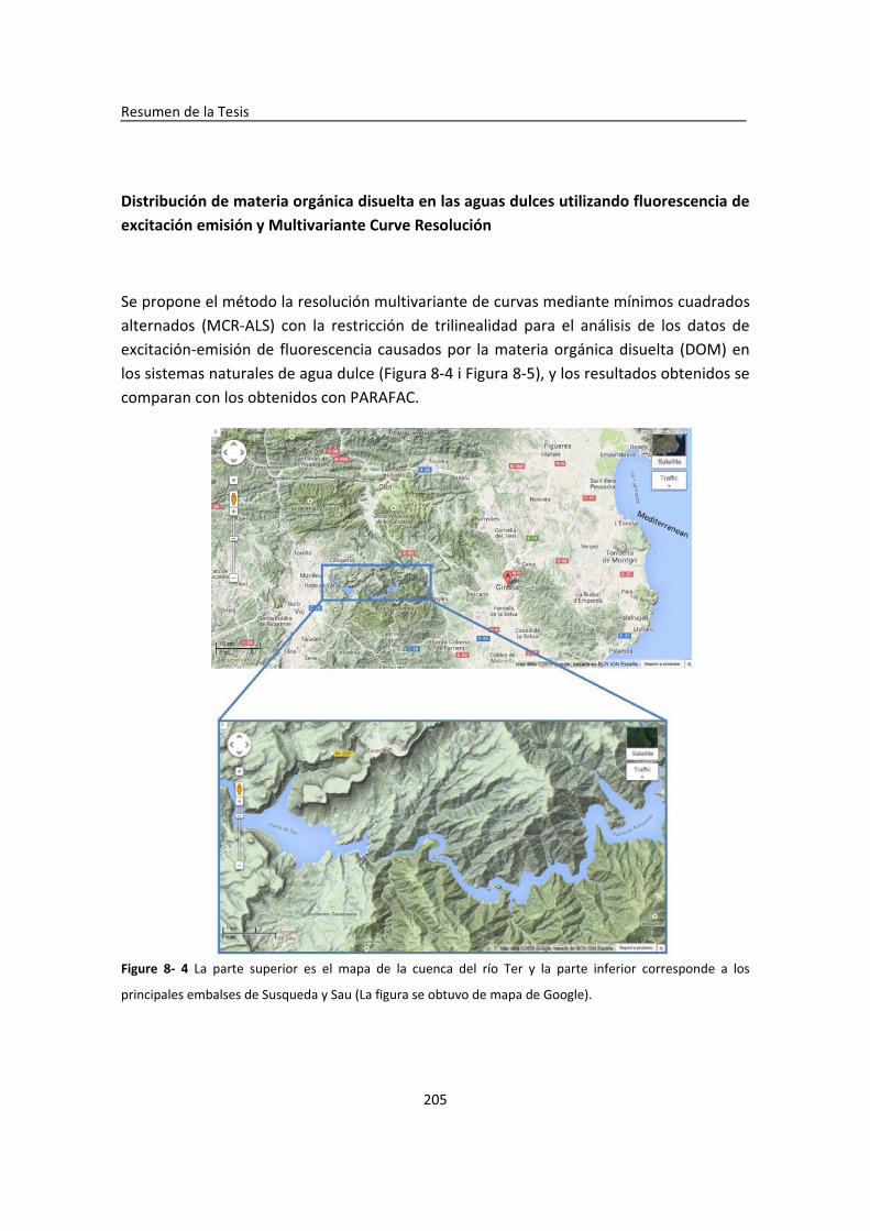
Resumen�de�la�Tesis�
205��
�
Distribución�de�materia�orgánica�disuelta�en�las�aguas�dulces�utilizando�fluorescencia�de�excitación�emisión�y�Multivariante�Curve�Resolución�
�
Se�propone�el�método�la�resolución�multivariante�de�curvas�mediante�mínimos�cuadrados�alternados� (MCR�ALS)� con� la� restricción� de� trilinealidad� para� el� análisis� de� los� datos� de�excitación�emisión�de� fluorescencia�causados�por� la�materia�orgánica�disuelta� (DOM)�en�los�sistemas�naturales�de�agua�dulce�(Figura�8�4�i�Figura�8�5),�y�los�resultados�obtenidos�se�comparan�con�los�obtenidos�con�PARAFAC.�
Figure� 8�� 4� La� parte� superior� es� el� mapa� de� la� cuenca� del� río� Ter� y� la� parte� inferior� corresponde� a� los�
principales�embalses�de�Susqueda�y�Sau�(La�figura�se�obtuvo�de�mapa�de�Google).�
�

Resumen�de�la�Tesis�
206��
Los�efectos�del�diferente�número�de�componentes�y� las� limitaciones�sobre� la�estabilidad�de� los� modelos� propuestos� se� comparan.� Se� demuestra� que� MCR�ALS� es� una� manera�eficaz�para�caracterizar�y�resolver�las�fuentes�de�DOM�en�los�sistemas�naturales�de�agua�dulce�a�partir�de�datos�de�EEM,�con�buena�correlación�con�los�valores�de�concentración�de�DOM�medidos�experimentalmente.�
�
Figure�8��5�La�ubicación�de�la�cuenca�del�río�Ter�en�Catalunya,�España.�
�
La� utilidad� de� mapas� (mapping)� georeferenciados� de� MATLAB� se� utiliza� para� ilustrar� la�distribución�geográfica�de�las�contribuciones�DOM�resueltos.�Los�espectros�resueltos�por�MCR�ALS� se� utilizan� para� reconocer� los� grupos� químicos� correspondientes� a� las� posibles�fuentes�de�DOM.�Las�relaciones�entre�las�actividades�humanas�y�la�situación�ambiental�del�sistema�fluvial�se�discuten�a�partir�de�estas�posibles�fuentes�de�DOM.�
�
El�artículo�publicado�en�el�presente�capítulo�es:�
ZHANG,�Xin.,�Marcé,�R.,�Armengol,�J.,�&�Tauler,�R.�Distribution�of�dissolved�organic�matter�in�freshwaters�using�excitation�emission�fluorescence�and�Multivariate�Curve�Resolution.�Chemosphere,�2014,�111,�120�128�� �
Resumen�de�la�Tesis�
207��
Conclusiones��
Conclusiones�de�la�aplicación�de�métodos�quimiométricas�
�
1)�Los�resultados�obtenidos�en�esta�Tesis�muestran�que�el�método�de�MCR�ALS�puede�ser�utilizado�con�éxito�para� fines�de�resolución�de� imagenes�hiperespectrales.�Los�espectros�puros�de�los�constituyentes�presentes�en��las�imágenes�hiperespectrales�y�la�distribución�de�sus�concentraciones�a�nivel�de�píxel�pueden�estimarse.�
�
2)� La� aplicación� de� los� métodos� de� pretratamiento� de� datos� de� imagenes� como� por�ejemplo� el� método� Multiplicative� Scater� Correction� (MSC),� el� método� Assymetric� Least�Squares�(AsLS)�y�el�método�de�suavización�Savitzky�Golay�(SG),�reduce�significativamente�la�presencia�de�algunos�inconvenientes�como�son�la�fuerte�fluorescencia�de�fondo�en�las�imágenes� hiperespectrales� Raman.� En� contraste,� las� imágenes� hiperespectrales� de�infrarrojos� no� se� ven� afectadas� por� la� fluorescencia.� El� método� de� transformación� de�Kramers�Kronig�permite�calcular�los�espectros�de�absorción�en�caso�de�que�solamente�se�puedan�medir�los�espectros�de�reflectancia�infrarroja.�
�
3)� El� grado� de� ambigüedad� rotacional� asociada� al� procedimiento� MCR�ALS� y� a� otros�métodos�de�resolución�(como�VCA�(Vertex�Component�Analysis)�o�MVSA�(Minimal�Volum�Simplex�Analysis)�puede�ser�bastante�alta�cuando�se�aplican�a� la�resolución�de�imagenes�hiperespectrales� que� tienen� un� elevado� grado� de� ruido� experimental.� La� resolución�correcta� de� las� imágenes� hiperespectrales� sólo� puede� garantizarse� si� se� aplican�restricciones� adicionales,� tales� como� las� que� proporcionan� información� sobre� el� rango�local� de� las� imágenes,� es� decir� sobre� la� presencia� o� ausencia� de� los� diferentes�constituyentes�(componentes)�en�los�píxeles�de�la�imagen.�Sólo�de�esta�manera�es�posible�aumentar�la�fiabilidad�de�las�soluciones�proporcionadas�por�los�métodos�MCR�y�disminuir�las�incertidumbres�asociadas�a�ellos.�El�uso�apropiado�del�rango�local�y�de��la�información��de�selectividad�puede�mejorar�significativamente�la�calidad�de�los�espectros�puros�(firmas)�y�de�los�mapas�de�distribución�de�los�constituyentes�resueltos�por�el�análisis�MCR�ALS�de�imágenes�hiperespectrales�en�los�estudios�de�teledetección.�
�
Resumen�de�la�Tesis�
208��
4)�Se� muestra� por� primera� vez�el� uso� de� los� coeficientes� de� correlación� entre�espectros�seleccionados� y� los� espectros� de� píxeles� de� las� imágenes� para� proporcionar� una� forma�alternativa� para� la� aplicación� de� la� restricción� de� selectividad� en� imágenes�hiperespectrales.�Este�método�alternativo�resultó�ser�satisfactorio�cuando�existen�píxeles�puros.�
�
5)�El�método�Area�of�Feasible�Solutions�(AFS)�representa�geométricamente�el�conjunto�de��soluciones�posibles.�La�extensión�de�la�ambigüedad�rotacional�calculada�por�MCR�BANDS�y�por�AFS�están�de�acuerdo.�
�
6)� MCR�ALS� con� la� restricción� de� trilinealidad� es� una� manera� eficaz� para� caracterizar� y�resolver� los� componentes� fluorescentes� de� mezclas� a� partir� de� datos� de� matriz� de�Excitación�Emisión� (EEM).� El� procedimiento� de� Mapping� georeferenciado� utilizando�MATLAB� es� un� método� de� visualización� muy� útil� para� describir� de� forma� concisa� la�distribución�geográfica�de� las�fuentes�de�materia�orgánica�disuelta�(DOM)�a�partir�de�los�resultados�MCR�ALS�aplicados�a�datos�EEM.�
�
Conclusiones� de� análisis� de� muestras� de� alimentos� y� ambiental� utilizando� imágenes�hiperespectrales�y�los�métodos�de�Multivariante�Curve�Resolución�
�
1)� En� el� análisis� de� imágenes� hiperespectrales� obtenidas� a� partir� de� procedimientos� de�teledetección� procedentes� de� la� región� de� Cuprita� en� Nevada,� del� aeropuerto� de� San�Diego�y�del�campo�Moffet�en�California,� los�resultados�MCR�ALS�muestran�claramente�la�presencia� de� varios� objetos� como� aviones,� zonas� de� plantas� verdes,� lagos,� campos� de�tierra� dura� y� otros� objetos� relacionados� con� la� imagen.� El� examen� de� los� resultados�obtenidos� a� partir� del� análisis� MCR�ALS� de� datos� de� teledetección� de� imágenes�hiperespectrales�sobre��mapas�de�distribución�permite�la�toma�de�decisiones.��
�
2)�El�acoplamiento�del�análisis�micro�hiperespectral�de�imágenes�y�del�análisis�MCR�ALS�se�confirma� ser� un� instrumento� adecuado� para� el� análisis� directo� de� los� constituyentes� de�muestras� de� chocolate,� y,� por� extensión,� se� propone� también� para� el� análisis� de� otros�componentes�de�mezclas�en�muestras�de�alimentos�comerciales.�Los�resultados�obtenidos�

Resumen�de�la�Tesis�
209��
en�este�trabajo�son�representativos�de�las�posibilidades�que�ofrece�el�análisis�de�imágenes�hiperespectrales� de� muestras� de� alimentos,� y� ha� confirmado� el� uso� potencial� del�procedimiento�MCR�ALS�como�herramienta�complementaria�para�este�tipo�de�análisis.�La�aplicación�de�esta�combinación�de�métodos�(de�análisis�de�imágenes�hiperespectrales�y�de�análisis� MCR�ALS)� se� puede� proponer� para� el� análisis� de� muestras� en� otros� campos�similares,� incluyendo� el� análisis� de� superficies� de� materiales,� de� productos� de� la�agricultura,�así�como�el�análisis�de�tejidos�biológicos�en�medicina.�
�
3)�Los�espectros�de� fluorescencia� (EEM)�proporciona�una� forma�poderosa�y�conveniente�para� la� investigación� de� las� fuentes� de� materia� orgánica� disuelta� (DOM)� en� las� cuencas�hidrográficas.� Las� fuentes� de� materia� orgánica� disuelta� (DOM)� fluorescente� resueltas� y�asignadas�son�la�fracción�UVC�húmica,�la�fracción�UVA�húmica/fúlvica,�la�fracción�UVT,�y�la�fracción�de�proteínas�y�triptófano.�La�distribución�geográfica�resuelta�de�estas�tres�fuentes�DOM� diferentes� a� lo� largo� del� área� investigada� en� este� trabajo� (cuenca� del� rio� Ter),�muestra� aumentos� y� disminuciones� de� las� contribuciones� relativas� de� DOM� de� fuentes�naturales� de� acuerdo� con� diferentes� factores� tales� como� el� flujo� del� río,� las� actividades�humanas�en�la�zona�y�su�población.��
� �

Resumen�de�la�Tesis�
210��
�
�

References�
211��
References �
1.� G.� ElMasry,� D.�W.� Sun.� "Principles� of� hyperspectral� imaging� technology".� Hyperspectral�imaging�for�food�quality�analysis�and�control�2010.�3�43.�2.� A.� Gowen,� C.� O'Donnell,� P.� Cullen,� G.� Downey,� J.� Frias.� "Hyperspectral� imaging–an�emerging� process� analytical� tool� for� food� quality� and� safety� control".� Trends� Food� Sci.� Technol.�2007.�18(12):�590�598.�3.� D.�W.�Sun.�"Hyperspectral�imaging�for�food�quality�analysis�and�control".�Elsevier:�2010.�4.� A.�O'SULLIVAN,�B.�O'CONNOR,�A.�Kelly,�M.J.�McGRATH.�"The�use�of�chemical�and�infrared�methods�for�analysis�of�milk�and�dairy�products".�Int.�J.�Dairy�Technol.�1999.�52(4):�139�148.�5.� N.B.�Colthup,�L.H.�Daly,�S.E.�Wiberley.�"Introduction�to�infrared�and�Raman�spectroscopy".�Elsevier:�1990.�6.� A.F.H.� Goetz.� "Three� decades� of� hyperspectral� remote� sensing� of� the� Earth:� A� personal�view".�Remote�Sens.�Environ.�2009.�113,�Supplement�1(0):�S5�S16.�7.� H.J.� Kramer.� "Observation� of� the� Earth� and� its� Environment:� Survey� of� Missions� and�Sensors".�Springer�Science�&�Business�Media:�2002.�8.� A.F.� Goetz,� B.N.� Rock,� L.C.� Rowan.� "Remote� sensing� for� exploration;� an� overview".�Economic�Geology�1983.�78(4):�573�590.�9.� R.O.�Green,�M.L.�Eastwood,�C.M.�Sarture,�T.G.�Chrien,�M.�Aronsson,�B.J.�Chippendale,�J.A.�Faust,� B.E.� Pavri,� C.J.� Chovit,� M.� Solis.� "Imaging� spectroscopy� and� the� airborne� visible/infrared�imaging�spectrometer�(AVIRIS)".�Remote�Sens.�Environ.�1998.�65(3):�227�248.�10.� A.A.�Gowen,�C.P.�O'Donnell,�P.J.�Cullen,�G.�Downey,�J.M.�Frias.�"Hyperspectral�imaging�–�an�emerging�process�analytical�tool�for�food�quality�and�safety�control".�Trends�in�Food�Science�&�Technology�2007.�18(12):�590�598.�11.� R.A.� Schultz,� T.� Nielsen,� J.R.� Zavaleta,� R.� Ruch,� R.� Wyatt,� H.R.� Garner.� "Hyperspectral�imaging:�A�novel�approach�for�microscopic�analysis".�Cytometry�2001.�43(4):�239�247.�12.� A.F.H.�Goetz,�B.�Curtiss.�"Hyperspectral�imaging�of�the�earth:�remote�analytical�chemistry�in�an�uncontrolled�environment".�Field�Analytical�Chemistry�&�Technology�1996.�1(2):�67�76.�13.� F.D.�van�der�Meer,�H.M.A.�van�der�Werff,�F.J.A.�van�Ruitenbeek,�C.A.�Hecker,�W.H.�Bakker,�M.F.� Noomen,� M.� van� der� Meijde,� E.J.M.� Carranza,� J.B.d.� Smeth,� T.� Woldai.� "Multi�� and�hyperspectral� geologic� remote� sensing:� A� review".� International� Journal� of� Applied� Earth�Observation�and�Geoinformation�2012.�14(1):�112�128.�14.� A.�Buades,�B.�Coll,�J.�M.�Morel.�"A�review�of�image�denoising�algorithms,�with�a�new�one".�Multiscale�Modeling�&�Simulation�2005.�4(2):�490�530.�15.� G.�Lu,�B.�Fei.�"Medical�hyperspectral�imaging:�a�review".�Journal�of�Biomedical�Optics�2014.�19(1):�010901�010901.�16.� Y.� Garini,� I.T.� Young,� G.� McNamara.� "Spectral� imaging:� Principles� and� applications".�Cytometry�Part�A�2006.�69A(8):�735�747.�17.� M.E.�Hankus,�H.�Li,�G.J.�Gibson,�B.M.�Cullum.�"Surface�enhanced�Raman�scattering�based�nanoprobe�for�high�resolution,�non�scanning�chemical�imaging".�Anal.�Chem.�2006.�78(21):�7535�7546.�
References�
212��
18.� M.R.� Descour,� C.E.� Volin,� E.L.� Dereniak,� K.J.� Thome,� A.� Schumacher,� D.W.� Wilson,� P.D.�Maker.� "Demonstration� of� a� high�speed� nonscanning� imaging� spectrometer".� Opt.� Lett.� 1997.�22(16):�1271�1273.�19.� M.D.� Schaeberle,� H.R.� Morris,� J.F.T.� Ii,� P.J.� Treado.� "Peer� Reviewed:� Raman� Chemical�Imaging�Spectroscopy".�Analytical�Chemistry�1999.�71(5):�175A�181A.�20.� E.�Lewis.�"Education�for�sustainability�at�a�primary�school:�From�silos�to�systems�thinking".�Environmental�Education�Research�2014.�20(3):�432�433.�21.� T.�Awad,�H.�Moharram,�O.�Shaltout,�D.�Asker,�M.�Youssef.�"Applications�of�ultrasound� in�analysis,�processing�and�quality�control�of�food:�A�review".�Food�Res.�Int.�2012.�48(2):�410�427.�22.� P.� Mandal,� A.� Biswas,� K.� Choi,� U.� Pal.� "Methods� for� rapid� detection� of� foodborne�pathogens:�an�overview".�American�Journal�Of�Food�Technology�2011.�6(2):�87�102.�23.� T.� Kourti.� "Application� of� latent� variable� methods� to� process� control� and� multivariate�statistical� process� control� in� industry".� International� Journal� of� Adaptive� Control� and� Signal�Processing�2005.�19(4):�213�246.�24.� J.A.�Fernández�Pierna,�P.�Vermeulen,�O.�Amand,�A.�Tossens,�P.�Dardenne,�V.�Baeten.�"NIR�hyperspectral� imaging� spectroscopy� and� chemometrics� for� the� detection� of� undesirable�substances�in�food�and�feed".�Chemometrics�Intellig.�Lab.�Syst.�2012.�117(0):�233�239.�25.� H.� Kataoka,� H.L.� Lord,� J.� Pawliszyn.� "Applications� of� solid�phase� microextraction� in� food�analysis".�J.�Chromatogr.�A�2000.�880(1):�35�62.�26.� J.�Rosén,�K.�E.�Hellenäs.�"Analysis�of�acrylamide�in�cooked�foods�by�liquid�chromatography�tandem�mass�spectrometry".�Analyst�2002.�127(7):�880�882.�27.� J.H.�Clark.�"Green�chemistry:�challenges�and�opportunities".�Green�Chemistry�1999.�1(1):�1�8.�28.� G.M.�Strasburg,�R.D.�Ludescher.�"Theory�and�applications�of�fluorescence�spectroscopy�in�food�research".�Trends�Food�Sci.�Technol.�1995.�6(3):�69�75.�29.� P.�Williams,�K.�Norris.� "Near�infrared�technology� in� the�agricultural�and� food� industries".�American�Association�of�Cereal�Chemists,�Inc.:�1987.�30.� Y.�W.� Wu,� S.�Q.� Sun,� Q.� Zhou,� H.�W.� Leung.� "Fourier� transform� mid�infrared� (MIR)� and�near�infrared� (NIR)� spectroscopy� for� rapid� quality� assessment� of� Chinese� medicine� preparation�Honghua�Oil".�J.�Pharm.�Biomed.�Anal.�2008.�46(3):�498�504.�31.� R.� Kizil,� J.� Irudayaraj,� D.� Sun.� "Spectroscopic� technique:� Fourier� transform� Raman� (FT�Raman)�spectroscopy".�Modern�techniques�for�food�authentification�2008.�185�203.�32.� M.�Blanco,�I.�Villarroya.�"NIR�spectroscopy:�a�rapid�response�analytical�tool".�TrAC,�Trends�Anal.�Chem.�2002.�21(4):�240�250.�33.� B.G.�Osborne.� "Near infrared�spectroscopy� in� food�analysis".�Encyclopedia�of�analytical�Chemistry�2000.�34.� J.F.� Pierna,� P.� Vermeulen,� O.� Amand,� A.� Tossens,� P.� Dardenne,� V.� Baeten.� "NIR�hyperspectral� imaging� spectroscopy� and� chemometrics� for� the� detection� of� undesirable�substances�in�food�and�feed".�Chemometrics�Intellig.�Lab.�Syst.�2012.�117:�233�239.�35.� M.�Delhaye,�P.�Dhamelincourt.�"Raman�microprobe�and�microscope�with�laser�excitation".�Journal�of�Raman�Spectroscopy�1975.�3(1):�33�43.�36.� I.W.�Levin,�R.�Bhargava.�"FOURIER�TRANSFORM�INFRARED�VIBRATIONAL�SPECTROSCOPIC�IMAGING:�Integrating�Microscopy�and�Molecular�Recognition*".�Annu.�Rev.�Phys.�Chem.�2005.�56:�429�474.�37.� L.�Opilik,�T.�Schmid,�R.�Zenobi.�"Modern�Raman�imaging:�vibrational�spectroscopy�on�the�micrometer�and�nanometer�scales".�Analytical�Chemistry�2013.�6.�

References�
213��
38.� Y.�Jung,�J.�Tam,�H.R.�Jalian,�R.R.�Anderson,�C.L.�Evans.�"Longitudinal,�3D�In�Vivo�Imaging�of�Sebaceous� Glands� by� Coherent� Anti�Stokes� Raman� Scattering� Microscopy:� Normal� Function� and�Response�to�Cryotherapy".�Journal�of�Investigative�Dermatology�2014.�39.� N.L.�Garrett,�L.�Godfrey,�A.�Lalatsa,�D.R.�Serrano,�I.F.�Uchegbu,�A.�Schatzlein,�J.�Moger.� In�"Detecting� polymeric� nanoparticles� with� coherent� anti�stokes� Raman� scattering� microscopy� in�tissues�exhibiting�fixative�induced�autofluorescence",�2015;�2015;�Pp�932922�932922�8.�40.� C.W.�Freudiger,�W.�Min,�B.G.�Saar,�S.�Lu,�G.R.�Holtom,�C.�He,�J.C.�Tsai,�J.X.�Kang,�X.S.�Xie.�"Label�free�biomedical�imaging�with�high�sensitivity�by�stimulated�Raman�scattering�microscopy".�Science�2008.�322(5909):�1857�1861.�41.� M.N.� Slipchenko,� T.T.� Le,� H.� Chen,� J.�X.� Cheng.� "High�speed� vibrational� imaging� and�spectral� analysis� of� lipid� bodies� by� compound� Raman� microscopy".� The� Journal� of� Physical�Chemistry�B�2009.�113(21):�7681�7686.�42.� D.�Fu,�G.�Holtom,�C.�Freudiger,�X.�Zhang,�X.S.�Xie.�"Hyperspectral�imaging�with�stimulated�Raman� scattering� by� chirped� femtosecond� lasers".� The� Journal� of� Physical� Chemistry� B� 2013.�117(16):�4634�4640.�43.� H.� Yuan,� A.M.� Fales,� C.G.� Khoury,� J.� Liu,� T.� Vo Dinh.� "Spectral� characterization� and�intracellular�detection�of�Surface Enhanced�Raman�Scattering� (SERS) encoded�plasmonic�gold�nanostars".�Journal�of�Raman�Spectroscopy�2013.�44(2):�234�239.�44.� S.� Lee,� H.� Chon,� J.� Lee,� J.� Ko,� B.H.� Chung,� D.W.� Lim,� J.� Choo.� "Rapid� and� sensitive�phenotypic� marker� detection� on� breast� cancer� cells� using� surface�enhanced� Raman� scattering�(SERS)�imaging".�Biosens.�Bioelectron.�2014.�51:�238�243.�45.� M.�Vendrell,� K.K.� Maiti,�K.�Dhaliwal,� Y.�T.�Chang.� "Surface�enhanced�Raman�scattering� in�cancer�detection�and�imaging".�Trends�Biotechnol.�2013.�31(4):�249�257.�46.� H.� Kneipp,� N.� Møbjerg,� A.� Jørgensen,� H.G.� Bohr,� C.� H lix Nielsen,� J.� Kneipp,� K.� Kneipp.�"Surface�enhanced�Raman�scattering�on�Tardigrada towards�monitoring�and� imaging�molecular�structures�in�live�cryptobiotic�organisms".�journal�of�biophotonics�2013.�6(10):�759�764.�47.� C.H.�Moran,�M.�Rycenga,�X.�Xia,�C.M.�Cobley,�Y.�Xia.�"Using�well�defined�Ag�nanocubes�as�substrates� to� quantify� the� spatial� resolution� and� penetration� depth� of� surface�enhanced� Raman�scattering�imaging".�Nanotechnology�2014.�25(1):�014007.�48.� E.L.� Izake,� B.� Cletus,� W.� Olds,� S.� Sundarajoo,� P.M.� Fredericks,� E.� Jaatinen.� "Deep� Raman�spectroscopy� for� the� non�invasive� standoff� detection� of� concealed� chemical� threat� agents".�Talanta�2012.�94(0):�342�347.�49.� B.�Zachhuber,�H.�Östmark,�T.�Carlsson.� In�"Spatially�offset�hyperspectral�stand�off�Raman�imaging� for� explosive� detection� inside� containers",� SPIE� Defense+� Security,� 2014;� International�Society�for�Optics�and�Photonics:�2014;�Pp�90730J�90730J�5.�50.� S.� Wallin,� A.� Pettersson,� H.� Önnerud,� H.� Östmark,� M.� Nordberg,� E.� Ceco,� A.� Ehlerding,� I.�Johansson,� P.� Käck.� In� "Possibilities� for� standoff� Raman� detection� applications� for� explosives",�2012;�2012;�Pp�83580P�83580P�9.�51.� W.J.�Olds,�E.� Jaatinen,�P.�Fredericks,�B.�Cletus,�H.�Panayiotou,�E.L.� Izake.� "Spatially�offset�Raman� spectroscopy� (SORS)� for� the� analysis� and� detection� of� packaged� pharmaceuticals� and�concealed�drugs".�Forensic�Sci.�Int.�2011.�212(1–3):�69�77.�52.� X.� Zhang,� A.d.� Juan,� R.� Tauler.� "Multivariate� Curve� Resolution� applied� to� hyperspectral�imaging�analysis�of�chocolate�samples".�Appl.�Spectrosc.�2015.�53.� N.� Jamin,� P.� Dumas,� J.� Moncuit,� W.�H.� Fridman,� J.�L.� Teillaud,� G.L.� Carr,� G.P.� Williams.�"Highly�resolved�chemical�imaging�of�living�cells�by�using�synchrotron�infrared�microspectrometry".�Proceedings�of�the�National�Academy�of�Sciences�1998.�95(9):�4837�4840.�
References�
214��
54.� L.�Kidder,� I.� Levin,�E.N.� Lewis,�V.�Kleiman,� E.�Heilweil.� "Mercury� cadmium�telluride� focal�plane�array�detection�for�mid�infrared�Fourier�transform�spectroscopic�imaging".�Opt.�Lett.�1997.�22(10):�742�744.�55.� L.M.� Kehlet,� P.� Tidemand�Lichtenberg,� J.S.� Dam,� C.� Pedersen.� "Infrared� upconversion�hyperspectral�imaging".�Opt.�Lett.�2015.�40(6):�938�941.�56.� K.�Yeh,�S.�Kenkel,�J.�N.�Liu,�R.�Bhargava.�"Fast�Infrared�Chemical�Imaging�with�a�Quantum�Cascade�Laser".�Anal.�Chem.�2015.�87(1):�485�493.�57.� M.� Manley.� "Near�infrared� spectroscopy� and� hyperspectral� imaging:� non�destructive�analysis�of�biological�materials".�Chem.�Soc.�Rev.�2014.�43(24):�8200�8214.�58.� P.R.� Griffiths.� "Infrared� and� Raman� instrumentation� for� mapping� and� imaging".� Infrared�and�Raman�spectroscopic�imaging�2009.�3�64.�59.� G.�Tøgersen,�T.�Isaksson,�B.�Nilsen,�E.�Bakker,�K.�Hildrum.�"On�line�NIR�analysis�of�fat,�water�and�protein�in�industrial�scale�ground�meat�batches".�Meat�Science�1999.�51(1):�97�102.�60.� P.�Williams.�"Secondary�ion�mass�spectrometry".�Annu.�Rev.�Mater.�Sci.�1985.�15(1):�517�548.�61.� J.� Baker.� "Secondary� Ion� Mass� Spectrometry".� In� Practical� Materials� Characterization,�Sardela,�M.,�Ed.�Springer�New�York:�2014;�Pp�133�187.�62.� J.S.� Fletcher,� J.C.� Vickerman,� N.� Winograd.� "Label� free� biochemical� 2D� and� 3D� imaging�using�secondary�ion�mass�spectrometry".�Curr.�Opin.�Chem.�Biol.�2011.�15(5):�733�740.�63.� M.�Mohri,�K.�Watanabe,�T.�Yamashina.�"Sputtering�process�of�a�silicon�carbide�surface�with�energetic�ions�by�means�of�an�AES�SIMS�FDS�combined�system".�J.�Nucl.�Mater.�1978.�75(1):�7�13.�64.� M.�Holzweber,�A.�Lippitz,�K.�Krueger,�J.�Jankowski,�W.E.�Unger.�"Surface�characterization�of�dialyzer� polymer� membranes� by� imaging� ToF�SIMS� and� quantitative� XPS� line� scans".�Biointerphases�2015.�10(1):�019011.�65.� L.� Carlred,� A.� Gunnarsson,� S.� Solé�Domènech,� B.� Johansson,� V.� Vukojevi�,� L.� Terenius,� A.�Codita,�B.�Winblad,�M.�Schalling,�F.�Höök,�P.�Sjövall.�"Simultaneous�Imaging�of�Amyloid� �and�Lipids�in� Brain� Tissue� Using� Antibody�Coupled� Liposomes� and� Time�of�Flight� Secondary� Ion� Mass�Spectrometry".�J.�Am.�Chem.�Soc.�2014.�136(28):�9973�9981.�66.� C.� Bich,� D.� Touboul,� A.� Brunelle.� "Cluster� TOF�SIMS� imaging� as� a� tool� for� micrometric�histology�of�lipids�in�tissue".�Mass�Spectrom.�Rev.�2014.�33(6):�442�451.�67.� N.� Desbenoit,� I.� Schmitz�Afonso,� C.� Baudouin,� O.� Laprévote,� D.� Touboul,� F.� Brignole�Baudouin,�A.�Brunelle.�"Localisation�and�quantification�of�benzalkonium�chloride�in�eye�tissue�by�TOF�SIMS� imaging� and� liquid� chromatography� mass� spectrometry".� Anal.� Bioanal.� Chem.� 2013.�405(12):�4039�4049.�68.� L.� Piruzyan.� "Feasibility� of� Novel� Atomic�Molecular� Resuscitation� Tools".� Bulletin� of�experimental�biology�and�medicine�2012.�152(5):�646�652.�69.� B.�Bleaney.�"Physics�at�the�University�of�Oxford".�European�Journal�of�Physics�1988.�9(4):�283.�70.� M.� Sathiya,� J.B.� Leriche,� E.� Salager,� D.� Gourier,� J.M.� Tarascon,� H.� Vezin.� "Electron�paramagnetic�resonance�imaging�for�real�time�monitoring�of�Li�ion�batteries".�Nat�Commun�2015.�6.�71.� M.�Abou�Fadel,�X.�Zhang,�A.�de�Juan,�R.�Tauler,�H.�Vezin,�L.�Duponchel.�"Extraction�of�Pure�Spectral� Signatures� and� Corresponding� Chemical� Maps� from� EPR� Imaging� Data� Sets:� Identifying�Defects�on�a�CaF2�Surface�Due�to�a�Laser�Beam�Exposure".�Anal.�Chem.�2015.�87(7):�3929�3935.�72.� H.K.� Noh,� R.� Lu.� "Hyperspectral� laser�induced� fluorescence� imaging� for� assessing� apple�fruit�quality".�Postharvest�Biol.�Technol.�2007.�43(2):�193�201.�

References�
215��
73.� V.� Studer,� J.� Bobin,� M.� Chahid,� H.S.� Mousavi,� E.� Candes,� M.� Dahan.� "Compressive�fluorescence� microscopy� for� biological� and� hyperspectral� imaging".� Proceedings� of� the� National�Academy�of�Sciences�2012.�109(26):�E1679�E1687.�74.� G.� Zavattini,� S.� Vecchi,� G.� Mitchell,� U.� Weisser,� R.M.� Leahy,� B.J.� Pichler,� D.J.� Smith,� S.R.�Cherry.�"A�hyperspectral�fluorescence�system�for�3D�in�vivo�optical�imaging".�Physics�in�medicine�and�biology�2006.�51(8):�2029.�75.� W.F.J.� Vermaas,� J.A.� Timlin,� H.D.T.� Jones,� M.B.� Sinclair,� L.T.� Nieman,� S.W.� Hamad,� D.K.�Melgaard,� D.M.� Haaland.� "In� vivo� hyperspectral� confocal� fluorescence� imaging� to� determine�pigment� localization� and� distribution� in� cyanobacterial� cells".� Proceedings� of� the� National�Academy�of�Sciences�2008.�105(10):�4050�4055.�76.� S.G.�Kong,�Y.�R.�Chen,�I.�Kim,�M.S.�Kim.�"Analysis�of�hyperspectral�fluorescence�images�for�poultry�skin�tumor�inspection".�Appl.�Opt.�2004.�43(4):�824�833.�77.� E.M.� Sevick�Muraca.� "Translation� of� Near�Infrared� Fluorescence� Imaging� Technologies:�Emerging�Clinical�Applications".�Annu.�Rev.�Med.�2012.�63(1):�217�231.�78.� W.R.�Johnson,�D.W.�Wilson,�W.�Fink,�M.�Humayun,�G.�Bearman.�"Snapshot�hyperspectral�imaging�in�ophthalmology".�Journal�of�biomedical�optics�2007.�12(1):�014036�014036�7.�79.� A.� Bodkin,� A.� Sheinis,� A.� Norton,� J.� Daly,� S.� Beaven,� J.� Weinheimer.� In� "Snapshot�hyperspectral�imaging:�the�hyperpixel�array�camera",�2009;�2009;�Pp�73340H�73340H�11.�80.� R.T.� Kester,� N.� Bedard,� L.� Gao,� T.S.� Tkaczyk.� "Real�time� snapshot� hyperspectral� imaging�endoscope".�Journal�of�Biomedical�Optics�2011.�16(5):�056005�056005�12.�81.� Z.� Gao,� L.� Zeng,� Q.� Wu.� In� "AOTF�based� near�infrared� imaging� spectrometer� for� rapid�identification�of�camouflaged�target",�2014;�2014;�Pp�92980R�92980R�8.�82.� Q.� Li,� D.� Xu,� X.� He,� Y.� Wang,� Z.� Chen,� H.� Liu,� Q.� Xu,� F.� Guo.� "AOTF� based� molecular�hyperspectral� imaging� system� and� its� applications� on� nerve� morphometry".� Appl.� Opt.� 2013.�52(17):�3891�3901.�83.� G.�Konda�Naganathan,�K.�Cluff,�A.�Samal,�C.�Calkins,�D.D.�Jones,�C.�Lorenzen,�J.�Subbiah.�"A�prototype�on�line�AOTF�hyperspectral�image�acquisition�system�for�tenderness�assessment�of�beef�carcasses".�2015.�84.� J.� Gómez�Sanchis,� D.� Lorente,� E.� Soria�Olivas,� N.� Aleixos,� S.� Cubero,� J.� Blasco.�"Development� of� a� hyperspectral� computer� vision� system� based� on� two� liquid� crystal� tuneable�filters� for� fruit� inspection.� Application� to� detect� citrus� fruits� decay".� Food� and� bioprocess�technology�2014.�7(4):�1047�1056.�85.� F.� Scholkmann,� S.� Kleiser,� A.J.� Metz,� R.� Zimmermann,� J.M.� Pavia,� U.� Wolf,� M.� Wolf.� "A�review� on� continuous� wave� functional� near�infrared� spectroscopy� and� imaging� instrumentation�and�methodology".�NeuroImage�2014.�85:�6�27.�86.� D.J.�Kissick,�D.�Wanapun,�G.J.�Simpson.�"Second�Order�Nonlinear�Optical�Imaging�of�Chiral�Crystals".�Annu.�Rev.�Anal.�Chem.�2011.�4(1):�419�437.�87.� F.�Blanchard,�A.�Doi,�T.�Tanaka,�K.�Tanaka.�"Real�time,�subwavelength�terahertz�imaging".�Annual�Review�of�Materials�Research�2013.�43:�237�259.�88.� M.�Abou�Fadel,�X.�Zhang,�A.�de�Juan,�R.�Tauler,�H.�Vezin,�L.�Duponchel.�"Extraction�of�Pure�Spectral� Signatures� and� Corresponding� Chemical� Maps� from� EPR� Imaging� Data� Sets:� Identifying�Defects�on�a�CaF2�Surface�Due�to�a�Laser�Beam�Exposure".�Anal.�Chem.�2015.�89.� T.� Blaschke.� "Object� based� image� analysis� for� remote� sensing".� ISPRS� journal� of�photogrammetry�and�remote�sensing�2010.�65(1):�2�16.�90.� R.A.� Schowengerdt.� "Remote� sensing:� models� and� methods� for� image� processing".�Academic�press:�2006.�91.� N.B.�Grimm,� J.G.�Grove,�S.T.�Pickett,�C.L.�Redman.�"Integrated�Approaches� to�Long�Term�Studies� of� Urban� Ecological� Systems� Urban� ecological� systems� present� multiple� challenges� to�

References�
216��
ecologists—pervasive� human� impact� and� extreme� heterogeneity� of� cities,� and� the� need� to�integrate�social�and�ecological�approaches,�concepts,�and�theory".�Bioscience�2000.�50(7):�571�584.�92.� M.� Govender,� K.� Chetty,� H.� Bulcock.� "A� review� of� hyperspectral� remote� sensing� and� its�application�in�vegetation�and�water�resource�studies".�Water�Sa�2007.�33(2).�93.� W.B.� Cohen,� S.N.� Goward.� "Landsat's� role� in� ecological� applications� of� remote� sensing".�Bioscience�2004.�54(6):�535�545.�94.� X.�Zhang,�A.d.� Juan,�R.�Tauler.� "Local� rank�based�spatial� information� for� improvement�of�remote�sensing�hyperspectral�imaging�resolution".�95.� X.� Zhang,� R.� Tauler.� "Application� of� Multivariate� Curve� Resolution� Alternating� Least�Squares�(MCR�ALS)�to�remote�sensing�hyperspectral�imaging".�Anal.�Chim.�Acta�2013.�762(0):�25�38.�96.� M.�Moeller.�"Remote�sensing�for�the�monitoring�of�urban�growth�patterns".�world�1950.�1975:�2000.�97.� J.�Im,�J.R.�Jensen,�R.R.�Jensen,�J.�Gladden,�J.�Waugh,�M.�Serrato.�"Vegetation�cover�analysis�of� hazardous� waste� sites� in� Utah� and� Arizona� using� hyperspectral� remote� sensing".� Remote�Sensing�2012.�4(2):�327�353.�98.� P.S.� Thenkabail,� R.B.� Smith,� E.� De� Pauw.� "Hyperspectral� vegetation� indices� and� their�relationships�with�agricultural�crop�characteristics".�Remote�Sens.�Environ.�2000.�71(2):�158�182.�99.� D.�Haboudane,�J.R.�Miller,�N.�Tremblay,�P.J.�Zarco�Tejada,�L.�Dextraze.�"Integrated�narrow�band� vegetation� indices� for� prediction� of� crop� chlorophyll� content� for� application� to� precision�agriculture".�Remote�Sens.�Environ.�2002.�81(2):�416�426.�100.� T.�Selige,�J.�Böhner,�U.�Schmidhalter.�"High�resolution�topsoil�mapping�using�hyperspectral�image� and� field� data� in� multivariate� regression� modeling� procedures".� Geoderma� 2006.� 136(1):�235�244.�101.� F.A.�Kruse.�"Use�of�Airborne�Imaging�Spectrometer�data�to�map�minerals�associated�with�hydrothermally� altered� rocks� in� the� northern� Grapevine� Mountains,� Nevada,� and� California".�Remote�Sens.�Environ.�1988.�24(1):�31�51.�102.� J.�Ellis,�H.�Davis,�J.�Zamudio.�"Exploring�for�onshore�oil�seeps�with�hyperspectral�imaging".�Oil�Gas�J.�2001.�99(37):�49�58.�103.� K.�Smith,�M.�Steven,�J.�Colls.�"Use�of�hyperspectral�derivative�ratios�in�the�red�edge�region�to�identify�plant�stress�responses�to�gas�leaks".�Remote�Sens.�Environ.�2004.�92(2):�207�217.�104.� A.� Barducci,� D.� Guzzi,� P.� Marcoionni,� I.� Pippi.� "Aerospace� wetland� monitoring� by�hyperspectral� imaging�sensors:�A�case� study� in�the�coastal� zone�of�San�Rossore�Natural�Park".� J.�Environ.�Manage.�2009.�90(7):�2278�2286.�105.� G.P.� Asner,� J.� Boardman,� C.B.� Field,� D.E.� Knapp,� T.� Kennedy�Bowdoin,� M.O.� Jones,� R.E.�Martin.� "Carnegie� airborne� observatory:� in�flight� fusion� of� hyperspectral� imaging� and� waveform�light� detection� and� ranging� for� three�dimensional� studies� of� ecosystems".� Journal� of� Applied�Remote�Sensing�2007.�1(1):�013536�013536�21.�106.� B.�C.� Gao,� M.J.� Montes,� Z.� Ahmad,� C.O.� Davis.� "Atmospheric� correction� algorithm� for�hyperspectral�remote�sensing�of�ocean�color�from�space".�Appl.�Opt.�2000.�39(6):�887�896.�107.� D.� Manolakis,� G.� Shaw.� "Detection� algorithms� for� hyperspectral� imaging� applications".�Signal�Processing�Magazine,�IEEE�2002.�19(1):�29�43.�108.� W.L.�Smith,�D.K.�Zhou,�F.W.�Harrison,�H.E.�Revercomb,�A.M.�Larar,�H.�L.�Huang,�B.�Huang.�In� "Hyperspectral� remote� sensing� of� atmospheric� profiles� from� satellites� and� aircraft",� Second�International� Asia�Pacific� Symposium� on� Remote� Sensing� of� the� Atmosphere,� Environment,� and�Space,�2001;�International�Society�for�Optics�and�Photonics:�2001;�Pp�94�102.�

References�
217��
109.� L.J.� Rickard,� R.W.� Basedow,� E.F.� Zalewski,� P.R.� Silverglate,� M.� Landers.� In� "HYDICE:� An�airborne� system� for� hyperspectral� imaging",� Optical� Engineering� and� Photonics� in� Aerospace�Sensing,�1993;�International�Society�for�Optics�and�Photonics:�1993;�Pp�173�179.�110.� P.� Colarusso,� L.H.� Kidder,� I.W.� Levin,� J.C.� Fraser,� J.F.� Arens,� E.N.� Lewis.� "Infrared�spectroscopic�imaging:�from�planetary�to�cellular�systems".�Appl.�Spectrosc.�1998.�52(3):�106A.�111.� S.L.�Ustin,�D.A.�Roberts,�J.A.�Gamon,�G.P.�Asner,�R.O.�Green.�"Using�Imaging�Spectroscopy�to�Study�Ecosystem�Processes�and�Properties".�Bioscience�2004.�54(6):�523�534.�112.� G.�Vane,�A.F.�Goetz.�"Terrestrial�imaging�spectroscopy".�Remote�Sens.�Environ.�1988.�24(1):�1�29.�113.� L.C.� Rowan,� A.F.� Goetz,� R.P.� Ashley.� "Discrimination� of� hydrothermally� altered� and�unaltered� rocks� in� visible� and� near� infrared� multispectral� images".� Geophysics� 1977.� 42(3):� 522�535.�114.� J.W.�Boardman.� In�"Automating�spectral�unmixing�of�AVIRIS�data�using�convex�geometry�concepts",�Summaries�4th�Annu.�JPL�Airborne�Geoscience�Workshop,�1993;�1993;�Pp�11�14.�115.� M.� Moroni,� E.� Lupo,� E.� Marra,� A.� Cenedese.� "Hyperspectral� Image� Analysis� in�Environmental� Monitoring:� Setup� of� a� New� Tunable� Filter� Platform".� Procedia� Environmental�Sciences�2013.�19(0):�885�894.�116.� G.A.�Blackburn.�"Hyperspectral�remote�sensing�of�plant�pigments".�J.�Exp.�Bot.�2007.�58(4):�855�867.�117.� G.A.� Blackburn,� J.G.� Ferwerda.� "Retrieval� of� chlorophyll� concentration� from� leaf�reflectance�spectra�using�wavelet�analysis".�Remote�Sens.�Environ.�2008.�112(4):�1614�1632.�118.� R.F.� Kokaly,� R.N.� Clark.� "Spectroscopic� determination� of� leaf� biochemistry� using� band�depth� analysis� of� absorption� features� and� stepwise� multiple� linear� regression".� Remote� Sens.�Environ.�1999.�67(3):�267�287.�119.� K.S.�He,�D.�Rocchini,�M.�Neteler,�H.�Nagendra.�"Benefits�of�hyperspectral� remote�sensing�for�tracking�plant�invasions".�Divers.�Distrib.�2011.�17(3):�381�392.�120.� M.� Herold,� M.E.� Gardner,� D.A.� Roberts.� "Spectral� resolution� requirements� for� mapping�urban�areas".�Geoscience�and�Remote�Sensing,�IEEE�Transactions�on�2003.�41(9):�1907�1919.�121.� G.A.�Blackburn.�"Spectral�indices�for�estimating�photosynthetic�pigment�concentrations:�a�test�using�senescent�tree�leaves".�Int.�J.�Remote�Sens.�1998.�19(4):�657�675.�122.� D.A.�Sims,�J.A.�Gamon.�"Estimation�of�vegetation�water�content�and�photosynthetic�tissue�area� from� spectral� reflectance:� a� comparison� of� indices� based� on� liquid� water� and� chlorophyll�absorption�features".�Remote�Sens.�Environ.�2003.�84(4):�526�537.�123.� L.G.� Olmanson,� P.L.� Brezonik,� M.E.� Bauer.� "Airborne� hyperspectral� remote� sensing� to�assess�spatial�distribution�of�water�quality�characteristics�in�large�rivers:�The�Mississippi�River�and�its�tributaries�in�Minnesota".�Remote�Sens.�Environ.�2013.�130(0):�254�265.�124.� F.�Salem,�M.�Kafatos,�T.�El Ghazawi,�R.�Gomez,�R.�Yang.�"Hyperspectral�image�assessment�of�oil contaminated�wetland".�Int.�J.�Remote�Sens.�2005.�26(4):�811�821.�125.� J.B.� German.� "Looking� into� the� future� of� foods� and� health".� Innovation:� Management,�Policy�&�Practice�2008.�10(1):�109�120.�126.� J.E.� Hobbs,� L.M.� Young.� "Closer� vertical� co�ordination� in� agri�food� supply� chains:� a�conceptual� framework� and� some� preliminary� evidence".� Supply� Chain� Management:� An�International�Journal�2000.�5(3):�131�143.�127.� R.� Karoui,� J.� De� Baerdemaeker.� "A� review� of� the� analytical� methods� coupled� with�chemometric�tools�for�the�determination�of�the�quality�and�identity�of�dairy�products".�Food�Chem.�2007.�102(3):�621�640.�128.� C.�J.� Du,� D.�W.� Sun.� "Recent� developments� in� the� applications� of� image� processing�techniques�for�food�quality�evaluation".�Trends�Food�Sci.�Technol.�2004.�15(5):�230�249.�

References�
218��
129.� V.�Narendra,�K.�Hareesha.� "Prospects�of�computer�vision�automated�grading�and�sorting�systems� in� agricultural� and� food� products� for� quality� evaluation".� International� Journal� of�Computer�Applications�2010.�1(4):�1�9.�130.� P.� Butz,� C.� Hofmann,� B.� Tauscher.� "Recent� developments� in� noninvasive� techniques� for�fresh�fruit�and�vegetable�internal�quality�analysis".�J.�Food�Sci.�2005.�70(9):�R131�R141.�131.� E.�Audesse,�L.�Huston,�L.�Palmer,�A.�Westlund,�Tungsten�halogen�lamp.�In�Google�Patents:�1974.�132.� J.B.�Buschmann,�K.R.�Davies,�J.E.�Oetken,�Tungsten�halogen�lamp.�In�Google�Patents:�2005.�133.� G.�Polder,�G.W.�van�der�Heijden.� In�"Calibration�and�characterization�of�spectral� imaging�systems",�Multispectral�Image�Processing�and�Pattern�Recognition,�2001;�International�Society�for�Optics�and�Photonics:�2001;�Pp�10�17.�134.� M.�Bigas,�E.�Cabruja,�J.�Forest,�J.�Salvi.�"Review�of�CMOS�image�sensors".�Microelectron.�J.�2006.�37(5):�433�451.�135.� W.W.�Morey,�G.�Meltz,�W.H.�Glenn.�In�"Fiber�Optic�Bragg�Grating�Sensors",�1990;�1990;�Pp�98�107.�136.� T.K.�Gangopadhyay.�"Prospects�for�fibre�Bragg�gratings�and�Fabry�Perot�interferometers�in�fibre�optic�vibration�sensing".�Sensors�and�Actuators�A:�Physical�2004.�113(1):�20�38.�137.� M.� Kamruzzaman,� G.� ElMasry,� D.�W.� Sun,� P.� Allen.� "Application� of� NIR� hyperspectral�imaging�for�discrimination�of�lamb�muscles".�J.�Food�Eng.�2011.�104(3):�332�340.�138.� P.M.� Mehl,� Y.�R.� Chen,� M.S.� Kim,� D.E.� Chan.� "Development� of� hyperspectral� imaging�technique�for�the�detection�of�apple�surface�defects�and�contaminations".�J.�Food�Eng.�2004.�61(1):�67�81.�139.� G.� ElMasry,� N.� Wang,� A.� ElSayed,� M.� Ngadi.� "Hyperspectral� imaging� for� nondestructive�determination�of�some�quality�attributes�for�strawberry".�J.�Food�Eng.�2007.�81(1):�98�107.�140.� D.P.� Ariana,� R.� Lu,� D.E.� Guyer.� "Near�infrared� hyperspectral� reflectance� imaging� for�detection�of�bruises�on�pickling�cucumbers".�Comput.�Electron.�Agric.�2006.�53(1):�60�70.�141.� N.�Wang,�G.�ElMasry,�S.�Sevakarampalayam,�J.�Qiao.�"Spectral�imaging�techniques�for�food�quality�evaluation".�Stewart�Postharvest�Review�2007.�3(1):�1�8.�142.� B.S.� Sorg,� O.� Donovan,� Y.� Cao,� M.W.� Dewhirst,� B.J.� Moeller.� "Hyperspectral� imaging� of�hemoglobin� saturation� in� tumor� microvasculature� and� tumor� hypoxia� development".� Journal� of�biomedical�optics�2005.�10(4):�044004�044004�11.�143.� K.�Chao,�C.�Yang,�Y.�Chen,�M.�Kim,�D.�Chan.�"Hyperspectral�multispectral�line�scan�imaging�system� for� automated� poultry� carcass� inspection� applications� for� food� safety".� Poultry� science�2007.�86(11):�2450�2460.�144.� J.�Qiao,�M.O.�Ngadi,� N.� Wang,�C.� Gariépy,�S.O.�Prasher.� "Pork�quality�and�marbling� level�assessment�using�a�hyperspectral�imaging�system".�J.�Food�Eng.�2007.�83(1):�10�16.�145.� G.K.� Naganathan,� L.M.� Grimes,� J.� Subbiah,� C.R.� Calkins,� A.� Samal,� G.E.� Meyer.�"Visible/near�infrared� hyperspectral� imaging� for� beef� tenderness� prediction".� Comput.� Electron.�Agric.�2008.�64(2):�225�233.�146.� M.� Kamruzzaman,� G.� ElMasry,� D.�W.� Sun,� P.� Allen.� "Non�destructive� prediction� and�visualization� of� chemical� composition� in� lamb� meat� using� NIR� hyperspectral� imaging� and�multivariate�regression".�Innovative�Food�Science�&�Emerging�Technologies�2012.�16:�218�226.�147.� X.�Fu,�Y.�Ying.�"Food�safety�evaluation�based�on�near�infrared�spectroscopy�and�imaging:�a�review".�Crit.�Rev.�Food�Sci.�Nutr.�2014.�(just�accepted):�00�00.�148.� A.A.� Gowen,� J.� Burger,� D.� O’Callaghan,� C.� O’Donnell.� In� "Potential� applications� of�hyperspectral�imaging�for�quality�control�in�dairy�foods",�1st�international�workshop�on�computer�image�analysis�in�agriculture,�Potsdam,�Germany,�2009;�2009.�

References�
219��
149.� P.�Geladi,�K.�Esbensen.�"The�start�and�early�history�of�chemometrics:�Selected�interviews.�Part�1".�J.�Chemom.�1990.�4(5):�337�354.�150.� B.R.�Kowalski.� "Chemometrics:� views�and�propositions".� Journal�of�Chemical� Information�and�Computer�Sciences�1975.�15(4):�201�203.�151.� J.W.� Einax.� "Chemometrics� in� analytical� chemistry".� Anal.� Bioanal.� Chem.� 2008.� 390(5):�1225�1226.�152.� P.K.�Hopke.�"The�evolution�of�chemometrics".�Anal.�Chim.�Acta�2003.�500(1):�365�377.�153.� B.K.�Lavine,�J.�Workman.�"Chemometrics".�Anal.�Chem.�2002.�74(12):�2763�2770.�154.� H.L.�Wu,�M.�Shibukawa,�K.�Oguma.�"An�alternating�trilinear�decomposition�algorithm�with�application�to�calibration�of�HPLC–DAD�for�simultaneous�determination�of�overlapped�chlorinated�aromatic�hydrocarbons".�J.�Chemom.�1998.�12(1):�1�26.�155.� B.J.� Prazen,� C.A.� Bruckner,� R.E.� Synovec,� B.R.� Kowalski.� "Second order� chemometric�standardization� for� high speed� hyphenated� gas� chromatography:� Analysis� of� GC/MS� and�comprehensive�GC×�GC�data".�J.�Microcolumn�Sep.�1999.�11(2):�97�107.�156.� M.� Praisler,� J.� Van� Bocxlaer,� A.� De� Leenheer,� D.� Massart.� "Chemometric� detection� of�thermally�degraded�samples� in�the�analysis�of�drugs�of�abuse�with�gas�chromatography–Fourier�transform�infrared�spectroscopy".�J.�Chromatogr.�A�2002.�962(1):�161�173.�157.� A.�Nordström,�G.�O'Maille,�C.�Qin,�G.�Siuzdak.�"Nonlinear�data�alignment�for�UPLC�MS�and�HPLC�MS�based�metabolomics:�quantitative�analysis�of�endogenous�and�exogenous�metabolites�in�human�serum".�Anal.�Chem.�2006.�78(10):�3289�3295.�158.� S.� Sentellas,� J.� Saurina.� "Chemometrics� in� capillary� electrophoresis.� Part� A:� Methods� for�optimization".�J.�Sep.�Sci.�2003.�26(9 10):�875�885.�159.� F.�T.� Chau,� Y.�Z.� Liang,� J.� Gao,� X.�G.� Shao.� "Chemometrics:� from� basics� to� wavelet�transform".�John�Wiley�&�Sons:�2004;�Vol.�234.�160.� M.�Kim,�Y.�Chen,�P.�Mehl.�"Hyperspectral�reflectance�and�fluorescence�imaging�system�for�food�quality�and�safety".�Transactions�American�Society�of�Agricultural�Engineers�2001.�44(3):�721�730.�161.� D.T.�Dicker,�J.�Lerner,�P.�Van�Belle,�t.�Guerry,�DuPont,�M.�Herlyn,�D.E.�Elder,�W.S.�El�Deiry.�"Differentiation� of� normal� skin� and� melanoma� using� high� resolution� hyperspectral� imaging".�Cancer�biology�&�therapy�2006.�5(8):�1033�1038.�162.� Q.�Wang.�"Raman�spectroscopic�characterization�and�analysis�of�agricultural�and�biological�systems".�2013.�163.� C.J.� Behrend,� C.P.� Tarnowski,� M.D.� Morris.� "Identification� of� outliers� in� hyperspectral�Raman�image�data�by�nearest�neighbor�comparison".�Appl.�Spectrosc.�2002.�56(11):�1458�1461.�164.� L.�Zhang,�M.J.�Henson.�"A�practical�algorithm�to�remove�cosmic�spikes� in�Raman�imaging�data�for�pharmaceutical�applications".�Appl.�Spectrosc.�2007.�61(9):�1015�1020.�165.� F.�Ehrentreich,�L.�Sümmchen.�"Spike�removal�and�denoising�of�Raman�spectra�by�wavelet�transform�methods".�Anal.�Chem.�2001.�73(17):�4364�4373.�166.� M.� Vidal,� J.M.� Amigo.� "Pre�processing� of� hyperspectral� images.� Essential� steps� before�image�analysis".�Chemometrics�Intellig.�Lab.�Syst.�2012.�117:�138�148.�167.� P.H.�Eilers.�"Parametric�time�warping".�Anal.�Chem.�2004.�76(2):�404�411.�168.� P.H.�Eilers.�"A�perfect�smoother".�Anal.�Chem.�2003.�75(14):�3631�3636.�169.� P.� Geladi,� D.� MacDougall,� H.� Martens.� "Linearization� and� scatter�correction� for� near�infrared�reflectance�spectra�of�meat".�Appl.�Spectrosc.�1985.�39(3):�491�500.�170.� H.�Martens,�J.P.�Nielsen,�S.B.�Engelsen.�"Light�scattering�and�light�absorbance�separated�by�extended� multiplicative� signal� correction.� Application� to� near�infrared� transmission� analysis� of�powder�mixtures".�Anal.�Chem.�2003.�75(3):�394�404.�
References�
220��
171.� J.� Burger,� P.� Geladi.� "Spectral� pre�treatments� of� hyperspectral� near� infrared� images:�analysis�of�diffuse�reflectance�scattering".�J.�Near�Infrared�Spectrosc.�2007.�15(1):�29.�172.� A.A.� Gowen,� M.� Taghizadeh,� C.P.� O’Donnell.� "Identification� of� mushrooms� subjected� to�freeze�damage�using�hyperspectral�imaging".�J.�Food�Eng.�2009.�93(1):�7�12.�173.� Q.�Guo,�W.�Wu,�D.�Massart.�"The�robust�normal�variate�transform�for�pattern�recognition�with�near�infrared�data".�Anal.�Chim.�Acta�1999.�382(1):�87�103.�174.� A.� Savitzky,� M.J.E.� Golay.� "Smoothing� and� Differentiation� of� Data� by� Simplified� Least�Squares�Procedures".�Anal.�Chem.�1964.�36(8):�1627�1639.�175.� P.A.� Gorry.� "General� least�squares� smoothing� and� differentiation� by� the� convolution�(Savitzky�Golay)�method".�Anal.�Chem.�1990.�62(6):�570�573.�176.� M.U.� Bromba,� H.� Ziegler.� "Application� hints� for� Savitzky�Golay� digital� smoothing� filters".�Anal.�Chem.�1981.�53(11):�1583�1586.�177.� T.� Isaksson,� T.� Næs.� "The� effect� of� multiplicative� scatter� correction� (MSC)� and� linearity�improvement�in�NIR�spectroscopy".�Appl.�Spectrosc.�1988.�42(7):�1273�1284.�178.� S.� Romero�Torres,� J.D.� Pérez�Ramos,� K.R.� Morris,� E.R.� Grant.� "Raman� spectroscopic�measurement�of�tablet�to�tablet�coating�variability".�J.�Pharm.�Biomed.�Anal.�2005.�38(2):�270�274.�179.� W.K.�Newey,�J.L.�Powell.�"Asymmetric�least�squares�estimation�and�testing".�Econometrica:�Journal�of�the�Econometric�Society�1987.�819�847.�180.� J.� Peng,� S.� Peng,� A.� Jiang,� J.� Wei,� C.� Li,� J.� Tan.� "Asymmetric� least� squares� for� multiple�spectra�baseline�correction".�Anal.�Chim.�Acta�2010.�683(1):�63�68.�181.� F.�Vogt,� M.�Tacke.� "Fast�principal�component�analysis�of� large�data�sets".�Chemometrics�and�intelligent�laboratory�systems�2001.�59(1):�1�18.�182.� J.�Zabalza,� J.�Ren,�M.�Yang,�Y.�Zhang,�J.�Wang,�S.�Marshall,� J.�Han.�"Novel�Folded�PCA�for�improved� feature� extraction� and� data� reduction� with� hyperspectral� imaging� and� SAR� in� remote�sensing".�ISPRS�Journal�of�Photogrammetry�and�Remote�Sensing�2014.�93(0):�112�122.�183.� C.F.�Caiafa,�E.�Salerno,�A.N.�Proto,�L.�Fiumi.�"Blind�spectral�unmixing�by�local�maximization�of�non�Gaussianity".�Signal�Processing�2008.�88(1):�50�68.�184.� A.�Hyvärinen,�J.�Karhunen,�E.�Oja.�"Independent�component�analysis".�John�Wiley�&�Sons:�2004;�Vol.�46.�185.� J.L.� Rodgers,� W.A.� Nicewander,� L.� Toothaker.� "Linearly� independent,� orthogonal,� and�uncorrelated�variables".�The�American�Statistician�1984.�38(2):�133�134.�186.� W.� Windig,� M.R.� Keenan.� "Homeopathic� ICA:� A� simple� approach� to� expand� the� use� of�independent�component�analysis�(ICA)".�Chemometrics�Intellig.�Lab.�Syst.�2015.�142(0):�54�63.�187.� J.M.�Nascimento,�J.M.�Bioucas�Dias.�"Vertex�component�analysis:�A�fast�algorithm�to�unmix�hyperspectral�data".�Geoscience�and�Remote�Sensing,�IEEE�Transactions�on�2005.�43(4):�898�910.�188.� J.� Li,� J.M.�Bioucas�Dias.� In�"Minimum�volume�simplex�analysis:�a� fast�algorithm�to�unmix�hyperspectral� data",� Geoscience� and� Remote� Sensing� Symposium,� 2008.� IGARSS� 2008.� IEEE�International,�2008;�IEEE:�2008;�Pp�III250�III253.�189.� J.�Li,� J.M.�Bioucas�Dias.� In�"Minimum�volume�simplex�analysis:�A� fast�algorithm�to�unmix�hyperspectral� data",� Geoscience� and� Remote� Sensing� Symposium,� 2008.� IGARSS� 2008.� IEEE�International,�2008;�IEEE:�2008;�Pp�III�250�III�253.�190.� F.�Chaudhry,�C.�C.�Wu,�W.�Liu,�C.�I.�Chang,�A.�Plaza.�"Pixel�purity�index�based�algorithms�for�endmember�extraction�from�hyperspectral�imagery".�Recent�Advances�in�Hyperspectral�Signal�and�Image�Processing�2006.�37(661):�2.�191.� J.W.� Boardman.� "Automating� spectral� unmixing� of� AVIRIS� data� using� convex� geometry�concepts".�1993.�
References�
221��
192.� R.�Neville,�K.�Staenz,�T.�Szeredi,�J.�Lefebvre,�P.�Hauff.�In�"Automatic�endmember�extraction�from�hyperspectral�data�for�mineral�exploration",�Proc.�21st�Can.�Symp.�Remote�Sens,�1999;�1999;�Pp�21�24.�193.� C.�I.�Chang,�C.�C.�Wu,�W.�m.�Liu,�Y.�C.�Ouyang.�"A�new�growing�method�for�simplex�based�endmember� extraction� algorithm".� Geoscience� and� Remote� Sensing,� IEEE� Transactions� on� 2006.�44(10):�2804�2819.�194.� T.�H.�Chan,�C.�Y.�Chi,�Y.�M.�Huang,�W.�K.�Ma.�"A�convex�analysis�based�minimum�volume�enclosing�simplex�algorithm�for�hyperspectral�unmixing".�Signal�Processing,� IEEE�Transactions�on�2009.�57(11):�4418�4432.�195.� J.M.� Bioucas�Dias.� In� "A� variable� splitting� augmented� Lagrangian� approach� to� linear�spectral�unmixing",�Hyperspectral�Image�and�Signal�Processing:�Evolution�in�Remote�Sensing,�2009.�WHISPERS'09.�First�Workshop�on,�2009;�IEEE:�2009;�Pp�1�4.�196.� Y.� Altmann,� N.� Dobigeon,� J.Y.� Tourneret.� "Unsupervised� Post�Nonlinear� Unmixing� of�Hyperspectral� Images� Using� a� Hamiltonian� Monte� Carlo� Algorithm".� Image� Processing,� IEEE�Transactions�on�2014.�23(6):�2663�2675.�197.� Y.� Altmann,� N.� Dobigeon,� J.Y.� Tourneret,� S.� McLaughlin.� In� "Nonlinear� unmixing� of�hyperspectral� images�using�radial�basis� functions�and�orthogonal� least�squares",�Geoscience�and�Remote� Sensing� Symposium� (IGARSS),� 2011� IEEE� International,� 24�29� July� 2011,� 2011;� 2011;� Pp�1151�1154.�198.� Y.�Altmann.�Nonlinear�unmixing�of�hyperspectral� images.� Institut�National�Polytechnique�de�Toulouse���INPT,�2013.�199.� C.� Jie,� C.� Richard,� P.� Honeine.� "Nonlinear� Unmixing� of� Hyperspectral� Data� Based� on� a�Linear�Mixture/Nonlinear�Fluctuation�Model".�Signal�Processing,�IEEE�Transactions�on�2013.�61(2):�480�492.�200.� R.� Tauler,� A.� Smilde,� B.� Kowalski.� "Selectivity,� local� rank,� three way� data� analysis� and�ambiguity�in�multivariate�curve�resolution".�J.�Chemom.�1995.�9(1):�31�58.�201.� N.E.� Llamas,� M.� Garrido,� M.S.� Di� Nezio,� B.S.F.� Band.� "Second� order� advantage� in� the�determination� of� amaranth,� sunset� yellow� FCF� and� tartrazine� by� UV–vis� and� multivariate� curve�resolution�alternating�least�squares".�Anal.�Chim.�Acta�2009.�655(1):�38�42.�202.� M.�López�Pastor,�M.J.�Ayora�Cañada,�M.�Valcárcel,�B.�Lendl.�"Association�of�methanol�and�water� in� ionic� liquids�elucidated�by� infrared�spectroscopy�using�two�dimensional�correlation�and�multivariate�curve�resolution".�The�Journal�of�Physical�Chemistry�B�2006.�110(22):�10896�10902.�203.� R.� Tauler,� D.� Barceló.� "Multivariate� curve� resolution� applied� to� liquid� chromatography—diode�array�detection".�TrAC,�Trends�Anal.�Chem.�1993.�12(8):�319�327.�204.� N.B.�Gallagher,�J.M.�Shaver,�E.B.�Martin,�J.�Morris,�B.M.�Wise,�W.�Windig.�"Curve�resolution�for� multivariate� images� with� applications� to� TOF�SIMS� and� Raman".� Chemometrics� Intellig.� Lab.�Syst.�2004.�73(1):�105�117.�205.� W.� Windig,� B.� Antalek,� M.J.� Robbins,� N.� Zumbulyadis,� C.E.� Heckler.� "Applications� of� the�direct�exponential�curve�resolution�algorithm�(DECRA)�to�solid�state�nuclear�magnetic�resonance�and�mid infrared�spectra".�J.�Chemom.�2000.�14(3):�213�227.�206.� D.M.�Haaland,�J.A.�Timlin,�M.B.�Sinclair,�M.H.�Van�Benthem,�M.J.�Martinez,�A.D.�Aragon,�M.�Werner�Washburne.� In� "Multivariate� curve� resolution� for� hyperspectral� image� analysis:�applications� to� microarray� technology",� Biomedical� Optics� 2003,� 2003;� International� Society� for�Optics�and�Photonics:�2003;�Pp�55�66.�207.� M.�Esteban,�C.�Arino,� J.�D�az�Cruz,�M.�D�az�Cruz,�R.�Tauler.�"Multivariate�curve�resolution�with� alternating� least� squares� optimisation:� a� soft�modelling� approach� to� metal� complexation�studies�by�voltammetric�techniques".�TrAC,�Trends�Anal.�Chem.�2000.�19(1):�49�61.�

References�
222��
208.� P.D.� Wentzell,� T.K.� Karakach,� S.� Roy,� M.J.� Martinez,� C.P.� Allen,� M.� Werner�Washburne.�"Multivariate� curve� resolution� of� time� course� microarray� data".� BMC� Bioinformatics� 2006.� 7(1):�343.�209.� M.� Farrés,� B.� Piña,� R.� Tauler.� "Chemometric� evaluation� of� Saccharomyces� cerevisiae�metabolic�profiles�using�LC–MS".�Metabolomics�2015.�11(1):�210�224.�210.� J.� Jaumot,� A.� de� Juan,� R.� Tauler.� "MCR�ALS� GUI� 2.0:� New� features� and� applications".�Chemometrics�Intellig.�Lab.�Syst.�2015.�140:�1�12.�211.� A.�Malik,�R.�Tauler.�"Performance�and�validation�of�MCR�ALS�with�quadrilinear�constraint�in�the�analysis�of�noisy�datasets".�Chemometrics�Intellig.�Lab.�Syst.�2014.�135(0):�223�234.�212.� A.L.� Pomerantsev,� Y.V.� Zontov,� O.Y.� Rodionova.� "Nonlinear� multivariate� curve� resolution�alternating�least�squares�(NL�MCR�ALS)".�J.�Chemom.�2014.�28(10):�740�748.�213.� A.�Atifi,�K.�Czarnecki,�H.�Mountacer,�M.D.�Ryan.�"In�Situ�Study�of�the�Photodegradation�of�Carbofuran� Deposited� on� TiO2� Film� under� UV� Light,� Using� ATR�FTIR� Coupled� to� HS�MCR�ALS".�Environ.�Sci.�Technol.�2013.�47(15):�8650�8657.�214.� A.�Malik,�R.�Tauler.�"Exploring�the�interaction�between�O3�and�NOx�pollution�patterns�in�the�atmosphere�of�Barcelona,�Spain�using�the�MCR–ALS�method".�Sci.�Total�Environ.�2015.�517(0):�151�161.�215.� C.� Fernández,� M.� Pilar� Callao,� M.� Soledad� Larrechi.� "UV–visible�DAD� and� 1H�NMR�spectroscopy�data�fusion�for�studying�the�photodegradation�process�of�azo�dyes�using�MCR�ALS".�Talanta�2013.�117(0):�75�80.�216.� M.J.�Culzoni,�A.�Mancha�de�Llanos,�M.M.�De�Zan,�A.�Espinosa�Mansilla,�F.�Cañada�Cañada,�A.� Muñoz� de� la� Peña,� H.C.� Goicoechea.� "Enhanced� MCR�ALS� modeling� of� HPLC� with� fast� scan�fluorimetric�detection�second�order�data�for�quantitation�of�metabolic�disorder�marker�pteridines�in�urine".�Talanta�2011.�85(5):�2368�2374.�217.� K.� Kumar,� A.K.� Mishra.� "Application� of� ‘multivariate� curve� resolution� alternating� least�square� (MCR–ALS)’� analysis� to� extract� pure� component� synchronous� fluorescence� spectra� at�various� wavelength�offsets� from� total� synchronous� fluorescence�spectroscopy� (TSFS)� data� set� of�dilute�aqueous�solutions�of�fluorophores".�Chemometrics�Intellig.�Lab.�Syst.�2012.�116(0):�78�86.�218.� G.� Ahmadi,� R.� Tauler,� H.� Abdollahi.� "Multivariate� calibration� of� first�order� data� with� the�correlation�constrained�MCR�ALS�method".�Chemometrics�Intellig.�Lab.�Syst.�2015.�142(0):�143�150.�219.� M.�Abou�Fadel,�A.�de�Juan,�N.�Touati,�H.�Vezin,�L.�Duponchel.�"New�chemometric�approach�MCR�ALS�to�unmix�EPR�spectroscopic�data�from�complex�mixtures".�J.�Magn.�Reson.�2014.�248(0):�27�35.�220.� B.� Hemmateenejad,� A.� Safavi,� F.� Honarasa.� "Electrochemical� study� of� weak� inclusion�complex� interactions� by� simultaneous� MCR�ALS� analyses� of� potential� step�chronoamperometric�data�matrices".�Anal.�Methods�2012.�4(6):�1776�1782.�221.� A.�Folch�Fortuny,�M.�Tortajada,�J.M.�Prats�Montalbán,�F.�Llaneras,�J.�Picó,�A.�Ferrer.�"MCR�ALS� on� metabolic� networks:� Obtaining� more� meaningful� pathways".� Chemometrics� Intellig.� Lab.�Syst.�2015.�142(0):�293�303.�222.� S.� Grassi,� C.� Alamprese,� V.� Bono,� E.� Casiraghi,� J.� Amigo.� "Modelling� Milk� Lactic� Acid�Fermentation� Using� Multivariate� Curve� Resolution�Alternating� Least� Squares� (MCR�ALS)".� Food�and�Bioprocess�Technology�2014.�7(6):�1819�1829.�223.� M.A.�Hegazy,�N.S.�Abdelwahab,�A.S.�Fayed.�"A�novel�spectral�resolution�and�simultaneous�determination�of�multicomponent�mixture�of�Vitamins�B1,�B6,�B12,�Benfotiamine�and�Diclofenac�in� tablets�and�capsules�by�derivative� and�MCR–ALS".�Spectrochimica�Acta�Part�A:�Molecular�and�Biomolecular�Spectroscopy�2015.�140(0):�524�533.�

References�
223��
224.� S.� Piqueras,� L.� Duponchel,� R.� Tauler,� A.� De� Juan.� "Resolution� and� segmentation� of�hyperspectral�biomedical�images�by�multivariate�curve�resolution�alternating�least�squares".�Anal.�Chim.�Acta�2011.�705(1):�182�192.�225.� W.� Windig,� J.� Guilment.� "Interactive� self�modeling� mixture� analysis".� Anal.� Chem.� 1991.�63(14):�1425�1432.�226.� M.H.�Van�Benthem,�M.R.�Keenan.�"Fast�algorithm�for�the�solution�of� large scale�nonnegativity constrained�least�squares�problems".�J.�Chemom.�2004.�18(10):�441�450.�227.� W.H.�Lawton,�E.A.�Sylvestre.�"Self�modeling�curve�resolution".�Technometrics�1971.�13(3):�617�633.�228.� C.L.�Lawson,�R.J.�Hanson.�"Solving�least�squares�problems".�SIAM:�1974;�Vol.�161.�229.� R.�Bro,�S.�De�Jong.�"A�fast�non�negativity�constrained�least�squares�algorithm".�J.�Chemom.�1997.�11(5):�393�401.�230.� A.� De� Juan,� Y.� Vander� Heyden,� R.� Tauler,� D.� Massart.� "Assessment� of� new� constraints�applied�to�the�alternating�least�squares�method".�Anal.�Chim.�Acta�1997.�346(3):�307�318.�231.� P.� Geladi,� S.� Wold.� "Local� principal� component� models,� rank� maps� and� contextuality� for�curve�resolution�and�multi�way�calibration�inference".�Chemometrics�Intellig.�Lab.�Syst.�1987.�2(4):�273�281.�232.� F.R.�Gantmacher.�"The�theory�of�matrices".�Taylor�&�Francis:�1964.�233.� E.� Sanchez,� B.R.� Kowalski.� "Generalized� rank� annihilation� factor� analysis".� Anal.� Chem.�1986.�58(2):�496�499.�234.� A.� de� Juan,� M.� Maeder,� T.� Hancewicz,� R.� Tauler.� "Local� rank� analysis� for� exploratory�spectroscopic� image� analysis.� Fixed� size� image� window�evolving� factor� analysis".� Chemometrics�Intellig.�Lab.�Syst.�2005.�77(1):�64�74.�235.� P.�Saikkonen,�H.�Lütkepohl.�"Local�power�of�likelihood�ratio�tests�for�the�cointegrating�rank�of�a�VAR�process".�Econometric�Theory�1999.�15(01):�50�78.�236.� H.� Keller,� D.� Massart.� "Evolving� factor� analysis".� Chemometrics� Intellig.� Lab.� Syst.� 1991.�12(3):�209�224.�237.� A.�De� Juan,�R.�Tauler.� "Chemometrics�applied� to�unravel�multicomponent�processes�and�mixtures:�Revisiting� latest�trends� in�multivariate�resolution".�Anal.�Chim.�Acta�2003.�500(1):�195�210.�238.� R.� Tauler,� B.� Walczak,� S.D.� Brown.� "Comprehensive� chemometrics:� chemical� and�biochemical�data�analysis".�Elsevier:�2009.�239.� "MATLAB.�The�Mathworks,�Inc.".�240.� K.S.� Booksh,� B.R.� Kowalski.� "Theory� of� analytical� chemistry".� Anal.� Chem.� 1994.� 66(15):�782A�791A.�241.� R.A.�Harshman,�M.E.�Lundy.�"PARAFAC:�Parallel�factor�analysis".�Comput.�Stat.�Data�Anal.�1994.�18(1):�39�72.�242.� R.� Tauler,� I.� Marqu s,� E.� Casassas.� "Multivariate� curve� resolution� applied� to� three way�trilinear� data:� Study� of� a� spectrofluorimetric� acid base� titration� of� salicylic� acid� at� three�excitation�wavelengths".�Journal�of�Chemometrics�1998.�12(1):�55�75.�243.� R.�Bro.�"PARAFAC.�Tutorial�and�applications".�Chemometrics�Intellig.�Lab.�Syst.�1997.�38(2):�149�171.�244.� R.� Tauler,� I.� Marqués,� E.� Casassas.� "Multivariate� curve� resolution� applied� to� three�way�trilinear�data:�Study�of�a�spectrofluorimetric�acid–base�titration�of�salicylic�acid�at�three�excitation�wavelengths".�Journal�of�Chemometrics�1998.�12(1):�55�75.�245.� E.�Spjøtvoll,�H.�Martens,�R.�Volden.�"Restricted�least�squares�estimation�of�the�spectra�and�concentration� of� two� unknown� constituents� available� in� mixtures".� Technometrics� 1982.� 24(3):�173�180.�

References�
224��
246.� J.�Jaumot,�R.�Tauler.�"MCR�BANDS:�A�user�friendly�MATLAB�program�for�the�evaluation�of�rotation� ambiguities� in� Multivariate�Curve�Resolution".�Chemometrics�and� Intelligent� Laboratory�Systems�2010.�103(2):�96�107.�247.� H.� Abdollahi,� R.� Tauler.� "Uniqueness� and� rotation� ambiguities� in� multivariate� curve�resolution�methods".�Chemometrics�Intellig.�Lab.�Syst.�2011.�108(2):�100�111.�248.� R.� Tauler.� "Comments� on� a� recently� published� paper� some� surprising� properties� of�multivariate� curve� resolution alternating� least� squares� (MCR ALS)� algorithms ".� J.� Chemom.�2010.�24(2):�87�90.�249.� H.�Abdollahi,�M.�Maeder,�R.�Tauler.�"Calculation�and�Meaning�of�Feasible�Band�Boundaries�in� Multivariate� Curve� Resolution� of� a� Two�Component� System".� Anal.� Chem.� 2009.� 81(6):� 2115�2122.�250.� A.� Golshan,� H.� Abdollahi,� M.� Maeder.� "The� reduction� of� rotational� ambiguity� in� soft�modeling�by�introducing�hard�models".�Anal.�Chim.�Acta�2012.�709:�32�40.�251.� O.S.� Borgen,� B.R.� Kowalski.� "An� extension� of� the� multivariate� component�resolution�method�to�three�components".�Analytica�Chimica�Acta�1985.�174(0):�1�26.�252.� M.�Sawall,�C.�Kubis,�D.�Selent,�A.�Börner,�K.�Neymeyr.�"A�fast�polygon�inflation�algorithm�to�compute� the� area� of� feasible� solutions� for� three component� systems.� I:� concepts� and�applications".�J.�Chemom.�2013.�27(5):�106�116.�253.� O.S.� Borgen,� B.R.� Kowalski.� "An� extension� of� the� multivariate� component�resolution�method�to�three�components".�Anal.�Chim.�Acta�1985.�174:�1�26.�254.� R.C.� Henry,� B.M.� Kim.� "Extension� of� self�modeling� curve� resolution� to� mixtures� of� more�than�three�components:�Part�1.�Finding�the�basic�feasible�region".�Chemometrics�Intellig.�Lab.�Syst.�1990.�8(2):�205�216.�255.� M.N.�Leger,�P.D.�Wentzell.�"Dynamic�Monte�Carlo�self�modeling�curve�resolution�method�for�multicomponent�mixtures".�Chemometrics�Intellig.�Lab.�Syst.�2002.�62(2):�171�188.�256.� R.� Rajkó,� K.� István.� "Analytical� solution� for� determining� feasible� regions� of� self�modeling�curve� resolution� (SMCR)� method� based� on� computational� geometry".� J.� Chemom.� 2005.� 19(8):�448�463.�257.� A.� Golshan,� M.� Maeder,� H.� Abdollahi.� "Determination� and� visualization� of� rotational�ambiguity�in�four�component�systems".�Anal.�Chim.�Acta�2013.�796:�20�26.�258.� M.�Sawall,�K.�Neymeyr.�"A�fast�polygon�inflation�algorithm�to�compute�the�area�of�feasible�solutions�for�three component�systems.�II:�Theoretical�foundation,�inverse�polygon�inflation,�and�FAC PACK�implementation".�J.�Chemom.�2014.�28(8):�633�644.�259.� R.�Tauler.� "Calculation�of�maximum� and�minimum�band�boundaries� of� feasible� solutions�for� species� profiles� obtained� by� multivariate� curve� resolution".� Journal� of� Chemometrics� 2001.�15(8):�627�646.�260.� A.�de� Juan,�E.�Casassas,�R.�Tauler.�"Soft�Modeling�of�Analytical�Data".� In�Encyclopedia�of�Analytical�Chemistry,�John�Wiley�&�Sons,�Ltd:�2006.�261.� R.N.� Clark,� G.A.� Swayze,� R.� Wise,� K.E.� Livo,� T.M.� Hoefen,� R.F.� Kokaly,� S.J.� Sutley.� "USGS�digital�spectral�library�splib06a".�US�Geological�Survey�Reston,�VA:�2007.�262.� http://aviris.jpl.nasa.gov/data/free_data.html,�In�NASA,�Jet�Propulsion�Laboratory:�1997.�263.� A.F.�Goetz,�V.�Srivastava.�In�"Mineralogical�mapping�in�the�Cuprite�mining�district,�Nevada",�Proc.�Airborne�Imaging�Spectrometer�Data�Analysis�Workshop,�1985;�1985;�Pp�22�29.�264.� J.M.P.� Nascimento,� J.M.B.� Dias.� "Vertex� component� analysis:� A� fast� algorithm� to� unmix�hyperspectral�data".�Geoscience�and�Remote�Sensing,�IEEE�Transactions�on�2005.�43(4):�898�910.�265.� A.� Plaza,� P.� Martínez,� R.� Pérez,� J.� Plaza.� "Spatial/spectral� endmember� extraction� by�multidimensional�morphological�operations".�Geoscience�and�Remote�Sensing,� IEEE�Transactions�on�2002.�40(9):�2025�2041.�
References�
225��
266.� X.�Zhang,�R.�Tauler.�"Application�of�multivariate�curve�resolution�alternating�least�squares�(MCR�ALS)�to�remote�sensing�hyperspectral�imaging".�Analytica�chimica�acta�2013.�762:�25�38.�267.� X.�Zhang,�R.�Tauler.�"Measuring�and�comparing�the�resolution�performance�and�the�extend�of�rotation�ambiguities�in�bilinear�modelling�methods".�2015.�268.� A.� Plaza,� P.� Martinez,� R.� Pérez,� J.� Plaza.� "Spatial/spectral� endmember� extraction� by�multidimensional�morphological�operations".�Geoscience�and�Remote�Sensing,� IEEE�Transactions�on�2002.�40(9):�2025�2041.�269.� J.M.� Bioucas�Dias.� In� "A� variable� splitting� augmented� Lagrangian� approach� to� linear�spectral�unmixing",�Hyperspectral�Image�and�Signal�Processing:�Evolution�in�Remote�Sensing,�2009.�WHISPERS�'09.�First�Workshop�on,�26�28�Aug.�2009,�2009;�2009;�Pp�1�4.�270.� Z.�Xiaobo,�Z.�Jiewen,�M.�Holmes,�M.�Hanpin,�S.�Jiyong,�Y.�Xiaopin,�L.�Yanxiao.�"Independent�component� analysis� in� information� extraction� from� visible/near�infrared� hyperspectral� imaging�data�of�cucumber�leaves".�Chemometrics�Intellig.�Lab.�Syst.�2010.�104(2):�265�270.�271.� M.Z.� Baghbidi,� K.� Jamshidi,� A.R.N.� Nilchi,� S.� Homayouni.� "Improvement� of� Anomoly�Detection�Algorithms� in�Hyperspectral� Images�using�Discrete�Wavelet�Transform".�arXiv�preprint�arXiv:1201.2025�2012.�272.� D.� Manolakis,� D.� Marden,� G.A.� Shaw.� "Hyperspectral� image� processing� for� automatic�target�detection�applications".�Lincoln�Laboratory�Journal�2003.�14(1):�79�116.�273.� K.� Tiwari,� M.� Arora,� D.� Singh.� "An� assessment� of� independent� component� analysis� for�detection� of� military� targets� from� hyperspectral� images".� International� Journal� of� Applied� Earth�Observation�and�Geoinformation�2011.�13(5):�730�740.�274.� K.� Tiwari,� M.� Arora,� D.� Singh.� In� "Subpixel� target� detection� and� enhancement� in�hyperspectral�images",�SPIE�Defense,�Security,�and�Sensing,�2011;�International�Society�for�Optics�and�Photonics:�2011;�Pp�80481T�80481T�11.�275.� J.B.�Campbell.�"Introduction�to�remote�sensing".�CRC�Press:�2002.�276.� Y.�Z.�Feng,�D.�W.�Sun.�"Application�of�hyperspectral�imaging�in�food�safety�inspection�and�control:�a�review".�Crit.�Rev.�Food�Sci.�Nutr.�2012.�52(11):�1039�1058.�277.� E.O.� Afoakwa,� A.� Paterson,� M.� Fowler.� "Factors� influencing� rheological� and� textural�qualities�in�chocolate–a�review".�Trends�in�Food�Science�&�Technology�2007.�18(6):�290�298.�278.� C.� Ieggli,� D.� Bohrer,� P.� Do� Nascimento,� L.� De� Carvalho.� "Determination� of� sodium,�potassium,� calcium,� magnesium,� zinc� and� iron� in� emulsified� chocolate� samples� by� flame� atomic�absorption�spectrometry".�Food�Chem.�2011.�124(3):�1189�1193.�279.� S.T.�Beckett.�"Is�the�taste�of�British�milk�chocolate�different?".�Int.�J.�Dairy�Technol.�2003.�56(3):�139�142.�280.� J.J.�O'rourke,�Chocolate�product�and�process.�In�Google�Patents:�1959.�281.� E.O.�Afoakwa,�A.�Paterson,�M.�Fowler,�A.�Ryan.�"Matrix�effects�on�flavour�volatiles�release�in�dark�chocolates�varying�in�particle�size�distribution�and�fat�content�using�GC–mass�spectrometry�and�GC–olfactometry".�Food�Chem.�2009.�113(1):�208�215.�282.� A.� Krishna,� M.� Morrin.� "Does� touch� affect� taste?� The� perceptual� transfer� of� product�container�haptic�cues".�Journal�of�Consumer�Research�2008.�34(6):�807�818.�283.� I.� Larmour,� K.� Faulds,� D.� Graham.� "Rapid� Raman� mapping� for� chocolate� analysis".� Anal.�Methods�2010.�2(9):�1230�1232.�284.� J.M.� Amigo,� I.� Martí,� A.� Gowen.� "Hyperspectral� imaging� and� chemometrics:� a� perfect�combination� for� the� analysis� of� food� structure,� composition� and� quality".� In� Data� Handling� in�Science�and�Technology.�Vol�28,�2013;�Pp�343�370.�285.� G.� Elmasry,� M.� Kamruzzaman,� D.�W.� Sun,� P.� Allen.� "Principles� and� applications� of�hyperspectral� imaging� in�quality�evaluation�of�agro�food�products:�a�review".�Crit.�Rev.�Food�Sci.�Nutr.�2012.�52(11):�999�1023.�
References�
226��
286.� E.O.� Afoakwa,� A.� Paterson,� M.� Fowler,� J.� Vieira.� "Particle� size� distribution� and�compositional� effects� on� textural� properties� and� appearance� of� dark� chocolates".� J.� Food� Eng.�2008.�87(2):�181�190.�287.� J.M.�Amigo.�"Practical�issues�of�hyperspectral�imaging�analysis�of�solid�dosage�forms".�Anal.�Bioanal.�Chem.�2010.�398(1):�93�109.�288.� A.� Gowen,� C.� O’Donnell,� P.J.� Cullen,� S.� Bell.� "Recent� applications� of� chemical� imaging� to�pharmaceutical�process�monitoring�and�quality�control".�European�Journal�of�Pharmaceutics�and�Biopharmaceutics�2008.�69(1):�10�22.�289.� S.� Moussaoui,� H.� Hauksdottir,� F.� Schmidt,� C.� Jutten,� J.� Chanussot,� D.� Brie,� S.� Douté,� J.A.�Benediktsson.� "On� the� decomposition� of� Mars� hyperspectral� data� by� ICA� and� Bayesian� positive�source�separation".�Neurocomputing�2008.�71(10):�2194�2208.�290.� S.�Beyramysoltan,�R.�Rajkó,�H.�Abdollahi.�"Investigation�of�the�equality�constraint�effect�on�the� reduction� of� the� rotational� ambiguity� in� three�component� system� using� a� novel� grid� search�method".�Anal.�Chim.�Acta�2013.�791:�25�35.�291.� C.J.�Vörösmarty,�P.�McIntyre,�M.O.�Gessner,�D.�Dudgeon,�A.�Prusevich,�P.�Green,�S.�Glidden,�S.E.� Bunn,� C.A.� Sullivan,� C.R.� Liermann.� "Global� threats� to� human� water� security� and� river�biodiversity".�Nature�2010.�467(7315):�555�561.�292.� P.� Debels,� R.� Figueroa,� R.� Urrutia,� R.� Barra,� X.� Niell.� "Evaluation� of� water� quality� in� the�Chillán�River�(Central�Chile)�using�physicochemical�parameters�and�a�modified�water�quality�index".�Environ.�Monit.�Assess.�2005.�110(1�3):�301�322.�293.� C.�Evans,�D.�Monteith,�D.�Cooper.�"Long�term�increases�in�surface�water�dissolved�organic�carbon:�observations,�possible�causes�and�environmental� impacts".�Environ.�Pollut.�2005.�137(1):�55�71.�294.� C.A.� Stedmon,� S.� Markager,� R.� Bro.� "Tracing� dissolved� organic� matter� in� aquatic�environments�using�a�new�approach�to�fluorescence�spectroscopy".�Mar.�Chem.�2003.�82(3):�239�254.�295.� D.P.�Morris,�H.�Zagarese,�C.E.�Williamson,�E.G.�Balseiro,�B.R.�Hargreaves,�B.�Modenutti,�R.�Moeller,�C.�Queimalinos.�"The�attenuation�of�solar�UV�radiation�in�lakes�and�the�role�of�dissolved�organic�carbon".�Limnology�and�Oceanography�1995.�1381�1391.�296.� C.�Stedmon,�S.�Markager.�"The�optics�of�chromophoric�dissolved�organic�matter�(CDOM)�in�the� Greenland� Sea:� An� algorithm� for� differentiation� between� marine� and� terrestrially� derived�organic�matter".�Limnology�and�Oceanography�2001.�2087�2093.�297.� C.H.�Lochmueller,�S.S.�Saavedra.�"Conformational�changes�in�a�soil�fulvic�acid�measured�by�time�dependent�fluorescence�depolarization".�Analytical�Chemistry�1986.�58(9):�1978�1981.�298.� P.G.�Coble.�"Characterization�of�marine�and�terrestrial�DOM�in�seawater�using�excitation�emission�matrix�spectroscopy".�Marine�Chemistry�1996.�51(4):�325�346.�299.� S.�Opsahl,�R.�Benner,�R.M.W.�Amon.�"Major� flux�of� terrigenous�dissolved�organic�matter�through�the�Arctic�Ocean".�Limnology�and�Oceanography�1999.�2017�2023.�300.� P.R.� Kannel,� S.� Lee,� S.R.� Kanel,� S.P.� Khan.� "Chemometric� application� in� classification� and�assessment�of�monitoring�locations�of�an�urban�river�system".�Anal.�Chim.�Acta�2007.�582(2):�390�399.�301.� X.S.�Xie,�J.K.�Trautman.�"Optical�studies�of�single�molecules�at�room�temperature".�Annu.�Rev.�Phys.�Chem.�1998.�49(1):�441�480.�302.� J.C.E.�da�Silva,�M.J.�Tavares,�R.�Tauler.�"Multivariate�curve�resolution�of�multidimensional�excitation–emission� quenching� matrices� of� a� Laurentian� soil� fulvic� acid".� Chemosphere� 2006.�64(11):�1939�1948.�
References�
227��
303.� Y.� Yamashita,�R.� Jaffé,� N.� Maie,� E.�Tanoue.� "Assessing� the�dynamics�of�dissolved� organic�matter� (DOM)� in� coastal� environments� by� excitation� emission� matrix� fluorescence� and� parallel�factor�analysis�(EEM PARAFAC)".�Limnol.�Oceanogr.�2008.�53(5):�1900�1908.�304.� A.� Astel,� S.� Tsakovski,� P.� Barbieri,� V.� Simeonov.� "Comparison� of� self�organizing� maps�classification� approach� with� cluster� and� principal� components� analysis� for� large� environmental�data�sets".�Water�Res.�2007.�41(19):�4566�4578.�305.� T.�Kowalkowski,�R.�Zbytniewski,�J.�Szpejna,�B.�Buszewski.�"Application�of�chemometrics�in�river�water�classification".�Water�Res.�2006.�40(4):�744�752.�306.� S.� Mas,� A.� de� Juan,� R.� Tauler,� A.C.� Olivieri,� G.M.� Escandar.� "Application� of� chemometric�methods� to� environmental� analysis� of� organic� pollutants:� a� review".� Talanta� 2010.� 80(3):� 1052�1067.�307.� X.� Zhang,� R.� Marcé,� J.� Armengol,� R.� Tauler.� "Distribution� of� dissolved� organic� matter� in�freshwaters� using� excitation� emission� fluorescence� and� Multivariate� Curve� Resolution".�Chemosphere�2014.�111:�120�128.�308.� A.�de� Juan,�S.C.�Rutan,�R.�Tauler,�D.L.�Massart.�"Comparison�between�the�direct� trilinear�decomposition� and� the� multivariate� curve� resolution�alternating� least� squares� methods� for� the�resolution�of�three�way�data�sets".�Chemometrics�and�Intelligent�Laboratory�Systems�1998.�40(1):�19�32.�309.� A.�de� Juan,�R.�Tauler.�"Comparison�of� three way� resolution�methods� for�non trilinear�chemical�data�sets".�Journal�of�Chemometrics�2001.�15(10):�749�771.�310.� R.� Cespedes,� S.� Lacorte,� A.� Ginebreda,� D.� Barceló.� "Occurrence� and� fate� of� alkylphenols�and�alkylphenol�ethoxylates�in�sewage�treatment�plants�and�impact�on�receiving�waters�along�the�Ter�River�(Catalonia,�NE�Spain)".�Environ.�Pollut.�2008.�153(2):�384�392.�311.� "http://ccaa.elpais.com/ccaa/2013/03/25/catalunya/1364245730_525669.html".�312.� J.�Armengol,�R.�Merce�The�Characteristics�of�Spanish�Reservoirs;�DTIC�Document:�2003.�313.� R.�Céspedes,�S.�Lacorte,�A.�Ginebreda,�D.�Barceló.�"Chemical�monitoring�and�occurrence�of�alkylphenols,� alkylphenol� ethoxylates,� alcohol� ethoxylates,� phthalates� and� benzothiazoles� in�sewage� treatment� plants� and� receiving� waters� along� the� Ter� River� basin� (Catalonia,� NE� Spain)".�Anal.�Bioanal.�Chem.�2006.�385(6):�992�1000.�314.� R.� Céspedes,� S.� Lacorte,� A.� Ginebreda,� D.� Barceló.� "Occurrence� and� fate� of� alkylphenols�and�alkylphenol�ethoxylates�in�sewage�treatment�plants�and�impact�on�receiving�waters�along�the�Ter�River�(Catalonia,�NE�Spain)".�Environ.�Pollut.�2008.�153(2):�384�392.�315.� D.�S�awi�ska,�K.�Polewski,�P.�Rolewski,�P.�Pluci�ski,�J.�S�awi�ski.�"Spectroscopic�studies�on�UVC�induced�photodegradation�of�humic�acids".�Development�2002.�5(2).�316.� C.A.� Stedmon,� S.� Markager.� "Resolving� the� variability� in� dissolved� organic� matter�fluorescence� in� a� temperate�estuary�and� its� catchment�using�PARAFAC�analysis".� Limnology� and�Oceanography�2005.�50(2):�686�697.�317.� J.� Rogan,� D.� Chen.� "Remote� sensing� technology� for� mapping� and� monitoring� land�cover�and�land�use�change".�Progress�in�Planning�2004.�61(4):�301�325.�318.� C.� Fischer,� I.� Kakoulli.� "Multispectral� and� hyperspectral� imaging� technologies� in�conservation:�current�research�and�potential�applications".�Reviews�in�conservation�2006.�7:�3�16.�319.� S.�Wold,�K.�Esbensen,�P.�Geladi.�"Principal�component�analysis".�Chemometrics�Intellig.�Lab.�Syst.�1987.�2(1):�37�52.�320.� T.�Azzouz,�R.�Tauler.�"Application�of�multivariate�curve�resolution�alternating�least�squares�(MCR�ALS)�to�the�quantitative�analysis�of�pharmaceutical�and�agricultural�samples".�Talanta�2008.�74(5):�1201�1210.�

References�
228��
321.� M.�Garrido,�F.�Rius,�M.� Larrechi.� "Multivariate�curve� resolution–alternating� least� squares�(MCR�ALS)� applied� to� spectroscopic� data� from� monitoring� chemical� reactions� processes".�Analytical�and�Bioanalytical�Chemistry�2008.�390(8):�2059�2066.�322.� R.�Tauler,�B.�Kowalski,�S.�Fleming.�"Multivariate�curve�resolution�applied�to�spectral�data�from�multiple�runs�of�an�industrial�process".�Anal.�Chem.�1993.�65(15):�2040�2047.�323.� E.� Peré�Trepat,� S.� Lacorte,� R.� Tauler.� "Solving� liquid� chromatography� mass� spectrometry�coelution� problems� in� the� analysis� of� environmental� samples� by� multivariate� curve� resolution".�Journal�of�Chromatography�A�2005.�1096(1–2):�111�122.�324.� J.�Saurina,�S.�Hernández�Cassou,�R.�Tauler,�A.�Izquierdo�Ridorsa.�"Multivariate�resolution�of�rank�deficient�spectrophotometric�data�from�first�order�kinetic�decomposition�reactions".�Journal�of�Chemometrics�1998.�12(3):�183�203.�325.� R.� Tauler,� S.� Lacorte,� M.� Guillamón,� R.� Cespedes,� P.� Viana,� D.� Barceló.� "Chemometric�modeling�of�main�contamination�sources�in�surface�waters�of�Portugal".�Environmental�Toxicology�and�Chemistry�2004.�23(3):�565�575.�326.� S.� Piqueras,� L.� Duponchel,� R.� Tauler,� A.� De� Juan.� "Resolution� and� segmentation� of�hyperspectral� biomedical� images� by� Multivariate� Curve� Resolution�Alternating� Least� Squares".�Analytica�chimica�acta�2011.�705(1�2):�182�192.�327.� A.� de� Juan,� M.� Maeder,� T.� Hancewicz,� L.� Duponchel,� R.� Tauler.� "Chemometric� Tools� for�Image� Analysis".� In� Infrared� and� Raman� Spectroscopic� Imaging,� Wiley�VCH� Verlag� GmbH� &� Co.�KGaA:�2009;�Pp�65�109.�328.� A.� de� Juan,� M.� Maeder,� T.� Hancewicz,� R.� Tauler.� "Use� of� local� rank�based� spatial�information�for�resolution�of�spectroscopic�images".�J.�Chemom.�2008.�22(5):�291�298.�329.� J.M.� Amigo,� J.� Cruz,� M.� Bautista,� S.� Maspoch,� J.� Coello,� M.� Blanco.� "Study� of�pharmaceutical� samples� by� NIR� chemical�image� and� multivariate� analysis".� TrAC� Trends� in�Analytical�Chemistry�2008.�27(8):�696�713.�330.� S.�Piqueras,�J.�Burger,�R.�Tauler,�A.�de�Juan.�"Relevant�aspects�of�quantification�and�sample�heterogeneity� in� hyperspectral� image� resolution".� Chemometrics� and� Intelligent� Laboratory�Systems�2011.�DOI:�10.1016/j.chemolab.2011.12.004(DOI:�10.1016/j.chemolab.2011.12.004).�331.� J.�Jaumot,�R.�Gargallo,�A.�de�Juan,�R.�Tauler.�"A�graphical�user�friendly�interface�for�MCR�ALS:� a� new� tool� for� multivariate� curve� resolution� in� MATLAB".� Chemometrics� Intellig.� Lab.� Syst.�2005.�76(1):�101�110.�332.� D.J.�Leggett.�"Numerical�analysis�of�multicomponent�spectra".�Analytical�Chemistry�1977.�49(2):�276�281.�333.� R.� Tauler,� A.� Smilde,� B.� Kowalski.� "Selectivity,� local� rank,� three�way� data� analysis� and�ambiguity�in�multivariate�curve�resolution".�Journal�of�Chemometrics�1995.�9(1):�31�58.�334.� A.� de� Juan,� Y.� Vander� Heyden,� R.� Tauler,� D.L.� Massart.� "Assessment� of� new� constraints�applied�to�the�alternating�least�squares�method".�Analytica�chimica�acta�1997.�346(3):�307�318.�335.� A.d.� Juan,�R.�Tauler,�R.�Dyson,�C.�Marcolli,�M.�Rault,�M.�Maeder.� "Spectroscopic� imaging�and� chemometrics:� a� powerful� combination� for� global� and� local� sample� analysis".� TrAC,� Trends�Anal.�Chem.�2004.�23(1):�70�79.�336.� A.�de�Juan,�S.�Navea,�J.�Diewok,�R.�Tauler.�"Local�rank�exploratory�analysis�of�evolving�rank�deficient�systems".�Chemometrics�and�Intelligent�Laboratory�Systems�2004.�70(1):�11�21.�
�
Copyright © 2022 FDOKUMEN