1368 IEEE TRANSACTIONS ON GEOSCIENCE AND REMOTE SENSING, VOL. 39, NO. 7, JULY 2001

Best-Bases Feature Extraction Algorithms forClassification of Hyperspectral Data

Shailesh Kumar, Joydeep Ghosh, and Melba M. Crawford, Member, IEEE

Abstract—Due to advances in sensor technology, it is nowpossible to acquire hyperspectral data simultaneously in hundredsof bands. Algorithms that both reduce the dimensionality of thedata sets and handle highly correlated bands are required toexploit the information in these data sets effectively. We proposea set of best-bases feature extraction algorithms that are simple,fast, and highly effective for classification of hyperspectral data.These techniques intelligently combine subsets of adjacent bandsinto a smaller number of features. Both top-down and bottom-upalgorithms are proposed. The top-down algorithm recursivelypartitions the bands into two (not necessarily equal) sets of bandsand then replaces each final set of bands by its mean value. Thebottom-up algorithm builds an agglomerative tree by merginghighly correlated adjacent bands and projecting them onto theirFisher direction, yielding high discrimination among classes.Both these algorithms are used in a pairwise classifier frameworkwhere the original -class problem is divided into a set of

2

two-class problems.The new algorithms 1) find variable length bases localized in

wavelength, 2) favor grouping highly correlated adjacent bandsthat, when merged either by taking their mean or Fisher linearprojection, yield maximum discrimination, and 3) seek orthogonalbases for each of the

2two-class problems into which a -class

problem can be decomposed. Experiments on an AVIRIS data setfor a 12-class problem show significant improvements in classifi-cation accuracies while using a much smaller number of features.Moreover, the proposed methodology facilitates the extraction ofvaluable domain knowledge regarding the importance of certainbands for discriminating specific groups of classes.

I. INTRODUCTION

D ISCRIMINATION among different landcover typesusing remotely sensed data is an important application

of pattern classification. Advances in sensor technology havemade possible the simultaneous acquisition of hyperspectraldata in more than two hundred individual bands, where eachspectral band covers a fixed range of wavelengths. Althoughhyperspectral data are becoming more widely available, al-gorithms that exploit the potential of the narrow bands whilebeing computationally tractable, are needed. The responsefrom each pixel in the hyperspectral image can be representedby a -dimensionalordered vectoror “signal” that ischaracterized by highly correlated spectrally adjacent bands.

Manuscript received July 24, 2000; revised March 3, 2001. This work wassupported by ARO Contracts DAAD19-99-1-0012, DAAG55-98-1-0230,and DAAG55-98-1-0287, NSF Grant ECS-9900353, the Texas AdvancedTechnology Research Program (CSRA-ATP-009), and the NASA Solid Earthand Natural Hazards Program (NAG5-7660(LA)).

S. Kumar and J. Ghosh are with the Department of Electrical and ComputerEngineering, The University of Texas, Austin, TX 78712 USA (e-mail:skumar@lans.ece.utexas.edu).

M. M. Crawford is with the Center for Space Research, The University ofTexas, Austin, TX 78712 USA.

Publisher Item Identifier S 0196-2892(01)05489-4.

A feature extractor for hyperspectral data should utilize theseproperties while obtaining “signatures” for discriminatingamong different landcover types or classes. Feature selectionmethods based on Bhattacharya distance [1] and feature extrac-tion methods based on Karhunen–Loéve (K–L) transforms [2]have been proposed to reduce the number of features used inclassification. However, while feature selection methods ignorethe fact that adjacent bands are generally correlated, featureextraction methods do not utilize the ordering informationbetween adjacent bands at all. Moreover, only one set offeatures is typically used for labeling all the classes. Whileselection of a single “global” set of features leads to inefficientutilization of information from multispectral data, it is evenmore problematic in hyperspectral data analysis as it defeatsthe primary motivation for acquiring hyperspectral data: tocharacterize the unique class specific responses of individualland cover types.

A new algorithm has been developed that extracts class-spe-cific features for classification. First, a -class problem isdecomposed into two-class problems. For each pair ofclasses, features are extracted independently, and a Bayesianclassifier is learned on this feature space. The results of all the

classifiers are then combined to determine the class label ofa pixel. This paper focuses on the feature extraction componentof the algorithm for two-class problems. These techniquesinvolve merging adjacent subsets of bands to yield a smallnumber of highly discriminatory features. Two algorithms forfinding such feature spaces are proposed: 1) a fast, greedytop-down approach that recursively partitions a set of adjacentbands into two sets and merges each final group of bands intoits mean [3], and 2) a bottom-up agglomerative clusteringapproach that merges adjacent highly correlated bands byprojecting them onto their Fisher direction that maximizes theseparation between two classes [4].

The paper is organized as follows. In Section II, the character-istics of hyperspectral data are reviewed, and the pairwise clas-sifier framework is presented. The new top-down and bottom-upalgorithms are described in Sections III and IV, respectively. Ex-perimental results highlighting the efficacy of the best-bases al-gorithms in improving classification accuracy, reducing the fea-ture space, and extracting domain knowledge are presented inSection V.

II. BACKGROUND

Hyperspectral sensors simultaneously acquire information inhundreds of spectral bands. A hyperspectral image is essen-tially a three-dimensional (3-D) array , wheredenotes a pixel location in the image, anddenotes a spectral

0196–2892/01$10.00 ©2001 IEEE

KUMAR et al.: BEST-BASES FEATURE EXTRACTION ALGORITHMS 1369

Fig. 1. Correlation matrix of AVIRIS data set: Adjacent bands typically exhibithigher correlation (white).

band (wavelength). The value stored at is the response(reflectance or emittance) from the pixel at a wavelengthcorresponding to spectral band. The input space for a hyper-spectral data (classification problem) is an ordered vector of realnumbers of length , the number of spectral bands, where bandsthat are spectrally “near” each other tend to be highly correlated(see Fig. 1). The goal of a feature extraction algorithm for hyper-spectral classification is to obtain mappings of the informationfrom the original set of bands that characterize the spectral sig-natures of the classes that are being discriminated.

A. Related Work in Feature Extraction for Hyperspectral Data

Analysis of hundreds of simultaneous channels of data ne-cessitates the use of either feature selection or extraction algo-rithms prior to classification. Feature selection algorithms forhyperspectral classification are costly, while feature extractionmethods based on K–L transforms, Fisher’s discriminant, orBhattacharya distance cannot be used directly in the input spacebecause the covariance matrices required by all these methodsare highly unreliable given the ratio of the amount of trainingdata to the number of input dimensions.

Lee and Landgrebe [1] proposed methods forfeature extrac-tion based on decision boundariesfor both Bayesian and neuralnetwork based classifiers. The data is projected normally to thedecision boundary found by learning a classifier in the inputspace itself. Jia and Richards [2]–[5] proposed a feature extrac-tion technique based on the segmented principal componentstransformation (SPCT) for two-class problems involving hyper-spectral data. The K–L transform is applied to each group of ad-jacent highly correlated bands, and a subset of principal compo-nents from each group is selected based on their discriminationcapacity. Recently, Jimenez and Landgrebe [6] proposed a fea-ture reduction algorithm for hyperspectral data based on projec-tion pursuit [7]. Using Bhattacharya distance as the projectionindex, a linear transformation of the input space is sought. The

projection matrix is constrained to partition all the bands intosmaller groups of adjacent bands and project each group into asingle feature.

B. Desired Properties of a Hyperspectral Feature Extractor

The three main properties of the desired feature extractionalgorithm identified in [3] are as follows.

1) Class dependence:Different subsets of classes are bestdistinguished by different feature sets. Hence, feature ex-tractors for specific groups of classes should be deter-mined separately. Most classifiers seek only one set offeatures that distinguishes among all the classes simulta-neously. This not only increases the complexity of the po-tential decision boundary, but also requires a large numberof features and reduces the interpretability of the resultingfeatures.

2) Ordering constraint:The characteristics that bands areordered and adjacent bands are correlated should be ex-ploited by the feature extraction algorithm. A Fisher orK–L transform on all the bands does not treat the inputvector as a signal and hence is not ideal for hyperspectraldata feature extraction. Both the SPCT based feature ex-tractor [2] and the projection pursuit based algorithm [6]utilize the ordering and locality properties of hyperspec-tral data. In general, any transformation should involveadjacent groups of bands.

3) Discriminating transforms:The transformations shouldtry to maximize discrimination among classes, and thususe class label information. The K–L transform, used inSPCT, for example, is suited for preserving the variancein the data, but does not necessarily increase the discrim-inatory capacity of the feature space. Use of Fisher dis-criminant or Bhattacharya distance (as used in decisionboundary feature extractors) is therefore more desirablefor feature extraction.

In order to satisfy Property 1, a pairwise classifier with a classpair specific feature extractor is used. This pairwise classifierarchitecture is described in the following section.

C. The Pairwise Classification Framework

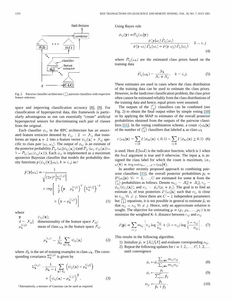
The conventional approach to classification problemsis to first transform an input space(which is the hyperspec-tral signal here) to a feature spacein which the discriminationamong all the classes in class set is high then to use a singleclassifier that distinguishes all the classes simultaneously.In this paper, however, we use a Bayesian pairwise classifier(BPC) framework [8], [9] that we developed previously for clas-sification problems with a moderately large number of classes.In the BPC framework shown in Fig. 2, a-class problem isfirst decomposed into a set of two-class problems for allpairs . Each of the two-class problemsis solved independently, and their results are combined to obtainthe result for the original -class problem.

A customized feature extraction approach for each pair ofclasses is especially advantageous in remote sensing applica-tions, where extraction of domain knowledge about specificclass characteristic, is as important as reducing the feature

1370 IEEE TRANSACTIONS ON GEOSCIENCE AND REMOTE SENSING, VOL. 39, NO. 7, JULY 2001

Fig. 2. Pairwise classifier architecture: pairwise classifiers with respectivefeature selectors.

space and improving classification accuracy [8], [9]. Forclassification of hyperspectral data, this framework is partic-ularly advantageous as one can essentially “create” artificialhyperspectral sensors for discriminating each pair of classesfrom the original.

Each classifier in the BPC architecture has an associ-ated feature extractor denoted by that trans-forms an input into a feature vector spe-cific to class pair . The output of is an estimate ofthe posterior probability (and

). Each is implemented as a maximumaposterior Bayesian classifier that models the probability den-sity functions , as:1

(1)

where;

dimensionality of the feature space ;mean of class in the feature space .

(2)

where is the set of training examples in class. The corre-sponding covariance is given by

(3)

1Alternatively, a mixture of Gaussian can be used as required.

Using Bayes rule

(4)

where are the estimated class priors based on thetraining data

(5)

These estimates are used in cases where the class distributionof the training data can be used to estimate the class priors.However, in the landcover classification problem, the class prioroften cannot be estimated reliably from the class distributions ofthe training data and hence, equal priors were assumed.

The outputs of the classifiers can be combined (seeFig. 2) to obtain the final output either by simple voting [10]or by applying the MAP to estimates of the overall posteriorprobabilities obtained from the outputs of the pairwise classi-fiers [11]. In the voting combination scheme, a countof the number of classifiers that labeled as class

(6)

is used. Here is the indicator function, which is 1 whenthe argument is true and 0 otherwise. The inputis as-signed the class label for which the count is maximum, i.e.,

.In another recently proposed approach to combining pair-

wise classifiers [11], the overall posterior probabilitiesare estimated for some from the

probabilities as follows. Denote ,, and . The goal is to find an

estimate of true posteriors such that is closeto , . Since there are independent parametersbut equations, it is not possible in general to estimatesothat . Hence, only an approximate solution issought. The objective for estimating is tominimize the weighted K–L distance between and

(7)

This results in the following algorithm.

1) Initialize and evaluate corresponding .2) Repeat the following updates for

until convergence

(8)

(9)

(10)

KUMAR et al.: BEST-BASES FEATURE EXTRACTION ALGORITHMS 1371

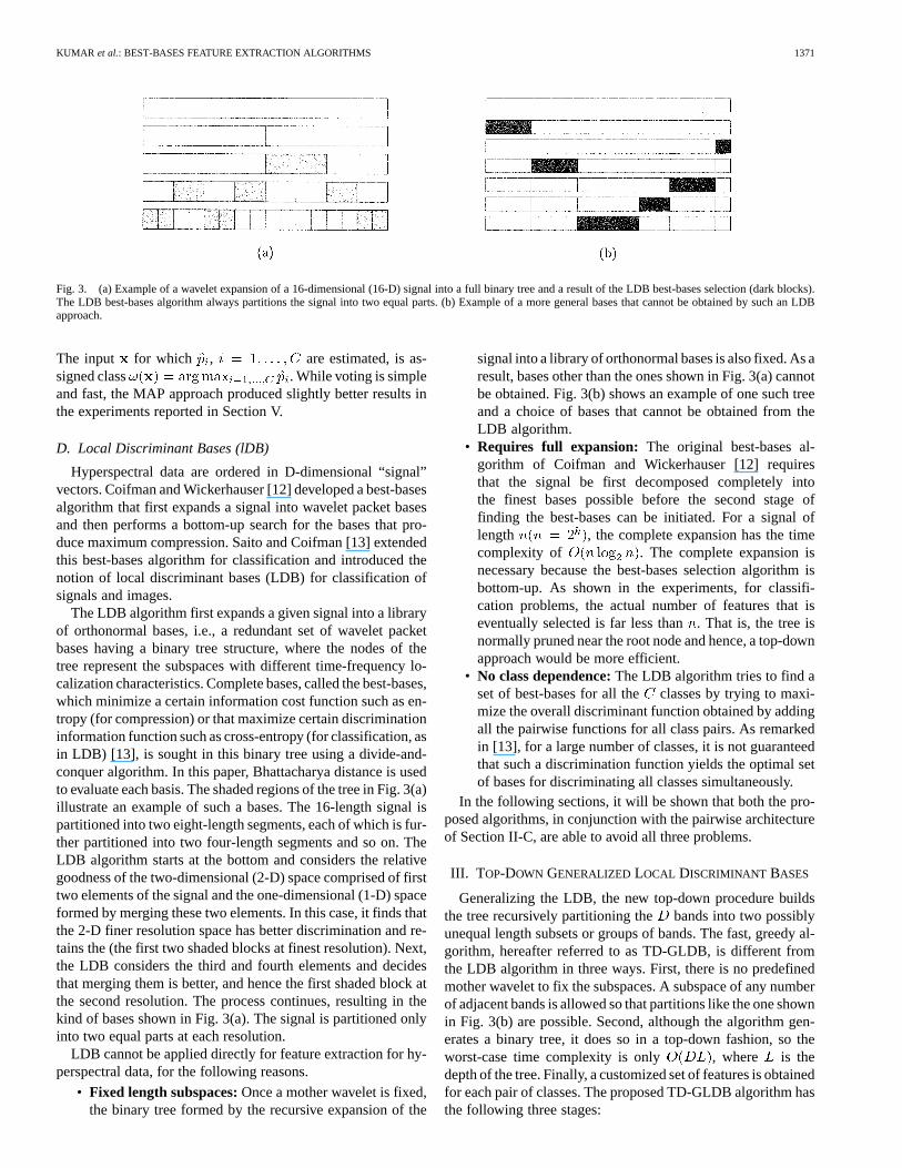
Fig. 3. (a) Example of a wavelet expansion of a 16-dimensional (16-D) signal into a full binary tree and a result of the LDB best-bases selection (dark blocks).The LDB best-bases algorithm always partitions the signal into two equal parts. (b) Example of a more general bases that cannot be obtained by such an LDBapproach.

The input for which , are estimated, is as-signed class . While voting is simpleand fast, the MAP approach produced slightly better results inthe experiments reported in Section V.

D. Local Discriminant Bases (lDB)

Hyperspectral data are ordered in D-dimensional “signal”vectors. Coifman and Wickerhauser [12] developed a best-basesalgorithm that first expands a signal into wavelet packet basesand then performs a bottom-up search for the bases that pro-duce maximum compression. Saito and Coifman [13] extendedthis best-bases algorithm for classification and introduced thenotion of local discriminant bases (LDB) for classification ofsignals and images.

The LDB algorithm first expands a given signal into a libraryof orthonormal bases, i.e., a redundant set of wavelet packetbases having a binary tree structure, where the nodes of thetree represent the subspaces with different time-frequency lo-calization characteristics. Complete bases, called the best-bases,which minimize a certain information cost function such as en-tropy (for compression) or that maximize certain discriminationinformation function such as cross-entropy (for classification, asin LDB) [13], is sought in this binary tree using a divide-and-conquer algorithm. In this paper, Bhattacharya distance is usedto evaluate each basis. The shaded regions of the tree in Fig. 3(a)illustrate an example of such a bases. The 16-length signal ispartitioned into two eight-length segments, each of which is fur-ther partitioned into two four-length segments and so on. TheLDB algorithm starts at the bottom and considers the relativegoodness of the two-dimensional (2-D) space comprised of firsttwo elements of the signal and the one-dimensional (1-D) spaceformed by merging these two elements. In this case, it finds thatthe 2-D finer resolution space has better discrimination and re-tains the (the first two shaded blocks at finest resolution). Next,the LDB considers the third and fourth elements and decidesthat merging them is better, and hence the first shaded block atthe second resolution. The process continues, resulting in thekind of bases shown in Fig. 3(a). The signal is partitioned onlyinto two equal parts at each resolution.

LDB cannot be applied directly for feature extraction for hy-perspectral data, for the following reasons.

• Fixed length subspaces:Once a mother wavelet is fixed,the binary tree formed by the recursive expansion of the

signal into a library of orthonormal bases is also fixed. As aresult, bases other than the ones shown in Fig. 3(a) cannotbe obtained. Fig. 3(b) shows an example of one such treeand a choice of bases that cannot be obtained from theLDB algorithm.

• Requires full expansion: The original best-bases al-gorithm of Coifman and Wickerhauser [12] requiresthat the signal be first decomposed completely intothe finest bases possible before the second stage offinding the best-bases can be initiated. For a signal oflength , the complete expansion has the timecomplexity of . The complete expansion isnecessary because the best-bases selection algorithm isbottom-up. As shown in the experiments, for classifi-cation problems, the actual number of features that iseventually selected is far less than. That is, the tree isnormally pruned near the root node and hence, a top-downapproach would be more efficient.

• No class dependence:The LDB algorithm tries to find aset of best-bases for all the classes by trying to maxi-mize the overall discriminant function obtained by addingall the pairwise functions for all class pairs. As remarkedin [13], for a large number of classes, it is not guaranteedthat such a discrimination function yields the optimal setof bases for discriminating all classes simultaneously.

In the following sections, it will be shown that both the pro-posed algorithms, in conjunction with the pairwise architectureof Section II-C, are able to avoid all three problems.

III. T OP-DOWN GENERALIZED LOCAL DISCRIMINANT BASES

Generalizing the LDB, the new top-down procedure buildsthe tree recursively partitioning the bands into two possiblyunequal length subsets or groups of bands. The fast, greedy al-gorithm, hereafter referred to as TD-GLDB, is different fromthe LDB algorithm in three ways. First, there is no predefinedmother wavelet to fix the subspaces. A subspace of any numberof adjacent bands is allowed so that partitions like the one shownin Fig. 3(b) are possible. Second, although the algorithm gen-erates a binary tree, it does so in a top-down fashion, so theworst-case time complexity is only , where is thedepth of the tree. Finally, a customized set of features is obtainedfor each pair of classes. The proposed TD-GLDB algorithm hasthe following three stages:

1372 IEEE TRANSACTIONS ON GEOSCIENCE AND REMOTE SENSING, VOL. 39, NO. 7, JULY 2001

1) Recursive partitioning of adjacent bands intononoverlapping groups (subspaces):All the bandsin the hyperspectral data set are recursively partitionedinto a number of groups of adjacent bands as shown inFig. 3(b). Each group is denoted by an intervalcomprised of all the bands between and including bands

through .2) Merging bands within each group: Bands within

each group are linearly combined to give single“group-bands”. A user definedmerge functionde-noted by is used to merge bands in the group

. Herein, for simplicity, the mean of all the bandswithin a group is used as the merge function

(11)

In general, any linear combination such as a Fisher dis-criminant projection could be used as the merge function.

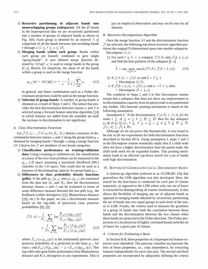
3) Selection of group-bands:A number of group-bands isobtained as a result of Steps 1 and 2. The subset that pro-vides the best discrimination between classesand isselected using a forward feature selection algorithm [14]in which features are added from the available set untilthe increase in discrimination is not significant.

A. Class Discrimination Functions

Let denote a measure of dis-crimination between classesand along the group-bandobtained by merging bandsthrough using a merge function

. Choices for are members of two broad categories.

1) Classification performance on training/validationdata: Using a training or validation set, the classificationaccuracy of the two-class problem can be measured in the

1-D space assuming a maximum likelihood (ML)classifier in the 1-D space. This could also be used as ameasure of discriminating capacity for group-band.

2) Differences in class probability density functions(pdfs): If the pdfs and are estimatedfrom the data sets and , then the discriminationbetween classes and can be evaluated in terms ofsome difference measure between the two pdfs (e.g., theKullback-Leibler divergence [15], Bhattacharya distance[16], etc.) In this paper, we use a discriminant measurebased on the log-odds of (pairwise) class posteriorprobabilities [8], [9]

(12)

where is the (estimated) pairwise classposterior probability of projected on the basis forclass and . Thislog-odds ratio gave better performance than Bhattacharyadistance and K–L divergence in our experiments. This is

just an empirical observation and may not be true for alldatasets.

B. Recursive Decomposition Algorithm

Once the merge function and the discrimination functionare selected, the following top-down recursive algorithm par-

titions the original D-dimensional space into smaller subspaces.Decompose

1) For each compute andand find the best partition of the subspace

(13)

2) If and• Decompose .

3 If and , then• Decompose .

The condition in Steps 2 and 3 in this Decompose routineensure that a subspace that does not show any improvement inits discrimination capacity from its parent node is not partitionedany further. This heuristic pruning mechanism is based on thefollowing assumption.

Assumption I: If the discrimination forsome , then for any subspace

of i.e., ,.

Although we do not prove this theoretically, it was found tobe true in all our experiments for both discrimination functionsdescribed in Section III-A. Using assumption I, steps 2 and 3in the Decompose routine essentially imply that if a child nodedoes not have a higher discrimination than the parent node, thechild node need not be expanded further. This pruning mech-anism leads to an efficient top-down search for a set of bandswith high discrimination.

IV. BOTTOM-UP GENERALIZED LOCAL DISCRIMINANT BASES

A bottom-up algorithm (referred to as GLDB-BU [4]) thatgeneralizes the LDB algorithm was also developed. Here, thesearch for the best-bases is conducted for each pair of classesseparately, as opposed to the LDB where only one set of basesis extracted for distinguishing all classes simultaneously. It alsoallows the flexibility of merging any set of adjacent bands asopposed to merging bands obtained by recursively partitioningthe set of bands into two equal groups in each level of the tree,as in LDB. Finally, the criteria used to measure the goodnessof a group of bands uses both the correlation between thosebands and the discrimination between the two classes whenthese bands are projected in the Fisher direction. The Fisher pro-jections of a localized set of highly correlated bands yield the setof bases for a given pair of classes.

A. Criteria for Evaluating a Basis

In Section II-B, three properties of a hyperspectral feature ex-tractor were identified. The pairwise classifier incorporates thefirst of those properties, i.e., class dependence, by extractingfeatures independently for each class pair. The second and thirdproperties are incorporated by adequately defining the criteria

KUMAR et al.: BEST-BASES FEATURE EXTRACTION ALGORITHMS 1373

for evaluating a basis. One such criteria is proposed in this sec-tion.

The second property requires that the high correlation valuesbetween spectrally adjacent hyperspectral bands be utilized.Thus, the criteria should reward combining highly correlatedbands rather than combining less correlated bands. There area number of ways of defining the correlation among a groupof bands in terms of the correlation between all pairs of bandsgiven by a correlation matrix (e.g., Fig. 1)

(14)

where is the covariance matrix

(15)

and is the mean over the two classes

(16)

The criteria used to quantify the correlation among the bandsfor any group of bands is definedby the correlation measure as theminimumof all thecorrelations between every pair of bands in the range

(17)

The group of bands is highly correlated if is large.The third property in Section II-B requires that the basis be

discriminating. Thus, the criteria should reward a highly dis-criminating basis more than a less discriminating basis. Dis-crimination between the two classes can be quantified as theFisher discriminant in the 1-D Fisher projection obtained fromthe subspace . Let and be the subvectors con-taining dimensions through of the mean vectors andcorresponding to the classesand . Let and be thesubmatrices containing rows and columnsthrough of theclass covariance matrices and of these classes, then thewithin class covariance for the two-class problem is givenby

(18)

where is the prior probability of class . The betweenclass covariance is given by

(19)

We define the discrimination measure for groupingthese bands as the Fisher discriminant of the subspace inducedby bands through . Since we are considering only a two-classproblem, the Fisher discriminant projects this subspace intoa 1-D space through a Fisher projection vector thatmaximizes

(20)

yielding the projection vector

(21)

The product of the correlationmeasure and the discrimination measure is used as the measureof goodness of the “group-band” . The correspondingbasis is given by the Fisher projection vector . A bottom-upsearch algorithm, described next, is used for finding the bestset of bases for each class pair using this criteria.

B. Bottom-Up Search for the Best-bases

In the bottom-up search algorithm, letdenote the set of actual bands that belong to theth “group-band” and denote the number of such group-bands at level

.

1) Initialize (finest level), ,. .

2) Find the best pair of bands to merge• for .

— Form a group-band by merging group-bandsand

(22)

— Evaluate the group-band.

• Find the position of the best pair of bands at thislevel

(23)

3) If thencontinue; otherwise stop.

4) Update bands at the next level• If then , i.e.,

, .• , i.e.,

.• If then ,

i.e., ,.

5) Move to the next level: , .Return to Step 2.

The process of merging adjacent bands continues until a level(i.e., ), at which merging any two adjacent group-bands yieldsa worse (in terms of ) group-band than either of the two group-bands being merged (Step 3). Each of the group-bands

obtained as a result of this process is associated

with the corresponding Fisher projection vector

that forms the bases of projection being sought. All the se-lected bases are mutually orthogonal as the group-bands do notoverlap. Instead of using all the bases, a forward featureselection algorithm is applied to the resulting set of bases to se-lect a subset such that adding any more bases will not lead to asignificant increase (i.e., user-specified 1%) in the classificationaccuracy of the training set. Let denote the final

1374 IEEE TRANSACTIONS ON GEOSCIENCE AND REMOTE SENSING, VOL. 39, NO. 7, JULY 2001

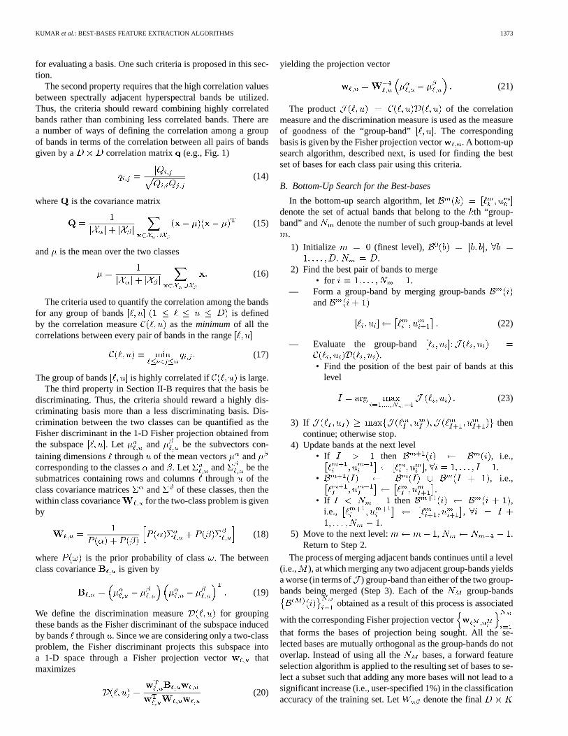
Fig. 4. Hyperspectral data: The AVIRIS Hyperspectral data obtainedby NASA over Kennedy Space Center, FL. The bands corresponding towavelengths of 1999 nm, 953 nm, and 527 nm were used for RGB channels fordisplaying purpose.

matrix containing the orthogonal bases after the feature selec-tion process for distinguishing class pair .

C. A Bayesian Classifier for GLDB-BU

The classifier for class-pair utilizes: 1) the bases vec-tors found by the algorithm presented in Section IV-B, 2)the K-dimensional means and in the projectedspace, and 3) the covariance matrices and

. In terms of the pairwise classifier architecture, forany novel input , the feature extractor transforms it intoas

(24)

The pdf in the feature space for class is given by

(25)

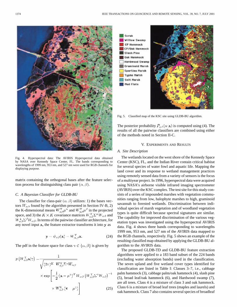
Fig. 5. Classified map of the KSC site using GLDB-BU algorithm.

The posterior probability is computed using (4). Theresults of all the pairwise classifiers are combined using eitherof the methods noted in Section II-C.

V. EXPERIMENTS AND RESULTS

A. Site Description

The wetlands located on the west shore of the Kennedy SpaceCenter (KSC), FL, and the Indian River contain critical habitatfor several species of water fowl and aquatic life. Mapping theland cover and its response to wetland management practicesusing remotely sensed data from a variety of sensors is the focusof a multiyear project. In 1996, hyperspectral data were acquiredusing NASA’s airborne visible infrared imaging spectrometer(AVIRIS) over the KSC complex. The test site for this study con-sists of a series of impounded marshes with vegetation commu-nities ranging from low, halophyte marshes to high, graminoidsavannah to forested wetlands. Discrimination between indi-vidual species of marsh vegetation and of woodland vegetationtypes is quite difficult because spectral signatures are similar.The capability for improved discrimination of the various veg-etation types was investigated using the hyperspectral AVIRISdata. Fig. 4 shows three bands corresponding to wavelengths1999 nm, 953 nm, and 527 nm of the AVIRIS data mapped tothe RGB channels, respectively. Fig. 5 shows an example of theresulting classified map obtained by applying the GLDB-BU al-gorithm to the AVIRIS data.

The proposed GLDB-TD and GLDB-BU feature extractionalgorithms were applied to a 183 band subset of the 224 bands(excluding water absorption bands) used in the classification.The seven upland and five wetland cover types identified forclassification are listed in Table I: Classes 3–7, i.e., cabbagepalm hammock (3), cabbage palm/oak hammock (4), slash pine(5), broad leaf/oak hammock (6), and Hardwood swamp (7),are all trees. Class 4 is a mixture of class 3 and oak hammock.Class 6 is a mixture of broad leaf trees (maples and laurels) andoak hammock. Class 7 also contains several species of broadleaf

KUMAR et al.: BEST-BASES FEATURE EXTRACTION ALGORITHMS 1375

TABLE ITWELVE CLASSES IN THEAVIRIS HYPERSPECTRALDATASET

trees. These classes have similar spectral signatures and are verydifficult to discriminate in multispectral and even hyperspectraldata using traditional methods.

There were examples for each class. These were ran-domly partitioned into 50% training and 50% test sets for eachof the ten experiments. The proposed algorithms were comparedto the SPCT and the LDB approach in terms of classification ac-curacy and reduction in the feature space. Since there is no sys-tematic way of estimating the parameters of the training priorsfor each class, equal priors are assumed instead of using (5) (thenumber of training examples only reflects training samples thatwe were able to collect, but does not reflect the true prior of theclasses).

B. Experimental Results

Table II contains the test set accuracies of the SPCT (uppertriangular) and LDB (lower triangular) algorithms over all the66 pairwise classifiers, while Table III contains the numberof corresponding features used by each of these classifiers forSPCT and LDB. Although most pairs of classes were reason-ably well discriminated by the features extracted by SPCTand LDB, the class pairs [cabbage palm/oak hammock (4),hardwood swamp (7)], [cabbage palm/oak hammock (4), broadleaf/oak hammock(6)], [slash pine(5), hardwood swamp(7)],and [cabbage palm/oak hammock(4), slash pine(5)] were notdiscriminated easily. Their classification accuracies over thetest set were significantly less than the mean accuracy of 93%(see Table VII) over all the 66 pairwise classifiers. Further, thenumber of features selected for class pair (4,5) by SPCT (i.e.,15) and LDB (i.e., ten) is also largeer than the average numberof features utilized (ten for SPCT and seven for LDB).

The classification accuracies over test sets for the GLDB-TDalgorithm for all the 66 pairwise classifiers for both objective

TABLE IIPAIRWISE CLASSIFIER ACCURACIES ONTEST SET FOR SPCT (UPPER

TRIANGULAR) AND LDB (LOWER TRIANGULAR) FEATURE EXTRACTION

ALGORITHMS

TABLE IIIAVERAGE NUMBER OFFEATURESUSED FORSPCT (UPPERTRIANGULAR) AND

LDB (LOWERTRIANGULAR) FEATURE EXTRACTION ALGORITHMS

functions, classification accuracy on the training set (upper tri-angular), and log-odds ratio of posterior probabilities (lower tri-angular) are shown in Table IV. The corresponding number offeatures averaged over ten experiments are listed in Table V forthe GLDB-TD algorithm. There is an average improvement ofalmost 5% in classification accuracies in all class pairs whenusing GLDB-TD feature extractor as compared to the SPCT orLDB feature extractors. Moreover, the classification accuracyover the difficult class pairs (4,5), (4,6), and (5,7) also improvedby similar amounts. However, as a mixture class, class pair (4,7)still remains difficult to discriminate even by the GLDB-TDalgorithm. Only 2–4 features were utilized by most of the 66pairwise classifiers when using the GLDB-TD feature extractorcompared to 7–12 features used by SPCT and 5–11 featuresused by LDB-based classifiers.

Table VI contains the average classification accuracies overthe test sets (upper triangular matrix) and the number of featuresin the reduced space (lower triangular matrix) for the GLDB-BUalgorithm applied to the same data set. For most class pairs,the classification accuracy was almost 100% and the minimumof 92.5% was for class pair (4,5), one of the problematic class

1376 IEEE TRANSACTIONS ON GEOSCIENCE AND REMOTE SENSING, VOL. 39, NO. 7, JULY 2001

TABLE IVCLASSIFIER ACCURACIES FOR THEGLDB-TD FEATURE EXTRACTION

ALGORITHM. THE UPPERTRIANGULAR MATRIX CONTAINS ACCURACIES

FORJ = CLASSIFICATION ACCURACY ON TRAINING SET AND THE

LOWER TRIANGULAR MATRIX CONTAINS ACCURACIES FORJ =

LOG-ODDS RELEVANCE (12)

TABLE VAVERAGE NUMBER OF FEATURES USED BY THE GLDB-TD FEATURE

EXTRACTION ALGORITHM. THE UPPERTRIANGULAR MATRIX IS FORJ =

CLASSIFICATION ACCURACY ONTRAINING SET AND THE LOWERTRIANGULAR

MATRIX IS FORJ = LOG-ODDS RELEVANCE

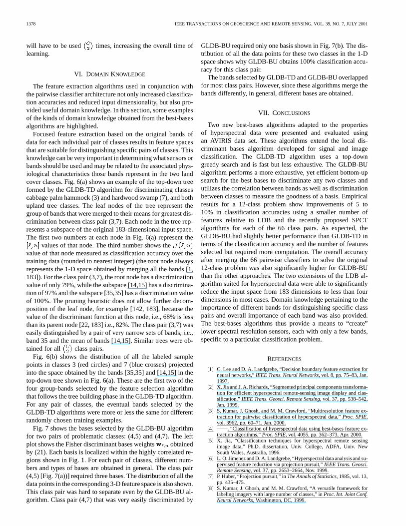
pairs. Further, note that class pair (4,7) had a classification ac-curacy of 100% as compared to 82% by GLDB-TD andby LDB and SPCT. Class pair (4,6) was also classified easilyby the GLDB-BU to yield almost 100% classification accuracycompared to by SPCT and LDB and 91% by GLDB-TD.Further, only one feature was required by GLDB-BU to discrim-inate class pair (4,7) compared to more than four by GLDB-TD,15 by SPCT, and six by LDB. The number of features requiredby most of the classifiers based on GLDB-BU feature extrac-tion was 1–2, with class pair (4,5) requiring more and still notbeing as well-discriminated as other pairs. Fig. 7(a) shows thebases and distribution of points in the three dimensional (3-D)feature space for class pair (4,5). Similarly, Fig. 7(b) shows thebases selected by GLDB-BU for class pair (4,7) and the corre-sponding distribution of points in the projected 1-D space.

Improvement in classification accuracy with a simultaneousreduction in the number of features in the feature space can be

attributed mainly to the generalization of the LDB algorithm.While only highly correlated bands were allowed to merge, theirusefulness was measured in terms of how well they can discrim-inate the two classes. Since SPCT uses the K–L transform toreduce the dimensionality, it does not necessarily transform theinput into a highly discriminatory feature space. LDB is lim-ited by the types of subspaces it can select, and hence its sub-spaces are inferior to those of the proposed algorithms. Com-pared to GLDB-TD, the proposed GLDB-BU performs betterboth in terms of classification accuracy and the number of re-quired features. This can be attributed to the following differ-ences between the two algorithms (i) GLDB-BU is bottom-upand hence searches through the space of possible bases more ex-haustively than the top-down GLDB-TD; (ii) The merge func-tion for GLDB-TD is just the mean while in GLDB-BU, themerge function is the Fisher direction of projection, which isexpected to perform better in terms of discrimination betweenthe two classes.

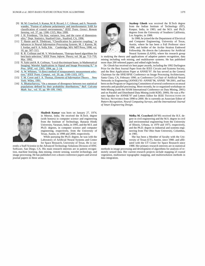
Table VII summarizes the results of Tables I–VI. The originalproblem was a 12-class problem that was decomposed into 66two-class problems, then the 66 pairwise classifiers were com-bined using the method proposed by Tibshirani [11] (describedin Section II-C). Overall test accuracies for all the four algo-rithms are contained in Table VII. The high values of classifica-tion accuracies from GLDB-TD and GLDB-BU for each pair ofclasses also resulted in higher accuracies in the overall-classproblem.

C. Computational Complexity

There are three components of the total time complexityof the feature extraction algorithms that sought a set of lineartransformations or bases. The four algorithms: SPCT, LDB,TD-GLDB, and BU-GLDB are evaluated in terms of thesethree components.

1) Time to evaluate a basis:The goodness of a single basisis measured by some criteria such as the Bhattacharya dis-tance in LDB, the amount of variance preserved or eigenvalues in SPCT, log-odds ratio of posterior probabilitiesin TD-GLDB, and Fisher discriminant in BU-GLDB al-gorithms. For an -dimensional subset of bands fromthrough , computation of Bhattacharyadistance (LDB), PCA projection (SPCT) and Fisher pro-jection (GLDB-BU) take time. In GLDB-TD, onlythe mean of the bands is computed, which requires

time.2) Time to search for a bases set:The feature extraction

algorithms seek multiple localized set of bases. TheLDB algorithm uses the wavelet packet best-bases searchapproach that takes for a signal of length .The SPCT algorithm utilizes edge detection algorithmson the correlation matrices to first isolate groups oflocalized highly correlated bands. This process takes

time. The TD-GLDB algorithm does a top-downsearch and prunes the search based on Assumption 1.This takes time, where is the depth of the tree.The GLDB-BU algorithm requires time asit is also bottom-up like the LDB algorithm.

KUMAR et al.: BEST-BASES FEATURE EXTRACTION ALGORITHMS 1377

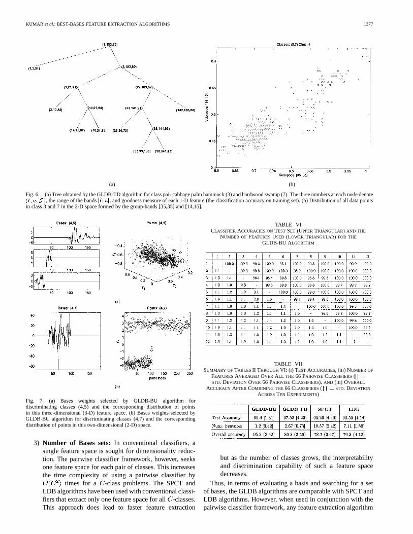
(a) (b)

Fig. 6. (a) Tree obtained by the GLDB-TD algorithm for class pair cabbage palm hammock (3) and hardwood swamp (7). The three numbers at each node denote(`; u;J ), the range of the bands[`; u], and goodness measure of each 1-D feature (the classification accuracy on training set). (b) Distribution of all data pointsin class 3 and 7 in the 2-D space formed by the group-bands [35,35] and [14,15].

Fig. 7. (a) Bases weights selected by GLDB-BU algorithm fordiscriminating classes (4,5) and the corresponding distribution of pointsin this three-dimensional (3-D) feature space. (b) Bases weights selected byGLDB-BU algorithm for discriminating classes (4,7) and the correspondingdistribution of points in this two-dimensional (2-D) space.

3) Number of Bases sets:In conventional classifiers, asingle feature space is sought for dimensionality reduc-tion. The pairwise classifier framework, however, seeksone feature space for each pair of classes. This increasesthe time complexity of using a pairwise classifier by

times for a -class problems. The SPCT andLDB algorithms have been used with conventional classi-fiers that extract only one feature space for all-classes.This approach does lead to faster feature extraction

TABLE VICLASSIFIER ACCURACIES ONTEST SET (UPPERTRIANGULAR) AND THE

NUMBER OF FEATURES USED (LOWER TRIANGULAR) FOR THE

GLDB-BU ALGORITHM

TABLE VIISUMMARY OF TABLES II THROUGHVI: ( I) TESTACCURACIES, (III ) NUMBER OF

FEATURESAVERAGED OVER ALL THE 66 PAIRWISE CLASSIFIERS([] =STD. DEVIATION OVER 66 PAIRWISE CLASSIFIERS), AND (III ) OVERALL

ACCURACY AFTER COMBINING THE 66 CLASSIFIERS(fg = STD. DEVIATION

ACROSSTEN EXPERIMENTS)

but as the number of classes grows, the interpretabilityand discrimination capability of such a feature spacedecreases.

Thus, in terms of evaluating a basis and searching for a setof bases, the GLDB algorithms are comparable with SPCT andLDB algorithms. However, when used in conjunction with thepairwise classifier framework, any feature extraction algorithm

1378 IEEE TRANSACTIONS ON GEOSCIENCE AND REMOTE SENSING, VOL. 39, NO. 7, JULY 2001

will have to be used times, increasing the overall time oflearning.

VI. DOMAIN KNOWLEDGE

The feature extraction algorithms used in conjunction withthe pairwise classifier architecture not only increased classifica-tion accuracies and reduced input dimensionality, but also pro-vided useful domain knowledge. In this section, some examplesof the kinds of domain knowledge obtained from the best-basesalgorithms are highlighted.

Focused feature extraction based on the original bands ofdata for each individual pair of classes results in feature spacesthat are suitable for distinguishing specific pairs of classes. Thisknowledge can be very important in determining what sensors orbands should be used and may be related to the associated phys-iological characteristics those bands represent in the two landcover classes. Fig. 6(a) shows an example of the top-down treeformed by the GLDB-TD algorithm for discriminating classescabbage palm hammock (3) and hardwood swamp (7), and bothupland tree classes. The leaf nodes of the tree represent thegroup of bands that were merged to their means for greatest dis-crimination between class pair (3,7). Each node in the tree rep-resents a subspace of the original 183-dimensional input space.The first two numbers at each node in Fig. 6(a) represent the

values of that node. The third number shows thevalue of that node measured as classification accuracy over thetraining data (rounded to nearest integer) (the root node alwaysrepresents the 1-D space obtained by merging all the bands [1,183]). For the class pair (3,7), the root node has a discriminationvalue of only 79%, while the subspace [14,15] has a discrimina-tion of 97% and the subspace [35,35] has a discrimination valueof 100%. The pruning heuristic does not allow further decom-position of the leaf node, for example [142, 183], because thevalue of the discriminant function at this node, i.e., 68% is lessthan its parent node [22, 183] i.e., 82%. The class pair (3,7) waseasily distinguished by a pair of very narrow sets of bands, i.e.,band 35 and the mean of bands [14,15]. Similar trees were ob-tained for all class pairs.

Fig. 6(b) shows the distribution of all the labeled samplepoints in classes 3 (red circles) and 7 (blue crosses) projectedinto the space obtained by the bands [35,35] and [14,15] in thetop-down tree shown in Fig. 6(a). These are the first two of thefour group-bands selected by the feature selection algorithmthat follows the tree building phase in the GLDB-TD algorithm.For any pair of classes, the eventual bands selected by theGLDB-TD algorithms were more or less the same for differentrandomly chosen training examples.

Fig. 7 shows the bases selected by the GLDB-BU algorithmfor two pairs of problematic classes: (4,5) and (4,7). The leftplot shows the Fisher discriminant bases weights obtainedby (21). Each basis is localized within the highly correlated re-gions shown in Fig. 1. For each pair of classes, different num-bers and types of bases are obtained in general. The class pair(4,5) [Fig. 7(a))] required three bases. The distribution of all thedata points in the corresponding 3-D feature space is also shown.This class pair was hard to separate even by the GLDB-BU al-gorithm. Class pair (4,7) that was very easily discriminated by

GLDB-BU required only one basis shown in Fig. 7(b). The dis-tribution of all the data points for these two classes in the 1-Dspace shows why GLDB-BU obtains 100% classification accu-racy for this class pair.

The bands selected by GLDB-TD and GLDB-BU overlappedfor most class pairs. However, since these algorithms merge thebands differently, in general, different bases are obtained.

VII. CONCLUSIONS

Two new best-bases algorithms adapted to the propertiesof hyperspectral data were presented and evaluated usingan AVIRIS data set. These algorithms extend the local dis-criminant bases algorithm developed for signal and imageclassification. The GLDB-TD algorithm uses a top-downgreedy search and is fast but less exhaustive. The GLDB-BUalgorithm performs a more exhaustive, yet efficient bottom-upsearch for the best bases to discriminate any two classes andutilizes the correlation between bands as well as discriminationbetween classes to measure the goodness of a basis. Empiricalresults for a 12-class problem show improvements of 5 to10% in classification accuracies using a smaller number offeatures relative to LDB and the recently proposed SPCTalgorithms for each of the 66 class pairs. As expected, theGLDB-BU had slightly better performance than GLDB-TD interms of the classification accuracy and the number of featuresselected but required more computation. The overall accuracyafter merging the 66 pairwise classifiers to solve the original12-class problem was also significantly higher for GLDB-BUthan the other approaches. The two extensions of the LDB al-gorithm suited for hyperspectral data were able to significantlyreduce the input space from 183 dimensions to less than fourdimensions in most cases. Domain knowledge pertaining to theimportance of different bands for distinguishing specific classpairs and overall importance of each band was also provided.The best-bases algorithms thus provide a means to “create”lower spectral resolution sensors, each with only a few bands,specific to a particular classification problem.

REFERENCES

[1] C. Lee and D. A. Landgrebe, “Decision boundary feature extraction forneural networks,”IEEE Trans. Neural Networks, vol. 8, pp. 75–83, Jan.1997.

[2] X. Jia and J. A. Richards, “Segmented principal components transforma-tion for efficient hyperspectral remote-sensing image display and clas-sification,” IEEE Trans. Geosci. Remote Sensing, vol. 37, pp. 538–542,Jan. 1999.

[3] S. Kumar, J. Ghosh, and M. M. Crawford, “Multiresolution feature ex-traction for pairwise classification of hyperspectral data,”Proc. SPIE,vol. 3962, pp. 60–71, Jan. 2000.

[4] , “Classification of hyperspectral data using best-bases feature ex-traction algorithms,”Proc. SPIE, vol. 4055, pp. 362–373, Apr. 2000.

[5] X. Jia, “Classification techniques for hyperspectral remote sensingimage data,” Ph.D. dissertation, Univ. College, ADFA, Univ. NewSouth Wales, Australia, 1996.

[6] L. O. Jimenez and D. A. Landgrebe, “Hyperspectral data analysis and su-pervised feature reduction via projection pursuit,”IEEE Trans. Geosci.Remote Sensing, vol. 37, pp. 2653–2664, Nov. 1999.

[7] P. Huber, “Projection pursuit,” inThe Annals of Statistics, 1985, vol. 13,pp. 435–475.

[8] S. Kumar, J. Ghosh, and M. M. Crawford, “A versatile framework forlabeling imagery with large number of classes,” inProc. Int. Joint Conf.Neural Networks, Washington, DC, 1999.

KUMAR et al.: BEST-BASES FEATURE EXTRACTION ALGORITHMS 1379

[9] M. M. Crawford, S. Kumar, M. R. Ricard, J. C. Gibeaut, and A. Neuensh-wander, “Fusion of airborne polarimetric and interferometric SAR forclassification of coastal environments,”IEEE Trans. Geosci. RemoteSensing, vol. 37, pp. 1306–1315, May 1999.

[10] J. H. Friedman, “On bias, variance, loss, and the curse of dimension-ality,” Dept. Statistics, Stanford Univ., Stanford, CA, 1996.

[11] T. Hastie and R. Tibshirani, “Classification by pairwise coupling,” inAdvances in Neural Information Processing Systems, M. J. Karens, M.I. Jordan, and S. A. Solla, Eds. Cambridge, MA: MIT Press, 1998, vol.10, pp. 507–513.

[12] R. R. Coifman and M. V. Wickerhauser, “Entropy-based algorithms forbest basis selection,”IEEE Trans. Inform. Theory, vol. 38, pp. 713–719,Mar. 1992.

[13] N. Saito and R. R. Coifman, “Local discriminant bases, in MathematicalImaging: Wavelet Applications in Signal and Image Processing II,” inProc. SPIE, vol. 2303, 1994, pp. 2–14.

[14] A. W. Whitney, “A direct method of nonparametric measurement selec-tion,” IEEE Trans. Comput., vol. 20, pp. 1100–1103, 1971.

[15] T. M. Cover and J. A. Thomas,Elements of Information Theory. NewYork: Wiley, 1991.

[16] A. Bhattacharyya, “On a measure of divergence between two statisticalpopulations defined by their probability distributions,”Bull. CalcuttaMath. Soc., vol. 35, pp. 99–109, 1943.

Shailesh Kumar was born on January 27, 1974,in Meerut, India. He received the B.Tech. degree(with honors) in computer science and engineeringfrom the Institute of Technology, Banaras HinduUniversity, Varanasi, India, in 1995, and the M.S. andPh.D. degrees, in computer science and computerengineering, respectively, from the University ofTexas, Austin, in 1998 and 2000, respectively.

While pursuing the Ph.D. degree, he was with theLaboratory of Artificial Neural Systems and Centerfor Space Research, University of Texas. He is cur-

rently a Staff Scientist in the Advanced Technology Solutions Division of HNCSoftware, San Diego, CA. His main research interests are in pattern recogni-tion, machine learning, data mining, remote sensing, wavelet technology, andimage processing. He has published over a dozen conference papers and severaljournal papers in these areas.

Joydeep Ghoshwas received the B.Tech degreefrom the Indian Institute of Technology (IIT),Kanpur, India, in 1983, and the M.S. and Ph.D.degrees from the University of Southern California,Los Angeles, in 1988.

In 1988, he joined the the Department of Electricaland Computer Engineering, University of Texas,Austin, where he has been a Full Professor since1998, and holder of the Archie Straiton EndowedFellowship. He directs the Laboratory for ArtificialNeural Systems (LANS), where his research group

is studying the theory and applications of adaptive pattern recognition, datamining including web mining, and multilearner systems. He has publishedmore than 200 refereed papers and edited eight books.

Dr. Ghosh has received six best paper awards, including the 1992 DarlingtonPrize for the Best Journal Paper from the IEEE Circuits and Systems Society,and the Best Applications Paper at ANNIE’97. He has served as the GeneralChairman for the SPIE/SPSE Conference on Image Processing Architectures,Santa Clara, CA, February 1990, as Conference Co-Chair of Artificial NeuralNetworks in Engineering (ANNIE)’93 -ANNIE’96, ANNIE ’98-2001, and hasbeen on the Program or Organizing Committees of several conferences on neuralnetworks and parallel processing. More recently, he co-organized workshops onWeb Mining (with the SIAM International Conference on Data Mining, 2001)and on Parallel and Distributed Data Mining (with KDD, 2000). He was a Ple-nary Speaker for ANNIE’97 and Letters Editor for IEEE TRANSACTIONS ON

NEURAL NETWORKSfrom 1998 to 2000. He is currently an Associate Editor ofPattern Recognition, Neural Computing Surveys, and theInternational Journalof Smart Engineering Design.

Melba M. Crawford (M’90) received the B.S. de-gree in civil engineering and the M.S. degree in civiland environmental engineering from the Universityof Illinois, Urbana, in 1970 and 1973, respectively,and the Ph.D. degree in industrial and systems engi-neering from The Ohio State University, Columbus,in 1981.

She has been a Member of faculty with the Uni-versity of Texas (UT), Austin, since 1980. and affil-iated with the UT Center for Space Research since1988. Her primary research interests are in statistical

methods in image processing and development of algorithms for analysis of re-motely sensed data. Her current research projects include mapping of coastalvegetation, multisensor topographic mapping, and multiresolution methods indata integration.