R

La

b

a

ARRAA

KFVNSV

1

ismssrl

UT

0d

Analytica Chimica Acta 732 (2012) 16–25

Contents lists available at SciVerse ScienceDirect

Analytica Chimica Acta

journa l homepage: www.e lsev ier .com/ locate /aca

apid monitoring of grapevine reserves using ATR–FT-IR and chemometrics

eigh M. Schmidtkea,b,∗, Jason P. Smithb, Markus C. Müllera,b, Bruno P. Holzapfelb

School of Agriculture and Wine Sciences, Charles Sturt University, Wagga Wagga, New South Wales 2678, AustraliaNational Wine and Grape Industry Centre, Charles Sturt University, Wagga Wagga, New South Wales 2678, Australia

r t i c l e i n f o

rticle history:eceived 11 August 2011eceived in revised form 21 October 2011ccepted 25 October 2011vailable online 6 November 2011

eywords:ourier transform infrared spectroscopyine reservesitrogentarchitis vinifera

a b s t r a c t

Predictions of grapevine yield and the management of sugar accumulation and secondary metaboliteproduction during berry ripening may be improved by monitoring nitrogen and starch reserves in theperennial parts of the vine. The standard method for determining nitrogen concentration in plant tissue isby combustion analysis, while enzymatic hydrolysis followed by glucose quantification is commonly usedfor starch. Attenuated total reflectance Fourier transform infrared spectroscopy (ATR–FT-IR) combinedwith chemometric modelling offers a rapid means for the determination of a range of analytes in pow-dered or ground samples. ATR–FT-IR offers significant advantages over combustion or enzymatic analysisof samples due to the simplicity of instrument operation, reproducibility and speed of data collection. Inthe present investigation, 1880 root and wood samples were collected from Shiraz, Semillon and Rieslingvineyards in Australia and Germany. Nitrogen and starch concentrations were determined using standardanalytical methods, and ATR–FT-IR spectra collected for each sample using a Bruker Alpha instrument.Samples were randomly assigned to either calibration or test data sets representing two thirds and onethird of the samples respectively. Signal preprocessing included extended multiplicative scatter correc-tion for water and carbon dioxide vapour, standard normal variate scaling with second derivative andvariable selection prior to regression. Excellent predictive models for percent dry weight (DW) of nitro-gen (range: 0.10–2.65% DW, median: 0.45% DW) and starch (range: 0.25–42.82% DW, median: 7.77% DW)using partial least squares (PLS) or support vector machine (SVM) analysis for linear and nonlinear regres-sion respectively, were constructed and cross validated with low root mean square errors of prediction(RMSEP). Calibrations employing SVM-regression provided the optimum predictive models for nitrogen

2 2

(R = 0.98 and RMSEP = 0.07% DW) compared to PLS regression (R = 0.97 and RMSEP = 0.08% DW). Thebest predictive models for starch was obtained using PLS regression (R2 = 0.95 and RSMEP = 1.43% DW)compared to SVR (R2 = 0.95; RMSEP = 1.56% DW). The RMSEP for both nitrogen and starch is below thereported seasonal flux for these analytes in Vitis vinifera. Nitrogen and starch concentrations in grapevinetissues can thus be accurately determined using ATR–FT-IR, providing a rapid method for monitoringvine reserve status under commercial grape production.

. Introduction

Seasonal patterns of carbohydrates reserve storage and mobil-sation in grapevines is strongly influenced by the developmentaltage, and the photosynthetic balance between vine growth andaintenance requirements. Developing shoot growth in early

pring massively increases carbohydrate demands and mobili-

ation of storage reserves. As the growing season progresses,eserve dynamics are strongly influenced by factors such as cropoad, canopy size, irrigation and climatic conditions that influence

∗ Corresponding author at: School of Agricultural and Wine Sciences, Charles Sturtniversity, Locked Bag 588, Wagga Wagga, NSW 2678 Australia.el.: +61 02 69334025; fax: +61 02 69332107.

E-mail address: lschmidtke@csu.edu.au (L.M. Schmidtke).

003-2670/$ – see front matter © 2011 Elsevier B.V. All rights reserved.oi:10.1016/j.aca.2011.10.055

© 2011 Elsevier B.V. All rights reserved.

photosynthesis and capacity of the vine for carbon acquisition[1]. Consequently, the over-wintering carbohydrate reserve sta-tus of vines may vary from season to season according to bothclimatic and vineyard management factors. Nitrogen reserves arealso stored in the perennial tissues of grapevines and play animportant role in supporting early season canopy growth [2]. Thenitrogen content of perennial tissues is responsive to nitrogenfertilizer applications, and like carbohydrates, concentrations atdormancy and the changes in concentrations between develop-ment stages may also vary between seasons [3]. Studies linkingcarbohydrate and nitrogen reserves in grapevines with vegeta-tive growth and fruiting responses suggest that monitoring stored

reserves at dormancy could provide an advanced indication of yieldand growth potential in the following season [4–6]. Recently wehave also observed that seasonal differences in the compositionof Shiraz grapes were associated with a contrasting pattern of

ica Chi

cacwm

soatrohmtHmi

toioamtti[yra[dn[iWnaro[

iytitwtatcplrutr(thstm

L.M. Schmidtke et al. / Analyt

arbohydrate reserve storage and mobilisation between floweringnd harvest [1]. This suggests that monitoring changes in reserveoncentrations between key development stages may also assistith understanding the impact of management practice and cli-atic factors on berry development and fruit quality.Regular monitoring of the carbohydrate and nitrogen reserve

tatus of grapevines will be of commercial interest; however somebstacles must first be overcome. Characterization of existing vari-tion in reserve concentrations such that context is provided forhe interpretation of analysis undertaken is the first challenge. Cur-ent methods of analysis based upon single analyte determinationf nitrogen is by combustion, and for starch requires enzymaticydrolysis with the resulting measurement of glucose, and theseethods may be too slow for basing management decisions, or

oo laborious and expensive for widespread commercial adoption.ence there is a requirement for a more rapid and lower costethod for measuring carbohydrate and nitrogen concentrations

n grapevine tissues.Attenuated total reflectance Fourier transform infrared spec-

roscopy (ATR–FT-IR) combined with chemometric modellingffers a rapid means for the determination of a range of analytesn powdered or ground samples. This process involves collectionf the infrared spectra of samples and correlating the absorbancet specific wavelengths to analyte concentration with predictiveodels constructed that can be used to determine the concen-

ration of analytes in other samples. Typically wavelengths inhe near infrared (750–2500 nm or 13,333–4000 cm−1) or midnfrared (2500–25,000 nm or 4000–400 cm−1) spectrum are used7]. ATR–FT-IR offers significant advantages over traditional anal-sis methods due to the simplicity of instrument operation,eproducibility and speed of data collection. ATR–FT-IR has beenpplied to the detection of adulterants in a variety of edible foods8], quality control in food manufacture [9], monitoring oil degra-ation arising from thermal exposure [10], on-line monitoring ofutrient concentration and biomass during antibiotic production11], the rapid determination of organic acids and carbohydratesn fruits [12] and prediction of olive oil sensory qualities [13].

ithin the wine industry FT-IR is used extensively for determi-ation of ethanol, pH, volatile acidity, glucose and fructose [14],nd ATR sampling methods are more commonly being used, withecent investigations employing this technique for discriminationf wine variety [15] and for real time juice and wine analysis16,17].

Predictive models for the estimation of analyte concentrationsn samples are constructed from the spectra using regression anal-sis and typically partial least squares (PLS) algorithms are used forhis purpose. Data are first pre-processed in an attempt to removenterference and to linearise signal response to analyte concentra-ion. Mathematical models that relate signal intensity at multipleavelengths with a measured, or known, analyte concentration are

hen constructed so that the concentration of that analyte can beccurately predicted in ‘unknown’ samples. Advantages of mul-ivariate calibrations using PLS regression are efficiency in dataollection, sample handling and expedition of results, hence theopularity of applying mathematical models to chemical prob-

ems. The underlying assumption of a linear dependency of signalesponse to analyte concentration does not always hold, partic-larly in complex samples containing interfering substances andhus non-linear predictive models may offer solutions in which PLSegressions model underperform [18]. Support vector regressionSVR), with its origins in machine learning and statistical learningheory [19], are becoming increasingly popular chemical models to

andle non-linear data. The basic concept of support vector regres-ion is to map the calibration data to a high dimension space,ermed hyperplanes, using a kernel function from which a linear

odel can be constructed. Deviations of predicted quantity (or

mica Acta 732 (2012) 16–25 17

class) from actual are allowed within an error margin (denotedε) while maintaining a constraint that minimises individual sam-ple weighting but maximises sample distance for each hyperplane.Such constraints are not always possible to achieve and a penaltyerror or cost function (denoted C) is fitted to the model to explicitlydeal with samples which cannot be thus fitted. The deviation abovethe error margin is termed the slack variable in soft margin SVR, andthe cost function essentially determines the compromise betweendata fit and the size of the slack variables [20], and is referred toas the ε-insensitive loss function [19]. An analogy is a tube witha diameter equal to the acceptable error margin fitted to the dataand samples that lie on or beyond the boundary are support vectors.Thus for small values of ε larger numbers of support vectors willbe used for modelling purposes with lower prediction errors in themodel but this increases the risk of over fitting the data [18]. Con-versely a lower number of support vectors increases the predictiveerror of the model. Large values of C effectively force samples withslack margins back within the error margin of the fitted model andthus decreases the number of support vectors.

The ability of support vector regression to accommodate non-linear data arises from the kernel based manner in which thedata is initially mapped into a high dimension subspace. Radialbasis functions (RBF) are commonly employed for mapping datato the high dimension space [18], although numerous alternativessuch as linear, polynomial, sigmoidal, splines, multi-layer percep-trons, wavelets and tensor product functions have been described[19,21–23]. In the application of RBF transformations the diameterof the radius must also be carefully chosen. If the radial diameter(denoted �) is too small an overly complex solution is determinedwith greater numbers of support vectors that will lead to data over-fit, whereas a flatter radius will lead to larger predictive error. Oftenthe RBF tuning parameter is described in terms of the standard devi-ation of the overall data (denoted �) rather than � with an inversesquared relationship existing between them; hence low � will infera larger � and vice versa [18]. Again, a trade-off between complex-ity and optimum fit is required and in practise the best approachfor determining the optimum RBF parameter (� or �), acceptableerror margin (ε) and the cost penalty (C) is a grid search with crossvalidation to find minima of predictive errors [22]. One must beaware however, that a workable solution may not exist for all datasets in spite of computational programs providing values for eachof these parameters [18].

The purpose of the present investigation was to investigate thefeasibility of ATR–FT-IR spectroscopy for the rapid measurement ofimportant vine reserve components. The sample set was designedto be representative of the variability within the range of analyticalattributes typically found in vine tissue samples across a numberof vineyard sites and Vitis vinifera varieties.

2. Experimental

2.1. Materials

All chemicals were of analytical grade and purchased fromBDH Australia. Deionized water (18 M� cm−1) was prepared usinga MilliQ filtration system. Thermostable �-amylase, amyloglu-cosidase and the glucose oxidase/peroxidase based assay werepurchased from Megazyme International.

2.2. Instrumentation

Infrared spectra of dried and powdered vine samples werecollected using two Alpha Fourier transform spectrophotome-ters (Bruker) configured for attenuated total reflectance (ATR) atambient temperature. Each sample was measured once where

18 L.M. Schmidtke et al. / Analytica Chimica Acta 732 (2012) 16–25

Table 1Sample details (year, location and vine tissue) in calibration and test sets with random allocation.

Calibration set (n = 1239) Test set (n = 641)

Riesling Semillon Shiraz Total Riesling Semillon Shiraz Total

Year2006 148 148 92 922007 47 98 243 388 25 46 113 1842008 203 158 90 451 109 82 54 2452009 163 89 252 65 55 120

LocationGundagai 58 58 32 32Hilltops 74 74 44 44Riverina 302 345 310 957 154 183 162 499Tumbarumba 39 39 21 21Rheingau 111 111 45 45

74

t3saahvp3apsac

2

2

stvpnnsivim

TS

Vine tissueWood 270 178 297Root 143 167 184

he ATR spectra were averaged from 64 scans over the region74–7496 cm−1 at 1.4 cm−1 resolution, with a background mea-urement against air conducted every 10 samples. Spectra werecquired using OPUS software version 6.5 provided by Bruker. Thispproach enabled approximately 30 samples to be measured everyour. Data was converted to ascii format and imported into Matlabersion 7.4.0.287 R2007a (The Mathworks, Natick). For the pur-oses of exploratory data and regression analysis ATR data between74 and 3958 cm−1 was extracted from each sample measurementnd converted to absorbance to correct for differences in sampleenetration of the beam at different wavelengths. Five independentpectra of deionised water and powdered starch were also collectednd averaged as reference for use in extended multiplicative scatterorrection.

.3. Procedure

.3.1. Vine samplesWood and root tissue samples for modelling purposes were

elected from an archived collection of several thousand poten-ial candidate samples collected from viticultural research trials orineyard surveys conducted between 2006 and 2009 (Table 1). Theurposes of the trial sites was to investigate the implications ofitrogen and water supply on the reserve dynamic of the peren-ial structure and on the composition of the grapes, while theurvey sites were aimed to gain a better understanding of the

ntra-seasonal changes of winter vine reserves in relation to yieldariation and prediction. A detailed description of these studiess beyond the scope of the present paper, and background infor-

ation has been presented in an earlier review [1]. Samples were

able 2ample details (year, location and vine tissue) in calibration and test sets following outlie

Calibration set (n = 1114)

Riesling Semillon Shiraz

Year2006 1472007 43 83 2392008 190 111 1212009 100 80

LocationGundagai 59Hilltops 81Riverina 254 274 331Tumbarumba 36Rheingau 79

Vine tissueWood 180 120 328Root 153 154 179

45 126 86 153 36594 73 97 106 276

chosen to represent a range of analytical values, growing years,conditions and grape varieties experienced during the conduct ofthese projects. A total of 1880 grapevine (Vitis Vinifera L.) tissuesamples were collected from thirty-five vineyards over a period offour years consisting of three field trials and thirty-two survey sites(Tables 1 and 2), these were located within the Riverina and southeastern slopes of New South Wales (Australia) and in the Rheingauwine region in Hessen (Germany).

Thirty-two Shiraz and Chardonnay blocks in commercially oper-ated vineyards were selected across the Riverina and Gundagai,Tumbarumba and Hilltops regions. Within each survey block, fivepanels of four vines were selected after leaf fall in 2005. The positionof each replicated panel was not chosen based on any pre-existingspatial information, but where possible, one panel of vines waslocated near the centre of the block, and the other four approxi-mately within each quarter of the block. Prior to pruning in 2005,2006 and 2007 root, wood and cane samples were collected fromeach panel of four vines. Root samples (diameter range ∼3–7 mm)were manually dug from near the base of each vine. Wood sampleswere collected with a 4.8 mm drill bit to a depth visually estimatedas the centre of the cordon and trunk. Two 4-node canes were col-lected from each vine, of which the basal two nodes (subsequentlyreferred to as spurs) of four canes were used for carbohydrate andnitrogen analysis.

The Semillon and Riesling samples were collected from twocommercially operated vineyards in the Riverina at five key

phenological stages (budbreak, flowering, veraison, harvest anddormancy) commencing in 2007 and ending in July 2009. Each vine-yard trial consisted of 24 plots with five vines being sampled at eachstage. Root samples (diameter range ∼3–7 mm) were manually dug

r removal and D-optimal criteria selection.

Test set (n = 575)

Total Riesling Semillon Shiraz Total

147 25 25365 29 59 80 168422 115 123 10 248180 71 63 134

59 10 1081 17 17

859 197 245 75 51736 13 1379 18 18

628 157 144 102 403486 58 101 13 172

ica Chimica Acta 732 (2012) 16–25 19

fwting1ctaa

2

dattGpmwbfigc

re8S2aaA(tdtSmioca

2

awisttci

2

wtwstat

L.M. Schmidtke et al. / Analyt

rom near the base of each vine, while wood samples were collectedith a 4.8 mm drill bit to a depth visually estimated as the centre of

he cordon and trunk. From the third experimental vineyard locatedn the Rheingau only wood samples were collected at four key phe-ological stages (budbreak, flowering, veraison and harvest) in therowing season 2008 and 2009. This vineyard was subdivided in2 plots with four vines being sampled per date, the samples wereollected by randomly cutting off one spur including the cane ofhe cordon. The collected spur was considered as 2 year old woodnd the cane sample as 1 year old wood and was separated in spurnd cane sections prior to further sample preparation.

.3.2. Nitrogen and starch analysisRoots were washed in phosphate free detergent and rinsed with

eionized water, both wood and root tissues were either oven driedt 70 ◦C (survey sites, Riesling Rhinegau) or freeze dried (Riverinarials). Following the drying processes the samples were groundo 0.12 mm with a heavy duty cutting mill (Retsch ZM2000, Haan,ermany) and an ultra-centrifugal mill (Retsch ZM200); the sam-les from the Rhinegau trial were ground to 0.2 mm with a cuttingill (Retsch SM200). Non-structural carbohydrate concentrationsere determined on a 20 mg sub-sample of each tissue as outlined

elow. For total nitrogen, an equal proportion of tissue from theve replicate locations in each vineyard was bulked, and a nitro-en content of a 50 mg sub-sample determined with a VarioMAXombustion analyser (Elementar, Hanau, Germany).

For starch determination, free soluble carbohydrates were firstemoved from a 20 mg sample with three 1 mL aliquots of 80% (v/v)thanol. The first two aliquots were incubated in a water bath at0 ◦C for 10 min, and the third at room temperature for 10 min.tarch from the remaining wood sample was then solubilized in00 �L of dimethylsulfoxide at 98 ◦C for 10 min. Thermostable �-mylase (29 U mL−1) in 300 �L of MOPS buffer (pH 7) was thendded; the samples incubated for 15 min, and then allowed to cool.myloglucosidase (32 U mL−1) in 400 �L of sodium acetate buffer

pH 4.5) was added, the samples incubated at 50 ◦C for 60 min andhen centrifuged at 10,000 rpm for 2 min. The supernatant wasiluted 1:6 (wood) or 1:11 (roots), and the glucose concentra-ion determined using a glucose oxidase/peroxidase based assay.amples were tested with either a Konelab Arena 20 XT or inicroplate format using a Biotek �Quant microplate reader after

ncubation at 40 ◦C for 30 min. Glucose standard curves in the rangef 0–5000 mg L−1 were prepared for each run of samples and starchoncentration in the original 20 mg sample was then calculated aspercentage of dry weight.

.3.3. Exploratory data analysisSpectra from all samples, and the 95% confidence interval for

bsorbance, was plotted (Fig. 1) along with spectra obtained forater, carbon dioxide and starch (Fig. 1S) to identify regions with

nteresting variation. A principal component analysis (PCA) of thetandard normal variate (SNV) scaled and mean centred (MC) spec-ral data between the regions 875–1800 cm−1 was conducted usinghe singular value decomposition (SVD) algorithm with principalomponents (PC) 1–2 and associated loadings plotted (Fig. 2) todentify specific groups of samples.

.3.4. Selection of samples for calibration and test setsTwo approaches to constructing calibration and test data sets

ere conducted; first random assignment of samples to a calibra-ion or test set based so that approximately two thirds of samplesere designated calibration and one third as an independent test

et. The second approach involved interrogation of the MIR spec-ra to identify outlier samples. PCA was conducted as describedbove and the chosen number of PC was determined from the rela-ive decrease in eigenvalues and the variance captured for each PC.

Fig. 1. ATR–FTIR mean spectra and 95% confidence interval of all samples prior tooutlier detection.

Sample outlier and influence plots were constructed (Fig. 3) to iden-tify samples with Q residuals or Hotelling T2 values exceeding the95% confidence interval. Samples with high Q residuals are poorlymodelled with the chosen number of principal components [24],whereas samples with high Hotelling T2 have specific attributesthat deviate further from mean observations and may exert a dis-proportionate leverage upon the models [25,26]. For the purposesof further modelling, samples with high Hotelling T2 and/or Q resid-uals were excluded. Calibration samples were chosen from theremaining sample matrix based upon the D-optimal criteria [27]such that two thirds of samples were assigned to the calibration set.D-optimal computation was conducted on the SNV treated spectrausing PLS toolbox (Eigenvector, Wenatchee). Samples not selectedfor calibration were assigned to the test data set. Calibration andtest set sample details are shown in Tables 1 and 2 for random andD-optimal criteria allocation respectively, and data set attributesare shown in Table 3.

2.3.5. Data pre-processing and regression analysisCalibration and test data were pre-processed using SNV

scaling followed by calculating the second derivative using aSavitzky–Golay [28] filter prior to variable selection. Alternatively,multiplicative scatter correction (MSC) or extended multiplicativescatter correction (EMSC) using reference spectra for water andcarbon dioxide vapour were applied to the calibration data setusing a second order polynomial filter in accordance with describedprocedures [29–31] prior to variable selection. Spectra for carbondioxide were obtained from an online database [32] at a resolu-tion of 0.1 cm−1, were de-resolved and re-sampled to match thereflectance spectra of samples. For the purposes of applying MSCand EMSC, the mean spectra of the calibration samples were usedas the reference spectra. Variable selection within the calibrationblock was conducted using the forward interval PLS (iPLS) regres-sion for each analyte and model combination [33].

2.3.6. Regression modelling of dataPredictive models of the spectra for nitrogen and starch

were constructed using either PLS regression or support vectorregression analysis. For PLS regression the pre-treated data weremodelled using the SIMPLS algorithm with cross validation usingrandom sample subsets with ten data splits of the calibration block.

The number of latent variables chosen for each model was deter-mined from eigenvalues and minima of the root mean squareerrors of calibration, cross validation and prediction. Support vec-tor regression using a radial basis kernel was conducted using the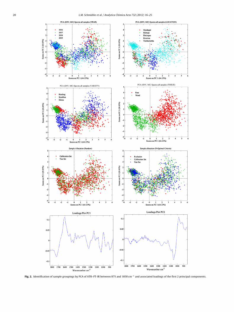

20 L.M. Schmidtke et al. / Analytica Chimica Acta 732 (2012) 16–25

Fig. 2. Identification of sample groupings by PCA of ATR–FT-IR between 875 and 1850 cm−1 and associated loadings of the first 2 principal components.

L.M. Schmidtke et al. / Analytica Chimica Acta 732 (2012) 16–25 21

Table 3Calibration and test set characteristics for regression analysis.

Calibration and test set sample allocation

Random Outlier removal and D-optimal criteria

Calibration set Test set Calibration set Test set

Nitrogen (%DW)Mean 0.65 0.68 0.70 0.51Median 0.46 0.57 0.53 0.29Range 0.11–2.65 0.10–2.31 0.10–2.39 0.11–1.81Standard deviation 0.50 0.50 0.52 0.41

Starch (%DW)Mean 10.24 11.08 11.05 8.38Median 7.49 7.77 8.01 7.01Range 0.25–47.85 0.30–42.82 0.34–47.85 1.26–28.78Standard deviation 7.55 8.04 8.06 4.18

Number of samples 1239 641 1114 575

Table 4Regression performance of predictive models for nitrogen.

Calibration and test set sample allocation Regression performance PLS SVR

Random sample allocation Pre-processinga SNV/2nd Der/MC/iPLS MSC/2nd Der/MC/iPLSR2b 0.97 0.97RMSEP 0.09 0.08Bias 0.00 0.00No. LV/SVc 6 6/562Hyperparameter valuescost function (C)

10

Error margin (ε) 0.1RBF parameter (�) 0.032

Outlier removal D-optimal allocation Pre-processing EMSC, 2nd Der, MC, iPLS SNV/2nd Der/MC/iPLSR2 0.97 0.98RMSEP 0.08 0.07Bias 0.00 0.00No. LV/SV 6 6/472Hyperparameter valuescost function (C)

10

Error margin (ε) 0.1RBF parameter (�) 0.032

a MSC,l

sets.rs use

Ltdt

TR

l

SNV, standard normal variate scaling; MSC, multiplicative scatter correction; Eeast squares variable selection; 2nd Der, Savitzky-Golay 2nd derivative.

b Calculated as the mean R2 for calibration, cross validation and independent testc Number of latent variables used for data compression/number of support vecto

IBSVM algorithm with a grid search for optimising cost func-ion (C), RBF parameter (�) and error margin (ε) with RMSECVetermined with a five-fold data split for cross validation. Fea-ure selection, Hotelling T2, Q residuals, PLS and support vector

able 5egression performance of predictive models for starch.

Calibration and test set sample allocation Regression performance

Random sample allocation Pre-processinga

R2b

RMSEPBiasNo. LV/SVc

Hyperparameter valuescost function (C)Error margin (ε)RBF parameter (�)

Outlier removal D-optimal allocation Pre-processingR2

RMSEPBiasNo. LV/SVHyperparameter valuescost function (C)Error margin (ε)RBF parameter (�)

a SNV, standard normal variate scaling; MSC, multiplicative scatter correction; EMSC,east squares variable selection; 2nd Der, Savitzky-Golay 2nd derivative.

b Calculated as the mean R2 for calibration, cross validation and independent test sets.c Number of latent variables used for data compression/number of support vectors use

extended multiplicative scatter correction; MC, mean centre; iPLS, interval partial

d for modelling.

regressions were conducted in PLS Toolbox (version 6.2, Eigenvec-tor Research Inc., Wenatchee, Washington). Predictive model char-acteristics for nitrogen and starch are presented in Tables 4 and 5and Figs. 4 and 5 respectively.

PLS SVR

MSC/2nd Der/MC MSC/2nd Der/MC/iPLS0.94 0.961.73 1.60−0.14 −0.138 6/668

31.6

0.10.010

SNV/2nd Der/MC/iPLS SNV/MC0.95 0.951.43 1.560.20 0.306 6/595

10

0.10.032

extended multiplicative scatter correction; MC, mean centre; iPLS, interval partial

d for modelling.

22 L.M. Schmidtke et al. / Analytica Chi

Fu

3

3

s3A

ig. 3. Identification of sample outliers and influence using Hotelling T2 and Q resid-als.

. Results and discussion

.1. Exploratory data analysis

The ATR–FT-IR spectra of the dried and powdered vine tis-ue samples (Fig. 1) is characterized by dominant peaks between75–800, 875–1800 and a broad peak between 3000–3500 cm−1.broad absorbance band between 3000–3500 cm−1 characteristic

Fig. 4. Regression plots for predicti

mica Acta 732 (2012) 16–25

of O–H bond stretching dominates the spectra and could berelated to the presence of carbohydrates or residual moisture [34](Fig. 1 Supporting Information). The spectral region with the mostinteresting variation occurs between 875–1800 cm−1 (Fig. 1) andPCA of the SNV and MC treated spectra from this region clearly sep-arates samples according to grapevine tissue type (root and wood;Fig. 2) with the first two PC modelling approximately 84% of thedata variability. Distinction of samples based upon grapevine tis-sue is expected to occur as the tissue vary significantly in theirreserve composition [1,35]. Sample groupings according to loca-tion are also evident with samples from the Rheingau groupedtightly together in the centre of the plot of PC1 and PC2. Samplesfrom other locations appear well dispersed, as do growing yearsand grape variety. The spectral bands characterising carbohydratesare typically observed in the 3600–2800 cm−1, 1500–1200 cm−1,1200–950 cm−1 and 950–700 cm−1 regions corresponding to O–Hand C–H bond stretching; bending of symmetric HCH bonds; C–Oand C–C bond stretching and COH, CCH and OCH bond bending[34]. Loading plots for PC1 and PC2 show the spectral variationsresponsible for this discrimination, with regions between 1650and 1550 cm−1 highly positively loaded onto PC1, with a smallercontribution between 1500 and 1300 cm−1. Regions between 1150and 1050 cm−1 are negatively correlated with PC2 and the regionbetween 1000 and 875 cm−1, are positively correlated.

Examination of the score plots also reveals the spread of sam-ples allocated to the calibration and test data sets by random or theD-optimal criteria (Fig. 2). Test and calibration samples appear to be

well distributed along the first 2 PCs for both approaches to calibra-tion and test sample set allocation. For the purposes of regressionmodelling samples from the entire data set were retained ratherthan separated into their distinct groups (i.e. Vinifera species,

on of nitrogen by ATR–FT-IR.

L.M. Schmidtke et al. / Analytica Chimica Acta 732 (2012) 16–25 23

redic

ld

dfisib5wbwoSsslsbcaefpeatnao

Fig. 5. Regression plots for p

ocations or tissue type) with calibration and test sets allocated asescribed above.

An important consideration when using SVR is to ensure thatata over fitting does not arise as there are no specific rules fortting the data unlike PLS [18]. Comparison of the number ofupport vectors used with the total number of samples in the cal-bration models show that between 43 and 45% of samples haveeen classified as support vectors for the nitrogen models and4% of samples used for starch models. This compared favourablyith the previous reports in which around 85% of samples have

een used in least squares SVR [36]. Various spectral processingas conducted for each model (data not shown) to determine the

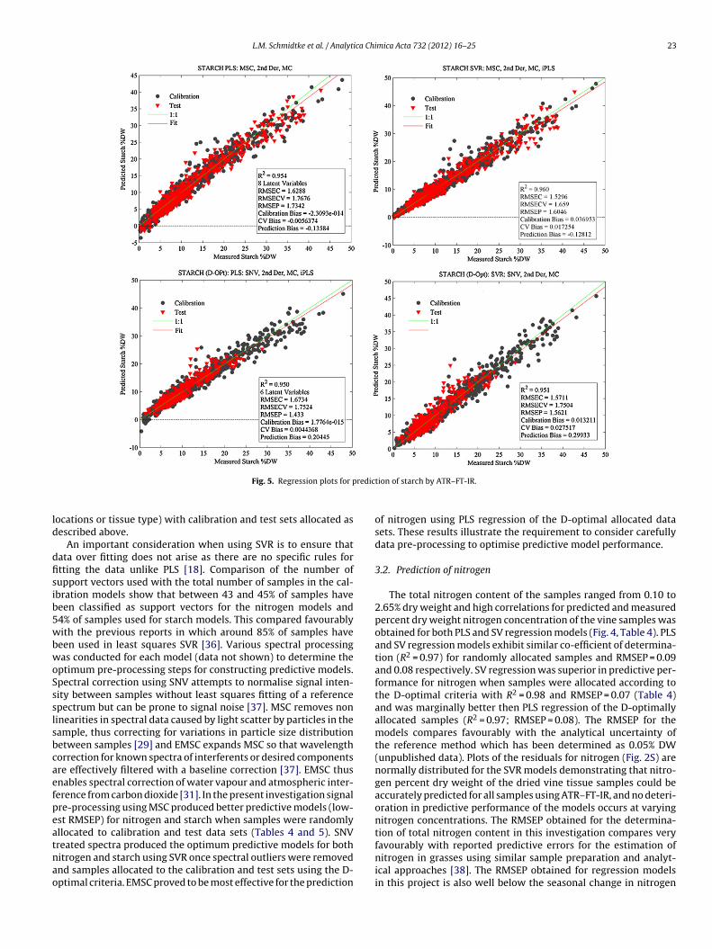
ptimum pre-processing steps for constructing predictive models.pectral correction using SNV attempts to normalise signal inten-ity between samples without least squares fitting of a referencepectrum but can be prone to signal noise [37]. MSC removes noninearities in spectral data caused by light scatter by particles in theample, thus correcting for variations in particle size distributionetween samples [29] and EMSC expands MSC so that wavelengthorrection for known spectra of interferents or desired componentsre effectively filtered with a baseline correction [37]. EMSC thusnables spectral correction of water vapour and atmospheric inter-erence from carbon dioxide [31]. In the present investigation signalre-processing using MSC produced better predictive models (low-st RMSEP) for nitrogen and starch when samples were randomlyllocated to calibration and test data sets (Tables 4 and 5). SNV

reated spectra produced the optimum predictive models for bothitrogen and starch using SVR once spectral outliers were removednd samples allocated to the calibration and test sets using the D-ptimal criteria. EMSC proved to be most effective for the prediction

tion of starch by ATR–FT-IR.

of nitrogen using PLS regression of the D-optimal allocated datasets. These results illustrate the requirement to consider carefullydata pre-processing to optimise predictive model performance.

3.2. Prediction of nitrogen

The total nitrogen content of the samples ranged from 0.10 to2.65% dry weight and high correlations for predicted and measuredpercent dry weight nitrogen concentration of the vine samples wasobtained for both PLS and SV regression models (Fig. 4, Table 4). PLSand SV regression models exhibit similar co-efficient of determina-tion (R2 = 0.97) for randomly allocated samples and RMSEP = 0.09and 0.08 respectively. SV regression was superior in predictive per-formance for nitrogen when samples were allocated according tothe D-optimal criteria with R2 = 0.98 and RMSEP = 0.07 (Table 4)and was marginally better then PLS regression of the D-optimallyallocated samples (R2 = 0.97; RMSEP = 0.08). The RMSEP for themodels compares favourably with the analytical uncertainty ofthe reference method which has been determined as 0.05% DW(unpublished data). Plots of the residuals for nitrogen (Fig. 2S) arenormally distributed for the SVR models demonstrating that nitro-gen percent dry weight of the dried vine tissue samples could beaccurately predicted for all samples using ATR–FT-IR, and no deteri-oration in predictive performance of the models occurs at varyingnitrogen concentrations. The RMSEP obtained for the determina-tion of total nitrogen content in this investigation compares very

favourably with reported predictive errors for the estimation ofnitrogen in grasses using similar sample preparation and analyt-ical approaches [38]. The RMSEP obtained for regression modelsin this project is also well below the seasonal change in nitrogen

2 ica Chi

cmo

3

brori(ooutSsdusphwactfriwmm

lwawaeifstlar

4

rasattnapaadr

[[[

[

[

[

[

[

[[

[

[

[

[

[[

[

[[[[[[

4 L.M. Schmidtke et al. / Analyt

oncentration measured for vine samples [35] thus making theseodels suitable for the determination of inter and intra season flux

f total nitrogen.

.3. Prediction of starch

Excellent predictive models for starch were also obtained usingoth PLS and SV regression (Fig. 5, Table 5). Regression analysis withandomly allocated samples produced models with co-efficientf determination of 0.94 and 0.96 for PLS and SV regressionespectively and RMSEP of 1.73 and 1.60 respectively. Interest-ngly the lowest predictive error was obtained using PLS regressionRMSEP = 1.43) compared to SV regression (RMSEP = 1.56) in the D-ptimal allocated samples, with equal co-efficient of determinationf 0.95. These values compare most favourably with the analyticalncertainty associated with the calibrant was has been determinedo be 1.62% DW (unpublished data). An interesting feature of theV regressions is the lack of negative predicted values at low mea-ured starch concentrations, whereas the PLS regression analysisoes not predict low starch quantities as well. Plots of starch resid-als (Fig. 3S) do not display a normal distribution with negativekew apparent at higher starch concentrations. Residual skew isarticularly apparent in the PLS models and the reduced data fit atigher starch concentrations may have arisen from inefficienciesith enzymatic digestion of ground vine tissue for starch extraction

nd subsequent measurement [35]. Improved data fit at low starchoncentrations and decreased residual skew at higher concentra-ions suggests SV regression models may be a better predictive toolor the estimation of starch in the samples rather than the PLSegressions. The observed magnitude of starch flux within grow-ng seasons is reported to be between approximately 2 and 4% dry

eight thus RMSEP below this quantity indicates that SV and PLSodels provide a suitable means for the rapid determination andonitoring of vine starch reserves.It is recognised that the RMSEP of predictive models for ana-

ytes is generally an overestimation of the actual error associatedith the predictands as the calibrants have associated systematic

nalytical error [39–42]. Random errors within the calibrants areell modelled using PLS regression with a tendency to cancel out

nd thus can be considered to be inconsequential to the predictionrror [43]. In the absence of a quantified analytical error for the cal-brants, a sample specific error of prediction could be determinedrom the sample leverage in the predictive model which has beenhown to be lower than the RMSEP [44]. Such error estimates mayhus become important for samples with low intra seasonal ana-yte variation. Overall the predictive models from this investigationre useful for monitoring the seasonal flux of nitrogen and starcheserves in grapevine tissue.

. Conclusion

The results from this investigation show that starch and nitrogeneserves in grape vine tissue can be measured with good precisionnd accuracy using ATR–FT-IR and PLS or SV regression. SV regres-ion models were marginally better than PLS regression modelsnd predictive errors were below the reported seasonal flux forotal nitrogen and starch for vine samples. In the present investiga-ion, the RMSEP is well below the reported flux of storage reserveitrogen and starch in Vitis vinifera. The predictive models could bepplied to vine samples from different regions and varieties thusroviding a useful analytical tool for monitoring vine carbohydrate

nd nitrogen reserve status. Total analytical time for ATR–FT-IR isround 60 s per sample once dried and ground, compared to severalays to extract and quantify by enzymatic analysis. Sample prepa-ation is relatively simple and this technique will make it possible

[

[

mica Acta 732 (2012) 16–25

for vineyard managers and personnel to rapidly monitor winter andintra-seasonal changes in vine reserve starch and nitrogen and pro-vide information about potential vine growth and development inthe following season.

Acknowledgements

The loan of ATR–FT-IR instruments from Bruker Optics, Australiais gratefully acknowledged. Vine reserve trials were funded by theAustralian wine and grape industry through the Grape and WineIndustry Development Corporation, Australia, while the Rieslingtrial in Germany received funding from the Geisenheim ResearchCentre. Considered discussion of support vector regression byDonal O’Sullivan is gratefully acknowledged.

Appendix A. Supplementary data

Supplementary data associated with this article can be found, inthe online version, at doi:10.1016/j.aca.2011.10.055.

References

[1] B.P. Holzapfel, J.P. Smith, S.K. Field, W.J. Hardie, Hort. Rev. 36 (2010) 143.[2] W.J. Conradie, in: J.P. Christensen, D.R. Smart (Eds.), Proceedings for the Soil

Environment and Vine Mineral Nutrition Symposium, American Society forEnology and Viticulture, Davis, California, 2005, p. 68.

[3] M.T. Treeby, D.M. Wheatley, Aust. J. Exp. Agric. 46 (2006) 1207.[4] K.M. Weyand, H.R. Schultz, Am. J. Enol. Vitic. 57 (2006) 172.[5] L. Cheng, G. Xia, T. Bates, J. Am. Soc. Hort. Sci. 129 (2004) 660.[6] J. Bennett, P. Jarvis, G.L. Creasy, M.C.T. Trought, Am. J. Enol. Vitic. 56 (2005) 386.[7] M. Lin, B.A. Rasco, A.G. Cavinato, M. Al-Holy, in: D.-W. Sun (Ed.), Infrared Spec-

troscopy for Food Quality Analysis and Control, Academic Press, Burlington,Mass., 2009, p. 119.

[8] N. Koca, N.A. Kocaoglu-Vurma, W.J. Harper, L.E. Rodriguez-Saona, Food Chem.121 (2010) 778.

[9] C. Shiroma, L. Rodriguez-Saona, J. Food Compos. Anal. 22 (2009) 596.10] R.C. Pinto, N. Locquet, L. Eveleigh, D.N. Rutledge, Food Chem. 120 (2010) 1170.11] P. Roychoudhury, L.M. Harvey, B. McNeil, Anal. Chim. Acta 561 (2006) 218.12] S. Bureau, D. Ruiz, M. Reich, B. Gouble, D. Bertrand, J.-M. Audergon, C.M.G.C.

Renard, Food Chem. 115 (2009) 1133.13] N. Sinelli, L. Cerretani, V.D. Egidio, A. Bendini, E. Casiraghi, Food Res. Int. 43

(2010) 369.14] D. Cozzolino, R. Dambergs, in: D.-W. Sun (Ed.), Infrared Spectroscopy for Food

Quality Analysis and Control, Academic Press, Burlington, Mass., 2009, p. 377.15] P.A. Tarantilis, V.E. Troianou, C.S. Pappas, Y.S. Kotseridis, M.G. Polissiou, Food

Chem. 111 (2008) 192.16] N. Shah, W. Cynkar, P. Smith, D. Cozzolino, J. Agric. Food. Chem. 58 (2010)

3279.17] A. Urtubia, J.R. Pérez-correa, F. Pizarro, E. Agosin, Food Control 19 (2008)

382.18] R.G. Brereton, G.R. Lloyd, Analyst 135 (2010) 230.19] A.J. Smola, B. Schölkopf, A Tutorial on Support Vector Regression, NeuroCOLT2

Technical Report Series, Berlin, 1998, p. 71.20] S.S. Fong, P. Rearden, C. Kanchagar, C. Sassetti, J. Trevejo, R.G. Brereton, Anal.

Chem. 83 (2011) 1537.21] S.R. Gunn, Support Vector Machines for Classification and Regression, Univer-

sity of Southampton, Southampton, 1998, p. 54.22] C.-W. Hsu, C.-C. Chang, C.-J. Lin, A Practical Guide to Support Vector Classifi-

cation, Department of Computer Science, National Taiwan University, Taipei,2010, p. 1.

23] J. Suykens, in: D.B. Stephen, T. Romà, W. Beata (Eds.), Comprehensive Chemo-metrics, Elsevier, Oxford, 2009, p. 437.

24] J.A. Westerhuis, S.P. Gurden, A.K. Smilde, J. Chemom. 14 (2000) 335.25] A.J. Ferrer-Riquelme, in: S.D. Brown, R. Tauler, B. Walczak (Eds.), Compre-

hensive Chemometrics: Chemical and Biochemical Data Analysis, Elsevier,Amsterdam, London, 2009, p. 97.

26] R.G. Brereton, Chemometrics for Pattern Recognition, Wiley, Chichester, WestSussex, UK; Hoboken, NJ, 2009.

27] J. Ferré, F.X. Rius, Trac-Trend. Anal. Chem. 16 (1997) 70.28] A. Savitzky, M.J.E. Golay, Anal. Chem. 36 (1964) 1627.29] A. Rinnan, F.v.d. Berg, S.B. Engelsen, Trac-Trend. Anal. Chem. 28 (2009) 1201.30] H. Martens, J.P. Nielsen, S.r.B. Engelsen, Anal. Chem. 75 (2003) 394.31] N.B. Gallagher, T.A. Blake, P.L. Gassman, J. Chemom. 19 (2005) 271.32] S.W. Sharpe, R.L. Sams, T.J. Johnson, P.M. Chu, G.C. Rhoderick, F.R. Guenther,

SPIE Proc. 4577 (2002) 12.33] L. Norgaard, A. Saudland, J. Wagner, J.P. Nielsen, L. Munck, S.B. Engelsen, Appl.

Spectrosc. 54 (2000) 413.34] E. Dufour, in: D.-W. Sun (Ed.), Infrared Spectroscopy for Food Quality Analysis

and Control, Academic Press, Burlington, Mass, 2009, p. 3.

ica Chi

[

[

[

[

[

L.M. Schmidtke et al. / Analyt

35] J. Smith, L. Quirk, M. Müller, L. Schmidtke, B. Holzapfel, Variation in Starch andNitrogen Reserve Storage by Grapevines and Measurement by ATR–FT-IR Spec-troscopy, 17th International Symposium GiESCO 2011 Group of InternationalExperts of Vitivinicultural Systems for Co-Operation, Asti, Italy, 2011.

36] N. Hernández, I. Talavera, R.J. Biscay, D. Porro, M.M.C. Ferreira, Anal. Chim. Acta642 (2009) 110.

37] A. Rinnan, L. Norgaard, F. van den Berg, J. Thygesen, R. Bro, S.B. Engelsen, in:D.-W. Sun (Ed.), Infrared Spectroscopy for Food Quality Analysis and Control,Academic Press, Burlington, Mass, 2009, p. 29.

[[[[[

mica Acta 732 (2012) 16–25 25

38] G.G. Allison, C. Morris, E. Hodgson, J. Jones, M. Kubacki, T. Barraclough, N.Yates, I. Shield, A.V. Bridgwater, I.S. Donnison, Bioresour. Technol. 100 (2009)6428.

39] K. Faber, B.R. Kowalski, Appl. Spectrosc. 51 (1997) 660.

40] N.M. Faber, R. Bro, Chemometr. Intell. Syst. 61 (2002) 133.41] R. DiFoggio, Appl. Spectrosc. 49 (1995) 67.42] R. DiFoggio, Appl. Spectrosc. 54 (2000) 94A.43] P. Geladi, B.R. Kowalski, Anal. Chim. Acta 185 (1986) 1.44] N.M. Faber, X.H. Song, P.K. Hopke, Trac-Trend. Anal. Chem. 22 (2003) 330.