Urban tree species mapping using hyperspectral and lidar data fusion

Remote Sensing of Environment 148 (2014) 70–83

Contents lists available at ScienceDirect

Remote Sensing of Environment

j ourna l homepage: www.e lsev ie r .com/ locate / rse

Urban tree species mapping using hyperspectral and lidar data fusion

Michael Alonzo ⁎, Bodo Bookhagen, Dar A. RobertsGeography Department, Ellison Hall 1832, UC Santa Barbara, CA 93106-4060, USA

⁎ Corresponding author. Tel.: +1 805 883 8821.E-mail address: [email protected] (M. Alonz

http://dx.doi.org/10.1016/j.rse.2014.03.0180034-4257/© 2014 Elsevier Inc. All rights reserved.

a b s t r a c t
a r t i c l e i n f o
Article history:Received 28 October 2013Received in revised form 19 March 2014Accepted 23 March 2014Available online xxxx

Keywords:Data fusionTree species classificationUrban remote sensingLidar dataHyperspectral imageryDiscriminant analysisWatershed segmentation

In this study we fused high-spatial resolution (3.7 m) hyperspectral imagery with 22 pulse/m2 lidar data at theindividual crown object scale to map 29 common tree species in Santa Barbara, California, USA.We first adaptedandparallelized awatershed segmentation algorithm to delineate individual crowns from agridded canopymax-ima model. From each segment, we extracted all spectra exceeding a Normalized Difference Vegetation Index(NDVI) threshold and a suite of crown structural metrics computed directly from the three-dimensional lidarpoint cloud. The variables were fused and crowns were classified using canonical discriminant analysis. Thefull complement of spectral bands along with 7 lidar-derived structural metrics were reduced to 28 canonicalvariates and classified. Species-level and leaf-type level maps were produced with respective overall accuraciesof 83.4% (kappa = 82.6) and 93.5%. The addition of lidar data resulted in an increase in classification accuracyof 4.2 percentage points over spectral data alone. The value of the lidar structural metrics for urban species dis-crimination became particularly evident when mapping crowns that were either small or morphologicallyunique. For instance, the accuracy with which we mapped the tall palm species Washingtonia robusta increasedfrom 29% using spectral bands to 71%with the fused dataset. Additionally, we evaluated the role that automatedsegmentation plays in classification error and the prospects for mapping urban forest species not included in atraining sample. The ability to accurately map urban forest species is an important step towards spatially expliciturban forest ecosystem assessment.

© 2014 Elsevier Inc. All rights reserved.

1. Introduction

As of 2011, more than 50% of all humans live in cities (UN-Habitat,2011). Cities play an outsized role in driving global climate change(Schneider, Friedl, & Potere, 2010) and are uniquely susceptible toclimate change impacts. Urban areas suffer from higher temperatures,poorer air quality, and increased peak flow of stormwater runoff,when compared to their rural neighbors (Escobedo & Nowak, 2009;Lee & Bang, 2000; Voogt, 2002). Optimally arranged green infrastruc-ture in cities can reduce impacts by facilitating reduced urban tempera-tures, improving air quality, and dampening peak flow (Bolund &Hunmammar, 1999; Myint, Brazel, Okin, & Buyantuyev, 2010). Urbantrees in particular provide a range of ecosystem services, along withsome disservices (e.g. Lyytimaki et al., 2008), but the magnitude ofservice depends on tree species, structure, and locational context(Escobedo & Nowak, 2009; Manning, 2008; McCarthy & Pataki, 2010,McPherson, Simpson, Xiao, & Wu, 2011; Simpson, 2002; Urban, 1992).Presently, the Urban Forest Effects model (UFORE, Nowak et al., 2008)is commonly implemented in urban areas worldwide to produce city-wide estimates of urban forest structure, species diversity, and

o).

ecosystem function. However, urban forest inventory, particularly onprivate properties, is labor intensive and the results are not spatiallyexplicit.

Mapping the extents of urban tree canopy using aerial or satelliteimagery is currently operational (MacFaden, O'Neil-Dunne, Royar, Lu,& Rundle, 2012; McGee, Day, Wynne, & White, 2012). However, thesemaps rarely provide information on tree species, age class, or leaf areaindex (LAI), which are common prerequisites to estimates of ecosystemfunction. Mapping tree species is challenging in urban environmentsdue to the fine characteristic scale of spatial variation (Welch, 1982)and potentially very high species diversity. While some space-borne,broadband sensors (e.g., IKONOS, GeoEye) are capable of achievingb3 m multispectral spatial resolution, they lack the spectral range andresolution required to resolve the subtle chemical and structural signa-tures upon which species discrimination relies (Clark, Roberts, & Clark,2005). Hyperspectral imagery has proven useful in mapping tree speciesat the pixel level based on variability in spectral reflectance at leaf tocrown scales (Boschetti, Boschetti, Oliveri, Casati, & Canova, 2007; Clarket al., 2005; Dennison & Roberts, 2003; Franke, Roberts, Halligan, &Menz, 2009; Martin, Newman, Aber, & Congalton, 1998; van Aardt &Wynne, 2007; Yang, Everitt, Fletcher, Jensen, & Mausel, 2009;Youngentob et al., 2011). In an urban setting, Xiao, Ustin, andMcPherson (2004) mapped 22 common species in Modesto, Californiawith 70% accuracy at the species level and 94% accuracy at the leaf-type(i.e., broadleaf, conifer, palm) level.

http://crossmark.crossref.org/dialog/?doi=10.1016/j.rse.2014.03.018&domain=pdf

http://dx.doi.org/10.1016/j.rse.2014.03.018

mailto:[email protected]


http://www.sciencedirect.com/science/journal/00344257

71M. Alonzo et al. / Remote Sensing of Environment 148 (2014) 70–83

Classification accuracies for pixel-based algorithms in highly mixedurban landscapes are limited by extreme spectral variation over smallspatial extents. In response there has been increased use of object-based image analysis (OBIA), which relies on image segmentationroutines to group spectrally similar and spatially proximate pixels intoobjects to reduce undesirable noise common in pixel-level results(Benz, Hofmann, Willhauck, Lingenfelder, & Heynen, 2004; Blaschke,2010;Myint, Gober, Brazel, Grossman-Clarke, &Weng, 2011). This tech-nique has been applied with some success to tree species identificationusing hyperspectral imagery either through crown-level spectral aver-aging or pixel-majority classification (Alonzo, Roth, & Roberts, 2013;Clark et al., 2005; van Aardt & Wynne, 2007; Zhang & Qiu, 2012). In asuburban setting north of Dallas, Texas, Zhang and Qiu (2012) achieveda classification accuracy of 69% for 40 tree species using a “treetop-based” approach. They selected the single highest pixel per crownobject in order to ensure sunlit spectra whenever possible. Alonzoet al. (2013) showed that for manually delineated urban tree crownsin Santa Barbara, the pixel majority approach using all crown pixels ex-ceeding a Normalized Difference Vegetation Index (NDVI) thresholdwas effective, especially with limited training data. Their classificationof 15 urban species with Airborne Visible/Infrared Imaging Spectrome-ter (AVIRIS) data resulted in an overall accuracy of 86%. Nevertheless,Castro-Esau, Sanchez-Azofeifa, Rivard, Wright, and Quesada (2006),while producing strong species classification results using leaf-levelspectra, showa linear decline in classification accuracieswith increasingnumbers of species. This suggests that 1) it may not be currently possi-ble to map all species simultaneously in biodiverse forests and 2)that expanding the classification feature space with non-spectral datamay be required for significant advances.

Lidar data allow for the generation of a set of crown structural vari-ables based on either the ranges and intensities of individual pulsereturns or characterization of the full waveform. Lidar data have beenemployed frequently to measure forest parameters such as tree height(e.g., Andersen et al., 2006; Edson & Wing, 2011; Lim, Treitz, Wulder,St-Onge, & Flood, 2003), biomass (e.g., Asner et al., 2011; Mascaro,Detto, Asner, & Muller-Landau, 2011; Næsset & Gobakken, 2008;Popescu, Wynne, & Nelson, 2003; Shrestha & Wynne, 2012), and LAI(e.g., Morsdorf, Kotz, Meier, Itten, & Allgower, 2006; Solberg et al.,2009; Tang et al., 2012; Zhao & Popescu, 2009). Classification of treesusing pulse range and intensity metrics has been undertaken atthe leaf type (e.g., Kim, Mcgaughey, Andersen, & Schreuder, 2009;Ørka et al., 2009; Yao, Krzystek, & Heurich, 2012), genus (e.g., Kim,Hinckley, & Briggs, 2011), and species levels (e.g., Brandtberg, 2007;Holmgren & Persson, 2004). Other work has shown that retaining thefull lidarwaveform can provide a set of discriminatory variables derivedfrom, for example, echo width and amplitude (Heinzel & Koch, 2011;Vaughn, Moskal, & Turnblom, 2012). Suites of canopy structural vari-ables (e.g. tree height, crown base height, vertical intensity profiles)extracted from the lidar point cloud at the individual tree level offercomplementary information to the biochemical and biophysical datagarnered from optical data. However, it has thus far not been demon-strated that lidar-variables alone are sufficient for discriminatingamong large numbers of species in biodiverse environments.

“Fusion” is a ubiquitous term in the remote sensing literature thatgenerally refers to the combination of multisensor spatial data, at eitherthe pixel, feature, or decision level (Pohl and Van Genderen, 1998).Increasingly, lidar and either multispectral (e.g., Holmgren, Persson, &Söderman, 2008; Ørka et al., 2012) or hyperspectral (e.g., Asner et al.,2008; Dalponte, Bruzzone, & Gianelle, 2008; Dalponte, Bruzzone, &Gianelle, 2012; Dalponte, Ørka, Ene, Gobakken, & Næsset, 2014; Jones,Coops, & Sharma, 2010; Liu et al., 2011; Voss & Sugumaran, 2008)data are fused together at the pixel or feature level for tree speciesclassification and quantification of forest inventory parameters(e.g., Anderson et al., 2008; Clark, Roberts, Ewel, & Clark, 2011; Latifi,Fassnacht, & Koch, 2012; Lucas, Lee, & Bunting, 2008; Swatantran,Dubayah, Roberts, Hofton, & Blair, 2011). In some cases the value of

fusion has come from the addition of structural variables (e.g., height,standard deviation of all height points within a pixel) that are minimal-ly correlated with spectral bands (Dalponte et al., 2008; Dalponte et al.,2012; Jones et al., 2010; Voss & Sugumaran, 2008). In others, fusion hasadded value indirectly through improved image segmentation andcrown-object creation (Alonzo et al., 2013; Dalponte et al., 2014;Voss & Sugumaran, 2008; Zhang & Qiu, 2012). However, to theauthors' knowledge, there has beenminimal research focused on im-proving tree species classification using crown-object level fusion ofhyperspectral imagery and structural metrics extracted directly fromthe 3-D lidar point cloud. Moreover, the prospects for mapping an entire,biodiverse urban forest to the leaf-type level with hyperspectral-lidardata fusion, have not been evaluated. Finally, there is limited knowledgeof howautomated image segmentation impacts the accuracy of classifica-tion results in a highly complex urban environment.

The goal of this study is to improve the accuracy of tree speciesmap-ping in the biodiverse city of Santa Barbara, California, through crown-object level fusion of AVIRIS (Green et al., 1998) imagery and highpoint-density lidar data. This paper builds significantly on the work byAlonzo et al. (2013) which focused on classifying manually-delineatedtree crowns using hyperspectral imagery. In particular, we now includelidar-derived structural metrics in classification algorithms and delin-eate crowns using watershed segmentation. The specific aims of thispaper are:

1) For our urban study area, within crown objects delineated usingwatershed segmentation, classify 29 common tree species usingcrown-level fusion of hyperspectral imagery and lidar data.

2) Test the extent to which all of the urban forest's canopy can be clas-sified to the leaf type level using classification functions developedfor the 29 common species. Leaf-type level classification is frequentlysufficient for parameterizing estimates of urban ecosystem functionthat are largely mediated by crown structure measurements andtotal leaf area.

3) Evaluate the impact of segmentation error on classification accuracythrough comparison of results from automatically delineated andmanually delineated crowns.

4) Isolate particular spectral regions and lidar-derived structural vari-ables that hold promise for improving discrimination among urbantree species and leaf types.

Our study helps cities move closer to a spatially explicit accountingof the common species in their urban forest. Further, it facilitates betterunderstanding of the spectral and structural contributions to speciesdiscrimination as well as the benefits and errors associated with object-oriented approaches.

2. Data and methods

2.1. Study area and sample

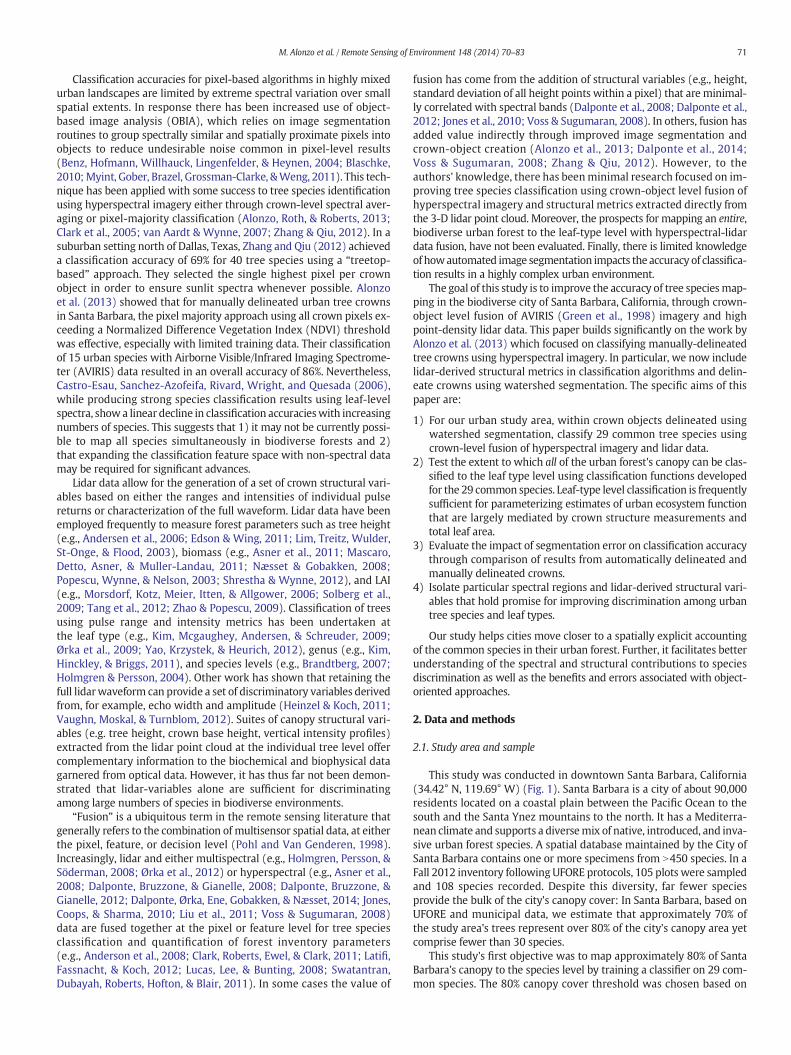
This study was conducted in downtown Santa Barbara, California(34.42° N, 119.69° W) (Fig. 1). Santa Barbara is a city of about 90,000residents located on a coastal plain between the Pacific Ocean to thesouth and the Santa Ynez mountains to the north. It has a Mediterra-nean climate and supports a diversemix of native, introduced, and inva-sive urban forest species. A spatial database maintained by the City ofSanta Barbara contains one or more specimens from N450 species. In aFall 2012 inventory following UFORE protocols, 105 plots were sampledand 108 species recorded. Despite this diversity, far fewer speciesprovide the bulk of the city's canopy cover: In Santa Barbara, based onUFORE and municipal data, we estimate that approximately 70% ofthe study area's trees represent over 80% of the city's canopy area yetcomprise fewer than 30 species.

This study's first objective was to map approximately 80% of SantaBarbara's canopy to the species level by training a classifier on 29 com-mon species. The 80% canopy cover threshold was chosen based on

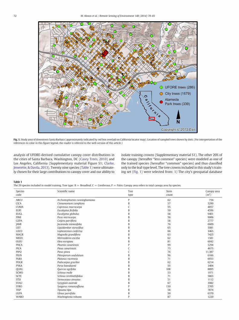
Fig. 1. Study area of downtown Santa Barbara (approximately indicated by red box overlaid on California locator map). Location of sampled trees shown by dots. (For interpretation of thereferences to color in this figure legend, the reader is referred to the web version of this article.)

72 M. Alonzo et al. / Remote Sensing of Environment 148 (2014) 70–83

analysis of UFORE-derived cumulative canopy cover distributions inthe cities of Santa Barbara, Washington, DC (Casey Trees, 2010) andLos Angeles, California (Supplementary material Figure S1; Clarke,Jenerette, & Davila, 2013). Twenty nine species (Table 1)were ultimate-ly chosen for their large contributions to canopy cover and our ability to

Table 1The 29 species included in model training. Tree type: B = Broadleaf, C = Coniferous, P = Pal

Speciescode

Scientific name

ARCU Archontophoenix cunninghamianaCICA Cinnamomum camphoraCUMA Cupressus macrocarpaEUFI Eucalyptus ficifoliaEUGL Eucalyptus globulusFIMI Ficus microcarpaGEPA Geijera parvifloraJAMI Jacaranda mimosifoliaLIST Liquidambar styracifluaLOCO Lophestemon confertusMAGR Magnolia grandifloraMEEX Metrosideros excelsaOLEU Olea europaeaPHCA Phoenix canariensisPICA Pinus canariensisPIPI2 Pinus pineaPIUN Pittosporum undulatumPLRA Platanus racemosaPOGR Podocarpus graciliorPYKA Pyrus kawakamiiQUAG Quercus agrifoliaSCMO Schinus molleSCTE Schinus terebinthifoliusSTSI Stenocarpus sinuatusSYAU Syzygium australeSYRO Syagarus romanzoffianaTISP Tipuana tipuULPA Ulmus parvifoliaWARO Washingtonia robusta

isolate training crowns (Supplementary material S1). The other 20% ofthe canopy (hereafter “less common” species) were modeled as one ofthe trained species (hereafter “common” species) and thus classifiedonly to the leaf-type level. The tree crowns included in this study's train-ing set (Fig. 1) were selected from: 1) The city's geospatial database

m. Canopy area refers to total canopy area by species.

Treetype

Stemcount

Canopy area(m2)

P 62 756B 57 5290C 55 4857B 50 4596B 58 9401B 56 9006B 58 2777B 76 6609B 65 5081B 66 3465B 63 7425B 62 1581B 81 6042P 99 5294C 73 4675C 76 11,387B 96 6166B 71 6933B 62 6214B 55 3404B 108 8895B 53 1971B 71 5863B 51 1112B 67 3982P 130 2705B 58 7874B 50 6370P 87 1220

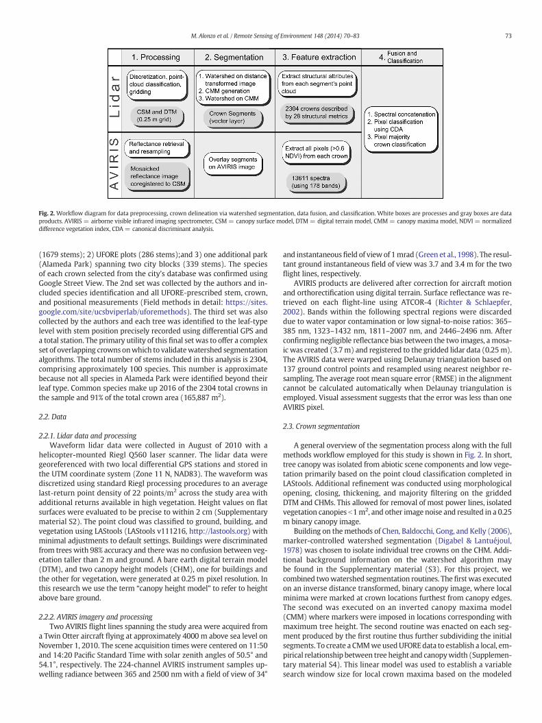
Fig. 2. Workflow diagram for data preprocessing, crown delineation via watershed segmentation, data fusion, and classification. White boxes are processes and gray boxes are dataproducts. AVIRIS = airborne visible infrared imaging spectrometer, CSM = canopy surface model, DTM = digital terrain model, CMM = canopy maxima model, NDVI = normalizeddifference vegetation index, CDA = canonical discriminant analysis.


(1679 stems); 2) UFORE plots (286 stems);and 3) one additional park(Alameda Park) spanning two city blocks (339 stems). The speciesof each crown selected from the city's database was confirmed usingGoogle Street View. The 2nd set was collected by the authors and in-cluded species identification and all UFORE-prescribed stem, crown,and positional measurements (Field methods in detail: https://sites.google.com/site/ucsbviperlab/uforemethods). The third set was alsocollected by the authors and each tree was identified to the leaf-typelevel with stem position precisely recorded using differential GPS anda total station. The primary utility of this final set was to offer a complexset of overlapping crownsonwhich to validatewatershed segmentationalgorithms. The total number of stems included in this analysis is 2304,comprising approximately 100 species. This number is approximatebecause not all species in Alameda Park were identified beyond theirleaf type. Common species make up 2016 of the 2304 total crowns inthe sample and 91% of the total crown area (165,887 m2).

2.2. Data

2.2.1. Lidar data and processingWaveform lidar data were collected in August of 2010 with a

helicopter-mounted Riegl Q560 laser scanner. The lidar data weregeoreferenced with two local differential GPS stations and stored inthe UTM coordinate system (Zone 11 N, NAD83). The waveform wasdiscretized using standard Riegl processing procedures to an averagelast-return point density of 22 points/m2 across the study area withadditional returns available in high vegetation. Height values on flatsurfaces were evaluated to be precise to within 2 cm (Supplementarymaterial S2). The point cloud was classified to ground, building, andvegetation using LAStools (LAStools v111216, http://lastools.org) withminimal adjustments to default settings. Buildings were discriminatedfrom trees with 98% accuracy and there was no confusion between veg-etation taller than 2 m and ground. A bare earth digital terrain model(DTM), and two canopy height models (CHM), one for buildings andthe other for vegetation, were generated at 0.25 m pixel resolution. Inthis research we use the term “canopy height model” to refer to heightabove bare ground.

2.2.2. AVIRIS imagery and processingTwo AVIRIS flight lines spanning the study area were acquired from

a Twin Otter aircraft flying at approximately 4000 m above sea level onNovember 1, 2010. The scene acquisition times were centered on 11:50and 14:20 Pacific Standard Time with solar zenith angles of 50.5° and54.1°, respectively. The 224-channel AVIRIS instrument samples up-welling radiance between 365 and 2500 nm with a field of view of 34°

and instantaneousfield of view of 1mrad (Green et al., 1998). The resul-tant ground instantaneous field of view was 3.7 and 3.4 m for the twoflight lines, respectively.

AVIRIS products are delivered after correction for aircraft motionand orthorectification using digital terrain. Surface reflectance was re-trieved on each flight-line using ATCOR-4 (Richter & Schlaepfer,2002). Bands within the following spectral regions were discardeddue to water vapor contamination or low signal-to-noise ratios: 365–385 nm, 1323–1432 nm, 1811–2007 nm, and 2446–2496 nm. Afterconfirming negligible reflectance bias between the two images, a mosa-ic was created (3.7m) and registered to the gridded lidar data (0.25m).The AVIRIS data were warped using Delaunay triangulation based on137 ground control points and resampled using nearest neighbor re-sampling. The average root mean square error (RMSE) in the alignmentcannot be calculated automatically when Delaunay triangulation isemployed. Visual assessment suggests that the error was less than oneAVIRIS pixel.

2.3. Crown segmentation

A general overview of the segmentation process along with the fullmethods workflow employed for this study is shown in Fig. 2. In short,tree canopy was isolated from abiotic scene components and low vege-tation primarily based on the point cloud classification completed inLAStools. Additional refinement was conducted using morphologicalopening, closing, thickening, and majority filtering on the griddedDTM and CHMs. This allowed for removal of most power lines, isolatedvegetation canopies b1m2, and other image noise and resulted in a 0.25m binary canopy image.

Building on themethods of Chen, Baldocchi, Gong, and Kelly (2006),marker-controlled watershed segmentation (Digabel & Lantuéjoul,1978) was chosen to isolate individual tree crowns on the CHM. Addi-tional background information on the watershed algorithm maybe found in the Supplementary material (S3). For this project, wecombined twowatershed segmentation routines. The first was executedon an inverse distance transformed, binary canopy image, where localminima were marked at crown locations furthest from canopy edges.The second was executed on an inverted canopy maxima model(CMM) where markers were imposed in locations corresponding withmaximum tree height. The second routine was enacted on each seg-ment produced by the first routine thus further subdividing the initialsegments. To create a CMMweusedUFOREdata to establish a local, em-pirical relationship between tree height and canopywidth (Supplemen-tary material S4). This linear model was used to establish a variablesearch window size for local crown maxima based on the modeled

https://sites.google.com/site/ucsbviperlab/uforemethods

https://sites.google.com/site/ucsbviperlab/uforemethods

http://lastools.org

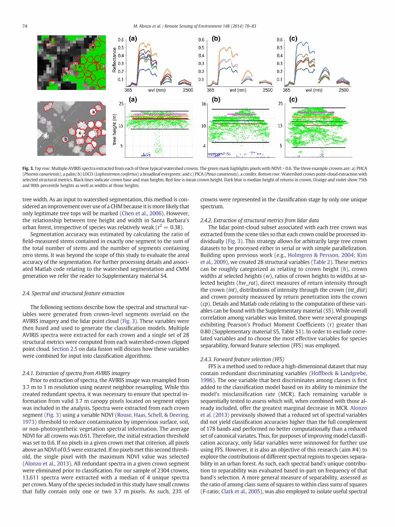
Fig. 3. Top row: Multiple AVIRIS spectra extracted from each of three typical watershed crowns. The greenmask highlights pixels with NDVI N 0.6. The three example crowns are: a) PHCA(Phoenix canariensis), a palm; b) LOCO (Lophostemon confertus) a broadleaf evergreen; and c) PICA (Pinus canariensis), a conifer. Bottom row:Watershed crown point-cloud extractionwithselected structural metrics. Black lines indicate crown base andmax heights. Red line is mean crown height. Dark blue is median height of returns in crown. Orange and violet show 75thand 90th percentile heights as well as widths at those heights.


tree width. As an input to watershed segmentation, this method is con-sidered an improvement over use of a CHMbecause it ismore likely thatonly legitimate tree tops will be marked (Chen et al., 2006). However,the relationship between tree height and width in Santa Barbara'surban forest, irrespective of species was relatively weak (r2 = 0.38).

Segmentation accuracy was estimated by calculating the ratio offield-measured stems contained in exactly one segment to the sum ofthe total number of stems and the number of segments containingzero stems. It was beyond the scope of this study to evaluate the arealaccuracy of the segmentation. For further processing details and associ-ated Matlab code relating to the watershed segmentation and CMMgeneration we refer the reader to Supplementary material S4.

2.4. Spectral and structural feature extraction

The following sections describe how the spectral and structural var-iables were generated from crown-level segments overlaid on theAVIRIS imagery and the lidar point cloud (Fig. 3). These variables werethen fused and used to generate the classification models. MultipleAVIRIS spectra were extracted for each crown and a single set of 28structural metrics were computed from each watershed-crown clippedpoint cloud. Section 2.5 on data fusion will discuss how these variableswere combined for input into classification algorithms.

2.4.1. Extraction of spectra from AVIRIS imageryPrior to extraction of spectra, the AVIRIS image was resampled from

3.7 m to 1 m resolution using nearest neighbor resampling. While thiscreated redundant spectra, it was necessary to ensure that spectral in-formation from valid 3.7 m canopy pixels located on segment edgeswas included in the analysis. Spectra were extracted from each crownsegment (Fig. 3) using a variable NDVI (Rouse, Haas, Schell, & Deering,1973) threshold to reduce contamination by impervious surface, soil,or non-photosynthetic vegetation spectral information. The averageNDVI for all crowns was 0.61. Therefore, the initial extraction thresholdwas set to 0.6. If no pixels in a given crown met that criterion, all pixelsabove anNDVI of 0.5were extracted. If nopixelsmet this second thresh-old, the single pixel with the maximum NDVI value was selected(Alonzo et al., 2013). All redundant spectra in a given crown segmentwere eliminated prior to classification. For our sample of 2304 crowns,13,611 spectra were extracted with a median of 4 unique spectraper crown.Many of the species included in this study have small crownsthat fully contain only one or two 3.7 m pixels. As such, 23% of

crowns were represented in the classification stage by only one uniquespectrum.

2.4.2. Extraction of structural metrics from lidar dataThe lidar point-cloud subset associated with each tree crown was

extracted from the scene tiles so that each crown could be processed in-dividually (Fig. 3). This strategy allows for arbitrarily large tree crowndatasets to be processed either in serial or with simple parallelization.Building upon previous work (e.g., Holmgren & Persson, 2004; Kimet al., 2009), we created 28 structural variables (Table 2). These metricscan be roughly categorized as relating to crown height (h), crownwidths at selected heights (w), ratios of crown heights to widths at se-lected heights (hw_rat), direct measures of return intensity throughthe crown (int), distributions of intensity through the crown (int_dist)and crown porosity measured by return penetration into the crown(cp). Details and Matlab code relating to the computation of these vari-ables can be foundwith the Supplementarymaterial (S5).While overallcorrelation among variables was limited, there were several groupingsexhibiting Pearson's Product Moment Coefficients (r) greater than0.80 (Supplementary material S5, Table S1). In order to exclude corre-lated variables and to choose the most effective variables for speciesseparability, forward feature selection (FFS) was employed.

2.4.3. Forward feature selection (FFS)FFS is a method used to reduce a high-dimensional dataset that may

contain redundant discriminating variables (Hoffbeck & Landgrebe,1996). The one variable that best discriminates among classes is firstadded to the classification model based on its ability to minimize themodel's misclassification rate (MCR). Each remaining variable issequentially tested to assess which will, when combined with those al-ready included, offer the greatest marginal decrease in MCR. Alonzoet al. (2013) previously showed that a reduced set of spectral variablesdid not yield classification accuracies higher than the full complementof 178 bands and performed no better computationally than a reducedset of canonical variates. Thus, for purposes of improvingmodel classifi-cation accuracy, only lidar variables were winnowed for further useusing FFS. However, it is also an objective of this research (aim #4) toexplore the contributions of different spectral regions to species separa-bility in an urban forest. As such, each spectral band's unique contribu-tion to separability was evaluated based in-part on frequency of thatband's selection. A more general measure of separability, assessed asthe ratio of among class sums of squares to within class sums of squares(F-ratio; Clark et al., 2005), was also employed to isolate useful spectral

Table 2Lidar-derived structural variables. Bold entries were selected for inclusion in classificationmodels for watershed crowns.

Variable Description

h_1 Max crown heighth_2 Median height of returns in crownh_3 Crown surface height: 0.25 m spatial resolutionh_4 Crown surface height: 1 m spatial resolutionh_5 Crown base heightw_1 Crown width at median height of returns in crownw_2 Crown width at 50th percentile heightw_3 Crown width at 75th percentile heightw_4 Crown width at 90th percentile heighthw_rat_1 Ratio of crown length to tree heighthw_rat_2 Ratio of crown height to width: median heighthw_rat_3 Ratio of crown height to width: 90th percentile heighthw_rat_4 Ratio of crown height to width: 75th percentile heighthw_rat_5 Ratio of width at 90th percentile height to mean heighthw_rat_6 Ratio of N-S width to E-W widthint_1 Average intensity above median heightint_2 Average intensity belowmedian heightint_3 Crown surface intensity: 0.25 m spatial resolutionint_4 Crown surface intensity: 1 m spatial resolutionint_dist_1 Crown surface intensity/overall average crown intensityint_dist_2 Skewness of intensity distribution through crownint_dist_3 Surface intensity (0.25 m)/surface intensity (1 m)int_dist_4 Return intensity above median crown height/belowcp_1 Surface heights (0.25 m)/surface heights (1 m)cp_2 (Mean crown height - median height of returns)/crown heightcp_3 Count of returns in 0.5 m vertical slice at 90th

percentile height divided by width at that heightcp_4 Count of returns in 0.5 m vertical slice at mean crown height

divided by width at that heightcp_5 Count of returns in 0.5 m vertical slice at median height of

crown returns divided by width at that height


regions and categories of structural metrics (e.g. all variables related toheight).

To explore the sensitivity of the structural variables to crown seg-mentation error, FFS was run on both manually delineated crowns(hereafter manual crowns) and watershed segments (hereafter water-shed crowns). FFSwas run on each set 100 timeswith crowns randomlypartitioned each run into training and validation sets tomitigate the im-pact of crown variability in the sample. The seven structuralmetrics thatwere chosen using manual crowns in more than 30% of the runs andthat demonstrated minimal intercorrelation were retained for furtheruse. Accordingly, the 7 most-frequently selected metrics exhibitinglow correlation were chosen for the watershed crowns (Table 2).

2.5. Data fusion and classification

2.5.1. Fusing spectral and structural data at the crown levelIn this study, themajority of tree crowns containedmultiple, unique

spectra meeting the 0.6 NDVI threshold. However, there was only oneset of structural metrics extracted per crown (Fig. 3). Alonzo et al.(2013) demonstrated that retaining multiple pixels per crown andassigning a class to the crown object using a pixel majority (“winner-take-all”) approachwasmore accurate than classification using a single,crown-mean spectrum. As such, for each crown, we chose to replicatethe set of structuralmetrics to correspondwith the number of extractedspectra. The resulting data matrix for manual crowns contained 12,773rows and 206 columns, where each row represents a unique spectrumand each column contains either one of 178 spectral bands or one of28 structuralmetrics. The same structurewas created for thewatershedcrowns but with 13,317 rows.

2.5.2. Canonical discriminant analysis (CDA)All classifications in this study were conducted using canonical var-

iates in a linear discriminant analysis (LDA) classifier. LDA has proven

useful previously in remote sensing research for separating highly over-lapping classes in (e.g., Clark et al., 2005; Pu, 2009; Yu, Ostland, Gong, &Pu, 1999). In LDA, classification equations are formulated based onthe pooled within-class covariance matrix of the set of independentvariables. An observation is assigned to the class with the highest classi-fication function score (Duda & Hart, 1973). In canonical discriminantanalysis one replaces p original variables with up to g − 1 derived ca-nonical variates, where g is the number of classes (i.e., 29 tree species;Klecka, 1980). Whereas principal components analysis (PCA) and min-imum noise fraction (MNF) summarize the total variability among theset of independent variables, the canonical rotation summarizes the be-tween class variance among g classes. The derived canonical discrimi-nant functions are linear combinations of the original variables wherethe coefficients maximize the between-group separation. Data reduc-tionwith this technique has been successfully applied to remote sensingclassification problems including urban tree species discrimination(Alonzo et al., 2013; Pu & Liu, 2011; Zhao & Maclean, 2000). Comparedto LDA on p original variables, CDA dramatically improves computation-al performance and, in the case of limited training data, can avoid the ill-posed problem where the number of variables is greater than thenumber of observations.

2.5.3. Classification candidate setsThe primary goal of this research was to assess the accuracy with

which we could map tree species in a heterogeneous urban forestusing fused hyperspectral and lidar data. We attempt to map 29 com-mon species that comprise much of Santa Barbara's canopy area andprovide the majority of urban-forest derived ecosystem services. Weacknowledge that it is currently impossible to train a classification algo-rithm on all species present in an urban area. Thus, we trained our CDAclassifier to label all crowns as one of the 29 common species. At theleaf-type level, the classification was deemed successful when acrown was labeled as a common species with a matching leaf type.For example, if a Quercus suber (less common species) was classifiedas Quercus agrifolia (common species) then the leaf-type classificationwas correct.

In order to separately assess classification accuracy for the 29 com-mon species and the ~70 less common species we subdivided the2304 total crowns into the four overlapping sets listed below (each cor-responding research aim from the Introduction section is also noted):

1) Accuracy for mapping 29 common species (2016 crowns) to thespecies level (aims #1 & #3)

2) Accuracy for mapping same 29 common species to the leaf-typelevel (aims #2 & #3)

3) Accuracy for mapping ~70 less common species (288 crowns) to theleaf-type level (aims #2 & #3)

4) Accuracy for mapping ~100 total species (2304 crowns) to the leaf-type level (aims #2 & #3)

2.5.4. Variable combinationsEach candidate set listed in Section 2.5.3 was classified using four

different variable subsets. The purpose of adding and holding out vari-ables linkswith research aim#1:we seek to assess the respective valuesof hyperspectral data, lidar data, and object-level fusion of both inclassification accuracy at the species and leaf-type levels. Prior to classi-fication, for the sake of computational efficiency and methodologicalconsistency, each variable combination was reduced to the maximumnumber of canonical variates with significant discriminating power(α = 0.05). The rotated variable sets used to generate classificationequations were thus:

1) All hyperspectral bands (178) and all lidar-based structure variables(28) reduced to 28 canonical variates (hereafter: CDA-full).

2) All spectral bands and the subset of 7 lidar variables selected usingFFS, reduced to 28 canonical variates (CDA-7fuse).

Table 3Segmentation accuracy. In bold: 1960 stems were appropriately placed in one watershedcrown. Eighty-five segments were without stems.

Stems in segment 0 1 2 3 4 5 6 7 8Segment count 85 1960 75 27 10 5 1 1 1


3) All hyperspectral bands (178) reduced to 28 canonical variates(CDA-spec).

4) Seven FFS-selected lidar bands reduced to 5 significant canonicalvariates (CDA-lid).

2.5.5. Classification approachOf the 2304 crowns included in this study, 25 manually delineated

crowns fromeach of the 29 common species, 725 in total, were random-ly selected and permanently set aside for model training, leaving 1579for testing at the leaf-type level and 1291 for testing at the specieslevel. It is necessary to train an object-level classification model usingmanually delineated crowns in order to assure that the full segmentarea is composed of one and only one known species (Dalponte et al.,2014). The set of watershed crowns that spatially aligned with the725 manual crowns was also excluded from the testing to ensure dis-joint training and test sets. Ultimately, the 1579 manual crowns andthe spatially coincident set of watershed crowns were each classified.The manual crowns were classified in order to evaluate the potentialclassification errors associated with automatic segmentation (aim #3).

To accommodate the dataset's high within-species structural andspectral variation and so to minimize the impact of outlier crowns ondiscriminant function generation, the 725 training crowns weresubsampled with replacement for each of 50 model runs (mr). That is,for each model run, the discriminant functions were generated using(29 species) × (20 crowns/species) × (an average of 4 spectra percrown) = 2320 fused spectra. Bootstrapping over more model runs(mr = 100) was also investigated but model stability was deemedadequate with mr = 50.

In each model run, discriminant functions were generated based onthe current subset of trainingpixels. This set of 28 (g− 1) functionswas,in turn, multiplied through the run's training and testing datasets toproduce the canonical variates. Pixel level LDA classificationwas carriedout on the test set of canonical variates. Upon completion of eachmodelrun, a species label was assigned to each crown based on the pixel ma-jority classification. After completion of all 50 runs, the mode crown-level result was calculated and retained for final map creation and accu-racy assessment. Pixel-level classifications were also retained for com-parison with results from object-oriented approaches.

Thefinal classifications for the 1579manual crowns and the spatiallycoincident watershed segments were mapped in a GIS. A manuallydelineated ground-reference map with species information for the 29common species and leaf-type information for the less common specieswas used for spatial validation.Watershed crown accuracywas assessedonly on a canopy-area basis by spatially intersecting the validation mapwith the classified segments. Percent correctly classified canopy areahas been chosen in lieu of the number of correctly classified stems asthe primary method for reporting results for two reasons: First, froman urban forest and ecosystem services management perspective it ismore important to gather detailed information on species dominantin the local canopy. Second, it is not feasible to conduct stem-countaccuracy assessment when the unit of analysis is the potentially-misaligned crown segment. Still, to better understand the utility oflidar for classifying smaller crowns stem count accuracy was assessedfor manual crowns.

3. Results

3.1. Crown segmentation accuracy

Assessed against field observations, 83% of the watershed segmentscontained a single tree stem indicating overall good agreement(Table 3). However, the segmentation accuracy when evaluating onlytrees from UFORE plots or from Alameda Park decreased to 55%. Thisis because Alameda Park, in particular, is a highly complex urban forestsetting, with significant crown overlap among trees of all sizes and spe-cies (Fig. 4). In this type of environment, as evident in Fig. 4, there is

clear omission error. This is likely because the window size of theCMM was determined based on a weak relationship between treeheight and width. It is particularly noticeable in this figure that thewidths of tall but slender palm trees were not modeled well leadingto inclusion of neighboring stems in their segments. Still, evaluatedagainst segmentation using the CHM, there was a small overall im-provement in segmentation accuracy (1%). The improvement may bemore pronounced in densely forested areas but this was not evaluated.

3.2. Forward feature selection of structural variables and spectral bands

Using the cross-validated misclassification rate, 7 variables were se-lected for classifyingmanual crowns. The samenumberwas selected forwatershed crowns. Six of those variables appear in both selection sets,perhaps indicating that watershed crowns and manual crowns can beclassified using the same set of structural metrics (Fig. 5). The onlyvariables differing between the two sets were h_1 (max crown height)and h_2 (median height of returns in crown). For simplicity, and givenstrong intercorrelation, all further analysis was conducted using h_2and the six structural variables selected for bothmanual andwatershedcrowns. Overall, variables related to tree height and return intensitystand out with respect to their high between-class to within-class vari-ance as quantified by the normalized F-ratio. When taking variableintercorrelation into account, one heightmetric (h_2), onewidthmetric(w_1), one height-to-width ratio metric (hw_rat_2), two intensity met-rics (int_2 and int_3) and two crown porosity metrics (cp_1 and cp_3)were selected in more than 30% of the watershed crown model runs(Fig. 6). That the set of variables selected for each set of objects is nearlyidentical may highlight the success of segmenting an image largelycomprising street trees. It may also indicate that the selected variablesare robust to minor aberrations in morphology.

Spectral bands were chosen most consistently from the visibleregion of the spectrum (VIS, 394–734 nm; Fig. 6). This correspondswith an F-ratio that is relatively high from 400 nm until the red edgeat approximately 700 nm. In particular, bands were selected surround-ing the green peakbetween 520 and 590nm. Selection frequency in thatregion was driven by discriminatory power and also by relatively lowcorrelation with neighboring bands in the VIS as well as with bands inthe shortwave infrared 2 (SWIR2, 2018–2425 nm; Supplementary ma-terial S6). The near infrared region (NIR, 744–1313 nm) displayed lowF-ratios and yielded one band selected with particular frequency inthe liquid water absorption feature centered on 1197 nm. The short-wave infrared 1 region (SWIR1, 1443–1802 nm) and SWIR2 regionsyielded high F-ratios but only SWIR1 held bands selected in more than30% of model runs. The lack of band selection from SWIR2 may be aresult of high overall correlation with the VIS (r = 0.84) and theSWIR1 (r = 0.83).

3.3. Classification results

3.3.1. Classification of the 29 common speciesThe CDA-7fuse variable combination yielded the highest overall

species-level classification accuracy (83.4% of canopy area, kappa =82.6) for watershed crowns containing common species (Fig. 7a).Species-level classification accuracy with only hyperspectral data(CDA-spec) was 79.2%. Lidar data only (CDA-lid) yielded an accuracy of32.9%. The best fused result using the manual crowns was 85.4%, sug-gesting minimal impact on classification accuracy by segmentationerror (Fig. 8). These object-level results compare favorably to 68%

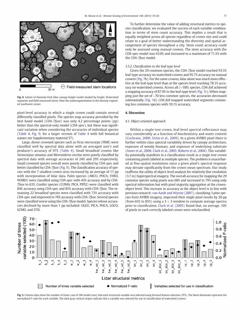
Fig. 4. Subset of Alameda Park lidar canopy height model shaded by height. Watershedsegments and field-measured stems. Note the undersegmentation in the densely vegetat-ed southwest corner.


pixel-level accuracy in which a single crown could contain severaldifferently classified pixels. The species map accuracy provided by thebest fused model (CDA-7fuse) was only 4.2 percentage points (pp)better than the spectral-only model (CDA-spec), but there was signifi-cant variation when considering the accuracies of individual species(Table 4, Fig. 9; for a larger version of Table 4 with full botanicalnames see Supplementary material S7).

Large, dense crowned species such as Ficus microcarpa (FIMI) wereclassified well by spectral data alone with an averaged user's andproducer's accuracy of 97% (Table 4). Small broadleaf crowns likeStenocarpus sinuatus and Metrosideros excelsa were poorly classified byspectral data with average accuracies of 24% and 29% respectively.Small crowned species overall were poorly classified by CDA-spec andbetter classified by CDA-7fuse (Fig. 9). The classification accuracy of spe-cies with the 7 smallest crown sizes increased by an average of 17 ppwith incorporation of lidar data. Palm species (ARCU, PHCA, SYRO,WARO) were classified using CDA-spec with 43% accuracy and by CDA-7fuse to 63%. Conifer species (CUMA, PICA, PIPI2) were classified with84% accuracy using CDA-spec and 85% accuracy with CDA-7fuse. The re-maining 22 broadleaf species were classified with 73% accuracy withCDA-spec and improved to 78% accuracywith CDA-7fuse. Several specieswere classifiedworse using the CDA-7fusemodel. Specieswhose accura-cies declined by more than 1 pp included: OLEU, PICA, PHCA, LOCO,SCMO, and STSI.

Fig. 5. Column data show the number of times (out of 100model runs) that each structural varinormalized F-ratio for each variable. The dark gray vertical stripes indicate that a variable was

To further determine the value of adding structural metrics to spe-cies classification, we evaluated the success of each variable combina-tion in terms of stem count accuracy. This implies a result that isequally weighted across all species regardless of crown size and couldrelate to a goal of better understanding the diversity and spatial ar-rangement of species throughout a city. Stem count accuracy couldonly be assessed using manual crowns. The stem accuracy with theCDA-spec model was 63.0% and increased to a maximum of 71.5% withthe CDA-7fuse model.

3.3.2. Classification to the leaf-type levelGiven the 29 common species, the CDA-7fuse model reached 93.5%

leaf-type accuracy on watershed crowns and 95.7% accuracy onmanualcrowns (Fig. 7b). For the same crowns, lidar alonewasmuchmore effec-tive at the leaf-type level than at the species level reaching 78.1% accu-racy on watershed crowns. Across all (~100) species, CDA-full achievedamapping accuracy of 87.9% to the leaf-type level (Fig. 7c). Whenmap-ping just the set of ~70 less common species, the accuracies decreasedsubstantially (Fig. 7d). CDA-full mapped watershed segments contain-ing less common species with 59.1% accuracy.

4. Discussion

4.1. Object oriented approach

Within a single tree crown, leaf-level spectral reflectance mayvary considerably as a function of biochemistry and water content(Cochrane, 2000; Ustin et al., 2009). In a given AVIRIS pixel there isfurther within-class spectral variability driven by canopy architecture,exposure of woody biomass, and exposure of underlying substrate(Asner et al., 2008; Clark et al., 2005; Roberts et al., 2004). This variabil-ity potentially manifests in a classification result as a single tree crowncontaining pixels labeled asmultiple species. The problem is exacerbat-ed at fine-spatial resolutions since a given pixel's spectral responsemay deviate significantly from the crown mean spectrum. Our studyreaffirms the utility of object-level analysis for relatively fine resolution(3.7m) hyperspectral imagery. The overall accuracy formapping the 29common species using pixels was 68% and increased to 79% using onlyspectral information but with pixel majority aggregation at the crown-object level. This increase in accuracy at the object level is in line withprevious research: van Aardt andWynne (2007), classifying 3 pine spe-cies from AVIRIS imagery, improved their single pixel results by 20 pp(from 65% to 85%) using a 3 × 3 window to compute average spectraprior to classification. Clark et al. (2005) found that, on average, 10%of pixels in each correctly labeled crown were misclassified.

able was selected using forward feature selection (FFS). The black diamonds represent theselected for use in classification of watershed crowns.

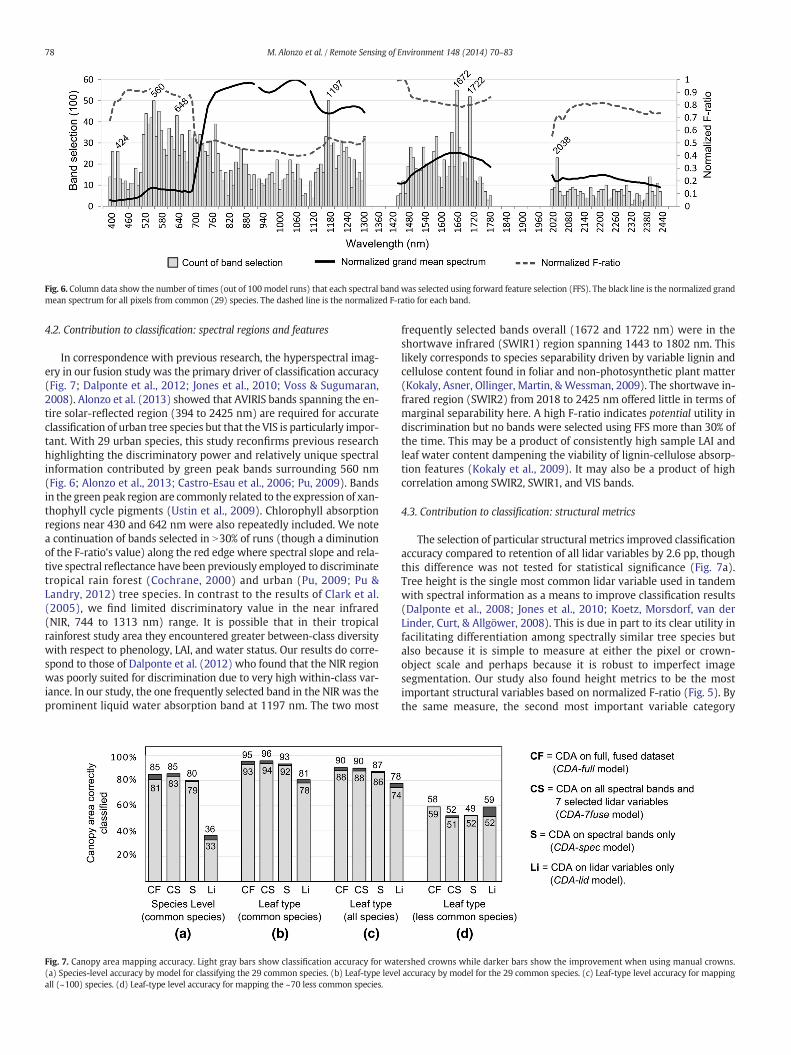
Fig. 6. Column data show the number of times (out of 100model runs) that each spectral band was selected using forward feature selection (FFS). The black line is the normalized grandmean spectrum for all pixels from common (29) species. The dashed line is the normalized F-ratio for each band.


4.2. Contribution to classification: spectral regions and features

In correspondence with previous research, the hyperspectral imag-ery in our fusion study was the primary driver of classification accuracy(Fig. 7; Dalponte et al., 2012; Jones et al., 2010; Voss & Sugumaran,2008). Alonzo et al. (2013) showed that AVIRIS bands spanning the en-tire solar-reflected region (394 to 2425 nm) are required for accurateclassification of urban tree species but that the VIS is particularly impor-tant. With 29 urban species, this study reconfirms previous researchhighlighting the discriminatory power and relatively unique spectralinformation contributed by green peak bands surrounding 560 nm(Fig. 6; Alonzo et al., 2013; Castro-Esau et al., 2006; Pu, 2009). Bandsin the green peak region are commonly related to the expression of xan-thophyll cycle pigments (Ustin et al., 2009). Chlorophyll absorptionregions near 430 and 642 nm were also repeatedly included. We notea continuation of bands selected in N30% of runs (though a diminutionof the F-ratio's value) along the red edge where spectral slope and rela-tive spectral reflectance have been previously employed to discriminatetropical rain forest (Cochrane, 2000) and urban (Pu, 2009; Pu &Landry, 2012) tree species. In contrast to the results of Clark et al.(2005), we find limited discriminatory value in the near infrared(NIR, 744 to 1313 nm) range. It is possible that in their tropicalrainforest study area they encountered greater between-class diversitywith respect to phenology, LAI, and water status. Our results do corre-spond to those of Dalponte et al. (2012) who found that the NIR regionwas poorly suited for discrimination due to very high within-class var-iance. In our study, the one frequently selected band in the NIR was theprominent liquid water absorption band at 1197 nm. The two most

Fig. 7. Canopy area mapping accuracy. Light gray bars show classification accuracy for wat(a) Species-level accuracy by model for classifying the 29 common species. (b) Leaf-type leveall (~100) species. (d) Leaf-type level accuracy for mapping the ~70 less common species.

frequently selected bands overall (1672 and 1722 nm) were in theshortwave infrared (SWIR1) region spanning 1443 to 1802 nm. Thislikely corresponds to species separability driven by variable lignin andcellulose content found in foliar and non-photosynthetic plant matter(Kokaly, Asner, Ollinger, Martin, & Wessman, 2009). The shortwave in-frared region (SWIR2) from 2018 to 2425 nm offered little in terms ofmarginal separability here. A high F-ratio indicates potential utility indiscrimination but no bands were selected using FFS more than 30% ofthe time. This may be a product of consistently high sample LAI andleaf water content dampening the viability of lignin-cellulose absorp-tion features (Kokaly et al., 2009). It may also be a product of highcorrelation among SWIR2, SWIR1, and VIS bands.

4.3. Contribution to classification: structural metrics

The selection of particular structural metrics improved classificationaccuracy compared to retention of all lidar variables by 2.6 pp, thoughthis difference was not tested for statistical significance (Fig. 7a).Tree height is the single most common lidar variable used in tandemwith spectral information as a means to improve classification results(Dalponte et al., 2008; Jones et al., 2010; Koetz, Morsdorf, van derLinder, Curt, & Allgöwer, 2008). This is due in part to its clear utility infacilitating differentiation among spectrally similar tree species butalso because it is simple to measure at either the pixel or crown-object scale and perhaps because it is robust to imperfect imagesegmentation. Our study also found height metrics to be the mostimportant structural variables based on normalized F-ratio (Fig. 5). Bythe same measure, the second most important variable category

ershed crowns while darker bars show the improvement when using manual crowns.l accuracy by model for the 29 common species. (c) Leaf-type level accuracy for mapping

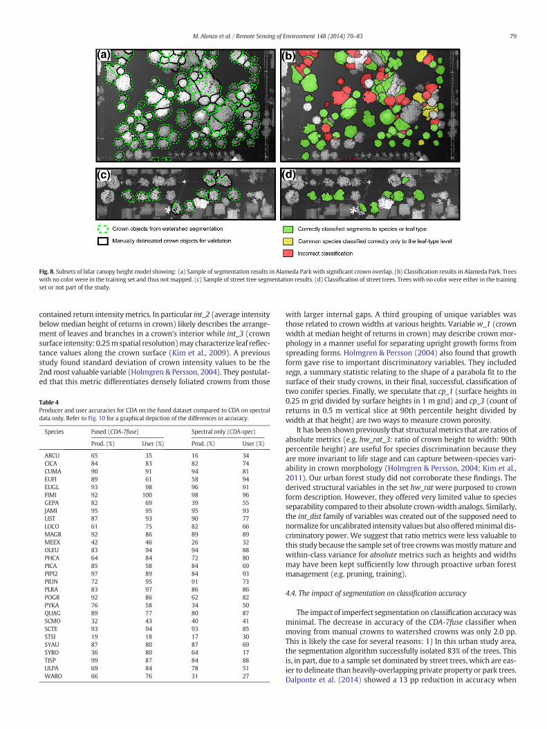
Fig. 8. Subsets of lidar canopy height model showing: (a) Sample of segmentation results in Alameda Parkwith significant crown overlap. (b) Classification results in Alameda Park. Treeswith no color were in the training set and thus not mapped. (c) Sample of street tree segmentation results. (d) Classification of street trees. Trees with no color were either in the trainingset or not part of the study.


contained return intensitymetrics. In particular int_2 (average intensitybelow median height of returns in crown) likely describes the arrange-ment of leaves and branches in a crown's interior while int_3 (crownsurface intensity: 0.25m spatial resolution)may characterize leaf reflec-tance values along the crown surface (Kim et al., 2009). A previousstudy found standard deviation of crown intensity values to be the2ndmost valuable variable (Holmgren & Persson, 2004). They postulat-ed that this metric differentiates densely foliated crowns from those

Table 4Producer and user accuracies for CDA on the fused dataset compared to CDA on spectraldata only. Refer to Fig. 10 for a graphical depiction of the differences in accuracy.

Species Fused (CDA-7fuse) Spectral only (CDA-spec)

Prod. (%) User (%) Prod. (%) User (%)

ARCU 65 35 16 34CICA 84 83 82 74CUMA 90 91 94 81EUFI 89 61 58 94EUGL 93 98 96 91FIMI 92 100 98 96GEPA 82 69 39 55JAMI 95 95 95 93LIST 87 93 90 77LOCO 61 75 82 66MAGR 92 86 89 89MEEX 42 46 26 32OLEU 83 94 94 88PHCA 64 84 72 80PICA 85 58 84 69PIPI2 97 89 84 93PIUN 72 95 91 73PLRA 83 97 86 86POGR 92 86 62 82PYKA 76 58 34 50QUAG 89 77 80 87SCMO 32 43 40 41SCTE 93 94 93 85STSI 19 18 17 30SYAU 87 80 87 69SYRO 36 80 64 17TISP 99 87 84 88ULPA 69 84 78 51WARO 66 76 31 27

with larger internal gaps. A third grouping of unique variables wasthose related to crown widths at various heights. Variable w_1 (crownwidth at median height of returns in crown) may describe crown mor-phology in a manner useful for separating upright growth forms fromspreading forms. Holmgren & Persson (2004) also found that growthform gave rise to important discriminatory variables. They includedsegp, a summary statistic relating to the shape of a parabola fit to thesurface of their study crowns, in their final, successful, classification oftwo conifer species. Finally, we speculate that cp_1 (surface heights in0.25 m grid divided by surface heights in 1 m grid) and cp_3 (count ofreturns in 0.5 m vertical slice at 90th percentile height divided bywidth at that height) are two ways to measure crown porosity.

It has been shownpreviously that structuralmetrics that are ratios ofabsolute metrics (e.g. hw_rat_3: ratio of crown height to width: 90thpercentile height) are useful for species discrimination because theyare more invariant to life stage and can capture between-species vari-ability in crown morphology (Holmgren & Persson, 2004; Kim et al.,2011). Our urban forest study did not corroborate these findings. Thederived structural variables in the set hw_rat were purposed to crownform description. However, they offered very limited value to speciesseparability compared to their absolute crown-width analogs. Similarly,the int_dist family of variables was created out of the supposed need tonormalize for uncalibrated intensity values but also offeredminimal dis-criminatory power. We suggest that ratio metrics were less valuable tothis study because the sample set of tree crownswasmostlymature andwithin-class variance for absolute metrics such as heights and widthsmay have been kept sufficiently low through proactive urban forestmanagement (e.g. pruning, training).

4.4. The impact of segmentation on classification accuracy

The impact of imperfect segmentation on classification accuracywasminimal. The decrease in accuracy of the CDA-7fuse classifier whenmoving from manual crowns to watershed crowns was only 2.0 pp.This is likely the case for several reasons: 1) In this urban study area,the segmentation algorithm successfully isolated 83% of the trees. Thisis, in part, due to a sample set dominated by street trees, which are eas-ier to delineate than heavily-overlapping private property or park trees.Dalponte et al. (2014) showed a 13 pp reduction in accuracy when

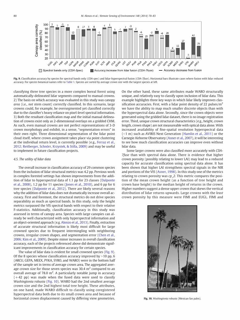
Fig. 9. Classification accuracy by species for spectral bands only (CDA-spec) and lidar-hyperspectral fusion (CDA-7fuse). Horizontal bars illustrate cases where fusion with lidar reducedaccuracy. For species botanical names refer to Table 1. Species are sorted by average crown size with the largest species at left.

Fig. 10.Washingtonia robusta (Mexican fan palm).


classifying three tree species in a more complex boreal forest usingautomatically-delineated lidar segments compared to manual crowns.2) The basis on which accuracy was evaluated in this study was canopyarea (i.e., not stem count) correctly classified. In this scenario, largecrowns could, for example, be oversegmented yet classified correctlydue to the classifier's heavy reliance on pixel-level spectral information.3) Both the resultant classification map and the initial manual delinea-tion of crowns exist only as 2-dimensional overlays on a gridded CHM.As such, even manual crowns are not perfect representations of 3-Dcrown morphology and exhibit, in a sense, “segmentation errors” intheir own right. Three dimensional segmentation of the lidar pointcloud itself, where crown assignment takes place via point clusteringat the individual return level, is currently possible (e.g., Ferraz et al.,2012; Reitberger, Schnörr, Krzystek, & Stilla, 2009) and may be usefulto implement in future classification projects.

4.5. The utility of lidar data

The overall increase in classification accuracy of 29 common speciesfrom the inclusion of lidar structural metrics was 4.2 pp. Previous workin complex forested settings has shown improvements from the addi-tion of lidar to hyperspectral data of 1.1 pp for 23 classes (Dalponteet al., 2008), 1.2 pp for 11 species (Jones et al., 2010), and 6 pp for 6tree species (Dalponte et al., 2012). There are likely several reasonswhy the addition of lidar data does not dramatically increase overall ac-curacy. First and foremost, the structural metrics do not drive speciesseparability as much as spectral bands. In this study, only the heightmetrics surpassed the VIS spectral bands with respect to their relativeF-statistics. Additionally, classification accuracy in this study wasassessed in terms of canopy area. Species with large canopies can al-ready be well characterized with only hyperspectral information andan object-oriented approach (e.g. Alonzo et al., 2013). Finally, extractionof accurate structural information is likely most difficult for largecrowned species due to frequent intermingling with neighboringcrowns, irregular crown shapes, and segmentation error (Chen et al.,2006; Kim et al., 2009). Despite minor increases in overall classificationaccuracy, each of the projects referenced above did demonstrate signif-icant improvements in classification accuracy for certain species.

The value of lidar data is evident for small crowned species (Fig. 9).Of the 8 species whose classification accuracy improved by N10 pp, 6(ARCU, GEPA, MEEX, PYKA, SYRO, and WARO) were in the bottom halfof the sample set in terms of average crown area. The aggregated aver-age crown size for those seven species was 30.4 m2 compared to anoverall average of 78.0 m2. A particularly notable jump in accuracy(+42 pp) was made when the fused data were used to classifyWashingtonia robusta (Fig. 10). WARO had the 2nd smallest averagecrown size and the 2nd highest total tree height. These attributes,on one hand, made WARO difficult to classify using coregisteredhyperspectral data both due to its small crown area and because ofhorizontal crown displacement caused by differing view geometries.

On the other hand, these same attributes made WARO structurallyunique, and relatively easy to classify upon inclusion of lidar data. Thisexample highlights three key ways in which lidar likely improves clas-sification accuracies. First, with a lidar point density of 22 pulses/m2

we have the ability to map much smaller discrete objects than withthe hyperspectral data alone. Secondly, since the crown objects weregenerated using the gridded lidar dataset, there is no image registrationerror. Third, unique crown structural characteristics (e.g., height, crownlength, crown shape) are notmeasureable with optical data alone.Withincreased availability of fine-spatial resolution hyperspectral data(b1 m) such as AVIRIS Next Generation (Hamlin et al., 2011) or theCarnegie Airborne Observatory (Asner et al., 2007), it will be interestingto see how much classification accuracies can improve even withoutlidar data.

Some larger crowns were also classified more accurately with CDA-7fuse than with spectral data alone. There is evidence that highercrown porosity (possibly relating to lower LAI) may lead to a reducedcapacity for accurate classification using spectral data alone. It hasbeen shown that higher LAI strengthens spectral signals in the NIRand portions of the VIS (Asner, 1998). In this study one of the metricsrelating to crown porosity was cp_2. This metric compares the posi-tion of the mean crown height (as a function of tree height andcrown base height) to the median height of returns in the crown.Higher numbers suggest a dense upper crown that skews the verticaldistribution of lidar returns upwards. Large crowns with the leastcrown porosity by this measure were FIMI and EUGL. FIMI and


EUGLwere both classifiedwell with spectral data alone (97% and 93%average accuracies respectively) but they were also ranked 3rd and1st respectively in terms of average crown size. Large and mediumcrowns with the highest porosity were PLRA, PYKA, PICA and ULPA.From the addition of lidar data they gained 4, 25, −6, and 12 pp, re-spectively. We assume that PICA was ranked highly by this metricmore from a combination of upright crown geometry and off-nadirlidar pulses than actual high porosity.

4.6. Classification of less common species

The original choice to map 30 species was made because 80% ofSanta Barbara's canopy cover comprises roughly 30 species and thereappeared to be diminishing increases in canopy for each additional spe-cies added after this point (Supplementary material Figure S1). In SantaBarbara, 23% of the total canopy cover sampled in the UFORE field col-lection was from two species: the native Q. agrifolia (Coast live oak)and the introduced Syagrus romanzoffiana (Queen palm). This relation-ship between species mix and canopy cover may hold in other partsof the country as well. For instance, based on a 2009 UFORE study inWashington, DC (Casey Trees, 2010), roughly the same relationshipwas established with 25% of canopy composed of two native species:Fagus grandifolia (American beech) and Liriodendron tulipifera (Tuliptree). In Los Angeles, with a very arid climate and a lack of native canopydominants, the relationship shifts somewhat but 30 species would stillequate to roughly 70% of canopy cover. Given an increase in availabilityof lidar and hyperspectral datasets, these species–canopy relationshipsindicate the transferability of the methods established in this paper toconduct similar assessments for the canopy dominants in other, largercities.

In large cities, with established urban forest management programs,it is feasible to collect training data for and map ~30 species to thespecies level. However, for those, potentially, hundreds of species withlow stem counts representing the remaining 20 or 30% of canopy area,it will be pragmatic to classify only to the leaf-type level. In this study,mapping to the leaf-type level meant modeling the less commonspecies as one of the common species and checking for leaf-type agree-ment. Over the entire dataset of 2304 crowns (~100 species), leaf-typemapping reached 87.9% accuracy using CDA-full. However, when onlyclassifying the ~70 less common species the accuracy declined to59.1%. We surmise that the low accuracy with which these specieswere classified is a product of our choice to use a CDA classifier. The clas-sification functions generated were specifically tailored to maximizeseparability among the input training classes, which did not includethe less common species. This leads to a well-tuned classifier for thecommon species but one that may not be able to capture the variationin the dataset comprising the less common species. Other classificationmethods may ultimately prove superior for hierarchical classificationschemes wherein all trees are classified first to the leaf-type leveland then common species are further classified to the species level.For example, Multiple Endmember Spectral Mixture Analysis(MESMA: Roberts et al., 1998) allows for constrained classificationbased on a target spectrum's similarity to reference spectra suchthat species not represented in a spectral library would rightlyremain unclassified.

5. Conclusions

This research sought to improve species and leaf-type level mappingin the urban forest. We first selected 29 common species that dominatethe canopy in Santa Barbara, California and classified themusing CDAoncombined hyperspectral and high point-density lidar data.We achieveda species-level accuracy among trained species of 83.4%. We mappedthe entire set of sample crowns, including ~70 less common species, tothe leaf-type level with 87.9% accuracy.We believe that this study dem-onstrates the potential for separating highly overlapping species classes

using data fusion at the crown-object level. In an immediate, operation-al sense, the techniques described in this paper are likely applicablewith high accuracy (and perhaps with lower point density lidar data)for discriminating among urban vegetation growth forms (e.g. herbs,shrubs, trees) where simple structural metrics could vastly improveseparability when combined with either multi- or hyperspectral data.The data to accomplish this sort of classification are available in manycities today and the results even at this generalized level could informpolicy relating to the spatial distribution of urban ecosystem structureand function.

In line with previous research, classification accuracies in this studywere bolstered by lidar variables pertaining to tree height, crown mor-phology, and perhaps the internal arrangement of leaves and branches.In particular, we showed that small crowns and crowns with uniquemorphological characteristics were more apt to be correctly labeledwith the inclusion of structural data. Further, we showed that classifica-tion following automated crown segmentation was more accurate thana pixel-level result and the diminution in accuracy introduced fromsegmentation error was quite small. As many cities have gained accessto high-accuracy canopy coverage maps it is a reasonable next step toimplement simple crown segmentation algorithms to generate service-able crown objects for further analysis. Ultimately, the ability to bothmap dominant canopy species and inventory common but smaller spe-cies is important if we're to operationalize remotely sensed urban forestinventory.

Acknowledgments

The authors would like to thank the Naval Postgraduate School forfunding this research through grant N00244-11-1-0028, “Quantifyingthe Structure and Function of an Urban Ecosystem Using Imaging Spec-trometry, Thermal Imagery, and Small Footprint LiDAR”. Special thanksalso to: Seth Gorelik, Keri Opalk, Alex Sun, Randy Baldwin, and MattRitter for their assistance with field data collection; Joe McFadden forsupporting field work and helping to refine the manuscript; the City ofSanta Barbara for providing ground reference data; Keely Roth andSeth Peterson for help creating and fine-tuning the technical methods;and the four anonymous reviewers for their valuable comments andsuggestions.

Appendix A. Supplementary material

Supplementarymaterial for this article can be found online at http://dx.doi.org/10.1016/j.rse.2014.03.018.

References

Alonzo, M., Roth, K., & Roberts, D. (2013). Identifying Santa Barbara's urban tree speciesfrom AVIRIS imagery using canonical discriminant analysis. Remote Sensing Letters,4(5), 513–521.

Andersen, H. -E., Reutebuch, S. E., & McGaughey, R. J. (2006). A rigorous assessment oftree height measurements obtained using airborne lidar and conventional fieldmethods. Canadian Journal of Remote Sensing, 32(5), 355–366.

Anderson, J., Plourde, L., Martin, M., Braswell, B., Smith, M., Dubayah, R., et al. (2008). In-tegrating waveform lidar with hyperspectral imagery for inventory of a northerntemperate forest. Remote Sensing of Environment, 112(4), 1856–1870.

Asner, G. (1998). Biophysical and biochemical sources of variability in canopy reflectance.Remote Sensing of Environment, 64(3), 234–253.

Asner, G. P., Knapp, D. E., Kennedy-Bowdoin, T., Jones, M.O., Martin, R. E., Boardman, J.,et al. (2007). Carnegie airborne observatory: In-flight fusion of hyperspectral imagingand waveform light detection and ranging for three-dimensional studies of ecosys-tems. Journal of Applied Remote Sensing, 1(1), 1–21.

Asner, G. P., Knapp, D. E., Kennedy-Bowdoin, T., Jones, M.O., Martin, R. E., Boardman, J.,et al. (2008). Invasive species detection in Hawaiian rainforests using airborne imag-ing spectroscopy and LiDAR. Remote Sensing of Environment, 112(5), 1942–1955.

Asner, G. P., Mascaro, J., Muller-Landau, H. C., Vieilledent, G., Vaudry, R., Rasamoelina, M.,et al. (2011). A universal airborne LiDAR approach for tropical forest carbon mapping.Oecologia, 168(4), 1147–1160.

Benz, U. C., Hofmann, P., Willhauck, G., Lingenfelder, I., & Heynen, M. (2004). Multi-resolution, object-oriented fuzzy analysis of remote sensing data for GIS-ready infor-mation. ISPRS Journal of Photogrammetry and Remote Sensing, 58(3–4), 239–258.



http://refhub.elsevier.com/S0034-4257(14)00104-7/rf0005






















Blaschke, T. (2010). Object based image analysis for remote sensing. ISPRS Journal ofPhotogrammetry and Remote Sensing, 65(1), 2–16.

Bolund, P., & Hunmammar, S. (1999). Ecosystem services in urban areas. EcologicalEconomics, 29, 293–301.

Boschetti, M., Boschetti, L., Oliveri, S., Casati, L., & Canova, I. (2007). Tree species mappingwith airborne hyperspectral MIVIS data: The Ticino Park study case. InternationalJournal of Remote Sensing, 28, 1251–1261.

Brandtberg, T. (2007). Classifying individual tree species under leaf-off and leaf-onconditions using airborne lidar. ISPRS Journal of Photogrammetry and RemoteSensing, 61(5), 325–340.

Casey Trees (2010). i-Tree Ecosystem Analysis: Washington, DC. (URL: http://caseytrees.org/wp-content/uploads/2012/02/report-2010-01-ufore2009.pdf).

Castro-Esau, K., Sanchez-Azofeifa, G., Rivard, B.,Wright, S. J., &Quesada,M. (2006). Variabilityin leaf optical properties of Mesoamerican trees and the potential for species classifica-tion. American Journal of Botany, 93(4), 517–530.

Chen, Q., Baldocchi, D., Gong, P., & Kelly, M. (2006). Isolating individual trees in a savannawoodland using small footprint LiDAR data. Photogrammetric Engineering & RemoteSensing, 72(8), 923–932.

Clark, M. L., Roberts, D. A., & Clark, D. B. (2005). Hyperspectral discrimination of trop-ical rain forest tree species at leaf to crown scales. Remote Sensing of Environment,96(3–4), 375–398.

Clark, M. L., Roberts, D. A., Ewel, J. J., & Clark, D. B. (2011). Estimation of tropical rain forestaboveground biomass with small-footprint lidar and hyperspectral sensors. RemoteSensing of Environment, 115(11), 2931–2942.

Clarke, L. W., Jenerette, D.G., & Davila, A. (2013). The luxury of vegetation and the legacyof tree biodiversity in Los Angeles, CA. Landscape and Urban Planning, 116, 48–59.

Cochrane, M. (2000). Using vegetation reflectance variability for species level classificationof hyperspectral data. International Journal of Remote Sensing, 21(10), 2075–2087.

Dalponte, M., Bruzzone, L., & Gianelle, D. (2008). Fusion of hyperspectral and LIDARremote sensing data for classification of complex forest areas. IEEE Transactions onGeoscience and Remote Sensing, 46(5), 1416–1427.

Dalponte, M., Bruzzone, L., & Gianelle, D. (2012). Tree species classification inthe Southern Alps based on the fusion of very high geometrical resolutionmultispectral/hyperspectral images and LiDAR data. Remote Sensing ofEnvironment, 123, 258–270.

Dalponte, M., Ørka, H. O., Ene, L. T., Gobakken, T., & Næsset, E. (2014). Tree crown delin-eation and tree species classification in boreal forests using hyperspectral and ALSdata. Remote Sensing of Environment, 140, 306–317.

Dennison, P. E., & Roberts, D. A. (2003). The effects of vegetation phenology onendmember selection and species mapping in southern California chaparral. RemoteSensing of Environment, 87(2), 295–309.

Digabel, H., & Lantuéjoul, C. (1978). Iterative algorithms. Proc. 2nd European Symp.Quantitative analysis of microstructures in material science. Biology and Medicine,Vol. 19, No. 7. (pp. 8). Stuttgart, West Germany: Riederer Verlag.

Duda, R. O., & Hart, P. E. (1973). Pattern classification and scene analysis. New York: JohnWiley and Sons, Inc.

Edson, C., &Wing,M.G. (2011). Airborne light detection and ranging (LiDAR) for individualtree stem location, height, and biomass measurements. Remote Sensing, 3(12),2494–2528.

Escobedo, F. J., & Nowak, D. J. (2009). Spatial heterogeneity and air pollution removal byan urban forest. Landscape and Urban Planning, 90(3–4), 102–110.

Ferraz, A., Bretar, F., Jacquemoud, S., Gonçalves, G., Pereira, L., Tomé, M., et al. (2012). 3-Dmapping of a multi-layered Mediterranean forest using ALS data. Remote Sensing ofEnvironment, 121, 210–223.

Franke, J., Roberts, D. A., Halligan, K., &Menz, G. (2009). Hierarchical multiple endmemberspectral mixture analysis (MESMA) of hyperspectral imagery for urban environments.Remote Sensing of Environment, 113(8), 1712–1723.

Green, R., Eastwood, M., Sarture, C., Chrien, T., Aronsson, M., Chippendale, B., et al. (1998).Imaging spectroscopy and the airborne visible/infrared imaging spectrometer(AVIRIS). Remote Sensing of Environment, 65(3), 227–248.

Hamlin, L., Green, R. O., Mouroulis, P., Eastwood, M., Wilson, D., Dudik, M., et al. (2011).Imaging spectrometer science measurements for terrestrial ecology: AVIRIS andnew developments. Aerospace Conference, 2011 IEEE.

Heinzel, J., & Koch, B. (2011). Exploring full-waveform LiDAR parameters for tree speciesclassification. International Journal of Applied Earth Observation and Geoinformation,13(1), 152–160.

Hoffbeck, J., & Landgrebe, D. (1996). Classification of remote sensing images having highspectral resolution. Remote Sensing of Environment, 57, 119–126.

Holmgren, J., & Persson, Å. (2004). Identifying species of individual trees using airbornelaser scanner. Remote Sensing of Environment, 90(4), 415–423.

Holmgren, J., Persson, Å., & Söderman, U. (2008). Species identification of individual treesby combining high resolution LiDAR data with multi‐spectral images. InternationalJournal of Remote Sensing, 29(5), 1537–1552.

Jones, T. G., Coops, N. C., & Sharma, T. (2010). Assessing the utility of airbornehyperspectral and LiDAR data for species distribution mapping in the coastal PacificNorthwest, Canada. Remote Sensing of Environment, 114(12), 2841–2852.

Kim, S., Hinckley, T., & Briggs, D. (2011). Classifying individual tree genera using stepwisecluster analysis based on height and intensity metrics derived from airborne laserscanner data. Remote Sensing of Environment, 115(12), 3329–3342.

Kim, S., Mcgaughey, R. J., Andersen, H., & Schreuder, G. (2009). Tree species differentiationusing intensity data derived from leaf-on and leaf-off airborne laser scanner data.Remote Sensing of Environment, 113(8), 1575–1586.

Klecka, W. (1980). Discriminant analysis. Beverly Hills: Sage Publications.Koetz, B., Morsdorf, F., van der Linder, S., Curt, T., & Allgöwer, B. (2008). Multi-source land

cover classification for forest fire management based on imaging spectrometry andLiDAR data. Forest Ecology and Management, 256, 263–271.

Kokaly, R. F., Asner, G. P., Ollinger, S. V.,Martin,M. E., &Wessman, C. A. (2009). Characterizingcanopy biochemistry from imaging spectroscopy and its application to ecosystemstudies. Remote Sensing of Environment, 113, S68–S91.

Latifi, H., Fassnacht, F., & Koch, B. (2012). Forest structure modeling with combinedairborne hyperspectral and LiDAR data. Remote Sensing of Environment, 121, 10–25.

Lee, J. H., & Bang, K. W. (2000). Characterization of urban stormwater runoff. WaterResearch, 34(6), 1773–1780.

Lim, K., Treitz, P., Wulder, M., St-Onge, B., & Flood, M. (2003). LiDAR remote sensing of foreststructure. Progress in Physical Geography, 27(1), 88–106.

Liu, L., Pang, Y., Fan, W., Li, Z., & Li, M. (2011). Fusion of airborne hyperspectral and LiDARdata for tree species classification in the temperate forest of northeast China.Geoinformatics, 2011 19th International Conference on Geoinformatics, 1–5.

Lucas, R. M., Lee, A.C., & Bunting, P. J. (2008). Retrieving forest biomass through inte-gration of CASI and LiDAR data. International Journal of Remote Sensing, 29(5),1553–1577.

Lyytimäki, J., Petersen, L. K., Normander, B., & Bezák, P. (2008). Nature as a nuisance? Eco-system services and disservices to urban lifestyle. Environmental Sciences, 5(3),161–172.

MacFaden, S. W., O'Neil-Dunne, J. P., Royar, A.R., Lu, J. W., & Rundle, A. G. (2012). High-resolution tree canopy mapping for New York City using LIDAR and object-basedimage analysis. Journal of Applied Remote Sensing, 6(1).

Manning,W. J. (2008). Plants in urban ecosystems: Essential role of urban forests in urbanmetabolism and succession toward sustainability. The International Journal ofSustainable Development and World Ecology, 15(4), 362–370.

Martin, M. E., Newman, S. D., Aber, J.D., & Congalton, R. G. (1998). Determining forest speciescomposition using high spectral resolution remote sensing data. Remote Sensing ofEnvironment, 65, 249–254.

Mascaro, J., Detto, M., Asner, G. P., & Muller-Landau, H. C. (2011). Evaluating uncertaintyin mapping forest carbon with airborne LiDAR. Remote Sensing of Environment,115(12), 3770–3774.

McCarthy, H. R., & Pataki, D. E. (2010). Drivers of variability in water use of native andnon-native urban trees in the greater Los Angeles area. Urban Ecosystems, 13(4),393–414.

McGee, J. A., Day, S. D., Wynne, R. H., & White, M. B. (2012). Using geospatial tools toassess the urban tree canopy: Decision support for local governments. Journal ofForestry, 110(5), 275–286.

McPherson, E. G., Simpson, J. R., Xiao, Q., & Wu, C. (2011). Million trees Los Angelescanopy cover and benefit assessment. Landscape and Urban Planning, 99(1),40–50.

Morsdorf, F., Kotz, B., Meier, E., Itten, K., & Allgower, B. (2006). Estimation of LAI and frac-tional cover from small footprint airborne laser scanning data based on gap fraction.Remote Sensing of Environment, 104(1), 50–61.

Myint, S. W., Brazel, A., Okin, G., & Buyantuyev, A. (2010). Combined effects of impervioussurface and vegetation cover on air temperature variations in a rapidly expandingdesert city. GIScience & Remote Sensing, 47(3), 301–320.

Myint, S. W., Gober, P., Brazel, A., Grossman-Clarke, S., & Weng, Q. (2011). Per-pixel vs.object-based classification of urban land cover extraction using high spatial resolutionimagery. Remote Sensing of Environment, 115(5), 1145–1161.

Næsset, E., & Gobakken, T. (2008). Estimation of above- and below-ground biomassacross regions of the boreal forest zone using airborne laser. Remote Sensing ofEnvironment, 112(6), 3079–3090.

Nowak, D., Crane, D., Stevens, J., Hoehn, R., Walton, J., & Bond, J. (2008). A ground-basedmethod of assessing urban forest structure and ecosystem services. Arboriculture &Urban Forestry, 34(6), 347–358.

Ørka, H. O., Gobakken, T., Næsset, E., Ene, L., & Lien, V. (2012). Simultaneously acquiredairborne laser scanning and multispectral imagery for individual tree species identi-fication. Canadian Journal of Remote Sensing, 38(02), 125–138.

Ørka, H. O., Næsset, E., & Bollandsås, O. M. (2009). Classifying species of individual treesby intensity and structure features derived from airborne laser scanner data.Remote Sensing of Environment, 113(6), 1163–1174.

Pohl, C., & Van Genderen, J. (1998). Review article Multisensor image fusion in remotesensing: concepts, methods and applications. International Journal of RemoteSensing, 19(5), 37–41.

Popescu, S., Wynne, R., & Nelson, R. (2003). Measuring individual tree crown diameterwith lidar and assessing its influence on estimating forest volume and biomass.Canadian Journal of Remote Sensing, 29(5), 564–577.

Pu, R. (2009). Broadleaf species recognition with in situ hyperspectral data. InternationalJournal of Remote Sensing, 30(11), 2759–2779.

Pu, R., & Landry, S. (2012). A comparative analysis of high spatial resolution IKONOSand WorldView-2 imagery for mapping urban tree species. Remote Sensing ofEnvironment, 124, 516–533.

Pu, R., & Liu, D. (2011). Segmented canonical discriminant analysis of in situ hyperspectraldata for identifying 13 urban tree species. International Journal of Remote Sensing,32(8), 2207–2226.

Reitberger, J., Schnörr, C., Krzystek, P., & Stilla, U. (2009). 3D segmentation of single treesexploiting full waveform LIDAR data. ISPRS Journal of Photogrammetry and RemoteSensing, 64(6), 561–574.

Richter, R., & Schlaepfer, D. (2002). Geo-atmospheric processing of airborne imagingspectrometry data. Part 2: Atmospheric/topographic correction. International Journalof Remote Sensing, 23, 37–41.

Roberts, D. A., Gardner, M., Church, R., Ustin, S., Scheer, G., & Green, R. O. (1998). Mappingchaparral in the Santa Monica Mountains using multiple endmember spectral mix-ture models. Remote Sensing of Environment, 65(3), 267–279.

Roberts, D. A., Ustin, S. L., Ogunjemiyo, S., Greenberg, J., Dobrowski, S. Z., Chen, J., et al.(2004). Spectral and structural measures of northwest forest vegetation at leaf tolandscape scales. Ecosystems, 7(5), 545–562.











http://caseytrees.org/wp-content/uploads/2012/02/report-2010-01-ufore2009.pdf

http://caseytrees.org/wp-content/uploads/2012/02/report-2010-01-ufore2009.pdf































































































































































Rouse, J. W., Haas, R. S., Schell, J. A., & Deering, D. W. (1973). Monitoring vegetation sys-tems in the Great Plains with ERTS. Proceedings, 3rd ERTS symposium, 1. (pp. 48–62).

Schneider, A., Friedl, M. A., & Potere, D. (2010). Mapping global urban areas using MODIS500-m data: Newmethods and datasets based on “urban ecoregions”. Remote Sensingof Environment, 114(8), 1733–1746.

Shrestha, R., &Wynne, R. H. (2012). Estimating biophysical parameters of individual treesin an urban environment using small footprint discrete-return imaging lidar. RemoteSensing, 4(12), 484–508.

Simpson, J. (2002). Improved estimates of tree-shade effects on residential energy use.Energy and Buildings, 34(10), 1067–1076.

Solberg, S., Brunner, A., Hanssen, K. H., Lange, H., Næsset, E., Rautiainen, M., et al. (2009).Mapping LAI in a Norway spruce forest using airborne laser scanning. Remote Sensingof Environment, 113(11), 2317–2327.

Swatantran, A., Dubayah, R., Roberts, D., Hofton, M., & Blair, J. B. (2011). Mapping biomassand stress in the Sierra Nevada using lidar and hyperspectral data fusion. RemoteSensing of Environment, 115(11), 2917–2930.

Tang, H., Dubayah, R., Swatantran, A., Hofton, M., Sheldon, S., Clark, D. B., et al. (2012).Retrieval of vertical LAI profiles over tropical rain forests using waveform lidar at LaSelva, Costa Rica. Remote Sensing of Environment, 124, 242–250.

UN-Habitat (2011). Cities and climate change: Global report on human settlements. UnitedNations Human Settlements Programme.

Urban, J. (1992). Bringing order to the technical dysfunction within the urban forest.Journal of Arboriculture, 18(2), 85–90.

Ustin, S. L., Gitelson, A., Jacquemoud, S., Schaepman, M., Asner, G. P., Gamon, J., et al.(2009). Retrieval of foliar information about plant pigment systems from high reso-lution spectroscopy. Remote Sensing of Environment, 113, S57–S67.

van Aardt, J., & Wynne, R. H. (2007). Examining pine spectral separability usinghyperspectral data from an airborne sensor: An extension of field‐based results.International Journal of Remote Sensing, 28(1).

Vaughn, N. R., Moskal, L. M., & Turnblom, E. C. (2012). Tree species detection accuraciesusing discrete point lidar and airborne waveform lidar. Remote Sensing, 4(2),377–403.

Voogt, J. A. (2002). Urban heat island. In I. Douglas (Ed.), Causes and consequences of globalenvironmental change, Vol. 3. (pp. 660–666). Chichester: John Wiley & Sons, Ltd.

Voss, M., & Sugumaran, R. (2008). The seasonal effect on tree species classification inan urban environment using hyperspectral data, LiDAR, and an object-orientedapproach. Sensors, 8(5), 3020–3036.

Welch, R. (1982). Spatial resolution requirements for urban studies. International Journalof Remote Sensing, 3(2), 139–146.

Xiao, Q., Ustin, S. L., & McPherson, E. G. (2004). Using AVIRIS data and multiple-maskingtechniques to map urban forest tree species. International Journal of Remote Sensing,25(24), 5637–5654.

Yang, C., Everitt, J. H., Fletcher, R. S., Jensen, R. R., & Mausel, P. W. (2009). EvaluatingAISA + hyperspectral imagery for mapping black mangrove along the South TexasGulf Coast. Photogrammetric Engineering & Remote Sensing, 75(4), 425–435.

Yao, W., Krzystek, P., & Heurich, M. (2012). Tree species classification and estimationof stem volume and DBH based on single tree extraction by exploiting airbornefull-waveform LiDAR data. Remote Sensing of Environment, 123, 368–380.

Youngentob, K. N., Roberts, D. A., Held, A. A., Dennison, P. E., Jia, X., & Lindenmayer, D. B.(2011). Mapping two Eucalyptus subgenera using multiple endmember spectralmixture analysis and continuum-removed imaging spectrometry data. RemoteSensing of Environment, 115(5), 1115–1128.

Yu, B., Ostland, M., Gong, P., & Pu, R. (1999). Penalized discriminant analysis of in situhyperspectral data for conifer species recognition. IEEE Transactions on Geoscienceand Remote Sensing, 37(5), 2569–2577.

Zhang, C., & Qiu, F. (2012). Mapping individual tree species in an urban forest usingairborne lidar data and hyperspectral imagery. Photogrammetric Engineering &Remote Sensing, 78(10), 1079–1087.

Zhao, G., & Maclean, A. (2000). A comparison of canonical discriminant analysis andprincipal component analysis for spectral transformation. Photogrammetric Engineering& Remote Sensing, 66(7), 841–847.

Zhao, K., & Popescu, S. (2009). Lidar-based mapping of leaf area index and its use forvalidating GLOBCARBON satellite LAI product in a temperate forest of the southernUSA. Remote Sensing of Environment, 113(8), 1628–1645.





























































Urban tree species mapping using hyperspectral and lidar data fusion

Documents

Transcript of Urban tree species mapping using hyperspectral and lidar data fusion