�����������������

Citation: Liu, L.; He, J.; Ren, K.; Xiao,

Z.; Hou, Y. A LiDAR–Camera Fusion

3D Object Detection Algorithm.

Information 2022, 13, 169. https://

doi.org/10.3390/info13040169

Academic Editor: Stefano Berretti

Received: 21 February 2022

Accepted: 24 March 2022

Published: 26 March 2022

Publisher’s Note: MDPI stays neutral

with regard to jurisdictional claims in

published maps and institutional affil-

iations.

Copyright: © 2022 by the authors.

Licensee MDPI, Basel, Switzerland.

This article is an open access article

distributed under the terms and

conditions of the Creative Commons

Attribution (CC BY) license (https://

creativecommons.org/licenses/by/

4.0/).

information

Article

A LiDAR–Camera Fusion 3D Object Detection AlgorithmLeyuan Liu 1, Jian He 1,2,*, Keyan Ren 1,2,*, Zhonghua Xiao 3 and Yibin Hou 1,2

1 Faculty of Information Technology, Beijing University of Technology, Beijing 100124, China;chinaleyuan@emails.bjut.edu.cn (L.L.); ybhou@bjut.edu.cn (Y.H.)

2 Beijing Engineering Research Center for IOT Software and Systems, Beijing University of Technology,Beijing 100124, China

3 Suzhou Exinova Robot Technology Co., Ltd., Suzhou 215163, China; xiaozhonghua@exinova.cn* Correspondence: jianhee@bjut.edu.cn (J.H.); keyanren@bjut.edu.cn (K.R.)

Abstract: 3D object detection with LiDAR and camera fusion has always been a challenge forautonomous driving. This work proposes a deep neural network (namely FuDNN) for LiDAR–camera fusion 3D object detection. Firstly, a 2D backbone is designed to extract features from cameraimages. Secondly, an attention-based fusion sub-network is designed to fuse the features extracted bythe 2D backbone and the features extracted from 3D LiDAR point clouds by PointNet++. Besides, theFuDNN, which uses the RPN and the refinement work of PointRCNN to obtain 3D box predictions,was tested on the public KITTI dataset. Experiments on the KITTI validation set show that theproposed FuDNN achieves AP values of 92.48, 82.90, and 80.51 at easy, moderate, and hard difficultylevels for car detection. The proposed FuDNN improves the performance of LiDAR–camera fusion3D object detection in the car category of the public KITTI dataset.

Keywords: 3D object detection; LiDAR–camera fusion; LiDAR point cloud; KITTI benchmark

1. Introduction

Object detection is one of the issues that has received much attention in autonomousdriving. In the process of autonomous driving, cars need to detect and track objects inreal-time, such as cars, bicycles, pedestrians, etc. [1]. According to the types of perceptionsensors, object detection can be divided into camera-based object detection, LiDAR-based3D object detection, and LiDAR–camera fusion object detection [2].

Over recent years, camera-based 2D object detection had achieved unprecedentedprogress. Starting from the RCNN (Region with CNN Feature) [3], camera-based 2D objectdetection algorithms began to develop rapidly. A series of studies [4,5] started to usetwo-stage approaches, using a Region Proposal Network (RPN) to propose candidateproposals and then refining the candidate proposals for classification. Redmon et al. [6]originally proposed the one-stage object detection architecture, which provided fast andsimple architecture, but the effect was not as good as the two-stage approaches. Lin et al. [7]employed a focal loss function that enables the one-stage approach to outperform thetwo-stage approaches in both accuracy and efficiency. Although camera-based 2D objectdetection algorithms had achieved excellent results, they were easily affected by factorssuch as lighting and weather in autonomous driving scenarios [8]. CaDDN [9] generateddepth distributions for each pixel of the image and combined them with image features forcamera-based 3D object detection. GUPNet [10] alleviated the error amplification problemof inference by computing deep uncertainty in monocular 3D object detection. As thedepth obtained from the image was not as accurate as LiDAR, the detection performanceimprovement was limited.

In recent years, with the continuous improvement of LiDAR hardware, LiDAR-based3D object detection research has increased. LiDAR-based 3D object detection mainlyincludes three categories: Voxel-based methods, point-based methods, and graph-based

Information 2022, 13, 169. https://doi.org/10.3390/info13040169 https://www.mdpi.com/journal/information

Information 2022, 13, 169 2 of 11

methods [11], as shown in Table 1. The voxel-based methods first divided the point cloudsinto voxels and then input the voxelized point clouds into the backbone network for featureextraction. For instance, VoxelNet [12] extracted features from equidistant 3D voxelizedpoint clouds and fed them to RPN to predict 3D bounding boxes. However, VoxelNet wasvery slow due to the 3D convolutions. SECOND [13] improved the efficiency of VoxelNetwith a sparse convolutional network (SparsConv) and improved the detection performancethrough data augmentation. Shi et al. [14] combined the point method with SECONDand proposed PV-RCNN, which achieved high detection results. After PV-RCNN, thevoxel-based methods could not be improved on a large scale. The point-based methodsdirectly extracted features from point clouds. Since PointNet [15] and PointNet++ [16] couldeffectively extract point cloud features, they were used as a backbone by many methods.PointRCNN [17] used PointNet++ as the backbone to extract the features of point cloudsand generate candidate boxes. The candidate boxes were then refined to generate the finaldetection results. STD [18], which had a high recall and low computational time, adopted aspherical anchor mechanism to generate proposals and implemented a parallel intersection-over-union (IoU) branch to improve positioning accuracy and detection performance. Thegraph-based methods used a graph neural network (GNN) to extract features of pointclouds. For example, Point-GNN [19] efficiently encoded point clouds in a fixed-radiusnearest-neighbor graph and used a GNN to obtain the 3D box predictions. Since the LiDARpoint cloud of distant objects is very sparse, it encounters difficulties in detecting distantor small objects [20]. Moreover, the LiDAR point cloud provides little color and textureinformation, which limits further performance improvements [21].

Recently, some studies have explored LiDAR–camera fusion object detection methods,as shown in Table 1. Some multi-view methods transformed point clouds into a bird’s-eyeview (BEV), front view (FV), or range view (RV), and then fused the features of these viewswith image features [22,23]. For instance, MV3D [24] generated 3D object proposals fromBEVs, which were projected to BEVs, FVs, and image views. The features of different viewswere then fused to predict 3D object-bounding boxes. AVOD [25] extended MV3D to extractequal-sized features from BEVs and image views and then fused these features using anaverage pooling operation. The disadvantages of multi-view methods are computationallyintensive and time-consuming. Some frustum-based methods utilized existing 2D detectorsto generate frustum proposals in the image and then learned the corresponding frustumpoint cloud features for 3D box predictions. For instance, Frustum PointNet [26] generated2D object region proposals in images via a CNN, and then extruded each 2D region toa 3D frustum. Finally, PointNet was used to predict a 3D bounding box of each objectfrom the points in the frustum. The performances of frustum-based methods are easilylimited by 2D image detectors. Later methods tended to design independent backbonenetworks to extract features from RGB images and raw LiDAR point clouds, and thenthe two kinds of features were fused for 3D box predictions. For instance, 3D-CVF [27]used an image backbone to extract image features and converted them to BEV domainfeatures. Next, a gated feature fusion network was utilized to combine image features withpoint cloud features. At last, a fusion network based on the 3D region of interest (ROI)was used to refine proposals and predict the output. EPNet [28] fused image features withpoint cloud features five times, which improved the prediction performance. PI-RCNN [29]proposed a multi-task LiDAR–camera fusion object detection method that combined imagesegmentation and 3D detection. These methods using two independent feature extractorshave made progress, but the performance needs to be further improved [30].

Information 2022, 13, 169 3 of 11

Table 1. Classification of different methods using LiDAR.

Modality Method Category Method

LiDAR-basedVoxel-based methods VoxelNet [12], SECOND [13], PV-RCNN [14],Point-based methods PointNet [15], PointNet++ [16], PointRCNN [17], STD [18]Graph-based methods Point-GNN [19]

LiDAR–camera fusionMulti-view methods MV3D [24], AVOD [25]

Frustum-based methods Frustum PointNet [26]Independent backbone methods 3D-CVF [27], EPNet [28], PI-RCNN [29]

Focusing on the problem that the accuracy of LiDAR–camera fusion object detectionmethods is not high enough, this work proposes a new deep neural network (namelyFuDNN) for LiDAR–camera fusion 3D object detection. First, a 2D backbone is proposedto learn 2D features from camera images. Second, an attention-based fusion sub-network isdesigned to fuse the 2D features and the 3D features extracted from 3D LiDAR point clouds.Finally, the FuDNN is verified in the experiments using the KITTI [31] 3D object detectionbenchmark dataset. The major contributions of this work are two-fold. First, the proposed2D backbone has a more compact structure than the commonly used 2D backbones buthas better performance. Second, the proposed attention-based fusion sub-network onlyneeds to fuse point cloud features and image features once to achieve better results. Thefollow-up content is organized as follows: Section 2 introduces the architecture of FuDNNand the overall loss function. Section 3 elaborates the KITTI dataset, the FuDNN training,the performance metrics, and the analysis of the results. Section 4 provides a summary ofthe entire work and the follow-up research directions.

2. FuDNN for 3D Object Detection2.1. FuDNN Architecture

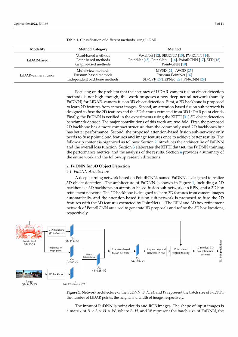
A deep learning network based on PointRCNN, named FuDNN, is designed to realize3D object detection. The architecture of FuDNN is shown in Figure 1, including a 2Dbackbone, a 3D backbone, an attention-based fusion sub-network, an RPN, and a 3D boxrefinement network. The 2D backbone is designed to learn 2D features from camera imagesautomatically, and the attention-based fusion sub-network is proposed to fuse the 2Dfeatures with the 3D features extracted by PointNet++. The RPN and 3D box refinementnetwork of PointRCNN are used to generate 3D proposals and refine the 3D box locations,respectively.

Information 2022, 13, x FOR PEER REVIEW 3 of 11

Table 1. Classification of different methods using LiDAR.

Modality Method Category Method

LiDAR-based Voxel-based methods VoxelNet [12], SECOND [13], PV-RCNN [14], Point-based methods PointNet [15], PointNet++ [16], PointRCNN [17], STD [18] Graph-based methods Point-GNN [19]

LiDAR–camera fusion Multi-view methods MV3D [24], AVOD [25]

Frustum-based methods Frustum PointNet [26] Independent backbone methods 3D-CVF [27], EPNet [28], PI-RCNN [29]

Focusing on the problem that the accuracy of LiDAR–camera fusion object detection methods is not high enough, this work proposes a new deep neural network (namely FuDNN) for LiDAR–camera fusion 3D object detection. First, a 2D backbone is proposed to learn 2D features from camera images. Second, an attention-based fusion sub-network is designed to fuse the 2D features and the 3D features extracted from 3D LiDAR point clouds. Finally, the FuDNN is verified in the experiments using the KITTI [31] 3D object detection benchmark dataset. The major contributions of this work are two-fold. First, the proposed 2D backbone has a more compact structure than the commonly used 2D back-bones but has better performance. Second, the proposed attention-based fusion sub-net-work only needs to fuse point cloud features and image features once to achieve better results. The follow-up content is organized as follows: Section II introduces the architec-ture of FuDNN and the overall loss function. Section III elaborates the KITTI dataset, the FuDNN training, the performance metrics, and the analysis of the results. Section IV pro-vides a summary of the entire work and the follow-up research directions.

2. FuDNN for 3D Object Detection 2.1. FuDNN Architecture

A deep learning network based on PointRCNN, named FuDNN, is designed to real-ize 3D object detection. The architecture of FuDNN is shown in Figure 1, including a 2D backbone, a 3D backbone, an attention-based fusion sub-network, an RPN, and a 3D box refinement network. The 2D backbone is designed to learn 2D features from camera im-ages automatically, and the attention-based fusion sub-network is proposed to fuse the 2D features with the 3D features extracted by PointNet++. The RPN and 3D box refinement network of PointRCNN are used to generate 3D proposals and refine the 3D box locations, respectively.

2D backbone

3D backbone(PointNet++)

FP（B×128×N）

FI（B×128×H/2×W/2）

Pxy（B×N×2）

Projecting to image plane

Bilinear Interpolation

Point cloud（B×N×3）

Image（B×3×H×W）

FFu（B×128×N）

FBI（B×128×N）

Attention-based fusion network

Region proposal network (RPN)

Canonical 3D box refinement

network

3D b

ox p

redi

ctio

ns

Point cloud region pooling

Figure 1. Network architecture of the FuDNN. B, N, H, and W represent the batch size of FuDNN, the number of LiDAR points, the height, and width of image, respectively. Figure 1. Network architecture of the FuDNN. B, N, H, and W represent the batch size of FuDNN,the number of LiDAR points, the height, and width of image, respectively.

The input of FuDNN is point clouds and RGB images. The shape of input images isa matrix of B × 3 × H × W, where B, H, and W represent the batch size of FuDNN, the

Information 2022, 13, 169 4 of 11

height, and the width of the image, respectively. The shape of input point clouds is a matrixof B × 3 × N, where N is the number of LiDAR points.

The architecture of the 2D backbone is shown in Figure 2. The first layer (Conv1) of the2D backbone is a 2D convolutional layer with 128 convolution kernels, each 7 × 7, usinga stride of 1. The output of Conv1 is a matrix of B × 128 × H ×W. The research of Ioffeand Szegedy [32] showed that the batch normalization method could speed up networkconvergence and reduce training difficulty, so a batch normalization layer (BN1) was usedafter Conv1. A rectified linear unit layer (ReLU1) is added after the BN1 layer to avoidgradient disappearance. The output shape of BN1 and ReLU1 is the same as that of Conv1.To reduce the amount of calculation, a max-pooling layer (S1) with a kernel size of 2 × 2is adopted after ReLU1, and its output shape is B × 128 × H/2 ×W/2. Next, the similarstructures repeat two times: The 2D convolutional layer (Conv2) with 256 convolutionkernels, each 5 × 5, is followed by the batch normalization layer (BN2). Then there is theReLU2. At last, the 2D convolutional layer (Conv3) with 128 convolution kernels, each3 × 3, is followed by the ReLU3. The 2D backbone outputs the image feature matrix FI ofthe shape B × 128 × H/2 ×W/2.

Information 2022, 13, x FOR PEER REVIEW 4 of 11

The input of FuDNN is point clouds and RGB images. The shape of input images is a matrix of B × 3 × H × W, where B, H, and W represent the batch size of FuDNN, the height, and the width of the image, respectively. The shape of input point clouds is a ma-trix of B × 3 × N, where N is the number of LiDAR points.

The architecture of the 2D backbone is shown in Figure 2. The first layer (Conv1) of the 2D backbone is a 2D convolutional layer with 128 convolution kernels, each 7 × 7, using a stride of 1. The output of Conv1 is a matrix of B × 128 × H × W. The research of Ioffe and Szegedy [32] showed that the batch normalization method could speed up network con-vergence and reduce training difficulty, so a batch normalization layer (BN1) was used after Conv1. A rectified linear unit layer (ReLU1) is added after the BN1 layer to avoid gradient disappearance. The output shape of BN1 and ReLU1 is the same as that of Conv1. To reduce the amount of calculation, a max-pooling layer (S1) with a kernel size of 2 × 2 is adopted after ReLU1, and its output shape is B × 128 × H/2 × W/2. Next, the similar struc-tures repeat two times: The 2D convolutional layer (Conv2) with 256 convolution kernels, each 5 × 5, is followed by the batch normalization layer (BN2). Then there is the ReLU2. At last, the 2D convolutional layer (Conv3) with 128 convolution kernels, each 3 × 3, is followed by the ReLU3. The 2D backbone outputs the image feature matrix 𝐹 of the shape B × 128 × H/2 × W/2.

7×7 conv2D, 128

Image

Batch normalization

ReLU

Pool, /2

5×5 conv2D, 256

Batch normalization

ReLU

3×3 conv2D, 128

Batch normalization

ReLU

Output: FI Figure 2. Network architecture of the 2D backbone.

Since point cloud features and image features lack correspondence, it is necessary to establish the correspondence between image features and point cloud features before pro-jecting the point clouds to the image plane. The point clouds (x, y, z) are mapped to the image plane (u, v) via a transformation matrix M, as shown in Equations (1) and (2): (𝑢, 𝑣, 1) = 𝐌 ∙ (𝑥, 𝑦, 𝑧, 1) (1)

𝐌 = 𝐏 ∙ 𝐑 𝐭0 1 (2)

where 𝐏 is the projection matrix, 𝐑 is the 3 × 3 rotation matrix, and 𝐭 is the 1 × 3 translation vector from the LiDAR to the camera, respectively. Projecting the point clouds to the image plane obtains a B × N × 2 matrix 𝑃 .

The point cloud feature 𝐹 and the image feature 𝐹 need to have the same dimen-sion to be fused, so the bilinear interpolation method is used to sample 𝐹 to obtain the same dimension as 𝐹 . First, 𝑃 is expanded from B × N × 2 to obtain a B × 1 × N × 2

Figure 2. Network architecture of the 2D backbone.

Since point cloud features and image features lack correspondence, it is necessaryto establish the correspondence between image features and point cloud features beforeprojecting the point clouds to the image plane. The point clouds (x, y, z) are mapped to theimage plane (u, v) via a transformation matrix M, as shown in Equations (1) and (2):

(u, v, 1)T = M·(x, y, z, 1)T (1)

M = Prect·(

RcamLiD tcam

LiD0 1

)(2)

where Prect is the projection matrix, RcamLiD is the 3 × 3 rotation matrix, and tcam

LiD is the 1 × 3translation vector from the LiDAR to the camera, respectively. Projecting the point cloudsto the image plane obtains a B × N × 2 matrix Pxy.

The point cloud feature FP and the image feature FI need to have the same dimensionto be fused, so the bilinear interpolation method is used to sample FI to obtain the samedimension as FP. First, Pxy is expanded from B × N × 2 to obtain a B × 1 × N × 2matrix. Second, with the B × 1 × N × 2 matrix as the guide map, FI is sampled by bilinear

Information 2022, 13, 169 5 of 11

interpolation to obtain the feature map of B × 128 × 1 × N, which is then removed by thedimension of 1 to obtain the final feature map FBI of B × 128 × N.

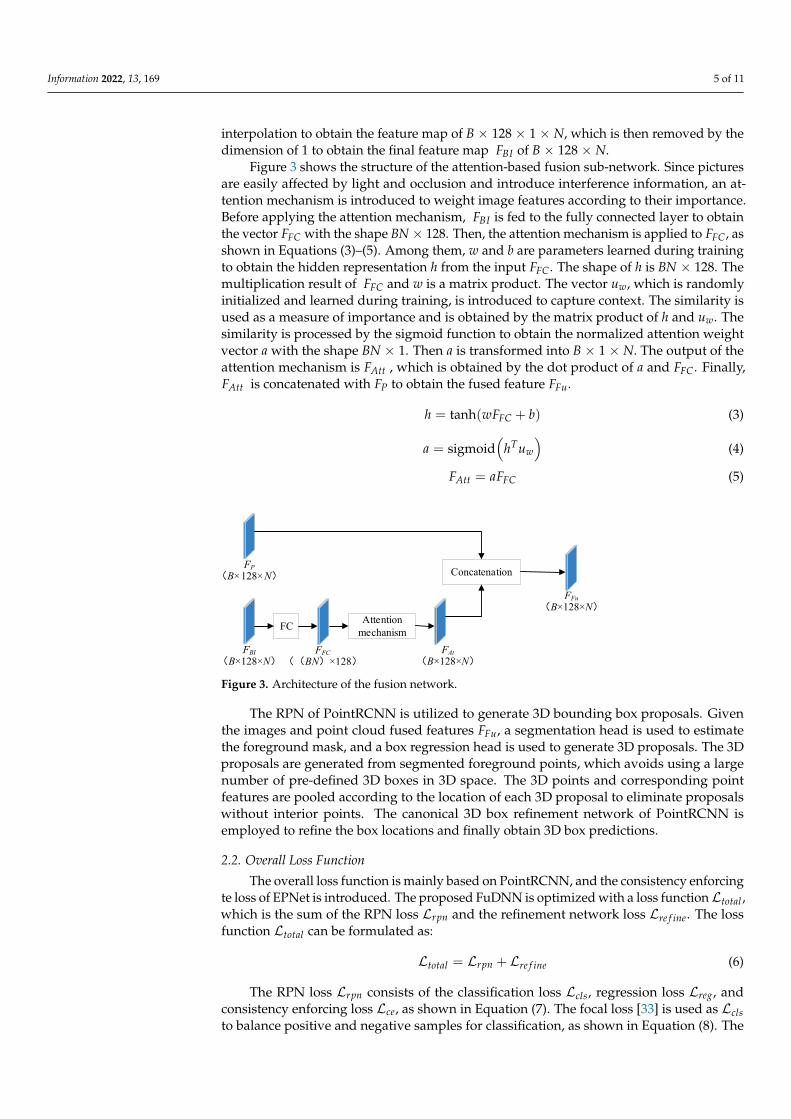
Figure 3 shows the structure of the attention-based fusion sub-network. Since picturesare easily affected by light and occlusion and introduce interference information, an at-tention mechanism is introduced to weight image features according to their importance.Before applying the attention mechanism, FBI is fed to the fully connected layer to obtainthe vector FFC with the shape BN × 128. Then, the attention mechanism is applied to FFC, asshown in Equations (3)–(5). Among them, w and b are parameters learned during trainingto obtain the hidden representation h from the input FFC. The shape of h is BN × 128. Themultiplication result of FFC and w is a matrix product. The vector uw, which is randomlyinitialized and learned during training, is introduced to capture context. The similarity isused as a measure of importance and is obtained by the matrix product of h and uw. Thesimilarity is processed by the sigmoid function to obtain the normalized attention weightvector a with the shape BN × 1. Then a is transformed into B × 1 × N. The output of theattention mechanism is FAtt , which is obtained by the dot product of a and FFC. Finally,FAtt is concatenated with FP to obtain the fused feature FFu.

h = tanh(wFFC + b) (3)

a = sigmoid(

hTuw

)(4)

FAtt = aFFC (5)

Information 2022, 13, x FOR PEER REVIEW 5 of 11

matrix. Second, with the B × 1 × N × 2 matrix as the guide map, 𝐹 is sampled by bilinear interpolation to obtain the feature map of B × 128 × 1 × N, which is then removed by the dimension of 1 to obtain the final feature map 𝐹 of B × 128 × N.

Figure 3 shows the structure of the attention-based fusion sub-network. Since pic-tures are easily affected by light and occlusion and introduce interference information, an attention mechanism is introduced to weight image features according to their im-portance. Before applying the attention mechanism, 𝐹 is fed to the fully connected layer to obtain the vector 𝐹 with the shape BN × 128. Then, the attention mechanism is applied to 𝐹 , as shown in Equations (3)–(5). Among them, 𝑤 and b are parameters learned dur-ing training to obtain the hidden representation ℎ from the input 𝐹 . The shape of ℎ is BN × 128. The multiplication result of 𝐹 and 𝑤 is a matrix product. The vector 𝑢 , which is randomly initialized and learned during training, is introduced to capture con-text. The similarity is used as a measure of importance and is obtained by the matrix prod-uct of ℎ and 𝑢 . The similarity is processed by the sigmoid function to obtain the normal-ized attention weight vector 𝑎 with the shape BN × 1. Then 𝑎 is transformed into B × 1 × N. The output of the attention mechanism is 𝐹 , which is obtained by the dot product of 𝑎 and 𝐹 . Finally, 𝐹 is concatenated with 𝐹 to obtain the fused feature 𝐹 . ℎ = tanh(𝑤𝐹 + 𝑏) (3) 𝑎 = sigmoid(ℎ 𝑢 ) (4) 𝐹 = 𝑎𝐹 (5)

FBI（B×128×N）

FP（B×128×N）

FC Attention mechanism

FAt（B×128×N）

Concatenation

FFu（B×128×N）

FFC（（BN）×128）

Figure 3. Architecture of the fusion network.

The RPN of PointRCNN is utilized to generate 3D bounding box proposals. Given the images and point cloud fused features 𝐹 , a segmentation head is used to estimate the foreground mask, and a box regression head is used to generate 3D proposals. The 3D proposals are generated from segmented foreground points, which avoids using a large number of pre-defined 3D boxes in 3D space. The 3D points and corresponding point fea-tures are pooled according to the location of each 3D proposal to eliminate proposals with-out interior points. The canonical 3D box refinement network of PointRCNN is employed to refine the box locations and finally obtain 3D box predictions.

2.2. Overall Loss Function The overall loss function is mainly based on PointRCNN, and the consistency enforc-

ing te loss of EPNet is introduced. The proposed FuDNN is optimized with a loss func-tion ℒ , which is the sum of the RPN loss ℒ and the refinement network loss ℒ . The loss function ℒ can be formulated as: ℒ = ℒ + ℒ (6)

The RPN loss ℒ consists of the classification loss ℒ , regression loss ℒ , and con-sistency enforcing loss ℒ , as shown in Equation (7). The focal loss [33] is used as ℒ to

Figure 3. Architecture of the fusion network.

The RPN of PointRCNN is utilized to generate 3D bounding box proposals. Giventhe images and point cloud fused features FFu, a segmentation head is used to estimatethe foreground mask, and a box regression head is used to generate 3D proposals. The 3Dproposals are generated from segmented foreground points, which avoids using a largenumber of pre-defined 3D boxes in 3D space. The 3D points and corresponding pointfeatures are pooled according to the location of each 3D proposal to eliminate proposalswithout interior points. The canonical 3D box refinement network of PointRCNN isemployed to refine the box locations and finally obtain 3D box predictions.

2.2. Overall Loss Function

The overall loss function is mainly based on PointRCNN, and the consistency enforcingte loss of EPNet is introduced. The proposed FuDNN is optimized with a loss functionLtotal ,which is the sum of the RPN loss Lrpn and the refinement network loss Lre f ine. The lossfunction Ltotal can be formulated as:

Ltotal = Lrpn + Lre f ine (6)

The RPN loss Lrpn consists of the classification loss Lcls, regression loss Lreg, andconsistency enforcing loss Lce, as shown in Equation (7). The focal loss [33] is used as Lclsto balance positive and negative samples for classification, as shown in Equation (8). The

Information 2022, 13, 169 6 of 11

parameters of focal loss keep the default values of c = 0.25 and r = 2. The definition of Lce isshown in Equation (9), where D denotes the predicted bounding box, G denotes the groundtruth, and k denotes the classification confidence of D.

Lrpn = Lcls + Lreg + λLce (7)

Lcls = −c(1− pt)r log pt (8)

Lce = − log(

k× Area(D ∩ G)

Area(D ∪ G)

)(9)

The regression loss Lreg is used to constrain the bounding box (x, y, z, h, w, l, θ), where(x, y, z) is the center, (h, w, l) is the size, and θ is the orientation. PointRCNN divides eachforeground point-surrounding area into bins along the X and Z axes, and Lreg is thebin-based regression loss. The calculation process of Lreg is as follows:

Lbin = ∑uε{x,z,θ}

(E(

b̂u, bu

)+ S(r̂u, ru)

)(10)

Lres = ∑vε{y,h,w,l}

S(rv, r̂v) (11)

Lreg =1

Npos∑

pεpos(Lbin + Lres) (12)

where E represents the cross-entropy loss, S represents the smooth L1 loss, b̂u and bu arethe predicted bin assignments and the ground-truth bin assignments, r̂u and ru are theresiduals and the ground-truth residuals, and Npos is the number of foreground points.Each residual is a variable for further optimizing the position of the specified bin, and itscalculation process is detailed in PointRCNN.

3. Experiments and Analysis3.1. Dataset

The KITTI 3D object detection benchmark dataset is used as the experimental dataset.KITTI was collected by an equipment platform fixed on the top of the car, including twograyscale cameras, two color cameras, a Velodyne 64-line 3D LiDAR, four optical lenses,and one GPS/IMU system. KITTI was sampled and synchronized at 10 Hz, including7481 training samples and 7581 testing samples. Each sample provides both the pointcloud and the camera image. The labels of KITTI were divided into three subsets: Easy,moderate, and hard, according to the heights of their 2D bounding boxes, occlusion levels,and truncation levels. The easy difficulty level has a minimum 2D bounding box heightof 40 Px, an occlusion level of full visibility, and a maximum truncation level of 15%. Theminimum 2D bounding box height, occlusion level, and maximum truncation level ofmoderate difficulty level are 25 Px, partial occlusion, and 30%, respectively. The minimum2D bounding box height for the hard difficulty level is 25 Px, the occlusion level is hard tosee, and the maximum truncation level is 50%.

The image data of color camera 2 and the point cloud data of Velodyne LiDAR are usedin this work. Since the test samples of KITTI are not labeled, the approach of Shi et al. [17]is adopted to further divide the training samples into 3712 samples for training and3769 samples for validation. Only visible objects in the image are labeled, so according tothe general practice of previous studies [19,24], only the LiDAR points projected into theimage are used. The LiDAR points are mapped at the camera coordinates X (right) axis[−40, 40] meters, Y (down) axis [−1, 3] meters, and Z (forward) axis [0, 70.4] meters. Therange of point clouds is [−π, π].

Information 2022, 13, 169 7 of 11

3.2. FuDNN Training

The experiments were carried out on a server with the Ubuntu 16.04.1 LTS system.The server GPU was GeForce RTX 3090 24 GB, the CPU was Intel E5-2620V4@2.10 GHz,and the RAM size was 256 GB. The main installation packages required by the runningenvironment of the program are shown in Table 2.

Table 2. Main installation packages required by the running environment.

Package Name Version

Python 3.7.6CUDA 11.3

PyTorch 1.10.1TensorboardX 2.4.1

Numpy 1.21.2Pillow 8.4.0

Numba 0.54.1Opencv-python 4.5.5.62

Torchvision 0.11.2

The FuDNN was trained in an end-to-end manner. During the data preprocessingstage, the images were scaled to a uniform size of 384 × 1280. Each point cloud wassubtracted or supplemented to ensure that the number of points in each point cloud was16,384. Several data augmentation techniques were employed on the point clouds to avoidover-fitting, which are widely used in [1,12,13], including flip (along the forwarding axis),random scaling (scale factor 0.95∼1.05 for all 3 axes), and rotation (−10∼10 degrees alongthe vertical axis). The data augmentation was only used for training. During networktraining, the network parameters were optimized by the Adam method [34]. The initiallearning rate and weight decay of the network were set to 0.002 and 0.001, respectively. Themodel was trained for 150 epochs with a batch size of 4 and saved every 5 epochs. Thethreshold of IoU was set to 0.7 to distinguish between true positives and false positives.

3.3. Performance Metrics

According to the latest rules of KITTI, the 40-point Interpolated Average Precisionmetric was used as the performance metric, as shown in Equation (13):

AP|R40 =1|R40| ∑

r∈R40

ρinterp(r) (13)

where R40 = {1/40,2/40,3/40, . . . ,1} and |R40| = 40. The interpolation function ρinterp isdefined as:

ρinterp(r) = maxr′ :r′≥r

ρ(r′)

(14)

where ρ(r) is the precision at recall r. ρinterp(r) is the value at recall r on the smoothedprecision–recall curve, not the actual precision values ρ(r). Furthermore, ρinterp(r) is greaterthan or equal to ρ(r).

3.4. Results and Discussion

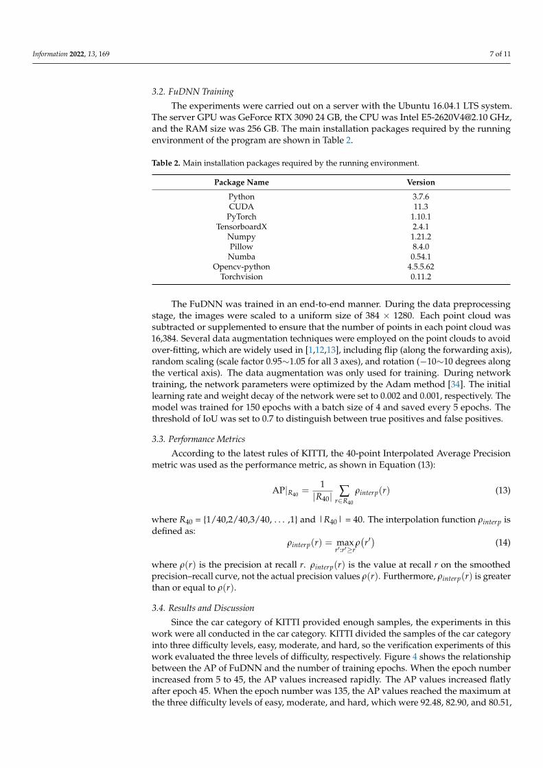
Since the car category of KITTI provided enough samples, the experiments in thiswork were all conducted in the car category. KITTI divided the samples of the car categoryinto three difficulty levels, easy, moderate, and hard, so the verification experiments of thiswork evaluated the three levels of difficulty, respectively. Figure 4 shows the relationshipbetween the AP of FuDNN and the number of training epochs. When the epoch numberincreased from 5 to 45, the AP values increased rapidly. The AP values increased flatlyafter epoch 45. When the epoch number was 135, the AP values reached the maximum atthe three difficulty levels of easy, moderate, and hard, which were 92.48, 82.90, and 80.51,

Information 2022, 13, 169 8 of 11

respectively. When the epoch number was greater than 135, the AP values did not exceedthat of epoch 135. Therefore, the model of epoch 135 was used as the best-trained model.

Information 2022, 13, x FOR PEER REVIEW 8 of 11

after epoch 45. When the epoch number was 135, the AP values reached the maximum at the three difficulty levels of easy, moderate, and hard, which were 92.48, 82.90, and 80.51, respectively. When the epoch number was greater than 135, the AP values did not exceed that of epoch 135. Therefore, the model of epoch 135 was used as the best-trained model.

Figure 4. The AP values for different training epoch numbers.

Table 3 shows the AP comparison between the proposed FuDNN and the previous methods on the car class of KITTI validation set with the IoU threshold of 0.7. The AP values of FuDNN in the moderate and hard difficulty levels were higher than those of other methods. At the easy difficulty level, the AP value of FuDNN reached 92.48, which was 4.73 higher than the lowest PointPillars [1], but slightly lower than the best PointRCNN [17]. At the moderate difficulty level, the AP value of FuDNN showed a 4.51 improvement over the lowest PointPillars and a 0.31 improvement over the best EPNet [28]. At the hard difficulty level, the AP value of FuDNN outperformed the lowest PointPillars and the best EPNet by 5.33 and 0.37, respectively. Although the AP value of FuDNN was 0.06 lower than PointRCNN at the easy difficulty level, it was 0.74 and 2.63 higher than PointRCNN at moderate and hard difficulty levels, respectively. PointPillars achieved a speed of 62.0 fps, but its AP values were too low. SECOND was also fast, reach-ing 26.3 fps, but its AP values were lower than the proposed FuDNN. The speed of FuDNN was similar to PointRCNN, 3D-CVF, EPNet, and PI-RCNN. Therefore, the overall effect of FuDNN was better than that of PointRCNN. The above comparisons demon-strated the effectiveness of FuDNN. Since the car samples in the KITTI dataset all have different degrees of occlusion and truncation, the AP of object detection will be limited. Especially for the hard difficulty level, the occlusion level is hard to see, and the cutoff level is 50%, so it is very important to improve the AP value.

Table 3. AP comparison of different 3D object detection algorithms in the car class of KITTI valida-tion set with IoU threshold 0.7.

Method Modality Easy Moderate Hard Speed (fps) PointPillars [1] LiDAR-based 87.75 78.39 75.18 62.0 SECOND [13] LiDAR-based 90.97 79.94 77.09 26.3

PointRCNN [17] LiDAR-based 92.54 82.16 77.88 10.0 3D-CVF [27] LiDAR–camera fusion 89.67 79.88 78.47 13.3 EPNet [28] LiDAR–camera fusion 92.28 82.59 80.14 10.0

PI-RCNN [29] LiDAR–camera fusion 88.27 78.53 77.75 11.1 FuDNN (Proposed) LiDAR–camera fusion 92.48 82.90 80.51 10.5

Table 4 shows a set of ablation experiments to compare the effects of different 2D backbones in the car class of the KITTI validation set with an IoU threshold of 0.7. Models A, B, C, and D were obtained by replacing the 2D backbone of FuDNN with Resnet50 [35],

Figure 4. The AP values for different training epoch numbers.

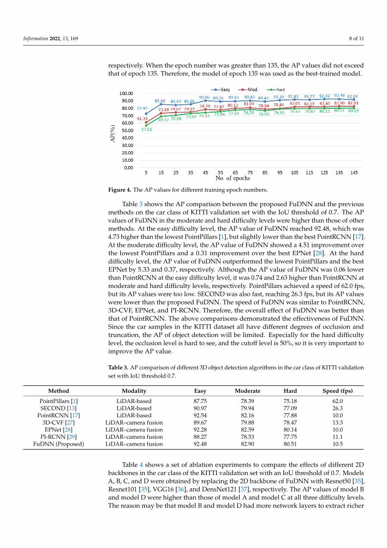
Table 3 shows the AP comparison between the proposed FuDNN and the previousmethods on the car class of KITTI validation set with the IoU threshold of 0.7. The APvalues of FuDNN in the moderate and hard difficulty levels were higher than those of othermethods. At the easy difficulty level, the AP value of FuDNN reached 92.48, which was4.73 higher than the lowest PointPillars [1], but slightly lower than the best PointRCNN [17].At the moderate difficulty level, the AP value of FuDNN showed a 4.51 improvement overthe lowest PointPillars and a 0.31 improvement over the best EPNet [28]. At the harddifficulty level, the AP value of FuDNN outperformed the lowest PointPillars and the bestEPNet by 5.33 and 0.37, respectively. Although the AP value of FuDNN was 0.06 lowerthan PointRCNN at the easy difficulty level, it was 0.74 and 2.63 higher than PointRCNN atmoderate and hard difficulty levels, respectively. PointPillars achieved a speed of 62.0 fps,but its AP values were too low. SECOND was also fast, reaching 26.3 fps, but its AP valueswere lower than the proposed FuDNN. The speed of FuDNN was similar to PointRCNN,3D-CVF, EPNet, and PI-RCNN. Therefore, the overall effect of FuDNN was better thanthat of PointRCNN. The above comparisons demonstrated the effectiveness of FuDNN.Since the car samples in the KITTI dataset all have different degrees of occlusion andtruncation, the AP of object detection will be limited. Especially for the hard difficultylevel, the occlusion level is hard to see, and the cutoff level is 50%, so it is very important toimprove the AP value.

Table 3. AP comparison of different 3D object detection algorithms in the car class of KITTI validationset with IoU threshold 0.7.

Method Modality Easy Moderate Hard Speed (fps)

PointPillars [1] LiDAR-based 87.75 78.39 75.18 62.0SECOND [13] LiDAR-based 90.97 79.94 77.09 26.3

PointRCNN [17] LiDAR-based 92.54 82.16 77.88 10.03D-CVF [27] LiDAR–camera fusion 89.67 79.88 78.47 13.3EPNet [28] LiDAR–camera fusion 92.28 82.59 80.14 10.0

PI-RCNN [29] LiDAR–camera fusion 88.27 78.53 77.75 11.1FuDNN (Proposed) LiDAR–camera fusion 92.48 82.90 80.51 10.5

Table 4 shows a set of ablation experiments to compare the effects of different 2Dbackbones in the car class of the KITTI validation set with an IoU threshold of 0.7. ModelsA, B, C, and D were obtained by replacing the 2D backbone of FuDNN with Resnet50 [35],Resnet101 [35], VGG16 [36], and DensNet121 [37], respectively. The AP values of model Band model D were higher than those of model A and model C at all three difficulty levels.The reason may be that model B and model D had more network layers to extract richer

Information 2022, 13, 169 9 of 11

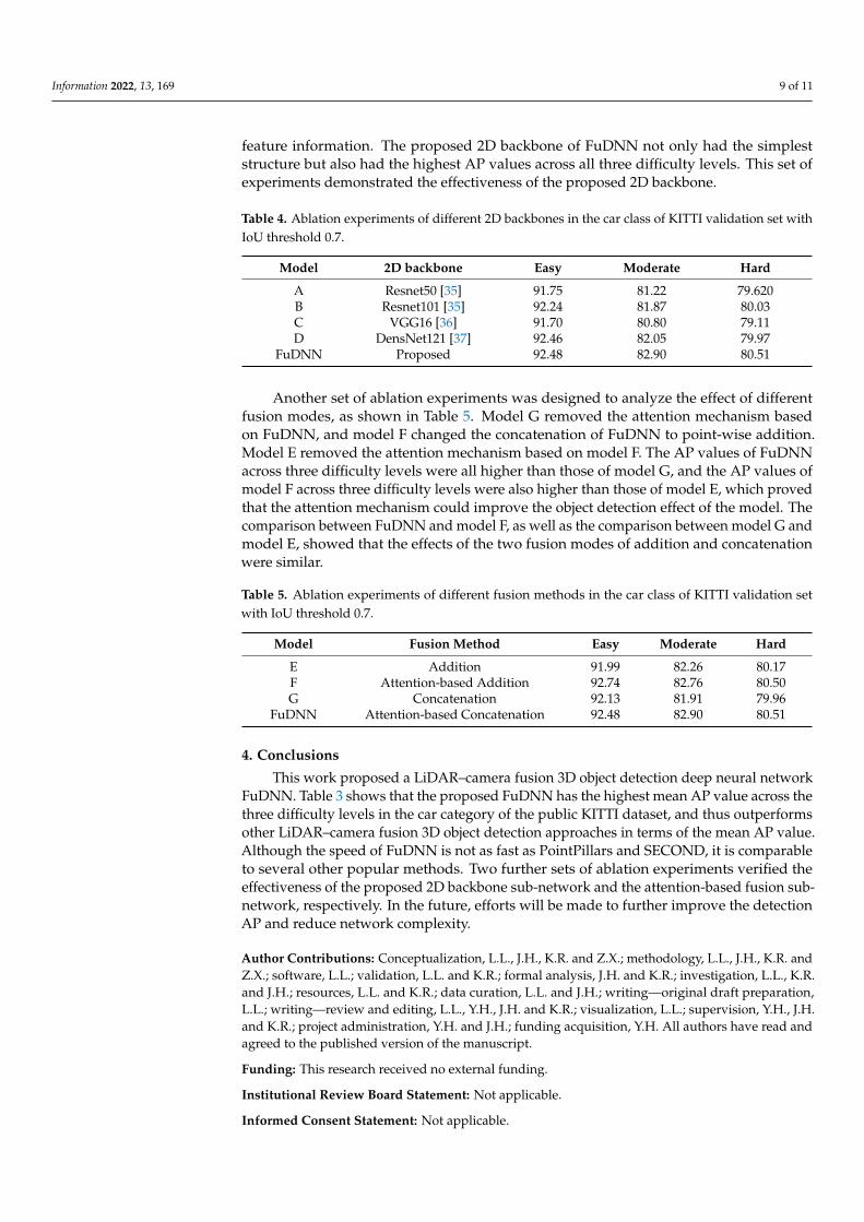
feature information. The proposed 2D backbone of FuDNN not only had the simpleststructure but also had the highest AP values across all three difficulty levels. This set ofexperiments demonstrated the effectiveness of the proposed 2D backbone.

Table 4. Ablation experiments of different 2D backbones in the car class of KITTI validation set withIoU threshold 0.7.

Model 2D backbone Easy Moderate Hard

A Resnet50 [35] 91.75 81.22 79.620B Resnet101 [35] 92.24 81.87 80.03C VGG16 [36] 91.70 80.80 79.11D DensNet121 [37] 92.46 82.05 79.97

FuDNN Proposed 92.48 82.90 80.51

Another set of ablation experiments was designed to analyze the effect of differentfusion modes, as shown in Table 5. Model G removed the attention mechanism basedon FuDNN, and model F changed the concatenation of FuDNN to point-wise addition.Model E removed the attention mechanism based on model F. The AP values of FuDNNacross three difficulty levels were all higher than those of model G, and the AP values ofmodel F across three difficulty levels were also higher than those of model E, which provedthat the attention mechanism could improve the object detection effect of the model. Thecomparison between FuDNN and model F, as well as the comparison between model G andmodel E, showed that the effects of the two fusion modes of addition and concatenationwere similar.

Table 5. Ablation experiments of different fusion methods in the car class of KITTI validation setwith IoU threshold 0.7.

Model Fusion Method Easy Moderate Hard

E Addition 91.99 82.26 80.17F Attention-based Addition 92.74 82.76 80.50G Concatenation 92.13 81.91 79.96

FuDNN Attention-based Concatenation 92.48 82.90 80.51

4. Conclusions

This work proposed a LiDAR–camera fusion 3D object detection deep neural networkFuDNN. Table 3 shows that the proposed FuDNN has the highest mean AP value across thethree difficulty levels in the car category of the public KITTI dataset, and thus outperformsother LiDAR–camera fusion 3D object detection approaches in terms of the mean AP value.Although the speed of FuDNN is not as fast as PointPillars and SECOND, it is comparableto several other popular methods. Two further sets of ablation experiments verified theeffectiveness of the proposed 2D backbone sub-network and the attention-based fusion sub-network, respectively. In the future, efforts will be made to further improve the detectionAP and reduce network complexity.

Author Contributions: Conceptualization, L.L., J.H., K.R. and Z.X.; methodology, L.L., J.H., K.R. andZ.X.; software, L.L.; validation, L.L. and K.R.; formal analysis, J.H. and K.R.; investigation, L.L., K.R.and J.H.; resources, L.L. and K.R.; data curation, L.L. and J.H.; writing—original draft preparation,L.L.; writing—review and editing, L.L., Y.H., J.H. and K.R.; visualization, L.L.; supervision, Y.H., J.H.and K.R.; project administration, Y.H. and J.H.; funding acquisition, Y.H. All authors have read andagreed to the published version of the manuscript.

Funding: This research received no external funding.

Institutional Review Board Statement: Not applicable.

Informed Consent Statement: Not applicable.

Information 2022, 13, 169 10 of 11

Data Availability Statement: A publicly available dataset was analyzed in this study. This dataset canbe found here: http://www.cvlibs.net/datasets/kitti/eval_object.php?obj_benchmark=3d, accessedon 16 February 2022.

Conflicts of Interest: The authors declare no conflict of interest.

References1. Lang, A.H.; Vora, S.; Caesar, H.; Zhou, L.; Yang, J.; Beijbom, O. Pointpillars: Fast encoders for object detection from point clouds.

In Proceedings of the IEEE/CVF Conference on Computer Vision and Pattern Recognition, Long Beach, CA, USA, 16–17 June2019; pp. 12697–12705.

2. Wang, Y.; Mao, Q.; Zhu, H.; Zhang, Y.; Ji, J.; Zhang, Y. Multi-modal 3d object detection in autonomous driving: A survey. arXiv2021, arXiv:2106.12735.

3. Girshick, R.; Donahue, J.; Darrell, T.; Malik, J. Rich feature hierarchies for accurate object detection and semantic segmentation.In Proceedings of the IEEE Conference on Computer Vision and Pattern Recognition, Columbus, OH, USA, 23–28 June 2014;pp. 580–587.

4. He, K.; Gkioxari, G.; Dollár, P.; Girshick, R. Mask r-cnn. In Proceedings of the IEEE International Conference on Computer Vision,Venice, Italy, 22–29 October 2017; pp. 2961–2969.

5. Ren, S.; He, K.; Girshick, R.; Sun, J. Faster r-cnn: Towards real-time object detection with region proposal networks. Adv. NeuralInf. Process. Syst. 2015, 28, 91–99. [CrossRef] [PubMed]

6. Redmon, J.; Divvala, S.; Girshick, R.; Farhadi, A. You only look once: Unified, real-time object detection. In Proceedings of theIEEE Conference on Computer Vision and Pattern Recognition, Honolulu, HI, USA, 21–26 July 2016; pp. 779–788.

7. Liu, W.; Anguelov, D.; Erhan, D.; Szegedy, C.; Reed, S.; Fu, C.-Y.; Berg, A.C. Ssd: Single shot multibox detector. In Proceedings ofthe European Conference on Computer Vision, Amsterdam, The Netherlands, 11–14 October 2016; Springer: Berlin/Heidelberg,Germany, 2016; pp. 21–37.

8. An, P.; Liang, J.; Yu, K.; Fang, B.; Ma, J. Deep structural information fusion for 3D object detection on LiDAR–camera system.Comput. Vis. Image Underst. 2022, 214, 103295. [CrossRef]

9. Reading, C.; Harakeh, A.; Chae, J.; Waslander, S.L. Categorical depth distribution network for monocular 3d object detection. InProceedings of the IEEE/CVF Conference on Computer Vision and Pattern Recognition, Nashville, TN, USA, 20–25 June 2021;pp. 8555–8564.

10. Lu, Y.; Ma, X.; Yang, L.; Zhang, T.; Liu, Y.; Chu, Q.; Yan, J.; Ouyang, W. Geometry uncertainty projection network for monocular3d object detection. In Proceedings of the IEEE/CVF International Conference on Computer Vision, Montreal, BC, Canada, 11–17October 2021; pp. 3111–3121.

11. Guo, Y.; Wang, H.; Hu, Q.; Liu, H.; Liu, L.; Bennamoun, M. Deep learning for 3d point clouds: A survey. IEEE Trans. Pattern Anal.Mach. Intell. 2020, 43, 4338–4364. [CrossRef] [PubMed]

12. Zhou, Y.; Tuzel, O. Voxelnet: End-to-end learning for point cloud based 3d object detection. In Proceedings of the IEEE Conferenceon Computer Vision and Pattern Recognition, Salt Lake City, UT, USA, 18–23 June 2018; pp. 4490–4499.

13. Yan, Y.; Mao, Y.; Li, B. Second: Sparsely embedded convolutional detection. Sensors 2018, 18, 3337. [CrossRef] [PubMed]14. Shi, S.; Guo, C.; Jiang, L.; Wang, Z.; Shi, J.; Wang, X.; Li, H. Pv-rcnn: Point-voxel feature set abstraction for 3d object detection.

In Proceedings of the IEEE/CVF Conference on Computer Vision and Pattern Recognition, Seattle, WA, USA, 13–19 June 2020;pp. 10529–10538.

15. Qi, C.R.; Su, H.; Mo, K.; Guibas, L.J. Pointnet: Deep learning on point sets for 3d classification and segmentation. In Proceedingsof the IEEE Conference on Computer Vision and Pattern Recognition, Honolulu, HI, USA, 21–26 July 2017; pp. 652–660.

16. Qi, C.R.; Yi, L.; Su, H.; Guibas, L.J. Pointnet++: Deep hierarchical feature learning on point sets in a metric space. Adv. Neural Inf.Process. Syst. 2017, 30, 5105–5114.

17. Shi, S.; Wang, X.; Li, H. Pointrcnn: 3d object proposal generation and detection from point cloud. In Proceedings of the IEEE/CVFConference on Computer Vision and Pattern Recognition, Long Beach, CA, USA, 15–20 June 2019; pp. 770–779.

18. Yang, Z.; Sun, Y.; Liu, S.; Shen, X.; Jia, J. Std: Sparse-to-dense 3d object detector for point cloud. In Proceedings of the IEEE/CVFInternational Conference on Computer Vision, Seoul, Korea, 27–28 October 2019; pp. 1951–1960.

19. Shi, W.; Rajkumar, R. Point-gnn: Graph neural network for 3d object detection in a point cloud. In Proceedings of the IEEE/CVFConference on Computer Vision and Pattern Recognition, Seattle, WA, USA, 13–19 June 2020; pp. 1711–1719.

20. Mao, J.; Niu, M.; Bai, H.; Liang, X.; Xu, H.; Xu, C. Pyramid r-cnn: Towards better performance and adaptability for 3d objectdetection. In Proceedings of the IEEE/CVF International Conference on Computer Vision, Montreal, BC, Canada, 11–17 October2021; pp. 2723–2732.

21. Wen, L.-H.; Jo, K.-H. Fast and accurate 3D object detection for lidar-camera-based autonomous vehicles using one sharedvoxel-based backbone. IEEE Access 2021, 9, 22080–22089. [CrossRef]

22. Lu, H.; Chen, X.; Zhang, G.; Zhou, Q.; Ma, Y.; Zhao, Y. SCANet: Spatial-channel attention network for 3D object detection.In Proceedings of the ICASSP 2019–2019 IEEE International Conference on Acoustics, Speech and Signal Processing (ICASSP),Brighton, UK, 12–17 May 2019; IEEE: New York, NY, USA, 2019; pp. 1992–1996.

Information 2022, 13, 169 11 of 11

23. Liang, M.; Yang, B.; Wang, S.; Urtasun, R. Deep continuous fusion for multi-sensor 3d object detection. In Proceedings of theEuropean Conference on Computer Vision (ECCV), Munich, Germany, 8–14 September 2018; pp. 641–656.

24. Chen, X.; Ma, H.; Wan, J.; Li, B.; Xia, T. Multi-view 3d object detection network for autonomous driving. In Proceedings of theIEEE Conference on Computer Vision and Pattern Recognition, Honolulu, HI, USA, 21–26 July 2017; pp. 1907–1915.

25. Ku, J.; Mozifian, M.; Lee, J.; Harakeh, A.; Waslander, S.L. Joint 3d proposal generation and object detection from view aggregation.In Proceedings of the 2018 IEEE/RSJ International Conference on Intelligent Robots and Systems (IROS), Madrid, Spain,1–5 October 2018; IEEE: New York, NY, USA, 2018; pp. 1–8.

26. Qi, C.R.; Liu, W.; Wu, C.; Su, H.; Guibas, L.J. Frustum pointnets for 3d object detection from rgb-d data. In Proceedings of theIEEE Conference on Computer Vision and Pattern Recognition, Salt Lake City, UT, USA, 18–22 June 2018; pp. 918–927.

27. Yoo, J.H.; Kim, Y.; Kim, J.; Choi, J.W. 3d-cvf: Generating joint camera and lidar features using cross-view spatial feature fusion for3d object detection. In Proceedings of the European Conference on Computer Vision, Glasgow, UK, 23–28 August 2020; Springer:Berlin/Heidelberg, Germany, 2020; pp. 720–736.

28. Huang, T.; Liu, Z.; Chen, X.; Bai, X. Epnet: Enhancing point features with image semantics for 3d object detection. In Proceedingsof the European Conference on Computer Vision, Glasgow, UK, 23–28 August 2020; Springer: Berlin/Heidelberg, Germany, 2020;pp. 35–52.

29. Xie, L.; Xiang, C.; Yu, Z.; Xu, G.; Yang, Z.; Cai, D.; He, X. PI-RCNN: An efficient multi-sensor 3D object detector with point-basedattentive cont-conv fusion module. In Proceedings of the AAAI Conference on Artificial Intelligence, New York, NY, USA, 7–12February 2020; pp. 12460–12467.

30. Wen, L.-H.; Jo, K.-H. Three-attention mechanisms for one-stage 3-d object detection based on LiDAR and camera. IEEE Trans. Ind.Inform. 2021, 17, 6655–6663. [CrossRef]

31. Geiger, A.; Lenz, P.; Urtasun, R. Are we ready for autonomous driving? The kitti vision benchmark suite. In Proceedings of the2012 IEEE Conference on Computer Vision and Pattern Recognition, Providence, RI, USA, 16–21 June 2012; IEEE: New York, NY,USA, 2012; pp. 3354–3361.

32. Ioffe, S.; Szegedy, C. Batch normalization: Accelerating deep network training by reducing internal covariate shift. In Proceedingsof the International Conference on Machine Learning, Lille, France, 6–11 July 2015; PMLR: New York, NY, USA, 2015; pp. 448–456.

33. Lin, T.-Y.; Goyal, P.; Girshick, R.; He, K.; Dollár, P. Focal loss for dense object detection. In Proceedings of the IEEE InternationalConference on Computer Vision, Venice, Italy, 22–29 October 2017; pp. 2980–2988.

34. Da, K. A method for stochastic optimization. arXiv 2014, arXiv:1412.6980.35. He, K.; Zhang, X.; Ren, S.; Sun, J. Deep residual learning for image recognition. In Proceedings of the IEEE Conference on

Computer Vision and Pattern Recognition, Las Vegas, NV, USA, 27–30 June 2016; pp. 770–778.36. Simonyan, K.; Zisserman, A. Very deep convolutional networks for large-scale image recognition. arXiv 2014, arXiv:1409.1556.37. Huang, G.; Liu, Z.; Van Der Maaten, L.; Weinberger, K.Q. Densely connected convolutional networks. In Proceedings of the IEEE

Conference on Computer Vision and Pattern Recognition, Honolulu, HI, USA, 21–26 July 2017; pp. 4700–4708.