Fusing LIDAR, camera and semantic information:

a context-based approach for pedestrian detection

Cristiano Premebida and Urbano Nunes

This is a pre-print version.The final version is available at: http://ijr.sagepub.com/content/32/3.toc

Abstract

In this work, a context-based multisensor system, applied for pedes-trian detection in urban environment, is presented. The proposed systemcomprises three main processing modules: (i) a LIDAR-based moduleacting as primary object detection, (ii) a module which supplies the sys-tem with contextual information obtained from a semantic map of theroads, and (iii) an image-based detection module, using sliding-windowdetectors, with the role of validating the presence of pedestrians in re-gions of interest (ROIs) generated by the LIDAR module. A Bayesianstrategy is used to combine information from sensors on-board the vehicle(‘local’ information) with information contained in a digital map of theroads (‘global’ information). To support experimental analysis, a mul-tisensor dataset, named Laser and Image Pedestrian Detection dataset(LIPD), is used. The LIPD dataset was collected in an urban environ-ment, at day light conditions, using an electrical vehicle driven at lowspeed. A down sampling method, using support vectors extracted frommultiple linear-SVMs, was used to reduce the cardinality of the trainingset and, as consequence, to decrease the CPU-time during the trainingprocess of image-based classifiers. The performance of the system is eval-uated, in terms of true positive rate and false positives per frame, usingthree image-detectors: a linear-SVM, a SVM-cascade, and a benchmarkmethod. Additionally, experiments are performed to assess the impact ofcontextual information on the performance of the detection system.

1 Introduction

Multisensor data fusion plays an important role in the field of Intelligent Trans-portation Systems (ITS) and Intelligent Vehicles (IV), evidenced by a significantnumber of work in these areas, for instance the recent surveys of Faouzi et al.(2011), Stiller et al. (2011), Dollar et al. (2012) and Geronimo et al. (2010). Ad-vanced Driver Assistance Systems (ADAS) have deserved much attention in therecent years because of many applications in the automotive market e.g., Adap-tive Cruise Control (ACC), Lane Departure Warning (LDW), Anti-lock Braking

1

System (ABS), Collision Warning Systems (CWS), and Pedestrian ProtectionSystems (PPS). The later, which is emphasized in this work, can be divided,in general words, in two fields of research: passive and active systems as men-tioned by Gandhi and Trivedi (2007). The former is characterized by built-insafety features on vehicles, designed primary to mitigate possible injuries onpedestrians due to an impact e.g., special designed front bumper, deformablehood, specific air-bags placed nearby the frontal columns of the vehicle, andso on. Whereas, active pedestrian protection systems are based on sensors on-board the vehicle, and/or on the infrastructure, with the role of predicting andanticipating possible risks of collisions.

On-board sensor-based pedestrian detection systems, see the relevant sur-vey of Gandhi and Trivedi (2007), in the domain of ADAS applications, isa research topic which has received considerable attention, evidenced by theworks of Markoff (2010), Navarro-Serment et al. (2010), Spinello et al. (2010),Douillard et al. (2011), Felzenszwalb et al. (2010), and Garcia et al. (2011).In particular, context-based perception systems use contextual cues extractedfrom still frames e.g., scene attributes and spatial relations among objects asproposed by Perko and Leonardis (2010), or contextual information like scale,distance, and road location, which can be obtained by LIDARs or stereo-visionas discussed by Geronimo et al. (2010). The aforementioned works share a com-mon element: the information is extracted from on-board sensors. On the otherhand, solutions for pedestrian detection combining ‘external’ sources of con-textual information e.g., GPS-based semantic map, seems to be an interestingapproach that have been rarely addressed, if ever, by the IV/ITS community.

Information from image-based detectors (‘local’ information) is combinedwith information contained in the semantic map (‘global’ information) by meansof a Maximum A-Posteriori (MAP) strategy. More specifically, the confidencescores of the image-detectors are obtained from the classifier outputs which arehandled as conditional probabilities, while the information obtained from themap enters into the system in the form of prior probabilities. Finally, the MAPdecision module outputs the set of detection windows with their a-posterioriconfidence score.

In this work, we propose an active pedestrian detection system which com-bines data from a LIDAR and a monocular camera, mounted on-board an elec-trical vehicle (see Fig. 8), with information obtained from a semantic map ofthe roads driven by the vehicle. Some regions of this map were labeled as re-gions where the presence of potential pedestrians is more ‘likely’ to occur e.g.,cross-walks and bus stop. The multisensor information is processed using anarchitecture which comprises three main processing modules: (i) LIDAR-basedmodule; (ii) Context-based module; and (iii) Image-based module. The LIDAR-based module is in charge of primary objection detection i.e., it generates a setof detected objects in the form of laser-segments, or clusters, which are trans-formed to a local navigation system where the position of the objects in themap is used as contextual information. Since the laser is calibrated w.r.t. thecamera, the position of the set of objects are used to project a set of regions ofinterest (ROIs) in the image plane. Inside each ROI, a image-based classifier is

2

Laser­to­imagetransformation

LIDAR­based module

Image­based module

SegmentationLIDAR­Data Processing

Imageframe

ROIsDecision module

Context­basedprocessing

Transformation toENU coordinates

Semanticregions

Context­based module

PotentialpedestrianDecision

making: MAP

Semantic Map

Figure 1: Block diagram illustrating the main processing modules comprised inthe pedestrian detection system with contextual information incorporated intothe system.

used in the form of a multiscale sliding-window detectors which are shifted inposition and size for searching pedestrian evidence. These sliding-window de-tectors, or simply detection windows, are characterized by spatial parameters,in pixel coordinates, and by a confidence score given by a classification method.

Concerning the Image-based module, our proposed SVM-cascade method,succinctly presented by Ludwig et al. (2011), is compared in terms of detectionperformance with a single linear-SVM and with the Deformable Parts-basedModels proposed by Felzenszwalb et al. (2010) and available on Felzenszwalbet al. (2012). Additionally, we propose a down sampling method, using supportvectors extracted from multiple linear-SVMs, to reduce the cardinality of thetraining set and to decrease the CPU-time during the training process of theclassifiers.

In summary, the proposed system’s architecture is illustrated in Fig. 1. TheLIDAR-based module and its processing stages are described in Section 2, whilethe Image-based module, the down sampling approach and the SVM-cascade aredetailed in Section 3. The Context-based module, using a map of context-regionsof the scenario, is presented in Section 4. Experiments in pedestrian detection,using the LIPD dataset, is reported in Section 5. Finally, Section 6 presents theconclusions.

2 LIDAR-based module

Our LIDAR based system acts as primary object detector, where each detectedobject constitutes a hypothesis of being a positive (pedestrian) or a negative

3

(non-pedestrian). This module outputs a set of laser-segments, henceforth calledsegments, that are transformed into image coordinates and projected on theimage frame in the form of ROIs, as depicted in Fig. 2. Concisely, the mainprocessing modules performed in the LIDAR-based module are:

1. Pre-segmentation and filtering: comprehends a set of pertinent data pro-cessing tasks, necessary to decrease complexity and processing time ofsubsequent stages, such as: filtering-out isolated/spurious range-points,discarding measurements that occur out a predefined FOV, and data align-ment.

2. LIDAR Segmentation: this module outputs a set of segments obtained bya range-data segmentation method.

3. Transformation to ENU coordinates: the 2D Cartesian dimensions of thesegments are transformed to a ‘local’ navigation system, defined by theeast, north and up (ENU) reference system, as detailed by Drake (2002).

4. Laser to image transformation: defined as the set of rigid coordinate trans-formations necessary to project the segments into the image plane. Thismodule outputs the set of ROIs.

Figure 2 illustrates the spatial evolving of the laser data thought the process-ing stages of our LIDAR-based module. This module receives, in each iterationstep, a raw scan of laser-points which are processed towards ROI generation onthe image frame. The color of the laser-points follows the standard conventionadopted by the laserscanner manufacture.

Raw­data(Scan)

Pre­segmentationand filtering

SegmentationLaser to imagetransformation

Projected points(ROI generation)

(a) (b) (c) (d)

Figure 2: Main processing steps in the LIDAR-based module. (a) Raw range-points in Cartesian coordinates. (b) Points are filtered and grouped per layer,where each color indicates a given layer. (c) Range-points outside the cameraFOV are discarded. (d) Projection of the points, per layer, on the image frame.

The laser and the monocular camera were calibrated according to the fol-lowing steps: (1) a calibration dataset, with synchronized laser scans and imageframes, were collect. The platform was held stationary, while the checkerboardwas positioned from 2 to 7 meters away the platform; (2) the intrinsic andextrinsic parameters of the camera were estimated using the Bouguet (2007)

4

calibration toolbox; (3) finally, the extrinsic parameters of the camera w.r.t.the laser was obtained using the method proposed by Vasconcelos et al. (2012).These parameters were assumed to be constant during the experimental datasetcollection. Points in the camera reference system PC = [PC

X , PCY , P

CZ ] can be

transformed into the laser coordinate system PL = [PLX , P

LY , P

LZ ] using the trans-

formation PL = RLCP

C +TLC ), where RL

C is the 3x3 orthonormal rotation matrixrepresenting the camera’s orientation relative to the laser and TL

C is the 3- di-mensional vector representing the relative position. The method described byVasconcelos et al. (2012) was used to estimate RL

C and TLC . The transformation

between a point in the laser coordinate system PL to a point in the camerareference system PC is obtained by PC = (PL − TL

C )/RLC . The 3D point PC is

normalized and the distortion coefficients are applied in order to obtain Xn, asdescribed by Heikkila and Silven (1997). Finally, the pixel coordinates in theimage plane is calculated as follows.

Denoting a point in the image plane by P I = [u, v], where u and v arepixel coordinates, and considering a pinhole model, the coordinates of P I arecalculated: u

v

1

= K

Xn(1)

Xn(2)

1

(1)

with the camera matrix K given by

K =

fc(1) αcfc(2) cc(1)

0 fc(2) cc(2)

0 0 1

(2)

where fc is the focal length, cc is the principal point, and αc is the skew coeffi-cient.

With the LIDAR data it is only possible to obtain the horizontal limits ofthe object position on the image. If it is assumed that the vehicle moves on a“flat” surface, and knowing the distance from the laser to the ground, it is easyto calculate the bottom limit of the ROI. The top limit of the ROI was estimatedusing the distance to the object and considering 2.5m as the maximum heightof a pedestrian. The following matrix, necessary to make a rigid correspondencebetween the laserscanner and the camera reference system, was obtained:

RLCT

LC =

0.99986 −0.014149 −0.0093947 11.917

0.014395 0.99954 0.026672 −161.26

0.009013 −0.026804 0.9996 0.77955

(3)

where the translational vector components are in mm.

5

3 Image-based module

The pedestrian detection system involves a number of spatio-temporal process-ing techniques aiming to obtain, on the image frame, the estimated position andthe size (scale) of potential pedestrians. One of the key problems in monocu-lar image-based pedestrian detection is the huge amount of negatives (potentialfalse alarms) in contrast with the number of positives, what demands vast pro-cessing time and a high confidence detector. The adopted approach to dealwith this problem was to use a LIDAR to generate a set of ROIs on the im-age frame. Inside each ROI, a image-based classifier is used in the form of adetection window which is shifted in position and size for searching pedestrianevidence. This approach decreases the computational processing time, restrict-ing the zones of interest on the image to a dozen of ROIs at most, and reducingthe false positives.

The Image-based system discussed in this work is composed by a image-based classification method, in the form of a detection window, followed by anon-maximum suppression filtering and a decision making stage:

1. Detection window: a image-based classifier, in the form of a multiscalesliding-window detector, is the primary stage used to identify potentialpedestrians inside the ROIs.

2. Non-maximum suppression: a pairwise non-maximum suppression tech-nique is used to discard the less confident detector, of every pair of detec-tion windows, that spatially overlap a region on the image.

3. Decision making: a MAP decision rule, integrating the confident scoresα and contextual priors, is used to decide the presence of a potentialpedestrian on the image.

Three image-based classification methods are used in this work: a linear-SVM, the proposed SVM-cascade, and the Deformable Parts-based Model. Themodels were learned using our training set composed of HOG1 descriptors,whereas in the first two methods we have used the codes available by Dollaret al. (2012) to extract HOG features. A detection window, denoted by DWi, isused under a multiscale sliding approach thus, DWi is shift inside each ROI byvarying the location (xi, yi) and the size (wi, hi) as function of a spatial stridesteps and scale factors; see Fig. 3. A given detector DWi = [pxi, pyi, wi, hi, αi]is defined by a rectangular area Ai in the ROI, with position [pxi, pyi] and withsize given by wi (width) and hi (height) in pixel coordinates, and by a confidencevalue αi which is the output of the classifier associated with it.

An inevitable problem that arises in multiscale sliding window approachis the occurrence of multiple detection windows in the same ‘neighborhood’area in the ROI. To solve this problem, a non-maximum suppression method,inspired in the methods of Enzweiler and Gavrila (2009) and Dollar et al. (2009),was used to discard multiple-detector occurrence around close/similar locations.

1HOG denotes Histogram of Oriented Gradients, introduced by Dalal and Triggs (2005).

6

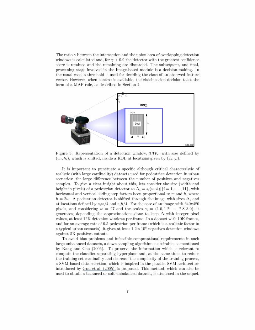
The ratio γ between the intersection and the union area of overlapping detectionwindows is calculated and, for γ > 0.9 the detector with the greatest confidencescore is retained and the remaining are discarded. The subsequent, and final,processing stage involved in the Image-based module is a decision-making. Inthe usual case, a threshold is used for deciding the class of an observed featurevector. However, when context is available, the classification decision takes theform of a MAP rule, as described in Section 4.

(1,1)

(640,480)

Y

X

(xi,yi)

hi

wi

DWi

ROI(i)

Figure 3: Representation of a detection window, DWi, with size defined by(wi, hi), which is shifted, inside a ROI, at locations given by (xi, yi).

It is important to punctuate a specific although critical characteristic ofrealistic (with large cardinality) datasets used for pedestrian detection in urbanscenarios: the large difference between the number of positives and negativessamples. To give a clear insight about this, lets consider the size (width andheight in pixels) of a pedestrian detector as ∆i = si(w, h)|i = 1, · · · , 11, withhorizontal and vertical sliding step factors been proportional to w and h, whereh = 2w. A pedestrian detector is shifted through the image with sizes ∆i andat locations defined by siw/4 and sih/4. For the case of an image with 640x480pixels, and considering w = 27 and the scales si = (1.0, 1.2, · · · , 2.8, 3.0), itgenerates, depending the approximations done to keep ∆ with integer pixelvalues, at least 12K detection windows per frame. In a dataset with 10K frames,and for an average rate of 0.5 pedestrian per frame (which is a realistic factor ina typical urban scenario), it gives at least 1.2×108 negatives detection windowsagainst 5K positives cutouts.

To avoid bias problems and infeasible computational requirements in suchlarge unbalanced datasets, a down sampling algorithm is desirable, as mentionedby Kang and Cho (2006). To preserve the information which is relevant tocompute the classifier separating hyperplane and, at the same time, to reducethe training set cardinality and decrease the complexity of the training process,a SVM-based data selection, which is inspired in the parallel SVM architectureintroduced by Graf et al. (2005), is proposed. This method, which can also beused to obtain a balanced or soft-unbalanced dataset, is discussed in the sequel.

7

3.1 SVM-based down sampling algorithm

The notations used to explain the SVM-based data selection algorithm are:XP = XP (i) : i ∈ Ip = 1, · · · , np is the input set of positive training exam-ples.XS

P = XSP (i) : i ∈ Sp ⊂ Ip is the subset of Selected positive training set.

XN = XN(i) : i ∈ In = 1, · · · , nn is the input set of negative trainingexamples.XS

N = XSN(i) : i ∈ Sn ⊂ In is the subset of Selected negative training set.

XP,N = XP , XN is the complete training set composed of XP and XN .XS

P,N = XSP , X

SN is the selected training set.

XN−Ω = XN(i) : i ∈ In\Ω is the subset of negatives instances XN with thosein Ω removed, where Ω ⊂ XN .

The number of negative instances nn in a realistic dataset heavily outnumberthe positive instances np, hence np nn. For this reason, the down samplingalgorithm applied in this work selects, from the negative training set XN , asubset of instances XS

N with |Sn| < |In|. Given the initial training set XP,N ,with np positive and nn negative training examples, this under-sampling al-gorithm selects ns instances which correspond to the support vectors of XN ,where |SV| = ns. The first step of the down sampling algorithm is to splitXN on n subsets Ωi ⊂ XN , i = 1, · · · , n; further, for each subset Ωi, a SVMclassifier is used to extract the support vectors which will be used to composeSV. Thus, each ith-SVM is trained with a subset comprising np positives andnnn negatives. The final step is to aggregate all the negative support vectors

obtained from the n SVMs. Lastly, this method outputs the selected negativetraining set which is composed by the negative support vectors: XS

N ← SV (seeAlgorithm 1). Figure 4 illustrates, in the row (a), some negative samples whosetraining feature vectors do not correspond to support vectors and, in the row(b), some samples which correspond to SV.

We performed experiments on a validation set to assess the performanceof the proposed down sampling approach in terms of classification. A linear-SVM and the Fisher’s Linear Discriminant classifiers were trained with (i) allexamples of a training set, having 100000 negatives examples, and with (ii) areduced subset constituted of support vectors (SV) obtained from the formertraining set; thus, two models have been learned. Then, we applied the classifierson a testing set and, in average, both classifiers obtained a similar hit rate buta reduction of the order of 10% in the number of false positives was observedon the models learned with support vectors.

3.2 SVM-cascade method

The proposed SVM-cascade is trained using a boosting process where the num-ber of features, in a given stage, increases wrt to the preceding stage; thus,the complexity of the cascade and its classification capability increase as morestages are added to the structure. The SVM-cascade is a cascade of linear-

8

Algorithm 1 SVM-based down sampling algorithm for negative examples se-lection

Input: XP,N = XP , XN: training set;Output: XS

N : set of selected negative samples;1: SVi: set of support vectors; n: number of iterations;2: Ωi: subset of XN ;// Initialization:

3: XSN ← : empty set;

4: Decompose XN on n subsets Ωi, where Ωi ⊂ XN ;// Selecting samples:

5: for i = 1; i < n; i+1 do6: Train a linear-SVM classifier using XP ,Ωi;7: Use the ‘negative’ support vectors, from Ωi, to generate SVi;8: end for// Composing XS

N:

9: XSN ← SVi, i = 1, · · · , n.

(a)

(b)

Figure 4: Negative samples which possess feature vectors positioned ‘far’ fromthe separation margin (a); and samples which correspond to support vectors(b).

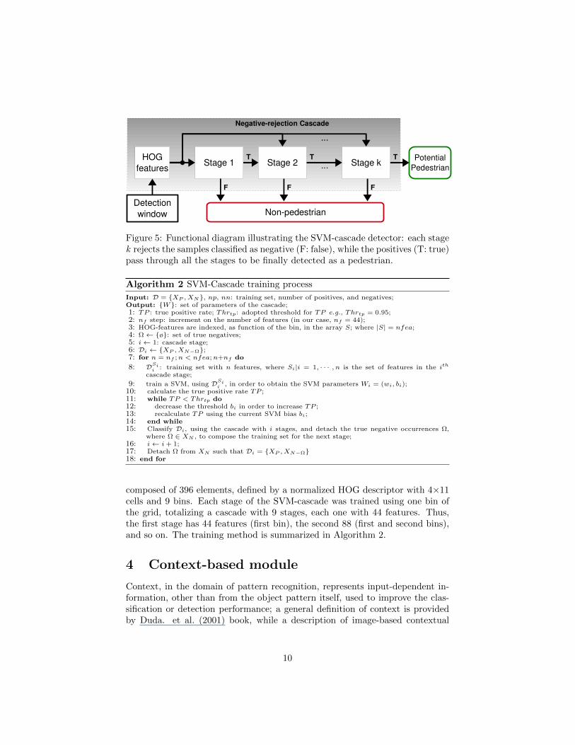
SVMs in series, which eliminates negatives in each stage, as proposed by Violaand Jones (2001); thus, at each stage the instances classified as negatives areeliminated and, conversely, the positives follow through the cascade structureas illustrated in Fig. 5. Each stage of the cascade is trained to classify a giventrue positive rate (TP ), by adjusting the separating hyperplane of the SVM inthe current stage, while rejecting the negatives correctly classified. This processis performed varying the bias (threshold) of the component SVM until TP isachieved. The subsequent stage of the cascade receives all the positives andthe false negatives instances from the previous stage, consequently, the trainingset becomes more and more difficult to classify. To improve the classificationcapability, the number of features is incremented progressively as the number ofstages increases; that is, the number of features (and the complexity) of a givenstage is increased by adding nf features wrt the previous stage.

The feature vector used to train the SVM-cascade, and a linear-SVM, is

9

Negative­rejection Cascade

HOGfeatures

Stage 1 Stage 2 Stage k PotentialPedestrian

Non­pedestrian

...T

F F F

T T

...

Detectionwindow

Figure 5: Functional diagram illustrating the SVM-cascade detector: each stagek rejects the samples classified as negative (F: false), while the positives (T: true)pass through all the stages to be finally detected as a pedestrian.

Algorithm 2 SVM-Cascade training process

Input: D = XP , XN, np, nn: training set, number of positives, and negatives;Output: W: set of parameters of the cascade;1: TP : true positive rate; Thrtp: adopted threshold for TP e.g., Thrtp = 0.95;2: nf step: increment on the number of features (in our case, nf = 44);3: HOG-features are indexed, as function of the bin, in the array S; where |S| = nfea;4: Ω← ø: set of true negatives;5: i← 1: cascade stage;6: Di ← XP , XN−Ω;7: for n = nf ;n < nfea;n+nf do

8: DSii : training set with n features, where Si|i = 1, · · · , n is the set of features in the ith

cascade stage;

9: train a SVM, using DSii , in order to obtain the SVM parameters Wi = (wi, bi);

10: calculate the true positive rate TP ;11: while TP < Thrtp do12: decrease the threshold bi in order to increase TP ;13: recalculate TP using the current SVM bias bi;14: end while15: Classify Di, using the cascade with i stages, and detach the true negative occurrences Ω,

where Ω ∈ XN , to compose the training set for the next stage;16: i← i + 1;17: Detach Ω from XN such that Di = XP , XN−Ω18: end for

composed of 396 elements, defined by a normalized HOG descriptor with 4×11cells and 9 bins. Each stage of the SVM-cascade was trained using one bin ofthe grid, totalizing a cascade with 9 stages, each one with 44 features. Thus,the first stage has 44 features (first bin), the second 88 (first and second bins),and so on. The training method is summarized in Algorithm 2.

4 Context-based module

Context, in the domain of pattern recognition, represents input-dependent in-formation, other than from the object pattern itself, used to improve the clas-sification or detection performance; a general definition of context is providedby Duda. et al. (2001) book, while a description of image-based contextual

10

(a) (c)

(b)

Restaurant

40°11'08.80'' N8°24'50.00'' W

Figure 6: Digital map of the environment where the dataset were collected. (a)Satellite image of scenario with the map of the roads marked in white. Examplesof incidence zones, used in the context-based module, are given in (b) and (c).

cues is given by Perko and Leonardis (2010). Here, context refers to the po-sition of the object in a semantic map, as opposed to the object pattern itselfwhich refers to a given model learned from a classifier trained in a set of ‘local’image-descriptors. In short, the contextual information, incorporated into thepedestrian detection system, is based on prior knowledge of the object positionin a semantic map of the roads.

In the decision module, shown in Fig. 1 as part of the Image-based mod-ule, the contextual information is processed in the form of prior probabilitiesaccording to a MAP decision framework. As consequence, the response of theimage-based detectors, used in the decision module, has to be posed in proba-bilistic terms as well; more specifically, the response of the classifiers are modeledby probabilistic distributions in order to obtain class-conditional probabilitieswhich are used in the MAP decision rule.

4.1 Context-based module using object position in a se-mantic map

Context-based prior probabilities are used as function of the position, actuallypresence, of the objects in specific regions in the scenario. A semantic map ofthe roads traveled by the ISRobotCar was built with the aid of satellite imageryfrom the Google Earth©, as illustrated in Fig. 6(a). A set of regions on themap was selected and identified as regions with a high potential of pedestrianoccurrence. The idea was to assign a confidence score, characterized by a priorknowledge, to the zones on the map that are more likely to contain pedestrians,hereafter called incidence regions. The incidence regions defined on the map are:crosswalks, regions nearby restaurants, bus-stops, and cafeterias, and the zonewhich covers the roundabout in front of the main secretariat building. Someexamples of incidence zones are shown in Fig. 6(b) and Fig. 6(c).

The map of the roads, and consequently the incidence regions, are definedin GPS coordinates, more specifically, GPS data is defined in terms of latitude,

11

longitude and altitude (lla) in the World Geodetic System 1984 (WGS84). How-ever, the objects (segments) detected in the LIDAR-based module have coordi-nates defined by a local Cartesian system. Thus, it is necessary to establish acorrespondence between the GPS coordinate system and the ‘local’ coordinatesystem of the laserscanner, and vice versa.

A solution for obtaining the objects coordinates, in the LIDAR referencesystem, with respect to a point in the map is to convert the GPS coordinatesinto local navigation coordinates. This ‘local’ navigation system is determinedby the east, north and up (ENU) reference system as described in the work ofDrake (2002). Therefore, it is necessary to transform the regions of the mapand the objects coordinates to a common ENU reference system in order todetermine if a detected object, in a given frame, is inside or not an incidenceregion.

Using the Google Earth© software, the regions on the map were manuallydrawn as polygons in satellite images of the scenario. Thereafter, the position ofthese regions, defined by four pairs of points in GPS coordinates, were convertedto a ENU reference system. Regarding the position of a given detected object,defined in Cartesian coordinates centered in the laser, its has to be converted toa reference point in the vehicle, aligned with the GPS rover-station, and thenconverted to the same ENU reference system used on the map. In summary,the transformation of any point PGPS

2 in GPS coordinates to ENU is a threestage process:1. Define a reference point in the map, here denoted by Pref , in lla coordinates;2. Express PGPS , defined in lla coordinates, in Earth Centered Earth Fixed(ECEF) coordinates. In this work, the lla2ecef Matlab© function was used forthis purpose; in Matlab© notation: PECEF =lla2ecef (PGPS , ‘WGS84’);3. Convert PECEF to the ENU coordinate. Denoting by PENU a point in thenavigation coordinates, in Matlab© notation we have:PENU =ecef2lv(PECEF ,Pref ,ellipsoid), where ellipsoid represents the Ellipsoidfitted around the Earth globe. Using the Matlab© almanac function: ellipsoid= almanac(‘earth’,‘ellipsoid’,‘kilometers’,‘WGS84’ ).

A Differential-GPS, which operates with a ground referenced station (basestation), has an absolute precision measurement much more accurate than aGPS system. The base station communicates with the moving station (mountedon the vehicle) at UHF frequency. The information shared between the stationshas an average cycle of 200 ms (5 Hz), which supports the RTK designation.However, DGPS is not immune to errors. In our database, some position mea-surements suffered with the multi-path, or occlusions, problem. Moreover, thelack of credibility of GPS in some parts of the trajectory occurred due to tem-porary lost of communication between the rover and the base station. To reducethe uncertainties and errors of GPS systems, a multisensor fusion approach suchas the proposed by Bento et al. (2012), can be used to estimate and to correctthe position measurements of DGPS units.

2whatever the point represents the position of a detected object or one of the corners ofthe polygon that defines an incidence region.

12

−3 −2 −1 0 1 2 30

0.1

0.2

0.3

0.4

0.5

0.6

−10 −8 −6 −4 −2 0 2 40

0.1

0.2

0.3

0.4

0.5

0.6

data1

data2

PED

nPED

Figure 7: Histogram and Normal distribution fitted to the output scores, on thetraining set, of a linSVM and the Deformable Parts-based Model.

4.2 MAP decision rule using contextual information

As described in previous sections, the contextual information is processed interms of prior probabilities. Therefore, the class-conditional probability, or sim-ply likelihood, is obtained from the classification method used in the decisionmodule. Thus, the outputs of the image-based detectors, obtained from thetraining set, were modeled according to a probabilistic distribution. Figure7 shows the distributions of a lin-SVM and the Parts-based Model. The his-tograms, plotted as function of the classifier’s scores, were modeled by a Normaldistribution which will be used as likelihood function in the MAP decision. Inthis case, the problem resumes to the particular case of decision making us-ing univariate-Normal densities. Designating by P (ω1) the prior probability ofpedestrian occurrence in an incidence zone, for the non-incidence zones the priorwas considered to be mutually exclusive and exhaustive so, if an object is lo-cated in a non-incidence zone, its prior is equal to 1−P (ω1). If P (ω1) = P (ω0)3,the decision resumes to the case of ML rule. If the prior probabilities are notequal, that is, P (ω1) 6= P (ω0), the decision threshold shifts away from the morelikely class.

Denoting by TΛ the decision threshold when P (ω0) = P (ω1), as the valueof P (ωi|i=0,1) varies during the experiments using context, TΛ also varies.Let N (µ1, σ

21) and N (µ0, σ

20) be the Normal distributions for the positive and

negative classes respectively, and denoting the posterior probability of the eventbe a pedestrian by P (ω1|x ≥ 0), the Bayes’formula is expressed by

P (ω1|x) =p(x|ω1)P (ω1)

p(x|ω1)P (ω1) + p(x|ω0)P (ω0)(4)

3Both classes are likely to occur.

13

where p(x|ωi), i = 0, 1 are the class-conditional probability density functionsmodeled by the Normals N (µi, σ

2i ). Rearranging (4), we have

p(x|ω1) = p(x|ω1)P (ω1|x)(1− P (ω1))

P (ω1)(1− P (ω1|x))(5)

Using the natural logarithm in both sides of (5) and expanding the squares,it follows that

(x2 − 2xµ1 + µ21)

2σ21

=(x2 − 2xµ0 + µ2

0)

2σ20

− ln(σ1

σ0P) (6)

where P = P (ω1|x)(1 − P (ω1))/P (ω1)(1 − P (ω1|x)), c.f. (5). Thus, the valueof the decision boundary’s threshold for any P (ω1) > 0 is the solution of thequadratic equation:

(σ21 − σ2

0)x2 + 2(σ20µ1 − σ2

1µ0)x−(2σ2

1σ20W + σ2

0µ21 − σ2

1µ20) = 0

(7)

where,

W = lnσ1(P (ω1|x = TΛ)− P (ω1)P (ω1|x = TΛ))

σ0(P (ω1)− P (ω1)P (ω1|x = TΛ))(8)

Equation (8) is valid when the detected object is inside an incidence zone,otherwise P (ω1) should be replaced by P (ω0). Notice that the variable x denotesthe classification score, where x = TΛ (usually TΛ=0) is the ‘optimal’ thresholdwhen P (ω1|x) = P (ω0|x). As the priors are changed, the thresholds changed aswell. If P (ω1) > P (ω0) the decision boundary shifts away from the more likelyclass, ω1, and vice-versa.

5 Experiments

The main objective of the experiments reported in this paper is to evaluate thedetection performance of the system regarding (i) the classification method usedin the Image-based module, and as function of (ii) the prior probabilities thatcharacterize the incidence zones in the semantic map. To support experimentalanalysis, the multisensor LIPD dataset was used (see Section 5.2 for details). InSection 5.3, the classification methods are evaluated without contextual infor-mation. After, the influence of priors in the MAP decision rule is shown on theexperimental results presented in Section 5.4. To have coherent results amongthe evaluated methods, all the parameters and variables of the preprocessingand segmentation stages used in the LIDAR-based module were rigorously thesame during the experiments. In other words: the results reported in the se-quel depend, exclusively, on the classification methods and on the context-basedapproach.

14

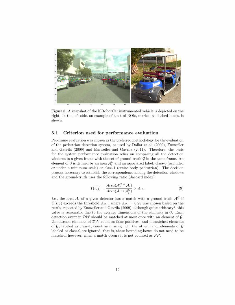
Figure 8: A snapshot of the ISRobotCar instrumented vehicle is depicted on theright. In the left-side, an example of a set of ROIs, marked as dashed-boxes, isshown.

5.1 Criterion used for performance evaluation

Per-frame evaluation was chosen as the preferred methodology for the evaluationof the pedestrian detection system, as used by Dollar et al. (2009), Enzweilerand Gavrila (2009) and Enzweiler and Gavrila (2011). Therefore, the basisfor the system performance evaluation relies on comparing all the detectionwindows in a given frame with the set of ground-truth G in the same frame. Anelement of G is defined by an area AG

j and an associated label: class-0 (occludedor under a minimum scale) or class-1 (entire body pedestrian). The decisionprocess necessary to establish the correspondence among the detection windowsand the ground-truth uses the following ratio (Jaccard index):

Υ(i, j) =Area(AG

j ∩ Ai)

Area(Ai ∪ AGj )

> Athr (9)

i.e., the area Ai of a given detector has a match with a ground-truth AGj if

Υ(i, j) exceeds the threshold Athr, where Athr = 0.25 was chosen based on theresults reported by Enzweiler and Gavrila (2009); although quite arbitrary4, thisvalue is reasonable due to the average dimensions of the elements in G. Eachdetection event in DW should be matched at most once with an element of G.Unmatched elements of DW count as false positives, and unmatched elementsof G, labeled as class-1, count as missing. On the other hand, elements of Glabeled as class-0 are ignored, that is, these bounding-boxes do not need to bematched; however, when a match occurs it is not counted as FP .

15

(a)

(b)

Figure 9: LIPD dataset examples: (first row) labeled pedestrians used on thetraining set; (middle row) full images on the testing set; (last row) screen shotof ROI projections, blue rectangles, on testing images.

5.2 The LIPD dataset

The Laser and Image Pedestrian Detection (LIPD) dataset, designated DLIPD,comprises two sets, Dtrain and Dtest; the former is used for training purposes,and the later constitutes the testing set. The entire set5 contains, besides monoc-ular images and LIDAR scans, data from two proprioceptive sensors, an IMUand an incremental encoder, and also data from a differential GPS. The datasetwas recorded from the sensor acquisition system mounted on the ISRobotCar,an instrument Yamaha vehicle shown in Fig. 8, driving through the areas of theTechnological Campus of the University of Coimbra and in the neighboring6.

Due to the fact that the dataset was obtained in outdoor conditions, andsince the sensor apparatus has been exposed to weather and environmentalconditions, not unexpectedly, some ‘difficulties’ have occurred namely: lightexposure variations, vibrations, oscillations, noise, dust and particles on the air,among others. Perhaps one of the main problems during the data recording wasthe occurrence of some spots in the images due to dust on the lens.

The training part of the dataset contains 4606 manually labeled positives(image’s cutouts of pedestrian in up-right entire body), and 2444 full-frames640x480 resolution images without any pedestrian evidence. Thus, the elementsof the training set are the aforementioned 5327 positives cutouts (or boundingboxes) and a free-number of negative instances which can be extracted from thenegatives frames. The current testing set contains 4823 full-frame images, anddetailed annotations regarding the pedestrians appearance (in terms of occlu-sion), namely: occluded/partial pedestrians (class-0) and entire body pedestri-ans (class-1). A summary of the dataset is given in Table 1.

4Other possible value for Athr is 0.5 as suggested by Dollar et al. (2009)5available on the Web: http://www.isr.uc.pt/~cpremebida/dataset6http://www.isr.uc.pt/~cpremebida/PoloII-Google-map.pdf

16

Table 1: Statistics of DLIPD

Training set

Set Npos Nneg Description

Dtrain 4606 2444Sunny days, autumn season. Negatives instances should beextracted from the 2444 frames.

Testing set

Dtest 698 ∗Sunny days, autumn season. The number of negatives (∗)depends the detection approach to be used (which can takeadvantage of the LIDAR information or not).

5.3 Performance evaluation of the image-based detectors

A linear SVM, the proposed SVM-cascade and the Deformable Parts-basedModel (hereafter called DPM), were evaluated and the detection performanceon the LIPD-testing set (Dtest) is reported in the sequel. The classifier’s modelswere learned using all the positives examples and a subset of ‘hard’ negativesextracted from Dtrain using the proposed SVM-based down sampling algorithmpresented in Section 3.1. Detection rate versus false positives per frame was thecondition used to evaluate the performance of these methods in Dtest. In orderto analyze, in particular, the generalization capability of the DPM method andalso to have a fair comparison with the others methods, this detector was eval-uated using a model learned on the LIPD-training set (designated by DPM-1)and the model originally learned on the INRIA dataset and available by Felzen-szwalb et al. (2012), which we called DPM-2. Both models are shown in Fig.10.

Figure 10: Pedestrian models obtained with the DPM method. First row rep-resents the INRIA-based model (DPM-2), which is available on the website ofFelzenszwalb et al. (2012). The second row shows the model obtained with theLIPD dataset (DPM-1). From left to right: the root filter’s model, followed bypart filters, and spatial model for the location of each part relative to the root.

To evaluate detection performance, with no use of context, on entire im-ages in contrast with ROI-based images, we consider the DPM method andthe codes available by Felzenszwalb et al. (2012) as benchmark. Moreover, to

17

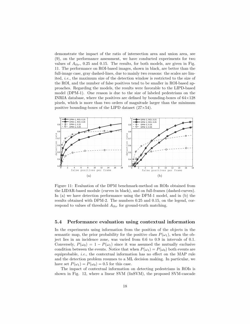
demonstrate the impact of the ratio of intersection area and union area, see(9), on the performance assessment, we have conducted experiments for twovalues of Athr, 0.25 and 0.15. The results, for both models, are given in Fig.11. The performance on ROI-based images, shown in black, are better than thefull-image case, gray dashed-lines, due to mainly two reasons: the scales are lim-ited, i.e., the maximum size of the detection window is restricted to the size ofthe ROI, and the number of false positives tend to be smaller in ROI-based ap-proaches. Regarding the models, the results were favorable to the LIPD-basedmodel (DPM-1). One reason is due to the size of labeled pedestrians on theINRIA database, where the positives are defined by bounding-boxes of 64×128pixels, which is more than two orders of magnitude larger than the minimumpositive bounding-boxes of the LIPD dataset (27×54).

0 2 4 6 8 10 12 14 16 180.3

0.4

0.5

0.6

0.7

0.8

0.9

1

false positives per frame

detection rate

DPM−1, ROI, 0.15DPM−1, ROI, 0.25DPM−1, 0.15DPM−1, 0.25

(a)

0 2 4 6 8 10 12 14 16 180.3

0.4

0.5

0.6

0.7

0.8

0.9

1

false positives per frame

detection rate

DPM−2, ROI, 0.15DPM−2, ROI, 0.25DPM−2, 0.15DPM−2, 0.25

(b)

Figure 11: Evaluation of the DPM benchmark-method on ROIs obtained fromthe LIDAR-based module (curves in black), and on full-frames (dashed-curves).In (a) we have detection performance using the DPM-1 model, and in (b) theresults obtained with DPM-2. The numbers 0.25 and 0.15, on the legend, cor-respond to values of threshold Athr for ground-truth matching.

5.4 Performance evaluation using contextual information

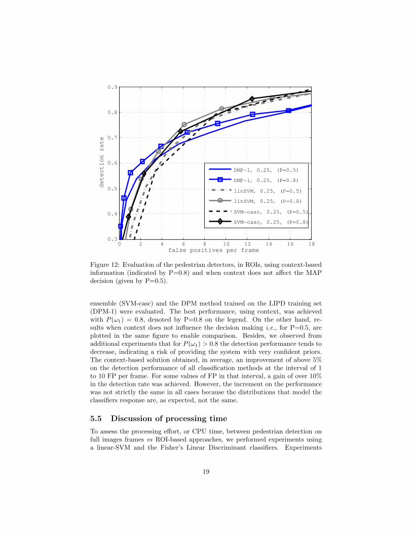
In the experiments using information from the position of the objects in thesemantic map, the prior probability for the positive class P (ω1), when the ob-ject lies in an incidence zone, was varied from 0.6 to 0.9 in intervals of 0.1.Conversely, P (ω0) = 1 − P (ω1) since it was assumed the mutually exclusivecondition between the events. Notice that when P (ω1) = P (ω0) both events areequiprobable, i.e., the contextual information has no effect on the MAP ruleand the detection problem resumes to a ML decision making. In particular, wehave set P (ω1) = P (ω0) = 0.5 for this case.

The impact of contextual information on detecting pedestrians in ROIs isshown in Fig. 12, where a linear SVM (linSVM), the proposed SVM-cascade

18

0 2 4 6 8 10 12 14 16 180.3

0.4

0.5

0.6

0.7

0.8

0.9

false positives per frame

de

tect

ion

ra

te

DMP−1, 0.25, (P=0.5)

DMP−1, 0.25, (P=0.8)

linSVM, 0.25, (P=0.5)

linSVM, 0.25, (P=0.8)

SVM−casc, 0.25, (P=0.5)

SVM−casc, 0.25, (P=0.8)

Figure 12: Evaluation of the pedestrian detectors, in ROIs, using context-basedinformation (indicated by P=0.8) and when context does not affect the MAPdecision (given by P=0.5).

ensemble (SVM-casc) and the DPM method trained on the LIPD training set(DPM-1) were evaluated. The best performance, using context, was achievedwith P (ω1) = 0.8, denoted by P=0.8 on the legend. On the other hand, re-sults when context does not influence the decision making i.e., for P=0.5, areplotted in the same figure to enable comparison. Besides, we observed fromadditional experiments that for P (ω1) > 0.8 the detection performance tends todecrease, indicating a risk of providing the system with very confident priors.The context-based solution obtained, in average, an improvement of above 5%on the detection performance of all classification methods at the interval of 1to 10 FP per frame. For some values of FP in that interval, a gain of over 10%in the detection rate was achieved. However, the increment on the performancewas not strictly the same in all cases because the distributions that model theclassifiers response are, as expected, not the same.

5.5 Discussion of processing time

To assess the processing effort, or CPU time, between pedestrian detection onfull images frames vs ROI-based approaches, we performed experiments usinga linear-SVM and the Fisher’s Linear Discriminant classifiers. Experiments

19

with full frames demanded, in average, a computational time three times higherthan the ROI-based approach. However the CPU time of all the LIDAR-basedprocessing stages involved in our system was not strictly taken into account inour experiments.

We also did runtime analysis between the SVM-cascade and a linSVM, whichhas been of the order of five times faster to the later method. Nevertheless, bothmethods are slightly similar in terms of classification performance as shown inFig. 12. On the other hand, the majority of the computational cost imposedby the Context-based module depends on the processing time involved in theLIDAR-based module.

6 Conclusions

This work presented a context-based multisensor fusion architecture for pedes-trian detection in urban environment. The proposed architecture comprisesthree main processing stages: (i) a LIDAR-based module acting as primaryobject detection and ROI generator, (ii) a Image-based module using sliding-window detectors with the role of validating the presence of pedestrians in ROIs,and (iii) a module which supplies the system with contextual information ob-tained from a semantic map. The LIPD dataset, which is high imbalanced, wereused for experimental evaluation. Moreover, a down sampling method, usingsupport vectors extracted from multiple linear-SVMs, was used to reduce thecardinality of the training set and, as consequence, to decrease the CPU-timeduring the training process.

Experiments demonstrate that contextual information enhances the perfor-mance of a pedestrian detection system. The experiments were performed usinga linear-SVM, a proposed SVM-cascade and the DPM method. However, simi-lar tendency in the performance is expected using other classification methodssince the contextual information enters in the system as prior probabilities whichare independent of the conditional probabilities given by the classifier. The useof incidence regions clearly enhanced the detection performance, which demon-strates that the probability of pedestrian occurrence in some specific zones (e.g.,crosswalks, bus-stops) is higher than other zones. The use of context in suchperception system seems to be a promising area since plenty of contextual infor-mation, other than the critical regions, can be used, such as: day-time, weathercondition, object velocity, infrastructure-based information, and so on.

7 Acknowledgments

This work was supported by National Funds through Fundacao para a Ciencia ea Tecnologia de Portugal (FCT), under project grant PTDC/EEA-AUT/113818/2009.The authors thank the reviewers for their insightful comments and valuable sug-gestions.

20

References

Bento, L. C., Parafita, R., and Nunes, U. (2012). Inter-vehicle sensor fusion foraccurate vehicle localization supported by v2v and v2i communications. In In-telligent Transportation Systems, ITSC. 15th IEEE International Conferenceon, pages 907–914, USA.

Bouguet, J. Y. (2007). Camera calibration toolbox for matlab [online].http://www.vision.caltech.edu/bouguetj/calib doc/.

Dalal, N. and Triggs, B. (2005). Histograms of oriented gradients for humandetection. In Computer Vision and Pattern Recognition, CVPR. IEEE Con-ference on, pages 886–893, Washington, DC, USA. IEEE Computer Society.

Dollar, P., Wojek, C., Schiele, B., and Perona, P. (2009). Pedestrian detection:A benchmark. In Computer Vision and Pattern Recognition, IEEE ComputerSociety Conference on, pages 304–311, Los Alamitos, CA, USA.

Dollar, P., Wojek, C., Schiele, B., and Perona, P. (2012). Pedestrian detection:An evaluation of the state of the art. IEEE Transactions on Pattern Analysisand Machine Intelligence, 34(4):743–761.

Douillard, B., Fox, D., Ramos, F., and Durrant-Whyte, H. (2011). Classificationand semantic mapping of urban environments. The International Journal ofRobotics Research, 30(1):5–32.

Drake, S. (2002). Converting gps coordinates (lla) to navigation coordinates(enu). Dsto-tn-0432, DSTO Electronics and Surveillance Research Labora-tory, Australia.

Duda., R. O., Hart, P. E., and Stork, D. G. (2001). Pattern classification. JohnWiley & Sons, Inc, NY.

Enzweiler, M. and Gavrila, D. (2011). A multilevel mixture-of-experts frame-work for pedestrian classification. Image Processing, IEEE Transactions on,20(10):2967–2979.

Enzweiler, M. and Gavrila, D. M. (2009). Monocular pedestrian detection: Sur-vey and experiments. IEEE Transactions on Pattern Analysis and MachineIntelligence, 31(12):2179–2195.

Faouzi, N.-E. E., Leung, H., and Kurian, A. (2011). Data fusion in intelli-gent transportation systems: Progress and challenges - a survey. InformationFusion, 12(1):4–10.

Felzenszwalb, P. F., Girshick, R. B., and McAllester, D. (Accessed onJuly, 2012). Discriminatively trained deformable part models, release 4.http://people.cs.uchicago.edu/ pff/latent-release4/.

21

Felzenszwalb, P. F., Girshick, R. B., McAllester, D., and Ramanan, D. (2010).Object detection with discriminatively trained part-based models. IEEETransactions on Pattern Analysis and Machine Intelligence, 32:1627–1645.

Gandhi, T. and Trivedi, M. (2007). Pedestrian protection systems: issues, sur-vey, and challenges. Intelligent Transportation Systems, IEEE Transactionson, 8(3):413–430.

Garcia, F., de la Escalera, A., Armingol, J., Herrero, J., and Llinas, J. (2011).Fusion based safety application for pedestrian detection with danger estima-tion. In Information Fusion (FUSION), 2011 Proceedings of the 14th Inter-national Conference on, pages 1 –8.

Geronimo, D., Lopez, A. M., Sappa, A. D., and Graf, T. (2010). Survey onpedestrian detection for advanced driver assistance systems. IEEE Transac-tions on Pattern Analysis and Machine Intelligence, 32(7):1239–1258.

Graf, H. P., Cosatto, E., Bottou, L., Durdanovic, I., and Vapnik, V. (2005).Parallel support vector machines: The cascade svm. In In Advances in NeuralInformation Processing Systems, NIPS, pages 521–528.

Heikkila, J. and Silven, O. (1997). A four-step camera calibration procedurewith implicit image correction. In Computer Vision and Pattern Recognition,CVPR. IEEE Conference on, pages 1106–1112.

Kang, P. and Cho, S. (2006). Eus svms: Ensemble of under-sampled svms fordata imbalance problems. In Neural Information Processing, volume 4232 ofLecture Notes in Computer Science, pages 837–846. Springer Berlin / Heidel-berg.

Ludwig, O., Premebida, C., Nunes, U., and Araujo, R. (2011). Evaluationof boosting-svm and srm-svm cascade classifiers in laser and vision-basedpedestrian detection. In Intelligent Transportation Systems, ITSC. IEEEInternational Conference on, pages 1574–1579, USA.

Markoff, J. (Oct 9, 2010). Google cars drive themselves, in traffic. New YorkTimes.

Navarro-Serment, L. E., Mertz, C., and Hebert, M. (2010). Pedestrian detectionand tracking using three-dimensional ladar data. The International Journalof Robotics Research, 29(12):1516–1528.

Perko, R. and Leonardis, A. (2010). A framework for visual-context-aware ob-ject detection in still images. Computer Vision and Image Understanding,114(6):700 – 711.

Spinello, L., Triebel, R., and Siegwart, R. (2010). Multiclass multimodal de-tection and tracking in urban environments. The International Journal ofRobotics Research, 29(12):1498–1515.

22

Stiller, C., Leon, F. P., and Kruse, M. (2011). Information fusion for automotiveapplications - an overview. Information Fusion, 12(4):244–252.

Vasconcelos, F., Barreto, J., and Nunes, U. (2012). A minimal solution for theextrinsic calibration of a camera and a laser-rangefinder. Pattern Analysisand Machine Intelligence, IEEE Transactions on.

Viola, P. and Jones, M. (2001). Rapid object detection using a boosted cascadeof simple features. In IEEE Computer Vision and Pattern Recognition (CVPR01), volume 1, pages 511–518, Hawaii,USA.

23