Non-Overlapping Multi-camera Detection and Tracking of Vehicles in Tunnel Surveillance
Pedestrian Tracking-by-Detection for Video Surveillance ...
275
Pedestrian Tracking-by-Detection for Video Surveillance Applications vorgelegt von Dipl.-Ing. Volker Eiselein von der Fakultät IV – Elektrotechnik und Informatik der Technischen Universität Berlin zur Erlangung des akademischen Grades Doktor der Ingenieurwissenschaften - Dr.-Ing. - genehmigte Dissertation Promotionsausschuss: Vorsitzender: Prof. Dr. rer. nat. Anatolij Zubow Gutachter: Prof. Dr.-Ing. Thomas Sikora Gutachter: Prof. Dr.-Ing. Olaf Hellwich Gutachter: Prof. Dr. Jian Zhang Tag der wissenschaftlichen Aussprache: 20. Mai 2019 Berlin 2019
-
Upload
khangminh22 -
Category
Documents
-
view
4 -
download
0
Transcript of Pedestrian Tracking-by-Detection for Video Surveillance ...

Pedestrian Tracking-by-Detection for
Video Surveillance Applications
vorgelegt von
Dipl.-Ing. Volker Eiselein
von der Fakultät IV – Elektrotechnik und Informatik
der Technischen Universität Berlin
zur Erlangung des akademischen Grades
Doktor der Ingenieurwissenschaften
- Dr.-Ing. -
genehmigte Dissertation
Promotionsausschuss:
Vorsitzender: Prof. Dr. rer. nat. Anatolij Zubow
Gutachter: Prof. Dr.-Ing. Thomas Sikora
Gutachter: Prof. Dr.-Ing. Olaf Hellwich
Gutachter: Prof. Dr. Jian Zhang
Tag der wissenschaftlichen Aussprache: 20. Mai 2019
Berlin 2019


Eidesstattliche Versicherung
Ich erkläre hiermit, dass ich die vorliegende Arbeit ohne unzulässige Hilfe Dritter
und ohne Benutzung anderer als der angegebenen Hilfsmittel angefertigt habe; die
aus fremden Quellen direkt oder indirekt übernommenen Gedanken sind als solche
kenntlich gemacht. Insbesondere habe ich nicht die Hilfe eines kommerziellen Pro-
motionsberaters in Anspruch genommen. Dritte haben von mir weder unmittelbar
noch mittelbar geldwerte Leistungen für Arbeiten erhalten, die im Zusammenhang
mit dem Inhalt der vorgelegten Dissertation stehen. Ich erkläre, dass mir die gelten-
de Promotionsordnung bekannt ist. Die Arbeit wurde bisher weder im Inland noch
im Ausland in gleicher oder ähnlicher Form als Dissertation eingereicht und ist als
Ganzes auch noch nicht veröffentlicht.
Berlin, den .................
Volker Eiselein
iii


To Anne, Mats and Till


Acknowledgments
My sincere gratitude goes to the supervisor of this thesis, Prof. Dr.-Ing. Thomas
Sikora, who gave me the opportunity to join the Communication Systems Group
at Technische Universität Berlin (Fachgebiet Nachrichtenübertragung, TUB-NÜ)
and who supported my work through his advise and guidance. I also want to thank
Prof. Dr.-Ing. Olaf Hellwich and Prof. Dr. Jian Zhang for their detailed review of
this thesis which improved its quality significantly and Prof. Dr. rer. nat. Anatolij
Zubow for his engagement as jury president.
During my time at TUB-NÜ, I met a number of great colleagues who were not
only always available to discuss scientific results and further research ideas, but also
made working on joint research projects real fun. Although the list of names could
be much longer, I would like to thank in particular Dr.-Ing. Tobias Senst, Michael
Pätzold, Dr.-Ing. Rubén Heras Evangelio, Erik Bochinski, Markus Küchhold, and
Maik Simon for their inspiration and the good times we had.
I am also grateful to the students who worked together with me on this research
field and contributed additional insights by writing their Master’s and Diploma the-
ses on related topics, especially Daniel Arp, Gleb Sternharz, Tino Kutschbach and
Sezgin Ceyhan. In addition, I would like to thank the people who provided the en-
vironment in which this research work has been possible, especially Birgit Boldin
for her invaluable dedication to TUB-NÜ and Prof. Dr. Ivo Keller.
And, above all, my biggest thanks go to my family and friends who have hel-
ped me through the discouraging and boring phases of such a work. Especially my
wife Anne and my children have been giving me enormous emotional support and
continuous motivation for finalizing this thesis.
vii


Abstract
This dissertation presents new approaches and methods for the application of tracking-
by-detection algorithms for pedestrian tracking in video surveillance scenarios with
static cameras. Using a modular state-of-the-art tracking-by-detection framework
based on a Gaussian Mixture Probability Hypothesis Density (GM-PHD) Filter, this
work analyzes the challenges of tracking pedestrians in surveillance and develops
approaches to deal with them.
On the detector side, filters based on local crowd density and geometric priors
are proposed in order to improve pedestrian detection in crowds. Compared to
the baseline, these filters reduce bad detections and allow for adaptive dynamic
thresholding in the detection process, thus enhancing the detection results.
To improve the tracking process in ambiguous scenarios, feature-based label
trees are proposed which maintain a visual model of the tracked objects and al-
low their re-identification after crossing situations. Performance improvements to
the baseline are shown both in simulation and practical experiments.
Further tracker improvements include extensions to enable the usage of multiple,
complementary detectors in the framework and the proposal of a novel update step
which is independent of the sensor order. A theoretical justification and practical
validation in experiments show that this method yields better results for visual track-
ing than the individual sensors or the commonly used iterated corrector approach.
The mathematical concept of a critical path of missed detections inspires the
usage of motion cues for post-filtering detections in order to improve the tracking
further. The proposed filtering concept is modular and independent of the detector
used. Thanks to a reduction of missed detections it improves both the detection and
tracking results which is shown on different data sets.
In order to enable further integration of visual information cues into the tracking
framework, three different runtime-efficient person re-identification methods and
their parametrization are also assessed on four different datasets in this work and
integrated into a powerful multi-cue re-identification method. Therefore, different
greedy and non-greedy fusion strategies are validated. In order to improve the com-
parison of region covariance features, the baseline metric is extended by a novel
pre-processing step in order to ensure the full rank of the covariance matrix. This
reduces bad metric results by rank issues and improves the re-identification process.


Zusammenfassung
Diese Arbeit behandelt neue Ansätze für die visuelle Objektverfolgung in Video-
überwachungsanwendungen mit Hilfe des Tracking-by-detection-Prinzips. Ausge-
hend von einem Gaussian Mixture Probability Hypothesis Density Filter als Bei-
spielverfahren werden Probleme und Schwierigkeiten analysiert, die bei seiner An-
wendung für die Videoüberwachung mit statischen Kameras entstehen, und es wer-
den Ansätze entwickelt, diesen entgegenzuwirken.
Um die Ergebnisse auf der Sensorebene zu verbessern, werden Filter vorgeschla-
gen, die anhand von lokaler Menschenmengendichte und geometrischen Nebenbe-
dingungen falsche Detektionen reduzieren und durch adaptive dynamische Schwel-
lenwerte bessere Detektionsergebnisse erzielen.
Für die Verfolgung sich kreuzender Objekte wird eine Erweiterung der Label-
Bäume vorgeschlagen, die mittels eines Modells der verfolgten Objekte die späte-
re korrekte Zuordnung der Objekte ermöglicht. Simulationen und praktische Ex-
perimente zeigen, dass diese Integration visueller Merkmale in die Label-Bäume
Performance-Verbesserungen erzielt.
Weitere vorgeschlagene Verbesserungen in dieser Arbeit sind die Integration
mehrerer Detektoren zur Erhöhung der Detektionswahrscheinlichkeit mittels eines
neuartigen Korrektorschritts. Im Gegensatz zum bisher üblichen iterierten Korrek-
torschritt ist die Sensorreihenfolge beim entwickelten Verfahren egal, und die Per-
formance wird verbessert, was theoretisch und durch Experimente gezeigt wird.
Das Konzept eines kritischen Pfads von Fehldetektionen inspiriert die Nutzung
von Bewegungsinformationen für die Nachfilterung von Detektionen, um die Ob-
jektverfolgung weiter zu verbessern. Dieser Ansatz ist modular und unabhängig
vom Detektionsalgorithmus einsetzbar. Dank einer Reduzierung der Fehldetektio-
nen verbessert es sowohl die Objektdetektion als auch die -verfolgung, was auf
mehreren Datensätzen gezeigt wird.
Für eine Integration weiterer visueller Informationen in das Objektverfolgungs-
system werden zusätzlich in dieser Arbeit laufzeiteffiziente Verfahren zur Perso-
nenwiedererkennung evaluiert und mittels verschiedener Fusionsmethoden in ein
Multideskriptorsystem kombiniert. Um Fehler durch die Vergleichsmetrik der ver-
wendeten Region Covariance-Methoden auszuschließen, wird das bisherige Ver-
fahren um einen neuen Vorverarbeitungsschritt erweitert, der den vollen Rang der
Matrizen sicherstellt und so die Wiedererkennung verbessert.


Contents
1 Introduction 1
1.1 Video Surveillance and Multi-Object Tracking . . . . . . . . . . . . 1
1.2 Thesis Objectives . . . . . . . . . . . . . . . . . . . . . . . . . . . 4
1.3 Principal Contributions and Novelties of This Thesis . . . . . . . . 5
1.4 Thesis Overview . . . . . . . . . . . . . . . . . . . . . . . . . . . 7
1.5 List of Publications . . . . . . . . . . . . . . . . . . . . . . . . . . 9
2 Pedestrian Detection 15
2.1 Algorithms for Activity Detection . . . . . . . . . . . . . . . . . . 16
2.2 Histograms of Oriented Gradients for Pedestrian Detection . . . . . 18
2.3 Pedestrian Detection in This Thesis . . . . . . . . . . . . . . . . . 23
3 Object Tracking 25
3.1 Tracking-by-Detection: Bayesian Trackers for the Single-Object Case 31
3.1.1 The Kalman Filter . . . . . . . . . . . . . . . . . . . . . . 33
3.1.2 Sequential Monte Carlo Methods . . . . . . . . . . . . . . 35
3.2 Tracking-by-Detection: Multi-Object Case . . . . . . . . . . . . . . 37
3.2.1 Multiple Hypothesis Tracking . . . . . . . . . . . . . . . . 40
3.2.2 Particle Filter-Based Multi-Object Trackers . . . . . . . . . 42
3.2.3 Random Finite Sets in Tracking Theory . . . . . . . . . . . 43
A) The Multi-Target Bayes Filter . . . . . . . . . . . 46
B) Standard Prediction and Measurement Model . . 49
C) Discussion of the Standard Prediction and Mea-
surement Model . . . . . . . . . . . . . . . . . . 50
3.2.4 Tracking Using Probability Hypothesis Density . . . . . . . 51
A) The Concept of Probability Hypothesis Density . 51
xiii

B) The Probability Hypothesis Density Filter . . . . 52
C) Prediction Step . . . . . . . . . . . . . . . . . . . 54
D) Update Step . . . . . . . . . . . . . . . . . . . . 55
E) Complexity Reduction in the GM-PHD filter . . . 59
F) State Extraction and Target Association in the GM-
PHD filter . . . . . . . . . . . . . . . . . . . . . 60
3.2.5 Comparison of GM-PHD Filter with State-of-the-Art for
Visual Tracking: the Need for High Detection Rates . . . . 64
4 Proposed Tracking Framework 81
4.1 Improving Human Detection in Crowds . . . . . . . . . . . . . . . 82
4.1.1 Dynamic Detection Thresholds Based on Crowd Density . . 83
A) Estimation of Crowd Density Maps . . . . . . . . 83
B) Crowd Density-Sensitive Pedestrian Detection . . 87
4.1.2 Geometric Priors for Pedestrian Detection . . . . . . . . . . 90
A) Filtering Detections According to Aspect Ratio . 92
B) Filtering Detections According to Expected Height 94
4.1.3 Experimental Evaluation . . . . . . . . . . . . . . . . . . . 95
A) Baseline Performance . . . . . . . . . . . . . . . 97
B) Dynamic Thresholding Based on Crowd Density . 98
C) Performance Improvement by Geometric Priors . 102
D) Combining Crowd Density-Based Thresholding
and Geometric Priors . . . . . . . . . . . . . . . 109
4.1.4 Conclusion on Detector Improvements . . . . . . . . . . . . 110
4.2 Improving the PHD Filter for Visual Tracking . . . . . . . . . . . . 114
4.2.1 Feature-based Label Trees: Using Image Cues for Object
Association . . . . . . . . . . . . . . . . . . . . . . . . . . 114
4.2.2 Usage of Multiple Detectors . . . . . . . . . . . . . . . . . 120
A) Shortcomings of the Iterated Corrector Approach
by Mahler . . . . . . . . . . . . . . . . . . . . . 121
B) Replacement of the Iterated Corrector Approach
by a Novel Update Procedure . . . . . . . . . . . 128
4.2.3 Conclusion . . . . . . . . . . . . . . . . . . . . . . . . . . 132
4.3 Active Post-Detection Filtering Using Optical Flow . . . . . . . . . 134

4.3.1 Theoretical Considerations for Post-Filtering of Person De-
tections in a Tracking-by-Detection Framework . . . . . . . 137
4.3.2 Using Motion Information as a Temporal Filter for Person
Detections . . . . . . . . . . . . . . . . . . . . . . . . . . 142
4.3.3 Experimental Results for Post-Detection Filter . . . . . . . 145
4.3.4 Conclusion on Active Post-Detection Filters Using Optical
Flow in the Tracking Process . . . . . . . . . . . . . . . . . 153
5 Person Re-Identification in Tracking Contexts 155
5.1 Review of Low-Complexity Person Re-Identification Methods and
Evaluation Methodology . . . . . . . . . . . . . . . . . . . . . . . 158
5.2 Feature Point-based Descriptors . . . . . . . . . . . . . . . . . . . 162
5.2.1 Partitioning Schemes Improve the Re-Identification Perfor-
mance . . . . . . . . . . . . . . . . . . . . . . . . . . . . . 168
5.2.2 Run-time of Pedestrian Re-Identification Using Point Features170
5.3 Color Histogram-based Descriptors . . . . . . . . . . . . . . . . . 172
5.3.1 Partitioning Schemes for Color Histograms . . . . . . . . . 176
5.3.2 Run-time of Pedestrian Re-Identification Using Color His-
tograms . . . . . . . . . . . . . . . . . . . . . . . . . . . . 177
5.4 Region Covariance Descriptors . . . . . . . . . . . . . . . . . . . . 179
5.4.1 Metric for Region Covariance Descriptors . . . . . . . . . . 180
5.4.2 Feature Configuration for Region Covariance . . . . . . . . 184
5.5 Multi-Feature Person re-Identification Framework . . . . . . . . . . 187
5.6 Conclusion . . . . . . . . . . . . . . . . . . . . . . . . . . . . . . 198
6 Conclusions and Outlook 201
6.1 Achievements . . . . . . . . . . . . . . . . . . . . . . . . . . . . . 202
6.2 Conclusions . . . . . . . . . . . . . . . . . . . . . . . . . . . . . . 204
6.3 Outlook . . . . . . . . . . . . . . . . . . . . . . . . . . . . . . . . 205
A Datasets 207
A.1 Datasets and Videos Used for Person Detection . . . . . . . . . . . 207
A.1.1 PETS 2009 . . . . . . . . . . . . . . . . . . . . . . . . . . 207
A.1.2 INRIA 879-42_I . . . . . . . . . . . . . . . . . . . . . . . 207
A.1.3 UCF 879-38 . . . . . . . . . . . . . . . . . . . . . . . . . 208

A.2 Datasets Used for Tracking . . . . . . . . . . . . . . . . . . . . . . 209
A.2.1 MOT17 Tracking Benchmark . . . . . . . . . . . . . . . . 209
A.2.2 UA-DETRAC Vehicle Tracking Benchmark . . . . . . . . . 210
A.2.3 PETS 2009 (Tracking) . . . . . . . . . . . . . . . . . . . . 211
A.2.4 TUB Walk . . . . . . . . . . . . . . . . . . . . . . . . . . 211
A.2.5 TownCentre Dataset . . . . . . . . . . . . . . . . . . . . . 212
A.2.6 CAVIAR . . . . . . . . . . . . . . . . . . . . . . . . . . . 213
A.2.7 Parking Lot . . . . . . . . . . . . . . . . . . . . . . . . . . 214
A.3 Datasets Used for Person Re-Identification . . . . . . . . . . . . . . 214
A.3.1 CAVIAR4REID . . . . . . . . . . . . . . . . . . . . . . . 214
A.3.2 ETHZ . . . . . . . . . . . . . . . . . . . . . . . . . . . . . 215
A.3.3 VIPeR . . . . . . . . . . . . . . . . . . . . . . . . . . . . . 216
A.3.4 PRID 2011 . . . . . . . . . . . . . . . . . . . . . . . . . . 216
A.4 Measures Used for Object Detection . . . . . . . . . . . . . . . . . 217
A.4.1 Multi-Object Detection Accuracy (MODA) . . . . . . . . . 217
A.4.2 Normalized Multi-Object Detection Accuracy (N-MODA) . 219
A.4.3 Multiple Object Detection Precision (MODP) . . . . . . . . 219
A.4.4 Normalized Multi-Object Detection Precision (N-MODP) . 220
A.5 Measures Used for Tracking . . . . . . . . . . . . . . . . . . . . . 220
A.5.1 MOTA . . . . . . . . . . . . . . . . . . . . . . . . . . . . 221
A.5.2 MOTP . . . . . . . . . . . . . . . . . . . . . . . . . . . . . 222
A.5.3 OSPA / OSPA-T measures . . . . . . . . . . . . . . . . . . 222
A) Globally Optimal Assignment of Tracks . . . . . 222
B) Metric Computation . . . . . . . . . . . . . . . . 223
A.6 Basic Measures Used for Evaluation of Person Re-Identification
Methods . . . . . . . . . . . . . . . . . . . . . . . . . . . . . . . . 224
A.6.1 True Positive Rate (TPR) . . . . . . . . . . . . . . . . . . . 225
A.6.2 True Negative Rate (TNR) . . . . . . . . . . . . . . . . . . 225
A.6.3 False Positive Rate (FPR) . . . . . . . . . . . . . . . . . . 225
A.6.4 False Negative Rate (FNR) . . . . . . . . . . . . . . . . . . 225
A.6.5 Confusion Matrix . . . . . . . . . . . . . . . . . . . . . . . 225

List of Figures
1.1 Common scheme of automated video surveillance systems . . . . . 2
2.1 Visualization of histogram of oriented gradients (HOG) features . . 20
2.2 Visualization of trained DPM person model . . . . . . . . . . . . . 21
3.1 Comparison of different generic tracking schemes . . . . . . . . . . 30
3.2 Approximation of general density function . . . . . . . . . . . . . . 36
3.3 Illustration of state and observation space for multi-object tracking . 39
3.4 Illustration of multiple hypothesis tracking . . . . . . . . . . . . . . 41
3.5 Illustration of labeling error . . . . . . . . . . . . . . . . . . . . . . 44
3.6 Illustration of error due to missed objects . . . . . . . . . . . . . . 45
3.7 PHD representation by Gaussian mixture model . . . . . . . . . . . 53
3.8 GM-PHD filter: Prediction step . . . . . . . . . . . . . . . . . . . . 56
3.9 GM-PHD filter: Update step . . . . . . . . . . . . . . . . . . . . . 58
3.10 GM-PHD filter: Label trees . . . . . . . . . . . . . . . . . . . . . . 61
4.1 Illustration of crowd density estimation process . . . . . . . . . . . 88
4.2 Exemplary results of size filter for DPM detector . . . . . . . . . . 91
4.3 Detection results for baseline DPM detector . . . . . . . . . . . . . 97
4.4 DPM baseline detection results . . . . . . . . . . . . . . . . . . . . 99
4.5 Crowd density estimates for different values of σ . . . . . . . . . . 100
4.6 Detection results for height filter . . . . . . . . . . . . . . . . . . . 104
4.7 Detection results for aspect ratio filter . . . . . . . . . . . . . . . . 107
4.8 Association problem for crossing targets . . . . . . . . . . . . . . . 115
4.9 Possible errors for crossing targets . . . . . . . . . . . . . . . . . . 117
4.10 Proposed solution for crossing targets . . . . . . . . . . . . . . . . 118
4.11 Simulation results for FBLTs . . . . . . . . . . . . . . . . . . . . . 119
4.12 Exemplary visual result for FBLTs . . . . . . . . . . . . . . . . . . 120
xvii

4.13 State space illustration for multiple detectors . . . . . . . . . . . . . 122
4.14 Iterative baseline scheme for multiple detectors . . . . . . . . . . . 123
4.15 Tracking result for iterated corrector step (1) . . . . . . . . . . . . . 126
4.16 Tracking result for iterated corrector step (2) . . . . . . . . . . . . . 127
4.17 Proposed additive sensor fusion model . . . . . . . . . . . . . . . . 130
4.18 Improved tracking result for additive corrector step (1) . . . . . . . 132
4.19 Improved tracking result for additive corrector step (2) . . . . . . . 133
4.20 Length of critical path for different detection probabilities . . . . . . 140
4.21 Probability of tracking failure depending on detection probability . . 141
4.22 Scheme of proposed active post-detection filter . . . . . . . . . . . 144
4.23 Probability of tracking failure using active post-detection filter . . . 145
4.25 N-MODP values for different detector thresholds . . . . . . . . . . 148
4.26 Post-detection filter results (CAVIAR) . . . . . . . . . . . . . . . . 151
5.1 Concepts for using image information in TbD systems . . . . . . . 156
5.2 Filter principle used by SIFT algorithm [Lowe, 2004] . . . . . . . . 163
5.3 Person re-identification system from [Hamdoun et al., 2008] . . . . 164
5.4 Influence of image scaling for SIFT & SURF with different config-
urations . . . . . . . . . . . . . . . . . . . . . . . . . . . . . . . . 167
5.5 Overlap parameter for partitioning scheme . . . . . . . . . . . . . . 168
5.6 Re-identification performance for point feature methods . . . . . . . 169
5.7 Training times for person re-id system from [Hamdoun et al., 2008] 171
5.8 Testing times for person re-id system from [Hamdoun et al., 2008] . 173
5.9 Re-identification performance for color histograms . . . . . . . . . 175
5.10 Run-time for color histograms (training) . . . . . . . . . . . . . . . 177
5.11 Run-time for color histograms (testing) . . . . . . . . . . . . . . . 178
5.12 Influence of α parameter for baseline norm . . . . . . . . . . . . . 182
5.13 Results for different region covariance features (CAVIAR4REID) . 188
5.14 Results for different region covariance features (ETHZ) . . . . . . . 189
5.15 Results for different region covariance features (VIPeR) . . . . . . . 190
5.16 Results for different region covariance features (PRID) . . . . . . . 191
5.17 CMC for single descriptors and proposed fusion approach . . . . . . 192
5.18 Re-identification performance for non-greedy fusion schemes . . . . 194
5.19 Re-identification performance for exemplary greedy fusion schemes 197

A.1 Exemplary frames of the PETS 2009 dataset . . . . . . . . . . . . . 208
A.2 Exemplary frame of the INRIA 879-42_I video . . . . . . . . . . . 208
A.3 Exemplary frames of MOT 17 videos . . . . . . . . . . . . . . . . 209
A.4 Exemplary frames of the UA-DETRAC dataset . . . . . . . . . . . 210
A.5 Exemplary frames of the TUB Walk video . . . . . . . . . . . . . . 211
A.6 Exemplary frames of the TownCentre video . . . . . . . . . . . . . 212
A.7 Exemplary frames of the CAVIAR videos used . . . . . . . . . . . 213
A.8 Exemplary frames of the Parking Lot videos . . . . . . . . . . . . . 214
A.9 Sample images from the CAVIAR4REID dataset . . . . . . . . . . 215
A.10 Sample images from the ETHZ dataset . . . . . . . . . . . . . . . . 216
A.11 Sample images from the VIPeR dataset . . . . . . . . . . . . . . . 217
A.12 Sample images from the PRID 2011 dataset . . . . . . . . . . . . . 218

List of Tables
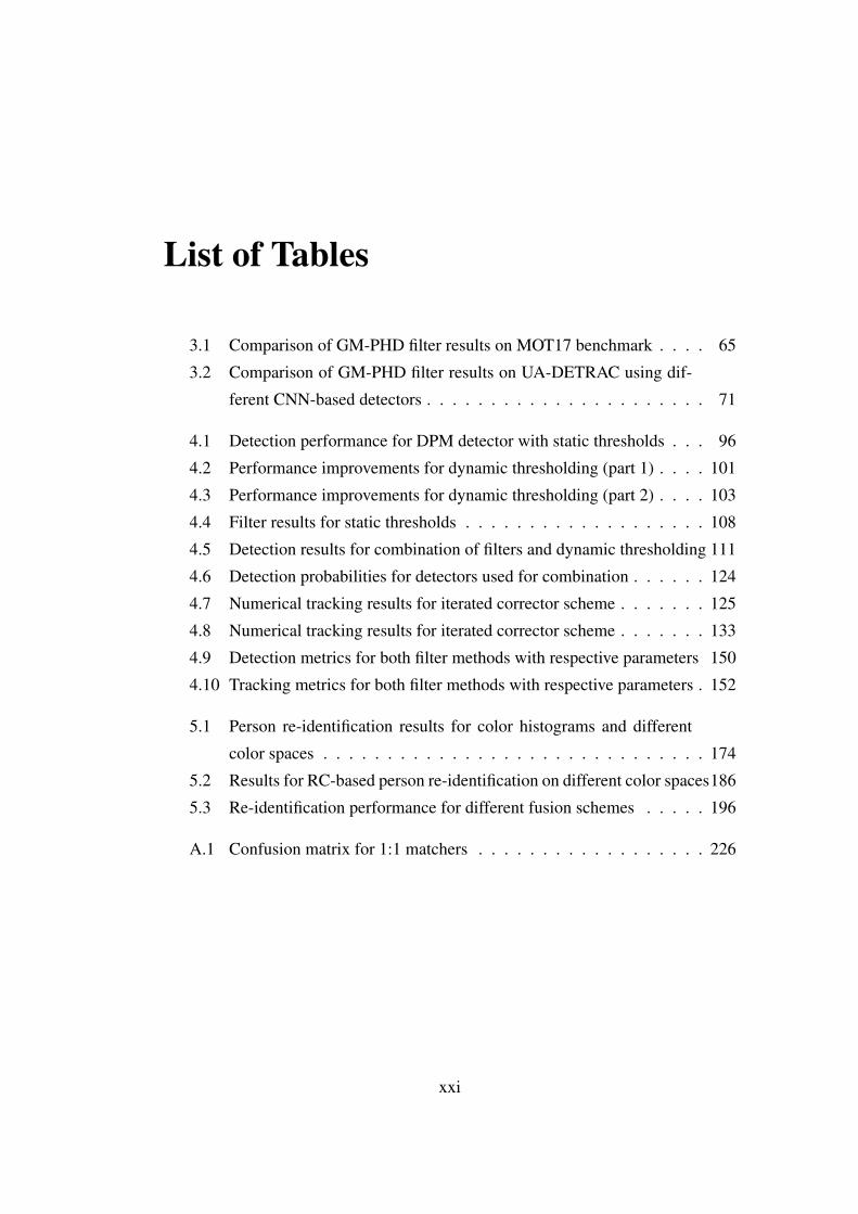
3.1 Comparison of GM-PHD filter results on MOT17 benchmark . . . . 65
3.2 Comparison of GM-PHD filter results on UA-DETRAC using dif-
ferent CNN-based detectors . . . . . . . . . . . . . . . . . . . . . . 71
4.1 Detection performance for DPM detector with static thresholds . . . 96
4.2 Performance improvements for dynamic thresholding (part 1) . . . . 101
4.3 Performance improvements for dynamic thresholding (part 2) . . . . 103
4.4 Filter results for static thresholds . . . . . . . . . . . . . . . . . . . 108
4.5 Detection results for combination of filters and dynamic thresholding 111
4.6 Detection probabilities for detectors used for combination . . . . . . 124
4.7 Numerical tracking results for iterated corrector scheme . . . . . . . 125
4.8 Numerical tracking results for iterated corrector scheme . . . . . . . 133
4.9 Detection metrics for both filter methods with respective parameters 150
4.10 Tracking metrics for both filter methods with respective parameters . 152
5.1 Person re-identification results for color histograms and different
color spaces . . . . . . . . . . . . . . . . . . . . . . . . . . . . . . 174
5.2 Results for RC-based person re-identification on different color spaces186
5.3 Re-identification performance for different fusion schemes . . . . . 196
A.1 Confusion matrix for 1:1 matchers . . . . . . . . . . . . . . . . . . 226
xxi


List of acronyms
BGS Background subtraction
CCTV Closed-circuit television
CMC Cumulative match characteristic
GM-PHD Gaussian mixture probability hypothesis density
GMM Gaussian mixture model
HOG Histogram of oriented gradients
IOU Intersection-over-union
MODA Multiple object detection accuracy
MODP Multiple object detection precision
MOTA Multiple object tracking accuracy
MOTP Multiple object tracking precision
N-MODA Normalized Multiple object detection accuracy
N-MODP Normalized Multiple object detection precision
N-MOTA Normalized Multiple object tracking accuracy
N-MOTP Normalized Multiple object tracking precision
OF Optical flow
PHD Probability hypothesis density
PTZ camera Pan-tilt-zoom camera
xxiii

RGB Red / Green / Blue (image channels)
ROC Receiver operating characteristic
RoI Region of interest
SIFT Scale-invariant features transform
SMC Sequential Monte Carlo
SURF Speeded up robust features
SVM Support Vector machine
TbD Tracking-by-detection
TUB-NÜ Technische Universität Berlin, Institut für
Nachrichtenübertragung / Communication
Systems Group

Chapter 1
Introduction
1.1 Video Surveillance and Multi-Object Tracking
IN recent years, video surveillance (often also called CCTV for "Closed-Circuit
Television" which is used synonymously in this work) has spread almost ubiq-
uitously in most western civilizations and also in many other countries in the world.
It is often connoted with and politically advocated as a measure to ensure security
in a given area, however, the main use of this technology appears to be in helping
in the investigation of criminal acts after their occurrence rather than in preventing
crimes from happening (see e.g. [Cerezo, 2013] as a related study for the city of
Málaga / Spain).
Nonetheless, a potential novel need for security is not the only reason why this
technology has increasing economical success and sees every year more installa-
tions and applications. It is also in the course of technological advancements that
new applications are found and introduced for existing systems. In many cases,
those novel applications are designed to build upon existing infrastructures and net-
works and can thus benefit from already existing video surveillance systems. It can
also be assumed (e.g. in [Langheinrich et al., 2014]) that with every new use case
and installation, people will become more accustomed to cameras and the related
analysis in their lives and will be more likely to accept the usage of this technol-
ogy for further aspects. Some examples for spreading usage of video surveillance
are surveillance in critical infrastructures such as airports or train stations, traffic
surveillance, crowd monitoring in mass events like concerts or demonstrations. It
also plays an important role in the preservation of evidence and further in the foren-
1

CHAPTER 1.1: Video Surveillance and Multi-Object Tracking
Figure 1.1: Common processing flow for automated video surveillance systems
sic analysis of events (e.g. theft or robbery in shops).
All of these applications coincide with a generally increasing amount of multi-
media data in our societies and the desire of analyzing them. Consequently, new
developments e.g. in automated video summarization, semantic scene analysis and
so on can often be adapted also for video surveillance systems and facilitate their
development.
The current focus of CCTV for human-assisting and forensic applications is also
due to the fact the amount of CCTV footage is extending the real-time analyzing ca-
pabilities of human operators. As an example according to [Lewis, 2011], the Lon-
don tube network alone accounts for a number of 11,000 cameras and it becomes
clear that not all of the video streams they record can be viewed and analyzed in
real-time by human operators at acceptable costs.
While many concepts and developments of the previous paragraphs refer to video
surveillance in general, it is important to distinguish automated systems which are
also often named "smart" video surveillance systems. As an answer to the increas-
ing amount of video data mentioned before, automation of surveillance is an often-
desired task in order to reduce costs for human operators and to enable them to
consider more specifically only events which appear suspicious instead of watching
all incoming video streams without prioritization.
Automated video surveillance requires different sub-tasks. In order to establish
a general architecture for such a system, publications like [Foresti, 1998] or [Foresti
2

CHAPTER 1.1: Video Surveillance and Multi-Object Tracking
et al., 2005] propose a processing flow similar to the one shown in Figure 1.1.
In this common approach, automated analysis is used to recognize events or
properties from a video stream which are relevant to a human operator. These
events can include e.g. left-luggage items or violence detection while potentially
interesting properties are an estimate of the number of persons in a crowd, crowd
density, crowd motion and so on.
In order to identify these events and properties, tracking plays a major role as it
provides another often desired information: the path a person (or more generally:
a moving object) took during the time he or she has been monitored in the scene.
While this property itself may appear of lesser interest, it lays the grounds for further
analysis in the scene such as e.g.
• Person counting (e.g. in public transport or retail environments).
• Loitering detection (according to [Gasserm et al., 2004], loitering can be used
to indicate possible drug dealing activity in public transport).
• Statistical analysis such as common paths in a scene and detection of abnor-
mal, potentially dangerous events such as trespassing by unauthorized per-
sons or traffic / crowd flow analysis.
• General action recognition (which often needs analysis of an object over mul-
tiple frames) such as e.g. assaults, vandalism or graffiti spraying.
• Analysis of customer behavior by identifying the path of customers in a shop,
further estimate personal properties such as gender, age etc. and concluding
on the products the person shows interest for (e.g. in [Popa et al., 2010]).
Generally speaking, for any additional analysis in the objects themselves, track-
ing can be helpful as it indicates the position of objects in the image and their indi-
vidual history in the scene. This position then enables both a more detailed analysis
and potential information fusion such as e.g. averaging of related information cues
over multiple frames. While this thesis focuses specificly on the pedestrian use case,
in practice the aforementioned conclusions are valid for any kind of distinct object
which is of interest to the observer.
3

CHAPTER 1.2: Thesis Objectives
1.2 Thesis Objectives
This work investigates the usage of tracking-by-detection (TbD) algorithms for
multi-human tracking in modern video surveillance algorithms. These approaches
split pedestrian detection and the tracking process in separate tasks and in each
frame assign tracks to the previously estimated detections. Consequently, TbD al-
gorithms by design rely on accurate human detections and can behave poorly in
their absence.
However, reliable human detection independent of e.g. pose, crowd density and
image properties such as noise, resolution etc. is still an unsolved problem es-
pecially in real-time scenarios although big improvements have been achieved in
recent times. While in other tracking domains such as e.g. radar-based airspace
surveillance or sonar-based marine tracking scenarios, high detection rates can be
presumed, video surveillance scenarios thus often cannot provide this asset.
This problem of reliable pedestrian detection is the basis for further investigation
within this work and research is carried out addressing the following points:
• How can TbD methods be embedded into a general tracking framework for
video surveillance applications?
• How do TbD algorithms perform in pedestrian tracking surveillance setups?
• What factors limit the usage of TbD approaches for human tracking in surveil-
lance contexts?
• Identify improvements in order to address these related weaknesses of TbD
systems and assess their performance within a multi-target pedestrian tracking
system.
• As a key aspect of this thesis, the application and camera setups shall be kept
as unrestricted as possible so the resulting methods and improvements should
not require special a-priori knowledge (e.g. camera calibration information)
which is not at hand in general surveillance scenarios.
It shall be noted that in order to address these questions, the focus of this work is
not on using the latest pedestrian detector available but instead emphasis is placed
on investigating and reducing the effect of bad detections in the tracking system in
4

CHAPTER 1.3: Principal Contributions and Novelties of This Thesis
order to obtain universal insights which can be generalized for different detection
methods.
1.3 Principal Contributions and Novelties of This The-
sis
In the course of work for this thesis, the following main novelties and contributions
have been developed in response to the previously formulated points:
• A framework for multi-pedestrian tracking in video surveillance setups
using the tracking-by-detection paradigm and probability hypothesis den-
sity (PHD): As an example for a tracking-by-detection tracker, a Gaussian
mixture probability hypothesis density (GM-PHD) filter has been integrated
into a modular tracking framework which allows using different pedestrian
detectors as input for the tracker. The system supports a dimensionality ex-
pansion of the state and observation spaces from pointwise detections to re-
gions of interest which are more common in computer vision applications.
The pedestrian tracking framework can be easily extended to other object
classes such as cars, boats, animals etc. as long as reliable object detection
and description methods for those object classes are available.
• A novel approach for ambiguous situations during the tracking process
The baseline GM-PHD filter does not exploit visual information but relies
solely on detections provided by a detector (tracking-by-detection principle).
In case of multiple objects near each other, this can lead to ambiguous situ-
ations. Introducing novel feature-based label trees for the GM-PHD tracker
allows for the incorporation of visual cues into the framework and thus im-
proves the handling of occlusions and near objects by the system.
• A thorough sensitivity assessment regarding missed detections for the
GM-PHD filter used in this thesis: The GM-PHD filter is theoretically an-
alyzed and a sensitivity analysis for missed detections is performed. The
proposed concept of a critical path allows to describe the risk of a tracking
failure in relation to a pedestrian detector’s detection probability. This sensi-
tivity assessment lays the theoretical foundations for improvements regarding
5

CHAPTER 1.3: Principal Contributions and Novelties of This Thesis
consecutive missed detections.
• A method for inclusion of multiple detectors into the GM-PHD frame-
work which allows exploitation of potentially complementary informa-
tion provided and thus improves detection and tracking results: In con-
trast to a previously formulated fusion method using an iterated corrector
step, the proposed approach does not depend on the order in which the detec-
tors are used nor requires very high detection rates. Nonetheless, results are
significantly improved compared to both the usage of only one detector and
the iterated corrector approach using two detectors. The proposed concept
has been tested with two human detectors based on background subtraction
techniques and histograms of oriented gradients but can easily be extended to
further detectors.
• The introduction of motion cues into the tracking in order to compensate
errors in the pedestrian detection process: Using highly efficient sparse op-
tical flow, a post-detection filter is proposed which accommodates for missed
detections and thus improves the tracking performance. The filter is tested
extensively on various datasets and experimentally validated.
• An outlook into crowd applications where local crowd information is in-
corporated into the human detector: It is shown that for crowded scenarios,
crowd density estimation can be exploited in order to improve the pedestrian
detection process. This facilitates the parametrization of standard person de-
tectors and achieves better detection results because the detector settings can
be adapted automatically for different crowd density settings.
• Assessment and extensive parameter evaluation of run-time-efficient per-
son re-identification methods for the tracking system: For this purpose,
the visual features must be extracted in an efficient and reliable manner from
known appearance models of a person and stored for future reference. By
combining different feature types based on color, gradient and texture infor-
mation, a reliable multi-feature person re-identification method is developed
which proves favorable compared to single-feature methods. It is shown how
the pedestrian descriptor developed can be integrated in the overall tracking
framework. However, an explicit integration is left as future work.
6

CHAPTER 1.4: Thesis Overview
• An improved scheme for comparing region covariance features: For the
comparison of region covariance features in the re-identification step, the im-
portance of full-rank matrices is shown in this work in order to avoid ambigu-
ous results. A new pre-processing step for covariance matrices is proposed
which ensures that the matrices used for comparison have full rank. Com-
pared to other approaches which add an identity matrix to the features, this
step is mathematically consistent, does not need any further parametrization
and avoids introducing an additional bias.
1.4 Thesis Overview
The structure of the thesis is as follows: Chapter 2 introduces common methods for
pedestrian detection which allow an automated detection of pedestrians in an image
and thus build the basis for respective tracking applications.
In Chapter 3, a literature overview on relevant tracking methods is provided.
While this thesis focuses on tracking improvements using the tracking-by-detection
paradigm, also other methods have been proposed in the literature and are presented
in order to give an outline of current tracking methods. Tracking-by-detection is
introduced as a state-of-the-art paradigm which builds the basis for the framework
in this thesis and the Gaussian mixture probability hypothesis density (GM-PHD)
filter is given as a state-of-the-art example using this paradigm. Advantages and
issues related to the GM-PHD filter are also discussed in this chapter.
The framework used in this thesis is outlined in Chapter 4 which introduces the
adaptation of the GM-PHD filter for visual tracking and explains enhancements for
both the pedestrian detection used as well as for the tracking method itself.
Pedestrian detection is especially challenging in crowded environments which is
the topic of Section 4.1. Due to occlusion and low target visibility, the performance
of pedestrian detectors decreases in areas with high crowd density. Therefore, an
adaptive method of using local crowd density information as a cue for enhancing
object detection in crowds is shown and geometrical filters are introduced as an
additional measure to improve upon the gains obtained.
While enhancements on the detection level are a good basis in order to improve
the overall tracking performance, Section 4.2 treats aspects of the tracker. Porting
the PHD filter from its domain of origin (sonar / radar domain) to the field of visual
7

CHAPTER 1.4: Thesis Overview
surveillance brings the need for adaptations, one of which is the specific treatment
of occlusion situations. The introduction of visual feature-based label trees into the
tracker shown in Section 4.2.1 allows distinguishing between close targets and thus
improves the tracking performance.
Another improvement of the PHD filter developed in this thesis is the usage of
multiple pedestrian detectors for the framework. Section 4.2.2 shows examples of
using two complementary pedestrian detectors and how their order heavily influ-
ences the respective tracking performance in the baseline PHD filter. As a remedy,
in this work a method has been developed which improves the performance com-
pared to the baseline system while, at the same time, the ordering of the detectors is
irrelevant.
While Section 4.1.1 described improvements for pedestrian detection in crowded
environments, the availability of image information for the PHD filter also brings
up ways of improving detections in low-crowded scenarios. Therefore, as a remedy
for potentially low detection probabilities for pedestrian detectors, in Section 4.3,
motion information has been included into the tracking framework in order to com-
pensate for missed detections. After a sensitivity analysis against missed detections
for the GM-PHD filter, a mathematical justification for this approach is derived in
Section 4.3.1 and the concept of a critical path of missed detections is proposed
for description and analysis. Section 4.3.2 outlines the implementation of an active
post-detection filter which uses motion information in order to improve arbitrarily
generated detections. The concept is in accordance with the theoretical consider-
ations made before and is experimentally validated on different datasets in Sec-
tion 4.3.3 for region of interest-based detections.
Person re-identification and visual descriptors for tracking are closely related
and the existence of many appearance-based tracking algorithms shows the need
for object descriptors which are suitable for tracking applications. This does not
only mean that they must be accurate in distinguishing between different targets but
they also have to be fast to compute and compare.
Chapter 5 provides a detailed overview of state-of-the-art low-level re-identification
algorithms and shows how they can be integrated into the presented tracking frame-
work. Results for a developed multi-cue person re-identification algorithm are given
and show how the performance over baseline methods is enhanced.
The thesis concludes with Chapter 6 where the main achievements of this work
8

CHAPTER 1.5: List of Publications
are highlighted, an overall summary and an outlook to questions which could be
addressed in future investigations is given.
The Appendix contains an overview of datasets and performance metrics which
have been used to evaluate the proposed methods and algorithms.
1.5 List of Publications
Achievements of this thesis have been published in the following scientific publica-
tions:
1. Eiselein, V.; Bochinski, E.; Sikora, T., 2017. Assessing Post-Detection Fil-
ters for a Generic Pedestrian Detector in a Tracking-By-Detection Scheme.
In: Analysis of video and audio "in the Wild" workshop at 14th IEEE Interna-
tional Conference on Advanced Video and Signal-Based Surveillance (AVSS
2017), Lecce, Italy, 29.08.2017
2. Eiselein, V.; Sternharz, G.; Senst, T.; Keller, I.; Sikora, T., 2014. Person
Re-identification Using Region Covariance in a Multi-Feature Approach. In:
Proceedings of International Conference on Image Analysis and Recognition
(ICIAR 2014), Part II, LNCS 8815, 2014, Vilamoura, Portugal, 22.10.2014 -
24.10.2014
3. Eiselein, V.; Fradi, H.; Keller, I.; Sikora, T.; Dugelay, J.-L., 2013. Enhanc-
ing Human Detection using Crowd Density Measures and an adaptive Cor-
rection Filter. In: Proceedings of the 10th IEEE International Conference on
Advanced Video and Signal-Based Surveillance (AVSS 2013), Kraków, Polen,
27.08.2013 - 30.08.2013
4. Eiselein, V.; Senst, T.; Keller, I.; Sikora, T., 2013. A Motion-Enhanced
Hybrid Probability Hypothesis Density Filter for Real-Time Multi-Human
Tracking in Video Surveillance Scenarios. In: Proceedings of 15th IEEE
International Workshop on Performance Evaluation of Tracking and Surveil-
lance (PETS 2013). Clearwater Beach, USA, 16.01.2013 - 18.01.2013
5. Eiselein, V.; Arp, D.; Pätzold, M.; Sikora, T., 2012. Real-Time Multi-
Human Tracking Using a Probability Hypothesis Density Filter and Multi-
ple Detectors. In: 9th IEEE International Conference on Advanced Video
9

CHAPTER 1.5: List of Publications
and Signal-Based Surveillance (AVSS 2012), Beijing, China, 18.09.2012 -
21.09.2012
During my work at Communication Systems Group, Technische Universität Berlin,
I had the chance and pleasure to collaborate with different experts in the field of
multimedia signal processing. Many fruitful discussions with my colleagues and
also with external visiting researchers helped to get new insights into our individual
fields of work. Among these, namely Dr. Tobias Senst, Dr. Rubén Heras Evangelio,
Michael Pätzold, Thilo Borgmann, Gleb Sternharz, Erik Bochinski shall be thanked
for their always inspiring advice and numerous both helpful and encouraging com-
ments.
Exchanges of views and ideas towards joint research led to interesting scientific
achievements and further joint publications in conferences and journals which are
not explicitly part of this thesis but can give hints to related areas or point to potential
applications of the techniques presented here:
(Journals)
6. Senst, T.; Eiselein, V.; Kuhn, A.; Sikora, T., 2017. Crowd Violence De-
tection Using Global Motion-Compensated Lagrangian Features and Scale-
Sensitive Video-Level Representation. In: IEEE Transactions on Information
Forensics and Security, IEEE, vol. 12, no. 12, 11.12.2017, pp. 2945–2956,
Print ISSN: 1556-6013, Online ISSN: 1556-6021(journal)
7. Fradi, H.; Eiselein, V.; Dugelay, J.-L.; Keller, I.; Sikora, T., 2015. Spatio-
Temporal Crowd Density Model in a Human Detection and Tracking Frame-
work. In: Signal Processing: Image Communication, vol. 31, February 2015,
pp: 100–111, ISSN=0923-5965 (journal)
8. Senst, T.; Eiselein, V.; Sikora, T., 2012. Robust Local Optical Flow for
Feature Tracking. In: IEEE Transactions on Circuits and Systems for Video
Technology (TCSVT), IEEE, vol. 22, no. 9, September 2012, pp. 1377–1387,
ISSN=1051-8215 (journal)
(Magazines)
9. Axenopoulos, A.; Eiselein, V.; Penta, A.; Koblents, E.; La Mattina, E.;
Daras, P., 2017. A framework for large-scale analysis of video ’in the Wild’
10

CHAPTER 1.5: List of Publications
to assist digital forensic examination. In: IEEE Security & Privacy Magazine,
Special Issue on Digital Forensics, IEEE, 2017 (magazine)
(Conferences)
10. Bochinski, E.; Bacha, G.; Eiselein, V.; Walles, T. J. W.; Nejstgaard, J.
C.; Sikora, T., 2018. Deep Active Learning for In Situ Plankton Classifi-
cation. In: 24th International Conference on Pattern Recognition (ICPR),
Workshop on Computer Vision for Analysis of Underwater Imagery, Beijing,
China, 20.08.2018
11. Küchhold, M.; Simon, M.; Eiselein, V.; Sikora, T., 2018. Scale-Adaptive
Real-Time Crowd Detection and Counting for Drone Images. In: 25th IEEE
International Conference on Image Processing (ICIP), Athens, Greece, 07.10.2018
- 10.10.2018
12. Krusch, P.; Bochinski, E.; Eiselein, V.; Sikora, T., 2017. A Consistent
Two-Level Metric for Evaluation of Automated Abandoned Object Detection
Methods. In: 24th IEEE International Conference on Image Processing, Bei-
jing, China, 17.09.2017 - 20.09.2017
13. Siwei Lyu, Ming-Ching Chang, Dawei Du, Longyin Wen, Honggang Qi,
Yuezun Li, Yi Wei, Lipeng Ke, Tao Hu, Marco Del Coco, Pierluigi Carcagnì,
Dmitriy Anisimov, Erik Bochinski, Fabio Galasso, Filiz Bunyak, Guang
Han, Hao Ye, Hong Wang, Kannappan Palaniappan, Koray Ozcan, Li
Wang, Liang Wang, Martin Lauer, Nattachai Watcharapinchai, Nenghui
Song, Noor M Al-Shakarji, Shuo Wang, Sikandar Amin, Sitapa Rujiki-
etgumjorn, Tatiana Khanova, Thomas Sikora, Tino Kutschbach, Volker
Eiselein, Wei Tian, Xiangyang Xue, Xiaoyi Yu, Yao Lu, Yingbin Zheng,
Yongzhen Huang, Yuqi Zhang, UA-DETRAC 2017: Report of AVSS2017
& IWT4S Challenge on Advanced Traffic Monitoring, In: 14th IEEE Interna-
tional Conference on Advanced Video and Signal-Based Surveillance (AVSS
2017), Lecce, Italy, 29.08.2017 - 01.09.2017
14. Kutschbach, T.; Bochinski, E.; Eiselein, V.; Sikora, T., 2017. Sequen-
tial Sensor Fusion Combining Probability Hypothesis Density and Kernel-
ized Correlation Filters for Multi-Object Tracking in Video Data. In: Inter-
national Workshop on Traffic and Street Surveillance for Safety and Security
11

CHAPTER 1.5: List of Publications
at 14th IEEE International Conference on Advanced Video and Signal-Based
Surveillance (AVSS 2017), Lecce, Italy, 29.08.2017 - 01.09.2017
15. Bochinski, E.; Eiselein, V.; Sikora, T., 2017. High-Speed Tracking-by-
Detection Without Using Image Information. In: International Workshop on
Traffic and Street Surveillance for Safety and Security at 14th IEEE Interna-
tional Conference on Advanced Video and Signal-Based Surveillance (AVSS
2017), Lecce, Italy, 29.08.2017 (challenge winner)
16. Bochinski, E.; Eiselein, V.; Sikora, T., 2016. Training a Convolutional Neu-
ral Network for Multi-Class Object Detection Using Solely Virtual World
Data. In: IEEE International Conference on Advanced Video and Signal-
Based Surveillance (AVSS 2016), volume 2010/2, Colorado Springs, CO,
USA, 23.08.2016 - 26.08.2016
17. Badii, A.; Korshunov, P.; Oudi, H.; Ebrahimi, T.; Piatrik, T.; Eiselein,
V.; Ruchaud, N.; Fedorczak, C.; Dugelay, J.-L.; Fernandez Vazquez, D.,
2015. Overview of the MediaEval 2015 Drone Protect Task. In: MediaEval
2015 Workshop, Wurzen, Germany, 14.09.2015 - 15.09.2015
18. Senst, T.; Eiselein, V.; Sikora, T., 2015. A Local Feature based on La-
grangian Measures for Violent Video Classification. In: 6th International
Conference on Imaging for Crime Detection and Prevention (ICDP-15). Lon-
don, UK, 15.07.2015 - 17.07.2015 (awarded the best paper award)
19. Tok, M.; Eiselein, V.; Sikora, T., 2015. Motion Modeling for Motion Vector
Coding in HEVC. In: 31st IEEE Picture Coding Symposium, Cairns, Aus-
tralia, 31.05.2015 - 03.06.2015
20. Senst, T.; Eiselein, V.; Keller, I.; Sikora, T., 2014. Crowd Analysis in
Non-Static Cameras Using Feature Tracking and Multi-Person Density. In:
21th IEEE International Conference on Image Processing (ICIP 2014), Paris,
France, 27.10.2014 - 30.10.2014
21. Badii, A.; Ebrahimi, T.; Fedorczak, C.; Korshunov, P.; Piatrik, T.; Eise-
lein, V.; Al-Obaidi, A. A., 2014. Overview of the MediaEval 2014 Visual
Privacy Task. In: MediaEval 2014 Workshop, Barcelona, Spain, 16.10.2014 -
17.10.2014
12

CHAPTER 1.5: List of Publications
22. Eiselein, V.; Senst, T.; Keller, I.; Sikora, T., 2013. MediaEval 2013 Vi-
sual Privacy Task: Using Adaptive Edge Detection for Privacy in Surveil-
lance Videos. In: MediaEval 2013 Workshop, Barcelona, Spain, 18.10.2013
- 19.10.2013
23. Senst, T.; Eiselein, V.; Badii, A.; Einig, M.; Keller, I.; Sikora, T., 2013.
A decentralized Privacy-sensitive Video Surveillance Framework. In: Pro-
ceedings of 18th IEEE International Conference on Digital Signal Processing
(DSP 2013). Santorini, Greece, 01.07.2013 - 03.07.2013
24. Fradi, H.; Eiselein, V.; Keller, I.; Dugelay, J.-L.; Sikora, T., 2013. Crowd
Context-Dependent Privacy Protection Filters. In: Proceedings of 18th IEEE
International Conference on Digital Signal Processing (DSP 2013), San-
torini, Greece, 01.07.2013 - 03.07.2013
25. Senst, T.; Eiselein, V.; Pätzold, M.; Sikora, T., 2011. Efficient Real-Time
Local Optical Flow Estimation by Means of Integral Projections. In: Pro-
ceedings of the 18th IEEE International Conference on Image Processing
(ICIP 2011), Brussels, Belgium, 11.09.2011 - 14.09.2011
26. Senst, T.; Pätzold, M.; Heras Evangelio, R.; Eiselein, V.; Keller, I.; Sikora,
T., 2011. On Building Decentralized Wide-Area Surveillance Networks based
on ONVIF. In: Workshop on Multimedia Systems for Surveillance (MMSS) in
conjunction with 8th IEEE International Conference on Advanced Video and
Signal-Based Surveillance (AVSS 2011), volume 2011. Klagenfurt, Austria,
30.08.2011 - 02.09.2011
27. Senst, T.; Eiselein, V.; Heras Evangelio, R.; Sikora, T., 2011. Robust Mod-
ified L2 Local Optical Flow Estimation and Feature Tracking. In: IEEE
Workshop on Motion and Video Computing (WMVC 2011). Kona, USA,
05.01.2011 - 07.01.2011
28. Senst, T.; Eiselein, V.; Sikora, T., 2010. II-LK-A Real-Time Implementa-
tion for sparse Optical Flow. In: Proceedings of International Conference on
Image Analysis and Recognition (ICIAR 2010), volume 6111, Part I, LNCS
6111. Povoa de Varzim, Portugal, 21.06.2010 - 23.06.2010
13

CHAPTER 1.5: List of Publications
29. Senst, T.; Heras Evangelio, R.; Eiselein, V.; Pätzold, M.; Sikora, T., 2010.
Towards Detecting People Carrying Objects: A Periodicity Dependency Pat-
tern Approach. In: International Conference on Computer Vision Theory and
Applications (VISAPP 2010), volume 2010/2. Angers, France, 17.05.2010 -
21.05.2010.
During the course of this work I also supervised numerous bachelor’s and mas-
ter’s theses. Among all of them, the following students had a very close contact
with the field related to this work and I am thankful for their help in implementation
and testing of the framework developed:
1. Arp, Daniel (Multi-Objekt-Analyse in Videodaten unter Verwendung mo-
mentbasierter Random-Finite-Set-Methoden), supervised by Volker Eiselein /
Thomas Sikora, Technische Universität Berlin, 04/2012 (unpublished)
2. Sternharz, Gleb (Implementierung und Vergleich von Methoden zur Perso-
nenbeschreibung für Multi-Objekt-Tracker), supervised by Volker Eiselein /
Thomas Sikora, Technische Universität Berlin, 03/2014 (unpublished)
3. Ceyhan, Sezgin (Integration von visuellen Merkmalen zur Personenverfol-
gung in einem Tracking-by-Detection Framework), supervised by Volker Eise-
lein / Thomas Sikora, Technische Universität Berlin, 05/2016 (unpublished)
4. Kutschbach, Tino (Combining Probability Hypothesis Density and Correla-
tion Filters for Multi-Object Tracking in Video Data), supervised by Volker
Eiselein / Thomas Sikora, Technische Universität Berlin, 11/2017 (unpub-
lished)
14

Chapter 2
Pedestrian Detection
OBJECT and specifically pedestrian detection is a challenging task in computer
vision systems. Semantic understanding of videos and images has been an
important issue since the first days of image and video processing. As the co-
existence of human beings, computers and cameras in daily life (e.g. CCTV systems
and their related analytics engines but also mobile phones with on-board cameras
and so on) presents a high number of analytics opportunities, the need for reliable
object identification in videos is a special focus of researchers. The upcoming do-
main of robotics, especially the area of moving robots or autonomously driving cars,
also created a lot of interest for automatic person detection and object recognition.
Depending on the specific purpose and application, a number of different ap-
proaches have been proposed. As the most significant ones, algorithms for activity
detection and object recognition can be distinguished. The first are capable of iden-
tifying areas in a given scene where changes happen or activity is perceived. Most
types of activity in a scene can usually be related to actions by objects or creatures
and thus lead to the deduction that in spaces with activity an object or creature
can be expected. Activity detection algorithms are often change-based, i.e. they
identify pixel- or block-wise changes in an image compared to a model of the un-
changed scene (i.e. background). Without additional analysis, the methods may
detect pedestrians walking or a bird flying by but cannot classify the object any
further.
On the other hand, model-based object recognition algorithms are designed in
order to detect instances of a certain object class which may comprehend human
beings or other object classes such as types of animals, chairs, cars etc. This class
15

CHAPTER 2.1: Algorithms for Activity Detection
of methods uses pre-trained models of the objects to be recognized and is often
closely connected with modern machine learning methods, such as support vec-
tor machines, boosting techniques or convolutional neural networks. Thus, it also
benefits from the increasing success of these methods.
In summary, it can be said that the difference between the two method classes
is often inspired by data availability or the need for a specific object model in the
application. While activity recognition does not build upon a specific model, no
training data for a particular object class is needed. As a result of this unspecificity,
it can thus also be seen as an unsupervised method. In contrast, the model-based
approaches require supervised learning, usually based on a large number of exam-
ple objects in order to obtain a high generalization of the method, but also enable
applications as detecting e.g. only dogs or cars in the scene.
It seems intuitive that the identification of one specific object class out of many
poses many more problems than just identifying some object – and thus algorithms
for activity detection can generally be kept simpler than methods for identification
of a certain object as will be shown in the next paragraphs. Thus, despite its lower
specificity, activity detection is traditionally a popular area in the surveillance do-
main because it requires less computational complexity or less training effort than
sophisticated machine learning strategies. If more detailed analysis is needed, ac-
tivity detection can often still limit the search space and thus reduce the overall
run-time when further methods are applied.
2.1 Algorithms for Activity Detection
Activity detection as described before is closely related to change detection. The
focus of these methods is usually on the pixel level, i.e. no specific object detection
is necessary. While on the one hand those changes can be perceived in relation to a
stationary background, also changes from a temporal perspective are possible. One
of the simplest methods for this purpose is frame differencing as proposed in [Jain
and Nagel, 1979; Haritaoglu et al., 2000] where the difference between consecutive
frames allows per-frame detection of motion boundaries in a video and thus yields
silhouettes of moving objects.
Algorithms exploiting stationary background are often called background sub-
traction techniques, meaning that once an estimate of the scene background is avail-
16

CHAPTER 2.1: Algorithms for Activity Detection
able, differences in the current image from this background can be found in princi-
ple by simple subtraction. Such differences indicate activity and can be assumed to
correspond to objects in this area. However, most modern techniques refrain from
using a simple differencing scheme but instead apply models based on probabilities.
The well-known approach from [Stauffer and Grimson, 1999], which uses a
Mixture-of-Gaussian approach (MoG) in order to describe the background prob-
ability distribution per pixel, has been the basis for many algorithms. A survey
comparing some of the most relevant ones can be found in [Bouwmans et al., 2008;
Heras Evangelio, 2014].
Variants of this algorithm have e.g. been developed at TUB-NÜ for static object
detection [Heras Evangelio et al., 2011] or abandoned luggage detection [Smith
et al., 2006]. Concerning the computational load, for sparsely crowded scenes of
576× 720 pixels RGB resolution [Heras Evangelio, 2014] gives values between
33 and 43 frames per second (fps) which shows that the complexity for activity
detection can be kept suitable for real-time processing for standard image sizes.
Less popular approaches for background subtraction include other statistical mod-
els such as codebooks [Kim et al., 2004] or eigenbackgrounds [Tian et al., 2013].
It should be mentioned that most of the background subtraction algorithms rely
on a static camera setup or at least need an accurate image registration because
statistics are built upon individual pixels which must be regarded over multiple
frames in time. Therefore, modern surveillance concepts tend to avoid using these
concepts in order to remain flexible and allow e.g. an application on video data
from PTZ (pan-tilt-zoom) cameras.
Inspired by the aforementioned methods using pixel features and a static back-
ground, another class of activity detection algorithms uses motion information. At
TUB-NÜ, approaches using optical flow trajectories in a video ([Senst et al., 2012b,
2014]) have been developed in order to identify point movements over longer peri-
ods. These movements are grouped and allow distinguishing between background
and foreground or even between multiple objects. A camera motion estimation step
as e.g. in [Senst et al., 2014] even helps accounting for slight camera movement.
While these methods benefit from recent improvements in sparse optical flow com-
putation, it has to be said that their resolution and thus accurate object segmentation
is still limited by a higher computational complexity compared to traditional back-
ground subtraction techniques. Thanks to increasing processing power and paral-
17

CHAPTER 2.2: Histograms of Oriented Gradients for Pedestrian Detection
lelization options, it can be expected that such methods will be more common in the
future.
2.2 Histograms of Oriented Gradients for Pedestrian
Detection
As mentioned before, methods for detection of certain object classes give more spe-
cific results than pixel-based activity detection algorithms. An algorithm designed
to identify a clearly defined object class such as e.g. humans or dogs is expected
to distinguish those classes from other objects such as e.g. cars or giraffes. Evi-
dently, such methods exploit previous knowledge. Therefore, they usually learn a
model of the respective object class and can thus only detect objects which have
been pre-defined in such a model.
Despite this specificity in the object classes given, most approaches for object
detection or recognition aim at general frameworks which can be used for different
object classes as long as they reveal enough individual differences in their general
feature representation. Therefore, these frameworks use a twofold approach: In a
first step, the extraction of feature descriptors from an image is performed and in
a second step, machine learning enables a classification of these descriptors. Rele-
vant features for different applications can be color values (RGB), edges, contours
and so on on the pixel level. These features are then combined into feature vec-
tors for classification, often by using higher-level descriptors such as histograms or
covariance representations of the features.
The authors of [Dollár et al., 2012] present a good overview on relevant tech-
nologies for pedestrian detection. Features used by many algorithms consider the
shape of an object by modeling its gradient distribution. One of the first approaches
following this idea and still a very popular one was described in [Dalal and Triggs,
2005] and became known as histograms of oriented gradients (HOG). Due to its
flexibility and applicability to different object classes, it has become a de facto stan-
dard for object detection with hand-crafted feature vectors. In this method, images
are decomposed into individual cells in which gradients and their respective ori-
entation are quantized into histograms. The result is normalized in a block-wise
fashion and yields a descriptor which is returned for every cell. A visualization for
18

CHAPTER 2.2: Histograms of Oriented Gradients for Pedestrian Detection
this method can be seen in Figure 2.1 where the extracted gradients are shown per
cell.
Using a pre-defined set of training images, the descriptors for specific objects can
be trained to a support vector machine (SVM) [Cortes and Vapnik, 1995] which is
further used to identify feature vectors matching the trained model. In order to keep
the trained model comparable to candidate regions in an image which might poten-
tially have different sizes, these candidate regions are usually resized (i.e. scaled)
to the region size of the model. Using this technique, objects of different size can
be found in the image using the same pre-trained model.
In order to localize objects in an image, it is necessary to compare the resulting
descriptor for multiple positions over the image. This is usually done in a window-
ing approach, i.e. the region in which the HOG feature vector is computed is shifted
over the image and the detection scores returned by the SVM allow estimating the
most probable position of objects in an image, e.g. using non-maxima suppression
as in [Dalal and Triggs, 2005]. As mentioned before, this HOG approach relies
on gradient information of an object and can thus be used for a number of differ-
ent object classes. However, its limitations are given when object classes are not
distinguishable only by gradient or shape information.
In contrast to the previously described method which uses standard derivative
filters in order to compute histograms of oriented gradients, alternative approaches
have been proposed. [Wang et al., 2009] uses local binary patterns [Ojala et al.,
1994, 1996] for feature extraction and a model for partial occlusion. According to
[Wang et al., 2009], a higher performance can thus be achieved on some datasets.
The HOG principle has inspired a number of derived works. A detector based on
the Ω-shape of human head and shoulders has been proposed in works from TUB-
NÜ ([Pätzold et al., 2010]). The target representation is learned in a support vector
machine and matched against information collected in a windowing approach from
current frames. Additional cues for validation are obtained using motion informa-
tion and a motion coherency measure.
Another extension, which is used for a number of experiments in this thesis,
has been proposed by [Felzenszwalb et al., 2010a] as the DPM (deformable parts
model) detector. Its main contribution enriches the standard descriptor by Dalal
and Triggs using a so-called "star-structured" part-based model. While the model
defined in [Dalal and Triggs, 2005] is used as "root model", additional, smaller
19

CHAPTER 2.2: Histograms of Oriented Gradients for Pedestrian Detection
Figure 2.1: Visualization of histogram of oriented gradients (HOG) features: object shapes
in original images (left) are described using their gradient orientation (right). The HOG
feature vector includes multiple gradient directions coded as a histogram (cell size 8, 20
histogram bins for orientation).
20

CHAPTER 2.2: Histograms of Oriented Gradients for Pedestrian Detection
Figure 2.2: Visualization of trained person model using [Felzenszwalb et al., 2010a]. Left:
root filter with eight object parts and their respective deformation model. Right: Exemplary
human detections (red) with blue boxes describing object parts found. Image has been
published in [Eiselein et al., 2013a]
models are defined for object parts. All of these features can be seen as simple
filters which are convolved over the image using the Dalal-Triggs feature vector.
Part models in this method have twice the spatial resolution than the root filter
in order to capture smaller image cues. These different scales are also taken into
account for extraction in order to reduce the computational effort. Particularly, finer
scales are only evaluated at positions where the root score on the coarse grid is
sufficiently high.
The final detection score at a certain position is then computed as the sum of
the root filter score at the given location and the maxima scores for parts at their
respective position related to the root filter. Additionally, a bias and a deformation
cost accounting for position offsets compared to the part position in the pre-trained
model are introduced. By using a windowing scheme and returning the detection
scores per pixel and scale, the result is a set of detections which are post-processed
using a non-maxima suppression (NMS) explained in detail in Section 4.1.2.
The DPM detector achieves good performance on many public databases but also
has a higher computational load than the baseline method from [Dalal and Triggs,
2005]. Figure 2.2 (left) shows a visualization of a star model for person detection
using the feature model proposed in [Felzenszwalb et al., 2010a]. An exemplary
detection result is shown in Figure 2.2 (right).
The importance of gradient information for object detection has also been em-
phasized in another class of pedestrian detection methods which is based on boosted
21

CHAPTER 2.2: Histograms of Oriented Gradients for Pedestrian Detection
features, such as e.g. [Dollár et al., 2014]. With pixel-wise image transforms (e.g.
intensity values, gradients and so on), a set of weak classifier can be obtained. A
weak classifier gives a binary classification result and in average obtains a classifi-
cation probability above 50% [Alpaydın, 2008], but generally does not obtain very
high classification accuracy. Nonetheless, the combination of multiple weak clas-
sifiers can lead to superior classification results as shown in [Freund and Schapire,
1997]. In this way, high-level classifiers can be built on top of a hierarchy of weak
ones using boosting theory.
In [Dollár et al., 2014], the authors propose Accumulated Channel Features
(ACF) and use the AdaBoost algorithm, proposed by Freund and Schapire in 1997
[Freund and Schapire, 1997], in order to build a tree of weighted weak classifiers
on top of an efficient multi-scale feature extraction.
Features used in [Dollár et al., 2014] are the pixel-wise normalized gradient mag-
nitude, a 6-channel histogram of oriented gradients and LUV color channels, all
collected over different scales within a region of interest in the image. This method
may appear simple but nonetheless achieves a good person detection performance
on common datasets such as the Caltech benchmark [Dollár et al., 2009; Dollár
et al., 2012]. Therefore, the proposed technique has inspired a number of other
works. For example, in [Nam et al., 2014], features are locally decorrelated before
training and classification in so-called orthogonal trees (similar to ACF). While this
may increase the run-time for training, it achieves both a reduction of the detection
time and an improvement of the detection performance.
Methods based on convolutional neural networks (CNNs) have recently become
particularly popular for object detection, too (e.g. [Girshick et al., 2014] or a method
developed at TUB-NÜ [Bochinski et al., 2016]). These do not use hand-crafted fea-
ture vectors but instead automatically learn the feature cues which are most impor-
tant for classification. This is done by performing a training on a large number of
samples and adjusting the weights in the neural network in order to minimize the
classification error. CNN-based methods are currently among the best-performing
pedestrian detectors but require high-end graphics processors, large training and
test datasets, long training times and careful parametrization which can be difficult
when using 3rd party networks. For this work, the focus is therefore on non-CNN
methods.
The advent of methods such as [Dollár et al., 2014; Nam et al., 2014] led to a
22

CHAPTER 2.3: Pedestrian Detection in This Thesis
number of other, similar publications with boosting approaches and it also coin-
cided temporally with an increase of interest in pedestrian detectors for automotive
applications. This is mirrored in a change in the evaluation procedure for pedestrian
detectors. The Caltech pedestrian dataset [Dollár et al., 2009; Dollár et al., 2012]
taken from dashboard cameras within driving cars has become a de facto standard
and symbolizes this development.
On the one hand, this dataset contains very many pedestrian images (192k for
training / 155k for testing), but the size of persons to be detected is also significantly
smaller than in common surveillance videos. As a consequence, the DPM detector
has difficulties matching the part models for far-scale detections [Dollár et al., 2012]
which appear at lower resolution.
For standard surveillance datasets, however, the performance of ACF is similar
to DPM as has been shown in the works of our group at TUB [Bochinski et al.,
2016]. It is therefore that the very popular DPM detector which is available both as
C++ 1 and MATLAB implementation [Felzenszwalb et al., 2010b] has been taken
as basis for experiments in this work. It represents a sufficiently accurate detection
method and its code is available for experiments.
2.3 Pedestrian Detection in This Thesis
In this thesis, different detectors based on algorithms from the previous sections
are used in various settings in order to show the flexibility of the tracking approach
which does not depend on a certain algorithm for pedestrian detection.
Particularly, two scenarios are defined which differ in the dimensionality of the
measurement / state space (introduced in the next chapter) and in the computational
complexity for the overall detection process: The first configuration reflects needs
for embedded devices with small processing capacity. Accordingly, also pedes-
trian detectors with lower computational demands are considered in this scenario.
Therefore, both an activity detection method using background subtraction as in
Section 2.1 and a simple detector based on histograms of oriented gradients have
been used in this thesis.
The first one is based on a foreground detection algorithm developed at TUB-NÜ
[Heras Evangelio et al., 2011] including an additional morphological filtering step
1from http://www.opencv.org
23

CHAPTER 2.3: Pedestrian Detection in This Thesis
in order to remove false detections by noise. Its output is an estimate for the head
position of a pedestrian which is assumed in the horizontal center of the respective
bounding box and at 85% of the bounding box’s height. The detector has an over-
all good detection probability but can be hampered e.g. by clutter due to lighting
changes. Due to its rather low computational complexity, it could also be used on
embedded devices such as e.g. smart cameras.
The second detector is based on the TUB-NÜ algorithm from [Pätzold et al.,
2010] and uses histograms of oriented gradients. It is trained on the head / shoulder
shape of pedestrians. Due to the smaller size of the target pattern, it returns only
the central x- and y-position of the head and no bounding box for the person silhou-
ette. Another drawback of the small size of the target pattern is a lower detection
probability compared to other approaches.
This simple HOG detector is more suited for small devices such as smart cameras
or embedded systems because it does not use scaling of the target image (i.e. it
assumes a given size of the target in the image) and also uses only one resolution for
the HOG representation. Therefore, it has much lower computational requirements
than other, more sophisticated methods such as [Felzenszwalb et al., 2010a].
For this scenario, the tracking filter uses a measurement model as proposed e.g.
in [Mahler, 2007]. The measurements are two-dimensional, i.e. pointwise detec-
tions are used comprising the center x/y coordinates of a person’s head.
The second configuration relates to a case which is more common for high-
performance computers and uses regions of interest-based pedestrian detections.
For this use case, the DPM approach [Felzenszwalb et al., 2010a] is applied which
has a higher computational complexity than the previously mentioned methods but
also achieves a much higher detection performance. According to [Felzenszwalb
et al., 2010a], the processing time on a standard PC is around is around 2 seconds
for an image of the PASCAL Visual Object Classes Challenge 2007 dataset [Ev-
eringham et al., 2007] (varying resolution, 500×500 pixels maximum). Other ex-
periments conducted in this thesis indicate run-times of approximately 7-8 seconds
(single-threaded) for Full HD content (1920×1080 pixels) on current PC hardware.
For this thesis, a DPM detector with a model trained on the PASCAL VOC
2007 dataset is used and the detection results are a four-tuple composed by x-/y-
coordinates of the upper left corner of the region of interest and the respective width
/ height.
24

Chapter 3
Object Tracking
OBJECT tracking in videos in its simplest form can be formulated as the task of
estimating the trajectory of a given object over a set of video frames while
the object moves in the scene and its trajectory is projected onto the image plane.
An exemplary application for this task could be a forensic search where a CCTV op-
erator designates a person to a tracking algorithm and wants to know this person’s
trajectory at other time instants in the given video until a time frame is reached
when the person’s face or other characteristics can be seen. Such tracking is known
as visual tracking and can be considered instance-specific because it follows a des-
ignated, individual instance of an object class. In the given case, the class is a
specified person but it could also be a cell under the microscope or a persons’s hand
in order to recognize gestures. Instance-specific tracking usually requires a model
of the individual properties of the tracked object instance (e.g. color, shape or tex-
ture information for image processing applications) which can be extracted directly
from the video and the initial, known object position. Please note that in this work,
the terms target and object for the tracked entity are used synonymously.
Another tracking application case is multi-object tracking, i.e. the extraction
of ideally all trajectories related to a specific object class in a video which can be
helpful for analyzing those objects’ behaviour. As an example, shopping centers are
often interested in analyzing their clients’ paths through a shop and their shopping
interests in order to optimize the presentation of products in the shop and thus to
increase overall sales.
Further applications for tracking arise in the area of home automation for the el-
derly and disabled: In order to enable elder people to live as long as possible in their
25

Chapter 3. Object Tracking
known environment, it is necessary to provide them with help in their daily routine.
However, already for economic reasons, human caretakers cannot be around every
cared for person 24/7. Thus automated solutions are considered which are e.g. able
to determine if an accident happened, if the person took their medication etc. and
human staff can then react on those events if needed. In order to extract this seman-
tic information from video footage, video analytics systems necessarily also need
to track known and unknown persons in a home environment.
The following sections will provide an overview of different tracking techniques.
Instance-specific methods will be presented first because they symbolize traditional
concepts for visual tracking based on the aforementioned initial target annotation.
In a second step, an extension to general detection-based, single- and multi-object
tracking techniques will be given as these methods represent the main application
focus for this work. Furthermore, a state-of-the-art overview of current tracking
methods can be found in Section 3.2.5.
As a general concept, instance-specific or visual tracking methods have to deal
with errors known in the literature as "tracking drift" [Zhang et al., 2012]: If the
model to be tracked appears too similar to other object instances or the background,
the situation becomes ambiguous for the tracker and tracking failure is likely.
The "drift" concept arises from the early beginning of visual tracking using tem-
plate matching (e.g. [Peacock et al., 2000; Kaneko and Hori, 2002; Matthews et al.,
2004]) and is caused by small tracking errors or noise introduced which is accu-
mulated over time and at some point becomes too large for the tracker to operate
correctly.
An often-applied remedy is thus to update the tracked model continuously. The
reason for such an update can be changing lighting conditions over the whole scene,
noise, different object appearance from changing views and so on. However, every
update again bears the risk of introducing errors into the model e.g. due to segmen-
tation noise. According to [Liu et al., 2014], an often-applied method in such cases
is to limit the changes allowed for the model update and to keep the model thus near
a prior appearance model. Nonetheless, the authors mention that rapid changes and
multiple similar objects remain challenging for most existing methods.
Visual tracking can be applied for numerous applications which vary e.g. in the
objects to be tracked. The survey in [Yilmaz et al., 2006] mentions applications
for tracking such as traffic monitoring, video indexing, motion-based recognition
26

Chapter 3. Object Tracking
and more. Also medical applications such as cell-tracking or the tracking of human
body movements for human-computer interaction are mentioned here for the sake
of completeness but will generally require different approaches in terms of problem
modeling and integration of prior information. The focus in this work will remain
on automated person tracking.
A more recent survey with a focus on visual tracking and thanks to the choice
of the dataset also partially pedestrian tracking is [Smeulders et al., 2014]. It gives
experimental results on different feature tracking approaches for which public im-
plementations are available. In contrast to the work in this thesis, the objects to be
tracked have to be initialized manually which is not feasible for real-world applica-
tions and thus not the application scope of this work.
Experiments in [Smeulders et al., 2014] involve trackers using sparse optical flow
([Baker and Matthews, 2004]) and the Struck method [Hare et al., 2011] which
uses a kernelized structured output support vector machine (SVM) learned on-
line on the tracking targets. Other, on the given dataset often better performing
methods are "Tracking, Learning and Detection" [Kalal et al., 2012] which com-
bines optical flow tracking with discriminative classifier learning, the Foreground-
Background Tracker [Chu and Smeulders, 2010] which uses a linear discriminant
classifier trained on Gabor features and "Tracking by Sampling Trackers" [Kwon
and Lee, 2011] relying on multiple basic trackers which are sampled in order to
provide both the most promising target hypotheses and appearance / tracking mod-
els.
The previously mentioned overview on visual tracking techniques in [Yilmaz
et al., 2006] is a good introduction into general tracking concepts but does not cover
recent developments. However, it bridges foundations of both visual tracking (e.g.
optical flow or mean-shift tracking [Comaniciu et al., 2000]) to multi-object data
association such as MHT [Reid, 1979] and also covers related aspects of visual
object detection and segmentation.
Due to their time of publication, both survey articles miss currently popular ap-
proaches such as correlation trackers. These came up beginning with the formu-
lation of the "Minimum Output Sum of Squared Error" filter [Bolme et al., 2010]
as an extension of traditional correlation filters to the Fourier domain. A similar
scheme was then used for multi-dimensional feature vectors (e.g. histograms of
oriented gradients) [Danelljan et al., 2014]. Additional work has been done for the
27

Chapter 3. Object Tracking
"kernelized correlation filter" [Henriques et al., 2015] by applying the kernel trick
for ridge regression with a linear kernel and using circulant matrices for efficient
computation.
For this thesis, automated tracking systems for surveillance purposes are of main
interest. In contrast to the previously mentioned visual tracking methods, they usu-
ally cannot rely on manual selection of tracking targets e.g. by a human opera-
tor. Instead they need some possibility of automated initialization, i.e. detection
of the targets to track. As a result, because the tracking algorithm lacks knowl-
edge about specific object instances of interest, such algorithms are not necessarily
instance-specific but need to detect and track a whole class of objects. Therefore,
one could call them class-specific trackers or more commonly multi-object tracking
or tracking-by-detection (TbD) systems. Different algorithms suitable for automatic
object detection and the ones used for the framework of this thesis have been intro-
duced in Chapter 2.
In order to use the resulting detections for tracking with automated initializa-
tion of new tracks, both error sources of missed (false negative) and supernumerous
(false positive) detections have to be considered. As an additional issue, in general
tracking setups, the number of tracked objects is not known. In light of all these un-
certainties, standard approaches for multi-object tracking often involve probabilistic
formulations.
A first differentiation between different methods is due to the target state space.
It can differ significantly between different applications and different tracking al-
gorithms. As has been shown in Chapter 2, pedestrian detections can include both
position and size (generally width / height of the associated bounding box) so that
a region of interest can be used in the object representation. If the observable input
of the tracker is only a position, the width and height information are not available
and thus cannot be used for the object’s state vector.
Section 2.3 already explained how both approaches have been used in the context
of this thesis: For a potential use case of low-performance hardware (e.g. smart
cameras) only pointwise detections for the estimated head position of a pedestrian
are used and the position part of the state vector is thus a two-dimensional point. On
the other hand, for applications with more computational power at hand, the DPM
detector [Felzenszwalb et al., 2010a] provides regions of interest and the tracker can
thus exploit a four-dimensional state space of position, width and height. Additional
28

Chapter 3. Object Tracking
information for both scenarios is the object’s velocity which is also included in the
state space.
The position, size and velocity information in this thesis refers to pixel coordi-
nates. While these are directly available from the video frame, it is also possible to
use a camera calibration for the scene and relate pixel coordinates to their 3d-world
positions. This calibration information can be helpful in order to improve the track-
ing process because the relation between distances in pixel and world coordinates is
dependent on the camera view and the usage of pixel coordinates can thus result in
an inappropriate motion model for the objects in the scene. E.g. the assumption of a
linear motion model is often justified in real-world coordinates but can be erroneous
in the pixel domain.
However, camera calibration information is usually not available in general sce-
narios and in most cases must be obtained manually, which can be a costly, tedious
work and inhibits an on-line application. Therefore, in this work the state space is
composed by pixel coordinates.
For this thesis, the following guidelines have been identified for the visual track-
ing task:
• The tracking algorithm should be independent of the detector method used.
• The tracking algorithm should be automatic, i.e. especially the initialization
of a track and all object detection and tracking steps should be automatic.
• The complexity of the tracking algorithm should be low in order to allow for
near real-time processing on a standard PC.
• The tracking algorithm should be as general as possible, i.e. no assumptions
on the nature of objects shall be made as long as an automatic object detection
algorithm from visual data exists. This shall enable the usage of the developed
system for different object classes although in this thesis only persons are
considered as tracking targets.
As mentioned before, according to these requirements, instance-specific tracking
is not suitable. Different object classes for which the tracking may be applied will
most probably have different visual features and as a result, the comparison of spe-
cific instances in one class must focus on different cues than in another class. Con-
sequently, a general visual feature vector for instance-specific tracking of different
29

Chapter 3. Object Tracking
Figure 3.1: Depending on the scenario characteristics, different tracking-by-detection
methods have been developed in the literature.
object classes appears less promising. On the other hand, the tracking-by-detection
paradigm can be easily combined with detection methods for different object classes
and will thus be used in this thesis.
Should it become necessary, differentiation between several object instances can
be added according to a specific object class. Foundations of such extensions are
given in this thesis and could in the future be used to enable feedback between the
tracking position and the detector used in order to improve the detection results (as
e.g. [Xue et al., 2010]).
From a conceptual view, tracking algorithms can be classified according to the
difficulty of the individual tracking scenario. Figure 3.1 shows how an increasing
number of unknowns aggravates the tracking problem and requires more complex
solutions. The easiest scenario (green path) shown involves only one object and
at most one detection per frame (i.e. no clutter). For this case, the Kalman fil-
ter [Kálmán, 1960] or one of its variants (extended [Kálmán, 1960] / unscented
Kalman filter [Julier and Uhlmann, 1997]) are popular and efficient solutions. The
difficulty for tracking-by-detection algorithms increases when association uncer-
30

CHAPTER 3.1: Tracking-by-Detection: Bayesian Trackers for the Single-Object
Case
tainty between detections and tracks increases. The yellow path represents a single
target with clutter and can be solved e.g. using the Probabilistic Data Associa-
tion Filter (PDAF) [Bar-Shalom and Tse, 1975] which associates detections to the
previously estimated track. In contrast to the previous ones, the red path addition-
ally involves an unknown number of targets. Therefore, also the number of false
positive and false negative detections received is unclear which makes it the most
challenging case shown. For this scenario with an even increased association effort,
the Joint Probabilistic Data Association Filter (JPDAF) or the PHD filter shown in
Section 3.2.4 are possible remedies.
As a general conclusion, it can be said that the tracking process becomes more
difficult, the more objects are to be tracked and the more uncertainty (noisy data,
missed detections, clutter) is present in the overall process. Pedestrian tracking in
video surveillance applications generally involves detection noise, unknown motion
models, missed detections, clutter, and an unknown number of objects in the scene.
Therefore it can be considered a very challenging use case as shown in the red path.
In the following sections, an overview on tracking-by-detection methods is given.
Starting with popular Bayesian approaches for the single-target tracking case, rele-
vant multi-target trackers extending the single-target case are presented. The chap-
ter concludes with a detailed description of the PHD filter used in this thesis and the
related challenges for application.
3.1 Tracking-by-Detection: Bayesian Trackers for the
Single-Object Case
The term tracking commonly implies an estimation or prediction step due to detec-
tion uncertainty. If it was possible to detect any tracking target continuously without
errors over all video frames, tracking would be simplified to an association problem.
In light of imperfect detections, tracking has a tight connection with statistical and
probabilistic methods because target states (and thus trajectories) can be treated as
statistical variables. As an example from daily life, it would be intuitive to assume
(or predict in Bayesian terms) the position of an object "somewhere around" the last
position where it has been observed before. In other words, the probability P(xk+1)
of a certain target state at time k+ 1 is expected to depend on the last state xk of
31
CHAPTER 3.1: Tracking-by-Detection: Bayesian Trackers for the Single-Object
Case
that target and the related uncertainty increases with the time an object state cannot
be confirmed. This simple example shows the importance of state probabilities in
object tracking and is a basic motivation for using Bayesian Trackers.
Considering the tracking problem as a state estimation problem, the measure-
ments are influenced by noise, and depending on the underlying process, not all state
variables may be observable (e.g. in CCTV applications, velocity is an often-used
state variable but usually not measured from video frames). A popular approach
for modeling tracking problems relies on the Bayes theorem and models the related
state uncertainties statistically. The general Bayes formula relating likelihood and
prior / posterior probability
Posterior prob. = P(A|B) = P(B|A) ·P(A)P(B)
=likelihood · prior prob.
evidence(3.1)
is valid for P(B) 6= 0 and computes the probability P of an event A given the
condition B. Here, P(A) and P(B) are the probabilities of observing A and B re-
spectively, while P(B|A) is the likelihood of event B occurring under condition A.
For tracking using the single-sensor, single-target Bayes filter, equation (3.1)
is typically solved iteratively by solving the related predictor and corrector equa-
tions (3.2) and (3.3). The presentation here follows the explanation in [Mahler,
2007] to which the reader is referred for further details. With x, x as the current and
previously estimated states and Zk : z1,z2, ...,zk as the time sequence of observed
detections, the predictor step
Pk+1|k(x|Zk) =∫
Pk+1|k(x|x) ·Pk|k(x|Zk)dx (3.2)
is executed for every time step, followed by the corrector step:
Pk+1|k+1(x|Zk+1) =Pk+1(zk+1|x) ·Pk+1(x|Zk)
Pk+1(zk+1|Zk). (3.3)
The term
Pk+1(zk+1|Zk) =∫
Pk+1(zk+1|x) ·Pk+1(x|Zk)dx
is the Bayesian normalization factor. As a result of the filtering step, a sequence
of posterior probability distributions is computed:
32

CHAPTER 3.1: Tracking-by-Detection: Bayesian Trackers for the Single-Object
Case
P0|0(x|Z0)→ P1|0(x|Z0)→ P1|1(x|Z1)→ ·· · → Pk|k(x|Zk)
→ Pk+1|k(x|Zk)→ Pk+1|k+1(x|Zk+1)
A theoretical justification for both the predictor and the corrector step of a Bayes
filter is provided in [Mahler, 2007]. Well-known methods relying on such a re-
cursive solution of the Bayes problem are the Gaussian-based Kalman filter and
sequential Monte Carlo (SMC) [Isard and Blake, 1998] techniques, also known as
particle filters.
3.1.1 The Kalman Filter
The Kalman filter [Kálmán, 1960] named after Rudolf Kálmán is the more common
name of the process of linear quadratic estimation (LQE) which is an often-used
concept e.g. in control theory and signal processing. It considers the state estimate
in the k-th time step tk to contain all information from previous time steps leading
to a recursive formulation of the estimation problem.
Considering a random process formulation for the tracking task, the Kalman
filter takes into account the stream of previously received noisy input data (i.e. ob-
servations) and generates a statistically optimal state estimate for the tracked object.
With a common object state x =(
x y·x
·y)T
comprising position and velocity,
the uncertainty is modeled as a respective covariance F for this state vector. Fol-
lowing [Mahler, 2007], the process and the observations can be described by:
xk+1 = Mkxk +wk (3.4)
zk = Hkxk +vk (3.5)
with wk and vk as the process noise and measurement noise, respectively. The
state transition matrix Mk (also known as motion model or state transition matrix)
and the measurement matrix Hk describe the target motion from one time step to
the next and the deterministic state-to-measurement transform, respectively. The
related noise covariance matrices are
33

CHAPTER 3.1: Tracking-by-Detection: Bayesian Trackers for the Single-Object
Case
Qk = E[wkwT
k
](3.6)
and
Rk = E[vkvT
k
]. (3.7)
Both process noise and measurement noise are considered white sequences and as
such statistically independent from each other and statistically independent in time.
The algorithm implemented in the Kalman filter is based on two steps:
1. In the prediction step, estimates of the predicted state are generated together
with their respective degree of uncertainty. For control systems, a control
vector is usually modeled as input here as well, however can be omitted in
tracking applications for the sake of simplicity. The prediction step thus in-
volves the previous state of the object with related uncertainty and a motion
model M which describes the expected position in the next image:
xk|k−1 = Mkxk−1|k−1 (3.8)
Pk|k−1 = MkPk−1|k−1MTk +Qk (3.9)
2. In the update step (or corrector step), the predicted object state is adjusted
according to the received measurement zk. For this update, in each iteration
the so-called Kalman gain Kk is computed as follows (a detailed derivation
can be found e.g. in [Grover Brown and Hwang, 2012]):
Kk = Pk|k−1HT (HPk|k−1HT +Rk)−1 (3.10)
xk|k = xk|k−1 +Kk(zk −Hxk|k−1) (3.11)
Pk|k = (I −KkH)Pk|k−1 (3.12)
Kk thus can be seen as importance weight of incoming measurements. In
case of higher measurement noise or a certain state estimate, the impact by
new measurements is reduced while in the opposite case, Kk favors novel
information from recent measurements.
34

CHAPTER 3.1: Tracking-by-Detection: Bayesian Trackers for the Single-Object
Case
In the last decades, the Kalman filter has proven to be a powerful filter for state
estimation and is still used in a number of tracking publications (e.g. [Reid, 1979;
Marcenaro et al., 2002] or [Pätzold et al., 2012] developed at TUB-NÜ). How-
ever, it has certain limitations which are to be considered when it is used for video
surveillance-based object tracking:
• The Kalman filter estimates only one object state and does not account for
multiple hypotheses. When dealing with multiple objects, typically a Kalman
filter needs to be initialized for every object (e.g. in [Marcenaro et al., 2002;
Pätzold et al., 2012]).
• The Kalman filter uses a linear motion model for state transition which might
not be suitable perfectly for all applications. E.g. pedestrians in common
CCTV videos usually do not follow a linear motion model. While this can be
accounted for to a certain degree by adjusting the process noise, the model
may still be too strict for certain applications. An alternative to adjusting the
process noise can be the usage of an Extended Kalman Filter (EKF) [Jazwin-
ski, 1966] or Unscented Kalman filter (UKF) [Julier and Uhlmann, 1997]
which both provide solutions for nonlinear processes.
• The filter gives optimal results for Gaussian-distributed white measurement
and process noise. In practice however, the filter may also converge to a
different (usually non-optimal!) solution in case the noise distributions take a
different form.
3.1.2 Sequential Monte Carlo Methods
SMC methods (also called particle filters) are another class of Bayesian filters which
approximate the posterior distribution of a tracked object by using a number of
weighted samples (Figure 3.2 shows an example for the one-dimensional case).
One could intuitively describe each of those samples as an individual guess of the
object’s current state which is then assigned a likelihood according to a known
model.
The advantage of this method is its ability to deal with nonlinear systems be-
cause the sampled distribution is not restricted in its form. Additionally, different
hypotheses about an object’s state are implicitly possible without the need for e.g.
35

CHAPTER 3.1: Tracking-by-Detection: Bayesian Trackers for the Single-Object
Case
Figure 3.2: A general density function (roughly) approximated by weighted samples. Sam-
ples are shown by circles with diameters according to their respective weight.
hierarchical approaches. Nonetheless, in order to obtain a good estimate of the
distribution, a high number of samples is required.
In the computer vision community, the ConDensation algorithm (Conditional
Density Propagation) which has firstly been described by Isard and Blake in [Isard
and Blake, 1998] is one of the most prominent SMC approaches. It models a general
probability density function using a set of weighted samples:
p(x|z)≈N
∑i=1
ω(i)δ (x−x(i)),N
∑i=1
ω(i) = 1 (3.13)
with δ (x) as the Dirac function.
The main idea of SMC methods such as "Sampling Importance Resampling" /
"Sequential Importance Resampling" (SIR) or "Sequential Importance Sampling"
(SIS) lies in the propagation of "successful" estimates into the next iteration. The
SIR method shown here can be considered a general formulation of which different
specializations have been formulated (e.g. bootstrap filter, SIS, stratified resam-
pling) [Heine, 2005].
Following the description in [Grover Brown and Hwang, 2012], the resampling
step in particle filters attributes new weights to particles:
wik ∝ wi
k−1
L(zk|xik)p(xi
k|xik−1)
q(xik|xi
k−1,zk)(3.14)
with L(zk|xik) as the likelihood of a particle according to its position, p(xi
k|xik−1)
as the transition prior (motion model) and q(xik|xi
k−1,zk) as the proposal importance
density which is used for sampling the "best fitting" particles (usually related to the
particles’ weight). The likelihood can be chosen as a measure of similarity of the
estimated state to a known model (e.g. distance to a known appearance model).
This approach iteratively favors nearly correct state estimates and discards bad
guesses. In the transition prior, artificial noise can be integrated in order to scatter
36

CHAPTER 3.2: Tracking-by-Detection: Multi-Object Case
particles around "good" states and thus improve the robustness of the estimate.
A common problem, the "degeneracy phenomenon" appears when after a num-
ber of iterations, only few particles remain with a high weight, thus inhibiting
the selection of particles with lower weight. As a remedy, SIR applies a resam-
pling step where particle weights are re-distributed e.g. to a uniform distribution
[Grover Brown and Hwang, 2012].
Sequential Monte Carlo methods are often-used as non-linear state estimators
and are especially interesting because they implicitly allow for multiple state hy-
potheses at the same time. However they have a few disadvantages which are men-
tioned in the following:
• The final state is not directly accessible but instead has to be obtained from the
particles e.g. in a clustering process or by weighed averaging of the particle
states.
• The accuracy of the estimate is increased with the number of particles used.
However, the computational effort also rises with the number of particles.
This can be a problem when the likelihood computation is computationally
more demanding (e.g. often when based on image information).
• If n objects are to be tracked, the number of particles necessary for state
estimation usually also increases by the factor n. An additional computational
burden here can be the need for clustering in order to find individual objects
from the set of particles.
In comparison to that, the Kalman filter allows to estimate an individual ob-
ject’s state and the related probability density without the need for clustering which
makes the Kalman filter in general faster to compute than SMC methods. However,
for both methods, their application to multi-object tracking is not trivial and needs
additional effort as will be shown in the following chapter.
3.2 Tracking-by-Detection: Multi-Object Case
In the last section, two implementations of the single-sensor, single-object Bayes
tracker have been presented. These can be built upon in order to obtain solutions
for the multi-object case which are presented in Sections 3.2.1 and 3.2.2. Recent
37

CHAPTER 3.2: Tracking-by-Detection: Multi-Object Case
approaches involve the usage of random finite sets for object tracking and are pre-
sented in Section 3.2.3. These approaches aim at seeking solutions for a general
Bayesian formulation for a multi-sensor, multi-object tracker and attract increasing
interest in the tracking community. In this thesis, a PHD tracker is used which is
presented in Section 3.2.4. In order to give the reader an introduction into the topic
of multi-object tracking, its challenges are outlined in the next paragraphs.
When advancing from single-object to multi-object tracking, it may seem an
intuitive expectation that every object accounts for one detection per frame and
that these detections then are to be accumulated to tracks. However, in reality this
assumption generally does not hold.
The visual multi-object tracking problem under general circumstances is hard
because it involves a number of unknowns:
• The correct number of detections: Object detection is subject to different
errors. Full or partial occlusion of an object is an intuitive problem for detec-
tion algorithms, but also the pose of an object, its color and the overall lighting
constraints in the scene (e.g. contrast or brightness) have influence on the de-
tection algorithm. In addition, low camera resolution and both motion blur
and defocalization can reduce the detection probability for the methods pre-
sented in Chapter 2 and thus lead to an increased number of false negatives.
As an additional source of errors for the tracker, false positive detections are
also possible. Detection algorithms based on histograms of oriented gradients
can be deluded by objects which appear similar to this model (e.g. tripods
can have a gradient structure similar to persons), leading to false positive
detections. By parametrization (e.g. score threshold), detection methods can
be adjusted to favor either of these two errors but commonly not both of them
can be reduced to zero at the same time.
It can thus be said that the multi-object tracking algorithm has to handle situ-
ations in which compared to the ground truth both a higher or a lower number
of detections can be received.
• The correct number of objects which are present in the scene: Due to the
aforementioned problem of accurate detection, the cardinality of the state es-
timate does not necessarily reflect reality. If the number of objects was known
in advance, the problem of incorrect detections could be alleviated. However,
38

CHAPTER 3.2: Tracking-by-Detection: Multi-Object Case
Figure 3.3: Illustration of state space and observation space for a multi-object tracker:
Difficulties in tracking can arise due to erroneous detections. The assignment of states (xi)
and detections (zi) is mostly intuitive for the given case. However, for z2 a decision has to
be taken: It could belong to x2 though there seems to be a higher probability that z3 should
be assigned to x2 (depending e.g. on the previous motion). However, z2 could also be a false
positive detection or a new object.
in general scenarios new objects may enter the scene or existing objects leave
and the number of tracked objects can only be an estimate.
• The association of objects and detections is more complicated than in the
single-object case. Due to the unknown number of real objects, this process is
highly error-prone because objects may be associated wrongly or the creation
or deletion of tracks may be incorrect. Related decisions have to be drawn
automatically and on-line and can only be based on the knowledge from pre-
vious frames.
An example for a situation with ambiguous measurements is given in Figure 3.3
where 3 object states and 4 detections received are shown. In order to make a qual-
ified decision in this case, the tracker should provide an assessment for all possible
options. While the detections z1 and z4 can be assigned to an object with high prob-
ability, it is not directly clear if x2 accounts for z2 or z3 (or none of them). If not,
at least one of the two detections can be a false positive detection or a new object.
All these options have to be considered and evaluated in the tracking algorithm.
It is common practice to base the final decision about currently estimated object
states on the past, i.e. on the measurements received and on previous decisions.
Especially for the on-line tracking case considered in this thesis, in such ambiguous
cases different options must be kept in memory in order to correct decisions proving
39

CHAPTER 3.2: Tracking-by-Detection: Multi-Object Case
less probable during future evaluation.
In order to cope with these requirements, different solutions have been proposed.
One way is the usage of one individual tracker per object and a higher-order logic
for association of object detections to the respective filter and creation / deletion of
tracks. A related example is shown in Section 3.2.1 where multiple Kalman filters
are used and combined in a tree-based approach in order to model different object
tracks (multiple hypothesis tracking).
Due to memory and processing power constraints, the tree has to be restricted to
the most probable branches so that not all associations between objects and detec-
tions can be maintained for all frames. This approach is therefore a greedy algo-
rithm which at a certain time removes improbable hypotheses from the past and for
further processing relies only on the most likely ones.
Another approach is the design of real multi-object trackers which can also be
based on a multi-object formulation of a Bayes tracker. Random finite set-based
trackers have been proposed exactly for this application. Their main idea is to model
both the target states and the received detections as sets. This allows the formulation
of a Bayesian multi-object tracker and is explained in more detail in Section 3.2.3.
3.2.1 Multiple Hypothesis Tracking
Multiple hypothesis tracking (MHT) has been first proposed in [Reid, 1979]. The
algorithm builds a tree of all possible associations between received measurements
and current tracks. An example for three objects and four detections is shown in
Figure 3.4 and should be read as follows: Track x1 can be assigned four detections,
each leading to a related updated state. Depending on the respective assignment,
other states are assigned the remaining detections. Practical implementations also
need to consider possible false positive detections and newly created tracks, both
leading to further branches which have been omitted for simplicity in the schema.
The actual state estimation for every object is traditionally done using an individ-
ual Kalman filter per object which receives the detection assigned in the respective
branch. As a result, the estimated states for all objects in this hypothesis are avail-
able and can also be used in order to derive the joint probability of the hypothesis
40

CHAPTER 3.2: Tracking-by-Detection: Multi-Object Case
Figure 3.4: Illustration of multiple hypothesis tracking principle: Measurements zi are
assigned consecutively to the different tracks leading to updated states. Only one detection
can be assigned to a track which reduces the number of possible assignments with increasing
depth. Options for newly created tracks and false positive detections are omitted for better
readability.
as a whole [Reid, 1979]:
Pki =
1c
PNDTD (1−PD)
(NT GT−NDT )β NFTFT β NNT
NT ×[
NDT
∏m=1
N (Zm −Hx,C)
]Pk−1
i (3.15)
with Pki as the hypothesis probability and PD as the detection rate. NDT , NFT , NNT
represent the number of measurements associated with prior objects, false alarms
and new targets, respectively. β NFTFT and β NNT
NT are the densities of false detection
and new targets. The individual object state is estimated by a Kalman filter as a
Gaussian distribution with mean x and covariance C, c is a normalization constant.
The tree within a MHT tracker can easily extend to a very high number of nodes
and connections. It is therefore critical in this algorithm to restrict it to contain only
the most probable branches and to use a gating procedure in order to allow only
detections to be assigned to an object which are near the expected position of that
object.
Additional procedures for removing unlikely hypotheses comprise e.g. pruning
of branches with a probability below a certain threshold or n-pruning which ensures
that all branches in the tree should share a common node n frames ago in the past
(other branches are deleted).
41

CHAPTER 3.2: Tracking-by-Detection: Multi-Object Case
MHT has proven a very successful algorithm for multi-object tracking and also
newer extensions have been developed for visual tracking (e.g. in [Pätzold et al.,
2012] developed at TUB-NÜ or [Kim et al., 2015]). However it can be criticized
from both theoretical and practical considerations.
The theoretical approach of MHT is a greedy method, i.e. the tree of possible ob-
ject paths is quickly restricted only to the most likely ones. If a decision for a certain
node in the tree has been taken and other branches in the tree are deleted, there is no
option to go back and choose a different object configuration even though it might
seem more likely in the current time step than a previously chosen hypothesis.
The practical implementation of MHT is highly demanding in terms of memory
and computation. The hypotheses tree (or a matrix representing the tree) has to
be kept in memory and it grows exponentially with the number of detections and
tracked objects. This makes the algorithm hard to implement in embedded systems
such as e.g. smart cameras but also poses a significant computational burden on
standard PCs, especially when considering additional analytics modules which may
be run on the same hardware as the tracker.
3.2.2 Particle Filter-Based Multi-Object Trackers
Particle filters can also be extended in order to estimate a joint probability distribu-
tion consisting of multiple single-object states (e.g. in [Khan et al., 2005]). This
approach is computationally much more intensive than single-object particle filters
because the state vectors can change in dimensionality according to the number of
objects in the scene. In [Khan et al., 2005], Markov Chain Monte Carlo (MCMC)
methods are therefore used in order to ensure a more efficient sampling of the par-
ticles. In particular, reversible-jump MCMC (RJMCMC) sampling allows for di-
mensionality changes of particle states. As an interaction model for the targets, a
Markov random field (MRF) is proposed.
MCMC methods are iterative algorithms which can sample from an unknown,
potentially very complex probability distribution. This sampling is performed using
the unknown distribution as the equilibrium distribution of a Markov chain built. By
simulating the chain for a number of steps, its state can be used in order to obtain
a sample of the desired distribution (details can e.g. be found in [Asmussen and
Glynn, 2007]).
RJMCMC allow for changes in state dimensionality. Considering a single-object
42

CHAPTER 3.2: Tracking-by-Detection: Multi-Object Case
state xs =
(x
y
)and a multi-object state xm, xm can be built by stacking multiple xs
on top of each other. For k individual objects, the multi-object configuration can
then be expressed by:
xm =
xs1
xs2...
xsk
=
(x1
y1
)
(x2
y2
)
...(xk
yk
)
. (3.16)
Equation (3.16) shows the overall system state can have different dimensions at
different time instants. During the sampling, RJMCMC methods allow to switch
between dimensions by using the operation pair add / delete. These operations are
used to extend the sampling candidate’s system state with an additional object or
a missing object (with respect to the current state). The sampling for a variable
number of objects in [Khan et al., 2005] is then done using a Metropolis-Hastings
algorithm [Metropolis et al., 1953] which is common in many MCMC-based state
estimators.
Despite of allowing a generally more efficient sampling compared to standard
particle filters, the main drawback of the RJMCMC method mirrors the drawback
of particle filters: The computational complexity can be very high, especially in
embedded systems or smart cameras where the processing capabilities at hand are
low. Due to the increased system state dimensionality and the need for sampling
potential candidate states from higher- or lower-dimensional spaces, the particle
number needed is usually high although the efficient MCMC sampling reduces it
compared to standard SIR methods as presented in Section 3.1.2.
3.2.3 Random Finite Sets in Tracking Theory
In the previous sections, a number of different approaches to both single- and multi-
object tracking have been presented. A common drawback for many of them is their
computational complexity. Intuitively, in a system with no objects, it can usually be
expected that the number of detections received increases linearly with the number
43

CHAPTER 3.2: Tracking-by-Detection: Multi-Object Case
Figure 3.5: Illustration of a correct state estimate with labeling error: Using a standard
error metric for a multi-object state X = (x1,x2)′, the error e =
∥∥∥X − X
∥∥∥ depends on the
order of the objects in the overall state (symbolized as black dotted line).
of targets. Assuming every object could have generated every detection, the effort
for assigning detections and objects in order to obtain the next state estimate thus
becomes factorial in the number of objects.
With an overall system state X built by stacked individual states xi as in Equa-
tion (3.16), an additional problem can arise from the comparison between estimated
states and observed states. Figure 3.5 shows a situation where the error between
two estimated objects and two ground truth objects is to be computed. While the
objects themselves are estimated in the correct locations, an identification error has
occurred, i.e. their labels are wrong. Assuming e.g. x1 =
(0
0
)and x2 =
(1
1
), the
error becomes e=∥∥∥X − X
∥∥∥= 2 although both individual states have been estimated
correctly. The problem becomes even more evident when many correctly estimated
objects are considered and the metric value changes as a function of the distance
between only two wrongly labeled states.
While the estimation error thus gives different values depending on the order in
which individual objects are considered for the overall system state, it is still com-
putable in the previous example. However, the situation can become more com-
plicated when different dimensions of estimate and ground truth are considered.
Figure 3.6 shows two ground truth objects of which only one has been estimated
near its correct position. Mathematically, the error between a two-dimensional es-
timate and a four-dimensional ground truth vector is not clearly defined. Following
this argumentation, it becomes clear that a multi-object state represented by using a
44

CHAPTER 3.2: Tracking-by-Detection: Multi-Object Case
Figure 3.6: Illustration of an estimation error in object dimension: While in the left image,
x1 has been estimated near its correct position, x2 has not been estimated. Mathematically,
this error is not defined clearly if a multi-object state vector is used. In the right image, a
similar problem appears for an estimated state x2 which does not exist as ground truth state.
single vector suffers from the same data-association issues as multiple single object
states used for tracking (as e.g. in MHT). For evaluation, it thus becomes almost a
philosophical question how dimensionality issues should be penalized and to which
degree labeling errors should contribute to a tracking metric.
A remedy for the aforementioned issues has been introduced using random finite
sets (RFS). A RFS is a finite set with a random number of elements which them-
selves are random numbers as well. While a set is generally not ordered, this formu-
lation thus allows a mathematically rigorous error estimation in the aforementioned
cases and circumvents the computationally expensive data association issue. It is
also mathematically possible to measure distances between two sets A,B of poten-
tially different cardinality [Vo, 2008], e.g. using the Hausdorff metric. Considering
the distance between a point x and a nonempty, compact set S as:
D(x,S) = mind(x,s)|s ∈ S,
with d(x,y) as a metric of the space over which the set is defined (e.g. using
an L1- or L2 norm over Rn), the Hausdorff metric between two object sets A,B is
defined as
dHausdor f f (A,B) = maxmaxD(a,B)|a ∈ A,maxD(b,A)|b ∈ B. (3.17)
Using the Hausdorff metric, the previously mentioned estimation error issue in
45

CHAPTER 3.2: Tracking-by-Detection: Multi-Object Case
Figure 3.5 can be resolved. With X as an estimate for the ground truth multi-object
state X , the Hausdorff metric is computed as follows:
dHausdor f f (X , X) = maxmaxD(x1, X),D(x2, X),maxD(x1,X),D(x2,X).
Reducing the formula by solving for D and using an L1 norm for d then gives:
maxmaxd(x1,x1),d(x2,x2,maxd(x1,x1),d(x2,x2)= maxmax0,0= 0
The Hausdorff measure can also be used in order to measure an error in car-
dinality/dimensionality. Considering the previous example shown in Figure 3.6,
X = x1,x2 and X = x1. The Hausdorff measure thus gives:
dHausdor f f (X , X) = maxmaxD(x1, X),D(x2, X),D(x1,X) (3.18)
= maxd(x1,x2),d(x1,x1)= d(x1,x2)
As a critique on the usage of the Hausdorff metric for this application, [Vo, 2008]
mentions its relative insensitivity to cardinality errors in the estimate. This can
be understood by considering a perfect state estimate (dHausdor f f = 0) where an
additional ground truth state is added. The Hausdorff metric will then take different
values depending on the distance of this new state to its closest neighboring state.
This behavior may not be suitable or desired for all applications of a multi-object
tracking system. As a remedy, [Vo, 2008] mentions a Wasserstein-based method
from [Hoffman and Mahler, 2004] where this drawback has been reduced. Based
on this distance, other metrics have been proposed which are further adopted to the
tracking problem (e.g. [Schuhmacher et al., 2008; Ristic et al., 2011]). The metrics
used in this work are presented and discussed in detail in Appendix A.5.
A) The Multi-Target Bayes Filter
With this knowledge about RFS methods, it is possible to extend the single-sensor,
single-target Bayes filter presented in Section 3.1 to multiple objects and multi-
ple detectors using so-called meta-states and meta-observations [Mählisch, 2009].
46

CHAPTER 3.2: Tracking-by-Detection: Multi-Object Case
Instead of modeling the different objects individually, a meta-state is introduced
which represents them all together in a finite set of state vectors
X =
x1,x2, ...,xn, n, |X | ∈ N (3.19)
with both the vectors and their number being random variables. Therefore, this
formulation allows different cardinalities in the set which then corresponds to dif-
ferent numbers of objects being tracked. X = /0 would e.g. represent the hypothesis
of no object being tracked. Such a formulation is especially important for the multi-
target Bayes formulation as it allows covering different hypotheses in a single set.
As any ordinary set, X has no order and thus represents no ordering in objects.
Therefore, it covers all n! permutations of the individual object states. Similarly,
meta-observations are sets of individual measurements / observations:
Z =
z1,z2, ...,zm, m, |X | ∈ N (3.20)
Using the Finite Set Statistics (FISST) developed by R. Mahler [Mahler, 2007],
a closed-form expression for the multi-target Bayes filter can be obtained. Not
surprisingly, its structure is very similar to the single-target Bayes filter presented
in Section 3.1:
Pk+1|k(X |Z(k)) =∫
Pk+1|k(X |X) ·Pk|k(X |Z(k))δ X (3.21)
Pk+1|k+1(X |Z(k+1)) =Pk+1(Zk+1|X) ·Pk+1(X |Z(k))
Pk+1(Zk+1|Z(k))(3.22)
with Z(k) : Z1, ...,Zk as a time sequence of measurement sets, Pk+1|k(X |X) as the
multi-target Markov density and Pk+1(Z|X) as the multisource likelihood function
(both as introduced in [Mahler, 2007]).
Pk+1(Zk+1|Z(k)) =∫
Pk+1(Zk+1|X) ·Pk+1|k(X |Z(k))dX
is the Bayesian normalization factor. The result of the filtering step is again a
sequence of posterior probability distributions:
P0|0(X |Z(0))→ P1|0(X |Z(0))→ P1|1(X |Z(1))→ ·· · → Pk|k(X |Z(k))
→ Pk+1|k(X |Z(k))→ Pk+1|k+1(X |Z(k+1))
47

CHAPTER 3.2: Tracking-by-Detection: Multi-Object Case
As can be seen from these equations, the universal mathematical foundations of
the Bayes theorem do not change using the FISST formulation. Unfortunately, a
practical implementation is generally impossible due to high dimensional integrals
(potentially even without closed form!) and a too high computational load [Mahler,
2004b; Mählisch, 2009].
For a better understanding, it will also be necessary to describe the special case of
changing cardinalities in the object / measurement representations which are mod-
eled implicitly using FISST because it avoids any explicit ordering or assignment
of objects and measurements [Mählisch, 2009]. Such cardinality changes in the
detection set may occur e.g. due to
• False detections (i.e. false positives or clutter): Imperfections of the detection
algorithm can cause detections to be measured at positions with no object /
person present.
• Missed detections: Similarly, objects might not be detected by the detection
algorithm although they are visible in the scene.
• Lack of separability: A number of close objects may be detected as one ob-
ject (e.g. the part-based pedestrian detector may combine parts over multiple
persons into one larger detection).
• Multiple detections: An object may be detected multiple times (special case
of clutter, due to implicit maxima filtering in many visual object detection
algorithms often less relevant in computer vision application).
Cardinality changes in the object set include
• Occurrence of an object: A new person appears in the scene.
• Disappearing of an object: A person leaves the scene.
• Splitting / Spawning of objects: Less relevant in surveillance scenarios. A
often-cited military context for this case is a fighter jet launching missiles.
• Merging of objects: Also less relevant in surveillance scenarios. Could be
used e.g. for group tracking or in military contexts.
48

CHAPTER 3.2: Tracking-by-Detection: Multi-Object Case
B) Standard Prediction and Measurement Model
From these considerations, the following standard prediction model and standard
measurement model have been defined (e.g. in [Mählisch, 2009; Mahler, 2007]).
The standard prediction model involves the following points which have become a
de-facto standard in many tracking applications:
1. Object motion is described by the transition probability p(xk+1|xk). The
Markov property states that the next state depends only on the current state
but not on past states.
2. An object "survives" with a survival probability pS and disappears accord-
ingly with the probability 1− pS.
3. The appearance of new objects is described using the "birth" density b(x).
The number of new objects follows a Poisson distribution.
4. Object appearance, disappearance and survival for any two objects are pair-
wise statistically independent.
5. Persistent objects spawn with probability Pspawn and remain a single object
with 1−Pspawn. This case will not be considered in this thesis.
The "standard measurement model" from [Mahler, 2007] describes the following
principles:
1. No measurement / detection is created by more than one object.
2. An object can either create one detection (with probability pD) or it can create
no detection (i.e. a missed detection, with probability 1− pD).
3. The false alarm error follows a Poisson distribution in time and is uniformly
distributed in space (with clutter rate C ).
4. Target-generated measurements are conditionally independent of state while
also statistical independence of false alarms and object measurement pro-
cesses is presumed.
49
CHAPTER 3.2: Tracking-by-Detection: Multi-Object Case
C) Discussion of the Standard Prediction and Measurement Model
While these models originated mostly in the radar and sonar domains, they can be
considered universal for many multi-target tracking applications. Despite the po-
tential need for approximations for any real-life scenario, it makes particular sense
to discuss some of the resulting implications on computer vision applications. E.g.
the error distribution may in reality differ from the assumptions given in the stan-
dard measurement model. While (in computer vision as in other applications) its
presumed Poisson-shaped distribution (with a-priori known parameters) in time can
already be questioned, its distribution in space may be an even bigger issue because
in real applications, it will not necessarily be uniform. One could think of a mirror-
ing glass or any other area with frequent false alarms which confuse the detection
algorithm. HOG-based pedestrian detectors could e.g. be fooled by person-shaped
objects such as tripods, activity detection methods suffer from sensitivity against
e.g. lighting changes, changes in the background and so on, thus causing false
alarms in a systematic fashion often at certain areas in the scenery.
Also the detection probability in surveillance setups may not be constant but in-
stead dependent on the person’s position. For example due to the view geometry in
many surveillance camera setups, there are spaces in the scenery where a pedestrian
detector works better than in others. This can be due to resolution issues (size of
the person in that specific position) or also due to changing lighting or contrast over
the scene.
These considerations should not be understood as a general restriction inhibiting
the usage of these standard models in practical applications, and their existence is
certainly not restricted to the field of computer vision. However, it should be taken
carefully into account that the assumptions in the standard measurement model are
directly incorporated into the tracking method, and it would be desirable to deal
with such imperfections as mentioned before directly in the detector in order to
avoid further difficulties for the tracker.
The motivation of using random finite sets in tracking theory has given rise to
a big field of algorithms and methods for tracking applications. By usual con-
vention in the tracking community, methods which extract the individual object
states without consideration of their order (i.e. without labeling) are referred to
as filtering methods while tracking methods are supposed to preserve the correct
object labeling. The next chapter will present the Probability Hypothesis Density
50

CHAPTER 3.2: Tracking-by-Detection: Multi-Object Case
(PHD)[Mahler, 2003] filter which is used for multi-object tracking within this thesis
and serves as an exemplary case of RFS-based trackers.
3.2.4 Tracking Using Probability Hypothesis Density
The probability hypothesis density (PHD) filter solves the problem of the potentially
intractable multi-target Bayes filter by using an approximation of the underlying
probability distribution. Instead of propagating the multi-target posterior density,
it propagates the multi-target intensity which is the first-order statistical moment of
the posterior multi-target state [Mahler, 2003]. This intensity is also known as PHD.
One of the first PHD filters for tracking applications has been published in [Siden-
bladh, 2003] using sequential Monte Carlo techniques. Closed-form versions of the
filter followed (e.g. [Vo and Ma, 2005, 2006] and soon attracted interest in the
signal-processing community. This chapter will describe the PHD filter in detail
and discusses advantages and issues related to this specific RFS-based filter. How-
ever, a complete derivation of the filter is omitted as this would be out of scope for
this thesis and has already been given in thorough detail e.g. in [Mahler, 2007].
Section A) presents the underlying theoretical concept which is then exploited
in the following paragraphs. All the derivation and nomenclature of variables fol-
lows largely [Mahler, 2007] to which the reader is also referred for more detailed
explanations. Section 3.2.5 then discusses the method theoretically and focuses on
the filter’s need for high detection probabilities which is not unusual compared to
other tracking-by-detection methods but needs to be kept in mind when applying
the algorithm in computer vision scenarios.
Remedies which have been developed within this work for the issues found are
presented in Chapter 4.
A) The Concept of Probability Hypothesis Density
Ronald Mahler who first described the FISST theory for tracking applications and
introduced the mathematical foundations in this field also described the probabil-
ity hypothesis density (PHD) [Mahler, 2003, 2007] commonly denoted as D. It is
defined to be the first statistical moment (the "expected value") of a multi-target
probability distribution of a random finite set. The PHD lives on the single-object
state space and assigns to every point in it the sum of probability densities for the
51

CHAPTER 3.2: Tracking-by-Detection: Multi-Object Case
possible meta states (cf. Equation (3.19)) containing an element at that point [Mäh-
lisch, 2009]:
D(x) =∞
∑n=0
1n!
∫p(x,y1, ...,yn)dy1...dyn (3.23)
Here, n can be an arbitrary number of objects in the scene and is thus part of
an infinite sum over all possible numbers of objects. The factor 1n! accounts for
multiple permutations of the same meta state containing n elements.
Although its name might suggest it, the PHD is not a probability density. When
summed up over a given region in the single-object state space, the expected number
of objects in that region is obtained. Formally, with Ψ as an RFS in the state space
and S as the region, the following relation holds [Mahler, 2007]:
∫
SDΨ(x)dx = E [|S∩Ψ|] . (3.24)
An example of PHD (using a Gaussian mixture representation) for four objects
is shown in Figure 3.7 (left). The related object configuration is given in Figure 3.7
(right). Independently from the objects’ identity, their probabilities of existence
are summed up for all points yielding two smaller peaks for x1,x2 and a larger and
broader distribution for x3,x4 which are closer to each other than the former objects.
Consequently, the PHD does itself not contain any information about the objects’
identity because it maps information into the single-object state space in which
relations between several objects are not visible. In the next sections, approaches to
maintain such information will be presented.
However, information about the objects’ position can be obtained through the
PHD which implicitly contains it in its form (though as a sum over all objects).
Consequently, the PHD is an intensity function [Mählisch, 2009] and one can intu-
itively imagine a tracking process based on the PHD as the identification of peaks
in the PHD and an assignment of them to the tracks known so far.
B) The Probability Hypothesis Density Filter
Ronald Mahler proposed the PHD filter in [Mahler, 2003] as a recursive Bayes filter
which estimates the PHD in every time step. Its implementation can be done us-
ing different methods but due to complexity issues, an approximation to the general
PHD filter formulation [Mahler, 2003] is always necessary. Therefore, different
52

CHAPTER 3.2: Tracking-by-Detection: Multi-Object Case
Figure 3.7: Schematic representation of probability hypothesis density approximated by
Gaussian mixtures (left). The related object configuration (right).
approaches have been proposed in the literature. One of the very first practical
implementations used SMC methods [Vo et al., 2005] while also Gaussian mix-
ture models [Vo and Ma, 2005; Clark et al., 2006] have been developed. For higher
nonlinear, non-Gaussian systems, a spline-based implementation has also been pub-
lished ([Sithiravel et al., 2013]).
In the context of this thesis, the Gaussian mixture probability hypothesis density
(GM-PHD) filter is used. It assumes linear target dynamics for the transition density
fk|k−1(xk|xk−1) and the single target likelihood function g(z|x) [Clark et al., 2006]
fk|k−1(xk|xk−1) = N (xk;Fk−1xk−1,Qk−1) (3.25)
gk(zk|xk) = N (zk;Hkxk,Rk). (3.26)
In these equations, Fk−1 is the transition matrix and Qk−1 the covariance matrix
of the measurement noise (similar as for the Kalman filter). Hk is the observation
matrix, and Rk is the observation noise covariance.
For time step k, a PHD representation constituted by a mixture of Jk Gaussian
distributions with weights w(i)k , mean values µ
(i)k and covariance matrices C
(i)k is
used:
Dk(x) =Jk
∑i=1
w(i)k N (x; µ
(i)k ,C
(i)k ). (3.27)
53

CHAPTER 3.2: Tracking-by-Detection: Multi-Object Case
The advantages of the GM-PHD filter over e.g. the SMC implementation lay
especially in the lower computational complexity and the closed-form formulation
for the PHD which avoids the need for particle clustering in order to obtain the final
object states. In the following chapters, the PHD filter is therefore introduced side-
by-side with the GM-PHD approximations in order to enable the reader to directly
understand both the filtering technique used and its mathematical foundations. De-
tailed derivations of the filter are omitted here but can be obtained from [Mahler,
2003, 2007].
The first initialization of the filter is done using an appropriate PHD prior:
D0|0(x) = D0|0(x|Z(0)) = n0 · s0(x) (3.28)
with s0(x) as a probability density with peaks in the prior target positions [Mahler,
2007] and n0 as an initial guess of the number of expected targets. In cases where
no knowledge is available about current object positions, the PHD can be initialized
as an empty distribution, i.e. for the GM-PHD filter as an empty list of Gaussian
distributions.
The actual multi-target filtering process is then done in two steps: the prediction
and the update (correction) step.
C) Prediction Step
The predictor equation of the PHD filter in (3.29) shows that the PHD in time step
k is influenced by two kinds of targets. New targets and already known targets are
considered separately:
Dk|k−1(xk) = b(xk)︸ ︷︷ ︸
new targets
+∫
pS(xk−1) · f (xk|xk−1) ·Dk−1|k−1(xk−1)dxk−1︸ ︷︷ ︸
already known targets
(3.29)
Here, xk and xk−1 represent the estimated target states in the last and current
frame. The birth intensity b(x) in (3.29) models the appearance of new targets.
Previously known targets are propagated into the next frame with survival proba-
bility pS and their position in the next frame is predicted using the motion model
f (xk|xk−1). As mentioned before, the case of spawning targets is not considered in
the context of this thesis.
54

CHAPTER 3.2: Tracking-by-Detection: Multi-Object Case
The birth distributions in the birth intensity b(x) are chosen to have a very small
variance and are centered in the detections received. An example is shown in Fig-
ure 3.8. The resulting prediction step in the GM-PHD filter then becomes (omitting
the state subscripts for simplicity):
Dk|k−1(x) = b(x)+Jk−1
∑j=1
pS(x) ·w(i)k−1 ·N (x; µ
(i)S,k|k−1,C
(i)S,k|k−1) (3.30)
with µ(i)S,k|k−1 = Fk−1µ
(i)k−1 and C
(i)S,k|k−1 = Qk−1 + Fk−1C
(i)k−1FT
k−1 similar to the
Kalman predictor step (Equation (3.9)).
As a conclusion, the prediction step serves for initialization of new objects and
for propagating (or extrapolating) targets from the last time step, leading thus to
a PHD representation which represents a list of expected target positions in the
current frame.
D) Update Step
After the prediction step, the expected target positions are updated using the current
measurement set Zk = z1, . . . ,zm:
Dk|k(x) = (1− pD(x)) ·Dk|k−1(x)
︸ ︷︷ ︸missed targets
+ ∑z∈Zk
pD(x) ·Lz(x) ·Dk|k−1(x)
C +∫
pD(x) ·Lz(x) ·Dk|k−1(x)dx︸ ︷︷ ︸
targets associated to detections
(3.31)
Similar to the Kalman filter, the result of the correction step (3.31) in the PHD fil-
ter is a mixture distribution for both missed and detected targets. With (1− pD(x))
as the probability of missed detections, the first part of the equation accounts for un-
detected targets and just propagates the predicted PHD with a new, reduced weight
according to the expected pD. The lower pD, the more emphasis is placed on the
predicted PHD while a high pD emphasizes the second term where the PHD is up-
dated according to the detections received. Detection probability must be known
beforehand and is a constant value in the system.
The second term is a sum over all detections which contribute to the target state
by their individual likelihood value. This term can be explained most simply by
first looking at the numerator. It contains the product of the previously estimated
PHD, a likelihood function Lz which describes how probable a given detection has
been produced by the target with the given state and the probability of receiving a
55

CHAPTER 3.2: Tracking-by-Detection: Multi-Object Case
Figure 3.8: Illustration of prediction step for GM-PHD filter using the PHD from Fig-
ure 3.7: The previous PHD estimate is propagated using the motion model f (x|x′) and the
survival probability pS. In a second step, the birth density b(x) is added. In this example,
the birth density is chosen related to four detections received, i.e. a birth distribution with
initial small variance is added for every detection. The result of the predictor step, shown in
the last image, is a superposition of both intermediate results.
56

CHAPTER 3.2: Tracking-by-Detection: Multi-Object Case
detection for the given state. Lz can be chosen on different grounds (e.g. distance or
similarity of the target with a previously established model). In the tracking system
used within this thesis, a simple spatial approach is applied by using a L2 distance
in x/y distance (2D case) or an overlap ratio of bounding boxes (4D case).
The denominator in the second term serves as a normalization over all target
states and detections. The normalization ensures that the maximal attributed weight
per detection and state is 1 while potential surplus detections are accounted for by
the average clutter intensity C .
For a better explanation of this normalization, consider the simplified example
of a predicted PHD with value zero in the whole state space except for one position
x0 = 3. This describes 3 expected targets at x0 and none elsewhere. The detection
probability pD(x0) = 1. If in this case one target detection z0 has been received in x0
and the likelihood Lz0(x0) = 1 states that the detection has certainly been produced
by a target in x0, the corrected PHD becomes:
Dk|k(x0) =pD(x0) ·Dk|k−1(x0)
C + pD(x0) ·Lz(x0) ·Dk|k−1(x0)=
1 ·3C +1 ·1 ·3 =
3C +3
. (3.32)
With a clutter intensity C = 0, this term thus becomes Dk|k(x0) = 1. The inter-
pretation is that for three targets, pD = 1 and C = 0, three detections are expected in
order to maintain all targets. If only one is received, the expected number of targets
in this position reduces accordingly.
Now, let also clutter be present: C = 3, i.e. in average three false positive detec-
tions can be expected per frame. The result becomes:
Dk|k(x0) =3
3+3=
12. (3.33)
which shows that the received detections for the system have similar weight as
the constantly expected clutter detections. In this case, the overall number of targets
in x0 thus reduces to 0.5 because the average contribution of a detection received is
lower than in cases with no clutter.
The GM-PHD filter uses the same principle as given by Equation (3.31) but
57

CHAPTER 3.2: Tracking-by-Detection: Multi-Object Case
Figure 3.9: Illustration of update step for target x1 (red circle) in the GM-PHD filter: For
every detection (blue stars), a new curve between detection and target state is created (green
circles). Its weight and covariance matrix depend on the likelihood Lz relating state and
detection, on the noise parameters and on the previous state estimate.
builds upon the corrector step used in the Kalman filter:
Dk|k(x) = (1− pD) ·Dk|k−1(x)+ ∑z∈Zk
Jk−1
∑j=1
pD(x) ·Lz(x) ·w( j)k|k−1
C +Jk−1
∑l=1
pD(x) ·L(l)z (x) ·w(l)
k|k−1
(3.34)
In the first term, the Jk Gaussian distributions are weighted with a factor 1− pD in
order to account for missed targets. In the second term, for every pair of received
detection d j and predicted Gaussian distribution Npred(x; µ( j)pred,k|k−1,C
( j)pred,k|k−1), a
new corrected Gaussian Ncorr(x; µ( j)corr,k|k,C
( j)corr,k|k) is created with
µ( j)corr,k|k = µ
( j)pred,k|k−1 +K
( j)k (z−Hkµ
( j)pred,k|k−1)
C( j)corr,k|k = (I −K
( j)k Hk)C
( j)pred,k|k−1 (3.35)
K( j)k =C
( j)pred,k|k−1HT
k (HkC( j)pred,k|k−1HT
k +Rk)−1
and weights as the fraction term:
w(l)k|k =
pD(x) ·Lz(x) ·w( j)k|k−1
C +Jk−1
∑l=1
pD(x) ·L(l)z (x) ·w(l)
k|k−1
. (3.36)
Doing so thus creates a new Gaussian in the state space with mean position be-
tween the target position and the detection associated. Figure 3.9 shows an example
58

CHAPTER 3.2: Tracking-by-Detection: Multi-Object Case
for this procedure with only one target state (x1) being corrected. In the update
step such a correction is performed for every target hypothesis, leading thus to the
creation of (Jk−1 + |Zk|) · (1+ |Zk|) Gaussians after this procedure.
E) Complexity Reduction in the GM-PHD filter
In both the predictor and update step, the number of components in the Gaussian
mixture model increases rapidly over time. As mentioned before, its number after
both steps is
Jk|k = (Jk−1 + Jbirth,k) · (1+ |Zk|). (3.37)
All of these components represent a potential target hypothesis and their mixture
gives an approximation of the overall likelihood for target existence in the state
space. Components with high probability have higher weights while improbable
states are weighted with less importance.
Given the rapid growth in the number of components, it is crucial for the perfor-
mance of the system to include a way of focusing only on the most important states
and remove the irrelevant ones. Therefore, additional merging and pruning steps
are performed as described in [Clark and Vo, 2007].
In the pruning step, curves with negligible weights wi < wprune are removed.
This is another approximation in the algorithm apart from the Gaussian mixture
model but appears to not have significant effects on the tracking performance (as
shown in [Vo and Ma, 2006] and a diploma thesis conducted at TUB-NÜ [Arp,
2012]). The system in this thesis uses a constant pruning threshold of wprune = 10−5.
Another way of reducing the complexity in the system is performed in the merg-
ing step. This procedure consists of computing the pairwise similarity of the Gaus-
sian components in the PHD and of merging the ones which describe similar target
states. Remember that the PHD can take values higher than one for positions with
more than one target in the state space, then the merging of L Gaussian hypotheses
N (x; µ(i)k ,C
(i)k ) into one new Gaussian component is performed as follows ([Clark
and Vo, 2007]):
59

CHAPTER 3.2: Tracking-by-Detection: Multi-Object Case
w(new)k =∑
i∈L
w(i)k ,
µ(new)k =
1
w(new)k
∑i∈L
w(i)k µ
(i)k , (3.38)
C(new)k =
1
w(new)k
∑i∈L
w(i)k (C
(i)k +(µ
(new)k −µ
(i)k ) · (µ(new)
k −µ(i)k )T )
Different comparisons are possible in order to assess the similarity between mul-
tiple Gaussian components. In the framework used for this thesis, the similarity is
computed using the Alspach distance ([Alspach, 1970]):
dAlsp(m(i)k ,m( j)
k ) = (m(i)k −m( j)
k )TC(i)k
−1(m(i)
k −m( j)k ) (3.39)
For the merging process, equation (3.39) is computed for a given component
and all possible merge candidates. Therefore, the covariance matrix C(i)k of the first
merging candidate for this comparison is used in equation (3.39) although it will
generally differ from the second one. In practice however, this approximation does
not change the system’s performance notably and as important advantage of this
distance formulation, low computational complexity is achieved.
Curves with dAlsp(m(i)k ,m( j)
k )< Tmerge are merged. The merging process contin-
ues iteratively until no more merging candidates are found.
F) State Extraction and Target Association in the GM-PHD filter
Iterative application of prediction and update step in the GM-PHD filter yields a set
of Gaussian distributions. Knowing the number of objects nob jects as the integral of
the PHD representation, the nob jects highest peaks in this multi-modal distribution
can be used as target state estimates. Another, more common way was proposed
in [Clark et al., 2006] and uses a constant extraction threshold Textract = 0.5. In
concordance with the standard measurement model used for the PHD filter, a hy-
pothesis can be attributed a weight of approximately ∆wk = 1 per measurement in
the corrector step equation (3.34). In case of multiple objects, the overall contribu-
tion is split between them. It is therefore natural to treat hypotheses with a weight
w(i)k > Textract as target states while the ones with lower weight are potential target
states which are not extracted. As shown in a diploma thesis carried out at TUB-NÜ
[Arp, 2012], the splitting of weights between updated curves has also implications
60
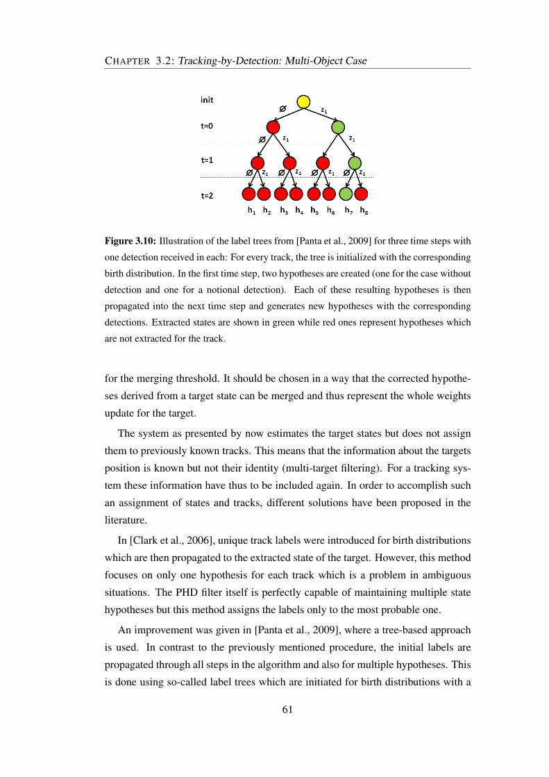
CHAPTER 3.2: Tracking-by-Detection: Multi-Object Case
Figure 3.10: Illustration of the label trees from [Panta et al., 2009] for three time steps with
one detection received in each: For every track, the tree is initialized with the corresponding
birth distribution. In the first time step, two hypotheses are created (one for the case without
detection and one for a notional detection). Each of these resulting hypotheses is then
propagated into the next time step and generates new hypotheses with the corresponding
detections. Extracted states are shown in green while red ones represent hypotheses which
are not extracted for the track.
for the merging threshold. It should be chosen in a way that the corrected hypothe-
ses derived from a target state can be merged and thus represent the whole weights
update for the target.
The system as presented by now estimates the target states but does not assign
them to previously known tracks. This means that the information about the targets
position is known but not their identity (multi-target filtering). For a tracking sys-
tem these information have thus to be included again. In order to accomplish such
an assignment of states and tracks, different solutions have been proposed in the
literature.
In [Clark et al., 2006], unique track labels were introduced for birth distributions
which are then propagated to the extracted state of the target. However, this method
focuses on only one hypothesis for each track which is a problem in ambiguous
situations. The PHD filter itself is perfectly capable of maintaining multiple state
hypotheses but this method assigns the labels only to the most probable one.
An improvement was given in [Panta et al., 2009], where a tree-based approach
is used. In contrast to the previously mentioned procedure, the initial labels are
propagated through all steps in the algorithm and also for multiple hypotheses. This
is done using so-called label trees which are initiated for birth distributions with a
61

CHAPTER 3.2: Tracking-by-Detection: Multi-Object Case
unique label. In this step, the tree is composed only by one node (the birth distribu-
tion). During the life-time of this target, its potential positions are added to the label
tree as new nodes. Traversing the nodes upwards in this tree from the last extracted
state to the root node thus reveals a target’s path from the last frame to the initial
starting point (see Figure 3.10).
The figure shows the tree for one target. After initialization, there are two hy-
potheses in the system which relate to the case of an undetected target and the cor-
responding hypothesis for a detection received. In the following time steps, these
hypotheses are the basis for further state estimates which are added to the respective
node in the tree. Remember that in this example, only one detection per time frame
is shown for simplicity. If at any time step more or less than one detection was
received, the number of nodes in this time step would change accordingly.
The leaves of the tree are the potential current state estimates which form the
PHD contribution for this target. Green circles in the tree symbolize the hypotheses
with highest weight which are extracted in each time step in order to form the track
estimate. By traversing the tree along these state estimates, the target path can be
retrieved.
This method of constructing a tree-shaped data structure for the tracks appears
similar to the MHT tree. However, the PHD filter still has some peculiarities com-
pared to MHT, namely e.g. the higher number of trees (one tree per target instead
of one overall tree in MHT) and the non-usage of a gating procedure in the standard
approach (though it could be applied as e.g. proposed in [Macagnano and de Abreu,
2011]).
From this example it becomes clear that the number of branches in the tree grows
exponentially and in order to maintain a suitable run-time and memory require-
ments, the tree must regularly be reduced to a smaller size. On the one hand, this is
done using the aforementioned pruning and merging methods which are executed
only for hypotheses in the same tree: If a leaf is removed from the PHD, the respec-
tive branch is pruned, too. If hypotheses are merged, the branch with the highest
weigh among them is kept.
However, the hierarchical information structure of the tree can also be used in
order to further reduce the number of Gaussians in the PHD. One option used in the
system for this thesis is based on a confirmation threshold Tcon f irm. Whenever a
state has a weight wi < Tcon f irm, it is marked as tentative (otherwise as confirmed).
62

CHAPTER 3.2: Tracking-by-Detection: Multi-Object Case
Branches which have not been confirmed for a longer period of time are removed
as the corresponding hypotheses are not reliable. Also branches which have been
marked as tentative for several consecutive frames are removed from the tree.
An additional pruning of branches is done using the so-called n-pruning [Black-
man, 2004] which is common in multiple hypothesis tracking. This method assumes
that the tree should never be ambiguous for more than the last nn−pruning frames and
builds on the idea that possible changes should be more likely in the recent nodes.
Therefore a decision for older time steps is enforced by removing all branches from
the node of age t − nn−pruning or older which do not lead to the currently extracted
hypothesis.
Another general parameter in the proposed system is the extraction lifetime
threshold textract . By comparison of the current frame number with the time stamp
of the first appearance of a label tree, its lifetime tage can be computed. In order to
reduce false positive detections which might appear only in a few frames, the sys-
tem extracts merely tracks of the label trees for which tage ≥ textract . A usual choice
for this parameter is textract = 5, i.e. tracks of younger age are not extracted.
In order to avoid problems in cases with crossing targets, [Panta et al., 2009]
proposes a log-likelihood-based scheme for track association which relates the can-
didate hypothesis with the state history of known targets. It computes the log-
likelihood ratio (LLR) over mean and covariance of the states and chooses the can-
didate with the highest LLR which is equivalent to comparing the motion model to
its historic values and choosing the target hypothesis which follows the historical
model best. However, it has been shown in the context of a diploma thesis [Arp,
2012] that an increased sensor and process noise level can reduce the advantages of
the LLR-extension considerably.
Consequently, for applications such as vessel or plane tracking, the LLR-based
association model seems helpful. However, its advantage in terms of pedestrian
tracking is questionable. Especially the fact that an increased noise level is needed
for pedestrian tracking makes it necessary to apply different methods in this domain.
Section 4.2 shows how the system used within this thesis has been enhanced by
applying an image cue-based association method.
63

CHAPTER 3.2: Tracking-by-Detection: Multi-Object Case
3.2.5 Comparison of GM-PHD Filter with State-of-the-Art for
Visual Tracking: the Need for High Detection Rates
The PHD filter is a powerful tracking algorithm relying on the Bayes theorem. It
uses a set-based formulation in order to extend the Bayes filter to the multi-target
case and is at the same time mathematically sound but also intuitive and elegant.
The performance of the PHD filter especially in scenarios with a high amount of
noise has been shown to be better than e.g. MHT [Mahler, 2007]. However, its
origin lies in the radar / sonar tracking domain where mostly linear motion models
and high detection rates can be presumed. This is a major difference to the context
of this thesis which is the application for visual pedestrian tracking in the CCTV
domain.
In order to show the general suitability of the proposed PHD filter for visual
tracking, tests on two standard benchmarks have been conducted.
The first benchmark is the MOT17 dataset and presented in Table 3.1. It clearly
shows that the GM-PHD filter implementation from this work which has been
firstly published in the year 2012 has recently been outperformed by newer ap-
proaches. One of the reasons of its lower performance is due to the nature of the
dataset. MOT17 contains a set of highly different and heterogeneous videos (Exam-
ple frames shown in Appendix A.2.1) and it is very hard to parametrize the method
for all videos using the same parameters. Especially videos with moving camera are
hard because no camera motion estimation is performed in the GM-PHD filter and
the internal motion model becomes thus unreliable. It is therefore that the MOT17
dataset is not suitable in the context of this thesis and will not be used furthermore.
However, as an advantage of the GM-PHD filter, its low computational complexity
can be mentioned as it is among the three fastest methods in Table 3.1.
The best performing method shown in the table is eTC17 [Wang et al., 2018]
which uses a neural network-based tracking method called TrackletNet Tracker
(TNT) combining temporal and appearance information in a unified graph model
framework. First, tracklets for each object are obtained using CNN feature in-
formation and intersection-over-union (IOU) with epipolar constraints in order to
address potential camera motion in the video. Using a multi-scale neural network
(TrackletNet), the similarity between two tracklets can be assessed and afterwards,
the tracklets are grouped in order to obtain the final object IDs.
64

CH
AP
TE
R3.2:
Track
ing-b
y-D
etection:
Multi-O
bject
Case
Tracker Year of Publication MOTA IDF1 MT ML FP FN ID Sw. Frag FPS
eTC17[Wang et al., 2018] 2018 51.9±12.4 58.1 23.1% 35.5% 36164 232783 2288 (38.9) 3071 (52.3) 0.7
eHAF17[Sheng et al., 2018b] 2018 51.8±13.2 54.7 23.4% 37.9% 33212 236772 1834 (31.6) 2739 (47.2) 0.7
AFN17[Shen et al., 2018] 2018 51.5±13.0 46.9 20.6% 35.5% 22391 248420 2593 (46.3) 4308 (77.0) 1.8
FWT[Henschel et al., 2017] 2017 51.3±13.1 47.6 21.4% 35.2% 24101 247921 2648 (47.2) 4279 (76.3) 0.2
jCC[Keuper et al., 2018] 2018 51.2±14.5 54.5 20.9% 37.0% 25937 247822 1802 (32.1) 2984 (53.2) 1.8
MOTDT17[Chen et al., 2018] 2018 50.9±11.9 52.7 17.5% 35.7% 24069 250768 2474 (44.5) 5317 (95.7) 18.3
MHT_DAM[Kim et al., 2015] 2015 50.7±13.7 47.2 20.8% 36.9% 22875 252889 2314 (41.9) 2865 (51.9) 0.9
TLMHT[Sheng et al., 2018a] 2018 50.6±12.5 56.5 17.6% 43.4% 22213 255030 1407 (25.7) 2079 (37.9) 2.6
EDMT17[Chen et al., 2017] 2017 50.0±13.9 51.3 21.6% 36.3% 32279 247297 2264 (40.3) 3260 (58.0) 0.6
HAM_SADF17[Yoon et al., 2018] 2018 48.3±13.2 51.1 17.1% 41.7% 20967 269038 1871 (35.8) 3020 (57.7) 5.0
DMAN[Zhu et al., 2018] 2018 48.2±12.3 55.7 19.3% 38.3% 26218 263608 2194 (41.2) 5378 (100.9) 0.3
AM_ADM17[Lee et al., 2018] 2018 48.1±13.8 52.1 13.4% 39.7% 25061 265495 2214 (41.8) 5027 (94.9) 5.7
PHD_GSDL17[Fu et al., 2018] 2018 48.0±13.6 49.6 17.1% 35.6% 23199 265954 3998 (75.6) 8886 (168.1) 6.7
MHT_bLSTM[Kim et al., 2018] 2018 47.5±12.6 51.9 18.2% 41.7% 25981 268042 2069 (39.4) 3124 (59.5) 1.9
IOUT[Bochinski et al., 2017] 2017 45.5±13.6 39.4 15.7% 40.5% 19993 281643 5988 (119.6) 7404 (147.8) 1522.9
FPSN[Lee and Kim, 2018] 2018 44.9±13.9 48.4 16.5% 35.8% 33757 269952 7136 (136.8) 14491 (277.8) 10.1
HISP_T17[Baisa, 2018] 2018 44.6±14.2 38.8 15.1% 38.8% 25478 276395 10617 (208.1) 7487 (146.8) 4.7
GMPHD_SHA[Song and Jeon, 2016] 2016 43.7±12.5 39.2 11.7% 43.0% 25935 287758 3838 (78.3) 5056 (103.2) 9.2
SORT17[Bewley et al., 2016] 2016 43.1±13.3 39.8 12.5% 42.3% 28398 287582 4852 (99.0) 7127 (145.4) 143.3
EAMTT[Sanchez-Matilla et al., 2016] 2016 42.6±13.3 41.8 12.7% 42.7% 30711 288474 4488 (91.8) 5720 (117.0) 12.0
visGMPHD*[Kutschbach, 2017] 2017 40.3 38.0 8.4% 44.7% 5281 7814 42542 289233 1.5
GMPHD_KCF*[Kutschbach et al., 2017] 2017 39.6±13.6 36.6 8.8% 43.3% 50903 284228 5811 (117.1) 7414 (149.4) 3.3
GM_PHD[Eiselein et al., 2012] 2012 36.4±14.1 33.9 4.1% 57.3% 23723 330767 4607 (111.3) 11317 (273.5) 38.4
Table 3.1: Tracking results compared with state-of-the-art trackers on MOT17 benchmark using public detections (from MOT-Challenge website,
due date 31.12.2018, anonymous or incomplete references omitted). Entries marked with * indicate modifications of the GM-PHD scheme evaluated
in a master’s thesis conducted at TUB-NÜ [Kutschbach, 2017].
65

CHAPTER 3.2: Tracking-by-Detection: Multi-Object Case
In eHAF17 [Sheng et al., 2018b], a "Heterogeneous Association Fusion" (HAF)
is used performing a fusion of both high-level detections and low-level image data
to associate targets to tracks. The resulting association graph and track trees are then
fed into a MHT tracking step in order to solve for the most probable track associa-
tions. Additionally, the framework allows for adaptation of the weights controlling
the contribution of motion and appearance information.
[Shen et al., 2018] propose to combine the often-split tasks affinity learning and
data association into a unified framework with data-driven association, namely the
Tracklet Association Tracker (TAT). Using a bi-directional optimization framework,
association of targets can be directly learned from the extracted features in the video.
The usage of raw detections and hierarchical association allows for a significant
speed-up while the performance is still among the best in the table.
In [Henschel et al., 2017], a fusion of two detectors is performed by formulating
a weighted graph labeling problem over the detections received from the usual full-
body detector and an additional head detector. The resulting NP-hard optimization
problem is solved by approximation based on the Frank-Wolfe algorithm and a new
solver proposed by the authors.
[Keuper et al., 2018] formulate visual tracking as a co-clustering problem by
combining bottom-up grouping with top-down detection and tracking. The group-
ing step in this paper involves bottom-up motion information coming from seg-
mented point feature trajectories while top-down tracking information is derived
from clustered bounding boxes. Solving the joint problem then yields the tracking
results.
Deep learning is a basis for [Chen et al., 2018] in order to cope with unreli-
able detections caused e.g. by occlusion. Therefore, match candidates from both
tracking and detection candidates are jointly processed in order to complement each
other in unclear situations. A fully convolutional neural network trained on large
person re-identification datasets is used for scoring and experiments show real-time
performance using a high-end graphics engine.
An extension of the classical MHT method is proposed in [Kim et al., 2015] by
introducing an on-line appearance learning step. Using a regularized least-squares
framework, the number of hypotheses in the system is reduced and the algorithm
becomes more discriminative than the standard MHT. This is achieved at a slightly
higher computational cost than classical MHT, yet not real-time capable on PC hard-
66
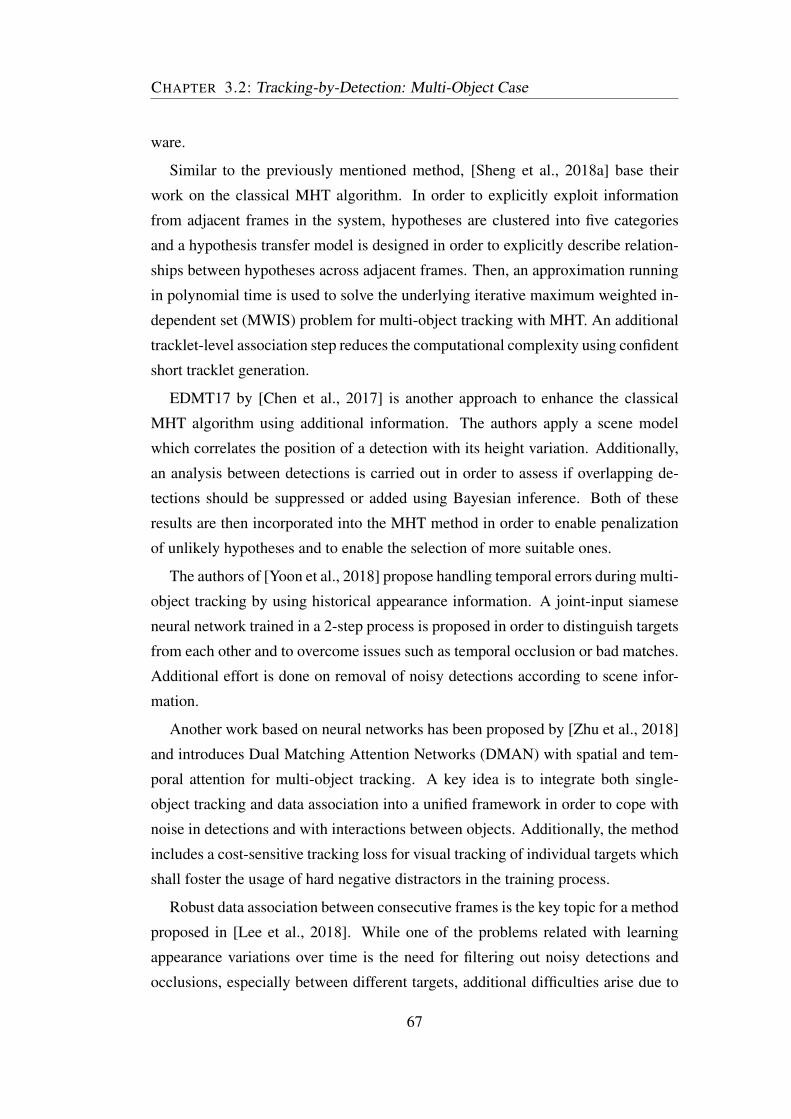
CHAPTER 3.2: Tracking-by-Detection: Multi-Object Case
ware.
Similar to the previously mentioned method, [Sheng et al., 2018a] base their
work on the classical MHT algorithm. In order to explicitly exploit information
from adjacent frames in the system, hypotheses are clustered into five categories
and a hypothesis transfer model is designed in order to explicitly describe relation-
ships between hypotheses across adjacent frames. Then, an approximation running
in polynomial time is used to solve the underlying iterative maximum weighted in-
dependent set (MWIS) problem for multi-object tracking with MHT. An additional
tracklet-level association step reduces the computational complexity using confident
short tracklet generation.
EDMT17 by [Chen et al., 2017] is another approach to enhance the classical
MHT algorithm using additional information. The authors apply a scene model
which correlates the position of a detection with its height variation. Additionally,
an analysis between detections is carried out in order to assess if overlapping de-
tections should be suppressed or added using Bayesian inference. Both of these
results are then incorporated into the MHT method in order to enable penalization
of unlikely hypotheses and to enable the selection of more suitable ones.
The authors of [Yoon et al., 2018] propose handling temporal errors during multi-
object tracking by using historical appearance information. A joint-input siamese
neural network trained in a 2-step process is proposed in order to distinguish targets
from each other and to overcome issues such as temporal occlusion or bad matches.
Additional effort is done on removal of noisy detections according to scene infor-
mation.
Another work based on neural networks has been proposed by [Zhu et al., 2018]
and introduces Dual Matching Attention Networks (DMAN) with spatial and tem-
poral attention for multi-object tracking. A key idea is to integrate both single-
object tracking and data association into a unified framework in order to cope with
noise in detections and with interactions between objects. Additionally, the method
includes a cost-sensitive tracking loss for visual tracking of individual targets which
shall foster the usage of hard negative distractors in the training process.
Robust data association between consecutive frames is the key topic for a method
proposed in [Lee et al., 2018]. While one of the problems related with learning
appearance variations over time is the need for filtering out noisy detections and
occlusions, especially between different targets, additional difficulties arise due to
67

CHAPTER 3.2: Tracking-by-Detection: Multi-Object Case
similar appearance between targets, potentially leading to low discriminability be-
tween them. In this publication, an online appearance learning step using a partial
least square (PLS) method is applied on on-line-collected training samples from
the tracking process. These are continuously refined using PLS subspaces and the
projection of the trained features onto these. An evaluation of the feature discrim-
inability allows the selection of only those targets with low separability and thus
reduces the computational effort significantly.
The work in [Fu et al., 2018] presents a SMC-PHD method and elaborates espe-
cially on two key ideas: It proposes a novel gating concept and an on-line group-
structured dictionary learning step. The first is supposed to enable a knowledge-
based selection of a suitable gating size and thus a reduction of the clutter inference
in cluttered environments. Group-structured dictionary learning then serves to ro-
bustly estimate the target birth intensity. Consequently, newly created targets can
be derived from noisy sensor results while simultaneous code word optimization
for the dictionary update stage is applied in order to enhance the adaptability of the
dictionary to appearance and illumination changes.
[Kim et al., 2018] give another example of a method based on MHT by incor-
porating neural networks into this classical approach. The authors propose using
a Bilinear Long Short-term Memory (LSTM), a recurrent network model which
allows learning of long-term appearance models. According to the authors, the cou-
pling of the LSTM building blocks in a multiplicative manner instead of an additive
one is beneficial for appearance modeling. Furthermore, data augmentation is em-
ployed for efficient training of score models for appearance and motion as a basis
for the final tracking using MHT.
The "Intersection-over-union tracker"’ (IOUT) [Bochinski et al., 2017] also de-
veloped at TUB-NÜ uses the principle of overlapping bounding boxes around ob-
jects in consecutive frames. It can basically both maintain and expand the target
tracks by identifying the detection with the highest intersection-over-union ratio
compared to the last detection in the existing frame. For reasons of stability, a
certain minimal threshold is required for this step. In many cases, these assign-
ments yield a number of unmatched detections which are considered sources of
new tracks. On the other hand, tracks that have not been updated for a number
of frames are considered dead and will be removed eventually. Additional perfor-
mance improvements are achieved by using a filtering step to delete all tracks of
68

CHAPTER 3.2: Tracking-by-Detection: Multi-Object Case
short length and/or low-confidence detections.
In [Lee and Kim, 2018], a novel Feature Pyramid Siamese Network (FPSN) is
proposed for multi-object tracking. The authors claim that this concept is advanta-
geous for learning the similarity metric of targets and detections compared to a plain
Siamese network as used previously. The FPSN aims at combining architectures of
feature pyramid networks (FPN) and Siamese networks and, as a result, enables
the usage of multi-level discriminative features. In order to add motion information
into the system, a spatiotemporal motion feature is proposed to enhance the tracking
performance.
While many of the former methods concentrate on changing some partial as-
pects of already established methods, [Baisa, 2018] is an implementation of a rather
novel tracking concept. This TbD algorithm is based on the Hypothesized and In-
dependent Stochastic Population (HISP) filter which combines aspects from both
traditional tracking approaches like MHT and set-based methods, such as the PHD
filter. The HISP filter is linear in complexity and can keep track identities as MHT
does. The authors propose an additional mechanism in order to avoid having multi-
ple targets with the same label by considering their weights propagated over time.
In [Song and Jeon, 2016], a variation of the GM-PHD filter is applied. As the
algorithm is able to cope with noise and false positives very well but suffers from
false negative detections, the authors add a hierarchical framework for association
of fragmented or wrongly assigned targets. This is done by contribution of two addi-
tional data association steps on low- and mid-level. It can be seen that this measure
gives already a good improvement although it does not suffice to outperform other
tracking methods.
A rather pragmatic approach for multi-object tracking is "Simple Online and
Realtime Tracking" in [Bewley et al., 2016] which uses Kalman filtering and the
Hungarian algorithm for assignment of tracks and detections. As an additional con-
tribution in the paper, the need for accurate detections is emphasized and the authors
propose using CNN detectors for their highly improved performance compared to
traditional approaches. As a result, the proposed method allows for real-time per-
formance at 260 fps and was among the most accurate trackers at the time of publi-
cation.
[Sanchez-Matilla et al., 2016] propose another SMC-PHD-based tracking ap-
proach which distinguishes strong and weak detections and processes them differ-
69

CHAPTER 3.2: Tracking-by-Detection: Multi-Object Case
ently. Weak detections, i.e. detections of low confidence, are used only for label
propagation while strong detections are additionally used for initialization of new
targets. The sampling itself is applied in a perspective-respecting manner, i.e. dis-
tortions due to the camera view are filtered out. Data association in this paper hap-
pens after the predication step which shall remove the need for additional clustering
of particles in order to associate the correct label.
GMPHD-KCF is a Gaussian Mixture Probability Hypothesis Density Filter ex-
tended by Kernelized Correlation Filters, a variant of the GM-PHD tracker in this
work, which has been developed at TUB-NÜ in the framework of a master’s the-
sis [Kutschbach et al., 2017; Kutschbach, 2017]. It applies visual correlation filters
(namely Kernelized Correlation Filters (KCF) [Henriques et al., 2015]) in order to
enhance the tracking in situations with missed detections. The approach followed
is similar to [Danelljan et al., 2014] and splits the overall target model into two
separate models for estimation of target translation and target scale. Thanks to the
small variations between consecutive frames and the motion model of most scenes,
this split appears natural as in most visual tracking scenarios, targets change much
more in position than in scale over consecutive frames. It thus becomes possible to
perform translation estimation and scale estimation subsequently and independently
from each other which is done in this method using FHOG-features from [Dollár,
2016]. The kernel used for translation estimation in the KCF is a Gaussian kernel
while for scale estimation a filter with a linear kernel is used.
The visGMPHD [Kutschbach, 2017] filter is an extension to the previously pre-
sented GMPHD-KCF method and has also been developed as a part of a master’s
thesis at TUB-NÜ. It does not only perform visual object tracking as the GMPHD-
KCF approach but furthermore uses the KCF-framework for visual re-identification
by regarding the trained correlation filters as sources of target-specific image cues.
On that account, the correlation filter information motivates and enables the com-
putation of a visual likelihood model and is used for merging of label trees. As a
result, some drawbacks of the KCF-filter extension, such as an increased sensitivity
to false positives are alleviated at the cost of a much higher computational load.
Table 3.2 shows results for the University at Albany DEtection and TRACking
(UA-DETRAC) dataset [Wen et al., 2015]. This benchmark for vehicle tracking
uses traffic cameras with comparable viewpoints in every video and pre-computed
detections for several detectors (details in Appendix A.2.2). Apart from the class of
70

CHAPTER 3.2: Tracking-by-Detection: Multi-Object Case
Methods Year of Publication PR-MOTA PR-MOTP
Evolving Boxes [Wang et al., 2017] detections
IOUT [Bochinski et al., 2017] 2017 16.4 26.7
GM-PHD [Eiselein et al., 2012] 2012 14.4 26.5
GMPHD-KCF* [Kutschbach, 2017] 2017 14.1 25.9
CompACT [Cai et al., 2015] detections
GM-PHD [Eiselein et al., 2012] 2012 14.3 36.3
JTEGCTD [Tian and Lauer, 2017] 2017 14.2 34.4
HGFT 2017 12.1 33.5
MTT [Zhang et al., 2017] 2017 12.0 35.7
GMPHD-KCF* [Kutschbach, 2017] 2017 12.0 33.8
GOG [Pirsiavash et al., 2011] 2011 11.7 34.4
CCM 2017 10.7 33.8
CMOT [Bae and Yoon, 2014] 2014 10.3 33.4
H2T [Wen et al., 2014] 2014 10.1 33.6
IHTLS [Dicle et al., 2013] 2013 8.7 34.2
CEM [Milan et al., 2014] 2014 4.5 33.2
Table 3.2: Tracking performance on the UA-DETRAC "experienced" dataset (values from
[Kutschbach, 2017]). Entries marked with * indicate modifications of the GM-PHD scheme
evaluated in a master’s thesis conducted at TUB-NÜ [Kutschbach, 2017]. The GM-PHD
filter generally performs on a good level and is only outperformed by the off-line IOUT
method developed at TUB-NÜ [Bochinski et al., 2017].
71
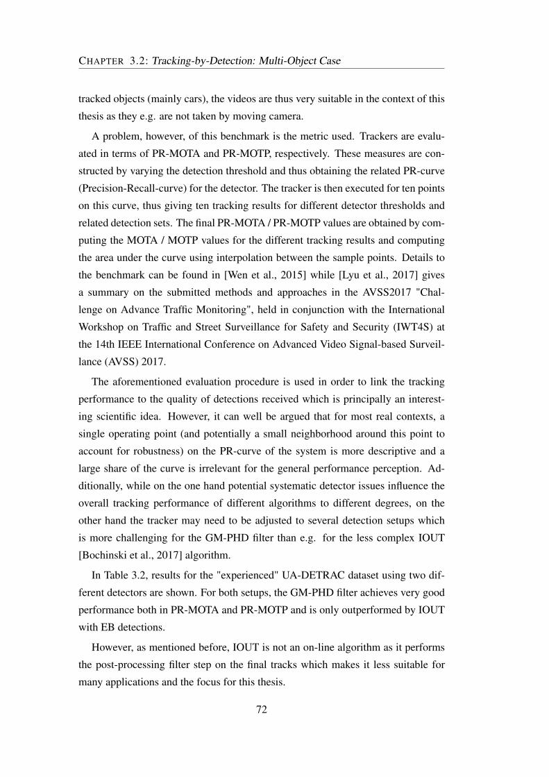
CHAPTER 3.2: Tracking-by-Detection: Multi-Object Case
tracked objects (mainly cars), the videos are thus very suitable in the context of this
thesis as they e.g. are not taken by moving camera.
A problem, however, of this benchmark is the metric used. Trackers are evalu-
ated in terms of PR-MOTA and PR-MOTP, respectively. These measures are con-
structed by varying the detection threshold and thus obtaining the related PR-curve
(Precision-Recall-curve) for the detector. The tracker is then executed for ten points
on this curve, thus giving ten tracking results for different detector thresholds and
related detection sets. The final PR-MOTA / PR-MOTP values are obtained by com-
puting the MOTA / MOTP values for the different tracking results and computing
the area under the curve using interpolation between the sample points. Details to
the benchmark can be found in [Wen et al., 2015] while [Lyu et al., 2017] gives
a summary on the submitted methods and approaches in the AVSS2017 "Chal-
lenge on Advance Traffic Monitoring", held in conjunction with the International
Workshop on Traffic and Street Surveillance for Safety and Security (IWT4S) at
the 14th IEEE International Conference on Advanced Video Signal-based Surveil-
lance (AVSS) 2017.
The aforementioned evaluation procedure is used in order to link the tracking
performance to the quality of detections received which is principally an interest-
ing scientific idea. However, it can well be argued that for most real contexts, a
single operating point (and potentially a small neighborhood around this point to
account for robustness) on the PR-curve of the system is more descriptive and a
large share of the curve is irrelevant for the general performance perception. Ad-
ditionally, while on the one hand potential systematic detector issues influence the
overall tracking performance of different algorithms to different degrees, on the
other hand the tracker may need to be adjusted to several detection setups which
is more challenging for the GM-PHD filter than e.g. for the less complex IOUT
[Bochinski et al., 2017] algorithm.
In Table 3.2, results for the "experienced" UA-DETRAC dataset using two dif-
ferent detectors are shown. For both setups, the GM-PHD filter achieves very good
performance both in PR-MOTA and PR-MOTP and is only outperformed by IOUT
with EB detections.
However, as mentioned before, IOUT is not an on-line algorithm as it performs
the post-processing filter step on the final tracks which makes it less suitable for
many applications and the focus for this thesis.
72

CHAPTER 3.2: Tracking-by-Detection: Multi-Object Case
Another challenge participant evaluated on "Evolving Boxes" detections is the
previously explained method "Gaussian Mixture Probability Hypothesis Density
Filter extended by Kernelized Correlation Filters" (GMPHD-KCF) by [Kutschbach
et al., 2017; Kutschbach, 2017], a variant of the GM-PHD tracker in this work,
which has been developed at TUB-NÜ in the framework of a master’s thesis.
The second-best contribution using CompACT detections in the challenge is
"Joint tracking with event grouping and constraints in time domain" (JTEGCTD)
published in [Tian and Lauer, 2017]. The method first applies a grouping step to
deal with assignments for detection-to-tracks which is used in order to reduce the
target drift due to object mismatches in crowded scenes. Its main idea relies on
evaluation of the inter-object motion relationships within crowds. In order to re-
establish tracks and rediscover targets after a long disappearance, the second com-
ponent in the method applies subgraph models and Binary Integer Programming
(BIP).
"Higher-order Graph and Flow network based Tracker" (HGFT) is a method
submitted for evaluation by Xiaoyi Yu and Guang Han. It is based on the below-
mentioned GOG tracking algorithm from [Pirsiavash et al., 2011] which applies a
min-cost flow network with a number of modifications. According to [Lyu et al.,
2017], the differences to the original approach include "high-order temporal rela-
tions among detections in the confidence calculation" using spatial features such as
overlap and height ratio of detections over multiple frames to improve the tracking
performance.
Zhang et al. proposed with [Zhang et al., 2017] "Multi-task Deep Learning for
Fast Online Multiple Object Tracking" (MTT) a method based on deep neural net-
works. By using an appearance feature extractor trained by triplet loss function and
the assessment of the detection quality before the actual tracking step (by compar-
ison of ground truth and detection positions / regions-of-interest and training of a
binary classification network), the network is able to use only high-quality detec-
tions for training. Consequently, the joint network becomes a multitask network
sharing the computation of the convolutional layers in both parts and achieves good
overall tracking results.
GOG ("Globally optimal greedy algorithms for tracking a variable number of
objects") has been published by H. Pirsiavash, D. Ramanan, and C. C. Fowlkes
in the year 2011 [Pirsiavash et al., 2011] and proposes a formulation of the multi-
73
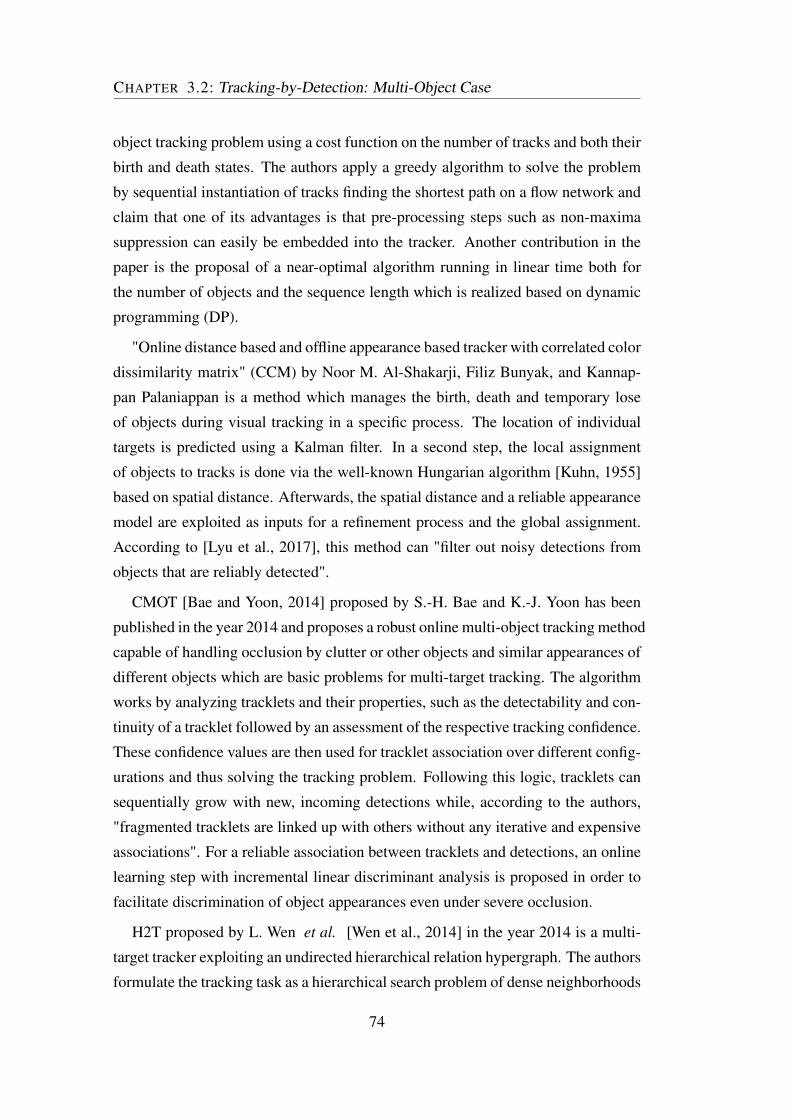
CHAPTER 3.2: Tracking-by-Detection: Multi-Object Case
object tracking problem using a cost function on the number of tracks and both their
birth and death states. The authors apply a greedy algorithm to solve the problem
by sequential instantiation of tracks finding the shortest path on a flow network and
claim that one of its advantages is that pre-processing steps such as non-maxima
suppression can easily be embedded into the tracker. Another contribution in the
paper is the proposal of a near-optimal algorithm running in linear time both for
the number of objects and the sequence length which is realized based on dynamic
programming (DP).
"Online distance based and offline appearance based tracker with correlated color
dissimilarity matrix" (CCM) by Noor M. Al-Shakarji, Filiz Bunyak, and Kannap-
pan Palaniappan is a method which manages the birth, death and temporary lose
of objects during visual tracking in a specific process. The location of individual
targets is predicted using a Kalman filter. In a second step, the local assignment
of objects to tracks is done via the well-known Hungarian algorithm [Kuhn, 1955]
based on spatial distance. Afterwards, the spatial distance and a reliable appearance
model are exploited as inputs for a refinement process and the global assignment.
According to [Lyu et al., 2017], this method can "filter out noisy detections from
objects that are reliably detected".
CMOT [Bae and Yoon, 2014] proposed by S.-H. Bae and K.-J. Yoon has been
published in the year 2014 and proposes a robust online multi-object tracking method
capable of handling occlusion by clutter or other objects and similar appearances of
different objects which are basic problems for multi-target tracking. The algorithm
works by analyzing tracklets and their properties, such as the detectability and con-
tinuity of a tracklet followed by an assessment of the respective tracking confidence.
These confidence values are then used for tracklet association over different config-
urations and thus solving the tracking problem. Following this logic, tracklets can
sequentially grow with new, incoming detections while, according to the authors,
"fragmented tracklets are linked up with others without any iterative and expensive
associations". For a reliable association between tracklets and detections, an online
learning step with incremental linear discriminant analysis is proposed in order to
facilitate discrimination of object appearances even under severe occlusion.
H2T proposed by L. Wen et al. [Wen et al., 2014] in the year 2014 is a multi-
target tracker exploiting an undirected hierarchical relation hypergraph. The authors
formulate the tracking task as a hierarchical search problem of dense neighborhoods
74

CHAPTER 3.2: Tracking-by-Detection: Multi-Object Case
on a dynamically constructed undirected affinity graph. Considering high-order
relationships of detections over the spatio-temporal domain improves the robustness
of the system against similarly looking targets close to each other. A hierarchical
optimization process, on the other hand, helps the tracker to overcome difficulties
of long-term occlusion.
Iterative Hankel Total Least Squares (IHTLS) proposed by C. Dicle, O. I. Camps,
and M. Sznaier is a computationally efficient algorithm for multi-object tracking-
by-detection. In their publication [Dicle et al., 2013], the authors claim to address
four main challenges for visual tracking: similar appearances between different tar-
gets, lack of knowledge about targets that are occluded or outside the camera field of
view, crossing of trajectories between targets, and moving cameras. This is achieved
by using motion dynamics in order to differentiate between targets with similar ap-
pearance, minimize mis-identification of targets and recover missing data. A com-
putationally efficient Generalized Linear Assignment (GLA) approach is combined
with further processing steps to recover missing data and evaluate the complexity
of target dynamics for comparison. It is possible to apply this scheme for tracklets
of arbitrary length and no a-priori dynamical model for target motion is required.
Thanks to its exploitation of motion cues, the algorithm is especially suitable for
scenarios with little or poor appearance cues.
A. Milan, S. Roth, and K. Schindler proposed Continuous Energy Minimization
for Multi-Target Tracking (CEM) [Milan et al., 2014]. This algorithm formulates
the multi-target tracking problem as a minimization of a continuous energy func-
tion. In contrast to other, similar methods, CEM is designed to model an energy
function corresponding to a more complete representation of the problem instead
of one suitable for global optimization approaches. Therefor, the authors make use
of image data as well as physical considerations such as e.g. target dynamics, mu-
tual exclusion, and persistence of tracks. The system performs explicit occlusion
handling in order to exploit also partial image evidence and uses a target appear-
ance model to resolve ambiguities between different targets. A sophisticated opti-
mization scheme is proposed which combines both conjugate gradient descent and
trans-dimensional jumps in an alternating fashion in order to resolve the underlying
non-convex energy function. The moves are applied in such a way that the energy is
always minimized but still weak minima can be left in the search for other, stronger
ones. Additionally, the method allows exploring larger portions of the search space
75

CHAPTER 3.2: Tracking-by-Detection: Multi-Object Case
of varying dimensionality.
The above comparison shows that the performance of the GM-PHD filter is gen-
erally on a good level compared to other methods and benefits especially from better
detectors, such as EB. However, in the context of this thesis, both MOT17 (due to
the heterogeneous videos) and UA-DETRAC (due to the nature of tracked objects
and the metric issues) have only been shown for the sake of completeness but other,
more suitable videos are used to show the improvements of this work.
The computational complexity of the proposed GM-PHD method is low, i.e. for
the pure tracking process without detection, it is possible to achieve 30-40 frames
per second as shown in Table 3.1. Depending on the configuration, also higher
values can be obtained. From both the performance and the computational com-
plexity, it can be concluded that the GM-PHD filter is generally a suitable tool for
multi-target tracking in surveillance scenarios.
However, it appears that the GM-PHD filter just recently became more popular
in the visual tracking community. This is partially because in the last years, much
research has been dedicated to instance-specific tracking of individual objects and
related feature extraction (e.g. correlation filters such as [Danelljan et al., 2014;
Henriques et al., 2015]). It is likely that continuous improvement in tracking single
objects will also help in tracking multiple of them at the same time.
Nonetheless, as mentioned before, it is of crucial interest for multi-target tracking
that solutions of dealing with false positive and false negative detections which arise
in the context of automated object detection for multiple tracks are found. It is in this
area where the GM-PHD filter provides good foundations which are mathematically
justified. It is therefore that with the rise of better detectors based on convolutional
neural networks (CNNs), some of the problems mentioned below may be reduced
for future developments.
A number of tracking approaches based on PHD filters have been published in
the visual tracking literature, e.g. PHD filters using SMC methods (e.g. [Maggio
et al., 2007; Wang et al., 2008; Maggio and Cavallaro, 2009; Feng et al., 2017].
The GM-PHD tracker proposed in [Wang et al., 2007] relies on background sub-
traction techniques for detecting objects as do some of the previously mentioned
SMC methods. This is advantageous because background subtraction detectors can
be adjusted to have a very low false negative rate.
The authors of [Pollard et al., 2009] use a GM-PHD method in order to track
76

CHAPTER 3.2: Tracking-by-Detection: Multi-Object Case
vehicles in unmanned aerial vehicle (UAV) video footage and propose a GPU im-
plementation in order to obtain real-time performance.
The authors of [Zhou et al., 2014] propose a novel birth distribution approach for
GM-PHD filters based on previous detections which is mainly a solution in case of
many re-appearing false positive detections.
In [Baisa and Wallace, 2017], the authors used a tri-GM-PHD filter in order to
track three different types of targets in a video and showed how their approach
improves upon using multiple individual filters.
A game-theoretical approach is used in [Zhou et al., 2015] in order to deal with
occluded targets. This, however, increases the computational load considerably
and is therefore not suitable for the focus of this work. Another recent tracking
approach using a GM-PHD filter has been proposed by [García et al., 2018] for
vehicle tracking.
Group tracking of pedestrians using a GM-PHD filter has been performed by
[Edman et al., 2013]. The method uses a projection of the pedestrians’ positions into
world coordinates in order to track and cluster them. It is mentioned that "The low
probability of detection implied by image detection algorithms is a slight problem
for the GM-PHD filter. If a group is obscured by another group for several frames
the group will disappear from the filter."
Although found in the context of group tracking, this result is consistent with the
experimental outcomes in this thesis: the sensitivity of the GM-PHD filter to missed
detections is a main concern for its applicability to visual tracking. Considering the
corrector step equation (3.31), it becomes clear that the PHD filter relies on high
detection rates. In case of e.g. a general, state-independent pD = 0.8, the corrector
becomes
Dk|k(x)≈ (0.2) ·Dk|k−1(x)
︸ ︷︷ ︸small contributionby missed targets
+(0.8) · ∑z∈Zk
Lz(x) ·Dk|k−1(x)
C +∫
Lz(x) ·Dk|k−1(x)dx︸ ︷︷ ︸
high contributionby associated detections
(3.40)
which shows that the new state largely (80% as given by the detection probabil-
ity) depends on the detections received and their likelihood-dependent contribution
to the previously estimated states. In the example, the contribution according to
previously estimated states is relatively small (20%). However, in practice the de-
tection rate is given as an average value over time and usually empirically justified.
77

CHAPTER 3.2: Tracking-by-Detection: Multi-Object Case
As such, in on-line scenarios with changing characteristics, it may be hard to define
a suitable value beforehand.
Following the previous reasoning, if a state estimate cannot be confirmed by
a detection, the summed likelihood term over all detections is small because the
respective detection (which would contribute with a high likelihood) is missing. As
a result, the overall contribution by the detections is small and the weight for the
current PHD component quickly drops.
This effect clearly depends on the detection probability but it is important to
note that already one missed detection can cause the overall weight of the PHD
to drop below the extraction threshold which is usually chosen as Textract = 0.5.
In such a case, the state estimate is not extracted and a tracking failure (in this
case a missed track) occurs. If the detection is received again in the next frame,
the tracker might recover due to the now high likelihood and re-raise the dropped
weight of the hypothesis again. However, if a detection is missed for a number
of consecutive frames it is also possible that the hypothesis weights drop below
the pruning threshold wprune which lets the tracker remove all information about the
track. This behavior is desired for tracks which leave the scene but can be a problem
if the track should be continued.
Unfortunately, the performance of usual, camera-based pedestrian detection al-
gorithms in terms of detection probability is even for recently developed methods
far from optimal values. This makes it necessary to develop strategies to overcome
the problems related to missed detections. Chapter 4 shows a mathematical analy-
sis of the issue and approaches taken in the course of this thesis in order to improve
the tracking performance of the PHD filter for environments with lower detection
probabilities.
One could argue that in order to reduce the impact on the performance reduc-
tion for the tracking system, a different tracker than the PHD filter could be used.
However, when relying on the tracking-by-detection (TbD) paradigm, the problem
remains the same in different algorithms. As in these methods tracks are extracted
from the detections received, it is always the question how to proceed with tracks
which have not been confirmed by a detection. In such a case, there are only two
choices to the tracking algorithm: complete removal of the track or extrapolation of
the new position using information from the last states. While the first is the cor-
rect solution in case of targets leaving the scene, the latter is preferable for missed
78

CHAPTER 3.2: Tracking-by-Detection: Multi-Object Case
detections but at the very moment of the missed detection, there is not enough in-
formation to solve the problem. This dilemma can be taken as fundamental for
multi-target tracking applications.
Thus, regardless of the tracking algorithm applied, the basic problem remains
the same. The issues described are in principle valid for any TbD system and it is
without loss of generality that the PHD filter can be used in this thesis.
However, apart from its mathematically rigorous foundation, a major advantage
of the PHD filter (and especially the GM-PHD implementation) compared to other
tracking methods is its very low computational complexity which is linear in both
the number of targets and detections ([Mahler, 2007]) and thus is very well suited
for real-time applications.
79

CHAPTER 3.2: Tracking-by-Detection: Multi-Object Case
80

Chapter 4
Proposed Tracking Framework
IN the previous chapters, theoretical foundations for the tracking framework in
this thesis have been laid and advantages and potential issues of the baseline
PHD filter used for pedestrian tracking in surveillance scenarios have been dis-
cussed.
In this section, the overall tracking framework which has been developed for this
thesis is explained in detail. Several improvements are contributed which can over-
come the difficulties and problems identified previously, especially the sensitivity
with regard to missed detections which is an important drawback for tracking-by-
detection methods and will be a major subject to improvements. Depending on the
circumstances and specific use cases of the final application of the tracking frame-
work, different approaches are shown to contribute to a higher detection or tracking
performance and are thus an important outcome of this thesis.
In summary, the main methodological contributions in this chapter are:
• An improved human detection method in scenarios with groups and medium-
dense crowds of pedestrians where the detection rate decreases due to over-
lapping regions-of-interest (presented in Section 4.1).
• A label tree extension using visual information for the tracker which avoids
labeling errors for overlapping objects (given in Section 4.2).
• A methodology for using multiple pedestrian detectors in the tracking frame-
work which can complement each other in order to improve the detection
performance (given in Section 4.2.2).
81

CHAPTER 4.1: Improving Human Detection in Crowds
• The introduction of motion information into the tracking process by means of
active post-detection filters in order to add additional "artificial" detections to
improve the tracker (presented in Section 4.3).
4.1 Improving Human Detection in Crowds
Parts of the work in this chapter have been published in
• Eiselein, V.; Fradi, H.; Keller, I.; Sikora, T.; Dugelay, J.-L., 2013. Enhanc-
ing Human Detection using Crowd Density Measures and an adaptive Cor-
rection Filter. In: Proceedings of the 10th IEEE International Conference on
Advanced Video and Signal-Based Surveillance (AVSS 2013), Kraków, Polen,
27.08.2013 - 30.08.2013
• Fradi, H.; Eiselein, V.; Dugelay, J.-L.; Keller, I.; Sikora, T., 2015. Spatio-
Temporal Crowd Density Model in a Human Detection and Tracking Frame-
work. In: Signal Processing: Image Communication, vol. 31, February 2015,
pp: 100–111, ISSN=0923-5965 (journal)
Automatic pedestrian detection in crowded environments poses a number of
challenges which cause significantly lower detection rates than in uncrowded sce-
narios. The main reason for these impairments is the high occlusion when multiple
people are present in the scene. It is therefore that tracking of pedestrians in crowds
is generally a very hard problem and cannot be considered solved yet.
In scenarios with significant overlapping between individuals, standard pedes-
trian detectors such as the HOG-based methods presented in Chapter 2 have diffi-
culties because they usually do not use specific occlusion handling. Therefore, if a
part of a person is not visible, this part cannot contribute to the detection process
and the final detection score is lower than it would be for a non-occluded person.
Additionally, both detection and tracking methods are often trained for individuals
instead of crowds which makes it difficult to transfer approaches from single-target
scenarios to crowds.
Consequently, parametrization of the pedestrian detector (especially the detec-
tion threshold) becomes more complex because not only the usual scene charac-
teristics such as lighting conditions, camera view, image quality and so on are to
be regarded, but also the expected crowd density attributes directly to the detection
82

CHAPTER 4.1: Improving Human Detection in Crowds
results. Static detection thresholds are difficult to apply because depending on the
current scene crowdiness, the detector may systematically miss pedestrians (missed
detections) or may report too many (false alarms). A solution to this problem will
be discussed in Section 4.1.1 and uses dynamic thresholding based on crowd den-
sity maps estimated for the scene. This approach is simple and efficient but allows
for the usage of multiple detection thresholds within the same image and can thus
increase the detection performance in denser scenes significantly.
Additional problems can occur in the deformable parts-based detector (DPM)
[Felzenszwalb et al., 2010a] because individual parts from different pedestrians can
be fused to a (wrong) single detection result because the detector itself does not per-
form any checks regarding the size of the detection output or the aspect ratio. Such
undesired behaviour can be overcome using geometrical filters which will be ex-
plained in Section 4.1.2. Section 4.1.3 presents results for the dynamic thresholding
based on crowd density and for two filter implementations based on aspect ratio and
height. The section concludes with Section 4.1.4 with a discussion of these results.
4.1.1 Dynamic Detection Thresholds Based on Crowd Density
In order to enable the pedestrian detector to take into account how many people are
expected in a scene and to facilitate its parametrization by the user, a crowd density-
based approach is used in this thesis. Motion tracking is used in order to establish
long-term trajectory information for points and to identify areas in the scene where
the likelihood for pedestrians is high. This information leads to crowd density maps
which are estimated as shown in detail in the next paragraph. Based on a local
density value, the detector can be adjusted to the current scene characteristics. This
process is shown in the following paragraphs.
A) Estimation of Crowd Density Maps
In order to allow for a local change in the parameters of the pedestrian detector,
local density information is needed. While other options could be the estimate of
the overall number of people in the scene as e.g. in [Hou and Pang, 2011], such
information would not be helpful if the crowd density varies over the scene. Ad-
ditionally it should be mentioned that estimating the number of persons in a scene
is generally a difficult task by itself and usually one of the applications of a pedes-
83

CHAPTER 4.1: Improving Human Detection in Crowds
trian detector. It is thus hard to introduce such a-priori information which actually
results from accurate pedestrian detection beforehand. Crowd density information
however can be computed for arbitrary areas and can deliver all desired information
regarding detection and localization of crowds up to pixel-wise level of detail.
A similar approach has been proposed in [Rodriguez et al., 2011a] using an en-
ergy formulation. In contrast to the work in this thesis, the author uses the detection
scores of a person detector which can be considered a drawback as it does not in-
troduce additional knowledge into the detection process. The system presented in
[Rodriguez et al., 2011a] also requires an additional learning process with human-
annotated ground truth detections.
For this thesis, a crowd-density estimation approach from [Fradi and Dugelay,
2013] has been chosen. It computes a crowd density map using local features (e.g.
SURF [Lowe, 2004] or FAST [Rosten et al., 2010]) as an observation of a proba-
bilistic crowd function. The underlying assumption is that in average, there should
be a similar number of local features on every person in the scene. While one might
expect this to be dependent e.g. on image contrast, lighting conditions or clothing
of the people in the scene, the assumption has been shown in several publications
[Fradi and Dugelay, 2013; Fradi et al., 2015; Senst et al., 2014] to hold for compu-
tation of sufficiently accurate crowd density maps.
The basis for the feature tracking step is a set St of m points in frame t = t0 which
are initialized using the FAST method [Rosten et al., 2010]:
St0 =
x0,t0
x1,t0...
xm,t0
(4.1)
with xi,t j=(xi,t j
,yi,t j
)T. In this work, a detection threshold of ξ = 20 is used for
FAST which is suitable for the data used but depending on contrast and resolution
of the video data, other choices here can be used in order to increase or reduce the
number of trajectories.
A direct usage of these feature points without any additional pre-processing
would yield at least two issues: On the one hand, the processing time would be
greatly increased but (more importantly), the system would also not be able to dis-
84

CHAPTER 4.1: Improving Human Detection in Crowds
tinguish between points on foreground objects, which are interesting in order to
compute the crowd density, and irrelevant background information.
Therefore, in order to identify motion in the scene and to concentrate the crowd
density estimation on foreground objects, local feature tracking is used. This is an
alternative to background subtraction methods which could also be used for this
task. [Fradi and Dugelay, 2013] shows that the tracking step improves the system’s
performance compared to background subtraction based on gaussian mixture mod-
els (GMM).
Feature tracking is done using the robust local optical flow (RLOF) method
[Senst et al., 2012a] developed at TUB-NÜ. Based on the assumption that the main
foreground objects in the scene are persons, these can then be differentiated from
background by their non-zero motion vectors. The method used in this thesis ap-
plies RLOF in consecutive frames in order to build trajectories for the m points
tracked:
Stn =
x0,t0 ,x0,t1 , . . .x0,tn
x1,t0 ,x1,t1 , . . .x1,tn...
xm,t0 ,xm,t1 , . . .xm,tn
(4.2)
Therefore, to obtain Stn , RLOF is applied to every point xi,tn−1 in the (n− 1)-th
frame in order to determine its motion vector mn−1 = (∆xn−1,∆yn−1). New point
coordinates can then be computed as
xi,tk = xi,tk−1 +mk−1 (4.3)
A trajectory set such as Stn allows the observation of motion over multiple frames
and enables more sophisticated motion measures such as the average or maximal
motion over time while standard optical flow only focuses on the motion within the
last frame. The system in this thesis is thus less prone to errors due to change in the
motion signatures (e.g. due to pedestrians walking and standing still for a while).
The reason for using RLOF instead of e.g. Lucas-Kanade optical flow [Lucas
and Kanade, 1981; Bouguet, 2000] (as used in the well-known KLT feature tracker
[Tomasi and Kanade, 1991]) is its superior performance with regard to noise. RLOF
85

CHAPTER 4.1: Improving Human Detection in Crowds
uses a robust norm for error minimization which reduces the effect of outliers and
thus improves the position estimate in ambiguous cases.
A common problem for point trackers using local optical flow is the choice of
feature points to be tracked. These are usually chosen depending on texture and
local gradient information, and thus often do not lie on the center of an object but
rather at its borders. As in this case they can easily be affected by other motion
patterns or by occlusion, the feature point tracking is impeded.
RLOF handles such effects better than e.g. the standard KLT tracker [Tomasi
and Kanade, 1991] but in order to avoid preventible issues, in this work, a forward-
backward verification scheme is used. The resulting position of a point in a frame
is used as input to the same motion estimation step from the second frame into the
first one. Points for which this ‘reverse motion’ results in a position highly different
from their respective initial position are presumed to be subject of occlusion and are
thus discarded.
In order to identify feature points lying on foreground objects, in every time
step, the overall mean motion mt of a trajectory t is compared to a certain threshold
βmotion. βmotion can be set according to the image resolution, camera perspective
and expected motion patterns. Features with sufficient motion in their history are
then identified by the relation mt > βmotion while the others are considered part of
the static background. The choice of βmotion does mostly not appear to be critical,
in this work βmotion = 1px is used. The advantage of using trajectories in this sys-
tem instead of computing the motion vectors only between two consecutive frames
is that the estimate is more robust to noise and the overall motion information is
more accurate. The process can be seen as an implicit temporal filtering step which
improves the consistency of the results compared to using only two consecutive
frames.
With the moving feature points given, the actual crowd density estimation step
consists of a kernel density estimation using Gaussian kernels and the positions of
local features. Using the assumption of a similar distribution of feature points on the
different foreground objects (i.e. persons), it appears natural and intuitive to expect
a higher crowd density for local feature points being located closer to each other.
In contrast, in areas where the points have a large spatial distance, it is unlikely to
expect a high crowd density.
Accordingly, a probability density function is estimated using a Gaussian kernel
86

CHAPTER 4.1: Improving Human Detection in Crowds
density. Considering a set of nk local features extracted from a given image at their
respective locations (xi,yi), i ∈ 1..nk, the density C(x,y) is defined as follows:
C(x,y) =1√
2πσ
nk
∑i=1
exp−((x− xi)
2 +(y− yi)2
2σ2 ) (4.4)
with σ as the bandwidth of the 2-dimensional Gaussian kernel. The resulting den-
sity function is then used as a crowd density map with image resolution and pro-
vided to the detection modules. A visualization of the overall process of crowd
density estimation using local features is given in Figure 4.1.
B) Crowd Density-Sensitive Pedestrian Detection
Many common pedestrian detection algorithms use a pre-configured static detection
threshold τ . In real-world applications, such static thresholds can cause difficulties
because beforehand, it is not clear to the user how to adapt the algorithm to a new
scene and how to choose the thresholding value which influences both the detection
rate (i.e. the true positive rate) and the clutter (i.e. the false positive rate). Addi-
tionally, factors such as the number of persons in a scene, image contrast, camera
motion and even perspective distortions may vary over different videos and even
within a single video over time. They can thus easily influence the choice of a
suitable threshold.
While lower values will usually increase the number of detections and allow rec-
ognizing more persons, they will also most likely increase the number of false pos-
itives. On the other hand, higher thresholds will only detect more reliable candidate
regions and might cause the detector to miss people in the scene. As a compro-
mise between true and false positives needs to be found, common practice mostly
involves the usage of training videos of the given scene for which the best static
threshold is assessed (using a person-annotated ground truth) and then used during
future processing.
However, this methodology is especially error-prone in heterogeneous scenes
with both crowded and uncrowded areas or in scenes where the number of persons
changes over time. In crowded areas, usually lower thresholds would be suitable
as due to occlusions, the overall detection scores are not as high as for individuals.
Higher thresholds, on the other hand, have the advantage of reducing the number
of false positives in lesser crowded spaces and are thus favorable in order to avoid
clutter.
87

CHAPTER 4.1: Improving Human Detection in Crowds
Figure 4.1: Different steps in crowd density estimation process using local FAST features
shown on two videos: Features are tracked over multiple frames in order to create trajec-
tories with motion information associated (top left). Red features are assumed background
due to low motion (top right). Kernel density estimation yields the final density estimate,
shown in red (bottom left). For comparison, the density estimate without background re-
moval is also shown (bottom right).
88

CHAPTER 4.1: Improving Human Detection in Crowds
It is therefore desirable to find a way of automatically setting the detection
threshold τ according to the crowd density– or in other words: to the probability es-
timate that people are present in a certain position of the image. The density maps
as computed in the previous paragraph provide exactly this information. There-
fore, they form the basis in order to automatically adjust the detection threshold
according to the local crowd density and finally improve the detection accuracy of
pedestrian detectors.
Assuming an image I of size M×N pixels, the crowd density function is defined
pixel-wise according to Equation (4.4). The detector, on the other hand, yields a
set of candidate detections for a given threshold τ . Considering them as regions
of interest (RoIs) with x-/y-coordinates, width and height, they form a set D(τ) =
d1,d2, ...,dn with di = xi,yi,wi,hi,si.
Here, xi,yi denotes the position of detection di and wi,hi the respective width
and height. Every detection has an associated score si which reflects the detector’s
confidence regarding the similarity to a previously trained pedestrian model.
For most scenes, it makes sense to consider a pre-defined range of detection
thresholds given by an upper / lower boundary τmax/τmin. These values represent
suitable detection thresholds for crowded and uncrowded scenes and are chosen
beforehand by the user.
For the system used in this thesis, the final value of the detection threshold then
varies between these two boundaries and is computed as:
τdyn = τmin +(τmax − τmin) ·C(di), (4.5)
with
C(di) =
hi−1∑j=0
wi−1∑
k=0C(xi + j,yi + k)
wi ·hi(4.6)
as the average crowd density value for detection di.
In other words, the area of each detection received is evaluated regarding the
estimated crowd density. The average density estimate over the whole detection
area is normalized to a value C(di) ∈ [0;1] according to which the final detection
threshold is set for the respective detection.
An effective, yet simple implementation of this procedure is ensured by first
89

CHAPTER 4.1: Improving Human Detection in Crowds
identifying a set of detections
D(τmin) = d1min,d2min
, ...,dnmin (4.7)
which have a score si greater or equal to the minimal detection threshold τmin.
In a second step, the surplus detections which do not fit to the underlying crowd
density estimate need to be filtered out. Therefore, the detections from the set
D(τmin) are now assessed individually in order to adapt their respective detection
thresholds according to the particular crowd density estimate.
This is done by computing the average crowd density estimate C(di) over wi and
hi as in equation (4.6) and inserting the result into Equation (4.5). The resulting
threshold τdyn is individually computed for detection di and its crowd context and
thus dynamically adapts to the crowd density level in the respective image area.
In a final step, τdyn is compared to si in order to identify if the detection should
be filtered out or kept:
di :
si ≥ τdyn : kept
si < τdyn : f iltered out(4.8)
The final set of detections is post-processed by a non-maxima suppression step
as in the standard method [Felzenszwalb et al., 2010b]. This is explained in more
detail in Section 4.1.2.
4.1.2 Geometric Priors for Pedestrian Detection
A major problem for pedestrian detectors is the varying scale and shape of persons
in a video. While current state-of-the-art pedestrian detectors usually handle differ-
ent scaling levels, the aspect ratio of a person can vary a lot depending on e.g. the
individual physique of a person and the person’s pose in relation to the camera.
Especially the often-used part-based pedestrian detector from [Felzenszwalb et al.,
2010a] faces specific challenges in crowded scenarios because it uses multiple part
models attributing to the overall filter score. As a consequence of this combination
of part scores, it is possible that parts coming from multiple different persons are
combined erroneously to a non-existing single one. The reason is that such a com-
bination may yield higher final scores than the true detections if some of their parts
90

CHAPTER 4.1: Improving Human Detection in Crowds
Figure 4.2: Effects of the proposed geometric prior on a frame of the PETS 2009 dataset
[Ferryman and Shahrokni, 2009]: Detections without filtering (left), remaining detections
after filtering according to aspect ratio (center) and remaining detections after filtering ac-
cording to height (right). While the unfiltered detections may include too large candidates
(red) and detections comprising several persons at correct height (yellow), the geometrical
filters are able to reduce such false detections according to their respective properties.
are occluded. Examples for such a situation are highlighted in yellow in Figure 4.2
(left) showing detections with a wrong aspect ratio.
Notwithstanding that, it makes sense to ensure a consistent detection height be-
tween consecutive frames. However, due to the commonly used camera perspective
in video surveillance applications, it is improbable that every person in the im-
age is perceived with the same height in pixels. Apart from rather small potential
height differences in the persons themselves, the position in the image has a much
more important impact on the pixel height of a person. Assuming a common video
surveillance perspective of the camera, the same person walking in the scene from
the lower part of the image towards the upper boundary of the image will appear
smaller and smaller as the distance to the camera increases.
As this relation is not considered in common pedestrian detectors, no prior in-
formation is used in the detection algorithm and accordingly, candidate detections
are not restricted in their size by the detector. This is visualized in Figure 4.2 (left)
where two detections of excessive height (marked in red) are provided by the algo-
rithm.
An additional issue with both mentioned error types arises due to the selection
method used by common pedestrian detectors in order to identify the best-fitting
detection for a person. As a result of the windowed classification step over the input
image, the detector returns a set of candidate detections:
D(τ) = d1,d2, ...,dn (4.9)
91

CHAPTER 4.1: Improving Human Detection in Crowds
which have at least the detection score si ≥ τ but may be overlapping in the
image domain. In order to find the best subset of detections for the current image, a
non-maxima suppression (NMS) scheme is applied as follows ([Felzenszwalb et al.,
2010b]):
• Sort D(τ) according to the detection scores received for every candidate de-
tection. Set the result set D(τ) = /0.
• Pick the di with the highest score from D(τ) according to the detection scores
received for every candidate detection.
• Remove all d j ∈D(τ) which overlap with di to a higher degree than Tmaxoverlap
by computing their spatial overlap. Frequently, Tmaxoverlap = 0.5 is used.
• Add di to the result set: D(τ) = D(τ)∪di and remove it from D(τ).
• Repeat until D(τ) = /0.
If the detection score of a false detection (e.g. a detection which is larger or
wider than desired) is higher than of the overlapping detection candidates, these are
suppressed. It is therefore probable that such bad detections decrease the detection
result twice: Firstly by introducing an additional undesired detection of wrong size
and secondly by suppressing potentially good detections which otherwise would
have contributed to the detection result in a positive way. In order to alleviate this
issue, in this thesis two filtering steps are proposed to cope with bad detections of
wrong size. These are introduced in the following.
A) Filtering Detections According to Aspect Ratio
The first filter defined in this thesis exploits human symmetry by applying a re-
striction on the aspect ratio of a person, i.e. the ratio of width and height of the
respective region of interest. Except for small changes caused e.g. by backpacks or
other items carried by a person, this aspect ratio does not change significantly when
looking at the same person from different views. Small changes in the physique
over multiple persons, however, can be accounted for by using a threshold in the
classification process as shown in the following.
92

CHAPTER 4.1: Improving Human Detection in Crowds
Defining
r = median (width(di)
height(di)), i ∈ 1..n (4.10)
over a set of candidate RoIs D = d1,d2, ...,dn, the current aspect ratio estimate
r can be computed iteratively over all accepted detections in the person detection
process, i.e. the outcome of previous frames is used in order to obtain a stable
parameter estimate for the scene.
A new detection candidate with aspect ratio ri is only accepted if it deviates less
than a given threshold ∆r, i.e.
di :
ri < (1−∆r) · r : filtered out
ri > (1−∆r) · r∧
ri < (1+∆r) · r : kept
ri > (1+∆r) · r : filtered out.
(4.11)
In the experiments for this thesis, ∆r is set to ∆r = 0.3. An example of this
correction filter can be seen in Figure 4.2 (center) where false positive detections
from the original image are suppressed because they have been found to expose an
unexpected aspect ratio.
An advantage of the iterative definition of the filtering procedure is its adapta-
tion to unknown scene parameters. No user input is required in order to identify
suitable values for the aspect ratio. At the same time, it can be argued that the fil-
tering mechanism is greedy and thus relies too strongly on a number of accurate
detections in the beginning of the learning period. However, it has been shown in
experiments with the [Felzenszwalb et al., 2010a] pedestrian detector, the algorithm
is able to converge to a suitable estimate of the aspect ratio and yields good results
(see Section 4.1.3).
Another drawback of the method is that it relies on static camera views which
may be a problem, e.g. when PTZ cameras are used. While the spread of PTZ
camera increases, they are still not as common as static cameras which have been
installed much more often during the last decades. PTZ cameras are also often
rather a tool used for an inspection of suspicious events while it is uncommon that
the camera operator changes the camera view on a regular basis. Given that, the
view towards the people walking through the scene commonly does not change
a lot which allows the design of a correction filter based on static cameras. In
93

CHAPTER 4.1: Improving Human Detection in Crowds
cases of PTZ cameras, a change of the camera view can be detected (e.g. using a
homography-based method such as [Su et al., 2005]) and the estimation of r can be
re-initialized once the camera motion stops and the view remains static again.
B) Filtering Detections According to Expected Height
With the same assumption of a static camera view as described for the detection
filter exploiting the aspect ratio, it is possible to exploit a person’s height as another
human property to filter out incorrect detections. Considering a standard surveil-
lance setup, i.e. an overhead camera, a relationship between a person’s position
and their height can be assumed. As mentioned previously, an intuitive relationship
would be to expect a greater pixel height of a person close to the camera (and in the
mentioned camera setup thus in the lower parts of the image). On the other hand,
a person further from the camera will be found in the upper parts of an image and
will appear smaller in the pixel representation.
This intuitive relation can be described mathematically using perspective trans-
formations. Assuming the pedestrians in the scene to walk on a common ground
plane and a zero-roll angle of the camera (i.e. image lines are parallel to the ground
plane), the following relationship has been derived in [Hoiem et al., 2006]:
yw ≈ yc ·hi
vi − v0(4.12)
where yw and hi are the real-world 3D- and image heights of an object, yc the
height of the camera mount, v0 the horizon position in pixel coordinates and vi the
image (row) position of a pedestrian’s feet. Resolving equation (4.12) for hi yields
vi − v0
yc· yw ≈ hi. (4.13)
Making the assumption that all persons in the scene have the same height allows
substituting yw for a constant. The horizon position and the camera height are fur-
ther constants which can be reduced in order to finally represent the term for frame
k as
γ · vi +δ ≈ hi (4.14)
In the approach used in this thesis, a self-adapting mechanism is used which
estimates γk and δk in all frames. For frame k, this is done as a least-squares fit
94

CHAPTER 4.1: Improving Human Detection in Crowds
over the so far accepted detections from previous frames. Initialization is done
using the detections of the first frame while new detections are accepted if they are
within a range of relative deviation (error threshold) of ±∆size. An example for the
application of this correction filter can be seen in Figure 4.2 (right) where two false
positive regions of wrong size (red) are suppressed.
Again, it should be mentioned that the presumption of a static camera view for
this filter may appear restrictive but could be alleviated easily using a camera motion
estimation step as noted in Section A). Another important restriction (as mentioned
also in [Hoiem et al., 2006]) is that the height filter inhibits detection of pedestrians
at unexpected heights. E.g. detections for a person standing on a roof top will likely
be suppressed as the height of such a person will not match the expected height.
However, as most surveillance systems are set up in structured environments with
approximately planar ground surfaces and one main ground level, this issue appears
less critical.
4.1.3 Experimental Evaluation
In order to assess the performance increase for the three proposed enhancements
for pedestrian detection in crowds, four different video sequences are used. The
datasets, namely the videos "S1.L1 13.57" and "S1.L1 13.59" from the PETS 2009
dataset, the "TownCentre" sequence, the video "INRIA 879-42_I" and "UCF 879-
38", are publicly available and presented in the appendix in Appendix A.1.
These videos have been chosen because they exhibit both areas with little activ-
ity as regions with higher crowd density which is important in order to show the
improvements by the dynamic thresholding mechanism. The two PETS sequences
have a common surveillance camera view and are well established, UCF shows a
scene of very dense crowd which is highly challenging for the pedestrian detector.
The INRIA video has been recorded with an uncommonly steep camera view which
again is a major difficulty for the detector and also shows very dense crowds. The
video with the lowest crowd density is the TownCentre sequence which shows both
individuals and groups in a pedestrian zone. It has been added to the evaluation
in order to show the system’s performance on groups and scenes with lower crowd
density.
95

CHAPTER 4.1: Improving Human Detection in Crowds
PETS 13.57 PETS 13.59 TownCentre INRIA UCF ∅
τstatic N-MODA / N-MODP
-1.5 -0.394 / 0.568 -0.840 / 0.599 -2.219 / 0.685 -0.011 / 0.345 0.298 / 0.548 -0.633 / 0.549
-1.4 -0.127 / 0.569 -0.425 / 0.599 -1.647 / 0.686 0.050 / 0.346 0.307 / 0.549 -0.368 / 0.550
-1.3 0.139 / 0.570 -0.019 / 0.600 -1.170 / 0.687 0.122 / 0.348 0.321 / 0.549 -0.122 / 0.551
-1.2 0.354 / 0.573 0.243 / 0.606 -0.785 / 0.688 0.179 / 0.349 0.336 / 0.550 0.065 / 0.553
-1.1 0.459 / 0.580 0.440 / 0.614 -0.463 / 0.688 0.222 / 0.349 0.360 / 0.551 0.204 / 0.556
-1 0.531 / 0.587 0.558 / 0.624 -0.193 / 0.690 0.252 / 0.346 0.386 / 0.552 0.307 / 0.560
-0.9 0.557 / 0.601 0.599 / 0.637 0.036 / 0.691 0.270 / 0.344 0.420 / 0.554 0.376 / 0.565
-0.8 0.559 / 0.612 0.612 / 0.648 0.205 / 0.692 0.283 / 0.343 0.459 / 0.557 0.423 / 0.571
-0.7 0.542 / 0.628 0.602 / 0.660 0.334 / 0.694 0.280 / 0.347 0.472 / 0.564 0.446 / 0.579
-0.6 0.513 / 0.642 0.581 / 0.672 0.441 / 0.696 0.262 / 0.350 0.466 / 0.573 0.452 / 0.587
-0.5 0.476 / 0.654 0.556 / 0.682 0.515 / 0.698 0.223 / 0.353 0.441 / 0.580 0.442 / 0.593
-0.4 0.443 / 0.660 0.529 / 0.689 0.566 / 0.701 0.180 / 0.343 0.402 / 0.588 0.424 / 0.596
-0.3 0.398 / 0.671 0.491 / 0.695 0.605 / 0.705 0.138 / 0.342 0.354 / 0.595 0.397 / 0.602
-0.2 0.357 / 0.674 0.446 / 0.704 0.625 / 0.708 0.102 / 0.342 0.296 / 0.598 0.365 / 0.605
-0.1 0.311 / 0.677 0.399 / 0.714 0.637 / 0.711 0.072 / 0.322 0.245 / 0.604 0.333 / 0.606
0 0.270 / 0.668 0.356 / 0.705 0.645 / 0.714 0.049 / 0.287 0.196 / 0.607 0.303 / 0.596
0.1 0.226 / 0.669 0.313 / 0.704 0.648 / 0.717 0.035 / 0.261 0.157 / 0.609 0.276 / 0.592
0.2 0.187 / 0.660 0.273 / 0.682 0.640 / 0.720 0.024 / 0.207 0.119 / 0.605 0.248 / 0.575
0.3 0.153 / 0.631 0.236 / 0.663 0.628 / 0.723 0.016 / 0.163 0.091 / 0.608 0.225 / 0.557
0.4 0.125 / 0.596 0.201 / 0.641 0.610 / 0.726 0.011 / 0.127 0.069 / 0.577 0.203 / 0.534
0.5 0.097 / 0.582 0.174 / 0.620 0.589 / 0.728 0.007 / 0.083 0.047 / 0.526 0.183 / 0.508
Table 4.1: Baseline method for pedestrian detection: performance measured using the
DPM detector [Felzenszwalb et al., 2010b] with static thresholds on different test videos. A
threshold of τstatic =−0.8 gives best results on PETS and INRIA datasets while for UCF, a
similar value of τstatic =−0.7 should be chosen. Only for TownCentre, τstatic = 0.1 giving
best results is very different from the other datasets. Averaging over all datasets in order
to find a suitable average value for different environments yields τstatic = −0.6 (gray cells
indicate respective detection performance per video).
96

CHAPTER 4.1: Improving Human Detection in Crowds
Figure 4.3: True positive and false positive rates for the baseline DPM detector [Felzen-
szwalb et al., 2010b] and different static detection thresholds. Values have been normalized
using the number of ground truth persons in the scene.
A) Baseline Performance
In the first performance test, the baseline DPM detector has been applied on the
test videos using varying static detection thresholds and no post-filters. Results
are reported using the normalized MODA (N-MODA) and normalized MODP (N-
MODP) measures for the whole video sequence and are shown in Table 4.1. Both
measures are described in Appendices A.4.2 and A.4.4.
As N-MODA describes the statistics of successfully matched detection results in
terms of correct, missed and supernumerous detections, it is more expressive than
N-MODP which describes the spatial fitting accuracy of detections to the ground
truth. Therefore, the performance evaluation in this section will focus on N-MODA.
It can be seen that, in general, the highest N-MODA values are achieved with a
threshold of τstatic = −0.8 for PETS and INRIA sequences and τstatic = −0.7 for
UCF respectively. For TownCentre however, it turns out that a value of τstatic = 0.1
is preferable. The default detection threshold resulting from the pre-trained VOC
2007 model [Everingham et al., 2007] is τde f ault =−1.44 which is a huge contrast
and can only be explained by a discrepancy in the characteristics of the training
and test data. In order to have one single parameter setting for comparison in the
next experiments, the individual results have been averaged over all datasets, thus
yielding τstatic =−0.6 as the best compromise for the different scenarios.
All these values show that relying on a pre-trained, default parameter is not nec-
essarily a good idea for pedestrian detectors and that usually a number of test runs
97

CHAPTER 4.1: Improving Human Detection in Crowds
are necessary in order to identify a suitable detection threshold. However, such a
pre-trained model represents the common case in real-world applications as it is
unrealistic to annotate training videos in every setup and to re-train a detection al-
gorithm on these data for every single camera.
For the PETS and TownCentre sequences, generally higher detection perfor-
mances are achieved which is due to the camera view and a higher similarity with
the pre-trained pedestrian model. The camera view in the UCF and INRIA datasets
is more tilted which makes a pedestrian’s silhouette differ from the pre-trained
model. Consequently, the detection rates are lower for these datasets. The N-
MODA values are computed using false positive detections and true positive de-
tections. An overview of these two measures can be found in Figure 4.3 where
the respective results are given for a range of detection thresholds. As one would
expect, with higher thresholds, both false positive and true positive rates decrease.
Highest true positive rates are obtained for TownCentre while UCF and INRIA are
the sequences with the lowest detection rates. Sample result frames for the different
videos are given in Figure 4.4.
B) Dynamic Thresholding Based on Crowd Density
One of the main parameters of the underlying crowd density estimation step as
outlined in Section 4.1.1 is the σ value for the kernel density estimation. In order to
identify suitable values for this parameter, experiments have been conducted which
are shown in the following. Crowd density estimation as outlined in Section 4.1.1
is a relative method which gives locally relative density estimates. As such, it is
less suitable for estimation of the exact number of persons in a scene but gives
information about how much denser the crowd in one area of the image is compared
to another area. Consequently, no numerical evaluation is done here in order to
define a suitable σ . Instead, the crowd density and related parameters are compared
subjectively by comparing the resulting crowd density maps given in Figure 4.5.
Figure 4.5 shows different crowd density maps computed for varying values of
σ . It can be seen that the density maps generated with low σ values tend to be "un-
dersegmented" while results for higher σ values lose local specificity because gaps
between people are also filled in the density map. A value of σ = 25 appears visu-
ally appropriate for the test videos and will be used in the following experiments.
In order to assess the performance of the dynamical thresholding step, Tables 4.2
98

CHAPTER 4.1: Improving Human Detection in Crowds
Figure 4.4: Exemplary pedestrian detection results for the baseline DPM detector [Felzen-
szwalb et al., 2010b] using static detection threshold (set to -0.6) in PETS 13.57, PETS
13.59 (top row), INRIA, UCF (second row) and TownCentre (third row) datasets.
99

CHAPTER 4.1: Improving Human Detection in Crowds
Figure 4.5: Exemplary visual results for crowd density estimation on PETS 13.59 and
INRIA sequences using different kernel bandwidth parameters (first row for both sequences:
σ = 5, σ = 15, σ = 25, second row: σ = 35, σ = 45, σ = 55). In order to preserve the
locality information in the density maps, a σ value of 25 appears suitable. Lower values
expose holes in homogeneous regions, higher values tend to "oversegment" crowds and
generate rather coarse maps.
100

CHAPTER 4.1: Improving Human Detection in Crowds
PETS 13.57 PETS 13.59 TownCentre INRIA UCF ∅
τ ∈ [τmin;τmax] N-MODA / N-MODP
indiv. best static 0.559 / 0.612 0.612 / 0.648 0.648 / 0.717 0.283 / 0.343 0.472 / 0.564 0.452 / 0.587
base(-0.6) 0.513 / 0.642 0.581 / 0.672 0.441 / 0.696 0.262 / 0.350 0.466 / 0.573 0.452 / 0.587
[−2;0.2] 0.573 / 0.605 0.600 / 0.652 0.673 / 0.702 0.257 / 0.481 0.382 / 0.578 0.497 / 0.604
[−2;0.1] 0.583 / 0.601 0.608 / 0.647 0.649 / 0.701 0.255 / 0.480 0.412 / 0.575 0.502 / 0.601
[−2;0] 0.589 / 0.596 0.613 / 0.641 0.621 / 0.698 0.254 / 0.479 0.438 / 0.573 0.503 / 0.597
[−2;−0.1] 0.589 / 0.592 0.605 / 0.637 0.587 / 0.696 0.249 / 0.480 0.453 / 0.570 0.497 / 0.595
[−2;−0.2] 0.589 / 0.586 0.601 / 0.631 0.539 / 0.695 0.246 / 0.478 0.463 / 0.568 0.488 / 0.591
[−2;−0.3] 0.585 / 0.583 0.590 / 0.627 0.488 / 0.693 0.242 / 0.476 0.471 / 0.563 0.475 / 0.589
[−2;−0.4] 0.578 / 0.580 0.580 / 0.623 0.429 / 0.692 0.237 / 0.477 0.467 / 0.560 0.458 / 0.586
[−2;−0.5] 0.565 / 0.575 0.563 / 0.619 0.356 / 0.691 0.232 / 0.476 0.457 / 0.556 0.434 / 0.583
[−2;−0.6] 0.544 / 0.572 0.540 / 0.614 0.268 / 0.691 0.224 / 0.475 0.433 / 0.554 0.402 / 0.581
[−1.6;0.2] 0.534 / 0.629 0.585 / 0.671 0.684 / 0.706 0.267 / 0.479 0.340 / 0.584 0.482 / 0.614
[−1.6;0.1] 0.550 / 0.623 0.596 / 0.667 0.669 / 0.703 0.277 / 0.478 0.372 / 0.584 0.493 / 0.611
[−1.6;0] 0.565 / 0.617 0.606 / 0.662 0.640 / 0.702 0.263 / 0.477 0.404 / 0.580 0.496 / 0.608
[−1.6;−0.1] 0.577 / 0.611 0.614 / 0.657 0.612 / 0.699 0.264 / 0.476 0.431 / 0.576 0.500 / 0.604
[−1.6;−0.2] 0.589 / 0.605 0.618 / 0.650 0.577 / 0.696 0.260 / 0.478 0.451 / 0.573 0.499 / 0.601
[−1.6;−0.3] 0.595 / 0.599 0.617 / 0.646 0.532 / 0.694 0.255 / 0.479 0.468 / 0.569 0.493 / 0.597
[−1.6;−0.4] 0.596 / 0.594 0.618 / 0.637 0.474 / 0.693 0.250 / 0.478 0.476 / 0.565 0.483 / 0.593
[−1.6;−0.5] 0.590 / 0.588 0.605 / 0.632 0.409 / 0.692 0.246 / 0.477 0.471 / 0.561 0.464 / 0.590
[−1.6;−0.6] 0.582 / 0.583 0.600 / 0.626 0.325 / 0.691 0.240 / 0.476 0.458 / 0.556 0.441 / 0.586
Table 4.2: First part of comparison between baseline pedestrian detection method and pro-
posed dynamic thresholding on different test videos (σ = 25, motion parameter βmotion = 1).
Gray lines indicate the parameter setting found as the best compromise on all datasets, "in-
dividually best static" describes the best results with static τ and varying parameter sets
for different datasets. The results indicate that the proposed dynamic thresholding step im-
provements can achieve better detection results compared to the baseline method (see also
Table 4.3).
and 4.3 give numerical values for the proposed adaptive thresholding with different
ranges of τ ∈ [τmin;τmax].
It is shown that the usage of a dynamical detection threshold can improve upon
both the best baseline performance obtained using an individual parameter set per
video and especially upon the usage of a single parameter set for all videos (gray
cells). Here, the average performance improves from 0.452 to 0.503 (~+11%)
which is a substantial enhancement. In this case, the detection performance could
be enhanced over all individual videos except for UCF and INRIA. Especially for
PETS 13.57 or TownCentre, the results are significantly better than for a static
threshold of τstatic = −0.6 (~+15% and ~+41%, respectively). On the other hand,
the detection performance on UCF and INRIA drops by ~6% and ~3% for these
101

CHAPTER 4.1: Improving Human Detection in Crowds
settings because the parameters matching other scenarios are not working similarly
well on UCF. However, despite the variety of the datasets, an overall performance
gain is obtained even with one overall setting which may not be perfect in the indi-
vidual scenarios.
On the other hand, the performance improvements are mainly in videos with
changing crowd dynamics (i.e. PETS and TownCentre), while the system shows
a slightly better performance on videos with high crowd density and little density
variation (UCF and INRIA) when parametrized with static thresholds.
Similarly improved results can be found when looking at the individually best
parameter settings for static thresholds (first line) and the individually best dynamic
thresholding parameter sets marked in bold font in the individual columns. In this
case, improvements can be achieved in every single dataset tested. The biggest
achievements are obtained on the PETS 13.57 and TownCentre datasets where the
proposed dynamic thresholding step improves the N-MODA measure in both se-
quences by ~+6%. It should also be mentioned that in the case of individually
optimal parameters, small enhancements are also obtained on UCF. However, simi-
larly as in the previous test, no enhancements are obtained on INRIA. The detection
performance drops slightly (~-2%).
It is thus demonstrated that the proposed dynamic thresholding concept is a suit-
able measure in order to enhance pedestrian detection in crowded scenarios. It is
especially suited for videos with changing crowd densities where the highest gains
are to be expected. Considering the fact that no new detection method or re-training
is necessary when applying this algorithm to a pedestrian detector, the possible per-
formance gain is very high.
C) Performance Improvement by Geometric Priors
The second improvement proposed in this chapter is the usage of geometrical filters
in order to ensure a correct size of detections and to inhibit oversized results. In
order to parametrize the filters, a maximal error threshold ∆size for the size filter and
∆r for the aspect ratio must be chosen. The influence of this parameter on the height
filter is shown in Figure 4.6. As one might expect, the overall impact of the filtering
mechanism on the detection results is different in each of the test videos and the
influence of ∆size varies over the different sequences, too.
The curves generally start at lower N-MODA values because for low error thresh-
102
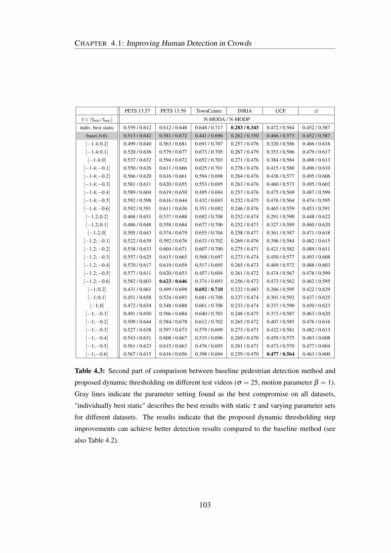
CHAPTER 4.1: Improving Human Detection in Crowds
PETS 13.57 PETS 13.59 TownCentre INRIA UCF ∅
τ ∈ [τmin;τmax] N-MODA / N-MODP
indiv. best static 0.559 / 0.612 0.612 / 0.648 0.648 / 0.717 0.283 / 0.343 0.472 / 0.564 0.452 / 0.587
base(-0.6) 0.513 / 0.642 0.581 / 0.672 0.441 / 0.696 0.262 / 0.350 0.466 / 0.573 0.452 / 0.587
[−1.4;0.2] 0.499 / 0.640 0.563 / 0.681 0.691 / 0.707 0.257 / 0.476 0.320 / 0.586 0.466 / 0.618
[−1.4;0.1] 0.520 / 0.636 0.579 / 0.677 0.673 / 0.705 0.267 / 0.479 0.353 / 0.586 0.479 / 0.617
[−1.4;0] 0.537 / 0.632 0.594 / 0.672 0.652 / 0.703 0.271 / 0.476 0.384 / 0.584 0.488 / 0.613
[−1.4;−0.1] 0.550 / 0.626 0.611 / 0.666 0.625 / 0.701 0.278 / 0.476 0.415 / 0.580 0.496 / 0.610
[−1.4;−0.2] 0.566 / 0.620 0.616 / 0.661 0.594 / 0.698 0.264 / 0.476 0.438 / 0.577 0.495 / 0.606
[−1.4;−0.3] 0.581 / 0.611 0.620 / 0.655 0.553 / 0.695 0.263 / 0.476 0.460 / 0.573 0.495 / 0.602
[−1.4;−0.4] 0.589 / 0.604 0.619 / 0.650 0.495 / 0.694 0.257 / 0.476 0.475 / 0.569 0.487 / 0.599
[−1.4;−0.5] 0.592 / 0.598 0.616 / 0.644 0.432 / 0.693 0.252 / 0.475 0.476 / 0.564 0.474 / 0.595
[−1.4;−0.6] 0.592 / 0.591 0.611 / 0.636 0.351 / 0.692 0.246 / 0.476 0.465 / 0.559 0.453 / 0.591
[−1.2;0.2] 0.468 / 0.651 0.537 / 0.688 0.692 / 0.708 0.252 / 0.474 0.291 / 0.590 0.448 / 0.622
[−1.2;0.1] 0.486 / 0.648 0.558 / 0.684 0.677 / 0.706 0.252 / 0.473 0.327 / 0.589 0.460 / 0.620
[−1.2;0] 0.505 / 0.643 0.574 / 0.679 0.655 / 0.704 0.258 / 0.477 0.361 / 0.587 0.471 / 0.618
[−1.2;−0.1] 0.522 / 0.639 0.592 / 0.676 0.633 / 0.702 0.269 / 0.476 0.396 / 0.584 0.482 / 0.615
[−1.2;−0.2] 0.538 / 0.633 0.604 / 0.671 0.607 / 0.700 0.275 / 0.471 0.421 / 0.582 0.489 / 0.611
[−1.2;−0.3] 0.557 / 0.625 0.615 / 0.665 0.568 / 0.697 0.273 / 0.474 0.450 / 0.577 0.493 / 0.608
[−1.2;−0.4] 0.570 / 0.617 0.619 / 0.659 0.517 / 0.695 0.265 / 0.473 0.469 / 0.572 0.488 / 0.603
[−1.2;−0.5] 0.577 / 0.611 0.620 / 0.653 0.457 / 0.694 0.261 / 0.472 0.474 / 0.567 0.478 / 0.599
[−1.2;−0.6] 0.582 / 0.603 0.623 / 0.646 0.374 / 0.693 0.256 / 0.472 0.473 / 0.562 0.462 / 0.595
[−1;0.2] 0.431 / 0.661 0.499 / 0.698 0.692 / 0.710 0.222 / 0.483 0.266 / 0.595 0.422 / 0.629
[−1;0.1] 0.451 / 0.658 0.524 / 0.693 0.681 / 0.708 0.227 / 0.474 0.301 / 0.592 0.437 / 0.625
[−1;0] 0.472 / 0.654 0.548 / 0.688 0.661 / 0.706 0.233 / 0.474 0.337 / 0.590 0.450 / 0.623
[−1;−0.1] 0.491 / 0.650 0.566 / 0.684 0.640 / 0.703 0.248 / 0.475 0.373 / 0.587 0.463 / 0.620
[−1;−0.2] 0.509 / 0.644 0.584 / 0.678 0.612 / 0.702 0.265 / 0.472 0.407 / 0.585 0.476 / 0.616
[−1;−0.3] 0.527 / 0.638 0.597 / 0.673 0.579 / 0.699 0.273 / 0.473 0.432 / 0.581 0.482 / 0.613
[−1;−0.4] 0.543 / 0.631 0.608 / 0.667 0.535 / 0.696 0.269 / 0.470 0.459 / 0.575 0.483 / 0.608
[−1;−0.5] 0.561 / 0.623 0.615 / 0.663 0.476 / 0.695 0.261 / 0.471 0.473 / 0.570 0.477 / 0.604
[−1;−0.6] 0.567 / 0.615 0.616 / 0.656 0.398 / 0.694 0.259 / 0.470 0.477 / 0.564 0.463 / 0.600
Table 4.3: Second part of comparison between baseline pedestrian detection method and
proposed dynamic thresholding on different test videos (σ = 25, motion parameter β = 1).
Gray lines indicate the parameter setting found as the best compromise on all datasets,
"individually best static" describes the best results with static τ and varying parameter sets
for different datasets. The results indicate that the proposed dynamic thresholding step
improvements can achieve better detection results compared to the baseline method (see
also Table 4.2).
103

CHAPTER 4.1: Improving Human Detection in Crowds
Figure 4.6: Relevant N-MODA curves for proposed height filter parametrized with differ-
ent error thresholds. The error threshold determines which maximal relative deviation the
filter allows based on the estimated pedestrian model established in previous frames and
differs over different test videos. Generally, the τ values for best performance decrease
compared to the baseline detection process due to the filtering step.
104

CHAPTER 4.1: Improving Human Detection in Crowds
olds, only few detections are accepted and no usable scene parameter model can be
computed. Accordingly, the filtering step leads to bad results. With suitable, higher
error thresholds, the filtering excludes incorrect candidate detections and uses the
remaining ones to model usable scene parameters. The performance thus rises.
At some point, the filter threshold becomes too high and the number of accepted
detections increases, leading to a bad scene model and high acceptance probabil-
ity for bad detections. As a consequence, the overall detection performance drops
again. The maximum N-MODA value is achieved at different error thresholds,
however, a sweet spot for most sequences exists for ∆size ≈ 0.25. In the following
experiments, the height filter will thus be parametrized with ∆size = 0.25.
It is important to note that the usage of a height prior allows to apply significantly
lower detection thresholds. Figure 4.6 shows that in order to achieve best results,
τ can be lowered by 0.3 (PETS, INRIA) or even more (UCF, TownCentre). This
shows that the filter performs according to the formulated expectations and filters
less suited candidate detections which are replaced by better-matching detections of
lower score.
The height filter improves the system’s performance over all test videos as can
also be seen in Table 4.4. The table shows the results for a range of different τ
values. Compared to the baseline method, the improvement by the height filter is
very high. This outcome is especially found when looking at the gain achieved using
only one parameter for all datasets: For this experiment, the height filter improves
the N-MODA value from 0.452 to 0.569 (~+26%).
However, also when choosing individually best parameters per dataset, the de-
tection performance is enhanced on every single dataset:
• For PETS 13.57, the performance improves from 0.559 to 0.646 (~+16%).
• For PETS 13.59, the performance improves from 0.612 to 0.645 (~+5%).
• For TownCentre, the performance improves from 0.648 to 0.694 (~+7%).
• For INRIA, the performance improves from 0.283 to 0.501 (~+77%).
• For UCF, the performance improves from 0.472 to 0.588 (~+25%).
Especially on INRIA and UCF, very high gains can be achieved using a height
filter. The result on these datasets can be explained by both relatively low perfor-
mance by the baseline method and the scene characteristics of high crowd density
105
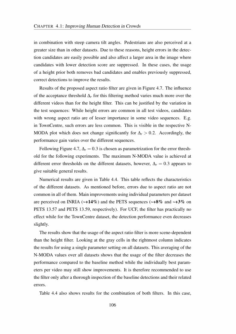
CHAPTER 4.1: Improving Human Detection in Crowds
in combination with steep camera tilt angles. Pedestrians are also perceived at a
greater size than in other datasets. Due to these reasons, height errors in the detec-
tion candidates are easily possible and also affect a larger area in the image where
candidates with lower detection score are suppressed. In these cases, the usage
of a height prior both removes bad candidates and enables previously suppressed,
correct detections to improve the results.
Results of the proposed aspect ratio filter are given in Figure 4.7. The influence
of the acceptance threshold ∆r for this filtering method varies much more over the
different videos than for the height filter. This can be justified by the variation in
the test sequences: While height errors are common in all test videos, candidates
with wrong aspect ratio are of lesser importance in some video sequences. E.g.
in TownCentre, such errors are less common. This is visible in the respective N-
MODA plot which does not change significantly for ∆r > 0.2. Accordingly, the
performance gain varies over the different sequences.
Following Figure 4.7, ∆r = 0.3 is chosen as parametrization for the error thresh-
old for the following experiments. The maximum N-MODA value is achieved at
different error thresholds on the different datasets, however, ∆r = 0.3 appears to
give suitable general results.
Numerical results are given in Table 4.4. This table reflects the characteristics
of the different datasets. As mentioned before, errors due to aspect ratio are not
common in all of them. Main improvements using individual parameters per dataset
are perceived on INRIA (~+14%) and the PETS sequences (~+8% and ~+3% on
PETS 13.57 and PETS 13.59, respectively). For UCF, the filter has practically no
effect while for the TownCentre dataset, the detection performance even decreases
slightly.
The results show that the usage of the aspect ratio filter is more scene-dependent
than the height filter. Looking at the gray cells in the rightmost column indicates
the results for using a single parameter setting on all datasets. This averaging of the
N-MODA values over all datasets shows that the usage of the filter decreases the
performance compared to the baseline method while the individually best param-
eters per video may still show improvements. It is therefore recommended to use
the filter only after a thorough inspection of the baseline detections and their related
errors.
Table 4.4 also shows results for the combination of both filters. In this case,
106

CHAPTER 4.1: Improving Human Detection in Crowds
Figure 4.7: Relevant N-MODA curves for proposed aspect ratio filter parametrized with
different error thresholds. The error threshold determines which maximal relative deviation
the filter allows based on the estimated pedestrian model established in previous frames and
differs over different test videos. For aspect ratio filtering, the τ values for best performance
decrease less than for height filtering.
107
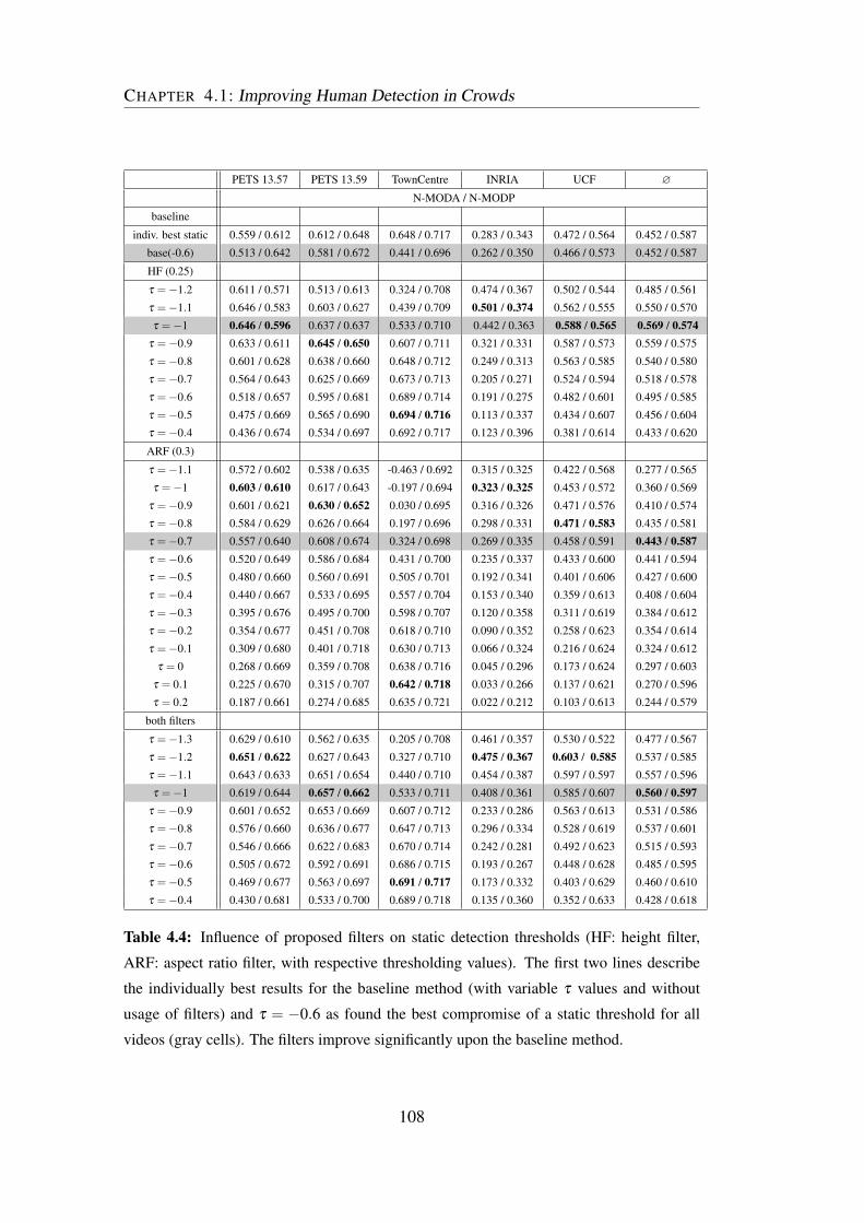
CHAPTER 4.1: Improving Human Detection in Crowds
PETS 13.57 PETS 13.59 TownCentre INRIA UCF ∅
N-MODA / N-MODP
baseline
indiv. best static 0.559 / 0.612 0.612 / 0.648 0.648 / 0.717 0.283 / 0.343 0.472 / 0.564 0.452 / 0.587
base(-0.6) 0.513 / 0.642 0.581 / 0.672 0.441 / 0.696 0.262 / 0.350 0.466 / 0.573 0.452 / 0.587
HF (0.25)
τ =−1.2 0.611 / 0.571 0.513 / 0.613 0.324 / 0.708 0.474 / 0.367 0.502 / 0.544 0.485 / 0.561
τ =−1.1 0.646 / 0.583 0.603 / 0.627 0.439 / 0.709 0.501 / 0.374 0.562 / 0.555 0.550 / 0.570
τ =−1 0.646 / 0.596 0.637 / 0.637 0.533 / 0.710 0.442 / 0.363 0.588 / 0.565 0.569 / 0.574
τ =−0.9 0.633 / 0.611 0.645 / 0.650 0.607 / 0.711 0.321 / 0.331 0.587 / 0.573 0.559 / 0.575
τ =−0.8 0.601 / 0.628 0.638 / 0.660 0.648 / 0.712 0.249 / 0.313 0.563 / 0.585 0.540 / 0.580
τ =−0.7 0.564 / 0.643 0.625 / 0.669 0.673 / 0.713 0.205 / 0.271 0.524 / 0.594 0.518 / 0.578
τ =−0.6 0.518 / 0.657 0.595 / 0.681 0.689 / 0.714 0.191 / 0.275 0.482 / 0.601 0.495 / 0.585
τ =−0.5 0.475 / 0.669 0.565 / 0.690 0.694 / 0.716 0.113 / 0.337 0.434 / 0.607 0.456 / 0.604
τ =−0.4 0.436 / 0.674 0.534 / 0.697 0.692 / 0.717 0.123 / 0.396 0.381 / 0.614 0.433 / 0.620
ARF (0.3)
τ =−1.1 0.572 / 0.602 0.538 / 0.635 -0.463 / 0.692 0.315 / 0.325 0.422 / 0.568 0.277 / 0.565
τ =−1 0.603 / 0.610 0.617 / 0.643 -0.197 / 0.694 0.323 / 0.325 0.453 / 0.572 0.360 / 0.569
τ =−0.9 0.601 / 0.621 0.630 / 0.652 0.030 / 0.695 0.316 / 0.326 0.471 / 0.576 0.410 / 0.574
τ =−0.8 0.584 / 0.629 0.626 / 0.664 0.197 / 0.696 0.298 / 0.331 0.471 / 0.583 0.435 / 0.581
τ =−0.7 0.557 / 0.640 0.608 / 0.674 0.324 / 0.698 0.269 / 0.335 0.458 / 0.591 0.443 / 0.587
τ =−0.6 0.520 / 0.649 0.586 / 0.684 0.431 / 0.700 0.235 / 0.337 0.433 / 0.600 0.441 / 0.594
τ =−0.5 0.480 / 0.660 0.560 / 0.691 0.505 / 0.701 0.192 / 0.341 0.401 / 0.606 0.427 / 0.600
τ =−0.4 0.440 / 0.667 0.533 / 0.695 0.557 / 0.704 0.153 / 0.340 0.359 / 0.613 0.408 / 0.604
τ =−0.3 0.395 / 0.676 0.495 / 0.700 0.598 / 0.707 0.120 / 0.358 0.311 / 0.619 0.384 / 0.612
τ =−0.2 0.354 / 0.677 0.451 / 0.708 0.618 / 0.710 0.090 / 0.352 0.258 / 0.623 0.354 / 0.614
τ =−0.1 0.309 / 0.680 0.401 / 0.718 0.630 / 0.713 0.066 / 0.324 0.216 / 0.624 0.324 / 0.612
τ = 0 0.268 / 0.669 0.359 / 0.708 0.638 / 0.716 0.045 / 0.296 0.173 / 0.624 0.297 / 0.603
τ = 0.1 0.225 / 0.670 0.315 / 0.707 0.642 / 0.718 0.033 / 0.266 0.137 / 0.621 0.270 / 0.596
τ = 0.2 0.187 / 0.661 0.274 / 0.685 0.635 / 0.721 0.022 / 0.212 0.103 / 0.613 0.244 / 0.579
both filters
τ =−1.3 0.629 / 0.610 0.562 / 0.635 0.205 / 0.708 0.461 / 0.357 0.530 / 0.522 0.477 / 0.567
τ =−1.2 0.651 / 0.622 0.627 / 0.643 0.327 / 0.710 0.475 / 0.367 0.603 / 0.585 0.537 / 0.585
τ =−1.1 0.643 / 0.633 0.651 / 0.654 0.440 / 0.710 0.454 / 0.387 0.597 / 0.597 0.557 / 0.596
τ =−1 0.619 / 0.644 0.657 / 0.662 0.533 / 0.711 0.408 / 0.361 0.585 / 0.607 0.560 / 0.597
τ =−0.9 0.601 / 0.652 0.653 / 0.669 0.607 / 0.712 0.233 / 0.286 0.563 / 0.613 0.531 / 0.586
τ =−0.8 0.576 / 0.660 0.636 / 0.677 0.647 / 0.713 0.296 / 0.334 0.528 / 0.619 0.537 / 0.601
τ =−0.7 0.546 / 0.666 0.622 / 0.683 0.670 / 0.714 0.242 / 0.281 0.492 / 0.623 0.515 / 0.593
τ =−0.6 0.505 / 0.672 0.592 / 0.691 0.686 / 0.715 0.193 / 0.267 0.448 / 0.628 0.485 / 0.595
τ =−0.5 0.469 / 0.677 0.563 / 0.697 0.691 / 0.717 0.173 / 0.332 0.403 / 0.629 0.460 / 0.610
τ =−0.4 0.430 / 0.681 0.533 / 0.700 0.689 / 0.718 0.135 / 0.360 0.352 / 0.633 0.428 / 0.618
Table 4.4: Influence of proposed filters on static detection thresholds (HF: height filter,
ARF: aspect ratio filter, with respective thresholding values). The first two lines describe
the individually best results for the baseline method (with variable τ values and without
usage of filters) and τ = −0.6 as found the best compromise of a static threshold for all
videos (gray cells). The filters improve significantly upon the baseline method.
108

CHAPTER 4.1: Improving Human Detection in Crowds
the filters are applied consecutively to the candidate detections and they are trained
using only the detections which remained after both filtering steps.
In this case, improvements are visible on all datasets, both for the case of individ-
ual parameters per dataset and for one parameter setting on all datasets. However,
when looking at the individually best parameter sets, it is visible for the combi-
nation of both filters that the results are not always better than the results of pure
height-based filtering. The reason here is that the filtering step based on the aspect
ratio of candidate detections does not improve results on all datasets, which is also
the case in the combination of both filters. For the two PETS sequences and the
UCF dataset, the results are slightly better than using only height filtering, results
for TownCentre are on a similar level and for INRIA are slightly worse than for pure
height filtering with individually chosen parameters. For averaged parameter val-
ues, the overall picture is similar: On PETS 13.59, the filter combination performs
a bit better than pure height filtering but for the other datasets, results are slightly
worse.
It can thus be concluded that the height filter should be preferred over the aspect
ratio filter because it is less sensitive to the video scenario. However, if pedestrians
are to be detected at different height levels, the aspect ratio filter will be advanta-
geous due to the underlying assumptions.
D) Combining Crowd Density-Based Thresholding and Geometric Priors
Results for a combination of both enhancements proposed in this chapter, i.e. the
usage of a dynamically chosen detection threshold according to crowd density esti-
mates and of geometrical filters in order to ensure suitable detection candidates are
visible in Table 4.5. The first rows in the table summarize the previous experiments
in this chapter by giving results for the baseline method, for the filtering methods
using static detection thresholds and for dynamic detection thresholds without geo-
metrical filters. These results allow for a proper comparison and for quantification
of the performance improvements provided by the individual factors.
Generally, the results in Table 4.5 are in accordance with the previously drawn
conclusions. By comparing the results of dynamically chosen detection thresholds
without filtering with the version using additional height filtering, it can be found
that results are improved on all datasets. The heighest gains are obtained for INRIA
(from 0.278 to 0.451, ~+62%) and UCF (from 0.477 to 0.612, ~+28%). The aver-
109

CHAPTER 4.1: Improving Human Detection in Crowds
age N-MODA performance over all datasets improves from 0.503 to 0.598, i.e. by
a gain of ~+19%.
In contrast, filtering according to the aspect ratio enhances the performance less
than height filtering when used with dynamic thresholds. When compared to dy-
namic thresholding without filtering, the average performance over all datasets re-
mains on a similar level. Higher improvements are visible for PETS 13.57 (from
0.596 to 0.652, ~+9%) and INRIA (from 0.278 to 0.338, ~+22%) while values for
TownCentre and UCF are almost the same as without filtering.
The combination of both filters gives similar results as using the height filter
alone. For the PETS sequences and TownCentre, the values are almost the same.
For INRIA, slight improvements are obtained using both filters while for UCF, the
usage of only a height filter is preferable. The average gain of both filters over all
datasets is on a similar level as for using the height filter only.
When comparing the filtering results for static and dynamic thresholding, it can
be seen that enhancements are possible for almost all combinations. Results for
the height filter approach are enhanced on every dataset except for INRIA using
dynamic thresholding. The averaged N-MODA performance also rises from 0.569
to 0.598 (~+5%). Results for aspect ratio filtering are even clearer: On every sin-
gle dataset and for averaged results, the performance is enhanced by the proposed
dynamic thresholding (~+14% for averaged results).
The conclusion for using both filters is again more dependent on the dataset:
While average N-MODA values improve from 0.560 to 0.603 (~+8%), the main
gains are obtained on PETS 13.57, TownCentre and INRIA. Results for UCF are
slighly worse, and PETS 13.59 remains on a similar level.
4.1.4 Conclusion on Detector Improvements
In this chapter, three improvements for pedestrian detection frameworks have been
shown and validated in an extensive evaluation. During the experiments, it was
found that the standard detection threshold τ =−1.44 used in the DPM pedestrian
detector and the VOC2007 Model is highly unsuitable for common test videos.
Albeit testing a large range of τ values in a manual selection, it was possible to
enhance the detection results over all datasets using a simple crowd density model
for dynamic parametrization of the pedestrian detector.
Enhancements for dynamical thresholding using a single parameter set on all
110

CHAPTER 4.1: Improving Human Detection in Crowds
PETS 13.57 PETS 13.59 TownCentre INRIA UCF ∅
N-MODA / N-MODP
indiv. best static 0.559 / 0.612 0.612 / 0.648 0.648 / 0.717 0.283 / 0.343 0.472 / 0.564 0.452 / 0.587
indiv. best static HF (0.25) 0.646 / 0.596 0.645 / 0.650 0.694 / 0.716 0.501 / 0.374 0.588 / 0.565 0.569 / 0.574
indiv. best static ARF (0.3) 0.603 / 0.610 0.630 / 0.652 0.642 / 0.718 0.323 / 0.325 0.471 / 0.583 0.443 / 0.587
indiv. best static both 0.651 / 0.622 0.657 / 0.662 0.691 / 0.717 0.475 / 0.367 0.603 / 0.585 0.560 / 0.597
indiv. best dynamic 0.596 / 0.594 0.623 / 0.646 0.692 / 0.710 0.278 / 0.476 0.477 / 0.564 0.503 / 0.597
τdyn, HF (0.25)
[−2;0.2] 0.592 / 0.614 0.611 / 0.658 0.718 / 0.717 0.356 / 0.373 0.360 / 0.601 0.527 / 0.593
[−2;−0.6] 0.661 / 0.571 0.595 / 0.620 0.664 / 0.710 0.191 / 0.263 0.612 / 0.571 0.545 / 0.547
[−1.8;−0.4] 0.658 / 0.589 0.631 / 0.636 0.690 / 0.713 0.451 / 0.345 0.559 / 0.586 0.598 / 0.574
[−1.6;−0.6] 0.672 / 0.586 0.636 / 0.633 0.675 / 0.711 0.174 / 0.249 0.594 / 0.579 0.550 / 0.552
[−1.2;−0.6] 0.626 / 0.616 0.646 / 0.655 0.683 / 0.712 0.191 / 0.259 0.551 / 0.589 0.539 / 0.566
τdyn, ARF (0.3)
[−2;−0.5] 0.650 / 0.601 0.624 / 0.640 0.346 / 0.695 0.331 / 0.339 0.477 / 0.579 0.486 / 0.571
[−1.8;−0.6] 0.652 / 0.602 0.623 / 0.641 0.288 / 0.695 0.332 / 0.337 0.476 / 0.578 0.474 / 0.571
[−1.6;−0.4] 0.623 / 0.621 0.631 / 0.657 0.464 / 0.697 0.338 / 0.333 0.461 / 0.588 0.503 / 0.579
[−1.6;−0.6] 0.642 / 0.610 0.631 / 0.648 0.316 / 0.695 0.333 / 0.331 0.477 / 0.579 0.480 / 0.573
[−1.4;−0.6] 0.628 / 0.617 0.633 / 0.654 0.341 / 0.696 0.333 / 0.328 0.473 / 0.583 0.482 / 0.576
[−1;0.2] 0.429 / 0.667 0.500 / 0.700 0.686 / 0.712 0.144 / 0.374 0.230 / 0.621 0.398 / 0.615
τdyn, both (0.25 / 0.3)
[−2;−0.4] 0.650 / 0.634 0.650 / 0.658 0.684 / 0.713 0.494 / 0.394 0.536 / 0.615 0.603 / 0.603
[−2;−0.6] 0.670 / 0.624 0.650 / 0.650 0.663 / 0.712 0.307 / 0.278 0.583 / 0.610 0.575 / 0.575
[−2;0.2] 0.569 / 0.656 0.610 / 0.680 0.716 / 0.717 0.321 / 0.356 0.355 / 0.621 0.514 / 0.606
[−1.4;−0.6] 0.622 / 0.648 0.653 / 0.668 0.678 / 0.713 0.370 / 0.284 0.536 / 0.617 0.572 / 0.586
Table 4.5: Results of combined dynamical thresholding and geometrical filters as proposed
in this thesis. For better readability, only results with best parameter sets found for individ-
ual videos are given. The first lines show summarized results from previous experiments in
order to allow a comparison of the individual performance enhancements of the proposed
improvements. τdyn: dynamically chosen detection threshold, HF: Height filter, ARF: As-
pect ratio filter.
111

CHAPTER 4.1: Improving Human Detection in Crowds
videos have been shown to be approximately ~+11%. Improvements for individual
parameter settings per video have also been shown in this chapter.
Additional improvements to the detection algorithm have been proposed as ge-
ometrical filters which sort out bad detection candidates based on their aspect ratio
or height. In order to find suitable parameters for the filtering process, the proposed
system performs an effective self-adaptive, on-line training mechanism.
Despite a certain variation over the different datasets (which were deliberately
chosen as very different videos!), a general observation is that the height filter con-
tributes a higher additional performance to the detector than filtering according to
the aspect ratio. This may be biased by the used detection algorithm which im-
plicitly uses a pedestrian shape model but it is visible that especially in the case of
dynamically chosen detection thresholds, filtering according to the aspect ratio can
also deteriorate the detection performance.
Height filtering on the other hand can improve the detection performance in all
tested scenarios. The usage of dynamical detection thresholds generally also adds
an additional improvement to the detection performance using filters. While this
additional enhancement again may vary over different datasets and also depends on
the choice of filtering applied, the overall results are encouraging and the system
can be recommended for scenarios of changing crowd densities.
It should be mentioned that the different performance improvements by the indi-
vidual steps are not mutually exclusive but the overall detection improvement tends
to find a saturation level. Therefore, it cannot be expected to gain additional perfor-
mance by performing all proposed improvements compared to e.g. using only dy-
namic thresholding and a height filter. Also, pedestrian detection candidates which
are already very unlikely for the baseline detector most probably won’t be found
using the filters, either.
The idea of the methods realized in this work is to identify ways of enhancing
the performance of a pedestrian detection system but it is clear that certain limits are
set by the choice of the baseline system [Felzenszwalb et al., 2010b]. Due to e.g.
an imperfect training process or uncommon pedestrian poses which may not have
been part of the training set, the detection algorithm has imperfections which cannot
be accounted for completely by the enhancements in this chapter. However, the
proposed improvements can also be applied for other pedestrian detection methods
which can be affected by similar basic issues as this often-used detection algorithm.
112

CHAPTER 4.1: Improving Human Detection in Crowds
The system as proposed in this work has the limitation of using static cameras.
The reason for this is that the underlying crowd density maps used for parametriza-
tion have been obtained with the requirement of a static camera setting in order
to separate background and foreground pixels. If necessary, this limitation can be
avoided by using developments such as [Senst et al., 2014] from TUB-NÜ which
indicates that small camera motion can already be compensated for in the compu-
tation of crowd density maps. It can therefore be expected that in the future, crowd
density maps might also be generated with sufficient accuracy for larger camera
motion, such as PTZ cameras or UAV platforms.
Concerning the additional computational complexity for dynamic thresholding,
within the context of this thesis, it is difficult to give general values. The reason
is that for a correct comparison, the detector from [Felzenszwalb et al., 2010b] has
been used which is written in MATLAB. The motion trajectories, however, have
been computed using a more efficient optical flow implementation in C++ while the
density estimates, again, are based on MATLAB code.
Hence, in order to assess the computational burden, the reader is referred to
the above mentioned [Senst et al., 2014] where an implementation from TUB-NÜ
shows that accurate density maps can be estimated in approximately 60 ms per
frame (thus approximately 16 frames per second) on a standard PC (image resolu-
tion 768×576 pixels). Experiments show that the run-time for the C++ implemen-
tation of [Felzenszwalb et al., 2010a] from the OpenCV library is approximately 1s
in such an image. Therefore, the effort for filtering appears negligible compared to
the plain detection. Newer pedestrian detectors may perform faster but according
to the survey from [Dollár et al., 2012], the fastest one ("The Fastest Pedestrian De-
tector in the West", [Dollár et al., 2010]) achieves 6.5 frames per second for VGA
images (640× 480 pixels). This shows that the additional computational effort in-
troduced by the density filtering is small and, if needed, the process can even be
implemented as an individual thread parallel to the detection task.
Similar considerations can be made for filtering according to height and aspect
ratio. While, again, the implementations for this thesis have been made using MAT-
LAB, the learning of the parameters and the filtering of the final detection results
have an O(n) complexity (linear in the number of detections) and is thus negligible
compared to finding detection candidates.
113

CHAPTER 4.2: Improving the PHD Filter for Visual Tracking
4.2 Improving the PHD Filter for Visual Tracking
While the previous chapter introduced detector enhancements for a tracking-by-
detection (TbD) system and crowded scenarios, this section will focus on the track-
ing part by suggesting enhancements for visual tracking using a probability hypoth-
esis density (PHD) filter.
As discussed in previous chapters, the application of a PHD filter (or a general
TbD tracker) for pedestrian tracking in the surveillance domain offers both prob-
lems and chances. While a major problem has been identified in the rather low
detection rates of computer vision pedestrian detection systems, the availability of
image information is a big advantage compared to domains such as radar or sonar.
It is thus natural to consider these information for extensions to the baseline PHD
filter in order to increase its performance for video-based tracking.
The first adaptation is thus an extension for the label trees in the PHD filter (see
Section 3.2.4 F) ) using image features. This proposed object track extraction is
especially helpful for tracking near objects and is shown in Section 4.2.1.
A second extension for the PHD filter involves the design of a model for using
multiple, complimentary pedestrian detectors in order to address low detection rates
in visual tracking scenarios. The standard combination using an iterated corrector
step is evaluated and it is shown why this approach relies on high detection rates. A
new model is proposed and evaluated using two simple pedestrian detectors (Sec-
tion 4.2.2).
4.2.1 Feature-based Label Trees: Using Image Cues for Object
Association
Parts of the work in this chapter have been published in Eiselein, V.; Arp, D.; Pät-
zold, M.; Sikora, T., 2012. Real-Time Multi-Human Tracking Using a Probability
Hypothesis Density Filter and Multiple Detectors. In: 9th IEEE International Con-
ference on Advanced Video and Signal-Based Surveillance (AVSS 2012), Beijing,
China, 18.09.2012 - 21.09.2012 .
One problem for the baseline PHD tracker appears when crossing targets are
present. As mentioned in Section 3.2.4 F), the log-likelihood ratio (LLR)-based
system from [Panta et al., 2009] is not suitable for pedestrian tracking as this sce-
114

CHAPTER 4.2: Improving the PHD Filter for Visual Tracking
Figure 4.8: Illustration of association problem for crossing targets: The GM-PHD label-tree
approach [Panta et al., 2009] maintains two targets h1 and h2. With the targets approaching
each other, the uncertainty in the system increases until the targets are indistinguishable
(symbolized by cloud). The tracker needs to maintain two hypotheses per target, thus at the
time of resolution, both estimated states have high probabilities for both labels (the correct
h1,1 and h2,2 but due to the lack of image information also h2,1 and h1,2) which makes the
inevitably upcoming track assignment error-prone.
nario generally involves higher noise ratios for which the LLR is not helpful for
track association. The reason is that with higher noise ratios, real-life situations as
temporary encounters (e.g. shaking hands and leaving) between two persons can
appear similar to two persons with crossing paths.
The main problem related to crossing objects is shown in Figure 4.8 for two
objects far from each other (for the sake of simplicity shown with the help of two
objects but the issue importance increases with higher numbers of objects). Due to
the distance, detections generated by one target have almost no affect on the other
one and newly generated hypotheses for the other target’s detections (i.e. for target 1
the detection generated by target 2 and vice versa) are quickly pruned and removed
from the individual label trees. Only the ones generated by the target itself remain
as belonging to the same track. This changes when the objects start approaching
each other.
The spatially closer the detections are received, the higher is the impact of detec-
tions generated by the other target. At some point, the impact by "bad" contributions
increases to levels at which the resulting hypotheses are not pruned from the label
trees anymore. While the additional hypotheses might be merged with the correct
ones in each label tree as long as the targets are very close, this will no longer be the
115

CHAPTER 4.2: Improving the PHD Filter for Visual Tracking
case when the targets veer away from each other. With the distance increasing, two
different hypotheses are maintained for every target and it is unclear which assign-
ment should be made for the tracks after the crossing situation because both of the
candidates have similar probability and detections for the track confirm both (see
Figure 4.8).
Possible errors for the tracker resulting from the ambiguity of a situation with
near targets are shown in Figure 4.9. A first issue are potential labeling errors if
the wrong label is assigned to each track (see Figure 4.9 (left)). Another error may
occur because the filter assignments in a label tree are made independently from
other label trees. It is thus possible that both labels are assigned to the same track
and one target is lost. However, for the lost target, detections will be received again,
so the tracker will start a new track with a new label here (see Figure 4.9 (right)).
For the two labels assigned to only one target, only one detection will be received.
Consequently, at some point one of them will afterwards be removed by the system.
The proposed solution to these problems is the usage of image information in
feature-based label trees (FBLT) although this introduces an additional computa-
tional burden. While the tracking filter runs on the detections which have already
been found in the current frame, the time for computing individual visual target
appearance models adds up to the run-time of the object detection method. It is
therefore necessary to reduce the usage of image information to a minimum level
needed in order to maintain an acceptable overall run-time. The system developed
in this thesis does this by identifying situations in which the additional information
should be used. A central criterion for this decision is the vicinity to other objects.
By finding spatially near pairs of tracks in the totality of tracks, the targets with
increased ambiguity level are identified and can be managed specifically.
The following procedure is performed in order to avoid tracking errors for cross-
ing objects:
1. Targets far from each other: At the time of the first extraction of a new label
(i.e. the start of a new track), a characteristic image feature is computed for
the target. In the related publication [Eiselein et al., 2012], color histograms
are used for this purpose as they are quickly computable and reliable in many
environments. However, also other image cues can be used, e.g. histograms
of oriented gradients, feature points or contour information. As long as no
other targets are near, this information is updated in every frame to maintain
116

CHAPTER 4.2: Improving the PHD Filter for Visual Tracking
Figure 4.9: Illustration of potential problems related to the ambiguity for crossing targets.
Without the usage of image information, the uncertainty in the crossing situation can lead
to wrong id assignments (left) or even to double assignments of labels to a target (right). In
this case, one of the two tracks assigned to the same target will most likely later be pruned
and for the remaining target, a new track label is created (yellow).
it recent and robust. With other objects in vicinity, the updating mechanism
for the feature is stopped in order to avoid degeneration influences from other
targets.
2. Targets in proximity: In case of near targets (i.e. within a proximity radius
of dvicinity), pruning of branches and also n-pruning is deactivated for the re-
spective label trees in order to maintain all relevant hypotheses in the trees.
If one of the branches were removed by pruning, the respective label might
be deleted forever, thus inhibiting a correct assignment in the future. In this
phase, two state estimates exist in both label trees and their weights are unre-
liable. Therefore only feature information is now used for state extraction. In
this area, both objects have very similar states and a potentially wrong label
(e.g. due to occlusion) needs to be corrected afterwards.
3. Targets in withdrawal: When the two targets leave the vicinity area, the la-
bel assignment becomes more reliable than in the phase before. The targets
can now be supposed to not overlap anymore and to be fully separable by
their features. In addition to a suitable distance threshold dvicinity, only reli-
able states with a minimal weight of 0.3 are extracted. This ensures that the
extracted states are sufficiently dependable.
117

CHAPTER 4.2: Improving the PHD Filter for Visual Tracking
Figure 4.10: Proposed solution for resolving the ambiguity of crossing targets: By com-
puting an instance-specific image feature for every target (left), in the vicinity area with
other targets, image cues can be used for identification of the correct target hypothesis. Af-
ter leaving the vicinity area, for each target the most similar hypothesis with respect to the
known image cue is chosen. Other hypotheses with a high distance to the extracted one are
considered to belong to the other target and are removed (right).
In order to remove the duplicate hypotheses in both label trees, hypotheses far
from the extracted state must be pruned in every tree. For this decision, the
system uses a cut-off radius of 0.66 ·dvicinity but tests revealed that this value is
not performance-critical as long as all hypotheses generated by other objects
are removed. In Figure 4.10 this procedure is shown. After the crossing
situation, hypothesis h1,1 is extracted and h1,2 is removed. For the other target
h2,2 is extracted and h2,1 is removed.
In order to test the feature-base label tree concept, both simulations on virtual
data and tests on real video footage are conducted. Figure 4.11 shows a numer-
ical evaluation of a crossing between two targets with different color in a virtual
environment. The plot is averaged over 1000 simulation runs, the targets cross be-
tween frames #60-65. The OSPA-T distance is at a maximum level of 100 for the
first frames because tracks are only extracted when they are confirmed for at least
5 frames. At this point, the OSPA-T metric falls rapidly to a lower value (which is
greater than zero due to process and measurement noise).
For the standard GM-PHD filter using label trees without additional image fea-
ture information, an increased uncertainty level is visible around frame #60 where
the OSPA-T level rises. When the two targets overlap, the distance decreases
118

CHAPTER 4.2: Improving the PHD Filter for Visual Tracking
#frames
0 5 10 15 20 25 30 35 40 45 50 55 60 65 70 75 80 85 90 95 100
OS
PA
-T d
ista
nce
0
20
40
60
80
100
120
baseline PHD
LLR-PHD
Feature-based PHD
Figure 4.11: Values of the OSPA-T metric show an improvement of the feature-based label
trees (yellow) compared to standard label-trees (blue) and log-likelihood-based label-trees
(red) using a simulation of two crossing objects. Results are averaged over 1000 simulation
runs.
slightly because within this short time interval, the two target states are almost iden-
tical and even with wrong assignments, the error metric falls. However, as soon as
the targets veer away from each other, the OSPA-T distance rises again up to a max-
imum. Afterwards, the spatial distance between the targets increases again and at
some point, the filter extracts the two target labels for assignment to both tracks.
As mentioned before, at this point, the state extraction is error-prone and will not
be correct in all cases. Depending on the target motion and the noise in the scene,
the percentage of wrongly assigned labels can be as high as 50%. This is why the
averaged OSPA-T distance over all runs now gives a higher error than before the
crossing situation. The description for the performance graph of the log-likelihood
(LLR) approach can be explained by the same principles and shows no significant
improvement.
In contrast, after the initial track extraction, the proposed FBLT approach with
assignments using image features shows a low OSPA-T distance for the whole test
case.
A real-world use case is shown in Figure 4.12 where two frames from the ex-
emplary PETS S1.L2 12.34 sequence are shown together with the tracks generated
by the standard GM-PHD filter (upper row) and the GM-PHD filter using the FBLT
119

CHAPTER 4.2: Improving the PHD Filter for Visual Tracking
Figure 4.12: Illustration of the effect of the feature-based label trees (FBLT) on video
frames #450 - 468 from PETS 2009 S1.L2 12.34 dataset (point detections): Without FBLT
(top row) the lady in the red parka cannot be tracked within the crossing situation with
another person. Using FBLT (bottom row), the lady is tracked correctly over the ambiguous
situation. Image has been published in [Eiselein et al., 2012].
extension (bottom row). In this sequence, the FBLT approach is able to track the
lady in the red parka over the crossing situation between frames #450-468 while the
baseline algorithm fails and loses the track.
With the evaluation on both virtual simulation data and real video footage, the
usefulness of the feature-based label trees becomes evident. It is a valuable mech-
anism which provides important information in order to reduce tracking errors and
to enhance the overall correctness of the tracks in ambiguous situations.
4.2.2 Usage of Multiple Detectors
Apart from improving sensor performance as shown in Section 4.1, another ap-
proach in order to deal with low detection probabilities can be the usage of multiple
120

CHAPTER 4.2: Improving the PHD Filter for Visual Tracking
sensors. Different detectors can have very different characteristics which leads to
the assumption that a combination of multiple, complementary detectors could be
more effective than a single one. It will be shown in this paragraph that this as-
sumption can be made but its realization in the PHD tracker requires a substantially
different approach than has been previously proposed.
A) Shortcomings of the Iterated Corrector Approach by Mahler
In [Mahler, 2003, 2004a, 2007], Mahler proposed a way of using multiple detectors
in the PHD filter which involves an iterative approximation because "The rigorous
formula for the PHD corrector step appears to be too complicated to be of practical
use." ([Mahler, 2007], p. 594).
According to this, given a set of detectors S[1],S[2] . . . ,S[s] and their multisensor
observation set
Zk+1 = Z[1]k+1 ∪·· ·∪Z
[s]k+1, (4.15)
the multisensor-corrected PHD can be approximated as
Dk+1|k+1(x)≈s
∏j=1
F[ j]k+1(Z
[ j]k+1|x) ·Dk+1|k(x) (4.16)
with the term
F[ j]k+1(Z
[ j]k+1|x) = 1− p
[ j]D (x)+ ∑
z j∈Z[ j]k+1
p[ j]D (x)L[ j]
z[ j](x)
C [ j](z[ j])+∫
p[ j]D (x) ·L[ j]
z (x) ·Dk+1|k(x)dx,
j ∈ 1 . . .s(4.17)
previously known from the single-tracker update step.
In a more intuitive description, this means to perform a state estimate using the
prediction step and then to run an iterative update procedure where the output PHD
D[ j]k+1(Z
[ j]k+1|x) of update step j is used as input for the next update step j+1.
The conclusion from Mahler is "The heuristic approach is not entirely satisfac-
tory since changing the order in which the sensor outputs are processed will pro-
duce different numerical results. In practice, however, simulations seem to show
that sensor order does not actually result in observable differences in the behav-
ior of the PHD filter. This may be because the PHD approximation itself loses so
121

CHAPTER 4.2: Improving the PHD Filter for Visual Tracking
Figure 4.13: Illustration of the state space with 5 targets and detection spaces D[1],D[2] for
two noise-affected detectors. X1, X2 and X3 are detected by both detectors while X4 and X5
are missed by one detector each.
much information that any information loss due to heuristic multisensor fusion is
essentially irrelevant." ([Mahler, 2007], p. 595)
For the application of visual tracking in video surveillance scenarios however,
this conclusion does not appear correct. A closer (though approximate) look to the
problem reveals the reason for this which is given in Figure 4.13 where detections
are shown as circles in the respective detection spaces (in this case x/y dimension
without scale for the sake of simplicity). Every detection generates a high likelihood
within its neighborhood. The likelihood decreases with the distance to the detection
(represented as level sets in Figure 4.13).
As shown in Equation (4.16), the iterated update step can be roughly approxi-
mated by a pointwise multiplication with the "PHD pseudolikelihood" F[ j]k+1(Z
[ j]k+1|x)
(a more accurate mathematical derivation is given in [Mahler, 2007] but is not nec-
essary here). Considering the example of Figure 4.13, this means that the impact by
the detections generated for x1,x2,x3 remains with high probability while z[1]4 and
z[2]4 are multiplied with a low probability from the other detection space and will
consequently be considered only with little probability for the tracking process.
This process shown in Figure 4.14 can be useful for high detection probabilities
and clutter detections distributed independently in the two detection spaces. In this
case the iterative corrector step effectively wipes out the noisy detections while
maintaining the correct ones. However, this behavior is not desirable in case of
122

CHAPTER 4.2: Improving the PHD Filter for Visual Tracking
Figure 4.14: Illustration of the baseline method for multiple sensors as proposed in [Mahler,
2003, 2007] on the previous example: The iterative corrector step effectively wipes out
detections from the first sensor which are not found in the second sensor (here generated
by x5). While this is useful in case of clutter, it is a major disadvantage in case of targets
correctly detected by only one sensor.
lower detection probabilities where both detectors might miss a target. For visual
tracking, the iterated corrector approach as formulated in [Mahler, 2003, 2007] is
thus not suitable.
Another problem of this method is its susceptibility to the order in which the
individual detectors are used. While Mahler’s iterated corrector approach may be
correct in cases where all objects are highly probable to be detected by both sensors,
Figure 4.15 shows exemplary results for the iterated corrector with varying detector
order in cases with low detection probabilities and it can be seen that the results are
highly different.
The reason for these differences lies in the characteristics of the detectors used.
Their detection rates are given in Table 4.6. Observe that the background subtraction-
based activity detector generally has a higher detection probability than the head de-
tector which is based on a histogram of oriented gradients. However, it suffers from
a higher clutter due to illumination issues and cannot distinguish multiple overlap-
ping persons in the scene. On the other hand, the head detector has been tuned to
generate very few clutter detections but, as shown in Table 4.6, also has a much
lower average detection rate.
Now, if the iterated detector step is executed with two detectors having detection
123

CHAPTER 4.2: Improving the PHD Filter for Visual Tracking
PETS 2009 TUB Walk
HOG-based Head detector 0.34 0.46
GMM-based activity detector 0.84 0.79
Table 4.6: Average detection probabilities pD for two detectors on different videos. Detec-
tions have been counted manually over the videos.
probabilities pD1, pD2 and clutter rates C1, C2, the following cases can be distin-
guished:
1. pD1 = pD2: In this case, the ordering differences are only due to the clutter
rates. Supposing randomly distributed, independent clutter, the clutter from
the second sensor remains while the first one is reduced by the factor (1−pD2). Therefore, it makes sense to use the sensor with higher clutter first
because its weight will be reduced in the second update. If the order was
reversed, the bad hypotheses generated from clutter would remain with their
initial, higher weight.
2. pD1 6= pD2: The detections in the first detector D1 are either confirmed in
the second detector D2 (detection case, yielding a hypothesis weight of ≈ 1
or higher after the update step) or weighted with a factor of (1− pD2) (case
of pedestrian not being detected in the detector D2). A lower pD2 as to be
expected in visual surveillance scenarios thus reduces the hypothesis weight
less. In order to keep the weight of unextracted hypotheses high, it theoreti-
cally makes sense to use the detector with a higher pD first and thus decrease
the weighting factor for missed detections in the second sensor. However,
the detection probabilities may not be known exactly in advance or remain
constant over the video. At times sensor D2 detects many less detections in a
frame than D1, it would be better to use the opposite order (D2 first, then D1)
which increases the hypothesis weight for detections not found in sensor D2.
The clutter rates C1, C2 complicate the issue even more: Similar to the first
case, if the first sensor D1 generates clutter, it can survive the update step in
sensor D2 with a lower weight and the respective hypothesis still remains in
the system. On the other hand, clutter induced in the second sensor D2 will
be kept with a higher hypothesis weight which generally makes it preferable
124

CHAPTER 4.2: Improving the PHD Filter for Visual Tracking
PETS 2009 TUB Walk (excerpt) TUB Walk (full)
HOG Head detector only: 76.6 74.6 56.6
Activity detector only: 50.2 70.7 38.5
Iterated (Activity before Head) 47.5 59.9 39.5
Iterated (Head before Activity) 50.8 69.9 38.4
Table 4.7: Averaged OSPA-T measure for different example videos (lower is better): Eval-
uation of PETS 2009 sequence "S2.L1" (view 1) starting from frame #150 due to training
phase for activity detector. Excerpt of TUB Walk sequence refers to a part (frame #3300-
#3500) especially chosen for a high number of people over the whole image (values from
[Eiselein et al., 2012]).
to use the detector with a lower clutter rate in the second update iteration.
Given these reasons for different results according to the sensor order in an it-
erated update step, it shall also be noted that it cannot always be foreseen which
sensor order is advantageous in a given scenario. Background subtraction-based
detectors e.g. may have fundamentally different clutter characteristics in sunlight
where reflections, shadows, lighting changes etc. may occur more often than e.g.
in cloudy or rainy scenarios. Due to lack of perfect training examples, detectors
based on histograms of oriented gradients may have a preferred position in which a
pedestrian is detected better than in others (e.g. from the back or in profile view).
Consequently, it can be very hard to generalize about the best sensor order when
applying a tracking system with two detectors in a real-world scenario.
Practical examples for this difficulty can be seen in Figures 4.15 and 4.16 where
exemplary tracking results for both detectors and their combinations are shown. The
improvement by using a combination of the two detectors appears small and while
in Figure 4.15 longer tracks are maintained using the HOG-based detector before
the background subtraction-based (BG) one, Figure 4.16 shows a case where the
opposite ordering seems favorable.
These rather subjective, visual results are supported by objective tracking mea-
sures in Table 4.7 for the TUB Walk sequence. The table shows numerical results
for the whole video sequence (10.000 frames) and for a smaller part ("excerpt" with
a length of 200 frames) of it where a higher number of individuals is walking by.
The OSPA-T distance for using the BGS detector before the Head HOG detector
125

CHAPTER 4.2: Improving the PHD Filter for Visual Tracking
Figure 4.15: Exemplary tracking result using the iterated-corrector scheme and changes
induced by sensor order on TUB Walk sequence. Top row: Background subtraction-based
detector only (left), HOG-based head detector only (right), bottom row: iterated corrector
(HOG before BG), iterated corrector (BG before HOG). "BG only" or the combination
"HOG before BG" seem to achieve best results.
126

CHAPTER 4.2: Improving the PHD Filter for Visual Tracking
Figure 4.16: Exemplary tracking result using the iterated-corrector scheme and changes
induced by sensor order on TUB Walk sequence. Top row: Background subtraction-based
detector only (left), HOG-based head detector only (right), bottom row: iterated correc-
tor (HOG before BG), iterated corrector (BG before HOG). Results are contradictory to
Figure 4.15 as "HOG only" or the combination "BG before HOG" seem to be best.
127

CHAPTER 4.2: Improving the PHD Filter for Visual Tracking
is lower for the excerpt part but higher over the whole video sequence. This result
again shows the difficulty in choosing the correct sensor order, even when regard-
ing the data within a single video with practically constant external characteristics
(camera view, lighting conditions etc.).
A closer look to the detection probabilities of the sensors described in Table 4.6
reveals that the probability of a pedestrian in the TUB Walk sequence being detected
by both detectors at the same time is only
P = (pD1 · pD2)≈ 0.36.
Yet, by counting the detections, it has been found that pedestrians are detected
with PD = 0.86 by at least one of the detectors which promises an enhanced per-
formance for a suitable combination of both detectors. This clearly indicates the
need for an appropriate sensor fusion method in the GM-PHD filter when applied
to a video surveillance scenario with lower detection probabilities. The developed
fusion method should follow these requirements:
1. Detections in both sensors should contribute to the tracking according to their
respective likelihood.
2. If one detector fails to detect a person but the other succeeds, the failure
should be at least partially compensated.
3. The sensor order should not matter.
4. The computational complexity of the new update step should not be signifi-
cantly higher than for an iterated one.
B) Replacement of the Iterated Corrector Approach by a Novel Update Pro-
cedure
According to requirements formulated in the previous paragraph, a change in the
update procedure for multiple detectors was developed in this thesis. Its main idea
is to avoid the implicit multiplication of likelihoods between multiple sensors and to
exchange it with an additive approach. The different single-sensor likelihoods are
combined into a pseudo-likelihood L which incorporates the averaged sum of the
individual likelihoods over multiple detectors. Implementing this idea, the formula
of the proposed update step for two detectors can be altered to
128

CHAPTER 4.2: Improving the PHD Filter for Visual Tracking
Dk|k(x) = L ·Dk|k−1(x)
= ((1− pD,1)+(1− pD,2)
2+
L1Z1(x)+L2
Z2(x)
2) ·Dk|k−1(x) (4.18)
= (1− (pD,1 + pD,2)
2+
L1Z1(x)+L2
Z2(x)
2) ·Dk|k−1(x)
with
L1Z1(x) = ∑
z j∈Z1k
pD,1(x) ·L1z j(x)
C1 +∫
pD,1(x) ·L1z j(x) ·Dk|k−1(x)dx
, (4.19)
L2Z2(x) = ∑
z j∈Z2k
pD,2(x) ·L2z j(x)
C2 +∫
pD,2(x) ·L2z j(x) ·Dk|k−1(x)dx
. (4.20)
In Equation (4.19), L1Z1(x) is the contribution with respect to the first sensor:
Similar to the one-sensor case, all detections z j in the current detection set Z1k
are iterated and for each of them the update contribution is summed up using the
detector-specific detection rate pD,1, clutter rate C1 and the respective likelihood
L1z j(x). L2
Z2(x) is computed accordingly for the second sensor.
The first term is the equivalent of the converse detection probability in the one-
sensor case. It combines the individual converse detection probabilities for every
sensor in a way that ensures the overall likelihood sum
Loverall =(1− pD,1)+(1− pD,2)+ pD,1 + pD,2
2(4.21)
over all detection cases reduces correctly to unity. This is important because
otherwise a bias could exist, leading to a systematical growth or shrinkage of the
probability hypothesis density D. Apart from this purely mathematical necessity, a
lower interpretability for this term can be considered a disadvantage compared to
the baseline case.
The proposed pseudo-likelihood fulfills all requirements as listed above: The
detections in both sensors contribute according to their likelihood and the respec-
tive sensor characteristics (requirement 1). Without loss of generality, considering
L1Z1(x) = 0, Equation (4.18) reduces to
129

CHAPTER 4.2: Improving the PHD Filter for Visual Tracking
Figure 4.17: Illustration of proposed additive sensor fusion model on the previously de-
scribed example: Despite a potentially smaller hypothesis weight, targets x4 and x5 are
maintained throughout the update step regardless of sensor order.
Dk|k(x) = L ·Dk|k−1(x) (4.22)
= ((1−pD,1)+(1−pD,2)
2 +0+L2
Z2(x)
2 ) ·Dk|k−1(x)
= ((1−pD,1)+(1−pD,2)+L2
Z2(x)
2 ) ·Dk|k−1(x)
which still enables the system to track a pedestrian with a detection from the
second sensor if there are no detections from the first one (requirement 2).
In the proposed fusion model, the sensor order does not matter because addition
is a commutative operation (requirement 3). Requirement 4 is also fulfilled be-
cause computing a weighted sum of two likelihoods does not require substantially
more operations than an iterative computation of them. The proposed update step
for two sensors has thus been shown to comply with all requirements listed. It shall
be noted here that in [Streit, 2008], another approach of solving the problems re-
lated to the iterated corrector step by an averaged PHD has been proposed but was
mathematically rebutted in [Mahler, 2013]. Therefore it is important to emphasize
that this proposed novel update step is an approximation and improvement for the
case of visual tracking but has not been proven to generally give superior results.
An illustration of the proposed additive update step for multiple detectors is given
in Figure 4.18 where the effect in the previous example is shown: Regardless of
the sensor order, both detections which have only been detected by one sensor are
130

CHAPTER 4.2: Improving the PHD Filter for Visual Tracking
maintained as hypotheses for the next step.
The proposed model can even be extended to multiple sensors, although this has
not been tested in practical applications for this thesis. Considering a set of sensors
S = S1,S2, ...,Snwith s = |S| as the number of sensors and a set of detection sets,
Equation (4.18) can be extended to
Dk|k(x) = L ·Dk|k−1(x) (4.23)
= 1s· (
s
∑i=1
(1− pD,s)+s
∑i=1
LsZs(x)) ·Dk|k−1(x)
with
LsZs(x) = ∑
z j∈Zsk
pD,s(x) ·Lsz j(x)
Cs +∫
pD,s(x) ·Lsz j(x) ·Dk|k−1(x)dx
Although due to lack of a higher number of complementary pedestrian detectors
no tests for s > 2 have been conducted in this thesis, it appears intuitive that using
this model, the advantage of a higher number of sensors can be exploited better than
in the iterative baseline approach because an erroneous last sensor cannot wipe out
the impact of detections from previous sensors.
However, this approximation comes at a price which is a higher state variance
compared to the iterated corrector approach. In practical application however, this
does not appear critical. Indeed, with every correct detection of a track, the co-
variance in the individual sensors’ output decreases and the estimate becomes more
precise again. Experimental results of this method are given in Table 4.8 extending
Table 4.7 where it is shown that the proposed fusion approach outperforms both de-
tectors in the single-sensor case and both ways of iterative combination of the two
detectors on different videos. The gains are especially high for the video parts with
higher number of people in the scene ("excerpt") as the overall video also contains
frames with an empty scene which generate good metric results anyway and thus
levels differences in the numerical results.
Those results are visualized by exemplary frames from the TUB Walk sequence
in Figures 4.18 and 4.19 which show the proposed approach compared to the previ-
ously shown both sensor orders in the iterated detector case. While in Figure 4.18,
the proposed additive fusion performs slightly better than the iterated "HOG-before-
BG" case and much better than the iterated "BG-before-HOG", Figure 4.19 shows
131

CHAPTER 4.2: Improving the PHD Filter for Visual Tracking
Figure 4.18: Improved tracking result for additive corrector step. Top row: Iterated correc-
tor (HOG before BG), iterated corrector (BG before HOG). Bottom row: Proposed additive
approach.
that the number of tracks and their length for the proposed method are favorable to
both iterated variants.
4.2.3 Conclusion
This chapter introduced the proposed adaptations for a probability hypothesis den-
sity filter applied in a video surveillance scenario. The first approach developed
aims at reducing ambiguities in crossing-target situations. Thanks to the image in-
formation available in the video domain, it is possible to train models for each target
and to compare them in order to avoid confusing the tracks.
Based on this principle, this chapter proposed an implementation using feature-
based label trees which incorporate visual features built on color histograms for
their low computational complexity. These are updated in every frame and included
directly into the target data structure for usage in cases of ambiguity. The perfor-
132

CHAPTER 4.2: Improving the PHD Filter for Visual Tracking
Figure 4.19: Improved tracking result for additive corrector step. Top row: Iterated correc-
tor (HOG before BG), iterated corrector (BG before HOG). Bottom row: Proposed additive
approach.
PETS 2009 TUB Walk (excerpt) TUB Walk (full)
HOG Head detector only: 76.6 74.6 56.6
Activity detector only: 50.2 70.7 38.5
Iterated (Activity before Head) 47.5 59.9 39.5
Iterated (Head before Activity) 50.8 69.9 38.4
Proposed method 38.2 58.2 36.5
Table 4.8: Averaged OSPA-T measure for different example videos (lower is better)): Eval-
uation of PETS 2009 sequence "S2.L1" (view 1) starting from frame #150 due to training
phase for activity detector. Excerpt of TUB Walk sequence refers to a part (frame #3300-
#3500) especially chosen for a high number of people over the whole image. The proposed
method outperforms all variants using an iterated corrector step or a single sensor.
133

CHAPTER 4.3: Active Post-Detection Filtering Using Optical Flow
mance improvement for feature-based label trees compared to the baseline without
usage of visual information has been shown both in a simulation and in practical
examples.
A second adaptation has been proposed in case of multiple pedestrian detectors
available. In a first theoretical assessment, the baseline scheme for incorporating
multiple detectors into a PHD filter has been assessed and weaknesses have been
identified. The baseline iterative scheme essentially represents the case of a mul-
tiplicative combination and consequently, as an especially undesired property, the
sensor order is important if the baseline assumptions of very high detection proba-
bility and low clutter are not met.
In this work, a different way of integrating multiple pedestrian detectors has been
proposed: Instead of using a multiplicative combination, an additive blending of
both detection results is proposed. This leads to the desirable result that detections
in only one sensor are not neglected as it may happen in the baseline method but
can be maintained and tracked. As an additional improvement, sensor order does
not matter for the proposed combination.
It has been shown on surveillance videos that the proposed approach achieves
better results than all four competing methods of using the individual detectors or
the iterative baseline scheme with two different sensor orders.
While this chapter discussed the usage of two complimentary detectors in order
to tackle the problem of low detection probabilities for visual pedestrian detectors,
it has to be mentioned that in practice, such usage of two detectors is only possible
if both of them have a suitably low computational complexity. It is therefore that
the related experiments in this chapter have used a background subtraction-based
detector and a simple HOG detector.
The next chapter again focuses on the use case of only one detector and shows
how its results can be enhanced by an additional post-filtering step in order to in-
crease the tracking performance also for scenarios with computationally more com-
plex detection methods where only one sensor is used.
4.3 Active Post-Detection Filtering Using Optical Flow
Parts of the work in this chapter have been published in
• Eiselein, V.; Senst, T.; Keller, I.; Sikora, T., 2013. A Motion-Enhanced
134

CHAPTER 4.3: Active Post-Detection Filtering Using Optical Flow
Hybrid Probability Hypothesis Density Filter for Real-Time Multi-Human
Tracking in Video Surveillance Scenarios. In: Proceedings of 15th IEEE
International Workshop on Performance Evaluation of Tracking and Surveil-
lance (PETS 2013). Clearwater Beach, USA, 16.01.2013 - 18.01.2013
• Eiselein, V.; Bochinski, E.; Sikora, T., 2017. Assessing Post-Detection Fil-
ters for a Generic Pedestrian Detector in a Tracking-By-Detection Scheme.
In: Analysis of video and audio "in the Wild" workshop at 14th IEEE Interna-
tional Conference on Advanced Video and Signal-Based Surveillance (AVSS
2017), Lecce, Italy, 29.08.2017 .
As shown in Chapter 2, research in the area of pedestrian detection using cam-
eras has become increasingly popular in the past years and person detectors have
been improved substantially in recent time. However, current algorithms still do
not reach detection rates from other tracking areas. As an example, in the field of
plane or vessel tracking using radar / sonar measurements, in which the PHD filter
used for tracking in this thesis originated, it is not uncommon to expect detection
rates of e.g. more than pD = 0.98 (as in the rather outdated [Stone and Anderson,
1989]) at an expectedly also increased false positive (i.e. clutter) rate. In radar /
sonar applications, the clutter is usually considered randomly distributed. While the
PHD filter can handle such randomly distributed clutter better than other tracking
algorithms, due to its usage of the tracking-by-detection concept, it is very sensitive
to missed detections and it has been shown previously (see Section 3.2.5) that its
performance thus suffers from lower detection rates.
As shown in Figure 4.3 on page 97, the detection rates of the DPM detector
[Felzenszwalb et al., 2010b] used in this thesis are much lower than detection rates
by radar sensors. E.g. on the TownCentre dataset, for the detection threshold of
σ = 0.1 (best N-MODA value), the detection probability is pD ≈ 0.73 while the
per-image clutter (false positive) rate is C ≈ 0.08.
If the detection threshold is lowered in order to reduce the number of false nega-
tives, the drawback is an increase of systematic false positives. A detection thresh-
old of e.g. σ = −0.7 increases the detection probability in the aforementioned
example to pD ≈ 0.9 while the clutter rate rises to C ≈ 0.6. Due to the nature of
the pedestrian detectors used, these errors occur in background areas for which the
feature representation appears similar to the one of a pedestrian and as such, with
135

CHAPTER 4.3: Active Post-Detection Filtering Using Optical Flow
a lowered σ , the probability of false positives found systematically over multiple
frames in a more or less static background increases. Such systematic clutter detec-
tions (in contrast to randomly distributed ones) are difficult to handle for a tracking
algorithm because without additional prior knowledge it is hard to differentiate be-
tween repeated false positives and correctly detected new tracks. Therefore, with
a lower detection threshold, a higher probability of false positive tracks is to be
expected in the tracking results.
Having these basic considerations in mind, one solution can be the usage of
multiple detectors as shown in Section 4.2.2. However, running two independent
detectors may not be desirable in all scenarios e.g. because of the increased run-
time of the overall tracking process which makes this method more appropriate for
simple pedestrian detectors.
Therefore, it appears natural to also consider improvements for a single detector.
The goal of such improvements will be to avoid temporal gaps in the detection
process while at the same time no additional false positives should be generated.
In this thesis, a novel way of incorporating motion information into the detection
process is proposed which can increase the detection rate of arbitrary pedestrian
detectors in surveillance scenarios. In particular, a temporal filtering step using the
concept of optical flow is proposed which is presented in detail in the following
sections. On the one hand, this concept allows re-using detections from previous
frames and thus improving the detection performance while on the other hand, de-
tector parametrization becomes easier than in the baseline case. The approach can
be seen as an additional simple tracking step improving the input detections for the
main tracker.
As a major contribution, this concept is not only applicable to PHD filters or
specific detection algorithms but can be considered a new formulation of integrat-
ing motion information into visual tracking-by-detection algorithms. The compu-
tational complexity of the method is negligible compared to a standard pedestrian
detector.
Tracking using motion information is not uncommon. In the scientific literature,
a number of ways have been proposed in order to introduce motion information into
the tracking process: Apart from optical flow-based trackers such as [Choi, 2015]
implementing a descriptor based on aggregated local flow or [Fragkiadaki and Shi,
2011] which separates persons from the background using trajectories and motion
136

CHAPTER 4.3: Active Post-Detection Filtering Using Optical Flow
saliency, [Milan et al., 2015] use optical flow and color for background / foreground
separation with superpixels and train a classificator to distinguish background and
foreground objects. In [Xiang et al., 2015], the stability of pedestrian detections is
assessed using a divergence measure of sparse optical flow within their regions of
interest. A similar approach has been published in works from TUB-NÜ [Pätzold
et al., 2010] where dense optical flow is used to confirm head detection candidates
before tracking.
The post-detection filter proposed in this thesis follows similar ideas and can be
seen as a way of coupling the detection and tracking processes in a tracking frame-
work. Different approaches have been published in the literature which combine
these two elementary steps: [Andriluka et al., 2008] proposed to use a Gaussian
process latent variable model in order to improve hypotheses for human pose in
subsequent frames. In [Gepperth et al., 2014], dense appearance-based likelihood
maps are combined with spatial priors from a particle filter. This, however, requires
access to both the detector and tracker internal information, e.g. in order to de-
rive a dense likelihood map. For general detectors, especially proprietary ones, the
method might therefore be impractical. [Wang et al., 2012] proposed a two-step al-
gorithm where a second detector is trained in an unsupervised manner on the results
of a first detection step. This requires additional re-training and thus potentially
leads to a higher runtime.
Also to be mentioned is the usage of other information priors serving as proposal
distribution for pedestrian detections. An example is the usage of crowd density
estimates as described in Section 4.1.
The organization of this chapter is as follows: Section Section 4.3.1 explains
theoretical considerations related to the concept of post-filtering detections while
Section 4.3.2 explains the proposed filtering concept using optical flow information.
Section 4.3.3 gives an evaluation and results of the proposed concept.
4.3.1 Theoretical Considerations for Post-Filtering of Person De-
tections in a Tracking-by-Detection Framework
In order to motivate the usage of a post-detection filter in a tracking-by-detection
framework, this chapter takes a closer look at the sensitivity of an exemplary tracking-
by-detection tracker against missed detections. The GM-PHD filter presented in
137

CHAPTER 4.3: Active Post-Detection Filtering Using Optical Flow
Section 3.2.4 B) is used as a tracking-by-detection method which can be described
in a mathematically rigorous manner but its underlying principles extend to other
tracking-by-detection trackers as well. However, separate considerations for other
trackers would be out of scope for this work.
For the theoretical analysis of post-detection filters, a quick review of the update
procedure (Equation (3.34)) is taken: The result of this step is a set of Gaussian
distributions with their associated weights according to the confidence in the related
track hypothesis. As outlined in Section 3.2.4 F), the state extraction in the filter
uses a constant extraction threshold Textract = 0.5 in order to identify the hypotheses
with sufficiently high scores to be reported in every time step.
The usual weight of a confirmed state hypothesis i is wi ≈ 1. In case of a missed
detection in Equation (3.34), it is multiplied by a factor (1− pD). If this happens
in N consecutive frames, the weight of the state hypothesis will consequently be
multiplied by (1− pD)N . Now, in case the respective weight falls below Textract ,
the state is not extracted and will not be reported in the result set of estimated
hypotheses, although the respective hypothesis may still exist in the internal label
trees of the PHD filter. One could argue that such disregarding and not reporting
an existing low-weight hypothesis may be undesired from an application point of
view but in practice, due to the uncertainty about the respective target state, this can
be considered the best solution in ambiguous cases. It could e.g. be the case that
the target has left the scene which is a situation where continuous reporting of a
low-weight track would produce continuous errors.
However, in case of multiple consecutively missed detections for a hypothesis,
wi might drop below the pruning threshold tprune and at this point, the tracker will
discard the track and remove the remaining internal label tree. If later new measure-
ments are received from the given target, the tracker will re-initialize a new track
with a different label and will not re-use the previous one.
It is important to note that in the application scenario of this thesis, i.e. the
tracking of pedestrians in a video surveillance context, the probability of several
consecutive missed detections cannot be neglected. Consecutive video frames often
differ only in small details. This causes a large similarity between consecutive video
frames which makes it probable that a detector failing to recognize an object in one
frame might also fail in the following frames. Together with a generally lower pD,
the risk for consecutively missed detections is thus much higher than e.g. in the
138
CHAPTER 4.3: Active Post-Detection Filtering Using Optical Flow
sonar / radar domain.
Just lowering tprune in order to account for this issue is not a good solution be-
cause in this case, the number of Gaussians will increase and create an undesired
high additional burden during the whole tracking process.
Also, decreasing the expected detection probability pD below the real detection
rate of the used detector is not suitable as it will force the system into maintaining
old hypotheses for a longer time than needed and inhibits a quick adaptation to new
measurements. Indeed, the state estimates will become biased by giving too much
weight to previous states. In both cases, the system’s uncertainty about state esti-
mates increases unnecessarily which lowers the tracking performance accordingly.
In the following paragraph, a sensitivity analysis will be made in order to assess
the effect of missed detections from a theoretical point of view. The following
assumptions are made for this analysis:
1. The object extraction threshold is Textract = 0.5. Whenever the hypothesis
weight falls below this value, the respective target is considered non-existent
and will not be shown by the tracker. This situation will thus be considered a
tracking failure because the number of targets is estimated wrongly.
2. It is assumed that tracking failure is mainly perceived in a wrong estimate
of the number of targets and does not have significant influences to labeling
errors. This is indeed not an improbable assumption because generally, the
tracker easily maintains track labels as long as the track itself can be estab-
lished. For this however, new detections near the previous track are necessary.
3. The tracker parameters (e.g. process noise) are expected to model the tar-
get motion sufficiently and the detector shall have no offset, i.e. received
detections are always near their expected value. Therefore, their respective
likelihood is high and a detection near a target estimate increases this track’s
weight almost instantly to one.
From these assumptions, it can be deduced that tracking failure occurs whenever
a critical path of ncrit ∈ N successively missed detections is reached. The value
of ncrit is not fixed but depends on pD. With the aforementioned assumptions, the
139

CHAPTER 4.3: Active Post-Detection Filtering Using Optical Flow
Figure 4.20: Length of critical path for missed detections over detection probability
(Textract = 0.5): The higher the detection probability, the shorter becomes the critical path.
Discontinuities are due to rounding to natural numbers for ncrit .
relation can be modelled as
ncrit =
⌊log(Textract)
log(1− pD)
⌋=
⌊log(0.5)
log(1− pD)
⌋. (4.24)
Figure 4.20 shows the length of the critical path for different detection proba-
bilities. Only natural numbers are possible as a result for the number of frames
which leads to discontinuities at rounding points. Note that clutter influence and
noise effects can cause a track’s weight to exceed unity and might thus add some
positive margin to the numbers shown but theoretically, for pD > 0.5, only a single
detection needs to be missed in order to cause a tracking failure if no other detection
is received in proximity.
This model of a critical path to be avoided in order to inhibit tracking failure
is an important concept in order to assess the sensitivity of the PHD filter against
missed detections. However, the graph in Figure 4.20 only shows the length of
140

CHAPTER 4.3: Active Post-Detection Filtering Using Optical Flow
Figure 4.21: Probability of tracking failure due to reaching a critical path for a single track
on a sequence of 10 frames.
a critical path depending on pD but not its probability of occurrence during the
tracking process.
As a general formulation, the probability for tracking failure of a single track
in the next m consecutive frames PFailure(m) can be modeled as the sum of failure
probabilities in the individual frames. As an example, with a critical path of length
ncrit = 3, the probability of failure in the next 5 frames is the sum of failure prob-
abilities in frame 3, 4 and 5. In the first 2 frames, no failure can happen due to the
length of ncrit .
The relation can be formulated mathematically as:
PFailure(m) = PConsMiss(ncrit ,m), ncrit ,m ∈ N (4.25)
with PConsMiss(n,m) as the probability of missing at least n consecutive detections
of a target within the following m frames.
PConsMiss(n,m) can be computed in a recursive fashion:
PConsMiss(n,m) =
1, if n = 0
0, if m = 0,n > 0
pD ·PConsMiss(n,m−1)
+(1− pD) ·PConsMiss(n−1,m−1), otherwise
(4.26)
The first case explains as: PConsMiss(0,m) = 1 because missing at least 0 detec-
tions is a certain event regardless of the number of frames. In the second case,
141

CHAPTER 4.3: Active Post-Detection Filtering Using Optical Flow
PConsMiss(n,0) = 0 for more than 0 detections because it is impossible to miss n
detections in 0 frames.
In all other cases, a binary decision tree can be built with path probabilities pD
and 1− pD, respectively: If a detection has currently been received (with probability
pD), in the following m− 1 frames at least ncrit detections must be missed for a
tracking failure. In case of a currently missed detection (with probability 1− pD),
n− 1 more consecutive misses have to occur in the remaining frames in order to
reach a critical path.
Due to the recursive structure of Equation (4.26), results cannot be computed for
several hundreds or even thousands of video frames in a normal video. In order to
obtain at least an intuitive understanding of the values to be expected, Figure 4.21
shows the probability for tracking failure PFailure in a sequence of m = 10 frames
(red graph). Discontinuities in the graph are due to the dependency of ncrit which
changes with pD but remains a natural number.
For a high pD, tracking failure is unlikely as the probability of several consecu-
tive missed detections is low. On the other hand, a very low pD ≈ 0.067 or lower
would require more than 10 missed detections to make the estimate’s weight fall
below 0.5. Therefore, the probability of a tracking failure in 10 consecutive frames
becomes 0 for very low detection probabilities. In between these two bounds, the
probability of a tracking failure is relatively high. Only for values of pD > 0.95, the
risk of failure becomes significantly lower. It is obvious that improvements for the
tracking process with common detection probabilities in video surveillance scenar-
ios are needed, especially when considering that a higher number of frames (e.g.
for a whole video of hundreds or thousands of frames) will inevitably lead to even
higher failure probabilities.
4.3.2 Using Motion Information as a Temporal Filter for Person
Detections
In the last section, the need for techniques to reduce the number of missed detections
for pedestrian detectors has been outlined. With this motivation in mind, post-
detection filters can be designed relying on either a passive or an active filtering
scheme.
A common passive approach involves the usage of a hysteresis-based passive
142

CHAPTER 4.3: Active Post-Detection Filtering Using Optical Flow
detection filter as outlined in two TUB-NÜ publications [Bochinski et al., 2016;
Eiselein et al., 2017] which accepts low-scoring detection candidates overlapping
with previously received detections in order to avoid missed detections. This ap-
proach will be used for comparison in the results section.
In the following, an active post-detection filter based on optical flow informa-
tion is proposed in order to re-use detections from previous frames. Its goal is to
artificially increase the detection probability without adding unnecessary additional
clutter. The filter is designed to have low run-time constraints and to be fully in-
dependent of the underlying detection method as well as independent of the (TbD-
based) tracking algorithm.
The overall post-filtering scheme is visualized in Figure 4.22. The active filter
computes sparse optical flow information vt(x,y) from the previous and the cur-
rent image frames It−1, It using a pyramidal implementation of [Lucas and Kanade,
1981].
With the region of interest for every detection in Dt−1 = d0, . . .dN−1, these
motion estimates allow the propagation of previous detections into the current frame
as propagated positions dti :
dti = dt−1
i +vt−1i (4.27)
with vt−1,ti as the local displacement for dt−1
i . For pointwise detections without
related bounding box, a quadratic area around the detections can be taken as region
of interest.
In order to reduce the number of bad motion estimates, a forward-backward
scheme is applied, i.e. the resulting position in the second image is again used as an
input to the optical flow estimation and its backward motion into the first frame is
computed. Only if the resulting position is sufficiently close (i.e. within 1.5 pixels
in this work) to the source position, it is considered for matching.
This gives the propagated detection set Dt =
dt0, . . . , d
tN−1
which contains cur-
rent position estimates of all detections from the last frame. However, these may
overlap with the detection set Dt received by the sensor in the current frame.
In order to avoid two measurements for one object (this would violate funda-
mental assumptions for tracking systems as formulated in Section 3.2.3 B)), a com-
parison between the two detection sets Dt and Dt is performed. For detections with
143

CHAPTER 4.3: Active Post-Detection Filtering Using Optical Flow
Figure 4.22: Scheme of the proposed motion-based filtering step for pedestrian detections
(nprop = 1): Detections di,t−1,d j,t−1 are propagated from the previous frame (left) into the
current one using optical flow. The resulting red detections di,t , d j,t (center) are compared
with newly received detections in the current frame. Propagated detections matching a
newly received detection are removed, the others are kept. The final result is shown at the
right.
bounding boxes, the spatial overlap as the intersection-over-union IOU with
IOU(dti ,d
tj) =
A(dti )⋂
A(dtj)
A(dti )⋃
A(dtj)
(4.28)
is computed for all detection pairs constituted of a propagated and a non-propagated
detection. IOU is taken here for its simplicity and low run-time but it would also
be possible to apply other distance measures, e.g. image information of detections,
such as color / gradient distribution. Using the constraint IOU(dti ,d
tj) > 0.5, prop-
agated detections for which a matching candidate in Dt is found are removed from
Dt . The result is a filtered set Dtf iltered . In case of pointwise detections, the IOU
criterion can be replaced e.g. by a L2 norm for which a maximal accepted value
needs to be set.
Now, detections in the current frame can be "filled up" with propagated detec-
tions from Dtf ilter and the resulting detection set is
Dtf inal = Dt ∪ Dt
f iltered,
Dtf iltered =
dt
i
: IOU(dt
i ,dtj)< 0.5 ∀dt
i ∈ Dt ,dtj ∈ Dt . (4.29)
In principle, this concept of propagating detections from previous images into
the current one can be done for arbitrary numbers of frames npropagation. As an
example, for npropagation = 2, a detection in frame t would be propagated into the
144

CHAPTER 4.3: Active Post-Detection Filtering Using Optical Flow
Figure 4.23: Probability of tracking failure due to reaching a critical path for a single track
on a sequence of 10 frames. The red graph represents the baseline case with npropagation = 0
shown in Figure 4.21, other colors show the improvement using the proposed active post-
detection filter with different propagation lengths.
frames t +1 and t +2 and so on for greater values of npropagation. The double filter
effectively inhibits too many false positives but on the other hand, the gain is limited
due to saturation effects.
This can be seen when looking at Figure 4.23 where the risk of reaching a critical
path is shown for different detection probabilities and different propagation lengths.
Similar to Figure 4.21, it is based on Equation (4.26) but additionally the effect
of the active post-detection filter with different npropagation is shown. Figure 4.23
shows that with increasing npropagation, the overall risk of tracking failure is reduced.
The absolute gain difference between two npropagation levels becomes smaller for
increasing npropagation which shows a saturation effect of the filter. Nonetheless, the
probability of tracking failure can be largely reduced compared to the baseline case
(red line).
4.3.3 Experimental Results for Post-Detection Filter
In this section, results for the proposed post-detection filter are given. This work
focuses on the usage of detections providing a region of interest which are more
145

CHAPTER 4.3: Active Post-Detection Filtering Using Optical Flow
common for modern detectors in the surveillance domain. Results for pointwise
detections can be found in [Eiselein et al., 2013b].
The evaluation is done on a set of very different video sequences which reflect
different challenges for pedestrian detection and tracking. From the well-known
CAVIAR1 dataset, the four videos EnterExitCrossingPaths1cor ("CAVIAR1"), Walk-
ByShop1cor ("CAVIAR2"), ThreePastShop1cor ("CAVIAR3") and ThreePastShop-
2cor ("CAVIAR4") are used which show an indoor corridor view of a shopping mall
in low resolution. Pedestrians near the camera are usually well detected but a per-
son standing on the other side of the corridor is perceived too small for the part-
based detector which leads to constant miss-detections in this area. The sequence
S2.L1 12-34 from PETS2009 dataset [Ferryman and Shahrokni, 2009] is an outside
scenery with 720×576 pixels resolution and many people changing their directions
quickly. A lamp post in the middle of the scene poses specific occlusion problems.
In order to show the performance of the system on high definition video content, the
Full HD videos PL1 and PL2 from Parking Lot dataset [Shu et al., 2012] are taken
which show a denser group of pedestrians captured on an outdoor parking lot.
As performance measure, the Clear metrics [Bernardin and Stiefelhagen, 2008]
computed by the development kit of the MOT challenge [Milan et al., 2016] are
used. Following [Bochinski et al., 2016], in order to account for inaccuracies in
the ground truth annotation, a correct match in this evaluation is required to give a
minimum IOU of 0.2 instead of 0.5.
Baseline detections have been obtained using a DPM v5 implementation [Felzen-
szwalb et al., 2010b] and the VOC2007 model. For comparison, a passive post-
detection filtering approach described in the works by TUB-NÜ [Bochinski et al.,
2016; Eiselein et al., 2017] uses a purely hysteresis-based model in which lower-
scoring detections in the current frame are accepted as long as they overlap signifi-
cantly with detections from previous frames ("passive filter").
Figures 4.24 and 4.25 show N-MODA and N-MODP values of the filtered and
unfiltered detections for different detector thresholds. For these experiments, a
range of parameters (i.e. the low-confidence threshold σl in the passive post-detection
filter and the maximum propagation times nprop, tMAX in both filters) has been eval-
uated in order to maximize the performance. In case of the passive post-detection
filter, the threshold shown is equivalent to σh for the high-confidence detections.
1http://homepages.inf.ed.ac.uk/rbf/CAVIAR/
146

CHAPTER 4.3: Active Post-Detection Filtering Using Optical Flow
Figure 4.24: Best N-MODA values for different detector thresholds for all test sequences.
Image has been published in [Eiselein et al., 2017].
147

CHAPTER 4.3: Active Post-Detection Filtering Using Optical Flow
Figure 4.25: Best N-MODP values for different detector thresholds for all test sequences.
Image has been published in [Eiselein et al., 2017].
148

CHAPTER 4.3: Active Post-Detection Filtering Using Optical Flow
When assessing object detection performance, the detection accuracy N-MODA
is usually considered of major importance. For this measure, the baseline results
generally rise from lower thresholds to a maximum value before decreasing again.
The reason is that N-MODA essentially is a normalized sum of false positive and
false negative detections. For lower thresholds, many false positives are obtained
while higher thresholds lead to fewer detections and thus many missed detections.
A peak is reached in between these two extremal scenarios.
The proposed active post-detection filter generally increases the number of de-
tections regardless of them being true or false positive. Its performance therefore
drops below the baseline for thresholds with many false positives. This underper-
formance is less relevant for most applications because the detection performance
can be much higher for correctly parametrized, higher thresholds. However, with an
increasing detection threshold, the number of false positives decreases and missed
detections become more relevant. At this point, the filter outperforms the system’s
performance considerably for a wide range of detector thresholds. For even higher
thresholds, the performance remains on a higher level compared to the baseline but
decreases again.
As an additional, important advantage, the filter facilitates the detector configu-
ration because the possible range of suitable detection thresholds is increased.
Similar observations are made for the passive post-detection filter but its effect
is generally lower compared to its active counterpart. The N-MODA peak for the
active filter is generally higher than for passive filtering and the range of possible
thresholds is larger. A reason for this is that the passive post-detection filter does not
restrict the size of a candidate’s detection bounding box and therefore, size changes
are possible after a number of propagations. As a result, the assignment in the N-
MODA computation becomes less clear. The size of the active-filtered regions of
interest, however, remains the same as the very first one over time which is con-
sistent with the expectation that a person appears at similar size over consecutive
frames.
As visible in Table 4.9, for the PETS09-S2L1 sequence the gain for active fil-
tering and the optimal value for nprop are lower than in other videos. This can be
explained by occlusions generated by the lamp post in the middle of the scene. Oc-
clusions generally reduce the accuracy of optical flow estimates but the performance
of the active filter still improves over the baseline results and the passive filter.
149
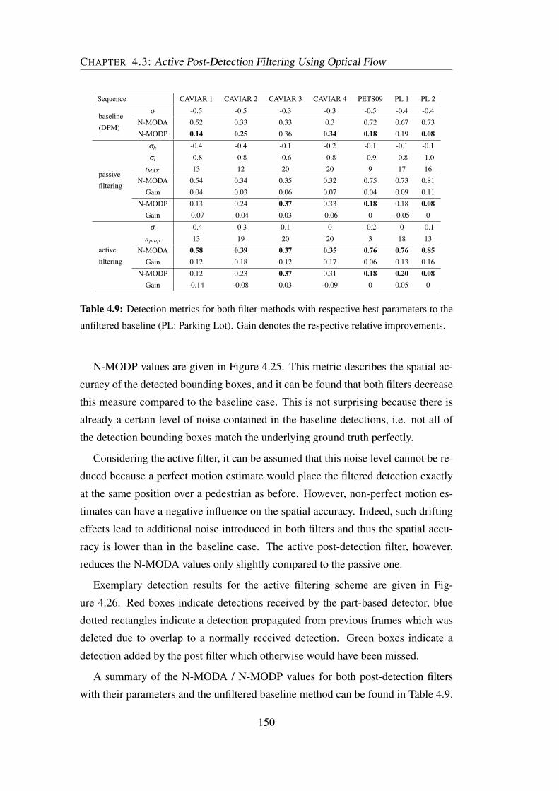
CHAPTER 4.3: Active Post-Detection Filtering Using Optical Flow
Sequence CAVIAR 1 CAVIAR 2 CAVIAR 3 CAVIAR 4 PETS09 PL 1 PL 2
baseline
(DPM)
σ -0.5 -0.5 -0.3 -0.3 -0.5 -0.4 -0.4
N-MODA 0.52 0.33 0.33 0.3 0.72 0.67 0.73
N-MODP 0.14 0.25 0.36 0.34 0.18 0.19 0.08
passive
filtering
σh -0.4 -0.4 -0.1 -0.2 -0.1 -0.1 -0.1
σl -0.8 -0.8 -0.6 -0.8 -0.9 -0.8 -1.0
tMAX 13 12 20 20 9 17 16
N-MODA 0.54 0.34 0.35 0.32 0.75 0.73 0.81
Gain 0.04 0.03 0.06 0.07 0.04 0.09 0.11
N-MODP 0.13 0.24 0.37 0.33 0.18 0.18 0.08
Gain -0.07 -0.04 0.03 -0.06 0 -0.05 0
active
filtering
σ -0.4 -0.3 0.1 0 -0.2 0 -0.1
nprop 13 19 20 20 3 18 13
N-MODA 0.58 0.39 0.37 0.35 0.76 0.76 0.85
Gain 0.12 0.18 0.12 0.17 0.06 0.13 0.16
N-MODP 0.12 0.23 0.37 0.31 0.18 0.20 0.08
Gain -0.14 -0.08 0.03 -0.09 0 0.05 0
Table 4.9: Detection metrics for both filter methods with respective best parameters to the
unfiltered baseline (PL: Parking Lot). Gain denotes the respective relative improvements.
N-MODP values are given in Figure 4.25. This metric describes the spatial ac-
curacy of the detected bounding boxes, and it can be found that both filters decrease
this measure compared to the baseline case. This is not surprising because there is
already a certain level of noise contained in the baseline detections, i.e. not all of
the detection bounding boxes match the underlying ground truth perfectly.
Considering the active filter, it can be assumed that this noise level cannot be re-
duced because a perfect motion estimate would place the filtered detection exactly
at the same position over a pedestrian as before. However, non-perfect motion es-
timates can have a negative influence on the spatial accuracy. Indeed, such drifting
effects lead to additional noise introduced in both filters and thus the spatial accu-
racy is lower than in the baseline case. The active post-detection filter, however,
reduces the N-MODA values only slightly compared to the passive one.
Exemplary detection results for the active filtering scheme are given in Fig-
ure 4.26. Red boxes indicate detections received by the part-based detector, blue
dotted rectangles indicate a detection propagated from previous frames which was
deleted due to overlap to a normally received detection. Green boxes indicate a
detection added by the post filter which otherwise would have been missed.
A summary of the N-MODA / N-MODP values for both post-detection filters
with their parameters and the unfiltered baseline method can be found in Table 4.9.
150

CHAPTER 4.3: Active Post-Detection Filtering Using Optical Flow
Figure 4.26: Examples of the proposed motion-based post-detection filter on the CAVIAR
1 video: Red detections have been received normally, blue dotted detections are candidates
from post-detection filter which have been filtered out due to overlap with normally received
detection. Green detections are added as a result from proposed active post-detection filter.
151

CHAPTER 4.3: Active Post-Detection Filtering Using Optical Flow
Sequence CAVIAR 1 CAVIAR 2 CAVIAR 3 CAVIAR 4 PETS09 PL 1 PL 2
baseline
(DPM)
N-MOTA 0.44 0.29 0.25 0.28 0.67 0.51 0.72
N-MOTP 0.14 0.25 0.37 0.37 0.12 0.29 0.06
passive
filtering
N-MOTA 0.46 0.30 0.27 0.28 0.62 0.59 0.71
Gain 0.05 0.03 0.08 0 -0.07 0.16 -0.01
N-MOTP 0.14 0.24 0.34 0.36 0.13 0.29 0.06
Gain 0 -0.04 -0.08 -0.03 0.08 0 0
active
filtering
N-MOTA 0.53 0.35 0.30 0.28 0.67 0.69 0.77
Gain 0.2 0.21 0.2 0 0 0.35 0.07
N-MOTP 0.10 0.21 0.35 0.33 0.12 0.26 0.06
Gain -0.29 -0.16 -0.05 -0.11 0 -0.1 0
Table 4.10: Tracking metrics for both filter methods to the unfiltered baseline (PL: Parking
Lot). Gain denotes the respective relative improvements.
As discussed before, the minimum IOU for correctly matched true positive detec-
tions has been set to a value of 0.2, thus leading to a general decrease in the N-
MODP values.
Another important advantage is that for all experiments, higher detection scores
can be used than in the baseline method. This leads to fewer false positives and
higher N-MODA values. The overall gains have been computed in order to show
the improvements of the two filtering schemes compared to the baseline. For the
proposed active filter, N-MODA gains are usually at a level of 10% or more. Only
for PETS, the gain is at 2% due to the reasons discussed before.
Tracking results using these filtered detections and the GM-PHD filter frame-
work presented in Section 4.2.1 are shown in Table 4.10. For the entry "active
filtering", the tracker parameters (especially pD and clutter) are the same for all
comparisons and have been optimized on the baseline results for a fair comparison.
An adaptation of these parameters to the improved detections will likely enhance
upon these results.
Generally, the improved detection quality leads to better tracking results even
with the same parameters. Due to the low-pass properties of the tracker, however,
this effect varies over the different videos. While the N-MOTA performance is
never worse than the baseline, for CAVIAR 1, CAVIAR 2 and CAVIAR 3 the gain
is around 20% and in the case of Parking Lot 1, the gain reaches even 35%.
The N-MOTP measure is the tracking equivalent to N-MODP and shows the
spatial accuracy of the estimated tracks. As for N-MOTP, the filtered results perform
less accurate here due to the reasons given in relation to N-MODP.
152

CHAPTER 4.3: Active Post-Detection Filtering Using Optical Flow
The high performance gain in terms of N-MODA comes at a slightly higher
computational load. Both filters increase the computational complexity but only
to a very low degree. While the passive filter only requires analysis of previous
detection results and computation of the respective overlap ratios, its main increase
in complexity comes from the higher number of detections received by lowering
the detection thresholds. The filtering effort, however, is negligible compared to
running a state-of-the-art pedestrian detector over a full image.
The active post-detection filter computes sparse optical flow per detection and
is thus much more demanding in terms of computational load. However, a set of
detections for usual surveillance videos contains less than 20 detections. The re-
lated effort for computing the motion vectors is higher than for the passive filtering
approach but still far below a detection cycle over a full image and can even be par-
allelized. As a consequence, both filters are real-time capable for standard videos
and in addition theoretically suitable for any type of pedestrian detector.
4.3.4 Conclusion on Active Post-Detection Filters Using Optical
Flow in the Tracking Process
This section motivated the need of high detection rates in tracking-by-detection sys-
tems theoretically and proposed a solution for CCTV scenarios with lower detection
probabilities by using an active, motion-based post-detection filter.
After a detailed state-of-the-art analysis of related concepts from the literature,
a mathematical analysis of the risk for tracking failure has been formulated which
shows how crucial the treatment of missed detections is for such tracking methods.
The results of this analysis inspired the design of an active post-detection filter
which uses sparse optical flow information between consecutive frames in order to
artificially increase the detection probability and reduce the related issues.
The filter achieves high gains on a variety of datasets both in terms of detection
and tracking performance. As an additional advantage apart from the performance
enhancement, its runtime is low and can be neglected compared to usual detectors.
The filter is fully independent of the pedestrian detection method used and can even
be used without access to or modification of the detector code. As it can generally
be used for any kind of tracking-by-detection system, it is thus very interesting for
real-world applications.
153

CHAPTER 4.3: Active Post-Detection Filtering Using Optical Flow
154

Chapter 5
Person Re-Identification in Tracking
Contexts
Parts of the work in this chapter have been published in Eiselein, V.; Sternharz,
G.; Senst, T.; Keller, I.; Sikora, T., 2014. Person Re-identification Using Region
Covariance in a Multi-Feature Approach. In: Proceedings of International Confer-
ence on Image Analysis and Recognition (ICIAR 2014), Part II, LNCS 8815, 2014,
Vilamoura, Portugal, 22.10.2014 - 24.10.2014
IN the previous chapters, a tracking-by-detection framework has been proposed
for pedestrian tracking in surveillance scenarios. Apart from a mechanism to
separate crossing targets, image information has only been used for detection of
pedestrians and for enhancing these detections prior to the tracking process. This
is a contrast to template trackers or correlation-based trackers which extract image
features from a given region of interest and estimate the most likely position of that
region in the next frame.
For certain reasons, it can be helpful to introduce image information in the track-
ing process and to extract specific features on a per-target basis:
1. For specific applications, it can become necessary to distinguish between
multiple targets even if no continuous perception of them can be guaranteed.
Using a target model built by extracting instance-specific image features, such
distinction can be achieved for application cases as e.g. loitering, person re-
identification or cross-camera tracking.
155

Chapter 5. Person Re-Identification in Tracking Contexts
Figure 5.1: Two concepts are shown for the usage of image information in tracking-by-
detection systems: In every frame, input images of pedestrians are collected from the tracks
and transformed into a pedestrian model built from feature vectors which is updated reg-
ularly (basic functionality required for both applications, blue). 1) In order to re-identify
(green) previously known pedestrians, a data storage is needed which contains the feature
models for all tracked pedestrians known so far. A feature vector of a newly extracted pedes-
trian track is compared to these known candidates and its tracking id can be set accordingly.
2) In case of tracking failure, the feature model built from previous frames can be used to
search the target in the current frame (not regarded in this thesis).
156

Chapter 5. Person Re-Identification in Tracking Contexts
2. In case of missed detections, image cues can help providing a suitable guess
for the current target state. In this case, the area where a target is expected
is searched for feature vectors associated with the respective target. The best
matching position is returned as possible target location.
The described feature extraction and indexing concepts are shown in Figure 5.1.
Regardless of the exact motivation, the establishment of a target model based on
extracted feature vectors requires a recent target model which has to be updated
regularly (usually on a per-frame basis). This means that for every target, a model
has to be extracted in every frame for a given location and integrated into the pre-
viously known feature representation. This feature representation is then stored in
a data structure enabling operations such as fast retrieval of a given id or matching
of a feature vector with all stored target models. All of these operations must be
performed in a very fast manner as the tracking process should not be slowed down
more than necessary. The main reason why processing time is of special importance
is that the feature retrieval and comparison between matching candidates may have
to be performed multiple times per video frame. It is therefore that in the context of
this work, fast person re-identification methods will be preferred and a combination
of multiple basic methods is shown in order to improve re-identification results.
As an additional point, in the second case mentioned above (i.e. the usage of
feature vectors for improvements in the tracking process) it is also necessary to
provide a mechanism of searching for a given feature vector within a region of the
current image. This can be done by using a sliding window approach and extracting
feature vectors in every position. The resulting feature vectors are compared to the
ones stored in the database and the best match represents a potential candidate of the
current target state. As outlined in [Bolme et al., 2010], this procedure is very time-
consuming and requires a lot of effort in order to ensure both a suitable accuracy in
the target location estimate and a short run-time. It would thus be out of scope for
this thesis.
Therefore, within this work, multiple person re-identification techniques are in-
vestigated in order to lay the foundations for an integration of pedestrian descriptors
into the tracking-by-detection framework proposed previously. As a main challenge
for later integration, run-time must be taken into account and should be kept at a
very low level.
The chapter is organized as follows: The next paragraph provides an overview of
157

CHAPTER 5.1: Review of Low-Complexity Person Re-Identification Methods and
Evaluation Methodology
low-complexity state-of-the-art pedestrian re-identification methods and the evalu-
ation methodology (Section 5.1). In the following chapters the feature descriptors
evaluated for pedestrian re-identification are outlined. In this thesis, point feature
descriptors (Section 5.2), color histograms (Section 5.3) and region covariance de-
scriptors (Section 5.4) are investigated. Section 5.4.1 explains a metric issue for
region covariance descriptors related to eigenvalue computation and proposes a
pre-processing step in order to solve the problem. Together with the choice of a
suitable feature vector and a new partitioning scheme, this novel way of avoiding
rank deficiency in the covariance matrices contributes to a considerably improved
re-identification process compared to previous region covariance methods.
A fusion of multiple descriptors in order to enhance the re-identification perfor-
mance is proposed in Section 5.5 which also contains experiments and results for
the approach developed as a follow-up of the publication [Eiselein et al., 2014].
Section 5.6 concludes the chapter.
5.1 Review of Low-Complexity Person Re-Identification
Methods and Evaluation Methodology
Person re-identification algorithms can be divided into methods based on point fea-
ture descriptors (e.g. [Hamdoun et al., 2008] [Khedher et al., 2013]) presented in
Section 5.2 and methods extracting appearance information for a whole image patch
within a region of interest. A very common example for the latter are pedestrian ap-
pearance models based on color histograms (e.g. [Zoidi et al., 2013; Possegger
et al., 2015]) which have the huge advantage of low run-time and memory con-
straints. They are presented in Section 5.3. Another region-based approach investi-
gated in this work is region covariance [Tuzel et al., 2006] shown in Section 5.4.
Apart from these methods, other more sophisticated but generally also computa-
tionally more expensive object descriptors have been developed, e.g. Fisher vectors
[Jaakkola and Haussler, 1999] which can also be applied for person re-identification
[Perronnin and Dance, 2007; Ma et al., 2012]. Fisher vectors have been evaluated
in a Master’s thesis at TUB-NÜ [Sternharz, 2014] and, due to their complexity and
run-time constraints, are not considered in this thesis.
The choice of suitable image features for general application of person re-identifi-
158

CHAPTER 5.1: Review of Low-Complexity Person Re-Identification Methods and
Evaluation Methodology
cation methods can be a difficult task and is also directly related to the metric chosen
to discriminate between the respective feature vectors. Instead of finding the best
performing feature vector, it is thus also possible to modify the metric used to com-
pare two multi-dimensional feature vectors.
Learning a discriminative metric directly from the known ground truth samples
has been proposed e.g. in [Weinberger and Saul, 2008], [Davis et al., 2007] and
[Guillaumin et al., 2009]. Although it can be said that once the metric is learned, its
application can often be done by simple matrix operations, it usually requires a high
computational effort in order to derive such a metric. As a remedy, in [Hirzer et al.,
2012] the authors propose to reduce the mathematical constraints for a metric and to
neglect easily-separable samples for the metric estimation but the computation pro-
cess still appears too costly if performed for every person in a video frame in order
to improve tracking results. Another reason why metric learning is not considered
in this work is that these methods usually require a large, pre-labeled training set
of pedestrian samples and in tracking approaches, the number of training samples
obtained from tracks is often limited.
Other person re-identification approaches are given in [Goldmann et al., 2006]
where background subtraction is used in order to generate binary masks and model
only a person without the surrounding background pixels. In a similar, derived
method, in [Farenzena et al., 2010] segmentation information is exploited by defin-
ing symmetry axes in a person’s silhouette. Results are promising but depend on a
previous background / foreground separation step. In general CCTV environments
such information might not be available e.g. due to a high number of people in the
scene, occlusion or changing lighting conditions which inhibit a good separation
of individual silhouettes. In such cases, a good person segmentation is already a
challenging task itself. Therefore in this thesis, a generic person re-identification
process without background separation is used, which, however, could be enhanced
by segmentation information if available.
The evaluation process of a person re-identification system is usually done on
a statistical level. In most cases, person re-identification can be considered an ap-
plication of either a 1 : 1 or a 1 : N matcher. While a 1 : 1 matcher performs a
verification step (e.g. answers the question "Is this person the same as that person?"
or as a possible application "Does this feature vector obtained from a camera at a
customs counter correspond to the identification cues stored on a given passport?"),
159

CHAPTER 5.1: Review of Low-Complexity Person Re-Identification Methods and
Evaluation Methodology
a 1 : N matcher performs an identification step, i.e. a search of a single query sam-
ple qi in a database of N candidate samples from a given gallery G = c1, ...,cn.
In other words, it finds the most similar known sample to a query sample. In this
work, we assume the typical case that the candidate samples ci in the gallery are
pairwise distinct (i.e. no duplicate identities) and the "closed universe" assumption
holds (i.e. for all query samples, the gallery contains a correct match). However,
both constraints may be weakened in other applications which might then yield the
need of extensions to the principles outlined here.
For a 1 : 1 matcher, statistical evaluation often relies on the computation of the
False Acceptance Rate (FAR) and the False Rejection Rate (FRR, also false negative
rate or miss rate) [Bolle et al., 2004, 2005] which describe the false positive and
false negative decisions produced by the system. Its computation is based on a
confusion matrix (see Table A.1) where the entries are computed as outlined in
Appendix A.6.
The entries of the confusion matrix often depend on the parametrization of the
algorithm. Therefore, for better comparability of two different methods, a Receiver
Operating Characteristic (ROC) curve can be used in which both values are plotted
against each other in order to show the system-specific trade-off between them.
ROC curves have the advantage of being a very common tool exploiting standard
statistical properties and are as such easily understandable while providing a way of
abstraction from parametrization.
In contrast to 1 : 1 matchers, a 1 : N matching system returns the one sample
out of N candidates which is considered to correspond best to the query sample
according to some feature representation. The evaluation of such a system can be
more complicated than in the 1 : 1 case if more than only the best rank is considered.
In this case, a standard performance measure is the Cumulative Matching Curve
(CMC) [Grother and Phillips, 2004]. This measure assesses the system’s capability
of ranking potential match candidates correctly. Assuming a probe (or query) set
Q = q1, ...qm of cardinality M, the matcher can be used in order to compute a
similarity score s(qi,ci) for each query sample qi and all candidate samples in the
gallery set. Ordering these scores for each qi yields:
s(qi,ci1)≥ s(qi,ci2)≥ s(qi,ci3)
160

CHAPTER 5.1: Review of Low-Complexity Person Re-Identification Methods and
Evaluation Methodology
and thus the ranking of the probe sample is
R(qi) = in,
with in as the position in the sorted list (e.g. R(qi) = 3 if the true match of
sample qi has the 3rd highest score). Doing so assigns a rank position to every
possible similarity score and candidate sample of query qi.
Obtaining the CMC now requires the discrete rank probabilities P(k) which de-
scribe the average probability of assigning a specific rank to some query. Usually,
these probabilities are estimated using the normalized true frequencies of occur-
rence of the different ranks, computed over the query set:
Prank(k) =1M(#(R(qi) == k)), k = 1, ...,N. (5.1)
Prank(k) thus contains the normalized number of samples for which the true rank
is k. Accordingly, Prank(x) is an estimate of the probability that the rank R of any
probe computed by the system is x. For usual applications, probability mass func-
tions with lower average ranks are considered better because they show that the
system in average computes high similarity measures for correct matches and only
a small number of attempts is necessary to obtain a correct match.
Based on Prank(x), the CMC measure is then computed as follows:
CMC(k) =k
∑r=1
Prank(r), k = 1, ...,N. (5.2)
It can be interpreted as a measure of how many guesses by the system are needed
in order to obtain a certain probability that the genuine sample is returned. For real
applications this makes sense because even assuming that no automatic identifi-
cation system is perfect, the system can still narrow down the search space for a
human user. A system could e.g. return the 10 samples with the highest similarity
scores and the user then identifies which of them corresponds to the query sample.
The CMC is an effective measure in order to assess such a system’s performance,
e.g. an estimate of CMC(10) = 0.7 would mean that with an average probability of
0.7 the user is shown the right match in the first 10 samples returned by the system.
Both, the CMC- and the ROC measure return values in the interval of [0;1].
The CMC curve over a set of k candidates increases monotonically because of its
formulation as a recursive sum over the values of k. With increasing k, it converges
161

CHAPTER 5.2: Feature Point-based Descriptors
to 1 and its slope - as a measure of this convergence - can be seen as a description
of the likelihood of genuine matches for smaller gallery sizes.
The advantage of the CMC compared to a ROC measure is that it not only takes
a value of "true" or "false" as input but also considers the system’s ranking capabil-
ities. Assume e.g. the outputs of two 1 : N matchers are to be compared and system
A returns the true candidate sample in average at the 2nd position. Another system B
might return the true sample in average at the 20th position. If both systems were to
be regarded as 1 : 1 matchers and the first match was considered to be the resulting
match decision, their performance in terms of ROC could be the same as long as the
first match would be equally bad in both systems. However, using the CMC mea-
sure, system B is considered worse than system A because it systematically returns
higher ranks for correct matches.
In order to compress the description of a ROC or CMC curve into a single value,
the area under the respective curve (AUC) measure can be used. Normalized over
the number of gallery samples (CMC) or the interval of [0;1] (ROC), it is another
description of the same system properties. In this work, ROC-AUC is used for
configuration of individual feature properties because it is more expressive for slight
changes and the final system evaluation is done using CMC measure because it is
the most common measure for this application.
The datasets used for evaluation of pedestrian re-identification are summarized
in Appendix A.3. For none of them, foreground masks are available or have been
used.
5.2 Feature Point-based Descriptors
In the computer vision community, feature points are often-used ways of extract-
ing image features and detecting characteristics in a picture. The main idea of this
approach is to use feature distributions around characteristic points which should
ideally be independent of illumination, rotation, shift and image noise. By re-
identifying those points in a different image of the same object, it is thus possible to
infer e.g. motion information between these images or deduce similarities between
points and their spatial environment.
Often-used approaches build a scale-space using low-pass filters of different
bandwidth. Foundations for this approach have been laid in [Lindeberg, 1994].
162

CHAPTER 5.2: Feature Point-based Descriptors
Figure 5.2: In the SIFT algorithm [Lowe, 2004], in each octave the initial image is repeat-
edly Gaussian-filtered (left). Differences between adjacent Gaussian images are used for
extrema detection. After every octave, the image is downsampled and the process repeated.
Extremal points in a scale-space represent sources and sinks of intensity flow and
are seen as characteristic points. Identification of these points can be done using an
(often approximated) Laplacian of Gaussian filtering process which can be seen as
bandpass filter of the image.
Common feature point extraction methods include algorithms such as "Scale-
invariant features transform" (SIFT) [Lowe, 2004] or "Speeded Up Robust Fea-
tures" (SURF) [Bay et al., 2008] and derived works [Ke and Sukthankar, 2004;
Winder and Brown, 2009; Chandrasekhar et al., 2011]. An overview with com-
parisons and evaluations of different approaches can be found in [Mikolajczyk and
Schmid, 2005]. An overview of suitable feature types for person re-identification is
given in [Bäuml and Stiefelhagen, 2011].
Figure 5.2 shows the principle used in the SIFT algorithm: The input image
is repeatedly convolved with a Gaussian kernel. While a Laplacian-of-Gaussian
(LoG) representation has been shown in [Lindeberg, 1994] to allow for scale invari-
ance, difference-of-Gaussians (DoG) images can be seen as an approximation for
LoG images. Therefore in SIFT, the difference between two of the resulting Gaus-
sian images is used in order to build up a scale-space in which extremal points are
searched. Scaling down the input image after each octave reduces the computational
effort.
Accordingly, for SIFT the number of octaves and the number of scales in every
individual octave are two parameters which have to be considered in the evaluation
163

CHAPTER 5.2: Feature Point-based Descriptors
Figure 5.3: Schematic of the point feature-based person re-identification system from
[Hamdoun et al., 2008] which builds the basis for the point-feature classification in the
proposed method.
of its descriptor when used for re-identification. The feature descriptor itself is
then extracted as gradient orientation histograms defined over the region around a
keypoint (details can be found in [Lowe, 2004]).
Compared to SIFT, SURF features [Bay et al., 2008] have been optimized for
speed, e.g. instead of using Gaussian filters, box filters are applied because they
can be computed faster by using integral images [Viola and Jones, 2001]. The use
of integral images also allows for building the scale-space by scaling up the filter
window instead of reducing the image size which can be done in a constant time
due to the integral images. Thus, pre-filtering the images can be omitted.
In order to use local point features for person re-identification, a number of ap-
proaches have been proposed. Once feature points are found and feature vectors are
extracted, these need to be matched against reference models in order to identify
the person. For quick comparisons and a fast id retrieval, the authors of [Hamdoun
et al., 2008] propose a k-d tree to store the feature vectors and use a majority vote
over the points found to determine the object id. A schematic representation of
this person re-identification system is shown in Figure 5.3. For this thesis, the idea
of using a tree-based data structure is adopted, however, a FLANN-based method
[Muja and Lowe, 2009] is used for performance reasons.
Khedher et al. use in [Khedher et al., 2012] an automatic method of acceptance
164

CHAPTER 5.2: Feature Point-based Descriptors
of SURF correspondences based on GMMs learned on the reference set and a model
of the distance distribution resulting from matches of the same person and with
different persons respectively. This allows to adjust thresholding parameters for the
feature matching process on-line without the need for presets and also increases the
system’s performance in cases where camera views are very different.
For this thesis, a multi-cue person re-identification scheme is proposed for which
the combination of individual steps is naturally computationally more intensive than
a single-cue re-identification step. Additionally, for tracking purposes appearance
differences of an object between individual frames are small which reduces the
advatages of the GMM-based approach from [Khedher et al., 2012]. Instead, for
run-time reasons the points found are matched and a majority vote as in Figure 5.3
is performed.
In [Khedher et al., 2013], the method from [Hamdoun et al., 2008] is refined
using the "Least Absolute Shrinkage and Selection Operator" (LASSO) algorithm
which performs a regression on the feature vectors of the model and the query in or-
der to reduce the feature dimensions and use a sparse representation by the minimal
number of points which contribute to the person appearance. As the performance
improvement of this algorithm compared to the baseline method seems rather low
but the algorithm uses an iterative scheme which has to be re-computed on-line
for new persons, we refrain from the LASSO method in this thesis and prefer the
quicker baseline approach.
Again, it can be argued that the possible improvements for the point feature-
based re-identification step could enhance the overall system’s performance which
is not questioned here. However, the focus in this chapter is to provide means of
person re-identification with very low run-time in order to use it not only for re-
identification but also for improving the system’s tracking performance. Nonethe-
less, it could be a focus of future work to include individual enhancements as the
ones mentioned above while still maintaining the overall computational efficiency.
Conducting experiments regarding the pedestrian re-identification performance
of the system in Figure 5.3 reveals that a number of its parameters are inherently
connected: The number of octaves used for computation of the feature points and
the number of scale levels per octave L are to be seen in connection with the image
scale which is intuitive considering that during the computation of SIFT and SURF,
feature vectors are extracted at extremal points in a scale-space of the image. This
165

CHAPTER 5.2: Feature Point-based Descriptors
relationship is especially relevant considering that the resolution in CCTV footage is
often low. Consequently, the resolution pyramid built in order to extract the feature
points can easily be too coarse for a proper representation of the features.
The solution to this problem can be two-fold: On the one hand, it is possible to
increase the number of scales (i.e. reduce the step size between them) used within an
octave which enhances the systems’s resolution for image details. On the other hand
the image can also be scaled up (i.e. bi-linearly interpolated in this thesis) which
is a better solution for SURF features where for performance reasons the step size
follows a scheme fixed by the size of the filter kernels and cannot be altered.
SURF thus can also be parametrized implicitly using the image scale while SIFT
features rather benefit from adjusting the number of scales per octave or using a
different value for σ in the lowest octave. Exemplary results for these parameter
settings are shown in Figure 5.4 where the x-axis shows the minimal area of the
image patches after upscaling. All patches are resized with the same scale per ex-
periment, however, due to the different size of the patches, the minimal value is
given.
Apart from the VIPeR dataset where higher values give better results, the curves
show no significant improvements after images have been rescaled to approximately
80.000 pixels. However, for the other datasets the performance does not deteriorate
after this value, either. It seems thus suitable to choose a rather high value for the
minimal image size while not taking an inappropriately high value for performance
reasons (run-time increases linearly with the number of pixels as will be shown
later).
Especially for the datasets ETHZ and CAVIAR, the SURF variant not using the
reference orientation (labeled "u" for "upright") shows superior results. This can
be explained by the fact that all persons in the dataset are provided with the same
orientation. Computation of a reference orientation is thus not needed and can only
introduce errors.
From the results in the experiments, the performance of SURF (both in its 64-
and 128-bit variant) appears to be generally better than the performance of SIFT.
This conclusion should be taken with care as it still depends on various parameter
settings. However, considering also the lower run-time of SURF compared to SIFT
and the intuitive way of parameterizing it using the image scale, in this thesis SURF
is chosen over SIFT. Accordingly, the following experiments are based on these
166

CHAPTER 5.2: Feature Point-based Descriptors
0 50 100 150 200minimal area after upscaling (in [10^3 pix])
0.1
0.2
0.3
0.4
0.5
0.6
0.7
0.8
Norm
alized ROC-AUC
CAVIAR4REID
surf64u (L2, 4 octaves)
surf64 (L2, 4 octaves)
surf128u (L2, 4 octaves)
surf128 (L2, 4 octaves)sift128u L5 σ1.4
sift128u L4 σ1.4
sift128u L3 σ1.6
sift128u L3 σ1.4
sift128 L3 σ1.6
0 50 100 150 200minimal area after upscaling (in [10^3 pix])
0.2
0.3
0.4
0.5
0.6
0.7
0.8
0.9
1.0
Norm
alized ROC-AUC
ETHZ
surf64u (L2, 4 octaves)
surf64 (L2, 4 octaves)
surf128u (L2, 4 octaves)
surf128 (L2, 4 octaves)sift128u L5 σ1.4
sift128u L4 σ1.4
sift128u L3 σ1.6
sift128u L3 σ1.4
sift128 L3 σ1.6
0 50 100 150 200minimal area after upscaling (in [10^3 pix])
0.0
0.1
0.2
0.3
0.4
0.5
0.6
0.7
Norm
alized ROC-A
UC
VIPeR
surf64u (L2, 4 octaves)
surf64 (L2, 4 octaves)
surf128u (L2, 4 octaves)
surf128 (L2, 4 octaves)sift128u L5 σ1.4
sift128u L4 σ1.4
sift128u L3 σ1.6
sift128u L3 σ1.4
sift128 L3 σ1.6
0 50 100 150 200minimal area after upscaling (in [10^3 pix])
0.0
0.1
0.2
0.3
0.4
0.5
0.6
0.7
0.8
Norm
alized ROC-A
UC
PRID2011
surf64u (L2, 4 octaves)
surf64 (L2, 4 octaves)
surf128u (L2, 4 octaves)
surf128 (L2, 4 octaves)sift128u L5 σ1.4
sift128u L4 σ1.4
sift128u L3 σ1.6
sift128u L3 σ1.4
sift128 L3 σ1.6
Figure 5.4: Influence of image scaling for SIFT & SURF with different configurations used
in the person re-identification system proposed by [Hamdoun et al., 2008]. For SIFT, the
value of σ in the lowest octave and the number of layers per octave L are given in the
legend, SURF has been tested with both the standard (SURF64) and extended (SURF128)
descriptor. For both methods "u" symbolizes the upright descriptor. The ROC-AUC shows
that the SURF implementations benefit from scaling while SIFT remains mostly unaffected
by this parameter. Even over multiple parameter sets, SIFT generally shows a lower perfor-
mance than SURF. SURF on the other hand should be considered with image scaling as a
parameter in mind.
167

CHAPTER 5.2: Feature Point-based Descriptors
Figure 5.5: Schematic illustration of the overlap parameter in the partitioning scheme.
For this example of a 4x6 partition, the red rectangle shows an overlap of 0.5, i.e. its
center position remains the same but its area is extended in a way that it covers neighboring
partitions to 50% of their width / height. Feature points are only matched in their respective
partition.
conclusions and will use "upright" SURF features without reference orientation and
an image up-sampling step to 100.000 pixels.
5.2.1 Partitioning Schemes Improve the Re-Identification Per-
formance
In order to further increase the performance of the re-identification system based
on feature points, a partition scheme is introduced (shown in Figure 5.5). The par-
titioning is done via rectangular sub-spacing of the input region and inhibits the
matching of points which are improbable matches due to their spatial positions in
the image (i.e. a point on the head of a person should be found in another image
at a similar location and not e.g. on the foot of a person). In order to compen-
sate potential alignment issues in imperfect partitions between consecutive images,
subregions are allowed to overlap.
In every subregion, feature detection is performed and the respective descrip-
tors are matched against their stored reference descriptors in that region. Doing so
ensures only correct feature point matches within one subregion but increases the
processing time and memory requirements because one search tree per subregion
needs to be kept in memory and all trees need to be searched for matches. The final
matching id is obtained in a voting scheme over the different partitions.
Results of applying the partitioning scheme are shown in Figure 5.6 where the
recognition performance (ROC-AUC measure) is shown over the partition overlap
168

CHAPTER 5.2: Feature Point-based Descriptors
Figure 5.6: Performance comparison (ROC-AUC) for person re-identification system from
[Hamdoun et al., 2008] with different partitioning schemes x×y and overlaps o. All experi-
ments are conducted with a rescaling to 100.000 pixels as an outcome of previous tests. The
extended detector in general does not improve the performance while an overlap of 0 = 0.5
in the partitioning scheme seems a good compromise for all datasets.
169

CHAPTER 5.2: Feature Point-based Descriptors
for a number of partitioning schemes. It can be seen that no specific partition-
ing scheme gives best results on all datasets, however, the usage of a partitioning
scheme can always enhance results compared to an approach without partitioning
(i.e. a single (1x1) partition). Possible performance gains are between 5% (on
CAVIAR4REID) and 14% (on PRID2011), depending on the dataset, partitioning
scheme and overlap ratio. Suitable overlaps and the best number of partitions in x-
/ y-axis depend on the dataset but differences are generally small. The overlap of
o = 0.5 can be considered a good trade-off for most scenarios tested.
Concerning the usage of an extended descriptor in the SURF feature, Figure 5.6
shows no general enhancement in the system’s accuracy, except for the PRID dataset
where the extended descriptor enhances results considerably and almost regard-
less of the partitioning scheme used. For future experiments, a 7× 11 partitioning
scheme with overlap o = 0.5 will be chosen.
5.2.2 Run-time of Pedestrian Re-Identification Using Point Fea-
tures
Feature matching in this approach is performed using FLANN trees [Muja and
Lowe, 2009] which are a faster, approximate extension to k-d trees. Since without
knowledge about the structure of the dataset and the parameters used, this algorithm
is difficult to analyze, a closer theoretical look shall be taken at a standard k-d tree.
The average search time in a k-d tree is
O(logn)
in the number of feature points [Bentley, 1975]. Generally, such a performance
can be considered fast. When using more than one partition, the number of trees
increases. The drawback of the related re-identification performance gain are thus
increased memory and computational needs. Assuming equally distributed feature
points over the image, the search in k trees for n/k points each results in
O(k log(n/k)) = k ·O(log(n/k))(again)= O(logn) (5.3)
and is effectively (though not visible in the Big O notation) a higher computa-
tional load than searching one tree for n features. The invisibility of this effect in
the Big O notation is due to the fact that for its computation the number of features
170

CHAPTER 5.2: Feature Point-based Descriptors
Figure 5.7: Training times for point feature-based person re-identification system from
[Hamdoun et al., 2008] using different partitioning schemes from previous configurations.
Times are normalized per test instance and include pre-processing such as scaling and color
conversion which explains differences between the datasets. The usage of an extended
descriptor increases the run-time considerably. The run-time is increased by higher number
of partitions.
171

CHAPTER 5.3: Color Histogram-based Descriptors
is considered approaching infinity. k would thus theoretically be omitted in this
consideration as shown in Equation (5.3).
However, in real use cases the number of features in every search tree must be
kept to a suitable limit in order to obtain both an acceptable re-identification ac-
curacy and a low run-time. Therefore, the effect of several parallel trees remains
noticeable in practice (see Figures 5.7 and 5.8).
Considering re-identification for a future integration into a tracking process, two
steps can be distinguished which both contribute to the overall computational com-
plexity. On the one hand, it is necessary to train the algorithm with images of known
persons as long as the tracks of them can be extracted (Figure 5.7). On the other
hand, in order to support the tracking process in ambiguous situations, candidate
images of unknown persons are matched against the database in order to be identi-
fied (Figure 5.8) when the tracking process fails.
Thus, both the run-times spent for training a model of a person and the testing
of a candidate image are very important in the tracking process. As shown in Fig-
ures 5.7 and 5.8, the training step can be done in less than 0.02 s (i.e. more than 50
frames per second) for a 1x1 partition scheme while the testing step depends on the
size of the database and thus differs to a higher degree between different datasets.
However, matching a query image in small candidate galleries is also feasible in
similar time. For both cases, a more complex partitioning scheme and the usage of
extended descriptors increase the run-time because more internal comparisons are
necessary.
It is also visible that for higher overlaps, generally the run-times increase more
than linearly. The reason for this increase is that for higher overlaps, feature points
found in the border areas of a partition will be considered in multiple partitions. The
higher the overlap value, the higher is in average also the number of points which
have to be considered in more than one partition. As a result, the number of points
which are searched for in the FLANN tree increases and thus require additional
overhead.
5.3 Color Histogram-based Descriptors
Gradient-based feature points, as shown in the previous section, are well-established
for object re-identification. However, as gradient extraction is normally done in
172

CHAPTER 5.3: Color Histogram-based Descriptors
Figure 5.8: Testing run-times for point feature-based person re-identification system from
[Hamdoun et al., 2008] using different partitioning schemes from previous configurations.
Times are computed for a pre-trained system and normalized per test instance. Differences
between datasets are due to pre-processing and different numbers of trained samples in the
data structures (e.g. VIPeR contains 632 images vs. 72 in CAVIAR4REID.
173

CHAPTER 5.3: Color Histogram-based Descriptors
ROC-AUC HSV (1x1) Lab (1x1) RGB (1x1) XYZ (1x1) YCbCr (1x1)
CAVIAR4REID 0.277 0.175 0.264 0.256 0.174
ETHZ 0.214 0.185 0.167 0.181 0.144
VIPeR 0.038 0.025 0.027 0.035 0.028
PRID 0.125 0.063 0.118 0.090 0.075
Table 5.1: Area under ROC curve (ROC-AUC) for pedestrian re-identification using color
histograms over different color spaces (no partitioning). Over all datasets, HSV gives sig-
nificantly better results than other color spaces.
grayscale images, it is intuitive to additionally exploit color information in order to
increase the recognition performance.
A basic method exploiting information from multiple channels of an image patch
is the usage of color histograms which estimate the frequency of a range of intensity
values in an image. They have been introduced firstly by [Swain and Ballard, 1991]
and since then have become a standard tool for image analysis. Thanks to their
simplicity and low computational complexity, color histograms are widely used in
the computer vision community.
Similar to the previously shown point feature methods, the reference color his-
tograms are stored in a FLANN tree structure [Muja and Lowe, 2009] for quick
search and retrieval. An important histogram parameter is the number of bins used
for quantization. Figure 5.9 shows results on this parameter and shows that the
re-identification performance for different partitioning schemes over a wide range
of bin numbers yields similar runs of the curves. For CAVIAR4REID and ETHZ,
higher numbers of bins lead to decreasing performance, PRID and VIPeR show
slight improvements in this case until reaching saturation. The maximum for VIPeR
is at 16 bins which can be explained by dataset characteristics. The VIPeR dataset
has a better color and spatial resolution compared to the other datasets which makes
it reasonable to apply a higher resolution of the histogram as well here, but the over-
all performance improvement by choosing 16 bins seems small. For the following
experiments, a value of 5 is thus taken, given that this value provides good results
for all datasets.
The histogram feature vectors are built in HSV color space which was found
favorable compared to other color spaces (descriptions of different color spaces can
be found e.g. in [Priese, 2015]). Experiments on color spaces are given in Table 5.1.
The results show clearly that for the re-identification task, HSV outperforms RGB
174

CHAPTER 5.3: Color Histogram-based Descriptors
Figure 5.9: Re-identification performance using color histograms, different partitioning
schemes (x× y) and a L1 norm for different numbers of histogram bins.
175

CHAPTER 5.3: Color Histogram-based Descriptors
and other color spaces.
In order to obtain the final feature vector, histograms from all channels are con-
catenated. This has the advantage that only one reference database for known per-
sons is needed while otherwise a database for every channel would be required. Es-
pecially for higher numbers of persons in the database, the speed-up for this method
is useful while no significant performance reduction was found according to [Stern-
harz, 2014].
A number of works (e.g. [Vadivel et al., 2003; Pele and Werman, 2010] have
focused on the best metric for histogram comparison. While bin-to-bin distances
such as Ln distances are dependent on the number of bins and can become less
discriminative for higher number of bins, they are still much faster to compute than
cross-bin distances such as e.g. the Earth-Mover’s distance [Monge, 1781; Rubner
et al., 2000] and are therefore advantageous for the proposed application.
Thus, for a fast and in most cases reliable comparison of feature vectors with a
number of stored models and in accordance with these previously mentioned find-
ings, the L1 norm (Manhattan distance) is used for ranking the different stored mod-
els against the query feature vector and obtain the individual scores and the final
person match. For future work, the inclusion of metrics such as e.g. [Pele and
Werman, 2009] could be possible in order to assess the recognition performance
improvement against a potentially higher run-time.
5.3.1 Partitioning Schemes for Color Histograms
Color histograms are especially suited for scenarios with good color saturation and
lighting conditions and their application can show difficulties under low resolution
and noise. In order to increase the re-identification performance, a partitioning
scheme as presented in Section 5.2.1 is used in this thesis. Similar to the previously
explained approach for point features, the region of interest is divided into a set of
overlapping areas, histograms are computed in these areas and concatenated. A final
matching score is obtained using a voting procedure over all partitions. The positive
effect of this partitioning is shown in Figure 5.9 where different colors represent
different partitioning schemes. In order to avoid issues due to bad segmentation, an
overlap of o = 0.5 is used as in the feature point-based methods.
The graphs show that there is no partition scheme which gives best results for all
datasets. Overall, a saturation is visible for the number of partitions. On VIPeR and
176

CHAPTER 5.3: Color Histogram-based Descriptors
2 3 4 5 6 7 8 9 10number of histogram bins
0.000
0.002
0.004
0.006
0.008
0.010
0.012
0.014
0.016
tra
inin
g r
un
-tim
e p
er
pe
rso
n (
s)
CAVIAR4REID
Color Hist (L1)_7x10 (o=0.5)
Color Hist (L1)_10x10 (o=0.5)
Color Hist (L1)_10x15 (o=0.5)
Color Hist (L1)_13x15 (o=0.5)
Color Hist (L1)_1x1
2 3 4 5 6 7 8 9 10number of histogram bins
0.000
0.002
0.004
0.006
0.008
0.010
0.012
0.014
0.016
training run-time per person (s)
ETHZ
Color Hist (L1)_7x10 (o=0.5)
Color Hist (L1)_10x10 (o=0.5)
Color Hist (L1)_10x15 (o=0.5)
Color Hist (L1)_13x15 (o=0.5)
Color Hist (L1)_1x1
2 3 4 5 6 7 8 9 10number of histogram bins
0.000
0.002
0.004
0.006
0.008
0.010
0.012
0.014
0.016
training run-time per person (s)
VIPeR
Color Hist (L1)_7x10 (o=0.5)
Color Hist (L1)_10x10 (o=0.5)
Color Hist (L1)_10x15 (o=0.5)
Color Hist (L1)_13x15 (o=0.5)
Color Hist (L1)_1x1
2 3 4 5 6 7 8 9 10number of histogram bins
0.000
0.002
0.004
0.006
0.008
0.010
0.012
0.014
0.016
training run-time per person (s)
PRID2011
Color Hist (L1)_7x10 (o=0.5)
Color Hist (L1)_10x10 (o=0.5)
Color Hist (L1)_10x15 (o=0.5)
Color Hist (L1)_13x15 (o=0.5)
Color Hist (L1)_1x1
Figure 5.10: Run-time for color histograms: train time for different partitioning schemes
PRID which generally show more distinctive colors and better resolution, the per-
formance increase by a more detailed partitioning is bigger than for CAVIAR4REID
and ETHZ. As a configuration suitable for most scenarios, in future experiments the
system will be configured with 13×15 partitions (overlap o = 0.5).
5.3.2 Run-time of Pedestrian Re-Identification Using Color His-
tograms
An important benefit of using color histograms is their computational efficiency.
Figures 5.10 and 5.11 show the run-times for the training and testing case for dif-
ferent partitioning schemes and bin numbers. Overall per-person training times for
177

CHAPTER 5.3: Color Histogram-based Descriptors
2 3 4 5 6 7 8 9 10number of histogram bins
0.000
0.005
0.010
0.015
0.020
0.025
0.030
0.035
test
ing
ru
n-t
ime
pe
r p
ers
on
(s)
CAVIAR4REID
Color Hist (L1)_7x10 (o=0.5)
Color Hist (L1)_10x10 (o=0.5)
Color Hist (L1)_10x15 (o=0.5)
Color Hist (L1)_13x15 (o=0.5)
Color Hist (L1)_1x1
2 3 4 5 6 7 8 9 10number of histogram bins
0.000
0.005
0.010
0.015
0.020
0.025
0.030
0.035
0.040
0.045
testing run-time per person (s)
ETHZ
Color Hist (L1)_7x10 (o=0.5)
Color Hist (L1)_10x10 (o=0.5)
Color Hist (L1)_10x15 (o=0.5)
Color Hist (L1)_13x15 (o=0.5)
Color Hist (L1)_1x1
2 3 4 5 6 7 8 9 10number of histogram bins
0.00
0.01
0.02
0.03
0.04
0.05
0.06
0.07
0.08
testing run-time per person (s)
VIPeR
Color Hist (L1)_7x10 (o=0.5)
Color Hist (L1)_10x10 (o=0.5)
Color Hist (L1)_10x15 (o=0.5)
Color Hist (L1)_13x15 (o=0.5)
Color Hist (L1)_1x1
2 3 4 5 6 7 8 9 10number of histogram bins
0.000
0.005
0.010
0.015
0.020
0.025
0.030
0.035
0.040
0.045
testing run-time per person (s)
PRID2011
Color Hist (L1)_7x10 (o=0.5)
Color Hist (L1)_10x10 (o=0.5)
Color Hist (L1)_10x15 (o=0.5)
Color Hist (L1)_13x15 (o=0.5)
Color Hist (L1)_1x1
Figure 5.11: Run-time for color histograms: test time for different partitioning schemes
178

CHAPTER 5.4: Region Covariance Descriptors
suitable configurations are in the range of 3-10 milliseconds, common testing times
range from 10-25 milliseconds per person except for VIPeR where, again, the higher
number of samples in the database increases the time for a match to 15-40 millisec-
onds. These times are considerably lower than the counterparts using feature points
(Figures 5.7 and 5.8) which is an important advantage especially when considering
that multiple matches per frame might be necessary in an application case.
Run-times increase practically linearly with the number of bins because the run-
time of the metric used for comparison depends linearly on this parameter while
it has no significant effect on the quantization process, i.e. the creation of the his-
tograms. A more detailed partitioning scheme also increases the run-time but for
smaller bin numbers (e.g. values around 5), the difference appears less critical.
Using integral histograms [Porikli, 2005], it is even possible to reduce the com-
putation of histograms in rectangular regions of interest to a sum of four compo-
nents which makes the feature extraction even faster. However, integral histograms
are not used in this work. The main reason is that standard datasets for evaluation
already come with an annotation given either as bounding boxes around a person or
as the image file containing only the person. The advantage of integral histograms is
therefore limited compared to e.g. a whole frame in which several bounding boxes
around persons were to be evaluated. Additionally, persons in the datasets are usu-
ally given at a small scale which reduces the effort needed for computation of the
histogram in the respective area.
As a result, even for the case of using multiple overlapping partitions within the
region of interest, the advantage of an integral histogram seems of little importance
compared to the effort of building the integral histogram over the whole image.
However, for a possible future integration of the method into a tracker, integral
histograms may be useful. Considering a person track lost by the GM-PHD tracker,
the presented feature extraction could be used in order to find the person’s current
location in the image. As in this case different pixel positions would have to be
evaluated, integral histograms could speed up the extraction process considerably.
5.4 Region Covariance Descriptors
The region covariance descriptor was firstly presented in [Tuzel et al., 2006] and
can incorporate different feature cues in a given region of interest. For an image
179

CHAPTER 5.4: Region Covariance Descriptors
I(x,y), a d-dimensional F(x,y) = Φ(I,x,y,) can be defined as a general, pixel-wise
mapping of image features, e.g. position, color or intensity values, gradients and so
on:
F(x,y) = Φ(I,x,y,) =
z1
z2...
zd
(5.4)
with zi as the individual pixel-wise image features mapped to the i-th channel of
the feature matrix F. From this feature representation, the region covariance matrix
CR for a given region R ⊂ F with n pixels in the image can be computed. This
matrix incorporates the variances of individual channels and is computed as
CR =1
n−1
n
∑k=1
(zk −µµµ)(zk −µµµ)T (5.5)
with µµµ as the mean vector of the points. The resulting CR is of dimension d ×d
and can be computed quickly using integral images [Tuzel et al., 2006].
Similar as for the color histogram, scores and final person matches are given by a
ranking according to a non-euclidean distance based on the generalized eigenvalues
of two covariance matrices [Förstner and Moonen, 1999]. This process and possible
issues which can occur for cases of singular covariance matrices will be explained
in the following paragraph. In this thesis, a novel pre-processing step is proposed
in order to enhance the metric to avoid these problems.
5.4.1 Metric for Region Covariance Descriptors
An important property of covariance matrices is that they do not lie in Euclidean
space. It is therefore necessary to apply a non-trivial metric for feature comparison.
In order to compute the distance between two covariance matrices C1,C2 of dimen-
sion d, Förstner et al. [Förstner and Moonen, 1999] proposed a metric based on
generalized eigenvalues:
d1(C1,C2) =
√√√√ d
∑i=1
ln2(λi(C1,C2)) (5.6)
180

CHAPTER 5.4: Region Covariance Descriptors
with λi as the i-th generalized eigenvalue. The set of (λ1, . . . ,λd) is obtained by
solving the generalized eigenvalue problem
C1v =C2vΛ (5.7)
with
Λ =
λ1 0 . . . 0
0 λ2 . . . 0... 0
. . ....
0 . . . 0 λd
.
An intuitive explanation behind this metric is to compute to what extent an ellip-
soid represented by C1 must be shrinked or stretched in each dimension in order to
be mapped onto the ellipsoid given by C2. Another formulation of this metric for
covariance matrices has been proposed by [Palaio and Batista, 2008] and is based
on matrix exponential and logarithm:
d2(C1,C2) = tr(log2(
√C
−1/21 C2 C
−1/21 )) (5.8)
with tr() as the trace of the resulting matrix.
Both of these metric formulations require full-rank matrices C1,C2 in order to
give meaningful results. While the logarithm and square root functions of a matrix
in Equation (5.8) require invertible matrices, the related generalized eigenvalue λi in
Equation (5.7) becomes 0 or approaches ∞ in case of a rank deficiency in C1 or C2,
respectively. ln2 in Equation (5.6) then causes the final distance to take intractably
large values (d1 → ∞).
However, rank-deficiency can appear easily in a covariance matrix. The more
dimensions are considered for the covariance feature, the higher the risk for a sin-
gularity in one of the matrices. A singularity is especially bad for evaluation of
pedestrian similarity when it occurs in the query matrix. In this case, all known per-
son models will be compared to a rank-deficient query matrix resulting in the same
distance regardless of the stored candidate for comparison and a certain amount of
randomness is introduced into the evaluation. In an ideal case, there should be small
differences in the assigned metric values between several candidates, in order to ob-
181

CHAPTER 5.4: Region Covariance Descriptors
Figure 5.12: Influence of α parameter (weight of identity matrix) for generalized eigen-
value metric (red: [Förstner and Moonen, 1999], blue: proposed enhancement) using 1.000
runs with random matrices. Varying α leads to significantly different metric values but there
is no general rule on how this parameter should be chosen. The proposed method ensures
a full rank of the covariance matrix, thus does not need α and gives always reproducible
results.
tain a systematic assignment in the evaluation. In case of rank deficiency, such a
ranking is impeded because of infinite values in the metric.
In order to avoid such behaviour, Tuzel et al. proposed in [Tuzel et al., 2007] to
add a low-weighted identity matrix I to the computed covariance matrix:
C1 =C1 +α · I,α ∈ R (5.9)
This may be suitable in some use cases but poses a number of questions. It is
e.g. unclear if α · I should always be added or only in cases of rank deficiency. In
the latter case, the singularity level needs to be defined but it is not sure when a case
is severely enough to add this term. It is also undefined if α should be chosen as a
constant value or changing in order to avoid a certain numerical singularity level. In
certain cases, it might even be necessary to perform an iterative check, i.e. adding
the term and checking for singularity and adding it again, if needed.
As a strong disadvantage of this remedy, the additive term effectively changes the
feature vectors and it might be necessary to decide from case to case on the weight
182

CHAPTER 5.4: Region Covariance Descriptors
for the identity matrix. The influence of α is illustrated in Figure 5.12 (red line)
where the baseline metric [Förstner and Moonen, 1999] (Equation (5.6)) is used in
an experiment of a comparison between two random 10× 10 covariance matrices,
one of which is singular. The metric value changes considerably depending on the
value chosen for α . Results are averaged over 1.000 runs.
In this thesis, a different way is taken in order to avoid the aforementioned rank
issues. By removing collinear rows in the comparison candidates, a full rank for the
feature matrices can be ensured.
Algorithm 1 Scheme for feature relation-preserving full-rank reduction1: procedure REDUCE(C1,C2)
2: removedDims1 ← , removedDims2 ←
3: C1,reduced ← [ ], C2,reduced ← [ ]
4: i ← 0
5: while (i < rows(C1)) do
6: A1 ←[
C1,reduced
row(C1, i)
]
7: if hasFullRank(A1) then C1reduced ← A1
8: else
9: push_back(removedDims1, i)
10: i ← i+1
11: i ← 0
12: while (i < rows(C2)) do
13: A2 ←[
C2,reduced
row(C2, i)
]
14: if hasFullRank(A2) then C2reduced ← A2
15: else
16: push_back(removedDims2, i)
17: i ← i+1
18: if removedDims2 6= removedDims1 then
19: removeDims(C1,reduced ,removedDims2)
20: removeDims(C2,reduced ,removedDims1)
21: ensureQuadraticForm(C1,reduced ,removedDims1)
22: ensureQuadraticForm(C2,reduced ,removedDims2)
Algorithm 1 shows the proposed enhancement in the metric used for comparison
of region covariance features. Its main idea is to identify rows leading to singularity
(i.e. collinear rows) and to remove them from both of the matrices to be compared.
The removal from both matrices is crucial in order to not compare different feature
types, i.e. (co-)variances of the pixel x position in C1 with (co-)variances of the x
gradient in C2. The proposed algorithm works in an iterative manner and system-
atically builds full-rank matrices C1,reduced,C2,reduced by adding row after row and
keeping track of the row indices which have been sorted out due to collinearity. As
183

CHAPTER 5.4: Region Covariance Descriptors
a final step, the corresponding columns for every removed row are deleted, in order
to ensure a quadratic form of the result matrix.
For the following example, collinearity will be symbolized by ||, i.e. for two
vectors v1,v2, v1||v2 → v1 = a ·v2, with a ∈ R.
In the case of two matrices C1 and C2 of dimension 5×5 being compared,
C1 =
r1,1
r1,2
r1,3
r1,4
r1,5
=
c1,11 c1,12 . . . . . . . . .
c1,21 c1,22 . . . . . . . . ....
.... . . . . . . . .
......
.... . . . . .
c1,51 c1,52 c1,53 c1,54 c1,55
C2 =
r2,1
r2,2
r2,3
r2,4
r2,5
=
c2,11 c2,12 . . . . . . . . .
c2,21 c2,22 . . . . . . . . ....
.... . . . . . . . .
......
.... . . . . .
c2,51 c2,52 c2,53 c2,54 c2,55
.
Assuming r1,1||r1,3 and r2,2||r2,4 leads to the removal of r1,3 and r2,4 and accord-
ingly also r2,3 and r1,4. After the proposed reduction step the resulting full-rank
matrices thus become
C1,reduced =
c1,11 c1,12 c1,15
c1,21 c1,22 c1,25
c1,51 c1,52 c1,55
, C2,reduced =
c2,11 c2,12 c2,15
c2,21 c2,22 c2,25
c2,51 c2,52 c2,55
and the metric value can be computed accordingly to Equation (5.6) or Equa-
tion (5.8). As mentioned before, this procedure removes effectively the dependency
of an undesired additional parameter α and behaves predictable as shown in Fig-
ure 5.12 (blue line).
5.4.2 Feature Configuration for Region Covariance
Region covariance, as proposed in the baseline paper [Tuzel et al., 2006] for track-
ing applications, uses a feature vector comprising x- and y-coordinate, RGB val-
ues and the magnitudes of first and second order gray-scale x / y derivatives. In
184

CHAPTER 5.4: Region Covariance Descriptors
[Bak et al., 2010], for their work on person re-identification, the authors propose a
11-dimensional feature vector composed by x- and y-coordinate, intensity values,
gradient magnitude and orientation, all of the latter in R, G and B channel. It is
therefore that the first experiments for region covariance conducted in this thesis
focus on the configuration of the feature vector and the choice of a suitable parti-
tioning scheme.
Results shown in Figures 5.13 to 5.16 indicate that the choice of the best feature
vector is not only related to the dataset used in the evaluation, but also depends to a
certain degree on the partitioning scheme used. The approach by [Tuzel et al., 2006]
uses a custom partitioning scheme composed of 5 regions: the full region, and left
/ right / upper and lower half, respectively. Consequently, in the plots, the related
curve is a line because the results are not varied over the number of x / y partitions.
Figures 5.13 to 5.16 show an evolution from smaller feature vectors to the one
which is proposed in this thesis (14×14 dimensions):
F =
Ic,Y, |Icx | ,
∣∣Icy
∣∣ ,θ c, Igrayxy
, ∀c ∈ 1,2,3 (5.10)
with
X/Y (position of pixel)
Igray/Ic (intensity)∣∣∣Igray
x/y
∣∣∣/∣∣∣Ic
x/y
∣∣∣ (magnitude of image gradient)
θ gray/θ c (gradient orientation)∣∣∣Igray
xx/yy/xy
∣∣∣/∣∣∣Ic
xx/yy/xy
∣∣∣ (magnitude of 2nd order derivatives)
and gray,c indicating grayscale and individual channels’ values, respectively. The
plots show a general, slight improvement with additional cues in this feature vector.
In the experiments, it turned out that this feature vector gives especially good
results when used in HSV color space. Related experiments are given in Table 5.2.
As with the previously described feature vectors, the re-identification perfor-
mance increases generally with more detailed partition schemes. However, this
effect appears to be less important compared to feature point descriptors or color
histograms.
While the plots in Figures 5.13 to 5.16 generally indicate that the configurations
proposed in [Tuzel et al., 2006] and [Bak et al., 2010] can be improved by using
other features, the possible gain depends largely on the number of partitions. With
185

CHAPTER 5.4: Region Covariance Descriptors
Dataset RGB HSV XYZ Lab YCrCb
CAVIAR4REID ROC-AUC 0.756 0.757 0.756 0.752 0.756
CMC-AUC 0.626 0.633 0.628 0.596 0.595
ETHZ 0.825 0.827 0.830 0.813 0.820
0.801 0.806 0.782 0.795 0.784
VIPeR 0.755 0.767 0.757 0.753 0.757
0.598 0.601 0.603 0.632 0.602
PRID 0.754 0.767 0.769 0.762 0.752
0.563 0.532 0.595 0.577 0.547
average 0.773 0.780 0.778 0.770 0.771
0.647 0.643 0.652 0.650 0.632
Table 5.2: Area under ROC / CMC for the proposed feature vector on different color spaces
(2×3 partitions). Although differences are small on this non-optimal partitioning scheme,
results on RGB are worse than e.g. on HSV or XYZ.
increasing number of x and y partitions, the re-identification performance improves
but it is to be mentioned that this comes at a cost of linearly rising run-time. The
reason is that due to the special metrics used for comparison of region covariance,
no efficient data structure for feature retrieval (such as e.g. the FLANN tree used
for point features and color histograms) can be used and thus a 1:1 comparison
between the query feature and all candidates is required. With an increasing number
of partitions, this effort rises linearly. It should be mentioned that theoretically, the
matching process could be parallelized, i.e. an individual thread could be used for
each matching candidate. In this case, a linear speed-up by the number of parallel
threads could be reached but such an approach has not been implemented for this
thesis.
As an additional worsening point, the metric used for comparison is computa-
tionally much more expensive than e.g. a L1 norm used for color histograms or
point features and the run-time increases with bigger feature vectors. These two
points add up to a much higher computational load of region covariance compared
to the previously shown point features and color histograms.
Consequently, the evaluation regarding the best suitable partitioning scheme for
region covariance in a tracking framework must be a trade-off in terms of recogni-
tion accuracy and computational complexity.
Assuming an average gallery size of 100 person candidates in an application and
the requirement of an approximate matching time of 0.1 seconds, CAVIAR4REID
(72 candidate images) and ETHZ (120 candidate images) are the most relevant
186

CHAPTER 5.5: Multi-Feature Person re-Identification Framework
datasets for an application use case and 2×3 is a suitable partitioning scheme.
5.5 Multi-Feature Person re-Identification Framework
In the previous sections, different approaches for person re-identification have been
shown and suitable configurations have been identified. While many performance
assessments using ROC-AUC for the individual methods have already been shown
in the last sections, Figure 5.17 shows a CMC plot for them. The CMC measure is
used here because it represents a standard and well-known performance assessment
for 1:N matchers and also allows a very intuitive understanding of the system’s
performance.
In Figure 5.17, it is visible that none of the previously described features ranks
best over all datasets. Feature points (SURF) generally show very good perfor-
mance compared to region covariance and color histograms but for VIPeR, their
performance is at least for galleries of less than 200 candidates the worst among all
methods.
It is therefore intuitive to search for information fusion strategies for the different
methods in order to combine their strengths and obtain better results than the indi-
vidual methods. The presented single-feature re-identification algorithms used are
at least partially complementary and different strategies can be exploited for their
fusion. With a set of individual matchers M1 . . .Mi returning result scores si,n for
a query sample q and each of the N gallery candidates c1 . . .cN , the following fusion
strategies have been implemented and tested:
• Max value fusion: The individual result scores si,n from each method are
normalized to si,n in order to lie in the same value range and the maximal
value over the individual matching scores and all gallery candidates is chosen
as the final score:
s f inal(q) = maxn=1...N
max∀i
si,n(q).
The related id is returned as the final re-identification result.
• Additive average fusion: The individual result scores from each method are
fused by an additive averaging step. The maximal value / id pair is chosen as
187

CHAPTER 5.5: Multi-Feature Person re-Identification Framework
Figure 5.13: Area under normalized ROC and related run-time for region covariance and
different feature configurations (CAVIAR4REID). Top row: 1 x-partition, centre row: 2
x-partitions, bottom row: 3 x-partitions.
188

CHAPTER 5.5: Multi-Feature Person re-Identification Framework
Figure 5.14: Area under normalized ROC and related run-time for region covariance and
different feature configurations (ETHZ). Top row: 1 x-partition, centre row: 2 x-partitions,
bottom row: 3 x-partitions.
189

CHAPTER 5.5: Multi-Feature Person re-Identification Framework
Figure 5.15: Area under normalized ROC and related run-time for region covariance and
different feature configurations (VIPeR). Top row: 1 x-partition, centre row: 2 x-partitions,
bottom row: 3 x-partitions.
190

CHAPTER 5.5: Multi-Feature Person re-Identification Framework
Figure 5.16: Area under normalized ROC and related run-time for region covariance and
different feature configurations (PRID). Top row: 1 x-partition, centre row: 2 x-partitions,
bottom row: 3 x-partitions.
191

CHAPTER 5.5: Multi-Feature Person re-Identification Framework
0 10 20 30 40 50 60 70Gallery size
0.0
0.2
0.4
0.6
0.8
1.0
Identifica
tion probability
CAVIAR4REID
averaged (+), norm
ColorHist
SURF
RegCov 2x3
0 20 40 60 80 100Gallery size
0.0
0.2
0.4
0.6
0.8
1.0
Ide
nti
fica
tio
n p
rob
ab
ility
ETHZ
averaged (+), norm
ColorHist
SURF
RegCov 2x3
0 100 200 300 400 500 600Gallery size
0.0
0.2
0.4
0.6
0.8
1.0
Ide
nti
fica
tio
n p
rob
ab
ility
VIPeR
averaged (+), norm
ColorHist
SURF
RegCov 2x3
0 50 100 150 200Gallery size
0.0
0.2
0.4
0.6
0.8
1.0
Ide
nti
fica
tio
n p
rob
ab
ility
PRID2011
averaged (+), norm
ColorHist
SURF
RegCov 2x3
Figure 5.17: Cumulative matching characteristic for single descriptors and proposed ap-
proach using multiple descriptors.
192

CHAPTER 5.5: Multi-Feature Person re-Identification Framework
the final re-identification result:
s f inal(q) = maxn=1...N
∑∀i
si(q).
• Multiplicative average fusion: The individual result scores from each method
are fused by a multiplicative averaging step. The maximal value / id pair is
chosen as the final re-identification result:
s f inal(q) = maxn=1...N
∏∀i
si(q).
• Iterative removal fusion: The individual methods are combined hierarchi-
cally. For every matcher, a given percentage of the lowest scores is removed
from the candidate set. In the last step, the best-matching candidate among
all remaining is selected according to an additive average fusion.
• Iterative thresholding fusion: The individual methods are combined hier-
archically. For every matcher, scores below a given threshold t are removed
from the candidate set. In the last step, the best-matching candidate among
all remaining is selected according to an additive average fusion.
• Accumulative weight fusion: The individual methods are combined hierar-
chically. For every matcher, the best scores are summed until reaching a given
weight (survival weight). All other candidates are removed. In the last step,
the best-matching candidate among all remaining is selected according to an
additive average fusion.
The different strategies can be classified as greedy and non-greedy fusion ap-
proaches. Greedy strategies sort out candidates performing bad in one re-id step
and deny them to be considered in further steps. Non-greedy approaches allow all
candidates to be considered in the final step, regardless of their scores in previous
re-id steps.
As an additional measure known from machine learning literature, a score nor-
malization (labeled "norm" in the graphs) between the different methods has been
implemented. In order to map the score ranges and distributions of all individual
person descriptors onto a common space, vector unity x′ = x‖x‖ is used for normal-
ization.
193
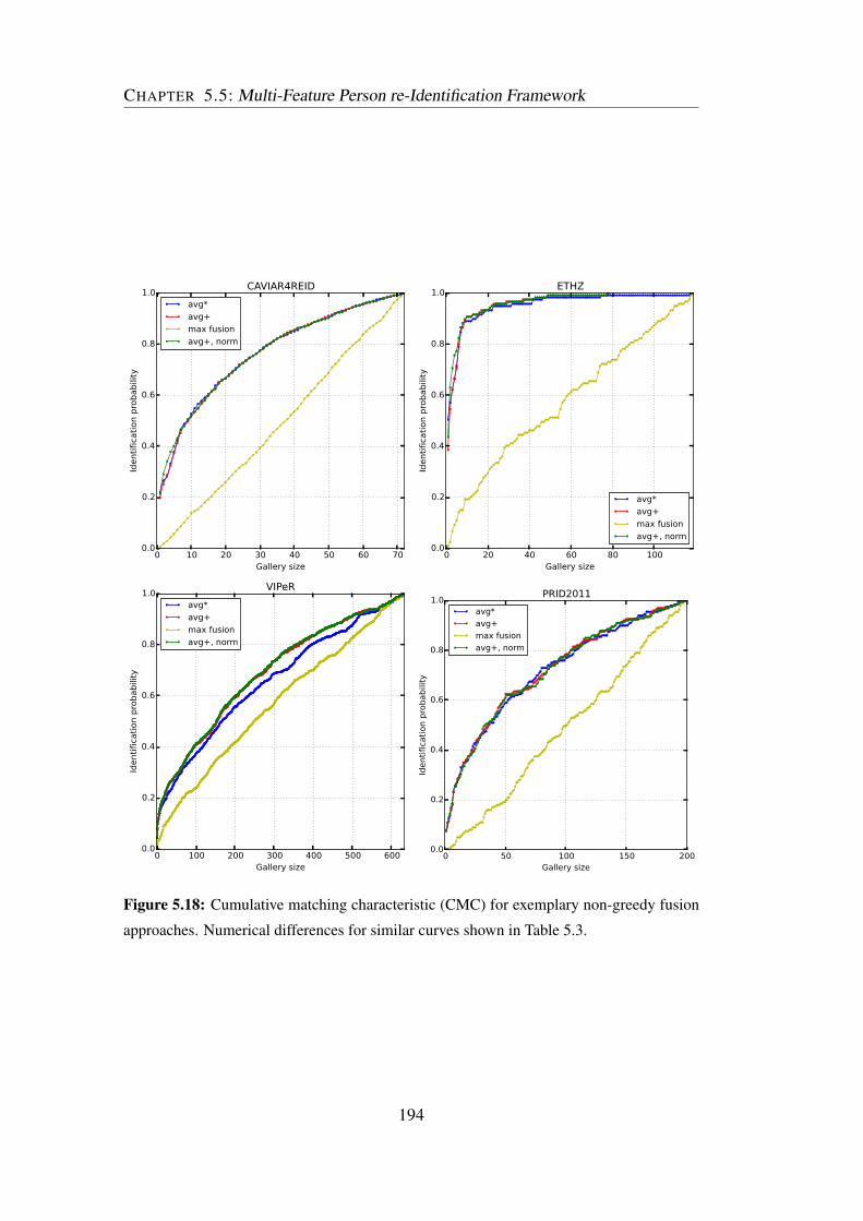
CHAPTER 5.5: Multi-Feature Person re-Identification Framework
0 10 20 30 40 50 60 70Gallery size
0.0
0.2
0.4
0.6
0.8
1.0
Identification probability
CAVIAR4REID
avg*
avg+
max fusion
avg+, norm
0 20 40 60 80 100Gallery size
0.0
0.2
0.4
0.6
0.8
1.0
Identifica
tion p
robabili
ty
ETHZ
avg*
avg+
max fusion
avg+, norm
0 100 200 300 400 500 600Gallery size
0.0
0.2
0.4
0.6
0.8
1.0
Identifica
tion probability
VIPeR
avg*
avg+
max fusion
avg+, norm
0 50 100 150 200Gallery size
0.0
0.2
0.4
0.6
0.8
1.0
Identifica
tion p
robabili
ty
PRID2011
avg*
avg+
max fusion
avg+, norm
Figure 5.18: Cumulative matching characteristic (CMC) for exemplary non-greedy fusion
approaches. Numerical differences for similar curves shown in Table 5.3.
194

CHAPTER 5.5: Multi-Feature Person re-Identification Framework
Results for the non-greedy strategies are presented in Figure 5.18. Obviously,
max fusion is not a good option because in all datasets, the identification probability
does not exceed significantly the performance for a random guess. This explains by
the very diverse score distributions among the different base methods. Especially
region covariance computes a distance measure in a logarithmic space and despite a
normalization approach in order to map the similarity scores of different re-id steps
onto a common interval, the values appear to be too different.
Multiplicative averaging obtains worse results compared to additive averaging.
Again, this can be explained by the complementarity of the feature descriptors and
thus inhomogeneity of the scores of the individual base methods for the same query
samples. Therefore, if e.g. one score is low and two are higher, an additive fusion
does not penalize the lower score as much as a multiplicative one and correct can-
didates getting a bad ranking in the first feature matcher steps can catch up in the
later ones. In contrast, additive fusion improves the system’s robustness against an
outlier from a single matcher. For better readability, Table 5.3 gives numerical re-
sults on the experiment and also shows the slight improvement by the normalization
approach.
Figure 5.19 indicates results for greedy strategies. The results support the previ-
ous conclusions about inhomogeneity in the individual features’ similarity scores.
It is well visible from the graphs that the iterative removal of candidates after every
feature step does not improve the overall re-identification performance. Regardless
of removing a certain percentage of bad candidates in every step or e.g. threshold-
ing the ones with low scores, a simple averaging scheme obtains far better results
than the greedy schemes. The performance decreases with increasing number of
candidates removed, i.e. with an increasing level of greediness.
Numerical results (CMC-AUC) in Table 5.3 support the conclusions drawn and
show the details more precisely. Again, the results support the finding that the re-
moval of bad candidates in an iterative scheme gives worse results than maintaining
all potential matching candidates over all feature steps. The higher the number of
candidates removed in individual steps (i.e. higher parameters in "thresh" / "iter
removal" or lower percentages in "survival weight"), the lower is generally the per-
formance.
For easy performance comparison of the data fusion from different feature de-
scriptors, Figure 5.17 shows a CMC plot of the individual re-identification steps
195

CHAPTER 5.5: Multi-Feature Person re-Identification Framework
CAVIAR4REID ETHZ VIPeR PRID average
avg* 0.771 0.954 0.660 0.715 0.775
avg+ 0.768 0.940 0.691 0.724 0.781
avg+, norm 0.771 0.945 0.693 0.723 0.783
max fusion 0.503 0.583 0.571 0.486 0.536
thresh(0.002), avg+ 0.635 0.811 0.555 0.521 0.631
thresh(0.005), avg+ 0.639 0.799 0.508 0.506 0.613
thresh(0.01), avg+ 0.625 0.756 0.501 0.513 0.599
thresh(0.015), avg+ 0.624 0.712 0.501 0.502 0.585
thresh(0.02), avg+ 0.603 0.658 0.501 0.502 0.566
survival weight 0.9 0.638 0.855 0.597 0.626 0.679
survival weight 0.95 0.683 0.891 0.622 0.65 0.711
survival weight 0.98 0.727 0.909 0.636 0.68 0.738
survival weight 0.99 0.75 0.94 0.641 0.695 0.756
0.001 iter removal 0.769 0.94 0.69 0.725 0.781
0.01 iter removal 0.769 0.94 0.676 0.721 0.777
0.05 iter removal 0.754 0.928 0.652 0.689 0.756
0.1 iter removal 0.743 0.915 0.644 0.685 0.747
0.15 iter removal 0.73 0.914 0.643 0.657 0.736
ColorHist 0.71 0.857 0.642 0.598 0.702
SURF 0.749 0.946 0.61 0.709 0.754
RegCov 2x3 0.633 0.806 0.601 0.532 0.643
Table 5.3: Results of different fusion schemes on the test datasets based on area under CMC
curve (CMC-AUC; "thresh(t), avg+": iterative thresholding, "survival weight w": accumu-
lative weight fusion, "iter removal": Iterative removal fusion, additive average "avg+" for
comparison). Baseline descriptors given for reference.
196

CHAPTER 5.5: Multi-Feature Person re-Identification Framework
Figure 5.19: Cumulative matching characteristic for exemplary greedy fusion approaches
("thresh(t), avg+": iterative thresholding, "survival weight w": accumulative weight fusion,
"iter removal": Iterative removal fusion, additive average "avg+" for comparison). Numeri-
cal values given in Table 5.3.
197

CHAPTER 5.6: Conclusion
and their combination in the fused method. It is visible that the fusion enhances
the results considerably on all datasets, however, a feature point-based approach
("SURF") can also show good performance in some cases. Depending on the ap-
plication case, it is therefore worth considering either a rather simple feature point
re-identification step or the more complex but also more powerful fusion found in
this thesis.
Considering the run-time of the fusion methods, it can generally be said that the
influence of the fusion scheme is small compared to the individual computational
complexities. Therefore, keeping in mind the rather high computational demand for
region covariance in comparison to point features and color histograms, the region
covariance influence dominates the overall run-time.
5.6 Conclusion
In this chapter, the application case of pedestrian re-identification for tracking use
cases has been analyzed. The main contributions include
• The development of guidelines regarding the system design for potential use
cases in tracking applications.
• A thorough analysis of three basic pedestrian re-identification methods which
have been tested and evaluated on four different datasets.
• The investigation of suitable parametrizations of the different re-identification
methods, including the usage of partitioning schemes for performance en-
hancements.
• The identification of potential rank issues in the metric for region covariance
matrices and the development of a pre-processing step in order to remove
collinear rows in the matrices and to ensure their full rank.
• The development of fusion strategies for single-feature matchers and their
comparison in a detailed analysis which results in a proposal for a multi-
feature pedestrian re-identification system for tracking applications.
Three baseline feature descriptors for pedestrian re-identification have been ex-
tensively assessed and compared on four different datasets. It has been found that
198

CHAPTER 5.6: Conclusion
for single-cue methods especially feature point-based approaches combine high per-
formance and acceptable run-time. Color histograms are a simple and fast method
which shows acceptable results with very little computational complexity. Region
covariance approaches, however, suffer from their high computational demands and
have thus to be parametrized with very small partitioning schemes for tracking con-
texts. With these restrictions, their re-identification performance decreases signifi-
cantly.
In order to further enhance the re-identification performance, fusion strategies
have been developed and tested in this work. These include greedy and non-greedy
approaches. Greedy methods generally have lower performance because they re-
strict the number of candidates in each feature descriptor step, and due to the com-
plementarity of the different base descriptors, this fusion approach has been proven
less powerful than non-greedy approaches. Best results have been obtained using
vector unity normalization and the non-greedy additive averaging scheme.
Opportunities for future work are especially in the efficient application of the
findings to a tracking process. In order to further reduce the run-time, this could
include e.g. the usage of integral images for color histograms or region covariance
and a multi-threading implementation on descriptor and partition level. Additional
work could be done for the efficient retrieval of a given descriptor in an image
region.
199

CHAPTER 5.6: Conclusion
200

Chapter 6
Conclusions and Outlook
THE objective of this thesis was to investigate the usage of tracking-by-detection
methods for the task of pedestrian tracking in video surveillance scenarios.
While in the current literature especially visual trackers are very popular, tracking-
by-detection algorithms for multi-target tracking have been proposed and refined
especially in the radar / sonar tracking community which is a very different environ-
ment compared to camera-based computer vision and has fundamentally different
requirements.
In this thesis, the Gaussian mixture probability hypothesis density (GM-PHD)
filter has been used as a popular example for tracking-by-detection filters which
has a low computational complexity and can be used for arbitrary objects as long
as they can be detected in a designated object detection step. For the GM-PHD
filter, a thorough analysis has been performed in order to assess its performance for
pedestrian tracking in surveillance contexts. Due to the fact that reliable pedestrian
detection in arbitrary scenarios is still an open area of research, a major weakness of
the GM-PHD filter has been found in its requirement for very high detection rates
which has been justified by an analysis of its theoretical foundations.
In order to tackle the problem of low detection probabilities, this work proposes
different remedies for various application scenarios both for the detection and the
tracking part of the system. For the integration of further image information into the
proposed tracking-by-detection framework, the thesis provides an in-depth evalua-
tion of three fast feature extraction methods for person re-identification which en-
ables the future integration of image cues into the framework and will likely give an
additional performance boost.
201

CHAPTER 6.1: Achievements
The following sections present the achievements, the drawable conclusions and
potential future research topics of this thesis.
6.1 Achievements
After a detailed introduction of single- and multi-target tracking algorithms and
their mathematical foundations, a first achievement of this thesis is the development
of a flexible tracking-by-detection framework for multi-person tracking in video
surveillance contexts. The framework is modular and capable of using different
pedestrian detectors as well as both pointwise detections and detections with regions
of interest. With a GM-PHD filter as the main tracking component, the system is
fast and can be applied to virtually any object class with an appropriate detection
method. Table 3.2 shows that its performance is on a good level compared to other
tracking approaches.
Secondly, the detector side of the framework is addressed by proposing a para-
metrization using local crowd density maps and geometric correction filters. Pedes-
trian detectors require the setting of suitable parameters such as the detection thresh-
old beforehand. This is especially challenging in scenarios with medium or dense
crowds where occlusion inhibits a good detection performance. This thesis pro-
poses a method of dynamically parametrizing the detector based on estimates of
local crowd density. Compared to the baseline method, this approach performs bet-
ter in terms of detection accuracy and is more flexible with temporarily changing
crowd densities in the scene. An additional advantage is proposed by using geomet-
rical correction filters which use constraints on the size or aspect ratio of detections
which are inherent to the scene characteristics. The filters learn a scene model in
a greedy fashion based on previously received detections and are not restricted for
use with a certain pedestrian detector.
On the tracker side, another improvement is proposed by feature-based label
trees which extend baseline label trees with visual information cues. When two
tracked pedestrians approach or their paths even cross each other, a purely detection-
based tracker has difficulties to maintain track labels. It is shown how this problem
can be reduced by using image information which allows distinguishing state hy-
potheses according to visual information cues. The improvement by feature-based
label trees has been shown both in a simulation and on practical examples.
202

CHAPTER 6.1: Achievements
The fourth advancement in this thesis is a novel step for integrating multiple
pedestrian detectors into the GM-PHD filter framework. A theoretical analysis of
the baseline approach led to the conclusion that the iterated-corrector step is not
suitable for visual pedestrian trackers. Important drawbacks are its inherent need
for very high detection rates which are not given in this field of application and,
consequently, a performance dependency from the sensor order. This thesis pro-
poses a remedy using an additive update step which both removes the sensor-order
dependency and yields better results.
As a fifth contribution of this thesis, a thorough analysis of the GM-PHD filter
regarding false negative detections is performed and the concept of a critical path
of missed detections is introduced in order to mathematically describe the risk of
tracking failure. These theoretical foundations are used in order to motivate an in-
troduction of motion cues using an active post-detection filter which is the sixth
improvement made by this thesis. This concept can be applied to both pointwise
and region of interest-based detections. The active post-detection filter is sensor-
independent and can even be used on 3rd party detectors without access to the de-
tector code. It has been tested on different datasets and shows high improvements
both for detection and tracking.
In order to enable future integration of further image cues into the proposed
tracking-by-detection framework, the next contribution is an in-depth evaluation of
runtime-efficient person re-identification methods and their parametrization. Three
methods based on point features, color histograms and region covariance and the ap-
plication of partition schemes for performance improvements are assessed on four
different datasets. In order to combine these different approaches into a more pow-
erful re-identification method, different greedy and non-greedy fusion strategies are
exploited and tested, thus yielding a multi-cue system which performs better than
the single-cue methods on a variety of datasets.
Within these experiments, the last improvement proposed by this thesis is an
enhanced scheme for comparison of region covariance features. The baseline metric
suffers from potential rank issues in the covariance feature. The proposed extension
removes collinear rows from the feature matrix while respecting the feature order
in the two matrices for comparison. It therefore ensures a proper comparison and
reduces bad metric results by rank issues.
203

CHAPTER 6.2: Conclusions
6.2 Conclusions
The GM-PHD pedestrian tracking-by-detection framework developed in this the-
sis has proven its potential as a modular, flexible pedestrian tracker with differ-
ent enhancements in order to deal with lower detection probabilities in the video
surveillance domain. It has been shown that with an open implementation of the
deformable parts model (DPM) detector, good tracking results can be obtained and
that different enhancements allow to increase the detection and tracking perfor-
mance additionally.
Pedestrian detection in denser crowds is still an area of active research and far
from being solved. The adaptive correction filters proposed in this work have
been shown to contribute to a higher detection performance by removing detections
which are likely to be incorrect. A dynamic parametrization based on geometric
correction filters for size and aspect ratio and estimation of the local crowd density
can significantly reduce the number of outliers and also allows for correct detec-
tions which otherwise would have been eliminated by the non-maxima suppression
in standard object detectors.
For the tracking of close objects, the GM-PHD filter has been extended with
visual features which help maintaining the correct labels for tracks in ambiguous
situations, such as crossing of targets. However, it can be said that, despite these
improvements, even with this extension the plain vanilla GM-PHD filter still suffers
from the lower object detection probability in visual tracking scenarios. In this
work, this has been theoretically justified by a sensitivity analysis of the GM-PHD
filter with regard to missed detections. Especially the proposed concept of a critical
path helps to understand intuitively where the problem arises.
The first improvement in order to deal with the aforementioned lower object de-
tection probabilities involves the combination of multiple object detection methods.
If applicable in the respective application case, this approach has been shown to
improve the tracking performance significantly. Due to the data fusion from two
detectors, complementary information can be used which would not be available
with only one detector. Especially the replacement of the iterative corrector step by
an additive one which has been proposed in this work is a major step towards better
performance for surveillance scenarios with lower detection probabilities.
As in some scenarios, only one object detector may be available or the com-
204

CHAPTER 6.3: Outlook
putational load of using two detectors may be undesired, the usage of active post-
detection filters in this work has been theoretically motivated and shows very promis-
ing results. Compared to the baseline system and a passive filter using hysteresis
thresholding, the active filter performs significantly better and adds only a small
additional effort for computation of local optical flow. The developed concept sup-
ports on-line and real-time processing and can easily be realized for different object
types and detection algorithms.
Further work in this thesis lays the foundations for introducing new visual cues
into the tracking framework. By assessing a number of low-level re-identification
methods for the pedestrian case, it has been found that apart from color histograms,
especially feature point descriptors such as SURF can be used for describing a per-
son’s appearance in a fast and reliable manner. In comparison, region covariance
descriptors are more demanding in computational terms and are thus less suitable
for visual tracking. All of the mentioned approaches can be parametrized with par-
titioning schemes which improve their re-identification performance but also lead
to a higher run-time.
Additionally, the application of region covariance has been shown to suffer from
the risk of potential rank issues, leading to problems in the respective metric. This
work proposes a remedy by removing collinear rows in order to ensure full rank
in the matrices but, unfortunately, this step increases the computational load for
region covariance even more. If run-time is less of an issue, region covariance
can still be used as it generally gives good re-identification results. However, in
this case especially a fusion of different feature descriptors should be taken into
account which supports the usage of complementary information in the descriptors
and achieves best performance on a variety of datasets.
6.3 Outlook
Within the course of this work, some ideas could not be realized and shall be
highlighted in order to direct further research in the future: Regarding the afore-
mentioned sensitivity against false negative detections, it would be interesting to
perform detailed analyses for comparison with other trackers such as e.g. multi-
hypothesis tracking (MHT). The GM-PHD filter which has been used as an example
in this thesis is a modern, generalizable and popular tracking-by-detection example
205

CHAPTER 6.3: Outlook
but its sensitivity still might differ in some points from other approaches.
With the rise of new pedestrian detectors, e.g. methods based on convolutional
neural networks (CNNs), new options are available in order to tune the detection
part of the framework. In this thesis, the popular DPM method has been chosen
because it is openly available both in MATLAB and C++ implementations. CNN
approaches require high-end graphics processors and their re-implementation from
a publication takes a lot of specialized machine learning know-how in order to tune
the parameters to a given dataset. While this was the reason they have not been
regarded in this work, it would be interesting to see e.g. results of the dynamic
thresholding according to crowd density for such approaches.
The tests on different person re-identification methods performed within this the-
sis are detailed and allow for the design of a system exploiting such information
cues in order to enable e.g. cross-camera tracking or re-identify lost tracks. Due
to time constraints, within the work of this thesis only standard re-identification
datasets have been used and no final integration into the tracking framework has
been done. Such an implementation of person re-identification methods within the
tracking framework would yield opportunities to both improve the system’s perfor-
mance by improving the quality of the tracks and to address new applications such
as cross-camera tracking or loitering detection which could be subject to future
work.
206

Appendix A
Datasets
A.1 Datasets and Videos Used for Person Detection
A.1.1 PETS 2009
The PETS 2009 dataset [Ferryman and Shahrokni, 2009] has been published and
used for the 11th IEEE International Workshop on Performance Evaluation of Track-
ing and Surveillance (PETS 2009). Since then it has been the basis for evaluation
and competitions in this workshop and numerous publications. It comprises multi-
ple views recorded on campus at University of Reading, UK. While some sequences
are recorded for evaluation of tracking purposes, it also provides sequences for per-
son count and crowd density estimation, flow analysis and event recognition. Person
sizes differ due to the camera view between approx. 30 and 150 pixels height.
For person detection in crowds only the first view (768× 576 pixels) has been
used and two video sequences ("S1.L1 13.57", "S1.L1 13.59") with 220 and 241
frames respectively were annotated manually. Example frames of these sequences
can be found in Figure A.1 (top).
A.1.2 INRIA 879-42_I
This video is part of the Data-driven Crowd Analysis Dataset described in [Ro-
driguez et al., 2011b] released in collaboration with the Institut national de recherche
en informatique et en automatique (INRIA). It shows a scene where a dense group
of pedestrians passes walking in one direction while a single person goes in the
opposite direction. The scene is recorded at 480× 360 pixels from an almost ver-
207

CHAPTER A.1: Datasets and Videos Used for Person Detection
Figure A.1: Exemplary frames of the PETS 2009 dataset (left: crowd sequence, right:
tracking sequence).
Figure A.2: Left: Exemplary frame of the INRIA 879-42_I video. The high number of per-
sons and the unusual camera perspective make it a very hard video for pedestrian detection.
Right: Exemplary frame of the UCF 879_38 video. Due to a high number of overlapping
people, pedestrian detection is also relatively difficult for this video.
tical camera perspective which makes it challenging for usual pedestrian detectors.
Pedestrians are perceived at a height of approximately 100-120 pixels. A sample
frame is shown in Figure A.2 (left). The detection experiments focus on the first
430 frames of this sequence and discard the following empty frames.
A.1.3 UCF 879-38
This video is taken from the UCF crowd segmentation dataset [Ali and Shah, 2007]
and has a resolution of 720×480 pixels. All the videos from this dataset show high
density moving objects. The video shows a public plaza with many pedestrians
walking in all directions, approaching and avoiding collision with each other. De-
208

CHAPTER A.2: Datasets Used for Tracking
Figure A.3: Exemplary frames of MOT 17 videos. The videos vary largely in terms of
crowd density, scene content and camera motion.
spite a rather high resolution (a single pedestrian has a height from approximately
150 to 190 pixels), the video is very challenging due to a rather steep camera view, a
very high crowd density and many occlusions. A manual annotation for the first 200
frames has been conducted as no official ground truth was available. An exemplary
frame is shown in Figure A.2 (right).
A.2 Datasets Used for Tracking
A.2.1 MOT17 Tracking Benchmark
MOT17 [Milan et al., 2016] is a public1 benchmark for multiple-object tracking. It
consists of a training and a test set, each composed of 21 videos with pedestrians
in various scenarios. Detections are provided for three pedestrian detectors. The
resolution of the videos is VGA (640× 480) or Full HD (1080× 1920). Trackers
can be parametrized using the test data with ground truth available and benchmark
results are obtained by uploading the tracking results on the test set onto a test server
which evaluates the results and provides scores such as MOTA, MOTP and so on.
The videos are highly challenging as they are very heterogeneous and it is expected
to find a common parametrization for a tracker to be benchmarked. Additionally,
1download from tt♣s♠♦t♥♥tt
209

CHAPTER A.2: Datasets Used for Tracking
Figure A.4: Exemplary frames of the UA-DETRAC dataset.
many videos have been recorded with a moving camera, e.g. from cars or robot
platforms which is a problem for trackers based on an internal motion model. Con-
sequently, in this thesis, the benchmark is only used for a general validation of the
system but more suitable videos have been chosen for detailed evaluation.
A.2.2 UA-DETRAC Vehicle Tracking Benchmark
The University at Albany DETection and tRACking (UA-DETRAC) benchmark
dataset [Wen et al., 2015] is a public2 real-world multi-object detection and multi-
object tracking benchmark. The dataset has been captured at 24 different locations
in China and comprises 10 hours of videos recorded using a digital single-lens re-
flex (DSLR) camera. Videos are of 960× 540 pixels resolution and captured at
25 frames per second (fps). In total, 8520 vehicles have been annotated manually,
leading to over 1.2 million labeled bounding boxes in the videos which have been
categorized into the three levels "Easy", "Medium", and "Hard". The "Beginner"
challenge requires participants to submit results for 10 test videos marked as "easy"
while the "Experienced" set contains 30 videos labeled as "Medium" or "Hard". The
dataset has been the basis for a tracking benchmark at IEEE AVSS 2017 conference.
After using the ground truth provided for some training sequences for parametriza-
tion of the tracker, evaluation is done by uploading the results onto a test server,
where the tracking scores are computed using the test set ground truth (unknown to
the participants). The most important evaluation measures used comprise the rather
uncommon PR-MOTA / PR-MOTP curves which are constructed by firstly varying
the detection threshold and thus obtaining the related PR-curve (Precision-Recall-
curve) for the object detector.
2download from tt♣trrt♥②
210

CHAPTER A.2: Datasets Used for Tracking
Figure A.5: Exemplary frames of the TUB Walk video sequence recorded at Technische
Universität Berlin. Video characteristics are a traditional surveillance camera view from
high altitude and a semi-dense scene.
The tracker is then executed for ten sample points on this curve, yielding the
respective tracking results. Finally, the MOTA/MOTP values for these points are
computed and the area under the curve (AUC) is computed by interpolation. Details
on the computation can be found in [Wen et al., 2015].
Due to the nature of the tracked objects and the uncommon metric, the dataset is
only used for a general validation of the system but more suitable videos have been
chosen for detailed evaluation.
A.2.3 PETS 2009 (Tracking)
The PETS 2009 dataset mentioned in Appendix A.1.1 for crowd applications also
contains a suitable video for object tracking applications. Therefore, for the se-
quence "S2.L1 12.34", head positions have been annotated manually for all per-
sons visible (for pointwise detections) and body bounding boxes have been obtained
from Multiple Object Tracking (MOT) 2015 benchmark [Leal-Taixé et al., 2015],
respectively. An example frame of this video can be seen in Figure A.1 (right). The
video contains 795 frames at a frame rate of approx. 6-7 frames per second (fps).
A.2.4 TUB Walk
The TUB Walk sequence has been recorded on the campus of Technische Univer-
sität Berlin (TUB) with the aim of creating a new video which meets typical con-
ditions for CCTV applications in real life. While the camera in this sequence is at
211

CHAPTER A.2: Datasets Used for Tracking
Figure A.6: Exemplary frames of the TownCentre video sequence. Video characteristics
are an over-head mounted surveillance camera view in an average-dense scenery.
overhead height (approx. 10 meters) with a down-tilt view typical for video surveil-
lance, it gives a frame size of 800× 600 pixels with rather low contrast and low
color resolution. The scene recorded is a pedestrian way on TUB campus where
mostly pedestrians and bikers are perceived. For this sequence, the heads of the
persons in the bottom region of the scene have been manually annotated for evalua-
tion in 10400 video frames. The person size is generally small (between 32 and 64
pixels height), it should also be noted that due to the camera view, persons far from
the camera appear much smaller than the ones near the camera. Exemplary frames
of this video can be found in Figure A.5.
A.2.5 TownCentre Dataset
The TownCentre dataset has been published in [Benfold and Reid, 2011] and is
available on the website3 of the University of Oxford. It contains a real-life video
sequence of 4500 frames recorded in a busy town centre street. The video data is
of very good visual quality as it is high definition (1920x1080 pixels) recorded at
25 fps. The camera view is a typical surveillance view from an overhead-mounted
camera. According to [Benfold and Reid, 2011], its ground truth is hand-labelled
and the video shows an average of sixteen people visible at any time. These persons
are walking both alone and in groups and are mostly perceived in a side-front or
side-rear view. An exemplary TownCentre frame is shown in Figure A.6.
3download from tt♣sr♦♦ts♦①t❱s♦♥srPr♦ts
♥♦❴♣♦s♣r♦tt♠
212

CHAPTER A.2: Datasets Used for Tracking
Figure A.7: Exemplary frames of the CAVIAR videos "EnterExitCrossingPaths1cor",
"WalkByShop1cor" (top), "ThreePastShop2cor", "ThreePastShop1cor" (bottom).
A.2.6 CAVIAR
The "Context Aware Vision using Image-based Active Recognition" (CAVIAR)
dataset is a well-known video surveillance dataset and has been used in many scien-
tific publications. It has been obtained in the EC Funded CAVIAR project/IST 2001
37540 and can be found at tt♣♦♠♣s♥r❱.
As the sequences cover different activities aimed especially at action recognition
(e.g. person falling, leaving bags, fighting and so on), not all of them are relevant
for tracking. Therefore, four videos have been chosen from the dataset which show
the traditional over-head camera position and a corridor view: 1) "EnterExitCross-
ingPaths1cor" (383 frames), 2) "WalkByShop1cor" (2360 frames), 3) "ThreePast-
Shop1cor" (1650 frames), 4) "ThreePastShop2cor" (1521 frames). Sample frames
are shown in Figure A.7. The videos have rather low resolution (384×288 pixels),
low contrast and suffer from compression artifacts.
213

CHAPTER A.3: Datasets Used for Person Re-Identification
Figure A.8: Exemplary frames of the Parking Lot videos "Parking Lot 1" (left) and "Parking
Lot 2" (right).
A.2.7 Parking Lot
The Parking Lot sequences [Shu et al., 2012; Dehghan et al., 2015] have been pub-
lished by University of Central Florida4 and provide videos of a parking lot recorded
in Full HD (1920×1080 pixels) at high frame rates (30 and 29 frames per second,
respectively). Both videos have been recorded from a far-distance, high camera
position and show relatively crowded scenes with pedestrians walking in queues,
long-term inter-object occlusions and abrupt motion. The video lengths are 1000
frames and 1500 frames, respectively. Tracking ground truth is provided in the
dataset. Figure A.8 shows sample images for both sequences.
A.3 Datasets Used for Person Re-Identification
A.3.1 CAVIAR4REID
CAVIAR4REID has been published in [Cheng et al., 2011] and contains pedestrian
images taken from the aforementioned CAVIAR [CAVIAR Dataset, 2007] dataset.
The size of the images varies from 17× 39 to 72× 144 pixels. For 72 persons,
images from one camera view are provided. For 50 of them, a second camera
view is also available. The authors of [Cheng et al., 2011] claim to have chosen
camera views "maximizing the variance with respect to resolution changes, light
conditions, occlusions, and pose changes". Examples of this dataset can be found
in Figure A.9. It is a challenging dataset with images of usually lower resolution,
lower contrast and more coding artifacts than other datasets. For evaluation, 72
4download at tt♣rtPr♥
214

CHAPTER A.3: Datasets Used for Person Re-Identification
Figure A.9: Sample images from the CAVIAR4REID dataset illustrating the scale differ-
ences within the data. Two persons are shown (1st and 2nd row, 3rd and 4th row) from two
different camera views.
images of individual persons are searched in a training set of 72 other images, both
taken from the "corridor" sequences.
A.3.2 ETHZ
The basis for the ETHZ dataset [Schwartz and Davis, 2009] is the image data from
[Ess et al., 2007] which has been captured using moving cameras at head height.
For person re-identification, all image samples have been resized to 32× 64 pix-
els. While the dataset contains images of rather good quality in terms of resolution,
contrast and sharpness, it is still challenging due to illumination changes and occlu-
sions. For our tests, we use the first appearance of every individual as the training
image and search a query image which has been recorded 25 frames later than the
training image in a set of 120 samples. Sample images can be found in Figure A.10.
215

CHAPTER A.3: Datasets Used for Person Re-Identification
Figure A.10: Sample images from the ETHZ dataset. Two persons are shown. Although
images are shown here with the same height, in general the size of the images is not the
same for different persons and images.
A.3.3 VIPeR
The VIPeR dataset has been published in [Gray et al., 2007]. It contains two views
of 632 pedestrians, each pair of views composed by images of 48×128 pixels size
taken from different cameras. Due to varying viewpoint, pose and lighting condi-
tions, it can be considered a very challenging dataset available for single-shot person
re-identification. Visual examples of this dataset can be found in Figure A.11. For
evaluation in this work, 632 test images are randomly chosen and must be retrieved
from a training set of 632 images.
A.3.4 PRID 2011
Published in [Hirzer et al., 2011], the PRID 2011 dataset has been recorded on the
basis of person trajectories from two different cameras. One major difficulty of this
dataset is its differently textured background (street with / without a crosswalk). The
single views contain 753 resp. 475 persons of which 245 appear in both views. All
images are normalized to a size of 64× 128 pixels. For experiments in this work,
216

CHAPTER A.4: Measures Used for Object Detection
Figure A.11: Sample images from the VIPeR dataset containing images from different
viewpoints. Images of the same persons are in the same column. All images are normalized
to a size of 48×128 pixels.
each of the first 200 persons appearing in one camera is searched in the images
taken from the other one. Examples of this dataset can be found in Figure A.12.
A.4 Measures Used for Object Detection
Regardless of the nature of objects (pedestrians, cars etc.), the detection of multiple
objects in a video frame can intuitively be described as two main tasks:
• Detecting the correct number of objects in a video frame.
• Localizing the objects as close as possible to their ground truth position.
Both of these tasks are evaluated in the Multiple Object tracking (MOT) metrics
published in [Stiefelhagen et al., 2007; Bernardin and Stiefelhagen, 2008] and are
presented in the following.
A.4.1 Multi-Object Detection Accuracy (MODA)
MODA published in [Stiefelhagen et al., 2007; Bernardin and Stiefelhagen, 2008]
measures the accuracy of the detection process for a given frame and takes into
217

CHAPTER A.4: Measures Used for Object Detection
Figure A.12: Sample images from the PRID 2011 dataset containing images from different
viewpoints. Images of the same persons are in the same column. All images are normalized
to a size of 64×128 pixels.
account the number of missed detections M(t) and the number of false positive
detections FP(t) at time t:
MODA(t) = 1− cm ·M(t)+ c f ·FP(t)
NG(t)(A.1)
with NG(t) as the number of ground truth objects in frame t and cm,c f as the cost
functions for missed detections and false alarms, respectively (costs set to one for
evaluations in this thesis). A detection is classified as matched when a specific over-
lap between ground truth detection and estimated detection is found (see definition
of MODP for details). In case of M(t) = FP(t) = NG(t) = 0, the MODA value is
set to 1.
It can be argued that Equation (A.1) becomes less intuitive in the case of FP(t)>
0 and NG(t) = 0. In this case, the MODA value for the respective frame becomes
−∞ regardless of the number of false positives. So, if the detection algorithm es-
timates 1.000 false positives, it would be rated as bad as another method which
might only yield 1 false positive. Though it would be possible e.g. to use a con-
stant denominator of value one in such cases, this change would come at a cost of
interpretability when comparing with other frames. MODA is a relative measure
describing errors in relation to the ideal case and can be compared on a per-frame
basis. Following [Stiefelhagen et al., 2007; Bernardin and Stiefelhagen, 2008], the
218

CHAPTER A.4: Measures Used for Object Detection
ratio between detection errors and ground truth is therefore not altered in order to
ensure an equal interpretation over all frames.
A.4.2 Normalized Multi-Object Detection Accuracy (N-MODA)
N-MODA [Stiefelhagen et al., 2007; Bernardin and Stiefelhagen, 2008] is based on
the previously described framewise MODA measure and computes the normalized
MODA for the whole video:
N-MODA = 1− ∑N f rames
t=1 (cm ·M(t)+ c f ·FP(t))
∑N f rames
i=1 NG(i). (A.2)
Note that this measure does not just average the MODA values in order to avoid
issues with MODA(t) = −∞ (see definition of MODA measure in Appendix A.4.1
for details). Instead, a normalization of the summed MODA enumerators over the
summed target numbers is used. The maximal value for N-MODA is one, i.e. no
false positives or missed objects are reported.
A.4.3 Multiple Object Detection Precision (MODP)
MODP measures the average overlap ratio between the ground truth bounding boxes
and the detected objects for a given frame. Missed or falsely identified objects are
only implicitly taken into consideration. This requires the first step in computing
the measure to be a matching of the set of detections D = d1,d2, ...,dn and the
corresponding ground truth detections G = g1,g2, ...,gnin order to identify which
ground truth detections have been found by the detector. For this matching step, the
overlap ratio Φ is defined as:
Φ(t) =Nmapped(t)
∑i=1
∣∣∣g(t)i
⋂d(t)i
∣∣∣∣∣∣g(t)i
⋃d(t)i
∣∣∣(A.3)
with Nmapped(t) as the number of assigned object regions in frame t.
Taking Φ(t) between all pairs as input, in this thesis the well-known Hungarian
algorithm [Kuhn, 1955] is used for assignment. As proposed in [Stiefelhagen et al.,
2007], a threshold of 0.2 for the overlap ratio prevents assignments between badly
matching pairs.
219

CHAPTER A.5: Measures Used for Tracking
Once the assignment for all frames is done, MODP (t) is computed as the summed
and normalized overlap ratio between all assigned pairs in the image:
MODP(t) =
0, i f Nmapped(t) = 0
otherwiseΦ(t)
Nmapped(t).
(A.4)
A.4.4 Normalized Multi-Object Detection Precision (N-MODP)
Similar as N-MODA to MODA, N-MODP [Stiefelhagen et al., 2007; Bernardin and
Stiefelhagen, 2008] is closely related to MODP and gives normalized localization
results for the entire sequence by averaging the individual values:
N-MODP =∑
N f rames
t=1 MODP(t)
N f rames
. (A.5)
A.5 Measures Used for Tracking
According to [Bernardin and Stiefelhagen, 2008], for the aims of a perfect multi-
object tracking algorithm, the following points should be considered:
• The tracker should correctly estimate the number of objects in every video
frame.
• The tracker should assign every object an ID which is consistent throughout
the whole video.
• The tracker should estimate every object state as close as possible to its real
state.
However, as no perfect multi-object tracker exists, an evaluation metric should
measure the differences to this ideal system. The design of a multi-object tracking
metric should thus consider the following principles:
• The number of missed objects (false negatives) should increase the metric.
• The number of wrongly detected objects (false positives) should increase the
metric.
220

CHAPTER A.5: Measures Used for Tracking
• The distance between estimated positions of all objects and known ground
truth states should increase the metric.
• Labeling errors should increase the metric.
On the other hand, [Ristic et al., 2011] claim that a measure for multi-object
tracking should have a rigorous mathematical foundation based on finite set theory.
In this context, properties such as
• Being a metric on the space of finite sets
• A meaningful physical interpretation
• The meaningful capture of cardinality errors
• An easy computation
are also desired. It can be seen that the evaluation of a multi-object tracking
algorithm comprises a number of requirements which may be prioritized differently
according to the application case. Also, for individual aspects, a specific measure
can be used or a combination involving e.g a weighted sum of the individual terms
for the whole evaluation can be applied.
As a result, different methods have been proposed for evaluation of a multi-object
tracker. In this thesis, two measures for region-of-interest-based detections / tracks
(N-MOTA / N-MOTP) and one for point-based detections / tracks (OSPA-T) are
used.
A.5.1 MOTA
The MOTA [Stiefelhagen et al., 2007; Bernardin and Stiefelhagen, 2008] measure
essentially is an extension of the MODA measure for object detection shown pre-
viously in Appendix A.4.1 but also takes into account the number of wrong label
assignments (i.e. ID changes or mismatch errors) MME(t):
MOTA(t) = 1− cm ·M(t)+ c f ·FP(t)+ cl ·MME(t)
NG(t). (A.6)
The cost function cl is set to one for all evaluations in this thesis. Similar to N-
MODA (see Equation (A.2)), N-MOTA can be computed as a normalized version
of MOTA for a full video.
221

CHAPTER A.5: Measures Used for Tracking
A.5.2 MOTP
This measure essentially is an application of the previously shown MODP measure
for tracking purposes. MOTP as published in [Bernardin et al., 2006; Bernardin
and Stiefelhagen, 2008] measures the total position error over all frames between
the ground truth objects and the estimated objects:
MOT P =∑i,t di(t)
∑t ct(A.7)
with di(t) as the geometric distance between ground truth object i and its tracked
counterpart for frame t. In this thesis, di(t) is an overlap ratio as in Equation (A.3)
for tracks based on region-of-interest detections. Similar to N-MODP (see Equa-
tion (A.5)), N-MOTP can be computed as a normalized version of MOTP for a full
video.
A.5.3 OSPA / OSPA-T measures
The Optimal SubPattern Assigment for Tracking (OSPA-T) metric has been in-
troduced in [Ristic et al., 2011] as a mathematically consistent methodology for
evaluation of multi-object tracking algorithms. It extends the OSPA metric from
[Schuhmacher et al., 2008] using a track assignment scheme and additionally ex-
ploits label information in order to account for identity changes. Both metrics,
OSPA and OSPA-T, are based on pointwise detection / track states.
A) Globally Optimal Assignment of Tracks
In order to compare all estimated and ground truth tracks, the first step is their
definition for every time step. Using an existence indicator eik defining if a track i
exists in a certain time step k, in frame k track T i is represented as
T ik =
/0 if eik = 0
(l,xk if eik = 1
(A.8)
with l ∈ N as the track label and xk as the state estimate in frame k.
For an object appearing in frame 2 of 5 video frames and existing till the end of
the video, the track could thus be described as T i = /0,(l,x2),(l,x3),(l,x4),(l,x5).
222

CHAPTER A.5: Measures Used for Tracking
Using a method such as the Hungarian algorithm [Kuhn, 1955], the globally
optimal assignment λ ∗ between the set of ground truth tracks X1,X2, . . . ,XL and
estimated tracks Y 1,Y 2, . . . ,Y R can be computed for the case L ≤ R as
λ ∗ = arg minλ∈ΛR
L
∑l=1
K
∑k=1
[el
keλ (l)k min(∆,
∥∥∥xlk −yλ (l)
k
∥∥∥2)
+(1− elk)e
λ (l)k ∆+ el
k(1− eλ (l)k )∆
](A.9)
with ΛR as the set of permutations of length L with elements from 1,2, . . . ,Rand ∆ as the penalty / cutoff parameter. The case L ≥ R is treated accordingly.
In Equation (A.9), the first term accounts for the case of both objects present
in a frame while the second and third term, respectively, penalize false positive
and missing tracks. Indeed, the procedure is an application of the OSPA metric
[Schuhmacher et al., 2008] with n = 2 and c = ∆, meaning that the global OSPA
metric is minimized for all K frames in order to find the perfect assignment for
estimated tracks to ground truth.
As a result of this step, ∀i ∈ 1...L, λ ∗ allows a mapping of Label [Y λ (i)] and
Label [X i] between ground truth and track estimates.
B) Metric Computation
Let Tk = xk,1, l1, ...,xk,m, lm and Ek = yk,1,h1, ...,yk,n,hm be the exist-
ing ground truth position sets and the multi-object state estimates (also in set for-
mulation) produced by the tracking system at timestep k. Labels between ground
truth and estimated states have been harmonized by the assignment procedure in the
last paragraph.
The OSPA distance between X and Y is then defined as
OSPAp,c(Tk,Ek) =
[1n
(minπ∈Πn
m
∑i=1
(dc(xi,yπ(i)))p +(n−m) · cp)
)] 1p
(A.10)
with
• d(x,y) as the base distance between two tracks (see below)
• dc(x,y) = min(c,d(x,y) as the so-called cut-off distance between two tracks
with c > 0. This parameter allows setting the maximum penalty for state
errors.
223

CHAPTER A.6: Basic Measures Used for Evaluation of Person Re-Identification
Methods
• m,n as the cardinalities of the two track sets
• Πn as the set of permutations (possible point assignments) of length m ≤ n
with elements 1,2, ...,n
• 1 ≤ p < ∞ as the OSPA metric order
The base distance accounts for estimation errors in both the state and label infor-
mation. It is defined as
d(x,y) = d(x, l,y,h) =(
dstate(x,y)+dlabel(l,h)
) 1p′
(A.11)
with the state distance as
dstate(x,y) = ‖x−y‖p′ (A.12)
and the labeling distance
dlabel(l,h) = α ·δ [h, l] . (A.13)
In this thesis, the penalty for wrong labels is set to α = 30 and p = p′ = 2.
δ [a,b] is the Kronecker complement which returns 0 for identical labels and 1 in
the opposite case. Further explanations on the base distance as well as the OSPA-T
metric in general can be found in [Ristic et al., 2011].
As a result of the previously described process, Equation (A.10) returns the min-
imal distance over all possible combinations of state estimates and ground truth
states, taking into account a cut-off distance for states, wrong labels and cardinality
errors.
A.6 Basic Measures Used for Evaluation of Person
Re-Identification Methods
For person re-identification, usually statistical measures are used. In order to de-
rive the values for receiver operating characteristic (ROC) and cumulative matching
characteristic (CMC) shown in Section 5.1, basic statistical measures are outlined
in this chapter.
224

CHAPTER A.6: Basic Measures Used for Evaluation of Person Re-Identification
Methods
A.6.1 True Positive Rate (TPR)
The true positive rate, also known as recall or sensitivity, is computed as the fraction
of correctly assigned samples over known positive samples:
T PR =#T P
#P=
#T P
#T P+#FN(A.14)
A.6.2 True Negative Rate (TNR)
The true negative rate, also known as specificity, is computed as the fraction of
correctly not assigned samples over the known negative samples:
T NR =#T N
#N=
#T N
#FP+#T N(A.15)
A.6.3 False Positive Rate (FPR)
The false positive rate is computed as the fraction of wrongly assigned samples over
the known negative samples:
FPR =#FP
#FP+#T N= 1−T NR (A.16)
A.6.4 False Negative Rate (FNR)
The false negative rate is computed as the fraction of wrongly assigned samples
over the known positive samples:
FNR =#FN
#FN +#T P= 1−T PR (A.17)
A.6.5 Confusion Matrix
Based on the previously outlined statistical measures TPR,TNR,FPR,FNR, a confu-
sion matrix can be used in order to describe the statistical properties of a 1:1 feature
matcher (scheme given in Table A.1).
225

CHAPTER A.6: Basic Measures Used for Evaluation of Person Re-Identification
Methods
actual positive actual negative
predicted as positive TP FP
predicted as negative FN TN
Table A.1: Confusion matrix for 1:1 matchers
226

Bibliography
[Ali and Shah 2007] ALI, S. ; SHAH, M.: A Lagrangian Particle Dynamics Ap-
proach for Crowd Flow Segmentation and Stability Analysis. In: Computer Vi-
sion and Pattern Recognition (CVPR 07), 2007, S. 1–6
[Alpaydın 2008] ALPAYDIN, E.: Maschinelles Lernen. Oldenbourg, 2008. – ISBN
9783486581140
[Alspach 1970] ALSPACH, D. L.: A Bayesian Approximation Technique for Esti-
mation and Control of Discrete Systems, University California, Diss., 1970
[Andriluka et al. 2008] ANDRILUKA, M. ; ROTH, S. ; SCHIELE, B.: People-
Tracking-by-Detection and People-Detection-by-Tracking. In: 2008 IEEE Con-
ference on Computer Vision and Pattern Recognition, 2008. – ISSN 1063–6919,
S. 1–8
[Arp 2012] ARP, D.: Multi-Objekt-Analyse in Videodaten unter Verwendung mo-
mentbasierter Random-Finite-Set-Methoden (unpublished), Technische Univer-
sität Berlin, Diplomarbeit, April 2012
[Asmussen and Glynn 2007] ASMUSSEN, S. ; GLYNN, P.W.: Stochastic Simulation:
Algorithms and Analysis. Springer New York, 2007 (Stochastic Modelling and
Applied Probability). – ISBN 9780387690339
[Bae and Yoon 2014] BAE, S.-H. ; YOON, K.-J.: Robust online multi-object track-
ing based on tracklet confidence and online discriminative appearance learning.
In: Proceedings of the IEEE conference on computer vision and pattern recogni-
tion, 2014, S. 1218–1225
[Baisa 2018] BAISA, N. L.: Online Multi-target Visual Tracking using a HISP
Filter. In: Proceedings of the 13th International Joint Conference on Computer
227

Bibliography
Vision, Imaging and Computer Graphics Theory and Applications VISIGRAPP
(5: VISAPP), 2018, S. 429–438
[Baisa and Wallace 2017] BAISA, N. L. ; WALLACE, A. M.: Multiple Target,
Multiple Type Visual Tracking using a Tri-GM-PHD Filter. In: VISIGRAPP (6:
VISAPP), 2017, S. 467–477
[Bak et al. 2010] BAK, S. ; CORVEE, E. ; BREMOND, F. ; THONNAT, M.: Per-
son Re-Identification Using Spatial Covariance Regions of Human Body Parts.
In: 7th IEEE International Conference on Advanced Video and Signal-Based
Surveillance, AVSS - 2010. Boston, USA : IEEE Computer Society, August 2010,
435-440
[Baker and Matthews 2004] BAKER, Simon ; MATTHEWS, Iain: Lucas-Kanade 20
Years On: A Unifying Framework. In: International Journal of Computer Vision
56 (2004), March, Nr. 1, S. 221–255
[Bar-Shalom and Tse 1975] BAR-SHALOM, Y. ; TSE, E.: Tracking in a Cluttered
Environment with Probabilistic Data Association. In: Automatica 11 (1975), Nr.
5, S. 451 – 460
[Bäuml and Stiefelhagen 2011] BÄUML, M. ; STIEFELHAGEN, R.: Evaluation
of Local Features for Person Re-Identification in Image Sequences. In: 8th
IEEE International Conference on Advanced Video and Signal-Based Surveil-
lance (AVSS), 2011, S. 291–296
[Bay et al. 2008] BAY, H. ; ESS, A. ; TUYTELAARS, T. ; VAN GOOL, L.: SURF:
Speeded Up Robust Features. In: Computer Vision and Image Understanding
110 (2008), Nr. 3, S. 346–359
[Benfold and Reid 2011] BENFOLD, B. ; REID, I.: Stable Multi-Target Tracking in
Real-Time Surveillance Video. In: CVPR, 2011, S. 3457–3464
[Bentley 1975] BENTLEY, J. L.: Multidimensional Binary Search Trees Used for
Associative Searching. In: Commun. ACM 18 (1975), September, Nr. 9, S. 509–
517
228

Bibliography
[Bernardin et al. 2006] BERNARDIN, K. ; ELBS, E. ; STIEFELHAGEN, R.: Multiple
Object Tracking Performance Metrics and Evaluation in a Smart Room Environ-
ment. May 2006
[Bernardin and Stiefelhagen 2008] BERNARDIN, K. ; STIEFELHAGEN, R.: Eval-
uating Multiple Object Tracking Performance: The CLEAR MOT Metrics. In:
Journal on Image and Video Processing 2008 (2008), Januar, S. 1:1–1:10
[Bewley et al. 2016] BEWLEY, A. ; GE, Z. ; OTT, L. ; RAMOS, F. ; UPCROFT, B.:
Simple online and realtime tracking. In: 2016 IEEE International Conference on
Image Processing (ICIP) IEEE, 2016, S. 3464–3468
[Blackman 2004] BLACKMAN, S.S.: Multiple Hypothesis Tracking for Multiple
Target Tracking. In: Aerospace and Electronic Systems Magazine, IEEE 19
(2004), Jan., Nr. 1, S. 5 –18. – ISSN 0885–8985
[Bochinski et al. 2016] BOCHINSKI, E. ; EISELEIN, V. ; SIKORA, T.: Training
a Convolutional Neural Network for Multi-Class Object Detection Using Solely
Virtual World Data. In: 13th IEEE International Conference on Advanced Video
and Signal-Based Surveillance (AVSS) 2016. Colorado Springs, CO, USA : IEEE
Computer Society, August 2016, S. 278–285
[Bochinski et al. 2017] BOCHINSKI, E. ; EISELEIN, V. ; SIKORA, T.: High-
Speed Tracking-by-Detection Without Using Image Information. In: Interna-
tional Workshop on Traffic and Street Surveillance for Safety and Security at
IEEE AVSS 2017. Lecce, Italy : IEEE, August 2017, S. 1–6
[Bolle et al. 2004] BOLLE, R. M. ; CONNELL, J. H. ; PANKANTI, S. ; RATHA, N. K.
; SENIOR, A. W.: Guide to Biometrics. Springer, 2004
[Bolle et al. 2005] BOLLE, R.M. ; CONNELL, J.H. ; PANKANTI, S. ; RATHA, N.K.
; SENIOR, A.W.: The Relation Between the ROC Curve and the CMC. In:
Automatic Identification Advanced Technologies, 2005. Fourth IEEE Workshop
on, 2005, S. 15–20
[Bolme et al. 2010] BOLME, David S. ; BEVERIDGE, J R. ; DRAPER, Bruce A.
; LUI, Yui M.: Visual object tracking using adaptive correlation filters. In:
Computer Vision and Pattern Recognition (CVPR), 2010 IEEE Conference on
IEEE, 2010, S. 2544–2550
229

Bibliography
[Bouguet 2000] BOUGUET, J.-Y.: Pyramidal Implementation of the Lucas Kanade
Feature Tracker. 2000
[Bouwmans et al. 2008] BOUWMANS, T. ; BAF, F. E. ; VACHON, B.: Background
Modeling using Mixture of Gaussians for Foreground Detection - A survey. In:
Recent Patents on Computer Science, 2008, S. 219–237
[Cai et al. 2015] CAI, Z. ; SABERIAN, M. ; VASCONCELOS, N.: Learning
Complexity-Aware Cascades for Deep Pedestrian Detection. In: The IEEE In-
ternational Conference on Computer Vision (ICCV), 2015
[CAVIAR Dataset 2007] EC Funded CAVIAR project/IST 2001 37540.
http://homepages.inf.ed.ac.uk/rbf/CAVIAR/, 2007
[Cerezo 2013] CEREZO, A.: CCTV and Crime Displacement: A Quasi-
Experimental Evaluation. In: European Journal of Criminology 10 (2013), Nr. 2,
S. 222–236
[Chandrasekhar et al. 2011] CHANDRASEKHAR, V. ; TAKACS, G. ; CHEN, D. M.
; TSAI, S. S. ; REZNIK, Y. ; GRZESZCZUK, R. ; GIROD, B.: Compressed His-
togram of Gradients: A Low-Bitrate Descriptor. In: International Journal of
Computer Vision 96 (2011), Mai, Nr. 3, S. 384–399
[Chen et al. 2017] CHEN, J. ; SHENG, H. ; ZHANG, Y. ; XIONG, Z.: Enhancing
Detection Model for Multiple Hypothesis Tracking. In: Proceedings of the IEEE
Conference on Computer Vision and Pattern Recognition Workshops, 2017, S.
18–27
[Chen et al. 2018] CHEN, L. ; AI, H. ; ZHUANG, Z. ; SHANG, C.: Real-time
Multiple People Tracking with Deeply Learned Candidate Selection and Person
Re-Identification. In: CoRR abs/1809.04427 (2018). tt♣r①♦rs
[Cheng et al. 2011] CHENG, D. S. ; CRISTANI, M. ; STOPPA, M. ; BAZZANI, L.
; MURINO, V.: Custom Pictorial Structures for Re-Identification. In: British
Machine Vision Conference (BMVC), 2011. – ISBN 1–901725–43–X, S. 68.1–
68.11. – http://dx.doi.org/10.5244/C.25.68
230

Bibliography
[Choi 2015] CHOI, W.: Near-Online Multi-Target Tracking With Aggregated Local
Flow Descriptor. In: The IEEE International Conference on Computer Vision
(ICCV), 2015
[Chu and Smeulders 2010] CHU, D. M. ; SMEULDERS, A. W. M.: Color Invariant
SURF in Discriminative Object Tracking. In: ECCV Workshop on Color and
Reflectance in Imaging and Computer Vision, 2010
[Clark and Vo 2007] CLARK, D. ; VO, B.-N.: Convergence Analysis of the Gaus-
sian Mixture PHD Filter. In: IEEE TRANSACTIONS ON SIGNAL PROCESSING
Bd. 55, 2007, S. 1208–1209
[Clark et al. 2006] CLARK, D. E. ; PANTA, K. ; VO, B. N.: The GM-PHD Filter
Multiple Target Tracker. In: Information Fusion, 2006 9th International Confer-
ence on, 2006, S. 1–8
[Comaniciu et al. 2000] COMANICIU, D. ; RAMESH, V. ; MEER, P.: Real-time
tracking of non-rigid objects using mean shift. In: Proceedings IEEE Conference
on Computer Vision and Pattern Recognition. CVPR 2000 (Cat. No.PR00662)
Bd. 2, 2000, 142–149 vol.2
[Cortes and Vapnik 1995] CORTES, C. ; VAPNIK, V.: Support-Vector Networks. In:
Machine Learning 20 (1995), Sep, Nr. 3, S. 273–297
[Dalal and Triggs 2005] DALAL, N. ; TRIGGS, B.: Histograms of Oriented Gradi-
ents for Human Detection. In: CVPR Bd. 2, 2005, 886-893
[Danelljan et al. 2014] DANELLJAN, M. ; HÄGER, G. ; KHAN, F. ; FELSBERG, M.:
Accurate scale estimation for robust visual tracking. In: British Machine Vision
Conference, Nottingham, September 1-5, 2014 BMVA Press, 2014
[Davis et al. 2007] DAVIS, J. V. ; KULIS, B. ; JAIN, P. ; SRA, S. ; DHILLON,
I. S.: Information-Theoretic Metric Learning. In: Proceedings of the 24th Inter-
national Conference on Machine Learning. New York, NY, USA : ACM, 2007
(ICML ’07). – ISBN 978–1–59593–793–3, 209–216
[Dehghan et al. 2015] DEHGHAN, A. ; MODIRI ASSARI, S. ; SHAH, M.: Gmmcp
tracker: Globally optimal generalized maximum multi clique problem for multi-
231

Bibliography
ple object tracking. In: Proceedings of the IEEE Conference on Computer Vision
and Pattern Recognition, 2015, S. 4091–4099
[Dicle et al. 2013] DICLE, C. ; CAMPS, O. I. ; SZNAIER, M.: The Way They
Move: Tracking Multiple Targets with Similar Appearance. In: 2013 IEEE In-
ternational Conference on Computer Vision (ICCV). Los Alamitos, CA, USA :
IEEE Computer Society, dec 2013. – ISSN 1550–5499, 2304-2311
[Dollár 2016] DOLLÁR, P.: Piotr’s Computer Vision Matlab Toolbox (PMT), v3.50.
tt♣st♦♠♣♦rt♦♦♦①, 2016
[Dollár et al. 2014] DOLLÁR, P. ; APPEL, R. ; BELONGIE, S. ; PERONA, P.: Fast
Feature Pyramids for Object Detection. In: Pattern Analysis and Machine Intel-
ligence, IEEE Transactions on 36 (2014), Nr. 8, S. 1532–1545
[Dollár et al. 2010] DOLLÁR, P. ; BELONGIE, S. ; PERONA, P.: The Fastest Pedes-
trian Detector in the West. In: British Machine Vision Conference (BMVC), 2010
[Dollár et al. 2009] DOLLÁR, P. ; WOJEK, C. ; SCHIELE, B. ; PERONA, P.: Pedes-
trian Detection: A Benchmark. In: 2009 IEEE Conference on Computer Vision
and Pattern Recognition, 2009. – ISSN 1063–6919, S. 304–311
[Dollár et al. 2012] DOLLÁR, P. ; WOJEK, C. ; SCHIELE, B. ; PERONA, P.: Pedes-
trian Detection: An Evaluation of the State of the Art. In: PAMI 34 (2012)
[Edman et al. 2013] EDMAN, V. ; ANDERSSON, M. ; GRANSTRÖM, K. ; GUSTAFS-
SON, F.: Pedestrian group tracking using the GM-PHD filter. In: 21st European
Signal Processing Conference (EUSIPCO 2013), 2013. – ISSN 2219–5491, S.
1–5
[Eiselein et al. 2012] EISELEIN, V. ; ARP, D. ; PÄTZOLD, M. ; SIKORA, T.: Real-
Time Multi-Human Tracking Using a Probability Hypothesis Density Filter and
Multiple Detectors. In: 12th IEEE International Conference on Advanced Video
and Signal-Based Surveillance (AVSS) 2012, 2012, S. 325–330
[Eiselein et al. 2017] EISELEIN, V. ; BOCHINSKI, E. ; SIKORA, T.: Assessing Post-
Detection Filters for a Generic Pedestrian Detector in a Tracking-by-Detection
Scheme. In: 14th IEEE International Conference on Advanced Video and Signal
232

Bibliography
Based Surveillance (AVSS) 2017. Lecce, Italy : IEEE Computer Society, August
2017, S. 1–6
[Eiselein et al. 2013a] EISELEIN, V. ; FRADI, H. ; KELLER, I. ; SIKORA, T. ;
DUGELAY, J.-L.: Enhancing Human Detection Using Crowd Density Measures
and an Adaptive Correction Filter. In: 10th IEEE International Conference on
Advanced Video and Signal-Based Surveillance (AVSS) 2013. Kraków, Polen :
IEEE Computer Society, August 2013
[Eiselein et al. 2013b] EISELEIN, V. ; SENST, T. ; KELLER, I. ; SIKORA, T.: A
Motion-Enhanced Hybrid Probability Hypothesis Density Filter for Real-Time
Multi-Human Tracking in Video Surveillance Scenarios. In: 15th IEEE In-
ternational Workshop on Performance Evaluation of Tracking and Surveillance
(PETS) 2013. Clearwater Beach, USA : IEEE Computer Society, Januar 2013, S.
6–13
[Eiselein et al. 2014] EISELEIN, V. ; STERNHARZ, G. ; SENST, T. ; KELLER, I.
; SIKORA, T.: Person Re-Identification Using Region Covariance in a Multi-
Feature Approach. In: International Conference on Image Analysis and Recog-
nition (ICIAR) 2014, 2014
[Ess et al. 2007] ESS, A. ; LEIBE, B. ; VAN GOOL, L.: Depth and Appearance for
Mobile Scene Analysis. In: ICCV, IEEE, 2007, 1-8
[Everingham et al. 2007] EVERINGHAM, M. ; VAN GOOL, L. ; WILLIAMS,
C. K. I. ; WINN, J. ; ZISSERMAN, A.: The PASCAL Visual
Object Classes Challenge 2007 (VOC2007) Results. http://www.pascal-
network.org/challenges/VOC/voc2007/workshop/index.html, 2007
[Farenzena et al. 2010] FARENZENA, M. ; BAZZANI, L. ; PERINA, A. ; MURINO,
V. ; CRISTANI, M.: Person Re-Identification by Symmetry-Driven Accumulation
of Local Features. In: 2010 IEEE Conference on Computer Vision and Pattern
Recognition (CVPR) IEEE, 2010, S. 2360–2367
[Felzenszwalb et al. 2010a] FELZENSZWALB, P. F. ; GIRSHICK, R. B. ;
MCALLESTER, D. ; RAMANAN, D.: Object Detection with Discriminatively
Trained Part-Based Models. In: IEEE Transactions on Pattern Analysis and Ma-
chine Intelligence 32 (2010), Nr. 9, S. 1627–1645
233

Bibliography
[Felzenszwalb et al. 2010b] FELZENSZWALB, P. F. ; GIRSHICK, R. B. ;
MCALLESTER, D. ; RAMANAN, D.: Object Detection with Discriminatively
Trained Part Based Models. http://people.cs.uchicago.edu/ rbg/latent-release5/,
2010
[Feng et al. 2017] FENG, P. ; WANG, W. ; DLAY, S. ; NAQVI, S. M. ; CHAMBERS,
J.: Social Force Model-Based MCMC-OCSVM Particle PHD Filter for Multiple
Human Tracking. In: IEEE Transactions on Multimedia 19 (2017), April, Nr. 4,
S. 725–739. – ISSN 1520–9210
[Ferryman and Shahrokni 2009] FERRYMAN, J. ; SHAHROKNI, A.: PETS2009:
Dataset and Challenge. In: PETS, 2009, S. 1–6
[Foresti 1998] FORESTI, G.L.: A Real-Time System for Video Surveillance of
Unattended Outdoor Environments. In: Circuits and Systems for Video Technol-
ogy, IEEE Transactions on 8 (1998), Oct, Nr. 6, S. 697–704. – ISSN 1051–8215
[Foresti et al. 2005] FORESTI, G.L. ; MICHELONI, C. ; SNIDARO, L. ; RE-
MAGNINO, P. ; ELLIS, T.: Active Video-Based Surveillance System: the Low-
Level Image and Video Processing Techniques Needed for Implementation. In:
Signal Processing Magazine, IEEE 22 (2005), March, Nr. 2, S. 25–37
[Förstner and Moonen 1999] FÖRSTNER, W. ; MOONEN, B.: A Metric for Covari-
ance Matrices. 1999
[Fradi and Dugelay 2013] FRADI, H. ; DUGELAY, J.-L.: Crowd Density Map
Estimation Based on Feature Tracks. In: Multimedia Signal Processing (MMSP),
2013 IEEE 15th International Workshop on, 2013, S. 040–045
[Fradi et al. 2015] FRADI, H. ; EISELEIN, V. ; DUGELAY, J.-L. ; KELLER, I. ;
SIKORA, T.: Spatio-Temporal Crowd Density Model in a Human Detection and
Tracking Framework. In: Signal Processing: Image Communication 31 (2015),
Februar, Nr. C, S. 100–111
[Fragkiadaki and Shi 2011] FRAGKIADAKI, K. ; SHI, J.: Detection-Free Track-
ing: Exploiting Motion and Topology for Segmenting and Tracking Under En-
tanglement. In: Computer Vision and Pattern Recognition (CVPR), 2011 IEEE
Conference on IEEE, 2011, S. 2073–2080
234

Bibliography
[Freund and Schapire 1997] FREUND, Y. ; SCHAPIRE, R. E.: A Decision-Theoretic
Generalization of On-Line Learning and an Application to Boosting. In: J. Com-
put. Syst. Sci. 55 (1997), August, Nr. 1, S. 119–139
[Fu et al. 2018] FU, Z. ; FENG, P. ; ANGELINI, F. ; CHAMBERS, J. ; NAQVI, S. M.:
Particle phd filter based multiple human tracking using online group-structured
dictionary learning. In: IEEE Access 6 (2018), S. 14764–14778
[García et al. 2018] GARCÍA, F. ; PRIOLETTI, A. ; CERRI, P. ; BROGGI, A.: PHD
filter for vehicle tracking based on a monocular camera. In: Expert Systems with
Applications 91 (2018), Nr. Supplement C, S. 472 – 479
[Gasserm et al. 2004] GASSERM, G. ; BIRD, N. ; MASOUD, O. ; PAPANIKOLOPOU-
LOS, N.: Human Activities Monitoring at Bus Stops. In: Robotics and Au-
tomation, 2004. Proceedings. ICRA ’04. 2004 IEEE International Conference on
Bd. 1, 2004. – ISSN 1050–4729, S. 90–95 Vol.1
[Gepperth et al. 2014] GEPPERTH, A. ; SATTAROV, E. ; HEISELE, B. ; FLORES,
S. A. R.: Robust Visual Pedestrian Detection by Tight Coupling to Tracking.
In: 17th International IEEE Conference on Intelligent Transportation Systems
(ITSC), 2014. – ISSN 2153–0009, S. 1935–1940
[Girshick et al. 2014] GIRSHICK, R. ; DONAHUE, J. ; DARRELL, T. ; MALIK, J.:
Rich Feature Hierarchies for Accurate Object Detection and Semantic Segmen-
tation. In: Computer Vision and Pattern Recognition, 2014
[Goldmann et al. 2006] GOLDMANN, L. ; KARAMAN, M. ; MINQUEZ, J. T. S. ;
SIKORA, T.: Appearance-Based Person Recognition for Surveillance Applica-
tions. In: 7th International Workshop on Image Analysis for Multimadia Interac-
tive Services (WIAMIS 2006), Incheon, Korea, 2006
[Gray et al. 2007] GRAY, D. ; BRENNAN, S. ; TAO, H.: Evaluating Appear-
ance Models for Recognition, Reacquisition, and Tracking. In: 10th IEEE In-
ternational Workshop on Performance Evaluation of Tracking and Surveillance
(PETS), 2007, S. n.a.
[Grother and Phillips 2004] GROTHER, P. ; PHILLIPS, P.J.: Models of Large Pop-
ulation Recognition Performance. In: Computer Vision and Pattern Recognition,
235

Bibliography
2004. CVPR 2004. Proceedings of the 2004 IEEE Computer Society Conference
on Bd. 2, 2004. – ISSN 1063–6919, S. II–68–II–75 Vol.2
[Grover Brown and Hwang 2012] GROVER BROWN, R. ; HWANG, P.Y.C.: Intro-
duction to Random Signals and Applied Kalman Filtering : with Matlab Exer-
cises. 4. ed. Hoboken, NJ : Hoboken, NJ : Wiley, 2012
[Guillaumin et al. 2009] GUILLAUMIN, M. ; VERBEEK, J. ; SCHMID, C.: Is That
You? Metric Learning Approaches for Face Identification. In: Computer Vision,
2009 IEEE 12th International Conference on, 2009. – ISSN 1550–5499, S. 498–
505
[Hamdoun et al. 2008] HAMDOUN, O. ; MOUTARDE, F. ; STANCIULESCU, B.
; STEUX, B.: Person Re-Identification in Multi-Camera System by Signature
Based on Interest Point Descriptors Collected on Short Video Sequences. In: 2nd
ACM/IEEE International Conference on Distributed Smart Cameras (ICDSC-
08), 2008. – ISBN 9781424426652, S. 0–5
[Hare et al. 2011] HARE, S. ; SAFFARI, A. ; TORR, P.: Struck: Structured output
tracking with kernels. In: Proceedings of the IEEE International Conference on
Computer Vision (ICCV), 2011, S. 263–270
[Haritaoglu et al. 2000] HARITAOGLU, I. ; HARWOOD, D. ; DAVIS, L. S.: W4:
Real-Time Surveillance of People and Their Activities. In: IEEE Transactions
on Pattern Analysis and Machine Intelligence 22 (2000), Nr. 8, S. 809–830. –
ISSN 0162–8828
[Heine 2005] HEINE, K.: Unified Framework for Sampling/Importance Resampling
Algorithms. In: Information Fusion, 2005 8th International Conference on Bd. 2
IEEE, 2005, S. 6–pp
[Henriques et al. 2015] HENRIQUES, J. F. ; CASEIRO, R. ; MARTINS, P. ; BATISTA,
J.: High-Speed Tracking with Kernelized Correlation Filters. In: Pattern Analysis
and Machine Intelligence, IEEE Transactions on (2015)
[Henschel et al. 2017] HENSCHEL, R. ; LEAL-TAIXÉ, L. ; CREMERS, D. ; ROSEN-
HAHN, B.: Improvements to Frank-Wolfe optimization for multi-detector multi-
object tracking. In: CoRR abs/1705.08314 (2017). tt♣r①♦rs
236

Bibliography
[Heras Evangelio 2014] HERAS EVANGELIO, R.: Background Substraction for
the Detection of Moving and Static Objects in Video Surveillance, Technische
Universität Berlin, Diss., Februar 2014
[Heras Evangelio et al. 2011] HERAS EVANGELIO, R. ; SENST, T. ; SIKORA, T.:
Detection of Static Objects for the Task of Video Surveillance. In: Applications
of Computer Vision (WACV), 2011 IEEE Workshop on, 2011. – ISSN 1550–5790,
S. 534–540
[Hirzer et al. 2011] HIRZER, M. ; BELEZNAI, C. ; ROTH, P.M. ; BISCHOF, H.:
Person Re-Identification by Descriptive and Discriminative Classification. In:
Image Analysis (2011)
[Hirzer et al. 2012] HIRZER, M. ; ROTH, P.M. ; BISCHOF, H.: Person Re-
Identification by Efficient Impostor-Based Metric Learning. In: Advanced Video
and Signal-Based Surveillance (AVSS), 2012 IEEE Ninth International Confer-
ence on, 2012, S. 203–208
[Hoffman and Mahler 2004] HOFFMAN, J.R. ; MAHLER, R.P.S.: Multitarget Miss
Distance via Optimal Assignment. In: Systems, Man and Cybernetics, Part A:
Systems and Humans, IEEE Transactions on 34 (2004), May, Nr. 3, S. 327–336.
– ISSN 1083–4427
[Hoiem et al. 2006] HOIEM, D. ; EFROS, A.A. ; HEBERT, M.: Putting Objects in
Perspective. In: CVPR Bd. 2, 2006. – ISSN 1063–6919, S. 2137–2144
[Hou and Pang 2011] HOU, Y. L. ; PANG, G. K. H.: People Counting and Human
Detection in a Challenging Situation. In: IEEE Transactions on Systems, Man,
and Cybernetics, Part A Bd. 41, 2011, S. 24–33
[Isard and Blake 1998] ISARD, M. ; BLAKE, A.: Condensation - Conditional Den-
sity Propagation for Visual Tracking. In: International journal of computer vision
29 (1998), Nr. 1, S. 5–28
[Jaakkola and Haussler 1999] JAAKKOLA, T. ; HAUSSLER, D.: Exploiting Gener-
ative Models in Discriminative Classifiers. In: Advances in Neural Information
Processing Systems, 1999, S. 487–493
237

Bibliography
[Jain and Nagel 1979] JAIN, R. ; NAGEL, H.-H.: On the Analysis of Accumulative
Difference Pictures from Image Sequences of Real World Scenes. In: Pattern
Analysis and Machine Intelligence, IEEE Transactions on PAMI-1 (1979), April,
Nr. 2, S. 206–214. – ISSN 0162–8828
[Jazwinski 1966] JAZWINSKI, A.: Filtering for Nonlinear Dynamical Systems. In:
Automatic Control, IEEE Transactions on 11 (1966), Oct, Nr. 4, S. 765–766. –
ISSN 0018–9286
[Julier and Uhlmann 1997] JULIER, S. J. ; UHLMANN, J. K.: New Extension of the
Kalman Filter to Nonlinear Systems. In: KADAR, I. (Hrsg.): Signal Processing,
Sensor Fusion, and Target Recognition VI Bd. 3068, 1997 (Society of Photo-
Optical Instrumentation Engineers (SPIE) Conference Series), S. 182–193
[Kalal et al. 2012] KALAL, Z. ; MIKOLAJCZYK, K. ; MATAS, J.: Tracking-
Learning-Detection. In: Pattern Analysis and Machine Intelligence (2012)
[Kálmán 1960] KÁLMÁN, R. E.: A New Approach to Linear Filtering and Predic-
tion Problems. In: Transactions of the ASME–Journal of Basic Engineering 82
(1960), Nr. Series D, S. 35–45
[Kaneko and Hori 2002] KANEKO, T. ; HORI, O.: Template Update Criterion for
Template Matching of Image Sequences. In: ICPR (2), IEEE Computer Society,
2002. – ISBN 0–7695–1695–5, 1-5
[Ke and Sukthankar 2004] KE, Y. ; SUKTHANKAR, R.: PCA-SIFT: a More Dis-
tinctive Representation for Local Image Descriptors. In: Computer Vision and
Pattern Recognition, 2004. CVPR 2004. Proceedings of the 2004 IEEE Computer
Society Conference on School of Computer Science, Carnegie Mellon University;
Intel Research Pittsburgh, 2004, S. II–506–II–513 Vol.2
[Keuper et al. 2018] KEUPER, M. ; TANG, S. ; ANDRES, B. ; BROX, T. ; SCHIELE,
B.: Motion Segmentation & Multiple Object Tracking by Correlation Co-
Clustering. In: IEEE Transactions on Pattern Analysis and Machine Intelligence
(2018)
[Khan et al. 2005] KHAN, Z. ; BALCH, T. ; DELLAERT, F.: MCMC-based Par-
ticle Filtering for Tracking a Variable Number of Interacting Targets. In: IEEE
Transactions on Pattern Analysis and Machine Intelligence 27 (2005), S. 2005
238

Bibliography
[Khedher et al. 2012] KHEDHER, M.I ; EL-YACOUBI, M.A ; DORIZZI, B.: Prob-
abilistic Matching Pair Selection for SURF-Based Person Re-Identification. In:
Biometrics Special Interest Group (BIOSIG), 2012 BIOSIG - Proceedings of the
International Conference of the, 2012. – ISSN 1617–5468, S. 1–6
[Khedher et al. 2013] KHEDHER, M.I. ; EL YACOUBI, M.A. ; DORIZZI, B.: Multi-
shot SURF-based Person Re-Identification via Sparse Representation. In: Ad-
vanced Video and Signal Based Surveillance (AVSS), 2013 10th IEEE Interna-
tional Conference on, 2013, S. 159–164
[Kim et al. 2015] KIM, C. ; LI, F. ; CIPTADI, A. ; REHG, J. M.: Multiple Hypothesis
Tracking Revisited. In: Proceedings of the IEEE International Conference on
Computer Vision (ICCV), 2015, S. 4696–4704
[Kim et al. 2018] KIM, C. ; LI, F. ; REHG, J. M.: Multi-object tracking with
neural gating using bilinear lstm. In: Proceedings of the European Conference
on Computer Vision (ECCV), 2018, S. 200–215
[Kim et al. 2004] KIM, K. ; CHALIDABHONGSE, T.H. ; HARWOOD, D. ; DAVIS,
L.: Background Modeling and Subtraction by Codebook Construction. In: Image
Processing, 2004. ICIP’04. 2004 International Conference on Bd. 5 IEEE, 2004,
S. 3061–3064
[Kuhn 1955] KUHN, H.: The Hungarian Method for the Assigning Problem. In:
Naval Research Logistics Quaterly (1955), S. 83–87
[Kutschbach 2017] KUTSCHBACH, T.: Combining Probability Hypothesis Density
and Correlation Filters for Multi-Object Tracking in Video Data (unpublished),
Technische Universität Berlin, Masterarbeit, Dezember 2017
[Kutschbach et al. 2017] KUTSCHBACH, T. ; BOCHINSKI, E. ; EISELEIN, V. ;
SIKORA, T.: Sequential sensor fusion combining probability hypothesis den-
sity and kernelized correlation filters for multi-object tracking in video data. In:
2017 14th IEEE International Conference on Advanced Video and Signal Based
Surveillance (AVSS), 2017, S. 1–5
[Kwon and Lee 2011] KWON, J. ; LEE, K. M.: Tracking by Sampling Trackers. In:
ICCV, 2011, S. 1195–1202
239

Bibliography
[Langheinrich et al. 2014] LANGHEINRICH, M. ; FINN, R. ; COROAMA, V. ;
WRIGHT, D.: Quo Vadis Smart Surveillance? How Smart Technologies Combine
and Challenge Democratic Oversight. In: Reloading Data Protection. Springer,
2014, S. 151–182
[Leal-Taixé et al. 2015] LEAL-TAIXÉ, L. ; MILAN, A. ; REID, I. ; ROTH, S. ;
SCHINDLER, K.: MOTChallenge 2015: Towards a Benchmark for Multi-Target
Tracking. In: arXiv:1504.01942 [cs] (2015), April. tt♣r①♦rs
. – arXiv: 1504.01942
[Lee and Kim 2018] LEE, S. ; KIM, E.: Multiple Object Tracking via Feature
Pyramid Siamese Networks. In: IEEE Access 7 (2018), 12, S. 8181–8194.
tt♣①♦♦r. – DOI 10.1109/AC-
CESS.2018.2889442
[Lee et al. 2018] LEE, S.-H. ; KIM, M.-Y. ; BAE, S.-H.: Learning discriminative ap-
pearance models for online multi-object tracking with appearance discriminabil-
ity measures. In: IEEE Access 6 (2018), S. 67316–67328
[Lewis 2011] LEWIS, P.: You’re being watched: there’s one CCTV camera for every
32 people in UK. http://www.theguardian.com/uk/2011/mar/02/cctv-cameras-
watching-surveillance, 2011. – [Accessed Nov. 27, 2014]
[Lindeberg 1994] LINDEBERG, T.: Scale-Space Theory: a Basic Tool for Analyzing
Structures at Different Scales. In: Journal of applied statistics 21 (1994), Nr. 1-2,
S. 225–270
[Liu et al. 2014] LIU, Q. ; ZHAO, X. ; HOU, Z.: Survey of Single-Target Visual
Tracking Methods Based on Online Learning. In: Computer Vision, IET 8 (2014),
Nr. 5, S. 419–428
[Lowe 2004] LOWE, D. G.: Distinctive Image Features from Scale-Invariant Key-
points. In: International Journal of Computer Vision 60 (2004), S. 91–110
[Lucas and Kanade 1981] LUCAS, B. D. ; KANADE, T.: An Iterative Image Reg-
istration Technique with an Application to Stereo Vision. In: International Joint
Conference on Artificial Intelligence (IJCAI 1981), 1981, S. 674–679
240

Bibliography
[Lyu et al. 2017] LYU, S. ; CHANG, M. C. ; DU, D. ; WEN, L. ; QI, H. ; LI, Y. ; WEI,
Y. ; KE, L. ; HU, T. ; COCO, M. D. ; CARCAGNI, P. ; ANISIMOV, D. ; BOCHIN-
SKI, E. ; GALASSO, F. ; BUNYAK, F. ; HAN, G. ; YE, H. ; WANG, H. ; PALA-
NIAPPAN, K. ; OZCAN, K. ; WANG, L. ; WANG, L. ; LAUER, M. ; WATCHARAP-
INCHAI, N. ; SONG, N. ; AL-SHAKARJI, N. M. ; WANG, S. ; AMIN, S. ; RUJIKI-
ETGUMJORN, S. ; KHANOVA, T. ; SIKORA, T. ; KUTSCHBACH, T. ; EISELEIN,
V. ; TIAN, W. ; XUE, X. ; YU, X. ; LU, Y. ; ZHENG, Y. ; HUANG, Y. ; ZHANG,
Y.: UA-DETRAC 2017: Report of AVSS2017 IWT4S Challenge on Advanced
Traffic Monitoring. In: 2017 14th IEEE International Conference on Advanced
Video and Signal Based Surveillance (AVSS), 2017, S. 1–7
[Ma et al. 2012] MA, B. ; SU, Y. ; JURIE, F.: Local Descriptors Encoded by
Fisher Vectors for Person Re-Identification. In: Computer Vision–ECCV 2012.
Workshops and Demonstrations Springer, 2012, S. 413–422
[Macagnano and de Abreu 2011] MACAGNANO, D. ; ABREU, G. T. F.: Gating
for Multitarget Tracking with the Gaussian Mixture PHD and CPHD Filters. In:
Positioning Navigation and Communication (WPNC), 2011 8th Workshop on,
2011, S. 149–154
[Maggio and Cavallaro 2009] MAGGIO, E. ; CAVALLARO, A.: Learning Scene
Context for Multiple Object Tracking. In: Image Processing, IEEE Transactions
on 18 (2009), Aug, Nr. 8, S. 1873–1884. tt♣①♦♦rP
. – DOI 10.1109/TIP.2009.2019934. – ISSN 1057–7149
[Maggio et al. 2007] MAGGIO, E. ; PICCARDO, E. ; REGAZZONI, C. ; CAVAL-
LARO, A.: Particle PHD filtering for multi-target visual tracking. In: Acoustics,
Speech and Signal Processing, 2007. ICASSP 2007. IEEE International Confer-
ence on Bd. 1 IEEE, 2007, S. I–1101
[Mahler 2013] MAHLER, R.: "Statistics 102" for Multisource-Multitarget Detection
and Tracking. In: IEEE Journal of Selected Topics in Signal Processing 7 (2013),
June, Nr. 3, S. 376–389
[Mahler 2003] MAHLER, R. P. S.: Multitarget Bayes Filtering via First-Order Mul-
titarget Moments. In: IEEE Transactions on Aerospace and Electronic Systems
39 (2003), Oct, Nr. 4, S. 1152–1178
241

Bibliography
[Mahler 2004a] MAHLER, R. P. S.: Multitarget Sensor Management of Dispersed
Mobile Sensors. In: GRUNDEL, D. (Hrsg.) ; MURPHEY, R. (Hrsg.) ; PARDALOS,
P. (Hrsg.): Theory and Algorithms for Cooperative Systems. World Scientific,
2004, S. 239–310
[Mahler 2004b] MAHLER, R. P. S.: "Statistics 101" for Multisensor, Multitarget
Data Fusion. In: Aerospace and Electronic Systems Magazine, IEEE 19 (2004),
Nr. 1, S. 53–64
[Mahler 2007] MAHLER, R. P. S.: Statistical Multisource-Multitarget Information
Fusion. Norwood, MA, USA : Artech House, Inc., 2007. – ISBN 1596930926,
9781596930926
[Mählisch 2009] MÄHLISCH, M.: Filtersynthese zur simultanen Minimierung von
Existenz-, Assoziations-und Zustandsunsicherheiten in der Fahrzeugumfelderfas-
sung mit heterogenen Sensordaten. Mirko Mählisch, 2009
[Marcenaro et al. 2002] MARCENARO, L. ; FERRARI, M. ; MARCHESOTTI, L.
; REGAZZONI, C.S.: Multiple Object Tracking Under Heavy Occlusions by
Using Kalman Filters Based on Shape Matching. In: Image Processing. 2002.
Proceedings. 2002 International Conference on Bd. 3 IEEE, 2002, S. III–341
[Matthews et al. 2004] MATTHEWS, I. ; ISHIKAWA, T. ; BAKER, S.: The Template
Update Problem. In: IEEE Trans. Pattern Anal. Mach. Intell. 26 (2004), Juni, Nr.
6, S. 810–815. – ISSN 0162–8828
[Metropolis et al. 1953] METROPOLIS, N. ; ROSENBLUTH, A.W. ; ROSENBLUTH,
M.N. ; TELLER, A.H. ; TELLER, E.: Equation of State Calculations by Fast
Computing Machines. In: The Journal of Chemical Physics 21 (1953), Juni, Nr.
6, S. 1087–1092. – ISSN 0021–9606
[Mikolajczyk and Schmid 2005] MIKOLAJCZYK, K. ; SCHMID, C.: A Performance
Evaluation of Local Descriptors. In: IEEE Trans. Pattern Anal. Mach. Intell. 27
(2005), Oktober, Nr. 10, S. 1615–1630. – ISSN 0162–8828
[Milan et al. 2016] MILAN, A. ; LEAL-TAIXÉ, L. ; REID, I. ; ROTH, S. ;
SCHINDLER, K.: MOT16: A Benchmark for Multi-Object Tracking. In:
arXiv:1603.00831 [cs] (2016), März. – arXiv: 1603.00831
242

Bibliography
[Milan et al. 2015] MILAN, A. ; LEAL-TAIXÉ, L. ; SCHINDLER, K. ; REID, I.:
Joint Tracking and Segmentation of Multiple Targets. In: The IEEE Conference
on Computer Vision and Pattern Recognition (CVPR), 2015
[Milan et al. 2014] MILAN, A. ; ROTH, S. ; SCHINDLER, K.: Continuous En-
ergy Minimization for Multitarget Tracking. In: IEEE Transactions on Pat-
tern Analysis and Machine Intelligence 36 (2014), Jan, Nr. 1, S. 58–72. tt♣
①♦♦rP. – DOI 10.1109/TPAMI.2013.103.
– ISSN 0162–8828
[Monge 1781] MONGE, G.: Mémoire sur la théorie des déblais et des remblais. In:
Histoire de l’Académie Royale des Sciences (1781), S. 666–704
[Muja and Lowe 2009] MUJA, M. ; LOWE, D. G.: Fast Approximate Nearest Neigh-
bors with Automatic Algorithm Configuration. In: In VISAPP International Con-
ference on Computer Vision Theory and Applications, 2009, S. 331–340
[Nam et al. 2014] NAM, W. ; DOLLÁR, P. ; HAN, J. H.: Local Decorrelation for
Improved Pedestrian Detection. In: Advances in Neural Information Processing
Systems, 2014, S. 424–432
[Ojala et al. 1994] OJALA, T. ; PIETIKAINEN, M. ; HARWOOD, D.: Performance
Evaluation of Texture Measures with Classification Based on Kullback Discrim-
ination of Distributions. In: Pattern Recognition, 1994. Vol. 1 - Conference A:
Computer Vision amp; Image Processing., Proceedings of the 12th IAPR Inter-
national Conference on Bd. 1, 1994, S. 582–585 vol.1
[Ojala et al. 1996] OJALA, T. ; PIETIKÄINEN, M. ; HARWOOD, D.: A Comparative
Study of Texture Measures with Classification Based on Featured Distributions.
In: Pattern Recognition 29 (1996), Januar, Nr. 1, S. 51–59. – ISSN 00313203
[Palaio and Batista 2008] PALAIO, H. ; BATISTA, J.: Multi-Object Tracking Using
an Adaptive Transition Model Particle Filter with Region Covariance Data Asso-
ciation. In: 2008 19th International Conference on Pattern Recognition, 2008. –
ISSN 1051–4651, S. 1–4
[Panta et al. 2009] PANTA, K. ; CLARK, D.E. ; VO, B.-N.: Data Association
and Track Management for the Gaussian Mixture Probability Hypothesis Density
243

Bibliography
Filter. In: Aerospace and Electronic Systems, IEEE Transactions on 45 (2009),
july, Nr. 3, S. 1003 –1016. – ISSN 0018–9251
[Pätzold et al. 2010] PÄTZOLD, M. ; HERAS EVANGELIO, R. ; SIKORA, T.: Count-
ing People in Crowded Environments by Fusion of Shape and Motion Informa-
tion. In: Proceedings of the IEEE International Conference on Advanced Video
and Signal Based Surveillance, (PETS Workshop 2010). Boston, USA : IEEE
Computer Society, 2010, S. 157–164
[Pätzold et al. 2012] PÄTZOLD, M. ; HERAS EVANGELIO, R. ; SIKORA, T.: Boost-
ing Multi-Hypothesis Tracking by Means of Instance-Specific Models. In: 9th
IEEE International Conference on Advanced Video and Signal-Based Surveil-
lance. Beijing, China : IEEE, September 2012. – ISBN: 978-1-4673-2499-1
[Peacock et al. 2000] PEACOCK, A.M. ; MATSUNAGA, S. ; RENSHAW, D. ; HAN-
NAH, J. ; MURRAY, A.: Reference Block Updating When Tracking with Block
Matching Algorithm. In: Electronics Letters 36 (2000), Feb, Nr. 4, S. 309–310.
– ISSN 0013–5194
[Pele and Werman 2009] PELE, O. ; WERMAN, M.: Fast and Robust Earth Mover’s
Distances. In: Computer vision, 2009 IEEE 12th international conference on
IEEE, 2009, S. 460–467
[Pele and Werman 2010] PELE, O. ; WERMAN, M.: The Quadratic-Chi Histogram
Distance Family. In: Computer Vision–ECCV 2010. Springer, 2010, S. 749–762
[Perronnin and Dance 2007] PERRONNIN, F. ; DANCE, C.: Fisher Kernels on
Visual Vocabularies for Image Categorization. In: Computer Vision and Pattern
Recognition, 2007. CVPR’07. IEEE Conference on IEEE, 2007, S. 1–8
[Pirsiavash et al. 2011] PIRSIAVASH, H. ; RAMANAN, D. ; FOWLKES, C. C.:
Globally-optimal Greedy Algorithms for Tracking a Variable Number of Objects.
In: Proceedings of the 2011 IEEE Conference on Computer Vision and Pattern
Recognition. Washington, DC, USA : IEEE Computer Society, 2011 (CVPR
’11). – ISBN 978–1–4577–0394–2, 1201–1208
[Pollard et al. 2009] POLLARD, E. ; PLYER, A. ; PANNETIER, B. ; CHAMPAGNAT,
F. ; BESNERAIS, G. L.: GM-PHD filters for multi-object tracking in uncalibrated
244

Bibliography
aerial videos. In: 2009 12th International Conference on Information Fusion,
2009, S. 1171–1178
[Popa et al. 2010] POPA, M. ; ROTHKRANTZ, L. ; YANG, Z. ; WIGGERS, P. ;
BRASPENNING, R. ; SHAN, Caifeng: Analysis of Shopping Behavior Based
on Surveillance System. In: Systems Man and Cybernetics (SMC), 2010 IEEE
International Conference on, 2010. – ISSN 1062–922X, S. 2512–2519
[Porikli 2005] PORIKLI, F.: Integral Histogram: a Fast Way to Extract Histograms
in Cartesian Spaces. In: Proc. IEEE Conf. on Computer Vision and Pattern
Recognition, 2005, S. 829–836
[Possegger et al. 2015] POSSEGGER, H. ; MAUTHNER, T. ; BISCHOF, H.: In
Defense of Color-Based Model-Free Tracking. In: The IEEE Conference on
Computer Vision and Pattern Recognition (CVPR), 2015
[Priese 2015] PRIESE, L.: Computer Vision - Einführung in die Verarbeitung und
Analyse digitaler Bilder. Springer Verlag, 2015. – ISBN 978–3–662–45129–8
[Reid 1979] REID, D.: An Algorithm for Tracking Multiple Targets. In: IEEE
Trans. Automatic Control 24 (1979), Nr. 6, S. 843–854
[Ristic et al. 2011] RISTIC, B. ; VO, B.-N. ; CLARK, D. ; VO, B.-T.: A Met-
ric for Performance Evaluation of Multi-Target Tracking Algorithms. In: IEEE
Transactions on Signal Processing 59 (2011), Nr. 7, S. 3452–3457
[Rodriguez et al. 2011a] RODRIGUEZ, M. ; LAPTEV, I. ; SIVIC, J. ; AUDIBERT, J.-
Y.: Density-Aware Person Detection and Tracking in Crowds. In: ICCV, 2011,
S. 2423–2430
[Rodriguez et al. 2011b] RODRIGUEZ, M. ; SIVIC, J. ; LAPTEV, I. ; AUDIBERT,
J.-Y.: Data-Driven Crowd Analysis in Videos. In: ICCV, 2011, S. 1235–1242
[Rosten et al. 2010] ROSTEN, E. ; PORTER, R. ; DRUMMOND, T.: Faster and
Better: A Machine Learning Approach to Corner Detection. In: IEEE Trans.
Pattern Analysis and Machine Intelligence 32 (2010), S. 105–119
[Rubner et al. 2000] RUBNER, Y. ; TOMASI, C. ; GUIBAS, L. J.: The Earth Mover’s
Distance as a Metric for Image Retrieval. In: International Journal of Computer
Vision 40 (2000), Nr. 2, S. 99–121
245

Bibliography
[Sanchez-Matilla et al. 2016] SANCHEZ-MATILLA, R. ; POIESI, F. ; CAVALLARO,
A.: Online multi-target tracking with strong and weak detections. In: European
Conference on Computer Vision Springer, 2016, S. 84–99
[Schuhmacher et al. 2008] SCHUHMACHER, D. ; VO, B.-T. ; VO, B.-N.: A Consis-
tent Metric for Performance Evaluation of Multi-Object Filters. In: IEEE Trans-
actions on Signal Processing 56 (2008), Nr. 8-1, S. 3447–3457
[Schwartz and Davis 2009] SCHWARTZ, W. R. ; DAVIS, L. S.: Learning Discrim-
inative Appearance-Based Models Using Partial Least Squares. In: 2009 XXII
Brazilian Symposium on Computer Graphics and Image Processing (2009), Ok-
tober, S. 322–329. ISBN 978–1–4244–4978–1
[Senst et al. 2014] SENST, T. ; EISELEIN, V. ; KELLER, I. ; SIKORA, T.: Crowd
Analysis in Non-Static Cameras Using Feature Tracking and Multi-Person Den-
sity. In: IEEE International Conference on Image Processing (ICIP) 2014, 2014.
– ISSN 1522–4880, S. 6041–6045
[Senst et al. 2012a] SENST, T. ; EISELEIN, V. ; SIKORA, T.: Robust Local Optical
Flow for Feature Tracking. In: Transactions on Circuits and Systems for Video
Technology 09 (2012), Nr. 99
[Senst et al. 2012b] SENST, T. ; EVANGELIO, R. H. ; KELLER, I. ; SIKORA, T.:
Clustering Motion for Real-Time Optical Flow-based Tracking. In: IEEE Inter-
national Conference on Advanced Video and Signal-Based Surveillance (AVSS
2012). Beijing, China : IEEE, September 2012, S. 410–415. – ISBN: 978-1-
4673-2499-1, DOI: 10.1109/AVSS.2012.20
[Shen et al. 2018] SHEN, H. ; HUANG, L. ; HUANG, C. ; XU, W.: Tracklet Associ-
ation Tracker: An End-to-End Learning-based Association Approach for Multi-
Object Tracking. In: CoRR abs/1808.01562 (2018). tt♣r①♦rs
[Sheng et al. 2018a] SHENG, H. ; CHEN, J. ; ZHANG, Y. ; KE, W. ; XIONG,
Z. ; YU, J.: Iterative Multiple Hypothesis Tracking with Tracklet-level Asso-
ciation. In: IEEE Transactions on Circuits and Systems for Video Technology
(2018), S. 1–1. tt♣①♦♦r❱. – DOI
10.1109/TCSVT.2018.2881123. – ISSN 1051–8215
246

Bibliography
[Sheng et al. 2018b] SHENG, H. ; ZHANG, Y. ; CHEN, J. ; XIONG, Z. ; ZHANG,
J.: Heterogeneous Association Graph Fusion for Target Association in Multiple
Object Tracking. In: IEEE Transactions on Circuits and Systems for Video Tech-
nology (2018), S. 1–1. tt♣①♦♦r❱.
– DOI 10.1109/TCSVT.2018.2882192. – ISSN 1051–8215
[Shu et al. 2012] SHU, G. ; DEHGHAN, A. ; OREIFEJ, O. ; HAND, E. ; SHAH,
M.: Part-Based Multiple-Person Tracking with Partial Occlusion Handling. In:
Computer Vision and Pattern Recognition (CVPR), 2012 IEEE Conference on
IEEE, 2012, S. 1815–1821
[Sidenbladh 2003] SIDENBLADH, H.: Multi-Target Particle Filtering for the Prob-
ability Hypothesis Density. In: Proc. International Conference on Information
Fusion, 2003, S. 800–806
[Sithiravel et al. 2013] SITHIRAVEL, R. ; CHEN, X. ; THARMARASA, R. ; BALAJI,
B. ; KIRUBARAJAN, T.: The Spline Probability Hypothesis Density Filter. In:
Signal Processing, IEEE Transactions on 61 (2013), Nr. 24, S. 6188–6203
[Smeulders et al. 2014] SMEULDERS, A.W.M. ; CHU, D.M. ; CUCCHIARA, R. ;
CALDERARA, S. ; DEHGHAN, A. ; SHAH, M.: Visual Tracking: An Experimen-
tal Survey. In: Pattern Analysis and Machine Intelligence, IEEE Transactions on
36 (2014), Nr. 7, S. 1442–1468
[Smith et al. 2006] SMITH, K. ; QUELHAS, P. ; GATICA-PEREZ, D.: Detecting
Abandoned Luggage Items in a Public Space. In: PETS 2006 (2006), S. 75
[Song and Jeon 2016] SONG, Y. ; JEON, M.: Online multiple object tracking
with the hierarchically adopted GM-PHD filter using motion and appearance.
In: 2016 IEEE International Conference on Consumer Electronics-Asia (ICCE-
Asia), 2016, S. 1–4
[Stauffer and Grimson 1999] STAUFFER, C. ; GRIMSON, W.E.L.: Adaptive Back-
ground Mixture Models for Real-Time Tracking. In: Proceedings of the IEEE
Conference on Computer Vision and Pattern Recognition, 1999, S. 246–252
[Sternharz 2014] STERNHARZ, G.: Implementierung und Vergleich von Methoden
zur Personenbeschreibung für Multi-Objekt-Tracker (unpublished), Technische
Universität Berlin, Diplomarbeit, März 2014
247

Bibliography
[Stiefelhagen et al. 2007] STIEFELHAGEN, R. ; BERNARDIN, K. ; BOWERS, R.
; GAROFOLO, J. ; MOSTEFA, D. ; SOUNDARARAJAN, P.: The CLEAR 2006
Evaluation. In: Multimodal Technologies for Perception of Humans Bd. 4122,
2007. – ISBN 978–3–540–69567–7, S. 1–44
[Stone and Anderson 1989] STONE, M.L. ; ANDERSON, J.R.: Advances in
Primary-Radar Technology. In: The Lincoln Laboratory Journal 2 (1989), Nr.
3, S. 363–380
[Streit 2008] STREIT, R. L.: Multisensor multitarget intensity filter. In: 2008 11th
International Conference on Information Fusion, 2008, S. 1–8
[Su et al. 2005] SU, Y. ; SUN, M.-T. ; HSU, V.: Global Motion Estimation from
Coarsely Sampled Motion Vector Field and the Applications. In: IEEE Trans-
actions on Circuits and Systems for Video Technology 15 (2005), Feb, Nr. 2, S.
232–242. – ISSN 1051–8215
[Swain and Ballard 1991] SWAIN, M. J. ; BALLARD, D. H.: Color Indexing. In:
International Journal of Computer Vision 7 (1991), S. 11–32
[Tian and Lauer 2017] TIAN, W. ; LAUER, M.: Joint tracking with event group-
ing and temporal constraints. In: 2017 14th IEEE International Conference on
Advanced Video and Signal Based Surveillance (AVSS), 2017, S. 1–5
[Tian et al. 2013] TIAN, Y. ; WANG, Y. ; HU, Z. ; HUANG, T.: Selective Eigen-
background for Background Modeling and Subtraction in Crowded Scenes. In:
Circuits and Systems for Video Technology, IEEE Transactions on 23 (2013), Nr.
11, S. 1849–1864
[Tomasi and Kanade 1991] TOMASI, C. ; KANADE, T.: Detection and Tracking of
Point Features / CMU. 1991 (3). – Technical Report CMU-CS-91-132. – in press
[Tuzel et al. 2006] TUZEL, O. ; PORIKLI, F. ; MEER, P.: Region Covariance: A
Fast Descriptor for Detection and Classification. In: Computer Vision - ECCV
2006 (2006)
[Tuzel et al. 2007] TUZEL, O. ; PORIKLI, F. ; MEER, P.: Human Detection via Clas-
sification on Riemannian Manifolds. In: Computer Vision and Pattern Recogni-
tion, 2007. CVPR ’07. IEEE Conference on, 2007. – ISSN 1063–6919, S. 1–8
248
Bibliography
[Vadivel et al. 2003] VADIVEL, A. ; MAJUMDAR, A. ; SURAL, S.: Performance
Comparison of Distance Metrics in Content-Based Image Retrieval Applications.
In: in Proc. International Conference on Information Technology (CIT), 2003, S.
159–164
[Viola and Jones 2001] VIOLA, P. ; JONES, M.: Robust Real-Time Face Detection.
In: International Journal of Computer Vision Bd. 2, 2001, 747
[Vo and Ma 2005] VO, B.-N. ; MA, W.-K.: A Closed-Form Solution for the Proba-
bility Hypothesis Density Filter. In: Information Fusion, 2005 8th International
Conference on Bd. 2, 2005, S. 8 pp.
[Vo and Ma 2006] VO, B.-N. ; MA, W.-K.: The Gaussian Mixture Probability Hy-
pothesis Density Filter. In: Signal Processing, IEEE Transactions on 54 (2006),
nov., Nr. 11, S. 4091 – 4104. – ISSN 1053–587X
[Vo et al. 2005] VO, B.-N. ; SINGH, S. ; DOUCET, A.: Sequential Monte Carlo
Methods for Multitarget Filtering with Random Finite Sets. In: Aerospace and
Electronic Systems, IEEE Transactions on 41 (2005), oct., Nr. 4, S. 1224 – 1245.
– ISSN 0018–9251
[Vo 2008] VO, B. T.: Random Finite Sets in Multi-Object Filtering, University of
Western Australia, Diss., 2008
[Wang et al. 2018] WANG, G. ; WANG, Y. ; ZHANG, H. ; GU, R. ; HWANG, J.-
N.: Exploit the Connectivity: Multi-Object Tracking with TrackletNet. In: arXiv
e-prints (2018), Nov, S. arXiv:1811.07258
[Wang et al. 2017] WANG, L. ; LU, Y. ; WANG, H. ; ZHENG, Y. ; YE, H. ; XUE,
X.: Evolving boxes for fast vehicle detection. In: 2017 IEEE International
Conference on Multimedia and Expo (ICME), 2017, S. 1135–1140
[Wang et al. 2009] WANG, X. ; HAN, T.X. ; YAN, S.: An HOG-LBP Human
Detector with Partial Occlusion Handling. In: Computer Vision, 2009 IEEE 12th
International Conference on, 2009. – ISSN 1550–5499, S. 32–39
[Wang et al. 2012] WANG, X. ; HUA, G. ; HAN, T. X.: Detection by Detections:
Non-Parametric Detector Adaptation for a Video. In: 2012 IEEE Conference on
Computer Vision and Pattern Recognition, 2012. – ISSN 1063–6919, S. 350–357
249

Bibliography
[Wang et al. 2007] WANG, Y.-D. ; WU, J.-K. ; HUANG, W. ; KASSIM, A. A.:
Gaussian mixture probability hypothesis density for visual people Tracking. In:
2007 10th International Conference on Information Fusion, 2007, S. 1–6
[Wang et al. 2008] WANG, Y.-D. ; WU, J.-K. ; KASSIM, A. A. ; HUANG, W.:
Data-driven probability hypothesis density filter for visual tracking. In: IEEE
Transactions on Circuits and Systems for Video Technology 18 (2008), Nr. 8, S.
1085–1095
[Weinberger and Saul 2008] WEINBERGER, K.Q. ; SAUL, L.K.: Fast Solvers and
Efficient Implementations for Distance Metric Learning. In: Proceedings of the
25th International Conference on Machine Learning ACM, 2008, S. 1160–1167
[Wen et al. 2015] WEN, L. ; DU, D. ; CAI, Z. ; LEI, Z. ; CHANG, M.-C. ; QI, H.
; LIM, J. ; YANG, M.-H. ; LYU, S.: UA-DETRAC: A New Benchmark and Pro-
tocol for Multi-Object Detection and Tracking. In: arXiv CoRR abs/1511.04136
(2015)
[Wen et al. 2014] WEN, L. ; LI, W. ; YAN, J. ; LEI, Z. ; YI, D. ; LI, S. Z.: Mul-
tiple target tracking based on undirected hierarchical relation hypergraph. In:
Proceedings of the IEEE conference on computer vision and pattern recognition,
2014, S. 1282–1289
[Winder and Brown 2009] WINDER, S. ; BROWN, M.: Picking the Best DAISY.
In: 2009 IEEE Conference on Computer Vision and Pattern Recognition (2009),
Juni, S. 178–185
[Xiang et al. 2015] XIANG, Y. ; ALAHI, A. ; SAVARESE, S.: Learning to Track:
Online Multi-Object Tracking by Decision Making. In: The IEEE International
Conference on Computer Vision (ICCV), 2015
[Xue et al. 2010] XUE, J. ; MA, Z. ; ZHENG, N.: Hierarchical Model for Joint
Detection and Tracking of Multi-Target. In: ZHA, H. (Hrsg.) ; TANIGUCHI,
R. (Hrsg.) ; MAYBANK, S. (Hrsg.): Computer Vision - ACCV 2009 Bd. 5995.
Springer Berlin Heidelberg, 2010, S. 160–171
[Yilmaz et al. 2006] YILMAZ, A. ; JAVED, O. ; SHAH, M.: Object Tracking: A
Survey. In: ACM Comput. Surv. 38 (2006), Dezember, Nr. 4
250

Bibliography
[Yoon et al. 2018] YOON, Y. ; BORAGULE, A. ; SONG, Y. ; YOON, K. ; JEON, M.:
Online Multi-object Tracking with Historical Appearance Matching and Scene
Adaptive Detection Filtering. In: 2018 15th IEEE International Conference on
Advanced Video and Signal-based Surveillance (AVSS) IEEE, 2018, S. 1–6
[Zhang et al. 2012] ZHANG, T. ; GHANEM, B. ; LIU, S. ; AHUJA, N.: Low-Rank
Sparse Learning for Robust Visual Tracking. In: Computer Vision - ECCV 2012
- 12th European Conference on Computer Vision, Florence, Italy, October 7-13,
2012, Proceedings, Part VI, 2012, 470–484
[Zhang et al. 2017] ZHANG, Y. ; HUANG, Y. ; WANG, L.: Multi-task Deep Learning
for Fast Online Multiple Object Tracking. In: 2017 4th IAPR Asian Conference
on Pattern Recognition (ACPR) IEEE, 2017, S. 138–143
[Zhou et al. 2014] ZHOU, X. ; LI, Y. ; HE, B.: Entropy distribution and cover-
age rate-based birth intensity estimation in GM-PHD filter for multi-target visual
tracking. In: Signal Processing 94 (2014), S. 650–660
[Zhou et al. 2015] ZHOU, X. ; YU, H. ; LIU, H. ; LI, Y.: Tracking multiple video
targets with an improved GM-PHD tracker. In: Sensors 15 (2015), Nr. 12, S.
30240–30260
[Zhu et al. 2018] ZHU, J. ; YANG, H. ; LIU, N. ; KIM, M. ; ZHANG, W. ; YANG, M.-
H.: Online Multi-Object Tracking with Dual Matching Attention Networks. In:
FERRARI, Vittorio (Hrsg.) ; HEBERT, Martial (Hrsg.) ; SMINCHISESCU, Cristian
(Hrsg.) ; WEISS, Yair (Hrsg.): Computer Vision – ECCV 2018. Cham : Springer
International Publishing, 2018, S. 379–396
[Zoidi et al. 2013] ZOIDI, O. ; TEFAS, A. ; PITAS, I.: Visual Object Tracking
Based on Local Steering Kernels and Color Histograms. In: IEEE Transactions
on Circuits and Systems for Video Technology 23 (2013), Nr. 5, S. 870–882
251