
Video Tracking in Complex Scenes for Surveillance Applications
160
EURASIP Journal on Image and Video Processing Video Tracking in Complex Scenes for Surveillance Applications Guest Editors: Andrea Cavallaro, Fatih Porikli, and Carlo S. Regazzoni
-
Upload
khangminh22 -
Category
Documents
-
view
1 -
download
0
Transcript of Video Tracking in Complex Scenes for Surveillance Applications

EURASIP Journal on Image and Video Processing
Video Tracking in Complex Scenes for Surveillance Applications
Guest Editors: Andrea Cavallaro, Fatih Porikli,and Carlo S. Regazzoni

Video Tracking in Complex Scenes forSurveillance Applications

EURASIP Journal on Image and Video Processing
Video Tracking in Complex Scenes forSurveillance Applications
Guest Editors: Andrea Cavallaro, Fatih Porikli,and Carlo S. Regazzoni

Copyright © 2008 Hindawi Publishing Corporation. All rights reserved.
This is a special issue published in volume 2008 of “EURASIP Journal on Image and Video Processing.” All articles are open accessarticles distributed under the Creative Commons Attribution License, which permits unrestricted use, distribution, and reproductionin any medium, provided the original work is properly cited.

Editor-in-ChiefJean-Luc Dugelay, EURECOM, France
Associate Editors
Driss Aboutajddine, MoroccoTsuhan Chen, USAIngemar J. Cox, UKA. Del Bimbo, ItalyTouradj Ebrahimi, SwitzerlandPeter Eisert, GermanyJames E. Fowler, USAChristophe Garcia, FranceLing Guan, AustraliaE. Izquierdo, UKAggelos K. Katsaggelos, USA
Janusz Konrad, USAR. L. Lagendijk, The NetherlandsKenneth Lam, Hong KongRiccardo Leonardi, ItalySven Loncaric, CroatiaBenoit Macq, BelgiumFerran Marques, SpainGeovanni Martinez, Costa RicaGerard G. Medioni, USANikos Nikolaidis, GreeceJorn Ostermann, Germany
Francisco Jose Perales, SpainThierry Pun, SwitzerlandKenneth Rose, USAB. Sankur, TurkeyDietmar Saupe, GermanyT. K. Shih, TaiwanY.-P. Tan, SingaporeA. H. Tewfik, USAJ.-P. Thiran, SwitzerlandAndreas Uhl, AustriaJian Zhang, Australia

Contents
Video Tracking in Complex Scenes for Surveillance Applications, Carlo S. Regazzoni, Andrea Cavallaro,and Fatih PorikliVolume 2008, Article ID 659098, 2 pages
Track and Cut: Simultaneous Tracking and Segmentation of Multiple Objects with Graph Cuts,Aurelie Bugeau and Patrick PerezVolume 2008, Article ID 317278, 14 pages
Iterative Object Localization Algorithm Using Visual Images with a Reference Coordinate,Kyoung-Su Park, Jinseok Lee, Milutin Stanacevic, Sangjin Hong, and We-Duke ChoVolume 2008, Article ID 256896, 16 pages
Efficient Adaptive Combination of Histograms for Real-Time Tracking, F. Bajramovic, B. Deutsch,Ch. Graßl, and J. DenzlerVolume 2008, Article ID 528297, 11 pages
Tracking of Moving Objects in Video Through Invariant Features in Their Graph Representation,O. Miller, A. Averbuch, and E. NavonVolume 2008, Article ID 328052, 14 pages
Feature Classification for Robust Shape-Based Collaborative Tracking and Model Updating, M. Asadi,F. Monti, and C. S. RegazzoniVolume 2008, Article ID 274349, 21 pages
A Scalable Clustered Camera System for Multiple Object Tracking, Senem Velipasalar, Jason Schlessman,Cheng-Yao Chen, Wayne H. Wolf, and Jaswinder P. SinghVolume 2008, Article ID 542808, 22 pages
Robust Real-Time 3D Object Tracking with Interfering Background Visual Projections, Huan Jin andGang QianVolume 2008, Article ID 638073, 14 pages
Evaluating Multiple Object Tracking Performance: The CLEAR MOT Metrics, Keni Bernardin andRainer StiefelhagenVolume 2008, Article ID 246309, 10 pages
A Review and Comparison of Measures for Automatic Video Surveillance Systems, Axel Baumann,Marco Boltz, Julia Ebling, Matthias Koenig, Hartmut S. Loos, Marcel Merkel, Wolfgang Niem,Jan Karl Warzelhan, and Jie YuVolume 2008, Article ID 824726, 30 pages

Hindawi Publishing CorporationEURASIP Journal on Image and Video ProcessingVolume 2008, Article ID 659098, 2 pagesdoi:10.1155/2008/659098
Editorial
Video Tracking in Complex Scenes for Surveillance Applications
Carlo S. Regazzoni,1 Andrea Cavallaro,2 and Fatih Porikli3
1 Department of Biophysical and Electronic Engineering, University of Genova, 16145 Genova, Italy2 Multimedia and Vision Group, Queen Mary, University of London, London E1 4NS, UK3 Mitsubishi Electric Research Laboratories (MERL), Mitsubishi Electric Corporation, Cambridge, MA 02139, USA
Correspondence should be addressed to Andrea Cavallaro, [email protected]
Received 31 December 2008; Accepted 31 December 2008
Copyright © 2008 Carlo S. Regazzoni et al. This is an open access article distributed under the Creative Commons AttributionLicense, which permits unrestricted use, distribution, and reproduction in any medium, provided the original work is properlycited.
Tracking moving objects is one of the basic tasks per-formed by surveillance systems. The current position ofa target and its movements over time represent relevantinformation that enables several applications, such as activityanalysis, objects counting, identification, and stolen objectdetection. Although several tracking algorithms have beenapplied to surveillance applications, when the scene orthe object dynamics is complex, then their performancesignificantly decreases thus affecting further surveillancefunctionalities.
In surveillance applications, a scene is considered com-plex depending on the interrelationships between threefactors, namely, the targets (their number, their behaviour,their appearance, and so on), the scene (its complexity,presence of dynamic texture, the illumination), and thesensor setup (when the scene is observed by multiplesensors). In real scenarios, a large number of distractingmoving targets may appear, there might be a number of staticand dynamic nonstationary occlusions, and the surveillancesystem might be requested to work outdoor 24/7 in all-weather conditions. In particular, the typologies of thescenes under surveillance should be taken into account withrespect to the type of complexity they are associated with,such as environmental conditions, spatial density of theobjects with respect to the field of view or coverage of thesensors, and the temporal density of the events. To addressthese issues, a new generation of video tracking algorithmsis appearing that is characterized by new functionalities.Examples are collaborative trackers, and robust and fastmultiobject trackers. The scope of this special issue of theEURASIP Journal on Image and Video Processing is topresent original contributions in the field of video-based
tracking, and especially for complex scenes and surveillanceapplications.
This special issue is organized in four parts. Thefirst two papers address the low-complexity segmentationand tracking problem by simultaneously segmenting andtracking multiple objects using graph cuts or by localizingobjects from unreliable estimate coordinates. Bugeau andPerez combine predictions and object detections in anenergy function that is minimized via graph cuts to achievesimultaneous tracking and segmentation of multiple objects.The paper by Park et al. describes an approach to localizeobjects using multiple images via a parallel projection modelthat supports zooming and panning. An iterative process isused to minimize localization error.
The second group of papers deals with the problemof defining an appropriate target model using weightedcombinations of feature histograms, contour, or shape infor-mation. Bajramovic et al. compare template- and histogram-based trackers, and present three adaptation mechanisms forweighting combinations of feature histograms. Miller et al.represent the contour of a target with a region adjacencygraph of its junctions, which are considered its signature. Thepaper by Asadi et al. presents a feature classification and acollaborative tracking algorithm for shape estimation withmultiple interacting targets.
The third group of papers addresses tracking issues inmulticamera settings. Velipasalar et al. present a peer-to-peermulticamera multiobject tracking algorithm that does notuse a centralized server and a communication protocol thatincorporates variable synchronization capabilities to accountfor processing delays. The paper by Jin and Qian describesa multiview 3D object tracker and its use in interactive

2 EURASIP Journal on Image and Video Processing
environments characterized by dynamic visual projection onmultiple planes.
The fourth and last group of papers covers performanceevaluation and validation issues. Bernardin and Stiefelhagenpresent two performance measures for target tracking thatestimate the object localization precision and the accuracyof the results, and evaluate them on a series of multipleobject tracking results. Finally, the paper by Baumann et al.presents an overview of performance evaluation algorithmsfor surveillance, the definition and generation of the groundtruth, and the choice of a representative benchmark data setto test the algorithms. Performance evaluation and validationis still an important open problem in target tracking,due to the lack of commonly accepted test sequences andperformance measures. To help overcome this problem, theSPEVI initiative has set up a web site (http://www.spevi.org/)whose aim is to distribute datasets and evaluation toolsto the research community. This initiative is supportedby the UK Engineering and Physical Sciences ResearchCouncil (EPSRC), under grant EP/D033772/1. The aim ofthis initiative is to allow a widespread access to commondatasets for the evaluation and comparison of algorithmsthat will in turn favor progress in the domain.
To conclude, we would like to thank the authors for theirsubmissions, the reviewers for their constructive comments,and the editorial team of the EURASIP Journal on Image andVideo Processing for their effort in the preparation of thisspecial issue. We hope that this issue will allow you to get aninsight in the recent advances on object tracking for videosurveillance.
Carlo S. RegazzoniAndrea Cavallaro
Fatih Porikli

Hindawi Publishing CorporationEURASIP Journal on Image and Video ProcessingVolume 2008, Article ID 317278, 14 pagesdoi:10.1155/2008/317278
Research ArticleTrack and Cut: Simultaneous Tracking and Segmentationof Multiple Objects with Graph Cuts
Aurelie Bugeau and Patrick Perez
Centre Rennes-Bretagne Atlantique, INRIA, Campus de Beaulieu, 35 042 Rennes Cedex, France
Correspondence should be addressed to Aurelie Bugeau, [email protected]
Received 24 October 2007; Revised 26 March 2008; Accepted 14 May 2008
Recommended by Andrea Cavallaro
This paper presents a new method to both track and segment multiple objects in videos using min-cut/max-flow optimizations. Weintroduce objective functions that combine low-level pixel wise measures (color, motion), high-level observations obtained via anindependent detection module, motion prediction, and contrast-sensitive contextual regularization. One novelty is that externalobservations are used without adding any association step. The observations are image regions (pixel sets) that can be providedby any kind of detector. The minimization of appropriate cost functions simultaneously allows “detection-before-track” tracking(track-to-observation assignment and automatic initialization of new tracks) and segmentation of tracked objects. When severaltracked objects get mixed up by the detection module (e.g., a single foreground detection mask is obtained for several objects closeto each other), a second stage of minimization allows the proper tracking and segmentation of these individual entities despite theconfusion of the external detection module.
Copyright © 2008 A. Bugeau and P. Perez. This is an open access article distributed under the Creative Commons AttributionLicense, which permits unrestricted use, distribution, and reproduction in any medium, provided the original work is properlycited.
1. INTRODUCTION
Visual tracking is an important and challenging problem incomputer vision. Depending on applicative context underconcern, it comes into various forms (automatic or manualinitialization, single or multiple objects, still or movingcamera, etc.), each of which being associated with anabundant literature. In a recent review on visual tracking[1], tracking methods are divided into three categories:point tracking, silhouette tracking, and kernel tracking.These three categories can be recast as “detect-before-track”tracking, dynamic segmentation and tracking based ondistributions (color in particular). They are briefly describedin Section 2.
In this paper, we address the problem of multiple objectstracking and segmentation by combining the advantages ofthe three classes of approaches. We suppose that, at eachinstant, the moving objects are approximately known thanksto some preprocessing algorithm. These moving objects formwhat we will refer to as the observations (as explained inSection 3). As possible instances of this detection module,we first use a simple background subtraction (the connectedcomponents of the detected foreground mask serve as high-
level observations) and then resort to a more complexapproach [2] dedicated to the detection of moving objectsin complex dynamic scenes. An important novelty of ourmethod is that the use of external observations does notrequire the addition of a preliminary association step. Theassociation between the tracked objects and the observationsis conducted jointly with the segmentation and the trackingwithin the proposed minimization method.
At each time instant, tracked object masks are prop-agated using their associated optical flow, which providespredictions. Color and motion distributions are computedon the objects in the previous frame and used to eval-uate individual pixel likelihoods in the current frame.We introduce, for each object, a binary labeling objectivefunction that combines all these ingredients (low-levelpixel wise features, high-level observations obtained viaan independent detection module and motion predictions)with a contrast-sensitive contextual regularization. Theminimization of each of these energy functions with min-cut/max-flow provides the segmentation of one of thetracked objects in the new frame. Our algorithm also dealswith the introduction of new objects and their associatedtrackers.

2 EURASIP Journal on Image and Video Processing
When multiple objects trigger a single detection due totheir spatial vicinity, the proposed method, as most detect-before-track approaches, can get confused. To circumventthis problem, we propose to minimize a secondary multilabelenergy function, which allows the individual segmentation ofconcerned objects.
This article is an extended version of the work pre-sented in [3]. They are however several noticeable improve-ments, which we now briefly summarize. The most impor-tant change concerns the description of the observations(Section 3.2). In [3], the observations were simply charac-terized by the mean value of their colors and motions. Here,as the object, they are described with mixtures of Gaussians,which obviously offers better modeling capabilities. Due tothis new description, the energy function (whose minimiza-tion provides the mask of the tracked object) is different fromthe one in [3]. Also, we provide a more detailed justificationof the various ingredients of the approach. In particular,we explain in Section 4.1 why each object has to be trackedindependently, which was not discussed in [3]. Finally, weapplied our method with the sophisticated multifeaturedetector we introduced in [2], while in [3] only a very simplebackground subtraction method was used as the sourceof object-based detection. This new detector can handlemuch more complex dynamic scenes but outputs only sparseclusters of moving points, not precise segmentation masks asbackground subtraction does. The use of this new detectordemonstrates not only the genericity of our segmentationand tracking system, but also its ability to handle rough andinaccurate input measurements to produce good tracking.
The paper is organized as follows. In Section 2, a reviewof existing methods is presented. In Section 3, the notationsare introduced and the objects and the observations aredescribed. In Section 4, an overview of the method is given.The primary energy function associated to each trackedobject is introduced in Section 5. The introduction of newobjects is also explained in this section. The secondaryenergy function permitting the separation of objects wronglymerged in the first stage is presented in Section 6. Exper-imental results are finally reported in Section 7, where wedemonstrate the ability of the method to detect, track, andcorrectly segment objects, possibly with partial occlusionsand missing observations. The experiments also demonstratethat the second stage of minimization allows the segmenta-tion of individual objects, when proximity in space (but alsoin terms of color and motion in case of more sophisticateddetection) makes them merge at the object detection level.
2. EXISTING METHODS
In this section, we briefly describe the three categories(“detect-before-track,” dynamic segmentation, and “kerneltracking”) of existing tracking methods.
2.1. “Detect-before-track” methods
The principle of “detect-before-track” methods is to matchthe tracked objects with observations provided by an inde-
pendent detection module. Such a tracking can be performedwith either deterministic or probabilistic methods.
Deterministic methods amount to matching by mini-mizing a distance between the object and the observationsbased on certain descriptors (position and/or appearance)of the object. The appearance—which can be, for example,the shape, the photometry, or the motion of the object—is often captured via empirical distributions. In this case,the histograms of the object and of a candidate observationare compared using an appropriate similarity measure, suchas correlation, Bhattacharya coefficient, or Kullback-Leiblerdivergence.
The observations provided by a detection algorithm areoften corrupted by noise. Moreover, the appearance (motion,photometry, shape) of an object can vary between twoconsecutive frames. Probabilistic methods provide means totake measurement uncertainties into account. They are oftenbased on a state space model of the object properties and thetracking of one object is performed using a Bayesian filter(Kalman filtering [4], particle filtering [5]). Extension tomultiple object tracking is also possible with such techniques,but a step of association between the objects and the observa-tions must be added. The most popular methods for multipleobject tracking in a “detect-before-track” framework are themultiple hypotheses tracking (MHT) and its probabilisticversion (PMHT) [6, 7], and the joint probability dataassociation filtering (JPDAF) [8, 9].
2.2. Dynamic segmentation
Dynamic segmentation aims at extracting successive seg-mentations over time. A detailed silhouette of the targetobject is thus sought in each frame. This is often done bymaking evolve the silhouette obtained in the previous frametoward a new configuration in current frame. The silhouettecan either be represented by a set of parameters or by anenergy function. In the first case, the set of parameters can beembedded into a state space model, which permits to trackthe contour with a filtering method. For example, in [10],several control points are positioned along the contour andtracked using a Kalman filter. In [11], the authors proposedto model the state with a set of splines and a few motionparameters. The tracking is then achieved with a particlefilter. This technique was extended to multiple objects in[12].
Previous methods do not deal with the topology changesof an object silhouette. However, these changes can be han-dled when the object region is defined via a binary labelingof pixels [13, 14] or by the zero-level set of a continuousfunction [15, 16]. In both cases, the contour energy includessome temporal information in the form of either temporalgradients (optical flow) [17–19] or appearance statisticsoriginated from the object and its surroundings in previousimages [20, 21]. In [22], the authors use graph cuts tominimize such an energy functional. The advantages of min-cut/max-flow optimization are its low computational cost,the fact that it converges to the global minimum withoutgetting stuck in local minima and that no prior on the globalshape model is needed. They have also been used in [14] in

A. Bugeau and P. Perez 3
order to successively segment an object through time using amotion information.
2.3. “Kernel tracking”
The last group of methods aims at tracking a region ofsimple shape (often a rectangle or an ellipse) based on theconservation of its visual appearance. The best location of theregion in the current frame is the one for which some featuredistributions (e.g., color) are the closest to the reference onesfor the tracked object. Two approaches can be distinguished:the ones that assume a short-term conservation of theappearance of the object and the ones that assume thisconservation to last in time. The most popular methodbased on short-term appearance conservation is the so-calledKLT approach [23], which is well suited to the tracking ofsmall image patches. Among approaches based on long-termconservation, a very popular approach has been proposed byComaniciu et al. [24, 25], where approximate “mean shift”iterations are used to conduct the iterative search. Graphcuts have also been used for illumination invariant kerneltracking in [26].
Advantages and limits of previous approaches
These three types of tracking techniques have differentadvantages and limitations and can serve different purposes.The “detect-before-track” approaches can deal with theentrance of new objects in the scene or the exit of existingones. They use external observations that, if they are ofgood quality, might allow robust tracking. On the contrary,if they are of low quality the tracking can be deteriorated.Therefore, “detect-before-track” methods highly dependon the quality of the detection process. Furthermore, therestrictive assumption that one object can only be associatedto at most one observation at a given instant is often made.Finally, this kind of tracking usually outputs bounding boxesonly.
By contrast, silhouette tracking has the advantage ofdirectly providing the segmentation of the tracked object.Representing the contour by a small set of parametersallows the tracking of an object with a relatively smallcomputational time. On the other hand, these approaches donot deal with topology changes. Tracking by minimizing anenergy functional allows the handling of topology changesbut not always of occlusions (it depends on the dynamicsused.) It can also be computationally inefficient and theminimization can converge to local minima of the energy.With the use of recent graph cuts techniques, convergenceto the global minima is obtained at a modest computationalcost. However, a limit of most silhouette tracking approachesis that they do not deal with the entrance of new objects inthe scene or the exit of existing ones.
Finally, kernel tracking methods based on [24], thanksto their simple modeling of the global color distribution oftarget object, allow robust tracking at low cost in a wide rangeof color videos. However, they do not deal naturally withobjects entering and exiting the field of view, and they do not
provide a detailed segmentation of the objects. Furthermore,they are not well adapted to the tracking of small objects.
3. OBJECTS AND OBSERVATIONS
We start the presentation of our approach by a formaldefinition of tracked objects and of observations.
3.1. Description of the objects
Let P denote the set of N pixels of a frame from an inputimage sequence. To each pixel s ∈ P of the image at time t isassociated a feature vector:
zt(s) =(
z(C)t (s), z(M)
t (s))
, (1)
where z(C)t (s) is a 3-dimensional vector in the color space
and z(M)t (s) is a 2-dimensional vector measuring the apparent
motion (optical flow). We consider a chrominance colorspace (here we use the YUV space, where Y is the luminance,U and V the chrominances) as the objects that we trackoften contain skin, which is better characterized in sucha space [27, 28]. Furthermore, a chrominance space hasthe advantage of having the three channels, Y, U, and V,uncorrelated. The optical flow vectors are computed using anincremental multiscale implementation of Lucas and Kanadealgorithm [29]. This method does not hold for pixels withinsufficiently contrasted surroundings. For these pixels, themotion is not computed and color constitutes the only low-level feature. Therefore, although not always explicit in thenotation for the sake of conciseness, one should bear in mindthat we only consider a sparse motion field. The set of pixelswith an available motion vector will be denoted as Ω ⊂ P .
We assume that, at time t, kt objects are tracked. The ith
object at time t, i = 1 . . . kt, is denoted as O(i)t and is defined
as a set of pixels, O(i)t ⊂ P . The pixels of a frame that do not
belong to the object O(i)t constitute its “background.” Both
the objects and the backgrounds will be represented by adistribution that combines motion and color information.Each distribution is a mixture of Gaussians—All mixturesof Gaussians in this work are fitted using the expectation-maximization (EM) algorithm. For object i at instant t, this
distribution, denoted as p(i)t , is fitted to the set of values
{zt(s)}s∈O(i)t
. This means that the mixture of Gaussians ofobject i is recomputed at each time instant, which allows ourapproach to be robust to progressive illumination changes.For computational cost reasons, one could instead use afixed reference distribution or a progressive update of thedistribution (which is not always a trivial task [30, 31]).
We consider that motion and color information is inde-pendent. Hence, the distribution p(i)
t is the product of a color
distribution, p(i,C)t (fitted to the set of values {z(C)
t (s)}s∈O(i)t
)
and a motion distribution p(i,M)t (fitted to the set of values
{z(M)t (s)}s∈O(i)
t ∩Ω). Under this independence assumption forcolor and motion, the likelihood of individual pixel featurezt(s) according to previous joint model is
p(i)t
(zt(s)
) = p(i,C)t
(z(C)t (s)
)p(i,M)t
(z(M)t (s)
), (2)

4 EURASIP Journal on Image and Video Processing
(a) (b) (c)
Figure 1: Observations obtained with background subtraction: (a) reference frame, (b) current frame, and (c) result of backgroundsubtraction (pixels in black are labeled as foreground) and derived object detections (indicated with red bounding boxes).
(a) (b)
Figure 2: Observations obtained with [2] on a water skier sequenceshot by a moving camera: (a) detected moving clusters superposedon the current frame and (b) mask of pixels characterizing theobservation.
when s ∈ O(i)t ∩Ω. As we only consider a sparse motion field,
color distribution only is taken into account for pixels with
no motion vector: p(i)t (zt(s)) = p(i,C)
t (z(C)t (s)) if s ∈ O(i)
t \Ω.The background distributions are computed in the same
way. The distribution of the background of object i at time
t, denoted as q(i)t , is a mixture of Gaussians fitted to the set
of values {zt(s)}s∈P \O(i)t
. It also combines motion and colorinformation:
q(i)t
(zt(s)
) = q(i,C)t
(z(C)t (s)
)q(i,M)t
(z(M)t (s)
). (3)
3.2. Description of the observations
Our goal is to perform both segmentation and tracking to get
the object O(i)t corresponding to the object O(i)
t−1 of previousframe. Contrary to sequential segmentation techniques [13,32, 33], we bring in object-level “observations.” We assumethat, at each time t, there are mt observations. The jth,
i = 1 . . .mt , observation at time t is denoted as M( j)t and is
defined as a set of pixels, M( j)t ⊂ P .
As objects and backgrounds, observation j at time t
is represented by a distribution, denoted as ρ( j)t , which
is a mixture of Gaussians combining color and motioninformation. The mixture is fitted to the set {zt(s)}s∈M
( j)t
andis defined as
ρ( j)t
(zt(s)
) = ρ( j,C)t
(z(C)t (s)
)ρ
( j,M)t
(z(M)t (s)
). (4)
The observations may be of various kinds (e.g., obtainedby a class-specific object detector, or motion/color detec-tors). Here, we will consider two different types of observa-tions.
3.2.1. Background subtraction
The first type of observations comes from a preprocessingstep of background subtraction. Each observation amountsto a connected component of the foreground detection mapobtained by thresholding the difference between a referenceframe and the current frame and by removing small regions(Figure 1). The connected components are obtained usingthe “gap/mountain” method described in [34].
In the first frame, the tracked objects are initialized as theobservations themselves.
3.2.2. Moving objects detection in complex scenes
In order to be able to track objects in more complexsequences, we will use a second type of objects detector.The method considered is the one from [2] that can bedecomposed in three main steps. First, a grid G of movingpixels having valid motion vectors is selected. Each point isdescribed by its position, its color, and its motion. Then thesepoints are partitioned based on a mean shift algorithm [35],leading to several moving clusters. Finally, segmentationof the objects are obtained from the moving clusters byminimizing appropriate energy functions with graph cuts.This last step can be avoided here. Indeed, as we here proposea method that simultaneously track and segment objects,the observations do not need to be fully segmented objects.Therefore, the observations will simply be the detectedclusters of moving points (Figure 2).
The segmentation part of the detection preprocessingwill only be used when initializing new objects to be tracked.When the system declares that a new tracker should becreated from a given observation, the tracker is initializedwith the corresponding segmented detected object.
In this detection method, motion vectors are onlycomputed on the points of sparse grid G. Therefore, in ourtracking algorithm, when using this type of observations,we will stick to this sparse grid as the set of pixels that aredescribed both by their color and by their motion (Ω = G).
A. Bugeau and P. Perez 5
Instant t − 1 Instant t
1st example
2nd example
Object 1 Object 2 Object 1
Object 1
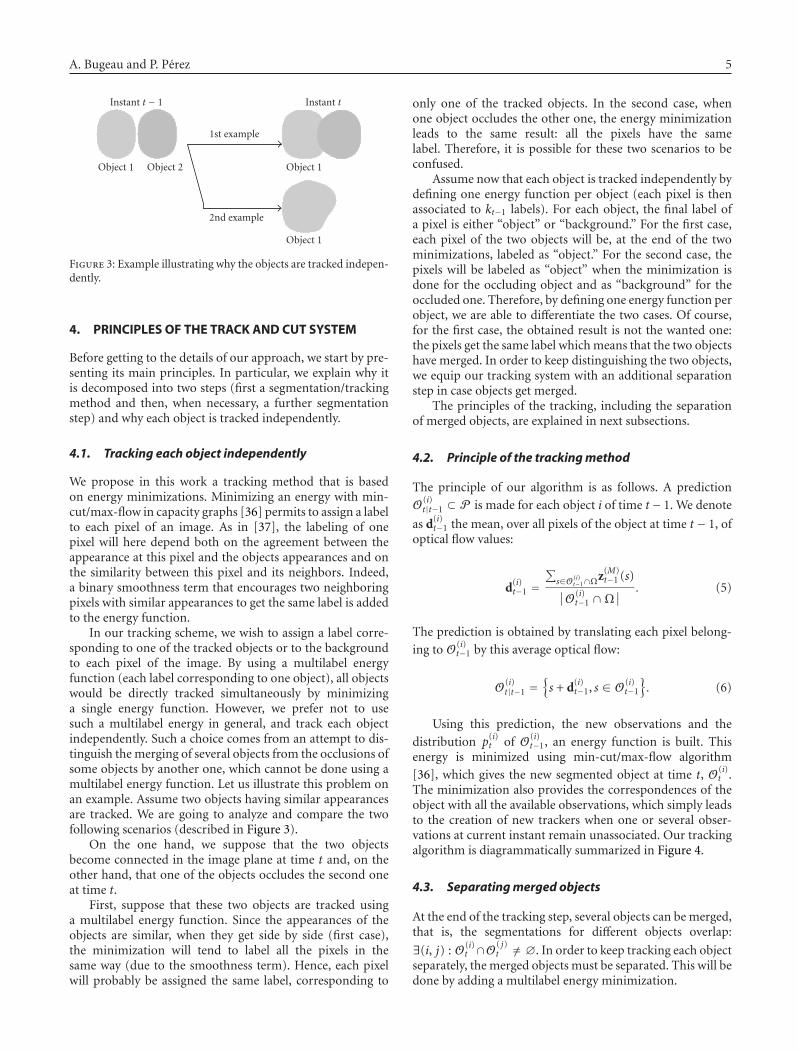
Figure 3: Example illustrating why the objects are tracked indepen-dently.
4. PRINCIPLES OF THE TRACK AND CUT SYSTEM
Before getting to the details of our approach, we start by pre-senting its main principles. In particular, we explain why itis decomposed into two steps (first a segmentation/trackingmethod and then, when necessary, a further segmentationstep) and why each object is tracked independently.
4.1. Tracking each object independently
We propose in this work a tracking method that is basedon energy minimizations. Minimizing an energy with min-cut/max-flow in capacity graphs [36] permits to assign a labelto each pixel of an image. As in [37], the labeling of onepixel will here depend both on the agreement between theappearance at this pixel and the objects appearances and onthe similarity between this pixel and its neighbors. Indeed,a binary smoothness term that encourages two neighboringpixels with similar appearances to get the same label is addedto the energy function.
In our tracking scheme, we wish to assign a label corre-sponding to one of the tracked objects or to the backgroundto each pixel of the image. By using a multilabel energyfunction (each label corresponding to one object), all objectswould be directly tracked simultaneously by minimizinga single energy function. However, we prefer not to usesuch a multilabel energy in general, and track each objectindependently. Such a choice comes from an attempt to dis-tinguish the merging of several objects from the occlusions ofsome objects by another one, which cannot be done using amultilabel energy function. Let us illustrate this problem onan example. Assume two objects having similar appearancesare tracked. We are going to analyze and compare the twofollowing scenarios (described in Figure 3).
On the one hand, we suppose that the two objectsbecome connected in the image plane at time t and, on theother hand, that one of the objects occludes the second oneat time t.
First, suppose that these two objects are tracked usinga multilabel energy function. Since the appearances of theobjects are similar, when they get side by side (first case),the minimization will tend to label all the pixels in thesame way (due to the smoothness term). Hence, each pixelwill probably be assigned the same label, corresponding to
only one of the tracked objects. In the second case, whenone object occludes the other one, the energy minimizationleads to the same result: all the pixels have the samelabel. Therefore, it is possible for these two scenarios to beconfused.
Assume now that each object is tracked independently bydefining one energy function per object (each pixel is thenassociated to kt−1 labels). For each object, the final label ofa pixel is either “object” or “background.” For the first case,each pixel of the two objects will be, at the end of the twominimizations, labeled as “object.” For the second case, thepixels will be labeled as “object” when the minimization isdone for the occluding object and as “background” for theoccluded one. Therefore, by defining one energy function perobject, we are able to differentiate the two cases. Of course,for the first case, the obtained result is not the wanted one:the pixels get the same label which means that the two objectshave merged. In order to keep distinguishing the two objects,we equip our tracking system with an additional separationstep in case objects get merged.
The principles of the tracking, including the separationof merged objects, are explained in next subsections.
4.2. Principle of the tracking method
The principle of our algorithm is as follows. A prediction
O(i)t|t−1 ⊂ P is made for each object i of time t− 1. We denote
as d(i)t−1 the mean, over all pixels of the object at time t − 1, of
optical flow values:
d(i)t−1 =
∑s∈O(i)
t−1∩Ωz(M)t−1 (s)
∣∣O(i)t−1 ∩Ω
∣∣ . (5)
The prediction is obtained by translating each pixel belong-
ing to O(i)t−1 by this average optical flow:
O(i)t|t−1 =
{s + d(i)
t−1, s ∈ O(i)t−1
}. (6)
Using this prediction, the new observations and the
distribution p(i)t of O(i)
t−1, an energy function is built. Thisenergy is minimized using min-cut/max-flow algorithm
[36], which gives the new segmented object at time t, O(i)t .
The minimization also provides the correspondences of theobject with all the available observations, which simply leadsto the creation of new trackers when one or several obser-vations at current instant remain unassociated. Our trackingalgorithm is diagrammatically summarized in Figure 4.
4.3. Separating merged objects
At the end of the tracking step, several objects can be merged,that is, the segmentations for different objects overlap:
∃(i, j) : O(i)t ∩O
( j)t /= ∅. In order to keep tracking each object
separately, the merged objects must be separated. This will bedone by adding a multilabel energy minimization.
6 EURASIP Journal on Image and Video Processing
5. ENERGY FUNCTIONS
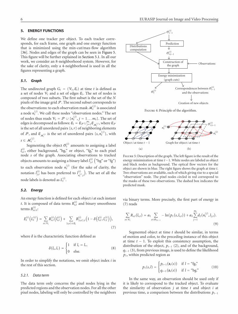
We define one tracker per object. To each tracker corre-sponds, for each frame, one graph and one energy functionthat is minimized using the min-cut/max-flow algorithm[36]. Nodes and edges of the graph can be seen in Figure 5.This figure will be further explained in Section 5.1. In all ourwork, we consider an 8-neighborhood system. However, forthe sake of clarity, only a 4-neighborhood is used in all thefigures representing a graph.
5.1. Graph
The undirected graph Gt = (Vt, Et) at time t is defined asa set of nodes Vt and a set of edges Et . The set of nodes iscomposed of two subsets. The first subset is the set of the Npixels of the image grid P . The second subset corresponds to
the observations: to each observation mask M( j)t is associated
a node n( j)t . We call these nodes “observation nodes.” The set
of nodes thus reads Vt = P ∪ {n( j)t , j = 1 . . .mt}. The set of
edges is decomposed as follows: Et = EP∪mtj=1EM
( j)t
, where EP
is the set of all unordered pairs {s, r} of neighboring elements
of P , and EM
( j)t
is the set of unordered pairs {s,n( j)t }, with
s ∈M( j)t .
Segmenting the object O(i)t amounts to assigning a label
l(i)s,t , either background, ”bg,” or object, “fg,” to each pixelnode s of the graph. Associating observations to tracked
objects amounts to assigning a binary label l(i)j,t(
“bg” or “fg”)
to each observation node n( j)t (for the sake of clarity, the
notation l(i)j,t has been preferred to l(i)n
( j)t ,t
). The set of all the
node labels is denoted as L(i)t .
5.2. Energy
An energy function is defined for each object i at each instant
t. It is composed of data terms R(i)s,t and binary smoothness
terms B(i)s,r,t:
E(i)t
(L(i)t
)=∑
s∈Vt
R(i)s,t
(l(i)s,t)
+∑
{s,r}∈Et
B(i){s,r},t
(1− δ
(l(i)s,t , l
(i)r,t
)),
(7)
where δ is the characteristic function defined as
δ(ls, lr
) =⎧⎨⎩
1 if ls = lr ,
0 else.(8)
In order to simplify the notations, we omit object index i inthe rest of this section.
5.2.1. Data term
The data term only concerns the pixel nodes lying in thepredicted regions and the observation nodes. For all the otherpixel nodes, labeling will only be controlled by the neighbors
Prediction
Observations
O(i)t−1
O(i)t|t−1
O(i)t
Creation of new objects
Distributionscomputation
Construction ofthe graph
Energy minimization(graph cuts)
Correspondences between O(i)t−1
and the observations
Figure 4: Principle of the algorithm.
Object i at time t − 1
(a)
Graph for object i at time t
n(1)t
n(2)t
O(i)t|t−1
(b)
Figure 5: Description of the graph. The left figure is the result of theenergy minimization at time t−1. White nodes are labeled as objectand black nodes as background. The optical flow vectors for theobject are shown in blue. The right figure shows the graph at time t.Two observations are available, each of which giving rise to a special“observation” node. The pixel nodes circled in red correspond tothe masks of these two observations. The dashed box indicates thepredicted mask.
via binary terms. More precisely, the first part of energy in(7) reads
∑
s∈Vt
Rs,t(ls,t) = α1
∑
s∈Ot|t−1
− ln(p1(s, ls,t
))+ α2
mt∑
j=1
d2(n
( j)t , l j,t
).
(9)
Segmented object at time t should be similar, in termsof motion and color, to the preceding instance of this objectat time t − 1. To exploit this consistency assumption, thedistribution of the object, pt−1 (2), and of the background,qt−1 (3), from previous image, is used to define the likelihoodp1, within predicted region as
p1(s, l) =⎧⎨⎩pt−1
(zt(s)
)if l = “fg,”
qt−1(
zt(s))
if l = “bg.”(10)
In the same way, an observation should be used only ifit is likely to correspond to the tracked object. To evaluatethe similarity of observation j at time t and object i atprevious time, a comparison between the distributions pt−1

A. Bugeau and P. Perez 7
and ρ( j)t (4) and between qt−1 and ρ
( j)t must be performed
through the computation of a distance measure. A classicaldistance to compare two mixtures of Gaussians, G1 and G2,is the Kullback-Leibler divergence [38], defined as
KL(G1,G2
) =∫G1(x) log
G1(x)G2(x)
dx. (11)
This asymmetric function measures how well distributionG2 mimics the variations of distribution G1. Here, we wantto know if the observations belongs to the object or tothe background but not the opposite, and therefore we willmeasure if one or several observations belong to one object.The data term d2 is then
d2(s, l) =⎧⎪⎨⎪⎩
KL(ρ
( j)t , pt−1
)if l = “fg,”
KL(ρ
( j)t , qt−1
)if l = “bg.”
(12)
Two constants α1 and α2 are included in the data term in(9) to give more or less influence to the observations. In ourexperiments, they were both fixed to 1.
5.2.2. Binary term
Following [37], the binary term between neighboring pairsof pixels {s, r} of P is based on color gradients and has theform
B{s,r},t = λ11
dist(s, r)e−(‖z(C)
t (s)−z(C)t (r)‖2)/σ2
T . (13)
As in [39], the parameter σT is set to σT = 4·〈(z(C)t (s) −
z(C)t (r))2〉, where 〈·〉 denotes expectation over a box sur-
rounding the object.For graph edges between one pixel node and one
observation node, the binary term depends on the distancebetween the color of the observation and the pixel color.More precisely, this term discourages the cut of an edgelinking one pixel to an observation node, if this pixel has ahigh probability (through its color and motion) to belongto the corresponding observation. This binary term is thencomputed as
B{s,n( j)t },t = λ2ρ
( j)t
(z(C)t (s)
). (14)
Parameters λ1 and λ2 are discussed in the experiments.
5.2.3. Energy minimization
The final labeling of pixels is obtained by minimizing,with the min-cut/max-flow algorithm proposed in [40], theenergy defined above:
L (i)t = arg min
L(i)t
E(i)t
(L(i)t
). (15)
This labeling finally gives the segmentation of the ith objectat time t as
O(i)t =
{s ∈ P : l (i)
s,t = “fg”}. (16)
(a) Result of the tracking algorithm.3 objects have merged
(b) Corresponding graph
Figure 6: Graph example for the segmentation of merged objects.
5.3. Creation of new objects
One advantage of our approach lies in its ability to jointlymanipulate pixel labels and track-to-detection assignmentlabels. This allows the system to track and segment theobjects at time t, while establishing the correspondencesbetween an object currently tracked and all the approxima-tive candidate objects obtained by detection in the currentframe. If, after the energy minimization for an object i, an
observation node n( j)t is labeled as “fg” (l (i)
t, j = “fg”) it meansthat there is a correspondence between the ith object and thejth observation. Conversely, if the node is labeled as “bg,” theobject and the observation are not associated.
If for all the objects (i = 1, . . . , kt−1), an observation node
is labeled as “bg” (∀i, l (i)t, j = “bg”), then the corresponding
observation does not match any object. In this case, a newobject is created and initialized with this observation. Thenumber of tracked objects becomes kt = kt−1 + 1, and thenew object is initialized as
O(kt)t =M
( j)t . (17)
In practice, the creation of a new object will be onlyvalidated, if the new object is associated to at least oneobservation at time t + 1, that is, if ∃ j ∈ {1, . . . ,mt+1} such
that l (kt)j,t+1 = “fg.”
6. SEGMENTING MERGED OBJECTS
Assume now that the results of the segmentations for differ-ent objects overlap, that is to say
∃(i, j), O(i)t ∩O
( j)t /= ∅. (18)
In this case, we propose an additional step to determinewhether these segmentation masks truly correspond to thesame object or if they should be separated. At the end of thisstep, each pixel must belong to only one object.
Let us introduce the notation
F = {i ∈ {1, . . . , kt} | ∃ j /= i such that O(i)
t ∩O( j)t /= ∅
}.
(19)
A new graph Gt = (Vt, Et) is created, where Vt = ∪i∈F O(i)t
and Et is composed of all unordered pairs of neighboringpixel nodes in Vt. An example of such a graph is presentedin Figure 6.

8 EURASIP Journal on Image and Video Processing
(a) (b) (c)
Figure 7: Results on sequence from PETS 2006 (frames 81, 116, 146, 176, 206, and 248): (a) original frames, (b) result of simple backgroundsubtraction and extracted observations, and (c) tracked objects on current frame using the primary and the secondary energy functions.

A. Bugeau and P. Perez 9
The goal is then to assign to each node s of Vt a labelψs ∈ F . Defining L = {ψs, s ∈ Vt} the labeling of Vt, a newenergy is defined as
Et(L) =∑
s∈Vt
− ln(p3(s,ψs
))
+ λ3
∑
{s,r}∈Et
1dist(s, r)
e−(‖z(C)s −z(C)
r ‖2)/σ23(1− δ(ψs,ψr
)).
(20)
The parameter σ3 is here set as σ3 = 4·〈(zt(s)(i,C)−zt(r)
(i,C))2〉with the averaging being over i ∈ F and {s, r} ∈ E . Thefact that several objects have been merged shows that theirrespective feature distributions at previous instant did notpermit to distinguish them. A way to separate them is thento increase the role of the prediction. This is achieved bychoosing function p3 as
p3(s,ψ) =⎧⎨⎩p
(ψ)t−1
(zt(s)
)if s /∈ O
(ψ)t|t−1,
1 otherwise.(21)
This multilabel energy function is minimized using theexpansion move algorithm [36, 41]. The convergence tothe global optimal solution with this algorithm cannot beproved. Only the convergence to a locally optimal solutionis guaranteed. Still, in all our experiments, this methodgave satisfactory results. After this minimization, the objects
O(i)t , i ∈ F are updated.
7. EXPERIMENTAL RESULTS
This section presents various results of joint tracking/seg-mentation, including cases, where merged objects have tobe separated in a second step. First, we will consider arelatively simple sequence, with static background, in whichthe observations are obtained by background subtraction(Section 3.2.1). Next, the tracking method will be com-bined to the moving objects detector introduced in [2](Section 3.2.2).
7.1. Tracking objects detected withbackground subtraction
In this section, tracking results obtained on a sequencefrom the PETS 2006 data corpus (sequence 1 camera 4) arepresented. They are followed by an experimental analysis ofthe first energy function (7). More precisely, the influence ofeach of its four terms (two for the data part and two for thesmoothness part) is shown in the same image.
7.1.1. A first tracking result
We start by demonstrating the validity of the approach,including its robustness to partial occlusions and its abilityto segment individually objects that were initially merged.
Following [39], the parameter λ3 was set to 20. However,parameters λ1 and λ2 had to be tuned by hand to get better
results (λ1 = 10, λ2 = 2). Also, the number of classes for theGaussian mixture models was set to 10.
First results (Figure 7) demonstrate the good behaviorof our algorithm even in the presence of partial occlusionsand of object fusion. Observations, obtained by subtractinga reference frame (frame 10 shown in Figure 1(a)) to thecurrent one, are visible in the second column of Figure 7,the third column contains the segmentation of the objectswith the subsequent use of the second energy function. Inframe 81, two objects are initialized using the observations.Note that the connected component extracted with the“gap/mountain” method misses the legs for the person inthe upper right corner. While this has an impact on theinitial segmentation, the legs are recovered in the finalsegmentation as soon as the following frame.
Let us also underline the fact that the proposed methodeasily deals with the entrance of new objects in the scene.This result also shows the robustness of our method to partialocclusions. For example, partial occlusions occur when theperson at the top passes behind the three other ones (frames176 and 206). Despite the similar color of all the objects, thisis well handled by the method, as the person is still trackedwhen the occlusion stops (frame 248).
Finally note that even if from frame 102, the two personsat the bottom correspond to only one observation and havea similar appearance (color and motion), our algorithmtracks each person separately (frames 116, 146) thanks to thesecond energy function. In Figure 8, we show in more detailsthe influence of the second energy function by comparingthe results obtained with and without it. Before frame 102,the three persons at the bottom generate three distinctobservations, while, passed this instant, they correspond toonly one or two observations. Even if the motions and colorsof the three persons are very close, the use of the secondmultilabel energy function allows their separation.
7.1.2. A qualitative analysis of the first energy function
We now propose an analysis of the influence on the resultsof each of the four terms of the energy defined in (7). Theweight of each of these terms is controlled by a parameter.Indeed, we remind that the complete energy function hasbeen defined as
Et(Lt) =∑
s∈Vt
[α1
∑
s∈Ot|t−1
− ln(P1(s, ls,t
))+ α2
mt∑
j=1
d2(n
( j)t , l j,t
)]
+ λ1
∑
{s,r}∈EP
B{s,r},t(1− δ(ls,t, lr,t
))
+ λ2
mt∑
j=1
∑
{s,r}∈EM
( j)t
B{s,r},t(1− δ(ls,t, lr,t
)).
(22)
To show the influence of each term, we successively setone of the parameters λ1, λ2, α1, and α2 to zero. The resultson a frame from the PETS sequence are visible on Figure 9.Figure 9(a) presents the original image, Figure 9(b) presetsthe extracted observation after background subtraction, and

10 EURASIP Journal on Image and Video Processing
(a) (b) (c)
Figure 8: Separating merged objects with the secondary minimization (frames 101 and 102): (a) result of simple background subtraction andextracted observations, (b) segmentations with the first energy functions only, and (c) segmentation after postprocessing with the secondaryenergy function.
(a) Original image (b) Extracted observations (c) Tracked object (d) Tracked object if λ1 = 0
(e) Tracked object if λ2 = 0 (f) Tracked object if α1 = 0 (g) Tracked object if α2 = 0
Figure 9: Influence of each term of the first energy function on the frame 820 of the PETS sequence.
Figure 9(c) presents the tracked object when using thecomplete energy equation (22) with λ1 = 10, λ2 = 2, α1 = 1,and α2 = 2.
If the parameter λ1 is equal to zero, it means thatno spatial regularization is applied to the segmentation.The final mask of the object then only depends on theprobability of each pixel to belong to the object, thebackground, and the observations. That is the reason whythe object is not well segmented in Figure 9(d). If λ2 =0, the observations do not influence the segmentation ofthe object. As can been seen in Figure 9(e), it can leadto a slight undersegmentation of the object. In the casethat α2 = 0, the labeling of an observation node onlydepends on the labels of the pixels belonging to thisobservation. Therefore, this term mainly influences theassociation between the observations and the tracked objects.Nevertheless, as can be seen in Figure 9(g), it also slightlymodifies the mask of a tracked object, and switching it offmight produce an undersegmentation of the object. Finally,when α1 = 0, the energy minimization yields to the spatialregularization of the observation mask thanks to the binary
smoothness term. The mask of the object then stops on thestrong contours but does not take into account the colorand motion of the pixels belonging to the prediction. InFigure 9(f), this leads to an oversegmentation of the objectcompared to the segmentation of the object at previous timeinstants.
This experiment illustrates that each term of the energyfunction plays a role of its own on the final segmentation ofthe tracked objects.
7.2. Tracking objects in complex scenes
We are now showing the behavior of our tracking algo-rithm when the sequences are more complex (dynamicbackground, moving camera, etc.). For each sequence, theobservations are the moving clusters detected with themethod of [2]. In all this subsection, the parameter λ3 wasset to 20, λ1 to 10, and λ2 to 1.
The first result is on a water skier sequence (Figure 10).For each image, the moving clusters and the masks
of the tracked objects are superimposed on the original

A. Bugeau and P. Perez 11
t = 80
t = 58
t = 51
t = 31
(a)
t = 243
t = 225
t = 215
t = 177
(b)
Figure 10: Results on a water skier sequence. The observations are moving clusters detected with the method in [2]. At each time instant,the observations are shown in the left image, while the masks of the tracked objects are shown in the right image.
image. The proposed tracking method permits to correctlytrack the water skier (or more precisely his wet suit) allalong the sequence, despite fast trajectory changes, drasticdeformations, and moving surroundings. As can be seenin the figure (e.g., at time 58), the detector sometimesfails to detect the skier. No observations are availablein these cases. However, by using the prediction of theobject, our method handles well such situations and keepstracking and segmenting correctly the skier. This showsthe robustness of the algorithm to missing observations.However, if some observations are missing for severalconsecutive frames, the segmentation can get deteriorated.Conversely, this means that the incorporation of the obser-vations produced by the detection module enables to getbetter segmentations than when using only predictions. Onseveral frames, moving clusters are detected in the water.Nevertheless, no objects are created in concerned areas.The reason is that the creation of a new object is onlyvalidated, if the new object is associated to at least oneobservation in the following frame. This never happened inthe sequence.
We end by showing results on a driver sequence(Figure 11). The first object detected and tracked is the face.Once again, tracking this object shows the robustness of ourmethod to missing observations. Indeed, even if from frame19, the face does not move and therefore is not detected, thealgorithm keeps tracking and segmenting it correctly untilthe driver starts turning it. The most important result onthis sequence is the tracking of the hands. In image 39, themasks of the two hands are merged: they have a few pixels incommon. The step of segmentation of merged objects is thenapplied and allows the correct separation of the two masks,which permits to keep tracking these two objects separately.Finally, as can been seen on frame 57, our method deals wellwith the exit of an object from the scene.
8. CONCLUSION
In this paper, we have presented a new method thatsimultaneously segments and tracks multiple objects invideos. Predictions along with observations composed ofdetected objects are combined in an energy function which

12 EURASIP Journal on Image and Video Processing
t = 35
t = 29
t = 16
t = 13
(a)
t = 63
t = 57
t = 43
t = 39
(b)
Figure 11: Results on a driver sequence. The observations are moving clusters detected with the method in [2]. At each time instant, theobservations are shown in the left image, while the masks of the tracked objects are shown in the right image.
is minimized with graph cuts. The use of graph cuts permitsthe segmentation of the objects at a modest computationalcost, leaving the computational bottleneck at the level of thedetection of objects and of the computation of GMMs.
An important novelty is the use of observation nodesin the graph which gives better segmentations but alsoenables the direct association of the tracked objects to theobservations (without adding any association procedure).The observations used in this paper are obtained firstly bya simple background subtraction based on a single referenceframe and secondly by a more sophisticated moving objectdetector. Note however that any object detection methodcould be used as well, with no change to the approach, assoon as the observations can be represented by a set of pixels.
The proposed method combines the main advantages ofeach of the three categories of existing methods presented inSection 2. It deals with the entrance of new objects in thescene and the exit of existing ones, as “detect-before-track”methods do; as silhouette tracking methods, the energyminimization directly outputs the segmentation mask of theobjects; it allows robust tracking in a wide range of color
videos thanks to the use of global distributions, as with otherkernel tracking algorithms.
As shown in the experiments, the algorithm is robustto partial occlusions and to missing observations anddoes not require accurate observations to provide goodsegmentations. Also, several observations can correspond toone object (water skier sequence) and several objects cancorrespond to one observation (PETS sequence). Thanks tothe use of a second multilabel energy function, our methodallows individual tracking and segmentation of objects whichwere not distinguished from each other in the first stage.
As we use feature distributions of objects at previoustime to define current energy functions, our method handlesprogressive illumination changes but breaks down in extremecases of abrupt illumination changes. However, by adding anexternal detector of such changes, we could circumvent thisproblem by keeping only the prediction and by updating thereference frame when the abrupt change occurs.
Also, other cues, such as shapes, could probably beadded to improve the results. The problem would then beto introduce such a global feature into the energy function.
A. Bugeau and P. Perez 13
As it turns out, it is difficult to add a global term in anenergy function that is minimized by graph cuts. Anothersolution could be to select a compact characterization ofthe shape (e.g., pose parameters [42], ellipse parameters[43], normalized central moments [44], or some top-downknowledge [45]) and to add a term such as the face energyterm proposed in [43] into the energy function.
Apart from these rather specific problems, severalresearch directions are open. One of them concerns thedesign of an unifying energy framework that would allowsegmentation and tracking of multiple objects, while pre-cluding the incorrect merging of similar objects getting closeto each other in the image plane. Another direction ofresearch concerns the automatic tuning of the parameters,which remains an open problem in the recent literature onimage labeling (e.g., figure/ground segmentation) with graphcuts.
REFERENCES
[1] A. Yilmaz, O. Javed, and M. Shah, “Object tracking: a survey,”ACM Computing Surveys, vol. 38, no. 4, p. 13, 2006.
[2] A. Bugeau and P. Perez, “Detection and segmentation ofmoving objects in highly dynamic scenes,” in Proceedings ofthe IEEE Computer Society Conference on Computer Vision andPattern Recognition (CVPR ’07), pp. 1–8, Minneapolis, Minn,USA, June 2007.
[3] A. Bugeau and P. Perez, “Track and cut: simultaneoustracking and segmentation of multiple objects with graphcuts,” in Proceedings of the 3rd International Conference onComputer Vision Theory and Applications (VISAPP ’08), pp.1–8, Madeira, Portugal, January 2008.
[4] R. Kalman, “A new approach to linear filtering and predictionproblems,” Journal of Basic Engineering, vol. 82, pp. 35–45,1960.
[5] N. J. Gordon, D. J. Salmond, and A. F. M. Smith, “Novelapproach to nonlinear/non-Gaussian Bayesian state estima-tion,” IEE Proceedings F: Radar and Signal Processing, vol. 140,no. 2, pp. 107–113, 1993.
[6] D. Reid, “An algorithm for tracking multiple targets,” IEEETransactions on Automatic Control, vol. 24, no. 6, pp. 843–854,1979.
[7] I. J. Cox, “A review of statistical data association techniques formotion correspondence,” International Journal of ComputerVision, vol. 10, no. 1, pp. 53–66, 1993.
[8] Y. Bar-Shalom and X. Li, Estimation and Tracking: Principles,Techniques, and Software, Artech House, Boston, Mass, USA,1993.
[9] Y. Bar-Shalom and X. Li, Multisensor-Multitarget Tracking:Principles and Techniques, YBS Publishing, Storrs, Conn, USA,1995.
[10] D. Terzopoulos and R. Szeliski, “Tracking with Kalmansnakes,” in Active Vision, pp. 3–20, MIT Press, Cambridge,Mass, USA, 1993.
[11] M. Isard and A. Blake, “Condensation—conditional densitypropagation for visual tracking,” International Journal ofComputer Vision, vol. 29, no. 1, pp. 5–28, 1998.
[12] J. MacCormick and A. Blake, “A probabilistic exclusionprinciple for tracking multiple objects,” International Journalof Computer Vision, vol. 39, no. 1, pp. 57–71, 2000.
[13] N. Paragios and R. Deriche, “Geodesic active regions formotion estimation and tracking,” in Proceedings of the 7thIEEE International Conference on Computer Vision (ICCV ’99),vol. 1, pp. 688–694, Kerkyra, Greece, September 1999.
[14] A. Criminisi, G. Cross, A. Blake, and V. Kolmogorov, “Bilayersegmentation of live video,” in Proceedings of the IEEEComputer Society Conference on Computer Vision and PatternRecognition (CVPR ’06), vol. 1, pp. 53–60, New York, NY, USA,June 2006.
[15] N. Paragios and G. Tziritas, “Adaptive detection and localiza-tion of moving objects in image sequences,” Signal Processing:Image Communication, vol. 14, no. 4, pp. 277–296, 1999.
[16] Y. Shi and W. C. Karl, “Real-time tracking using level sets,”in Proceedings of the IEEE Computer Society Conference onComputer Vision and Pattern Recognition (CVPR ’05), vol. 2,pp. 34–41, San Diego, Calif, USA, June 2005.
[17] M. Bertalmio, G. Sapiro, and G. Randall, “Morphing activecontours,” IEEE Transactions on Pattern Analysis and MachineIntelligence, vol. 22, no. 7, pp. 733–737, 2000.
[18] D. Cremers and C. Schnorr, “Statistical shape knowledge invariational motion segmentation,” Image and Vision Comput-ing, vol. 21, no. 1, pp. 77–86, 2003.
[19] A.-R. Mansouri, “Region tracking via level set PDEs withoutmotion computation,” IEEE Transactions on Pattern Analysisand Machine Intelligence, vol. 24, no. 7, pp. 947–961, 2002.
[20] R. Ronfard, “Region-based strategies for active contour mod-els,” International Journal of Computer Vision, vol. 13, no. 2,pp. 229–251, 1994.
[21] A. Yilmaz, X. Li, and M. Shah, “Contour-based object trackingwith occlusion handling in video acquired using mobilecameras,” IEEE Transactions on Pattern Analysis and MachineIntelligence, vol. 26, no. 11, pp. 1531–1536, 2004.
[22] N. Xu and N. Ahuja, “Object contour tracking using graphcuts based active contours,” in Proceedings of the IEEEInternational Conference on Image Processing (ICIP ’02), vol.3, pp. 277–280, Rochester, NY, USA, September 2002.
[23] J. Shi and C. Tomasi, “Good features to track,” in Proceedingsof the IEEE Conference on Computer Vision and PatternRecognition (CVPR ’94), pp. 593–600, Seattle, Wash, USA,June 1994.
[24] D. Comaniciu, V. Ramesh, and P. Meer, “Real-time trackingof non-rigid objects using mean shift,” in Proceedings of theIEEE Computer Society Conference on Computer Vision andPattern Recognition (CVPR ’00), vol. 2, pp. 142–149, HiltonHead Island, SC, USA, June 2000.
[25] D. Comaniciu, V. Ramesh, and P. Meer, “Kernel-based opticaltracking,” IEEE Transactions on Pattern Analysis and MachineIntelligence, vol. 25, no. 5, pp. 564–577, 2003.
[26] D. Freedman and M. W. Turek, “Illumination-invarianttracking via graph cuts,” in Proceedings of the IEEE ComputerSociety Conference on Computer Vision and Pattern Recognition(CVPR ’05), vol. 2, pp. 10–17, San Diego, Calif, USA, June2005.
[27] R. Kjeldsen and J. Kender, “Finding skin in color images,” inProceedings of the 2nd International Conference on AutomaticFace and Gesture Recognition (FG ’96), pp. 312–317, Killington,Vt, USA, October 1996.
[28] M. Singh and N. Ahuja, “Regression based bandwidth selec-tion for segmentation using Parzen windows,” in Proceedingsof the 9th IEEE International Conference on Computer Vision(ICCV ’03), vol. 1, pp. 2–9, Nice, France, October 2003.

14 EURASIP Journal on Image and Video Processing
[29] B. D. Lucas and T. Kanade, “An iterative technique of imageregistration and its application to stereo,” in Proceedings ofthe 7th International Joint Conference on Artificial Intelligence(IJCAI ’81), Vancouver, Canada, August 1981.
[30] A. D. Jepson, D. J. Fleet, and T. F. El-Maraghi, “Robust onlineappearance models for visual tracking,” IEEE Transactions onPattern Analysis and Machine Intelligence, vol. 25, no. 10, pp.1296–1311, 2003.
[31] H. T. Nguyen and A. W. M. Smeulders, “Fast occluded objecttracking by a robust appearance filter,” IEEE Transactions onPattern Analysis and Machine Intelligence, vol. 26, no. 8, pp.1099–1104, 2004.
[32] O. Juan and Y. Boykov, “Active graph cuts,” in Proceedings ofthe IEEE Computer Society Conference on Computer Vision andPattern Recognition (CVPR ’06), vol. 1, pp. 1023–1029, NewYork, NY, USA, June 2006.
[33] P. Kohli and P. Torr, “Effciently solving dynamic markovrandom fields using graph cuts,” in Proceedings of the 10thIEEE International Conference on Computer Vision (ICCV ’05),pp. 922–929, Beijing, China, October 2005.
[34] Y. Wang, J. F. Doherty, and R. E. Van Dyck, “Moving objecttracking in video,” in Proceedings of the 29th Applied ImageryPattern Recognition Workshop (AIPR ’00), p. 95, Washington,DC, USA, October 2000.
[35] D. Comaniciu and P. Meer, “Mean shift: a robust approachtoward feature space analysis,” IEEE Transactions on PatternAnalysis and Machine Intelligence, vol. 24, no. 5, pp. 603–619,2002.
[36] Y. Boykov, O. Veksler, and R. Zabih, “Fast approximate energyminimization via graph cuts,” IEEE Transactions on PatternAnalysis and Machine Intelligence, vol. 23, no. 11, pp. 1222–1239, 2001.
[37] Y. Boykov and M.-P. Jolly, “Interactive graph cuts for optimalboundary & region segmentation of objects in N-D images,”in Proceedings of the 8th IEEE International Conference onComputer Vision (ICCV ’01), vol. 1, pp. 105–112, Vancouver,Canada, July 2001.
[38] S. Kullback and R. A. Leibler, “On information and suffi-ciency,” Annals of Mathematical Statistics, vol. 22, no. 1, pp.79–86, 1951.
[39] A. Blake, C. Rother, M. Brown, P. Perez, and P. Torr,“Interactive image segmentation using an adaptive GMMRFmodel,” in Proceedings of the 8th European Conference onComputer Vision (ECCV ’04), pp. 428–441, Prague, CzechRepublic, May 2004.
[40] Y. Boykov and V. Kolmogorov, “An experimental comparisonof min-cut/max-flow algorithms for energy minimization invision,” IEEE Transactions on Pattern Analysis and MachineIntelligence, vol. 26, no. 9, pp. 1124–1137, 2004.
[41] Y. Boykov, O. Veksler, and R. Zabih, “Markov random fieldswith efficient approximations,” in Proceedings of the IEEEComputer Society Conference on Computer Vision and PatternRecognition (CVPR ’98), pp. 648–655, Santa Barbara, Calif,USA, June 1998.
[42] M. Bray, P. Kohli, and P. Torr, “PoseCut: simultaneous seg-mentation and 3D pose estimation of humans using dynamicgraph-cuts,” in Proceedings of the 9th European Conference onComputer Vision (ECCV ’06), pp. 642–655, Graz, Austria, May2006.
[43] J. Rihan, P. Kohli, and P. Torr, “Objcut for face detection,” inProceedings of the 4th Indian Conference on Computer Vision,Graphics and Image Processing (ICVGIP ’06), pp. 861–871,Madurai, India, December 2006.
[44] L. Zhao and L. S. Davis, “Closely coupled object detection andsegmentation,” in Proceedings of the 10th IEEE InternationalConference on Computer Vision (ICCV ’05), vol. 1, pp. 454–461, Beijing, China, October 2005.
[45] D. Ramanan, “Using segmentation to verify object hypothe-ses,” in Proceedings of the IEEE Computer Society Conferenceon Computer Vision and Pattern Recognition (CVPR ’07),Minneapolis, Minn, USA, June 2007.

Hindawi Publishing CorporationEURASIP Journal on Image and Video ProcessingVolume 2008, Article ID 256896, 16 pagesdoi:10.1155/2008/256896
Research ArticleIterative Object Localization Algorithm Using Visual Imageswith a Reference Coordinate
Kyoung-Su Park,1 Jinseok Lee,1 Milutin Stanacevic,1 Sangjin Hong,1 and We-Duke Cho2
1 Mobile Systems Design Laboratory, Department of Electrical and Computer Engineering, Stony Brook University,Stony Brook, NY 11794, USA
2 Department of Electronics Engineering, College of Information Technology, Ajou University, Suwon 443-749, South Korea
Correspondence should be addressed to We-Duke Cho, [email protected]
Received 29 July 2007; Revised 11 March 2008; Accepted 4 July 2008
Recommended by Carlo Regazzoni
We present a simplified algorithm for localizing an object using multiple visual images that are obtained from widely used digitalimaging devices. We use a parallel projection model which supports both zooming and panning of the imaging devices. Ourproposed algorithm is based on a virtual viewable plane for creating a relationship between an object position and a referencecoordinate. The reference point is obtained from a rough estimate which may be obtained from the preestimation process. Thealgorithm minimizes localization error through the iterative process with relatively low-computational complexity. In addition,nonlinearity distortion of the digital image devices is compensated during the iterative process. Finally, the performances of severalscenarios are evaluated and analyzed in both indoor and outdoor environments.
Copyright © 2008 Kyoung-Su Park et al. This is an open access article distributed under the Creative Commons AttributionLicense, which permits unrestricted use, distribution, and reproduction in any medium, provided the original work is properlycited.
1. INTRODUCTION
The object localization is one of the key operations in manytracking applications such as surveillance, monitoring andtracking [1–8].In these tracking systems, the accuracy of theobject localization is very critical and poses a considerablechallenge. Most of localization methods use geometricrelationship between the object and sensors. Acoustic sensorshave been widely used in many localization applicationsdue to their flexibility, low cost, and easy deployment. Theacoustic sensor provides directional information in angleof the source with respect to the sensor coordinates whichare used to create a geometry for localization. However,an acoustic sensor is extremely sensitive to its surroundingenvironment with noisy data and does not fully satisfy therequirement of consistent data [9]. Thus as a reliable trackingmethod, visual sensors are often used for tracking andmonitoring systems as well [10, 11]. The visual localizationhas a potential to yield noninvasive, accurate, and low-costsolution [12–14].
Multiple-image-based multiple-object detection andtracking are used in indoor and outdoor surveillance, andgive a delicate and complete history of an interested object’s
action [2, 15, 16]. The object tracking can be simplyconcerned into a 2D tracking problem on the groundplane [2, 17–19]. The establishment of correspondences inmultiple images can be achieved by using a field of viewlines [2, 20]. Besides, for the selection of the best view aboutinterested objects, a camera movement such as zooming andpanning is required [19].
There are many localization methods which use imagesensors [5, 6, 13, 21–25]. Most of conventional localizationmethods follow two steps of operation. Initially, the cameraparameters are computed offline using known objects orpattern images. Then using additional information such ascontrol points in the scene or techniques such as structurefrom motion, the relative displacements of a camera areestimated [21, 26]. Basically, these studies can sufficientlylocalize objects from 3D reconstruction. Once the sufficientnumber of points is observed in multiple images fromdifferent positions, it is mathematically possible to deducethe locations of the points as well as the positions of theoriginal cameras, up to a known factor of scale [21]. Inthe localization method based on a perspective projectionmodel, the camera calibration is critical. The calibrationusually uses a flat plate with a regular pattern [14, 27, 28].

2 EURASIP Journal on Image and Video Processing
However, in many applications, it is not easy to obtaincalibration patterns [29, 30]. In order to alleviate the effectof the calibration patterns, some methods based on self-calibration use the point matching from image sequences[29–34]. In these methods, the image feature extractionshould be very accurate since this procedure is very sensitiveto the noise [21, 27, 35]. Moreover, if a pair of stereo imagesfor a single scene is not calibrated and the motions betweentwo images are unknown, the image matching requiresprohibitively high complexity [27, 34–36].
The localization method based on the affine recon-struction can be used for object localization without theconcern of the complex calibration [37–40]. Basically, therelationships between physical space and geometric prop-erties of a set of cameras are considered. The methoduses two uncalibrated perspective images where an imageis induced by a plane to infinity [37–39, 41–44]. Especially,the factorization method based on the paraperspectiveprojection model can be used for localization [42, 44, 45]. In[42], three well-known approximations such as orthography,weak perspective and paraperspective are involved to full-perspective projection in the affine projection model. In [44,45], shape and motion recovery is used for less complexity indepth computation. However, the localization method basedon the affine structure requires at least five correspondencesin two images [37–39]. On the other hand, our proposedmethod requires only one correspondence (i.e., a centroidcoordinate of the detected object) in two images, whereeach correspondence represents the same object. Thus, thecritical requirements of an effective localization algorithm intracking applications are the computational simplicity witha simpler model where 3D reconstruction is not necessary aswell as the robust adaptation of camera’s movement duringtracking (i.e., zooming and panning) without requiring anyadditional imaging device calibration from the images. Thecontribution of this paper is to simplify localization methodwith efficiency which does not consider 3D reconstructionand complex calibration.
In this paper, we propose a simplified algorithm forlocalizing multiple objects in a multiple-camera environ-ment, where images are obtained from traditional digitalimaging devices. Figure 1 illustrates the application modelwhere multiple people are localized in a multiple-cameraenvironment. The cameras can freely move with zoomingand panning capabilities. Within a tracking environment, theproposed method uses detected object points to find objectlocation. We use the 2D global coordinate to represent theobject location. In our localization algorithm, the distancebetween an object and a camera is provided by a referencepoint. Since the reference point is initially a rough estimate,we are motivated to obtain a more accurate referencepoint. Here, we use an iterative process which substitutesa previously localized position with a new reference pointclose to a real-object location. In addition, the proposedlocalization method has an advantage of using a zoomingfactor without being concerned about a focal length. Thus,the computational complexity is simplified in determiningan object’s position which supports both zooming andpanning features. In addition, the localization algorithm
Camera 1
Camera 2
A
BC
Figure 1: Illustration of the model of application.
P
dp
Lc Oc
Ls
uppPp
u
Ppup
Viewablerange
Object plane
Virtual viewableplane
Actual cameraplane
Figure 2: Illustration of the parallel projection model.
sufficiently compensates a nonideal property such as opticalcharacteristics of a camera lens.
The rest of this paper is organized as follows. Section 2briefly describes a parallel projection model with a singlecamera. Section 3 illustrates the visual localization algorithmin a 2D coordinate with multiple cameras. In Section 4, wepresent analysis and simulation results where the localizationerrors are minimized by compensating for nonlinearity ofthe digital imaging devices. An application that uses theproposed algorithm for tracking people within a closedenvironment is illustrated. Section 5 concludes the paper.
2. CHARACTERIZATION OF VIEWABLE IMAGES
2.1. Basic concept of a parallel projection model
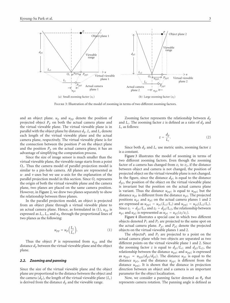
In this section, we introduce a parallel projection model tosimplify the visual localization, which is basically comprisedof three planes: an object plane, a virtual viewable plane andan actual camera plane. In Figure 2, an object P placed onan object plane is projected to both a virtual viewable planeand an actual camera plane, and Pp denotes the projectedobject point on the virtual viewable plane. The distancedp denotes the distance between a virtual viewable plane
Kyoung-Su Park et al. 3
P
dp1
Lc1
Oc
Ls
upp1 Ppp1u
Ppp1
up1
Viewablerange
Object plane 1
Virtual viewableplane 1
Actual cameraplane 1
(a) Small zooming factor (z1)
P
dp2
Lc2Oc
Lsupp2 Ppp2
u
Ppp2
up2
Viewablerange
Object plane 2
Virtual viewableplane 2
Actual cameraplane 2
(b) Large zooming factor (z2)
Figure 3: Illustration of the model of zooming in terms of two different zooming factors.
and an object plane. up and upp denote the position ofprojected object Pp on both the actual camera plane andthe virtual viewable plane. The virtual viewable plane is inparallel with the object plane by distance dp. Lc and Ls denoteeach length of the virtual viewable plane and the actualcamera plane, respectively. The virtual viewable plane is forthe connection between the position P on the object planeand the position Pp on the actual camera plane; it has anadvantage of simplifying the computation process.
Since the size of image sensor is much smaller than thevirtual viewable plane, the viewable range starts from a pointOc. Thus the camera model of parallel projection model issimilar to a pin-hole camera. All planes are represented asu- and v-axes but we use u-axis for the explanation of theparallel projection model in this section. Since Oc representsthe origin of both the virtual viewable plane and the cameraplane, two planes are placed on the same camera position.However, in Figure 2, we drew two planes separately to showthe relationship between three planes.
In the parallel projection model, an object is projectedfrom an object plane through a virtual viewable plane toan actual camera plane. Hence, as formulated in (1), upp isexpressed as Lc, Ls, and up through the proportional lines oftwo planes as the following:
upp = up
(LcLs
). (1)
Thus the object P is represented from upp and thedistance dp between the virtual viewable plane and the objectplane.
2.2. Zooming and panning
Since the size of the virtual viewable plane and the objectplane are proportional to the distance between the object andthe camera (dp), the length of the virtual viewable plane (Lc)is derived from the distance dp and the viewable range.
Zooming factor represents the relationship between dpand Lc. The zooming factor z is defined as a ratio of dp andLc as follows:
z = dpLc. (2)
Since both dp and Lc use metric units, zooming factor zis a constant.
Figure 3 illustrates the model of zooming in terms oftwo different zooming factors. Even though the zoomingfactor of a camera has changed from z1 to z2, if the distancebetween object and camera is not changed, the position ofprojected object on the virtual viewable plane is not changed.In the figure, since the distance dp1 is equal to the distancedp2, the position of the object on the virtual viewable planeis invariant but the position on the actual camera planeis variant. Thus the distance upp1 is equal to upp2 but thedistance up1 is different from the distance up2. The projectedpositions up1 and up2 on the actual camera planes 1 and 2are expressed as upp1 = up1(Lc1/Ls) and upp2 = up2(Lc2/Ls).Since z1 = dp1/Lc1 and z2 = dp2/Lc2, the relationship betweenup1 and up2 is represented as up1 = up2(z2/z1).
Figure 4 illustrates a special case in which two differentobjects denoted P1 and P2 are projected to the same spot onthe actual camera plane. Pp1 and Pp2 denote the projectedobjects on the virtual viewable planes 1 and 2.
The objectsP1 and P2 are projected to a point on theactual camera plane while two objects are separated as twodifferent points on the virtual viewable plane 1 and 2. Sincethe zooming factor z is equal to dp1/Lc1 and dp2/Lc2, therelationship between the distance upp1 and upp2 is expressedas upp1 = upp2(dp1/dp2). The distance up1 is equal to thedistance up2, and the distance upp1 is different from thedistance upp2. It is shown that the distance in projectiondirection between an object and a camera is an importantparameter for the object localization.
Now, we consider a panning factor denoted as θp thatrepresents camera rotation. The panning angle is defined as
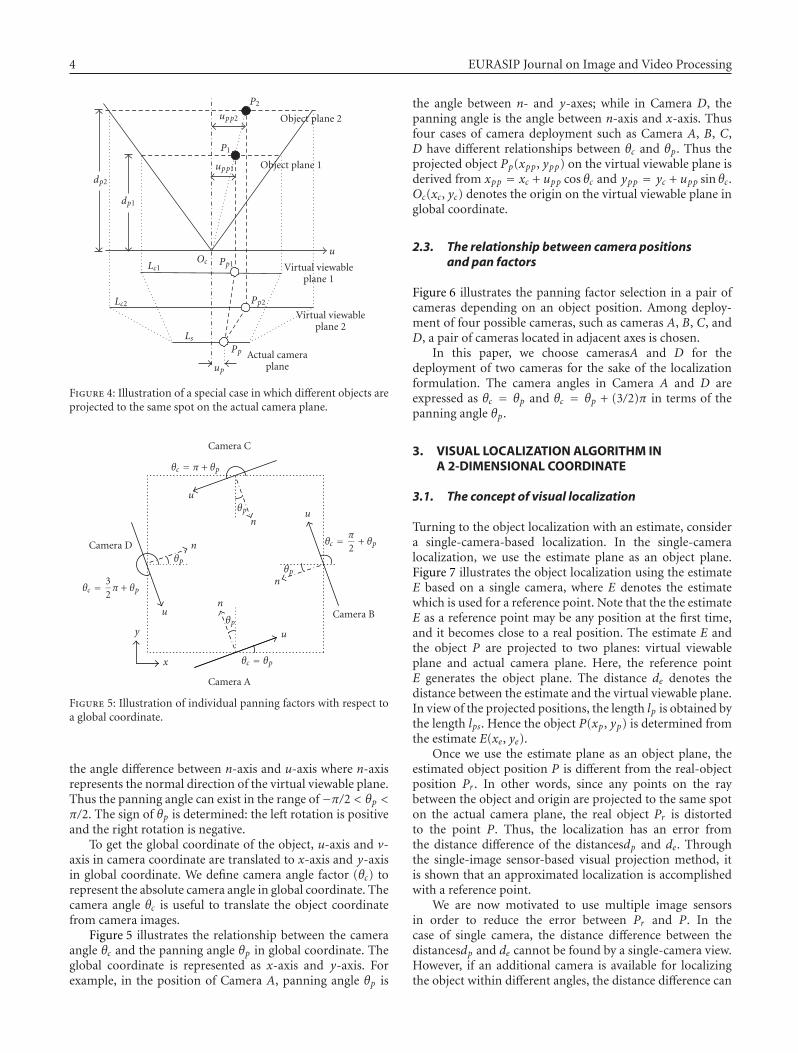
4 EURASIP Journal on Image and Video Processing
P2
upp2 Object plane 2
P1
upp1 Object plane 1
dp1
dp2
Lc1
Lc2
Oc
Ls
Pp1
Pp2
u
up
Virtual viewableplane 2
Actual cameraplane
Pp
Virtual viewableplane 1
Figure 4: Illustration of a special case in which different objects areprojected to the same spot on the actual camera plane.
Camera C
θp
θc = π + θp
u
n
Camera B
θp
θc = π
2+ θp
u
n
Camera A
θp
θc = θp
u
n
Camera Dθp
θc = 32π + θp
u
n
y
x
Figure 5: Illustration of individual panning factors with respect toa global coordinate.
the angle difference between n-axis and u-axis where n-axisrepresents the normal direction of the virtual viewable plane.Thus the panning angle can exist in the range of−π/2 < θp <π/2. The sign of θp is determined: the left rotation is positiveand the right rotation is negative.
To get the global coordinate of the object, u-axis and v-axis in camera coordinate are translated to x-axis and y-axisin global coordinate. We define camera angle factor (θc) torepresent the absolute camera angle in global coordinate. Thecamera angle θc is useful to translate the object coordinatefrom camera images.
Figure 5 illustrates the relationship between the cameraangle θc and the panning angle θp in global coordinate. Theglobal coordinate is represented as x-axis and y-axis. Forexample, in the position of Camera A, panning angle θp is
the angle between n- and y-axes; while in Camera D, thepanning angle is the angle between n-axis and x-axis. Thusfour cases of camera deployment such as Camera A, B, C,D have different relationships between θc and θp. Thus theprojected object Pp(xpp, ypp) on the virtual viewable plane isderived from xpp = xc + upp cos θc and ypp = yc + upp sin θc.Oc(xc, yc) denotes the origin on the virtual viewable plane inglobal coordinate.
2.3. The relationship between camera positionsand pan factors
Figure 6 illustrates the panning factor selection in a pair ofcameras depending on an object position. Among deploy-ment of four possible cameras, such as cameras A, B, C, andD, a pair of cameras located in adjacent axes is chosen.
In this paper, we choose camerasA and D for thedeployment of two cameras for the sake of the localizationformulation. The camera angles in Camera A and D areexpressed as θc = θp and θc = θp + (3/2)π in terms of thepanning angle θp.
3. VISUAL LOCALIZATION ALGORITHM INA 2-DIMENSIONAL COORDINATE
3.1. The concept of visual localization
Turning to the object localization with an estimate, considera single-camera-based localization. In the single-cameralocalization, we use the estimate plane as an object plane.Figure 7 illustrates the object localization using the estimateE based on a single camera, where E denotes the estimatewhich is used for a reference point. Note that the the estimateE as a reference point may be any position at the first time,and it becomes close to a real position. The estimate E andthe object P are projected to two planes: virtual viewableplane and actual camera plane. Here, the reference pointE generates the object plane. The distance de denotes thedistance between the estimate and the virtual viewable plane.In view of the projected positions, the length lp is obtained bythe length lps. Hence the object P(xp, yp) is determined fromthe estimate E(xe, ye).
Once we use the estimate plane as an object plane, theestimated object position P is different from the real-objectposition Pr . In other words, since any points on the raybetween the object and origin are projected to the same spoton the actual camera plane, the real object Pr is distortedto the point P. Thus, the localization has an error fromthe distance difference of the distancesdp and de. Throughthe single-image sensor-based visual projection method, itis shown that an approximated localization is accomplishedwith a reference point.
We are now motivated to use multiple image sensorsin order to reduce the error between Pr and P. In thecase of single camera, the distance difference between thedistancesdp and de cannot be found by a single-camera view.However, if an additional camera is available for localizingthe object within different angles, the distance difference can

Kyoung-Su Park et al. 5
1
2
A B
C D
Object
(a) θp1 > 0 and θp2 > 0
1
2
A B
C D
Object
(b) θp1 > 0 and θp2 < 0
1
2
A B
C D
Object
(c) θp1 < 0 and θp2 > 0
1
2
A B
C D
Object
(d) θp1 < 0 and θp2 < 0
Figure 6: Illustration of panning factor selection in a pair of cameras depending on an object position.
Pr
PE
dp
de
LcOc
Ls
lpl
PpEp
lps
Object plane
Object plane′
Virtual viewableplane
Actual cameraplane
Figure 7: Illustration of the visual localization in a single camera.
be compensated by the relationship between two cameraviews.
Figure 8 illustrates the localization using two cameras fora simple case where both panning factors are zero, and thedirections of l1- and l2-axes are aligned to y- and x-axes.Given by a reference point E, the virtual viewable planes fortwo cameras are determined. Pr1 and Pr2 are the obtainedobject coordinates in each single camera. In view of camera1, the length lp1 between the projected points Pp1 and Ep1
supports the distance between the object plane of camera
2 and the point P. Similarly, in the view of camera 2, thelength lp2 between the projected points Pp2 and Ep2 supportsa distance between the object plane of camera 2 and thepoint P. Therefore, the basic compensation algorithm is thatcamera 1 compensates y-direction by the length lp1, andcamera 2 compensates x-direction by the length lp1 given bya reference point E.
Through one additional image sensor, both l1 in y-direction and l2 in x-direction make a reference pointE(xe, ye) closer to a real-object position. Hence P(xp, yp) iscomputed by xp = xe + lp2 and yp = ye + lp1. Note that P isthe localized object position through the two cameras, whichstill results in an error with the real-object position Pr . Theerror can be reduced by obtaining a reference point E closerto a real position Pr . In Section 3.5, an iterative approach isintroduced for improving localization. In the next section,we formulate the multiple image sensor-based localization.
3.2. 2D localization
3.2.1. 2D localization model
In this section, we introduce a simplified localization model.If the estimate E and the object P have the same z-coordinateand v-axis is aligned with z-axis, all points are placed on aplane. Thus the localization is simplified in 2D coordinate.The 2D localization is simple and has an advantage formapping the test environment. Moreover, once the object

6 EURASIP Journal on Image and Video Processing
Pp1 Pr1
Pr
P
lp1Ep1 E Pr2
Oc1
Ep2 Pp2
Oc2 lp2
y
x l2
l1
Camera 1
Camera 2
Virtual viewableplane 1
Virtual viewableplane 2
Figure 8: Illustration of the localization in multiple cameras.
l1Pp1
lp1
Ep1
dp1
de1
P
l
E
dp2
de2lp2 l2
Pp1
Ep1v1
u1v2
u2
Virtual viewableplane 2
Virtual viewableplane 1
Figure 9: Illustration of basic localization algorithm.
is represented as P(xp, yp) in global coordinate, the 2Dlocalization gives a feasible solution.
To derive 2D localization equations, we use vectornotation which has a benefit to express the relationshipbetween the estimate and the object where “ ” denotes aunit vector and “→” represents a vector. For example, onevector �r is represented as Aax + Bay + Caz, where ax, ay , andaz denote unit vectors toward x-, y-, and z-axes and A, B,and C are the magnitude of x-, y-, and z-axes, respectively.Figure 9 shows the basic model of object localization. The
vectors �l, �lp1, and �lp2 denote the vector from the estimate Eto the object P, the vector from the projected estimate Ep1 tothe projected object Pp1 on the virtual viewable plane 1, andthe vector from the projected estimate Ep2 to the projectedobject Pp2 on the virtual viewable plane 2, respectively. The
lengthslp1 and lp1 are the projections of the vector �l on thevirtual viewable planes 1 and 2.
Figure 10 shows the projected image on the virtualviewable planes 1 and 2 where the projected points Pp1 andPp2 are expressed as Pp1 (upp1, vpp1) and Pp2 (upp2, vpp2) onthe virtual viewable planes 1 and 2. zp1 and zp2 denote thez-coordinates of the projected objects in global coordinateand are equal to zc1 + vpp1 and zc2 + vpp2. Since the estimate
Pp1
vlEp1
upp1zp1
vpp1 lp1
u1
Virtual viewableplane 1
(a)
Ep2
v2
Pp2
upp2
zp2vpp2
lp2
u2
Virtual viewableplane 2
(b)
Figure 10: Illustration of the projected images on the virtualviewable planes 1 and 2.
has some height with the object, the projected estimate andobject have the same z-coordinate on the virtual viewableplane 1 and 2. Thus in the figure, vpp1 is different from vpp2
while zp1 is equal to zp2. Since an estimate is a reference point,the actual estimates in the figure are not displayed on the
actual camera plane. Since the projected vectors �lp1 and �lp2
are the projection of vector �l toward l1-axis and l2-axis, the
lengths lp1 and lp2 are equal to�l·al1 and�l·al2 .
3.2.2. Object localization based on a single camera
The projected object Pp(lpp) in l-axis is transformed intoPp(xpp, ypp) in global coordinate. The origin Oc(xc, yc) is thecenter of virtual viewable plane. The camera deployment isexpressed as the origin Oc(xc, yc) and camera angle θc.
Figure 11 shows the estimation with a reference point,
and a projected object. �lp denotes the vector from theorigin Oc to the estimate E. The object P, estimate E,projected objects Pp, and projected estimates Ep are denotedas P(xp, yp), E(xe, ye), Pp(xpp, ypp), and Ep(xpe, ype) in global
coordinate. The vector �lp is expressed in two ways which have
different points of view: �lp = (lpp − lpe)al on the virtual

Kyoung-Su Park et al. 7
viewable plane and �lp = (xp − xc)ax + (yp − yc)ay in globalcoordinate.
The unit vector al is represented in global coordinateas al = cos θcax + sin θcay . The vector �e is expressed as(xe − xc)ax + (ye − yc)ay . Since the length lpe is equal to theprojection of vector �e toward l-axis (�e·al), the length lpe isrepresented as:
lpe =(xe − xc
)cos θc +
(ye − yc
)sin θc. (3)
Once we assume the estimate is close to the object, thelength lpp is represented as
lpp = lps
(dpzLs
)� lps
(dezLs
), (4)
where the length lps is the length of the projected estimateand object on the actual camera plane.
In Figure 11, since the vector �lp is equal to lppal − lpeal,the length of vector lp is represented as follows:
lp = lpp − lpe. (5)
Since the length lp is the projection of the vector�l toward
l-axis (�l·al), the global coordinate P(xp, yp) is related withE(xe, ye) as follows:
(xp − xe
)cos θc1 +
(yp − ye
)sin θc = lp. (6)
Note that since there are two unknown values ofP(xp, yp), two equations are necessary.
3.2.3. Object localization based on multiple cameras
As shown in Figure 9, once there are two available cameraswhich show an object at the same time, two cameras have thefollowing relationship:
(xp − xe
)cos θc1 +
(yp − ye
)sin θc1 = lp1,
(xp − xe
)cos θc2 +
(yp − ye
)sin θc2 = lp2.
(7)
The projected vector sizes of the vectors �lp1 and �lp2 arederived from lp1 = lpp1 − lpe1 and lp2 = lpp2 − lpe2 in (5). Thelengthslpp1 and lpp2 are represented as lpp1 � lp1(de1/z1Ls1)and lpp2 � lp2(de2/z2Ls2) in (4). The length between Oc1 andPp1 in an actual camera plane (lp1) and the length betweenOc2 and Pp2 in an actual camera plane (lp2) are obtained fromdisplayed images.
Therefore, the object position P(xp, yp) is represented asfollows:
⎡⎣xpyp
⎤⎦ =
⎡⎣xeye
⎤⎦ +
⎡⎣cos θc1 sin θc1
cos θc2 sin θc2
⎤⎦−1 ⎡⎣lp1
lp2
⎤⎦ . (8)
3.3. Effect of zooming and lens distortion
The errors caused by zooming effect and lens distortion arethe reason of scale distortion. In practice, since every general
P
l
E
dp
dee
ep lp
Oc Ep Pp
lpe
lpp
l
Object plane
Object plane′
Virtual viewableplane
Figure 11: The estimation of a projected object.
Pr
PE
dpde
OczLc PpEp lp
z′
L′c P′pEp l′p
l
Object plane
Object plane′
Ideal viewableangle
Virtual viewableplane
Virtual viewableplane′
Actual viewableangle
Figure 12: Illustration of actual zooming model caused by lensdistortion.
camera lens has nonlinear viewable range, the zoomingfactor is not a constant. Moreover, since a reference point isa rough estimate, the distance dp could be different from thedistance de. However, in (4), the distance de, instead of thedistance dp, is used to get the length lpp.
Figure 12 illustrates the actual (nonideal) zoomingmodel caused by lens distortion where the dashed lineand the solid line indicate ideal viewable angle and actualviewable angle, respectively.
For reference, zooming distortion is illustrated inFigure 13 with the function of distance from the camera andvarious actual zooming factors measured by Canon DigitalRebel XT with Tamron SP AF 17–50 mm Zoom Lens [46, 47]where the dashed line is the ideal zooming factor and thesolid line is the actual (nonideal) zooming factor. As thedistance increases, the nonlinearity property of zoomingfactor decreases.
To reduce the localization error, we update the length lp.The lengths lpp and l′pp are equal to lps(Lc/Ls) and lps(L′c/Ls),respectively. Due to the definition of zooming factor, z andz′ are expressed as de/Lc and dp/L′c. Since the objectsP and Prare projected at the same point on the actual camera plane inFigure 12, P and Pr have the same length lps on the actual

8 EURASIP Journal on Image and Video Processing
camera plane. Thus the actual length l′p is represented asfollows:
l′p = lpp
(dpde
)(z
z′
)− lpe. (9)
The distances de and dp are derived from
de =√(
xe − xpe)2
+(ye − ype
)2,
dp =√(
xp − xpp)2
+(yp − ypp
)2,
(10)
where xpe, ype, xpp, and ypp, are equal to xc + lpe cos θc, yc +lpe sin θc, xc + lpp cos θc, and yc + lpp sin θc, respectively.
Finally, the compensated object position P(xpr , ypr) isdetermined as follows:
⎡⎣xprypr
⎤⎦ =
⎡⎣xeye
⎤⎦ +
⎡⎣cos θc1 sin θc1
cos θc2 sin θc2
⎤⎦−1⎡⎢⎣l′p1
l′p2
⎤⎥⎦ , (11)
where the lengths l′p1 and l′p2 are equal to lpp1(dp1/de1)(z1/z′1)
− lpe1 and lpp2(dp2/de2)(z2/z′2)− lpe1, respectively.
3.4. Effect of lens shape
The virtual viewable plane is a plane, and real cameradisplays a curved space. Thus, unit distances per pixel inu- and v-axes are nonlinear on the actual camera plane.Figure 14 shows the error caused by lens shape, where thedistances dp1 and dp2 denote two different distances betweenthe estimates and the camera.
Figure 15 illustrate the distribution of unit distance of u-and v-axes on the actual camera plane. The distance betweencamera and calibration sheet is 35 inches and an unit distanceis 1 inch.
The translation of the distance between the estimate andthe object needs the compensation for the nonlinearity bycamera calibration. In Figure 15(a), the unit distance foru-axis is invariant in v-axis and in Figure 15(b), the unitdistance for v-axis is also invariant in u-axis. Hence inFigure 10, the height differences of two different camerashave little effect for the overall localization error.
3.5. Iterative localization for error minimization
Once the virtual viewable plane is defined by the estimate, thelocalized result has the error caused by the distance differencebetween the estimate E and the real object Pr . Thus thedistance between the object and the estimate is important forreducing the localization error.
The basic concept of iterative approach is to use theprevious localized position P as a new reference point E forthe localization of object Pr . Thus since the reference pointE is closer to a real position Pr , the localized position P isgetting closer to a real position Pr .
Figure 16(a) illustrates the basic localization based ontwo cameras where Pr represents the real object. If thedistance dp is equal to the distance de, the obtained object
0.5 1 1.5 2 2.5 3 3.5 4
The distance of object plane andvirtual viewable plane (m)
0.6
0.8
1
1.2
1.4
1.6
1.8
2
2.2
2.4
2.6
Zoo
mfa
ctor
(z)
17 mm24 mm
35 mm50 mm
Figure 13: Illustration of zooming distortion on a function ofdistance from the camera and various actual zooming factors used.
Ep2
Ep1 E1
E2
Oc
Lc1
Lc2d1
d2
Object plane
Ideal viewablerange
Virtual viewableplane
Actual viewable range
Figure 14: Illustration of the error caused by lens shape.
coordinate uses the coordinate of Pp1 and Pp2 to translate theglobal coordinate of the object. Thus the object point P iscloser to the real object point Pr .
Figure 16(b) shows the iterative localization. Each iter-ation gives closer object coordinate with relative computa-tional complexity. Thus the iterative approach can reducethe localization error. Furthermore, through the iterationprocess, the localization is becoming insensitive to thenonlinear properties.
3.6. Effect of tilting angle
In surveillance system, a camera can have tilting angle toincrease viewable area. The tilting angle φc represents theangle difference between z-axis and v-axis on the virtualviewable plane. The tilting angle has the range as −π/2 ≤φc < π/2.
Figure 17 illustrates an example of the tilting angle whereone plane is placed on z-axis and the other has θc tiltingangle. The tilting angle φc is equal to the angle differencebetween virtual viewable plane and virtual viewable plane′.

Kyoung-Su Park et al. 9
u-axis
103
104
105
106
107
108
v-ax
is
(a) Δu
u-axis
104
105
106
107
108
v-ax
is
(b) Δv
Figure 15: Illustration of unit distance distribution due to cameranonlinearity on the actual camera plane.
Since u-axis is invariant for the variation of tilting angle, u-axis on the virtual viewable plane is the same as u′-axis onthe virtual viewable plane′.
The tilting angle is the reason for distortion in u-and v-axes as shown in Figure 18. P(up, vp) and P′(u′p, v′p)denote the project object positions of the same object withindifferent tilting angles. The tilting angle is not affecting thevariation in u-axis. However, the tilting angle changes thedistance of the object and camera. Thus, once the distanceof object and camera is changed, the zooming factor isalso changed. Therefore, the tilting angle distorts the objectposition in u-axis.
In Figure 18, the distance up is different from the distanceu′p even if the position of camera and object is not changed.Since up and u′p on the actual camera plane are translatedto upp and u′pp using the zooming factor and the distancebetween the object and camera, the tilting angle is the reasonfor the localization error.
Figure 19 illustrates the effect of tilting angle in termsof the distance between the object and the virtual viewableplane. The heightshp and hc denote the object height and thecamera height. If the camera has φc tilting angle, the distancedp is changed by the distance d′p.
In order to compensate the localization error from tiltingangle, we update the distance dp to d′p and then change the
l1
Pp1
lp1Oc1
Ep1
dp1
de1
Pr1
Pr
P
Pr2
l
E
dp2
de2lp2
l2
Pp2
Ep2
Oc2Virtual viewable
plane 2
Virtual viewableplane 1
(a) Basic
l1
Pp1
Ep1
lp1
Oc1
dp1
Pr
Pl
E
dp2lp2
l2
Pp2
Oc2
Virtual viewableplane 2
Virtual viewableplane 1
(b) First iteration
Figure 16: Illustration of iterative localization.
v v′
u,u′
φc
Oc
Virtual viewableplane
Virtual viewableplane’
Figure 17: Illustration of an example of the tilting angle.
zooming factor for the distance d′p. Thus the length l′p in (9)is updated as follows:
l′p = lpp
(d′pde
)(z
z′
)− lpe, (12)
where z′ denotes the zooming factor when the distancebetween the object and the virtual viewable plane is d′p.
The distance d′p is derived as follows:
d′p =(dp + do
)cosφc, (13)

10 EURASIP Journal on Image and Video Processing
up
Pp
vp
v
u
(a) φc = 0
u′pP′p
v′p
v
u
(b) φc = 10◦
Figure 18: Illustration of the distortion by the tilting angle (φc).
v
n
vppP′p
v′
φc
Oc
Pp
do dp
d′p
P
hp
hc
Ground
Figure 19: Illustration of the effect of tilting angle.
where the distance do is computed as
do =(hc − hp
)tan−1φc. (14)
To quantify the localization error caused by tilting angle,we tested the localization error in the simple case. Figure 23shows the setup of experiment where two cameras are placedon the left side for camera 1 and the bottom side for camera2 in Cartesian coordinate. For simplicity, the panning factorsθp1 and θp2 are both zero. We denote the object is placed onP(1.8 m, 1.8 m) and E(1.5 m, 1.5 m).
−0.8 −0.6 −0.4 −0.2 0 0.2 0.4
hp − hc (m)
−0.06
−0.05
−0.04
−0.03
−0.02
−0.01
0
0.01
0.02
0.03
0.04
Err
or(m
)
0 deg4.6 deg8.7 deg
12.4 deg16.3 deg19.9 deg
(a) Without compensation for tilting angle error
−0.8 −0.6 −0.4 −0.2 0 0.2 0.4
hp − hc (m)
−0.06
−0.05
−0.04
−0.03
−0.02
−0.01
0
0.01
0.02
0.03
0.04
Err
or(m
)
0 deg4.6 deg8.7 deg
12.4 deg16.3 deg19.9 deg
(b) With compensation for tilting angle error (hp − hc = −0.2 m)
Figure 20: Illustration of the localization error in terms of tiltingangle variation.
Figure 20(a) illustrates the localization error in terms oftilting angle variation. If the tilting angle is zero, the heightdifference between the camera and the object (hp − hc) doesnot affect the localization result while the higher tilting anglemakes the higher localization error. Thus the tilting angle φcis the reason for localization error. For example, if the heightof the object is 0.2 m lower than the camera height, the rangeof localization error is from 0.003 to 0.025 m.
Once object height is provided, the localization error iscompensated by (12). In Figure 20(b), we compensated thelocalization error by denoting the camera height as 1.8 mand the object height as 1.6 m. The overall error caused bythe tilting angle has the error range from 0.003 to 0.011 m.If we know the camera height and object height, the error iscompensated. Moreover, once the height difference betweenthe object and the camera is unknown, the localization

Kyoung-Su Park et al. 11
−0.8 −0.6 −0.4 −0.2 0 0.2 0.4
hp − hc (m)
−0.03
−0.02
−0.01
0
0.01
0.02
0.03
0.04
0.05
0.06
Err
or(m
)
1.8 (m)2.1 (m)2.4 (m)
2.7 (m)3 (m)3.3 (m)
(a) Without compensation for tilting angle error
−0.8 −0.6 −0.4 −0.2 0 0.2 0.4
hp − hc (m)
−0.03
−0.02
−0.01
0
0.01
0.02
0.03
0.04
0.05
0.06
Err
or(m
)
1.8 (m)2.1 (m)2.4 (m)
2.7 (m)3 (m)3.3 (m)
(b) With compensation for tilting angle error (hp − hc = −0.2 m)
Figure 21: Illustration of the localization error in terms of thedistance dp (φc = 12.4 deg).
error in high-tilting angle, the localization error is obviouslyimproved. Therefore, if we expect the height of the object,the localization error can be successfully compensated.
When the height difference between the object and cam-era is an unknown value, the compensation for localizationcaused by tilting angle is difficult. However, if the distancedp is much longer than the distance do, the tilting angle haslittle effect for the localization error. Figure 21 illustrates thelocalization error in terms of the distance dp where the tiltingangle is 12.4 degree. When the distance dp increases, thelocalization error increases but after dp is 2.7 m, the erroris saturated. In the worst case, the error rate is 0.01 m errorper 0.2 m height distance. For example, once the cameraheight difference is 6 m, the expected error is about 0.3 m.Moreover, when the camera height is 0.2 m taller than the
Plp1
E
v
u
(a) Camera 1
Elp2
P
v
u
(b) Camera 2
Figure 22: Illustration of two images of camera 1 and camera 2.
object, the error range is from 0.023 to 0.04 m. Once weassume the object is placed on 0.2 m lower than the camera,the compensation reduces the error to the range of 0.006 to0.024 m.
4. ANALYSIS AND SIMULATION
4.1. Simulation setup: basic illustration
The objective in this simulation ensures the proposed local-ization algorithm by measuring the localization error in thereal case. To show the compensation for camera nonlinearity,we chose small space which is close to the camera. In thecase of Figure 13, the distortion from camera nonlinearityexists in 2.0 m inside space. Thus in this simulation, we use4 m× 4 m area.
Our target application is a surveillance system wheremost of target objects are human or vehicle. However, inthis simulation, we use a small ball as a target object tosimplify the target detection. There are many reasons forlocalization error caused by detection. For example, thecentroid detection of a human is important for reducinglocalization error since a human is represented as a point.If we use different positions between two camera images,the localization result has some centroid error. Thus in thissetup, we use a small ball. Moreover, after taking pictures,we manually search the center of ball. We analyze thelocalization error in 2D global coordinate. The object isrepresented as P(xp, yp).

12 EURASIP Journal on Image and Video Processing
PCamera 1
Camera 2
Viewablerange
4 m
4 m
Figure 23: Illustration of experimental setup for localizing anactual object.
1 1.5 2 2.5 3
x-axis (m)
0
0.1
0.2
0.3
0.4
Err
or(m
)
Basic1st
2nd3rd
(a)
1 1.5 2 2.5 3
y-axis (m)
0
0.1
0.2
0.3
0.4
0.5
Err
or(m
)
Basic1st
2nd3rd
(b)
Figure 24: Illustration of error comparison based on the numberof iterations.
Figure 22 shows the displayed images in two cameraswhere the lengthslp1 and lp2 are distances between a referencepoint E and a real-object point P in camera 1 and camera2, respectively. To explain the test setup, we showed thereference point E in Figures 22(a) and 22(b), but actually thereference point is a virtual point.
Figure 23 shows the experiment setup to measure anactual object. In this experiment, the actual position of theobject is calculated from the reference based on the parallelprojection model. In Figure 23, two cameras are placed on
0 0.5 1 1.5 2 2.5 3 3.50
0.5
1
1.5
2
2.5
3
3.5
(a) Trajectory performance
0 2 4 6 8 10 12
Time
0
0.5
1
1.5
2
2.5
3
3.5
x-ax
is(m
)
RealEstimate
BasicFirst iteration
(b) x-axis performance
0 2 4 6 8 10 12
Time
0
0.5
1
1.5
2
2.5
3
3.5
y-ax
is(m
)
RealEstimate
BasicFirst iteration
(c) y-axis performance
Figure 25: Application of the noniterative localization in tracking atrajectory with rough estimates.

Kyoung-Su Park et al. 13
0 0.5 1 1.5 2 2.5 3 3.50
0.5
1
1.5
2
2.5
3
3.5
E
RealBasic
First iterationSecond iteration
Figure 26: Application of the iterative localization with singleestimate.
the left side for camera 1 and the bottom side for camera 2 inCartesian coordinate. Both camera panning factors θp1 andθp2 are at zero.
The actual zooming factors are z1 = de1/Lc1 and z2 =de2/Lc2, where z′1 is the zooming factor when the distancebetween the object plane and the virtual viewable planeis dp1, and z′2 is the zooming factor when the distancebetween the object plane and the virtual viewable plane isdp2. Now, we analyze the localization result and compare thelocalization error depending on the iteration process calledcompensation.
4.2. Localization error and objecttracking performance
Figure 24 shows the error distribution of the algorithm wheretwo cameras are positioned atOc1(1.8, 0) andOc2(0, 1.8). Theactual object is located at P(1.5, 1.5). The figures illustrate theamount of localization error as a function of the referencecoordinate. Since each camera has limited viewable angles,the reference coordinate located on the outside of viewableangle cannot be considered. Note that the error is minimizedwhen the reference points are close to the actual object point.The localization error can be further reduced with multipleiterations.
The proposed localization algorithm is also used for atracking example. In this example, an object moves within a4 m × 4 m area, and the images are obtained from the realcameras. We first applied the proposed noniterative local-ization algorithm with compensation in tracking problems.Each time the object changes coordinates, its correspondingestimation is generated. Figure 25(a) illustrates the trajectoryresult of localization. After the compensation, the trackingperformance is improved. Figures 25(b) and 25(c) illustratethe tracking performance in the x-axis and the y-axis. These
(a) Snapshot 1
(b) Snapshot 2
Figure 27: The snapshots of the tracking environment with movingcamera based on the proposed localization algorithm. Humanface is used to localize a person. The circle represents the actualcoordinate of the person within the room.
figures clearly show that the compensation improves thetracking performance but the localization error still exists.
Similarly, the proposed iterative localization algorithmis used in the same tracking example. In this case, onlyone reference coordinate is used for the entire localization.The chosen estimate is outside the trajectory as shownin Figure 26. This figure illustrates the trajectory resultof localization. There is a significant error with the oneiteration since the estimated coordinate is not close to theobject. Note that the error increases if the object is furtheraway from the estimated coordinate. However, successiveiterations eliminated the localization error as shown in thefigure.
4.3. Application of the algorithms
Figure 27 shows a tracking environment with moving cam-eras where the proposed localization algorithm is applied.For illustration, two sequences of images are shown. The

14 EURASIP Journal on Image and Video Processing
(a) Frame1 inCamera1
(b) Frame2 inCamera1
(c) Frame3 inCamera1
(d) Frame4 inCamera1
(e) Frame5 inCamera1
(f) Frame1 inCamera2
(g) Frame2 inCamera2
(h) Frame3 inCamera2
(i) Frame4 inCamera2
(j) Frame5 inCamera2
Figure 28: Illustration of detection results for people localization in an outdoor environment.
0 2 4 6 8 10 12 14 160
2
4
6
8
10
12
14
16
18
20
3◦34◦
Person A (actual)Person A (computed)
Person B (actual)Person B (computed)
Camera 1 Camera 2
Figure 29: Illustration of two objects trajectory in an outdoorenvironment.
coordinates of the center of the room is chosen as the initialreference coordinate. The cameras follow the object duringthe localization. When the object is detected by individualcamera, the coordinate of the camera images are combinedfor actual coordinate. The actual coordinate is shown inthe tracking environment. In the experiment, cameras arefollowing the object through panning.
Figure 28 illustrates object detection in outdoor envi-ronment where two objects are used for evaluating theproposed localization algorithm. Both cameras are placedon the same side and the panning angles for camera 1 andcamera 2 are 3◦ and 34◦, respectively. Figure 29 illustratestwo objects trajectories in an outdoor environment. Sincethe method is computationally simple, the total computationtime is proportional to the the number of objects, whichis not a significant with respect to overall computation.As shown in the figure, the trajectory computation errorsare negligibly small for the practical use. The average errorin terms of the distance between the actual trajectoriesand the computed trajectories is 0.294 m and 0.296 m for
personsA and B, respectively. However, the maximum errorcan go up to as much as 0.608 m (3%) for person B. Inaddition to the localization algorithm computation errors,note that additional contributing factors on the errors arethe measurements of the distances between the cameras andpersons, and the selected center point of the detected regionsof the persons used in the computation.
5. CONCLUSION
This paper proposes an accurate and effective object localiza-tion algorithm with visual images from unreliable estimatecoordinates. In order to simplify the modeling of visuallocalization, the parallel projection model is presented wheresimple geometry is used in computation. The algorithmminimizes the localization error through iterative approachwith relatively low-computational complexity. Nonlinearitydistortion of the digital image devices is compensated duringthe iterative approach. The effectiveness of the proposedalgorithm in object position localization as well as tracking isillustrated. The proposed algorithm can be effectively appliedin many tracking applications where visual imaging devicesare used.
ACKNOWLEDGMENTS
This research is supported by Foundation of UbiquitousComputing and Networking (UCN) project, the Ministryof Knowledge Economy (MKE) 21st Century Frontier R&DProgram in Korea, and a result of subproject UCN 08B3-O4-30S.
REFERENCES
[1] R. Okada, Y. Shirai, and J. Miura, “Object tracking based onoptical flow and depth,” in Proceedings of the IEEE/SICE/RSJInternational Conference on Multisensor Fusion and Integrationfor Intelligent Systems, pp. 565–571, Washington, DC, USA,December 1996.
[2] S. Khan and M. Shah, “Consistent labeling of tracked objectsin multiple cameras with overlapping fields of view,” IEEETransactions on Pattern Analysis and Machine Intelligence, vol.25, no. 10, pp. 1355–1360, 2003.

Kyoung-Su Park et al. 15
[3] A. Bakhtari, M. D. Naish, M. Eskandari, E. A. Croft, andB. Benhabib, “Active-vision-based multisensor surveillance—an implementation,” IEEE Transactions on Systems, Man, andCybernetics C, vol. 36, no. 5, pp. 668–680, 2006.
[4] N. X. Dao, B.-J. You, S.-R. Oh, and Y. J. Choi, “Simplevisual self-localization for indoor mobile robots using singlevideo camera,” in Proceedings of the IEEE/RSJ InternationalConference on Intelligent Robots and Systems (IROS ’04), vol.4, pp. 3767–3772, Sendai, Japan, September 2004.
[5] V. Ayala, J. B. Hayet, F. Lerasle, and M. Devy, “Visuallocalization of a mobile robot in indoor environments usingplanar landmarks,” in Proceedings of the IEEE/RSJ Interna-tional Conference on Intelligent Robots and Systems (IROS ’00),vol. 1, pp. 275–280, Takamatsu, Japan, October 2000.
[6] K. Nickel, T. Gehrig, R. Stiefelhagen, and J. McDonough,“A joint particle filter for audio-visual speaker tracking,” inProceedings of the 7th International Conference on MultimodalInterfaces (ICMI ’05), pp. 61–68, Torento, Italy, October 2005.
[7] D. N. Zotkin, R. Duraiswami, and L. S. Davis, “Joint audio-visual tracking using particle filters,” EURASIP Journal onApplied Signal Processing, vol. 2002, no. 11, pp. 1154–1164,2002.
[8] G. Pingali, G. Tunali, and I. Carlbom, “Audio-visual trackingfor natural interactivity,” in Proceedings of the 7th ACM Inter-national Conference on Multimedia, pp. 373–382, Orlando, Fla,USA, October 1999.
[9] D. B. Ward, E. A. Lehmann, and R. C. Williamson, “Particlefiltering algorithms for tracking an acoustic source in areverberant environment,” IEEE Transactions on Speech andAudio Processing, vol. 11, no. 6, pp. 826–836, 2003.
[10] H. Lee and H. Aghajan, “Collaborative node localizationin surveillance networks using opportunistic target observa-tions,” in Proceedings of the 4th ACM International Workshopon Video Surveillance and Sensor Networks, pp. 9–18, SantaBarbara, Calif, USA, October 2006.
[11] O. Yakimenko, I. Kaminer, and W. Lentz, “A three pointalgorithm for attitude and range determination using vision,”in Proceedings of the American Control Conference (ACC ’00),vol. 3, pp. 1705–1709, Chicago, Ill, USA, June 2000.
[12] H. Tsutsui, J. Miura, and Y. Shirai, “Optical flow-basedperson tracking by multiple cameras,” in Proceedings of theInternational Conference on Multisensor Fusion and Integrationfor Intelligent Systems (MFI ’01), pp. 91–96, Baden-Baden,Germany, August 2001.
[13] V. Lepetit and P. Fua, “Monocular model-based 3D tracking ofrigid objects: a survey,” Foundations and Trends in ComputerGraphics and Vision, vol. 1, no. 1, pp. 1–89, 2005.
[14] Z. Zhang, “A flexible new technique for camera calibration,”IEEE Transactions on Pattern Analysis and Machine Intelligence,vol. 22, no. 11, pp. 1330–1334, 2000.
[15] M. Han, A. Sethi, W. Hua, and Y. Gong, “A detection-based multiple object tracking method,” in Proceedings of theInternational Conference on Image Processing (ICIP ’04), vol. 5,pp. 3065–3068, October 2004.
[16] I. Haritaoglu, D. Harwood, and L. S. Davis, “W4: real-timesurveillance of people and their activities,” IEEE Transactionson Pattern Analysis and Machine Intelligence, vol. 22, no. 8, pp.809–830, 2000.
[17] H. Jin and G. Qian, “Robust multi-camera 3D peopletracking with partial occlusion handling,” in Proceedings ofthe IEEE International Conference on Acoustics, Speech andSignal Processing (ICASSP ’07), vol. 1, pp. 909–912, Honolulu,Hawaii, USA, April 2007.
[18] J. Berclaz, F. Fleuret, and P. Fua, “Robust people trackingwith global trajectory optimization,” in Proceedings of the IEEEComputer Society Conference on Computer Vision and PatternRecognition (CVPR ’06), vol. 1, pp. 744–750, New York, NY,USA, June 2006.
[19] K. Nummiaro, E. Koller-Meier, T. Svoboda, D. Roth, andL. Van Gool, “Color-based object tracking in multi-cameraenvironments,” in Proceedings of 25th DAGM Symposiumon Pattern Recognition, pp. 591–599, Magdeburg, Germany,September 2003.
[20] O. Javed, S. Khan, Z. Rasheed, and M. Shah, “Camera handoff:tracking in multiple uncalibrated stationary cameras,” inProceedings of the IEEE Workshop on Human Motion (HUMO’00), pp. 113–118, Los Alamitos, Calif, USA, December 2000.
[21] P. E. Debevec, Modeling and rendering architecture fromphotographs, Ph.D. thesis, University of California at BerkeleyComputer Science Division, Berkeley Calif, USA, 1996.
[22] M. Watannabe and S. K. Nayar, “Telecentric optics forcomputational vision,” in Proceedings of the 4th EuropeanConference on Computer Vision (ECCV ’96), vol. 2, pp. 439–451, Cambridge, UK, April 1996.
[23] M. A. Fischler and R. C. Bolles, “Random sample consensus: aparadigm for model fitting with applications to image analysisand automated cartography,” Communications of the ACM,vol. 24, no. 6, pp. 381–395, 1981.
[24] C. Geyer and K. Daniilidis, “Omnidirectional video,” TheVisual Computer, vol. 19, no. 6, pp. 405–416, 2003.
[25] S. Spors, R. Rabenstein, and N. Strobel, “A multi-sensor objectlocalization system,” in Proceedings of the Vision Modelingand Visualization Conference (VMV ’01), pp. 19–26, Stuttgart,Germany, November 2001.
[26] S. Bougnoux, “From projective to Euclidean space under anypractical situation, a criticism of self-calibration,” in Proceed-ings of the 6th IEEE International Conference on ComputerVision (ICCV ’98), pp. 790–796, Bombay, India, January 1998.
[27] R. K. Lenz and R. Y. Tsai, “Techniques for calibration of thescale factor and image center for high accuracy 3-D machinevision metrology,” IEEE Transactions on Pattern Analysis andMachine Intelligence, vol. 10, no. 5, pp. 713–720, 1988.
[28] J. Heikkila and O. Silven, “A four-step camera calibrationprocedure with implicit image correction,” in Proceedings ofthe IEEE Computer Society Conference on Computer Vision andPattern Recognition (CVPR ’97), pp. 1106–1112, San Juan,Puerto Rico, USA, June 1997.
[29] F. Lv, T. Zhao, and R. Nevatia, “Camera calibration from videoof a walking human,” IEEE Transactions on Pattern Analysisand Machine Intelligence, vol. 28, no. 9, pp. 1513–1518, 2006.
[30] O. D. Faugeras, Q.-T. Luong, and S. J. Maybank, “Camera self-calibration: theory and experiments,” in Proceedings of the 2ndEuropean Conference on Computer Vision (ECCV ’92), pp. 321–334, Santa Margherita Ligure, Italy, May 1992.
[31] A. Zisserman, P. A. Beardsley, and I. D. Reid, “Metriccalibration of a stereo rig,” in Proceedings of the IEEE Workshopon Representation of Visual Scenes (WVRS ’95), pp. 93–100,Cambridge, Mass, USA, June 1995.
[32] E. Horster, R. Lienhart, W. Kellermann, and J.-Y. Bouguet,“Calibration of visual sensors and actuators in distributedcomputing platforms,” in Proceedings of the 3rd ACM Interna-tional Workshop on Video Surveillance & Sensor Networks, pp.19–28, Hilton, Singapore, November 2005.
[33] P. F. Sturm and S. J. Maybank, “On plane-based cameracalibration: a general algorithm, singularities, applications,”in Proceedings of the IEEE Computer Society Conference on

16 EURASIP Journal on Image and Video Processing
Computer Vision and Pattern Recognition (CVPR ’99), vol. 1,pp. 432–437, Fort Collins, Colo, USA, June 1999.
[34] Z. Zhang, R. Deriche, O. Faugeras, and Q.-T. Luong, “A robusttechnique for matching two uncalibrated images throughthe recovery of the unknown epipolar geometry,” ArtificialIntelligence, vol. 78, no. 1-2, pp. 87–119, 1995.
[35] Q. Memon and S. Khan, “Camera calibration and three-dimensional world reconstruction of stereo-vision using neu-ral networks,” International Journal of Systems Science, vol. 32,no. 9, pp. 1155–1159, 2001.
[36] R. Cipolla, T. W. Drummond, and D. Robertson, “Cameracalibration from vanishing points in images of architecturalscenes,” in Proceedings of the British Machine Vision Confer-ence, vol. 2, pp. 382–391, Nottingham, UK, September 1999.
[37] P. A. Beardsley, A. Zisserman, and D. W. Murray, “Sequentialupdating of projective and affine structure from motion,”International Journal of Computer Vision, vol. 23, no. 3, pp.235–259, 1997.
[38] O. Faugeras, “Stratification of three-dimensional vision: pro-jective, affine, and metric representations: errata,” Journal ofOptical Society of America, vol. 12, no. 3, pp. 465–484, 1995.
[39] T. Moons, L. Van Gool, M. Proesmans, and E. Pauwels, “Affinereconstruction from perspective image pairs with a relativeobject-camera translation in between,” IEEE Transactions onPattern Analysis and Machine Intelligence, vol. 18, no. 1, pp.77–83, 1996.
[40] M. Pollefeys and L. Van Gool, “A stratified approach to metricself-calibration,” in Proceedings of the IEEE Computer SocietyConference on Computer Vision and Pattern Recognition (CVPR’97), pp. 407–412, San Juan, Puerto Rico, USA, June 1997.
[41] P. A. Beardsley and A. Zisserman, “Affine calibration of mobilevehicles,” in Proceedings of the Europe-China Workshop onGeometrical Modelling and Invariants for Computer Vision(GMICV ’95), Xi’an, China, April 1995.
[42] J. J. Koenderink and A. J. van Doorn, “Affine structure frommotion,” Journal of the Optical Society of America A, vol. 8, no.2, pp. 377–385, 1991.
[43] P. Sturm and L. Quan, “Affine stereo calibration,” in Proceed-ings of the 6th International Conference on Computer Analysisof Images and Patterns (CAIP ’95), pp. 838–843, Prague, CzechRepublic, September 1995.
[44] C. Tomasi and T. Kanade, “Shape and motion from imagestreams under orthography: a factorization method,” Interna-tional Journal of Computer Vision, vol. 9, no. 2, pp. 137–154,1992.
[45] C. J. Poelman and T. Kanade, “A paraperspective factorizationmethod for shape and motion recovery,” IEEE Transactions onPattern Analysis and Machine Intelligence, vol. 19, no. 3, pp.206–218, 1997.
[46] http://www.usa.canon.com/.[47] http://www.tamron.com/.

Hindawi Publishing CorporationEURASIP Journal on Image and Video ProcessingVolume 2008, Article ID 528297, 11 pagesdoi:10.1155/2008/528297
Research ArticleEfficient Adaptive Combination of Histograms forReal-Time Tracking
F. Bajramovic,1 B. Deutsch,2 Ch. Graßl,2 and J. Denzler1
1 Department of Mathematics and Computer Science, Friedrich-Schiller University Jena, 07737 Jena, Germany2 Computer Science Department 5, University of Erlangen-Nuremberg, 91058 Erlangen, Germany
Correspondence should be addressed to F. Bajramovic, [email protected]
Received 30 October 2007; Revised 14 March 2008; Accepted 12 July 2008
Recommended by Fatih Porikli
We quantitatively compare two template-based tracking algorithms, Hager’s method and the hyperplane tracker, and threehistogram-based methods, the mean-shift tracker, two trust-region trackers, and the CONDENSATION tracker. We performsystematic experiments on large test sequences available to the public. As a second contribution, we present an extension to thepromising first two histogram-based trackers: a framework which uses a weighted combination of more than one feature histogramfor tracking. We also suggest three weight adaptation mechanisms, which adjust the feature weights during tracking. The resultingnew algorithms are included in the quantitative evaluation. All algorithms are able to track a moving object on moving backgroundin real time on standard PC hardware.
Copyright © 2008 F. Bajramovic et al. This is an open access article distributed under the Creative Commons Attribution License,which permits unrestricted use, distribution, and reproduction in any medium, provided the original work is properly cited.
1. INTRODUCTION
Data driven, real-time object tracking, is still an importantand in general unsolved problem with respect to robustnessin natural scenes. For many high-level tasks in computervision, it is necessary to track a moving object—in manycases on moving background—in real time without havingspecific knowledge about its 2D or 3D structure. Exam-ples are surveillance tasks, action recognition, navigationof autonomous robots, and so forth. Usually, tracking isinitialized based on change detection in the scene. From thismoment on, the position of the moving target is identified ineach consecutive frame.
Recently, two promising classes of 2D data-driven track-ing methods have been proposed: template- (or region-)based tracking methods and histogram-based methods. Theidea of template-based tracking consists of defining a regionof pixels belonging to the object and using local optimizationmethods to estimate the transformation parameters of theregion between two consecutive images. Histogram-basedmethods represent the object by a distinctive histogram,for example, a color histogram. They perform tracking bysearching for a region in the image whose histogram bestmatches the object histogram from the first image. The
search is typically formulated as a nonlinear optimizationproblem.
As the first contribution of this paper, we present acomparative evaluation (previously published at a confer-ence [1]) of five different object trackers, two template-based [2, 3] and three histogram-based approaches [4–6]. Wetest the performance of each tracker with pure translationestimation, as well as with translation and scale estimation.Due to the rotational invariance of the histogram-basedmethods, further motion models, such as rotation or generalaffine motion, are not considered. In the evaluation, we focusespecially on natural scenes with changing illuminations andpartial occlusions based on a publicly available dataset [7].
The second contribution of this paper concentrates onthe promising class of histogram-based methods. We presentan extension of the mean-shift and trust-region trackers,which allows using a weighted combination of several dif-ferent histograms (previously published at a conference [8]).We refer to this new tracker as combined histogram tracker(CHT). We formulate the tracking optimization problem ina general way such that the mean-shift [9] as well as thetrust-region [10] optimization can be applied. This allowsfor a maximally flexible choice of the parameters which
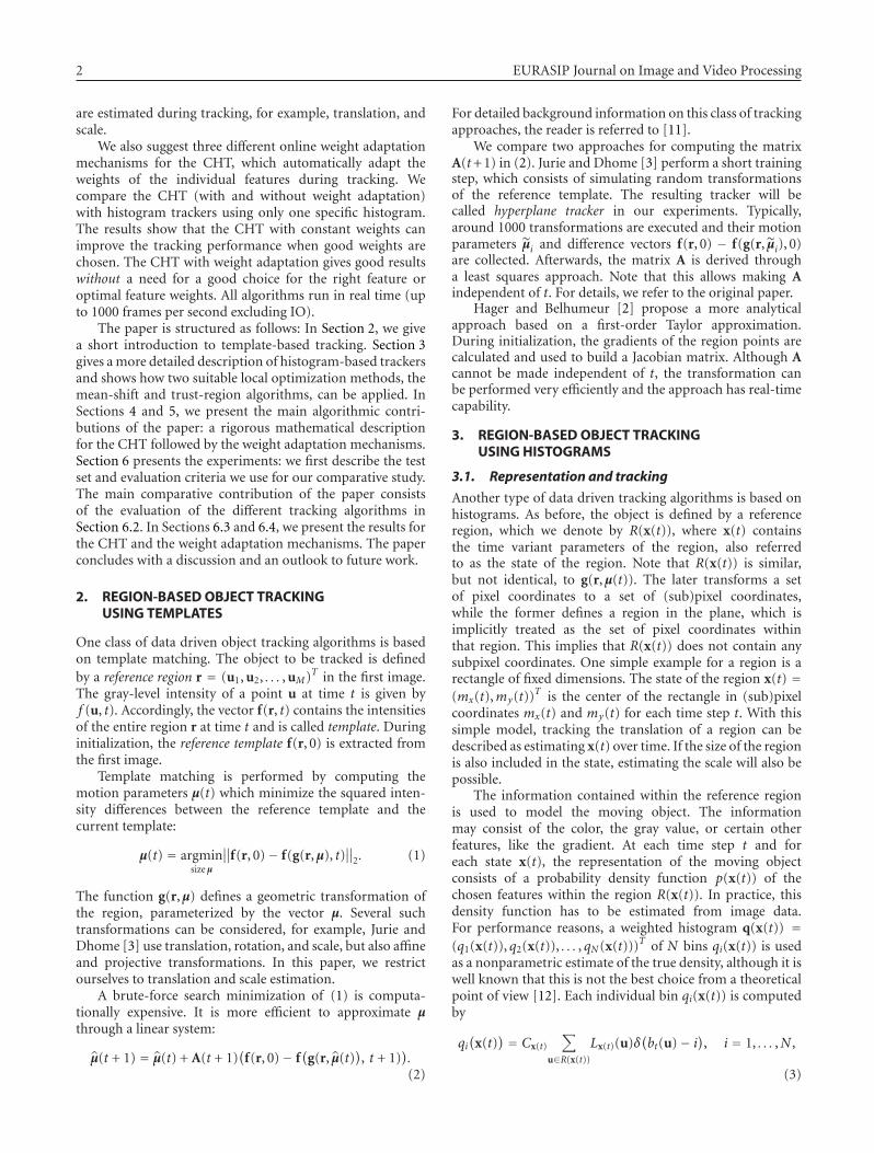
2 EURASIP Journal on Image and Video Processing
are estimated during tracking, for example, translation, andscale.
We also suggest three different online weight adaptationmechanisms for the CHT, which automatically adapt theweights of the individual features during tracking. Wecompare the CHT (with and without weight adaptation)with histogram trackers using only one specific histogram.The results show that the CHT with constant weights canimprove the tracking performance when good weights arechosen. The CHT with weight adaptation gives good resultswithout a need for a good choice for the right feature oroptimal feature weights. All algorithms run in real time (upto 1000 frames per second excluding IO).
The paper is structured as follows: In Section 2, we givea short introduction to template-based tracking. Section 3gives a more detailed description of histogram-based trackersand shows how two suitable local optimization methods, themean-shift and trust-region algorithms, can be applied. InSections 4 and 5, we present the main algorithmic contri-butions of the paper: a rigorous mathematical descriptionfor the CHT followed by the weight adaptation mechanisms.Section 6 presents the experiments: we first describe the testset and evaluation criteria we use for our comparative study.The main comparative contribution of the paper consistsof the evaluation of the different tracking algorithms inSection 6.2. In Sections 6.3 and 6.4, we present the results forthe CHT and the weight adaptation mechanisms. The paperconcludes with a discussion and an outlook to future work.
2. REGION-BASED OBJECT TRACKINGUSING TEMPLATES
One class of data driven object tracking algorithms is basedon template matching. The object to be tracked is definedby a reference region r = (u1, u2, . . . , uM)T in the first image.The gray-level intensity of a point u at time t is given byf (u, t). Accordingly, the vector f(r, t) contains the intensitiesof the entire region r at time t and is called template. Duringinitialization, the reference template f(r, 0) is extracted fromthe first image.
Template matching is performed by computing themotion parameters µ(t) which minimize the squared inten-sity differences between the reference template and thecurrent template:
µ(t) = argminsize µ
∥∥f(r, 0)− f(g(r,µ), t)∥∥
2. (1)
The function g(r,µ) defines a geometric transformation ofthe region, parameterized by the vector µ. Several suchtransformations can be considered, for example, Jurie andDhome [3] use translation, rotation, and scale, but also affineand projective transformations. In this paper, we restrictourselves to translation and scale estimation.
A brute-force search minimization of (1) is computa-tionally expensive. It is more efficient to approximate µthrough a linear system:
µ(t + 1) = µ(t) + A(t + 1)(
f(r, 0)− f(
g(r, µ(t)), t + 1)
).(2)
For detailed background information on this class of trackingapproaches, the reader is referred to [11].
We compare two approaches for computing the matrixA(t+1) in (2). Jurie and Dhome [3] perform a short trainingstep, which consists of simulating random transformationsof the reference template. The resulting tracker will becalled hyperplane tracker in our experiments. Typically,around 1000 transformations are executed and their motionparameters µi and difference vectors f(r, 0) − f(g(r, µi), 0)are collected. Afterwards, the matrix A is derived througha least squares approach. Note that this allows making Aindependent of t. For details, we refer to the original paper.
Hager and Belhumeur [2] propose a more analyticalapproach based on a first-order Taylor approximation.During initialization, the gradients of the region points arecalculated and used to build a Jacobian matrix. Although Acannot be made independent of t, the transformation canbe performed very efficiently and the approach has real-timecapability.
3. REGION-BASED OBJECT TRACKINGUSING HISTOGRAMS
3.1. Representation and tracking
Another type of data driven tracking algorithms is based onhistograms. As before, the object is defined by a referenceregion, which we denote by R(x(t)), where x(t) containsthe time variant parameters of the region, also referredto as the state of the region. Note that R(x(t)) is similar,but not identical, to g(r,µ(t)). The later transforms a setof pixel coordinates to a set of (sub)pixel coordinates,while the former defines a region in the plane, which isimplicitly treated as the set of pixel coordinates withinthat region. This implies that R(x(t)) does not contain anysubpixel coordinates. One simple example for a region is arectangle of fixed dimensions. The state of the region x(t) =(mx(t),my(t))T is the center of the rectangle in (sub)pixelcoordinates mx(t) and my(t) for each time step t. With thissimple model, tracking the translation of a region can bedescribed as estimating x(t) over time. If the size of the regionis also included in the state, estimating the scale will also bepossible.
The information contained within the reference regionis used to model the moving object. The informationmay consist of the color, the gray value, or certain otherfeatures, like the gradient. At each time step t and foreach state x(t), the representation of the moving objectconsists of a probability density function p(x(t)) of thechosen features within the region R(x(t)). In practice, thisdensity function has to be estimated from image data.For performance reasons, a weighted histogram q(x(t)) =(q1(x(t)), q2(x(t)), . . . , qN (x(t)))T of N bins qi(x(t)) is usedas a nonparametric estimate of the true density, although it iswell known that this is not the best choice from a theoreticalpoint of view [12]. Each individual bin qi(x(t)) is computedby
qi(
x(t)) = Cx(t)
∑
u∈R(x(t))
Lx(t)(u)δ(bt(u)− i), i = 1, . . . ,N ,
(3)
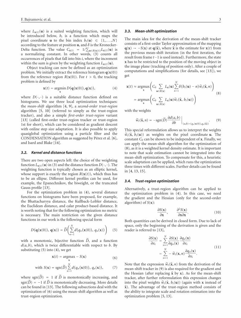
F. Bajramovic et al. 3
where Lx(t)(u) is a suited weighting function, which willbe introduced below, bt is a function which maps thepixel coordinate u to the bin index bt(u) ∈ {1, . . . ,N}according to the feature at position u, and δ is the Kronecker-Delta function. The value Cx(t) = 1/
∑u∈R(x(t))Lx(t)(u) is
a normalizing constant. In other words, (3) counts alloccurrences of pixels that fall into bin i, where the incrementwithin the sum is given by the weighting function Lx(t)(u).
Object tracking can now be defined as an optimizationproblem. We initially extract the reference histogram q(x(0))from the reference region R(x(0)). For t > 0, the trackingproblem is defined by
x(t) = argminx
D(
q(
x(0)), q(x)
), (4)
where D(·, ·) is a suitable distance function defined onhistograms. We use three local optimization techniques:the mean-shift algorithm [4, 9], a second-order trust-regionalgorithm [5, 10] (referred to simply as the trust-regiontracker), and also a simple first-order trust-region variant[13] (called first-order trust-region tracker or trust-region1st for short), which can be considered as gradient descentwith online step size adaptation. It is also possible to applyquasiglobal optimization using a particle filter and theCONDENSATION algorithm as suggested by Perez et al. [6],and Isard and Blake [14].
3.2. Kernel and distance functions
There are two open aspects left: the choice of the weightingfunction Lx(t)(u) in (3) and the distance functionD(·, ·). Theweighting function is typically chosen as an elliptic kernel,whose support is exactly the region R(x(t)), which thus hasto be an ellipse. Different kernel profiles can be used, forexample, the Epanechnikov, the biweight, or the truncatedGauss profile [13].
For the optimization problem in (4), several distancefunctions on histograms have been proposed, for example,the Bhattacharyya distance, the Kullback-Leibler distance,the Euclidean distance, and calar product-based distance. Itis worth noting that for the following optimization no metricis necessary. The main restriction on the given distancefunctions in our work is the following special form
D(
q(
x(0)), q(x)
) = D
( N∑
n=1
d(qn(
x(0)), qn(x)
))(5)
with a monotonic, bijective function D, and a functiond(a, b), which is twice differentiable with respect to b. Bysubstituting (5) into (4), we get
x(t) = argmaxx
− S(x) (6)
with S(x) = sgn(D)N∑n=1
d(qn(
x(0)), qn(x)
), (7)
where sgn(D) = 1 if D is monotonically increasing, andsgn(D) = −1 if D is monotonically decreasing. More detailscan be found in [13]. The following subsections deal with theoptimization of (6) using the mean-shift algorithm as well astrust-region optimization.
3.3. Mean-shift optimization
The main idea for the derivation of the mean-shift trackerconsists of a first-order Taylor approximation of the mappingq(x) → −S(x) at q(x), where x is the estimate for x(t) fromthe previous mean-shift iteration (in the first iteration, theresult from frame t−1 is used instead). Furthermore, the statex has to be restricted to the position of the moving object inthe image plane (tracking of position only). After a couple ofcomputations and simplifications (for details, see [13]), weget
x(t) ≈ argmaxx
(C0
∑
u∈R(x)
Lx(u)N∑
n=1
δ(bt(u)− n)wt(x,n)
)
= argmaxx
(C0
∑
u∈R(x)
Lx(u)wt(
x, bt(u)))
(8)
with the weights
wt(x,n) = −sgn(D)∂d(a, b)∂b
∣∣∣∣(a,b)=(qn(x(0)),qn(x))
. (9)
This special reformulation allows us to interpret the weightswt(x, bt(u)) as weights on the pixel coordinate u. Theconstant C0 can be shown to be independent of x. Finally, wecan apply the mean-shift algorithm for the optimization of(8), as it is a weighted kernel density estimate. It is importantto note that scale estimation cannot be integrated into themean-shift optimization. To compensate for this, a heuristicscale adaptation can be applied, which runs the optimizationthree times with different scales. Further details can be foundin [4, 13, 15].
3.4. Trust-region optimization
Alternatively, a trust-region algorithm can be applied tothe optimization problem in (4). In this case, we needthe gradient and the Hessian (only for the second-orderalgorithm) of S(x):
∂S(x)∂x
,∂2S(x)∂x∂x
. (10)
Both quantities can be derived in closed form. Due to lack ofspace, only the beginning of the derivation is given and thereader is referred to [13],
∂S(x)∂xi
=N∑
n=1
∂S(x)∂qn(x)
∂qn(x)∂xi
=N∑
n=1
− wt(x,n)∂qn(x)∂xi
.
(11)
Note that the expression wt(x,n) from the derivation of themean-shift tracker in (9) is also required for the gradient andthe Hessian (after replacing x by x). As for the mean-shifttracker, after further reformulation this expression changesinto the pixel weights wt(x, bt(u)) (again with x instead ofx). The advantage of the trust-region method consists ofthe ability to integrate scale and rotation estimation into theoptimization problem [5, 13].

4 EURASIP Journal on Image and Video Processing
3.5. Example for mean-shift tracker
We give an example for the equations and quantitiespresented above. Using the Bhattacharyya distance betweenhistograms (as in [4]),
D(
q(
x(0)), q(
x(t))) =
√1− B(q
(x(0)
), q(
x(t)))
(12)
with
B(
q(
x(0)), q(
x(t))) =
N∑
n=1
√qn(
x(0)) · qn
(x(t)
), (13)
we have D(a) = √1− a, d(a, b) = √a·b, and
wt(n) = 12
√√√√qn(
x(0))
qn(
x(t)) . (14)
4. COMBINATION OF HISTOGRAMS
Up to now, the formulation of histogram-based trackinguses the histogram of a certain feature, defined a priorifor the tracking task at hand. Examples are gray valuehistograms, gradient strength (edge) histograms, and RGBor HSV color histograms. Certainly, using several differentfeatures for representing the object to be tracked will resultin better tracking performance, especially if the differentfeatures are weighted dynamically according to the situationin the scene. For example, a color histogram may performbadly, if illumination changes. In this case, information onthe edges might be more useful. On the other hand, in case ofa uniquely colored object in a highly textured environment,color is preferable over edges.
It is possible to combine several features by usingone high-dimensional histogram. The problem with thisapproach is the curse of dimensionality; high-dimensionalfeatures result in very sparse histograms and thus a veryinaccurate estimate of the true and underlying density.Instead, we propose a different solution for combiningdifferent features for object tracking. The key idea is touse a weighted combination of several low-dimensional(weighted) histograms. Let H = {1, . . . ,H} be the set offeatures used for representing the object. For each feature
h ∈ H , we define a separate function b(h)t (u). The number
of bins in histogram h is Nh and may differ between thehistograms. Also, for each histogram, a different weighting
function L(h)x(t)(u) can be applied, that is, different kernels
for each individual histogram are possible if necessary. Thisresults inH different weighted histograms q(h)(x(t)) with thebins
q(h)i
(x(t)
) = C(h)x(t)
∑
u∈R(x(t))
L(h)x(t)(u)δ
(b(h)t (u)− i),
h ∈H , i = 1, . . . ,Nh.
(15)
We now define a combined representation of the objectby φ(x(t)) = (q(h)(x(t)))h∈H and a new distance function
(compare (4) and (5)), based on the weighted sum of thedistances for the individual histograms,
D∗(x) =∑
h∈H
βhDh(
q(h)(x(0)), q(h)(x(t)
)), (16)
where βh ≥ 0 is the contribution of the individual histogramh to the object representation. The quantities βh can beadjusted to best model the object in the current contextof tracking. In Section 5, we will present a mechanismfor online adaptation of the feature weights. Alternatively,instead of the linear combination D∗(x) of the distancesDh(q(h)(x(0)), q(h)(x(t))), a linear combination of the sim-plified expressions Sh(x) (straight forward generalization of(7)) can be used as follows:
S∗(x) =∑
h∈H
βhSh(
x(t)). (17)
In the single histogram case, minimizingD(q(x(0)), q(x(t)))is equivalent to minimizing S(x). In the combined histogramcase, however, the equivalence of minimizing D∗(x) andS∗(x) can only be guaranteed, if Dh(a) = ±a for all h ∈ H .Nevertheless, S∗(x) can still be used as an objective function,if this condition is not fulfilled. Because of its simpler formand the lack of obvious advantages of D∗(x), we choose thefollowing optimization problem for the combined histogramtracker:
x(t) = argmaxx
S∗(x). (18)
From a theoretical point of view, using the simplifiedobjective function S∗ is equivalent to restricting the classof distance measures Dh for each feature h to those thatfulfill Dh(a) = ±a (as in this case Dh = Sh). For example,this excludes the Euclidean distance, but does allow for thesquared Euclidean distance.
4.1. Mean-shift optimization
For the mean-shift tracker, we have to use the same weightingfunction Lx(t)(u) for all histograms h and again the state xhas to be restricted to the position of the moving object inthe image plane. After a technically somewhat tricky, butconceptually straight forward extension of the derivation forthe single histogram mean-shift tracker, we get
x(t) ≈ argmaxx
C0
∑
u∈R(x)
Lx(u)∑
h∈H
wh,t(
x, b(h)t (u)
),
︸ ︷︷ ︸:=wt(x,u)
(19)
which is again a weighted kernel density estimate. Thecorresponding pixel weights are
wt(x, u) =∑
h∈H
wh,t(
x, b(h)t (u)
)
=∑
h∈H
− βhsgn(Dh)∂dh(a, b)
∂b
∣∣∣∣(a,b)=(q(h)
bt (u)(x(0)),q(h)bt (u)(x))
,
(20)
where dh(a, b) is defined as in (5) for each individualfeature h.

F. Bajramovic et al. 5
0
20
40
60
80
ec
0 0.2 0.4 0.6 0.8
Quantile
HagerHyperplaneCONDENSATION
Trust regionTrust region 1stMean shift
(a)
0
20
40
60
80
ec
0 0.2 0.4 0.6 0.8
Quantile
HagerHyperplaneCONDENSATION
Trust regionTrust region 1stMean shift
(b)
0
0.2
0.4
0.6
0.8
1
er
0 0.2 0.4 0.6 0.8
Quantile
HagerHyperplaneCONDENSATION
Trust regionTrust region 1stMean shift
(c)
0
0.2
0.4
0.6
0.8
1
er
0 0.2 0.4 0.6 0.8
Quantile
HagerHyperplaneCONDENSATION
Trust regionTrust region 1stMean shift
(d)
Figure 1: The result graphs for the tracker comparison experiments. The top row shows the distance error ec, the bottom row shows theregion error er . The left-hand column contains the results for trackers without scale estimation, the right-hand column those with scaleestimation. The horizontal axis does not correspond to time, but to sorted aggregation over all test videos. In other words, each graph shows“all” error quantiles (also known as percentiles). The vertical axis for ec has been truncated to 100 pixels to emphasize the relevant details.
4.2. Trust-region optimization
For the trust-region optimization, again the gradient and theHessian of the objective function have to be derived. As thesimplified objective function S∗(x) is a linear combinationof the simplified distance measures Sh(x) for the individualhistograms h, the gradient of S∗(x)) is a linear combinationof the gradient in the single histogram case Sh(x),
∂S∗(x)∂xi
= ∂
∂xi
( ∑
h∈H
βhSh(x)
)=∑
h∈H
βh∂Sh(x)∂xi
, (21)
The same applies to the Hessian,
∂2S∗(x)∂xj∂xi
= ∂
∂xj
(∂S∗(x)∂xi
)
= ∂
∂xj
( ∑
h∈H
βh∂Sh(x)∂xi
)
=∑
h∈H
βh∂
∂xj
(∂Sh(x)∂xi
).
(22)
The factor ∂Sh(x)/∂xi is the ith component of the gradient inthe single histogram case. The factor ∂/∂xj(∂Sh(x)/∂xi) is theentry (i, j) of the Hessian in the single histogram case. Detailscan be found in [13].

6 EURASIP Journal on Image and Video Processing
0
20
40
60
80
ec
0 0.2 0.4 0.6 0.8
Quantile
1004004000
(a)
0
20
40
60
80
ec
0 0.2 0.4 0.6 0.8
Quantile
1004004000
(b)
0
0.2
0.4
0.6
0.8
1
er
0 0.2 0.4 0.6 0.8
Quantile
1004004000
(c)
0
0.2
0.4
0.6
0.8
1
er
0 0.2 0.4 0.6 0.8
Quantile
1004004000
(d)
Figure 2: Same evaluation as in Figure 1 for three configurations of the CONDENSATION tracker with different numbers of particles.
Note that for the trust-region trackers, the simplifica-tion of the objective function D∗ to S∗ is not necessary.However, without the simplification, the gradient and theHessian of the objective function D∗(x) are no longer linearcombinations of the gradient and the Hessian for the fullsingle histogram distance measuresDh and thus the resultingexpressions are more complicated and computationally moreexpensive—without an obvious advantage. Note also, thatfor the case of a common kernel for all features, the differencebetween the single histogram and the multiple histogramcase is that the expression wt(x,n) is replaced by wt(x,n),which is the same expression as for the combined histogrammean-shift tracker (see Sections 3.4 and 4.1).
5. ONLINE ADAPTATION OF FEATURE WEIGHTS
As described in Section 4, the feature weights βh,h ∈ Hare constant throughout the tracking process. However,the most discriminative feature combination can vary overtime. For example, as the object moves, the surroundingbackground can change drastically, or motion blur can havea negative influence on edge features for a limited period oftime. Several authors have proposed online feature selectionmechanisms for tracking. They either select one feature [16]or several features which they combine empirically afterperforming tracking with each winning feature [17, 18].A further approach computes an “artificial” feature using

F. Bajramovic et al. 7
principal component analysis [19]. Democratic integration[20], on the other hand, assigns a weight to each featureand adapts these weights based on the recent performanceof the individual features. Given our combined histogramtracker (CHT), we follow the idea of dynamically adaptingthe weight βh of each individual feature h. To emphasize this,we use the notation βh(t) in this section. Unlike DemocraticIntegration, we perform weight adaptation in an explicit andvery efficient tracking framework.
The central part of feature selection as well as adaptiveweighting is a measure for the tracking performance of eachfeature. Typically, the discriminability between object andsurrounding background is estimated for each feature. In ourcase, this quality measure is used to increase the weights ofgood features and decrease the weights of bad features. Inthe context of this work, a natural choice for such a qualitymeasure is the distance,
ρh(t) = Dh(
q(h)(x(t)), p(h)(x(t)
)), (23)
between the object histogram q(h)(x(t)) and the histogramp(h)(x(t)) of an area surrounding the object ellipse. Bothhistograms are extracted after tracking in frame t. We applythree different weight adaptation strategies.
(1) The weight of the feature h with the best quality ρh(t)is increased by multiplying with a factor γ (set to 1.3),
βh(t + 1) = γβh(t). (24)
Accordingly, the feature h′ with the worst qualityρh′(t) is decreased by dividing by γ,
βh′(t + 1) = βh′(t)γ
. (25)
Upper and lower limits are imposed on βh for everyfeature h to keep weights from diverging. We used thebounds 0.01 and 100. This adaptation strategy is onlysuited for two features (H = 2).
(2) The weight βh(t + 1) of each feature h is set to itsquality measure ρh(t),
βh(t + 1) = ρh(t). (26)
(3) The weight βh(t+1) of each feature h is slowly adaptedtoward ρh(t) using a convex combination (IIR filter)with parameter ν (set to 0.1 in our experiments),
βh(t + 1) = νρh(t) + (1− ν)βh(t). (27)
6. EXPERIMENTAL EVALUATION
6.1. Test set and evaluation criteria
In the experiments, we use some of the test videos ofthe CAVIAR project [7], originally recorded for action andbehavior recognition experiments. The videos are perfectlysuited, since they are recorded in a “natural” environment,with change in illumination and scale of the moving
0
0.2
0.4
0.6
0.8
er
0 t1 400t2 t3 800
Frame
HagerCONDENSATION
Figure 3: Comparison of the Hager and CONDENSATIONtrackers using the er error measure (28). The black rectangle showsthe ground truth. The white rectangle is from the Hager tracker,the dashed rectangle from the CONDENSATION tracker. Thetop, middle, and bottom images are from frames t1, t2, and t3,respectively. The tracked person (almost) leaves the camera’s fieldof view in the middle image, and returns shortly before time t3. TheHager tracker is more accurate, but loses the person irretrievably,while the CONDENSATION tracker is able to reacquire the person.
persons as well as partial occlusions. Most importantly, themoving persons are hand-labelled, that is, for each frame, aground truth rectangle is stored. In case of the mean-shiftand trust-region trackers, the ground truth rectangles aretransformed into ellipses to avoid systematic errors in thetracker evaluation based on (27).
In each experiment, a specific person was tracked. Thetracking system was given the frame number of the firstunoccluded appearance of the person, the accordant groundtruth rectangle around the person as initialization, andthe frame of the person’s disappearance. Aside from thisinitialization, the trackers had no access to the ground truthinformation. Twelve experiments were performed on sevenvideos (some videos were reused, tracking a different personeach time).
To evaluate the results of the original trackers as well asour extensions, we used an area-based criterion. We measurethe difference er of the region A computed by the tracker andthe ground-truth region B,
er(A,B) := |A \ B| + |B \ A||A| + |B| = 1− |A∩ B|
1/2(|A| + |B|) , (28)
where |A| denotes the number of pixels in region A. Thiserror measure is zero if the two regions are identical, andone if they do not overlap. If the two regions have the samesize, the error increases with increasing distance between the

8 EURASIP Journal on Image and Video Processing
0
0.2
0.4
0.6
0.8
1
er
0 0.2 0.4 0.6 0.8
Quantile
rgbEdge
rgb-edgefwa3-rgb-edge
Evaluation using all frames
(a)
0
0.2
0.4
0.6
0.8
1
er
0 0.2 0.4 0.6 0.8
Quantile
fwa1-rgb-edgefwa2-rgb-edgefwa3-rgb-edge
Evaluation using all frames
(b)
Figure 4: Sorted error (i.e., all quantiles as in Figure 1) using CHT with RGB and gradient strength with constant weights (rgb-edge) andthree different feature weight adaptation mechanisms (fwa1-rgb-edge, fwa2-rgb-edge, and fwa3-rgb-edge), as well as single histogram trackersusing RGB (rgb) and edge histogram (edge). Results are given for the mean-shift tracker with scale estimation, Biweight-Kernel, and Kullback-Leibler distance for all individual histograms.
center of both regions. Equal centers but different sizes arealso taken into account. We also compare the trackers usingthe Euclidean distance ec between the centers of A and B.
6.2. General comparison
In the first part of the experiments, we give a generalcomparison of the following six trackers, which were testedwith pure translation estimation, as well as with translationand scale estimation.
(i) The region tracking algorithm of Hager and Bel-humeur [2], working on a three-level Gaussian imagepyramid to enlarge the basin of convergence.
(ii) The hyperplane tracker, using a 150-point region andinitialized with 1000 training perturbation steps.
(iii) The mean-shift and two trust-region algorithms,using an Epanechnikov weighting kernel, the Bhattacharyyadistance measure, and the HSV color histogram featureintroduced by Perez et al. [6] for maximum comparability.
(iv) Finally, the CONDENSATION-based color his-togram approach of Perez et al. [6]. As this tracker iscomputationally expensive, we choose only 400 particlesfor the main comparison, and alternatively 100 and 4000.Furthermore, we kept the particle size as low as possible:two position parameters and an additional scale parameterif applicable. The algorithm is thus restricted to a simplifiedmotion model, which estimates the velocity of the object bytaking the difference between the position estimates fromthe last two frames. The predicted particles are diffused by azero-mean Gaussian distribution with a variance of 5 pixelsin each dimension.
These experiments were timed on a 2.8 GHz Intel Xeonprocessor. The methods differ greatly in the time taken for
Table 1: Timing results for the first sequence, in milliseconds. Foreach tracker, the time taken for initialization and the average timeper frame are shown with and without scale estimation.
Without scale With scale
Initial Per frame Initial Per frame
Hager 4 2.40 5 2.90
Hyperplane 557 2.22 548 2.21
Mean shift 2 1.04 2 2.75
Trust region 9 4.01 18 8.63
Trust region 1st 5 7.25 6 12.09
CONDENSATION 100 11 27.71 11 40.50
CONDENSATION 400 11 79.67 11 109.85
CONDENSATION 4000 14 706.62 14 962.02
initialization (once per sequence) and tracking (once perframe). Table 1 shows the results for the first sequence. Notethe long initialization of the hyperplane tracker due to train-ing, and the long per-frame time of the CONDENSATION.
For each tracker, the errors ec and er from all sequenceswere concatenated and sorted. Figure 1 shows the measureddistance error ec and the region error er for all trackers,with and without scale estimation. Performance varieswidely between all tested trackers, showing strengths andweaknesses of each individual method. There appears to beno method which is universally “better” than the others.
The structure-based region trackers, Hager and hyper-plane, are potentially very accurate, as can be seen at the left-hand side of each graph, where they display a larger numberof frames with low errors. However, both are prone to losingthe target rather quickly, causing their errors to climb faster

F. Bajramovic et al. 9
than the other three methods. Particularly when scale isalso estimated, the additional degree of freedom typicallyprovides additional accuracy, but causes the estimation todiverge sooner. This is due to strong appearance changes ofthe tracked regions in these image sequences.
The CONDENSATION method, for the most part, is notas accurate as the three local optimization methods: mean-shift and the two trust-region variants. Figure 2 shows theperformance with three different numbers of particles, thesevere influence on computation times can be seen in Table 1.As expected, increasing the number of particles improvesthe tracking results. However, the relative performance incomparison with the other trackers is mostly unaffected.We believe that this is partly due to the fact that timeconstraints necessitate the use of a quickly computableparticle evaluation function, which does not include a spatialkernel—in contrast to the other histogram-based methods.
Figure 3 shows a direct comparison between a locallyoptimizing structural tracker (Hager) and the globallyoptimizing histogram-based CONDENSATION tracker. Itis clearly visible that the Hager tracker provides moreaccurate results, but cannot reacquire a lost target. TheCONDENSATION tracker, on the other hand, can continueto track the person after it reappears.
The mean-shift and both trust-region trackers showa very similar performance and provide the best overalltracking if scale estimation is turned off. With scale estima-tion, however, the mean-shift algorithm performs noticeablybetter than the first-order trust-region approach, whichin turn is better than second-order trust-region tracker.This is especially visible when comparing the region errorer (Figure 1(d)), where the error in the scale componentplays an important role. This is probably caused by thevery different approaches to scale estimation in the twotypes of trackers. While the trust-region trackers directlyincorporate scale estimation with variable aspect ratio intothe optimization problem, the mean-shift tracker uses aheuristic approach which limits the maximum scale changeper frame (to 1% in our experiments [4, 13]). It seemsthat this forcedly slow scale adaptation keeps the mean-shifttracker from over adapting the scale to changes in objectand/or background appearance. The first-order trust-regiontracker seems to benefit from the fact that its first-orderoptimization algorithm has worse convergence propertiesthan the second-order variant, which seems to reduce thescale over adaption of the scale parameters.
Another very interesting aspect to note is that trackingtranslation and scale, as opposed to tracking translation only,does not generally improve the results of most trackers. Thetwo template trackers gain a little extra precision, but lose theobject much earlier. The changing appearance of the trackedpersons is a strong handicap for them as the image constancyassumption is violated. The additional degree of freedomopens up more chances to diverge toward local optima,which causes the target to be lost sooner. The mean-shifttracker does actually perform better with scale estimation.The other histogram-based trackers are better in case of puretranslation estimation. They suffer from the fact that thefeatures themselves are typically rather invariant under scale
(a) (b)
Figure 5: Tracking results for one of the CAVIAR images sequences(first and last image of the successfully tracked person). Thetracking results are almost identical to the ground truth regions(ellipses). Note the scale change of the person between the twoimages.
changes. Once the scale is wrong, small translations of thetarget can go completely unnoticed.
6.3. Improvements of the combined histogram tracker
In the second part of the experiments, we combinedtwo different histograms. The first is the standard colorhistogram consisting of the RGB channels, abbreviated inthe figures as rgb. The second histogram is computed froma Sobel edge strength image (edge), with the edge strengthnormalized to fit the gray-value range from 0 to 255.
In Figure 4, the tracking accuracy of the mean-shifttracker is shown. The graph displays the error er accumulatedand sorted over all sequences (same scheme as in Figure 1).In other words, the graph shows “all” error quantiles. Thereader can verify that a combination of RGB and gradientstrength histograms leads to an improvement of trackingaccuracy compared to a pure RGB histogram tracker, eventhough the object is lost a bit earlier. We got similar results forthe corresponding trust-region tracker with our extension tocombined histograms. The weights βh for combining RGBand edge histograms (compare (16)) have been empiricallyset to 0.8 and 0.2. The computation time for one image ison average approximately 2 milliseconds on a 3.4 GHz P4compared to approximately 1 millisecond for a tracker usingone histogram only. A successful tracking example includingcorrect scale estimation is shown in Figure 5.
6.4. Improvements with weight adaptation
In the third part of the experiments, we evaluate theperformance of the CHT with weight adaptation. We includethe three feature weight adaptation mechanisms (fwa1, fwa2,fwa3 according to the numbers in Section 5) in the experi-ment of Section 6. All adaptation mechanisms are initializedwith both feature weights set to 0.5. Results are given inFigure 4. The third weight adaptation mechanism (fwa3-rgb-edge) performs almost as good as the manually optimizedconstant weights (rgb-edge). Figure 4(b) gives a comparisonof the three feature weight adaptation mechanisms. Here, thethird adaptation mechanism gives the best results.
As the RGB histogram dominates the gradient strengthhistogram, we use the blue- and green color channels as

10 EURASIP Journal on Image and Video Processing
0
0.2
0.4
0.6
0.8
1
er
0 0.2 0.4 0.6 0.8
Quantile
GreenBlue
Green-bluefwa1-green-blue
Evaluation using all frames
(a)
0
0.2
0.4
0.6
0.8
1
er
0 0.2 0.4 0.6 0.8
Quantile
fwa1-green-bluefwa2-green-bluefwa3-green-blue
Evaluation using all frames
(b)
Figure 6: Sorted error (i.e., all quantiles as in Figure 1) using CHT with green and blue histograms with constant weights (green-blue) andthree different feature weight adaptation mechanisms (fwa1-green-blue, fwa2-green-blue, and fwa3-green-blue), as well as single histogramtrackers using a green (green) and a blue histogram (blue). Results are given for the mean-shift tracker with scale estimation, biweight-kernel,and Kullback-Leibler distance for all individual histograms.
individual features in the second experiment. Both featureweights are set to 0.5 for the CHT with and without weightadaptation. All other parameters are kept as in the previousexperiment. The results are displayed in Figure 6. The singlehistogram tracker using the green feature performs betterthan the blue feature. The CHT gives similar results to theblue feature, which is caused by bad feature weights. Withweight adaptation, the performance of the CHT is greatlyimproved and almost reaches that of the green feature.This shows that, even though the single histogram trackerwith the green feature gives the best results, the CHT withweight adaptation performs almost equally well without agood initial guess for the best single feature or the bestconstant feature weights. Figure 6(b) gives a comparisonof the three feature weight adaptation mechanisms. Here,the first adaptation mechanism gives the best results. Theaverage computation time for one image is approximately 4milliseconds on a 3.4 GHz P4 compared to approximately 2milliseconds for the CHT with constant weights.
7. CONCLUSIONS
As the first contribution of this paper, we presented acomparative evaluation of five state-of-the-art algorithmsfor data-driven object tracking, namely Hager’s regiontracking technique [2], Jurie’s hyperplane approach [3], theprobabilistic color histogram tracker of Perez et al. [6],Comaniciu’s mean-shift tracking approach [4], and the trust-region method introduced by Liu and Chen [5]. All ofthose trackers have the ability to estimate the position andscale of an object in an image sequence in real-time. Thecomparison was carried out on part of the CAVIAR videodatabase, which includes ground-truth data. The results of
our experiments show that, in cases of strong appearancechange, the template-based methods tend to lose the objectsooner than the histogram-based methods. On the otherhand, if the appearance change is minor, the template-basedmethods surpass the other approaches in tracking accuracy.Comparing the histogram-based methods among each other,the mean-shift approach [4] leads to the best results. Theexperiments also show that the probabilistic color histogramtracker [6] is not quite as accurate as the other techniques,but is more robust in case of occlusions and appearancechanges. Note, however, that the accuracy of this trackerdepends on the number of particles, which has to be chosenrather small to achieve real-time precessing.
As the second contribution of our paper, we presenteda mathematically consistent extension of histogram-basedtracking, which we call combined histogram tracker (CHT).We showed that the corresponding optimization problemscan still be solved using the mean-shift as well as the trust-region algorithms without loosing real-time capability. Theformulation allows for the combination of an arbitrarynumber of histograms with different dimensions and sizes,as well as individual distance functions for each feature. Thisallows for high flexibility in the application of the method.
In the experiments, we showed that a combination oftwo features can improve tracking results. The improvementof course depends on the chosen histograms, the weights,and the object to be tracked. We would like to stress againthat similar results were achieved using the trust-regionalgorithm, although the presentation in this paper wasfocused on the mean-shift algorithm. For more details, thereader is referred to [13]. We also presented three onlineweight adaptation mechanisms for the combined histogramtracker. The benefit of feature weight adaptation is that an

F. Bajramovic et al. 11
initial choice of a single best feature or optimal combinationweights is no longer necessary, as has been shown in theexperiments. One important result is that the CHT with (andalso without) weight adaptation can still be applied in real-time on standard PC hardware.
In our future work, we will evaluate the performanceof the weight adaptation mechanisms on more than twofeatures and investigate more sophisticated adaptation mech-anisms. We are also going to systematically compare the CHTwith the other trackers described in this paper.
ACKNOWLEDGMENTS
This work was partially funded by the German ScienceFoundation (DFG ) under grant SFB 603/TP B2. This workwas partially funded by the European Commission 5th ISTProgramme—Project VAMPIRE.
REFERENCES
[1] B. Deutsch, Ch. Graßl, F. Bajramovic, and J. Denzler, “Acomparative evaluation of template and histogram based 2Dtracking algorithms,” in Proceedings of the 27th Annual Meetingof the German Association for Pattern Recognition (DAGM ’05),pp. 269–276, Vienna, Austria, August-September 2005.
[2] G. D. Hager and P. N. Belhumeur, “Efficient region trackingwith parametric models of geometry and illumination,” IEEETransactions on Pattern Analysis and Machine Intelligence, vol.20, no. 10, pp. 1025–1039, 1998.
[3] F. Jurie and M. Dhome, “Hyperplane approach for templatematching,” IEEE Transactions on Pattern Analysis and MachineIntelligence, vol. 24, no. 7, pp. 996–1000, 2002.
[4] D. Comaniciu, V. Ramesh, and P. Meer, “Kernel-based objecttracking,” IEEE Transactions on Pattern Analysis and MachineIntelligence, vol. 25, no. 5, pp. 564–577, 2003.
[5] T.-L. Liu and H.-T. Chen, “Real-time tracking using trust-region methods,” IEEE Transactions on Pattern Analysis andMachine Intelligence, vol. 26, no. 3, pp. 397–402, 2004.
[6] P. Perez, C. Hue, J. Vermaak, and M. Gangnet, “Color-basedprobabilistic tracking,” in Proceedings of the 7th EuropeanConference on Computer Vision (ECCV ’02), vol. 1, pp. 661–667, Copenhagen, Denmark, May 2002.
[7] CAVIAR, EU funded project, IST 2001 37540, 2004,http://homepages.inf.ed.ac.uk/rbf/CAVIAR.
[8] F. Bajramovic, Ch. Graßl, and J. Denzler, “Efficient combina-tion of histograms for real-time tracking using mean-shift andtrust-region optimization,” in Proceedings of the 27th AnnualMeeting of the German Association for Pattern Recognition(DAGM ’05), pp. 254–261, Vienna, Austria, August-September2005.
[9] Cheng, “Mean shift, mode seeking, and clustering,” IEEETransactions on Pattern Analysis and Machine Intelligence, vol.17, no. 8, pp. 790–799, 1995.
[10] A. R. Conn, N. I. M. Gould, and P. L. Toint, Trust-RegionMethods, SIAM, Philadelphia, Pa, USA, 2000.
[11] S. Baker, R. Gross, and I. Matthews, “Lucas-Kanade 20 yearson: a unifying framework: part 4,” Tech. Rep. CMU-RI-TR-04-14, Robotics Institute, Carnegie Mellon University, Pittsburgh,Pa, USA, 2004.
[12] M. P. Wand and M. C. Jones, Kernel Smoothing, Chapman &Hall/CRC, Boca Raton, Fla, USA, 1995.
[13] F. Bajramovic, Kernel-basierte Objektverfolgung, M.S. thesis,Computer Vision Group, Department of Mathematics andComputer Science, University of Passau, Lower Bavaria,Germany, 2004.
[14] M. Isard and A. Blake, “CONDENSATION—conditionaldensity propagation for visual tracking,” International Journalof Computer Vision, vol. 29, no. 1, pp. 5–28, 1998.
[15] D. Comaniciu and P. Meer, “Mean shift: a robust approachtoward feature space analysis,” IEEE Transactions on PatternAnalysis and Machine Intelligence, vol. 24, no. 5, pp. 603–619,2002.
[16] H. Stern and B. Efros, “Adaptive color space switchingfor tracking under varying illumination,” Image and VisionComputing, vol. 23, no. 3, pp. 353–364, 2005.
[17] R. T. Collins, Y. Liu, and M. Leordeanu, “Online selection ofdiscriminative tracking features,” IEEE Transactions on PatternAnalysis and Machine Intelligence, vol. 27, no. 10, pp. 1631–1643, 2005.
[18] B. Kwolek, “Object tracking using discriminative featureselection,” in Proceedings of the 8th International Conference onAdvanced Concepts for Intelligent Vision Systems (ACIVS’06),pp. 287–298, Antwerp, Belgium, September 2006.
[19] B. Han and L. Davis, “Object tracking by adaptive featureextraction,” in Proceedings of the International Conference onImage Processing (ICIP ’04), vol. 3, pp. 1501–1504, Singapore,October 2004.
[20] J. Triesch and C. von der Malsburg, “Democratic integration:self-organized integration of adaptive cues,” Neural Computa-tion, vol. 13, no. 9, pp. 2049–2074, 2001.

Hindawi Publishing CorporationEURASIP Journal on Image and Video ProcessingVolume 2008, Article ID 328052, 14 pagesdoi:10.1155/2008/328052
Research ArticleTracking of Moving Objects in Video Through InvariantFeatures in Their Graph Representation
O. Miller,1 A. Averbuch,2 and E. Navon2
1 ArtiVision Technologies Pte. Ltd., 96 Robinson Road #13-02, Singapore 0688992 School of Computer Science, Tel Aviv University, Tel Aviv 69978, Israel
Correspondence should be addressed to A. Averbuch, [email protected]
Received 21 July 2007; Accepted 10 July 2008
Recommended by Fatih Porikli
The paper suggests a contour-based algorithm for tracking moving objects in video. The inputs are segmented moving objects.Each segmented frame is transformed into region adjacency graphs (RAGs). The object’s contour is divided into subcurves.Contour’s junctions are derived. These junctions are the unique “signature” of the tracked object. Junctions from two consecutiveframes are matched. The junctions’ motion is estimated using RAG edges in consecutive frames. Each pair of matched junctionsmay be connected by several paths (edges) that become candidates that represent a tracked contour. These paths are obtained bythe k-shortest paths algorithm between two nodes. The RAG is transformed into a weighted directed graph. The final trackedcontour construction is derived by a match between edges (subcurves) and candidate paths sets. The RAG constructs the trackedcontour that enables an accurate and unique moving object representation. The algorithm tracks multiple objects, partially covered(occluded) objects, compounded object of merge/split such as players in a soccer game and tracking in a crowded area forsurveillance applications. We assume that features of topologic signature of the tracked object stay invariant in two consecutiveframes. The algorithm’s complexity depends on RAG’s edges and not on the image’s size.
Copyright © 2008 O. Miller et al. This is an open access article distributed under the Creative Commons Attribution License,which permits unrestricted use, distribution, and reproduction in any medium, provided the original work is properly cited.
1. INTRODUCTION
Object tracking is an important task for a variety of computervision applications such as monitoring [1], perceptual userinterfaces [2], video compression [3], vehicular navigation,robotic control, motion recognition, video surveillance,and many more. These applications require reliable objecttracking techniques that satisfy real-time constraints. Forexample, object tracking is a key component for efficientalgorithms in video processing and compression for content-based indexing [4, 5]. In MPEG-4, the visual informationis organized on the basis of the video object (VO) concept,which represents a time-varying visual entity with arbitraryshape. Tracking these video objects along the scene enablesindividual manipulation of its shape and combines it withother similar entities to produce a scene.
A robust tracking system should meet the followingchallenges: tracking of multiple objects that are partiallycovered (occluded) by other objects, tracking a compoundedobject of merge and split as players in a soccer game, trackingof slow disappearance of an object from a scene and then
its reappearance after several frames, tracking in a crowdedarea for surveillance applications. Many of the trackingtechniques utilize the model shape [6] of the tracked objectto overcome the errors produced by the use of an estimatedmotion vector. Unfortunately, an object may translate androtate in three-dimensional space while its projection onthe image plane undergoes projective transformations thatcause substantial deformations in its two-dimensional shape.Furthermore, an object may change its real (original) shapein physical space, for example, in the case of a human objectchanging its body position. In this situation, it is necessaryto decide whether the model that describes the object hasto be updated, or whether the change in its shape will beconsidered as a transitory event. In other cases, the first frameof the sequence may consist of two different objects that arevery close to each other, and the object extraction processconsiders them as a single object. Then, the “single” objectmay split, after a few frames, into two objects. Depending onthe adopted based technique, the object’s shape model willhave to be reinitialized according to the new tracked objectsin successive frames.

2 EURASIP Journal on Image and Video Processing
Producing an automatic robust tracking system is asignificant challenge. There have been a lot of efforts thatproduce solutions to handle the tracking problem. Theexisting techniques in the literature can be roughly classifiedinto the following groups of trackers: region-based, contour-based, and model-based.
1.1. Region-based trackers
An adaptive algorithm, which updates the histogram ofthe tracked object in order to account for changes incolor, illumination, pose, and scale, was presented in [7].The tracked object is represented as “blobs” in the back-projection [8]. This technique has a low complexity, andthus suits real-time systems. Other techniques, which utilizestructural features such as texture, color and luminance, areproposed in [9–11]. For example, [9] suggested a movingobject tracking algorithm that is based on a combination ofadaptive texture and color segmentation. They use Gibbs-Markov random field to model the texture, and a two-dimensional Gaussian distribution to model the color. Thetracked target is obtained by a probabilistic framework ofthe texture and color cues at region level and by adaptingboth the texture and color segmentation over time. Similartechniques were used earlier in [10, 11]. However, when fastmotion of the object and significant change in behavior areallowed, color- or texture-based techniques are not sufficientto detect a long-term tracking. Region-based algorithms todeal with the above were suggested in [12, 13]. The method in[12] is based on a modified version of Kalman’s filter. A four-step tracking technique using motion projection, markerextraction, clustering and region merging was suggestedin [13]. The motion projection represented by a linearmotion model is calculated on the reliable parts of theprojected object. These parts are called marker points andtheir extractions are based on the assumption about therelationship between the projected and real objects. Then,starting from these markers, a modified watershed transfor-mation followed by a region-merging algorithm producesthe complete segmentation of the next frame. The advantageof the techniques in [12, 13] is in their abilities to deal withsignificant changes in the object’s regions.
1.2. Contour-based trackers
These algorithms detect and track only the contour of theobject. For example, the snake algorithm [6] does it by usinga converged snake in the reference frame as the initial snakein the successive frame. However, the algorithm blurs theimage to disperse gradient information. Therefore, it has alimited search area and it is unable to track changes in thecontour that lie outside the range of the blurred gradientoperator. As a consequence, this method is effective onlywhen the motions and changes in the object’s shape betweenconsecutive frames are small. To overcome this limitation,some use dynamic programming that increases the searcharea of the snake. Temporal information to bias the snaketoward the shape of the segmentation in the previous frameis used in [14]. This method improves the shape memory
of the snake but does not adequately track large-scale objectmovements or significant changes in its shape. Conversely,[15] suggested a tracker, which handles significant changesin the shape. It partitions the object’s contour into severalcurves and estimate the motions of each curve independentlyof the others. Then, the predicted location of the completecontour is obtained by using dynamic programming. Aparticle filter-based subspace projection method, whichneither causes blur nor demands an expensive dynamicprogramming, is presented in [16].
1.3. Model-based trackers
A generic solution to object tracking is still a challengingproblem. Therefore, model-based techniques, which demanda priori information regarding the object’s shape and type,were developed for suitable applications. For example, [17]suggested a model, which is based on edge detector, to extractmoving edges that are grouped together by a predefinedmodel shape. A similar concept was used in [18], whichgroups the edges by using the Hough transform. In addition,the use of deformable templates has been very commonin model-based techniques. A deformable template enablesto track large movements and changes, and also providesglobal shape memory for the tracked object. For example,a known model of a key is defined in [19]. This approachallows both affine transformations of the entire key and localdeformations in the form of variations in the notches ofthe key. A similar approach of deformable templates wasused in [20] for tracking a human hand by global and localdeformation templates, which were defined for movementchanges and for finger motions, respectively. Recently, adynamic-model-based technique [21], which decreases theconstraint limitation by having a predefined model, wassuggested. It uses a hierarchy of separate deformationstages: global affine deformations, local (segmented) affinedeformations, and snake-based continuous deformations.This approach provides a shape memory update of theobject’s model and thus, enables the snake algorithm to beused for final contour refinement after each frame.
Our proposed algorithm is classified as a contour-basedtechnique. The algorithm gets as an input the contour(curve) of the moving object to be tracked and twoconsecutive frames It and It+1 in times t and t+1, respectively.Initially, we apply a still-segmentation process on It and It+1.Region adjacency graphs (RAGs), denoted by Gt and Gt+1,are the constructed data structures from the segmentation ofIt and It+1, respectively. Then, the contour of the extractedobject in Gt is segmented into subcurves while interiorjunctions are marked. Each subcurve represents a differenthomogeneous region in Gt. The interior junctions connectbetween two different subcurves. These junctions are calledimportant (easy) points to track. Motion estimation of thesejunctions is performed where the search area is the edgesin Gt+1. For each pair of tracked junctions in Gt, thereexists a small number of “candidate paths,” which connectthe estimated pair in Gt+1. These paths are obtained by analgorithm that finds the k shortest path between two nodesin weighted and directed graph. We claim that only one of

O. Miller et al. 3
the candidate paths accurately represents the single-trackedsubcurve between a pair of junctions. Then, the constructionof the tracked object is actually a process that matchesbetween a single edge (signature) in Gt and a set of candidatepaths in Gt+1.
The matching process has a low complexity due to thelimited number of candidate paths. The tracked contouris constructed from all the matched paths between pairsof estimated junctions. We show that the probability ofmatching the right path is proportional to the number ofpoints that participate in the matching process.
In contrast to other contour-based techniques such as in[6, 14, 15], our algorithm does not use the snake algorithm[6] to obtain the predicted curve of the object. Therefore, thesuggested algorithm does not have limitations on the object’smotion or changes in the object’s pose. Furthermore, it doesnot require a priori information about its shape, type, ormotion as in [17, 19, 20].
The rest of the paper is organized as follows. Section 2introduces the notation and outlines the main steps ofthe algorithm. Section 3 describes the object’s contoursegmentation. The estimation of the junction’s motion andthe algorithm for finding the candidate paths is given inSection 4. Section 5 presents the matching process that con-structs the tracked contour. Implementation and complexityanalysis is given in Section 6. Experimental results are givenin Section 7.
2. NOTATION AND OUTLINE OF THE ALGORITHM
The following notations are used; see Figure 1 for illus-tration. The flow of the algorithm is given in Figure 2.Let It and It+1 be the inputs of the source frame and itsconsecutive frame, respectively. We denote by {Rti}, i =1, . . . ,nt and {Rt+1
j }, j = 1, . . . ,nt+1 the sets of nt and nt+1
non-overlapping regions that are generated by a still imagesegmentation (Section 3.1 using [22–24]) of It and It+1,respectively. Region adjacency graphs (RAGs) Gt = (Vt,Et)and Gt+1 = (Vt+1,Et+1) are the data structures that representthe segmentation of It and It+1, respectively. The nodes ofthe RAGs represent the regions Rti , i = 1, . . . ,nt. An edgee(i, j) ∈ Et represents a shared common boundary of Rti andRtj such that (x, y) ∈ e(i, j), for all (x, y) ∈ Rti∩Rtj . The sameis true for Gt+1 = (Vt+1,Et+1).
Let Ct be the closed input curve that belongs to theobject’s contour to be tracked in It such that Ct ⊆ Et and letCt+1 be the tracked contour in It+1. We assume that Ct+1 ⊆Et+1. The “important” points in Ct are called junctions (seeSection 3.2). They are denoted by Jk, k = 1, . . . ,N , which isthe set of theN junctions on the curveCt . Thus,Ct (source) issegmented into subcurves, denoted by Pk,k+1
t , k = 1, . . . ,N ,where the indices that enumerate the junctions are k =1, . . . ,N − 1 and the Nth junction is connected to 1. Eachsubcurve Pk,k+1
t is actually the edge that connects the pair Jkand Jk+1. The corresponding points of Jk, k = 1, . . . ,N inIt+1 are denoted by Sk, k = 1, . . . ,N , such that each matchedpoint in Sk corresponds to a junction in Jk. In other words,a set of matched points in Jk, k = 1, . . . ,N , in It+1 will be
detected by a block-matching process (Section 4.1) that isbased on SAD minimization of the matched squared errorsbetween Jk, k = 1, . . . ,N , and a searched area in It+1. The setof matched points in It+1 is Sk, k = 1, . . . ,N .
The construction of Ct+1 is achieved by the applicationof the matching procedure (Section 5.1) that measures thesimilarity between the edges of It and It+1. We will show(Section 5.1) that each subcurve in Ct (the edge between Jkand Jk+1) has a single matched edge in Ct+1 (the edge thatconnects Sk and Sk+1). However, several edges may connectthe matched pointsSk and Sk+1. We call this set of edges“candidate paths” (destination), denoted by Pk,k+1
t+1 , r =1, . . . ,Rk, where Rk is the number of candidate paths betweeneach Jk and Jk+1. We say that Ct+1 ⊆ Pk,k+1
t+1,r , r = 1, . . . ,Rk.
There exists rk, 1 ≤ rk ≤ Rk, such that a path Pk,k+1t+1,rk that
satisfies Pk,k+1t+1,rk ∈ Ct+1 is called a matched path, denoted by
mpk,k+1t+1 . Then, Ct+1 = ∪k=1,...,N−1mp
k,k+1t+1 . In other words, the
new object’s curve Ct+1 is formed by sets of matched pathsmpk,k+1
t+1 between Sk and Sk+1, k = 1, . . . ,N .
3. CURVE SEGMENTATION
Assume we have the two input frames It and It+1 and anobject’s contour Ct . Segmentation of the object’s contour(curve) Ct into subcurves is required since the object maytranslate and rotate in three-dimensional space, while itsprojection onto the image plane causes substantial deforma-tions in its two-dimensional shape. Therefore, it is betterto estimate separately the motion of each subcurve ratherthan estimating the motion of the entire object’s contour.The segmentation of the object’s contour into subcurvesis achieved by finding a set of junctions, which connectthe subcurves between themselves and separate betweenhomogenous regions. In (Section 3.2), we justify why thesejunctions are well-tracked points that faithfully represent therest of the points that belong to Ct. These junctions comprisethe signature of the tracked object that will characterize ituniquely.
In order to partition the object’s curve into subcurves, weutilize the still-segmentation results of It. We require fromthe still segmentation to produce homogeneous regions suchthat only the boundaries of the regions overlap each other.
3.1. Image segmentation
The performance of the algorithm is directly affected by thenumber of segments from the two input frames It and It+1.We want produce a minimal number of segmented regionswhile preserving the homogeneity criteria. For this purpose,we apply the segmentation algorithm in [22–24].
This algorithm uses the watershed algorithm [25] fol-lowed by an iterative merging process, which generates localthresholds. The watershed algorithm gets the gradients ofa gray-scale image of the input color image. The imageis considered as a topographic relief. By flooding thetopographic surface from its lowest altitude, the algorithmdefines lakes and dams. Dams are watershed lines thatseparate adjacent lakes. When the whole surface is immersed,

4 EURASIP Journal on Image and Video Processing
R11 R14
R8
R6
R10
R1
R13
R4
R2
R12
R3
R5
(a) (b)
Figure 1: (a) Still segmentation of It . Ct (source) is the green closed curve. The red contours are the segmented boundaries. The black arrowspoint to two different junctions J1 and J2. (b) Still segmentation of It+1. Ct+1 is the tracked green closed curve and the black arrows point tothe matched points S1 and S2 that correspond to the junctions J1 and J2, respectively. The yellow curves are the paths of P1,2
t+1,r , r = 1, . . . , 3and the blue curve is the matched path denoted by mp1,2
t+1.
It Ct It+1
Ct+1
Curve segmentation
Segmentation of It and It+1
Detection of junction in Ct
Finding candidates paths
Estimating the matched pointsin It+1 to junctions in Ct
Finding candidate pathsbetween estimated junctions
Construction of the tracked curve
Figure 2: Flow diagram of the proposed algorithm where It andIt+1 are two consecutive input frames, and Ct is the input object’scontour to be tracked. Ct+1 is the tracked contour in It+1.
the image is divided into lakes. Each lake represents a region.However, due to its sensitivity to weak edges, the watershedalgorithm generates oversegmented output. Therefore, itsoutput is used as an initial guess for the merging processphase, which aims at reducing the number of segments. The
merging process is done iteratively. At any iteration duringthe merging process, the most similar adjacent regions aremerged. The similarity between any pair of adjacent regionsis measured by the outcome of a dissimilarity function [22–24]. Local thresholds are derived by an automatic process,where local information is taken into consideration. Anythreshold refers to a specific region and its surroundings.The number of thresholds that defines the final regions isknown only when the process is terminated. The outputof the segmentation is represented by Rti , i = 1, . . . ,nt,which partitions It. These partitions construct the initialdata structures that we use during the entire duration ofthe algorithm. Recall that Gt = (Vt,Et) (Section 2) is anundirected graph that represents the partition of It. Theregion Rti is represented by a node vi ∈ Vi. An edge e(i, j)exists only if Rti and Rtj are adjacent, where adjacent regionsshare a boundary. The edge e(i, j) contains all the pixels thatlie between Rti and Rtj . Hence, all the pixels of the segmentedboundaries are represented by Et. The same is true for thegraph Gt+1 = (Vt+1,Et+1).
3.2. Detection of a junction
The proposed algorithm first tracks the “important” points(junctions) Jk, k = 1, . . . ,N . We will show here that thesepoints are sufficient to produce reliable tracking without theneed to have the rest of the points in Ct.
We assume that pixels in homogeneous areas are difficultto track while pixels in high-textured areas, which arecharacterized by having more content, are more likely to bewell tracked. A method to identify good features to track wasintroduced in [26]. This method derives a set of interestingpoints by simultaneously tracking them. The points thatoptimize the trackers’ accuracy are chosen as good feature.

O. Miller et al. 5
The algorithm mainly detects corners as well-tracked points.Hence, corners are considered important points to track.
A corner is defined as a meeting point of two (or more)straight edge lines [26–29]. Following this definition, eachcorner contains at least two different edges and at leasttwo different regions, which together create two-dimensionalstructures. Since real images do not contain geometric shapesonly or rigid objects, corners are related to curvature on thecontour. L-junction, T-junction, and X-junction are differentcorner types, where the number of regions that meet in thecorner determines the corner type. Examples of a T-junctionprofile and corners in a synthetic image are illustrated inFigure 3.
The corners, as a source for rich information, are used asan anchor points for tracking. Corners can be tracked withhigh accuracy as it is demonstrated in [26, 30]. In [31, 32]corner tracking is used for robot homing and low bit ratevideo codec, respectively.
Since corners are well-tracked points, we are motivatedto associate the important points in Ct with corners. Hence,the important points (which are called junctions) are definedas follows.
Definition 1. Let Ct be the contour of a given object. LetRtk, k = 1, . . . ,N , be the subset of Rti , i = 1, . . . ,nt, whichis represented by Gt = (Vt,Et). Assume N (N ≤ nt) regionsof the object intersect Ct. The N regions are renumbered1, . . . ,N such that Rtk is adjacent to Rtk−1 and Rtk+1 for allk = 1, . . . ,N . A junction Jk, k = 1, . . . ,N , on Ct is defined as
JkΔ= (x, y), where (x, y) ∈ Ct and (x, y) ∈ e(k, k+1), e ∈ Et.
In other words, a junction is defined as a point on Ctwhere two interior segments of the object meet. Junctionsare distinguished from corners by the fact that they arenot necessarily represented as a meeting point of straightlines and do not necessarily represent a curvature in Ct (seeFigure 4). However, like corners, junctions contain at leasttwo different edges (lines). They represent a meeting pointof at least two different homogenous regions of the object,while a corner may represent only homogeneous region ofthe object. They are considered as good features and are usedin our application as “important” anchor points to base thetracking on them.
4. FINDING THE CANDIDATE PATHS
In Section 3, we discussed the advantages of having junctionsinCt as well-tracked points. The junctions enable to find a setof matched points Sk, k = 1, . . . ,N in It+1 and the candidatepaths Pk,k+1
t+1,r , r = 1, . . . ,Rk for the construction of Ct+1.The construction of the object’s contour Ct+1 in
It+1 relies on the fact that the set Jk, k = 1, . . . ,N ,is defined as connected points between homogeneousregions in Ct (see Figure 4). Any pair of consecu-tive junctions Jk and Jk+1 is connected by a subcurvePk,k+1t . This subcurve is an edge in Gt that represents
the boundary of a homogeneous region. As defined inSection 2, Sk, k = 1, . . . ,N , is a set of matched points
Gray level 1
Gray level 2 Gray level 3
(a) (b)
Figure 3: (a) Profile of T-junction. (b) Corner map (red dots) of asynthetic image.
J1 J2
J3
J4J5
J6
R1
R3
R5
R2
R4
Figure 4: Syntactic illustration of detected junctions in Ct . Theblue curve is the object contour Ct . Each homogeneous region inCt is bounded by a green curve. The red crosses on Ct representa set of six junctions Jk , k = 1, . . . , 6. Each connection betweentwo consecutive junctions Jk and Jk+1, represents a homogeneousregion. Each junction Jk , k = 1, . . . , 6 is a connection between two(or more) segmented regions Ri and Rj , i, j = 1, . . . , 5 and i /= j. Thetwo top corners are the curvature regions of Ct that do not satisfyDefinition 1.
(in Gt+1) to set Jk, k = 1, . . . ,N (in Gt). Each consecutivepair Sk and Sk+1 can be connected by several paths which areedges in Gt+1 (see Figure 1). However, based on our imagesegmentation assumption, the contour of the tracked objectCt+1 is an integral part of the segmentation outputs suchthat Ct+1 ⊆ Et+1. Since all possible paths between Sk andSk+1, k = 1, . . . ,N , satisfy Et+1 = ∪k=1,...,N , r=1,...,RkP
k,k+1t+1,r we
get that Ct+1 ⊆ ∪k=1,...,N ,r=1,...,RkPk,k+1t+1,r . After these sets of
paths (candidate paths) between each pair in Sk are obtained,the construction of Ct+1 is done by the application of thematching process between a single edge Pk,k+1
t to the setPk,k+1t+1,r , r = 1, . . . ,Rk. These paths mean that we actually
transform the tracking of the entire curve into a problem ofhow to identify match between edges.
This section describes how to find the matched points Skfor Jk, k = 1, . . . ,N in Et+1 (Section 4.1). Then, we describethe algorithm that finds candidate paths Pk,k+1
t+1,r , r = 1, . . . ,Rkbetween any pair of matched points Sk and Sk+1.
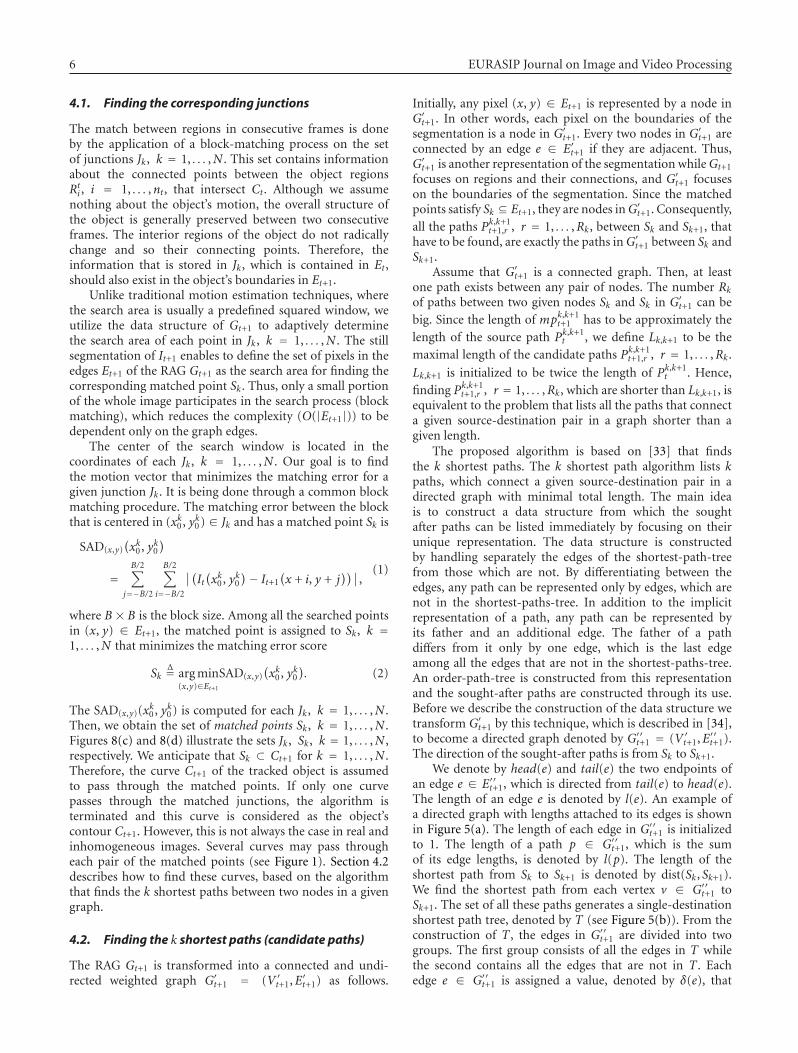
6 EURASIP Journal on Image and Video Processing
4.1. Finding the corresponding junctions
The match between regions in consecutive frames is doneby the application of a block-matching process on the setof junctions Jk, k = 1, . . . ,N . This set contains informationabout the connected points between the object regionsRti , i = 1, . . . ,nt, that intersect Ct. Although we assumenothing about the object’s motion, the overall structure ofthe object is generally preserved between two consecutiveframes. The interior regions of the object do not radicallychange and so their connecting points. Therefore, theinformation that is stored in Jk, which is contained in Et,should also exist in the object’s boundaries in Et+1.
Unlike traditional motion estimation techniques, wherethe search area is usually a predefined squared window, weutilize the data structure of Gt+1 to adaptively determinethe search area of each point in Jk, k = 1, . . . ,N . The stillsegmentation of It+1 enables to define the set of pixels in theedges Et+1 of the RAG Gt+1 as the search area for finding thecorresponding matched point Sk. Thus, only a small portionof the whole image participates in the search process (blockmatching), which reduces the complexity (O(|Et+1|)) to bedependent only on the graph edges.
The center of the search window is located in thecoordinates of each Jk, k = 1, . . . ,N . Our goal is to findthe motion vector that minimizes the matching error for agiven junction Jk. It is being done through a common blockmatching procedure. The matching error between the blockthat is centered in (xk0 , yk0 ) ∈ Jk and has a matched point Sk is
SAD(x,y)(xk0 , yk0
)
=B/2∑
j=−B/2
B/2∑
i=−B/2
∣∣(It(xk0 , yk0
)− It+1(x + i, y + j
))∣∣,(1)
where B × B is the block size. Among all the searched pointsin (x, y) ∈ Et+1, the matched point is assigned to Sk, k =1, . . . ,N that minimizes the matching error score
SkΔ= arg min
(x,y)∈Et+1
SAD(x,y)(xk0 , yk0
). (2)
The SAD(x,y)(xk0 , yk0 ) is computed for each Jk, k = 1, . . . ,N .Then, we obtain the set of matched points Sk, k = 1, . . . ,N .Figures 8(c) and 8(d) illustrate the sets Jk, Sk, k = 1, . . . ,N ,respectively. We anticipate that Sk ⊂ Ct+1 for k = 1, . . . ,N .Therefore, the curve Ct+1 of the tracked object is assumedto pass through the matched points. If only one curvepasses through the matched junctions, the algorithm isterminated and this curve is considered as the object’scontour Ct+1. However, this is not always the case in real andinhomogeneous images. Several curves may pass througheach pair of the matched points (see Figure 1). Section 4.2describes how to find these curves, based on the algorithmthat finds the k shortest paths between two nodes in a givengraph.
4.2. Finding the k shortest paths (candidate paths)
The RAG Gt+1 is transformed into a connected and undi-rected weighted graph G′t+1 = (V ′
t+1,E′t+1) as follows.
Initially, any pixel (x, y) ∈ Et+1 is represented by a node inG′t+1. In other words, each pixel on the boundaries of thesegmentation is a node in G′t+1. Every two nodes in G′t+1 areconnected by an edge e ∈ E′t+1 if they are adjacent. Thus,G′t+1 is another representation of the segmentation whileGt+1
focuses on regions and their connections, and G′t+1 focuseson the boundaries of the segmentation. Since the matchedpoints satisfy Sk ⊆ Et+1, they are nodes inG′t+1. Consequently,all the paths Pk,k+1
t+1,r , r = 1, . . . ,Rk, between Sk and Sk+1, thathave to be found, are exactly the paths inG′t+1 between Sk andSk+1.
Assume that G′t+1 is a connected graph. Then, at leastone path exists between any pair of nodes. The number Rkof paths between two given nodes Sk and Sk in G′t+1 can bebig. Since the length of mpk,k+1
t+1 has to be approximately thelength of the source path Pk,k+1
t , we define Lk,k+1 to be themaximal length of the candidate paths Pk,k+1
t+1,r , r = 1, . . . ,Rk.
Lk,k+1 is initialized to be twice the length of Pk,k+1t . Hence,
finding Pk,k+1t+1,r , r = 1, . . . ,Rk, which are shorter than Lk,k+1, is
equivalent to the problem that lists all the paths that connecta given source-destination pair in a graph shorter than agiven length.
The proposed algorithm is based on [33] that findsthe k shortest paths. The k shortest path algorithm lists kpaths, which connect a given source-destination pair in adirected graph with minimal total length. The main ideais to construct a data structure from which the soughtafter paths can be listed immediately by focusing on theirunique representation. The data structure is constructedby handling separately the edges of the shortest-path-treefrom those which are not. By differentiating between theedges, any path can be represented only by edges, which arenot in the shortest-paths-tree. In addition to the implicitrepresentation of a path, any path can be represented byits father and an additional edge. The father of a pathdiffers from it only by one edge, which is the last edgeamong all the edges that are not in the shortest-paths-tree.An order-path-tree is constructed from this representationand the sought-after paths are constructed through its use.Before we describe the construction of the data structure wetransform G′t+1 by this technique, which is described in [34],to become a directed graph denoted by G′′t+1 = (V ′
t+1,E′′t+1).The direction of the sought-after paths is from Sk to Sk+1.
We denote by head(e) and tail(e) the two endpoints ofan edge e ∈ E′′t+1, which is directed from tail(e) to head(e).The length of an edge e is denoted by l(e). An example ofa directed graph with lengths attached to its edges is shownin Figure 5(a). The length of each edge in G′′t+1 is initializedto 1. The length of a path p ∈ G′′t+1, which is the sumof its edge lengths, is denoted by l(p). The length of theshortest path from Sk to Sk+1 is denoted by dist(Sk, Sk+1).We find the shortest path from each vertex v ∈ G′′t+1 toSk+1. The set of all these paths generates a single-destinationshortest path tree, denoted by T (see Figure 5(b)). From theconstruction of T , the edges in G′′t+1 are divided into twogroups. The first group consists of all the edges in T whilethe second contains all the edges that are not in T . Eachedge e ∈ G′′t+1 is assigned a value, denoted by δ(e), that

O. Miller et al. 7
s
t
2 20 14
9 10 25
18 8 11
13
15
27
20
14
12
15
7
(a)
55 56 36 22
42 33 23 7
37 19 11 0
(b)
s
t
3
9
10
4
6
1
(c)
{}
{3} {6} {10}
{3, 1} {3, 4}
{3, 1, 9} {3, 4, 6} {3, 4, 9}(d)
Figure 5: (a) A directed graph G with different edge lengths. The nodes which are marked by “s” and “t” are the source sk and destinationsk+1, respectively. (b) The single-destination shortest path tree T . (c) The values of δ(e) of all the edges in G − T . (d) The order path tree isconstructed by the father-son representation while only sidetracks are used.
measures the difference between dist(tail(e), Sk+1) and theshortest path from tail(e) to Sk+1 that contains e. In otherwords, δ(e) measures the lost distance caused by adding e tothe shortest path. δ(e) is defined as
δ(e)Δ= l(e) + dist
(head(e), Sk+1
)− dist(tail(e), Sk+1
). (3)
Then, for any e ∈ T , we get that δ(e) = 0 and for any e ∈G′′t+1 − T , δ(e) > 0. We call the edges with δ(e) > 0 (theedges in the second group) “sidetrack” edges. Examples of alle ∈ G′′t+1 − T and their δ(e) values are shown in Figure 5(c).
Any path p ∈ G′′t+1 is described by a sequence of edgesthat contains edges in T and sidetrack edges. Listing only thesidetracked edges was found to be a unique representation ofp since every pair of nodes, which are the endpoints of twosuccessive sidetrack edges in p, is uniquely connected by theshortest path between them (from edges in T). If p does notcontain sidetracks, p is the shortest path in T . Consequently,the length of p, which connects the nodes Sk and Sk+1, canbe computed as the sum of dist(Sk, Sk+1) and the length of itssidetracks. From the fact that any path can be representedonly by its sidetracks, an additional interpretation can beused. Let prepath(p) be the sidetracks of p except for thelast one. We call the path, which is defined by the set ofprepath(p), the father of p. Any path p with at least onesidetrack can be represented by its prepath(p) and by its lastsidetrack. From the father-son relation, we can construct anorder-path-tree (see Figure 5(d)) in which all the paths inG′′t+1 are represented. The order path tree contains only theedges in G′′t+1 − T since the edges in T are already storedin an appropriate data structure (which is T itself) that fits
the implicit representation. This data structure, which isdescribed next, is constructed from different heaps into afinal graph. All the paths Pk,k+1
t+1,r , r = 1, . . . ,Rk, in G′′t+1 willbe represented by paths from the final graph.
We denote each vertex v ∈ G′′t+1 by out(v) of the edges inG′′t+1 − T with a tail in v. For each v ∈ G′′t+1, we construct aheap Hout(v) from the edges in out(v). Each node in Hout(v)has at least two sons, while the root has only one. HT(v) is aheap of v that contains all the roots ofHout(w), where w is onthe path from v to Sk+1. HT(v) is built by merging the root ofHout(v) into HT(nextT(v)), where nextT(v) is the next nodethat follows after v on the path from v to Sk+1 in T (Figure 6).We formed HG′′t+1
(v) by connecting each node w in HT(v) tothe rest of the heapHout(w) except for the two nodes it pointsto in HT(v). By merging allHG′′t+1
(v) for each v ∈ G′′t+1, we geta direct acyclic graphD(G′′t+1) (see Figure 7(a)). We denote byh(v) the root of HG′′t+1
(v) and use δ(v) instead of δ(e), wheree is the edge in G′′t+1 that corresponds to v.
D(G′′t+1) is augmented to the path graph, that is denotedby P(G′′t+1) (see Figure 7(b)). The nodes of P(G′′t+1) belongto D(G′′t+1) with the root r = r(Sk) as an additional node.The nodes of P(G′′t+1) are unweighted but the edges are.Three types of edges exist in P(G′′t+1). (1) The first type isthe edges in D(G′′t+1). Each (u, v) has a length δ(v) − δ(u).(2) The second type is the edges from v to h(w), wherev ∈ P(G′′t+1) corresponds to an edge (u, v) ∈ G′′t+1 − T .These edges are called cross-edges. (3) A single edge between rand h(w) with length δ(h(Sk))represents the third type. Fromthe construction process, there is one-to-one correspondencebetween the paths starting from r ∈ P(G′′t+1) and all the

8 EURASIP Journal on Image and Video Processing
3∗
6∗ 10
9∗1∗
4∗1∗
6∗
10∗9∗6∗
9∗9∗
Figure 6: HT(v) of each node in G in Figure 5(a), where out(v) isnot empty. For any v ∈ G in Figure 5, out(v) contains only onenode, therefore, HG(v) is equal to HT(v).
s · · · 3
d· · · 6
e· · · 6
f· · · 9
a· · · 1
b· · · 1
6 9
10
9
4
(a)
r3
3 3
1
7
43
3
9
3
6 9
(b)
Figure 7: (a) D(G). It has a node for each node that is markedby (∗) in Figure 6. The nodes that are marked by (∗) are thenodes that were updated by the insertion of the root of out(v) intoHT(nextT(v)). (b) P(G).
paths from Sk to Sk+1 ∈ G′′t+1. To prove this claim, we haveto show that any path p ∈ G′′t+1 corresponds to a path p′ ∈P(G′′t+1) that starts from r, and any path p′ from r ∈ P(G′′t+1)corresponds to a path p ∈ G′′t+1, which is represented by itssidetracks.
Next we outline the proof that any path p′ from r ∈P(G′′t+1) corresponds to a path p ∈ G′′t+1. We list for any pathp′ ∈ P(G′′t+1) a sequence of sidetracks, which represents itscorresponding path p ∈ G′′t+1, as follows. For any cross-edgein p′, the edge in G′′t+1, which corresponds to the tail of thecross edge, is added to the sequence. The last edge added isthe edge in G′′t+1 that corresponds to the last vertex in p′.Since each node in P(G′′t+1) corresponds to a unique edge inG′′t+1−T , the sequence of edges, which is formed to representp, consists only of sidetrack edges.
Given the representation of all paths inG′′t+1, we constructthe heap H(G′′t+1) in order to list only the sought-afterpaths, which are shorter than the given threshold. H(G′′t+1)is constructed by forming a node for each path in P(G′′t+1)rooted at R. The parent of a path is the path that is achievedby the removal of the last sidetrack. The weights of the nodes
are the length of the paths. From the construction, each sonis shorter than its father, and the weights are heap-ordered.
Finally, we apply the length-limited depth first search(DFS) [27] on H(G′′t+1). The length-limited DFS is theregular DFS algorithm with the following modification. Ifthe weight of the current node is bigger than Lk,k+1, theprocess is regressed and continues with the node that wasreached before the current node. The search results are theset of nodes that reached weights smaller than Lk,k+1. Then,we translate the search results to a full description of thepaths with the representation discussed above (any path isdescribed as a sequence of edges in T and edges in G′′t+1−T).This translation generates all the candidate paths Pk,k+1
t+1,r , r =1, . . . ,Rk between Sk and Sk+1, that are shorter than Lk,k+1.
5. CONSTRUCTION OF THE TRACKED CONTOUR
We claim that there exists a strong similarity betweenmpk,k+1
t+1 ⊆ Pk,k+1t+1,r , r = 1, . . . ,Rk, and the original (source)
path Pk,k+1t in Ct . This similarity exists due to the fact that
the segmentation of the contour Ct represents homogeneoussubcurves (edges) Pk,k+1
t , k = 1, . . . ,N (Section 3.2), by thehomogeneity criteria. Homogeneous subcurves in Ct arelikely to preserve their contents between consecutive frames.Furthermore, the candidate path Pk,k+1
t+1,r , r = 1, . . . ,Rk,represents different homogeneous edges (see Section 3.1).Thus, even if the content of the edge is changed such thatPk,k+1t becomes different from mpk,k+1
t+1 , it is unreasonablethat Pk,k+1
t will transform its content to be similar to one inPk,k+1t+1,r −mpk,k+1
t+1 , r = 1, . . . ,Rk.
We are given the candidate paths Pk,k+1t+1,r , r = 1, . . . ,Rk,
k = 1, . . . ,N . The construction of the tracked curve Ct+1 istransformed into a process that matches between the edges.The tracked contour Ct+1 will be constructed by the matchedpaths mpk,k+1
t+1 , k = 1, . . . ,N , which are independent of eachother. All its candidate paths Pk,k+1
t+1,r , r = 1, . . . ,Rk betweeneach pair of successive points Sk and Sk+1 are listed. Then, thepath which is the most similar path to Pk,k+1
t (the connectionbetween Jk and Jk+1) among all Pk,k+1
t+1,r , r = 1, . . . ,Rk, is
considered as the matched path mpk,k+1t+1 ∈ Ct+1.
5.1. Match between paths
The process that finds Pk,k+1t+1,r , r = 1, . . . ,Rk, k = 1, . . . ,N , is
based only on the segmented boundaries. On the other hand,the detection of the matched paths mpk,k+1
t+1 is performedusing the original input contour Ct . Since Pk,k+1
t is composedof one homogeneous region, not all its points are needed inthe matching procedure.
Let SPk,k+1t be a subset of β independent points in Pk,k+1
t .
A search for the best match between any pixel (x, y) ∈ SPk,k+1t
and all the pixels in Pk,k+1t+1,r , r = 1, . . . ,Rk, is performed.
A matched grade is computed for every (x, y) ∈ Pk,k+1t+1,r ,
r = 1, . . . ,Rk, using (1). The matched value is assigned tothe pixel that minimizes the SAD (2) among all the searched

O. Miller et al. 9
(a) (b) (c)
(d) (e) (f)
Figure 8: Step-by-step illustrations of the main steps of the algorithm. (a) and (b) are the input frames. (c) and (d) illustrate the junctiondetection with their matched points, respectively. (e) illustrates a single set of candidate paths, and (f) is the final tracked object.
Sf(p)
0
5
10
15
20
25
30
35
40
Sample size (%)
20 50 80 100
Path1Path2
Path3Path4
Figure 9: The values of S fk(p) (6) as function of β (sample size) forthe four paths in Figure 8(e). β is assumed to be 20%, 50%, 80%,and 100%.
pixels (x, y) ∈ Pk,k+1t+1,r , r = 1, . . . ,Rk. We call this point the best
point and denote it by bpk,k+1t+1 (x, y). In addition, BPk,k+1
t+1 (x, y)denotes the set of all the best point that corresponds to thesubset SPk,k+1
t . Then, for k = 1, . . . ,N , we have
BPk,k+1t+1 = {bpk,k+1
t+1 (x, y) | (x, y) ∈ Pk,k+1t+1,r , r = 1, . . . ,Rk
}.(4)
If BPk,k+1t+1 belongs entirely to a single path p, p ∈ Pk,k+1
t+1,r ,
r = 1, . . . ,Rk, such that BPk,k+1t+1 ⊆ p, then this path is
considered as the matched path mpk,k+1t+1 in Ct+1. Otherwise,
we differentiate between the paths by giving a grade to eachp ∈ Pk,k+1
t+1,r , r = 1, . . . ,Rk as follows. For k = 1, . . . ,N and for
each (x, y) ∈ Pk,k+1t+1,r , r = 1, . . . ,Rk, the characteristic function
fk(x, y) is defined as follows:
fk(x, y)Δ=⎧⎨⎩
1, (x, y) ∈ BPk,k+1t+1 ,
0 otherwise.(5)
Each path p ∈ Pk,k+1t+1,r , r = 1, . . . ,Rk is assigned with a
matched grade S fk(p) by
S fk(p)Δ=
∑
(x,y)∈pfk(x, y). (6)
Then, we consider the path that maximizes S fk(p) as the
matched path mpk,k+1t+1 :
mpk,k+1t+1
Δ= arg maxp∈Pk,k+1
t+1,r , r=1,...,Rk
S fk(p). (7)
Although not all the best points satisfy BPk,k+1t+1 = mpk,k+1
t+1 ,most of them do. The use of a set of best points in eachsubcurve Pk,k+1
t is aimed to offset and correct the errorsproduced by the minimization of the SAD measurementsof a single point. However, since the searched area {(x, y) :
(x, y) ∈ Pk,k+1t+1,r , r = 1, . . . ,Rk} is characterized by different
homogeneous edges, it reduces the probability of a mismatchbetween similar closed points. In other words, using the datastructureGt+1 = (Vt+1,Et+1) as a limited search area, enforces

10 EURASIP Journal on Image and Video Processing
(a) (b) (c)
(d) (e) (f)
Figure 10: Final tracking results for five successive frames taken from “Stefan” video sequence.
bpk,k+1t+1 (x, y) to reside either in Ct+1 or in a relatively far and
dissimilar region. Note that the grades, which distinguishbetween the path mpk,k+1
t+1 and the other paths Pk,k+1t+1,r −
mpk,k+1t+1 , r = 1, . . . ,Rk, are affected by the subset size β.
Decreasing the size of β reduces the computational time,especially for longer paths. Subset paths of β = 30% from
the original subcurve Pk,k+1t are sufficient to reliably produce
the contour Ct+1.
6. IMPLEMENTATION AND COMPLEXITY
Our method stresses the accuracy in finding the object’scontour and not the area where it is located. An efficientimplementation is achieved while preserving the accuracy ofthe final results.
6.1. Implementation
input: It, Ct, It+1
output: Ct+1
process:(1) Still segmentation in Section 3.1 that uses [22–24]
is applied on It and It+1. Rti , i = 1, . . . ,nt and Rt+1j , j =
1, . . . ,nt+1 are the segmentations of It and It+1, respectively.(2) Gt = (Vt,Et) and Gt+1 = (Vt+1,Et+1) are constructed.
They represent the segmentation of It and It+1, respectively.(3) For every (x, y) ∈ Ct, we check whether (x, y) satisfies
the junction definition. If it does, we add (x, y) to the set ofjunctions Jk, k = 1, . . . ,N .
(4) Ct is segmented into Pk,k+1t , k = 1, . . . ,N subcurves
that correspond to the set of junctions Jk, k = 1, . . . ,N .
(5) For every junction Jk, k = 1, . . . ,N , do the following.
(a) Its SADs (1) are calculated in the correspondingsearched area in Et+1.
(b) The point with the minimal SAD 2 is added toSk list.
(6) The graph G′′t+1 is constructed from Gt+1.
(7) For every Sk and Sk+1, k = 1, . . . ,N , do the following.
(a) All the candidate paths Pk,k+1t+1,r , r = 1, . . . ,Rk
that are shorter than twice the length of Pk,k+1t
(Section 4.2) are found.
(b) The matched path mpk,k+1t+1 ∈ Pk,k+1
t+1,r , r =1, . . . ,Rk, among all the paths Pk,k+1
t+1,r , r =1, . . . ,Rk are found as follows.
(i) The subset SPk,k+1t of β independent points
from Pk,k+1t is constructed.
(ii) We find for each (x, y) ∈ SPk,k+1t a point
(using (1) and (2)) that belongs to one setin Pk,k+1
t+1,r , r = 1, . . . ,Rk, and assign it to
BPk,k+1t+1 .
(iii) For all (x, y) ∈ Pk,k+1t+1,r , r = 1, . . . ,Rk,
fk(x, y) is computed.
(iv) For all p ∈ Pk,k+1t+1,r , r = 1, . . . ,Rk, S fk(p)
(using (6)) is calculated.(v) mpk,k+1
t+1 is the path that maximizes (7)S fk(p), r = 1, . . . ,Rk.

O. Miller et al. 11
(a) (b) (c)
(d) (e) (f)
Figure 11: Final tracking results for five successive frames taken from “soccer” video sequence.
6.2. Complexity analysis
We present here the complexity analysis of the implemen-tation in Section 6.1. The numbers refer to the steps inSection 6.1.
(1) Image segmentation is done in O(N + K·|E| log |E|)operations, where K is the number of iterations (see[14, 22–24]).
(2) The construction of the RAG requires one scan on theboundaries of the segmentation. Therefore, the constructionof Gt = (Vt,Et) and Gt+1 = (Vt+1,Et+1) requires O(|Et+1| +|Et|) operations, where |Et| is the number of pixels that isstored in Et.
(3) Let n be the number of pixels on the object’s contourCt. Finding junctions on Ct is done in one scan of Ct , whichrequires O(n) operations. The following steps are performedfor each (x, y) ∈ Ct: (i) its eight neighbors are extracted;(ii) the label of (x, y) and the labels of its neighbors arecompared. O(1) operations are needed to accomplish step(i), since (x, y) ∈ Ct, (x, y) ∈ Rk, k = 1, . . . ,N . Step (ii)checks whether there exists at least one neighbor (x′, y′) of(x, y) such that (x′, y′) ∈ Rk−1 or (x′, y′) ∈ Rk+1. If k = 1,then Rk−1 is RN . If k = n, then Rk+1 is R1. If (x, y) has sucha neighbor, then it is a junction. Otherwise, it is not. Thisstep requires O(1) operations when segmentation labeling isused. Since the size of Ct in the worst case is O(|Et|), thenfinding these junctions requires O(|Et|) operations.
(4) The segmentation of a closed curve Ct on a givenset of junctions Jk, k = 1, . . . ,N , into Pk,k+1
t , k = 1, . . . ,N ,subcurves is done by one scan of Ct . This requires Noperations. Thus, in the worst case, N = |Et|. Thesegmentation of Ct requires O(|Et|) operations.
(5) The number of required operations in the matchingprocess of any junction depends on the number of candidatepoints in the search area and on the number of operationsrequired to find the minimal SAD. Since the size of the SADwindow is predefined, the SAD operations are consideredto be constant. In the worst case, the number of candidatepoints in the search area is O(|Et+1|). The number ofjunctions (in the worst case) is O(|Et|). Therefore, thematching process for all the junctions requires O(|Et·|Et+1|)operations.
(6) The construction of G′′t+1, which is linear in the graphsize, requires O(|E′′t+1|) operations.
(7) We estimate here the cost of the two main procedures:finding candidate paths (Section 4.1) and the matchingprocess (Section 5.1). In Section 4.1, the algorithm that findsthe k shortest path between a pair of matched points is used.It requires O(|E′′t+1| + |V ′
t+1| + k) operations, where k is thenumber of paths (see the analysis in [35]). The number ofpair of junctions in the worst case is O(|Et+1|/2). Therefore,the overall complexity of Section 4.1 is O(|Et+1||E′′t+1| +|V ′
t+1| + k). The match process inc Section 5.1 betweenβ points on Ct and all the candidate paths is done inO(|Et·|Et+1|) operations since β is equal (at most) to |Et|and the size of all the candidate paths in the worst case isO(|Et+1|).
The total number of operations after we sum each step inthe above operations is(O(∣∣Et
∣∣) +∣∣Et
∣∣·∣∣Et+1∣∣ +
∣∣Et+1∣∣(∣∣E′′t+1
∣∣ +∣∣V ′
t+1
∣∣ + k)).
(8)
Since consecutive frames have similar content, we assumethat O(|Et|) ≈ O(|Et+1|). From the construction of G′t+1,
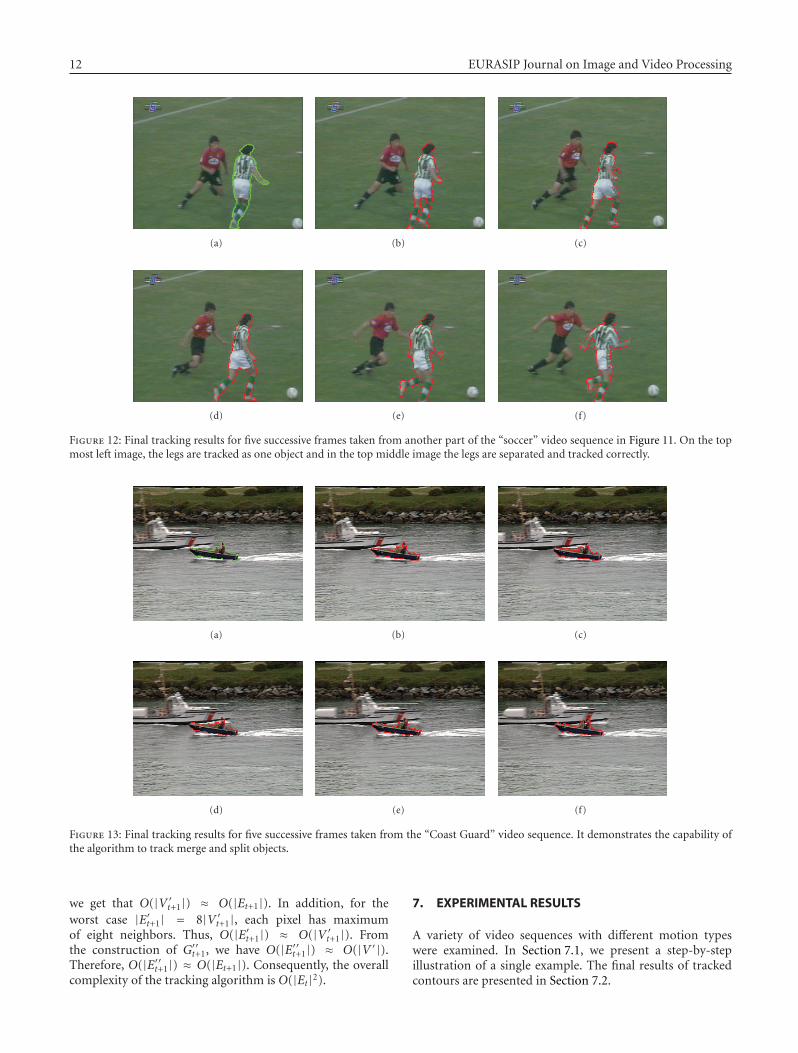
12 EURASIP Journal on Image and Video Processing
(a) (b) (c)
(d) (e) (f)
Figure 12: Final tracking results for five successive frames taken from another part of the “soccer” video sequence in Figure 11. On the topmost left image, the legs are tracked as one object and in the top middle image the legs are separated and tracked correctly.
(a) (b) (c)
(d) (e) (f)
Figure 13: Final tracking results for five successive frames taken from the “Coast Guard” video sequence. It demonstrates the capability ofthe algorithm to track merge and split objects.
we get that O(|V ′t+1|) ≈ O(|Et+1|). In addition, for the
worst case |E′t+1| = 8|V ′t+1|, each pixel has maximum
of eight neighbors. Thus, O(|E′t+1|) ≈ O(|V ′t+1|). From
the construction of G′′t+1, we have O(|E′′t+1|) ≈ O(|V ′|).Therefore, O(|E′′t+1|) ≈ O(|Et+1|). Consequently, the overallcomplexity of the tracking algorithm is O(|Et|2).
7. EXPERIMENTAL RESULTS
A variety of video sequences with different motion typeswere examined. In Section 7.1, we present a step-by-stepillustration of a single example. The final results of trackedcontours are presented in Section 7.2.

O. Miller et al. 13
7.1. Step-by-step illustration of the algorithm
Figure 8 is a step-by-step evolution of the tracking algorithmand how the final tracked contour is constructed. Figures8(a) (It) and 8(b) (It+1) are frames 1 and 3, respectively,from the “Tennis” sequence. The input contour of theobject to be tracked is surrounded by a green curve inFigure 8(a). The segmented curve of the first frame is shownin Figure 8(c) (It+1). Each pair of consecutive junctions Jkand Jk+1, k = 1, . . . ,N , is marked by white crosses. Thejunction that is marked with a yellow arrow in Figure 8(c)represents the intersection of two different homogeneousregions (the red pants and the blue shirt of the player), whichis obtained from its still image segmentation process. Thetwo other arrows (blue and green), marked in Figure 8(d)(It+1), represent the corresponding matched points (blueand green) from Figure 8(c) (It), respectively. As shown,all the detected junctions in Figure 8(c) are located on theboundaries between different homogeneous areas, and thus,are classified as “important” and well-tracked points that willbe used in the next steps of the algorithm.
A particular example of a curve construction of a pairof matched points S1 and S2 is given in Figure 8(e). Forthis pair (marked by two white crosses in Figure 8(e)), aset consisting of four different candidate paths P1,2
t+1,r , r =1, . . . , 4 (marked by four different colors) is found. The pinkpath, in this example, represents the matched path mp1,2
t+1.This path is located after the application of the matchingprocedure between the set P1,2
t+1,r , r = 1, . . . , 4 and P1,2t
(shown by the final constructed contour in Figure 8(f)). Thematched grades S f1(p) of P1,2
t+1,r , r = 1, . . . , 4, are given inFigure 9 as a function of four different β values (20%, 50%,80%, and 100%). As shown in Figure 9, the maximal S f1(p)was obtained for the pink path, for all β values. Differentvalues of β affect only the ratio between the right path (pink)and the other paths.
7.2. Final results
The examples in Figures 10, 11, 12, and 13 demonstratethe final results of tracked contours in four different videosequences. All the experiments were performed withouttuning of any parameters. The input object to be tracked inall the examples is marked by a green contour. Red contourrepresents the algorithm’s final output in the current frame.
8. CONCLUSIONS
In this paper, we propose a novel contour-based algorithmfor tracking a moving object. Based on the RAG datastructure, accurate results are achieved while preserving alow complexity. In the initialization step, two consecutiveinput frames are segmented with respect to a semantichomogeneous criterion. Their corresponding RAGs areconstructed to represent the partitions of the frames. Theobject’s contour is segmented into subcurves according to thedetected junctions that reside on the contour. The subcurvesof the object’s contour are the basis for the construction ofthe new tracked contour. A corresponding point for each
junction in It+1 is searched only in the RAG edges of theconsecutive frame. Then, each pair of matched points is con-nected by a set of candidate paths. Among all the candidatepaths, the path that is most similar to its correspondingsubcurve is considered to be a part of the tracked contour.Hence, only one of the RAG’s edges represents the trackedcontour. Consequently, the new object’s contour is accuratelyconstructed by the matched paths, and the overall complexityof the algorithm is proportional to the edges of the RAG.Note that representation of RAG edges usually consists of10% of the entire image.
REFERENCES
[1] Y. Cui, S. Samarasekera, Q. Huang, and M. Greiffenhagen,“Indoor monitoring via the collaboration between a periph-eral sensor and a foveal sensor,” in Proceedings of IEEEWorkshop on Visual Surveillance (VS ’98), pp. 2–9, Bombay,India, January 1998.
[2] G. R. Bradski, “Real time face and object tracking as acomponent of a perceptual user interface,” in Proceedings ofthe 4th IEEE Workshop on Applications of Computer Vision(WACV ’98), pp. 214–219, Princeton, NJ, USA, October 1998.
[3] A. Vetro, H. Sun, and Y. Wang, “MPEG-4 rate control formultiple video objects,” IEEE Transactions on Circuits andSystems for Video Technology, vol. 9, no. 1, pp. 186–199, 1999.
[4] M. R. Naphade, I. V. Kozintsev, and T. S. Huang, “Factor graphframework for semantic video indexing,” IEEE Transactions onCircuits and Systems for Video Technology, vol. 12, no. 1, pp.40–52, 2002.
[5] M. R. Naphade and T. S. Huang, “A probabilistic frameworkfor semantic video indexing, filtering, and retrieval,” IEEETransactions on Multimedia, vol. 3, no. 1, pp. 141–151, 2001.
[6] M. Kass, A. Witkin, and D. Terzopoulos, “Snakes: activecontour models,” International Journal of Computer Vision,vol. 1, no. 4, pp. 321–331, 1988.
[7] J. I. Agbinya and D. Rees, “Multi-object tracking in video,”Real-Time Imaging, vol. 5, no. 5, pp. 295–304, 1999.
[8] M. J. Swain and D. H. Ballard, “Color indexing,” InternationalJournal of Computer Vision, vol. 7, no. 1, pp. 11–32, 1991.
[9] E. Ozyildiz, N. Krahnst”over, and R. Sharma, “Adaptivetexture and color segmentation for tracking moving objects,”Pattern Recognition, vol. 35, no. 10, pp. 2013–2029, 2002.
[10] D. Yang and H.-I. Choi, “Moving object tracking by opti-mizing active models,” in Proceedings of the 14th InternationalConference of Pattern Recognition (ICPR ’98), vol. 1, pp. 738–740, Brisbane, Australia, August 1998.
[11] R. Murrieta-Cid, M. Briot, and N. Vandapel, “Landmark iden-tification and tracking in natural environment,” in Proceedingsof IEEE/RSJ International Conference on Intelligent Robots andSystems (IROS ’98), vol. 1, pp. 179–184, Victoria, Canada,October 1998.
[12] D.-S. Jang, S.-W. Jang, and H.-I. Choi, “2D human bodytracking with structural Kalman filter,” Pattern Recognition,vol. 35, no. 10, pp. 2041–2049, 2002.
[13] D. Wang, “Unsupervised video segmentation based on water-sheds and temporal tracking,” IEEE Transactions on Circuitsand Systems for Video Technology, vol. 8, no. 5, pp. 539–546,1998.
[14] C. L. Lam and S. Y. Yuen, “An unbiased active contouralgorithm for object tracking,” Pattern Recognition Letters, vol.19, no. 5-6, pp. 491–498, 1998.

14 EURASIP Journal on Image and Video Processing
[15] Y. Fu, A. T. Erdem, and A. M. Tekalp, “Occlusion adaptivemotion snake,” in Proceedings of IEEE International Conferenceon Image Processing (ICIP ’98), vol. 3, pp. 633–637, Chicago,Ill, USA, October 1998.
[16] J. Shao, F. Porikli, and R. Chellappa, “A particle filter basednon-rigid contour tracking algorithm with regulation,” in Pro-ceedings of IEEE International Conference on Image Processing(ICIP ’06), Atlanta, Ga, USA, October 2006.
[17] D. G. Lowe, “Robust model-based motion tracking throughthe integration of search and estimation,” International Journalof Computer Vision, vol. 8, no. 2, pp. 113–122, 1992.
[18] P. Wunsch and G. Hirzinger, “Real-time visual tracking of 3-D objects with dynamic handling of occlusion,” in Proceedingsof IEEE International Conference on Robotics and Automation(ICRA ’97), vol. 4, pp. 2868–2873, Albuquerque, NM, USA,April 1997.
[19] K. F. Lai and R. T. Chin, “Deformable contours: modeling andextraction,” IEEE Transactions on Pattern Analysis and MachineIntelligence, vol. 17, no. 11, pp. 1084–1090, 1995.
[20] C. Kervrann and F. Heitz, “Hierarchical Markov modelingapproach for the segmentation and tracking of deformableshapes,” Graphical Models and Image Processing, vol. 60, no.3, pp. 173–195, 1998.
[21] T. Schoepflin, V. Chalana, D. R. Haynor, and Y. Kim,“Video object tracking with a sequential hierarchy of templatedeformations,” IEEE Transactions on Circuits and Systems forVideo Technology, vol. 11, no. 11, pp. 1171–1182, 2001.
[22] E. Navon, Image segmentation based on minimum spanningtree and computation of local threshold, M.S. thesis, Tel-AvivUniversity, Tel-Aviv, Israel, October 2002.
[23] E. Navon, O. Miller, and A. Averbuch, “Color image segmen-tation based on adaptive local thresholds,” Image and VisionComputing, vol. 23, no. 1, pp. 69–85, 2004.
[24] E. Navon, O. Miller, and A. Averbuch, “Color image segmen-tation based on automatic derivation of local thresholds,” inProceedings of the 7th Digital Image Computing, Techniques andApplications Conference (DICTA ’03), pp. 571–580, Sydney,Australia, December 2003.
[25] L. Vincent and P. Soille, “Watersheds in digital spaces: anefficient algorithm based on immersion simulations,” IEEETransactions on Pattern Analysis and Machine Intelligence, vol.13, no. 6, pp. 583–598, 1991.
[26] J. Shei and C. Tomasi, “Good feature to track,” in Proceedingsof IEEE Computer Society Conference on Computer Vision andPattern Recognition (CVPR ’94), pp. 593–600, Seattle, Wash,USA, June 1994.
[27] R. Laganiere, “A morphological operator for corner detection,”Pattern Recognition, vol. 31, no. 11, pp. 1643–1652, 1998.
[28] J.-S. Lee, Y.-N. Sun, and C.-H. Chen, “Multiscale cornerdetection by using wavelet transform,” IEEE Transactions onImage Processing, vol. 4, no. 1, pp. 100–104, 1995.
[29] C. Harris and M. Stephens, “A combined corner and edgedetector,” in Proceedings of the 4th Alvey Vision Conference(AVC ’88), pp. 147–151, Manchester, UK, August-September1988.
[30] P. Smith, D. Sinclair, R. Cipolla, and K. Wood, “Effectivecorner matching,” in Proceedings of the 9th British MachineVision Conference (BMVC ’98), pp. 545–556, Southampton,UK, September 1998.
[31] A. A. Argyros, K. E. Bekris, and S. C. Orphanoudakis, “Robothoming based on corner tracking in a sequence of panoramicimages,” in Proceedings of IEEE Computer Society Conferenceon Computer Vision and Pattern Recognition (CVPR ’01), vol.2, pp. 3–10, Kauai, Hawaii, USA, December 2001.
[32] G. Srivastava, G. Agarwal, and S. Gupta, “A very low bit ratevideo codec with smart error resiliency features for robustwireless video transmission,” in Proceedings of IEEE Interna-tional Conference on Acoustics, Speech and Signal Processing(ICASSP ’02), vol. 4, p. 4191, Orlando, Fla, USA, May 2002.
[33] D. Eppstein, “Finding the k shortest paths,” SIAM Journal onComputing, vol. 28, no. 2, pp. 652–673, 1998.
[34] R. K. Ahuja, T. L. Magnanti, and J. B. Orlin, Network Flows,Prentice-Hall, Englewood Cliffs, NJ, USA, 1993.
[35] A. Zisserman, A. Blake, and R. Curwen, “A framework forspatio-temporal control in the tracking of visual contours,” inReal-Time Computer Vision, C. M. Brown and D. Terzopoulos,Eds., pp. 3–33, Cambridge University Press, Cambridge, UK,1995.

Hindawi Publishing CorporationEURASIP Journal on Image and Video ProcessingVolume 2008, Article ID 274349, 21 pagesdoi:10.1155/2008/274349
Research ArticleFeature Classification for Robust Shape-Based CollaborativeTracking and Model Updating
M. Asadi, F. Monti, and C. S. Regazzoni
Department of Biophysical and Electronic Engineering, University of Genoa, Via All’Opera Pia 11a, 16145 Genoa, Italy
Correspondence should be addressed to M. Asadi, [email protected]
Received 14 November 2007; Revised 27 March 2008; Accepted 10 July 2008
Recommended by Fatih Porikli
A new collaborative tracking approach is introduced which takes advantage of classified features. The core of this tracker is asingle tracker that is able to detect occlusions and classify features contributing in localizing the object. Features are classified infour classes: good, suspicious, malicious, and neutral. Good features are estimated to be parts of the object with a high degree ofconfidence. Suspicious ones have a lower, yet significantly high, degree of confidence to be a part of the object. Malicious featuresare estimated to be generated by clutter, while neutral features are characterized with not a sufficient level of uncertainty to beassigned to the tracked object. When there is no occlusion, the single tracker acts alone, and the feature classification module helpsit to overcome distracters such as still objects or little clutter in the scene. When more than one desired moving objects boundingboxes are close enough, the collaborative tracker is activated and it exploits the advantages of the classified features to localize eachobject precisely as well as updating the objects shape models more precisely by assigning again the classified features to the objects.The experimental results show successful tracking compared with the collaborative tracker that does not use the classified features.Moreover, more precise updated object shape models will be shown.
Copyright © 2008 M. Asadi et al. This is an open access article distributed under the Creative Commons Attribution License,which permits unrestricted use, distribution, and reproduction in any medium, provided the original work is properly cited.
1. INTRODUCTION
Target tracking in complex scenes is an open problem inmany emerging applications, such as visual surveillance,robotics, enhanced video conferencing, and sport videohighlighting. It is one of the key issues in the video analysischain. This is because the motion information of all objectsin the scene can be fed into higher-level modules of thesystem that are in charge of behavior understanding. To thisend, the tracking algorithm must be able to maintain theidentities of the objects.
Maintaining the track of an object during an inter-action is a difficult task mainly due to the difficulty insegmenting object appearance features. This problem affectsboth locations and models of objects. The vast majorityof tracking algorithms solve this problem by disablingthe model updating procedure in case of an interaction.However, the drawback of these methods arises in case of achange in objects appearance during occlusion.
While in case of little clutter and few partial occlusionsit is possible to classify features [1, 2], in case of heavyinteraction between objects, sharing trackers informationcan help to avoid the coalescence problem [3].
In this work, a method is proposed to solve these prob-lems by integrating an algorithm for feature classification,which helps in clutter rejection, in an algorithm for thesimultaneous and collaborative tracking of multiple objects.To this end, the Bayesian framework developed in [2] forshape and motion tracking is used as the core of the singleobject tracker. This framework was shown to be a suboptimalsolution with respect to the single-target-tracking problem,where a posterior probabilities of the object position andthe object shape model are maximized separately andsuboptimally [2]. When an interaction occurs among someobjects, a newly developed collaborative algorithm, capableof feature classification, is activated. The classified featuresare revised using a collaborative approach based on therationale that each feature belongs to only one object [4].
The contribution of this paper is to introduce a collabo-rative tracking approach which is capable of feature classifi-cation. This contribution can be seen as three major points.
(1) Revising and refining the classified features. A collab-orative framework is developed that is able to reviseand refine classes of features that have been classifiedby the single object tracker.

2 EURASIP Journal on Image and Video Processing
(2) Collaborative position estimation. The performanceof the collaborative tracker is improved using therefined classes.
(3) Collaborative shape updating. While the methodsavailable in literature are mainly interested in the col-laborative estimation, the proposed method imple-ments a collaborative appearance updating.
The rest of the paper is organized as follows. Section 2discusses the related works. Section 3 describes the single-tracking algorithm and its Bayesian origin. In Section 4, thecollaborative approach is described. Experimental results arepresented in Section 5. Finally in Section 6 some concludingremarks are provided.
2. RELATED WORK
Simultaneous tracking of visual objects is a challengingproblem that has been approached in a number of differentways. A common approach to solve the problem is theMerge-Split approach: in an interaction, the overlappingobjects are considered as a single entity. When they separateagain, the trackers are reassigned to each object [5, 6]. Themain drawbacks of this approach are the loss of identities andthe impossibility of updating the object model.
To avoid this problem, the objects should be tracked andsegmented also during occlusion. In [7], multiple objectsare tracked using multiple independent particle filters. Incase of independent trackers, if two or more objects comeinto proximity, two common problems may occur: “labelingproblem” (the identities of two objects are inverted) and“coalescence problem” (one object hijacks more than onetracker). Moreover, the observations of objects that comeinto proximity are usually confused and it is difficult tolearn the object model correctly. In [8] humans are trackedusing a priori target model and a fixed 3D model of thescene. This allows the assignment of the observations usingdepth ordering. Another common approach is to use a joint-state space representation that describes contemporarilythe joint state of all objects in the scene [9–13]. Okumaet al. [11] use a single particle filter tracking frameworkalong with a mixture density model as well as an offlinelearned Adaboost detector. Isard and MacCormick [12]model persons as cylinders to model the 3D interactions.Although the above-mentioned approaches can describethe occlusion among targets correctly, they have to modelall states with exponential complexity without consideringthat some trackers may be independent. In the last fewyears, new approaches have been proposed to solve theproblem of the exponential complexity [5, 13, 14]. Li etal. [13] solve the complexity problem using a cascadeparticle filter. While good results are reported also in low-frame rate video, their method needs an offline learneddetector and hence it is not useful when there is no a prioriinformation about the objects class. In [5], independenttrackers are made collaborative and distributed using aparticle filter framework. Moreover, an inertial potentialmodel is used to predict the tracker motion. It solves the“coalescence problem,” but since global features are used
without any depth ordering, updating is not feasible duringocclusion. In [14], a belief propagation framework is used tocollaboratively track multiple interacting objects. Again, thetarget model is learned offline.
In [15], the authors use an appearance-based reasoningto track two faces (modeled as multiple view templates)during occlusion by estimating the occlusion relation (depthordering). This framework seems limited to two objects andsince it needs multiple view templates and the model is notupdated during tracking, it is not useful when there is no apriori information about the targets. In [16], three Markovrandom fields (MRFs) are coupled to solve the trackingproblem: a field for the joint state of multiple targets; a binaryrandom process for the existence of each individual target;and a binary random process for the occlusion of each dualadjacent target. The inference in the MRF is solved by usingparticle filtering. This approach is also limited to a predefinedclass of objects.
3. SINGLE-OBJECT TRACKER ANDBAYESIAN FRAMEWORK
The role of the single tracker—introduced in [2]—is toestimate the current state of an object, given its previous stateand current observations. To this end, a Bayesian frameworkis presented in [2]. The framework also is briefly introducedhere.
Initialization
A desired object is specified with a bounding box. Then, allcorners, say M, inside the bounding box are extracted andthey are considered as the object features. They are shownas Xc,t = {Xm
c,t}1≤m≤M = {(xmt , ymt )}1≤m≤M where the pair(xmt , ymt ) is the absolute coordinates of corner m and thesubscript c denotes corner. A reference point, for example, thecenter of the bounding box, is chosen as the object position.In addition, an initial persistency value PI is assigned to eachcorner. It is used to show the consistency of that cornerduring time.
Target model
The object shape model is composed of two elements: Xs,t ={Xm
s,t}1≤m≤M = {[DXmc,t,P
mt ]}1≤m≤M . The element DXm
c,t =Xmc,t−Xp,t is the relative coordinates of corner m with respect
to the object position Xp,t = (xreft , yref
t ). Therefore, the objectstatus at time t is defined as Xt = {Xs,t , Xp,t}.
Observations
The observations set Zt = {Znt }1≤n≤N = {[xnt , ynt ]}1≤n≤N at
any time t is composed of the coordinates in the image planeof all extracted corners inside a bounding box Q of the samesize as the one in the last frame, centered at the last referencepoint Xp,t−1.

M. Asadi et al. 3
Probabilistic Bayesian framework
In the probabilistic framework, the goal of the tracker isto estimate the posterior p(Xt | Zt, Xt−1 = X∗
t−1). In thispaper, random variables are vectors and they are shown usingbold fonts. When the value of a random variable is fixed,an asterisk is added as a superscript of the random variable.Moreover, for simplification, the fixed random variables arereplaced just by their values: p(Xt | Zt , Xt−1 = X∗
t−1) =p(Xt | Zt, X∗
t−1). Moreover, at time t it is supposed that theprobability of the variables at time t − 1 has been fixed. Theother assumption is that since Bayesian filtering propagatesdensities and in the current work no density or errorpropagation is used, the probabilities of the random variablesat time t − 1 are redefined as Kronecker delta functions, forexample, p(Xt−1) = δ(Xt−1 − X∗
t−1). Using Bayesian filteringapproach and considering the independence between shapeand motion one can write [2]
p(
Xt | Zt , X∗t−1
)
= p(Xp,t, Xs,t | Zt, X∗p,t−1, X∗
s,t−1
)
= p(Xs,t | Zt , X∗p,t−1, X∗
s,t−1, Xp,t)·p(Xp,t | Zt , X∗
p,t−1, X∗s,t−1
).
(1)
Maximizing separately each of the two terms at the right-hand side of (1) provides a suboptimal solution to theproblem of estimating the posterior of Xt . The first term isthe posterior probability of the shape object model (shapeupdating phase). The second term is the posterior probabilityof the object global position (object tracking).
3.1. The global position model
The posterior probability of the object global positioncan be factorized into a normalization factor, the positionprediction model (a priori probability of the object position),and the observation model (likelihood of the object position)using the chain rule and considering the independencebetween shape and model [2]:
p(
Xp,t | Zt, X∗p,t−1, X∗
s,t−1
)
= k·p(Xp,t | X∗p,t−1
) · p(Zt | X∗p,t−1, X∗
s,t−1, Xp,t).
(2)
3.1.1. The position prediction model(the global motion model)
The prediction model is selected with the rationale thatan object cannot move faster than a given speed (inpixels). Moreover, defining different prediction models givesdifferent weights to different global object positions in theplane. In this paper, a simple global motion prediction modelof a uniform windowed type is used:
p(
Xp,t | X∗p,t−1
) =
⎧⎪⎪⎨⎪⎪⎩
1Wx·Wy
if(
Xp,t −X∗p,t−1
) ≤ W2
,
0 elsewhere,(3)
where W is a rectangular area Wx ×Wy initially centered onX∗p,t−1. If more a priori knowledge about the object global
motion is available, it will be possible to assign differentprobabilities to different positions inside the window usingdifferent kernels.
3.1.2. The observation model
The position observation model is defined as follows:
p(
Zt | X∗p,t−1, X∗
s,t−1, Xp,t) = 1− e−Vt(Xp,t ,Zt ,X∗p,t−1,X∗s,t−1)
∑Zt
(1− e−Vt(Xp,t ,Zt ,X∗p,t−1,X∗s,t−1)
) ,
(4)
where Vt(Xp,t, Zt, X∗p,t−1, X∗
s,t−1) is the number of votes to apotential object position. It is defined as follows:
Vt(
Xp,t, Zt, X∗p,t−1, X∗
s,t−1
)
=N∑
n=1
M∑
m=1
KR(dm,n
(Xmc,t−1 −X∗
p,t−1, Znt −Xp,t
)),
(5)
where dm,n(·) is the Euclidean distance metric and itevaluates the distance between a model element m and anobservation element n. If this distance falls within the radiusRR of a position kernel KR(·), m and n will contribute toincrease the value of Vt(·) based on the definition of thekernel. It is possible to have different types of kernels, basedon the a priori knowledge about the rigidity of desiredobjects. Each kernel has a different effect on the amount ofthe contribution [2]. Having a look at (5), it is seen thatan observation element n may match with several modelelements inside the kernel to contribute to a given positionXp,t. The fact that a rigidity kernel is defined to allow possibledistorted copies of the model elements contribute to a givenposition is called regularization. In this work, a uniformkernel is defined:
KR(dm,n
(Xmc,t−1 −X∗
p,t−1, Znt −Xp,t
))
=⎧⎨⎩
1 if dm,n(
Xmc,t−1 −X∗
p,t−1, Znt −Xp,t
) ≤ RR,
0 otherwise.
(6)
The proposed suboptimal algorithm fixes as a solution thevalue Xp,t = X∗
p,t that maximizes the product in (2).
3.1.3. The hypotheses set
To implement the object position estimation, (5) is imple-mented. Therefore, it provides an estimation for each pointXp,t of the probability that the global object position iscoincident with Xp,t itself. The resulting function can beunimodal or multimodal (for details, see [1, 2]). Since theshape model is affected by noise (and consequently it cannotbe defined as ideal) and observations are also affected by theenvironmental noise, for example, clutter in the scene anddistracters, a criterion must be fixed to select representativepoints from the estimated function (2). One possible choiceis considering a set of points such that they correspond

4 EURASIP Journal on Image and Video Processing
A B
CF
DE
(a)
A B
CF
DE
(b)
X∗p,t−1 Xp,t,1
Xp,t,2
(c)
(d) (e)
Figure 1: (a) An object model with six model corners at time t − 1. (b) The same object at time t along with distortion of two corners“D” and “E” by one pixel in the direction of y-axis. Blue and green arrows show voting to different positions. (c) The motion vector of thereference point related to both candidates in (b). (d) The motion vector of the reference point to a voted position along with regularization.(e) Clustering nine motion hypotheses in the regularization process using a uniform kernel of radius
√2.
to sufficiently high values of the estimated function (highnumber of votes) and they are spatially well separated. In thisway, it can be shown that a set of possible alternative motionhypotheses of the object are considered corresponding toeach selected point. As an example, one can have a look atFigure 1.
Figure 1(a) shows an object with six corners at time t−1.The corners and the reference point are shown with red colorand light blue, respectively. The arrows show the position ofthe corners with respect to the reference point. Figure 1(b)shows the same object at time t, while two corners “D”and “E” are distorted by one pixel in the direction of y-axis. The dashed lines indicate the original figure withoutany change. For localizing the object, all six corners votebased on the model corners. In Figure 1(b), only six votesare shown without considering regularization. The four bluearrows show the votes of corners “A,” “B,” “C,” and “F” for aposition indicated by the light blue color. This position canbe a candidate for the new reference point and is shown byXp,t,1 in Figure 1(c). Two corners “E” and “D” are voting toanother position marked with a green-colored circle. Thisposition is called Xp,t,2 and it is located below the Xp,t,1
with a distance of one pixel. Figure 1(c) plotted the referencepoint at time t − 1 and the two candidates at time t in thesame Cartesian system. Black arrows in Figure 1(c) indicatethe displacement of the old reference point considering eachcandidate at time t to be the new reference point. Thesethree figures make the aforementioned reasoning clearer.From the figures, it is clear that each position in the votingspace corresponds either to one motion vector (if there isno regularization) or to a set of motion vectors (if there isregularization (Figures 1(d) and 1(e))). Each motion vector,in turn, corresponds to a subset of observations that aremoving with the same motion. In case of regularization,
these two motion vectors can be clustered together sincethey are very close. This is shown in Figures 1(d) and 1(e).In case of using a uniform kernel with a radius of
√2 (6),
all eight pixels around each position are clustered in thesame cluster as the position. Such a clustering is depictedin Figures 1(d) and 1(e) where the red arrow shows themotion of the reference point at time t − 1 to a candidateposition. Figure 1(e) shows all nine motion vectors that canbe clustered together. Figures 1(d) and 1(e) are equivalent.In the current work, a uniform kernel with a radius of√
8 is used (therefore, 25 motion hypotheses are clusteredtogether).
To limit the computational complexity, a limited numberof candidate points, say h, are chosen (in this paper h = 4).If the function produced by (5) is unimodal, only the peakis selected as the only hypothesis, and hence the new objectposition. If it is multimodal, four peaks are selected using themethod described in [1, 2]. The h points corresponding tothe motion hypotheses are called maxima and the hypothesesset is called the maxima set, HM = {X∗
p,t,h | h = 1 · · · 4}.In the next subsection and using Figure 1, it is shown that
a set of corners can be associated with each maximum h inthe HM that corresponds to observations that supported aglobal motion equal to the shift from X∗
p,t−1 to X∗p,t,h. There-
fore, the distance in the voting space between two maximah and h′ can be also interpreted as the distance betweenalternative hypotheses of the object motion vectors, that is,as alternative global object motion hypothesis. As a conse-quence, points in the HM that are close to each other, cor-respond to hypotheses characterized by similar global objectmotion. On the contrary, points in the HM that are far fromeach other correspond to hypotheses characterized by inco-herent global motion hypotheses with respect to each other.

M. Asadi et al. 5
In the current paper, the point in HM with the highestnumber of votes is chosen as the new object position (thewinner). Then, other maxima in the hypotheses set areevaluated based on their distance from the winner. Anymaximum that is close enough to the winner is consideredas a member of the pool of winners WS and the maximathat are not in the pool of winners are considered as farmaxima forming the far maxima set FS = HM−WS.However,having a priori knowledge about the object motion makesit is possible to choose other strategies for ranking the fourhypotheses. More details can be found in [1, 2]. The nextstep is to classify features (hereinafter referred to as corners)based on the pool of winners and the far maxima set.
3.1.4. Feature classification
Now, all observations must be classified, based on theirvotes to the maxima, to distinguish between observationsthat belong to the distracter (FS) and other observations.To do this, the corners are classified into four classes: good,suspicious, malicious, and neutral. The classes are defined inthe following way.
Good corners
Good corners are those that have voted at least for onemaximum in the “pool of winners” but they have not votedfor any maximum in the “far maxima” set. In other words,good corners are subsets of observations that have motionhypotheses coherent with the winner maximum. This class isshown by SG as follows:
SG =⋃
i=1···N(WS)
Si −⋃
j=1···N(FS)
Sj , (7)
where Si is the set of all corners that have voted for the ithmaximum and N(WS) and N(FS) are the number of maximain the “pool of winners” and “far maxima set” respectively.
Suspicious corners
Suspicious corners are those that have voted at least for onemaximum in the “pool of winners” and they have also votedfor at least one maximum in the “far maxima” set. Sincecorners in this set voted for pool of winners and far maximaset, they can introduce two sets of motion hypotheses. Oneset is coherent with the motion of the winner, while the otherset of motion hypotheses is incoherent with the winner. Thisclass is shown by SS as follows:
SS =⋂( ⋃
i=1···N(WS)
Si,⋃
j=1···N(FS)
Sj
). (8)
Malicious corners
Malicious corners are those that have voted to at least onemaximum in the far maxima set, but they have not voted forany maximum in the pool of winners. Motion hypotheses
corresponding to this class are completely incoherent withthe object global motion. This class is formulated as follows:
SM =⋃
j=1···N(FS)
Sj −⋃
i=1···N(WS)
Si. (9)
Neutral corners
Neutral corners are those that have not voted to any max-imum. In other words, no decision can be made regardingthe motion hypotheses of these corners. This class is shownby SN .
These four classes are passed to the updating shape-basedmodel module (first term in (1)).
Figure 2 shows a very simple example in which a squareis tracked. The square is shown using red dots representingits corners. Figure 2(a) is the model represented by fourcorners {A1,B1,C1,D1}. The blue box at the center of thesquare indicates the reference point. Figure 2(b) shows theobservations set composed by four corners. These cornersare voting based on (5). Therefore, if observation A isconsidered as the model corner D1, it will vote based onthe relative position of the reference point with respectto D1, that is, it will vote to the top left (Figure 2(b)).The arrows in Figure 2(b) show the voting procedure. Inthe same way, all observations vote. Figure 2(d) shows thenumber of votes acquired from Figure 2(b). In Figure 2(c), atriangle has been shown with its corners. The blue crossesindicate the triangle corners. In this example, the triangleis considered as a distracter whose corners are consideredas a part of observations and may change the number ofvotes for different positions. In this case, the point “M1”receives five votes from {A,B,C,D,E} (consider that dueto regularization, the number of votes to “M1” is equalto the summation of votes to its neighbors). The relativevoting space is shown in Figure 2(e). In case corner “B” isoccluded, the points “M1” to “M3” will receive one vote less.The points “M1” to “M3” show three maxima. Assuming“M1” as the winner and as the only member of the poolof winners, M2 and “M3” are considered as far maxima:HM = {M1,M2,M3}, WS = {M1}, and FS = {M2,M3}.In addition, we can define the set of corners voting foreach candidate: obs(M1) = {A,B,C,D,E}, obs(M2) ={A,B,E,F}, and obs(M3) = {B,E,F,G}, where obs(M)indicates the observations voting for M. Using formulas (7)to (9), observations can be classified as SG = {C,D}, SS ={A,B,E}, and SM = {F,G}. In Figure 2(c), the brown cross“H” is a neutral corner (SN = {H}) since it is not voting toany maxima.
3.2. The shape-based model
Having found the new estimated global position of theobject, the shape must be estimated. This means to apply astrategy to maximize the probability of the posterior p(Xs,t |Zt , X∗
p,t−1, X∗s,t−1, X∗
p,t) where all terms in the conditional parthave been fixed. Since the new position of the object Xp,t hasbeen fixed to X∗
p,t in the previous step, the posterior can be

6 EURASIP Journal on Image and Video Processing
A1 B1
C1 D1
(a)
A,D1
BA
D
(b)
M2 M3
A
C D
E B
F G
M1 H
(c)
1 2 1
2 4
1 2 1
2
(d)
1 2 1
1 4 4 1
2 5 3 1 1
1 2 1 1 1
(e)
Figure 2: Voting and corners classification. (a) The shape model in red dots and the reference point in blue box. (b) Observations and votingin an ideal case without any distracter. (c) Voting in the presence of a distracter in blue cross. (d) The voting space related to (b). (e) Thevoting space related to (c) along with three maxima shown by green circles.
written as p(Xs,t | Zt , X∗p,t−1, X∗
s,t−1, X∗p,t). With a reasoning
approach similar to the one related to (2), one can write
p(
Xs,t | Zt, X∗p,t−1, X∗
s,t−1, X∗p,t
)
= k′·p(Xs,t | X∗s,t−1
)·p(Zt | Xs,t , X∗p,t−1, X∗
s,t−1, X∗p,t
),
(10)
where the first term at the right-hand side of (10) is the shapeprediction model (a priori probability of the object shape)and the second term is the shape updating observation model(likelihood of the object shape).
3.2.1. The shape prediction model
Since small changes are assumed in the object shape in twosuccessive frames, and since the motion is assumed to beindependent from the shape and its local variations, it isreasonable to have the shape at time t be similar to theshape at time t − 1. Therefore, all possible shapes at timet that can be generated from the shape at time t − 1 withsmall variations form a shape subspace and they are assignedsimilar probabilities. If one considers the shape as generatedindependently bymmodel elements, then the probability canbe written in terms of the kernel Kls,m of each model elementas
p(Xs,t | X∗s,t−1) =
∏mKls,m(Xm
s,t ,ηms,t)∑Xs,t
∏mKls,m(Xm
s,t ,ηms,t)
(11)
ηms,t is the set of all model elements at time t − 1 that liesinside a rigidity kernel KR with the radius RR centered on
Xms,t : ηms,t = {X
js,t−1 : dm, j(DXm
c,t, DXjc,t−1) ≤ RR}. The
subscript ls stands for the term “local shape.” As in (12) thelocal shape kernel of each shape element depends on therelation between that shape element and each single elementinside the neighborhood as well as the effect of the singleelement on the persistency of the shape element:
Kls,m(
Xms,t,η
ms,t
)
=∑
j:Xjs,t−1∈ηms,t
Kj
ls,m
(Xms,t , X
js,t−1
)
=∑
j:Xjs,t−1∈ηms,t
KR(dm, j
(DXm
c,t , DXjc,t−1
)) · K jP,m
(Xms,t , X
js,t−1
).
(12)
The last term in (12) allows us to define different effects onthe persistency, for example, based on distance of the singleelement from the shape element. Here, a simple function ofzero and one is used:
KjP,m
(Xms,t, X
js,t−1
)
=⎧⎨⎩
1 if(Pmt − P j
t−1
) ∈ {1,−1,Pth,PI , 0,−Pmt−1
},
0 elsewhere.
(13)

M. Asadi et al. 7
The set of possible values of the difference between twopersistency values is computed by considering different cases(appearing, disappearing, flickering . . .) that may occur for agiven corner between two successive frames. For more detailson how it is computed one can refer to [2].
3.2.2. The shape updating observation model
According to the shape prediction model, only a finite set(even though quite large) of possible new shapes (Xs,t) can beobtained. After prediction of the shape model at time t, theshape model can be updated by an appropriate observationmodel that filters the finite set of possible new shapes toselect one of the possible predicted new shape models (Xs,t).To this end, the second term in (10) is used. To computethe probability, a function q is defined on Q whose domainis the coordinates of all positions inside Q and its range is{0, 1}. A zero value for a position (x, y) shows the lack of anobservation at that position; while a one value indicates thepresence of an observation at that position. The function q isdefined as follows:
q(x, y) =⎧⎨⎩
1 if (x, y) ∈ Zt
0 if (x, y) ∈ Zct ,
(14)
where Zct is the complimentary set of Zt : Zc
t = Q −Zt . Therefore, using (14) and having the fact that theobservations in the observations set are independent fromeach other, the second probability term in (10) can be writtenas a product of two terms:
p(
Zt | Xs,t, X∗p,t−1, X∗
s,t−1, X∗p,t
)
=∏
(x,y)∈Zt
p(q(x, y) = 1 | X∗
p,t−1, X∗s,t−1, Xs,t, X∗
p,t
)
·∏
(x,y)∈Zct
p(q(x, y) = 0 | X∗
p,t−1, X∗s,t−1, Xs,t, X∗
p,t
).
(15)
Based on the presence or absence of a given model cornerin two successive frames and based on its persistency value,different cases for that model corner can be investigatedin two successive frames. Investigating different cases, thefollowing rule is derived that maximizes the probability valuein (15) [2]:
Pnt =
⎧⎪⎪⎪⎪⎪⎪⎪⎪⎪⎪⎪⎪⎪⎪⎪⎪⎪⎪⎪⎪⎪⎪⎨⎪⎪⎪⎪⎪⎪⎪⎪⎪⎪⎪⎪⎪⎪⎪⎪⎪⎪⎪⎪⎪⎪⎩
Pjt−1 +1 if ∃ j : X
js,t−1∈ηns,t , P
jt−1≥Pth, q(xn, yn)=1
(the corner exists in both frames),
Pjt−1−1 if ∃ j : X
js,t−1 ∈ ηns,t, P
jt−1>Pth, q(xn, yn)=0
(the corner disappears),
0 if ∃ j : Xjs,t−1 ∈ ηns,t,P
jt−1=Pth, q(xn, yn)=0
(the corner disappears),
PI if � j : Xjs,t−1 ∈ ηns,t, q(xn, yn) = 1
(a new corner appears).(16)
To implement model updating, (16) is implemented consid-ering also the four classes of corners (see Section 3.1.4). Tothis end, the corners in the malicious class are discarded.The corners in the good and suspicious classes are fed toformula (16). The neutral corners can be treated differently.They may be fed to (16). This can be done when allhypotheses belong to the pool of winners, that is, when nodistracter is available. If this is not the case, the neutralcorners are also discarded. Although some observationsare discarded (malicious corners), the compliancy to theBayesian framework is achieved through the following:
(i) adaptive shape noise (e.g., occluder, clutter, dis-tracter) model estimation;
(ii) filtering observations Zt to produce a reduced obser-vation set Z′t ;
(iii) substitute Z′t in (15) to compute an alternativesolution X′
s,t .
The above-mentioned procedure simply says that discardedobservations are noise.
In the first row of (16), there may be more than onecorner in the neighborhood of a given corner (ηns,t). In thiscase, the closest one to the given corner is chosen, see [1, 2]for more details on updating.
4. COLLABORATIVE TRACKING
Independent trackers are prone to merge error and labelingerror in multiple target applications. While it is a commonsense that a corner in the scene can be generated by onlyone object and can therefore participate in the positionestimation and shape updating of only one tracker, this rule issystematically violated when multiple independent trackerscome into proximity. In this case, in fact, the same cornersare used during the evaluation of (2) and (10) with allproblems described in the related work section. To avoidthese problems, an algorithm that allows the collaboration oftrackers and that exploits feature classification information isdeveloped. Using this algorithm, when two or more trackerscome to proximity, they start to collaborate both during theposition and the shape estimation.
4.1. General theory of collaborative tracking
In multiple object tracking scenarios, the goal of the trackingalgorithm is to estimate the joint state of all tracked objects[X1
p,t, X1s,t, . . . , XG
p,t, XGs,t], where G is the number of tracked
objects. If objects observations are independent, it will bepossible to factor the distributions and to update each trackerseparately from others.
In case of dependent observations, their assignmentshave to be estimated considering the past shapes andpositions of interacting trackers. Considering that not alltrackers interact (far objects do not share observations), it ispossible to simplify the tracking process by factoring the jointposterior in dynamic collaborative sets. The trackers shouldbe divided into sets considering their interactions: one set foreach group of interacting targets.

8 EURASIP Journal on Image and Video Processing
To do this, the overlap between all trackers is evaluatedby checking if there is a spatial overlap between shapes oftrackers at time t − 1.
The trackers are divided into J sets such that objectsassociated to trackers of each set interact with each otherwithin the same set (intraset interaction) but they do notoverlap any tracker of any other set (there is no intersetinteraction).
Since there is no interset interaction, observations of eachtracker in a cluster can be assigned conditioning only ontrackers in the same set. Therefore, it is possible to factor thejoint posterior into the product of some terms each of whichassigned to one set:
p(
X1p,t, X1
s,t, . . . , XGp,t, XG
s,t | Z1t , . . . , ZG
t ,
X∗1p,t−1, X∗1
s,t−1, . . . , X∗Gp,t−1, X∗G
s,t−1
)
=J∏
j=1
p(
XNjt
p,t , XNjt
s,t | ZNjt
t , X∗N jt
p,t−1, X∗N jt
s,t−1
),
(17)
where J is the number of collaborative sets and XNjt
p,t , XNjt
s,t and
ZNjt
t are the states and observations of all trackers in the setN
jt , respectively. In this way, there is no necessity to create
a joint-state space with all trackers, but only J spaces. Foreach set, the solution to the tracking problem is estimatedby calculating the joint state in that set that maximizes theposterior of the same collaborative set.
4.2. Collaborative position estimation
When an overlap between the trackers is reported, they are
assigned to the same set Njt . While the a priori position
prediction is done independently for each tracker in the sameset (3), the likelihood calculation, that is not factorable, isdone in a collaborative way.
The union of observations of trackers in the collaborative
set ZNjt
t is considered as generated by L trackers in the set.Considering that during an occlusion event, there is alwaysan object that is more visible than the others (the occluder),with the aim of maximizing (17), it is possible to factor thelikelihood in the following way:
p(
ZNjt
t | X∗N jt
s,t−1, XNjt
p,t , X∗N jt
p,t−1
)
= p(Ξ | ZN
jt
t \ Ξ, X∗N jt
s,t−1, XNjt
p,t , X∗N jt
p,t−1
)
· p(
ZNjt
t \ Ξ | X∗N jt
s,t−1, XNjt
p,t , X∗N jt
p,t−1
),
(18)
where the observations are divided into two sets: Ξ ⊂ ZNjt
t
and the remaining observations ZNjt
t \ Ξ. To maximize (18),it is possible to proceed by separately (and suboptimally)finding a solution to the two terms assuming that the productof the two partial distributions will give rise to a maximumin the global distribution. If the lth object is perfectly visible,
and if Ξ is chosen as Zlt, the maximum will be generated only
by observations of the lth object. Therefore, one can write
max p(Ξ | ZN
jt
t \ Ξ, X∗N jt
s,t−1, XNjt
p,t , X∗N jt
p,t−1
)
= max p(
Zlt | X∗l
s,t−1, Xlp,t, X∗l
p,t−1
).
(19)
Assuming that the tracker under analysis is associated tothe most visible tracker, it is possible to use the algorithmdescribed in Section 3 to estimate its position using all
observations ZNjt
t .It is possible to state that the position of the winner
maximum estimated using all observations ZNjt
t will be inthe same position as if it were estimated using Zl
t. Thisis true because if all observations of the lth tracker are
visible, p(ZNjt
t |X∗ls,t−1, Xl
p,t, X∗lp,t−1) will have one peak in X∗l
p,t
and some other peaks in correspondence of some positionsthat correspond to groups of observations that are similarto X∗l
s,t−1. However, using motion information as well, it ispossible to filter existing peaks which do not correspondto the true position of the object. Using the selectedwinner maximum and the classification information, onecan estimate the set of observations Ξ. To this end, only SG(7) is considered as Ξ. Corners that belong to SS (8) andSM (9) have voted for the far maxima as well. Since in aninteraction, far maxima can be generated by the presence ofsome other object, these corners may belong to other objects.Considering that the assignment of the corners belongingto the SS is not certain (considering the nature of the set),the corners belonging to this set are stored together with theneutral corners SN for an assignment revision in the shape-estimation step.
So far, it has been shown how to estimate the positionof the most visible object and the corners belonging to it,assuming that the most visible object is known. However, theID, position, and observations of the most visible object areall unknown and they should be estimated together. To dothis, to find the tracker that maximizes the first term of (18),the single tracking algorithm is applied to all trackers in thecollaborative set to select a winner maximum for each tracker
in the set using all observations associated to the ser ZNjt
t .For each tracker l, the ratio Q(l) between the number of
elements in its SG and in its shape model X∗lt−1,s is calculated.
A value near 1 means that all model points have receiveda vote, and hence there is full visibility, while a value near0 means full occlusion. The tracker with the highest valueof Q(l) is considered as the most visible one and its ID isassigned toO(1) (a vector that keeps the order of estimation).Then, using the procedure described in Section 3, its positionis estimated and is considered as the position of its winnermaximum. In a similar manner, its observations ZO(1)
t areconsidered as the corners belonging to the set Ξ.
To maximize the second term of (18), it is possible toproceed in an iterative way. The remaining observations arethe observations that remain in the scene when the evidencethat certainly belongs to O(1) is removed from the scene.Since there is no evidence of the tracker O(1), by defining

M. Asadi et al. 9
ZNjt \O(1)
t as ZNjt
t \ Ξ, it is possible to state that
max p(
ZNjt \O(1)
t | X∗N jt
s,t−1, XNjt
p,t , X∗N jt
p,t−1
)
= max p(
ZNjt \O(1)
t | X∗N jt \O(1)
s,t−1 , XNjt \O(1)
p,t , X∗N jt \O(1)
p,t−1
).
(20)
Now, one can sequentially estimate the next tracker byiterating (18).
Therefore, it is possible to proceed greedily with theestimation of all trackers in the set. To this end, the order ofthe estimation, the position of the desired object, and cornersassignment are estimated at the same time. The objects thatare more visible are estimated at the beginning and theirobservations are removed from the scene. During shapeestimation, corner assignment will be revised using featureclassification information and the models of all objects willbe updated accordingly.
4.3. Collaborative shape estimation
After estimation of the objects positions in the collaborative
set (here it is indicated with X∗N jt
p,t ), their shapes should beestimated. The shape model of an object cannot be estimatedseparately from the other objects in the set, because eachobject may occlude or be occluded by the others. For thisreason, the joint global shape distribution is factored intwo parts, the first one predicts the shape model, and thesecond term refines the estimation using the observationinformation. With the same reasoning that led to (10), it ispossible to write
p(
XNjt
s,t | ZNjt
t , X∗N jt
p,t−1, X∗N jt
s,t−1, X∗N jt
p,t
)
= k·p(
XNjt
s,t | X∗N jt
s,t−1, X∗N jt
p,t−1, X∗N jt
p,t
)
·p(
ZNjt
t | XNjt
s,t , X∗N jt
s,t−1, X∗N jt
p,t−1, X∗N jt
p,t
),
(21)
where k is a normalization constant. The dependency of XNjt
s,t
on the current and past positions means that the a prioriestimation of the shape model should take into account therelative positions of the tracked object on the image plane.
4.3.1. A priori collaborative shape estimation
The a priori joint shape model is similar to the single objectmodel. The difference with the single object case is that in thejoint shape estimation model, points of different trackers thatshare the same position on the image plane cannot increasetheir persistency at the same time. In this way, since theincrement of persistency of a model point is strictly relatedto the presence of a corner in the image plane, the commonsense stating that each corner can belong only to one objectis implemented [4].
The same position on the image plane of a model pointcorresponds to different relative positions in the referencesystem of each tracker; that is, it depends on the global
Boundingbox object 2
Boundingbox object 3
Bounding box object 1
X
X∗N j
ts,t−1centered on their respective X
∗N jt
p,t
(a)
X
Bounding boxobject 1
X
Bounding boxobject 2
X
Bounding boxobject 3
Position of model point under analysisin the three different reference systems
X model point under analysis
(b)
Figure 3: Example of the different reference systems in which it ispossible to express the coordinates of a model point. (a) three modelpoints of three different trackers share the same absolute position(xm, ym) and hence they belong to the same set Cm. (b) the threemodel points are expressed in the reference system of each tracker.
positions of the trackers at time t, X∗N jt
p,t . For a tracker j, the
lth model point has the absolute position (xjm, y
jm) = (x
jref +
dxjm, y
jref + dy
jm). This consideration is easily understood
from Figure 3 where a model point is on the left shown inits absolute position while the trackers have been centered ontheir estimated global positions. On the right side of Figure 3,each tracker is considered by itself with the same model pointhighlighted in the local reference system.
The framework derived for the single object shapeestimation is here extended with the aim of assigning a zeroprobability to configurations in which multiple model pointsthat lie on the same absolute position have an increase ofpersistency.
Given an absolute position (xm, ym), it is possible todefine the set Cm which contains all the model pointsof the trackers in the collaborative set that are projectedwith respect to their relative position on the same position(xm, ym) (see Figure 3).
Considering all the possible absolute positions (thepositions that are covered by at least one bounding box of the

10 EURASIP Journal on Image and Video Processing
trackers in Njt ), it is possible to define the following set that
contains all the model points that share the same absoluteposition with at least another model point of another tracker,
I = {Ci : card (Ci) > 1}. (22)
In Figure 3, it is possible to visualize all the model points thatare part of I as the model points that lie in the intersectionof at least two bounding boxes. With this definition, it ispossible to factor the a priori shape probability density in twodifferent terms as follows:
(1) a term that takes care of the model points that arein a zone where there are not model points of othertrackers (model points that do not belong to I);
(2) a term that takes care of the model points thatbelong to the zones where the same absolute positioncorresponds to model points of different trackers(model points that belong to I).
This factorization can be expressed in the following way:
p(
XNjt
s,t | X∗N jt
s,t−1, X∗N jt
p,t−1, X∗N jt
p,t
)
= k
[∏
m /∈IKls,m(Xm
s,t,ηms,t)
]
×[∏
m∈IKex
(XCms,t ,ηC
m
s,t
) ∏
i∈CmKls,m
(XCm(i)s,t ,ηC
m(i)s,t
)],
(23)
where k is a normalization constant. The first factor is relatedto the first bullet. It is the same as in the noncollaborativecase. The model points that lie in a zone where there isno collaboration in fact follow the same rules of the singletracking methodology.
The second factor is instead related to the second bullet.This term is composed by two subterms. The rightmostproduct, by factoring the probabilities of model pointsbelonging to the same Cm using the same kernel as in(12), considers each model point independently from theothers even if they lie on the same absolute position. Thefirst subterm Kex(XCm
s,t ,ηCm
s,t ), named the exclusion kernel, isinstead in charge of setting the probability of the wholeconfiguration involving the model points in Cm to zero ifthe updating of the model points in Cm are violating the“exclusion rule” [4].
The exclusion kernel is defined in the following way:
Kex(
XCms,t ,ηC
m
s,t
)
=
⎧⎪⎪⎪⎪⎨⎪⎪⎪⎪⎩
1 if ∀Plt−1 ∈ ηCm(i)
s,t ,(PC
m(i)t − P j
t−1
) ∈ {1,Pw}
for no more than one model point i∈Cm,
0 otherwise.(24)
The kernel in (24) implements the exclusion principle bynot allowing configurations in which there is an increase inpersistency for more than one model point belonging to thesame absolute position.
4.3.2. Collaborative shape updating observation modelwith feature classification
The shape updating likelihood, once the a priori shapeestimation has been carried on in a joint way, is similarto the noncollaborative case. Since the exclusion principlehas been used in the a priori shape estimation, and sinceeach tracker has the list of its own features available, itwould be possible to simplify the rightmost term in (21)by using directly (15) for each tracker. As already stated inthe introduction, in fact, the impossibility in segmenting theobservations is the cause of the dependence of the trackers;at this stage, instead, the feature segmentation has alreadybeen carried on. It is however possible to exploit the featureclassification information in a collaborative way to refinethe shape classification and have a better shape estimationprocess. This refinement is possible because of the jointnature of the right term in (21) and it would not be possiblein an independent case.
Each tracker i belonging to Njt has, at this stage, already
classified its observations in four sets:
ZNjt (i)
t ={SN
jt (i)
G , SNjt (i)
S , SNjt (i)
M , SNjt (i)
N
}. (25)
Since a single object tracker does not have a completeunderstanding of the scene, the proposed method lets theinformation about feature classification be shared betweenthe trackers for a better classification of features that belong
to the set Njt . As an example to motivate this refinement,
a feature could be seen as a part of SN by one tracker (saytracker 1) and as a part of SG by another tracker (say tracker2). This means that the feature under analysis is classifiedas “new” by tracker 1 even if it is generated, with a highconfidence, by the object tracked by the second tracker (see,e.g., Figure 4). This situation is by common sense due to thefact that, when two trackers come into proximity, the firsttracker sees the feature belonging to the second tracker as anew feature.
If two independent trackers were instantiated, in thiscase, tracker 1 would erroneously insert the feature into itsmodel. By sharing information between the trackers, it isinstead possible to recognize this situation and prevent thatthe feature is added by tracker 1.
To solve this problem, the list of classified informationis shared by the trackers belonging to the same set. Thefollowing two rules are implemented.
(i) If a feature is classified as good (belonging to SG) fora tracker, it is removed from any SS or SN of othertrackers.
(ii) If a feature is classified as suspicious (belonging toSS) for a tracker, it is removed from any SN of othertrackers.
By implementing these rules, it is possible to remove thefeatures that belong to other objects with a high confidencefrom the lists of classified corners of each tracker. Therefore,for each tracker, the modified sets S′S and S′N are obtained.The SG and SM will be instead unchanged (see Figure 4(e)).

M. Asadi et al. 11
Tracker 1
Tracker 2
(a) (b)
Tracker 1
Tracker 2
A BC
E
F
D
G
(c)
Corner classification in single object tracker
S1G = {A,B,D,E}S1N = {F}
S2G = {C,F,G}S2N = {B,E}
(d)
Corner classification after collaborative revision
S1G = {A,B,D,E}S′1N = {}
S2G = {C,F,G}S′2N = {}
(e)
Figure 4: Collaborative corners revision. (a) The shape models in red dots and the reference points in blue boxes of two trackers at time t−1.(b) Observations at time t of the two interacting objects. (c) Positions (correctly) estimated by the position updating step. The observationsof tracker 1 are in the bounding box of tracker 2 and vice versa. (d) Corners classification by each tracker. (e) The corners are revised by thecollaborative classification rules.
After this refinement, each tracker will form the set of
observations called Z′Njt (i)
t as the union of SG, S′S which willbe used in the shape estimation and S′N . These reduced sets of
observations are therefore used, instead of the ZNjt (i)
t in (15).The joint effect of the collaborative a priori shape esti-
mation with exclusion principle (that prevents that multiplemodel points of different trackers in the same absoluteposition are increased in persistency at the same time) andthe corner classification refinement will, as it will be clearin the experimental result part, greatly improve the shapeestimation process in case of interaction of the trackers.
4.4. Collaborative tracking discussion
Using the proposed framework, an algorithm for the collab-orative estimation of the states of interacting targets has beendeveloped. In this section, the algorithm will be discussedthrough an example.
4.4.1. Position estimation
During trackers interaction, the collaborative tracking algo-rithm uses the single tracking maximum selection strategyas a base for the estimation of the winner maxima of thetrackers.
The tracking procedure which is an implementation ofthe sequential procedure described in Section 4.2 is describedin Algorithm 1. The collaborative tacking procedure will beexplained discussing a step of the algorithm using a sequencetaken from the PETS2001 dataset. Figure 5(a) shows thetracking problem. There is a man that is partially occludedby a van. At the first step, as explained in Table 1, the singleobject tracking algorithm is used for both the van and theman as if they were alone in the scene. The likelihood isshown in Figure 6. In Figures 6 and 7, the winner maximum
O(0) = ∅
for i = 0 to L− 1
R = Njt \
[O(0) · · ·O(i)
]
for l = 1 to L− iWinner maximum estimation for tracker R(l)Corner classification for tracker S(l)Q(l) = size
(SlG)/size
(Xls,t−1
)
end
O(i) = R(
argmaxk
Q(k))
Assign the winner maximum position to XO(i)p,t
Assign the corners in SG, SS, and SN of O(i) to the set ofobservation of O(i)Remove SG of O(i) from the scene
end
Algorithm 1: Position estimation in collaborative tracking.
is plotted as a square, while the far maxima (that area symptom of multimodality) are plotted as circles. Tomaintain the figures clear, the close maxima that are near thewinner maximum are not plotted because they do not giveinformation about the multimodality of the distribution.Since always 4 maxima are extracted, considering that one ofthem is the winner, in the figures where less than 4 maximaare plotted, it should be considered that k (where k = 3-number of far maxima) near maxima are extracted but notplotted. As it is possible to see, while the voting space ofthe van in Figure 6(b) is mainly monomodal (only one farmaximum is extracted), the voting space in Figure 6(a) thatcorresponds to the occluded man is multimodal, because alsothe corners belonging to the van participate in the voting.
The Q(l) for each object is evaluated and the van iscorrectly selected as the first object to be estimated and its

12 EURASIP Journal on Image and Video Processing
(a) (b) (c)
Figure 5: (a) Problem formulation. (b) Van’s good corners at first step. (c) Man’s good corners at first step.
Table 1: Position estimation in collaborative tracking.
Sequence 1 Sequence 2 Sequence 3
108 frames resolution 85 frames resolution 101 frames resolution
720× 576 320× 240 768× 576
Collaborative with featureclassification
Successful Successful Successful
Noncollaborative with fea-ture classification
Fails at the interac-tion between trackedtargets
Fails for model cor-ruption at frame 80
Fails at the interac-tion between trackedtargets
Collaborative without fea-ture classification
Successful Fails Fails after few frames
ID is assigned to O(1). Since the van is perfectly visible, it
is possible to estimate its position XO(1)p,t as if it were alone
in the scene; the corners belonging to SG, SS, and SN areassigned as the observations that belong to the tracker O(1)(see Figure 5(b)); the corners belonging to SG are removedfrom the scene, and the procedure is iterated. In this wayonly the corners that do not belong to the van (Figure 5(c))are used for the estimation of the position of the man. Asit is possible to see from Figure 7(a) the voting space of theman, after the corners of the van have been removed, ismonomodal (the number of far maxima is decreased from3 as in Figure 6(a) to 1) and its maximum corresponds to theposition of man in the image.
The collaborative shape estimation is a greedy methodthat solves at the same time the position estimation and theobservation assignment. As all the sequential methods, itis in theory prone to accumulation of errors (i.e., a wrongestimation of one tracker can generate an unrecoverablefailure in the tracking process of all the trackers that areestimated after it). Our method is however quite robust.
The proposed method can make essentially two kinds oferrors:
(1) an error in the estimation order;
(2) an error in the estimated position of one or moretrackers.
An error of kind 1 would damage the shape model but,due to the presence in the shape model of points withhigh persistency, the model would resist for some frames
to this kind of error. An error of kind 2 generates adisplacement of the bounding box that can, in the shapeupdating process, damage the model. Since the search space(defined as the zone where the observations are extracted) inthe collaborative modality is the union of the search regionsof the single trackers, in case of collaboration, a displacementerror can be recovered with more ease since the search regionis larger.
4.4.2. Shape estimation
The shape estimation is realized in two steps: at firstthe a priori shape estimation with exclusion principle isrealized, and then the estimation is corrected by using theobservations. The a priori shape estimation does not allowan increase of persistency in more than a model point ifthey lie on the same absolute position. After this joint shapea priori estimation, the assignment of features is revisedusing the feature classification information in a collaborativeway.
As a first step, for each tracker, a set containing thecorners form SG, SS, and SN is created. Each tracker has inSG the corners that have voted only for its winner maximumand that were removed from the scene, and in SS, the cornersthat have voted both for the winner maxima and one of thefar maxima. As from the single tracker perspective, it is notpossible to decide if these corners have voted for the winnermaxima because of a false match or because they reallybelong to that tracker, the trackers share their informationabout the corners and decide the assignment of each of them.

M. Asadi et al. 13
700650600550500
Voting space seen by 1
450
400
350
(a)
700650600550500
Voting space seen by 2
450
400
350
(b)
Figure 6: Likelihood estimation at first step. (a) V(·) seen by the man’s tracker. (b) V(·) seen by the van’s tracker. The winner maximum isplotted as a square and the far maxima are plotted as circles.
700650600550500
Voting space seen by 1
450
400
350
(a)
700650600550500
Voting space seen by 2
450
400
350
(b)
Figure 7: Likelihood estimation at second step. (a) V(·) seen by the man’s tracker. (b) V(·) seen by the van’s tracker. The winner maximumis plotted as a square and the far maxima are plotted as circles.
Figure 8: Corners updated in the van’s and person’s models.
The rules defined in Section 4.3.2 are implemented andthe corners are assigned accordingly. The results of applyingthis method to the frame in Figure 5(a) are reported inFigure 8 where the model points that had an increase inpersistence, considering both the shape a priori estimationand the likelihood calculation are shown. As it is possible tosee from the figure that each tracker was updated correctly(no model points were added or increased in persistence for
the man in the zone of the van and vice versa) demonstratinga correct feature classification.
5. EXPERIMENTAL RESULTS
The proposed method has been evaluated on a number ofdifferent sequences.
This section illustrates and evaluates the performancesby discussing some examples that show the benefits of thecollaborative approach and by proposing some qualitativeand quantitative results. The complete sequences presentedin this paper are available at our website [17].
As a methodological approach for the comparison,considering that this paper focuses on the classification ofthe features in the scene and on their use for collaborativetracking, mainly results related to occlusion situations willbe presented.
5.1. Comparison with single-tracking methodology
At first, the results of the new collaborative approach havebeen compared to the results obtained using the singletracking methodology and to an approach of collaborativetracking that does not use classification information [18].
The first example (Sequence 1) is a difficult occlusionscene taken from the PETS2006 dataset where three objects

14 EURASIP Journal on Image and Video Processing
Frame 10
(a)
Frame 27
(b)
Frame 40
(c)
Frame 48
(d)
(e) (f) (g) (h)
Figure 9: Sequence 1. Tracking results. Upper row: collaborative approach. Lower row: noncollaborative approach.
Frame 27
(a)
Frame 35
(b)
Figure 10: Sequence 1. Shape-updating results during collaboration.
interact with severe occlusion. In the sequence, two personscoming from the left of the scene interact constantly withpartial occlusion; another person with a trolley coming fromthe right walks between the two persons occluding one ofthem and being occluded by the other. The persons weardark clothes, and hence it is difficult to extract corners whenthere is an overlap between the silhouettes. In Figure 9, theresults obtained using three independent trackers (bottomrow) and those obtained using the proposed collaborativemethod (upper row) are compared.
As it is possible to see, one of the independent trackerslooses track because it uses for shape-model updating thecorners belonging to the other tracker. In the figure, theconvex hull of Xs,t centred on Xp,t is plotted using a dashedline while the bounding box is plotted using a solid line.As it is possible to see by comparing the estimated shapes,the shape estimation using the collaborative methodology ismore accurate than the independent one.
In Figure 10, the updated corners are plotted on top ofthe image to show which corners are updated and by whichtracker (the background corners are not plotted for ease ofvisualization). As it is possible to see, each model is updated
using only the corners that belong to the tracked object andnot to other objects.
At frame 35, it is possible to see that the shape model ofthe man coming from the right is correctly updated at its leftand right sides, while in the centre, due to the presence of theforeground person, the algorithm chooses not to update themodel.
The next example (Sequence 2) is a sequence taken froma famous soccer sequence in which the tracked objects areinvolved in constant self occlusion. The quality of the imagesis low due to compression artefacts. In Figure 11, someframes of the sequence are displayed. As it is possible to see,the tracking process is successful and the shape is updatedcorrectly. Figure 12(a) contains the results obtained with theproposed approach while Figure 12(b) contains the resultsof the noncollaborative approach. As it is possible to see,the convex hull of Xs,t is accurate in case of collaboration.If the trackers do not share information, they include in theirmodel also corners of other objects (see the central object inFigure 12(b)) and fail in few frames due to model corruption.
In Figure 13, a comparison between the proposedapproach (Figure 13 central column) and a collaborative
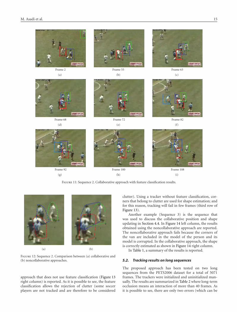
M. Asadi et al. 15
Frame 2
(a)
Frame 55
(b)
Frame 63
(c)
Frame 68
(d)
Frame 72
(e)
Frame 82
(f)
Frame 92
(g)
Frame 100
(h)
Frame 108
(i)
Figure 11: Sequence 2. Collaborative approach with feature classification results.
(a) (b)
Figure 12: Sequence 2. Comparison between (a) collaborative and(b) noncollaborative approaches.
approach that does not use feature classification (Figure 13right column) is reported. As it is possible to see, the featureclassification allows the rejection of clutter (some soccerplayers are not tracked and are therefore to be considered
clutter). Using a tracker without feature classification, cor-ners that belong to clutter are used for shape estimation; andfor this reason, tracking will fail in few frames (third row ofFigure 13).
Another example (Sequence 3) is the sequence thatwas used to discuss the collaborative position and shapeupdating in Section 4.4. In Figure 14 left column, the resultsobtained using the noncollaborative approach are reported.The noncollaborative approach fails because the corners ofthe van are included in the model of the person and itsmodel is corrupted. In the collaborative approach, the shapeis correctly estimated as shown in Figure 14 right column.
In Table 1, a summary of the results is reported.
5.2. Tracking results on long sequences
The proposed approach has been tested on two longsequences from the PETS2006 dataset for a total of 5071frames. The trackers were initialized and uninitialized man-ually. The results are summarized in Table 2 where long-termocclusion means an interaction of more than 40 frames. Asit is possible to see, there are only two errors (which can be

16 EURASIP Journal on Image and Video Processing
Figure 13: Sequence 2. Comparison between collaborative approach with feature classification (central column) and collaborative approachwithout feature classification (right column).
considered as one error since the two trackers which failedwere collaborating) that occur after 500 frames from theinitialization of the trackers. During these 500 frames, thetrackers experienced a constant interaction between themand with another tracker in a cluttered background. The low-error rate demonstrates the capabilities of the algorithm alsoon long sequences. Sequences 4 and 5 are available at ourwebsite [17].
5.3. Quantitative-shape estimation evaluation
To discuss the shape-updating process and the benefits ofcollaboration from a quantitative point of view, some resultsthat are related to Sequence 2 are provided in Figures 15and 16. A particularly interesting measure of the benefitsof the collaborative approach with feature classification ispresented in Figure 15. The convex hull of the target labeledas 1 in Figure 11 has been manually extracted. By countingthe number of model points that, due to the updatingprocess, have an increased persistence and that are outsidethis manually extracted convex hull and which thereforebelong to clutter or other objects, it is possible to have a
measure of the correctness of the shape update process. Fromthe graph, it is clear that from frames 3 to 10 and particularlyafter frame 55 (the heavy occlusion of Figure 12), manymore model points are updated or added outside the target’sconvex hull by the noncollaborative approach. This is dueto the fact the algorithm inserted model points using theevidence of other objects. This errors lead to a failure afterfew frames (for this reason, the noncollaborative approachgraph ends at frame number 80).
In Figure 16, the number of updated, decreased in per-sistence, removed, and added model points in collaborative(left column) and noncollaborative approach (right column)for targets labeled as 1 (first row), 2 (second row), and3 (third row) in Figure 11 are shown. As it is possible tosee, especially in case of targets 1 and 2, after frame 55the number of corners that have their persistence increased(added corners and updated corners) is much larger in caseof noncollaborative approach. After frame 70, when thenoncollaborative approach is beginning to fail, the numberof corners with increased persistence by the collaborativeapproach algorithm is very low and this is due to the factthat the visible part of target is very little. This is a further
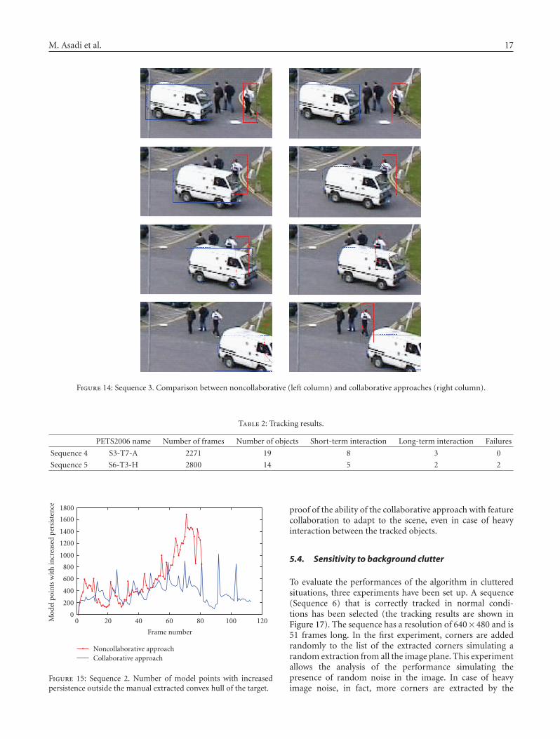
M. Asadi et al. 17
Figure 14: Sequence 3. Comparison between noncollaborative (left column) and collaborative approaches (right column).
Table 2: Tracking results.
PETS2006 name Number of frames Number of objects Short-term interaction Long-term interaction Failures
Sequence 4 S3-T7-A 2271 19 8 3 0
Sequence 5 S6-T3-H 2800 14 5 2 2
120100806040200
Frame number
Noncollaborative approachCollaborative approach
0
200
400
600
800
1000
1200
1400
1600
1800
Mod
elp
oin
tsw
ith
incr
ease
dpe
rsis
ten
ce
Figure 15: Sequence 2. Number of model points with increasedpersistence outside the manual extracted convex hull of the target.
proof of the ability of the collaborative approach with featurecollaboration to adapt to the scene, even in case of heavyinteraction between the tracked objects.
5.4. Sensitivity to background clutter
To evaluate the performances of the algorithm in clutteredsituations, three experiments have been set up. A sequence(Sequence 6) that is correctly tracked in normal condi-tions has been selected (the tracking results are shown inFigure 17). The sequence has a resolution of 640×480 and is51 frames long. In the first experiment, corners are addedrandomly to the list of the extracted corners simulating arandom extraction from all the image plane. This experimentallows the analysis of the performance simulating thepresence of random noise in the image. In case of heavyimage noise, in fact, more corners are extracted by the
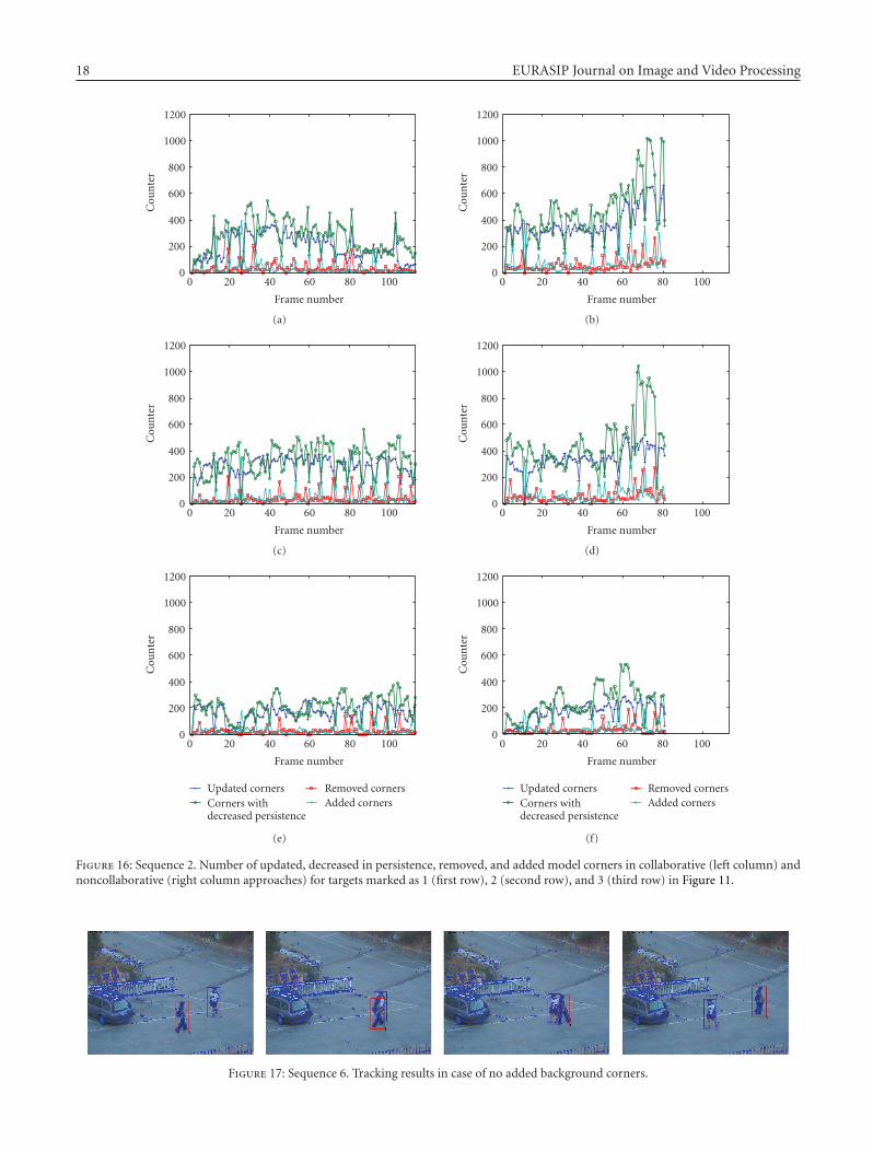
18 EURASIP Journal on Image and Video Processing
100806040200
Frame number
0
200
400
600
800
1000
1200
Cou
nte
r
(a)
100806040200
Frame number
0
200
400
600
800
1000
1200
Cou
nte
r
(b)
100806040200
Frame number
0
200
400
600
800
1000
1200
Cou
nte
r
(c)
100806040200
Frame number
0
200
400
600
800
1000
1200
Cou
nte
r
(d)
100806040200
Frame number
Updated cornersCorners withdecreased persistence
Removed cornersAdded corners
0
200
400
600
800
1000
1200
Cou
nte
r
(e)
100806040200
Frame number
Updated cornersCorners withdecreased persistence
Removed cornersAdded corners
0
200
400
600
800
1000
1200
Cou
nte
r
(f)
Figure 16: Sequence 2. Number of updated, decreased in persistence, removed, and added model corners in collaborative (left column) andnoncollaborative (right column approaches) for targets marked as 1 (first row), 2 (second row), and 3 (third row) in Figure 11.
Figure 17: Sequence 6. Tracking results in case of no added background corners.

M. Asadi et al. 19
(a) (b) (c)
Figure 18: Sequence 6. Example of different levels of simulated clutter on Sequence 4. (a) 2 corners were randomly added for a patch of10× 10 pixels; (b) 6 corners were randomly added for a patch of 10× 10 pixels; (c) 8 corners were added for a patch of 10× 10 pixels.
8654321Level of clutter: number of
corners added for 10× 10 patch
0102030405060708090
100
Mea
nov
erla
pex
pec
ted
(a)
8654321Level of clutter: number of
corners added for 10× 10 patch
0102030405060708090
100
Mea
nov
erla
pex
pec
ted
(b)
8654321Level of clutter: number of
corners added for 10× 10 patch
0102030405060708090
100
Mea
nov
erla
pex
pec
ted
(c)
Figure 19: Sequence 6. Tracking results in terms of overlap between the target and the estimated shape model for different levels of clutterin case of (a) experiment number 1; (b) experiment number 2; (c) experiment number 3.
corner extractor generating a really cluttered environment.The second experiment simulates the presence of a texturedtime-variant background (i.e., trees in a windy day). To dothat, the corners are added randomly at each frame to thelist of the extracted corners simulating the extraction fromthe entire image plane but the zone of the targets (that arein foreground) which was manually segmented. The thirdexperiment finally simulates the condition of a fixed clutteredbackground. To simulate this condition, a random patternof corners is generated at the beginning of the sequence.These corners are added to the list of the extracted corners,but at each frame the corners that are in the zone of thetarget are discarded. To evaluate the performances, the meanexpected overlap between the convex hull of the estimatedshape of each target and the ground truth convex hull thatcontains the target is estimated in different conditions ofclutter by using a Monte Carlo technique. The mean numberof added corners for a patch of 10 × 10 pixels is used toquantify the level of clutter. Some examples of the differentlevels of clutter are shown in Figure 18. The results for thethree experiments are shown in Figure 19 where a line hasbeen plotted to highlight the condition of 75% overlap. Tobetter understand the reported values, it is worth sayingthat due to the length and symmetry of the sequence (theocclusion situation occurs in the middle), a mean overlapof 75% means that during the occlusion, the track of onetarget is lost. While an overlap of more than 85% means that
the trackers tracked correctly and that there are no visuallyperceptible errors. As it is possible to see, the proposedalgorithm, by exploiting the strong geometrical relationsbetween the model points, is stable also in heavy clutter.
5.5. Comparison with other trackers
In this paragraph, our algorithm will be compared to somesuccessful methods for multiple target tracking. In particular,the algorithm will be compared to the boosted particlefilter (BPF) [11], the netted collaborative autonomoustrackers (NCATs) [14], the particle based belief propagation(PBBP) [16], and the multiple hypothesis filter (MHT)[19]. Moreover, the results will be compared to the resultsobtained by multiple independent color-based trackers [7].This comparison is possible thanks to the work presented in[16] and to the sequence provided by Okuma [11] on hiswebsite.
The results of the proposed method on the hockeysequence (Sequence 7) are reported in Figure 20. As itis possible to see, during all the sequence by using ourapproach, there are no labeling or merging errors.
To correctly compare the proposed approach with theapproaches in literature, a brief description of the featuresused by the above-mentioned methods is here reported. BothBPF and PBBP use the simple Bhattacharyya similarity coef-ficient to measure the similarity between the target model

20 EURASIP Journal on Image and Video Processing
(a) (b) (c)
(d) (e) (f)
Figure 20: Sequence 7. Tracking results of the proposed method.
and the image region (likelihood computation), the priordistribution that is used to sample the particles, on the otherhand, is the result of a fusion between the a priori motionmodel of the targets and the detections of an offline learneddetector (Adaboost for BPF and SVM for PBBP). The NCATapproach uses to model the target a color-histogram trainedoffline in a boosted fashion. The results provided in [16]by using the MHT method are similarly obtained by usingan offline-trained SVM classifier. The color-based trackers in[7] finally use a Bhattacharyya similarity coefficient and thestates of the targets are propagated by using the particle filterapproach.
All these methods (apart from [7]) use strong a prioriinformation about the target to be tracked, and it is nottherefore possible to track different classes of targets withoutretraining the classifier. The proposed approach on the otherhand is general and does not need any a priori informationabout the target appearance or motion. It can in fact beused to track without any modification a pedestrian or avan (see Figure 14). Some quantitative results about thehockey sequence are shown in Figure 21. In this figure,the coordinates of the targets labeled as 1, 2, 3 estimatedby using our approach are reported by using a solid line,the ground truth (hand labeled in [16] and here reported)is plotted by using a dashed line while the results of thePBBP approach are shown by using only the markers. Whilethe positions of targets 1 and 3 are estimated correctlyduring all the sequence by the proposed method, during thecomplete occlusion of target 2, the position is estimated withan error of about 10 pixels for some frames but, after theocclusion, the correct position is recovered. PBBP, on theother hand, tracks the object with more precision duringall the occlusion. This difference in performances is due tothe fact that the proposed method uses, for each target, anindependent (and in this case uniform) motion model and
10095908580757065
Frame number
Target1 [our approach]Target2 [our approach]Target3 [our approach]Target1 [ground truth]Target2 [ground truth]
Target3 [ground truth]Target1 [PBBP]Target2 [PBBP]Target3 [PBBP]
100
110
120
130
140
150
160
170
180
xco
ordi
nat
e
Figure 21: Sequence 7. Estimated coordinates of trackers 1, 2, and3. Solid line: proposed approach. Dashed line: ground truth. Circles:PBBP approach [16].
the tracking results are therefore governed by observations.In case of occlusion, the proposed approach does not let thetrackers use the same observation and therefore the smallnumber of observations can cause an inaccurate estimation.On the other hand, PBBP bypasses the problem of lack ofobservation by modelling the motion during interaction.In [16], it is stated that among the compared trackers,PBBP obtains the best performances followed by NCAT that

M. Asadi et al. 21
obtain similar performances on the hockey sequence. BPF isless accurate than PBBP but is still capable of tracking thehockey sequence with good performances. Finally both MHTand the approach in [7] fail in tracking targets during theocclusion situation.
Summarizing our approach by obtaining results com-parable to state-of-the-art methods that use offline-learnedmodels and by outperforming methods like [7] can be theright choice when strong a priori information about theappearance or the motion of the targets to be tracked is notavailable.
6. CONCLUSION AND FUTURE WORKS
In this paper, an algorithm for feature classification and itsexploitation for both single and collaborative tracking havebeen proposed. It is shown that the proposed algorithmis a solution to the Bayesian tracking problem that allowsposition and shape estimation even in clutter or whenmultiple targets interact and occlude each other. The featuresin the scene are classified as good, suspicious, malicious, andneutral, and this information is used for avoiding clutteror distracters in the scene and for allowing continuousmodel updating. In case of multiple tracked objects, whenthe algorithm detects an interaction between them, thecollaboration and the sharing of classification informationallow the segmentation and the assignment of features tothe trackers. The reported experimental results showed thatthe use of feature classification improves the tracking resultsboth for single- and multitarget trackings.
As a feature work, the possibility of improving thetracking performances by using an MRF approach in theshape-updating process with the aim of maintaining shapecoherence and assigning observation to the correct trackerduring collaboration is being evaluated. The other possibilityfor the future development of this method is to considererror propagation in the Bayesian filtering.
REFERENCES
[1] M. Asadi, A. Dore, A. Beoldo, and C. S. Regazzoni, “Trackingby using dynamic shape model learning in the presence ofocclusion,” in Proceedings of IEEE Conference on AdvancedVideo and Signal Based Surveillance (AVSS ’07), pp. 230–235,London, UK, September 2007.
[2] M. Asadi and C. S. Regazzoni, “Tracking using continuousshape model learning in the presence of occlusion,” EURASIPJournal on Advances in Signal Processing, vol. 2008, Article ID250780, 23 pages, 2008.
[3] W. Qu, D. Schonfeld, and M. Mohamed, “Real-time dis-tributed multi-object tracking using multiple interactivetrackers and a magnetic-inertia potential model,” IEEE Trans-actions on Multimedia, vol. 9, no. 3, pp. 511–519, 2007.
[4] J. MacCormick and A. Blake, “A probabilistic exclusionprinciple for tracking multiple objects,” International Journalof Computer Vision, vol. 39, no. 1, pp. 57–71, 2000.
[5] M. Bogaert, N. Chleq, P. Cornez, C. S. Regazzoni, A. Teschioni,and M. Thonnat, “The passwords project,” in Proceedings ofIEEE International Conference on Image Processing (ICIP ’96),vol. 3, pp. 675–678, Lausanne, Switzerland, September 1996.
[6] S. J. McKenna, S. Jabri, Z. Duric, A. Rosenfeld, and H.Wechsler, “Tracking groups of people,” Computer Vision andImage Understanding, vol. 80, no. 1, pp. 42–56, 2000.
[7] P. Perez, C. Hue, J. Vermaak, and M. Gangnet, “Color-basedprobabilistic tracking,” in Proceedings of the 7th EuropeanConference on Computer Vision (ECCV ’02), vol. 1, pp. 661–675, Copenhagen, Denmark, May 2002.
[8] T. Zhao and R. Nevatia, “Tracking multiple humans incomplex situations,” IEEE Transactions on Pattern Analysis andMachine Intelligence, vol. 26, no. 9, pp. 1208–1221, 2004.
[9] Y. Bar-Shalom and T. E. Fortmann, Tracking and DataAssociation, Academic Press, New York, NY, USA, 1988.
[10] C. Hue, J.-P. Le Cadre, and P. Perez, “A particle filter to trackmultiple objects,” in Proceedings of IEEE Workshop on Multi-Object Tracking (MOT ’01), pp. 61–68, Vancouver, Canada,July 2001.
[11] K. Okuma, A. Taleghani, N. de Freitas, J. J. Little, and D.G. Lowe, “A boosted particle filter: multitarget detection andtracking,” in Proceedings of the 8th European Conference onComputer Vision (ECCV ’04), vol. 3021, pp. 28–39, Prague,Czech Republic, May 2004.
[12] M. Isard and J. MacCormick, “BraMBLe: a Bayesian multiple-blob tracker,” in Proceedings of the 8th IEEE InternationalConference on Computer Vision (ICCV ’01), vol. 2, pp. 34–41,Vancouver, Canada, July 2001.
[13] Y. Li, H. Ai, T. Yamashita, S. Lao, and M. Kawade, “Trackingin low frame rate video: a cascade particle filter with discrim-inative observers of different lifespans,” in Proceedings of IEEEComputer Society Conference on Computer Vision and PatternRecognition (CVPR ’07), pp. 1–8, Minneapolis, MN, USA, June2007.
[14] T. Yu and Y. Wu, “Decentralized multiple target tracking usingnetted collaborative autonomous trackers,” in Proceedings ofIEEE Computer Society Conference on Computer Vision andPattern Recognition (CVPR ’05), vol. 1, pp. 939–946, SanDiego, Calif, USA, June 2005.
[15] Y. Wu, T. Yu, and G. Hua, “Tracking appearances with occlu-sions,” in Proceedings of IEEE Computer Society Conference onComputer Vision and Pattern Recognition (CVPR ’03), vol. 1,pp. 789–795, Madison, Wis, USA, June 2003.
[16] J. Xue, N. Zheng, J. Geng, and X. Zhong, “Tracking multiplevisual targets via particle-based belief propagation,” IEEETransactions on Systems, Man, and Cybernetics, Part B, vol. 38,no. 1, pp. 196–209, 2008.
[17] http://www.isip40.it/index.php?mod=04 Demos/sequences.html.
[18] F. Monti and C. S. Regazzoni, “Joint collaborative trackingand multitarget shape updating under occlusion situations,”submitted to IEEE Transactions on Image Processing.
[19] I. J. Cox and S. L. Hingorani, “An efficient implementation ofReid’s multiple hypothesis tracking algorithm and its evalua-tion for the purpose of visual tracking,” IEEE Transactions onPattern Analysis and Machine Intelligence, vol. 18, no. 2, pp.138–150, 1996.

Hindawi Publishing CorporationEURASIP Journal on Image and Video ProcessingVolume 2008, Article ID 542808, 22 pagesdoi:10.1155/2008/542808
Research ArticleA Scalable Clustered Camera System forMultiple Object Tracking
Senem Velipasalar,1 Jason Schlessman,2 Cheng-Yao Chen,2 Wayne H. Wolf,3 and Jaswinder P. Singh4
1 Electrical Engineering Department, University of Nebraska-Lincoln, Lincoln, NE 68588, USA2 Electrical Engineering Department, Princeton University, Princeton, NJ 08544, USA3 School of Electrical and Computer Engineering, Georgia Institute of Technology, GA 30332, USA4 Computer Science Department, Princeton University, Princeton, NJ 08544, USA
Correspondence should be addressed to Senem Velipasalar, [email protected]
Received 1 November 2007; Revised 21 March 2008; Accepted 12 June 2008
Recommended by Andrea Cavallaro
Reliable and efficient tracking of objects by multiple cameras is an important and challenging problem, which finds wide-rangingapplication areas. Most existing systems assume that data from multiple cameras is processed on a single processing unit or bya centralized server. However, these approaches are neither scalable nor fault tolerant. We propose multicamera algorithms thatoperate on peer-to-peer computing systems. Peer-to-peer vision systems require codesign of image processing and distributedcomputing algorithms as well as sophisticated communication protocols, which should be carefully designed and verified to avoiddeadlocks and other problems. This paper introduces the scalable clustered camera system, which is a peer-to-peer multicamerasystem for multiple object tracking. Instead of transferring control of tracking jobs from one camera to another, each camera inthe presented system performs its own tracking, keeping its own trajectories for each target object, which provides fault tolerance.A fast and robust tracking algorithm is proposed to perform tracking on each camera view, while maintaining consistent labeling.In addition, a novel communication protocol is introduced, which can handle the problems caused by communication delaysand different processor loads and speeds, and incorporates variable synchronization capabilities, so as to allow flexibility withaccuracy tradeoffs. This protocol was exhaustively verified by using the SPIN verification tool. The success of the proposed systemis demonstrated on different scenarios captured by multiple cameras placed in different setups. Also, simulation and verificationresults for the protocol are presented.
Copyright © 2008 Senem Velipasalar et al. This is an open access article distributed under the Creative Commons AttributionLicense, which permits unrestricted use, distribution, and reproduction in any medium, provided the original work is properlycited.
1. INTRODUCTION
This paper takes a holistic view of the problems that need tobe solved to build scalable multicamera systems. Scalabilityhas two aspects: computation and communication. In orderto address scalability in both of these aspects, we presentthe scalable clustered camera system (SCCS), which is adistributed smart camera system for multiobject tracking. In asmart camera system, each camera is attached to a computingcomponent, in this case different CPUs. In other words, inSCCS, a different processing unit is used to process eachcamera, which provides scalability in computation power.Moreover, processing units communicate with each otherin a peer-to-peer fashion eliminating the need for a centralserver, and thus providing scalability on the communicationside and also removing a single point of failure.
Reliable and efficient tracking of objects by multiplecameras is an important and challenging problem, whichfinds wide-ranging application areas such as video surveil-lance, indexing and compression, gathering statistics fromvideos, traffic flow monitoring, and smart rooms. Due tothe inherent limitations of a single visual sensor, such aslimited field of view and delays due to panning and tilting,using multiple cameras has become inevitable for objecttracking in applications requiring increased coverage ofareas. Multiple cameras can enhance the capability of visionapplications, providing fault-tolerance and robustness forissues such as target occlusion. Hence, many research groupshave studied multicamera systems [1–30].
Yet, using multiple cameras to track multiple objectsposes additional challenges. One of these challenges is

2 EURASIP Journal on Image and Video Processing
the consistent labeling problem, that is, establishing cor-respondences between moving objects in different views.Multicamera systems, rather than treating each cameraindividually, compare features and trajectories from differentcameras in order to obtain history of the object movements,and handle the loss of the target objects which may be causedby occlusion or errors in the background subtraction (BGS)algorithms.
Different approaches have been taken to solve theconsistent labeling problem. Kelly et al. [14] assume thatall cameras are fully calibrated. Funiak et al. [31] proposea distributed calibration algorithm for camera networks.Chang and Gong [8] and Utsumi et al. [25] employ fea-ture matching. Yet, relying on feature matching can causeproblems as the features can be seen differently by differentcameras due to lighting variations. In addition, calibratingcameras fully is expensive and impractical to install by theend user, since it requires some expert intervention.
Kettnaker and Zabih [15] use observation intervals andtransition times of objects across cameras for tracking.Lee et al. [18] assume that the intrinsic camera parametersare known and use the centroids of the tracked objects toestimate a homography and to align the scene ground planeacross multiple views. Khan and Shah [16] present a methodthat uses field of view (FOV) lines and does not require thecameras to be calibrated. However, due to the way the linesare recovered, they may not be localized reliably, and if thereis dense traffic around the FOV line, the method can resultin inconsistent labels. More recently, Calderara et al. [6, 7]and Hu et al. [12] presented methods for consistent labelingmaking use of the principle axes of people.
Cai and Aggarwal [5] present a system in which onlythe neighboring cameras are calibrated to their relativecoordinates. Targets are tracked using a single camera viewuntil the system predicts that the active camera will no longerhave a good view of the object. The tracking algorithm thenswitches to another camera. Nguyen et al. [22] introduce asystem in which all cameras are calibrated, and the mostappropriate camera is chosen to track each object. Thetracking job is assigned to the camera that is closest tothe object. However, with a handoff or switching approach,even though increased coverage is provided, and objects canbe tracked for longer periods of time, the tracking is stillbeing performed on one camera view at a time. This isnot a fault-tolerant approach, since the camera responsiblefor tracking can break down, and detecting and recoveringfrom this, if recovery is possible, can introduce some delay.In addition, the camera assigned for the tracking of anobject may not have the view of the object we are interestedin. For instance, the camera closest to a person may beviewing that person from the back while the interest is seeingthat person’s face. Moreover, occlusions, merging/splitting ofobjects, foreground blobs that are detected incompletely maycause frequent switching of cameras.
In order to provide fault-tolerance, robustness, and mul-tiple views of the tracked targets, objects in the overlappingregions of the fields of view of cameras should be trackedsimultaneously on those views with consistent labels. Thisway, even if a camera breaks down, other cameras can still
continue tracking and trajectories of the same object fromdifferent views can be obtained. Also, in the case of occlusionor loss of target objects, data about the object features andtrajectories in different camera views can be exchanged tokeep the trajectories updated in all camera views.
As cameras become less expensive, many systems will uselarge numbers of cameras for better coverage and higheraccuracy. Thus, scalability and computational efficiency ofmulticamera systems are very important issues that needto be addressed. The performance and scalability of suchsystems should not be debilitated with additional cameras.Although many groups have developed methods to combinedata from multiple cameras, much less attention has beenpaid to the computational efficiency and scalability. Manyexisting systems assume that multiple cameras are processedon a single CPU or by a centralized server. However, these arenot scalable approaches, and they introduce a single pointof failure. Chang and Gong [8] propose a system that isimplemented on an SGI workstation with two cameras. Fora single CPU system, the amount of processing necessary totrack multiple objects on multiple views can be excessive forreal-time performance. Moreover, scalability is debilitatedas each additional camera imposes greater performancerequirements.
In order to increase processing power, and handle mul-tiple video streams, distributed systems have been employedinstead of using a single CPU. In a distributed system,different CPUs are used to process inputs from differ-ent cameras. Yet, most existing distributed multicamerasystems use a centralized server/control center. Yuan et al.[30] present a distributed surveillance system in whichcomputers are connected to a server, and camera units donot collaborate with each other or exchange information.Collins et al. [9, 10] introduced the VSAM system, where allresulting object hypotheses from all sensors are transmittedat every frame back to a central operator control unit.Nguyen et al. [20] propose a multicamera system where allthe local processing results are sent to a main controller.Lo et al. [32] introduce a multisensor distributed systemwhere a central server coordinates the processing of thesensor inputs. Krumm et al. [17] present a multicamera mul-tiperson tracking system for the EasyLiving project. They usetwo sets of color stereo cameras, each connected to its owncomputer. A program called stereo module locates people-shaped blobs, and reports the 2D ground plane locationsof these blobs to a tracking program running on a thirdcomputer. Using a central server or a control unit for datacoordination/integration simplifies some problems, suchas video synchronization and communication between thealgorithms handling the various cameras. But server-basedmulticamera systems have a bandwidth scaling problem,since the central server can quickly become overloaded withthe aggregate sum of messages/requests from an increasednumber of nodes. Also, the server is a single point of failurefor the whole system. In addition, server-based systemsare not practical in many realistic environments, and havehigh installation costs. Besides the algorithm development,hardware design and resource management have also beenconsidered for parallel processing. Watlington and Bove [33]

Senem Velipasalar et al. 3
propose a data-flow model and use a distributed resourcemanager to support parallelism for media processing.
The aforementioned problems of server-based systemsnecessitate the use of peer-to-peer systems, where individualnodes communicate with each other without going througha centralized server. Several important issues need to beaddressed when designing peer-to-peer systems. First, com-munication between processing elements takes a significantamount of time. This necessitates the design of tracking algo-rithms requiring relatively little interprocess communicationbetween the nodes. Decreasing the number of messagesbetween the nodes also requires a careful design and choiceof when to trigger the data transfer, what data to send in whatfashion, and to whom to send this data. The system mustalso maintain the consistency of data across nodes as well asoperations upon the data without use of a centralized server.Also, even if the cameras and input video sequences aresynchronized, communication and processing delays pose aserious problem. Depending on the amount of processingeach processor has to do, one processor can run faster/slowerthan the other. Thus, when a processor receives a request,it may be ahead/behind compared to the requester. Theseissues mandate efficient and sophisticated communicationprotocols for peer-to-peer systems.
Atsushi et al. [1] use multiple cameras attached todifferent PCs connected to a network. They calibrate thecameras to track objects in world-coordinates, and sendmessage packets between stations. Ellis [11] also uses anetwork of calibrated cameras. Bramberger et al. [3] presenta distributed embedded smart camera system with looselycoupled cameras. They use predefined migration regions tohandover the tracking process from one camera to another.But, these methods do not discuss the type and details ofcommunication, and how to address the communication andprocessing delay issues.
As stated previously, peer-to-peer systems require effi-cient and sophisticated communication protocols. Theseprotocols find use in real-time systems, which tend tohave stringent requirements for proper system functionality.Hence, the protocol design for these systems necessitatestranscending typical qualitative analysis using simulationand instead, requires verification. The protocol must bechecked to ensure that it does not cause unacceptable issuessuch as deadlocks and process starvation, and has correctnessproperties such as the system eventually reaching specifiedoperating states.
Verification of communication protocols is a richtopic, particularly for security and cryptographic systems.Karlof et al. [34] analyzed the security properties of twocryptographic protocols. Evans and Schneider [35] veri-fied time-dependent authentication properties of securityprotocols. Vanackere [36] modeled cryptographic protocolsas a finite number of processes interacting with a hostileenvironment, and proposed a protocol analyzer trust forverification. Finally, a burgeoning body of work exists per-taining to the formal verification of networked multimediasystems. Bowman et al. [37] described multimedia stream asa timed automata, and verified the satisfaction of quality ofservice (QoS) properties including throughput and end-to-
end latency. Sun et al. [38] proposed a testing method forverifying QoS functions in distributed multimedia systems,where media streams are modeled as a set of timed automata.
Our previous work [27, 28] introduced some of the toolsnecessary towards building a peer-to-peer camera system.The work presented in [28] performs multicamera trackingand information exchange between cameras. However, it wasimplemented on a single CPU in a sequential manner, andthe tracking algorithm used required more data transfer.This paper presents SCCS together with its communicationprotocol and its exhaustive verification results. SCCS is ascalable peer-to-peer multicamera system for multiobjecttracking. It is a smart camera system wherein each camerais attached to a computing component, in this case differentCPUs. The peer-to-peer communication protocol is designedso that the number of messages that are sent between thenodes is decreased, and the system synchronization issue isaddressed.
A computationally efficient and robust tracking algo-rithm is presented to perform tracking on each cameraview, while maintaining consistent labeling. Instead oftransferring control of tracking jobs from one camera toanother, each camera in SCCS performs its own trackingand keeps its own trajectories for each target object, thusproviding fault tolerance. Cameras can communicate witheach other to resolve partial/complete occlusions, and tomaintain consistent labeling. In addition, if the locationof an object cannot be determined at some frame reliablydue to the errors resulted from BGS, the trajectory ofthat object is robustly updated from other cameras. SCCSkeeps trajectories updated in all views without any need foran estimation of the moving speed and direction, even ifthe object is totally invisible to that camera. Our trackingalgorithm deals with the cases of merging/splitting on asingle camera view without sending requests to other nodesin the system. Thus, it provides coarse object localizationwith sparse message traffic.
In addition, we introduce a novel communication pro-tocol that coordinates multiple tracking components acrossthe distributed system, and handles the processing and com-munication delay issues. The decisions about when and withwhom to communicate are made such that the frequency andsize of transmitted messages are kept small. This protocolincorporates variable synchronization capabilities, so as toallow flexibility with accuracy tradeoffs. Nonblocking sendsand receives are used for message communication, since foreach camera it is not possible to predict when and how manymessages will be received from other cameras. Moreover, thetype of data that is transferred between the nodes can bechanged, depending on the application and what is available,and our protocol remains valid and can still be employed. Forinstance, when full calibration of all the cameras is tolerated,the 3D world coordinates of the objects can be transferredbetween the nodes. We exhaustively verified this protocolwith success by using the SPIN verification tool.
We introduced the initial version of the SCCS andits communication protocol in [29, 39]. We extended thecommunication protocol to address real-time concerns, andto handle conflicts in received replies. In this paper, we

4 EURASIP Journal on Image and Video Processing
Invis.
p(i)1
p(i)2
p(i)3
p(i)4
p(i)b1 p(i)
b2
Ci
p(i)r1, j
p(i)r2, jp(i)
m, j
Lj,ri
(a)
Invis.
Invis.
p( j)1
p( j)2
p( j)3
p( j)4
p( j)b1,i
p( j)b2,i
C j
p( j)r1
p( j)r2
p( j)m
Li,bj
L1,lj
(b)
Figure 1: p( j)b1,i and p
( j)b2,i are the corresponding locations of p(i)
b1and p(i)
b2, respectively, and the recovered FOV line passing through p
( j)b1,i and
p( j)b2,i is shown with a dashed green line on the view of C j .
present this protocol and its verification results in detail. Wealso compare the number of messages that need to be sentaround in a server-based scenario and in our system, andpresent results of this comparison. We show that, contraryto the server-based scenario, the total number of messagessent around by our system is independent of the number oftrackers in each camera view. In addition, we compare theserver-based system scenario with our peer-to-peer systemin terms of the message loads on the individual nodes, andshow that the number of messages a single node has tohandle is considerably less in our peer-to-peer system. Wepresent results of different sets of experiments that wereperformed to obtain the speed up provided by SCCS, tomeasure average data transfer accuracy and average waitingtime. Experimental results demonstrate the success of theproposed peer-to-peer multicamera tracking system, witha minimum accuracy of 94.2% and 90% for new labeland lost label cases, respectively, with a high frequencyof synchronization. We also present the results obtainedafter exhaustively verifying the presented communicationprotocol with different communication scenarios.
The rest of the paper is organized as follows: Section 2describes the computer vision algorithms in general. Morespecifically, the recovery of FOV lines, the consistent labelingalgorithm, and the tracking algorithm are described inSections 2.1.1, 2.2, and 2.3, respectively. The communicationprotocol is introduced in Section 3, and its verification andobtained results are described in Section 4. Section 5 presentsthe experimental results obtained with several different videosequences with varying difficulty, and Section 6 concludesthe paper.
2. MULTICAMERA MULTIOBJECT TRACKING
2.1. Field of view (FOV) lines
Khan and Shah [16] introduced the FOV lines, and showedthat when FOV lines are recovered, the consistent labelingproblem can be solved successfully. The 3D FOV lines ofcamera C i are denoted by Li,s [16], where s ∈ {r, l, t, b}correspond to one of the sides of the image plane. Theprojections of the 3D FOV lines of camera C i onto the image
plane of camera C j will result in 2D lines denoted by Li,sj , andcalled the FOV lines.
2.1.1. Recovery of field of view lines
Khan and Shah [16] recover FOV lines by observingmoving objects in different views and using entry/exit events.However, since the method relies on object movement inthe environment, there needs to be enough traffic across aparticular FOV line to be able to recover it. In addition, theoutput of this method can be affected by the performance ofthe BGS algorithm. Depending on the size of the objects, theymay not be detected instantly or entirely, and thus, FOV linesmay not be located reliably.
Since FOV lines will play an important role in ourconsistent labeling algorithm and also in our communicationprotocol later, it is necessary to recover all of them in a robustway. We present robust and reliable methods for recoveringFOV lines and for consistent labeling. The method presentedfor the recovery of FOV lines does not rely on the objectmovement in the scene or on the performance of BGSalgorithms. This way, all visible FOV lines in a camera viewcan be recovered at the beginning even if there is no trafficat the corresponding region. In addition, there is no needto know the intrinsic or extrinsic camera parameters. It isassumed that cameras have overlapping fields of view, andthe scene ground is planar. Then a homography is estimatedto recover the FOV lines.
The inputs to the proposed system are four pairs ofcorresponding points (chosen offline on the ground plane)on two camera views. These points in the views of C i
and C j are denoted by P(i) = {p(i)1 , . . . , p(i)
4 } and P( j) ={p( j)
1 , . . . , p( j)4 }, respectively, and are displayed in black in
Figure 1. Let �p(i)k = (x(i)
k , y(i)k , 1)T , where k ∈ {1, . . . , 4},
denote the homogeneous coordinates of the input point
p(i)k = (x(i)
k , y(i)k ). Then, a homography (H) is estimated
from {�p(i)1 , . . . , �p(i)
4 } and {�p( j)1 , . . . , �p( j)
4 } by using the directlinear transformation algorithm described by Hartley andZisserman [40].

Senem Velipasalar et al. 5
(a) Setup 1—Camera 1 (b) Setup 1—Camera 2 (c) Setup 2—Camera 1 (d) Setup 2—Camera 2
Figure 2: (a)-(b) and (c)-(d) show the recovered FOV lines for two different camera setups. The shaded regions are outside the FOV of theother camera.
(a) (b) (c)
Figure 3: (a), (b), and (c) show the recovered FOV lines. The shaded regions are outside the FOV of the other cameras.
The image of the camera view whose FOV lines will berecovered on the other view is called the field image. After thehomography is estimated, the system finds two points on oneof the boundaries of the field image, so that each of them isin general position with the four input points. Then it checkswith the user that these boundary points are coplanar withthe four input points. Let us denote the two points found onthe image boundary s of the camera C i by p(i)
s1 = (x(i)s1 , y(i)
s1 )
and p(i)s2 = (x(i)
s2 , y(i)s2 ), where s ∈ {r, l, t, b} correspond to one
of the sides of the image plane (Figure 1). The corresponding
locations of (x(i)s1 , y(i)
s1 ) and (x(i)s2 , y(i)
s2 ) on the view of camera
C j are denoted by p( j)s1,i = (x
( j)s1,i, y
( j)s1,i) and p
( j)s2,i = (x
( j)s2,i, y
( j)s2,i),
and computed by using
H�p(i)sn∼= �p( j)
sn,i, (1)
where n ∈ {1, 2}, �p(i)sn = (x(i)
sn , y(i)sn , 1)T , and �p( j)
sn,i denotes the
homogeneous coordinates of p( j)sn,i = (x
( j)sn,i, y
( j)sn,i). x
( j)sn,i and y
( j)sn,i
are obtained by normalizing �p( j)sn,i, so that its third entry is
equal to 1. Once p( j)s1,i and p
( j)s2,i are obtained on the other
view, the line going through these points defines the FOVline corresponding to the image boundary s of the cameraC i. Two points are found on each boundary of interest andthe FOV line corresponding to that boundary is recoveredsimilarly. Let us illustrate these steps by an example referringto Figure 1. Let the boundary of interest be the bottomboundary of the view of C i, thus side s is b. The system finds
p(i)b1
and p(i)b2
on this boundary, which are displayed in greenin Figure 1(a), as described above. Then, the correspondinglocations of these points on the view of C j are computed by
using (1). These corresponding points are denoted by p( j)b1,i
and p( j)b2,i, and are displayed in green in Figure 1(b). The line
going through p( j)b1,i and p
( j)b2,i is the FOV line corresponding to
the bottom boundary of camera C i. This line is denoted byLi,bj , and is shown with a dashed green line on the view of C j
in Figure 1(b).Figures 2 to 4 show the recovered FOV lines for different
video sequences and camera setups. Although there wasno traffic along the right boundary of Figure 2(b), thecorresponding FOV line is successfully recovered as shownin Figure 2(a).
2.1.2. Checking object visibility
As stated previously, Li,sj denotes the projection of the 3DFOV line Li,s onto the view of C j and is represented bythe equation of the line, which is written as y = Sx + C.
Henceforth, a point p( j)m = (x
( j)m , y
( j)m ) will be considered on
the visible side of Li,sj if sign(y( j)m − Sx
( j)m − C) = sign(y
( j)a −
Sx( j)a − C), where (x
( j)a , y
( j)a ) are the coordinates of the p
( j)a
which is any one of the input points in P( j).When an objectO( j) enters the view of C j , BGS is applied
first and a bounding box around the foreground (FG) objectis obtained. Then, its visibility in the view of C i is checked
by employing Li,sj . The midpoint (p( j)m ) of the bottom line of
the bounding box of the object is used as its location. If thispoint lies on the visible side of Li,sj , for all s ∈ {r, l, t, b}, then
it is deduced that O( j) is visible by C i (Figure 1).

6 EURASIP Journal on Image and Video Processing
(a) (b) (c)
Figure 4: (a), (b), and (c) show the recovered FOV lines. The shaded regions are outside the FOV of the other cameras.
2.2. Consistent labeling
The consistent labeling scheme of Khan and Shah [16] isbased on the minimum distance between FG objects and aFOV line. However, performing the labeling based only onthe FOV lines can be error-prone as more than one object canbe in the vicinity of the line especially in crowded scenes, ormultiple people can enter one view at the same time. Also, ifthe entry of an object is detected with a delay due to the errorsin BGS, the corresponding object in the other camera willmove further away from the line which may cause anotherobject with the wrong label to be closer to the FOV line.
Instead of relying only on the FOV lines, the followingsteps are employed for more robustness: first, the visibilityof a new object O( j), entering the view of C j from sides, by C i is checked as described in Section 2.1.2. Then,
the corresponding location (p(i)m, j) of p
( j)m in the view of
C i is calculated by using (1) as depicted in Figure 1. Theforeground objects in the view of C i, which were on the
invisible side of Lj,si and move in the direction of the visible
side of the line, are determined. From those foreground
objects, the one that is closest to the point p(i)m, j is found, and
its label is given to theO( j). Similarly, if multiple people enterthe scene simultaneously, the algorithm uses their calculatedcorresponding locations in the other view to resolve theambiguity.
2.3. The tracking algorithm: coarse object localizationwith sparse message traffic
Our proposed tracking algorithm allows for sparse messagetraffic by handling the cases of merging and splitting withina single camera view without sending request messages toother cameras.
First, FG objects are segmented from the backgroundin each camera view by using the BGS algorithm presentedby Stauffer and Grimson [41], which employs adaptivebackground mixture models. Then, connected componentanalysis is performed, which results in FG blobs. When a newFG blob is detected within the camera view, a new trackeris created, and a mask for the tracker is built where the FGpixels from this blob and background pixels are set to be 1and 0, respectively. The box surrounding the FG pixels of themask is called the bounding box. Then, the color histogram of
the blob is learned from the input image, and is saved as themodel histogram of the tracker.
At each frame, the trackers are matched to detectedFG blobs by using a computationally efficient blob trackerwhich uses a matching criteria based on the boundingbox intersection and the Bhattacharya coefficient ρ(y) [42]defined by
ρ(y) ≡ ρ[p(y), q
] =∫ √
pz(y)qzdz. (2)
In (2), z is the feature representing the color of the targetmodel and is assumed to have a density function qz whilepz(y) represents the color distribution of the candidate FGblob centered at location y. The Bhattacharya coefficient isderived from the sample data by using
ρ(y) ≡ ρ[
p(y), q] =
m∑
u=1
√pu(y)qu, (3)
where q = {qu}u=1...m, and p(y) = { pu(y)}u=1...m arethe probabilities estimated from the m-bin histogram ofthe model and the candidate blobs, respectively. Theseprobabilities are estimated by using the color informationat the nonzero pixel locations of the masks. If the boundingbox of an FG blob intersects with that of the current modelmask of the tracker, the Bhattacharya coefficient between themodel histogram of the tracker and the color histogram ofthe FG blob is calculated by using (3). The tracker is assignedto the FG blob which results in the highest Bhattacharyacoefficient, and the mask, and thus the bounding box, ofthe tracker are updated. The Bhattacharya coefficient withwhich the tracker is matched to its object is called thesimilarity coefficient. If the similarity coefficient is greaterthan a predefined distribution update threshold, the modelhistogram of the tracker is updated to be the color histogramof the FG blob to which it is matched.
Based on this matching criteria, when objects merge,multiple trackers are matched to one FG blob, and thelabels of all matched trackers are displayed on this blob, asshown in Figures 5, 6, 23, and 24. The masks of the trackersare then updated in the previously discussed fashion. Thetrackers that are matched to the same FG blob are put intoa merge state, and in this state their model histograms arenot updated. When objects split from each other, trackers

Senem Velipasalar et al. 7
(a) Frame 530 (a′) Frame 530 (b) Frame 570 (b′) Frame 570 (c) Frame 590 (c′) Frame 590
Figure 5: Example of successfully resolving a merge. (a), (b), (c), (a′), (b′), and (c′) show the original images, and the tracked objects withtheir labels, respectively.
(a) Frame 795 (b) Frame 815 (c) Frame 877 (d) Frame 920 (e) Frame 950
Figure 6: Example of resolving the merging of multiple objects.
are matched to their targets based on the bounding boxintersection and Bhattacharya coefficient criteria mentionedabove.
There may be rare but unfavorable cases where an FGobject, appearing after the split of merged objects, may notbe matched to its tracker. We deal with these cases as follows:denote two trackers by T1 and T2, and their target objects byO1 and O2, respectively. When these objects merge, O1∪2 isformed, and T1 and T2 are both matched to O1∪2. After O1
and O2 split, BTiOj are calculated, where {i, j} ∈ {1, 2}, andBTiOj denotes the Bhattacharya coefficient calculated betweenthe histograms of Ti and Oj . Based on BTiOj , both T1 andT2 can still be matched to O2, for instance, and stay in themerge state. Denote the similarity coefficient of Ti by STi .Thus, in this case, ST1 = B12 and ST2 = B22. This canhappen because the model distributions of the trackers arenot updated during the merge state, and there may be changesin the color of O1 during and after merging. Another reasonmay be O1 and O2 having similar colors from the outset.When this occurs, O1 is compared against the trackers whichare in the merge state and intersect with the bounding box ofO1. That is, it is compared against T1 and T2, and BT1O1 andBT2O1 are calculated. Then, O1 is assigned to the tracker Ti∗ ,where
i∗ = argmini∈{1,2}
(STi − BTiO1
). (4)
If a foreground blob cannot be matched to any of thetrackers, and if there are trackers in the merge state, theunmatched object is compared against those trackers byusing the logic in (4), which is also applicable if there aremore than two trackers in the merge state as shown in Figures6 and 23.
As stated previously, this algorithm provides coarserobject localization and decreases the message traffic by notsending a request message each time a merging or splittingoccurs. If the exact location of an object in the blob, formedafter the merging, is required, we propose another algorithmthat can be used at the expense of more message traffic:
when a tracker is in the merge state, other nodes that cansee its most recent location can be determined as describedin Section 2.1.2, and a request message can be sent to thesenodes to retrieve the location of the tracker in the merge state.If the current location of the tracker is not visible by any ofthe other cameras, then the mean-shift tracking [42] can beactivated.
The mean-shift tracking is error-prone since it can bedistracted by the background. It is also computationallymore expensive. Thus, when a tracker is in the merge state,it is preferable to send messages to other nodes, and requestthe location of this tracker, if its most recent location is intheir FOV. Thus, this algorithm requires additional messagetraffic. We proposed this second algorithm as an alternativeif the exact location of each tracker in the merge stateis required. The experiments presented in Section 5 wereperformed by using the first proposed algorithm as thetracking component of the SCCS.
3. INTER-CAMERA COMMUNICATION PROTOCOL
One issue that needs to be addressed when using peer-to-peer systems is that communication is expensive and takesa significant amount of time. Also, the number of messagesthat are sent between the nodes should be decreased tosave power and increase speed. Another issue is maintainingconsistency for data across cameras as well as operationsupon the data without the use of a centralized server. Evenif the cameras and input video sequences are synchronized,communication and processing delays pose a serious prob-lem. The processors will have different amounts of processingto do, and may also run at different processing rates. These,coupled with potential network delays, cause one processorto be ahead of/ behind the others during execution. Thus,when a processor receives a request, it may be ahead/behindcompared to the requester. Hence, system synchronizationbecomes very important to ensure the transfer of coherentvision data between cameras. All these issues mandate anefficient and sophisticated communication protocol.

8 EURASIP Journal on Image and Video Processing
Tracker container
Check lost Check new
Receive lost Receive new
Updatetracker container
MPIlibrary
Find label ofclosest tracker
Find coordinatesof input label
FG
blobsSynch frame Synch frame
new label req new label req
lst label req
lst label rep
lst label req
lst label rep
new label rep new label rep
Camera Ci Camera Cj
Figure 7: Communication between two cameras.
The protocol of SCCS utilizes point-to-point communi-cation, as opposed to some previous approaches that requirea central message processing server. Our approach offers alatency advantage and removes the single point of failure.Moreover, nodes do not need to send the state of the trackersto a server at every single frame. Thus, contrary to the server-based scenario, the total number of messages sent aroundby our system is independent of the number of trackers ineach camera view. This decreases the number of messagesconsiderably as will be discussed in Section 3.5. Furthermore,compared to server-based systems, the proposed protocoldecreases the message load on each node. This design ismore scalable, since for a central server implementation, theserver quickly becomes overloaded with the aggregate sum ofmessages and requests from an increased number of nodes.
In this section, the protocol of SCCS is presented, whichis a novel peer-to-peer communication protocol that canhandle communication and processing delays and hencemaintain consistent data transfer across multiple cameras.This protocol is designed by determining the answers to thefollowing questions.
(a) When to communicate: determining the events whichwill require the transfer of data from other cameras.These events will henceforth be referred to as requestevents.
(b) With whom to communicate: determining the camerasto which requests should be sent.
(c) What to communicate: choosing the data to betransferred between the cameras.
(d) How to communicate: designing the manner in whichthe messages are sent, and determining the pointsduring execution at which data transfers should bemade.
The protocol is designed so that the number of messagesthat are sent between the nodes is decreased, and the systemsynchronization issue is addressed.
The block diagram in Figure 7 illustrates the conceptsdiscussed in this section. It should be noted that, at somepoint during execution, each camera node can act as therequesting or replying node. The implementation of theproposed system consists of a parallel computing clusterwith communication between the nodes performed by themessage passing interface (MPI) library [43]. In this work,the use of MPI is illustrative but not mandatory since it,like other libraries, provides well-defined communicationoperations including blocking/nonblocking send and receive,broadcast, and gathering. MPI is also well defined forinter- and intra-group communication and can be usedto manage large camera groups. We take advantage of theproven usefulness of this library, and treat it as a transparentinterface between the camera nodes.
3.1. When to communicate: request events
A camera will need information from the other cameraswhen (a) a new object appears in its FOV, or (b) a trackercannot be matched to its target object. These events are calledrequest events, and are referred to as new label and lost labelevents, respectively. If one of these events occurs within acamera’s FOV, the processor processing that camera needs tocommunicate with the other processors.
In the new label case, when a new object is detected inthe current camera view, it is possible that this object wasalready being tracked by other cameras. If this is the case,the camera will issue a new label request to those camerasto receive the existing label of this object, and to maintainconsistent labeling.
Camera C i could also need information from anothernode when a tracker in C i cannot be matched to its targetobject, and this is called the lost label case. This may occur,for instance, if the target object is occluded in the scene orcannot be detected as an FG object at some frame due to thefailure of the BGS algorithm. In this case, a lost label request

Senem Velipasalar et al. 9
will be sent to the appropriate node to retrieve and updatethe object location.
Another scenario where communication between thecameras may become necessary is when trackers are mergedand the location of each merged object is required. However,if the exact location of the object is not required, andcoarser localization is tolerated, then the tracking algo-rithm introduced in Section 2.3 can be used to handle themerging/splitting within single camera view without sendingrequest messages to the other nodes.
3.2. With whom to communicate
The proposed protocol is designed such that rather thansending requests to every single node in the system, requestsare sent to the processors who can provide the answers forthem. This is achieved by employing the FOV lines.
When a request needs to be made for an object O( j) inthe view of C j , the visibility of this object by camera C i ischecked using the FOV lines as described in Section 2.1.2.If it is deduced that the object is visible by C i, a requestmessage targeted for node i is created and the ID of the targetprocessor, which is i in this case, is inserted into this message.Similarly, a list of messages for all the cameras that can seethis object is created.
3.3. What to communicate
The protocol sends minimal amounts of data betweendifferent nodes. Messages consist of 256-byte packets, withcharacter command tags, integers, and floats for track labelsand coordinates, respectively, and integers for camera IDnumbers. Clearly, this is significantly less than the amountof data inherent in transferring streams of video or evenimage data and features. Considering that integers and floatsare 4 bytes, and a character is 1 byte, we currently do notuse all of the 256 bytes. As more features are discoveredthat are useful and important to transfer between cameras,they will be inserted into the message packets. Messagesthat are sent between the processors are classified into fourcategories: (1) new label request messages, (2) lost labelrequest messages, (3) new label reply messages, and (4) lostlabel reply messages.
3.3.1. New label request case
If an FG object viewed by camera C i cannot be matched toany existing tracker, a new tracker is created for it, all thecameras that can see this object are found by using the FOVlines, and a list of cameras to communicate is formed. Arequest message is created to be sent to the cameras in thislist. The format of this message is
Cmd tag Target id Curr id Side x y Curr label.(5)
In this case, Cmd tag is a character array that holdsNEW LABEL REQ indicating that this is a request messagefor the new label case. Target id and Curr id are integers.
Target id is the ID of the node to which this message isaddressed, and Curr id is the ID of the node that processesthe input of the camera which needs the label information.For instance, Curr id is i in this case. These ID numbersare assigned to the nodes by MPI at the beginning of theexecution. Side is a character array that holds informationabout the side of the image from which the object enteredthe scene. Thus, it can be right, left, top, bottom, or middle.The next two entities, x and y, are floats representing
the coordinates of the location (p(i)m ) of the object in the
coordinate system of C i. Finally, Curr label is an integerholding the temporary label given to this object by C i. Theimportance and benefit of using this temporary label will beclarified in Sections 3.4 and 5.
3.3.2. Lost label request case
For every tracker that cannot find its match in the currentframe, the cameras that can see the most recent location of itsobject are determined by using FOV lines. Then, a lost labelrequest message is created to be sent to the appropriate nodesto retrieve the updated object location. The format of alost label message is
Cmd tag Target id Curr id Lost label x y. (6)
Cmd tag is a character array that holds LOST LABEL REQindicating that this is a request message for the lost labelcase. Target id and Curr id are the same as described above.Lost label is an integer that holds the label of the tracker,which could not be matched to its target object. Finally, xand y are floats that are the coordinates of the latest location
(p(i)m ) of the tracker in the coordinate system of C i.
3.3.3. New label reply case
If node j receives a message, and the Cmd tag of this messageholds NEW LABEL REQ, then node j needs to send back areply message. The format of this message is
Cmd tag Temp label Answer label Min pnt dist.(7)
In this case, Cmd tag is a string that holds NEW LABELREP indicating that this is a reply message to a new labelrequest. Temp label and Answer label are integers.Temp label is the temporary label given to a new objectby the requesting camera, and Answer label is the labelgiven to the same object by the replying camera. Finally,Min pnt dist is the distance between the correspondinglocation of the sent point and the current location of theobject.
As stated in Section 3.3.1, the NEW LABEL REQ mes-sage has information about the requester ID, side, and object
coordinates in the requester coordinate system. Let p(i)m =
(x, y) denote the point sent by node i. When camera node jreceives this message from node i, the corresponding location
of p(i)m in the view of C j is calculated by using (1) as described
in Section 2.1.1, and this corresponding location is denoted

10 EURASIP Journal on Image and Video Processing
by p( j)m,i. If the received Side information is not middle, the
FOV line, Li,sj , corresponding to this side of the requestercamera view is found. Then, the FG objects in the view ofC j , which were on the invisible side of Li,sj and move in thedirection of the visible side of the line, are determined. Fromthose FG objects, the one that is closest to the point p
( j)m,i
is found, and its label is sent back as the Answer label. If,on the other hand, the received Side information is middle,then it means that this object appeared in the middle of thescene. In this case, FOV lines cannot be used, and the labelof the object that is closest to the p
( j)m,i is sent back as the
Answer label. The Min pnt dist that is included in the reply
message is the distance between p( j)m,i and the location of the
object that is closest p( j)m,i.
The proposed protocol also handles the case where thelabels received from different cameras do not match. In thiscase, the label is chosen so that Min pnt dist is the smallestamong all the reply messages.
3.3.4. Lost label reply case
If node j receives a message from node i, and the Cmd tag ofthis message holds LOST LABEL REQ, then node j needs tosend back a lost label reply message to node i. The format ofthis message is
Cmd tag Lost label x reply y reply. (8)
Cmd tag is a string that holds LOST LABEL REP indicatingthat this is a reply message to a lost label request. Lost labelis an integer, which is the label of the tracker in C i that couldnot be matched to its target object. When node j receives alost label request, it sends back the coordinates of the currentlocation of the tracker with the label Lost label as x replyand y reply. These coordinates are floats, and are in thecoordinate system of C j . When a reply message is receivedby node i, the corresponding point of the received locationis calculated on the view of C i as described in Section 2.1.1,and the location of the tracker is updated.
3.4. How to communicate
The steps so far provide an efficient protocol both byreducing the number of times a message must be sent aswell as the message size. This part of the protocol addressesthe issue of handling the communication and processingdelays without using a centralized server. This process willhenceforth be called the system synchronization. It should benoted that system synchronization is different from camera orinput video synchronization as mentioned above.
The SCCS protocol utilizes nonblocking send and receiveprimitives for message communication. This effectivelyallows for a camera node to make its requests, noting therequests it made, and then continuing its processing with theexpectation that the requestee will issue a reply message atsome point later in execution. This is in contrast to blockingcommunication where the execution is blocked until a replyis received for a request. With blocking communication, the
potential for parallel processing is reduced, as a camera nodemay be stuck waiting for its reply, while the processingprogram will likely require stochastic checks for messages.It is very difficult for each camera to predict when andhow many messages will be received from other cameras.In the nonblocking case, checks for messages can take placein a deterministic fashion. Another possible problem withblocking communication is the increased potential for dead-locks. This can be seen by considering the situation whereboth cameras are making requests at or near simultaneousinstances, as neither can process the other node’s requestwhile each waits for a reply.
System synchronization ensures the transfer of coherentvision data between cameras. To the best of our knowledge,existing systems do not discuss how to handle commu-nication and processing delays without using blockingcommunications. Even if the cameras are synchronized ortime-stamp information is available, communication andprocessing delays pose a problem for peer-to-peer camerasystems. For instance, if cameraC i sends a message to cameraC j asking for information, it incurs a communication delay.When camera C j receives this message, it could be ona frame behind camera C i depending on the amount ofprocessing its processor has to do, or it can be aheadof C i due to the communication delay. As a result, thedata received may not correspond to the data appropriateto the requesting camera’s time frame. To alleviate thisand achieve system synchronization, our protocol providessynchronization points, where all nodes are required to waituntil every node has reached the same point. These pointsare determined based on a synchronization rate which willhenceforth be called synch rate. Synchronization points occurevery synch rate frames.
Between two synchronization points, each camerafocuses on performing its local tracking tasks, saving therequests that it will make at the next synchronization point.When a new object appears in a camera view, a new labelrequest message is created for this object, and the object isassigned a temporary label. Since a camera node does notsend the saved requests, and thus cannot receive a reply untilthe next synchronization point, the new object is trackedwith this temporary label until receiving a reply back. Once areply is received, the label of this object is updated.
Typical units of synchronization rate are time-stampinformation for live camera input, or specific frame numberfor a recorded video. Henceforth, to be consistent, werefer to the number of video frames between each syn-chronization point when we use the terms synchronizationrate or synchronization interval. There is no deterministiccommunication pattern for vision systems, so it is expectedthat the camera processors will frequently have to probe forincoming request messages. Although the penalty of probingis smaller than that of a send or receive operation, it is stillnecessary to decrease the number of probes because of powerconstraints. In order to decrease the amount of probing, wemake each camera probe only when it finishes its local tasksand reaches a synchronization point.
Figure 8 shows a diagram of the system synchronizationmechanism. This figure illustrates the camera states at the

Senem Velipasalar et al. 11
Probingprev done &processing
req/rep
Sendingself done &processing
req/rep
Processingtracking &
sendingrequest
Probingall done &processing
request
Prev donereceived
All donereceived
Prev donenot
received
Finishedtracking
Notfinishedtracking
Notfinished
Finishsendingself done
&processing
reply
Not finished
Ci−1Ci+1
Ci
Figure 8: Camera states at the synchronization point.
synchronization point. In the first state, the camera finishesits local tracking, and the processor sends out all of its savedrequests. Then, the camera enters the second state and beginsto probe to see if a done message has been received fromthe previous camera. If not, this node probes for incomingrequests from the other nodes and replies to them whilewaiting for the replies to its own requests. When the donemessage is received from the previous camera the cameraenters the third state. When all of its own requests arefulfilled, it sends out a done message to the next camera. Inthe fourth state, each camera node still processes requestsfrom other cameras, and keeps probing for the overall donemessage. Once it is received, a new cycle starts and the nodereturns back to the first state.
The done messages in our protocol are sent by using a ringtype of message routing to reduce the number of messages.Thus, each node receives a done message only from itsprevious neighbor node and passes that message to the nextadjacent node when it finishes its own local operations andhas received replies to all its requests for that cycle. However,based on the protocol, all the cameras need to make sure thatall the others already have finished their tasks before startingthe next interval. Thus, a single pass of the done message isinsufficient. If we have N cameras (C i, i = 0, . . . ,N − 1), asingle pass of the done message will be from C 0 to C 1, C 1 toC 2, and so on. In this case,C i−1 will not know whetherC i hasfinished its task since it will only receive done messages fromC i−2. Thus, a second ring pass or a broadcast of an overalldone message will be needed. In the current implementation,the overall done message is broadcasted from the first camerain the ring since the message is the same for every camera.
This protocol can handle the problems caused by com-munication delays and different processor loads and speeds,and incorporates variable synchronization capabilities, so asto allow flexibility with accuracy tradeoffs. As will be illus-trated in Section 5 by Figures 18 and 19, the synchronization
rate affects how soon a new label is received from the othercameras. In this protocol, the synchronization rate can beset by the end user depending on the system specification.Different synchronization rates are desirable in differentsystem setups. For instance, for densely overlapped cameras,it is necessary to have a shorter synchronization intervalbecause an object can be seen by several cameras at thesame time, and each camera may need to communicate withothers frequently. On the other hand, for loosely overlappedcameras, the synchronization interval can be longer since theprobability for communication is lower and as a result, excesscommunication due to superfluous synchronization points iseliminated.
3.5. Comparison of the number of messages fora server-based scenario and for SCCS
3.5.1. A server-based system scenario for multicameramultiobject tracking
As stated before, server-based multicamera systems have abandwidth scaling problem, and are limited by the servercapacity. In order to illustrate the excessive number ofmessages and the load a server needs to handle, and comparethese to the number of messages for our peer-to-peercommunication protocol, we will introduce a server-basedsystem scenario in this section. In this server-based system,the nodes keep the server updated by sending it messagesfor each tracker in their FOV. To make a fair comparisonbetween this scenario and our communication protocol, weassume that these messages are sent at the synchronizationpoints, which were defined in Section 3.4. In practice, due todifferent processing rates of the distinct processors coupledwith communication delays, a server keeps the received databuffered to provide consistent data transfer between thenodes. However, this is not a practical approach since the

12 EURASIP Journal on Image and Video Processing
Number of synchronization points
1000080006000400020000Number of nodes
3020
100
Tota
lnu
mbe
rof
mes
sage
s
0
1
2
3
4
5
6
7
8×10⁶
T = 20
T = 15
T = 10
T = 5
T = 1
(a)
Number of synchronization points100008000
6000400020000Number of nodes
3020
100
Tota
lnu
mbe
rof
mes
sage
s
0
1
2
3
4
5
6
7
8×10⁶
T = 1, 5, 10, 15, 20
(b)
Figure 9: Comparison of the total number of messages for the server-based scenario and our peer-to-peer protocol: (a) and (b) show the totalnumber of messages that need to be sent, for T = 1, 5, 10, 15, 20, with the server-based scenario and our peer-to-peer protocol, respectively.T is the number of trackers in a camera view. For our peer-to-peer protocol, the same surface represents all different values of T .
buffer size may need to be very large. Thus, we designedthis scenario so that the server does not need a buffer. Thenodes are required to wait at each synchronization pointuntil they receive an overall done message from the server. Ata synchronization point, each node needs to send a messagefor each tracker. These messages also indicate if the nodehas a request from any of the other nodes or not. Then, theserver handles all these messages, determines the replies foreach request, if there were any, and sends the replies to thecorresponding nodes. The nodes update their trackers afterreceiving the replies, and acknowledge the server that theyare done. After receiving a done message from all the nodes,the server sends an overall done message to the nodes so thatnodes can move on. Based on this scenario, the total numberof messages that are sent can be determined by using
Mserver = S× 2×N +N∑
i=1
Ei + S×N∑
i=1
Ti, (9)
where S is the number of synchronization points, N is thenumber of nodes/cameras and Ei is the total number ofevents that will trigger requests in the view of camera C i.Ti is the total number of trackers in the view of C i, and inthis formula, without loss of generality, it is assumed that,for camera C i, Ti remains the same during the video. In theserver-based case, all these messages go through the server,and this argument will be revisited below.
On the other hand, for our protocol employed in SCCS,the total number of messages that are sent around is equal to
MSCCS = S× (2×N − 1) + 2× (N − 1)×N∑
i=1
Ei. (10)
It should be noted that, when calculating MSCCS, thisequation considers the worst possible scenario, where it isassumed that all the cameras in the system view a common
portion of the scene, and all the events happen in thisoverlapping region. This setup is highly unlikely since Ncameras will be setup so that they are spatially distributed,and can cover a larger portion of the scene. In this worst-case scenario, in our peer-to-peer protocol,N nodes will sendN − 1 request messages to the other nodes for Ei events andwill receive N − 1 replies, hence the 2 × (N − 1) × ∑N
i=1 Eiterm. At each synchronization point, each node will send adone message to its next neighbor in the ring, and the firstnode will send an overall done message toN−1 nodes, hencethe S× (2×N − 1) term.
As seen from (10), contrary to the server-based scenario,the total number of messages sent around by our system isindependent of the number of trackers in each camera view,since the communication is done in a peer-to-peer manner.This fact can also be seen by comparing Figures 9(a) and9(b). These figures were obtained by setting Ei = 20 and Ti =T , for all i, where T ∈ {1, 5, 10, 15, 20}. It should be notedthat Figures 9(a) and 9(b) are plotted so that their verticalaxes have the same scale. As can be seen in Figure 9(b), forour peer-to-peer protocol, the same surface represents allthe different values of T since the total number of messagesis independent of the number of trackers in each cameraview. In addition, (9) and (10), and Figure 9 show that theserver-based scenario does not scale well with the increasingnumber of trackers in each camera view.
Now, we will compare the server-based system scenariowith our peer-to-peer system in terms of the message loadson the individual nodes, which is a very important point.By load, we mean the number of messages that go througha node. In other words, we will compare the number ofmessages handled by the server in the server-based scenarioand by the individual nodes of the SCCS. For the server-based scenario, all of the messages in (9) go through theserver. Whereas, in SCCS, one ordinary node i has to sendonly S + (N − 2) × Ei +
∑Nk=1 Ek messages and receive

Senem Velipasalar et al. 13
Number of
synchronization points
100006000
2000Number of nodes
30252015105
Tota
lnu
mbe
rof
mes
sage
s
0
0.5
1
1.5
2
2.5×10⁶
Server
SCCS node sendingthe overall done msg.
Other nodesof SCCS
(a) T = 5
Number of
synchronization points
100006000
2000Number of nodes
30252015105
Tota
lnu
mbe
rof
mes
sage
s
0
1
2
3
4
5
6×10⁶
Server
SCCS node sendingthe overall done msg.
Other nodesof SCCS
(b) T = 15
Figure 10: Comparison of the message loads: number of messages handled by the server in the server-based scenario and by the nodes ofSCCS. (a) and (b) show the number of messages that are sent and received by the server and by the nodes of SCCS for T = 5 and T = 15,respectively.
Number of synchronization points100008000600040002000Number of nodes
30252015105
Tota
lnu
mbe
rof
mes
sage
s
0
0.5
1
1.5
2
2.5×10⁶
Server-based
SCCS
(a) T = 5
Number of
synchronization points
100006000
2000Number of nodes
30252015105
Tota
lnu
mbe
rof
mes
sage
s
0
1
2
3
4
5
6×10⁶
Server-based
SCCS
(b) T = 15
Figure 11: Comparison of the total number of messages for the server-based scenario and our peer-to-peer protocol for T = 15 and T = 20.For SCCS, it was assumed that all cameras have overlapping views and all events happen in overlapping region, which is highly unlikely.
2×S+(N−2)×Ei+∑N
k=1 Ek messages. The node j sending theoverall done message has to send S×N+(N−2)×Ej+
∑Nk=1 Ek
messages, and receive S + (N − 2) × Ej +∑N
k=1 Ek messages.These numbers are plotted in Figures 10(a) and 10(b) forT = 5 and T = 15, respectively. As can be seen, the numberof messages sent or received by the server is much larger thanthe number of messages sent or received by any node of theSCCS.
Figures 11(a) and 11(b) compare the total number ofmessages sent in the server-based scenario and our peer-to-peer protocol for T = 5 and T = 15, respectively, whereTi in (9) is set to be T , for all i ∈ 1, . . . ,N . It should benoted that this is the total number of messages. As statedbefore, in the server-based scenario, all of these messagesgo through the server. However, as seen in Figure 10, in
our peer-to-peer protocol, each node handles a portion ofthis total number of messages. Thus, the load on a serveris much larger than the load on the individual nodes of theSCCS. Another very important point to note is that the totalnumber of messages for the SCCS is obtained for the worstpossible scenario, where it is assumed that all the camerasin the system view a common portion of the scene, and allthe events happen in this overlapping region. This is a highlyunlikely case, since in real-life settings not all the cameraswill have overlapping fields of view. Thus, in an N-nodesystem, when an event happens in the view of camera C i,it will only send request messages to the cameras which haveoverlapping fields of view with C i, and can see this event. Inother words, it will not need to send N − 1 messages, and
the 2× (N − 1)×∑Ni=1 Ei term in (10) will be much smaller.

14 EURASIP Journal on Image and Video Processing
Number of synchronization points
54321
Nu
mbe
rof
stat
es
0
5000
10000
15000
20000
25000
30000
35000
79 7473751
12259
30879
(a) Scenario (a)
Number of synchronization points
54321
Nu
mbe
rof
stat
es
0
10000
20000
30000
40000
50000
60000
70000
106 8754770
19369
65630
(b) Scenario (b)
Number of synchronization points
54321
Nu
mbe
rof
stat
es
0e + 00
1e + 07
2e + 07
3e + 07
4e + 07
5e + 07
6e + 07
7e + 07
5.46e2 2.16e4 4.35e5
5.85e6
6.27e7
(c) Scenario (c)
Figure 12: Number of states reached during verification of different communication scenarios.
For example, let us consider the case where there are N = 32nodes in the system, Ei = 40, and every camera overlaps with3 other cameras (not withN−1 = 31 cameras as in the worst-case scenario). Then there will be a 10% decrease in the totalnumber of messages sent by SCCS compared to the worst-case calculations. Even with the worst case assumptions forthe SCCS, the total number of messages sent is still muchless than that of a server-based system, as can be seen inFigure 11.
4. VERIFICATION OF THE PROTOCOL
Communicating between nodes in a peer-to-peer fashionand eliminating the use of a centralized server remove thesingle point of failure, decreases the number of messagessent around, and provide scalability and latency advantages.However, this requires a sophisticated communication pro-tocol, which finds use in real-time systems having stringentrequirements for proper system functionality. Hence, theprotocol design for these systems necessitates transcendingtypical qualitative analysis using simulation; and instead,requires verification. The protocol must be checked to ensurethat it does not cause unacceptable issues such as deadlocksand process starvation, and has correctness properties suchas the system eventually reaching specified operating states.Formal verification methods of protocols can be derivedfrom treating the individual nodes of a system as finite stateautomata. These then emulate communication through theabstraction of a channel.
SPIN is a powerful software tool used for the formal ver-ification of distributed software systems [44]. It can analyzethe logical consistency of concurrent systems, specifically ofdata communication protocols. A system is described in amodeling language called Promela (process meta language).Communication via message channels can be defined tobe synchronous or asynchronous. Given a Promela model,SPIN can either perform random simulations of the sys-tem execution or it can perform exhaustive verification ofcorrectness properties. It goes through all possible systemstates, enabling designers to discover potential flaws whiledeveloping protocols. This tool was used to analyze and
Table 1: Comparison of exhaustive verification outputs forsynch rate of 1.
No. ofstates
State-vector size(bytes)
Total memoryusage (MB)
Depth
2 Proc. (a) 12259 496 3.017 159
3 Proc. (b) 19369 1252 3.217 182
3 Proc. (c) 5846880 1252 146.417 202
verify the communication protocol used in SCCS anddescribed in Section 3.
To analyze and verify the communication protocol of theSCCS, we first described our system by using Promela. Wemodeled three different scenarios: (a) a 2-processor systemwith full communication, where full communication meansevery processor in the system can send requests and replies toeach other, (b) a 3-processor system, where the first processorcan communicate with the second and third, the secondprocessor can only communicate with the first, and the thirdone only replies to incoming requests, and (c) a 3-processorsystem with full communication. The reason of modelingscenario (b) is clarified below.
After modeling different scenarios, we first performedrandom simulations. With random simulation, every runmay produce a different type of execution. In all thesimulations of all three scenarios, all the processors ofthe model are terminated properly. However, each randomsimulation goes through one possible set of states. Thus, anexhaustive search of the state space is needed to guaranteethat the protocol is error-free. We performed exhaustiveverification of the three different scenarios with differentsynchronization rates. We also inserted an assertion into themodel to ensure that a processor starts a new synchronizationinterval only if every processor in the system has sent adone message at the synchronization point. All of our threescenarios have been verified exhaustively with no errors.Table 1 shows the results obtained, where the synch rateis 1, and there are 4 synchronization points. (a), (b), and(c) correspond to the scenarios described above. As can beseen in the table, when three processors are used with fullcommunication, the number of states becomes very high

Senem Velipasalar et al. 15
(a) (b) (c) (d)
Figure 13: (a) Locations of the cameras for the first camera setup; (b) environment state for the lost label experiments; (c) a photograph ofthe first camera setup; (d) the view of the environment state from one of the cameras in the first setup.
(a) (b) (c) (d)
Figure 14: (a) Locations of the cameras for the second camera setup; (b) environment state for the lost label experiments; (c) a photographof the second camera setup showing two cameras placed on one side; (d) another photograph of the second camera setup showing the onecamera placed on the opposite side.
compared to other scenarios, thus the search requires morememory. Scenario (b) was modeled so that we can comparescenario (c) to (b), and see the increase in the number ofstates and memory requirement. The total memory usage inthe table is the “total actual memory usage” output of theSPIN verification. This is the amount after the compressionperformed by SPIN, and includes the memory used for ahash table of states.
Figure 12 shows the number of states reached with thethree scenarios, and with different number of synchroniza-tion points. For the 3-processor and full communicationscenario, the number of states increases very fast withincreasing number of communication points. Since thememory requirement increases with the number of states,the scenario (c) requires the largest amount of memory forverification. In addition, when the synch rate is increased,the number of states increases for the same number ofsynchronization points, as the requests of the local trackersare saved until the next synchronization point, and then sentout. These results illustrate that, as is well known in the fieldof communications, verification of complicated protocols isnot a straightforward task. Also, careful modeling of the largesystems having many possible states is very important forexhaustive verification.
Another important issue is how to handle system failureand reconfiguration. In order to address this issue with
the ring type of message routing, we will incorporatethe following steps into our communication protocol. Weconsider two cases of system failure: nonfunctioning camerasand nonfunctioning processors. For the nonfunctioningcamera case, the processor itself can detect this type offailure, and then issue a broadcast message to other cameraswhich have overlapping fields of view with the failing camera.By checking the field of view overlap first, we will notbroadcast to all the cameras in the network and thus decreasethe number of messages. Those cameras will receive thisfailure indication message at the synchronization point. Theywill then recheck their pending label requests before sendingthem, and reassign, if possible, any messages pertaining tothe nonfunctioning camera node.
Processor failure is more challenging to detect internally.To achieve this, we propose to employ a lifetime checkingmechanism. We will treat each done message as a heartbeatsignal, and use a time-out criterion to detect the processorfailure. If processor Pi, which corresponds to camera i, doesnot receive correspondence from Pi−1 after ttime-out, it willassume that there is a problem, and seek to determinewhether the problem is with Pi−1 or any processor before it.So Pi will send a checking message to Pi−2. If Pi−2 has alreadysent out its done message to Pi−1, it will send back a responseto Pi, and this will indicate a failure in Pi−1. Then Pi willissue a broadcast message to every camera in the group and

16 EURASIP Journal on Image and Video Processing
update the group information. Cameras having overlappingfields of view with Pi−1 will ignore Pi−1. This will implicitlyform an updated communication ring as well. On the otherhand, if Pi sends a checking message to Pi−2, and Pi−2 repliesthat it is still waiting for a done message from Pi−3, then Pi−1
is potentially not at fault, and thus Pi would simply keepwaiting. In this way, a fault at Pi−3 or further left in the ringwill be handled only by its right neighbor, which reducescomplexity as well as overhead due to fault checking.
Although this checking mechanism consumes time, theelapsed time will be bounded by a limit set by the user. Thatis, the checking and updating will be completely finishedby ttime-out + tnon-functioning, where tnon-functioning is the timefor sending and receiving one message (since all the cameranodes do the same checking at the same time) plus the timefor a broadcast.
5. EXPERIMENTAL RESULTS
5.1. Camera setups
We have implemented SCCS on Linux using PC platformsand Ethernet. The system consists of a parallel computingcluster with uniprocessor nodes, each with a 1.5 GHz CPU.This section describes the results of experiments on a 3-camera 3-CPU system. Different types of experiments withdifferent camera setups and video sequences of varyingdifficulty have been performed by using SCCS and theproposed communication protocol.
Figures 13 and 14 show the two different camera setupsand two types of environment states used for the indoorexperiments. We formed different environment states byplacing or removing occluding structures, for instance alarge box in our case, into the environment. As shown inFigures 13(a) and 14(a), we placed three cameras in twodifferent configurations in a room. In the first configuration,all cameras are on one side of the room, whereas in thesecond configuration, two cameras are placed on one side,and the third one is placed on the opposite side. Figures13(a) versus 13(b), and 14(a) versus 14(b) illustrate the twodifferent environment states, that is, scenes with or withoutan occluding box. As seen in Figures 13(c), 13(d), 14(c),and 14(d), three remotely controlled cars/trucks have beenused to experiment with various occlusion, merging, andsplitting cases. We also captured different video sequences byoperating one, two, or three cars at a time.
First, processing times of a single processor system anda distributed multicamera system incorporating peer-to-peer communication were compared. Figure 15 shows thespeedup attained using our system relative to a uniprocessorimplementation for two cases: processing input from twocameras and from three cameras. In the figure, processingtimes are normalized with respect to the uniprocessor caseprocessing inputs from three cameras, which takes thelongest processing time. As can be seen, the uniprocessorapproach does not scale very well as processing the inputfrom three cameras takes 3.57 times as long compared toprocessing input from two cameras. Whereas, in our case,processing inputs from three cameras by using three CPUs
Configuration
3 Proc3 Cam
2 Proc2 Cam
1 Proc3 Cam
1 Proc2 Cam
Exe
cuti
onti
me
0
0.2
0.4
0.6
0.8
1
0.28
1
0.083 0.098
Figure 15: Comparison of the processing times required forprocessing inputs from two and three cameras by a uniprocessorsystem and by SCCS. 2Proc-2Cam and 3Proc-3Cam denote thetimes required by SCCS.
takes only 1.18 times as long compared to processing inputsfrom two cameras by using two CPUs. Hence, it is demon-strated that the execution time required is maintained,without significant increase, while adding the beneficialfunctionality of an additional camera. In addition, ourapproach provides 3.37× and 10.2× speedups for processinginputs from two and three cameras, respectively, comparedto a uniprocessor system.
5.2. Waiting time experiments
In this set of experiments, we measured the average elapsedtime between the instance an event occurs and the nextsynchronization point, where the reply of the requestcorresponding to this event is received. Henceforth, thiselapsed time will be referred to as waiting time. For instance,if the synch rate is 10, then the synchronization points willbe located at frames 1, 11, 21, . . . , 281, 291, 301 . . ., and so on.If a new object appears in a camera’s FOV at frame 282, thenthe waiting time will be 9 frames, as the next synchronizationpoint will be at frame 291.
Figure 16 shows the average waiting time for experimentsperformed with different video sequences with differentsynch rate values. As can be seen, even when the synch rateis 60 frames, the average waiting times are 33.06 and 26.3frames for different video sequences.
5.3. Accuracy of the data transfer
In this set of experiments, we measured the accuracy of thedata transfer and data updates. This accuracy is determinedby the following formula:
data transfer accuracy = #correct updatestotal requests
∗100, (11)

Senem Velipasalar et al. 17
Synchronization rate (frames)
60301051
Ave
rage
wai
tti
me
betw
een
even
tan
dre
ply
(fra
mes
)
0
5
10
15
20
25
30
35
2.915.07
13.55
33.06
(a)
Synchronization rate (frames)
60301051
Ave
rage
wai
tti
me
betw
een
even
tan
dre
ply
(fra
mes
)
0
5
10
15
20
25
30
35
2.11
5.08
12.69
26.3
(b)
Figure 16: Waiting times for different videos and environment setups; (a) and (b) show the waiting times for the videos captured withindoor setup 1 and indoor setup 2, respectively.
Synchronization rate (frames)
New
labe
lLo
stla
bel
1
New
labe
lLo
stla
bel
5
New
labe
lLo
stla
bel
10
New
labe
lLo
stla
bel
30
New
labe
lLo
stla
bel
60
Ave
rage
accu
racy
(%)
0
20
40
60
80
100
120
80 80
Communication errorCorrect
(a)
Synchronization rate (frames)
New
labe
lLo
stla
bel
1
New
labe
lLo
stla
bel
5
New
labe
lLo
stla
bel
10
New
labe
lLo
stla
bel
30
New
labe
lLo
stla
bel
60
Ave
rage
accu
racy
(%)
0
20
40
60
80
100
12094.2 94.7 94.2
94.7 93.8 90 93.895.3
Communication error CorrectVision error
(b)
Synchronization rate (frames)
New
labe
lLo
stla
bel
1
New
labe
lLo
stla
bel
5
New
labe
lLo
stla
bel
10
New
labe
lLo
stla
bel
30
New
labe
lLo
stla
bel
60
Ave
rage
accu
racy
(%)
0
20
40
60
80
100
120
90 88.9 90 90 80 90.9
70
60
Communication error CorrectVision error
(c)
Figure 17: Average accuracy of the data transfer for indoor (a), (b) and outdoor (c) sequences.
where #correct updates represents the number of timesa new label or lost label request is correctly fulfilled andthe corresponding tracker is correctly updated (its label orits location). The determined accuracy values are shownin Figure 17. Red and green segments correspond to theerror percentages caused by communication and visionalgorithms, respectively. Communication errors depend onthe synch rate, because when synch rate increases, nodesexchange data less often. Let the synch rate be 60 frames.
If node A loses an object at frame 121, for instance, it willbe able to send a LOST LABEL REQ to node B at frame180. During these 59 frames, the object of interest candisappear or merge with other objects in camera B’s view,which will cause an error in the reply. This effect can beseen from Figure 17, where errors related to communicationincrease, in general, with increasing synch rate. Overall,for a synch rate of 1, the system achieves a minimum of94.2% accuracy for the new label requests/updates on both

18 EURASIP Journal on Image and Video Processing
(a1) Camera 1—frame 2373 (b1) Camera 2—frame 2373 (c1) Camera 3—frame 2373
(b2) Camera 2—frame 2378 (b3) Camera 2—frame 2381
Figure 18: New label example for the first camera setup with a synch rate of 10.
(a1) Camera 0—frame 1468 (b1) Camera 1—frame 1468 (c1) Camera 2—frame 1468
(b2) Camera 1—frame 1496 (b3) Camera 1—frame 1501
Figure 19: New label example for the second camera setup with a synch rate of 60.
indoor and outdoor videos. For the lost label requests, aminimum of 90% accuracy is achieved for both indoor andoutdoor videos with a synch rate of 1. Further, even withallowing the processors to operate up to 2 seconds withoutcommunication, a minimum of 90% accuracy is still attainedfor new label requests with indoor sequences, while 90.9%accuracy is obtained for the outdoor sequence. Again, withallowing the processors to operate up to 2 seconds withoutcommunication, a level of 80% or higher accuracy is attained
for lost label requests with indoor sequences, while 60%accuracy is obtained for the outdoor sequence.
Figures 18, 19, and 23 illustrate the success of theconsistent labeling algorithm, where the same objects aregiven the consistent labels in different camera views. Figures18 and 19 show examples of receiving the label of a newtracker from the other nodes, and updating the label ofthe tracker in the current view accordingly. For Figure 18,the synch rate is 10. As can be seen in Figure 18(b1), when

Senem Velipasalar et al. 19
(a1) Frame 681 (a2) Frame 686 (a3) Frame 691 (a4) Frame 696
(a5) Frame 716 (a6) Frame 721 (a7) Frame 736 (a8) Frame 741
· · ·
· · ·
Figure 20: Lost object example for the first camera setup with a synch rate of 5.
(a1) Camera 1—frame 810 (b1) Camera 2—frame 810 (c1) Camera 3—frame 810
(a1) Frame 810 (a2) Frame 832 (a3) Frame 852 (a4) Frame 914
Figure 21: Lost object example for the second camera setup with a synch rate of 1.
(a) Frame 1876 (b) Frame 2001 (c) Frame 2013 (d) Frame 2045
Figure 22: Lost object example for the outdoor sequence with a synch rate of 1.
(a1) Cam. 1—frame 1902 (a2) Cam. 1—frame 2151 (a3) Cam. 1—frame 2301 (a4) Cam. 1—frame 2476
(b1) Cam. 3—frame 1902 (b2) Cam. 3—frame 2151 (b3) Cam. 3—frame 2301 (b4) Cam. 3—frame 2476
Figure 23: Successfully resolving the merging/splitting of three objects.

20 EURASIP Journal on Image and Video Processing
(a) Frame 411 (b) Frame 431 (c) Frame 436
Figure 24: Successfully resolving a merge/split event on a PETS sequence.
Input video
Setup 1indoor
Setup 2indoor
PETSoutdoor
Acc
ura
cy(%
)
0
20
40
60
80
100 95% 94.12%
75%
Figure 25: Accuracy of handling merge/split cases for indoor andoutdoor sequences.
the car first appears in the view of camera 2, it is given atemporary label of 52, and is tracked with this label untilthe next synchronization point. Then, the correct label isreceived from the other nodes in the system and the labelof the tracker in the view of camera 2 is updated to be 51as seen in Figure 18(b3). Figure 19 is another example for asynch rate of 60 for the second camera setup. Again, the labelof the tracker, created at frame 1468 and given a temporarylabel of 56, is updated successfully at frame 1501 from theother nodes in the system.
Figures 20, 21, and 22 show examples of updating thelocation of a tracker, whose target object is lost, from theother nodes. For Figure 20, the synch rate is 5, and theviews of the three cameras are as seen in Figures 18(a1),18(b1) and 18(c1). As seen in Figures 20(a1) through 20(a8),the location of the car behind the box is updated every 5frames from the other nodes, until it reappears. Figure 21 isanother example for a synch rate of 1 for the second camerasetup. The location of the tracker is updated at every frame.Figure 22 shows an example, where the location of peopleoccluded in an outdoor sequence is updated.
Figures 23 and 24 show examples of SCCS dealing withthe merge/split cases on a single camera view for indoor
Synchronization rate (frames)
60301051
Nu
mbe
rof
mes
sage
s
0
100
200
300
400
500
600
10
574
238
128
5230
New labelLost label
Figure 26: Number of new label and lost label requests fordifferent synch rates.
and outdoor videos, respectively. The accuracy of givingthe correct labels to objects after they split is displayed inFigure 25.
Figure 26 shows the number of new label and lost labelrequests for different synchronization rates for the videocaptured by the first camera setup with the box placed in theenvironment. As expected, with a synch rate of 1, a lost labelrequest is sent at each frame as long as the car is occludedbehind the box. Thus, the number of lost label requests is thehighest for the synch rate of 1, and decreases with increasingsynch rate.
6. CONCLUSIONS
This paper has presented the scalable clustered camerasystem, which is a peer-to-peer multicamera system formultiple object tracking. Each camera is connected to aCPU, and individual nodes communicate with each otherdirectly eliminating the need for a centralized server. Insteadof transferring control of tracking jobs from one camerato another, each camera in the presented system keeps its

Senem Velipasalar et al. 21
own trajectories for each target object, which provides faulttolerance. A fast and robust tracking algorithm was proposedto perform tracking on each camera view, while maintainingconsistent labeling.
Peer-to-peer systems require sophisticated communica-tion protocols that can handle communication and process-ing delays. These protocols need to be evaluated and verifiedagainst potential deadlocks, and their correctness propertiesneed to be checked. We introduced a novel communicationprotocol designed for peer-to-peer vision systems, whichcan handle the communication and processing delays. Thereasons of processing delays include heterogenous proces-sors, different loads at different processors, and instruc-tion and task scheduling within the node processing unit.The protocol presented in this paper incorporates variablesynchronization capabilities. Moreover, compared to server-based systems, it decreases the number of messages that asingle node has to handle as well as the total number ofmessages that need to be sent considerably. We then analyzedand exhaustively verified this protocol, without any errors orredundancies, by using the SPIN verification tool.
Video sequences with varying levels of difficulty havebeen captured by using different camera setups and environ-ment states. Different experiments were performed to obtainthe speed up provided by SCCS, to measure average datatransfer accuracy and average waiting time. Experimentalresults demonstrate the success of the SCCS, with high datatransfer accuracy rates.
REFERENCES
[1] N. Atsushi, K. Hirokazu, H. Shinsaku, and I. Seiji, “Trackingmultiple people using distributed vision systems,” in Pro-ceedings of the IEEE International Conference on Robotics andAutomation (ICRA ’02), vol. 3, pp. 2974–2981, Washington,DC, USA, May 2002.
[2] D. Beymer, P. McLauchlan, B. Coifman, and J. Malik, “A real-time computer vision system for measuring traffic parame-ters,” in Proceedings of the IEEE Computer Society Conferenceon Computer Vision and Pattern Recognition (CVPR ’97), pp.495–501, San Juan, Puerto Rico, USA, June 1997.
[3] M. Bramberger, A. Doblander, A. Maier, B. Rinner, andH. Schwabach, “Distributed embedded smart cameras forsurveillance applications,” Computer, vol. 39, no. 2, pp. 68–75,2006.
[4] Q. Cai and J. K. Aggarwal, “Automatic tracking of humanmotion in indoor scenes across multiple synchronized videostreams,” in Proceedings of the 6th IEEE International Confer-ence on Computer Vision (ICCV ’98), pp. 356–362, Bombay,India, January 1998.
[5] Q. Cai and J. K. Aggarwal, “Tracking human motion instructured environments using a distributed-camera system,”IEEE Transactions on Pattern Analysis and Machine Intelligence,vol. 21, no. 11, pp. 1241–1247, 1999.
[6] S. Calderara, R. Cucchiara, and A. Prati, “Group detectionat camera handoff for collecting people appearance in multi-camera systems,” in Proceedings of the IEEE InternationalConference on Advanced Video and Signal Based Surveillance(AVSS ’06), pp. 36–41, Sydney, Australia, November 2006.
[7] S. Calderara, R. Cucchiara, and A. Prati, “Bayesian-competitive consistent labeling for people surveillance,” IEEETransactions on Pattern Analysis and Machine Intelligence, vol.30, no. 2, pp. 354–360, 2008.
[8] T.-H. Chang and S. Gong, “Tracking multiple people with amulti-camera system,” in Proceedings of the IEEE Workshop onMulti-Object Tracking (WOMOT ’01), pp. 19–26, Vancouver,Canada, July 2001.
[9] R. T. Collins, A. J. Lipton, T. Kanade, et al., “A system forvideo surveillance and monitoring: VSAM final report,” Tech.Rep. CMU-RI-TR-00-12, Robotics Institute, Carnegie MellonUniversity, Pittsburgh, Pa, USA, May 2000.
[10] R. T. Collins, A. J. Lipton, H. Fujiyoshi, and T. Kanade, “Algo-rithms for cooperative multisensor surveillance,” Proceedingsof the IEEE, vol. 89, no. 10, pp. 1456–1477, 2001.
[11] T. Ellis, “Multi-camera video surveillance,” in Proceedings ofthe 36th IEEE Annual International Carnahan Conference onSecurity Technology (ICCST ’02), pp. 228–233, Atlantic City,NJ, USA, October 2002.
[12] W. Hu, M. Hu, X. Zhou, T. Tan, J. Lou, and S. Maybank, “Prin-cipal axis-based correspondence between multiple cameras forpeople tracking,” IEEE Transactions on Pattern Analysis andMachine Intelligence, vol. 28, no. 4, pp. 663–671, 2006.
[13] O. Javed, S. Khan, Z. Rasheed, and M. Shah, “Camera handoff:tracking in multiple uncalibrated stationary cameras,” inProceedings of the Workshop on Human Motion (HUMO ’00),pp. 113–118, Austin, Tex, USA, December 2000.
[14] P. H. Kelly, A. Katkere, D. Y. Kuramura, S. Moezzi, S. Chat-terjee, and R. Jain, “An architecture for multiple perspectiveinteractive video,” in Proceedings of the 3rd ACM InternationalConference on Multimedia (MULTIMEDIA ’95), pp. 201–212,San Francisco, Calif, USA, November 1995.
[15] V. Kettnaker and R. Zabih, “Bayesian multi-camera surveil-lance,” in Proceedings of the IEEE Computer Society Conferenceon Computer Vision and Pattern Recognition (CVPR ’99), vol.2, pp. 253–259, Fort Collins, Colo, USA, June 1999.
[16] S. Khan and M. Shah, “Consistent labeling of tracked objectsin multiple cameras with overlapping fields of view,” IEEETransactions on Pattern Analysis and Machine Intelligence, vol.25, no. 10, pp. 1355–1360, 2003.
[17] J. Krumm, S. Harris, B. Meyers, B. Brumitt, M. Hale, and S.Shafer, “Multi-camera multi-person tracking for EasyLiving,”in Proceedings of the 3rd IEEE International Workshop on VisualSurveillance (VS ’00), pp. 3–10, Dublin, Ireland, July 2000.
[18] L. Lee, R. Romano, and G. Stein, “Monitoring activities frommultiple video streams: establishing a common coordinateframe,” IEEE Transactions on Pattern Analysis and MachineIntelligence, vol. 22, no. 8, pp. 758–767, 2000.
[19] C. Madden, E. D. Cheng, and M. Piccardi, “Tracking peopleacross disjoint camera views by an illumination-tolerantappearance representation,” Machine Vision and Applications,vol. 18, no. 3-4, pp. 233–247, 2007.
[20] K. Nguyen, G. Yeung, S. Ghiasi, and M. Sarrafzadeh, “Ageneral framework for tracking objects in a multi-cameraenvironment,” in Proceedings of the 3rd International Workshopon Digital and Computational Video (DCV ’02), pp. 200–204,Cleanvater Beach, Fla, USA, November 2002.
[21] N. T. Nguyen, H. H. Bui, S. Venkatesh, and G. West,“Recognizing and monitoring high-level behaviors in complexspatial environments,” in Proceedings of the IEEE ComputerSociety Conference on Computer Vision and Pattern Recognition(CVPR ’03), vol. 2, pp. 620–625, Madison, Wis, USA, June2003.

22 EURASIP Journal on Image and Video Processing
[22] N. T. Nguyen, S. Venkatesh, G. West, and H. H. Bui,“Multiple camera coordination in a surveillance system,” ActaAutomatica Sinica, vol. 29, no. 3, pp. 408–422, 2003.
[23] H. Pasula, S. J. Russell, M. Ostland, and Y. Ritov, “Trackingmany objects with many sensors,” in Proceedings of the16th International Joint Conference on Artificial Intelligence(IJCAI ’99), pp. 1160–1171, Stockholm, Sweden, July-August1999.
[24] I. Pavlidis, V. Morellas, P. Tsiamyrtzis, and S. Harp, “Urbansurveillance systems: from the laboratory to the commercialworld,” Proceedings of the IEEE, vol. 89, no. 10, pp. 1478–1497,2001.
[25] A. Utsumi, H. Mori, J. Ohya, and M. Yachida, “Multiple-camera-based human tracking using non-synchronous obser-vations,” in Proceedings of 4th Asian Conference on ComputerVision (ACCV ’00), pp. 1034–1039, Taipei, Taiwan, January2000.
[26] S. Velipasalar, L. M. Brown, and A. Hampapur, “Specifying,interpreting and detecting high-level, spatio-temporal com-posite events in single and multi-camera systems,” in Pro-ceedings of the International Workshop on Semantic LearningApplications in Multimedia (SLAM) in Conjunction with IEEEConference on Computer Vision and Pattern Recognition, pp.110–117, New York, NY, USA, June 2006.
[27] S. Velipasalar and W. Wolf, “Recovering field of view linesby using projective invariants,” in Proceedings of the IEEEInternational Conference on Image Processing (ICIP ’04), vol. 5,pp. 3069–3072, Singapore, October 2004.
[28] S. Velipasalar and W. Wolf, “Multiple object tracking andocclusion handling by information exchange between uncal-ibrated cameras,” in Proceedings of the IEEE InternationalConference on Image Processing (ICIP ’05), vol. 2, pp. 418–421,Genova, Italy, September 2005.
[29] S. Velipasalar, J. Schlessman, G.-Y. Chen, W. Wolf, and J.P. Singh, “SCCS: a scalable clustered camera system formultiple object tracking communicating via message passinginterface,” in Proceedings of the IEEE International Conferenceon Multimedia and Expo (ICME ’06), pp. 277–280, Toronto,Canada, July 2006.
[30] X. Yuan, Z. Sun, Y. Varol, and G. Bebis, “A distributed visualsurveillance system,” in Proceedings of the IEEE Conference onAdvanced Video and Signal Based Surveillance (AVSS ’03), pp.199–204, Miami, Fla, USA, July 2003.
[31] S. Funiak, M. Paskin, C. Guestrin, and R. Sukthankar, “Dis-tributed localization of networked cameras,” in Proceedings ofthe 5th International Conference on Information Processing inSensor Networks (IPSN ’06), pp. 34–42, Nashville, Tenn, USA,April 2006.
[32] B. P. L. Lo, J. Sun, and S. A. Velastin, “Fusing visual and audioinformation in a distributed Intelligent surveillance system forpublic transport systems,” Acta Automatica Sinica, vol. 29, no.3, pp. 393–407, 2003.
[33] J. A. Watlington and V. M. Bove Jr., “A system for parallelmedia processing,” Parallel Computing, vol. 23, no. 12, pp.1793–1809, 1997.
[34] C. Karlof, N. Sastry, and D. Wagner, “Cryptographic votingprotocols: a systems perspective,” in Proceedings of the 14thUSENIX Security Symposium (USENIX Security ’05), pp. 33–49, Baltimore, Md, USA, August 2005.
[35] N. Evans and S. Schneider, “Analysing time dependentsecurity properties in CSP using PVS,” in Proceedings of the6th European Symposium on Research in Computer Security(ESORICS ’00), pp. 222–237, Toulouse, France, October 2000.
[36] V. Vanackere, “The TRUST protocol analyser, automatic andefficient verification of cryptographic protocols,” in Proceed-ings of the Verification Workshop (VERIFY ’02), pp. 17–27,Copenhagen, Denmark, July 2002.
[37] H. Bowman, G. Faconti, and M. Massink, “Specification andverification of media constraints using UPPAAL,” in Proceed-ings of the 5th Eurographics Workshop on the Design, Specifi-cation and Verification of Interactive Systems (DSV-IS ’98), pp.261–277, Abingdon, UK, June 1998.
[38] T. Sun, K. Yasumoto, M. Mori, and T. Higashino, “QoSfunctional testing for multi-media systems,” in Proceedings ofthe 23rd IFIP International Conference on Formal Techniques forNetworked and Distributed Systems (FORTE ’03), pp. 319–334,Berlin, Germany, September-October 2003.
[39] S. Velipasalar, C.-H. Lin, J. Schlessman, and W. Wolf, “Designand verification of communication protocols for peer-to-peermultimedia systems,” in Proceedings of the IEEE InternationalConference on Multimedia and Expo (ICME ’06), pp. 1421–1424, Toronto, Canada, July 2006.
[40] R. Hartley and A. Zisserman, Multiple View Geometry inComputer Vision, Cambridge University Press, Cambridge,UK, 2001.
[41] C. Stauffer and W. E. L. Grimson, “Adaptive backgroundmixture models for real-time tracking,” in Proceedings of theIEEE Computer Society Conference on Computer Vision andPattern Recognition (CVPR ’99), vol. 2, pp. 246–252, FortCollins, Colo, USA, June 1999.
[42] D. Comaniciu, V. Ramesh, and P. Meer, “Real-time trackingof non-rigid objects using mean shift,” in Proceedings of theIEEE Computer Society Conference on Computer Vision andPattern Recognition (CVPR ’00), vol. 2, pp. 142–149, HiltonHead Island, SC, USA, June 2000.
[43] The MPI Standard, September 2001, http://www.unix.mcs.anl.gov/mpi.
[44] G. J. Holzmann, The SPIN Model Checker: Primer andReference Manual, Addison-Wesley, Boston, Mass, USA, 2004.

Hindawi Publishing CorporationEURASIP Journal on Image and Video ProcessingVolume 2008, Article ID 638073, 14 pagesdoi:10.1155/2008/638073
Research ArticleRobust Real-Time 3D Object Tracking with InterferingBackground Visual Projections
Huan Jin1, 2 and Gang Qian1, 3
1 Arts, Media and Engineering Program, Arizona State University, Tempe, AZ 85287, USA2 Department of Computer Science and Engineering, Arizona State University, Tempe, AZ 85287, USA3 Department of Electrical Engineering, Arizona State University, Tempe, AZ 85287, USA
Correspondence should be addressed to Huan Jin, [email protected]
Received 2 November 2007; Revised 8 March 2008; Accepted 9 May 2008
Recommended by Carlo Regazzoni
This paper presents a robust real-time object tracking system for human computer interaction in mediated environments withinterfering visual projection in the background. Two major contributions are made in our research to achieve robust objecttracking. A reliable outlier rejection algorithm is developed using the epipolar and homography constraints to remove falsecandidates caused by interfering background projections and mismatches between cameras. To reliably integrate multiple estimatesof the 3D object positions, an efficient fusion algorithm based on mean shift is used. This fusion algorithm can also reduce trackingerrors caused by partial occlusion of the object in some of the camera views. Experimental results obtained in real life scenariosdemonstrate that the proposed system is able to achieve decent 3D object tracking performance in the presence of interferingbackground visual projection.
Copyright © 2008 H. Jin and G. Qian. This is an open access article distributed under the Creative Commons Attribution License,which permits unrestricted use, distribution, and reproduction in any medium, provided the original work is properly cited.
1. INTRODUCTION
Movement-driven mediated environments attract increasinginterests many interactive applications, including mediatedand interactive learning, performing arts, and rehabilitation,just to name a few. The well-known immersive virtual realitysystem CAVE [1] is a good example of such movement-driven interactive environments. A mediated environmenthas both a movement sensing/analysis module and afeedback module. Users interact with the environmentthrough their body movements (e.g., 2D/3D locations,facing direction, gestures), and/or by manipulating objectsbeing tracked. Based on the movement analysis results,the feedback module produces real-time video and audiofeedback which correlates with the users’ movement. Figures1(a) and 1(b) show examples of object tracking in mediatedenvironments.
Although a large amount of effort has been made todevelop video-based human movement analysis algorithms,(e.g., [2, 3] see for recent literature survey), reliable trackingand understanding of human movement in a mediated envi-ronment remain a significant challenge to computer vision.
In this paper, we focus our discussion on robust 3D objecttracking in complex environment with dynamic, interferingbackground visual projections. Objects can be tracked usingdifferent sensing modalities. In spite of many commerciallyavailable object tracking systems (e.g., InterSense IS-900Precision Motion Tracker [4] built on hybrid ultrasound-inertial tracking technology, and Flock of Birds electromag-netic tracking from Ascension, Vt, USA [5]), video-basedsystems pose as an attractive solution to object trackingmainly due to its low cost. However, reliable and precisetracking of multiple objects from video in visually mediatedenvironments is a nontrivial problem for computer vision.Visual projections used as part of the real-time feedback ina mediated environment often present a fast-changing anddynamic background. Moreover, in many applications, thebackground projections contain visual patterns similar tothe appearance of objects being tracked in terms of color,brightness, and shape. We coin such background visualpatterns interfering background projection since they interferewith vision-based tracking. False objects introduced by suchinterfering background can easily cause tracking failure ifno enough care is taken. Multiple users interacting with

2 EURASIP Journal on Image and Video Processing
Table 1: Characteristics of tracking systems.
Flock of birds [5] InterSense IS-900 [4] Vision-based tracker (proposed)
Data acquisition Electromagnetic fields Ultrasound/inertia sensors Color and IR cameras
Degree of freedom (DOF) 6 (location+orientation) 6 (location+orientation) 3 (location only)
Maximum tracking area (m2) 36 140 225
Accuracy (location) (mm) 1-2 2-3 4-5
Sensitivity (jitter) Sensitive to ambient Sensitive to number and Sensitive to IR sources
Electromagnetic environment Distribution of emitters
Update rate (frames per second) 144 180 40–60 (number of objects dependent)
cost Medium High ($29,900) Low ($6,000 with 6 cameras+1 PC)
each other in the environment often make the objects beingtracked partially or fully occluded in some of the cameraviews. In addition, to increase the visibility of the visualprojection, the lighting condition of the environment is oftendimmed and suboptimal for video tracking. Reliable objecttracking in 3D space with dynamic interfering backgroundpresents a challenging research problem. Many existingobject tracking algorithms focus on robust 2D tracking incluttered/dynamic scenes [6–8]. For example, [9] utilizedthe epipolar geometry in a particle filtering framework tohandle object occlusions in crowded environments usingmultiple collaborative cameras. Some 3D object trackingalgorithms utilize background subtraction and temporalfiltering techniques to track objects in 3D space with theassumption of simple or stationary background [10, 11].References [12, 13] used the planar homography to establishthe object correspondence in overlapping field of view (FOV)between multiple views. Thus, tracking is limited in 2Dplane coordinate systems essentially. Different from theseexisting methods, our approach uses the planar homographyto remove the 2D false candidates on the known planes, andobjects are tracked in 3D space. Moreover, to the best ofour knowledge, no existing vision-based systems have beenreported to be able to reliably track objects in 2D or 3D inenvironments with the interfering background projectionsthat we are dealing with in this paper.
To overcome the aforementioned challenges, in thispaper we present a working system we have developed forreal-time 3D tracking of objects in a mediated environmentwhere interfering visual feedback is projected onto theground and vertical planes. The ground plane covered bywhite mats using an overhead projector through a reflectingmirror. The vertical plane visualizes the projections froma projector outside the tracking space. To deal with thedimmed lighting conditions, we use custom-made battery-powered glowing balls with built-in color LEDs as the objectsto be tracked by the system. Different balls emit differentcolor light spectrums. To alleviate the ambiguity caused byvisual projections, we adopt a multimodal sensing frame-work using both color and infrared (IR) cameras. IR camerasare immune to visual projections while color cameras arenecessary to maintain the target identities. IR-reflectivepatches were put on the balls to make them distinct from thebackground in the IR cameras. Homography mappings for
(a) (b)
Figure 1: Examples of mediated environments with interferingbackground visual projections ((a) photo courtesy of Ken Howie,Studios, copyright 2007 Arizona State University, (b) photo cour-tesy of Tim Trumble Photography, copyright 2007 Arizona StateUniversity).
all camera pairs with respect to the planes are recovered andused to remove false candidates caused by the projections onthose planes. To better handle occlusions and minimize theeffects on the objects’ 3D locations caused by partial occlu-sion or outliers, we use a mixture of Gaussian to representthe multimodal distribution of all objects being tracked foreach frame. Each mixture component corresponds to a targetobject with a Gaussian distribution. The kernel-based mean-shift algorithm is deployed for each object to find the optimal3D location. Kalman filtering finally smoothes 3D locationand provides a predicted 3D location for outlier rejection andkernel bandwidth selection. The proposed tracking systemhas been tested in various real-life scenarios, for example, forembodied and mediated learning [14]. Satisfactory trackingresults have been obtained. Table 1 summarizes comparisonof the proposed vision-based tracking with the state-of-the-art tracking techniques, namely Ascension’s Flock of Birdsand the IS-900 system from InterSense, Mass, USA. Clearlythe proposed vision-based tracking system is much cheaperthan the other two popular tracking systems, while withcomparable location tracking performance. As mentioned inthe future work, we are extending the proposed system byincluding inertial sensors for the orientation recovery of theobjects.
2. OBJECT APPEARANCE MODEL
To ensure the visibility of the visual feedback, the ambientillumination needs to be on a dim level. As a result, a

H. Jin and G. Qian 3
color object is very hard to be seen by color cameras. Theobject identity cannot be maintained in such low ambientillumination. Therefore, we use custom-designed battery-driven glowing balls with sufficient built-in color LEDs astracking objects. Sufficient small IR-reflective patches areattached on them evenly so that they can be detected as brightblobs in IR cameras lightened by infrared illuminators.The reason that we use infrared illuminators instead ofplugging in infrared LEDs in glowing balls is due to thefact that infrared LEDs consume much more power thancolor LEDs. A fully charged battery usually can last abouttwo hours to power a glowing ball at sufficient brightnesslevel for tracking. In fact, the tracking objects can be inany shape since the 2D shape is not exploited in tracking.In our experiments, we use balls as tracking objects sincethey are easy to be manipulated by subjects, for example,tossed between two interacting subjects. Multiple objectscan be tracked by our proposed system. One assumptionmade in the system development is that different objects areidentifiable by their unique colors, that is, two objects cannotshare the same color.
2.1. Color model
Color histogram provides an effective feature for objecttracking as it is computationally efficient, robust to partialocclusion, and invariant to rotation and 2D size scaling. Weadopt hue, saturation, value (HSV) color space because itseparates out hue (color) from saturation and brightnesschannels, and hue channel is relatively reliable to identifydifferent color objects under varying illuminations. A colorhistogram H j for the target object j is computed inthe tracking initialization stage using a function b(qi) ∈{1, . . . ,Nb} that assigns the hue value qi to its correspondingbin:
H j ={h(u)(Rj)
}u=1...Nb
= λ
NRj∑
i=1
δ[b(qi)− u
], (1)
where δ is the Kronecker delta function, λ is the normalizingconstant, and NRj is the number of pixels in the initial objectregion Rj . In our practice, we divide the hue channel intoNb = 16 bins in order to make the tracker less sensitiveto color changes due to visual projections on the objects.We observe that a glowing ball emits stable color spectrumsin two hours given that the battery is fully recharged. Thehistogram is not updated during the tracking in that thevisual feedback might be projected on objects.
2.2. Gray-scale threshold
We use gray-scale thresholding method to detect the reflec-tive objects that have bright blobs in IR camera views.Since all objects being tracked share the same reflectivematerial, they have the same gray scale lower- and upper-bound thresholding parameters T = {Tmin, Tmax}. Thegray-scale thresholding parameters are determined in thetracking initialization stage and need to be adjusted only
when the infrared spectrum of the ambient illumination issubstantially changed.
3. MULTIVIEW TRACKING
3.1. System overview
An overview of the proposed tracking system is given by thediagram shown in Figure 2. We will briefly introduce eachmodule.
Initialization
The tracking initialization is to manually obtain cameraprojection matrices, homogeneous plane coefficients, andthe histogram of objects, and the gray-scale thresholds forIR cameras. It is a one-time process, and all the parameterscan be saved for the future use.
2D localization and outlier rejection
Object histogram and gray-scale thresholds are used to locatethe target in the color and IR camera view, respectively. 2Dsearch region predicted by Kalman filtering helps removing2D false candidates.
2D pairwise verification
A pair of 2D candidates from two different views is examinedby epipolar constraint and planar homography test. Labelinformation is considered in this step.
3D localization
Each valid pair corresponds to a 3D triangulation result.The unlabeled pair from two different IR cameras might beobtained from 2D false candidates such as reflective or brightspots. The predicted 3D location and velocity from Kalmanfiltering help detecting those false pairs.
Multiview fusion
The distribution of all the objects being tracked is mod-eled as a mixture of Gaussian. Each mixture componentcorresponds to a target object. The kernel-based mean-shiftalgorithm is employed for each target to find the optimal 3Dlocation.
Kalman filtering and occlusion handling
Each target is assigned a Kalman filter that plays the roleof a smoother and predictor. The partial occlusions arealleviated by the mean-shift algorithm while the completeocclusions that occur in some camera views are automaticallycompensated by other nonoccluded camera views.
3.2. System calibration and tracking initialization
System calibration consists of camera calibration, scenecalibration, and object template extraction. The cameras

4 EURASIP Journal on Image and Video Processing
Trackinginitialization IR
camerasColor
cameras
Search withinsearch region
Colorsegmentation
Gray-scalethresholding
Searchwhole image
2D outlier rejection 2D localization
Occlusion framecounter resets
Objectmissing
# of occludedframes
# > MTH
# ≤MTH
Occlusion framecounter Adds 1
Keep tracking using resultsfrom the previous frame
Smoothed3D location
2D candidatepairs j = 1, . . . ,N
Epipolar constraintenforcement
Homography testPairwise
candidateverification
Triangulation &3D outlier rejection
For each target
# of verifiedpairs
# = 0
# > 0
Occlusion framecounter resets
Mean shift procedure
3D Kalman filteringPredicted
3D position
Figure 2: Diagram of the proposed object tracking system.
are calibrated using the multicamera self-calibration toolkitdeveloped by Svoboda et al. [15]. We use a small kryptonflashlight bulb as the calibration object that is visible in bothcolor and IR cameras. Given N camera projection matrices{Pi}Ni=1, the fundamental matrices, {Fi j}Ni, j=1;i /= j , which are
useful to enforce the epipolar constraint, can be computedeasily [16].
The purpose of the scene calibration is to obtain theequations of the 3D planes on which visual feedback isprojected. In our case, they are the ground plane andvertical plane. The plane equation is used to get the planarhomography which removes visual projections on the plane.The reason that we do not use 2D feature correspondencesto compute homography is that the color points projectedon the plane are invisible in IR cameras. Thus, we fit a planebased on the 3D point locations computed by triangulationusing the 2D feature correspondences in color cameras. Oncewe have the 3D plane equations and camera projectionmatrices, planar homography {Hi j}Ni, j=1;i /= j can be computed
between any different cameras.An object template includes object’s gray-scale threshold,
color histogram, and 2D size range in each camera view.Currently, the object templates are obtained manually as partof the system calibration process. The color histogram is
computed for each color camera by choosing the area of anobject in that camera view, while the gray-scale thresholdsare learned by waving a reflective ball evenly in 3D mediatedspace and then extracting blobs’ minimum and maximumbrightness values in IR cameras. The 2D size of an object isuseful to reject 2D false candidates in each camera view. The2D size range (i.e., minimum and maximum size values) foreach object is retrieved by counting the number of pixels inthe object’s corresponding segmented region in each cameraview.
System calibration and object templates can be savedin the system configuration, from which tracking can berestored efficiently and bypasses the initialization stagewhenever it restarts. An object template needs to be reini-tialized only if its color is changed.
3.3. 2D localization and outlier rejection
In our mediated environment, the background subtraction isnot helpful to detect desired objects because of the projectedvisual feedback and human interaction in the space. There-fore, we directly segment out the object candidates based onits color histogram and gray-scale thresholds for the colorand IR cameras, respectively. Given a color image, we identify

H. Jin and G. Qian 5
all the pixels with hue values belonging to the object’s colorhistogram. Given a gray-scale image from an IR camera, wesegment out all the pixels whose brightness values are withinTmin and Tmax. Then, we employ connected componentanalysis to get all pixel-connected blobs in both gray-scaleor color image. A blob is valid only if its size is within thecorresponding object’s size range. Finally, we take the blob’scenter to represent its 2D coordinates. Size control is usefulto combat the background projection, especially when a ballis submerged by a large projection with similar color in somecolor camera views. After size control, the projection will beremoved from the list of valid 2D candidates. Essentially, theball is considered to be “occluded” by the projection in suchcases.
For color images, we further verify each valid blob lby comparing its histogram Hl, with the object templatehistogram H using the Bhattacharyya coefficient metric,which represents a similarity metric with respect to thetemplate histogram. The metric is given by
ρ(Hl, H
) =Nb∑
b=1
√h(b)l h(b), (2)
where Nb is the number of bins, and h(b)l is the normalized
value for bin b in the lth blob’s histogram Hl. ρ(Hl, H) rangesfrom 0 to 1, with 1 indicating a perfect match. A blob is avalid object candidate only if its Bhattacharyya coefficientis greater than a certain similarity threshold Ts. A smallthreshold Ts = 0.8 was taken because of high occurrence ofuniformly colored targets in our applications.
To remove 2D outliers introduced by cluttered anddynamic scenes, we specify a search region. It is given by acircular region centered at the predicted 2D location whichis reprojected from 3D Kalman predicted location (3.7). The
radius of the search region T(k,i)2D (t) for object k in camera
view i is determined by
T(k,i)2D (t) =
⎧⎨⎩
TH, Δ(k,i)2D (t) ≤ TH,
α·Δ(k,i)2D (t), otherwise,
(3)
where Δ(k,i)2D (t) is the 2D pixel distance, the object is expected
to travel from t − 1 to t. Given the final location estimatesof the object at t − 1 and t − 2, the 2D locations of object kin camera view i in the two previous frames can be found.
Δ(k,i)2D (t) is then computed as the pixel distance between these
two 2D locations. α is a scaling factor. TH is the lower boundfor the search radius. In our implementation, we set α = 1.5and TH = 10 pixels. A 2D blob for the target is identified asan outlier if it is out of the target’s search region. After this2D outlier rejection step, for each object k a candidate list of
2D locations {X (n)k,i (t)} is formed in every camera view i at
time t. n is the index of the valid blob in 2D candidate list.In an IR camera view, the 2D candidate list of an object
consists of the blobs within the search region of the object.In a color camera view, the valid 2D candidates of an objectare blobs inside the search region with a histogram similarity(Bhattacharyya distance) above a threshold to that object.
Please note that when two objects are close to each otherin an IR camera view with overlapping search areas, a 2Dcandidate is allowed to be included in the candidate lists ofboth objects.
3.4. 2D candidate pair verification
Point correspondences from two or more camera views areneeded to compute 3D locations using triangulation. An
initial set of candidate pairs {X (n)k,i (t),X (m)
k, j (t)}i< j
is formed
by pairing up 2D candidates in different views. When thesepairs are formed, 2D candidates associated with differentobjects are not allowed to be paired up. The resulting list of2D candidate pairs might include false candidate pairs notcorresponding to any object, such as pairs related to floorprojections, or pairs not related to any physical objects in thespace.
To remove such false pairs, we first verify each pair by theepipolar constraint, that is, XT
2 F21X1 = 0. Pairs with epipolardistance ED(X2,X1) < TED are classified into the valid pairset Xe, where TED is the epipolar distance threshold.
Due to the visual feedback projected on the groundplane or vertical plane, some projections sharing a similarcolor histogram with the target may be observed in twocolor camera views. Such projections satisfy the epipolarconstraint. To remove projections, we apply the planarhomography test against the pairs in Xe. The pair that haspassed the homography test, that is, ‖X2 − H21X1‖ > TH ,is not corresponding to projections and will be put into thefinal valid pair set X, where TH is the homography testthreshold.
The object, however, may actually be laid on or close toone of the planes for visual projection. To prevent valid pairsfrom being removed by the homography test in this case, wefirst search through all the color-IR pairs to see if there isany color-IR pair {Xe
2,Xe1} ∈ Xe satisfying ‖X2 −H21X1‖ <
TH . If there are such color-IR pairs, there is a good chancethat the ball is on the floor. All the indices of related colorblobs in those color-IR pairs are recorded in a valid bloblist B. If a color-color candidate pair fails the homographytest (i.e., they satisfy the homography constraint w.r.t. theground plane), but one of the blobs is in B, meaning thatthe ball is on the plane and it is expected for the related colorblobs to fail the homography test, this color-color pair is stillregarded as a valid pair and put into the final valid pair setX. In our experiment, we set both TED and TH to a smallvalue (3 pixels). After this step of 2D candidate verification,
X = {Xn}Np
n=1 is established, where Np is the number of valid2D pairs.
3.5. Triangulation and outlier rejection
The 3D positions of the objects need to be computed usingthe filtered list of 2D pairs. Triangulation is commonly usedto localize a 3D point from its 2D projections in two ormore camera views. Although multiple 2D pairs of the sameobject can be triangulated to find the corresponding 3Dlocation, it is challenging to reliably segment IR-IR pairs
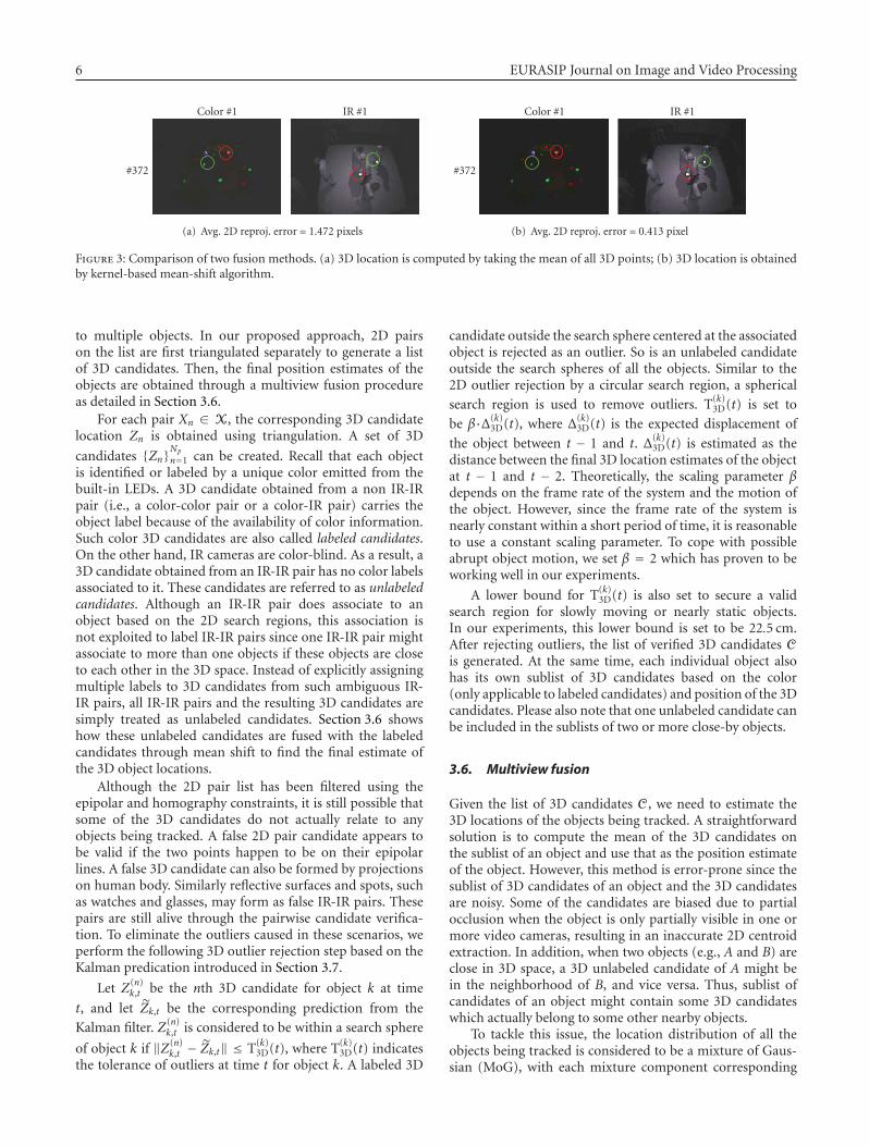
6 EURASIP Journal on Image and Video Processing
#372
Color #1 IR #1
(a) Avg. 2D reproj. error = 1.472 pixels
#372
Color #1 IR #1
(b) Avg. 2D reproj. error = 0.413 pixel
Figure 3: Comparison of two fusion methods. (a) 3D location is computed by taking the mean of all 3D points; (b) 3D location is obtainedby kernel-based mean-shift algorithm.
to multiple objects. In our proposed approach, 2D pairson the list are first triangulated separately to generate a listof 3D candidates. Then, the final position estimates of theobjects are obtained through a multiview fusion procedureas detailed in Section 3.6.
For each pair Xn ∈ X, the corresponding 3D candidatelocation Zn is obtained using triangulation. A set of 3D
candidates {Zn}Np
n=1 can be created. Recall that each objectis identified or labeled by a unique color emitted from thebuilt-in LEDs. A 3D candidate obtained from a non IR-IRpair (i.e., a color-color pair or a color-IR pair) carries theobject label because of the availability of color information.Such color 3D candidates are also called labeled candidates.On the other hand, IR cameras are color-blind. As a result, a3D candidate obtained from an IR-IR pair has no color labelsassociated to it. These candidates are referred to as unlabeledcandidates. Although an IR-IR pair does associate to anobject based on the 2D search regions, this association isnot exploited to label IR-IR pairs since one IR-IR pair mightassociate to more than one objects if these objects are closeto each other in the 3D space. Instead of explicitly assigningmultiple labels to 3D candidates from such ambiguous IR-IR pairs, all IR-IR pairs and the resulting 3D candidates aresimply treated as unlabeled candidates. Section 3.6 showshow these unlabeled candidates are fused with the labeledcandidates through mean shift to find the final estimate ofthe 3D object locations.
Although the 2D pair list has been filtered using theepipolar and homography constraints, it is still possible thatsome of the 3D candidates do not actually relate to anyobjects being tracked. A false 2D pair candidate appears tobe valid if the two points happen to be on their epipolarlines. A false 3D candidate can also be formed by projectionson human body. Similarly reflective surfaces and spots, suchas watches and glasses, may form as false IR-IR pairs. Thesepairs are still alive through the pairwise candidate verifica-tion. To eliminate the outliers caused in these scenarios, weperform the following 3D outlier rejection step based on theKalman predication introduced in Section 3.7.
Let Z(n)k,t be the nth 3D candidate for object k at time
t, and let Zk,t be the corresponding prediction from the
Kalman filter. Z(n)k,t is considered to be within a search sphere
of object k if ‖Z(n)k,t − Zk,t‖ ≤ T(k)
3D(t), where T(k)3D(t) indicates
the tolerance of outliers at time t for object k. A labeled 3D
candidate outside the search sphere centered at the associatedobject is rejected as an outlier. So is an unlabeled candidateoutside the search spheres of all the objects. Similar to the2D outlier rejection by a circular search region, a spherical
search region is used to remove outliers. T(k)3D(t) is set to
be β·Δ(k)3D(t), where Δ(k)
3D(t) is the expected displacement of
the object between t − 1 and t. Δ(k)3D(t) is estimated as the
distance between the final 3D location estimates of the objectat t − 1 and t − 2. Theoretically, the scaling parameter βdepends on the frame rate of the system and the motion ofthe object. However, since the frame rate of the system isnearly constant within a short period of time, it is reasonableto use a constant scaling parameter. To cope with possibleabrupt object motion, we set β = 2 which has proven to beworking well in our experiments.
A lower bound for T(k)3D(t) is also set to secure a valid
search region for slowly moving or nearly static objects.In our experiments, this lower bound is set to be 22.5 cm.After rejecting outliers, the list of verified 3D candidates Cis generated. At the same time, each individual object alsohas its own sublist of 3D candidates based on the color(only applicable to labeled candidates) and position of the 3Dcandidates. Please also note that one unlabeled candidate canbe included in the sublists of two or more close-by objects.
3.6. Multiview fusion
Given the list of 3D candidates C, we need to estimate the3D locations of the objects being tracked. A straightforwardsolution is to compute the mean of the 3D candidates onthe sublist of an object and use that as the position estimateof the object. However, this method is error-prone since thesublist of 3D candidates of an object and the 3D candidatesare noisy. Some of the candidates are biased due to partialocclusion when the object is only partially visible in one ormore video cameras, resulting in an inaccurate 2D centroidextraction. In addition, when two objects (e.g., A and B) areclose in 3D space, a 3D unlabeled candidate of A might bein the neighborhood of B, and vice versa. Thus, sublist ofcandidates of an object might contain some 3D candidateswhich actually belong to some other nearby objects.
To tackle this issue, the location distribution of all theobjects being tracked is considered to be a mixture of Gaus-sian (MoG), with each mixture component corresponding

H. Jin and G. Qian 7
to one object. Object tracking is cast into a mode seekingproblem using the 3D candidates. Consequently, the effect ofmissing 3D candidates due to the complete occlusion in someviews, inclusion of unlabeled candidates of other objects,and biased 3D localization caused by partial occlusionon the tracking results will be significantly reduced byselecting proper forms of kernel and weight functions. Sincethe goal is to locate the modes from the 3D candidates,instead of learning the complete parameters of the MoGusing the expectation-maximization (EM) algorithm, a fastmode-seeking procedure based on mean shift is taken inour proposed approach. Figure 3 shows comparison of twofusion methods with associated 2D reprojection errors,namely, the mean of 3D candidates and the mode obtainedby kernel-based mean-shift algorithm. It can be seen thatmean shift provides smaller reprojection error.
The mean-shift algorithm is an efficient and nonpara-metric method for clustering and mode seeking [17–19]based on kernel density estimation. Let S be a finite set ofsample points. The weighted sample mean at x is
m(x) =∑
s∈SKh(s− x)w(s)s∑s∈SKh(x− s)w(s)
, (4)
where Kh(·) is the kernel function, h is the bandwidthparameters, and w(·) is the weight function. Mean shiftrecursively moves the center of the kernel to a new locationby the mean-shift vector Δx = m(x) − x. The mean-shiftprocedure is guaranteed to be convergent if the kernel K(x)has a convex and monotonically decreasing profile k(‖x‖2)[18]. An important property of the mean-shift algorithm isthat the mean-shift vector computed using the kernel G is anestimate of the normalized density gradient computed usingthe kernel K , where G satisfies the relationship g(‖x‖2) =−ck′(‖x‖2), c is a normalizing constant. g and k arethe profiles of kernel G and K , respectively. In order tofacilitate real-time implementation, we take advantage of theintermediate results, namely, the prediction and covariancematrix of Kalman filtering (see Section 3.7) to approximatethe initial center and bandwidth.
Integration of mean shift and Kalman filter has beenintroduced in [18], where mean shift is used to locate theoptimal target position in an image based on the predictionfrom a Kalman filter. Then, the result of mean shift is used asthe measurement vector to the Kalman filter. Our proposedapproach for multiview fusion follows [18] in spirit in termsof the relationship of mean shift and Kalman filter. Themajor difference between our approach and is that we usemean shift as a fusion mechanism to find optimal object3D locations using both labeled and unlabeled 3D positioncandidates obtained from triangulation of point pairs.
Center initialization
A good initial center will expedite the convergence of themean-shift procedure. For each object being tracked, thereis one corresponding center initialized. In our approach,y = (yx, yy , yz), the predicted location by the Kalman filter atthe previous frame is taken as the initial center since y gives
1 2 3 4 5 6 7 8 9 10 11 12
Mean shift iterations
0
100
200
300
400
500
600
700
800
Fram
eco
un
t
Kalman prediction as initial center
Weighted mean as initial center
Histograms of mean shift iterations
Figure 4: Histogram comparison of mean-shift iterations withdifferent initial centers.
a good guess of object location at the current frame. Notethat another possible choice for the initial center is taking theweighted mean of the 3D candidates. We compare the mean-shift iterations with these two initial centers and the samebandwidth using a 1420-frame video sequence (sequence1). In the histogram shown in Figure 4, x-axis indicatesthe number of mean-shift iterations while y-axis indicatesthe number of frames corresponding to each iteration. Forinstance, to converge to optimal points, about 750 framestake 4 iterations using Kalman prediction as initial center,while about 600 frames take the same iterations usingweighted mean as initial center. The iteration histogramshows that our approximation takes slightly more mean-shiftiterations. But the approximation gains the benefit of noextra computation for initial center.
Bandwidth selection
A proper bandwidth for the kernel function is critical tothe mean-shift algorithm in terms of estimation perfor-mance and efficiency [20]. Reference [21] lists four differenttechniques for bandwidth selection. In [22], the bandwidthselection theorem is shown that if the true underlyingdistribution of samples is a Gaussian N (µ,Σ), for the fixed-bandwidth mean shift, the optimal bandwidth for a Gaussiankernel Kh that maximizes the bandwidth-normalized normof the mean shift vector is given by h = Σ.
In our approach, MoG is used to represent the jointposition distribution of all the object, and the marginaldistribution of a single object is described by a singleGaussian. In practice, Σ the true covariance matrix of theGaussian related to an object is unknown. However, Σ thecorresponding covariance matrix of the predicted objectposition in Kalman filter provides a good approximationto Σ since it resembles the uncertainty of the sample point

8 EURASIP Journal on Image and Video Processing
Table 2: Coefficients of fitted planes.
Plane Homogeneous coefficients
Ground plane [−0.0022, 0.0039, 0.9999, 0.0132]
Vertical plane [0.9889,−0.1338, 0.0628, 0.0144]
distribution. Thus in our proposed approach, h = (hx,hy ,hz)
is formed by the diagonal terms of Σ.
Kernel setup
Labeled sample points have explicit identity informationwhile unlabeled ones do not. Two different kernel functionsare applied to labeled and unlabeled sample points. Bothkernel functions share the same bandwidth h. Since a labeled3D candidate is expected to be within an ellipsoid centeredat the mode, and all the 3D candidates within the ellipsoidare considered equally important from the perspective of thekernel function, a truncated flat kernel (6) is used for thelabeled 3D candidates. Let Qh be an ellipsoid centered at ywith three axes given by h:
Qh(x, y) = (xx − yx)2
h2x
+(xy − yy)
2
h2y
+(xz − yz)
2
h2z
− 1.
(5)
The truncated flat kernel for labeled samples is given by
Kh(x− y) ={
1, if Qh(x, y) < 0,
0, otherwise.(6)
On the other hand, we assume that the contribution to themode estimation made by an unlabeled 3D candidate is lessthan that of a labeled candidate. The contribution of anunlabeled 3D candidate to the mode estimation is computedaccording to the distance from the unlabeled point to themode so that a distant point has small contributions. Hence,a truncated Gaussian kernel (7) is applied to all unlabeledsample points as follows:
Kh(x− y) =⎧⎪⎨⎪⎩
exp{− ‖x− y‖2
max2(hx,hy ,hz)
}, if Qh(x, y) < 0,
0, otherwise.(7)
Weight assignment
All the sample points in the final set are the survivors throughthe 2D pairwise verification process and 3D outlier rejection.Each 3D point is associated with a small epipolar distancedED(x) < TED. Thus, the epipolar distance is a good indicatorto represent the weight of each sample point. A Gaussiankernel (8) is used to compute the weight for each samplepoint:
w(x) = e−d2ED(x)/α, (8)
where α = 2T2ED.
YX
(1, 0, 0)IR #1 Color #1(0, 0, 0)
(0, 1, 0) IR #2 Color #2 (1, 1, 0)
Ver
tica
lpla
ne
15 feet
Col
or#3
IR#3
15fe
et
Visual feedbackprojection area(ground plane)
Figure 5: Illustration of the real system setup in top-down view.
The above mean-shift procedure iteratively updates theposition estimates of all objects being tracked. The positionof one object is considered converged when the norm ofcorresponding mean-shift vector is less than a prechosenthreshold (e.g., 0.5 mm in our implementation).
3.7. Smoothing and prediction using kalman filter
In the proposed tracking system, Kalman filters are usedto smooth position estimates obtained using mean shiftand predict object positions for the next time instant. Eachtarget object is assigned with a Kalman filter to performsmoothing and prediction based on a first-order motionmodel. The position estimates obtained using mean shift aretreated as measurements and input to the Kalman filters. Thesmoothed 3D locations are then used as the final trackingresults of the objects. It is possible, and perhaps desirable,to estimate the measurement noisy covariance matrix basedon the results of the mean shift. In our implementation, toreduce computational cost a constant diagonal measurementnoisy covariance matrix is used instead. The results obtainedare still good enough for our applications. The predictedobject locations are projected onto all camera views toform 2D search region for the next time instant. These 2Dsearch regions can substantially reduce the number of 2Dfalse candidate blobs as described in Section 3.3. Similarly,these location predictions also serve as centers of searchingspheres for 3D outlier rejection as discussed in Section 3.5. Inaddition, the covariance matrices of the predicted positionsalso inform the bandwidth selection in Section 3.6.
3.8. Handling complete occlusion and tracking failure
When complete occlusion occurs in some camera views, the2D candidates in other nonoccluded camera views can stillbe coupled to form pairs for triangulation. As long as anobject is visible in at least two camera views, the trackingof the object can be consistently achieved. Sometimes due

H. Jin and G. Qian 9
Color #1
Color #2
Color #3
IR #1
IR #2
IR #3
#85 #398 #426 #429 #723
Figure 6: Two-object tracking results using sequence 1. A large amount of interfering visual patterns was present in the background. Boldgreen (red) circles indicate the reprojected 2D locations of the green (red) object. The slim red circles show the 2D candidates in each cameraview. The large slim yellow circles are the predicted search regions for the removal of 2D false candidates. The mean (μ) and std (σ) of thereprojection errors in pixels are as follows. For the green object, μ1 = 0.823 and σ1 = 0.639. For the red object, μ2 = 0.758 and σ2 = 0.607.Note that the blue points are deliberately added as the interfering background projections, which are different from tracking objects’ colors,to test the robustness of our tracking approach.
to severe occlusions or fast and abrupt moving directionchanges, an object is only detected in one camera view orcompletely invisible by all the cameras. Consequently, novalid 2D pair of the object can be formed in such scenariosand the tracking system issues a tracking failure event for thisobject as no pair exists. To recover the tracking of the missingobject, we search valid color-IR pairs in the whole image inboth color and IR camera views, without enforcing distance-based outlier rejection scheme according to search regions.During the detection phase of a lost object, the existence ofa color-color pair matching, the color of the object, or anIR-IR pair alone cannot claim the detection of the objectsince a color-color pair may be caused by background visualprojection, and an unlabeled IR-IR pair does not provide anyidentity information and it may not actually correspond toany objects to be tracked. In this case, most of outliers areremoved by color-IR pair selection, and the final result isrefined by mean-shift-based multiview fusion. Once a lostobject has been detected, the tracking can be resumed.
Occasionally, an occluded object will reappear againshortly at a position close to where it got lost. In suchcases, there is no need to search the object in the entireimage. To accommodate such scenarios, some extra steps aretaken in our current system implementation as shown in theright column in Figure 2. In the current implementation, amissing-frame counter (MFC) is associated to each objectbeing tracked. When an object is not visible in at least twocameras views, the corresponding MFC is triggered to countthe number of frames that the object is continually missing.When the reading of the MFC is less than a certain thresholdMTH , for example, 25 frames in our implementation, thetracking system will keep trying to search for the objectin all of the camera views within search regions accordingto its 3D location at the last time instant when the objectwas successfully tracked. If the object reappears in thesearch regions of two of more camera views during thisperiod, the MFC will be set to zero and the tracking ofthe object continues. If the object cannot be found during

10 EURASIP Journal on Image and Video Processing
Color #1
Color #2
Color #3
IR #1
IR #2
IR #3
#103 #128 #200 #298 #482
Figure 7: Three-object tracking results using sequence 2. The statistics of the reprojection errors in pixels are μ1 = 0.788 and σ1 = 0.609 forthe green object, μ2 = 0.891 and σ2 = 0.681 for red object, and μ3 = 0.884 and σ3 = 0.523 for the blue object.
this period, the MFC gets reset and the systems start tosearch for the object in the whole images from all the cameraviews according to the procedure described in the previousparagraph.
4. EXPERIMENTAL RESULTSAND PERFORMANCE ANALYSIS
The proposed tracking system has been implemented usingsix CCD cameras (Dragonfly 2, Point Grey Research, Ariz,USA), including three color cameras and three IR cameras.Figure 5 illustrates the real system setup in top-down view.The cameras are mounted about 14 feet high from theground on a steel truss. The tracking system software isprogrammed using C++ with multithreading on a PC (IntelXeon 3.6 GHz, 1 GB RAM) running Windows XP. Imageresolution is set to 320 × 240. All cameras are synchronizedand calibrated in advance. The dimension of the spaceis aligned to predefined coordinate systems with 1 unit= 15 feet. To better cover the activity space, large FOVsare applied to all the cameras. So, lens distortion [16] isalso recovered for each frame using the camera calibration
toolbox [23]. Visual projections are projected onto twoplanes—the ground plane and a vertical plane parallel to y-axis at the boundary of the capture volume. Table 2 showsthe homogeneous coefficients of the two planes. This systemruns in real-time at 60 fps when tracking three objects, and40 fps when tracking six objects. In this six-camera setting,approximately 10∼18 pairs per object will appear in the final2D pair set. The number of pairs varies based on occlusionsand the number of neighboring objects. Occlusions causemissing pairs while neighboring objects result in moreunlabeled IR-IR pairs appearing in the final set.
To evaluate and analyze the performance of the trackingsystem, a large amount of fast time changing visual patternswas projected onto the ground and vertical planes. Thesevisual patterns often carry similar colors to the objectsbeing tracked. In this section, tracking results obtained usingthree sequences are presented to demonstrate the robusttracking performance of the proposed system in the presenceof interfering visual projection, occlusion, and multiplesubjects in the space. Sequence 1 shows reliable trackingof two objects with interfering visual projection on themultiple projection planes. Sequence 2 has three objects and

H. Jin and G. Qian 11
Color #1
Color #2
Color #3
IR #1
IR #2
IR #3
#53 #221 #284 #388 #801
Figure 8: Two-ball tracking results using sequence 3. Four people were moving in the space and interacting with the mediated environment.The statistics of the reprojection errors in pixels are μ1 = 0.732 and σ1 = 0.511 for the green object, and μ2 = 0.755 and σ2 = 0.549 for thered object.
frequent occlusion. In sequence 3, four subjects interact withthe mediated environment using two objects. Partial andcomplete occlusions also frequently occur in sequence 3.
In the first experiment using sequence 1 (1420 frameslong), two glowing balls (green and red, 6 inches in diameter)patched with reflective material were tracked with interferingvisual patterns of similar color projected onto two planes.Sample frames from all six cameras (frames 85, 398, 426,429, and 723) are shown in Figure 6 with reprojected 2Dlocations (small bold circles) and search regions (large slimcircles) superimposed for both objects. The bold green andred circles indicate the green and red objects’ 2D locationsreprojected from the final 3D locations, respectively. Thelarge slim yellow circle is the predicted search region used toremove 2D false candidates. In these frames, a great amountof 2D false candidates did appear in the entire image butthey were effectively removed through the predicted searchregion. The plane projections were successfully eliminatedby the homography test. Some bright spots, for example, thespots on the upper body of the subjects in frames 398 and723 in all three IR cameras, had no much negative effectson tracking due to 3D outlier rejection and mean-shift-based multiview fusion steps introduced earlier. Objects can
be continually tracked when they were put on the groundplane without being confused with floor projections. Objectidentities were successfully maintained in some challengingscenarios, for example, when two objects were rolling onthe ground plane and passing by each other in frames 426and 429. In this case, it can be seen from Figure 6 that thecenters of the reprojected 2D locations were exactly on theobjects being tracked. We also projected final 3D locationonto all camera views and calculated the average reprojectionerror over all cameras for each frame. In this experiment,the reprojection errors over all the frames are 0.823 pixelswith standard deviation 0.639 pixels for the green object, and0.758 pixels with standard deviation 0.607 pixels for the redobject.
The second sequence (see Figure 7) is 658 frames long,consisting of three moving objects with interfering visualpatterns projected on the two projection planes. A personswitches green and red objects between his hands aroundframes 103, 128, 200, and 298. Partial and completeocclusions occurred in these views but the objects weretracked accurately without lose or exchanging of identities.In frame 482, three objects were placed on the groundplane at the same time, and objects were covered by bowing

12 EURASIP Journal on Image and Video Processing
0.1 0.20.3 0.4
0.5 0.6 0.7 0.8 0.9Y
−0.2
0
0.2
0.4
0.6
Z
1.21
0.80.6
0.40.2
0−0.2
X
3D trajectories on frame 400-500
(a)
400 410 420 430 440 450 460 470 480 490 500
Frame index
−0.20
0.2
0.4
0.6
0.8
1
1.2
Val
ue
X-Y-Z 2D trajectories (red ball) on frame 400-500
400 410 420 430 440 450 460 470 480 490 500
Frame index
−0.20
0.2
0.4
0.6
0.8
1
1.2
Val
ue
X-Y-Z 2D trajectories (green ball) on frame 400-500
X
Y
Z
(b)
Figure 9: Trajectories of the two objects in sequence 1 betweenframe 400 and frame 500. The two objects were rolling on theground plane and passing by each other.
persons in some views. In such severe occlusions withsimilar color visual projection, all three objects were stilltracked accurately. The reprojection errors over all framesin sequence 2 are 0.788 pixels with standard deviation 0.609pixels for the green ball, 0.891 pixels with standard deviation0.681 pixels for the red object, and 0.884 pixels with standarddeviation 0.523 pixels for the blue object.
In Figure 8, there are 1180 frames. In this experiment,two balls were successfully tracked in the presence offour people moving in the space and interacting with the
−0.2 00.2 0.4
0.6 0.81 1.2X
00.10.20.30.40.50.60.7
Z
0.20.3
0.40.5
0.60.7
0.80.9
1
Y
3D trajectories on frame 100-200
(a)
100 110 120 130 140 150 160 170 180 190 200
Frame index
−0.20
0.20.40.60.8
Val
ue
X-Y-Z 2D trajectories (blue ball) on frame 100-200
100 110 120 130 140 150 160 170 180 190 200
Frame index
0
0.5
1
1.5
Val
ue
X-Y-Z 2D trajectories (red ball) on frame 100-200
100 110 120 130 140 150 160 170 180 190 200
Frame index
0.2
0.4
0.6
0.8
1
Val
ue
X-Y-Z 2D trajectories (green ball) on frame 100-200
XY
Z
(b)
Figure 10: Trajectories of the three objects in sequence 2 betweenframe 100 and frame 200. The green and red objects weremanipulated by one subject, and the blue object was handled byanother person.
mediated environment. A large amount of moving visualpatterns with varying illumination was projected on bothplanes. Occlusions of the objects occurred frequently duringthe tracking. In frame 801, it can be seen that two ballswere put close to each other. However, our system canstill maintain precise tracking in this challenging case. Theobjects were successfully tracked in the whole sequence. Theaverage 2D reprojection errors for the green and red ball are0.732 and 0.755 pixels with standard deviation 0.511 and0.549 pixels, respectively.

H. Jin and G. Qian 13
Table 3: Jerk cost of trajectory.
SequenceJerk Cost
Object 1 Object 2 Object 3
1 0.0355 0.1813 N/A
2 0.0149 0.1266 0.0098
3 0.0184 0.0126 N/A
Our method is able to recover and resume the correcttracking of the same object when it is lost as described inSection 3.8. The false object detection rate after trackingfailure in the tested sequences is less than 1% in therecovery phase. A false object detection may happen whenthe changing background has similar color to the lostobject, and there exists an IR-color pair which satisfies bothepipolar constraint and homography test coincidentally. Theprobability of the coincident scenario is very low in practice.
Since ground truth data of the object 3D positions isnot available to benchmark our tracking system, the jerkcost was computed to gauge the tracking accuracy andconsistency. Reference [24] notes that the smoothness of atrajectory can be quantified as a function of jerk, which isthe time derivative of acceleration. Hence, jerk is the third-time derivative of location. For a system x(t), the jerk of thatsystem is
J(x(t)) = d3x(t)dt3
. (9)
For a particular 3D trajectory x(t) that starts at t1 and endsat t2, the smoothness can be measured by calculating a jerkcost:
JC(x) =∫ t2t1
(d3xx(t)
dt3
)2
+(d3xy(t)
dt3
)2
+(
d3xz(t)dt3
)2
dt.
(10)
Three subsequences of 101 frames were selected, onefrom each video sequence. Table 3 lists the jerk cost oftracked object trajectories in these subsequences. Small jerkcost indicates smooth motion. The 3D trajectories and X , Y ,and Z positions over time of objects are plotted. Figure 9shows these trajectories between frames 400 and 500 ofsequence 1. In the first half of this subsequence, the twoobjects were rolling on the ground plane and passing byeach other very closely. Figure 10 shows trajectories betweenframes 100 to 200 from sequence 2, in the beginning ofwhich the green and red objects were very close to each other.Trajectories of two objects from frame 700 to 800 of sequence3 are presented in Figure 11.
5. CONCLUSIONS AND FUTURE WORK
This paper reports a real-time system for multiview 3Dobject tracking for interactive mediated environments withdynamic background projection. The experiment resultsshow that the reported system can robustly provide accurate
10.9
0.80.7
0.60.5
0.4Y
0.1
0.2
0.3
0.4
0.5
0.6
Z
00.2
0.4 0.60.8
11.2
1.4
X
3D trajectories on frame 700-800
(a)
700 710 720 730 740 750 760 770 780 790 800
Frame index
00.20.4
0.6
0.8
1
1.2
1.4
Val
ue
X-Y-Z 2D trajectories (red ball) on frame 700-800
700 710 720 730 740 750 760 770 780 790 800
Frame index
0.10.20.30.40.50.60.70.80.9
1
Val
ue
X-Y-Z 2D trajectories (green ball) on frame 700-800
X
Y
Z
(b)
Figure 11: Trajectories of the two objects in sequence 2 from frame700 to 800.
3D object tracking in the presence of dynamic visualprojection on multiple planes. This system has foundimportant applications in embodied and mediate learning(http://ame2.asu.edu/projects/ameed/). It can also be easilyused in many other visually mediated environment to pro-vide reliable object tracking for embodied human computerinteraction. We are currently working on integrating built-in inertial sensors such as accelerometers and rotationrate sensors with vision-based tracking. In so doing, theorientation information of the object can also be recovered.In addition, inertial information can improve and maintain

14 EURASIP Journal on Image and Video Processing
consistent tracking when the object is completely visuallyoccluded in all camera views.
ACKNOWLEDGMENT
This paper is based upon work partly supported by U.S.National Science Foundation on CISE-RI no. 0403428 andIGERT no. 0504647. Any opinions, findings and conclusionsor recommendations expressed in thismaterial are those ofthe author(s) and do not necessarily reflect the views of theU.S. National Science Foundation (NSF).
REFERENCES
[1] Cave Automatic Virtual Environment, http://www.en.wiki-pedia.org/wiki/Cave Automatic Virtual Environment.
[2] T. B. Moeslund, A. Hilton, and V. Kruger, “A survey ofadvances in vision-based human motion capture and analy-sis,” Computer Vision and Image Understanding, vol. 104, no.2-3, pp. 90–126, 2006.
[3] L. Wang, W. Hu, and T. Tan, “Recent development in humanmotion analysis,” Pattern Recognition, vol. 36, no. 3, pp. 585–601, 2003.
[4] Intersense, http://www.isense.com/.[5] Ascension, http://www.ascension-tech.com/.[6] Y. Huang and I. Essa, “Tracking multiple objects through
occlusions,” in Proceedings of the IEEE Computer SocietyConference on Computer Vision and Pattern Recognition(CVPR ’05), vol. 2, p. 1182, San Diego, Calif, USA, June 2005.
[7] J. Pan and B. Hu, “Robust occlusion handling in object track-ing,” in Proceedings of the IEEE Conference on Computer Visionand Pattern Recognition (CVPR ’07), pp. 1–8, Minneapolis,Minn, USA, June 2007.
[8] T. Yang, S. Z. Li, Q. Pan, and J. Li, “Real-time multipleobjects tracking with occlusion handling in dynamic scenes,”in Proceedings of the IEEE Computer Society Conference onComputer Vision and Pattern Recognition (CVPR ’05), vol. 1,pp. 970–975, San Diego, Calif, USA, June 2005.
[9] W. Qu, D. Schonfeld, and M. Mohamed, “DistributedBayesian multiple-target tracking in crowded environmentsusing multiple collaborative cameras,” EURASIP Journal onAdvances in Signal Processing, vol. 2007, Article ID 38373, 15pages, 2007.
[10] J. Black, T. Ellis, and P. Rosin, “Multi view image surveillanceand tracking,” in Proceedings of the Workshop on Motion andVideo Computing (Motion ’02), pp. 169–174, Orlando, Fla,USA, December 2002.
[11] F. Jurie and M. Dhome, “Real time tracking of 3D objectswith occultations,” in Proceedings of the IEEE InternationalConference on Image Processing (ICIP ’01), vol. 1, pp. 413–416,Thessaloniki, Greece, October 2001.
[12] S. M. Khan and M. Shah, “Consistent labeling of trackedobjects in multiple cameras with overlapping fields of view,”IEEE Transactions on Pattern Analysis and Machine Intelligence,vol. 25, no. 10, pp. 1355–1360, 2003.
[13] S. M. Khan and M. Shah, “A multiview approach to track-ing people in crowded scenes using a planar homographyconstraint,” in Proceedings of the 9th European Conferenceon Computer Vision (ECCV ’06), vol. 4, pp. 133–146, Graz,Austria, May 2006.
[14] Smallab, http://ame2.asu.edu/projects/ameed/.[15] T. Svoboda, D. Martinec, and T. Pajdla, “A convenient multi-
camera self-calibration for virtual environments,” PRESENCE:
Teleoperators and Virtual Environments, vol. 14, no. 4, pp. 407–422, 2005.
[16] R. I. Hartley and A. Zisserman, Multiple View Geometry inComputer Vision, Cambridge University Press, Cambridge,UK, 2nd edition, 2004.
[17] Y. Cheng, “Mean shift, mode seeking and clustering,” IEEETransactions on Pattern Analysis and Machine Intelligence, vol.17, no. 8, pp. 790–799, 1995.
[18] D. Comaniciu, V. Ramesh, and P. Meer, “Real-time trackingof non-rigid objects using mean shift,” in Proceedings of theIEEE Conference on Computer Vision and Pattern Recognition(CVPR ’00), vol. 2, pp. 142–149, Hilton Head Island, SC, USA,June 2000.
[19] K. Fukunaga and L. D. Hostetler, “The estimation of thegradient of a density function, with application in patternrecognition,” IEEE Transactions on Information Theory, vol. 21,no. 1, pp. 32–40, 1975.
[20] D. Comaniciu, V. Ramesh, and P. Meer, “The variablebandwidth mean shift and data-driven scale selection,” in Pro-ceedings of the 8th IEEE International Conference on ComputerVision (ICCV ’01), vol. 1, pp. 438–445, Vancouver, Canada,July 2001.
[21] D. Comaniciu and P. Meer, “Mean shift: a robust approachtoward feature space analysis,” IEEE Transactions on PatternAnalysis and Machine Intelligence, vol. 24, no. 5, pp. 603–619,2002.
[22] D. Comaniciu, “An algorithm for data-driven bandwidthselection,” IEEE Transactions on Pattern Analysis and MachineIntelligence, vol. 25, no. 2, pp. 281–288, 2003.
[23] Camera calibration toolbox for matlab, http://www.vision.caltech.edu/bouguetj/calib doc/.
[24] T. Flash and N. Hogan, “The coordination of arm movements:an experimentally confirmed mathematical model,” The Jour-nal of Neuroscience, vol. 5, no. 7, pp. 1688–1703, 1985.

Hindawi Publishing CorporationEURASIP Journal on Image and Video ProcessingVolume 2008, Article ID 246309, 10 pagesdoi:10.1155/2008/246309
Research ArticleEvaluating Multiple Object Tracking Performance:The CLEAR MOT Metrics
Keni Bernardin and Rainer Stiefelhagen
Interactive Systems Lab, Institut fur Theoretische Informatik, Universitat Karlsruhe, 76131 Karlsruhe, Germany
Correspondence should be addressed to Keni Bernardin, [email protected]
Received 2 November 2007; Accepted 23 April 2008
Recommended by Carlo Regazzoni
Simultaneous tracking of multiple persons in real-world environments is an active research field and several approaches havebeen proposed, based on a variety of features and algorithms. Recently, there has been a growing interest in organizing systematicevaluations to compare the various techniques. Unfortunately, the lack of common metrics for measuring the performance ofmultiple object trackers still makes it hard to compare their results. In this work, we introduce two intuitive and general metrics toallow for objective comparison of tracker characteristics, focusing on their precision in estimating object locations, their accuracyin recognizing object configurations and their ability to consistently label objects over time. These metrics have been extensivelyused in two large-scale international evaluations, the 2006 and 2007 CLEAR evaluations, to measure and compare the performanceof multiple object trackers for a wide variety of tracking tasks. Selected performance results are presented and the advantages anddrawbacks of the presented metrics are discussed based on the experience gained during the evaluations.
Copyright © 2008 K. Bernardin and R. Stiefelhagen. This is an open access article distributed under the Creative CommonsAttribution License, which permits unrestricted use, distribution, and reproduction in any medium, provided the original work isproperly cited.
1. INTRODUCTION
The audio-visual tracking of multiple persons is a very activeresearch field with applications in many domains. Theserange from video surveillance, over automatic indexing, tointelligent interactive environments. Especially in the lastcase, a robust person tracking module can serve as a powerfulbuilding block to support other techniques, such as gesturerecognizers, face or speaker identifiers, head pose estimators[1], and scene analysis tools. In the last few years, more andmore approaches have been presented to tackle the problemsposed by unconstrained, natural environments and bringperson trackers out of the laboratory environment and intoreal-world scenarios.
In recent years, there has also been a growing inter-est in performing systematic evaluations of such trackingapproaches with common databases and metrics. Examplesare the CHIL [2] and AMI [3] projects, funded by theEU, the U.S. VACE project [4], the French ETISEO [5]project, the U.K. Home Office iLIDS project [6], the CAVIAR[7] and CREDS [8] projects, and a growing number ofworkshops (e.g., PETS [9], EEMCV [10], and more recently
CLEAR [11]). However, although benchmarking is ratherstraightforward for single object trackers, there is still nogeneral agreement on a principled evaluation procedureusing a common set of objective and intuitive metrics formeasuring the performance of multiple object trackers.
Li et al. in [12] investigate the problem of evaluatingsystems for the tracking of football players from multiplecamera images. Annotated ground truth for a set of visibleplayers is compared to the tracker output and 3 measuresare introduced to evaluate the spatial and temporal accuracyof the result. Two of the measures, however, are ratherspecific to the football tracking problem, and the moregeneral measure, the “identity tracking performance,” doesnot consider some of the basic types of errors made bymultiple target trackers, such as false positive tracks orlocalization errors in terms of distance or overlap. This limitsthe application of the presented metric to specific types oftrackers or scenarios.
Nghiem et al. in [13] present a more general frameworkfor evaluation, which covers the requirements of a broadrange of visual tracking tasks. The presented metrics aimat allowing systematic performance analysis using large
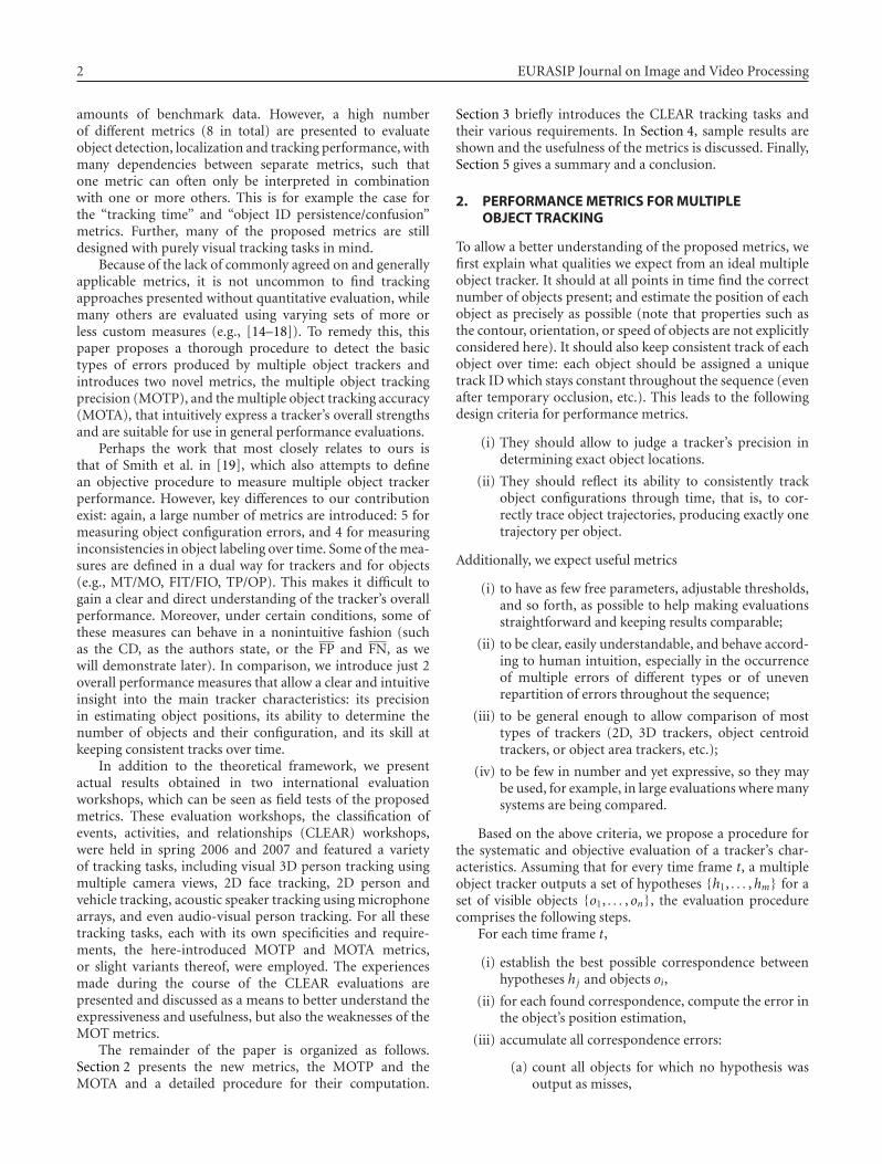
2 EURASIP Journal on Image and Video Processing
amounts of benchmark data. However, a high numberof different metrics (8 in total) are presented to evaluateobject detection, localization and tracking performance, withmany dependencies between separate metrics, such thatone metric can often only be interpreted in combinationwith one or more others. This is for example the case forthe “tracking time” and “object ID persistence/confusion”metrics. Further, many of the proposed metrics are stilldesigned with purely visual tracking tasks in mind.
Because of the lack of commonly agreed on and generallyapplicable metrics, it is not uncommon to find trackingapproaches presented without quantitative evaluation, whilemany others are evaluated using varying sets of more orless custom measures (e.g., [14–18]). To remedy this, thispaper proposes a thorough procedure to detect the basictypes of errors produced by multiple object trackers andintroduces two novel metrics, the multiple object trackingprecision (MOTP), and the multiple object tracking accuracy(MOTA), that intuitively express a tracker’s overall strengthsand are suitable for use in general performance evaluations.
Perhaps the work that most closely relates to ours isthat of Smith et al. in [19], which also attempts to definean objective procedure to measure multiple object trackerperformance. However, key differences to our contributionexist: again, a large number of metrics are introduced: 5 formeasuring object configuration errors, and 4 for measuringinconsistencies in object labeling over time. Some of the mea-sures are defined in a dual way for trackers and for objects(e.g., MT/MO, FIT/FIO, TP/OP). This makes it difficult togain a clear and direct understanding of the tracker’s overallperformance. Moreover, under certain conditions, some ofthese measures can behave in a nonintuitive fashion (suchas the CD, as the authors state, or the FP and FN, as wewill demonstrate later). In comparison, we introduce just 2overall performance measures that allow a clear and intuitiveinsight into the main tracker characteristics: its precisionin estimating object positions, its ability to determine thenumber of objects and their configuration, and its skill atkeeping consistent tracks over time.
In addition to the theoretical framework, we presentactual results obtained in two international evaluationworkshops, which can be seen as field tests of the proposedmetrics. These evaluation workshops, the classification ofevents, activities, and relationships (CLEAR) workshops,were held in spring 2006 and 2007 and featured a varietyof tracking tasks, including visual 3D person tracking usingmultiple camera views, 2D face tracking, 2D person andvehicle tracking, acoustic speaker tracking using microphonearrays, and even audio-visual person tracking. For all thesetracking tasks, each with its own specificities and require-ments, the here-introduced MOTP and MOTA metrics,or slight variants thereof, were employed. The experiencesmade during the course of the CLEAR evaluations arepresented and discussed as a means to better understand theexpressiveness and usefulness, but also the weaknesses of theMOT metrics.
The remainder of the paper is organized as follows.Section 2 presents the new metrics, the MOTP and theMOTA and a detailed procedure for their computation.
Section 3 briefly introduces the CLEAR tracking tasks andtheir various requirements. In Section 4, sample results areshown and the usefulness of the metrics is discussed. Finally,Section 5 gives a summary and a conclusion.
2. PERFORMANCE METRICS FOR MULTIPLEOBJECT TRACKING
To allow a better understanding of the proposed metrics, wefirst explain what qualities we expect from an ideal multipleobject tracker. It should at all points in time find the correctnumber of objects present; and estimate the position of eachobject as precisely as possible (note that properties such asthe contour, orientation, or speed of objects are not explicitlyconsidered here). It should also keep consistent track of eachobject over time: each object should be assigned a uniquetrack ID which stays constant throughout the sequence (evenafter temporary occlusion, etc.). This leads to the followingdesign criteria for performance metrics.
(i) They should allow to judge a tracker’s precision indetermining exact object locations.
(ii) They should reflect its ability to consistently trackobject configurations through time, that is, to cor-rectly trace object trajectories, producing exactly onetrajectory per object.
Additionally, we expect useful metrics
(i) to have as few free parameters, adjustable thresholds,and so forth, as possible to help making evaluationsstraightforward and keeping results comparable;
(ii) to be clear, easily understandable, and behave accord-ing to human intuition, especially in the occurrenceof multiple errors of different types or of unevenrepartition of errors throughout the sequence;
(iii) to be general enough to allow comparison of mosttypes of trackers (2D, 3D trackers, object centroidtrackers, or object area trackers, etc.);
(iv) to be few in number and yet expressive, so they maybe used, for example, in large evaluations where manysystems are being compared.
Based on the above criteria, we propose a procedure forthe systematic and objective evaluation of a tracker’s char-acteristics. Assuming that for every time frame t, a multipleobject tracker outputs a set of hypotheses {h1, . . . ,hm} for aset of visible objects {o1, . . . , on}, the evaluation procedurecomprises the following steps.
For each time frame t,
(i) establish the best possible correspondence betweenhypotheses hj and objects oi,
(ii) for each found correspondence, compute the error inthe object’s position estimation,
(iii) accumulate all correspondence errors:
(a) count all objects for which no hypothesis wasoutput as misses,
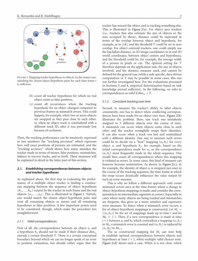
K. Bernardin and R. Stiefelhagen 3
o1
h1
h2
h5
o2
o8Misses
t
t
t
t
Falsepositives
Figure 1: Mapping tracker hypotheses to objects. In the easiest case,matching the closest object-hypothesis pairs for each time frame tis sufficient.
(b) count all tracker hypotheses for which no realobject exists as false positives,
(c) count all occurrences where the trackinghypothesis for an object changed compared toprevious frames as mismatch errors. This couldhappen, for example, when two or more objectsare swapped as they pass close to each other,or when an object track is reinitialized with adifferent track ID, after it was previously lostbecause of occlusion.
Then, the tracking performance can be intuitively expressedin two numbers: the “tracking precision” which expresseshow well exact positions of persons are estimated, and the“tracking accuracy” which shows how many mistakes thetracker made in terms of misses, false positives, mismatches,failures to recover tracks, and so forth. These measures willbe explained in detail in the latter part of this section.
2.1. Establishing correspondences between objectsand tracker hypotheses
As explained above, the first step in evaluating the perfor-mance of a multiple object tracker is finding a continu-ous mapping between the sequence of object hypotheses{h1, . . . ,hm} output by the tracker in each frame and the realobjects {o1, . . . , on}. This is illustrated in Figure 1. Naively,one would match the closest object-hypothesis pairs andtreat all remaining objects as misses and all remaininghypotheses as false positives. A few important points needto be considered, though, which make the procedure lessstraightforward.
2.1.1. Valid correspondences
First of all, the correspondence between an object oi anda hypothesis hj should not be made if their distance disti, jexceeds a certain threshold T . There is a certain conceptualboundary beyond which we can no longer speak of an errorin position estimation, but should rather argue that the
tracker has missed the object and is tracking something else.This is illustrated in Figure 2(a). For object area trackers(i.e., trackers that also estimate the size of objects or thearea occupied by them), distance could be expressed interms of the overlap between object and hypothesis, forexample, as in [14], and the threshold T could be set to zerooverlap. For object centroid trackers, one could simply usethe Euclidian distance, in 2D image coordinates or in real 3Dworld coordinates, between object centers and hypotheses,and the threshold could be, for example, the average widthof a person in pixels or cm. The optimal setting for Ttherefore depends on the application task, the size of objectsinvolved, and the distance measure used, and cannot bedefined for the general case (while a task-specific, data-drivencomputation of T may be possible in some cases, this wasnot further investigated here. For the evaluations presentedin Sections 3 and 4, empirical determination based on taskknowledge proved sufficient). In the following, we refer tocorrespondences as valid if disti, j < T .
2.1.2. Consistent tracking over time
Second, to measure the tracker’s ability to label objectsconsistently, one has to detect when conflicting correspon-dences have been made for an object over time. Figure 2(b)illustrates the problem. Here, one track was mistakenlyassigned to 3 different objects over the course of time.A mismatch can occur when objects come close to eachother and the tracker wrongfully swaps their identities.It can also occur when a track was lost and reinitializedwith a different identity. One way to measure such errorscould be to decide on a “best” mapping (oi,hj) for everyobject oi and hypothesis hj , for example, based on theinitial correspondence made for oi, or the correspondence(oi,hj) most frequently made in the whole sequence. Onewould then count all correspondences where this mappingis violated as errors. In some cases, this kind of measure canhowever become nonintuitive. As shown in Figure 2(c), if,for example, the identity of object oi is swapped just once inthe course of the tracking sequence, the time frame at whichthe swap occurs drastically influences the value output bysuch an error measure.
This is why we follow a different approach: only countmismatch errors once at the time frames where a change inobject-hypothesis mappings is made; and consider the corre-spondences in intermediate segments as correct. Especially incases where many objects are being tracked and mismatchesare frequent, this gives us a more intuitive and expressiveerror measure. To detect when a mismatch error occurs, alist of object-hypothesis mappings is constructed. Let Mt ={(oi,hj)} be the set of mappings made up to time t and letM0 = {·}. Then, if a new correspondence is made at timet + 1 between oi and hk which contradicts a mapping (oi,hj)in Mt, a mismatch error is counted and (oi,hj) is replaced by(oi,hk) in Mt+1.
The so constructed mapping list Mt can now helpto establish optimal correspondences between objects andhypotheses at time t + 1, when multiple valid choices exist.Figure 2(d) shows such a case. When it is not clear, which

4 EURASIP Journal on Image and Video Processing
o1
h1
h1
h1
o1o1
Miss
t t + 1 t + 2
Falsepositive
Dist.> T
(a)
o1
h1
h2
h3
o2
o3Mismatch
Mismatch
t t + 1 t + 2 t + 3 t + 4 t + 5 t + 6 t + 7
(b)
o1
h1
h2
Case 1:
o1
h1 h2
Case 2:
t t + 1 t + 2 t + 3 t + 4 t + 5 t + 6 t + 7 t + 8
t t + 1 t + 2 t + 3 t + 4 t + 5 t + 6 t + 7 t + 8
(c)
o1
h1
h1
h2
Miss
o1 o1
t t + 1 t + 2
Falsepositive Dist.< T
(d)
Figure 2: Optimal correspondences and error measures. (a) When the distance between o1 and h1 exceeds a certain threshold T , one canno longer make a correspondence. Instead, o1 is considered missed and h1 becomes a false positive. (b): Mismatched tracks. Here, h2 is firstmapped to o2. After a few frames, though, o1 and o2 cross paths and h2 follows the wrong object. Later, it wrongfully swaps again to o3. (c):Problems when using a sequence-level “best” object-hypothesis mapping based on most frequently made correspondences. In the first case,o1 is tracked just 2 frames by h1, before the track is taken over by h2. In the second case, h1 tracks o1 for almost half the sequence. In bothcases, a “best” mapping would pair h2 and o1. This however leads to counting 2 mismatch errors for case 1; and 4 errors for case 2, althoughin both cases only one error of the same kind was made. (d): Correct reinitialization of a track. At time t, o1 is tracked by h1. At t + 1, thetrack is lost. At t + 2, two valid hypotheses exist. The correspondence is made with h1 although h2 is closer to o1, based on the knowledge ofprevious mappings up to time t + 1.
hypothesis to match to an object oi, priority is given toho with (oi,ho) ∈ Mt, as this is most likely the correcttrack. Other hypotheses are considered false positives, andcould have occurred because the tracker outputs severalhypotheses for oi, or because a hypothesis that previouslytracked another object accidentally crossed over to oi.
2.1.3. Mapping procedure
Having clarified all the design choices behind our strategy forconstructing object-hypothesis correspondences, we sum-marize the procedure as follows.
Let M0 = {·}. For every time frame t, consider thefollowing.
(1) For every mapping (oi,hj) in Mt−1, verify if it is stillvalid. If object oi is still visible and tracker hypothesishj still exists at time t, and if their distance does
not exceed the threshold T , make the correspondencebetween oi and hj for frame t.
(2) For all objects for which no correspondence wasmade yet, try to find a matching hypothesis. Allowonly one-to-one matches, and pairs for which thedistance does not exceed T . The matching shouldbe made in a way that minimizes the total object-hypothesis distance error for the concerned objects.This is a minimum weight assignment problem,and is solved using Munkres’ algorithm [20] withpolynomial runtime complexity. If a correspondence(oi,hk) is made that contradicts a mapping (oi,hj) inMt−1, replace (oi,hj) with (oi,hk) in Mt. Count thisas a mismatch error and let mmet be the number ofmismatch errors for frame t.
(3) After the first two steps, a complete set of matchingpairs for the current time frame is known. Let ct be

K. Bernardin and R. Stiefelhagen 5
the number of matches found for time t. For each oftheses matches, calculate the distance dit between theobject oi and its corresponding hypothesis.
(4) All remaining hypotheses are considered false posi-tives. Similarly, all remaining objects are consideredmisses. Let f pt and mt be the number of falsepositives and misses, respectively, for frame t. Let alsogt be the number of objects present at time t.
(5) Repeat the procedure from step 1 for the next timeframe. Note that since for the initial frame, the set ofmappings M0 is empty, all correspondences made areinitial and no mismatch errors occur.
In this way, a continuous mapping between objects andtracker hypotheses is defined and all tracking errors areaccounted for.
2.2. Performance metrics
Based on the matching strategy described above, two veryintuitive metrics can be defined.
(1) The multiple object tracking precision (MOPT):
MOTP =∑
i,tdit∑
tct. (1)
It is the total error in estimated position for matchedobject-hypothesis pairs over all frames, averagedby the total number of matches made. It showsthe ability of the tracker to estimate precise objectpositions, independent of its skill at recognizingobject configurations, keeping consistent trajectories,and so forth.
(2) The multiple object tracking accuracy (MOTA):
MOTA = 1−∑
t(mt + f pt +mmet)∑tgt
, (2)
where mt, f pt, and mmet are the number of misses,of false positives, and of mismatches, respectively, fortime t. The MOTA can be seen as derived from 3 errorratios:
m =∑
tmt∑tgt
, (3)
the ratio of misses in the sequence, computed overthe total number of objects present in all frames,
f p =∑
t f pt∑tgt
, (4)
the ratio of false positives, and
mme =∑
tmmet∑tgt
, (5)
the ratio of mismatches.
o1
h1
o2
o3
o4
Misses
t t + 1 t + 2 t + 3 t + 4 t + 5 t + 6 t + 7
Figure 3: Computing error ratios. Assume a sequence length of 8frames. For frames t1 to t4, 4 objects o1, . . . , o4 are visible, but noneis being tracked. For frames t5 to t8, only o4 remains visible, and isbeing consistently tracked by h1. In each frame t1, . . . , t4, 4 objectsare missed, resulting in 100% miss rate. In each frame t5, . . . , t8,the miss rate is 0%. Averaging these frame level error rates yields aglobal result of (1/8)(4.100 + 4.0) = 50% miss rate. On the otherhand, summing up all errors first, and computing a global ratioyield a far more intuitive result of 16 misses/20 objects = 80%.
Summing up over the different error ratios gives us the totalerror rate Etot, and 1− Etot is the resulting tracking accuracy.The MOTA accounts for all object configuration errors madeby the tracker, false positives, misses, mismatches, over allframes. It is similar to metrics widely used in other domains(such as the word error rate (WER), commonly used inspeech recognition) and gives a very intuitive measure ofthe tracker’s performance at detecting objects and keepingtheir trajectories, independent of the precision with whichthe object locations are estimated.
Remark on computing averages: note that for both MOTPand MOTA, it is important to first sum up all errors acrossframes before a final average or ratio can be computed.The reason is that computing ratios rt for each frame tindependently before calculating a global average (1/n)
∑trt
for all n frames (such as, e.g., for the FP and FN measuresin [19]) can lead to nonintuitive results. This is illustratedin Figure 3. Although the tracker consistently missed mostobjects in the sequence, computing ratios independently perframe and then averaging would still yield only 50% missrate. Summing up all misses first and computing a singleglobal ratio, on the other hand, produces a more intuitiveresult of 80% miss rate.
3. TRACKING EVALUATIONS IN CLEAR
The theoretical framework presented here for the evalua-tion of multiple object trackers was applied in two largeevaluation workshops. The classification of events, activities,and relationships (CLEARs) workshops [11] as organizedin a collaboration between the European CHIL project, theU.S. VACE project, and the National Institute of Standardsand Technology (NIST) [21] (as well as the AMI project, in2007), and were held in the springs of 2006 and 2007. They

6 EURASIP Journal on Image and Video Processing
represent the first international evaluations of their kind,using large databases of annotated multimodal data, andaimed to provide a platform for researchers to benchmarksystems for acoustic and visual tracking, identification,activity analysis, event recognition, and so forth, usingcommon task definitions, datasets, tools, and metrics. Theyfeatured a variety of tasks related to the tracking of humansor other objects in natural, unconstrained indoor andoutdoor scenarios, and presented new challenges to systemsfor the fusion of multimodal and multisensory data. Acomplete description of the CLEAR evaluation workshops,the participating systems, and the achieved results can befound in [22, 23].
The authors wish to make the point here, that theseevaluations represent a systematic, large-scale effort usinghours of annotated data, and with a substantial amountof participating systems, and can therefore be seen as atrue practical test of the usefulness of the MOT metrics.The experience from these workshops was that the MOTmetrics were indeed applicable to a wide range of trackingtasks, made it easy to gain insights into tracker strengthsand weaknesses, to compare overall system performances,and helped researchers publish and convey performanceresults that are objective, intuitive, and easy to interpret.In the following, the various CLEAR tracking tasks arebriefly presented, highlighting the differences and specifici-ties that make them interesting from the point of viewof the requirements posed to evaluation metrics. Whilein 2006, there were still some exceptions, in 2007 alltasks related to tracking, for single or multiple objects,and for all modalities, were evaluated using the MOTmetrics.
3.1. 3D visual person tracking
The CLEAR 2006 and 2007 evaluations featured a 3D persontracking task, in which the objective was to determine thelocation on the ground plane of persons in a scene. Thescenario was that of small meetings or seminars, and severalcamera views were available to help determine 3D locations.Both the tracking of single persons (the lecturer in front of anaudience) and of multiple persons (all seminar participants)were attempted. The specifications of this task posed quite achallenge for the design of appropriate performance metrics:measures such as track merges and splits, usually found inthe field of 2D image-based tracking, had little meaningin the 3D multicamera tracking scenario. On the otherhand, errors in location estimation had to be carefully dis-tinguished from false positives and false track associations.Tracker performances were to be intuitively comparable forsequences with large differences in the number of groundtruth objects, and thus varying levels of difficulty. In the end,the requirements of the 3D person tracking task drove muchof the design choices behind the MOT metrics. For this task,error calculations were made using the Euclidian distancebetween hypothesized and labeled person positions on theground plane, and the correspondence threshold was set to50 cm.
Figure 4 shows examples for the scenes from the seminardatabase used for 3D person tracking.
3.2. 2D face tracking
The face tracking task was to be evaluated on two differentdatabases: one featuring single views of the scene and onefeaturing multiple views to help better resolve problems ofdetection and track verification. In both cases, the objectivewas to detect and track faces in each separate view, estimatingnot only their position in the image, but also their extension,that is, the exact area covered by them. Although in the 2006evaluation, a variety of separate measures were used, in the2007 evaluation, the same MOT metrics as in the 3D persontracking task, with only slight variations, were successfullyapplied. In this case, the overlap between hypothesized andlabeled face bounding boxes in the image was used asdistance measure, and the distance error threshold was setto zero overlap.
Figure 5 shows examples for face tracker outputs on theCLEAR seminar database.
3.3. 2D person and vehicle tracking
Just as in the face tracking task, the 2D view-based trackingof persons and vehicles was also evaluated on different setsof databases representing outdoor traffic scenes, using onlyslight variants of the MOT metrics. Here also, bounding boxoverlap was used as the distance measure.
Figure 6 shows a scene from the CLEAR vehicle trackingdatabase.
3.4. 3D acoustic and multimodal person tracking
The task of 3D person tracking in seminar or meetingscenarios also featured an acoustic subtask, where trackingwas to be achieved using the information from distributedmicrophone networks, and a multimodal subtask, where thecombination of multiple camera and multiple microphoneinputs was available. It is noteworthy here, that the MOTmeasures could be applied with success to the domain ofacoustic source localization, where overall performance istraditionally measured using rather different error metrics,and is decomposed into speech segmentation performanceand localization performance. Here, the miss and falsepositive errors in the MOTA measure accounted for seg-mentation errors, whereas the MOTP expressed localizationprecision. As a difference to visual tracking, mismatches werenot considered in the MOTA calculation, as acoustic trackerswere not expected to distinguish the identities of speakers,and the resulting variant, the A − MOTA, was used forsystem comparisons. In both, the acoustic and multimodalsubtasks, systems were expected to pinpoint the 3D locationof active speakers and the distance measure used was theEuclidian distance on the ground plane, with the thresholdset to 50 cm.

K. Bernardin and R. Stiefelhagen 7
ITC-irst UKA AIT IBM UPC
Figure 4: Scenes from the CLEAR seminar database used in 3D person tracking.
UKA AIT
Figure 5: Scenes from the CLEAR seminar database used for face detection and tracking.
Figure 6: Sample from the CLEAR vehicle tracking database (i-LIDS dataset [6]).
4. EVALUATION RESULTS
This section gives a brief overview of the evaluation resultsfrom select CLEAR tracking tasks. The results serve todemonstrate the effectiveness of the proposed MOT metricsand act as a basis for discussion of inherent advantages,drawbacks, and lessons learned during the workshops. For amore detailed presentation, the reader is referred to [22, 23].
Figure 7 shows the results for the CLEAR 2007 Visual 3Dperson tracking task. A total of seven tracking systems withvarying characteristics participated. Looking at the first col-umn, the MOTP scores, one finds that all systems performedfairly well, with average localization errors under 20 cm. Thiscan be seen as quite low, considering the area occupied onaverage by a person and the fact that the ground truth itself,representing the projections to the ground plane of headcentroids, was only labeled to 5–8 cm accuracy. However, onemust keep in mind that the fixed threshold of 50 cm, beyondwhich an object is considered as missed completely by thetracker, prevents the MOTP from rising too high. Even inthe case of uniform distribution of localization errors, theMOTP value would be 25 cm. This shows us that, consideringthe predefined threshold, System E is actually not very preciseat estimating person coordinates, and that System B, on theother hand, is extremely precise, when compared to ground
Site/system MOTP Miss rateFalse pos.
rate Mismatches MOTASystem A 92 mm 30.86% 6.99% 1139 59.66%System B 91 mm 32.78% 5.25% 1103 59.56%System C 141 mm 20.66% 18.58% 518 59.62%System D 155 mm 15.09% 14.5% 378 69.58%System E 222 mm 23.74% 20.24% 490 54.94%System F 168 mm 27.74% 40.19% 720 30.49%System G 147 mm 13.07% 7.78% 361 78.36%
Figure 7: Results for the CLEAR’07 3D multiple person trackingvisual subtask.
truth uncertainties. More importantly still, it shows usthat the correspondence threshold T strongly influences thebehavior of the MOTP and MOTA measures. Theoretically,a threshold of T = ∞ means that all correspondencesstay valid once made, no matter how large the distancebetween object and track hypothesis becomes.This reducesthe impact of the MOTA to measuring the correct detectionof the number of objects, and disregards all track swaps,stray track errors, and so forth, resulting in an also unusableMOTP measure. On the other hand, if T approximates 0,all tracked objects will eventually be considered as missed,and the MOTP and MOTA measures lose their meaning. Asa consequence, the single correspondence threshold T mustbe carefully chosen based on the application and evaluationgoals at hand. For the CLEAR 3D person tracking task,the margin was intuitively set to 50 cm, which producedreasonable results, but the question of determining theoptimal threshold, perhaps automatically in a data drivenway, is still left unanswered.
The rightmost column in Figure 7, the MOTA measure,proved somewhat more interesting for overall performancecomparisons, at least in the case of 3D person tracking, asit was not bounded to a reasonable range, as the MOTPwas. There was far more room for errors in accuracy inthe complex multitarget scenarios under evaluation. The

8 EURASIP Journal on Image and Video Processing
best and worst overall systems, G and F reached 78% and30% accuracy, respectively. Systems A, B, C, and E, on theother hand, produced very similar numbers, although theyused quite different features and algorithms. While theMOTA measure is useful to make such broad high-levelcomparisons, it was felt that the intermediate miss, falsepositive and mismatch errors measures, which contribute tothe overall score, helped to gain a better understanding oftracker failure modes, and it was decided to publish themalongside the MOTP and MOTA measures. This was useful,for example, for comparing the strengths of systems B and C,which had a similar overall score.
Notice that in contrast to misses and false positives,for the 2007 CLEAR 3D person tracking task, mismatcheswere presented as absolute numbers as the total number oferrors made in all test sequences.This is due to an imbalance,which was already noted during the 2006 evaluations, andfor which no definite solution has been found as of yet: fora fairly reasonable tracking system and the scenarios underconsideration, the number of mismatch errors made in asequence of several minutes labeled at 1 second intervals isin no proportion to the number of ground truth objects,or, for example, to the number of miss errors incurring ifonly one of many objects is missed for a portion of thesequence.This typically resulted in mismatch error ratios ofoften less than 2%, in contrast to 20–40% for misses orfalse positives, which considerably reduced the impact offaulty track labeling on the overall MOTA score. Of course,one could argue that this is an intuitive result becausetrack labeling is a lesser problem compared to the correctdetection and tracking of multiple objects, but in the endthe relative importance of separate error measures is purelydependent on the application. To keep the presentation ofresults as objective as possible, absolute mismatch errorswere presented here, but the consensus from the evaluationworkshops was that according more weight to track labelingerrors was desirable, for example, in the form of trajectory-based error measures, which could help move away fromframe-based miss and false positive errors, and thus reducethe imbalance.
Figure 8 shows the results for the visual 3D single persontracking task, evaluated in 2006. As the tracking of a singleobject can be seen as a special case of multiple objecttracking, the MOT metrics could be applied in the sameway. Again, one can find at a glance the best performingsystem in terms of tracking accuracy, System D with 91%accuracy, by looking at the MOTA values. One can alsoquickly discern that, overall, systems performed better on theless challenging single person scenario. The MOTP columntells us that System B was remarkable, among all others, inthat it estimated target locations down to 8.8 cm precision.Just as in the previous case, more detailed components ofthe tracking error were presented in addition to the MOTA.In contrast to multiple person tracking, mismatch errorsplay no role (or should not play any) in the single personcase. Also, as a lecturer was always present and visible in theconsidered scenarios, false positives could only come fromgross localization errors, which is why only a detailed analysisof the miss errors was given. For better understanding,
Site/system MOTPMiss rate(dist > T)
Miss rate(no hypo) MOTA
System A 246 mm 88.75% 2.28% −79.78%System B 88 mm 5.73% 2.57% 85.96%System C 168 mm 15.29% 3.65% 65.44%System D 132 mm 4.34% 0.09% 91.23%System E 127 mm 14.32% 0% 71.36%System F 161 mm 9.64% 0.04% 80.67%System G 207 mm 12.21% 0.06% 75.52%
Figure 8: Results for the CLEAR’06 3D Single Person Trackingvisual subtask
they were broken down into misses resulting from failuresto detect the person of interest (miss rate (no hypo)), andmisses resulting from localization errors exceeding the 50 cmthreshold (miss rate (dist > T)). In the latter case, as aconsequence of the metric definition, every miss error wasautomatically accompanied by a false positive error, althoughthese were not presented separately for conciseness.
This effect, which is much more clearly observable in thesingle object case, can be perceived as penalizing a trackertwice for gross localization errors (one miss penalty, and onefalse positive penalty). This effect is however intentional anddesirable for the following reason: intelligent trackers thatuse some mechanisms such as track confidence measures,to avoid outputting a track hypothesis when their locationestimation is poor, are rewarded compared to trackers whichcontinuously output erroneous hypotheses. It can be arguedthat a tracker which fails to detect a lecturer for half of asequence performs better than a tracker which consistentlytracks the empty blackboard for the same duration of time.This brings us to the noteworthy point: just as much asthe types of tracker errors (misses, false positives, distanceerrors, etc.) that are used to derive performance measures,precisely “how” these errors are counted, the procedure fortheir computation when it comes to temporal sequences,plays a major role in the behavior and expressiveness of theresulting metric.
Figure 9 shows the results for the 2007 3D persontracking acoustic subtask. According to the task definition,mismatch errors played no role and just as in the visualsingle person case, components of the MOTA score werebroken down into miss and false positive errors resultingfrom faulty segmentation (true miss rate, true false pos. rate),and those resulting from gross localization errors (loc. errorrate). One can easily make out System G as the overall bestperforming system, both in terms of MOTP and MOTA, withperformance varying greatly from system to system. Figure 9demonstrates the usefulness of having just one or two overallperformance measures when large numbers of systems areinvolved, in order to gain a high-level overview before goinginto a deeper analysis of their strengths and weaknesses.
Figure 10, finally, shows the results for the 2007 facetracking task on the CLEAR seminar database. The maindifference to the previously presented tasks lies in thefact that 2D image tracking of the face area is performedand the distance error between ground truth objects andtracker hypotheses is expressed in terms of overlap of the

K. Bernardin and R. Stiefelhagen 9
Site/system MOTPTrue miss
rateTrue falsepos. rate
Loc. errorrate A-MOTA
System A 257 mm 35.3% 11.06% 26.09% 1.45%System B 256 mm 0% 22.01% 41.6% −5.22%System C 208 mm 11.2% 7.08% 18.27% 45.18%System D 223 mm 11.17% 7.11% 29.17% 23.39%System E 210 mm 0.7% 21.04% 23.94% 30.37%System F 152 mm 0% 22.04% 14.96% 48.04%System G 140 mm 8.08% 12.26% 12.52% 54.63%System H 168 mm 25.35% 8.46% 12.51% 41.17%
Figure 9: Results for the CLEAR’07 3D person tracking acousticsubtask.
Site/systemMOTP
(overlap) Miss rateFalse pos.
rateMismatch
rate MOTASystem A 0.66 42.54% 22.1% 2.29% 33.07%System B 0.68 19.85% 10.31% 1.03% 68.81%
Figure 10: Results for the CLEAR’07 face tracking task.
respective bounding boxes. This is reflected in the MOTPcolumn. As the task required the simultaneous tracking ofmultiple faces, all types of errors, misses, false positives, andmismatches were of relevance, and were presented alongwith the overall MOTA score. From the numbers, one canderive that although systems A and B were fairly equal inestimating face extensions once they were found, System Bclearly outperformed System A when it comes to detectingand keeping track of these faces in the first place. This caseagain serves to demonstrate how the MOT measures can beapplied, with slight modifications but using the same generalframework, for the evaluation of various types of trackerswith different domain-specific requirements, and operatingin a wide range of scenarios.
5. SUMMARY AND CONCLUSION
In order to systematically assess and compare the perfor-mance of different systems for multiple object tracking,metrics which reflect the quality and main characteristics ofsuch systems are needed. Unfortunately, no agreement on aset of commonly applicable metrics has yet been reached.
In this paper, we have proposed two novel metrics for theevaluation of multiple object tracking systems. The proposedmetrics—the multiple object tracking precision (MOTP)and the multiple object tracking accuracy (MOTA)—areapplicable to a wide range of tracking tasks and allow forobjective comparison of the main characteristics of trackingsystems, such as their precision in localizing objects, theiraccuracy in recognizing object configurations, and theirability to consistently track objects over time.
We have tested the usefulness and expressiveness of theproposed metrics experimentally, in a series of internationalevaluation workshops. The 2006 and 2007 CLEAR work-shops hosted a variety of tracking tasks for which a largenumber of systems were benchmarked and compared. Theresults of the evaluation show that the proposed metricsindeed reflect the strengths and weaknesses of the variousused systems in an intuitive and meaningful way, allow for
easy comparison of overall performance, and are applicableto a variety of scenarios.
ACKNOWLEDGMENT
The work presented here was partly funded by the EuropeanUnion (EU) under the integrated project CHIL, Computers inthe Human Interaction Loop (Grant no. IST-506909).
REFERENCES
[1] M. Voit, K. Nickel, and R. Stiefelhagen, “Multi-view head poseestimation using neural networks,” in Proceedings of the 2ndWorkshop on Face Processing in Video (FPiV ’05), in associationwith the 2nd IEEE Canadian Conference on Computer andRobot Vision (CRV ’05), pp. 347–352, Victoria, Canada, May2005.
[2] CHIL—Computers In the Human Interaction Loop, http://chil.server.de/.
[3] AMI—Augmented Multiparty Interaction, http://www.amiproject.org/.
[4] VACE—Video Analysis and Content Extraction, http://www.informedia.cs.cmu.edu/arda/vaceII.html.
[5] ETISEO—Video Understanding Evaluation, http://www.silogic.fr/etiseo/.
[6] The i-LIDS dataset, http://scienceandresearch.homeoffice.gov.uk/hosdb/cctv-imaging-technology/video-based-detection-systems/i-lids/.
[7] CAVIAR—Context Aware Vision using Image-based ActiveRecognition, http://homepages.inf.ed.ac.uk/rbf/CAVIAR/.
[8] F. Ziliani, S. Velastin, F. Porikli, et al., “Performance evaluationof event detection solutions: the CREDS experience,” inProceedings of the IEEE International Conference on AdvancedVideo and Signal Based Surveillance (AVSS ’05), pp. 201–206,Como, Italy, September 2005.
[9] PETS—Performance Evaluation of Tracking and Surveillance,http://www.cbsr.ia.ac.cn/conferences/VS-PETS-2005/.
[10] EEMCV—Empirical Evaluation Methods in ComputerVision, http://www.cs.colostate.edu/eemcv2005/.
[11] CLEAR—Classification of Events, Activities and Relation-ships, http://www.clear-evaluation.org/.
[12] Y. Li, A. Dore, and J. Orwell, “Evaluating the performance ofsystems for tracking football players and ball,” in Proceedingsof the IEEE International Conference on Advanced Video andSignal Based Surveillance (AVSS ’05), pp. 632–637, Como, Italy,September 2005.
[13] A. T. Nghiem, F. Bremond, M. Thonnat, and V. Valentin,“ETISEO, performance evaluation for video surveillance sys-tems,” in Proceedings of the IEEE International Conference onAdvanced Video and Signal Based Surveillance (AVSS ’07), pp.476–481, London, UK, September 2007.
[14] R. Y. Khalaf and S. S. Intille, “Improving multiple peopletracking using temporal consistency,” MIT Department ofArchitecture House n Project Technical Report, MassachusettsInstitute of Technology, Cambridge, Mass, USA, 2001.
[15] A. Mittal and L. S. Davis, “M2Tracker: a multi-view approachto segmenting and tracking people in a cluttered sceneusing region-based stereo,” in Proceedings of the 7th EuropeanConference on Computer Vision (ECCV ’02), vol. 2350 ofLecture Notes in Computer Science, pp. 18–33, Copenhagen,Denmark, May 2002.
[16] N. Checka, K. Wilson, V. Rangarajan, and T. Darrell, “A prob-abilistic framework for multi-modal multi-person tracking,”

10 EURASIP Journal on Image and Video Processing
in Proceedings of the IEEE Workshop on Multi-Object Tracking(WOMOT ’03), Madison, Wis, USA, June 2003.
[17] K. Nickel, T. Gehrig, R. Stiefelhagen, and J. McDonough,“A joint particle filter for audio-visual speaker tracking,” inProceedings of the 7th International Conference on MultimodalInterfaces (ICMI ’05), pp. 61–68, Torento, Italy, October 2005.
[18] H. Tao, H. Sawhney, and R. Kumar, “A sampling algorithm fortracking multiple objects,” in Proceedings of the InternationalWorkshop on Vision Algorithms (ICCV ’99), pp. 53–68, Corfu,Greece, September 1999.
[19] K. Smith, D. Gatica-Perez, J. Odobez, and S. Ba, “Evaluatingmulti-object tracking,” in Proceedings of the IEEE Workshopon Empirical Evaluation Methods in Computer Vision (EEMCV’05), vol. 3, p. 36, San Diego, Calif, USA, June 2005.
[20] J. Munkres, “Algorithms for the assignment and transporta-tion problems,” Journal of the Society of Industrial and AppliedMathematics, vol. 5, no. 1, pp. 32–38, 1957.
[21] NIST—National Institute of Standards and Technology,http://www.nist.gov/.
[22] R. Stiefelhagen and J. Garofolo, Eds., Multimodal Technologiesfor Perception of Humans: First International Evaluation Work-shop on Classification of Events, Activities and Relationships,CLEAR 2006, vol. 4122 of Lecture Notes in Computer Science,Springer, Berlin, Germany.
[23] R. Stiefelhagen, J. Fiscus, and R. Bowers, Eds., MultimodalTechnologies for Perception of Humans, Joint Proceedings of theCLEAR 2007 and RT 2007 Evaluation Workshops, vol. 4625 ofLecture Notes in Computer Science, Springer, Berlin, Germany.

Hindawi Publishing CorporationEURASIP Journal on Image and Video ProcessingVolume 2008, Article ID 824726, 30 pagesdoi:10.1155/2008/824726
Research ArticleA Review and Comparison of Measures forAutomatic Video Surveillance Systems
Axel Baumann, Marco Boltz, Julia Ebling, Matthias Koenig, Hartmut S. Loos, Marcel Merkel,Wolfgang Niem, Jan Karl Warzelhan, and Jie Yu
Corporate Research, Robert Bosch GmbH, D-70049 Stuttgart, Germany
Correspondence should be addressed to Julia Ebling, [email protected]
Received 30 October 2007; Revised 28 February 2008; Accepted 12 June 2008
Recommended by Andrea Cavallaro
Today’s video surveillance systems are increasingly equipped with video content analysis for a great variety of applications.However, reliability and robustness of video content analysis algorithms remain an issue. They have to be measured againstground truth data in order to quantify the performance and advancements of new algorithms. Therefore, a variety of measureshave been proposed in the literature, but there has neither been a systematic overview nor an evaluation of measures forspecific video analysis tasks yet. This paper provides a systematic review of measures and compares their effectiveness for specificaspects, such as segmentation, tracking, and event detection. Focus is drawn on details like normalization issues, robustness, andrepresentativeness. A software framework is introduced for continuously evaluating and documenting the performance of videosurveillance systems. Based on many years of experience, a new set of representative measures is proposed as a fundamental partof an evaluation framework.
Copyright © 2008 Axel Baumann et al. This is an open access article distributed under the Creative Commons Attribution License,which permits unrestricted use, distribution, and reproduction in any medium, provided the original work is properly cited.
1. INTRODUCTION
The installation of videosurveillance systems is driven by theneed to protect privateproperties, and by crime prevention,detection, and prosecution, particularly for terrorism inpublic places. However, the effectiveness of surveillancesystems is still disputed [1]. One effect which is thereby oftenmentioned is that of crime dislocation. Another problem isthat the rate of crime detection using surveillance systems isnot known. However, they have become increasingly usefulin the analysis and prosecution of known crimes.
Surveillance systems operate 24 hours a day, 7 days aweek. Due to the large number of cameras which have tobe monitored at large sites, for example, industrial plants,airports, and shopping areas, the amount of information tobe processed makes surveillance a tedious job for the securitypersonnel [1]. Furthermore, since most of the time videostreams show ordinary behavior, the operator may becomeinattentive, resulting in missing events.
In the last few years, a large number of automatic real-time video surveillance systems have been proposed in theliterature [2] as well as developed and sold by companies.
The idea is to automatically analyze video streams and alertoperators of potentially relevant security events. However,the robustness of these algorithms as well as their perfor-mance is difficult to judge. When algorithms produce toomany errors, they will be ignored by the operator, or evendistract the operator from important events.
During the last few years, several performance evaluationprojects for video surveillance systems have been undertaken[3–9], each with different intentions. CAVIAR [3] addressescity center surveillance and retail applications. VACE [9]has a wide spectrum including the processing of meetingvideos and broadcasting news. PETS workshops [8] focuson advanced algorithms and evaluation tasks like multipleobject detection and event recognition. CLEAR [4] deals withpeople tracking and identification as well as pose estimationand face tracking while CREDS workshops [5] focus on eventdetection for public transportation security issues. ETISEO[6] studies the dependence between video characteristicsand segmentation, tracking and event detection algorithms,whereas i-LIDS [7] is the benchmark system used by the UKGovernment for different scenarios like abandoned baggage,parked vehicle, doorway surveillance, and sterile zones.

2 EURASIP Journal on Image and Video Processing
Decisions on whether any particular automatic videosurveillance system ought to be bought; objective qualitymeasures, such as a false alarm rate, are required. This isimportant for having confidence in the system, and to decidewhether it is worthwhile to use such a system. For the designand comparison of these algorithms, on the other hand, amore detailed analysis of the behavior is needed to facilitatea feeling of the advantages and shortcomings of differentapproaches. In this case, it is essential to understand thedifferent measures and their properties.
Over the last years, many different measures have beenproposed for different tasks; see, for example, [10–15].In this paper, a systematic overview and evaluation ofthese measures is given. Furthermore, new measures areintroduced, and details like normalization issues, robust-ness, and representativeness are examined. Concerning thesignificance of the measures, other issues like the choiceand representativeness of the database used to generate themeasures have to be considered as well [16].
In Section 2, ground truth generation and the choice ofthe benchmark data sets in the literature are discussed. Asoftware framework to continuously evaluate and documentthe performance of video surveillance algorithms using theproposed measures is presented in Section 3. The survey ofthe measures can be found in Section 4 and their evaluationin Section 5, finishing with some concluding remarks inSection 6.
2. RELATED WORK
Evaluating performance of video surveillance systemsrequires a comparison of the algorithm results (ARs) with“optimal” results which are usually called ground truth(GT). Before the facets of GT generation are discussed(Section 2.2), a strategy which does not require GT isput forward (Section 2.1). The choice of video sequenceson which the surveillance algorithms are evaluated has alarge influence on the results. Therefore, the effects andpeculiarities of the choice of the benchmark data set arediscussed in Section 2.3.
2.1. Evaluation without ground truth
Erdem et al. [17] applied color and motion features insteadof GT. They have to make several assumptions such as objectboundaries always coinciding with color boundaries. Fur-thermore, the background has to be completely stationary ormoving globally. All these assumptions are violated in manyreal world scenarios, however, the tedious generation of GTbecomes redundant. The authors state that measures basedon their approach produce comparable results to GT-basedmeasures.
2.2. Ground truth
The requirements and necessary preparations to generate GTare discussed in the following subsections. In Section 2.2.1,file formats for GT data are presented. Different GT gen-
eration techniques are compared in Section 2.2.2, whereasSection 2.2.3 introduces GT annotation tools.
2.2.1. File formats
For the task of performance evaluation, file formats for GTdata are not essential in general but a common standardizedfile format has strong benefits. For instance, these includethe simple exchange of GT data between different groupsand easyintegration. A standard file format reduces the effortrequired to compare different algorithms and to generate GTdata. Doubtlessly, a diversity of custom file formats existsamong research groups and the industry. Many file formatsin the literature are based on XML. The computer visionmarkup language (CVML) has been introduced by List andFisher [18] including platform independent implementa-tions. The PETS metric project [19] provides its own XMLformat which is used in the PETS workshops and challenges.The ViPER toolkit [20] employs another XML-based fileformat. A common, standardized, widely used file formatdefinition providing a variety of requirements in the nearfuture are doubtful as every evaluation program in the pastintroduced new formats and tools.
2.2.2. Ground truth generation
A vital step prior to the generation of GT is the defini-tion of annotation rules. Assumptions about the expectedobservations have to be made, for instance, how long doesluggage have to be left unattended before an unattendedluggage event is raised. This event might, for example, beraised as soon as the distance between luggage and personin question reaches a certain limit, or when the person wholeft the baggage leaves the scene and does not return for atleast sixty seconds. ETISEO [6] and PETS [8] have made theirparticular definitions available on their websites. As withfile formats, a common annotation rule definition does notexist. This complicates the performance evaluation betweenalgorithms of different groups.
Three types of different approaches are described in theliterature to generate GT. Semiautomatic GT generationis proposed by Black et al. [11]. They incorporate thevideo surveillance system to generate the GT. Only trackswith low object activity, as might be taken from recordingsduring weekends, are used. These tracks are checked forpath, color, and shape coherence. Poor quality tracks areremoved. The accepted tracks build the basis of a videosubset which is used in the evaluation. Complex situationssuch as dynamic occlusions, abandoned objects, and otherreal-world scenarios are not covered by this approach. Ellis[21] suggests the use of synthetic image sequences. GTwould then be known a priori, and tedious manual labelingis avoidable. Recently, Taylor et al. [22] propose a freelyusable extension of a game engine to generate syntheticvideo sequences including pixel accurate GT data. Modelsfor radial lens distortion, controllable pixel noise levels, andvideo ghosting are some of the features of the proposedsystem. Unfortunately, even the implementation of a simplescreenplay requires an expert in level design and takes a lot

Axel Baumann et al. 3
of time. Furthermore, the applicability of such sequences toreal-world scenarios is unknown. A system which works wellon synthetic data does not necessarily work equally well onreal-world scenarios.
Due to the limitations of the previously discussedapproaches, the common approach is the tedious labor-intensive manual labeling of every frame. While this taskcan be done relatively quickly for events, a pixel accurateobject mask for every frame is simply not feasible forcomplete sequences. A common consideration is to labelon a bounding box level. Pixel accurate labeling is doneonly for predefined frames, like every 60th frame. Youngand Ferryman [13] state that different individuals producedifferent GT data of the same video. To overcome thislimitation, they suggest to let multiple humans label thesame sequence and use the “average” of their results asGT. Another approach is labeling the boundaries of objectmasks as an own category and exclude this category in theevaluation [23]. List et al. [24] let three humans annotatethe same sequence and compared the result. About 95%of the data matched. It is therefore unrealistic to demanda perfect match between GT and AR. The authors suggestthat when more than 95% of the areas overlap, then thealgorithm should be considered to have succeeded. Higherlevel ground truth like events can either be labeled manually,or be inferred from a lower level like frame-based labeling ofobject bounding boxes.
2.2.3. Ground truth annotation tools
A variety of annotation tools exist to generate GT datamanually. Commonly used and freely available is the ViPER-GT [20] tool (see Figure 1), which has been used, forexample, in the ETISEO [6] and the VACE [9] projects. TheCAVIAR project [3] used an annotation tool based on theAviTrack [25] project. This tool has been adapted for thePETS metrics [19]. The ODViS project [26] provides its ownGT tool. All of the above-mentioned GT annotation toolsare designed to label on a bounding box basis and providesupport to label events. However, they do not allow the userto label the data at a pixel-accurate level.
2.3. Benchmark data set
Applying an algorithm to different sequences will producedifferent performance results. Thus, it is inadequate toevaluate an algorithm on a single arbitrary sequence. Thechoice of the sequence set is very important for the meaning-ful evaluation of the algorithm performance. Performanceevaluation projects for video surveillance systems [3–9]therefore provide a benchmark set of annotated videosequences. However, the results of the evaluation still dependheavily on the chosen benchmark data set.
The requirements of the video processing algorithmsdepend heavily on the type of scene to be processed.Examples for different scenarios range from sterile zonesincluding fence monitoring, doorway surveillance, parkingvehicle detection, theft detection, to abandoned baggagein crowded scenes like public transport stations. For each
Figure 1: Freely available ground truth annotation tool Viper-GT[20].
of these scenarios, the surveillance algorithms have to beevaluated separately. Most of the evaluation programs focuson only a few of these scenarios.
To gain more granularity, the majority of these evaluationprograms [3–5, 8, 9] assign sequences to different levels ofdifficulty. However, they do not take the step to declare dueto which video processing problems these difficulty levelsare reached. Examples for challenging situations in videosequences are a high-noise level, weak contrasts, illuminationchanges, shadows, moving branches in the background, thesize and amount of objects in the scene, and different weathercondition. Further insight into the particular advantages anddisadvantages of different video surveillance algorithms ishindered by not studying these problems separately.
ETISEO [6], on the other hand, also studies thedependencies between algorithms and video characteristics.Therefore, they propose an evaluation methodology thatisolates video processing problems [16]. Furthermore, theydefine quantitative measures to define the difficulty level ofa video sequence with respect to the given problem. Thehighest difficulty level for a single video processing probleman algorithm can cope with can thus be estimated.
The video sequences used in the evaluations are typicallyin the range of a few hundred to some thousand frames. Witha typical frame rate of about 12 frames per second, a sequencewith 10000 frames is approximately 14 minutes long. Com-paring this to the real-world utilization of the algorithmswhich requires 24/7 surveillance including the changes fromday to night, as well as all weather conditions for outdoorapplications, raises the question of how representative theshort sequences used in evaluations really are. This questionis especially important as many algorithms include a learningphase and continuously learn and update the background tocope with the changing recording conditions [2]. i-LIDS [7]is the first evaluation to use long sequences with hours ofrecording of realistic scenes for the benchmark data set.
3. EVALUATION FRAMEWORK
To control the development of a video surveillance system,the effects of changes to the code have to be determined and

4 EURASIP Journal on Image and Video Processing
PC1master
Database
XMLresults
HTMLlogfiles
Resync sources
Local resync Local resync
Start testenv
Compile Compile
Process data Process data
Consist check Consist check
Calculate measures
PostGreSQL database server
PC2slave
Database
HTMLlogfiles
XMLresults
HTML-embeddedgnuplot charts
Figure 2: Schematic workflow of the automatic test environment.
GTCVML input
ARCVML input
Determination of frame-wise object correspondences
Calculation of frame-wisemeasures
Segmentation
Detection
Localization
Classification
Averaging offrame-wisemeasures
Frame-wiseoutput
Calculation of globalmeasures
Tracking
Event detection
Alarm
Global output
Figure 3: Workflow of the measure tool. The main steps arethe reading of the data to compare, the determination of thecorrespondences between AR and GT objects, the calculation of themeasures, and finally the output of the measure values.
evaluated regularly. Thereby modifications to the softwareare of interest as well as changes to the resulting performance.When changing the code, it has to be checked whetherthe software still runs smoothly and stable, and whether
changes of the algorithms had the desired effects to theperformance of the system. If, for example, after changingthe code no changes of the system output are anticipated, thishas to be verified with the resulting output. The algorithmperformance, on the other hand, can be evaluated with themeasures presented in this paper.
As the effects of changes of the system can be quitedifferent in relation to the processed sequences, preferably alarge number of different sequences should be used for theexamination. The time and effort of conducting numeroustests for each code change by hand are much too large,which leads to assigning these tasks to an automatic testenvironment (ATE).
In the following subsections, such an evaluation frame-work is introduced. A detailed system setup is describedin Section 3.1, and the corresponding system work flow ispresented in Section 3.2. In Section 3.3, the computationframework of the measure calculation can be found. Thepreparation and presentation of the resulting values areoutlined in Section 3.4. Figure 2 shows an overview of thesystem.
3.1. System setup
The system consists of two computers operating in synchro-nized work flow: a Windows Server system acting as theslave system and a Linux system as the master (see Figure 2).Both systems feature identical hardware components. Theyare state-of-the-art workstations with dual quad-core Xeonprocessors and 32 GB memory. They are capable of simul-taneously processing 8 test sequences under full usage ofprocessing power. The sources are compiled with commonlyused compilers GCC 4.1 on the Linux system and MicrosoftVisual Studio 8 on the Windows system. Both systems arenecessary as the development is either done on Windowsor Linux and thus consistency checks are necessary on bothsystems.

Axel Baumann et al. 5
3.2. Work flow
The ATE permanently keeps track of changes to the sourcecode version management. It checks for code changes andwhen these occur, it starts with resyncing all local sourcesto their latest versions and compiling the source code. Inthe event of compile errors of essential binaries preventinga complete build of the video surveillance system, alldevelopers are notified by an email giving information aboutthe changes and their authors. Starting the compile processon both systems provides a way of keeping track of compiler-dependent errors in the code that might not attract attentionwhen working and developing with only one of the twosystems.
At regular time intervals (usually during the night,when major code changes have been committed to theversion management system), the master starts the algorithmperformance evaluation process. After all compile taskscompleted successfully, a set of more than 600 video testsequences including subsets of the CANDELA [27], CAVIAR[3], CREDS [5], ETISEO [6], i-LIDS [7], and PETS [8]benchmark data sets is processed by the built binaries onboth systems. All results are stored in a convenient way forfurther evaluation.
After all sequences have been processed, the resultsof these calculations are evaluated by the measure tool(Section 3.3). As this tool is part of the source code, it is alsoupdated and compiled for each ATE process.
3.3. Measure tool
The measure tool compares the results from processingthe test sequences with ground truth data and calculatesmeasures describing the performance of the algorithm.Figure 3 shows the workflow. For every sequence, it startswith reading the CVML [18] files containing the data tobe compared. The next step is the determination of thecorrespondences between AR and GT objects, which isdone frame by frame. Based on these correspondences, theframe-wise measures are calculated and the values storedin an output file. After processing the whole sequence, theframe-wise measures are averaged and global measures liketracking measures are calculated. The resulting sequence-based measure values are stored in a second output file.
The measure tool calculates about 100 different mea-sures for each sequence. Taking into account all includedvariations, their number raises to approximately 300. Thecalculation is done for all sequences with GT data, whichare approximately 300 at the moment. This results in about90000 measure values for one ATE run not including theframe-wise output.
3.4. Preparation and presentation of results
In order to easily access all measure results, which representthe actual quality of the algorithms, they are stored in arelational database system. The structured query language(SQL) is used as it provides very sophisticated ways ofquerying complex aspects and correlations between all
measure values associated with sequences and the time theywere created.
In the end, all results and logging information aboutsuccess, duration, problems, or errors of the ATE process aretransferred to a local web server that shows all this data in aneasily accessible way including a web form to select complexparameters to query the SQL database. These parts of theATE are scripted processes implemented in Perl.
When selecting query parameters for evaluating mea-sures, another Perl/CGI-script is being used. Basically, itcompares the results of the current ATE pass with a previ-ously set reference version which usually represents a certainpoint in the development where achievements were madeor an error-free state had been reached. The query providesan evaluation of results for single selectable measures over acertain time in the past, visualizing data by plotted graphsand emphasizing various deviations between current andreference versions and improvements or deteriorations ofresults.
The ATE was build in 2000 and since then, it runsnightly and whenever the need arises. In the last seven years,this accumulated to over 2000 runs of the ATE. Startedwith only the consistency checks and a small set of metricswithout additional evaluations, the ATE grew to a powerfultool providing meaningful information presented in a wellarranged way. Lots of new measures and sequences havebeen added over time so that new automatic statisticalevaluations to deal with the mass of produced data had to beintegrated. Further information about statistical evaluationcan be found in Section 5.4.
4. METRICS
This section introduces and discusses metrics for a numberof evaluation tasks. First of all, some basic notations andmeasure equations are introduced (Section 4.1). Then, theissue of matching algorithm result objects to ground truthobjects and vice versa is discussed (Section 4.2). Structuringof the measures themselves is done according to the differ-ent evaluation tasks like segmentation (Section 4.3), objectdetection (Section 4.4), and localization (Section 4.5), track-ing (Section 4.6), event detection (Section 4.7), object clas-sification (Section 4.8), 3D object localization (Section 4.9),and multicamera tracking (Section 4.10). Furthermore, sev-eral issues and pitfalls of aggregating and averaging measurevalues to obtain single representative values are discussed(Section 4.11).
In addition to metrics described in the literature, customvariations are also listed, and a selection based on theirusefulness is made. There are several criteria influencingthe choice of metrics to be used, including the use of onlynormalized metrics where a value of 0 represents the worstand a value of 1 the best result. This normalization providesa chance for unified evaluations.
4.1. Basic notions and notations
Let GT denote the ground truth and AR the result of thealgorithm. True positives (TPs) relate to elements belonging

6 EURASIP Journal on Image and Video Processing
Table 1: Frequently used notations. (a) basic abbreviations. (b)indices to distinguish different kinds of result elements. An elementcould be a frame, a pixel, an object, a track, or an event. (c) someexamples.
(a) Basic abbreviations
GT Ground truth element
AR Algorithm result element
FP False positive, an element present in AR, but not in GT
FN False negative, an element present in GT, but not in AR
TP True positive, an element present in GT and AR
TN True negative, an element neither present in GT nor AR
# number of
→ Left element assigned to right element
(b) Subscripts to denote different elements
Element Index Used counter
Frame f j
Pixel p k
Object o l
Track tr i
Event e m
(c) Examples
#GToNumber of objects in groundtruth
#GT fNumber of frames containing atleast one GTo
#(GTtr → ARtr(i)) Number of GT tracks which areassigned to the ith AR track
to both GT and AR. False positive (FP) elements are thosewhich are set in AR but not in GT. False negatives (FNs), onthe other hand, are elements in the GT which are not in theAR. True negatives (TNs) occur neither in the GT nor in theAR. Please note that while true negative pixels and framesare well defined, it is not clear what a true negative object,track, or event should be. Depending on the type of regardedelement—a frame, a pixel, an object, a track, or an event—asubscript will be added (see Table 1).
The most common measures precision, sensitivity(which is also called recall in the literature), and F-scorecount the number of TP, FP, and FN. They are used insmall variation for many different tasks and will thus occurmany more times in this paper. For clarity and reference, thestandard formulas are presented here. Note that counts arerepresented by a #.
Precision (Prec)
Measures the number of false positives:
Prec = #TP#TP + #FP
. (1)
Sensitivity (Sens)
Measures the number of false negatives. Synonyms inliterature are true positive rate (TPR), recall and hit rate
Sens = #TP#TP + #FN
. (2)
Specificity (Spec)
The number of false detections in relation to the totalnumber of negatives. Also called true negative rate (TNR)
Spec = #TN#TN + #FP
. (3)
Note that Spec should only be used for pixels or frameelements as true negatives are not defined otherwise.
False positive rate (FPR)
The number of negative instances that were erroneouslyreported as being positive:
FPR = #FP#FP + #TN
= 1− Spec. (4)
Please note that true negatives are only well defined for pixelor frame elements.
False negative rate (FNR)
The number positive instances that were erroneouslyreported as negative:
FNR = #FN#FN + #TP
= 1− Sens. (5)
F-Measure
Summarizes Prec and Sens by weighting their effect with thefactor α. This allows the F-Measure to emphasize one of thetwo measures depending on the application
F-Measure = 1α·(1/Sens) + (1− α)·(1/Prec)
= #TP#TP + α·#FN + (1− α)·#FP
.(6)
F-Score
In many applications the Prec and Sens are of equalimportance. In this case, α is set to 0.5 and called F-Scorewhich is in this case the the harmonic mean of Prec and Sens:
F-Score = 2·Precseg·Sensseg
Precseg + Sensseg= #TP
#TP + (1/2)(#FN + #FP).
(7)
Usually, systems provide ways to optimize certain aspectsof performance by using an appropriate configuration or

Axel Baumann et al. 7
parameterization. One way to approach such an optimiza-tion is the receiver operation curve (ROC) optimization [28](Figure 4). ROCs graphically interpret the performance ofthe decision-making algorithm with regard to the decisionparameter by plotting TPR (also called Sens) against FPR.Each point on the curve is generated for the range of decisionparameter values. The optimal point is located on the upperleft corner (0, 1) and represents a perfect result.
As Lazarevic-McManus et al. [29] point out, an object-based performance analysis does not provide essential truenegative objects, and thus ROC optimization cannot be used.They suggest to use the F-Measure when ROC optimizationis not appropriate.
4.2. Object matching
Many object- and track-based metrics, as will be presented,for example, in Sections 4.4, 4.5, and 4.6, assign AR objectsto specific GT objects. The method and quality used for thismatching greatly influence the results of the metrics based onthese assignments.
In this section, different criteria found in the literature tofulfill the task of matching AR and GT objects are presentedand compared using some examples. First of all, assignmentsbased on evaluating the objects centroids are describedin Section 4.2.1, then the object area overlaps and othermatching criteria based on this are presented in Section 4.2.2.
4.2.1. Object matching approach based on centroids
Note that distances are given within the definition of thecentroid-based matching criteria. The criterion itself isgained by applying a threshold to this distance. When thedistances are not binary, using thresholds involves the usualproblems with choosing the right threshold value. Thus,the threshold should be stated clearly when talking aboutalgorithm performance measured based on thresholds.
Let→bGT be the bounding box of an GT object with
centroid→xGT and let dGT be the length of the bounding box’
diagonal of the GT object. Let→bAR and
→xAR be the bounding
box and the centroid of an AR object.
Criterion 1. A first criterion is based on the thresholdedEuclidean distance between the object’s centroids, and canbe found for instance in [14, 30]
D1 =∣∣→xGT − →
xAR∣∣. (8)
Criterion 2. A more advanced version is given by normaliz-ing the diagonal of the GT object’s bounding box:
D2 =∣∣→xGT − →
xAR∣∣
dGT. (9)
Another method to determine assignments between GT
and AR objects checks if the centroid→xi of one bounding box
→bi lies inside the other. Based on this idea, different criteriacan be derived.
Criterion 3.
D3 =⎧⎨⎩
0 :→xGT is inside
→bAR,
1 : else.(10)
Criterion 4 (e.g., [30]).
D4 =⎧⎨⎩
0 :→xAR is inside
→bGT,
1 : else.(11)
Criterion 5.
D5 =⎧⎨⎩
0 :→xGT is inside
→bAR, or
→xAR is inside
→bGT,
1 : else.(12)
Criterion 6 (e.g., [30]).
D6 =⎧⎨⎩
0 :→xGT is inside
→bAR, and
→xAR is inside
→bGT,
1 : else.(13)
Criterion 7. An advancement of the Criterion 6 uses thedistances dGT,AR and dAR,GT from the centroid of one objectto the closest point of the bounding box of the other object[10]. The distance is 0 if Criterion 6 is fulfilled,
D7 =
⎧⎪⎪⎪⎨⎪⎪⎪⎩
0 :→xGT is inside
→bAR,
and→xAR is inside
→bGT,
min(dGT,AR,dAR,GT) : else,(14)
where dk,l is the distance from the centroid→xk to the closest
point of the bounding box→bl (see Figure 5).
Criterion 8. A criterion similar to Criterion 7 but based onCriterion 5 instead of Criterion 6:
D8 =
⎧⎪⎪⎪⎨⎪⎪⎪⎩
0 :→xGT is inside
→bAR,
or→xAR is inside
→bGT,
min(dGT,AR,dAR,GT) : else.
(15)
Criterion 9. Using the minimal distance affects some draw-backs, which will be discussed later, we tested anothervariation based on Criterion 7, which uses the average of thetwo distances:
D9 =
⎧⎪⎪⎪⎪⎨⎪⎪⎪⎪⎩
0 :→xGT is inside
→bAR,
and→xAR is inside
→bGT,
dGT,AR + dAR,GT
2: else.
(16)
The above-mentioned methods to perform matchingbetween GT and AR objects via the centroid’s position arerelatively simple to implement and incur low calculationcosts. Methods using a distance threshold have the disadvan-tage of being influenced by the image resolution of the video
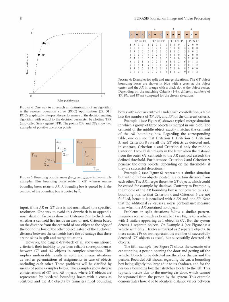
8 EURASIP Journal on Image and Video Processing
10
False positive rate
1
Tru
ep
osit
ive
rate OP1
OP2
Figure 4: One way to approach an optimization of an algorithmis the receiver operation curve (ROC) optimization [28, 31].ROCs graphically interpret the performance of the decision makingalgorithm with regard to the decision parameter by plotting TPR(also called Sens) against FPR. The points OP1 and OP2 show twoexamples of possible operation points.
−→b GT
−→b AR −→
d AR, GT
−→d GT, AR
−→x AR
−→x GT
−→b AR
−→x AR
−→x GT
−→b GT
Figure 5: Bounding box distances→dGT,AR and
→dAR,GT in two simple
examples. Blue bounding boxes relate to GT, whereas orange
bounding boxes relate to AR. A bounding box is quoted by→b, the
centroid of the bounding box is quoted by→x.
input, if the AR or GT data is not normalized to a specifiedresolution. One way to avoid this drawback is to append anormalization factor as shown in Criterion 2 or to check onlywhether a centroid lies inside an area or not. Criteria basedon the distance from the centroid of one object to the edge ofthe bounding box of the other object instead of the Euclideandistance between the centroids have the advantage that thereare no skips in split and merge situations.
However, the biggest drawback of all above-mentionedcriteria is their inability to perform reliable correspondencesbetween GT and AR objects in complex situations. Thisimplies undesirable results in split and merge situationsas well as permutations of assignments in case of objectsoccluding each other. These problems will be clarified bymeans of some examples below. The examples show diverseconstellations of GT and AR objects, where GT objects arerepresented by bordered bounding boxes with a cross ascentroid and the AR objects by frameless filled bounding
1
34
6
2
5
789
0
00
1
0
0
100
0
02
2
2
0
202
3
31
1
1
3
131
1
34
6
2
5
789
0
01
1
1
0
101
0
02
2
2
0
202
2
30
0
0
3
030
1
34
6
2
5
789
0
20
2
0
0
202
0
00
0
0
0
000
3
13
1
3
3
131
1
34
6
2
5
789
0
20
2
0
0
202
0
00
1
0
0
101
2
02
0
2
2
020
1 2 3 4
TP FN FP TP FN FP TP FN FP TP FN FP
Figure 6: Examples for split and merge situations. The GT objectbounding boxes are shown in blue with a cross at the objectcenter and the AR in orange with a black dot at the object center.Depending on the matching Criteria (1–9), different numbers ofTP, FN, and FP are computed for the chosen situations.
boxes with a dot as centroid. Under each constellation, a tablelists the numbers of TP, FN, and FP for the different criteria.
Example 1 (see Figure 6) shows a typical merge situationin which a group of three objects is merged in one blob. Thecentroid of the middle object exactly matches the centroidof the AR bounding box. Regarding the correspondingtable, one can see that Criterion 1, Criterion 3, Criterion5, and Criterion 8 rate all the GT objects as detected and,in contrast, Criterion 4 and Criterion 6 only the middle.Criterion 1 would also results in the latter when the distancefrom the outer GT centroids to the AR centroid exceeds thedefined threshold. Furthermore, Criterion 7 and Criterion 9penalize the outer objects, depending on the thresholds, ifthey are successful detections.
Example 2 (see Figure 6) represents a similar situationbut with only two objects located in a certain distance fromeach other. The AR merges these two GT objects, which couldbe caused for example by shadows. Contrary to Example 1,the middle of the AR bounding box is not covered by a GTbounding box, so that Criterion 4 and Criterion 6 are notfulfilled, hence it is penalized with 2 FN and one FP. Notethat the additional FP causes a worse performance measurethan when the AR contained no object.
Problems in split situations follow a similar pattern.Imagine a scenario such as Example 3 (see Figure 6): a vehiclewith 2 trailers appearing as 1 object in GT. But the systemdetects 3 separate objects. Or Example 4 (see Figure 6): avehicle with only 1 trailer is marked as 2 separate objects. Inthese cases, TPs do not represent the number of successfullydetected GT objects as usual, but successfully detected ARobjects.
The fifth example (see Figure 7) shows the scenario of acar stopping, a person opening the door and getting off thevehicle. Objects to be detected are therefore the car and theperson. Recorded AR shows, regarding the car, a boundingbox being slightly too large (due to its shadow), and for theperson a bounding box that stretches too far to the left. Thistypically occurs due to the moving car door, which cannotbe separated from the person by the system. This exampledemonstrates how, due to identical distance values between

Axel Baumann et al. 9
Figure 7: Example 5: person getting out of a car. The positions ofthe object centroids lead to assignment errors as the AR personscentroid is closer to the centroid of the car in the GT and vice versa.The GT object bounding boxes are shown in blue with a cross at theobject center and the AR in orange with a black dot at the objectcenter.
GT-AR object combinations, the described methods lack adecisive factor or even result in misleading distance values.The latter is the case, for example, Criterion 1 and Criterion2, because the AR centroid of the car is closer to the centroidof the GT person, rather than the GT car, and vice versa.
Criterion 3 and Criterion 5 are particularly unsuitable,because there is no way to distinguish between a comparablyharmless merge and cases where the detector identifies largesections of the frame as one object due to global illuminationchanges. Criterion 4 and Criterion 6 are rather generouswhen the AR object covers only fractions of the GT object.This is because a GT object is rated to be detected as soon asa smaller AR object (according to the size of the GT object)covers it.
Figure 8 illustrates the drawback of Criterion 7, Criterion8, and Criterion 9. This is due to the fact that for thehuman eye quality wise different detection results cannot bedistinguished by the given criteria. This leads to problemsespecially when multiple objects are located very close toeach other and distances of possible GT/AR combinationsare identical. Figure 8 shows five different patterns of oneGT and one AR object as well as the distance values forthe three chosen criteria. In the table in Figure 8, it can beseen that only Criterion 9 allows a distinct discriminationbetween configuration 1 and the other four. Furthermore,it can be seen that using Criterion 7, configuration 2 gets aworse distance value than configuration 3. Aside these twocases, the mentioned criteria are incapable of distinguishingbetween the five paradigmatic structures.
The above-mentioned considerations demonstrate thecapability of the centroid-based criteria to represent simpleand quick ways of assigning GT and AR objects to eachother in test sequences with discrete objects. However, incomplex problems such as occlusions or split and merge,their assignments are rather random. Thus, the content ofthe test sequence influences the quality of the evaluationresults. While replacing object assignments has no effect onthe detection performance measures, it impacts strongly onthe tracking measures, which are based on these assignments,to.
1 2
3 4
5
Criterion 1 2 3 4 57 0 d72 0 ≈ 0 ≈ 08 0 0 0 ≈ 0 ≈ 09 0 d92 d93 ≈ d92 d94 ≈ d93 d95 ≈ d94
Figure 8: Drawbacks of matching Criterion 7 to Criterion 9. Fivedifferent configurations are shown to demonstrate the behavior ofthese criteria. The GT object bounding boxes are shown in bluewith a cross at the object center and the AR in orange with ablack dot at the object center. The distances dcrit,conf of possible GT-AR combinations as computed by the Criterion 7 to Criterion 9are either zero or identical to the distances of the other examplesthrough these distances are visually different.
AGT
AAR⋂AGT
AAR
Figure 9: The area distance computes the overlap of the GT and ARbounding boxes.
4.2.2. Object matching based on object area overlap
A reliable method to determine object assignments isprovided by area distance calculation based on overlappingbounding box areas (see Figure 9).
Frame detection accuracy (FDA) [32]
Computes the ratio of the spatial intersection between twoobjects and their spatial union for one single frame:
FDA = overlap(GT, AR)(1/2)
(#GTo + #ARo
) , (17)
where again #GTo is the number of GT objects for a givenframe (#ARo accordingly). The overlap ratio is given by
overlap(GT, AR) =#(ARo→GTo)∑
l=1
∣∣AGT(l)∩ AAR(l)∣∣
∣∣AGT(l)∪ AAR(l)∣∣ . (18)
Here, #(ARo → GTo) is the number of mapped objects inframe t, by mapping objects according to their best spatialoverlap (which is a symmetric criterion and thus #(ARo →GTo) = #(GTo → ARo)), AGT is the ground truth objectarea and AAR is the detected object area by an algorithmrespectively.
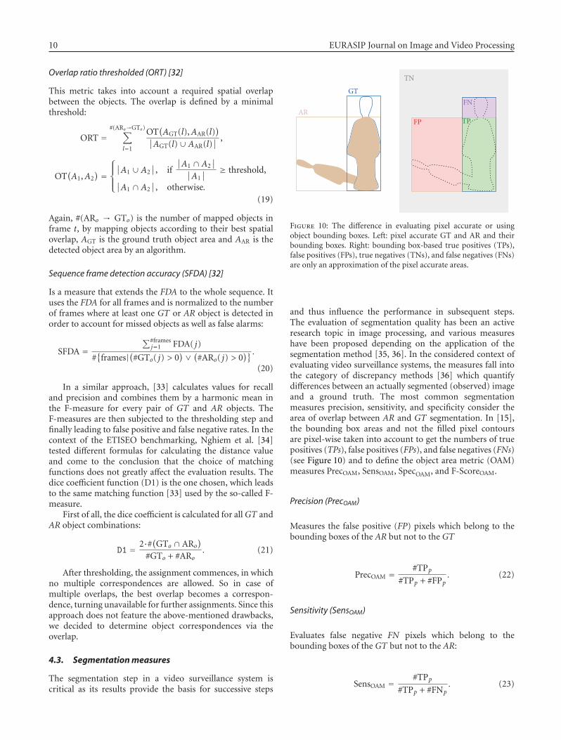
10 EURASIP Journal on Image and Video Processing
Overlap ratio thresholded (ORT) [32]
This metric takes into account a required spatial overlapbetween the objects. The overlap is defined by a minimalthreshold:
ORT =#(ARo→GTo)∑
l=1
OT(AGT(l),AAR(l)
)∣∣AGT(l)∪ AAR(l)
∣∣ ,
OT(A1,A2
) =⎧⎪⎨⎪⎩
∣∣A1 ∪ A2∣∣, if
∣∣A1 ∩ A2∣∣
∣∣A1∣∣ ≥ threshold,
∣∣A1 ∩ A2∣∣, otherwise.
(19)
Again, #(ARo → GTo) is the number of mapped objects inframe t, by mapping objects according to their best spatialoverlap, AGT is the ground truth object area and AAR is thedetected object area by an algorithm.
Sequence frame detection accuracy (SFDA) [32]
Is a measure that extends the FDA to the whole sequence. Ituses the FDA for all frames and is normalized to the numberof frames where at least one GT or AR object is detected inorder to account for missed objects as well as false alarms:
SFDA =∑#frames
j=1 FDA( j)
#{
frames|(#GTo( j) > 0)∨ (#ARo( j) > 0
)} .(20)
In a similar approach, [33] calculates values for recalland precision and combines them by a harmonic mean inthe F-measure for every pair of GT and AR objects. TheF-measures are then subjected to the thresholding step andfinally leading to false positive and false negative rates. In thecontext of the ETISEO benchmarking, Nghiem et al. [34]tested different formulas for calculating the distance valueand come to the conclusion that the choice of matchingfunctions does not greatly affect the evaluation results. Thedice coefficient function (D1) is the one chosen, which leadsto the same matching function [33] used by the so-called F-measure.
First of all, the dice coefficient is calculated for all GT andAR object combinations:
D1 = 2·#(GTo ∩ ARo)
#GTo + #ARo. (21)
After thresholding, the assignment commences, in whichno multiple correspondences are allowed. So in case ofmultiple overlaps, the best overlap becomes a correspon-dence, turning unavailable for further assignments. Since thisapproach does not feature the above-mentioned drawbacks,we decided to determine object correspondences via theoverlap.
4.3. Segmentation measures
The segmentation step in a video surveillance system iscritical as its results provide the basis for successive steps
AR
GT
TN
FP
FN
TP
Figure 10: The difference in evaluating pixel accurate or usingobject bounding boxes. Left: pixel accurate GT and AR and theirbounding boxes. Right: bounding box-based true positives (TPs),false positives (FPs), true negatives (TNs), and false negatives (FNs)are only an approximation of the pixel accurate areas.
and thus influence the performance in subsequent steps.The evaluation of segmentation quality has been an activeresearch topic in image processing, and various measureshave been proposed depending on the application of thesegmentation method [35, 36]. In the considered context ofevaluating video surveillance systems, the measures fall intothe category of discrepancy methods [36] which quantifydifferences between an actually segmented (observed) imageand a ground truth. The most common segmentationmeasures precision, sensitivity, and specificity consider thearea of overlap between AR and GT segmentation. In [15],the bounding box areas and not the filled pixel contoursare pixel-wise taken into account to get the numbers of truepositives (TPs), false positives (FPs), and false negatives (FNs)(see Figure 10) and to define the object area metric (OAM)measures PrecOAM, SensOAM, SpecOAM, and F-ScoreOAM.
Precision (PrecOAM)
Measures the false positive (FP) pixels which belong to thebounding boxes of the AR but not to the GT
PrecOAM =#TPp
#TPp + #FPp. (22)
Sensitivity (SensOAM)
Evaluates false negative FN pixels which belong to thebounding boxes of the GT but not to the AR:
SensOAM =#TPp
#TPp + #FNp. (23)
Axel Baumann et al. 11
Specificity (SpecOAM)
Considers true negative (TN) pixels, which neither belong tothe AR nor to the GT bounding boxes:
SpecOAM =#TNp
N. (24)
N is the number of pixels in the image.
F-Score (F-ScoreOAM)
Summarizes sensitivity and precision:
F-ScoreOAM =2·Precseg·Sensseg
Precseg + Sensseg. (25)
Further measures can be generated by comparing thespatial, temporal, or spatiotemporal accuracy between theobserved and ground truth segmentation [35]. Measuresfor the spatial accuracy comprise shape fidelity, geometricalsimilarity, edge content similarity and statistical data sim-ilarity [35], negative rate metric, misclassification penaltymetric, rate of misclassification metric, and weighted qualitymeasure metric [13].
Shape fidelity
Is computed by the number of misclassified pixels of the ARobject and their distances to the border of the GT object.
Geometrical similarity [35]
Measures similarities of geometrical attributes between thesegmented objects. These include size (GSS), position (GSP),elongation (GSE), compactness (GSC), and a combination ofelongation and compactness (GSEC):
GSS=∣∣area(GT)− area(AR)∣∣,
GSP=[(gravX(∣∣area(GT)− gravX(AR)
∣∣))2
− (gravY(∣∣area(GT)− gravY (AR)
∣∣))2]1/2,
GSE(O)= area(O)(2× thickness(O)
)2 ,
GSC(O)= perimeter2(O)area(O)
,
GSEC=∣∣∣∣
GSE(GT)−GSE(AR)10
+GSC(GT)−GSC(AR)
150
∣∣∣∣,
(26)
where area represents the segmented area of the objects,gravX(O) and gravY (O)are the center coordinates of thegravity of an object O, and thickness(O)is the number ofmorphological erosion steps until an object disappears.
Edge content similarity (ECS) [35]
Yields a similarity based on edge content
ECS = avg(|Sobel(GT− AR)|) (27)
with avg as average value and Sobel the result of edgedetection by a Sobel filter.
Statistical data similarity [35]
Measures distinct statistical properties using brightness andredness (SDS)
SDS = 34× 255
∣∣avgY(GT)− avgY(AR)∣∣
+∣∣avgV(GT)− avgV(AR)
∣∣.(28)
Here, avgY and avgV are average values calculated in theYUV color model.
Negative rate (NR) metric [13]
Measures a false negative rate NRFN and false positive rateNRFP between matches of ground truth GT and result AR ona pixel-wise basis. The negative rate metric uses the numberof false negative #FNp and false positive pixels #FPp and isdefined via the arithmetic mean in contrast to the harmonicmean used in the F-Scoreseg:
NR = 12
(NRFN + NRFP
),
NRFN =#FNp
#TPp + #FNp,
NRFP =#FPp
#TNp + #FPp.
(29)
Misclassification penalty metric (MPM) [13]
Values misclassified pixels by their distances from the GTobject border
MPM = 12
(MPMFN + MPMFP
),
MPMFN = 1D
#FNp∑
k=1
dFN(k),
MPMFP = 1D
#FPp∑
k=1
dFP(k),
(30)
where dFN/FP(k) is the distance of the kth false negative/falsepositive pixel from the GT object border, and D is anormalization factor computed from the sum over alldistances between FP and FN pixels and the object border.
Rate of misclassification metric (RMM) [13]
Describes the false segmented pixels by the distance to theborder of the object in pixel units
RMM = 12
(RMMFN + RMMFP
),
RMMFN = 1#FNp
#FNp∑
k=1
dFN(k)Ddiag
,
RMMFP = 1#FPp
#FPp∑
k=1
dFP(k)Ddiag
,
(31)
where Ddiag is the diagonal distance of the considered frame.

12 EURASIP Journal on Image and Video Processing
Weighted quality measure metric (WQM) [13]
Evaluates the spatial difference between GT and AR by thesum of weighted effects of false positive and false negativesegmented pixels
WQM = ln(
12
(WQMFN + WQMFP
)),
WQMFN = 1#FNp
#FNp∑
k=1
wFN(dFN(k)
)dFN(k),
WQMFP = 1#FPp
#FPp∑
k=1
wFP(dFP(k)
)dFP(k),
wFP(dFP
) = B1 +B2
dFP + B3, wFN
(dFN
) = C·dFN.
(32)
The constants were proposed as B1 = 19, B2 = 178.125, B3 =9.375, and C = 2 [13].
Temporal accuracy takes video sequences into con-sideration and assesses the motion of segmented objects.Temporal and spatiotemporal measures are often used invideo surveillance, for example, misclassification penalty,shape penalty, and motion penalty [17].
Misclassification penalty (MPpix) [17]
Penalizes the misclassified pixels that are farther from the GTmore heavily:
MPpix =∑
x,y I(x, y, t)cham(x, y, t)∑x,y cham(x, y, t)
, (33)
where I(x, y, t) is an indicator function with value 1 if ARand GT are different, and cham denotes the chamfer distancetransform of the boundary of GT.
Shape penalty (MPshape) [17]
Considers the turning angle function of the segmentedboundaries:
MPshape =∑K
k=1
∣∣ΘtGT(k)−Θt
AR(k)∣∣
2πK, (34)
and ΘtGT(k), Θt
AR(k) denote the turning angle function ofthe GT and AR, and K is the total number of points in theturning angle function.
Motion penalty (MPmot) [17]
Uses the motion vectors→v (t) of GT and AR objects
MPmot =∥∥→vGT(t)− →
vAR(t)∥∥
∥∥→vGT(t)∥∥ +
∥∥→vAR(t)∥∥ . (35)
Nghiem et al. [16, 34] propose further segmentationmeasures adapted to the video surveillance application.These measures take into account how well a segmentationmethod performs in special cases such as appearance of
shadows (shadow contrast levels) and handling of split andmerge situations (split metric and merge metric).
4.3.1. Chosen segmentation measure subset
Due to the enormous costs and expenditure of time to gener-ate pixel-accurate segmentation ground truth, we decided tobe content with an approximation of the real segmentationdata. This approximation is given by the already labeledbounding boxes and enables us to apply our segmentationmetric to a huge number of sequences, which makes it easierto get more representative results. The metrics we chose isequal to the above mentioned object area metric proposed in[15]:
(i) PrecOAM (22),
(ii) SensOAM (23),
(iii) F-ScoreOAM (25).
The benefit of this metric is its independence fromassignments between GT and AR objects as described inSection 4.2. Limitations are given by inexactness due tothe discrepancy between the areas of the objects and theirbounding boxes as well as the inability to take into accountthe areas of occluded objects.
4.4. Object detection measures
In order to get meaningful values that represent the ability ofthe system to fulfill the object detection tasks, the numbersof correctly detected, falsely detected, or misdetected objectsare merged into appropriate formulas to calculate detectionmeasures like detection rates or precision and sensitivity.Proposals for object detection metrics mostly concur in theiruse of formulas, however the definition of a good detectionof an object differs.
4.4.1. Object-counting approach
The simplest way to calculate detection measures is tocompare the AR objects to the GT object according only totheir presence whilst disregarding their position and size.
Configuration distance (CD) [33]
Smith et al. [33] present the configuration distance, whichmeasures the difference between the number of GT and ARobjects and is normalized by the instantaneous number ofGT objects in the given frame
CD = #ARo − #GTo
max(#GTo, 1
) , (36)
where #ARo is the number of AR objects and #GTo thenumber of GT objects in the current frame. The result iszero if #GTo = #ARo, negative when #GTo > #ARo, andpositive when #GTo < #ARo, which gives an indication ofthe direction of the failure.

Axel Baumann et al. 13
Number of objects [15]
The collection of the metrics evaluated by [15] contains ametric only concerning the number of objects, consisting ofa precision and a sensitivity value
PrecNO = min(#ARo, #GTo
)
#ARo,
SensNO = min(#ARo, #GTo
)
#GTo.
(37)
The global values are computed by averaging the frame-wisevalues taking into account only frames containing at least oneobject. Further information about averaging can be found inSection 4.11.
The drawback of the approaches based only on countingobjects is that multiple failures could compensate andresult in an apparently perfect values for these measures.Due to the limited significance of measures based only onobject counts, most approaches for detection performanceevaluation contain metrics taking into account the matchingof GT and AR objects.
4.4.2. Object-matching approach
Object matching based on centroids as well as on the objectarea overlap is described in detail in Section 4.2. Though thematching based on object centroids is a quick and easy wayto assign GT and AR objects, it does not provide reliableassignments in complex situations (Section 4.2.1). Since thematching based on the object area overlap does not featurethese drawbacks (Section 4.2.2), we decided to determineobject correspondences via the overlap and to add this metricto our environment. After the assignment step, precision andsensitivity are calculated according to ETISEO metric M1.2.1[15]. This corresponds to the following measures which weadded to our environment:
Precdet = #TPo#TPo + #FPo
, (38)
Sensdet = #TPo#TPo + #FNo
, (39)
F-Scoredet = 2·Precdet·Sensdet
Precdet + Sensdet. (40)
The averaged metrics for a sequence are computed asthe sum of the values per frame divided by the numberof frames containing at least one GT object. Identical tothe segmentation measure, we use the harmonic mean ofprecision and sensitivity for evaluating the balance betweenthese aspects.
The fact that only one-to-one correspondences areallowed results in the deterioration of this metric in mergesituations. Thus, it can be used to test the capabilities of thesystem to separately detect single objects, which is of majorimportance in cases of groups of objects or occlusions.
The property mentioned above makes this metric onlypartly appropriate to evaluate the detection capabilities ofa system independently from the real number of objects
DetOvl Det
TP FN FP TP FN FP
TP FN FP TP FN FP
TP FN FP TP FN FP
TP FN FP TP FN FP
2 0 0 1 1 0
2 1 0 1 2 0
2 0 0 1 0 1
2 0 1 1 0 2
TPFNFP
Figure 11: Comparison of strict and lenient detection measures.
in segmented blobs. In test sequences where single personsare merged into groups, for example, this metric gives theillusion that something was missed, though there was just noseparation of groups of persons into single objects.
In addition to the strict metric, we use a lenient metricallowing multiple assignments and being content with aminimal overlap. Calculation proceeds in the same manneras for the strict metric, except that due to the modifiedmethod of assignment, the deviating definitions of TP, FP,and FN result in these new measures.
(i) PrecdetOvl,
(ii) SensdetOvl,
(iii) F-ScoredetOvl.
Figure 11 exemplifies the difference between the strictand the lenient metric applied to two combinations for thesplit and the merge case. The effects of the strict assignmentcan be seen in the second column where each object isassigned to only one corresponding object, and all the othersare treated as false detections, although they have passed thedistance criterion. The consequences in the merge case aremore FNs and in the split case more FPs.
There are metrics directly addressing the split and mergebehavior of the algorithm. In the split case, the number of ARobjects which can be assigned to a GT object is counted and

14 EURASIP Journal on Image and Video Processing
in the case of a merge, it is determined how many GT objectscorrespond to an AR object. This is in accordance with theETISEO metrics M2.2.1 and M2.3.1 [15]. The definition ofthe ETISEO metric M2.2.1 is
Split = 1#GT f
·∑
GT f
(1
#GTo
#GTo∑
l=1
1#(ARo −→ GTo(l)
))
, (41)
where #(ARo → GTo(l)) is the number of AR objects forwhich the matching criteria allow an assignment to thecorresponding GT objects and #GT f is the number of frameswhich contain at least one GT object. For every frame, theaverage inverse over all GT objects is computed. The valuefor the whole sequence is then determined by summing thevalues of every frame and dividing by the number of framesin which at least one GT object occurs.
For this measure, the way of assigning the objects is ofparamount importance. When objects fragment into severalsmaller objects, the single fragments often do not meet thematching criteria used for the detection measures. Therefore,a matching criterion that allows to assign AR objects whichare much smaller then the corresponding GT objects needsto be used. For the ETISEO benchmarking [6], the distancemeasure D5-overlapping [15] was used as it satisfies thisrequirement.
Another problem is that in the case of complex sceneswith occlusions, fragments of one AR object should notbe assigned to several GT objects simultaneously as thiswould falsely worsen the value of this measure. Each ARobject which represents a fragment should only be allowedto be counted once. Therefore, the following split measure isintegrated in the presented ATE:
Split resistance (SR)
SR = 1#GTo
·#GTo∑
l=1
11 + #add. split fragments (l)
,
SRAvM = 1#GT f
·∑
GT f
SR.
(42)
The assignment criteria used here are constructed to allowminimal overlaps to lead to an assignment, thus avoiding theoverlooking of fragments.
The corresponding metric for the merge case presentedby ETISEO M2.3.1 [15] is
Merge = 1#GT f
·∑
GT f
(1
#ARo
#ARo∑
l=1
1#(GTo −→ ARo(l)
))
, (43)
where #(GTo → ARo(l)) is the number of GT objects whichcan be assigned to the corresponding AR objects due to thematching criterion used.
For the merge case, the same problems concerning theassignment must be addressed as for the split case. Thus, theproposed metric for the merge case is
Merge resistance (MR)
MR = 1#ARo
#ARo∑
l=0
11 + #add.merged objects (l)
,
MRAvM = 1#AR f
∑
AR f
MR.
(44)
The classification if there is a split or merge situationcan also be achieved by storing matches between GT and ARobjects in a matrix and then analyzing its elements and sumsover columns and rows [37]. A similar approach is describedby Smith et al. [33], which use configuration maps contain-ing the associations between GT and AR objects to identifyand count configuration errors like false positives, falsenegatives, merging and splitting. An association between aGT and an AR object is given if they pass the coverage test,that is, the matching value exceeds the applied threshold.To infer FPs and merging, a configuration map from theperspective of the ARs is inspected, and FNs and splitting areidentified by a configuration map from the perspective of theGTs. Multiple entries indicate merging, respectively, splittingand blank entries indicate FPs, respectively, FNs.
4.4.3. Chosen object detection measure subset
To summarize the section above, these are the objectdetection measures used in our ATE.
(i) Detection performance (strict assignment):
(a) Precdet (38),
(b) Sensdet (39),
(c) F-Scoredet (40).
(ii) Detection performance (lenient assignment):
(a) PrecdetOvl,
(b) SensdetOvl,
(c) F-ScoredetOvl.
(iii) Merge resistance:
(a) MR (44).
(iv) Split resistance:
(a) SR (42).
In addition, we use a normalized measure for the rate ofcorrectly detected alarm situations, where an alarm situationis a frame containing at least one object of interest.
Alarm correctness rate (ACR)
The number of correctly detected alarm and nonalarmsituations in relation to the number of frames:
ACR = #TP f + #TN f
#frames. (45)
Axel Baumann et al. 15
4.5. Object localization measures
The metrics above give insight into the system’s capability ofdetecting objects. However, they do not provide informationof how precisely objects have been detected. In other words,how precisely region and position of the assigned AR matchthe GT bounding boxes.
This requires certain metrics expressing the precisionnumerically. The distance of the centroids discussed inSection 4.2.1 is one possibility, which requires normalizationto keep the desired range of values. The problem lies inthis very fact, since finding a normalization which doesnot deteriorating the metric’s relevance is difficult. Thefollowing section introduces our experiment and finallyexplains why we are not completely satisfied with its results.In order to make 0 the worst, and 1 the best value,we have to transform the Euclidean distance used in thedistance definitions of the object centroid matching into amatching measure by subtracting the normalized distancefrom 1. Normalization commences along the larger of thetwo bounding box’s diagonals. This results in the followingobject localization measure definitions for each pair ofobjects:
Relative object centroid distance (ROCD)
ROCD =√(xGT − xAR
)2+(yGT − yAR
)2
max(dGT,dAR
) , (46)
Relative object centroid match (ROCM)
ROCM = 1− ROCD. (47)
In theory, the worst value 0 is reached as soon as thecentroid’s distance equals or exceeds the larger boundingbox’s diagonal. In fact, this case will not come about, sincethese AR/GT combinations of the above-described matchingcriteria are not meant to occur in the first place. Theirbounding boxes do not overlap anymore here. Unfortunately,this generous normalization results in merely exploiting onlythe upper possible range of values, and in only a minordeviation between the best and worst value for this metric.In addition, significant changes in detection precision arerepresented only by moderate changes of the measure.Another drawback is at hand. When an algorithm tends tooversegment objects, it will have a positive impact on thevalue of ROCM, lowering its relevance.
A similar problem occurs when introducing a metricfor evaluating the size of AR bounding boxes. One wayto resolve this would be to normalize the absolute regiondifference [14], another would be using a ratio of AR andGT bounding boxes’ regions. We added the metric relativeobject area match (ROAM) to our ATE, which represents thediscrepancy of the sizes of AR and GT bounding boxes. Theratio is computed by dividing the smaller by the larger size,in order to not exceed the given range of value, that is,
Relative object area match (ROAM)
ROAM = min(AGT,AAR)max(AGT,AAR)
. (48)
Information about the AR bounding boxes being toolarge or too small compared to the GT bounding boxes islost in the process.
Still missing is a metric representing the precision ofthe detected objects. Possible metrics were presented withPrecOAM, SensOAM, and F-ScoreOAM in Section 4.3. Instead ofglobally using this metric, we apply them to certain pairs ofGT and AR objects (in parallel to [33]) measuring the objectarea coverage. For each pair, this results in values for PrecOAC,SensOAC, and F-ScoreOAC. As mentioned above, F-ScoreOAC isidentical to the computed dice coefficient (21).
The provided equations of the three different metrics thatevaluate the matching of GT and AR bounding boxes relateto one pair in each case. In order to have one value for eachframe, the values, resulting in the object correspondences,are averaged. The global value for a whole sequence is theaverage value over all frames featuring at least one objectcorrespondence.
Unfortunately, averaging raises dependencies to thedetection rate, which can lead to distortion of results whencomparing different algorithms. The problem lies in the factthat only values of existing assignments have an impacton the average value. If a system is parameterized to beinsensitive, it will detect only very few objects but theseprecisely. Such a system will achieve much better results thana system detecting all GT objects but not matching themprecisely.
Consequently, these metrics should not be evaluatedseparately, but always together with the detection measures.The more the values of the detection measures differ, themore questionable the values of the localization measuresbecome.
4.5.1. Chosen object localization measure subset
Here is a summarization of the object localization measureschosen by us:
(i) relative object centroid match:
(a) ROCM (47),
(ii) relative object area match:
(a) ROAM (48),
(iii) object area coverage:
(a) PrecOAC,
(b) SensOAC,
(c) F-ScoreOAC.
4.6. Tracking measures
Tracking measures apply over the lifetime of single objects,which are called tracks. In contrast to detection measures,
16 EURASIP Journal on Image and Video Processing
which evaluate the detection rate of anonymous objects forevery single frame, tracking measures compute the abilityof a system to track objects over time. The discriminationbetween different objects is usually done via an unique IDfor every object. The tracking measures for one sequence arethus not computed via an averaging of frame-based values,but rather by using averaging over the frame-wise valuesof the single tracks. The first step consists therefore of theassignment of AR to GT tracks. Two different approaches canbe found for this task.
4.6.1. Track assignment based on trajectory matching
Senior et al. [10] match the trajectories. For this purpose,they compute for every AR and GT track combination adistance value which is defined as follows:
DAR,GT(i1, i2
) = 1NAR,GT
(i1, i2
)
×∑
j
(∣∣→xAR(i1, j
)− →xGT
(i2, j
)∣∣2
+∣∣→vAR
(i1, j)− →
vGT(i2, j
)∣∣2
+∣∣→sAR
(i1, j
)− →sGT
(i2, j
)∣∣2)1/2
,
(49)
where NAR,GT(i1, i2) is the number of points in both tracks
ARtr(i1) and GTtr(i2),→xAR(i1, j) or
→xGT(i2, j) is the centroid
of the bounding box of an AR or GT track at frame
j,→vAR(i1, j) or
→vGT(i2, j) is the velocity and
→sAR(i1, j) or
→sGT(i2, j) is the vector of width and height of track i1 or i2at frame j.
This way of comparing trajectories, which takes theposition, the velocities, and the objects’ bounding boxesinto account, is also used in a reduced version of (49) in[11, 14, 30] considering only the position of the object:
DAR,GT(i1, i2
) = 1NAR,GT
(i1, i2
)∑
j
∣∣→xAR(i1, j
)− →xGT
(i2, j
)∣∣.
(50)
The calculation of the distance matrix according to (50) isincluded in Figure 12 and marked as Step 2. Step 1 representsthe analysis of temporal correspondence and hence thecalculation of the number of overlapping frames. In orderto actually establish the correspondence between AR and GTtracks, a thresholding step (Step 3 in Figure 12) has to beapplied. The resulting track correspondence is represented bya binary mask, which is simply calculated by assigning a oneto those matrix elements which exceed a given threshold andzero in the alternative case.
Track correspondence is established by thresholding thismatrix. Each track in the ground truth can be assigned toone or more tracks from the results. This accommodatesfragmented tracks. Once the correspondence between theground truth and the result tracks is established, the follow-ing error measures are computed between the correspondingtracks:
False positive track error rate (TERFP)
TERFP = #ARtr − #(ARtr −→ GTtr
)
#GTtr, (51)
False negative track error rate (TERFN)
TERFN = #ARtr − #(GTtr −→ ARtr
)
#GTtr. (52)
Object detection lag
This is the time difference between the ground truthidentifying a new object and the tracking algorithm detectingit. Time-shifts between tracks and an evaluation of (spatio-)temporally separated GT and AR tracks using statistics arediscussed in more detail by [38].
If an AR track is assigned to a GT track, metrics areneeded to assess the quality of the representation by the ARtrack. One criterion for that is the temporal overlap, respec-tively, the temporal incongruity as rated in the followingmetric.
Track incompleteness factor (TIF)
TIF = #FN f (i) + #FP f (i)
#TP f (i), (53)
where FN f (i) is the false negative frame count, that is, thenumber of frames that are missing from the AR Track, FP f (i)is the false positive frame count, that is, the number of framesthat are reported in the AR which are not present in the GT,and TP f (i) is the number of frames present in both AR andGT.
Once not only the presence but also the the correspon-dence between the ground truth and the result tracks isestablished according to the trajectory matching, the follow-ing error measures are computed between the correspondingtracks.
Track detection rate (TDR)
The track detection rate indicates the tracking completenessof a specific ground truth track. The measure is calculated asfollows
TDR = #TP f (i)
#frames GTtr(i), (54)
where #frames GTtr(i) is the number of the frames of the ithGT track. In [11], #TP f (i) is defined as the number of framesof the ith GT track that correspond to an AR track.
Tracker detection rate (TRDR)
This measure characterizes the tracking performance of theobject tracking algorithm. It is basically similar to the TDRmeasure, but considers entities larger than just single tracks
TRDR =∑
i #TP f (i)∑i #frames GTtr(i)
, (55)

Axel Baumann et al. 17
Ground truth (GT)tracks Result tracks
Checking for temporalcorrespondence and calculation ofnumber of overlapping frames
Calculation of distance d for eachtemporal corresponding result track /
GT track combination
Calculation of a threshold matrixmask (threshold depending on used
distance function d i j)
Measure calculation, classification oftrue positive and false negative
tracks
Statistical analysis of matrixelements (e.g. averaging)
Step 1
Step 2
Step 3
Step 4
Step 5
GT track iResult track j
Overlap o i jFrame no (time)
Result tracks
Result tracks
Result tracks
Result tracks
GT
trac
ksG
Ttr
acks
GT
trac
ksG
Ttr
acks
[o 11, o 12, . . ., o 1Nr]
[o 21, o 22, . . ., o 2Nr]
[o Ng1, . . ., o NgNr]· · ·
Ng×Nr correspondencematrix with number of
overlapping frames
[d 11 ,d 12, . . ., d 1Nr]
[d 21 ,d 22, . . ., d 2Nr]· · ·
[d Ng1, . . ., d NgNr]
Ng×Nr distance matrix
[1 0 · · · 1 1]
[0 1 · · · 1 0]
[· · · · · · · · · · · ·][0 1 · · · 1 0]
Ng×Nr binary matrix
[d 11, d 12, . . ., d 1Nr]
[d 21, d 22, . . ., d 2Nr]· · ·
[d Ng1, . . ., d NgNr]
Ng×Nr distance /measure matrix
d avg
di j = 1Oij
∑f (BB, euclD, . . .)
overlappingframes
{
Figure 12: Overview of the measure calculation procedure as applied in [14]. Step 1 represents the analysis of temporal correspondence andhence the calculation of the number of overlapping frames. The calculation of the distance matrix according to (50) is performed in Step 2.In order to actually establish the correspondence between AR and GT tracks, a thresholding step has to be applied (Step 3). The resultingtrack correspondence is represented by a binary mask, which is simply calculated by assigning a one to those matrix elements which exceeda given threshold and zero in the alternative case. In Step 4, the actual measures are computed. Further, additional analysis is performed inStep 5.

18 EURASIP Journal on Image and Video Processing
where #frames GTtr(i) is the number of the frames of the ithGT track.
False alarm rate (FAR)
The FAR measures also the tracking performance of theobject tracking algorithm. It is defined as follows
FAR =∑
i #FP f (i)∑i #frames ARtr(i)
, (56)
where #frames ARtr(i) is the number of the frames of the ithAR track. In [11], FP f (i) is defined as one object of the ithAR track, that is tracked by the system and does not have amatching ground truth point.
Track fragmentation (TF)
Number of result tracks matched to a ground truth track
TF = 1#TPGTtr
∑
i
#(ARtr −→ GTtr(i)
). (57)
Occlusion success rate (OSR)
OSR = Number of successful dynamic occlusionsTotal number of dynamic occlusions
. (58)
Tracking success rate (TSR)
TSR = Number of non-fragmented tracked GT tracks#GTtr
.
(59)
4.6.2. Track assignment based on frame-wiseobject matching
The second approach to assign the AR to the GT tracksis to use the same frame-wise object correspondences asfor the detection measures as mentioned in Section 4.4.However, those correspondences are not always correct.Ideally, each GT track is matched by exactly one AR track,though it does not necessary hold in practice. To associateidentities properly it has been proposed that identificationassociations can be formed on a “majority rule” basis [33],where an AR track is assigned to the GT track with whichit has the maximal corresponding time, and a GT track isassigned to the AR track which corresponds to it for thelargest amount of time. Based on the definitions above, fourtracking measures are introduced. Two of them measure theidentification errors.
Falsely identified tracker (FIT)
An AR track segment which passes the coverage test for a GTtrack but is not the identifying AR track for it (see Figure 13):
FIT = 1#frames
∑
j
#FIT( j)max
(#GTtr(i)( j), 1
) . (60)
AR1
AR2
AR3 GT1
GT2
GT3
FIT
FIO
Figure 13: Example for identification errors proposed by [33].Three GT objects are tracked by three AR objects. A falsely identifiedtracker error (FIT) occurs when GT1 is tracked by a secondcorresponding AR track AR3. A falsely identified object error (FIO)occurs when an AR track swaps the corresponding GT track, herethis is the case for AR2 swapping from GT2 to GT3. The timeintervals where a FIT, respectively, FIO occur are marked.
Falsely identified object (FIO)
A GT track segment which passes the coverage test for an ARbut is not the identifying GT track (see Figure 13):
FIO = 1#frames
∑
j
#FIO( j)max
(#GTtr( j), 1
) . (61)
The other two measures are similar to TDR and FAR butmore strict, because they rate only correspondences with theidentifying track as correct.
Tracker purity (TPU)
The tracker purity indicates the degree of consistency towhich an AR track identifies a GT track
TPU = #correct frames ARtr(i)#frames ARtr(i)
, (62)
where #framesAR(i) is the number of frames of the ith ARtrack and #correct framesAR(i) the number of frames that theith AR track identifies a GT track correctly.
Object purity (OPU)
The object purity indicates the degree of consistency to whicha GT track is identified by an AR track:
OPU = #correct frames GTtr(i)#frames GTtr(i)
, (63)
where #frames GTtr(i) is the number of the frames of theith GT track and #correct frames GTtr(i) is the number offrames that the ith GT track is identified by an AR trackcorrectly.
The ETISEO metrics [15] provide tracking measureswhich are similar to the above-mentioned ones. Met-ric M3.2.1 calculates a track-based Prectrack , Senstrack,and F-Scoretrack. The Senstrack conforms to (52), becauseSenstrack = 1−TERFN, but the Prectrack differs from 1−TERFP
(51), because it refers to the number of AR tracks insteadof the number of GT tracks. Another metric in [15] is the

Axel Baumann et al. 19
“tracking time” (M3.3.1), which is the same as the OPUabove.
To assess the consistency of the object IDs, the metricspersistence (M3.4.1) and confusion (M3.5.1) are used.
Persistence (Per)
Evaluates the persistence of the ID
Per = 1#GTtr
∑
i
1#(ARtr −→ GTtr(i)
) . (64)
Confusion (Conf)
Indicates the robustness to confusion along the time
Conf = 1#(GTtr −→ ARtr
)∑
i
1#(GTtr −→ ARtr(i)
) , (65)
where #(ARtr → GTtr(i)) indicates the number of AR tracksthat correspond to the ith GT track and vice versa for#(GTtr → ARtr(i)).
4.6.3. Chosen tracking measure subset
For our evaluations, the assignment of tracks is done viaframe-based correspondences as described in Section 4.6.2.Using that strategy, we compute the following measures.
False positive track resistance (TRFP)
Assesses the ability of the system to prevent FP tracks, whichare AR tracks without any correspondence to a GT track:
TRFP = 1− #ARtr − #(ARtr −→ GTtr
)
#ARtr. (66)
Note the division by #ARtr instead of #GTtr (compare to(51)).
False negative track resistance (FNTR)
Assesses the ability of the system to prevent FN tracks, whichare GT tracks without any correspondence to an AR track
TRFN = 1− TERFN. (67)
Track coverage rate (TCR)
Measures how long an AR track has correspondences to GTtracks in relation to its lifetime
TCR = #ass. frames GTtr(i)#frames GTtr(i)
, (68)
where #frames GTtr(i) is the number of frames of the ith GTtrack and #ass. frames GTtr(i) is the number of frames thatthe ith GT track is identified by at least one AR track.
Track fragmentation resistance (TFR)
Assesses the ability to track an GT object without changingthe ID of the AR track. The more AR tracks are assigned overthe GT track’s lifetime, the worse is the value of this metric:
TFR = 1#TPGTtr
∑
i
1#(ARtr −→ GTtr(i)
)1:1
, (69)
where #(ARtr → GTtr(i))1:1 indicates the number of ARtracks that correspond to the ith GT track. If there aremultiple correspondences at the same time for one GTtrack, the best one is taken into account. GT tracks withoutcorrespondences (FNtr) are omitted.
Tracking success rate (TSR)
Analogue to (59). We also adopt the four tracking measuresfrom [33] with partially small modifications.
Tracker purity (TPU)
Is identical to (62), but with NAR as the number of ARtracks excluding FP tracks. Otherwise, the FP tracks woulddominate this measure and the changes that this measure isestablished to assess would be occluded.
Object purity (OP)
Equal to (63).To fulfill our normalization constraints, we transform the
errors FIT and FIO into resistances.
Falsely identified tracker resistance (FITR)
FITR = 1− 1#ass. framesAR,GT
∑
j
#FIT( j)max
(#GTtr( j), 1
) .
(70)
Falsely identified object resistance (FIOR)
FIOR = 1− 1#ass. framesAR,GT
∑
j
#FIO( j)max
(#GTtr( j), 1
) ,
(71)
where #ass. framesAR,GT is the number of frames containingat least one correspondence between a GT and an AR object.Using the frame count of the sequence according to thedefinition in [33] would give empty scenes an occludinginfluence on the value of this measure. #FIT( j) and #FIO( j)are the number of FIT and FIO, respectively, in frame jaccording to the definitions of (60) and (61).
4.7. Event detection measures
The most important step for event detection measures isthe matching of GT data and AR data, which can be

20 EURASIP Journal on Image and Video Processing
AR
GT
1 2 3 4
A B C D
Time
Figure 14: Time-line of events. What is the best matching betweenevents?
solved by simple thresholding. Most of the proposals inthe literature match events by using the shortest time delaybetween the events in GT and AR. In the event that thetime delay exceeds a certain threshold, matching fails. Thisis a reliable approach for simple scenarios with few events.However, considering real world scenarios, this approachdoes not return the correct match. A simple example isdepicted in Figure 14, where one match might be A-1, B-2, and C-4 and a second one might be A-1, B-2, C-3, D-4, among other possible matches. Desurmont et al. [39]propose a dynamic realignment algorithm using dynamicprogramming to compute the best match between GT andAR events. The algorithm incorporates a maximum alloweddelay between events.
The CREDS project [40] classifies correct detectioninto three categories: perfect, anticipated, and delayed. Eachevent in the GT data may be associated to a single correctdetection. Multiple overlaps in time are not covered in detail,the first occurrence is matched and the remaining eventsare treated as FP. The authors define a score function ofdelay/anticipation and a ratio between GT event duration(GTed) and AR event duration (ARed):
SCD(t, ARed, GTed) =
⎧⎪⎪⎪⎪⎪⎪⎪⎨⎪⎪⎪⎪⎪⎪⎪⎩
0, (t < B)∨ (t > D),S
A− B (t − B), B ≤ t ≤ A,
S, A ≤ t ≤ 0,S
D(D − t), 0 ≤ t ≤ D.
(72)
S represents the maximum score associated with a correctdetection. The authors compute it as follow:
S =
⎧⎪⎪⎪⎨⎪⎪⎪⎩
50∗[
2−(
1− ARed
GTed
)2]
, 0 ≤ ARed
GTed≤ 2,
50,ARed
GTed> 2.
(73)
The maximum tolerated delay is expressed by D inmilliseconds, whereas A represents the accepted anticipationin milliseconds. B stands for the maximum tolerated antici-pation in milliseconds. The valuesD,A, and B are dependenton the event type (warning event, alarm event, or criticalevent).
The ETISEO [15] project defined a set of metrics forevents to. Measures for correctly detected events over thewhole sequence are defined. In the first set of event detectionmeasures M5.1.1, only whether events occurred is comparedand not their time of occurrence nor object association. Timeconstraints are added to M5.1.1 in the second measure setM5.1.2. A last set of measures M5.3.1 is defined which facil-itates correct detection in time and parameters. Parameters
are object classes, so called contextual zones (areas such as astreet, a bus stop) and involved physical objects. For instance,an event “car parked in forbidden zone” has to be raisedonce a physical object, which has been classified as car, isidle for longer than a defined time interval in a contextualzone which is marked as “no parking area.” The formulas formeasures M5.1.1, M5.1.2, and M5.3.1 are defined identically,only the matching criteria are different. Precevent, Sensevent,and F-Scoreevent are used by ETISEO [15]:
Precevent = #TPe#TPe + #FPe
,
Sensevent = #TPe#TPe + #FNe
,
F-Scoreevent = 2·Precevent·Sensevent
Precevent + Sensevent.
(74)
TP relates to a match between GT and AR.
4.7.1. Chosen event detection measure subset
We choose M5.1.2 defined in [15] with the dice coefficient(21) for the matching of the time intervals as event detectionmetric:
(i) Precevent TI,
(ii) Sensevent TI,
(iii) F-Scoreevent TI.
4.8. Object classification measures
Senior et al. [10] propose the measure Object type error whichsimply counts the number of tracks with incorrect classifi-cation. The definition is somewhat vague as it is unknownif a track has to be classified more than fifty percent of thetime correctly to be treated as correctly classified. ETISEO[15] uses different measures classes. A simple class (M4.1.1)uses the number of correctly classified physical objects ofinterest in each frame. The second measure class (M4.1.2)matches, in addition to M4.1.1, the bounding boxes ofthe objects. ETISEO distinguishes between misclassificationscaused by classification shortcomings and misclassificationscaused either in the object detection or the classification step:
Precclass = #TPc#TPc + #FPc
, (75)
Sensclass = #TPc#TPc + #FNc
, (76)
Sensclass,det = #TPc#TPc + #FNc,det
, (77)
F-Scoreclass = 2·Precclass·Sensclass
Precclass + Sensclass, (78)
F-Scoreclass,det = 2·Precclass·Sensclass,det
Precclass + Sensclass,det. (79)
Axel Baumann et al. 21
#TPc refers to the number of objects types classifiedcorrectly. #FNc is the number of false negatives caused byclassification shortcomings, for example, unknown class,#FNc,det refers to the number of false negatives, caused byobject detection errors or by classification shortcomings.
In M4.1.3, the measures in M4.1.2 are enhanced by theID persistence criteria. Precclass, Sensclass, and F-Scoreclass
are computed and used as measure. Due to the separationbetween misclassifications, two Sensclass and F-Scoreclass
measures are defined in each measure class. The measuresin M4.1.1 through M4.1.3 are computed at frame level.Percentages for a complete sequence are computed as follows.The sum of percentages per image divided by the number ofimages containing at least one GT object.
Precclass, Sensclass, and F-Scoreclass are computed perobject type in M4.2.1. Therefore, the number of measuresequals the number of existing object types. The timepercentage of good classification is computed in M4.3.1:
∣∣GTd ∩ ARd, Type(ARd
) = Type(GTd
)∣∣∣∣GTd ∩ ARd
∣∣ . (80)
GTd relates to the time interval in GT data, whereas ARd
relates to the time interval in AR data. Nghiem et al. [34]suggest to use M4.1.2.
4.8.1. Chosen classification measure subset
Class correctness rate (CCR)
Assesses the percentage of correctly classified objects. There-fore, the types of the objects, which are assigned to eachother by the assignment step described in context of thedetection measures, are compared and the correct and falseclassifications are counted:
CCR = 1#ass. framesAR,GT
∑
j
#CC( j)#CC( j) + #FC( j)
, (81)
where #CC( j) and #FC( j) are the number of correctly,respectively, falsely classified objects in frame j, and#ass. framesAR,GT is the number of frames containing at leastone correspondence between GT and AR objects.
We also use a metric according to ETISEO’s M4.2.1,which consists of two different specifications. The firstconsiders only the classification shortcomings and the otherincludes the shortcomings of the detection to. With the firstspecification, we agree, leading to the definition in (75), (76),and (78).
Object classification performance by type
(i) Precclass (75),
(ii) Sensclass (76),
(iii) F-Scoreclass (78).
In the second specification, we differ from ETISEObecause we also take FP objects into account.
Object detection and classification performance by type
Precclass,det = #TPc#TPc + #FPc,det
,
Sensclass,det = #TPc#TPc + #FNc,det
,
F-Scoreclass,det = 2·Precclass·Sensclass,det
Precclass + Sensclass,det,
(82)
where, in contrast to (75), FPc,det is used as the number offalse positives caused by shortcomings in the detection orclassification steps.
4.9. 3D object localization measures
3D object localization measures are defined in [15]. Theaverage, variance, minimum, and maximum of distancesbetween objects in AR as well as the trajectories of the objectsin GT are computed. Object gravity centers are used tocalculate the distances.
Average of object gravity center distance (AGCD) [15]
Measures the average of the distance between gravity centersin AR and GT:
di =∥∥TOCGT(i)− TOCAR(i)
∥∥2, AGCD = 1
N
N∑
i
di,
(83)
where TOC(i) is the trajectory of the object’s center of gravityat time i and N is the amount of elements.
Variance of object gravity center distance (VGCD) [15]
Computes the variance of the distance between gravitycenters in AR and GT:
VGCD = 1N
N∑
i
(di − AGCD
)2. (84)
Minimum and maximum distance of object gravity centers(MIND, MAXD) [15]
Considers the minimum distance between centers of gravityin AR and GT:
MIND = inf{d ∈ D}, MAXD = sup{d ∈ D}, (85)
where D is the set of all di. Nghiem et al. [34] state thatdetection errors on the outline are not taken into accountin [15]. Moreover there is no consensus on how to computethe 3D gravity center of certain objects, like cars.
Note that when evaluating 3D information inferred from2D data, the effects of calibration have to be taken intoaccount. If both AR and GT are generated from 2D data andprojected into 3D, the calibration error will be systematic.

22 EURASIP Journal on Image and Video Processing
If the GT is obtained in 3D, for example, using a differentialglobal positioning system (DGPS), and the AR still generatedfrom 2D images, then the effects of calibration errors have tobe taken into account.
4.10. Multicamera measures
Tracking across different cameras includes identifying anobject correctly in all views from different cameras. Thistask, and possibly a subsequent 3D object localization(Section 4.9), are the only differences to tracking within onecamera view only. Note that an object can be in severalviews from different cameras at once, or it can disappearfrom one view to appear in the view of another camerasome time later. The most important measure to quantifythe object identification is the ID persistence (64), which canbe evaluated for each view separately once the GT is labeledaccordingly and averaged afterwards. Again, the averaginghas to be chosen carefully, just as in the computation of mea-sures within one camera view (Section 4.11). Multicamerameasures applying tracking measures (Section 4.6) using 3Dinstead of 2D coordinates have been proposed for specificapplications such as tracking football players [41] or objectsin traffic scenes [42].
4.11. The problem of averaging
At different stages during the computation of the measures,single results of the measures are combined by averaging.Within one frame, for example, the values for differentobjects may be merged into one value for the whole frame.The single frame-based values of the measures are thenaggregated to gain a value for the whole sequence. Thesesequence-based values are again combined for a subset ofexamined sequences to one value for each metric.
Regarding the performance profile for a set of differentsequences, it has to be known which averaging strategywas used for the aggregation of the measures. The chosenaveraging strategy may tip the scales of the resulting measurevalue. In the following sections, several issues concerning thedifferent averaging steps are highlighted.
4.11.1. Averaging within a frame
The metrics concerning object localization (Section 4.5)are an example for the combination of measure values ofseveral objects to an aggregated value for one frame. Theunique assignment as used for the strict detection measures(Section 4.4.2) provides a basis for the computation here.For each GT object to which an AR object was assigned,a value exists for the corresponding metric. Concerningthe averaging, two different possibilities exist. Either theunassigned GT objects get the worst value of zero for notbeing localized and the averaging is done via the number ofGT objects, or only the existing assignments are consideredand the averaging and normalization is done via theirnumber.
The first approach has the disadvantage of placing toomuch emphasis on the detection performance and thus
masking the localization effects. A bad detection rate wouldthus decrease the values of the localization significantly. Thesecond approach favors algorithms which detect only a fewobjects but do so precisely. Algorithms, which find objectswhich are hard to detect and localize precisely, are at adisadvantage here. This disadvantage could be avoided byusing only these GT objects which were detected by bothalgorithms in the averaging for the algorithm comparison.
4.11.2. Averaging within a sequence
Basically, there are two ways to combine object-basedmeasures for a sequence. One is to calculate a total value foreach GT track and then to average over all GT tracks. Theother way is to average the frame-wise results into one totalvalue for the whole sequence.
Averaging by track values
On the one hand, localization metrics for example donot have to be combined frame-wise only, as describedabove. They can be combined track-wise as well. In thiscase, each measure is averaged over the lifetime of thetrack. Similar to averaging frame-wise, time instants, whenthe corresponding track cannot be assigned, have differenteffects on the averaging. On the other hand, there arepure track-based measures such as track coverage rate (68)or track fragmentation resistance (69). On averaging trackvalues, the way in which FN tracks, which are GT tracksthat are never assigned to an AR track, are handled has tobe considered in both cases. Identical conclusions have tobe drawn as for frame-wise averaging regarding FN objectsmentioned above.
Averaging by frame values
Calculating an average value of a metric for the wholesequence can be done in various ways. An important factorin this is mainly the number of frames to average over. Whichway is more meaningful depends on the correspondingmetric. The problem is that for certain measures there isnot necessarily a defined value in all frames. For a frame,which has no GT object, there is no value for examplefor detection sensitivity. In parallel, there is no value fordetection precision for a frame lacking an AR object. As aresult of this, there is no value for the F-Score for framesnot featuring values for sensitivity nor precision. One wayto handle this is to define missing values, that is, assuming anoptimal value of 1 and dividing the sum of all frame values bythe number of frames in the sequence. As consequence, thesevalues would prefer sequences with only objects appearingfor a short duration. Another method is to sum up valuesand divide by the number of frames, showing at least on GTobject [15]. This is an appropriate approach for those metricsthat can only be calculated when a GT object exists, as for thedetection sensitivity. There are drawbacks in this approachfor other metrics. The value for detection precision is alsodefined in frames, not showing a GT object. It is definedas 0. This results in FP objects being excluded from the
Axel Baumann et al. 23
averaging of the detection precision in frames not showinga GT object. Such a method would result in strict detectionprecision (38) and lenient detection precision (Section 4.4.2)being incapable of representing an increase or decrease ofFP objects in empty scenes when comparing two algorithms.This is not an issue when dividing by the number of frameswith AR objects in these situations, instead of using thenumber of frames with GT objects. A deterioration of valuesfor detection precision as predicted can be ensured, when ARobjects are falsely detected in frames not showing GT objects.Accordingly, the sum of all F-Score values has to be dividedby the number of frames showing at least one GT object orat least one AR object.
4.11.3. Averaging over a collection of sequences
The single performance profiles for different sequences haveto be combined in the last step to an overall profile fora sequence subset. The obvious approach is to sum thesequence values for each measure and divide by the numberof sequences. The disadvantage is that the value of eachsequence is weighted the same for the overall value. As thesequences differ greatly in length, number of GT objects, andlevel of difficulty, this distorts the overall result. An extremeexample is a sequence with 200 000 frames and numerouschallenges for the algorithm being weighted the same as asequence with 200 frames showing only some disturbers,but no objects of interest. For the latter, even one FP objectleads to a detection precision of zero. Combining these twosequences equally weighted leads to a performance profilewhich does not represent the performance of the algorithmappropriately.
To avoid these effects, weights could be assigned to thesequences and included in the computation of the averaging.However, a sensible choice of the weighting factors is neithereasy nor obvious. A second possibility is the purposefulselection of sequence subsets for which the averaging of themeasure values results in an adequately representative result.
5. EVALUATION
The above-mentioned metrics provide information aboutvarious aspects of the system’s performance. As indicatedalready, it is usually not possible to draw conclusions con-cerning the differences in performance of two algorithms bymeans of a single measure without considering the interplayof interdependent measures. This section also shows howto recognize strengths and weaknesses of an algorithmby means of the metrics chosen in Section 4. Therefore,considering various performance aspects, relevant combi-nations of different metrics are listed and their evaluationis explained starting with general remarks about measureselection (Section 5.1) and sequence subsets (Section 5.2).
The ATE (Section 3) is generally used to compare perfor-mances of different versions of the video surveillance systemsin the development stage. Usually, two different versionsare chosen and their results compared. On the one hand,this happens graphically by means of bar charts featuringpredefined subsets of calculated measures. Evaluating these
so-called performance profiles is described by means of twoexamples in Section 5.3. One the other hand, a statisticalevaluation is done as will be described in Section 5.4. Themetrics used in the ATE (Section 3) are all normalized,so at evaluation time they can all be treated alike. Thissimplifies the statistical evaluation of results as well as theirvisualization.
5.1. Selecting and prioritizing measures
After having presented measures for each stage of asurveillance system such as segmentation (Section 4.3),object detection (Section 4.4), object localization(Section 4.5), tracking (Section 4.6), event detection(Section 4.7), object classification (Section 4.8), 3D objectlocalization (Section 4.9), and multicamera tracking(Section 4.10), is there any importance ranking between thedifferent families of measures? What are the most reliablemeasures for an end-user? Is there a range or threshold forsome or all measures which qualifies a surveillance systemto be “good enough” for a user? The only general answer tothese questions is that it usually depends on the chosen task.
5.1.1. Balancing of false and miss detections
In assessing detection rates by means of precision andsensitivity, for example, it was assumed that false and missdetections are equally spurious. Based on this assumption,the F-Score was used as a balancing measure. In fact,depending on the application either FPs or FNs can representa greater problem.
Concerning live alarming systems, FPs are at leastdistracting, since too many false alarms distract securitypersonnel. Consequently, parameterization makes the systemless sensitive to keep the false alarm rate low, thus acceptingmissed events. For retrieval applications, FPs are less prob-lematic, because they can be identified and discarded quickly.FNs, on the other hand, would diminish the benefit of theretrieval system and are therefore especially spurious.
In these cases, the F-Score is less useful, because nonequalweighting of precision and sensitivity is necessary. The F-Measure provides a solution for the discussed drawback byadjusting the weighting.
5.1.2. Priority selection of measures
Depending on the performance aspect to be assessed, themeasures are also examined with different priorities. Theend-user may be interested in a specific event in a well-defined scene, for example, “intrusion: detect an object goingthrough a fence from a public into a secure area” or “checkif there are more than 15 objects in the specified area atthe same time.” In scenarios like these, the end-user is mostinterested in best performance regarding event detectionmeasures (detect all events without any false positives). Incomparison of different surveillance systems, the one withthe best event detection results is preferred. This is how i-LIDS [7] benchmarks their participants.

24 EURASIP Journal on Image and Video Processing
For a developer of an existing system, the event measuresmay be too abstract to get an insight if a small algorithmchange; a new feature or a different parameter set hasimproved the system. Depending on the modification,the most significant measure may be that for detection,localization or tracking, or a combination of all of them.
In the case of evaluating, for example, the performanceof an algorithm for perimeter protection, it is first andforemost important how many of the intruders are detectedin relation to the amount of false alarms. The values of theevent detection measures Precevent, Sensevent, and F-Scoreevent
with respect to the event “Intrusion” are of most significancehere.
In a next step, false positive and false negative track resis-tance (FPTR and FNTR), as well as the frame-based alarmcorrectness rate (ACR), can be regarded. All other measures,like the different detection or segmentation measures, areonly of interest if more precise information is asked for.As a rule, this is the case if the coarse-granular results arescrutinized. A meaningful evaluation for this task wouldthus cover the above-mentioned measures as well as somefine-granular like detection measures to support the resultsfurther.
In the case of a less specific evaluation task, the usualprocedure is to start with coarse-granular measures and toproceed to the more fine-granular measures. That meansthat, similar to the example of perimeter protection above,first of all the event detection measures are regarded,continuing with tracking measures, which express whethercomplete tracks were missed or falsely detected. The nextlevel is object based and includes the detection measures,which express how well the detection of objects over time isdone. The finest level corresponds to pixel-based analysis ofthe algorithm behavior and includes the segmentation andobject localization measures. Here, it is not analyzed whetherthe objects are detected, but how well the detection is donein terms of localization and precise segmentation.
The measures within the above-mentioned granularitylevels can be again prioritized from elemental measures toothers describing more detailed information. The trackingmeasures, for example, can be structured by the followingaspects.
(i) A track was found (FNTR).
(ii) Duration of the detected track (TCR).
(iii) Continuity of the tracking (TFR, OP, FITR, . . .).
This is also motivated by the observation of dependenciesbetween different measures. An example is track fragmenta-tion resistance (TFR) and track coverage rate (TCR). A valueindicating a good track fragmentation resistance becomesless significant if the track coverage rate is bad because theTFR is based on only a few matches. If the TFR changes forthe better, but the TCR for the worse, then it can be assumedthat the tracking performance deteriorates.
A complete prioritization of the presented measures isstill an open issue. It is a big challenge as the definition of
Frame 22 Frame 55 Frame 80
(a)
AC
R
Obj
ect
puri
ty
Mer
gere
sist
ance
Split
resi
stan
ce
TR
FSco
re
FNT
R
FPT
R
FSco
rede
tOvl
Sen
s det
Ovl
Pre
c det
Ovl
FSco
rede
t
Sen
s det
Pre
c det
FSco
reO
AM
Sen
s OA
M
Pre
c OA
M0
0.1
0.2
0.3
0.4
0.5
0.6
0.7
0.8
0.9
1
(b)
9080706050403020100
Frames
0
0.2
0.4
0.6
0.8
1
Scor
e
Precsegm
Senssegm
Precdet
Sensdet
FScoredet
Merge resistance
(c)
Figure 15: Example 1: crossing of a person and a car, an extractfrom the PETS 2001 training dataset 1. Simulation of algorithmdeficit by merging the two objects. (a) Three screen shots from thesequence with bounding boxes of GT (top) and results of simulateddetection algorithm (bottom) added. (b) The performance profileof the simulated algorithm result. (c) The temporal development ofselected measures displays selected measure values for each frame.
good performance depends often on the chosen task. Theamount of measures and their interdependencies furthercomplicate the prioritization.

Axel Baumann et al. 25
Table 2: Observations (F1–F6) of the behavior of the measures in the performance profile shown in Figure 15(b). Out of these observations,the above listed assumptions (A1–A3) of the algorithm performance can be made.
F1 SensOAM is nearly maximal, but PrecOAM is only around 0.85
F2 The strict detection measures behave the other way round: Precdet is maximal, but Sensdet is approximately 0.7
F3 The lenient detection measures are maximal
F4 FP track resistance (FPTR) and FN track resistance (FPTR) are maximal
F5 Merge resistance is about 0.7
F6 Object purity is about 0.7
A1F1, F3, F4
no regions with activity were overlooked
A2F2, F3, F5
some objects were not separated but merged. This can be derived directly from the nonoptimal values of the merge resistance.The observation is confirmed by the strict Sensdet being nonoptimal in contrast to the lenient SensdetOvl
A3F6
at least one GT object is not being tracked correctly for a significant amount of time
5.2. Sequence subsets for scenario evaluation
As described in Section 2.3, it is important to establish theresults using an appropriate sequence subset. In the caseof perimeter protection, for example, it is of no use toevaluate the algorithms using sequences containing scenariosfrom a departure platform. Then, the performance of thealgorithm will depend on acquisition conditions as well assequence content, both containing more or less challengingsituations. For a better evaluation of the algorithms, dividingthe sequences into subsets and analyzing each conditionseparately are often necessary.
Furthermore, different parameter settings might be usedin the system for day and night scenarios, or other acquisitionconditions. Then, the algorithm should be evaluated foreach of these scenarios separately on representative sequencesets. However, in practice, the surveillance system willeither run on one parameter set the whole time, or it willneed to determine the different conditions itself and switchthe parameters automatically. Therefore, a wide variety ofacquisition conditions need to be evaluated for an overallbehavior of the system.
In the ATE, the algorithms are evaluated on all availablesequences. For the evaluation task, individual subsets of thesesequences can then be chosen for deeper investigations ofalgorithm performance.
5.3. Performance profiles
Parallel visualization of multiple measure values representsthe performance profile for one or several aspects for thedifferent algorithm versions simultaneously. The bars ofthe resulting measures of the two versions to be comparedare always arranged next to each other. This methodimmediately highlights to improvements or deterioration.Evaluating the performance profile requires experience, sincethe metrics are subject to certain dependencies. Isolatedobservation of some measures, for example, regarding
precision without sensitivity, is thus not very reasonableeither.
Due to the amount of different measures, displayingthem all together in a performance profile is not feasible.For a specific evaluation task, typically only a certain subsetis of interest. For example, a developer who is interested inevaluating changes to a tracking algorithm does not want toregard classification measures. Therefore, a preselection ofmeasures to be displayed is usually done.
To demonstrate how metrics reflect the weaknesses ofalgorithms, two short sections of the well-known PETS 2001dataset [8] were chosen and typical errors like merging anddisturbance regions were simulated by labeling them. Fromthe manually generated AR data and the corresponding GT,selected measures were computed and will be analyzed in thefollowing.
5.3.1. Example 1: reading performance profiles
Figure 15(a) shows the first simple example from the PETS2001 training dataset 1, where the passing of a car and aperson can be seen. Here, it is simulated that the videoanalysis system is not capable of tracking both objectsseparately but rather merging them into a single object.
Usually, the measures are regarded without knowingwhich errors the algorithm has made. With the help ofa performance profile (see Figure 15(b)), the performanceand shortcomings of the algorithm can be analyzed. Thus,the task is to draw conclusions concerning the algorithmbehavior out of the observed measures. For our example, theobservations and subsequent assumptions can be found inTable 2.
The temporal development of the measures(Figure 15(c)) displays effectively the frames in whichmeasures are affected. The upward trend of the curverepresenting PrecOAM is mostly due to the effects of theapproximation using the bounding box. At the beginningof the merge, a large bounding box is spanned over both

26 EURASIP Journal on Image and Video Processing
Frame 0 Frame 55 Frame 90 Frame 170 Frame 265 Frame 320
(a)
AC
RFI
TR
FIO
RO
bjec
tpu
rity
Trac
ker
puri
tyM
erge
resi
stan
ceSp
litre
sist
ance
TR
FSco
reO
vlFN
TR
Ovl
FPT
RO
vlT
RFS
core
FNT
RFP
TR
FSco
rede
tOvl
Sen
s det
Ovl
Pre
c det
Ovl
FSco
rede
t
Sen
s det
Pre
c det
FSco
reO
AM
Sen
s OA
M
Pre
c OA
M
00.10.20.30.40.50.60.70.80.9
1
Algorithm1Algorithm2
(b)
350300250200150100500
Frames
0
0.2
0.4
0.6
0.8
1
350300250200150100500
Frames
0
0.2
0.4
0.6
0.8
1
Precdet
Sensdet
PrecdetOvl
SensdetOvl
(c)
Figure 16: Example 2: two people crossing a waving tree, extract from the PETS 2001 testing dataset 3. Simulation of two algorithms copingdifferently with the movement of the tree and generating false detections there. (a) Screen shots from the sequence with bounding boxes ofGT (top) and the results of Algorithm 1 (middle) and Algorithm 2 (bottom) added. (b) Performance profile of the two simulated algorithmsvisualized in parallel to compare the overall measures for them. (c) The temporal development of selected measures for Algorithm 1 (top)and Algorithm 2 (bottom) displays selected measure values for each frame.
car and person. This bounding box shrinks successively, andthus also the segmented space between the two GT objectswhich caused the bad values of PrecOAM.
5.3.2. Example 2: comparing performance profiles
Example 1 (Section 5.3.1) shows a case in which algorithmerrors are successfully identified via their effects on thechosen measures. In practice, it is usually not so simple.When several objects occur simultaneously in a sequence,the complexity grows rapidly. Example 2 (see Figure 16(a))shows an extract from the PETS 2001 testing dataset 3, inwhich two people walk past a moving tree. In contrast to
the last example, two different, fictive algorithm versionsare compared here. The algorithms differ in their reactionto the moving tree. The first algorithm detects the movingtree continuously as one single large object, and the secondalgorithm finds six small objects in the region of the tree.Note that the tree should not be detected at all.
Examining the corresponding performance profile (seeFigure 16(b)), several facts can be observed and lead to thehypotheses in Table 3. Based on these statements, assump-tions of the changes between the two algorithm versions canbe made. First of all, the presence of permanent disturbancescan be assumed (A1 and A2) for both algorithms. ForAlgorithm 2, more AR objects result from the disturbance

Axel Baumann et al. 27
Table 3: Observations (F1–F10) on the behavior of the measures in the performance profiles shown in Figure 16(b). Algorithm 1 is usedas reference version, and the changes to Algorithm 2 are described. Out of the observations, the above listed assumptions (A1–A7) of thealgorithm performances can be made.
F1 PrecOAM is on a low level, but significant improvements can be seen, whereas SensOAM is near maximum but decreases slightly
F2 Precdet is on a low level and deteriorates further, whereas Sensdet nearly doubles to 0.8
F3 PrecdetOvl drops from a high level to low values, and SensdetOvl is maximal in both cases
F4Strict FP track resistance (FPTR) starts from a middle level and degrades significantly, while the strict FN track resistance(FNTR) is maximal in both cases
F5 The lenient FP track resistance (FPTR Ovl) drops from maximum to mid-level
F6 Merge resistance, which is considerably lower than maximum, improves slightly
F7 Tracker purity drops from maximum to mid-level
F8 Object purity is on a middle level and changes only marginal
F9 FIT resistance (FITR) drops from maximum to mid-level
F10 The alarm correctness rate (ACR) stays unchanged at around 0.8
A1F3, F10
in about 20 percent of the frames, objects are detected though none are contained in the GT. No alarm case has been overlookedas SensdetOvl is maximal
A2F4
no GT track has been overlooked
A3F1, F4, F5
the amount of FP tracks is increased. Instead of some large objects, there are now more smaller objects, as PrecOAM has grown
A4F3, F4, F5
all FP objects of Algorithm 1 touch for at least one frame a GT Objekt, whereas this is not the case for Algorithm 2 as thelenient FP track resistance is not maximal there
A5F2, F3, F4, F10
for a large amount of the sequence there exist FP objects as the detection rate is on a low level and the strict FP track resistanceat middle values
A6F2, F8, F9
the detection rate is enhanced because of additional AR objects which correspond to GT objects
A7F7
the additional AR objects (A5) of Algorithm 2 only have short correspondences to GT objects in comparison to their lifetime
region but collectively, they are smaller in comparison toAlgorithm 1 (A3). The fundamental problem of Algorithm1, the alarm status being wrong for 20 percent of the frames(A5), is still in existence for Algorithm 2. The seeminglysignificant improvement of Sensdet is due to coincidentalcorrespondences to the disturbance objects (A6, A7) andno real performance enhancement of the algorithm. Thisconclusion is confirmed by the fact that F-Scoredet is equalfor both algorithms.
The performance profile used for this example with ashort sequence, and only one challenge is already quitecomplex and not easy to evaluate. Considering the case ofan evaluation over a large number of sequences at once, itbecomes obvious that, due to blending and compensationeffects of algorithm peculiarities, it is even more difficult todraw conclusions about the change between two versions ofan algorithm. Here, statistical analysis as provided by theATE, for example, information about which sequences havethe largest changes for distinct measures, can help. Woulda change like the one of Sensdet in Example 2 occur in thestatistics, a next step would be to take a specific look at theperformance profile of this sequence and at the temporal
progress of Sensdet and other relevant measures for furtheranalysis.
Regarding the temporal progress curves in Figure 16(c),it can be seen that Precdet is never maximal for the wholesequence for both algorithms. This indicates the presenceof FP objects for the duration of the whole sequence. Fur-thermore, the temporal range in the middle of the sequence,where both algorithms have problems, attracts attentionimmediately as well as the time slots where Algorithm 2performed better than Algorithm 1 for Sensdet. This explainsthe strong improvement of the average value of this measurefor Algorithm 2.
A next step could be to look at the frames in which errorswere identified, with GT and AR bounding boxes overlaid, tofind the real cause of the problem. This approach is especiallyhelpful if the sequence is too long to view it completely at areasonable expenditure of time.
5.4. Automatic evaluation
The procedure described in Section 5.3.2 for comparingtwo ATE passes by manually comparing their performance

28 EURASIP Journal on Image and Video Processing
profiles is applicable as long as the focus is on only afew different sequences or all sequences are similar andnot all measures are included into the evaluation process.If the evaluation commences on a rather large set ofdifferent sequences and the amount of relevant measurescannot be limited preliminarily, this evaluation methodwill be very laborious. This is where automatic statisticalarrangements support in pointing out significant differencesand in visualizing them. ATE output answering for examplethe following questions can be considered.
(i) Which measure changed most significantly on aver-age?
(ii) Which sequences show most changes?
(iii) Which sequences feature the best or worst results fora certain measure?
(iv) How many sequences show improvements, howmany show deterioration?
Automatic profile evaluation can also support qualitativestatements such as the following.
(i) “The current version is more sensitive than thereference version.”
(ii) “The current version is more capable of detectingobjects separately than the reference version.”
(iii) “The current version is less sensitive to disturbances.”
Very often it can be observed that optimization of thealgorithm resulting in improvements for certain sequenceshas a negative impact on other sequences. Averaging themeasure values over all kinds of sequences may lead tocompensational effects which distort the impression of thechanges. Therefore, it is better to categorize sequences intosubsets which are then evaluated separately. Another wayis to have the ATE cluster single sequences by certainfeatures and providing statements such as: “64 percent ofthe sequences featuring illumination changes have fewerfalse alarms.” Meaningfully sorted arrangements give a quickoverview on which performance differences two comparedversions of the algorithm have. Furthermore, they providestarting points for thoroughly inspecting the results. Forframe-based measures, for example, the temporal progressof the measures for single sequences can be examined next,including looking at interesting parts of the video by meansof GT and AR bounding boxes drawn into the frame.
6. SUMMARY AND CONCLUSION
This paper presents an overview of surveillance video algo-rithm performance evaluation. Starting with environmentalissues like ground truth generation (Section 2.2) and thechoice of a representative benchmark data set to test thealgorithms (Section 2.3), a complete evaluation frameworkhas been presented (Section 3). The choice of the benchmarkdata set is of great importance as the explanatory power ofthe measures is not retained for a badly arranged compilationof the sequences.
The automated test environment (ATE, Section 3) aidsdevelopers in getting a general idea of the performanceof an algorithm via an overview of the measures for agroup of sequences. Furthermore, it aids in systematicallyfinding critical regions within a single sequence to examinespecific behavioral details of algorithms. However, the testenvironment can only be used sensibly if the user has anaccurate knowledge of the employed measures as well as theirinteractions. Important questions are, for example, whatdoes a specific measure actually measure, and how are themeasure values combined. Computational details have to beconsidered for these questions as well. It is not possible toappropriately describe the performance of an algorithm withonly one measured value though, for specific algorithms,emphasis can be laid on single measures by assigning themlarger weights in their aggregation.
For a better understanding of surveillance video algo-rithm performance metrics published in the literature, anexhaustive overview together with an discussion of theirusefulness has been given (Section 4). The definitions ofthese measures often differ only marginally or even not at all.The differences can usually be found in the implementationdetails like using different averaging strategies. These com-putational details are of crucial importance for the result-ing measure values. However, they are often documentedinsufficiently. An example is the assignment of AR and GTobjects (Section 4.2), which is an important step in thecomputation of many measures and should be implementedwith particular care. Here, uniqueness and comprehensibilityare of significance. Special attention has also been given tothe problem of averaging measures within the frames aswell as over one or several sequences (Section 4.11) as thishas a large impact on the expressiveness of the computedmeasures.
Out of the results of the analysis of the measures and thepresentation of desirable modifications, a subset of expedientmeasures is proposed for the thorough analysis of videoalgorithm performances. Evaluation of measures has beendone exemplarily for two simple scenarios, the first analyzinga performance profile of a merge of a car and a person(Section 5.3.1), and the second analyzing the differences inthe performance of two different fictional algorithms copingwith two people walking past a moving tree (Section 5.3.2).Even for these simple examples, the derivation of thealgorithm peculiarities out of the regarded measures is achallenging task. When the sequences are longer, or a largeset of sequences is regarded, the interactions of the differentphenomena and effects on the measures become quite com-plex. Therefore, statistical analysis for systematic detectionand evaluation of regions of interesting algorithm behaviorin complex scenarios has been introduced (Section 5.4).
With this paper, a better understanding of evaluatingvideo surveillance system performance is propagated byincreasing the comprehension of the properties and peculiar-ities of hitherto published measures and the computationaland environmental details which have a large impact onthe evaluation results. Attention is brought to these detailsto encourage researchers to document them properly whendescribing the performance of their algorithms. Thus, the

Axel Baumann et al. 29
comparability of published algorithms is also augmented asthe understanding of the different measures used for theirevaluations allows a better judgement of their performance.
REFERENCES
[1] H. Dee and S. Velastin, “How close are we to solvingthe problem of automated visual surveillance? A reviewof real-world surveillance, scientific progress and evaluativemechanisms,” Machine Vision and Applications. In press.
[2] F. Porikli, “Achieving real-time object detection and trackingunder extreme conditions,” Journal of Real-Time Image Pro-cessing, vol. 1, no. 1, pp. 33–40, 2006.
[3] CAVIAR, “Context aware vision using image-based activerecognition,” http://homepages.inf.ed.ac.uk/rbf/CAVIAR/.
[4] CLEAR, “Classification of events, activities andrelationships—evaluation campaign and workshop,” http://www.clear-evaluation.org/.
[5] CREDS, “Call for real-time event detection solutions (creds)for enhanced security and safety in public transportation,”http://www.visiowave.com/pdf/ISAProgram/CREDS.pdf.
[6] ETISEO, “Video understanding evaluation,” http://www-sop.inria.fr/orion/ETISEO/.
[7] i-LIDS, “Image library for intelligent detection systems,”http://scienceandresearch.homeoffice.gov.uk/hosdb2/physical-security/detection-systems/i-lids/.
[8] IEEE International Workshop on Performance Evaluation ofTracking and Surveillance (PETS), http://pets2007.net/.
[9] VACE, “Video analysis and content extraction,” http://www.perceptual-vision.com/vt4ns/vace brochure.pdf.
[10] A. Senior, A. Hampapur, Y. Tian, L. Brown, S. Pankanti,and R. Bolle, “Appearance models for occlusion handling,”in Proceedings of the IEEE International Workshop on VisualSurveillance and Performance Evaluation of Tracking andSurveillance (VS-PETS 01), Kauai, Hawaii, USA, December2001.
[11] J. Black, T. Ellis, and P. Rosin, “A novel method for videotracking performance evaluation,” in Proceedings of the IEEEInternational Workshop on Visual Surveillance and PerformanceEvaluation of Tracking and Surveillance (VS-PETS 03), pp.125–132, Nice, France, October 2003.
[12] L. M. Brown, A. W. Senior, Y. Tian, J. Connell, and A.Hampapur, “Performance evaluation of surveillance systemsunder varying conditions,” in Proceedings of the 2nd Joint IEEEInternational Workshop on Visual Surveillance and PerformanceEvaluation of Tracking and Surveillance (VS-PETS 05), Beijing,China, October 2005.
[13] D. P. Young and J. M. Ferryman, “PETS metrics: on-lineperformance evaluation service,” in Proceedings of the 2ndJoint IEEE International Workshop on Visual Surveillance andPerformance Evaluation of Tracking and Surveillance (VS-PETS 05), pp. 317–324, Beijing, China, October 2005.
[14] S. Muller-Schneiders, T. Jager, H. S. Loos, and W. Niem,“Performance evaluation of a real time video surveillancesystem,” in Proceedings of the 2nd Joint IEEE InternationalWorkshop on Visual Surveillance and Performance Evaluationof Tracking and Surveillance (VS-PETS 05), vol. 2005, pp. 137–143, Beijing, China, October 2005.
[15] ETISEO, “Internal technical note metrics definition—version 2.0,” 2006, http://www.silogic.fr/etiseo/iso album/eti-metrics definition-v2.pdf.
[16] A. T. Nghiem, F. Bremond, M. Thonnat, and R. Ma, “Anew evaluation approach for video processing algorithms,”
in Proceedings of the IEEE Workshop on Motion and VideoComputing (WMVC 07), p. 15, Austin, Tex, USA, February2007.
[17] C. E. Erdem, B. Sankur, and A. M. Tekalp, “Performancemeasures for video object segmentation and tracking,” IEEETransactions on Image Processing, vol. 13, no. 7, pp. 937–951,2004.
[18] T. List and R. B. Fisher, “CVML—an XML-based computervision markup language,” in Proceedings of the 17th Interna-tional Conference on Pattern Recognition (ICPR 04), vol. 1, pp.789–792, Cambridge, UK, August 2004.
[19] PETS metrics on-line evaluation service, http://www.petsmetrics.net/.
[20] ViPER, “The video performance evaluation resource,”http://viper-toolkit.sourceforge.net/.
[21] T. Ellis, “Performance metrics and methods for tracking insurveillance,” in Proceedings of the 3rd IEEE InternationalWorkshop on Visual Surveillance and Performance Evaluationof Tracking and Surveillance (VS-PETS 02), pp. 26–31, Copen-hagen, Denmark, June 2002.
[22] G. R. Taylor, A. J. Chosak, and P. C. Brewer, “OVVV: usingvirtual worlds to design and evaluate surveillance systems,”in Proceedings of the IEEE Computer Society Conference onComputer Vision and Pattern Recognition (CVPR 07), pp. 1–8,Minneapolis, Minn, USA, June 2007.
[23] M Nilsback and A. Zimmerman, “Delving into the whorl offlower segmentation,” in Proceedings of the British MachineVision Conference, Warwick, UK, September 2007.
[24] T. List, J. Bins, J. Vazquez, and R. Fisher, “Performanceevaluating the evaluator,” in Proceedings of the 2nd Joint IEEEInternational Workshop on Visual Surveillance and PerformanceEvaluation of Tracking and Surveillance (VS-PETS 05), pp.129–136, Beijing, China, October 2005.
[25] AVITrack, “Aircraft surroundings, categorised vehicles & indi-viduals tracking for apron’s activity model interpretation &check,” http://www.avitrack.net/.
[26] C. Jaynes, S. Webb, R. Steele, and W. Xiong, “An opendevelopment environment for evaluation of video surveillancesystems,” in Proceedings of the 3rd IEEE International Workshopon Visual Surveillance and Performance Evaluation of Trackingand Surveillance (VS-PETS 02), pp. 32–39, Copenhagen,Denmark, June 2002.
[27] CANDELA, “Content analysis and network delivery architec-tures,” http://www.hitech-projects.com/euprojects/candela/.
[28] T. Fawcett, “An introduction to ROC analysis,” Pattern Recog-nition Letters, vol. 27, no. 8, pp. 861–874, 2006.
[29] N. Lazarevic-McManus, J. Renno, G. A. Jones, et al., “Perfor-mance evaluation in visual surveillance using the F-measure,”in Proceedings of the 4th ACM International Workshop on VideoSurveillance and Sensor Networks, pp. 45–52, Santa Barbara,Calif, USA, October 2006.
[30] F. Bashir and F. Porikli, “Performance evaluation of objectdetection and tracking systems,” in Proceedings of the 9th IEEEInternational Workshop on Visual Surveillance and PerformanceEvaluation of Tracking and Surveillance (VS-PETS 06), NewYork, NY, USA, June 2006.
[31] N. Lazarevic-McManus, J. Renno, D. Makris, and G. Jones,“Designing evaluation methodologies: the case of motiondetection,” in Proceedings of the 9th IEEE International Work-shop on Visual Surveillance and Performance Evaluation ofTracking and Surveillance (VS-PETS 06), pp. 23–30, New York,NY, USA, June 2006.
[32] V. Manohar, P. Soundararajan, H. Raju, D. Goldgof, R.Kasturi, and J. Garofolo, “Performance evaluation of object

30 EURASIP Journal on Image and Video Processing
detection and tracking in video,” in Proceedings of the 7th AsianConference on Computer Vision (ACCV 06), vol. 3852 of LectureNotes in Computer Science, pp. 151–161, Hyderabad, India,January 2006.
[33] K. Smith, D. Gatica-Perez, J. Odobez, and S. Ba, “Evaluatingmulti-object tracking,” in Proceedings of the IEEE ComputerSociety Conference on Computer Vision and Pattern Recognition(CVPR 05), vol. 3, p. 36, San Diego, Calif, USA, June 2005.
[34] A. T. Nghiem, F. Bremond, M. Thonnat, and V. Valentin,“ETISEO, performance evaluation for video surveillance sys-tems,” in Proceedings of the IEEE Conference on Advanced Videoand Signal Based Surveillance (AVSS 07), pp. 476–481, London,UK, September 2007.
[35] P. Correia and F. Pereira, “Objective evaluation of relativesegmentation quality,” in Proceedings of the IEEE InternationalConference on Image Processing (ICIP 00), vol. 1, pp. 308–311,Vancouver, Canada, September 2000.
[36] Y. Zhang, “A review of recent evaluation methods for imagesegmentation,” in Proceedings of the 6th International Sympo-sium on Signal Processing and Its Applications (ISSPA 01), vol.1, pp. 148–151, Kuala Lumpur, Malaysia, August 2001.
[37] J. C. Nascimento and J. S. Marques, “Performance evaluationof object detection algorithms for video surveillance,” IEEETransactions on Multimedia, vol. 8, no. 4, pp. 761–774, 2006.
[38] C. Needham and R. Boyle, “Performance evaluation metricsand statistics for positional tracker evaluation,” in Proceedingsof the 3rd International Conference on Computer Vision Systems(ICVS 03), pp. 278–289, Graz, Austria, April 2003.
[39] X. Desurmont, R. Sebbe, F. Martin, C. Machy, and J.-F.Delaigle, “Performance evaluation of frequent events detec-tion systems,” in Proceedings of the 9th IEEE InternationalWorkshop on Visual Surveillance and Performance Evaluation ofTracking and Surveillance (VS-PETS 06), New York, NY, USA,June 2006.
[40] F. Ziliani, S. Velastin, F. Porikli, et al., “Performance evaluationof event detection solutions: the CREDS experience,” inProceedings of the IEEE International Conference on AdvancedVideo and Signal Based Surveillance (AVSS 05), pp. 201–206,Como, Italy, September 2005.
[41] Y. Li, A. Dore, and J. Orwell, “Evaluating the performance ofsystems for tracking football players and ball,” in Proceedingsof the IEEE International Conference on Advanced Video andSignal Based Surveillance (AVSS 05), pp. 632–637, Como, Italy,September 2005.
[42] R. Spangenberg and T. Doring, “Evaluation of object trackingin traffic scenes,” in Proceedings of the ISPRS CommissionV Symposium on Image Engineering and Vision Metrology(IEVM 06), Dresden, Germany, September 2006.