Labeling 3D scenes for Personal Assistant RobotsHema Swetha Koppula∗, Abhishek Anand∗, Thorsten Joachims, Ashutosh Saxena

Department of Computer Science, Cornell University.{hema,aa755,tj,asaxena}@cs.cornell.edu

Abstract—Inexpensive RGB-D cameras that give an RGBimage together with depth data have become widely available.We use this data to build 3D point clouds of a full scene. In thispaper, we address the task of labeling objects in this 3D pointcloud of a complete indoor scene such as an office. We proposea graphical model that captures various features and contextualrelations, including the local visual appearance and shape cues,object co-occurrence relationships and geometric relationships.With a large number of object classes and relations, the model’sparsimony becomes important and we address that by usingmultiple types of edge potentials. The model admits efficientapproximate inference, and we train it using a maximum-marginlearning approach. In our experiments over a total of 52 3Dscenes of homes and offices (composed from about 550 views,having 2495 segments labeled with 27 object classes), we get aperformance of 84.06% in labeling 17 object classes for offices,and 73.38% in labeling 17 object classes for home scenes. Finally,we applied these algorithms successfully on a mobile robot forthe task of finding an object in a large cluttered room.

I. INTRODUCTION

Inexpensive RGB-D sensors that augment an RGB imagewith depth data have recently become widely available. Atthe same time, years of research on SLAM (SimultaneousLocalization and Mapping) now make it possible to mergemultiple RGB-D images into a single point cloud, easilyproviding an approximate 3D model of a complete indoorscene (e.g., a room). In this paper, we explore how this movefrom part-of-scene 2D images to full-scene 3D point cloudscan improve the richness of models for object labeling.

In the past, a significant amount of work has been done insemantic labeling of 2D images. However, a lot of valuableinformation about the shape and geometric layout of objectsis lost when a 2D image is formed from the corresponding3D world. A classifier that has access to a full 3D model, canaccess important geometric properties in addition to the localshape and appearance of an object. For example, many objectsoccur in characteristic relative geometric configurations (e.g.,a monitor is almost always on a table), and many objectsconsist of visually distinct parts that occur in a certain relativeconfiguration. More generally, a 3D model makes it easy toreason about a variety of properties, which are based on 3Ddistances, volume and local convexity.

In our work, we first use SLAM in order to compose mul-tiple views from a Microsoft Kinect RGB-D sensor togetherinto one 3D point cloud, providing each RGB pixel with anabsolute 3D location in the scene. We then (over-)segmentthe scene and predict semantic labels for each segment (seeFig. 1). We predict not only coarse classes like in [1, 2] (i.e.,

∗ indicates equal contribution.

wall, ground, ceiling, building), but also label individual ob-jects (e.g., printer, keyboard, mouse). Furthermore, we modelrich relational information beyond an associative coupling oflabels [2].

In this paper, we propose and evaluate the first model andlearning algorithm for scene understanding that exploits richrelational information derived from the full-scene 3D pointcloud for object labeling. In particular, we propose a graphicalmodel that naturally captures the geometric relationships of a3D scene. Each 3D segment is associated with a node, andpairwise potentials model the relationships between segments(e.g., co-planarity, convexity, visual similarity, object occur-rences and proximity). The model admits efficient approximateinference [3], and we show that it can be trained using amaximum-margin approach [4, 5, 6] that globally minimizesan upper bound on the training loss. We model both associativeand non-associative coupling of labels. With a large numberof object classes, the model’s parsimony becomes important.Some features are better indicators of label similarity, whileother features are better indicators of non-associative relationssuch as geometric arrangement (e.g., “on top of,” “in front of”).We therefore model them using appropriate clique potentialsrather than using general clique potentials. Our model ishighly flexible and we have made our software available fordownload to other researchers in this emerging area of 3Dscene understanding.

To empirically evaluate our model and algorithms, weperform several experiments over a total of 52 scenes of twotypes: offices and homes. These scenes were built from about550 views from the Kinect sensor, and they will also be madeavailable for public use. We consider labeling each segment(from a total of about 50 segments per scene) into 27 classes(17 for offices and 17 for homes, with 7 classes in common).Our experiments show that our method, which captures sev-eral local cues and contextual properties, achieves an overallperformance of 84.06% on office scenes and 73.38% on homescenes. We also consider the problem of labeling 3D segmentswith multiple attributes meaningful to robotics context (such assmall objects that can be manipulated, furniture, etc.). Finally,we successfully applied these algorithms on a mobile robotfor the task of finding an object in a large cluttered room.

II. RELATED WORK

There is a huge body of work in the area of scene un-derstanding and object recognition from 2D images. Previousworks focus on several different aspects: designing good localfeatures such as HOG (histogram-of-gradients) [7] and bag ofwords [8], designing good global (context) features such as

arX

iv:1

106.

5551

v1 [

cs.R

O]

28

Jun

2011

Fig. 1. Office scene (top) and Home scene (bottom with the corresponding label coloring above the images. The left-most is the originalpoint cloud, the middle is the ground truth labeling and the right most is the point cloud with predicted labels.

GIST features [9], and combining multiple tasks [10]. How-ever, these approaches do not consider the relative arrangementof the parts of the object or of multiple objects with respect toeach other. A number of works propose models that explicitlycapture the relations between different parts of the object [11],and between different objects in 2D images [12, 13]. However,a lot of valuable information about the shape and geometriclayout of objects is lost when a 2D image is formed fromthe corresponding 3D world. In some recent works, 3D layoutor depths have been used for improving object detection (e.g.,[14, 15, 16, 17, 18]). Here a rough 3D scene geometry (e.g., themain surfaces in a scene) is inferred from a single 2D image ora stereo video, respectively. However, the estimated geometryis not accurate enough to give significant improvements. With3D data, we can more precisely determine the shape, sizeand geometric orientation of the objects, and several otherproperties and therefore capture much stronger context.

The recent availability of synchronized videos of both colorand depth obtained from RGB-D (Kinect-style) depth cameras,shifted the focus to making use of both visual as well asshape features for object detection [19, 20, 21, 22, 23] and3D segmentation (e.g., [24]). These methods demonstratethat augmenting visual features with 3D information canenhance object detection in cluttered, real-world environments.However, these works do not make use of the contextualrelationships between various objects which have been shownto be useful for tasks such as object detection and sceneunderstanding in 2D images. Our goal is to perform semanticlabeling of indoor 3D scenes by modeling and learning severalcontextual relationships.

There is also some recent work in labeling outdoor scenesobtained from LIDAR data into a few geometric classes (e.g.,ground, building, trees, vegetation, etc.). [25, 26] capturecontext by designing node features and [27] do so by stackinglayers of classifiers; however these methods do not model thecorrelation between the labels. Some of these works modelsome contextual relationships in the learning model itself. Forexample, [2, 28] use associative Markov networks in order tofavor similar labels for nodes in the cliques. However, manyrelative features between objects are not associative in nature.For example, the relationship “on top of” does not hold inbetween two ground segments, i.e., a ground segment cannotbe “on top of” another ground segment. Therefore, using an

associative Markov network is very restrictive for our problem.All of these works [2, 26, 27, 28] were designed for outdoorscenes with LIDAR data (without RGB values) and thereforewould not apply directly to RGB-D data in indoor environ-ments. Furthermore, these methods only consider very fewgeometric classes (between three to five classes) in outdoorenvironments, whereas we consider a large number of objectclasses for labeling the indoor RGB-D data.

The most related work to ours is [1], where they label theplanar patches in a point-cloud of an indoor scene with fourgeometric labels (walls, floors, ceilings, clutter). They use aCRF to model geometrical relationships such as orthogonal,parallel, adjacent, and coplanar. The learning method for esti-mating the parameters was based on maximizing the pseudo-likelihood resulting in a sub-optimal learning algorithm. Incomparison, our basic representation is 3D segments (ascompared to planar patches) and we consider a much largernumber of classes (beyond just the geometric classes). Wecapture a much richer set of relationships between pairs ofobjects, and use a principled max-margin learning method tolearn the parameters of our model.

III. APPROACHWe now outline our approach, including the model, its

inference methods, and the learning algorithm. Our input ismultiple Kinect RGB-D images of an indoor scene stitchedinto a single 3D point cloud using RGBDSLAM [29]. Eachsuch point cloud is then over-segmented based on smoothness(i.e., difference in the local surface normals) and continuityof surfaces (i.e., distance between the points). These segmentsare the atomic units in our model. Our goal is to label eachof them.

Before getting into the technical details of the model, thefollowing outlines the properties we aim to capture:Visual appearance. The reasonable success of object detec-tion in 2D images shows that visual appearance is a goodindicator for labeling scenes. We therefore model the localcolor, texture, gradients of intensities, etc. for predicting thelabels. In addition, we also model the property that if nearbysegments are similar in visual appearance, they are more likelyto belong to the same object.Local shape and geometry. Objects have characteristicshapes—for example, a table is horizontal, a monitor isvertical, a keyboard is uneven, and a sofa is usually smoothly

curved. Furthermore, parts of an object often form a convexshape. We compute 3D shape features to capture this.Geometrical context. Many sets of objects occur in character-istic relative geometric configurations. For example, a monitoris always on-top-of a table, chairs are usually found neartables, a keyboard is in-front-of a monitor. This means that ourmodel needs to capture non-associative relationships (i.e., thatneighboring segments differ in their labels in specific patterns).

Note that the examples given above are just illustrative. Forany particular practical application, there will likely be otherproperties that could also be included. As demonstrated in thefollowing section, our model is flexible enough to include awide range of features.A. Model Formulation

We model the three-dimensional structure of a scene using amodel isomorphic to a Markov Random Field with log-linearnode and pairwise edge potentials. Given a segmented pointcloud x = (x1, ..., xN ) consisting of segments xi, we aimto predict a labeling y = (y1, ..., yN ) for the segments. Eachsegment label yi is itself a vector of K binary class labelsyi = (y1i , ..., y

Ki ), with each yki ∈ {0, 1} indicating whether a

segment i is a member of class k. Note that multiple yki canbe 1 for each segment (e.g., a segment can be both a “chair”and a “movable object”). We use such multi-labelings in ourattribute experiments where each segment can have multipleattributes, but not in segment labeling experiments where eachsegment can have only one label.

For a segmented point cloud x, the prediction y is computedas the argmax of a discriminant function fw(x,y) that isparameterized by a vector of weights w.

y = argmaxy

fw(x,y) (1)

The discriminant function captures the dependencies betweensegment labels as defined by an undirected graph (V, E)of vertices V = {1, ..., N} and edges E ⊆ V × V . Wedescribe in Section III-B how this graph is derived from thespatial proximity of the segments. Given (V, E), we define thefollowing discriminant function based on individual segmentfeatures φn(i) and edge features φt(i, j) as further describedbelow.

fw(y,x) =∑i∈V

K∑k=1

yki

[wk

n · φn(i)]

+∑

(i,j)∈E

∑Tt∈T

∑(l,k)∈Tt

yliykj

[wlk

t · φt(i, j)]

(2)

The node feature map φn(i) describes segment i through avector of features, and there is one weight vector for eachof the K classes. Examples of such features are the onescapturing local visual appearance, shape and geometry. Theedge feature maps φt(i, j) describe the relationship betweensegments i and j. Examples of edge features are the onescapturing similarity in visual appearance and geometric con-text.1 There may be multiple types t of edge feature maps

1Even though it is not represented in the notation, note that both the nodefeature map φn(i) and the edge feature maps φt(i, j) can compute theirfeatures based on the full x, not just xi and xj .

φt(i, j), and each type has a graph over the K classes withedges Tt. If Tt contains an edge between classes l and k, thenthis feature map and a weight vector wlkt is used to modelthe dependencies between classes l and k. If the edge is notpresent in Tt, then φt(i, j) is not used.

We say that a type t of edge features is modeled by anassociative edge potential if Tt = {(k, k)|∀k = 1..K}.And it is modeled by an non-associative edgepotential if Tt = {(l, k)|∀l, k = 1..K}. Finally, itis modeled by an object-associative edge potential ifTt = {(l, k)|∃object, l, k ∈ parts(object)}

Parsimonious model. In our experiments we distinguishedbetween two types of edge feature maps—“object-associative”features φoa(i, j) used between classes that are parts of thesame object (e.g., “chair base”, “chair back” and “chair backrest”), and “non-associative” features φna(i, j) that are usedbetween any pair of classes. Examples of features in theobject-associative feature map φoa(i, j) include similarity inappearance, co-planarity, and convexity—i.e., features thatindicate whether two adjacent segments belong to the sameclass or object. A key reason for distinguishing betweenobject-associative and non-associate features is parsimonyof the model. In this parsimonious model (referred to assvm mrf parsimon), we model object associative featuresusing object-associative edge potentials and non-associativefeatures as non-associative edge potentials. As not all edge fea-tures are “non-associative”, we avoid learning weight vectorsfor relationships which do not exist. Note that |Tna| >> |Toa|since, in practice, the number of parts of an objects is muchless than K. Due to this, the model we learn with both typeof edge features will have much lesser number of parameterscompared to a model learnt with all edge features as “non-associative features”.

B. FeaturesTable I summarizes the features used in our experiments.

λi0, λi1 and λi2 are the 3 eigen-values of the scatter matrixcomputed from the points of segment i in increasing order. ciis the centroid of segment i. ri is the ray vector to the ci fromthe camera in which it was captured. rhi is the projection of rion horizontal plane. ni is the unit normal of segment i whichpoints towards the camera (ri.ni < 0).

The node features φn(i) consist of visual appearance fea-tures based on histogram of HSV values and the histogram ofgradients (HOG), as well as local shape and geometry featuresthat capture properties such as how planar a segment is, itsabsolute location above ground, and its shape. Some featurescapture spatial location of an object in the scene (e.g., N9).

We connect two segments (nodes) i and j by an edge ifthere exists a point in segment i and a point in segment jwhich are less than context range distance apart. This capturesthe closest distance between two segments (as compared tocentroid distance between the segments)—we study the effectof context range more in Section IV. The edge features φt(i, j)(Table I-right) consist of associative features (E1) based onvisual appearance and local shape, as well as non-associative

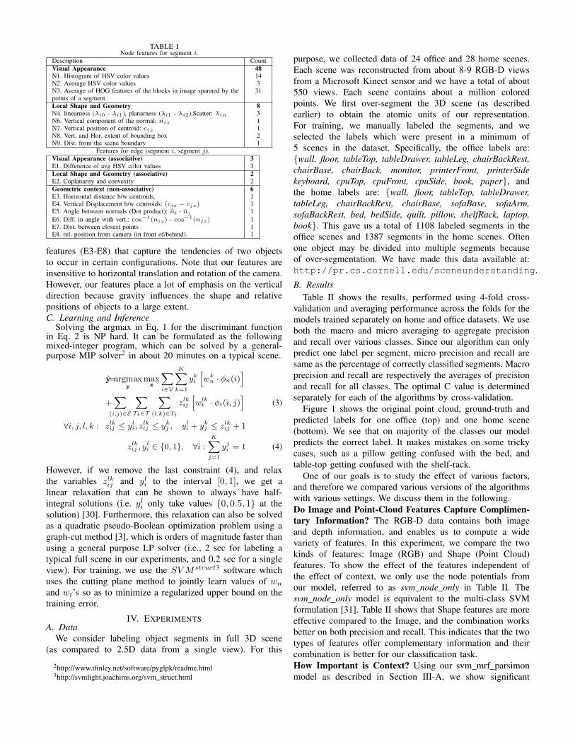
TABLE INode features for segment i.

Description CountVisual Appearance 48N1. Histogram of HSV color values 14N2. Average HSV color values 3N3. Average of HOG features of the blocks in image spanned by thepoints of a segment

31

Local Shape and Geometry 8N4. linearness (λi0 - λi1), planarness (λi1 - λi2),Scatter: λi0 3N6. Vertical component of the normal: niz 1N7. Vertical position of centroid: ciz 1N8. Vert. and Hor. extent of bounding box 2N9. Dist. from the scene boundary 1

Features for edge (segment i, segment j).Visual Appearance (associative) 3E1. Difference of avg HSV color values 3Local Shape and Geometry (associative) 2E2. Coplanarity and convexity 2Geometric context (non-associative) 6E3. Horizontal distance b/w centroids. 1E4. Vertical Displacement b/w centroids: (ciz − cjz) 1E5. Angle between normals (Dot product): ni · nj 1E6. Diff. in angle with vert.: cos−1(niz) - cos−1(njz) 1E7. Dist. between closest points 1E8. rel. position from camera (in front of/behind). 1

features (E3-E8) that capture the tendencies of two objectsto occur in certain configurations. Note that our features areinsensitive to horizontal translation and rotation of the camera.However, our features place a lot of emphasis on the verticaldirection because gravity influences the shape and relativepositions of objects to a large extent.C. Learning and Inference

Solving the argmax in Eq. 1 for the discriminant functionin Eq. 2 is NP hard. It can be formulated as the followingmixed-integer program, which can be solved by a general-purpose MIP solver2 in about 20 minutes on a typical scene.

y=argmaxy

maxz

∑i∈V

K∑k=1

yki

[wk

n · φn(i)]

+∑

(i,j)∈E

∑Tt∈T

∑(l,k)∈Tt

zlkij

[wlk

t · φt(i, j)]

(3)

∀i, j, l, k : zlkij ≤ yli, zlkij ≤ ykj , yli + ykj ≤ zlkij + 1

zlkij , yli ∈ {0, 1}, ∀i :

K∑j=1

yji = 1 (4)

However, if we remove the last constraint (4), and relaxthe variables zlkij and yli to the interval [0, 1], we get alinear relaxation that can be shown to always have half-integral solutions (i.e. yli only take values {0, 0.5, 1} at thesolution) [30]. Furthermore, this relaxation can also be solvedas a quadratic pseudo-Boolean optimization problem using agraph-cut method [3], which is orders of magnitude faster thanusing a general purpose LP solver (i.e., 2 sec for labeling atypical full scene in our experiments, and 0.2 sec for a singleview). For training, we use the SVMstruct3 software whichuses the cutting plane method to jointly learn values of wnand wt’s so as to minimize a regularized upper bound on thetraining error.

IV. EXPERIMENTSA. Data

We consider labeling object segments in full 3D scene(as compared to 2.5D data from a single view). For this

2http://www.tfinley.net/software/pyglpk/readme.html3http://svmlight.joachims.org/svm struct.html

purpose, we collected data of 24 office and 28 home scenes.Each scene was reconstructed from about 8-9 RGB-D viewsfrom a Microsoft Kinect sensor and we have a total of about550 views. Each scene contains about a million coloredpoints. We first over-segment the 3D scene (as describedearlier) to obtain the atomic units of our representation.For training, we manually labeled the segments, and weselected the labels which were present in a minimum of5 scenes in the dataset. Specifically, the office labels are:{wall, floor, tableTop, tableDrawer, tableLeg, chairBackRest,chairBase, chairBack, monitor, printerFront, printerSidekeyboard, cpuTop, cpuFront, cpuSide, book, paper}, andthe home labels are: {wall, floor, tableTop, tableDrawer,tableLeg, chairBackRest, chairBase, sofaBase, sofaArm,sofaBackRest, bed, bedSide, quilt, pillow, shelfRack, laptop,book}. This gave us a total of 1108 labeled segments in theoffice scenes and 1387 segments in the home scenes. Oftenone object may be divided into multiple segments becauseof over-segmentation. We have made this data available at:http://pr.cs.cornell.edu/sceneunderstanding.

B. ResultsTable II shows the results, performed using 4-fold cross-

validation and averaging performance across the folds for themodels trained separately on home and office datasets. We useboth the macro and micro averaging to aggregate precisionand recall over various classes. Since our algorithm can onlypredict one label per segment, micro precision and recall aresame as the percentage of correctly classified segments. Macroprecision and recall are respectively the averages of precisionand recall for all classes. The optimal C value is determinedseparately for each of the algorithms by cross-validation.

Figure 1 shows the original point cloud, ground-truth andpredicted labels for one office (top) and one home scene(bottom). We see that on majority of the classes our modelpredicts the correct label. It makes mistakes on some trickycases, such as a pillow getting confused with the bed, andtable-top getting confused with the shelf-rack.

One of our goals is to study the effect of various factors,and therefore we compared various versions of the algorithmswith various settings. We discuss them in the following.Do Image and Point-Cloud Features Capture Complimen-tary Information? The RGB-D data contains both imageand depth information, and enables us to compute a widevariety of features. In this experiment, we compare the twokinds of features: Image (RGB) and Shape (Point Cloud)features. To show the effect of the features independent ofthe effect of context, we only use the node potentials fromour model, referred to as svm node only in Table II. Thesvm node only model is equivalent to the multi-class SVMformulation [31]. Table II shows that Shape features are moreeffective compared to the Image, and the combination worksbetter on both precision and recall. This indicates that the twotypes of features offer complementary information and theircombination is better for our classification task.How Important is Context? Using our svm mrf parsimonmodel as described in Section III-A, we show significant

TABLE IIAVERAGE MICRO PRECISION/RECALL, AVERAGE MACRO PRECISION AND RECALL FOR HOME AND OFFICE SCENES.

Office Scenes Home Scenesmicro macro micro macro

features algorithm P/R Precision Recall P/R Precision RecallNone chance 26.23 5.88 5.88 29.38 5.88 5.88Image Only svm node only 46.67 35.73 31.67 38.00 15.03 14.50Shape Only svm node only 75.36 64.56 60.88 56.25 35.90 36.52Image+Shape svm node only 77.97 69.44 66.23 56.50 37.18 34.73Image+Shape & context single frames 84.32 77.84 68.12 69.13 47.84 43.62Image+Shape & context svm mrf assoc 75.94 63.89 61.79 62.50 44.65 38.34Image+Shape & context svm mrf nonassoc 81.45 76.79 70.07 72.38 57.82 53.62Image+Shape & context svm mrf parsimon 84.06 80.52 72.64 73.38 56.81 54.80

improvements in the performance over using svm node onlymodel on both datasets. In office scenes, the micro precisionincreased by 6.09% over the best svm node only model thatdoes not uses any context. In home scenes the increase is muchhigher, 16.88%.

The type of contextual relations we capture depend onthe type of edge potentials we model. To study this, wecompared our method with models using only associative(svm mrf assoc) or only non-associative (svm mrf nonassoc)edge potentials. We observed that modeling all edge featuresusing associative potentials is poor compared to our fullmodel. In fact, using only associative potentials showed adrop in performance compared to svm nodeonly model onthe office dataset. This indicates it is important to capturethe relations between regions having different labels. Oursvm mrf non assoc model does so, by modeling all edgefeatures using non-associative potentials, which can favour ordisfavour labels of different classes for nearby segments. Itgives higher precision and recall compared to svm nodeonlyand svm mrf assoc.

However, not all the edge features are non-associativein nature, modeling them using only non-associative po-tentials could be an overkill (each non-associative featureadds K2 more parameters to be learnt). Therefore using oursvm mrf parsimon model to model these relations achieveshigher performance in both datasets.How Large should the Context Range be?

Fig. 2. Effect of context range onprecision (=recall here).

Context relationshipsof different objectscan be meaningfulfor different spatialdistances. This rangemay vary dependingon the environment aswell. For example, inan office, keyboard andmonitor go together,but they may have littlerelation with a sofa that is slightly farther away. In a house,sofa and table may go together even if they are farther away.

In order to study this, we compared our svm mrf parsimonwith varying context range for determining the neighborhood(see Figure 2 for average micro precision vs range plot). Notethat the context range is determined from the boundary of onesegment to the boundary of the other, and hence it is somewhat

independent of the size of the object. We note that increasingthe context range increases the performance to some level,and then it drops slightly. We attribute this to the fact thatwith increasing the context range, irrelevant objects may getan edge in the graph, and with limited training data, spuriousrelationships may be learned. We observe that the optimalcontext range for office scenes is around 0.3 meters and 0.6meters for home scenes.How does a Full 3D Model Compare to a 2.5D Model? InTable II, we compare the performance of our full model witha model that was trained and tested on single views of thesame scene. During the comparison, the training folds wereconsistent with other experiments, however the segmentationof this point-cloud was different (because the input point-clouditself is from single view). This makes the micro precisionvalues not meaningful because the distribution of labels is notsame for the two cases. In particular, many large object inscenes (e.g., wall, ground) get split up into multiple segmentsin single views. We observed that the macro precision andrecall are higher when multiple views are combined to formthe scene. We attribute the improvement in macro precisionand recall to the fact that larger scenes have more context,and models are more complete because of multiple views.What is the Effect of the Inference Method? The resultsfor svm mrf algorithms Table II were generated using theMIP solver. The graph-cut algorithm however, gives a higherprecision and lower recall on both datasets. For example, onoffice data, the graphcut inference for our svm mrf parsimongave a micro precision of 90.25 and micro recall of 61.74.Here, the micro precision and recall are not same as some ofthe segments might not get any label. Since it is orders ofmagnitude faster, it is ideal for realtime robotic applications.C. Robotic experiments

The ability to label segments is very useful for roboticsapplications, for example, in detecting objects (so that a robotcan find/retreive an object on request) or for other robotic taskssuch as manipulation. We therefore performed two relevantrobotic experiments.Attribute Learning: In some robotic tasks, such as roboticgrasping [32] or placing [33], it is not important to knowthe exact object category, but just knowing a few attributesof an object may be useful. For example, if a robot has toclean a floor, it would help if it knows which objects it canmove and which it cannot. If it has to place an object, itshould place them on horizontal surfaces, preferably where

Fig. 3. Cornell’s POLAR (PersOnaL Assistant Robot) using ourclassifier for detecting a keyboard in a cluttered room.

humans do not sit. With this motivation we have designed 8attributes, each for the home and office scenes, giving a total of10 unique attributes, comprised of: wall, floor, flat-horizontal-surfaces, furniture, fabric, heavy, seating-areas, small-objects,table-top-objects, electronics. Note that each segment in thepoint cloud can have multiple attributes and therefore we canlearn these attributes using our model which naturally allowsmultiple labels per segment. We compute the precision andrecall over the attributes by counting how many attributes werecorrectly inferred. In home scenes we obtained a precision of83.12% and 70.03% recall, and in the office scenes we obtain87.92% precision and 71.93% recall.Robotic Object Detection: We finally use our algorithmon a mobile robot, mounted with a Kinect, for completingthe goal of finding an object such as a keyboard inan extremely cluttered room (Fig. 3). The following videoshows our robot successfully finding the keyboard in an office:http://pr.cs.cornell.edu/sceneunderstanding

In conclusion, we have proposed and evaluated the firstmodel and learning algorithm for scene understanding thatexploits rich relational information from full-scene 3D pointclouds. We applied this technique to object labeling problem,and studied affects of various factors on a large dataset.Our robotic applications shows that such inexpensive RGB-Dsensors can be quite useful for scene understanding by robots.

Acknowledgements. We thank Gaurab Basu, Matthew Congand Yun Jiang for the robotic experiments.

REFERENCES

[1] X. Xiong and D. Huber, “Using context to create semantic 3dmodels of indoor environments,” in BMVC, 2010.

[2] D. Anguelov, B. Taskar, V. Chatalbashev, D. Koller, D. Gupta,G. Heitz, and A. Ng, “Discriminative learning of markovrandom fields for segmentation of 3d scan data,” in CVPR, 2005.

[3] C. Rother, V. Kolmogorov, V. Lempitsky, and M. Szummer,“Optimizing binary mrfs via extended roof duality,” in CVPR,2007.

[4] B. Taskar, V. Chatalbashev, and D. Koller, “Learning associativemarkov networks,” in ICML, 2004.

[5] I. Tsochantaridis, T. Hofmann, T. Joachims, and Y. Altun, “Sup-port vector machine learning for interdependent and structuredoutput spaces,” in ICML, 2004.

[6] T. Finley and T. Joachims, “Training structural svms when exactinference is intractable,” in ICML, 2008.

[7] N. Dalal and B. Triggs, “Histograms of oriented gradients forhuman detection,” in CVPR, 2005.

[8] G. Csurka, C. Dance, L. Fan, J. Willamowski, and C. Bray,“Visual categorization with bags of keypoints,” in Workshop onstatistical learning in computer vision, ECCV, 2004.

[9] A. Torralba, “Contextual priming for object detection,” IJCV,vol. 53, no. 2, pp. 169–191, 2003.

[10] C. Li, A. Kowdle, A. Saxena, and T. Chen, “Towards holisticscene understanding: Feedback enabled cascaded classificationmodels,” in NIPS, 2010.

[11] P. Felzenszwalb, D. McAllester, and D. Ramanan, “A discrimi-natively trained, multiscale, deformable part model,” in CVPR,2008.

[12] K. P. Murphy, A. Torralba, and W. T. Freeman, “Using the forestto see the trees: a graphical model relating features, objects andscenes,” NIPS, 2003.

[13] G. Heitz and D. Koller, “Learning spatial context: Using stuffto find things,” in ECCV, 2008.

[14] A. Saxena, S. H. Chung, and A. Y. Ng, “Learning depth fromsingle monocular images,” in NIPS, 2005.

[15] D. Hoiem, A. A. Efros, and M. Hebert, “Putting objects inperspective,” in In CVPR, 2006.

[16] A. Saxena, M. Sun, and A. Y. Ng, “Make3d: Learning 3d scenestructure from a single still image,” IEEE PAMI, vol. 31, no. 5,pp. 824–840, 2009.

[17] D. C. Lee, A. Gupta, M. Hebert, and T. Kanade, “Estimatingspatial layout of rooms using volumetric reasoning about objectsand surfaces,” in NIPS, 2010.

[18] B. Leibe, N. Cornelis, K. Cornelis, and L. V. Gool, “Dynamic3d scene analysis from a moving vehicle,” in CVPR, 2007.

[19] S. Gould, P. Baumstarck, M. Quigley, A. Y. Ng, and D. Koller,“Integrating Visual and Range Data for Robotic Object Detec-tion,” in ECCV workshop Multi-camera Multi-modal (M2SFA2),2008.

[20] M. Quigley, S. Batra, S. Gould, E. Klingbeil, Q. V. Le, A. Well-man, and A. Y. Ng, “High-accuracy 3d sensing for mobilemanipulation: Improving object detection and door opening.”in ICRA, 2009.

[21] R. B. Rusu, Z. C. Marton, N. Blodow, M. Dolha, and M. Beetz,“Towards 3d point cloud based object maps for householdenvironments,” Robot. Auton. Syst., vol. 56, pp. 927–941, 2008.

[22] K. Lai, L. Bo, X. Ren, and D. Fox, “A Large-Scale HierarchicalMulti-View RGB-D Object Dataset,” in ICRA, 2011.

[23] ——, “Sparse Distance Learning for Object Recognition Com-bining RGB and Depth Information,” in ICRA, 2011.

[24] A. Collet Romea, S. Srinivasa, and M. Hebert, “Structurediscovery in multi-modal data : a region-based approach,” inICRA, 2011.

[25] A. Golovinskiy, V. G. Kim, and T. Funkhouser, “Shape-basedrecognition of 3d point clouds in urban environments,” ICCV,2009.

[26] R. Shapovalov, A. Velizhev, and O. Barinova, “Non-associativemarkov networks for 3d point cloud classification,” in ISPRSComm III Symp PCV, 2010.

[27] X. Xiong, D. Munoz, J. A. Bagnell, and M. Hebert, “3-d sceneanalysis via sequenced predictions over points and regions,” inICRA, 2011.

[28] D. Munoz, N. Vandapel, and M. Hebert, “Onboard contex-tual classification of 3-d point clouds with learned high-ordermarkov random fields,” in ICRA, 2009.

[29] “RGBDSLAM,” http://openslam.org/rgbdslam.html.[30] P. Hammer, P. Hansen, and B. Simeone, “Roof duality, com-

plementation and persistency in quadratic 0–1 optimization,”Mathematical Programming, vol. 28, no. 2, pp. 121–155, 1984.

[31] T. Joachims, T. Finley, and C. Yu, “Cutting-plane training ofstructural SVMs,” Machine Learning, vol. 77, no. 1, p. 27, 2009.

[32] Y. Jiang, S. Moseson, and A. Saxena, “Efficient grasping fromrgbd images: Learning using a new rectangle representation,”in ICRA, 2011.

[33] Y. Jiang, C. Zheng, M. Lim, and A. Saxena, “Learning to placenew objects,” in RSS workshop on mobile manipulation, 2011.