2488 IEEE TRANSACTIONS ON GEOSCIENCE AND REMOTE SENSING, VOL. 41, NO. 11, NOVEMBER 2003

A Credit Assignment Approach to Fusing Classifiersof Multiseason Hyperspectral Imagery

Charles M. Bachmann, Member, IEEE, Michael H. Bettenhausen, Member, IEEE, Robert A. Fusina, Member, IEEE,Timothy F. Donato, Member, IEEE, Andrew L. Russ, Joseph W. Burke, Gia M. Lamela, W. Joseph Rhea,

Barry R. Truitt, and John H. Porter

Abstract—A credit assignment approach to decision-basedclassifier fusion is developed and applied to the problem ofland-cover classification from multiseason airborne hyperspectralimagery. For each input sample, the new method uses a smoothedestimated reliability measure (SERM) in the output domain ofthe classifiers. SERM requires no additional training beyond thatneeded to optimize the constituent classifiers in the pool, and itsgeneralization (test) accuracy exceeds that of a number of otherextant methods for classifier fusion. Hyperspectral imagery fromHyMAP and PROBE2 acquired at three points in the growingseason over Smith Island, VA, a barrier island in the NatureConservancy’s Virginia Coast Reserve, serves as the basis forcomparing SERM with other approaches.

Index Terms—Barrier Islands, decision-based classifier fusion,hyperspectral remote sensing, land-cover classification, maximumestimated reliability measure (MAXERM), multiple classifiersystems, multiple classification system, multiseason classification,smooth estimated reliability measure (SERM), Virginia CoastReserve.

I. INTRODUCTION

I T IS WELL KNOWN that the accuracy of land-cover clas-sification can be improved by the use of multitemporal or

multisource data [5], [17], [27], [32], [35]. This is particularlytrue in remote sensing of coastal land-cover, where there aremany sources of variability such as inundation in beach zonesand tidally influenced wetlands, atmospheric water vapor, andseasonal variations in vegetation. Combining the results of clas-sifiers obtained at different points in the growing cycle or tidalstage can be used to reduce noise and achieve better classi-fication accuracy. Airborne hyperspectral imagery provides apowerful means of discriminating coastal land-cover types withfine detail [2], [12], but yields large data volumes, especiallywhen multiseason data are used. At the same time, many real-

Manuscript received September 20, 2002; revised August 5, 2003. Thiswork was supported by the Office of Naval Research under ContractsN0001400WX40016, N0001401WX40009, and N0001402WX30017.

C. M. Bachmann, M. H. Bettenhausen, R. A. Fusina, T. F. Donato, G. M.Lamela, and W. J. Rhea are with the Remote Sensing Division, Naval ResearchLaboratory, Washington, DC 20375 USA (e-mail: bachmann@nrl.navy.mil).

A. L. Russ is with the Department of Geography, University of Maryland,College Park, MD 20742 USA and also with the USDA Agricultural ResearchService, Hydrology and Remote Sensing Laboratory, Beltsville, MD 20705USA.

J. W. Burke is with the Department of Geography, University of Maryland,College Park, MD USA 20742.

B. R. Truitt is with the The Nature Conservancy, Virginia Coast Reserve,Nassawadox, VA USA 23413 (e-mail: btruitt@tnc.org).

J. H. Porter is with the Department of Environmental Sciences, University ofVirginia, Charlottesville, VA 22904-41231 USA.

Digital Object Identifier 10.1109/TGRS.2003.818537

world applications demand reasonable “turnaround” time to beof practical utility in a production mode, especially when a largevolume of data must be processed. Even in a research envi-ronment, large data volumes may limit the practical utility ofalgorithms that are too slow. In this study, for example, thethree-season hyperspectral imagery of Smith Island amounts to

6 GB of data, and Smith Island is just one of six islands forwhich we have acquired multiseason imagery in our study area.Thus, we seek approaches that are either: 1) as accurate as ex-isting methods but significantly faster or 2) more accurate thanexisting methods without dramatically sacrificing processingspeed. This paper focuses on a new approach to decision-basedfusion of classifiers, building on the work of a number of au-thors [5], [6], [31], [35], [36], [39], [42], who have addressedthe problem of classifier fusion either in remote sensing or otherapplications. The new method of classifier fusion that we de-velop here is as accurate or better than many competing optionsbut is significantly faster because it does not require additionaltraining beyond the training of the constituent classifiers. SERMalso scales better as the number of classifiers in the pool in-creases. Results of the new approach are evaluated using multi-season hyperspectral imagery of land-cover on a barrier islandthat was previously studied using single-season hyperspectralimagery [2]. Ultimately, the new approach, SERM, achievedthe highest test accuracy of all methods that we explored in thisstudy.

The rest of our paper is organized as follows. In Section II,after providing a historical context and perspective for our work,we present the new approach. In Section III, we briefly describethe hyperspectral data and ground truth used in our experiments.In Section IV, we present the results comparing the new ap-proach to the performance of single-season classifiers and othermulticlassifier fusion algorithms, and in Section V, we summa-rize the results and draw conclusions.

II. A PPROACH ANDMETHODS

A. Combining Classifiers: A Historical Perspective

A variety of approaches to the problem of combining classi-fiers have been proposed over the years. These include the BordaCount [19], Bayesian classifiers, Dempster–Shafer [16], [40],and optimal weighted averaging with linear or log pools [6],[14]. In some instances, the problem of credit assignment hasalso been directly addressed. The problem of credit assignmentis fundamental to the successful fusion of classifiers. By somemeans, the goal is that the composite output should produce a

0196-2892/03$17.00 © 2003 IEEE

BACHMANN et al.: FUSING CLASSIFIERS OF MULTISEASON HYPERSPECTRAL IMAGERY 2489

result that is more robust than the performance of any single con-stituent classifier. This can be achieved in several ways: by par-titioning the problem into credit assignment zones in the inputdomain [21], by smoothing in either the input domain [36], [39]or the output domain [15], [28], [29], [40] to reduce noise, orby hierarchical methods [6], [24]. In some instances, smoothingand hierarchical processing are combined [6]. For high-dimen-sional data sources such as hyperspectral imagery, output do-main approaches that focus on the classifier posterior proba-bilities may be preferable to input domain approaches becauseoutput domain methods involve lower dimensional informationand, thus, avoid problems related to the curse of dimension-ality [4] and multidimensional scaling [9]; output domain ap-proaches are also usually less computationally intensive in thesecircumstances.

Multiple classifier fusion has been viewed from the perspec-tive of the well-known bias-variance dilemma [13], [37]. Clas-sifier error can be decomposed into two terms: one is the classi-fier bias, and the other is the variance of the classifier estimate.Many multiclassifier algorithms fuse classifiers with approxi-mately the same bias but different error distributions; combiningthese classifiers then reduces the variance term in the error madein approximating the true mapping [37]. There are several waysto produce uncorrelated errors in the pool of classifiers to befused [37]; these include: 1) varying the architecture of the clas-sifier (e.g., the number of nodes and free parameters in a neuralnetwork), 2) varying the choice of algorithm (e.g., see [36]), or3) varying the training data which is known as “bagging” or“boosting” [8]. In remote sensing applications, variance reduc-tion also can be achieved by using multisensor or multitemporaldata to produce a pool of classifiers with decorrelated error dis-tributions. In this paper, we use hyperspectral data from threedifferent seasons to train a set of classifiers that will producestatistically decorrelated errors. We also combine different al-gorithms in a second set of experiments and examine the ro-bustness of fusion algorithms when weak classifiers are addedto the pool.

B. Overview of Competing Approaches to Fusing Classifiers:Experimental Design

In Section IV, we compare multiseason classification resultsproduced by classifier fusion using two local reliability esti-mates, one which we call the maximum estimated reliabilitymeasure (MAXERM) an averaged version of a measure foundin [35] and a smoothed version of this (SERM); these are com-pared with several other methods for fusing classifiers. Algo-rithms also evaluated included the generalized ensemble model(GEM) [31], a decoupled GEM (DGEM), majority vote, and asimple composite approach. Each of these algorithms was usedto produce a multiseason classification using the outputs of thethree single-season classifiers trained on either data from theHyMAP1 May 2000 imagery, PROBE22 August 2001 imagery,or PROBE2 October 2001 imagery. Each multiseason classifi-cation was also compared against the performance of individualclassifiers applied to single-source data. In the first set of ex-

1Analytical Imaging and Geophysics, LLC. See http://www.aigllc.com.2ESSI. See http://www.earthsearch.com.

periments, the single-season constituent classifiers were opti-mized using the backward propagation neural network [34] witha cross-entropy cost function [33] and an adaptive sampling al-gorithm known as adaptive resampling strategy for error proneexemplars (ARESEPE) [1]. Each of the classifier fusion ap-proaches was applied to this constituent pool of three single-season BPCE-ARESEPE (BPCE using the ARESEPE adaptivesampling strategy) classifiers. In a second set of experiments,we added three additional single-season constituent classifiers.The goal in these experiments was to test the robustness ofclassifier fusion algorithms to the presence of weak, subop-timal classifiers in the pool. We added three single-season clas-sifiers to the pool, consisting of either: 1) principal componentsanalysis (PCA) [43] followed by a distance weighted K-nearestneighbor (DWKNN) classifier [10] or 2) DWKNN by itself. Inthe PCA-DWKNN case, each suboptimal classifier consisted ofa two-stage process in which spectra were projected using PCAand then classified using DWKNN . For the PCAanalysis, 30 components were retained for each season, sincethis explained 99.99% of the variance. DWKNN test accuracywas not very sensitive to , so we used an intermediate value.The primary reason for using PCA was to decrease the dimen-sionality of the DWKNN reference codebook (the training set).In Sections II-C–II-I, we briefly describe the other single-seasonand multiseason classifier fusion algorithms.

C. BPCE Classifier

In the first set of experiments described in Section IV, single-season classifiers were all developed using the backward propa-gation of error classifier [34] with a cross-entropy cost function(BPCE) [33]. The BPCE cost function is

(1)where the superscript is the last layer in an -layer classifier,

is the desired output, either 0 or 1, for one of the categorynodes at the output of the classifier, is the actual responseof the output node to a particular input pattern propagated for-ward through the classifier, and is the netinput to that node, with the weight vector and the offset.We use the cross-entropy cost function because it is less proneto local minima than the originally proposed least mean square(LMS) error, owing to the form of the gradient used in the sto-chastic gradient descent [2], [33]. Specifically, the presence ofthe logarithms in (1) eliminates terms in the last layer gradientthat are present when an LMS cost function is used

BPCE (2)

BPLMS (3)

2490 IEEE TRANSACTIONS ON GEOSCIENCE AND REMOTE SENSING, VOL. 41, NO. 11, NOVEMBER 2003

Fig. 1. Schematic diagrams for (left) the simple composite and (right) SERM. The simple composite uses the same algorithm in the back-end classifier thatwas used in the constituent single-season classifiers, BPCE with ARESEPE. SERM computes a smoothed estimated reliability measure without further training.Smoothing is done at both the classifier and pool levels.

Here is the last layer “error signal” [34], which is thenegative partial derivative of the cost function with respectto the node net input , and is the gain of the sigmoidaltransfer function . The gradientwith respect to the weight vector is just the product of theerror signal and the input vector from the previous layer:

, and as usual, the weight up-date rule is ,where (set to 0.6 in the experiments described here) is the“momentum” term, and is the time-dependent learningrate, which decreases (in our case) logarithmically with time[18]. Comparing (2) and (3), it is obvious that BPLMS hastwo local minima when and andlikewise at and ; BPCE does not havethese local minima. Thus, BPCE is less likely to be trappednear a local minimum in which the desired pattern responseis at one extreme, while the actual response is antipodal. Notethat because of the backward propagation of the error signal

[34], these localminima can effect all layers in BPLMS, whereas this effect iseliminated for all layers when BPCE is used.

One additional feature of our classifier implementation wasthe use of a resampling buffer which detects the presence of pat-terns causing classifier output errors and resamples these morefrequently during the optimization cycle. A more thorough de-scription of the ARESEPE algorithm is given in [1]. We give ashort overview in Section II-D.

D. ARESEPE

Active sampling training strategies have been studied in thecontext of a variety of pattern recognition applications [20], [30],[41]. These strategies aim to reduce significantly the amount oftraining time required to optimize classifiers and in some casesalso produce more accurate results. These methods focus opti-mization sampling on pattern boundaries between categories.ARESEPE [1] achieves this by using a resampling buffer that ispart of the total input stream along with the regular data streamthat comprises the training set. Entry into the resampling bufferis determined for each sample as it is processed, a categoryresponse determined, and updates performed. The buffer entrycriterion is proportional to the degree of misclassification thatoccurs. Patterns that do not produce error should not enterthe buffer, while those that cause the most error should be themost likely to enter the resampling buffer. ARESEPE uses amisclassification measure that was first defined as an alternative

-category discriminant function [22]

(4)

where index is the true category associated with input samplevector . The asymptotic limit as is just

(5)where is the maximum responding discriminant functionnot equal to the true discriminant function. Thus, a positivevalue of represents the amount by which the winning

BACHMANN et al.: FUSING CLASSIFIERS OF MULTISEASON HYPERSPECTRAL IMAGERY 2491

TABLE ISUMMARY OF ALGORITHM ACRONYMS

discriminant function was larger than the true discriminant func-tion. Let

(6)

for each category node, where as before,is the index of thetrue category, and then compute

(7)

then the sign of indicates whether the pattern was misclas-sified and automatically determines the quantity; when apattern is misclassified, entry to the resampling buffer is propor-tional to . Further implementation details are in [1]; however,the main reason for using ARESEPE is that convergence timefor this hyperspectral data is improved by one or two orders ofmagnitude depending on the rate of resampling from the buffer[1]. In thispaper, forallexperiments,butacompleteanalysisof thisparameterand thebuffersizeappears in [1].

E. Majority Vote

Consensus voting schemes have been widely used in manyapplications [5], [14]. As implemented here, when a majorityof classifiers in the pool respond with the same classificationlabel, that label becomes the classification of the composite. Ifa tie occurs, then the label is chosen randomly from the tiedcategories. We are actually describing a plurality voting rule

[15]: the majority in [15] actually requires that more than halfagree on the same label; however, in the results below, pluralityand majority are equivalent in the three-classifier pools. Con-sensus votes are known to improve results provided the con-stituent classifiers generalize well and the distribution of errorsis somewhat decorrelated [15].

F. GEM

The generalized ensemble model [31] is a general frameworkfor combining the results of classifiers, independent of the un-derlying form of the algorithm, or the data distribution to bemodeled. However, it is a linear pool, which is known to havelimitations [6]. Given a set of classifiers, with output , theoutput probability of the ensemble estimate, is

where (8)

The principal weakness of GEM is that it does not perform creditassignment on a local basis; it achieves an optimal solution onlyin an average sense by inverting a conglomerate error covariancematrix

(9)

As a result, it will be biased toward the dominant categories inthe training set.

2492 IEEE TRANSACTIONS ON GEOSCIENCE AND REMOTE SENSING, VOL. 41, NO. 11, NOVEMBER 2003

G. Decoupled GEM

In Section IV, we also include a decoupled version of GEM(DGEM) in which the ensemble estimate over all categories isreplaced by separate estimates and error covariance matrices,one associated with each category

(10)

(11)

(12)

DGEM primarily addresses the problem of sparsely representedcategories butnot the problemofcomplex categorydistributions:each category node in the fused classifier output still has onlyone associated error covariance matrix for all input vectors.Section IV shows that even DGEM cannot compete with trulylocal credit assignment classifier fusion algorithms such asSERM.

H. Simple Composite Classifier

One of the simplest decision-based fusion options is to usethe same algorithm [BPCE (with ARESEPE)] that was used tooptimize the single-season classifiers, to develop a simple com-posite classifier. In this approach, we use the outputs of thesingle-season classifiers as inputs to a back-end BPCE/ARE-SEPE classifier; subsequently we refer to this approach as thesimple composite (Fig. 1). Compared to GEM and DGEM, thisapproach has the advantage that it provides additional decisionhyperplanes, rather than a single decision hyperplane across theentire data space. The principal disadvantages of the simplecomposite are the need for additional training of the back-endclassifier and poor scaling with increasing pool size. The latterstems from the fact that constituent classifier output vectorsare concatenated as inputs to the back-end classifier, leading toback-end classifiers with many more parameters to optimize,and also slower feedforward propagation.

I. MAXERM and SERM

The output vector elements for the th classifier are pro-portional to the posterior probabilities that the classifier assignsto each category. Therefore, choosing the category of the outputnode with the largest response will be equivalent to choosing thecategory with the maximuma posteriori(MAP) probability asthe predicted category label. For classifier, this is

(13)

In the first experiment of Section IV, our constituent classifiersare neural networks optimized using BPCE with ARESEPE. Formany neural networks, including BPCE, each output categoryresponse must be divided by the sum of these responses toobtain posterior probabilities on a per-sample basis

(14)

The output domain neighborhood around a particular classifier’sresponse to input vectorcan be described by the set of output

domain responses obtained for perturbations accordingto

(15)

When is low dimensional, the approaches described in [36]and [39] effectively sample the input domain subset describedby (15) at the available sample points, although the distance-weighted KNN approach used in [36] probably does a betterjob of ensuring that the neighborhoods remain relatively small.However, for very high dimensional vectors, multidimensionalscaling problems can distort the concept of proximity in theinput space when simple distance measures are used. Thus, wefocus on the output domain in deriving classifier reliability mea-sures.

A zero-order approximation to (15) is to replace the Taylorseries by the first term, namely

(16)

In this approximation, the probabilities described in (14) can bethought of as representing a zeroth-order sample of the outputdomain neighborhood around the sample point, and in partic-ular are related to the probability that another class label wouldbe returned from a nearby sample. Thus, if theth classifier’spredicted category label is given by (13), then a measure of theclassifier’s self-reported reliability can be written as

(17)We note that this is a sum over a set of local category reliabilitymeasures originally defined in [35]

(18)

where . In [35], (18) ap-peared as a local reliability estimate in a penalty term of a loglikelihood function that was used to model temporal transitionprobabilities in multidate SAR and Landsat Thematic Mapperimagery. In the present work, we use a sum over local relia-bility estimates for each category to derive a reliability (17) forthe classifier label returned by (13). Equation (17) is the first oftwo reliability expressions that will be evaluated in Section IV.Specifically, the approach that we call MAXERM assigns thefused class label for a particular sample to that of the classifierwith the maximum reliability determined by (17)

(19)

When all of the category probabilities are the same, the self-reported local reliability estimate in (17) is zero; however, whenthe output response is unity for one category and zero for allother categories, then the classifier reports perfect reliability.

In order to minimize the risk of using the self-reported re-liabilities, we can smooth the reliability estimates over the setof classifiers. To achieve this, we compute the predicted classlabels from (13) for each classifier and the corresponding self-reported reliability from (17), and calculate the sum of the re-liabilities for each category over the set of classifiers. For each

2493 IEEE TRANSACTIONS ON GEOSCIENCE AND REMOTE SENSING, VOL. 41, NO. 11, NOVEMBER 2003

Fig

.2.

(Top

)T

hree

-sea

son

airb

orne

hype

rspe

ctra

lim

ager

yof

Sm

ithIs

land

.R

GB

com

posi

tes:

(left)

May

HyM

AP

scen

e(

R=

650.

5nm

,G=

542.

8nm

,B=

452.

1nm

);(m

iddl

e)A

ugus

tP

RO

BE

2sc

ene

(R=

645.

9nm

,G=

552.

8nm

,B=

446.

2nm

);(r

ight

)O

ctob

erP

RO

BE

2sc

ene

(RG

Bch

anne

lssa

me

asA

ugus

t).

(Mid

dle)

Enl

arge

men

ts,

sout

hern

end

ofS

mith

Isla

nd,

show

ing

seas

onal

varia

tio

ns,

espe

cial

lyin

swal

eve

geta

tion.

(Bot

tom

)G

roun

dph

otog

raph

sof

ado

min

ants

wal

egr

ass

Dis

tich

lissp

ica

tase

enin

the

mid

dle

row

.(Le

ft)M

ay20

01,(

mid

dle)

Aug

ust2

001,

and

(rig

ht)

Oct

ober

,200

1,(n

earb

yH

ogIs

land

).

2494 IEEE TRANSACTIONS ON GEOSCIENCE AND REMOTE SENSING, VOL. 41, NO. 11, NOVEMBER 2003

TABLE II

possible output category label, we take the sum over the clas-sifier reliabilities

(20)

The final predicted category of the composite classification isthe category with the largest

(21)

Equations(13), (17), (20), and (21) define the SERM algorithm,the second new reliability method for fusing classifiers (Fig. 1).

J. Summary of Algorithms

Table I contains a summary of the algorithms used in thispaper. The acronym for each algorithm is followed by a briefdescription of the algorithm, the type of approach it represents,and references to the algorithm in the literature. We havefirst listed the classifiers used in single-season models, aswell as ARESEPE, the active sampling strategy describedearlier. The second half of the table consists entirely of themultiple-classification systems (MCS) [36]. Under the heading“Type of Approach,” the MCS algorithms are characterizedusing the taxonomy defined in [36], where algorithms aredefined as performing either “classifier selection” or “classifierfusion.” “Classifier selection” implies that the label of the bestclassifier in the MCS pool, using some measure of fitness, is theresponse of the MCS, while “classifier fusion” implies that allclassifiers in the MCS pool play a role in the final answer. Notethat given this MAXERM [see (19)] is a “classifier selection”algorithm, while SERM [see (20) and (21)] is a “classifierfusion” algorithm. All but one of the MCS algorithms are“Type III” [36], meaning that they use some measures of theconstituent classifier outputs to determine the MCS output,while the majority vote is “Type I” [36], indicating that it usesonly the labels themselves in determining the MCS output.Before describing the data and results, it is worth emphasizingthat DGEM, MAXERM, and SERM are novel algorithms inthis paper. Although MAXERM uses a reliability measurefirst defined in [35], the use of the reliability measure forclassifier selection is novel to this paper; in [35], the reliabilitymeasure was used to model temporal transition probabilities inmultitemporal data, but not for classifier selection. Likewise,SERM is novel in a second way because it performs smoothingby summing these reliabilities over all classifiers representedin the pool.

Rather than an exhaustive comparison, we chose a subsetof algorithms that are in common usage or representative ofextant algorithms for relatively fast, decision-based classifierfusion to compare against the new algorithms SERM andMAXERM. The majority vote is, of course, widely used.Likewise, GEM was chosen because it is popular in the neuralnetwork community and optimizes quite quickly, but as wewill see, GEM generalization accuracy is suboptimal becauseit does not perform credit-assignment on a local basis. DGEMwas an attempt to make GEM a little more local by decouplingthe covariance matrices, but its performance on the databaseused in this paper was not significantly different from that ofGEM. The simple composite architecture is included becauseit is the simplest approach for classifier fusion; it is also widelyused, and achieves good results. However, the simple compositedoes require further optimization once the constituent pool isoptimized. MAXERM and SERM were developed to avoid therequirement of further optimization in the simple compositewhile still achieving good classification results.

III. D ATA AND STUDY AREA

A. Virginia Coast Reserve

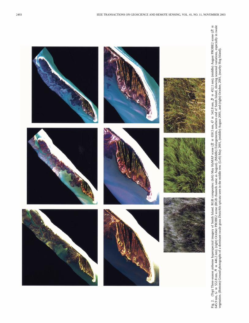
The present study builds upon earlier research [2], in whichland-cover classification of Smith Island, a barrier island inthe Virginia Coast Reserve (VCR), was investigated using aHyMAP image acquired in May 2000.3 In this paper, mul-tiseason classifications are compared against single-seasonclassifications of airborne hyperspectral imagery acquired atthree points in the growing cycle. HyMAP [25] imagery ofSmith Island was acquired on May 8, 2000, and PROBE2imagery was subsequently acquired on August 22 and October18, 2001. RGB composites derived from these data are shownin Fig. 2. PROBE2 and HyMAP are similar hyperspectralsensors that cover the spectral range between 440–2500 nmwith a spectral FWHM of typically 15–20 nm. Both sensorshave 128 spectral channels, but for these collections, there were124 usable channels for PROBE2, and 126 for HyMAP. Scenedimensions are approximately 16.1 km2.5 km (HyMAP),12.4 km 2.6 km (PROBE2, August), and 12.2 km2.5 km(PROBE2, October). Atmospheric corrections for the HyMAPscene were applied using ATREM/EFFORT by AIG priorto delivery. For the PROBE2 data, we applied an algorithmdescribed in [11], commonly known as the 6S model, to theradiance data, which we then polished using the EFFORTalgorithm [7]. The May HyMAP imagery and the August

3Web site for the University of Virginia’s Long Term Ecological ResearchProgram. See http://www.vcrlter.virginia.edu.

BACHMANN et al.: FUSING CLASSIFIERS OF MULTISEASON HYPERSPECTRAL IMAGERY 2495

TABLE IIIPERCENTAGE ACCURACY FOR TRAINING AND TEST SETS. OPTIMIZATION TIMES ARE FOR AN ATHLON XP 1800+ PROCESSOR.

FOR ARESEPE EXPERIMENTS, r = 0:5

PROBE2 imagery were acquired near high tide, while the Oc-tober PROBE2 imagery was acquired near low tide. The earlyMay scene is taken in a period during which the vegetation willtypically be a mixture of new growth and senescent vegetationfrom the previous season; the senescent vegetation may partlyobscure the emerging new growth beneath it. The mid-Augustscene was acquired during the peak of the growing season,while the mid-October scene was acquired as the vegetationhad begun to senesce. In the latter case, some vegetation willshow more deeply contrasting colors, and tonal changes in thevisible part of the spectrum may provide better contrast fordiscrimination purposes.

B. Land-Cover Categories and Ground Data

Our supervised classification category maps have been val-idated within situ observations made by us during a series offield surveys with global positioning system (GPS) and differ-ential GPS conducted on Smith Island as described in [2]. Sur-veyed regions were used to create spectral libraries from thegeorectified and coregistered HyMAP and PROBE2 imagery.These spectra were divided into a training set (3632 pixels), across-validation test set (1971 pixels) used to stop optimization,and a second sequestered test set (2834 pixels) that served as anindependent assessment of expected performance. The DGPSground data also were used to improve georectification of theimagery. The categories used in this study appear in Table II.

IV. RESULTS

Ten trials were performed for each single-season classifierand the corresponding three-season fused classification algo-

rithms, which used these as inputs. Mean and standard deviationof accuracies of all classification approaches are shown inTable III. It is not surprising that the single-season May HyMAPclassification results are significantly lower than those obtainedfor the August and October PROBE2. We expect this becauseof the seasonal variations in vegetation previously describedin Section III-A. For the first multiclassifier experiments usingthe three single-season BPCE-ARESEPE classifiers as input,Table III shows that the best results for the test data sets wereachieved by the SERM and simple composite algorithms;SERM mean accuracy for the sequestered test set exceededsimple composite accuracy by roughly one standard deviation.All other competing techniques produced less accurate gener-alization to test data. In the second set of experiments in whichthe weak classifiers based on PCA-DWKNN or DWKNN wereadded to the pool, we compared only the simple composite,MAXERM, and SERM and found that SERM and MAXERMaccuracy did not change by a statistically significant amount,while the simple composite performance dropped considerably.

Looking at the results for the three-classifier pools, wesee that smoothing in SERM, achieved by the two sets ofsums in (17) and (20), which effectively averages at boththe classifier and pool level, is apparently more robust thanjust averaging at the classifier level as is done in MAXERM.SERM test accuracy exceeded that of the simple compositeapproach despite the large number of free parameters availablein the simple composite, and SERM performance was achievedwithout the need for back-end optimization. Likewise, as thepool size and complexity grew, optimization time for the simplecomposite grew considerably (Table III). SERM also achieved

2496 IEEE TRANSACTIONS ON GEOSCIENCE AND REMOTE SENSING, VOL. 41, NO. 11, NOVEMBER 2003

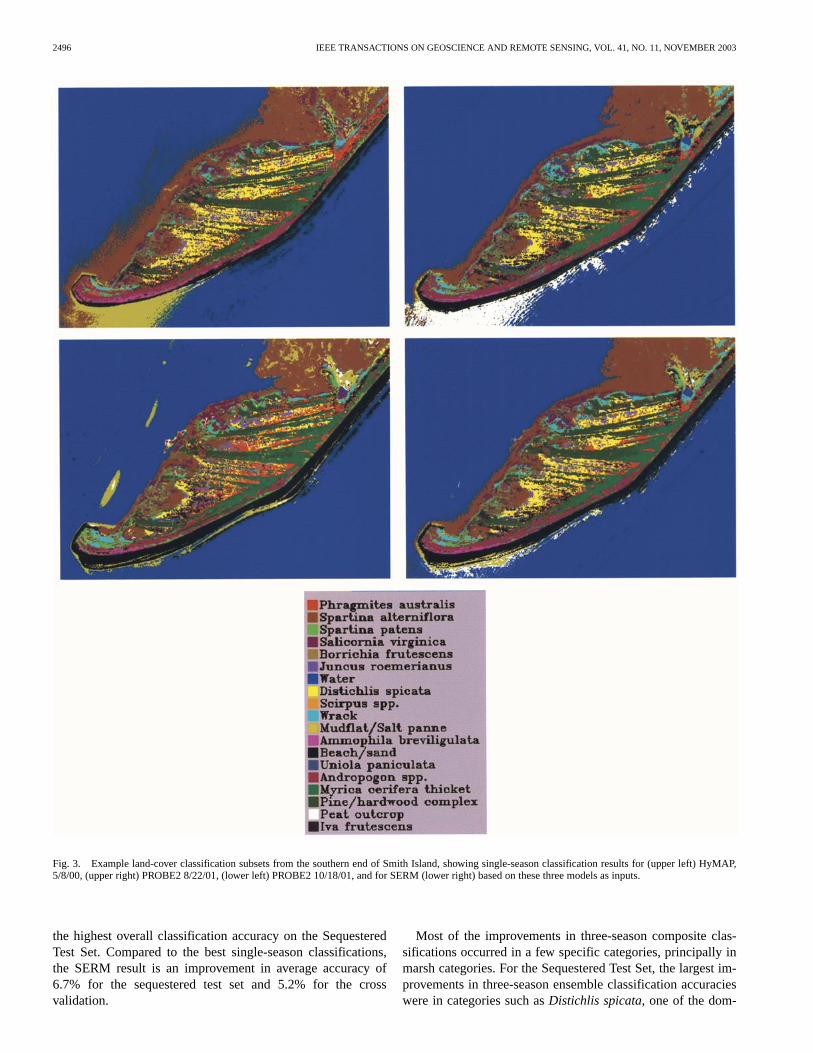
Fig. 3. Example land-cover classification subsets from the southern end of Smith Island, showing single-season classification results for (upper left) HyMAP,5/8/00, (upper right) PROBE2 8/22/01, (lower left) PROBE2 10/18/01, and for SERM (lower right) based on these three models as inputs.

the highest overall classification accuracy on the SequesteredTest Set. Compared to the best single-season classifications,the SERM result is an improvement in average accuracy of6.7% for the sequestered test set and 5.2% for the crossvalidation.

Most of the improvements in three-season composite clas-sifications occurred in a few specific categories, principally inmarsh categories. For the Sequestered Test Set, the largest im-provements in three-season ensemble classification accuracieswere in categories such asDistichlis spicata, one of the dom-

BACHMANN et al.: FUSING CLASSIFIERS OF MULTISEASON HYPERSPECTRAL IMAGERY 2497

inant swale grasses,Juncus roemerianus, Wrack, andSpartinaalterniflora, the dominant salt marsh vegetation. In the single-season classifications, some categories were more accuratelyidentified in a particular season. For example, among single-season classifications,Iva frutescenswas most readily identi-fied in the August classifiers; the May classifiers were less ac-curate because the leaves have typically not emerged this earlyin the growing season; likewise, in October the leaves may havesenesced to a great degree or fallen off completely. Algorithmssuch as SERM and the simple composite are able to select thebest performance in one category from a particular classifier,such asIva, so that it is included in the composite classifica-tion. We see this, for example, in Fig. 3. Likewise, artifacts thatappeared in specific single-scene classifiers, e.g., water regionsmislabeled because of glint, have been corrected in the fusedclassification. Furthermore, the SERM classification in Fig. 3also shows a dramatic reduction in false alarms for the inva-sive plantPhragmites australis. Looking beyond the test setaccuracy, we know from our surveys that most of the SERMimprovement in this example came from the removal of falsepositives that occurred in the center of swales and on the westernedge of the back-dune vegetation in the single-season classifi-cations. These successes are due to the local nature of the creditassignment achieved in SERM.

V. SUMMARY AND CONCLUSION

We have introduced two new approaches to fusing classifiersthat relied on single-sample estimated reliability measures, onebased on the maximum classifier reliability (MAXERM) andanother based on a smoothed version (SERM), which averagesover the reliability of all predicted category labels across allclassifiers in the pool. The reliability measures are directlyavailable from the outputs of the pool of trained classifiersto be fused, without further optimization. These measures donot depend on the specific type of classifiers in the pool. Astatistical argument was advanced to show that these reliabilitymeasures directly estimate a zeroth-order approximation tothe output domain neighborhood of the classifier posteriorprobability. For the initial set of illustrative hyperspectral land-cover classification experiments, SERM was superior to avariety of different approaches to fusing classifiers includingGEM, DGEM, and majority vote, and about one standarddeviation better than the simple composite. Likewise, once theclassifier pool was assembled, SERM required no optimization,while the simple composite did require further optimization. Thesimple composite also scales poorly in terms of optimizationtime and feedforward complexity (number of free parameters)as the pool size grows, while SERM scales well, relyingonly on simple formulas that are functions of the classifieroutputs to classify novel inputs. SERM was the most robustclassifier fusion algorithm, as the pool size was increased andweak classifiers were added to the initial pool of three single-season hyperspectral classifiers, while the simple compositeperformance degraded significantly when the weak classifierswere added.

ACKNOWLEDGMENT

The authors acknowledge computing resources provided bythe DOD High Performance Computing (HPC) ModernizationProgram, including SMDC, the Maui High Performance Com-puting Center (MHPCC), and the Army Research Laboratory’sMajor Shared Resource Center (ARLMSRC).

REFERENCES

[1] C. M. Bachmann, “Improving the performance of classifiers in high-di-mensional remote sensing applications: An adaptive resampling strategyfor error-prone exemplars (ARESEPE),”IEEE Trans. Geosci. RemoteSensing, vol. 41, pp. 2101–2112, Sept. 2003.

[2] C. M. Bachmann, T. F. Donato, G. M. Lamela, W. J. Rhea, M. H. Bet-tenhausen, R. A. Fusina, K. DuBois, J. H. Porter, and B. R. Truitt, “Au-tomatic classification of land-cover on Smith Island, VA using HYMAPimagery,”IEEE Trans. Geosci. Remote Sensing, vol. 40, pp. 2313–2330,Oct. 2002.

[3] G. D. Bailey, S. Raghavan, N. Gupta, B. Lambird, and D. Lavine, “In-Fuse—An integrated expert neural network for intelligent sensor fu-sion,” in Proc. IEEE/ACM Int. Conf. Developing and Managing ExpertSystem Programs, 1991, pp. 196–201.

[4] R. Bellman,Adaptive Control Processes: A Guided Tour. Princeton,NJ: Princeton Univ. Press, 1961.

[5] J. A. Benediktsson and P. H. Swain, “Consensus theoretic classificationmethods,”IEEE Trans. Syst., Man, Cybern., vol. 22, pp. 688–704, Apr.1992.

[6] J. A. Benediktsson and I. Kanellopoulos, “Classification of multisourceand hyperspectral data based on decision fusion,”IEEE Trans. Geosci.Remote Sensing, vol. 37, pp. 1367–1377, May 1999.

[7] J. Boardman, “Post-ATREM polishing of AVIRIS apparent reflectancedata using EFFORT: A lesson in accuracy versus precision,” inSum-maries of the 7th Annu. JPL Airborne Geoscience Workshop. Pasadena,CA, 1998.

[8] G. J. Briem, J. A. Benediktsson, and J. R. Sveinsson, “Multiple classi-fiers applied to multisource remote sensing data,”IEEE Trans. Geosci.Remote Sensing, vol. 40, pp. 2291–2299, Oct. 2002.

[9] R. O. Duda, P. E. Hart, and D. G. Stork,Pattern Classification, 2nded. New York: Wiley, 2001.

[10] S. A. Dudani, “The distance-weighted k-nearest-neighbor rule,”IEEETrans. Syst. Man, Cybern., vol. SMC-6, pp. 325–327, 1976.

[11] B. Gao and C. O. Davis, “Development of a line-by-line atmosphereremoval algorithm for airborne and spaceborne imaging spectrometers,”Proc. SPIE, vol. 3118, pp. 132–141, 1997.

[12] M. Garcia and S. L. Ustin, “Detection of interannual vegetationresponses to climactic variability using AVIRIS data in a CoastalSavanna in California,”IEEE Trans. Geosci. Remote Sensing, vol. 39,pp. 1480–1490, July 2001.

[13] S. Geman, E. Bienenstock, and R. Doursat, “Neural networks and thebias/variance dilemma,”Neural Comput., vol. 4, pp. 1–58, 1992.

[14] C. Genest and J. V. Zidek, “Combining probability distributions: Acritique and an annotated bibliography,”Stat. Sci., vol. 1, no. 1, pp.114–148, 1986.

[15] L. K. Hansen and P. Salamon, “Neural network ensembles,”IEEE Trans.Pattern Anal. Machine Intell., vol. 12, pp. 993–1001, Oct. 1990.

[16] S. Le Hegarat-Mascle, I. Bloch, and D. Vidal-Madjar, “Application ofDempster-Shafer evidence theory to unsupervised classification in mul-tisource remote sensing,”IEEE Trans. Geosci. Remote Sensing, vol. 32,pp. 768–778, July 1994.

[17] S. Le Hegarat-Mascle, A. Quesney, D. Vidal-Madjar, and O. Taconet,“Land cover discrimination from multitemporal ERS images and multi-spectral Landsat images: A study case in an agricultural area in France,”Int. J. Remote Sens., vol. 21, no. 3, pp. 435–456.

[18] T. M. Heskes, E. T. P. Slijpen, and B. Kappen, “Cooling schedules forlearning in neural networks,”Phys. Rev. E, vol. 47, no. 6, pp. 4457–4464,1993.

[19] T. K. Ho, J. J. Hull, and S. N. Srihari, “Decision combination in multipleclassifier systems,”IEEE Trans. Pattern Anal. Machine Intell., vol. 16,pp. 66–75, Jan. 1994.

[20] J.-N. Hwang, J. J. Choi, S. Oh, and R. J. Marks, II, “Query-basedlearning applied to partially trained multilayer perceptrons,”IEEETrans. Neural Networks, vol. 2, pp. 131–136, Jan. 1991.

2498 IEEE TRANSACTIONS ON GEOSCIENCE AND REMOTE SENSING, VOL. 41, NO. 11, NOVEMBER 2003

[21] R. A. Jacobs, M. I. Jordan, S. J. Nowlan, and G. E. Hinton, “Adaptivemixtures of local experts,”Neural Comput., vol. 3, pp. 79–87, 1991.

[22] J. H. Juang and S. Katagiri, “Discriminative learning for minimum errorclassification,”IEEE Trans. Signal Processing, vol. 40, pp. 3043 –3054,Dec. 1992.

[23] L. Kanal and S. Raghavan, “Hybrid systems—A key to intelligent pat-tern recognition,” inProc. Int. Joint Conf. Neural Networks, vol. IV,1992, pp. 177–183.

[24] S. Kumar, J. Ghosh, and M. Crawford, “Hierarchical fusion of multipleclassifiers for hyperspectral data analysis,”Pattern Anal. Applicat., vol.5, pp. 210–220, 2002.

[25] F. A. Kruse, J. W. Boardman, A. B. Lefkoff, J. M. Young, and K. S.Kierein-Young, “The 1999 AIG/HyVista HyMap group shoot: Commer-cial hyperspectral sensing is here,” inProc. SPIE Int. Symp. AeroSense.Orlando, FL, 2000.

[26] P. Loonis, E.-H. Zahzah, and J.-P. Bonnefoy, “Multi-classifiers neuralnetwork fusion versus Dempster-Shafer’s orthogonal rule,” inProc.IEEE Int. Conf. Neural Networks, vol. 4, 1995, pp. 2162–2165.

[27] F. Melgani and S. Serpico, “A statistical approach to the fusion of spec-tral and spatio-temporal contextual information for the classification ofremote sensing images,”Pattern Recognit. Lett., vol. 23, pp. 1053–1061,2002.

[28] C. J. Merz, “Using correspondence analysis to combine classifiers,”Mach. Learn., vol. 36, no. 1–2, pp. 33–58, July 1999.

[29] C. J. Merz and M. J. Pazzani, “A principal components approach to com-bining regression estimates,”Mach. Learn., vol. 36, no. 1–2, pp. 9–32,July 1999.

[30] J.-M. Park and Y. H. Hu, “Adaptive on-line learning of optimal decisionboundary using active sampling,” inProc. 1996 Workshop Neural Net-works for Signal Processing VI, S. Usui, Y. Tohkura, S. Katagiri, and E.Wilson, Eds. Kyoto, Japan: IEEE, 1996, pp. 253–262.

[31] M. P. Perrone and L. N. Cooper, “When networks disagree: Ensemblemethods for hybrid neural networks,” inArtificial Neural Networks forSpeech and Vision, R. J. Mammone, Ed. New York: Chapman Hall,1993.

[32] L. E. Pierce, K. M. Bergen, M. C. Dobson, and F. T. Ulaby, “Multitem-poral land-cover classification using SIR-C/X-SAR imagery,”RemoteSens. Environ., vol. 64, pp. 20–33, 1998.

[33] M. D. Richard and R. P. Lippman, “Neural network classifiers estimateBayesian a posteriori probabilities,”Neural Comput., vol. 3, pp.461–483, 1991.

[34] D. E. Rumelhart, G. E. Hinton, and R. J. Williams, “Learning in-ternal representations by error propagation,” inParallel DistributedProcessing, Explorations in the Microstructure of Cognition, D. E.Rumelhart and J. L. McClelland, Eds. Cambridge, MA: MIT Press,1986, vol. 1, Foundations, pp. 318–362.

[35] A. H. Schistad Solberg, A. K. Jain, and T. Taxt, “Multisource classifica-tion of remotely sensed data: Fusion of Landsat TM and SAR images,”IEEE Trans. Geosci. Remote Sensing, vol. 32, pp. 768–778, July 1994.

[36] P. C. Smits, “Multiple classifier systems for supervised remote sensingimage classification based on dynamic classifier selection,”IEEE Trans.Geosci. Remote Sensing, vol. 40, pp. 801–813, Apr. 2002.

[37] A. J. C. Sharkey, “Multi-net systems,” inCombining Artificial NeuralNets, Ensemble and Modular Multi-Net Systems. Berlin, Germany:Springer-Verlag, 1999.

[38] J. T. Tou and R. C. Gonzales,Pattern Recognition Principles. Reading,MA: Addison-Wesley, 1974.

[39] K. Woods, W. P. Kegelmeyer Jr., and K. Bowyer, “Combination of mul-tiple classifiers using local accuracy estimates,”IEEE Trans. PatternAnal. Machine Intell., vol. 19, pp. 405–410, Apr. 1997.

[40] L. Xu, A. Krzyzak, and C. Y. Suen, “Methods of combining multipleclassifiers and their applications to handwriting recognition,”IEEETrans. Syst., Man, Cybern., vol. 22, pp. 418–435, Mar. 1992.

[41] K. Yamauchi, N. Yamaguchi, and N. Ishii,An Incremental LearningMethod With Relearning of Recalled Interfered Patterns, S. Usui, Y.Tohkura, S. Katagiri, and E. Wilson, Eds. Piscataway, NJ: IEEE, 1996,pp. 243–252.

[42] A. Verikas, A. Lipnickas, K. Malmqvist, M. Bacauskiene, and A.Gelzinis, “Soft combination of neural classifiers: A comparative study,”Pattern Recognit. Lett., pp. 429–444, 1999.

[43] J. H. Wilkinson and C. Reinsch,Handbook for Automatic Computation,1971, vol. 2, Linear Algebra.

Charles M. Bachmann (M’92) received the A.B.degree from Princeton University, Princeton, NJ, in1984, and the Sc.M. and Ph.D. degrees from BrownUniversity, Providence, RI, in 1986 and 1990,respectively, all in physics.

While at Brown University, he participated ininterdisciplinary research in the Center for NeuralScience, investigating adaptive models related toneurobiology and to statistical pattern recognitionsystems for applications such as speech recognition.In 1990, he joined the Naval Research Laboratory

(NRL), Washington, DC, as a Research Physicist in the Radar Division, servingas a Section Head in the Airborne Radar Branch from 1994 to 1996. In 1997,he moved to the Remote Sensing Division, where he is currently Head ofthe Coastal Science and Interpretation Section of the new Coastal and OceanRemote Sensing Branch. He has been a Principal Investigator for projectsfunded by the Office of Naval Research, and more recently for an internal NRLproject that focused on coastal land-cover from hyperspectral and multisensorimagery. His research interests include image and signal processing techniquesand adaptive statistical pattern recognition methods and the instantiation ofthese methods in software. His research also focuses on specific applicationareas such as multispectral and hyperspectral imagery, field spectrometry,SAR, and multisensor data as these apply to environmental remote sensing,especially wetlands and coastal environments.

Dr. Bachmann is a member of the American Geophysical Union, the Societyof Wetland Scientists, and the Sigma Xi Scientific Research Society. He is therecipient of two NRL Alan Berman Publication Awards (1994 and 1996) and anInteractive Session Paper Prize at IGARSS ’96.

Michael H. Bettenhausen(S’93–M’95) received the B.S., M.S., and Ph.D. de-grees in electrical engineering from the University of Wisconsin, Madison, in1983, 1990, and 1995, respectively.

His graduate research focussed on theoretical and computational studies ofradio frequency heating in plasmas. He did software development and algorithmresearch for particle simulation while with the Mission Research Corporation,Santa Barbara, CA, from 1997 to 2000. In 2000, he joined Integrated Manage-ment Services, Inc., Arlington, VA, where he worked on projects for analysisand processing of hyperspectral remote sensing data and inverse synthetic aper-ture radar data. He is currently with the Remote Sensing Division of the NavalResearch Laboratory, Washington, DC. His research interests include analysisof hyperspectral remote sensing data, high-performance computing, and passivemicrowave remote sensing.

Robert A. Fusina (M’01) received the B.S. degree from Manhattan College,NY, and the M.S. and Ph.D. degrees from the State University of New York,Albany, all in physics.

He has been with the Remote Sensing Division, Naval Research Laboratory,Washington, DC, since 1993. His current research involves land cover classifica-tion, hyperspectral remote sensing, and data fusion. His previous work includedcalculation of radar scattering from ocean waves.

Timothy F. Donato (M’99) was born in Washington, DC, on August 8, 1961. Hereceived the B.S. degree in biology from Christopher Newport College, NewportNews, VA, in 1986, and the M.S. degree in physical oceanography from NorthCarolina State University (NCSU), Raleigh, in 1994. He is currently pursuingthe Ph.D. degree in physical ocean sciences and engineering at the College ofMarine Studies, University of Delaware, Newark.

He has conducted research on the active microwave observations of the GulfStream frontal region at low grazing angles in support of a Naval Research Lab-oratory (NRL), Washington, DC, Advanced Research Initiative. He is currentlya Geophysicist with the Remote Sensing Division, NRL. He has been with NRLsince 1995, and his current research involves quantitative interpretation andanalysis of moderate- to high-resolution (spatial and spectral) satellite imagery(hyperspectral, multispectral, and synthetic aperture radar imagery) in coastalenvironments, continental shelf plankton dynamics, hydrodynamic modeling ofthe coastal ocean, remote sensing data fusion, and the integration of hydrody-namic models and the landscape/ecosystems analysis of coastal wetlands. Con-currently, with his M.S. work at NCSU, he worked for Science ApplicationsInternational Corporation (SAIC), Raleigh, NC as a Satellite Oceanographer.While at SAIC, he conducted work on a variety of coastal and open ocean envi-ronmental-related projects for Mobile Oil, the Minerals Management Service,and the Environmental Protection Agency, Washington, DC. In 1993, he joinedAllied Signal Technical Services (now Honeywell) as a Research Scientist, per-forming work for the Remote Sensing Division at the NRL on the analysis ofactive microwave back scatter from open ocean environments.

BACHMANN et al.: FUSING CLASSIFIERS OF MULTISEASON HYPERSPECTRAL IMAGERY 2499

Andrew L. Russ received the B.S. degree in biological sciences and the M.A.degree in geography from the University of Maryland, College Park, in 1993and 2003, respectively.

He is currently with the USDA Agricultural Research Service, Beltsville,MD. His research involves hyperspectral remote sensing data analysis for theretrieval of plant biophysical parameters.

Joseph W. Burke received the B.S. degree from Louisiana State University,Baton Rouge, in 2000, and the M.A. degree from the University of Maryland,College Park, in 2003, both in geography.

His undergraduate work focused on coastal geomorphology and coastalmarsh processes. The focus of his graduate research was on coastal remotesensing and mapping.

Gia M. Lamela received the B.S. degree (with honors) in biological sciencesfrom the University of Maryland, Baltimore County in 2000.

She has been with the Naval Research Laboratory, Washington, DC, since1989 and joined the Optical Sensing Section in 1996.

W. Joseph Rheareceived the B.S. degree in oceanography from the Universityof Washington, Seattle, WA, in 1986.

From 1985 to 1988, he was an Assistant Scientist for the Oceanographic andMeteorological Science Group of Envirosphere Company, Bellevue, WA. From1988 to 1994, he was with the Biological and Polar Oceanography Group, JetPropulsion Laboratory, Pasadena, CA. Since 1994, he has been with the OpticalSensing Section, Naval Research Laboratory, Washington, DC.

Barry R. Truitt was born on October 8, 1948, in Norfolk, VA. He received theB.S. degree in biology from Old Dominion University, Norfolk, VA, in 1971.

He is currently Chief Conservation Scientist, responsible for the design andimplementation of site conservation plans, research, and biological monitoring.He has been with The Nature Conservancy since 1976 at the Virginia Coast Re-serve. His main professional interests include island biogeography, landscapeecology, conservation science, and marine and migratory bird conservation. Heconducts and coordinates with other partners a 28-year-long colonial waterbirdand shorebird monitoring program on the seaside. He is also involved in effortsto restore eelgrass and oyster reefs in the coastal bays. His interest in landscapeecology and barrier island history led to the publication, with Miles Barnes,of Seashore Chronicles: Three Centuries of the Virginia Barrier Islands(Char-lottesville, VA: University of Virginia Press: 1999).

John H. Porter received the A.A. degree from Montgomery College, in 1974,the B.S. degree from Dickinson College, Carlisle, PA, in 1976, and the M.S.and Ph.D. degrees from the University of Virginia, Charlottesville, in 1980 and1988, respectively.

He is currently a Research Assistant Professor in the Department ofEnvironmental Sciences, University of Virginia. He is the Information Managerand one of the three lead Principal Investigators of the Virginia Coast ReserveLong-Term Ecological Research Project.