Combining classifiers through fuzzy cognitive maps in natural images

112

&

www.ietdl.org

Published in IET Computer VisionReceived on 2nd April 2008Revised on 19th April 2009doi: 10.1049/iet-cvi.2008.0023

ISSN 1751-9632

Combining classifiers through fuzzy cognitivemaps in natural imagesG. Pajares1 M. Guijarro2 P.J. Herrera1 A. Ribeiro3

1Departamento de Ingenierıa del Software e Inteligencia Artificial, Facultad Informatica, Universidad Complutense,28040 Madrid, Spain2Centro Superior de Estudios Felipe II, Ingenierıa Tecnica en Informatica de Sistemas, 28300 Aranjuez, Madrid, Spain3Instituto de Automatica Industrial, Consejo Superior de Investigaciones Cientıficas, Arganda del Rey, Madrid, SpainE-mail: [email protected]

Abstract: A new automatic hybrid classifier for natural images by combining two base classifiers through the fuzzycognitive maps (FCMs) approach is presented in this study. The base classifiers used are fuzzy clustering (FC) andthe parametric Bayesian (BP) method. During the training phase, different partitions are established until a validpartition is found. Partitioning and validation are two automatic processes based on validation measurements.From a valid partition, the parameters of both classifiers are estimated. During the classification phase, FCprovides for each pixel the supports (membership degrees) that determine which cluster the pixel belongs to.These supports are punished or rewarded based on the supports (probabilities) provided by BP. This isachieved through the FCM approach, which combines the different supports. The automatic strategy and thecombined strategy under the FCM framework make up the main findings of this study. The analysis of theresults shows that the performance of the proposed method is superior to other hybrid methods and moreaccurate than the single usage of existing base classifiers.

1 IntroductionOne of the key applications for aerial images is theidentification of natural textures. This task can be carriedout by applying classification methods. There are manyclassical base classifiers. To improve the performance ofthe classification, this paper proposes a new automatichybrid classifier where two base classifiers can beconveniently combined. The two base classifiers are fuzzyclustering (FC) [1, 2] and the probabilistic parametricBayesian (BP) method [1]. Combining the two classifiersthrough the fuzzy cognitive maps (FCMs) [3–7]strategy makes up the main finding of this work. The goalof this paper is the classification of the natural texturesexisting in aerial images. The method can be applied toother types of images and also with different baseclassifiers. In this section, we provide more details aboutthe classification of textures in images and justify the use ofthe fusion strategy for classification under the FCMparadigm.

The Institution of Engineering and Technology 2009

1.1 Classification of textures in naturalimages

The increasing applications of aerial imaging demandtechnological improvements. One such application isnatural texture classification. Results for texture in highimage spatial resolution are suitable to study cropplacement, forest area determination, urban identification,catastrophic damage evaluation, dynamic path planningduring rescue operations and intervention services innatural disasters (fires, floods etc.). The proposed approachis applied with data from textured images. The first step isto select features. The behaviour of different features hasbeen studied in texture classifications, with a set of featuresdescribing each pattern [8–10]. There are pixel-based [11–13] and region-based approaches [9, 14–17]. Pixel-basedapproaches attempt to classify each pixel as belonging toone of the clusters. Region-based approaches identifypatterns of textures within the image and describe eachpattern by applying filtering (laws masks, Gabor filters,

IET Comput. Vis., 2009, Vol. 3, Iss. 3, pp. 112–123doi: 10.1049/iet-cvi.2008.0023

IETdoi

www.ietdl.org

Wavelets etc.). As each texture displays different levels ofenergy, the texture can be identified at different scales. Theaerial images used in our experiments do not display texturepatterns, so textured regions cannot be identified. In thispaper, we focus on the pixel-based category. Since we areclassifying multi-spectral textured images, the spectralcomponents, that is, the red, green and blue (RGB) colourmapping, are used as the attribute vectors. In ourexperiments we have verified that the RGB map performsbetter than other colour representations [18], justifying itschoice.

1.2 Combination of classifiers

One important conclusion reported in the literature is thatthe combination of classifiers performs better than simpleclassifiers [8, 19–23]. Specifically, the studies carried out in[24] and [25] report the advantages of using combinedclassifiers rather than simple ones. This is because eachclassifier produces errors on a different region of the inputpattern space [26].

Nevertheless, the main problem is: what is the best strategyfor combining simple classifiers? This is still an openquestion. Indeed in [20] it is stated that there is no bestcombination method. In [22] and [27] a review of differentapproaches is reported that includes the way in which theclassifiers are combined. Some important conclusions are:(a) if only labels are available, a majority vote should besuitable; (b) if continuous outputs such as posteriorprobabilities are supplied, an average or some other linearcombinations are suggested; (c) if the classifier outputs areinterpreted as fuzzy membership values, fuzzy approachescould be used; (d) also it is possible to train the outputclassifier separately using the outputs of the input classifiersas new features. As regards (a), a selection criterion isapplied; for (b) and (c), a fusion strategy is carried out; and,in (d) a hierarchical approach is used [8].

Because we have continuous outputs, we propose a newfusion approach that combines the FC and BP baseclassifiers. As usual, the hybrid classifier involves twophases: training and decision. During the training phase,these two base classifiers are trained and an optimalpartition is established from the available data through theFC classifier. This makes the approach automatic. Duringthe decision or classification phase, the base classifiers makeindividual decisions classifying each pixel in the image asbelonging to a kind of texture. The decisions are madeaccording to the supports provided by each classifier (FCgives membership degrees and BP probabilities). Also,during the classification phase, our proposed hybridapproach combines these supports by applying the FCMparadigm and makes decisions based on a new combinedsupport. FCMs are well-suited methods for dynamicsystems [28]; they have been studied in terms of stability[29, 30] and applied to different areas [31].

Comput. Vis., 2009, Vol. 3, Iss. 3, pp. 112–123: 10.1049/iet-cvi.2008.0023

The paper is organised as follows. In Section 2, the designof the automatic classifier is explained, where the mostsignificant details are given for both base classifiers duringthe training and classification phases. The strategy forestimating the best partition is provided based on avalidation criterion. The combination of the base classifiersthrough the FCM is also explained. In Section 3, we givedetails about the performance of the proposed strategyapplied to the classification of textures in natural images. InSection 4, conclusions are presented.

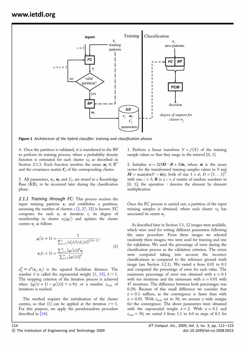
2 Design of the automatic hybridclassifierAs mentioned above, the system works in two phases:training and classification. Fig. 1 displays its architecture.The training patterns are supplied to the FC classifier,which automatically establishes a partition assuming anumber of clusters c, starting from c ¼ 1 and untilvalidation of the partition. This makes the processautomatic [1]. For each cluster, FC computes the clustercentres and BP estimates a probability density functionwith the mean and covariance matrix as parameters. Thecentres, means and covariance matrices are stored in theKnowledge Base (KB) and then recovered during theclassification phase. Given a pattern xs, it is classified asbelonging to a cluster wj by combining, through the FCMapproach, its membership degrees (provided by FC) andprobabilities (supplied by BP).

2.1 Training phase

This phase consists of the following steps:

1. We start with the observation of a set X of n trainingsamples, that is, X ¼ x1, x2, . . . , xn

� �[ <d , where d is

the data dimensionality. Each sample is to be assigned to agiven cluster wj, where the number of possible clusters is c,that is, j ¼ 1, 2, . . . , c. Each training sample vector xi

represents an image pixel, where its components are thethree RGB values of that pixel at the image location (x,y).This means that in our experiments the data dimensionalityis d ¼ 3. The RGB is the colour space used, as mentionedin Section 1.1.

2. We start by assuming that initially the number of clustersis c ¼ 1; under this assumption the training samplesare supplied to the FC clustering approach, whichdetermines the unique cluster centre v1 [ <d according tothe training procedure described below (Section 2.1.1).

3. The partition established in Step 2 is submitted to avalidation process according to the criterion described inSection 2.1.2. If it is not validated, we set c ¼ cþ 1 and goto Step 2 where c new centres, vj [ <d , are computed.Steps 2 and 3 are repeated until we achieve a valid partition.

113

& The Institution of Engineering and Technology 2009

11

&

www.ietdl.org

Figure 1 Architecture of the hybrid classifier: training and classification phases

4. Once the partition is validated, it is transferred to the BPto perform its training process, where a probability densityfunction is estimated for each cluster wj as described inSection 2.1.3. Each function involves the mean mj [ <d

and the covariance matrix Cj of the corresponding cluster.

5. All parameters, vj, mj and Cj, are stored in a KnowledgeBase (KB), to be recovered later during the classificationphase.

2.1.1 Training through FC: This process receives theinput training patterns xi and establishes a partition,assuming the number of clusters c [2, 27, 32] is known. FCcomputes for each xi at iteration t, its degree ofmembership in cluster wj(m

ji ) and updates the cluster

centres vj as follows

mji (t þ 1) ¼

1Pcr¼1 (dij(t)=dir(t))2=(b�1)

,

vj(t þ 1) ¼

Pni¼1 [m

ji (t)]bxiPn

i¼1 [mji (t)]b

(1)

d 2ij ; d 2(xi, vj) is the squared Euclidean distance. The

number b is called the exponential weight [1, 33], b . 1.The stopping criterion of the iteration process is achievedwhen km

ji (t þ 1)� m

ji (t)k , 1 8ij or a number tmax of

iterations is reached.

The method requires the initialisation of the clustercentres, so that (1) can be applied at the iteration t ¼ 1.For this purpose, we apply the pseudorandom proceduredescribed in [34]:

4The Institution of Engineering and Technology 2009

1. Perform a linear transform Y ¼ f (X ) of the trainingsample values so that they range in the interval [0, 1].

2. Initialise v ¼ 2D �M W RþD �m, where �m is the meanvector for the transformed training samples values in Y and�M ¼ max abs Y � �mð Þð Þ, both of size 1� d ; D ¼ [1 . . . 1]T

with size c � 1; R is a c � d matrix of random numbers in[0, 1]; the operation W denotes the element by elementmultiplication.

Once the FC process is carried out, a partition of the inputtraining samples is obtained, where each cluster wj hasassociated its centre vj.

As described later in Section 3.1, 12 images were available,which were used for setting different parameters followingthe same procedure. From these images we selectedrandomly three images; two were used for training and onefor validation. We used the percentage of error during theclassification process as the validation criterion. The errorswere computed taking into account the incorrectclassifications as compared to the reference ground truthimage (see Section 3.2.1). We varied 1 from 0.01 to 0.1and computed the percentage of error for each value. Themaximum percentage of error was obtained with 1 ¼ 0:1with ten iterations and the minimum with 1 ¼ 0:01 with47 iterations. The difference between both percentages was0.2%. Because of this small difference we consider that1 ¼ 0:1 suffices, as the convergence is faster than with1 ¼ 0:01. With tmax set to 50, we assume a wide marginfor the convergence. The above parameters were obtainedwith the exponential weight b ¼ 2. With 1 ¼ 0:1 andtmax ¼ 50, we varied b from 1.1 to 4.0 in steps of 0.1 for


IETdo

www.ietdl.org

the same data sets, verifying that the best performance interms of percentage of error was obtained for b ¼ 2.0.

2.1.2 Validation of the partition: This topic has beenwidely studied (see [35] and related references). We foundacceptable performance was achieved through the sum-of-squared error criterion (SE) [1], which uses the clustercentres vj obtained by FC as follows

SE(vj , x, c) ¼Xc

j¼1

Xx[wj

x� vj

�� 2(2)

SE decreases rapidly until reaching the best partition(equivalent to the best number of clusters c ¼ c), decreasingmuch more slowly thereafter until it reaches zero when thenumber of clusters is equal to the number of samples, thatis, c ¼ n. Given a number of clusters c, we compute thedelta function D

SE(c) ¼ SE(c þ 1)� SE(c), c ¼ 1, . . . ,G 2 1 which represents the difference in value for twoconsecutive numbers of clusters, where G is the last numberof clusters evaluated. We then normalise these differencesto range between [0, 1], as follows,

DSE(c) ¼

DSE(c)PG�1

i¼1 DSE(c)(3)

Starting from c ¼ 1, a partition is validated for a givennumber of clusters c when we find DSE(c) , T ; T has beenobtained after experimentation with the followingcategories of data: (a) nine data sets from the MachineLearning Repository [32] (bupa, cloud, glass, imageSegm,iris, magi4, thyroid, pimaIndians and wine); (b) threesynthetic data sets manually generated with differentnumber of clusters and (c) four data sets coming fromoutdoor natural images, also with different number ofclusters. Because we know the true number of clusters foreach category, we compute the coefficient according to (c)observing that for the true number of clusters and for eachcategory its value is less than 0.1, hence T is set to this value.

2.1.3 Training through the parametric Bayesianclassifier: Following Duda et al. [1], the Bayesian’sclassifier makes the decision about any sample x, which isto be classified, according to the following rule,

x [ wj if p(xjwj)P(wj) . p(xjwh)P(wh), 8h = j (4)

P (wj) and P(wh) are the prior probabilities that x [ wj andx [ wh, respectively; p(xjwj) and p(xjwh) are thelikelihoods that x [ wj and x [ wh, respectively. Becausewe do not have prior information about samples x, whichare to be classified, we assume that P(wj) ¼ P(wh). Thismeans that the decision is made based only on thelikelihoods, generally modelled as normal (Gaussian)probability density functions, where a function is obtained

Comput. Vis., 2009, Vol. 3, Iss. 3, pp. 112–123i: 10.1049/iet-cvi.2008.0023

for each cluster wj as follows,

p(xjwj) ¼1

2pð Þd=2 Cj

�� 1=2 exp �1

2(x�mj)

TC�1j (x�mj)

� �

(5)

d is the data dimensionality, that is, d ¼ 3 in this work.

The goal of the training process for this classifier is toestimate both parameters: the mean mj and the covarianceCj, both for each cluster wj with nj samples. Thisestimation is carried out through maximum likelihoodestimation from the validated partition supplied by FC,Fig. 1, as follows

mj ¼1

nj

Xnj

k¼1

xk, Cj ¼1

nj � 1

Xnj

k¼1

xk �mj

� xk �mj

� T

(6)

where T denotes transpose.

2.2 Classification phase

After the training phase and according to the scheme on theright part of Fig. 1, a new sample xs [ <d must be classifiedas belonging to a cluster wj. This sample, like each trainingsample, represents a pixel at the image location (x, y) withthe R, G, B components. BP computes the probabilitiesthrough (5); these probabilities can be used for classifyingxs according to the rule in (4). This allows comparing theperformance of BP with FCM. FC computes themembership degrees for xs to each cluster according to (1)and classifies the pixel according to the following rule:xs [ wj if m

ji . mh

i for all h = j. So, we can also comparethe performance of FC with FCM (see Table 2). Given animage to be classified, we compute these probabilities andmembership degrees for each pixel in the image before theFCM is started. The membership degrees are used forinitialising the networks as described in the next section.

2.2.1 Network topology of the FCMs: Now, we willdescribe the FCM approach which combines the informationprovided by the base classifiers, Fig. 1. As before, given thenew sample xs, the problem is to classify it as belonging toa cluster wj. The rule for making this decision is given.

FCMs are networks used to create models as collections ofconcepts and the various causal relations that exist betweenthese concepts [3–7]. The concepts are represented bynodes and the causal relationships by directed arcs betweenthe nodes. Each arc is accompanied by a causal weight thatdefines the type of causal relation between the two nodes.

For each cluster wj, we build a network of nodes, netj,where the topology of this network is established by thespatial distribution of the pixels in the image to beclassified with size M � N. Each node i in netj isassociated to the pixel location (x, y) in the image, that is

115


11

&

www.ietdl.org

i ; (x, y). Hence, the number of nodes in netj isq ¼M � N. For simplicity, instead of using sample xs withits R, G, B components at (x, y), we say that node i is tobe classified. Node i in netj is initialised with themembership degree m

ji provided by FC according to (1),

but mapped linearly for ranging in [�1, þ1] instead of[0, þ1]. The network states (activation levels) are themembership degrees associated to the nodes. Through theFCM these network states are reinforced or punishediteratively based on the influences exerted by theirneighbours. The goal is to make the best decision based onmore stable state values. The causal weights s

jik are the

values of the causal relations between nodes i and k in thenetwork netj, taking values in the fuzzy causal interval[�1, þ1]; they indicate the influence exerted by node kover i, increasing or decreasing the network state in i,depending on positive or negative causality values,respectively. s

jik ¼ 0 means no causality. In FCMs no

feedback from a node to itself is allowed [5, 6], so sj

ii ¼ 0.Given an image of size M � N, the goal is to classify thepixel (node) i located at (x, y) as belonging to a cluster wj.The initial states at t ¼ 0, m

ji (0) ; m

ji , are updated

based on the causal influences at each iteration t. Everynode is positively or negatively activated to a certain degree.At the end of the iterative process, the decision about thecluster to which it belongs is made based on maximumstate values considering all j networks.

2.2.2 Iterative updating process: According to [3]and [4], the activation level at the iteration tþ 1 iscomputed as

mji (tþ1)¼ f (m

ji (t), A

ji )¼ f m

ji(t),

Xq

k¼1

sjik(t)m

jk(t)

!�d

ji m

ji (t)

(7)

where mji (t) is the activation of certainty neuron i at iteration

t in network netj. Each causal weight sj

ik is defined as acombination of two coefficients representing the mutualinfluence exerted by k neighbours over i: (a) a regularisationcoefficient which computes the consistency between thestates of the nodes and the supports provided by BP in agiven neighbourhood for each netj; (b) a contextualcoefficient which computes the consistency between theclustering labels. A

ji is the sum of the weighted influence

that certainty neuron i receives at the iteration t from allother neurons. The term d

ji [ [0, 1] is the decay factor of

certainty neuron i. This factor determines the fraction ofthe current activation level that will be subtracted from thenew activation level as a result of the neuron’s naturalintention to get closer to activation level zero. The biggerthe decay factor, the stronger the decay mechanism.Following [3] and [4] function f is that used in theMYCIN expert system for the aggregation of the certainty


factors [36, 37], defined as follows,

f (x, y)¼xþy(1�x) if x, y�0,xþy(1þx) if x, y , 0,

(xþy)=(1�min( xj j, y�� )) else

8<: (8)

where xj j, y�� 1;m

ji (t) is always in that interval. However,

this does not apply for Aji , as a concept can be influenced

by many concepts and perhaps the sumPq

k¼1 sj

ikmjk(t) can

take a value outside the interval [21,þ 1]. In order tokeep A

ji within this interval it is passed through the

sigmoid function, that is, Aji¼ tanh(A

ji ), as suggested in [4].

So, under the FCM framework the influences are mappedin A

ji as consistencies, assuming that they could be non-

symmetric; the self-influence is embedded in the mji (t)

memory term. Taking into account (7), the goal is tocompute: (a) the causal weights s

jik(t) and (b) the decay

factor. A detailed analysis of the characteristics of thefunction in (8) can be found in [38].

2.2.3 Computation of the causal weights: Asmentioned before, the causal weight s

jik is the combination

of the regularisation and contextual coefficients. We defineboth coefficients and then we combine them for obtainingthe causal weights. This is described below. Taking intoaccount the mapping between a pixel location (x, y) andnode i at each netj, the neighbourhood N m

i contains mnodes surrounding i, mapped from the image andrepresenting the m-connected spatial region around thepixel (x, y). A typical value of m used in the literature is 8,which defines a 3 � 3 region; 8 is the value chosen in thispaper. We tested other values greater than 8, verifying anover-influence of the neighbourhood in (7). As can beobserved, index i varies from 1 to q, that is, this is thenumber of neighbours explored at each netj. For bordersnodes in the image, the neighbourhood only includes thepixels belonging to the image, that is, m ¼ 3 in the fourcorners and m ¼ 5 in the remainder borders.

We define the regularisation coefficient at the iteration t asfollows

rj

ik(t) ¼1� m

ji (t)� p

jk

�� k [ N mi , i = k

0 k � N mi , i ¼ k

((9)

where pj

k is supplied by BP, the probability is that node(pixel) k with attributes xk belongs to cluster wj, computedthrough (5), that is p

jk ; p xkjwj

� . These values are

mapped linearly to range between [21, þ1] instead of [0,þ1]. From (9) we can see that r

jik(t) ranges between [21,

þ1] where the lower/higher limit means minimum/maximum influence, respectively. The contextual coefficientfor node i for the cluster j at the iteration t is defined


IETdo

www.ietdl.org

taking into account the clustering labels li and lk as follows,

cik(t) ¼þ1 l i ¼ lk k [ N m

i , i = k�1 l i = lk k [ N m

i , i = k0 k � N m

i , i ¼ k

8<: (10)

where values of 21 and þ1 mean negative and positiveinfluences, respectively. Labels li and lk are obtained asfollows: Given node i, at each iteration t, we know its stateat each netj as given by (7); we determine that node ibelongs to cluster wj if m

ji (t) . mh

i (t)8j = h, so we set li tothe j value which identifies the cluster, j ¼ 1, . . . , c. Labellk is set similarly. Thus, this coefficient is independent ofthe netj, because it is the same for all networks.

Both coefficients are combined as the following averagedsum, taking into account the signs,

zj

ik(t) ¼ grj

ik(t)þ 1� gð Þcik(t), sj

ik

¼ sgn zjik

� h iv

zj

ik, sgn zj

ik

� ¼�1 z

jik � 0

þ1 zj

ik . 0

((11)

g [ [0, 1] represents the trade-off between both coefficients;sgn is the signum function and v is the number of negativevalues in set C ; W

jik (t), r

jik(t), cik(t)

n o, that is, given

S ; q [ C=q , 0� �

# C, v ¼ card(S).

2.2.4 Computation the decay factor: We define thedecay factor based on the assumption that high stability inthe network states implies that the activation level for node iin network netj would be to lose some of its activation. Webuild an accumulator of cells of size q ¼M � N, where eachcell i is associated to the node of identical name. Each cell icontains the number of times, h

ji , that node i has changed

significantly its activation level in the netj. Initially, all hji

values are set to zero and then hji ¼ h

ji þ 1 if

mji (t þ 1)� m

ji (t)

�� . 1. The stability of node i is measuredas the fraction of changes accumulated by cell i comparedwith the changes in its neighbourhood k [ N m

i and thenumber of iterations t. The decay factor is computed as follows

dj

i ¼

0 hji ¼ 0 and h

jk ¼ 0

hji

�hj

k þ hji

� t

otherwise

8>><>>: (12)

where hji is defined above and �h

j

k is the average valueaccumulated by nodes k [ N m

i . As one can see, from (12), ifh

ji ¼ 0 and h

jk ¼ 0, the decay factor takes the null value,

this means that no changes occur in the network states, thatis, high stability is achieved; if the fraction of changes issmall, the stability of node i is also high and the decay termtends towards zero. Even if the fraction is constant the decayterm tends to zero as t increases, this means that perhapsinitially some changes can occur and then no more changesare detected, this is another sign of stability. The decay


factor subtracts from the new activation level a fraction; thisimplies that the activation level could take values lesser/greater than 21 or þ1. In these cases, the activation level isset to 21 or þ1, respectively.

2.2.5 Summary of the full FCM process: adjustingthe parameters: The iterative process ends if all nodes inthe network fulfil the convergence criterionm

ji (t � 1)� m

ji (t)

�� . 1 or a number of iterations, tmax, arereached.

Next, we give details about the setting of parameter g in(11), also 1 and tmax for the convergence. We use theimages described in Section 3.1 and the same procedure asthat used for adjusting the parameters in Section 2.1.1. Theexperiments here are carried out by testing differentcombinations of g (ranging from 0.1 to 0.9 in steps of 0.1)and 1 (from 0.01 to 0.1 in steps of 0.01). With g ¼ 0:8and 1 ¼ 0:05 we achieve a percentage of error for theclassification of 12.2% with 15 iterations. With othercombinations and these parameters ranging from0:75 , g , 0:85 to 0:01 , 1 , 0:05 the error is reducedby about 0.1% but at the expense of the number ofiterations, which is considerably increased with values closeto 50. Based on these experiments, in the end we set g to0.80, 1 to 0.05 and tmax to 50 (considering a wide marginfor the number of iterations).

The FCM process is synthesised as follows:

1. Initialise: load each node with mji (t ¼ 0) as given by (1);

set 1 ¼ 0:05 and tmax ¼ 50. Define nc as the number ofnodes that change their state values at each iteration.

2. FCM process:

t ¼ 0whereas t , tmax or nc = 0

t ¼ tþ 1; nc ¼ 0;for each node i

update mji (t) according to (7)

if jmji (t)� m

ji (t � 1)j . 1 then

nc ¼ ncþ 1end if;

end for;end while

3. Outputs: the states mji (t) for all nodes updated.

2.2.6 Summary of the full process: The methodproposed, involving both the training and decision phases,can be summarised in the following steps. In the trainingphase, a number of clusters c are determined. Based on thedistribution of the samples in the c clusters, the clustercentres vj are computed through FC and the means mj andcovariance matrices Cj through BP, j ¼ 1, . . . , c. All arestored in KB. During the classification phase, given animage to be classified, we compute for each pixel i its

117


11

&

www.ietdl.org

membership degree of belonging to each cluster wj, through(1), by recovering vj from KB. For the same pixel, wecompute its probability of belonging to cluster wj through(5), recovering mj and Cj from KB. The membershipdegrees are used to initialise the networks. Then the FCMprocess for adjusting the node values starts. Once thisprocess finishes, a decision is made for each node aboutwhich cluster it belongs to. The decision about theclassification of node i with attributes xi as belonging to thecluster wj is made as: i [ wj if m

ji (t) . mh

i (t), 8j = hwhere j and h are identifiers of the clusters and t representsthe last iteration. Hence, the decision is made based on themaximum state values considering all j networks.

3 Comparative analysis andperformance evaluationTo assess the validity and performance of the proposedapproach, we describe the tests carried out according toboth processes: training and classification.

3.1 Training: estimating the bestpartition

We used a set of 36 digital aerial images acquired duringMay, 2006, from the Abadia region of Lugo (Spain). Theyare multi-spectral images, 512 � 512 pixels in size. Theimages were taken during different days from an area withseveral natural textures. We selected randomly 12 imagesfrom the set of 36 available. This set, hereinafter identifiedas ST, was used for training and the remainder set ofimages for testing. With this number of images for trainingand testing, we carried out four experiments interchangingimages between both sets, with similar results in the fourcases. Each image in the training set is down-sampled bytwo, obtaining the training samples used in this initialtraining phase, that is, the number of training samples wasn0 ¼ 12 � 256 � 256 ¼ 786 432.

Before the initial training phase started, the freeparameters described in Section 2.1.1 had to be adjusted.To do this, we randomly selected three images from ST,where the pixels excluded by the down-sampling in thethree images were used for setting these parameters. Weknew the distribution of these samples in clusters, becausethe ground truth was known. We followed the processdescribed in this section, varying the parameters andtraining with the samples extracted from two of the threeimages, that is, with 2 � 256 � 256 samples; the samplesfrom the third image were used for computing the


classification error. We selected five subsets of three imagesfrom ST without affecting the setting of the freeparameters. Once the initial process was finished with theabove n samples, we adjusted the parameters described inSection 2.2.5 before the FCM process. The samples usedfor this task were exactly those used for the above-mentioned adjustments of the three images.

Table 1 shows the behaviour of DSE(c) against the numberof clusters c ranging from c ¼ 1 to G–1, where G is set to 8 inour experiments. This is because we have not found imageswith more than 8 clusters. We can see that with T ¼ 0.1(see Section 2.1.2) the condition DSE(c) , T is fulfilled forc ¼ 4, which in the end was selected as the number ofclusters estimated.

Once the number of clusters was established, the clustercentres obtained by FC (vj) and BP (mj) and thecovariance matrices Cj for BP were stored in KB. At thisstage, because the number of clusters was already estimated,all the pixels should be classified in one of the four clusters.This implies that the set of images in the initial trainingphase must be as representative as possible of all imagesavailable. To solve this, several sets of training images mustbe selected. This justifies the experiments carried out withfour different sets of 12 images, as described above.

3.2 Classification: comparative analysis

As mentioned previously, the remaining 24 images from theset of 36 were used as images for testing. Four sets, S0, S1, S2and S3 of six images each, were processed during the testaccording to the strategy described below. The imagesassigned to each set were randomly selected from the 24images available.

3.2.1 Design of a test strategy: In order to assess thevalidity and performance of the proposed approach wedesigned a test strategy with two purposes: (a) to verify theperformance of our approach as compared with someexisting strategies; (b) to study the behaviour of the methodas the training (i.e. the learning) increases.

Our combined FCM (FM) method was compared withthe base classifiers used for the combination. FM was alsocompared with the following classical hybrid strategies [22]:Mean (ME), Max (MA) and Min (MI). Given node i withsupports m

ji and p

ji provided by FC and BP, respectively,

ME computes the mean value, that is, (mji þ p

ji )=2; MA

the maximum value, that is, maxfmji , p

ji g and MI the

minimum value, that is, minfmji , p

ji g. They were studied in

Table 1 Behaviour of the DSE (c)

C 1 2 3 4 5 6 7

D c1–c2 c2–c3 c3–c4 c4–c5 c5–c6 c6–c7 c7–c8

DSE (c) 0.4951 0.2433 0.1221 0.0728 0.0611 0.0381 0.0301


IETdoi

www.ietdl.org

terms of reliability [39]. The final decision was made basedon the maximum fused value for all clusters. Yager [40]proposed a multicriteria decision-making approach basedon fuzzy sets aggregation. So, FM was also comparedagainst the fuzzy aggregation (FA) defined by (13)

gj

i ¼ 1�min 1, 1� mji

� a

þ 1� pji

� a� 1=a �

, a � 1

(13)

This represents the joint support provided by FC and BP; thedecision is made based on the maximum support for allclusters. The parameter a is adjusted from the set of imagesdescribed in Section 3.1 and following the same procedureas that used for setting other parameters (Sections 2.1.1and 2.2.5). Two images are used for training bothclassifiers FC and BP and the third for validation. Theexperiments were carried out by varying the parameter afrom 1 to 8. The minimum error rate was achieved witha ¼ 4, which in the end was the value used for thisparameter. The decision made according to node i with thesupports provided by (13) was based on the maximumvalue, in keeping with the following rule: i [ wj

if gj

i . g hi , 8h = j.

In order to verify the behaviour of each method as thelearning degree increases, we carried out the experimentsaccording to the following three steps, described below:

Step 1: we classify the images in sets S0 and S1, where eachpixel is assigned to one of the four clusters estimatedduring the initial training phase with set ST. We computethe percentage of error for both sets according to theprocedure described in Section 3.2.2. The classifiedsamples from S1 are combined with the initial trainingsamples in ST and the resulting set is used for the trainingof the system. Hence, the number of training samples isn1 ¼ n0þ 6 � 512 � 512, where n0 is the number ofinitial training samples coming from ST. This trainingprocess is carried out assuming that the number of clustersis known (i.e. c ¼ 4). Therefore it is a partial process of thedefined in Fig. 1 because the number of clusters does not

Comput. Vis., 2009, Vol. 3, Iss. 3, pp. 112–123: 10.1049/iet-cvi.2008.0023

need to be estimated. This implies that only the parametersestimated by each classifier are updated and stored in KB.Set S0 is used as a pattern set in order to verify theperformance of the training process as the learningincreases. Note that it is not considered for training.

Step 2: we classify the images in sets S0 and S2 according tothe four clusters (based on the previous training with sets STand S1) and compute the percentage of error for both sets asbefore. Now, sets ST, S1 and S2 are combined and theresulting set is used for the training of the system withoutestimating the number of clusters, as before. Now, thenumber of samples is n2 ¼ n1þ 6 � 512 � 512. The newparameters are stored also in KB.

Step 3: we classify the images into sets S0 and S3 alsoaccording to the four clusters (based on the previoustraining with sets ST, S1 and S2) and compute thepercentage of error for both sets.

To verify the performance for each method we have built aground truth for each image under the supervision of theexpert human criterion. Based on the assumption that theautomatic training process determines four classes, weclassify each image pixel with the simple classifiers,obtaining a labelled image with four expected clusters. Foreach class we build a binary image, which is manuallytouched up until a satisfactory classification is obtainedunder human supervision.

Fig. 2(a) displays an original image belonging to set S0;Fig. 2(b) displays the correspondence between the classesand the label assigned to the corresponding cluster centreaccording to a labelling map previously defined; Fig. 2(c)labelled image for the four clusters obtained by ourproposed FM approach. The labels are artificial greyintensities identifying each cluster. The correspondencebetween labels and the different textures is: 1 – withforest vegetation; 2 – with bare soil; 3 – with agriculturalcrop vegetation; 4 – with buildings and man madestructures.

Figure 2 Mapping between original textures and labels

a Original image belonging to set S0b Correspondence between labels and clustersc Labelled image with the four clusters according to (b)

119


12

&

www.ietdl.org

Fig. 3 displays the binary ground truth images for eachcluster, where the white pixels represent the correspondingcluster; Figs. 3(a)–(d ) represent the clusters numbers 1–4,respectively, identified in Fig. 2.

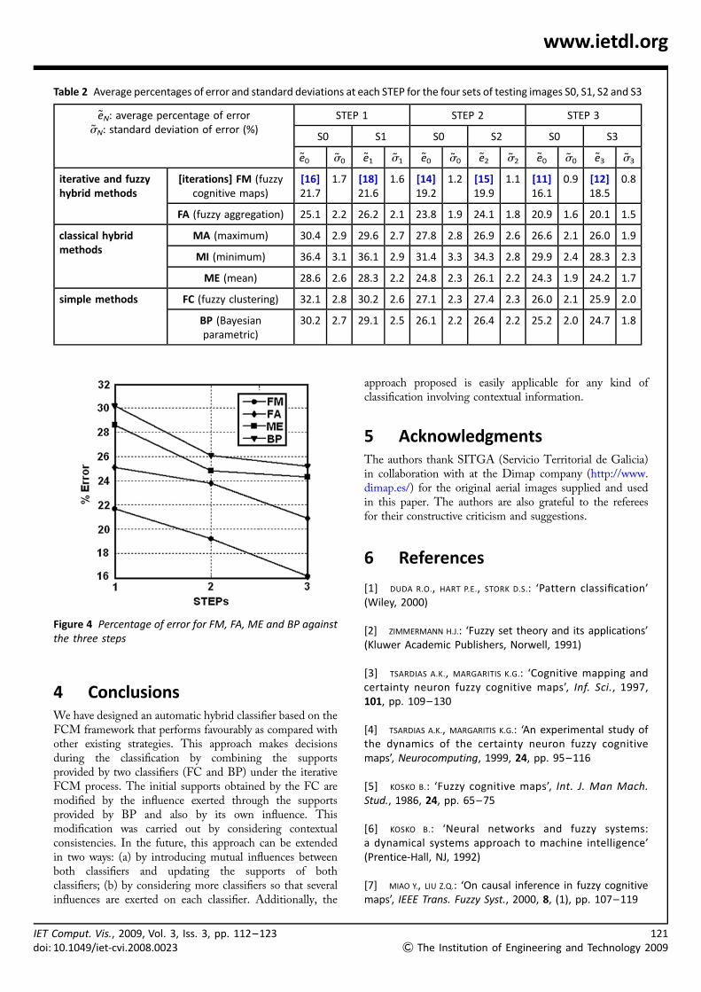
3.2.2 Results: Table 2 shows the percentage of error duringthe classification for the different classifiers. For each step, from1 to 3, we show the results obtained for both sets of tested imagesS0 and either S1 or S2 or S3. These percentages are computed asfollows. Let I r

N be an image r(r ¼ 1, . . . , 6) belonging to set SN(N ¼ 0, 1, 2, 3); i is the node at location (x, y) in I r

N . An errorcounter Er

N is initially set to zero for each image r in set SN ateach step and for each classifier. Based on the correspondingdecision process, each classifier determines the cluster towhich node i belongs, i [ wj . If the same pixel location onthe corresponding ground truth image is black, then the pixelis incorrectly classified and Er

N ¼ ErN þ 1. The error rate of

the image I rN is: er

N ¼ ErN =Z, where Z is the image size, that

is, 512 � 512. The average error rate for set SN at eachstep is: �eN ¼ 1=6

P6r¼1 er

N and the standard deviation

�sN ¼

ffiffiffiffiffiffiffiffiffiffiffiffiffiffiffiffiffiffiffiffiffiffiffiffiffiffiffiffiffiffiffiffiffiffiffiffiffiffiffiffiffi1=5

P6r¼1 (er

N � �eN )2q

. In Table 2, they are displayed

as percentages, that is, ~eN ¼ 100�eN and ~sN ¼ 100 �sN . Thenumbers in square brackets in the row FM indicate therounded and averaged number of iterations required by eachset at each step.

3.2.3 Discussion: From the results in Table 2, it is seenthat the best performance is achieved by the proposed FM


strategy. The best performance for the classical hybridmethods is achieved by ME and for the simple methods byBP. The best performances are established in terms of theleast average percentage of error and the least standarddeviation values. For clarity, in Fig. 4 the performanceof the proposed FM approach for set SP0 is displayedagainst FA and the best methods at each group, that is,ME for the classical hybrid approaches and BP for simplemethods.

The results show that the hybrid approaches performfavourably for the data sets used. The MA and ME fusionmethods provide better results than the individual ones.This means that fusion strategies are suitable forclassification tasks. This agrees with the conclusionreported in [27] about the choice of combiners.

Moreover, as the learning increases through steps 1–3, theperformance improves and the number of iterations for S0decreases. This means that the learning phase is importantand that the number of samples affects the performance.

The main drawback of the FCM approach is its executiontime, which is greater than for the remaining methods anddirectly proportional to the number of iterations. All testshave been implemented in MATLAB and executed on aPentium M, 1.86 GHz with 1 GB RAM. On average, theexecution per iteration is 17.2 s.

Figure 3 Ground truth images (a)–(d ) for the four clusters 1–4 displayed in Fig. 2


IEdo

www.ietdl.org

Table 2 Average percentages of error and standard deviations at each STEP for the four sets of testing images S0, S1, S2 and S3

eN: average percentage of errorsN: standard deviation of error (%)

STEP 1 STEP 2 STEP 3

S0 S1 S0 S2 S0 S3

e0 s0 e1 s1 e0 s0 e2 s2 e0 s0 e3 s3

iterative and fuzzyhybrid methods

[iterations] FM (fuzzycognitive maps)

[16]21.7

1.7 [18]21.6

1.6 [14]19.2

1.2 [15]19.9

1.1 [11]16.1

0.9 [12]18.5

0.8

FA (fuzzy aggregation) 25.1 2.2 26.2 2.1 23.8 1.9 24.1 1.8 20.9 1.6 20.1 1.5

classical hybridmethods

MA (maximum) 30.4 2.9 29.6 2.7 27.8 2.8 26.9 2.6 26.6 2.1 26.0 1.9

MI (minimum) 36.4 3.1 36.1 2.9 31.4 3.3 34.3 2.8 29.9 2.4 28.3 2.3

ME (mean) 28.6 2.6 28.3 2.2 24.8 2.3 26.1 2.2 24.3 1.9 24.2 1.7

simple methods FC (fuzzy clustering) 32.1 2.8 30.2 2.6 27.1 2.3 27.4 2.3 26.0 2.1 25.9 2.0

BP (Bayesianparametric)

30.2 2.7 29.1 2.5 26.1 2.2 26.4 2.2 25.2 2.0 24.7 1.8

Ti:

4 ConclusionsWe have designed an automatic hybrid classifier based on theFCM framework that performs favourably as compared withother existing strategies. This approach makes decisionsduring the classification by combining the supportsprovided by two classifiers (FC and BP) under the iterativeFCM process. The initial supports obtained by the FC aremodified by the influence exerted through the supportsprovided by BP and also by its own influence. Thismodification was carried out by considering contextualconsistencies. In the future, this approach can be extendedin two ways: (a) by introducing mutual influences betweenboth classifiers and updating the supports of bothclassifiers; (b) by considering more classifiers so that severalinfluences are exerted on each classifier. Additionally, the

Figure 4 Percentage of error for FM, FA, ME and BP againstthe three steps

Comput. Vis., 2009, Vol. 3, Iss. 3, pp. 112–12310.1049/iet-cvi.2008.0023

approach proposed is easily applicable for any kind ofclassification involving contextual information.

5 AcknowledgmentsThe authors thank SITGA (Servicio Territorial de Galicia)in collaboration with at the Dimap company (http://www.dimap.es/) for the original aerial images supplied and usedin this paper. The authors are also grateful to the refereesfor their constructive criticism and suggestions.

6 References

[1] DUDA R.O., HART P.E., STORK D.S.: ‘Pattern classification’(Wiley, 2000)

[2] ZIMMERMANN H.J.: ‘Fuzzy set theory and its applications’(Kluwer Academic Publishers, Norwell, 1991)

[3] TSARDIAS A.K., MARGARITIS K.G.: ‘Cognitive mapping andcertainty neuron fuzzy cognitive maps’, Inf. Sci., 1997,101, pp. 109–130

[4] TSARDIAS A.K., MARGARITIS K.G.: ‘An experimental study ofthe dynamics of the certainty neuron fuzzy cognitivemaps’, Neurocomputing, 1999, 24, pp. 95–116

[5] KOSKO B.: ‘Fuzzy cognitive maps’, Int. J. Man Mach.Stud., 1986, 24, pp. 65–75

[6] KOSKO B.: ‘Neural networks and fuzzy systems:a dynamical systems approach to machine intelligence’(Prentice-Hall, NJ, 1992)

[7] MIAO Y., LIU Z.Q.: ‘On causal inference in fuzzy cognitivemaps’, IEEE Trans. Fuzzy Syst., 2000, 8, (1), pp. 107–119

121


12

&

www.ietdl.org

[8] VALDOVINOS R.M., SANCHEZ J.S., BARANDELA R.: ‘Dynamic andstatic weighting in classifier fusion’ in MARQUES J.S., PEREZ

DE LA BLANCA N., PINA P. (EDS.) : ‘Pattern recognition andimage analysis’ (Lecture notes in computer scienceSpringer-Verlag, Berlin, 2005), pp. 59–66

[9] PUIG D., GARCIA M.A.: ‘Automatic texture feature selectionfor image pixel classification’, Pattern Recognit., 2006, 39,(11), pp. 1996–2009

[10] HANMANDLU M., MADASU V.K., VASIKARLA S.: ‘A fuzzy approachto texture segmentation’. Proc. IEEE Int. Conf. InformationTechnology: Coding and Computing (ITCC’04), TheOrleans, Las Vegas, Nevada, USA, 2004, pp. 636–642

[11] RUD R., SHOSHANY M., ALCHANATIS V., COHEN Y.: ‘Application ofspectral features’ ratios for improving classification inpartially calibrated hyperspectral imagery: a case study ofseparating Mediterranean vegetation species’, J. Real-Time Image Process., 2006, 1, pp. 143–152

[12] KUMAR S., GHOSH J., CRAWFORD M.M.: ‘Best-bases featureextraction for pairwise classification of hyperspectraldata’, IEEE Trans. Geosci. Remote Sens., 2001, 39, (7),pp. 1368–1379

[13] YU H., LI M., ZHANG H.J., FENG J.: ‘Color texture moments forcontent-based image retrieval’. Proc. Int. Conf. ImageProcessing, 2002, vol. 3, pp. 24–28

[14] MAILLARD P.: ‘Comparing texture analysis methodsthrough classification’, Photogram. Eng. Remote Sens.,2003, 69, (4), pp. 357–367

[15] RANDEN T., HUSØY J.H.: ‘Filtering for texture classification:a comparative study’, IEEE Trans. Pattern Anal. Mach.Intell., 1999, 21, (4), pp. 291–310

[16] WAGNER T.: ‘Texture analysis’ in JAHNE B., HAUbECKER H.,GEIbLER P. (EDS.) : ‘Handbook of computer vision andapplications’ (Academic Press, 1999, vol. 2), (SignalProcessing and Pattern Recognition)

[17] SMITH G., BURNS I.: ‘Measuring texture classificationalgorithms’, Pattern Recognit. Lett., 1997, 18, pp. 1495–1501

[18] DR.IMBAREAN A., WHELAN P.F.: ‘Experiments in colourtexture analysis’, Pattern Recognit. Lett., 2003, 22, (4),pp. 1161–1167

[19] KONG Z., CAI Z.: ‘Advances of research in fuzzy integralfor classifier’s fusion’. Proc. Eighth ACIS Int. Conf. SoftwareEngineering, Artificial Intelligence, Networking andParallel/Distributed Computing, 2007, vol. 2, pp. 809–814

[20] KUNCHEVA L.I.: ‘“Fuzzy” vs “non-fuzzy” in combiningclassifiers designed by boosting’, IEEE Trans. Fuzzy Syst.,2003, 11, (6), pp. 729–741


[21] KUMAR S., GHOSH J., CRAWFORD M.M.: ‘Hierarchical fusion ofmultiple classifiers for hyperspectral data analysis’, PatternAnal. Appl., 2002, 5, pp. 210–220

[22] KITTLER J., HATEF M., DUIN R.P.W., MATAS J.: ‘On combiningclassifiers’, IEEE Trans. Pattern Anal. Mach. Intell., 1998,20, (3), pp. 226–239

[23] CAO J., SHRIDHAR M., AHMADI M.: ‘Fusion of classifierswith fuzzy integrals’. Proc. Third Int. Conf. DocumentAnalysis and Recognition (ICDAR’95), 1995, vol. 1,pp. 108–111

[24] PARTRIDGE D., GRIFFITH N.: ‘Multiple classifier systems:software engineered, automatically modular leading to ataxonomic overview’, Pattern Anal. Appl., 2002, 5,pp. 180–188

[25] DENG D., ZHANG J.: ‘Combining multipleprecision-boosted classifiers for indoor-outdoor sceneclassification’, Inf. Technol. Appl., 2005, 1, (4 – 7),pp. 720–725

[26] ALEXANDRE L.A., CAMPILHO A.C., KAMEL M.: ‘On combiningclassifiers using sum and product rules’, Pattern Recognit.Lett., 2001, 22, pp. 1283–1289

[27] KUNCHEVA L.I.: ‘Combining pattern classifiers: methodsand algorithms’ (Wiley, 2004)

[28] STACH W., KURGAN L., PEDRYCZ W., REFORMAT M.: ‘Evolutionarydevelopment of fuzzy cognitive maps’. Proc. IEEE Conf.Fuzzy Syst., 2005, pp. 619–624

[29] CHENG Q., FANG Z.T.: ‘The stability problem for fuzzybidirectional associative memories’, Fuzzy Sets Syst., 2002,132, pp. 83–90

[30] MARTCHENKO A.S., ERMOLOV I.L., GROUMPOS P.P., PODURAEV J.V.,STYLIOS C.D.: ‘Investigating stability analysis issues for fuzzycognitive maps’. 11th Mediterranean Conf. Control andAutomation, 2003, pp. 619–624

[31] AGUILAR J.: ‘A survey about fuzzy cognitive maps papers’,Int. J. Comput. Cogn., 2005, 3, (2), pp. 27–33

[32] ASUNCION A., NEWMAN D.J.: ‘UCI machine learning repository’(University of California, School of Information and ComputerScience, Irvine, CA, 2008), available on-line http://www.ics.uci.edu/~mlearn/MLRepository.html

[33] BEZDEK J.C.: ‘Pattern recognition with fuzzy objectivefunction algorithms’ (Kluwer, Plenum Press, New York,1981)

[34] BALASKO B., ABONYI J., FEIL B.: ‘Fuzzy clusteringand data analysis toolbox for use with Matlab’(Veszprem University, Hungary, 2008), (available from


IETdo

www.ietdl.org

URL: http://www.fmt.vein.hu/softcomp/fclusttoolbox/FuzzyClusteringToolbox.pdf)

[35] VOLKOVICH Z., BARZILY Z., MOROZENSKY L.: ‘A statistical modelof cluster stability’, Pattern Recognit., 2008, 41, (7),pp. 2174–2188

[36] BUCHANAN B.G., SHORLIFFE E.H. (EDS.): ‘Rule-based expertsystems. The MYCIN experiments of the Stanford HeuristicProgramming Project’ (Addison-Wesley, Reading, MA, 1984)

[37] SHORLIFFE E.H.: ‘Computer-based medical consultations:MYCIN’ (Elsevier, New York, NY, 1976)


[38] TSARDIAS A.K., MARGARITIS K.G.: ‘The MYCIN certainty factorhandling as uniform operator and its use as thresholdfunction in artificial neurons’, Fuzzy Sets Syst., 1998, 93,pp. 263–274

[39] CABRERA J.B.D.: ‘On the impact of fusion strategies onclassification errors for large ensambles of classifiers’,Pattern Recognit., 2006, 39, pp. 1963 –1978

[40] YAGER R.R.: ‘On ordered weighted averagingaggregation operators in multicriteria decision making’,IEEE Trans. Syst. Man Cybern., 1988, 18, (1),pp. 183– 190

123


Combining classifiers through fuzzy cognitive maps in natural images

Documents

Transcript of Combining classifiers through fuzzy cognitive maps in natural images