Multivariate calibration of hyperspectral g-rayenergy spectra for proximal soil sensing

R. A. VISCARRA ROSSEL, H. J. TAYLOR & A. B. MCBRATNEY

Australian Centre for Precision Agriculture, The University of Sydney, Sydney, NSW 2006, Australia

Summary

The development of proximal soil sensors to collect fine-scale soil information for environmental moni-

toring, modelling and precision agriculture is vital. Conventional soil sampling and laboratory analyses

are time-consuming and expensive. In this paper we look at the possibility of calibrating hyperspectral

g-ray energy spectra to predict various surface and subsurface soil properties. The spectra were collected

with a proximal, on-the-go g-ray spectrometer. We surveyed two geographically and physiographically

different fields in New South Wales, Australia, and collected hyperspectral g-ray data consisting of 256

energy bands at more than 20 000 sites in each field. Bootstrap aggregation with partial least squares

regression (or bagging-PLSR) was used to calibrate the g-ray spectra of each field for predictions of

selected soil properties. However, significant amounts of pre-processing were necessary to expose the

correlations between the g-ray spectra and the soil data. We first filtered the spectra spatially using local

kriging, then further de-noised, normalized and detrended them. The resulting bagging-PLSR models of

each field were tested using leave-one-out cross-validation. Bagging-PLSR provided robust predictions of

clay, coarse sand and Fe contents in the 0–15 cm soil layer and pH and coarse sand contents in the 15–50

cm soil layer. Furthermore, bagging-PLSR provided us with a measure of the uncertainty of predictions.

This study is apparently the first to use a multivariate calibration technique with on-the-go proximal g-rayspectrometry. Proximally sensed g-ray spectrometry proved to be a useful tool for predicting soil proper-

ties in different soil landscapes.

Introduction

The acquisition of fine-scale information on the variation of soil

properties usingmanual soil sampling and conventional labora-

tory analyses is time-consuming and expensive. The develop-

ment of alternative methods for attaining this information is

crucial for soil monitoring, modelling and precision agriculture

(Viscarra Rossel & McBratney, 1998a). Potentially, proximal

soil sensors provide a rapid and inexpensive solution to this

problem through their ability to collect high-resolution data in

real-time, by taking measurements as frequently as once every

second (Viscarra Rossel & McBratney, 1998b; Sudduth et al.,

1997). Currently electrical resistivity (ER) and electromagnetic

induction (EMI) sensors are the only real-time proximal soil

sensors that are widely used commercially (Adamchuk et al.,

2004), although there are other sensors under development

(Sudduth et al., 1997).

At the very short wavelength/high frequency end of the elec-

tromagnetic spectrum, with discrete energy values of more than

40 keV, there is potential for the use of g-radiometric methods in

soil survey (Billings, 1998). The basis of g-ray spectrometry is

that g-ray photons have discrete energies, which are character-

istic of the radioactive isotopes from which they originate

(IAEA, 2003). By measuring the energies of g-ray photons, it is

possible to determine the source of the radiation. Gamma-rays

interact with atoms of matter through: (i) photoelectric absorp-

tion at low energies; (ii) Compton scattering, which is the dom-

inant process for g-rays of terrestrial origin; and (iii) pair

production, which occurs at higher energies (ICRU, 1994).

While many naturally occurring elements have radioactive iso-

topes, only potassium (40K) and the decay series of uranium

(238U and 235U and their daughters) and thorium (232Th and

its daughters) have long half-lives, are abundant in the envi-

ronment, and produce g-rays of sufficient energy and intensity

to be measured by g-ray spectrometry.

Gamma-ray spectrometers typically measure 256 channels

that comprise an energy spectrum ranging from 0 to 3 MeV

(Figure 1). Radiation not originating from the earth’s surface

is regarded as background and is removed during data pre-

processing. The main sources of background radiation are

atmospheric radon (222Rn), cosmic sources and instrumental

Correspondence: R. A. Viscarra Rossel. E-mail: r.viscarra-rossel@usyd.

edu.au

Received 14 December 2005; revised version accepted 26 May 2006

European Journal of Soil Science, February 2007, 58, 343–353 doi: 10.1111/j.1365-2389.2006.00859.x

# 2006 The Authors

Journal compilation # 2006 British Society of Soil Science 343

sources (IAEA, 2003). The conventional approach to the

acquisition and processing of g-ray data is to monitor four

broad spectral windows or regions of interest (ROI) corre-

sponding to K (ROIK), U (ROIU), Th (ROITh) and the total

count (ROITC). ROIK monitors the 1.460 MeV g-rays emitted

by 40K, while ROIU and ROITh monitor g-ray emissions of

decay products in the U and Th decay series. For ROIU the

energy of the photopeak is centred on 1.765 MeV and for

ROITh it is centred on 2.614 MeV (Figure 1). The ROITC gives

a measure of total radioactivity and it is the integrated count

over the 0.4–2.81 MeV range (Figure 1).

Typically, g-ray photons lose energy byCompton scattering in

the source, the detector and in matter between the source and

detector. The relative intensity of g-rays depends on the source-

detector geometry and the amount of attenuating material

between the source and the detector (Grasty, 1979). Due to the

interaction of g-rays with matter, the intensity of radiation will

decrease with increasing distance from the source and radiation

will be attenuated in the source and by material between the

source and detector (IAEA, 2003).

In soil surveying, the value of g-ray spectrometry lies princi-

pally in the fact that different rock types contain varying

amounts of radioisotopes of K, U and Th, as do the soil profiles

to which they weather (Dickson & Scott, 1997). Approximately

95% of the measurable g-radiation is emitted from the upper

0.5 m of the profile (Gregory & Horwood, 1961). The attenua-

tion of g-rays through the soil varies with bulk density andwatercontent (Taylor et al., 2002). Signal attenuation increases by

approximately 1% for each 1% increase in volumetric water

content (Cook et al., 1996). The half thickness (i.e. the thick-

ness of absorbing material that will reduce the radiation to

half its value) of dry soil with a bulk density of 1.6 Mg m–3 is

10 cm (Grasty, 1979). The half thickness for air is 121 m for

a 2 MeV source (Grasty, 1979), thus making possible the

detection of g-rays from airborne platforms.

Numerous studies using airborne g-ray spectrometry surveys

have identified relationships between the g-ray ROI counts and

soil type, which are a function of parent material and the pedo-

genesis of the soils (e.g. Darnley & Ford, 1987; Dickson et al.,

1996; Dickson & Scott, 1997). Airborne g-radiometry has been

used for the past 30 years for mineral exploration due to the

relationship that exists between the material forming the sur-

face and the underlying geology (Darnley & Ford, 1987; Dick-

son & Scott, 1997). However, these airborne studies cannot

always distinguish soils with a common parent material because

of the changes in radioelement concentrations that occur during

pedogenesis (e.g. Cook et al., 1996; Wilford et al., 1997). More

recent studies use g-radiometrics to map soil types according to

the relationship that exists between individual soil properties

and the g-ray ROI data. Pracilio et al. (2003) compared pre-

dictions, obtained with linear regressions of soil properties such

as (log-transformed) clay content on the ROI counts, between

study sites on contrasting parent materials. They reported a R2

value of 0.68 for the regression of clay content on ROITh.

Similar studies have also been conducted with ground-based

g-ray spectrometers. For example, ground-based g-radiometrics

has been used to establish relationships between ROIK counts

and apparent topsoil dust accumulations, which were identi-

fied as containing appreciable feldspar and illite (Cattle et al.,

2003). Rampant & Abuzar (2004) used ROI counts to identify

yield management zones for precision agriculture. Many stud-

ies also report considerably better relationships between the

ROI data and soil properties than do airborne surveys.

Wong & Harper (1999) identified excellent linear relationships

between ROIK and available potassium. Pracilio et al. (2004a)

showed that there was a significant relationship between log

ROITh and gravel content (R2 ¼ 0.63) at a site in western Aus-

tralia. They also identified significant relationships between

the log ROITC and clay content (R2 ¼ 0.63). Taylor et al.

(2002) identified similar linear relationships between ROITCand clay content (R2 ¼ 0.71). These authors also found rela-

tionships between ROITh and ironstone gravel (R2 ¼ 0.23) and

between ROIK and total feldspar content (R2 ¼ 0.62). Pracilio

et al. (2004b) attempted to improve the linear prediction

models created by Pracilio et al. (2003) by using regression

trees, which combined the ROIK,U,Th counts with topographic

data to predict soil properties. The technique improved R2

values for predictions of clay content but not for available K.

Whilst these mostly univariate relationships between ROI

counts and soil properties have been identified by various

authors, we have not found any literature on the use of the

g-ray hyperspectra with multivariate calibration in soil or envi-

ronmental studies. In remote sensing it has been shown that

much more information can be obtained from hyperspectral

(> 128 channels) imagery than from multispectral (3–10 chan-

nels) (Tsai & Philpot, 1998). It may be possible to improve

Potassium

Energy /MeV

Inte

nsity

/cou

nts

s-1

0 0.5 1.5 3.02.52.01.0

0

10

20

30

40

50

60

70

Uranium Thorium

Total count

Figure 1 Typical gamma-ray spectrum and position of the regions of

interest (ROI) for potassium (ROIK), uranium (ROIU), thorium

(ROITh), and total count (ROITC). The energies of the photopeaks

are: ROIK ¼ 1.460 MeV (range of 1.370–1.570 MeV); ROIU ¼ 1.765

MeV (range of 1.660–1.860 MeV); and ROITh ¼ 2.614 MeV (range of

2.410–2.810 MeV). The range of ROITC is 0.4–2.810 MeV. (Modified

from Wilford et al., 1997.)

344 R. A. Viscarra et al.

# 2006 The Authors

Journal compilation # 2006 British Society of Soil Science, European Journal of Soil Science, 58, 343–353

predictions of soil properties using all 256 channels of the g-rayspectrometer, rather than just the ROIs. Multivariate chemo-

metric methods such as partial-least-squares regression (PLSR)

may be applied to discern the more complex attenuated g-rayemissions fromfield soil. PLSRhas been usedwith hyperspectral

visible and infrared soil data for predictionof soil properties (e.g.

Viscarra Rossel et al., 2006). Thus, the aim of this work is to

calibrate the hyperspectral information from a proximal g-rayspectrometer for prediction of field soil properties.

Materials and methods

Field sites

The study was conducted at two geographically and physio-

graphically different sites in New South Wales, Australia. The

first site, Nowley (30.23°S, 150.24°E) consists of three fields

(F-Brigalow, 12-Brigalow and Coda), with a combined area of

190-ha. TheNowley site is located in the Liverpool Plains on the

Northwest Slopes and Plains. It is located in the Trinkey Forest

soil landscape of the Curlewis 1:100 000 sheet (Banks, 1995). It

has topography of extensive foot slopes (> 2 km) of undulating

low hills and hills derived from alluvial fan systems. This trans-

ferral landscape consists predominantly of deep deposits of par-

ent materials eroded from quartzose and lithic sandstones, silty

sandstones andmudstones of the Jurassic Purlewaugh Beds and

Pilliga Sandstones (Banks, 1995). The second site, Stanleyville

(30.32°S, 148.23°E) is a 202-ha field located on the eastern fringeof the Upper Western Region of New South Wales near Gular-

gambone. The Stanleyville site forms part of the Carrabear For-

mation formed during the late Pleistocene from the alluvial

deposition of parent material sourced from the quartz rich

Jurassic Pilliga sandstone (Banks, 1995). The fields consist

mostly of backplain facies formed by the sedimentation of silts

and clays during overbank flow, resulting in plains with very low

slopes and minimal relief.

Soil sampling and laboratory analysis

A Latin hypercube sampling strategy (Minasny & McBratney,

2006) based on proximally sensed electrical conductivity and

g-ray ROI data was used to select 20 sample sites in each of the

studyfields.At each sample site a 1msoil corewas placed inPVC

piping and wrapped securely in plastic. Soil from 0–15 cm and

15–50 cm was removed from each core and homogenized. The

pHCa (pH measured in a 0.01-M CaCl2 solution) and electrical

conductivity (EC) of these samples were measured according

to the methods outlined in the Australian laboratory hand-

book of soil and water chemical methods (Rayment & Higginson,

1992). Particle-size analysis was by the hydrometer method

(Gee & Bauder, 1986) to determine percentage clay, silt, coarse

sand and fine sand. Citrate/dithionite-extractable iron and

bicarbonate-extractable potassium (Rayment & Higginson,

1992) were estimated by atomic absorption spectroscopy for

the 0–15 cm samples only.

Proximal soil sensing using the g-ray spectrometer

Radiometric measurements were made using the GR320 porta-

ble g-ray spectrometer (Exploranium� Radiation Detection

Systems, Toronto, Canada), with a 4.2-litre thallium-activated

sodium iodide detector crystal. The g-ray spectrometer was

mounted in a wooden cradle on the front of a four-wheel-drive

vehicle for on-the-go fieldmeasurements. The vehicle was driven

at approximately 3 m s–1 and the data were recorded at a fre-

quency of 1 Hz, together with positioning information from an

Omnistar HP single-frequency carrier phase DGPS (Omnistar,

Fugro, Australia). Both the radiometric regions of interest

(ROITC, ROIK, ROIU and ROITh) and the hyperspectral

information consisting of 256 channels of information were

logged (every second) into a customized data logger directly

into a laptop computer.

g-ray data processing

The g-ray spectral channels were converted to energy (E) accord-ing to the following relationship:

EðMeVÞ ¼ ð11:7gÞ1000

; ð1Þ

where g is the channel number, an increment of which is equiv-

alent to 11.7 keV.

Preprocessing of g-ray spectra for multivariate calibration

To improve the signal-to-noise ratio, the raw g-ray spectra in

each field were filtered with the kriging algorithm using local

variograms. We did this with VESPER (Minasny et al., 2003).

Each of the 256 energy bands was kriged onto the 20 sample

sites across each field. Kriging of the spectra was found to

work more effectively than the more conventional hyper-

spectral pre-processing techniques such as the Savitzky-Golay

technique (Tsai & Philpot, 1998). The spectra were pre-

processed further by wavelet de-noising with soft thresholding

(Donoho, 1995) by using a Daubechies wavelet with four van-

ishing moments and the principle of Stein’s Unbiased Risk

Estimate (SURE) (e.g. Zhang & Desai, 1998). The noise stan-

dard deviation was calculated from the wavelet coefficients at

each wavelet scale independently. Then, the noise variance was

used to rescale the threshold. The standard normal variate

(SNV) correction (Candolfi et al., 1999; Luypaert et al., 2004)

with wavelet detrending was applied to correct baseline shifts

and to remove curvilinearity in the spectra. The SNV correc-

tion normalizes each spectrum by the standard deviation of

the responses across the entire spectral range:

XiðSNVÞ ¼xi � �xiffiffiffiffiffiffiffiffiffiffiffiffiffiffiffiffiffiffiffiffiffi+p

j ¼ 1

ðxi;j � �xiÞ2

ðp � 1Þ

s ; ð2Þ

where X is an n by p matrix of the spectra for all energies, xi is

a 1 by p vector of the responses for a single spectrum, x�i is the

Calibration of hyperspectral g-ray energy spectra 345

# 2006 The Authors

Journal compilation # 2006 British Society of Soil Science, European Journal of Soil Science, 58, 343–353

average of the spectral responses in the vector, n is the number

of samples and p is the number of energy levels in the spectra.

Wavelet detrending was implemented by applying the discrete

wavelet transform, as above, and setting the approximation

coefficients to zero and reconstructing the signal based on all

the detailed coefficients. When combined with the kriging fil-

ter, these techniques produced the best results and improved

the robustness of our g-ray hyperspectral calibrations. A prin-

cipal components analysis (PCA) of the data was conducted

prior to modelling.

Multivariate calibration of g-ray spectra

We had a total of 20 points from each field. Each field was

calibrated separately. The partial least-squares 1 (PLSR1) algo-

rithm (Wold et al., 1983) for a single y-variable was used to

model the data. PLSR1 allowed us to formulate calibration

equations from the highly collinear g-ray spectra to predict

various soil properties. Bootstrap aggregation or bagging

(Breiman, 1996) was used to get a more robust, aggregated

predictor, where the bagging-PLSR estimates are calculated

from the mean of the bootstrap and their uncertainty using

their 95% confidence intervals. Briefly, the bootstrap measures

the uncertainty of a prediction by generating different models

from different realizations of the data. It assumes that the

training (or calibration) data set is a representation of the popu-

lation, and that multiple realizations of the population may be

simulated from a single data set (Hastie et al., 2001). The boot-

strap is conducted by repeated random ‘sampling with replace-

ment’ of the original data set of size N to obtain B bootstraps,

each of size N. Thus for each field, we had 50 PLSR models for

each soil property, each with 20 random samples.

Leave-one-out cross-validation (Efron & Tibshirani, 1993)

was used to select the best bagging-PLSR predictors for each

field. These models were assessed using the root mean-squared

error (RMSE), the mean error (ME) and the standard deviation

(SDE) of the error distribution, which measure their accuracy,

bias and precision, respectively. We also recorded the adjusted

coefficient of determination, R2adj., which measures the pro-

portion of the variation in the response that may be attributed

to the model rather than to random error. The adjustment

makes the coefficient more comparable between models with

different numbers of parameters than the usual R2 as it uses

the degrees of freedom in its computation. Finally, we recor-

ded the ratio of percentage deviation (RPD), which is the ratio

of the standard deviation of the laboratory measured (refer-

ence) data to the RMSE of the cross-validation (Williams,

1987). It is the factor by which the prediction accuracy has

been increased compared with using the mean of the original

data. We classified RPD values as follows: RPD < 1.0 indi-

cates very poor model and/or predictions and their use is not

recommended; RPD between 1.0 and 1.4 indicates poor model

and/or predictions where only high and low values are distin-

guishable; RPD between 1.4 and 1.8 indicates fair model

and/or predictions that may be used for assessment and corre-

lation; RPD values between 1.8 and 2.0 indicates good model

and/or predictions where quantitative predictions are possible;

RPD between 2.0 and 2.5 indicates very good, quantitative

model and/or predictions, and RPD > 2.5 indicates excellent

model and/or predictions.

Bagging-PLSR predictions of field soil properties

and mapping

Asbefore, all of the g-ray spectra collectedon-the-go fromeachof

the two fields (Figure 2) were filtered by kriging. For every spec-

trum in each field, each of the 256 energy bands was kriged onto

5-m grids. These data were pre-processed further as described

previously and bagging-PLSR was used to predict the surface-

soil and subsoil properties with the best cross-validation results.

Hence, we created maps of clay and Fe content for the 0–15 cm

layer at Nowley and pHCa and coarse sand content for the

15–50 cm layer at Stanleyville using ArcMap (ESRI, 2002).

The pre-processing, PCA analysis, PLSR and bagging-PLSR

modelling and predictions were made using ParLeS v2.1

(Viscarra Rossel, 2005).

Results

The soil in the study fields

The 20 sampling points in each field, as well as the locations of

the 35 000 and 23 000 proximally sensed g-ray spectra across

the Nowley and Stanleyville fields, respectively, are shown in

Figure 2.

Larger ROITC values were evident on the eastern halves

of both fields (Figure 2). Descriptive statistics of laboratory-

measured soil data are given in Table 1.

Table 1 shows that the soil atNowley tended to bemore acidic

and with less clay than those at Stanleyville. The soil at Nowley

consisted of mostly Dermosols and Chromosols (Isbell, 1996),

while that at Stanleyville consisted of mainly Vertosols and

Dermosols (Isbell, 1996). The FAO-WRB classification of

these soils (FAO, 1998) is given in Table 1. In a number of the

Vertosols at Staneyville, lime (CaCO3) and gypsum (CaSO4)

were present in increasing amounts down the soil profile. Lime

was also found in some of the subsoils at Nowley, reflecting

the less arid climate with larger rainfall at Nowley, which

allows more water to enter the soil profile.

Pre-processing and principal components analysis (PCA)

of the g-ray spectra

The raw g-ray spectra were very noisy (Figure 3a), and initially

the data did not appear to havemuch correlation with any of the

soil properties investigated. Spatial aggregation with the kriging

filter improved the signal-to-noise ratio (Figure 3b), and further

pre-processingproduced smoother, detrended spectra (Figure 3c).

346 R. A. Viscarra et al.

# 2006 The Authors

Journal compilation # 2006 British Society of Soil Science, European Journal of Soil Science, 58, 343–353

The first two PCA loadings of the raw, the kriged and the pre-

processed spectra are given in Figure 3(d,e,f), respectively.

These PCA loadings highlight the effects of the kriging filtering

and supplementary pre-processing, which revealed various

energy bands in the spectra (Figure 3c,f).

Bagging-PLSR cross-validation

Bagging-PLSR cross-validation results for each study field are

shown in Table 2. At Nowley in the 0–15 cm soil layer, predic-

tions by cross-validationwere excellent for Fe (RPD¼ 2.9), very

good for clay and coarse sand contents (RPD ¼ 2.12 and 2.01,

respectively) and only fair for EC and K (RPD¼ 1.65 and 1.63,

respectively). Fine sandwas not correlatedwith the g-ray spectra(RPD< 1). In the 15–50 cm layer, only predictions of pHCa and

clay content were fair (RPD ¼ 1.67 and 1.53, respectively)

(Table 2). At Stanleyville, in the 0–15 cm soil layer, pre-

dictions by cross-validation were good for coarse sand content

(RPD ¼ 1.9) and fair for clay and silt contents (RPD ¼ 1.62

and 1.41, respectively). Fine sand content, K and Fe were not

correlated with the spectra (RPD < 1). In the 15–50 cm layer,

predictions were very good for coarse sand content (RPD ¼2.12), good for pHCa (RPD ¼ 1.9) and fair for EC and clay

content (RPD ¼ 1.71 and 1.61, respectively). Silt content was

Figure 2 Sample site locations (black circles) and g-ray total-count (TC) measurements at (a) Nowley and (b) Stanleyville. There were 35 000 and

23 000 proximally sensed locations at Nowley and Stanleyville, respectively. For each sensed site we collected information on ROIK, ROIU, ROIThand ROITC, as well as the hyperspectral information consisting of 256 channels of data.

Table 1 Descriptive statistics of soil properties in both study fields

ASCa

Nowley (n ¼ 20) Stanleyville (n ¼ 20)

12 Dermosols, 7 Chromosols, 1 Sodosol 4 Dermosols, 14 Vertosols, 2 Chromosols

Mean SD Med. Min. Max. Mean SD Med. Min. Max.

Soil 0–15 cm

pHCa 5.56 0.64 5.35 4.76 7.05 6.89 0.96 7.19 5.48 8.07

EC/mS m�1 91.47 46.21 91.70 23.0 168.0 96.54 63.84 89.50 28.2 312.0

Clay/dag kg�1 30.65 11.35 34.02 9.81 46.74 38.53 10.64 41.96 14.23 48.27

Silt/dag kg�1 6.22 3.33 7.42 1.51 12.92 9.52 2.57 9.64 5.34 13.63

Fine sand/dag kg�1 21.58 3.75 22.11 14.51 30.82 16.78 2.55 16.24 14.04 24.08

Coarse sand/dag kg�1 41.77 16.67 34.65 24.5 77.59 36.64 11.98 31.82 24.22 64.63

K/mg kg�1 365.10 136.24 392.01 104.12 610.61 348.76 213.68 311.50 128.10 1174.90

Fe/mg kg�1 12 898.00 4446.03 13 537.00 3453.00 19 922.00 4845.83 1469.23 4581.40 3161.90 8735.50

Soil 15–50 cm

pHCa 6.85 0.71 6.92 5.61 805 7.75 0.78 8.11 5.78 8.31

EC/mS m�1 80.79 58.37 59.45 15.1 203.0 145.67 77.42 154.50 17.60 330.00

Clay/dag kg�1 43.15 12.82 47.93 9.90 57.40 40.27 10.79 43.96 14.31 52.20

Silt/dag kg�1 5.07 3.02 4.61 0.98 10.52 9.68 2.62 9.15 4.97 14.90

Fine sand/dag kg�1 18.78 3.91 18.27 12.07 26.62 15.85 3.02 14.82 12.46 4.01

Coarse sand/dag kg�1 33.84 13.33 32.61 18.78 74.30 34.78 11.10 32.20 22.70 61.62

aFAO/WRB soil classification: Ferric Calcisol (Dermosol); Luvisol (Chromosol); Solonetz (Sodosol); and Vertisol (Vertosol).

Calibration of hyperspectral g-ray energy spectra 347

# 2006 The Authors

Journal compilation # 2006 British Society of Soil Science, European Journal of Soil Science, 58, 343–353

not correlated with the g-ray spectra (Table 2). Bagging-PLSR

cross-validations and 95% confidence intervals for predictions

of clay and Fe contents of the 0–15 cm layer at Nowley

and coarse sand content and pHCa of the 15–50 cm layer at

Stanleyville are shown in Figure 4.

The bagging-PLSR models

The first few bagging-PLSR loading-weight spectramay be con-

sidered as indicators of the correlations between the g-ray energybands and the soil property, as they explain a large proportion of

the variation in the data. Figure 5 shows the first loading-weight

spectra for the soil properties in Figure 4 and identifies the

regions that contributed to their predictions.

The most prominent positive loading-weights for clay and Fe

contents of the 0–15 cm layer at Nowley are centred on 0.2, 0.4,

0.9, 1.4, 1.7 and 2.55MeV (Figure 5a). The energy bands around

1.4, 1.7 and 2.55MeV correspond to the diagnostic energy peaks

proportional to totalK,UandTh, respectively, which are due to

the natural decay of these elements. Note that the loading-

weight spectrum of Fe, unlike that of clay, does not have a peak

at 1.7MeV.The loading-weights spectra of the 15–50 cm layer at

Stanleyville are less distinct and more complex than those of the

surface layer as there is greater attenuation of the g-rays by the

soil material and soil water. The loading-weights for coarse sand

content and pHCa are almost a mirror image of each other,

which highlights the inverse relationship between these soil

properties (Figure 5b). Their peaks are centred on 0.3, 0.55,

1.3, 1.4, 2.3 and 2.45 MeV. The energy bands around 1.4

and 2.45 MeV correspond to the diagnostic energy peaks

proportional to K and Th, respectively. Other peaks in the

loading-weight spectra of both layers may be attributed to

g-ray emissions from the products of the decay series of U and

Th. Peaks in the 0–0.4 MeV range may be attributed to the

interaction of g-rays with other atoms in the soil by the photo-

electric effect, which is the predominant absorption process at

low energies (IAEA, 2003).

Bagging-PLSR predictions of soil properties across

the field sites

Using bagging-PLSR, we produced maps of clay and Fe con-

tents for the 0–15 cm layer at Nowley and pHCa and coarse sand

content for the 15–50 cm layer at Stanleyville (Figure 6).

Larger clay contents in the 0–15 cm layer are apparent in the

eastern half of the Nowley site, while the pasture field in the

southwest quartile hasmuch less clay (Figure 6a). Predicted clay

content atNowley ranged from 4% to 56%. There appears to be

an Fe-rich band extending from the eastern boundary of the

Nowley site across to the northwest corner (Figure 6b), which

follows the trend in clay content for this layer. Predicted Fe

content ranged from 100 mg kg–1 to 18 000 mg kg–1. Smaller

0

10

20

30

40

50

60

70

80(a)

(d) (e) (f)

0 0.5 1.5 2 2.51 3

Energy /MeV

0 0.5 1.5 2 2.51 3

Energy /MeV0 0.5 1.5 2 2.51 3

Energy /MeV0 0.5 1.5 2 2.51 3

Energy /MeV

Cou

nts

/s -1

(b)

0 0.5 1.5 2 2.51 3

Energy /MeV

Cou

nts

/s -1

0

10

20

30

40

50

60

70

80 (c)

0 0.5 1.5 2 2.51 3

Energy /MeV

-2.5

-1.5

-0.5

0.5

1.5

2.5

Arb

itrar

y un

its

-0.5-0.4-0.3-0.2-0.1

00.10.20.30.40.5

-0.5-0.4-0.3-0.2-0.1

00.10.20.30.40.5

Loa

ding

s

Loa

ding

s

Loa

ding

s

-0.5-0.4-0.3-0.2-0.1

00.10.20.30.40.5

Figure 3 Examples of (a) the raw g�ray spectra, (b) the filtered spectra using kriging and (c) the wavelet de-noised, standard normal variate

(SNV) normalized and detrended spectra. Corresponding principal component (PC) loading plots for the first two PCs are given in (d), (e) and (f),

respectively.

348 R. A. Viscarra et al.

# 2006 The Authors

Journal compilation # 2006 British Society of Soil Science, European Journal of Soil Science, 58, 343–353

subsoil pHCa values and larger proportions of coarse sand

are apparent in the northwestern portion of the field at

Stanleyville (Figure 6c,d). In the 15–50 cm layer, pHCa values

ranged from 5.6 to 8.8, while coarse sand content ranged

from 20% to 60%. Larger pHCa values in the lower half of the

field are due to the presence of lime in the subsoil. Our maps

are in good agreement with the field descriptions summarized

above.

Discussion

Spatial aggregation by kriging improved the signal-to-noise

ratio of the g-ray spectra. Hence, g-ray counts were integrated

in space rather than sampling time, the standard approach in

g-ray spectrometry. Furthermore, kriging filtered the nugget

variance of the spectra across each field, as the soil data and

spectra were not coincident in space.

The acquisition of g-ray spectra in the field by proximal sens-

ing is a function of: (i) the concentration and distribution of the

radioactive source in the soil; (ii) the height of the detector above

the soil surface; (iii) the thickness of the (non-radioactive) soil

material through depth; and (iv) the response function of the

detector. Hence, proximally sensed g-ray spectra are a complex

mixture of effects that result from the integration of attenuated

g-ray emissions through approximately the top 0.5 m of the soil

profile. For these reasons, we believe that multivariate calibra-

tion of the g-ray hyperspectra by PLSR is a better technique than

conventional univariate or peak-area ROI measurements.

The mineralogy and geochemistry of the parent material, as

well as its weathering, influence the concentration of radioiso-

topes of K, U and Th in soil. We have little mineralogical and

limited geochemical information on the soils of our study sites.

However, we can speculate that good calibrations were obtained

for predictions of clay and Fe contents of the surface soil at

Nowley because of the dominance of red Dermosols (possibly

Ferric Calcisols) in this field, with large concentrations of

haematite-rich clay in the surface soil. Of the soil particle-

size fraction data, generally good calibrations were obtained

for clay and coarse sand contents. For clay content, positive

PLSR loading-weight spectral peaks (Figure 5) were obtained

at energies that correspond to K, U and Th, and may be due

to these elements being adsorbed onto clay particles and Fe

oxides (Megumi & Mamuro, 1977). Although large positive

loading-weight peaks were found at energies < 0.4 MeV, inter-

pretation of their influence on the predictions is somewhat

difficult.

Conclusions

Significant amounts of pre-processing were necessary to

expose the correlations between the g-ray spectra and the soil

data. Proximally sensed g-ray spectrometry that makes use of

Table 2 Statistics for bagging-PLSR cross-validations for individual fields, each with 20 data points

Nowley Stanleyville

NFa RMSEb MEc SDEd R2adj. RPDe NFa RMSEa MEa SDEa R2

adj. RPDa

Soil 0–15 cm

pHCa 4 0.48 0.05 0.49 0.40 1.35 4 0.72 �0.05 0.73 0.41 1.34

EC/mS m�1 3 27.96 2.19 28.60 0.60 1.65 1 31.58 �0.81 32.43 0.31 1.26

Clay/dag kg�1 2 5.34 0.21 5.48 0.76 2.12 4 6.56 �1.32 6.59 0.63 1.62

Silt/dag kg�1 2 2.46 �0.16 2.52 0.40 1.36 1 1.83 0.00 1.88 0.44 1.41

Fine sand/dag kg�1 1 3.96 �0.04 4.06 0.05 0.95 3 2.28 0.29 2.32 0.15 1.14

Coarse sand/dag kg�1 3 8.28 0.75 8.46 0.73 2.01 6 6.25 1.66 6.19 0.76 1.92

K/mg kg�1 3 83.57 �11.99 84.86 0.61 1.63 1 228.75 6.38 234.60 0.03 0.93

Fe/mg kg�1 6 1531.62 �121.60 1566.45 0.87 2.90 1 1507.04 6.76 1546.17 0.05 0.97

Soil 15–50 cm

pHCa 5 0.43 �0.09 0.43 0.63 1.67 4 0.41 �0.08 0.41 0.75 1.90

EC/mS m�1 1 46.55 0.27 47.76 0.30 1.25 3 38.44 �6.71 38.89 0.63 1.71

Clay/dag kg�1 4 8.40 �1.23 8.53 0.54 1.53 4 6.75 �0.78 6.89 0.61 1.61

Silt/dag kg�1 4 2.29 �0.46 2.30 0.40 1.32 1 2.90 �0.19 2.97 0.03 0.90

Fine sand/dag kg�1 1 3.23 0.25 3.30 0.31 1.21 2 2.39 0.26 2.43 0.31 1.26

Coarse sand/dag kg�1 3 10.33 1.99 10.40 0.37 1.29 6 5.30 0.74 5.39 0.79 2.12

aNF is the number of PLSR factors.bRMSE is the root mean-square-error (accuracy).cME is the mean error (bias).dSDE is the standard deviation of the error (precision).eRPD is the relative prediction deviation.

Calibration of hyperspectral g-ray energy spectra 349

# 2006 The Authors

Journal compilation # 2006 British Society of Soil Science, European Journal of Soil Science, 58, 343–353

10

20

30

40

50(a)

(b)

(c)

(d)

10 20 30 40 50

Clay /%

Pred

icte

d cl

ay /

0 2 4 6 8 10 12 14 16 18 20

10

0

20

30

40

50

Pred

icte

d cl

ay /

Sample number

Nowley 0-15 cm

R2adj. = 0.77

RMSE = 5.3ME = 0.21RPD = 2.1

Nowley 0-15 cm

R2adj. = 0.87

RMSE = 1531ME = -121RPD = 2.9

3000

8000

13000

18000

3000 8000 13000 18000

Fe /mg kg-1

Pred

icte

d Fe

/mg

kg-1

Nowley 0-15 cm

0 2 4 6 8 10 12 14 16 18 20

Sample number

Pred

icte

d Fe

/mg

kg-1

1500

6500

11500

16500

21500 Nowley 0-15 cm

Pred

icte

d co

arse

san

d /

R2adj. = 0.79

RMSE = 5.30ME = 0.74RPD = 2.1

20

30

40

50

20 30 40 50 60

Coase sand /%

Stanleyville 15-50 cm

0 2 4 6 8 10 12 14 16 18 20

Sample number

Pred

icte

d co

arse

san

d /

15

25

35

45

55

65Stanleyville 15-50 cm

Pred

icte

d pH

Ca

R2adj. = 0.75

RMSE = 0.41ME = -0.08RPD = 1.9

5.5 6.5 7.5 8.5

pHCa

5.5

6.5

7.5

8.5 Stanleyville 15-50 cm

0 2 4 6 8 10 12 14 16 18 20

Sample number

Pred

icte

d pH

Ca

5.5

6

6.5

7

7.5

8

8.5

9 Stanleyville 15-50 cm

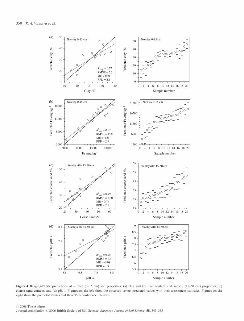
Figure 4 Bagging-PLSR predictions of surface (0–15 cm) soil properties: (a) clay and (b) iron content and subsoil (15–50 cm) properties, (c)

coarse sand content, and (d) pHCa. Figures on the left show the observed versus predicted values with their assessment statistics. Figures on the

right show the predicted values and their 95% confidence intervals.

350 R. A. Viscarra et al.

# 2006 The Authors

Journal compilation # 2006 British Society of Soil Science, European Journal of Soil Science, 58, 343–353

all 256 channels of information, combined with bagging-

PLSR, proved to be a useful technique for predicting various

soil properties in both the 0–15 cm and 15–50 cm soil layers of

both our study sites. The technique appears promising for, at

least, similar landscapes elsewhere in the world.

Future work

We plan to improve our calibration models by further develop-

ing our g-ray spectral library. Because the spectra require a

significant amount of pre-processing, we will formalize the

procedures and develop software to automate the process.

0

0 0.5 1 1.5 2 2.5 3

Energy /MeV

-0.4

-0.3

-0.2

-0.1

0.1

0.2

0.3

0.4(a) (b)

Loa

ding

wei

ghts

, w

Clay

Fe

Nowley 0-15 cm

0 0.5 1 1.5 2 2.5 3

Energy /MeV

-0.4

-0.3

-0.2

-0.1

0

0.1

0.2

0.3

0.4

Loa

ding

wei

ghts

, w

Coarse sand

pH

Stanleyville 15-50 cm

Figure 5 PLSR loading-weight spectra for (a) clay and iron content of the 0–15 cm soil layer at Nowley and (b) coarse sand content and pHCa of

the 15–50 cm soil layer at Stanleyville. A typical g-ray spectrum is superimposed on the figures (dashed line), showing energies of photopeaks for

ROIK (1.460 MeV), ROIU (1.765 MeV) and ROITh (2.614 MeV).

Figure 6 Bagging-PLSR maps of (a) clay and (b) Fe content for the 0–15 cm soil layer at Nowley and (c) coarse sand content and (d) pHCa for

the 15–50 soil layer at Stanleyville.

Calibration of hyperspectral g-ray energy spectra 351

# 2006 The Authors

Journal compilation # 2006 British Society of Soil Science, European Journal of Soil Science, 58, 343–353

Acknowledgements

We thank the Associate Editor of the journal, DrMurray Lark,

and two anonymous referees for their insightful comments.

References

Adamchuk, V.I., Hummel, J.W., Morgan, M.T. & Upadhyaya, S.K.

2004. On-the-go soil sensors for precision agriculture. Computers

and Electronics in Agriculture, 44, 71–91.

Banks, R.G. 1995. Soil Landscapes of the Curlewis 1: 100 000 Sheet

Report. NSW Department of Conservation and Land Manage-

ment, Sydney.

Billings, S.D. 1998. Geophysical Aspects of Soil Mapping Using Air-

borne Gamma-Ray Spectrometry. Degree of Doctor of Philosophy.

The University of Sydney, Sydney.

Breiman, L. 1996. Bagging predictors. Machine Learning, 24, 123–140.

Candolfi, A., De Maesschalck, R., Jouan-Rimbaud, D., Hailey, P.A.

& Massart, D.L. 1999. The influence of data pre-processing in the

pattern recognition of excipients near-infrared spectra. Journal of

Pharmaceutical and Biomedical Analysis, 21, 115–132.

Cattle, S.R., Meakin, S.N., Ruszkowski, P. & Cameron, R.G. 2003.

Using radiometric data to identify aeolian dust additions to topsoil

of the Hillston district, western NSW. Australian Journal of Soil

Research, 41, 1439–1456.

Cook, S.E., Corner, R.J., Groves, P.R. & Grealish, G.J. 1996. Use of

airborne gamma radiometric data for soil mapping. Australian

Journal of Soil Research, 34, 183–194.

Darnley, A.G. & Ford, K.L. 1987. Regional airborne gamma-ray

surveys: a review. In: Exploration ’87 (ed. G.D. Garland), pp. 229–

240. Third Decennial International Conference on Geophysical

and Geochemical Exploration for Minerals and Groundwater.

Special Volume 3. Geological Survey of Canada, Ontario, Canada.

Dickson, B.L., Fraser, S.J. & Kinsey-Henderson, A. 1996. Interpret-

ing aerial gamma-ray surveys utilising geomorphological and

weathering models. Journal of Geochemical Exploration, 57, 75–88.

Dickson, B.L. & Scott, K.M. 1997. Interpretation of aerial gamma-

ray surveys: adding the geochemical factors. AGSO. Journal of

Australian Geology and Geophysics, 17, 187–200.

Donoho, D.L. 1995. De-noising by soft-thresholding. IEEE Trans-

actions on Information Theory, 41, 613–627.

Efron, B. & Tibshirani, R.J. 1993. An Introduction to the Bootstrap.

Monographs on Statistics and Applied Probability 57. Chapman &

Hall Inc, New York.

ESRI 2002. ArcView GIS 8.2. Environmental Systems Research Insti-

tute Inc, Redlands, California.

FAO 1998. World Reference Base for Soil Resources. Food and Agri-

culture Organization of the United Nations, Rome.

Gee, G.W. & Bauder, J.W. 1986. Particle-size analysis. In: Methods of

Soil Analysis, Part 1. Physical and Mineralogical Methods (ed. A.

Klute), pp. 383–411. Agronomy Monograph 9 (2nd edn). ASA-

CSSA-SSSA, Madison, Wisconsin.

Grasty, R.L. 1979. Gamma-ray spectrometric methods in uranium

exploration: theory and operational procedures. In: Geophysics

and Geochemistry in Search of Metallic Ores (ed. P.J. Hood), pp.

147–161. Geological Survey of Canada Economic Report, No. 31.

Geological Survey of Canada, Ottawa, Canada.

Gregory, A.F. & Horwood, J.L. 1961. A Laboratory Study of Gamma-

Ray Spectra at the Surface of Rocks. Mines Branch Research Report

R.85. Department of Mines and Technical Surveys, Ottawa.

Hastie, T., Tibshirani, R. & Friedman, J. 2001. The Elements of Statis-

tical Learning: Data Mining, Inference and Prediction. Springer-

Verlag, New York.

International Atomic Energy Agency, IAEA 2003. Guidelines for

Radioelement Mapping Using Gamma Ray Spectrometry Data. IAEA-

TECDOC-1363. IAEA, Vienna.

International Commission on Radiation Units and Measurements,

ICRU 1994. Gamma Ray Spectrometry in the Environment. ICRU

report 53. ICRU, Bethesda.

Isbell, R.F. 1996. The Australian Soil Classification. Australian Soil and

Land Survey Handbook. CSIRO Publishing, Melbourne.

Luypaert, J., Heuerding, S., Vander Heyden, Y. & Massart, D.L.

2004. The effect of preprocessing methods in reducing interfering

variability from near-infrared measurements of creams. Journal of

Pharmaceutical and Biomedical Analysis, 36, 495–503.

Megumi, K. & Mamuro, T. 1977. Concentrations of uranium series

nuclides in soil particles in relation to their size. Journal of Geo-

physical Research, 82, 353–356.

Minasny, B. & McBratney, A.B. 2006. A conditioned Latin hyper-

cube method for sampling in the presence of ancillary information.

Computers and Geosciences, in press.

Minasny, B., McBratney, A.B. & Whelan, B.M. 2003. VESPER, Ver-

sion 1.6. Australian Centre for Precision Agriculture, McMillan

Building A05, The University of Sydney, NSW 2006. http://www.

usyd.edu.au/su/agric/acpa

Pracilio, G., Adams, M.L. & Smettem, K.R.J. 2003. Use of airborne

gamma radiometric data for soil property and crop biomass assess-

ment, northern dryland agricultural region, western Australia.

In: Precision Agriculture ’03: Proceedings of the 4th European Con-

ference (eds J.V. Stafford & A. Werner), pp. 551–557. Wageningen

Academic Publishers, Wageningen, The Netherlands.

Pracilio, G., Adams, M.L. & Smettem, K.R.J. 2004b. Gamma ray

spectrometry used to spatially predict soil properties important

to plant growth. In: Proceedings of the Seventh International Con-

ference on Precision Agriculture and Other Resources Manage-

ment (ed. D.J. Mulla). ASA-CSSA-SSSA, Madison, Wisconsin

[CD-ROM].

Pracilio, G., Smettem, K.R.J. & Harper, R. 2004a. New soil survey

technologies to map landscape properties relevant to perennial

plant performance. In: Salinity Solutions, Working with Science

and Society (eds A. Ridley, P. Feikama, S. Bennet, M.-J. Rogers,

R. Wilkinson & J. Hirth). Proceedings of the Salinity Solutions

Conference, Bendigo, Victoria, Australia, 2–5 August 2004

[CD-ROM].

Rampant, P. & Abuzar, M. 2004. Geophysical tools and digital

elevation models: tools for understanding crop yield and soil

variability. In: Supersoil 2004 (ed. B. Singh). Third Australian/

New Zealand Soils Conference, University of Sydney, Sydney,

Australia. The Regional Institute Ltd., Gosford (http://www.regional.

org.au/au/asssi/supersoil2004)

Rayment, G.E. & Higginson, F.R. 1992. Australian Laboratory Hand-

book of Soil and Water Chemical Methods. Inkata Press, Melbourne.

Sudduth, K.A., Hummel, J.W. & Birrell, S.J. 1997. Sensors for site-

specific management. In: The State of Site Specific Management for

352 R. A. Viscarra et al.

# 2006 The Authors

Journal compilation # 2006 British Society of Soil Science, European Journal of Soil Science, 58, 343–353

Agriculture (eds F.J. Pierce & E.J. Sadler), pp. 183–207. ASA/

CSSA/SSSA, Madison, Wisconsin.

Taylor, M.J., Smettem, K., Pracilio, G. & Verboom, W. 2002. Rela-

tionships between soil properties and high-resolution radiometrics,

central eastern Wheatbelt, western Australia. Exploration Geo-

physics, 33, 95–102.

Tsai, F. & Philpot, W. 1998. Derivative analysis of hyperspectral

data. Remote Sensing of Environment, 66, 41–51.

Viscarra Rossel, R.A. 2005. ParLeS v2.1a. Shareware for Spectroscopy

and Chemometrics. Australian Centre for Precision Agriculture,

McMillan Building A05, The University of Sydney, NSW 2006.

At: http://www.usyd.edu.au/su/agric/people/rvrossel/soft01.htm

Viscarra Rossel, R.A. & McBratney, A.B. 1998a. Soil chemical ana-

lytical accuracy and costs: implications from precision agriculture.

Special Issue: Moving towards precision with soil and plant analy-

sis. Australian Journal of Experimental Agriculture, 38, 765–775.

Viscarra Rossel, R.A. & McBratney, A.B. 1998b. Laboratory evalua-

tion of a proximal sensing technique for simultaneous measure-

ment of soil clay and water content. Geoderma, 85, 19–39.

Viscarra Rossel, R.A., Walvoort, D.J.J., McBratney, A.B., Janik,

L.J. & Skjemstad, J.O. 2005. Visible, near infrared, mid infrared or

combined diffuse reflectance spectroscopy for simultaneous assess-

ment of various soil properties. Geoderma, 131, 59–75.

Wilford, J.R., Bierwirth, P.N. & Craig, M.A. 1997. Application of

airborne gamma-ray spectrometry in soil/regolith mapping and

applied geomorphology. AGSO Journal of Australian Geology and

Geophysics, 17, 201–216.

Williams, P.C. 1987. Variables affecting near-infrared reflectance

spectroscopic analysis. In: Near-Infrared Technology in the Agricul-

tural and Food Industries (eds P. Williams & K. Norris), pp. 143–166.

American Association of Cereal Chemists, St Paul, Minnesota.

Wold, S., Martens, H. & Wold, H. 1983. The multivariate calibration

method in chemistry solved by the PLS method. In: Lecture Notes

in Mathematics (eds A. Ruhe & B. Kagstrom), pp. 286–293.

Proceedings of the Conference on Matrix Pencils. Springer-Verlag,

Heidelberg.

Wong, M.T.F. & Harper, R.J. 1999. Use of on-ground gamma-

ray spectrometry to measure plant-available potassium and

other topsoil attributes. Australian Journal of Soil Research, 37,

267–277.

Zhang, X.-P. & Desai, M.D. 1998. Adaptive denoising based on

SURE risk. IEEE Signal Processing Letters, 5, 265–267.

Calibration of hyperspectral g-ray energy spectra 353

# 2006 The Authors

Journal compilation # 2006 British Society of Soil Science, European Journal of Soil Science, 58, 343–353