/ ] / / ( / #10/??® *<*-*** ^

Anthony R.P. Janse

Sound absorption at the soil surface

Proefschrift ter verkrijging van de

graad van doctor in de landbouwwetenschappen

aan de Landbouwhogeschool te Wageningen,

op gezag van de Rector Magnificus,

Dr.Ir. F. Hellinga, hoogleraar in de cultuurtechniek,

in het openbaar te verdedigen

in de aula van de Landbouwhogeschool op

dinsdag 4 maart 1969 te 16.00 uur

1969 Centre for Agricultural Publishing and Documentation

Wageningen

/$ H=/0<//6r-o3

BIBLIOTREEK

IAND50U?;-: locrscnoot WAGEKIKGEN.

© Centre for Agricultural Publishing and Documentation,

Wageningen 1969

This thesis is also published as Agricultural Research Reports 715

STELLINGEN

1. Het meten van akoestische impedanties aan bodemstrukturen biedt waardevolle

perspektieven voor him karakterisering.

2. Het meten van de mechanische impedantie van het bodemoppervlak om hieruit een

stabiliteitsmaat van de bodemstruktuur te verkrijgen biedt geen perspektieven

3. De buigstijfheid van bladeren van planten is een goede maat voor de beschik-

baarheid van het bodemvocht.

4. Bij de klassifikatie van bodemfysische grootheden dient men rekening te hou-

den met de amplituden van de praktisch voorkomende veranderingen.

5. Bij het laten verrichten van praktikumproeven verdienen de bepalingen, waarin

processen worden gevolgd, de voorkeur boven het vaststellen van statische

grootheden, zoals gehalten.

6. Bij het opstellen van een bemestingsadvies zal men de waarden van bodemfysi­

sche grootheden mede in rekening moeten brengen.

7. Het leren toepassen van schaalregels bevordert in hoge mate het inzicht in

de werkwijze van een wetenschappelijke benadering.

8. Het gebruik van eerder gebrachte stellingen behoeft niet zonder meer te wor­

den afgeraden.

9. Men dient geen steun toe te zeggen aan zg. personeelsverenigingen.

10. Bij de expertise van kunstvoortbrengselen, in het bijzonder van schilderij-

en wordt nog te weinig gebruik gemaakt van de resultaten van een grafolo-

gisch onderzoek.

Wageningen, 4 maart 1969. Proefschrift A.R.P.Janse

Voorwoord

Het werken aan een proefschrift gelijkt op het schrijven en regisseren van een

toneelstuk. Men gaat uit van een min of meer toevallig ontdekt verband, dat ver-

heldering behoeft. Met het aanvoeren van de benodigde argumenten groeit het in-

zicht in de probleemstelling. Telkens weer moet men op een weg, die aanvankelijk

hoopvol was ingeslagen, terugkeren. De detailproblemen lijken moeilijk tot een

eenheid te kunnen worden gebracht. Het hoofdprobleem schijnt zich minder duide-

lijk af te tekenen; een verwante behandeling van deelproblemen in andere weten-

schappen maken een verantwoorde keuze van de begrippen en de toekenning van hun

inhoud moeilijk. Soms verhogen gedachtenflitsen of aanvankelijk oppervlakkig ge-

dane vaarnemingen de spanning.

In tegenstelling met de bevrijdende katharsis raakt het probleem slechts scher-

per gesteld: de oplossing wordt naar een meer verwijd gebied verschoven. De

katharsis is in feite een nieuwe uitdaging.

Het gekozen uitgangspunt was vreemd in het gegeven werkmilieu. De geboden kansen

waren daardoor in het begin zeer ruim. De kans op een suksesvolle uitwerking was

nogal klein. Zo werden bijvoorbeeld aanvankelijk veel trillingsmetingen aan de

vaste bodemfase verricht. Tamelijk laat bleek dat zowel de meettechniek als de

oplossing van de mathematische problemen weinig mogelijkheden bood.

Ook het zoeken naar begrijpende belangstellenden was moeilijk, in het bijzonder

door het aanvankelijk onnauwkeurig afgestemd zijn van de ontvanger. Dat er thans

een verdedigbare tekst openbaar wordt, is zeker ook te danken aan het mede pein-

zend zwoegen van Ir. D.W. van Wulfften Palthe, die vooral in de wiskundige pro-

blematiek de soms zwijgende souffleur was of de toneelknecht, welke achteraf

terecht de deur gesloten hield.

Dat Professor Schuffelen, als een schouwburgdirekteur, na een orienterende be-

oordeling het stuk koos, de regie voor een groot deel overliet aan Professor

Kosten, stemdede vrijheidsminnende onderzoeker dankbaar. Ook de afdeling Wiskunde,

van zowel de Landbouwhogeschool als de Technische Hogeschool te Delft, welke met

de geboden hulp bij het programmeren voor schone requisieten zorgde, zij gaarne

dank gebracht.

Contents

List of symbols 1

Introduction 8

In-1 The concept soil structure 8

In-2 Total pore space 11

In-3 The characterization of pore space 11

1 Plane waves and interferometry 17

1.1 Introduction 17

1.2 The wave equation 19

1.3 Complex representation 22

1.4 Interferometry 27

1.5 The velocity of sound in a mixture of ideal gases 35

1.6 Intensity, decibel, damping in air 39

1.7 Velocities in air 40

1.8 The heat generated 4!

1.9 Sound waves in porous media 41

1.10 Presentation of the normalized specific acoustic impedance 44

1.11 The behaviour of the function Z = W coth(yl) in the

impedance plane 49

2 The experimental equipment and its accuracy 53

2.1 Introduction 53

2.2 The interferometers 54

2.3 The electronic equipment 58

2.4 The measurement 61

2.5 Accuracy of the measurements 63

3 The relation between the acoustical properties and the

geometrical arrangement of pores in soils 73

3.1 Introduction 73

3.2 Numerical examples of calculating Z and Y from

measurements at layer thicknesses 77

3.3 The logarithmic impedance plane as a tool for the

numerical evaluation of W and y 83 m m

3.4 The simple model of Zwikker & Kosten 89

3.5 The choice of model 97

3.6 The capillary model 103

3.7 The fissure model 110

3.8 Comparison of the behaviour of the capillary and

the fissure model 112

3.9 Discussion on the possibilities of scale-rules 114

3.10 The model of the prismatic soil structures 119

3.11 Electro-equivalent networks 123

4 Some experiments discussed 126

4.1 Introduction 126

4.2 Materials studied, presentation of the data 127

4.3 Comments on the calculation of the impedance curls 128

4.4 Discussion of the results of measurements 145

4.5 Considerations on the improvement of mathematical models 166

4.6 Measurements on layers of straw 171

4.7 Conclusions 172

Summary 173

Samenvatting 175

Literature 177

Appendices 183

Appendix A. Basic formulae from the theory of vibrations 185

Appendix B. Derivation of the perturbation factors for

homogeneous channels 188

Appendix C. Calculation on the function H(x) and its

associated functions 194

Appendix D. Some remarks on the calculation of the locus of the

sample surface impedance in the complex plane 212

Acknowledgments 215

List of symbols

The symbols

The numbers

Symbol

A

a

b , , b 2

m

Sfk

pk

: d , C h

V

D,.D2 .D3

d

F

N_1m

N m

j V

A"

m s

- 2

are defined or first used in or near the equations cited,

refer to the chapters, the characters refer to the appendices.

Name and description Ref. Units

constant, integration constant B-2

1) absorption coefficient of sample

at normal incidence 1-38

2) radius of calibration plate 2-13 m

dimensionless measure for tube radius 3-62

limits for b, calculated values 3-64

1) mechanical compliance A-l

2) electrical capacity A-l 2

effective compression modulus 3-2

specific heat per mol at constant

volume for component k in gas.mixture 1-28

specific heat per mol at constant pressure

for component k in gas mixture 1-41

velocity of sound for free, undamped

wave 1-6

velocities of sound in dry and humid

air respectively l-48a m s

specific heat per unit mass at constant

pressure 1-4 Jkg

velocity of longitudinal waves in a

plate 2-13 m s"

specific heat per unit mass at constant

volume 1-4 Jkg

1) fissure width B-l m

2) main slit width 3-126 m

average value for D 3-93 m

special values for D 3-94,3-95,3-96 m

crack width 3-126 m

acoustical quantity 3-117

kmol

kmol

0R-1

V1

F(x) auxiliary function

Ff(x)

f 1) mathematical function

2) frequency

3) force

f, mass fraction of gas component

f(x) auxiliary arbitrary distribution

function

G(x) auxiliary function

G specific acoustic parallel conductance

per unit length

g ratio of partial gaspressures

g.,g2,g_ weighting factors, calculated

values

H(x) auxiliary function

H,(x) auxiliary function

h 1) volumetric fraction of pores

2) thickness of calibration plate

3) number of degrees of freedom

4) crack length

I intensity of sound, sound power

density transmitted

I reference intensity of sound o J

K compression modulus

k wave number, free undamped wave

Boltzmann's constant *B k structure factor

m

L coefficient of self-induction

L(x) auxiliary function

L critical length, integration interval 3-46

LT sound intensity level

L sound pressure level

1 thickness of sample

1, thermal boundary layer thickness

1 . (positive) distance between pressure

minimum and sample surface

1 viscous boundary layer thickness

1) modulus of logarithmic spiral

2) molecular mass

v

3-71

3-97

1-13

2-1

A- l

1-41

3-25

3-81

.e

3-2 l-48a

3-64a

3-70

3-102

3-21

2-13

1-5,1-48a

3-127

1-20

1-49

1-2

1-8

1-51

3-22

A-l 2

3-82

3-46

1-50

1-50

1-56

B-14

1-34

B-3

1-65

1-51

— --Hz

N

-

-

-

2 « - ' - ' m N s -

-

---

m

-

m

W m~2

W m~2

N m~2

-1 m JV 1

-H

-m

- 1 2 - 2 dB(10 Wm )

dB(2'10~5Nm"2)

m

m

m

m

-

kg kmol

M(x)

n

P

P

P- >P *i'*r

P >P • max r m m

Q

3Q/3t

q

auxiliary function 3-72

molecular mass of component k 1-41

1) dimensionless variable for layer

thickness 3-47

2) dimensionless variable for

distribution functions 3-

3) mass A-

kg kmol

number of channels per unit area normal

to direction of propagation

scale factor

1) sound pressure in free wave

2) average sound pressure in pores

complex pressure amplitude

the peak values of p. and p , resp.

partial pressure, component k

sound pressure maxima and minima,resp. 1-1

1-

A-

B-

3-

3-

1-

barometric pressure

electrical charge

net flow of heat per unit mass

auxiliary variable

fissure width ratio

1) gas constant per mol

2) dimensionless radius of circle with

constant reflection coefficient I-

3) radius of equivalent tube 3-

4) radius of curvature of the impedance

spiral T)-

5) electrical resistance A-

a prefixed value of R(4) D'

gas constant per unit mass 1

1) pressure reflection coefficient 1-

2) relative partial gas pressure of

water vapour 1

3) radius of reference sphere 3-

4) mechanical resistance A-

1) cross-sectional area of channel 3'

2) total entropy of 1 kg gas mixture I'

average value of S(l) 3-

-62

-2

25

118

1

52

13

11,1-8

41

35

-3

-12

-10

-12a

-96

-41

-60

-62

-4

-12

-10

-42

-26

-48a

-62

-7

-44

-42

-44

kg

-2

N m

N m

N m

N m~

N m

N m

N m

C

-2 i

-2

-2 L

-2 i

-2

W kg

kmol K

m

a

m J kg K

N m

m

N s m 2

-1

J kg K 2

m

ds

6s

s n

T

T s

t

U

u

u

u

V

x3,x6 x i >xo »XA *^S

xi >x2>x3

x4'x5'x6

entropy of component k 1-42

cross-sectional area 1-1

1) standing wave ratio in tube with

negligible losses 1-37

2) standing wave ratio, extrapolated to

sample surface in tube with losses 1-37

a line element of the impedance spiralD-1

a maximum value of ds D-l

ratio of specific maximum to specific

minimum sound pressure 1-39

absolute temperature 1-41

static value of absolute temperature B-7

time 1-1

volume velocity per channel 3-45

1) particle velocity in direction of

propagation 3-51

2) volume velocity per unit area normal

to direction of propagation 3-3

3) real part of reflection coefficient1-62

particle velocity (peak value) 1-49

complex particle velocity amplitude 1-19

1) volume 1-2

2) volume of 1 kg gas mixture 1-41

RMS value of the thermal velocity of

molecules 1-51

imaginary part of reflection

coefficient 1-62

specific acoustic wave impedance 1-55

1) spatial co-ordinate in direction

of propagation 1-1

2) Cartesian co-ordinate

auxiliary variable

frequency dependent factors

auxiliary variables

special values for auxiliary

variables

special values for auxiliary

variables 3-105

J kg K

m

m

s 3 -1

m s

-1

m s

-1

m s 3

m m kg

-1

N s m -3

3-73,3-83,3-98,3-103

3-75,2-84

3-76,3-77,3-84,3-85

3-100

Y acoustical admittance per unit length 3-128 a

Y specific acoustic parallel admittance

per unit length Y acoustical admittance at the mouth

s

of a slit

y 1) transverse co-ordinate

2) Cartesian co-ordinate

Z specific acoustic impedance

(at the sample surface)

Z specific acoustic series impedance

per unit length

Ty. mechanical impedance

z 1) spatial co-ordinate in direction of

channels

2) Cartesian co-ordinate

a attenuation constant, real part of y 1-65

a attenuation constant in tube o

6 phase constant, imaginary part of y

y propagation constant

3 relative error in sound pressure

A 1) tangent of loss angle

2) phase displacement

C normalized specific acoustic impedance 1-28 -

n 1) normalized specific acoustic reactance

imaginary part of c 1-28 _2

2) dynamic coefficient of viscosity 1-47 N s m

ri imaginary co-ordinate of the apex of

impedance curl in the £-plane 3-15

n thermal perturbation factor for m

inclined inhomogeneous channel 3-50 -

ri thermal perturbation factor for

cylindrical tube 3-90

nf thermal perturbation factor for

fissures 3-106

thermal perturbation factor for

homogeneous channels 3-46

thermal perturbation factor for

cylindrical tubes 3-84

3-128

1-53

3-127

B-l

*•

1-27

1-52

A-15

B-l

-

1-65

l-23a

1-65

1-18,1-54

2-8

3-12a

1-34

N"1

m 2 fl

m 4 H

m

m

N s

N s

N s

m

m -1

m -1 m -1 m -1 m -

-

3 -1 m s

-1 -1 s

-1 -1 s

-3 m

-4 m

-1 m

radian

n thermal perturbation factor for m

n thermal perturbation factor for

r.f thermal perturbation factor for

fissures 3-104.B-18

9 1) incremental temperature, due to

sound field B-7 K

2) angle of rotation of log. spiral 1-65 radian

3) angle between direction of

propagation and of channels 3-25 radian

K Poisson ratio 1-4

X 1) thermal conductivity 1-48 Wm K

2) wave length 1-34 m

X apparent thermal conductivity B-22 Wm K

y 1) mass of hydrogen atom 1-51 kg

2) Poisson ratio 2-1

3) dimensionless boundary layer

thickness for viscous flow 3-32a

E 1) small displacement in x-direction 1-2 m

2) real part of C 1-28

E real co-ordinate of the apex of an

impedance spiral in the C-plane

E viscous perturbation factor for m

inhomogeneous channel 3-49

E viscous perturbation factor for

cylindrical tubes 3-80

E, viscous perturbation factor for

fissure 3-101

E viscous perturbation factor for

homogeneous channels 3-45 t

E viscous perturbation factor for

cylindrical tubes 3-74

Ef thermal perturbation factor for

fissures 3-79

p incremental density due to sound -3

fields 1-1 kg m -3

p static specific mass 1-1 kg m s -3

P apparent specific mass 3-1 kg m Z auxiliary variable 3-32

. . . -4 a specific flow resistance 3-1 N s m

-4 a static value of a B-22 N s m m

j s

6

T relaxation time A-10 s -4 a specific flow resistance 3-22 N s m

<(> 1) phase angle - radian

2) phase angle of reflection

coefficient 1-30 radian

3) angle between the tangents of the

impedance spiral 3-38 radian

6$ arbitrarily chosen maximum value of

radian

radian

radian

-1 s

*

u

The following Symbol a c d e f h h i k 1 1 M m P P r s V

v,V z o

<K3) D-10

1) phase angle 1-10

2) phase angle of the sound pressure 1-22

3) argument of log. spiral 1-65

angular frequency 1-8

suscripts are used: Referring to average value cylindrical tube model in a tube electrical circuit fissure tube model thermal boundary layer high frequency approximation incident wave serial number of component in gas mixture local value low frequency approximation mechanical in porous material plane wave constant pressure reflected wave static value viscous boundary layer constant volume in channel reference value

R ,q ,6 ,£ ,o »Y , g'^a' p'^o* o' a* Y s c c a. exceptions W C d , C h ' a o

same sample shortly after the first measurement or at a later date. Changes

in structure with time can then be analysed and described in particular prob­

lems concerning the influences of climate, plant growth and tillage in the

deve1jpment of structure.

d. There should be an acceptable basis to examine existing structures in full.

In other words, it should be possible to make a significant approach to the

structural unit (Bolt, Sehuffelen and Janse, 1958). If the soil surface cracks

every 15 cm there is little value in examining a sample with 5 cm diameter.

e. At least in principle it should be possible to take measurements in the field.

For various reasons, such as study of the microclimate the complete ecological

horizon must be identified. In this examination of the ecological horizon the

pore system is of much importance.

Among the many workers, that have measured the distribution and behaviour of gas­

es in the soil, are Lundegardh, Free and Cannon. The physical aspects of gas ex­

change appear to be of particularly great importance. It was established that

CO. percentages higher than 1% are often deleterious, and that 12 - 15% 0„ should

be present in the soil for normal crop production. It was rightly stated that a

study of transport processes is also of fundamental importance. The partly theo­

retical studies of Penman and later those of van Bavel helped especially to clari­

fy how widely the magnitude and effect of the (mechanical) diffusion constant

can vary and, for deep rooting plants in particular how much this constant can

be affected by the structure of the soil profile.

The biological and microbiological activities, such as nitrification, are also

influenced by the availability of Cv. Furthermore in an insufficiently aerated

soil compounds of Fe and Mn can be locally reduced.

A separate problem which is difficult to analyse is answering the question of

the required sensitivity and reproducibility of the measurements. Although this

point will be discussed later in more detail, it can be stated here that:

a. the sensitivity and the required reproducibility in general is determined by

the purpose for which the measurement is made. When studying for instance dif­

fusion processes in the soil, the required level of sensitivity will usually

be lower than that for investigations of heat transfer in soil.

b. the reproducibility will often vary widely in practice. A more or less homo­

geneous soil will show less scattering of data than a strongly inhomogeneous

soil. Samples taken from different sections of a field will show a certain

spread. The argument that the reproducibility of the experimental equipment

10

need not exceed that of the sampling may well be spurious in certain in­

stances, e.g. if the progress of some process is being followed and the vari­

ation of some quantity under observation is of greater interest than its

absolute value.

In-2 Total pore space

Soil is a three-phase system; the volume ratios of a multiphase system can easi­

ly be determined by drying and weighing after determination of the densities of

the various components. Since the latter in the solid phase of the soil often

show little variation, use can be made of an average density. The calculated air

volume is usually given as a quantity without dimension; it varies linearly with

moisture content. Separate weighings are necessary; from these the geometry of

pore system cannot be evaluated.

Of more recent date are investigations on the occurrence of pore space based on

the intrinsic properties of the material in which the air voids have been formed

by tillage and fertilizer application etc. In this manner significant corre-

lationships have been found with the clay fractions (Hooghoudt, 1948), with

texture (Fraser, 1935)and with the nature of adsorbed ions (Aylmore, 1966).

A method more immediately directed to measure pore space is one based on con­

necting a sample with unknown pore space and known total volume with a sealed

vessel of known volume, attached to a manometer.

This "gas expansion method" has been studied extensively in various countries.

The "porosimeters", also called air pycnometers have been constructed in many

forms and tested by Bourrier (1951), Loebell (1956), Misono (1961), Alten and

Loofman (1962), and others. Comparable apparatus was constructed and used for

routine measurements at our laboratory. In dry samples, the influence of the

pressure range appears to be small. In moist samples, serious problems are

caused by the release of adsorbed and dissolved gases. Changes in vapour

pressure and slow attainment of equilibrium conditions are difficult to correct

for in measurements and calculations.

In-3 The characterization of pore space

The study of the structure of porous materials is a fascinating one as is evi­

dent from the extensive literature. Many authors in the field of ceramics, filter­

ing technology, geophysics and soil science are in fact interested in the charac-

11

terization or pore geometry. There are some handbooks in the almost endless

array of publications as for instance those of Mc Dalla Valle (1943), Muskat

(1946), carman (1956), Scheidegger (1957), and Lykow (1958). Their approaches

are predominantly directed towards selections of parameters which can represent

the fluid flow resistance of the material.

The main object is often the reduction of the number of characteristic parame­

ters or concepts determining the flow resistance. In this context, a homoge­

neous and isotropic configuration is often assumed. The introduction of but one

parameter is much favoured and it is remarkable in this respect that so few

publications deal with the effect of two or more parameters.

In 3.1 The Static specific flow resistance

Porous materials may be investigated by static or dynamic methods of measurement.

For a static method, the variables,excess pressure and particle velocity-?- do not

vary in time or vary so slowly that they can be considered constant. For a dy­

namic method the variables are functions of time and if these functions are peri­

odic, the method is a steady state one. Static methods fall into the steady

state class too as the limiting case of infinitely long period.

Swelling and often low mechanical stability of the soil samples still offer

insurmountable difficulties for correct measurements of permeability, i.e. the

reciprocal value of specific flow resistance for water. It is therefore not

advisable to calculate intrinsic resistances for the soils and loosely packed

materials from measurements with water.

Many simple devices are available for measuring air resistance. The value, ob­

tained from the volume rate of flow at a certain induced, usually constant,

pressure gradient. The volume rate of flow is measured for various pressure drops

over the sample; the proportionality constant between the two quantities is a

measure for the static flow resistance. In the flow resistance meter (see

figure), used to measure the resistances of most of the samples investigated

here, use is made of a sample holder encased in 0-rings and connected with a

pressure line in the laboratory. The pressure difference between the pressure

gaskets is read from a Micro-Fuess manometer. The pressure difference across the

sample can usually be limited to 0.04 cm water pressure. A calibrated Fisher and

Porter microflowrator (type 130-13) is inserted into the circuit. The volume

rates of flow are also kept low and lie between 0.1 and 0.3 cm /sec. The re­

lationship between the volume velocity and the pressure drop usually proved to

be linear, the slope varied slightly. The specific acoustic flow resistance was

12

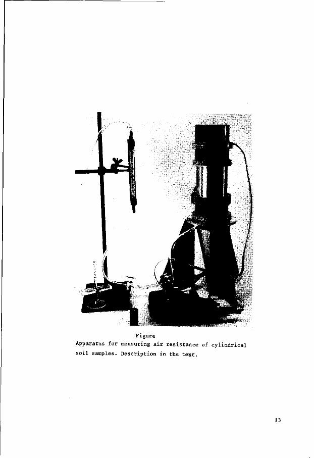
Figure

Apparatus for measuring air resistance of cylindrical

soil samples. Description in the text.

13

obtained as the extrapolated value for vanishing pressure gradients. The concept

of specific air flow resistance assumes a laminar flow. One of the reasons for

measuring with low rates of flow is the avoidance of turbulence.

For measurements of air flow resistance, sample holders of various diameters were

used. Wide holders were used primarily for coaVse materials. It can easily calcu­

lated that only through use of the wide holders the effects due to the irregu­

larities in the arrangements of the particles or aggregates near the walls of

the sample-holder could be kept within experimental error.

Small pressure differences are to be preferred with moist samples, where moisture

is easily displaced and where, at low moisture tensions, rupture of the menisci

can occur.

It is remarkable that so little literature exists on experiments measuring both

air resistance and water permeability of a porous material. Covey (1963) gives

a brief summary and an interesting graph for the relative permeability for air

and water in a soil sample.

The literature yields many references on the relationship between specific flow

resistance and specific surface area of a sample material. An attempt was made

to verify this relationship. For fine grained materials no linear relation

exists between the total frictional area and flow resistance. For increasing

fineness of the material the deviations from linearity became more important.

The relationship between packing density and flow resistance was not linear. The

results will be discussed in another publication.

Conversely the specific air flow resistance is no unambiguous measure for the

frictional area per unit volume and as it fails to yield even this limited infor­

mation this subject, will not be further pursued.

In 3.2 The acoustical approach

Soil as a porous system often with an extremely complicated structure cannot

easily be described in simple terms. Two further remarks are necessary on this

point.

1. Only part of the air is in free communication with the atmosphere contributing

to the exchange of gases, such as CO., H.O and 0„. This fraction of the total

pore space fluctuates enormously with variations in moisture content.

Measurements of total pore space or of mean pore diameter (whatever this may

be) are therefore bound to be inadequate.

2. For various diverse reasons, the packing density of soil particles varies

widely and usually increases with depth. This excludes the possibility to

14

obtain a true impression of the nature of spatial arrangements in a soil

from flow resistances.

The question arises whether other methods can be used to supply information on

this spatial arrangement. The problem parallels that confronting an acoustician,

developing a sound absorbing material, even if the aims differ. Whereas the

acoustician is interested principally in increasing sound absorption in the

audible frequency range, here the sound-absorbing properties of a material, i.e.

a soil sample, may be determined in order to gain insight into the spatial ar­

rangement .

An advantage of this procedure is that the analytical and experimental methods,

devised by acousticians for the investigation of sound-absorbing materials, may

be employed.

The interesting question is therefore whether and, if so, to what extent a soil

surface will absorb sound and whether this property can yield information on the

spatial (in agriculture often "structural") arrangement of soil particles.

A comparison between porous materials developed for sound absorption and soil

samples shows that it is certainly so. A practical tool for measuring the a-

coustical properties of soil samples seems to be the interferometer (arrange­

ment), sometimes called the standing wave tube. The instrument will be dis­

cussed in detail in the following sections.

Acoustical investigation of soil samples presents several attractive features.

1. Sound pressures are so low (typically less than 10 atmosphere) that the

sample is not disturbed; the method is non-destructive.

2. The effects of temperature and composition (e.g. humidity) of the gaseous

medium in the pores of the material on its acoustical properties are slight;

the results are thus governed principally by the spatial arrangement of the

material.

3. Only those pores in open communication with the atmosphere contribute to a-

coustical behaviour.

4. Acoustical measurements yield more information on these pores than any other

method, small pores especially having a relatively large effect on acoustical

performance.

When a plane sound wave of a certain frequency impinges on the soil part of the

incident energy will be reflected. The ratio of reflected to incident energy,

the "energy reflection coefficient", can be measured. As a rule there is a phase

15

jump | $ | between the reflected and the incident wave at the surface of the

sample. This phase jump can be determined too. Energy reflection coefficient

and phase jump can be studied in a large frequency range, so that a large num­

ber of quantities can be measured.

16

1 Plane waves and interferometry

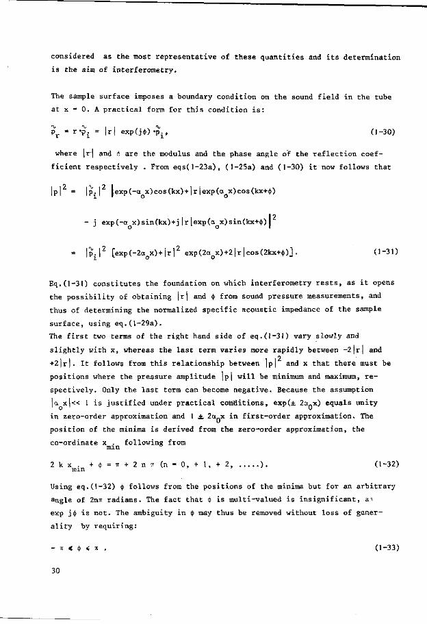
1.1 Introduction

The interferometer consists of a rigid cylindrical tube, fitted with a loud­

speaker at one end and the sample (with its surface normal to the direction of

the tube) at the other (see figure la). The loudspeaker generates harmonic plane

waves in the tube. In the present context, plane waves are characterized by con­

stant sound pressure in planes normal to the direction of the tube (an exception

must be made for a slight perturbation near the walls of the tube). Thus only

one spatial co-ordinate, to be designated X, directed along the tube, will be of

predominant importance. The following conventions will apply: the positive x

direction is from the loudspeaker towards the sample and the sample surface is

situated at x = 0 (x thus takes on negative values inside the tube).

The sound field in the tube may be considered as the superposition of two waves,

the incident wave, travelling from the loudspeaker towards the sample and im­

pinging on the sample surface at normal incidence (p. in figure la) and the re­

flected wave returning from the sample (p« in figure 1 a ) . These waves set up an

interference pattern, determined by the acoustical properties of the sample, in

the tube. This pattern may be explored with the aid of a movable microphone.

More detailed consideration requires the introduction of a number of physical

concepts and quantities. As far as possible, nomenclature, symbols and units

have been chosen in accordance with the recommendations given in "Ontwerp voor

akoestische begrippen en grootheden (V 1029)" and in the draft "Electroakoestiek

(V 1077)" and are conform to the recommendations given in the "IS0N0RM 31". A

summary of general vibration theory, given in Appendix A, forms the basis for the

definition of the concepts involved. Next, a discussion will be given of the

method of employing the standing wave tube in the determination of acoustical

quantities. Attention will also be paid in this first chapter to the manner in

which the results obtained may be presented.

17

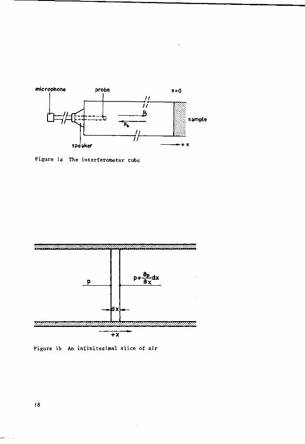
microphone probe

speaker

Figure la The interferometer tube

X=0

sample

—+ x

<»Ud^J»fcM^*MJ^«JJJrfJJJ*JJ*JJJAJJAJ^^JJJ^***MdJ*MJdUMbMA***J I I I I I I I ^hhfcfc****

yyyy^y^ryyvyyr

<"&»

+ X

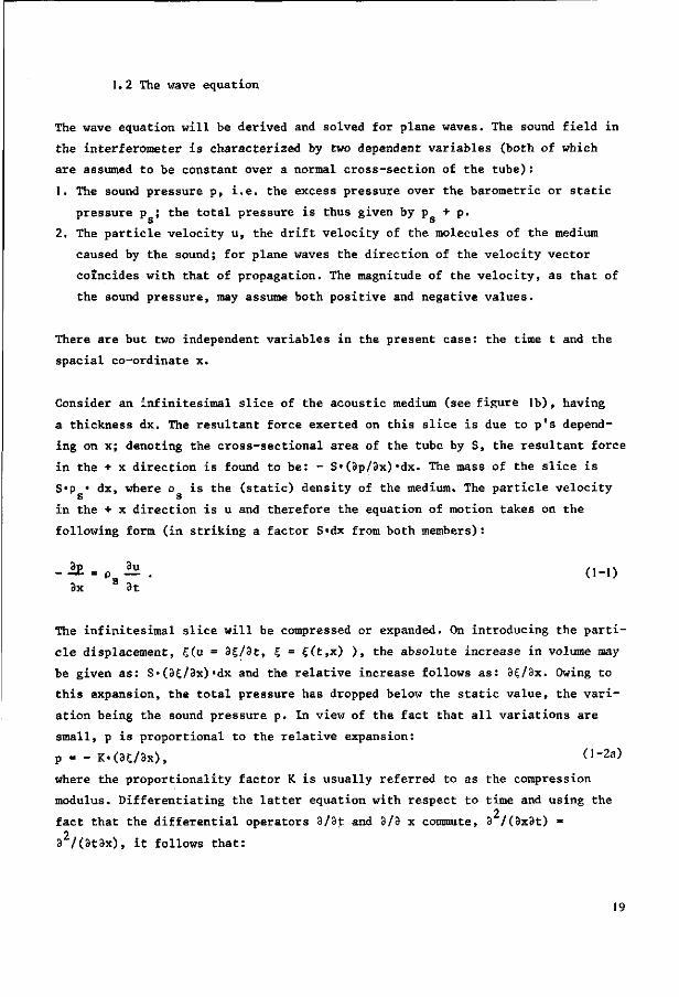
Figure lb An infinitesimal slice of air

18

1.2 The wave equation

The wave equation will be derived and solved for plane waves. The sound field in

the interferometer is characterized by two dependent variables (both of which

are assumed to be constant over a normal cross-section of the tube):

1. The sound pressure p, i.e. the excess pressure over the barometric or static

pressure p ; the total pressure is thus given by p + p. s s

2. The particle velocity u, the drift velocity of the molecules of the medium

caused by the sound; for plane waves the direction of the velocity vector

coincides with that of propagation. The magnitude of the velocity, as that of

the sound pressure, may assume both positive and negative values.

There are but two independent variables in the present case: the time t and the

spacial co-ordinate x.

Consider an infinitesimal slice of the acoustic medium (see figure lb), having

a thickness dx. The resultant force exerted on this slice is due to p's depend­

ing on x; denoting the cross-sectional area of the tube by S, the resultant force

in the + x direction is found to be: - S«(3p/3x)«dx. The mass of the slice is

S«p « dx, where p is the (static) density of the medium. The particle velocity

in the + x direction is u and therefore the equation of motion takes on the

following form (in striking a factor S«dx from both members):

- i E - P > i ! i . ( i - i ) 3x S 3t

The infinitesimal slice will be compressed or expanded. On introducing the parti­

cle displacement, £(u = 3£/3t, S = 5(t,x) ) , the absolute increase in volume may

be given as: S»(3?/3x),dx and the relative increase follows as: 3?/3x. Owing to

this expansion, the total pressure has dropped below the static value, the vari­

ation being the sound pressure p. In view of the fact that all variations are

small, p is proportional to the relative expansion:

p = - K.(3C/3x), d - 2 a )

where the proportionality factor K is usually referred to as the compression

modulus. Differentiating the latter equation with respect to time and using the 2

fact that the differential operators 3/3t and 3/3 x commute, 3 /(3x3t) = 2

3 /(3t3x), it follows that:

19

_ Ju = 1 i£ • 0-2b) 3x K 3t

Eq.(l-2b) is a specialized form of the "equation of continuity". A value for K

may be derived on introducing certain assumptions. They are:

1. The medium is an ideal gas.

2. Its chanpps of state are adiabatic. Especially this latter assumption needs

some justification. Heat exchange within the medium may be shown to introduce

only negligible effects in air in the audible frequency range. Heat exchange

between the medium and the walls of the tube does, however, affect wave propa­

gation. This point will be discussed in a future section: for the moment it will

be disregarded as being of secondary importance.

For an ideal gas and an adiabatic change of state:

(p + p)(V + 6V) K = constant = p «V K , (1-3)

where p and V are the barometric (static) pressure and the volume of the gas

under consideration at pressure p , respectively, p and 6V the sound pressure

and the change in V due to p, respectively, and < is the ratio of the specific s

heats at constant pressure (c ) and at constant volume (c ) : p v

K = c /c . (1-4) P v

(N.B.: In the following c and c should be conceived as specific heats per

unit mass .)

In first order approximation, eq.(l-3) yields:

p = -Kps.6V/Vs ,

and thus, from the definition of K,eq.(l-2a),it follows that:

K = K P . (1-5) r s

Kinetic gas theory predicts values for K for ideal gases. Let h, represent the

number of degrees of freedom of a molecule, then:

K = 1 + 2/h ,

where, for diatomic molecules, h, = 5 and for triatomic molecules h, * 6. For

air, a value of < slightly below 1.4 would be expected; the experimental value

20

2 2 3 p 1 3

proved to be 1.403, in adequate agreement with theory.

2 Differentiating eq.(l-l) for x and eq.(l-2) for t and eliminating 3 u/(3x3t)

(remembering that 3/3x and 3/3t commute), the wave equation for p is as follows

a'2-"2 »;"*• ° " 6 )

3x c 3t

where

c = A<P S /P S ) • (1-7)

The meaning of the constant c will emerge later. If p is eliminated from eqs

(1-1) and (1-2) instead of u, the wave equation for u results. This equation

turns out to be identical with eq.(l-6) on replacing p by u.

Eq.(l-6) is a linear, homogeneous, partial differential equation of the second

order and possesses as such a general solution composed of two independent

functions, each incorporating two integration constants. The general solution

may be represented in various ways, the following form being appropriate to

harmonic waves:

p = p. cos((ut - kx + <)>.) + p ? cos(ut + kx + <(i„) , (1-8)

where

to = the angular frequency (= 2TI times frequency) ,

k = the wave number, k = ui/c,

P]> f>2 a r e integration constants having the character of peak values of sound

pressures,

$., i|>9 are integration constants having the character of phase angles.

Consider the first term on the right-hand side of eq.(l-8). For an observer

moving with velocity dx/dt = c in the + x direction, the argument of the cosine

will remain constant, t - x/c being constant. Thus the conclusion may be drawn

that this term represents a wave travelling in the + x direction with a phase

velocity c; in future c will be referred to as the velocity of sound. A similar

consideration shows that the second term on the right-hand side of eq.(l-8)

represents a wave travelling in the - x direction with the same velocity.

Using eq.(1—1), it follows that

21

P l . . . , . . x P2 cos(wt - kx + $.) cos(wt + kx + (JO . (1-9) P C P C

s s

A comparison of eqs (1-8) and (1-9) shows that, for waves travelling in the + x

direction ,

p/u = ogc,

and for waves, travelling in the - x direction,

p/u = - p c. s

The ratio p/u is thus independent of time.position and, but for the change in

sign, direction of travel.

The quantity p c, which is characteristic for the medium, is known as the spe-. s . . . . . -3

cific acoustic wave impedance of the medium, its dimension being N s m or, kg s m

1.3 Complex representation

The complex representation of the dependent variables, customary in acoustics

when harmonic phenomena are considered , is founded on de Moivre's theorem,

exp(jijj) = cos(iji) + j sin(t)j) , (1-10)

where j = -J-\ and i|» is an angle expressed in radians. The representation is

introduced by an example; that of a plane, harmonic wave travelling in the + x

direction. According to eq.(l-8), the sound pressure due to such a wave is

represented by:

p = p COs(tdt - kx + (j)), (1-11)

where p is the peak value of the sound pressure and <j> is the phase angle.

On referring to eq.(l-lO), the following equation,

p = Re [p exp(jiot - jkx '+ j<t>)]> (1-12)

is seen to be identical with eq.(l-ll) since the symbol Re before a function

indicates that the real part of that function should be taken. For the future,

the symbol Im is introduced. This symbol implies that the imaginary part of the

function must be taken. In this book, the convention will apply that the factor j

22

in the imaginary part of the function is stated explicitly, thus, for any

function f,

f = Re(f) + j Im(f),

and Im(f) itself is real.

The complex pressure amplitude, p, of the wave is introduced with the aid of

the defining equation

% 1 p = — p exp(j<j,), (1-13)

•2

and eq.(l-12) thus reduces to

p = /2 Re[p exp(jut - jkx)] . (1-14)

Eq.(1—14) still represents the real sound pressure dependent on time and place

and is identical with eq.(1—11). The complex representation, indicated by p, is

obtained by performing the following operations:

1. omit the factor exp(jcot),

2. omit the operator Re ,

3. omit the factor /2

The result of these operations is:

— *v p = p exp(-jkx) . (1-15)

The first two of the above operations may be considered as short cuts: the real

representation of p is obtained simply by re-instating exp(jut) and Re. The

last of the operations has further implications. Thus |p] corresponds to the

R M S value rather than to the peak value of p; the function of the modulus

bars may be clarified by the following equation: |a + jb| = /(a + b ) . The

a* ,

introduction of the complex R M S quantity p is a concession made to the wide­

spread custom of giving R M S values for alternating quantities and of cali­

brating instruments in such values. A consequence is, for instance that sound *2

powers, which are proportional to |p in the real representation, are pro­lyl 2 .

portional to |p| v.\ the complex representation. The problem of R M S against

peak value is, however, of little importance for this text, since interest is

centred on ratios of alternating quantities.

The derivation of the instantaneous, real value p from the complex represen­

tation p, c.f. eq.(l-15), may be illustrated by a vector diagram in the complex

23

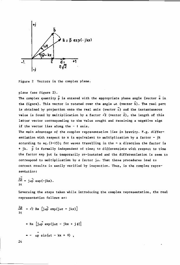
a:p exp(-jkx)

Figure 2 Vectors in the complex plane.

plane (see figure 2 ) .

The complex quantity p is entered with the appropriate phase angle (vector a in

the figure). This vector is rotated over the angle cot (vector b ) . The real part

is obtained by projection onto the real axis (vector c) and the instantaneous

value is found by multiplication by a factor /2 (vector d ) , the length of this

latter vector corresponding to the value sought and receiving a negative sign

if the vector lies along the - 1 axis.

The main advantage of the complex representation lies in brevity. E.g. differ­

entiation with respect to x is equivalent to multiplication by a factor - jk

according to eq.(l-15); for waves travelling in the - x direction the factor is

+ jk. p is formally independent of time; to differentiate with respect to time

the factor exp jut is temporarily re-instated and the differentiation is seen to

correspond to multiplication by a factor jio. That these procedures lead to

correct results is easily verified by inspection. Thus, in the complex repre­

sentation:

i£ = 3t

jiop exp(-jkx).

Reversing the steps taken while introducing the complex representation, the real

representation follows as:

—*- = Jl Re [jup exp (jut - jkx)J 3t

= Re [jup exp(jojt - jkx + j <j>)j

24

cop sin (tot - kx + <t>) ,

precisely the same result as found when differentiating eq.(l-ll) with respect

to time.

It is no cause for surprise that integration with respect to place and time

corresponds to multiplication by factors - l/jk, l/jk and 1/jw, respectively,

in the complex representation.

Ratios in the complex representation require interpretation. Consider, for

instance, a sound pressure p and an associated particle velocity u, given by

p = p cos(iot + $) , (1-16)

u = u cos(ut + 10 , (1-17)

in the real representation. Eqs(l~16) and (1-17) imply that p is advanced in

time by a phase angle $ - iji with respect to u. The ratio of the peak values of

p and u is p/u. Now, in the complex representation:

i> = P> (1-18)

u = u, (1-19)

where p = — p exp(j<(>); u = — u exp(jip). In this representation

p/u = p/u = (p/u)exp(j<)> - jij>) .

One notes from the above equation that [p/u| equals p/u and that the phase

angle of p/u, <t> - iji, corresponds to the positive phase shift of p in relation

to u.

A weak point in the complex representation is that products of quantities in

this representation are meaningless. To obtain significant results, artifices

have to be introduced, which detract from the elegance of the representation.

This problem is illustrated by the concept of sound intensity.

In a plane wave, including the case of two waves travelling in opposite di­

rections, the instantaneous value of the power transmitted in the selected

positive direction per unit of cross-sectional area may be seen to be p*u, in

the real representation. As a rule, the sound intensity I, the time average of

the sound power transmitted per unit area, is the quantity of major interest.

For harmonic waves p and u may be introduced from eqs(l-16) and (1-17) and the

time average is readily obtained:

25

T I = Lim — / pu cos(wt + <|))cos((j)t + ijj)dt

T-> » T JO

Lim -EH [T COS((|> - i|0 + — sin(2iot + <|> + 1J1) L ] T -» » 2T 2OJ

= { pu cos(<() - * ) . (1-20)

The validity of eq.(l-20) is confined to plane harmonic waves. In travelling

waves, p and u are in phase and have a constant ratio for their peak values,

as was discussed in section 1.2, c.f. eqs(l-8) and (1-9). Thus, for a wave

travelling in the + x direction , the intensity is given by:

I, = h P,/(?sc) , (l-21a)

and for one travelling in the - x direction by

I2 = " I v\l^s^) , (l-21b)

the negative sign in eq.(l-21b) indicating that power is transmitted in the

- x direction. The net power for two waves travelling in opposite directions,

transmitted per unit area, the net intensity, is given by

1 = X' + h '

the sum of the intensities of the two constituent travelling waves. That in­

tensities may thus be added follows when p and u are introduced from eqs(l-8)

and (1-9) and the time average of the product is determined. It should be noted

however, that the summation of intensities leads to incorrect results for waves

travelling in the same direction.

The hope that the quantity p*u (c.f. eqs(l-18) and (l-19))might be significant

in determining the (net) intensity I is not realized.

The correct equation turns out to be either

I = Re(p**u) , (l-22a)

or I = Re(p-u*) , (l~22b)

both of these equations proving to be identical with eq.(l-20) on introducing

p and u from eqs(l-18) and (1-19) and taking into account that p* and u* are

26

the complex conjugates of p and u, respectively, having the signs of their im­

aginary parts reversed. The introduction of the operator Re and the complex

conjugate of one of the dependent variables in eqs(l-22a), (1-22b) are the arti­

fices referred to earlier.

The concept of and the equations for sound intensity, discussed above, are

limited to plane harmonic waves. Extension of the concept to other sound fields

is beyond the scope of this book.

In future complex representation will be used almost exclusively. Departures

from this representation will become clear from the context. Under these

circumstances, the retention of the vector bars indicating complex represen­

tation of the dependent variables, as in p and u, is unnecessary and these bars

will thus be omitted.

1.4 Interferometry

The interferometer was introduced briefly in section 1.1. The present section

will be devoted to the formal description of the sound field in the tube in its

relation to the acoustical properties of the sample surface. Essentially, the

sound field is represented by eqs(l-8) and (1-9). The notation will be altered

slightly here, the incident wave being designated by p. (travelling towards the

sample) and the reflected wave by p . Moreover complex notation will be used.

There are complications, however. In deriving the wave equation (c.f. section

1.2), perturbations in the sound field due to the proximity of the tube walls

were alluded to. The principal effects are heat exchange between the medium and

the tube walls and viscous friction of the medium along those walls. These

effects are confined to the thermal and viscous boundary layers respectively

and in a well designed interferometer the thicknesses of these layers are small

in relation to the transverse dimensions of the tube. The influence on wave

propagation is thus slight but, unfortunately not entirely negligible.

Sound power is dissipated in the boundary layers and this results in attenu­

ation of travelling waves. In section 3.8 and 3.10 this attenuation is investi­

gated in detail. For the present purpose it may be accounted for by the ad­

dition of an attenuation factor exp(- cux) for waves travelling in the +x-

direction and a factor exp(+oux) for waves travelling in the reverse direction.

The "attenuation constant", a., may be derived theoretically, assuming a smooth

tube. In practice, tubes are not perfectly smooth and cu must be determined

experimentally. The values thus obtained exceed the theoretical ones by factors

typically of the order 1.5 to 2.

27

Following the same procedure as in the discussion of eqs(l-8) and (1-9), the

sound field in the tube is considered to be composed of two travelling waves,

an incident and a reflected wave, described by:

the sound pressure of the incident wave,

p = Pj, exp(- aQx - jkx) , (l-23a)

and its accompanying particle velocity,

u. = u. exp(- a x - jkx), (l-23b)

their interrelation being given by:

p. = D c u. , (l-23c)

*i s i

the sound pressure of the reflected wave,

pr = pr exp(+ aQx + jkx), (l-24a)

and its accompanying particle velocity,

u = u exp(+ a.x + jkx), (1-24b)

their interrelation being given by:

p = - p c u . (l-24c)

*r s r The total sound pressure now results as:

P = Pi + Pr»

and the total particle velocity as:

u = u. + u , (l-25b) I r

and therefore (c.f. eqs(l-23c) and (l-24c)):

(l-25a)

p c u = p. - p . s i r

28

(l-25c)

Properly speaking, these equations no longer satisfy eqs(l-l), (1-2) and (1-6).

The quantities o and K, introduced in these latter equations for free waves,

cannot be retained for plane waves constricted by tubes, a point discussed

extensively in chapter 3. The error introduced by the retention of k in eqs

(l-23a), (l-23b), (l-24a) and (l-24b) is quite negligible. The error in the

factor p c, appearing in eqs(1-23c), (l-24c) is somewhat larger, but still in­

significant when compared to the other errors to which interferometry is heir.

For an arbitrary (normal) cross-section of the interferometer tube, three ad­

ditional quantities are defined. The first is the pressure reflection coef­

ficient r:

r = Pr/P i, (1-26)

r is often referred to, briefly but ambiguously, as the reflection coefficient,

and is essentially a complex quantity. Next, the specific acoustic impedance is

defined as:

Z = p/u, (1-27)

and finally the normalized specific acoustic impedance c is defined as:

5 = C + jn = Z/P S C = p/pgcu, (1-28)

where £ and n are the real and imaginary parts or the resistive and reactive

parts of C respectively.

Referring to eqs(l-25a), (l-25c), it follows from eq.(l-28) that:

? = (Pi + PjJ/CPi-P,.).

and thus that:

C = (l+r)/(l-r), (1-29a)

and conversely that

r = (C-D/(C + 1). (l-29b)

Unless specifically stated otherwise, r, t and Z will in future apply to the

plane x = 0, the sample surface. These quantities are interrelated and charac­

teristic for the acoustical properties of the sample. Specifically, c, is to be

29

considered as the most representative of these quantities and its determination

is the aim of interferometry.

The sample surface imposes a boundary condition on the sound field in the tube

at x = 0. A practical form for this condition is:

Pr = r-p^ = |r| exp^^-p.,, (1-30)

where |r| and c|> are the modulus and the phase angle of the reflection coef­

ficient respectively . From eqs(l-23a), (l-25a) and (1-30) it now follows that

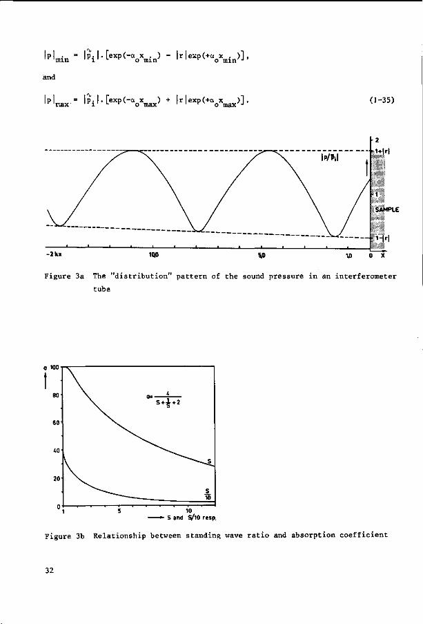
|p| = |p.| |exp(-a x)cos(kx)+|r |exp(a x)cos(kx+<)>)

- j exp(-a x)sin(kx)+j|r|exp(a x)sin(kx+c(>) I

= |p.|2 [exp(-2aox)+|r|2 exp(2aox)+2|r|cos(2kx+<t.)1. (1-31)

Eq.(l-31) constitutes the foundation on which interferometry rests, as it opens

the possibility of obtaining |r| and <(> from sound pressure measurements, and

thus of determining the normalized specific acoustic impedance of the sample

surface, using eq.(l-29a).

The first two terms of the right hand side of eq.(l-31) vary slowly and

slightly with x, whereas the last term varies more rapidly between -2|r] and

+2|r|. It follows from this relationship between |p| and x that there must be

positions where the pressure amplitude |p| will be minimum and maximum, re­

spectively. Only the last term can become negative. Because the assumption

|a x | « 1 is justified under practical conditions, exp(± 2a.x) equals unity

in zero-order approximation and 1 ±. 2a_x in first-order approximation. The

position of the minima is derived from the zero-order approximation, the

co-ordinate x . following from m m °

2 k x . +<t>=ir + 2 n T T ( n = 0, + l, + 2 ) . (1-32) m m

Using eq.(l-32) <|> follows from the positions of the minima but for an arbitrary

angle of 2nn radians. The fact that $ is multi-valued is insignificant, ai

exp j<(> is not. The ambiguity in § may thus be removed without loss of gener­

ality by requiring:

- TT < <)> < TT . ( 1 - 3 3 )

30

<)> is determined from the measured position of the minima, in preference to

those of the maxima, as the minima are the sharper of the two (see figure 3a).

The movable microphone used in the measurement is one of the type having an

acoustic centre or pressure-sensitive point, i.e. the output e.m.f. is pro­

portional to the sound pressure at one point. The position of the acoustic

centre in relation to the microphone often depends on frequency and must be

determined by acoustic measurement. This calibration of the microphone is

incorporated in the procedure described below.

Microphone position is measured on a scale having an increasing reading for

displacement away from the sample towards the loudspeaker. Note that this is

the - x direction. The reading for the first minimum, i.e. the minimum nearest

the sample, is 1 . and thus

x . - - 1 . , + 1 , mini mini cor

where x . , is the value of x for the first minimum and 1 is an unknown, mini cor

possibly frequency-dependent, length incorporating such effects as dis­

placement of the scale zero in relation to the sample surface and shift of the

acoustic centre.

The sample is now replaced by a rigid plate, and the position of the first

minimum is read from the scale: i'. ,. Now for such a plate 4 = 0 and the value mini e T

for x for the first minimum is thus known from eq.(l-32):

, = fl Xminl " " 2 k •

Now 1 may be found: cor J

1 = 1' - — • cor mini „, '

and using this value it follows that

* = 4,Taminl - i m i n l ^ ' C " 3 4 )

where X is the wavelength and the range for A is in accordance with requirement

(1-33).

Although consideration of the first minimum suffices in principle, further

minima have often to be evaluated as the sound field may be distorted near the

sample surface through the inhomogeneity of the sample.

For the sound pressures in the minima and the maxima, respectively, it now

follows from eq.(l-31) that

31

[exp(-a x . ) - |r|exp(+a x . ) ] ,

and

[exp(-a x ) + |r|exp(+a x )1 . L r o max ' ' v o max J (1-35)

Figure 3a The "distribution" pattern of the sound pressure in an interferometer

tube

o 100

10 S and S/10 resp.

Figure 3b Relationship between standing wave ratio and absorption coefficient

32

Since in ' f i r s t -order approximation |a x | « 1, i t can now be written iflsst

p | . = | p . | . f l - i r l - ( l + | r | ) o x . 1 r lmm " 1 1 L ° minj

- |p.| .f"l+|r|-(l-|t |).o x 1. l r r [ ' • ' ' o maxj

and

I P I . (1-36)

In figure 3a, p is shown schematically as a function of x. Consider IpI . r'min

as a linear function of x (c.f. eq.(1-36). a may be eliminated by extrapolating

|p| . to x = 0, the extrapolated value equalling (l-|r D-lrJ. on x to a lesser degree; extrapolation is unnecessary, and |p|

with sufficient accuracy.

IP I max

= (l + |r|)|p

depends ^ i

The standing wave ratio s (dimensionless) is defined as the ratio of the maximum

sound pressure and that of the minimum sound pressure. In a loss free tube, s is

a fixed quantity. For a tube with attenuation, where the minima differ measur­

ably in magnitude, one defines, unless specifically stated otherwise, the

the standing-wave ratio as the ratio of the maximum pressure and the minimum

pressure, both extrapolated to the sample surface:

" I P I 1 max

Jpl«in l-l x=0

Hr|

1- r

(1-37)

so

| r |

that

s-1

s+1 (l-37a)

The absorption coefficient a of the sample surface (dimensionless) is defined

as the ratio of the absorbed sound power to the incident power.

According to eqs(l-21a) and (l-21b) the incident and reflected powers are pro­

portional to |p.| en |p | , respectively. The absorbed power is thus pro­

portional to |p.| - |p | and, using eq.(l-26) it follows that (see also V

1020-26)

a = 1- r s+l/s+2

(1-38)

33

The number of maxima and minima that can be detected depends on the length of

the interferometer tube. In an interferometer of a length of 1.5 meter, e.g.,

only one minimum is found below about 200 Hz. Extrapolation of |p| . to the

site x = 0 is then no longer possible. Nevertheless |r| at x = 0 can be deter­

mined in the following way. Instead of extrapolating s to x = 0 and converting

s there into |r| with eq.(l-37) one can convert s at the minimum into |r| at

the minimum with eq.(l-37) and extrapolate |r| to x = 0 with the equation:

r • 1 'mm |r| x = 0 exp(2 V m . n ). (1-39)

One needs then to know, however, a... Since this is not the case one has to carry

out an extra experiment, viz. after replacing the sample by a rigid, massive

non-absorbing plate. In this case |r| _. = 1, so that

|r'I . = exp(2anx' . ). (1-40) ' 'min r 0 min

r'|and x' are measured and an can be calculated.

At very low frequencies, no maximum is available within the finite length of

the tube. However, in that case and for the sample used, sound pressure at the

sample surface is practically maximum. Thus an approximate value for the

standing-wave ratio may be found by introducing the sound pressure at the

sample surface as the maximum value.

Under these conditions, - only one minimum available - the wavelength cannot be

measured and accurate determination of the phase angle is impossible. A value

for this latter quantity is then estimated by extrapolation from measurements

at higher frequencies.

Summarizing one may state that the analysis of the standing wave pattern

consists of determining the positions of the minima and the magnitudes of the

sound pressures at maxima and minima.

Under these conditions - only one minimum available - the wavelength cannot be

surface (which is usually the obvious plane of reference) as a function of

frequency. From this function conclusions may be drawn about the acoustical

properties of the sample material.

34

Nm -2

1.5 The velocity of sound in a mixture of ideal gases

Before a discussion of the velocity of sound in porous materials, some remarks

will be made on the velocity of sound in air. In particular, attention will be

paid to possible changes in velocity through changes in experimental conditions.

The velocity can be calculated from the kinetic gas theory. Hardy, Telfair and

Pielemeier (1941) made extensive investigations on the velocity of sound in

gases of various composition and under various pressures. Starting from eq.(l-7)

for the velocity of sound the question stated above can be formulated as follows*

What are the values for K and o for a mixture of gases with known partial

pressures? To answer this question the following quantities are introduced

f, = the mass fraction of component k k

p = the partial pressure of component k

R = the gas constant per kmol

M. = the molar mass of component k

T = the absolute temperature (identical for all components)

V = the total volume of 1 kg of the gas mixture

(identical for all components)

c,„ = the molar specific heat of component k at Vk

constant volume

c , = the molar specific heat of component k at

constant pressure

S, = the entropy of component k

p = the total pressure of the gas mixture

S = the total entropy of 1 kg of the gas mixture

Assuming Dalton's law to hold the equation of state for component k in 1 kg of

the mixture is:

A" kmol"1

kg kmol

°K 3.

m kg

J°K-

J°K-

J V

Nnf2

J V

-1

kmol

kmol

' k g

' k g " 1

Pvv RT.

\ (1-41)

For component k in 1 kg of the gas mixture the first law of thermodynami

yields

35

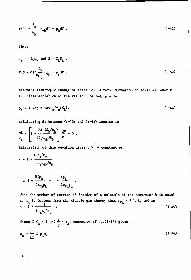
T d S k = ~ cvkdT + Pkdv (1-42)

"k

Since

p s = £ k p k and S = Z k S k ,

TdS = dTX — c,n + p dV W ^ s (1-43)

Assuming isentropic change of state TdS is zero. Summation of eq.(l-41) over k

and differentiation of the result obtained, yields

p dV + Vdp - RdTIk(fk/Mk). (1-44)

Eliminating dT between (1-43) and (1-44) results in

*E + RZ

1 +

(V>V If.

k C V k / M k

dV 0 .

Integration of this equation gives p V = constant or

K = 1 + B £ £ k / M k

k Vk'

1 + "«*,,

1 + RP„

re Vkpk EcVkPk

When the number of degrees of freedom of a molecule of the component k is equal

to h, it follows from the kinetic gas theory that c„, = J \.R> an& s °

< = 1 + . (1-45) a A / p s

Since £ f, = 1 and — = o , summation of eq.(l-27) gives: k V s

S RT k k (1-46)

36

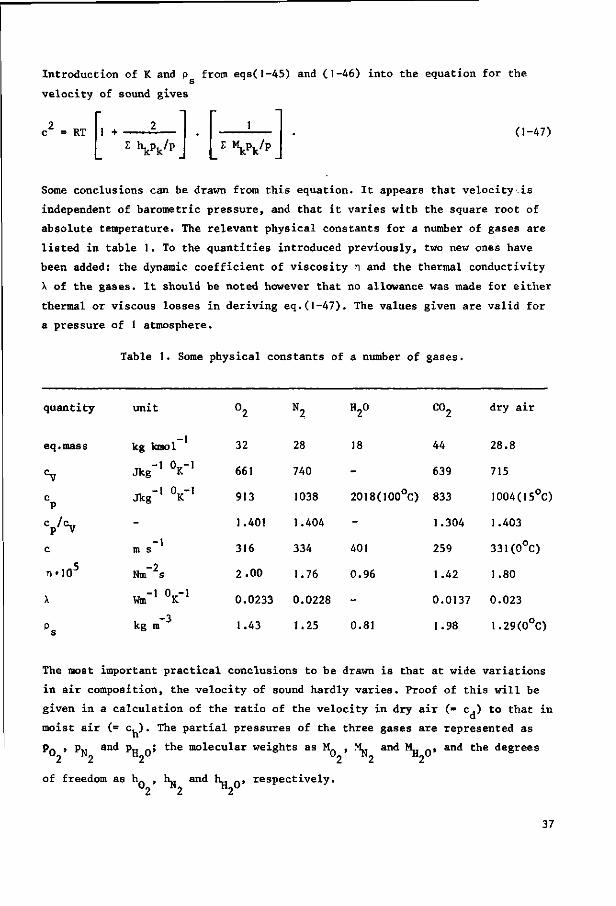
Introduction of K and p from eqs(l-45) and (1-46) into the equation for the

velocity of sound gives

2 c2 = RT 1 +

E Vk/p w> (1-47)

Some conclusions can be drawn from this equation. It appears that velocity is

independent of barometric pressure, and that it varies with the square root of

absolute temperature. The relevant physical constants for a number of gases are

listed in table 1. To the quantities introduced previously, two new ones have

been added: the dynamic coefficient of viscosity n and the thermal conductivity

X of the gases. It should be noted however that no allowance was made for either

thermal or viscous losses in deriving eq.(l-47). The values given are valid for

a pressure of 1 atmosphere.

Table 1. Some physical constants of a number of gases.

quantity

eq.mass

c P

Cp/cV

c

T l O 5

X

p

unit

-1 kg kmol

Jkg K

Jkg K

-1

Nm s

W,"1 V 1

kg m -3

°2

32

661

913

1.40!

316

2.00

N2

28

740

1038

1.404

334

1.76

H20

18

-

2018(100°C)

-

401

0.96

co2

44

639

833

1.304

259

1.42

dry air

28.8

715

1004(15°C)

1.403

331(0°C)

1.80

0.0233 0.0228

1.43 1.25

0.0137 0.023

0.81 1.98 1.29(0°C)

The most important practical conclusions to be drawn is that at wide variations

in air composition, the velocity of sound hardly varies. Proof of this will be

given in a calculation of the ratio of the velocity in dry air (= c,) to that in

moist air (= c, ). The partial pressures of the three gases are represented as

p_ , p„ and p„ Q; the molecular weights as M0 , VL, and H^ Q, and the degrees

of freedom as h- , \ . and tv, n, respectively. °2 ^2 ^2°

37

Int roducing hQ = h^ = h , pQ /p^ «•• g and pR Q / p g = r , and us ing e q . ( l - 47 )

one f i nds :

c d 2 _ ' + < V o / h - '>'r

cn2 * + CV" h ) - r / ( 2 + h ) 1 - (1 -

O+g)*^, 22_

V + ^02 ( l -48a)

As r is a small quantity at room temperature, eq.(l-48a) may be approximated as

*I J.r. (l-48b)

For air, at a relative humidity of 100%, a temperature of 20 C and a pressure of

76 cm Hg,

Sub stituting g = 1/4, h^ = h = 5, h ^ = 6, - 28, M = 32 and M ^ 18

into eq.(l-48b) yields : c./c, = 0.9963. d h

Hence, the conclusion can be drawn that the velocity of sound is barely af­

fected by the pressure of water vapour in air. This conclusion will also apply

for changes in C0„ pressure of the same order as those in pressure of water

vapour. Furthermore, one may infer from eq.(l-47) that a 2 increase in tempera­

ture at room temperature affects the velocity of sound to the same extent as

does saturating dry air with water vapour. The effect of variations in the

composition of the gas on sound velocity is slightly greater than the effect of

variations in the temperature of the gas under practical circumstances. However

both have little influence. Thus, for the present purpose, conversions to normal

pressure and/or temperature are unnecessary. It can also be inferred from the

data of table 1 that the product p c does depend on gas pressure and it might be

argued that a correction for this effect should be introduced. This effect may

cause variations of the order of 1%. As shown in Chapter 2 the accuracy of the

measurements is of the same order so neither corrections will be made for vari­

ations in barometric pressure.

38

1 .6 Intensity, decibel, damping in air

The concept of sound intensity was introduced in section 1-3. Intensities are

often expressed on a logarithmic scale; the intensity level LT is then defined

by

Lj - 10 log (I/I0), (1-49)

where I is the reference intensity, standardized at 10 W/m .

L_ is given in decibels, abbreviated to dB, and the reference quantity should

always be given, e.g. in parenthesis, behind this unit; L_ is thus given in

dB(10~12 W / m 2 ) .

One of the advantages of the introduction of the decibel scale is that the

numerically wide range of intensities encountered in acoustical practice, e.g. — 12_ 2 2

from 10 w/m to 1 W/m , is considerably reduced on the intensity level scale,

from 0 dB(10"12W/m2) to 120 dB(10~ W / m 2 ) .

The difference in intensity level A L for two intensities, I. and I„, now

follows as

AL]. = 10 log(I,/l2), (1-50)

where AL is expressed in dB, the reference quantity being omitted as being

arbitrary for level differences.

For sound pressures too, a logarithmic scale has been defined, the sound

pressure level L . For a sound pressure having an RMS value p

L p = 20 log(pe/po),

—5 2 where p is the reference pressure, standardized at 2*10 N/m . L is ex-

0 -5 2 p

pressed in dB(2#10 N/m ) . p has been so selected, that for a plane wave

travelling in air, LT = L with an accuracy that is usually adequate. To gain

some insight into the magnitudes of the quantities introduced it is noteworthy -5 2

that the threshold of hearing at 1000 Hz is roughly 0 dB(2-10 N/m ) and that -5 2

a sound pressure level of 130 dB (2*10 N/m ) is experienced as painful. That

sound pressures are relatively small may be concluded from the fact that

p re 2*10 atmosphere. In section 1»5, it was shown that in air the velocity

of sound is hardly affected by the composition of the gas mixture. Besides

damping in the interferometer tube through losses along the walls, a slight

damping occurs in the air itself. This damping can be ascribed to several

causes:

1. A viscous damping of the free wave exists due to diffusion of impulse.

39

?, Thermal losses occur in the free wave due to diffusion of kinetic energy.

3. Over and above these above mentioned causes, which constitute portions of

the "classical damping", a molecular damping occurs through the "long" relax­

ation time of a rotational level of the oxygen molecules.

This relaxation time is strongly dependent on the content of water vapour.

Reference is made to the work of Kneser (1931) and Harris (1963).

It appears from this investigation that for the present purpose this damping

will be unimportant. No further attention will therefore be paid to it.

1.7 Velocities in air

To avoid possible confusion, the various velocities obtaining in gases will be

commented on briefly. Air, considered as an ideal diatomic gas having a molecu­

lar mass M = 29, will serve as illustration, the approximation involved being

acceptable for the present purpose.

The following velocities are distinguished.

1. The thermal velocity of the molecules, represented by its RMS value V . The

average required may be taken in time for one molecule or over an ensemble of

molecules, the results being identical as the system is ergodic.

2. The particle velocity u of the molecules. This is the drift velocity due to

a sound field, the average velocity vector of the molecules in a domain that

contains a large number of molecules, but is small in relation to wavelength.

For such a domain the average thermal velocity vector approaches zero.

3. The velocity of propagation of a sound wave or the velocity of sound, c.

The kinetic theory of gases states that the average energy per degree of

freedom and per molecule equals JknT, where k^ is Boltzmann's constant and T

is the absolute temperature. The kinetic energy of translation of a molecule 3

is thus given by -z k_T, as it corresponds to three degrees of freedom. This

energy is also given by jM'vi'V , where M is the molecular mass of the molecule

and v is the unit of atomic mass (roughly that of a hydrogen atom). Thus

Ve = /(3kBT/yM). (1-51)

Introduction of the numerical values k„ = 1.38 • 10~ J°K~ , T = 293 °K, -27

M = 29, y =• 1.66 • 10 kg, into eq.(l-51) yields the numerical value for air

at room temperature of V = 502 m s . The particle velocity due to a sound

field is essentially much smaller. For a plane wave having a sound pressure level

40

_5 -2 -2 -2

of 70 dB(2»10 N m ) , i.e. having an RMS sound pressure of 6.3*10 N m , the

RMS particle velocity is found, making use of the numerical value of the specific

acoustic wave impedance (see section 1.2), p c = 420 Nts m ; |u| =• 1.5 • 10 -1 s

m s

The velocity of sound is closely related to the thermal velocity of the mole­

cules. Appealing to simple kinetic gas theory once again and using eq.(l-7), it

follows that

c = Ve/(</3).

Introduction of V = 502 m/s and K = I.4 yields approximately c = 340 m/s, in

agreement with experiment.

1.8 The heat generated

It is reasonable to think that heat dissipation as a result of absorption of

sound energy will give rise to a measurable increase in temperature.

To take an example, a sound pressure level for the incident wave in the inter--5 2

ferometer of 70 dB (2*10 N/m ) , thermal power developed in the sample per unit -5 -2

area will be less than 10 W m

For comparison, the radiation energy reaching the earth from the sun is approxi--2

mately 1000 W m . The resulting rise in temperature will be at the most a few

tenths of degrees. Thus it will be clear that the heat developed in an ab­

sorbing material by a sound wave will not give rise to a measurable temperature

increase. For this reason no evaporation or temperature gradient will occur in

the sample when sound absorption is measured. Hence, water will not be displaced

by convective currents.

I.9 Sound waves in porous media

For a free wave, the pressure gradient in the gaseous medium is governed by the

inertia of that medium. In a porous material, however, consisting of intercon­

nected, gas-filled pores enclosed in a rigid solid frame, sound waves propa­

gating in the pores will encounter higher forces of inertia as the gas is ac­

celerated through narrow vents and viscous friction will have to be overcome.

Considered in time the viscous drag will give rise to a component in the

pressure gradient in phase with the particle velocity while the forces of

inertia correspond to a component at right angles to that gradient (this latter

component performs no work on the medium). Thus the resultant complex pressure

4J

gradient is no longer at right angles to the particle velocity, which may be

accounted for by restating eq.(l-l) for harmonic waves:

l£ = Z u, (1-52) o m

dx

where p is the actual sound pressure in the pores but u is the volume velocity

of the gas per unit area (the actual particle velocity in the pores will be

higher). The complex, frequency-dependent factor Z will be called the specific . m . . -4

acoustic series impedance per unit length; its dimension is Nsm

The compressibility of the gas in the pores differs from that for a free wave,

part of the available space being occupied by the solid frame and heat exchange

taking place between the gas and the frame. As the exchange of thermal energy

takes time, the relative compression of the medium and the sound pressure are

no longer in phase. Indeed a small ellipse is traversed in the pV diagram. This

results in a change in the difference of the phase between the complex velocity

gradient and the complex sound pressure, now being less than TT/2. In free air

this last value will be found. The change may be accounted for by restating eq.

(1-2) for harmonic waves

- — - Y D , (1-53) 3x m

where the complex, frequency»dependent factor Y is called the specific acoustic -1 -1 2 parallel admittance per unit length ; its dimension is N s m .

Acoustically the material is characterized completely by the complex frequency-

dependent factors Z and Y . The central problem of this text are the experi­

mental determination of these factors and their relationship to the structure

of the material, which will be discussed in detail in chapter 3.

For the time being, Z and Y are introduced formally and, as in section 1.2, u

m m J

is here eliminated from eqs(l-52) and (1-53) yielding

^ 2 " V Y m P. ,. I m m 3x

an equation of the Helmholtz type, as explicit differentiation to time is ab­

sent.

Travelling waves in porous materials will undergo attenuation. Following a

course suggested by eqs(l-23a) .. . (l-25c), derived for waves, attenuated in

42

interferometers, a complex propagation constant is introduced,

Y = a + j0 , m m J m

and a s o lu t ion of the form

p = p\ exp(- Yffix) + p r exp(Ymx),

is essayed. It satisfies the Helmholtz equation if

Y = /(Z -Y ) . (1-54) m m m

Using eqs(l-52) and (1-54), the solution for u follows

pi pr u = — exp(- Y x) exp(Y x ) ,

W W m m

where the specific acoustic wave impedance of the material, W , is given by

Wm = /(Z /Y ) . (1-55) m m m

It will be clear from eqs(l-54) and (1-55) that the material is also specified

acoustically by the pair of complex quantities Y and W . m m

Now consider a sample of porous material fitted to the end of an interferometer

tube in a sample holder. The interface between the air column in the tube and

the sample material is at x = 0. Note that the quantities p and u in the ma­

terial have been so defined that they are continuous with the quantities p and

u in the tube at the interface.

Supposing the sample to have a rigid backing at x = 1, in practice a thick metal

plate (see section 2.5), the boundary condition there is u = 0 and thus

p /p. = exp(-2Y 1). Introduction of this quantity and of x = 0 into the e-

quations for p and u yields the values for these latter two at the sample

surface

p = pi|l+exp(-2Yml)J

u = [l-exp(-2Yml)]/Wm

43

The specific acoustic impedance at the sample surface now follows from its

definition, eq.(l-27) as

Z = W coth(y 1 ) , (1-56) m m

the fundamental relationship between the measurable quantity Z and the material

constants W and Y . m m

In principle, this type of derivations may be extended to stratified samples,

consisting of layers of porous materials with various acoustical properties

(Kosten, 1953).

Before going into the problems raised by the transcendental nature of eq.(l-56),

the derivation of Z, or rather of the closely related quantity C, c.f. eq.(l-28),

from the quantities which follow more directly from measurement, as |r| and <j>,

and forms of graphical representation for <; will be discussed.

1.10 Presentation of the normalized specific acoustic impedance

The measurements in the interferometer tube lead directly to numerical values

for 1 . and s from which by simple computation <|> and r can be derived with min

the aid of eq.(l-32) and eq.(l-38) respectively. <|> and |r| determine the complex

reflection coefficient r, from which the normalized specific acoustic impedance

of the sample can be found by using the equation

c = 111 = 2s + j(s2-l)sin 4. _ ( ] _ 2 9 a )

1-r s + 1 - (s -l)cos <t>

This computation of r, via s and i is time consuming. To avoid this difficulty

some handy tools have been developed. One can transform the complex r plane

into a complex £ plane or vice versa, which enables one to read the complex

value £ for a given complex value of r or in the reverse sense if desired. This

transformation from r to C is a conformal transformation. In such a transfor­

mation a circle in one plane corresponds to a circle in the transformed plane;

angles between lines in both planes remain unchanged. Two of these types of

transformations, that are in practical use will be considered now.

A The impedance diagram

This diagram is the transformation of the complex r-plane into the complex c~

plane (see figure 4 ) . Any point in this diagram represents a value of the

44

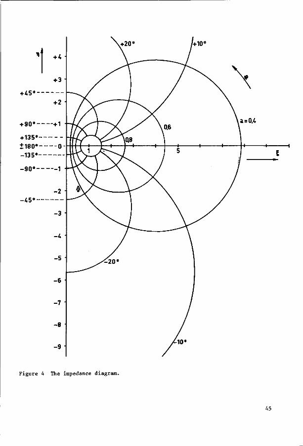
Figure 4 The impedance diagram.

45

complex quantity C = 5 + j>1.

The real part is the distance to the vertical (imaginary) axis; the imaginary

part, the distance to the horizontal (real) axis. From eq.(l-29a) it follows

that for each point in the C-plane, a corresponding value of r = |r| exp(j<j>) can

be obtained. Therefore lines of constant ]r| and of constant $ can be drawn in

this plane. Since a = /(l-|r| ) lines of constant |r| are also lines of constant

absorption coefficient.

From

5 -J±Ld«EE<it), (1-57) l-|r|exp(j<t>)

it follows that

,2 1- r

l+|r|2 - 2lr|cos> (1-58)

and

n 2 H s i n * . (1-59)

l+|r| " 2|r|cos<t>

The1)1 is eliminated from eqs(l-58) and (1-59) and |r| is retained as a parame­

ter. Thus a family of curves for constant |r| is generated in the £ plane, a

member of the family being given by

[5 - (l + |r|2)/(l-|r|2)] + n 2 = [i>|r |/(l-|r | 2 ) ] 2 . (1-60)

The curves prove to be circles, having their centres at

5 = (l+|r|2)/(l-|r|2), n = 0,

and radii given by

R = 2|r|/(l-|r|2).

Similarly,|r|may be eliminated and $ retained as parameter. A family of circles

for constant <t> is thus generated, which proves to intersect the ones for

constant Ir|at right angles. A member of the family is given by

[n - cot(*)]2 + S 2 = [l/sin(+)]2, (1-61)

46

these circles having their centres at

5 = 0, n = cot(*),

and their radii are given by

R = l/sin(<|>).

In figure 4, a number of circles from these families of circles is drawn. As

was argued in section 1-4, an unambiguous value for $ may be obtained by im­

posing condition (1-33). Eq.(l-59) shows that, for 0«t><ir- n>0 and conversely

that, for -Tr<<|><0->n<0.

Thus the circles for constant 4> are given positive values above the real axis

and negative values below this axis.

When, for instance, |r| and <(> are known from measurements, values of 5 and n

can be read from the diagram. As an example, the position of one point A has

been indicated in figure 4.

From the diagram it can be read that |r| « 0.86 and <J> sa 50 , £ = 0.5 and n =

- 2.0.

B The Smith diagram

This diagram presents the reflection coefficient r = |r|exp(j4>) = u + jv in the

complex plane. In this case lines of constant £ and n are circles. The loci of

constant 5 and n can be calculated from the eq.(l-29b)

u + j v = is+jnidL. (,-62)

(C+jn) + l

When £ is constant, n can be eliminated. This yields

(u - - M 2 + v2 = (-L)2, (1-63)

e+i 5+1

and, concomitantly, when n is constant, it follows that

(u-1)2 + ( v - - ) 2 = (-1)2. (1-64)

Ti n Some circle segments of these families of circles are shown.

When the position |r|j <|> in polar co-ordinates is known from measurements, it

can be plotted in the Smith diagram. The values of the corresponding £ and n

can now be read from the loci.

47

Figure 5 The Smith diagram.

48

In figure 5 one point A is the transformation of the point denoted by the same

symbols in figure 4.

An advantage of the Smith diagram is that all values lie within one circle,

whereas the impedance diagram is a semi-infinite plane and a finite part of it

cannot show values for £ and n beyond its limits.

The impedance diagram is not accurate for small values of £. In the Smith dia­

gram, which is often used in electronics, the large values of 5, which occur

frequently in acoustics, cannot be read with any accuracy, which constitutes a

major disadvantage for its adoption here. In the following chapters, the im­

pedance diagram will be used exclusively.

1.11 The behaviour of the function Z = W coth (yl) in the impedance

plane

To gain at least a qualitative insight into the locus in the complex plane of

the specific acoustic impedance at the sample surface, see eq.(l-56), the function

Z = W coth (yl) will be discussed, partly after Zwikker and Kosten (1949).

W and y are complex constants of the sample material. They will depend upon the

structure and the frequency. According to eqs(l-54) and (1-55) they are connected

with Z and Y as follows: y = /(Z Y ) and W = /(Z /Y ) , where Z and Y are m m m m m m m m m m

defined with the fundamental differential equations (1-52) and (1-53) resp­

ectively. Z and Y are- also complex. In free air they are equal to jcoo and

jw/K respectively, so that in air Ym = W ( p / K ) = jco/c and W = /(Kp) = p c

respectively. In free air, therefore, Y is proportional to frequency; W is

independent of frequency.

In loose soil samples, therefore, W will probably vary slowly and slightly with

frequency, where as y will probably vary rather rapidly with frequency,

increasing approximately proportionally with frequency. Introducing Y = a +jB ,

8 will probably be approximately proportional to frequency, but a - the

attenuation coefficient of travelling waves in the material - will, again, be a

weak function of frequency.

The denser the material is, the larger will be the difference from the behaviour

of free air, but anyhow it seems reasonable to expect W "rather" constant and

Y "more or less" proportional to frequency. The results of measurements m

corroborate these expectations.

Based on this consideration the behaviour of the function Z = W coth(Yl)can be

studied in the complex plane.

49

*

•

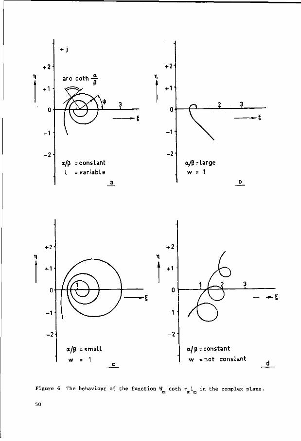
+ 2

+ 1 •

n u •

- 1 '

- 2 -

+ j

arc coth-^-

m>^\* [\zJ \

a/p = constant I = variable

a

3

— 1

i

a/p = large

w = 1

a/p = small

w = 1

+ 2i

+H

- 1 1

a/p =constant

w =not constant

Figure 6 The behaviour of the function W coth y 1 in the complex plane. tn m m

50

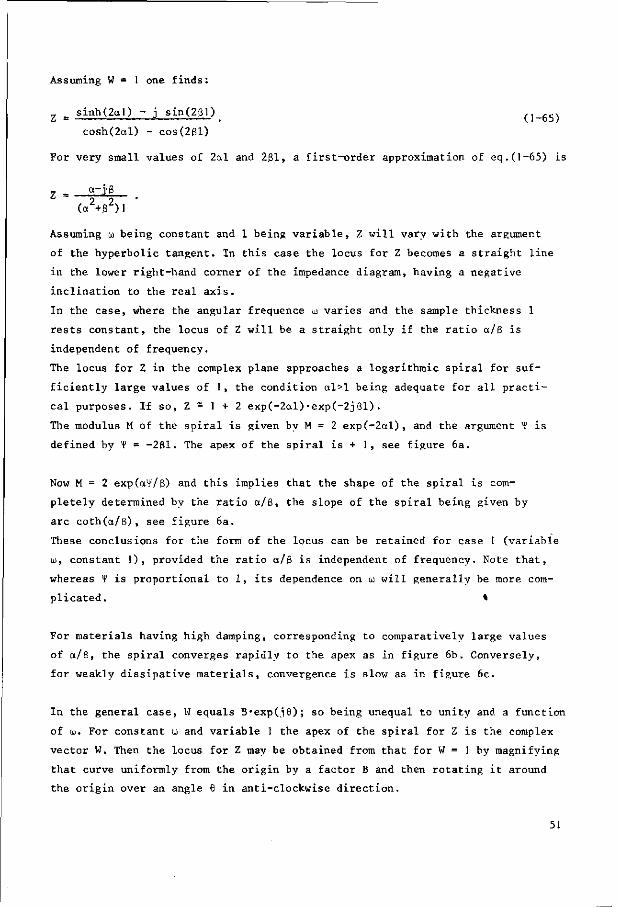
Assuming W = 1 one finds:

Z = sinn(2al) ~ J sin(2g1) (1-651

cosh(2al) - cos(261)

For very small values of 2al and 281, a first-order approximation of eq.(l-65) is

Z = <*-jB 2 2

Assuming u> being constant and 1 being variable, Z will vary with the argument

of the hyperbolic tangent. In this case the locus for Z becomes a straight line

in the lower right-hand corner of the impedance diagram, having a negative

inclination to the real axis.

In the case, where the angular frequence to varies and the sample thickness 1

rests constant, the locus of Z will be a straight only if the ratio ot/B is

independent of frequency.

The locus for Z in the complex plane approaches a logarithmic spiral for suf­

ficiently large values of 1, the condition al>l being adequate for all practi­

cal purposes. If so, Z - 1 + 2 exp(-2al)-exp(-2jBl) •

The modulus M of the spiral is given by M = 2 exp(-2al), and the argument ¥ is

defined by ¥ = -281. The apex of the spiral is + 1, see figure 6a.

Now M = 2 expCaV/B) and this implies that the shape of the spiral is com­

pletely determined by the ratio a/8, the slope of the spiral being given by

arc coth(a/B), see figure 6a.

These conclusions for the form of the locus can be retained for case 1 (variable

ID, constant 1), provided the ratio a/B is independent of frequency. Note that,

whereas 1 is proportional to 1, its dependence on u will generally be more com­

plicated. »

For materials having high damping, corresponding to comparatively large values

of a/8, the spiral converges rapidly to the apex as in figure 6b. Conversely,

for weakly dissipative materials, convergence is slow as in figure 6c.

In the general case, W equals B'exp(ie); so being unequal to unity and a function

of u. For constant u and variable 1 the apex of the spiral for Z is the complex

vector W. Then the locus for Z may be obtained from that for W = 1 by magnifying

that curve uniformly from the origin by a factor B and then rotating it around

the origin over an angle 6 in anti-clockwise direction.

51

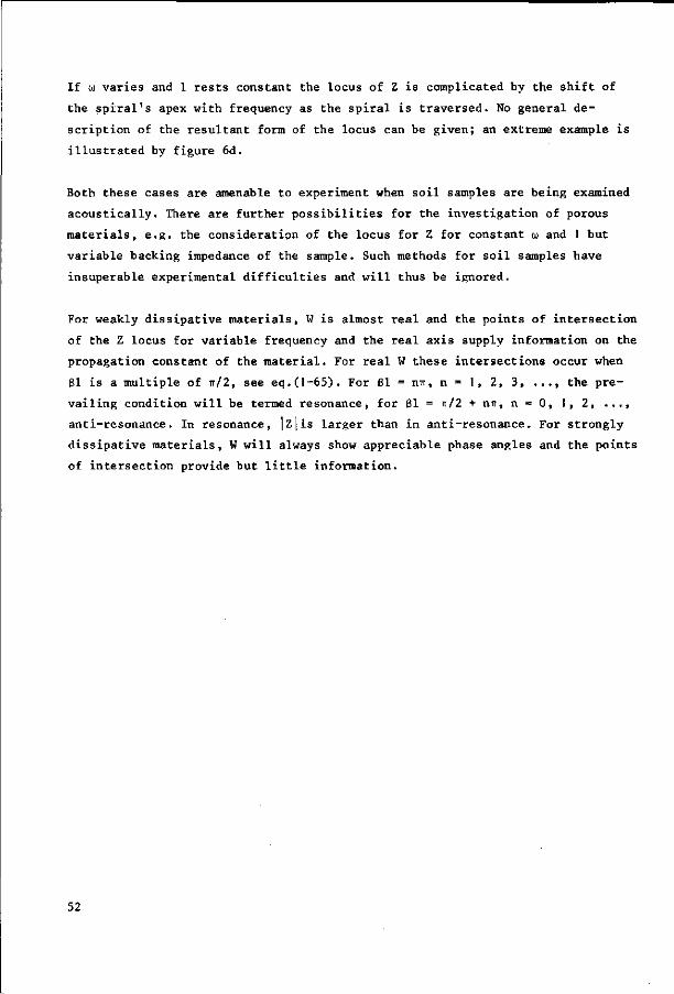
If a) varies and 1 rests constant the locus of Z is complicated by the shift of

the spiral's apex with frequency as the spiral is traversed. No general de­

scription of the resultant form of the locus can be given; an extreme example is

illustrated by figure 6d.

Both these cases are amenable to experiment when soil samples are being examined

acoustically. There are further possibilities for the investigation of porous

materials, e.g. the consideration of the locus for Z for constant o> and 1 but

variable backing impedance of the sample. Such methods for soil samples have

insuperable experimental difficulties and will thus be ignored.

For weakly dissipative materials, W is almost real and the points of intersection

of the Z locus for variable frequency and the real axis supply information on the

propagation constant of the material. For real W these intersections occur when

61 is a multiple of TT/2, see eq.(l-65). For 61 = nti, n = 1, 2, 3, ..., the pre­

vailing condition will be termed resonance, for 61 = W 2 + nir, n = 0, 1,2

anti-resonance. In resonance, |z|is larger than in anti-resonance. For strongly

dissipative materials, W will always show appreciable phase angles and the points

of intersection provide but little information.

52

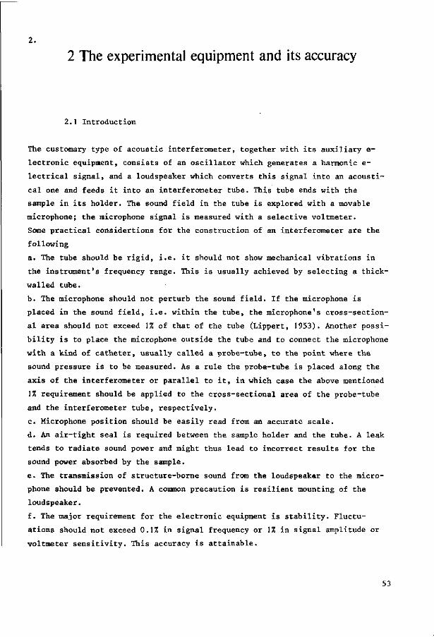
2 The experimental equipment and its accuracy

2.1 Introduction

The customary type of acoustic interferometer, together with its auxiliary e-

lectronic equipment, consists of an oscillator which generates a harmonic e-

lectrical signal, and a loudspeaker which converts this signal into an acousti­

cal one and feeds it into an interferometer tube. This tube ends with the

sample in its holder. The sound field in the tube is explored with a movable

microphone; the microphone signal is measured with a selective voltmeter.

Some practical considertions for the construction of an interferometer are the

following

a. The tube should be rigid, i.e. it should not show mechanical vibrations in

the instrument's frequency range. This is usually achieved by selecting a thick-

walled tube.

b. The microphone should not perturb the sound field. If the microphone is

placed in the sound field, i.e. within the tube, the microphone's cross-section­

al area should not exceed 1% of that of the tube (Lippert, 1953). Another possi­

bility is to place the microphone outside the tube and to connect the microphone

with a kind of catheter, usually called a probe-tube, to the point where the

sound pressure is to be measured. As a rule the probe-tube is placed along the

axis of the interferometer or parallel to it, in which case the above mentioned

1% requirement should be applied to the cross-sectional area of the probe-tube

and the interferometer tube, respectively.

c. Microphone position should be easily read from an accurate scale.

d. An air-tight seal is required between the sample holder and the tube. A leak

tends to radiate sound power and might thus lead to incorrect results for the

sound power absorbed by the sample.

e. The transmission of structure-borne sound from the loudspeaker to the micro­

phone should be prevented. A common precaution is resilient mounting of the

loudspeaker.

f. The major requirement for the electronic equipment is stability. Fluctu­

ations should not exceed 0.1% in signal frequency or 1% in signal amplitude or

voltmeter sensitivity. This accuracy is attainable.

53

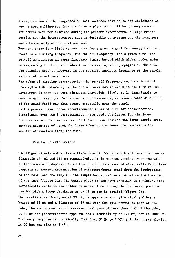
A complication is the roughness of soil surfaces that is to say deviations of

one or more millimetres from a reference plane occur. Although very coarse

structures were not examined during the present experiments, a large cross-

section for the interferometer tube is desirable to average out the roughness

and inhomogeneity of the soil surface.

However, there is a limit to tube size for a given signal frequency; that is,

there is a limiting frequency, the cut-off frequency, for a given tube. The

cut-off constitutes an upper frequency limit, beyond which higher-order modes,

corresponding to oblique incidence on the sample, will propagate in the tube.

The quantity sought, however, is the specific acoustic impedance of the sample,

surface at normal incidence.

For tubes of circular cross-section the cut-off frequency may be determined

from k R = 1.84, where k is the cut-off wave number and R is the tube radius, c c

Wavelength is then 1.7 tube diameters (Rayleigh, 1910). It is inadvisable to

measure at or even just below the cut-off frequency, as considerable distortion

of the sound field may then occur, especially near the sample.

In the present case, three interferometer tubes of circular cross-section,

distributed over two interferometers, were used, the larger for the lower

frequencies and the smaller for the higher ones. Besides the large sample area,

another advantage of using the large tubes at the lower frequencies is the

smaller attenuation along the tube.

2.2 The interferometers

The larger interferometer has a flame-pipe of 155 cm length and inner- and outer

diameters of 162 and 171 mm respectively. It is mounted vertically on the wall

of the room. A loudspeaker 12 cm from the top is suspended elastically from three

supports to prevent transmission of structure-borne sound from the loudspeaker

to the tube (and the sample). The sample-holder can be attached to the lower end

of the tube (figure 7a). The bottom plate of the sample-holder is a piston, that

hermetically seals in the holder by means of an 0-ring. In its lowest position

samples with a layer thickness up to 16 cm can be studied (figure 7b).

The Ronette microphone, model MC 65, is approximately cylindrical and has a

height of 12 mm and a diameter of 29 mm. With its axis normal to that of the

tube, the microphone has a cross-sectional area of less than 0.5% of the tube.

It is of the piezo-electric type and has a sensitivity of 1.7 mV/ybar at 1000 Hz.

Frequency response is practically flat from 30 Hz to 1 kHz and then rises slowly.

At 10 kHz the rise is 8 <1B.

54

The microphone is attached to an endless belt running inside the tube 4 mm from

the inner wall. Outside the tube the belt has been provided with a gauge. The

displacement of the microphone can easily be read in fifths of a millimeter.

The Philips loudspeaker, model 9744, has a cone diameter of 130 mm, a voice coil

impedance of 5 Q at 1 kHz and a nominal power-handling capacity of 3 W.

The frequency range of the interferometer ranges from 50 - 1100 Hz.

For the measurement of the porosity of the sample a special lid that fits to the

upper end of the sample-holder has been constructed. By a thick-walled plastic

tube attached to an opening in this lid, the sample-holder can be connected with

a porosimeter.

The porosimeter is founded on Boyle's law: p-V = constant. The porous material

under test is enclosed in a container of known value. The actual volume avail­

able to the gas, however, is that of the container diminished by that of the

solid matter in the sample.

The porosity of the material is easily calculated if the actual gas volume has

been determined and this is done by introducing a known change in volume,

measuring pressure both before and after the change. The initial value of the

actual volume is now the only unknown and Boyle's law may be solved for it. As

will have become apparent from the selection of a gas law, changes of state are

assumed to be so slow that they are isothermal.

Porosimeters have been described, e.g. Loebell (1935), Bourrier (1951), Alten

and Loofmann (1956). The instrument is satisfactory for samples composed of

gases and impervious solid matter. But where liquids may evaporate during ex­

pansion or adsorbed gases may be freed, results will be unreliable. And as such

conditions commonly prevail in soils, other methods must be sought for de­

termining their porosity.

In principle measurements of resistance to air flow can also be made on the

sample. With a reinforced "sieve plate" at the upper end of the sample-holder,

the sample can be turned upside down. Next, the bottom plate can be removed.

In this position, the sample-holder can be attached to the lower end of a gas con­

tainer. In many cases the samples do not permit such a treatment without a dis­

turbance of their geometrical arrangement. Therefore the required additional

measurements were performed on separate samples in most instances. Measurements

of air-flow resistance can also be made on samples contained in wide vessels.

If so, the standing-wave tube is extended by a cylinder of the correct inner

diameter, having a gasket at the top, sealing it to the main tube, and a cutting

edge at the bottom. The cutting edge is driven into the sample.

55

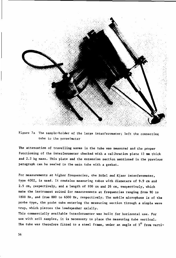
Figure 7a The sample-holder of the large interferometer; left the connecting

tube to the porosimeter

The attenuation of travelling waves in the tube was measured and the proper

functioning of the interferometer checked with a calibration plate 12 mm thick

and 2.2 kg mass. This plate and the extension section mentioned in the previous

paragraph can be sealed to the main tube with a gasket.

For measurements at higher frequencies, the Bruel and Kjaer interferometer,

type 4002, is used. It contains measuring tubes with diameters of 9.9 cm and

2.9 cm, respectively, and a length of 100 cm and 26 cm, respectively, which

make the instrument suited for measurements at frequencies ranging from 90 to

1800 Hz, and from 800 to 6500 Hz, respectively. The mobile microphone is of the

probe type, the probe tube entering the measuring section through a simple wave

trap, which pierces the loudspeaker axially.

This commercially available interferometer was built for horizontal use. For

use with soil samples, it is necessary to place the measuring tube vertical.

The tube was therefore fitted to a steel frame, under an angle of 5° from verti-

56

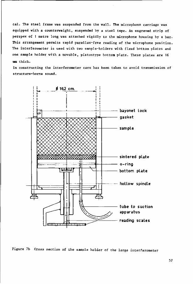
cal. The steel frame was suspended from the wall. The microphone carriage was

equipped with a counterweight, suspended by a steel tape. An engraved strip of

perspex of 1 metre long was attached rigidly to the microphone housing by a bar.

This arrangement permits rapid parallax-free reading of the microphone position.

The interferometer is used with two sample-holders with fixed bottom plates and

one sample holder with a movable, pistontype bottom plate. These plates are 16

mm thick.

In constructing the interferometer care has been taken to avoid transmission of

structure-borne sound.

bayonet lock

gasket

sample

sintered plate

o-r ing

bottom plate

hollow spindle

tube to suction apparatus

reading scales

Figure 7b Cross section of the sample holder of the large interferometer

57

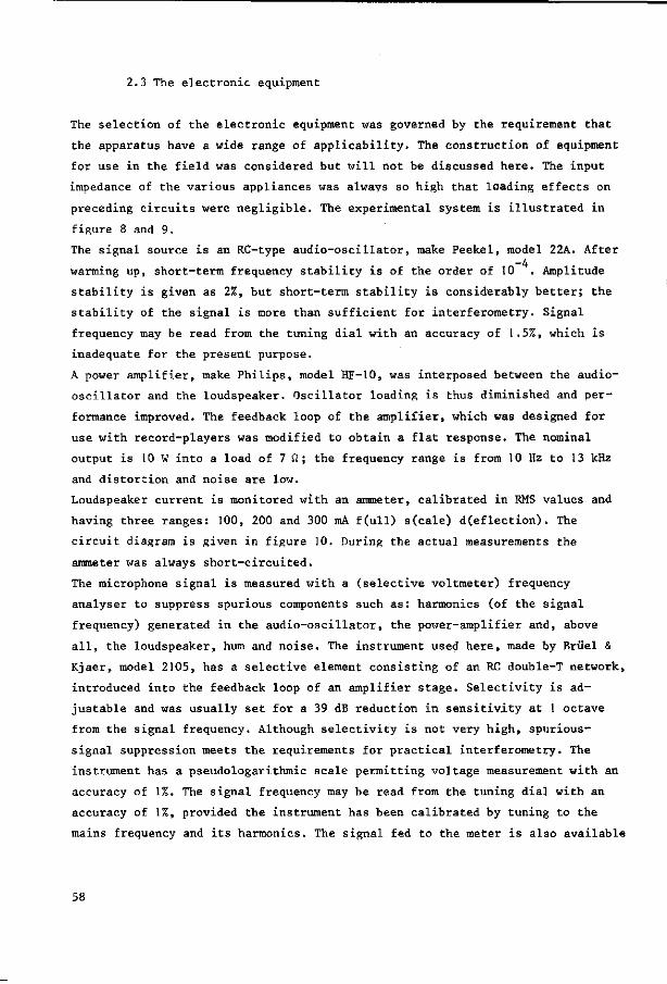
2.3 The electronic equipment

The selection of the electronic equipment was governed by the requirement that

the apparatus have a wide range of applicability. The construction of equipment

for use in the field was considered but will not be discussed here. The input

impedance of the various appliances was always so high that loading effects on

preceding circuits were negligible. The experimental system is illustrated in

figure 8 and 9.

The signal source is an RC-type audio-oscillator, make Peekel, model 22A. After -4

warming up, short-term frequency stability is of the order of 10 . Amplitude

stability is given as 2%, but short-term stability is considerably better; the

stability of the signal is more than sufficient for interferometry. Signal

frequency may be read from the tuning dial with an accuracy of 1.5%, which is

inadequate for the present purpose.

A power amplifier, make Philips, model HF-10, was interposed between the audio-

oscillator and the loudspeaker. Oscillator loading is thus diminished and per­

formance improved. The feedback loop of the amplifier, which was designed for

use with record-players was modified to obtain a flat response. The nominal

output is 10 W into a load of 7 £2 ; the frequency range is from 10 Hz to 13 kHz

and distortion and noise are low.

Loudspeaker current is monitored with an ammeter, calibrated in RMS values and

having three ranges: 100, 200 and 300 mA f(ull) s(cale) d(eflection). The

circuit diagram is given in figure 10. During the actual measurements the

ammeter was always short-circuited.

The microphone signal is measured with a (selective voltmeter) frequency

analyser to suppress spurious components such as: harmonics (of the signal

frequency) generated in the audio-oscillator, the power-amplifier and, above

all, the loudspeaker, hum and noise. The instrument used here, made by Briiel &

Kjaer, model 2105, has a selective element consisting of an RC double-T network,

introduced into the feedback loop of an amplifier stage. Selectivity is ad­

justable and was usually set for a 39 dB reduction in sensitivity at 1 octave

from the signal frequency. Although selectivity is not very high, spurious-

signal suppression meets the requirements for practical interferometry. The

instrument has a pseudologarithmic scale permitting voltage measurement with an

accuracy of 1%. The signal frequency may be read from the tuning dial with an

accuracy of 1%, provided the instrument has been calibrated by tuning to the

mains frequency and its harmonics. The signal fed to the meter is also available

58

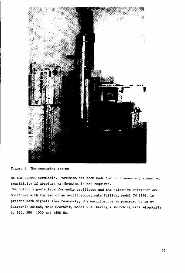
Figure 8 The measuring set-up

at the output terminals. Provision has been made for continuous adjustment of

sensitivity if absolute calibration is not required.

The output signals from the audio oscillator and the selective voltmeter are

monitored with the aid of an oscilloscope, make Philips, model GM 3156. To

present both signals simultaneously, the oscilloscope is preceded by an e-

lectronic switch, make Heathkit, model S-3, having a switching rate adjustable

to 150, 500, 1000 and 1500 Hz.

59

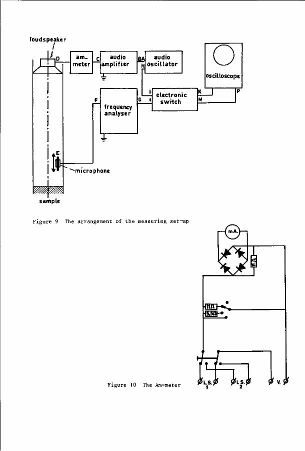
loudspeaker

1/ am­meter

audio amplifier

li — • • "-microphone

frequency analyser

X

§A a l -audio oscillator O

oscilloscope

electronic switch

sample

Figure 9 The arrangement of the measuring se t -up

Figure 10 The Am-meter LS.J 1

PL! s.p $ V. $

2.4 The measurement

For rapid and complete tabulation the experimental data are entered on data

sheets (see example). A sheet consists of a heading, giving general information,

and a number of sections, each of which is devoted to a particular measuring

frequency.

The heading gives the following information: type of material (Monster), grain

size or texture, in mm (Monstermat.), sample thickness in the interferometer in

cm (Laagdikte), porosity in % as derived for the dry sample from the amount of

solid matter (Por. volume), moisture content in percentage weight of dry ma-3 -3

terial (Vochtgehalte), total mass in g (Gewicht), density in kg/m . 10 (S.g.),

specific acoustic static air flow resistance (a), special remarks (Opm.), po­

sition of the sample surface in cm (meetniveau), sample number (No.), sample

series (Serie), date of measurement (Datum), time of day (Tijd), ambient temper­

ature in C (Temp.).

Each of the sections has been divided into six columns. The upper half of the

first column lists values for frequency in Hz, as read from the audio-oscil­

lator (T), as read from the selective voltmeter (V) and as determined from

wavelength, c.f. column 3, (G).

The upper figure in the second column is the position of the first minimum

diminished by a quarter wavelength, in cm. The following figures are the

readings for positions of the minima, in cm. In the third column, the upper

figure is the average for the quarter wavelength, the following figures are

values for the half wavelength in cm as derived from the second column and the

average for the half wavelength is entered at the bottom of the column.

The second half of the first column gives the displacement of the first minimum

in cm, in relation to that minimum with a hard termination at the sample surface.

This requires the introduction of corrections for the position of the sample

surface and the properties of the microphone (see section 2.5, point B 5) ( ) ,

the wavelength in cm as obtained from the third column (X) and the phase angle

of the reflection coefficient in radians (<j>).

The first figure of the fourth column is the value of the minimum sound pressure,

extrapolated to the sample surface and in arbitrary units (voltmeter readings),

entered under -. The following figures give the values for the various minima (in

the same units). The same is done for the maxima in the fifth column, the extra­

polated value being entered under +.

The sixth column gives the standing wave ratio at the sample surface (r), some

61

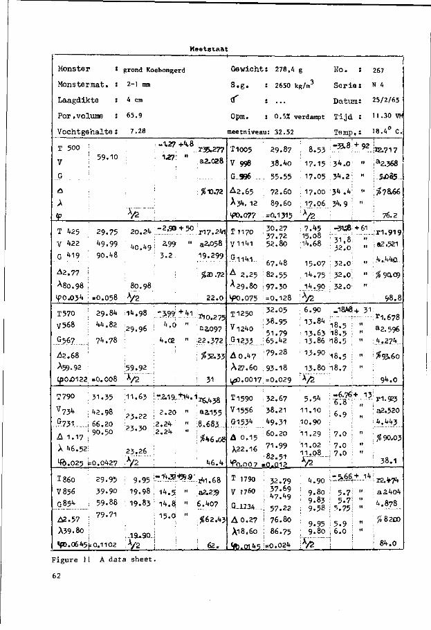
Meetstaat

Mons te r *

M o n s t e r m a t . s

L a a g d i k t e s

P o r . v o l u m e :

Vo ch t g e

T 500

V

G

<Q

A

<P

X 425

V 422

G "*19

A2 .77

^ 8 0 . 9 8

tpo.031*

T570

V568

G567

A2 .68

•^59-92

1^0.0122

T790

V 7 3 4

...9.73.1

A 1.17

X 46 .52

^ . 0 2 5 .

T860

V856

G854

A2.57

A39.80

«fD.0645

h a l t e :

59 .10

29 . 75

^9 .99

90 .48

=0 .058

29 .84

44 .82

74 .78

=0 .008

31 .35

42 .98

66 .20 90 .50

=0.0427

29 .95

39 .90

59 .88

79 .71

= 0.1102

— i

grond Koebongerd Gewicht

2-1 mm S . g .

4 cm 0

65.9 Opitl.

, : 278,4

: 2650

: . . .

: 0.5%

7.28 meetniveau: 32.52

-\Z? +4.8 T35.277

1 - 2 7 : " 32 . (28

#10.72

^ ;

20 . 24 . - 2 >5 0 . + 5 ° . r 1 7 . 2 4 i

40 .49 ^ a " " a 2 - 0 5 8

3.2 19 .299

#20.72

80 .98

V 2 : 2 2 . 0

^ • 9 8 , - 399 ; + .41. ^ ^

4 n " ;29.96 • * £2,097

4.02 " .22.372

! ; #32.33

59 .92 :

V2 31

11 .63 L - 2 . 1 9 . + t o . 1 r 6 A 3 8

2 3 > 2 2 ; 2 .20 " a a i 5 5

23*30 2'2k " 8 * 6 6 3

23.30 , 2 > 2 l f ,,

$ 46 .08

23 .26 ; V2 46.4

19 .98 J 14.5; " ;a2.233

19 .83 ! 14.81 " 6 .407

M 5 i " # 6 2 . 4 5

ia--9o..i

V2 1 ! 62.

T1005

v 998

G 996

A 2 . 6 5

A 34. 12

Y>0.07?

T 1170

V1141

G 1141

A 2 . 25

^ 2 9 . 8 0

^PO.075

T1250

^ 1240

G I???.

A 0 . 47

A27.60

1^0.0017

T1590

V1556

G1531*

A 0 . 15

X22.16

^ 0 . 0 0 7

T 1790

V 1760

G..1734

A 0 .27

A18.60

<fc.Ol45

29 .87

38 .4o

: 5 5 .55

72 .60

89 .60

=0.1315

•30 .27 37 .72 52 .80

67 .48

82 .55

| 9 7 . 30

' =0 .128

; 32 .05

: 38 .95

51 .79 ; 65 .42 : 79 .28

193.18

;=0 .029

; 32 .67

38.21

60 .20

71 .99

82 .51 .0 .012.

32 .79 : 3 7 .69 I 47 .49

j 57 .22

i 76 .80

: 86 .75

i=0.024

g H o . : 3

kg/m S e r i e :

D a t um :

/erdampt T i j d :

T e m p . :

: 8 .53 - 3 5 - 8 + 9 2

17 .15 ^ . O ; "

17 .05 3"t.2; "

: 17 .00 34 .4 ; "

: 17 .06 3^.9 : " A / 2

1M -31J8+61 ': 15.08 r , R: ;;•" 14 68 5 ' °

; , b 0 3 2 . 0 "

15 .07 ; 3 2 . 0 ; "

: 14 .75 32 .0 ; "

14 .90 32 . 0 "

V 6.90 ..18.43+ 31

: 13 .63 18 .5 i " 13 .86 1 8 . 5

; 1 3 ' 9 0 18 .5 ; "

13 .80 1 8 . 7 : "

M ; k ; - 6 .76+ 13

P 1 ' 1 0 ! 6 . 9 i „ 1 0 . 90 ;

11 .29 ; 7 .0 I "

11 .02 '• 7 . 0 ': " 1 1 . 08 ! 7 . 0 ; " Kfr

, . 9 0 ; . ^ 6 £ t . i . 4

; 9 . 80 ; 5 .7- " : 9 .83 \ 5 .7 ! " ; 9 .58 ; 5 . 75 ; "

• 9 .95 i 5 . 9 ! " ; 9 .80 j 6 .0 ! "

V2

267

N 4

25/2/65

11.30 VM

18.4° C.

1X2.717

la2.368

; 5J085

^ 7 a 6 6

76.2

J r l . 9 1 9

i 82.521

;..4.44o.

#90.09

9 8 . 8

; r l . 6 7 8 a 2 .596

A , 274

; $93-60

9^ .0

r 1.923

; a2.520

• 4 . 443

I % 90.03

: 3 8 . 1

•[12.V74

; a a 4 o 4

4 .878

^ 8200

I 8 4 . 0

Figure l1

62

A data sheet.

auxiliary quantities (sub a) and the absorption coefficient in % (%). Usually

the absorption coefficient, read directly from the selective voltmeter and thus

ignoring tube attenuation, was entered at the bottom of the column. Its value

can serve e.g. as a control during the measurements. Without any further calcu­

lation one can conclude at the end of a series of readings at different frequen­

cies and after checking the readings at a few of those frequencies, that the

sample was not disturbed during measurement. Noteworthy points are as follows.

The loudspeaker in the interferometer does not constitute an ideal piston even

at low frequencies. The sound field near the loudspeaker may thus be distorted

and no measurements should be taken close to it.

The measuring system has it own acoustical and mechanical resonance frequencies.

The acoustical resonance frequencies can be heard easily; the detection of me­

chanical resonances in the measuring system is more difficult. They may origi­

nate from different sources and can sometimes not be traced. When these

frequencies are suspected, measurements are made after a small shift in

frequency. In the beginning the frequencies at which readings are made are

chosen quite arbitrarily. All series of readings have been read for at least

twelve frequencies. More readings were necessary with samples of high air re­

sistance. The criterion chosen was determined by the accuracy with which the

impedance curl could be drawn.

Through the imperfect homogeneity of the sample surface the readings of the

sound pressure at some frequencies at the first minimum, nearest to the sample,

were unreliable. If so the minima were extrapolated after starting from the

following minimum. Then the value of the phase shift was derived from the

readings of three-quarters of a wavelength, neglecting the position of the

probe at the first minimum.

The value for the sound pressure at the maxima often do not show substantial

variation for one frequency eq.(1-36). Extrapolation is then not necessary.

2.5 Accuracy of the measurements

The specific acoustic impedance of a sample is determined in the standing wave

tube in some reference plane and the worker is free in his choice of this plane

as long as the impedance itself is the only quantity of interest.

But a different situation arises if material constants of the sample are to be

derived from the specific acoustic impedance. If so, the interface between the

air column and the sample material is selected as reference plane and the as­

sumption is introduced that the properties of the medium change abruptly from

those of air to those of the sample in this plane.

63

The concept of a plane of discontinuity is realistic enough for fine-grained

materials, but for coarse-grained ones a transition may well exist where the

properties of the medium change almost continuously. At present there appears

to be no feasible procedure for incorporating the effect of such a transition

into the calculations, e.g. for finding an optimum position for the reference

plane somewhere in the range. Therefore the simple procedure of laying the

reference plane through the highest peaks of the sample surface has been

followed and no account was taken of any errors thus introduced. Thin layers

are most severely affected by these errors.

Another problem presented by coarse-grained materials is that a specific sample

may well be far from representative for the bulk of the material, the number of

grains in the sample being limited. Here too the answer to the problem is far

from obvious and was not further pursued. The problem was discussed in more

detail for perforated panels by Mawardi (1956).

The following is confined to the errors inherent in the determination of the

specific acoustic impedance, commencing with those in the modulus |r| and the

phase angle <j> of the sample's pressure reflection coefficient r.

Now |r| follows immediately from the stand5.ng wave ratios, c.f. eq.(l-38).

Assuming an error 6|r| in |r| and 6s in s, one can derive from eq.(l-37) that

ill 2s 6s i/1 i 12-.6s /0 ... 6|r| >= 2 — = J(l-M ^~ • (2-1)

(s+l) s s

Thus the absolute value of the error in |r| is always less than half the absolute

value of the relative error in s, vanishing for vanishing sample absorption.

The relative error 6 a/a in the absorption coefficient a is aloo of interest,

especially if sample absorption is low. From eqs(l-38) and (2-1) one concludes

that

i2. 6s 6a =- 2jr| * |-- M (1-|rJ2)^

i£ - -.5=! . i £ . (2-2) a s+1 s

The absolute value of the relative error in a is always smaller than in s,

approaching this latter value for vanishing sample absorption.

64

Eqs (2-1) and (2-2) show that the errors in |r| or a follow immediately from

those in s, which will therefore be scrutinized.

In considering the errors in the determination of 4, errors in position are

converted into errors in angle - expressed in radians - by multiplying the

error in position by the wave number k.

One can now compile a list of sources of error, adding a short discussion and

an estimate for the probable value of each error.

Table 3

Sources of error

A. In the determination of s: B. In the determination of *:

1) The reading error of the wave 1) The reading error in probe

analyzer microphone position

2) The error in probe position when 2) The error in probe position when

adjusting for pressure minimum adjusting for pressure minimum

3) The error in extrapolation of the 3) The error in the wave number

minima 4) The error in the position of the

4) The error due to interfering sample surface

signals. 5) The error in the correction for

the probe's pressure-sensitive

position.

Ad A 1. A relative error in the wave-analyser reading in an extreme will give

rise to an equal relative error in s, when absolute values are considered. The

wave-analyser having an approximately logarithmic scale, the relative reading

error is approximately constant. The probable value, which represents the

instrument's accuracy, may be 1%.

Ad A 2. The customary procedure for finding a minimum is the following. The

probe microphone is swung to and fro past the minimum with reducing amplitude

and keeping the wave-analyser readings at opposite ends of the swing equal.

Finally the probe is brought to rest at the estimated midway position for the

smallest swing, always coming from the same direction and it is then assumed

to be at the minimum.

As a change in wave-analyser reading of 1% is clearly visible, the limiting

process described above will presumably yield a relative error of less than

0.5% for the value of the minimum. Smaller errors will obtain for the maxima

and also for the minima for highly absorbant samples because of the slow change

in reading of the wave-analyser with probe position. However errors in minima

will be rather large for samples with very low absorption.

65

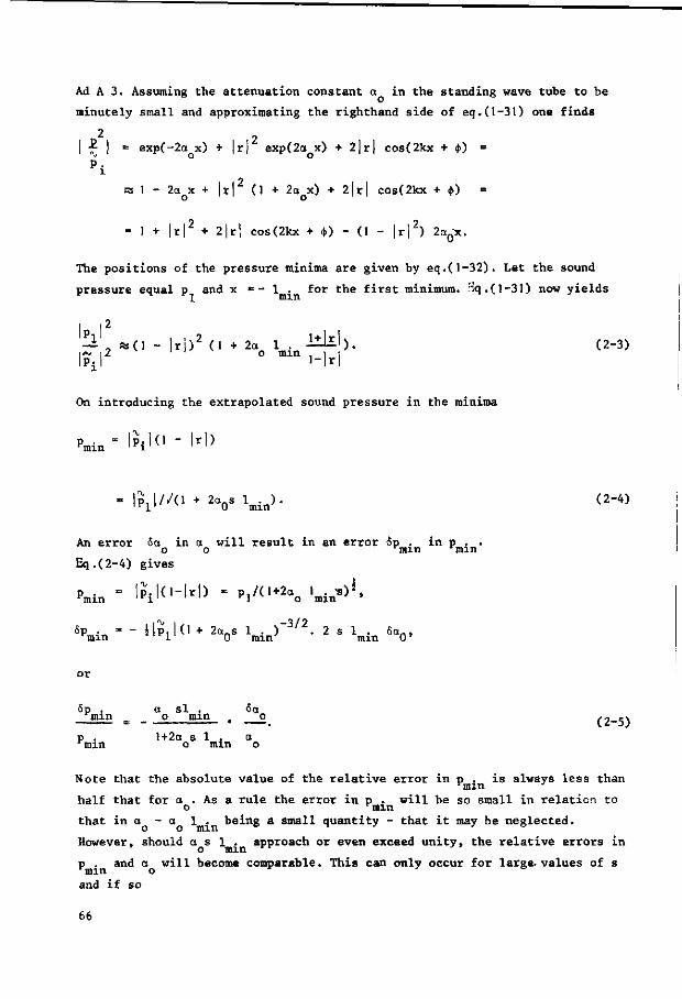
Ad A 3. Assuming the attenuation constant a in the standing wave tube to be

minutely small and approximating the righthand side of eq.(l-31) one finds

2 ,

| •£ | = exp(-2a x) + jr| exp(2a x) + 2|r| cos(2kx + <)))•= P.

w 1 - 2a x + Irl (1 + 2 a x ) + 2|r| cos(2kx + <j>) o o

= 1 + |r|2 + 2|r| cos(2kx + <t>) - (1 - |r|2) 2aQx.

The positions of the pressure minima are given by eq.(l-32). Let the sound

pressure equal p and x c - 1 . for the first minimum. Bq.(1-31) now yields

I I 2

!i *<1 - |r'|)2 (1 + 2a 1 i l W ) . (2-3) |p.|2 ° m x n l-|r|

On introducing the extrapolated sound pressure in the minima

Pmin= IPilO-M)

• W" + 2V W- (2"4)

An error 5a in a will result in an error Sp . in p . . o o r m m *min Eq.(2-4) gives

"min * IP i lO- I r l ) - , , / ( l *2« o l ^ s ) ' ,

^ m i n ' - l l P l I 0 * 2 ^ 8 1 ^ " 3 7 2 - 2 s l m i n 6 V

or

5p . a si . 6a nun o nun . o (2-5)

p . l+2a s i . a r m m o m m o

Note that the absolute value of the relative error in p . is always less than r m m J

half that for a . As a rule the error in p . will be so small in relation to o nun

that in a - a 1 . being a small quantity - that it may be neglected.

However, should a s 1 . approach or even exceed unity, the relative errors in * o min vr J

p . and a will become comparable. This can only occur for large, values of s

and if so 66

1+r _ s+1 + ( s -1) cos<)> + j ( s - l ) s in( | ) (o-f,\

1-r s+1 - ( s -1) cos4> - j(s-l)sin<t>

» 2/s + j sin » _ (2_7)

1-cos $ + (1+cos $)/s

C is thus rather insensitive to errors in s, unless $ approaches zero, when c

approaches s.

Fortunately the combination of factors which make for large extrapolation errors

is rare and mostly the probable relative error in s due to faulty extrapolation

will remain below 0.5%

The errors due to interference have been discussed.Hectrical cross-talk betrays

itself by a regular fluctuation in the magnitudes of the minima and an inade­

quate signal-to-noise ratio may usually be avoided by a slight shift in

frequency.

Taking the sources of error in s together, the probable value for the relative

error in |r| will usually remain below 2%, bringing the probable value of the

relative error down to less than 1%.

Ad B 1. The reading error 6x for the probe microphone position is of the order

of 0.5 mm. On converting this error to radians by multiplication with k one

finds an error that is proportional to frequency. For the highest frequency

used, « 2000 Hz, k|6x| =0.02 radians.

Ad B 2. It was assumed in A 2 that the probe microphone was not adjusted cor­

rectly to the minimum, thus introducing a difference 6 between the ratio p/p .

p min and 6 as compared to unity.

— 2 - = 1 + & . (2-8) P • P r m m

The probe position deviates by Sx from the correct position for a minimum. Thus,

on referring to eq.(l-32), probe position is given by

2kx = TT — cp -*- 2k5x. (2-9)

On neglecting attenuation by introducing a =o into eq.(l-31), it follows that

|p/p.|2 = 1 + |r|2 + 2|r|cos(2kx + <f>). (2-10)

67

Elimination of 2kx from eq.(2-10) by means of eq.(2-9), and assuming kx is much

less than unity, yields

|p/p.|2 = (l-|r|)2 + |r|(2k6x)2, (2-11)

and, on considering that |p . /p. | = I — jIT] ,

comparison of eqs(l-8) and (1-11) yields

k|«x| = (l"|r|) /(J 6 / | r | ) . (2-12)

To elucidate the magnitude of the error from faulty probe position in the minima,

a short table is composed, introducing probable values for S in accordance with

A 2.

M 0.9

0.5

0.25

0.1

For values of |r| as low as 0.1 the present approach is inappropriate. The rari­

ty of such values justifies their exclusion from further discussion here.

Ad B 3. The wave number is derived from the measurement of the distance between

two adjacent minima and, as such, is 'subject to the errors mentioned under B 1

and B 2. These errors are absolute errors, however, and as a rule there are a

number of minima available over which the distance may be averaged. This reduces

the relative error in k to such an extent that it may be omitted from further

consideration, except for the lowest frequencies where errors of the order given

under B 2 may prevail.

Ad B 4. The position of the sample surface is determined with a flat plate,

fitted with a vertical bar consisting of plexiglass on which a calibrated scale

has been engraved. The sample is introduced into its holder and the plate is

placed on the smoothed surface. The scale is then sighted along the rim of the

sample holder. The errors inherent in this procedure are so small compared to

others that they may be neglected.

The sample-holder was usually filled completely, the material being levelled off

to the rim of the holder.

68

Table 4

Error due to faulty probe

5 .103

P 5

5

5

2.5

pos it ion

k|5x| in radians

0.005

0.035

0.075

0.1

Ad B 5. In interferometry, sound pressure is measured along the axis of the

interferometer tube and the ideal instrument for this purpose would be an infi­

nitely small microphone. Although the microphones used in interferometry are

always small in relation to the wavelength, their dimensions are unfortunately

finite and the e.m.f. at the electrical output terminals will be proportional

to a weighted average of the various sound pressures prevailing at the micro­

phone's surface. The e.m.f. is thus no longer a measure for the sound pressure

at a given point.

Fortunately however there are microphones with 'pressure-sensitive points'.

For such a microphone at a given frequency, the output e.m.f. is proportional

to the sound pressure at the (pressure) sensitive point which is characterized

by an invariant position in relation to the microphone, i.e. the proportionality

factor referred to above is independent of the nature of the sound field in

which the microphone is placed (thus for the interferometer, in a pressure

maximum,in a minimum or between,for high or low standing wave ratio). The

proportionality factor between the e.m.f. and the sound pressure in the sensi­

tive point and the position of that point may vary with frequency. The position

of the sensitive point should be determined experimentally as consideration of

microphone construction may lead the unwary worker to fallacious conclusions,

e.g. for the probe-tube microphone with a simple open-ended probe tube (a type

popular in interferometry), the sensitive point might be imagined to lie in the

centre of the orifice at the end of the tube. In fact it lies a fraction of a

tube diameter ahead of that end.

In section 1-4 the procedure was described for eliminating the unknown position

of the sensitive point experimentally, using a hard termination for the inter­

ferometer, a rigid plate to be referred to as the calibration plate. In the

present context, the position of the sensitive point is being considered as a

possible source of error and the question of the accuracy of determining its

position thus arises.

In an interferometer terminated by a calibration plate the standing-wave ratio

is high so wavelength may be determined with great accuracy and the first

pressure minimum lies a quarter wavelength in front of the calibration plate.

By adjusting the microphone to this minimum, the position of the sensitive point

in relation to the microphone may be determined. Various authors, such as Scott

(1946) and Lippert (1?53) have investigated the positions of the sensitive

points for various types of microphones. Figure 12 gives the distance between

the sensitive point and the end of the probe tube as a function of frequency,

for microphones with simple open-ended probe tubes. Lippert's (1953) values for

69

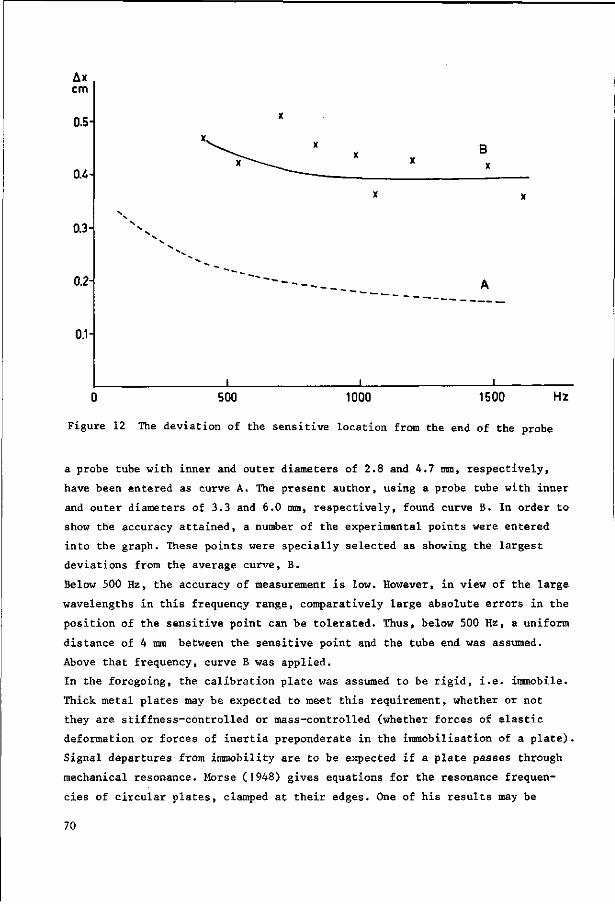
B x

Ax cm

0.5-

0.4-

0.3-

0.2-

0.1-

0 500 1000 1500 H z

Figure 12 The deviation of the sensitive location from the end of the probe

a probe tube with inner and outer diameters of 2.8 and 4.7 mm, respectively,

have been entered as curve A. The present author, using a probe tube with inner

and outer diameters of 3.3 and 6.0 mm, respectively, found curve B. In order to

show the accuracy attained, a number of the experimental points were entered

into the graph. These points were specially selected as showing the largest

deviations from the average curve, B.

Below 500 Hz, the accuracy of measurement is low. However, in view of the large

wavelengths in this frequency range, comparatively large absolute errors in the

position of the sensitive point can be tolerated. Thus, below 500 Hz, a uniform

distance of 4 mm between the sensitive point and the tube end was assumed.

Above that frequency, curve B was applied.

In the foregoing, the calibration plate was assumed to be rigid, i.e. immobile.

Thick metal plates may be expected to meet this requirement, whether or not

they are stiffness-controlled or mass-controlled (whether forces of elastic

deformation or forces of inertia preponderate in the immobilisation of a plate).

Signal departures from immobility are to be expected if a plate passes through

mechanical resonance. Morse (1948) gives equations for the resonance frequen­

cies of circular plates, clamped at their edges. One of his results may be

70

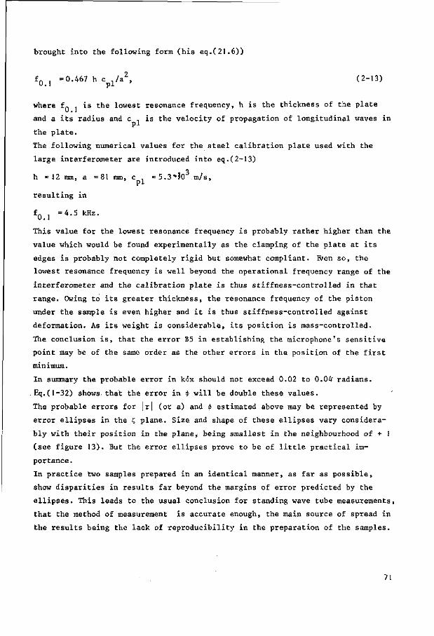
brought into the following form (his eq.(21.6))

f„ , =0.467 h c Ja2, (2-13) 0.1 pi

where fn . is the lowest resonance frequency, h is the thickness of the plate

and a its radius and c . is the velocity of propagation of longitudinal waves in

the plate.

The following numerical values for the steel calibration plate used with the

large interferometer are introduced into eq.(2-13)

h =12 mm, a =81 mm, c , =5.3*10 m/s, Pi

resulting in

fQ =4.5 kHz.

This value for the lowest resonance frequency is probably rather higher than the

value which would be found experimentally as the clamping of the plate at its

edges is probably not completely rigid but somewhat compliant. B/en so, the

lowest resonance frequency is well beyond the operational frequency range of the

interferometer and the calibration plate is thus stiffness-controlled in that

range. Owing to its greater thickness, the resonance frequency of the piston

under the sample is even higher and it is thus stiffness-controlled against

deformation. As its weight is considerable, its position is mass-controlled.

The conclusion is, that the error B5 in establishing the microphone's sensitive

point may be of the same order as the other errors in the position of the first

minimum.

In summary the probable error in k<5x should not exceed 0.02 to 0.04" radians.

. Eq.(l-32) shows that the error in <j> will be double these values.

The probable errors for |r| (or a) and $ estimated above may be represented by

error ellipses in the £ plane. Size and shape of these ellipses vary considera­

bly with their position in the plane* being smallest in the neighbourhood of + 1

(see figure 13). But the error ellipses prove to be of little practical im­

portance .

In practice two samples prepared in an identical manner, as far as possible,

show disparities in results far beyond the margins of error predicted by the

ellipses. This leads to the usual conclusion for standing wave tube measurements,

that the method of measurement is accurate enough, the main source of spread in

the results being the lack of reproducibility in the preparation of the samples.

71

^0.30 s

/ \

I s \ (U0 \

/ / - .. \ \ // ^ ** \ \

/ . — . \0-60 \ \

\0-90 J^-O-i 1 j—i 1—!—i 1 i LJ n' ; i L \ T e c 7 J sec j \ »ioec ;

; /

v ^ - - " / / ' x - ^ . - ' /

W I

/ I

/ I

/ \ \ s

s

\ - • - . . - - /

s s

.'

' S I \ \ » \ \

\ ;

Figure 13 The size and the position of the error

ellipses in the c;-plane

72

3 The relation between the acoustical properties and

the geometrical arrangement of pores in soils

3.1 Introduction

A soil sample is usually of a rather complicated composition, consisting of

three phases: solid, liquid and gas. In the literature on soils the description

of the sample is commonly approached from the build-up of the various aggregates

in the solid phase and little attention is paid to the space surrounded by this

phase: the pores. Sometimes attempts have been made to relate pore size and

distribution with the processes of formation of the solid phase. Some studies

on flocculation and sedimentation could be cited in this context, but liter­

ature on the subject is scarce and significant results can be found only in a

few special cases.

The approach followed here is of a complementary nature, based on the ar­

rangement of the pores rather than of the solid phase. Especially those pores

in open communication with one another are of interest to the soil physicist,

because gas-exchange or variation of moisture content play an important role in

physical, chemical or biological processes in the soil.

Various methods of measurement have been developed to estimate characteristic

quantities of the arrangement of the pores, total pore space often being the

prime object. Ignoring transient methods, the stationary methods may be subdi­

vided into a static group, discussed in the Introduction and to be discussed

further in section 3.7, and a dynamic group1 Various static methods have been

developed for determining characteristic properties of the pore system and

various authors have introduced various characteristic quantities. But the

amount of information thus gathered is rather limited and dynamic methods of

measurement extend the range of information available, at least in principle,

as static methods restrict the frequency scale to the degenerate case of zero

frequency.

Acoustic measurements fall into the dynamic group. Ernsthausen (1939) and Kaye-

Evans (1949) were among the first to carry out such measurements, confining

themselves to the determination of absorption coefficients. But no attempt was

made to correlate the results with pore geometry.

Acoustical methods give rise to certain complications. A fairly obvious one is

that the frame of solid matter, which is stationary in static methods of measure­

ment, may be set into vibration in acoustical ones, thus complicating the inter-

73

pretation of the results. The vibrations will be especially pronounced for the

resonance frequencies of the frame. Fortunately, for the majority of the samples

considered here, frame damping was high enough to prevent significant frame vi­

bration, even in resonance (see Appendix A ) .

Thus the assumption of a stationary frame is quite acceptable for most of the

samples considered and departures from this assumption will be noted explicitly

in future. It is customary to refer to stationary frames as 'rigid', although

their immobility may well be due to inertia rather than to stiffness.

The interferometric method of measurement was selected for this book and here

plane acoustic waves propagate in the sample. Now a second complication arises:

the sample material must be homogeneous, at least in the direction of propa­

gation, if significant quantitative results are to be obtained. Homogeneity, in

the acoustic sense, implies that regions may be selected in the sample, large

enough to be representative for the sample material, yet still small in relation

to wavelength.

A related complication is caused by the assumption of a plane interface, where

the properties of the medium change discontinuously from those of the gas (air)

in the interferometer tube to those of the sample. For coarse, granular materials

there is no clear plane of discontinuity but a transitional range and the scien­

tist can only estimate a position for an equivalent interface some-uhare in this

range, thus introducing an element of uncertainty in his results.

A restriction, which is not fundamentally essential but does facilitate the

interpretation of the results, is confinement to what amounts acoustically to a

two-phase system: a solid frame enclosing pores which are completely filled with

water and are thus immobilized for sound propagation, and interconnected gas-

filled pores. In other words: all menisci are assumed to be immobilized. The

samples selected for quantitative evaluation all belong to this group.

The variation of the moisture content of the pore system has a pronounced effect

on the acoustic properties of the sample.but in the present stage of investi­

gation the reduction of the observed effects to characteristic quantities of the

sample material does not seem feasible.

Sample materials consisting of a rigid frame containing interconnected pores

were formally introduced in section 1.9. Acoustically, such materials are com­

pletely defined by a pair of frequency-dependent complex quantities. As such,

Z and Y are appropriate (eqs(l-52) and (l-53))but W and y may serve just as

well (eqs(l-54) and (1-55)). In view of the simplicity of the latter two e-

quations, the two pairs of quantities may be considered equivalent.

74

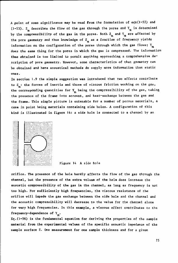
A point of some significance may be read from the formulation of eq's(l-52) and

(1-53). Z describes the flow of the gas through the pores and Y is determined m m

by the compressibility of the gas in the pores. Both Z and Y^ are affected by

the pore geometry and thus knowledge of Z as a function of frequency yields

information on the configuration of the pores through which the gas flows; Y^

does the same thing for the pores in which the gas is compressed. The information

thus obtained is too limited to permit anything approaching a comprehensive de­

scription of pore geometry. However, some characteristics of that geometry can

be obtained and here acoustical methods do supply more information than static

ones.

In section 1.9 the simple suggestion was introduced that two effects contribute to Z : the forces of inertia and those of viscous friction working on the gas,

m

the corresponding quantities for Y being the compressibility of the gas, taking

the presence of the frame into account, and heat-exchange between the gas and

the frame. This simple picture is untenable for a number of porous materials, a

case in point being materials containing side holes. A configuration of this

kind is illustrated in figure 14: a side hole is connected to a channel by an

Figure 14 A side hole

orifice. The presence of the hole hardly affects the flow of the gas through the

channel, but the presence of the extra volume of the hole does increase the

acoustic compressibility of the gas in the channel, as long as frequency is not

too high. For sufficiently high frequencies, the viscous resistance of the

orifice will impede the gas exchange between the side hole and the channel and

the acoustic compressibility will decrease to the value for the channel alone

for very high frequencies. In this example, a viscous effect contributes to the

frequency-dependence of Y .

Eq.(l-56) is the fundamental equation for deriving the properties of the sample

material from the experimental values of the specific acoustic impedance of the

sample surface Z. One measurement for one sample thickness and for a given

75

frequency yields only one complex quantity and if Y and Z are to be determined

separately at least one further measurement at the same frequency is essential.

Obvious solutions to this problem are: a change in sample thickness or the re­

placement of the rigid back-plate of the sample by another, known backing im­

pedance (in the latter case, a modified version of eq.(l-56) must be used).

The method of variable sample thickness was followed in some cases but was in­

applicable in others. Many materials, especially those of granular composition,

are extremely sensitive in geometrical configuration and any mechanical inter­

ference with the sample tends to alter the acoustical properties of the material.

For such materials, another solution must be sought.

The solution adopted here assumes a pore geometry, characterized by a limited

number of parameters, not departing too far from reality but still simple enough

to be amenable to calculation. Such a geometric arrangement can be conceived as

a mathematical model and will yield a locus for Z in the complex impedance plane

for variable frequency and constant sample thickness. By variation of the pa­

rameters a family of such loci may be generated. Measurements on the sample are

also carried out for variable frequency and constant sample thickness and the

resulting experimental locus for Z is compared to the family of theoretical ones.

The numerical values of the parameters pertaining to the theoretical locus giving

the best fit are accorded the status of characteristic quantities of the sample

material.

As an example, a very simple model for pore geometry is considered, consisting

of identical circularly cylindrical tubes drilled into the frame material in

the direction of propagation of the acoustic waves. This model has only two

parameters : the tube radius and the number of tubes per unit area. A more

sophisticated version is obtained by drilling all the tubes at the same angle

to the direction of propagation, thus introducing a third parameter. In fact,

an infinite variety of arrangements may be postulated with any number of pa­

rameters. As will become clear in chapter 4 however, the introduction of more

parameters beyond a fairly low limit does not increase information about the

sample material.

A serious defect of the procedure considered is that Z and Y cannot be de-m m

termined separately and thus that differentiation between effects due to gas

flow and effects due to gas compression is impossible.

The principal aim of this chapter is the consideration of the various pro­

cedures for obtaining characteristic material constants from interferometric

measurements. In this context, the following subjects will be discussed in. more

detail.

76

1. The method of Ferrero & Sacerdote (1960), which is founded on the use of

very thin samples, permitting analytical approximation of the transcendental

function appearing in eq.(!-56).

2. A method based on the use of two or more sample thicknesses, incorporating a

graphical aid for the solution of eq.(l-56).

3. A simple mathematical model by Zwikker & Kosten (1941), which employs three

parameters and does not require specification of the pore geometry.

4. The applicability of rules of proportionality for porous materials.

5. The formulation of two variants of the channel-type geometrical model, the

channels consisting of circular cylindrical tubes in one case and of fissures in

the other. The channels are inclined at a constant angle to the direction of

propagation and have variable cross-sections. Besides the restrictions mentioned

before (rigid frame, no liquid flow) a further assumption is added: the frame

possesses sufficient thermal inertia to ensure that its temperature may !be

considered constant.

6. The formulation of a geometrical model for prismatic structures. These occur

in heavy clay and slaked soils when dehydrated. This model allows for side holes.

7. The possibility of composing an analogous electrical circuit of the trans­

mission-line type for the porous material. Essentially such a circuit would not

contribute new information but might help in the understanding of wave propa­

gation in porous materials.

3.2 Numerical examples of calculating Z and Y from measurements at

layer thicknesses

Various authors have introduced different representations for Z and Y . Follow-m m

ing Ferrero & Sacerdote (1960), modifying their notation slightly, the two

quantities can be presented in the following general form:

Z = o + iioo (3-1) m m J m

Y = G + jwC (3-2) m m m

where the values of the real material constants a , o , G and C may be m m m m

frequency dependent. The material constants are the specific flow resistance of

the material, the effective density, the conductance and the reciprocal of the

effective compression modulus, respectively.

At low frequencies, air movement in the material will be hampered particularly

77

by viscous forces originating from friction along the walls of the capillary

tubes in the porous material. In these cases a velocity distribution, as assumed

in the Poiseuille flow, can be adopted and then o stands for the static spe­

cific flow-resistance in the material. At higher frequencies, the air will oscil­

late more like a plug. Although it is customary to refer to high frequencies

when the linear dimensions of the pore system under consideration are large in

relation to wavelength, a modified criterion is intended here: the frequency is

considered high when the linear dimensions are large relative to boundary-layer

thickness. The viscous boundary layer thickness is given, for example, by

Crandall (1927) and appears in this book as eq.(B-3).

In a cylindrical tube, o decreases with frequency, as the boundary layer

thickness decreases, and so does p , as air flow is less restricted to the ' m

centre of the tube. In eq.(3-2), C represents the compliance of the gas in the pores, taking into

m

account the reduction of the available space owing to the finite volume of the

solid or liquid matter. If for example the porosity is 10%, the value of C

becomes 10% of its value in free air. Sections 1-9 and 3-2 described dissipative

mechanisms associated with compression; the results of such losses is repre­

sented by the term G . As far as the thermal losses are concerned, the situation

m'

is partly analogous to that of viscous losses. Provided that frequency is high,

in the sense discussed above (see eq.B-14), the changes in state of the gas are

nearly adiabatic.

For low frequencies those changes in state are nearly isothermal and in this

case thermal losses are low. For such frequencies viscous losses are however

high. Thermal effects are discussed by Kirchhoff (1927) and Zwikker & Kosten

(1948).

Making use of eqs(l-54) and (1-55), eqs(3-l) and (3-2) may be written as:

° + jupm = y W (3-3) m m mm

Gm + jwC = Y /Wm (3-4) m m m m

Eqs(3-3) and (3-4) show that the four characteristic quantities, o , D , G and m m m

C may be calculated from experimentally derived values of the complex quanti­

ties Y and W . These latter quantities require at least two measurements for a

given frequency, as one measurement on one sample yields only two values.

The technique developed by Ferrero & Sacerdote (1960) attempts to circumvent

this problem by performing measurements on very thin samples. One of the princi-

78

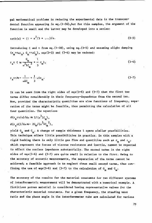
pal mathematical problems in reducing the experimental data is the transcen­

dental function appearing in eq.(1-56),but for thin samples, the argument of the

function is small and the latter may be developed into a series:

coth(z) = (1 + z2/3 + ...)/z. (3-5)

Introducing B, and n from eq.(l-28), using eq.(3-5) and assuming slight damping

(a «up ; G <<wC ) , eqs(3-3) and (3-4) may be reduced: m m m m

p c ^ - J ^ t - a l , (3-6) co2lC 2 3 m

m

0 cnfes + — wlo . (3-7) uuC 3

m

It can be seen from the right sides of eqs(3-6) and (3-7) that the first two

terms differ considerably in their frequency-dependence from the second two.

Now, provided the characteristic quantities are slow functions of frequency, sepa­

ration of the terms might be feasible, thus permitting the calculation of all

four quantities. The equations

d(p cn/o))/diD « 2/(u3lC ), s m

d(pBcC)/du.w- 2Gm/((03lCm2),

yield G and C . A change of sample thickness 1 opens similar possibilities.

This technique offers little possibilities in practice. In thin samples with a

rigid backing there is only little gas flow and quantities such as a and o , m m

which represent the forces of viscous resistance and inertia, cannot be expected

to affect the surface impedance substantially. The second terms in the right

sides of eqs(3-6) and (3-7) are quite small in relation to the first. Owing to

the accuracy of acoustic measurements, the separation of the terms cannot be

achieved; a feasible approach is to neglect these small second terms, thus con­

fining the use of eqs(3-6) and (3-7) to the calculation of G and C . m m

The accuracy of the results for the material constants for two different systems

of interferometric measurement will be demonstrated with a numerical example. A

fictitious porous material is considered having representative values for the

characteristic material constants. For a given frequency, the standing wave

ratio and the phase angle in the interferometer tube are calculated for various

79

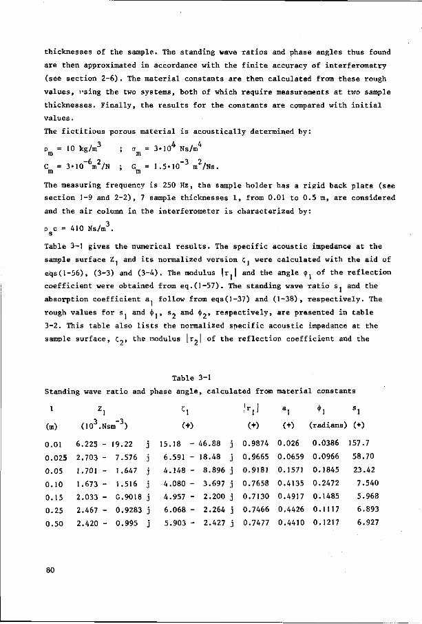
thicknesses of the sample. The standing wave ratios and phase angles thus found

are then approximated in accordance with the finite accuracy of interferometry

(see section 2-6). The material constants are then calculated from these rough

values, I'sing the two systems, both of which require measurements at two sample

thicknesses. Finally, the results for the constants are compared with initial

values.

The fictitious porous material is acoustically determined by:

P = 1 0 kg/m3 ; a = 3-104 Ns/m4

m m

C = 3-10~6m2/N ; G = 1.5*10~3 m2/Ns. m m

The measuring frequency is 250 Hz, the sample holder has a rigid back plate (see

section 1-9 and 2-2), 7 sample thicknesses 1, from 0.01 to 0.5 m, are considered

and the air column in the interferometer is characterized by:

p c = 410 Ns/m3. s

Table 3-1 gives the numerical results. The specific acoustic impedance at the

sample surface Zj and its normalized version 5. were calculated with the aid of

eqs(l-56), (3-3) and (3-4). The modulus |r.| and the angle <j> of the reflection

coefficient were obtained from eq.(l-57). The standing wave ratio s. and the

absorption coefficient a. follow from eqs(l-37) and (1-38), respectively. The

rough values for s1 and $., s,, and <(>_, respectively, are presented in table

3-2. This table also lists the normalized specific acoustic impedance at the

sample surface, C9> the modulus |r-| of the reflection coefficient and the

Table 3-1

Standing wave ratio and phase angle, calculated from material constants

C, |r,] a, *, s,

(+) (+) (+) (radians) (+)

15.18 - 46.88 j 0.9874 0.026 0.0386 157.7

6.591 - 18.48 j 0.9665 0.0659 0.0966 58.70

4.148 - 8.896 j 0.9181 0.1571 0.1845 23.42

4.080 - 3.697 j 0.7658 0.4135 0.2472 7.540

4.957 - 2.200 j 0.7130 0.4917 0.1485 5.968

6.068 - 2.264 j 0.7466 0.4426 0.1117 6.893

5.903 - 2.427 j 0.7477 0.4410 0.1217 6.927

80

1

(m)

0.01

0.025

0.05

0.10

0.15

0.25

0.50

Z l

(103.Nsm 3 )

6.225 -

2.703 -

1.701 -

1.673 -

2.033 -

2.467 -

2.420 -

19.22

7.576

1.647

1.516

0.9018

0.9283

0.995

j

j

j

j

j

j

j

absorption coefficient a~, as obtained from s« and <(>_ by the reverse process of

calculation.

Table 3-2

Impedance calculated from standing wave ratio and phase shift, read in the im­

pedance diagram

1

(m)

0.01

0.025

0.05

0.10

0.15

0.25

0.50

s2

(+>

157

59

23

7

6

6

6

4

5

0

9

9

|r2l

(+)

0.987

0.966

0.918

0.765

0.714

0.747

0.747

1

(

-

-

-

-

-

-

-

h °)

2

5.5

10.5

14

8.5

6.5

7

*2

(radians)

- 0.0349

- 0.0960

- 0.1833

- 0.2443

- 0.1484

- 0.1135

- 0.1222

a2

(+)

0.026

0.067

0.157

0.415

0.49

0.44

0.44

19.

6.7

4.2

4.1

5.0

6.0

5.9

c2

(+)

- 50 j

- 18.5 j

- 9.0 j

- 3.7 j

- 2.18 j

- 2.29 j

- 2.43 j

The first system of deriving the material constants from the supposedly measured

results in table 3-2 uses the fact that for infinitely thick samples, the spe­

cific acoustic impedance at the sample surface equals the wave impedance of the

sample material: Z = W . Consider the transcendental factor in eq.(l-56);

c o t h [ ( a m + V1] " [' + «P<-2«ml " 2jBml)]/[l - exP(-2anl - 2jSnl)]. (3-8)

For large values of a 1, exp(-2a 1) is small and eq.(3-8) may be approximated

to:

cothKam + jBm)ll«l + 2-exp(-2aml)-exp(-2j6 1). (3-8a)

For variable 1 this function is a logarithmic spiral in the complex plane with

its apex at +1. In the present sense, a 1 is large at numerically moderate

values. Thus, for a 1>2.1, the spiral is within an absolute distance of 0.03

from its apex, and in this range the sample behaves as though infinitely thick. In

the present instance the difference in results for 1 = 0.25 m and 1 = 0.50 m is

so small that no great error will results if the value found for 1 = 0.50 m is

assumed to hold for an infinitely thick sample.

Replacing C» by (cJ and selecting a second measurement for a sample thickness

1, yielding (£«)1 , the derivation leads to

81

<52V<C2>- = C° t h[ ( am2 + J V 1 ] - ( 3"9)

Selecting 1 = 0.05 m for the finite value of 1 and assuming the value of c„ for

1 = 0.5 m to be an adequate approximation of that for 1 = », eq.(3-9) and table

3-2 yield the following numerical results:

Wm2 = (-2A1 ~ U 0 ° J ) , l t ) 3 N s/m 3»

coth]"(am2 + J6m2)l]= 1.1535 - 1.054 j, 1 = 0.05 m.

The solution of the equation:

tanh(x + jy) = a + jb,

derived from the nomograms in Rybners book (1947, p.27) prove to be rather in­

accurate; the exact solutions are to be prefered:

tanh(x) = [a2 + b2 + 1 -/((a2 + b V - 2(a2 - b2) + l)]2a, (3-10)

(y) = [a2 + b2 - 1 - /((a2 + b 2 ) 2 - 2(a2 - b2) + 0^2b, (3-11) tan

x and y following to the desired degree of accuracy from the relevant tables.

The numerical result in the present case is:

V + J6m2= (8-' + 9-9 J)n"1-The numerical values for the material constants now follow eqs(3-3) and (3-4):

pm2 = 9 > 9 k g / m 3 ; am2 = 2-9-104 Ns/m4

Cm 2 = 2.9-10-6 m2/N ; Gm2 = 1.43-10-3 m2/Ns.

Agreement with the initial values is quite good, apparently the approximations

introduced have had only a slight adverse effect. The method has disadvantages

when applied to the measurements in this book, not only because of the dis­

turbance of the sample when altering its thickness but also because soil samples

are rarely homogeneous over the necessary thickness. The further disadvantage of

the amount of material required for a sample which can be considered infinitely

thick may be avoided by extrapolation from finite thicknesses. An appropriate

graphical method will be described in section 3-4.

The second method to be investigated follows Ferrero & Sacerdote (1960). Two

thin samples are considered, having 1 = 0.01 m and 1 • 0.025 m. Eqs(3-6) and

(3-7) are used, neglecting the second terms in the right sides. The results for

C and G are given under C , and G _ in Table 3-3. This table also lists the m m m3 m3 2

quantity p c£/l, which should be inversely proportional to 1 if all the approxi-

82

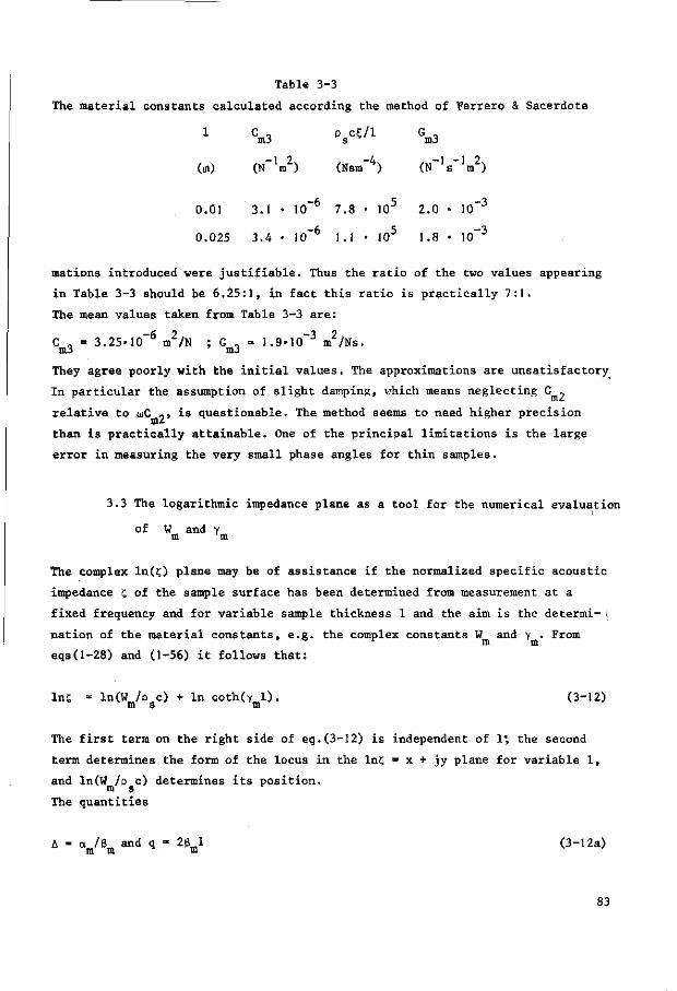
Table 3-3

The material constants calculated according the method of Ferrero & Sacerdote

1 Cm3 p s c 5 / 1 Gm3

(in) (N-1m2) (Nsm"4) (N_ 1s_ 1m2)

0.01 3.1 • 10~6 7.8 • 105 2.0 • 10"3

0.025 3.4 • 10~6 1.1 • 105 1.8 • 10 _ 3

mations introduced were justifiable. Thus the ratio of the two values appearing

in Table 3-3 should be 6.25:1, in fact this ratio is practically 7:1.

The mean values taken from Table 3-3 are:

C , = 3.25«10-6 m2/N ; G , = 1.9»10~3 m2/Ns. mo mJ

They agree poorly with the initial values. The approximations are unsatisfactory

In particular the assumption of slight damping, which means neglecting G _

relative to uC o l is questionable. The method seems to need higher precision

than is practically attainable. One of the principal limitations is the large

error in measuring the very small phase angles for thin samples.

3.3 The logarithmic impedance plane as a tool for the numerical evaluation

of W and y m m

The complex ln(?) plane may be of assistance if the normalized specific acoustic

impedance £ of the sample surface has been determined from measurement at a

fixed frequency and for variable sample thickness 1 and the aim is the determi- \

nation of the material constants, e.g. the complex constants W and y . From

° r m m eqs ( l -28) and (1-56) i t follows t h a t :

In? = ln(W h c) + In coth(y 1 ) . (3-12) m s m

The first term on the right side of eq.(3-12) is independent of 1*, the second

term determines the form of the locus in the In? = x + jy plane for variable 1,

and ln(W /p c) determines its position, m s

The quantities

A = am /6m and q = 2Bffil (3-12a)

83

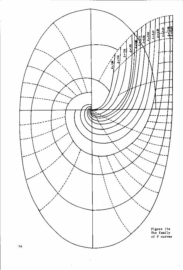
Figure 15a The family of F curves

S4

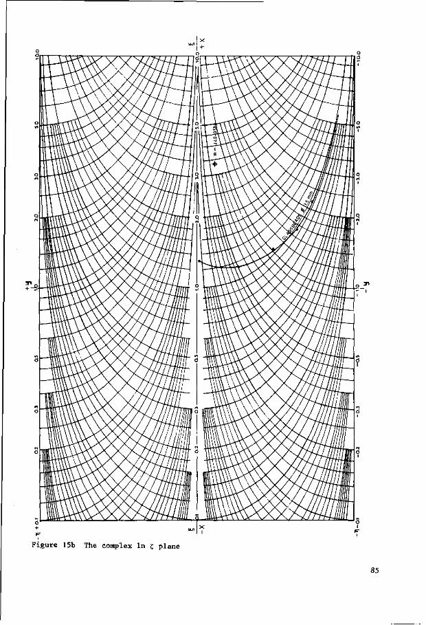
Figure 15b The complex In z, plane

85

are introduced and the locus of the function:

F = In coth(yml) = In coth|j(A + j)q], (3-13)

in the complex x',y' plane is investigated for variable q and with A as parame­

ter. As q approaches infinity, the argument of the natural logarithm in eq.(3-13)

approaches unity and F approaches zero, the origin of the x',y' plane. A family

of curves for F for a series of values of A now be constructed and plotted on

transparent paper. The curves prove to have the form of a spiral (figure 15a).

The experimental values for lnf; have been entered in the x,y plane. The x1 ,y'

plane, carrying the loci for F, is now placed on the x,y plane and shifted until

the locus for F best fits the experimental points, keeping the x and x' axes

(or y and y' axes, respectively) parallel. Under these conditions, the position

of the origin of the x',y' plane lies at the point ln(W /p c) in the x,y plane;

the use of the In x, plane is essentially the extrapolation of the spiral for In C

to its apex, the point for infinite layer thickness, which is determined by the

specific acoustic wave impedance of the material, W . Once W is known, various r r m m

paths are open for the determinaion of y = a + jg . The best fitting spiral for F yields some information on the value of a /6 , if the associated value for

J m m' A is known. Let the apex of the spiral for In z, be determined by £ = ZQ + jig, SQ and HQ

being the quantities yielding the real and imaginary parts of W , after multi­

plication by p c (see eq.(3-12)). A rapid estimate for 5 and n is facilitated

if the loci £ = constant and n = constant are entered in the x,y plane. From

x + jy = ln(5 + jn), (3-14)

it follows that

-2 . 2 x = J ln(5 + n ) ; y = arctan (n/E)• (3-15)

In eq.(3-15), y has more than one value. It is the phase angle of the wave im­

pedance of the sample. As passive samples only are considered, £&0, and the

imposition of the condition:

- TT/ZSV<TT/2, (3-16)

does not entail a loss of generality. It may now be seen from eq.(3-15) that y

86

and n must be accorded the same sign.

Solving eq.(3-14) for £ and n yields

exp(x) • cos(y) = £, (3-17)

exp(x) • sin(y) = n« (3-18)

Eqs(3-17) and (3-18) are useful for the calculation of the loci. Then these

equations may be brought into the form:

exp[x - In £J» cos(y) = 1,

expjx - In]n|J * |sin(y)| = 1,

and from this formulation it will be seen that a change in one of the parameters,

either £ or |n|, corresponds to a parallel shift of the locus in the x direction.

It is thus sufficient to calculate the locus, for example, for constant £ se­

lecting a simple value for £ (as such £ = 1 springs to mind) and to obtain the

other loci by shifting the curve along the x axis. The loci thus calculated may

be applied to the construction of those for constant n by substituting

y = 2 + TT/2, allowing that negative values of y correspond to negative values of

n. The family of curves for constant £ and that for constant n intersect or­

thogonally, eq.(3-14) representing a conformal transformation (see figure 15b).

The construction of a family of curves for F in the x',y' plane (see eq.(3-13))

presents more difficulties. Reduction of equations given by Rybner (1947, p.25)

yields

J In cosh A»q + cos q

cosh(A*q) - cos q

arctan sinh(A»q)

(3-19)

(3-20)

These equations give the spirals in parametric form. As mentioned previously,

the asymptotic point for large values of q is x' = y' = 0; for small values of q

the spiral approaches an asymptote given by:

y' = - arccot(A).

With a Fortran programme, the co-ordinates x',y' for spirals corresponding to 14

values of A were generated.

87

The In £ plane was used to determine the normalized specific acoustic wave im­

pedance of the sample material in a number of cases. As an example, a number of

measured points for various sample thicknesses at one frequency have been entered

in Figure 15b. In this cas- , the best fit is obtained for a spiral having an esti­

mated parameter A = 0.25, and the result for the wave impedance is estimated at

W h c = 3.40 - 0.56 j m s J

A Fortran programme was devised to calculate the other material constants.

The In g plane, considered as a tool for estimating the wave impedance of the

sample material, has several drawbacks. There are areas where the accuracy in

reading £ and n is small, especially near the asymptotes. This disadvantage can

be avoided only by dropping the conformality of the transformation, eq.(3-14),

and stretching the plane uniformly in the y direction.

3.4 The simple model of Zwikker & Kosten

As was discussed in Section 3.1, methods of interferometry requiring variation

of the sample thickness are not feasible for soil samples, and so an alternative

procedure will be followed here, based on variation of frequency and involving

the introduction of a mathematically accessible model for the sample material.

The first of such models to be considered is a simple model from Zwikker & Kosten

(3940, which can be considered as a base for the other models. Subsequent ex­

tension of the simple model will be ignored here.

The principal task of the models is to predict the frequency-dependence of the

material constants, and in the present context the specific acoustic series im­

pedance per unit, length Zm and the specific parallel admittance per unit

length Y (see Section 1-9, eqs(l-52) and (1-53)) are selected as such. The

models are introduced to limit the number of parameters.

The first model allows for the fact that only a part h (the porosity) of the

total volume is available for compression and expansion of the gas, but that the

changes in state are adiabatic. These considerations yield

Y = jwh/Kp . (3-21) m fa

The viscous losses are accounted for in Z by the introduction of the specific

flow-resistance a . The forces of intertia are also incorporated in Z . The fact m v m

that the average particle velocity in the pores is a factor 1/h higher than the

volume velocity per unit area of the material, suggests the introduction of that

factor in the term corresponding to the effects of inertia. There are, however,

further effects which tend to increase this term, one of the principal ones

being the irregularity of the pores. These effects are accounted for by the intro­

duction of the structure factor k in the term iup . The above considerations m m

yield

Z = o + itop k /h. (3-22) m m J s m

To start with, a is considered frequency-dependent. In the simple model it is

equated with its static value o , which is defined by

- 3p/8x = o u, where p and u are time-independent.

Comparison of the present notation with that introduced in Section 3.2, eqs

(3-3) and (3-4), shows:

89

o = k p / h ; a = C T (3-23a,23b) m ra s m s

C = h/icp ; G = 0. (3-24a,24b) m s m

To familiarize the reader with the concept of structure factor, two special

cases will be discussed.

1. The porous material consists of uniform tubes, all at an angle 8 to the

direction of propagation. The particle velocity in the tubes can be presented

as u/h cos 9, the pressure gradient along the tubes as - p -r— u/h cos 9, and

the pressure gradient in the direction of propagation (the x direction) in the

equation:

3p 1 3 u -K = . 0s , 3x cos 9 3 t h cos 8

2 so that now k = 1/cos 9.

m

2. The porous material consists of tubes parallel to the direction of propa­

gation but with cross-sections S = S(x) according to location. The average cross-

section is given by

1 S a = - / S(x) dx. 1 f S(x

1 Jo

It is assumed that, for sufficiently large values of 1, S approaches a limit,

which is the same for all tubes.

The function f is defined by

f(x) = S(x)/S . (3-25) a

With N tubes per unit surface area, the porosity follows as

h = N S , a

and the particle velocity in a tube, u,, follows from

u u 1 u, = =

N S f(x) h f(x) a

The pressure gradient can be presented as

3p 3 u ps ~~ '

3x 3t hf(x)

90

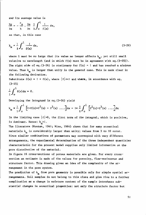
and its average value is

i £ = _ ! _ s 3u 1 fX 1 dx,

8x h 3t IJo f (x)

so t h a t , in t h i s case

k = - f —1— dx, (3-26) m \J0 f(x)

where 1 must be so large that its value no longer affects k , yet still small

relative to wavelength (and in which f(x) must be in agreement with eq.(3-25)).

The right side of eq.(3-26) is stationary for f(x) = 1 and has reached a minimum

value. Thus k is larger than unity in the general case. This is made clear in

the following derivation.

Substitute f(x) = 1 + <5(x), where |6|«1 and where, in accordance with eq.

(3-25)

- I a(x)dx = 0. l^o

Developing the integrand in eq.(3-26) yield

km = - f [l-5(x) + 62(x) - 63(x) ....]dx= 1 + - / [s2(x)-63(x) . . . .] dx

In the limiting case |6|-K), the first term of the integral, which is positive,

is dominant. Hence: k >1. m

The literature (Kosten, 1941; Bies, 1964) shows that for many acoustical

materials k is considerably larger than unity; values from 3 to 10 occur.

Since similar combinations of parameters may correspond with very different

arrangements, the experimental determination of the three independent quantities

characteristic for the present model supplies only limited information on the

pore distribution of the material.

In figure 16 cross-sections of porous materials are given. For every cross-

section an estimate is made of the values for porosity, flow-resistance and

structure factor. This drawing gives an idea of the complexity of the ar­

rangement in the pore system.

The prediction of k from pore geometry is possible only for simple spatial ar­

rangements. Soil samples do not belong to this class and give rise to a further

complication as a change in moisture content of the sample introduces sub­

stantial changes in acoustical properties: not only the structure factor but

91

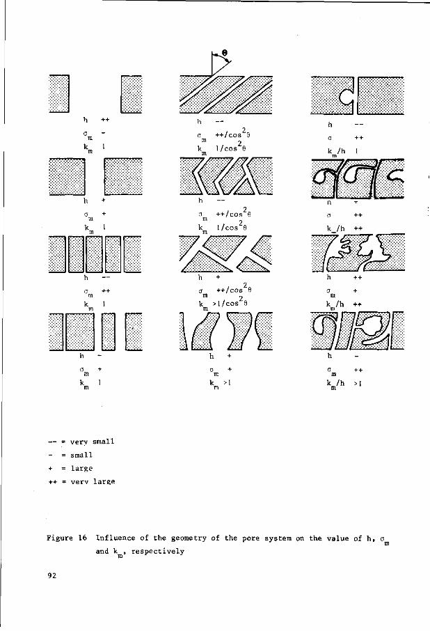
h ++

a m k 1 m

1 1 1 1 1 > 1 1 1 1 1 1

h +

a + m k 1 m

h

a + m k 1 m

a ++/cos e m ~

k 1/cos 6 m

a ++/cos e m 2

k 1/cos 9 in

a ++/cos 8 m ~

k >i/cos e m

h

0 m

k m

+

+

>1

k /h 1

— = verv small

= small

+ = large

++ = verv large

Figure 16 Influence of the geometry of the pore system on the value of h, a n

and k , respectively

92

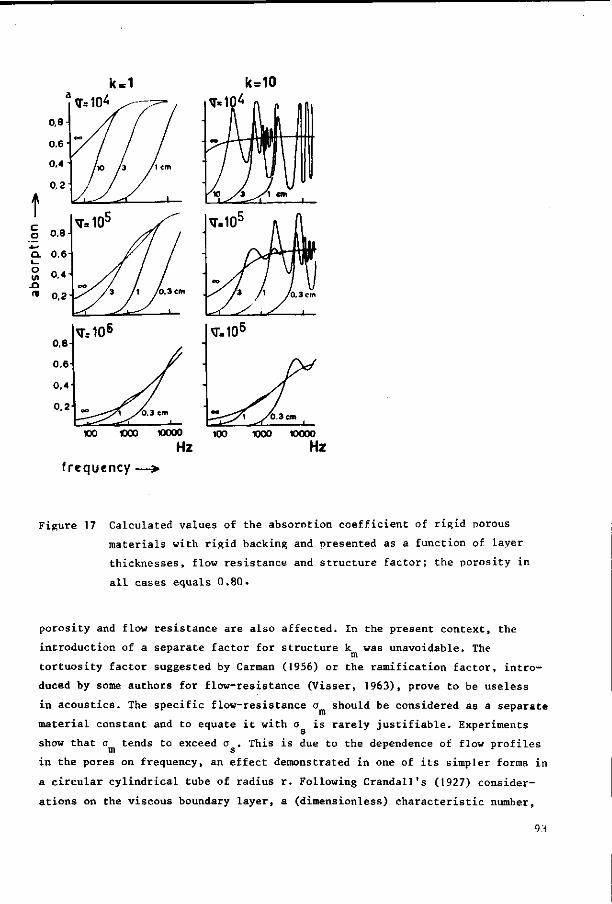
k=1 k=10

t c o

o XI

frequency

Figure 17 Calculated values of the absorption coefficient of rigid porous

materials with rigid backing and presented as a function of layer

thicknesses, flow resistance and structure factor; the porosity in

all cases equals 0.80.

porosity and flow resistance are also affected. In the present context, the

introduction of a separate factor for structure k was unavoidable. The m

tortuosity factor suggested by Carman (1956) or the ramification factor, intro­

duced by some authors for flow-resistance (Visser, 1963), prove to be useless

in acoustics. The specific flow-resistance a should be considered as a separate

material constant and to equate it with o is rarely justifiable. Experiments show that o tends to exceed a . This is due to the dependence of flow profiles

m s

in the pores on frequency, an effect demonstrated in one of its simpler forms in

a circular cylindrical tube of radius r. Following Crandall's (1927) consider­

ations on the viscous boundary layer, a (dimensionless) characteristic number,

u = r/(u)pg/n), (3-27)

is introduced, where r\ is the dynamic coefficient of viscosity.

The magnitude of this number determines the nature of the flow profile in the

tube. Thus, for u<l, Poiseuille flow is approached, with a parabolic distri­

bution of particle velocity across the tube, and a approaches o where

os = 8n/r2. (3-28)

For y>10, plug flow occurs: particle velocity is practically constant across

the tube except for a sharp drop to zero at the tube walls. Now Helmholtz's

approximation applies and

a « /(2oinn /r). (3-29) m s

On determining the ratio of o and a from eqs(3-28) and (3-29) it follows that

for u>10

o 7a = u/4/2, (3-30) m s

and so a tends to exceed a as frequency increases, see eq.(3-27). m s

In the transitional range, l<y<10, the flow profile is more complicated, and

formal expressions may be found in appendix B. Note that eq.(3-30) does not

hold in this range. Although the effect is not considered for the present

simple model, it should be realized that the changes of state of the gas in the

tube vary from isothermal to adiabatic in the same transitional range as de­

fined for the flow profile in the tube, at least if the limits of the range are

conceived as crude indications rather than as exact figures.

This apparent coincidence is due to the nearly equal thicknesses of the vis­

cous and thermal boundary layers.

Using eqs(l-54), (1-55), (1-56), (3-21) and (3-22), it follows that

Z = (p c/h)/(k (1+ho /icon k ))coth jkl/(k (1+ho /iuo k ) ) , (3-31) s m m s m m m ~ s m

which equation may be abbreviated by the introduction of the normalized speci­

fic acoustic impedance and of

Z = ha /cap , (3-32) m s

94

thus reducing it to

;h = /(k (1-jZ/k ))coth["jkl/(k (1-iS/k )J . (3-33) m m L m ' m -*

For the discussion, eq.(3-33) is brought into the form

Ch = /(km(l-jZ/km))coth y2Jkl/km[_/(1+j:2/k2rn>+]"l + i^kl/kJ/(l+E2/k2

m)-ll^. (3-33a)

Eq.(3-33a) is taken to represent the locus of C in the complex plane for a given

frequency and variable sample thicknesses 1, the locus having the general form

of a spiral, converging to an apex for large values of 1 (see section 1.11). For

a given value of Z/k , an increase in k has the following results (excluding a

limiting case, to be discussed later):

1. The velocity of propagation is reduced, being inversely proportional to /k .

2. The modulus of the apex is increased by a factor /k . J m

3. The spiral converges more swiftly to the apex (see the discussion on eq.(3-8a).

For a given value of k , an increase in 1 results in a shift of the apex, the

reactive part becoming more negative and the resistive part increasing, although

the latter effect is always the smaller. The swiftness of conversion of the

spiral on the apex is increased (see eq.(3-8a)).

The apex corresponds to the normalized acoustic.wave impedance of the sample

material; thermal and equivalent losses increase the reactive component of this

impedance but viscous losses decrease it, as may seen from eqs(3-3) and (3-4),

which yield

W - {(p - jo/u)/(C - jG /u)}1. m m m m m

Now in samples consisting of porous solid frames the viscous losses preponderate,

driving the apex of the impedance curl below the real axis.

An increase in h, keeping £ and k constant, results in a reduction in size of

the spiral towards the origin, but does not affect its shape.

The effects of variations of k in the range l<k <10 and of a in the range 4 7 - 4 m m ra

10 <a <10 Ns m are well illustrated (although for the absorption coefficient

a only) by Kosten (Richardson, 1953, Vol.1, chapter 4) (see figure 17).

In figures 18 and 19 a number of loci for h are presented in the complex plane.

They were derived from eq.(3-33), but now for constant sample thickness and

variable frequency, conditions corresponding to those under which most of the

measurements were performed. These figures demonstrate the effects of vari-

95

ations in k and o on the loci. The following values were selected: m m 5

for k : 2 and 8, m 3 4 5 - 4 for a : 10 , 10 and 10 Ns m ,

m

for 1: 0.040 and 0.072 m.

The frequency scale is indicated by points on the loci, corresponding to multi­

ples of 200 Hz. The points for 0.4, 1 and 1.6 kHz are marked by the numbers 4,

10 and 16, respectively.

In the limiting case of low damping is

H/k << 1, m

a condition consistent with u>10, as discussed previously. If so eq.(3-33) may

be approached by

Ch;(l-jZ/2k )/(k )coth klE/2/(k )+jkl/(k )|. (3-33b) m m L m m j

The locus for <; in the complex plane, for constant frequency and variable sample

thickness is now-a wide spiral, converging slowly on an apex just below the real

axis. In the present case, information may be obtained from the anti-resonances

and resonances of (,, where c, is real (see Section 1-11). But, as Kosten (1947)

has pointed out, preference should be accorded to the selection of minimum and

maximum values for |C|. Thus | | achieves its minimum for

kl/k = TT/2, (3-34) m

and, in the p r eva i l i ng order of approximation, t h i s y i e l d s :

Ch = JTTE/A . (3-35)

Values for k and for l/h = a /uin may now be derived from eqs(3-34) and (3-35).

m m s

These two equations hardly differ from those of the first anti-resonance (see

section 1.11), especially if damping is very low. No great error will ensue in

applying eqs(3-34) and (3-35) to the first anti-resonance.

In the general case of low damping, eqs(3-34) and (3-35) do not apply if sample

thickness is kept constant and frequency varies, because h, E and k should then

be considered as functions of frequency. In many cases, however, these quanti­

ties vary very slowly with frequency and the equations will yield approximations for k and o .

m m

The present considerations were not extended to anti-resonances of higher order

or to resonances, as these occurred only sporadically in the frequency range

and for the samples investigated in this book.

96

3.5 The choice of a model

For a better agreement between the structure of a geometric model and the soil

structure, a number of supplementary assumptions should be made.

In the literature on porous media, Carman (1956), Scheidegger (1957) and

Dallavalle (1943) particularly commented on many views and hypotheses in this

field. Also, in the literature on soil physics pertaining directly to the ori­

entation of pores, many models can be found (de Vries, 1952; van Bavel, 1952).

Some points of consideration are listed here. Research on diffusion of gases was

said to show that except for the effect of path length (Penman, 1940; Call, 1947),

only the total pore space is of importance. The very short free path lengths of

the diffusing molecules as a result of mutual collisions cause this effect. The

contributions of large and small pores are in proportion. The arrangement of

pore spaces is therefore of no importance. Variation, for instance, in the

density of packing does not cause systematic rearrangement of pores.

Total porosity should be estimated by the expansion method (see section 4-2).

Starting from data on weight and specific weight of the sample material erroneous

results will be found because isolated pores are included.

Many measurements and considerations are partially based directly on mass flow

of gases or liquids through porous media (Poiseuille). The largest pores and

capillary tubes contribute most, leading to a small sensitivity for the detection

of pores of small diameter. Even less information was available on the occurrence

of pores in a certain fluctuating regularity and to the effect of a changing pore

diameter. This lack of information is partly due to the fact that often only two

independent variables, namely pressure gradient and flow, can be correlated.

The simple model introduced by Zwikker & Kosten (1941) (see section 3-5), had

the advantage that no assumptions are introduced a priori about pore geometry;

the major disadvantage is that the frequency-dependent effects due to viscous

and thermal boundary layers are ignored.

The introduction of a mean radius or any related quantity, as found in litera­

ture on flow, turns out to be inadequate, as can be seen from eq.(3-27), which

suggests that any averaging process will require some type of weighting factor.

Therefore it seems logical to start with a model, based on channels with a

variable cross-section. Soils can be very often considered as a packing of soil

aggregates. Each aggregate consists of soil particles cemented together. The

volume-weight corresponds roughly to a value equal to that of a dense packing of

spheres.

97

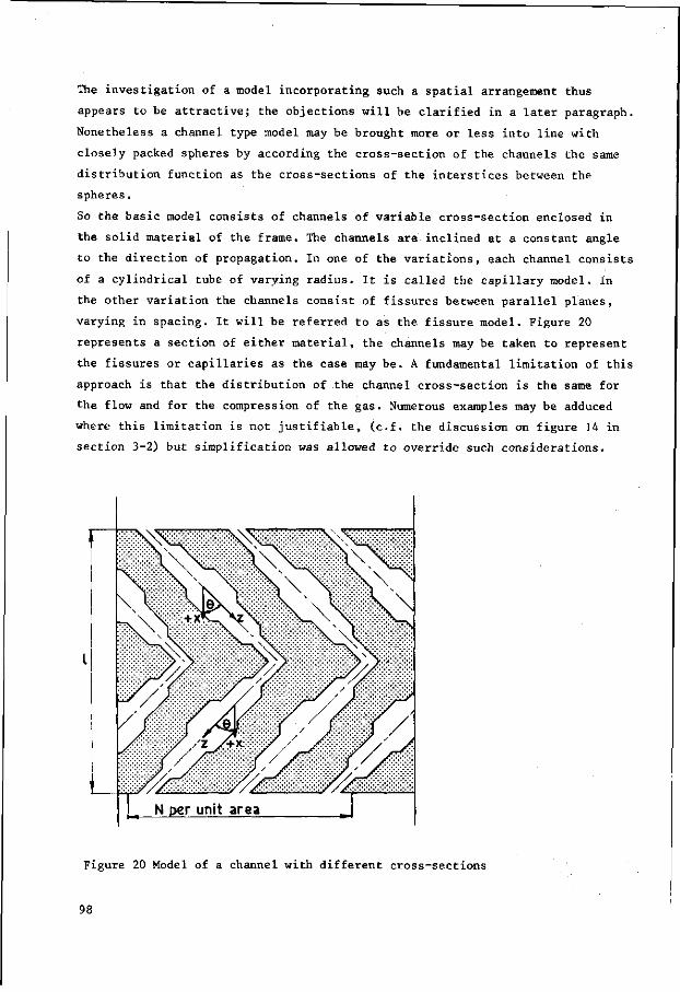
The investigation of a model incorporating such a spatial arrangement thus

appears to be attractive; the objections will be clarified in a later paragraph.

Nonetheless a channel type model may be brought more or less into line with

closely packed spheres by according the cross-section of the channels the same

distribution function as the cross-sections of the interstices between the

spheres.

So the basic model consists of channels of variable cross-section enclosed in

the solid material of the frame. The channels are inclined at a constant angle

to the direction of propagation. In one of the variations, each channel consists

of a cylindrical tube of varying radius. It is called the capillary model. In

the other variation the channels consist of fissures between parallel planes,

varying in spacing. It will be referred to as the fissure model. Figure 20

represents a section of either material, the channels may be taken to represent

the fissures or capillaries as the case may be. A fundamental limitation of this

approach is that the distribution of the channel cross-section is the same for

the flow and for the compression of the gas. Numerous examples may be adduced

where this limitation is not justifiable, (c.f. the discussion on figure 14 in

section 3-2) but simplification was allowed to override such considerations.

Figure 20 Model of a channel with different cross-sections

98

Zwikker & Kosten (1949, p.25) did consider the effects of boundary layer

thickness, in later papers departing from the case of the homogeneous, circular

cylindrical pore. In this case homogeneous means having constant cross-section.

For the purpose of this book, their work was extended to inhomogeneous channels.

An alternative approach was followed by Korringa, Kronig and Smit (1945). They

selected a model with a cubic packing of spheres and succeeded in calculating

the characteristic quantities. An attractive feature of this model is that it

has two geometrical parameters for fitting theory to experiment:

1. Sphere radius

2. Lattice constant.

The porosity of cubic packing is unfortunately far higher than anything en­

countered in experimental samples. The results were therefore rejected from

consideration. This model yields values for specific acoustic impedance at the

sample surface which do not agree with experimental results.

I did not, however, work out the extension of the Korringa, Kronig and Smit

model for a hexagonal packing, which yields a porosity in better agreement with

those encountered in soil samples. The principal reasons are: the mathematical

difficulties involved and the fact that such a model is still only an ideali­

zation of the structures prevailing in practice.

For the general description of the channel type model the following symbols will

apply:

x = direction of propagation

z = direction of channel

9 = angle between z and x axis, x = zcos 9

N = number of channels per unit area normal to x

U = volume velocity per channel, u = NU

S = cross-sectional area of a channel, normal to z, S = S(z)

S = average of S over z.

A number of these definitions are significant for fine-grained materials only.

From the definitions one has for the porosity

h = N Sa/cbs 9. (3-44)

Now a short section of a channel is considered, S being assumed constant over

this section. Equations of motion and continuity for the section may be given

(3-45)

(3-46)

i n

—

-

the form Op a / 3 z )

(3U/3z)1 =

. Jtopg

S a

juiSa

K?s

5

n

m

m

S

S_

S a

u,

V

99

where p is average sound pressure in a cross-section of the channel, U is the

volume velocity and £ ' and n ' are referred to as the perturbation factors J m m

for homogeneous channels, i.e. having a constant cross-section. The subscript 1

indicates that the local values of the pressure gradient and the volume veloci­

ty-divergence are intended. Values for £ ' and n1 will be derived in appendix m m

B, replacement of subscript m bv subscript c denoting cylindrical capillaries

and f that of the fissures.

Referring once again to the assumption of a fine-grained material, an interval

L in z is selected, large enough to encompass a representative range of values

for £ ' , n ' and S, yet small relative to wavelength. Thus U in eq. (3-45) m m

and p in eq. (3-46) may be considered constant over L .

Now eqs(3-45) and (3-46) are averaged over the interval L in z and the following m °

quantities are defined:

1 „L S £'

5 = f ™ -UL_d z > m L JO S

m

m L J0

L m S n'

m

S a

dt,

where, from the definition

L Jr\ S = / S dz. a KJo

m

Elegance is enhanced by the introduction of a dimensionless variable m,

m = z/L , 0 < m < 1, (3-47) TTl

I I and consider ing S, £ , n as a function of m. Thus m m 1

70 S a = / S(m) dm, (3-48)

1 S lm = / —— 5* (m) dm, (3-49)

m Jo S(m) m

1 f S(m) / n ' (m) dm, (3-50) Jn c m

1 S(m)

n ,n ^ 0 S a

100

aP

3z

3U

3z

J (1)0

~ 5m

U > s m

a

J a "" n „ P»

m

5 and n will be referred to as perturbation factors, the subscript m being m m

replaced by c or f for capillaries and fissures, respectively. In the absence

of heat conduction, viscosity and variations in channel cross-section, g and ' J m

1 both equal unity.

The average values of the pressure gradient and the volume-velocity divergence

along the channel, follow from eqs(3-45), (3-46), (3-47), (3-49) and (3-50):

(3-51)

(3-52)

On referring to the definition of u, it follows that eqs(3-51) and (3-52) may

be restated in the following form:

_ = u> (3-53) N S cos6

a

3u juiNS n

3 K Kp cos6

and, a comparison of these eqs to eqs(1-52) and (1-53) and making use of eqs

(1-54), (1-55) and (3-44) shows that:

V

w = m

j k , o / ( 5 n ) ,

cos 8 m m P c

u ___„ m m

(3-55)

(3-56) h cose

No allowance is made for edge effects in deriving thase results. Such edge

effects occur at discontinuities in the cross-sections of the channels and

are essentially due to local distortions of the sound field. Their exclu­

sion is clear from eqs (3-49) and (3-50), where the quantities £' and n' m m

are valid for homogeneous channels only . The correlation between E,' and

n' was not taken into account. This may be seen from the separate averaging

processes introduced in the equations mentioned. In other words: no attempt

was made to solve the equations for the sound field on the inhomogeneous trans­

mission line.

101

Various arguments may be cited to justify the crudity of the above procedure,

the principal one being that the edge effects and the parameters chosen to

obtain the model are arbitrary and there is little reason to suppose that they

correspond to anything in a real material. It is thus doubtful whether their

inclusion would constitute an improvement.

As was stated previously the adoption of the same channel profiles for the

determination of both £ and n is incorrect for certain structures, e.g. those m m

having dead end side pores, which may exercise considerable influence on n

while hardly affecting £ . However adherence to the simple assumption avoids

an unmanageable number of parameters. Eqs (3-55) and (3-56), in conjunction

with eq.(l-56), solve the problem of calculating sample impedance, as long as

the perturbation factors are known. These factors may be considered as a

further addition to the ways of representing Z and Y , as introduced in eqs ' r a m m

(1-52) and (1-53). It is thus desirable to connect the present representation

with the previous ones, the general notation following Ferrero & Sacerdote

(1960) being the first choice (see eqs(3-l) and (3-2)). Eqs(3-55) and (3-56)

in conjunction with eqs(3-3) and (3-4) show that

G = - — ~ Im n , (3-57) m k-p m

s

C = - Re n , (3-58) m Kp m

*s

too am = ! ^ _ Im £ , (3-59)

h COS a

0

p = 5 _ Re E , (3-60) m u 2 A m h cos g

where C and o are, in first order approximation, independent of frequency. A

comparison of the simple model of Zwikker & Kosten (1941) with the present

results shows that the former is equivalent to the assumption n = 1 (compare m

eqs(3-24a) and (3-24b)) and that (see eqs(3-23a) and (3-23b))

'• - ' Re C (3-61) 2 , m

cos 6

a according with eq(3-59). These latter equations are presented principally

102

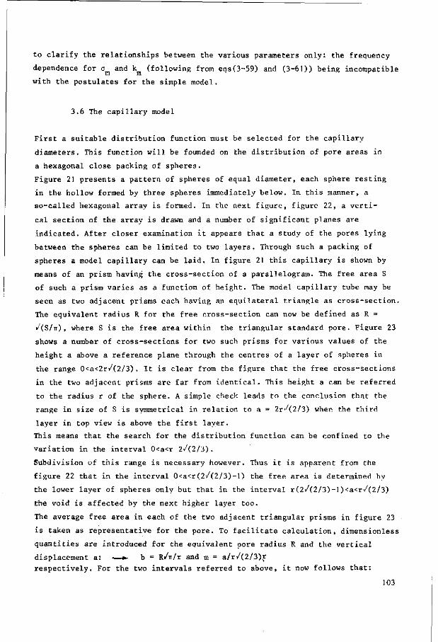
to clarify the relationships between the various parameters only: the frequency

dependence for o and k (following from eqs(3-59) and (3-61)) being incompatible

with the postulates for the simple model.

3.6 The capillary model

First a suitable distribution function must be selected for the capillary

diameters. This function will be founded on the distribution of pore areas in

a hexagonal close packing of spheres.

Figure 21 presents a pattern of spheres of equal diameter, each sphere resting

in the hollow formed by three spheres immediately below. In this manner, a

so-called hexagonal array is formed. In the next figure, figure 22, a verti­

cal section of the array is drawn and a number of significant planes are

indicated. After closer examination it appears that a study of the pores lying

between the spheres can be limited to two layers. Through such a packing of

spheres a model capillary can be laid. In figure 21 this capillary is shown by

means of an prism having the cross-section of a parallelogram. The free area S

of such a prism varies as a function of height. The model capillary tube may be

seen as two adjacent prisms each having an equilateral triangle as cross-section.

The equivalent radius R for the free cross-section can now be defined as R =

/(S/n), where S is the free area within the triangular standard pore. Figure 23

shows a number of cross-sections for two such prisms for various values of the

height a above a reference plane through the centres of a layer of spheres in

the range 0<a<2r/(2/3). It is clear from the figure that the free cross-sections

in the two adjacent prisms are far from identical. This height a can be referred

to the radius r of the sphere. A simple check leads to the conclusion that the

range in size of S is symmetrical in relation to a = 2r'/(2/3) when the third

layer in top view is above the first layer.

This means that the search for the distribution function can be confined to the

variation in the interval 0<a<r 2/(2/3).

Subdivision of this range is necessary however. Thus it is apparent from the

figure 22 that in the interval 0<a<r(2/(2/3)-l) the free area is determined by

the lower layer of spheres only but that in the interval r(2/(2/3)-I)<a<r/(2/3)

the void is affected by the next higher layer too.

The average free area in each of the two adjacent triangular prisms in figure 23

is taken as representative for the pore. To facilitate calculation, dimensionless

quantities are introduced for the equivalent pore radius R and the vertical

displacement a: — » - b = R/ir/r and m = a/r/(2/3)r

respectively. For the two intervals referred to above, it now follows that:

103

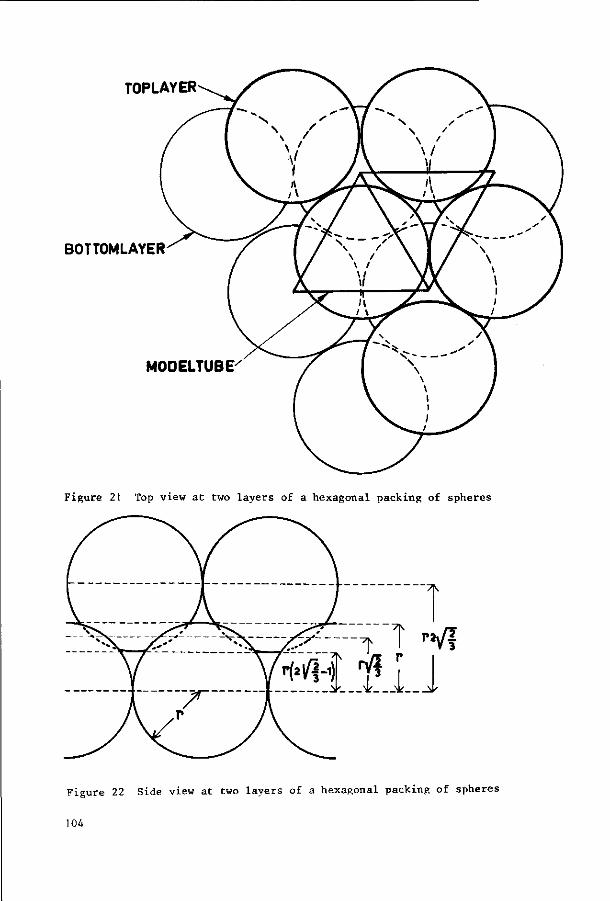
TOPLAYER

BOTTOMLAYER

MODELTUBE

Figure 21 Top view at two layers of a hexagonal packing of spheres

T W!

Figure 22 Side view at two layers of a hexagonal packing of spheres

104

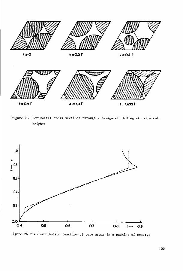
a-O a=0.3T a = 0 7 T

a =0.9 r a = 1.3 r a =1.633 T

Figure 23 Horizontal cross-sections through a hexagonal packing at different

heights

0-4 OS 0.6 0 7 CX8 b-* 0.9

Figure 24 The distribution function of pore areas in a packing of snheres

105

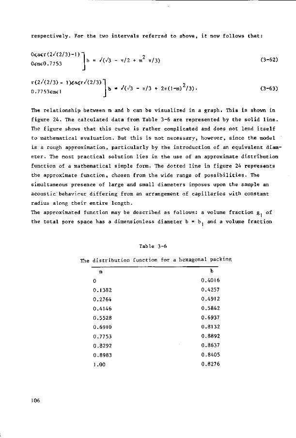
respectively. For the two intervals referred to above, it now follows that:

0^0.7753 jb = /(/3 - W 2 + m2 ,/3) (3-62)

r ( 2 / ( 2 / 3 ) - l>Ja<r/(2/3)1 , 0.7753««1 J b = /(/3 - fl/3 + 2-(>-m)Z/3). (3-63)

The relationship between m and b can be visualized in a graph. This is shown in

figure 24. The calculated data from Table 3-6 are represented by the solid line.

The figure shows that this curve is rather complicated and does not lend itself

to mathematical evaluation. But this is not necessary, however, since the model

is a rough approximation, particularly by the introduction of an equivalent diam­

eter. The most practical solution lies in the use of an approximate distribution

function of a mathematical simple form. The dotted line in figure 24 represents

the approximate function, chosen from the wide range of possibilities. The

simultaneous presence of large and small diameters imposes upon the sample an

acoustic behaviour differing from an arrangement of capillaries with constant

radius along their entire length.

The approximated function may be described as follows: a volume fraction g of

the total pore space has a dimensionless diameter b = b. and a volume fraction

Table 3-6

The distribution function for a hexagonal packing

m b

0 0.4016

0.1382 0.4257

0.2764 0.4912

0.4146 0.5842

0.5528 0.6937

0.6910 0.8132

0.7753 0.8892

0.8292 0.8637

0.8983 0.8405

1.00 0.8276

106

g9 has a diameter b = b~, b < b „. The remaining pores possess a dimensionless

radius b given by

b = b, + (m - g,) (b2 - bj) / g3; b] * b 4 h2, (3-64)

where g3 = 1 - g, - %r

The numerical values selected are:

g = 0.20; g2 = 0.25; g3 = 0.55; b, = 0.4.25; \>2 = 0.850, (3-64a)

and eq.(3-64) is brought into the form:

m = - 0.35 + 1.294 b; 0.20<m<0.75.

Summarizing, it can be said that in the total pore space 20% is occupied bv

pores with a radius R = —' r = 0.2398 r, and 257 is occupied by pores with a 0 850 radius R = —7 r = 0.4796 r, while the remaining pores have radii with equal

KIT ~ ~

statistical weight, between the two above radii. These occupy 55% of the total

pore space.

Applying eq.(3-48) one finds

•1-g,

'1 ' "2 J g, S = (g.w R 2 ), + (g TT R2) + f 2 TT R2 dm. (3-65)

a ' bi 2 h? J R,

On replacing R by b, and using eq.(3-64) in the form

go dm = - r — — - db, (3-66)

b 2 - b,

the formula may be integratedjit follows that

S a = r2 { g,b2 + g2b2 + jg3(b2 + b,b2 + b2)} . (3-67)

Introduction of the numerical values from eq.(3-64a) vields

Sa = 0.4485 r2. (3-68)

Assuming in this way that the porous material is characterized by inhomogeneous

pores with a given distribution function and inclined with an angle 9 to the

direction of propagation, the porosity can, making use of eqs(3-44) and (3-68),

be calculated. One finds

h = 0.4485 r2 N/cos 9 . (3-69)

The following auxiliary functions for the calculation of £ can be defined: c

107

2 J H(x) . — (x /-j), (3-70)

x /-j JQ

with the abbreviated notation:

J, J,(x) — (x) = , J0 JQ(x)

F(x) = l-H(x), and (3-71)

M(x) = I-^ dx, (3-72) = I ~ dx, J x F(x)

where x = R/(IDP /n). (3-73)

Comparing eq.(3-71), in conjunction with eqs(3-70) and (3-73), with eq.(B-2) in

appendix B, one sees that

V c = 1/F(x). (3-74)

As special value for x is introduced

x3 = r /(u)ps/7rn), (3-75)

and i t i s noted tha t

for b = b —*• x = x = b . x . , (3-76)

for b = b 2 -* -x = x 2 = b 2 x 3 , (3-77)

? 0 7 7 ? ? S = TTR = b r = x r / x 3 , (3-78)

and, by using eqs (3 -66) , (3-73) and (3 -75) , t ha t

g3 1

dm = — - — . - dx. (3-79)

V b l x3 Eq.(3-49) can be used now for the calculation of E, , the integration in the

right side presents hardly any problem for the intervals in m where b is constant.

In the interval where such is not the case, x is introduced as the integration

variable, S being eliminated with the aid of eq.(3-78) and m with the aid of

eq.(3-79). Referring to the definition eq.(3-72) one finds

X M S2 83x3 X2 . ' (3-80)

xl '

£ = -4 < j + -—=-— + - ^ - M(x) -- ' b,F(x,) b2F(x2) b2-b,

2 where S /r may be obtained from eq.(3-68) and the other numerical values for

factors and arguments from eqs(3-64), (3-76) and (3-77).

'"he following additional auxiliary functions are defined for the calculations of

108

G(x) = 1 + 0 . 4 H(x), (3-81)

L(x) = fx2 G(x) dx, (3-82)

where, in t h i s ins tance

x = R/(ujp C / \ ) (3-83)

s p

and a comparison of eq.(3-81) in conjunction with eqs(3-83) and (3-70) with

eq.B-22) as cited in appendix B, shows that n' = G(x), (3-84)

c

with adequate accuracy for bi-atomic gases.

A special value for x is introduced (3-85) x 6 =

and

for

for

= r/

it

b =

b =

(up c IT. s p

is

b

b

noted

l"^ X

2 - ^ x

A),

that:

= *4 =

= x 5 =

b

b

lx6'

2X6'

(3-86)

(3-87)

S = x2r2/Xg, (see eq.(3-78)), (3-88)

and eqs(3-66), (3-83) and (3-85) show that

dm = — . — dx. (3-89)

V b l x6 Eq.(3-50) is now used for the calculations of n , the integration in the right

side presenting few problems for the intervals in m where b is constant. In the

interval where such is not the case x is introduced as the integration variable,

S being eliminated with the aid of eq.(3-88) and m with the aid of eq.(3-89).

On referring to the definition, eq.(3-82), one finds

^c = 7 { S.b? G(x4> + *2b2 G(x5> + 7 ~ ~ • 3 L(X)|X5} Sa < ( b 2 _ b l ) x6 K>

(3-90)

where r /s may be obtained from eq.(3-68) and the other numerical values for

the factors and arguments from eqs(3-64a), (3-86) and (3.-87). Note that the-

various definitions given for x in eqs(3-73) and (3-83) no longer affect the

results, eqs(3-80) and (3-90). The model has been idealized to such an extent

that r and 8 are formal parameters and cannot be derived from the geometrical

parameters of a sample material considered.

109

In the special case of static flow, the specific resistance a may be obtained

from eqs(3-59) and (3-80), permitting u to approach zero. In that case, the

arguments of the function F(x) (see eqs(3-75), (3-76) and (3-77)) are small and

the function approaches

F(x) jx2/8.

This approximation yields

8 Tin 2., , . t 2

a = S a i 8 l +

8 2 + l W V M n < m r I b, b„ 3 b. • b . J s , 2 2

h t c o I "2 ^ "1 "2

and, on introducing the numerical values from eqs(3-64a) and (3-68) the result

is

o = i29-920 . (3-92)

s u 2 2A h r cos 6

Eq.(3-92) is in accordance with the model rule for static-flow resistances,

eq.(3-121).

3.7 The fissure model

The study of the fissure model will run along the same lines as that of the

capillary model. TThere possible similar symbols will be used. The cross-sectional

area of a channel is obtained by considering a slab of material of unit thickness

in the direction normal to the plane of drawing figure 20. Thus for a fissure of

width T) the cross-sectional area is D times unit length.

In future, the unit length as factor will be omitted from the equations.

A rather simple distribution function for the fissure widths D will be intro­

duced, which, while showing some resemblance to the distribution function for

the capillary radii, avoids the necessity of solving the integrals appearing

on the right side of the defining eqs(3-49) and (3-50).

For the inhomogeneous fissure the following assumptions are made with respect

to the distribution function for the fissure widths. 2

a fraction 0.25 has a width D, = 4 D /(l + q ) , (3-94) 1 a na ~

a fraction 0.50 has a width D = 4 D q /(l + q ) , (3-95) 2 ana. na „

a fraction 0.25 has a width D = 4 D q i/(\ + q ) . (3-96) i a a a

where D is the average fissure width, independent from the value selected for q . The ratio of the widths of the widest and the narrowest parts of the in-

3 2 homogeneous fissure, the fissure width ratio equals q

110

For the calculation of £f the following auxiliary function is defined now:

F 00 = ,-tanJxAj). f (3_97)

x / - i

where

x =(D/2)/(o)o /n) (3-98)

A comparison of eq.(3-97) in conjunction with eq.(3-98) and (B-6), shows that

V t = 1/Ff(x) . (3-99)

On introducing the special values:

2 Da CODS „

x = %r • / — - ; x = q x 5 x = q x , (3-100) ' (1+q r n 3

the right-hand side of eq.(3-49) is readily integrated resulting in

v2

5f = + qa) ( 1 2 1

{ + + -5 > • (3-101) 16 I F.(x.) qF.(x.) qFf(x,))

The following auxiliary function for the calculation of nf is defined as

tan(x / - j) Hf(x) = (3-102)

x / - i

where

x = -j /(up c A ) . (3-103)

•Comparison of eq.(3-102) in conjunction with eq .(3-103) with eq . (B-18) , as d e ­

r ived in appendix B, y i e lds

n ' = 1 + 0.4 H (x) (3-104) f f

111

with adequate accuracy for bi-atomic gases.

On introducing the special values:

2 D x 2 A ~ ^ / ' X5 = qa X 4 * x6 = qa V (3-105a,b,c) 4 (1+q

the right side of eq.(3-50) is readily integrated and yields:

0.4 n = 1 + . _ { H,(x.) + 2 q H.(x,) + q H,(x,) } (3-106)

t / i ^ x ^ 1 4 a r 5 a t o (1 + qa)

As in the case of the capillary model D ,q and 9 should the considered as

formal parameters, not related directly to the sample geometry. Eqs(3-59) and

(3-106) yield the static specific flow resistance for the fissure model by

permitting w to vanish. In that case the arguments of F, (x) are small(compare

eq.(3-105, a,b and c)) and hence

1/Ff(x) « -3j/x2

(l + l/qa)6. (l+qa)2

The

o « s

r e s u l t

3

64

i s

h

n

cos 2e D

a

2 (3-107)

in accordance with the scale rule (eq.(3-121)).

3.8 Comparison of the behaviour of the capillary and the fissure model

As stated prevously, eqs(3-56) and (3-55) furnish the solution for the specific

acoustic impedance Z of the sample surface, where £ and n may be introduced

from eqs(3-80) and (3-90) or alternatively £ and n from eqs(3-102) and (3-106}

for the capillary and fissure models, respectively. Computers were used for

the numerical calculations, and the locus of Z was determined for constant

absolute steps in frequency. A consequence is that the steps in Z vary consider­

ably in the complex plane. However it was not felt worthwhile to correct for

this tendency as that would involve extremely complicated programmes and

excessive computation times. The problem is reconsidered in appendix D.

112

The auxiliary functions Ff(x) and H (x) , see eqs(3-97) and (3-102),for the

fissure model present no difficulties. Greater problems are encountered in the

calculation of the auxiliary functions for the capillary model, H(x), F(x),

M(x) and L(x) (see eqs(3-70), (3-72), (3-71) and (3-82))and appendix C has been

devoted to this subject.

For the cylindrical capillary model, two geometrical parameters are available

for fitting the theoretical curves to the experimental ones: (1) the sphere

radius r and (2) the angle 6. For the fissure model, in addition to the average

fissure width D and the angle 9, a third parameter is available: the fissure 2 a . . . . .

width ratio q . The introduction of this parameter in the fissure model only

appeared to be ?:he wisest course, as this model is more sensitive to changes in

the distribution function of the channel cross-sectional areas than is the capillary model. This may be seen from the following argument. The locus of Z may be shifted by variation in the phase angles of Z and Y and

J m m here £ and £, are far more effective than n and n,. the latter two quantities

c f c f

departing but little from the real axis. The attention is thus focused on the

two former quantities and restricted to the high-frequency range, where |R/1 |,

||D/1 |>>1 (see appendix B). One can thus find the approximations for large values

of the argument:

l/F(x)»l-i A—) , (3-108) s

1/F,(x)«l-J- /(i2~). (3-109) 1 D up

s

In these two cases, the approximations eqs(3-108) and (3-109) reduce eq.(3-A9)

to

1

Sf * Da / I o J<- ) I dm. (3-111)

1 a Jo | D DZ uo ) w s

Eqs(3-110) and (3-111) are now compared under the special conditions:

R2(m) = D^f(m), (3-112)

D(m) = Daf(m), (3-113)

1 13

the definition of D (see eqs(3-48) and (3-93)) requiring

j f(m) dm = 1, (3-114)

0

where f(m) may be any function of m. However monotonic functions are applied in

the present models exclusively.

By eqs(3-112) and (3-113), eqs(3-110) and (3-111) may be reduced to

5 -fX\ -! W ~ / (--) I dm, (3-115) Jn ' f(m) D f ' (m) coo ' 0 a s

Cf =/" I k / (-21-) j dm. (3-116) J < f(m) D f (m) u)o ' 0 a s

It should be noted that the real parts of E and £ are identical. A variation

in f(m), of such a nature that eq.(3-114) is still satisfied, will however tend

to introduce a larger change in the imaginary cart of £ than in £_ as f(m) c r

appears to a higher absolute power in the former case. The change in phase angle

for £. will thus exceed that in £ • This suggests that the fissure model may be

appropriate in those cases, where substantial variations in phase angle of the

propagation constant especially are required to match theoretical and experi­

mental data. Physically it is significant that the capillary of circular cross-

section has the minimum possible wall area for a given cross-sectional area.

3.9 Discussion on the possibilities of scale-rules

Before selecting simple spatial arrangements as models for porous materials

it is worthwhile noting that the results for such models, culminating in the

impedance at the sample surface, will depend on absolute geometrical dimensions

and the frequency as separate quantities?in other words scale rules do not

apply in cases of this kind. What a scale rule implies may be clarified by an

example: an acoustical system is Characterized by the spatial dimensions a,

b,...,and some acoustical quantity. F is calculated for a given wave number,

k. The result is of the general form

F = F (k,a,b,...). (3-117)

If this result may be brought into the form

114

F = F (k-a, k«b,...),

then a scale rule applies for the system. If so, increasing all linear di­

mensions by an arbitrary factor and decreasing the frequency and thus the

wave number by the reciprocal of that factor, will yield the same solution F,

the quantities k«a, k'b,... remaining the same.

That solutions of this type do not obtain for porous materials may be con­

cluded on considering two samples of such materials, A and B, where all geo­

metrical dimensions of sample B have been scaled down by a factor n(n >1) in

relation to sample A.

So B has the same shape as A, but is smaller in size. If a scale rule is to

apply, the sound field in sample B must have the same form as in A, only

reduced in dimension by the factor 1/n. This imposes, e.g., the thicknesses of

the viscous and thermal boundary layers must be reduced by 1/n and the free

wave-length must be reduced by 1/n.

On assuming the same ideal gas to be the acoustic medium in both samples,

the boundary layer thicknesses are universely proportional to the square root

of frequency (see appendix B ) , thus requiring an increase in frequency by a 2

factor n for sample B in relation to sample A, whereas the free wavelength

is inversely proportional to frequency, thus requiring an increase in

frequency by a factor n. Excepting trivial cases, both conditions cannot be

met simultaneously, and no frequency can be indicated for sample B, yielding

a sound field of the same form as for sample A.

The problem may be illustrated by deriving a scale rule for the static value

of the specific acoustic flow resistance and investigating its consequences

for the sound fields in the two samples. In the case of static flow, the

forces exerted by the frames of the samples on the medium are viscous ones

and the compressibility of the medium is irrelevant; generality is not im­

paired by assuming an incompressible medium. These considerations are express­

ed in three-dimensional notation in general form:

2 2 3p/3xi = n 1.3 u./3x. ; i,j = x.y.z (3-118)

The incompressibility can be expressed by

Si3ui/3xi = 0, (3-119)

where x. is the generalized spatial co-ordinate and u. is the generalized

component of particle velocity. Note that eq.(3-118) in fact represents three

equations.

115

One solution for sample A is assumed to be known:

IK = 1\(x,y,z),

and a second assumption is that a solution of the same form holds for sample

B. The generalized spatial co-ordinate for sample A is indicated by x., that

for B by £.:

n£. = x.. (3-l20a)

Requiring equal particle velocities in corresponding points in the two samples

implies that for sanrole B:

u.-*.(ne., nSj, nek),

a solution which satisfies the boundary conditions automatically and, after

some consideration, is seen to satisfy eq.(3-ll9) too.

Sound pressure is indicated by q for sample B and eq.(3-118) yields

3q/3£. = n I. 3 u./3£. = n3q/3x. = nn2 £.3 Y. (x., x., x ) /3x? . i J 1 . 1 H i J i i J k J

This equation is identical with that for case A, if

q = np.

The flow-resistance for flow in the direction k follows from

(3-120b)

- 3p/3x, = du, . (3-120c) r k k

where p the average sound pressure in the pores and u is the volume velocity per

unit area.

In the present instance, an averaging process is required over an area large

enough to be representative for the sample and thus the flow resistance now

follows a s :

for sample A . - X . / 2 rX./2

- l L - f X dx / J dx i E hX.X. / - X . / 2 axiJ-X./2 a x j 3x,

a4 = Lim — ± 1 ^ ^ n . <3-121a) A X~72 / .X. /2

*•**-*" n r K > 2 dx^-v2 d"Uk i j

1 16

for sample B

2 /-X./2n /»X./2n

(3-121b) aB = Lim

X . , X . — - < » l J

hX.X. . i .1

2 n

x, x4^

/ - X . / 2 n ^ „ l

- X . / 2 n

/ -X . / 2n d £ .

J - X . / 2 n u t i j 35,

, . X . / 2 n

/ - X 7 2 n d 5 j u k

The limits introduced above are assumed to exist. Taking into account that:-

3 q/3£k = 3np/3(xk/n) = n23p/3xk> (3-122)

and reducing the integration variables in eq.(3-121b) to x. and x., it follows

from eqs(3-121a) and (3-121b) that

oR = n oA. (3-123)

Eq.(3-123) is a scale rule but not in the general sense required in acoustics

as its validity has been proven only for static flow.

Now eq.(l-l) is adduced; the limitation to one spatial dimension does not

affect the principles involved. Air, as medium, is permitted to retain its

density but its motion is assumed to be hampered by a flow resistance, a or

a respectively for the two samples under consideration. The sound fields B

generated in these samples are harmonic, having circular frequencies w and OJ ,

respectively. Thus

for sample A

-3p/3x = (ju> o +o.) u, (3-124a)

for sample B

-3q/35 = (ju)B og+oB) u . (3-124b)

Using eqs(3-122) and (3-123), eq.(3-124b) is seen to be identical with eq.

(3-124a), if:

w„ = n2oo, . (3-l24c) B A

This result was to be expected on the grounds of the frequency dependence

of the boundary layers. That it clashes with the requirement imposed on the-

free wavelength will become apparent from eq.(l-2), which yields:

117

for sample A

for sample B

-3u/3x = jco. p/K,

-3u/9£ = jioB q/K.

(3-125a)

(3-125b)

Eqs(3-120a), (3-120b) and (3-120c) reduce eq.(3-125b) to:

2 -3u/3x = j n UK p/K,

which is not in accordance with eq.(3-125a), thus showing that the scale rules

eqs(3-120a), (3-120b) and (3-120c) lead to an inconsistency, although essential

for eqs(3-118) and (1-1). Hence a scale rule for porous materials proves

impossible.

118

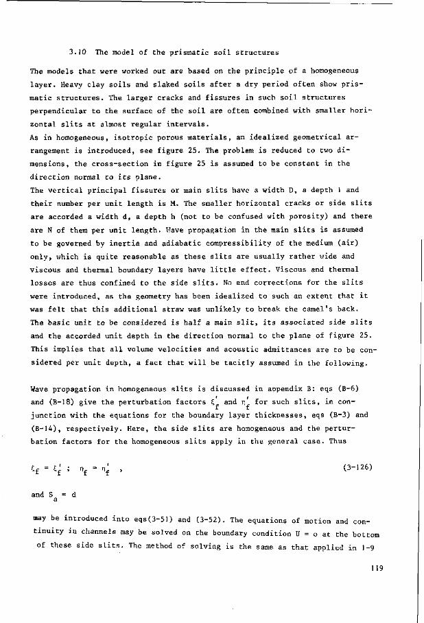
3.10 The model of the prismatic soil structures

The models that were worked out are based on the principle of a homogeneous

layer. Heavy clay soils and slaked soils after a dry period often show pris­

matic structures. The larger cracks and fissures in such soil structures

perpendicular to the surface of the soil are often combined with smaller hori­

zontal slits at almost regular intervals.

As in homogeneous, isotropic porous materials, an idealized geometrical ar­

rangement is introduced, see figure 25. The problem is reduced to two di­

mensions, the cross-section in figure 25 is assumed to be constant in the

direction normal to its plane.

The vertical principal fissures or main slits have a width D, a depth 1 and

their number per unit length is M. The smaller horizontal cracks or side slits

are accorded a width d, a depth h (not to be confused with porosity) and there

are N of them per unit length. Have propagation in the main slits is assumed

to be governed by inertia and adiabatic compressibility of the medium (air)

only, which is quite reasonable as these slits are usually rather wide and

viscous and thermal boundary layers have little effect. Viscous and thermal

losses are thus confined to the side slits. No end corrections for the slits

were introduced, as the geometry has been idealized to such an extent that it

was felt that this additional straw was unlikely to break the camel's back.

The basic unit to be considered is half a main slit, its associated side slits

and the accorded unit depth in the direction normal to the plane of figure 25.

This implies that all volume velocities and acoustic admittances are to be con­

sidered per unit depth, a fact that will be tacitly assumed in the following.

Wave propagation in homogeneous slits is discussed in appendix B: eqs (B-6)

and (B-18) give the perturbation factors £ and n for such slits, in con­

junction with the equations for the boundary layer thicknesses, eqs (B-3) and

(B-14), respectively. Here, the side slits are homogeneous and the pertur­

bation factors for the homogeneous slits apply in the general case. Thus

e f = Vt ; nf - n^ , (3-126)

and S = d a

may be introduced into eqs(3-51) and (3-52). The equations of motion and con­

tinuity in channels may be solved on the boundary condition U = o at the bottom

of these side slits. The method of solving is the same as that applied in 1-9

119

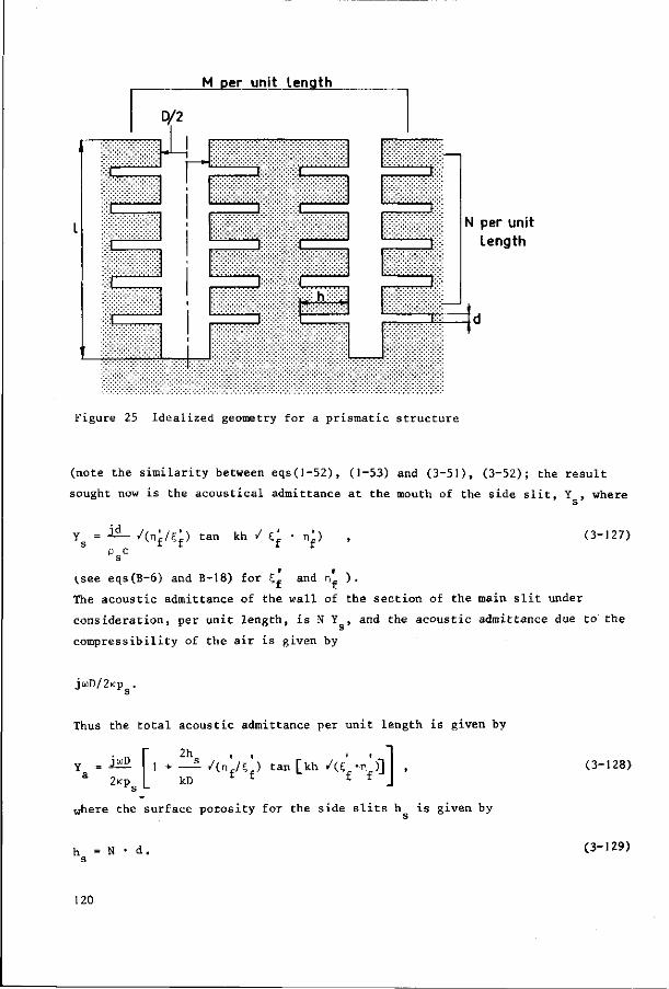
M per unit length

N per unit length

Figure 25 Idealized geometry for a prismatic structure

(note the similarity between eqs(l-52), (1-53) and (3-51), (3-52); the result

sought now is the acoustical admittance at the mouth of the side slit, Y , where

(3-127) Vs= — -/(nf/SJ) tan kh / (,' • n') , p s C

(.see eqs(B-6) and B-18) for £f and n ) .

The acoustic admittance of the wall of the section of the main slit under

consideration, per unit length, is N Y , and the acoustic admittance due to the

compressibility of the air is given by

jooD/2<p .

Thus the total acoustic admittance per unit length is given by

2h ltoD

2<p r c

1 + —- / (n f /5 ) tan [kh /(5 kD - l

;•<>]] , where the surface porosity for the side slits h is given by

(3-128)

h = N • d, s

(3-129)

120

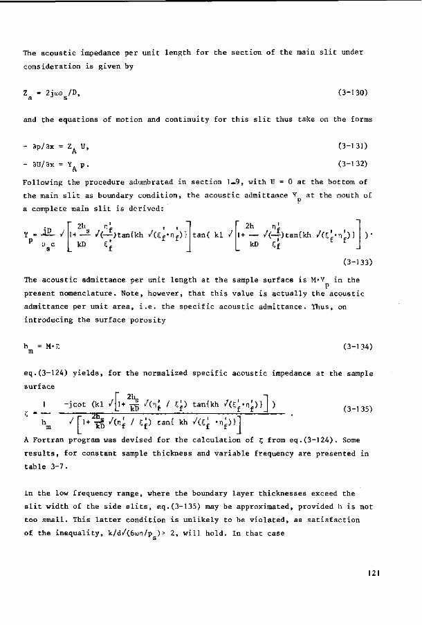
The acoustic impedance per unit length for the section of the main slit under

consideration is given by

Z = 2ju)D /D, (3-130) a J s

and the equations of motion and continuity for this slit thus take on the forms

- 3p/3x = Z U,

- 3U/8x = YA p. A

(3-131)

(3-132)

Following the procedure adumbrated in section 1—9, with II = 0 at the bottom of

the main slit as boundary condition, the acoustic admittance Y at the mouth of

a complete main slit is derived:

p s c

2h n' H _ s /(_E)tan{kh /(ef-nf)}

kD £' -f n f tan( kl /

2h n' 1+ _ /(-4)tan{kh./(c'-nl)}

ID £f f f .

(3-133)

The acoustic admittance per unit length at the sample surface is M«Y in the

present nomenclature. Note, however, that this value is actually the acoustic

admittance per unit area, i.e. the specific acoustic admittance. Thus, on

introducing the surface porosity

h = H'T. m (3-134)

eq.(3-124) yields, for the normalized specific acoustic impedance at the sample

surface

' 2hs . / i r\ i >• l r a n - f i / h i / ( t • n \ I I i

(3-135) 1 -jcot (kl /

/ "2K;

1+ -j~ /<n' I Vf) tanlkh /(S^n^)}] )

[1+ kD / ( nf ' e P tan{ kh / ( Sf 'nf) }l A Fortran program was devised for the calculation of Z, from eq.(3-124). Some

results, for constant sample thickness and variable frequency are presented in

table 3-7.

In the low frequency range, where the boundary layer thicknesses exceed the

slit width of the side slits, eq.(3-135) may be approximated, provided h is not

too small. This latter condition is unlikely to be violated, as satisfaction

of the inequality, k/d/(6un/p )> 2, will hold. In that case

121

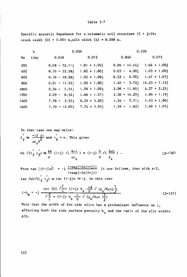
Table 3-7

Specific acoustic impedance for a prismatic soil structure (£ + jn)h;

crack width (D) = 0.001 m.slit width (d) = 0.008 m.

Hz

200

400

600

800

1000

1200

1400

1600

h

Km)

O.C

0.040

0.08 - 72.11J

0.10 - 33.58J

0.10 - 19.59J

0.01 - 11.52j

0.34 - 5.51j

2.09 - 0.34j

7.26 - 2.57J

7.70 - 12.00J

50

0.072

1 .01 +

1 .02 +

1 .02 +

1.00 +

1 .06 +

1 .46 +

6.25 +

7.74 +

l.OOj

l.OOj

l.OOj

l.OOj

l.OOj

1.07J

3.20J

3.93j

0

0.06

0.05

0.53

1.40

2.06

2.36

1.34

1.26

0.

.040

- 14.14J

- 4.90J

- 0.50J

- 3.72J

- 11.60J

- 14.29J

- 5.71 j

- 1 .62j

100

0.072

1.04 + 1.00j

1 .03 + 1.00j

1.47 + 1.07j

14.23 + 7.15j

4.27 + 2.25j

1.86 + 1 .19j

1.43 + 1 .06j

1.40 + 1.05j

In that case one may write:

£; Ss i— and n = K. This gives f * s d '

kh /(f j n p w ^ (,-j) /( n ) - (i-j) * /( H ) . (3-136)

d u P g d ps

From tan {(l-j)XS> - -j '~exP(~2x( 1+j)> j.t n o w follows, that with x>2,

l+exp(-2x(l+j)) i i

tan (kh/(Cf nf) « tan (l-j)x « - j . In this case

cot (kl /fi+ (l-j) ho -Si / (p /6un)l)

c-hm = -j — - r 1 ^ - i - 2 s -I (3_137)

/|l + (l-j) hs -^- / (p8/6mn )J)

Note that the width of the side slits has a predominant influence on t,

affe

d/D.

affecting both the side surface porosity h and the ratio of the slit widths

122

3.11 Electro-acoustical equivalent networks

Sometimes the behaviour of an acoustical system may be classified by examining

its electrical analogous circuit. In the present instance, a porous material

is such a system and eqs (1-52) and (1-53) indicate the procedure for transi­

tion from acoustical to electrical symbolism. If p is conceived as the voltage

on an electrical transmission line, u as the current, and Z and Y are taken m m

to represent the series impedance and parallel admittance per unit length of

that line, respectively, the equations named become identical with the telegraph

equations.

In electrical analogous circuits of the sort intended here, masses are replaced

by self-inductances, flow resistances by resistors and compliances with damping

by combinations of capacitors and resistors. In the present section, the possi­

bility of composing reasonably simple electrical equivalent circuits for Z and

Y is examined; complicated circuitry may be ignored as it does not contribute

to clarity

A simple porous material will be considered, consisting of cylindrical pores of

constant, circular cross-section of radius R. The pores are inclined from the

direction of propagation, the angle of inclination does not need to be constant

if the material remains homogeneous in the acoustical sense. For frequencies so

low that boundary layer thickness exceed tube radius, Zwikker & Kosten's (1949,

p. 38) results may be applied and after some reduction it follows that

4 iojk p 8 k n Z - J L £ + — J S _ , (3-J38)

m * 3 h hR2

Y ml

„2 p o c p R

s .. I ,1 s v s

— + (<-l) — — juh 8hA

(3-139)

where the added subscript I indicates the low-frequency approximation and h

stands for porosity.

For comparison an electrical transmission line is considered, a unit length of

which is represented in Figure 26.

From this circuit diagram it follows that:

Zme = ja)L + R l ' (3-140)

123

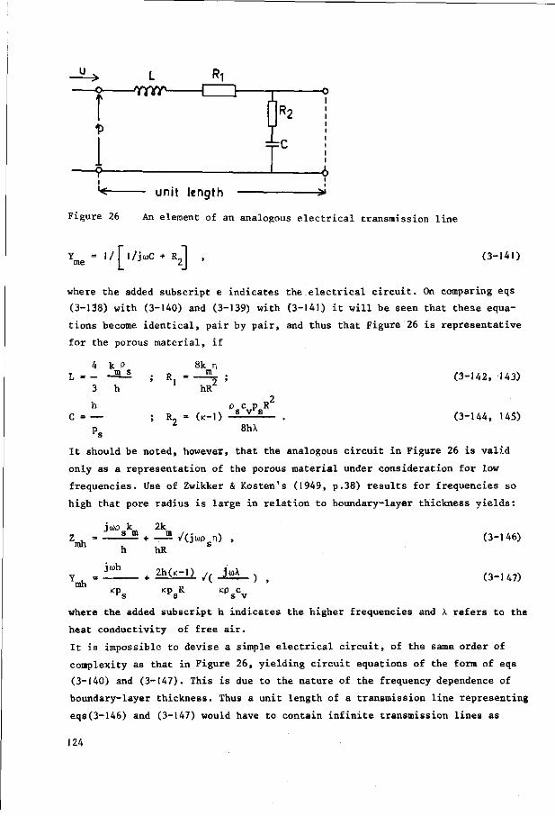
L * i -CZZ1-

R2

4=c

-o I

I I I

-6 unit length

Figure 26 An element of an analogous electrical transmission line

l/M/jmC + R J , (3-141)

where the added subscript e indicates the electrical circuit. On comparing eqs

(3-138) with (3-140) and (3-139) with (3-141) it will be seen that these equa­

tions become identical, pair by pair, and thus that Figure 26 is representative

for the porous material, if

4 k P T _ m s

h C = —

R. = 8k n

m

hR 2

(K-0 p c p R

s v*s

8hX

(3-142, 143)

(3-144, 145)

It should be noted, however, that the analogous circuit in Figure 26 is valid

only as a representation of the porous material under consideration for low

frequencies. Use of Zwikker & Kosten's (1949, p.38) results for frequencies so

high that pore radius is large in relation to boundary-layer thickness yields:

jwp k 2k „ s in m //. v Z = + /(jtop n) , ^ h hR

jioh

mh + 2h(<-l) / ( jaX

)

(3-146)

(3-147)

*Pc <p R *s

icp c s V

where the added subscript h indicates the higher frequencies and X refers to the

heat conductivity of free air.

It is impossible to devise a simple electrical circuit, of the same order of

complexity as that in Figure 26, yielding circuit equations of the form of eqs

(3-140) and (3-147). This is due to the nature of the frequency dependence of

boundary-layer thickness. Thus a unit length of a transmission line representing

eqs(3-146) and (3-147) would have to contain infinite transmission lines as

124

circuit elements and even if these latter can be approximated by a finite num­

ber of elements, discernability is lost.

It seems impossible to compose a satisfactory equivalent electrical circuit for

the geometrically simule porous material considered, covering the entire fre­

quency range. Thus no further efforts were made to search for equivalent cir­

cuits for more complex materials.

125

4 Some experiments discussed

4.I Introduction

The principal aim of this chapter is the examination of the applicability of the

three mathematical models discussed in the previous chapter to the description

of soil-like materials. The examination is carried out by comparing measured and

calculated curves for the quantity C h , the product of normalized sample surface

impedance and porosity, for samples of given thickness and for variable frequen­

cy. In assessing a mathematical model, two questions are posed: does the model,

with its parameters adjusted to optimum fit, describe the sample and do these

parameters yield information on the geometrical arrangement of the sample

material?

The quantity c*h is appropriate in the present instance as all three models

happen to yield expressions for it which are independent of h. The calculated

curves are determined by the values of c h for a series of frequencies with

spacings of 100 Hz in most cases. Measurements were made from about 150 to 1750

Hz, but could not be carried out systematically at the spot frequencies. This is

due to the exigencies of the interferometer (e.g. resonances in the tube) and

the following procedure was introduced to find interpolated values for ?*h at

the spot frequencies. The measured points for C are entered in the complex plane

and the absorption coefficient a is plotted against the frequency f. In both

cases smooth curves are drawn through the points. From the a-f diagram values

of a for the spot frequencies are found and these values are used to find the

complex value of c*h in the complex plane.

z, was measured with the equipment described in chapter 2 and h was found by a

static method (cf. Introduction). In addition, the specific static flow

resistance a was determined (cf. Introduction), s

The measured curves were matched with those obtained from the models, the latter

being constructed for various values of the parameters. A number of provisional

fits were obtained by comparing tables of measured and calculated values for c;*h.

However the calculated curve giving the best fit was selected graphically, by

visual examination, taking into account the local accuracy in the C'h plane

(cf. figure 14) and the sensitivity of the calculated curves for variations in

the parameter. Special attention was paid to those sections of the curve where

126

the absorption coefficient is high, as accuracy is high there too. These sections

are commonly found near the first anti-resonance.

In a small number of cases the value of a parameter was interpolated after

matching one measured curve with two or more calculated ones. Thus broken values

for k have been found notwithstanding the fact that the calculations were

carried out with integer values.

With the imperfection of the models in view, no effort was made to develop a nu­

merical method of comparison. Such a method would be feasible after transfor­

mation of the locus from the C*n plane to another plane having e.g. an invariant

error circle. The derivation of an appropriate transformation presents consider­

able difficulties however. Better fitting curls could undoubtedly have been

calculated in some instances. This was not done, as the selected models were in

need of further refinement anyway.

4.2 Materials studied

For the purpose of matching measured and calculated curves three types of sample

materials were used: isodiametrical spheres, gravel and crushed bricks. The first

series of measurements were made on isodiametrical spheres. The balls were made

of steel, glass or polystyrene. The steel balls, obtained from a ball bearing

factory, were perfectly round, and did not lend themselves to loose packing. The

glass spheres served their purpose, the very thin layer of water, always covering

them in the conditions of the experiment, made it possible to obtain packings of

varying densities. The polystyrene spheres had the same disadvantage as the steel

ones. Gravel and crushed bricks were also used, since they allowed not only a

study of the effects of variable porosity, but also permitted variation of the

pore size distribution function. The gravel used consisted of both rounded

particles and particles that had been crushed to create sharp edges. Two sample

thicknesses were used practically exclusively: 40 and 72 mm. The spheres and the

gravels hardly absorb any water (in the order of 0.15 - 0.30 weight percent), so

crushed bricks are a better simulation of soil than the other materials. The

material sometimes possesses many small pores which may or may "mot be filled with

water. It was chosen as it does not show any rearrangement or desintegration (of

particles) upon changes in moisture content resulting from variations in moisture

tension. This might have occurred in soil aggregates as these are subject to

structural changes through swelling and air explosions. No attempt was made to

explain the effect of moisture content with the aid of a model as adequate models

incorporating the effect of water content at a given suction on accessible pores

127

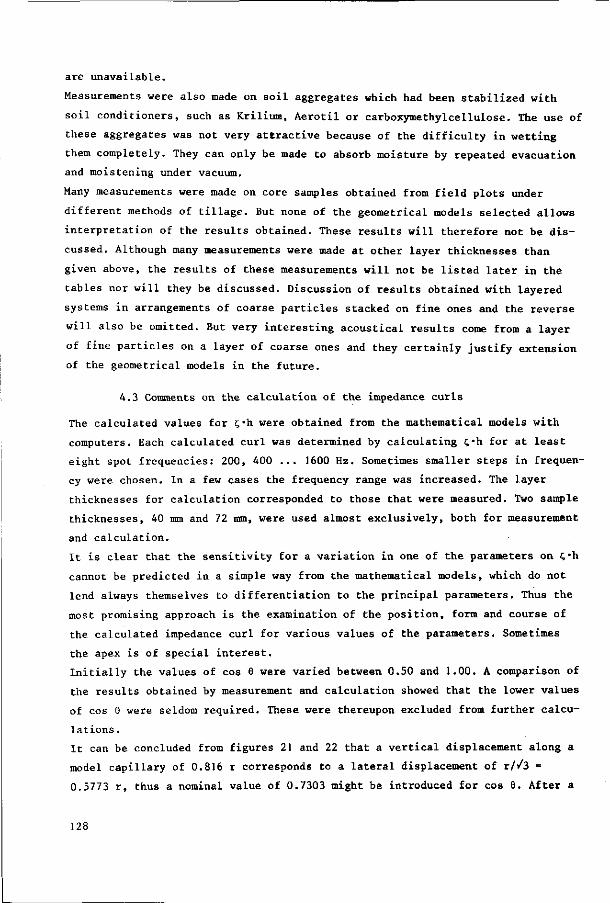
are unavailable.

Measurements were also made on soil aggregates which had been stabilized with

soil conditioners, such as Krilium, Aerotil or carboxymethylcellulose. The use of

these aggregates was not very attractive because of the difficulty in wetting

them completely. They can only be made to absorb moisture by repeated evacuation

and moistening under vacuum.

Many measurements were made on core samples obtained from field plots under

different methods of tillage. But none of the geometrical models selected allows

interpretation of the results obtained. These results will therefore not be dis­

cussed. Although many measurements were made at other layer thicknesses than

given above, the results of these measurements will not be listed later in the

tables nor will they be discussed. Discussion of results obtained with layered

systems in arrangements of coarse particles stacked on fine ones and the reverse

will also be omitted. But very interesting acoustical results come from a layer

of fine particles on a layer of coarse ones and they certainly justify extension

of the geometrical models in the future.

4.3 Comments on the calculation of the impedance curls

The calculated values for c,mh were obtained from the mathematical models with

computers. Each calculated curl was determined by calculating C'h for at least

eight spot frequencies: 200, 400 ... 1600 Hz. Sometimes smaller steps in frequen­

cy were chosen. In a few cases the frequency range was increased. The layer

thicknesses for calculation corresponded to those that were measured. Two sample

thicknesses, 40 mm and 72 mm, were used almost exclusively, both for measurement

and calculation.

It is clear that the sensitivity for a variation in one of the parameters on C*h

cannot be predicted in a simple way from the mathematical models, which do not

lend always themselves to differentiation to the principal parameters. Thus the

most promising approach is the examination of the position, form and course of

the calculated impedance curl for various values of the parameters. Sometimes

the apex is of special interest.

Initially the values of cos 6 were varied between 0.50 and 1.00. A comparison of

the results obtained by measurement and calculation showed that the lower values

of cos 6 were seldom required. These were thereupon excluded from further calcu­

lations .

It can be concluded from figures 21 and 22 that a vertical displacement along a

model capillary of 0.816 r corresponds to a lateral displacement of r//3 =

0.5773 r, thus a nominal value of 0.7303 might be introduced for cos 9. After a

128

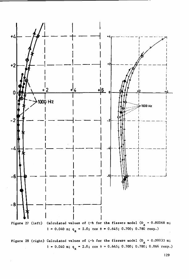
Figure 27 (left) Calculated values of C*h for the fissure model (D = 0.00068 m;

1 = 0.040 m; q = 2.0; cos 8 = 0.645; 0.700; 0.780 resp.)

Figure 28 (right) Calculated values of C'h for the fissure model (D = 0.00033 m;

1 = 0.040 m; q = 2.0; cos 6 = 0.645; 0.700; 0.780; 0.866 resp.)

129

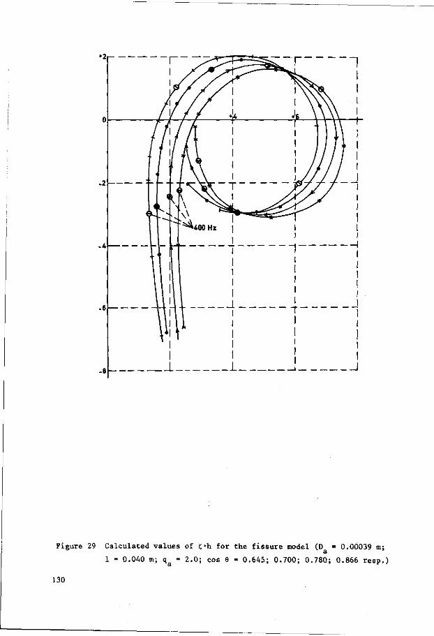
Figure 29 Calculated values of C*h for the fissure model (D = 0.00039 m;

1 = 0.040 m; q = 2.0; cos 6 = 0.645; 0.700; 0.780; 0.866 resp.)

130

Figure 30 Calculated values of c»h for the fissure model (D = 0.00022 m;

1 = 0.072 m; q = 2.0; cos 6 = 0.500; 0.645; 0.700; 0.780 resp.)

131

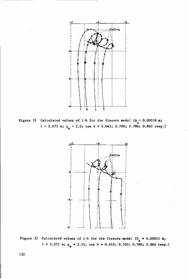
Figure 31 Calculated values of C'h for the fissure model (D = 0.00018 m; a

1 = 0.072 m; q = 2.0; cos 6 = 0.645; 0.700; 0.780; 0.860 resp.)

Figure 32 Calculated values of C-h for the fissure model (D = 0.00022 m;

1 = 0.072 m; q^ = 2.45; cos 9 = 0.645; 0.700; 0.780; 0.866 resp.)

132

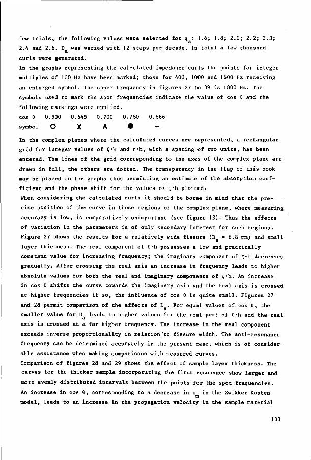
few trials, the following values were selected for q : 1.6; 1.8; 2.0; 2.2; 2.3;

2.4 and 2.6. D was varied with 12 steps per decade. In total a few thousand

curls were generated.

In the graphs representing the calculated impedance curls the points for integer

multiples of 100 Hz have been marked; those for 400, 1000 and 1600 Hz receiving

an enlarged symbol. The upper frequency in figures 27 to 39 is 1800 Hz. The

symbols used to mark the spot frequencies indicate the value of cos 8 and the

following markings were applied.

cos 6 0.500 0.645 0.700 0.780 0.866

symbol O X A 9 —

In the complex planes where the calculated curves are represented, a rectangular

grid for integer values of £*h and n'h, with a spacing of two units, has been

entered. The lines of the grid corresponding to the axes of the complex plane are

drawn in full, the others are dotted. The transparency in the flap of this book

may be placed on the graphs thus permitting an estimate of the absorption coef­

ficient and the phase shift for the values of £«h plotted.

When considering the calculated curls it should be borne in mind that the pre­

cise position of the curve in those regions of the complex plane, where measuring

accuracy is low, is comparatively unimportant (see figure 13). Thus the effects

of variation in the parameters is of only secondary interest for such regions.

Figure 27 shows the results for a relatively wide fissure (D = 6 . 8 mm) and small

layer thickness. The real component of c*h possesses a low and practically

constant value for increasing frequency; the imaginary component of ?'h decreases

gradually. After crossing the real axis an increase in frequency leads to higher

absolute values for both the real and imaginary components of C'h. An increase

in cos 9 shifts the curve towards the imaginary axis and the real axis is crossed

at higher frequencies if so, the influence of cos 8 is quite small. Figures 27

and 28 permit comparison of the effects of D . For equal values of cos 6, the

smaller value for D leads to higher values for the real part of C'h and the real

axis is crossed at a far higher frequency. The increase in the real component

exceeds inverse proportionality in relation"to fissure width. The anti-resonance

frequency can be determined accurately in the present case, which is of consider­

able assistance when making comparisons with measured curves.

Comparison of figures 28 and 29 shows the effect of sample layer thickness. The

curves for the thicker sample incorporating the first resonance show larger and

more evenly distributed intervals between the points for the spot frequencies.

An increase in cos 9, corresponding to a decrease in k in the Zwikker Kosten m

model, leads to an increase in the propagation velocity in the sample material

133

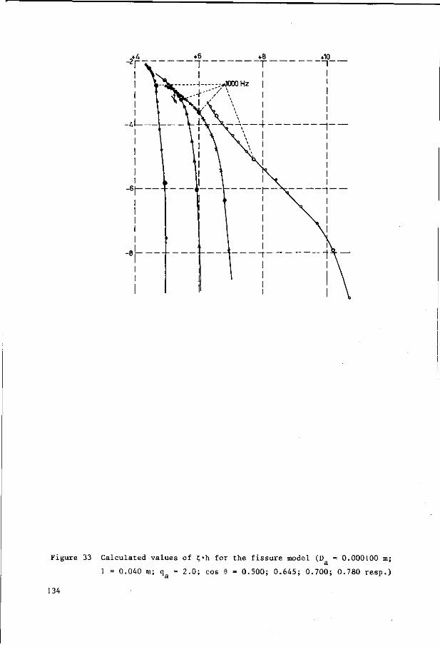
Figure 33 Calculated values of ?'h for the fissure model (D = 0.000100 m;

1 = 0.040 m; q = 2.0; cos 0.500; 0.645; 0.700; 0.780 resp.)

134

as may be seen from, for instance the points for 1000 Hz in the figures 28 and

29, respectively. This result was to be expected (cf. eq.3-55) as the direction

of propagation in the pores now coincides more closely with that of the sound

wave in the material.

The apexes of the curls in figure 29 lie below the real axis (cf. eq.3-56). This

is due to the preponderance of the viscous losses over the thermal ones, as may

be proved mathematically.

Figure 30 gives curls for a very small fissure width but with the same values of

the other parameters as those for figure 29. An interesting feature can be de­

tected: as values of cos 6 increase the apex of the curl shifts towards the real

axis and the propagation velocity in the material obviously decreases.

Figure 31 shows the effect of cos 0 on the position of the curl. At the higher

frequencies the curl approaches its apex fairly closely and the effect of cos 9

on the propagation constant is rather small at the lower frequencies. Note that

the apexes corresponding to the wave impedances should be considered slow

functions of frequency. The figure demonstrates that the wave impedances are very

nearly real and not very large. All this means that in this sort of case accurate

comparison with measured curls is feasible.

Another phenomenon appearing in figure 31 is that some of the curls intersect

themselves. This implies that at least one point is bi-valued for frequency.

In figure 32 q has been increased in relation to figure 31, and D increased

slightly. It shows the transition from impedance curls with a loop to those that

are characterized by more simple forms. For very fine slits and a large variation

in pore size (q = 2.45) high absorption coefficient will be attained at moderate

frequencies. The distribution of the frequency markers along the curls is regular

above 1000 Hz. Thus interpolation between the spot frequencies is facilitated and

assists in the comparison with measured curls.

For this small figure width, the air flow resistance is high. The coth con­

verges towards unity for high frequency, so the upper part of the impedance curl

should approach the form of a rectangular hyperbola (Zwikker & Kosten, 1948,

p.47).

As in figure 31, the curves approach their wave impedances for higher frequencies.

These impedances are nearly real and determined to a large extent by specific

flow resistance. The figure shows that for larger values of cos 9 and thus for

lower resistances the real part of ^-h decreases almost in inverse proportion to 2

cos 9.

At low frequencies the same trend for all curls is characteristic; the absorption

coefficient is proportional to the real part of c-h. Here the result is a family

135

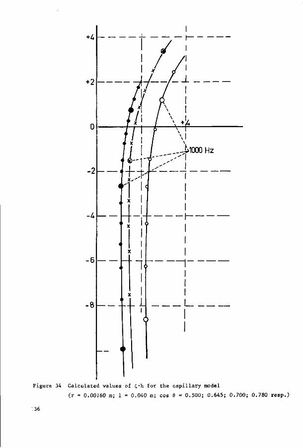
+A

+ 2

-2

-U

-8

44—!--

1

L

— T

Figure 34 Calculated values of C'h. for the capillary model

(r = 0.00160 m; 1 = 0.040 m; cos 6 = 0.500; 0.645; 0.700; 0.780 resp.)

:36

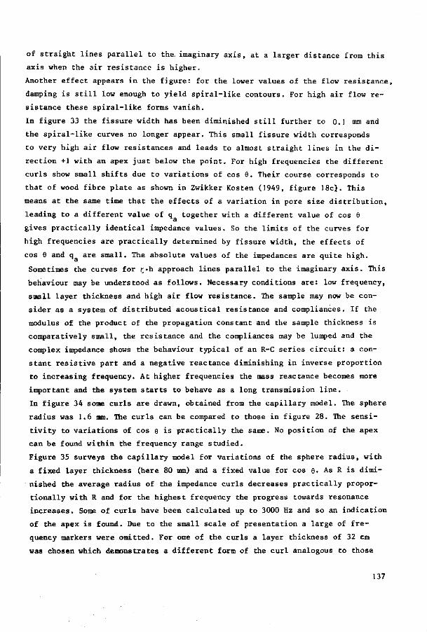
of straight lines parallel to the. imaginary axis, at a larger distance from this

axis when the air resistance is higher.

Another effect appears in the figure: for the lower values of the flow resistance,

damping is still low enough to yield spiral-like contours. For high air flow re­

sistance these spiral-like forms vanish.

In figure 33 the fissure width has been diminished still further to 0.1 mm and

the spiral-like curves no longer appear. This small fissure width corresponds

to very high air flow resistances and leads to almost straight lines in the di­

rection +1 with an apex just below the point. For high frequencies the different

curls show small shifts due to variations of cos 0. Their course corresponds to

that of wood fibre plate as shown in Zwikker Kosten (1949, figure 18c). This

means at the same time that the effects of a variation in pore size distribution,

leading to a different value of q together with a different value of cos 6

gives practically identical impedance values. So the limits of the curves for

high frequencies are practically determined by fissure width, the effects of

cos 9 and q are small. The absolute values of the impedances are quite high.

Sometimes the curves for £-h approach lines parallel to the imaginary axis. This

behaviour may be understood as follows. Necessary conditions are: low frequency,

small layer thickness and high air flow resistance. The sample may now be con­

sider as a system of distributed acoustical resistance and compliances. If the

modulus of the product of the propagation constant and the sample thickness is

comparatively small, the resistance and the compliances may be lumped and the

complex impedance shows the behaviour typical of an R-C series circuit: a con­

stant resistive part and a negative reactance diminishing in inverse proportion

to increasing frequency. At higher frequencies the mass reactance becomes more

important and the system starts to behave as a long transmission line.

In figure 34 some curls are drawn, obtained from the capillary model. The sphere

radius was 1.6 mm. The curls can be compared to those in figure 28. The sensi­

tivity to variations of cos e is practically the same. No position of the apex

can be found within the frequency range studied.

Figure 35 surveys the capillary model for variations of the sphere radius, with

a fixed layer thickness (here 80 mm) and a fixed value for cos 6. As R is dimi­

nished the average radius of the impedance curls decreases practically propor­

tionally with R and for the highest frequency the progress towards resonance

increases. Some of curls have been calculated up to 3000 Hz and so an indication

of the apex is found. Due to the small scale of presentation a large of fre­

quency markers were omitted. For one of the curls a layer thickness of 32 cm

was chosen which demonstrates a different form of the curl analogous to those

137

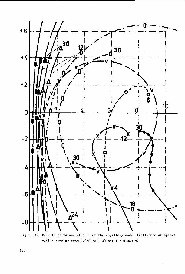
Figure 35 Calculated values of C-h for the capillary model (influence of sphere

radius ranging from 0.050 to 1.00 nun; 1 = 0.080 m)

138

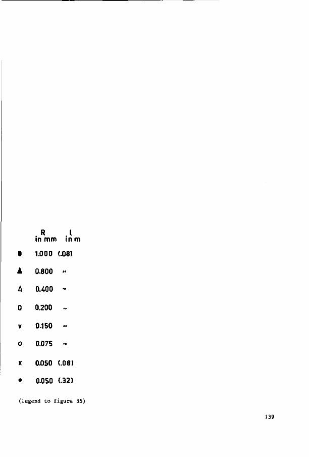
R I in mm in m

• 1.000 (48)

• 0.800 <•

A 0.400 -

0 0.200 ..

v 0.150 »

o 0.075 «

x 0.050 (.06)

• 0.0S0 (.32)

(legend to figure 35)

139

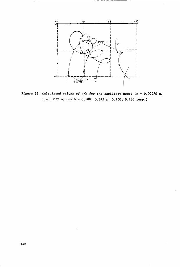
Figure 36 Calculated values of £-h for the capillary model (r = 0.00070 m;

1 = 0.072 m; cos 6 = 0.500; 0.645 m; 0.700; 0.780 resp.)

140

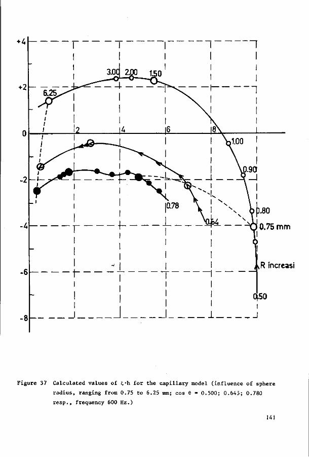
Figure 37 Calculated values of fti for the capillary model (influence of sphere

radius, ranging from 0.75 to 6.25 mm; cos 6 = 0.500; 0.645; 0.780

resp., frequency 600 Hz.)

141

in figure 33. For small values of R and as resonance is approached,|£ -h| becomes

large and comparison to measured curves is very difficult as measuring accuracy

is low.

In figure 36 some curls for fine-grained materials are given in more detail. The

interesting shift of the apex with frequency is very clear and resembles that

in figure 31. The loops in the curls are smaller at lower values of cos 6. With

those complicated contours interpolation between various curls is impossible as

is obvious from the figure, certainly this will be the case at the higher fre-

quenc ies.

Figure 37 presents the results for C*h for the capillary model in a different

manner. For one frequency, 600 Hz, loci for varying sphere radius have been

entered, with cos 6 as parameter. For this low frequency the comparatively

straight-forward course of the curves permits interpolation. For higher frequen­

cies this is no longer possible.

Calculations for the Zwikker Kosten model were carried out on the IBM 1620 com­

puter and took about 2 minutes per curve (eight spot frequencies) . From a pre­

liminary comparison with the results of the measurements it soon appeared that

the structure factor for the materials discussed seldom exceeds A. In total more

than 600 curls were generated with this model. From the results of these calcu­

lations selection for steps and ranges for o, and k could be determined. It

turned out that large ranges for 0 J were required. Although the effect of k is

quite large at high frequencies, its influence at low frequencies is only slight.

For low frequencies k hardly affects the real part of £.h. The flow resistance

o, has a slight effect of a few percent on the imaginary part. This result is

in accordance with the low frequency behaviour as discussed for the capillary

model.

These conclusions are confirmed by figures 14 and 15 and the results shown in

tabel 4-1.

142

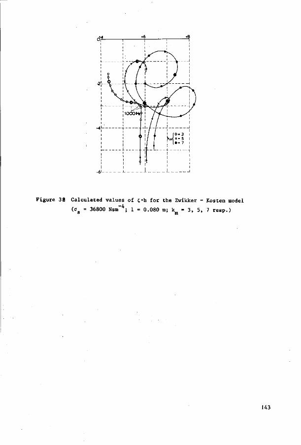
-4"-

Figure 38 Calculated values of C'h for the Zwikker - Kosten model

(cg = 36800 Nsnf4; 1 - 0.080 m; k = 3, 5, 7 resp.)

143

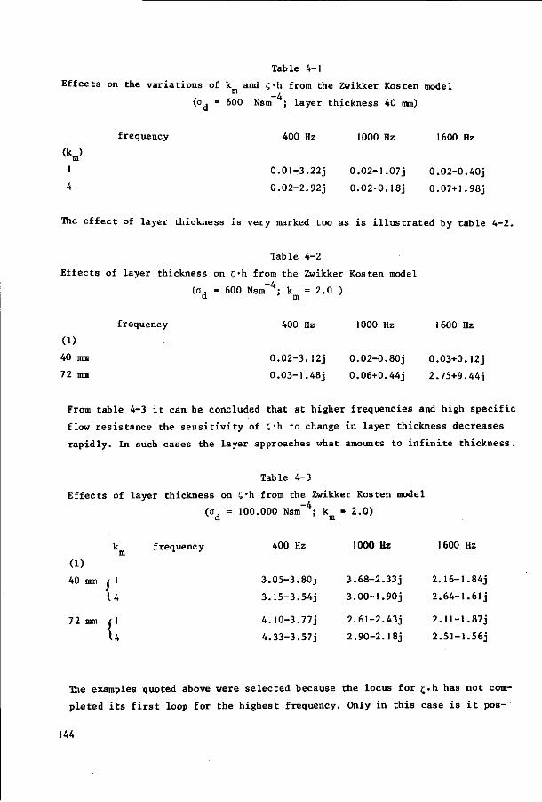
Table 4-1

Effects on the variations of k and C'h from the Zwikker Kosten model m -4

(o , = 600 Nsm ; layer thickness 40 mm)

frequency 400 Hz 1000 Hz 1600 Hz

m I 0.01-3.22J 0.02-1.07J 0.02-0.40J

4 0 .02-2.92j 0 .02-0.18j 0.07+1.98J

The e f f e c t of layer th ickness i s very marked too as i s i l l u s t r a t e d by t ab le 4 -2 .

Table 4-2

Effects of layer thickness on C'h from the Zwikker Kosten model (a, = 600 Nsm~4; k = 2.0 )

a m

frequency 400 Hz 1000 Hz 1600 Hz

(1)

40mm 0.02-3.12j 0.02-0.80J 0.03+0.12j

72mm 0.03-1.48J 0.06+0.44J 2.75+9.44J

From tab le 4-3 i t can be concluded tha t a t h igher f requencies and high s p e c i f i c

flow r e s i s t a n c e the s e n s i t i v i t y of t - h to change in l ayer th ickness decreases

r ap id ly . In such cases the layer approaches what amounts to i n f i n i t e t h i ckne s s .

Table 4-3

Effects of l ayer th ickness on £ 'h from the Zwikker Kosten model

(a_, = 100.000 Nsm~4; k = 2 . 0 ) a m

k frequency 400 Hz 1000 Hz 1600 Hz

(1)

40 mm f 1 3.05-3.80J 3.68-2.33J 2.16-1.84J

.4 3.15-3.54J 3.00-1.90J 2 .64-1 .61j {. 72mm (1 4.10-3.77J 2.61-2.43J 2 .11-1.87j

U 4.33-3.57J 2 .90-2.18j 2.51-1.56J

The examples quoted above were selected because the locus for £.h has not com­

pleted its first loop for the highest frequency. Only in this case is it pos-

144

sible to gain insight into the form of the locus for the three frequencies

given.

In figure 38 the shift of the apex is shown for the Zwikker Kosten model. It

occurs at high values of k and at relatively high air flow resistances. These

figures show an analogous behaviour to those in figure 31, although the change

in the size of the loops and in their position are different for the two

models. This difference is presumably due to the fact that in the channel-type

models, a and k are frequency-dependent.

It is apparent from the calculated curls for £;>h (cf. figures 27 ... 38) that

the comparatively simple mathematical models used can produce quite complicated

contours, incorporating loops, multiple loops and similar features which one

would not expect at first sight.

The Zwikker Kosten model and the two channel-type models differ in this res­

pect that, whereas in the former the two adjustable parameters introduced can­

not be correlated directly with the pore geometry, in the latter the parame­

ters are geometrically significant and may render at least some assistance in

comprehending the acoustical behaviour of the sample.

The channel-type models are but crude approximations of the real pore geometry,

as has been stated previously. They are thus incapable of rendering a compre­

hensive description of the samples, Further refinement is required if the de­

sired end is to be obtained. This might, but neet not, lead to an increase in

the number of adjustable parameters.

The problem of the number of significant parameters is complicated considerably

by not only the relatively low experimental accuracy, but also by the wide vari­

ations in sensitivity to parameter variation occurring along a curl and from

curl to curl.

4.4 Discussion of the results of measurements

In tables 4-4 to 4-9 the results for f h of some series of measurements are

compared with calculated curves. The tables have been divided into two sections,

except table 4-5. The upper section is subdivided into two parts, corresponding

to the two sample thicknesses. The first two rows of each of these subsections

give, respectively: the layer thickness and the column indications, under I the

measured values of a and h, under II the numerical values of the parameters for

the Zwikker Kosten model, under III those for the capillary model and under IV

145

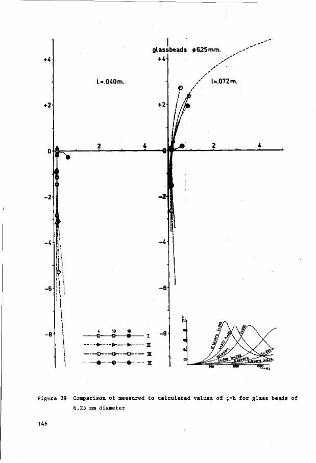
+4

+2

-U

-6

r ©

-8

4

l=.040m.

-OH­IO 16

glassbeads 0625mm.

+ * •

.

+2

<''

• •

/ U.072m.

9 /

•' ^ / / > if

. II

- 2

-t.

-8

—*> >~—• i —©——o— -—© u

O 4> •©• H

Figure 39 Comparison, of measured to calculated values of C-h for glass beads of

6.25 mm diameter

146

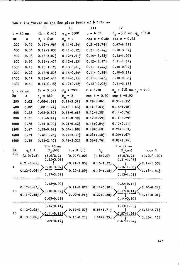
Table 4-4 Values of C'h for glass beads of ((l 6.25

1 = 4C

Hz

200

400

600

800

1000

1200

1400

1600

1 - 7 2 Hz

200

400

600

800

1000

1200

1400

1600

Hz 100

0 4

0

0 10

0,

0, 16

0

1 fBm

a

0.02

0.04

0.06

0.10

0.16

0.29

0.47

0.69

: mm a

0 .03

0.08

0.22

0.51

0.78

0.47

0.29

0.20

(2 .0 /2

. 21 -3 .

. 22 -3 .

.11-0 .

.11-0.

.12-0.

.13-0 .

I

(h = 0.41)

o = 650 s 0.12-4.96J

0.12-2.80J

0.13-2.07J

0.13-1.47J

0.13-1.12J

0.13-0.83J

0.13-0.41J

0.14-0.15J

(h = 0.39)

a - 880 s 0 .08-1.62J

0.08-1.24J

0.08-0.625

0.11-0.24J

0.13+0.02J

0.28+0.69j

0.48+1.25J

0.92+2.40j

1 = 40

I I

o d = 3500

k = 2 m 0.11-6.54J

0.11-3.12J

0.12-1.915

0.12-1.25J

0 .13-0.81j

0.14-0.64J

0.14-0.15J

0.17+0.125

a d = 2000

k = 2 m 0 .11-3 .51j

0.12-1.48J

0.13-0.66J

0.16-0.09J

0.21+0.42J

0.34+1.09J

0.79+2.30J

5.49+5.32j

mm ) D (mm) cos 6 ( a .3) ( 5 .6 /8 .2 ) ( 0 . 9 0 / 1 .

0.25-3.03J 05j | , 0 . 21 -3 .

> 0 . 2 0 - 3 . 0 7 j < 06j / | N 0 . 20 -3 .

0 . 1 7 - 3 . l l j

0 .12-0 . 87j |

> 0 . 1 0 - 0 . 88j / |

0 .08-0 .

0 .14-0 . 03j |

\o.n-o. 06j / |

0 .09-0 .

90j / 0 .11-0 .

N 0 .09-0 . 93 j

y 0 .12-0 .

N 0 .10-0 . 14j

I I I

r = 6.00

cos 9 = 0.80

0 .51-19.78j

0 . 2 1 - 5.24j

0 .14- 3.255

0 .12- 2.17J

0 . 1 1 - 1.A4j

0 . 11 - 0.88j

0 . 1 H 0.41 j

0.12+ 0.02J

r = 6.30

cos e = 0.90

0 .29-5.86j

0.14-2.63J

0.12-1.38J

0.12-0.59J

0.14+0.04j

0.18+0.68J

0.28+1.48J

0.56+2.76J

00) ( 1 .8 /2 .0 )

05j 0.15-1.52J

09j 0 .19-1.48;

87j 0.14+0.10;

96j 0.22+0.20;

03j 0 .66+1.71;

21 j 1.44+2.35;

IV D =6 .8 mm q = 2 . 0 a Ma cos e = 0 .95

0 .47-6 .21j

0 .20-3.07 j

0 .13-1.94j

0.11-1.325

0.10-0.92J

0.10-0.61.5

0.10-0.36J

0.11-0.135

D = 6.8 mm q = 2.0 a n a

cos 6 =0.95

0 .30-3 .35j

0.16-1.505

0.14-0.765

0.14-0.295

0 .17+0 . l l j

0.24+0.535

0.39+1.075

0.87+1.965

1 = 72 mm D (mm) cos

a ( 5 .6 /8 .2 ) (0 .90/ 0.21-1.485

i . ] / 0 . 1 7 - 1 \ 0 . 1 6 - 1 . 5 0 5 <

i / | N 0 .16-1 0.13-1.535

0.22+0.135 i | / 0 . 2 0 + 0

\ 0 . 1 7 + 0 . 1 1 5 < i / j ^ 0.15+0,

0.14+0.105

1.13+1.935 i . 1 / 1-62+2,

\ 0 . 8 7 + 1 . 9 6 5 < \ / | ^ 0.55+1,

0.67+1.945

8

1.00)

•535

.535

.245

.015

•715

•455

147

those for the fissure model. The values for the parameters given are those for

the best fitting calculated curls.

Sometimes interpolated values for the parameters were introduced; now and then

these values could only be found by graphical interpolation from the curls with

adjacent values of the parameters.

The lower section is confined to the three principal spot frequencies given in

the first column. It also gives values for £*h and illustrates the selection of

the best fitting curl for the fissure model. In each case two values for q ,

three for D and one or two for cos 9 are considered. The values of these para­

meters are given in the heads of the sections for the two layer thicknesses. The

resulting combination corresponding to the best fit is underlined. Note that the

corresponding values of the parameters for these cases are identical with those

given in column IV in the upper section. This procedure justifies the choice

made, it also provides some information about the influences of the steps in the

parameters.

Figures 39 to 43 present, in graphical form, the curves obtained from both measu­

rement and calculation, the latter for all three models. The marks for the main

spot frequencies are enlarged as in the former figures. The marks for these main

frequencies are provided with a special indication, shown in the legend of figure

39. The numbers in the legend indicate the frequency divided by 100. At the same

time the frequency marks along the lines correspond to the values for f h in the

column I, II, III and IV. The numbers I, II, III and IV in the legend of figure

39 correspond to the numbers of the columns in the tables 4-5 to 4-9.

148

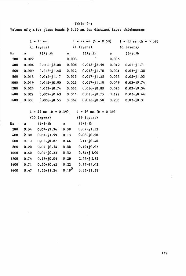
Table 4-U

Values of £>hfor glass beads (|) 6.25 mm for distinct layer thicknesses

Hz

200

400

600

800

1000

1200

1400

1600

Hz

200

400

600

800

1000

1200

1400

1600

1 =

(3

a

0.022

0.004

0.009

0.014

0.019

0.023

0.027

0.030

1 =

(10

a

0.04

0.08

0.10

0.20

0.40

0.74

0.71

0.47

16 mm

layers)

a+jn)b.

0.006-J2.00

0.012-J1.48

0.012-J1.17

0.012-J0.90

0.012-J0.74

0.009-J0.63

0.006-J0.55

56 • (h = 0

layers)

(£+jn)h

0.07-J2.34

0.07-J1.59

0.06-J0.87

0.07-J0.54

0.07-J0.33

0.13+J0.04

0.30+J0.42

1.22+j1.24

1 =

(4

a

0.003

0.006

0.012

0.019

0.026

0.033

0.044

0.062

.39)

a

0

0

0

0

0

0

0

0

.08

.13

.44

.88

.52

.29

.22

.195

= .27 mm (h = 0.

layers)

(S+jn)h

0.018-J2.59

0.018-jl .70

0.017-j1.25

0.017-jl.lO

0.016-J0.89

0.016-J0.75

0.016-J0.58

L = 86 mm (h =

[16 layers)

(C+jn)h

0.07-J1.23

0.08-J0.90

0.11-J0.40

0.19+J0.07

0.81+j 1.00

2.53-j Z32

0.77-J2.03

0.23-J1.28

50) 1

(6

a

0.005

0.012

0.021

0.033

0.049

0.075

0.122

0.200

0.39)

= 35 mm (h = 0.39)

layers)

(S+jn)h

0.02-il.71

0.03-J1.38

0.03-J1.03

0.03-10.74

0.03-i0.54

0.03-J0.44

0.03-J0.31

149

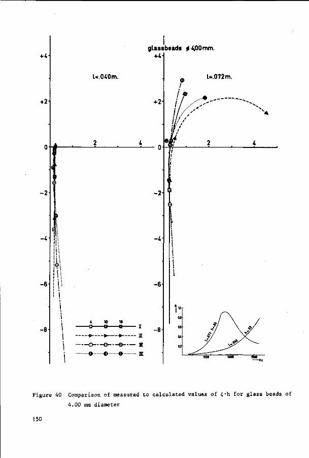
+4

+2

-2

-4

-6

-8

l=.040m.

glassbeads 0 4,00 mm +4i

4

-0--

© -

«•

10

— 0 —

~ o -. A . . .

16

- - • -—O

•••••©•

I

ffl 17

l=.072m.

Figure 40 Comparison of measured to calculated values of 5*h for glass beads of

4.00 mm diameter

150

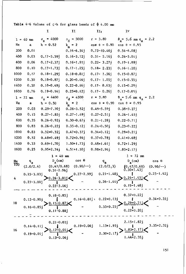
Table 4-6 Values of f h for glass beads of (J 4.00 mm

I II II( IV

1 =

Hz

200

400

600

800

1000

1200

1400

1600

1 =

Hz

200

400

600

800

1000

1200

1400

1600

Hz TSO

4

40 mm

a

0.01

0.03

0.06

0.10

0.17

0.30

0.50

0.76

72 mm

a

0.03

0.15

0.35

0.83

0.83

0.52

0.33

0.25

qa (2.0/2.

0.25-3.

0.27-3.

o = 4000 s

h = 0.52

0.17-3.59J

0.17-2.37J

0.17-1.73J

0.18-1.29J

0.18-0.87J

0.18-0.49J

0.19-0.14J

a = 4400 s

h = 0.50

0.29-7.70J

0.27-1 .85j

0.26-0.92J

0.26-0.22J

0.32+0.32J

0.48+0.49J

0.69+1.70J

0.95+2.34j

a, = 5000 a k = 2 m 0.16-6.54J

0.16-3.12J

0.16-1.91j

0.17-1.25J

0.18-0.81J

0.20-0.46 j

0.22-0.I6j

0.25+0.12j

a, = 4500 a k = 2

0.26-3.52J

0.27-1.49J

0.30-0.67j

0.35-0.12j

0.47+0.37J

0.72+0.96J

1.50+1.73J

4.51+1.50J

1 = 40 mm D (cm) cos 9

a 4) (0.47/0.68) (0.90/-

0.31-2.96J 03j | 0.27-2.

>0.26-3.01j<' 00J |

0.22-3.06J

r = 3.80

cos 9 = 0.90

0.73-10.46j

0.31- 5.16J

0.22- 3.27j

0.18- 2.23J

0.17- 1.56j

0.17- 1.05J

0.17- 0.63J

0.17- 0.26j

r = 3.80

cos 9 = 0.90

0.49-5.59j

0.27-2.51j

0.21-1.28J

0.24-0.50j

0.34+0.12j

0.37+0.78J

0.48+1.61j

0.98+2.94j

Da= 5.6 mm qa =

cos 9 = 0.95

0.54-6.08J

0.26-3.01j

0.19-1.89J

0.16-1.28J

0.15-0.87J

0.15-0.55j

0.15-0.29J

0.17-0.05J

D = 5.6 mm q = a na cos 6 = 0.95

0.38-3.27j

0.24-1.45J

0.22-0.71J

0.23-0.22 j

0.29+0.21j

0.41+0.68J

0.72+1.29J

1 .83+2.17j

1 = 72 mm

qa Da(cm)

-) (2.0/2.3) (0.47/0.68) 0.30+1.43J

99j 0.21-1.48J | > 0.24-1.45j^

0.26-1.44J | ^ 0.19-1.48j

2.2

2.2

cos 6

(0.90/—)

0.25-1.42J

10

16

0.18-0.85j 0.37+0.22j 0.12-0.90J | 0.16-0.81j » 0.22+0.13j | 0.34+0.35J

>0.15-0.87j< 2>°- 2 9 + 0 - 2 'J< 0.16-0.85J I - 0.33+0.25^ I ^

0.11-0.88J 0.22+0.20J

0.21-0.03J 2.15+1.82J 0.14-0.11j | 0.19+0.06J 1.13+1.93J | 3.35+2.32J

^0.17-0.05j<; "S 1.83+2.17j^ 0.19-0.01j | ^ - 2.30+2.17j j

0.13-0.06J 1.44+2.35J

151

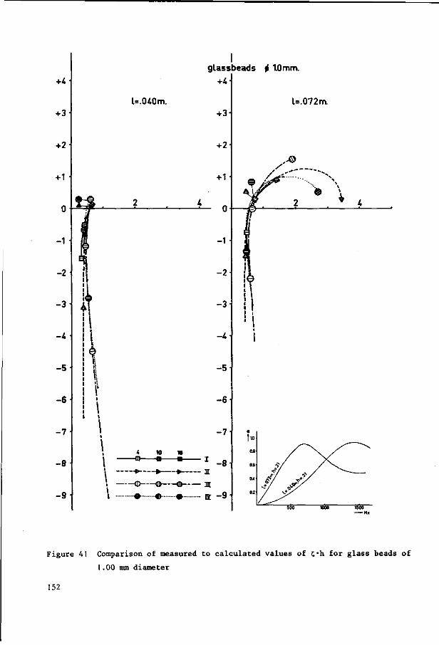
glassbeads i> 1.0mm.

l=.072m.

Figure 41 Comparison of measured to calculated values of C*h for glass beads of

1.00 mm diameter

152

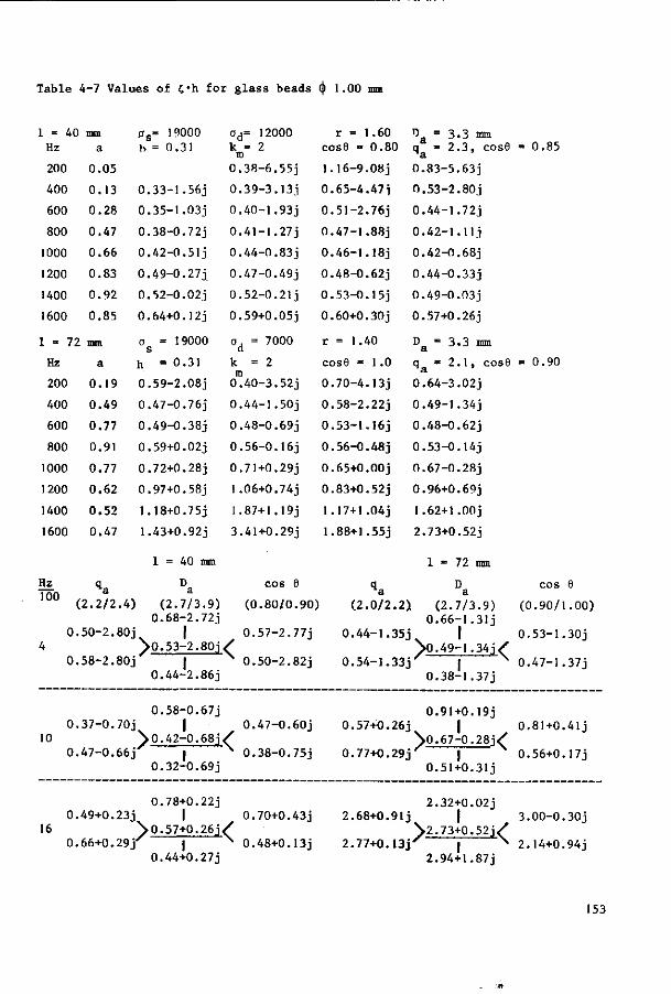
Table 4-7 Values of f h for glass beads (j) 1.00 mm

1 = 40 Hz

200

400

600

800

1000

1200

1400

1600

1 = 72

Hz

200

400

600

800

1000

1200

1400

1600

Hz 100

0. 4

0.

mm a

0.05

0.13

0.28

0.47

0.66

0.83

0.92

0.85

mm

a

0.19

0.49

0.77

0.91

0.77

0.62

0.52

0.47

os= 19000 h = 0.31

0.33-1.56J

0.35-1.03J

0.38-0.72J

0.42-0.51J

0 .49-0.27j

0 .52-0.02j

0.64+0.12j

o = 19000 s

h - 0.31

0.59-2.08J

0.47-0.76J

0 .49-0.38j

0.59+0.02J

0.72+0.28J

0.97+0.58j

1.18+0.75J

1.43+0.92J

1 = 40 mm

q D ^a a

2 . 2 /2 .4 ) ( 2 .7 /3 .9 ) 0.68-2.72J

50-2.80j | ]>0.53-2.80j

58-2.80j | 0 .44-2.86j

od= 12000 k = 2 m 0 .38-6 .55j

0 .39-3 .13j

0.40-1.93J

0.41-1.27J

0.44-0.83J

0.47-0.49J

0.52-0.21J

0.59+0.05J

a, = 7000 a k = 2 m

0 .40-3.52j 0.44-1.50J

0.48-0.69J

0 .56-0.16j

0.71+0.29J

1 .06+0.74J

1.87+1.19J

3.41+0.29J

r = 1.60 cose = 0.80

1.16-9.08J

0 .65-4.47i

0.51-2.76J

0 .47-1.88j

0.46-1.18J

0 .48-0.62j

0 .53-0 .15j

0.60+0.30j

r = 1.40

cosB = 1 .0

0 .70-4 .13j

0 .58-2.22j

0.53-1.16J

0.56-0.48J

0.65+0.00j

0.83+0.52j

1.17+1.04J

1.88+1.55J

V = 3 .3 mm q = 2 . 3 , cose a

0 .83-5.63J

0 .53-2.80j

0.44-1.72J

0.42-1.11 j

0 .42-0.68J

0 .44-0 .33j

0.49-0.03J

0.57+0.26j

D„ = 3.3 mm a q = 2 . 1 , cose n a 0.64-3.02J

0.49-1.34J

0.48-0.62J

0 .53-0.14j

0.67-0.28J

0.96+0.69J

1.62+l.OOj

2.73+0.52J

1 = 72 mm

cos 6 q D a a

(0 .80/0 .90) ( 2 . 0 /2 .2 ) ( 2 .7 /3 .9 ) 0 .66-1 .3H

0 .57-2 .77j

< N 0 .50-2 .82j

0.44-1.35J | V ) . 49-1.34 j /

0 .54-1.33J | N

0.38-1.37J

= 0.85

= 0.90

cos

(0 .90/

0.53-1

0.47-1

e

.00)

30j

37j

0.58-0.67J 0.91+0.19j 0.37-0.70j | 0.47-0.60J 0.57+0.26J | 0.81+0.41j

10 So.42-0.68j/" \0.67-0.28j^ 0.47-0.66J | N 0.38-0.75J 0.77+0.29jX | 0.56+0.17j

0.32-0.69J 0.51+0.31j

0.78+0.22j 0.49+0.23j | 0.70+0.43J

16 No.57+0.26j/ 0.66+0.29j |

0.44+0.27j

2.32+0.02J 2.68+0.91J | 3.00-0.30J

\2.73+0.52j/ ' 0.48+0.13j 2.77+0.13jX | N 2.14+0.94J

2.94+1.87J

153

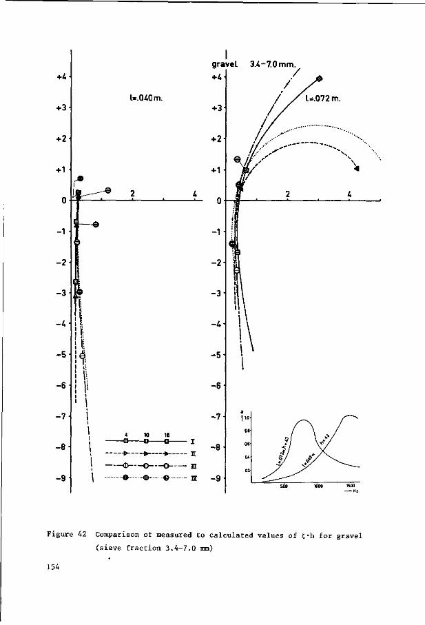
+4

+3

+2

+1

-1

-2

-3

-k

-5-

-6 -

-8

-9

I gravel 3.4-7.0 mm

U.tUOm.

1 10 16

.£- p. ^ _

CD © ©

o <& •©•

I

It

II

17

Figure 42 Comparison of measured to calculated values of C'h for gravel

(sieve fraction 3.4-7.0 mm)

154

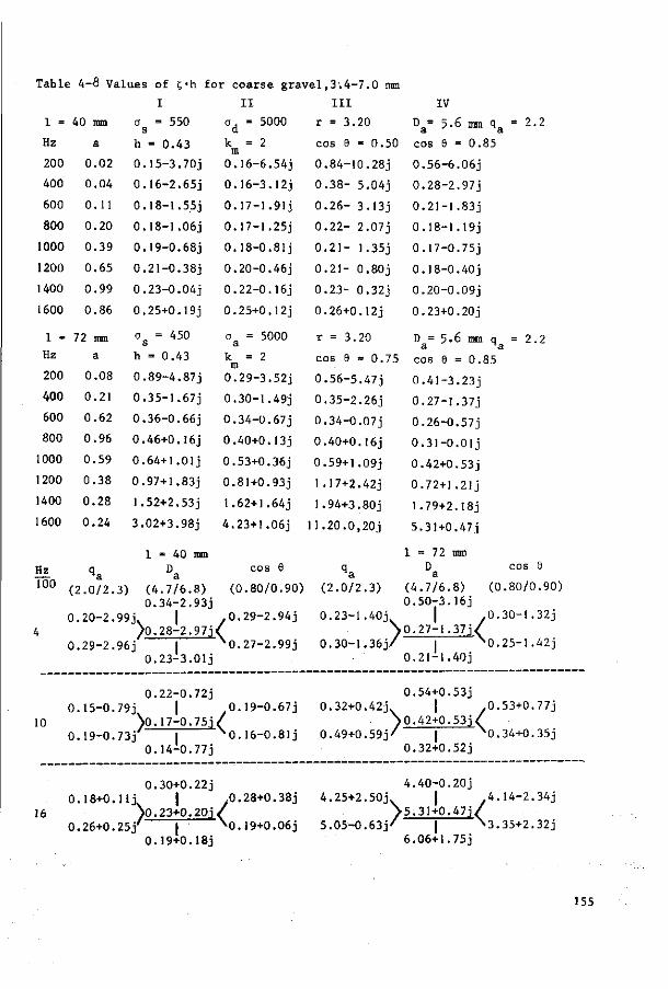
Table 4-8 Values of f h for coarse g r ave l , 3 . 4 -7 . 0 mm

I I I I I I IV

1 = 40 mm a = 550 a = 5000 r = 3 . 2 0 D = 5.6 m q = 2 . 2 s a a a

Hz a h = 0.43 k = 2 cos 6 = 0.50 cos 6 = 0.85 m

200 0.02 0.15-3.70J 0.16-6.54J 0 .84-10.28j 0.56-6.06J

400 0.04 0.16-2.65J 0.16-3.12J 0 .38- 5.04J 0.28-2.97J

600 0.11 0.18-1.5.5j 0.17-1 .91 j 0 . 26 - 3.13j 0.21-1 .83j

800 0.20 0.18-1.06J 0.17-1.25J 0 .22- 2.07j 0 .18-1.19j

1000 0.39 0.19-0.68J 0 .18-0.81j 0 . 2 1 - 1.35j 0.17-0.75J

1200 0.65 0.21-0.38J 0.20-0.46J 0 . 21 - 0.80J 0.18-0.40J

1400 0.99 0.23-0.04J 0 .22-0.16 j 0 .23- 0.32j 0.20-0.09J

1600 0.86 0.25+0.19j 0.25+0.12j 0.26+0.12j 0.23+0.20j 1 = 72 mm ° = 450 a = 5000 r = 3.20 D = 5.6 mm q = 2.2

B A a na

Hz a h = 0.43 km

= 2 cos 9 = 0.75 cos 6 = 0.85

200 0.08 0.89-4.87J 0.29-3.52J 0.56-5.47J 0.41-3.23J

400 0.21 0.35-1.67J 0.30-1.49J 0.35-2.26J 0.27-1.37J

600 0.62 0.36-0.66J 0.34-0.67J 0.34-0.07J 0.26-0.57J

800 0.96 0.46+0.J 6j 0.40+0.13j 0.40+0.16j 0.31-O.Olj

1000 0.59 0.64+1.01j 0.53+0.36J 0.59+1.09J 0.42+0.53J

1200 0.38 0.97+1.83J 0.81+0.93J 1.17+2.42J 0.72+1.21j

1400 0.28 1.52+2.53J 1 .62+1.64j 1.94+3.80J 1.79+2.18j

1600 0.24 3.02+3.98J 4.23+1.06J 11.20.0.20J 5.31+0.47J 1 = 40 mm 1 = 72 mm

Hz q Da cos 6 q & D& cos 6 1 0 0 ( 2 . 0 /2 .3 ) ( 4 .7 /6 .8 ) (0 .80/0 .90) ( 2 .0 /2 .3 ) ( 4 .7 /6 .8 ) (0 .80/0.90)

0.34-2.93J 0 .50-3.16j 0 .20-2 .99j v I . 0 .29-2 .94J 0.23-1.40J | - 0 . 30 - l . 32 j

4 ) 0 .28-2 .97 j< > 0 . 2 7 - 1 . 3 7 j ^ 0.29-2.96J I X 0 . 27 -2 . 99 j 0 . 3 0 - 1 . 3 6 j / | x 0 . 2 5 - 1 . 4 2 j

0.23-3.01J - 0 .21 - l . 40 j

0 .22-0.72j 0.54+0.53j 0.15-0.79J I 0.19-0.67J 0.32+0.42J | 0.53+0.77J

V ) . 1 7 - 0 . 7 5 j / > 0.42+0.53 j < 0.19-0.73J I N 0 . 1 6 - 0 . 8 1 j 0 . 49+0 .59 j / | N0.34+0.35j

0.14-0.77J 0.32+0.52J

10

16

0.30+0.22j 4 .40-0.20j 0.18+0.11j I ,0.28+0.383 4.25+2.50J. | 4 .14-2.34j

V . 23+0.20 j / > 5 . 3 1 + 0 . 4 7 j / 0 . 2 6+0 . 25 / [ X0.19+0.06j 5 .05-0 .63J ' | N3.35+2.32J

0.19+0.18J 6.06+1.75J

155

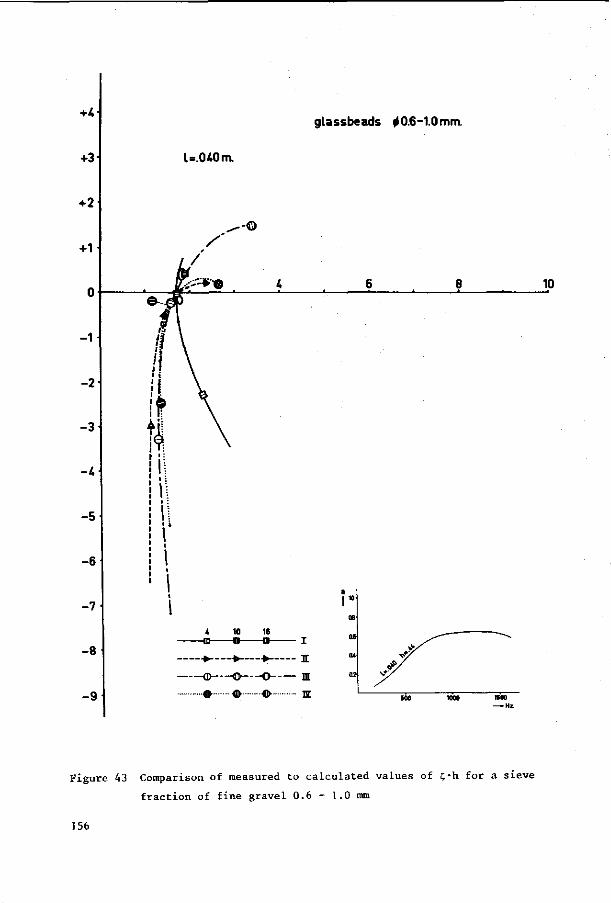
+4-

+3

+2

+1

glassbeads 00.6-1.0mm.

1=040 m.

10

-1

-2

-3

-k

-5

-6

-7

-8

-9

k 10 16

^ {, >_ n

© — — © — © n

o o «• E

,» 08

OS

04

02

1500 — Hi.

Figure 43 Comparison of measured to calculated values of e-h for a sieve

fraction of fine gravel 0.6 - 1.0 mm

156

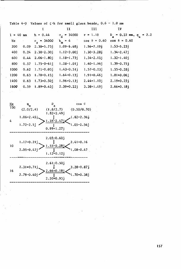
Table

1 = 40

Hz

200

400

600

800

1000

1200

1400

1600

4-9 Values of f h

mm

0.09

0.24

0.44

0.57

0.62

0.63

0.63

0.59

I

h = 0.44

a = 34000

2.30-5.73J

2.30-2.30J

2.06-1.80J

1.75-0-6 l j

1.71-0.03J

1.70-0.15J

1.73+0.50j

1.89+0.43j

for small g l

I I

o , = 34000 d

k = 4 m 1.09-6.48J

1.12-3.00J

1.18-1.73J

1.28-1.01j

1.43-0.51 j

1.64-0.13J

1.96+0.13J

2.39+0.22j

ass. beads , 0.6

I I I

r = 1.10

cos 6 = 0.60

1.56-7.19J

1.30-3.28J

1.34-2.15J

1.40-1.06J

1.57-0.23J

1.91+0.46J

2 .44+l . lOj

3.38+1.49J

- 1.0 mm

IV

D = 0.22 mm, q a na

cos 6 = 0.60

1.53-5.23j

I .34-2 .47j

1.32-1.40J

1.39-0.75J

1.55-0.28j

1.81+0.06J

2.19+0.25J

2.66+0.18j

2.2

Hz 100 (2 .0 /2 .4 )

1.06-2.45J

1.72-2.5J

H . 8 / 2 . 7 ) 1.82-2.49j

cos 9

(0 .50/0 .70)

" *> 1 .35 -2 .47 j<^

0.99+1.27J

1.82-2.36j

05-2.56j

2 .05-0.60j 1.17-0.21J |

10 p > 1 .55-0 .28j<^ 2 .00-0.47 j ^ I ^ 1 . 0 8 - 0 .

1.12-0.12J

2 .41-0.16

47

2.61-0.50J 2.31+0.71j | 3 .28-0.87J

16 J > 2 . 6 6 + 0 . 1 8 j < ^ 2 . 7 9 - 0 . 4 0 j ^ | ^ 1 . 7 0 + 0 . 3 8 j

2.50+0.95j

157

Table 4-10 recapitulates the values of the parameters for the fissure model, cho­

sen after an examination of the measured results for isodiametrical spheres. The

first three columns give, respectively, the diameters of the spheres, the sample

thichnesses and the measured values of the porosity h. The remainder of the ta­

ble has been sectioned solely to reduce its length. In each of the sections the

first three columns (numbers 4, 5, and 6; or 9, 10 and 11) give values for the

parameters, each combination yielding a reasonable fit with the measured curl.

One may conclude that sometimes a number of combinations of values of the para­

meters prove to be similar and can all be seen as acceptable selections. The

underlined combinations correspond to the fit finally estimated to be the best.

The nature and magnitude of the discrepancies between the measured and calcula­

ted curls is indicated to the right of the values for the parameters by two

vertical bars, the first corresponding to the real and the second to the imagi­

nary part of C'h. These vertical bars carry side bars whose meaning is explained

below in table 4-10. Side bars, when present at the low end of a vertical bar

indicate the magnitude of the discrepancies between a calculated curl and a

measured one at 200 Hz. The side bars at the upper end correspond to 1600 Hz.

Absence of a side bar implies an excellent fit.

On comparing measured and calculated values of £*h it should be considered that

accuracy is low when it departs appreciably from + 1. This situation occurs

fairly frequently for 200 Hz and thus relatively large discrepancies here may

well be rather unimportant.

Table 4-11 gives a general survey of the results for dry materials, for all

three models. The first column gives the size of the spheres or of the sieve

fractions, the second column the layer thickness and the third column the

measured value of the porosity. In the fourth column the mesured values for the

air flow resistance o are presented. The next three groups of columns evaluate

the results for the Zwikker Kosten, the capillary and the fissure models, res­

pectively. The first two or three columns of each group list the values of the

appropriate parameters for the best fit. The quality of the fit is indicated in

the same way as in table 4-10 .

In some case interpolated values of the parameters from table 4-10 have bi_en

introduced. For a number of samples some of the models failes to produce an

acceptable curl. These cases have been marked.

158

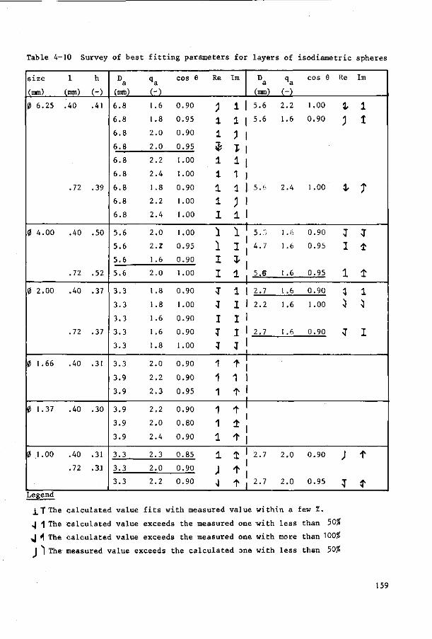
Table 4-10 Survey of best fitting parameters for layers of isodiametric spheres

size

(mm)

0 6.25

0 4.00

0 2.00

0 1.66

0 1.37

0 1.00

1

(mm)

.40

.72

.40

.72

.40

.72

.40

.40

.40

.72

h

<") .41

.39

.50

.52

.37

.37

.31

.30

.31

.3.1

D a

(mm)

6.8

6.8

6.8

6.8

6.8

6.8

6.8

6.8

6.8

5.6

5.6

5.6

5.6

3.3

3.3

3.3

3.3

3.3

3.3

3.9

3.9

3.9

3.9

3.9

3.3

3.3

3.3

qa (-) 1.6

1.8

2.0

2.0

2.2

2.4

1.8

2.2

2.4

2.0

1.1

1.6

2.0

1.8

1.8

1.6

1.6

1.8

2.0

2.2

2.3

2.2

2.0

2.4

2.3

2.0

2.2

cos 9

0.90

0.95

0.90

0.95

1.00

1.00

0.90

1.00

1.00

1.00

0.95

0.90

1.00

0.90

1.00

0.90

0.90

1.00

0.90

0.90

0.95

0.90

0.80

0.90

0.85

0.90

0.90

Re

J a a * i l i i i

1 1 i i

T J I

7

1 1 1

1 1 1

1

; J

Im

1 1 1 I 1 1 1

i

I i

i

i i i i

*

±

i

* t

D a

(mm)

5.6

5.6

.5.6

'5.3

4.7

5.6

1 2.7

1 2.2

1 2.7

2.7

2.7

qa (-)

2.2

1.6

2.4

1 .6

1 .6

1.6

1.6

1.6

1.6

2.0

2.0

cos 6

1.00

0.90

1.00

0.90

0.95

0.95

0.90

1.00

0.90

0.90

0.95

Re

I J

^

J I

1

1 }

•I

)

T

Im

1 1

7

T *

1

1 *

I

t

* Legend

I T The

,| 1 The

J 4 The

J The

calculated value fits with measured value within a few %.

calculated value exceeds the measured one -with less than I

calculated value exceeds the measured one with more than K

measured value exceeds the calculated one with less than »

159

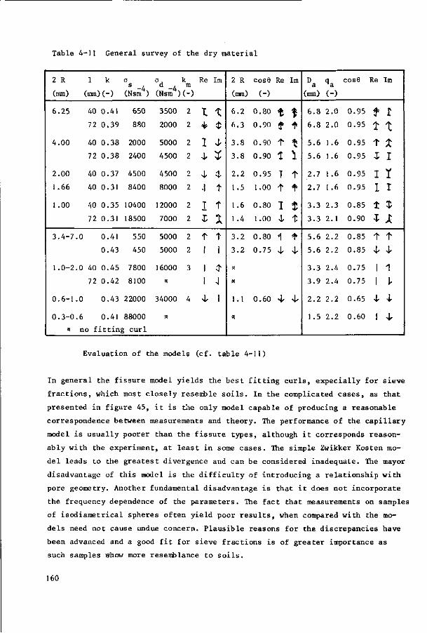
Table 4-11 General survey of the dry material

2 R

(mm)

6.25

4.00

2.00

1.66

1.00

3.4-7

1.0-2

0.6-1

0.3-0

a

1 k

(mm)(-)

40 0.41

72 0.39

40 0.38

72 0.38

40 0.37

40 0.31

40 0.35

72 0.31

.0 0.41

0.43

0 40 0.45

72 0.42

.0 0.43

.6 0.41

0 s -4

(Nsm )

650

880

2000

2400

4500

8400

10400

18500

550

450

7800

8100

22000

88000

no fitting curl

a. k Re d , m

(Nsm*) (-)

3500

2000

5000

4500

4500

8000

12000

7000

5000

5000

16000

*

34000

a

2 t 2 *

2 1 2 J,

2 4

2 .1

2 T

2 I

2 t

2 1

3 1

1

4 4,

Im

t $

4< X 4-t

t X t 1

t J

1

2 R

(mm)

6.2

6.3

3.8

3.8

2.2

1.5

1.6

1.4

3.2

3.2

a

a

1.1

a

cos9

(-)

0.80

0.90

0.90

0.90

0.95

1.00

0.80

1.00

0.80

0.75

0.60

Re Im

t | t * t t 1 1 T t

t *

I $ 4- t

1 t j, 4,

4- 4.

D q

(mm) (-)

6.8 2.0

6.8 2.0

5.6 1.6

5.6 1.6

2.7 l .6

2.7 1.6

3.3 2.3

3.3 2.1

5.6 2.2

5.6 2.2

3.3 2.4

3.9 2.4

2.2 2.2

1.5 2.2

cos6

0.95

0.95

0.95

0.95

0.95

0.95

0.85

0.90

0.85

0.85

0.75

0.75

0.65

0.60

Re Im

? r t t t x i i I Y I I t * I X t t

4- 4-

1 1

I V

4- 4-

I 4-

Evaluation of the models (cf. table 4-ll)

In general the fissure model yields the best fitting curls, expecially for sieve

fractions, which most closely resemble soils. In the complicated cases, as that

presented in figure 45, it is t5ie only model capable of producing a reasonable

correspondence between measurements and theory. The performance of the capillary

model is usually poorer than the fissure types, although it corresponds reason­

ably with the experiment, at least in some cases. The simple Zwikker Kosten mo­

del leads to the greatest divergence and can be considered inadequate. The mayor

disadvantage of this model is the difficulty of introducing a relationship with

pore geometry. Another fundamental disadvantage is that it does not incorporate

the frequency dependence of the parameters. The fact that measurements on samples

of isodiametrical spheres often yield poor results, when compared with the mo­

dels need not cause undue concern. Plausible reasons for the discrepancies have

been advanced and a good fit for sieve fractions is of greater importance as

such samples show more resemblance to soils.

160

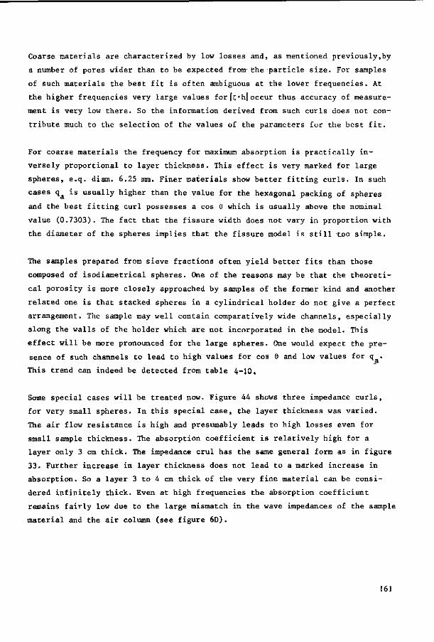
Coarse materials are characterized by low losses and, as mentioned previously,by

a number of pores wider than to be expected from- the particle size. For samples

of such materials the best fit is often ambiguous at the lower frequencies. At

the higher frequencies very large values for |c;'h| occur thus accuracy of measure­

ment is very low there. So the information derived from such curls does not con­

tribute much to the selection of the values of the parameters for the best fit.

For coarse materials the frequency for maximum absorption is practically in­

versely proportional to layer thickness. This effect is very marked for large

spheres, e.q. diam. 6.25 mm. Finer materials show better fitting curls. In such

cases qa is usually higher than the value for the hexagonal packing of spheres

and the best fitting curl possesses a cos 9 which is usually above the nominal

value (0.7303). The fact that the fissure width does not vary in proportion with

the diameter of the spheres implies that the fissure model is still too simple.

The samples prepared from sieve fractions often yield better fits than those

composed of isodiametrical spheres. One of the reasons may be that the theoreti­

cal porosity is more closely approached by samples of the former kind and another

related one is that stacked spheres in a cylindrical holder do not give a perfect

arrangement. The sample may well contain comparatively wide channels, especially

along the walls of the holder which are not incorporated in the model. This

effect will be more pronounced for the large spheres. One would expect the pre­

sence of such channels to lead to high values for cos 9 and low values for q .

This trend can indeed be detected from table 4-10.

Some special cases will be treated now. Figure 44 shows three impedance curls,

for very small spheres. In this special case, the layer thickness was varied.

The air flow resistance is high and presumably leads to high losses even for

small sample thickness. The absorption coefficient is relatively high for a

layer only 3 cm thick. The impedance crul has the same general form as in figure

33. Further increase in layer thickness does not lead to a marked increase in

absorption. So a layer 3 to 4 cm thick of the very fine material can be consi­

dered infinitely thick. Even at high frequencies the absorption coefficient

remains fairly low due to the large mismatch in the wave impedances of the sample

material and the air column (see figure 6D).

161

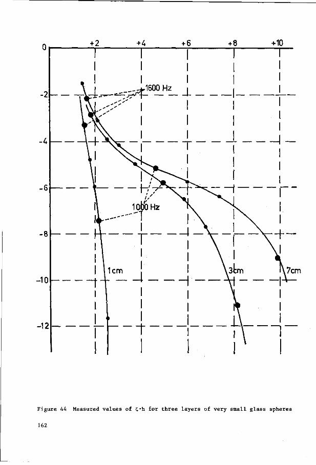
7cm

Figure 44 Measured values of C'h for three layers of very small glass spheres

162

0.2 mm

cos 9 = 0.86

= 2.45

\<—glass beads 0.3 - 0.6 mm h-(M1

Figure 45 Measured curve for 5-h for a fine sieve fraction of gravel compared

to a calculated curl with similar contour

163

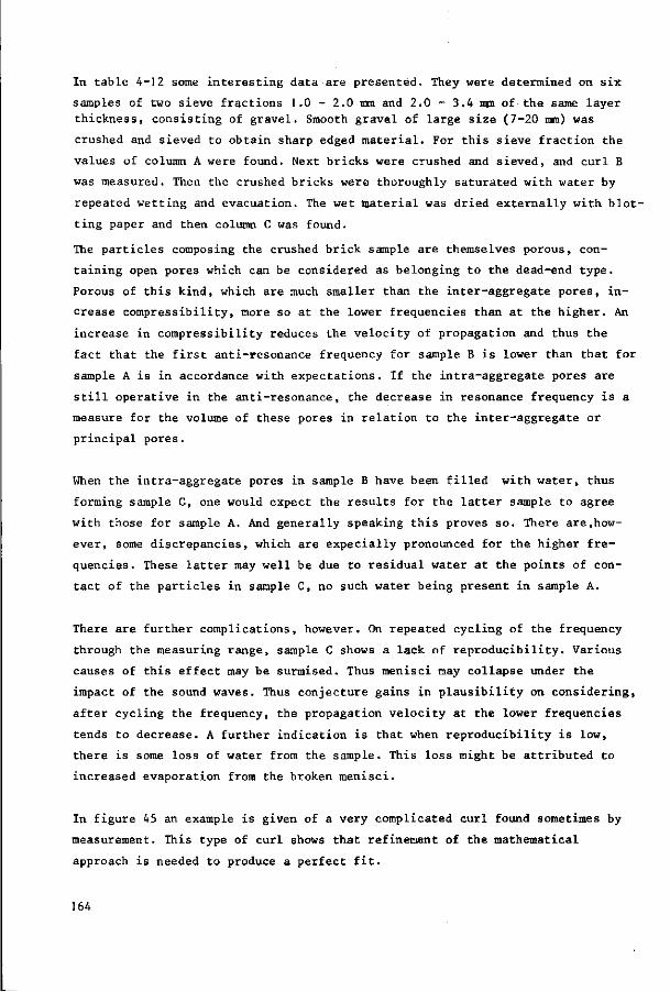
In table 4-12 some interesting data are presented. They were determined on six

samples of two sieve fractions 1.0 - 2.0 mm and 2.0 - 3.4 mm of the same layer

thickness, consisting of gravel. Smooth gravel of large size (7-20 ram) was

crushed and sieved to obtain sharp edged material. For this sieve fraction the

values of column A were found. Next bricks were crushed and sieved, and curl B

was measured. Then the crushed bricks were thoroughly saturated with water by

repeated wetting and evacuation. The wet naterial was dried externally with blot­

ting paper and then column C was found.

The particles composing the crushed brick sample are themselves porous, con­

taining open pores which can be considered as belonging to the dead-end type.

Porous of this kind, which are much smaller than the inter-aggregate pores, in­

crease compressibility, more so at the lower frequencies than at the higher. An

increase in compressibility reduces the velocity of propagation and thus the

fact that the first anti-resonance frequency for sample B is lower than that for

sample A is in accordance with expectations. If the intra-aggregate pores are

still operative in the anti-resonance, the decrease in resonance frequency is a

measure for the volume of these pores in relation to the inter-aggregate or

principal pores.

When the intra-aggregate pores in sample B have been filled with water, thus

forming sample C, one would expect the results for the latter sample to agree

with those for sample A. And generally speaking this proves so. There are,how­

ever, some discrepancies, which are expecially pronounced for the higher fre­

quencies. These latter may well be due to residual water at the points of con­

tact of the particles in sample C, no such water being present in sample A.

There are further complications, however. On repeated cycling of the frequency

through the measuring range, sample C shows a lack of reproducibility. Various

causes of this effect may be surmised. Thus menisci may collapse under the

impact of the sound waves. Thus conjecture gains in plausibility on considering,

after cycling the frequency, the propagation velocity at the lower frequencies

tends to decrease. A further indication is that when reproducibility is low,

there is some loss of water from the sample. This loss might be attributed to

increased evaporation from the broken menisci.

In figure 45 an example is given of a very complicated curl found sometimes by

measurement. This type of curl shows that refinement of the mathematical

approach is needed to produce a perfect fit.

164

Table 4-12 Values of f h for gravel, dry crushed bricks and crushed bricks,

partly filled with water

1 = 40 mm, h = 0.44

A

Hz a (S+jn)h

200 0.06 0.62-4.14j

400 0.14 0.54-2.21j

600 0.30 0.56-1.45J

800 0.58 0.60-0.97J

1000 0.79 0.65-0.57J

1200 0.92 0.73-0.18j

1400 0.91 0.77+0.05J

1600 0.81 0.92+0.49J

1 = 40 mm, h = 0.64

A

Hz a (5+jn)h

200 0.08 0.62-4.52j

400 0.17 0.50-2.50J

600 0.32 0.50-1.62J

800 0.57 0.94-1.15J

1000 0.77 0.56-0.65J

1200 0.97 0.60-0.20j

1400 0.98 0.60+0.I7j

1600 0.88 0.67+0.47J

1.0-2.0 mm

B

a (S+jn)h

0.25 0.86-3.85j

0.75 0.66-2.25j

0.79 0.59-1.36J

0.69 0.62-0.87J

0.62 0.77-0.43J

0.53 0.80-0.lOj

0.60 0.86+0.22J

0.71 0.91+0.48J

2.0-3.4 mm

B

a (5+jn)h

0.08 0.77-4.06J

0.17 0.85-3.24J

0.27 0.61-2.32J

0.46 0.56-1.28J

0.68 0.56-0.75j

0.93 0.59-0.32j

0.99 0.61-0.03J

0.81 0.62+0.35J

a (5+jn)h

0.07 0.58-4.36

0.19 0.59-2.27J

0.37 0.61-1.49J

0.61 0.67-0.94J

0.84 0.73-

0.96 0.78-0.04J

0.93 0.83+0.22J

0.84 0.92+0.48J

(- + 10.5% H20)

a (C+jn)h

0.05 0.64-4.96J

0.14 0.42-2.67j

0.37 0.38-1.79j

0.62 0.37-1.19j

0.90 0.40-0.71 j

0.99 0.43-0.29j

0.97 0.47+0.02J

0.92 0.34+0.88J

(= + 12% H20)

165

4.5 Considerations on the improvement of mathematical models

Of the three models considered, that of Zwikker Kosten is the simplest. Excluding

h, it contains only two parameters, which however are purely formal in nature:

even for a sample of precise and simple geometry, a and k cannot be predicted. d in

Essentially, of course, the quantities corresponding to o and k are frequency-

dependent.

The two channel-typemodels offer a geometry that bears at least some resemblance

to that of the sample material. Thus the parameters r and D determine the

absolute size of the pores and ought to correlate with the size of the

particles of the sample. This correlation however is still of a formal nature,

only for extremely simple materials would prediction of r and D present any

hope of success. The same applies for cos 9 and q which do depend on sample

geometry but the precise form of this dependence is obscure.

The geometrical simplifications introduced into the channel-type models are so

far-reaching that perfect matches between measured and calculated curls cannot

be expected. To name a few of the imperfections:

a. The arbitrary cross-sections of the pores in the models will differ from those

actually obtaining in the samples and thus both the flow and temperature profiles

in the samples pores will deviate from those in the models. As an example one

might consider flow in a tube of an equilateral triangular cross-section and one

having a circular one. For the former, at least at higher frequencies, the

viscous boundary layer will have a larger effect than for the latter. Here the

free area of the sample material surface per unit volume of material obviously

affects the results. Between the fissure and the circular cross-section the

differences will be even larger than in the previous case. Note that flow was

always laminar under the measuring conditions, Reynolds number being very low

and that contraction coefficients thus do not apply.

b. In actual samples the pore system consists of interconnected channels. Only a

fraction, albeit a large one, of these pores will carry the flow of air. The

remaining pores are limited to the function of acoustic compliance. Thus the

assumption of identical distribution functions for flow and compression in the

channel-type models is manifestly incorrect. It was introduced solely for sim-

plicitys sake. For the samples considered here, the pores acting only as com­

pliances are presumably accessible over the entire frequency range; side holes a /PVR,,

(-—><< 1000)

166

of the type represented in. figure 14 showing a series impedance at the entrance

are probably either absent or unimportant. Summarizing the porosity, as deter­

mined statically, is probably too high when flow is being considered,

c. The assumption that 9 is equal for all channels is also a simplification of

dubious validity. It is probably not far from the mark if channels of any se­

lected cross-section occur for the same distribution of the values of 9, the

latter then taking on the nature of an average. Should channel cross-section and

values of 9 be correlated the assumption should not be retained. Whether this

correlation does in fact exist is not yet known. (Marshall, 1958)

Although the present models show some promise for the description of the pore

geometries of the^materials considered, there are still discrepancies and the

mind turns to the possibilities of improvement. There appear to be various lines

of approach. For instance, the introduction of two porosities, for flow and re­

sistance respectively, correlated by a_p_riori geometrical considerations, might

improve the correspondence between theory and experiment. The general form of

the distribution function should be identical in the two cases. Similar con­

siderations hold for the introduction of a correlation between channel cross-

section and 6. Neither of the variations proposed above requires the introduction

of an extra adjustable parameter. Note that no account has been taken of the

probability distribution of two pores of given, different cross-sections ad­

joining each other. This is not necessary in the present case where the wave­

length is very large in relation to pore dimensions.

Should refinement of the models yield inadequate improvement, the introduction

of a further adjustable parameter may be considered, e.g. the introduction of

different distribution functions for the cross-sections of the pores carrying

the flow and those confined to compression. In the simplest case, only the ratio

of the porosities for the two kinds of pores could be introduced.

As stated above, the performance of the present models is not too bad. Thus it

is practically impossible to predict which and how many of the methods of im­

provement suggested above are required to render the correspondence between

theory and experiment completely acceptable. Even from the material now availa­

ble, the necessity for introducing one further parameter cannot be deduced. The

possibility that more than one extra parameter is required seems remote.

To elucidate the behaviour of the models as descriptive for the sample material,

further information is required. For all practical purposes this information must

be derived by increasing the frequency range of the measurements as the possi­

bilities for increasing the accuracy of interferometer measurements are indeed

limited. Except for some peculiar cases, increasing the number of measuring

167

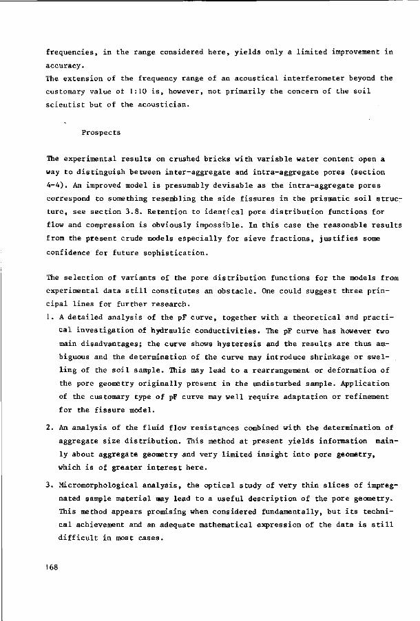
frequencies, in the range considered here, yields only a limited improvement in

accuracy.

The extension of the frequency range of an acoustical interferometer beyond the

customary value of 1:10 is, however, not primarily the concern of the soil

scientist but of the acoustician.

Prospects

The experimental results on crushed bricks with variable water content open a

way to distinguish between inter-aggregate and intra-aggregate pores (section

4-4). An improved model is presumably devisable as the intra-aggregate pores

correspond to something resembling the side fissures in the prismatic soil struc­

ture, see section 3.8. Retention to identical pore distribution functions for

flow and compression is obviously impossible. In this case the reasonable results

from the present crude models especially for sieve fractions, justifies some

confidence for future sophistication.

The selection of variants of the pore distribution functions for the models from

experimental data still constitutes an obstacle. One could suggest three prin­

cipal lines for further research.

1. A detailed analysis of the pF curve, together with a theoretical and practi­

cal investigation of hydraulic conductivities. The pF curve has however two

main disadvantages; the curve shows hysteresis and the results are thus am­

biguous and the determination of the curve may introduce shrinkage or swel­

ling of the soil sample. This may lead to a rearrangement or deformation of

the pore geometry originally present in the undisturbed sample. Application

of the customary type of pF curve may well require adaptation or refinement

for the fissure model.

2. An analysis of the fluid flow resistances combined with the determination of

aggregate size distribution. This method at present yields information main­

ly about aggregate geometry and very limited insight into pore geometry,

which is of greater interest here.

3. Micromorphological analysis, the optical study of very thin slices of impreg­

nated sample material may lead to a useful description of the pore geometry.

This method appears promising when considered fundamentally, but its techni­

cal achievement and an adequate mathematical expression of the data is still

difficult in most cases.

!68

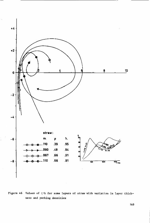
+4

-6

-8

straw

m

—CO—o—on—110

—1>—B>—1»_ .090

—<D—©—©—-067

— o — ® — © — n o

p 39

.48

66

66

h.

.95

.94

.91

.91

Figure 46 Values of c*h for some layers of straw with variation in layer thick­

ness and packing densities

169

Table 4-13

Values of a and C"h for some layers of straw at various layer thicknesses and

packing densities

Hz

200

400

600

800

1000

1200

1400

1600

a

0.12

0.30

0.55

0.77

0.73

0.64

0.61

0.70

1

h

= 67 nun

= 0.91

a 0.37

0.25

0.26

0.31

0.50

0.93

3.46

1.49

+

-

-

-

-

+

+

+

-

jn)h

J J J J

J J J J

2.76

1.33

0.61

0.08

1.05

1.33

1.16

1.41

a

0.12

0.30

0.55

0.67

0.63

0.52

0.57

0.72

1

h

= 90 mm

= 0.94

(5 +

0.44 -

0.15 -

0.20 -

0.28 +

0.50 +

2.87 +

2.22 "

1.06 -

jn)h

j 3.80

j 1.07

j 0.25

j 0.38

j 0.92

j 2.37

j 2.17

j 1.26

Hz

200

400

600

800

1000

1200

1400

1600

1

h

a

0.31

0.93

0.78

0.58

0.73

0.97

0.92

0.85

= 110 mm

= 0.91

a 0.32

0.41

0.64

3.50

2.97

0.94

0.85

1.03

+

-

-

+

+

-

-

+

+

jn)h

j 1.23

j 0.09

j 0.74

j 2.87

j 1.09

j 0.49

j 0.50

j 0.79

a

0.12

0.30

0.55

0.57

0.53

0.49

0.54

0.75

1 = 110

h = 0.9!

(C

0.15

0.12

0.11

0.29

0.57

5.67

1.06

0.38

mm

+

-

-

+

+

+

+

-

-

jn)h

j 2.15

j 0.63

j 0.10

j 0.66

j 1.31

j 0.55

j 1.80

j 0.40

170

4.6 Measurements on layers of straw

So far now all layer measured, could be considered acoustically rigid. That

means that only the air vibrated. As an example of a complete different material

some measurements were taken on straw. (See figure 46 and table 4-14).

Air-dry straw was cut in 3 cm lengths and packed into the sample holders.

Measurements were performed in both interometers.

Several conclusions can be drawn from these data. The impedance curls do not

form a logarithmic spiral. At higher frequencies absorbtion increases, because

of vibrations of the straw tubes. This effect originates partly from the reso­

nance properties of the straw tubes, which are open at one or both ends. The

problem of the resilient frame is discussed extensively by Zwikker and Kosten

( 1949). In the general case their results are extremely complicated but they

may be simplified by the introduction of certain assumptions, e.q. porosity

approaching unity. Loosely packed straw satisfies this assumption.

Some theoretical attempts were made to introduce their model with reasonable va­

lues for the parameters. The calculated curves for C'h departed significantly

from the measured ones and extension of the theory did not improve matters. In­

terpretation of the results is thus perforce postponed. One article was found

dealing with this problem. It discusses measurements on the acoustic behaviour

of steelwool (Bies, 1963). There an acceptable agreement was found with a sim­

plified model of Zwikker and Kosten. Steelwool does not however contain resona­

ting tubes.

171

4.7 Conclusions

1. The introduction of a geometrical model, characterized by a few parameters

that are considered to be representative for the material under study, has lead

to an acceptable relationship between calculated and measured impedance curls.

In some cases, especially for fine grained materials, more of parameters are

needed.

2. Layers of straw cannot be considered rigid in an acoustical sense. The frame

moves in the sound field. A more complex model is needed to describe their be­

haviour properly.

3. The method of Ferrero and Sacerdote offers no acceptable results in the de­

termination of the material constants by an extrapolating technique.

4. The introduction of a logarithmic impedance plane for separating the factors

W and Y niay help sometimes. m m ' r

5. Use of scale rules to limit theoretical problems, and more especially the

number of measurements to be made, cannot help in the acoustical study of porous

materials.

6. The acoustic behaviour of prismatic soil structures can be studied with the

aid of formulae given. The size and number of the small horizontal fissures

influences the results considerably.

7. The help of an electro-acoustical analogous network for understanding the

acoustical behaviour of an porous material is very limited.

172

Summary

The properties of a soil structure may be examined in various manners. As well

as a study of the stability, a knowledge of the geometry of the volume of air-

filled pores is often needed. The most common measurements, like those of

porosity and flow resistance to gases do not permit a detailed description of

this pore volume. Since wave phenomena are characterized by three independent

variables, viz. frequency, amplitude and phase, with frequency chosen freely,

the measurement of acoustical characteristics of the air in the soil offers new

opportunities. Also a determination of the acoustical properties of a JXDTOUS

material is non-destructive.

In chapter 1, a description is given of an interferometric method of measurement

following the derivation of the wave equation. The propagation velocity of sound

in air and the specific mass of air are the important physical quantities. The

change in these quantities is studied from variations in the experimental

conditions, such as temperature and humidity. Next the principles of the

propagation of sound in porous materials are presented. For a sample of thickness

1 and having a rigid backing, the specific acoustic impedance 7, at the free

surface is given by Z = W coth(y 1 ) , where Y is the propagation constant for

acoustical waves in the sample and W is the specific acoustic wave impedance.

Z, W and y are complex quantities. Z may be measured in an interferometer and m m

W and y characterize the sample material, Y and W considered as functions m m r m m

of frequency give more information on pore geometry than may be obtained from

static measurements. The loci of the function in two types of a complex plane

is studied. Finally the behaviour of this function in the complex planes is

shown with some examples.

Chapter 2 contains a discussion of the measuring equipment used and of the

calibration of the measuring set-up. After a discussion of the measuring

techniques, the sources of error are evaluated.

Chapter 3 deals with the propagation of waves in porous materials. Independent

determination of W and y proves impossible for soil samples. A method for

this, described in the literature, is rejected on the grounds of inadequate

accuracy. An alternative approach is followed: the material is described by

a mathematical model and the parameters in the model are considered as the

characteristic quantities for pore geometry. The models assume comparatively

173

simple geometries and may be considered an extension of the work of previous

authors. In addition a new proiection plane for the determination of y and W r J r m m

by a graphical method is discussed. Use of the plane is confined to cases where

the sample thickness may be varied. Also, formulas are derived with which the

acoustical properties of prismatic of structures soils can be studied. Finally,

the applicability of scale rules and the possibility of an electric-acoustical

equivalent network are examined for the sample material. Neither approach seems

promising.

Chapter 4 starts with a discussion of the problems to be expected on the com­

parison of calculated and measured curves for Z. Somes series of measurements

are discussed. The mathematical models selected yield a reasonably good relation­

ship between the theoretical and measured values. A short critical discussion is

given on the feasibility of an extension of the mathematical model.

In conclusion a brief discussion is devoted to measurements on layers whose

solid phases can no longer be considered as rigid, such as layers of mulch and

straw. Some results obtained with straw are dealt with.

174

Samenvatting

Het onderzoek naar de opbouw van een bodemstruktuur kan op uiteenlopende wijzen

plaatsvinden. Dikwijls wordt naast een onderzoek naar de stabiliteit een uit-

zicht verlangd in de geometrie van het met lucht gevulde porievolume. De meest

voorkomende metingen, zoals die van de porositeit en de stromingsweerstand voor

gassen laten geen gedetailleerde beschrijving van dit porievolume toe. Omdat

golfverschijnselen gekenmerkt kunnen worden door drie van elkaar onafhankelijke

parameters, nl. de frequentie, de amplitude en de fase, waarbij eerstgenoemde

vrij kan worden gekozen, biedt het meten van de akoestische eigenschappen van de

lucht in de bodem meer mogelijkheden. Daarenboven is een onderzoek van de akoes­

tische eigenschappen van een poreus materiaal non-destruktief.

In hoofdstuk 1 wordt een beschrijving van een interferometrische meetmethode ge-

geven, nadat eerst de golfvergelijking is afgeleid. De voortplantingssnelheid

van geluid in lucht en de specifieke massa van lucht zijn de belangrijkste fy-

sische grootheden. De wijzigingen in de waarde van deze grootheden onder varia-

ties van de meetomstandigheden, zoals de temperatuur en de vochtigheid worden

nader beschouwd. Vervolgens worden de beginselen van de voortplanting van geluid

in poreuze materialen gegeven. Van een monster met een laagdikte 1, dat aan de

achterzijde hard is afgesloten kan de specifieke akoestische impedantie Z aan

het vrij oppervlak van dit materiaal worden weergegeven door de betrekking Z =

W coth Y 1, waarin y de voortplantingsconstante voor geluidgolven in het mate­

riaal en W de specifieke akoestische golfimpedantie van dit materiaal voorstel-

len. Z, W en y zijn complexe grootheden. Z kan worden gemeten in een interfero­

meter: W en Y kenmerken het onderzochte materiaal. Y en W , als funktie van

m m m m

de frequentie geven meer inlichtingen over de opbouw van het porievolume dan de

resultaten van statische metingen.

Beschreven wordt vervolgens hoe de funktiewaarden in twee typen van een complex

vlak kunnen worden weergegeven. Tenslotte wordt met behulp van enkele voorbeel-

den het gedrag van deze funktie in bet komplexe vlak toegelicht.

Hoofdstuk 2 bevat een bespreking van de gebruikte meetapparatuur en de ijking

van de meetopstelling. Nadat de wijze van meten in detail is besproken, volgt

een analyse van de foutenbronnen.

In hoofdstuk 3 wordt op de voortplanting van geluidgolven in poreuze materialen

uitvoerig ingegaan. Een onafhankelijke bepaling van W en y blijkt voor bodem-

175

monsters niet uitvoerbaar. Een methode die in de literatuur voorkomt en voor dit

doel werd ontworpen wordt verworpen om redenen van ontoereikende nauwkeurigheid.

Daarom wordt een andere wijze van benaderen gevolgd. Het model wordt beschreven

met behulp van een mathematisch model en de parameters, die het model bezit wor-

den gedacht de karakteristieke grootheden van de opbouw van het porievolume te

vertegenwoordigen. De modellen bezitten een betrekkelijk eenvoudige opbouw en

kunnen beschouwd worden als een voortgezette studie van het werk van eerdere

schrijvers. Ook wordt een nieuw type projektievlak voor een grafische bepaling

van y en W besproken, Het bliikt dat dit vlak slechts hulp kan bieden, als de m m J r '

dikte van de monsterlaag kan worden gevarieerd. Er worden vervolgens vergelijkin-

gen afgeleid waarmede de akoestische eigenschappen van een prismatische bodem-

struktuur bestudeerd kunnen worden. Tenslotte wordt onderzocht of schaalregels,

respektievelijk een elektro-akoestisch analogon van nut kunnen zijn. Beide bena-

deringswijzen blijken geen perspektief te bieden.

In hoofdstuk 4 wordt eerst ingegaan op de problemen, die er rijzen wanneer geme-

ten en berekende waarden van Z met elkaar moeten worden vergeleken. Enkele series

meetresultaten worden nader beschouwd. De berekende waarden blijken een redelijke

overeenkomst te bezitten met de gemeten waarden. Aan een verdere uitbreiding van

het gekozen model wordt een korte beschouwing gewijd.

Ook worden in het kort enkele meetresultaten besproken, die werden verkregen aan

een materiaal waarvan gezegd kan worden dat het skelet bij de meting niet meer

stijf is, zoals een mulchlaag of een laag stro. Enkele resultaten die bij metin-

gen aan strolagen werden verkregen, worden gegeven.

176

Literature

van Bavel, C.H.M.

Beranek, L.L.

Beranek, L.L.

Bies, D.A.

Bruel Per

Carman, P.C.

Chisnell, R.E.

Eyk, J.v.d.

1951

1942

1949

1963

Brown, R.L. and Bolt, 1942

R.H.

Bruel Per 1951

1954

1956

1960

Crandall, I.B. 1927

(refers to Helmholtz)

Dallavalle, J.Mc 1943

Ernsthausen, W. und 1939

Witters, W.v.

1941

Eyk, J.v.d., Zwikker, C.1941

and Kosten, C.W.

Soil Aeration theory based on diffusion.

Soil Science 72, 33-46

Acoustic impedance of porous materials.

J.Ac.Soc.Amer. 13, 248-260.

Acoustic measurements.

Wiley, New York.

Acoustic properties of steel wool.

J.Ac.Soc.Amer. 35,4, 495-499

Measurement of flow resistance of porouw materials.

J.Ac.Soc.Amer. 13, 337

Sound insulation and room acoustics.

Chapman and Hall, London.

Introduction and applications: standing wave

apparatus, type 4002

Bruel-Kjaer, Kopenhagen.

Flow of gases through porous media.

Butterwordth, London.

Vibrating Systems.

Routledge-Kegan Paul, London.

Theory of Vibrating System and Sound.

MacMillan ltd. 229-241.

Micromeritics

The Technology of Fine Particles.

Pitman Publ. New York.

Eine Methode zur Bestimmung der Akustischen

Reflexionsvermogen von Bodenflachen.

Akustischen Zeitung. 4, 353-357.

Absorption of sound by porous materials I.

Physica VIII, 149-158.

Absorption of Sound by porous materials II.

Physica VIII, 469-476.

177

Ferrero, M.A., 1960 The acoustic impedance of thin layers of porous

Sacerdote, G.G. materials.

Akustica 10, 336-339.

Gonnagle, Mc, W.J. 1962 Non-destructive testing.

McGrow Hill (chapter 9, 279-301)

Hardy, H.C., Telfair,D.,1942 The velocity of sound in air.

Pielemeier, W.H. J.Ac.Soc.Amer. 13, 226-233.

Heaps, H.S. 1956 Reflection of a plane acoustic wave from a

surface of non-uniform impedance.

J.Ac.Soc.Amer. 28, 4, 666-671.

Jahnke, E. and Emde, F. 1945 Tables of functions.

Dover S 133.

Janse, A.R.P. and 1960 The determination of the air permeability of

Bolt, G.H. soils.

Neth.Journ.of Agr.Sci. 8, 124-131.

Kawasina, Y. 1960 Sound propagation in a fibre block.

Akustica 10, 208-217.

Kirchhoff, G. 1868 Ueber den Einfluss der Warmeleitung in einen

Gase auf die Schallbewegung.

Ann.Physik, 134, 177-193.

Korringa, J., Kronig, R.1945 On the theory of the reflection of sound by

and A. Smit porous media.

XI Physica, 4, 209-230.

Kosten, C.W., Zwikker ,C.T941 Theory of the absorption of sound by

compressible walls with a non-porous

surface-layer.

Physica VIII, 251-272.

Kosten, C.W. , Zwikker ,C'. 1941 Measurements of the absorption of sound by

porous rubber wall covering layers I.

Physica VIII, 933-946.

Idem 1941 Idem II.

Physica VIII, 947-956.

Idem 1941 Physica II.

Physica VIII, 957-967.

Kosten, C.W., 1957 Acoustic properties of flexible and porous

Janssen, J.H. materials.

Akustica 7, 6, 372-378.

178

Kosten, C.W., Zwikker,C.1941

McLacklan, N.W.

Marshall, T.J.

1951

1958

Lamb, H.

Lippert, W.K.R.

Loebell, R.

Mawardi, O.K.

1960

1953

1953

1956

Morse, P.M.

Muskat, M.

1948

1946

Nederveen, C.J. 1962

Wulfften Palthe, D.W. van

Nicols, R.H.

Parker, J.C.

Penman, H.L.,

Richardson, E.G.

Rayleigh, J.W.

1947

1956

1933

1945

Extended theory of the absorption of sound by

compressible wall-coverings.

Physica VIII, 9, 968-978.

Theory of vibrations.

Dover S. 190, 1-153.

A relation between permeability and size

distribution of pores.

J. of Soil Science 9, 1-8.

The dynamical theory of sound.

Dover, S 655, 1-307.

The practical representation of standing waves.

Akustica, 3, 154-160.

Barometerfreie Luftpyknometer.

Zeitschr. Bodenk. und Pflanzenern. 60, 2, 172.

Some notes on the measurement of acoustic

impedance.

J.Ac.Soc.Amer. 28, 3, 351-356.

Vibration and Sound.

McGraw Hill, 1-458.

The flow of homogeneous fluids through porous

media.

J.W. Edwards, Ann.Arbor. Michigan.

Resonance frequency of a gas in a tube with a

short closed side-tube.

Akustica, 13, 2, 65-70.

Flow-resistance characteristics of fibrous

acoustical materials.

J.Ac.Soc.Amer. 19, 866-871.

Reflection of plane sound waves from an

irregular surface.

J.Ac.Soc.Amer. 28, 4, 672-680.

The absorption by porous materials at normal

incidence - a comparison of theory and

experiment.

J.Ac.Soc.Amer. 4, 322-330.

The theory of sound, vol.1 and II.

Dover S 292, S 293.

179

Richardson, E.G. 1953

Rybner, J. 1947

van Santen, G.W. 1950

Scheidegger, A.E. 1957

Schuster, K., 1933

Hohlberg, A.

Schuylenborgh, J.v. 1947

Scott, R.A. 1946

Sharman, R.v. 1963

Shea, T.E. 1929

Skudrzyk, E. 1954

Visser, W.C., Stakman, 1962

W.G., a.o.

Wenke, W. 1939

Waetzmann, E., 1939

Wenke, W.

Wigan, E.R. 1963

Technical aspects of sound.Vol.l.

Elseviers Publ. Company

Esp.Introduction and Chapter 4.

Nomograms of complex hyperbolic functions

Copenhagen, 1-36.

Inleiding tot het gebied der mechanische

trillingen.

Ahrend, Amsterdam.

The physics of flow through porous media.

University of Toronto press.

Die Beeinflussung einer Telephonmembran durch

ein Luftpolster mit absorbierender Abschlusswand.

Ann.Phys. 5 Folge, Band 16. 203-216.

A study on soil structure.

Thesis Wageningen.

An apparatus for accurate measurement of the

acoustic impedance of sound absorbing materials.

Proc.Phys.Soc. 58, 253-264.

Vibrations and waves.

Butterworths, 1-253.

Transmission networks and wave filters.

Chapman, Hall, Chapter IV,100-123.

Die Grundlagen der Akustik.

Springer , Miinchen. 1-1084.

Conception and methods in relation to the

descriptions of soil structures by

physically significant parameters.

Rapport I.C.W. Wageningen 1-37.

Theoretische Bemerkungen zur Schalldampfungs-

messung and Rohren und Schlauchen.

Akustische Zeitschrift, 4, 1 1-9.

Schalldampfun in Rohren und Schlauchen.

Akustische Zeitschrift, 4, 1, 10-12.

Transmission parameters of porous sound

absorbers with particular reference to the

flow resistance.

Nature 6, 59-71.

180

Wiggs, P.K.C. 1958 The relation between gas permeability and

pore structure of solids.

10th Colston Symposium,

Butterworth, 183-188.

1941 Absorption of sound by porous materials IV.

Physica VIII, 1102-1106.

1948 Sound absorbing materials.

Elsevier, 1-174.

Zwikker, C , Eyk, J.v.d. 1941 Absorption of sound by porous materials III.

and C.W. Kosten Physica VIII, 1094-1101.

1951 Ontwerp electro akoestiek V 1097

Ned. Electro Comite

1942 Ontwerp akoestische begrippen en grootheden V 1029

Publ. Geluidstichting, Delft.

Zwikker, C.

Zwikker, C. and

Kosten, C.W.

181

Appendices

183

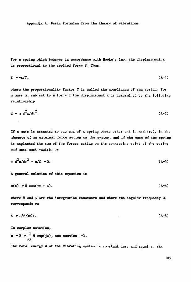
Appendix A. Basic formulae from the theory of vibrations

For a spring which behaves in accordance with Hooke's law, the displacement x

is proportional to the applied force f. Thus,

f «=-x/C, (A-l)

where the proportionality factor C is called the compliance of the spring. For

a mass m, subject to a force f the displacement x is determined by the following

relationship

f = m d2x/dt2. (A-2)

If a mass is attached to one end of a spring whose other end is anchored, in the

absence of an external force acting on the system, and if the mass of the spring

is neglected the sum of the forces acting on the connecting point of the spring

and mass must vanish, or

m d2x/dt2 + x/C = 0 . (A-3)

A general solution of this equation is

x(t) = x cos(ut + ifi) , (A-4)

where x and <$> are the integration constants and where the angular frequency to,

corresponds to

u * l / / ( m C ) . (A-5)

In complex notation,

x " S m — x exp(ji)>), see section 1-3. /2

The total energy W of the vibrating system is constant here and equal to the

185

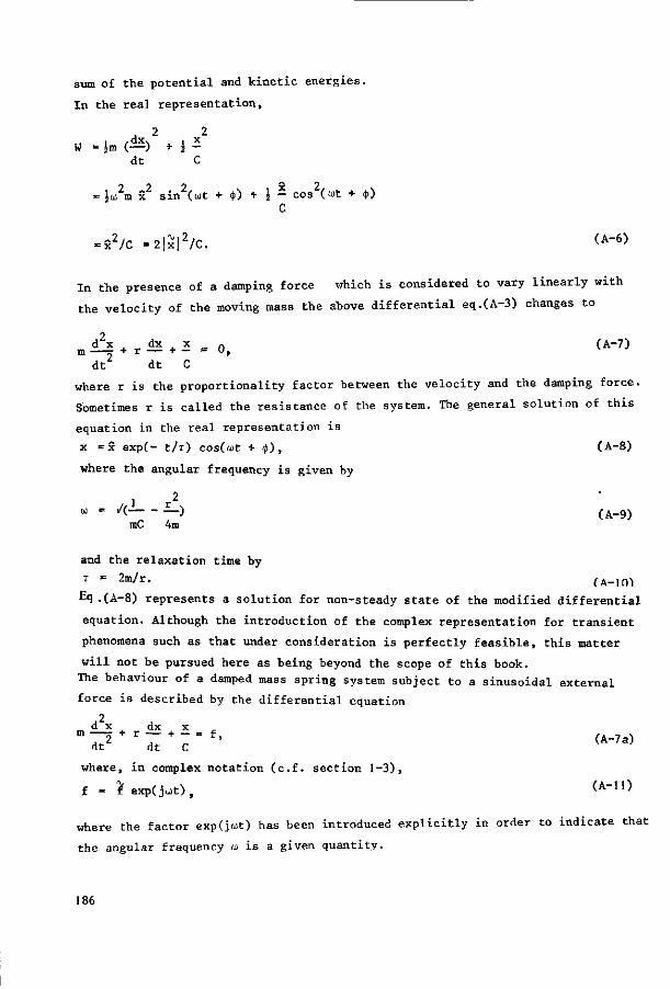
sum of the potential and kinetic energies.

In the real representation,

. 2 2 W = }m (—) + { -

dt C

9 2 2 X 2 = Jin m x sin (ojt + <t>) + ^ - cos (wt + <t>)

C

= x2/C =2|^|2/C. <A"6>

In the presence of a damping force which is considered to vary linearly with

the velocity of the moving mass the above differential eq.(A-3) changes to

m — » + r — + — — ut

dt dt C

where r is the proportionality factor between the velocity and the damping force.

Sometimes r is called the resistance of the system. The general solution of this

equation in the real representation is

x = x exp(- t/x) cos(iut + <(>), (A-8)

where the angular frequency is given by

2

mC 4m u = /( JL.) (A_9)

and the relaxation time by

T = 2m/r. CA_]n>l

Eq .(A-8) represents a solution for non-steady state of the modified differential

equation. Although the introduction of the complex representation for transient

phenomena such as that under consideration is perfectly feasible, this matter

will not be pursued here as being beyond the scope of this book.

The behaviour of a damped mass spring system subject to a sinusoidal external

force is described by the differential equation

d x dx x m — 2 r ~ + _ = f ' (A-7a)

dt2 at c K a)

where, in complex notation (c.f. section 1-3),

f = ? exp(ju)t), (A"n)

where the factor exp(jwt) has been introduced explicitly in order to indicate that

the angular frequency u is a given quantity.

186

This equation is analogous to the differential equation describing the electri­

cal behaviour of a series circuit of self-inductance L, resistance R and ca­

pacitance C,driven by a harmonic alternating voltage

L ± _ S + R i 2 + £ = % Mtp(jut.) (A-12) dt dt C

When the steady state has been reached the following particular solution of eq.

(A-7a) is found

x = * cos(ut - ») ^ (A_,3)

w/(r + (wm-l/uiC) )

or in complex notation,

x = \ , (A-14) 1/C - w m + jur

from which the dependence of x on the frequency is evident. Utilizing the complex

notation the concept of mechanical impedance was used'in this book. This quantity

Zy, is defined as the ratio of the complex force exerted on a point divided by the

complex velocity of that point.

\ - ! • ( A - I 5 )

u

with u « dx/dt.

The unit for Z, in S I -units is Nsm .

The mechanical impedance of the mass spring system is given by

f" 1 2^ = — - - r + jom + - — . (A-16)

jux juC It thus follows that

III /(r2 + (urn-—)2).

Note from eq.(A-17) that in resonance, when oo = l//(mC), lz.,1 is minimal and ' M'

equals r. Introductory textbooks on the theory of vibrations are: van Santen

(1950), Jones (1951), Mc Lachlan (1951), Sharman (1963). An introduction on sound

vibration is given by: Lamb (1960). Further details on the theory of sound can

be found in: Rayleigh (1945), Morse (1948), Beranek (1949), Skudrzyk (1949),

Wood (1966). 187

Appendix B. Derivation of the perturbation factors for homogeneous

channels

The viscosity and the thermal conductivity inherent in gaseous media cause

damping of acoustic waves propagating in channels. This damping may be ascribed

to two effects.

1. Wall absorption, comprising the losses in the viscous and thermal boundary

layers at the walls of the channel.

2. Volume absorption, which takes place in the body of the medium and corre­

sponds to the residual losses in free waves.

These two forms of absorption differ in that the first is caused by diffusion

of momentum and kinetic energy in directions normal to the direction of propa­

gation and the second by the diffusion of these same quantities in the di­

rection of propagation.

For the range of temperatures, barometric pressures, frequencies and channel

cross-sections encountered in the acoustical investigation of porous materials

the second effect is negligible in relation to the first and need not be further

considered.

In a homogeneous channel, i.e. one having a constant cross-section, the concept

of a plane wave, perturbed only near the channel walls by the boundary layers,

is appropriate only if the transverse dimensions of the channel are comparatively

large with respect to boundary layer thickness. As these transverse dimensions

diminish, the boundary layers tend to cover the entire cross-sectional area,

resulting in Poiseuille flow and isothermal changes of state in the limiting case

of very small dimensions. Although, in this latter case, the dissipation of

acoustic energy is distributed over the entire volume of the channel, the

dissipative mechanism is still that of wall absorption.

Taking into account that momentum and kinetic energy are carried by the same

molecules, one would expect the viscous and thermal boundary layers to have

thicknesses of the same order of. magnitude. That such is indeed the case will be

shown later in this section.

Kirchhoff solved the problem for the cylindrical tube in the high frequency ap­

proximation and found formulae for the velocity of sound and the attenuation of

waves. In this case the ratio of the thickness of the boundary layers and the

188

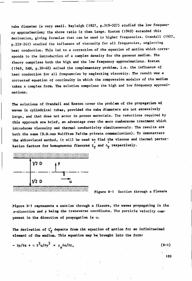
tube diameter is very small. Rayleigh (1927, p.319-327) studied the low frequen­

cy approximation; the above ratio is then large. Kosten (1949) extended this

derivation, giving formulae that can be used to higher frequencies. Crandall (1927,

p.229-241) studied the influence of viscosity for all frequencies, neglecting

heat conduction. This led to a correction of the equation of motion which corre­

sponds to the introduction of a complex density for the gaseous medium. The

theory comprises both the high and the low frequency approximations. Kosten

(1949, SAM, p.30-40) solved the complementary problem, i.e. the influence of

heat conduction for all frequencies by neglecting viscosity. The result was a

corrected equation of continuity in which the compression modulus of the medium

takes a complex form. The solution comprises the high and low frequency approxi­

mations .

The solutions of Crandall and Kosten cover the problem of the propagation of

waves in cylindrical tubes, provided the tube diameters are not excessively

large, and that does not occur in porous materials. The reductions required by

this approach are brief, an advantage over the more cumbersome treatment which

introduces viscosity and thermal conductivity simultaneously. The results are

both the same (D.W.van Wulfften Palthe private communication). To demonstrate

the abbreviated method, it will be used to find the viscous and thermal pertur-

bation factors for homogeneous fissures £„ and af respectively.

V2 D

T/2 D

y

z ^ u

Figure B-l Section through a fissure

Figure B-l represents a section through a fissure, the waves propagating in the

z-direction and y being the transverse coordinate. The particle velocity com­

ponent in the direction of propagation is u.

The derivation of £'f departs from the equation of motion for an infinitesimal

element of the medium. This equation may be brought into the form:

2 2 3p/3z + n 3 u/3y = p 3u/3t, (B-l)

189

where n is the dynamic coefficient of viscosity and p is assumed to be inde­

pendent of y. Solution of eq.(B-l) for harmonic time dependence and symmetry

in y yields:

u •= — -^ {1 + A cos((l-j)y/lv)}, (B-2) iup 3z

s

where the viscous boundary layer thickness 1 is given by

1 •= /(2n/up ). (B-3) v s

The integration constant A is eliminated from eq.(B-2) with the boundary con­

dition for a rigid frame: u = 0 for y = - JD:

u e - — L lE'ji - cos((1-j)y/lv)j t (B_4)

jwp 3z I cos(l(l-J)D7l))

Integrating eq.(B-4) over the interval -$D<y<jD, yields

U . / " ^ u d y 2_ i E J L , (B-5) f 9

3z Z,

where 5* . ,/j, _ tan(^(l-j)D/lvl _ ( B_6 )

£ ( J(l-j)D/lv \ t

Cf is the perturbation factor sought.

i

The derivation of nf is based on the following fundamental equations.

K The law of Boyle - Gay Lussac p = p R T , which reads in differential form s s g s

& = *£- + *i . (B-7) p p T rs s s

The differentials dp, dp, dt are the variables in the given case. They will be

indicated further on by p, p and 9. So one can write *— = — + — p P T *s s

p is the incremental density due to the sound field, T is the static absolute s

temperature,

190

0 is the incremental temperature due to the sound field,

R is the gas constant per unit mass.

As p, p and 0 are small quantities, a first order approximation of eq.(B-7) is:

P = p/(R T ) - PSQ/Tg. (B-8)

2. The equation of continuity. This expresses the fact that a gradient in parti­

cle displacement results in an incremental density. The appropriate form for

harmonic phenomena is

- p 3u/3z = jtop . (B-9)

3. The equation of heat transport: Assuming heat to be transported transversely

only, the net flow of heat per unit mass (having a volume l/p ) is given by:

3a . 2L i!|_ , (B-.O) 8t P S 3y

where X is the thermal conductivity of the medium. The appearance of the de­

rivative of the second order on the right side of eq.(B-lO) may be understood

by considering that heat flow density is proportional to temperature gradient

and that it is thus the variation in gradient which determines whether and

how much a net flow of heat into a given volume will result.

A. The First Law of Thermodynamics for an ideal gas. For harmonic phenomena this

equation, applied to the unit of mass for the flow of heat is given by

3Q/3t - juc 0 - joop/p. (B-ll) p s

where c is the specific heat per unit mass at constant pressure for the gaseous

medium.

Elimination of the term 3<)>/3t from the eqs(B-lO) and (B-ll) yields

-JiL. . ± | + Q = _ E _ . (B_12) U p s C p 3 y PsCp

Assuming p to be independent of y, a solution, symmetrical in y, is sought for

eq.(B-12):

191

0 = p{l + A cos((l-j)y/lh)}/pscp> (B-13)

where the thermal boundary layer thickness 1, has been introduced:

1. - /(2X/a)p c ) . (B-14) n s p

The integration constant A in eq.(B-13) is eliminated with the boundary con­

dition for a frame of constant temperature:

0 = 0 for y = ± JD so that

e . - ! — h _ cos((l-j)y/ln [, (B-15)

p c f. cos(J(l-J)D/lh ' s p

p is eliminated from eqs(B-8) and (B-9) which yields

- 3u/3z = jcop/p - ju)0/T . (B-16)

where e is given by eq.(B-15). Elimination of 9 and integration over the interval

-jD<y<jD yields

3U/3z = -/ — dy = ja>pDnf /i<pg> (B-17)

where

nl = 1 H- ( K - 1 ) tan(Kl-j)DAh), (B-18) f J(l-J)D/lh

Comparison of eqs(B-17) and (3-46) shows that n from eq.(B-18) is indeed the

perturbation factor sought.

Rayleigh (1927, II, p.327-328) considered a homogeneous fissure, confining the

results to the low and the high frequency approximations.

Discussion of the results

The quantities 1 and 1. prove to be measures for the thicknesses of the

boundary layers, e.g., if | D / L » 1 , in the range where jD-y<<iD:

0 = p {1 - exp((l+j)(y-jD)/lh)}/psCp . (B-19)

192

The right of eq.(B-19) shows that, on decreasing y from the value {D (where 0 =

0 ) , 0 rises to the value p/p c with a rapidity determined by 1. . Thus, for y •=

JD - lh, 10] •= 0.859 - E — . P c s p

A relation for ideal gases, due to Eucken (Physik.Z., 14, 324-332,1913).

X/nc •= (9K-5)/4IC . P

Using this equation together with eqs.(B-13) and (B-14), the ratio of the thermal

and viscous boundary layers is found to be:

1./1 = / ( 4 K / ( 9 K - 5 ) ) . (B-20) n v

As the gaseous medium is composed of gases ranging from monatomic to triatomic,

7/5<K<5/3 and thus, from eq.(B-20):

0.82<1,/l <0.87 . (B-20a) n v

Roughly, the two boundary layers prove to be equally thick.

The viscous and thermal perturbation factors for the homogeneous cylindrical i i

tube, £ and n , respectively, may be read directly from Crandall's and Kosten's

results as presented by Zwikker & Kosten (1949, SAM, p.25-40). It thus follows

from their eq.(2.06) that, on introducing the present notation:

{ «= 1/{I 1 Ix. ((l-j)R/l )}, (B-21)

(i-J)R/lv J Q

and from their eq.(2.13) that:

„' = 1+ ( K - 1 ) L((i-j)R/i ) , (B-22)

(l-j)R/lh JQ

where R is the radius of the tube.

Mote: Zwikker & Kosten's quantity v, defined on p.30, should be taken to equal X, /p c in their notation or X/p c in the notation used in this book, h o v s v

193

Appendix C Calculation of the function H(x) and its associated functions

There are three ranges for the arguments, the first is that where the function

is best described by its asymptotic behaviour for small values of the argument,

then there is a transition range and finally the range where the function is

best described by its asymptotic behaviour for large values of the argument. In

the present instance, the limits for the three ranges, respectively

0<;x«l .0 ; l<x<3.2 ; 3.2«x

appear to be the most practical with the computation of the numerical values-

of H(x) in view (see eq.(3-70).

Approximations valid for one of the ranges only are indicated by the subscripts

1, 2 and 3 to H(x), F(x), M(x), G(x) and L(x), defined by eqs(3-71), (3-72),

(3-81) and (3-82) respectively are also approximated and receive the same

subscript as H(x), indicating the range of validity for the argument.

Calculation of the function H(x) from series expansions of the Bessel functions.

As the polynomial series representing Bessel functions are convergent, an

algorithm for the generation of H(x) and suitable for computer processing may

be formulated. The result is the Bessel subroutine described below. It should

be noted that the argument of the Bessel function, z = x/-j is assumed to lie

in the fourth quadrant, the angle being —nlU;

x is the modulus of the argument. As H(z) is a symmetrical function in z with

respect to zero, the arbitrary selection of the fourth quadrant for z does not

restrict the generality of the results.

Rewriting a series expansion as given by Jahnke and Embde, (p.128) gives:

oo ., .2k , Jn(z) = E ( i z \ (-1)\

U k=0 (k'.r

,x.2k .k (y) • J

I ~ 2 = k=o , i , 2 , 3 ( k : r

~ (x }2k M ) k / 2 . (x }2k ( _ 0 ( k - . ) / 2

= l - i • j i - J = k=0,2,4 (k ' . r k=1.3.5 (k l ) 2

194

( | ) 4 k ( ~ O k 2 . 2 + j — I

(f) 4 k ("l)k

k=0,1.2 {(2k) ' .} 2 4 k=0 , l , 2 { ( l+2k) ' .} 2

Furthermore:

» , , .2k+l , ,Nk <» , , .2k+l ,k

j i ( z ) = s ii£> t i l = /-j s i W L k=0 k! (k+1)'. k=0 (k ' .T (k+1)

f

= Jx-/-j " - ( ^ ) 2 k ( - o ^ . ; ( i k ) 2 k ( - i ) f r - ' ) / 2

k=0.2,4 (k ' . )Z (k+1) k - 1 , 3 . 5 ( k ! ) 2 (k+1)

J j ( z ) = Jz (b)4k (-ok , , N4k . , . k 2 °° ( jx) (-1) .x z _

k = 0 , , • 2 { (2k) ' .} 2 (2k+l) 4 k -0 ,1 ,2 { (2k+ l ) !} 2 (2k+2).

The terms required for the calculation of Jn and J. can easily be derived 0 '1

consecutively. The following quantities are introduced:

p _ (x/2)4k (-l)k . n _ (x/2)4k (-l)k

{(2k) I}"1 fc {(2k+l)'.}Z

_ _ (x/2)4k (-Qk , „ _ (x/2)4k(-l)k

\ '-, ' sk 2 ' {(2k)2,.}(2k+l) ' k

The quantities are interrelated by:

Pk Pk Qk Q r ; R and S.

(2k+l) 2k+l 2k+2

rk+l rk -(x/2)^

(2k+l)2 (2k+2)2

-(x/2)" S

(2k+2)

The function H(x) can now be written as follows:

2J H(x) =-

,<*> I A + j ( x / 2 ) ZkSk

z JQ(z) EkPk + j(x/2) 2kQk

(C-l)

195

As P, is the largest of the quantities with the same subscript, £]Pk c a n best

serve as criterion for the required degree of accuracy. Eq.(C-l) has been

programmed and is referred to as the Bessel subroutine. In table C-l some

numerical values of H(x) are given.

table C-l

Numerical values of H(x) obtained from the Bessel subroutine

H(x) x H(x) x

0.2 0.999966-0.004999 j 2.2

0.4 0.999466-0.019986 j 2.4

0.6 0.997310-0.044833 j 2.6

0.8 0.991570-0.079073 j 2.8

1.0 0.979772-0.121525 j 3.0

1.2 0.959304-0.169931 j 3.2

1.4 0.928155-0.220811 j 3.4

J.6 0.885683-0.269752 j 3.6

1.8 0.833178-0.312268 j 3.8

2.0 0.773776-0.344894 j 4.0

0.711598-0.366031 j

0.650648-0.376057 j

0.593947-0.376765 j

0.543214-0.370598 j

0.499010-0.359962 j

0.461086-0.346849 j

0.428761-0.332719 j

0.401190-0.318544 j

0.377534-0.304900 j

0.357038-0.292089 j

In practice, the calculation turned out to be time consuming. For this reason,

another method of calculation was developed. Eventually this last method pro­

duced results with sufficient accuracy. The method described above was used as

a check only.

Calculation of the function H(x) and its associated functions (0<x<l)

The converging series for the Bessel functions were rewritten; a procedure which

is especially appropriate"if the argument of the Bessel function is relatively

small.

2 4 6 JQ(z) = 1 - -5- + I £ _

4 64 64.36

and

J.(z) = iz(l - - z 2 + — z 4 -8 J92 64*144

1 6 - •> z + ... ).

Making use of eq.(3-70) where H(x) has been defined, substitution and further

reduction leads to:

Hj(z) 2Jj(z)

zJ0(z)

. ' 2 1 * A 33 6 1 + —z + — z + — — — z + 48 64*144

196

where z = x/-j =((l-j)//2)x.

Separating the real and imaginary parts of the argument by:

z = x/ - j = (——l)x gives /2

4 2 . - 6 H.00 - 1 - 2 - . . . + J C - S - * ^ 5 — ..-> (C-2)

1 48 8 64.144

The last term of eq^c-2) influences the result of the calculated value of

H.(x) but slightly, the contribution of this term can therefore be neglected.

From this series the calculation of the values for F. (x) and G. (x) as defined

in eqs(3-72) and (3-82) can be done readily. The calculation of the integrals

in L.(x) and M.(x) merits further attention.

The integral_L._(x)^

Introduction of the above series expansion from eq.(C-l) into eq.(3-81) and (3-82) results in:

L,(x) -J {1 + 0.4(1 - J2_ - —x4)}x2dx =

48 . . . .5 7 = L$J _ j*_ _ x__ . (c_3) 3 100 120-7

Confining x to the interval 0<x<l limits the error at the upper bound within

1%.

_The aiculatipn. of £\& _in£.egjaJL_M. £xl.

Introducing the series expansion from eq.(C-2) into eq.(3-72) leads to:

Ml(x) = f p—r o f ___d2 48 f (*2 - 6j)dx

8 48 48 The solution of this integral can be obtained by separating the integrand:

J L M 48 The integral

2

(x) = /"iz_ - r±4* + r -x /36fj/6 dx_ (c_4) 1 J 36x2 J 6x4 J x4

+36 i n t e g r a l

r 2 , / — r ^ — dx, i s solved by s u b s t i t u t i n g x = /6 tan y , r e s u l t i n g i n :

J x4+36

f 6 /6tan2y _ 1 / / Z——2~ y — / 4 4

J 3 6 ( l+ t an y)cos y /6 7 cos y + s i n y +

s i n 2 2 , -o T- ** -—r—5 I n 2 2 s in y cos y - 2 s in y cos y

1 ,2x/3N 1 , i x2+2x/3+6J f r _ s ^ = —— a rc tan (-—*•) l n ^ - 5 — ~ ? ' C t i ;

4/3 6-x 8/3 <x -2x /3+6>

197

In an analogous way the solution of the following integral is found:

2. f dx

J x4+36

1

36 24/3

_ f 2x/3\ 1 . (x +2x/3+6\ :tan < *> + ln<-"3 ?•

l6-x ' 48/3 *x -2x/3+6'

The last term of the right hand side of eq.(C-3) can be written as:

2

- f-r— dx + X f-r— dx = 36 J x>36 6 J x +36

1 ,, ., ,. 2x/3 1 ,. ... x2+2x/3+6 (l-j)arc tan ^ + (l+j)ln

144/3 " 6-xz 288/3 " x2-2x/3+6

The integration of the two other terms presents no problems. Thus

4 M,(x)

3x

, 8j (1-j) _ f 2x/3 ) , 1+j, \ x2+2x/3+6 \ + —'-rr - -—•^ arc tan < y > + —•'-In 4 9 >.

3xJ 3/3 l 6 - x ^ ' 6/3 lx-2x/3+6)

(C-6)

The last two terms of the right side of eq.(C-6) can themselves be developed

into series for small values of the argument: ( X < < 1 ) .

2x/3 •1

3/3 (1-j) arc tan &Q) - l ( l+j) ln

6-xZ 6+x

1-2x/3

6+x

ft*

* - ('-3)[2x/3 _ 2L_ + C+J)[2x/3 + £1 _ 3/3 [_6-x2 3/3j 3/3 |_6+x2 3/3J*

* _ I l d i . i L . [1 + iL2 + C + J ) . x [1 i d ] « _ 2jx _ £ . 3/3 /3 L 18j 3/3 /3L 18J 9 81

Thus an analytic approximation is found:

v, , s 4 x 3 2- * 8 • M (x) = -jx + —5-J . 3x 81 9 3x

(C-7)

For a more accurate calculation of M. , more terms than in eq.(C-6) have to be

included in the integration. From a practical standpoint this is feasible by

numerical integration only. The influence of the number of steps per unit of x

was examined. The approximation directly from the program for the Bessel sub-

198

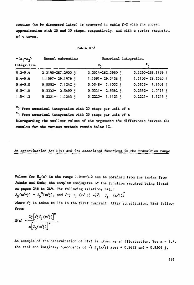
routine (to be discussed later) is compared in table C-2 with the chosen

approximation with 20 and 30 steps, respectively, and with a series expansion

of 4 terms.

-(x,-x2)

Integr.lim.

0.2-0.4

0.4-0.6

0.6-0.8

0.8-1.0

1.0-1.2

table C-2

Bessel subroutine

3.3190-287.2903 j

1.1097- 29.1976 j

0.5552- 7.1242 j

0.3332- 2.5400 j

0.2221- 1.1243 j

Numerical integration

°) 3.3034-282.0960 j

1.1081- 29.0438 j

0.5548- 7.1002 j

0.3331- 2.5362 j

0.2220- 1.1123 j

*) 3.3260-289,

1.1103- 29,

0.5553- 7,

0.3332- 2,

0.2221- 1,

.1789 j

.2520 j

.1306 j

.5413 j

.1243 j

) From numerical integration with 20 steps per unit of x

) From numerical integration with 30 steps per unit of x

Disregarding the smallest values of the arguments the differences between the

results for the various methods remain below 1%.

An approximation for H(x) and- its associated functions in the transition range

Values for H2(x) in the range 1.0<x<3.2 can be obtained from the tables from

Jahnke and Emde; the complex conjugates of the function required being listed

on pages 246 to 249. The following relations held:

V 3 0 ^ = V t x / j )> and /_J Ji (x/~i) H7J Ji <x/j)£ where Vj is taken to lie in the first quadrant. After substitution, H(x) follows

from:

2j[/jJ ,(x?j)T H(x) = t - -J .

X[jQ(x7j)]"

An example of the determination of H(x) is given as an illustration. For x = 1.8,

the real and imaginary components of /j J.(x/j) are: + 0.3612 and + 0.8509 j,

199

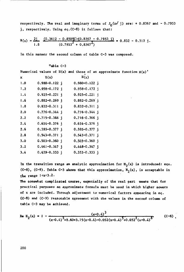
H(x)

respectively. The real and imaginary terms of Jn(x/ j) are: + 0,8367 and - 0.7953

j, respectively. Using eq.(C-8) it follows that:

(0.3612 - 0.8509JH0.8367 - 0.7953 j) _ Q ^ . Q ^ ._

(0.79532 + 0.83672)

In this manner the second column of table C-3 was composed.

Table C-3

Numerical values of H(x) and those of an approximate function H(x)'

1.8

x

1.0

1.2

1.4

1.6

1.8

2.0

2.2

2.4

2.6

2.8

3.0

3.2

3.4

H(x)

0.980-0.122

0.958-0.172

0.925-0.221

0.882-0.269

0.832-0.311

0.776-0.344

0.715-0.366

0.654-0.376

0.595-0.377

0.543-0.371

0.503-0.360

0.461-0.347 j

0.429-0,333 j

H(x)

0.980-0.122 j

0.958-0.172 j

0.925-0.221 j

0.882-0.269 j

0.832-0.311 j

0.776-0.344 j

0.716-0.366 j

0.654-0.376 j

0.595-0.377 j

0.543-0.371 j

0.503-0.360 j

0.448-0.347 j

0.353-0.333 j

In the transition range an analytic approximation for H-(x) is introduced: eqs.

(C-8), (C-9). Table C-3 shows that this approximation, H.(x), is acceptable in

the range l<x<3.2.

The somewhat complicated course, especially of the real part means that for

practical purposes an approximate formula must be used in which higher oowers

of x are included. Through adjustment to numerical factors appearing in eq.

(C-8) and (C-9) reasonable agreement with the values in the second column of

table C-3 may be achieved.

Re H2(x) = 1 - (x-0.4)J ,r_av

(x-0.4) +8.60+3.75(x-0.4)-0.052(x-0.4) +0.052 (x-0.4)

200

Im H,(x) = 0.122+0.249(x-1) ^— * . (C-9) z 0.514(x-l)+10(x-l) +26.66

With the use of eqs(C-8) and (C-9) the function F„(x) and 0„(x) can be written.

A polynomial through the calculated values of F.(x) and G„(x) will be given in

the survey at the end of appendix C.

The derivation of M2(x) and L.(x) is more difficult.

The integral_L.£x)

/ 2 [, (x-0.4)3 ] . I X • 1 X = 5 jr C J I (x-0.4) +8.60+3.75(x-0.4)-0.052(x-0.4) +0.052 (x-0.4)!J

Re L2(x) = — + 0.4 \ x % 11 , ^-^J. 5 -.|dx

Re L,(x) = + — x 3 - 0.4 I.. (C-10) 3

x-0.4 After the introduction of * u, u lying between 0.12 and 0.52, the integral

T can be transformed into

= J (55u5 + 0.8-54u4 + 0.16»53u3)d 5u J J 5 3 u 3 + 8.60 + 3.75-5 u - 0.052'55u5 + 0.0522'58-u8

= ,4.793 f s (u5 + 0 I6.u4 + 0.0064 u3)du ^ ^ J u - 0.15383 u + 0.11834 u + 0.017751 u + 0.008142

(C-ll)

Splitting of the denominator into the above integrand involves a search for a

number of complex or real roots of a polynomial. Kunz (1939) presents a

solution through use of the Lin-Bairstow method. A Fortran program was made for

this technique.

The real roots of the denominator turn out to be:

Uj = - 0.30145825

u 2 = - 0.59601104

while the products of the pairs of conjugated complex roots can be written as:

(u-u3)•(u-u4) = u 2 - 1.22857214 u + 0.47065730

(u-uc)•(u-u,) = u 2 - 0.24548668 u + 0.18610927 5 6 2

(u-u7)'(u-ug) - u + 0.57658953 u + 0.51734090

201

As a result of this, the integral I„ can be split up

Cu+D Eu+F Gu+H X 2 =

/

____. B _ . -_—__. + _____ + ___________________ -r _-___________-_----_ f -__-_-___----_-_-_»-

u-Uj u-u2 (u-u3)•(u-u^) (u-u5)•(u-u6) (u-u_)•(u-ug)j

du.

Solution of a matrix will lead to the coefficients of the numerators. This in­

volved more difficulties than anticipated and was possible only after repreated

programming, for which use was made of the well-known Crout-reduction method.

Substitution of the coefficients of the denominators leads to:

103222 + 0.33772185 + 0.38647294u + 0.01060727 ,

•/[*= (u-u3)•(u-u^)

-0.288872957u + 0.11556302 0.40321186u + 0.57094917

(u-u7)«(u-u8) du (C-12)

(u-u.)'(u-u6)

Integration of these partial subintegrals leads to further subdivision, since

/

Cu+D J Tc i / 2_ -. N, D-C'p/2 . u+p/2 "1 „ du = — ln(u +pu+q)+ & — — arc tan * „

u +pu+q )_2 /(q-p /4) /(q-p A)J (C-13)

where the limits for u are derived from u = 0.2x-0.08.

After integration of all the subintegrals, the function for the real part of

L„(x) can be written as:

Re L,(x) = — x3 - 5.9172 I.. 3

The imaginary component of L,(x) can be treated as follows:

-Im L„(x) =

0.4

0.4 J x 2 0.122 + 0.249(x-l) - (x-1)-

0.514(x-l)5+10(x-l)3+26.66 dx,

-(0.127+ 1

-) 0.514 3 4 0.514 J (x-1) + (x-1) +

0.514 0.514

(C-14)'

dx.

The last term of eq.(C-14) is defined as I,. This leads to

202

10 f (x-

.

• o 5+ 2(x-l)4+(x-

(x - l ) 5 +

- l ) 3+2 10

0.514

.666(x-

Cx-1)3+

l)2+5.332(x-26.66

0.514

-l)+2 666 _ 1 0 (J \2i.— tJ T Z.VA- I J TV.A— 1J -r£. . g U U l A - 1 ) T J . J J i U - l i T i . O O U j / . v

I, = •* f E T* 5 4£ LL d(x-U . J 0.51

On introducing v = and I, - =-(x+I, )it follows that 10 0.514

'f\ .. . 2v4-1.8455v + 0.02666v + 0.005332 v - 0.0049292] J I = / j ^ _ d v . * J ' v + 0.1946v + 51.87*10 3 J

When the denominator is split according to the method applied previously the

real root of the denominator is given by:

v, = - 0.1345979023,

while the coefficients of the pairs of conjugate complex roots meet the con­

ditions:

(v-v2)•(v-v3) - v2 - 0.1482298637 v + 0.0197654211

(v-v4)•(v-v5) - v 2 + 0.0136319614 v + 0.1949718380

Substitution of the calculated coefficients in the numerators of the integrands

now yields:

. •„.0001395136164 + 0.013801585v + 0.0032919790 + rfb-ooo! J [y+o.i: 4 ./ !_..„ 1345979o23 v2-0.1482298637v+0.0197654211

1.98605890v - 1.81716117

v2+0.0136319614v+0.1949718380 dv,

where the limits for v follow from v = (x-l)/10.

Integration can now be carried out immediately.

The high accuracy of the numerical factors in the above equations takes the

possibility into account that two numbers with a small difference will

be subtracted in the course of the calculations. It is not worthwhile analysing

whether this contingency is realized or not as a reduction in accuracy does not

increase the speed of the calculations.

It now follows that

+ Im L2(x) = - 0.0249 x 4 + 0.27632 x 3 - 15.1403 x - 15.1403 I . (C-15)

In the following table (C-4) are listed the results obtained from the ex­

pansions of LjCx). The values, as obtained by numerical integration of H(x) are

203

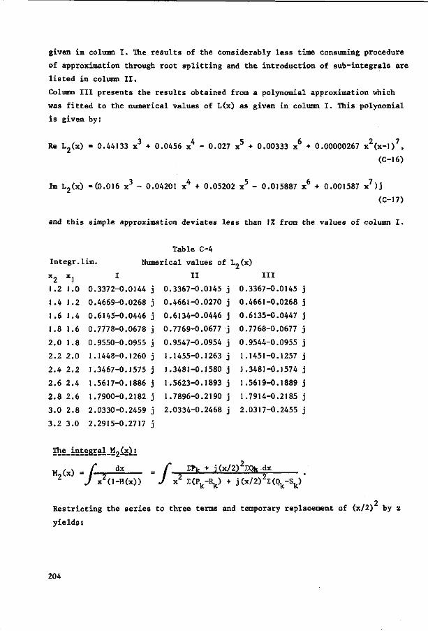
given in column I. The results of the considerably less time consuming procedure

of approximation through root splitting and the introduction of sub-integrals are

listed in column II.

Column III presents the results obtained from a polynomial approximation which

was fitted to the numerical values of L(x) as given in column I. This polynomial

is given by:

Re L2(x) = 0.44133 x3 + 0.0456 x4 - 0.027 x5 + 0.00333 x6 + 0.00000267 x2(x-l)7,

(C-16)

Im L2(x) -(0.016 x3 - 0.04201 x4 + 0.05202 x5 - 0.015887 x6 + 0.001587 x7)j

(C-17)

and this simple approximation deviates less than 1% from the values of column I.

Table C-4

Integr.lim. Numerical values of L»(x)

x2 X j I II III

1.2 1.0 0.3372-0.0144 j 0.3367-0.0145 j 0.3367-0.0145 j

1.4 1.2 0.4669-0.0268 j 0.4661-0.0270 j 0.4661-0.0268 j

1.6 1.4 0.6145-0.0446 j 0.6134-0.0446 j 0.6135-C.0447 j

1.8 1.6 0.7^78-0.0678 j 0.7769-0.0677 j 0.7768-0.0677 j

2.0 1.8 0.9550-0.0955 j 0.9547-0.0954 j 0.9544-0.0955 j

2.2 2.0 1.1448-0.1260 j 1.1455-0.1263 j 1.1451-0.1257 j

2.4 2.2 1.3467-0.1575 j 1.3481-0.1580 j 1.3481-0.1574 j

2.6 2.4 1.5617-0.1886 j 1.5623-0.1893 j 1.5619-0.1889 j

2.8 2.6 1.7900-0.2182 j 1.7896-0.2190 j 1.7914-0.2185 j

3.0 2.8 2.0330-0.2459 j 2.0334-0.2468 j 2.0317-0.2455 j

3.2 3.0 2.2915-0.2717 j

3£e_in^egral_M2£x^

P k _ V + Kx/2)^(Qk-Sk) M,(x) - f dx = /* Z*k+ J<*/2>

J x2(l-H(x)) J x2 2(P.-R.) + i' '"s2

2EQk dx

2 Restricting the series to three terms and temporary replacement of (x/2) by z

yields:

204

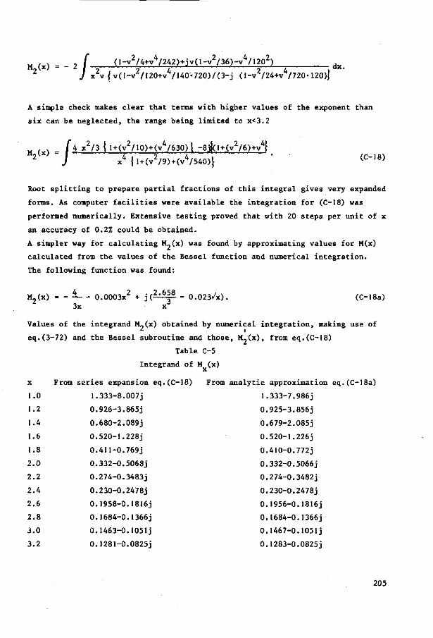
M . » _ , f (l-v2/4+v4/242)+jv(l-v2/36)-v4/1202) M „ W - - / I —T = T 1 j 7 QX.

./ x v Jv(l-v /120+v7140'720)/(3-j (1-v /24+v /720-1.20)}

A simple check makes clear that terms with higher values of the exponent than

six can be neglected, the range being limited to x<3.2

M,(x) [iJLU 3 { l+(v2/10)+(v4/630)} -8j{(l + (v2/6)+v4} 2 W " ' " x 4 { 1 + (v2/9) + (v4/540)} ' ( C H 8 )

Root splitting to prepare partial fractions of this integral gives very expanded

forms. As computer facilities were available the integration for (C-18) was

performed numerically. Extensive testing proved that with 20 steps per unit of x

an accuracy of 0.2% could be obtained.

A simpler way for calculating M„(x) was found by approximating values for M(x)

calculated from the values of the Bessel function and numerical integration.

The following function was found:

M2(x) = - — - 0.0003x2 + jC2,6^8 - 0.023/x). (C-18a) 3x x

Values of the integrand M~(x) obtained by numerical integration, making use of

eq.(3-72) and the Bessel subroutine and those, M.(x), from eq.(C-18)

Table C-5

Integrand of M (x)

x From series expansion eq.(C-18) From analytic approximation eq.(C-18a)

1.0 1.333-8.007j 1.333-7.986j

1.2 0.926-3.865j 0.925-3.856j

1.4 0.680-2.089j 0.679-2.085j

1.6 0.520-1.228j 0.520-1.226j

1.8 0.411-0.769j 0.410-0.772j

2.0 0.332-0.5068j 0.332-0.5066j

2.2 0.274-0.3483j 0.274-0.3482J

2.4 0.230-0.2478J 0.230-0.2478j

2.6 0.1958-0.1816j 0.1956-0.1816j

2.8 0.1684-0.1366j 0.1684-0.1366j

3.0 0.1463-0.1051 j 0.1467-0.1051j

3.2 0.1281-0.0825J 0.1283-0.0825j

205

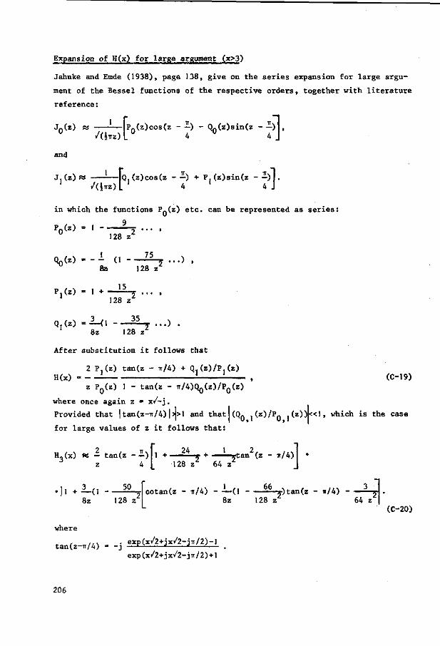
Expansion of H(x) for large argument (x>3)

Jahnke and Emde (1938), page 138, give on the series expansion for large argu­

ment of the Bessel functions of the respective orders, together with literature

reference:

J0(z) w —

and

PQ(z)cos(z - -) - QQ(z)sin(z - -) ,

J,(z)« —fQ.(z)cos(z - - ) + P.(z)sin(z - i)l.

' /(JTTZ)L 4 ' 4 J

in which the functions P0(z) etc. can be represented as series:

9 P.(z) = 1 =• ... ,

128 z*

Q0(z) - - - (1 " - ^ - j -..) , 8z> 128 z

P,(z) = 1 + 15

1 128 zz

Q,(z) =^-(1 - 3 5 b ...)

8z 128 z

After substitution it follows that

2 P.(z) tan(z - IT/4) + Q.(z)/P (z) H(x) ! l- • , (C-19)

z PQ(z) 1 - tan(z - TT/4)Q0(Z)/P0(Z)

case

where once again z = x/-j.

Provided that | tan(z-n/4) |>j>l and that (Q0 .(z)/PQ .(z))k<l, which is the

for large values of z it follows that:

H,(x) « - tan(z - 1 ) 1 + — ^ L - + — ^ t a n 2 ( z - TT/4) • J z 4 L '28 z 64 z J

• | l + — 0 5° | co t an (z - IT/4) - —(1 6 A T ) t a n ( z - TT/4) ^ 8z 128 z 8z 128 z 64 z

L (C-20)

where

.. , , , s • exp(x/2+jx/2-JTT/2)-l tan(z—n/4) = - j —c- i •> J—'—-— . exp(x/2+jx/2-j ir /2) + l

206

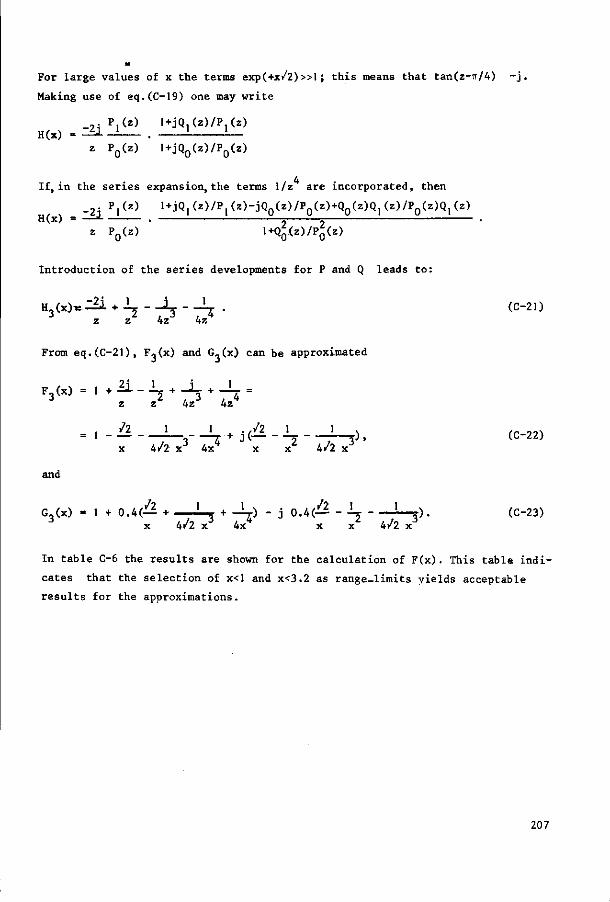
For large values of x the terms exp(+x/2) >>1; this means that tan(z-Tr/4) -j .

Making use of eq.(C-19) one may write

H(x) _ P j ( z ) l+jQ,(z)/Pj(z)

z PQ(z) l+jQ0(z)/P0(z)

4 If,in the series expansion, the terms 1/z are incorporated, then

_2. P,(z) l+jQ1(z)/P,(z)-jQ (z)/P (z)+Q0(z)Q,(z)/P0(z)Q1(z) H(x) = — 1 . = = .

z P0(z) 1 + Q Q ( Z ) / P Q ( Z )

Introduction of the series developments for P and Q leads to:

z z 4z 4z

From eq.(C-21), F,(x) and G«(x) can be approximated

z z 4z 4z

_ 1 _ + j ( ^ . _) , (C-22) x 4/2 x 4x x x 4/2 x

and

G3(x) = 1 + 0.4(— + L j + -ij) - j 0.4(— - i j L - 3 ) . (C-23) x 4/2 x 4x x x 4/2 x

In table C-6 the results are shown for the calculation of F(x). This table indi­cates that the selection of x<l and x<3.2 as range-limits yields acceptable resul ts for the approximations.

207

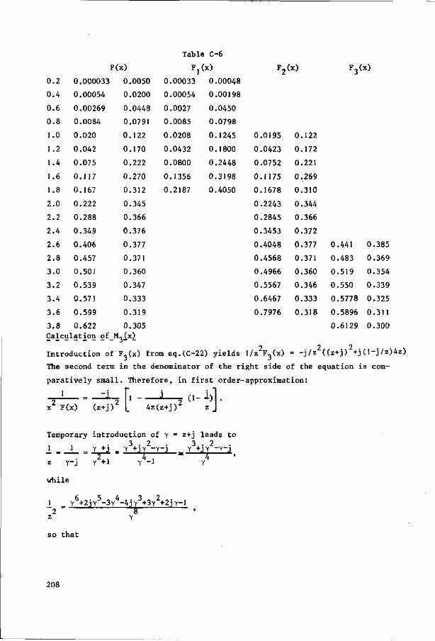
0.2

0.4

0.6

0.8

1.0

1.2

1.4

1.6

1.8

2.0

2.2

2.4

2.6

2.8

3.0

3.2

3.4

3.6

3.8

F(

0.000033

0.00054

0.00269

0.0084

0.020

0.042

0.075

0.117

0.167

0.222

0.288

0.349

0.406

0.457

0.501

0.539

0.571

0.599

0.622

x)

0.0050

0.0200

0.0448

0.0791

0.122

0.170

0.222

0.270

0.312

0.345

0.366

0.376

0.377

0.371

0.360

0.347

0.333

0.319

0.305

0

0

0

0

0

0

0

0

0

Table

V .00033

.00054

.0027

0085

.0208

.0432

.0800

1356

.2187

C

x)

0

0

0

0

0

0

0

0

0

-6

00048

.00198

.0450

0798

1245

1800

2448

3198

4050

F2

0.0195

0.0423

0.0752

0.1175

0.1678

0.2243

0.2845

0.3453

0.4048

0.4568

0.4966

0.5567

0.6467

0.7976

(x)

0.122

0.172

0.221

0.269

0.310

0.344

0.366

0.372

0.377

0.371

0.360

0.346

0.333

0.318

0

0

0

0

0

0

0

V

.441

.483

519

550

.5778

.5896

.6129

x)

0

0

0

0

0

0

0

385

.369

354

339

.325

.311

300 Calculation of_M,(x)

Introduction of F,(x) from eq.(C-22) yields 1/x F3(x) -j/z ((z+j) +j(l-j/z)4z)

The second term in the denominator of the right side of the equation is com­

paratively small. Therefore, in first order-approximation:

1

x2 F(x) (z+j) I J_

4z(z+j)' <l-±)\

Temporary introduction of y = z+j leads to 3 2 3 . 2

1 _ _J Y +J _ Y +JY -Tf-J Y +JY ~Y-j z Y"j Y +J Y -1 Y

while

J_ y +2jy -3y -4jy +3Y +2J7-1 2 H5

z Y

so that

208

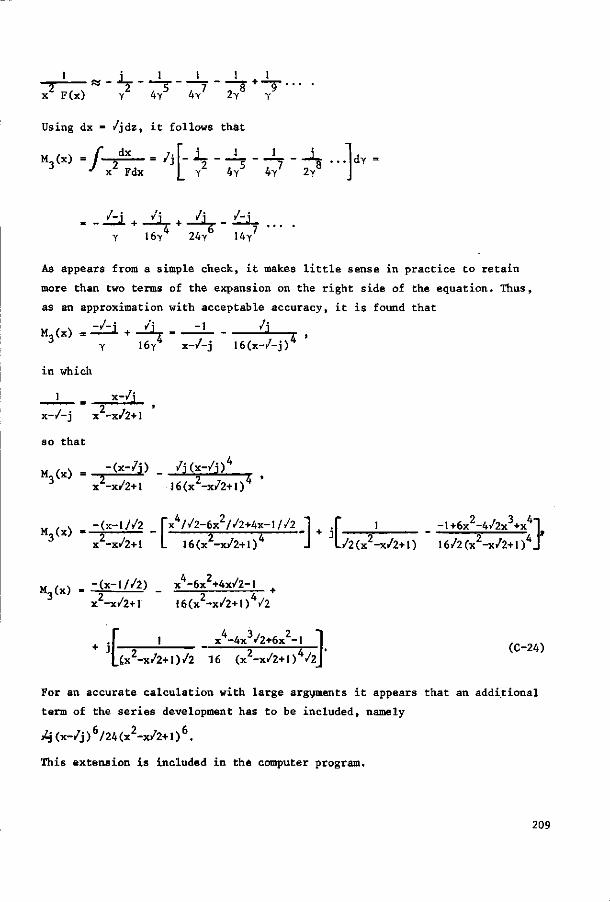
x F(x) Y 4 Y 4 Y

Using dx = /jdz, it follows that

2 Y Y

M3(x) f dx = y. T j _ _ 4 1

J x Fdx I Y 4 Y 4 Y 2Y dY

/-i /i /j /-j + — 4 + 6 7

Y 16Y 2 4 Y 14Y

As appears from a simple check, it makes little sense in practice to retain

more than two terms of the expansion on the right side of the equation. Thus,

as an approximation with acceptable accuracy, it is found that

M3(x) = ^ i + - l Y 16Y

-1 A 4 x-/-j I6(x-/-j)4

in which

1 x-/i

x-/-j x -x/2+1

so that

,.s4

J x -x/2+1 I6(x -x/2+1T

ft

u , v -(x-l//2 fx4/'/2-6x2//2+4x-l//2 M-(xJ =—=

x -x/2+1 6(x2-x/2+l)4

1 + .J" 1 -l+6x2-4/2x3+x4"|

J L/2(x2-x/2+l) 16/2(x2-x/2+l)4J

M (x) = -C« - ' / ^ ) _ x4-6x2+4x/2-l +

x -x/2+1 16(x -x/2+1) /2

[ 1 x4-4x3/2+6x2-l "j

Cx2-x/2+l)/2 16 (x2-x/2+l)4 /2j (C-24)

For an accurate calculation with large arguments it appears that an additional

term of the series development has to be included, namely

^j (x-/j ) 6/24(x2-x/2+1) 6.

This extension is included in the computer program.

209

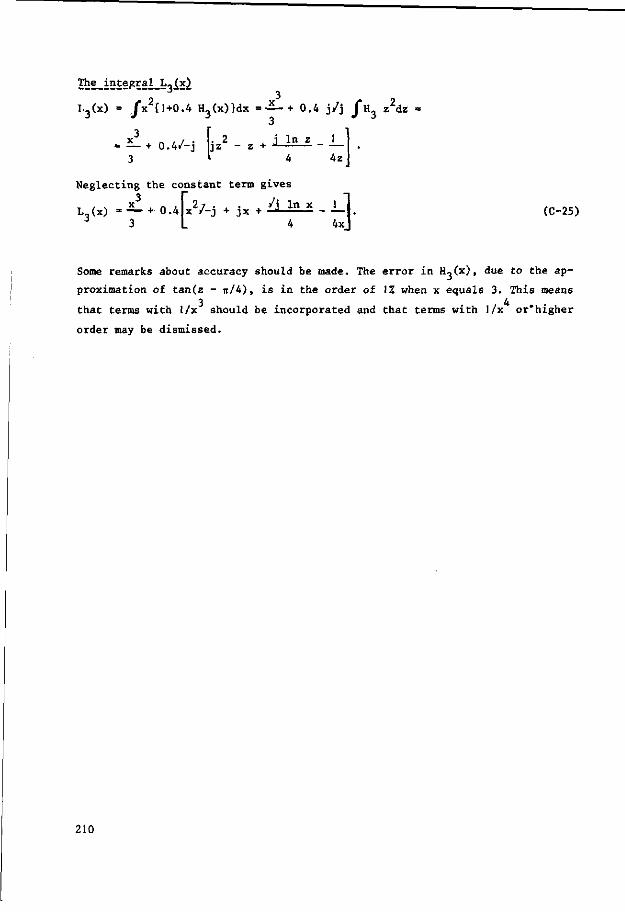
The i n t e g r a l L ^ x ^

I 3 ( x ) = J"x2{l+0.4 H3(x)}dx = - 2 - + 0.4 j / j J*H3 z2dz

L 3(x) = -S- + 0 . 4 | x V - j + j x + J - — | . (C-25)

Some remarks about accuracy should be made. The error in H,(x), due to the ap­

proximation of tan(z - it/4), is in the order of 1% when x equals 3. This means 3 4

that terms with 1/x should be incorporated and that terms with 1/x or*higher

order may be dismissed.

210

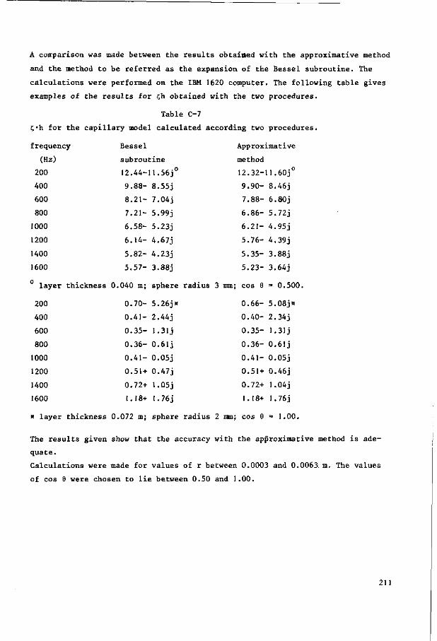
A comparison was made between the results obtained with the approximative method

and the method to be referred as the expansion of the Bessel subroutine. The

calculations were performed on the IBM 1620 computer. The following table gives

examples of the results for Jh obtained with the two procedures.

Table C-7

C"h for the capillary model calculated according two procedures.

Approximative

method

12.32-11.60j°

9 .90- 8.46j

7 .88- 6.80j

6 .86- 5.72j

6 . 2 1 - 4 .95j

5 .76- 4.39J

5 .35- 3.88j

5 . 23 - 3.64J

l ius 3 mm; cos 6 = 0.500.

0.66- 5.08j»

0.40- 2.34j

0.35- 1.31j

0.36- 0.61j

0.41- 0.05j

0.51+ 0.46j

0.72+ 1.04j

1.18+ 1.76j

» layer thickness 0.072 m; sphere radius 2 mm; cos 9 = 1.00.

The results given show that the accuracy with the approximative method is ade­

quate.

Calculations were made for values of r between 0.0003 and 0.0063: m. The values

of cos 6 were chosen to lie between 0.50 and 1.00.

frequency

(Hz)

200

400

600

800

1000

1200

1400

1600

layer thickness

200

400

600

800

1000

1200

1400

1600

Bessel

subroutine

12.44-

9.88-

8.21-

7.21-

6.58-

6.14-

5.82-

5.57-

0.040 m;

0.70-

0.41-

0.35-

0.36-

0.41-

0.51 +

0.72+

1.18+

11.56J0

8.55J

7.04J

5.99J

5.23J

4.67J

4.23J

3.88j

sphere

5.26JH

2.44J

1 -313

0.61J

0.05J

0.47J

1.05J

1.76J

211

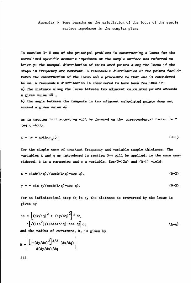
Appendix D Some remarks on the calculation of the locus of the sample

surface impedance in the complex plane

In section 3-10 one of the principal problems in constructing a locus for the

normalized specific acoustic impedance at the sample surface was referred to

briefly: the unequal distribution of calculated points along the locus if the

steps in frequency are constant. A reasonable distribution of the points facili­

tates the construction of the locus and a procedure to that end is considered

below. A reasonable distribution is considered to have been realized if:

a) The distance along the locus between two adjacent calculated points exceeds

a given value ds ,

b) the angle between the tangents in two adjacent calculated points does not

exceed a given value 6$.

As in section 1-11 attention will be focused on the transcendental factor in Z

(eq.(l-65)):

x + jy = coth(y 1 ) , 'D-l)

for the simple case of constant frequency and variable sample thickness. The

variables A and q as introduced in section 3-4 will be applied; in the case con­

sidered, A is a parameter and q a variable. Eqs(3-12a) and (D-l) yield:

x = sinh(A»q)/(cosh(A*q)-cos q) , (D-2)

y = - sin q/(cosh(A'q)-cos q ) . (D"3)

For an infinitesimal step dq in q, the distance ds traversed by the locus is

given by

ds = Kdx/dq)2 + (dy/dq)2]* dq

-[/(l+A2)/(cosh(A-q)-cos q)l dq (D-4>

and the radius of curvature, R, is given by

[n- (dy/dx) 2 ] 3 / 2 (dx/dq)

d(dy/dx)/dq

212

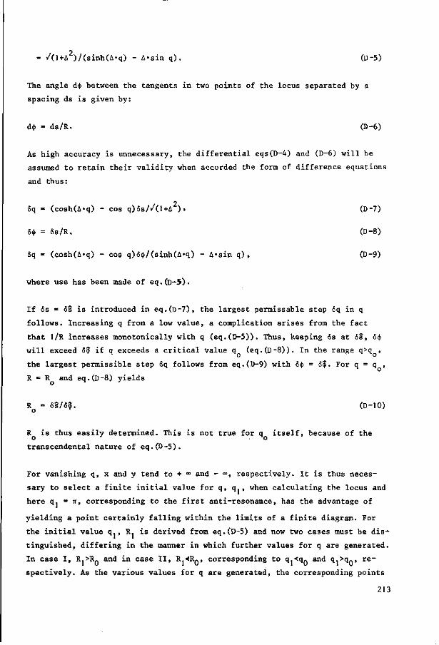
= /(1+A )/(sinh(A-q) - A-sin q) . (D-5)

The angle dij> between the tangents in two points of the locus separated by a

spacing ds is given by:

d<|> = ds/R. (B-6)

As high accuracy is unnecessary, the differential eqs(D-4) and (D-6) will be

assumed to retain their validity when accorded the form of difference equations

and thus:

6q = (cosh(A-q) - cos q)6s//(l+A )» (D-7)

5<|> = 6s/R. (D-8)

6q = (cosh(A»q) - cos q)6<j>/(sinh(A»q) - A«sin q) , (D-9)

where use has been made of eq.(D~5).

If 6s « 6s is introduced in eq.(D-7), the largest permissable step 6q in q

follows. Increasing q from a low value, a complication arises from the fact

that l/R increases monotonically with q (eq.(D-5)). Thus, keeping 6s at 6s, 6<j>

will exceed 6$ if q exceeds a critical value q (eq.(D-8)). In the range q>q ,

the largest permissible step 6q follows from eq.(D-9) with 6ij> = 6$. For q = q ,

R = R and eq.(D-8) yields

R = 6s/6$. (D-10) o

R is thus easily determined. This is not true for q itself, because of the o ' Mo

transcendental nature of eq.(D-5).

For vanishing q, x and y tend to + "» and - °°, respectively. It is thus neces­

sary to select a finite initial value for q, q., when calculating the locus and

here q. = TT, corresponding to the first anti-resonance, has the advantage of

yielding a point certainly falling within the limits of a finite diagram. For

the initial value q. , R. is derived from eq.(S>-5) and now two cases must be dis­

tinguished, differing in the manner in which further values for q are generated.

In case I, R,5"^ and in case II, R.<R0, corresponding to q.<qn and q.>qn, re­

spectively. As the various values for q are generated, the corresponding points

213

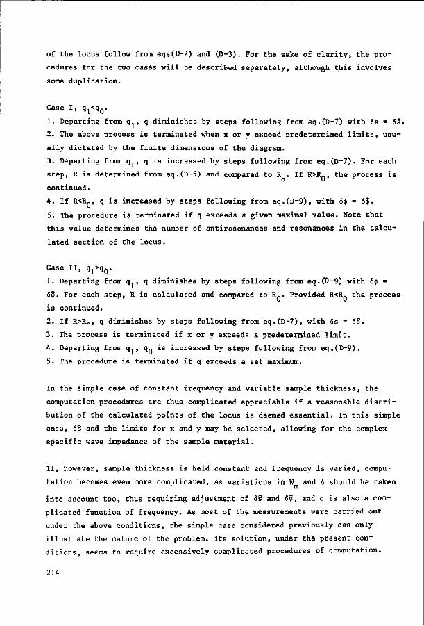
of the locus follow from eqs(D-2) and (D-3). For the sake of clarity, the pro­

cedures for the two cases will be described separately, although this involves

some duplication.

Case I, q,<q0.

1. Departing from q. , q diminishes by steps following from eq.(D-7) with 6s = 6s.

2. The above process is terminated when x or y exceed predetermined limits, uou-

ally dictated by the finite dimensions of the diagram.

3. Departing from q., q is increased by steps following from eq.(D-7). For each

step, R is determined from eq.(D-5) and compared to R . If R>Rn, the process is

continued.

4. If R^ni q is increased by steps following from eq.(D-9), with 5<(i = 6$.

5. The procedure is terminated if q exceeds a given maximal value. Note that

this value determines the number of antiresonances and resonances in the calcu­

lated section of the locus.

Case II, q,>qn.

1. Departing from q. , q diminishes by steps following from eq.(B-9) with 6(j> •

5$. For each step, R is calculated and compared to R-. Provided R<Rn the process

is continued.

2. If R>Rrt, q diminishes by steps following from eq.(D-7), with 6s = 6s.

3. The process is terminated if x or y exceeds a predetermined limit.

4. Departing from q. , q0 is increased by steps following from eq.(D-9).

5. The procedure is terminated if q exceeds a set maximum.

In the simple case of constant frequency and variable sample thickness, the

computation procedures are thus complicated appreciable if a reasonable distri­

bution of the calculated points of the locus is deemed essential. In this simple

case, 6s and the limits for x and y may be selected, allowing for the complex

specific wave impedance of the sample material.

If, however, sample thickness is held constant and frequency is varied, compu­

tation becomes even more complicated, as variations in W and A should be taken m

into account too, thus requiring adjustment of 6s and 6$, and q is also a com­

plicated function of frequency. As most of the measurements were carried out

under the above conditions, the simple case considered previously can only

illustrate the nature of the problem. Its solution, under the present con­

ditions, seems to require excessively complicated procedures of computation.

214

Acknowledgments

The present work was carried out at the Agricultural University of Wageningen,

The Netherlands. The author is greatly indebted to Ir. D.W. van Wulfften Palthe,

lecturer at the Delft University of Technology, under whose direction the

theories were developed and the experiments carried out.

215