Small Particle Transport in Fibrin Gels and High Throughput ...

Small Particle Transport in Fibrin Gels

andHigh Throughput Clot Characterization

byRichard Chasen Spero

A dissertation submitted to the faculty of the University of North Carolina at ChapelHill in partial fulfillment of the requirements for the degree of Doctor of Philosophy inthe Department of Physics and Astronomy.

Chapel Hill2010

Approved by:

Richard Superfine, Advisor

Michael R. Falvo, Reader

M. Gregory Forest, Reader

Leandra Vicci, Reader

Sean Washburn, Reader

Alisa S. Wolberg, Reader

c○ 2010

Richard Chasen Spero

ALL RIGHTS RESERVED

ii

This dissertation is dedicated to my father

without whom I certainly would

not have pursued this degree,

for better or worse.

It could have been, I am sure, much worse.

iii

ABSTRACTRICHARD CHASEN SPERO: Small Particle Transport in Fibrin Gels

andHigh Throughput Clot Characterization.

(Under the direction of Richard Superfine.)

The formation, function, and lysis of blood clots is largely governed by the trans-

port of nano- and micro-scale particles. Yet there is not fully established physics that

relates clot structure to transport phenomena such as fluid permeation and particle

diffusion. This dissertation explores small particle transport in fibrin. I report on

the size-dependence of particle mobility in fibrin, and discuss the implications of these

results for fibrinolytic drug design. I measure the relationship between fibrin permeabil-

ity and diffusion of 0.2–2.8 micron particles in fibrin gels, then determine the time and

length scales at which small particle diffusion is directly related to bulk gel permeabil-

ity. This result implies that one could develop a high throughput clot characterization

assay that provides more detail than turbidity, the predominant high throughput mea-

surement. I also present my work designing and developing systems to perform these

and other experiments in high throughput, which include novel technologies for optical

microscopy and magnetic force application.

iv

ACKNOWLEDGMENTS

Graduate work is professional training, so my thanks are due first to the trainers.In particular, Rich Superfine, Leandra Vicci, and Russ Taylor have packed the lastfive years with endless lessons—intentional and accidental, direct and indirect—in theproper conduct and professional execution of science, engineering, and management. Ihave learned a broader swath of these arts over these years than I can imagine havingequaled by any other endeavor, and for that privilege I am most grateful.

Graduate study is work, and other hands’ fingerprints cover too much in this dis-sertation to thank them all here; I have noted their contributions throughout the text.But I must thank especially the relentlessly productive David Bober and the endlesslyresilient Rachel Sircar, both of whom were always paddling whether or not I had mysenses at the till. There is also NSRG’s Matlab master, the goop king Jeremy Cribb,whose handiwork was never far below the surface of mine, and on whose shoulders Ihave spent much of my time attempting to perch.

Then there is what graduate school was not: it was not more than the hours I spentat it, not more than the education and opportunities and friends I gained, not my wholelife. That is the purview of my best friend, my wife, my best reason for doing anythingworth doing. Julie, I love you.

v

Contents

1 Introduction 11.1 Coagulation and Transport . . . . . . . . . . . . . . . . . . . . . . . . . 3

1.1.1 Studying clot transport . . . . . . . . . . . . . . . . . . . . . . . 51.2 Scope of this Research . . . . . . . . . . . . . . . . . . . . . . . . . . . 8

2 Transport in Fibrin: Theory 112.1 Expectations for particle motion in fibrin . . . . . . . . . . . . . . . . . 12

2.1.1 Single Particle Diffusion . . . . . . . . . . . . . . . . . . . . . . 122.1.2 Assumptions for fibrin modeling . . . . . . . . . . . . . . . . . . 152.1.3 Steric diffusion suppression . . . . . . . . . . . . . . . . . . . . . 182.1.4 Hydrodynamic diffusion suppression . . . . . . . . . . . . . . . . 212.1.5 Expectations for data . . . . . . . . . . . . . . . . . . . . . . . . 23

2.2 Fibrin Structure and Particle Diffusion . . . . . . . . . . . . . . . . . . 252.2.1 Ogston Model: diffusion with steric hinderance . . . . . . . . . 252.2.2 Phillips Model: a numerical solution . . . . . . . . . . . . . . . 27

2.3 Fibrin Structure and Hydraulic Permeability . . . . . . . . . . . . . . . 292.3.1 Darcy Theory . . . . . . . . . . . . . . . . . . . . . . . . . . . . 292.3.2 Carman-Kozeny relation . . . . . . . . . . . . . . . . . . . . . . 302.3.3 Fibrous media: Jackson-James and Davies equations . . . . . . 322.3.4 Permeability and turbidity . . . . . . . . . . . . . . . . . . . . . 34

2.4 Diffusion and Permeability . . . . . . . . . . . . . . . . . . . . . . . . . 382.4.1 Effective medium theory . . . . . . . . . . . . . . . . . . . . . . 40

2.5 Conclusion . . . . . . . . . . . . . . . . . . . . . . . . . . . . . . . . . . 41

3 Transport in Fibrin: Experiments 433.1 Measuring nanoparticle diffusion . . . . . . . . . . . . . . . . . . . . . . 44

3.1.1 Diffusion in fibrin is size-dependent and bimodal . . . . . . . . . 463.1.2 Sensitivity to clot structure . . . . . . . . . . . . . . . . . . . . 493.1.3 Long-time diffusion . . . . . . . . . . . . . . . . . . . . . . . . . 52

3.2 Clot permeability . . . . . . . . . . . . . . . . . . . . . . . . . . . . . . 533.2.1 Applicability of effective medium theory . . . . . . . . . . . . . 55

vi

3.2.2 Measuring permeability with effective medium theory . . . . . . 563.3 Discussion . . . . . . . . . . . . . . . . . . . . . . . . . . . . . . . . . . 59

3.3.1 Diffusion and permeability as a measurement of clot structure . 593.3.2 Diffusion as a guide for drug design . . . . . . . . . . . . . . . . 63

4 The Bead’s-eye View 654.1 Stuck particles . . . . . . . . . . . . . . . . . . . . . . . . . . . . . . . 654.2 Fibrin elasticity . . . . . . . . . . . . . . . . . . . . . . . . . . . . . . . 704.3 Future Directions . . . . . . . . . . . . . . . . . . . . . . . . . . . . . . 744.4 Conclusions . . . . . . . . . . . . . . . . . . . . . . . . . . . . . . . . . 74

5 Toward High Throughput 765.1 Panoptes: High Throughput Video Acquisition . . . . . . . . . . . . . . 79

5.1.1 Image quality: NA and z-focus . . . . . . . . . . . . . . . . . . 805.1.2 Imaging modes: brightfield and fluorescence . . . . . . . . . . . 825.1.3 Image quality and particle tracking signal-to-noise . . . . . . . . 87

5.2 Transitioning to High Throughput Protocols . . . . . . . . . . . . . . . 905.2.1 Data pathologies in fibrin diffusion measurements . . . . . . . . 915.2.2 DataBrowser . . . . . . . . . . . . . . . . . . . . . . . . . . . . 94

5.3 MHTS: High Throughput Manipulation . . . . . . . . . . . . . . . . . . 975.3.1 MHTS Design . . . . . . . . . . . . . . . . . . . . . . . . . . . . 985.3.2 MHTS Calibration . . . . . . . . . . . . . . . . . . . . . . . . . 1035.3.3 MHTS Application: Cell Mechanics . . . . . . . . . . . . . . . . 1055.3.4 MHTS Application: Mucus Viscometry . . . . . . . . . . . . . . 108

5.4 Governing Equations for MHTS Operation . . . . . . . . . . . . . . . . 1095.4.1 Calibration planning . . . . . . . . . . . . . . . . . . . . . . . . 1095.4.2 Planning strain stiffening measurements . . . . . . . . . . . . . 1165.4.3 Planning shear thinning measurements . . . . . . . . . . . . . . 118

5.5 High Throughput Data Collection . . . . . . . . . . . . . . . . . . . . . 1195.6 Conclusions . . . . . . . . . . . . . . . . . . . . . . . . . . . . . . . . . 119

A Experimental Protocols for Diffusion, Structure, and Permeability 122A.1 Clot preparation and Video Acquisition . . . . . . . . . . . . . . . . . . 122A.2 Automatic particle tracking and data filtering . . . . . . . . . . . . . . 123A.3 Calculation of diffusion coefficient . . . . . . . . . . . . . . . . . . . . . 123A.4 PEG Particle Preparation . . . . . . . . . . . . . . . . . . . . . . . . . 124A.5 Structure and Permeability . . . . . . . . . . . . . . . . . . . . . . . . . 124

B Panoptes Bill of Materials 125

C Panoptes Parts Schematics 126

D Metadata Types 129

vii

List of Figures

2.1 Defining typical clot phenotypes . . . . . . . . . . . . . . . . . . . . . . 152.2 Confocal microscopy of clot types studied . . . . . . . . . . . . . . . . . 162.3 Understanding steric diffusion suppression . . . . . . . . . . . . . . . . 192.4 Understanding Hydrodynamic diffusion suppression . . . . . . . . . . . 222.5 Expectations for diffusion experiments in fibrin . . . . . . . . . . . . . 242.6 The Ogston and Phillips models of diffusion suppression . . . . . . . . 262.7 Theories that predict gel permeability from structure . . . . . . . . . . 312.8 Interpreting turbidity to predict permeability . . . . . . . . . . . . . . 372.9 Summary of theoretical models . . . . . . . . . . . . . . . . . . . . . . 42

3.1 Overview of diffusion experiments in fibrin . . . . . . . . . . . . . . . . 453.2 Data analysis steps for fibrin diffusion data . . . . . . . . . . . . . . . . 463.3 Bimodality of diffusive behavior: α histograms . . . . . . . . . . . . . . 473.4 Size dependence of particle diffusion in fibrin . . . . . . . . . . . . . . . 473.5 Turbidity of fibrin . . . . . . . . . . . . . . . . . . . . . . . . . . . . . . 483.6 Deff two sizes of particles in various types of clots . . . . . . . . . . . . 503.7 Affect of particle presence on gel formation . . . . . . . . . . . . . . . . 513.8 Long-time diffusion of particles in fibrin . . . . . . . . . . . . . . . . . . 533.9 Overview of permeability experiments in fibrin . . . . . . . . . . . . . . 543.10 Fibrin permeability . . . . . . . . . . . . . . . . . . . . . . . . . . . . . 543.11 Verification of the effective medium theory . . . . . . . . . . . . . . . . 553.12 Scaled cartoon of 〈r2〉(τ) for comparing diffusion regimes across polymer

gels . . . . . . . . . . . . . . . . . . . . . . . . . . . . . . . . . . . . . . 573.13 Measuring fibrin permeability from diffusion . . . . . . . . . . . . . . . 583.14 Interpreting gel structure from transport measurements . . . . . . . . . 603.15 Cartoon of a large nanoparticle being used as a drug vector . . . . . . . 64

4.1 Overview of magnetic force experiments in fibrin . . . . . . . . . . . . . 664.2 Particle trajectories for magnetic force experiments . . . . . . . . . . . 674.3 Net particle travel: PEG vs. COOH particles . . . . . . . . . . . . . . 684.4 Storage modulus for fibrin: CAP vs. MHTS . . . . . . . . . . . . . . . 724.5 Measuring clot formation by microrheology . . . . . . . . . . . . . . . . 73

viii

4.6 Future directions: permeability and particle transport flowcell concept . 75

5.1 Panoptes optical path . . . . . . . . . . . . . . . . . . . . . . . . . . . . 835.2 Imaging contrast results in Panoptes . . . . . . . . . . . . . . . . . . . 855.3 Samples of cell imaging in Panoptes . . . . . . . . . . . . . . . . . . . . 885.4 Tracking noise measurements in Panoptes . . . . . . . . . . . . . . . . 885.5 Signal-to-noise results for various experiments in Panoptes . . . . . . . 905.6 Diffusion experiments workflow . . . . . . . . . . . . . . . . . . . . . . 925.7 Pathologies in auto-tracking . . . . . . . . . . . . . . . . . . . . . . . . 935.8 Databrowser, a data analysis and processing application . . . . . . . . 955.9 Cartoon of a magnetic force system . . . . . . . . . . . . . . . . . . . . 995.10 MHTS magnetics block schematic . . . . . . . . . . . . . . . . . . . . . 1005.11 Magnetic microplate fabrication . . . . . . . . . . . . . . . . . . . . . . 1015.12 Contour plot of an MHTS force calibration . . . . . . . . . . . . . . . . 1035.13 Pictures of the MHTS prototype . . . . . . . . . . . . . . . . . . . . . . 1045.14 Force crosstalk in the MHTS . . . . . . . . . . . . . . . . . . . . . . . . 1045.15 Well-to-well uniformity of force calibration in the MHTS . . . . . . . . 1065.16 Demonstration of a cell mechanics measurement in the MHTS . . . . . 1075.17 Demonstration of mucus viscometry in the MHTS . . . . . . . . . . . . 1095.18 Summary of a force calibration plan in the MHTS . . . . . . . . . . . . 1145.19 Summary of a strain stiffening experiment plan in the MHTS . . . . . . 1175.20 Data workflow for MHTS experiments . . . . . . . . . . . . . . . . . . 1205.21 Systems overview of the MHTS . . . . . . . . . . . . . . . . . . . . . . 121

B.1 Bill of materials for chosen parts. Designs for some components havenot been finalized, so their costs are not yet known. . . . . . . . . . . . 125

C.1 . . . . . . . . . . . . . . . . . . . . . . . . . . . . . . . . . . . . . . . . 126C.2 . . . . . . . . . . . . . . . . . . . . . . . . . . . . . . . . . . . . . . . . 127C.3 . . . . . . . . . . . . . . . . . . . . . . . . . . . . . . . . . . . . . . . . 128

D.1 . . . . . . . . . . . . . . . . . . . . . . . . . . . . . . . . . . . . . . . . 129

ix

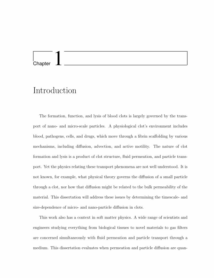
Chapter 1Introduction

The formation, function, and lysis of blood clots is largely governed by the trans-

port of nano- and micro-scale particles. A physiological clot’s environment includes

blood, pathogens, cells, and drugs, which move through a fibrin scaffolding by various

mechanisms, including diffusion, advection, and active motility. The nature of clot

formation and lysis is a product of clot structure, fluid permeation, and particle trans-

port. Yet the physics relating these transport phenomena are not well understood. It is

not known, for example, what physical theory governs the diffusion of a small particle

through a clot, nor how that diffusion might be related to the bulk permeability of the

material. This dissertation will address these issues by determining the timescale- and

size-dependence of micro- and nano-particle diffusion in clots.

This work also has a context in soft matter physics. A wide range of scientists and

engineers studying everything from biological tissues to novel materials to gas filters

are concerned simultaneously with fluid permeation and particle transport through a

medium. This dissertation evaluates when permeation and particle diffusion are quan-

titatively related. I show that the timescale of the diffusion measurement is critical in

establishing this relationship, and thereby explain why prior work attempting to verify

the effective medium theory showed poor agreement with experiment. Validating the

effective medium theory establishes fibrin as a useful model material for studying par-

ticle diffusion over specific time- and length-scale regimes that are difficult to measure

in other materials.

Like most of biology, coagulation is a phenomenon of many input parameters, in-

cluding fibrinogen and thrombin concentration, calcium concentration, ionic strength,

pH, crowding agent concentrations, and genotype. With the advent of siRNA libraries,

one can imagine triggering clotting over a cell culture substrate, systematically knocking

down each of the more than 21,000 human genes to see whether clot structure above the

substrate is affected. Such an experiment would provide an unprecedented panorama

of the genes involved in thrombin generation. Unfortunately, assays that provide de-

tailed characterization of clots are typically low-throughput and labor-intensive. The

techniques of this dissertation promise to provide high throughput characterization of

clot structure, fluid permeation, and particle transport. I report on high throughput

instrumentation that I have designed and developed to enable my experiments. These

systems include an automated microscope built with components that may be tiled up

to 12 times below a conventional microplate, and a multiforce high throughput system

(MHTS) for force application in biophysical experiments. In this dissertation I report

on the design and qualification of these technologies.

This high throughput technology has applications that range far beyond clot char-

2

acterization. High throughput screening is increasingly critical in cell microscopy, but

existing systems suffer from slow 3D imaging, low-bandwidth in time-lapse experiments,

and incompatibility with force application or other mechanical measurements. The high

throughput technology I present in this dissertation addresses these issues.

1.1 Coagulation and Transport

Fibrin is the polymer scaffolding of a blood clot (Weisel, 2005). Damage to the

vascular endothelium1 reveals tissue factor, which triggers a cascade of reactions culmi-

nating in the conversion of prothrombin to thrombin. Thrombin activates fibrinogen, a

340kDa glycoprotein that is always present in healthy blood. An activated fibrinogen

molecule is called a fibrin monomer, which in sufficient concentration self-assembles

into a fibrous gel. Physiologically, fibrin gels nucleate from activated platelets or the

endothelium, ultimately sealing vascular breaches and restoring haemostasis. Clots are

broken down when tissue Plasminogen activator (tPA) converts plasminogen—another

protein endemic to blood—to plasmin, the factor that begins fibrinolysis (fibrin diges-

tion) and therefore limits clot lifetime within the vasculature.

When it functions properly, therefore, clotting is essential to health. Yet because

pathological clotting is the central risk of cardiovascular disease, it is also the top

contributor to the global burden of disease (WHO, 2004), whether through an occlusive

thrombus2 triggering myocardial infarction3, or a deep vein thrombus that dislodges

1vascular endothelium: the cells of the blood vessel wall2thrombus: clot formation within the vasculature3mycardial infarction: heart attack

3

and results in pulmonary embolism4. These conditions arise from unwanted clotting;

failure to clot is similarly dangerous, as in hemophilia (Rodriguez-Merchan et al., 2000).

One might separate the requirements for clotting—both hemostatic (good) and

pathological (bad)—into the biochemical and the physical. The biochemical require-

ment is simply that to achieve coagulation there must be thrombin to activate fib-

rinogen, and that for lysis there must be plasmin to cleave fibrin. Hemophilia is an

example of a clotting pathology that is biochemical: this genetic disorder results in low

expression of Factors VIII or IX, both of which are involved in thrombin generation.

The physical requirement is that the factors must be at the sample location for suffi-

cient time to allow the reactions to occur. For example, thrombin is created when freely

circulating prothrombin is activated, near cells or platelets, by a complex of factors Va

and Xa. To achieve clotting, therefore, fibrinogen must come to these locations, or

thrombin must move away from them. Not surprisingly, then, the geometry of throm-

bin generation has an impact on gel structure (Wolberg and Campbell, 2008). Similarly,

to achieve clot lysis, plasminogen must encounter tPA to become plasmin, and must

then destroy the clot from the outside in, or travel into it; hence, the ability of a clot to

allow transport has an effect on the time required to dismantle it (Veklich et al., 1998).

Heart disease has been correlated to tight and rigid clots (Fatah et al., 1996), so clot

geometry is intimately tied with the difficulty in treating patients suffering myocardial

infarction due to thrombosis.

The physics of clotting includes kinetic considerations. The faster blood flows,

4pulmonary embolism: a thrombus that breaks free from a vessel wall and lodges in the lung

4

the less conducive the environment is to clotting. This is demonstrated at formation,

where poor circulation is a risk factor for deep vein thrombosis, and at lysis, where

forced perfusion is a common (and painful) treatment (Wicky, 2009). This treatment is

used because increasing gel perfusion accelerates clot destruction (Diamond and Anand,

1993).

The coincidence of clotting agents and the time that they have to interact are deter-

mined by transport of blood and the biochemical factors therein. Transport is therefore

a key issue in clotting pathology and treatment, including transport of coagulation fac-

tors, which must be present only in the locations where clotting is desired, and also

transport of blood itself, which must stay contained, yet circulate freely, within the

vasculature.

1.1.1 Studying clot transport

Clot transport in vivo is the product of five (often simultaneous) phenomena: dif-

fusion, advection, steric hinderance, hydrodynamics, and chemical interaction. All

objects in solution are subject to thermal diffusion, the random motion of particles due

to the non-zero net impulse of many random collisions with solvent molecules. Because

blood is pumped by the heart, objects in clots also experience advection, the transport

of a particle being carried by local solvent flow. The presence of solid barriers, including

the endothelium and the fibrin mesh, hinder objects’ transport by steric interaction,

the physical exclusion of a particle from space filled with other solid matter. These

solid barriers place boundary conditions on the solvent, so objects may experience an

5

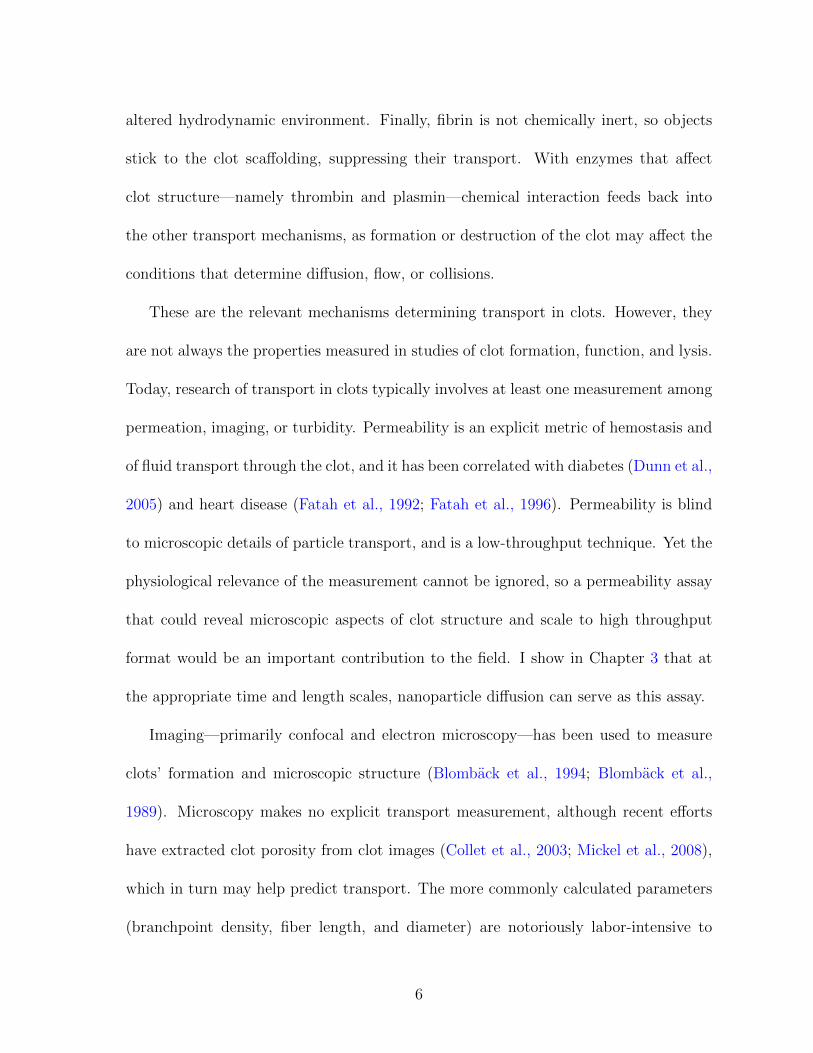
altered hydrodynamic environment. Finally, fibrin is not chemically inert, so objects

stick to the clot scaffolding, suppressing their transport. With enzymes that affect

clot structure—namely thrombin and plasmin—chemical interaction feeds back into

the other transport mechanisms, as formation or destruction of the clot may affect the

conditions that determine diffusion, flow, or collisions.

These are the relevant mechanisms determining transport in clots. However, they

are not always the properties measured in studies of clot formation, function, and lysis.

Today, research of transport in clots typically involves at least one measurement among

permeation, imaging, or turbidity. Permeability is an explicit metric of hemostasis and

of fluid transport through the clot, and it has been correlated with diabetes (Dunn et al.,

2005) and heart disease (Fatah et al., 1992; Fatah et al., 1996). Permeability is blind

to microscopic details of particle transport, and is a low-throughput technique. Yet the

physiological relevance of the measurement cannot be ignored, so a permeability assay

that could reveal microscopic aspects of clot structure and scale to high throughput

format would be an important contribution to the field. I show in Chapter 3 that at

the appropriate time and length scales, nanoparticle diffusion can serve as this assay.

Imaging—primarily confocal and electron microscopy—has been used to measure

clots’ formation and microscopic structure (Blomback et al., 1994; Blomback et al.,

1989). Microscopy makes no explicit transport measurement, although recent efforts

have extracted clot porosity from clot images (Collet et al., 2003; Mickel et al., 2008),

which in turn may help predict transport. The more commonly calculated parameters

(branchpoint density, fiber length, and diameter) are notoriously labor-intensive to

6

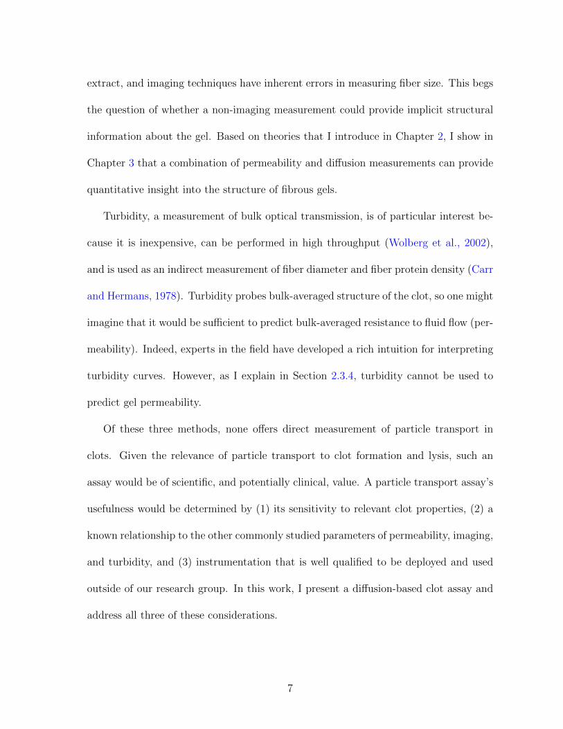
extract, and imaging techniques have inherent errors in measuring fiber size. This begs

the question of whether a non-imaging measurement could provide implicit structural

information about the gel. Based on theories that I introduce in Chapter 2, I show in

Chapter 3 that a combination of permeability and diffusion measurements can provide

quantitative insight into the structure of fibrous gels.

Turbidity, a measurement of bulk optical transmission, is of particular interest be-

cause it is inexpensive, can be performed in high throughput (Wolberg et al., 2002),

and is used as an indirect measurement of fiber diameter and fiber protein density (Carr

and Hermans, 1978). Turbidity probes bulk-averaged structure of the clot, so one might

imagine that it would be sufficient to predict bulk-averaged resistance to fluid flow (per-

meability). Indeed, experts in the field have developed a rich intuition for interpreting

turbidity curves. However, as I explain in Section 2.3.4, turbidity cannot be used to

predict gel permeability.

Of these three methods, none offers direct measurement of particle transport in

clots. Given the relevance of particle transport to clot formation and lysis, such an

assay would be of scientific, and potentially clinical, value. A particle transport assay’s

usefulness would be determined by (1) its sensitivity to relevant clot properties, (2) a

known relationship to the other commonly studied parameters of permeability, imaging,

and turbidity, and (3) instrumentation that is well qualified to be deployed and used

outside of our research group. In this work, I present a diffusion-based clot assay and

address all three of these considerations.

7

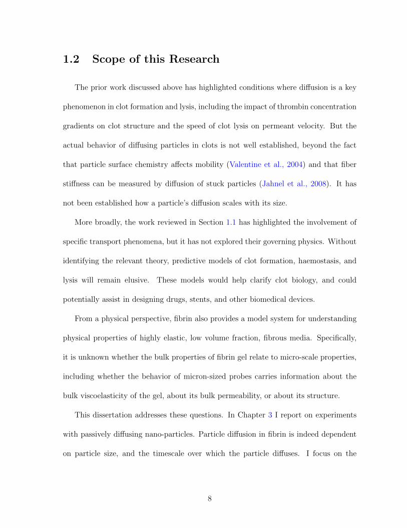
1.2 Scope of this Research

The prior work discussed above has highlighted conditions where diffusion is a key

phenomenon in clot formation and lysis, including the impact of thrombin concentration

gradients on clot structure and the speed of clot lysis on permeant velocity. But the

actual behavior of diffusing particles in clots is not well established, beyond the fact

that particle surface chemistry affects mobility (Valentine et al., 2004) and that fiber

stiffness can be measured by diffusion of stuck particles (Jahnel et al., 2008). It has

not been established how a particle’s diffusion scales with its size.

More broadly, the work reviewed in Section 1.1 has highlighted the involvement of

specific transport phenomena, but it has not explored their governing physics. Without

identifying the relevant theory, predictive models of clot formation, haemostasis, and

lysis will remain elusive. These models would help clarify clot biology, and could

potentially assist in designing drugs, stents, and other biomedical devices.

From a physical perspective, fibrin also provides a model system for understanding

physical properties of highly elastic, low volume fraction, fibrous media. Specifically,

it is unknown whether the bulk properties of fibrin gel relate to micro-scale properties,

including whether the behavior of micron-sized probes carries information about the

bulk viscoelasticity of the gel, about its bulk permeability, or about its structure.

This dissertation addresses these questions. In Chapter 3 I report on experiments

with passively diffusing nano-particles. Particle diffusion in fibrin is indeed dependent

on particle size, and the timescale over which the particle diffuses. I focus on the

8

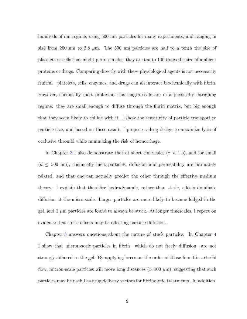
hundreds-of-nm regime, using 500 nm particles for many experiments, and ranging in

size from 200 nm to 2.8 µm. The 500 nm particles are half to a tenth the size of

platelets or cells that might perfuse a clot; they are ten to 100 times the size of ambient

proteins or drugs. Comparing directly with these physiological agents is not necessarily

fruitful—platelets, cells, enzymes, and drugs can all interact biochemically with fibrin.

However, chemically inert probes at this length scale are in a physically intriguing

regime: they are small enough to diffuse through the fibrin matrix, but big enough

that they seem likely to collide with it. I show the sensitivity of particle transport to

particle size, and based on these results I propose a drug design to maximize lysis of

occlusive thrombi while minimizing the risk of hemorrhage.

In Chapter 3 I also demonstrate that at short timescales (τ < 1 s), and for small

(d ≤ 500 nm), chemically inert particles, diffusion and permeability are intimately

related, and that one can actually predict the other through the effective medium

theory. I explain that therefore hydrodynamic, rather than steric, effects dominate

diffusion at the micro-scale. Larger particles are more likely to become lodged in the

gel, and 1 µm particles are found to always be stuck. At longer timescales, I report on

evidence that steric effects may be affecting particle diffusion.

Chapter 3 answers questions about the nature of stuck particles. In Chapter 4

I show that micron-scale particles in fibrin—which do not freely diffusion—are not

strongly adhered to the gel. By applying forces on the order of those found in arterial

flow, micron-scale particles will move long distances (> 100 µm), suggesting that such

particles may be useful as drug delivery vectors for fibrinolytic treatments. In addition,

9

I show that for particles at least 2.8 µm and smaller, driven micro-rheology measures a

local mechanical property of the clot, rather than the bulk viscoelastic properties of the

gel, and that it can measure time-dependent stiffening of fibrin during clot formation.

In addition to my scientific work focused on fibrin and other fibrous gels, I have

helped to design, build, and qualify systems for high throughput microscopy, manipu-

lation, and rheology that are designed to address the needs of these and other experi-

ments. They are core technologies for a microrheology and cell screening system that is

presently under development. These systems and my contributions to their realization

are the subject of Chapter 5.

10

Chapter 2Transport in Fibrin: Theory

When particles move in clots, what phenomena are at play? The physical environ-

ment for diffusing particles, and the fluidic environment during permeation, are not

well understood in clots. In this Chapter, I begin with the impact a gel is expected

to have on a diffusing particle and on a permeating fluid. The presence of a gel will

impose boundary conditions on the fluid, as well as on the particle motion. I determine

the relevant length and timescales for these effects.

In the remainder of this Chapter I explore the relationship of gel structure to trans-

port. Imaging has been used to extract gel structure, including fiber density (Campbell

et al., 2008), branchpoint density (Ryan et al., 1999), and gel porosity (Mickel et al.,

2008). However, this information has not been used to test the quantitative theories

that use these structural parameters to predict particle diffusion or fluid permeation.

Therefore, I will spend some pages looking in detail at the theoretical relationships

among structure, permeation, and particle transport. The goal of this Chapter is to

clarify what theories exist, which might be relevant in fibrin modeling, and how using

one theory might help validate or invalidate the applicability of others.

2.1 Expectations for particle motion in fibrin

2.1.1 Single Particle Diffusion

In classical physics, diffusion was understood through the lens of Fick’s laws, which

described the phenomenon in terms of concentration gradients (Cussler, 1997). It was

Einstein who provided the physical explanation for single particle diffusion (Einstein,

1905), often called Brownian motion. This explanation is captured in the Stokes-

Einstein relation, which states that for a sphere of diameter d in a fluid of viscosity

η,

D =kBT

f=

kBT

3πηd, (2.1)

where kB and T are Boltzmann’s constant and absolute temperature, respectively. D is

the diffusion coefficient of the material. For aspherical solutes, the denominator f may

be replaced by the Stokes drag formula (Happel and Brenner, 1983) for that geometry.

Einstein noted that D determines the time-averaged position of the particle

〈r2〉 = 4Dτ, (2.2)

12

where 〈r2〉 is mean squared displacement, and τ is the time between position mea-

surements during which the particle diffuses. Einstein also explained that the D of

Equation 2.1 can explain the bulk diffusion of Fick’s Laws, provided that material is

homogeneous and invariant in time.

While for many natural and engineered systems homogeneity and stasis are ap-

propriate assumptions, for biological systems it is rarely appropriate to apply either.

First, polymers are typically viscoelastic—namely, under stress they exhibit frequency-

dependent frictional loss and elastic energy storage (Ferry, 1980). Polymer solutions are

spatially heterogeneous on certain length scales, and the interaction of polymer chains

with suspended particles depends on the size of the particles, the physical parameters

of the chain (chain length and flexibility), and the nature of the solution (the quality of

the solvent and the concentration of polymer) (Rubinstein and Colby, 2003). Biological

materials can be even more heterogeneous; for example, mucus comprises pathogens

and particulates suspended amidst a solution of polydisperse mucins (Thornton et al.,

2008). Fibrin is viscoelastic (Roberts et al., 1974); it also exhibits temporal hetero-

geneity during clot formation and lysis, and spatial heterogeneity on length scales at

or below the mesh size of the gel.

Measurements of single-particle diffusion, made possible by advances in microscopy

and single-particle tracking, reveal some of these complexities. In homogenous but

viscoelastic materials, it has been observed that diffusion of particles is suppressed on

13

certain timescales such that

〈r2〉 ∝ τα (2.3)

where 0 < α < 1 (Wong et al., 2004). The powerlaw α may not be constant over

all timescales. However, for any range of τ over which α = 1, the average motion is

Brownian. (There are instances where the average motion is Brownian but the step

size distribution is non-gaussian (Wang et al., 2009); in this dissertation, I have seen

no evidence of such an effect.) In such cases it is useful to generalize Equation 2.2 by

taking D → Deff , with the “effective” subscript capturing the concept that the material

appears purely viscous, although no aspect of the particle-polymer-solvent system can

be said truly to have a viscosity corresponding to Deff .

For homogeneous media, variations in α can be explained as the result of frequency-

dependent elastic storage and viscous losses. Mason and Weitz have explained that the

complex modulus G∗(ω) of a bulk material may therefore be extracted from r(t) (Mason

and Weitz, 1995). This approach has since become a key technique in the larger field

of microrheology (Waigh, 2005; Cicuta and Donald, 2007; Kimura, 2009).

Fibrin, however, is not homogeneous on the micron length scale. Therefore, much

of microrheology is not expected to be relevant in this material. To develop a sound

model of transport, we need to be clear about valid assumptions one can make about

the gel.

14

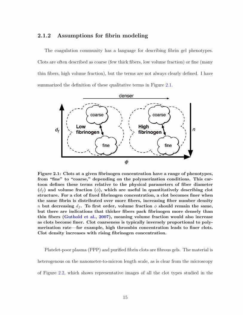
2.1.2 Assumptions for fibrin modeling

The coagulation community has a language for describing fibrin gel phenotypes.

Clots are often described as coarse (few thick fibers, low volume fraction) or fine (many

thin fibers, high volume fraction), but the terms are not always clearly defined. I have

summarized the definition of these qualitative terms in Figure 2.1.

Figure 2.1: Clots at a given fibrinogen concentration have a range of phenotypes,from “fine” to “coarse,” depending on the polymerization conditions. This car-toon defines these terms relative to the physical parameters of fiber diameter(df) and volume fraction (φ), which are useful in quantitatively describing clotstructure. For a clot of fixed fibrinogen concentration, a clot becomes finer whenthe same fibrin is distributed over more fibers, increasing fiber number densityn but decreasing df . To first order, volume fraction φ should remain the same,but there are indications that thicker fibers pack fibrinogen more densely thanthin fibers (Guthold et al., 2007), meaning volume fraction would also increaseas clots become finer. Clot coarseness is typically inversely proportional to poly-merization rate—for example, high thrombin concentration leads to finer clots.Clot density increases with rising fibrinogen concentration.

Platelet-poor plasma (PPP) and purified fibrin clots are fibrous gels. The material is

heterogenous on the nanometer-to-micron length scale, as is clear from the microscopy

of Figure 2.2, which shows representative images of all the clot types studied in the

15

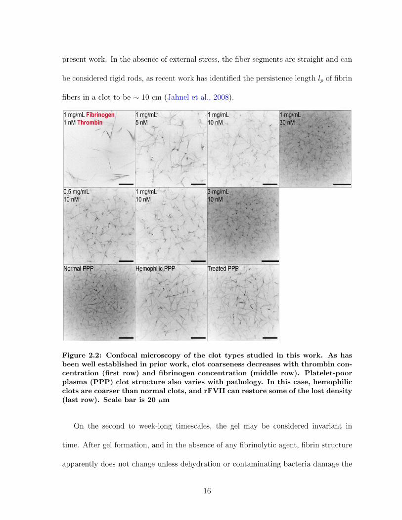
present work. In the absence of external stress, the fiber segments are straight and can

be considered rigid rods, as recent work has identified the persistence length lp of fibrin

fibers in a clot to be ∼ 10 cm (Jahnel et al., 2008).

1 mg/mL Fibrinogen1 nM Thrombin

1 mg/mL5 nM

1 mg/mL10 nM

1 mg/mL30 nM

0.5 mg/mL10 nM

1 mg/mL10 nM

3 mg/mL10 nM

Normal PPP Hemophilic PPP Treated PPP

Figure 2.2: Confocal microscopy of the clot types studied in this work. As hasbeen well established in prior work, clot coarseness decreases with thrombin con-centration (first row) and fibrinogen concentration (middle row). Platelet-poorplasma (PPP) clot structure also varies with pathology. In this case, hemophilicclots are coarser than normal clots, and rFVII can restore some of the lost density(last row). Scale bar is 20 µm

On the second to week-long timescales, the gel may be considered invariant in

time. After gel formation, and in the absence of any fibrinolytic agent, fibrin structure

apparently does not change unless dehydration or contaminating bacteria damage the

16

scaffolding. On minute and second timescales, the gel does not move under confocal

microscopy. From day to day, confocal images of the gel do not change in any discernible

way.

In fibrin networks there is little space that actually contains fibrin, a quality cap-

tured in the gel’s volume fraction, φ. For compacted clots, the densest of the phys-

iological gels, φ < 0.25, while for non-compacted clots, including arterial thrombi,

φ < 0.1 (Diamond, 1999). Clots can be coarse, with few thick (∼ 500 nm) fibers

separated by large (∼ 20 µm) distances, or fine, with many thin (∼ 100 nm) fibers

separated by short (∼ 1 µm) distances. Figure 2.2 indicates that the distance between

fibers can be ∼ 0.1− 10µm.

In spite of this open space, non-specific chemical adhesion of probes to fibrin prevents

long-distance transport of even nanometer-scale probes. Fibrin is notoriously sticky.

It is used as a tissue adhesive (Saxena et al., 2003), and shows non-specific adhesion

to everything from pipette tips to nanoparticles with carboxylate surface chemistry.

Polyethylene glycol (PEG) has been used to reduce, but not eliminate, the likelihood

of nanoparticle adhesion to fibrin (Valentine et al., 2004). Particles (including enzymes

and drugs) diffusing in a physiological clot typically would interact chemically with

fibrin; free diffusion of chemically active particles could be modeled as an equilibrium

between binding and unbinding events. In addition, enzymes such as thrombin and

plasmin are known alter the gel’s structure. In order to focus on the physical inter-

actions at play in nanoparticle diffusion, this dissertation will focus on the motion of

PEG-coated probes that neither stick to nor alter the gel.

17

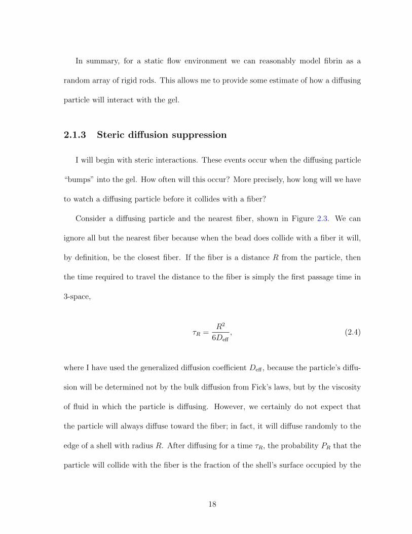
In summary, for a static flow environment we can reasonably model fibrin as a

random array of rigid rods. This allows me to provide some estimate of how a diffusing

particle will interact with the gel.

2.1.3 Steric diffusion suppression

I will begin with steric interactions. These events occur when the diffusing particle

“bumps” into the gel. How often will this occur? More precisely, how long will we have

to watch a diffusing particle before it collides with a fiber?

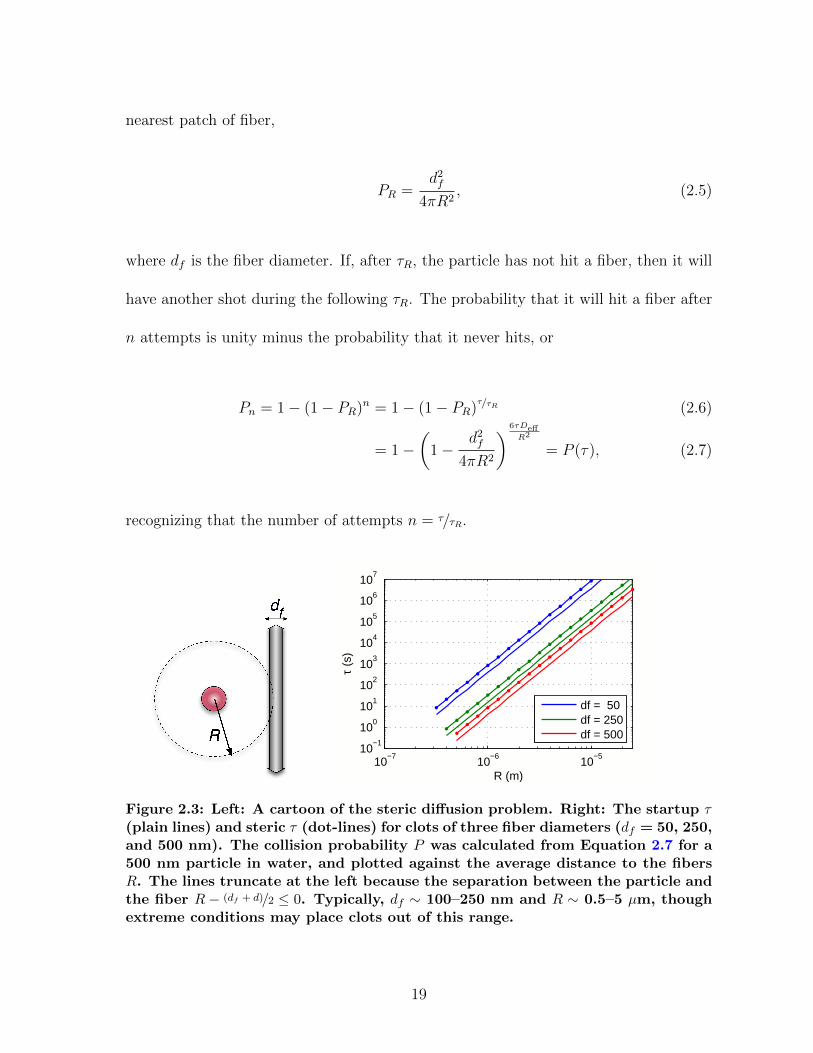
Consider a diffusing particle and the nearest fiber, shown in Figure 2.3. We can

ignore all but the nearest fiber because when the bead does collide with a fiber it will,

by definition, be the closest fiber. If the fiber is a distance R from the particle, then

the time required to travel the distance to the fiber is simply the first passage time in

3-space,

τR =R2

6Deff

, (2.4)

where I have used the generalized diffusion coefficient Deff , because the particle’s diffu-

sion will be determined not by the bulk diffusion from Fick’s laws, but by the viscosity

of fluid in which the particle is diffusing. However, we certainly do not expect that

the particle will always diffuse toward the fiber; in fact, it will diffuse randomly to the

edge of a shell with radius R. After diffusing for a time τR, the probability PR that the

particle will collide with the fiber is the fraction of the shell’s surface occupied by the

18

nearest patch of fiber,

PR =d2f

4πR2, (2.5)

where df is the fiber diameter. If, after τR, the particle has not hit a fiber, then it will

have another shot during the following τR. The probability that it will hit a fiber after

n attempts is unity minus the probability that it never hits, or

Pn = 1− (1− PR)n = 1− (1− PR)τ/τR (2.6)

= 1−(

1−d2f

4πR2

) 6τDeffR2

= P (τ), (2.7)

recognizing that the number of attempts n = τ/τR.

10−7

10−6

10−5

10−1

100

101

102

103

104

105

106

107

R (m)

τ (s

)

df = 50df = 250df = 500

Figure 2.3: Left: A cartoon of the steric diffusion problem. Right: The startup τ(plain lines) and steric τ (dot-lines) for clots of three fiber diameters (df = 50, 250,and 500 nm). The collision probability P was calculated from Equation 2.7 for a500 nm particle in water, and plotted against the average distance to the fibersR. The lines truncate at the left because the separation between the particle andthe fiber R − (df + d)/2 ≤ 0. Typically, df ∼ 100–250 nm and R ∼ 0.5–5 µm, thoughextreme conditions may place clots out of this range.

19

Solving for τ gives the time required to see a collision with probability P :

τ(P ) =R2

6Deff

ln(l − P )

ln(1− d2f

4πR2 )

To estimate the timescale over which a collision will occur, I can solve Equation 2.7 for

P = 1/e and 1− 1/e,

τsteric =−1

ln(1− d2f

4πR2 )

R2

6Deff

(2.8)

τstartup = 0.46 τsteric. (2.9)

I will call these cases the “startup τ” and the “steric τ”, because these are the timescales

at which a steric effect will begin to manifest, and when it will consistently contribute,

respectively.

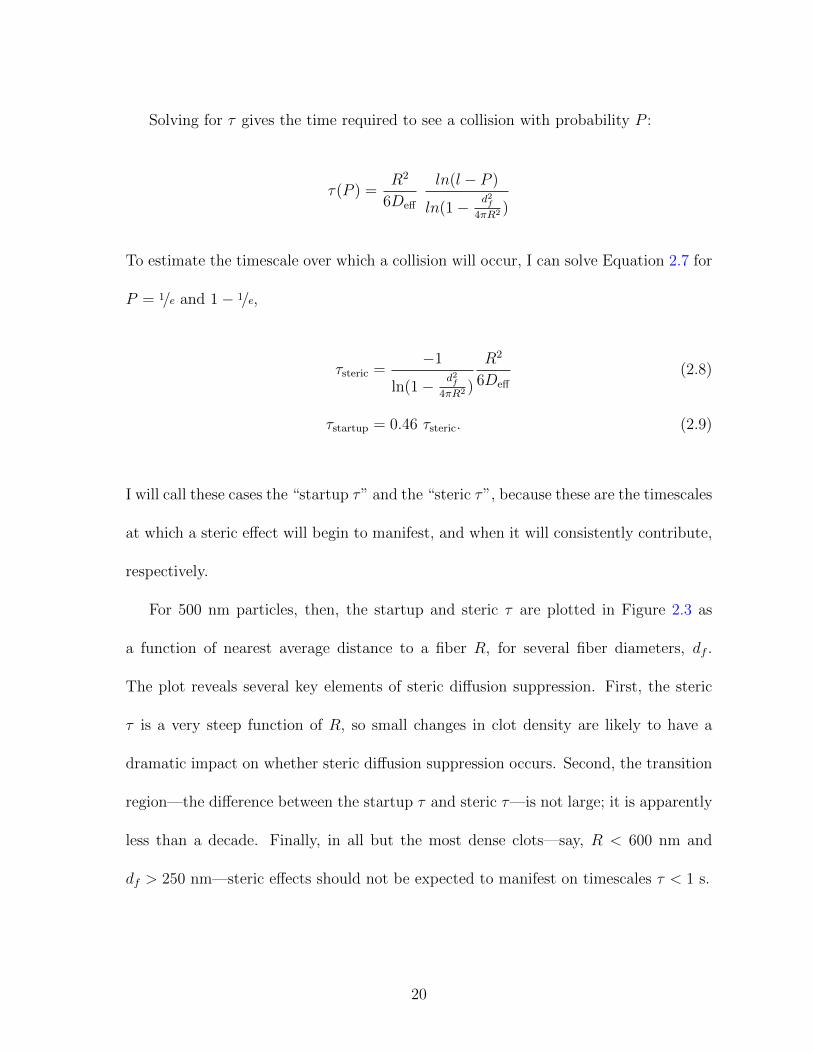
For 500 nm particles, then, the startup and steric τ are plotted in Figure 2.3 as

a function of nearest average distance to a fiber R, for several fiber diameters, df .

The plot reveals several key elements of steric diffusion suppression. First, the steric

τ is a very steep function of R, so small changes in clot density are likely to have a

dramatic impact on whether steric diffusion suppression occurs. Second, the transition

region—the difference between the startup τ and steric τ—is not large; it is apparently

less than a decade. Finally, in all but the most dense clots—say, R < 600 nm and

df > 250 nm—steric effects should not be expected to manifest on timescales τ < 1 s.

20

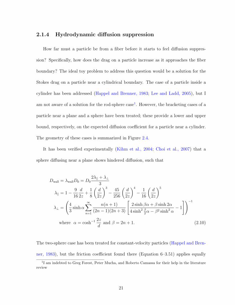
2.1.4 Hydrodynamic diffusion suppression

How far must a particle be from a fiber before it starts to feel diffusion suppres-

sion? Specifically, how does the drag on a particle increase as it approaches the fiber

boundary? The ideal toy problem to address this question would be a solution for the

Stokes drag on a particle near a cylindrical boundary. The case of a particle inside a

cylinder has been addressed (Happel and Brenner, 1983; Lee and Ladd, 2005), but I

am not aware of a solution for the rod-sphere case1. However, the bracketing cases of a

particle near a plane and a sphere have been treated; these provide a lower and upper

bound, respectively, on the expected diffusion coefficient for a particle near a cylinder.

The geometry of these cases is summarized in Figure 2.4.

It has been verified experimentally (Kihm et al., 2004; Choi et al., 2007) that a

sphere diffusing near a plane shows hindered diffusion, such that

Dwall = λwallD0 = D0

2λ|| + λ⊥3

λ|| = 1− 9

16

d

2z+

1

8

(d

2z

)3

− 45

256

(d

2z

)4

− 1

16

(d

2z

)5

λ⊥ =

(4

3sinhα

∞∑n=1

n(n+ 1)

(2n− 1)(2n+ 3)

[2 sinh βα + β sinh 2α

4 sinh2 β2α− β2 sinh2 α

− 1

])−1

where α = cosh−1 2z

dand β = 2n+ 1. (2.10)

The two-sphere case has been treated for constant-velocity particles (Happel and Bren-

ner, 1983), but the friction coefficient found there (Equation 6–3.51) applies equally

1I am indebted to Greg Forest, Peter Mucha, and Roberto Camassa for their help in the literaturereview

21

10−7

10−6

10−5

0

25

50

75

100

R (m)

Def

f/D0 (

%)

df = 50df = 250df = 500

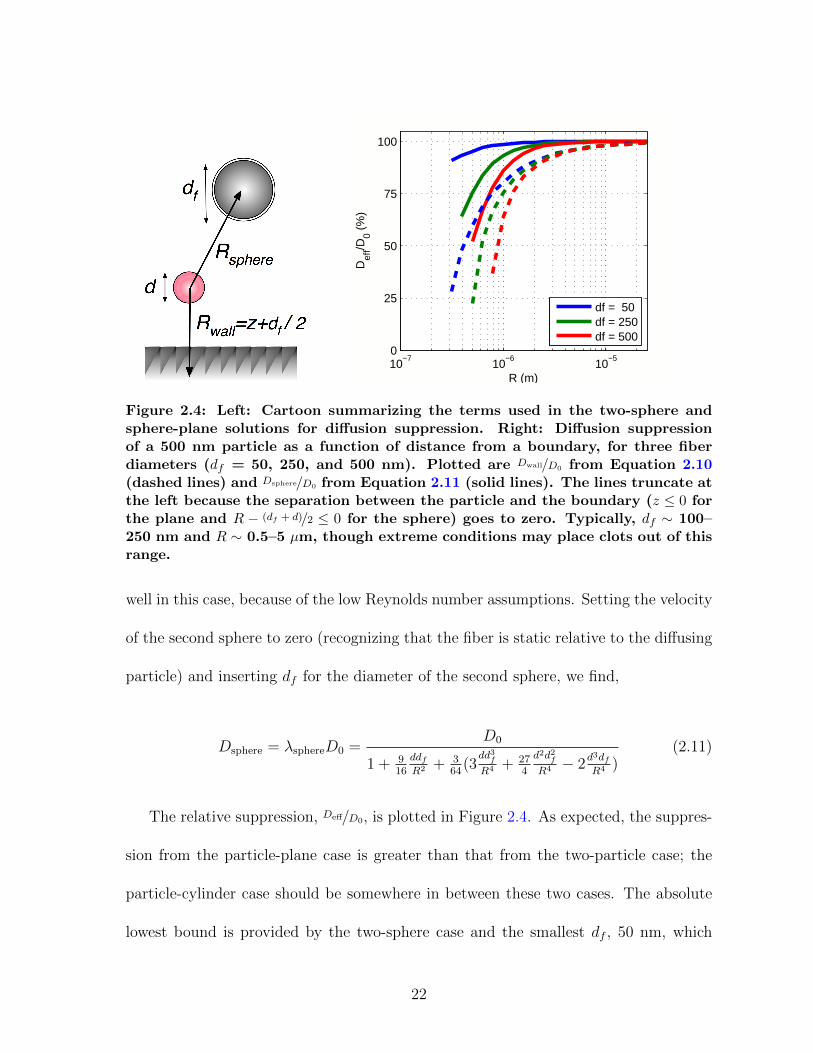
Figure 2.4: Left: Cartoon summarizing the terms used in the two-sphere andsphere-plane solutions for diffusion suppression. Right: Diffusion suppressionof a 500 nm particle as a function of distance from a boundary, for three fiberdiameters (df = 50, 250, and 500 nm). Plotted are Dwall/D0 from Equation 2.10(dashed lines) and Dsphere/D0 from Equation 2.11 (solid lines). The lines truncate atthe left because the separation between the particle and the boundary (z ≤ 0 forthe plane and R − (df + d)/2 ≤ 0 for the sphere) goes to zero. Typically, df ∼ 100–250 nm and R ∼ 0.5–5 µm, though extreme conditions may place clots out of thisrange.

well in this case, because of the low Reynolds number assumptions. Setting the velocity

of the second sphere to zero (recognizing that the fiber is static relative to the diffusing

particle) and inserting df for the diameter of the second sphere, we find,

Dsphere = λsphereD0 =D0

1 + 916

ddfR2 + 3

64(3

dd3f

R4 + 274

d2d2f

R4 − 2d3dfR4 )

(2.11)

The relative suppression, Deff/D0, is plotted in Figure 2.4. As expected, the suppres-

sion from the particle-plane case is greater than that from the two-particle case; the

particle-cylinder case should be somewhere in between these two cases. The absolute

lowest bound is provided by the two-sphere case and the smallest df , 50 nm, which

22

shows that at larger values of R—say, above 1 µm, little hydrodynamic effect should be

visible. While this plot cannot truly predict the diffusion of particles in fibrin, it does

suggest that some level of hydrodynamic diffusion suppression should be expected in

most clots, for four reasons. First, the actual hydrodynamic effect will be more severe

than the two-sphere case. Second, clots typically have fibers thicker than 50 nm. Third,

even in clots where R can be very large—say, 10 µm—the particle will spend some time

closer to the fibers, and the diffusion suppresses rapidly as the particle moves closer to

the boundary. Fourth, the hydrodynamic effect—unlike the steric effect—is additive,

meaning that every fiber contributes to the particle’s friction coefficient, not just the

nearest one.

One final comment on the hydrodynamic effect: while the amount of diffusion sup-

pression a particle will experience changes as a function of the particle’s position, it

will manifest, on average, at all τ . This is in contrast to the steric effect, which will

occur only at and above the timescale over which a particle travels from fiber to fiber.

Therefore, on timescales τ < 1 s I expect we will see only hydrodynamic diffusion

suppression.

2.1.5 Expectations for data

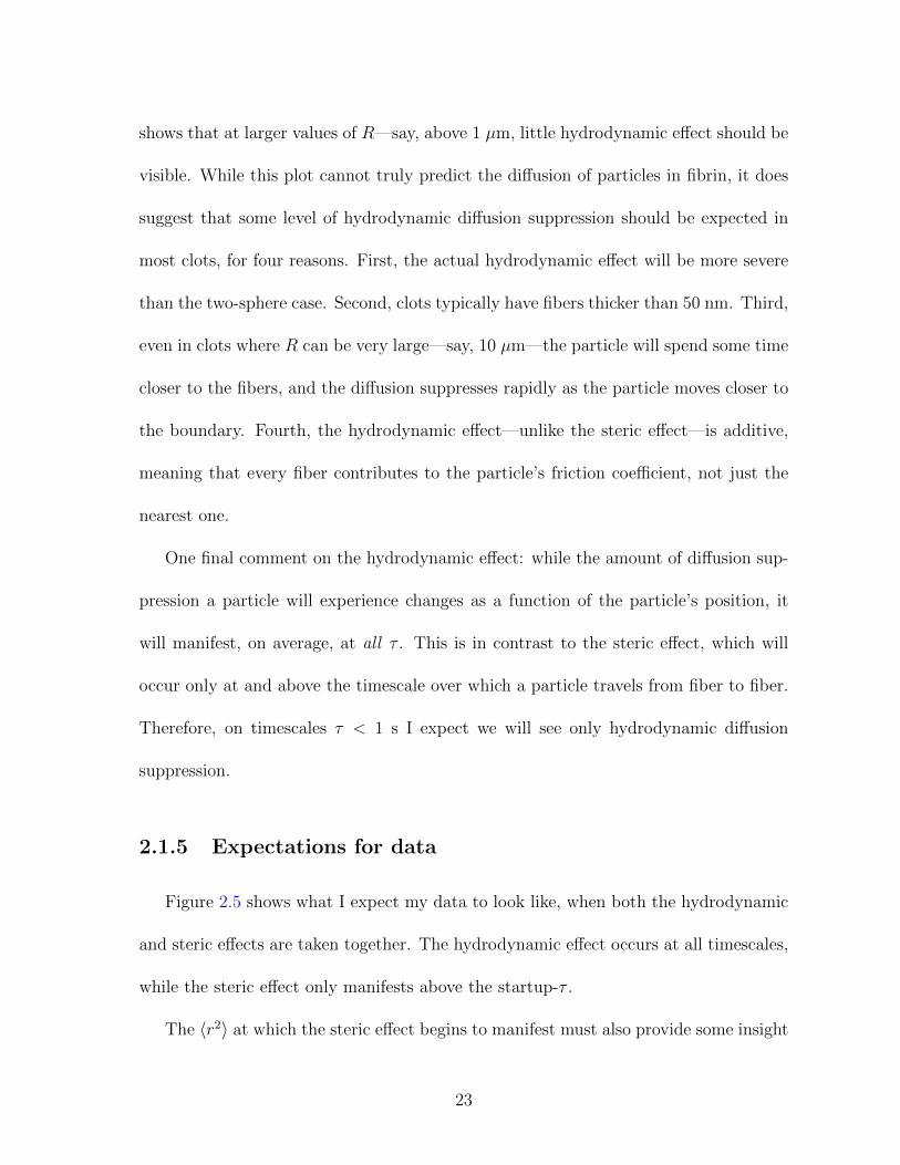
Figure 2.5 shows what I expect my data to look like, when both the hydrodynamic

and steric effects are taken together. The hydrodynamic effect occurs at all timescales,

while the steric effect only manifests above the startup-τ .

The 〈r2〉 at which the steric effect begins to manifest must also provide some insight

23

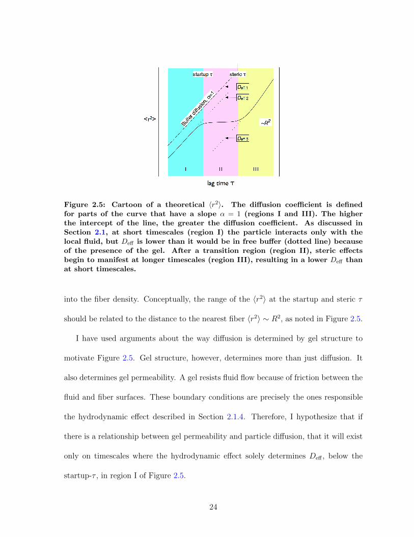
Figure 2.5: Cartoon of a theoretical 〈r2〉. The diffusion coefficient is definedfor parts of the curve that have a slope α = 1 (regions I and III). The higherthe intercept of the line, the greater the diffusion coefficient. As discussed inSection 2.1, at short timescales (region I) the particle interacts only with thelocal fluid, but Deff is lower than it would be in free buffer (dotted line) becauseof the presence of the gel. After a transition region (region II), steric effectsbegin to manifest at longer timescales (region III), resulting in a lower Deff thanat short timescales.

into the fiber density. Conceptually, the range of the 〈r2〉 at the startup and steric τ

should be related to the distance to the nearest fiber 〈r2〉 ∼ R2, as noted in Figure 2.5.

I have used arguments about the way diffusion is determined by gel structure to

motivate Figure 2.5. Gel structure, however, determines more than just diffusion. It

also determines gel permeability. A gel resists fluid flow because of friction between the

fluid and fiber surfaces. These boundary conditions are precisely the ones responsible

the hydrodynamic effect described in Section 2.1.4. Therefore, I hypothesize that if

there is a relationship between gel permeability and particle diffusion, that it will exist

only on timescales where the hydrodynamic effect solely determines Deff , below the

startup-τ , in region I of Figure 2.5.

24

2.2 Fibrin Structure and Particle Diffusion

We now have a broad picture of what physical phenomena govern particle diffusion

in clots, and the timescales on which they are relevant. In this section I expand on the

toy problems of Section 2.1 by highlighting specific models of particle motion in models

of fibrous materials.

2.2.1 Ogston Model: diffusion with steric hinderance

Consider fibrin to be a simple porous network, invariant in time, with a rigid scaf-

folding submerged in a background fluid, in which solute particles can move. Ogston

considered solute diffusion in a matrix of randomly oriented rods (Ogston et al., 1973).

He presented a stochastic argument, closely following Einstein’s 1905 approach. In

Ogston’s treatment, however, the presence of the rods sometimes prevent the particle

from translating. The result is that the particle moves less:

Deff

D0

= exp

[−φ d

df

]= e−

φ/λ, (2.12)

where D0 is the diffusion coefficient of the particle in pure background fluid, φ is the

volume fraction of the gel, and df is the diameter of the rods that form the matrix. The

predicted quantity, Deff , is the particle’s actual diffusion coefficient, which the theory

indicates will be below D0 due to the presence of the gel; this is shown in Figure 2.6.

Note that moving to coarser clots—increasing df at constant φ—restores the effective

diffusion coefficient closer to D0. This is because if the fibers get thicker while the

25

volume fraction remains steady, then the number of fibers must be decreasing; this in

turn, corresponds to an increase in the size of the open spaces (captured by the quantity

R in Section 2.1).

Figure 2.6: Two models of diffusion suppression for a 500 nm particle in a gelof varying fiber diameter (df = 50, 250, and 500 nm) as a function of volumefraction. The range 0.01 < φ < 0.2, is typical for fibrin gels. Top: The Ogstonmodel (Equation 2.12) (solid line), plotted with the steric-only term of the PhillipsModel S(f) (dots). The numerical solution in S(f) does not agree with the Ogstonmodel, but the reason for the disagreement is not well-explained in the litera-ture. Bottom: The Phillips Model (Equation 2.13) (dashed line), plotted with itshydrodynamic-only term F (stars). Also plotted is the df = 50 nm case for S(f)(dots). Comparing S(f) and F shows that at low volume fraction, the diffusionsuppression is primarily hydrodynamic, but as the gel becomes more dense, thesteric effect comes to dominate the supression.

At the time, Ogston showed that this theory explained experimental data of particle

sedimentation in hyaluronic acid, in a system where d/df ≈ 1.4. It has been revisited

26

regularly—recently, see (Johnson et al., 1996; Williams et al., 1998)—but I am not

aware of research testing its relevance in fibrin diffusion. The Ogston model accounts

only for steric interactions, and ignores any hydrodynamic effect that the gel might

have on the background fluid. Yet Figure 2.5 explains that we expect the hydrodynamic

effect to be present at all timescales. In Chapter 3 I show that the Ogston Model is

not consistent with my data, as expected.

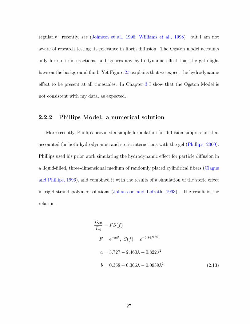
2.2.2 Phillips Model: a numerical solution

More recently, Phillips provided a simple formulation for diffusion suppression that

accounted for both hydrodynamic and steric interactions with the gel (Phillips, 2000).

Phillips used his prior work simulating the hydrodynamic effect for particle diffusion in

a liquid-filled, three-dimensional medium of randomly placed cylindrical fibers (Clague

and Phillips, 1996), and combined it with the results of a simulation of the steric effect

in rigid-strand polymer solutions (Johansson and Lofroth, 1993). The result is the

relation

Deff

D0

= FS(f)

F = e−aφb

, S(f) = e−0.84f1.09

a = 3.727− 2.460λ+ 0.822λ2

b = 0.358 + 0.366λ− 0.0939λ2 (2.13)

27

where F is a term that captures hydrodynamic diffusion suppression, S(f) captures

the steric diffusion suppression, f = φ(1 + 1λ)2, and λ = df/d.

We can apply this model to fibrin diffusion data whether hydrodynamic or steric

effects are responsible. As with the Ogston Model, the Phillips model has not been

tested against diffusion and structural data from fibrin gels. Because of the inherent

challenges of determining clot structure from microscopy, the validation of this theory

in fibrin is outside the scope of this dissertation. However, in Section 3.3.1 I show that

the Phillips model can be inverted, along with the Carman-Kozeny and Jackson-James

theories (see Section 2.3), to provide a reasonable prediction of clot structure.

The Phillips model, along with its constituent terms, S(f) and F , is plotted in

Figure 2.6. Except for the limiting cases of φ → 0 and φ → 1, S(f) does not agree

with the Ogston model as one might expect; unfortunately, this issue is not explained

in the literature. At low φ, the hydrodynamic term F is the one that dominates the

diffusion suppression; the steric term S(f) matches (then overtakes) the hydrodynamic

suppression at volume fractions of φ = 0.005–0.2, depending on df . Fibrin volume

fractions are within this range, so Figure 2.6 suggests that steric diffusion suppression

should be a factor in fibrin, but only if the transport is above the steric-τ .

28

2.3 Fibrin Structure and Hydraulic Permeability

2.3.1 Darcy Theory

Gels and porous media resist, but do not fully arrest, the flow of fluid. In 1856,

Henry Darcy published a treatise on the public fountains of Dijon, France, which in-

cluded exploration of how a filtration system (sand, in the case of his experimental

design) resisted the flow of fluid (Darcy, 1856). The observations of Darcy’s original

experiments can be generalized for permeants of arbitrary viscosity η and for perme-

ation driven by forces other than gravity (Bear, 1988) to state:

Q = κA∆P

ηL, (2.14)

where Q is the volumetric flow rate, A and L are the cross section and length of

the filter, and ∆P is the pressure drop across the filter. The coefficient κ has units

of area and is called the hydraulic conductivity, or Darcy constant; I will use these

terms interchangeably with “permeability”. The permeability of a classical porous

medium is invariant with the other parameters in Equation 2.14. If, for example, ∆P

were increased across a gel, then Q would increase in direct proportion, such that the

calculated κ would not change.

Blomback and Okada were among the first to recognize the potential value of mea-

suring permeability of fibrin (Blomback and Okada, 1982). Since that time, the cor-

relations of clot permeability with disease have established permeability as a critical

29

measurement, as discussed in Section 1.1.

The Darcy equation, though a powerful tool, is wholly phenomenological. In the

century and a half since his observations were published, much effort has been devoted

to predicting κ using information about the material’s structure. Initial work in the

late 19th and early 20th centuries considered a porous medium to be a collection of

capillaries. Intuitively, the volume fraction of the medium could be accounted for by

the effective diameter of the capillaries relative to the cross-section of the medium, and

the tortuosity of the flow through the medium could be accounted for by the effective

length of the capillaries relative to the length of the medium.

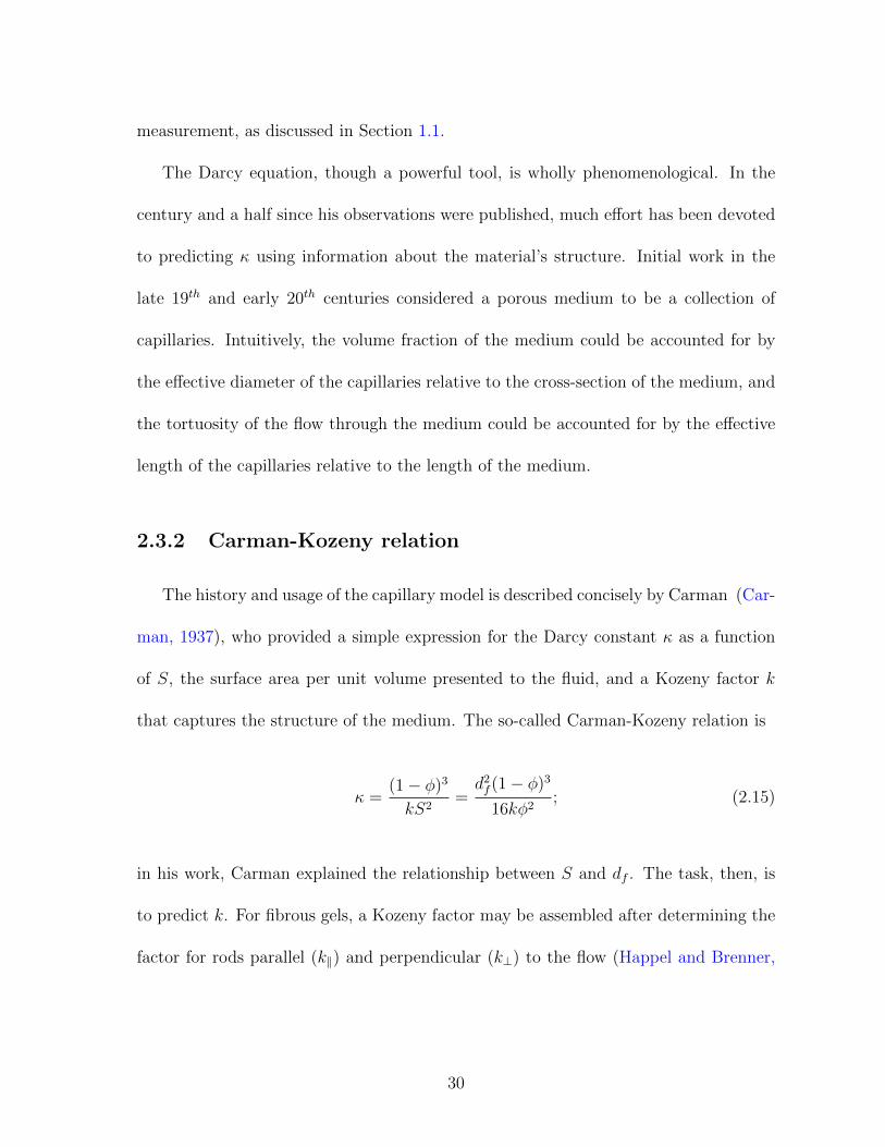
2.3.2 Carman-Kozeny relation

The history and usage of the capillary model is described concisely by Carman (Car-

man, 1937), who provided a simple expression for the Darcy constant κ as a function

of S, the surface area per unit volume presented to the fluid, and a Kozeny factor k

that captures the structure of the medium. The so-called Carman-Kozeny relation is

κ =(1− φ)3

kS2=d2f (1− φ)3

16kφ2; (2.15)

in his work, Carman explained the relationship between S and df . The task, then, is

to predict k. For fibrous gels, a Kozeny factor may be assembled after determining the

factor for rods parallel (k‖) and perpendicular (k⊥) to the flow (Happel and Brenner,

30

1983):

krand =2k⊥ + k‖

3=

1

3

(4(1− φ)3

φ(ln 1φ− 1−φ2

1+φ2 )+

2(1− φ)3

φ(2ln 1φ− 3 + 4φ− φ2)

). (2.16)

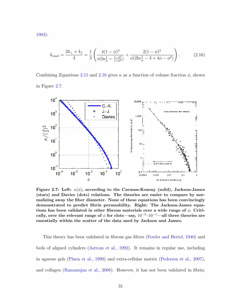
Combining Equations 2.15 and 2.16 gives κ as a function of volume fraction φ, shown

in Figure 2.7.

10,000

1,000 - N m , Y, x c 0 - - g 100 E a, a In u) a, C

In c

- 0 10

._ E n

1

0.1

1 Three-dimensional fiber networks

a - A

spielman a ~ o r m equat~on 15 Jackson 8 James equation 16

0.0001 0.001 0.01 0.1 1

Solid Volume Fraction (@)

Figure 4 - A comparison of three-dimensional models for fibrous porous media.

single cylinder problem, they used the Brinkman-Debye- Bueche (BDB) equation:

v p = p i 7 - 14V k

which is the superposition of Stokes equation and Darcy’s law. The velocity was required to vanish at the cylinder and to match the superficial velocity at infinity. Having avoided Stokes’ paradox because the Darcy term is dominant at large distances, they found the flow field and drag on an infinitely long cylinder. From the drag, the equivalent permeability was determined and this was taken to be the permeability k in the governing equation. Hence an implicit relation was found for k:

where K,, and Ki are modified Bessel functions of the second kind. This equation is plotted in Figure 3 and the curve lies about 25% above the accurate collective curve.

This novel approach of Spielman and Goren-now generally referred to as ‘swarm’ theory-led to a number of works which attempted to improve the concept. Howells (1974) extended the analysis by including a second fiber at random locations and accounting for its influence. His results agree with those of Spielman and Goren for + 5 0.3, and give lower permeabilities at higher +. Neale and Masliyah (1975) and Guzy et al. (1983) supposed that there is a fluid annulus around the single cylinder, inside of which Stokes’ equation applies and outside of which either Darcy’s equation or the BDB equation applies. This approach is, in effect, a combination of the circular cell model and the

two-zone concept of Spielman and Goren. Matching conditions at the edge of the envelope depend on which equation is specified for the outer region, but the resulting two predictions differ little for 4 < 0. I , as Guzy et al. show. If the two predictions were plotted in Figure 3, the curves would fall between the Happel curve and the collective curve (Kuwabara, etc.). The main point is that these refinements to a model flow do lead to results which are closer to the accurate solutions, i.e., to those of Hasimoto, Sangani & Acrivos and Drummond & Tahir.

FLOW THROUGH THREE-DIMENSIONAL ARRAYS

Spielman and Goren used the same technique to estimate the permeability of rods randomly oriented in all three directions. They solved the problem of a rod oblique to the superficial velocity by allowing the permeability to have different values in the directions parallel and perpendicular to the flow. Then, by averaging over all rod directions, they determined the permeability of this three-dimensional medium. Using the same notation as before, this result is

The only other work on three-dimensional arrays appears to be our own development of a cubical lattice model (Jack- son and James, 1982). In that work, it was argued that the permeability of a random medium like steel wool is equivalent to the permeability of a cubical lattice formed of the same material. The flow resistance of the lattice was estimated by adding the resistance of rods across the flow to that of rods aligned with the flow. The individual resistances were calculated from Happel’s relations and an overall permeability was predicted. Now that Drummond and Tahir’s more accurate equations are available, we now present a revised prediction for k/a’ , based on their Equations (2) and ( 1 I ) for square arrays:

3 - = - (-In + - 0.931 + O(ln + ) - I ) . . . . . . . a* 204

This equation and Spielman & Goren’s result (Equation 15) have been plotted in Figure 4. It is apparent that the two models agree reasonably well with each other and with the experimental data.

Conclusions

The conclusions of this work are best stated with reference to the figures: (i) Figure 1. The graph shows that permeability data for

diverse fibrous materials are correlated reasonably well when the co-ordinates k /a2 and 4 are used. The scatter is caused by inhomogeneity and by variations in fiber shape and arrangement. For example, if the graph could be restricted to media with uniformly distributed fibers, or to media where the fibers had a single orientation, then the scatter would be reduced considerably. Even with the scatter, though, the graph is useful for order of magnitude estimates of flow resistance when flow data are not available for a porous material but when fiber size and volume fraction are known.

(ii) Figure 2. For arrays of parallel fibers aligned with the flow, predictions by all analytical techniques agree

372 THE CANADIAN JOURNAL OF CHEMICAL ENGINEERING, VOLUME 64, JUNE 1986

Figure 2.7: Left: κ(φ), according to the Carman-Kozeny (solid), Jackson-James(stars) and Davies (dots) relations. The theories are easier to compare by nor-malizing away the fiber diameter. None of these equations has been convincinglydemonstrated to predict fibrin permeability. Right: The Jackson-James equa-tions has been validated in other fibrous materials over a wide range of φ. Criti-cally, over the relevant range of φ for clots—say, 10−3–10−1—all three theories areessentially within the scatter of the data used by Jackson and James.

This theory has been validated in fibrous gas filters (Fowler and Hertel, 1940) and

beds of aligned cylinders (Astrom et al., 1992). It remains in regular use, including

in agarose gels (Pluen et al., 1999) and extra-cellular matrix (Pedersen et al., 2007),

and collagen (Ramanujan et al., 2008). However, it has not been validated in fibrin;

31

because of the inherent challenges of determining clot structure from microscopy, the

validation of this theory in fibrin is outside the scope of this dissertation. However, in

Section 3.3.1 I show that the Carman-Kozeny theory can be inverted, along with the

Phillips Model, to provide a reasonable prediction of clot structure.

2.3.3 Fibrous media: Jackson-James and Davies equations

In an effort to find a solution specific to fibrous media, Jackson and James (Jackson

and James, 1986) offered another theoretical solution. They constructed a model using

prior theories of flow parallel (Sangani and Acrivos, 1982) (numerical) and perpendic-

ular (Drummond and Tahir, 1984) (analytical) to rigid rods in a square lattice. They

applied their equation to data on a wide variety of fibrous networks, including steel

wire crimps, wool, yarn, filters, acrylamide gel, collagen, and hyaluronic acid polymer.

The volume fractions ranged from 0.0003 < φ < 0.3. While fibrin were not included

in the fit, the wide variety of fibrous materials used to create the equation suggests it

may be broadly relevant for low-volume fraction gels. Their final result was

κ =−3

80

d2f

φ(lnφ+ 0.931). (2.17)

Figure 2.7 shows that the Jackson-James equation shows good agreement with the

Carman-Kozeny theory for random arrays of rods.

I have found one example in the literature where fibrin has been tested against a

theory of κ(φ). Diamond and Anand compared fibrin permeability for several types of

32

fibrin clots to an empirical equation developed by Davies (Diamond and Anand, 1993),

κ =d2f

70φ3/2(1 + 52φ3/2), (2.18)

concluding that this equation “accurately correlated” data that they had extracted from

earlier published results on fibrin permeability and imaging. However, neither the data

nor the method used to extract them were reported, so I cannot say to what precision

the Davies equation has been validated. Even more alarming, their citation leads to

an equation 4.1.8 in a text (Dullien, 1992) where the coefficients differ from those of

Equations 2.18, and the citation is an article I have not been able to find to resolve

the discrepancy. Because of its prior use in fibrin, I will bring Equation 2.18 through

my discussion in Chapter 3. However, as theoretical rather than empirical models, the

Jackson-James and Carman-Kozeny theories are ultimately more satisfying.

The ultimate question, however, is which equation is correct; therefore I stress that

the Davies, Jackson-James, and Carman-Kozeny equations, all plotted in Figure 2.7, do

not disagree dramatically over the relevant range of fibrin volume fractions (φ = 0.001–

0.1). In this range, the theories all appear to lie within the scatter of the data used to

determine the Jackson-James equation.

I must also stress that direct validation of any κ(φ, df ) theories is challenging,

because measuring fibrin fiber diameter and volume fraction is notoriously difficult.

Optical microscopy can image fibrin without drying, but it loses reliability for size

detection below the diffraction limit. Electron microscopy can easily resolve specimens

33

of that size, but the fibers must be dried before they can be imaged, in which case they

shrink and frequently collapse. Therefore, as an alternative to imaging based methods,

I show in Chapter 3 that by inverting these theories, measurements of diffusion and

permeability can provide insight into clot structure (df and φ).

2.3.4 Permeability and turbidity

I am discussing theories that predict κ(φ, df ). As explained in Section 1.1, turbid-

ity has been mentioned as a high-throughput measurement of clot structure. Could

turbidity therefore be used to find permeability?

The early work on light transmission through fibrin was traditional angle-dependent

light scattering (Carr et al., 2004). This work did indeed reveal fiber lengths and

diameters, but not all the fibrin studied were polymerized gels.

Carr and Hermans introduced fibrin turbidity shortly after, presumably because it

is simpler to perform than angle-dependent light scattering. Turbidity of a solution is

the decrease in transmitted light intensity due to scattering and can be calculated by

integration of the scattered intensity over all directions (Carr and Hermans, 1978):

T =44

15

πKρ0λµ

Ti(2.19)

where Ti is the turbidity at the start time, ρ0 is the fibrinogen concentration, λ is

the incident wavelength, µ is the linear mass density of the fiber (sometimes called

“mass-length ratio”), and K is a constant that captures the refractive index n of the

34

material,

K =2π2n2

NAλ4

(dn

dρ0

)2

,

where NA is Avogadro’s number.

The angular integration that makes turbidity so convenient as a methodology ruins

its potential as a complete probe of gel structure—namely, of φ and df . Consider the

definition of volume fraction,

φ =π

4nfd

2fLf (2.20)

where nf is the number density of fibers and Lf is the length of an average fiber. The

problem is already apparent: Equation 2.20 has three inputs, but turbidity provides

only two quantities related to structure, µ and ρ0. In detail, we would begin by using

Vf = (π/4)d2fLf to write

Lf =mf

µ=mN

µ(2.21)

nf =n

N=

ρ0

mN, (2.22)

where Vf is the volume of the fiber, mf is the average fiber mass, m is the mass of a

fibrin monomer, and N is the average number of fibrin monomers in a fiber. Eliminating

35

N , we find,

Lf =ρ0

µnf, so φ =

π

4

ρ0

µd2f , (2.23)

and we are left without df . Recognizing mf = ρVf , we can write

df = 2

√VfπLf

= 2

√µ

πρ, (2.24)

where ρ is the density of monomers in the fiber. This last quantity, ρ, is essentially

the packing of fibrin monomers in a fiber, and it is unknown. Fibrin fibers are under

tension, and that tension may increase as fiber diameter increases (Weisel, 2004), which

would cause ρ to scale with N . Studies with AFM of dried fibrin fibers have indicated

that the fiber density varies with the radial distance from the axis of the fiber (Guthold

et al., 2007). For these reasons, we cannot assume that ρ is constant. Thus, turbidity

cannot provide sufficient information to extract gel structure.

The coagulation community relies heavily on turbidity for understanding of clot

structure, and has built an intuition of how turbidity and permeability are related2. I

will linger on this topic to highlight a potential hazard in the way the measurement

is presently used. For two clots with the same polymerization rate, but different final

transmission, there is ambiguity in the clot structure, highlighted in Figure 2.8. The

lower final turbidity could be due either to a lower clot volume fraction at a constant

fiber diameter, or to a smaller fiber diameter at a constant volume fraction. The first

2My thanks to Alisa Wolberg for helpful conversations on this topic.

36

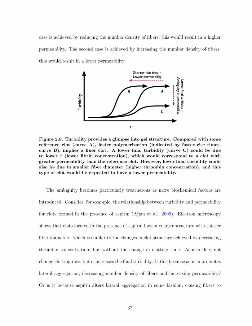
case is achieved by reducing the number density of fibers; this would result in a higher

permeability. The second case is achieved by increasing the number density of fibers;

this would result in a lower permeability.

Figure 2.8: Turbidity provides a glimpse into gel structure. Compared with somereference clot (curve A), faster polymerization (indicated by faster rise times,curve B), implies a finer clot. A lower final turbidity (curve C) could be dueto lower φ (lower fibrin concentration), which would correspond to a clot withgreater permeability than the reference clot. However, lower final turbidity couldalso be due to smaller fiber diameter (higher thrombin concentration), and thistype of clot would be expected to have a lower permeability.

The ambiguity becomes particularly treacherous as more biochemical factors are

introduced. Consider, for example, the relationship between turbidity and permeability

for clots formed in the presence of aspirin (Ajjan et al., 2009). Electron microscopy

shows that clots formed in the presence of aspirin have a coarser structure with thicker

fiber diameters, which is similar to the changes in clot structure achieved by decreasing

thrombin concentration, but without the change in clotting time. Aspirin does not

change clotting rate, but it increases the final turbidity. Is this because aspirin promotes

lateral aggregation, decreasing number density of fibers and increasing permeability?

Or is it because aspirin alters lateral aggregation in some fashion, causing fibers to

37

swell without changing their number density, causing no affect or a small decrease in

permeability? The complexity of the system leaves open questions which turbidity

alone cannot answer.

2.4 Diffusion and Permeability

A wide range of scientists and engineers are concerned simultaneously with fluid

permeation and particle transport through a medium. The filtration community is

concerned less with particle diffusion than with the rejection rate of particles moving

through a barrier (Zamani and Maini, 2009), and therefore pore sizes in the filter are

typically designed to be smaller than the particles expected to be passing through,

hydrodynamic effects are typically ignored, and electrostatic effects are considered in

detail (Wijmans and Baker, 1995; Szymczyk and Fievet, 2005). Geological sciences

consider gas perfusion through soil and rock (Hamamoto et al., 2009), but pressure-

driven advection make dispersion, or mixing, a more relevant phenomenon than in gels

studied in vitro. Novel device research can present an interesting area of overlap, as

some research considers how adding nano-devices to bulk material can enhance particle

diffusion or modify bulk permeability (Zhong et al., 2003; Srebnik and Sheintuch, 2009).

There is great interest in these two measurements in polymer gels community. Col-

lagen, extracellular matrix, and agarose have all been studied for this relationship (Ra-

manujan et al., 2008; Pedersen et al., 2007; Pluen et al., 1999; Levick, 1987). In these

experiments, the question is typically whether particle diffusion can be predicted from

38

permeability; the latter being a bulk measurement that requires no specialized equip-

ment. However, absent from the discussion about the relationship between the two

phenomena is the time- and length-scale dependence over which diffusion occurs will

have a dramatic impact.

Consider an effort to predict the speed of inter-cellular communication for cells

embedded in extracellular matrix. The distances are short—perhaps just tens of

nanometers—so steric effects between the diffusing molecule and the gel may not be

relevant, producing faster diffusion and therefore faster communication. Hydrodynamic

effects would still be present. Permeability is also a hydrodynamic effect. An equation

that linked hydrodynamic diffusion suppression with permeability could predict the

speed of this communication by measuring bulk gel permeability, which might be easier

than a nanometer-resolution, high-bandwidth measurement of diffusion.

Fibrin presents a convenient system to confirm such a theory, because the inter-fiber

distance is measured in hundreds of nanometers or more, where for some polymer gels

the distances can be tens of nanometers or smaller.

Furthermore, a relationship between permeability and diffusion would be especially

useful for coagulation science, because it presents the possibility that clot permeability

could be measured in high throughput. There is indeed a theory that relates Deff and

κ. In addition to establishing a relationship between these quantities, it can also help

isolate whether hydrodynamic or steric effects are dominating particle diffusion.

39

2.4.1 Effective medium theory

In 1949, Brinkman presented an “effective medium” theory to determine the force

on a granule suspended in a fluid-filled porous medium (Brinkman, 1949). He assumed

nothing about the medium except that it had a permeability κ. In his treatment,

the continuity condition on the fluid velocity at the edge of the pocket in which the

granule was located increased the friction on the granule—in short, it was a model for

the hydrodynamic effect discussed in Section 2.1.4. The theory is valid in the regime

φ < 0.6, which comfortably encompasses the full range of fibrin and plasma clots, and

many whole blood clots.

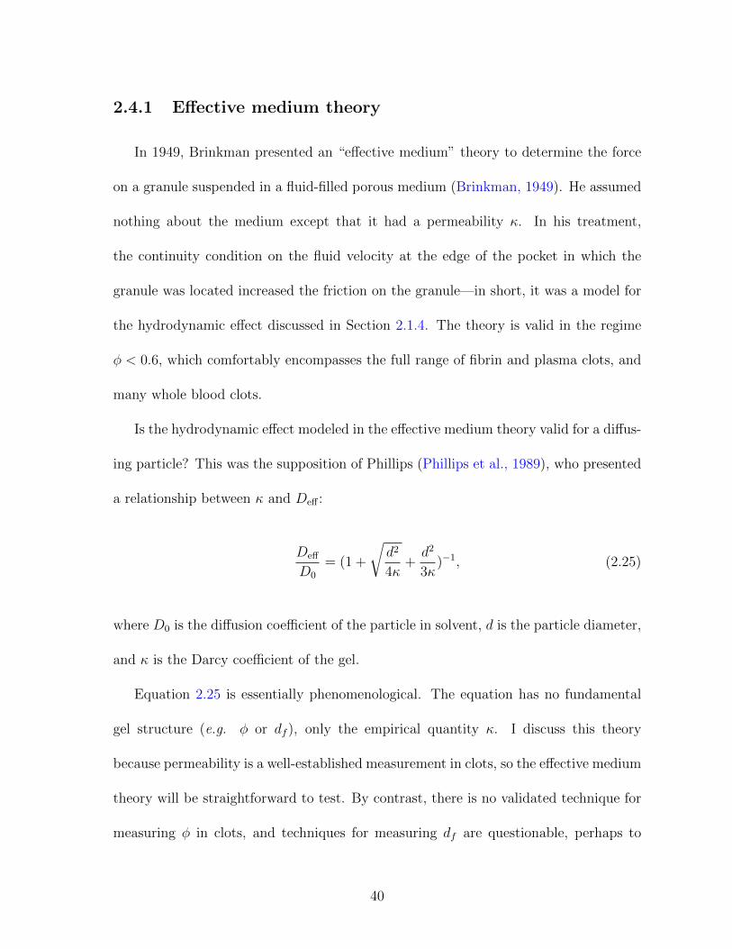
Is the hydrodynamic effect modeled in the effective medium theory valid for a diffus-

ing particle? This was the supposition of Phillips (Phillips et al., 1989), who presented

a relationship between κ and Deff :

Deff

D0

= (1 +

√d2

4κ+d2

3κ)−1, (2.25)

where D0 is the diffusion coefficient of the particle in solvent, d is the particle diameter,

and κ is the Darcy coefficient of the gel.

Equation 2.25 is essentially phenomenological. The equation has no fundamental

gel structure (e.g. φ or df ), only the empirical quantity κ. I discuss this theory

because permeability is a well-established measurement in clots, so the effective medium

theory will be straightforward to test. By contrast, there is no validated technique for

measuring φ in clots, and techniques for measuring df are questionable, perhaps to

40

within a factor of two, due to the potential effects of drying (electron microscopy) or

deconvolution (confocal microscopy). These experimental challenges present limitations

on the accuracy with which the above theories of Deff(φ, df ) and κ(φ, df ) could be tested

directly.

Because the effective medium theory only models hydrodynamic diffusion suppre-

sion, its validity would show that hydrodynamic, rather than steric effects, were deter-

mining particle diffusion. This result would be an important first step toward identify-

ing which of the Deff(φ, df ) and κ(φ, df ) were relevant.

It has been suggested, but not demonstrated, that effective medium theory applies

to nanoparticle diffusion in fibrin (Diamond, 1999). The effective medium theory has

been tested in agarose, where it was found to overestimate Deff/D0 (Johnson et al.,

1996). The issue in agarose appeared to be that steric effects were ignored. Using

Equation 2.25 as F from Equation 2.13 improved agreement. In Chapter 3, I explain

that this prior work was observing diffusion at timescales longer than the steric-τ . In

my work, I use a higher-bandwidth single-particle tracking technique, which measures

Deff over sub-micron distances. I show that the data appear to be within the startup-τ ,

and show that the effective medium theory therefore holds in fibrin gels.

2.5 Conclusion

For a fibrin gel, which may plausibly be modeled as a low-volume fraction, rigid

rod matrix, I have discussed the theoretical landscape connecting structure, diffusion,

41

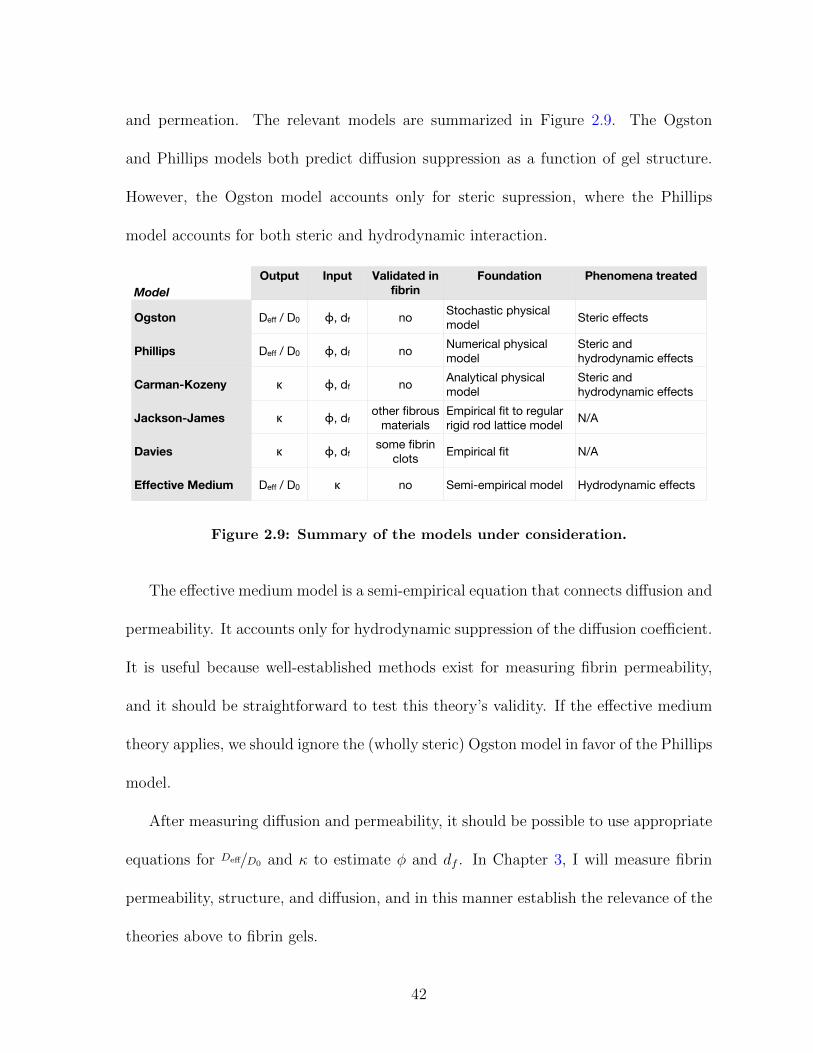
and permeation. The relevant models are summarized in Figure 2.9. The Ogston

and Phillips models both predict diffusion suppression as a function of gel structure.

However, the Ogston model accounts only for steric supression, where the Phillips

model accounts for both steric and hydrodynamic interaction.

Model

Output Input Validated in fibrin

Foundation Phenomena treated

Ogston

Phillips

Carman-Kozeny

Jackson-James

Davies

Effective Medium

Deff / D0 ϕ, df noStochastic physical model

Steric effects

Deff / D0 ϕ, df noNumerical physical model

Steric and hydrodynamic effects

κ ϕ, df noAnalytical physical model

Steric and hydrodynamic effects

κ ϕ, dfother fibrous

materialsEmpirical fit to regular rigid rod lattice model

N/A

κ ϕ, dfsome fibrin

clotsEmpirical fit N/A

Deff / D0 κ no Semi-empirical model Hydrodynamic effects

Figure 2.9: Summary of the models under consideration.

The effective medium model is a semi-empirical equation that connects diffusion and

permeability. It accounts only for hydrodynamic suppression of the diffusion coefficient.

It is useful because well-established methods exist for measuring fibrin permeability,

and it should be straightforward to test this theory’s validity. If the effective medium

theory applies, we should ignore the (wholly steric) Ogston model in favor of the Phillips

model.

After measuring diffusion and permeability, it should be possible to use appropriate

equations for Deff/D0 and κ to estimate φ and df . In Chapter 3, I will measure fibrin

permeability, structure, and diffusion, and in this manner establish the relevance of the

theories above to fibrin gels.

42

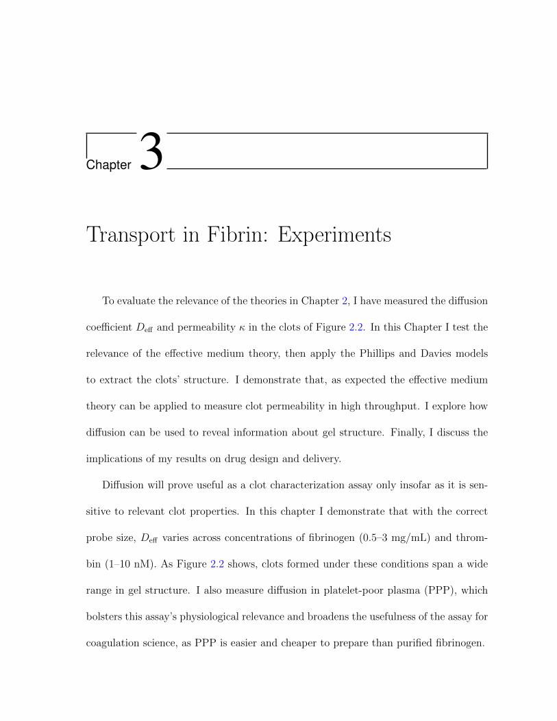
Chapter 3Transport in Fibrin: Experiments

To evaluate the relevance of the theories in Chapter 2, I have measured the diffusion

coefficient Deff and permeability κ in the clots of Figure 2.2. In this Chapter I test the

relevance of the effective medium theory, then apply the Phillips and Davies models

to extract the clots’ structure. I demonstrate that, as expected the effective medium

theory can be applied to measure clot permeability in high throughput. I explore how

diffusion can be used to reveal information about gel structure. Finally, I discuss the

implications of my results on drug design and delivery.

Diffusion will prove useful as a clot characterization assay only insofar as it is sen-

sitive to relevant clot properties. In this chapter I demonstrate that with the correct

probe size, Deff varies across concentrations of fibrinogen (0.5–3 mg/mL) and throm-

bin (1–10 nM). As Figure 2.2 shows, clots formed under these conditions span a wide

range in gel structure. I also measure diffusion in platelet-poor plasma (PPP), which

bolsters this assay’s physiological relevance and broadens the usefulness of the assay for

coagulation science, as PPP is easier and cheaper to prepare than purified fibrinogen.

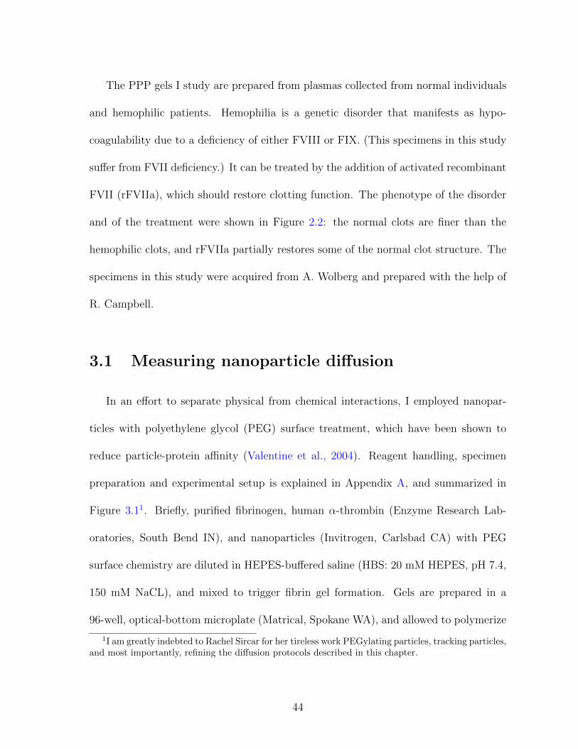
The PPP gels I study are prepared from plasmas collected from normal individuals

and hemophilic patients. Hemophilia is a genetic disorder that manifests as hypo-

coagulability due to a deficiency of either FVIII or FIX. (This specimens in this study

suffer from FVII deficiency.) It can be treated by the addition of activated recombinant

FVII (rFVIIa), which should restore clotting function. The phenotype of the disorder

and of the treatment were shown in Figure 2.2: the normal clots are finer than the

hemophilic clots, and rFVIIa partially restores some of the normal clot structure. The

specimens in this study were acquired from A. Wolberg and prepared with the help of

R. Campbell.

3.1 Measuring nanoparticle diffusion

In an effort to separate physical from chemical interactions, I employed nanopar-

ticles with polyethylene glycol (PEG) surface treatment, which have been shown to

reduce particle-protein affinity (Valentine et al., 2004). Reagent handling, specimen

preparation and experimental setup is explained in Appendix A, and summarized in

Figure 3.11. Briefly, purified fibrinogen, human α-thrombin (Enzyme Research Lab-

oratories, South Bend IN), and nanoparticles (Invitrogen, Carlsbad CA) with PEG

surface chemistry are diluted in HEPES-buffered saline (HBS: 20 mM HEPES, pH 7.4,

150 mM NaCL), and mixed to trigger fibrin gel formation. Gels are prepared in a

96-well, optical-bottom microplate (Matrical, Spokane WA), and allowed to polymerize

1I am greatly indebted to Rachel Sircar for her tireless work PEGylating particles, tracking particles,and most importantly, refining the diffusion protocols described in this chapter.

44

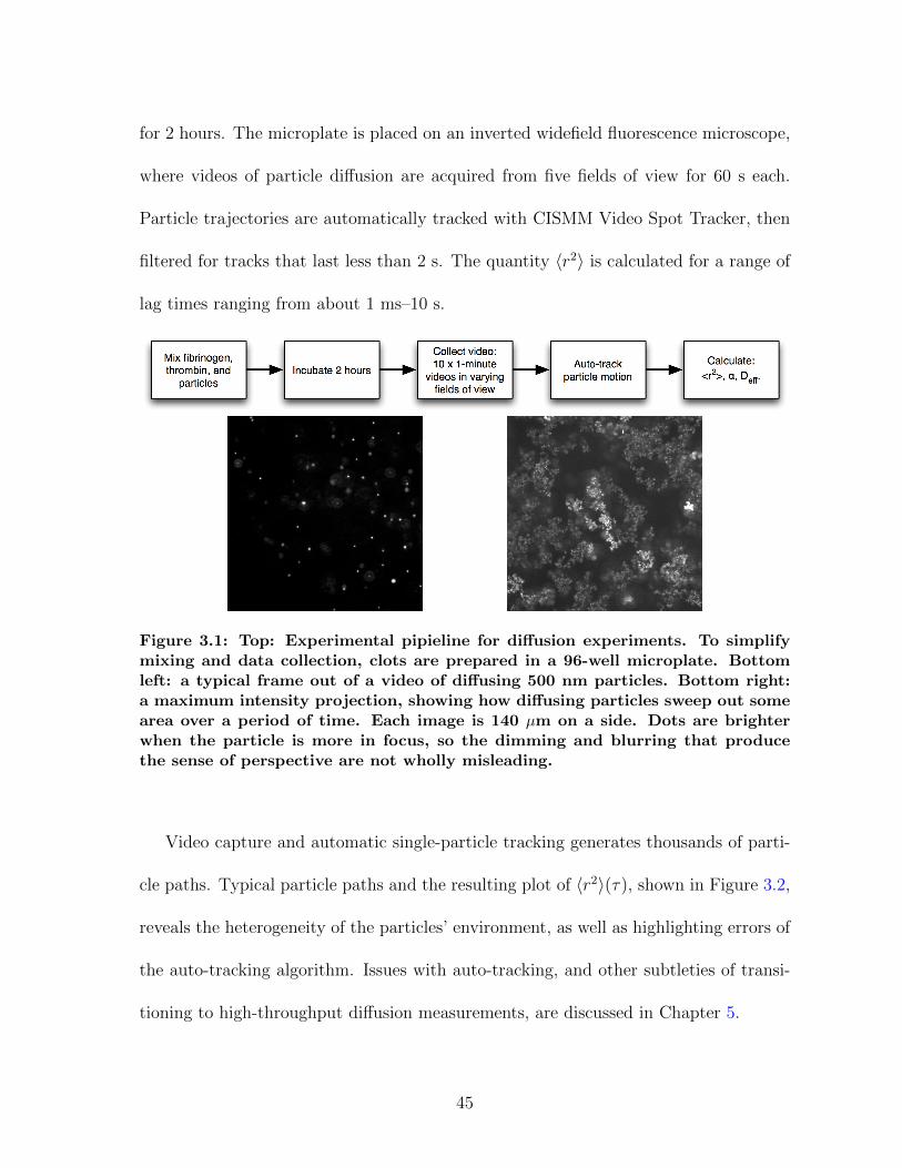
for 2 hours. The microplate is placed on an inverted widefield fluorescence microscope,

where videos of particle diffusion are acquired from five fields of view for 60 s each.

Particle trajectories are automatically tracked with CISMM Video Spot Tracker, then

filtered for tracks that last less than 2 s. The quantity 〈r2〉 is calculated for a range of

lag times ranging from about 1 ms–10 s.

Figure 3.1: Top: Experimental pipieline for diffusion experiments. To simplifymixing and data collection, clots are prepared in a 96-well microplate. Bottomleft: a typical frame out of a video of diffusing 500 nm particles. Bottom right:a maximum intensity projection, showing how diffusing particles sweep out somearea over a period of time. Each image is 140 µm on a side. Dots are brighterwhen the particle is more in focus, so the dimming and blurring that producethe sense of perspective are not wholly misleading.

Video capture and automatic single-particle tracking generates thousands of parti-

cle paths. Typical particle paths and the resulting plot of 〈r2〉(τ), shown in Figure 3.2,

reveals the heterogeneity of the particles’ environment, as well as highlighting errors of

the auto-tracking algorithm. Issues with auto-tracking, and other subtleties of transi-

tioning to high-throughput diffusion measurements, are discussed in Chapter 5.

45

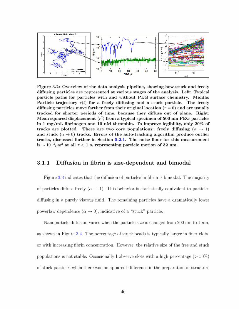
Figure 3.2: Overview of the data analysis pipeline, showing how stuck and freelydiffusing particles are represented at various stages of the analysis. Left: Typicalparticle paths for particles with and without PEG surface chemistry. Middle:Particle trajectory r(t) for a freely diffusing and a stuck particle. The freelydiffusing particles move farther from their original location (r = 0) and are usuallytracked for shorter periods of time, because they diffuse out of plane. Right:Mean squared displacement 〈r2〉 from a typical specimen of 500 nm PEG particlesin 1 mg/mL fibrinogen and 10 nM thrombin. To improve legibility, only 20% oftracks are plotted. There are two core populations: freely diffusing (α → 1)and stuck (α → 0) tracks. Errors of the auto-tracking algorithm produce outliertracks, discussed further in Section 5.2.1. The noise floor for this measurementis ∼ 10−3µm2 at all τ < 1 s, representing particle motion of 32 nm.

3.1.1 Diffusion in fibrin is size-dependent and bimodal

Figure 3.3 indicates that the diffusion of particles in fibrin is bimodal. The majority

of particles diffuse freely (α→ 1). This behavior is statistically equivalent to particles

diffusing in a purely viscous fluid. The remaining particles have a dramatically lower

powerlaw dependence (α→ 0), indicative of a “stuck” particle.

Nanoparticle diffusion varies when the particle size is changed from 200 nm to 1 µm,

as shown in Figure 3.4. The percentage of stuck beads is typically larger in finer clots,

or with increasing fibrin concentration. However, the relative size of the free and stuck

populations is not stable. Occasionally I observe clots with a high percentage (> 50%)

of stuck particles when there was no apparent difference in the preparation or structure

46

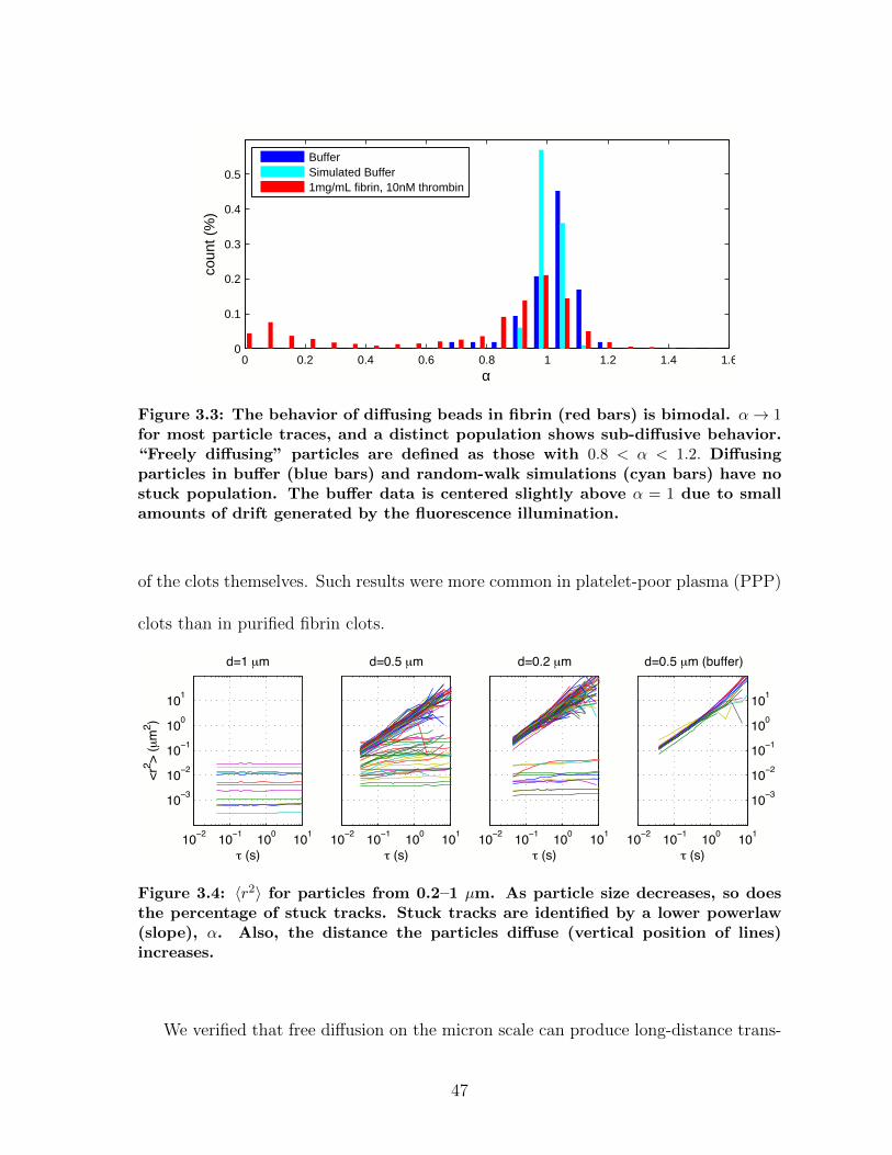
0 0.2 0.4 0.6 0.8 1 1.2 1.4 1.60

0.1

0.2

0.3

0.4

0.5

α

coun

t (%

)

BufferSimulated Buffer1mg/mL fibrin, 10nM thrombin

Figure 3.3: The behavior of diffusing beads in fibrin (red bars) is bimodal. α→ 1for most particle traces, and a distinct population shows sub-diffusive behavior.“Freely diffusing” particles are defined as those with 0.8 < α < 1.2. Diffusingparticles in buffer (blue bars) and random-walk simulations (cyan bars) have nostuck population. The buffer data is centered slightly above α = 1 due to smallamounts of drift generated by the fluorescence illumination.

of the clots themselves. Such results were more common in platelet-poor plasma (PPP)

clots than in purified fibrin clots.

10−2 10−1 100 101

10−3

10−2

10−1

100

101

d=1 µm

! (s)

<r2 >

(µm

2 )

10−2 10−1 100 101

d=0.5 µm

! (s)10−2 10−1 100 101

d=0.2 µm

! (s)10−2 10−1 100 101

10−3

10−2

10−1

100

101

d=0.5 µm (buffer)

! (s)

Figure 3.4: 〈r2〉 for particles from 0.2–1 µm. As particle size decreases, so doesthe percentage of stuck tracks. Stuck tracks are identified by a lower powerlaw(slope), α. Also, the distance the particles diffuse (vertical position of lines)increases.

We verified that free diffusion on the micron scale can produce long-distance trans-

47

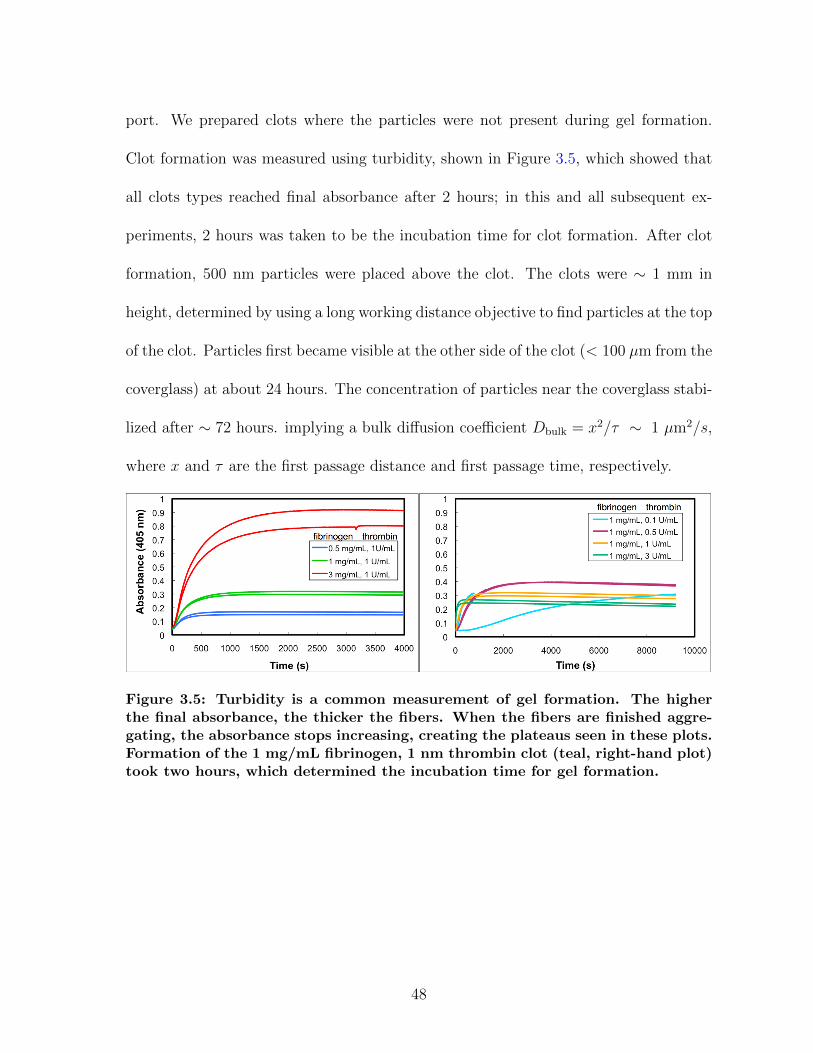
port. We prepared clots where the particles were not present during gel formation.

Clot formation was measured using turbidity, shown in Figure 3.5, which showed that

all clots types reached final absorbance after 2 hours; in this and all subsequent ex-

periments, 2 hours was taken to be the incubation time for clot formation. After clot

formation, 500 nm particles were placed above the clot. The clots were ∼ 1 mm in

height, determined by using a long working distance objective to find particles at the top

of the clot. Particles first became visible at the other side of the clot (< 100 µm from the

coverglass) at about 24 hours. The concentration of particles near the coverglass stabi-

lized after ∼ 72 hours. implying a bulk diffusion coefficient Dbulk = x2/τ ∼ 1 µm2/s,

where x and τ are the first passage distance and first passage time, respectively.

Figure 3.5: Turbidity is a common measurement of gel formation. The higherthe final absorbance, the thicker the fibers. When the fibers are finished aggre-gating, the absorbance stops increasing, creating the plateaus seen in these plots.Formation of the 1 mg/mL fibrinogen, 1 nm thrombin clot (teal, right-hand plot)took two hours, which determined the incubation time for gel formation.

48

3.1.2 Sensitivity to clot structure

We measured nanoparticle diffusion in a range of purified gel types, from low to

high thrombin concentration (1–30 nM) and low to high fibrinogen concentration (0.5–

3 mg/mL), with the two particle sizes (d = 260 and 500 nm) that have populations

where α → 1. For these freely diffusing particle traces, we calculated Deff from Equa-

tion 2.2. Although 〈r2〉 ∝ τ 1 is indicative of free diffusion, the fibrin gel apparently

suppresses the particles’ motion: where D0 = 0.94 ± 0.02µm2/s for 500 nm particles

in water, Deff drops with decreasing clot coarseness, reaching 75% of D0 in 1 mg/mL

fibrin and 30 nM thrombin and 58% of D0 3 mg/mL fibrinogen, 10 nM Thrombin.

In a purely viscous fluid, D = kBT3πηd

, where kB, T , and η are Boltzmann’s constant,

absolute temperature, and the dynamic viscosity, respectively. Therefore, the product

dDeff is a function exclusively of specimen parameters, and any variation with particle

size could be interpreted as a variation in the effective viscosity or temperature of the

particle’s environment. Results for dDeff of 500 and 260 nm particles are shown in

Figure 3.6. In coarser clots (namely, 1 mg/mL fibrinogen with 0–5 nM thrombin, and

0–0.5 mg/mL fibrinogen with 1 mg/mL thrombin), particles of both sizes experience a

similar environment that is effectively more viscous than pure buffer. As the clots grow

finer, the diffusion of 500 nm particles drops faster than that of 260 nm particles.

Nanoparticle diffusion in platelet-poor plasma (PPP) clots is also sensitive to struc-

ture. We measuredDeff for normal (0.51±0.005 µm2/s), hemophilic (0.58±0.007 µm2/s),

and recombinant factor VIIa (rFVIIa)-treated hemophilic (0.57±0.005 µm2/s) clots. In

agreement with the correlation seen in purified fibrinogen gels, the diffusion is greater in

49

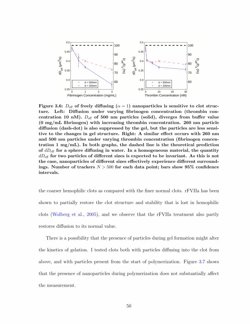
0 1 2 30.25

0.3

0.35

0.4

0.45

0.5

dDef

f (µm

3 /s)

Fibrinogen Concentration (mg/mL)

d = 500nmd = 200nm

60

70

80

90

100

Deff /D

0 (%)

0 10 20 300.25

0.3

0.35

0.4

0.45

0.5

dDef

f (µm

3 /s)

Thrombin Concentration (nM)

d = 500nmd = 200nm

60

70

80

90

100

Deff /D

0 (%)

Figure 3.6: Deff of freely diffusing (α = 1) nanoparticles is sensitive to clot struc-ture. Left: Diffusion under varying fibrinogen concentration (thrombin con-centration 10 nM). Deff of 500 nm particles (solid), diverges from buffer value(0 mg/mL fibrinogen) with increasing thrombin concentration. 260 nm particlediffusion (dash-dot) is also suppressed by the gel, but the particles are less sensi-tive to the changes in gel structure. Right: A similar effect occurs with 260 nmand 500 nm particles under varying thrombin concentration (fibrinogen concen-tration 1 mg/mL). In both graphs, the dashed line is the theoretical predictionof dDeff for a sphere diffusing in water. In a homogeneous material, the quantitydDeff for two particles of different sizes is expected to be invariant. As this is notthe case, nanoparticles of different sizes effectively experience different surround-ings. Number of trackers N > 500 for each data point; bars show 95% confidenceintervals.

the coarser hemophilic clots as compared with the finer normal clots. rFVIIa has been

shown to partially restore the clot structure and stability that is lost in hemophilic

clots (Wolberg et al., 2005), and we observe that the rFVIIa treatment also partly

restores diffusion to its normal value.

There is a possibility that the presence of particles during gel formation might alter

the kinetics of gelation. I tested clots both with particles diffusing into the clot from

above, and with particles present from the start of polymerization. Figure 3.7 shows

that the presence of nanoparticles during polymerization does not substantially affect

the measurement.

50

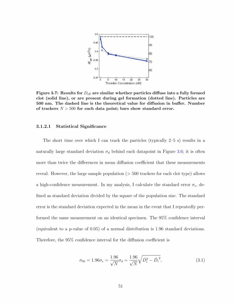
Figure 3.7: Results for Deff are similar whether particles diffuse into a fully formedclot (solid line), or are present during gel formation (dotted line). Particles are500 nm. The dashed line is the theoretical value for diffusion in buffer. Numberof trackers N > 500 for each data point; bars show standard error.

3.1.2.1 Statistical Significance

The short time over which I can track the particles (typically 2–5 s) results in a

naturally large standard deviation σd behind each datapoint in Figure 3.6; it is often

more than twice the differences in mean diffusion coefficient that these measurements

reveal. However, the large sample population (> 500 trackers for each clot type) allows

a high-confidence measurement. In my analysis, I calculate the standard error σe, de-

fined as standard deviation divided by the square of the population size. The standard

error is the standard deviation expected in the mean in the event that I repeatedly per-

formed the same measurement on an identical specimen. The 95% confidence interval

(equivalent to a p-value of 0.05) of a normal distribution is 1.96 standard deviations.

Therefore, the 95% confidence interval for the diffusion coefficient is

σ95 = 1.96σe =1.96√Nσd =

1.96√N

√D2i − Di

2, (3.1)

51

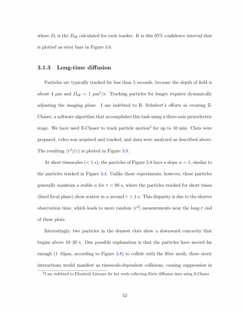
where Di is the Deff calculated for each tracker. It is this 95% confidence interval that

is plotted as error bars in Figure 3.6.

3.1.3 Long-time diffusion

Particles are typically tracked for less than 5 seconds, because the depth of field is

about 4 µm and Deff ∼ 1 µm2/s. Tracking particles for longer requires dynamically

adjusting the imaging plane. I am indebted to R. Schubert’s efforts in creating Z-

Chaser, a software algorithm that accomplishes this task using a three-axis piezoelectric

stage. We have used Z-Chaser to track particle motion2 for up to 10 min. Clots were

prepared, video was acquired and tracked, and data were analyzed as described above.

The resulting 〈r2〉(τ) is plotted in Figure 3.8.

At short timescales (< 1 s), the particles of Figure 3.8 have a slope α = 1, similar to

the particles tracked in Figure 3.4. Unlike those experiments, however, these particles

generally maintain a stable α for τ < 80 s, where the particles tracked for short times

(fixed focal plane) show scatter in α around τ > 1 s. This disparity is due to the shorter

observation time, which leads to more random 〈r2〉 measurements near the long-τ end

of these plots.

Interestingly, two particles in the densest clots show a downward concavity that

begins above 10–20 s. One possible explanation is that the particles have moved far

enough (1–10µm, according to Figure 3.8) to collide with the fiber mesh; these steric

interactions would manifest as timescale-dependent collisions, causing suppression in

2I am indebted to Elizabeth Littauer for her work collecting fibrin diffusion data using Z-Chaser

52

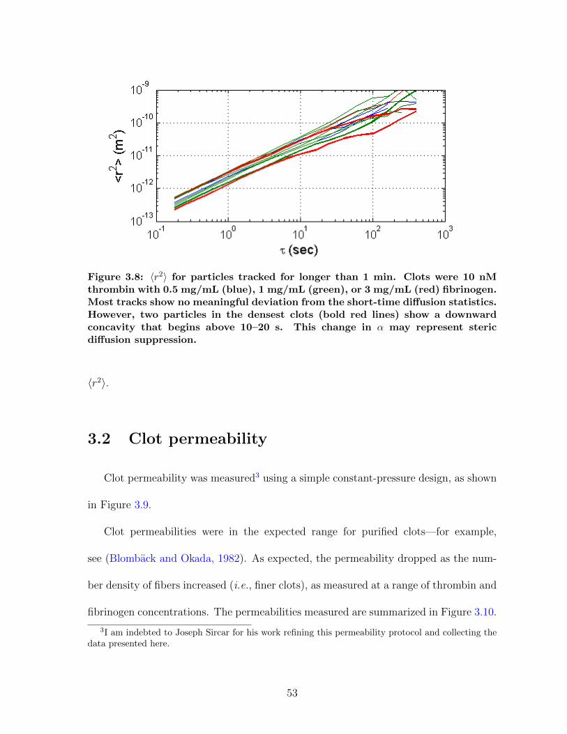
Figure 3.8: 〈r2〉 for particles tracked for longer than 1 min. Clots were 10 nMthrombin with 0.5 mg/mL (blue), 1 mg/mL (green), or 3 mg/mL (red) fibrinogen.Most tracks show no meaningful deviation from the short-time diffusion statistics.However, two particles in the densest clots (bold red lines) show a downwardconcavity that begins above 10–20 s. This change in α may represent stericdiffusion suppression.

〈r2〉.

3.2 Clot permeability

Clot permeability was measured3 using a simple constant-pressure design, as shown

in Figure 3.9.

Clot permeabilities were in the expected range for purified clots—for example,

see (Blomback and Okada, 1982). As expected, the permeability dropped as the num-

ber density of fibers increased (i.e., finer clots), as measured at a range of thrombin and

fibrinogen concentrations. The permeabilities measured are summarized in Figure 3.10.

3I am indebted to Joseph Sircar for his work refining this permeability protocol and collecting thedata presented here.

53

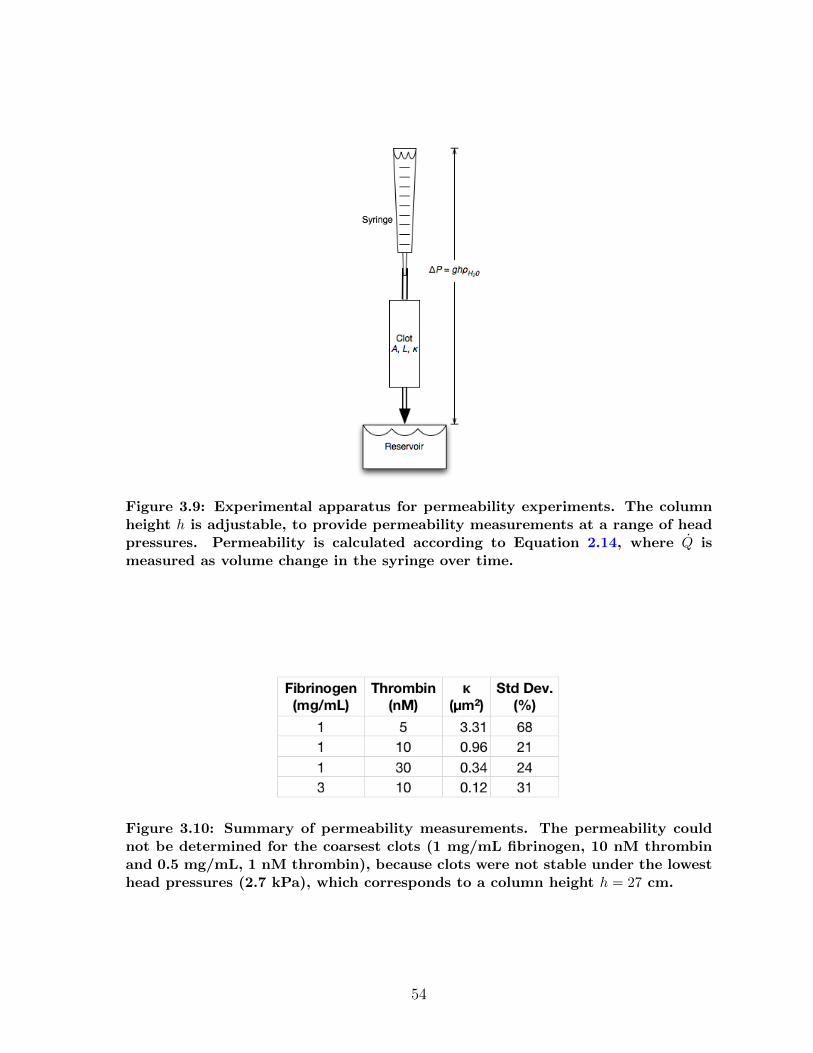
Figure 3.9: Experimental apparatus for permeability experiments. The columnheight h is adjustable, to provide permeability measurements at a range of headpressures. Permeability is calculated according to Equation 2.14, where Q ismeasured as volume change in the syringe over time.

Figure 3.10: Summary of permeability measurements. The permeability couldnot be determined for the coarsest clots (1 mg/mL fibrinogen, 10 nM thrombinand 0.5 mg/mL, 1 nM thrombin), because clots were not stable under the lowesthead pressures (2.7 kPa), which corresponds to a column height h = 27 cm.

54

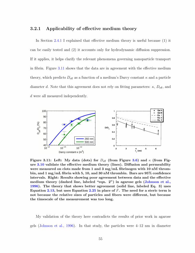
3.2.1 Applicability of effective medium theory

In Section 2.4.1 I explained that effective medium theory is useful because (1) it

can be easily tested and (2) it accounts only for hydrodynamic diffusion suppression.

If it applies, it helps clarify the relevant phenomena governing nanoparticle transport

in fibrin. Figure 3.11 shows that the data are in agreement with the effective medium

theory, which predicts Deff as a function of a medium’s Darcy constant κ and a particle

diameter d. Note that this agreement does not rely on fitting parameters: κ, Deff , and

d were all measured independently.

10−14

10−13

10−12

40

50

60

70

80

90

100

Darcy constant κ (m2)

Def

f/D0 (

%)

260 nm500 nm

Figure 3.11: Left: My data (dots) for Deff (from Figure 3.6) and κ (from Fig-ure 3.10 validate the effective medium theory (lines). Diffusion and permeabilitywere measured on clots made from 1 and 3 mg/mL fibrinogen with 10 nM throm-bin, and 1 mg/mL fibrin with 5, 10, and 30 nM thrombin. Bars are 95% confidenceintervals. Right: Results showing poor agreement between data and the effectivemedium theory (dashed line, labeled “eqn. 2”) in agarose gels (Johnson et al.,1996). The theory that shows better agreement (solid line, labeled Eq. 3) usesEquation 2.13, but uses Equation 2.25 in place of F . The need for a steric term isnot because the relative sizes of particles and fibers were different, but becausethe timescale of the measurement was too long.

My validation of the theory here contradicts the results of prior work in agarose

gels (Johnson et al., 1996). In that study, the particles were 4–12 nm in diameter

55

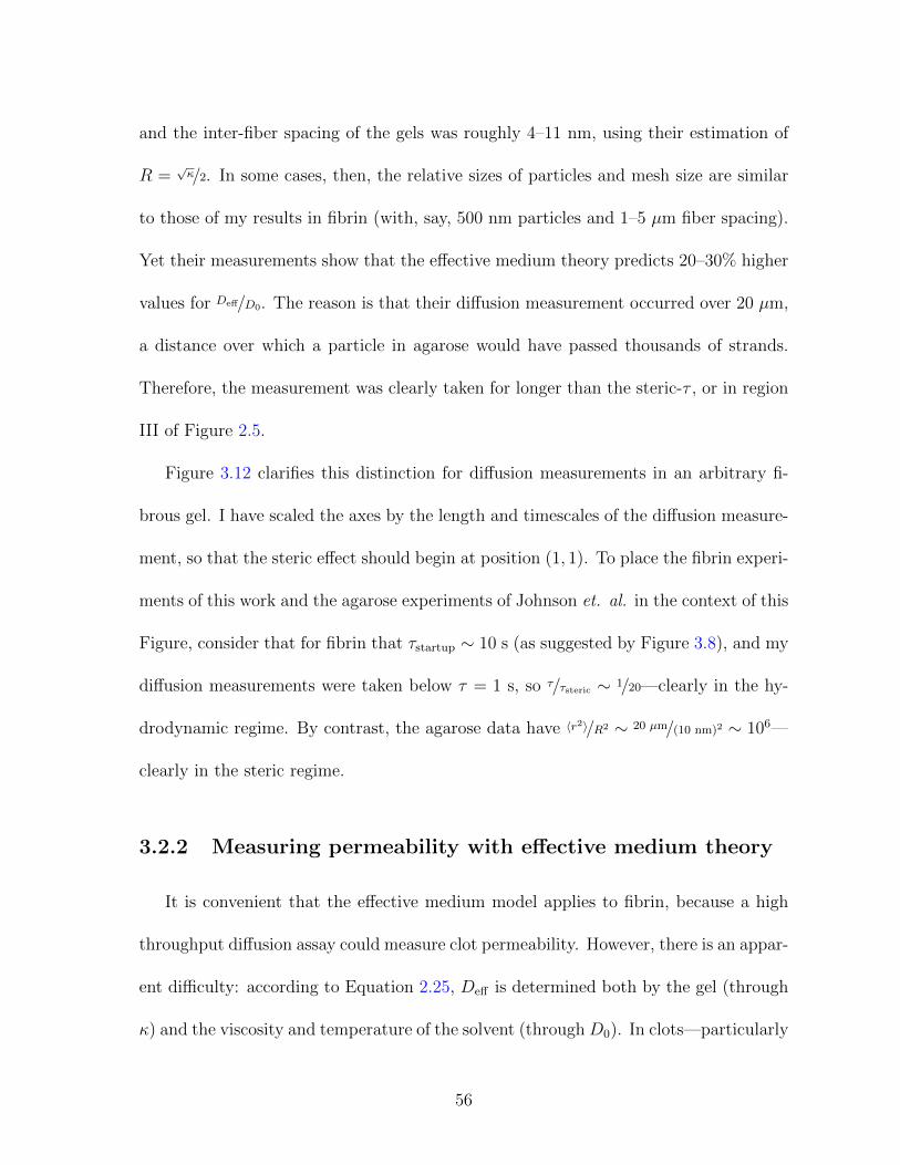
and the inter-fiber spacing of the gels was roughly 4–11 nm, using their estimation of

R =√κ/2. In some cases, then, the relative sizes of particles and mesh size are similar

to those of my results in fibrin (with, say, 500 nm particles and 1–5 µm fiber spacing).

Yet their measurements show that the effective medium theory predicts 20–30% higher

values for Deff/D0. The reason is that their diffusion measurement occurred over 20 µm,

a distance over which a particle in agarose would have passed thousands of strands.

Therefore, the measurement was clearly taken for longer than the steric-τ , or in region

III of Figure 2.5.

Figure 3.12 clarifies this distinction for diffusion measurements in an arbitrary fi-

brous gel. I have scaled the axes by the length and timescales of the diffusion measure-

ment, so that the steric effect should begin at position (1, 1). To place the fibrin experi-

ments of this work and the agarose experiments of Johnson et. al. in the context of this

Figure, consider that for fibrin that τstartup ∼ 10 s (as suggested by Figure 3.8), and my

diffusion measurements were taken below τ = 1 s, so τ/τsteric ∼ 1/20—clearly in the hy-

drodynamic regime. By contrast, the agarose data have 〈r2〉/R2 ∼ 20 µm/(10 nm)2 ∼ 106—

clearly in the steric regime.

3.2.2 Measuring permeability with effective medium theory

It is convenient that the effective medium model applies to fibrin, because a high

throughput diffusion assay could measure clot permeability. However, there is an appar-

ent difficulty: according to Equation 2.25, Deff is determined both by the gel (through

κ) and the viscosity and temperature of the solvent (through D0). In clots—particularly

56

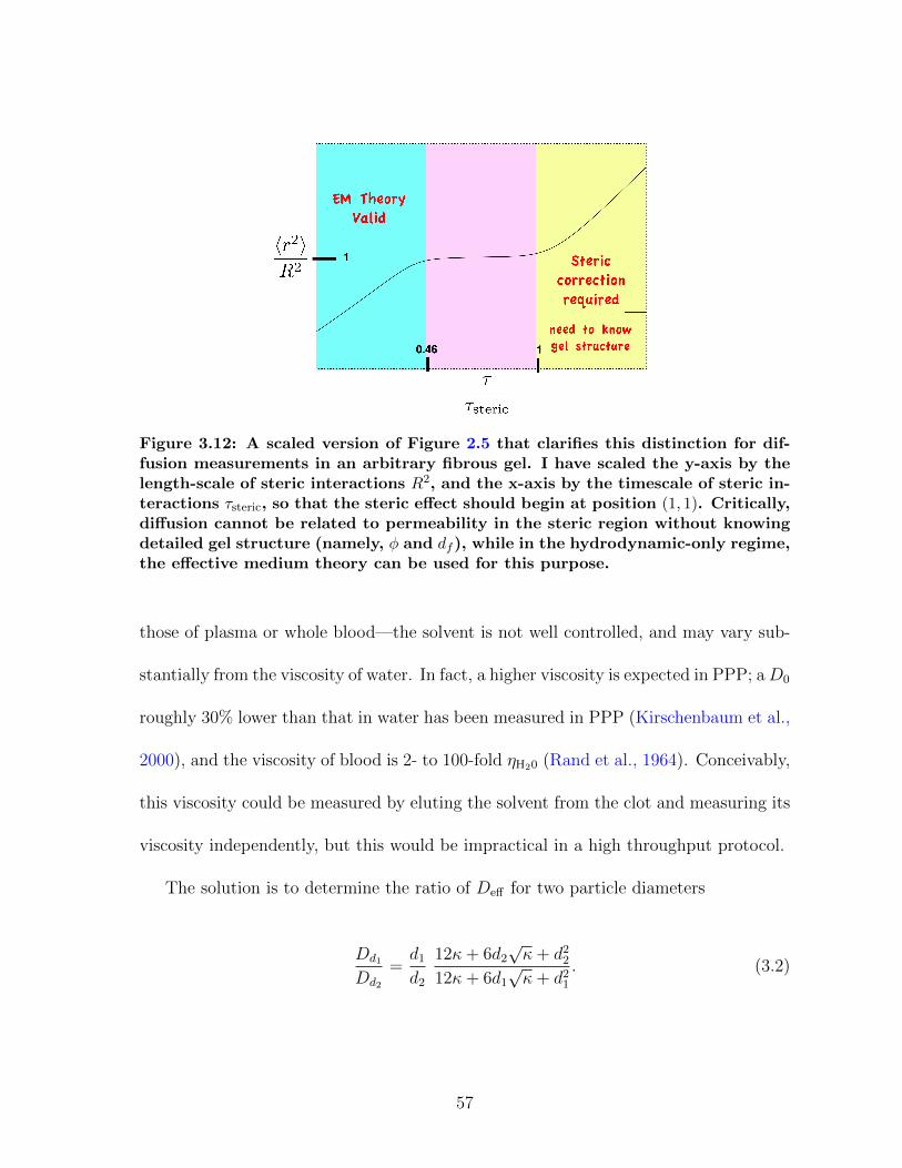
Figure 3.12: A scaled version of Figure 2.5 that clarifies this distinction for dif-fusion measurements in an arbitrary fibrous gel. I have scaled the y-axis by thelength-scale of steric interactions R2, and the x-axis by the timescale of steric in-teractions τsteric, so that the steric effect should begin at position (1, 1). Critically,diffusion cannot be related to permeability in the steric region without knowingdetailed gel structure (namely, φ and df), while in the hydrodynamic-only regime,the effective medium theory can be used for this purpose.

those of plasma or whole blood—the solvent is not well controlled, and may vary sub-

stantially from the viscosity of water. In fact, a higher viscosity is expected in PPP; aD0

roughly 30% lower than that in water has been measured in PPP (Kirschenbaum et al.,

2000), and the viscosity of blood is 2- to 100-fold ηH20 (Rand et al., 1964). Conceivably,

this viscosity could be measured by eluting the solvent from the clot and measuring its

viscosity independently, but this would be impractical in a high throughput protocol.

The solution is to determine the ratio of Deff for two particle diameters

Dd1

Dd2

=d1

d2

12κ+ 6d2

√κ+ d2

2

12κ+ 6d1

√κ+ d2

1

. (3.2)

57

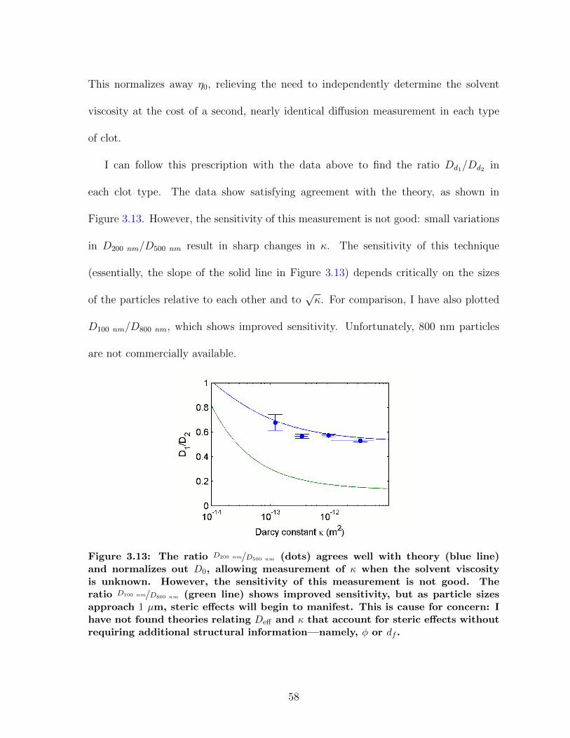
This normalizes away η0, relieving the need to independently determine the solvent

viscosity at the cost of a second, nearly identical diffusion measurement in each type

of clot.

I can follow this prescription with the data above to find the ratio Dd1/Dd2 in

each clot type. The data show satisfying agreement with the theory, as shown in

Figure 3.13. However, the sensitivity of this measurement is not good: small variations

in D200 nm/D500 nm result in sharp changes in κ. The sensitivity of this technique

(essentially, the slope of the solid line in Figure 3.13) depends critically on the sizes

of the particles relative to each other and to√κ. For comparison, I have also plotted

D100 nm/D800 nm, which shows improved sensitivity. Unfortunately, 800 nm particles

are not commercially available.

Figure 3.13: The ratio D200 nm/D500 nm (dots) agrees well with theory (blue line)and normalizes out D0, allowing measurement of κ when the solvent viscosityis unknown. However, the sensitivity of this measurement is not good. Theratio D100 nm/D800 nm (green line) shows improved sensitivity, but as particle sizesapproach 1 µm, steric effects will begin to manifest. This is cause for concern: Ihave not found theories relating Deff and κ that account for steric effects withoutrequiring additional structural information—namely, φ or df .

58

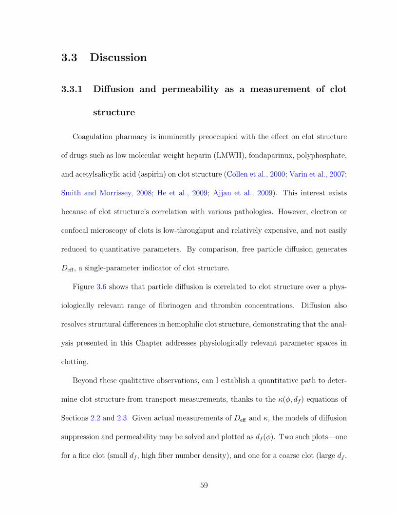
3.3 Discussion

3.3.1 Diffusion and permeability as a measurement of clot

structure

Coagulation pharmacy is imminently preoccupied with the effect on clot structure

of drugs such as low molecular weight heparin (LMWH), fondaparinux, polyphosphate,

and acetylsalicylic acid (aspirin) on clot structure (Collen et al., 2000; Varin et al., 2007;

Smith and Morrissey, 2008; He et al., 2009; Ajjan et al., 2009). This interest exists

because of clot structure’s correlation with various pathologies. However, electron or

confocal microscopy of clots is low-throughput and relatively expensive, and not easily

reduced to quantitative parameters. By comparison, free particle diffusion generates

Deff , a single-parameter indicator of clot structure.

Figure 3.6 shows that particle diffusion is correlated to clot structure over a phys-

iologically relevant range of fibrinogen and thrombin concentrations. Diffusion also

resolves structural differences in hemophilic clot structure, demonstrating that the anal-

ysis presented in this Chapter addresses physiologically relevant parameter spaces in

clotting.

Beyond these qualitative observations, can I establish a quantitative path to deter-

mine clot structure from transport measurements, thanks to the κ(φ, df ) equations of

Sections 2.2 and 2.3. Given actual measurements of Deff and κ, the models of diffusion

suppression and permeability may be solved and plotted as df (φ). Two such plots—one

for a fine clot (small df , high fiber number density), and one for a coarse clot (large df ,

59

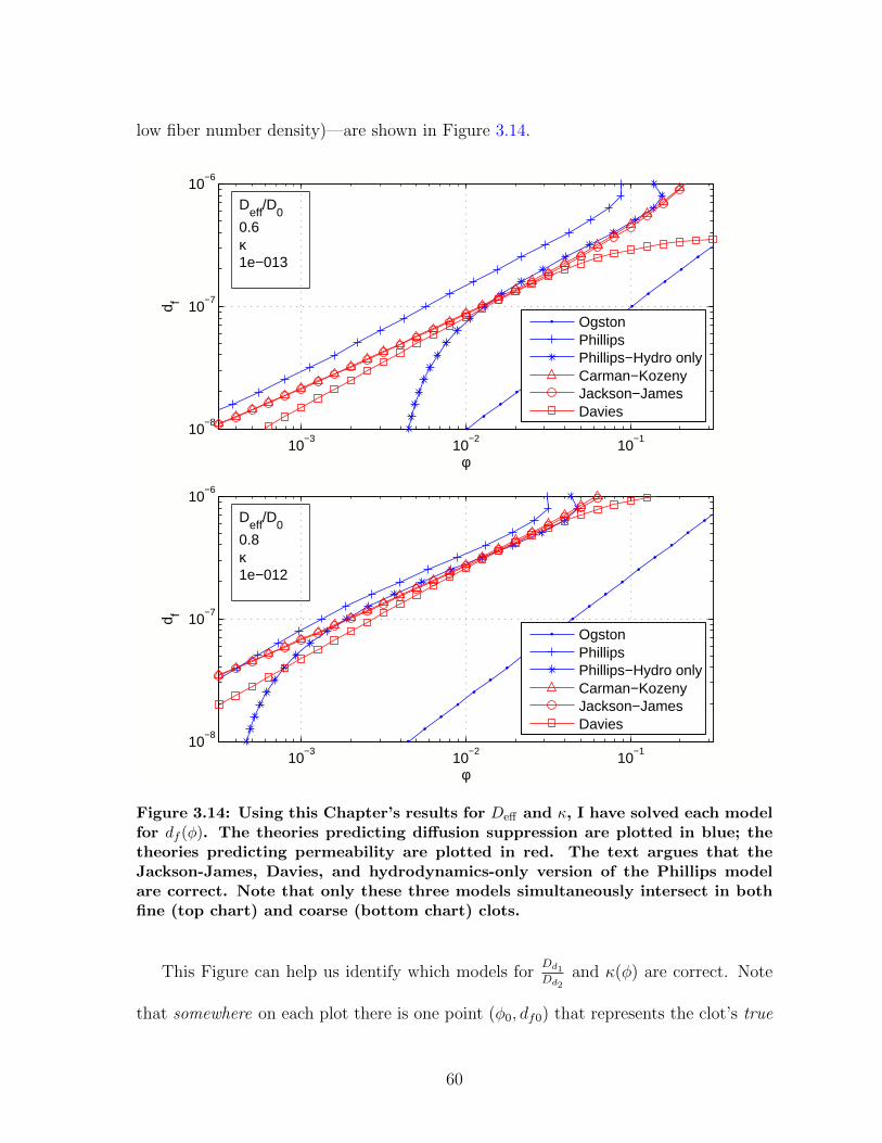
low fiber number density)—are shown in Figure 3.14.

10−3

10−2

10−1

10−8

10−7

10−6

φ

d f

OgstonPhillipsPhillips−Hydro onlyCarman−KozenyJackson−JamesDavies

Deff

/D0

0.6κ1e−013

10−3

10−2

10−1

10−8

10−7

10−6

φ

d f

OgstonPhillipsPhillips−Hydro onlyCarman−KozenyJackson−JamesDavies

Deff

/D0

0.8κ1e−012

Figure 3.14: Using this Chapter’s results for Deff and κ, I have solved each modelfor df (φ). The theories predicting diffusion suppression are plotted in blue; thetheories predicting permeability are plotted in red. The text argues that theJackson-James, Davies, and hydrodynamics-only version of the Phillips modelare correct. Note that only these three models simultaneously intersect in bothfine (top chart) and coarse (bottom chart) clots.

This Figure can help us identify which models forDd1Dd2

and κ(φ) are correct. Note

that somewhere on each plot there is one point (φ0, df0) that represents the clot’s true

60

values of fiber diameter and volume fraction. As shown in Figure 2.7, the models

expected to predict fibrin permeability (Jackson-James, Davies, and Carman-Kozeny

relations) are all similar to one another in the relevant ranges of φ and df . Therefore,

the true point of gel structure (φ0, df0) is expected to lie along the area swept out by

these lines.

Now consider the models treating diffusion. Because the (purely hydrodynamic)

effective medium theory holds, I do not expect the Ogston model, which is completely

steric, to be valid in fibrin. Figure 3.14 confirms this expectation: the Ogston model

either predicts extremely small fiber diameters (10–20 nm, equivalent to fibers com-

prising only one or two protofibrils), or extremely large volume fraction (5–10% for

100 nm fibers, a φ more consisent with platelet-retracted clots (Diamond, 1999)). The

Ogston model also never intersects the Davies and Jackson-James equations, which is

consistent with the Ogston Model being inaccurate in this material.

The Phillips model, on the other hand, agrees with the Davies, Jackson-James, and

Carman-Kozeny equations to within a factor of 2. Interestingly, ignoring the steric

term of the Phillips model (setting S(f) = 1) produces a function that agrees with the

κ(φ) models precisely at their location of closest approach. The intersection of these

three models provides a plausible prediction of df and φ that uses permeability and

diffusion.

This analysis raises two important questions. First, what does it mean to ignore the

steric term of the Phillips model, and is this justified? Second, what is the justification

for finding fiber diameter and volume fraction in this way, when for decades imaging

61

has been used for the same purpose?

To the first question, steric effects will manifest only if diffusion is measured over

timescales long enough to see particle collisions with the gel. Generally speaking, the

long-time diffusion of Figure 3.8 shows no variation in diffusion coefficient as a function

of τ , however, in the denser clots there is a gradual transition to a lower α for some

of the particles. Physical barriers that knock the particle backward (or prevent it from

advancing) can create such “sub-diffusive” behavior in 〈r2〉 curves. In these short-time

(< 10 s) experiments, therefore, steric effects do not manifest. Using the language

of Section 2.1.3, the transition τ to steric diffusion suppression is ∼ 1–10 s in high-

fibrinogen clots. This result is consistent with the analysis of that Section.

In a lab of infinite resources, the answer to the second question is to do all the

measurements. However, should resources be constrained, the technique presented

above offers two advantages. Permeability, measured directly or with the prescription

of Section 3.2.2, speaks specifically to issues of clot stability. Second, the diffusion and

permeability can be measured to arbitrary precision by increasing the volume sampled

and decreasing the head pressure, respectively. By contrast, confocal imaging has

fundamental precision limitations due to the diffraction limit, and electron microscopy

introduces uncertainty due to the required preparation. Therefore, the structure-from-

transport method potentially offers greater precision than structure-from-imaging.

62

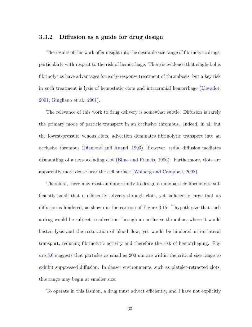
3.3.2 Diffusion as a guide for drug design

The results of this work offer insight into the desirable size range of fibrinolytic drugs,

particularly with respect to the risk of hemorrhage. There is evidence that single-bolus

fibrinolytics have advantages for early-response treatment of thrombosis, but a key risk

in such treatment is lysis of hemostatic clots and intracranial hemorrhage (Llevadot,

2001; Giugliano et al., 2001).

The relevance of this work to drug delivery is somewhat subtle. Diffusion is rarely

the primary mode of particle transport in an occlusive thrombus. Indeed, in all but

the lowest-pressure venous clots, advection dominates fibrinolytic transport into an

occlusive thrombus (Diamond and Anand, 1993). However, radial diffusion mediates

dismantling of a non-occluding clot (Blinc and Francis, 1996). Furthermore, clots are

apparently more dense near the cell surface (Wolberg and Campbell, 2008).

Therefore, there may exist an opportunity to design a nanoparticle fibrinolytic suf-

ficiently small that it efficiently advects through clots, yet sufficiently large that its

diffusion is hindered, as shown in the cartoon of Figure 3.15. I hypothesize that such

a drug would be subject to advection through an occlusive thrombus, where it would

hasten lysis and the restoration of blood flow, yet would be hindered in its lateral

transport, reducing fibrinolytic activity and therefore the risk of hemorrhaging. Fig-

ure 3.6 suggests that particles as small as 200 nm are within the critical size range to

exhibit suppressed diffusion. In denser environments, such as platelet-retracted clots,

this range may begin at smaller size.

To operate in this fashion, a drug must advect efficiently, and I have not explicitly

63

Figure 3.15: Concept for a diffusion-hindered fibrinolytic drug vector near avessel boundary. An ideal particle would be large enough that its diffusion washindered, yet small enough that it was not lodged in the fiber matrix, so that fluidflow could drive it down the vessel. This setup would be conducive to destroyingocclusive clots, but leaving hemostatic clots intact.

measured advective transport of PEG particles in fibrin. Also, the static PEG particles

merit further investigation, as the mechanism that prevents their diffusion is unclear.

I further investigate these issues in Section 4.1.

64

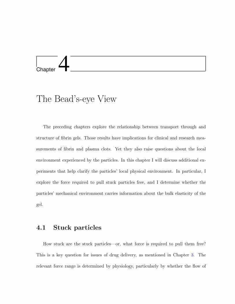
Chapter 4The Bead’s-eye View

The preceding chapters explore the relationship between transport through and

structure of fibrin gels. Those results have implications for clinical and research mea-

surements of fibrin and plasma clots. Yet they also raise questions about the local

environment experienced by the particles. In this chapter I will discuss additional ex-

periments that help clarify the particles’ local physical environment. In particular, I

explore the force required to pull stuck particles free, and I determine whether the

particles’ mechanical environment carries information about the bulk elasticity of the

gel.

4.1 Stuck particles

How stuck are the stuck particles—or, what force is required to pull them free?

This is a key question for issues of drug delivery, as mentioned in Chapter 3. The

relevant force range is determined by physiology, particularly by whether the flow of

blood would exert sufficient force to avoid association of the particle with the gels.

I have used a Multiforce High Throughput System (Spero et al., 2008) to force

PEG-coated magnetic particles through the gel. The experiment is summarized in

Figure 4.1. Briefly, clots of fibrinogen concentrations 0.5–3 mg/mL were prepared

(see Section 3.1), and plated into a magnetic microplate using the protocol of the

above reference. Super-paramagnetic 2.8 µm particles with both PEG and carboxylate

(COOH) surface chemistry were subjected to three force pulses that lasted 3 s each.

Figure 4.1: Top: experimental protocol for magnetic manipulation of 2.8 µmparticles. Clot types tested were 0.5, 1, and 3 mg/mL fibrinogen with 10 nMthrombin. Bottom left: time lapse (minimum intensity projection) image ofa typical PEG particle pulling experiment. Some particles oscillate back andforth (green ovals) while others jump long distances through the mesh, oftencoming into the field of view from far away. Bottom middle: particle trackingis performed with CISMM Video Spot Tracker except where otherwise noted.Scale bar in video image is 20 µm. Bottom right: radial displacement, r(t), isshown plotted for two particles in fibrin. The quantity ∆r, used in the section onfibrin elasticity, comes from the particle recovery after the magnets are turnedoff.

The motion of PEG and COOH particles is plotted in Figure 4.2. Because COOH

particles stick to fibrin, they oscillate back and forth as the force is turned on and off,

66

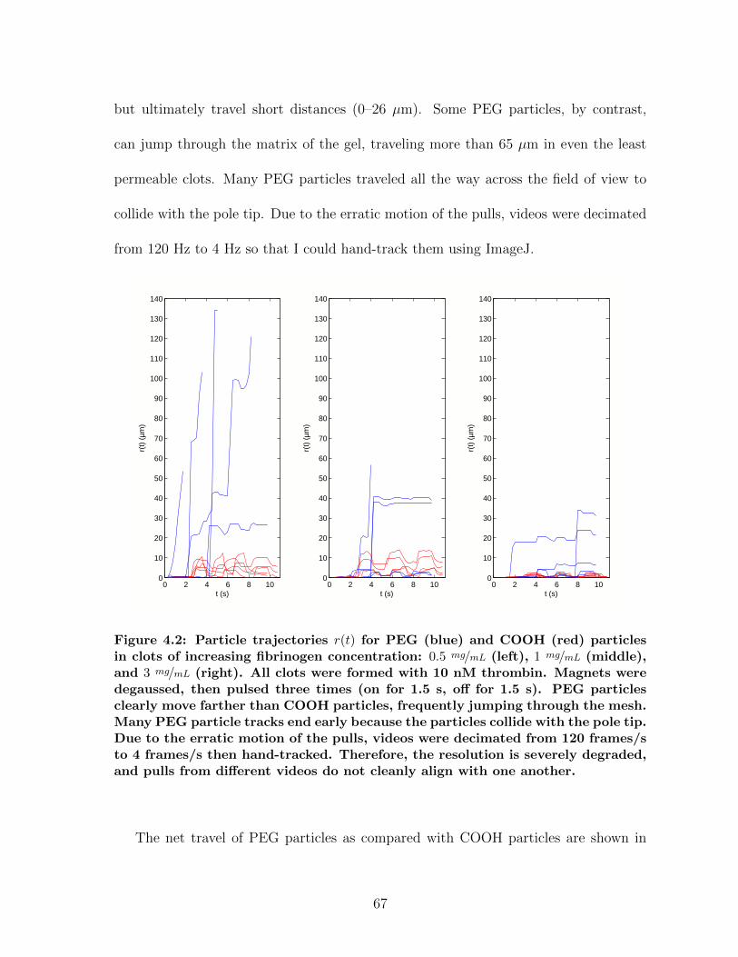
but ultimately travel short distances (0–26 µm). Some PEG particles, by contrast,

can jump through the matrix of the gel, traveling more than 65 µm in even the least

permeable clots. Many PEG particles traveled all the way across the field of view to

collide with the pole tip. Due to the erratic motion of the pulls, videos were decimated

from 120 Hz to 4 Hz so that I could hand-track them using ImageJ.

0 2 4 6 8 100

10

20

30

40

50

60

70

80

90

100

110

120

130

140

t (s)

r(t)

(µm

)

0 2 4 6 8 100

10

20

30

40

50

60

70

80

90

100

110

120

130

140

t (s)

r(t)

(µm

)

0 2 4 6 8 100

10

20

30

40

50

60

70

80

90

100

110

120

130

140

t (s)

r(t)

(µm

)

Figure 4.2: Particle trajectories r(t) for PEG (blue) and COOH (red) particlesin clots of increasing fibrinogen concentration: 0.5 mg/mL (left), 1 mg/mL (middle),and 3 mg/mL (right). All clots were formed with 10 nM thrombin. Magnets weredegaussed, then pulsed three times (on for 1.5 s, off for 1.5 s). PEG particlesclearly move farther than COOH particles, frequently jumping through the mesh.Many PEG particle tracks end early because the particles collide with the pole tip.Due to the erratic motion of the pulls, videos were decimated from 120 frames/sto 4 frames/s then hand-tracked. Therefore, the resolution is severely degraded,and pulls from different videos do not cleanly align with one another.

The net travel of PEG particles as compared with COOH particles are shown in

67

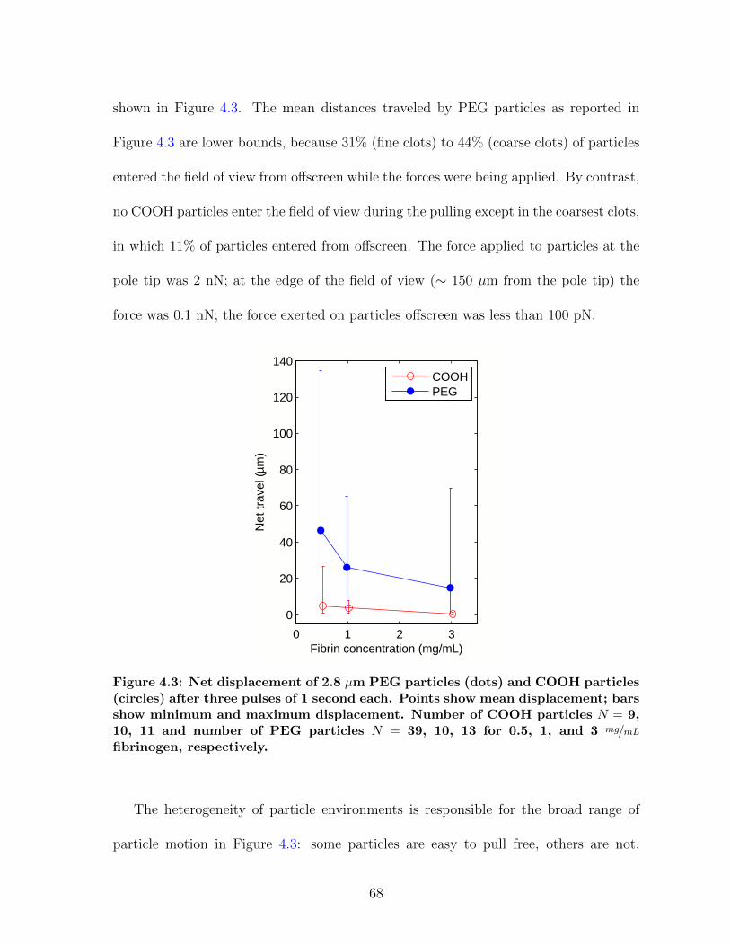
shown in Figure 4.3. The mean distances traveled by PEG particles as reported in

Figure 4.3 are lower bounds, because 31% (fine clots) to 44% (coarse clots) of particles

entered the field of view from offscreen while the forces were being applied. By contrast,

no COOH particles enter the field of view during the pulling except in the coarsest clots,

in which 11% of particles entered from offscreen. The force applied to particles at the

pole tip was 2 nN; at the edge of the field of view (∼ 150 µm from the pole tip) the

force was 0.1 nN; the force exerted on particles offscreen was less than 100 pN.

0 1 2 3

0

20

40

60

80

100

120

140

Fibrin concentration (mg/mL)

Net

trav

el (µ

m)

COOHPEG

Figure 4.3: Net displacement of 2.8 µm PEG particles (dots) and COOH particles(circles) after three pulses of 1 second each. Points show mean displacement; barsshow minimum and maximum displacement. Number of COOH particles N = 9,10, 11 and number of PEG particles N = 39, 10, 13 for 0.5, 1, and 3 mg/mLfibrinogen, respectively.

The heterogeneity of particle environments is responsible for the broad range of

particle motion in Figure 4.3: some particles are easy to pull free, others are not.

68

However, large forces were not always required—indeed, the particles that traveled

furthest started the greatest distance from the pole tip, and therefore experienced

the smallest force. Forces < 100 pN (the force at the edge of the field of view) are

adequate to drive PEGylated 2.8 µm particles long distances in these gels. A particle

in water experiences this force at a flow rate of v < 4 cm/s. The higher viscosity

of blood would further reduce the required flow rate. Arterial flow rates are about

75–110 mL/min (Knaapen et al., 2009), which for a typical artery lumen diameter of

4 mm (Dodge et al., 1992) corresponds to a fluid velocity of 10–15 cm/s. This result

suggests that whatever the reason for the association between stuck PEG particles and

fibrin, freely flowing blood may be able to prevent it from developing.

At this stage the mechanism of particle sticking remains unknown. However, I can

speculate on the responsible phenomena. The moderate forces required to pull stuck

PEG particles free suggests that there are no strong chemical associations between the

particles and the fibrin. The entrapment may be purely mechanical, with particles

captured among strands of fibrin. Physical entrapment is consistent with the result

that larger particles diffuse less.

Particles might also stick to fibrin fibers because of depletion flocculation, an en-

tropic effect where small solutes cause large colloids to aggregate. Depletion flocculation

has been proposed as a mechanism for lateral aggregation of fibrin fibers (Gelder et al.,

1996). Also, the higher concentration of macromolecules in PPP clots (the same ones

responsible for raising plasma’s background viscosity) could act as a crowding agent,

explaining the observation that the percentage of static particles was higher in plasma

69

clots than in purified gels.

4.2 Fibrin elasticity

Although this dissertation has focused primarily on transport, fibrin elasticity is also

an important clot property. Clots form an essentially mechanical function—stemming

the flow of blood—and it is well established that clot stiffness varies with clot struc-

ture (Ryan et al., 1999) and with risk of heart disease (Fatah et al., 1996). Clot

rheometry is even used as a clinical diagnostic, in a cup-and-bob geometry often called

thromboelastography (Evans et al., 2008).

The systems of Chapter 5 are well designed for high throughput characterization

of fibrin clot stiffness. From Mason and Weitz (Mason and Weitz, 1995) to Crocker

et al (Crocker et al., 2000) to Meehan and Cribb (Meehan et al., 2010), much work

has been done to identify conditions under which the bulk viscoelastic properties of

polymer media can be measured by nanoparticles. Magnetic microbead rheometry has

even been used to measure clot stiffness during gel formation (Ajjan et al., 2008). Yet

it remains unknown whether micro-scale techniques measure the same elastic modulus

of fibrin as conventional macro-scale techniques such as cone-and-plate (CAP).

I have checked for this correspondence by comparing the data from Section 4.1

against cone-and-plate (CAP) results. To extract a storage modulus from the r(t)

results discussed above, I calculated J(t) = 3πdr(t)/F (Ziemann et al., 1994). The

data are plotted against strain, defined for driven micro-rheometry as γ = 3∆rd (Cribb,

70

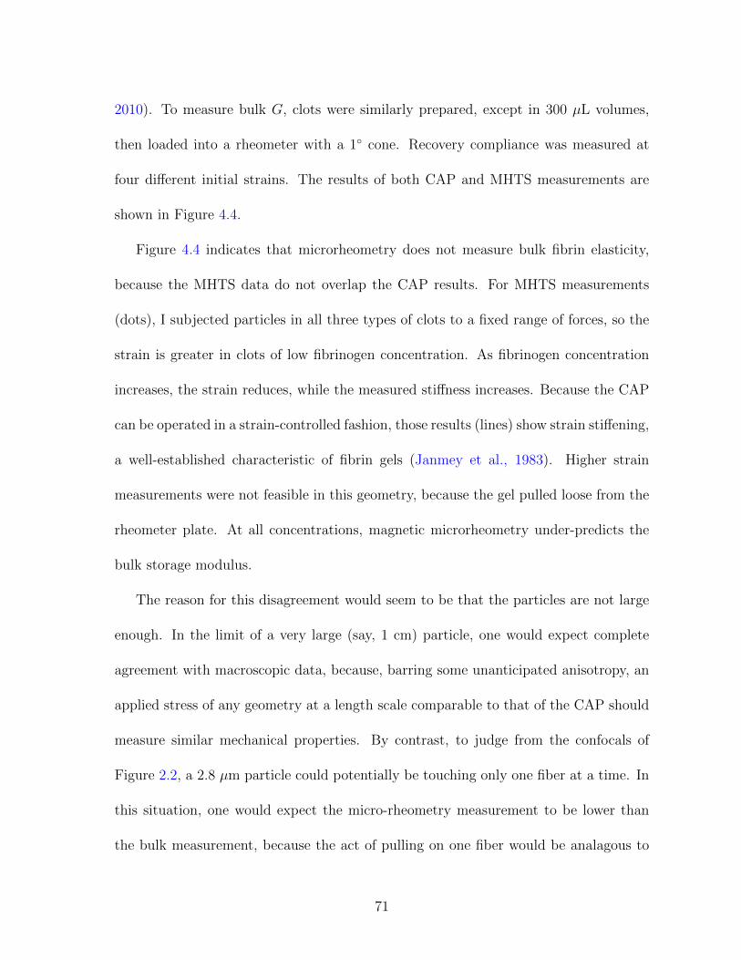
2010). To measure bulk G, clots were similarly prepared, except in 300 µL volumes,

then loaded into a rheometer with a 1◦ cone. Recovery compliance was measured at

four different initial strains. The results of both CAP and MHTS measurements are

shown in Figure 4.4.

Figure 4.4 indicates that microrheometry does not measure bulk fibrin elasticity,

because the MHTS data do not overlap the CAP results. For MHTS measurements

(dots), I subjected particles in all three types of clots to a fixed range of forces, so the

strain is greater in clots of low fibrinogen concentration. As fibrinogen concentration

increases, the strain reduces, while the measured stiffness increases. Because the CAP

can be operated in a strain-controlled fashion, those results (lines) show strain stiffening,

a well-established characteristic of fibrin gels (Janmey et al., 1983). Higher strain

measurements were not feasible in this geometry, because the gel pulled loose from the

rheometer plate. At all concentrations, magnetic microrheometry under-predicts the

bulk storage modulus.

The reason for this disagreement would seem to be that the particles are not large

enough. In the limit of a very large (say, 1 cm) particle, one would expect complete

agreement with macroscopic data, because, barring some unanticipated anisotropy, an

applied stress of any geometry at a length scale comparable to that of the CAP should

measure similar mechanical properties. By contrast, to judge from the confocals of

Figure 2.2, a 2.8 µm particle could potentially be touching only one fiber at a time. In

this situation, one would expect the micro-rheometry measurement to be lower than

the bulk measurement, because the act of pulling on one fiber would be analagous to

71

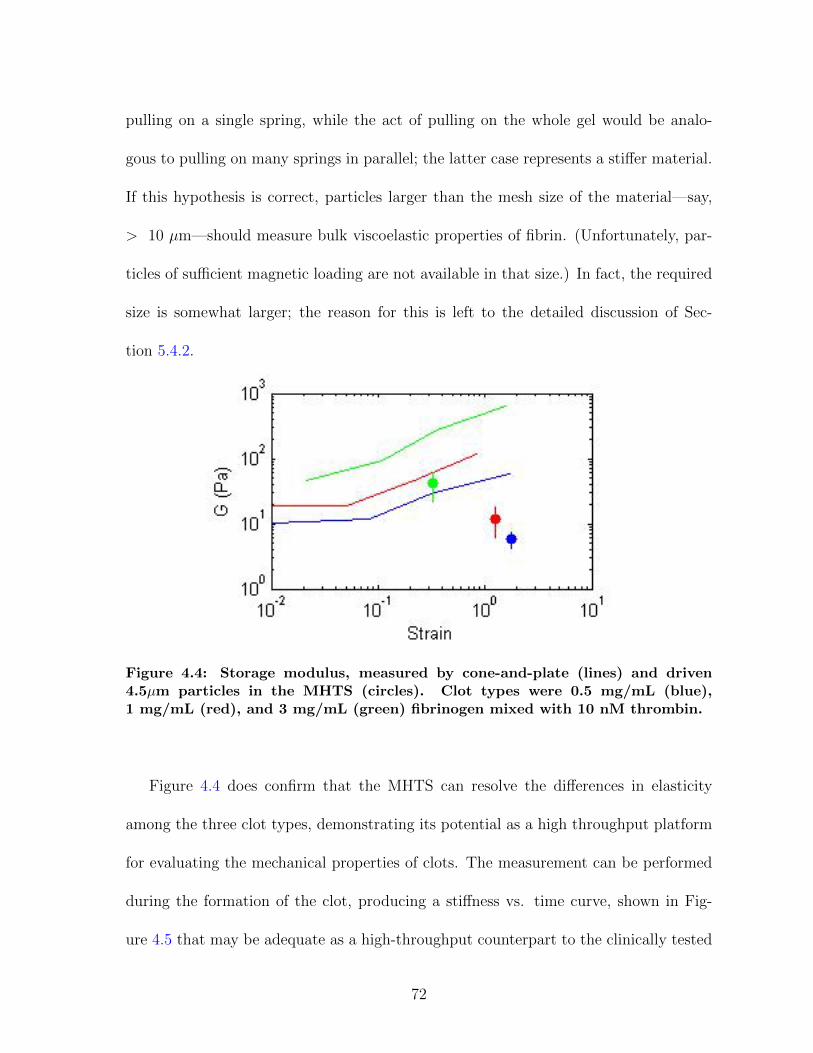
pulling on a single spring, while the act of pulling on the whole gel would be analo-

gous to pulling on many springs in parallel; the latter case represents a stiffer material.

If this hypothesis is correct, particles larger than the mesh size of the material—say,

> 10 µm—should measure bulk viscoelastic properties of fibrin. (Unfortunately, par-

ticles of sufficient magnetic loading are not available in that size.) In fact, the required

size is somewhat larger; the reason for this is left to the detailed discussion of Sec-

tion 5.4.2.

Figure 4.4: Storage modulus, measured by cone-and-plate (lines) and driven4.5µm particles in the MHTS (circles). Clot types were 0.5 mg/mL (blue),1 mg/mL (red), and 3 mg/mL (green) fibrinogen mixed with 10 nM thrombin.

Figure 4.4 does confirm that the MHTS can resolve the differences in elasticity

among the three clot types, demonstrating its potential as a high throughput platform

for evaluating the mechanical properties of clots. The measurement can be performed

during the formation of the clot, producing a stiffness vs. time curve, shown in Fig-

ure 4.5 that may be adequate as a high-throughput counterpart to the clinically tested

72

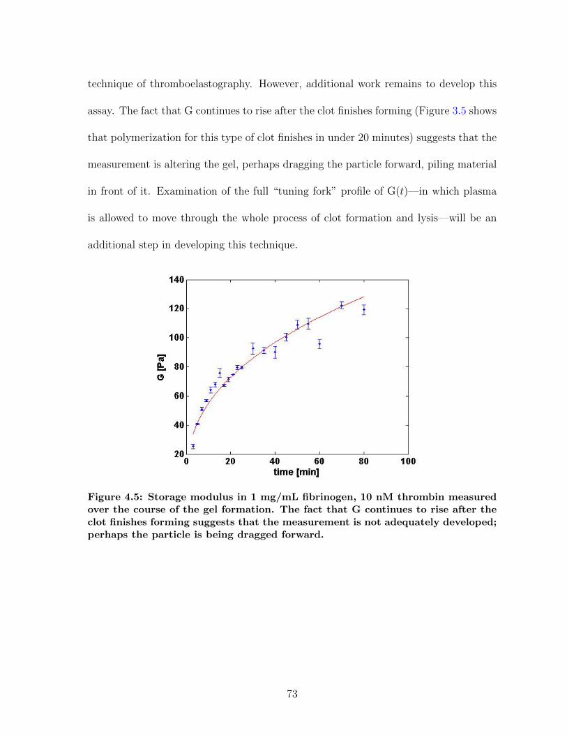
technique of thromboelastography. However, additional work remains to develop this

assay. The fact that G continues to rise after the clot finishes forming (Figure 3.5 shows

that polymerization for this type of clot finishes in under 20 minutes) suggests that the

measurement is altering the gel, perhaps dragging the particle forward, piling material

in front of it. Examination of the full “tuning fork” profile of G(t)—in which plasma

is allowed to move through the whole process of clot formation and lysis—will be an

additional step in developing this technique.

Figure 4.5: Storage modulus in 1 mg/mL fibrinogen, 10 nM thrombin measuredover the course of the gel formation. The fact that G continues to rise after theclot finishes forming suggests that the measurement is not adequately developed;perhaps the particle is being dragged forward.

73

4.3 Future Directions

The diffusion and magnetic microrheometry measurements made in this dissertation

have elucidated some of the specific phenomena relevant to particle transport in clots.

It has also opened new areas for inquiry, particularly regarding the dynamics of stuck

particles and the design of drug delivery vectors.

A new platform is required to fully characterize particle adhesion for vascular drug

delivery, one that can simultaneously measure clot permeability, particle diffusion, and

clot structure. A platform that better captures the geometry of a blood vessel is

also desirable. Figure 4.6 presents a flowcell concept drawing that addresses these

needs. The design of this device offers several benefits over a traditional permeability

measurement. First, it is flow-controlled, meaning it can measure permeability at a

much wider range of flow rates than practically achievable by gravity-driven (pressure-

controlled) flow. Second, it provides a “four-point” measurement of flow resistance

(analogous to the traditional four-point electronics measurement), eliminating errors

due to the resistance of the rest of the flow system. Third, the system is compatible

with high-NA microscopy, allowing permeability to be determined simultaneously with

clot structure, fiber deformation under flow, and particle diffusion and advection.

4.4 Conclusions

Chapter 3 demonstrated that the local environment of nano-particles in fibrin ap-

pears to be purely hydrodynamic for freely diffusing nanoparticles. In this Chapter I

74

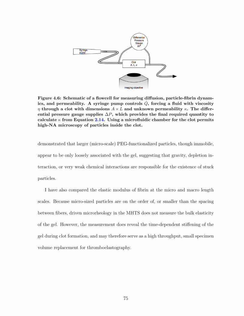
Figure 4.6: Schematic of a flowcell for measuring diffusion, particle-fibrin dynam-ics, and permeability. A syringe pump controls Q, forcing a fluid with viscosityη through a clot with dimensions A×L and unknown permeability κ. The differ-ential pressure gauge supplies ∆P , which provides the final required quantity tocalculate κ from Equation 2.14. Using a microfluidic chamber for the clot permitshigh-NA microscopy of particles inside the clot.

demonstrated that larger (micro-scale) PEG-functionalized particles, though immobile,

appear to be only loosely associated with the gel, suggesting that gravity, depletion in-

teraction, or very weak chemical interactions are responsible for the existence of stuck

particles.

I have also compared the elastic modulus of fibrin at the micro and macro length

scales. Because micro-sized particles are on the order of, or smaller than the spacing

between fibers, driven microrheology in the MHTS does not measure the bulk elasticity

of the gel. However, the measurement does reveal the time-dependent stiffening of the

gel during clot formation, and may therefore serve as a high throughput, small specimen

volume replacement for thromboelastography.

75

Chapter 5Toward High Throughput

My results have implications for coagulation research and drug design. But these

experiments’ long-term utility will be determined as much by the operational difficulty

of making the measurement as by the scientific questions at hand. In this Chapter I

present novel instrumentation for high-throughput characterization of clot transport

and mechanics. These systems are a high throughput “multiscope” and a microplate-

based force application system for biophysical experiments.

Biophysical experiments include more than diffusion and driven microrheology of

fibrin. The systems presented in this Chapter are designed to accelerate data acqui-

sition and processing for a wide range of measurements, including passive and driven

microrheology of fibrin, mucus, DNA, extracellular matrix, and other polymers; sin-

gle cell mechanics; cell migration and cytometry; and cell-substrate interaction using

microscale post arrays.

Transitioning any of these experiments to high throughput would require automated

microscopy, commonly called high content screening (HCS). The essential task in this

growing field is to take more images, faster, with less human intervention. The benefits

are evident in the wide range of results being acquired with HCS systems. These include

results on the proteins (Shen et al., 2006) and genes (Simpson et al., 2008) involved in

cell migration. Recent work used siRNA knockdown to identify every gene relevant to

cell division (Neumann et al., 2010). High content cell screening is increasingly critical

for drug discovery (Lang et al., 2006).

The benefit of an HCS system for the experiments in this dissertation are also

apparent. The fibrin diffusion experiments of Chapter 3 used 10 minutes of video per

specimen, assuming five videos per clot and two clots per preparation. The total from

eight specimens and two bead sizes—using 32 wells in a microplate—is nearly three

hours of video. Yet eight specimens is a tiny fraction of the parameter space we would

ideally hope to explore. Consider the human genome siRNA study of genes involved in

cell division, and consider a similar knockdown of the genes involved in clot formation

above cells, using recent experiments (Wolberg and Campbell, 2008) as a template.

One diffusion measurement would be required to test each gene (roughly 21,000) at

each particle size (at least 2), against a range of clot types (perhaps 4 donors’ worth

of healthy plasma). This experiment alone represents 420 mL of plasma per donor

(assuming 20 µL of plasma per well), and 168,000 measurements of Deff . At 10 minutes

of video per measurement, the experiment would last 28,000 hours, or 3.2 years, running

day and night. Clearly, an automated, highly parallel system would be required.

While HCS has improved throughput for cell imaging, it has left microrheology

behind. This is unfortunate, as microrheology shows promise as a tool for scientific

77

and industrial high throughput screening (Breedveld and Pine, 2003). However, the

specifications for a microrheology instrument are different in key ways. First, high

bandwidth video is desirable to capture dynamic phenomena. Second, the specimens

are not planar, because the particles are distributed through the material volume.

These specifications are not met by the various commercial HCS systems for imag-

ing cytometry. The manufacturers (Beckman Coulter, GE, Perkin Elmer, Roche, and

Thermo) provide software designed for snapshots, rather than high framerate (> 10 Hz)

video microscopy. Their autofocus routines are designed to identify planar specimens.

Their image processing software typically excels at cytometry (measuring cell area, cir-

cularity, migration), but lacks high-precision, automated particle tracking capability.

These design decisions make existing HCS systems impractical for microrheology.

These systems’ hardware designs also place limitations on experiments—both in cell

imaging and microrheology—that are undesirable. They are not compatible (in hard-

ware or software) with force application systems, including our magnetic microplate-

based design (Spero et al., 2008). Also, the systems are all essentially a traditional

microscope over which the specimen is systematically translated. Therefore, the length

of an experiment in such a system can never be shorter than the product Nti, where

N is the number of specimens and ti is the time to acquire data from each specimen.

In addition, the single-microscope design is incompatible with simultaneously imag-

ing multiple wells, which may be desirable for recording dynamic phenomena such as

time-dependent microrheology or cell migration; even if simultaneous imaging is not

required, for any non-stationary process, the maximum sample rate is 1/Nti.

78

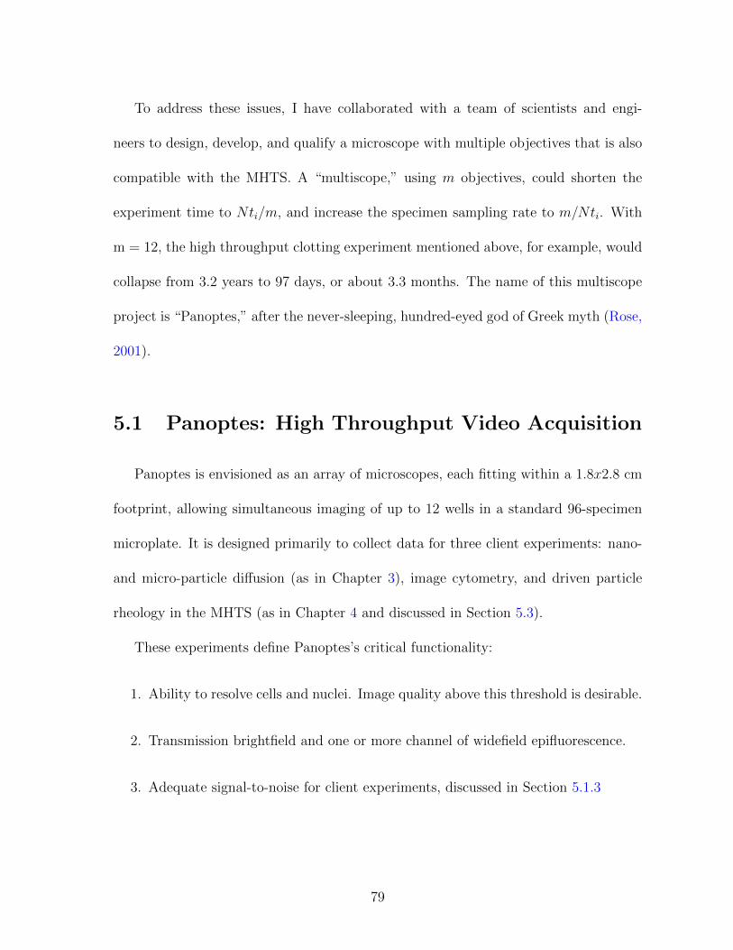
To address these issues, I have collaborated with a team of scientists and engi-

neers to design, develop, and qualify a microscope with multiple objectives that is also

compatible with the MHTS. A “multiscope,” using m objectives, could shorten the

experiment time to Nti/m, and increase the specimen sampling rate to m/Nti. With

m = 12, the high throughput clotting experiment mentioned above, for example, would

collapse from 3.2 years to 97 days, or about 3.3 months. The name of this multiscope

project is “Panoptes,” after the never-sleeping, hundred-eyed god of Greek myth (Rose,

2001).

5.1 Panoptes: High Throughput Video Acquisition

Panoptes is envisioned as an array of microscopes, each fitting within a 1.8x2.8 cm

footprint, allowing simultaneous imaging of up to 12 wells in a standard 96-specimen

microplate. It is designed primarily to collect data for three client experiments: nano-

and micro-particle diffusion (as in Chapter 3), image cytometry, and driven particle

rheology in the MHTS (as in Chapter 4 and discussed in Section 5.3).

These experiments define Panoptes’s critical functionality:

1. Ability to resolve cells and nuclei. Image quality above this threshold is desirable.

2. Transmission brightfield and one or more channel of widefield epifluorescence.

3. Adequate signal-to-noise for client experiments, discussed in Section 5.1.3

79

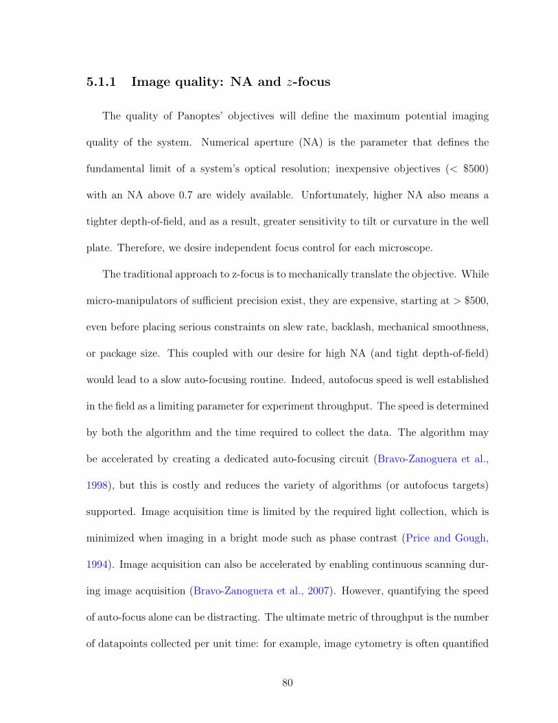
5.1.1 Image quality: NA and z-focus

The quality of Panoptes’ objectives will define the maximum potential imaging

quality of the system. Numerical aperture (NA) is the parameter that defines the

fundamental limit of a system’s optical resolution; inexpensive objectives (< $500)

with an NA above 0.7 are widely available. Unfortunately, higher NA also means a

tighter depth-of-field, and as a result, greater sensitivity to tilt or curvature in the well

plate. Therefore, we desire independent focus control for each microscope.

The traditional approach to z-focus is to mechanically translate the objective. While

micro-manipulators of sufficient precision exist, they are expensive, starting at > $500,

even before placing serious constraints on slew rate, backlash, mechanical smoothness,

or package size. This coupled with our desire for high NA (and tight depth-of-field)

would lead to a slow auto-focusing routine. Indeed, autofocus speed is well established

in the field as a limiting parameter for experiment throughput. The speed is determined

by both the algorithm and the time required to collect the data. The algorithm may

be accelerated by creating a dedicated auto-focusing circuit (Bravo-Zanoguera et al.,

1998), but this is costly and reduces the variety of algorithms (or autofocus targets)

supported. Image acquisition time is limited by the required light collection, which is

minimized when imaging in a bright mode such as phase contrast (Price and Gough,

1994). Image acquisition can also be accelerated by enabling continuous scanning dur-

ing image acquisition (Bravo-Zanoguera et al., 2007). However, quantifying the speed

of auto-focus alone can be distracting. The ultimate metric of throughput is the number

of datapoints collected per unit time: for example, image cytometry is often quantified

80

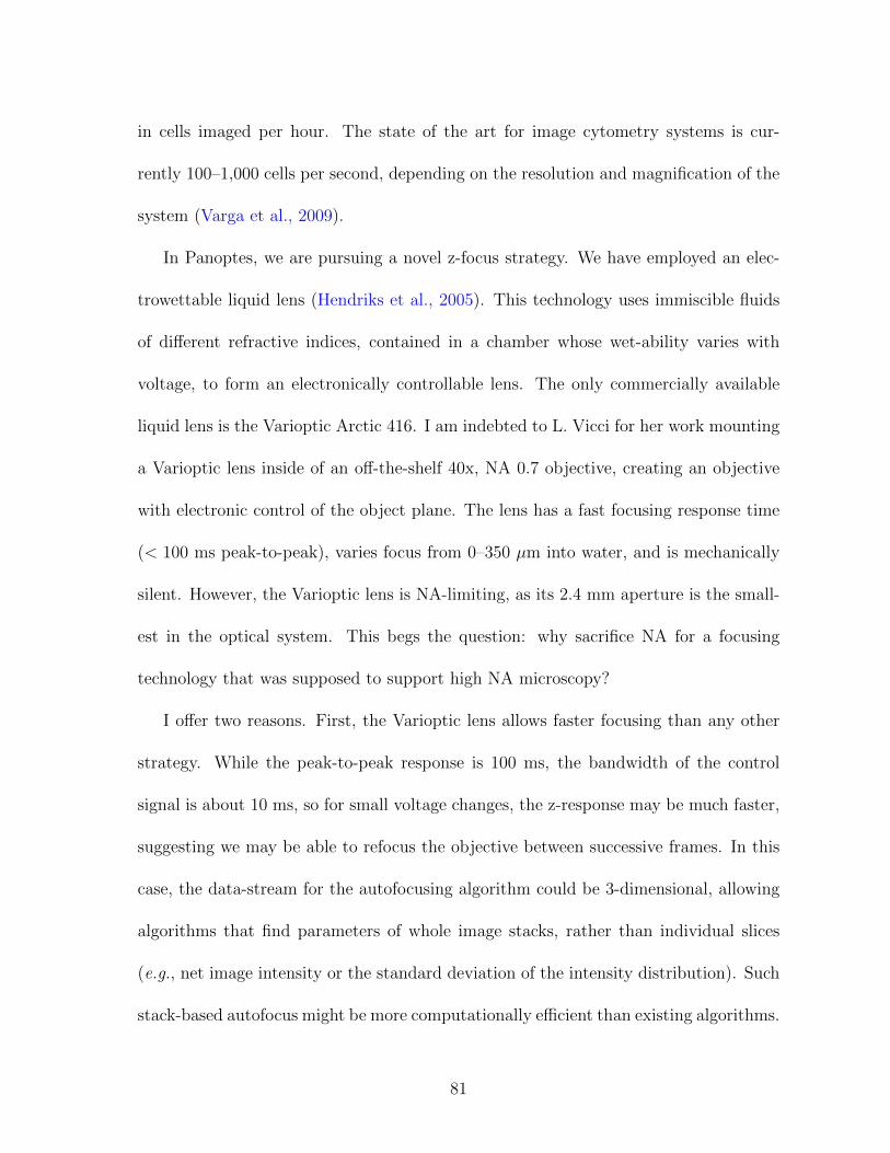
in cells imaged per hour. The state of the art for image cytometry systems is cur-

rently 100–1,000 cells per second, depending on the resolution and magnification of the

system (Varga et al., 2009).

In Panoptes, we are pursuing a novel z-focus strategy. We have employed an elec-

trowettable liquid lens (Hendriks et al., 2005). This technology uses immiscible fluids

of different refractive indices, contained in a chamber whose wet-ability varies with

voltage, to form an electronically controllable lens. The only commercially available

liquid lens is the Varioptic Arctic 416. I am indebted to L. Vicci for her work mounting

a Varioptic lens inside of an off-the-shelf 40x, NA 0.7 objective, creating an objective

with electronic control of the object plane. The lens has a fast focusing response time

(< 100 ms peak-to-peak), varies focus from 0–350 µm into water, and is mechanically

silent. However, the Varioptic lens is NA-limiting, as its 2.4 mm aperture is the small-

est in the optical system. This begs the question: why sacrifice NA for a focusing

technology that was supposed to support high NA microscopy?

I offer two reasons. First, the Varioptic lens allows faster focusing than any other

strategy. While the peak-to-peak response is 100 ms, the bandwidth of the control

signal is about 10 ms, so for small voltage changes, the z-response may be much faster,

suggesting we may be able to refocus the objective between successive frames. In this

case, the data-stream for the autofocusing algorithm could be 3-dimensional, allowing

algorithms that find parameters of whole image stacks, rather than individual slices

(e.g., net image intensity or the standard deviation of the intensity distribution). Such

stack-based autofocus might be more computationally efficient than existing algorithms.

81

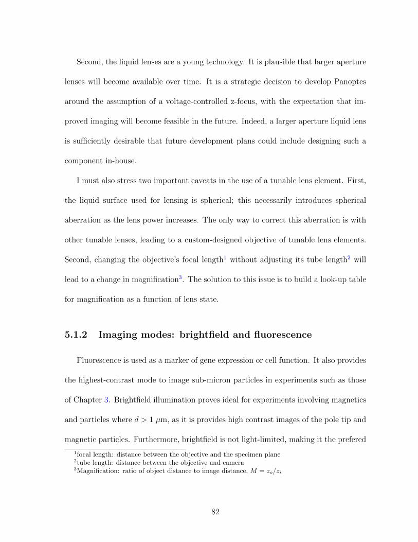
Second, the liquid lenses are a young technology. It is plausible that larger aperture

lenses will become available over time. It is a strategic decision to develop Panoptes

around the assumption of a voltage-controlled z-focus, with the expectation that im-

proved imaging will become feasible in the future. Indeed, a larger aperture liquid lens

is sufficiently desirable that future development plans could include designing such a

component in-house.

I must also stress two important caveats in the use of a tunable lens element. First,

the liquid surface used for lensing is spherical; this necessarily introduces spherical

aberration as the lens power increases. The only way to correct this aberration is with

other tunable lenses, leading to a custom-designed objective of tunable lens elements.

Second, changing the objective’s focal length1 without adjusting its tube length2 will

lead to a change in magnification3. The solution to this issue is to build a look-up table

for magnification as a function of lens state.

5.1.2 Imaging modes: brightfield and fluorescence

Fluorescence is used as a marker of gene expression or cell function. It also provides

the highest-contrast mode to image sub-micron particles in experiments such as those

of Chapter 3. Brightfield illumination proves ideal for experiments involving magnetics

and particles where d > 1 µm, as it is provides high contrast images of the pole tip and

magnetic particles. Furthermore, brightfield is not light-limited, making it the prefered

1focal length: distance between the objective and the specimen plane2tube length: distance between the objective and camera3Magnification: ratio of object distance to image distance, M = zo/zi

82

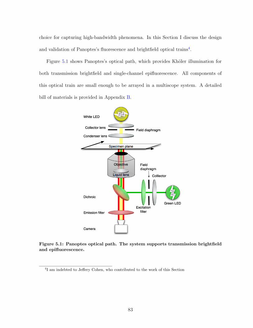
choice for capturing high-bandwidth phenomena. In this Section I discuss the design

and validation of Panoptes’s fluorescence and brightfield optical trains4.

Figure 5.1 shows Panoptes’s optical path, which provides Kholer illumination for

both transmission brightfield and single-channel epifluorescence. All components of

this optical train are small enough to be arrayed in a multiscope system. A detailed

bill of materials is provided in Appendix B.

Figure 5.1: Panoptes optical path. The system supports transmission brightfieldand epifluorescence.

4I am indebted to Jeffery Cohen, who contributed to the work of this Section

83

5.1.2.1 Single-channel widefield epifluorescence design

For epifluorescence, the condenser lens is also the imaging objective, and therefore

the back focal plane is not usually known. However, an image at a lens’s back focal

plane corresponds to a conjugate image at infinity in front of the lens. Therefore, we can

conveniently verify that we have achieved Kholer illumination by projecting the image

of the LED onto a screen placed at the objective’s far-field. The optimal collector lens

selection and position would ensure that the image of the LED at the objective’s back

focal plane is small enough to fit within the Varioptic lens aperture, and that the solid

angle collected from the LED captures as much light as possible.

Figure 5.2 helps clarify which adjustments can be made to optimize the fluorescence

illumination. Consider the objective location to be fixed. It is best to keep the collector

lens close to the objective, to minimize the magnification of the LED; the minimum

separation is set by the physical size of the objective and the need to place a dichroic

between these two elements. Reducing the collector lens aperture can improve con-

trast by reducing the illumination intensity above and below the imaging plane while

preserving the illumination intensity across the field of view. However, the smaller the

aperture, the smaller the solid angle collected from the LED, which reduces the overall

intensity and therefore the overall signal. The LED is moved into the correct position

behind the collector to achieve a focus at infinity on the far side of the objective.

To obtain the best possible illumination field, a small aperture, short focal length

collector lens is desirable, allowing minimum separation between the LED, collector,

and the objective. This maximizes contrast, maximizes the captured solid angle of

84

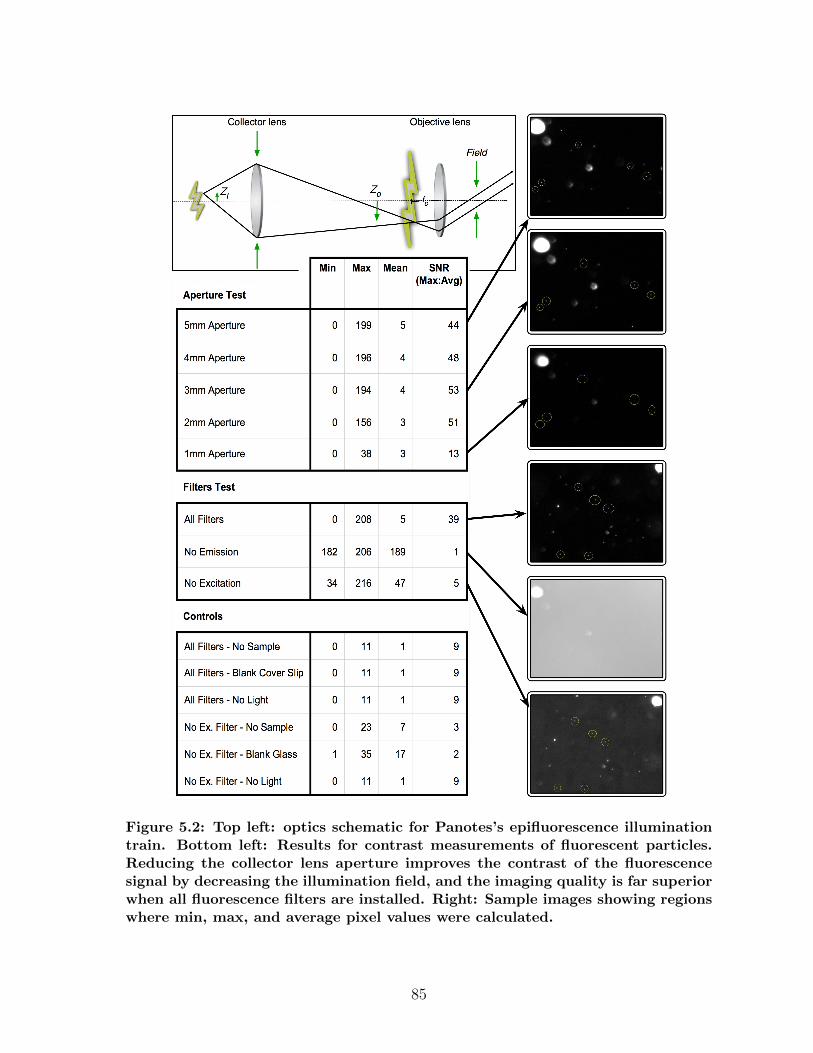
Figure 5.2: Top left: optics schematic for Panotes’s epifluorescence illuminationtrain. Bottom left: Results for contrast measurements of fluorescent particles.Reducing the collector lens aperture improves the contrast of the fluorescencesignal by decreasing the illumination field, and the imaging quality is far superiorwhen all fluorescence filters are installed. Right: Sample images showing regionswhere min, max, and average pixel values were calculated.

85

light from the LED, and minimizes overfilling of the back-aperture of the objective.

Currently, we are using an LED with an emitting diameter of 0.5 mm and half-cone

angle emission of 80◦, and a collector lens with an aperture of 15 mm and a focal length

f of 12 mm. To measure the contrast of this illumination arrangement, line scans of

200 and 500 nm particles were compared with and without a 4 mm aperture in front

of the collector lens. The data are shown in Figure 5.2. As anticipated, reducing the

collector lens aperture improves the contrast, at the expense of the total fluorescence

signal. In the next build of Panoptes, we will have a custom-cut dichroic that will allow

a shorter total optical path, and permit us to capture more solid angle from the LED,

while still improving image contrast.

5.1.2.2 Brightfield design

For brightfield, the condenser lens must focus light through the MHTS magnetics

block, which places a lower bound on its focal length (16 mm) and, thanks to the 1/8”

annulus, an upper bound on its NA (0.21). The images shown below use 1” optics; we

have deferred selection of final illumination optics until after the construction of the

inverted microscope. However, a wide range of LEDs and inexpensive, injection-molded

lenses are available.

We have chosen to not pursue phase contrast microscopy in this design, but I will

note that an interference imaging mode would be a minor modification to this design.

The traditional phase contrast microscope uses an amplitude mask on the illumination

side and a phase mask behind the imaging objective; newer approaches use so-called

86

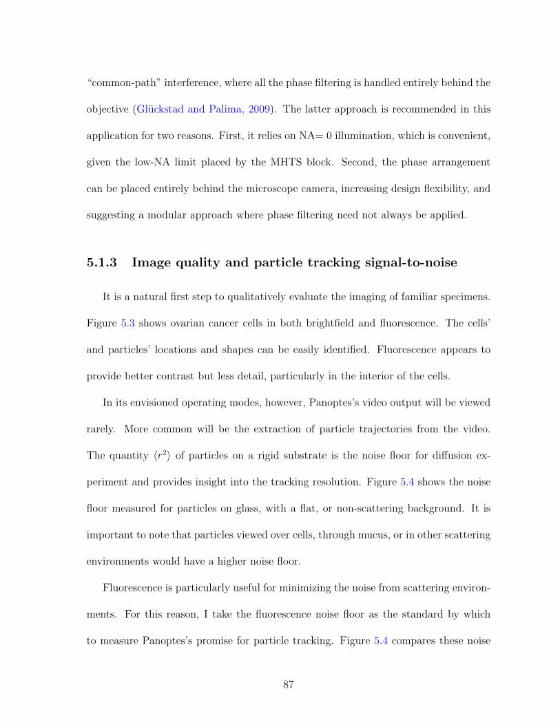
“common-path” interference, where all the phase filtering is handled entirely behind the

objective (Gluckstad and Palima, 2009). The latter approach is recommended in this

application for two reasons. First, it relies on NA= 0 illumination, which is convenient,

given the low-NA limit placed by the MHTS block. Second, the phase arrangement

can be placed entirely behind the microscope camera, increasing design flexibility, and

suggesting a modular approach where phase filtering need not always be applied.

5.1.3 Image quality and particle tracking signal-to-noise

It is a natural first step to qualitatively evaluate the imaging of familiar specimens.

Figure 5.3 shows ovarian cancer cells in both brightfield and fluorescence. The cells’

and particles’ locations and shapes can be easily identified. Fluorescence appears to

provide better contrast but less detail, particularly in the interior of the cells.

In its envisioned operating modes, however, Panoptes’s video output will be viewed

rarely. More common will be the extraction of particle trajectories from the video.

The quantity 〈r2〉 of particles on a rigid substrate is the noise floor for diffusion ex-

periment and provides insight into the tracking resolution. Figure 5.4 shows the noise

floor measured for particles on glass, with a flat, or non-scattering background. It is

important to note that particles viewed over cells, through mucus, or in other scattering

environments would have a higher noise floor.

Fluorescence is particularly useful for minimizing the noise from scattering environ-

ments. For this reason, I take the fluorescence noise floor as the standard by which

to measure Panoptes’s promise for particle tracking. Figure 5.4 compares these noise

87

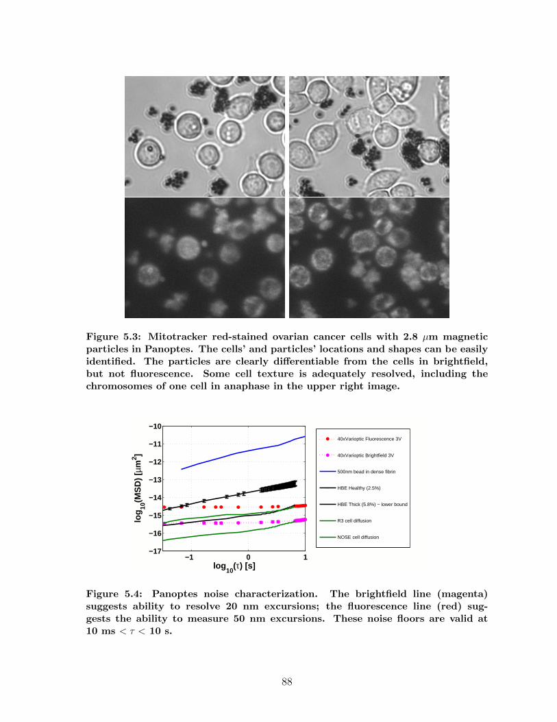
Figure 5.3: Mitotracker red-stained ovarian cancer cells with 2.8 µm magneticparticles in Panoptes. The cells’ and particles’ locations and shapes can be easilyidentified. The particles are clearly differentiable from the cells in brightfield,but not fluorescence. Some cell texture is adequately resolved, including thechromosomes of one cell in anaphase in the upper right image.

−1 0 1−17

−16

−15

−14

−13

−12

−11

−10

log10

(τ) [s]

log

10(M

SD

) [µ

m2 ]

40xVarioptic Fluorescence 3V

40xVarioptic Brightfield 3V

500nm bead in dense fibrin

HBE Healthy (2.5%)

HBE Thick (5.8%) − lower bound

R3 cell diffusion

NOSE cell diffusion

Figure 5.4: Panoptes noise characterization. The brightfield line (magenta)suggests ability to resolve 20 nm excursions; the fluorescence line (red) sug-gests the ability to measure 50 nm excursions. These noise floors are valid at10 ms < τ < 10 s.

88

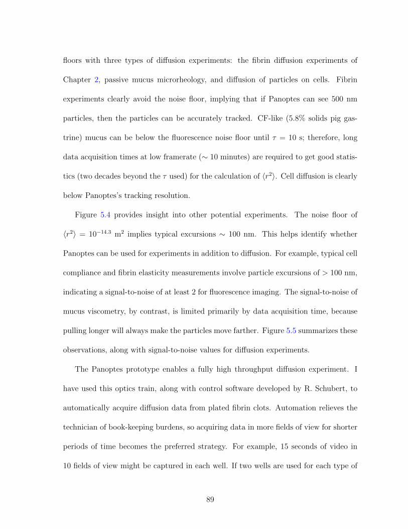
floors with three types of diffusion experiments: the fibrin diffusion experiments of

Chapter 2, passive mucus microrheology, and diffusion of particles on cells. Fibrin

experiments clearly avoid the noise floor, implying that if Panoptes can see 500 nm

particles, then the particles can be accurately tracked. CF-like (5.8% solids pig gas-

trine) mucus can be below the fluorescence noise floor until τ = 10 s; therefore, long

data acquisition times at low framerate (∼ 10 minutes) are required to get good statis-

tics (two decades beyond the τ used) for the calculation of 〈r2〉. Cell diffusion is clearly

below Panoptes’s tracking resolution.

Figure 5.4 provides insight into other potential experiments. The noise floor of

〈r2〉 = 10−14.3 m2 implies typical excursions ∼ 100 nm. This helps identify whether

Panoptes can be used for experiments in addition to diffusion. For example, typical cell

compliance and fibrin elasticity measurements involve particle excursions of > 100 nm,

indicating a signal-to-noise of at least 2 for fluorescence imaging. The signal-to-noise of

mucus viscometry, by contrast, is limited primarily by data acquisition time, because

pulling longer will always make the particles move farther. Figure 5.5 summarizes these

observations, along with signal-to-noise values for diffusion experiments.

The Panoptes prototype enables a fully high throughput diffusion experiment. I

have used this optics train, along with control software developed by R. Schubert, to

automatically acquire diffusion data from plated fibrin clots. Automation relieves the

technician of book-keeping burdens, so acquiring data in more fields of view for shorter

periods of time becomes the preferred strategy. For example, 15 seconds of video in

10 fields of view might be captured in each well. If two wells are used for each type of

89

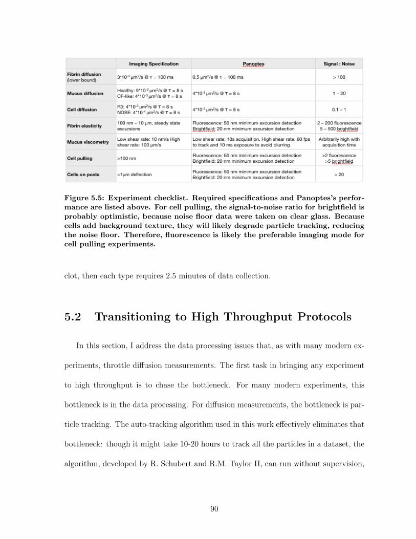
Figure 5.5: Experiment checklist. Required specifications and Panoptes’s perfor-mance are listed above. For cell pulling, the signal-to-noise ratio for brightfield isprobably optimistic, because noise floor data were taken on clear glass. Becausecells add background texture, they will likely degrade particle tracking, reducingthe noise floor. Therefore, fluorescence is likely the preferable imaging mode forcell pulling experiments.

clot, then each type requires 2.5 minutes of data collection.

5.2 Transitioning to High Throughput Protocols

In this section, I address the data processing issues that, as with many modern ex-

periments, throttle diffusion measurements. The first task in bringing any experiment

to high throughput is to chase the bottleneck. For many modern experiments, this

bottleneck is in the data processing. For diffusion measurements, the bottleneck is par-

ticle tracking. The auto-tracking algorithm used in this work effectively eliminates that

bottleneck: though it might take 10-20 hours to track all the particles in a dataset, the

algorithm, developed by R. Schubert and R.M. Taylor II, can run without supervision,

90

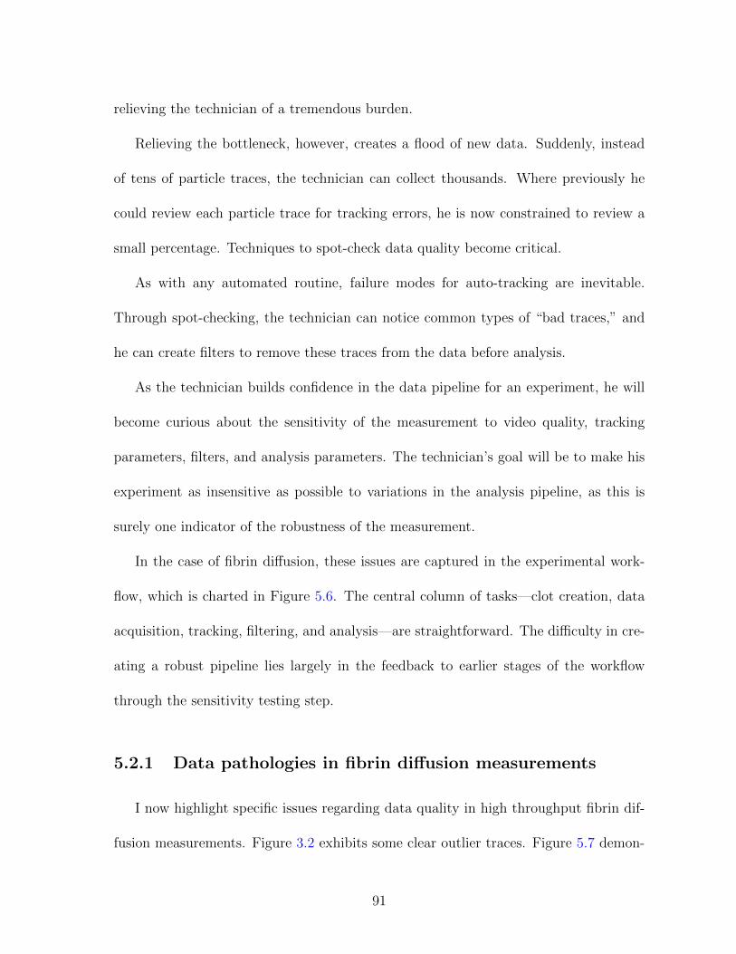
relieving the technician of a tremendous burden.

Relieving the bottleneck, however, creates a flood of new data. Suddenly, instead

of tens of particle traces, the technician can collect thousands. Where previously he

could review each particle trace for tracking errors, he is now constrained to review a

small percentage. Techniques to spot-check data quality become critical.

As with any automated routine, failure modes for auto-tracking are inevitable.

Through spot-checking, the technician can notice common types of “bad traces,” and

he can create filters to remove these traces from the data before analysis.

As the technician builds confidence in the data pipeline for an experiment, he will

become curious about the sensitivity of the measurement to video quality, tracking

parameters, filters, and analysis parameters. The technician’s goal will be to make his

experiment as insensitive as possible to variations in the analysis pipeline, as this is

surely one indicator of the robustness of the measurement.

In the case of fibrin diffusion, these issues are captured in the experimental work-

flow, which is charted in Figure 5.6. The central column of tasks—clot creation, data

acquisition, tracking, filtering, and analysis—are straightforward. The difficulty in cre-

ating a robust pipeline lies largely in the feedback to earlier stages of the workflow

through the sensitivity testing step.

5.2.1 Data pathologies in fibrin diffusion measurements

I now highlight specific issues regarding data quality in high throughput fibrin dif-

fusion measurements. Figure 3.2 exhibits some clear outlier traces. Figure 5.7 demon-

91

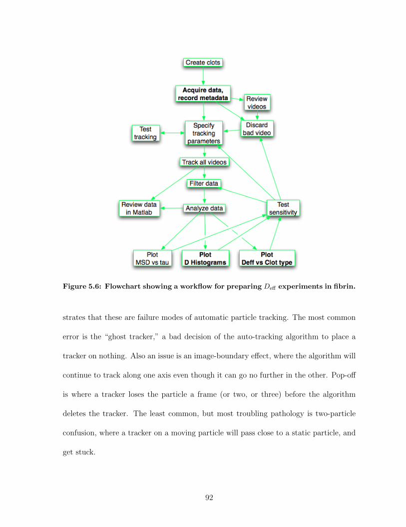
Figure 5.6: Flowchart showing a workflow for preparing Deff experiments in fibrin.

strates that these are failure modes of automatic particle tracking. The most common

error is the “ghost tracker,” a bad decision of the auto-tracking algorithm to place a

tracker on nothing. Also an issue is an image-boundary effect, where the algorithm will

continue to track along one axis even though it can go no further in the other. Pop-off

is where a tracker loses the particle a frame (or two, or three) before the algorithm

deletes the tracker. The least common, but most troubling pathology is two-particle

confusion, where a tracker on a moving particle will pass close to a static particle, and

get stuck.

92

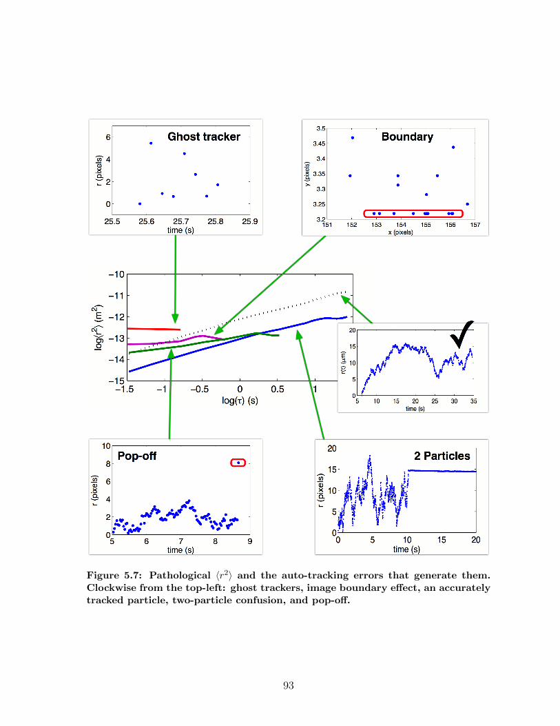
Figure 5.7: Pathological 〈r2〉 and the auto-tracking errors that generate them.Clockwise from the top-left: ghost trackers, image boundary effect, an accuratelytracked particle, two-particle confusion, and pop-off.

93

There are simple measures to filter each of these outlying trace types. Ghost trackers

are typically short-lived, and filtering trackers that last less than 2 seconds appears to

eliminate all of them. Wall-effect tracking errors occur at the extreme edge of the

image, and filtering trackers that come to the image boundary eliminates all of them.

Pop-on or pop-off trackers show sharp transitions in r2 at short timescales, so filtering

for non-stationary statistics would eliminate these trackers.

I contend that this experience in developing a high throughput fibrin diffusion exper-

iment has elements universal to bringing any experiment to a high throughput format.

Equally important, every new individual who decides to perform the measurement must

go through some version of this process. Skepticism of a new measurement will flourish

naturally; its natural predator is the ability to test the sensitivity of the measure-

ment against acquisition and processing parameters. The instrumentation designers’

responsibility, above all else, is to build a user interface hostile to the prey.

5.2.2 DataBrowser

I have designed a software interface to facilitate the process of experiment devel-

opment for high throughput microrheometry. I have based the interface around the

workflow of Figure 5.6. A mock-up is shown in Figure 5.8. The leftmost column of

interface elements provides a convenient environment to browse an experiment’s videos

and associated metadata. The types of metadata used in our experiments are cata-

logued in Appendix D.

The interface’s layout conforms to the central workflow of tracking, filtering, and

94

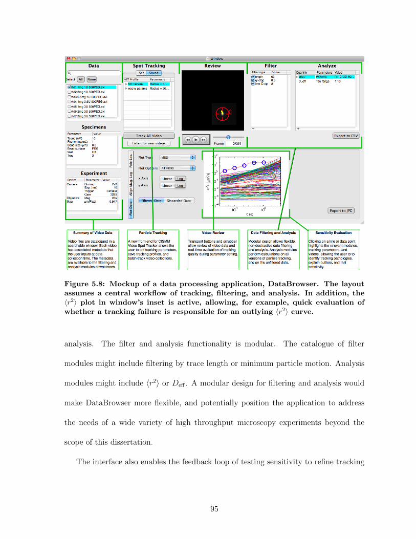
Figure 5.8: Mockup of a data processing application, DataBrowser. The layoutassumes a central workflow of tracking, filtering, and analysis. In addition, the〈r2〉 plot in window’s inset is active, allowing, for example, quick evaluation ofwhether a tracking failure is responsible for an outlying 〈r2〉 curve.

analysis. The filter and analysis functionality is modular. The catalogue of filter

modules might include filtering by trace length or minimum particle motion. Analysis

modules might include 〈r2〉 or Deff . A modular design for filtering and analysis would

make DataBrowser more flexible, and potentially position the application to address

the needs of a wide variety of high throughput microscopy experiments beyond the

scope of this dissertation.

The interface also enables the feedback loop of testing sensitivity to refine tracking

95

and filtering parameters through interactive plotting. Clicking on one 〈r2〉 curve would

allow the user to quickly review the raw video from which the tracking data were

collected. If the tracking were deemed faulty, the user could add a new filter intended

to eliminate that type of tracking error and immediately see whether it eliminates the

offending data.

Similarly, a module that calculated Deff would produce a plot similar to those in

Figures 3.6, and would support clicking on an individual datapoint. This action would

highlight the applied filters and the videos that compose the final datapoint. Un-

checking a video would trigger re-plotting without including that video’s data; the user

could then observe the sensitivity of the datapoint to that video—for example, the

unchecking of a bad video might cause the error bars of the datapoint to shrink.

The DataBrowser interface is intended to be extensible to other types of experiments

we perform in our research group, and potentially to a wide range of high throughput

microscopy experiments. Discussions with other scientists have revealed potential areas

for improvement or expansion of the DataBrowser interface. These include a step in

the pipeline for image analysis or processing (presumably before particle tracking), the

ability to import simulated tracking data, and the ability to append imaging data (for

example, quantities extracted from confocal images of clots) to the metadata of a video.

96

5.3 MHTS: High Throughput Manipulation

High throughput microbead rheology consists of more than diffusion measurements.

In particular, forcibly manipulating microparticles can provide a wealth of additional

information, including information about individual cell mechanics (Bausch et al., 1998)

and nonlinear polymer rheology (Meehan et al., 2010).

There has been little intersection between the high throughput trend and mechanical

study of biological systems. One high throughput nano-manipulation device, IBM’s

“Millipede” multi-tip AFM (Durig et al., 2000), is a notable exception, but its primary

application has been in data storage.

Among the systems for nano-manipulation, techniques using microbeads (particles

∼ 0.1− 10µm) have been widely applied. Microbeads are used to measure mechanical

properties of cells (Hubmayr et al., 1996; Bausch et al., 1999; Fabry et al., 2001; Lele

et al., 2007; Lenormand et al., 2007). Drug delivery strategies are being developed using

magnetic micro- and nano-particles (Dobson, 2006). Transfection efficiency has been

improved using “magnetofection,” where vectors are attached to magnetic particles

that are pushed against cells by magnetic fields (Plank et al., 2003).

Among microbead techniques, the “active,” or “driven” techniques, where an exter-

nal force is applied to a bead, can measure a wider range of moduli and are generally

more flexible than the passive techniques, where the bead motion is due to thermal dif-

fusion. Driven microrheology instrumentation includes laser traps (“optical tweezers”)

and paramagnetic attraction (“magnetic tweezers”). A laser trap offers high spatial

97

resolution and can be precisely calibrated (Neuman and Block, 2004). A magnetic

system can drive multiple beads simultaneously, produce higher forces at a given bead

size, and will neither heat nor otherwise interact with most biological specimens (Fisher

et al., 2006). The benefits of a driven system are apparent in this dissertation, as well,

as the results of Chapter 4 demonstrate.

In pursuit of HTS nano-manipulation, I have collaborated with a diverse team

of engineers and scientists to design, implement, and qualify a magnetics system for

microparticle manipulation that is compatible with high throughput screening stan-

dards (Spero et al., 2008). Briefly, the Magnetic High Throughput System (MHTS)

can apply forces ∼ 1pN–10nN . It is based on standard microplate geometry, and is

designed to be scalable to 96 wells. The force calibration is uniform from well to well

within a factor of two. The magnetic crosstalk among wells is < 5%. The temperature

is controllable by a fluid recirculation system, and maintains < 4◦C temperature rise

under the most pessimistic conditions. The MHTS has measured non-linear mucus

viscosity. Finally, cells have been successfully plated and their compliance has been

measured using the system.

5.3.1 MHTS Design

The present instrument, a Magnetic High Throughput System (MHTS) consists of

two components: 1) a magnetics block, which generates magnetic flux for each well, and

2) a magnetic microplate, a custom-designed high throughput tray that incorporates a

pole-flat in each specimen well. The arrangement of these components is summarized

98

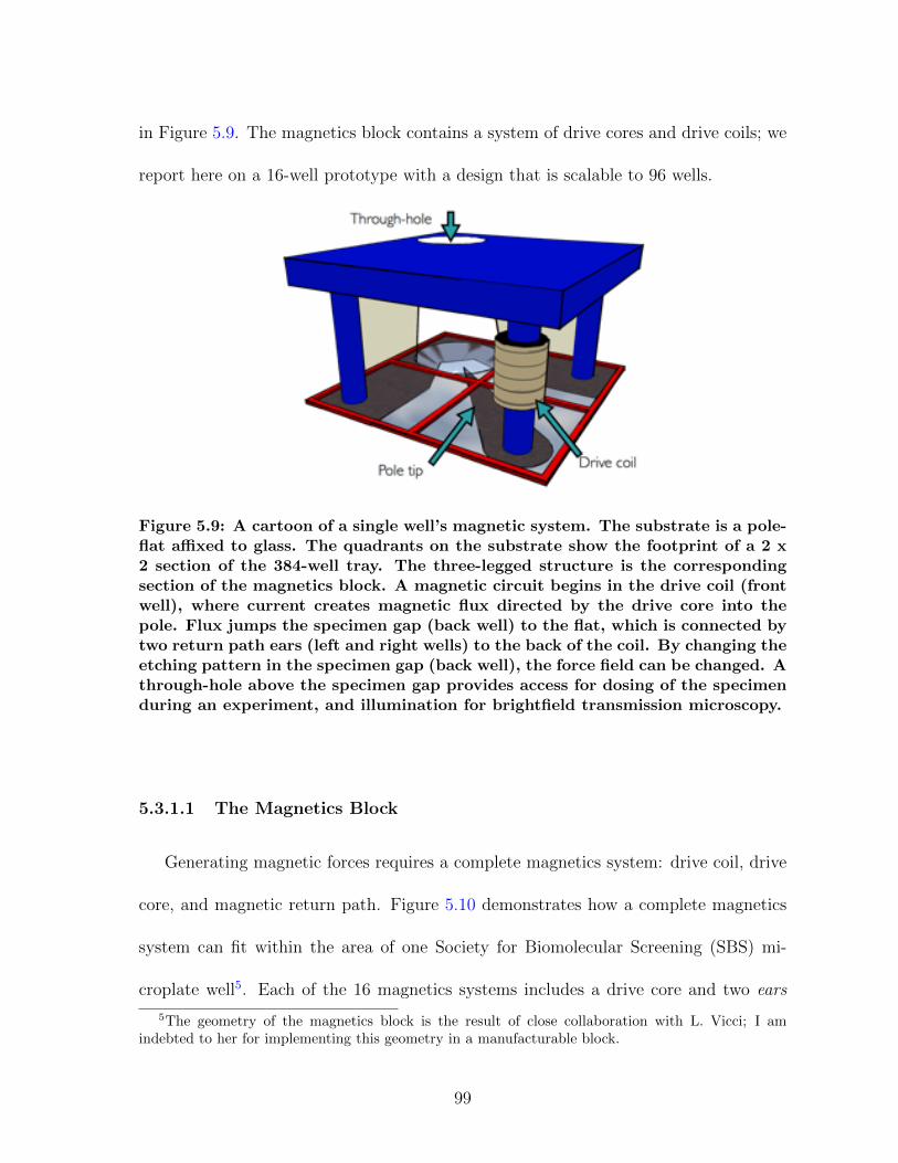
in Figure 5.9. The magnetics block contains a system of drive cores and drive coils; we

report here on a 16-well prototype with a design that is scalable to 96 wells.

Figure 5.9: A cartoon of a single well’s magnetic system. The substrate is a pole-flat affixed to glass. The quadrants on the substrate show the footprint of a 2 x2 section of the 384-well tray. The three-legged structure is the correspondingsection of the magnetics block. A magnetic circuit begins in the drive coil (frontwell), where current creates magnetic flux directed by the drive core into thepole. Flux jumps the specimen gap (back well) to the flat, which is connected bytwo return path ears (left and right wells) to the back of the coil. By changing theetching pattern in the specimen gap (back well), the force field can be changed. Athrough-hole above the specimen gap provides access for dosing of the specimenduring an experiment, and illumination for brightfield transmission microscopy.

5.3.1.1 The Magnetics Block

Generating magnetic forces requires a complete magnetics system: drive coil, drive

core, and magnetic return path. Figure 5.10 demonstrates how a complete magnetics

system can fit within the area of one Society for Biomolecular Screening (SBS) mi-

croplate well5. Each of the 16 magnetics systems includes a drive core and two ears

5The geometry of the magnetics block is the result of close collaboration with L. Vicci; I amindebted to her for implementing this geometry in a manufacturable block.

99

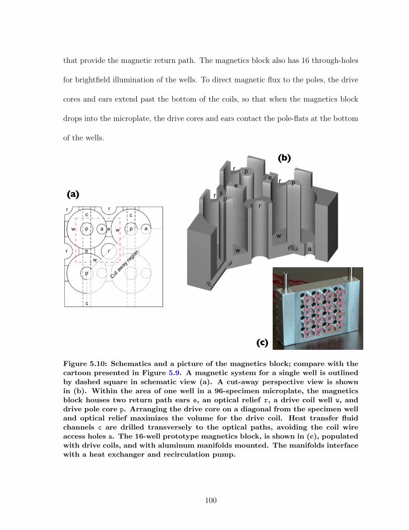
that provide the magnetic return path. The magnetics block also has 16 through-holes

for brightfield illumination of the wells. To direct magnetic flux to the poles, the drive

cores and ears extend past the bottom of the coils, so that when the magnetics block

drops into the microplate, the drive cores and ears contact the pole-flats at the bottom

of the wells.

(a)

(c)

(b)

Figure 5.10: Schematics and a picture of the magnetics block; compare with thecartoon presented in Figure 5.9. A magnetic system for a single well is outlinedby dashed square in schematic view (a). A cut-away perspective view is shownin (b). Within the area of one well in a 96-specimen microplate, the magneticsblock houses two return path ears e, an optical relief r, a drive coil well w, anddrive pole core p. Arranging the drive core on a diagonal from the specimen welland optical relief maximizes the volume for the drive coil. Heat transfer fluidchannels c are drilled transversely to the optical paths, avoiding the coil wireaccess holes a. The 16-well prototype magnetics block, is shown in (c), populatedwith drive coils, and with aluminum manifolds mounted. The manifolds interfacewith a heat exchanger and recirculation pump.

100

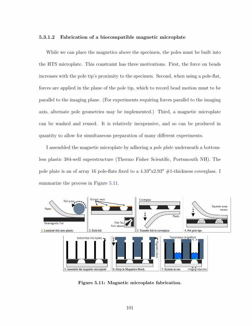
5.3.1.2 Fabrication of a biocompatible magnetic microplate

While we can place the magnetics above the specimen, the poles must be built into

the HTS microplate. This constraint has three motivations. First, the force on beads

increases with the pole tip’s proximity to the specimen. Second, when using a pole-flat,

forces are applied in the plane of the pole tip, which to record bead motion must to be

parallel to the imaging plane. (For experiments requiring forces parallel to the imaging

axis, alternate pole geometries may be implemented.) Third, a magnetic microplate

can be washed and reused. It is relatively inexpensive, and so can be produced in

quantity to allow for simultaneous preparation of many different experiments.

I assembled the magnetic microplate by adhering a pole plate underneath a bottom-

less plastic 384-well superstructure (Thermo Fisher Scientific, Portsmouth NH). The

pole plate is an of array 16 pole-flats fixed to a 4.33′′x2.93′′ #1-thickness coverglass. I

summarize the process in Figure 5.11.

Figure 5.11: Magnetic microplate fabrication.

101

We use a commercial photolithographic etching process (Fotofab Corporation, Chicago

IL) to manufacture the pole plate pattern. The poles must be isolated from any sur-

rounding magnetic material. Therefore, to maintain registration of these “floating”

poles relative to the flats, we bond the 0.004′′-thick foil (Magnetic Shield Corporation,

Bensenville IL) to a sacrificial sheet of 0.005′′-thick polycarbonate backing (K-mac Plas-

tics, Wyoming MI). Here I report on an array of pole flats (see the inset of Figure 5.11,

step 2), but any shape of pole tip may be specified at this stage. The pole plate pattern

is etched from the metal side of the foil-on-plastic.

To transfer the patterned foil to an optically clear substrate while maintaining

the registration of the poles, we roll UV-curable adhesive NOA 81 (Norland Optical

Adhesives, Cranburg NJ) onto the etched foil, cover it with #1-thickness coverglass,

press flat with a glass plate and cure, then remove the plastic backing. This orientation

places the sharp tip edge ∼ 100µm above the surface of the coverslip. A layer of

parylene, vapor-deposited at this stage, inhibits pole degradation.

The highest force is in the plane of the pole edge, where the force ranges as high

as ∼ 1nN (see Figure 5.12) on a 4.5µm bead. This geometry is desirable for some

applications, including rheometry of biomaterials. For other applications, including

cell force experiments, it is desirable to have the bottom of the well level with the pole.

To raise the cells to this height, we pot the foil in NOA 81, creating an optically clear

surface within 10µm of the plane of the poles. To create a surface conducive to cell

adhesion, we vapor-deposit 3-Aminopropyltriethoxysilane (Sigma-Aldrich, St. Louis

MO) solution onto the layer of NOA 81.

102

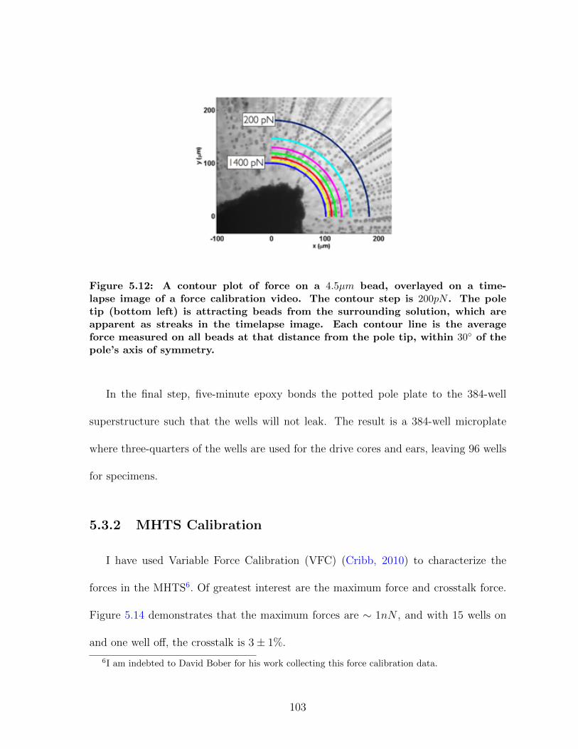
Figure 5.12: A contour plot of force on a 4.5µm bead, overlayed on a time-lapse image of a force calibration video. The contour step is 200pN . The poletip (bottom left) is attracting beads from the surrounding solution, which areapparent as streaks in the timelapse image. Each contour line is the averageforce measured on all beads at that distance from the pole tip, within 30◦ of thepole’s axis of symmetry.

In the final step, five-minute epoxy bonds the potted pole plate to the 384-well

superstructure such that the wells will not leak. The result is a 384-well microplate

where three-quarters of the wells are used for the drive cores and ears, leaving 96 wells

for specimens.

5.3.2 MHTS Calibration

I have used Variable Force Calibration (VFC) (Cribb, 2010) to characterize the

forces in the MHTS6. Of greatest interest are the maximum force and crosstalk force.

Figure 5.14 demonstrates that the maximum forces are ∼ 1nN , and with 15 wells on

and one well off, the crosstalk is 3± 1%.

6I am indebted to David Bober for his work collecting this force calibration data.

103

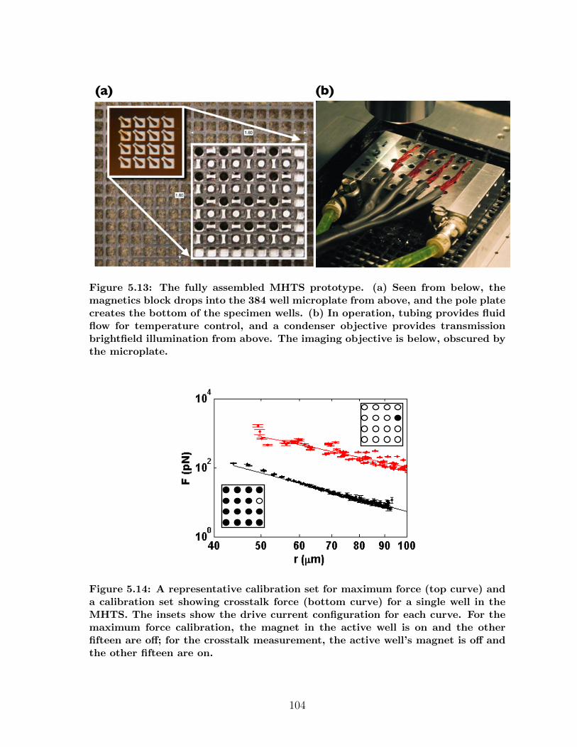
(a) (b)

Figure 5.13: The fully assembled MHTS prototype. (a) Seen from below, themagnetics block drops into the 384 well microplate from above, and the pole platecreates the bottom of the specimen wells. (b) In operation, tubing provides fluidflow for temperature control, and a condenser objective provides transmissionbrightfield illumination from above. The imaging objective is below, obscured bythe microplate.

Figure 5.14: A representative calibration set for maximum force (top curve) anda calibration set showing crosstalk force (bottom curve) for a single well in theMHTS. The insets show the drive current configuration for each curve. For themaximum force calibration, the magnet in the active well is on and the otherfifteen are off; for the crosstalk measurement, the active well’s magnet is off andthe other fifteen are on.

104

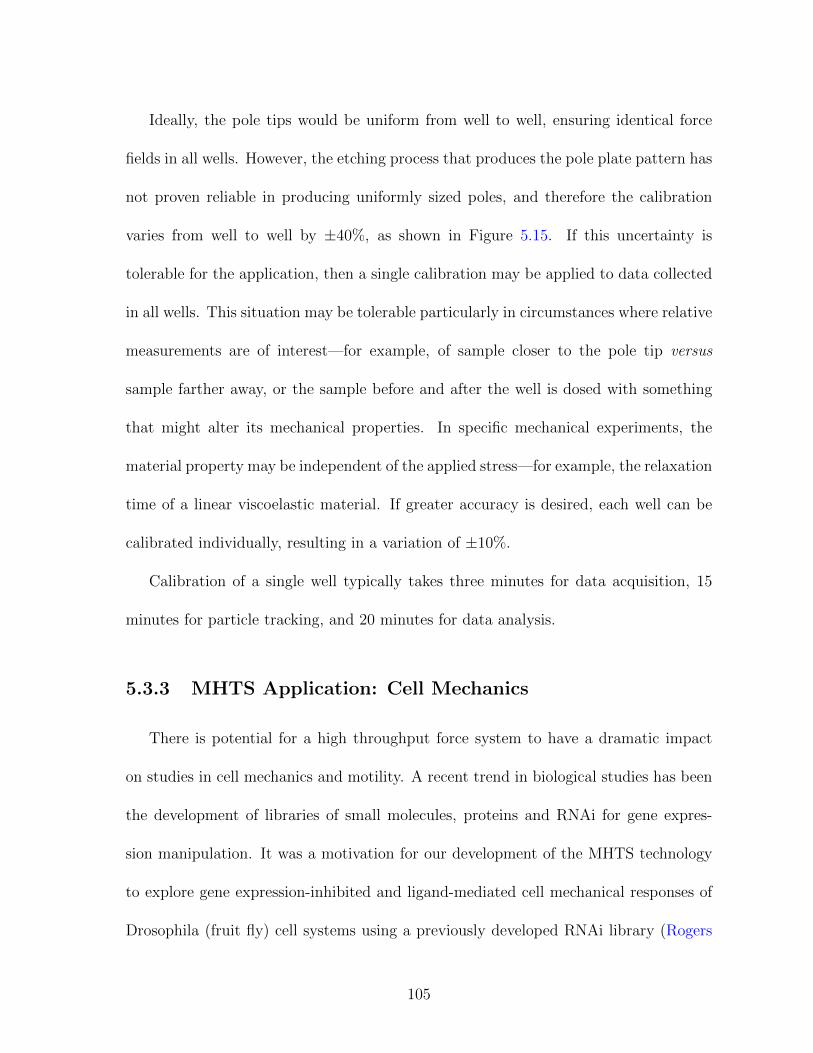
Ideally, the pole tips would be uniform from well to well, ensuring identical force

fields in all wells. However, the etching process that produces the pole plate pattern has

not proven reliable in producing uniformly sized poles, and therefore the calibration

varies from well to well by ±40%, as shown in Figure 5.15. If this uncertainty is

tolerable for the application, then a single calibration may be applied to data collected

in all wells. This situation may be tolerable particularly in circumstances where relative

measurements are of interest—for example, of sample closer to the pole tip versus

sample farther away, or the sample before and after the well is dosed with something

that might alter its mechanical properties. In specific mechanical experiments, the

material property may be independent of the applied stress—for example, the relaxation

time of a linear viscoelastic material. If greater accuracy is desired, each well can be

calibrated individually, resulting in a variation of ±10%.

Calibration of a single well typically takes three minutes for data acquisition, 15

minutes for particle tracking, and 20 minutes for data analysis.

5.3.3 MHTS Application: Cell Mechanics

There is potential for a high throughput force system to have a dramatic impact

on studies in cell mechanics and motility. A recent trend in biological studies has been

the development of libraries of small molecules, proteins and RNAi for gene expres-

sion manipulation. It was a motivation for our development of the MHTS technology

to explore gene expression-inhibited and ligand-mediated cell mechanical responses of

Drosophila (fruit fly) cell systems using a previously developed RNAi library (Rogers

105

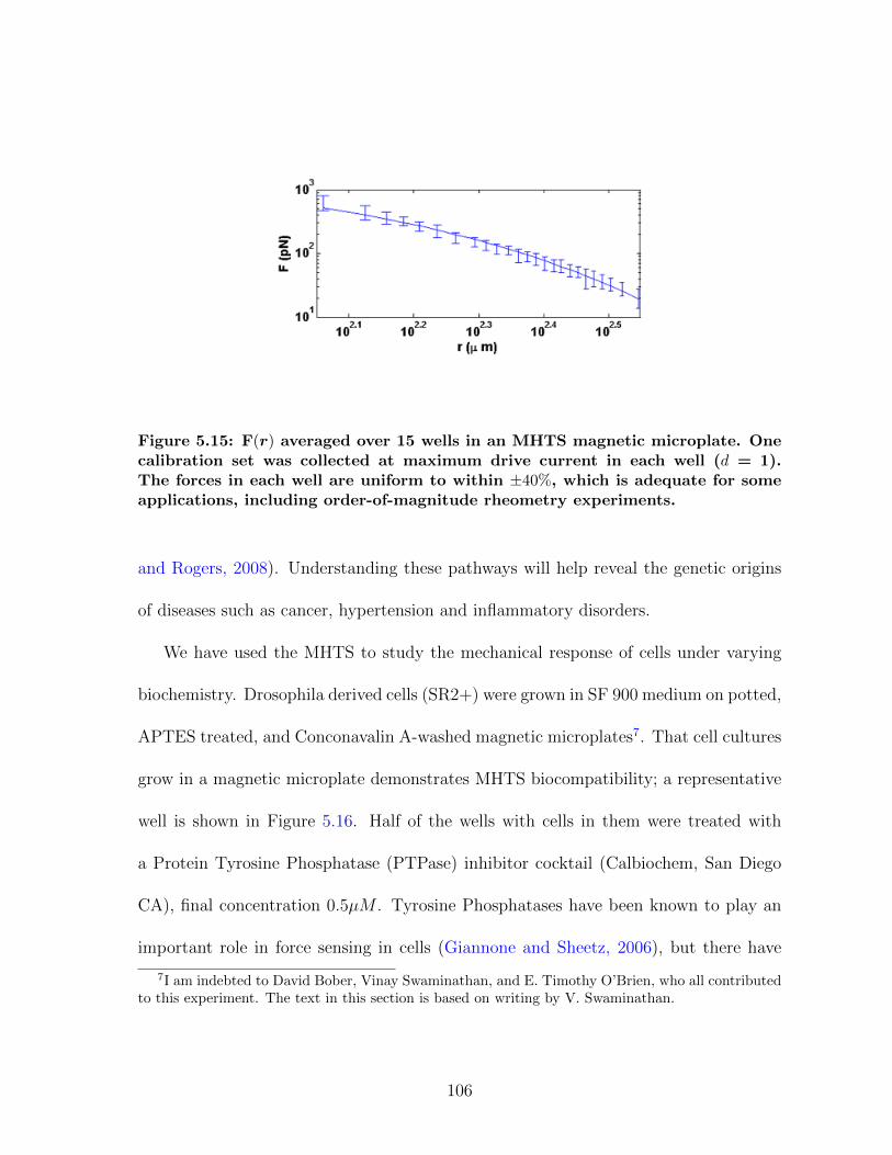
Figure 5.15: F(r) averaged over 15 wells in an MHTS magnetic microplate. Onecalibration set was collected at maximum drive current in each well (d = 1).The forces in each well are uniform to within ±40%, which is adequate for someapplications, including order-of-magnitude rheometry experiments.

and Rogers, 2008). Understanding these pathways will help reveal the genetic origins

of diseases such as cancer, hypertension and inflammatory disorders.

We have used the MHTS to study the mechanical response of cells under varying

biochemistry. Drosophila derived cells (SR2+) were grown in SF 900 medium on potted,

APTES treated, and Conconavalin A-washed magnetic microplates7. That cell cultures

grow in a magnetic microplate demonstrates MHTS biocompatibility; a representative

well is shown in Figure 5.16. Half of the wells with cells in them were treated with

a Protein Tyrosine Phosphatase (PTPase) inhibitor cocktail (Calbiochem, San Diego

CA), final concentration 0.5µM . Tyrosine Phosphatases have been known to play an

important role in force sensing in cells (Giannone and Sheetz, 2006), but there have

7I am indebted to David Bober, Vinay Swaminathan, and E. Timothy O’Brien, who all contributedto this experiment. The text in this section is based on writing by V. Swaminathan.

106

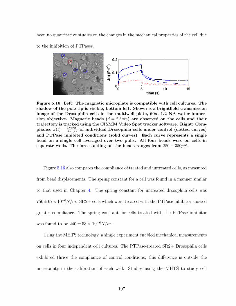
been no quantitative studies on the changes in the mechanical properties of the cell due

to the inhibition of PTPases.

0 5 10 150

0.1

0.2

time (s)

J(t

) (P

a!

1)

Figure 5.16: Left: The magnetic microplate is compatible with cell cultures. Theshadow of the pole tip is visible, bottom left. Shown is a brightfield transmissionimage of the Drosophila cells in the multiwell plate, 60x, 1.2 NA water immer-sion objective. Magnetic beads (d = 2.8µm) are observed on the cells and theirtrajectory is tracked using the CISMM Video Spot tracker software. Right: Com-pliance J(t) = 3πdr(t)

F (r,I) of individual Drosophila cells under control (dotted curves)

and PTPase inhibited conditions (solid curves). Each curve represents a singlebead on a single cell averaged over two pulls. All four beads were on cells inseparate wells. The forces acting on the beads ranges from 250 – 350pN .

Figure 5.16 also compares the compliance of treated and untreated cells, as measured

from bead displacements. The spring constant for a cell was found in a manner similar

to that used in Chapter 4. The spring constant for untreated drosophila cells was

756±67×10−6N/m. SR2+ cells which were treated with the PTPase inhibitor showed

greater compliance. The spring constant for cells treated with the PTPase inhibitor

was found to be 240± 53× 10−6N/m.

Using the MHTS technology, a single experiment enabled mechanical measurements

on cells in four independent cell cultures. The PTPase-treated SR2+ Drosophila cells

exhibited thrice the compliance of control conditions; this difference is outside the

uncertainty in the calibration of each well. Studies using the MHTS to study cell

107

mechanoresponse under varying biochemical conditions are ongoing.

5.3.4 MHTS Application: Mucus Viscometry

The MHTS is the first technology for rheometry that we know to be high-throughput

compatible. As an example of its use as a microrheometer, I have used the MHTS to

measure rheology of mucus8 (Cribb, 2010).

Broadly defined, mucus refers to a family of soft, viscoelastic materials secreted at

the cellular and tissue scales by a wide variety of organisms, vertebrates and inverte-

brates alike. Its persistence through the evolutionary record speaks to its success in

coating, protecting, and/or lubricating cells and cell surfaces often found at interfaces

with epithelial cells (Desseyn et al., 2000). In the airways, mucus serves as the first

line of defense against the inhalation of pollutants or pathogens during breathing. In

pathologies such as cystic fibrosis, changes in mucus rheology can have a catastrophic

effect on muco-cilliary clearance.

Figure 5.17 demonstrates that the MHTS can be used to measure mucus viscosity.

In particular, the data demonstrate that driven microrheology can see shear-thinning

of a polymer system, and can capture bulk viscosity of the material in a manner that

single particle diffusion cannot.

8I operated the MHTS to collect the data of this Section. I am indebted to J. Cribb for his workanalyzing and publishing these data, and the text in this Section is based on his work.

108

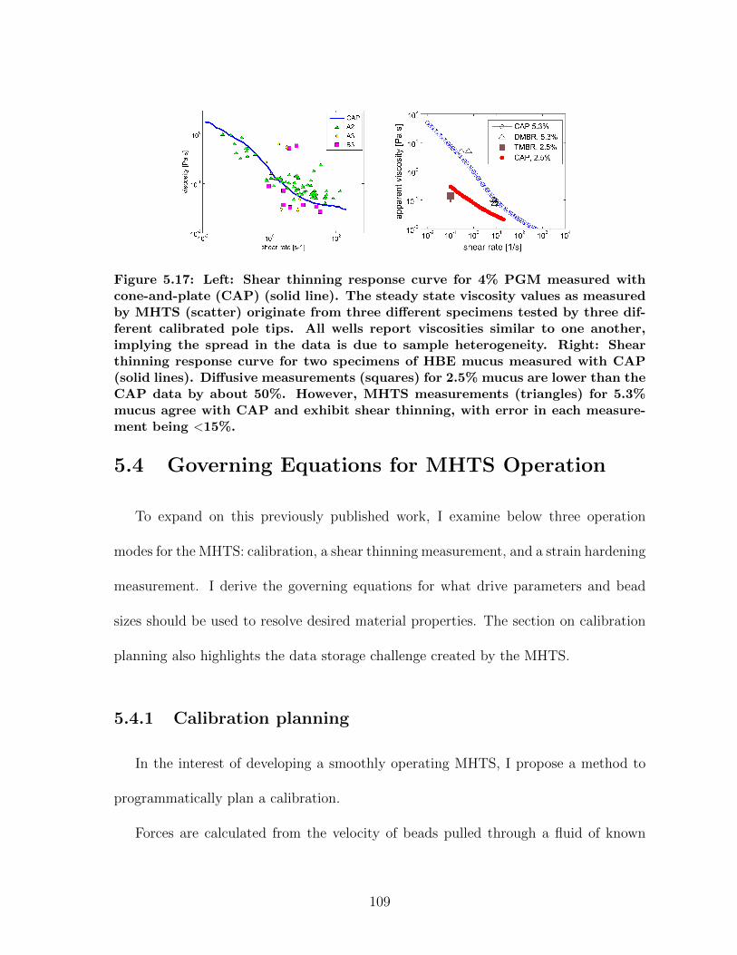
Figure 5.17: Left: Shear thinning response curve for 4% PGM measured withcone-and-plate (CAP) (solid line). The steady state viscosity values as measuredby MHTS (scatter) originate from three different specimens tested by three dif-ferent calibrated pole tips. All wells report viscosities similar to one another,implying the spread in the data is due to sample heterogeneity. Right: Shearthinning response curve for two specimens of HBE mucus measured with CAP(solid lines). Diffusive measurements (squares) for 2.5% mucus are lower than theCAP data by about 50%. However, MHTS measurements (triangles) for 5.3%mucus agree with CAP and exhibit shear thinning, with error in each measure-ment being <15%.

5.4 Governing Equations for MHTS Operation

To expand on this previously published work, I examine below three operation

modes for the MHTS: calibration, a shear thinning measurement, and a strain hardening

measurement. I derive the governing equations for what drive parameters and bead

sizes should be used to resolve desired material properties. The section on calibration

planning also highlights the data storage challenge created by the MHTS.

5.4.1 Calibration planning

In the interest of developing a smoothly operating MHTS, I propose a method to

programmatically plan a calibration.

Forces are calculated from the velocity of beads pulled through a fluid of known

109

viscosity. For Newtonian fluids with a low Reynolds number (Re < 10−4), the force on

a spherical object is equal to the Stokes drag multiplied by the particle’s velocity,

F = 3πdηv, (5.1)

where d is the sphere diameter, η is the dynamic viscosity of the fluid, and v is the

sphere’s velocity. Given fluid viscosity and the bead radius, the bead’s velocity uniquely

determines the force at a given position and drive current. Calibration is typically

performed using 2.5M sucrose (η = 0.12Pa s). Corn syrup (ACH Food Companies,

Memphis TN), a higher viscosity fluid (η = 3.4Pa s, verified using CAP), can be used

to calibrate higher force regimes.

The inputs from the user are the vector of drive currents I and the fields of view to

be calibrated9. The new work presented below can be summarized as determining the

vector of dwell times tFOV and the number of times to repeat the pulse sequence pFOV

in each field of view.

Step 1: Find the coordinate system origin r(x0, y0) = 0. The force on a bead is a

function of distance from the pole tip, r. Within a 30◦ cone of the pole tip there is

little azimuthal variation in the force, and it can be assumed to be dependent only on

the radial coordinate r. In this step, image analysis algorithms would determine the

location of the pole tip, define the origin of this coordinate system, and translate all

bead positions into this coordinate system. These algorithms are under development,

9For a thorough calibration, I = [0, 0.1, 0.25, 0.5, 0.75, 1, 1.5, 2, 2.5] is typical.

110

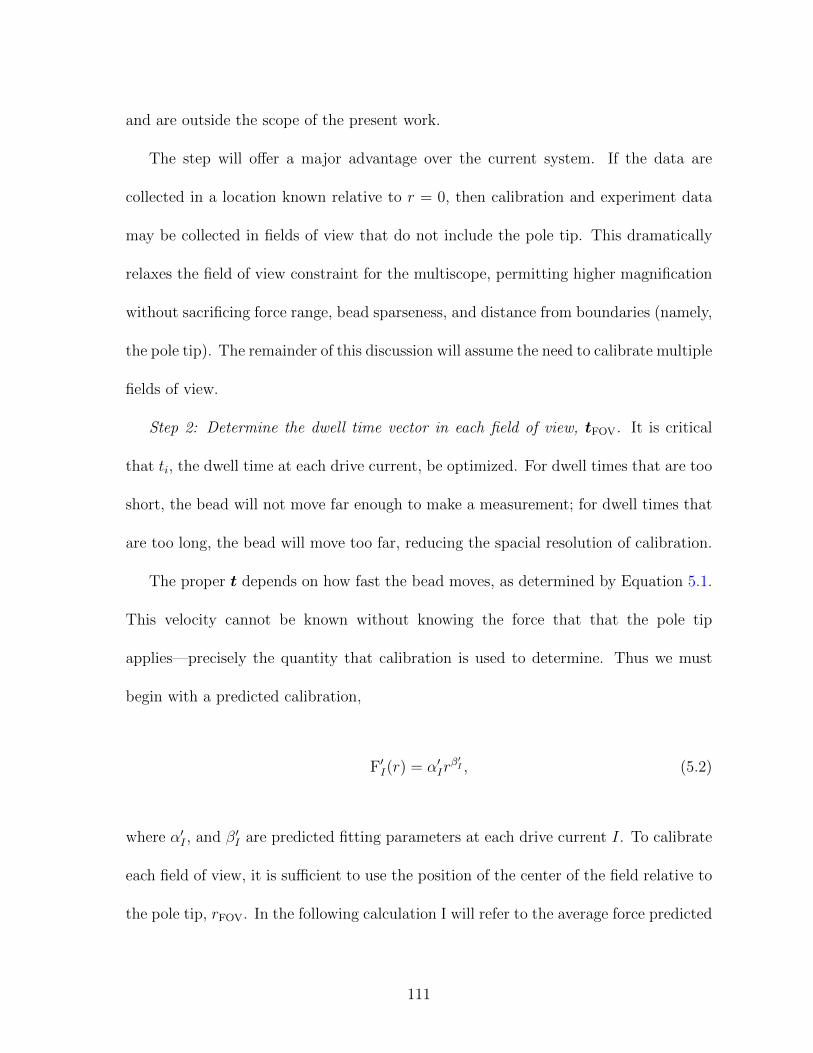
and are outside the scope of the present work.

The step will offer a major advantage over the current system. If the data are

collected in a location known relative to r = 0, then calibration and experiment data

may be collected in fields of view that do not include the pole tip. This dramatically

relaxes the field of view constraint for the multiscope, permitting higher magnification

without sacrificing force range, bead sparseness, and distance from boundaries (namely,

the pole tip). The remainder of this discussion will assume the need to calibrate multiple

fields of view.

Step 2: Determine the dwell time vector in each field of view, tFOV. It is critical

that ti, the dwell time at each drive current, be optimized. For dwell times that are too

short, the bead will not move far enough to make a measurement; for dwell times that

are too long, the bead will move too far, reducing the spacial resolution of calibration.

The proper t depends on how fast the bead moves, as determined by Equation 5.1.

This velocity cannot be known without knowing the force that that the pole tip

applies—precisely the quantity that calibration is used to determine. Thus we must

begin with a predicted calibration,

F′I(r) = α′Irβ′I , (5.2)

where α′I , and β′I are predicted fitting parameters at each drive current I. To calibrate

each field of view, it is sufficient to use the position of the center of the field relative to

the pole tip, rFOV. In the following calculation I will refer to the average force predicted

111

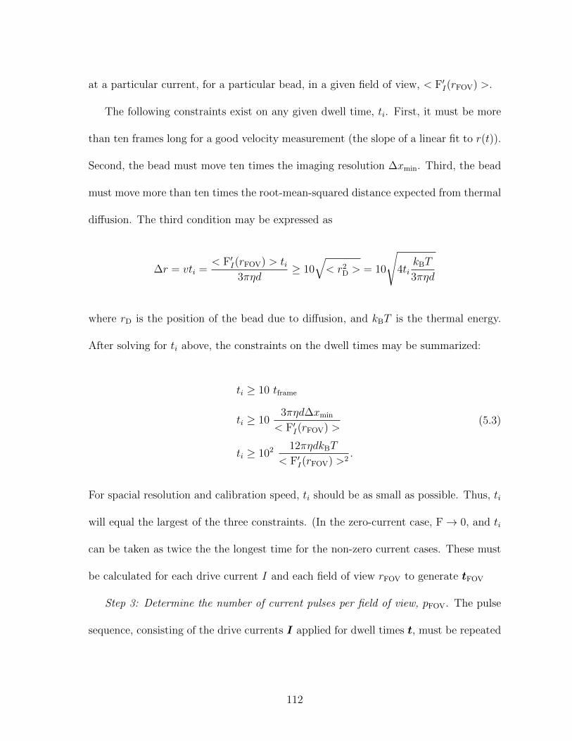
at a particular current, for a particular bead, in a given field of view, < F′I(rFOV) >.

The following constraints exist on any given dwell time, ti. First, it must be more

than ten frames long for a good velocity measurement (the slope of a linear fit to r(t)).

Second, the bead must move ten times the imaging resolution ∆xmin. Third, the bead

must move more than ten times the root-mean-squared distance expected from thermal

diffusion. The third condition may be expressed as

∆r = vti =< F′I(rFOV) > ti

3πηd≥ 10

√< r2

D > = 10

√4ti

kBT

3πηd

where rD is the position of the bead due to diffusion, and kBT is the thermal energy.

After solving for ti above, the constraints on the dwell times may be summarized:

ti ≥ 10 tframe

ti ≥ 103πηd∆xmin

< F′I(rFOV) >

ti ≥ 102 12πηdkBT

< F′I(rFOV) >2.

(5.3)

For spacial resolution and calibration speed, ti should be as small as possible. Thus, ti

will equal the largest of the three constraints. (In the zero-current case, F→ 0, and ti

can be taken as twice the the longest time for the non-zero current cases. These must

be calculated for each drive current I and each field of view rFOV to generate tFOV

Step 3: Determine the number of current pulses per field of view, pFOV. The pulse

sequence, consisting of the drive currents I applied for dwell times t, must be repeated

112

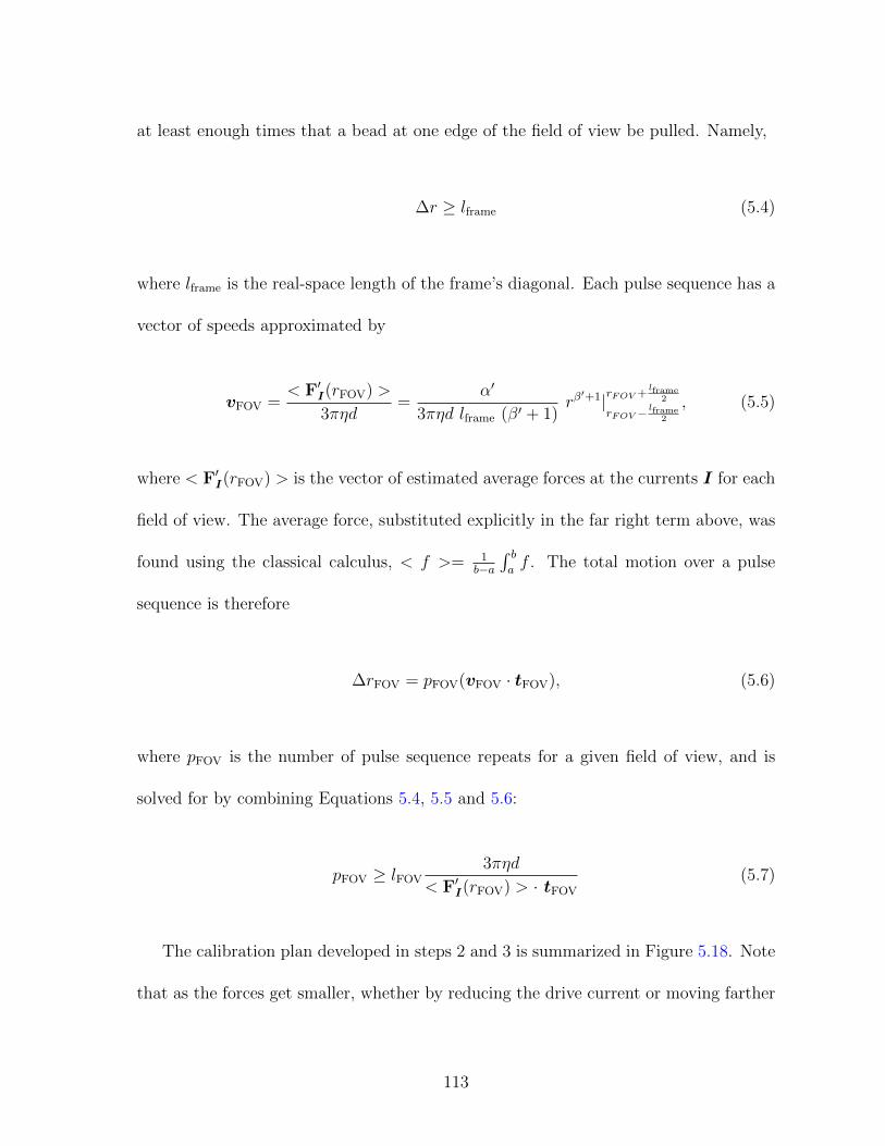
at least enough times that a bead at one edge of the field of view be pulled. Namely,

∆r ≥ lframe (5.4)

where lframe is the real-space length of the frame’s diagonal. Each pulse sequence has a

vector of speeds approximated by

vFOV =< F′I(rFOV) >

3πηd=

α′

3πηd lframe (β′ + 1)rβ

′+1|rFOV +lframe

2

rFOV −lframe

2

, (5.5)

where < F′I(rFOV) > is the vector of estimated average forces at the currents I for each

field of view. The average force, substituted explicitly in the far right term above, was

found using the classical calculus, < f >= 1b−a

∫ baf . The total motion over a pulse

sequence is therefore

∆rFOV = pFOV(vFOV · tFOV), (5.6)

where pFOV is the number of pulse sequence repeats for a given field of view, and is

solved for by combining Equations 5.4, 5.5 and 5.6:

pFOV ≥ lFOV3πηd

< F′I(rFOV) > · tFOV

(5.7)

The calibration plan developed in steps 2 and 3 is summarized in Figure 5.18. Note

that as the forces get smaller, whether by reducing the drive current or moving farther

113

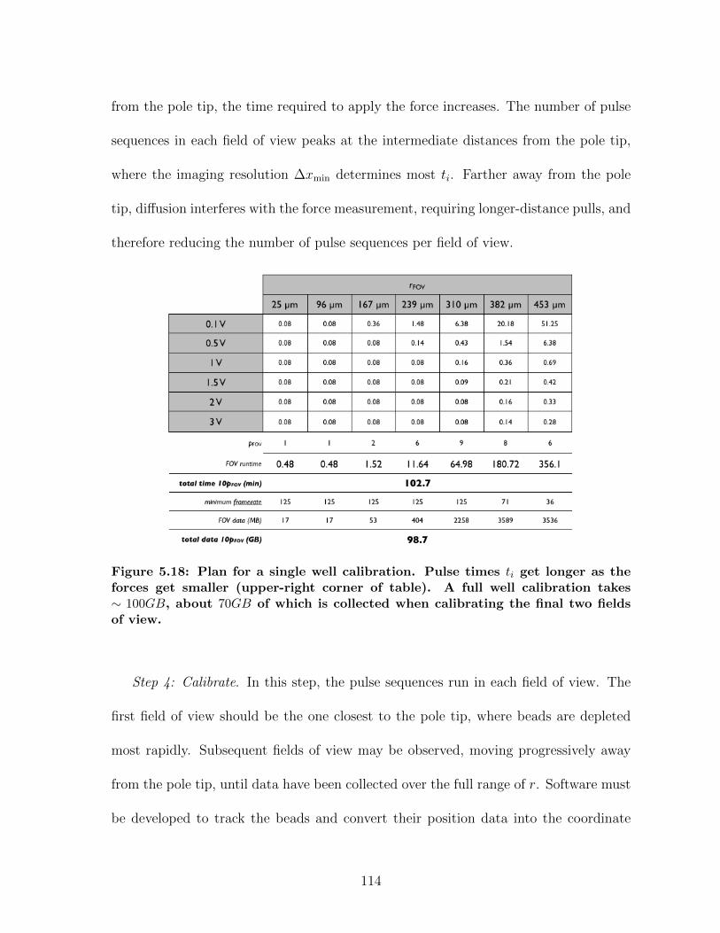
from the pole tip, the time required to apply the force increases. The number of pulse

sequences in each field of view peaks at the intermediate distances from the pole tip,

where the imaging resolution ∆xmin determines most ti. Farther away from the pole

tip, diffusion interferes with the force measurement, requiring longer-distance pulls, and

therefore reducing the number of pulse sequences per field of view.

Figure 5.18: Plan for a single well calibration. Pulse times ti get longer as theforces get smaller (upper-right corner of table). A full well calibration takes∼ 100GB, about 70GB of which is collected when calibrating the final two fieldsof view.

Step 4: Calibrate. In this step, the pulse sequences run in each field of view. The

first field of view should be the one closest to the pole tip, where beads are depleted

most rapidly. Subsequent fields of view may be observed, moving progressively away

from the pole tip, until data have been collected over the full range of r. Software must

be developed to track the beads and convert their position data into the coordinate

114

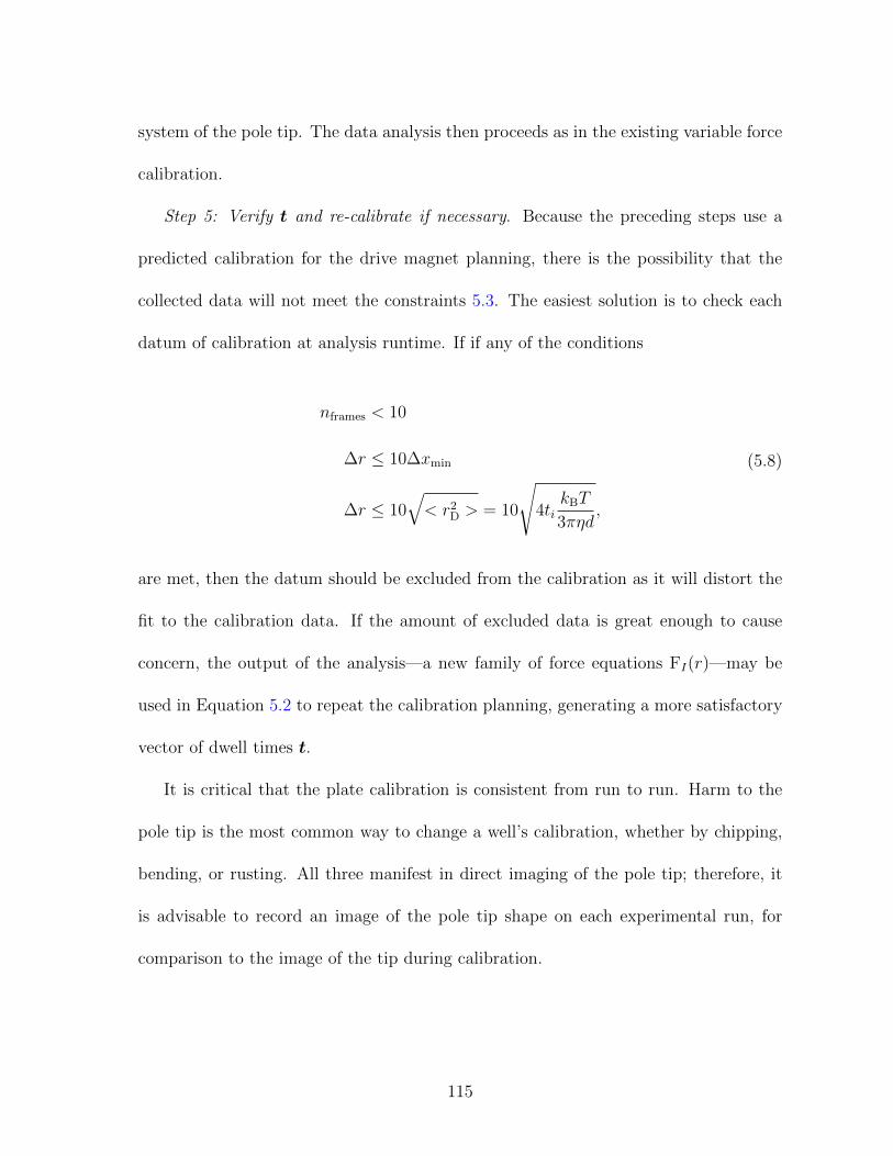
system of the pole tip. The data analysis then proceeds as in the existing variable force

calibration.

Step 5: Verify t and re-calibrate if necessary. Because the preceding steps use a

predicted calibration for the drive magnet planning, there is the possibility that the

collected data will not meet the constraints 5.3. The easiest solution is to check each

datum of calibration at analysis runtime. If if any of the conditions

nframes < 10

∆r ≤ 10∆xmin

∆r ≤ 10√< r2

D > = 10

√4ti

kBT

3πηd,

(5.8)

are met, then the datum should be excluded from the calibration as it will distort the

fit to the calibration data. If the amount of excluded data is great enough to cause

concern, the output of the analysis—a new family of force equations FI(r)—may be

used in Equation 5.2 to repeat the calibration planning, generating a more satisfactory

vector of dwell times t.

It is critical that the plate calibration is consistent from run to run. Harm to the

pole tip is the most common way to change a well’s calibration, whether by chipping,

bending, or rusting. All three manifest in direct imaging of the pole tip; therefore, it

is advisable to record an image of the pole tip shape on each experimental run, for

comparison to the image of the tip during calibration.

115

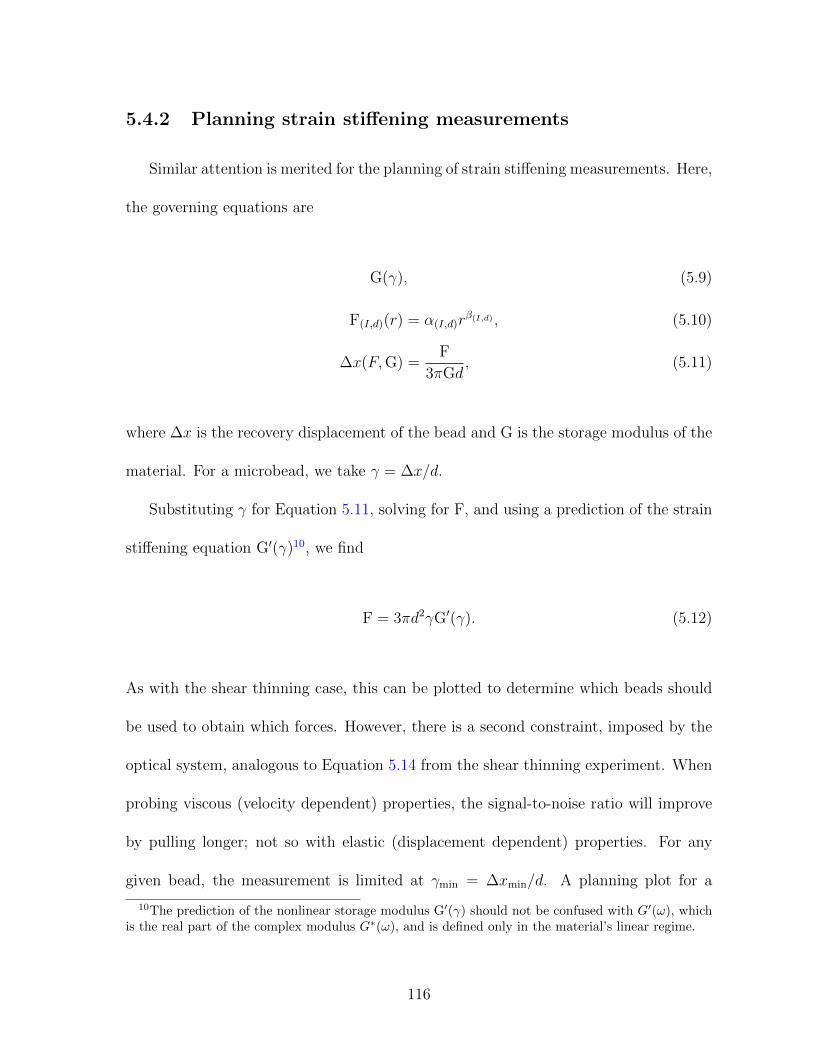
5.4.2 Planning strain stiffening measurements

Similar attention is merited for the planning of strain stiffening measurements. Here,

the governing equations are

G(γ), (5.9)

F(I,d)(r) = α(I,d)rβ(I,d) , (5.10)

∆x(F,G) =F

3πGd, (5.11)

where ∆x is the recovery displacement of the bead and G is the storage modulus of the

material. For a microbead, we take γ = ∆x/d.

Substituting γ for Equation 5.11, solving for F, and using a prediction of the strain

stiffening equation G′(γ)10, we find

F = 3πd2γG′(γ). (5.12)

As with the shear thinning case, this can be plotted to determine which beads should

be used to obtain which forces. However, there is a second constraint, imposed by the

optical system, analogous to Equation 5.14 from the shear thinning experiment. When

probing viscous (velocity dependent) properties, the signal-to-noise ratio will improve

by pulling longer; not so with elastic (displacement dependent) properties. For any

given bead, the measurement is limited at γmin = ∆xmin/d. A planning plot for a

10The prediction of the nonlinear storage modulus G′(γ) should not be confused with G′(ω), whichis the real part of the complex modulus G∗(ω), and is defined only in the material’s linear regime.

116

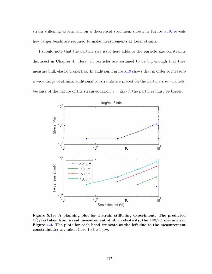
strain stiffening experiment on a theoretical specimen, shown in Figure 5.19, reveals

how larger beads are required to make measurements at lower strains.

I should note that the particle size issue here adds to the particle size constraints

discussed in Chapter 4. Here, all particles are assumed to be big enough that they

measure bulk elastic properties. In addition, Figure 5.19 shows that in order to measure

a wide range of strains, additional constraints are placed on the particle size—namely,

because of the nature of the strain equation γ = ∆x/d, the particles must be bigger.

Figure 5.19: A planning plot for a strain stiffening experiment. The predictedG′(γ) is taken from a real measurement of fibrin elasticity, the 1 mg/mL specimen inFigure 4.4. The plots for each bead truncate at the left due to the measurementconstraint ∆xmin, taken here to be 1 µm.

117

5.4.3 Planning shear thinning measurements

The stress geometry of the MHTS is best expressed in polar coordinates. This is not

the natural system for viscometry experiments, and as such, the experimental design

is critical to achieving a successful measurement. Prior work (Cribb, 2010) has noted

that the force required to see a given shear rate is

F = π γ d2 η′(γ). (5.13)

where γ is the shear rate, and η′(γ) is the predicted shear thinning curve.

To this I add a prescription for determining the time that force should be applied,

∆t. The imaging resolution, ∆xmin, sets one constraint, which paired with the minimum

time, ∆tmin, implies a velocity that can be entered into Stoke’s Law, v(F, η) = F3πηd

, to

find

∆tmin ≥ 3πd ∆xminη′(γ)

F(I,d)(r). (5.14)

A good rule of thumb sets ∆xmin = d. I also note we wish to avoid any force strong

enough that ∆t < tframe. Without this latter condition, the bead may move more

than its diameter in a single frame, making it difficult to track.

118

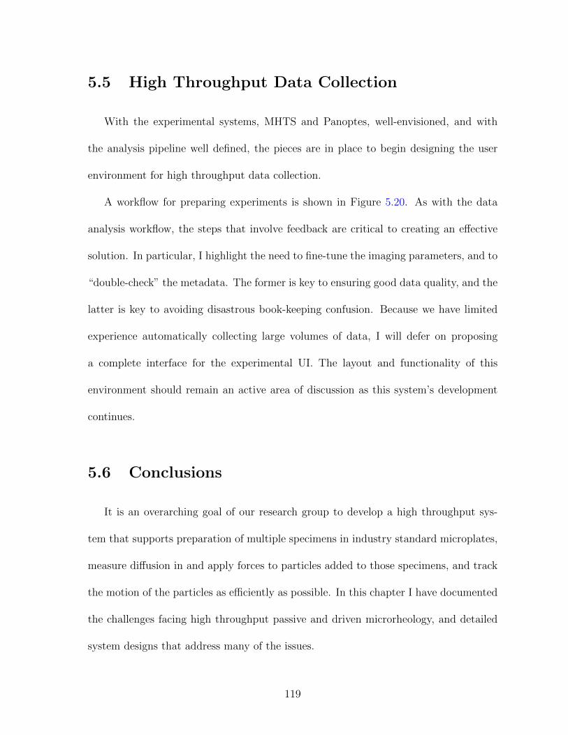
5.5 High Throughput Data Collection

With the experimental systems, MHTS and Panoptes, well-envisioned, and with

the analysis pipeline well defined, the pieces are in place to begin designing the user

environment for high throughput data collection.

A workflow for preparing experiments is shown in Figure 5.20. As with the data

analysis workflow, the steps that involve feedback are critical to creating an effective

solution. In particular, I highlight the need to fine-tune the imaging parameters, and to

“double-check” the metadata. The former is key to ensuring good data quality, and the

latter is key to avoiding disastrous book-keeping confusion. Because we have limited

experience automatically collecting large volumes of data, I will defer on proposing

a complete interface for the experimental UI. The layout and functionality of this

environment should remain an active area of discussion as this system’s development

continues.

5.6 Conclusions

It is an overarching goal of our research group to develop a high throughput sys-

tem that supports preparation of multiple specimens in industry standard microplates,

measure diffusion in and apply forces to particles added to those specimens, and track

the motion of the particles as efficiently as possible. In this chapter I have documented

the challenges facing high throughput passive and driven microrheology, and detailed

system designs that address many of the issues.

119

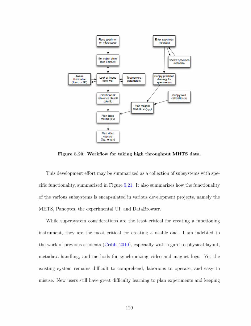
Figure 5.20: Workflow for taking high throughput MHTS data.

This development effort may be summarized as a collection of subsystems with spe-

cific functionality, summarized in Figure 5.21. It also summarizes how the functionality

of the various subsystems is encapsulated in various development projects, namely the

MHTS, Panoptes, the experimental UI, and DataBrowser.

While supersystem considerations are the least critical for creating a functioning

instrument, they are the most critical for creating a usable one. I am indebted to

the work of previous students (Cribb, 2010), especially with regard to physical layout,

metadata handling, and methods for synchronizing video and magnet logs. Yet the

existing system remains difficult to comprehend, laborious to operate, and easy to

misuse. New users still have great difficulty learning to plan experiments and keeping

120

Figure 5.21: Systems overview of the MHTS. The functionality can be brokeninto six projects (grey boxes), while the user experiences four modular products:experimental UI, DataBrowser, MHTS, and Panoptes.

track of files generated by data collection. The former consideration was the motivation

behind the experimental planning sections of this chapter; the latter was the motivation

for DataBrowser. With their adoption, I believe the system will improve dramatically

in usability.

121

Appendix AExperimental Protocols for Diffusion,

Structure, and Permeability

A.1 Clot preparation and Video Acquisition

Reagent handling, storage, thawing, and mixing. Particle concentrations were

planned to obtain sufficient number density n < 10−4µm−3 (φ < 7× 10−6).

Clots were formed in a glass-bottom 96-well microplate (NUNC, Rochester NY),

which was plasma cleaned to ensure uniform clotting and meniscus in all wells. Clots

were allowed to incubate for two hours, which was the time before the level section of

the slowest turbidity curve. For experiments where the particles diffused into the clot

from outside, particles were added after this two hour incubation. Clots were sealed to

prevent evaporation and diffusion proceeded at room temperature.

Video of nanoparticle diffusion was acquired on a inverted microscope (Nikon USA,

Melville NY) with a 60x, 1.2 NA water immersion objective (Olympus, Center Valley

122

PA), and a high-sensitivity EMCCD camera (Photometrics, Tucson AZ). Videos were

captured in at least five well-distributed fields of view, at a constant height of 50-70 µm

from the glass substrate, at rates of 24-31 frames per second, for at least 60 seconds.

A.2 Automatic particle tracking and data filtering

Particles were automatically tracked using CISMM Video Spot Tracker. Some false

positive particle tracks were inevitable; data were filtered to eliminate any tracks lasting

less than two seconds. There is a risk of biasing diffusion results by filtering in this

fashion, as it could asymmetrically trim the natural diffusion distribution. However,

a track of a real particle can be expected to last for the first passage time across

the imaging system’s depth of field of about 5 µm. For the smallest particles used

the average expected residence time in buffer is 3.4 seconds. After this filtering, the

greatest damage to data fidelity were due to trackers that lost a particle but continued

to log data. These “pop-offs” were pruned by hand in several datasets, and resulted in

corrections to Deff of under 5%.

A.3 Calculation of diffusion coefficient

Calculated 〈r2〉 from tracking data (x(t), y(t)). Calculated α by linear fit to 〈r2〉

over the range 0.1 < τ < 1. Filtered by 0.8 < α < 1.2. Computed Deff = 〈r2〉/4τ for

each tracker. Computed mean and standard error for Deff for each clot type.

123

A.4 PEG Particle Preparation

Carboxylate nanoparticles were functionalized as in (Lai et al., 2007). In an effort

to evaluate the sensitivity of our diffusion measurement, we compared the size of the

PEG- and COOH-functionalized particles. The presence of PEG at the surface of a

nanoparticle should increase its hydrodynamic size. Particle diameters were determined

by dynamic light scattering (DLS) (Malvern Instruments, Worcestershire UK) and from

particle diffusion in water. These data imply a corona around the particles that is 5 nm

(250 nm initial size) and 12 nm (490 nm initial size).

A.5 Structure and Permeability

Clotting time measured with turbidity. Gel structure was measured using confocal

microscopy of fluorescent fibrinogen. Alexa-fluor fibrinogen (AFF) was prepared by

Robert Campbell. Fibrin gels were prepared with plasma-purified fibrinogen doped

with 3% AFF. Stacks were acquired on an inverted microscope (Nikon USA, Melville

NY) with a 60x, 1.2 NA water immersion objective (Olympus, Center Valley PA),

a spinning disk, confocal fluorescence system (Yokogawa, Atlanta GA), and a CCD

camera (Photometrics, Tucson AZ). For each clot type, at least two stacks were taken

in different locations of the clot.

Clot permeability was measured for purified fibrin gels. Results agreed with estab-

lished values of κ = 10−13 – 10−12 m2 (Diamond, 1999), with finer clots exhibiting lower

Darcy constants.

124

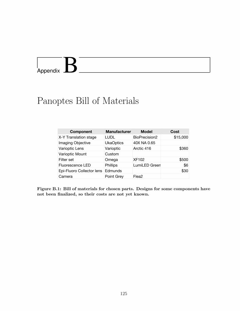
Appendix BPanoptes Bill of Materials

Component Manufacturer Model Cost

X-Y Translation stage LUDL BioPrecision2 $15,000Imaging Objective UkaOptics 40X NA 0.65Varioptic Lens Varioptic Arctic 416 $360Varioptic Mount CustomFilter set Omega XF102 $500Fluorescence LED Phillips LumiLED Green $6Epi-Fluoro Collector lens Edmunds $30Camera Point Grey Flea2

Figure B.1: Bill of materials for chosen parts. Designs for some components havenot been finalized, so their costs are not yet known.

125

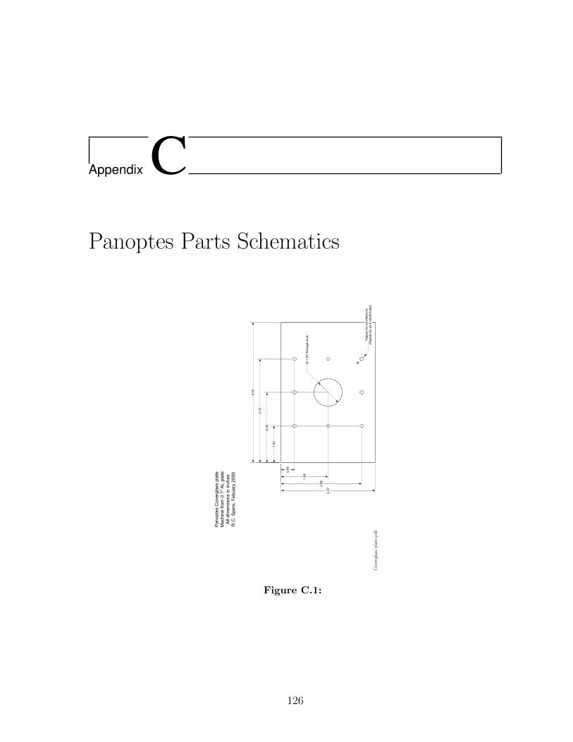
Appendix CPanoptes Parts Schematics

Cov

ergl

ass

pla

te.p

df

!"#!

$"%!

#"&$

'"$!

()**+,-./0-*0/12,+,-*23

45+*+)6-./0-)77-8-9:)77-;/7+9<

'"=8

!"88

$"$%

&">8

?-'"&&-(;0/@A;B;/7+

C)3/*6+9-D/1+0A7)99-*7)6+

E)F;23+-.0/:-&"'G-HI-*7)6+

H77-,2:+392/39-23-23F;+9

5"D"-J*+0/K-L+M@)0N-!&&O

Figure C.1:

126

LU

DL

Mou

nt.

pd

f

��

��

��

��

��

�� !��

"� ��!��

��

��#��$

��$��$%��&

'�� ()*(+��!��

",+ ��-�%��

��

��

��

��

��.�

��

��

��

��

��/

��

Figure C.2:

127

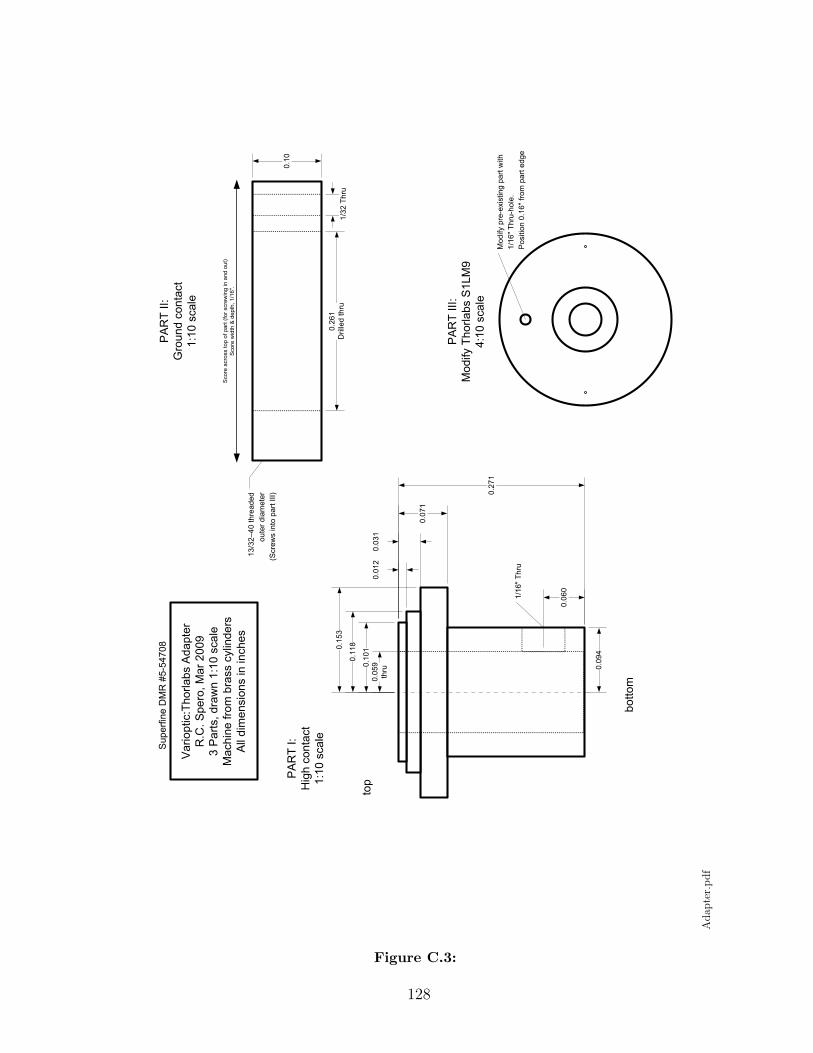
Adap

ter.

pdf

��

��

��

��

��

��

��

��

� ��

��

��

��

�� !

��

"��#��

�� !

$�� #��!�

��%��&�!��'�(��

��'�#��)�� !

(�� !�*��+ ��#!��

� �#��!�� !�

�,�-.��

��-�

��,�/0�� !�#!#�

��!��#��!�!�

1&��!)��2

��-�

3�� !#��

�,��

��

(�#�*+�� &�4(�

0�� !

(�#�*+��!5!6��)��

�,�-.�� 5 � !�

��-.�*��!#�!

��

��0

&��!�*��!�3(��7�5�0��

&��!��*��1*��!)��#��2

&��!�)�#� �8�#!�� '��,�-.�

Figure C.3:

128

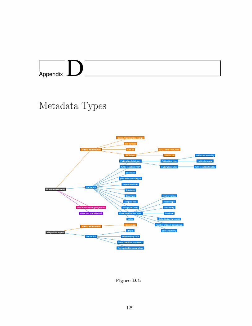
Appendix DMetadata Types

All video microscopy

Send to DataBrowser

Metadata

Min/Max Intensity Projection

video (not stored in full)

Calibration Datatypes

Paths to video & MIP

bead size

pole tip location (x,y,z)

experiment title

Specimen

Bead type

frame/tracking timestamps

Run number

Well ID

VST Output

Temperature

Image µm/pixel

Video Spot Tracker Input

Notes

Tracker radius

Kernel Type

Sensitivity

Precision

Auto-finding threshold

Number of beads to maintain

X, Y, Z, Roll, Pitch, Yaw

tracker ID

Magnet Datatypes

Send to Databrowser

metadata

DAQ ID

DAQ sampling rate

Force primitive sequences

Force primitive parameters

timestamp

Calibration: true

Calibration: false Path to calibration file

calibrator viscosity

calibrator name

Lost sensitivity

Figure D.1:

129

Bibliography

Ajjan, R., Lim, B. C. B., Standeven, K. F., Harrand, R., Dolling, S., Phoenix, F.,Greaves, R., Abou-Saleh, R. H., Connell, S., Smith, D. A. M., Weisel, J. W.,Grant, P. J., and Ariens, R. A. S. (2008). Common variation in the c-terminalregion of the fibrinogen beta-chain: effects on fibrin structure, fibrinolysis andclot rigidity. Blood, 111(2):643–50.

Ajjan, R. A., Standeven, K. F., Khanbhai, M., Phoenix, F., Gersh, K. C., Weisel, J. W.,Kearney, M. T., Ariens, R. A. S., and Grant, P. J. (2009). Effects of aspirin onclot structure and fibrinolysis using a novel in vitro cellular system. ArteriosclerThromb Vasc Biol, 29(5):712–7.

Astrom, B., Pipes, R., and Advani, S. (1992). On flow through aligned fiber bedsand its application to composites processing. Journal of Composite Materials,26(9):1351–1373. 10.1177/002199839202600907.

Bausch, A., Moller, W., and Sackmann, E. (1999). Measurement of local viscoelasticityand forces in living cells by magnetic tweezers. Biophysical Journal, 76(1):573–579.

Bausch, A., Ziemann, F., Boulbitch, A., Jacobson, K., and Sackmann, E. (1998). Localmeasurements of viscoelastic parameters of adherent cell surfaces by magneticbead microrheometry. BIOPHYSICAL JOURNAL, 75(4):2038–2049.

Bear, J. (1988). Dynamics of fluids in porous media. page 764.

Blinc, A. and Francis, C. (1996). Transport processes in fibrinolysis and fibrinolytictherapy. Thromb Haemostasis, 76(4):481–491.

Blomback, B., Carlsson, K., Fatah, K., Hessel, B., and Procyk, R. (1994). Fibrinin human plasma: gel architectures governed by rate and nature of fibrinogenactivation. Thrombosis research, 75(5):521.

Blomback, B., Carlsson, K., Hessel, B., Liljeborg, A., Procyk, R., and Aslund, N.(1989). Native fibrin gel networks observed by 3d microscopy, permeation andturbidity. Biochimica et biophysica acta, 997(1-2):96.

130

Blomback, B. and Okada, M. (1982). Fibrin gel structure and clotting time. Thrombosisresearch, 25(1-2):51.

Bravo-Zanoguera, M., Massenbach, B., and Kellner, A. (1998). High-performance aut-ofocus circuit for biological microscopy. Review of Scientific . . . .

Bravo-Zanoguera, M. E., Laris, C. A., Nguyen, L. K., Oliva, M., and Price, J. H. (2007).Dynamic autofocus for continuous-scanning time-delay-and-integration image ac-quisition in automated microscopy. Journal of biomedical optics, 12(3):034011.Most recent continuous scanning autofocus paper.

Breedveld, V. and Pine, D. (2003). Microrheology as a tool for high-throughput screen-ing. Journal of Materials Science, 38(22):4461–4470.

Brinkman, H. (1949). A calculation of the viscous force exerted by a flowing fluid on adense swarm of particles. Applied Scientific Research.

Campbell, R. A., Overmyer, K. A., Bagnell, C. R., and Wolberg, A. S. (2008). Cellularprocoagulant activity dictates clot structure and stability as a function of distancefrom the cell surface. Arterioscler Thromb Vasc Biol, 28(12):2247–54.

Carman, P. (1937). Fluid flow through granular beds. Chemical Engineering Researchand Design.

Carr, M. E. J., Shen, L., and Hermans, J. (2004). Mass-length ratio of fibrin fibersfrom gel permeation and light scattering. Biopolymers.

Carr, M. J. and Hermans, J. (1978). Size and density of fibrin fibers from turbidity.Macromolecules.

Choi, C., Margraves, C., and Kihm, K. (2007). Examination of near-wall hindered brow-nian diffusion of nanoparticles: Experimental comparison to theories by brenner(1961) and goldman et al.(1967). Physics of Fluids, 19:103305.

Cicuta, P. and Donald, A. (2007). Microrheology: a review of the method and appli-cations. Soft Matter, 3(12):1449–1455.

Clague, D. and Phillips, R. (1996). Hindered diffusion of spherical macromoleculesthrough dilute fibrous media. Physics of Fluids, 8(7):1720–1731.

Collen, A., Smorenburg, S., Peters, E., and Lupu, F. (2000). Unfractionated andlow molecular weight heparin affect fibrin structure and angiogenesis in vitro 1.Cancer Research.

Collet, J.-P., Lesty, C., Montalescot, G., and Weisel, J. W. (2003). Dynamic changes offibrin architecture during fibrin formation and intrinsic fibrinolysis of fibrin-richclots. J Biol Chem, 278(24):21331–5.

131

Cribb, J. (2010). Driven and thermal microparticle rheology of complex biopolymersystems. Thesis.

Crocker, J. C., Valentine, M. T., Weeks, E. R., Gisler, T., Kaplan, P. D., Yodh, A. G.,and Weitz, D. A. (2000). Two-point microrheology of inhomogeneous soft mate-rials. Physical Review Letters, 85(4):888–91.

Cussler, E. L. (1997). Diffusion: mass transfer in fluid systems. page 580.

Darcy, H. (1856). Les fontaines publiques de la ville de dijon: exposition et applicationdes .... page 641.

Desseyn, J. L., Aubert, J. P., Porchet, N., and Laine, A. (2000). Evolution of the largesecreted gel-forming mucins. Mol Biol Evol, 17(8):1175–84.

Diamond, S. L. (1999). Engineering design of optimal strategies for blood clot dissolu-tion. Annu Rev Biomed Eng, 1:427–462.

Diamond, S. L. and Anand, S. (1993). Inner clot diffusion and permeation duringfibrinolysis. BIOPHYSICAL JOURNAL, 65(6):2622–43.

Dobson, J. (2006). Magnetic micro-and nano-particle-based targeting for drug and genedelivery. Nanomedicine.

Dodge, J. T., Brown, B. G., Bolson, E. L., and Dodge, H. T. (1992). Lumen diameterof normal human coronary arteries. influence of age, sex, anatomic variation, andleft ventricular hypertrophy or dilation. Circulation, 86(1):232–46.

Drummond, J. and Tahir, M. (1984). Laminar viscous flow through regular arrays ofparallel solid cylinders. International Journal of Multiphase Flow.

Dullien, F. A. L. (1992). Porous media: fluid transport and pore structure. page 574.

Dunn, E. J., Ariens, R. A. S., and Grant, P. J. (2005). The influence of type 2 diabeteson fibrin structure and function. Diabetologia, 48(6):1198–206.

Durig, U., Cross, G., Despont, M., Drechsler, U., Haberle, W., Lutwyche, M.,Rothuizen, H., Stutz, R., Widmer, R., Vettiger, P., Binnig, G., King, W., andGoodson, K. (2000). “millipede” – an afm data storage system at the frontier ofnanotribology. Tribology Letters, 9(1):25–32.

Einstein, A. (1905). On the movement of small particles suspended in stationary liquidsrequired by the molecular-kinetic theory of heat. Annalen der Physik.

Evans, P. A., Hawkins, K., Lawrence, M., Williams, R. L., Barrow, M. S., Thirumalai,N., and Williams, P. R. (2008). Rheometry and associated techniques for bloodcoagulation studies. Med Eng Phys, 30(6):671–9.

132

Fabry, B., Maksym, G., Butler, J., Glogauer, M., Navajas, D., and Fredberg, J. (2001).Scaling the microrheology of living cells. Physical review letters, 87(14):148102.

Fatah, K., Hamsten, A., Blomback, B., and Blomback, M. (1992). Fibrin gel networkcharacteristics and coronary heart disease: relations to plasma fibrinogen . . . .Thromb Haemostasis.

Fatah, K., Silveira, A., Tornvall, P., and Karpe, F. (1996). Proneness to formation oftight and rigid fibrin gel structures in men with myocardial infarction at a youngage. Thromb Haemostasis.

Ferry, J. D. (1980). Viscoelastic properties of polymers. page 641.

Fisher, J. K., Vicci, L., Cribb, J., O’Brien, E. T., Taylor, R. M., and Superfine, R.(2006). Magnetic force micromanipulation systems for the biological sciences.Nano, 1(3):191–205.

Fowler, J. and Hertel, K. (1940). Flow of a gas through porous media. Journal ofApplied Physics.

Gelder, J. V., Nair, C., and Dhall, D. (1996). Colloid determination of fibrin networkpermeability. Blood Coagulation and Fibrinolysis.

Giannone, G. and Sheetz, M. P. (2006). Substrate rigidity and force define form throughtyrosine phosphatase and kinase pathways. Trends Cell Biol, 16(4):213–23.

Giugliano, R., McCabe, C., Antman, E., and Cannon, C. (2001). Lower-dose hep-arin with fibrinolysis is associated with lower rates of intracranial hemorrhage.American Heart Journal.

Gluckstad, J. and Palima, D. (2009). Generalized phase contrast: Applications in opticsand photonics. page 315.

Guthold, M., Liu, W., Sparks, E. A., Jawerth, L. M., Peng, L., Falvo, M., Superfine,R., Hantgan, R. R., and Lord, S. T. (2007). A comparison of the mechanicaland structural properties of fibrin fibers with other protein fibers. Cell BiochemBiophys, 49(3):165–81.

Hamamoto, S., Moldrup, P., Kawamoto, K., Komatsu, T., and Rolston, D. (2009).Unified measurement system for the gas dispersion coefficient, air permeability,and gas diffusion coefficient in variably saturated soil. SOIL SCIENCE SOCIETYOF AMERICA JOURNAL, 73(6):1921.

Happel, J. and Brenner, H. (1983). Low reynolds number hydrodynamics: with specialapplications to particulate media. page 553.

133

He, S., Bark, N., Wang, H., Svensson, J., and Blomback, M. (2009). Effects of acetylsal-icylic acid on increase of fibrin network porosity and the consequent upregulationof fibrinolysis. Journal of Cardiovascular Pharmacology.

Hendriks, B., Kuiper, S., As, M. V., Renders, C., and Tukker, T. (2005). Electrowetting-based variable-focus lens for miniature systems. Optical Review, 12(3):255–259.

Hubmayr, R., Shore, S., Fredberg, J., Planus, E., Panettieri, R., Moller, W., Heyder,J., and Wang, N. (1996). Pharmacological activation changes stiffness of culturedhuman airway smooth muscle cells. Am J Physiol Cell Physiol, 271(5):C1660–1668.

Jackson, G. and James, D. (1986). The permeability of fibrous porous media. Canadianjournal of chemical engineering.

Jahnel, M., Waigh, T. A., and Lu, J. R. (2008). Thermal fluctuations of fibrin fibresat short time scales. Soft Matter, 4(7):1438.

Janmey, P., Amis, E., and Ferry, J. (1983). Rheology of fibrin clots. vi. stress re-laxation, creep, and differential dynamic modulus of fine clots in large shearingdeformations. Journal of Rheology, 27:135.

Johansson, L. and Lofroth, J. (1993). Diffusion and interaction in gels and solu-tions 4. hard-sphere brownian dynamics simulations. JOURNAL OF CHEMICALPHYSICS, 98(9):7471–7479.

Johnson, E., Berk, D., Jain, R., and Deen, W. (1996). Hindered diffusion in agarose gels:test of effective medium model. BIOPHYSICAL JOURNAL, 70(2):1017–1023.

Kihm, K., Banerjee, A., Choi, C., and Takagi, T. (2004). Near-wall hindered browniandiffusion of nanoparticles examined by three-dimensional ratiometric total inter-nal reflection fluorescence microscopy (3-d r-tirfm). Exp Fluids, 37(6):811–824.

Kimura, Y. (2009). Microrheology of soft matter. Journal of the Physical Society ofJapan, 78(4):041005.

Kirschenbaum, L. A., Aziz, M., Astiz, M. E., Saha, D. C., and Rackow, E. C. (2000).Influence of rheologic changes and platelet-neutrophil interactions on cell filtrationin sepsis. Am J Respir Crit Care Med, 161(5):1602–7.

Knaapen, P., Camici, P. G., Marques, K. M., Nijveldt, R., Bax, J. J., Westerhof, N.,Gotte, M. J. W., Jerosch-Herold, M., Schelbert, H. R., Lammertsma, A. A., andvan Rossum, A. C. (2009). Coronary microvascular resistance: methods for itsquantification in humans. Basic Res Cardiol, 104(5):485–98.

Lai, S., O’Hanlon, D., Harrold, S., Man, S., Wang, Y., Cone, R., and Hanes, J. (2007).Rapid transport of large polymeric nanoparticles in fresh undiluted human mucus.Proceedings of the National Academy of Sciences, 104(5):1482.

134

Lang, P., Yeow, K., Nichols, A., and Scheer, A. (2006). Cellular imaging in drugdiscovery. Nature Reviews Drug Discovery, 5(4):343–356.

Lee, J. and Ladd, A. (2005). Axial segregation of a settling suspension in a rotatingcylinder. Physical Review Letters, 95(4):048001.

Lele, T., Sero, J., Matthews, B., Kumar, S., Xia, S., (true graphic)]Zavala, M. M.,Polte, T., Overby, D., Wang, N., and Ingber, D. (2007). Methods in cell biology.Volume 83:441, 443–472.

Lenormand, G., Bursac, P., Butler, J., and Fredberg, J. (2007). Out-of-equilibrium dy-namics in the cytoskeleton of the living cell. Physical review letters, 76(4):041901.

Levick, J. (1987). Flow through interstitium and other fibrous matrices. ExperimentalPhysiology.

Llevadot, J. (2001). Bolus fibrinolytic therapy in acute myocardial infarction. JAMA:The Journal of the American Medical Association, 286(4):442–449.

Mason, T. and Weitz, D. (1995). Linear viscoelasticity of colloidal hard sphere suspen-sions near the glass transition. Physical Review Letters.

Meehan, T., Cribb, J., Skinner, K., and Superfine, R. (2010). Cylinder vs spheres:Biofluid shear thinning in nanoparticle transport. Annals of Biomedical Engi-neering.

Mickel, W., Munster, S., Jawerth, L. M., Vader, D. A., Weitz, D. A., Sheppard, A. P.,Mecke, K., Fabry, B., and Schroder-Turk, G. E. (2008). Robust pore size analysisof filamentous networks from three-dimensional confocal microscopy. BIOPHYS-ICAL JOURNAL, 95(12):6072–80.

Neuman, K. and Block, S. (2004). Optical trapping. Review of Scientific Instruments.

Neumann, B., Walter, T., Heriche, J.-K., Bulkescher, J., Erfle, H., Conrad, C., Rogers,P., Poser, I., Held, M., Liebel, U., Cetin, C., Sieckmann, F., Pau, G., Kabbe, R.,Wunsche, A., Satagopam, V., Schmitz, M. H. A., Chapuis, C., Gerlich, D. W.,Schneider, R., Eils, R., Huber, W., Peters, J.-M., Hyman, A. A., Durbin, R., Pep-perkok, R., and Ellenberg, J. (2010). Phenotypic profiling of the human genomeby time-lapse microscopy reveals cell division genes. Nature, 464(7289):721–7.

Ogston, A., Preston, B., and Wells, J. (1973). On the transport of compact particlesthrough solutions of chain-polymers. Proceedings of the Royal Society of London.Series A.

Pedersen, J., Boschetti, F., and Swartz, M. (2007). Effects of extracellular fiber archi-tecture on cell membrane shear stress in a 3d fibrous matrix. Journal of biome-chanics, 40(7):1484–1492.

135

Phillips, R. (2000). A hydrodynamic model for hindered diffusion of proteins andmicelles in hydrogels. BIOPHYSICAL JOURNAL.

Phillips, R., Deen, W., and Brady, J. (1989). Hindered transport of spherical macro-molecules in fibrous membranes and gels. AIChE Journal.

Plank, C., Schillinger, U., Scherer, F., Bergemann, C., Remy, J.-S., Krotz, F., Anton,M., Lausier, J., and Rosenecker, J. (2003). The magnetofection method: usingmagnetic force to enhance gene delivery. Biol Chem, 384(5):737–47.

Pluen, A., Netti, P. A., Jain, R. K., and Berk, D. A. (1999). Diffusion of macromoleculesin agarose gels: comparison of linear and globular configurations. BIOPHYSICALJOURNAL, 77(1):542–52.

Price, J. H. and Gough, D. A. (1994). Comparison of phase-contrast and fluorescencedigital autofocus for scanning microscopy. Cytometry, 16(4):283–97.

Ramanujan, S., Pluen, A., Mckee, T. D., Brown, E. B., Boucher, Y., and Jain, R. K.(2008). Diffusion and convection in collagen gels: Implications for transport inthe tumor interstitium. BIOPHYSICAL JOURNAL, 83(3):1650–1660.

Rand, P., Lacombe, E., Hunt, H., and Austin, W. (1964). Viscosity of normal hu-man blood under normothermic and hypothermic conditions. journal of appliedphysiology.

Roberts, W., Kramer, O., Rosser, R., Nestler, F., and Ferry, J. (1974). Rheology offibrin clots. i. dynamic viscoelastic properties and fluid permeation. Biophysicalchemistry, 1(3):152.

Rodriguez-Merchan, E. C., Goddard, N. J., and Lee, C. A. (2000). Musculoskeletalaspects of haemophilia. page 236.

Rogers, S. L. and Rogers, G. C. (2008). Culture of drosophila s2 cells and their use forrnai-mediated loss-of-function studies and immunofluorescence microscopy. NatProtoc, 3(4):606–11.

Rose, C. (2001). Giants, monsters, and dragons: an encyclopedia of folklore, legend,and myth. page 428.

Rubinstein, M. and Colby, R. H. (2003). Polymer physics. page 440.

Ryan, E., Mockros, L., Weisel, J., and Lorand, L. (1999). Structural origins of fibrinclot rheology. BIOPHYSICAL JOURNAL.

Sangani, A. and Acrivos, A. (1982). Slow flow past periodic arrays of cylinders withapplication to heat transfer. International Journal of Multiphase Flow.

136

Saxena, S., Jain, P., and Shukla, J. (2003). Preparation of two component fibrin glueand its clinical evaluation in skin grafts and flaps. Indian Journal of PlasticSurgery.

Shen, F., Hodgson, L., Rabinovich, A., Pertz, O., Hahn, K., and Price, J. H. (2006).Functional proteometrics for cell migration. Cytometry A, 69(7):563–72.

Simpson, K., Selfors, L., Bui, J., Reynolds, A., Leake, D., Khvorova, A., and Brugge,J. (2008). Identification of genes that regulate epithelial cell migration using ansirna screening approach. Nat Cell Biol.

Smith, S. A. and Morrissey, J. H. (2008). Polyphosphate enhances fibrin clot structure.Blood, 112(7):2810–6.

Spero, R., Vicci, L., Cribb, J., Bober, D., Swaminathan, V., O’Brien, E., Rogers, S.,and Superfine, R. (2008). High throughput system for magnetic manipulation ofcells, polymers, and biomaterials. Review of Scientific Instruments, 79:083707.

Srebnik, S. and Sheintuch, M. (2009). Diffusion enhancement in composites of nan-otubes and porous structures. MOLECULAR SIMULATION, 35(1):100–108.

Szymczyk, A. and Fievet, P. (2005). Investigating transport properties of nanofiltrationmembranes by means of a steric, electric and dielectric exclusion model. Journalof membrane science, 252(1-2):77–88.

Thornton, D., Rousseau, K., and McGuckin, M. (2008). Structure and function of thepolymeric mucins in airways mucus. Annual Reviews.

Valentine, M., Perlman, Z., Gardel, M., Shin, J., Matsudaira, P., Mitchison, T., andWeitz, D. (2004). Colloid surface chemistry critically affects multiple particletracking measurements of biomaterials. BIOPHYSICAL JOURNAL, 86(6):4004–4014.

Varga, V. S., Ficsor, L., Kamaras, V., Jonas, V., Virag, T., Tulassay, Z., and Molnar,B. (2009). Automated multichannel fluorescent whole slide imaging and its ap-plication for cytometry. Cytometry A, 75(12):1020–30.

Varin, R., Mirshahi, S., Mirshahi, P., Kierzek, G., Sebaoun, D., Mishal, Z., Vannier,J.-P., Borg, J. Y., Simoneau, G., Soria, C., and Soria, J. (2007). Clot structuremodification by fondaparinux and consequence on fibrinolysis: a new mechanismof antithrombotic activity. Thromb Haemostasis, 97(1):27–31.

Veklich, Y., Francis, C. W., White, J., and Weisel, J. W. (1998). Structural studies offibrinolysis by electron microscopy. Blood, 92(12):4721–9.

Waigh, T. (2005). Microrheology of complex fluids. Reports on Progress in Physics,68(3):685–742.

137

Wang, B., Anthony, S. M., Bae, S. C., and Granick, S. (2009). Anomalous yet brownian.Proc Natl Acad Sci USA, 106(36):15160–4.

Weisel, J. (2004). The mechanical properties of fibrin for basic scientists and clinicians.Biophysical chemistry.

Weisel, J. (2005). Fibrinogen and fibrin. Advances in protein chemistry.

WHO (2004). The global burden of disease. pages 1–160.

Wicky, S. (2009). Acute deep vein thrombosis and thrombolysis. Techniques in Vascularand Interventional Radiology, 12(2):148–153.

Wijmans, J. and Baker, R. (1995). The solution-diffusion model: a review. Journal ofmembrane science, 107(1-2):1–21.

Williams, J. C., Mark, L. A., and Eichholtz, S. (1998). Partition and permeation ofdextran in polyacrylamide gel. BIOPHYSICAL JOURNAL, 75(1):493–502.

Wolberg, A. S., Allen, G. A., Monroe, D. M., Hedner, U., Roberts, H. R., and Hoffman,M. (2005). High dose factor viia improves clot structure and stability in a modelof haemophilia b. Br J Haematol, 131(5):645–55.

Wolberg, A. S. and Campbell, R. A. (2008). Thrombin generation, fibrin clot formationand hemostasis. Transfus Apher Sci, 38(1):15–23.

Wolberg, A. S., Gabriel, D. A., and Hoffman, M. (2002). Analyzing fibrin clot structureusing a microplate reader. Blood Coagul Fibrinolysis, 13(6):533–9.

Wong, I., Gardel, M., Reichman, D., Weeks, E., Valentine, M., Bausch, A., and Weitz,D. (2004). Anomalous diffusion probes microstructure dynamics of entangledf-actin networks. Physical Review Letters, 92(17):178101.

Zamani, A. and Maini, B. (2009). Flow of dispersed particles through porous media–deep bed filtration. JOURNAL OF PETROLEUM SCIENCE AND ENGINEER-ING.

Zhong, J., Wen, W., and Jones, A. (2003). Enhancement of diffusion in a high-permeability polymer by the addition of . . . . Macromolecules.

Ziemann, F., Radler, J., and Sackmann, E. (1994). Local measurements of viscoelasticmoduli of entangled actin networks using an oscillating magnetic bead micro-rheometer. BIOPHYSICAL JOURNAL, 66(6):2210–2216.

138

Small Particle Transport in Fibrin Gels and High Throughput ...

Documents

Transcript of Small Particle Transport in Fibrin Gels and High Throughput ...