arX

iv:0

704.

3573

v1 [

cond

-mat

.dis

-nn]

26

Apr

200

7

Simulating spin systems on IANUS, an

FPGA-based computer

F. Belletti a,b, M. Cotallo c,d, A. Cruz c,d, L. A. Fernandez e,d,

A. Gordillo f,d, A. Maiorano a,d, F. Mantovani a,b,∗, E. Marinari g,V. Martın-Mayor e,d, A. Munoz-Sudupe e,d, D. Navarro h,i,

S. Perez-Gaviro c,d, J.J. Ruiz-Lorenzo f,d, S. F. Schifano a,b,D. Sciretti c,d, A. Tarancon c,d, R. Tripiccione a,b, J. L. Velasco c,d

aDipartimento di Fisica, Universita di Ferrara, I-44100 Ferrara (Italy)bINFN, Sezione di Ferrara, I-44100 Ferrara (Italy)

cDepartamento de Fısica Teorica, Facultad de Ciencias,Universidad de Zaragoza, 50009 Zaragoza (Spain)

dInstituto de Biocomputacion y Fısica de Sistemas Complejos (BIFI), 50009Zaragoza (Spain)

eDepartamento de Fısica Teorica, Facultad de Ciencias Fısicas,Universidad Complutense, 28040 Madrid (Spain)

fDepartamento de Fısica, Facultad de Ciencia,Universidad de Extremadura, 06071, Badajoz (Spain)

gDipartimento di Fisica, Universita di Roma “La Sapienza”, I-00100 Roma (Italy)

hDepartamento de Ingenieria Electronica y Comunicaciones,Universidad de Zaragoza, CPS, Maria de Luna 1, 50018 Zaragoza (Spain)

iInstituto de Investigacion en Ingenieria de Aragon ( I3A),Universidad de Zaragoza, Maria de Luna 3, 50018 Zaragoza (Spain)

Abstract

We describe the hardwired implementation of algorithms for Monte Carlo simu-lations of a large class of spin models. We have implemented these algorithms asVHDL codes and we have mapped them onto a dedicated processor based on a largeFPGA device. The measured performance on one such processor is comparable toO(100) carefully programmed high-end PCs: it turns out to be even better for someselected spin models. We describe here codes that we are currently executing on theIANUS massively parallel FPGA-based system.

Key words: Spin models, Monte Carlo methods, reconfigurable computing.PACS: 05.10.Ln, 05.10.−a, 07.05.Tp, 07.05.Bx.

Preprint submitted to Computer Physics Communications 1 February 2008

1 Introduction

Numerical simulations with Monte Carlo (MC) techniques of spin systemsthat show a complex behavior (as, for example, because of the presence offrustrated quenched disorder, the so called spin glasses) require huge com-putational efforts: the non-trivial structure of the energy-landscape, the longdecorrelation time of the dynamics, the need to analyze several different re-alizations of the system all conspire to make the problem very challenging toclarify numerically. Reference [1] gives an introduction to numerical spin glasssystems, and discusses and elucidates a number of relevant details.

One of the bottom lines is that traditional computers are not optimized to-wards the computational tasks that are relevant in a context of discrete vari-ables: a large part of the needed CPU time is spent essentially performinglogical operations on individual bits or on variables that can only appear ina few states, at variance with arithmetics on long data words (32 or 64 bits)which is the typical workload for which computers are optimized today. Thisproblem can be turned into an opportunity by the proposal to develop a ded-icated computer optimized to handle the typical workload associated to theseapplications. The use of Field Programmable Gate Arrays (FPGAs) adds flex-ibility to a dedicated architecture: an FPGA based system can be configuredon-demand to perform with potentially very high efficiency on a variety ofdifferent algorithms.

The FPGA approach for the simulation of spin systems has been proposedseveral years ago [2], and is now revisited in the IANUS project, a massivelyparallel modular system based on a building block of 16 high-performance FP-GAs. The IANUS architectural concept has been described in [3], while detailsof the hardware prototype, currently undergoing final tests, will be describedelsewhere [4]. In this paper we focus on algorithm mapping: we explore severalavenues to map Monte Carlo algorithms for spin systems on FPGAs, providebenchmark results for the performance of several associated implementations,and present some very preliminary results of large scale numerical simulations,quantifying the potential performance of full-scale IANUS systems.

This paper is structured as follows: Section 2 describes the spin models and thealgorithms we have implemented as our first application for IANUS. Section3 gives details about the FPGA-based implementation of those models andalgorithms, covering various aspects of the VHDL design. In section 4 wepresent some results and performance figures for the test simulations of twodifferent spin models. Section 5 draws the conclusions of the work developed

∗ Corresponding author. Filippo Mantovani (filimanto@fe.infn.it), Dipartimentodi Fisica, Universita di Ferrara, via Saragat 1, I-44100 Ferrara (Italy),+39 0532 974610.

2

so far, and outlines prospects for the near future.

2 Monte Carlo simulations of Spin Glass systems

2.1 Models

IANUS has been designed as a multipurpose reprogrammable computer; itsfirst application is the simulation of spin models. We are interested in discretemodels whose variables (the spins) sit at the vertexes of a D−dimensionallattice (the sites of the system). The spin variable associated to site i (si) takeonly a discrete and finite set of values (in some cases, just two values).

We define an energy or cost function (the Hamiltonian H) that drives thedynamics of the system. Configurations of the system that appear in the courseof the dynamics, once reached an equilibrium state, are distributed accordingto the probability function

P ∼ e−βH , (1)

where β is the inverse of the temperature T and tunes the features of thetype of configurations that appear at equilibrium: when β becomes large onlyconfigurations that minimize H are important (when β → ∞ one looks foroptimal configurations, i.e. minima of H), while when β → 0 the weight is notimportant and spin configurations become equiprobable. Our local dynamicswill allow us, in this way, to determine important features of physical systemsor for example, in very strict analogy with it, of sets of equalities we want tosatisfy.

Each spin only interacts with its nearest neighbors, i.e. with spins sittingat sites that are exactly one lattice spacing far away. The strength of theinteraction of spins si and sj is proportional to the value of a coupling Jij ,which in some models (the classical Ising model) is constant over all the bonds

of the lattice (i.e. the connections among two first neighboring sites), or canvary randomly from pair to pair (in this case, for a given realization of themodel, Jij depends on i and j: it is fixed when defining the realization of themodel and does not change during the dynamics). The model can be extendedby adding an external magnetic field hi at every site (hi can also be a randomvariable), or also by considering the case of a diluted lattice (only certain sitesof the lattice are occupied by spins, while the others are empty, depending onthe value of the dilution, xi = 0, 1).

A generic Hamiltonian for two-state (si = ±1) models has the form

H −∑

<i,j>

Jijxixjsisj −∑

i

hixisi , (2)

3

where < i, j > means that the sum is taken on all pairs of neighboring sitesof the lattice.

Hamiltonians of the form (2) define several very interesting models. For in-stance, the Edward-Anderson (EA) spin glass [5] has xi = 1 and hi = 0 for allsites i, while Jij takes random values (±1 in our work) with both positive andnegative support. The random field Ising model (RFIM) [6,7] has xi = 1 andJij = 1 everywhere, but the field at each site takes random values hi = ± |h|.Another interesting case is the diluted antiferromagnet in a field (DAFF) [8],that has Jij = −1 and hi = h everywhere while dilution xi takes randomlythe value 0 or 1.

Models with two-state variables associated to the Hamiltonian (2) are usu-ally referred to as Ising-like and their implementation on our FPGA-basedcomputer are extensively discussed in this paper. Many other different spinmodels are very important: they have for example higher space dimensional-ity or are defined on non regular random graphs, longer range interactions ormultivalued spin variables (for example the Potts models). In this note we alsodiscuss the implementation of the dynamics of a four-state glassy Potts model

[9], defined by the Hamiltonian

H = −∑

<i,j>

δsiπi,j(sj) , (3)

where the sum runs over first-neighbor sites, and the site variables si can takefour values. πi,j are quenched random permutations of (0, 1, 2, 3) (there are4! of them): the pair of first neighboring spins (si, sj) has non zero energyonly if si = πi,j(sj). This model displays a number of features that are typicalof structural glasses, and could hopefully help describe the glassy state, thatstays difficult to understand.

2.2 Algorithms

Our goal is to analyze, by numerical Monte Carlo simulations, the propertiesof the models described above. We have implemented for the IANUS processortwo well-known algorithms, namely Metropolis and Heat Bath.

Both algorithms update a single spin at a time: they sweep the entire latticeand then start again. After a (long enough) number of steps one reaches, asdiscussed before, an equilibrium state, and the spin configurations that appearduring the dynamics are typical of the probability distribution (1).

In the case of the Metropolis algorithm we propose to update a spin si, andwe calculate the corresponding energy change ∆E. If ∆E < 0, the updatemakes the energy function lower, and change is accepted. Otherwise we do

4

not necessarily refuse the update (this would be a β = ∞ dynamics, where wemove to the closest local minimum of H) but we accept it with a probabilitypM = exp(−β∆E).

In the case of the Heat Bath algorithm we directly select the new value of thespin with a probability proportional to the Boltzmann factor

PHB(si = +1) =e−βE+

e−βE+ + e−βE−

, (4)

where E+ and E−

are the local energies of the two spin configurations forspin si pointing up (si = +1) or down (si = −1), respectively. Since when wechange si only a few terms of the energy function change (the ones containingspin si and its first neighbors), this is a fast and easy computation.

We define one full MC sweep to be the iteration of these simple steps for allsites of the lattice. The spin configurations that appear during the dynamicalprocess we are simulating are correlated : a spin configuration depends on theones that appeared at former times, and only when we consider large time sep-aration among two such configuration we can consider them as independent.In this way we can define a correlation time (that depends on β and char-acterizes the dynamics), that we can roughly define as the number of MonteCarlo sweeps it takes to make two spin configurations uncorrelated (see refs.[10] and [11]). An estimate of this correlation time is usually calculated dur-ing the simulation, taking configurations at various times and measuring theircorrelation.

Other algorithms are used in some simulations, as they offer higher efficiencyin decorrelating the spin configurations (see [12] for a review). On one side novery effective specialized algorithm exist, for example, for the very interestingcase of spin glasses (we have in mind here mainly cluster algorithms), and theirimplementation on IANUS would probably not be very effective: so we do notuse this kind of algorithms, and stay with simple, local dynamics. On theother side, algorithms like Parallel Tempering [13] are crucial for simulatingcomplex systems like spin glasses, but their implementation on our FPGAbased devices is a trivial add-on so we do not discuss them here.

3 Hardware implementation

3.1 Parallelism

The guiding line of our implementation strategy is to try to express all theparallelization opportunities allowed by the FPGA architecture, matching as

5

much as possible the potential for parallelism offered by spin systems. Letus start by noticing that, because of the locality of the spatial interaction[12], the lattice can be split in two halves in a checkerboard scheme (we aredealing with a so-called bipartite lattice), allowing in principle the parallelupdate of all white (or black) sites at once. Additionally, one can further boostperformance by updating in parallel more copies of the system. We do so byupdating at the same time two spin lattices (see later for further comments onthis point). Standard PCs cannot efficiently exploit all available parallelism forseveral reasons, the most fundamental one being memory architecture, thatprevents the processor from gathering fast enough all variables associatedto the computation. Sharing the simulation between several computers is aninteresting parallel solution, but optimization has a bottleneck in the limitedbandwidth and large latency associated to communication patterns (see [3]).

The hardware structure of FPGAs allows exploitation of the full parallelismavailable in the algorithm, with the only limit of logic resources. As we explainbelow, the FPGAs that we use (Virtex4/LX160 and Virtex4/LX200, manu-factured by Xilinx) have enough resources for the simultaneous update of halfthe sites for lattices of up to 83 sites. For larger systems there are not enoughlogic resources to generate all the random numbers needed by the algorithm(one number per update, see below for details), so we need more than oneclock cycle to update the whole lattice. In other words, we are in the veryrewarding situation in which: i) the algorithm offers a large degree of allowedparallelism, ii) the processor architecture does not introduce any bottleneckto the actual exploitation of the available parallelism, iii) performance of theactual implementation is only limited by the hardware resources contained inthe FPGAs.

We have developed a parallel update scheme, supporting 3-D lattices withL ≥ 16, associated to the Hamiltonian of (2). One only has to tune a fewparameters to adjust the lattice size and the physical parameters defined inH . We regard this as an important first step in the direction of creating flexibleenough libraries of application codes for an FPGA-based computers.

The number of allowed parallel updates depends on the number of logic cellsavailables in the FPGAs. For the Ising-like codes developed so far, we updateup to 1024 sites per clock cycle on a Xilinx Virtex4-LX200, and up to 512sites/cycle for the Xilinx Virtex4-LX160. The algorithm for the Potts modelrequires more logic resources and larger memories, so performances lowers to256 updates/cycle on both the LX200 and LX160 FPGAs.

6

3.2 Algorithm Implementation

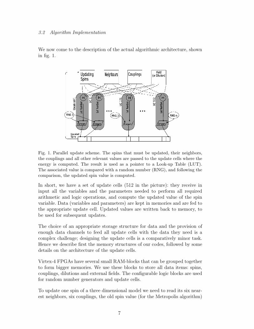
We now come to the description of the actual algorithmic architecture, shownin fig. 1.

Fig. 1. Parallel update scheme. The spins that must be updated, their neighbors,the couplings and all other relevant values are passed to the update cells where theenergy is computed. The result is used as a pointer to a Look-up Table (LUT).The associated value is compared with a random number (RNG), and following thecomparison, the updated spin value is computed.

In short, we have a set of update cells (512 in the picture): they receive ininput all the variables and the parameters needed to perform all requiredarithmetic and logic operations, and compute the updated value of the spinvariable. Data (variables and parameters) are kept in memories and are fed tothe appropriate update cell. Updated values are written back to memory, tobe used for subsequent updates.

The choice of an appropriate storage structure for data and the provision ofenough data channels to feed all update cells with the data they need is acomplex challenge; designing the update cells is a comparatively minor task.Hence we describe first the memory structures of our codes, followed by somedetails on the architecture of the update cells.

Virtex-4 FPGAs have several small RAM-blocks that can be grouped togetherto form bigger memories. We use these blocks to store all data items: spins,couplings, dilutions and external fields. The configurable logic blocks are usedfor random number generators and update cells.

To update one spin of a three dimensional model we need to read its six near-est neighbors, six couplings, the old spin value (for the Metropolis algorithm)

7

and some model-dependent information such as the magnetic field for RFIMand the dilution for DAFF. All these data items must be moved to the appro-priate update cells, in spite of the hardware bottleneck that only two memorylocations in each block can be read/written at each clock cycle.

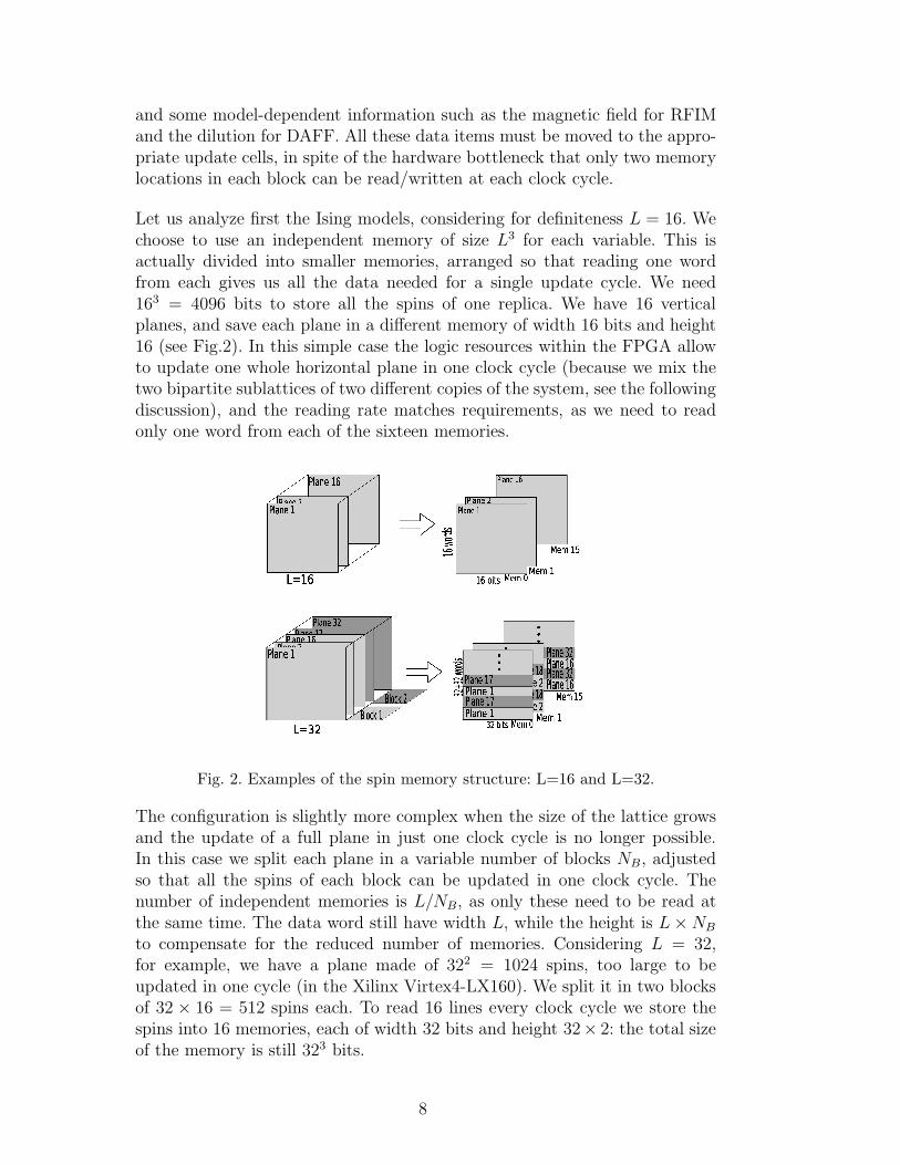
Let us analyze first the Ising models, considering for definiteness L = 16. Wechoose to use an independent memory of size L3 for each variable. This isactually divided into smaller memories, arranged so that reading one wordfrom each gives us all the data needed for a single update cycle. We need163 = 4096 bits to store all the spins of one replica. We have 16 verticalplanes, and save each plane in a different memory of width 16 bits and height16 (see Fig.2). In this simple case the logic resources within the FPGA allowto update one whole horizontal plane in one clock cycle (because we mix thetwo bipartite sublattices of two different copies of the system, see the followingdiscussion), and the reading rate matches requirements, as we need to readonly one word from each of the sixteen memories.

Fig. 2. Examples of the spin memory structure: L=16 and L=32.

The configuration is slightly more complex when the size of the lattice growsand the update of a full plane in just one clock cycle is no longer possible.In this case we split each plane in a variable number of blocks NB, adjustedso that all the spins of each block can be updated in one clock cycle. Thenumber of independent memories is L/NB, as only these need to be read atthe same time. The data word still have width L, while the height is L × NB

to compensate for the reduced number of memories. Considering L = 32,for example, we have a plane made of 322 = 1024 spins, too large to beupdated in one cycle (in the Xilinx Virtex4-LX160). We split it in two blocksof 32 × 16 = 512 spins each. To read 16 lines every clock cycle we store thespins into 16 memories, each of width 32 bits and height 32× 2: the total sizeof the memory is still 323 bits.

8

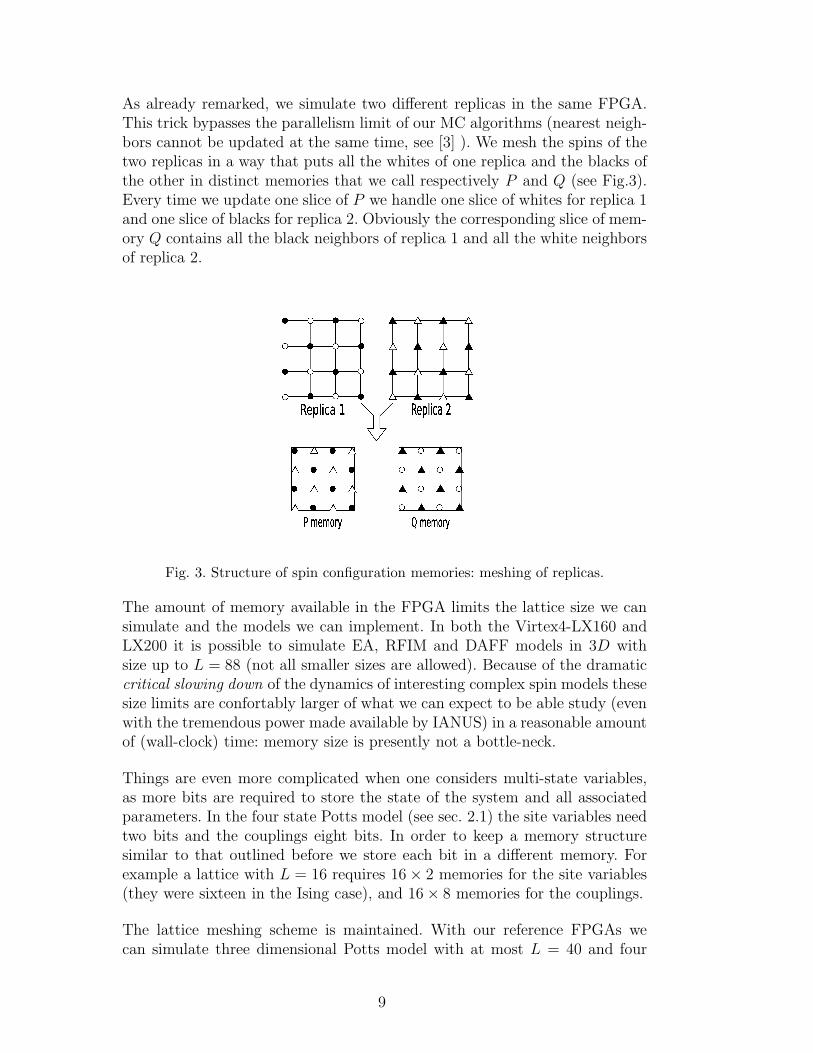
As already remarked, we simulate two different replicas in the same FPGA.This trick bypasses the parallelism limit of our MC algorithms (nearest neigh-bors cannot be updated at the same time, see [3] ). We mesh the spins of thetwo replicas in a way that puts all the whites of one replica and the blacks ofthe other in distinct memories that we call respectively P and Q (see Fig.3).Every time we update one slice of P we handle one slice of whites for replica 1and one slice of blacks for replica 2. Obviously the corresponding slice of mem-ory Q contains all the black neighbors of replica 1 and all the white neighborsof replica 2.

Fig. 3. Structure of spin configuration memories: meshing of replicas.

The amount of memory available in the FPGA limits the lattice size we cansimulate and the models we can implement. In both the Virtex4-LX160 andLX200 it is possible to simulate EA, RFIM and DAFF models in 3D withsize up to L = 88 (not all smaller sizes are allowed). Because of the dramaticcritical slowing down of the dynamics of interesting complex spin models thesesize limits are confortably larger of what we can expect to be able study (evenwith the tremendous power made available by IANUS) in a reasonable amountof (wall-clock) time: memory size is presently not a bottle-neck.

Things are even more complicated when one considers multi-state variables,as more bits are required to store the state of the system and all associatedparameters. In the four state Potts model (see sec. 2.1) the site variables needtwo bits and the couplings eight bits. In order to keep a memory structuresimilar to that outlined before we store each bit in a different memory. Forexample a lattice with L = 16 requires 16 × 2 memories for the site variables(they were sixteen in the Ising case), and 16 × 8 memories for the couplings.

The lattice meshing scheme is maintained. With our reference FPGAs wecan simulate three dimensional Potts model with at most L = 40 and four

9

dimensional Potts model with L = 16.

We now come to the description of the update cells. The Hamiltonian we havewritten is homogeneous: the interaction has the same form for every site ofthe lattice, and it only depends on the values of the couplings, the fields andthe dilutions. This means that we can write a standard update cell and use itas a black box to update all sites: it will give us the updated value of the spin(provided that we feed the correct inputs). This choice makes it easy to writea parametric program, where we instantiate the same update cell as manytimes as needed.

We have implemented two algorithms: Metropolis and Heat Bath. The updatecell receives in input couplings, nearest neighbors spins, field and dilution and,if appropriate, the old spin value (for the Metropolis dynamics). The cell usesthese values as specified by (2) and computes a numerical value between 0 and15 (the range varies depending on the model) used as an input to a LUT. Thevalue read from the LUT is compared with a random number and the new spinstate is chosen depending on the result of the comparison. Once again, thingsare slightly different for the Potts model due to the multi-state variables andcouplings.

Our goal is to update in parallel as many variables as possible, which meansthat we want to maximize the number of cells that will be accessing the LUTat the same time. In order to avoid routing congestion at the hardware layer wereplicate the LUTs: each instance is read only by two update cells. The wastein logic resources – the same information is replicated many times within theprocessor – is compensated by the higher allowed clock frequency.

3.3 Random numbers

Monte Carlo methods depend strongly on the random numbers used to drivethe updates: this determines the imperative need to implement a very reliablepseudo-random number generator (RNG), that produces a sequence of num-bers under the selected distribution, with no known or evident pathologies.

We use the Parisi-Rapuano shift register method [16] defined by the rules:

I(k) = I(k − 24) + I(k − 55) (5)

R(k) = I(k) ⊗ I(k − 61) ,

where I(k−24), I(k−55) and I(k−61) are elements (32-bit wide) of a so calledwheel that we initialize with externally generated random values. I(k) is thenew element of the updated wheel, and R(k) is the generated pseudo-random

10

value.

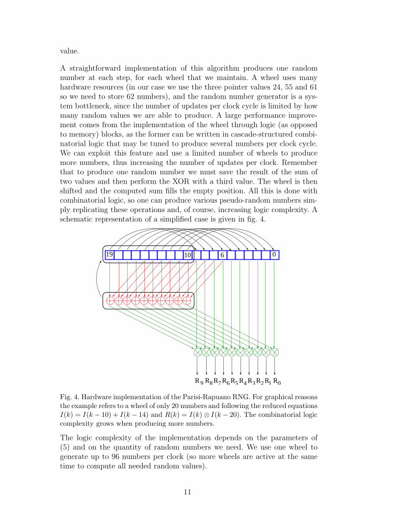
A straightforward implementation of this algorithm produces one randomnumber at each step, for each wheel that we maintain. A wheel uses manyhardware resources (in our case we use the three pointer values 24, 55 and 61so we need to store 62 numbers), and the random number generator is a sys-tem bottleneck, since the number of updates per clock cycle is limited by howmany random values we are able to produce. A large performance improve-ment comes from the implementation of the wheel through logic (as opposedto memory) blocks, as the former can be written in cascade-structured combi-natorial logic that may be tuned to produce several numbers per clock cycle.We can exploit this feature and use a limited number of wheels to producemore numbers, thus increasing the number of updates per clock. Rememberthat to produce one random number we must save the result of the sum oftwo values and then perform the XOR with a third value. The wheel is thenshifted and the computed sum fills the empty position. All this is done withcombinatorial logic, so one can produce various pseudo-random numbers sim-ply replicating these operations and, of course, increasing logic complexity. Aschematic representation of a simplified case is given in fig. 4.

RRRRRR R R R R 0123456789

19 10 6 0

Fig. 4. Hardware implementation of the Parisi-Rapuano RNG. For graphical reasonsthe example refers to a wheel of only 20 numbers and following the reduced equationsI(k) = I(k − 10) + I(k − 14) and R(k) = I(k) ⊗ I(k − 20). The combinatorial logiccomplexity grows when producing more numbers.

The logic complexity of the implementation depends on the parameters of(5) and on the quantity of random numbers we need. We use one wheel togenerate up to 96 numbers per clock (so more wheels are active at the sametime to compute all needed random values).

11

To keep the wheel safely below its period limit we choose to reload the wheelevery now and then (for example every 107 MC sweeps).

With respect to the choice of 32-bit random numbers, we have verified thatthis word size is sufficient for the models we want to simulate (our tests showthat 24-bit would be enough). Other models may require better random num-bers. We do not address this issue here. We just note that generating randomnumbers of larger size (e.g., 40 or even 64-bit) would be straightforward, atthe price, of course, of a larger resource usage.

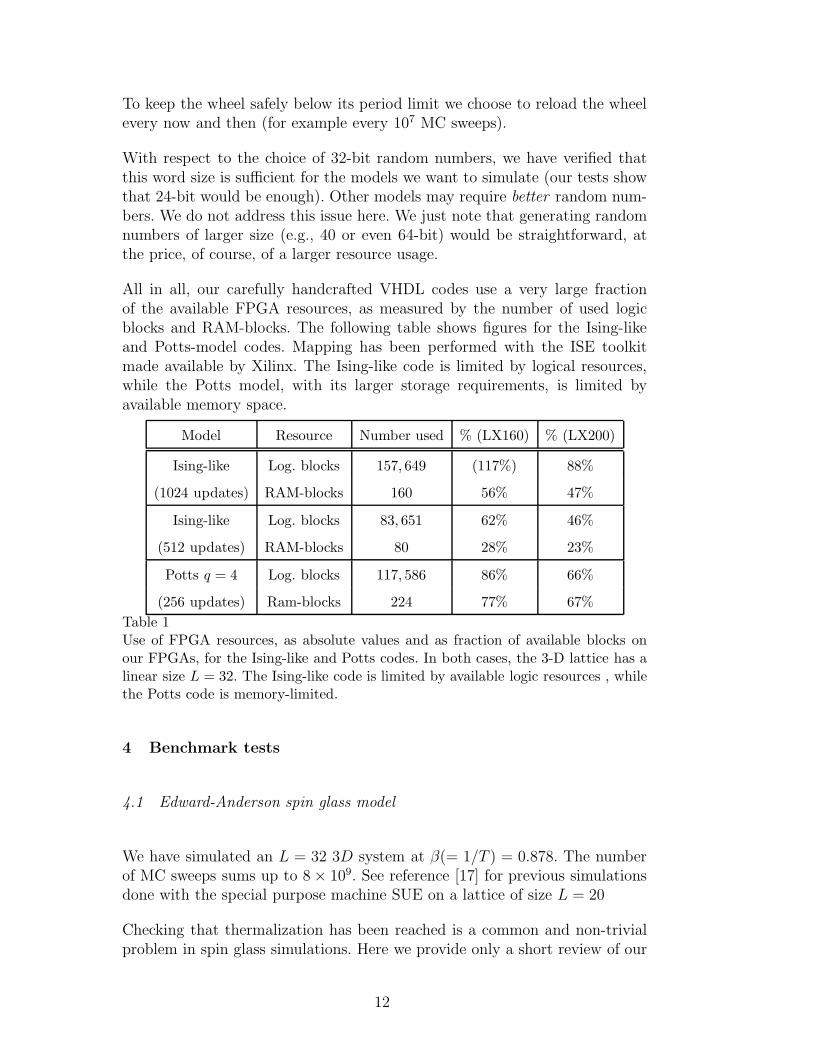
All in all, our carefully handcrafted VHDL codes use a very large fractionof the available FPGA resources, as measured by the number of used logicblocks and RAM-blocks. The following table shows figures for the Ising-likeand Potts-model codes. Mapping has been performed with the ISE toolkitmade available by Xilinx. The Ising-like code is limited by logical resources,while the Potts model, with its larger storage requirements, is limited byavailable memory space.

Model Resource Number used % (LX160) % (LX200)

Ising-like Log. blocks 157, 649 (117%) 88%

(1024 updates) RAM-blocks 160 56% 47%

Ising-like Log. blocks 83, 651 62% 46%

(512 updates) RAM-blocks 80 28% 23%

Potts q = 4 Log. blocks 117, 586 86% 66%

(256 updates) Ram-blocks 224 77% 67%

Table 1Use of FPGA resources, as absolute values and as fraction of available blocks onour FPGAs, for the Ising-like and Potts codes. In both cases, the 3-D lattice has alinear size L = 32. The Ising-like code is limited by available logic resources , whilethe Potts code is memory-limited.

4 Benchmark tests

4.1 Edward-Anderson spin glass model

We have simulated an L = 32 3D system at β(= 1/T ) = 0.878. The numberof MC sweeps sums up to 8 × 109. See reference [17] for previous simulationsdone with the special purpose machine SUE on a lattice of size L = 20

Checking that thermalization has been reached is a common and non-trivialproblem in spin glass simulations. Here we provide only a short review of our

12

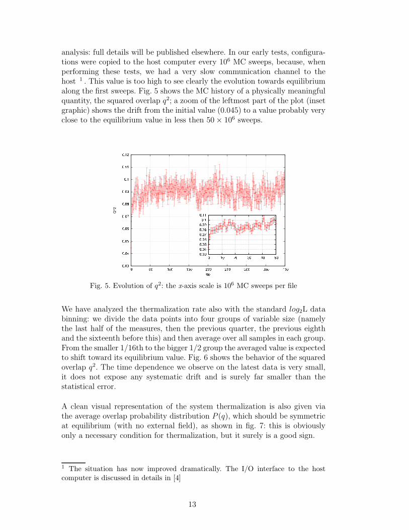
analysis: full details will be published elsewhere. In our early tests, configura-tions were copied to the host computer every 106 MC sweeps, because, whenperforming these tests, we had a very slow communication channel to thehost 1 . This value is too high to see clearly the evolution towards equilibriumalong the first sweeps. Fig. 5 shows the MC history of a physically meaningfulquantity, the squared overlap q2; a zoom of the leftmost part of the plot (insetgraphic) shows the drift from the initial value (0.045) to a value probably veryclose to the equilibrium value in less then 50 × 106 sweeps.

Fig. 5. Evolution of q2: the x-axis scale is 106 MC sweeps per file

We have analyzed the thermalization rate also with the standard log2L databinning: we divide the data points into four groups of variable size (namelythe last half of the measures, then the previous quarter, the previous eighthand the sixteenth before this) and then average over all samples in each group.From the smaller 1/16th to the bigger 1/2 group the averaged value is expectedto shift toward its equilibrium value. Fig. 6 shows the behavior of the squaredoverlap q2. The time dependence we observe on the latest data is very small,it does not expose any systematic drift and is surely far smaller than thestatistical error.

A clean visual representation of the system thermalization is also given viathe average overlap probability distribution P (q), which should be symmetricat equilibrium (with no external field), as shown in fig. 7: this is obviouslyonly a necessary condition for thermalization, but it surely is a good sign.

1 The situation has now improved dramatically. The I/O interface to the hostcomputer is discussed in details in [4]

13

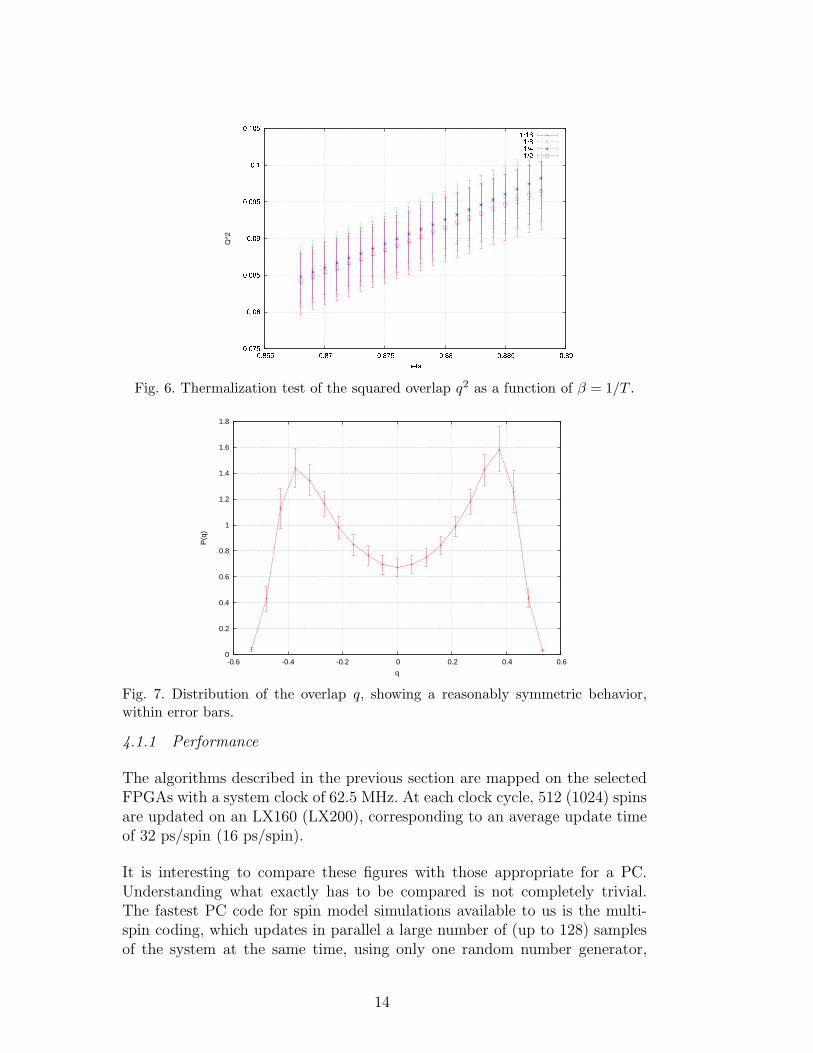
Fig. 6. Thermalization test of the squared overlap q2 as a function of β = 1/T .

0

0.2

0.4

0.6

0.8

1

1.2

1.4

1.6

1.8

-0.6 -0.4 -0.2 0 0.2 0.4 0.6

P(q

)

q

Fig. 7. Distribution of the overlap q, showing a reasonably symmetric behavior,within error bars.

4.1.1 Performance

The algorithms described in the previous section are mapped on the selectedFPGAs with a system clock of 62.5 MHz. At each clock cycle, 512 (1024) spinsare updated on an LX160 (LX200), corresponding to an average update timeof 32 ps/spin (16 ps/spin).

It is interesting to compare these figures with those appropriate for a PC.Understanding what exactly has to be compared is not completely trivial.The fastest PC code for spin model simulations available to us is the multi-spin coding, which updates in parallel a large number of (up to 128) samplesof the system at the same time, using only one random number generator,

14

which is shared across all samples: this scheme is useful to obtain a largenumber of configuration data, appropriate for statistical analysis. We call thisan asynchronous multi-spin coding (AMSC) as inside each sample there is noparallelism.

As we have stated before, the biggest problem with the models we want tostudy is the decorrelation time, and the large number of Monte Carlo sweepsthat it may take to bring a configuration to equilibrium. The AMSC procedurehas a serious problem here since each sample evolves for the same number ofsweeps as if it were the only one being simulated. In other words, efficientcodes on a PC achieve high overall performance by simulating for relativelyshort MC time a large number of independent samples. A code that updatesin parallel more spins belonging to the same system would be more useful toattain equilibrium, when working on large systems. The resulting algorithm,synchronous MSC (SMSC), takes less time to simulate one sample, but theglobal performance is lowered because of more complex operations involvedand the need to use an independent random number for each spin. The SMSCPC-code available to us updates up to 128 spins of a single sample. Syn-chronous codes are not commonly used in PC based numerical simulationsbecause of their globally poor performances.

Generally speaking we think that comparison with a SMSC code is appropriatefor a single FPGA system, while comparison with an AMSC code is morerelevant when considering a massively parallel IANUS system (we plan tobuild a system with 256 FPGA-based nodes). Here we simply present ourpreliminary comparison data for both cases in table 2.

LX160 LX200 PC (SMSC) PC (AMSC)

Update Rate 32 ps/spin 16 ps/spin 3000 ps/spin 700 ps/spin

Table 2Comparing the performances of two Xilinx Virtex4 FPGAs and two different codesrunning on a high-end PC.

The MSC values are referred to an Intel Core2Duo (64 bit) 1.6 GHz processor.Inspection of table 2 tells us that one LX160 runs as fast as 90 PCs, whilethe LX200 performance is comparable to that of 180 PCs. In other words,the 8× 109 MC iterations required to thermalize a lattice of size L = 32 tookapproximately 6 hours to be completed on just one Virtex4-LX200: they wouldtake 18 days on a PC running the SMSC algorithm.

Performance comparison with published work is difficult. As far as we knowthe SMSC is not used for massive simulations, so data on the performances ofthis algorithm is not widespread. The AMSC is commonly used. Even if it isconsidered almost a standard in spin glass simulations, we have not been ableto find recent speed analysis. The seminal works on this algorithm [14] and[15] are way too old in technology terms to allow a fair comparison. All in all,

15

we believe that the codes that we have used for performance comparison arestate-of-the-art PC implementations, and further optimizations could at mostimprove the performances by some 10−20%; we conclude that the performanceof one FPGA-processor is roughly ≃ 100 times better than possible on a PC.

4.2 Potts model

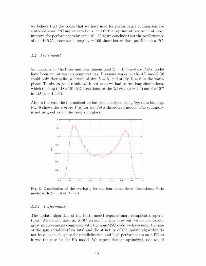
Simulations for the three and four dimensional L = 16 four-state Potts modelhave been run at various temperatures. Previous works on the 4D model [9]could only thermalize a lattice of size L = 5, and study L = 8 in the warmphase. To obtain good results with out tests we had to run long simulations,which took up to 18×1011 MC iterations for the 3D case (β = 2.4) and 6×1010

in 4D (β = 1.405).

Also in this case the thermalization has been analyzed using log2 data binning.Fig. 8 shows the average P (q) for the Potts disordered model. The symmetryis not as good as for the Ising spin glass.

0

0.2

0.4

0.6

0.8

1

1.2

1.4

-0.8 -0.6 -0.4 -0.2 0 0.2 0.4 0.6 0.8

P(q

)

q

Fig. 8. Distribution of the overlap q for the four-states three dimensional Pottsmodel with L = 16 at β = 2.4.

4.2.1 Performance

The update algorithm of the Potts model requires more complicated opera-tions. We do not have an MSC version for this case but we do not expectgreat improvements compared with the non-MSC code we have used: the sizeof the spin variables (four bits) and the structure of the update algorithm donot leave as much space for parallelization and high performances on a PC asit was the case for the EA model. We expect that an optimized code would

16

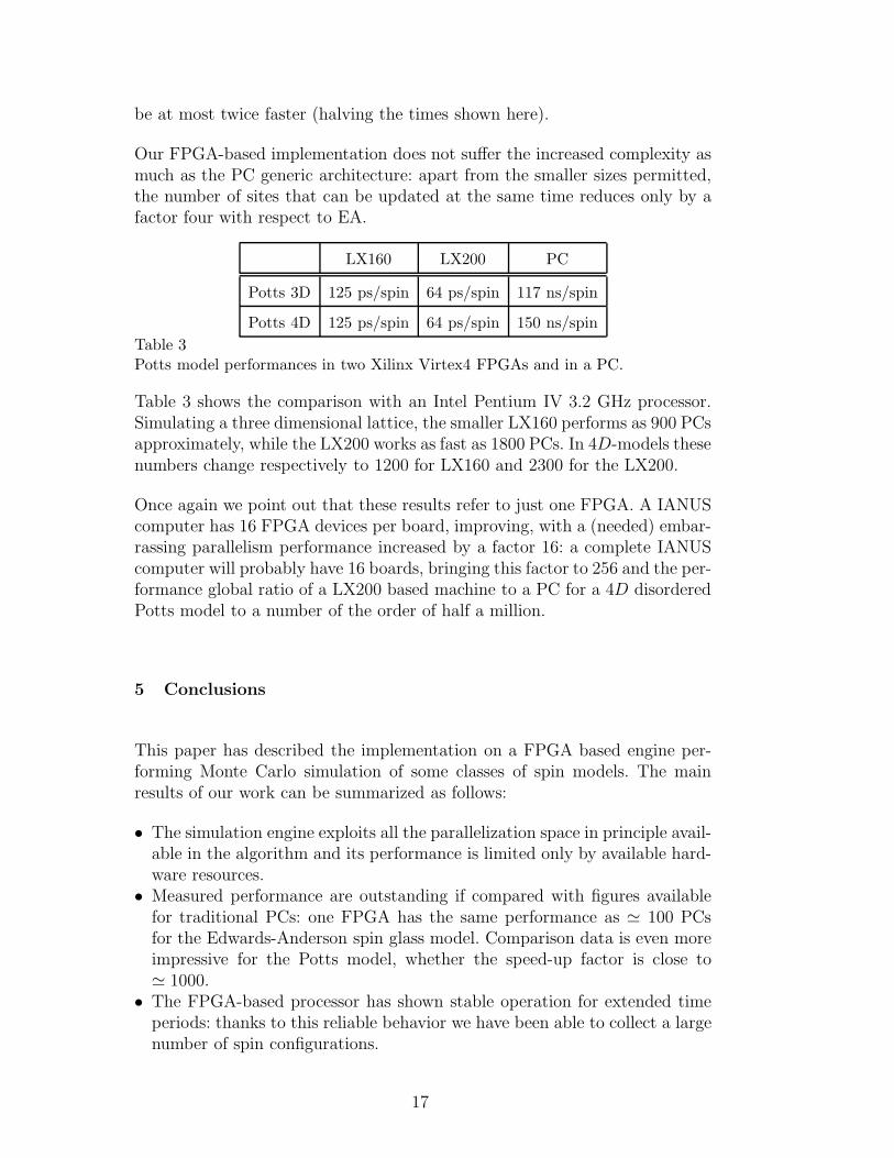
be at most twice faster (halving the times shown here).

Our FPGA-based implementation does not suffer the increased complexity asmuch as the PC generic architecture: apart from the smaller sizes permitted,the number of sites that can be updated at the same time reduces only by afactor four with respect to EA.

LX160 LX200 PC

Potts 3D 125 ps/spin 64 ps/spin 117 ns/spin

Potts 4D 125 ps/spin 64 ps/spin 150 ns/spin

Table 3Potts model performances in two Xilinx Virtex4 FPGAs and in a PC.

Table 3 shows the comparison with an Intel Pentium IV 3.2 GHz processor.Simulating a three dimensional lattice, the smaller LX160 performs as 900 PCsapproximately, while the LX200 works as fast as 1800 PCs. In 4D-models thesenumbers change respectively to 1200 for LX160 and 2300 for the LX200.

Once again we point out that these results refer to just one FPGA. A IANUScomputer has 16 FPGA devices per board, improving, with a (needed) embar-rassing parallelism performance increased by a factor 16: a complete IANUScomputer will probably have 16 boards, bringing this factor to 256 and the per-formance global ratio of a LX200 based machine to a PC for a 4D disorderedPotts model to a number of the order of half a million.

5 Conclusions

This paper has described the implementation on a FPGA based engine per-forming Monte Carlo simulation of some classes of spin models. The mainresults of our work can be summarized as follows:

• The simulation engine exploits all the parallelization space in principle avail-able in the algorithm and its performance is limited only by available hard-ware resources.

• Measured performance are outstanding if compared with figures availablefor traditional PCs: one FPGA has the same performance as ≃ 100 PCsfor the Edwards-Anderson spin glass model. Comparison data is even moreimpressive for the Potts model, whether the speed-up factor is close to≃ 1000.

• The FPGA-based processor has shown stable operation for extended timeperiods: thanks to this reliable behavior we have been able to collect a largenumber of spin configurations.

17

The work described here will continue with actual physics runs in which largestatistics will be collected for larger systems, as soon as large IANUS systemsare available. We also continue to work on the development of simulation codesfor other algorithms of scientific interest. Work is in progress in such areas asrandom graphs, surface growing and protein docking.

Acknowledgments

The help of G. Poli in the development of the IANUS Ethernet interface iswarmly acknowledged.

References

[1] E. Marinari, G. Parisi and J. J. Ruiz-Lorenzo, Numerical simulations of spinglass systems, in Spin Glasses and Random Fields, (A. P. Young editor) WorldScientific, Singapore, 1998.

[2] A. Cruz, et al., Comput. Phys. Commun. 133 (2001) 165-176.

[3] F.Belletti et al., Computing in Science and Engineering 8 (2006) 41-49.

[4] the Ianus Collaboration, work in progress.

[5] S. F. Edwards and P. W. Anderson, J. Phys. F: Mat. Phys. 5 (1975) 965-974.

[6] Y. Imry and S. Ma, Phys. Rev. Lett. 35 (1975) 1399-1401.

[7] D. P. Belanger and A. P. Young, J. of Magnetism and Magnetic Materials 100,(1991) pp. 272-291.

[8] A. D. Ogielski and D. A. Huse, Phys. Rev. Lett. 56 (1986) 1298-1301.

[9] E. Marinari et al., Phys. Rev. B, 59 (1999) 8401-8404.

[10] A.D. Sokal, Monte Carlo Methods in Statistical Mechanics: Foundations andNew Algorithms, Cours de Troisieme Cycle de la Physique en Suisse Romande(1989)

[11] D. J. Amit and V. Martın-Mayor, Field theory, renormalization group andcritical phenomena (third edition) World Scientific, Singapore (2005)

[12] D. P. Landau and K. Binder, A Guide to Monte Carlo Simulations in StatisticalPhysics Cambridge University Press (2005).

[13] E. Marinari and G. Parisi, Europhys. Lett. 19 (1992) 451. K. Hukushima andK. Nemoto, J. Phys. Soc. Jpn. 65 (1996) 1604. M. C. Tesi et al. J. Stat. Phys.82 (1996) 155.

18

[14] H. O. Heuer, Comput. Phys. Commun. 59 (1990) 387-398.

[15] H. Rieger, Jour. Stat. Phys, 70 (1993) 1063-1073.

[16] G.Parisi and F. Rapuano, Phys. Lett. B 157 (1985) 301-302.

[17] H.G. Ballesteros et al., Phys. Rev. B 62 (2000) 14237-14245.

19