Satellite-Based Energy Balance to Assess Within-Population Variance of Crop Coefficient Curves

plan-nce ET byte sensingd

mpacts ofinhetter fitoudy dates

gement;

Satellite-Based Energy Balance to Assess Within-PopulationVariance of Crop Coefficient Curves

Masahiro Tasumi1; Richard G. Allen2; Ricardo Trezza3; and James L. Wright4

Abstract: Quantifying evapotranspiration(ET) from agricultural fields is important for field water management, water resourcesning, and water regulation. Traditionally, ET from agricultural fields has been estimated by multiplying the weather-based referecrop coefficientssKcd determined according to the crop type and the crop growth stage. Recent development of satellite remoET models has enabled us to estimate ET andKc for large populations of fields. This study evaluated the distribution ofKc over space antime for a large number of individual fields by crop type using ET maps created by a satellite based energy balance(EB) model. Variationof Kc curves was found to be substantially larger than that for the normalized difference vegetation index because of the irandom wetting events onKc, especially during initial and development growth stages. Two traditionalKc curves that are widely usedIdaho for crop management and water rights regulation were compared against the satellite-derivedKc curves. Simple adjustment of ttraditionalKc curves by shifting dates for emergence, effective full cover, and termination enabled the traditional curves to beKc

curves as determined by the EB model. Applicability of the presented techniques in humid regions having higher chances of clwas discussed.

DOI: 10.1061/(ASCE)0733-9437(2005)131:1(94)

CE Database subject headings: Evapotranspiration; Satellites; Remote sensing; Irrigation scheduling; Water resources manaCrops.

apo-effi-

andl.

undereter-scriboncrop

irri-d/ord to

waterar-

uldr fieldtioneedent.

atel-might

chesp-iffer-

nl-er etughsuchethodl-l.

el,ine

ernaredica-

im-

nsioni@

earchail:

arch

mustoneitor.sible

per is

109/

Introduction

For more than 30 years, the primary method for estimating evtranspiration(ET) has been from reference ET and crop cocient sKcd curves(Jensen 1973; Allen et al. 1998). Crop coeffi-cients generally found in literature, such as by DoorenbosPruitt (1977), Wright (1981, 1982, and 1995), Snyder et a(1989a, 1989b), Jensen et al.(1990), and Allen et al.(1998),represent average to optimum agricultural managementwell-watered conditions. These coefficients are typically dmined from point-based measurements, and are unable to dethe variation inKc for the large population of fields in a regibecause “mean”Kc curves must represent a single averagedgrowth and water management condition. ActualKc populationshave inherent variation because of variation in crop variety,gation method, weather, soil type, salinity and fertility, anfield management that can be different from the field use

1Post-Doctoral Researcher, Univ. of Idaho Research and ExteCenter, 3793 N. 3600 E., Kimberly, ID 83341. E-mail: tasumkimberly.uidaho.edu

2Professor, Water Resources Engineering, Univ. of Idaho Resand Extension Center, 3793 N. 3600 E., Kimberly, ID 83341. [email protected]

3Associate Professor, Univ. of the Andes, Merida, Venezuela.4Soil Scientist, USDA-ARS Northwest Irrigation and Soils Rese

Laboratory, 3793 N. 3600 E., Kimberly, ID 83341.Note. Discussion open until July 1, 2005. Separate discussions

be submitted for individual papers. To extend the closing date bymonth, a written request must be filed with the ASCE Managing EdThe manuscript for this paper was submitted for review and pospublication on May 6, 2003; approved on January 8, 2004. This papart of theJournal of Irrigation and Drainage Engineering, Vol. 131,No. 1, February 1, 2005. ©ASCE, ISSN 0733-9437/2005/1-94–
$25.00.
94 / JOURNAL OF IRRIGATION AND DRAINAGE ENGINEERING © ASCE /

e

establish the literature values. This is especially true underlimiting or extreme salinity conditions. Quantification and chacterization ofKc populations for various crops in a region wobe valuable in defining average water use by crop type undeconditions and the range in water use. This type of informacan be helpful in determining impacts of water scarcity or nfor remedial help in improving water or agronomic managem

Alternative means for estimating field-scale ET include slite image-based remote sensing methods. These methodsbe divided into two categories: empirical/statistical approaand energy balance(EB) approaches. Empirical/statistical aproaches correlate ET either to air–surface temperature dences such as reported by Caselles et al.(1998), or to vegetatioindices as frequently used for “basal”Kc estimation for agricutural crops(Neale et al. 1989; Choudhury et al. 1994; Hunsakal. 2003). On the other hand, EB approaches derive ET throcompleting a full energy balance computation using methodsas a two-layer model and the dual-temperature-difference mdeveloped by Norman et al.(1995 and 2000), surface energy baance algorithms for land(SEBAL) model (Bastiaanssen et a1998a), and evaporation fraction estimation method forMODIS(Nishida et al. 2003). In this study, a satellite-based EB modwhich is a variant of the SEBAL model, was applied to determactual Kc for a large number of agricultural fields in southIdaho. Crop coefficients derived from the EB model are compto widely usedKc curves in Idaho, and the potential and applbility of satellite basedKc curves are discussed.

Energy Balance Model

The SEBAL is an ET estimation approach based on satellite
ages via the computation of a land surface energy balance meth-
JANUARY/FEBRUARY 2005

a;r ofain,inamakual.

3;edlturals tothei-ard-

nce

yidents thetingnd it

ap-for

pera-sen-nstantions

-

age-un-

sim-

ergyellitend

bal-

ing

eflec-thenated

sur-nallyce

theg

3 and

4,

byVI,

indated”r to

irns-

ibra-

tddif-pera-, forr-rity

faces re-ll-Thedata,

lfalfa-r

ased

e cal-d soils the

pre-tremeetldLfor

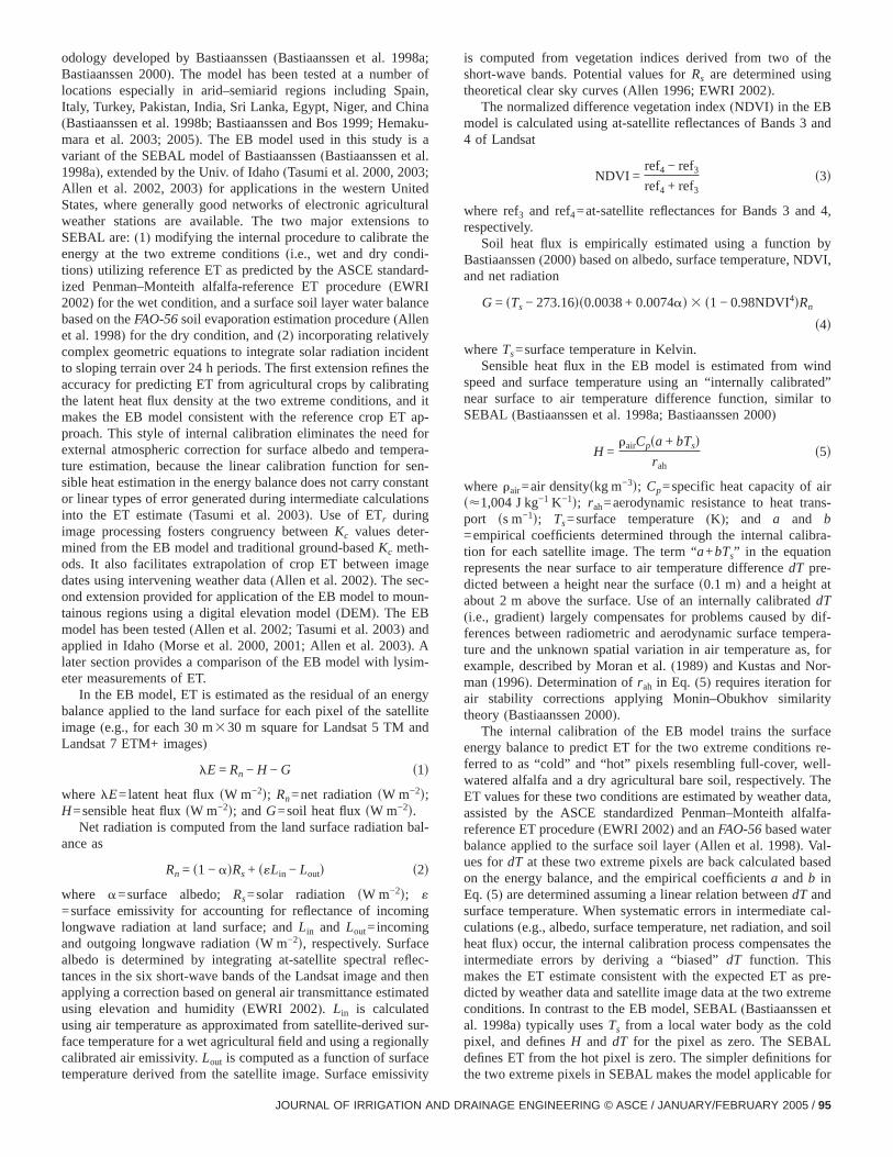
odology developed by Bastiaanssen(Bastiaanssen et al. 1998Bastiaanssen 2000). The model has been tested at a numbelocations especially in arid–semiarid regions including SpItaly, Turkey, Pakistan, India, Sri Lanka, Egypt, Niger, and Ch(Bastiaanssen et al. 1998b; Bastiaanssen and Bos 1999; Hemara et al. 2003; 2005). The EB model used in this study isvariant of the SEBAL model of Bastiaanssen(Bastiaanssen et a1998a), extended by the Univ. of Idaho(Tasumi et al. 2000, 200Allen et al. 2002, 2003) for applications in the western UnitStates, where generally good networks of electronic agricuweather stations are available. The two major extensionSEBAL are:(1) modifying the internal procedure to calibrateenergy at the two extreme conditions(i.e., wet and dry condtions) utilizing reference ET as predicted by the ASCE standized Penman–Monteith alfalfa-reference ET procedure(EWRI2002) for the wet condition, and a surface soil layer water balabased on theFAO-56soil evaporation estimation procedure(Allenet al. 1998) for the dry condition, and(2) incorporating relativelcomplex geometric equations to integrate solar radiation incto sloping terrain over 24 h periods. The first extension refineaccuracy for predicting ET from agricultural crops by calibrathe latent heat flux density at the two extreme conditions, amakes the EB model consistent with the reference crop ETproach. This style of internal calibration eliminates the needexternal atmospheric correction for surface albedo and temture estimation, because the linear calibration function forsible heat estimation in the energy balance does not carry coor linear types of error generated during intermediate calculainto the ET estimate(Tasumi et al. 2003). Use of ETr duringimage processing fosters congruency betweenKc values determined from the EB model and traditional ground-basedKc meth-ods. It also facilitates extrapolation of crop ET between imdates using intervening weather data(Allen et al. 2002). The second extension provided for application of the EB model to motainous regions using a digital elevation model(DEM). The EBmodel has been tested(Allen et al. 2002; Tasumi et al. 2003) andapplied in Idaho(Morse et al. 2000, 2001; Allen et al. 2003). Alater section provides a comparison of the EB model with lyeter measurements of ET.

In the EB model, ET is estimated as the residual of an enbalance applied to the land surface for each pixel of the satimage(e.g., for each 30 m330 m square for Landsat 5 TM aLandsat 7 ETM+ images)

lE = Rn − H − G s1d

wherelE=latent heat fluxsW m−2d; Rn=net radiationsW m−2d;H=sensible heat fluxsW m−2d; andG=soil heat fluxsW m−2d.

Net radiation is computed from the land surface radiationance as

Rn = s1 − adRs + s«Lin − Loutd s2d

where a=surface albedo; Rs=solar radiation sW m−2d; «=surface emissivity for accounting for reflectance of incomlongwave radiation at land surface; andLin and Lout= incomingand outgoing longwave radiationsW m−2d, respectively. Surfacalbedo is determined by integrating at-satellite spectral retances in the six short-wave bands of the Landsat image andapplying a correction based on general air transmittance estimusing elevation and humidity(EWRI 2002). Lin is calculatedusing air temperature as approximated from satellite-derivedface temperature for a wet agricultural field and using a regiocalibrated air emissivity.Lout is computed as a function of surfa
temperature derived from the satellite image. Surface emissivity
JOURNAL OF IRRIGATION AND DR

-

t

is computed from vegetation indices derived from two ofshort-wave bands. Potential values forRs are determined usintheoretical clear sky curves(Allen 1996; EWRI 2002).

The normalized difference vegetation index(NDVI ) in the EBmodel is calculated using at-satellite reflectances of Bands4 of Landsat

NDVI =ref4 − ref3ref4 + ref3

s3d

where ref3 and ref4=at-satellite reflectances for Bands 3 andrespectively.

Soil heat flux is empirically estimated using a functionBastiaanssen(2000) based on albedo, surface temperature, NDand net radiation

G = sTs − 273.16ds0.0038 + 0.0074ad 3 s1 − 0.98NDVI4dRn

s4d

whereTs=surface temperature in Kelvin.Sensible heat flux in the EB model is estimated from w

speed and surface temperature using an “internally calibrnear surface to air temperature difference function, similaSEBAL (Bastiaanssen et al. 1998a; Bastiaanssen 2000)

H =rairCpsa + bTsd

rahs5d

whererair=air densityskg m−3d; Cp=specific heat capacity of as<1,004 J kg−1 K−1d; rah=aerodynamic resistance to heat traport ss m−1d; Ts=surface temperature(K); and a and b=empirical coefficients determined through the internal caltion for each satellite image. The term “a+bTs” in the equationrepresents the near surface to air temperature differencedT pre-dicted between a height near the surfaces0.1 md and a height aabout 2 m above the surface. Use of an internally calibratedT(i.e., gradient) largely compensates for problems caused byferences between radiometric and aerodynamic surface temture and the unknown spatial variation in air temperature asexample, described by Moran et al.(1989) and Kustas and Noman(1996). Determination ofrah in Eq. (5) requires iteration foair stability corrections applying Monin–Obukhov similartheory (Bastiaanssen 2000).

The internal calibration of the EB model trains the surenergy balance to predict ET for the two extreme conditionferred to as “cold” and “hot” pixels resembling full-cover, wewatered alfalfa and a dry agricultural bare soil, respectively.ET values for these two conditions are estimated by weatherassisted by the ASCE standardized Penman–Monteith areference ET procedure(EWRI 2002) and anFAO-56based watebalance applied to the surface soil layer(Allen et al. 1998). Val-ues fordT at these two extreme pixels are back calculated bon the energy balance, and the empirical coefficientsa andb inEq. (5) are determined assuming a linear relation betweendT andsurface temperature. When systematic errors in intermediatculations(e.g., albedo, surface temperature, net radiation, anheat flux) occur, the internal calibration process compensateintermediate errors by deriving a “biased”dT function. Thismakes the ET estimate consistent with the expected ET asdicted by weather data and satellite image data at the two exconditions. In contrast to the EB model, SEBAL(Bastiaanssenal. 1998a) typically usesTs from a local water body as the copixel, and definesH and dT for the pixel as zero. The SEBAdefines ET from the hot pixel is zero. The simpler definitions
the two extreme pixels in SEBAL makes the model applicable for
AINAGE ENGINEERING © ASCE / JANUARY/FEBRUARY 2005 / 95

tain.a-

, the

herref-

g the.

ETto24 h

;--

elliteeter-Id.

ings

t im-180um

120siderved

oc-ent

apo-ther-reasavilynce.

rob-lts for-ob-

m-easonover.andof

xel asccu-sonal

edomover

nd

dahoi--iver, andthe

tatoes,

ges,y, 12

tertaer sky

beets00,

countries where high-quality weather data are difficult to obHowever, the practice of assumingH=0 at water body temperture may cause some error in the estimate ofH and ET for coldagriculture pixels in arid regions(Tasumi 2003).

Once ET at the moment of the satellite image is estimatedcrop coefficientsKcd is calculated for each image pixel as

Kc =ET

ETrs6d

where ETr =alfalfa reference ET calculated from local weatdata using the ASCE standardized Penman–Monteith alfalfaerence method(EWRI 2002) applied hourly.

For horizontal flat surfaces, 24 h ET is estimated by settin24 h averageKc equal to the “instantaneous”Kc calculated in Eq(6)

ETs24d = KcETrs24d s7d

TheKc in Eqs.(6) and(7) has also been referred to as ther

fraction sETrFd (Allen et al. 2002, 2003), and has been shownbe relatively consistent during daytime periods and betweenaverage and midday satellite image times(Allen et al. 2002Trezza 2002; Tasumi 2003; Romero 2003). Additional adjustments are applied during the extrapolation ofKc from instantaneous to 24 h for sloping surfaces. Monthly and seasonalKc andET can further be estimated by linearly interpolating theKc val-ues over periods inbetween two consecutive images.

Sample Comparison of Evapotranspiration and K cPredictions with Lysimeter Measurements

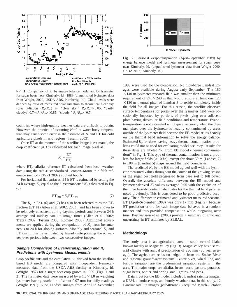
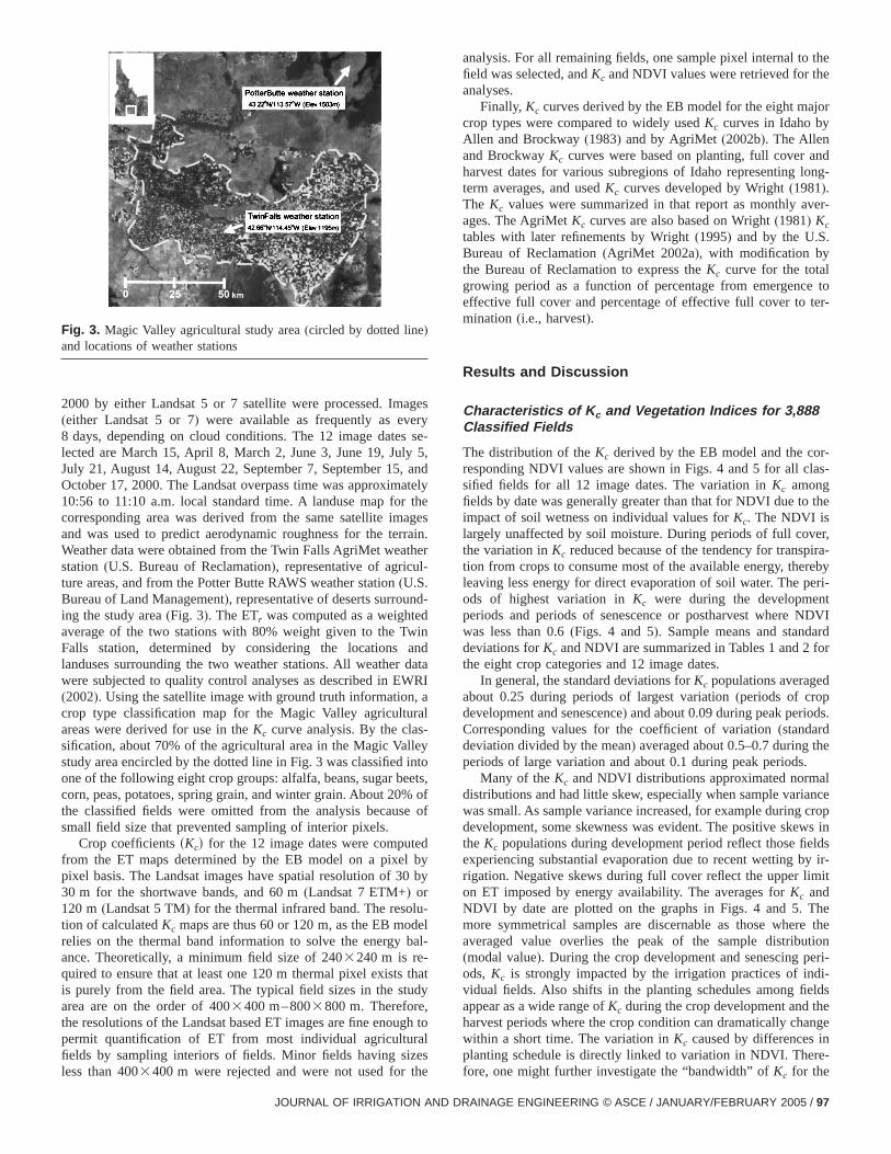
Crop coefficients and the cumulative ET derived from the satbased EB model are compared with independent lysimmeasured data from the USDA-ARS facility at Kimberly,(Wright 1982) for a sugar beet crop grown in 1989(Figs. 1 and2). The lysimeter data were measured by a 1.831.8 m weighinglysimeter having resolution of about 0.07 mm for daily read

Fig. 1. Comparison ofKc by energy balance model and by lysimefor sugar beets near Kimberly, Id., 1989(unpublished lysimeter dafrom Wright, 2000, USDA-ARS, Kimberly, Id.). Cloud levels werdefined by ratio of measured solar radiation to theoretical cleasolar radiation sRs/Rsod as; “clear sky:” Rs/Rsoù0.85; “partlycloudy:” 0.7øRs/Rso,0.85; “cloudy:” Rs/Rso,0.7.

(Wright 1991). Nine Landsat images from April to September

96 / JOURNAL OF IRRIGATION AND DRAINAGE ENGINEERING © ASCE /

1989 were used for the comparison. No cloud-free Landsaages were available during August–early September. The3140 m lysimeter research field was smaller than the minimrequirement of 2403240 m that would ensure at least one3120 m thermal pixel of Landsat 5 to reside completely inthe field for all images. For this reason, the satellite obsesurface temperatures for pixels over the lysimeter field werecasionally impacted by portions of pixels lying over adjacplots having dissimilar field conditions and temperature. Evtranspiration is not estimated with typical accuracy when themal pixel over the lysimeter is heavily contaminated by aoutside of the lysimeter field because the EB model relies heon the thermal band information to solve the energy balaEstimatedKc for dates having heavy thermal contamination plems could not be used for evaluating model accuracy. Resuthese dates are labeled “Kc from EB model(thermal contamination)” in Fig. 1. This type of thermal contamination is not a prlem for larger fieldss.10 had, except for about 50 m(Landsat 7)to 100 m(Landsat 5) strips around the field boundaries.

The predictedKc by the EB model agreed well with the lysieter measured values throughout the course of the growing sas the sugar beet field progressed from bare soil to full cOverall, the absolute difference between the EB modellysimeter-derivedKc values averaged 0.05 with the exclusionthe three heavily contaminated dates for the thermal band pinoted previously. This is considered to be good predictive aracy. The difference in estimated and lysimeter measured seaET (April–September 1989) was only 17 mm(Fig. 2), becausET prediction errors for each image date behaved in a ranmanner and thus provided compensation while integratingtime. Bastiaanssen et al.(2005) provide a summary of error auncertainty in ET estimates by SEBAL.

Methodology

The study area is an agricultural area in south central Iknown locally as Magic Valley(Fig. 3). Magic Valley has a semarid climate with annual precipitation of 280 mm(30 year average). The agriculture relies on irrigation from the Snake Rand regional groundwater systems. Center pivot, wheel linefurrow irrigation are the predominant irrigation systems inarea. The major crops are alfalfa, beans, corn, pasture, posugar beets, winter and spring small grains, and peas.

Data input for the EB model included Landsat satellite imaa DEM, a landuse map, and hourly weather data. In this stud

Fig. 2. Seasonal evapotranspiration(April–September 1989) byenergy balance model and lysimeter measurement for sugarnear Kimberly, Id.(unpublished lysimeter data from Wright 20USDA-ARS, Kimberly, Id.)

Landsat satellite images(path40/row30) acquired March–October

JANUARY/FEBRUARY 2005

ageserys se-ly 5,, andately

r theagesrrain.therl-

nd-edwinanddataWRI, aral

s-lleyinto

eets,% of

se of

tedl by0 by

lu-delbal-

-that

udy,

ugh toralzes

thehe

jory

andlong-

ver-

.

lce toter-

or-las-

the

ver,pira-reby

peri-ntNDVIardfor

d

ds.

the.alancecropws ineldsby ir-imit

There theutioneri-di-eldstheangeinre-

2000 by either Landsat 5 or 7 satellite were processed. Im(either Landsat 5 or 7) were available as frequently as ev8 days, depending on cloud conditions. The 12 image datelected are March 15, April 8, March 2, June 3, June 19, JuJuly 21, August 14, August 22, September 7, September 15October 17, 2000. The Landsat overpass time was approxim10:56 to 11:10 a.m. local standard time. A landuse map focorresponding area was derived from the same satellite imand was used to predict aerodynamic roughness for the teWeather data were obtained from the Twin Falls AgriMet weastation (U.S. Bureau of Reclamation), representative of agricuture areas, and from the Potter Butte RAWS weather station(U.S.Bureau of Land Management), representative of deserts surrouing the study area(Fig. 3). The ETr was computed as a weightaverage of the two stations with 80% weight given to the TFalls station, determined by considering the locationslanduses surrounding the two weather stations. All weatherwere subjected to quality control analyses as described in E(2002). Using the satellite image with ground truth informationcrop type classification map for the Magic Valley agricultuareas were derived for use in theKc curve analysis. By the clasification, about 70% of the agricultural area in the Magic Vastudy area encircled by the dotted line in Fig. 3 was classifiedone of the following eight crop groups: alfalfa, beans, sugar bcorn, peas, potatoes, spring grain, and winter grain. About 20the classified fields were omitted from the analysis becausmall field size that prevented sampling of interior pixels.

Crop coefficientssKcd for the 12 image dates were compufrom the ET maps determined by the EB model on a pixepixel basis. The Landsat images have spatial resolution of 330 m for the shortwave bands, and 60 m(Landsat 7 ETM+) or120 m(Landsat 5 TM) for the thermal infrared band. The resotion of calculatedKc maps are thus 60 or 120 m, as the EB morelies on the thermal band information to solve the energyance. Theoretically, a minimum field size of 2403240 m is required to ensure that at least one 120 m thermal pixel existsis purely from the field area. The typical field sizes in the starea are on the order of 4003400 m–8003800 m. Thereforethe resolutions of the Landsat based ET images are fine enopermit quantification of ET from most individual agricultufields by sampling interiors of fields. Minor fields having si

Fig. 3. Magic Valley agricultural study area(circled by dotted line)and locations of weather stations

less than 4003400 m were rejected and were not used for the


analysis. For all remaining fields, one sample pixel internal tofield was selected, andKc and NDVI values were retrieved for tanalyses.

Finally, Kc curves derived by the EB model for the eight macrop types were compared to widely usedKc curves in Idaho bAllen and Brockway(1983) and by AgriMet(2002b). The Allenand BrockwayKc curves were based on planting, full coverharvest dates for various subregions of Idaho representingterm averages, and usedKc curves developed by Wright(1981).The Kc values were summarized in that report as monthly aages. The AgriMetKc curves are also based on Wright(1981) Kc

tables with later refinements by Wright(1995) and by the U.SBureau of Reclamation(AgriMet 2002a), with modification bythe Bureau of Reclamation to express theKc curve for the totagrowing period as a function of percentage from emergeneffective full cover and percentage of effective full cover tomination (i.e., harvest).

Results and Discussion

Characteristics of K c and Vegetation Indices for 3,888Classified Fields

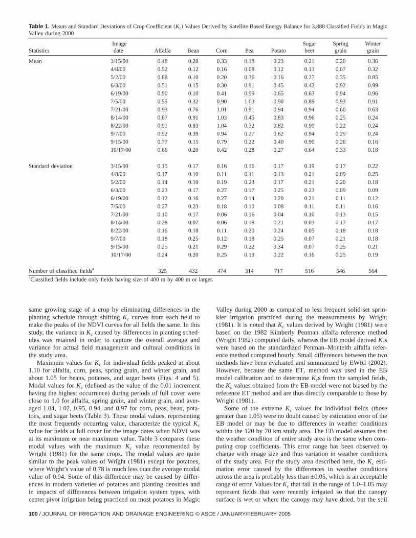
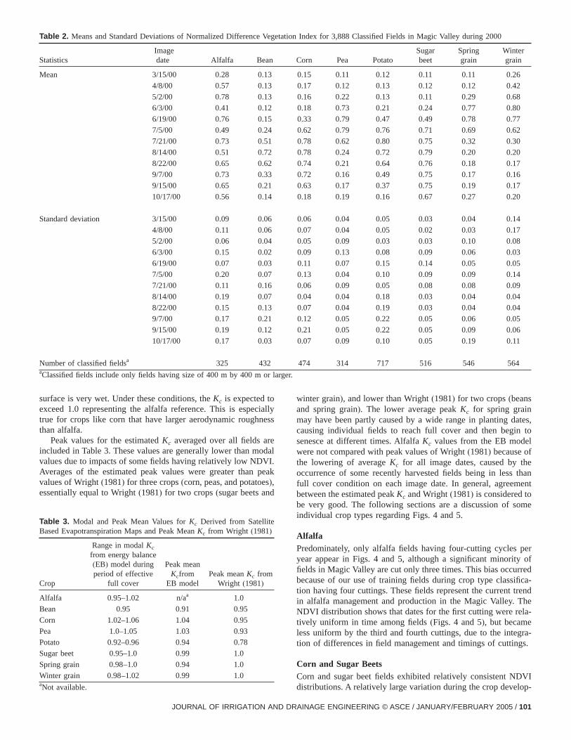
The distribution of theKc derived by the EB model and the cresponding NDVI values are shown in Figs. 4 and 5 for all csified fields for all 12 image dates. The variation inKc amongfields by date was generally greater than that for NDVI due toimpact of soil wetness on individual values forKc. The NDVI islargely unaffected by soil moisture. During periods of full cothe variation inKc reduced because of the tendency for transtion from crops to consume most of the available energy, theleaving less energy for direct evaporation of soil water. Theods of highest variation inKc were during the developmeperiods and periods of senescence or postharvest wherewas less than 0.6(Figs. 4 and 5). Sample means and standdeviations forKc and NDVI are summarized in Tables 1 and 2the eight crop categories and 12 image dates.

In general, the standard deviations forKc populations averageabout 0.25 during periods of largest variation(periods of cropdevelopment and senescence) and about 0.09 during peak perioCorresponding values for the coefficient of variation(standarddeviation divided by the mean) averaged about 0.5–0.7 duringperiods of large variation and about 0.1 during peak periods

Many of theKc and NDVI distributions approximated normdistributions and had little skew, especially when sample variwas small. As sample variance increased, for example duringdevelopment, some skewness was evident. The positive skethe Kc populations during development period reflect those fiexperiencing substantial evaporation due to recent wettingrigation. Negative skews during full cover reflect the upper lon ET imposed by energy availability. The averages forKc andNDVI by date are plotted on the graphs in Figs. 4 and 5.more symmetrical samples are discernable as those wheaveraged value overlies the peak of the sample distrib(modal value). During the crop development and senescing pods, Kc is strongly impacted by the irrigation practices of invidual fields. Also shifts in the planting schedules among fiappear as a wide range ofKc during the crop development andharvest periods where the crop condition can dramatically chwithin a short time. The variation inKc caused by differencesplanting schedule is directly linked to variation in NDVI. The
fore, one might further investigate the “bandwidth” ofKc for the

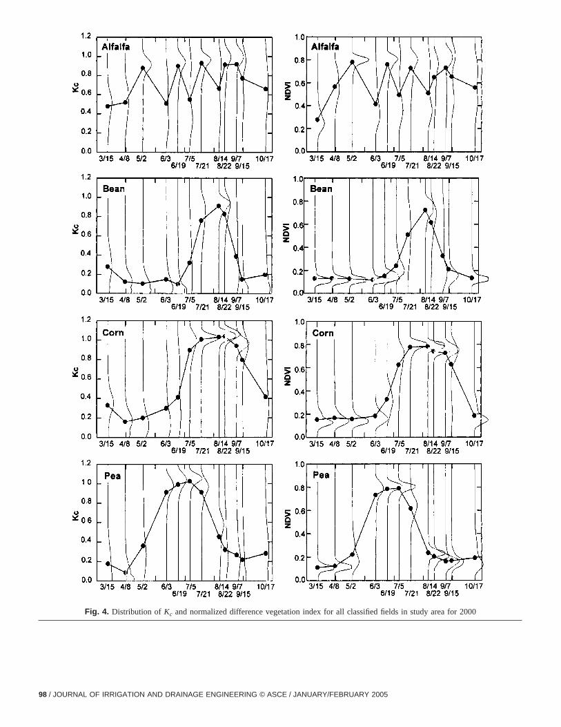
Fig. 4. Distribution of Kc and normalized difference vegetation index for all classified fields in study area for 2000

98 / JOURNAL OF IRRIGATION AND DRAINAGE ENGINEERING © ASCE / JANUARY/FEBRUARY 2005

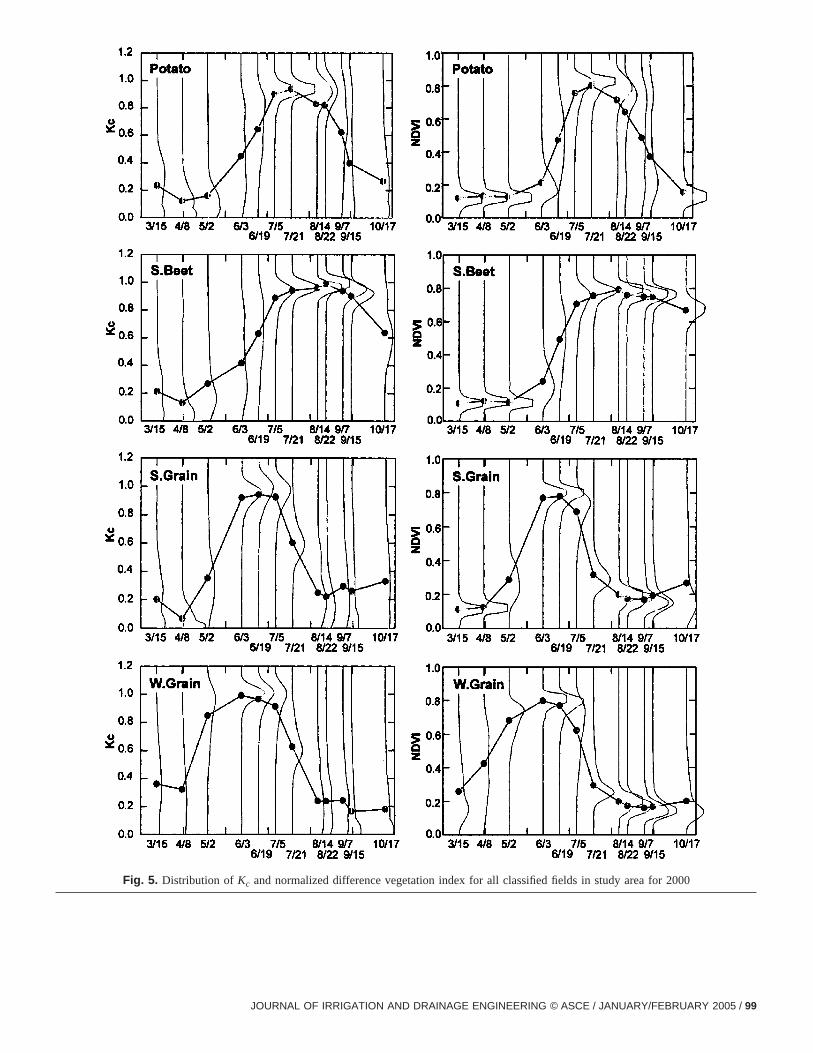
Fig. 5. Distribution of Kc and normalized difference vegetation index for all classified fields in study area for 2000

JOURNAL OF IRRIGATION AND DRAINAGE ENGINEERING © ASCE / JANUARY/FEBRUARY 2005 / 99

theothis

ed-and

s in

utand

entever-pota

inglas

theseyuite

s,odal

iffer-s andwith

prin-ight

thod

refer-e two

Bs,y these by

thetions

thatcom-ed toitions

tionsptableaynopy

Magic

2

same growing stage of a crop by eliminating differences inplanting schedule through shiftingKc curves from each field tmake the peaks of the NDVI curves for all fields the same. Instudy, the variance inKc caused by differences in planting schules was retained in order to capture the overall averagevariance for actual field management and cultural conditionthe study area.

Maximum values forKc for individual fields peaked at abo1.10 for alfalfa, corn, peas, spring grain, and winter grain,about 1.05 for beans, potatoes, and sugar beets(Figs. 4 and 5).Modal values forKc (defined as the value of the 0.01 incremhaving the highest occurrence) during periods of full cover werclose to 1.0 for alfalfa, spring grain, and winter grain, and aaged 1.04, 1.02, 0.95, 0.94, and 0.97 for corn, peas, bean,toes, and sugar beets(Table 3). These modal values, representthe most frequently occurring value, characterize the typicaKc

value for fields at full cover for the image dates when NDVI wat its maximum or near maximum value. Table 3 comparesmodal values with the maximumKc value recommended bWright (1981) for the same crops. The modal values are qsimilar to the peak values of Wright(1981) except for potatoewhere Wright’s value of 0.78 is much less than the average mvalue of 0.94. Some of this difference may be caused by dences in modern varieties of potatoes and planting densitiein impacts of differences between irrigation system types,

Table 1. Means and Standard Deviations of Crop CoefficientsKcd ValuesValley during 2000

StatisticsImagedate Alfalfa Bean

Mean 3/15/00 0.48 0.2

4/8/00 0.52 0.12

5/2/00 0.88 0.10

6/3/00 0.51 0.15

6/19/00 0.90 0.10

7/5/00 0.55 0.32

7/21/00 0.93 0.76

8/14/00 0.67 0.91

8/22/00 0.91 0.83

9/7/00 0.92 0.39

9/15/00 0.77 0.15

10/17/00 0.66 0.20

Standard deviation 3/15/00 0.15 0.

4/8/00 0.17 0.10

5/2/00 0.14 0.10

6/3/00 0.23 0.17

6/19/00 0.12 0.16

7/5/00 0.27 0.23

7/21/00 0.10 0.17

8/14/00 0.28 0.07

8/22/00 0.16 0.18

9/7/00 0.18 0.25

9/15/00 0.25 0.21

10/17/00 0.24 0.20

Number of classified fieldsa 325 432aClassified fields include only fields having size of 400 m by 400 m

center pivot irrigation being practiced on most potatoes in Magic

100 / JOURNAL OF IRRIGATION AND DRAINAGE ENGINEERING © ASCE

-

Valley during 2000 as compared to less frequent solid-set skler irrigation practiced during the measurements by Wr(1981). It is noted thatKc values derived by Wright(1981) werebased on the 1982 Kimberly Penman alfalfa reference me(Wright 1982) computed daily, whereas the EB model derivedKcswere based on the standardized Penman–Monteith alfalfaence method computed hourly. Small differences between thmethods have been evaluated and summarized by EWRI(2002).However, because the same ETr method was used in the Emodel calibration and to determineKcs from the sampled fieldtheKc values obtained from the EB model were not biased breference ET method and are thus directly comparable to thoWright (1981).

Some of the extremeKc values for individual fields(thosegreater than 1.05) were no doubt caused by estimation error ofEB model or may be due to differences in weather condiwithin the 120 by 70 km study area. The EB model assumesthe weather condition of entire study area is the same whenputing crop coefficients. This error range has been observchange with image size and thus variation in weather condof the study area. For the study area described here, theKc esti-mation error caused by the differences in weather condiacross the area is probably less than ±0.05, which is an accerange of error. Values forKc that fall in the range of 1.0–1.05 mrepresent fields that were recently irrigated so that the ca

ed by Satellite Based Energy Balance for 3,888 Classified Fields in

Corn Pea PotatoSugarbeet

Springgrain

Wintergrain

0.33 0.18 0.23 0.21 0.20 0.36

0.16 0.08 0.12 0.13 0.07 0.32

0.20 0.36 0.16 0.27 0.35 0.85

0.30 0.91 0.45 0.42 0.92 0.99

0.41 0.99 0.65 0.63 0.94 0.96

0.90 1.03 0.90 0.89 0.93 0.91

1.01 0.91 0.94 0.94 0.60 0.63

1.03 0.45 0.83 0.96 0.25 0.24

1.04 0.32 0.82 0.99 0.22 0.24

0.94 0.27 0.62 0.94 0.29 0.24

0.79 0.22 0.40 0.90 0.26 0.16

0.42 0.28 0.27 0.64 0.33 0.18

0.16 0.16 0.17 0.19 0.17 0.2

0.11 0.11 0.13 0.21 0.09 0.25

0.19 0.23 0.17 0.21 0.20 0.18

0.27 0.17 0.25 0.23 0.09 0.09

0.27 0.14 0.20 0.21 0.11 0.12

0.18 0.10 0.08 0.11 0.11 0.16

0.06 0.16 0.04 0.10 0.13 0.15

0.06 0.18 0.21 0.03 0.17 0.17

0.11 0.20 0.24 0.05 0.18 0.18

0.12 0.18 0.25 0.07 0.21 0.18

0.29 0.22 0.34 0.07 0.25 0.21

0.25 0.19 0.22 0.16 0.25 0.19

474 314 717 516 546 564

ger.

Deriv

8

17

or lar

surface is wet or where the canopy may have dried, but the soil

/ JANUARY/FEBRUARY 2005

ociallyness

reodalVI.peak

sd

ates,n toelf

thethan

mentoome

perty ofrredifica-trendTheela-egra-gs.

DVI

6

14

surface is very wet. Under these conditions, theKc is expected texceed 1.0 representing the alfalfa reference. This is espetrue for crops like corn that have larger aerodynamic roughthan alfalfa.

Peak values for the estimatedKc averaged over all fields aincluded in Table 3. These values are generally lower than mvalues due to impacts of some fields having relatively low NDAverages of the estimated peak values were greater thanvalues of Wright(1981) for three crops(corn, peas, and potatoe),essentially equal to Wright(1981) for two crops(sugar beets an

Table 2. Means and Standard Deviations of Normalized Difference

StatisticsImagedate Alfalfa Bean

Mean 3/15/00 0.28 0.13

4/8/00 0.57 0.13

5/2/00 0.78 0.13

6/3/00 0.41 0.12

6/19/00 0.76 0.15

7/5/00 0.49 0.24

7/21/00 0.73 0.51

8/14/00 0.51 0.72

8/22/00 0.65 0.62

9/7/00 0.73 0.33

9/15/00 0.65 0.21

10/17/00 0.56 0.14

Standard deviation 3/15/00 0.09 0.0

4/8/00 0.11 0.06

5/2/00 0.06 0.04

6/3/00 0.15 0.02

6/19/00 0.07 0.03

7/5/00 0.20 0.07

7/21/00 0.11 0.16

8/14/00 0.19 0.07

8/22/00 0.15 0.13

9/7/00 0.17 0.21

9/15/00 0.19 0.12

10/17/00 0.17 0.03

Number of classified fieldsa 325 432aClassified fields include only fields having size of 400 m by 400 m

Table 3. Modal and Peak Mean Values forKc Derived from SatelliteBased Evapotranspiration Maps and Peak MeanKc from Wright (1981)

Crop

Range in modalKc

from energy balance(EB) model duringperiod of effective

full cover

Peak meanKcfrom

EB modelPeak meanKc from

Wright (1981)

Alfalfa 0.95–1.02 n/aa 1.0

Bean 0.95 0.91 0.95

Corn 1.02–1.06 1.04 0.95

Pea 1.0–1.05 1.03 0.93

Potato 0.92–0.96 0.94 0.78

Sugar beet 0.95–1.0 0.99 1.0

Spring grain 0.98–1.0 0.94 1.0

Winter grain 0.98–1.02 0.99 1.0a
Not available.

winter grain), and lower than Wright(1981) for two crops(beansand spring grain). The lower average peakKc for spring grainmay have been partly caused by a wide range in planting dcausing individual fields to reach full cover and then begisenesce at different times. AlfalfaKc values from the EB modwere not compared with peak values of Wright(1981) because othe lowering of averageKc for all image dates, caused byoccurrence of some recently harvested fields being in lessfull cover condition on each image date. In general, agreebetween the estimated peakKc and Wright(1981) is considered tbe very good. The following sections are a discussion of sindividual crop types regarding Figs. 4 and 5.

AlfalfaPredominately, only alfalfa fields having four-cutting cyclesyear appear in Figs. 4 and 5, although a significant minorifields in Magic Valley are cut only three times. This bias occubecause of our use of training fields during crop type classtion having four cuttings. These fields represent the currentin alfalfa management and production in the Magic Valley.NDVI distribution shows that dates for the first cutting were rtively uniform in time among fields(Figs. 4 and 5), but becamless uniform by the third and fourth cuttings, due to the intetion of differences in field management and timings of cuttin

Corn and Sugar BeetsCorn and sugar beet fields exhibited relatively consistent N

ation Index for 3,888 Classified Fields in Magic Valley during 2000

Corn Pea PotatoSugarbeet

Springgrain

Wintergrain

0.15 0.11 0.12 0.11 0.11 0.2

0.17 0.12 0.13 0.12 0.12 0.42

0.16 0.22 0.13 0.11 0.29 0.68

0.18 0.73 0.21 0.24 0.77 0.80

0.33 0.79 0.47 0.49 0.78 0.77

0.62 0.79 0.76 0.71 0.69 0.62

0.78 0.62 0.80 0.75 0.32 0.30

0.78 0.24 0.72 0.79 0.20 0.20

0.74 0.21 0.64 0.76 0.18 0.17

0.72 0.16 0.49 0.75 0.17 0.16

0.63 0.17 0.37 0.75 0.19 0.17

0.18 0.19 0.16 0.67 0.27 0.20

0.06 0.04 0.05 0.03 0.04 0.

0.07 0.04 0.05 0.02 0.03 0.17

0.05 0.09 0.03 0.03 0.10 0.08

0.09 0.13 0.08 0.09 0.06 0.03

0.11 0.07 0.15 0.14 0.05 0.05

0.13 0.04 0.10 0.09 0.09 0.14

0.06 0.09 0.05 0.08 0.08 0.09

0.04 0.04 0.18 0.03 0.04 0.04

0.07 0.04 0.19 0.03 0.04 0.04

0.12 0.05 0.22 0.05 0.06 0.05

0.21 0.05 0.22 0.05 0.09 0.06

0.07 0.09 0.10 0.05 0.19 0.11

474 314 717 516 546 564

ger.

Veget

6

or lar

distributions. A relatively large variation during the crop develop-


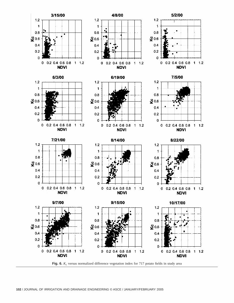
Fig. 6. Kc versus normalized difference vegetation index for 717 potato fields in study area


dualst

ersn inh ofOcto-

f veg-allrow-frost

ribu-ed

iod.tingstan-are

latefer-

est-ber

estab-

ale

sal”ation

ear

e towere

lues

ois-andayirri-

iodvingri-ortu-e ofeldsends

here

aws, forbothtri-

d asn-

soil

f ETor awe ETrageTheges

ing periods reflects differences in crop growth among indivifields. A very large variation inKc was exhibited during the laimage date October 17. By this date, it is likely that some farmhad already terminated irrigation, causing some reductioevaporation from soil, while others had not. In addition, mucthe corn crop appears to have been harvested for silage byber 17, according to the NDVI. Therefore the wide range inKc

reflects variation in soil wetness or the presence/absence oetation. The relatively high NDVI on October 17 for nearlysugar beet fields indicates that the crops were still actively ging, but with a reduced rate of transpiration, possibly due toor temperature effects on the stomatal opening.

Potato and GrainsPotato and grain fields had relatively wide and skewed disttions ofKc during the full cover period, while other crops showrelatively normal and symmetrical distributions for the perThis may have been caused by wider variation in the planschedules for these crops, or the effect of two or more subtially different crop varieties. Potato crops in Magic Valleycharacteristically split between early harvested varieties andharvested varieties. Also potato growth is greatly affected bytility and physical property of the soil. The wide range in harving is reflected in the wide range in NDVI during the Septemimage dates.

Relationship between K c and Normalized DifferenceVegetation Index

Several studies and applications of remote sensing havelished relationships betweenKc and NDVI for purposes of mapping spatial variability inKc (Neale et al. 1989; Bausch and Ne1989; Bausch 1993, 1995; Choudhury et al. 1994). Most of thesestudies predicted primarily the transpiration coefficient or “baKc, because vegetation indices are little impacted by evaporfrom soil. Fig. 6 shows a series of relationships betweenKc fromthe EB model and NDVI for potato fields throughout the y2000. As discussed previously in Figs. 4 and 5,Kc and NDVI

Fig. 7. Crop coefficient versus normalized difference vegetationarea of Idaho, for three Landsat dates in crop developing perio

have a clear relation during mid season, but, as expected, no clea


-

relation holds during periods having low ground cover dularge ranges in the soil evaporation component. Potato fieldsin a bare soil condition on March 15, and therefore NDVI vawere below 0.2 for most fields. However, theKc values variedfrom 0 to over 0.6 according to the level of residual surface mture from winter, which is impacted by the previous croptillage history. The same impact is shown for the April and Mimages and for June 3, where effects of pre- or postplantinggation created a substantial range inKc.

The NDVI andKc show a strong relationship during the perfrom June 19 to September 15. During this period, fields hahigh NDVI values also had highKc, because of the frequent irgation coupled with high transpiration rates and reduced oppnity for evaporation from soil. On September 15, a wide rangKc occurred in the fields having lower NDVI, because these fiwere likely harvested and therefore ET from such fields deponly on residual surface moisture. Finally, in the fall(October17), most fields returned to a bare soil condition, although twas still a large variation inKc.

The limitation ofKc estimation by NDVI is more clear whenseries ofKc versus NDVI relationships are overlaid. Fig. 7 shoKc versus NDVI relationships for potato and sugar beet fieldsthree satellite dates during the crop development period. Forcrops, theKc versus NDVI relationship appears as a similarangular shaped cloud of points, with the minimumKc increasingas NDVI increases. The bottom line of the triangle is indicatea “basalKc” in Fig. 7, and explains the contribution of crop traspiration in the totalKc. Any point above the “basalKc” linereflects some contribution of soil evaporation, where theevaporation portion is independent of NDVI.

From these analysis results, it is clear that the estimation ofor specific fields using a general crop coefficient curveNDVI-basedKc value is difficult, especially during periods of lovegetation cover. During these periods, an energy balancestimation model is a useful tool both for estimating the aveET of an area, and for estimating ET from individual fields.Kc distributions during mid-season typically had smaller ran

for 717 potato fields(left) and 516 sugar beet fields(right) in Magic Valleyring 2000

indexds du

rwith a more normal type of distribution. Therefore, estimating ET


id-ge

e ET.1

id-he

,lil

otirri-

edf

the

havevalu-asin

Rec-

rves

s withstart-rmed

l datathreead-ts by

ith, and

mix-k0.15llen,ivedpswayratherThed pes of

plant

gree-weeneded bybyy Ag-

gicoten--gion.

ed

f Ag-iMetjust-st ofthate tode tomaya fortnt to

s bycep-

anded to

ad-ey

gh agrainnot

mentad-

di-Met

nurset of

g set

per-ear-ctualgrow

sugar.e ad-s didB

andopri-

d toom-ore

urves

from traditional “mean”Kc curves is relatively easier during mseason periods if applied general curves describe the averaKc

for the area of interest. However, if one desires to estimatfrom individual fields using meanKc curves, a range of ±0variation in Kc values appears to exist even during the mseason. Therefore, even if theKc curve perfectly describes taverage values for the area of interest, a ±0.1 error inKc is inevi-table. The error range in predictedKc would reduce significantlyespecially during periods of low vegetation cover, if a duaKc

procedure that predicts the increase inKc caused by a wet sosurface layer were utilized, for example those by Wright(1982)or Allen et al.(1998, 2005). These types ofKc estimates were nevaluated during this study due to the lack of knowledge ofgation dates for individual fields.

Comparison of Mean K c Curves from Energy BalanceModel with Traditional K c Curves

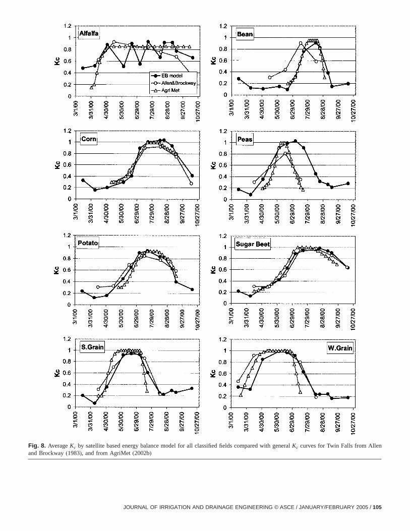
Averages of theKc derived by the EB model for all classififields are shown in Fig. 8 along with the generalKc curves oAllen and Brockway(1983) and AgriMet for year 2000(AgriMet2002b). The Allen and Brockway curves were developed forMagic Valley area usingKc tables of Wright(1981), and havebeen expressed in terms of monthly averages. The curvesbeen used by the Idaho Department of Water Resources for eating water rights transfers and for planning studies and bwide water balances. AgriMet curves by the U.S. Bureau oflamation(AgriMet 2002b) are a source of near-real timeKc andET information frequently applied in this region. The basic cufor AgriMet are based on Wright(1981, 1995) and are typicallyadjusted each year using cropping dates based on surveyUniversity extension services and other contacts. Once theing dates are determined for each crop, two other dates tecover date and terminate date are estimated using historicaand the basic curves are adjusted, timewise, based on the“key” dates. The initially determined curves are occasionallyjusted during the cropping season by AgriMet based on reporfield experts(AgriMet 2002a).

The Allen and Brockway curves agreed relatively well wthe EB-determined curves for sugar beet and grain cropsagreed fairly well with those for alfalfa, where theKc curve byAllen and Brockway was an averaged curve representing ature of cutting practices, and for potatoes, although the peaKc

for potatoes derived from the EB model averaged abouthigher than that by Allen and Brockway. The curves from Aand Brockway did not agree well for the three other crops(beanscorn, and peas). The good agreement between the satellite derand Allen and BrockwayKc curves for three to five of eight crois surprising when one considers that the Allen and Brockcurves represent long term averages developed in 1983than specific curves for 2000 as derived from the EB model.reasons for disagreement between curves for bean, corn, anfields are unknown, but it is possible that the popular varietiecrops or field management, including planting dates andspacing, might have changed since 1983.

The AgriMetKc curves agreed well with the ET-determinedKc

curves for alfalfa, bean, corn, potato, and sugar beet crops. Ament was poor for pea and grain fields. Most differences betestimated and AgriMet generalKc curves may have been causby nonrepresentative emergence and termination dates usAgriMet for the particular crops in the Magic Valley area, andmore rapid growth rates and senescence rates predicted b
riMet for peas and grain. In all situations, average peakKc values

,

a

by the EB model were equal to or greater than peakKc values byAgriMet and Allen and Brockway, indicating that sampled MaValley fields did not suffer reduced ET as compared to the ptial ET defined by the Wright(1981, 1995) Kc curves. This indicates good crop and water management practices in the re

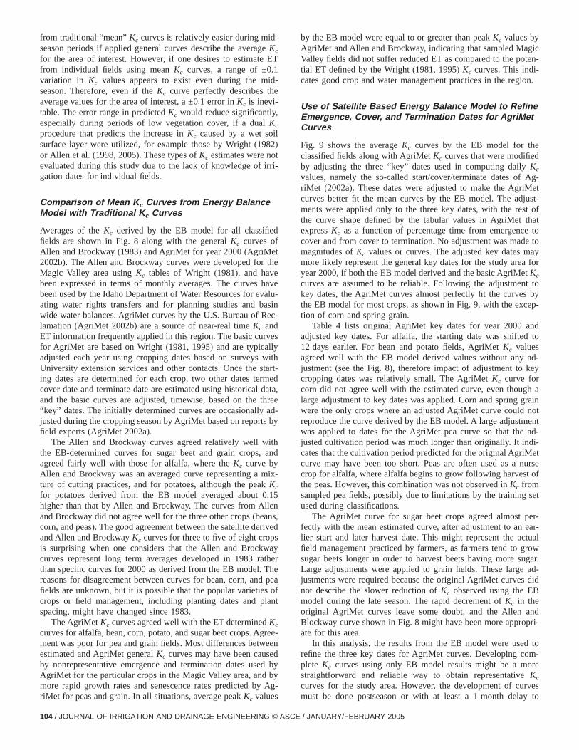
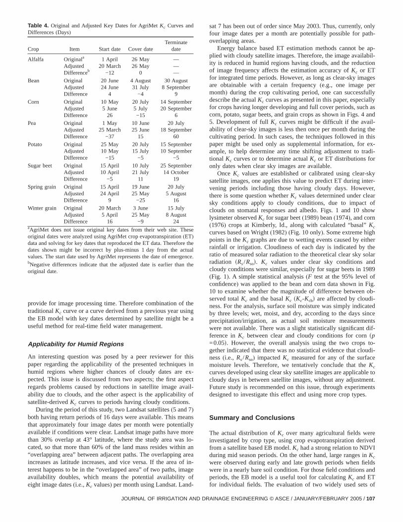
Use of Satellite Based Energy Balance Model to RefineEmergence, Cover, and Termination Dates for AgriMetCurves

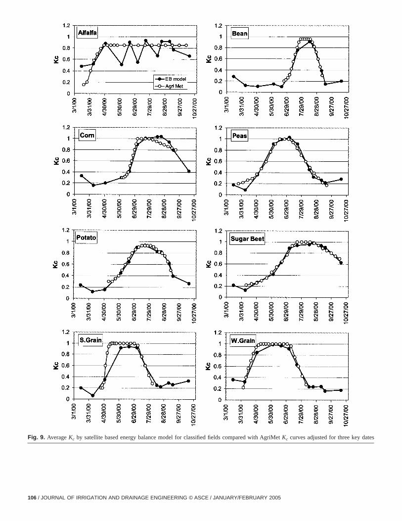
Fig. 9 shows the averageKc curves by the EB model for thclassified fields along with AgriMetKc curves that were modifieby adjusting the three “key” dates used in computing dailyKc

values, namely the so-called start/cover/terminate dates oriMet (2002a). These dates were adjusted to make the Agrcurves better fit the mean curves by the EB model. The adments were applied only to the three key dates, with the rethe curve shape defined by the tabular values in AgriMetexpressKc as a function of percentage time from emergenccover and from cover to termination. No adjustment was mamagnitudes ofKc values or curves. The adjusted key datesmore likely represent the general key dates for the study areyear 2000, if both the EB model derived and the basic AgriMeKc

curves are assumed to be reliable. Following the adjustmekey dates, the AgriMet curves almost perfectly fit the curvethe EB model for most crops, as shown in Fig. 9, with the extion of corn and spring grain.

Table 4 lists original AgriMet key dates for year 2000adjusted key dates. For alfalfa, the starting date was shift12 days earlier. For bean and potato fields, AgriMetKc valuesagreed well with the EB model derived values without anyjustment(see the Fig. 8), therefore impact of adjustment to kcropping dates was relatively small. The AgriMetKc curve forcorn did not agree well with the estimated curve, even thoularge adjustment to key dates was applied. Corn and springwere the only crops where an adjusted AgriMet curve couldreproduce the curve derived by the EB model. A large adjustwas applied to dates for the AgriMet pea curve so that thejusted cultivation period was much longer than originally. It incates that the cultivation period predicted for the original Agricurve may have been too short. Peas are often used as acrop for alfalfa, where alfalfa begins to grow following harvesthe peas. However, this combination was not observed inKc fromsampled pea fields, possibly due to limitations by the traininused during classifications.

The AgriMet curve for sugar beet crops agreed almostfectly with the mean estimated curve, after adjustment to anlier start and later harvest date. This might represent the afield management practiced by farmers, as farmers tend tosugar beets longer in order to harvest beets having moreLarge adjustments were applied to grain fields. These largjustments were required because the original AgriMet curvenot describe the slower reduction ofKc observed using the Emodel during the late season. The rapid decrement ofKc in theoriginal AgriMet curves leave some doubt, and the AllenBlockway curve shown in Fig. 8 might have been more apprate for this area.

In this analysis, the results from the EB model were userefine the three key dates for AgriMet curves. Developing cplete Kc curves using only EB model results might be a mstraightforward and reliable way to obtain representativeKc

curves for the study area. However, the development of c
must be done postseason or with at least a 1 month delay to

n
Fig. 8. AverageKc by satellite based energy balance model for all classified fields compared with generalKc curves for Twin Falls from Alleand Brockway(1983), and from AgriMet(2002b)
JOURNAL OF IRRIGATION AND DRAINAGE ENGINEERING © ASCE / JANUARY/FEBRUARY 2005 / 105

tes
Fig. 9. AverageKc by satellite based energy balance model for classified fields compared with AgriMetKc curves adjusted for three key da

f theing

be a

thises in

ex-spec

avail-ty ofs.

eanstiallymores lo-in anareaof in-

mageof

onlypath-

e ap-abil-ction

ageserfullyiallyh as4 andl-g the

thisr ex-radi-r

r-skynter-ver,ar

t ofshow

hitherthesolarnd989fFig.

n ob-i-catedsinceentsdif-

to-loudi-ceeble toent.ents

s.

rerivedIin

fieldsand

rr

r

rr

r

hese

re thectualgence

n the

provide for image processing time. Therefore combination otraditionalKc curve or a curve derived from a previous year usthe EB model with key dates determined by satellite mightuseful method for real-time field water management.

Applicability for Humid Regions

An interesting question was posed by a peer reviewer forpaper regarding the applicability of the presented techniquhumid regions where higher chances of cloudy dates arepected. This issue is discussed from two aspects; the first aregards problems caused by reductions in satellite imageability due to clouds, and the other aspect is the applicabilisatellite-derivedKc curves to periods having cloudy condition

During the period of this study, two Landsat satellites(5 and 7)both having return periods of 16 days were available. This mthat approximately four image dates per month were potenavailable if conditions were clear. Landsat image paths havethan 30% overlap at 43° latitude, where the study area wacated, so that more than 60% of the land mass resides with“overlapping area” between adjacent paths. The overlappingincreases as latitude increases, and vice versa. If the areaterest happens to be in the “overlapped area” of two paths, iavailability doubles, which means the potential availability

Table 4. Original and Adjusted Key Dates for AgriMetKc Curves andDifferences(Days)

Crop Item Start date Cover dateTerminate

date

Alfalfa Originala

AdjustedDifferenceb

1 April20 March

−12

26 May26 May

0

———

Bean OriginalAdjustedDifference

20 June24 June

4

4 August31 July

−4

30 August8 September

9

Corn OriginalAdjustedDifference

10 May5 June

26

20 July5 July−15

14 Septembe20 Septembe

6

Pea OriginalAdjustedDifference

1 May25 March

−37

10 June25 June

15

20 July18 Septembe

60

Potato OriginalAdjustedDifference

25 May10 May

−15

20 July15 July

−5

15 Septembe10 Septembe

−5

Sugar beet OriginalAdjustedDifference

15 April10 April

−5

10 July21 July

11

25 Septembe14 October

19

Spring grain OriginalAdjustedDifference

15 April24 April

9

19 June25 May

−25

20 July5 August

16

Winter grain OriginalAdjustedDifference

20 March5 April

16

3 June25 May

−9

15 July8 August

24aAgriMet does not issue original key dates from their web site. Toriginal dates were analyzed using AgriMet crop evapotranspiration(ET)data and solving for key dates that reproduced the ET data. Therefodates shown might be incorrect by plus-minus 1 day from the avalues. The start date used by AgriMet represents the date of emerbNegative differences indicate that the adjusted date is earlier thaoriginal date.

eight image dates(i.e.,Kc values) per month using Landsat. Land-


t

sat 7 has been out of order since May 2003. Thus, currently,four image dates per a month are potentially possible foroverlapping areas.

Energy balance based ET estimation methods cannot bplied with cloudy satellite images. Therefore, the image availity is reduced in humid regions having clouds, and the reduof image frequency affects the estimation accuracy ofKc or ETfor integrated time periods. However, as long as clear-sky imare obtainable with a certain frequency(e.g., one image pmonth) during the crop cultivating period, one can successdescribe the actualKc curves as presented in this paper, especfor crops having longer developing and full cover periods, succorn, potato, sugar beets, and grain crops as shown in Figs.5. Development of fullKc curves might be difficult if the avaiability of clear-sky images is less then once per month durincultivating period. In such cases, the techniques followed inpaper might be used only as supplemental information, foample, to help determine any time shifting adjustment to ttional Kc curves or to determine actualKc or ET distributions foonly dates when clear sky images are available.

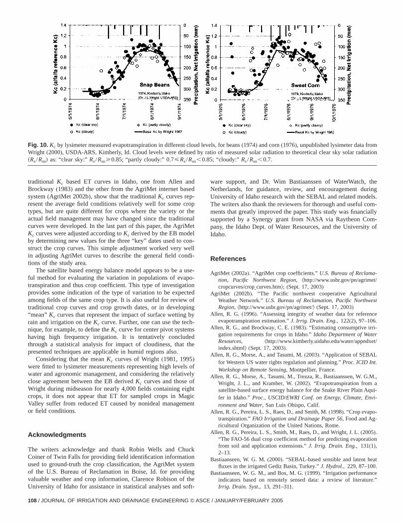
OnceKc values are established or calibrated using cleasatellite images, one applies this value to predict ET during ivening periods including those having cloudy days. Howethere is some question whetherKc values determined under clesky conditions apply to cloudy conditions, due to impacclouds on stomatal responses and albedo. Figs. 1 and 10lysimeter observedKc for sugar beet(1989) bean(1974), and corn(1976) crops at Kimberly, Id., along with calculated “basal”Kc

curves based on Wright(1982) (Fig. 10 only). Some extreme higpoints in theKc graphs are due to wetting events caused by erainfall or irrigation. Cloudiness of each day is indicated byratio of measured solar radiation to the theoretical clear skyradiation sRs/Rsod. Kc values under clear sky conditions acloudy conditions were similar, especially for sugar beets in 1(Fig. 1). A simple statistical analysis(F test at the 95% level oconfidence) was applied to the bean and corn data shown in10 to examine whether the magnitude of difference betweeserved totalKc and the basalKc sKc-Kcbd are affected by cloudness. For the analysis, surface soil moisture was simply indiby three levels; wet, moist, and dry, according to the daysprecipitation/irrigation, as actual soil moisture measuremwere not available. There was a slight statistically significantference inKc between clear and cloudy conditions for cornsp=0.05d. However, the overall analysis using the two cropsgether indicated that there was no statistical evidence that cness(i.e., Rs/Rso) impactedKc measured for any of the surfamoisture levels. Therefore, we tentatively conclude that thKc

curves developed using clear sky satellite images are applicacloudy days in between satellite images, without any adjustmFuture study is recommended on this issue, through experimdesigned to investigate this effect and using more crop type

Summary and Conclusions

The actual distribution ofKc over many agricultural fields weinvestigated by crop type, using crop evapotranspiration defrom a satellite based EB model.Kc had a strong relation to NDVduring mid season periods. On the other hand, large rangesKc

were observed during early and late growth periods whenwere in a nearly bare soil condition. For those field conditionsperiods, the EB model is a useful tool for calculatingKc and ET

.

for individual fields. The evaluation of two widely used sets of


nded

-cropthe

itionaliMetlcon-wellndi-

a usepo-tionctedw ofpingg bych-sed

t the

els oftivelyofightagicment

uckntemingf the

, theuringels.

com-ciallyom-ity of

a-t/

ralest

nce.i-ret/

.M.,aAqui-vi-

--

tion

eat.eture.”

mradiation

traditional Kc based ET curves in Idaho, one from Allen aBrockway (1983) and the other from the AgriMet internet bassystem(AgriMet 2002b), show that the traditionalKc curves represent the average field conditions relatively well for sometypes, but are quite different for crops where the variety oractual field management may have changed since the tradcurves were developed. In the last part of this paper, the AgrKc curves were adjusted according toKc derived by the EB modeby determining new values for the three “key” dates used tostruct the crop curves. This simple adjustment worked veryin adjusting AgriMet curves to describe the general field cotions of the study area.

The satellite based energy balance model appears to beful method for evaluating the variation in populations of evatranspiration and thus crop coefficient. This type of investigaprovides some indication of the type of variation to be expeamong fields of the same crop type. It is also useful for revietraditional crop curves and crop growth dates, or in develo“mean” Kc curves that represent the impact of surface wettinrain and irrigation on theKc curve. Further, one can use the tenique, for example, to define theKc curve for center pivot systemhaving high frequency irrigation. It is tentatively concludthrough a statistical analysis for impact of cloudiness, thapresented techniques are applicable in humid regions also.

Considering that the meanKc curves of Wright(1981, 1995)were fitted to lysimeter measurements representing high levwater and agronomic management, and considering the relaclose agreement between the EB derivedKc curves and thoseWright during midseason for nearly 4,000 fields containing ecrops, it does not appear that ET for sampled crops in MValley suffer from reduced ET caused by nonideal manageor field conditions.

Acknowledgments

The writers acknowledge and thank Robin Wells and ChCoiner of Twin Falls for providing field identification informatioused to ground-truth the crop classification, the AgriMet sysof the U.S. Bureau of Reclamation in Boise, Id. for providvaluable weather and crop information, Clarence Robison o

Fig. 10. Kc by lysimeter measured evapotranspiration in differentWright (2000), USDA-ARS, Kimberly, Id. Cloud levels were definsRs/Rsod as: “clear sky:”Rs/Rsoù0.85; “partly cloudy:” 0.7øRs/Rso

University of Idaho for assistance in statistical analyses and soft-


-

ware support, and Dr. Wim Bastiaanssen of WaterWatchNetherlands, for guidance, review, and encouragement dUniversity of Idaho research with the SEBAL and related modThe writers also thank the reviewers for thorough and usefulments that greatly improved the paper. This study was finansupported by a Synergy grant from NASA via Raytheon Cpany, the Idaho Dept. of Water Resources, and the UniversIdaho.

References

AgriMet (2002a). “AgriMet crop coefficients.”U.S. Bureau of Reclamtion, Pacific Northwest Region, ^http://www.usbr.gov/pn/agrimecropcurves/cropIcurves.htm&; (Sept. 17, 2003)

AgriMet (2002b). “The Pacific northwest cooperative AgricultuWeather Network.”U.S. Bureau of Reclamation, Pacific NorthwRegion, ^http://www.usbr.gov/pn/agrimet/& (Sept. 17, 2003)

Allen, R. G. (1996). “Assessing integrity of weather data for refereevapotranspiration estimation.”J. Irrig. Drain. Eng., 122(2), 97–106

Allen, R. G., and Brockway, C. E.(1983). “Estimating consumptive irrgation requirements for crops in Idaho.”Idaho Department of WateResources, ^http://www.kimberly.uidaho.edu/water/appndxindex.shtml& (Sept. 17, 2003).

Allen, R. G., Morse, A., and Tasumi, M.(2003). “Application of SEBALfor Western US water rights regulation and planning.”Proc. ICID Int.Workshop on Remote Sensing, Montpellier, France.

Allen, R. G., Morse, A., Tasumi, M., Trezza, R., Bastiaanssen, W. GWright, J. L., and Kramber, W.(2002). “Evapotranspiration fromsatellite-based surface energy balance for the Snake River Plainfer in Idaho.” Proc., USCID/EWRI Conf. on Energy, Climate, Enronment and Water, San Luis Obispo, Calif.

Allen, R. G., Pereira, L. S., Raes, D., and Smith, M.(1998). “Crop evapotranspiration.”FAO Irrigation and Drainage Paper 56, Food and Agricultural Organization of the United Nations, Rome.

Allen, R. G., Pereira, L. S., Smith, M., Raes, D., and Wright, J. L.(2005).“The FAO-56 dual crop coefficient method for predicting evaporafrom soil and application extensions.”J. Irrig. Drain. Eng., 131(1),2–13.

Bastiaanseen, W. G. M.(2000). “SEBAL-based sensible and latent hfluxes in the irrigated Gediz Basin, Turkey.”J. Hydrol., 229, 87–100

Bastiaanseen, W. G. M., and Bos, M. G.(1999). “Irrigation performancindicators based on remotely sensed data: a review of litera

levels, for beans(1974) and corn(1976), unpublished lysimeter data froratio of measured solar radiation to theoretical clear sky solar

5; “cloudy:” Rs/Rso,0.7.

clouded by,0.8

Irrig. Drain. Syst., 13, 291–311.


A. A.for

, G.,to

ions.”

, J.,r-

crop

v-

e

andte,

ugh-andi-

i-

rdiza-

qua-,

large

. A.th a

terk.

d

r

er, P.bin-data.”

andr

rough

e ofahoo.

forte

-ation-

ual-rors.”

nstion.”

os,

n,

o

ey,

po-. of

aho,

sat-

en-tion,

po-va-

ns-n-.

roponand

Bastiaanssen, W. G. M., Menenti, M., Feddes, R. A., and Holtslag,M. (1998a). “A remote sensing surface energy balance algorithmland (SEBAL): 1. Formulation.”J. Hydrol., 212–213, 198–212.

Bastiaanssen, W. G. M., Noordman, E. J. M., Pelgrum, H., Davidsand Allen, R. G.(2005). “SEBAL model with remotely sensed dataimprove water-resources management under actual field conditJ. Irrig. Drain. Eng., 131(1), 85–93.

Bastiaanssen, W. G. M., Pelgrum, H., Wang, J., Ma, Y., MorenoRoerink, G. J., and van der Wal, T.(1998b). “A remote sensing suface energy balance algorithm for land(SEBAL): 2. validation.” J.Hydrol., 212–213, 213–229.

Bausch, W. C.(1993). “Soil background effects on reflectance-basedcoefficients for corn.”Remote Sens. Environ., 46, 213–222.

Bausch, W. C.(1995). “Remote sensing of crop coefficients for improing the irrigation scheduling of corn.”Agric. Water Manage., 27,55–68.

Bausch, W. C., and Neale, C. M. U.(1989). “Spectral inputs improvcorn crop coefficients and irrigation scheduling.”Trans. ASAE, 32(6),1901–1908.

Caselles, V., Artigao, M. M., Hurtado, E., Coll, C., and Brasa, A.(1998).“Mapping actual evapotranspiration by combining Landsat TMNOAA-AVHRR images: Application to the Barrax area, AlbaceSpain.”Remote Sens. Environ., 63, 1–10.

Choudhury, B. J., Ahmed, N. U., Idso, S. B., Reginato, R. J., and Datry, C. S. T.(1994). “Relations between evaporation coefficientsvegetation indices studies by model simulations.”Remote Sens. Envron., 50, 1–17.

Doorenbos, J., and Pruitt, W. O.(1977). “Crop water requirements.”Ir-rigation and Drainage Paper No. 24, Food and Agricultural Organzation of the United Nations, Rome.

Environmental and Water Resources Institute of the ASCE Standation of Reference Evapotranspiration Task Committee(EWRI).(2002). “The ASCE standardized reference evapotranspiration etion.” ^http://www.kimberly.uidaho.edu/water/asceewri/& (Sept. 172003)

Hemakumara, H. M., Chandrapala, L., and Moene, A. F.(2003). “Evapo-transpiration fluxes over mixed vegetation areas measured fromaperture scintillometer.”Agric. Water Manage., 58, 109–122.

Hunsaker, D. J., Pinter, P. J., Jr., Barnes, E. M., and Kimball, B(2003). “Estimating cotton evapotranspiration crop coefficients wimultispectral vegetation index.”Irrig. Sci., 22(2), 95–104.

Jensen, M. E., ed.(1973). “Consumptive use of water and irrigation warequirements.” Irrigation and Drainage Division, ASCE, New Yor

Jensen, M. E., Burman, R. D., and Allen, R. G.,(ed.). (1990). “Evapo-transpiration and Irrigation water requirements.”ASCE Manual anReportNo. 70, ASCE, New York.

Kustas, W. P., and Norman, J. M.(1996). “Use of remote sensing foevapotranspiration monitoring over land surfaces.”Hydrol. Sci. J.,41(4), 495–516.

Moran, M. S., Jackson, R. D., Raymond, L. H., Gay, L. W., and SlatN. (1989). “Mapping surface energy balance components by coming Landsat thematic mapper and ground-based meteorologicalRemote Sens. Environ., 30, 77–87.

Morse, A., Allen, R. G., Tasumi, M., Kramber, W. J., Trezza, R.,Wright, J. L. (2001). “Application of the SEBAL methodology foestimating evapotranspiration and consumptive use of water thremote sensing.” Idaho Department of Water Resources, Idaho.

Morse, A., Tasumi, M., Allen, R. G., and Kramber, W. J.(2000). “Appli-


cation of the SEBAL methodology for estimating consumptive uswater and streamflow depletion in the Bear River Basin of Idthrough remote sensing.” Idaho Dept. of Water Resources, Idah

Neale, C. M. U., Bausch, W. C., and Heerman, D. F.(1989). “Develop-ment of reflectance-based crop coefficients for corn.”Trans. ASAE,32(6): 1891–1899.

Nishida, K., Nemani, R. R., Glassy, J. M., and Running, S. W.(2003).“Development of an evapotranspiration index from Aqua/MODISmonitoring surface moisture status.”IEEE Trans. Geosci. RemoSens., GE-41(2), 493–501.

Norman, J. M., Kustas, W. P., and Humes, K. S.(1995). “Source approach for estimating soil and vegetation energy fluxes in observof directional radiometric surface temperature.”Agric. Forest Meteorol., 77, 263–293.

Norman, J. M., Kustas, W. P., Prueger, J. H., and Diak, G. R.(2000).“Surface flux estimation using radiometric temperature: A dtemperature-difference method to minimize measurement erWater Resour. Res., 36(8), 2263–2274.

Romero, M. G.,(2003). “Daily evapotranspiration estimation by meaof evaporative fraction and reference evapotranspiration fracPhD dissertation, Utah State Univ., Logan, Utah.

Snyder, R. L., Lanini, B. J., Shaw, D. A., and Pruitt., W. O.(1989a).“Using reference evapotranspiration(ETo) and crop coefficients testimate crop evapotranspiration(ETc) for agronomic crops, grasseand vegetable crops.”Leaflet No. 21427, Cooperative ExtensioUniv. of California, Berkeley, Calif.

Snyder, R. L., Lanini, B. J., Shaw, D. A., and Pruitt, W. O.(1989b).“Using reference evapotranspiration(ETo) and crop coefficients testimate crop evapotranspiration(ETc) for trees and vines.”LeafletNo. 21428, Cooperative Extension, Univ. of California, BerkelCalif.

Tasumi, M.(2003). “Progress in operational estimation of regional evatranspiration using satellite imagery.” PhD dissertation, UnivIdaho, Moscow, Idaho.

Tasumi, M., Allen, R. G., and Bastiaanssen, W. G. M.(2000). “Thetheoretical basis of SEBAL.” Idaho Dept. of Water Resources, Id46–69.

Tasumi, M., Trezza, R., Allen, R. G., and Wright, J. L.(2003). “USvalidation tests on the SEBAL model for evapotranspiration viaellite.” Proc., ICID Int. Workshop on Remote Sensing, Montpellier,France.

Trezza, R.(2002). “Evapotranspiration using a satellite-based surfaceergy balance with standardized ground control.” PhD dissertaUtah State Univ., Logan, Utah.

Wright, J. L.(1981). “Crop coefficients for estimates of daily crop evatranspiration.”Irrigation scheduling for water and energy consertion in the 80s, ASAE, Dec. St. Joseph, Mich.

Wright, J. L.(1982). “New evapotranspiration crop coefficients.”J. Irrig.Drain. Div., 108(1), 57–74.

Wright, J. L. (1991). “Using weighing lysimeters to develop evapotrapiration crop coefficients.”Lysimeters for evapotranspiration and evironmental measurements, R. G. Allen, T. A. Howell, W. O. Pruitt, IA. Walter, and M. E. Jensen, eds., ASCE, New York, 191–199.

Wright, J. L. (1995). “Calibrating an ET procedure and deriving ET ccoefficients.” Proc., Seminar on Evapotranspiration and IrrigatiEfficiency, American Consulting Engineers Council of ColoradoColorado Division of Water Resources, Arvada, Colo.


Satellite-Based Energy Balance to Assess Within-Population Variance of Crop Coefficient Curves

Documents

Transcript of Satellite-Based Energy Balance to Assess Within-Population Variance of Crop Coefficient Curves