STANDARD STATE FUGACITY COEFFICIENT - ShareOK

STANDARD STATE FUGACITY COEFFICIENT~ FOR THE HYPOTHETICAL VAPOR

BY BRIDGING FROM THE REAL GAS FUGACITY COEFFICIENTS

THROUGH THE GIBBS-DUHEM EQUATION

By

Arthur Dale Godfrey //

Bachelor of Science

The University of Nebraska

Lincoln, Nebraska

1943

Submitted to the Faculty of the Graduate School of the Oklahoma. State University of Agriculture and

Applied Science in partial fulfillment of the requirements for the degree

of MASTER OF SCIENCE August, 1964

OKLAHOMA ITATE UNIVERSIT(

LIBRARY

JAN 5 1965

. . ' ~~~

STANuARD STAT!!.: FUGACITY COEFFICIENTS Fo:a. THE HYPOTHETICAL -----·-

VAPO.R BY BRIDGING FROM 'I'HE HEAL GAS FUGACITY COEFFICIENTS

Tl1ROUGH THE GIBBS-DUHEM EQUATION

Thesis Approved:

~c!··~ ~ ~is Lctviser .

Dean of the Graduate School

561!564

PREFACE

A generalized method for determining the standard state fugacity

coefficients for hypothetical vapors was developed by bridging from

·the fugacity coefficient of the real gaseous component to that of

the hypothetical gaseous component through the Gibbs-Duhem equation.

Binary systems of hydrogen sulfide with methane, ethane, propane and

n-pentane selected from the literature formed the basis for the

correlation.

The application of this method for the development of a similar

correlation for the standard state fugacity coefficients of hypo

thetical liquids is outlined.

I sincerely appreciate the aid of Professor W. C. Edmister in

suggesting the topic of this thesis and in guiding it to its com

pletion. I am also grateful to Professor.Edmister for arranging his

schedule to the convenience of the author as a "drive in 11 student.

I am greatly indebted to Mr. A. N. Stuckey, Jr. for his

suggestions and aid toward the completion of this work, particularly

his work in calculating the fugacity coefficients on the IIM-650

digital computer.

I wish particularly to express my gratitude to my wife, Maxine,

whose encouragement and patience provided the incentive to pursue this

work to its completion.

iii

TABLE OF CONTENTS

Chapter Page

I. IN"TRODUCTION • ••.••••••• ~ ••••••••••••••••••••••••••••••••••• 1

Purpose o·f This Work................................... 6

II. DEVELOPMENT OF EQUATIONS ••••••••••••••••••••••••••• ~ • • • • • • • 8

Chemical Potential............................ . . . . . . . . 8 FugaC i ty. . . . . . . . . . . . . . . . . . . . . . . . . . . . . . . . . . . . . . . . . . . . . . 11 Fugaci ty and Activity Coefficients.................... 13 Gibbs-Duhem Equation.................................. 17

III. METHOD OF PROCESSING DATA.................................. 20

Fugacity Coefficients of Vapor Phase.................. 20 Activity Coefficients in the Vapor Phase.............. 21 Hypothetical Fugacity Coefficient in Vapor Phase...... 22 Liquid Phase Activity Coefficient..................... 22

IV. DISCUSSION OF RESULTS....................................... 35

Liquid Phase Analysis................................. 38

V. RESULTS, RECOMI•IENDATIONS AND CONCLUSIONS................... 41

Results............................................... 41 Recommendations-.. • . . . . . • . . . . . . . • . • . . . • • • . . . . . . . . . • . . . • 42 Conclusions.. . . . . . . . . . . . . . . . . . . . . . . . . . . . . . . • . . . . . . . . . • 43

BIBLIOGRAPHY. • • • • • • • • • • • • • • • • • • • • • • • . • • • • • • • • . • • • • • • • • • • • • • • • • •. • •. • 44

APPENDIX A DATA COM:PIUTION •.•••••••• ••.••••••••••••••••••••••••

APPENDIX B - DISCUSSION OF THE REDLICH-KWONG ~UATION OF STATE FOR THE CALCULATION OF VAPOR PHASE

48

FUGACITY COEFFICIENTS................................ 70

APPENDIX C -.DISCUSSION OF THE CHAO-SEADER EQUATION FOR THE CALCULATION OF THE PURE LIQUJD FUGACITY COEFF IC I:ENTS ••••••••••••••••••••••••••••••••••••• ·• • • • 7 4

iv

APPENDIX D - VANLAAR EQUATION AS MODIFIED BY THE SCATCHARD-HILDEBRAND REGULAR SOLUTION TREATMENT. • • . . . . . . . . . . • . • • • • . • . . • . . • . • • . . . • • • • • • • • • • . 77

APPENDIXE - DISCUSSION OF THE WATSON VOLUME FACTOR AS MODIFIED BY STUCKEY. • . • . • • • • • . • • • . . . . . • . • • . • . . . . • 84

APPENDIX F - CALCULATION OF THE SOLUBILITY PARAMETER FOR HYDROGEN SULFIDE • ••••••••••••••••••••••••••••. ~ • • 88

APPENDIX G - PHYSICAL CONSTANTS.................................. 90

APPENDIX H - SAMPLE CALCULATION.................................. 91

Calculation of the Liquid Activity Coefficient. . . . . . . . . . . . . . . . . . . . . . . . . . .. . . . . . . . 101

Calculation of the Liquid Activity Coefficient by the Modified Van Laar Eq1.1a tion. . . . . . . . . . . . . . . . . . . . . . . . . . . . . . . . . . . . . 103

APPENDIX I - NOMENCLATURE. • • • • • • • • • • • • • • • . • • • • • • • • • • • • • • • • • • • . • • • 106

V

LIST OF TABLES

Tabie Page

I. Comparison of Hypothetical Vapor Phase Fugacity Coefficient Values . ...................................... 37

II. Comparison of the Hypothetical Vapor Phase Fugacity Coefficients of the Simple Fluid ••••••••••••••• 38

III. System: Methane - Hydrogen Sulfide, -40°F . •.•••••••••••.. 49

IV. System: Methane - Hydrogen Sulfide, QOF •••••••••••••••• 50

v. System: Methane - Hydrogen Sulfide, 400F •••••••••••••••• 51

VI. System: Methane - Hydrogen Sulfide, l00°F . ....•....•..... 52

VII. System: Methane - Hydrogen Sulfide, 160°F ••••••••.••.•••. 53

VIII. System: Ethane - Hydrogen Sulfide, 80°F ...•. . • .•....... • .. 54

IX. System: Ethane - Hydrogen Sulfide, 100°F . ......•......••. 55

x. System: Ethane - Hydrogen Sulfide, 120°F • •••••••••••••••• 56

XI. System: Ethane - Hydrogen Sulfide,. 14,0°F ••••••••••••••••• 57

Ill. System: Ethane - Hydrogen Sulfide, l60°F . ....... ,• ........ 58

IlII. System: Propane - Hydrogen Sulfide, l00°F . ............... 59

XIV. System: Propane - Hydrogen Sulfide, 120°F • ..•••••••••••• ~ 60

xv. System: Propane - Hydrogen Sulfide, 1400F • •• • • • • • • • • • • •• • 61

XVI. System: Propane - Hydrogen Sulfide, 160°F •••••..•••••..•• 62

XVII. System: Propane - Hydrogen Sulfide, 180~F ................ 63

XVIII. System: n-Pentane - Hydrogen Sulfide, 40°F .••••••.•.••. • 64

XIX. System: n-Pentane - Hydrogen Sulfide, 100°F •.•••.••••.... 65

xx. System: n-Pentane - Hydrogen Sulfide, l60°F •••••••••.•..• 66

XXI. System: n-Pentane - Hydrogen Sulfide, 220°F •. ~ ••••••••••. 67

vi

XXII. System: n-Pentane.- Hydrogen Sulfide., 280°F............. 68

XXIII. System: n-Pentane - Hydrogen Sulfide, 340°F............. 69

llIV. . Coefficients for iquation C-1.................... . . . . . . . . 75 XXV. Activity Coefficients for Methane in Equilibrium

With Hydrogen Sulfide at 40°F.......................... 96

XXV.I. Numerical Integration of Equation III-1.................. 98

vii

LIST OF FIGURES

Figure

1. Hypothetical Vapor Phase Fugacity Coefficient of Hydrogen Sulfide in Methane - Hydrogen Sulfide

Page

System.. • • • . . • . • • • • • • • . • . • . • . . • • • • • • • • • . • • . • • . . . • . • • . . • . • 2.3

2. Hypothetical Vapor Phase Fugacity Coefficient of Hydrogen Sulfide in Ethane - Hydrogen Sulfide SysteJD. •••• ••••••••••••••••••••••••••••••••••••••••••••••

3. Hypothetical Vapor Phase Fugacity Coefficient of Propane in Propane - Hydrogen Sulfide System............ 25

4. Hypothetical Vapor Phase Fugacity Coefficient of n-Pentane in n-Pentane - Hydrogen Sulfide S,.stmn.. • • • • • • • • • • • • • • • • • • • • • • • • • • • • • • • • • • • • • • • • • • • . • • • • • 26

5. Hypothetical Vapor Phase Fugacity Coefficient of Hydrogen Sulfide in Methane - Hydrogen Sulfide System.. • • • • • • • • • • • • • • • • • • • • • . • • • • • • • • • • • • • • • • • • • • • • • • • • • • 27

6. Hypothetical Vapor Phase Fugacity Coefficient of Propane in Propane - Hydrogen Sulfide System............ 28

7. Hypothetical Vapor Phase Fugacity Coefficient of n-Pentane in n-Pentane - Hydrogen Sulfide System.. . • • • . . . . • . . . . . • . . • • . . • • • . . • . . • . . • • • . . . . . . . . • • . • . . 29

8. Comparison of the Liquid Activity Coefficient of Hydrogen Sulfide Calculated by the Scatchard-Hildebrand Equation with the One Calculated by Equation III~3............... 32

9. Hypothetical Vapor Phase Fugacity Coefficient for the Simple Fluid ••••••••••••••••••••••••••••••••. •... 33

10. Correction to the Hypothetical Vapor Pha.se Fugacity Coefficient for Acentric Factor................ 34

11. Log Methane Vapor Activity Coefficient Versus Mole Fraction in Vapor. Methane in Equilibrium with Hydrogen Sulfide at 40°F................................ 97

viii

12. Log Vapor Activity Coefficient of Hydrogen Sulfide Versus Mole Fraction Methane in the Vapor. Methane in Equilibrium with Hydrogen Sulfide ·at 40°F . .... · ... _ .......... • . . . . . . . . . . . . . . . • . . . . • • . 100

ix

CHAPTER I

INTRODUCTION

The technological ad.vancee in the petroleum .and chemical indus

trie1 during the recent pa.et have demonstrated the need for composition

dependent distribution ratios, or K-values, for component, in coexisting

equilibrium liquid-vapor phases. The necessity of a quantitative expree-

1ion defining the distribution of a component in a mixture between the

ya:por and liquid phaees became apparent early in the century when the

invention or the internal combustion engine created an interest in nat-

ur&l gasoline and the "front end" components of crude oil as a fuel.

Raoult•a law expreeeed in equation form as

where

p • 1

p1 • J:)&rtial preeeure of component i 0 P1 • vapor pre11ure of pure component i

x1 • mole traction or component i in liquid

and Dalton'• law expreeeed in equation form ae

where

11 • mole traction ot component i in vapor

P • 171t1111. preeeure

l

(I-1)

(I-2)

2

supplied the basis for the first efforts to create an expression for

the equilibrium distribution ratio. Giving this equilibrium distri-

bution ratio the symbol, K, and defining it as the ratio of the mole

fraction of a component in the vapor t~ its mole fraction in the liquid,

a quantitative expression for K is written as.

K. = yi/x. 1 1

(I-3)

where

equilibrium distribution ratio of component i

Substitution of the values of x and y supplied by Raoult 1 s and Dalton's

lawa give this expression for K

• Pio /P (I-4)

Note that this K-value is a function only of the component ident

itr, the temperature and the pressure of the system.

Because or the fortuitous circumstances that the hydrocarbons con-

sidered formed nearly ideal solutions, the operating pressures were low

and loose product specifications permitted low product purity, the

liquid and vapor phases approached the performance of Raoult 1 s and

Dalt?n'e laws, The K-values so derived served the industry adequately

for man7 7ear1.

As the demand for purer products increased, the industry was

toroed to raise its operating pressures . At these higher pressures

deviations from the Raoult 1s-Da1ton's Law K increased until it did not

adequately define the equilibrium ratio. To correct for this fugacities

were substituted for pressures. This has for its basis the criterion

tor equilibrium that at a given system temperature and pressure the

3

chemical potential of El. given component is the sa'tle in both phases.

This is equivalent to equal fugacities of the component in both phases.

This is stated analytically as

where

-L fi -V f.

1

:::

-V f. l

fugacity of component i in liquid mixture

fugacity of component i in vapor mixture

(I-5)

and then assuming that the Lewis and Randall rule (which is based on

Am.agat•s law of additive volumes) applies

hence,

-L f. 1

and

V = y.f.

1 1

=

and substitution into equation I-3 gives for K

L V = f. /f.

1 1

Equation I-8 formed the basis for the MIT K charts of W. K.

Lewis (29) and the Michigan K charts of G. G. Brown (8). These

(I-6)

(I-7)

(I-8)

K-values assume ideal solutions in both phases, hence correct only

for the non-ideality of the vapor phase. These charts were widely

used during the 19J0's and 1940 1 s.

During the early 1940's catalytic cracking became a major process

in the petroleum industry and during the late 19401 s catalytic re-

forming came into the picture. With these processes came large quant-

ities of aromatics and other hydrocarbons as well as significient

quantities of nonhydrocarbons such as hydrogen, hydrogen sulfide and

carbon dioxide. Solutions of these new hydrocarbon types deviated

from ideality.

At this time it became apparent that the ideal K-values must be

modified. by a cam.position factor. One of the first attempts was the

Polyco charts prepared by Benedict, et al. (2,3,4) which used the

4

molal average boiling point as a parameter characterizing the solution.

A replot of these charts was published by The M. W. Kellogg Company (27).

DePriester (12) modified the Kellogg charts using two parameters,

one for the vapor phase and the other for the liquid phase, and with

additional experimental data reduced the number of charts from 144 to

2/+.

Edmister and Ruby (14) generalized the Kellogg charts by using

reduced temperatures and pressures, and the boiling point ratio. In

so doing they were able to reduce the number of charts to six while

at the same time making them more usuable.

Gamson and Watson (16) suggested a method of using the convergence

of the K-values to unity in calculating an activity coefficient to

account for the deviation from ideal behavior of the vapor and liquid

phases. This procedure was further developed by Smith and Watson (45)

and the charts published by Smith and Smith (44).

Prausnitz, Edmister and Chao (35) transformed equation I-3 to

the form

K. 1

where

v_L 9 activity coefficient of component i in liquid 1

¢i = fugacity coefficient of component i in vapor

(I-9)

2/i = fugacity coefficient of pure component i in liquid

These authors introduced the concept of calculating the liquid

activity coefficient through the solubility parameter and regular

solution theory of Hildebrand (20).

Pigg (32) simplified this work by the assumption that the term

involving the solubility parameters in the Scatchard-Hildebrand

equation wus insenstive to temperature as well as pressure.

Chao and Seader (9) used this same equation to make a general

correlation of a large quantity of nata.

Pipkin (33) as suggested by Edmister (15) transformed equation

5

I-9 by dividing the¢. term and the 2/. term by the fugacity coefficient 1 1

of pure component i in the vapor to

K. = l. ":. .. .,,. V

u i

(I-10)

where Kideal is the value defined by equation I-8. This equation was

used in correlating methane binaries.

The reader is referred to t~e original papers for the methods used

in developing the correlations. Stuckey (46), Pipkin (33) and

Edmister (15) present excellent reviews of the subject.

Purpose of This Work

The purpose of this work is to develop the necessary information

for calculating the activity coefficients of hydrogen sulfide - hydro

carbon binaries. In binary equilibria one of the components always

exists in the vapor at pressures above its vapor pressure and one

component exists in the liquid at pressures below its vapor pressure

6

or at temperatures above its critical temperature. The standard states

for the calculation of the activity coefficients of equation I-10

are therefore frequently hypothetical for the heavy component in the

vapor and for the light component in the liquid. This work using a

method proposed by Hoffman, et al. (22) and modified by Stuckey (46)

bridges from the activity coefficient of the light component in the

vapor phase through the Gibbs-Duhem equation to the activity coefficient

of the heavy component in the vapor phase. The hypothetical vapor

phase fugacity coefficient of the pure heavy component is then cal

culated from the derived vapor phase activity coefficient and the

fugacity coefficient of the component in the vapor mixture. From

the erite~ion or equilibrium that the fugacity of a component in the

vapor mixture must be equal to its fugacity in the liquid mixture,

the activity coefficient of the heavy component in the liquid is

calculated. This calculated activity coefficient is then compared to

the one calculated by the Scatchard-Hildebrand equation.

In summary this work accomplishes three things

1. Calculates the hypothetical fugacity coefficient of the

heavy component in the vapor

2. Calculates the activity coefficient of the heavy component

in the liquid by bridging from the fugacity coefficient of

this component in the vaoor mixture.

3. Comoares the activity coefficient calculated by the above

procedure with that calculated by the Scatchard-Hildebrand

equation.

7

CHAPTER II

DEVELOPMENT OF ~UATIONS

Chemical Potential

The free energy of a system defined in terms of temperature,

pressure and the moles of the components present and stated

mathematically is

~ dG = 1-a G~ dT + la Ql dP

L ! c? pl cJ T P ,n L _J T ,n N Iv

+ ~j-2'.l G] dn N-

LLd nJT P n i ' n N· ' ' j

1 " "-I N, !

(II-1)

where

G = free energy of the system

T system temperature

P = system pressure

~ N = total number of components present

/V n = total number of moles present

l'i - n. total number of moles of component j present t 1

~ -n = total nureber of moles of compone~ts other than i present ~ J ~"nN 2 = summation of all components from n1 to nN

N nl

A thermodynamic relationshir- for a closed system, i.e., o~e of

constant mass, states that

8

dG ·- -SdT + VdP (II-2)

which gives

[<'.J G°l = V [ ~:, Pj T ,n

(II-3)

therefore

dG = -SdT + VdP + I 1-~~J dni L UT,P,n.

J

(II-4)

Similarly a definition for the internal energy (E) as a function

of entropy (s), temperature (T), and the number of moles present (n)

is written as

~ di= ra ~l dS + [i§l dV + ~[2) EJ dn. Ls 3Jv n ~s n L () n1. S V n J. ' , n , , j

1

and from the relationship for a closed system , - ;:t Cl _ if t1V ~u i -1.

dE = TdS - PdV

which gives

[a ~ = -P [d VJs,n

therefore the expression for dE is

dE = TdS - PdV + Itf ~.~ dn1 iJs,v,nj

Writing the definition for the free energy of a system and

dir!erentiating gives

(II-5)

(II-6)

(II-7)

(II-8)

9

10

C ~ 1-1 - -;" ')

dG = dH - TdS - SdT (II-9)

or

dG :::: dE + PdV + VdP - TdS - SdT (II-10)

Substituting equation II-4 ~.nd II-8 into equation II-10 gives

(II-11)

Defining the partial quantities as

- -t~j G. - o 1 n T,P,nj

and (II-12)

gives from equation II-11

(II-13)

A similar analysis shows the partial enthalpy, Hi, and work

function, Ai, equal to each other and to G. and E .. J. Willard 1 l.

Gibbs termed these partial quantities, chemical potential.

The criterion tor equilibrium states that, at a constant system

temperature and pressure, the chemical potential of component i in the

vapor must be equal to its chemical potential in the liquid.

Stated symbolically

(II-14)

The chemical potential as such is difficult to use, however

fugacity, a much more convenient term, can be related to the ch~mical

potential through the free e~ergy.

11

.Fugacity

·rntegrating the second port;i.on of equationII-3 at constant

temperature gives

/p

=) 2 VdP ' pl

(II-15)

where the subscripts 1 and 2 r~present different points on the same

isotherm •

. For an ideal gas

(II-16)

Equation II-17 applies to an ideal gas only. Fugacity is an

expression for pressure that makes equation II-17 applicable to real

gases. Therefore for real gases

(II-18)

Equation II-18 in differential form is

dG = RT d(ln f) (II-19)

and defining the fugacity of component i in a mixture in a similar

manner lead.s to

(II-20)

12

or

d},/_. = dG = RT d(ln f ) i i i

(II-21)

Hence equating the fugacities of a component in both phases is

the equal of chemical potentials as a criterion of equilibrium.·

In tenns of a real gas equation II-15 can be.written in differ-

ential fonn as

(dG)T = ZRT dP = ZRT d(ln P) p . (II-22)

and substituting into equation II-19

ZRT d(ln P) = RT d(ln f)

or rearranging, subtracting one from each side ~d J.,~0~{~~/,~::.f \ ln(f/P) = (p (Z - 1) d(ln P) ~, \ - --' ~\d"' f

/Q

where

lim f/P = 1 P ~o +~ I'

or in tenns of volume l,~T ~ ln( f /P) = - - - - V dP RT P -0

f/P is by definition the fugacity coefficient of a pure

substance.

(II-23)

(II-24)

13

Fagacity ~ Activity.Coefficients

The fugacity coefficient of component i in a mixture is defined as

¢. = f./Py. 1 1 1

(II-26)

and the activity coefficient as

y. = f./f.x. . 1 1 l.1

(II-27)

The fugacity and activity coefficients are obtained from pressure,

volume, temperature and composition data. The free energy of an ideal

gas is given by the equation

* * * G = H -TS (II-28)

where -ii- refers to the ideal gaseous state. The entropy for an ideal

gaseous mixture is

(II-29)

Combining equations II-28 and II-29 gives for an ideal gas mixture

(II-30)

Since

i~ -)I- . * L n1.G. = L n.H. - T~ n.S 1 1 1 1 i

(II-31)

equation II-30 reduces to

(II-32)

14

and combining with equation II-15 leads to

f P * ! n. --G = -l} VdP + ~ niG. + RT~ n. lniI: 1 ;

_ p 1 _ 1 : n1_; (II-33)

~A-where G1 and G2 are equal to G and G respectively. Differentiating

equation II-33 with respect to the moles of component i gives

.21Q_ J (P: cl V ·1 ,~ -~n. = Ali = ) ~r---;>,-tdP + RT 1n ~ + Gi (II-34) U 1 p' ~-I n:L;

By definition

(p I -

)1 ~, V. dP = p'' 1

- ?f-RT ln(f ./f. )

1 1 (II-35)

applies to real gases. Combining this equation with equation II-34

gives

A Ii = RT ln(f.x./f. 1~) + G.* /~- . 1 1 1 1

(II-36)

7} * and choosing the ideal gas where f. = y P as the standard state and 1. i

changing~ toy. gives - 1 .

(II-37)

Equating the right hand sides of equations II-34 and II-37

" tp RT ln(f. /y. P;~) = - " V- dP 1 1 p-,, "' (II-38)

or

RT ln(f1/y1P*) • fr: ~T dP -t: [!;t -~dP (II-39)

R1 and integrating

15

_ l RT - · ·. tp ~ J' - - RT poll- p - Vi dP (II-40)

Allowing the lower limit of integration to become zero gives the

~igacity coefficient of a real gas in a mixture as

= - 1 (P !_ RT - V .l dP Rf}o ~p ~ (II-41)

Equation II-41 can be applied to a liquid mixture as well as a gaseous

mixture.

The activity coefficient is obtained by subtra·cting equation .

II-25 from equation II-41 giving

(II-42)

The activity coefficient of the liquid is written in the same

manner by substituting xi for yi and using the liquid volumes in place

of the vapor volumes thus,

lip L -L = - - (V - V ) dP

RT O -,. i (II-43)

.... L -V f" ·t· From the criterion of equilibrium that f. = f and the de mi ion · 1 i

of the K-value the equation for the calculation of K-values evolves

by subtracting equation II-43 from equation II-42

-L/ L -V/ V ln(f. x.r. ) - ln(f. y1f. ) 1 1 1 1 1

, lip~ L -L = - - (V - V. ) -RT O .:..j_ 1

(II-44)

16

or

r.L 1 · L -L

K. = Yi

= l. xi

pr lf. i --/ · (V. - V. ) -~ e RT/0 -:i. l.

fv (II-45)

i

Defining K.d 1 as f. 1/f.v and solving for the activity coefficients 1. ea 1. 1.

from equations II-42 and II-43, equation II-45 reduces to

K. l.

= = (II-46)

Equation II-45 is a rigorous thermodynamic relationship but is

of limited usefulness because of the difficulty in obtaining partial

molar volumes) It is here that equations of state with their com-;

promising simplifications are introduced to calculate fugacity coef-

ficients and activity coefficients. In this work the relatively

simple equation of state of Redlich and Kwong (41) is used to cal-

culate vapor phase fugacity coefficients for both components in the

vapor mixture and for the pure light component in the vapor. 'rhis

equation is further discussed in Appendix B.

Pure liquid fugacity coefficients for the heavy component in the

liquid were calculated by the Chao-Seader equation. This equation is

discussed in Appendix C.

The liquid activity coefficients were calculated for both com-

ponents in the liquid phase by use of the Scatchard-Hildebrand equation

as discussed in Appendix D.

Gibbs-Duheni Equation

Substitution of equation II-13, defining the chemical potential

in terms of Ei, into equation II-8 gives

17

dE = TdS - PdV + ~ M. dn 1 i

(II-47)

Integrating equation II-47 at constant composition

(II-48)

and then differentiating without any restrictions

dE = SdT + TdS - VdP -PdV + L µi dni + L n1 d).{i

(II-49)

Subtraction of equation II-47 from equation II-49 results in

(II-50)

At constant temperature and pressure

(II-51)

and dividing by r: ni gives

(Z: X:i_ d)..('i = O)T,P . (II-52)

This is one of the forms of the Gibbs-Duhem equation. Since

the use of chemical potentials is inconvenient, equation II-52 is

more usable in tenns of activity coefficients.

· The partial· derivative of equation II-21 with respect to x. at 1

constant temperature gives

r , -, l d 1n f.:

RT j 1 : dx. L 0 xiJT J.

and the same for equation II-52

1·- j I CJµ. I ,J. 1x,-'),.-d~ = O L_ 1 0 ~ ·r,P

Then for a binary mixture

and since d~ = -dx2

X r.-aln fll =

1L d x1 _J

Since the standard reference state fugacity is constant· at

18

(II-53)

(II-54)

(II-55)

(II-56)

constant temperature and pressure, and from the definition of the

activity coefficient, equation II-56 becomes

(II-57)

or

and since

= 1 (II-59)

equation II-56 becomes

For a binary solution

ox = 1

d (1 - xj

Therefore equation II-6Q; becomes

x d 1n ¥' = -x d 1n ~ 2 1 1 2

19

(II-60)

(II-61)

(II-62)

This is the form of the Gibbs-Duhem equation}used later in this

work to bridge from the activity coefficient of one component in a

binary mixture to the activity coefficient of the other component.

CHJ~FTER III

METHOD OF PROCE3SING DATA

Vapor-liquid equilibrium data for solutions of hydrogen sulfide

and methane, ethane, propane and n-pentane were selected from the

literature. This data was found either as x-y data, i.e., the com

position of each phase determined at specified temperature and pressure

conditions, or as P-V-T data, i. e., the pressure and temperature

at which a solution of given composition exists in the vapor phase

and in the liquid phase. The x-y data were used in this work. Where

necessary the P-V-T data were replotted as pressure versus the com

position of each phase at constant temperature. From these plots

the necessary x-y data were obtained for each system at the selected

isotherms.

Fugacity Coefficients 2£ Vapor Phase

The fugacity coefficients of each component in the vapor phase

mixture were calculated by the Redlich-Kwong equation of state as were

the fugacity coefficients of the pure light component. These cal

culations were made on an IBM-650 digital computer. The Redlich

Kwong equation of state is discussed in Appendix Band an example of

the calculating procedure is illustrated in Appendix H.

20

21

Activity Coefficients in~ Vapor~

The activity coefficient of the pure light component in the vapor

phase was calculated by dividing the fugacity coefficient of that com-

ponent in the mixture by its fugacity. coefficient in the pure state.

The standard state was defined as that of the pure component at the

same temperature and pressure conditions. Because of the conditions

selected the standard state of the heavy component in the mixture

becomes hypothetical, i.e., the pure heavy component cannot exist at

the pressure and temperature chosen. Therefore, a hypothetical fugacity

coefficient is necessary at these conditions to directly obtain an

activity coefficient for the heavy component in the vapor. In this

work, as suggested by Hoffman, et al. (22) and further developed by

Stuckey (46), the activity coefficient of the heavy component in the

vapor was calculated by bridging from the activity coefficient of the

light component in the vapor by use of the Gibbs-Duhem equation in

the form

1n 2(2 (III-1)

The logarithm of ~l' being determined as mentioned above from

the Redlich-Kwong fugacity coefficients, was plotted versus the mole

fraction of the light component in the vapor. The logarithm of ~ 2

was calculated by a numerical integration of equation III-1 as shown

in Appendix H. It is obvious from equation III-1 that reliable

values of~ 2 will result only when sufficient data points exist at

low concentrations of the light component to define adequately the

curve of the right hand side of equation III-1. Where necessary,

these points were obtained by extrapolation of the data by a plot of

log P versus y1 to the vapor pressure of the heavy component at

y1 = O. A sample calculation of (('1 and the numerical integration to

obtain '<{'2 are illustrated in Appendix H.

Hypothetical Fugacity Coefficient in Vapor Phase

The hypothetical vapor phase fugacity coefficient was calculated

by the equation

(III-2)

-V/ vV where (f2 Py2) and a 2 are calculated as described above.

The hypothetical vapor fugacity coefficients so calculated are

plotted in Figures 1 to 4 for several isotherms as a function of the V

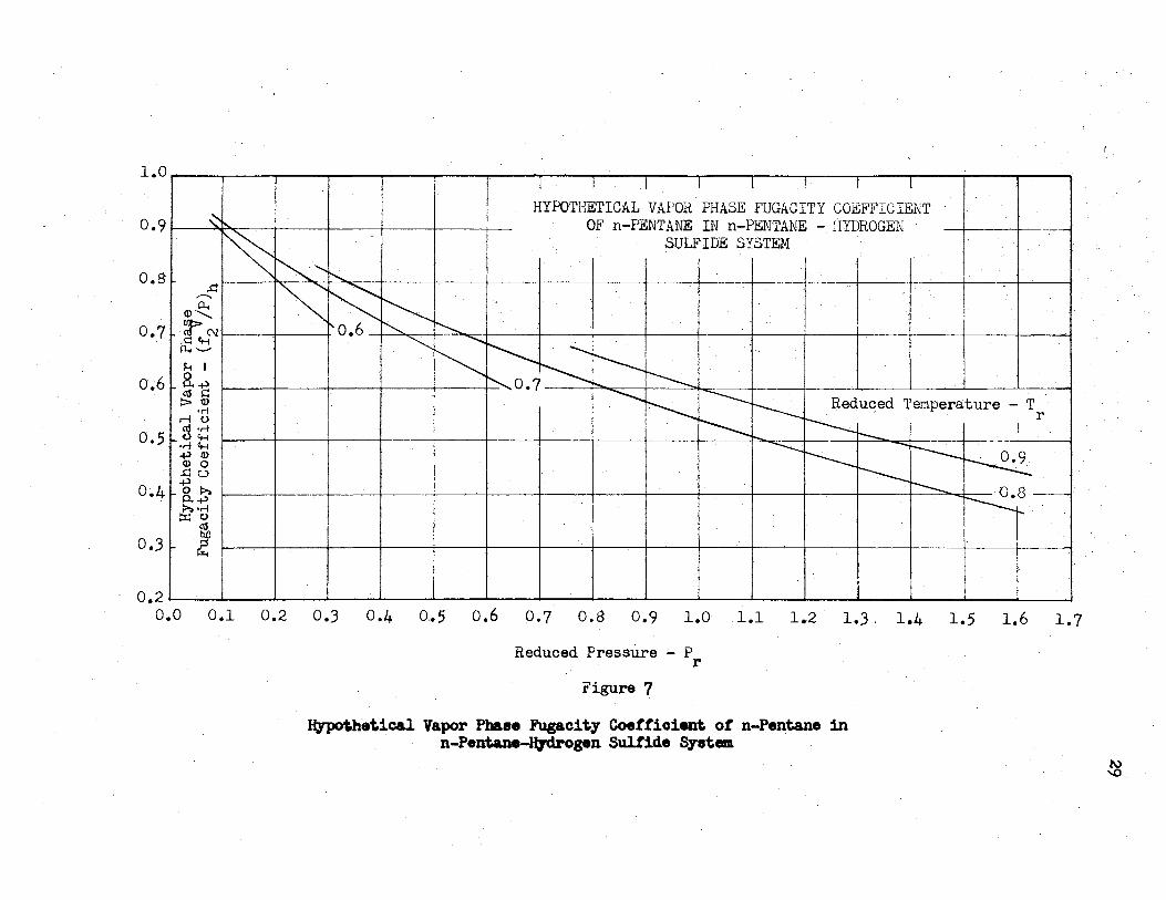
reduced pressure. Figures 5 to 7 show the (f2 /P)h data replotted

with even increments of reduced temperature as a parameter. These V

were obtained by first cross plotting the (!2 /P)h data of Figures

1-4 versus Tr e.t constant Pr' followed by the replots of Figures 5-7.

Liquid Phase Activity Coefficient

The activity coefficient of the heavy component in the liquid

was calculated by bridging from the fugacity coefficient of this

component in the vapor mixture. This can be done as a result of the

criterion of equilibrium that

-L -V f. = f.

1 1 (I-5)

22

l.O,---,--.....--,---.--,----,.-,--.,.._.,.--,----r-'----,,-~---,--"T"--,---r--,----.--,----,,----.--,--~-'----,.-,---..--____,

~ I -1 I - I I HYPOTHETICAL VAPOR PHASE FUGACITY COEFFic'IENT _ 0.,91 ~1.1"4t::: · . - · - - - · ·• OF HYDROGEN SULFIDE IN METHANE - -+--,---

.c: HYDROOEN SULFIDE SYSTEM ...... .e:_ 0.81 I '<I', v,d :w, _ I I J J I I 1 . I I I l I - I,

~N

~~ 11. 1 0.71 I I 'l: 's::: I's.:: I 1'2>, I wt«:....: I I I I I I I I · I i..

8. ~ "' I> > 'tl O .6 1----+---+-----+--...P...

r-i .....

~ t: ..... a,

Reduceq. Temperature - Tr

"\: 8 0.51 I I I I I I I l'...... l T ... ....,""" I I -::::::R>cl :!; t>.

~~ .

- ::i: i O •41 I I I I I I I l I I ::::-.e.....J I r.:::q.. '" l _._ - I

p,..

0.31 I· I I I I I I I I -I . I I r :J'he...L:

0.2L------L-------L_;_--L----...L---...--L-----L----....L....---------.,____,_._ __ ___._ ____ ..__ __ __._ _ __._ ____ .L-__ ~

o.o 0.1 0.2 0.3 0.4 0.5 o.6 0~1 o.a 0.9 1.0 1.1 1.2. 1.3 1.4 1.5 1.6 Reduced Pressure - P - - r

. Figure l

BJpotmtical Yapor PhilN "1peit7 ~tieieat ot lf1*oae Sllliicte· · - in Ket.bane ... JIJdrogen SUltide S7.t.• (28,37)-

~ .. . . ' . . . . . , . . . ··: :-.·.::,· -

! .

~-

.. - .

\

0 .66 ...,,,...._ .......... __ ...--.......... __ ...-_...,._.~ .......... -----'-----...__-__,_ _ __,.. 0.2 0.3 0.5

Reduced Pressure - Pr

Figure 2

o.6

Hypothetical V•por Phase Fugaeity Coefficient ot Hydrogen Sulfide in Ethane - Hydrogen Sulfide System (25)

I) fll cd

f J.t 0 p.,

: r-i

! orf

~ ..r: -+> 8. Pol -:r:

1.0 l . 1 l 1 1 1 l l

; HYPOTHETICAL VAPOR PHASE FUGACITY COEFFICIENT 0.9 OF PROPANE IN PROPANE -

HYDROGEN SULFIDE SYS'1$M -.c: - -

1, .....

~ ~

~ . . . .

~.31 "'-c

~ ~ ~ Reduced Temperature_- Tr ~840 I ~ ~ ... 0.961 ·.

0.870 ~~ 0.901 ~

~ ~ ~

-~ ~

.......... . .e:. o.s >

C'll fo..f --I 0.7

~ •rl o.6 0 orf ~-

"'"' I) 0 0.5 0

Pol ~ () 0.4

l 0 • .3

-0.2

o.o 0.1 0.2 0.3 0.4· 0.5 o.6 0.7 o.8 · 0.9 1.0 1.1 1.2. 1 • .3 1.4 1.5 1.6


Figttre 3

. Bypot.het.ical Yapor Pbaae ,._ci't.7 Coefficient. ot Propane in - . ~- SUl.t1de ~ (26) . '.

- I

N

"'

1.0

0.9

o.s~ .c: ,........ -.e:: I

~-0.7~ 11' '+-IC\I

.c: '-" 0..

~

o.6~ & ~ c1' Q) :> •r-1

t)

rl •r-1

0.5~ ~ ~ or-I Q) ,+l 0 Q) 0

.c: I>:, . 0.4~ ~ +l

~"8 ::i::: c1'

0.3~ gfl

i:::r..

I "" ',g

........ iv.... ~ I u

HYPOTHETICAL VAPOR-PHASE FUGACITYCOEFFICIENT -OF·n-PDTANE IN n-PmlTANE ~

HYDROGEN SULFIDE SYSTEM

Reduced Temperature - Tr . . . f

0.946

0.2L-~-L--~--L-~---1~~-L-~~~-L.~~L--~..J_~--l-~--l-~~-'--~...L-~--'-~---'~~-'-~--1-~---I o.o 0.1 · 0.2 0~3 0.4 Q.5 o.6 0.7 o.s _ 0.9 1.0 1.1 1.2 1.3 1.4 1.5 1.6 1.7


Figure 4

Hypothetical Vapor Phaae ~cit7 Coetticient ot _ n-Pentane in n-Pentane-ff;Jdrogen Sultide Sy-st• {39)

~

1.0

0.9

,.........c: ll.,

G> ;--- 0 .8 <IS ft-I C\I {I)

~ Jci 0 0..

~ rl <1' 0 ·rl +> Q)

.._,,

I 0.7

~ Cl)

·j o.6 •rl c...i c...i Cl)

25 0.5 :& ~ 0 +> ~ '8

::i::: ~ 0.4 ~ Ii.

0.3

0.2

',

'~ ~ , ...

"\

~ ~ ~ "\ ' r--- 0.7 ~·

'r-. o.6

J l . J I I J I I I HYPOTHETICAL VAPOR PHASE FUGACITY COEFFICIENT· I

I

OF HYDROGEN SULFIDE IN METHANE - I HYDROGEN SULFIDE SYSTEM I,

I

I I

-0 "'--

I'---.._ 1

~ ~ I i

~ ~ I I I

..... . Reduced T~mperature - Tr~ I~ ---~ ~

I

r----. ~' 0.9 ...... ~ ~ - 0.8 --,..

-----o.o 0.1 0.2 0.3 0.4 0.5 o.6 0.7 o.s 0.9 1.0 1.1 1.2 1.3 1.4 1.5

Reduced Pressure - P r

Figure 5

lfn,othetical Vapor Phase Fugacit7 Coetticient ot Hydrogen Sultide in . .lllrt,~ Sul.tide $yet.a . '

~

.t::

----I).,

' 4) >N fl)

cd t+-t if

..__,

H 0 +> A. ·s::: cd Q)

> •r-1 0

. rl •r-1 cd .~ () t+-t ·n Q)

+> 0 Cl)

.t:: 0

~ ~ +>

~ -·g ::r:: cd

bO :::s

j%.,

1.0 1 J I l l J J I

HYPOTHETICAL VAPOR PHASE FUGACITY COEFFICIENT -,

0.9. OF PROPANE IN PROPANE -. HYDROGEN SULFIDE SYSTEM

0.8 -

0.7

o.6

·~

~ ............._ --~"' -.·

~ ~ 0.85 ~ ~ ..

0.5

~ . ~~ Reduced Temperature - Tr· ·

0.90 ~ 0.95 . . -

0.4

0.3

<,

0.2 o.o 0.1 0.2 0.3 0.4 0.5 o.6 0.7 o.e 0.9 1.0 1.1 1.2. 1.3 1.4 1.5 1.6


Figure 6

}o"pothetical Vapor Phase Fugaoit7 Coefficient ot PJ-opane in Propane-Hydrogen Sultide_System

(

~

1.0 1 I I 1 I . 1 1 l

0.9 HYPOTHETICAL VAPOR PHASE FUGACI!Y COEFFICIENT

-~"'- OF n-PENTANE IN n-,PENTANE - HYDROGEN

~ SULFIDE SYSTEM

~' r-.... ..c:

~ R . .

~

~ l.> • . . • a..

Q) ...........

~N ~o.6 '- r---..... ..

.c:: 'H """'-- ........

~' 11., .._

~ r----. 1-4 I

b--. 0. 7 r----_ ~ B. of-) .

Ill~ --....... r----. ----r--._ Re<iuced Temperature - T -l> 11) •r-f -- - . -- r

,..; CJ

~ r---__ . j • Ill ,,-j 0 'H --- - r--._ T •ri "'--! r--._

~--.

+I Q) Q) 0 r--._ ..c: 0 +I . ---- ~~-.. ~~

•ri :I:: 0

Ill

0.8

0.7

o.6

0.5

0~4

0.3 .. l 0.2

o.o 0.1 0.2 0.3 0.4 0~5· o.6 0.7 o.s 0.9 · 1.0 1.1 1.2 1.3. 1.4 1.5 1.6 1.7


Figure 7

~hetical Vapor Phase Fugacit7 Coetticient. ot n-Pent.ane in n-Pentane-lqdrogen SUltide System ·

!

~

30

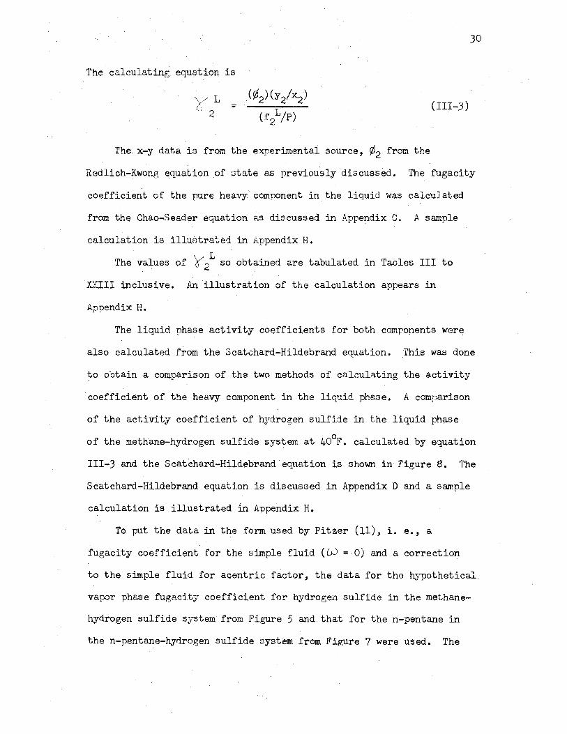
The calculating equation is

'\ / L Ci 2

.C¢2)(y2/x,) =

(f2L/P) (III-3)

The x-y data is from. the experimentai source, ¢2 from the

Redlich-Kwong equation ofotate as previously discussed. The fugacity

coefficient of the pure heavy· component in. the liquid was calcuJa.ted

from the Chao-Seader equation as discussed in Appe~dix C. A sample

calculation is illu.strated in Appendix H. . L

The values of ~ 2 so obtained are tabulated in Tables III to

XXIII inclusive. An illustration of the calculation appears in

Appendix H.

The liquid phase activity coefficients for both components were

also calculated from the Scatchard-Hildebrand equation. This was done

to obtain a comparison of the two !'llethods of calculating the activity

coefficient of the heavy component in the liquid phase. A comparison

of the activity coefficient of hydrogen sulfide in the liquid phase

of the methane-hydrogen sulfide system a~ 40°F. calculated by equation

III-3 and the Scatchard-Htldebrand equation is shown in·Figure 8. The

Scatchard-Hildebrand equation is discussed in Appendix D and a sample

calculation is illustrated in Appendix H~

To put the data in the form used by Pitzer (ll), i.e., a

fugacity coefficient for the simple .fluid (W = 0) and a correction

to the simple fluid for acentric factor, the data for the hypothetical

vapor phase fugacity coefficient for hydrogen sulfide in the methane-

hydrogen sulfide i;;ystem from Figure 5 and.that for the n-pentane in

the n-pent~e-hydrogen sulfide system from Figure 7 were used. The

31

equation

= (III-4)

V o was solved simultaneously for (f2 /P\ , the fugacity coefficient of

V I

the simple fluid, ~d (f 2 /P\ , the correction for acentric factor,

at valu~s of (t2V/P)h taken from Figures 5 and 7 at constant values

of T anq. P. The acentric factors for hydrogen sulfide and n-pentane r r

were used with the hypothetical vapor phase fugacity coefficients from

Figure 5 and Figure 7 respectively. The hypothetical vapor phase

fuga.c:j_tycoefficient so obtained for the simple fluid is plotted versus

the reduced pressure at several isotherms in Figure 9. The correction

for acentric factor is plotted similarly in Figure 10.

1.s--~~~~__:~r----r~-r~~~r--r~, 1 •4 • o Scatchard-Jffild.ebrand

+'

~ • 1.3 I (]~tion ~-3 ~ i ! i i i I .-ii "d l!iH!...t a;...i~ ~i 1.21--~--l'--~----l!-~~-ll-~~--4-~____::r,.,.......____::~~~--+~~-+-~~+-~--I Orll

>..i i! 11111» 1.1 I

..-1 2 Hydrogen Sulf'ide -t> ~ • ~ ::I:· m Methane-Hydrogen -u "'-« 1.0 Sulf'ide §ystem ..-f O at 40~. &• ....

IHI ll

0.9&--~--L-.~-L-~--"'~~..._~....._~---~--'---~---~--~--o.o 0.2 0.4 o.6

Mo1e Fraction Hydrogen Sul.fide in Liquid

Figure 8

"o.s

Canparison oft.he Liquid Activity Coefficient. of Hydrogen SUl:fide Calculated. by t.he ScatcbardHildebrand Equation with the One Calculated

by Equation III-3

1.0

\..i, N

1.0 1 1 l I l I

0.9

o..c: ~ 0.8

G) -.e: Ol >N ell ..c: "-i

11. ~ 0.7 J.., 0 P. ~ .ell > Q) o.6 •rl r-l 0

~ •rl "-i

•rl "-i ~ I)

0.5 II) 0 ..c: 0 ~

:>. & ~ I>. - •rl 0.4 ::C:' 0

"' ~ Ii.

-, V . ~ V j ~ V r " (£2 /P\ "' £2 /P\ . (£2 /P\

~ "- ' "" ['\_"" ~

~

0

~ "" ' I'-.....

"' "" ~ -~ I"-~ " 0.7 ~ o.6

' ·--.~

~ --......... ~ Reduced Temperature - Tr

'-....... . I'--..._

~ --....

i-,.... 0.9

~ ~

............ ~ ~ 0.8

o.J ~.

Chart 1 of 2 0.2 I I

O.O 0.1 0.2 O.J 0.4. 0.5 0.6 0.7 0.8 0.9 1.0 1.1 1.2 1.3 1.4 1.5 1.6

Reduced Pressure - P .- r

Figure 9

H::,pothetieal Vapor PhaN Fugaeit7· Coefficient tor th• Siaple Fluid·

~

..c: ,.....,, P-.

........... > C\I

Ct-t ..._,,

I

J'-1 0 .p ()

r:\1 rx.. ()

•rl J'-1

~ Q) 0

<I!

J'-1 0

.Ct-t

s::: 0 ·rl .p 0 Q) J'-1 J'-1 0 0

4.0 l . l I. J I I I 6,)

. V ~r2v/P\j ~r//P\J .._ (f2 /P\ =

/0.8 Reduced Temperature - Tr /

V '"

V 3.0

. ---

V V

V o.6 L------~

I / --- c-0.9

V l...------ 0.7 L--- L---i..---

V ---- ~ :_.. L------~ ~ -----

2.0

1.0

Chart 2 of 2

o.o I I

o.o 0.1 0.2 0.3 0.4 0.5 o.6 0.7 o.8 0.9 1.0 1.1 1.2 1.3 1.4 1.5 1.6


Figure 10

Correction to the Hypothetical Vapor Phase Fugacity Coefficient for Acentrie Factor

\,J ,I:-

CHAPTER IV

DISCUSSION OF RESULTS

Hoffman, et al. (22) first presented the idea of bridging from

the activity coefficient of the real gaseous component to that of the

hypothetical gas through the Gibbs-Duhem equation for the purpose of

calculating the standard state for the hypothetical gas. For this

they used the Van Laar equation, a partieular solution of the Gibbs-

Duhem equation, in the form 2

V 10g Yi - f

. ( +

a ij

a. /y. ]2 1, 1

a 2 j . y.

1 J

(IV-1)

The constants (aij & aji) of equation IV-1 were calculated by

fitting the equation to the activity coefficient for the light com-

ponent in the vapor phase calculated through the Cline Black equation

of state (7). After evaluation of the constants the vapor phase

activity coefficient of the heavy component was calculated by equation

IV-1. The hypothetical vapor phase fugacity coefficient was calculated

from this activity coefficient and the fugacity coefficient of the

component in the mixture, calculated by the Cline Black equation,

by means of equation III-2. Stuckey (46) proposed the numerical

integration of equation III-1 used in this work as a simpler and less

tedious method of bridging from the vapor phase activity coefficient

35

36

of the light component to that of the heavy component. Stuckey's

method has the disadvantage of requiring sufficient data to extrapolate

V the log ~l versus y1 curve to zero concentration of the light

component.

The fonn of the Gibbs-Duhem equation used is rigorous only at

constant pressure and temperature. For a binary mixture in vapor-

liquid equilibrium, it is not possible to vary the concentration of

a component in the mixture without a corresponding change in either

the temperature or pressure. The rigorous fonn of the Gibbs-Du.hem

equation at constant temperature is

= (IV-2)

The use of equation IV-2 requires volumetric data for evaluation.

The error in neglecting the pressure effect of equation IV~2 is small

and as pointed out by Thompson (47) is highly sensitive to small

errors in the volumetric data. It therefore appears that at this

stage of development that the added complexity of equation IV-2 may

be neglected in these calculations.

Prausnitz (36) developed an empirical method of arriving at the

hypothetical standard state by arbitarily drawing a smooth curve from

the vapor boundary of the two phase region of a PV plot and converging

with the fluid portion of the curve at .some high pressure. These

curves were developed for acentric factors of O.O, 0.2 and 0.4.

Edmister (15) replotted Prausnitz's data in the form used by Pitzer

(11), i. e., f/P as a function of the simple fluid and a simple fluid

correction for acentric factor. Table I presents a comparison of the

hypothetical vapor phase fugacity coefficients as calculated by

Edmister•s plots of Prausnitz (15), Hoffman, et al. (22), and this

work.

TABLE I

COMPARISON OF HYPOTHETICAL VAPOR PHASE FUGACITY COEFFICIENT VALUES

W == 0.2925

Edmister-

Tr_ Pr Prausnitz Ho.t'£ma.n 1 s Values Values

o.6 O.l 0.26 0.817 0.3 0.12 0.600

0.7 0.1 0.52 0.900 0.3 0 • .3.3 0.720

0.8 0.3 0.56 0.814 0.7 0 • .38 0.614 1.1 0.27 0.446 1 • .3 0.24

0.9 0.7 0.54 o.695 0.9 0.48 0.620 1.1 0.42

This Wor).c

0.925 0.741 0.90a 0.788 0.817 0.656 0.527 0.467 0.702 0.6.34 0.575

A comparison of the values in Table I show that those of this

work are considerab:cy higher than the values of Prausnitz. This

same trend was also observed by Stuckey (46). These values which

were calculated at an aeentric factor o.t' 0.2925 (equivalent to a

Zc o.t' 0.27), the point at which Hoffman, et al. (22) presented

their data, are appreciab~ higher than Hoffman's values. Stuckey

(46) found excellent agreement £or his values o.t' normal butane with

those of Ho.t'f'ma.n at Zc = O.Z7. An adequate explanation for these

differences is not apparent. It can on:cy be surmised that since

both correlations are based on a rather meager amount of x-y data,

additional data are reqUired to determine the correct values.

37

Table II compares the hy:pothetica.l vapor phasP. fugacity coef-

f:icient of the sirr.ple fluid as develoi:,ed by Stuckey (1-1-6) from ethane

binariee and from this work er. hyd:r:ogen sulfide binarie::.

TABLE II

COMPARISON OF HYFOTHETIChL VAPOR PHASE FUGACITY COEfi?ICIENTS OP THE SU:PLE FLUID

T 'C .. r r

0.7 0.4 0.8 0.4

0.6 0.8

0.9 o.6 0.8

G._") = 0

Hypothetical Vapor Phase Fugacity Coefficient for the Simple Fluid

Stuckey' s Values This Work

0.65 0.66 0.74 0.75 0.63 0.64 0.55 0.54 0-.?5 0.74 o.68 0.64

Excellent agreement is observed in the values of Table II. Thus

as the acentric factor increases from zero the difference between

Stuckey's velues and those of this work become larger indicating

possibly a need for a better method of correlation of \he values

for real fluids with those_ of the simple fluid.

Liquid Phase Analysis

Th~ .first step in ma.king a similar analysis of the liquid phase

38

is to calculate the activity coefficient of the real liquid component,

i. e., the heavy component in the liquid phase. This work, as pre

viously noted, calculates the a.ctivity coefficient of the heavy

component in the liquid by

39

0 L = 2

(¢2 )(y2/x2)

(fzL/P) (III-3)

wher~ ¢ is calculated by the Redlich-Kwong equation of state (41)

and (f21/P) is calculated by the Chao-Seader equation (9). Hoffman,

et al. (23) ma.de a similar analysis using the Black equation of

state to calculate ¢2 and the generalized fugacity coefficients of

Lyderson, Greenkorn and Hougen to obtain (f21 /P). ·

The Scatchard-Hildebrand equation (43) provides a means to

directly obtain these activity coefficients. This equation is based

upon the components in the liquid phase forming a •regular solution'

and as a result of simplification has the added restriction that all

activity coefficients are equal to or greater than unity, The

criterion of hydrocarbons behaving as •regular solutions' seems

justified when pressure and temperature conditions are such that the

normal state of aggregation of the components is liquid. There is,

however, a question of whether or not this is true of those liquid

solutions encountered in vapor-liquid equilibria in which the light

component in the liquid phase cannot exist in its pure state at the

given temperature and pressure. This question is further increased

when one of the components as in this work is a nonhydrocarbon and

a polar compound.

A comparison of the activity coefficients calculated by the

Scatchard-Hildebrand equation and by equation III-3 is illustrated

in Figure 8 for hydrogen sulfide in the methane-hydrogen sulfide

system at 40°F. The shape of the curves in Figure 8 is characteristic

of the systems studied. Comparisons of the remaining systems appear

in Tables III through XXIII.

It is apparent from Figure g that considerable difference exists

in the two methods of calculation. There is an apparent error in the

values obtained from equation III-3 as the pure liquid is approached

since at this point the activity coefficient is by definition unity.

This error is attributed to the failure of the Redlich-Kwong equation

of state and/or the Chao-Seader equation to fit the data perfectly.

Even with these inherent inadequacies equation III-3 appears to be

the preferrable method of calculating the liquid phase activity coef

ficient of the heavy component of a binary mixture since it removes

40

the restrictions of the Scatchard-Hildebrand equation that the solution

must be •regular' and that the activity coefficient must be equal to

or greater than unity.

CHAPTER V

RESULTS, RECOJ.vlMENDATIONS AND CONCLUSIONS

Results

The ultimate goal in this investigation was to establish a means

of determining the standard state fugacity coefficients for hypothetical

vapors and liquids. ~ethods are available for calculating the fugacity

coefficients of components in solution with one another. Knowing these

two fugacity coefficients, the activity coefficients of a component in

each phase is available as well as the ideal K-value, thus permitting

calculation of the actual K-value by means of

K. l

In this work on hydrogen sulfide binaries a standard state

(I-10)

fugacity coefficient correlation for the hypothetical vapor has been

successfully developed. These values are generalized using the

acentric factor as an identifying parameter and are presented graph-

ically in Figures 9 and 10.

Stuckey (46) and Hoffman, et al. (22) have presented similar data

on hydrocarbon binaries. A comparison of their work with this non-

hydrocarbon - hydrocarbon binary study indicates the possibility of

correlating nonhydrocarbon - hydrocarbon solutions into the same

framework used for strictly hydrocarbon solutions.

41

Further the Scatchard-Hildebrand equation (43) with its restric

tions does not appear as applicable to calculation o:f the liquid

phase activity coefficients as the method of bridging from the vapor

fugacity coefficient o.f the heavy component in the mixture to the

liquid fugacity co.efficient. Since the heavy component is a real

liquid its pure state fugacity coefficient can be calculated and

then its activity coefficient found. This was the limit of this

work.

Recommendations

To conclude the work the liquid phase analysis needs to be

completed. From the activity coefficient of the heavy component in

the liquid phase, the activity coefficient of the light component

42

can be calculated by bridging through the Gibbs-Duhem equation as was

done here for the vapor phase. The fugacity coefficient of the light

component in the mixture is then calculated from its fugacity coef

ficient in the vapor as calculated by an equation of state and then

bridging to the liquid using the criteria for equilibrium of equal

fugacities of a component in each pM.se. Knowing the fugacity coef

ficient of the light component in the liquid solution and its activity

coefficient, the standard state fugacity coefficient of the hypothetical

liquid is back calculated.

Considerable more work is needed on nonhydrocarbon - hydrocarbon

solutions to determine whether the methods used here for hydrogen

sulfide - hydrocarbon solutions are also applicable to other non

hydrocarbon - hydrocarbon solutions and to heterogeneous solutions

in general. Additional data is available in the literature for

carbon dioxide - hydrocarbon systems (1,13,31,34,38,48). Data is

available for the hydrogen sulfide - carbon dioxide system (6). It

is expected that analyses of these systems (1) hydrocarbon - hydro

carbon, (2) hydrogen sulfide - hydrocarbon, (3) carbon dioxide -

hydrocarbon, and (4) carbon dioxide - hydrogen sulfide would give an

excellent basis for a correla.tion involving the interaction effects

of hydrocarbons with other materials.

Conclusions

'rhe conclusions drawn in this work are:

43

1. The modified Hoffman procedure for calculating the standard

state fugacity coefficient of the hypothetical vapor gives the best

value available at this time. The method is applicable only if x-y

data are available over the entire concentration range of the solution.

In the event complete x-y data is not available Hoffman's (22) pro

cedure using the Van Laar equation may be used.

2. The standard state fugacity coefficients of the hypothetical

vapor can be generalized using the acentric factor of Pitzer and Curl

(11) as an identifying parameter.

J. The activity coefficients for the heavy component in the

liquid phase calculated by means of equation III-3 appear to be

preferable to those calculated by means of the Scatchard-Hildebrand

equation (4.3).

BIBLIOGRAPHY

1. Akers, W. W., R. E. Kelley and T. G. Lipscomb: "Low Temperature Phase Equilibria, Carbon Dioxide-Propane System. 11 Ind. Eng. Chem.~' 2535 (1954).

2. American Petroleum Institute: Research Project 44, Texas A & M College, College Station, Texas.

3. Benedict, M., G. B. Webb and L. C. Rubin: 11An Empirical Equation for Thermodynamic Properties of Light Hydrocarbons in Other Mixtures. 11 !h Chem. Phys.§., 334 (1940); 10, 747 (1942).

4. Benedict, M., G. B. Webb and L. C. Rubin: 11An Empirical Equation for Thermodynamic Properties of Light Hydrocarbons and Their Mixtures. 11 Chem. Eng. Progress il, 419 (1951); il, 449 (1951).

5. Benedict, M., G. B. Webb, L. C. Rubin and 1. Friend: 11AnEmpirical Equation for Thermodynamic Properties of Light Hydrocarbons and Their Mixtures • 11 Chem. Eng. Progress !IL, 571 (1951); il, 609 (1951). .

6. Bierlein, J. A. and W. B. Kay: 11 Phase Equilibrium Properties of System, Carbon Dioxide-Hydrogen Sulfide. 11 Ind. Eng. Chem.~' 618 (1953).

7. Black, C.: 11 Vapor Phase Imperfections in Vapor-Liquid Equilibria. 11

Ind. Eng. Chem • .2.Q, 391 (1958).

8. Brown, G. G.: 11 The Compressibility of Gases - Vapor~Liquid Equilibria in Hydrocarbon Systems • 11 Petroleum Engineer 11,

. 25 (1940); 12, 55 (1940).

9. Chao, K. C. and J. D. Seader: 11A General Correlation of Vapor-Liquid Equilibria in Hydrocarbon Mixtures •11 A.I.Ch.E. Journal 1, 598 (1961).

10. Chu, J.C., S. L. Wang, S. L. Levy and R. Paul: Vapor-Liquid Equilibrium Data. Edwards Brothers, Ann Arbor, Michigan (1956). ~

11. Curl, R. F., Jr. and K. S. Pitzer: Ind. Eng. Chem • .2.Q, 265 (1958).

12. DePriester, C. L.: Coefficients. 11

1 (1953).

11Light Hydrocarbon Vapor-Liquid Distribution Chem. Eng. Prog. Symposium Series No. 1, !±2.,

44

13.

14.

15.

16.

17.

45

Donnelly, H. G. and D. L. Katz: 11 Carbon Dioxide - Methane Systems. 11

Ind.~ Chem. !:tf?.., 511 (1954).

Edmister, W. C. and C. L. Ruby: 11 Generalized Activity Coefficients of Hydrocarbon Mixture Components. 11 Chem. Eng. Progress . 51, 95 (1955).

Edmister, W. C. : Applied Hydrocarbon Thermod~cs, Gulf Publishing Company, Houston, Texas (1961.

Ga.mson, B. W. and K. M. Watson: "High Pressure Vapor-Liquid Equilibria. 11 Nat'l. Petroleum News Tech. Sect. 36, R623 (Sept. 6, 1944).

Gamson, B. W. and K. M. Watson: 11 Thermodynamics of Solutions -Ideal Solutions at High Pressures. 11 Nat'l. Petroleum News 36, R258, R554 (1944).

18. Gilliland and Scheeline: "System: Hydrogen Sulfide-Propane. 11

Ind. ~ Chem. ;g, 48 (1940).

19. Haselden, G. G., F. A. Holland, M. B. King and R. F. StricklandConstable: 11 '.lwo-Phase Equilibrium in Binary and Ternary Systems, X. Phase Equilibria and Compressibility of the Systems Carbon Dioxide-Propylene, Carbon Dioxide-Ethylene and Ethylene-Propylene, and an Account of the Thermodynamic Functions of the System Carbon Dioxide-Propylene. 11 Proceeding of the Royal Society (London)~' l (1957).

20. Hildebrand, J. H.: 11Solubility: Regular Solutions. 11 !l..:. Am. Chem. Soc. 21, 66 (1929).

21. Hildebrand, J. H. and R. B. Scott: Solubility of Non-ElectroLytes. Reinhold Publishing Company, New York, New York (1950).

22. Hoffman, D. s., J. H. Weber, V. N. P. Rao and J. R. Welker: 11Vapor Phase Activity Coefficients and Standard State Vapor Fugacities for Hydrocarbons. 11 Paper presented at the 17th Armual Oklahoma State Tri-Sectional A.I.Ch.E. Meeting, Norman, Oklahoma (April 14, 1962).

23. Hoffman, D. s., J. R. Welker, R. E. Felt and J. H. Weber: 11Liquid Phase Activity Coefficients and Standard State Hypothetical Liquid Fugacities for Hydrocarbons. 11 A.I.Ch.E. Journal§., 508 (1962).

24 •. Hougen, O. A., K. M. Watson and R. A. Ragatz: Chemical Process · Principles, Part II, John Wiley & Sons, Inc. New York, New

York.

25. Kay, W. B. and D. B. Brice: "Liquid-Vapor Equilibria Relations in Ethane-Hydrogen Sulfide System. 11 Ind. ~ Chem. !:J:2., 615 (1953).

26. Kay, W. B. and G. M. Ra.mbosek: 11Liquid-Vapor Equilibrium Relations iii Binary Systems, Propane-Hydrogen Sulfide System. 11 Ind. Eng. Chem. !±2.., 221 (1953).

27. Kellogg, The M. W. Co.: 11 Liquid-Vapor Equilibria iii Mixtures of Light Hydrocarbons." ~ Equilibrium Constants, Polyco Data (1950).

28. Kohn, J.P. and F. Kurata: 11 Heterogeneous Phase Equilibria of the Methane - Hydrogen Sulfide System." A.I.Ch.E. Journal !±, 211 (1958).

46

29. Lewis, W. K. and W. C. Kay: 11 Fugacities of Various Hydrocarbons Above Their Vapor Pressures and Below Critical Temperatures. 11

Oil and Gas Journal, p40 (March 27, 1934).

30. Neusser, E.: Physik ~ .12., 738 (1934).

31. Olds, R. H., H. H. Reamer, B. H. Sage and W. N. Lacey: 11 Phase Equilibria in Hydrocarbon Systems, Then-Butane-Carbon Dioxide System. 11 Ind. Eng. Chem.~' 475 (1949).

32. Pigg, G. L.: 11Determination of Composition Dependent Liquid Activity Coefficients by the Use of the Van Laar Equation. 11

M.S. Thesis, Oklahoma State University, Stillwater, Oklahoma, (1961).

33. Pipkin, O. A.: 11 Correlation of Equilibrium Data for Methane Binaries Through Use of Solubility Parameters. 11 M.S. Thesis, Oklahoma State University, Stillwater, Oklahoma (1961).

34. Poettmann, F. H. and D. L. Katz: 11 Phase Behaviour of Binary .Carbon Dioxide-Paraffin Systems. 11 Ind.~ Chem. n_, 847 (1945).

35. Prausnitz, J.M., W. C. Edmister and K. C. Chao: 11Hydrocarbon Vapor-Liquid Equilibria and Solubility Parameter. 11 Paper presented at Atlantic City, New York meeting of A.I.Ch.E., (March, 1957).

36. Prausnitz, J.M.: "Hypothetical Standard States and the Thermodynamics of High-Pressure Phase Equilibria. 11 A.I.Ch.E. Journal 6, 78 (1960).

37. Reamer, H. H., B. H. Sage and W. N. Lacey: "Phase Equilibria iii Hydrocarbon Systems-Volumetric Behaviour of the Methane -Hydrogen Sulfide System. 11 Ind. Eng. Chem. ~' 976 (1951).

38. Reamer, H. H., B. H. Sage and W. N. Lacey: 11 Phase Equilibria in Hydrocarbon Systems, Volumetric and Phase Behaviour of the Propane-Carbon Dioxide System." Ind.~ Chem.~' 2515 (1951).

47

.39. Reamer, H. H., B. H. Sage and W. N. Lacey: 11 Phase Equilibria in Hydrocarbon Systems - Volumetric and Phase Behaviour of n-Pentane - Hydrocarbon Sulfide System. 11 Ind. ~ Chem. ~, 1805 (195.3).

40. Reamer, H. H., F. T. Selleck, B. H. Sage and W. N. Lacey: 11Phase Equilibria in Hydrocarbon Systems - Volumetric and Phase Behaviour of Decane-Hydrogen Sulfide System. 11 Ind.~ Chem •

. !:t2., 1810 (195.3). -

41. Redlich, Otto and J. N. s. Kwong: 110n the Thermodynamics of Solutions - An Equation of State. Fugacities of Gaseous Solutions. 11 Chemical Reviews !!!±., 2.3.3 (1949).

42. ·Robinson, C. S. and E. R. Gilliland: Elements of Fractional Distillation, Fourth Edition., McGraw-Hill Book Company, Inc. New York, New York (1950).

43. Scatchard, G.: 11Equilibrium in Non-Electrolyte Solutions in Relation to the Vapor Pressures and Densities of the Components. 11

Chemical Reviews §., 321 (1931).

44. Smith, K. A. and R. B. Smith: 11 Vaporization Equilibrium Constant and Activity Coefficient Charts. 11 Petroleum Processing!±, l355 (Dec., 1949).

45. Smith., K. A. and K. M. Watson: 11High Pressure Vapor-Liquid Equilibria - Activity Coefficients for Ideal Systems. 11 Chem. ~ Progress !:t2., 494 (1949).

46. Stuckey, A. N., Jr.: 110n Development of an Ideal K-Value Corre- · lation for Hydrocarbons and Associated Ga.ses. 11 M.S. Thesis., Oklahoma. State University, Stillwater, Oklahoma (1963).

47. Thompson, R. E.:· 11 Investigation of Vapor-Liquid Equilibria for Hydrogen - Six Carbon Hydrocarbons. 11 Ph.D. Thesis, Oklahoma State University, Stillwater., Oklahoma (1963). ,

48. Wan, S. and B. F. Dodge: 11S0lubility of Carbon Dioxide in Benzene at Elevated Pressure. 11 Ind.~ Chem. 32, 95 (1940).

49. West, J. R.: Chem. ~ Progress !!!±., 287 (1948).

APPENDIX A

DATA COMPILATION

48

\_

TABIE Irr~

SYSTEM: METHANE - HYDROGEN SULFIDE

Temperature: -,4o°F, Reduc~d Temperatures: Methane, l.220J Hydrogen Sulfide, 0.624

METHANE HYDROGEN SULFIDE

Va~r Phase Li9uid Phase ' Va12or Phase Liguid Phase Pressure

¢1 (r//P) "c( V L ¢2

V -;r'. V (r//P) · L <~})g" psia Pr Yl 1 Xl (ol )SH Pr (f2 /P\ 2 <~2 ):m 36.7 1 0.054 0.000 0,028 37.8 0.056 0.030 0.9959 0.9894 1.007 0.029 0.9639 0.9639 1.000 40,5 0.062 0.100 0.9947 0.9887 1.006 0.031 0.9614 0.9613 1 .• 000 53 0.079 0,300 0,9900 0.9852 1.005 0.041 0.9502 0.9498 . i:ooo 80 0,119 0.500 0.9815 0.9777 1.004 0,061 0.9274 0,92!>3;" 1,001

200 0 •. 297 0,754 0,9474 0.9449 1.003 0,0125 2.240 0,153 0,8333 0,8308 1.003 0.190 1.000 1.088 400 0.594 0.862 0.8937 0.8918 1.002 0.054 2.063 0.306 0.6915 o.6879 1.005 . 0,079 1.003 1.269 600 0,891 0,900 0.8427 0,8407 1.002 '0,0$3 1.951 0,459 . 0.5697 0.5673 1.004 o.o69 1.007 0.900

x-y Data Source: Kohn & Kurata, A.I.Ch.E, Journallt, 211(1958)

~

.<

Temperature: o°F,

METHANE Pressure Vapor Phase psia i

p .. Y1 ¢1 (flV /P) r --82,3 0.122 0.000 85 0.126 0,030 0,9946 0,9822 92 0,137 0.100 0,9924 0,9807

113. o.168 0.250 0.9864 0,9794 148 0.220 0.400 0,9778 0,9692 200 0.297 0.522 0;9662 0,9585 400 0,594 .0.720 0,9248 0,9186 600 0,891 0,792 0,8865 0.0003

TABLE IV.


Reduced Temperatures: Methane, 1,337; Hydrogen Sulfide, 0.684

' liYDROG:EN S!JLF'.ll)Jl:

LiCJYid Phase V vL ri_ Xi_ (o 1 )SH

1.013 1.012 1.010 1.009 1.008 1.007 1.007

0.009 0.045 0,072

2.161 2.017 1.920

p~-

0.065 . 0.070 0.087 0,113 0.153 0.306 0,459 -

Vapor Phase Li9uid Phase

¢2 V

(f2 /P)h ¥}- L yL (f2 '/P) . ( 2 )SH

0,9364 0,9364/ 1.000 0.9314 0,931:,.: · 1.000 0.9167 d.9163 1,000 0,8934 0,8924 1.001 0,8600 0,8585 1.002 0.411 1.000 0,7421 0.7392 1.004 0.214 1.002 0;6348 · 0.6329 1.003 0.148 1.006

x-y Data Source: Kohn & Kurata, A,I.Ch.E, Journal!!,· ;2ll(i958)

( 't/)d

1.009 1.013 0.961

~--

.~.

TABLE V


Temperature: 40°F, Reduced Temperatures: Methane, 1.453; Hydrogen Sulfide, O. 743.


Va:122r Phase Liguid Phase Va;eor Phase Pressure ~\- cr//P) ?{ V ca}\H ¢2 (r//P\_ '( V (f2L/P) psia Pr Y1 1 ~ Pr 2

169-l< 0.0000 0.0000 200 0.297 0.1371 0,9898 0.9686 1.022 0.0057 2.097 0.153 0.8816 0.8814 1.000 o. 738 -250 0,371 0.2783 0.9800 0.9607 1.020 0.0132 2.066 0.191 0.8543 0.8537 1.001 0.597 300 0.446 0.3896 0.9700 0,9530 1.018 0.0212 2,035 0.230 0.8287 0.8276 l,OCl 0.501 350 0.520 0.1,604 0.9615 0.9455 1.017 0,0284 2,009 0,268 0.8038 0.8019 1.0G2. 0.434 400 0.594 0.5126 0.9535 0.9380 1.016 0.0354 1.983 0.306 0.7795 0.7773 1.003 '.),381 450 0.669 0.5551 0,9456 0.9306 1.016 0.0424 1.958 0.345 0,7558 0.7532 1.003 0,343 500 0,743 0.5879 0.9381 0.9233 1.016 0.0493 1.934 0.383 0.7326 0,7298 1.004 0.312 600 0,891 o.6394 0.9235 U.9089 1.016 0.0636 1.886 0.459 o.6878 o.6853 1.0C4 0.265 700 l.OLrO 0.6755 0.9098 0.8948 1.017 0.0783 1.840 0.536 0.6446 0.6435 1.002 0.231 /300 1.129 o.6989 0.8971 0.8211 1.018 0.0930 1.796 0.613 0.6023 0.6031 0.999 0.206 900 1.337 0.7141 0.8855 0.8678 1.020 0.1083 1.752 o.689 0.5608 0.5647 0.993 0.186

lCOO l.Lr86 0.7242 0.8749 0.8548 1.024 0.1250 1.707 0.766 0.5202 0.5275 0.986 0.171 1100 1.634 0,7299 0.8656 0.8422 1.028 0.1433 1.661 0.842 0.4803 0,4913 0.978 0.162 1200 1.783 0.7321 0.2579 0.8300 1.034 0.1635 1.613 0,919 0.4411 0.4572 0,965 0.148 1250 1. 857 0.7319 0.8548 u.8241 l.037 0.1750 1.588 0.957 0.4217 0.4441 0,950 0.143 1300 1.931 o. 7306 0,8523 0.8182 1.042 0.1868 1.563 0.995 0.4022 0.4285 0.939 0.138 1400 2.080 0.7262 0.8491 0.8068 1.052 0.2137 1.508 1.072 0.3640 0,3992 0.912 0.131 1500 2.229 0.7185 0.13490 0.7959. 1.067 0.2450 1.451 1.149 0.3268 0.3791 0.862 0.122 1600 2.377 o,7c75 0,8523 0.7853 1.085 0,2798 1.395 1.225 0,2913 0.3458 0.842 (; .118 1700 2,526 0,b931 (.8589 0.7752 1.108 0.3240 1.331 1.302 0.2586 0.3206 l),807 0.113 1750 ;2.600 0.6828 0.8650 o. 7?04 1.123 0.3492 1.299 1.340 0.2426 0.3093 0,784 c.111 18D0 2J,74 o.6686 0.8751 0.7656 1.143 0.3758 1.260 1.378 0.2261 0.3011 0.751 0.109 19UO_ -'" 2.823 0.6130 0.9275 0.7564 1.226 0.4401 1.202 1.455 0.1870 0.2814 0.665 0.105 1949"" 2.896 o.55ou 1.0053 0,7521 1.337 0.5500 1.119 1.492 0.1611 0.2734 0,589

-i, Vapor prec:sure of hydrogen sulfide. -lP~ Estimated critical state

x-y I1ata ,::ource: Reamer, Sa?e & Lacey, Ind. Eng. Chem. 43, 976(1951)

Liguid Phase 't L

( 2 )SH

1.000 1.000 1.000 1.001 1.001 1.002 1.002 1.004 1.006 1.008 1.011 1.014 l.019 1.024 1.027 1.031 1.040 1.052 1.067 1.089 1.102 1.118 1.159 1.243

L ( ((2 ~

1.037 1.046 1.031 1.029 1.034 1.024 1.018 1.000 0.983 0.971 0.967 (;.959 0.935 0.954 0.958 0.966 0.968 0.999 1.003 l.G39 1.065 1.081 1.231

V1 1--'

TABLE VI·


Temperature: l00°F, Reduced Temperatures: Methane, 1.627; Hydrogen Sulfide, 0.832


Pressure Va12or Phase Li9uid Phase Va122r Phase Li9uid Phase psia p Y1 ¢1 (f//P) Y/ xl <Y/lsH Pr ¢2 . Cf//P)h '( V Cf//P) ( i/)SH ( ¥'/)d. -- r 2

394* 0.0000 400 0,594 0.0117 1.0123 0.9581 1.057 0.0007 2.010 0.306 0.8266 0.8266 1.000 1.000 450 0,669 0.0963 1.0055 0.9532 1.055 0.0067 2.001 0.345 0.8055 0.8055 1.000 0.702 1.000 1.044 500 0.743 0.1642 0.9995 0.9482 1.054 0.0128 1.978 0,383 0,7851 0,7851 1~000 0.637 1.000 1.043 550 0.817 0 .2203 0.9939 0.9433 1.054 0.0190 1.956 0.421 g~~tgi 0,7651 1.000 0,584 1.000 1.042 600 0.891 0.2688 0.9885 0,9385 1.053 0.0255 1.934 0.459 0.7458 1.000 0.539 1.001 1.039 700 1.040 0.3416 0.9796 0.9291 1.054 0.0385 1.890 0.536 0,7087 0.7087 1.000 0.469 1.001 1.035 800 1.189 0.3976 0.9715 0,9199 1.056 0.0523 1.846 0.613 0.6728 0.6733 0.999 0.417 1.003 1.026 900 1.337 0.4396 0.9648 0.9109 1.059 0.0670 1.802 o.689 0.6379 0.6399 0,997 0,376 1.004 1.019

1000 1.486 0.4707 0.9597 0.9022 1.064 0.0828 1.757 0.766 0.6037 0.6073 0.994. 0,344 1.006 1.013 1100 1.634 0.4923 0.9570 0.8937 1.071 0.0996 1.712 0.842 0.5697 0.5769 0!988 0.326 1.009 0.985 1200 1.783 0.5079 0,9563 0.8855 1~080 0.1182 1.665 0.919 0.5360 0.5485 0,,977 0.295 1.012 · 1.015 1250 1.857 0,5130 0.9573 0.8815 1.086 0.1282 1.641 0.957 0.5190 0.5331; - 0.974 0.285 1.014 1.017 1300 1.931 0.5182 0.9583 0.8775 1.092 0;1390 1.616 0,995 0.5025 0.5192 0.968 0.276 1.017' 1.019 1400 2;080 0.5240 0,9636 0.8698 1.108 0;1620 1.566 1.072 0,4690 0.4905 0.956 0.260 . 1.022 1.025 1500 2.229 0.5255 0.9730 0.8624 1.128 0.1885 1.512 1.149 0.4355 0.4640 0,939 0.247 1.030 1.036 1600 2.377 0.5195 0,9914 -0.8552 1.159 0.2192 1.456 1.225 0.4004 0.4441 0.902 0.234 1.040 1.042 1700 2.526 . 0,5058 1.0222 0.8483 1.205 0.2532 1-.401 1.302 0.3641 0.4190 o.869 0.224 1.052 1.059 1750 2.600 0.4947 1.0454 0.8449 1;237 0.2725 1.372 1.340 0.3451. 0.408.3. _0.$45 0.2)..9 1.o64 1.095 1800 2.674 0,4797 1.0750 0.8416 1.277 0.2940 1.342 1.378 0.3257 0.3982 0.818 0.214 1.070 1.122 1850 2.749 0,4580 1.1203 0.8384 1.336 0,3185 1.310 1.417 0.3050 0.3872 0,788 0.210 1.081 1.155 1900 2.823 0.4190 1.2036 0.8353. 1.441 . 0.3578 1.265 1.455 0.2801 0.3766 0.744 0.206 1.101 1.230 19071f* 2.833 0.3880 1.2770 0.8348 1.530 0.3880 1.233 1.460 0.2681 0.3750 0.715 1.117

* Vapor pressure of hydrogen sulfide ** Estimated critical state

x-y Data Source: Reamer, Sage & Lacey, Ind. Eng. Chem. JiJ., 976(1951)

~

' '

\_

TABLE VII


Temperature: 160 °F, ·Reduced Temperatures: Methane, 1,802; Hydrogen Sulfide, 0,921


Pressure Va12or Phase Li9uid Phase Va122r Phase Liguid Phase psia p ¢1 (f//P) 'l{ V <Y/)sH p ,2 (f//P\

·v (f//P) ( ¥/)SH <!/)d .·. r yl 1 ~ r ¥2 --778,9* 0,0000 0,0000 800 1.189 0.0196 1.076 0,946 1.137 0.0031 1.941 0.613 o,74o6 0,7406 1.000 o. 716 ., 1.000 1.017 850 1.263 0.0592 1.074 0,943 1.139 0.0098 1.918 0,651 0,7243 0.7243 1.000 0.677 1.000 1.017 900 1.337 0.0946 1.072 0.940 1.141 0.0167 1.895 o.689 0,7084 0,7083 1.000 0.644 1.000 1.013

1000 1.486 0.1553 1.069 0,934 1.145 0,0309 1,850 0.766 0.6775 0.6781 0,999 0.586 1.001 1,008 1100 1.634 0.2021 1.070 0,928 1.153 0.0459 1.805 0,842 0.6475 0.6490 0~~98 0,553 1.002 · 0,979 1200 1.783 0,2367 1.076 0,923 1.167 0.0622 1.760 0,919 0.6177 0.6205'°. 0,995 0,499 1.003 1.008 1250 1.857 0.2534 1.078 0,920 1.172 0,0720 1.731 0,957 0.6034 0.6079' 0,993 0.482 1.005. 1.007 1300 1.931 0.2646 1.085 0,917 1.183 0.0814 1.707 0,995 0,5884 0,5946 0.990 0,466 1.006 1.011 1400 2.080 0.2811 1.105 0,912 1.211 0.1021 1.655 1.072 0,5580 0.5690 0,981 0.437 · 1.009 1.02i 1500 2.229 0,2775 1.167 0,907 1.286 0.1245 1.603 1.149 0.5209 0,5442 0,957 0.413 1.013 1.041 1600 2,377 , 0,2580 1.309 0.902 1.451 0,1547 1~540 1.225 0.4752 0,5180 0,917 0,385 1.020 1.083 1650 2,451 0.2295 1.474 0.900 1.638 0.1830 1.486 1.263 · 0,4457 · 0.5057 0,881 0,382 1.027 1.100 1660** 2.466 0.2090 1.580 0.899 1.756 0.2090 l.,440 1.271 0,4349 0.5032 0.864 1,035

* Vapor pressure of hydrogen sulfide ** Estimated critical state

x-y Data Source: Reamer, Sage_& Lacey, Ind, Eng. Chem, l:!2, 976(1951)

~

Pressure psia p

·, I' --305 0.430 315 0,444 329 0,464 374 0.527· 424 0.597 476 0.671 531 0.748 582 0.820 618 0,871

x-y Data Source:

TABLE VIII

SYSTEM: ETHANE - HYDREJGEN SULFIDE

Temperature: 80°F, Reduced Temperatures: Ethane, 0.981; Hydrogen Sulfide, 0.803

ETHANE HYDROGEN SULFIDE

Vapor Phase Liguid Phase Va12or Phase

¢1 (r//P) '61v ( 6 /)SH ¢2 (r//P\ V <r//r) Y1 xl p (2 r

0.000 0,8491 0,8488 1.000 0.000 0,234 0,8536 0.8536 0.050 0,8442 0,8439 1.000 0.007 1.877 0.241 . 0,8488 0,8488 1.000 0.793 0.100 0,8373 0,8371 1.000 0.018 1.837 0.252 , 0.8420 0.8420 1.000 0.761 0.200 0.8154 0.8152 1.000 0.062 1.693 0.286 0,8203 0.8203 1.000 . 0.673 0.300 0.7909 0,7908 1.000 0~125 1.532 0.325 0.7960 0.7960 1.000 0.599 0.400 0.7654 0.7654 1.000 0.210 1.373 o.364 0.7702 0.7702 1:000 0.539 0,500 o. 7381 0,7381 1.000 0,330 1.223 0.407 . 0.7421 0,7420 ,' 1.000 0.487 0.600 0.7122 0.7122 1.000 0,495 1.102 0,446 0.7142 o. 7142' 1.000 0.448 0.700 0.6934 0.6932 1.000 0.653 1.041 0:473 0.6915 0.6919 0,999 0.425

Kay & Brice, Ind, Eng; Chem • .!±2., 615(1953)

Liguid Phase

( //)SH < X/)d.

1.000 1.024 1.000 1.013 1.004 1.040 1.0:U. 1.063 1.037 . 1.085 1.081 1.137 1.162 1.120 1.254 1.407

"' ~

'c

Pressure peia ''p

ll --396 0,558 414 ) 0,583 435 o.61J . 487 o.686 550 0,775 624 0.879 687 0.968 737 1;038 776 1.093. 785 1.106

x~y Data Source:

TABLE ll ~

SYSTEM: ETHANE - HYDROGEN SULFIDI

Temperature: 100°F, Reduced Temperatures: Ethane, l.018J Hydrogen Sulfide, 0,832


V&Eor Phase Liguid Phase :l&E2r fb!se -

Y1 ¢1 (r//P) ~v ,. 0(/)SH - p '¢ . (r/ /P)h 'I/ (r//P) 1 [ i Q.000 0.8246 0,8244 1.000 0.000 0.3032 0.8284 0.8284 1,000 0.050 0.8168 0,8166 1.000 0.012 1,832· 0,3170 "0.8206 0,8206 1,000 0,758 0.100 0,8077 0.8075 1.000 ci.028 1.777 0,3331 0,8114 0.8114 1.000- 0.724 0.200 0.7851 0.7850 1.000 0.076 1.634 0,3729 0,7885 0.7885 J_,000 0.652 0.300 0.7576 0.7576 1:000 0.148 1.469 o.~11 0.7603 0.7602 1::000 0,583 0.400 0,7251 0,7251 1.000 0.260 1.293 0,4778 0,7257 0,7257;: 1~000 0.519 0.500 0.6974 o.6968 1.001 00391 1,140 0.5260 0.6925 o.693Q:' · '0,999 0.476 0.600 0.7088 0.6733 1.053 0.500 1.097 0.5643 0.5590 0.447 0.700 o.6689 0.6537 1.023 0.665 1.037 0,59J.2 . 0.5517 0.427 0.730 0.6604 -0.6488 1.018 0.710 1.026 o.6o11 0,5515 0,423

Kay & Brice, Ind, Eng. Ch~. lJ:2,, 615(1953)

Liguid Phase

( 't/)sH <Y/),

1.000 1,041 1.001 1.038 1.005 1.047 1.019 , 1.072 1.052 1.134 1.106 1.194 1.160 1.000 1.255 1.158 1.283 1.214

V, V,

',

TABLE X ~

SYSTEM: ETHANE - HYDROGEN SULFIDE

.Temperature: 120°F, Reduced Temperatures: Ethane, 1.054; Hydrogen Sul.fide, 0.862


Va:eor Phase Liguid Phase <;; Va:eor Phase Liguid Phase

:l_ ¢1 (flV /P) l(' V Xi ('{ 11)SH Pr ¢2 (r//P\ l!' 2v cr//P) (~/)SH <Y/),._ . 1 Pressure

psia p --·- __ r_ 510 \ 0.719 0.000 0.7977 0.7976 1.000 0.000 0.391 e 0.7999 0.7999 1.000 530 o .• 747. ci.050 0.7900 0.7899 1.000 0.014 1.800 0.406 0.7920 0.7920 1.000 _ 0.736 1.000 1.036

0.100 0.7799 0.7798 1.000 0.033 1.738 9.426 0.7816 0.7816 1.000 0.704 1.001 1.034 0.200 0.7533 0.7533 1;000 0.093 1.573 0.479 0.7537 0.7537 i,-uoo 0.632 1.008 · 1.052

556 0,783 625 o.881

0.300 . 0.7236 0.7235 1.000 0.177 . 1.405 0.538 o.72u o.72u;: Lcioo 0.569 1.026 1.078 0.400 0~69u 0.290 1.248 0.601 0.515 1.062 ·

702 0,989 785 1.106 870 1.226 0.500 0.7025 0.6571 1.069 0.446 1.124 o.666 0.5584 0.471 1.130 1.071 893 1.258 0.520 o.6859 0.6477 1.059 0.503 1.093 o.6~ 0,5485 . 0.460 , 1.158 1.152

·x-y Data Source: ~y & Brice, Ind, Eng. Chem, !±2, 615(1953)

~

Pressure psia p

r --640 0.902 670 0,944 702 0.989 781 1.100 886 1.248 955 1.345 994 1.400

x-y Data Source:

TABLE XI "

SYSTEM: ETHANE - HYDROGEN SULFIDE

Temperature: 140°F, Reduced Temperatures: Ethane, 1.090; Hydrogen Sulfide, 0.892


VaEor Phase Liguid Phase VaEor.Phase

Y1 ¢1 (f//P) 't/ ~ (2(/)SH p ¢2 (f//P\ 't/ (f//P) r

0.000 0.7726 0.7725 1.000 0.000 0.490 ' 0.7721 0.7721 1.000 0.050 0.7623 0.7623 1.000 0.018 1.764 0.513 0.7611 0.7611 1.000 0.714 0.100 0.7515 0.7514 1..000 0.041 1.693 0.538 0.7493 0.7493 l.COOO o.683 0.200 0.7249 0.7246 1.000 0.109 1.528 0.598 0.7193 0.7194 HOOO 0.621 0.300 0.211 1.342 0.678 0.555 0.350 0.7426 0.6658 1.115 0.299 1.236 0.731 0.5813 0.519 0.375 0.7160 0.6528 1.097 0.365 1.176 0.761 0.5644 0.501

Kay & Brice, Ind. Eng·. Chem • .iJ:2, 615(1953)

Liguid Phase .

('?(21 )SH <¥/)4.

1.000 1.031 1.002 1.029 1.010 · 1.037 1.034 1.064. 1.038 1.090. 1.109

Vl· -:i

TABLE ID~

S!STEM: · ETHANE - HYDROGEN SULFIDE

.TemperatuI'.ei 160°F, Reduced Temperatures: Ethane, 1.127; Hydrogen Sulfide, 0.921

. ETHANE HYDROGEN SULFIDE

Pressure Va:eor Phase Liguid Phase ' VaEQr.Phase Liguid Phase

psia Pr Y1 ¢1 (f V /P) 't} xl (d'"/>s!! Pr ¢2 (r//P)h Y/ (r//P) ( 6"/)sH n< .• hd" -- l .

797 \ 1.123 0.000 0.7469 · 0.7468 1.000 0.000 · 0.610 C 0.7415 0.7415· 1.000 827 1.165· 0.050 0.7381 0.7378 1.000 0.017 1.747 o.633 0.7314 0.7314 1.000 .. 0.693 1.000 1.020 871 J,..227 0.100 0,7254 0.7247 1..001 0.045 1.664 o.667 0.7162 0.7162 1.900 0.661 1.002 1.021 992 1.398 0.200 0.6893 0.149 1.431 0.760 0.588 1.029

1065 1.500 0.250 .. 0.7581 o.6684 1.134 0.233 1.304 .0.815 0.5989 0.553 1.040 1.059 1080 1.522 0.260 o.7400 0.6642 1.126 0.246 1.288 0.827 0.5929 0.546 1.044. 1.065

x-y Data Source: Ka,y & Brfce, Ind. Eng. Chem. M, 615(1953)

~

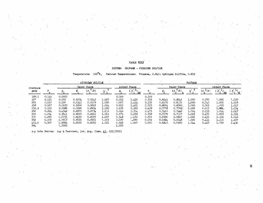
Pressure psia p ---...l r 189.1 o .• 145 197 0.151 205 0.157 218 0.167 252.5 0.193 292 0;224 332 0.254 370 0.283 392 0.300 401.5 0.307 394

x-y Data Source:

" TABLE XIII

SYSTEM: PROPANE - HYDROGEN SULFIDE . 0

Temperature: 100 F, Reduced Temperatures: Propane, 0.840; Hydrogen Sulfide, 0.832

HYDROGEN SULFIDE PROPANE

Va12or Phase Liguid Phase Va12or Phase

Y1 ¢1 (f//P) Y/ x.i. ( '){/\H p ¢2 r (f//P\ £ V 2

0.0000 0.000 0.306 0.050 0.9394 0.9143 1.027 0.012 1.422 0.319 0.8245 0.8245 1.000 0.100 0.9343 0.9109 1.026 0.027 1.414 0.332 0.8175 0.8172 i,.;ooo 0.1633 0.9269 0.9053 1.024 0.053 1.401 0.353 0.8064 0.8060 1.000 0.2986 0.9086 0.8904 1.020 0.136 1.360 0.409 0.7778 0.7766:' 1.002 0.4342 0.8875 0.8734 1.016 0.246 1.304 0.473 0.7469 0.7440 1.004 0.5641 0.8659 0.8561 1.011 0.375 1.238 0.538 0.7179 0.7117 1.009 0.6755 0.8459 0.8397 1.007 0.548 1.152 0.599 0.6926 Q.6817 1.016

,0.7817 0.8330 0.8301 1.003 o.687 1.087 0.635 0.6824 o.6648 1.026 0.8984 0.8266 0.8260 1.001 0.928 1.007 0.650. o.6849. 0.6560 1.044 1.0000 1.000

Kay & Rambosek, Ind. Eng. Chem • .!i2, 221(1953)

(f//P)

0.770 0.742 0.701 0.611 0.535 0.476 0.433 0.411 0.403

Liguid Phase

( ;r; L)SH ( C:/)d C

1.000 1.030 1.000 . 1.019 1.000 1.017 1.004 · 1.034 1.014 1.047 1.038 1.051 1.106 1.148 1.216 1.157 1.730 2;432

\11· -c

TABIE XIV

SYSTEM: PROPANE - HYDROGEN SULFIDE

Temperature: 120°F, Reduced Temperatures: Propane, 0,870; Hydrogen Sulfide, 0.862


Pressure Va2or Phase Liguid Phase Va2or Phase

¢1 (r//P) t} <Y/)s11 ¢2 (r//P\ yV psia p Y1 xl p

-- r __ r_ . 4 __

242,9 0.186 · 0.0000 0.000 0.393 254 0.194 0.050 0.9322 0.9001 1.036 0.020 1.406 0.411 0,7951 0.7950 1.000 266 0.204 0.100 0.9258 o.8954 1.034 0.042 1.395 0,431 0.7856 0.7853 1:000 282,5 0.216 0.1633 0.9172 0.8889 1.032 0.072 1.381 0.458 0,7728 o. 7725 '° i.ooo 322 0.246 0.2986 0.8968 0.8735 1.027 0.148 1.344 0.522 0.7434 0.7420 1.002 374,5 0.287 0.4342 0,8716 0.8531 1.022 0.267 1.285 0.607 0.7058 0.7016 1.006 427 0.327 0.5641 0.8456 0.8325 1.016 0.419 1.210 0.692 0.6712 0.6640 1.011 471 0.361 0.6755 0.8234 0.8153 1.010 0.564 1.140 0.763 0.6455 0.6327 1.020 498 0.381 0.7817 0.8084 0.8046 1.005 0.703 1 ;()78 0.807 0.6355 0.6140 1.035 510 0.391: 0.8984 0.8007 0.7999 1.001 0.941 1.005 0.826 o.6395 0.6016 1.063 503 0.385 1.0000 1.000

x-y Data Source: Kay & Rambosek, Ind. Eng. ·Chem. l±.2, 221(1953)

_<r}j!_)

0.750 0.717 0.678 0.602 0.525 0.467 0.429 0.409 0.401

Liguid Phase . L

( /(2 )SH _( 't/)ij

1.000 1.027 1.000 · 1.029 1.001 1.028 1.004 1.016 1.016 1.038,

· 1.049 1.078 1.112 1.119 1.227 1.142 1.763 2.746

°' 0

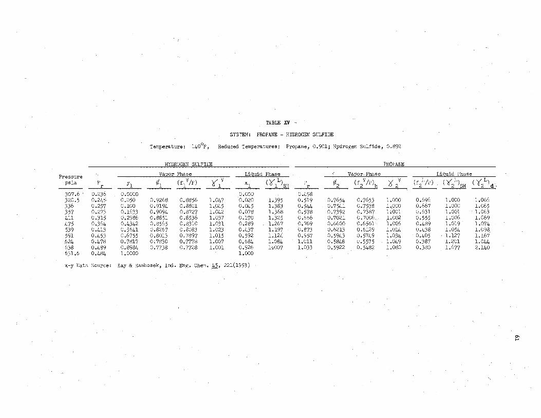
TABLE XV ~


Temperature: 140°F, Reduced Temperatures: Propane, 0.901; Hydrogen Sulfide, 0,892


Va12or Phase Li9uid Phase ' VaEorPhase Pressure psia p ¢1 (f//P) 't{ V xl 0(/)SH p ¢2 (f//P\ t/ r yl . 1 r --307.6 1 0.236 0.0000 0.000 0.498 320.5 0.245. 0,050 0.9268 0.8856 1.047 0.020 1.395 0.519 0.7654 0.7653 1.000 · 336 0.257 0.100 0.9194 0.880i 1.,045 0.045 1.383 0,544 0,7541 0,7538 1.,000 357 0.273 0.1633 0.9094 0,8727 1.042 0,07? 1.368 0,578 0,7392 0.7387 hOOl 411 0.315 0.2986 0.8851 0.8536 1.037 0.170 1.325 o.666 0.7021 0,7006;. 1.002 475 0.364 0,4342 0.8565 0.8310 1.031 0,289 1.267 0.769 0.6600 0.6561° 1.006 539 0.413 0,5641 0.8267 0.8083 1.023 0.437 1.197 0.873 0.6213 0.6129 1.014 591 0,453 0,6755 0.8013 0,7897 1.015 0.592 1.124 0.957 0.5943 0.5749 1.034 624 0,478 0.7817 0;7830 0.7778 1.007 o.684 1.084 1.011 0,5848 0.5575 1.049 638 0.489 ,0.8984 0.7738 0,7728 1.001 . 0.926 h007 1-033 0.5922 0,5482 1.080 631.6 0.484 1.0000 1.000

x-y Data Source: Kay & Rarnbosek, Ind. Eng. Chem. ~, 221(1953)

. (f//P)

0.696 0.667 (,,631 0,555 0.489 0.438 0.405 0.387 0,380

Li9uid Phase

(¥/\H ()'})d"

1.000 1.066 1.000 1.065 1.001 · 1.063 1.006 1.069 1.019. 1.074 1.054 1.098.

, 1.127 1.167 1.201 1.044 1.677 2,140

er,.. I-'

TABLE XVI··


Temperature: 160°F, Reduced Temperatures: Propane, 0.931; Hydrogen Sulfide, 0.921


VaEQr Phase Li9uid Phase ' Va12or Phase Pressure psia p Y1 f.\ (f//P) 't/ ~ (//)SH p ¢2 (f/ /P)h /I" V

r r 2 --384.5 0.294 0.0000 0.000 400 0;306. 0.050 0.9244 0.8702 1.062 0.023 1.384 0.648 0.7334 0.7334 1.000 . 419 0.321 0.100 0.9160 0.8642 1.060 0,050 1.371 0.679 0.7207 0.7204 1.000 447 0,342 0.1633 0.9047 0,8552 1.058 0.089 1.354 0,724 0,7022 0.7027 0,'999 519 0.397 0.2986 0,8780 0,8321 1.055 0.198 1.305 0.841 0,6551 o,6538<'· 1.002 596.5 0,457 0.4342 0.8475 0.8072 1.050 0,326 · 1.244 0.966 0.6059 o.603z 1.004 671 0,514 0,5641 0.8150 0,7831 1.041 0,470 1.177. 1.087 0.5612 0.5538 1.013 734 0,562 0,1,755 0,7846 0,7625 1.029 0.623 1.108 1.189 0.5282 0.5110 1.034 773 0.592 0.7817 0.7581 0,7496 1.011 0,759 1.053 1.252 0.5259 G,4863 · 1.081 790 0.605 0.8984 0,7453 o. 7439 1.002 0.925 1;007 1,280 0,5406 0,4765 1.135 781.6 0,598 1.0000 1.000

x-y Data Source: Kay & Rambosek, Ind, Eng. Chem, 1±2; 221(1953)

Li9uid Phase

Cf//P) ( 'tf})SH

0.712 1.000 0,683 1.000 0.644 l.OCl 0.563 1.008 0.513 1.025 0,461 1.064 0,428 '1.145 0.400 1.284 0~393 1,654

( t/)d

1.001 0,999

·1.001 1.018 0,991 1.001, 1.063 1.191 1.864

"' . 11.l

TABLE XVII


Temperature: Hl0°F, Reduced Temperatures: Propane, 0.961; Hydrogen Sulfide, 0,951


Pressure Va12or Phase Liguid Phase va12or Phase Liguid Phase

psia p Y1 !\ (f//P) ?( V xl (¥/)SH p ¢2 (f//P\ '6 V (f2L/P) <Y/)sH ct/>d -- r 1 r 2 474,8 .· 0.364 0.0000 0.000 496 0,380 0.050 0,9295 0,8535 1.089 0.026 1.373 0.803 0.6979 0.6979 1.000 u.684 1.000 0,995 521 0,399 0.100 0,9212 0.8462 1..089 0.057 1.359 0,844 0.6820 o.6818 1.000 0,654 1.000 0,995 558 0.427 0.1633 0,9120 0,8355 1.092 0.105 1.338 0,904 0.6580 0,6581 1.000 0.615 1.002 1.000 651 0,498 0,2986 0,9970 0,8083 1.233 0,230 1.281 1.055 0.5576 0,5806 0,960 0,536 1.011 0,948 748 0,573 0,4342 0,8908 0,7799 1.142 0,369 1.218 1.212 0.4999 0,4984 1.003 0,476 1.055 · 0.942 838,5 0.642 0,5641 0.8116 0,7531 1.078 0.522 1.149 1.358 0,4581 0,4302 1.065 0,432 1.084 0,967 904 0.692 0,6755 0,7627 0,7334 1.040 0,652 1,093 1.464 0,4336 0,3812 1.137 0,406 . 1.164 0,995· 945 0.724 0,7817 0,7342 0.7207 1.019 0.755 1.054 1.531 0,4214 0,3542 1.190 0,391 1.272 0.960 964,2 0,738 0,8984 o. 7173 0.7147 1.004 0,841 h026 1,567 0,4824 0,3759 1.283 0,384 1.861 0.803 956,4 0,732 1.0000 1.000

x-y Data Source: Kay & Rambosek, InEl, Eng. Chem. 45, 221(1953)

e,

TABLE XVIII,

SYSTEM: PENTANE - HYDROGEN SULFIDE

Temperature: 40°F, Reduced Temperatures: Pentane, 0.591; Hydrogen Sulfide, 0.743

HYDROGEN SULFIDE n-PENTANE

Pressure VaEor Phase Li9uid Phase Vae2r Phase Li9uid Phase

¢1 (flV /P) 1s} L ¢2 (r//P)h ~v (r//P) 0(/)sH ct/)d psia p Y1 ~ (o"l )SH p

2 r r -- ' 4.4* 0.0000 0.0000 4.5 0.0034 0.0300 1.0014 0.9974 1.004 0.0092 0.986-7 0.9940 0,993 4.8; 0.0037 0.1000 1.0010 0.9973 1.004 0.0098 0.9862 0.9861 1.000 5.3 0.0040 0.2000 1.0001 0.9969 1.003 0.0107 0.9848 0.9847 1.000 8.1 0.0062 · 0.5000 0.9972 0.9953 1.002 0.0166 0.978l 0,9773 1.001 •-

20 0.0153 0.7842 0,9889 0.9880 1.001 0.0617 1.126 0.0409 0.9531 0.9502 1..003 0.220 1.000 0.996 40 0.0306 0.8950 0.9765 0.9761 1.000 0.1425 l.llS 0.0817 0.9142 0.9088 1;006 0.114 1.001 · 0,978 60 0.0459 0.9304 0.9645 0.9642 1.000 0.2260 1.109 0.1226 0.8764 0.8696,;-· 1.008 0.075 1..003 1.051 80 0.0613 0.9534 0.9525 0.9523 .1.000 0.3232 1.097 0.1634 0.8402 0.8.32tf 1.009 - 0.057 1.007 i.016

100 0.0766 o.9685 0.9405 0.9404 1..000 0.4372 1.082 0.2043 0.8051 0.7963 1.011 0.046 1.016 0.980, 125 0.0957 0.9820 0.9256 0.9255 1.000 0.6106 1.055 0.2554 0.7628 0.7526 1.014 0.037 ' 1.045 0.952 150 0.1149 0;993 0.9107 b.9107 1.000 0 • .821 1.020 0.3064 0.7222 0.7099 1.017 0.031 1.146 0.955 169H 0.1294 1.000 1.000

* Vapor Pressure of n-Pentane -IHI- Vapor Pressure of Hydrogen Sulfide

x-y Data Source: Reamer, Sage & Lacey, Ind. Eng. Chem. 45) 1805(1953)

i-

TABLE XIX

SYSTEM: n-PENTANE - HYDROGEN SULFIDE

Temperature: l00°F, Reduced Temperatures: n-Pentane, 0.662; Hydrogen Sulfide, 0.832


Pressure Vaeor Phase Li9uid Phase Vaeor Phase psia p

Y1 ¢1 (f//P) Y/ ~ ( Y"/)SH p ¢2 <r2v/P\ 't/ r r --15.7-!.' 0.0000 0.0000 16.2 0.012 0.0300 1.0045 0.9930 1.012 0.033 0.9646 0.9646 1.000 17.J 0,013 0.1000 1.0031 0,9926 1.011 0.035 0,9625 0.9624 1.000 19,4 0.015 0.2000 1.0010 0.9915 1.010 0.040 0.9584 0,9582 1.000 26 0.020. 0.4000 0.9957 0.9886 1.007 0.053 0.9465 0.9452 1.001 50 0.038 0.6684 0.9824 0.9781 1.004 0.0788 . 1.115 0.102 0.9086 0.9043 l.005

100 0.076 0.8310 0.9586 0.9564 1.002 0,1951 1.103 0.204 0,8381 0.8290 l~:011 150 0.114 0,8970 0,9360 0.9347 1.001 Q,3151 1.090 0.306 0.7740 0.7606 i. 1.018 200 0.153 0.9280 0.9139 0,9131 1.001 0.4380 1.075 0.409 0.7127 0,6968"' 1.023 250 0.191 0.9491 0.8920 0.8915 1.001 0.5662 1.057 0.511 0.6547 0.6370 1.028 300 0.230 0.9675 0.8702 0.8699 1.000 0.7080 1.036 0.613 0.6009 0,5807 1.035 350 0.268 0.9850 0.8484 0.8483 1.000 0.860 1.012 0,715 0,5512 0.5276 1.045 394** 0.302 1.0000 1.000

* Vapor Pressure of n-Pentane ** Vapor Pressure of Hydrogen Sulfide

x-y Data Source: Reamer, Sage & Lacey, Ind; Eng. Chem, 1±.2.,· 1805(1953)

Li9uid Phase

(f//r:) ( ll'})SH

0.297 1.000 0.153 1.002 0.105 1.006 0.080 1.015 0.066 1.032 0.056 · 1.071 0.049 1.168

(';.{/)d

1.101 · 1.150 1.109 1.141 1.164. 1.194 1.215

0-. V,.

TABLE XX


Temperature.: 160°F, Reduced Temperatures: n..:.Pentane, 0.734; Hydrogen Sulfide, 0.92.1

HYDROGEN SULFIDE n-rEiTANE

Pressure Va122r Phase Li9tiid Phase Vaeor Phase

(r//P) Y/ L (r//P\ Y./ psia p Y1 ¢1 Xi ()J\ )SH p ¢2 -- r r

' 42.5* 0.0000 0.0000 44.0 0.034 0.0300 1.0118 0.9856 i.027 0.090 0.9274 0.9274 1.000 48.3 , 0.037 0.1000- 1.0090 0.9842 1.025 0.099 0.9206 0.9205 1.000 55.7 0.043 0.2000 1.0044 0.9817 1.023 0.114 '0.9096 0.9092 1.000 71.4 0.055· 0.3500 0.9958 0,9766 1.0-20 0.146 0.8880 0.8864 1.002

100 0.077 0.5124 0,9825 0.9671 1.016 0~0799 . 1.106 0.204 0,8525 0,8485 l.005 200 0.153 0.7355 0,9441 0,9347 1.010 0.2218 1.093 0,409 0.7451 0,7341 1;:015 300 0,230 0,8279 0.9088 0.9024 1.007 0,3626 1.078 0.613 0.6529 0,6359 2· 1,028 400 0.306 0.8840 0.8744 0.8702 1.005 0.4995 · 1.062 0.817 0,5714 0.5492•' 1.040 500 0.383 0.9277 0,8403 0,8382 1.003 0,6372 1.043. 1.021 0.5004 0.4711 1.062 600 0.459 0,9553 0.8072 0.8061 1.001 0.7687 1.024 1.226 0.4330 0,3978 1.088 700 0.536 0,981 0.7739 0.7736 1.000 0,900 1.007 1.430 0,3732 0~3333 · 1.120 778,'f)f* LOOO 1.000

* Vapor Pressure of n-Pentane ** Vapor Pressure of Hydrogen Sulfide

x-y Data Source: Reamer, Sage & Lacey, Ind; Eng. Chem. 45,· 1805(1953)

Li9:B:i.d Phase

(f//P) ( ){2 L)SH

0.392 1.000 0,205 1.003 0,143 1.008 0.113 1.020 0.094 1.045 0.082 '1.093 0.073 1.197

<i})4

1.152 · 1.235 1,233 1.172 1.061. 1.021 0,951

0-0'-

I.

TABLE lll.

SYSTEM1 n-PENTANE - HYDROGEN SULFIDE ~

Temperature: 220°F, Reduced Temperatures: n.:.Pentane, 0.804; Hydrogen Sulfide, 1.011


Pressure :l[a122r Phase ~:l,gW,d Phase Va:eor Phase

psia p YJ: ¢1 (flV /P) 'lf1v ~ 0(/)SH p ¢2 (r//P)h Y/ -- r: r

94.9* o~·cm 0.0000 0.0000 ' 100 o.m 0.0559 1.0249 0.9748 1..051 o.oo62. 1.105 · 0.204 0.8726 0.8725 1.000 200 0.153 0.4698 0.9820 0,9498 . 1.034 0.1014 1,098 0.409 0.7710 0.7658 1.007 JOO ) 0.230 0,6251 0,9502 0.9251 . 1.027 0.1965 1.090 0.613 "'0.6881 0,6782 1.015 400 0,306 · · 0,7147 0,9208 0.9005 1.022 0.2912 1,081 0.817 0.6159 0.6013 1.024 ·. 500 0,383 0,7745 0.8928 0,8761 1,019 0.3838 1.071 1.021 · 0.5509 0.5324 1.935 600 o.459 0.8185 ci.8656 0.8519 1.016 0,4740 1.061 · 1.226 0.4919 0,4701 1;,046 700 0,536 0.8518 0,8392 0~8277 1.014 0.5604 1.051 1.430 · 0.4372 0.4133 /· ) .• 058 800 0.613 0.8769 0.8136 · 0.8036 1.012 0.6421 1.040 1.634 0.3851 o.36otk 1.067 900 0,6B9 0.8963 0.7886 0.7796 1.012 0.7165 1.030 1,839 0.3345 0.3111 1.075

1000 0.766 0.9125 0,7639 0.7554 1.011 0.7859 1.020 2,043 0,2848 0.2642 1.078 1100 0.842 0,9289 0.7391 0,7309 1.011 0,8506 1.012 2,247 0.2362 0.2187 1.080 1200 0.919 ,0.9474 0,7138 0.7060 1.011 0.9110 1-:-005 2,451 0.1855 0.1714 1.082 1300 0.9.95 0.968 0.6856 0.6802 1.008 0.966 1.001 2.656 0.1372 · 1302** 0,997 0.966 o.6853 0.6797 1.008 0.966 1.001 2.660 0,1344

* Vapor Preaaure of n-Pentane ** Critical.State

x-y Data Sollftle1 Re&lller, Sage.& Lacey, Ind. _Eng, Chem • .!±2, 1805(1953)

(r//P)

0.808 0.420 0.292 0.228 0.190 0.165 0.147 0.133 0.123 0.115 0.108 0;102 0.098 0.098

· Liguid Phase

<Y/)SH <Y/),

1.000 1.026 1.000 1.083 1.002 1.100 1.004 1.087 1.009 1.044 1.016 . 1.029 1.027 1.003 1.043 . 0.996 1.065 0.995,

, l.096 1.012 1.138 1.041 1,196 1.075 1,277 1.277 1.277

°' . ...,;:i

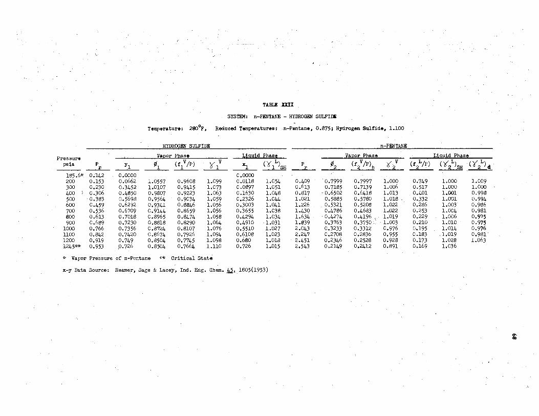
\. j

TABLE DII

SYSTEM1 n-PENTANE - HYDROGEN SUI.FI~

Temperature: 280°F, Reduced Temperatures: -n..;.Pentane, 0.875J Hydrogen Su;Ltide, 1.100


Pressure Va!!or Phase Liguid Phase Va!!or Phase Liguid Phase

¢1 (flV /P) 't lv Ct />sH ¢2 (t//P\ '6- V (r//P) . L - L

psia p Y1 ~ p <Y2 >sH ct2 >c1 r r 2 --

185.6* 0~142 0.0000 0.0000 (""

200 0.153 0.0662 1.0557 0,9608 1.099 0.0118 1.054 0.409 ·0.7999 0,7997 1.000 0.749 1,000 1.009 300 0.230 0,3452 1.0107 0.9415 1.073 0.0897 1.051 0.613 0.7185 0.7139 1.006 0.517 1.000 1.000 400 f o.3o6 0,4850 0.9807 0.9223 1.063 0.1630 1.048 0.817 ~0.6502 0.6418 1.013 0.401 1.001 0,998 500 · 0.383 0.5698 0.9564 0.9034 1.059 0;2326 1.044 1.021 0.5885 b.5780 1.018 - 0,332 1.001 0.994 600 0.459 0.6292 0,9341 0.8846 1.056 0.3003 1.041 1.226 . 0,5321 0.5208 1,.022 0.286 1.003 0.986 700 0,536 0.6709 0.9144 -0,8659 1.056 0,3655 1.038 1.43q 0,4786 0,4683 1.-022 0.253 1.004 '0,981 800 0.613 0,7018 0.8965 0,8474 1.058 0,4294 1.034 1,634 · 0,4274 0,4196 / 1~019 0,229 1.006 0.975 900 o,689 0.7230 0,8818 0.8290 1.o64 0.4910 -1.031 1.839 0,3763 0.3750,; · 1.003 0.210 1.010 · 0.975

1000 0,766 0.7356 0.8724 0,8107 1.076 0,5510 1.027 2.043 0,3233 0,3312 0,976 0,195 1.014 0.976 1100 0,842 0.7420 0.8674 0,7926 1.094 0.6108 1.023 2,247 0.2708 0,2836 0.955 0.183 , 1.019 0,981' 1200 0,919 0,749 0,8504 0,7745 1.098 0,680 1,018 2,451 0,2346 0,2528 . 0,928 0.173 1.028 1.063 1245** 0,953 ,0.726 0,8504 0.7664 1.liO 0.726 1.015 2,543 0.2149 0.2412 0.891 0.169 1.036

* Vapor Pre·ssure of n-Pentane ** Critical State

x-y Data Source: Reame_r, Sage & Lacey, Ind, Eng. Chem. l!:i,. 1805(1953)

g;

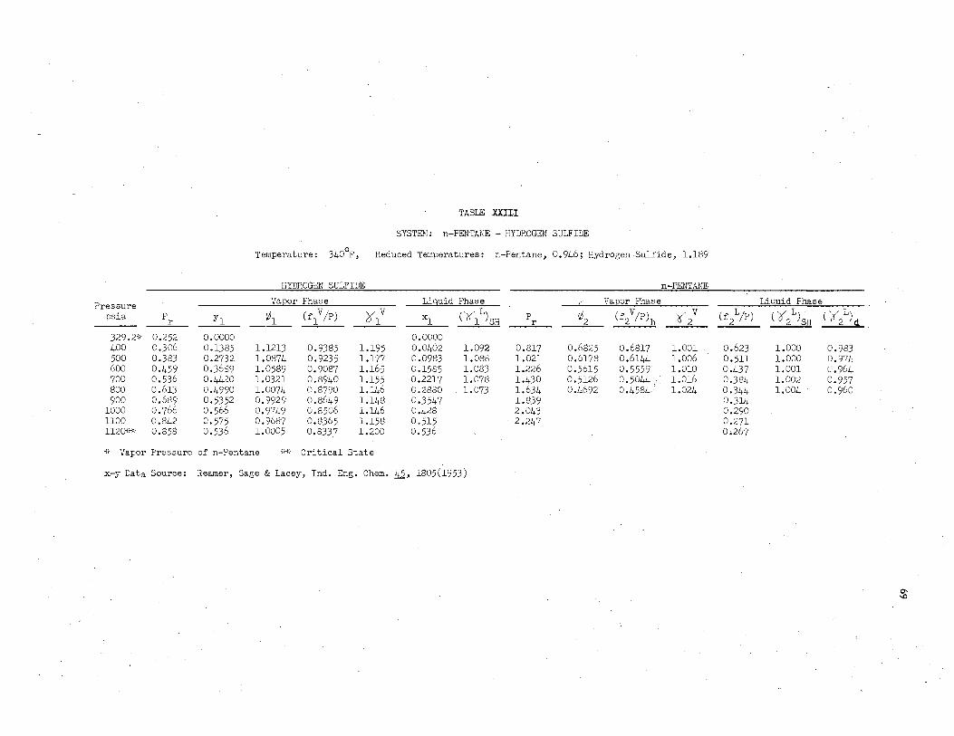
TABLE XXIII


Temperature: 340°F, Reduced Temperatures: n-Pentane, 0.946; Hydrogen Sulfide, 1.189


Pressure Va12or Phase Liguid Phase .: Va12or Phase Liguid Phase

psia ¢1 (f//P) >f/ L ¢2 (f//P)h 'i/ (f//P) ( Y/)sH cY/)d p Y1 xl (Yl )SH p

-- r r

329.2* 0.252 0.0000 0.0000 400 0,306 0.1385 1.1213 0.9385 1.195 0.0462 1.092 0.817 0.6825 o.6817 1.001 0.623 1.000 0.983 500 0.383 0.2732 1.0874 0.9235 1.177 0.0983 1.088 1.021 o.6178 0.6144 1.006 0.511 1.000 0.974 600 0.459 0.3689 1.0589 0.9087 1.165 0.1585 1.083 1.226 0.5615 0.5559 1.:010 0.437 1.001 · 0.964 700 0.536 0.4420 1.0321 0.8940 1.155 0.2217 1.078 1.430 0.5126 0.5044 .o: 1.016 0.384 1.002 0,957 800 0.613 0.4990 1.0074 0.8790 1.146 0.2880 1.073 1.634 0.4692 0,4584 1.024 0.344 1.004 · 0.960 900 0.689 o. 5352 0.9929 0.8649 1.148 0.3547 1.839 0.314

1000 0.766 0.566 0,9749 0.8506 1.146 0.428 2.043 0.290 1100 0.842 0.575 0.9687 0.8365 1.158 0.515 2.247 0.271 112()lH<· o.858 0.536 1.0005 0.8337 1.200 0.536 0.267

* Vapor Pressure of n-Pentane iH~- Critical State

x-y Data Source: Reamer, Sage & Lacey, Ind. Eng. Chem. 45,. 1805(1953)

$

APPENDIX B

DISCUSSION OF THE REDLICH-KWONG EQUATION OF STATE

FOR THE CALCULATION OF VAPOR PHASE

FUGACITY COEFFICIENTS

The Redlich-Kwong (41) equation of state, developed in 1949, is

an empirical two coefficient equation designed to describe the P-V-T

behaviour of gases at temperatures above the critical and at all pres-

sures. This equation is applicable to both pure gases and mixtures

of gases. Its utility lies upon the fact that with only two coef-

ficients it is relatively simple and that these coefficients are

derived from the readily attai.~able critical constants of the gases

in question.

The equation is represented by

p RT = ..,...(v-. ---b-...) -J.

a

T0 •5v (V. + b) -i -J.

(B-1)

Five auxiliary equations are presented to make equation B-1

usu able

z =

z

1 A21. h ] (1 - h) - ~l(l + h~

PV. """l.

RT

70

(B-2) ·

(B-3)

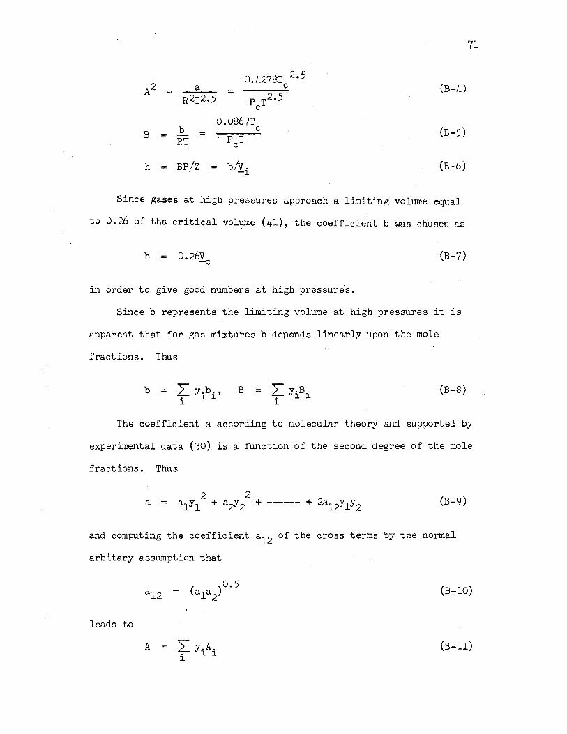
0 427~ 2·5 A2 a • C

= = R2T2.5 p T2.5

C

(B-4)

0.0867T b C

B = = RT PCT

(B-5)

h = BP/Z = b/y_. -1

(B-6)

Since gases at high pressures approach a limiting volume equal

to 0.26 of the critical volume (41), the coefficient b was chosen as

b = 0.26v _-c

in order to give good numbers at high pressures.

(B-7)

Since b represents the limiting volume at high pressures it is

apparent that for gas mixtures b depends linearly upon the mole

fractions. Thus

b = L y.b., • 1 l. 1

B = L y;Bi . 1 1

(B-8)

71

The coefficient a according to molecular theory and supported by

experimental data (30) is a function of the second degree of the mole

fractions. Thus

(B-9)

arid computing the coefficient a12 of the cross terms by the normal

arbitary assumption that

leads to

A = ~ y.A. i 1 1

(B-10)

(B-11)

72

The fugacity coefficient of compone~t i in a mixture is by

definition

(B-12)

and is obtained from the equation of state by integrating the equation

from P = 0 to P = P.

(z - 1) £f i . p

Integration of. this equation gives

. . B

log ~\ = Q.4343(z - 1) Bi - log (Z - BP)

_ i12Ai .... Bil. log [i + B~l. B-LA BJ ·. ZJ

(B-13)

(B-14)

For the details of the integration the reader is referred to the

original paper (41). ·

To simplify this equation in making hand calculations, it is

rearranged by use of two additional terms,

. (B-15)

W = 0.4343(z - 1) + 0,5U (B-16)

Substitution of these terms reduces equation B-14 to

log 4' = o.4343{z - 1) - log {Z - Bl') - f log ~ + ~~ (B-17)

'

log ¢1 = log lf - * {Ai - A) + J, (Bi - B:) (B-18)

This equation is used by first calculating the constants Ai' Bi, 2 .

A, B, and A /B under the known conditions of pressure, .temperature

73

and compositi,on by means. of equations B-4, B-5, B-8, and B-11. A

value of Z is assumed from which a value of his calculated by equation

B-6. Z is then calculated by means of equation B-2. The correct

value of Z is obtained when the calculated value checks the assumed

value. It is then ~sed in equations B-15 and B-16 to calculate U and

W. These values are substituted into equation B~l7 and B~l8 and the

fugacity coefficient of component i in the mixture is calculated. This

equation is valid for cale1,1lation of the fugacity coefficient of pure

components as the values of Ai and Bi become equal to A and B respec

tively, hence the last two terms of equation B-18 become zero and¢. l

becomes the fugacity coefficient of the pure component.

The use of the Redlich-Kwong equation of state in a sample

calculation is presented in Appendix H.

APPENDIX C

DISCUSSION OF THE CHAO-SEADER. EQUATION FOR CALCULATION

OF THE PURE LIQUID FUGACITY COEFFICIENTS

Chao and Seader developed an equatiori (9) for the pure liquid

fugacity coefficient within the framework of the generalized cor-

relation of Curl and Pitzer (11). This was done by developing

an algebraic form of the equation and extending with the use of

experimental data into the region of the hypothetical liquids,

i.e., into the region where a component cannot exist in the pure

state as when the system pressure is below the vapor pressure or the

temperature is above the critical temperature. The extension was

also made toward lower reduced temperatures.

where

The equation is given by

o (o) (1) log V = log7/ + WlogV

log 2) (o) = Ao + A1/Tr + A2Tr + A3Tr 2 + A4Tr3

2 + (A5 + A6Tr + A7Tr )Pr

+ (AS + A9T )P 2 - .log P r r · r

- 4.23893 + 8.65808Tr - 1.22060/Tr

- 3.15224T 3 - 0.025(P - 0.6) r r

74

(C-1)

(C-2)

(C-3)

The coefficients for equation C-2 are given in Table XXIV.

TABLE XXIV

COEFFICIENTS FOR EQUATION C-1

Coefficient Simple Fluid Methane Hzyrogen

Ao 5.75748 2.43840 1.96718

Al - 3.01761 - 2.24550 1.02972

A2 - 4.98500 - 0.34084 - 0.054009

A3 2.02299 0.00212 0.0005288

A4 o.oo - 0.00223 o.oo

A5 0.08427 0.10486 0.008585

A6 0.26667 - 0.03691 o.oo

A7 - 0.31138 o.oo o.oo

Ag - 0.02655 o.oo 0.00

A9 0.02883 o.oo o.oo

The term V (o) is the fugacity coefficient of the simple fluid

which is characterized by an acentric factor, 0..), of zero. The term

(>.:)"2/(l) is a correction applied to real fluids to account for their

departure from simple fluids.

The terms 2./(o) and 1/(l) are functions only of the reduced

temperature and pressure.

Special coefficients were devised when using this equation for

hydrogen and methane since the normal temperature of interest with

75

these compounds is far above their critical. The acentric factor for

these compounds is taken as zero.

The acentric factor measuring the deviation of a given real fluid

from a simple fluid is defined 'by Pitzer (11) as

w = 0

(1.000 + log Pr )T = 0•7 r

0 where P is the reduced vapor pressure at a reduced temperature

r

of 0.7.

76

Chao and Seader, however, used an acentric factor, only slightly

different, calculated in a manner to minimize the error between the

experimental 21° and the calculated 7..1°.

In this work, however, the value of UJ as calculated by the Pitzer

equation is used.

APPENDIX D

VAN LAAR EQUATION AS MODIFIED BY THE SCATCHARD

AND HILDEBRAND REGULAR SOLUTION TREATMENT

Van Laar using the constants in van der Vaals' equation of state

developed expressions for the activity coefficients of components in

solution with one another. These equations are stated as

1n yL = B'LT 1 (1 + A1x1/x2)2

(D-1)

L A'B'LT 1n ¥2 = . 2 (A'+ x2/x1 )

(D-2)

where

A' (D-3)

B'

a and bare the van der Vaals 1 constants.

If B1 is made equal to A and A' equal to A/B then

A (D-5)

77

78

1n }( L B = 2 ~ B12 l+-Ax1

(D-6)

where b b 0,5 o.j 2

A B' 1 al a2

= = - ---R bl b2

(D-7)

b b 0,5 o.~2 B L 2 al a2

= = ------A' R bl b2 (D-8)

For more complete details of the development of the Van Laar

equation the reader is referred to the text of Robinson and

Gilliland (42).

Scatchard (43) and Hildebrand (21) independently without the use

of the inexact van der Vaals fluid arrived at similar expressions.

These developments were based on 'regular solutions'. A 'regular

solution' may be defined as one having the properties:

1. The energy of a molecular pair is dependent only on their

relative position in the solution and their orientation and is

independent of all other molecules present and of the temperature.

2 •. The distribution and orientation of the molecules is random,

i. e., other molecules and temperature have no effect.

3 •. The volume of a component in the mixture does not change

upon mixing at constant pressure and temperature.

The development for a binary solution only will be described.

Using the above criteria for a 'regular solution' the cohesive

energy of one mole of a mixture is

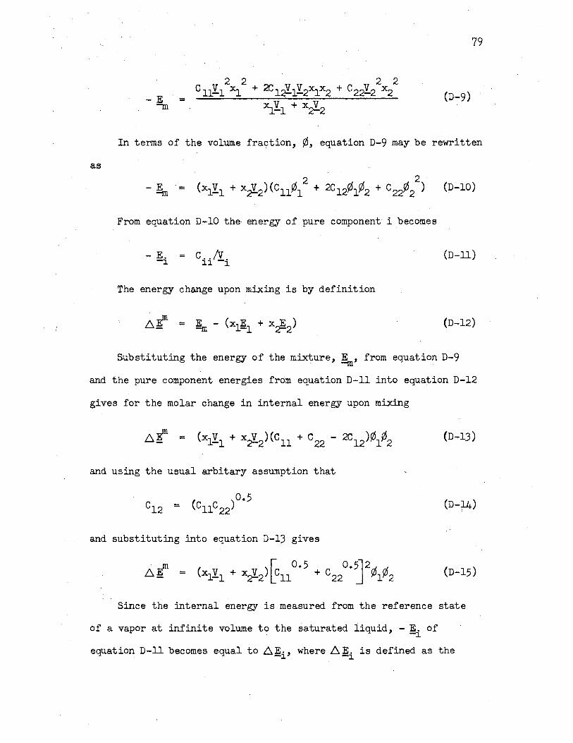
79

-E = (D-9) -m

In terms of the volume fraction,¢, equation D-9 may be rewritten

as

-E -m (D-10)

From equation n~10 the- energy of pure component i becomes

(D-11)

The energy change upon mixing is by definition

(D-12)

Substituting the energy of the mixture, E , from equation D-9 . . -m

and the pure component energies from equation D-11 into equation D-12

gives for the molar change in internal energy upon mixing

(D-13)

and using the usual arbitary assumption that

(D-14)

and substituting into equation D-13 gives

(D-15)

Since the internal energy is measured from the reference state

of a vapor at infinite volume to the saturated liquid, - ~ of

equation D-11 becomes equal to ~~i' where ~!i is defined as the

80

internal energy of va~orization to infinite volume. Hence from

equation D-11

C = [·.b:.Y.~11]0.5 [b:.~~0.5 · 11 and c22 = -V-

-2 (D-16)

The term (.6,~·IY. )0•5 was named the "solubility parameter11 with ... -i. .

the units of (cal/cc)0 •5 and given the symbol delta, 8, by Hildebrand.

Substituting the equivalents of c11 and c 22 into equation D-15

gives

(D-17)

or

(D-18)

From the definition of a 'regular solution' that i:).V. = 0 on -1

mixing

(D-19)

Thus converting equation D-18 to

(D-20)

and going to a total mole basis

(D-21)

and taking the partial deriative with respect to n1

U ~ 2 2 o. H = V ¢ ( S - 6 ) an -1 2 1 2 n2,P,T

(D-22)

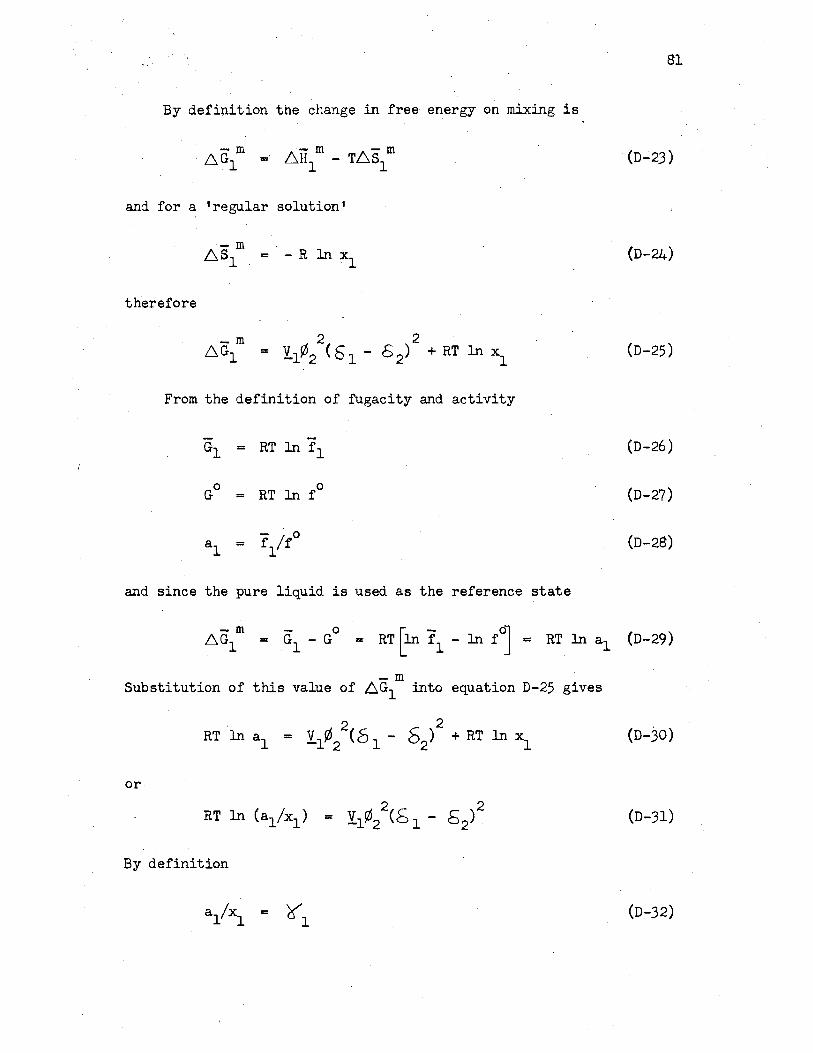
By definition the change in free energy on mixing is

and for a 'regular solution'

therefore

From the definition of fugacity and activity

G1 = RT 1n f 1

G0 = RT 1n f 0

-f /f0 al = 1

and since the pure liquid is used as the reference state

-m Substitution of this value of ~G1 into equation D-25 gives

or

( I ) ¢ 2( C C )2 RT 1n al xl = 11 2 o 1 - a2

By definition

81

(D-23)

(D-24)

(D-25)

(D-26)

(D-27)

(D-28)

(D-30)

(D-31)

(D-32)

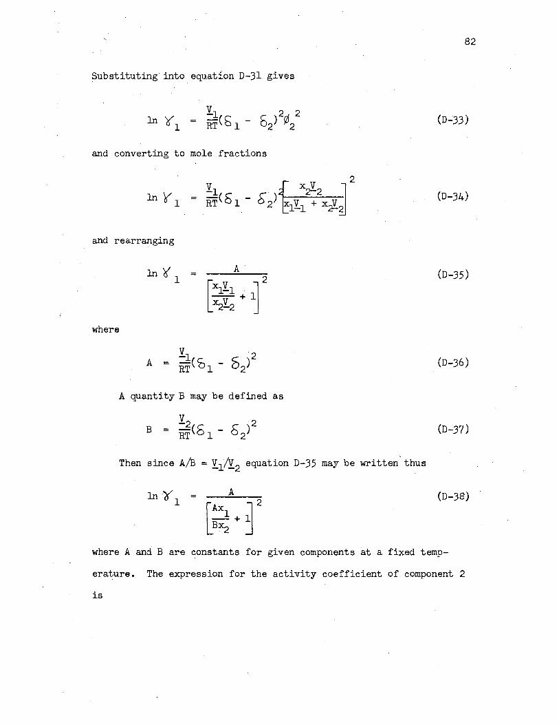
Substituting into equation D-31 gives

and converting to mole fractions

and rearranging

A

where

A quantity B may be defined as

Then since A/B = y1/y2 equation D-35 may be written,thus

1n ';( 1 =[ -A-x. __ A_~-2

--1: + 1 B~

82

(D-33)

(D-34)

(D-35)

(D-36)

(D-37)

(D-38)

where A and Bare constants for given components at a fixed temp-

erature. The expression for the activity coefficient of component 2

is

83

1n ?(2 B

(D-39)

and is derived in a like manner.

Note that these are forms of the Van Laar equations D-7 and D-8,

but do not depend upon the van der Vaals fluid to calculate the

constants A and B.

APPENDIX E

DISCUSSION OF THE WATSON VOLUME FACTOR

AS MODIFIED BY STUCKEY

Molar liquid volumes are necessary in the application of the

Scatchard-Hildebrand equation for the liquid activity coefficient.

An equation, E-1, first introduced by Gamson and Watson (17) permitted

calculation of the molar volume for both real and hypothetical liquids.

L V v1w (5.7 + 3.0 T)

1 r

where V 1w1 is a reference voiuP.J.e expansion factor

Watson initially applied to the liquid phase the gas phase

relationship that

PV ZRT

(E-1)

(E-2)

where Z is a generalized function of the reduced temperature and

pressure only. The expression for the liquid density obtained from

equation E-2 is

p M V

MP ZRT

P PM r C ---ZRT T

r C

WP M C

T C

where W, the expansion factor, is defined as

w p

_r_ ZRT

r

84

(E-3)

(E-4)

85

- 1 W has the units of R · and is a function of the reduced pressure and

temperature only.

The expansion factor, W, can be made dimensionless by redefining

it as the ratio of the ideal critical volume to the actual volume thus

RT /P p

w = Yc/Y ~/P C C = r (E-5) ZRT/P ZT

1. 1. r

where

V = ideal critical volume Ci

Pei = ideal critical density

Watson found that equation E-4 defining the expansion factor did

not give satisfactory results but that by applying the value of W

obtained for just one compound to all compounds gave a greatly im-

proved correlation. He used iso-pentane to obtain his initial plot

of the expansion factor. This was then applied to all compounds

through the equation

(E-6)

To apply this equation a single density at some convenient temperature

must be known. w1 is read from Watson's plot at the same temperature,

then Vat any other temperature is found by obtaining W from the plot

at this new temperature and applying equation E-4.

Equation E-4 was further simplified by Watson without a great

loss in accuracy by making

1/W = 5.7+3.0T r

W was selected at a sufficiently high pressure to make the

(E-7)

liquid phase essentially incompressible. The expansion factor then

86

becomes a function of only the reduced temperature.

Stuckey (46) .because of the difficulty in locating values of v1w1

and for ease of use on a digital computer defined a 'reduced expansion

factor' as

(E-8)

which he correlated with established values of v1w1 using the acentric

factor, 6J, as a third identifying parameter. The resulting equation

v' = 0.01361 - o.00328GJ - o.0244u.J2 + o.0599u.;?

- 0,0308W4 (E-9)

was further simplified to increase its usefulness without appreciable

loss in accuracy to

v' = 0.01361 - 0.00436 W (E-10)

The reduced volume, V, is calculated using the Watson form of the r

equation as

V = v 1 (5,7 + 3,0 T) r r

(E-11)

The reduced volume was separated into that of a simple fluid

(lu = 0) plus a correction for a real fluid by the equation

0 (E-12) V = V + !'.0V r r r

where

V reduced volume for the simple fluid r

V = correction for the acentric factor r

0 I V and V are linear functions of reduced temperature and as

r r

such are easily calculated. The molar liquid volume is calculated

from the reduced volume by

87

·. v1 == RT V L /P - C r C

(E-13)

. I

Stuckey (46) has tabulated the values of V~ and Vr · over the range

of reduced temperatures norm.ally encountered.

Stuckey found excellent agreement between the volumes calculated

by equation E-13 and those calculated by equation E-1.

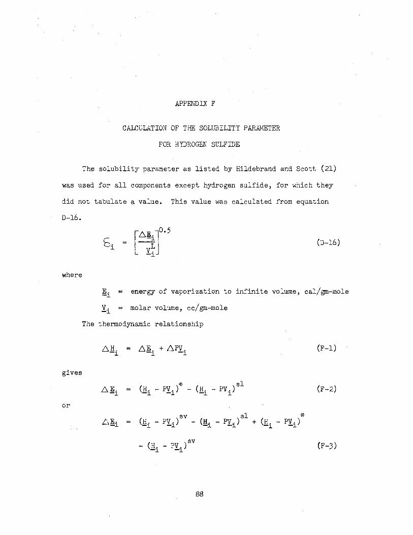
APPENDIX F

CALCULATION OF THE SOLUBILITY PARAJ.VlETER

FOR HYDROGEN SULFIDE

The solubility parameter as listed by Hildebrand and Scott (21)

was used for all components except hydrogen sulfide, for which they

did not tabulate a value. This value was calculated from equation

D-16.

where

(D-16)

E. = energy of vaporization to infinite volume, cal/gm-mole -1

v. = molar volume, cc/gm-mole -J..

The thermodynamic relationship

(F-1)

gives

(F-2)

or

_6E. = -J..

SV - (H. - PV.)

-1 -1 (F-J)

88

or * . SV . sl

6E, = H . t' + H. - H. + RT(Z - 1) (F-4) -i · -vaporiza ion -i -i i '

where sv, sl, and* refer to the saturated vapor state, saturated

liquid state and ideal gas state respectively.

. 0 For hydrogen sulfide at saturation and 25 C.

p r

= 0.224 (49)

Tr = 0.198 C49r

z = 0.278 (2) C

zsl == 0.034 (24) .

v1 = 0.02091 ft3/# (49)

Rvap = 183.2 BTU/# (49)

* n o (li - li )/Tc = 0.711 cal/gm-mole/ K (24)

* sv . 0 . (fl - li ) = (0. 711)(373.61. K) = 266 cal/gm-mole

y_1 = (0.02091 ft3/#)(34.08 #/#-mole)(62.422 cc/gm/ft3/#)

y_1 = 44.48 cc/gm-mole

89

H = (183.2 BTU/#)(34.08 #/#-mole)/(1.8 BTU/#-mole/cal/gm-mole) -vap

H = 3469 cal/gm-mole -vap

Substituting these values into equation F-4 gives

61 = (3469 cal/gm-mole)+ (266 cal/gm-mole)

+ (1. 987 cal/gm-mole/K)(373 .61°K)(0.034 - 1)

61 = 3163 cal/gm-mole

Then substituting into equation F-1 gives for the solubility parameter

APPENDIX G

PHYSICAL CONSTANTS

Component T - 0R P -Atm w (cal/cc)0•5 C' C

Methane 343. 91 45.80 0.013 5.45

Ethane 550.01 48.30 0.105 5.88

Propane 665.95 42.01 0.152 6.00

n-Pentane 845.60 33.31 0.252 7.05

Hydrogen Sulfide 672.5 88.87 0.100 8.43

The critical temperatures and pressures were taken from the

API Project 44 compilations (2).

The acentric factors are those tabulated by Pitzer (11).

The solubility parameters with the exception of hydrogen sulfide

which was calculated in Appendix F were taken from Hildebrand and

Scott (21).

90

APPENDIX H

SAMPLE CALCULATION

This sample calculatio~ illustrates the method used to obtain

the hypothetical vapor phase fugacity coefficient of the heavy com-

ponent in a binarysolution.

0 The methane-hydrogen sulfide system at 40 F. is used here for

illustrative purposes. The x-y data selected are those of Reamer,

Sage and Lacey tabulated in Table V.

Calculate the vapor phase fugacity coefficient via the Redlich-

Kwong equation of state for both components in the mixture at each

data point and the fugacity coefficient of the pure light component

(methane).

The data point at 600 psia is selected to illustrat~ the cal-

culation of fugacity coefficients by the Redlich-Kwong equation. The

Redlich-Kwong equation is further discussed in Appendix B.

The Redlich-Kwong equation is

log 4' = o.4343(z - 1) - log (z - BP) t log [1 + ~j (B-17)

(B-18)

91

Experimental data:

System: methane-hydrogen sulfide binary

Pressure:

Temperature:

600 psia - 40.827 atm.

40°F.

Mole fraction .methane:

Liquid (x): 0.0636

Vapor (y): 0.6394

Critical constants:

Methane:

Pc= 45.80 atm.

0 T = 343.91 R.

C

Hydrogen sulfide:

P = 88.87 atm. C

0 Tc = 672.5 R.

Calculate P and T: r r

Methane:

P = P/P = 40.827/45.80 = 0.891 r 1 C

T = T/T = 499.69/343.91 = 1.453 r 1 C

Hydrogen sulfide:

P = P/P = 40.827/88.87 = 0.459 r 2 C

T = T/T = 499.69/672.5 = 0.743 r 2 C

Calculate Ai and Bi:

Methane:

~ ~0.5

A = 0.4278 . 1 p T 2.5

C r ~ ~

0.5 0.4278 = 0.06059

(45.80)(1.453) 2·5 . . .

92

. O 0867 . 0.0867 Bl = p T == (45.80)(1.453) = 0.0013029

C r

Hydrogen sulfide:

.. A =~0.4278 ~ 0.5= [ 0.4278 ]0.5 = 0.10057 2 P T 2•5 (88.87)(0.743)2•5

C r

0.0867 0.0867 B2 = PcTr = (88.87)(0.743) = 0.0013130

2 Calculate A, B, and A /B:

For the mixture:

A = (0.6394)(0.06059) + (0.3606)(0.10057) = 0.07501

B = (o.6394)(0.0013029) + (o.3606)(0.0013130) = 0.0013065

Calculate Z

Assume Z == 0.80288

h = BP/Z = (o.0013065)(40.827)/(o.80288) = 0.06644

z - G : hJ - t~ ~ J z - [i.00000 : o,o66aj-

[(4.30654)(0.06644)1 = 0 80288 L 1.06644 J · . Z calculated equals Z assumed so is considered correct

Calculate log Lf

o.4343(z - 1) = 0.4343 (0.80288 - 1) = - 0.08561

93

.:.. log (z - BP) = - log [0.80288 - (o.0013065)(40.827)]

- log (Z - BP)= - 9.87480 + 10

_ A2 log [i + B2~ = 4•30654 log Ii + (o.0013065)(40.827)1 B j L . 0.80288 J

· - : 2 log .[1 + ~pj = - 0.12032

A2 [ B~l log Lp = 0.4343 (Z - 1) - log (Z - BP) - B log 1 + zJ

log L\> ;::: - 0.08561 - 9.87480 + 10 - 0.12032

log Lp = 9.91927 - 10

Calculate ¢1 and ¢2

2A2 BP u = T log (1 + z)

U = (2)(0.12032) = 0.24064

W = 0.4343 (Z - 1) + 0.5 U

W = - 0.08561 + 0.12032 = 0.03471

For methane

- (U/A)(A1 - A) g (o.24064/o.07501)(0.06059 - 0.07501)

- (U/A)(A1 - A)= 0.04626

(W/B)(B1 - B) = (o.03471/o.0013065)(0.0013029 - 0.0013065)

log ¢1 = log t.p - (U/A)(A1 - A) + (W/B)(B1 - B)

log ¢1 = 9.91927 - 10 + 0.04626 - 0.00009

log ¢1 = 9.96562 - 10

¢1 = 0.9235

For hydrogen sulfide

- (U/A)(A2 - A) = (o.24064/o.07501)(0.10057 - 0.07501)

- (U/A)(A2 - A)= - 0.08199

(W/B)(B2 - B) = (o.03471/o.0013065)(0.0013130 - 0.0013065)

94

(W/B)(B 2 - B) = 0.00017

log ¢2 = log~ - (U/A)(A2 - A.) + (W/B)(B 2 - B)

log ¢2 = 9.91927 - 10 - 0.08199 + 0.00017

log ¢2 ~ 9.83749 - 10

¢2 = o.6878

95

Repeating the above calculation for pure methane and remembering 0

that A = A1 and B = B1 makes log L? = log ¢1 • This calculation gives

0 log ¢1 = 9.95852 - 10

¢1° ~ 0.9089

Step~

Calculate the vapor activity coefficient ( )fV) for the light

component (methane).

Plot the mole fraction of the light component in the vapor

phase (methane) versus the logarithm of the vapor phase activity V

coefficient (¥'1 ). The data for the methane-hydrogen sulfide

system at 40°F~ from Table Vis retabulated in Table XXV and plotted

in Figure 11.

Step if.

Calculate the logarithm of the hydrogen sulfide activity coefficient

by numerically integrating equation III-1. Use Figure 11 to obtain the

relationship bet~een y1 and log ?f /. The integrating equation is.

LI.log 'I{/ - - LI, log l(/I.! r yl l + r yl 1 l (H-1) 2 · LRGJ ~ -y~~

The subscripts {j), and {2) refer to the initial and the terminal

values of the log ~lv increment. Log ")/'2V at any value of y1 is cal

""' V culated by the summation of all increments of log o 2 from y1 = 0

to y1 = y1 as indicated by the equation Y1

96

/::!. log Y 2V = L f::!.log Y/ 0

(H-2)

TABLE XXY

ACTIVITY COEFFICIENTS FOR METHANE IN EQUILIBRIUM

WITH HYDROGEN SULFIDE AT 40°F.

Pressure Mole Fraction yV log 'i/ psia in Vaoor 1

169 0.0000 178 0.053 l.023 0.00990 200 0.1371 1.022 0.00941 250 0.2783 1.020 0.00865 300 0.3896 1.018 0.00768 350 0.4604 1.017 0.00729 400 0.5126 1.016 0.00710 450 0.5551 1.016 0.00694 500 0.5879 1.016 0.00691 600 0.6394 1.016 0.00694 700 0.6755 1.017 · 0.00718 800 0.6989 1.018 0~00779 900 0.7141 1.020 0.00877

1000 o .. 7242 1.024 0.01009 1100 0.7299 1.028 0.01191 1200 o. 7321 1.034 0.01436 1250 0.7319 1.037 0.01589 1300 o. 7306 1.042 . 0.01773 1400 0.7262 1.052 0.02219 1500 0.7185 1.067 0.02809 1600 0.7075 1.085 0.03557 1700 0.6931 1.108 0.04452 1750 0.6828 1.123 0.05034 1800 o.6686 1.143 0.05804 1900 0.6130 1.226 0.08856 1949 0.5500 l.337 0.12602

-,-I I>. ..._,,

J.+ 0 p. m > .!:j Q)

~ ..c: +l Q)

::.:: § .,.... +l 0 <1' J.+

i:z.. Q)

,-I 0

::E:

o.s

o.6

0.4

0.2

o.o o.oo

~--,.p,- - - ~·-C·

I•)

• 0

C

I

•

C·

0.02

~-- ---L -ci>'- r----r--

~ -- -------··----

0.04 0.06 0.08 0.10 . V V

Log Methane Vapor Activity Coefficient ( o 1 )

Figure 11

r---:... ~

- -----·

0.12

Log Methane Vapor Activity Coefficient versus Mole Fraction in Vapor. Methane in Equilibrium with Hydrogen Sulfide at 40°F.

0.14

'° -..J

98

V The integration was performed by dividing the log ~l scale

of Figure 11 into sufficiently small increments so that the area

bounded by the limits of the increment, the abscissa and the curve

approximated a t~apezoid. The application of the integrating equation

is demonstrated in Table XXVI.

TABLE XXVI

NU}'IERICAL INTEGRATION OF EQUATION III-1

ll y A V

Log 'lf' V Log ¥° V l

Log K'/ 1 1 yl 1 - Yi Log ¥' 2

0.0103 0.000 0.00000 0.0100 -0.0003 0.050 0.05263 0.00001 0.00001 0.0095 -0.0005 0.150 0.17647 0.00006 0.00007 0.0090 -0.0005 0.225 o. 29032 0.00012 0.00019 0.0085 -0.0005 0.300 0.42857 0.00018 0.00037 0.0080 -0.0005 0.368 0.58227 0.00025 0.00062 0.0075 -0.0005 0.425 o. 73913 0.00033 0.00095 0.0070 -0.0005 0.545 1.19780 0.00048 0.00143 0.0068 -0.0002 0.615 1.59740 0.00028 0.00171 0.0070 0.0002 0.652 1.87356 -0.00035 0.00136 0.0075 0.0005 0.689 2.21543 -0.00102 0.00034 0.0080 0.0005 0.701 2.34448 -0.00114 -0.00080 0.0085 0.0005 0.710 2.44827 -0.00120 -0.00200 0.0090 0.0005 0.716 2.52112 -0.00124 -0.00324 0.0095 0.0005 0.720 2.57142 -0.00127 -0.00451 0.0100 0.0005 o. 723 2.61010 -0.00130 -0.00581 0.0105 0.0005 0.726 2.64963 -0.00131 -0.00712 0.0110 0.0005 0.727 2.66300 -0.00133 -0.00845 0.0115 0.0005 0.728 2.67647 -0.00133 -0.00978 0.0120 0.0005 0.731 2. 71747 -0.00135 -0.01113 0.0125 0.0005 0.731 2.71747 -0.00136 -0.01249 0.0130 0.0005 0.732 2. 73134 -0.00136 ~0.01385 0.0135 0.0005 0.733 2. 74531 -0.00137 -0.01522 0.0140 0.0005 0.733 2. 74531 -0.00137 -0.01659 0.0145 0.0005 0.733 2.74531 -0.00137 -0.01796 0.0150 0.0005 0.733 2. 74531 -0.00137 -0.01933 0.0200 0.0050 0.729 2.69003 -0.01359 -0.03292 0.0250 0.0050 0.724 2.62318 -0.01328 -0.04620 0.0300 0.0050 0.717 2.53356 -0.01289 -0.05909 0.0350 0.0050 0.709 2.43642 -0.01242 -0.07151 0.0400 0.0050 0.701 2.34448 -0.01195 -0.08346

TABLE XXVI (Continued)

6. V y

6. V Log l!f'/ 1

Log Y/ Log .}'1 Y1 1 - Yl Log ~2

0.0450 0..0050 0.692 2.24675 -0.01148 -0.09494 0.0500 0.0050 0.683 2.15457 -0.01100 -0.10594 0.0550 0.0050 0.675 2.07692 -0.01058 -0.11652 0.0600 0.0050 0.666 1.99401 -0.01018 -0.12670 0.0650 0.0050 0.657 1.91545 -0.00977 -0.13647 0.0700 0.0050 0.648 1.84090 -0.00939 -0.14586 0.0750 0.0050 0.639 1.77008 -0.00903 . -0.15489 0.0800 0.0050 0.630 1.70270 -0.00868 -0.16357 0.0850 0.0050 0.620 1.63157 -0.00834 -0.17191 0.0900 0.0050 0.611 1.57069 -0.00801 · -0.17992 0.0950 0.0050 . 0.601 1.50626 -0.00769 -O.H~761 0.1000 0.0050 0.593 1.45700 -0.00741 -0.19502 0.1050 0.0050 0.584 1.40384 -0.00715 -0.20217 0.1100 0.0050 0.576 1.35849 -0.00691 -0.20908 0.1150 0.0050 .0.568 1.31481 -0.00668 -0.21576 0.1200 0.0050 0.560 1.27272 -0.00647 -0.22223 0.1250 0.0050 0.552 1.23214 -0.00626 -0.22849 0.1260 0.0010 0.550 1.22222 -0.00123 -0.22972

Step .2

Plot the logarithm of the vapor activity coefficient of hydrogen

sulfide versus the mole fraction of methane in the vapor. This plot

is shown :in Figure 12.

The values for the logarithms of the vapor activity coefficients

of hydrogen sulfide are read from the curve in Figure 12 at values

-of the mole fractions of methane corresponding to the data points.

At these data points the fugacity coefficient of hydrogen sulfide

in the mixture was calculated as illustrated in step 1. Then the

fugacity coefficient for the hypothetical vapor of hydrogen sulfide

was calculated from its activity coefficient and its mixture fugacity

coefficient by equation III-2.

99

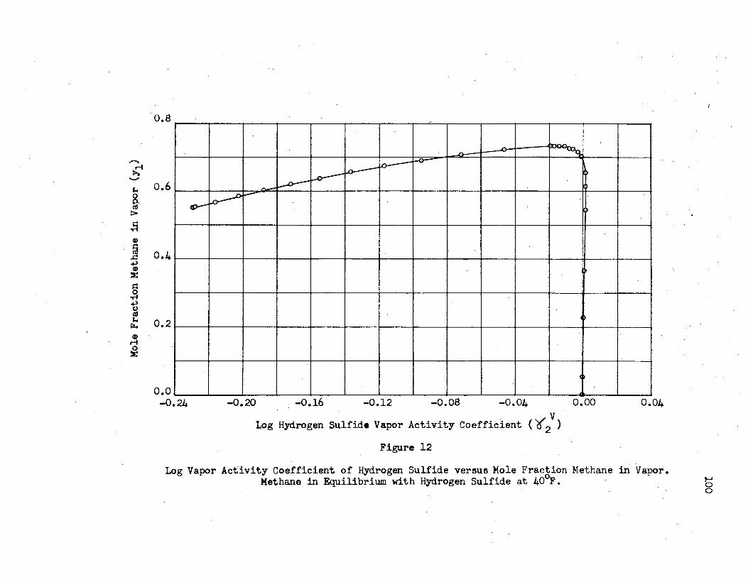
-~ -J.i 0 p.. «I > !1 II)

fa ..c: -+' II)

~

s:= ~ -+' 0

"' J.i rz.. a,

r-f

~

o.a

,,

o.6

0.4

0.2

o.o -0.24

u;,-

,

,,. '-'q

- ~ Lo--~

~ I

-~ .-0-- I

~ --I

~

~

l

-0.20 . -0.16 · -0.12 -0.08 -0.04 o.oo

Log Hydro.gen Sulfide Vapor Activity Coefficient ( '(2V}

Figure 12

,

0.04

Log Vapor Ac~ivity Coefficient of Hydrogen Sulfide versus Mole Fraction Methane in Vapor •. Methane in Equilibrium with Hydrogen Sulfide at 40°F. - b

0

101

(III-2)

r!. -V . log ~2 = log (f2 /Py2) = 9.83749 - 10 (at 600 psia)

V· log 't'2 = 0.0016 (at 600 psia)

hence V V

log (f2 /P\ = log ¢2 - log 2(2 = 9.83749 - 10 "'.'" 0.0016

log (f2v/P)h = 9.83589 - 10

V (f2 /P)h = 0.6853

Calculation of the Liquid Activity Coefficient

The activity coefficient of the heavy component in the liquid

was calculated from the activity coefficient of the light component

in the vapor by bridging to the activity coefficient of the heavy

component in the vapor and then to the heavy component in the liquid.

This is done by means of equation III-3 as will be demonstrated

for hydrogen sulfide in the methane-hydrogen sulfide system at 40°F.

and 600 psia.

The vapor fugacity coefficient of hydrogen sulfide in the

mixture (¢2) is calculated by the Redlich-Kwong equation of state

as previously demonstrated.

Step _g

The K-value (y2/x2) is from the experimental data using the same

point as used in determining the fugacity coefficient previously.

102

. L . The fugacity_coefficient of the pure liquid (f2 /P) is calculated

by the Chao-Seader equation which is stated as

L. o (o) (1) log (f; /P) = log V = log V + log 7/ (C-1)

1 .

where using the coefficients for a simple fluid

(o) . . · · 2 log V 2 · = 5-75748 - 3.01761/Tr - 4.98500 Tr+ 2.02299 Tr ·

2 + (0.08427 + 0.26667 T - 0.31138 T ) P r r r

2 + (- 0.02655 + 0.02883 Tr) P - log P r r

(1) . log ""'2/2 = - 4.23892 + 8.65808 Tr - 1.22060/Tr

3 . - 3.15224 T - 0.025 (P - 0.6) r r

For hydrogen sulfide W.= 0.100 and as previously determined 0

at 600 psia and 40 F., Tr= 0.743 and Pr= 0.459.

Therefore, the substitution of these numbe·rs into the above

equations gives

(o) log Z/2 = 5.75748 - 3.01761/0.743 - 4.98500. (0.743)

+ 2. 02299 ( O. 7 43 / + ~. 08427 + 0. 26667 ( 0. 7 43)

- 0.31138 (0. 743)~0.459 + [- 0.02655

+ 0.02883 (0.743)] (0.459) 2 - log 0.4,59 _,;(o)

log // 2 = 9.49688 - 10 .

. (1) log ]/'2 = - 4.23893 + 8.65808 (0.743) - 1.22060/(0.743)

3 . . - 3.15224 (0.743) - 0.025 (0.459 - o.6)

(1) log V 2 = - o. 73765

103

· log V O = 0.49688 - 10 + 0.100 (- o. 73765) = 9.42311 - 10 2 .

-11 o L £/ 2 · == f 2 /P = O. 26 5

Calculate the _liquid activity coefficient for pure hydrogen

sulfide

~ L = _(¢2)(y2/x2?

2 (fL/P). 2

't'21 = (0.6878)(0.3851)/(0.265) = 1.000

Calculation.£!~ Liquid Activity Coefficient

.el~ Modified Y§!£ Laar Equation

The modified Van Laar equation is

(D-38)

and

log '{ L = . 0.43429 B

2 ~B/A) (~/xl) + ~ 2 (D-39)

where L 2

A = <11 /RT)( 51 - S) cn..:.36)

L 2 B = (y2 /RT)(~ l - &} (D-37)

The volumes used are the generalized volumes of Watson as

modified by Stuckey.

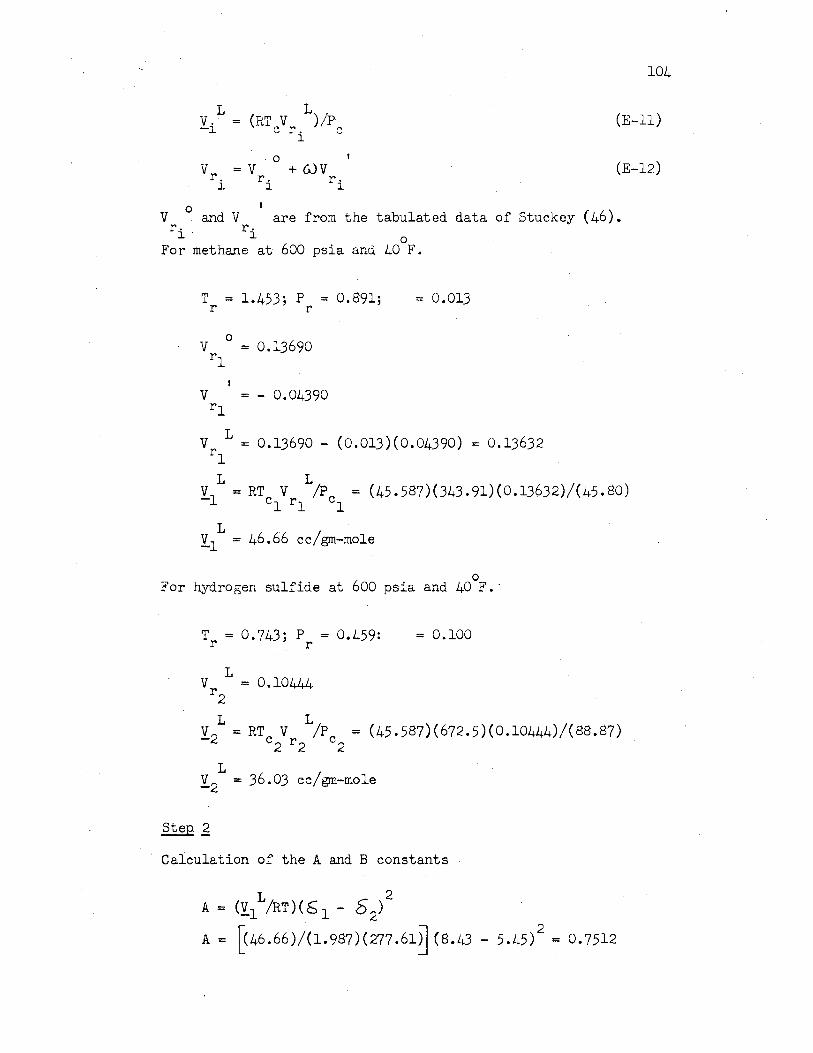
104

L L V . - = (RT V ) /P -i C r. C

(E-11) l

, 0 . I

V = V + 6JV r. r. r. l J. l

(E-12)

0 I V and V are from the tabulated aata of Stuckey (46). r. r.

l l o For methane at· 600 psia and 40 F.

T = 1.453; P = 0.891; r r

= 0.013.

0 V = 0.13690 rl

V = - 0.04390 r1

V L = 0.13690 - (0.013)(0.04390) = 0.13632 rl

L L vl = RT V /Pc = (45.587)(343.91)(0.13632)/(45.80) - cl rl 1

L . Y.1 = 46.66 cc/gm-mole

0 For hydrogen sulfide at 600 psia and 40 F.·

T = 0.743; P = 0.459: r r

L V = 0.10444

r2

= 0.100

L L v2 ·=RT V /Pc = (45.587)(672.5)(0.10444)/(88.87) - c2 r2 2

L y2 = 36.03 cc/gm-mole

· Calculation of the A and B constants

L 2 A= <Y1 /RT)(E;l - S2)

A = [(46.66)/(1.987)(277.61~ (8.43 - 5.45/ = 0.7512

. L - 2 B = <Y.2 /RT)(S1 - S2)

B = ~36.03)/(1.987)(277.61)](8.43 - 5~45) 2 = 0.5800

· L L Calculation of ?<1 and 6" 2

x1 = 0.0636; x2 == 0.9364

log ~ l L = 0. 43429 A 2 = _ _.___..._......._._._..,.._.__....._ ~x1/x2) (A/B) + iJ

L log i 1 = 0.2756

L 'o'l = 1.886

log y 1 = 0.43429 B = -=--(o_ ..... 4_34_2_9) .... (_o_.5,_8o_o __ )=-. 2 · ~x /x )(B/A) + 1J2 f [0.93641 [o.580Ql + 1] 2

L[b.0636J Lb. 751~

L log }(2 = 0.0016

L ¥2 = 1.004

105

APPENDIX I

NO.IY.:.ENCLATURE

A - parameter in the Redlich-Kwong equation of state

- parameter in the Scatchard-Hildebrand liquid activity coefficient equation

- parameter in the Chao-Seader equation

- thermodynamic work function

A' - parameter in the Van Laar liquid activity coefficient equation

a - parameter in the Van Laar liquid activity coefficient equation

- parameter in the Redlich-Kwong equation of state

- activity

B - parameter in the Redlich-Kwong equation of state

- parameter in the Scatchard-Hildebrand liquid activity coefficient equation

B1 - parameter in the Van Laar liquid activity coefficient equation

b - parameter in the Van Laar liquid activity coefficient equation

- parameter in the Redlich-Kwong equation of state

C - Scatchard's cohesive energy density

E · - internal energy

f - fugacity

G - Gibbs' free energy

H - enthalpy

106

107

h - auxiliary constant in Redlich-Kwong equation of state

K - vapor-liquid equilibrium distribution ratio

M - molecular weight

n - number of moles

P - system pressure

0 P - vapor pressure

p - partial pressure

R - universal gas constant

S - entropy

T - temperature

U - term of Redlich-Kwong equation of state defined by equation B-16

V - volume

v' Stuckey's reduced expansion factor

W - term of Redlich-Kwong equation of state defined by equation B-17

- Watson's expansion factor

x - mole fraction of component in liquid

y - mole fraction of component in vapor

Z - compressibility factor

Greek Symbols

V o - activity coefficient

!:,,. - difference

8 - Hildebrand's solubility parameter

.A,(_• - chemical potential

7) - fugacity coefficient of pure liquid

1P // - fti.gaci ty coefficient of pure real or hypothetical liquid by Chao-Seader equation

7.)(o) - fugacity coefficient of the simple fluid by Chao-Seader equation

.... ,( 1) . )/' - correction for acentric factor in the Chao-Seader equation

P - density

¢ fugacity coefficient of component in gaseous solution

- volume fraction

LP - fugacity coefficient of gaseous mixture

6J - acentric factor

Subscripts

c - property at critical conditions

d - liquid activity coefficient calculated from equation III-3

h - property of the hypothetical vapor or liquid

i - component i

j - component j

m - property of the mixture

N - number of components

r - reduced property

SH - liquid activity coefficient calculated from the ScatchardHildebrand equation

Superscripts

L - liquid phase

m - property change on mixing

o . - degree

- property of the simple fluid

- standard reference state

sl - saturated liquid

108

109

sv - saturated vapor

V - vapor phase

.. ~ ideal gas state

- correction applied to the simple fluid property for acentric factor

Miscellaneous

Superbar - partial molar property

Sub bar - molar property

1 & 2 - light and heavy component in the mixture respectively

VITA

Arthur Dale Godfrey

Candidate for the Degree of

Master of Science

Thesis: STANDARD STATE FUGACITY COEFFICIENTS FOR THE HYPOTHETICAL VAPOR BY BRIDGING FROM THE REAL GAS FUGACITY COEFFICIENTS THROUGH THE GIBBS-DUHEM EQUATION

Major Field: Chemical Engineering -

Biographical:

Personal Data: Born at Cozad, Nebraska, November 20, 1920, the son of Earl L. and Frances M. Godfrey. Married to Maxine E. Bailey, Parsons, Kansas, in June, 1961. One son, Kevin Arthur.

Education: Attended elementary school in Dawson county, Nebraska; graduated from Cozad High School, Cozad, Nebraska, in 1938; received Bachelor of Science degree in Chemical Engineering from the University of Nebraska, Lincoln, Nebraska, in August, 1943; completed requirements for Master of Science degree in August, 1964. Membership in American Institute of Chemical Engineers and American Chemical Society.

Professional Experience: Upon completion of the Ba.chelor 1 s degree began work with the refining division of the Cities Service Oil Company at Ponca City, Oklahoma. Held various positions as refinery chemist, operating foreman and department head; supervised crude distillation, steam generation, control laboratory and process engineers.

STANDARD STATE FUGACITY COEFFICIENT - ShareOK

Documents

Transcript of STANDARD STATE FUGACITY COEFFICIENT - ShareOK