SAMTAM: A Guide to Sawmill Profitability for Green and Beetle

aT^ .^^ United States '"' ' JJ) Department of

W Agriculture

Forest Service

Cooperative State Research Service

Agriculture Handbook 648

Integrated Pest Management Handbook

SAMTAM: A Guide to Sawmill Profitability for Green and Beetle- Killed Timber

Contents

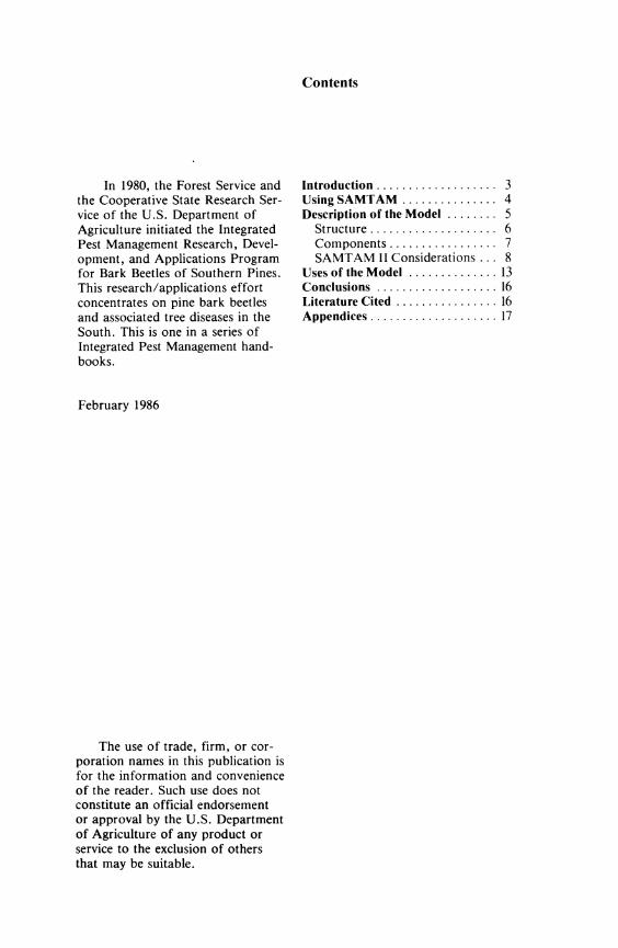
In 1980, the Forest Service and the Cooperative State Research Ser- vice of the U.S. Department of Agriculture initiated the Integrated Pest Management Research, Devel- opment, and Applications Program for Bark Beetles of Southern Pines. This research/applications effort concentrates on pine bark beetles and associated tree diseases in the South. This is one in a series of Integrated Pest Management hand- books.

Introduction 3 Using SAMTAM 4 Description of the Model 5

Structure 6 Components 7 SAMTAM II Considerations ... 8

Uses of the Model 13 Conclusions 16 Literature Cited 16 Appendices 17

February 1986

The use of trade, firm, or cor- poration names in this publication is for the information and convenience of the reader. Such use does not constitute an official endorsement or approval by the U.S. Department of Agriculture of any product or service to the exclusion of others that may be suitable.

SAMTAM: A Guide to Sawmill Profitability for Green and Beetle-Killed Timber David W. Patterson^

Introduction

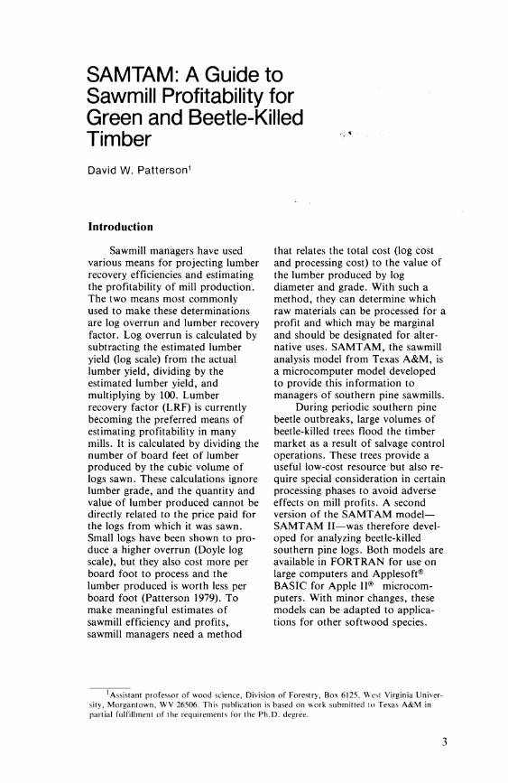
Sawmill managers have used various means for projecting lumber recovery efficiencies and estimating the profitability of mill production. The two means most commonly used to make these determinations are log overrun and lumber recovery factor. Log overrun is calculated by subtracting the estimated lumber yield (log scale) from the actual lumber yield, dividing by the estimated lumber yield, and multiplying by 100. Lumber recovery factor (LRF) is currently becoming the preferred means of estimating profitability in many mills. It is calculated by dividing the number of board feet of lumber produced by the cubic volume of logs sawn. These calculations ignore lumber grade, and the quantity and value of lumber produced cannot be directly related to the price paid for the logs from which it was sawn. Small logs have been shown to produce a higher overrun (Doyle log scale), but they also cost more per board foot to process and the lumber produced is worth less per board foot (Patterson 1979). To make meaningful estimates of sawmill efficiency and profits, sawmill managers need a method

that relates the total cost (log cost and processing cost) to the value of the lumber produced by log diameter and grade. With such a method, they can determine which raw materials can be processed for a profit and which may be marginal and should be designated for alter- native uses. SAMTAM, the sawmill analysis model from Texas A&M, is a microcomputer model developed to provide this information to managers of southern pine sawmills.

During periodic southern pine beetle outbreaks, large volumes of beetle-killed trees flood the timber market as a result of salvage control operations. These trees provide a useful low-cost resource but also re- quire special consideration in certain processing phases to avoid adverse effects on mill profits. A second version of the SAMTAM model— SAMTAM II—was therefore developed for analyzing beetle-killed southern pine logs. Both models are available in FORTRAN for use on large computers and Applesoft® BASIC for Apple II® microcom- puters. With minor changes, these models can be adapted to applications for other softwood species.

Assistant professor of wood science, Division of Forestry, Box 6125, West Virginia Univer- sity, Morgantown, WV 26506. This publication is based on work submitted to Texas A&M in partial fulfillment of the requirements for the Ph.D. degree.

Using SAMTAM

The SAMTAM microcomputer models provide mill managers with means for estimating the efficiency of mill operations using logs from either green or beetle-killed trees. This information can be used to identify needed improvements in mill operations or to determine costs and profits. Though the models will not point out the cause of specific problems, they will aid in recognizing areas that need attention.

The models also provide economic information to aid mill managers in determining which por-

tion of the sawlog resource generates a profit and which must be subsidized. They establish a cost and profit value for each log, then produce tables (by log grade) of log cost, value of lumber and residues produced, and profit or loss for each log length and diameter (table 1). The profit/loss tables not only provide the mill manager with predicted profit but also define the type of logs that are marginal to process for each log grade. (A marginal log is one with a profit potential of zero or very close to zero.) The model can also be used

Table \—Prof it/loss for grade 3 logs of various lengths calculated from SAMTAM using data from a mill study in east Texas^

Log diameter

Value ( Df grade 3 logs ($) 8 ft 10 ft 12 ft 14 ft 16 ft 18 ft 20 ft 22 ft 24 ft

6 in Value Cost Profit

5.711 2.281 3.431

6.321 3.181 3.141

6.941 4.081 2.861

7.561 4.981 2.581

8.181 5.881 2.291

8.801 6.781 2.011

9.421 7.681 1.741

10.041 8.591 1.441

10.661 9.491 1.171


6.601 3.581 3.021

7.441 4.811 2.621

8.281 6.031 2.251

9.131 7.261 1.861

9.971 8.491 1.481

10.811 9.711 1.091

11.651 10.941

.701

12.501 12.161

.331

13.341 13.391 -.059


7.631 5.081 2.551

8.731 6.681 2.041

9.831 8.291 1.531

10.931 9.891 1.031

12.031 11.491

.541

13.131 13.091

.031

14.231 14.691 -.469

15.331 16.291 -.969

16.431 17.891 -1.469


8.801 6.781 2.011

10.191 8.811 1.381

11.581 10.841

.731

12.981 12.861

.121

14.371 14.891 -.519

15.761 16.921 -1.169

17.151 18.941 -1.789

18.551 20.971 -2.429

19.941 23.001 -3.069


10.111 8.691 1.411

11.831 11.191

.631

13.541 13.691 -.159

15.261 16.191 -.929

16.981 18.691 -1.719

18.701 21.201 -2.499

20.421 23.701 -3.289

22.141 26.201 -4.069

23.861 28.701 -4.849

""The profit and loss figures are calculated as the difference between value and cost. The differences reflect rounding off in the computer.

Description of the Model

to evaluate managerial decisions that change efficiencies or affect costs to determine if marginal logs will be profitable or not.

The SAMT AM models provide a dynamic means for assessing profits that can be tailored to each particular mill based on its production costs and efficiencies. After cost and efficiency data are developed in a one-time mill study, the models can be rerun as often as necessary to project current profits in line with variations in mill operation and raw material costs, final lumber prices, and quantity and quality of beetle-killed timber on the market.

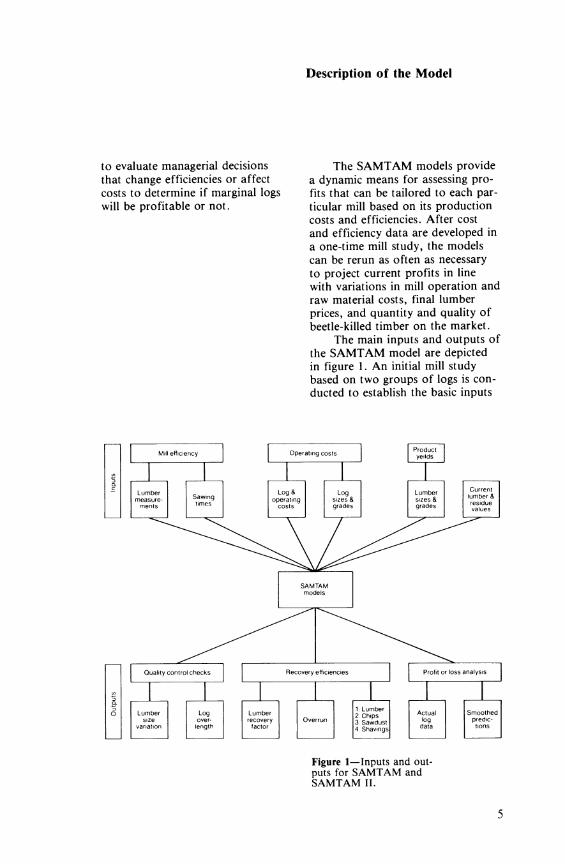
The main inputs and outputs of the SAMT AM model are depicted in figure 1. An initial mill study based on two groups of logs is conducted to estabUsh the basic inputs

Mill efficiency Operating costs Proc yei

Juct ds

Lurr ber Lo q& L Dg Lun iber measure- Odwi.iy operating sizes & sizes &

ments costs grades grades

Current lumber & residue values

SAMTAM models

Q uality control chec <s Recovery efficiencies p rofit or loss analys s

Q.

Lun- ber Lc q Lun- ber I.Lu 0 r.h

Tiber Act ual Smo Dthed

size over- recovery Overrun log predic- variation length factor 4. Shavings data tions

Figure 1—Inputs and outputs for SAMTAM and SAMTAM II.

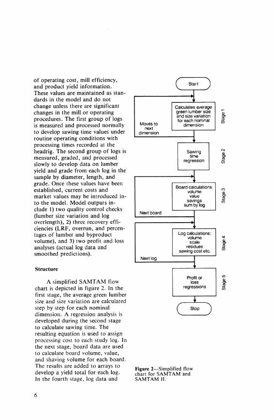
of operating cost, mill efficiency, and product yield information. These values are maintained as stan- dards in the model and do not change unless there are significant changes in the mill or operating procedures. The first group of logs is measured and processed normally to develop sawing time values under routine operating conditions with processing times recorded at the headrig. The second group of logs is measured, graded, and processed slowly to develop data on lumber yield and grade from each log in the sample by diameter, length, and grade. Once these values have been established, current costs and market values may be introduced in- to the model. Model outputs in- clude 1) two quality control checks (lumber size variation and log overlength), 2) three recovery efficiencies (LRF, overrun, and percentages of lumber and byproduct volume), and 3) two profit and loss analyses (actual log data and smoothed predictions).

Structure

A simplified SAMTAM flow chart is depicted in figure 2. In the first stage, the average green lumber size and size variation are calculated step by step for each nominal dimension. A regression analysis is developed during the second stage to calculate sawing time. The resulting equation is used to assign processing cost to each study log. In the next stage, board data are used to calculate board volume, value, and shaving volume for each board. The results are added to arrays to develop a yield total for each log. In the fourth stage, log data and

( Start ) 1

'i

Moves to next

Calculates average green lumber size and size variation for each nominal

dimension

dimension

1 Sawing

time regression

'; Board calculations:

volume value

savings sum by log

Next board

■■ r

Log calculations: volume scale

residues sawing cost etc.

Next log

1 '

Profit or loss

regressions

r Stop j

Figure 2—Simplified flow chart for SAMTAM and SAMTAM II.

board results are used to calculate log volume, scale, recovery efficiencies, residue volumes, log costs, and processing costs for individual logs. In the final stage, the log values and costs are separated by log grade (SAMTAM) or kill class (SAMTAM II). Log value and cost data for each log grade are smoothed by regression based on the square of the small-end diameter times the length of the log. The predicted profit or loss for each log size-class is presented as the difference between the smoothed log value and the smoothed log cost.

Components

The model user has a choice of three log rules for calculating log scale: 1) Doyle, 2) International 1/4-inch, or 3) Scribner-decimal C. Smalian's equation is used to calculate the cubic volume of logs.

V = (D2 + D2) X L X 0.002727

where V = the volume in cubic feet. D^ = the small-end diameter, D, = the large-end diameter, L = the log length, and 0.002727 = the product of TT and the necessary con- version factors.

One of the new approaches used in the model is the method of calculating the volumes of residue that are generated. When a sawmill study is conducted, it is easy to measure the logs going in and the lumber coming out, but because the residue goes in many directions and is in many forms, complete collec- tion is difficult. Because the lumber is readily available and requires a saw cut on each side, sawdust is the first type of residue to be estimated.

An example of the equations currently used to calculate sawdust volume is the equation pubHshed by Row et al. (1965):

sawdust weight = 0.068 x diameter squared x log length

These equations give the same esti- mate for all logs of the same size regardless of what is cut from the log. This approach can be greatly in error, especially for beetle-killed timber used in SAMTAM II. Many sawyers, seeing a log from a beetle- killed tree, will slab heavily, thereby reducing the amount of lumber produced, the number of saw lines, and the volume of sawdust produced. In SAMTAM and SAMTAM II, sawdust volume is estimated by use of the board foot total and piece count of the actual lumber cut from each log. Chip volume is established by subtracting lumber volume and estimated sawdust volume from total log volume.

Volumes are used in product yield calculations because of variations in weight resulting from changes in moisture content (for example, beetle-killed timber). Volumes change only after the moisture content goes below fiber saturation point, which is seldom reached in the mill until the lumber drying process begins. However, because residues are sold by weight, volume estimates are converted to weights for the final report using a density factor randomly selected from a density distribution function in the model. To reduce the vari- ability of the density factor, the density distribution function separates the values by butt or upper log and by diameter, then randomly

selects from values represented in the data subset. Because weights are assigned randomly through this process, dollar values of residue products could vary for the same log with successive model runs. To determine the effect of this variation on residue values, four runs of the model were made by use of the same input data from a sawmill study in east Texas. Results from these runs revealed that the variations in dollar values for logs and smoothed predictions for each run were not great enough in any case to shift the marginal log region from one class to another.

SAMTAM II Considerations

SAMT AM II differs from the conventional SAMTAM model in that it allows the user to consider

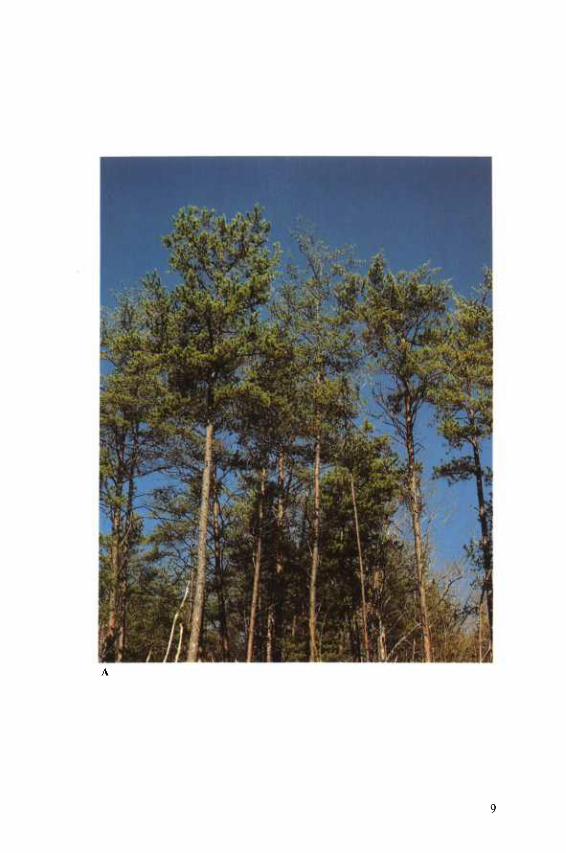
varying degrees of tree deterioration following beetle attack that are based upon the appearance of the tree before felling. The four appearance classes used may be distinguished from one another as follows: kill class 1—trees with green foliage or less than half of the foliage faded to yellow-green, kill class 2—trees with most or all of the foliage faded to yellow-green, kill class 3—trees with red and fall- ing foliage, and kill class 4—trees with most of the foliage gone and the smaller twigs starting to fall (fig. 3). Beetle-killed wood starts drying on the stump. Its consequent weight variation from green timber is ad- justed for by multiplying the estimated green weight by a moisture loss factor. There is a separate moisture loss factor (determined from actual data) for each kill class.

Figures 3A-D—The four kill classes used in SAMTAM II for beetle-killed timber.

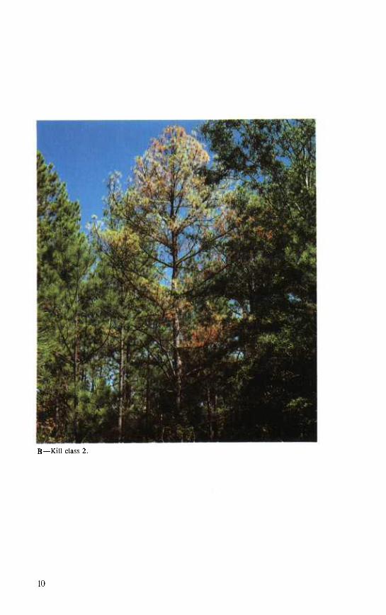
B—Kill class 2.

10

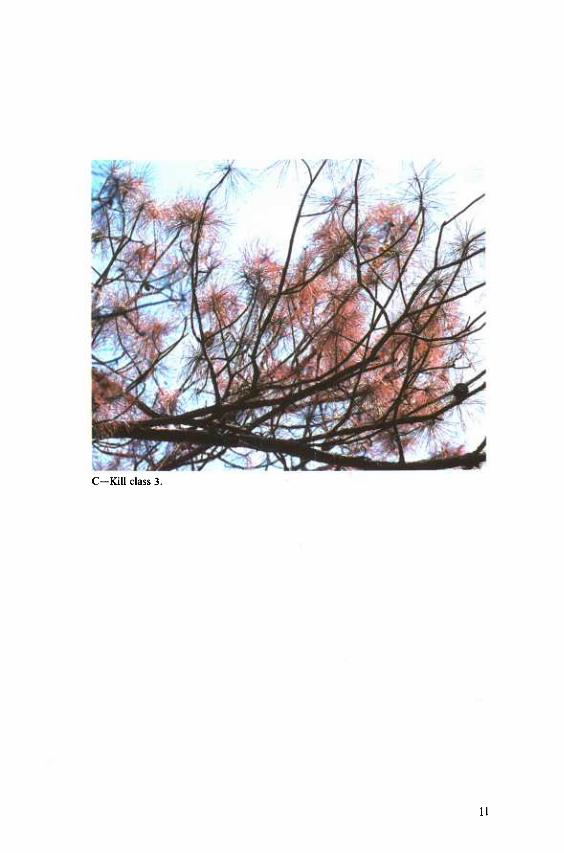
C—Kill class 3.

11

D—Kill class 4.

12

Uses of the Model

By using SAMT AM to analyze mill study data, the mill manager can discern not only the average recovery values for the mill, but also individual log production values. Using these values, the manager can determine if there is any log diameter or grade that causes a drastic change in recovery efficiency. Most mills currently have a minimum diameter limit at which they can operate. These data can help determine whether there should also be a maximum diameter limit. If a log is too large for normal processing and handling, the sawyer will **whittle" it down to a workable size, but at the expense of greatly extending processing time.

With the Applesoft versions of SAMTAM and SAMT AM II, the size variation and sawing time por- tions of the models can be used in- dependently of the remainder of the models if this information is of particular interest to the mill manager.

Examples of outputs from both the Applesoft and FORTRAN ver- sons of SAMTAM are presented in the appendix. Because of differences in the printers used, the printout from the Applesoft version (appendix A) appears different from that of the FORTRAN version (appendix B). Not all of the outputs from the FORTRAN version are presented, only those that differ from Applesoft.

The model can also be used by the manager to simulate the effects of change in resource cost and product price on expected profits. The results of such a simulation are

presented in figure 4. A normal run is used as a standard (a) with which the other results can be compared. Data for this run included lumber prices from the November 6, 1981, issue of Random Lengths (Lumber and Plywood Market Reporting Service 1981). These values were chips, $22; shavings, $16; sawdust, $9; bark, $9; logs to mills, $250/mbf Doyle; and processing, $11.50 per minute.

For the study logs at this mill (figure 4), a 20-percent increase in production cost more adversely af- fects the profit picture than either a 30-percent increase in log cost or a 25-percent decrease in lumber prices. As expected, a 25-percent increase in lumber price is more bene- ficial than a 50-percent increase in residue value. Because of the logs involved and the mill configuration, changes in the economic factors that determine the marginal log have an effect opposite that which is normally expected. Normally, the larger and longer a log is, the greater the potential profit will be. Therefore, the positive profit area in a profit and loss table would be below and to the right of the marginal log (toward the larger and longer logs). The data used in generating figure 4 are the exception. Grade 3 logs are those of the lowest quality, and the large grade 3 logs included were badly deteriorated. Because of their size, the mill manager felt that the logs should be sawn and not re- jected. Log 1 in the appendix (refer to data in appendix tables) is an example of these logs: diameter 21.6 inches; length 18.2 feet; log scale, 364 board feet; lumber produced, 257 board feet; total value, $65.04,

13

Log diameter

Log length

8 ft.

10 ft.

12 ft.

14 ft.

16 ft.

18 ft.

20 ft.

22 ft.

24 ft.

6 in. ^M H 7 in.

i.«s.,., á

8 in. ■ 9 in. i i ■ 10 in.

h ■ Hin. Hi 12 in. 1^ ■i 13 in. ■ 14 in. ^

^^H 16 in.

17 in.

18 in.

B Standard. Lumber prices increased 25 percent. Lumber prices decreased 25 percent. Residue values increased 50 percent. Log costs delivered to mill increased 30 percent. Processing costs at mill increased 20 percent.

Figure 4—Effects of cost and price ciiange on marginai log trends for grade 3 logs from a sawmill study in east Texas. Six simulation runs of SAMTAM were made with various changes in cost and prices.

14

total cost, $107.39; and net loss, $42.35. These data were included to point out that a log's large size is not necessarily an indication that it can be sawn for a profit.

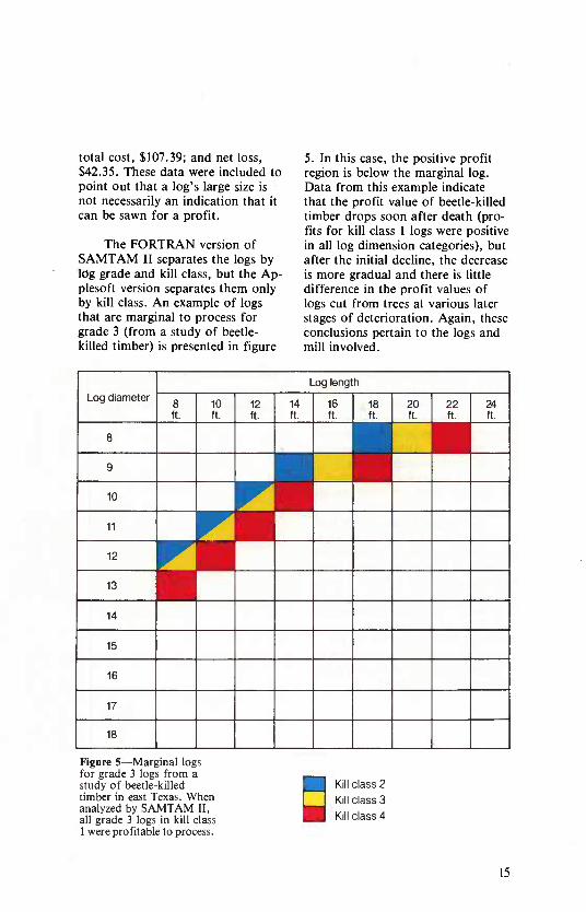
The FORTRAN version of S AMT AM II separates the logs by log grade and kill class, but the Ap- plesoft version separates them only by kill class. An example of logs that are marginal to process for grade 3 (from a study of beetle- killed timber) is presented in figure

5. In this case, the positive profit region is below the marginal log. Data from this example indicate that the profit value of beetle-killed timber drops soon after death (profits for kill class 1 logs were positive in all log dimension categories), but after the initial decline, the decrease is more gradual and there is little difference in the profit values of logs cut from trees at various later stages of deterioration. Again, these conclusions pertain to the logs and mill involved.

Log length

Log diameter g ^^ ^^ 14 16 18 20 22 24 ft. ft. ft. ft. ft. ft. ft. ft. ft.

1 ' Cfl tn

" Kß^ - PC 14

15

16

17

18

Figure 5—Marginal logs for grade 3 logs from a study of beetle-killed timber in east Texas. When analyzed by SAMTAM II, all grade 3 logs in kill class 1 were profitable to process.

D Kill class 2 Kill class 3 Kill class 4

15

Conclusions Literature Cited

SAMTAM was developed to aid sawmill managers in improving productivity and profitability by providing better information to base mill management decisions on. In the event of large quantities of beetle-killed timber becoming available on the market during bark beetle outbreak periods, SAMTAM II provides a means of reviewing and accurately evaluating the com- pounding influences of increased handling and operating costs and reduced product and grade yields in light of stumpage availability at greatly reduced prices. Both the SAMTAM and SAMTAM II models provide the manager with im- proved information for evaluating timber purchases as well as internal mill operations. Although presently written for the southern pines, SAMTAM can easily be modified for use with other softwood species.

Lumber and Plywood Market Reporting Service. Random Lengths. Eugene, OR: Random Lengths Publications, Inc.; November 6, 1981: 5-6.

Patterson, D.W. Log rules versus lumber value. Forest Products Notes. Lufkin, TX: Texas Forest Service; 1979; IV (10): 4 p.

Row, C; Fasick, C; Guttenberg, S. Improving sawmill profits through operations research. Res. Pap. SO-20. New Orleans: U.S. Department of Agriculture, Forest Service, Southern Forest Experiment Station; 1965. 26 p.

The Applesoft versions of both SAMTAM and SAMTAM II can be obtained by sending a blank diskette to Nona B. Huckabee, Forest Pest Management, USD A Forest Service, 1720 Peachtree Road, NW, Atlanta, G A 30367. The FORTRAN versions and technical assistance are available from Dr. David W. Pat- terson, Division of Forestry, West Virginia University, P.O. Box 6125, Morgantown, WV 26506.

16

Appendix A—A Portion of the Output From SAMTAM (Applesoft) Analysis of Mill Study Result in East Texas

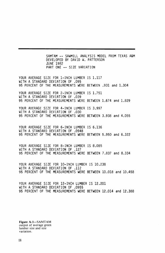
The Applesoft versions of (fig. A-1) are used as keyboard in- S AMT AM and SAMTAM II are puts to the third program (described made up of nine programs, the first on page 20). five for data input and storage on a diskette. Data are entered only once Figure A-1 shows the size varia- but can be used many times. The tion output from a mill study con- actual model is broken into four ducted in east Texas. The recom- programs, the first of which calcu- mended procedure is to measure 25 lates the size variation information. pieces of lumber for each size class. If this is all the manager desires at Each piece of lumber is measured at this time, the remaining programs three points—the middle and 2 feet do not have to be run. If the whole from each end. model is run, the average values

17

SAMTAM - SAWMILL ANALYSIS MODEL FROM TEXAS A&M DEVELOPED BY DAVID W. PATTERSON JUNE 1982 PART ONE - SIZE VARIATION

YOUR AVERAGE SIZE FOR 1-INCH LUMBER IS 1.117 WITH A STANDARD DEVIATION OF .095 95 PERCENT OF THE MEASUREMENTS WERE BETWEEN .931 and 1.304

YOUR AVERAGE SIZE FOR 2-INCH LUMBER IS 1.751 WITH A STANDARD DEVIATION OF .039 95 PERCENT OF THE MEASUREMENTS WERE BETWEEN 1.674 and 1.829






Figure A-1—SAMTAM output of average green lumber size and size variation.

18

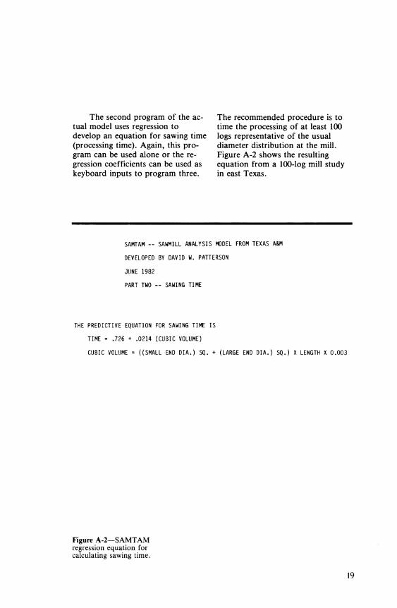
The second program of the actual model uses regression to develop an equation for sawing time (processing time). Again, this program can be used alone or the regression coefficients can be used as keyboard inputs to program three.

The recommended procedure is to time the processing of at least 100 logs representative of the usual diameter distribution at the mill. Figure A-2 shows the resulting equation from a 100-log mill study in east Texas.

SAMTAM — SAWMILL ANALYSIS MODEL FROM TEXAS A&M

DEVELOPED BY DAVID W. PATTERSON

JUNE 1982

PART TWO — SAWING TIME

THE PREDICTIVE EQUATION FOR SAWING TIME IS

TIME = .726 + .0214 (CUBIC VOLUME)

CUBIC VOLUME = ((SMALL END DIA.) SQ. + (LARGE END DIA.) SQ.) X LENGTH X 0.003

Figure A-2—SAMTAM regression equation for calculating sawing time.

19

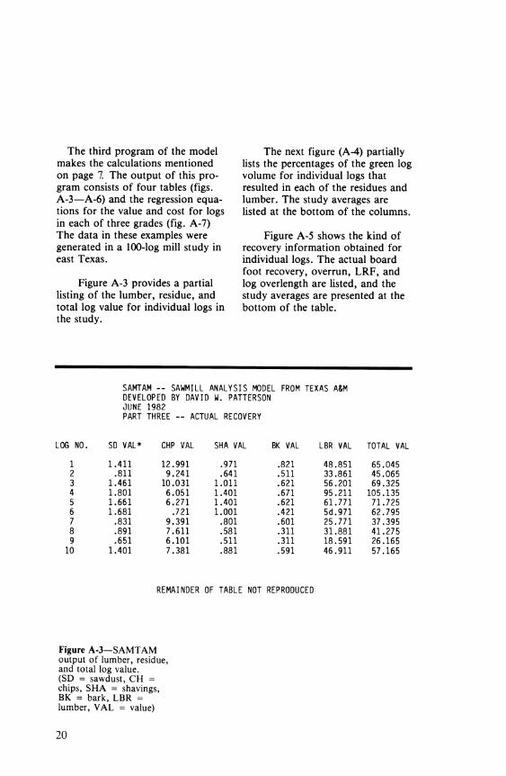
The third program of the model makes the calculations mentioned on page 7. The output of this program consists of four tables (figs. A-3—A-6) and the regression equations for the value and cost for logs in each of three grades (fig. A-7) The data in these examples were generated in a 100-log mill study in east Texas.

Figure A-3 provides a partial Hsting of the lumber, residue, and total log value for individual logs in the study.

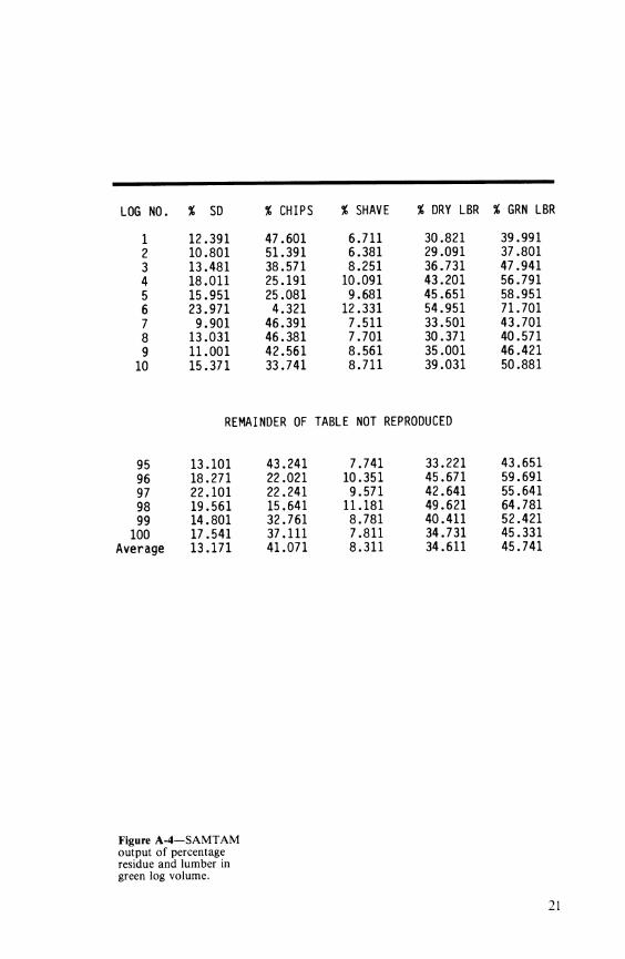
The next figure (A-4) partially lists the percentages of the green log volume for individual logs that resulted in each of the residues and lumber. The study averages are Usted at the bottom of the columns.

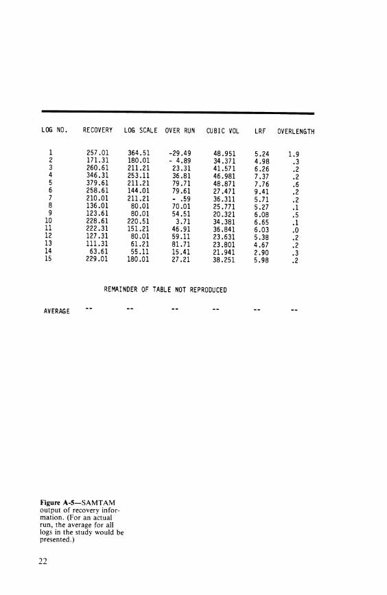
Figure A-5 shows the kind of recovery information obtained for individual logs. The actual board foot recovery, overrun, LRF, and log overlength are listed, and the study averages are presented at the bottom of the table.

SAMTAM — SAWMILL ANALYSIS MODEL FROM TEXAS A&M DEVELOPED BY DAVID W. PATTERSON JUNE 1982 PART THREE — ACTUAL RECOVERY

1 NO. SD VAL* CHP VAL SHA VAL BK VAL LBR VAL TOTAL VAL

1 1.411 12.991 .971 .821 48.851 65.045 2 .811 9.241 .641 .511 33.861 45.065 3 1.461 10.031 1.011 .621 56.201 69.325 4 1.801 6.051 1.401 .671 95.211 105.135 5 1.661 6.271 1.401 .621 61.771 71.725 6 1.681 .721 1.001 .421 5d.971 62.795 7 .831 9.391 .801 .601 25.771 37.395 8 .891 7.611 .581 .311 31.881 41.275 9 .651 6.101 .511 .311 18.591 26.165 .0 1.401 7.381 .881 .591 46.911 57.165

REMAINDER OF TABLE NOT REPRODUCED

Figure A-3—SAMTAM output of lumber, residue, and total log value. (SD = sawdust, CH = chips, SHA = shavings, BK = bark, LBR = lumber, VAL = value)

20

LOG NO. % SD % CHIPS % SHAVE % DRY LBR % GRN LBR

1 12.391 47.601 6.711 30.821 39.991 2 10.801 51.391 6.381 29.091 37.801 3 13.481 38.571 8.251 36.731 47.941 4 18.011 25.191 10.091 43.201 56.791 5 15.951 25.081 9.681 45.651 58.951 6 23.971 4.321 12.331 54,951 71.701 7 9.901 46.391 7.511 33.501 43.701 8 13.031 46.381 7.701 30.371 40.571 9 11.001 42.561 8.561 35.001 46.421

10 15.371 33.741 8.711 39.031 50.881


95 13.101 43.241 7.741 33.221 43.651 96 18.271 22.021 10.351 45,671 59.691 97 22.101 22.241 9.571 42.641 55.641 98 19.561 15.641 11.181 49.621 64.781 99 14.801 32.761 8.781 40.411 52.421 100 17.541 37.111 7.811 34.731 45.331

Average 13.171 41.071 8.311 34.611 45.741

Figure A-4—SAMTAM output of percentage residue and lumber in green log volume.

LOG NO. RECOVERY LOG SCALE OVER RUN CUBIC VOL LRF OVERLENGTH

1 257.01 364.51 -29.49 48.951 5.24 1.9 2 171.31 180.01 - 4.89 34.371 4.98 .3 3 260.61 211.21 23.31 41.571 6.26 .2 4 346.31 253.11 36.81 46.981 7.37 .2 5 379.61 211.21 79.71 48.871 7.76 .6 6 258.61 144.01 79.61 27.471 9.41 .2 7 210.01 211.21 - .59 36.311 5.71 .2 8 136.01 80.01 70.01 25.771 5.27 .1 9 123.61 80.01 54.51 20.321 6.08 .5

10 228.61 220.51 3.71 34.381 6.65 .1 11 222.31 151.21 46.91 36.841 6.03 .0 12 127.31 80.01 59.11 23.631 5.38 .2 13 111.31 61.21 81.71 23.801 4.67 .2 14 63.61 55.11 15.41 21.941 2.90 .3 15 229.01 180.01 27.21 38.251 5.98 .2

AVERAGE


Figure A-5—SAMTAM output of recovery information. (For an actual run, the average for all logs in the study would be presented.)

22

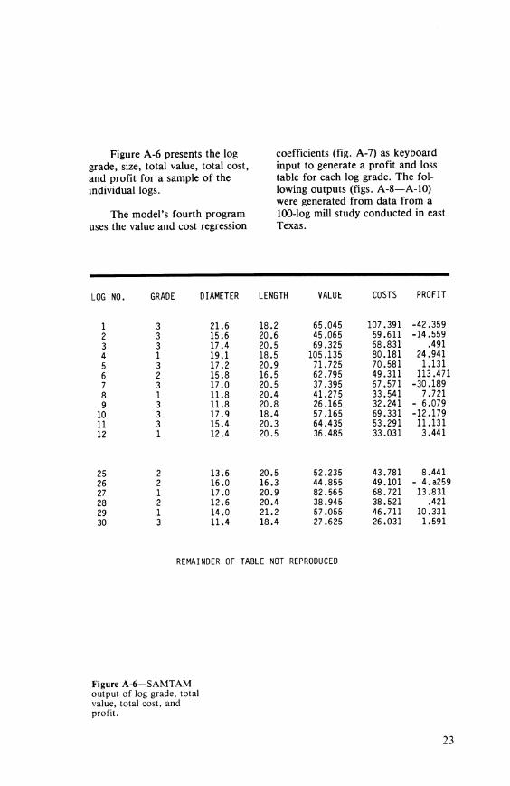
Figure A-6 presents the log coefficients (fig. A-7) as keyboard grade, size, total value, total cost, input to generate a profit and loss and profit for a sample of the table for each log grade. The fol- individual logs. lowing outputs (figs. A-8—A-10)

were generated from data from a The model's fourth program 100-log mill study conducted in east

uses the value and cost regression Texas.

LOG NO. GRADE DIAMETER LENGTH VALUE COSTS PROFIT

1 3 21.6 18.2 65.045 107.391 -42.359 2 3 15.6 20.6 45.065 59.611 -14.559 3 3 17.4 20.5 69.325 68.831 .491 4 1 19.1 18.5 105.135 80.181 24.941 5 3 17.2 20.9 71.725 70.581 1.131 6 2 15.8 16.5 62.795 49.311 113.471 7 3 17.0 20.5 37.395 67.571 -30.189 8 1 11.8 20.4 41.275 33.541 7.721 9 3 11.8 20.8 26.165 32.241 - 6.079

10 3 17.9 18.4 57.165 69.331 -12.179 11 3 15.4 20.3 64.435 53.291 11.131 12 1 12.4 20.5 36.485 33.031 3.441

25 2 13.6 20.5 52.235 43.781 8.441 26 2 16.0 16.3 44.855 49.101 - 4.a259 27 1 17.0 20.9 82.565 68.721 13.831 28 2 12.6 20.4 38.945 38.521 .421 29 1 14.0 21.2 57.055 46.711 10.331 30 3 11.4 18.4 27.625 26.031 1.591


Figure A-6—SAMTAM output of log grade, total value, total cost, and profit.

23

FOR GRADE 1 LOGS

VALUE -1.97665241 .0144353715 X (DIA)SQ X LENGTH COST -3.46962796 .0125083409 X (DIA)SQ X LENGTH

FOR GRADE 2 LOGS

VALUE -9.94125173 .0150002493 X (DIA)SQ X LENGTH COST - .766962351 .0117889845 X (DIA)SQ X LENGTH

FOR GRADE 3 LOGS

VALUE 3.23336502 8.64197729E-03 X (DIA)SQ X LENGTH COST -1.11224498 .0120325766 X (DIA)SQ X LENGTH

Figure A-7—SAMTAM regression equations for value and cost for each log grade.

SAMTAM -- SAWMILL ANALYSIS MODEL FROM TEXAS A&M DEVELOPED BY DAVID W. PATTERSON JUNE 1982 PROFIT OR LOSS --GRADE 1 LOGS

Dia

Value Cost Profit

Value Cost Profit

8 FT

5.411 2.931 2.481

7.371 4.631 2.731

10 FT 12 FT 14 FT 16 FT 18 FT 20 FT 22 FT 24 FT

7.261 4.531 2.731

9.101 6.131 2.961

9.711 12.051 6.661 3.041

8.681 3.371

10.951 12.801 14.651 16.501 18.341 20.191 7.731 3.211

9.331 10.931 12.541 14.141 15.741 3.471 3.711 3.961 4.201 4.451

14.391 16.731 19.061 21.401 23.741 26.081 10.711 12.741 14.761 16.791 18.811 20.841 3.681 3.991 4.301 4.931 4.931 5.231

10 Value 9.571 12.451 15.341 18.231 21.111 24.001 26.891 26.781 32.661


Figure A-8—Profit and loss table from SAMTAM for grade 1 logs.

24

PROFIT OR LOSS GRADE 2 LOGS

Loq diameter nches)

Log Length (feet)

(i Ö 10 12 14 16 18 20 22 24

6 Value Cost

Profit

00.000 2.731

-2.739

00.000 3.611

-3.619

00.000 4.501 -4.499

00.000 5.381

-5.389

00.000 6.271

-6.279

00.000 7.151

-7.159

.951 8.031

-7.089

2.031 8.921 -6.899

3.101 9.801

-6.709

7 Value Cost

Profit

00.000 4.011 -4.019

00.000 5.211

-5.219

00.000 6.411

-6.419

.441 7.621

-7.189

1.911 8.821 -6.909

3.371 10.021 -6.649

4.841 11.231 -6.389

6.301 12.431 -6.129

7.771 13.631 -5.859

8 Value Cost

Profit

00.000 5.481

-5.489

00.000 7.051

-7.059

1.671 8.621 -6.959

3.581 10.201 -6.619

5.491 11.771 -6.279

7.411 13.341 -5.929

9.321 14.911 -5.599

11.231 16.481 -5.249

13.151 18.051 -4.909

9 Value Cost

Profit

00.000 7.151

-7.159

2.301 9.141

-6.849

4.721 11.131 -6.409

7.141 13.121 -5.979

9.561 15.111 -5.559

11.981 17.101 -5.129

14.401 19.091 -4.699

16.821 21.081 -4.259

19.241 23.061 -3.829

10 Value Cost

Profit

2.151 9.021

-6.869

5.131 11.471 -6.339

8.121 13.931 -5.809

11.111 16.381 -5.279

14.101 18.841 -4.749

17.091 21.301 -4.209

20.081 23.751 -3.679

23.071 26.211 -3.149

26.061 28.661 -2.599

11 Value Cost

Profit

4.661 11.081 -6.419

8.271 14.051 -5.789

11.891 17.021 -5.139

15.511 19.991 -4.489

19.131 22.971 -3.839

22.741 25.941 -3.199

26.361 28.911 -2.549

29.981 31.881 -1.909

33.591 34.851 -1.259

12 Value Cost

Profit

7.411 13.341 -5.929

11.711 16.881 -5.179

16.021 20.411 -4.389

20.321 23.951 -3.639

24.631 27.491 -2.859

28.931 31.021 -2.099

33.241 34.561 -1.329

37.541 38.101 -.599

41.841 41.631

.211

13 Value Cost

Profit

10.401 15.801 -5.409

15.451 19.951 -4.509

20.501 24.101 -3.609

25.551 28.251 -2.709

30.601 32.401 -1.809

35.661 36.551 -.899

40.711 40.701 00.000

45.761 44.851

.911

50.811 49.001 1.811

14 Value Cost

Profit

13.621 18.451 -4.839

19.481 23.261 -3.789

25.341 28.081 -2.739

31.201 32.891 -1.689

37.061 37.701 -.649

42.921 42.521

.401

48.781 47.331 1.451

54.641 52.141 2.501

60.501 56.961 3.541

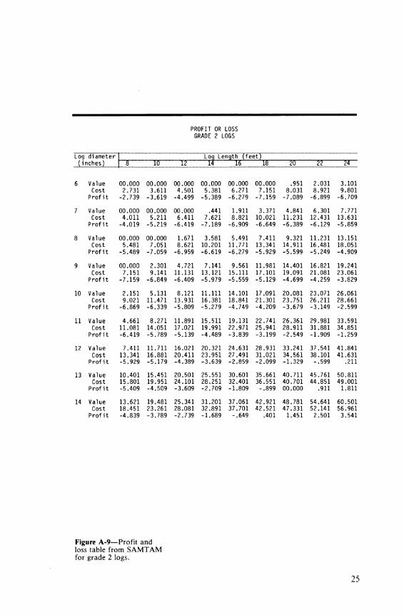
Figure A-9—Profit and loss table from SAMTAM for grade 2 logs.

25

PROFIT OR LOSS GRADE 3 LOGS

Log diameter nches)

Log Length (feet)

(i 8 10 12 14 16 18 20 22 24

6 Value 5.88 6.50 7.12 7.74 8.35 8.97 9.59 10.21 10.82 Cost 2.44 3.34 4.25 5.15 6.05 6.95 7.86 8.76 9.66

Profit 3.44 3.16 2.86 2.59 2.29 2.01 1.72 1.44 1.16

7 Value 6.77 7.62 8.46 9.30 10.14 10.98 11.82 12.66 13.50 Cost 3.75 4.97 6.20 7.43 8.66 9.88 11.11 12.34 13.57

Profit 3.02 2.64 2.26 1.86 1.48 1.10 .71 .32 -.08

8 Value 7.80 8.90 10.00 11.10 12.20 13.29 14.39 15.49 16.59 Cost 5.25 6.85 8.46 10.06 11.66 13.27 14.87 16.48 18.08

Profit 2.55 2.04 1.53 1.04 .53 .01 -.49 -1.00 -1.49

9 Value 8.97 10.36 11.75 13.14 14.53 15.92 17.31 18.70 20.09 Cost 6.951 8.98 11.01 13.04 15.07 17.10 19.13 21.16 23.19

Profit 2.01 1.37 .73 .10 -.54 -1.19 -1.83 -2.46 -3.10

10 Value 0.27 11.99 13.70 15.42 17.14 18.85 20.57 22.28 24.00 Cost 8.86 11.36 13.87 16.38 18.88 21.39 23.89 26.40 28.91

Profit 1.41 .62 -.18 -.97 -1.75 -2.54 -3.33 -4.12 -4.91

11 Value 11.71 13.79 15.87 17.94 20.02 22.09 24.17 26.24 28.32 Cost 10.96 13.99 17.03 20.06 23.09 26.12 29.16 32.19 35.22

Profit .75 -.20 -1.17 2.13 -3.08 -4.03 -4.99 -5.95 -6.90

12 Value 13.29 15.76 18.23 20.70 23.17 25.64 28.11 30.58 33.05 Cost 13.27 16.88 20.49 24.09 27.70 31.31 34.92 38.53 42.14

Profit .01 -1.13 -2.27 -3.40 -4.54 -5.68 -6.82 -7.96 -9.10

13 Value 15.01 17.91 20.81 23.71 26.60 29.50 32.40 35.30 38.20 Cost 15.77 20.01 24.24 28.48 32.71 36.95 41.18 45.42 49.66

Profit -.76 -2.11 -3.44 -4.77 -6.11 -7.46 -8.79 -10.13 -11.46

14 Value 16.86 20.22 23.59 26.95 31.31 33.67 37.03 40.40 43.76 Cost 18.48 23.39 28.30 33.22 38.13 43.04 47.95 52.86 57.77

Profit -1.62 -3.18 -4.71 -6.27 -7.82 -9.38 -10.93 -12.46 -14.00

Figure A-10—Profit and loss table from SAMT AM for grade 3 logs.

26

Appendix B—A Portion of the Output from SAMT AM (FORTRAN) Analysis of Mill Study Results in East Texas

The FORTRAN versions of SAMT AM and SAMT AM II consist of one program that calls the data from storage areas within the computer. Because of the larger memory and wider printer, the output differs from that of the Ap- plesoft versions. The dollar value inputs are printed with the output (fig. B-1) so that if more than one run is made with different value inputs, the outputs can be identified with the appropriate inputs.

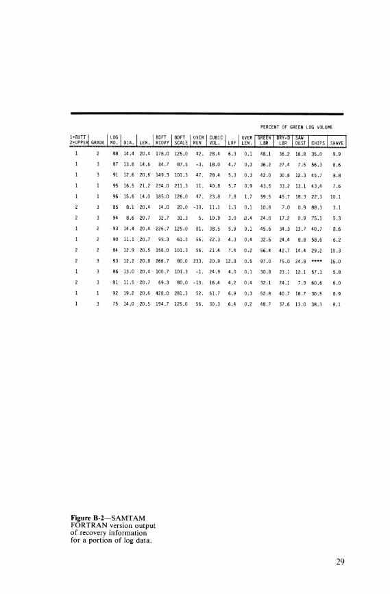
The information that was presented in four outputs by the third program of the Applesoft version (appendix A) is presented in two in the FORTRAN version. The first presents all of the recovery information (board feet, overrun, LRF, and

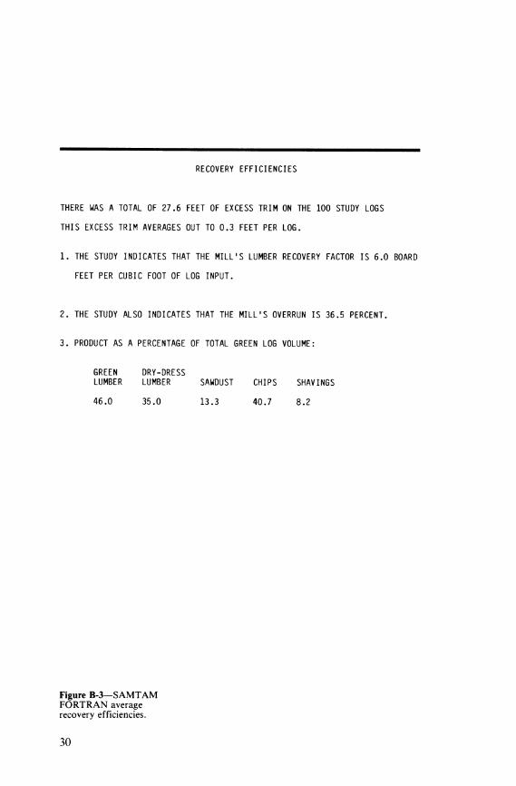
the percentages of the green log volume) along with the log size and grade and whether it is a butt log or upper log (fig. B-2). The study averages are grouped together on a separate page of printout (fig. B-3). Figure B-4 presents all of the value and cost information along with the log size and grade and whether it is a butt or upper log.

The FORTRAN versions do not output the regression equations for value and cost. Only the profit or loss tables are presented.

The following figures are por- tions of the FORTRAN printout resulting from analyzing the data from the same 100-log mill study conducted in east Texas that was used in appendix A:

27

LENGTHS (feet)

SIZE GRADE 8.0 10.0 12.0 14.0 16.0 18.0 20.0 22.0

2X4 1 185.00 185.00 185.00 180.00 200.00 230.00 230.00 265.00

2 153.00 155.00 163.00 160.00 188.00 168.00 168.00 250.00

3 136.00 136.00 136.00 136.00 136.00 136.00 136.00 136.00

4 90.00 90.00 90.00 90.00 90.00 90.00 90.00 90.00

2X6 1 205.00 205.00 230.00 210.00 225.00 215.00 250.00 370.00

2 165.00 165.00 215.00 185.00 215.00 1-95.00 205.00 315.00

3 131.00 131.00 131.00 131.00 131.00 131.00 131.00 131.00

4 90.00 90.00 90.00 90.00 90.00 90.00 90.00 90.00

••••••••••••••••••••••••••••••••••••••*••••••*••••••••••••••

2X8 1 190.00 190.00 230.00 195.00 195.00 200.00 240.00 300.00

2 155.00 160.00 210.00 166.00 163.00 163.00 200.00 285.00

3 116.00 116.00 116.00 116.00 116.00 116.00 116.00 116.00

4 90.00 90.00 90.00 90.00 90.00 90.00 90.00 90.00

•••••••••••••••••••••••••••••••••••••••••••••••••••••••••••••••^

2 X 10 1 200.00 200.00 260.00 260.00 260.00 240.00 260.00 325.00

2 185.00 185.00 235.00 235.00 235.00 215.00 220.00 310.00

3 125.00 125.00 125.00 125.00 125.00 125.00 125.00 125.00

4 90.00 90.00 90.00 90.00 90.00 90.00 90.00 90.00

••••••••••••••••*••••••••••••••••••••••••••••••••••**••••••

2 X 12 1 255.00 270.00 270.00 240.00 275.00 285.00 295.00 360.00

2 215.00 240.00 245.00 215.00 255.00 250.00 260.00 340.00

3 164.00 164.00 164.00 164.00 164.00 164.00 164.00 164.00

4 90.00 90.00 90.00 90.00 90.00 90.00 90.00 90.00

Figure B-1—SAMTAM FORTRAN output of market price of 2-inch lumber at the time of study.

28

GRADE LOG NO. DIA. LEN.

BDFT RCOVY

BDFT SCALE

OVER RUN

1 CUBIC VOL. LRF

OVER LEN.

PERCENT OF GREEN LOG VOLUME

1=BUTT 2=UPPER

GktLN LBR LBR

SAW DUST CHIPS SHAVE

2 88 14.4 20.4 178.0 125.0 42. 28.4 6.3 0.1 48.1 36.2 16.8 35.0 8.9

3 87 13.8 14.6 84.7 87.5 -3. 18.0 4.7 0.3 36.2 27.4 7.5 56.3 6.6

3 91 12.6 20.6 149.3 101.3 47. 28.4 5.3 0.3 42.0 30.6 12.3 45.7 8.8

1 95 16.5 21.2 234.0 211.3 11. 40.8 5.7 0.9 43.5 33.2 13.1 43.4 7.6

1 96 15.6 14.0 185.0 126.0 47. 23.8 7.8 1.7 59.5 45.7 18.3 22.3 10.1

3 85 8.1 20.4 14.0 20.0 -30. 11.1 1.3 0.1 10.8 7.0 0.9 88.3 3.1

3 94 8.6 20.7 32.7 31.3 5. 10.9 3.0 ÛA 24.0 17.2 0.9 75.1 5.3

2 93 14.4 20.4 226.7 125.0 81. 38.5 5.9 0.1 45.6 34.3 13.7 40.7 8.6

2 90 11.1 .20.7 95.3 61.3 56. 22.3 4.3 0.4 32.6 24.4 8.8 58.6 6.2

2 84 12.9 20.5 158.0 101.3 56. 21.4 7.4 0.2 56.4 42.7 14.4 29.2 10.3

3 53 12.2 20.8 266.7 80.0 233. 20.9 12.8 0.5 97.0 75.0 24.8 **•* 16.0

3 86 13.0 20.4 100.7 101.3 -1. 24.9 4.0 0.1 30.8 23.1 12.1 57.1 5.8

3 81 11.5 20.7 69.3 80.0 -13. 16.4 4.2 0.4 32.1 24.1 7.3 60.6 6.0

1 92 19.2 20.6 428.0 281.3 52. 61.7 6.9 0.3 52.8 40.7 16.7 30.5 8.9

3 75 14.0 20.5 194.7 125.0 56. 30.3 6.4 0.2 48.7 37.6 13.0 38.3 8.1

Figure B-2—SAMTAM FORTRAN version output of recovery information for a portion of log data.

29

RECOVERY EFFICIENCIES

THERE WAS A TOTAL OF 27.6 FEET OF EXCESS TRIM ON THE 100 STUDY LOGS

THIS EXCESS TRIM AVERAGES OUT TO 0.3 FEET PER LOG.

1. THE STUDY INDICATES THAT THE MILL'S LUMBER RECOVERY FACTOR IS 6.0 BOARD

FEET PER CUBIC FOOT OF LOG INPUT.

2. THE STUDY ALSO INDICATES THAT THE MILL'S OVERRUN IS 36.5 PERCENT.

3. PRODUCT AS A PERCENTAGE OF TOTAL GREEN LOG VOLUME:

GREEN DRY-DRESS LUMBER LUMBER SAWDUST CHIPS SHAVINGS

46.0 35.0 13.3 40.7 8.2

Figure B-3—SAMTAM FORTRAN average recovery efficiencies.

30

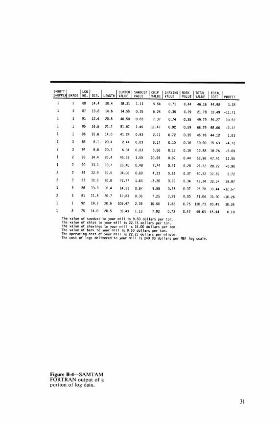
1=BUTT 1 2=UPPER| GRADE

LOG NO. DIA. LENGTH

LUMBER VALUE

SAWDUST VALUE

CHIP VALUE

1 SHAVING 1 VALUE

BARK VALUE

TOTAL VALUE

TOTAL COST PROFIT

2 88 14.4 20.4 38.31 1.11 5.54 0.75 0.44 46.16 44.98 1.18

3 87 13.8 14.6 14.55 0.35 6.24 0.35 0.29 21.78 33.49 -11.71

3 91 12.6 20.6 40.50 0.83 7.37 0.74 0.35 49.79 39.27 10.52

1 95 16.5 21.2 51.87 1.45 11.47 0.92 0.59 66.29 68.66 -2.37

1 96 15.6 14.0 41.24 0.93 2.71 0.72 0.35 45.95 44.12 1.83

3 85 8.1 20.4 2.44 0.03 8.17 0.10 0.16 10.90 15.63 -4.72

3 94 8.6 20.7 6.34 0.03 5.86 0.17 0.18 12.58 18.26 -5.69

2 93 14.4 20.4 45.36 1.50 10.68 0.97 0.44 58.96 47.41 11.55

2 90 11.1 20.7 18.40 0.48 7.74 0.41 0.28 27.32 28.22 -0.90

2 84 12.9 20.5 34.08 0.89 4.33 0.65 0.37 40.32 37.59 2.72

3 53 12.2 20.8 72.77 1.60 -3.36 0.99 0.34 72.34 32.37 39.97

3 86 13.0 20.4 14.23 0.87 9.88 0.43 0.37 25.78 38.44 -12.67

3 81 11.5 20.7 12.83 0.36 7.25 0.29 0.30 21.04 31.30 -10.26

1 92 19.2 20.6 105.47 2.39 10.50 1.62 0.75 120.73 90.49 30.24

3 75 14.0 20.5 35.43 1.12 7.92 0.72 0.42 45.63 45.44 0.19

The value of sawdust to your mill is 9.50 dollars per ton. The value of chips to your mill is 22.75 dollars per ton. The value of shavings to your mill is 16.00 dollars per ton. The value of bark to your mill is 9.50 dollars per ton. The operating cost of your mill is 22.23 dollars per minute. The cost of logs delivered to your mill is 240.00 dollars per MBF log scale.

Figure B-4—SAMTAM FORTRAN output of a portion of log data.

31

SAMTAM: A Guide to Sawmill Profitability for Green and Beetle

Documents

Transcript of SAMTAM: A Guide to Sawmill Profitability for Green and Beetle